Topological Queries in Spatial Databases

a

li

Rr

ia

f�

9

Journal of Computer and System Sciences 58, 29�53 (1999)

Topological Queries

C. H. Pap

University of CaE-mail: christos�

D. Su

AT H TE-mail: suciu�

an

V. V

University of CaliE-mail: vianu

Received December 31, 1

We study topological queries over two-dimensional spatialdatabases. First, we show that the topological properties of semi-algebraic spatial regions can be completely specified using a classicalfinite structure, essentially the embedded planar graph of the regionboundaries. This provides an invariant characterizing semi-algebraicregions up to homeomorphism. All topological queries on semi-algebraic regions can be answered by queries on the invariant whosecomplexity is polynomially related to the original. Also, we show thatfor the purpose of answering topological queries, semi-algebraicregions can always be represented simply as polygonal regions.

We then study query languages for topological properties of two-dimensional spatial databases, starting from the topological rela-tionships between pairs of planar regions introduced by Egenhofer. Weshow that the closure of these relationships under appropriate logicaloperators yields languages which are complete for topological proper-ties. This provides a theoretical a posteriori justification for the choiceof these particular relationships. Unlike the point-based languagesstudied in previous work on constraint databases, our languages areregion based��quantifiers range over regions in the plane. This yields afamily of languages, whose complexity ranges from NC to undecidable.Another type of completeness result shows that the region-basedlanguage of complexity NC expresses precisely the same topologicalproperties as well-known point-based languages. � 1999 Academic Press

Article ID jcss.1998.1597, available online at http:��www.idealibrary.com on

* This work was done while the author was visiting U.C. Sand Diego.- This author was supported in part by the NSF under Grant IRI-

9221268. An extended abstract of this paper appeared in ``Proc. ACMSIGACT�SIGART�SIGMOD Symp. on Principles of Database Systems,''pp. 81�92, 1996, under the same title.

29

in Spatial Databases

dimitriou

fornia, Berkeleycs.berkeley.edu

ciu*

esearchesearch.att.com

d

nu-

ornia, San Diegocs.ucsd.edu

96; revised May 28, 1998

1. INTRODUCTION

The manipulation of spatial data is an increasingly im-portant part of database systems. Spatial data are involvedin a wide range of applications: geographic informationvideo databases, medical imaging, CAD-CAM, VLSI,robotics, etc. Numerous models and languages for spatialdata have been proposed (e.g., see Paredaens's survey[Par95]). The present paper is a contribution to the formalstudy of query languages for spatial databases; in particular,we focus on topological query languages.

Different applications of spatial databases pose differentrequirements on query languages. In many cases the precisesize of the regions is important, while in other applicationswe may only be interested in the topological relationshipsbetween regions��intuitively, those that pertain to connec-tivity properties of the regions and are therefore invariantunder continuous bijections. Such differences in scope andemphasis are crucial, as they affect the data model, querylanguage, and performance. We can formalize the intuitivenotion of ``relevant information'' with respect to a certainclass of queries by specifying a group G of permutations(bijections) of the space which can be applied withoutchanging the answers to the queries of interest. Once G hasbeen defined, then the queries of interest are simply thosethat are G-generic [Par+94] (i.e., whose answer does notchange if the database undergoes any transformation inG ; this concept extends the notion of genericity of Chandraand Harel for classical queries). For example, the topolog-ical queries are those that are generic with respect to

0022-0000�99 �30.00Copyright � 1999 by Academic Press

All rights of reproduction in any form reserved.

homeomorphisms (continuous mappings with continuousinverses). Topological relationships turn out to be central tospatial databases (see [LT92, G94] for discussions of the roleof topological relationships in geographic informationsystems). A first group of results of this paper provides a keytechnical tool: we show that the topological properties of setsof semi-algebraic spatial regions can be completely specifiedusing a classical finite structure��intuitively, the embeddedplanar graph of the region boundaries. Such a structure actsas an invariant characterizing an equivalence class of sets ofspatial regions with respect to homeomorphism. It can beviewed as an abstraction capturing exactly the topologicalproperties of a set of regions. While abstractions of topologi-cal properties of this flavor have been considered before, thisis the first time, to our knowledge, that such an invariant isshown to completely characterize an arbitrary number ofregions up to homeomorphism in the setting we consider (seealso discussion below on related work).

We show that for inputs which are semi-algebraic regions,the invariant can be computed in polynomial time (andNC). Moreover, once this structure is computed, topologi-cal queries can be answered by classical database queriesposed against that structure, of complexity polynomiallyrelated to the original query. This provides a bridge betweenthe spatial and classical database domains. Furthermore,the invariants are used to show that each equivalence classof sets of semi-algebraic spatial regions with respect tohomeomorphism has a representative where the regions arepolygonal. This shows that, for the purpose of answeringtopological queries, semi-algebraic regions can always berepresented simply as polygonal regions.

Alternatively, the invariants can be used as the basis fora spatial model capturing precisely the topological proper-ties of regions. Indeed, the structures we produce containinformation similar to the PLA model proposed by the U.S.Census Bureau, which contains topological properties onpoints, lines, and areas [Cor79, Par95]. Our invariants canbe viewed as an augmentation of the PLA model. They arealso related to models in geographic information systemsusing decompositions of the space into cell complexes (e.g.,see [FK86, H91, W92]).

The invariant problem is related, more broadly, to multi-media databases. Such databases have to manage a mix ofclassical database information and information of some spe-cial type (spatial, video, sound, etc). The relation betweenthe two types of information is a fundamental problem insuch systems. Some queries are best answered by processingthe special information by specific means, while for others itmight be sufficient to keep annotations about the spatialdata in classical database form. The topological invariantcan be viewed as an annotation to spatial data��a simple

30 PAPADIMITRIOU, S

way of associating with each spatial database a relational``thematic'' database��that happens to be sufficient foranswering all topological queries.

The second part of this paper focuses on query languagesfor spatial databases, and particularly on languages forexpressing topological queries. For such query languages,one would like to have intuitive, natural primitives that aregeared toward topological information. For example, in a``topological'' language it is natural to talk about topologi-cal relationships among regions, but not about the distancebetween points. Given such a query language, several ques-tions come up: (i) Is there a sense in which the language iscomplete with respect to topological queries? If not, does itrepresent some significant fragment? (ii) What are theappropriate representations of spatial information so thattopological queries can be readily answered?

We consider such questions starting from a well-knownset of natural language constructs proposed for use intopological queries for geographic information systems (see[E89, EgFra91, PE88]). The constructs specify eighttopological relationships among pairs of regions, based onthe intersections of their topological interiors and bound-aries. Although there are 16 possible relations between tworegions based on empty or nonempty intersection of theirinteriors and boundaries, only 8 of those are realizable.These 8 mutually exclusive relations, called the 4-intersectionrelations, are named as follows: overlaps, disjoint, equal, meets(overlaps only at the boundary), contains, covers (contains,and also shares a boundary), and the inverses of the last two.For example, overlaps(A, B) indicates that all four intersec-tions are nonempty (the intersection of the interiors of thetwo regions, their boundaries, and as each region's interiorwith the other region's boundary). The 4-intersection rela-tionships are complete in a fairly weak sense, namely thatany two regions are in exactly one of those relationships toeach other, and furthermore no finer relationships can bedefined based only on the emptiness of the intersection ofthe interiors and boundaries of two regions.

The 4-intersection relationships between pairs of regionsare not sufficient to determine topological properties of a setof regions. For example, they cannot express the property ofnonempty intersection of three regions. Even when we onlyhave two regions, the 4-intersection relationships cannotexpress certain important topological properties of theregions, such as having a connected intersection. However,we show that under generous assumptions about the spatialregions, the closure of the 4-intersection predicates underappropriate logical operators provides a complete languagefor all topological queries. Of course, this language is nonef-fective, since it expresses noneffective topological queries.However, effective topological queries can be expressed inan effective way in the complete language.

A second kind of completeness result takes as a pointof reference a natural first-order spatial logic and shows

UCIU, AND VIANU

that a certain first-order closure of the 4-intersection pre-dicates can express all topological queries definable inthat language. This is related in spirit to what is done in

temporal databases, where languages with temporalpredicates are measured against temporal first-order logicthat explicitly manipulates temporal variables (see [K68,C93, AHB95]). The first-order closure we use is effective oninputs which are semi-algebraic regions and has data com-plexity NC. This stands in contrast to the completelanguage.

Previous formal work on query languages for spatial dataconsiders logic languages in which the database is a collec-tion of regions, and in which quantifiers range over realnumbers and�or over points. In contrast, in our languagesthe quantifiers range over regions. They come in severalvariations, depending on the nature of the regions handledby the database and on that of the quantified variables. Weconsider the question of decidability�complexity of thesevarious languages, as well as their relative expressiveness.

Related Work

Work in spatial databases has focused on developingmodels and query languages targeted to various applicationdomains, as well as appropriate data structures and efficientevaluation techniques. We refer to [Par95] for a survey ofthe field emphasizing geographic information systems. Ofparticular interest are the 4-intersection topological rela-tionships among regions [FK86, H91, W92]. The 4-inter-section model of topological relationships has been widelyadopted in geographic information systems and has beenused in several spatial query languages [E94, OV91, SZ91].The satisfiability problem for 4-intersection relationships(essentially, the existential fragment of our language,applied on the empty database) is investigated in [GPP95].The expressiveness of these relationships has beeninvestigated by Egenhofer and Franzosa [EgFra91], whomake the argument that they are natural and cognitivelyplausible, and observe that they cover all possibilities thatare expressible in the language that includes disjointness oftwo sets, interior, exterior, boundary, and Boolean connec-tives. The 4-intersection invariant was further refined byEgenhofer and Franzosa, by taking into account additionalinformation, such as the number and dimension of compo-nents of the boundary intersection of two regions[FraEg92, E93, EgFra95]. In particular, the invariantexhibited in [EgFra95] is claimed to completely charac-terize two regions (discs) up to homeomorphism (the resultis stated without proof).

The PLA model was proposed by the U.S. Census Bureauin [Cor79] (see also [Par95]). Its ability to capturetopological information has not been formally studied.Models using decompositions of the space into cell com-plexes have been used in the geographic informationsystems community for some time (e.g., see [FK86, H91,

TOPOLOGICAL QUERIES

W92]). The complexity of computing topological informa-tion based on cell complexes, similar to the PLA model andto our invariants, has been studied in computational

geometry [BKR84, KY85]. While a flaw has been dis-covered in the complexity analysis of [BKR84], latermodifications recovered and even improved upon theirupper bounds; see Renegar [Ren92]. Our complexityresults make extensive use of these results. Closest to ourtopological invariants is a representation of topologicalinformation proposed in [KPV95], which is lossless withrespect to isotopy-generic1 information and applies to aspatial model slightly different from ours. Query languagesare not considered in [KPV95].

Various notions of G-genericity for different groups G ofpermutations are discussed in [Par+94]. A spatialdatabase model that includes spatial and classical databaseinformation is proposed, along with a calculus and equiv-alent algebra.

Much of the formal work related to spatial databasesfocuses on ``constraint databases,'' consisting of relationswhose tuples represent semi-algebraic regions, specified bypolynomial inequalities. Such databases and correspondingquery languages were first considered in [KKR90]. In par-ticular, they investigate the question of when the answer ofa query on a constraint database is representable as a con-straint database. Their results are based on quantifierelimination in the first-order theory of the reals [Tar51].

Region-based logical formalisms date back to [Cla85]and have been intensively used in reasoning about spatialknowledge in AI [RC89, CRC94]. They use first-order logicto express topological relationships between regions startingfrom a single primitive connect. The main focus is on theadequacy of such formalisms to model domain-specificknowledge. This is typically discussed using case studies.The expressive power of the languages is not formallyinvestigated.

Logics over topological spaces are investigated intopological model theory (e.g., see [Zie85]). The underlyingstructure is a topological space and quantification is overopen sets. Research in this area typically considers classicalquestions such as compactness, the Lowenheim�Skolemproperty, recursive axiomatizability, preservation, anddefinability.

This paper is organized as follows. Section 2 introduces asimple spatial database model, several useful groups ofpermutations of R2, and a review of the 4-intersectionrelationships. The topological invariants are presented inSection 3. In Section 4 we define several first-order,region-based languages starting from the 4-intersectionrelationships and establish some facts on their relativeexpressive power. Completeness-style results on languagesbased on the 4-intersection relationships are provided inSection 5. Decidability and complexity results on the regionbased languages are provided in Section 6. We conclude in

31IN SPATIAL DATABASES

Section 7.

1 Intuitively, isotopies result from continuous deformation of the plane.

2. BASICS

Practical spatial databases (such as geographic systems)mix spatial information with classical database information(sometimes referred to as thematic). Answers to queries canalso be multisorted. Since our focus is on the spatial aspect,we adopt a simplified model where the only thematic infor-mation consists of region names. Also, for the sake of sim-plicity and uniformity, we only consider boolean queries,defining properties of sets of regions. We consider onlyregions in the two-dimensional space.

We will use the following model for spatial databases. Weassume given an infinite set Names (consisting of names ofregions). An instance I of a spatial database consists of afinite subset of Names denoted names(I), together with amapping ext(I, &) from names(I ) to subsets of R2. For eachr # names(I ), ext(I, r) provides a set of points called theextent of r. We generally refer to a set of points in the planeas a region. In practice, each ext(I, r) is finitely specified,although this may be transparent to the user. We use thenotation ext(r) whenever I is understood. Figure 1 givesfour examples of database instances.

As discussed earlier, the kind of spatial information rele-vant to a particular domain can be formalized by specifyinga group G of permutations (bijections) *: R2 � R2 thatpreserves that information. Our main interest is in queriesgeneric with respect to the group H of homeomorphisms,i.e., bijections *: R2 � R2 for which both * and *&1 are con-tinuous. We consider, however, other groups as well.

For some group G of permutations of R2 we say that twodatabase instances I and J are G-equivalent iff names(I)=names(J) and for some * # G, *(ext(I, r))=ext(J, r) for eachr # names(I ). A property of instances is G-generic if it isclosed under G-equivalence. When instances range oversome restricted set of regions, the definition of G-genericityis relativized to that set of regions; that is, a G-generic

32 PAPADIMITRIOU, S

FIG. 1. Four examples of spatial database instances.

property of such instances must be closed under G-equiv-alence among instances in that set of regions.

Note that G-equivalent instances have the same set ofnames. This factors out permutations of the names, whichare not an essential aspect here. It also simplifies dealingwith queries that mention region names explicitly, as theirG-genericity is not affected.

Example 2.1. Consider the property ``A & B has oneconnected component;'' this property is H-generic. Thedatabase instances of Figs. 1a�1c satisfy this property; thatof Fig. 1d does not.

The H-generic properties are called topological proper-ties. They are of particular importance in many domains.Egenhofer proposed eight binary topological relationsamong spatial regions as the basis for query languages forsuch application domains, including geographic informa-tion systems [E89]. These relations, called the 4-intersec-tion relations, are obtained by classifying the intersections ofthe interior and boundary of two spatial regions A and B :see Fig. 2 for an illustration.

The 4-intersection relationships do not determine aninstance up to H-equivalence and therefore do not providesufficient information for checking all topological proper-ties. More precisely, let us call two spatial instances I, I$4-intersection equivalent iff names(I )=names(I$) and forevery p, q # names(I ), ext( p) and ext(q) stand in the same4-intersection relationship in I as in I$. It is well known thatthere exist spatial instances I, I$ which are 4-intersection

UCIU, AND VIANU

FIG. 2. The four-intersection topological relationships.

equivalent but not topologically equivalent (e.g., see[FraEg92, E93, EgFra95]). Figure 1 contains two suchexamples: the instances in Figs. 1a and 1b are 4-intersectionequivalent, but not H-equivalent, and similarly for those inFigs. 1c and 1d.

In addition to H, we consider two other permutationgroups: symmetries and piecewise linear functions These aredefined next. Call a function \: R � R increasing iffx<x$ O \(x)<\(x$), and decreasing iff &\(x) is increasing;a function *: R2 � R2 is linear iff *((x, y) )=(ax+by+c,dx+ey+ f ) , for some a, b, c, d, e, f # Q.

v Symmetries: S =def [* | *((x, y) )=(\1 (x), \2 ( y))]_ [* | *((x, y) )=(\1 ( y), \2 (x))], with \1 , \2 : R � Rmonotone bijections (i.e., each is either increasing ordecreasing). Each such permutation maps horizontal linesto either horizontal or vertical lines, and similarly for verti-cal lines, but may map other lines into arbitrary curves.

v Piecewise linear: L is the group generated by con-tinuous 2-piece linear permutations of the form *((x, y) )=if x�x1 then *1 ((x1 , y) ) else *2 ((x1 , y) ), where *1 , *2

are linear mappings, and x1 # Q. Note that * is required tobe continuous, and this implies that *1 ((x, y))=*2 ((x, y) ),\y # R. Equivalently, * is piecewise linear if there exists atriangulation of R2 s.t. * is linear on each triangle. Note thatsuch functions map any line into some polygonal line withunbounded end segments.

Observe that S, L/H but S and L are incomparable.We consider throughout the paper the following types of

regions. In all cases, a region will be an open, simply con-nected, nonempty subset of R2, with a connected boundary.

v Disc consists of homeomorphic images of D2 =def

[(x, y) | x2+ y2<1].

TOPOLOGICAL QUERIES

FIG. 3. Examples of regions in Disc, Alg, Poly, Rect, and Rect*.

FIG. 4. Which Region is invariant under which group G.

v Alg consists of all discs of the form

{(x, y) } �i

�i

Cij (x, y)= ,

where each condition Cij (x, y) is of the form P(x, y)>0, forsome polynomial P with integer coefficients. This definitionis adapted from [KKR90]: equivalently, Alg consists of alldiscs whose boundaries are piecewise algebraic curves.

v Poly are all simple polygons (i.e., polygons with nonin-tersecting boundary, specified by linear inequalities withinteger coefficients).

v Rect =def [[(x, y) | x1 <x<x2 7 y1 < y< y2] | x1 <x2 7 y1< y2], where x1 , x2 , y1 , y2 # R. We call theseregions rectangles

v Rect* is the set of discs which are finite unions ofrectangles.

See Fig. 3 for some simple examples of regions in eachclass.

Unless otherwise stated, we will implicitly assume in whatfollows that every class of regions Region is one of theabove. Notice that Rect/Rect*/Disc and Poly/Alg/Disc. Importantly, instances over Poly and Alg are finitelyspecifiable; so are instances over Rect and Rect* when Rectconsists of rectangles with corners with rational coor-dinates. Among the finitely specifiable types of regions, Algis the most general we consider and is therefore of specialimportance in our investigation.

We say that a family of regions Region is invariant undersome group of permutations G if \r # Region, \* # G O*(r) # Region. Figure 4 summarizes which class of regions isinvariant under which of the groups described above.

3. THE TOPOLOGICAL INVARIANT

In this section we address the invariant problem: Can weextract from a spatial instance a finite structure which cap-tures exactly the topological properties of the spatialinstance? This is related to three important, overlappingproblems:


v The thematic problem: When can domain-specificqueries be answered by precomputed annotations stored inclassical (relational, say) database form?

v The spatial representation problem: Can spatialinstances over some class of regions always be representedby topologically equivalent spatial instances over somesimpler class of regions?

v The topological model problem: What is an appro-priate data model for storing and retrieving topologicalinformation?

We address the invariant question for topological querieson two-dimensional semi-algebraic regions, i.e., databaseinstances in Alg. For any semi-algebraic input, we constructin polynomial time (and in NC) a finite structure (relationalinstance) TI , called topological invariant of I, over a fixedrelational schema. Relational instance TI summarizes exactlythe spatial information needed to answer all topologicalqueries. To our knowledge, this is the first time such an explicitinvariant is obtained for topological queries on semi-algebraic regions (the proof uses classical results fromtopology). A similar result was independently announced(without proof) in [KPV95], with two differences: theinvariant captures isotopy-generic rather than H-genericinformation, and the spatial model is different from ours.

Topological queries on I can be answered by classicaldatabase queries against the invariant TI , of complexitypolynomially related to that of the original query; thisanswers the thematic problem. Furthermore TI can be usedto construct, for each spatial instance I in Alg, a topologi-cally equivalent spatial instance in Poly. This provides anelegant answer to the spatial representation problem: for thepurpose of answering topological queries, semi-algebraicspatial regions can always be represented simply bypolygonal regions. Finally, the invariant can provide thebasis for a topological model for spatial databases. In thisscenario, only the information in the invariant would bekept, without an underlying spatial instance. In particular,direct updates to the invariant would have to be allowed,which brings up the question of checking whether the resultof an update is in fact an invariant. We characterize struc-tures which are invariants and show that this can bechecked in NC.

Our construction of the invariant relies on results on cellcomplexes obtained by Kozen and Yap in [KY85]. Whilethose results rely on an earlier result by Ben-Or et al.[BKR84], whose complexity analysis was proven to bewrong, the results in [BKR84] were later fixed andimproved by Renegar [Ren92]. We start by recalling brieflythe terminology and results of [KY85]. Then we return toour framework and exhibit the topological invariant.

Cell complexes [KY85]. Given a set 7 of polynomialswith 2 variables (x, y) and with rational coefficients, a signassignment is a mapping _: 7 � [&1, 0, +1], and the sign

34 PAPADIMITRIOU, S

class of _ is I_ =def [(x, y) | sign( p(x, y))=_( p), \p # 7].The purpose in [KY85] is to describe, for a given 7, theconnected components of (the nonempty) I _, and their

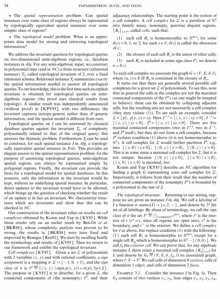
adjacency relationships. The starting point is the notion ofa cell complex. A cell complex for 7 is a partition of R2

into finitely many, nonempty, pairwise disjoint regions,[Rv]v # V , called cells, such that:

(1) each cell Rv is homeomorphic to R$(v), for some$(v)=0, 1, or 2; for each v # V, $(v) is called the dimensionof v ;

(2) the closure of each cell Rv is the union of other cells;

(3) each Rv is included in some sign class I _; we denote_=l(v).

To each cell complex we associate the graph G=(V, E, $, l ),where (u, v) # E iff Ru is contained in the closure of Rv .

It turns out that there are generally several possible cellcomplexes for a given set 7 of polynomials. To see this, notethat in general the cells in the complex are not the maximalconnected components of the I _'s (as one might be temptedto believe): these can be obtained by collapsing adjacentcells, but the resulting sets are not necessarily a cell complex(they may violate (1)). To see such an example, consider7=[ p], p(x, y)=xy. Here I+1=[(x, y) | xy>0], I&1=[(x, y) | xy<0], I0=[(x, y) | xy=0]. There are fivemaximal connected components (two in I +1, two in I&1,and I 0 itself ), but they do not form a cell complex, becauseI0 violates condition (1) above (it is not homeomorphic toR1). A cell complex for 7 would further partition I 0, e.g.,into [(x, 0) | x # R], [(0, y) | y>0], [(0, y) | y<0].This is in some sense a maximal cell complex for 7, but it isnot unique, because [(0, y) | y # R], [(x, 0) | x>0],[(x, 0) | x<0] is maximal, too.

Kozen and Yap [KY85] describe an NC algorithm forfinding a graph G representing some cell complex for 7:Importantly, it follows from their result that the number ofconnected components of the nonempty I _'s is bounded bya polynomial in the size of 7.

The topological invariant. Returning to our setting, sup-pose we are given an instance I in Alg. We call a labeling ofI a function _: names(I ) � [o, �, &], and denote by 3I theset of all labelings. By abuse of terminology, we call the signclass of _ the set I _ =def

�r # names(I ) r_(r), where ro is the inte-rior of r (ro=r, since all regions are open sets), r� is theboundary, and r& is the exterior. We define a cell complexfor I as above, but replace condition (1) with the following:(1$) each cell Rv is homeomorphic to R$(v), except for asingle cell Rf0

which is homeomorphic to R2&[(0, 0)]. Wecall f0 the exterior cell. We can prove that, for any algebraicinstance I, there exists a maximal cell complex [Rv]v # V forI, and denote by GI =def (V, E, $, f0 , l ) its associated graph,where l : V � 3I. We call cells of dimension 0 vertices, cells of

UCIU, AND VIANU

dimension 1 edges, and cells of dimension 2 faces.

Example 3.1. Consider the instance I in Fig. 1c. ThenGI consists of two vertices v1 , v2 , four edges e1 , e2 , e3 , e4 ,

and four faces, f0 , f1 , f2 , f3 ; see Fig. 5. The adjacency rela-tion E contains the edges

(v1 , e1), (v1 , e2), (v1 , e3), (v1 , e4),

(v2 , e1), (v2 , e2), (v2 , e3), (v2 , e4),

(e1 , f0), (e1 , f1), (e2 , f2), (e2 , f3),

(e3 , f3), (e3 , f1), (e4 , f0), (e4 , f2).

The labeling is

l(v1)=l(v2)=(A�, B�), l(e1)=(A�, B&),

l(e2)=(A�, Bo), l( f3)=(Ao, Bo), etc.

To see the importance of specifying the exterior cell, con-sider the instances I, I$ in Fig. 6. Both GI and GI$ have twovertices, five edges, and five faces. They coincide in theiradjacency relation E and their labeling l, except that GI 'sexterior cell is f0 , while GI$ 's exterior cell is f2 .

In summary, GI provides in a concise manner the follow-ing information: for each region name in names(I ), the cellsit contains (vertices, edges, faces); for each face, the edges onits boundary; for each edge, its endpoint(s); and finally theunbounded face, f0 .

It is worth noting that all the information provided by GI

is useful and essential. For example, the dimension $(v) of acell v # V cannot be determined from the its labeling: when,say, l(v)=(A�, B�), the dimension of v may be either 0 or 1.Also, the external face is not determined by the other infor-mation in GI . This is shown by Example 3.1. Note in par-ticular that the external face is not determined by its sign.Indeed, consider _=l( f0). Clearly, _(r)=&, \r # names(I ).However, f0 is not necessarily the unique such cell.

Before we proceed, we need the following terminology.Call a database instance I connected if �r # I r� is topologi-cally connected. Alternatively, I is connected if the subgraphof GI consisting only of vertices and edges (i.e., no faces) isconnected. For example, both database instances in Fig. 7aare nonconnected. Recall that a closed curve in the plane is

TOPOLOGICAL QUERIES

FIG. 5. The graph GI associated to an instance I.

FIG. 6. Except for the exterior cell, GI and GI$ are isomorphic.

simple, if it is non-self-intersecting.2 Call a database instanceI simple if the boundary of each face in GI is a simple curve.For example, all four instances in Fig. 1 are simple, whilethe four instances in Fig. 7 are not. A simple instance is alsoconnected, because otherwise it is easy to show that theboundary of the exterior cell is not a closed curve: theinstances in Fig. 7a illustrate this. The converse is not true:the two regions in Fig. 7b illustrate two connected instanceswhich are not simple (the boundary of the external face isnot simple).

GI is almost what we need for an invariant. Specifically,we have:

Lemma 3.2. Let I, I$ be simple spatial database instancesover Alg with names(I )=names(I$). Then I and I$ aretopologically equivalent iff GI and GI$ are isomorphic via anisomorphism which is the identity on names(I ). Moreover,any isomorphism . between GI and GI$ can be lifted to ahomeomorphism mapping I to I$.

Proof. Suppose first that I and I$ are spatial instancesover Alg such that names(I )=names(I$). It is clear that if Iand I$ are topologically equivalent, then GI and GI$ areisomorphic by an isomorphism which is the identity onnames(I ). Consider the converse. Let I, I$ be simple spatialinstances over Alg such that names(I )=names(I$), and sup-pose GI and GI$ , are isomorphic via an isomorphism whichis the identity on names(I ). We show that I and I$ aretopologically equivalent.

Let S be the union of all vertices and edges in the cellcomplex associated to I. We call S the skeleton of I : I is con-nected iff S is connected. Define S$ similarly for I$. S consistsof a finite set of points and edges, which are simple Jordancurves connecting two points. Since GI and GI$ areisomorphic, we can construct a homeomorphism *0 : S � S$(where both S and S$ are topological subspaces of R2),which extends the isomorphism from GI to GI$ , by patchingthe homeomorphisms between corresponding Jordan curves.


2 Formally, a closed Jordan curve is a continuous function.: [0, 1] � R2 such that .(0)=.(1). It is simple iff .(x)=.( y) with x{ yimplies [x, y]=[0, 1].

In order to extend *0 to a homeomorphism R2 � R2, we useScho� nflies' Theorem [Moi, pp. 72], stating that for anyclosed Jordan curve J, any homeomorphism *0 : J � R2 canbe extended to a homeomorphism *: R2 � R2. Namely, letRf be a two-dimensional cell in the cell decomposition asso-ciated to I, different from the exterior cell. Its boundary is aclosed Jordan curve, and we use Scho� nflies' Theorem toextend *0 to Rf (we discard the exterior part of the exten-sion). For the exterior cell Rf0

we proceed similarly, butkeep only the exterior part and drop the interior. Patchingtogether all *'s corresponding to different cells yields thedesired homeomorphism *: R2 � R2. K

Every homeomorphism *: R2 � R2 is isotopic to eitherthe identity or to a reflection [St93]: in short, there aretwo possible orientations for the homeomorphism *. InLemma 3.2, *'s orientation is uniquely determined by .,except for the degenerated case when both I and I$ consistof a single region (in this case GI has no vertices, one edgeand two faces). Indeed, it suffices to consider some face f inGI whose border has at least two vertices v1 , v2: it will alsohave at last two edges e1 , e2 , hence we have a unique orien-tation of f's border, and similarly a unique orientation of.( f )'s border. The relationship between these two orienta-tions dictates *'s orientation.

Lemma 3.2 cannot be extended to nonsimple instances.We illustrate this with the two examples in Fig. 7. In Fig. 7awe have two database instances I, I$ which are not con-nected. Here GI and GI$ are isomorphic, but I, I$ are nottopologically equivalent (there is no homeomorphism map-ping I to I$). Similarly for Fig. 7b, the two instances are con-nected, but not simple, because the boundary of the exteriorcell is a nonsimple curve, both in I and in I$.

It turns out that the only additional information neededto capture all topological information about nonsimpleinstances I is the order whereby all edges incident to eachvertex are arranged, clockwise say, around the vertex. This

36 PAPADIMITRIOU, S

FIG. 7. Two examples when GI , GI$ are isomorphic, but I, I$ are nottopologically equivalent.

is done by introducing a new relation O�[�# , /�]_V3,with the following meaning: (�# , v, e1 , e2) # O iff v is a ver-tex and e1 , e2 are clockwise consecutive3 edges incident to v,and (/� , v, e1 , e2) # O iff v is a vertex and e1 , e2 are coun-terclockwise consecutive edges incident to v. Note thatin the presence of loops at v, like in Fig. 7b, we may haveboth (�# , v, e, e), (/� , v, e, e) # O, or both (�# , v, e1 , e2),(/� , v, e1 , e2) # O for different e1 , e2 . We define thetopological invariant associated with an instance I to be thefollowing finite structure: TI=(V, E, $, f0 , l, O) whereGI=(V, E, $, f0 , l ) is the structure defined earlier, and O isdefined as above. Note that an isomorphism from TI to TI $ ,maps the set [�# , /�] to itself, possibly reversing theorientation.

Example 3.3. Continuing with the instance I in Fig. 1(recall also Fig. 5), the invariant TI would consist of theadjacency and labeling information (the graph GI) asdefined in the previous example, together with the followingorientation information:

O=[(�# , v1 , e1 ; e4), (�# , v1 , e4 , e2),(�# , v1 , e2 , e3), (�# , v1 , e3 , e1), (�# , v2 , e1 , e3),(�# , v2 , e3 , e2), (�# , v2 , e2 , e4), (�# , v2 , e4 , e1),(/� , v1 , e1 , e3)), (/� , v1 , e3 , e2),(/� , v1 , e2 , e4), (/� , v1 , e4 , e1), (/� , v2 , e1 , e4),(/� , v2 , e4 , e2), (/� , v2 , e2 , e3), (/� , v2 , e3 , e1), ].

We are now ready to show:

Theorem 3.4. Let I, I $ be spatial database instances overAlg with names(I )=names(I $). Then I and I $ are topologi-cally equivalent iff TI and TI $ are isomorphic via anisomorphism which is the identity on names(I ). Moreover,any isomorphism between TI and TI $ can be lifted to a homeo-morphism mapping I to I $.

Proof. Assume first that I is connected: this implies thatI $ is also connected. For each vertex v in GI , let e1 , ..., en bethe sequence of consecutive edges adjacent to v, in clockwiseorientation (note that an edge adjacent to v occurs once ortwice in the enumeration e1 , ..., en). Since all regions in I aresemi-algebraic, we can find a circle centered in v with aradius =v>0 small enough so that it intersects each edge eexactly as many times as e occurs in the sequence. LetDv=[p | p # R2, dist(p, v)<=v], and furthermore, assumethat the =v 's are small enough s.t. v{w O Dv & Dw=<.Construct similar discs D$v$ for I $. Let J =def I _ [Dv | v # V],J$ =def I $ _ [D$v$ | v$ # V$]: then both J and J$ are simple, bythe following argument. The faces in J either correspond toold faces in I with their corners chopped off or are new

UCIU, AND VIANU

3 Two edges e1 , e2 are consecutive if they share a face f and can be con-nected with a curve lying entirely in f, and which does note separate anyother two edges bordering f.

triangular faces. The first kind of faces will now have a simpleboundary even if the original face had not, because wechopped out the corners. For the second kind, it is easy tosee that each face with a triangle as a boundary (that is, withthree edges and three vertices) is simple.

Moreover, using the orientation information captured byO we will show that GJ and GJ$ are isomorphic. Hence J andJ$ are topologically equivalent by Lemma 3.2. It easilyfollows that I and I $ are also topologically equivalent.

So it remains to show that GJ , GJ$ are isomorphic. Let.: V � V$ be an isomorphism between TI and TI $ . We willextend it to an isomorphism between GJ and GJ$ . Take acloser look at how GJ is derived from GI . For some vertexv in GI , let us denote by L the circular list L=(e1 , f1 , e2 ,f2 , ..., ek&1 , fk&1 , ek , fk) consisting all outgoing edges fromv and adjacent faces, in clockwise fashion, as illustrated inFig. 8a. Note that we may have ei=ej , for i< j, when thereare loops in I : each edge e may occur once or twice in L.Moreover, a face may occur arbitrarily many times in L. Letv$=.(v), and let L$=(e$1 , f $1 , ..., e$k , f $k) be the circular listof edges and faces adjacent to v$ in GI $ , taken in clockwiseorder if .(�#)= �# , .(/�)=/� , and counterclockwiseotherwise. The notation does not imply that .(e1)=e$1 ,etc.4: all we know is that [.(e1), ..., .(ek)]=[e$1 , ..., e$k],and [.( f1), ..., .( fk)]=[f $1 , ..., f $k]. The key observation isthat the new vertices, edges, and faces in GJ ``around'' v areuniquely determined by the circular list L; see Fig. 8b.Namely, there are k new vertices u1 , ..., uk , 2k new edges,and k new faces. To prove that GJ and GJ$ are isomorphic,it suffices to show that . maps the circular list L into L$, i.e.,that there exists i�1 such that

(.(e1), .(f1), ..., .(ek), .( fk))

=(e$i , f $i , e$i+1 , f $i+1 , ..., e$i&1 , f $i&1) (1)

Before proving this, we make an observation about L (andL$): any consecutive edge�cell or cell�edge pair is unique inL. That is, for i< j, we have (ei , fi){(ej , f j) and ( fj&1 , e i){( fj&1 , ej). Back to proving (1), consider .(e1). There canbe at most two i 's for which ei$=.(e1): if there are two such,then we will pick that i for which .( f1)= f i . When there isa single i s.t. e$i=.(e1), we show that .( f1)= f $i . Indeed,then we have (�# , v, e1 , e2) # O; hence (.(�#), v$,.(e1), .(e2)) # O$. But we also have (.(�#), v$, e$i , e$i+1) # O$;hence e$i+1=.(e2). Now f1 is a common face for e1 and e2 ,so both .( f1) and f $i are common faces for e$i , e$i+1 . It is easyto show, in general, that in any cell complex, two edgessharing a common vertex v$ can have at most one commonface. Hence .( f1)= f $i . So we have chosen i such that (1)

TOPOLOGICAL QUERIES

4
L and L$ have the same length, because the length of L is uniquelydetermined by the number of edges incident to v and by the number of``loops'' at v, i.e., edges having v as the unique endpoint. Since GI and GI $
are isomorphic, it follows that L, L$ have the same length.

holds on the first two positions. We will prove that it holdson all positions. Comparing from left to right the twosequences in (1), consider the first position where they differ.If this is a face, then we have .( fj&1)= f $i+ j&2 , .(ej)=e$i+ j&1 , .( f j){ f $i+ j&1 . This is a contradiction, becausefj&1 , f j are the unique two faces adjacent to ej in GI andtherefore are mapped by . into f $i+ j&2 , f $i+ j&1 , which arethe unique two faces adjacent to e$i+ j&1 in GI $ . So supposeL, L$ differ first at an edge, i.e., .(ej&1)=e$i+ j&2 , .( f j&1)=f $i+ j&2 , .(e$j){e$i+ j&1 . Let e$=.(ej). Here we use theorientation information. We have (�# , v, ej&1 , ej) # O;hence (.(�#), v$, e$i+ j&2 , e$) # O$. This implies that e$i+ j&2

must occur a second time in L$, followed by e$. Moreover,f $i+ j&2 is the only common face to e$i+ j&2 , e$, so there existsp{ j such that e$i+ p&2=ei+ j&2 , f $i+ p&2= f $i+ j&2,e$i+ p&1=e$. But this is a contradiction because, as we saidearlier, any edge�face pair (ei+ j&2 , f i+ j&2) occurs at mostonce in the circular list L$.

Now assume that I is not connected (recall that thismeans its skeleton is not connected). For clarity assume thatit consists of two connected components I=I1 _ I2 and,hence, so does I $, I $=I $1 _ I $2 . Let us call .: TI � TI $ , theisomorphism between the first-order structures TI and TI $ :this splits into two isomorphisms .1 , .2 between TI1

and TI $1and TI2

and TI $2, respectively, which, in turn, extend to

homeomorphisms *1 , *2 , mapping I1 to I $1 and I2 to I $2 . Byapplying the construction above we can ensure that both I1

and I2 are simple. It is easy to see that all regions in I2

lie entirely inside one of the two-dimensional cells Rv of TI1

(not necessarily the exterior cell). Recall that everyhomeomorphism *: R2 � R2 is isotopic either to the identityor to a reflection. It is possible to show that we can join *1

and *2 together into a homeomorphism mapping I to I $,provided that *1 , *2 have the same ``orientation,'' i.e., areeither both isotopic to the identity, or both to a reflection.Hence we distinguish two cases:

1. We can choose the orientation of either *1 or *2 : sincewe assumed I1 , I2 to be simple, by the observation afterLemma 3.2 this is possible only if I1 (or I2) is degenerated,i.e., consists of a single region. Then we simply arrange for*1 , *2 to have the same orientation and are done.

2. The orientations of *1 and *2 are imposed and dis-agree (if they agree then we are done, of course). It is nothard to see that *1 is isotopic to the identity when.(�#)= �# , .(/�)= /� , and is isotopic to a reflectionwhen .(�#)= /� and .(/�)= �# . Similarly for *2 .This leads to a contradiction, since *1 , *2 have differentorientations. K

Theorem 3.4 says that each H-equivalence class of spatial


instances over Alg is characterized by its topologicalinvariant. Furthermore, the invariant, as well as a repre-sentative instance in Poly, can be constructed efficiently.

)
FIG. 8. Illustration of GI (a) and GJ (b
Theorem 3.5. For each instance I in Alg, we can com-pute in polynomial time (and in NC) the invariant TI , and aninstance I $ in Poly such that TI=TI $ .

Proof. For I in Alg, TI can be computed in NC using thecell decomposition algorithm of [KY85]. The topologicalinvariant also allows us to construct, for each H-equiv-alence class, a representative instance over Poly, as follows.

A classical result in graph theory known as Fa� ry'sTheorem [Fa� 48, Wag36, St51] states that any planar graphcan be embedded in, the plane so that all of its edges arestraight lines (except of its loops, of course, which can be tri-angles). Furthermore, this can be accomplished in lineartime. Notice that, once such a representation of the skeletonof I has been obtained, it can serve, appropriately labeled,as a representative instance over POLY. It is interesting toask whether such a representation (call it a Fa� ry representa-tion) can be obtained in NC ; we outline below an argumentthat it can. We are not aware of an explicit proof of thisresult in the literature, although, as we point out in whatfollows, such a proof does follow rather easily from knowntechniques and concepts.

If the graph is triply connected, then the standard parallelplanarity algorithms [JS85] produce a Fa� ry representation.In particular, a Fa� ry representation of a triply connectedgraph can be obtained by the following algorithm attributedto Tutte [Tut63]: Start by choosing one of the faces asouter, and embed it as an arbitrary convex polygon. Thenplace the remaining vertices on the plane so that each vertexis at the center of gravity of its adjacent nodes. This canbe accomplished by solving a square system of linearinequalities (one equation and one unknown for each vertexnot on the outer face), a task well known to be achievablein NC [KR91].

For a general graph, suppose that we have decomposed

38 PAPADIMITRIOU, S

the graph into triply connected components (this can bedone in NC) and that we have found, as above, Fa� ryrepresentations of all triply connected components, where

. In this example e1=e6 , f1= f3= f5 , etc.

each component represents the adjacent components asedges. We can then find a Fa� ry representation of the wholegraph as follows: We start from a component C and identifythe edges that stand for other components. Suppose thatedge [u, v] of C is indeed a triply connected component C$.We can assume that we have embedded all triply connectedcomponents so that u and v are on the outermost face of C$mapped to [(0, 0), (0, 1)], while the whole Fa� ry representa-tion of C$ fits within the ((&1, 0), (1, 0), (1, 1), (&1, 1))rectangle. Furthermore, without loss of generality thereare positive constants a, b>0 such that edge [u, v] of C ismapped to the segment [(0, 0), (0, a)] on the plane andthe image of no edge of C$ intersects the rectangle((&b, 0), (b, 0), (b, 1), (&b, 1)) (we can achieve this by arotation). In fact, the constants a and b can be taken to berational numbers involving integers bounded by anexponential in the number of nodes in C, as they are theresult of the solution of a system of that many linear equa-tions. By scaling the coordinates of the images of the nodesof C$ in the Fa� ry representation of C$ by a and b, we canembed C$ within this rectangle. (The case in which two ormore components are embedded in the same edge [u, v] ishandled similarly; the edges of the components adjacent tou and v may have to be represented by two line segments.)

Once all components adjacent to C have been embedded,we embed in them their adjacent components, and so on.The key observation for achieving all this (seeminglysequential) process in NC is that the graphs need not beembedded sequentially, but that the linear coordinate trans-formations that implement the embeddings can be com-posed in NC. The numbers involved, each being the productof polynomially many numbers, each with polynomiallymany bits, are of polynomial size.

Finally, once a Fa� ry representation of I has beenobtained, its nodes, edges, and faces can be labeled by the

UCIU, AND VIANU

regions of I through the embedding correspondence. Theresulting instance I$ in POLY obviously has the sameinvariant as I. K

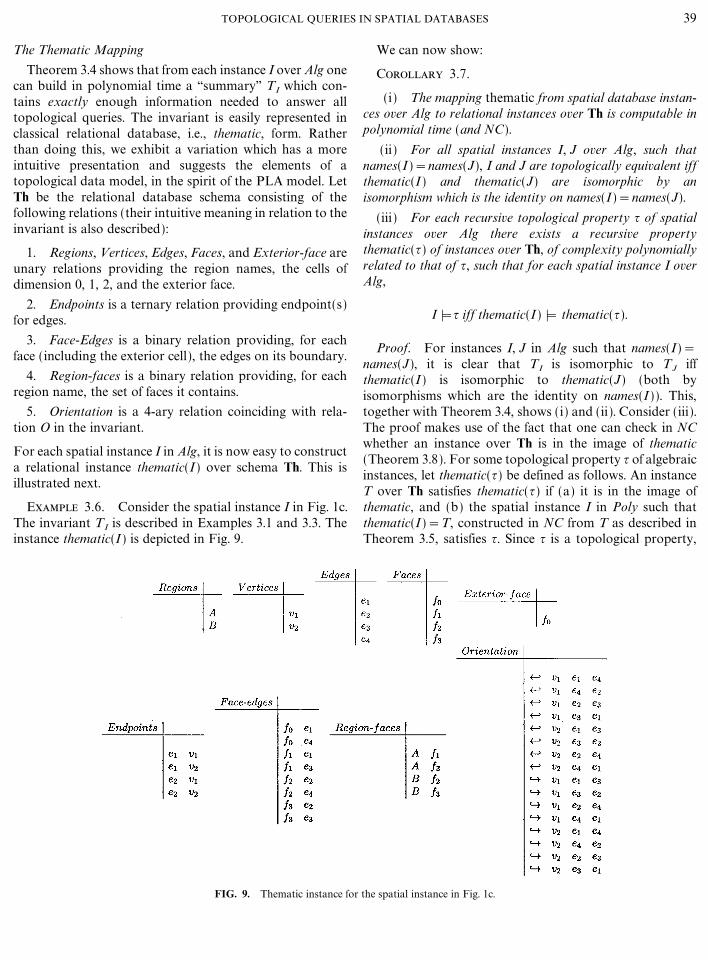
The Thematic MappingTheorem 3.4 shows that from each instance I over Alg one

can build in polynomial time a ``summary'' TI which con-tains exactly enough information needed to answer alltopological queries. The invariant is easily represented inclassical relational database, i.e., thematic, form. Ratherthan doing this, we exhibit a variation which has a moreintuitive presentation and suggests the elements of atopological data model, in the spirit of the PLA model. LetTh be the relational database schema consisting of thefollowing relations (their intuitive meaning in relation to theinvariant is also described):

1. Regions, Vertices, Edges, Faces, and Exterior-face areunary relations providing the region names, the cells ofdimension 0, 1, 2, and the exterior face.

2. Endpoints is a ternary relation providing endpoint(s)for edges.

3. Face-Edges is a binary relation providing, for eachface (including the exterior cell), the edges on its boundary.

4. Region-faces is a binary relation providing, for eachregion name, the set of faces it contains.

5. Orientation is a 4-ary relation coinciding with rela-tion O in the invariant.

For each spatial instance I in Alg, it is now easy to constructa relational instance thematic(I ) over schema Th. This isillustrated next.

Example 3.6. Consider the spatial instance I in Fig. 1c.The invariant TI is described in Examples 3.1 and 3.3. Theinstance thematic(I ) is depicted in Fig. 9.

TOPOLOGICAL QUERIES

FIG. 9. Thematic instance for

We can now show:

Corollary 3.7.

(i) The mapping thematic from spatial database instan-ces over Alg to relational instances over Th is computable inpolynomial time (and NC).

(ii) For all spatial instances I, J over Alg, such thatnames(I )=names(J), I and J are topologically equivalent iffthematic(I ) and thematic(J) are isomorphic by anisomorphism which is the identity on names(I)=names(J).

(iii) For each recursive topological property { of spatialinstances over Alg there exists a recursive propertythematic({) of instances over Th, of complexity polynomiallyrelated to that of {, such that for each spatial instance I overAlg,

I <{ iff thematic(I ) < thematic({).

Proof. For instances I, J in Alg such that names(I)=names(J), it is clear that TI is isomorphic to TJ iffthematic(I ) is isomorphic to thematic(J) (both byisomorphisms which are the identity on names(I )). This,together with Theorem 3.4, shows (i) and (ii). Consider (iii).The proof makes use of the fact that one can check in NCwhether an instance over Th is in the image of thematic(Theorem 3.8). For some topological property { of algebraicinstances, let thematic({) be defined as follows. An instanceT over Th satisfies thematic({) if (a) it is in the image ofthematic, and (b) the spatial instance I in Poly such thatthematic(I )=T, constructed in NC from T as described inTheorem 3.5, satisfies {. Since { is a topological property,


the spatial instance in Fig. 1c.

thematic({) does not depend on the particular choice of Iand so is well defined. K

In summary, it should be clear from our discussion thatfor a spatial instance I in Alg, TI and thematic(I ) are basi-cally cosmetic variants of each other. Also, it is easy toobtain thematic(I) given TI , and conversely. The invariantTI has the advantage of being closer to existing formalismdeveloped in the context of computational geometry (e.g.,[KY85]) while thematic(I ) is closer to topological datamodels. We note that, as a model for topological spatialinformation, thematic(I) can be viewed as an augmentationof the PLA model of [Cor79] (see also descriptions in[LT92, Par95]).

If topological invariants are to be used as a model fortopological spatial databases, it becomes important tocheck whether a given instance over Th is in fact in theimage of the thematic mapping. Indeed, this functions as anintegrity constraint when updates are performed. Clearly,not every instance over Th is a valid specification of atopological invariant. There are obvious integrity con-straints satisfied by every instance in the image of thematic.For example, the instance must represent a graph, so ver-tices and edges are disjoint sets and each edge has one ortwo endpoints (which must be vertices). But there are alsomore subtle constraints, such as the fact that Euler's for-mula must hold, that is, |Faces|=|Edges|& |Vertices|+2.To fully characterize the instances over Th which describevalid topological information, we characterize instanceswhich are invariants as labeled planar graphs. This will allowus to show the following:

Theorem 3.8. It can be checked in NC whether aninstance over Th is the image of a spatial instance over Alg viathe thematic mapping.

Closely related to this result is an elegant characterizationprovided independently in [KPV95] for a slightly differentthematic mapping.

We next present the characterization of topologicalinvariants as labeled planar graphs. This provides a purelycombinatorial (that is, with no recourse to geometry)characterization of the invariants. Although the definitionof labeled planar graph is common knowledge amongresearchers in algorithmic graph theory, we have beenunable to find a rigorous standard exposition.

The Topological Invariant as Labeled Planar Graph

In order to prove Theorem 3.8, consider an instance overTh. We use the terms vertex, edge, face, and exterior face forelements of relations Vertices, Edges, Faces, and Exterior-face, respectively. We begin by identifying some very basic

40 PAPADIMITRIOU, S

requirements of every instance which is in the image ofthematic, which essentially ensure that the instancerepresents a graph:

(1) Vertices, Edges, Faces, and Regions are pairwisedisjoint and Exterior-face consists of a single element inFaces. ?1 (Orientation) has two elements.

(2) ?1 (Endpoints ) � Edges, ?2 (Endpoints ) � Vertices,?1(Face �Edges)�Faces, ?2(Face� Edges)�Edges, ?2(Region& Faces ) � Faces, ?1 (Orientation ) has two elements,?2 (Orientation) = Vertices, ?3 (Orientation) _ ?4 (Orienta-tion) � Edges.

(3) Every edge has one or two vertices as endpoints (asspecified by relation Endpoints).

Call an instance satisfying (1)�(3) a candidate graph. Acandidate graph is connected if it is connected in the usualsense.

Notice that nothing has been said so far about the mean-ing of faces or of the orientation given in a candidate graph.Recall that the orientation is supposed to provide, for eachvertex, the clockwise and counterclockwise orientation of itsincident edges. This yields the following additional require-ment:

(4) For each ! # ?1 (Orientation) and v # Vertices,?3, 4 (_1=!, 2=v (Orientation)) is a cyclic permutation ofedges.

For a graph satisfying (4), let us fix ! # ?1 (Orientation) anddenote by ?v the cyclic permutation ?3, 4 (_1=!, 2=v (Orienta-tion)), for each vertex v. Intuitively, ?v is a clockwise (orcounterclockwise) arrangement of the edges incident upon v.

There is an important connection between faces and theorientation of edges. If e, f are edges that share an endpointv and are on the boundary of a face, then e and f are con-secutive with respect to ?v . This yields the next requirementon the candidate graph:

(5) For each face f and edge e of f, there is a unique edgee$ of f such that e and e$ share an endpoint v, and e, e$ areconsecutive edges (in this order) in ?v , and there is a uniqueedge e" of f such that e" and e share an endpoint u, and e",e are consecutive edges in ?u . That is to say, faces are sets ofclosed paths.

Let us call a candidate graph satisfying (4)�(5) an embeddedgraph. Unfortunately, we are not quite done: there are em-bedded graphs which are not invariants, because they cannotbe drawn in a planar fashion. For example, each such embeddedgraph, provided it is connected, must satisfy Euler's formula:

(6) |Faces|=|Edges|&|Vertices|+2.

A connected embedded graph satisfying (6) is called a con-nected planar graph.

To generalize this to the case when the embedded graphis not connected is not very hard, and we sketch one waybelow. Intuitively, the connected components of the graph

UCIU, AND VIANU

must be embedded in some face of one another; this``embedded-in'' relation is a tree. The faces of the overallgraph now contain the edges of the unbounded faces of the

graphs embedded in them. The unbounded face of the wholegraph is that of the root of the tree. Such an embeddedgraph is called a planar graph.

The last point to be dealt with is the assignment of facesto region names. We have to make sure that each region canbe embedded in the plane as a disc. This is done using thenotion of dual graph. The dual graph of a planar graph is agraph with Faces as nodes and with two faces connected iffthey share an edge. For example, the dual graph of theplanar graph in Fig. 5 is the graph consisting of the cycle[ f0 , f1 , f3 , f2]. The condition desired is now the following:

(7) For each X # Regions, let faces(X) be the set of facesin X (provided by Region-faces). Then for each region nameX, (i) the restrictions of the dual graph to faces(X) and toFaces�faces(X) are connected graphs, and (ii) f0 � faces(X)where f0 is the exterior face.

A planar graph satisfying (7) is called a labeled planar graph.For example, it is easily seen that the structure over Th in

Fig. 9 is a labeled planar graph.The following can now be shown:

Lemma 3.9. An instance over Th is an invariant iff it is alabeled planar graph.

Checking that a graph (an instance over Th) is a labeledplanar graph can be done in NC, since it only involves onlyarithmetic and variants of graph connectivity.

This observation, together with Lemma 3.9, yieldsTheorem 3.8.

4. REGION-BASED LANGUAGES

Recent work on constraint query languages [KKR90,GS94, GST94, Par+95, BDLW98] has focused onlanguages which have finitely specified regions as inputs andwhose variables range over reals and�or points. Here weinvestigate query languages for which both data andvariables range over regions. These languages can be viewedas natural closures of the four-intersection relationshipsunder first-order operators. The various languages we con-sider have the same syntax, but vary in the set of regionsover which their quantifiers range; this yields in effect afamily of region-based languages.

The syntax uses region variables p, r, ..., name variablesa, b, c, ..., and name constants A, B, ... from Names. A nameexpression is either a (a name variable) or A from Names.Region expressions are either a region variable or ext(a) fora a name expression. Atoms are expressions a=b with a, bname expressions, or relationship ( p, q) where relationship isone of the four-intersection relationships, and p, q areregion expressions. The boolean connectives and quantifiers

TOPOLOGICAL QUERIES

are standard. We will drop the ext(&) notation wheneverit is clear from the context; e.g., we will write _p . in-side( p, A) 7 inside( p, B) 7 inside( p, C) for the query testing

whether A & B & C{<, instead of the official _p . in-side( p, ext(A)) 7 inside( p, ext(B)) 7 inside( p, ext(C)). Fora given database instance I, the name variables range overnames(I ) (which is a finite set). The region variables rangeover an infinite set of regions, independent of I, consisting ofall regions of a certain type. Each of the languages weconsider is parameterized by both the type of regionsover which region variables range and the type of theinput regions as follows: FO(Region, Region$) denotes thelanguage where region variables range over Region andinputs are of type Region$. We always assume Region to bea basis of open sets5 for the topology on R2.

We shall denote by FOG(Region, Region$) the subsetof queries expressible in FO(Region, Region$) which areG-generic relative to Region$.

We note that the languages FO(Region, Region$) canbe assumed to only use the four-intersection relationshipdisjoint or, equivalently, its negation connect(r, r$) =def

cdisjoint(r, r$), which is topologically equivalent to r� &r� ${< (r� is the topological closure of r). Indeed, first observethat r�r$ is expressed as \r". (connect(r, r")Oconnect(r$, r")).We have overlap(r, r$)=_r". (r"�r 7 r"�r$) 7 c(r�r$)7 c(r$�r), meet(r, r$)=connect(r, r$) 7 coverlap(r, r$)7c(r�r$) 7c(r$�r), etc. Note that r�r$ & r" can be ex-pressed as r�r 7 r�r" and that r�r$ _ r" can be expressedas \q .connect(r, q) O connect(r$, q) 6 connect(r", q).

Example 4.1. We illustrate FO(Region, Region$), whereRegion can be any of Rect, Rect*, Poly, Alg, Disc. Considerthe two database instances I, I$ in Figs. 1a and 1b.The followingquery . separates them, in the sense that I < . butI$ <% . : .=_r . (r�A & B & C).

Example 4.2. We can test in FO(Region, Region$)whether a set is topologically connected, provided that werestrict Region to Rect*, Poly, Alg, Disc (i.e., it cannot beRect). Consider the two instances in Figs. 1c and 1d: theyare separated by \r .\r$ . (r _ r$�A & B O _r". (r"�A & B7connect(r", r) 7connect(r", r$))). Next consider the instancesI, I$ in Fig. 7b: they are separated by the query _r ._r$ .path(A, r, B) 7 path(C, r$, D) 7 r & r$=<. Here and in whatfollows we will use the ambiguous notation path(A, r, B) tomean that ``r is a path from A to B without touching theother regions,'' in our case: connect(A, r) 7 connect(B, r) 7cconnect(C, r) 7 cconnect(D, r). Finally, consider theinstances I, I$ in Fig. 7a. They are separated by the followingquery:

c(_r ._r$ ._r". path(A, r, D) 7 path(B, r$, E)


7 path(C, r", F ) 7disjoint(r, r$, r"))

5 That means that every r # Region is open, and for every open set s�R2

and every point x # s, there exists r # Region s.t. x # r�s.

i
FIG. 10. Groups with respect to which var
Consider a group G of permutations of the space. When-ever both Region and Region$ are invariant under G, allqueries expressed in FO(Region, Region$) are G-generic. Itfollows that the languages FO(Region, Disc) are genericwith respect to the groups shown in Fig. 10. Interestingly,even if Region and Region$ are not G-invariant, queries inFO(Region, Region$) may be G-generic (relative to Region$).Indeed, using a straightforward variant of the Ehren-feucht�Fraisse� games for FO and Theorem 3.4 we prove:

Proposition 4.3. All queries expressible in FO(Alg,Alg) and FO(Poly, Poly) are H-generic.

Proof. We sketch the proof for FO(Alg, Alg); the onefor FO(Poly, Poly) is similar. Given two homeomorphicinstances I, J in Alg, we have to show that

I < . � J < . (2)

for any formula . in FO(Alg, Alg).We define an Ehrenfeucht�Fraisse� game with unbounded

number of moves, which is played on two homeomorphicinstances I, J in Alg. As usual, the game is played by twoplayers, Spoiler and Duplicator. In the first move, Spoileraugments one of the instances, say I, with an additionalregion I1 in Alg, and Duplicator responds by augmenting Jwith a new region J1 in Alg. This is repeated, with Spoilerchoosing again one of the instances and Duplicator re-sponding in the opposite instance. Let I1 , ..., Ik be theregions added to I after k moves, and J1 , ..., Jk be thoseadded to J. A round of the game consists of a sequence ofpairs [(Ii , Ji)]1�i�k as above. The Duplicator wins theround [(Ii , Ji)]1�i�k if I augmented with I1 , ..., Ik and Jaugmented with J1 , ..., Jk are isomorphic as finite, first-order structures: this amounts to connect(Im , In) � connect(Jm , Jn), for m, n=1, k. The Duplicator has a winningstrategy if he can win any round k of any game, no matterhow Spoiler plays. Let us denote by IrJ the fact thatDuplicator has a winning strategy on I and J. The followingcan now be shown for I and J in Alg:

42 PAPADIMITRIOU, S

FIG. 11. Relationships between various languages FO(Region, Region$),for Alg, and * for disc.

ous languages FO(Region, Disc) are generic.

(-) if IrJ then I#FO(Alg, Alg) J ;

(�) if I and J are topologically equivalent then IrJ.

Note that the proposition follows from, (-) and (�). Theproof of (-) is as for classical games. We sketch a proof for(�). We show that the duplicator has a winning strategy ina harder game, namely in which he is required to makeI1 , ..., Ik homeomorphic to J1 , ..., Jk , for every k>0. Wehave to show that Duplicator can maintain indefinitely thehomeomorphism between the constructed instances, nomatter how Spoiler plays. Suppose I$, J$ extending I, Jhave been constructed and are homeomorphic by somehomeomorphism *, and suppose Spoiler augments I$ with Ik

(in Alg), yielding I". Clearly, J$ augmented with *(Ik) ishomeomorphic to I". Unfortunately, Duplicator cannotsimply choose .(Ik), since this region is not necessarily inAlg (we only know it is a disc). However, it is easily seenthat there exists a Jk in Alg (and even in Poly) such that J$augmented with Jk is homeomorphic to I". Intuitively, Jk isobtained by approximating the boundary of .(Ik) with apolygon closely enough that it generates the same topologi-cal invariant as .(Ik) (we omit the details). K

Relative Expressiveness

With some exceptions, the languages FO(Region,Region$) are incomparable. The following theorem summa-rizes their relationships when inputs range over Alg andDisc. This is mainly due to the different nontopologicalqueries they express: by restricting ourselves to topologicalqueries we obtain a nice hierarchy, which justifies in parttheir choice in this paper.

Theorem 4.4. The relationships of Fig. 11 hold betweenthe various languages FO(Region, Region$), for Region$ #[Alg, Disc]. Moreover:

FOH (Rect, Alg)/FOH (Rect*, Alg)=FOH (Poly, Alg)

=FOH (Alg, Alg)/FOH (Disc, Alg).

UCIU, AND VIANU

for Region$ # [Alg, Disc] : * denotes ``incomparable.'' The last entry is /

Proof (sketch). To prove most of the incomparabilityresults, consider, for some language FO(Region, Disc), thequery QRegion=(_r .r=A), stating that input region A is inRegion. To prove that FO(Region, Disc)�3 FO(Region$,Disc), it suffices to check in Fig. 4 that Region is notinvariant under the group G associated to FO(Region$,Disc) in Fig. 10. This proves all * entries except the thirdentry in the third column and those in the last column, andproves the � relationships for the last column. We use thecomplexity-theoretic arguments of Theorem 6.1 to provethe $3 relationships of the first and last column. The third *entry in the third column is proven by a standard game-theoretic argument. Finally FO(Rect, Disc)�FO(Rect*,Disc) follows from the following fact:

(-) FO(Rect*, Rect*)

can express the query ``is r a rectangle?''

TOPOLOGICAL QUERIES

FIG. 12. (a) How to encode a set X of three disjoint rectangles (black)of three nondisjoint rectangles as two sets X1 , X2 of disjoint rectangles and ain Rect* (not shown). Each r is uniquely determined by two rectangles r1 # Xby specifying three rectangles B1 , B2 , B which are bounding boxes for X1 , X

To prove (-), let

edge(r, r$) =def meet(r, r$)

7 _r" . (overlap(r, r") 7overlap(r$, r"))

be the predicate testing whether r, r$ meet and have at leasta nonzero length portion of an edge in common (meet(r, r$)only ensures that r� & r� {< and r & r=<, so r and r$ maytouch at a corner). Next, let corner(r, r$) =def meet(r, r$) 7cedge(r, r$). Then some r # Rect* is a rectangle when ``ithas exactly four corners,'' i.e., when there exist four pairwisedisjoint regions r1 , r2 , r3 , r4 cornering r, but there do notexist five such regions. K

As an aside, the relationship between FO(Rect, Region$)and FO (Rect*, Region$ ) is further illuminated by thefollowing result. We define the second-order query languageSO(Rect, Region$) by extending FO(Rect, Region$) as


as an intersection r1 & r2 , with r1 , r2 # Rect*. (b) How to encode a set X``correspondence'' C: hereC is represented as the intersection of two regions

1 , r2 # X2 in ``correspondence.'' The choice between r and its mirror is made

2 , and X, respectively (not shown), and requiring that r�B.

follows. The language uses second-order variablesX, Y, Z, ..., and atoms r # X, where r is a region variable.Both _X and \X quantifiers over the second-order variablesare allowed. The meaning is that the second-order variablesrange over finite sets of regions in Rect. A common queryin SO(Rect, Region$) is chain(X), testing whether X=[r1 , r2 , ..., rn] is such that connect(ri , ri+1), i=1, n&1 andc(connect(ri , rj)) for |i& j |>1. Namely we express chain(X)as _r1 ._rn . (r1 # X7 rn # X 7�), where � asserts that anyother r # X different from r1 , rn is connected to exactly tworegions in X, while r1 , rn are each connected to exactly oneregion in X.

Proposition 4.5. The following holds:

SO(Rect, Region$)=FO(Rect*, Region$).

Proof. The above result is quite intuitive, since quantify-ing over regions in Rect* is, in some sense, quantifying oversets of regions in Rect. But there are subtle technical dif-ferences between the two languages, since an arbitrary finiteset X of rectangles does not correspond immediately to aregion in Rect* (� X may be disconnected, or may haveholes). We sketch the proof below.

For FO(Rect*, Region$)�SO(Rect, Region$), let . be aformula in FO(Rect*, Region$). We replace each quantifier_r in . (where r ranges over Rect*) with _X . isDisc(X),and replace every subformula connect(r, ...) with _r$ # X .connect(r$, ...). Here isDisc(X) tests whether � X is in Disc,i.e., is topologically connected and has no holes. We can testconnectedness, because we can quantify over chains, seeabove. Testing whether � X has no holes amounts to testingwhether its complement is connected.

For the converse, SO(Rect, Region$)�FO(Rect*,Region$), we have to replace first-order quantifiers _r0 overRect with quantifiers over Rect*, and second-order quanti-fiers _X over finite sets or regions in Rect with quantifiersover Rect*. The first part is simple, because we can expressisRect(r) in FO(Rect*, Region$); see the proof of Theorem4.4. To see the difficulties for the second-order quantifier,not that even when � X is a disc, r=� X does not captureaccurately the information held by X, because there may beseveral ways to decompose r into a union of rectangles. Thefirst idea is to represent X as the intersection of two regionsr1 , r2 # Rect*: this works if all rectangles in X are disjoint,as illustrated in Fig. 12a. So assuming all rectangles in X tobe disjoint, we can replace the quantifier _X with _r1 _r2 ,and the atomic formulas r # X with isRect(r) 7 r�r1 7 r�r2 7 ``r is maximal such.'' So it suffices to observe that anarbitrary set X of rectangles can be encoded in terms of twosets X1 , X2 of disjoint rectangles, an a set C of correspondences;

44 PAPADIMITRIOU, S

see Fig. 12b. Here X, X1 , X2 all have the same number ofrectangles: n. The set C defines a bijection between the rect-angles in X1 and those in X2 : it consists of n disjoint chains,

each connecting some r1 # X1 with some r2 # X2 . We do nothave to express C in SO(Rect, Region$), but rather inFO(Rect*, Region$), as the intersection of two regions inRect*. The idea is that each rectangle r # X can be uniquelyidentified in FO(Rect*, Region$) from its two correspondingrectangles r1 # X1 , r2 # X2 , as having r1 , r2 as ``cartesiancoordinates''; see Fig. 12b. There is a single remaining twisthere: r has a mirror image having the same cartesian coor-dinates r1 , r2 , so it is not uniquely identifiable. To distinguishit from its mirror image, we define bounding boxes q, q1 , q2

for X, X1 , X2 , such that q1 , q2 are the cartesian coordinatesof q, require that the mirror image of q be disjoint from q,and finally require for all rectangles r # X, to satisfy r�q.We leave the details to the reader. K

5. COMPLETENESS

As promised, we will show that the closure of thefour-intersection relationships under appropriate logicaloperators is, in some sense, complete. We present two typesof results: first, we aim for ``absolute'' completeness byshowing how all topological properties of inputs over Algcan be expressed in languages based on the four-intersectionrelationships. Second, we look at ``relative'' completenessresult that take as their reference a point-based spatiallanguage: here we show that FO(Rect, Disc) expressesprecisely the same topological properties as those definablein the point-based language.

Absolute Completeness

We have seen that the pairwise four-intersection rela-tionships between pairs of regions in an instance are not suf-ficient to determine the input up to homeomorphism (seeFig. 1). However, the information provided by their first-order closure, in the style of our region-based languages, issufficient. The proofs use the topological invariants discussedat length in Section 3. This works for inputs in Alg, but notfor general inputs in Disc. The restriction to semi-algebraicregions is needed because, as discussed in Section 3, everydatabase instance in Alg has a topological invariantexpressible as a finite structure. For database instances inDisc the corresponding structure may be infinite.

Let #FO(Region, Alg) be the equivalence relation on spatialinstances over Alg defined as follows: I#FO(Region, Alg) J iff Iand J cannot be distinguished by sentences in FO(Region,Alg). Also, let I#H J denote the fact that I, J are H-equiv-alent. We will make use of the following key definabilityresult:

Proposition 5.1. Each H-equivalence class of spatialinstances over Alg is definable by a sentence in any of the

UCIU, AND VIANU

languages FO(Rect*�Disc, Alg).

Proof. For each instance I over Alg we construct a sen-tence .I that tests whether the topological invariant of

an instance I$ is isomorphic to TI . Then .I defines theH-equivalence class of I. First, .I checks if names(I$)=names(I ) = [R1 , ..., Rn] :.I=_a1 , ..., an . (�1�i�n ai = Ri) 7\a . (�1�i�n a=Ri) 7 �. Next, � checks whether a1 , ..., an

satisfy precisely the same topological relationships as dictatedby TI . For this, we start by picking a region rv for each cellRv , v # V : �=_r1 , ..., r |V| .|. Here, the problem is that zero-and one-dimensional cells Rv are not regions; hence we cannotrefer to them in the language FO(Region, Alg). Instead, in �we quantify over regions rv and state their relationship tothe cells Rv in |. Namely | ``says'' that the regions rv are dis-joint, that they are in one-to-one correspondence with thecells Rv in TI , and that their topological relationships arethose of TI . We explain next the one-to-one correspondenceand how to express it in |. For two-dimensional cells Rv ,the correspondence is rv �Rv ; for one-dimensional cells it isrv & Rv {<, while for vertices, it is simply Rv # rv . To statethat correspondence in |, recall that TI has a labelingcomponent l : V � 3I, assigning to each v a labell(v): names(I) � [o, �, &]: we will identify names(I) with[a1 , ..., an]. We illustrate how | expresses the corre-spondence for zero-dimensional cells v: one- and two-dimensional cells are treated similarly. Here | states over-lap(rv , ai) for every ai s.t. l(v)(ai)=�, rv �ai for every ai s.t.l(v)(ai)=o, and disjoint(rv , ai) for every ai s.t. l(v)(a i)=&.Note that if l(v)=l(v$) then | imposes the same conditionson rv and rv$ . Since, in addition, | states that the rv's aredisjoint, this ensures a one-to-many correspondence fromthe rv 's (associated to zero-dimensional cells) to the Rv 's:we force it to become one-to-one by imposing for any v # Vthat, for any other region r satisfying the same conditionsas rv , r must overlap with one of the regions rv , rv$ , rv" , ...having the same label as v (i.e., �l(v)=l(v$) overlap(r, rv$)).Finally, | checks, one by one, all relationships in TI . First,it checks that f0 is the exterior face: _r .a1 �r 7 } } } 7an �r 7 c(connect(r, rf0

)). Next check the adjacency rela-tionships in E. For an edge�face pair (e, f ) # E, check_r . path(re , r, rf), where path is in the spirit of Example 4.1:here it checks that r is connected to both re and rf , that it liesentirely in the regions ai for which the label of f isl( f )(ai)=o, and that it is disjoint from all regions ai forwhich l( f )(ai)=&. For a vertex�edge pair (v, e) # E andvertex�face pair (v, f ) # E we proceed similarly, with minorvariations. Finally, we check the orientations enforced byTI , using the idea in Example 4.1 to separate the instancesin Fig. 7a. Note that we use in an essential way the fact thateach of the languages FO(Region, Alg) considered canexpress the fact that a region is topologically connected. K

We can now show the following central result:

Theorem 5.2. For every pair of instances I, J over Alg

TOPOLOGICAL QUERIES

and Region # [Alg, Disc],

I#H J iff I#FO(Region, Alg) J.

The `ìf '' part of the theorem follows from Proposition 5.1,and the `ònly if '' part from Proposition 4.3.

For Region # [Rect, Rect*, Poly] only the `ìf '' part of theequivalence holds, but not the `ònly if '' part, because theselanguages can express properties which are not H-generic.Thus, we have:

Proposition 5.3. For Region # [Rect, Rect*, Poly], andinputs I, J in Alg,

I#FO(Region, Alg) J O I#H J.

Proof. The statement for Rect*, Poly follows again fromProposition 5.1. For Rect, a direct proof is used: for everypair of instances I, J over Alg which are not H-equivalent,we construct a sentence _I, J # FO(Rect, Alg) that separatesthem. This is done as in the proof of Proposition 5.1, up tothe existential quantifiers for rv , v # V. The only part we can-not express in FO(Rect, Alg) is _r . path(re , r, rf), whichasserts that some region r connects re with rf , and liesentirely within certain of the input regions R1 , ..., Rn . Butfor a particular input I, we can replace each such r with afixed number of rectangles: _r1 } } } _rp . path(re , r1 , r2) 7path(r2 , r3 , r4) 7 } } } 7 path(rp&1 , rp , rf), where p dependson the instance I. K

The question of finding a language expressing preciselythe topological properties of instances over Alg has beenopen [Par95]. Theorem 5.2 suggests both FO(Disc, Alg)and FO(Alg, Alg) as likely candidates. However, theyclearly cannot suffice, since there are uncountably manytopological properties of inputs in Alg, but only countablymany sentences in these languages. The required topologicallanguage is obtained by augmenting FO(Disc, Alg) orFO(Alg, Alg) with infinitary (countable) disjunction. Ofcourse, this language is noneffective, as it must express non-effective topological properties (as a matter of fact, evenFO(Disc, Alg) and FO(Alg, Alg) alone are noneffective; seeTheorem 6.1).

If F is a countable set of sentences, �F denotes theinfinitary disjunction of sentences in F. Let �FO(Region,Alg) be the set of infinitary formulas �F, where F is a setof FO(Region, Alg) sentences.

Theorem 5.4. A property of spatial instances over Alg isa topological property iff it is expressible in �FO(Region,Alg), for Region # [Alg, Disc].

Proof. All queries �FO(Region, Alg) are topologicallyinvariant, by Proposition 4.3. For the converse, let { be atopological property of instances, i.e., a union of classes oftopologically equivalent instances. Recall that, by Proposi-tion 5.1, each class e of topologically equivalent instances


is definable by a sentence _e in FO(Region, Alg). Let F

consist of all sentences _e for which e�{. Clearly, �F

defines {. K

Similarly to Proposition 5.3, we have:

Proposition 5.5. Every topological property of spatialinstances over Alg is expressible in

� FO(Region, Alg),

where Region # [Rect*, Poly].

In Proposition 5.5 only one direction of the implicationholds, because the languages can express nontopologicalproperties. For Rect, all topological properties can beexpressed in FO(Rect, Alg) augmented with both infinitarydisjunctions and conjunctions.

Note that there is an appealing analogy with classicalinfinitary logic (first-order logic closed under infinitary dis-junction and conjunction [BF85]), which can define allproperties of finite structures which are invariant underisomorphisms.

Now suppose we are interested in computable topologicalproperties. The following refines Theorem 5.4 and Proposi-tion 5.5. Region can be any of [Disc, Alg, Poly, Rect*].

Theorem 5.6. For each recursive topological property {of instances over Alg there exists a recursive set F ofFO(Region, Alg) sentences such that �F defines {;moreover, there exists a mapping f from instances over Alg toFO(Region, Alg) computable in polynomial time, such thatfor each instance I over Alg, I < f (I), and I < { iff f (I) # F.

Proof. By Theorem 3.5 and Proposition 5.1, for each Iin Alg one can construct in polynomial time a sentence _TI

in FO(Region, Alg), defining the equivalence class of I. Letthe mapping f be defined by f (I )=_TI

; clearly, f is com-putable in polynomial time and I < f (I ). Let { be a recur-sive topological property and F consist of the sentences _TI

where I < {. By definition, for every I in Alg, I < { ifff (I ) # F. Finally, since { is recursive, F is recursive: to checkif _ is in F, first verify that _=_Ti

for some invariant TI ,and if so reconstruct TI (an examination of the constructionin Proposition 5.1 shows that this reverse engineering canindeed be achieved). Next, use Theorem 3.5 to constructfrom TI an instance I$ in Poly such that TI=TI$ , and checkthat I$ < {. K

This provides an interesting normal form for computabletopological queries. It says that the purely spatial informa-tion needed to answer the query can be extracted from theinput at some bounded complexity cost (polynomial time);beyond this, the complexity is due to the logical complexityof the query (the complexity of deciding membership in F),independent of the input. Once again, there is an analogywith results within the realm of finite structures. A normal

46 PAPADIMITRIOU, S

form similar in flavor to the above is shown in [AVV95].The question of checking a computable property of finitestructures expressible in Lk

�| (infinitary logic with k

variables [Ba77]) is reduced in polynomial time to check-ing membership of a sentence in a particular recursive set ofFOk sentences.6

Relative Completeness

Most of the languages previously proposed for spatialdatabases, including constraint query languages [KKR90,GS94, GST94, Par+95, BDLW98], use variables rangingover numbers (reals or rationals) or over points. Theselanguages may express nontopological properties. Perhapssurprisingly, we show here that one such point-basedlanguage, with data complexity NC, expresses preciselythe same topological properties as FO(Rect, Alg). Thisresult, proving essentially the equivalence of a point-basedlanguage with a region-based language, is somewhat similarto what is done in temporal databases, where languageswith temporal predicates are measured against temporalfirst-order logic that explicitly manipulates temporalvariables.

There seem to be two alternative candidates as analogs offirst-order temporal logic to the spatial domain: (i) a logictalking about real values and about points as pairs of realvalues, or (ii) a logic talking explicitly about points in R2

using point variables. We consider both alternatives,and prove an elegant semantic connection between them,before proceeding with the comparison with region-basedlanguages.

We begin with alternative (i). As before, an input is a spa-tial instance. Since we must talk about real values as well asregions in the input, we need a two-sorted logic. There areregion variables a, b, c, ... ranging over names of regions inthe input, and variables x, y, z, ... ranging over real values.The atoms are of the form a(x, y), a=A, x< y, where x, yare real variables, a is a region variable, and A # Names.Boolean operators and quantifiers are standard, with realvariables ranging over R and name variables rangingover the finite set names(I ). This language is denotedFO(R, <, Region), if the inputs are restricted to regions oftype Region. It is similar to the dense linear-order constraintlanguages of [GS94, GS95, KG94] but works with Rinstead of Q.

For (ii), we use explicit point variables. Instead of theorder <, we use two order relations <x and <y with thefollowing meaning: p<x q iff the x-coordinate of p < thex-coordinate of q, and similarly for <y . The atoms area( p), a=A, p<x q, p<y q, where p, q are point variables, ais a region variable, and A # Names. The boolean connec-tives and quantifiers are standard, with point variablesranging over the set P of points in R2, and region variables

UCIU, AND VIANU

ranging over the names of regions in the input. This

6 FOk is first order with k variables.

language is denoted FO(P, <x , <y , Region), where Regiondesignates the type of regions to which inputs are restricted.

It is known that both of the above logics define com-putable queries with data complexity NC, when inputs arerestricted to Alg. This follows from results of [KKR90].

What is the connection between FO(R, <, Disc) andFO(P, <x , <y , Disc)? Clearly, FO(R, <, Disc) subsumesFO(P, <x , <y , Disc) and can express queries whichFO(P, <x , <y , Disc) cannot, such as ``does region A inter-sect the diagonal?'' as _x .A(x, x). To pinpoint the differencebetween them, we will consider the groups of isomorphismswith respect to which each language is generic: FO(P, <x ,<y , Disc) is generic with respect to the group of monotoneisomorphisms, M=[* | *((x, y) )=(\1 (x), \2 ( y))] with\1 , \2 : R � R bijective and increasing, while FO(R, <,Disc) is generic only with respect to the subgroupM0=[* | *((x, y) )=(\(x), \( y))], with \ bijective andincreasing. It turns out that FO(R, <x , <y , Disc) expressesprecisely those queries in FO(R, <, Disc) that areM-generic. Note that in many applications the origin ischosen arbitrarily, in which case one would only be inter-ested in M-generic queries. We have:

Proposition 5.7.

FOM (R, <, Disc)=FO(P, <x , <y , Disc).

Proof. The inclusion FO(R, <x , <y , Disc)�FOM (R,<, Disc) is straightforward: every query in FO(R, <x , <y ,Disc) can be translated into one in FO(R, <, Disc) and isobviously M-generic. For the converse, given . # FO(R, <,Disc), the main idea of the construction of � # FO(P, <x ,<y , Disc) from . is to ``simulate'' each real variable zi usedin . with two point variables, pi , qi . Intuitively, pi plays therole of the point (zi , 0) and qi that of the point (0, zi).However, this cannot be literally enforced, since FO(P, <x ,<y , Disc) cannot state that the x-coordinate of a point ( pi)equals the y-coordinate of another point (qi). Gettingaround this obstacle will require us to use the M-genericityof .. The idea is to use this property and the fact that I isbounded and move I to the quadrant [(x, y) | x>0,y<0]; that is, \a # names(I) .\x, y # R .a(x, y) O x>0 7y<0: we will assume from now on that I satisfies this property.Then, we will match the positive zi 's with the points pi andthe negative zi 's with the points qi . More precisely, letZ1 , ..., Zn # R and P0=Q0 =def (0, 0) , P1 , Q1 , ..., Pn , Qn # P(we will denote numbers and points with capital letters, todistinguish them from variables). We say that they arerelated, in notation related (Z� , P� , Q� ), if the following holds.We denote Z0 =def 0:

TOPOLOGICAL QUERIES

v The points P0 , P1 , ..., Pn are on the same Ox-axisPi=y Pj , i, j=0, n. Similarly, Q0 , ..., Qn are on the sameOy-axis, Qi=xQj , for all i, j=0, n.

v The order of P0 , P1 , ..., Pn is the same as that ofQ0 , Q1 , ..., Qn and the same as that of Z0 , ..., Zn ; that is,

Zi<Zj � Pi<x Pj � Qi<y Qj \i, j=0, n

Zi>Zj � Pi> x Pj � Qi> y Qj \i, j=0, n

v For every i=0, n, if Zi�0 then Pi=(Zi , 0) , and ifZi�0 then Qi=(0, Zi) . In particular P0=Q0=(0, 0) ,since Z0=0.

We formally prove the following property by structuralinduction on formulas . # FO(R, <, Disc). Let .(z� ) be sucha formula, where z� =z1 , ..., zn are its free variables rangingover real numbers (the variables ranging over region namesare not shown). We show that there exists a formula �( p� , q� )in FO(P, <x , <y , Disc), with 2(n+1) free variables p� =p0 , ..., pn , q� =q0 , ..., qn ranging over points such that forany instance I (included in the lower right quadrant) thefollowing holds, whenever related(Z� , P� , Q� ):

I < .(Z� ) � I < �(P� , Q� ). (3)

The region-valued free variables a of � are the same as thoseof . (and not shown). Note that this proves the statement ofthe theorem: it suffices to take n=0 and observe that I < .iff I < _p0 ._q0 . ( p0=q0 7�). We construct � by structuralinduction on .:

v When . is a=A, we take � also to be a=A.

v When . is zi<zj , we take � to be pi<x pj (no condi-tions are necessary on qi , qj).

v When . is a(zi , zj), we define � to be

_r . (r=x pi 7 r=y qj 7a(r)).

To prove (3) we note that if Pi=(X, 0) and Qj=(0, Y)then R=(X, Y) is the unique point satisfying r=x pi 7r=y qj . Hence condition (3) becomes

I < a(Zi , Zj) � I < a(X, Y).

For the implication O note that when I < a(Zi , Zj) thenZi>0 and Zj<0. Hence X=Zi and Y=Zj . Similarly forthe converse.

v For . of one of the forms c.1 , .1 7.2 , or .1 6.2

we first construct �1 and �2 , then take � to be one ofc�1 , �1 7 �2 , or �1 6 �2 .

v For . of the form _a ..1 , where a is a variable ranging


over regions, we first construct �1 , then take � to be _a .�1 .

v For . of the form _zn+1 ..1 (z1 , ..., zn+1), we first con-struct �1 ( p1 , q1 , ..., pn+1 , qn+1), then define � to be

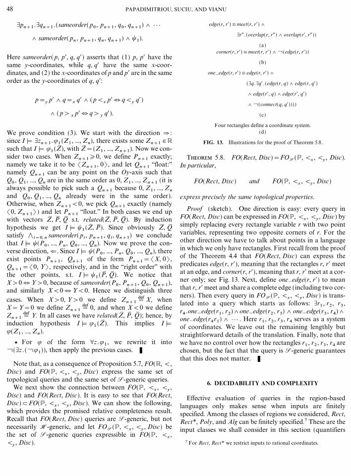
_pn+1 ._qn+1 . (sameorder( p0 , pn+1 , q0 , qn+1) 7 } } }

7 sameorder( pn , pn+1 , qn , qn+1) 7 �1).

Here sameorder( p, p$, q, q$) asserts that (1) p, p$ have thesame y-coordinates, while q, q$ have the same x-coor-dinates, and (2) the x-coordinates of p and p$ are in the sameorder as the y-coordinates of q, q$:

p=y p$ 7 q=x q$ 7 ( p<x p$ � q<y q$)

7 ( p> x p$ � q> y q$).

We prove condition (3). We start with the direction O :since I < _zn+1 ..1 (Z1 , ..., Zn), there exists some Zn+1 # Rsuch that I < .1 (Z� ), with Z� =(Z1 , ..., Zn+1). Now we con-sider two cases. When Zn+1�0, we define Pn+1 exactly;namely we take it to be (Zn+1 , 0), and let Qn+1 ``float:''namely Qn+1 can be any point on the Oy-axis such thatQ0 , Q1 , ..., Qn are in the same order as 0, Z1 , ..., Zn+1 (it isalways possible to pick such a Qn+1 because 0, Z1 , ..., Zn

and Q0 , Q1 , ..., Qn already were in the same order).Otherwise, when Zn+1<0, we pick Qn+1 exactly (namely(0, Zn+1) ) and let Pn+1 ``float.'' In both cases we end upwith vectors Z� , P� , Q� s.t. related(Z� , P� , Q� ). By inductionhypothesis we get I < �1 (Z� , P� ). Since obviously Z� , Q�satisfy � i=0, n sameorder( pi , pn+1 , qi , qn+1) we concludethat I < �(P0 , ..., Pn , Q0 , ..., Qn). Now we prove the con-verse direction, o . Since I < �(P0 , ..., Pn , Q0 , ..., Qn), thereexist points Pn+1 , Qn+1 of the form Pn+1=(X, 0) ,Qn+1=(0, Y) , respectively, and in the ``right order'' withthe other points, s.t. I < �1 (P� , Q� ). We notice thatX>0 � Y>0, because of sameorder(P0 , Pn+1 , Q0 , Qn+1),and similarly X<0 � Y<0. Hence we distinguish threecases. When X>0, Y>0 we define Zn+1 =def X, whenX=Y=0 we define Zn+1 =def 0, and when X<0 we defineZn+1 =def Y. In all cases we have related(Z� , P� , Q� ); hence, byinduction hypothesis I < .1 (Z� ). This implies I <.(Z1 , ..., Zn).

v For . of the form \z ..1 , we rewrite it intoc(_z . (c.1)), then apply the previous cases. K

Note that, as a consequence of Proposition 5.7, FO(R, <,Disc) and FO(P, <x , <y , Disc) express the same set oftopological queries and the same set of S-generic queries.

We next show the connection between FO(P, <x , <y ,Disc) and FO(Rect, Disc). It is easy to see that FO(Rect,Disc)/FO(P, <x , <y , Disc). We can show the following,which provides the promised relative completeness result.Recall that FO(Rect, Disc) queries are S-generic, but not

48 PAPADIMITRIOU, S

necessarily H-generic, and let FOS (P, <x , <y , Disc) bethe set of S-generic queries expressible in FO(P, <x ,<y , Disc).

edge(r, r$)#meet(r, r$) 7

_r" . (overlap(r, r") 7 overlap(r$, r"))

(a)corner(r, r$)#meet(r, r$) 7 c(edge(r, r$))

(b)

one�edge(r, r$)#edge(r, r$) 7

(_q ._q$ . (edge(r, q) 7 edge(r, q$)

7 edge(r$, q) 7 edge(r$, q$)

7 c(connect(q, q$))))

(c)

Four rectangles define a coordinate system.(d)

FIG. 13. Illustrations for the proof of Theorem 5.8.

Theorem 5.8. FO(Rect, Disc)=FOS (P, <x , <y , Disc).In particular,

FO(Rect, Disc) and FO(P, <x , <y , Disc)

express precisely the same topological properties.

Proof (sketch). One direction is easy: every query inFO(Rect, Disc) can be expressed in FO(P, <x , <y , Disc) bysimply replacing every rectangle variable r with two pointvariables, representing two opposite corners of r. For theother direction we have to talk about points in a languagein which we only have rectangles. First recall from the proofof the Theorem 4.4 that FO(Rect, Disc) can express thepredicates edge(r, r$), meaning that the rectangles r, r$ meetat an edge, and corner(r, r$), meaning that r, r$ meet at a cor-ner only; see Fig. 13. Next, define one�edge(r, r$) to meanthat r, r$ meet and share a complete edge (including two cor-ners). Then every query in FOS (P, <x , <y , Disc) is trans-lated into a query which starts as follows: _r1 , r2 , r3 ,r4 .one�edge(r1 , r2)7one�edge(r2 , r3) 7one�edge(r3 , r4)7one�edge(r4r1) 7 } } } . Here r1 , r2 , r3 , r4 serves as a systemof coordinates. We leave out the remaining lengthly butstraightforward details of the translation. Finally, note thatwe have no control over how the rectangles r1 , r2 , r3 , r4 arechosen, but the fact that the query is S-generic guaranteesthat this does not matter. K

6. DECIDABILITY AND COMPLEXITY

Effective evaluation of queries in the region-basedlanguages only makes sense when inputs are finitelyspecified. Among the classes of regions we considered, Rect,Rect*, Poly, and Alg can be finitely specified.7 These are the

UCIU, AND VIANU

input classes we shall consider in this section (quantifiers

7 For Rect, Rect* we restrict inputs to rational coordinates.

can again range over any class, finitely specifiable or not).Once we have finitely specified inputs, the notions ofdecidable query and of the data and query complexity of aquery are standard. In particular, data complexity is withrespect to the size of a standard encoding of an input I,which combines two factors: the size of names(I ) and thesize of the specifications of the regions in names(I ). Thesecomponents are to some extent orthogonal, and it is some-times useful to consider them separately (this is done, forexample, in Theorem 6.1).

We start with undecidability results. To succinctly stateour results we shall use expressions such as FO(Rect*&Disc, Rect*&Alg) to denote, in this example, all classes offirst-order queries whose quantification range is betweenRect* and Disc (that is, Rect*, Poly, Alg, or Disc) andwhose input domain is between Rect* and Alg (that is,Rect*, Poly, or Alg). Recall from [Rog] that the arithmeti-cal hierarchy is the set of properties over N which can beexpressed in the elementary arithmetic, i.e., in first-orderlogic over the symbols +, _, 0, 1, 2, 3, ... . This includes allrecursive properties,8 but many nonrecursive propertiesas well. To see this, recall that every property P(x) inthe arithmetical hierarchy can be expressed either as_x1 .\x2 ._x3 } } } Qnxn .R(x, x1 , ..., xn) or as \x1 ._x2 .\x3 } } }Qn xn .R(x, x1 , ..., xn), where R is a recursive predicate: theclass 7n consists of all properties of the first form, and 6n ofall those of the second form. Then 70=60 is the class ofrecursive, 71 that of recursively enumerable, and 61 of co-recursively enumerable properties. Moreover 70 /71 /72 / } } } and 60 /61 /62 / } } } form two strict hier-archies, whose limit is the arithmetical hierarchy, denotedAH.

Also, recall [Rog] that the analytical hierarchy, denotedhere AnH, is the set of properties over N expressible insecond-order logic over the symbols +, _, 0, 1, 2, 3, ..., inwhich the second-order variables range over functionsf : N � N. The analytical hierarchy contains even moreproperties than the arithmetical one. An example of aproperty in AnH but not in AH is

[x | ``x is the encoding of a true formula

in elementary arithmetic].

As usual, we extend the notations AH, AnH to instancesin Region. Namely some query Q of instances I # Alg is inAH (AnH) iff the set of encodings [encode(I ) | I # Q] is inAH (or AnH respectively). Of course, both definitionsdepend on Region, which also has to be finitely represent-able. For some group of permutations G, we define

TOPOLOGICAL QUERIES

8 By a theorem due to Go� del, every recursive relation R(x) can beexpressed as Q1 y1 .Q2 y2 } } } Qn yn .P(x, y1 , ..., yn)=0, where Qi # [\, _],for i=1, ..., n and P is a polynomial with integer coefficients.

AHG , AnHG to be the restrictions of AH, AnH to G-genericqueries.

Theorem 6.1 (Undecidability). The query classes

FO(Rect*&Disc, Rect&Alg)

are undecidable. Moreover, assuming that we restrict ourdatabase instances to have fined set of names, names(I)=[A1 , ..., Ak], we have the following characterization of theirexpressive power:

v FO(Alg, Rect&Alg)=AHH , FO(Poly, Rect&Poly)=AHH .

v AHH�FO(Rect*, Poly&Alg)�AH, AHH�FO(Poly,Alg)�AH.

v FO(Rect*, Rect&Rect*)=AHS .

v AnHH /FO(Disc, Rect&Alg).

Proof. We start by showing FO(Alg, Alg)�AH. Anyregion variable r # Alg can be encoded as a finite set of finitesets of finite sets of integers9 and, hence, as a single number.Thus, quantifiers over Alg become quantifiers over num-bers. Also, it is easy to see that connect(r, r$) is expressed asa recursive property on the encodings of r, r$. Next we showAHH �FO(Alg, Alg). Here the crucial observation is thatwe can encode numbers and the operations +, _, = inFO(Alg, Alg). Indeed, we express a natural number x as tworegions r, q # Alg s.t. r & q has x connected components. Weexpress equality of two numbers x, x$ represented byr, q, r$, q$ informally as follows: ``there exists a finite set ofregions S�Alg which is a one-to-one relation from the con-nected components of r & q to those of r$ & q$; i.e., (1) forevery connected component t of r & q there exists a uniqueconnected component t$ of r$ & q$ such that both t and t$ arecontained in some set s # S, and (2) for every connectedcomponent t$ of r$ & q$ there exists a unique connected com-ponent t of r & q such that t, t$ are contained in some sets # S.'' A finite set of regions S is encoded as the intersectionof two regions in Alg. The addition predicate x"=x+x$ isexpressed similarly: that is, assuming the connected com-ponents of r & q and r$ & q$ to be pairwise disjoint, we searchfor a one-to-one relation S from r" & s" and the union of theconnected components of r & s and r$ & s$. For multiplica-tion, x"=x_x$, we search for many-to-one relations S, S$from x to x" and x$ to x", respectively, and require the rela-tion [((c, c$), c") | (c, c") # S, (c$, c") # S$] to be one-to-one,where c, c$, c" are connected components of r & s, r$ & s$,r" & s", respectively. Hence, it follows that we can express inFO(Alg, Alg) all number-theoretic properties in AH.

Back to the proof of AHH �FO(Alg, Alg), suppose we are


given a formula . # AH expressing a topological property

9 Recall that a region in Alg is expressed as �i � j P ij (x, y)>0, where Pij

is a polynomial with integer coefficients.

over the number encoding of some input I # Alg. We have toconstruct some formula � # FO(Alg, Alg), having I as input.We do this in two steps. First, given I we compute someencoding of the invariant TI . Namely, following the proof ofProposition 5.1, the invariant TI can be represented by |V|regions, r1 , ...r |V| , where V is the set of cells in TI , and anumber of additional regions corresponding to the othercomponents of TI , such as the labeling relation l and theorientation O. Although the number |V| and other com-ponents of this representation depend on I, we can encodea set of regions as the connected components of the intersec-tion of two regions, and it follows that the entire invariantTI can be encoded by a fixed number of regions r1 , ..., rk (thenumber k depends only on the size of names(I), not on I ).In short, we can extract a number encoding of TI and thensearch for a number x representing an encoding of aalgebraic instance I$ for which TI and TI$ are isomorphic(recall that TI$ can be computed from I$ in NC). Finally wecheck .(x). In summary, we have so far proven thatFO(Alg, Alg)=AHH . Of course, this implies that FO(Alg,Rect&Alg)=AHH .

FO(Poly, Poly)=AHH and the relationships AHH�FO(Rect*, Poly&Alg)�AH and AHH �FO(Poly, Alg)�AH are proven similarly. Note that FO(Rect*, Poly&Alg) and FO(Poly, Alg) can express nontopological queriesso we do not have equality with AHH .

For FO(Rect*, Rect&Rect*)=AHS , we proceed as forFO(Alg, Alg)=AHH . We need, however, to generalizeTheorem 3.4 as follows. For any instance I in Rect*, we con-struct (in NC) an invariant SI such that I is S-equivalent toI$ iff SI is isomorphic to SI$ . Here SI has to capture in addi-tion to the information in TI , information about other ver-tices, edges, and faces generated by all points obtained asintersections of vertical and horizontal lines; see Fig. 14.Then the proof proceeds as for FO(Alg, Alg)=AHH .

50 PAPADIMITRIOU, S

FIG. 14. Illustrations of SI . Two instances I, I$ which are notS-equivalent (a) and their invariants SI , SI$ (b).

Finally, we sketch how to show AnHH � FO(Disc,Rect&Alg). First we notice that here r & q may have, ingeneral, infinitely many connected components; hence notevery pair r, q is a correct encoding of a number. However,we can test in FO(Disc, Rect&Alg) whether r & q hasfinitely many connected components, by checking that thereis no one-to-one relation from the set of connected com-ponents of r & q to a proper subset of it. So we proceed asin the proof of AHH �FO(Alg, Alg), but now we have toencode functions f : N � N in addition to numbers. The lat-ter can be encoded as follows in FO(Disc, Alg); see Fig. 15.First, given two regions r, q, the connected components ofr & q form a circular order defined by traversing the borderof r. This order can be expressed in FO(Disc, Alg): moreprecisely, given four regions c1 , c2 , c3 , c4 �r & q determin-ing four connected components of r & q, one can testwhether these connected components occur in that order onthe border or r (simply check whether there exists two dis-joint regions a, b�r s.t. a connects c1 with c2 and b connectsc3 with c4). Then a function is defined by six regionsr, q, r$, q$, c0 , c� s.t. (a) r & q has infinitely many con-nected components (see Fig. 15); (b) each connected com-ponent of r$ & q$ (the black regions in Fig. 15) is a subset ofsome connected component of r & q; (c) c0 �r$ & q$ is calledthe ``left-most'' black region (see Fig. 15), c� �r$ & q$ iscalled the ```right-most'' black region (not shown in Fig. 15);(d) there are infinitely many connected components in r & q``between'' c0 and c� , but only finitely many between anytwo black regions other than c� . All these properties can bechecked in FO(Disc, Alg); hence we can simulate quantifica-tion over functions f : N � N in FO(Disc, Alg). It remains toshow that we can express function application f (x). Givenan encoding for f and an encoding r & q for x (i.e., r & q hasx connected components), we find an encoding r$ & q$ ofy =def f (x) as follows. First identify the x th and (x+1)stblack regions in the encoding of f by finding a one-to-onecorrespondence between some initial segment of the blackregions and r & q. Next pick r$, q$ such that the connectedcomponents of r$ & q$ are precisely those of f ``between''those two black regions. K

Keeping fixed the set of region names does not have asmuch to do with the complexity of the queries as with thegeneric nature of the fragment of our languages dealingwith region names; e.g., the following property of instancesI is not expressible in FO(Disc, Alg): ``the cardinality ofnames(I ) is even.'' On the other hand, FO(Disc, Alg) canexpress the property ``[ext(a) | a # names(I )] consists of aneven number of disjoint regions.'' Thus, the characteriza-tions do not work if the set of names is allowed to vary.

In view of the very strong undecidability results in this

UCIU, AND VIANU

section, we are motivated to consider decidable fragments oftopological query languages. Unfortunately, we next notethat even extremely restricted fragments of these languages

o
FIG. 15. Encoding of the function f : N � N, f (0)=2, f (1)=0, f (2)=3,
The black regions are the connected components of the intersection of two

can be undecidable. Let us consider the query class71 (Rect*, <): existential sentences with quantifiers overfinite unions of rectangles, and not involving any inputregions. As it turns out, whether this theory is decidable isequivalent to a fairly well-known problem in graph theory,the string graph problem [EET76, Kra91, KM94], whichcan be restated as follows: Given a graph G, is it the intersec-tion graph of a set of curves on the plane? That is, is there aset of curves (non-self-intersecting paths on the infinite two-dimensional grid, say), one corresponding to each node,such that two curves intersect if and only if the corre-sponding vertices are connected in G? It is a fairly well-known open problem whether string graphs are decidable.

Proposition 6.2. 71 (Rect*, 0) is decidable if and only ifstring graphs are decidable.

Proof. To translate between curves and finite unions ofrectangles, in one direction we replace a region by a curvethat ``fills it,'' in the other we approximate a curve as closelyas desired by a finite union of ``very thin'' rectangles. Thusthe string graph problem is the special case of the71 (Rect*, <) sentences with matrix which is the conjunc-tion of literals of the form connect(A, B) or cconnect(A, B),one for each pair of quantified variables. Conversely,with exponentially many calls to an algorithm for thisfragment (one for each satisfying truth assignment of thematrix of the 71 (Rect*, <) sentence) we can answer anyquery. K

This result, together with the negative results in [Kra91,KM94] (NP-hardness of string graph recognition, and

TOPOLOGICAL QUERIES

an exponential lower bound on the size of the smalleststring model of a graph) has the following negative conse-quences:

... . The two regions r, q yield infinitely many connected components in r & q.ther regions, r$ & s$, not shown.

Corollary 6.3. 71 (Rect*, <) is NP-hard in terms ofquery complexity. Furthermore, for every n there is a true71 (Rect*, <) query with n symbols such that the smallest setof regions that can instantiate the existential quantifiers hastotal size that is doubly exponential.

We now turn to the decidable sublanguages, and theirdata complexity. Since queries in FO(Region, Alg) involvequantification over the infinite sets in Region, computingsuch queries must involve results along the lines of thewell-known quantifier elimination theorems a� la [Tar51].Indeed, the following is a direct consequence of results in[KKR90].

Theorem 6.4 Data Complexity). The queries in

FO(Rect, Rect&Alg)

are effectively computable and have data complexity NC.Similarly for queries in FO(P, <x , <y , Rect&Alg).

Finally, in terms of query complexity we have the follow-ing (we omit the straightforward proofs).

Theorem 6.5 (Query Complexity). The query complex-ity of FO(Rect, Rect&Alg) and FO(P, <x , <y , Rect&Alg)is PSPACE. The query complexity of the conjunctive queries(existential queries with conjunctive matrix) in FO(Rect,Rect*&Alg) and FO(P, <x , <y , Rect*&Alg) is NP, andthe query complexity of conjunctive queries in FO(Rect,Rect) and FO(P, <x, <y , Rect) is NC.

7. CONCLUSIONS AND FURTHER WORK


We have made progress toward the theoretical underpin-nings of the topological fragment of spatial databases. We

have identified the essential part of a spatial data base vis-a� -vis topological queries: It is the planar graph structure ofthe region boundaries. This structure can be represented asan instance of a simple and fixed relational scheme, and canbe extracted easily from any spatial instance. The resultingrelational instance can then be used to answer any topologi-cal query on the original spatial instance. It would be veryinteresting to find other domains in which this methodologyis useful; this line of research can result in database systemsfor extremely complex data which, however, also containsimple relational ``summaries'' that suffice for large ranges ofinteresting queries.

We have also introduced natural topological languages,first-order extensions of the well-known but insufficientfour-intersection relations, and discussed their expressi-bility, completeness, decidability, and complexity. We havemostly restricted ourselves to the domain ALG; similarresults can be obtained for the S-generic properties ofinputs over Rect* (as outlined in the proof of Theorem 6.1),and for L-generic properties of inputs over Poly. Thisincludes the existence and efficient construction of therespective invariants, and the definability of S-equivalenceclasses and L-equivalence classes by sentences in FO(Rect*,Rect*) and FO(Poly, Poly), respectively. The latter can alsobe used to obtain completeness results in the spirit of thoseof Section 5, only this time for the S-generic and L-genericproperties of inputs over Rect* and Poly.

One important question has been left open in this paper:Are there interesting tractable topological querylanguages10 that are more expressive than the Booleanclosure of the four-intersection relations? In work currentlyin progress, we have identified an interesting candidate: Thefirst-order closure of four-intersection relations where thequantifiers are restricted to two kinds of regions: (a) Oneweak class of quantifiers range over all cells of the plane asdivided by the boundaries of the instance. (b) A strongerquantifier ranges over all possible unions of cells that aredisc homeomorphs (that is to say, legitimate regions); arelated language quantifies over points and paths. The first-order closure of four-intersection relations under these twokinds of quantifiers seems to be very expressive��for exam-ple, the queries exemplified in Fig. 1a. vs Fig. 1b and Fig. 1cvs Fig. 1d, which are known not to be expressible byBoolean combinations of the four-intersection relations, areexpressible when these quantifiers are allowed. The datacomplexity of this language is NC, and the query complexityPSPACE. Finally, we hope to discover clean characteriza-tions of the expressive power of this language, and perhapsobtain a purely algebraic counterpart in the spirit of Codd'sTheorem.

52 PAPADIMITRIOU, S

10 Among the languages we considered, FO(Rect, Alg) is tractable, but isnot a purely topological language.

REFERENCES

[AHB95] S. Abiteboul, L. Herr, and J. Van den Bussche, Temporalconnectives versus explicit timestamps in temporal querylanguages, in ``Recent Advances in Temporal Databases''(J. Clifford and A. Tuzhilin, Eds.), pp. 43�57, Springer-Verlag,Berlin�New York, 1995.

[AVV95] S. Abiteboul, M. Vardi, and V. Vianu, Computing withinfinitary logic, Theoret. Comput. Sci. 149 (1995), 101�128.

[Ba77] J. Bairwise, On Moschovakis closure ordinals, J. SymbolicLogic 42 (1977), 292�296.

[BF85] J. Bairwise and S. Feferman (Eds.), ``Model-TheoreticLogics,'' Springer-Verlag, Berlin�New York.

[BDLW98] M. Benedikt, G. Dong, L. Libkin, L. Wong, Relationalexpressive power of constraint query languages, J. Assoc.Comput. Mach. 45 (1998), 1�34.

[BKR84] M. Ben-Or, D. Kozen, and J. Reif, The complexity of elemen-tary algebra and geometry, in ``Proc. 16th ACM Symp. onTheory of Computing,'' pp. 457�464, 1984.

[C93] J. Chomicki, Temporal databases, in ``Proc. ACMSIGACT�SIGMOD�SIGART Symp. on Principles ofDatabase Systems,'' 1993.

[Cla85] B. Clark, A calculus of individuals based on ``connection,''Notre Dame J. Formal Logic 22 (1985).

[CRC94] A. G. Cohn, D. A. Randell, and Z. Cui, Taxonomies oflogically defined qualitative spatial relations, in ``FormalOntology in Conceptual Analysis and Knowledge Represen-tation'' (N. Guarino and R. Poli, Eds.), Kluwer Academic,Dordrecht�Norwell, MA, 1994.

[Cor79] J. P. Corbett, Topological principles in cartography, Techni-cal Paper 48, U.S. Bureau of the Census, Washington DC,1979.

[E89] M. Egenhofer, A Formal Definition of Binary TopologicalRelationships, in ``Proc. Third International Conference onFoundations of Data Organization and Algorithms(FODO), Paris, France'' (W. Litwin and H.-J. Schek, Eds.),Lecture Notes in Computer Science, Vol. 367, pp. 457�472,Springer-Verlag, New York 1989.

[E93] M. Egenhofer, A model for detailed binary topological rela-tionships, Geomatica 47 (1993), 261�273.

[E94] M. Egenhofer, Spatial SQL: A query and presentationlanguage, IEEE Trans. Knowledge Data Engrg. 6 (1994),86�95.

[EgFra91] M. J. Egenhofer and R. Franzosa, Point-set topologicalspatial relations, Internat. J. Geographical Inform. Syst. 5(1991), 161�174.

[EgFra95] M. Egenhofer and R. Franzosa, On the equivalence oftopological relations, Internat. J. Geographical Inform. Syst.9, No. 2 (1995), 133�152.

[EET76] G. Ehrlich, S. Evenand, and R. E. Tarjan, Intersection graphsof curves on the plane, J. Combin. Theor. Ser. B 21 (1976),8�20.

[Fa� 48] I. Fa� ry, On straight line representation of planar graphs,Acta Sci. Math. (Szeged ) 11 (1948), 229�233.

[FK86] A. Frank and W. Kuhn, Cell graph: A provable correctmethod for the storage of geometry, in ``Proc. Second Inter-national Symposium on Spatial Data Handling'' (D. Marble,Ed.), pp. 411�436, Seattle, WA 1986.

[FraEg92] R. Franzosa and M. Egenhofer, Topological spatial relations

UCIU, AND VIANU

based on components and dimensions of set intersections,in ``Proc. SPIE's OE�Technology '92��Vision Geometry''(R. Melter and A. Wu, Eds.), pp. 236�246, Boston, MA,1992.

[GPP95] M. Grigni, D. Papadias, and C. H. Papadimitriou, Topologi-cal inference, in ``Proc. 14th Int'l. Joint Conf. on ArtificialIntelligence,'' pp. 901�906, 1995.

[GS94] S. Grumbach and J. Su, Finitely representable databases,in ``Proc. ACM SIGACT�SIGMOD�SIGART Symp. onPrinciples of Database Systems,'' pp. 289�300, 1994.

[GS95] S. Grumbach and J. Su, Dense-order constraint databases,in ``Proc. ACM SIGACT�SIGMOD�SIGART Symp. onPrinciples of Databases Systems,'' pp. 66�77, 1995.

[GST94] S. Grumbach, J. Su, and C. Tollu, Linear constraintdatabases, in ``Proc. Logic and Complexity Workshop''(D. Leivant, Ed.), Indiana, 1994.

[G94] R. Gu� ting, An introduction to spatial database systems,VLDB J. 3 (1994), 357�399.

[H91] J. Herring, TIGRIS: A data model for an object-orientedgeographic information system, Comput. Geosci. 18 (1991),443�452.

[JS85] J. Ja� Ja� and J. Simon, Parallel algorithms for graph theory:Planarity testing, SIAM J. Comput. 11 (1982), 314�328.

[K68] J. A. W. Kamp, ``Tense Logic and the Theory of LinearOrder,'' Ph.D. thesis, University of California, Los Angeles,1968.

[KG94] P. C. Kanellakis and D. Q. Goldin, Constraint programmingand database query languages, in ``Proc. 2nd Conf. onTheoretical Aspects of Computer Software (TACS), Sendai,Japan,'' Lecture Notes in Computer Science, Vol. 789,pp. 96�120, Springer, New York, 1994.

[KKR90] P. C. Kanellakis, G. M. Kuper, and P. Z. Revesz, Constraintquery languages, in ``Proc. ACM SIGACT�SIGMOD�SIGART Symp. on Principles of Database Systems,''pp. 299�313, 1990.

[KR91] R. M. Karp and V. Ramachandran, Parallel algorithms forshared-memory machines, in ``The Handbook of Theoret-ical Computer Science, Vol. A'' (J. van Leeuwen, Ed.),pp. 869�941, 1991.

[KY85] D. Kozen and C.-K. Yap, Algebraic cell decomposition inNC, in ``Proc. IEEE Symp. on Foundations of ComputerScience,'' pp. 515�521, 1985.

[Kra91] J. Kratochv@� l, String graphs. II. Recognizing string graphs isNP-hard, J. Combin. Theory Ser. B 52 (1991), 67�78.

[KM94] J. Kratochv@� l and J. Matous$ ek, Intersection graphs ofsegments, J. Combin. Theory Ser. B 62 (1994), 289�315.

[KPV95] B. Kuijpers, J. Paredaens, and J. Van den Bussche, Losslessrepresentation of topological spatial data, in ``Proc. FourthInt'l. Symp. on Large Spatial Databases,'' 1995.

[LT92] R. Laurini and D. Thompson, ``Fundamentals of SpatialInformation Systems,'' Academic Press, San Diego, 1992.

[Moi] E. Moise, ``Geometric Topology in Dimensions 2 and 3,''Springer-Verlag, Berlin�New York, 1977.

TOPOLOGICAL QUERIES

[OV91] P. van Oosterom and T. Vijlbrief, Building a GIS on topof the open DBMS postgres, in ``EGIS '91,'' pp. 775�787,Brussels, Belgium, 1991.

[Par+94] J. Paredaens, J. Van Den Bussche, and D. Van Gucht,Towards a theory of spatial databas queries, in ``Proc. ACMSymp. on Principles of Database Systems,'' pp. 279�288,1994.

[Par95] J. Paredaens, Spatial databases, the final frontier, in ``Proc.5th Int'l Conf. on Database Theory,'' pp. 14�32, 1995.

[Par+95] J. Paredaens, J. Van Den Bussche, and D. Van Gucht, First-order queries on finite structures over the reals, in ``Proc.Conf. on Logic in Computere Science,'' 1995.

[PE88] D. Pullar and M. Egenhofer, Towards formal definitions oftopological relations among spatial objects, in ``Proc. ThirdInternational Symposium on Spatial Data Handling''(D. Marble, Ed.), pp. 225�242, Sydney, Australia, 1988.

[RC89] D. A. Randell and A. G. Cohn, Modelling topological andmetrical properties of physical processes, in ``Proceedings, 1stInternational Conference on the Principles of KnowledgeRepresentation and Reasoning'' (R. Brachman, H. Levesque,and R. Reiter, Eds.), Morgan Kaufmann San Mateo, CA,1989.

[Ren92] J. Renegar, On the computational complexity and geometryof the first-order theory of the reals, J. Symbolic Comput. 13(1992), 252�299.

[Rog] H. Rogers, Jr., ``Theory of Recursive Functions and EffectiveComputability,'' MIT Press, Cambridge, MA, 1987.

[St51] S. K. Stein, Convex maps, Proc. Amer. Math. Soc. 2 (1951),464�466.

[St93] J. Stillwell, ``Classical Topology and Combinatorial GroupTheory,'' Springer-Verlag, Berlin�New York, 1993.

[SZ91] P. Svensson and H. Zhexue, Geo-SAL: A query language forspatial data analysis, in ``Proc. Advances in SpatialDatabases-Second Symposium, SSD '91'' (O. Gu� nther andH.-J. Schek, Eds.), Lecture Notes in Computer Science,Vol. 525, pp. 119�140, Springer-Verlag, New York, 1991.

[Tar51] A. Tarski, ``A Decision Method for Elementary Algebraand Geometry,'' University of California Press, Berkely,1951.

[Zie85] Topological model theory, in ``Model-Theoretic Logics''(J. Barwise and S. Feferman, Eds.), Springer-Verlag, Berlin�New York, 1985.

[Tut63] W. T. Tutte, How to draw a graph, Proc. London Math. Soc.13 (1963), 743�767.

[Wag36] K. Wagner, Bemerkungen zum Vierarbenproblem, Jahresber.Deutsch. Math.-Verein. 46 (1936), 26�32.

[W92] M. Worboys, A geometric model for planar geographicalobjects, Internat. J. Geographical Inform. Syst. 6 (1992),353�372.


Topological Queries in Spatial Databases

Documents

Transcript of Topological Queries in Spatial Databases