NOR'I}I- HOILAND

Approximate Topological Relations*

Eliseo Clementini and Paolino Di Felice Dipartimento di Ingegneria Elettrica, Universith di L'Aquila, L'Aquila, Italy

ABSTRACT

In spatial data models for various applications, such as geographical information systems (GISs), the importance of topological relations is widely recognized. Topology makes very general statements about the structure and the relations of spatial objects. A refinement of topology by means of other geometric aspects can help to bend the various models that have been developed for topological relations towards a more effective description of geographic space. The introduction of broad boundaries is a direction to define approximate topological relations between spatial objects. In this paper, approxi- mate topological relations are destined to capture boundary uncertainty, variations over time, proximity measures, and vector-raster representations. Approximate topological relations are structured in conceptual neighborhood graphs that have a twofoM interpre- tation: two neighboring relations are at topological distance 1 in terms of the nine-inter- section model and can be obtained, one from the other, by an elementary continuous deformation. © 1997 Elsevier Science Inc.

KEYWORDS: uncertainty, broad boundary, topological relation, deformation analysis, conceptual neighborhood

1. INTRODUCTION

Several models for topological relations have appeared in the literature [6, 8, 9, 16, 21, 22]. The common feature of these models is that they provide a computational basis for spatial reasoning, being a tradeoff between the formal ground needed by an information system and the human perception of geographic space. Despite being extensively studied

*This work was supported by the Italian MURST project "Basil di dati evolute: modelli, metodi e sistemi" and CNR project no. 95.00460.CT12 "Modelli e sistemi per il trattamento di dati ambientali e territoriali."

Address correspondence to Eliseo Clementini, Dipartimento di Ingegneria Elettrica, Universit~ di L 'Aquila, 67040 Poggio di Roio , L "Aquila, Italy. E-mail: eliseo@ing .univaq. it.

Received March 1, 1996; accepted October 1, 1996.

International Journal of Approximate Reasoning 1997; 16:173-204 © 1997 Elsevier Science Inc. 0888-613X/97/$17.00 655 Avenue of the Americas, New York, NY 10010 PII S0888-613X(96)00127-2

174 Elisio Clementini and Paolino Di Felice

in all their theoretical implications and even implemented in some GIS prototypes, models for topological relations suffer from the following critique: "This is a very nice and elegant model, but is it useful for a real geographic application after all?" The critique arises because the actors of these models are simple spatial entities of Euclidean geometry, while geographic reality is permeated by intrinsically complex entities.

A big limitation of current GIS data models is the mismatch between complex geographic reality (unstructured, with uncertain boundaries) and geometric modeling (simple objects with sharp boundaries). Spatial data types are prone to represent objects with a well-defined boundary; this is a good fit to objects on a small scale, but it is not suitable for objects on a geographic scale [4, 5]. The majority of models for representing spatial relations assume objects with a sharp boundary. What can be done to introduce "uncertainty" or "fuzziness" into these models? Some contribu- tions have focused on extending topological relations with fuzzy logic [17, 18] and probability functions [36]. A somehow complementary approach is to consider the degree of applicability of topological relations by introduc- ing a measure of set intersection [35].

Topological relations of Euclidean space make too sharp distinctions for the cases at hand. Think of two regions that come closer: there is a sudden transition from "disjoint" to "overlap" with only a single instant where the topological relation is "meet". This sudden change is probably what is most distant from reality. In [27], this phenomenon has been modeled with the concepts of perturbation and dominance. Galton distinguishes between modes that can be realized for isolated instants (states of position) and modes that can be realized over an interval (states of motion).

The description of a scene of various objects is better captured by a wider set of more gradual relations, still defined in terms of topology. In this paper, the introduction of broad boundaries contributes to making models for topological relations closer to reality, since they eliminate the states of position. The deformation between relations becomes a smoother transition from one relation to another. Hereafter, the relations between objects with broad boundary are called approximate topological relations, since they constitute an approximation of classic topological relations between objects with a sharp boundary. Approximate topological relations provide a more gradual set of qualitative distinctions to apply to the modeling of boundary uncertainty, variations over time, and proximity measures. Proximity measures are central to GIS analysis capabilities: various methods include buffer zones, minimum bounding rectangles (MBRs), and convex hulls.

The model of approximate topological relations presented here is based on previous work on topological relations for broad boundaries [7] and the nine-intersection model [22] in order to accommodate more flexible topo-

Approximate Topological Relations 175

logical relations. The concept of naive geography [24] influenced this paper with regard to the incremental approach (refinement of topology) and the treatment of uncertainty (qualitative methods). The approach pursued in this paper is coherent with the research directions that emerged from the recent GISDATA workshop on geographic objects with indeterminate boundaries [5].

The remainder of the paper is organized as follows. In Section 2, we discuss the correlation between broad boundaries, boundary uncertainty, and variations over time. Section 3 gives formal definitions for the new objects with a broad boundary. Section 4 proposes the extension of the nine-intersection model to objects with a broad boundary. In Section 5, approximate topological relations are studied in detail, structuring them in the conceptual-neighborhood graph and grouping them in clusters. It is shown that any path in the graph can be mapped to a continuous transformation of the objects. The generality of the conceptual neighbor- hood is due to the introduction of broad boundaries: thanks to them, each transition between two neighbors is a smooth transition. In other words, the elimination of sharp boundaries has the effect of eliminating relations that can be realized only for a single instant: as a result, all relations take place over an interval of time. In Section 6, the general model is special- ized to various interpretations of a broad boundary (buffer zones, MBRs, convex hulls, rasters) for proximity analysis, and to the hybrid case of topological relations between an object with a broad boundary and an object with a sharp boundary. In Section 7, we compare our model for broad boundaries with the egg-yolk theory of [11]. Section 8 draws some conclusions.

2. UNCERTAINTY AND BROAD BOUNDARIES

Uncertainty is intrinsically a property of the geographic space we live in. Our knowledge of the world is shaped by our limited means of acquiring information, whether natural senses or technical apparatus. This makes it impossible to elaborate general statements about the world without speci- fying what is the context in which a statement is valid and what degree of confidence one has in it. Geographic space, in the sense in which humans reason about it, is always the result of an abstraction process. Entities are built by an aggregation of more elementary entities, which can be homoge- neous or nonhomogeneous. Therefore, the kinds of geographic entities we deal with exist only at a certain scale of reasoning.

The nature of some geographic phenomena is better interpreted by fields instead of objects [14]. The process of extracting discrete entities from continuous fields (objectification) is especially suitable in certain

176 Elisio Clementini and Paolino Di Felice

contexts to-perform spatial reasoning and treat spatial relations between objects. Further, while the field view is better for analytically representing geographic phenomena, the object view is easier for people to understand. We are used to maps where most of the cartographic knowledge is expressed by sharp boundaries (regions, lines, and points) with few excep- tions (various altitude representations). Moreover, spatial data stored in computers are based on the same simple geometric modeling of the geographic reality.

Referring to Zubin's distinctions of objects in space [37], objects of type A (objects that are manipulable) have sharp boundaries, while objects of type D (objects in geographic space) have vague boundaries. In the latter case, when a sharp boundary exists, it is the result of an artificial imposi- tion (border between land parcels) or a simplification due to scaling (sea coastline). We cannot give an exhaustive treatment of boundary uncer- tainty and fuzziness, and we refer to [15] for an extensive classification.

There are three categories of models for representing boundary uncer- tainty: probabilistic, fuzzy, and extensions of exact models. Most proba- bilistic and fuzzy models have dealt with positional uncertainty, due to errors in measurements and finite representation of computer formats. Models for representing uncertain boundaries that are an extension of existing models for objects with a sharp boundary and focus on the relations between objects are [7, 11, 12]. Relations between objects with a broad boundary were also discussed in [1], though all topological relations between such regions were not found exhaustively.

Distinct from positional uncertainty, we will concentrate on a second type of uncertainty due to approximation methods (scaling process). Ac- cordingly to Couclelis [15], "scaling is the great boundary maker." In other words, objects come from approximations of continuous fields, represented on a sufficiently large scale and interpreted for a certain purpose. A frequent category of fields is that of mixture fields. Mixture fields are characterized by constant-valued attributes over large areas and rapidly changing transition zones between them [3]. Some fields can be modeled with two attributes, such as land-water, forest-grassland, and urban-rural. An abstraction process applied to mixture fields allows one to extract objects. If the scope is to obtain a sharp boundary between the two attribute values, then the boundary can be fixed at 50% for the two values (e.g., the values "forest" and "grassland"). Clearly, this leads to a poor approximation of the original meaning of the two attributes. With the introduction of a broad boundary, the areal transition zone preserves more of the original knowledge: the broad boundary can be naturally fixed by taking two cutting points for a given value (e.g., 90% and 10% of "forest").

Broad boundaries can model variations over time. This is a rough approximation if the application requires a detailed list of changes at

Approximate Topological Relations 177

several observation states. On the other hand, a category of geographic phenomena that have a duration over an interval of time can be observed by restricting attention to the initial state and the final state. An example could be the extent of a coastal region before and after a storm [34]. Also, cyclic events are suitable for modeling in this way. Fixing an appropriate interval of time, we observe the maximum and the minimum extent of the boundary of a spatial object, which make up the broad boundary. For example, a broad boundary can represent the land periodically affected by the ebb and flow of the tide.

3. THE SPATIAL DATA MODEL FOR OBJECTS WITH A BROAD BOUNDARY

Simple objects (regions, lines, and points) are widely discussed in the literature [6, 9, 21, 22]. A simple region is defined as a closed homoge- neously two-dimensional simply connected subset of E2. A simple line is a one-dimensional variety embedded in ~2 with exactly two endpoints and no self-intersections. A simple point is a connected 0-dimensional subset of I~ 2. For such objects, interior (o), boundary (d), and exterior ( - ) are defined with the plain topological sense [31].

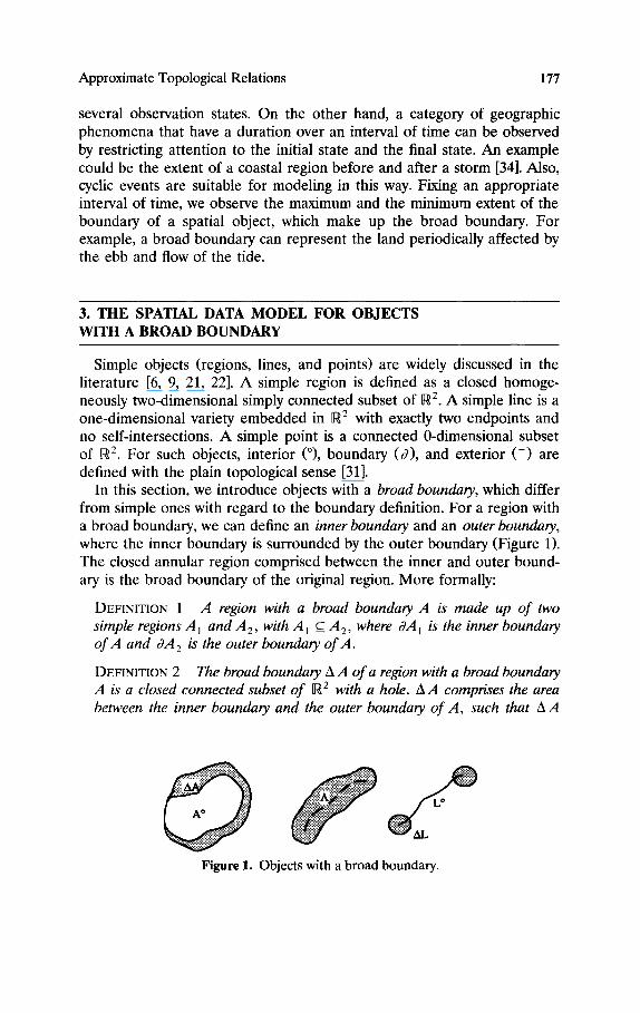
In this section, we introduce objects with a broad boundary, which differ from simple ones with regard to the boundary definition. For a region with a broad boundary, we can define an inner boundary and an outer boundary, where the inner boundary is surrounded by the outer boundary (Figure 1). The closed annular region comprised between the inner and outer bound- ary is the broad boundary of the original region. More formally:

DEFINITION 1 A region with a broad boundary A is made up of two simple regions A 1 and A 2, with A 1 c_A2, where dA m is the inner boundary of A and aA 2 is the outer boundary of A.

DEFINITION 2 The broad boundary A A of a region with a broad boundary A is a closed connected subset of ~ 2 with a hole. A A comprises the area between the inner boundary and the outer boundary of A, such that A A

0 J oS Figure 1. Objects with a broad boundary.

178 Elisio Clementini and Paolino Di Felice

= A 2 - A 1, or equivalently A A = A 2 - A1Q. I f a I c A2, then A A is two-dimensional; in the limit case A l = A2, A A is a one-dimensional sphere. I f aA 1 n 0.4 2 4: Q, then A A is not homogeneously two-dimen- sional and may present one-dimensional parts and separations in its interior.

DEFINITION 3 The interior, closure, and exterior o f a region with a broad boundary A are defined as A ° = A 2 - A A , . 4 = A ° U A A , and A - = ~ 2

- A , respectively.

Following from these definitions, the interior and exterior of a region with a broad boundary are open sets, while the broad boundary is a closed set. Simple regions can be seen as special cases of regions with a broad boundary in which the inner and outer boundaries coincide and therefore A A = 0.4.

For lines embedded in ~2, we can distinguish two kinds of broad boundaries, modeling either the position of the line or the position of its endpoints (Figure 1). The first kind of broad boundary is a region sur- rounding the whole line, while the second kind is made up of a region for each endpoint. We will refer to the first kind as a broad line and to the second as a line with a broad boundary. A broadpoint is a special case of a broad line. The following definitions hold:

DEFINITION 4 A broad line A is a simple region representing a family o f positions that a simple line L 1 can assume under a continuous deformation. The interior o f A is empty, while AA = A.

DEFINITION 5 A line with a broad boundary L is made up o f a simple line L 1 and two simple regions A 1 and A2, surrounding the two endpoints P1 and P2 o f the line L1, respectively.

DEFINITION 6 The broad boundary A L o f a line with a broad boundary L is the union o f the two simple regions A 1 and A 2, that is, A L = A 1 U A 2.

DEFINITION 7 The interior, closure, and exterior o f a line with a broad b_oundary L are defined as L ° = L 1 - - m L , T~ = L x U A L, and L - = R 2 _ L , respectively.

4. THE 9-1NTERSECTION MODEL FOR OBJECTS WITH A BROAD BOUNDARY

Topological relations are spatial relations that are preserved under such transformations as rotation, scaling, and rubber-sheeting. Binary topologi- cal relations between two objects, A and B, in •2 can be classified according to the intersection of A's interior, boundary, and exterior with

Approximate Topological Relations 179

B's interior, boundary, and exterior. The nine intersections between the six object parts describe a topological relation and can be concisely repre- sented by the following 3 × 3 matrix M, called the 9-intersection [22]:

M = A r i B ° A ° n OB A ° A B - t 3.4 A B ° 3/1 N OB 3tt A B - ) . A - A B ° A - A OB A - N B -

By considering the values empty (0) and nonempty (1), we can distinguish between 29 = 512 binary topological relations. For two simple regions with a one-dimensional boundary, only eight of them can be realized, whose names are disjoint, meet, overlap, coveredBy, inside, covers, contains, equal; for two simple lines there are 36 different relations in ~2; and between a simple line and a region there are 19 different topological relations. Each set of relations provides a complete coverage and is mutually exclusive [21].

The 9-intersection model can be extended to objects with a broad boundary. The matrix M needs to be redefined as follows, having a broad boundary in place of a sharp boundary:

M = A A B ° A ° n A B A ° N B - t AA A B ° AA n AB AA N B - ) . A - A B ° A - N AB A - A B -

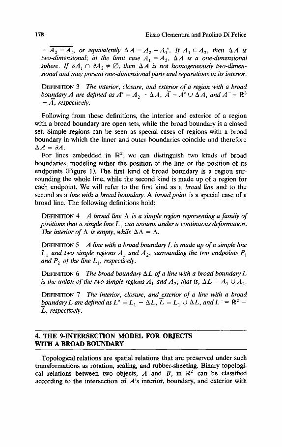
In [7], the authors developed the case of region-region relations and, by means of geometric conditions, showed that there are 44 realizable cases for regions with a broad boundary. The criteria for numbering the 44 relations were fixed in [7], and the same numbering is kept here for compatibility. Geometric interpretations of the 44 relations and the corre- sponding 9-intersection matrices are given in Figures 2-12. We have grouped them in several clusters which share similar geometric properties, and whose meaning will be discussed in the next section.

1 0

1

18 1

1

I 0i/ 39 0 1

40 0 0

Figure 2. The relations disjoint (1), overlap (18), Inside (39), and contains (40).

180 Elisio Clementini and Paolino Di Felice

2 1 1

3 1 1

6 1 1

9 I 1

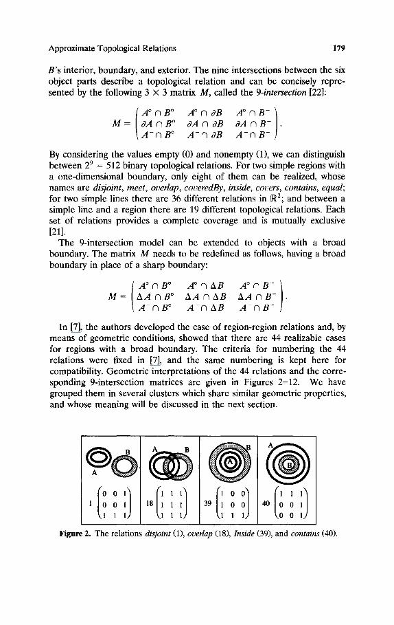
Figure 3. The relation meet (2) and the cluster nearbyOverlap (3, 6, 9).

In the remainder of the paper, we treat only region-region relations. Note, however, that a similar analysis could be performed to find out the realizable relations between lines with a broad boundary and between regions and lines. Broad lines, instead, can be simply considered degener- ate regions with a broad boundary in the case of an empty interior. Relations between a region with a broad boundary A and a broad line A are therefore expressed in terms of the following matrix:

AOAA AOAA - ) A A N A A A N A - . A - A A A - A A -

The 9-intersection model has been applied not only to simple objects; for instance, in [20], the model has been used to treat regions with holes. Each region with holes is represented by its generalized region (the union of the region and its holes) and the closure of each hole. Hence, the topological relation between two regions with holes is expressed by a set of topological relations between simple regions. The model for objects with a broad boundary presented in this paper can be used for regions with holes by replacing the basic eight relations for simple regions with the 44 relations for regions with a broad boundary.

4 1 1

o I o IYY/ 1o 1

1

11 1

1

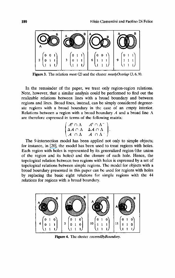
Figure 4. The cluster coveredByBoundary.

Approximate Topological Relations 181

G 7 1

1 lion/ 8 1

0

12 1

1

~ B

13 1 0

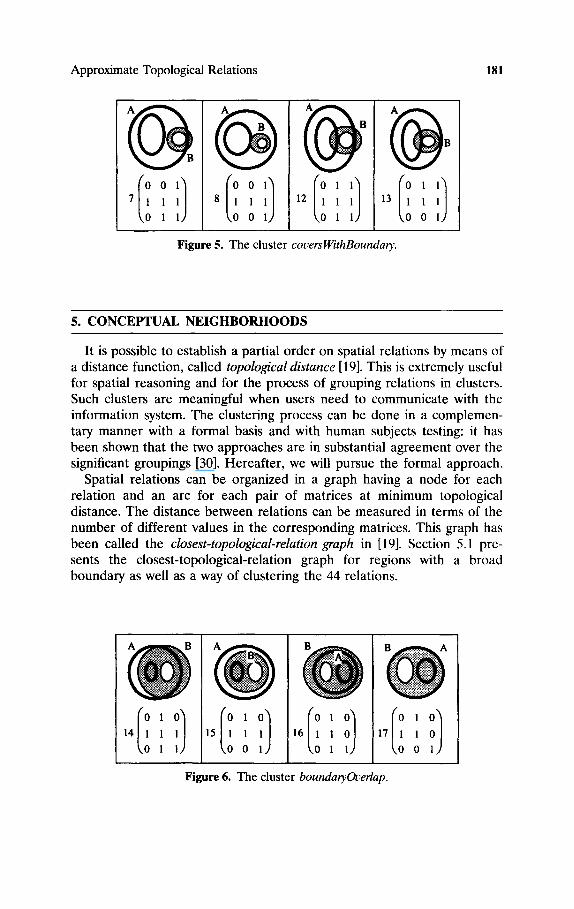
Figure 5. The cluster coversWithBoundary.

5. CONCEPTUAL NEIGHBORHOODS

It is possible to establish a partial order on spatial relations by means of a distance function, called topological distance [19]. This is extremely useful for spatial reasoning and for the process of grouping relations in clusters. Such clusters are meaningful when users need to communicate with the information system. The clustering process can be done in a complemen- tary manner with a formal basis and with human subjects testing: it has been shown that the two approaches are in substantial agreement over the significant groupings [30]. Hereafter, we will pursue the formal approach.

Spatial relations can be organized in a graph having a node for each relation and an arc for each pair of matrices at minimum topological distance. The distance between relations can be measured in terms of the number of different values in the corresponding matrices. This graph has been called the closest-topological-relation graph in [19]. Section 5.1 pre- sents the closest-topological-relation graph for regions with a broad boundary as well as a way of clustering the 44 relations.

14 1 1

15 1 0

16 1 1

17 1 0

Figure 6. The cluster boundaryOverlap.

182 Elisio Clementini and Paolino Di Felice

23 1 1

0 24 1

1

25 I

0

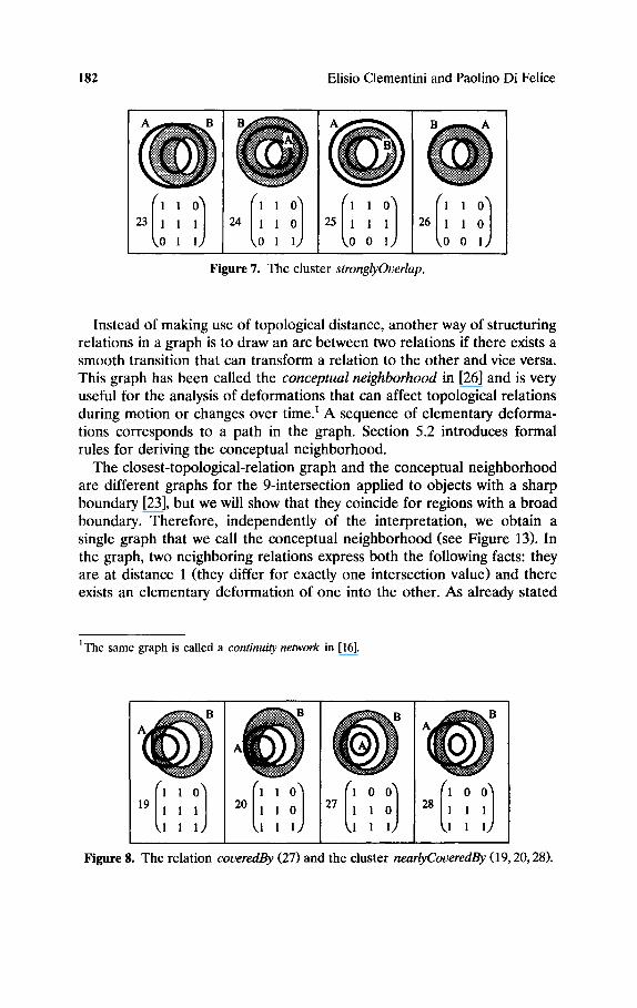
Figure 7. The cluster stronglyOverlap.

Instead of making use of topological distance, another way of structuring relations in a graph is to draw an arc between two relations if there exists a smooth transition that can transform a relation to the other and vice versa. This graph has been called the conceptual neighborhood in [26] and is very useful for the analysis of deformations that can affect topological relations during motion or changes over t ime: A sequence of elementary deforma- tions corresponds to a path in the graph. Section 5.2 introduces formal rules for deriving the conceptual neighborhood.

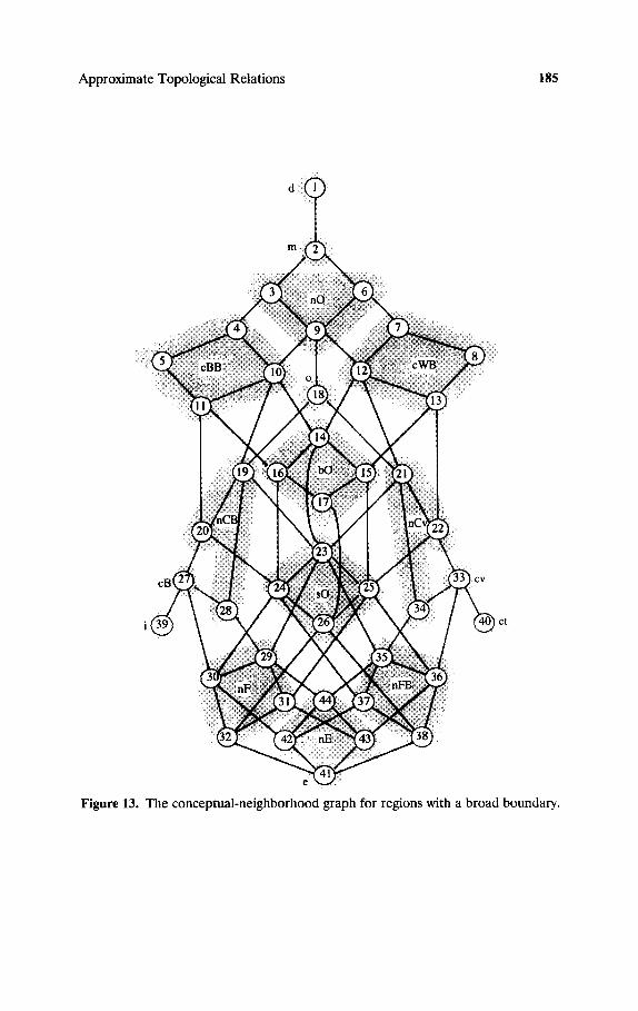
The closest-topological-relation graph and the conceptual neighborhood are different graphs for the 9-intersection applied to objects with a sharp boundary [23], but we will show that they coincide for regions with a broad boundary. Therefore, independently of the interpretation, we obtain a single graph that we call the conceptual neighborhood (see Figure 13). In the graph, two neighboring relations express both the following facts: they are at distance 1 (they differ for exactly one intersection value) and there exists an elementary deformation of one into the other. As already stated

IThe same graph is called a continuity network in [16].

20 1

I

27 1

1

28 1

1

Figure 8. The relation coveredBy (27) and the cluster neartyCoveredBy (19, 20, 28).

Approximate Topological Relations 183

21 1 1

22 1 0

33 0 1 0 0

Q 34 1

1

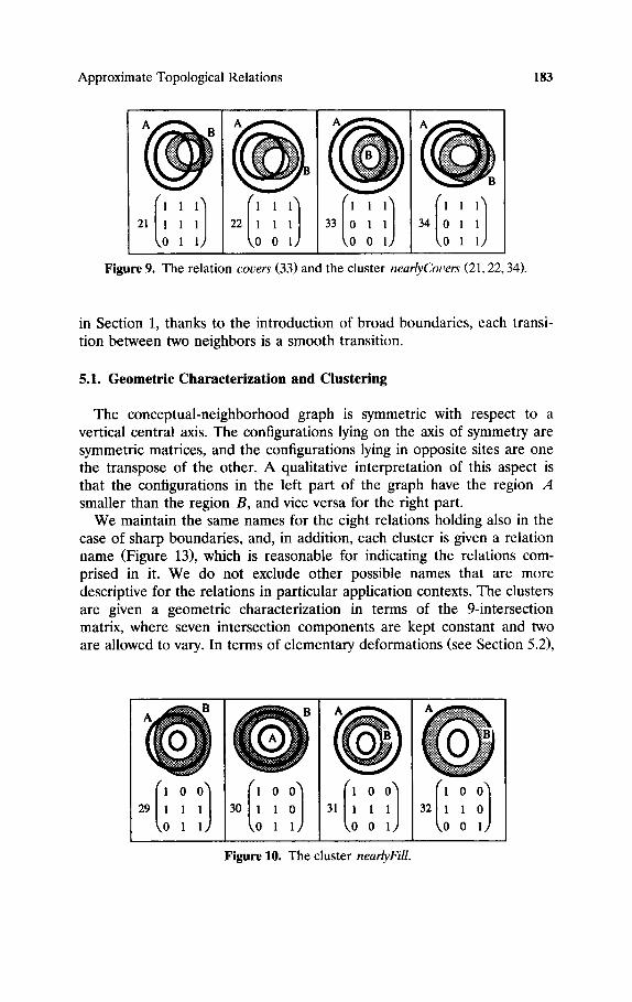
Figure 9. The relation covers (33) and the cluster nearlyCovers (21, 22, 34).

in Section 1, thanks to the introduction of broad boundaries, each transi- tion between two neighbors is a smooth transition.

5.1. G e o m e t r i c C h a r a c t e r i z a t i o n a n d C l u s t e r i n g

The conceptual-neighborhood graph is symmetric with respect to a vertical central axis. The configurations lying on the axis of symmetry are symmetric matrices, and the configurations lying in opposite sites are one the transpose of the other. A qualitative interpretation of this aspect is that the configurations in the left part of the graph have the region A smaller than the region B, and vice versa for the right part.

We maintain the same names for the eight relations holding also in the case of sharp boundaries, and, in addition, each cluster is given a relation name (Figure 13), which is reasonable for indicating the relations com- prised in it. We do not exclude other possible names that are more descriptive for the relations in particular application contexts. The clusters are given a geometric characterization in terms of the 9-intersection matrix, where seven intersection components are kept constant and two are allowed to vary. In terms of elementary deformations (see Section 5.2),

29 1 1

Q 10t 30 1

1 31 1

0

O f0t 32 1

0

Figure 10. The cluster nearlyFill.

184 Elisio Clementini and Paolino Di Felice

35 1

1

/il / 36 1

0

O 37 1

1

O 38 1

0

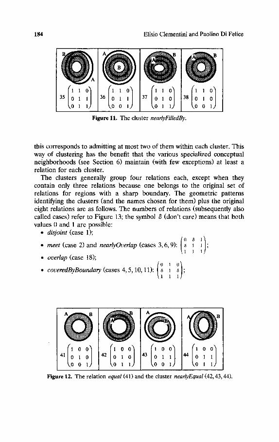
Figure 11. The cluster near(yFilledBy.

this corresponds to admitting at most two of them within each cluster. This way of clustering has the benefit that the various specialized conceptual neighborhoods (see Section 6) maintain (with few exceptions) at least a relation for each cluster.

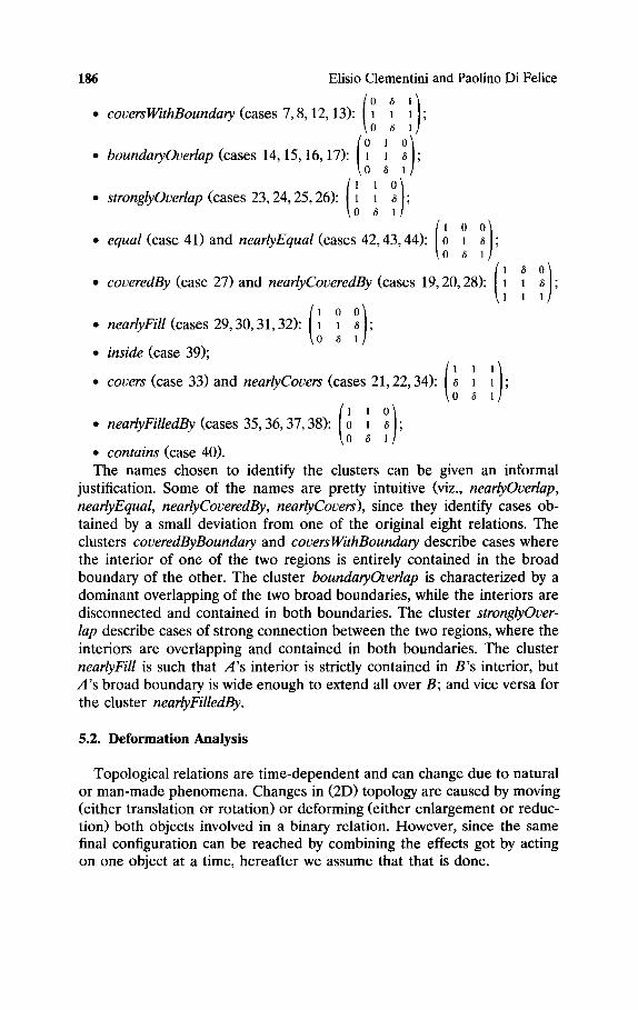
The clusters generally group four relations each, except when they contain only three relations because one belongs to the original set of relations for regions with a sharp boundary. The geometric patterns identifying the clusters (and the names chosen for them) plus the original eight relations are as follows. The numbers of relations (subsequently also called cases) refer to Figure 13; the symbol 8 (don't care) means that both values 0 and 1 are possible:

• disjoint (case 1); (0 1) • m e e t (case 2) and nearlyOverlap (cases 3, 6, 9): ~ 1 1 ;

1 1 1 • overlap (case 18);

• coveredByBoundary (cases 4, 5, 10, 11): 1 ; 1

Q 41 1

0

O 43 1

0

I°/ Figure 12. The relation equal (41) and the cluster nearlyEqual (42, 43, 44).

Approximate Topological Relations 185

Figure 13. The conceptual-neighborhood graph for regions with a broad boundary.

186 Elisio Clementini and Paolino Di Felice

• coversWithBoundary (cases 7, 8, 12, 13): 1 ; 6

• boundaryOverlap (cases 14, 15, 16, 17): 1 ; 6

• stronglyOverlap (cases 23, 24, 25, 26): 1 ; 6 (,00)

• equal (case 41) and nearlyEqual (cases 42, 43, 44): 0 a ~ ; 0 ~ 1

• coveredBy (case 27) and nearlyCoveredBy (cases 19, 20, 28): I I ; 1 1

• nearlyFill (cases 29, 30, 31, 32): 1 ;

• inside (case 39);

• covers (case 33) and nearlyCovers (cases 21, 22, 34): 1 i ; 8 1

• nearlyFilledBy (cases 35, 36, 37, 38): 0 i 6 ; 0 6 1

• contains (case 40). The names chosen to identify the clusters can be given an informal

justification. Some of the names are pretty intuitive (viz., nearlyOverlap, nearlyEqual, nearlyCoveredBy, nearlyCovers), since they identify cases ob- tained by a small deviation from one of the original eight relations. The clusters coveredByBoundary and coversWithBoundary describe cases where the interior of one of the two regions is entirely contained in the broad boundary of the other. The cluster boundaryOverlap is characterized by a dominant overlapping of the two broad boundaries, while the interiors are disconnected and contained in both boundaries. The cluster stronglyOver- lap describe cases of strong connection between the two regions, where the interiors are overlapping and contained in both boundaries. The cluster nearlyFill is such that A's interior is strictly contained in B's interior, but A's broad boundary is wide enough to extend all over B; and vice versa for the cluster neartyFilledBy.

5.2. Deformation Analysis

Topological relations are time-dependent and can change due to natural or man-made phenomena. Changes in (2D) topology are caused by moving (either translation or rotation) or deforming (either enlargement or reduc- tion) both objects involved in a binary relation. However, since the same final configuration can be reached by combining the effects got by acting on one object at a time, hereafter we assume that that is done.

Approximate Topological Relations 187

In this section, we introduce the concept of elementary deformation, which is the smallest deformation made on A (or B) able to change the binary topological relation between A and B. In terms of the 9-intersec- tion, this means that an elementary deformation is able to change at least one of the nine intersections from empty to nonempty (or the reverse). Furthermore, we introduce rules suitable to derive all the relations that can be reached starting from a given one, making an elementary deforma- tion each time. The relations we refer to are the 44 found in Section 4. This approach is inspired by the smooth transition model for line-region relations of [23]. The final objective is to build a graph based on the neighboring relations given by the rules and compare it with the graph based on topological distance. We then find that these two graphs are the same.

Each region A can be thought of as the union of three parts: the exterior (A- ) , the broad boundary (AA), and the interior (A°), which together cover the plane. With the introduction of an adjacency operator (adj), the following relationships exist among such parts: adj (A-) = AA, adj(AA) = (A °, A- ) , adj(A °) = AA. The elementary deformations that can be performed independently are as follows:

1. deforming A's outer boundary to intersect an adjacent part of B; 2. deforming A's inner boundary to intersect an adjacent part of B. As an example of elementary deformation, we can make a transition

from configuration 27 to configuration 28 (see Figure 8) by widening A's outer boundary until it overlaps the exterior of B. The change of the topological relation between A and B is limited to the intersection component A A N B-.

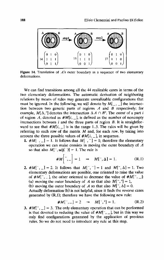
It is worthwhile to remark that in this context r/g/d transformations (rotation and translation) and scaling are not elementary and should be seen as composed of a sequence of elementary deformations. As an example of a rigid transformation let us refer to configurations 14 and 17 of Figure 6. We could try to go from 14 to 17 through a translation of A's outer boundary, but this is not possible because two elementary deforma- tions are required to realize the coincidence of the outer boundaries of regions A and B (see Figure 14): the first deformation stretches the right part of A's outer boundary (reaching the intermediate configuration 15), and the second deformation compresses the left part of A's outer bound- ary (reaching configuration 17). 2

2Configuration 15 is drawn differently in Figure 14 from Figure 6 to illustrate the elementary deformations taken into account in the example, but the two drawings are equivalent within the model (same M).

188 Elisio Clementini and Paolino Di Felice

14 1 15 1

1 0

s t e p 2

Figure 14. Translation of A's outer boundary as a sequence of two elementary deformations.

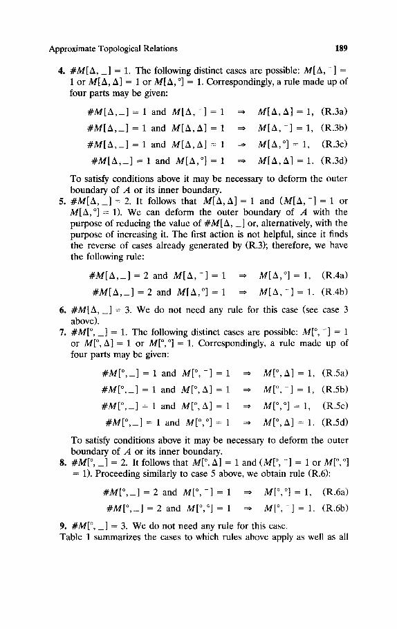
We can find transitions among all the 44 realizable cases in terms of the two elementary deformations. The automatic derivation of neighboring relations by means of rules may generate unrealizable configurations that must be ignored. In the following, we will denote by M[_ , _] the intersec- tion between two generic parts of regions A and B respectively; for example, M[A, o] denotes the intersection AA n B °. The extent of a part i of region A, denoted as #M[i, _], is defined as the number of nonempty intersections between i and the three parts of region B. It is straightfor- ward to see that #M[i, _] is in the range 1..3. The rules will be given by referring to each row of the matrix M and, for each row, by taking into account the three possible values of #M[i , _], in sequence.

1. #M[- , _] = 1. It follows that M[- , -] = 1; therefore the elementary operation we can make consists in moving the outer boundary of A so that also M[- , adj(-)] = 1. The rule is

[-1 # M ,_ = 1 =* M [ - , A ] = 1. (R.1)

2. # M [ - , _] = 2. It follows that M [ - , - ] = 1 and M[- , A] = 1. Two elementary deformations are possible, one oriented to raise the value of # M [ - , _], the other oriented to decrease the value of # M [ - , _]: (a) moving the outer boundary of A so that also M[- , °] = 1, (b) moving the outer boundary of A so that also M[- , A] = 0. Actually deformation (b) is not helpful, since it finds the reverse cases generated by (R.1); therefore we have the following new rule:

#M[- ,_] = 2 ~ M [ - , °] = 1. (R.2)

3. #M[-, _] = 3. The only elementary operation that can be performed is that devoted to reducing the value of #M[-, _], but in this way we only find configurations generated by the application of previous rules. So we do not need to introduce any rule at this step.

Approximate Topological Relations 189

4. #M[A, _] = 1. The following distinct cases are possible: M[A, -] = 1 or M[A, A] = 1 or M[A, °] = 1. Correspondingly, a rule made up of four parts may be given:

# M [ A , _ ] = I and M [ A , - ] = I ~ M [ A , A ] = I , (R.3a)

# M [ A , _ ] = I and M [ A , A ] = I ~ M [ A , - ] = I , (R.3b)

# M [ A , _ ] = I and M [ A , A ] = 1 = M[A, ° ] = 1, (R.3c)

# M [ A , _ ] = 1 and M I a , °] = 1 = M [ a , A ] = 1. (R.3d)

To satisfy conditions above it may be necessary to deform the outer boundary of A or its inner boundary.

5. # M [ A , _ ] = 2 . It follows that M [ A , A ] = 1 and ( M [ A , - ] = 1 or M[A, °] = 1). We can deform the outer boundary of A with the purpose of reducing the value of #M[A, _] or, alternatively, with the purpose of increasing it. The first action is not helpful, since it finds the reverse of cases already generated by (R.3); therefore, we have the following rule:

# M [ A , _ ] = 2 and M [ A , - ] = 1 = M[A, °] = 1, (R.4a)

# M [ A , _ ] = 2 and M[A, ° ] = 1 =~ M [ A , - ] = 1. (R.4b)

a. #M[A, _] = 3. We do not need any rule for this case (see case 3 above).

7. #M[ °, _] = 1. The following distinct cases are possible: M[ °, -] = 1 or M[ °, A] = 1 or M[°, °] = 1. Correspondingly, a rule made up of four parts may be given:

# M [ ° , _ ] = 1 and M[ ° , - ] = 1 ~ M[° ,A] = 1, (R.5a)

# M [ ° , _ ] = 1 and M [ ° , h ] = 1 ~ M[ ° , - ] = 1, (R.5b)

# M [ ° , _ ] = I and M[ ° , h ] = l ~ M[°, ° ] = 1, (R.5c)

# M [ ° , _ ] = 1 and M[°, °] = 1 = M[ o , a ] = 1. (R.Sd)

To satisfy conditions above it may be necessary to deform the outer boundary of A or its inner boundary.

8. #M[ °, _] = 2. It follows that M[ °, A] = 1 and (M[ °, -] = 1 or M[ °, °] = 1). Proceeding similarly to case 5 above, we obtain rule (R.6):

# M [ ° , _ ] = 2 and M[ ° , - ] = 1 ~ M[°, °] = 1, (R.6a)

# M [ ° , _ ] = 2 and M[°, ° ] = 1 ~ M[ ° , - ] = 1. (R.6b)

9. #M[ °, _] = 3. We do not need any rule for this case. Table 1 summarizes the cases to which rules above apply as well as all

190

Table .

Elisio Clementini and Paolino Di Felice

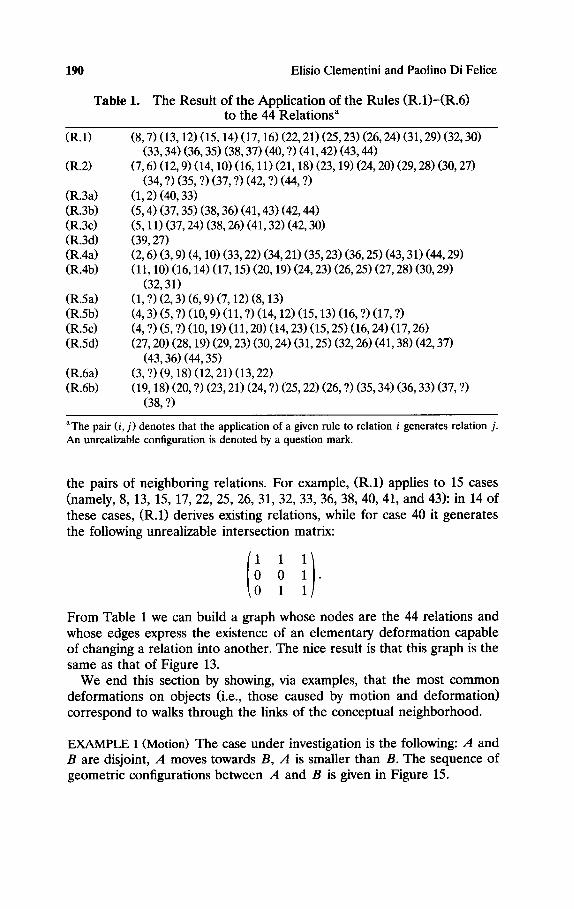
The Result of the Application of the Rules (R.1)-(R.6) to the 44 Relations a

(R.1)

(R.2)

(R.3a) (R.3b) (R.3c) (R.3d) (R.4a) (R.4b)

(R.5a) (R.5b) (R.5c) (R.5d)

(R.6a) (R.6b)

(8, 7) (13, 12) (15, 14) (17, 16) (22, 21) (25, 23) (26, 24) (31, 29) (32, 30) (33, 34) (36, 35) (38, 37) (40, ?) (41, 42) (43, 44)

(7, 6) (12, 9) (14, 10) (16, 11) (21, 18) (23, 19) (24, 20) (29, 28) (30, 27) (34, ?) (35, ?) (37, ?) (42, ?) (44, ?)

(1, 2) (40, 33) (5, 4) (37, 35) (38, 36) (41, 43) (42, 44) (5, 11) (37, 24) (38, 26) (41, 32) (42, 30) (39, 27) (2, 6) (3, 9) (4, 10) (33, 22) (34, 21) (35, 23) (36, 25) (43, 31) (44, 29) (11, 10) (16, 14) (17, 15) (20, 19) (24, 23) (26, 25) (27, 28) (30, 29)

(32, 31) (1, 7) (2, 3) (6, 9) (7, 12) (8, 13) (4, 3) (5, 7) (10, 9) (11, 7) (14, 12) (15, 13) (16, 7) (17, ?) (4, 7) (5, 7) (10, 19) (11, 20) (14, 23) (15, 25) (16, 24) (17, 26) (27, 20) (28, 19) (29, 23) (30, 24) (31, 25) (32, 26) (41, 38) (42, 37)

(43, 36) (44, 35) (3, ?) (9, 18) (12, 21) (13, 22) (19, 18) (20, ?) (23, 21) (24, ?) (25, 22) (26, ?) (35, 34) (36, 33) (37, ?)

(38, ?)

aThe pair (i, j) denotes that the application of a given rule to relation i generates relation j. An unrealizable configuration is denoted by a question mark.

the pairs of neighboring relations. For example, (R.1) applies to 15 cases (namely, 8, 13, 15, 17, 22, 25, 26, 31, 32, 33, 36, 38, 40, 41, and 43): in 14 of these cases, (R.1) derives existing relations, while for case 40 it generates the following unrealizable intersection matrix:

( i 1 i ) 0 • 1

From Table 1 we can build a graph whose nodes are the 44 relations and whose edges express the existence of an elementary deformation capable of changing a relation into another. The nice result is that this graph is the same as that of Figure 13.

We end this section by showing, via examples, that the most common deformations on objects (i.e., those caused by motion and deformation) correspond to walks through the links of the conceptual neighborhood.

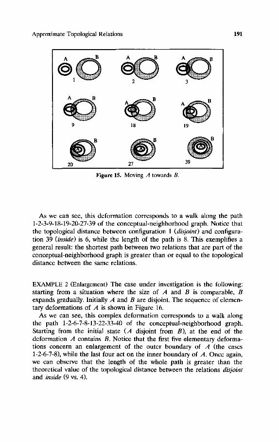
EXAMPLE 1 (Motion) The case under investigation is the following: A and B are disjoint, A moves towards B, A is smaller than B. The sequence of geometric configurations between A and B is given in Figure 15.

Approximate Topological Relations 191

9 18 19

20 27 39

Figure 15. Moving A towards B.

As we can see, this deformation corresponds to a walk along the path 1-2-3-9-18-19-20-27-39 of the conceptual-neighborhood graph. Notice that the topological distance between configuration 1 (disjoint) and configura- tion 39 (inside) is 6, while the length of the path is 8. This exemplifies a general result: the shortest path between two relations that are part of the conceptual-neighborhood graph is greater than or equal to the topological distance between the same relations.

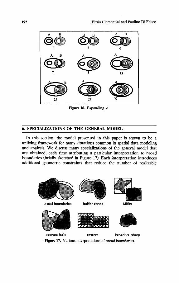
EXAMPLE 2 (Enlargement) The case under investigation is the following: starting from a situation where the size of A and B is comparable, B expands gradually. Initially A and B are disjoint. The sequence of elemen- tary deformations of A is shown in Figure 16.

As we can see, this complex deformation corresponds to a walk along the path 1-2-6-7-8-13-22-33-40 of the conceptual-neighborhood graph. Starting from the initial state (A disjoint from B), at the end of the deformation A contains B. Notice that the first five elementary deforma- tions concern an enlargement of the outer boundary of A (the cases 1-2-6-7-8), while the last four act on the inner boundary of A. Once again, we can observe that the length of the whole path is greater than the theoretical value of the topological distance between the relations disjoint and inside (9 vs. 4).

192 Elisio Clementini and Paolino Di Felice

A B A B

1 2

A B A

7 8

A B

6

A

13

22 33 4O

Figure 16. Expanding A.

6. SPECIALIZATIONS OF THE GENERAL MODEL

In this section, the model presented in this paper is shown to be a unifying framework for many situations common in spatial data modeling and analysis. We discuss many specializations of the general model that are obtained, each time attributing a particular interpretation to broad boundaries (briefly sketched in Figure 17). Each interpretation introduces additional geometric constraints that reduce the number of realizable

broad boundaries buffer zones

convex hulls rasters

MBRs

O broad vs. sharp

Figure 17. Various interpretations of broad boundaries.

Approximate Topological Relations 193

topological relations from the 44 of the general model. Consequently, in the corresponding conceptual neighborhoods there are arcs between con- figurations at topological distance 2.

First, broad boundaries can represent various approximations of the geometry of an object. Best-case approximations of objects are known as "containers" in computational geometry [32]. Two types of containers are MBRs and convex hulls. The role of approximate topological relations in this context is to give fast selection criteria. Second, broad boundaries can make a model for proximity measures. Buffer zones, MBRs, and convex hulls are all used in spatial analysis as a refinement of topological rela- tions. Third, broad boundaries have a direct application in raster data models. This section examines all these issues and develops also the hybrid case of relations between an object with a sharp boundary and an object with a broad boundary.

6.1. Small Boundaries

In [7], the conceptual neighborhood was developed under the assump- tion that the broad boundary of a region is much smaller than its interior (small-boundaries assumption): AA << A °. This hypothesis excludes from the graph four relations (cases 14, 15, 16, 17) that would need very thick boundaries and small interiors in their geometric interpretation.

6.2. Buffer Zones

A common GIS operation is the creation of buffer zones surrounding objects, comprised between the original boundary and a new parallel boundary, offset by a certain distance. Specifically, buffer zones refer to distances offset on the outside, while skeletons refer to distances offset on the inside [28]. Buffers are used to establish critical areas for analysis or to indicate proximity. If buffer zones are interpreted as broad boundaries, the general model applies with the exclusion of three cases (17, 26, 44). Such cases are not realizable because buffer zones are characterized by a constant width.

63. Minimum Bounding Rectangles

An MBR is a rectangle with edges parallel to the x and y axes that tightly encloses an object. MBRs are the most common approximations of objects used for spatial data indexing, since the coordinates of two points are sufficient to store them. Topological relations between MBRs have been studied as a fast selection criterion for finding the topological relations between objects represented with R-trees [33] and for optimiza- tion strategies for queries with topological constraints [10].

194 Elisio Clementini and Paolino Di Felice

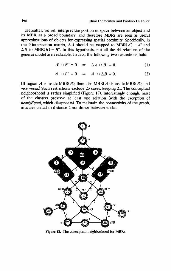
Hereafter, we will interpret the portion of space between an object and its MBR as a broad boundary, and therefore MBRs are seen as useful approximations of objects for expressing spatial proximity. Specifically, in the 9-intersection matrix, AA should be mapped to MBR(A) - A ° and AB to M B R ( B ) - B °. In this hypothesis, not all the 44 relations of the general model are realizable. In fact, the following two restrictions hold:

A ° r i B - = 0 ~ A A A B - = 0 , (1)

A - N B ° = O ~ A - A A B = O . (2)

[If region A is inside MBR(B), then also MBR(A) is inside MBR(B), and vice versa.] Such restrictions exclude 23 cases, keeping 21. The conceptual neighborhood is rather simplified (Figure 18). Interestingly enough, most of the dusters preserve at least one relation (with the exception of nearlyEqual, which disappears). To maintain the connectivity of the graph, arcs associated to distance 2 are drawn between nodes.

et

Figure 18. The conceptual neighborhood for MBRs.

Approximate Topological Relations 195

6.4. Convex Hulls

Convex hulls have been used as object approximations for spatial access [2]. The advantage is a tighter approximation than in the case of MBRs, but the disadvantage is more expensive computation and storage. Convex hulls are used in qualitative spatial reasoning as a refinement of topologi- cal relations, in order to distinguish between various kinds of "insides" [13]. Finally, convex hulls are used in map generalization for the aggrega- tion of areal objects [29].

Broad boundaries can be interpreted as convex hulls, by putting A A = C H ( A ) - A ° and AB = C H ( B ) - B °. The configurations that can be realized with convex hulls are very similar to the case of MBRs. In fact, the same two restrictions apply, rephrased as follows:

If region A is inside CH(B), then also CH(A) is inside CH(B), and vice versa.

Furthermore, we eliminate another case (17) with the restriction

(AA n B - = 0) A ( A - N AB = 0) =, A ° n B ° = 1. (1)

(If two regions have the same convex hull, then they intersect.) The resulting conceptual neighborhood for the 20 relations between

convex hulls is shown in Figure 19. Notice that the boundaryOverlap cluster is no longer present. In [13], the authors found a set of 22 base relations: the two additional relations are due to the fact that their restrictions are weaker than ours, since they take into account also regions with disconnected components.

6.5. Rasters

The general model presented in this paper subsumes the model for topological relations between rasters (Z2). This model [25] identifies 16 topological relations between rasters and builds the conceptual neighbor- hood for them.

We consider the following restrictions on the 9-intersection:

(A ° n AB = 1) A ( A - n B ° = 1) =* AA n B ° = 1, (1)

(AA N B ° = 1) A ( A ° N B - = 1) ~ A ° N A B = 1 (2)

(if A's interior overlaps B's boundary and B's interior is not all contained in A, then A's boundary must intersect B's interior, and vice versa);

A ° n AB = 1 ~ AA n B - = 1, (3)

AA N B ° = 1 =, A - N A B = 1 (4)

(if A's interior intersects B's boundary, then region B cannot cover the

196

entire region A, and vice versa);

Elisio Clementini and Paolino Di Felice

(A ° N B ° = 1) A (A ° N A B = 0 ) =* AA AB - = 0 , (5)

(A ° o B ° = 1) A ( A A O B ° = 0 ) =~ A - N A B = 0 (6)

(if A's interior is entirely contained in B's interior, then A's boundary cannot reach B's exterior, and vice versa).

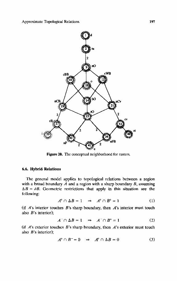
With the restrictions above, we eliminate 27 cases and find 17 possible cases (see Figure 20) between rasters. Similarly to the case of MBRs, at least one relation per cluster is maintained, with the exception of the nearlyEqual cluster. Compared to [25], case 14 (boundaryOverlap) is a new case, since in that paper the authors excluded very thin rasters (with 1-pixel-wide interior).

Figure 19. The conceptual neighborhood for convex hulls.

Approximate Topological Relations 197

Figure 20. The conceptual neighborhood for rasters.

CA

6.6. Hybrid Relations

The general model applies to topological relations between a region with a broad boundary A and a region with a sharp boundary B, assuming A B = aB, Geometric restrictions that apply in this situation are the following:

A ° N A B = 1 =~ A ° A B ° = 1 (1)

(if A's interior touches B's sharp boundary, then A's interior must touch also B's interior);

A - N A B = 1 ~ A - A B ° = 1 (2)

(if A's exterior touches B's sharp boundary, then A's exterior must touch also B's interior);

A ° n B - = O ~ A ° A A B = O (3)

198 Elisio Clementini and Paolino Di Felice

(if A's interior is entirely contained in B, then A's interior cannot intersect B's sharp boundary);

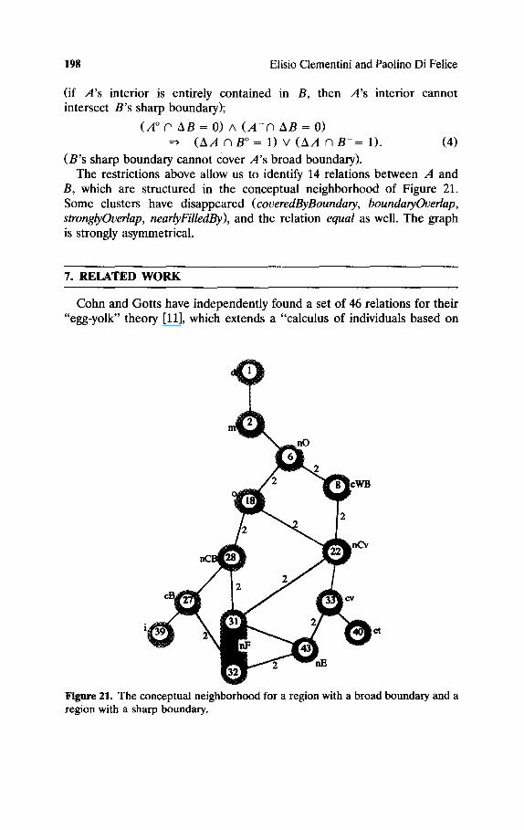
(A ° n A B = 0 ) A ( A - N A B = 0 ) (AA n B ° = 1) v (AA n B-= 1). (4)

(B's sharp boundary cannot cover A's broad boundary). The restrictions above allow us to identify 14 relations between A and

B, which are structured in the conceptual neighborhood of Figure 21. Some clusters have disappeared (coveredByBoundary, boundaryOverlap, stronglyOverlap, nearlyFilledBy), and the relation equal as well. The graph is strongly asymmetrical.

7. RELATED WORK

Cohn and Gotts have independently found a set of 46 relations for their "egg-yolk" theory [11], which extends a "calculus of individuals based on

nO

12

¢t

v n E

Figure 21. The conceptual neighborhood for a region with a broad boundary and a region with a sharp boundary.

Approximate Topological Relations 199

connection," and is expressed in a many-sorted logic. In this theory, a region with a broad boundary is modeled by an inner subregion (the yolk), an outer subregion (the white, corresponding to our broad boundary), and their union (the egg). Different configurations are classified according to the topological relations holding between the pairs egg-egg, yolk-yolk, and yolk-egg. Cohn and Gotts use a set of logically defined topological rela- tions called RCC-5, consisting of five relations (PO, PP, EQ, PPI, DR).

In essence, Cohn and Gotts's approach reuses the same relations hold- ing between regions with a sharp boundary to describe topological config- urations between egg-yolk pairs, while our approach is an extension of the 9-intersection leading to the consideration of a new set of base relations defined in terms of geometric criteria (empty or nonempty intersections between interiors, broad boundaries, and exteriors).

The two approaches are in substantial agreement on the topological configurations for pairs of regions with a broad boundary, though with some structural differences. A first difference is that some limit configura- tions involving inner and outer boundaries fall in different cases in the two approaches. In fact, in RCC-5 the case in which two regions are disjoint and the case in which two regions meet are grouped together in the same base relation (DR). This implies, for example, that the limit configuration in which two regions touch along their outer boundaries falls in case 1, whereas in our approach it falls in case 2. Another difference is that we define the broad boundary as a closed point set and the interior as an open point set, whereas Cohn and Gotts's yolk corresponds to a closed point set.

These differences have the effect of distinguishing two more cases in Cohn and Gotts's model: these are two limit configurations (i.e., when A's inner boundary coincides with B's outer boundary, and the reverse) that in our model are absorbed by case 36 and case 30, respectively.

Another result of Cohn and Gotts's work is to have found a conceptual neighborhood and clustering of relations that is similar to that of Figure 13. They consider "complete crispings" of egg-yolk pairs, which are regions whose sharp boundary lies between the limits defined by yolk and egg. To cluster the 46 relations, they group together those relations whose com- plete crispings have the same RCC-5 relations, obtaining 13 clusters. We can observe that there is a correspondence between such clusters and the groups of relations identified by the geometric patterns of Section 5.1, with some exceptions: there is a 16-relations cluster comprising all the relations stronglyOverlap, near!yEqual, equal, near!yFill, nearlyFilledBy; there are two clusters of one relation each corresponding to the two additional relations of Cohn and Gotts's model.

The process of obtaining a crisping from an egg-yolk pair is not an elementary deformation conforming to our definition, but it may be seen as a deformation that in general requires many elementary steps.

200 Elisio Clementini and Paolino Di Felice

clustering process, instead, is based on only two elementary deformations for each cluster. For this reason, the crisping process is not able to distinguish among the relations of the 16-relation cluster.

8. CONCLUSIONS

In this contribution we have extended an existing model for topological relations between objects with a sharp boundary (the 9-intersection) to model topological relations between objects with a broad boundary. This extension maintains all the properties of the original model: among others, it gives a mutually exclusive and complete set of relations, and serves as an algebraic basis for spatial reasoning. The extended model is simple and allows us to describe the indeterminacy in boundaries with the same language adopted for exact boundaries.

Major merits of the present contribution are as follows: • The 44 topological relations between two regions with a broad bound-

ary that are realizable in the general case were structured in a graph (the closest-topological-relation graph). The topological distance func- tion was used during both the structuring process and the clustering of the relations. The clustering of similar configurations gives a set of names that provides a qualitative description of topological scenes involving objects with broad boundaries. This set of names is a superset of the names for simple objects.

• A different way of structuring the 44 topological relations based on the notion of elementary deformation of a region was also proposed (the conceptual neighborhood graph). Formal rules for making such a derivation were given.

• The coincidence of the two graphs was the proof that the introduction of broad boundaries contributes to making models for topological relations closer to reality, as is pointed out. • by the elimination of configurations that can be realized only for a

moment in time (states of position according to [27]) and • by the fact that all the neighboring relations are at topological

distance 1. • The proposed model is suitable for reasoning about gradual changes

in topology due to objects motion and/or deformation over a period of time. We showed, through examples, that gradual changes in topology are equivalent to paths in the conceptual neighborhood.

• The model is very general, as was proved by the manifold specializa- tions given to it, each time adopting a different interpretation for the broad boundary. This was also a way of verifying the appropriateness

Approximate Topological Relations 201

of the clustering process, since the various specialized conceptual neighborhoods maintain (with few exceptions) at least one relation for each cluster.

ACKNOWLEDGMENTS

We would like to thank the anonymous reviewers for their useful comments and recommendations. We are grateful to Tony Cohn for many discussions comparing our work.

References

1. A1-Taha, K., Deformation analysis and geometric interpretations of imprecise binary topological relations, Tech. Rep., Dept. of Surveying Engineering, Univ. of Maine, 1992.

2. Brinkhoff, T., Kriegel, H.-P., and Schneider, R., Comparison of approximations of complex objects used for approximation-based query processing in spatial database systems, Ninth International Conference on Data Engineering, Vienna, IEEE Press, 81-90, 1993.

3. Bruegger, B. P., Spatial theory for the integration of resolution-limited data. PhD Thesis, Univ. of Maine, 1994.

4. Burrough, P. A., and Frank, A. U., Concepts and paradigms in spatial informa- tion: Are current geographic information systems truly generic? Internat. J. Geographical Inform. Systems 9(2), 101-116, 1995.

5. Burrough, P. A., and Frank, A. U. (Eds.), Geographic Objects with Indeterminate Boundaries, GISDATA Ser., Taylor & Francis, London, 1996.

6. Clementini, E., and Di Felice, P., A comparison of methods for representing topological relations. Inform. Sci. 3(3), 149-178, 1995.

7. Clementini, E., and Di Felice, P., An algebraic model for spatial objects with indeterminate boundaries, in Geographic Objects with Indeterminate Boundaries. (P. A. Burrough and A. U. Frank, Eds.), GISDATA Ser., Taylor & Francis, London, Chapter 11, 155-169, 1996.

8. Clementini, E., and Di Felice, P., A model for representing topological rela- tionships between complex geometric features in spatial databases. Inform. Sci. 90(1-4), 121-136, 1996.

9. Clementini, E., Di Felice, P., and van Oosterom, P., A small set of formal topological relationships for end-user interaction, Advances in Spatial

202 Elisio Clementini and Paolino Di Felice

Databases--Third International Symposium, SSD "93 (D. Abel and B. C. Ooi, Eds.), Lecture Notes in Comput. Sci. 692, Springer-Verlag, Singapore, 277-295, 1993.

10. Clementini, E., Sharma, J., and Egenhofer, M. J., Modelling topological spatial relations: Strategies for query processing, Comput. Graphics 18(6), 815-822, 1994.

11. Cohn, A. G., and Gotts, N. M., The "Egg-Yolk" representation of regions with indeterminate boundaries, in Geographic Objects with Indeterminate Boundaries (P. A. Burrough and A. U. Frank, Eds.), GISDATA Ser., Taylor & Francis, London, Chapter 12, 171-187, 1996.

12. Cohn, A. G., and Gotts, N. M., Representing spatial vagueness: A mereological approach, Principles of Knowledge Representation and Reasoning: Proceedings of the International Conference (KR96), Morgan Kaufmann, San Francisco, 1996.

13. Cohn, A. G., Randell, D. A., and Cui, Z., Taxonomies of logically defined qualitative spatial relations, Intemat. J. Human-Comput. Stud. 43(5-6), 831-846, 1995.

14. Couclelis, H., People manipulate objects (but cultivate fields): Beyond the raster-vector debate in GIS, in Theories and Methods ofSpatio-temporalReason- ing in Geographic Space (A. U. Frank, I. Campari, and U. Formentini, Eds.), Lecture Notes in Comput. Sci. 639, Springer-Verlag, Pisa, Italy, 65-77, 1992.

15. Couclelis, H., Towards an operational typology of geographic entities with ill-defined boundaries, in Geographic Objects with Indeterminate Boundaries (P. A. Burrough and A. U. Frank, Eds.), GISDATA Ser., Taylor & Francis, London, Chapter 3, 45-55, 1996.

16. Cui, Z., Cohn, A. G., and Randell, D. A., Qualitative and topological relation- ships in spatial databases, Advances in Spatial Databases--Third International Symposium, SSD '93 (D. J. Abel and B. C. Ooi, Eds.), Springer-Verlag, Singapore, Lecture Notes in Comput. Sci. 692, 296-315, 1993.

17. Dutta, S., Approximate spatial reasoning: Integrating qualitative and quantita- tive constraints, lnternat. J. Approx. Reason. 5, 307-331, 1991.

18. Dutta, S., Topological constraints: A representational framework for approxi- mate spatial and temporal reasoning, Advances in Spatial Databases--Second Symposium, SSD '91, Springer-Verlag, Zurich, 161-180, 1991.

19. Egenhofer, M. J., and AI-Taha, K., Reasoning about gradual changes of topological relationships, in Theories and Models of Spatio-temporal reasoning in Geographic Space (A. U. Frank, I. Campari, and U. Formentini, Eds.), Lecture Notes in Comput. Sci. 639, Springer-Verlag, Berlin, 196-219, 1992.

20. Egenhofer, M. J., Clementini, E., and Di Felice, P., Topological relations between regions with holes, Internat. J. Geographical Inform. Systems 8(2), 129-142, 1994.

21. Egenhofer, M. J., and Franzosa, R. D., Point-set topological spatial relations, Intemat. J. Geographical lnform. Systems 5(2), 161-174, 1991.

Approximate Topological Relations 203

22. Egenhofer, M. J., and Herring, J. R., Categorizing binary topological relation- ships between regions, lines, and points in geographic databases, Tech. Report, Dept. of Surveying Engineering, Univ. of Maine, Orono, 1991.

23. Egenhofer, M. J., and Mark, D. M., Modeling conceptual neighborhoods of topological line-region relations, lnternat. J. Geographical Inform. Systems 9(5), 555-565, 1995.

24. Egenhofer, M. J., and Mark, D. M., Naive geography, Spatial Information Theory: A Theoretical Basis for GIS--lnternational Conference, COSIT'95 (A. U. Frank and W. Kuhn, Eds.), Lecture Notes in Comput. Sci. 988, Springer-Verlag, Berlin, 1-15, 1995.

25. Egenhofer, M. J., and Sharma, J., Topological relations between regions in R 2 and Z 2, Advances in Spatial Databases--Third International Symposium, SSD '93 (D. Abel and B. C. Ooi, Eds.), Lecture Notes in Comput. Sci. 692, Springer-Verlag, Singapore, 316-336, 1993.

26. Freksa, C., Temporal reasoning based on semi-intervals, Artificial Intelligence 54, 199-227, 1992.

27. Galton, A., Towards a qualitative theory of movement, Spatial Information Theory: A Theoretical Basis for GIS--International Conference, COSIT'95 (A. U. Frank and W. Kuhn, Eds.), Lecture Notes in Comput. Sci. 988, Springer-Verlag, Berlin, 377-396, 1995.

28. Laurini, R., and Thompson, D., Fundamentals of Spatial Information Systems, Academic, New York, 1992.

29. Mackaness, W. A., Issues in resolving visual spatial conflicts in automated map design, Advances in GIS Research, Proceedings of the 6th International Sympo- sium on Spatial Data Handling, International Geographical Union (T. Waugh and R. Healey, Eds.), Taylor & Francis, Edinburgh, Scotland, 325-340, 1994.

30. Mark, D. M., and Egenhofer, M. J., Modeling spatial relations between lines and regions: Combining formal mathematical models and human subjects testing, Cartography and GIS 21(3), 195-212, 1994.

31. Munkres, J. R., Topology: A First Course, Prentice-Hall, Englewood Cliffs, N.J., 1975.

32. Nievergelt, J., 7 + 2 criteria for assessing and comparing spatial data struc- tures, Advances in Spatial Databases, 1st Symposium, SSD '89 (A. Buchmann, O. Giinther, T. R. Smith, and Y. F. Wang, Eds.), Lecture Notes in Comput. Sci. 409, Springer-Verlag, Santa Barbara, Calif., 3-27, 1989.

33. Papadias, D., Theodoridis, Y., Sellis, T., and Egenhofer, M. J., Topological relations in the world of minimum bounding rectangles: A study with R-trees, Proceedings of the ACM SIGMOD International Conference on Management of Data, ACM Press, San Jose, Calif., 92-103, 1995.

34. Story, P. A., and Worboys, M. F., A design support environment for spatiotem- poral database applications, Spatial Information Theory: A Theoretical Basis for

204 Elisio Clementini and Paolino Di Felice

GIS--International Conference, COSIT'95 (A. U. Frank and W. Kuhn, Eds.), Lecture Notes in Comput. Sci. 988, Springer-Verlag, Berlin, 413-430, 1995.

35. Wazinsky, P., Graduated topological relations, Tech. Report SFB 314 (VITRA) no. 54, Univ. des Saarlandes, Saarbriichen, Germany, 1993.

36. Winter, S., Uncertainty of topological relations in GIS, Proceedings of the ISPRS Commission III Symposium, SPIE, Munich, Germany, 924-930, 1994.

37. Zubin, D., Communication, Languages of Spatial Relations: Initiative Two Spe- cialist Meeting Report (D. M. Mark, A. U. Frank, M. J. Egenhofer, S. M. Freundschuh, M. McGranaghan, and R. M. White, Eds.), Tech. Paper 89-2, National Center for Geographic Information and Analysis, Santa Barbara, Calif., 13-17, 1989.