1

ADAPTIVE TRAFFIC SIGNAL CONTROL USING

APPROXIMATE DYNAMIC PROGRAMMING

Chen Cai *, Chi Kwong Wong, Benjamin G. Heydecker

Centre for Transport Studies

University College London

London WC1E 6BT

United Kingdom

ABSTRACT

This paper develops an adaptive traffic signal control method that optimizes performance over time. The

adaptive controller, instead of retrieving control parameters from a library according to changes in traffic,

allows the value of control parameters to be slowly time-varying so that controller’s behavior conforms to new

circumstance. The adaptive controller is developed on Approximate Dynamic Programming (ADP). By

replacing the look-up table containing real value of each state combination with an approximate function, ADP

obviates the limit of Dynamic programming in cases of high dimensionality and of incomplete information.

Approximation is progressively improved by employing online learning techniques. In this paper, we investigate

ADP approach with reinforcement learning and perturbation learning. Through numerical examples, this paper

shows that an adaptive controller based on ADP method is operational at isolated intersections while offering

potentials for network control. It also shows that a simple linear approximation is sufficient to provide practical

significance and to improve performance substantially towards theoretical limit.

2

1. INTRODUCTION

Operating traffic signal in urban area requires proper timings for signal indications so that varying demand

could be effectively managed and control objectives being met. Conventional algorithms are often so designed

that, with given input, they generate timings with fixed stage duration and sequence. Later development in

online control systems allows timings to be responsive (or vehicle actuate) by adjusting green extension or early

cut-off on the edge of stage change. Control parameters for responsive systems as such are usually preset and

retrieved in a library that requires manual updates periodically. To optimize performance over time, however, is

to progressively adapt control policy over time. In this regard, this paper we introduce an adaptive traffic signal

control method. The adaptive controller, instead of retrieving control parameters from a preset library according

to changes in traffic, allows the value of control parameters to be slowly time-varying so that controller’s

behavior conforms to new circumstance. Signal timings produced by the adaptive controller is free of

constraints on stage duration and stage orders, unless otherwise specified. The underlying theory for such an

adaptive controller is Approximate Dynamic Programming (ADP). The technique supervising time-varying

estimation of control parameters is reinforcement learning.

ADP is a theoretical framework that allows various approximation and learning techniques to be employed

to overcome the restrictions of Dynamic Programming (DP) in real-time adaptive control. Dynamic

programming, developed by Richard Bellman, traditionally, is the only exact and efficient way to solve

problems in optimization over time, in the general case where noise and nonlinearity are present (Werbos, 2004).

Key to the problem solving process in DP is the backward recursive estimation of the value of being in a state of

the current stage. Subject to the probability distribution of exogenous information, an optimal decision is to

optimize the overall utility in the process of transferring the state of current stage to the next state of the

following stage. In doing so, DP guarantees global optimum in problem solving. Powerful as it is, DP’s

usefulness in real-time control is severely limited. This is because of the exponential relationship between

computational burden and the size of state space, the complexity of probability distribution of information, and

the number of optional decisions. This relationship is often referred as ‘Three Curses of Dimensionality’

(Powell, 2007). Yet, this is not the end. Supplying complete information for evaluating policies, as required by

DP, is unrealistic in real-time control. In the introduction to fundamentals of ADP, we will show that, using an

approximate function to replace the exact values in DP, ADP drastically reduces computational burden, and by

adopting a forward algorithmic strategy, ADP utilizes limited real-time information to evaluate control policy

and update approximation.

The reason of introducing reinforcement learning is that parameters of the approximate function are not

known a priori, and we need a technique to learn the proper values in a changing environment where a ‘teacher’

is not available. Such a learning process is therefore unsupervised. Among a number of unsupervised learning

techniques, we select perturbation analysis and back-propagation neural network to provide the learning

capability.

3

The rest of the paper is organized as follows: Section 2 provides a review of existing traffic signal control

systems from which we identify the scope for development and the objective of this ADP approach. Section 3

shows the fundamentals of ADP technique, and how approximation can be progressively improved through

learning techniques. Section 4 introduces the numerical experiments and analyzes ADP results in comparisons.

Section 5 concludes this study and identifies the scope for future research in applying ADP to traffic control.

2. TRAFFIC SIGNAL CONTROL

The operation of traffic signal settings can be broadly classified into off-line and on-line approaches. Off-

line methods usually take on historical traffic data as inputs for the design of signal plans. Whereas on-line

approaches utilize real time traffic information collected from loop detectors to develop the responsive signal

settings. Here we focus the review only on online control systems. A terminology frequently used in both signal

control field and dynamic programming is stage. To avoid confusion between the terms we henceforth use

signal-stage to denote a group of one or more traffic/pedestrian phases which receive a green signal during a

particular period, i.e. the stage of signal control, and use stage to refer the term in dynamic programming.

Among online approaches, those who collect real-time traffic information from loop detectors and

evaluated instantaneously to generate the most up-to-date signal settings for implementation pertains to

responsive control; and those who also utilize real-time traffic information to select the pre-specified signal

plans which are best matches with the detected traffic pattern pertains to actuated control. Several well-known

traffic signal design packages are reviewed. Those important characteristics of the packages are summarized in

Table 1.

Table 1 Summary of different design programs for traffic signal control

Program Traffic data Decision on signalsettings

Signalcycle

Signalcoordination

Origincountry

Objective foroptimization

Servomechanism

OPAC On-line data from upstreamdetectors

Change of currentsignal settingsRolling forward

Acyclic Nil US Delay Decentralized

UTOPIA On-line data from upstreamdetectors

Green start andduration times andoffsets

Required With offsetoptimization

ITALY Delay and stop Centralized

SCATS On-line data from stop line(downstream)detector

Pre-sepcified signalplan replacement

Required With offsetoptimization

Australia Capacity* Centralized

SCOOT On-line data from upstreamdetectors

Change of wholesignal plan

Required With offsetoptimization

UK Delay, stop, andcongestion

Centralized

PRODYN On-line data from pair ofupstream detectors

Change of currentsignal settings

Acyclic Possible France Total delay Decentralized

MOVA On-line data from pair ofupstream detectors

Green extension ornot

N/A Nil UK Delay, stop andcapacity

Decentralized

DYPIC Off-line basis and perfectinformation

Complete signalsettings

Acyclic Nil UK Delay Decentralized

* Vehicle discharge rates are monitored and signal will be changed if it is found less than the saturation flow rate

4

SCOOT (Hunt et al., 1981) and SCATS (Luk, 1984) are basically online variants of offline optimization

strategies. Manual engineering work is required to update traffic data and feed them into offline optimizer,

TRANSYT for example, for a preparation of a library of plans that applies to different time periods of a day.

The ultimate performance of systems as those depends on the accuracy of database and its conformity to

software requirements. The online capability then enables the selection of the most appropriate plan from the

library according to detected traffic from sensors, adjusts offsets between adjacent intersections to facilitate

coordination, and makes small adjustment to the signal plans. SCOOT reduces delay to vehicles by 12% when

compared to up-to-date plans from TRANSYT. SCATS produces 23% reduction in travel time in comparison

with uncoordinated operations.

DYPIC (Robertson and Bretherton, 1974), OPAC (Gartner, 1983) and PRODYN (Henry et al., 1983) are

successively development in dynamic optimization of traffic signals. DYPIC is actually a backward dynamic

programming algorithm serves only for analytical purpose, which is to create a series of look-up tables

containing exact value associated with each state, along with performance indices serving as benchmarks. An

empirical function of quadratic form is proposed for a heuristic solution aiming for practical uses. The heuristic

solution adopts the concept of rolling horizon, which means that: first, a planning horizon is split into a ‘head’

period with detected traffic information and a ‘tail’ period with synthesized traffic information; second, an

optimal policy is calculated for the entire horizon, but is implemented only for the ‘head’ period; finally, when

next discrete time interval is arrived and newly detected information becomes available, the process rolls

forward and repeats itself. Gartner (1983) gives a detailed description of rolling horizon approach in his

introduction of OPAC. However, OPAC does not abide by the principle of optimality adherent to dynamic

programming, rather it uses Optimal Sequential Constrained (OSCO) search to plan for the entire horizon, and

employ terminal cost to penalize queues left after the horizon. OPAC in both simulation and field tests saves 5-

15% from existing traffic-actuated methods, with most of the benefits coming from situation of high degree of

saturation. The concerns with OPAC are that the restrictions in OSCO search reduces the flexibility of decision

making, and a long planning horizon (60s) raises practical questions about the value of optimizing far into the

future on the basis of synthesized information when the decisions planned may never the implemented.

PRODYN, also adopting rolling horizon approach, optimizes timings via a forward dynamic programming

(FDP). To avoid computing optimality equation at grid point that eventually poses the problem of

dimensionality, the FDP is particularly designed that it aggregates state variables into a few subsets, and the

value of being in a subset is only evaluated when it is actually being arrived at. Value function presenting the

future cost in the FDP is directly adopted from Robertson and Bretherton’s work. By evaluating all the subsets

that can be possibly arrived at, the FDP records the optimal trajectory of control policy in the planning horizon

(75s). And the process rolls forward as it is defined in rolling horizon approach. Experiments (Henry 1989)

show that PRODYN yields an average gain in total travel time of 10% with a 99.99% significance.

UPTOPIA (Urban Traffic Optimization by Integrated Automation, Mauro et al. 1984, 1989) is a hybrid

control system that combines online dynamic optimization and offline optimization. This is achieved by

5

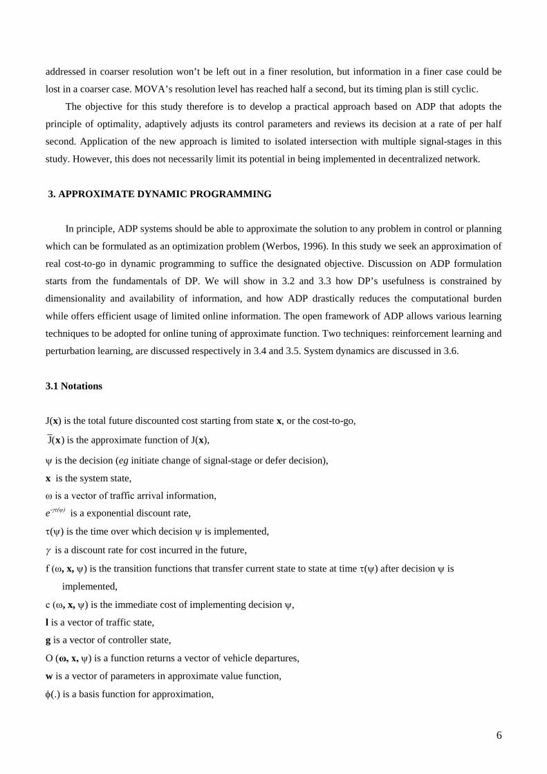
constructing system hierarchy with an area level and a local level. Area controller generates reference plan, and

local controllers adapt reference plan and dynamically coordinates signals in adjacent intersections. Rolling

horizon approach is again used by local controller to optimize performance, and the planning horizon is 120s,

with the process being repeated every 3 seconds. To automate the process of updating reference plans that are

generated by TRANSYT, an AUT (Automatic Updating of TRANSYT) module is developed. AUT first collects

traffic data continually by means of some of the detectors in the network. The data are processed to calculate

traffic flow pictures for various parts of the day. The model predicts the traffic flow profiles to be used when

calculating new reference plans. Afterwards AUT prepares the data to be used in the TRANSYT calculation and

starts TRANSYT optimization for selected effects. The benefits recorded after UTOPIA’s implementation show

an increase of 15% in average speed for private vehicles and 28% for public transport with priority.

MOVA (Vincent and Peirce, 1988) is the only one in this review package that is purposely designed for

isolated intersection. The system generates signal timings cycle-by-cycle that vary continuously according to the

latest traffic condition. Upon signal-stage change, MOVA uses vehicle gap detected through pairs of upstream

detectors to terminate green extension. The criterion for extension is whether the gap reaches certain critical

values. There are two operational modes for uncongested and congested conditions in which delay and stop

minimising and capacity maximising routines are adopted respectively. MOVA evaluates its control policy very

half second.

From the reviews on online traffic signal control systems, a scope for new development in this field is

perceived as the follows:

First, controller at a local intersection may dynamically adjust signal timings with a larger freedom so long

as it is conforming to the prevailing traffic and facilitates the overall traffic flow in a network, and certain

critical constraints such as minimum and maximum green time are not breached. This would allow controller to

give green indication regardless of preset signal-stage order, during and cycle time, and hence a larger levy in

controlling changing traffic. OPAC and PRODYN’s local controllers are already capable of doing this, but a

general formulation is yet to be shown for a multiple signal-stage intersection and DP’s principal of optimality

should be reaffirmed. The key issue here is how to build an algorithm on the principle of optimality in a forward

rolling process (thus unitizing limited online information), while preventing computational burden from

exploding towards intractable. As optimality in control is not particularly sensitive to variations in traffic

arrivals beyond 25s into the future (Robertson and Bretherton, 1974), the rolling horizon does not have to be

very long.

Second, controller may automatically adjust control policy so that it reflects the changes in prevailing

traffic in time and online. If the mechanism defining control policy over time is largely a dependant on internal

function parameters, the parameters then should be tuned intelligently and accordingly. Although UTOPIA is

capable of automating the updating of TRANSYT plans at area level, its local controllers are still subjective to

system-wide reference plans.

Third, a rapid review of control policy, i.e. a finer resolution in decision-making, is a definite advantage

over a slower review frequency, i.e. a coarser resolution in decision-making. This is because what could be

6

addressed in coarser resolution won’t be left out in a finer resolution, but information in a finer case could be

lost in a coarser case. MOVA’s resolution level has reached half a second, but its timing plan is still cyclic.

The objective for this study therefore is to develop a practical approach based on ADP that adopts the

principle of optimality, adaptively adjusts its control parameters and reviews its decision at a rate of per half

second. Application of the new approach is limited to isolated intersection with multiple signal-stages in this

study. However, this does not necessarily limit its potential in being implemented in decentralized network.

3. APPROXIMATE DYNAMIC PROGRAMMING

In principle, ADP systems should be able to approximate the solution to any problem in control or planning

which can be formulated as an optimization problem (Werbos, 1996). In this study we seek an approximation of

real cost-to-go in dynamic programming to suffice the designated objective. Discussion on ADP formulation

starts from the fundamentals of DP. We will show in 3.2 and 3.3 how DP’s usefulness is constrained by

dimensionality and availability of information, and how ADP drastically reduces the computational burden

while offers efficient usage of limited online information. The open framework of ADP allows various learning

techniques to be adopted for online tuning of approximate function. Two techniques: reinforcement learning and

perturbation learning, are discussed respectively in 3.4 and 3.5. System dynamics are discussed in 3.6.

3.1 Notations

J(x) is the total future discounted cost starting from state x, or the cost-to-go,

J(x) is the approximate function of J(x),

is the decision (eg initiate change of signal-stage or defer decision),

x is the system state,

ω is a vector of traffic arrival information,

e-γτ(ψ) is a exponential discount rate,

() is the time over which decision is implemented,

is a discount rate for cost incurred in the future,

f (ω, x, ) is the transition functions that transfer current state to state at time () after decision is

implemented,

c (ω, x, ) is the immediate cost of implementing decision ,

l is a vector of traffic state,

g is a vector of controller state,

O (ω, x, ) is a function returns a vector of vehicle departures,

w is a vector of parameters in approximate value function,

(.) is a basis function for approximation,

7

is a vector of (.).

3.2 Dynamic Programming

Dynamic programming decomposes a problem into a set of sub-problems denoted as stage, with a policy

decision required at each stage. Each stage has a number of states associated with the beginning of that stage. A

polciy decision at each stage is to transform the currentstate to a state asscociated with the beginning of the next

stage. To find an optimal policy for the overall problem, for example,

Min

E

e c

tf ,x,

t0

T

, (1)

DP recursively calculates

Jt(x) Min

E

ct,x, e

Jt1

f ,x,

, (2)

to guarantee that the policy being found leads to global optimum. Eq. (2) is also denoted the optimality equation.

Upon applying DP to traffic signal control, a stage is a discrete time interval along the planning period, and

a state of a stage is a combination of traffic state and controller state. A state of traffic at a intersection can be

specified by the number of vehicles queuing in each of the approaching links; the state of controller can be

specified by the signals which are green, any changes which are currently underway, the times at which they

will be completed and the times of expiry of any minimum or maximum permitted durations. A decision at a

stage can which to change the current indication, and if so, which stage of signal control is to change to. An

optimal policy for the overall signal control problem is then a set of decisions of alternating indications that

meet the objective in control.

Although (2) offers a simple and elegant way of problem solving, it can be computationally intractable

even for very small problems. This is because to evaluate a decision at a stage the algorithm loops over the

entire state space of the stage. As the number of state variable increases, the process has to consider all possible

combinations of values of the several state variables. The number of combinations can be as large as the product

of the number of possible values of the respective variables. The computational load therefore tends to explode

when additional state variables are introduced. For example, in developing PRODYN, Henry et al. (1983) has

found that the memory requirements for an intersection are:

2 l Cn

1

i1

I

TU

r1 r

2 , (3)

where 2 stands for the current and future tables of state values,

∆l: unit vehicle length,

I: number of links,

Cn1 : a combination with a subset size of 1, and a set size of n,

8

T: green time already elapsed,

U: number of signal-stages

r1 and r2: memory requirement for traffic state and controller state respectively.

If an intersection has four links in two signal-stages (I=4 and U=2), and no more than 19 vehicles could

possibly queue in a link (n=20, including 0 state), with ∆l=1 and a maximum green time of 60s (T=13 at a rate

of 5s per interval), r1=2 bytes, r2=2 bytes, the memory requirement is:

2 204 13 2 2 2 33280000 bytes .

If the complexity of the intersection rose to more combination of signal-stages and resolution refined to half a

second, for example, the requirements in computation and memories can even be proven (as it will show in

numerical experiment of this study) to be too costly for up-to-date computing facility with microprocessor. DP’s

vulnerability to increase in size of state space, the complexity of probability distribution of information, and the

number of optional decisions are frequently referred as ‘the Three Curse of Dimensionality’ (Powell, 2007).

Another concern restricts DP’s application in real-time control is that information from detectors about traffic

are normally of the next few (typically 10) seconds. In a rolling horizon approach, traffic models may

supplement information for the rest of the planning horizon, which is usually more than 60s in previous studies.

However, using DP means starting calculations at the end of the horizon where information on arrivals is least

certain. This scenario puts difficulty on the justification of using a costly optimization algorithm in a process

involving a large number of modeled information and decisions planned in the ‘tail’ period may never be

implemented.

Since the crux of DP algorithm is to establish a look-up table of exact state values, we may replace the state

values with an approximate function that is built on state variables. This would drastically reduce computational

burden, and in the mean time, it offers an alternative of stepping forward through time. In a forward process, the

more reliable part of information can be therefore utilized to produce decisions to accommodate the more

imminent demand. These are the premises for the introduction of approximate dynamic programming.

3.3 Approximation of Dynamic Programming

Let J(x) be a function that approximates the cost-to-go of DP, ADP is to meet objetive in (1) by forwardly

calculating

öJ (x) Min

E

ct,x, e

J n1 f ,x,

, (4)

where öJ (x) is a new observation of the cost-to-go at state x, and n denotes the number of updates to the

approximation function. How well ADP approach works largely depends on how good the approximation is,

and how much discount we give to cost further into the future. We may set the course to find a close-form

solution for (4), but this has been proven to be extremely difficult (Werbos, 2004). Without knowing the

approximate function a priori, we may hypothesis any structure that we deem as appropriate and employ a

9

machine learning technique to tune the functional parameters progressively. There are a large number of

approximation techniques available, including aggregation, regression and most frequently neural networks. Let

us assume that the approximate function is piecewise linear, which can be expressed as:

J x, w wT x . (5)

or

J w wT, (6)

where is a S K matrix whose kth column is equal to k; that is,

1L

k .

Using (5) to replace real cost-to-go J(x), the memory requirement for a four-link two signal-stages intersection

described above is

2 413 2 2 2 832 bytes.

This amount is one 2.5x10-5th of what would have been in classic DP. The efficiency in computing allows a

controller configured with average computing capacity of this day to work with comprehensive phase

combination and operate at rather fine resolution. And because it calculates forward, it starts decision making

with the actual data detected from online sensors, and implements decisions only for the ‘head’ period in a

rolling horizon approach. The head period, depending on the resolution in decision-making, is less or equal to

the period of actual data. The concern of starting planning backward from where data is least certain is then

circumvented.

We may further assume that a certain learning technique is supervising the adaptation of parameter vector

w whenever new observation öJ (x) is available. This can be expressed as:

J k x, w F öJ x , J k 1 x, w , w . (7)

Depending upon the specific technique in use, the objective of parameter tuning could be different, although a

least square approach for minimizing the error between estimation and observation is quite common.

Now we may summarize the general ADP algorithm, which is shown in Fig. 1.

3.4 Reinforcement learning

Reinforcement learning is a paradigm of learning without a ‘teacher’. It is a ‘behavioral’ learning problem:

It is performed through interaction between the learning system and its environment, in which the system seeks

to achieve a specific goal despite the presence of uncertainties (Barto et al., 1983; Sutton and Barto, 1998).

Trail and error search are important distinguishing characteristics of reinforcement learning.

A reinforcement learning agent generally consists of four basic components: a policy, a reward function, a

value function, and a model of the environment. In a problem defined by (1) and (2), the policy is the principal

of optimality shown in (2). The policy is the ultimate determinant of behavior and performance. The reward

function is shown as c(ω, x, ), which returns the immediate and defining feature of the problem faced by the

10

agent. Value function is presented by J(x), which predicts the rewards in the long run. And the model of the

environment is function f(ω, x, ), which predicts (in stochastic environment) or determines (in deterministic

environment) the next state. In an approximation that seeks to replace the exact J(x) with a function

approximator shown in (4), reinforcement learning technique updates the parameters of the function

approximator upon each observation of a state transition and the associated cost, with the objective of improving

approximations of long-term future cost as more and more state transitions are observed. The relationship

between the components of a reinforcement learning agent is shown in Fig. 2. The specific technique employed

in this study is a variant of temporal-difference learning (TD learning).

(TD) learning, originally proposed by Sutton (1988), is a method for approximating long-term future cost

as function of current state. Let us consider an irreducible aperiodic Markov process of infinite horizon whose

states lie in a finite or countable infinite space . The true cost-to-go J*: a associated with this Markov

process is defined by:

J x @E

e c f

t,x

t,

t x0 x

t0

, (8)

assuming that this expectation is well-defined. We consider a linear approximation of J*: a using a

function defined by (4), which is J(x, w) : K a ,with wK . The temporal difference dt

corresponding to xt to xt+1 is then defined as:

dt c

t,x

t,

t e J f

t,x

t,

t , wt J x

t, w

t . (9)

Then, for t=0,1, …, the temporal difference learning method updates wt according to the formula

wt1

wt

td

te (.)

t k

k0

t

w

J xt, w

t , (10)

or taking account of our case of linear approximation

wt1

wt

td

te (.)

t k

k0

t

xt . (11)

where t is a sequence of scalar step sizes that satisfy the following terms for convergence

t

t0

, (12)

and

t2

t0

. (13)

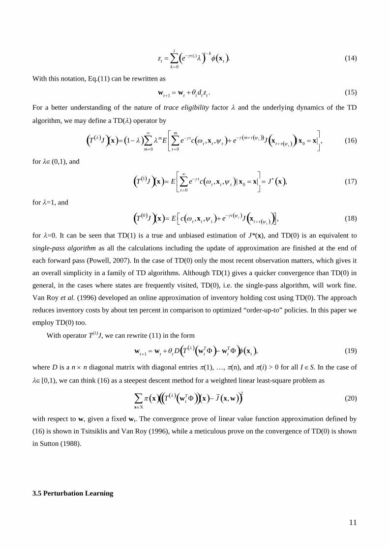
Parameter of (11) is known as trace eligibility factor, which takes value in [0,1]. Since temporal difference

learning is actually a continuum of algorithm parameterized by , it is often referred as TD(). A more

convenient representation of TD() can be obtained by defining a sequence of eligibility vectors zt by

11

zt e (.)

t k

k0

t

xt . (14)

With this notation, Eq.(11) can be rewritten as

wt1

wt

td

tz

t. (15)

For a better understanding of the nature of trace eligibility factor and the underlying dynamics of the TD

algorithm, we may define a TD() operator by

T J x 1 m

m0

E e t

t0

m

c t,x

t,

t e m t J x

t t | x0

x

, (16)

for (0,1), and

T1 J x E e t

t0

c t,x

t,

t | x0 x

J x , (17)

for =1, and

T0 J x E c

t,x

t,

t e t J x

t t

, (18)

for =0. It can be seen that TD(1) is a true and unbiased estimation of J*(x), and TD(0) is an equivalent to

single-pass algorithm as all the calculations including the update of approximation are finished at the end of

each forward pass (Powell, 2007). In the case of TD(0) only the most recent observation matters, which gives it

an overall simplicity in a family of TD algorithms. Although TD(1) gives a quicker convergence than TD(0) in

general, in the cases where states are frequently visited, TD(0), i.e. the single-pass algorithm, will work fine.

Van Roy et al. (1996) developed an online approximation of inventory holding cost using TD(0). The approach

reduces inventory costs by about ten percent in comparison to optimized “order-up-to” policies. In this paper we

employ TD(0) too.

With operator T()J, we can rewrite (11) in the form

wt1

wt

tD T

wt

T wt

T xt , (19)

where D is a n n diagonal matrix with diagonal entries (1), …, (n), and (i) > 0 for all I S. In the case of

[0,1), we can think (16) as a steepest descent method for a weighted linear least-square problem as

x x

T w

tT x J x, w

2

(20)

with respect to w, given a fixed wt. The convergence prove of linear value function approximation defined by

(16) is shown in Tsitsiklis and Van Roy (1996), while a meticulous prove on the convergence of TD(0) is shown

in Sutton (1988).

3.5 Perturbation Learning

12

Regression models mapping state to observation iteratively over time such as TD() offers one way of

approximating cost-to-go when the number of parameters are not to large. Otherwise the inverse of matrix in a

least-square problem would be too expensive for real-time operation. An alternative to regression model is to

explore the structure of the cost-to-go function, and the monotonicity in particular. In traffic signal control we

have a monotonic increase problem. This is to say that the cost-to-go value of a state increases as the number of

vehicles remaining in the system increases. Additionally, the value increases more rapidly when more vehicles

are remained in red links than in green. In real-time operation we may not have the knowledge of the exact cost-

to-go function, but we can approximate the property of monotonicity. Since monotonicity can be easily

maintained by a linear approximation, we may define a piecewise learning approximator on the basis of (5)

J x, w w k k1

K

k

x , (21)

where w(k) is the kth element of parameter vector w and each k is a fixed scalar function defined on the state

space . Since the partial differentiation of the linear approximator with respect to k(x) yields

J x, w

kx

w k ,

we can easily show that a new observation of w(k) can be obtained through

öw k öJ xek öJ xek

2 k

, (22)

where ek is a K-dimension vector of zeroes with a unit increment in the kth element, and öJ . calculated from (4).

With the new observation, we then smooth to obtain an updated estimate of the functional parameter

wn k 1n1 wn1 k n1

öw k , (23)

where n here denotes the number of updates.

Papadaki and Powell (2003) develop a similar ADP approach to (21) for stochastic batch dispatch problem,

in which results from both the linear and nonlinear (concave) approximation are compared. Although nonlinear

approximation works better than linear ones as iteration goes on, a large-scale problem may make nonlinear

approximation extremely difficult or impossible in implementation. For such problems, a linear approximation

is the best.

3.6 System dynamics

In this section we will show how the dynamics of a signal control system is formulated into the ADP

algorithm. Recalling that a state x of traffic control system is a combination of traffic state and controller state,

we denote traffic state by L and controller state by G. We further define that traffic state L by the number of

vehicles queuing in each of the approaching links, and controller state G by the state of signal (i.e. red or green,

13

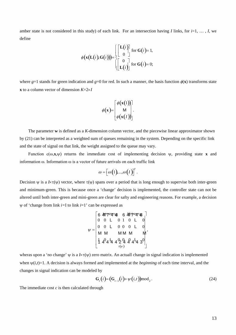
amber state is not considered in this study) of each link. For an intersection having I links, for i=1, … , I, we

define

x L i ,G i

L i 0

for G i 1,

0

L i

for G i 0;

where g=1 stands for green indication and g=0 for red. In such a manner, the basis function (x) transforms state

x to a column vector of dimension K=2I

x x 1

M

x I

.

The parameter w is defined as a K-dimension column vector, and the piecewise linear approximator shown

by (21) can be interpreted as a weighted sum of queues remaining in the system. Depending on the specific link

and the state of signal on that link, the weight assigned to the queue may vary.

Function c(ω,x,) returns the immediate cost of implementing decision , providing state x and

information ω. Information ω is a vector of future arrivals on each traffic link

1 ,..., I

T

.

Decision is a I() vector, where () spans over a period that is long enough to supervise both inter-green

and minimum-green. This is because once a ‘change’ decision is implemented, the controller state can not be

altered until both inter-green and mini-green are clear for safty and engineering reasons. For example, a decision

of ‘change from link i=I to link i=1’ can be expressed as

0 0 L 0

0 0 L 0

M M M

1 0 L 0

Inter-green6 744 84 41 0 L 0

0 0 L 0

M M M

0 0 L 0

Mini-green6 744 84 4

1 24 4 4 4 34 4 4 4

,

wheras upon a ‘no change’ is a I() zero matrix. An actuall change in signal indication is implemented

when (i,t)=1. A decision is always formed and implemented at the beginning of each time interval, and the

changes in signal indication can be modeled by

Gt

i Gt1

i i,t mod2

. (24)

The immediate cost c is then calculated through

14

c t,x

t,

t e t L

ti t

iO t

i, t ,x ti, t

i, t i1

I

t 0

, (25)

where O(ω(i), x(i), ) is the outflow function that returns

O t

i ,x ti , t

i Min s i , L

ti + t

i for g i =1,

0 for g i 0.

(26)

s(i) is the saturation departure rate for link i.

The transfer function f(ω, x, ) transfers the system from current state to the next state

f (t,x

t,

t)=

Lt

i Lt 1

i t 1i O

t 1

ti, t 1 ,x t 1

i , ti, t 1 ,

Gt

i Gt 1

i ti, t 1 mod

2,

(27)

for t t,...,t t ,and i 1,..., I .

In the following section we will discuss the testing environment for numerical experiment and its

realization in computer simulation.

4. EXPERIMENT AND RESULTS

In this section is organized as the following: we first introduce how the data for numerical experiment are

generated in computer simulation in 4.1, followed the design of testing bed in 4.2, the configuration of decision

set of ADP controller in 4.3 and the traffic flow setting that present different operation environment in 4.4.

Section 4.5 introduces the general simulation environment. Comparison between DP, ADP, and Fixed-time

performances in different circumstances are shown in 4.6. From these comparisons, we are able to discern the

advantages of ADP controller in online operation, and the difference between reinforcement learning and

perturbation learning.

4.1 Traffic Data

Traffic data is assumed to be detected from inductive loops imbedded upstream. Detectors provide arriving

traffic of the next 10 seconds for each traffic link, which is known at the beginning of each time interval. In the

coarser resolution, time is divided into short intervals of 5 seconds each, and traffic rate takes integer value of 0,

1, or 2 vehicles only; in the finer resolution, intervals are 0.5 seconds each, and traffic rate is a binary variable

taking either 0 or 1. Other assumptions for approaching traffic are:

1. Approaching traffic is homogenous.

2. Queue lengths are calculated at the end of each interval, neglecting the detail of vehicle behavior during

the interval. Signals may only be switched at the boundary between intervals.

15

The random arrival process for the coarser resolution is generated by binomial distribution. The maximum

rate of 2 is set so that the arrival rate could not exceed the capacity. Learning R be the random traffic rate, we

denote the cumulative distribution function by

F r P R r and probability of R=m, where m takes integer value of 0, 1, or 2, is

P R m n

m

pm 1 p nm

,m 0,1,...,n. (28)

Simulation of random arrival process is then realized by using Inverse Transformation Method (ITM), which

first generate a uniform random number z between 0 and 1, and then set F(r)=z and solve for r to produce the

desired random observation from the probability distribution.

To extend the random process to the finer resolution, a shifted Bernoulli process is adopted. With

probability P, an arrival is generated and the trial has duration Tg=nb∆t; with probability (1-P), no arrival is

generated and the trial has duration Tg=∆t. Thus the mean number of vehicles that are generated in a single trial

is E(N)=P, and the mean duration of the trial is E(T)=[Pnb+(1-P)] ∆t. An estimate of the mean rate of traffic

generation is given:

q E N E T

g

P

1 P(nb1) t

, (29)

The probability required to generate a certain mean arrival rate can be deduced by inversing the expression:

P qt

1 (nb1)qt

. (30)

The rest of the process for generating random traffic at finer resolution is identical to that of the coarser

resolution. Specifications for generating traffic data in both cases are summarized in Table 2.

Table 2 Generating Traffic Data

Time Interval Traffic Rate Random Process Simulation

Coarser Resolution 5 seconds 0, 1, or 2 Binomial ITM

Finer Resolution 0.5 seconds 0 or 1 Shifted Bernoulli ITM

It is worth noting that because queue lengths are calculated at the end of each interval. The delays measured in

the coarser resolution are not directly comparable to delays measured in the finer resolution. In particular, in the

case of the coarser resolution, no delay is attributed to either vehicle in a time increment during which two

depart, whilst in the finer resolution, delay would occur to one the vehicles for the whole of the departure time

of the other. To facilitate the comparison between the two resolutions, we record the decision series in the

coarser case and implement them in the finer case. The result thus obtained is then compared with performance

measure of the finer case.

16

4.2 Traffic Intersection

To demonstrate the readiness of the control approach for operation, we design an isolated intersection

having three signal-stages, as shown in Fig. 2. In designing the control environment, we also assume that:

1. Signal phases are composed of effective greens and effective reds only, and no amber interval is

considered.

2. There are no constraints on the maximum duration of a green period. Both inter-green and minimum

green are set as 5 seconds.

3. The saturation flow on all lanes is 2 vehicles per interval. This is equivalent to 1440 vehicles per hour, a

rate that is sufficiently close to the saturation flow of a single traffic lane.

Because we only consider an isolated intersection, there is no treatment of the physical length of traffic

queue, and 1therefore the queue length won’t affect approaching traffic or the detectors that are assumed to be

laid sufficiently upstream. For simplify the traffic state combination, especially to facilitate comparison with

other techniques such as DP, traffics on each signal-stage are grouped into a single link, such Link-A for signal-

stage 1, Link-B for signal-stage 2, and Link-C for signal-stage 3.

It is worth mentioning the treatment of lost time. Lost time in traffic engineering pertains to the time (in

seconds) during which vehicles receiving green signal are unable to pass through an intersection. The total lost

time is the sum of Start-up lost time and Clearance lost time. If no specific observations were made for the lost

times, the two elements of total lost time may either assumed to be 2 seconds (Roger P. Roess et al., 2004). In

the formulation and experiment presented here, lost time is not modeled for reasons of simplicity. It would

argue that without treating lost time, the optimal signal control is straightforward ––– serving one traffic stream

till queue is cleared, then switch to non-empty signal-stages. Since such a policy is not a feature in our ADP

approach, it would serve as a measurement of the performance.

4.3 Decision Set

The basic decision set is ‘change now’ (ψ=1) or ‘change later’ (ψ=0). However, if a change at any later

time that is within the ‘head’ of the planning horizon produces less delay than ‘change now’, the system will

remain the current signal indication. In the case of ‘change now’, the system will also decide which signal-stage

to call. To facilitate this decision-making policy, we have a planning horizon of 20s. The first 10s forms the

‘head’, which is fed with detected information, and the second 10s forms the ‘tail’, which is fed with modeled

data. The complete decision set is illustrated in general form in Fig. 4. In the numerical experiment, however,

we artificially set the time-span of a decision as 10s, which is identical to the period of detected information,

with 5s inter-green and 5s minimum green. This design is to facilitate comparison between different control

strategies. In the coarser resolution, decision is implemented for the first 5s, whereas in the finer resolution,

decision is only implemented for the first half-second, and then the system rolls forward.

17

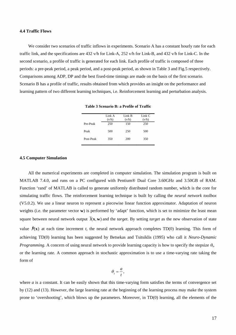
4.4 Traffic Flows

We consider two scenarios of traffic inflows in experiments. Scenario A has a constant hourly rate for each

traffic link, and the specifications are 432 v/h for Link-A, 252 v/h for Link-B, and 432 v/h for Link-C. In the

second scenario, a profile of traffic is generated for each link. Each profile of traffic is composed of three

periods: a pre-peak period, a peak period, and a post-peak period, as shown in Table 3 and Fig.5 respectively.

Comparisons among ADP, DP and the best fixed-time timings are made on the basis of the first scenario.

Scenario B has a profile of traffic, results obtained from which provides an insight on the performance and

learning pattern of two different learning techniques, i.e. Reinforcement learning and perturbation analysis.

Table 3 Scenario B: a Profile of Traffic

4.5 Computer Simulation

All the numerical experiments are completed in computer simulation. The simulation program is built on

MATLAB 7.4.0, and runs on a PC configured with Pentium® Dual Core 3.60GHz and 3.50GB of RAM.

Function ‘rand’ of MATLAB is called to generate uniformly distributed random number, which is the core for

simulating traffic flows. The reinforcement learning technique is built by calling the neural network toolbox

(V5.0.2). We use a linear neuron to represent a piecewise linear function approximator. Adaptation of neuron

weights (i.e. the parameter vector w) is performed by ‘adapt’ function, which is set to minimize the least mean

square between neural network output J(x, w) and the target. By setting target as the new observation of state

value öJ (x) at each time increment t, the neural network approach completes TD(0) learning. This form of

achieving TD(0) learning has been suggested by Betsekas and Tsitsiklis (1995) who call it Neuro-Dynamic

Programming. A concern of using neural network to provide learning capacity is how to specify the stepsize t,

or the learning rate. A common approach in stochastic approximation is to use a time-varying rate taking the

form of

t

a

t,

where a is a constant. It can be easily shown that this time-varying form satisfies the terms of convergence set

by (12) and (13). However, the large learning rate at the beginning of the learning process may make the system

prone to ‘overshooting’, which blows up the parameters. Moreover, in TD(0) learning, all the elements of the

Link A(v/h)

Link B(v/h)

Link C(v/h)

Pre-Peak 250 150 250

Peak 500 250 500

Post-Peak 350 200 350

18

parameter vector are updated at once, and there may not be a single rule that is going to be right for all of the

parameters. For these concerns, we use a constant learning rate =0.005 for neural network, at the expense of

slow convergence. In the case of perturbation analysis, because of the design of the algorithm, we are relieved

from the concern of overshooting and each parameter can be assigned a specific stepsize. Therefore, for each

parameter, we use

n

a

a n 1,

where a=40, and n counts the number of times the parameter has been updated (note that we use n rather than t

here).

4.6 Results and Comparison

With traffic scenario A, in which the hourly traffic rate on each link is constant and the overall degree of

saturation is high, we compare the results from different control strategies, including DP, ADP, and Fixed-time.

DP provides the benchmark on the higher end of performance, whereas Fixed-time provides the benchmark on

the lower end. In evaluating ADP performance, we obtain results from both the coarser resolution at 5s per

interval and the finer resolution at half-second per interval. It is also of our interest to see whether ADP with

different learning technique performances differently.

With traffic scenario B, in which a profile of traffic is generated, we compare the learning patterns from

different learning techniques in a noisy and changing environment, along with the respective performance over

time. In the rest of this section, we denote ADP with reinforcement learning by ADP_RL, and ADP with

perturbation learning by ADP_PL.

4.6.1 Traffic Scenario A

Since that both DP and ADP algorithms discount the delay incurred in the future by e- per time increment,

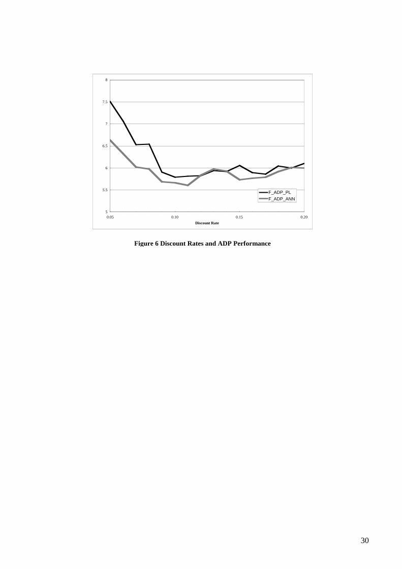
and there is no specific method to determine the best *, we employ exhaustive search to find the optimum

value. Fig. 5 plots the average performances of ADP_RL and ADP_PL over an hour at the finer resolution

(equivalent to 7200 time increments) against an array of discount rates. ADP_RL yields the best performance at

=0.10, while ADP_PL at =0.11. Since the actual difference between the best performances of each learning

technique is negligible, we round discount rate at =0.10 per time increment for later experiments on ADP. This

is equivalent to say that delay incurred one second later will be discounted by (1-e-2)100%=18%, and so on.

As for each decision , ()=20 increments, the magnitude of J(.) is discounted by (1-e-())100%=86%.

19

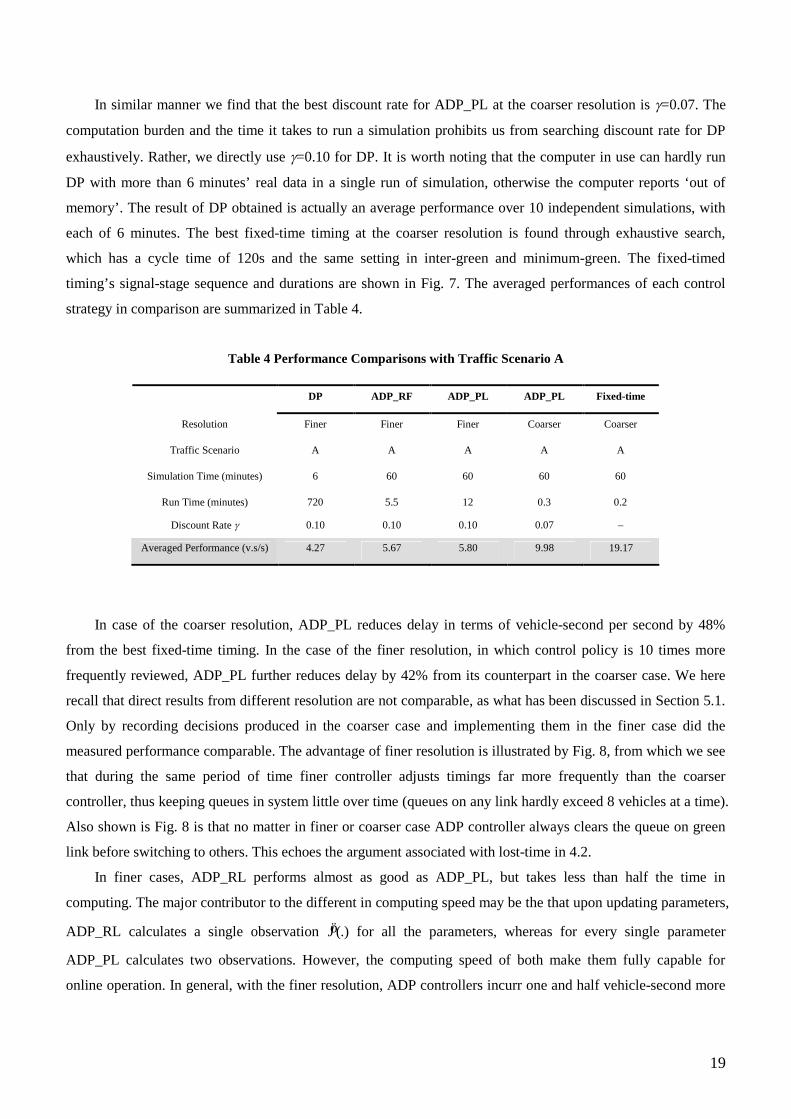
In similar manner we find that the best discount rate for ADP_PL at the coarser resolution is =0.07. The

computation burden and the time it takes to run a simulation prohibits us from searching discount rate for DP

exhaustively. Rather, we directly use =0.10 for DP. It is worth noting that the computer in use can hardly run

DP with more than 6 minutes’ real data in a single run of simulation, otherwise the computer reports ‘out of

memory’. The result of DP obtained is actually an average performance over 10 independent simulations, with

each of 6 minutes. The best fixed-time timing at the coarser resolution is found through exhaustive search,

which has a cycle time of 120s and the same setting in inter-green and minimum-green. The fixed-timed

timing’s signal-stage sequence and durations are shown in Fig. 7. The averaged performances of each control

strategy in comparison are summarized in Table 4.

Table 4 Performance Comparisons with Traffic Scenario A

DP ADP_RF ADP_PL ADP_PL Fixed-time

Resolution Finer Finer Finer Coarser Coarser

Traffic Scenario A A A A A

Simulation Time (minutes) 6 60 60 60 60

Run Time (minutes) 720 5.5 12 0.3 0.2

Discount Rate 0.10 0.10 0.10 0.07 –

Averaged Performance (v.s/s) 4.27 5.67 5.80 9.98 19.17

In case of the coarser resolution, ADP_PL reduces delay in terms of vehicle-second per second by 48%

from the best fixed-time timing. In the case of the finer resolution, in which control policy is 10 times more

frequently reviewed, ADP_PL further reduces delay by 42% from its counterpart in the coarser case. We here

recall that direct results from different resolution are not comparable, as what has been discussed in Section 5.1.

Only by recording decisions produced in the coarser case and implementing them in the finer case did the

measured performance comparable. The advantage of finer resolution is illustrated by Fig. 8, from which we see

that during the same period of time finer controller adjusts timings far more frequently than the coarser

controller, thus keeping queues in system little over time (queues on any link hardly exceed 8 vehicles at a time).

Also shown is Fig. 8 is that no matter in finer or coarser case ADP controller always clears the queue on green

link before switching to others. This echoes the argument associated with lost-time in 4.2.

In finer cases, ADP_RL performs almost as good as ADP_PL, but takes less than half the time in

computing. The major contributor to the different in computing speed may be the that upon updating parameters,

ADP_RL calculates a single observation öJ (.) for all the parameters, whereas for every single parameter

ADP_PL calculates two observations. However, the computing speed of both make them fully capable for

online operation. In general, with the finer resolution, ADP controllers incurr one and half vehicle-second more

20

than the DP controller per second. DP controller takes an enomous amount of time (12 hours or so) to finish a

simluation of 6-mintus operation at an intersection of only three confliting links.

The large ratio in discounting future delay also means that the approximator’s contribution to operation at

the finer resolution is limited. Fig. 5 shows that ignoring what’s to come 10s later only worsens performance by

half a vehicle-second, whereas taking a bigger account of it has strong negative impact on performance.

Therefore, it is of practical interest to remain the approximation function simple and easy to update.

5.6.2 Traffic Scenario B

In this scenario of traffic input, we would like to show the learning patterns of ADP in a changing and

noisy environment and in the mean time to test whether different learning techniques yield distinguishable

results. The examples of evolution of functional parameters of ADP_PL and ADP_RL are shown in Fig. 9 and

Fig. 10 respectively. Series in both figures can be divided into a group of higher values, which represents the

value of parameters assigned to red states, and a group of lower values, which represents parameters assigned to

green states. Because ADP_PL has time-varying learning rates that are large in the beginning, parameters of

ADP_PL start with strong oscillation and only begin to level off when the system enters post-peak time, partly

due to the diminishing learning rate and partly to the steadier environment. The ADP_RL, which by using

neural network adopts a constant learning of small magnitude, has more stable parameters over time.

The rising traffic volume in the middle of the controlling period gives sharp rise to parameters assigned to

green states, but not much to the other group of parameters. This pattern reflects the near saturation traffic

condition at the intersection, in which the amount of arriving traffic is close to the maximum departure rate.

Queues on green therefore dissipate much slower. Despite of the different learning technique, it is interesting to

see how similar the estimation of parameter is when system enters post-peak.

The paired performances of the two learning techniques in 10 independent simulations are recorded in

Table 5. The discount rate is set at =0.10 for both. We use two-sample t-test to test the hypothesis that the two

means are equal. At the degree of significance =0.05, and degree of freedom n=9, the two means are equal, as

shown in Table 5. Recalling that ADP_RL is actually a regression method that minimizes weighted square

errors and ADP_PL estimates gradients directly regardless of errors in prediction, the equality of the two means

suggests that learning techniques have limited effects on the performance when the approximation function is

piecewise linear, discount rate is large and decision is frequently reviewed.

The general conclusion we can draw from the numerical examples is that the ADP approach is fully

capable of online operation at an isolated intersection. It saves nearly half of the delays from the best fixed-time

timings at a resolution of 5s, and a further substantial reduction can be achieved by improving resolution to 0.5s.

For those benefits, the ADP controller only takes 10s data of future arrivals with a competitive computation

advantage. When arriving traffic changes over time, the learning pattern of the function parameters captures the

alternating trend in the environment. However, we also notice that the best performance of ADP is yielded at a

21

relatively large discount rate, and that different learning techniques make no difference in performance, and

little in learning. It suggests that a simple piecewise linear approximator is sufficient for online operation, and

the benefit of exploring complex approximation, such as nonlinear approximator, may not be well justified by

the cost in computation.

Table 5 Performance Comparisons with Traffic Scenario B

6. CONCLUSIONS

ADP is an emerging technique under intensive development in the fields of Artificial Intelligence.

Researches on its application have been pursued in power plant management, aerospace technology, robotic

control and environment protection. This study investigates ADP application to the field of traffic signal control,

aiming to develop a self-sufficient adaptive controller for online operation. Through the review on existing

traffic signal control systems and theories, we identify the objectives for this investigation in ADP controller as

providing dynamic control for real-time operation, being adaptive through online learning, and frequently

reviewing control policy. ADP controller achieves the objectives by replacing real cost-to-go in DP with a

simple piecewise linear approximation function, and uses specific learning techniques to tune the function

parameters online. We have shown that operating at a resolution of 5s, the ADP controller saves 48% of delays

from the best fixed-time timing, and that if operating at resolution of 0.5s, a further 42% reduction in delay can

be gained. In comparing with the result from DP, which is theoretical limit, ADP incurs only one and a half

second more delay per second while keeping computational requirement at manageable level for online

operation. These findings suggest ADP as a sufficient and practical approach to adaptive real-time operation at

an isolated intersection.

Sample ADP_PL ADP_RL

1 3.159583 3.376944

2 3.089722 2.974583

3 2.729583 2.623472

4 2.853194 2.985972

5 3.223472 3.3225

6 3.205278 3.184444

7 3.20375 3.286667

8 4.049861 4.266806

9 3.658611 3.522222

10 3.239028 3.215

Mean 3.2412082 3.275861

t Stat -0.819958009

P(T<=t) one-tail 0.216708989

t Critical one-tail 1.833112923

P(T<=t) two-tail 0.433417978

t Critical two-tail 2.262157158

22

Two learning techniques ––– reinforcement learning and perturbation learning respectively ––– are

investigated in this study. The crux of the reinforcement learning technique presented here is TD(0) method,

whereas perturbation learning directly estimates each parameter of the approximate function by perturbing

system state. Although each learning technique approaches to parameter estimation differently, the learning

effects are quite similar and no difference can be discerned from numerical experiments with a profile of traffic

flows. ADP controller equipped with either learning technique yields the best performance by discounting future

delay at about 18% per second, suggesting limited influence of approximated cost-to-go function in evaluating

optimum decision. Combining the equality between two learning techniques together with the limited influence

of the approximated cost-to-go, it suggests that a simple linear approximation is good enough to sustain the

superiority of ADP controller in real-time operation. Exploring more complex approximation may not be proven

as cost effective.

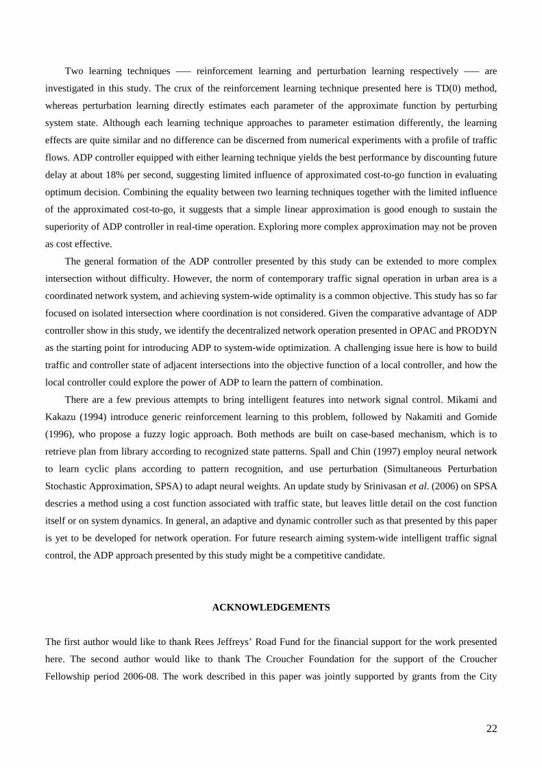
The general formation of the ADP controller presented by this study can be extended to more complex

intersection without difficulty. However, the norm of contemporary traffic signal operation in urban area is a

coordinated network system, and achieving system-wide optimality is a common objective. This study has so far

focused on isolated intersection where coordination is not considered. Given the comparative advantage of ADP

controller show in this study, we identify the decentralized network operation presented in OPAC and PRODYN

as the starting point for introducing ADP to system-wide optimization. A challenging issue here is how to build

traffic and controller state of adjacent intersections into the objective function of a local controller, and how the

local controller could explore the power of ADP to learn the pattern of combination.

There are a few previous attempts to bring intelligent features into network signal control. Mikami and

Kakazu (1994) introduce generic reinforcement learning to this problem, followed by Nakamiti and Gomide

(1996), who propose a fuzzy logic approach. Both methods are built on case-based mechanism, which is to

retrieve plan from library according to recognized state patterns. Spall and Chin (1997) employ neural network

to learn cyclic plans according to pattern recognition, and use perturbation (Simultaneous Perturbation

Stochastic Approximation, SPSA) to adapt neural weights. An update study by Srinivasan et al. (2006) on SPSA

descries a method using a cost function associated with traffic state, but leaves little detail on the cost function

itself or on system dynamics. In general, an adaptive and dynamic controller such as that presented by this paper

is yet to be developed for network operation. For future research aiming system-wide intelligent traffic signal

control, the ADP approach presented by this study might be a competitive candidate.

ACKNOWLEDGEMENTS

The first author would like to thank Rees Jeffreys’ Road Fund for the financial support for the work presented

here. The second author would like to thank The Croucher Foundation for the support of the Croucher

Fellowship period 2006-08. The work described in this paper was jointly supported by grants from the City

23

University of Hong Kong (Project Number: 7001967 and 7200040) and the Research Grants Council of the

Hong Kong Special Administrative Region, China (Project Number: 9041157).

REFERENCES

Allsop, R.E. (1971a) Delay-minimising settings for fixed-time traffic signals at a single road junction, Journal

of the Institute of Mathematics and its Applications, 8 (2) 164-185.

Allsop, R.E. (1971b) SIGSET: a computer program for calculating traffic signal settings, Traffic Engineering

and Control, 13, 58-60.

Allsop, R.E. (1972) Estimating the traffic capacity of a signalized road junction, Transportation Research, 6 (3)

245-255.

Allsop, R.E. (1976) SIGCAP: a computer program for assessing the traffic capacity of signal-controlled road

junctions, Traffic Engineering and Control, 17, 338-341.

Betsekas, D.P. and Tsitsiklis, J.N. (1995) Neuro-Dynamic programming, Belmont, MA: Athenas Scientific.

Gartner, N.H. (1983) OPAC: A demand-responsive strategy for traffic signal control, Transportation Research

Record 906, 75-81.

Henry, J.J., Farges, J.L., and Tuffal, J. (1983) The PRODYN real time traffic algorithm, Proceedings of the 4th

IFAC-IFIP-IFORS conference on Control in Transportation Systems, 307-311.

Heydecker, B.G. (1992) Sequencing of traffic signals, in J.D. Griffiths (Ed.) Mathematics in Transport and

Planning and Control, 57-67, Clarendon Press, Oxford.

Hunt, P.B., Robertson, D.I., and Bretherton, R.D. (1982) The SCOOT on-line traffic signal optimisation

technique, Traffic Engineering and Control, 23, 190-192.

Improta, G. and Cantarella, G.E. (1984) Control system design for an individual signalized junction.

Transportation Research, 18B (2) 147-167.

Luk, J.Y.K. (1984) Two traffic-responsive area traffic control methods: SCAT and SCOOT, Traffic Engineering

and Control, 25, 14-22.

Luenberger, D.G. (1984) Linear and Non-linear Programming, 2nd Edition, Reading, MA: Addison-Wesley.

Robertson, D.I. and Bertherton, R.D. (1974) Optimum control of an intersection for any known sequence of

vehicular arrivals, Proceedings of the 2nd IFAC-IFIP-IFORS Symposium on Traffic Control and

Transportation system, Monte Carlo.

Roger P. Roess, Elena S. Prassas, and William R. McShane, Traffic Engineering, 3rd Edition, Upper Saddle

River: Pearson Prentice Hall 2004. ISBN 0-13-142471-8)

Roozemond, D. (1996) Intelligent traffic management and urban traffic control based on autonomous objects.

Proceedings of the 6th Artificial Intelligence, Simulation, and Planning in High Autonomy Systems

International Conference, IEEE.

Sutton, R.S. (1988) Learning to predict by the methods of temporal differences, Machine Learning, 3, 9-44.

24

Sutton, R.S., and Barto, A.G. (1998) Reinforcement Learning: An Introduction, Cambridge, MA: MIT Press.

Vincent, R.A., Mitchell, A.I. and Robertson, D.I. (1980) User guide to TRANSYT version 8. Transport and

Road Research Laboratory Report, LR888, Crowthorne, Berkshire, U.K.

Vincent, R.A. and Peirce, J.R. (1988) MOVA: traffic responsive, self-optimising signal control for isolated

intersections, Transport and Road Research Laboratory Report RR 170, Crowthorne: TRRL.

Werbos, P. (2004) ADP: Goals, opportunities and Principles. Handbook of Learning and Approximate Dynamic

Programming, 2004 Wiley-IEEE.

Wong, C.K. and Wong, S.C. (2003a) Lane-based optimization of signal timings for isolated junctions,

Transportation Research, 37B (1) 63-84.

Wong, C.K. and Wong, S.C. (2003b) Lane-based optimization of traffic equilibrium settings for area traffic

control, Journal of Advanced Transport, 36 (3), 349-386.

Wong, C.K. and Wong, S.C. (2003c) A lane-based optimization method for minimizing delay at isolated signal-

controlled junctions. Journal of Mathematical Modelling and Algorithms, 2 (4), 379-406.

25

Figure 1 A General Approximate Dynamic Programming Algorithm

Step 0. Initialization:

a. Initialize J(.) .

b. Choose an initial state x0.

c. Set t=0, k=0.

Step 1. Receive random information ωt.

Step 2. While t<=T,

a. Solve Eq. (4) to find t*.

b. Update approximation through Eq. (6).

c. Implement t*, and compute xt+1=f(ωt, xt, t*).

Step 3. Let t=t+1. If t<T, go to step 1, otherwise stop.

26

Model of Environment

Policy

Reward Functionc(.)

Value Function

J .

State x Decision*

Learning System

F .Observation öJ x

Figure 2 Main Components of a Reinforcement Learning Agent

27

Figure 3 Intersection Layout

28

Figure 4 Decision Set for ADP in Signal Control

0

100

200

300

400

500

600

0 1000 2000 3000 4000 5000 6000 7000

Time Intervals

Link_A&C

Link_B

29

Figure 5 Profile of Traffic

5

5.5

6

6.5

7

7.5

8

0.05 0.10 0.15 0.20

Discount Rate

F_ADP_PL

F_ADP_ANN

30

Figure 6 Discount Rates and ADP Performance

31

Link_B(25s)

Link_C(40s)

Link_A(40s)

Figure 7 The Best Fixed-time Timing

Queues on Arm A

0

2

4

6

8

10

12

14

0 500 1000 1500 2000 2500 3000 3500 4000 4500 5000 5500 6000 6500 7000

Time Steps

32

Functional Parameters,ADP with Purturbation Analysis, 0.5s resolution

0

0.5

1

1.5

2

2.5

3

3.5

4

0 1000 2000 3000 4000 5000 6000 7000

Time Steps

Alpha A

Beta A

Alpha B

Beta B

Alpha C

Beta C

Figure 9

33

Functional Parameters, ADP with ANN,0.5s resolution

0

0.5

1

1.5

2

2.5

3

3.5

4

0 1000 2000 3000 4000 5000 6000 7000

Time Steps

Alpha A

Beta A

Alpha B

Beta B

Alpha C

Beta C

Figure 10