Adaptive Multi-Objective Reinforcement Learning with

Hybrid Exploration for Traffic Signal Control Based on

Cooperative Multi-Agent Framework

Mohamed A. Khamis∗, Walid Gomaa1

Department of Computer Science and Engineering, Egypt-Japan University of Scienceand Technology (E-JUST), P.O. Box 179, New Borg El-Arab City, Postal Code 21934

Alexandria, Egypt

Abstract

In this paper, we focus on computing a consistent traffic signal config-uration at each junction that optimizes multiple performance indices, i.e.,multi-objective traffic signal control. The multi-objective function includesminimizing trip waiting time, total trip time, and junction waiting time.Moreover, the multi-objective function includes maximizing flow rate, satis-fying green waves for platoons traveling in main roads, avoiding accidentsespecially in residential areas, and forcing vehicles to move within moderatespeed range of minimum fuel consumption. In particular, we formulate ourmulti-objective traffic signal control as a Multi-Agent System (MAS). Traf-fic signal controllers have a distributed nature in which each traffic signalagent acts individually and possibly cooperatively in a MAS. In addition,agents act autonomously according to the current traffic situation withoutany human intervention. Thus, we develop a multi-agent multi-objective Re-inforcement Learning (RL) traffic signal control framework that simulatesthe driver’s behavior (acceleration/deceleration) continuously in space andtime dimensions. The proposed framework is based on a multi-objective se-quential decision making process whose parameters are estimated based onthe Bayesian interpretation of probability. Using this interpretation together

∗Corresponding author. Mobile: +20-100-638-2428; telephone: +20-3-309-4075.Email addresses: mohamed.khamis@ejust.edu.eg (Mohamed A. Khamis),

walid.gomaa@ejust.edu.eg (Walid Gomaa)1Currently on-leave from Faculty of Engineering, Alexandria University, Alexandria

21544, Egypt

Preprint submitted to Engineering Applications of Artificial IntelligenceDecember 4, 2013

*Text Figure(s) Table(s)Click here to view linked References

with a novel adaptive cooperative exploration technique, the proposed trafficsignal controller can make real-time adaptation in the sense that it respondseffectively to the changing road dynamics. These road dynamics are simu-lated by the Green Light District (GLD) vehicle traffic simulator that is thetestbed of our traffic signal control. We have implemented the IntelligentDriver Model (IDM) acceleration model in the GLD traffic simulator. Thechange in road conditions is modeled by varying the traffic demand proba-bility distribution and adapting the IDM parameters to the adverse weatherconditions. Under the congested and free traffic situations, the proposedmulti-objective controller significantly outperforms the underlying single ob-jective controller which only minimizes the trip waiting time (i.e., the totalwaiting time in the whole vehicle trip rather than at a specific junction).For instance, the average trip and waiting times are lower ' 8 and 6 timesrespectively when using the multi-objective controller.

Keywords:adaptive optimization, multi-objective optimization, reinforcement learning,exploration, traffic signal control, cooperative multi-agent system

1. Introduction

In this paper, we focus on computing a consistent traffic signal config-uration at each junction that optimizes multiple performance indices (i.e.,multi-objective traffic signal control). Traffic signal control can be viewedas a multi-objective optimization problem. The multi-objective function canhave a global objective for the entire road network or there may be differentobjectives for the different parts of the road network (e.g., maximize safetyespecially in residential and schools areas), or even different times of the dayfor the same part of the road network.

Construction of a new infrastructure is expensive, thus the generally ac-ceptable solution is to improve the utilization of the existing resources bymoving towards Intelligent Transportation Systems (ITS) for traffic manage-ment and control. Traffic control is a set of methods that are used to enhancethe traffic network performance by, for example, controlling the traffic flowto minimize congestion, waiting times, fuel consumption and avoid accidents.Traffic control generally includes the following components; controlling thetraffic signals in urban areas, ramp-metering in highways, enforcing variablespeed limits (according to vehicles types), supporting the drivers with route

2

guidance based on the up-to-date traffic status using some kind of navigationsystems (e.g., GPS), enforcing overtaking rules, and using driver-assistancesystems (e.g., adaptive cruise control). In this paper, we particularly focuson controlling traffic signals in urban areas.

Another two important components of the ITS are traffic modeling andtraffic simulation. Traffic modeling is the formulation of rigorous mathemat-ical models that represent the various dynamics of the traffic system. Thisincludes drivers’ behavior in acceleration, deceleration, lane changing, phe-nomena such as rubbernecking, and behavior change under different weatherconditions. Traffic simulation is the virtual emulation of the traffic systemon digital computers. Traffic simulators are used for experimentation andvalidation of the underlying traffic models and traffic control mechanisms.

Intelligent traffic control has many challenges that include the continuingincrease in the number of vehicles (it is expected that 70% of the peopleworldwide will live in urban areas by 2050 (Pizam, 1999)), the high dynamicsand non-stationarity of the traffic network, and the nonlinear behavior of thedifferent components of the control system.

Nowadays, the different types of transportation means (specifically ve-hicles in urban areas) have major problems that governments are facing inboth developing and developed countries. Traffic of vehicles in urban areas,specifically, has many problems that include increase of traffic congestion,psychological stress of drivers that affects their behavior leading to a highrate of accidents, considerable time losses, and a high rate of vehicle emissionswhich severely affects the environment. Those problems have a considerablenegative effect on the country economy. Thus, in this paper, the proposedtraffic signal controller tackles most of those problems (e.g., minimizes thewaiting time of vehicles) as will be shown by the performance evaluation inSection 7.

In 2010, traffic costs (based on time loss and fuel consumption) about$115 billion in the US based on 439 urban areas (Schrank et al., 2011). Inthe same year, 32,885 people died in accidents in the US (U.S. Department ofTransportation, 2012). In Egypt, traffic problems are responsible for morethan 25,000 accidents in 2010 with more than 6,000 deaths per year (CAP-MAS). Deaths per million driving kilometers in Egypt is about 34 timesgreater than in the developed countries (Abbas, 2004). This value is about 3times greater than countries in the Middle East region (Abbas, 2004). Theauthors expect that this value is much worse in 2011-2013 due to the politicalupheaval in Egypt.

3

Recently, some computer science tools and technologies have been usedto address the traffic signal control complexities. Among these is the MASframework whose characteristics are similar in nature to the traffic problem(Shoham and Leyton-Brown, 2010; De-Oliveira and Camponogara, 2010).Such characteristics include distributivity, autonomy, intelligibility, on-linelearnability, and scalability. In particular, the formulation of the traffic sig-nal control problem as a multi-agent reinforcement learning (MARL) config-uration is very promising (as proposed in (Bazzan, 2009)).

In the current paper, we adopt a MARL framework in a cooperation-based configuration to comply with the distributed nature and complexityof the problem. Our work is a significant extension of the framework devel-oped by Wiering et al. in (Wiering, 2000; Wiering et al., 2004). Wiering’scontroller, namely TC-1, represents a pioneering step in the use of real-timereinforcement learning framework in modeling traffic signal control. TC-1outperforms traditional controllers (e.g., random, fixed time, longest queue,most cars). Moreover, TC-1 has proved its effectiveness and efficiency whenbeing applied to large scale traffic networks. In contrast, other controllersbased on reinforcement learning, e.g., (Thorpe and Anderson, 1996; Abdul-hai et al., 2003) suffer from exponential state-spaces when applied to largescale traffic networks. In addition, many latter researchers, e.g., (Houli et al.,2010; Kuyer et al., 2008; Schouten and Steingrover, 2007; Isa et al., 2006; Ste-ingrover et al., 2005), use TC-1 as a benchmark for performance evaluation.Each of these controllers contribute to TC-1 from a different prospective.For instance, in (Schouten and Steingrover, 2007), the authors overcome thepartial observability of the traffic state-space, while we assume that the state-space is fully-observable, i.e., the agent can perfectly sense its environment.

Nevertheless, as will be explained latter, we tackle some problems inwhich TC-1 fails to adapt with. This includes: (1) stable adaptation tothe limited-time congestion periods (using Bayesian probability interpreta-tion), (2) advanced reward formulation to adapt with the continuous-timecontinuous-space simulation platform, and (3) using a multi-objective re-ward formulation in an additive manner to optimize multiple performanceindices.

Moreover, we evaluate the performance of our proposed controller in com-parison with two adaptive control strategies which are also based on AImethods: Self-Organizing Traffic Lights (SOTL) (Cools et al., 2008) (thatoutperforms a traditional green wave controller) and a Genetic Algorithm(GA) (Wiering et al., 2004).

4

Particularly, our objective in this paper is to develop a traffic controlframework with the following characteristics: (1) inherently distributed throughthe use of a vehicle-based multi-agent system; there are two types of agents:traffic junction agents (active computing agents) which are responsible forthe decision making process (i.e., deciding on the proper traffic signal con-figuration) according to the information collected from the vehicle agents;vehicles agents (passive agents) which support the decision making pro-cess by communicating the necessary information to the junction agents, (2)online sequential decision making framework where decisions are taken inreal-time for signal splitting based on multiple optimization criteria; the coreof the applied mechanism is based on Dynamic Programming (DP) whichis very-well suited for sequential decision making tasks; the real-time opti-mization and decision making is done incrementally by integrating the onlinelearning with DP through the use of reinforcement learning, (3) effectivelyand efficiently handle the inherent complexity of the problem, the uncertain-ties involved, the incompleteness of information, the absence of a rigorousmodeling of the traffic volume and the general dynamics: through the useof stochastic and statistical tools to predict the unknown parameters andprovide an up-to-date model of the current traffic conditions, (4) adaptivesystem in the sense that it responds effectively to the road dynamics (vari-ations in traffic demand, changing weather conditions, etc.): through theuse of a Bayesian approach for estimating the parameters of the underlyingMarkov Decision Process (MDP) and the use of an adaptive cooperative hy-brid exploration technique, and (5) higher confidence in the validity of theproposed traffic signal controller: through the use of a more realistic sim-ulator as a testbed that is achieved by implementing the IDM accelerationmodel (Treiber et al., 2000) in the GLD vehicle traffic simulator (Wieringet al., 2004); moving from the unrealistic discrete-time discrete-space simu-lation platform to a continuous-time continuous-space one.

The discrete-time discrete-space simulation platform was unrealistic inthe sense that the first waiting vehicle jumps once the traffic signal turnsgreen. Now, by applying the more realistic IDM acceleration model, thevehicle takes the normal time to decelerate when a traffic signal turns redand accelerates back again to cross the junction when the signal turns green.This behavior, on the other side, causes some kind of sign oscillation whenbeing applied on the underlying RL model as will be shown later in Section

5

4 (which we called the Zeno phenomena 2) which results from the very slowacceleration of back vehicles when the traffic signal is just turning green.

Preliminary results of this work have been published in (Khamis et al.,2012a,b; Khamis and Gomaa, 2012). In this paper, we provide a more de-tailed description and improvements on the multi-objective function. Suchimprovements boost the performance of the multi-objective controller, par-ticularly when being compared to the underlying single objective one. Inaddition, we present a novel cooperative hybrid exploration that is moreadaptive to the changing dynamics in road conditions, i.e., improves the tripwaiting time of vehicles during transient periods. We also present a surveyof the state-of-the-art work.

The remaining part of this paper is organized as follows. The related workof urban traffic signal controllers is discussed in Section 2. A backgroundon the adopted traffic signal control and simulation models is presented inSection 3. The proposed framework including the improvements on the trafficsignal control and simulation models is presented in Section 4. Traffic non-stationarity is tackled by two models: MDP parameter estimation using theBayesian probability interpretation and a novel adaptive cooperative hybridexploration technique. These two models are presented in Section 5. Ourmulti-objective RL traffic signal control framework is discussed in Section 6.Section 7 presents the experiments conducted under this framework. Thissection includes the results of the experiments, discussion about these results,and how those results can be validated. Finally, Section 8 concludes the paperand proposes some directions for future work.

2. Related Work

There have been several approaches proposed in the literature for trafficsignal control. The two broad classes of these controllers are: traditionalcontrol paradigms and adaptive control paradigms. On the one hand, thesimplest intuitive type of traffic control is to allow every traffic direction topass for a fixed amount of time. This of course ignores the dynamics andthe high variability of the traffic network. Thus, this strategy can resultin very poor utilization of the traffic system and inefficient usage of theavailable resources. On the other hand, traffic signal controllers based on

2A Zeno phenomena occurs due to the infinitesimal motion of a particle continuouslywithin the same state.

6

robust models, e.g., petri-nets (Febbraro et al., 2004; List and Cetin, 2004),Model Predictive Control (MPC) (De-Oliveira and Camponogara, 2010; Linet al., 2011), etc., are hard to design and require a complete match withthe actual traffic network dynamics for optimal traffic signal control. Inparticular, as mentioned in (Rezaee et al., 2012), any uncertainty or mismatchin the network model will result in a suboptimal performance of the MPC.Hence, these models are rigid and non-adaptive to non-modeled variations.

Some traffic signal controllers are based on the dynamic programmingalgorithmic paradigm, e.g., (Heung et al., 2005; Sen and Head, 1997). DPis inherently a paradigm for sequential decision making hence it is very wellsuited to the nature of traffic signal control. However, most traffic signalcontrollers based on DP are applied on an isolated junction, thus it does nottake into account the inter-dependability between the different parts of thetraffic network. In addition, most traffic prediction is based on historicaltraffic data that is taken in the same time of the day during which traffic isbeing controlled, e.g., (Sen and Head, 1997).

2.1. AI-Based Traffic Signal Controllers

Modern traffic signal controllers tend to be more adaptive to the currenttraffic conditions than traditional controllers (e.g., fixed-time controllers).That is if a change occurs in the network dynamics (due to accidents, rushhours, etc.) those traffic signal controllers change accordingly the traffic sig-nal configuration by the way that optimizes the various performance indices(e.g., waiting time, queue lengths, etc.).

These controllers are mainly based on Artificial Intelligence (AI) ap-proaches, specifically based on Machine Learning (ML) techniques. Thereare two broad classes of the ML techniques; parametric and non-parametric.On the one hand, non-parametric ML techniques can be used to implicitlycapture the control model from the training data. On the other hand, para-metric ML techniques find the optimal estimated value for the control modelparameters (e.g., cycle time, offsets, splits, etc.) based on the training data.

For instance, parametric learning models are robust in the sense thatthere is no need for a complete mathematical model of the environment.Such controllers include artificial neural networks, e.g., (Smith and Chin,1995; Srinivasan et al., 2006), fuzzy logic, e.g., (Gokulan and Srinivasan,2010; Wenchen et al., 2012), evolutionary algorithms, e.g., (Lertworawanichet al., 2011; Sanchez-Medina et al., 2010). However, most of these approacheshave the same problem of being only applied on small scale traffic networks.

7

Moreover, most controllers are hard to be applied on large scale traffic net-works due to computational space and time constraints.

Generally, most of the previous work that is based on ML paradigms arenon-adaptive in the sense that the dynamics of the environment is assumed tobe non-changing (i.e., stationary). Particularly, after reaching steady state,the above learning algorithms can effectively converge to reasonable optimalconfiguration. However, if the road conditions change (due to rush hours,weather conditions, etc.), these methods fail to adapt to the new conditions,hence the performance indices might overshoot. In our traffic signal con-trol framework, we handle the traffic non-stationarity using: (1) Bayesianprobability interpretation for estimating the parameters of the MDP (thisestimation was found to be more stable, robust, and adaptive to the chang-ing environment dynamics), and (2) a novel adaptive cooperative explorationtechnique. We discuss these approaches in details in Section 5.

2.2. RL-Based Traffic Signal Controllers

The application of RL in the context of traffic signal control is pioneeredby Thorpe and Anderson (Thorpe and Anderson, 1996). This approach isbased on a State-Action-Reward State-Action (SARSA) RL algorithm. Thisapproach is based on a junction-based state-space representation which rep-resents all possible traffic configurations around a junction. In particular,each junction learns a Q-value that maps all possible traffic configurations tototal waiting times of all vehicles around the junction. As mentioned in (Ste-ingrover et al., 2005), this representation quickly leads to a very large state-space, because there are many possible configurations of vehicles waiting inthe ingoing lanes of any junction. Most RL-based traffic signal controllersproposed in the literature have junction-based full state representation (e.g.,(Abdulhai et al., 2003; El-Tantawy and Abdulhai, 2012; Medina and Beneko-hal, 2012)). This suffers from the curse of dimensionality, the state-actionspace is estimated at the size of 10101 (as mentioned in (Prashanth and Bhat-nagar, 2011)).

In our work, we adopted a different approach that is a vehicle-based state-space representation (Wiering, 2000). In this representation, the number ofstates will grow linearly in the number of lanes and vehicles positions andthus will scale well for large networks. The traffic signal decision is madeby combining the estimated gain (e.g., waiting time) of all vehicles arounda junction. Note that each vehicle does not have to represent its estimated

8

gain itself (this can be done by the traffic junction) but the representation isvehicle-based.

In (El-Tantawy and Abdulhai, 2012; Medina and Benekohal, 2012), theauthors proposed Q-learning algorithms for traffic signal control with ex-plicit coordination mechanisms among neighboring junctions. However, bothworks are based on junction-based state-space representation which consumeslarge space as discussed earlier. In addition, the latter work (Medina andBenekohal, 2012) uses the max-plus algorithm which is computationally de-manding.

These approaches are based on model-free RL algorithms (e.g., SARSA,Q-learning) in which the learning process is not guided by a state transitionprobability model. Although less computations per traffic signal decision isrequired by model-free RL methods relative to model-based ones, the conver-gence time is much smaller in model-based RL methods because the learningprocess is guided by a state transition probability model. The model-freeRL methods may be more convenient in some domains, e.g., robotics ap-plications where the computation and power capabilities of robots may belimited, while the number of iterations required for reaching the optimal pol-icy is not demanding in applications lacking real-time decision making, e.g.,mine sweeping using robots. Hence, we find that model-based RL methods(e.g., value iteration) are more convenient for traffic signal control in whichinvesting more computations per traffic signal decision is not a demand-ing issue (considering the computation capabilities of junction agents) whilereaching faster to the optimal learned values of traffic signal configurationsis demanding in real-time traffic signal control.

In this paper, we adopted the version of model-based RL presented byWiering in (Wiering, 2000). This particular version proves its effectivenesswhen being applied to large scale traffic networks.

In (Kuyer et al., 2008), the authors extended Wiering RL model for trafficsignal control (Wiering, 2000) by using max-plus and coordination graphs.This work implements an explicit coordination mechanism between the learn-ing junction agents. The max-plus algorithm is used to estimate the optimaljoint action by sending the locally optimized messages between neighboringjunctions. However, as mentioned in (El-Tantawy and Abdulhai, 2012), themax-plus algorithm is computationally demanding and therefore the agentsreport their current best action at anytime even if the action found so far issub-optimal.

In (Salkham et al., 2008), the authors proposed a collaborative RL ap-

9

proach using a local adaptive round robin phase switching model at eachjunction. Each junction collaborates with neighboring junctions in orderto learn appropriate phase timing based on traffic patterns. In (Richteret al., 2007), the authors exploited the natural actor-critic algorithm whichis based on four RL methods, i.e., policy gradient, natural gradient, tempo-ral difference, and least-square temporal difference. The authors extendedthe state-space of the agent to include the state of other agents to controla 10 × 10-junction grid. In (Arel et al., 2010), a distributed traffic signalcontrol method using ML-based neural networks have been proposed. In thisapproach, RL is used to control only the central junction in a network of 5junctions while the other 4 junctions use the longest-queue-first algorithmand collaborate with the central agent by providing it with the local trafficstatistics. However, due to the large state-space of junction-based methods,neural networks are used for better searching the state-space.

2.3. Wiering-Based Traffic Signal Controllers

For testing and experimentation of our traffic signal control, we use theGLD traffic simulator (Wiering et al., 2004), see Fig. 1. The GLD simula-tor was initially based on a very simple discrete-time discrete-space modelof traffic dynamics. Three previous extensions to the GLD traffic simulatorhave been implemented with simple acceleration models. The first extensionis due to Cools et al. (Cools et al., 2008) that proposes a simple rule-basedacceleration model based on the distance to the front vehicle. The secondextension is due to Schouten and Steingrover (Schouten and Steingrover,2007) that allows the vehicles to change their speed following either a Uni-form or a Gaussian distribution. The third extension is due to Kuyer et al.(Kuyer et al., 2008) who implement the same technique of Gaussian distri-bution using different values of speed thresholds. All the three extensionsare inherently discrete with respect to both the time and space domains.

An important concern in any traffic simulator is the generation of popu-lations of vehicles at different parts of the traffic network (i.e., simulating thetraffic demand). Two extensions have been added to the GLD in this context.Escobar et al. (Escobar et al., 2004) assume fixed generation frequency overextended periods of time, the generation frequency can be changed over non-overlapping intervals, the schedule of such change is specified in an XML file.Steingrover et al. (Steingrover et al., 2005) implement the same techniquethrough a screen graphical interface.

10

Figure 1: GLD vehicle traffic simulator: traffic network with 12 edge nodes and 9 trafficsignal nodes.

Two extensions have been added to the GLD to achieve traffic greenwaves. The first is implemented by Escobar et al. (Escobar et al., 2004).This work proposes a very simple rule-based method for implementing greenwaves which depends on successive green signals over consecutive junctionswith offsets. These offsets are determined based on the average speed ofvehicles between the junctions. This is implemented over fixed periods oftime. Since only the two opposite directions of the main road can have greenwaves simultaneously, traffic in the side roads will be delayed even whenthe traffic flow on the main road is very low. The second extension wasimplemented by Cools et al. (Cools et al., 2008). They propose a morerobust rule-based technique for implementing green waves. The integrity ofa platoon of vehicles is achieved by preventing the tail of the platoon frombeing cut (when switching the traffic signal), while allowing the division oflong platoons (in case there is a demand on the intersecting lanes) in orderto prevent platoons from growing too much.

Our traffic signal control framework handles the drawbacks of the previ-

11

ously mentioned extensions to the GLD: acceleration model, traffic demandsimulation, green wave implementation, etc. as will be shown in the proposedframework Section 4.

2.4. Multi-Objective Based Traffic Signal Controllers

To the best of our knowledge, few learning-based approaches are existingfor multi-objective urban traffic signal control, e.g., (Lertworawanich et al.,2011). On the one hand, the majority of these methods are based on ei-ther neuro-fuzzy or Multi-Objective Genetic Algorithms (MOGA). However,as mentioned in (Faye et al., 2012), the use of fuzzy logic is not sufficientto represent the real-time traffic uncertainties. Also, neural networks andgenetic algorithms require many computations and their parameters are dif-ficult to be determined. In addition, as mentioned in (Liu, 2007), trafficsignal control methods based on fuzzy logic are more suitable to control traf-fic at an isolated intersection. Also, evolutionary algorithms such as geneticalgorithms will spend huge time to converge to the optimal traffic signaldecision for large scale networks. On the other hand, some traffic signal con-trollers that are junction-based, e.g., (Abdulhai et al., 2003) implement RLmodels in which the reward is a function in both the total delay and thequeue length. However, as mentioned previously, junction-based methodssuffer from exponential state-space.

In (Wiering, 2000), the author proposes two controllers called TC-2 andTC-3. The number of vehicles waiting in the queue at the next traffic signalis considered in the Q-function. The state representation is the same as inTC-1 (the original model of Wiering). However, as mentioned in (Steingroveret al., 2005), the proposed Q-function leads to an unusual adaptation of thereal-time dynamic programming update in Eq. 1. In addition, the Q(s, a)’susually will not converge but instead keep oscillating between different values.

Houli et al. (Houli et al., 2010) present a multi-objective RL traffic signalcontrol model. However, the traffic adaptation is done offline by activatingone objective function at a time according to the current number of vehiclesentering the network per minute.

Steingrover et al. (Steingrover et al., 2005) present two traffic signalcontrollers, namely, State Bit for Congestion (SBC) and Gain Adapted byCongestion (GAC). Traffic junctions take into account congestion informa-tion from neighboring junctions. This extension allows the agents to learndifferent state transition probabilities and value functions when the outgoing

12

lanes are congested (i.e., optimizes the flow rate while optimizing the pri-mary objective; trip waiting time). However, adding a new bit to indicatethe degree of congestion in the next lane increases the state-space and slowsthe learning process. On contrary, in our model, the state-space representa-tion is the same in size as the underlying traffic signal controller (Wiering,2000). GAC (Steingrover et al., 2005) does not learn anything permanentabout congestion, also this approach can not be easily generalized. In thenext Section 3, we present the underlying traffic signal control and simulationmodels for our multi-objective traffic signal control framework.

3. Background: Traffic Signal Control and Simulation Models

3.1. Wiering RL Traffic Signal Control Model

In (Khamis et al., 2012a,b; Khamis and Gomaa, 2012), we adopted theRL model developed by Wiering (Wiering, 2000) for traffic signal control.Each junction is controlled by an active3 intelligent agent that learns a policyfor signal splitting through a guided trial-and-error life interaction processwith the environment to online optimizing some criteria (e.g., minimizing thewaiting time of vehicles). This approach is vehicle-based, that is, the state ofthe system is local and microscopic.

In Wiering’s approach, the state of the vehicle at a particular junctionconsists of the following pieces of information: (1) the traffic light of thelane in which the vehicle is moving or waiting, denoted tl, (2) the positionin which the vehicle is currently at, denoted p, and (3) the destination to-wards which the vehicle is traveling, denoted des. In a real-world application,drivers/vehicles can send the information required by the junction controlleragent (i.e., position and destination) for the junction to estimate the vehiclegain from the traffic signal decision. This can be achieved using some kindof sensors (e.g., sensors in smart phones) through a Vehicle-to-Infrastructure(V2I) communication protocol.

This approach is essentially a model-based value-iteration technique wherethe state transition probability is continually estimated to guide the learningand optimization process. The state transition probability is represented bya lookup table Pr(s, a, s′) where a is the action of the traffic signal (i.e.,

3Despite we consider the junction as the active agent and the vehicle as the passiveagent, our model is still vehicle-based not junction-based as the state definition is on thevehicle level.

13

red or green) that causes the vehicle to move from state s to the next states′. These probabilities are estimated based on the frequentist interpretationof probability: Pr(s, a, s′) = C(s, a, s′)/C(s, a) where C(s, a, s′) counts thenumber of transitions (s, a, s′) and C(s, a) counts the number of times avehicle was in state s and action a was taken. In (Khamis et al., 2012a), weused the Bayesian probability interpretation to estimate the parameters ofthese probabilities. This estimation was found to be more stable, robust, andcontinuously adaptive to the changing environment dynamics. We discussthis approach in Section 5.

The original model (Wiering, 2000) optimizes the cumulative waiting timeof all vehicles till arriving at their destinations. Thus, the Q-function repre-sents the estimated waiting time for a vehicle at state s until it arrives to itsdestination in case the action of the current traffic signal is a and is givenby:

Q(s, a) =∑s′

Pr(s, a, s′)(R(s, a, s′) + γV (s′)), (1)

where γ is a discount factor (0 < γ < 1) that discounts the influence of thepreviously learned V -values and ensures that the Q-values are bounded. Thereward function R(s, a, s′) is the immediate scalar reward. In the single objec-tive controller proposed in the original work (Wiering, 2000), R(s, a, s′) = 1in case the vehicle waits at the same position, otherwise equals 0. In (Khamiset al., 2012b; Khamis and Gomaa, 2012), we proposed a more elaborate de-sign for the reward function that is well-suited for a multi-objective trafficsignal control framework. The proposed multi-objective reward function isdiscussed in Section 6.

The V -function represents the estimated average waiting time for a vehicleat state s till leaving the traffic network regardless the current traffic signalaction and is given by:

V (s) =∑a

Pr(a|s)Q(s, a). (2)

The controller at each junction sums up the gains Q(s, red)−Q(s, green)of all vehicles waiting at the current junction and chooses the traffic signalconfiguration (consistent green lights on all directions of the junction) withthe maximum cumulative gain. In the proposed multi-objective traffic signalcontrol framework, we adopt the same gain definition of vehicles.

14

The possible traffic signal configurations (i.e., possible phases) representthe consistent green lights on all directions of the junction that do not causeany possible accidents between the crossing vehicles. Consider a junctioncontrolling the traffic between 4 intersecting roads. Each road consists of 4lanes, in which the ingoing lanes per each road are one lane for turning leftand one lane for going straight or turning right. According to this setting,there exist 8 possible traffic signal configurations4 (4 possible configurationsfor the traffic signals of each road to be green for left and straight/rightdirections and 4 possible configurations for the traffic signals of each oppositeroads to be green for left and straight/right directions).

For a fixed time controller, all possible phases should at least be greenonce within a cycle. In our multi-objective framework, we do not estimate theoptimal phase length, but rather, at each time step the junction agent chooses(based on the current traffic situation) either to extend the current phase orto begin another possible traffic signal configuration. In addition, the decisionis based on all vehicles in the lane (i.e., not only the vehicles queued at thetraffic signals), this setting is much consistent with the nature of the multi-objective function, i.e., formulation and evaluation of some objectives, e.g.,average trip time, average speed of vehicles, etc.

3.2. GLD Traffic Signal Simulation Model

In order to examine the proposed traffic signal control framework, someexperimentation platform is needed, that is a traffic simulator. In our work,we chose to extend the moreVTS vehicle traffic simulator (Cools et al., 2008)that is based on the GLD traffic signal simulation platform (Wiering et al.,2004). This is due to the following reasons: (1) the GLD is a widely usedopen source traffic simulator, e.g., used by (Cools et al., 2008; Steingroveret al., 2005; Kuyer et al., 2008; Prashanth and Bhatnagar, 2011), etc., (2)the ability to compare the proposed traffic signal controller with other majortraffic signal controllers implemented over the GLD, (3) collecting statisticsfrom a set of performance indices that are already available in the GLDwith the ability to add new performance indices, and (4) the visual ability toedit/create traffic networks and schedule traffic demands through a graphicalinterface, see Fig. 1.

4Note that the 8 possible traffic signal configurations per junction in the adopted modeldiffer from the number of phases at an ordinary traffic signal, i.e., green-amber-red.

15

4. Proposed Framework

Despite the aforementioned capabilities of the GLD, it still contains severedrawbacks resulting from oversimplifications that we fixed in our previouswork. We briefly mention our fixes here, and refer the reader to the originalpapers for more details (Khamis et al., 2012a), (Khamis et al., 2012b), and(Khamis and Gomaa, 2012).

4.1. Continuous-Time and Continuous-Space Simulation Platform

The GLD is a discrete-time discrete-space simulation platform that isbased on cellular automata in which each road is represented by discrete cells.A road cell can be occupied by a vehicle or can be empty. In (Khamis et al.,2012a), we implemented the more realistic IDM acceleration model (Treiberet al., 2000) that is used to simulate, in continuous-time and continuous-space, the acceleration and deceleration of vehicles. The vehicle accelerationdv/dt depends on: (1) the current velocity5 v, (2) the distance to the frontvehicle s, and (3) the difference in velocity ∆v that is positive when ap-proaching the front vehicle; the acceleration is given by:

dv

dt= a[1−

( vv0

)δ−(s∗s

)2],

s∗ = s0 +min[0,(vT +

v∆v

2√ab

)].

(3)

The acceleration model consists of two terms: the desired accelerationwhen the road is free a[1− ( v

v0)δ], and the braking deceleration when there is

a front vehicle −a[( s∗

s)2].

Accordingly, there are 3 clocks in our traffic signal control frameworkthat need to be synchronized: (1) the IDM modeler time, (2) the trafficsignal controller time, and (3) the GLD simulator time. The 3 clocks aresynchronized every δt as follows. First, the IDM modeler updates the state ofall vehicles in the entire traffic network where the new positions are calculatedas follows:

speednew = speedold + accelerationIDM × δt,positionnew = positionold − speednew × δt.

(4)

5In the rest of the paper, we refer to the vehicle absolute velocity by the vehicle speedwhich is always positive.

16

Note that in the GLD, the vehicles positions values are decreasing as vehiclesmove from its source nodes towards the junctions. This clarifies the negativesign in the position update, Eq. 4. Afterwards, the simulator gathers all theneeded statistics from the traffic network such as the average waiting time,the average queue length, etc. The controller updates the state transitionof each vehicle and recalculates the Q(s, a)’s and V (s)’s. Then the simula-tor updates the traffic network screen visualization. Afterwards, the trafficsignal controllers decide on the new actions at all junctions of the networkby calculating how every traffic signal should be switched. The new trafficsignal configurations are applied by switching the traffic signals to their ap-propriate values. Finally, the simulator schedules the next state for the nexttime step (e.g., new vehicles join the network following the scheduled trafficdemand).

4.2. IDM Impact on the RL Traffic Signal Control Model

In (Khamis and Gomaa, 2012), we analyzed and fixed some crucial prob-lems that appeared in the original RL traffic signal control model (Wiering,2000), particularly when applying the IDM acceleration model. As a result ofthe control being still discrete in nature, many IDM state transitions (poten-tially infinite) correspond to one state transition with respect to the control(the controller perceives the lane as an extension of discrete cells whereas theIDM views it as a continuous stretched line - recall that the vehicle positionis part of the controller state definition).

As a result, some ambiguity appears in the definition of the reward func-tion R(s, a, s′). In particular, if the reward value is depending on the distancetraveled by the vehicle, then there will be different immediate reward valuesfor the same controller state transition. We solved this problem by averagingthe reward values gained over time.

Another issue is the sign oscillation problem (a Zeno phenomena) thatresults from the infinitesimally slow acceleration of back vehicles when thetraffic signal is just turning green. In this case, the Q(s, green)’s of thosestationary vehicles will increase that decreases the cumulative gain and ac-cordingly forces the traffic signal to switch back to red (too early) before anyvehicle can cross the junction. We solved this issue by giving those station-ary vehicles some penalty smaller than the one given when the traffic signalis red, e.g. R(s, a, s′) for back stationary vehicles when the signal is green

17

equals 0.3 instead of one 6.

4.3. Traffic Demand Probability Distributions

The traffic demand in the GLD traffic simulation model (Wiering et al.,2004) is implemented by generating a uniform random number every simu-lation time step and checking its value against a fixed traffic demand rate∈ [0, 1]. In order to allow for variability and non-stationarity, we have im-plemented in the GLD varying probability distributions of the inter-arrivaltimes of the input vehicles in (Khamis et al., 2012a).

4.4. Exploration Policy

In the underlying traffic signal control model (Wiering, 2000), a randomtraffic signal configuration can be chosen with a small probability ε = 0.01for the exploration of the state-action space. In (Khamis and Gomaa, 2012),we also used ε-exploration, though we found that it is better to start initiallywith a high exploration rate (where there is still no much knowledge aboutthe optimal gain values to be exploited) and decrease the exploration rategradually in time; the exploration rate was given by εt = exp(−t/kt) wheret is the current simulation time step and kt is the Boltzmann temperaturefactor that decays by time till being fixed at the value of 1. In the currentpaper, we propose a novel hybrid exploration technique that uses softmaxexploration to better respond to transient periods (e.g., due to congestion atrush hours). This exploration technique is discussed in details in Section 5.

4.5. Fixing the Next States Definition in the GLD

The implementation of the underlying traffic signal control model loopson all the possible next states s′ according to the free positions ahead of avehicle at state s in the current time step. Particularly, this implementationassumes the next states by discretizing the free distance between the vehicleand the front one. Thus, the sum of the transition probabilities of thesenext states is not a must equal to 1 because the probability should be cal-culated and updated based on the actually experienced next states. Hence,this implementation is improper and in (Khamis and Gomaa, 2012) we in-stead loop on all the next states that are actually experienced (e.g., by other

6Note that all the reward values are then scaled (multiplied by 10) for better discrimi-nation between the reward values in case the traffic signal is red or green.

18

vehicles) starting from the same state s. The sum of these state transitionprobabilities equals 1.

4.6. New Performance Indices

The main performance measure in the GLD depends on the average delayof the vehicles. The junction delay of a vehicle is calculated as follows:

Junction Delay = (Time Step the Vehicle Crosses the Junction

− Time Step the Vehicle Joins the Junction Lane)

− (Lane Length/Lane Maximum Speed).

(5)

In (Khamis et al., 2012b), we defined the proper junction waiting time of avehicle as follows:

Junction Waiting Time = Time Step the Vehicle Crosses the Junction

− Time Step the Vehicle Joins the Junction Waiting Q,(6)

where joining the junction waiting queue is counted once the vehicle speeddrops beyond a specific threshold, 0.36 km/h 7 (Khamis and Gomaa, 2012).

In (Khamis et al., 2012b), we criticized the inefficiency of the GLD per-formance indices. The original average trip waiting time (ATWT) proved tobe insufficient because all vehicles not arrived yet to their destinations (forany reason, e.g., due to congested traffic) are not incorporated in the statis-tics. We include all vehicles even those that have not yet arrived to theirdestinations by adding for those vehicles the expected trip waiting time V (s)to the total waiting time they have experienced so far. The total waiting timethat a vehicle has experienced equals the summation of the waiting times atthe junctions that the vehicle has already crossed in Eq. 6. We call thispolicy the co-learning technique for calculating the performance indices. Wehave also implemented the co-learning average trip time (ATT). For moredetails and mathematical derivations of the co-learning performance indices,the reader is referred to (Khamis et al., 2012b). Despite we have implementedas well the co-learning average junction waiting time (AJWT) version, it is

7In the traffic simulator available at www.traffic-simulation.de which applies the IDMacceleration model, the minimum value of the desired velocity v0 in the “traffic light”scenario is 1 km/h. Thus, we set the stop speed to be lower than half this value (to beequal to 0.36 km/h).

19

not logically meaningful as the co-learning technique for calculating the per-formance indices is more convenient to the trip-based statistics (using theexpected remaining value till the end of the trip).

In the original GLD, the vehicles waiting in edge nodes (due to overfullingoing lanes) do not enter the traffic network and consequently are not in-corporated in many performance measures (e.g., ATWT, ATT, etc.). Wesolved this problem by rejecting the vehicles that are queued in edge nodesand use the percentage of rejected vehicles (Khamis et al., 2012b) as a morereasonable performance index. Moreover, we added the relative throughputperformance index (Khamis et al., 2012b) in the GLD. This performance in-dex equals the total number of arrived vehicles divided by the total numberof entered vehicles. In addition, we added the average speed performance in-dex (Khamis et al., 2012b). This performance index equals the total distancetraveled by all vehicles (either have arrived or have not arrived yet) dividedby the total time spent in the network.

In order to evaluate the performance of the green wave objective, weadded the average number of trip absolute stops performance index (Khamisand Gomaa, 2012). Once the vehicle joins the waiting queue (i.e., its speeddrops beyond 0.36 km/h, as mentioned earlier), we count 1 vehicle stop, andonce the vehicle joins the next waiting queue after crossing the current junc-tion, this count will be 2 vehicle stops. Since the vehicle stops increase the ve-hicle emission and oil consumption (as mentioned in (Houli et al., 2010)), weadded the average number of vehicles trip stops performance index (Khamisand Gomaa, 2012) to evaluate the performance of the fuel consumption ob-jective. This performance index equals the sum of all vehicles stops in thewhole trip divided by the number of arrived vehicles.

5. Handling Traffic Network Non-Stationarity

5.1. MDP Parameters Estimation Using Bayesian Probability Interpretation

We use the Bayesian probability interpretation for estimating the un-known parameters of the MDP probabilities instead of the frequentist inter-pretation that was originally proposed in (Wiering, 2000). In our approach,the current estimation becomes the prior for the next time step. This es-timation is more stable and more adaptable to the changing environmentdynamics. That is if a change occurs in the network dynamics (due to ac-cidents, rush hours, etc.) the controller using this probability estimation

20

can handle the traffic efficiently by the way that optimizes the various per-formance indices (e.g., waiting time, queue lengths, etc.) in the congestedperiods. The idea behind this state transition probability estimation is basedupon the simple Bayes’ rule: Let A and B be two events, then the posteriordensity of A given B has the following formula:

Pr(A|B) = Pr(B|A) Pr(A)/Pr(B). (7)

Let P be a random variable representing an estimator of some unknownparameter. In the proposed traffic signal control framework, such a parame-ter can be either (1) one of the parameters of Pr(a|s) which is the posteriorprobability of taking action a given state s, or (2) one of the parameters ofPr(s′|s, a) which is the transition probability of being in the next state s′ giventhe state/action pair (s, a). Following, we give an example for illustration.Fix some state s, then Pr(a|s) has one parameter P for the probability of a =RED. For every time index t, let It = j ≤ t : state s is occupied at time j.For every n = |It| ∈ N, define the Bernoulli random variable Xn as follows:

Xn =

1 a = RED at time k = max It,

0 o.w.,(8)

That is Xn is a sequence of Bernoulli random variables defined at the timeindices where the state s is occupied by a vehicle. When Xn+1 is defined, weestimate P by recursively applying the Bayesian inference rule as follows:

Posterior(n+ 1) =Likelihood(n+ 1)Prior(n+ 1)

Normalizing Factor(n+ 1). (9)

We take Prior(n + 1) = Posterior(n). Let Xn+1 = (X1, . . . , Xn+1). Thenwe have

Pr(Pn+1|Xn+1) =Pr(Xn+1|Pn+1) Pr(Pn+1)

Pr(Xn+1)

= η Pr(Xn+1|Pn+1) Pr(Pn+1|Xn),

(10)

where η is the normalization factor. Solving the above recursive equation

21

with the assumption that Xn+1 are independent random variables,

Pr(Pn+1|Xn+1) = α

n+1∏i=1

Pr(Xi|Pn+1) Pr(Pn+1|X0); Pr(Pn+1|X0) = 1

= α

n+1∏i=1

i∏j=1

Pr(Xj|Pn+1) = α

n+1∏i=1

i∏j=1

PXj

n+1(1− Pn+1)(1−Xj).

(11)For an easier differentiation, we find ln Pr(Pn+1|Xn+1) :

ln Pr(Pn+1|Xn+1) = lnα +n+1∑i=1

ln(i∏

j=1

PXj

n+1(1− Pn+1)(1−Xj))

= lnα +n+1∑i=1

i∑j=1

[Xj lnPn+1 + (1−Xj) ln(1− Pn+1)

].

(12)Differentiating with respect to Pn+1 and equating to 0, where ln Pr(Pn+1|Xn+1)and consequently Pr(Pn+1|Xn+1) are maximum:

∂ ln Pr(Pn+1|Xn+1)

∂Pn+1

=n+1∑i=1

i∑j=1

[ Xj

Pn+1

− (1−Xj)

(1− Pn+1)

]=

n+1∑i=1

i∑j=1

Xj −n+1∑i=1

i∑j=1

Pn+1

=n+1∑i=1

i∑j=1

Xj −Pn+1(n+ 1)(n+ 2)

2

= 0.

(13)

The posterior probability Pn+1 as a function of n+ 1 is given by:

Pn+1 =2

(n+ 1)(n+ 2)

n+1∑i=1

i∑j=1

Xj. (14)

Assuming that Pn = P , we get the following formula for the estimator P :

P =2

n(n+ 1)

n∑i=1

i∑j=1

Xj. (15)

22

5.2. Adaptive Cooperative Hybrid Exploration

In this paper, we propose a hybrid exploration technique based on bothε-exploration and softmax exploration. In softmax exploration, the traffic sig-nal decision is chosen proportionally to the gain values: exp(gi)/

∑giexp(gi),

where gi is the cumulative gain of the vehicles in the lanes of the traffic sig-nal configuration number i. This hybrid exploration is more adaptive tothe transient periods, particularly when a main road has very high conges-tion for some period of time (e.g., due to accidents or rush hours) while theside roads have much lower traffic demand. In this case, using ε-explorationsolely, leads to semi-permanent domination of the main road that causes longwaiting times to the vehicles in the side roads. Thus, we propose at everytime step each junction decides whether to use the network-level “default”ε-greedy exploration (ε = 0.01 as proposed in (Wiering, 2000)) or to usesoftmax exploration. We found that the softmax exploration gives bettertrip waiting time results in case the gain of some traffic signal configurationexceeds the gain of any other configuration by 20% of its value (i.e., dom-ination that might lead to blockage of the other possible configurations ifε-greedy exploration is used). This hybrid exploration technique requires anexplicit coordination between a junction agent and its neighboring junctions.A junction (or one of its direct neighbors) is said to be in a transient stateif the cumulative gain of all vehicles in this junction keeps increasing (ordecreasing) with 10% of its current value for 10 (or more) consecutive timesteps. The cooperation is used to check if some junction is in a transientstate, then this transient state will be most likely transferred soon to someneighboring junction; thus during this period it is preferable for the junctionto use the softmax exploration.

We have proposed another kind of cooperation in (Khamis and Gomaa,2012) that depends on transferring the learned Q-values (with some decayingcooperation factor) from the ingoing lanes of a junction to the outgoing lanes.This method leads to better performance in the transient period, however, wefind that the steady state is worse. The new cooperative hybrid explorationtechnique improves both the transient and steady state periods.

6. Multi-Objective RL model for Traffic Signal Control

As mentioned in (Jin and Sendhoff, 2008), little work has been done inmulti-objective RL with some exceptions, e.g., (Gabor et al., 1998; Mannorand Shimkin, 2004; Natarajan and Tadepalli, 2005). Thus, the framework

23

proposed in this paper is considered a novel contribution to the area of usingmulti-objective RL especially in the domain of traffic signal control.

In our model, we had two alternatives for implementing the multi-objectiveRL traffic signal control. The first is to use a separate Q-function for eachobjective, the second is consolidating all rewards in one Q-function. Wedecided to use the second alterative that is more suitable for the vehicle-based approach where each vehicle has two representative values Q(s, red)and Q(s, green). In particular, similar to the underlying traffic signal con-trol model (Wiering, 2000), s is the state of the vehicle and Pr(s, a, s′) is thestate transition probability; both values are the same for the various objec-tives with respect to the same vehicle. The innovative part in this modelspecifically (and in the RL generally) is the design of the reward function.The consolidated reward values represent the core of the model which leadto the final estimated gain of every vehicle which affects the decision of thetraffic signal controller.

The proposed multi-objective function is given by:

Q(s, a) =∑s′

Pr(s, a, s′)[(RATWT(s, a, s′) +RATT(s, a, s′) +RAJWT(s, a, s′)

+ CF (s, a, s′)×RFR(s, a, s′) +RGW(s, a, s′)

+RAA(s, a, s′) +RMS(s, a, s′))

+ γV (s′)].

(16)

Let the distance traveled by the vehicle in the current time step be equalto ∆p (always positive). The first reward represents the ATWT (the same asthe single objective of Wiering’s approach) and is given by: RATWT(s, a, s′)equals 10 or 3 in case the traffic signal is red or green respectively with∆p ' 0, otherwise equals 0.

The second reward represents the ATT. In this paper, we improve theATT reward function that we previously proposed in (Khamis and Gomaa,2012) in order to better discriminate the reward values in case the trafficsignal is red or green. For instance, if the vehicle waits at the current position,i.e., ∆p ' 0 (that leads to higher ATT), then it will be penalized by thereward value. In main roads, our controller enforces the ATT objective todominate by using a stronger reward function: RATT(s, a, s′) = CATT × (1−2−∆2p). In side roads (e.g., residential areas in which the main objective is toavoid accidents), the controller uses a weaker ATT reward function: CATT×

24

(1 − 2−∆p). CATT equals 10 or -10 in case the traffic signal is red or greenrespectively. Since the individual vehicle gain equals Q(s, red)−Q(s, green),the reward has negative value when the traffic signal is green.

The third reward represents the AJWT. If the vehicle waits at the cur-rent junction, i.e., tl′ = tl (that leads to higher AJWT), then it will bepenalized by the reward value. The AJWT reward function is given by:RAJWT(s, green, s′) = 0 in case tl′ 6= tl, otherwise equals 10 (the AJWT willincrease if the current lane has red signal or is congested with green signal).

The fourth reward represents the flow rate (FR) in which we consider thespatial queuing that considerably affects neighboring junctions performances.If there is high congestion in the next lane, then the vehicle will be penalizedby the reward value. The FR reward function is given by: RFR(s, green, s′) =10 in case tl′ 6= tl, otherwise equals 0. Assume the number of blocks 8 takenby the waiting vehicles in the next lane 9 and the length of the next lane tobe N and L respectively. Let W = N/L, then the Congestion Factor (CF)is given by (Houli et al., 2010):

CF (s, green, s′) =

0, if W ≤ θ,

10× (W − θ), if θ < W ≤ 1,

2, if W > 1.

(17)

θ is a threshold whose best value equals 0.8 (as mentioned in (Steingroveret al., 2005)). For instance, if N = 9 meters and L = 10 meters, thenCF (s, green, s′) = 1 (the traffic signal controller try to minimize the FRwhen the next lane is congested). If tl′ 6= tl, CF (s, green, s′) will decreasewhen the next lane at tl′ is free. In this case, Q(s, green) will decreaseand thus the cumulative gain will increase (recall that a vehicle gain equalsQ(s, red)−Q(s, green)) and accordingly the green phase length will be longerthat allows more traffic to pass through, i.e., increasing vehicles flow rate.

The fifth reward represents achieving a traffic green wave (GW) and isimplemented by checking the following conditions: (1) the current lane ispart of a main road, (2) the current traffic signal is green, and (3) the num-ber of vehicles within distance ω from the traffic junction is ∈ [1, µ], then,RGW(s, green, s′) = −10, otherwise equals 0. The best parameters values are

8Like moreVTS (Cools et al., 2008), we set 1 block = 1 meter.9Such kind of information can be coordinated between the neighboring junctions; each

junction has such information through V2I communication with surrounding vehicles.

25

ω = 25 meters (as proposed in (Cools et al., 2008)) and µ = 3 vehicles. Un-like the original RL model (Wiering, 2000) that considers only the gain of thewaiting vehicles when taking a traffic signal decision, our controller considersas well the approaching vehicles. In this case, the red signals might switchto green even before the vehicles reach the junctions creating an emergentgreen wave (the vehicles need not to slow down or stop at all). That occursdue to the increase of Q(s, red) for the approaching vehicles.

The sixth reward represents the accidents avoidance (AA). In this pa-per, we improve the safety reward function that we previously proposed in(Khamis and Gomaa, 2012) in order to better discriminate the reward valuesin case the traffic signal is red or green. The impact of an accident (i.e., vehi-cles moving with very slow speed or stationary at a short distance e beyonda green traffic signal) is propagated to the vehicles crossing the green signal.In this case, our controller uses a stronger AA reward function regardlessof the road type: RAA(s, a, s′) = CAA × (1/(∆2p + 1)). The best value ofthe short distance e beyond the traffic junction is 10 meters (as proposed in(Gershenson and Rosenblueth, 2009)). In residential and schools areas, ourcontroller alleviates driver’s aggressiveness by using the following AA rewardfunction: CAA× (1/(∆p+ 1)). CAA equals 10 or -10 in case the traffic signalis red or green respectively. This reward function assures that Q(s, green)will increase at high vehicle speeds that decreases the gain leading the trafficsignal to switch to red (i.e., forces vehicles to decelerate that helps in acci-dents avoidance in residential and schools areas). Note that in the simulationenvironment, the IDM acceleration model is a collision-free model (Treiberet al., 2000). Thus, we cannot measure efficiently the performance of the AAobjective, e.g., by using number of accidents performance index. However,other performance indices still can give good indication, e.g., average speedof vehicles.

The seventh reward represents forcing vehicles to move within moderatespeed (MS) range of minimum fuel consumption. In this paper, we im-prove the fuel consumption reward function that we previously proposed in(Khamis and Gomaa, 2012) in order to better discriminate the reward valuesin case the traffic signal is red or green. If the distance traveled per timestep (resulting in the motion from a controller state s to a next state s′) issmaller or greater than the moderate speed limits (for main roads is 60-70km/h and for side roads is 55-70 km/h), we set RMS(s, a, s′) to CMS or -CMS

respectively, otherwise equals 0. CMS equals 10 or -10 in case the traffic signalis red or green respectively.

26

7. Experimentation

7.1. Symmetric Network: horizontal main roads with vertical side roads

We use the traffic network in Fig. 1 for experimentation. This networkconsists of 12 edge nodes and 9 traffic signal nodes. There are 6 roads each of2 lanes in each direction. The 3 horizontal roads are the main roads (wherethere is higher possibility of traffic green wave creation) each of length equals1120 meters (2 entry links each of 300 meters, 2 links between intersectionseach of 200 meters, and 3 junctions each of 40 meters) and the 3 vertical roadsare the side roads each of length equals 920 meters (2 entry links each of 200meters, 2 links between intersections each of 200 meters, and 3 junctionseach of 40 meters). The road lengths and generation rates are chosen tosimulate a high congestion in main roads with less traffic in side roads. Thissetting is made to show how the proposed traffic signal controller can tacklethe possible long waiting vehicles in side roads. We assume that all vehicleshave equal length and number of passengers. The γ discount factor is set to0.9. The duration of each simulation time step is 0.25 second. The resultsof this experiment are averaged over 10 independent runs. Every run has aseed equals its starting computer clock time (in milliseconds) and consists of100,000 time steps which is about 400 minutes.

As mentioned in (Prashanth and Bhatnagar, 2011), the proportion ofvehicles flowing in a main road to those on a side road is in the ratio of 100:5(this setting is close to real-life traffic scenarios on many busy corridors andgrid networks). Accordingly, we set the default generation rate of the mainand side roads to 0.04 (576 vehicles per hour 10) and 0.002 (' 30 vehiclesper hour) respectively. We set the default weather condition in the mainand side roads to normal rain and sandstorm respectively and the IDMdesired velocity parameter v0 to 108 km/h and 77 km/h respectively. Formore details about the impact of weather conditions on the IDM accelerationmodel parameters, we refer the reader to (Khamis et al., 2012b). We set thespeed limit of the main and side roads to 60 km/h and 55 km/h respectively.For more details about the labeled roads and their characteristics, we referthe reader to (Khamis and Gomaa, 2012).

In order to clarify the case where the vehicles in the side roads will wait forvery long times, i.e., main road domination, when the controller uses ε-greedy

10This rate complies with the vehicles rate of Wetstraat at normal congestion periodswhich is provided by the Ministry of the Brussels-Capital region (Cools et al., 2008).

27

exploration, we schedule the destination frequency such that 90% of thetraffic demand generated from the source edge node of a main road will exitfrom its destination edge node. The remaining 10% of the generated trafficdemand will exit uniformly from the other 10 edge nodes. We use the samedestination frequency for the side roads. In order to simulate the transientperiods in the main roads, the traffic demand is dramatically changed every100 minutes where the distribution of the inter-arrival time is set to U(a =2, b = 4), i.e., at maximum a vehicle is generated every 2 time steps (7200vehicles per hour) and at minimum a vehicle is generated every 4 time steps(3600 vehicles per hour), continued for a period of 5 minutes (this correspondsto extremely high congested traffic situation). In these periods, we set theweather condition to dry and the IDM desired velocity parameter v0 to 120km/h. Dashed vertical lines clarify times at which changes occur in dynamics.

7.2. Results

Figures 2 through 9 compare the performance of the multi-objective con-troller (using the Bayesian probability estimation) with hybrid explorationbased on the transient state of the current and neighboring junctions (i.e.,cooperation-based) versus the TC-1 controller (Wiering, 2000) (single objec-tive with frequentist probability estimation using ε-exploration). The formercontroller is represented by blue long dashes, while the latter controller is rep-resented by red square dots. Note that the achievements added to the GLDtraffic simulator are applied on all controllers for fair performance evaluation.

We evaluate the performance of our proposed system in comparison withtwo adaptive control strategies which are also based on AI methods: Self-Organizing Traffic Lights (SOTL) (Cools et al., 2008) and a Genetic Algo-rithm (GA) (Wiering et al., 2004). Both controllers are already implementedin the GLD traffic simulator, namely “SOTL platoon” and “ACGJ-1” respec-tively. The SOTL controller turns a traffic signal to green if the time elapsed,since the signal turned red, reaches a certain threshold (φmin = 5 seconds).Given that the number of vehicles in the lane controlled by this traffic signalreaches another threshold (θ = 50 vehicles) within a distance of 80 metersfrom the red signal. In the intersecting lane (which will be switched to red),the integrity of a platoon of vehicles is maintained by preventing the platoontail from being cut (platoon tail ∈ [1, µ = 3 vehicles]) within a distance ω= 25 meters from the green signal, while allowing the division of long pla-toons. The ACGJ-1 controller creates a genetic population every time stepand tries to find the optimal city-wide configuration. The parameters of this

28

algorithm are as follows: mutation factor µ = 0.05, population size s = 200,and maximum number of generations maxGen = 100.

For performance evaluation, we use the following measures of effectiveness(MOEs): ATT, ATWT, average speed, average number of trip stops, averagenumber of trip absolute stops, percentage of arrived vehicles, percentage ofrejected vehicles (indicating network utilization), and the maximum queuelength.

Under the congested and free traffic situations (e.g., due to adverse weatherconditions), our controller significantly outperforms the single objective con-troller. For the co-learning ATT, Fig. 2, and the co-learning ATWT, Fig.3, the mean values are lower ' 8 and 6 times respectively when using themulti-objective controller. Figures 2 and 3 11 show that the multi-objectivecontroller has much more stable response to the changing dynamics (occur-ring every 100 minutes). The response of the single objective controller to thetransient periods is severe. Fig. 4 shows that the average speed of vehiclesis higher ' 8 times when using the multi-objective controller. This meanslower congestion and faster arrival to destinations (that increases the driver’ssatisfaction). Fig. 5 shows that when using the single objective controller,a vehicle stops at almost all junctions that the vehicle crosses before exitingthe network (' 3 junctions). Whereas, when using the multi-objective con-troller, a vehicle stops on average at only 1 junction. This creates a trafficgreen wave. Fig. 6 shows that the vehicle stops is lower ' 22 times whenusing the multi-objective controller. This will save fuel consumption andconsequently is more environment friendly. Moreover, the number of vehi-cles stops can be also considered as a good measure of the total delays thatencounter vehicles.

Fig. 7 shows that the mean value of the arrived vehicles percentage ishigher by ' 22% when using the multi-objective controller. This perfor-mance index is a good indicator of the network throughput, and accordinglythe traffic flow rate. Fig. 8 shows that the rejected vehicles percentage relativeto all generated vehicles (i.e., generated but cannot join the network due tooverfull ingoing lanes) is lower ' 4 times when using the multi-objective con-troller. This performance index is a good indicator of the network congestion,

11Note that for the SOTL and ACGJ-1 controllers, there is no estimator for the travelingvehicles in the co-learning performance indices, thus we measure the performance basedon the arrived vehicles only.

29

Figure 2: Co-learning average trip time.

and accordingly the network utilization.Fig. 9 shows that the mean value of the maximum number of vehicles

waiting at any junction in the entire network is lower by ' 10 vehicles whenusing the multi-objective controller. This performance index is a good indi-cator of the driver’s comfort (i.e., waiting in shorter queues).

We use the co-learning ATWT performance index in order to show theimpact of using the cooperative hybrid exploration (discussed in Section 5) onthe long waiting times of vehicles in side roads when using the ε-explorationsolely. Fig. 10 compares the co-learning ATWT of the multi-objective con-troller with hybrid exploration based on the transient state of the currentjunction, the neighboring junctions, or the current-neighboring junctions ver-sus the ε-exploration. The mean value of the multi-objective controller withhybrid exploration based on the current-neighboring junctions is lower by '10% than the multi-objective controller using ε-exploration.

7.3. Validation

In order to better realize the contributions presented in this paper, herewe give some insights about how the results presented in this paper can be

30

Figure 3: Co-learning average trip waiting time.

validated. Firstly, the mathematical model of estimating the parametersof the MDP based on the Bayesian probability interpretation presented inSection 5 represents one sort of system validation. In Eq. 15, the agenttakes the whole history into consideration in the learning process and giveshigher weight to the initial experiences than the most recent ones. Since non-stationarity in the traffic network (e.g., due to accidents, rush hours, etc.)lasts for some limited time (i.e., transient periods), the system performancewill be more stable and not much affected with these abrupt changes.

Secondly, the mathematical model of the accumulated reward (Q-function)formulation (Eq. 16) in which the various reward functions (even of the con-flicting objectives) work in harmony to optimize the final value function.This is generally achieved by decreasing Q(s, green) or increasing Q(s, red)and thus the cumulative gain will increase (recall that a vehicle gain equalsQ(s, red)−Q(s, green)) and accordingly the green phase length will be longerthat allows more deserving vehicles to cross the junction.

Thirdly, comparing the performance of our multi-objective traffic signalcontroller with the theoretically optimum solution may be computationally

31

Figure 4: Average speed.

prohibitive. Our multi-objective traffic signal controller is mainly based ononline decision making. Whereas, it is computationally demanding to com-pute the theoretical optimum solution at every time step, e.g., using Little’slaw of Queueing Theory which may ignore some traffic related characteristics,e.g., the speed of vehicles and the inter-dependability between consecutivejunctions, etc.. However, we can simply say that the theoretical optimumATWT is zero. In addition, the theoretical optimum ATT can be calculatedfrom the optimum average speed in main roads (equals 70 km/h ' 20 m/sec)and the average traveled distance (equals 1.12 km = 1120 m). Note that theaverage traveled distance is calculated based on the destination frequencies(where 90% of the traffic demand generated from the source edge node of amain road will exit from its destination edge node.) Moreover, this averagetraveled distance complies with the average absolute number of vehicle stops,i.e., 3 stops, Fig. 5. Thus, for the traffic network in Fig. 1, the theoreticaloptimum ATT equals 1120 m ÷ 20 m/sec = 56 sec ' 1 min. In compari-son with the performance of our multi-objective traffic signal controller (themean value of ATT ' 4 min and the mean value of ATWT ' 2 min) con-

32

Figure 5: Average number of trip absolute stops.

sidering the dramatic change in the traffic demand every 100 minutes; ourtraffic signal controller yields very good results.

Finally, the mean value of the average speed of our multi-objective con-troller is ' 17 km/h. This value complies with the average speed in manymega cities which guarantees safety in urban areas. Moreover, this averagespeed value is not too low in the sense that it yields lower fuel consumptionespecially when being compared to the performance of other controllers, Fig.4. In addition, the mean value of the average speed using our multi-objectivecontroller (i.e., ' 17 km/h) complies with the mean value of the ATT pre-sented in Fig. 2 (i.e., ' 4 min); given that the average traveled distance is1120 meters as mentioned previously. This yields some kind of validation forthe presented results.

7.4. Discussion

The proposed multi-objective traffic signal controller does not overshootat all in transient periods in Fig. 2 and 3. This is due to the triple effect of:(1) the reward function of the ATWT tackles the Zeno phenomena discussedin Section 4 (giving stationary vehicles some penalty smaller than the one

33

Figure 6: Average number of trip stops.

given when the traffic signal is red). In addition, the reward function of theATT is function in the road type as discussed in Section 6 (in main roads,our controller enforces the ATT objective to dominate by using a strongerreward function), (2) using the Bayesian probability interpretation for esti-mating the parameters of the underlying MDP which responds effectively tothe traffic non-stationarity lasting for limited period of time. As mentionedin Section 5, the current estimation becomes the prior for the next time step.This estimation is more stable and more adaptable to the changing envi-ronment dynamics, and (3) using the novel adaptive cooperative explorationtechnique (discussed in Section 5) in which the impact of any transient periodis propagated between the neighboring junctions to avoid very long waitingtimes in side roads (i.e., main road domination).

Note that the objectives could be classified into three conflicting groups:(1) ATWT, ATT, AJWT, FR, GW, (2) AA, and (3) MS. In particular, toposition our work in the scope of multi-objective reinforcement learning, wedo not compute the Pareto front (that is computationally demanding), werather use multi-objective scalar optimization (i.e., scalar addition for therewards representing the different objectives). For example, the Pareto front

34

Figure 7: Percentage of arrived to entered vehicles.

may include one optimal solution in which the trip time is minimized to thelevel that does not maximize the fuel consumption (in case a vehicle is movingtoo fast). The study of such points of optimality is subject to a future study.

Moreover, despite the proposed multi-objective traffic signal controller isbased on conflicting objectives, the performance indices are not conflicting.For instance, the number of vehicle stops is decreased when using our multi-objective controller, that indicates lower fuel consumption, while the triptime is also decreased, that indicates a possibility of higher fuel consumption.However, we ignore this possibility because in urban areas the trip time isscarcely decreased to the level at which high amount of fuel is consumed.

Table 1 presents the mean values of the various MOEs when adding theobjectives incrementally. This gives a better view about the impact of addingthe reward function of every objective on the various performance indices.One interesting conclusion is that the addition of every reward function al-most affects the entire set of MOEs, i.e., not just the corresponding MOEbeing optimized; this assures that machine learning is inherently a multi-objective task (as mentioned in (Jin and Sendhoff, 2008)). Moreover, this

35

Figure 8: Percentage of rejected to generated vehicles.

opens the door to a future study of the impact of every individual objective,i.e., instead of being added incrementally. In addition, one can examine theperformance when changing the order of adding the reward function of everyobjective. Finally, those proposed experiments should be tried on varioustraffic patterns; this can clearly show the impact of every objective underthe specific conditions at which this objective optimally behaves.

Table 1: The mean values of the various MOEs when adding the objectives incrementally.Objective/Index ATWT ATT AJWT Speed Abs. Stops Stops Arrived% Rejected% Avg. QATWT 0.14 2.43 0.03 26.59 0.52 1.76 96.06 15.48 0.04ATT 4.06 5.80 0.74 12.46 0.86 6.93 94.75 15.07 1.52AJWT 4.95 7.56 1.07 10.50 1.03 9.42 93.60 16.69 1.94FR 5.45 8.36 1.21 9.80 1.06 9.94 93.23 17.44 2.12GW 6.66 8.80 1.41 9.56 0.95 9.38 93.39 15.44 2.68AA 2.64 5.01 0.54 14.60 0.99 7.46 94.85 16.62 1.00MS 2.03 3.99 0.38 17.23 0.91 6.47 95.43 15.52 0.74

Another issue worth discussion is studying the time complexity of theproposed multi-objective traffic signal control framework. On the one hand,in the work presented in this thesis, we did not optimize the execution time

36

Figure 9: Maximum queue length.

of the controller, e.g., using parallel programming techniques. However, thetime complexity of the multi-objective controller versus the single objectiveone is comparable. This is mainly due to the scalar addition of the rewardfunctions of the multi-objective controller. Thus, the high performance gainof the multi-objective controller (as shown by the various performance in-dices) does not come with a high computation cost. On the other hand, theproposed traffic signal controller is based on online learning and accordinglyonline decision making, thus there is no specific time threshold for reaching aterminal state. This is mainly due to the continuous learning of the changingenvironment dynamics.

7.5. City Centre Network: competing demands with non-parallel arterials

In this section, we apply the proposed traffic signal controller on a differ-ent traffic pattern, Fig. 11 (non-symmetric network with competing demandsand not only parallel arterials). This traffic network complies with the citycentre traffic network presented in (Wiering et al., 2004). The inner edge-nodes represent a city centre.

37

Figure 10: Co-learning ATWT of the multi-objective controller with hybrid explorationtransient state based on: current junction, neighboring junctions, current-neighboringjunctions, and with ε-Exploration.

The settings of this traffic network are similar to those in the main sce-nario traffic network, Fig. 1; number of lanes in each direction, length andnumber of passengers of each vehicle, γ discount factor, and the duration ofeach simulation time step.

The horizontal and vertical roads highlighted by green are the main roads.The results of this experiment are averaged over 10 independent runs. Everyrun has a seed equals its starting computer clock time (in milliseconds) andconsists of 50,000 time steps which is about 200 minutes.

The generation and destination rates are chosen to simulate competingdemands where the default generation rate of all edge nodes is set to 0.01(144 vehicles per hour). The default weather condition is set to light fogand the IDM desired velocity parameter v0 to 90 km/h. We schedule thedestination rate of every edge node to be equiprobable to the rest of edgenodes, i.e., equals 1/8.

In order to simulate the transient periods at normal congestion periods(e.g., road users going to and leaving from the work), the traffic demand is

38

Figure 11: Traffic network with 9 edge nodes and 22 traffic signal nodes - City centre.

changed every 100 minutes where the distribution of the inter-arrival timeis set to 0.04 (576 vehicles per hour) continued for a period of 5 minutes.In these periods, we set the weather condition to normal rain and the IDMdesired velocity parameter v0 to 108 km/h. Dashed vertical lines clarify timesat which changes occur in dynamics.

Figures 12 through 15 show that the average junction waiting time (AJWT),the average number of trip stops, the percentage of rejected to generated ve-hicles, and the average number of vehicles waiting at any junction are betterwhen using the multi-objective controller compared to the other controllers.

39

Figure 12: Average junction waiting time - City centre.

7.6. Average Green Light Percentage

In order to determine how the proposed traffic signal controller dealswith congestion specifically and how it behaves generally, we added a newperformance index to the GLD traffic simulator, that is the average greenlight percentage 12 at each junction. This performance index represents thepercentage of time that a specific traffic light configuration 13 at a specificjunction is green. For space limitations, we mention here the traffic signaloperation at two junctions only (A and B), Fig. 16, that are highlighted byred boxes in Fig. 11.

Figures 17 through 20 show that the average green light percentage atjunction A using the proposed multi-objective controller is better than theother controllers. For instance, the proposed controller, Fig. 17, responds

12The average is considered due to sampling during the 50,000 time steps.13Recall that the traffic light configurations represent the consistent green lights on all

directions of a junction that do not cause any possible accidents between the crossingvehicles.

40

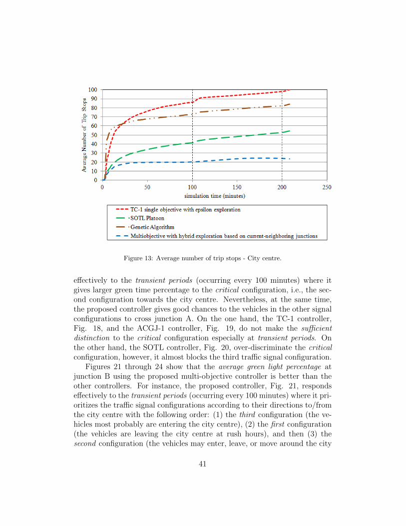
Figure 13: Average number of trip stops - City centre.

effectively to the transient periods (occurring every 100 minutes) where itgives larger green time percentage to the critical configuration, i.e., the sec-ond configuration towards the city centre. Nevertheless, at the same time,the proposed controller gives good chances to the vehicles in the other signalconfigurations to cross junction A. On the one hand, the TC-1 controller,Fig. 18, and the ACGJ-1 controller, Fig. 19, do not make the sufficientdistinction to the critical configuration especially at transient periods. Onthe other hand, the SOTL controller, Fig. 20, over-discriminate the criticalconfiguration, however, it almost blocks the third traffic signal configuration.

Figures 21 through 24 show that the average green light percentage atjunction B using the proposed multi-objective controller is better than theother controllers. For instance, the proposed controller, Fig. 21, respondseffectively to the transient periods (occurring every 100 minutes) where it pri-oritizes the traffic signal configurations according to their directions to/fromthe city centre with the following order: (1) the third configuration (the ve-hicles most probably are entering the city centre), (2) the first configuration(the vehicles are leaving the city centre at rush hours), and then (3) thesecond configuration (the vehicles may enter, leave, or move around the city

41

Figure 14: Percentage of rejected to generated vehicles - City centre.

centre). The TC-1 controller, Fig. 22, the ACGJ-1 controller, Fig. 23, andthe SOTL controller, Fig. 24, do not make such prioritization to the possibletraffic signal configurations.

8. Conclusions and Future Work

8.1. Conclusions

In this paper, we present an adaptive multi-objective reinforcement learn-ing system for traffic signal control based on a cooperative multi-agent frame-work. We show that using RL for solving control optimization problems incontinuous state-space (specifically in the traffic signal control domain) hassome challenges that affect the reward design of the model. In addition,we show that using the Bayesian probability interpretation to estimate theparameters of the MDP probabilities can result in a better response to thetraffic non-stationarity. Traffic non-stationarity are simulated by changingthe traffic flow and traffic demand resulting from changing the weather con-ditions.

42

Figure 15: Average queue length - City centre.

Generally, the application of multi-objective RL optimization is still achallenging task, and particularly, in the domain of traffic signal control.However, using an innovative reward design on a scalar-based form cangreatly boost the various performance indices without the overhead of othercomputationally demanding techniques (e.g., using Max-plus, Pareto frontoptimization, etc.)

Moreover, we show that the application of new exploration techniquesthat are adaptive to the current traffic conditions can greatly affect the per-formance of the traffic signal controller.

Under the congested and free traffic situations, the proposed multi-objectivetraffic signal controller significantly outperforms the underlying single objec-tive controller. For instance, the average trip and waiting times are lower '8 and 6 times respectively when using the multi-objective controller.

Finally, we show that the proposed traffic signal controller outperformsother controllers using the city centre traffic pattern with competing demands.This traffic network is unlike the typical traffic pattern of main arterials andside roads (that leads to a main road domination) where the proposed traffic

43

Figure 16: Traffic signal operation at two junctions (A and B).

signal controller optimally behaves.

8.2. Future Work

The work presented in this paper opens the door to a bulk of future work.For better organizing the suggested directions for future work, we categorizeour ideas into future work in traffic signal control model and future work intraffic signal simulation model.

8.2.1. Traffic Signal Control Model

Firstly, we want to investigate the multi-objective optimization using thePareto front approach. This will be a challenging task in the domain ofreinforcement learning traffic signal control. For instance, we may separatethe benefits associated with each traffic objective and identify the trade-offsassociated with each one. We can introduce the objectives one by one andshow how these objectives affect the various performance indices.

Secondly, we want to check the robustness/sensitivity of the proposedmulti-objective traffic signal controller due to noisy input provided by sen-sors, i.e., partial observability of state-space. In (Schouten and Steingrover,2007), the authors overcome the partial observability of the traffic state by

44

Figure 17: Average green light percentage at junction A using the multi-objective con-troller.

estimating belief states and combining this with multi-agent variants of ap-proximate Partially Observable Markov Decision Process (POMDP) solutionmethods. It was shown that the state transition model and value functioncould be estimated effectively under partial observability.

Thirdly, we plan to control traffic signals in roundabouts. An initial ideais based on game-theory ; every vehicle in every approach (i.e., road in theroundabout) will play a game with other vehicles in the other approaches.The precedence of roundabout crossing will be determined accordingly.

Fourthly, we want to check the role of further exploration techniques inenhancing the various performance indices (i.e., not only the trip waitingtime of vehicles). Another possible improvement is generalizing the role ofexploration in enhancing the performance when the congested periods arecontinued over an extended course of time or when no change in dynamicsoccur for a long period of time (despite these are rare cases).

Finally, our long-term goal is to implement and test the proposed con-troller on real traffic network in Egypt. However, there are some challengesof deployment in Egypt, e.g., unlanned roads, chaotic driving behavior, etc.

45

Figure 18: Average green light percentage at junction A using the TC-1 single-objectivecontroller.

We can overcome the unlanned roads by state-space approximation to the ve-hicles positions. For the chaotic driving behavior, the traffic signal controllercan learn the non-stationarities due to the aggressive undisciplined drivingbehavior in Egypt. We need to integrate the traffic control system with sen-sors (through loop detectors in roads, cameras, and/or communication withvehicles using GPS/Wi-Fi sensors).

8.2.2. Traffic Signal Simulation Model

Firstly, we need to examine the controller behavior when simulating anaccident at some part of the traffic network (that need special handling fromthe traffic signal controller) while in another part of the network there is afree-flowing traffic.

Secondly, we plan to use learning-based techniques to estimate the optimalvalues of the parameters of the IDM acceleration model based on the drivingbehavior in Egypt.

Finally, we need to use a more advanced traffic simulator (rather thanthe GLD) to simulate a real traffic network and examine the proposed con-

46

Figure 19: Average green light percentage at junction A using the ACGJ-1 genetic-basedcontroller.

troller behavior accordingly. One proposed solution is the integration of theproposed traffic signal control framework with a 3D traffic simulator thatallows for human drivers as well as agent vehicles. This simulator has beenbeing developed as a collaboration of our research team with the PrendingerLaboratory in the National Institute of Informatics (NII), Tokyo, Japan.

Acknowledgment

This work is mainly supported by IBM PhD Fellowship and E-JUSTResearch Fellowship, and partially by Pharco Pharmaceuticals Corporationgrant. The authors would like to thank the anonymous reviewers for theirvaluable comments and suggestions that helped improve this paper. Specialthanks are due to Prof. Ahmed El-Mahdy, the director of the Smart CityFacility at the Egypt-Japan University of Science and Technology (E-JUST),for fruitful discussions.

47

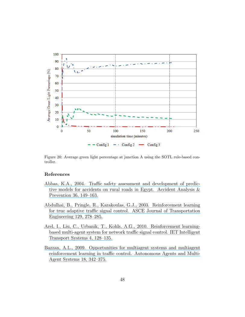
Figure 20: Average green light percentage at junction A using the SOTL rule-based con-troller.

References

Abbas, K.A., 2004. Traffic safety assessment and development of predic-tive models for accidents on rural roads in Egypt. Accident Analysis &Prevention 36, 149–163.

Abdulhai, B., Pringle, R., Karakoulas, G.J., 2003. Reinforcement learningfor true adaptive traffic signal control. ASCE Journal of TransportationEngineering 129, 278–285.

Arel, I., Liu, C., Urbanik, T., Kohls, A.G., 2010. Reinforcement learning-based multi-agent system for network traffic signal control. IET IntelligentTransport Systems 4, 128–135.

Bazzan, A.L., 2009. Opportunities for multiagent systems and multiagentreinforcement learning in traffic control. Autonomous Agents and Multi-Agent Systems 18, 342–375.

48

Figure 21: Average green light percentage at junction B using the multi-objective con-troller.

CAPMAS, 2010. Egypt Central Agency for Public Mobilization And Statis-tics (CAPMAS). Last accessed at 12th Jan 2013.

Cools, S.B., Gershenson, C., D’Hooghe, B., 2008. Self-organizing trafficlights: A realistic simulation. Advances in Applied Self-Organizing Sys-tems , 41–50.

De-Oliveira, L.B., Camponogara, E., 2010. Multi-agent model predictivecontrol of signaling split in urban traffic networks. Transportation ResearchPart C: Emerging Technologies 18, 120–139.

El-Tantawy, S., Abdulhai, B., 2012. Multi-agent reinforcement learning forintegrated network of adaptive traffic signal controllers (MARLIN-ATSC),in: Proc. IEEE 15th International Conference on Intelligent Transporta-tion Systems (ITSC 2012), Anchorage, AK. pp. 319–326.

Escobar, G.D., Pastorino, M., Brey, G., Espinosa, M., 2004. Intelligent Ar-gentinean TRAffic COntrol System (IATRACOS). Sourceforge repository.

49

Figure 22: Average green light percentage at junction B using the TC-1 single-objectivecontroller.

Faye, S., Chaudet, C., Demeure, I., 2012. A distributed algorithm for adap-tive traffic lights control, in: Proc. IEEE 15th International Conferenceon Intelligent Transportation Systems (ITSC 2012), Anchorage, AK. pp.1572–1577.

Febbraro, A.D., Giglio, D., Sacco, N., 2004. Urban traffic control structurebased on hybrid petri nets. IEEE Trans. Intell. Transp. Syst. 5, 224–237.

Gabor, Z., Kalmar, Z., Szepesari, C., 1998. Multi-criteria reinforcementlearning, in: Proc. of the 15th International Conf. on Machine Learning(ICML 1998), Madison, Wisconsin. pp. 197–205.

Gershenson, C., Rosenblueth, D.A., 2009. Modeling self-organizing trafficlights with elementary cellular automata. Technical Report Arxiv preprintarXiv:0907.1925. Universidad Nacional Autonoma de Mexico Ciudad Univ.

Gokulan, B.P., Srinivasan, D., 2010. Distributed geometric fuzzy multiagenturban traffic signal control. IEEE Trans. Intell. Transp. Syst. 11, 714–727.

50

Figure 23: Average green light percentage at junction B using the ACGJ-1 genetic-basedcontroller.

Heung, T.H., Ho, T.K., Fung, Y.F., 2005. Coordinated road-junction trafficcontrol by dynamic programming. IEEE Trans. Intell. Transp. Syst. 6,341–350.

Houli, D., Zhiheng, L., Yi, Z., 2010. Multiobjective reinforcement learning fortraffic signal control using vehicular ad hoc network. Journal on Advancesin Signal Processing (EURASIP) 2010, 7.

Isa, J., Kooij, J., Koppejan, R., Kuijer, L., 2006. DOAS 2006 Project: Re-inforcement Learning of Traffic Light Controllers Adapting to Accidents.Technical Report. Intelligent Autonomous Systems group, Informatics In-stitute, University of Amsterdam. Amsterdam, The Netherlands.

Jin, Y., Sendhoff, B., 2008. Pareto-based multiobjective machine learning:An overview and case studies. IEEE Trans. Syst., Man, Cybern. C 38,397–415.

Khamis, M.A., Gomaa, W., 2012. Enhanced multiagent multi-objective re-

51

Figure 24: Average green light percentage at junction B using the SOTL rule-based con-troller.

inforcement learning for urban traffic light control, in: Proc. IEEE 11thInternational Conference on Machine Learning and Applications (ICMLA2012), Boca Raton, Florida. pp. 586–591.

Khamis, M.A., Gomaa, W., El-Mahdy, A., Shoukry, A., 2012a. Adaptive traf-fic control system based on bayesian probability interpretation, in: Proc.IEEE 2012 Japan-Egypt Conference on Electronics, Communications andComputers (JEC-ECC 2012), Alexandria, Egypt. pp. 151–156.

Khamis, M.A., Gomaa, W., El-Shishiny, H., 2012b. Multi-objective trafficlight control system based on bayesian probability interpretation, in: Proc.IEEE 15th International Conference on Intelligent Transportation Systems(ITSC 2012), Anchorage, AK. pp. 995–1000.

Kuyer, L., Whiteson, S., Bakker, B., Vlassis, N., 2008. Multiagent reinforce-ment learning for urban traffic control using coordination graphs. MachineLearning and Knowledge Discovery in Databases , 656–671.

52

Lertworawanich, P., Kuwahara, M., Miska, M., 2011. A new multiobjectivesignal optimization for oversaturated networks. IEEE Trans. Intell. Transp.Syst. 12, 967–976.

Lin, S., Schutter, B.D., Xi, Y., Hellendoorn, H., 2011. Fast model predictivecontrol for urban road networks via MILP. IEEE Trans. Intell. Transp.Syst. 12, 846–856.

List, G.F., Cetin, M., 2004. Modeling traffic signal control using petri nets.IEEE Trans. Intell. Transp. Syst. 5, 177–187.

Liu, Z., 2007. A survey of intelligence methods in urban traffic signal control.International Journal of Computer Science and Network Security (IJCSNS)7, 105–112.

Mannor, S., Shimkin, N., 2004. A geometric approach to multi-criterionreinforcement learning. Journal of Machine Learning Research 5, 325–360.

Medina, J.C., Benekohal, R.F., 2012. Traffic signal control using reinforce-ment learning and the max-plus algorithm as a coordinating strategy, in:Proc. IEEE 15th International Conference on Intelligent TransportationSystems (ITSC 2012), Anchorage, AK. pp. 596–601.

Natarajan, S., Tadepalli, P., 2005. Dynamic preferences in multi-criteria re-inforcement learning, in: Proc. of the 22th International Conf. on MachineLearning (ICML 2005), Bonn, Germany.

Pizam, A., 1999. Life and tourism in the year 2050. International journal ofhospitality management 18, 331–343.

Prashanth, L.A., Bhatnagar, S., 2011. Reinforcement learning with functionapproximation for traffic signal control. IEEE Trans. Intell. Transp. Syst.12, 412–421.

Rezaee, K., Abdulhai, B., Abdelgawad, H., 2012. Application of reinforce-ment learning with continuous state space to ramp metering in real-worldconditions, in: Proc. IEEE 15th International Conference on IntelligentTransportation Systems (ITSC 2012), Anchorage, AK. pp. 1590–1595.

Richter, S., Aberdeen, D., Yu, J., 2007. Natural actor-critic for road traf-fic optimisation. Advances in Neural Information Processing Systems 19,1169–1176.

53

Salkham, A., Cunningham, R., Garg, A., Cahill, V., 2008. A collaborativereinforcement learning approach to urban traffic control optimization, in:Proc. IEEE/WIC/ACM International Conference on Web Intelligence andIntelligent Agent Technology, Sydney, Australia. pp. 560–566.

Sanchez-Medina, J.J., Galan-Moreno, M.J., Rubio-Royo, E., 2010. Trafficsignal optimization in “La Almozara” district in saragossa under conges-tion conditions, using genetic algorithms, traffic microsimulation, and clus-ter computing. IEEE Trans. Intell. Transp. Syst. 11, 132–141.

Schouten, R., Steingrover, M., 2007. Reinforcement Learning of Traffic LightControllers under Partial Observability. Master’s thesis. Faculty of ScienceUniversity of Amsterdam. Amsterdam, The Netherlands.

Schrank, D., Lomax, T., Eisele, B., 2011. TTI’s 2011 urban mobility re-port. TII Report Exhibit B-15. Texas Transportation Institute (TII), TheTexas A&M University System, U.S. Dept. of Transportation, UniversityTransportation Center for Mobility.

Sen, S., Head, K.L., 1997. Controlled optimization of phases at an intersec-tion. Transportation science 31, 5–17.

Shoham, Y., Leyton-Brown, K., 2010. Multiagent systems: Algorithmic,game-theoretic, and logical foundations. Cambridge Univ. Press.

Smith, R.H., Chin, D.C., 1995. Evaluation of an adaptive traffic controltechnique with underlying system changes, in: Proc. IEEE 27th WinterSimulation Conference (WSC 1995), Arlington, VA. pp. 1124–1130.

Srinivasan, D., Choy, M.C., Cheu, R.L., 2006. Neural networks for real-timetraffic signal control. IEEE Trans. Intell. Transp. Syst. 7, 261–272.

Steingrover, M., Schouten, R., Peelen, S., Nijhuis, E., Bakker, B., 2005.Reinforcement learning of traffic light controllers adapting to traffic con-gestion, in: Proc. of the 17th Belgium-Netherlands Conference on ArtificialIntelligence Conference (BNAIC 2005), Brussels, Belgium. pp. 216–223.

Thorpe, T.L., Anderson, C.W., 1996. Traffic Light Control Using SARSAwith Three State Representations. Technical Report. IBM Corporation.

54

U.S. Department of Transportation, N.H.T.S.A., 2012. 2010 Motor VehicleCrashes: Overview. Traffic Safety Facts Research Note DOT HS 811 552.NHTSA’s National Center for Statistics and Analysis. 1200 New JerseyAvenue SE., Washington, DC 20590.

Treiber, M., Hennecke, A., Helbing, D., 2000. Congested traffic states inempirical observations and microscopic simulations. Physical Review E62, 1805–1824.

Wenchen, Y., Lun, Z., Zhaocheng, H., Lijian, Z., 2012. Optimized two-stagefuzzy control for urban traffic signals at isolated intersection and paramicssimulation, in: Proc. IEEE 15th International Conference on IntelligentTransportation Systems (ITSC 2012), Anchorage, AK. pp. 391–396.

Wiering, M., 2000. Multi-agent reinforcement learning for traffic light control,in: Proc. of the 17th International Conf. on Machine Learning (ICML2000), pp. 1151–1158.

Wiering, M., Vreeken, J., van Veenen, J., Koopman, A., 2004. Simulationand optimization of traffic in a city, in: Proc. IEEE Intelligent Vehiclesymposium (IV 2004), Parma, Italy. pp. 453–458.

55