
Multi-Criteria Reinforcement Learning for Sequential Decision ...
220
Faculty of Science and Bio-Engineering Sciences Department of Computer Science Multi-Criteria Reinforcement Learning for Sequential Decision Making Problems Dissertation submitted in fulfilment of the requirements for the degree of Doctor of Science: Computer Science Kristof Van Moffaert Promotor: Prof. Dr. Ann Nowé
-
Upload
khangminh22 -
Category
Documents
-
view
2 -
download
0
Transcript of Multi-Criteria Reinforcement Learning for Sequential Decision ...

Faculty of Science andBio-Engineering Sciences
Department of Computer Science
Multi-Criteria Reinforcement Learning for SequentialDecision Making Problems
Dissertation submitted in fulfilment of the requirements for the degree of Doctor of Science: Computer Science
Kristof Van Mo�aert
Promotor: Prof. Dr. Ann Nowé

c� 2016 Kristof Van Mo�aert
2016 Uitgeverij VUBPRESS Brussels University PressVUBPRESS is an imprint of ASP nv (Academic and Scientific Publishers nv)Ravensteingalerij 28B-1000 BrusselsTel. +32 (0)2 289 26 50Fax +32 (0)2 289 26 59E-mail: [email protected]
ISBN 978 90 5718 094 1NUR 993Legal deposit D/2014/11.161/062
All rights reserved. No parts of this book may be reproduced or transmitted in any formor by any means, electronic, mechanical, photocopying, recording, or otherwise, withoutthe prior written permission of the author.

Luctor et emergo.
3


Abstract
Reinforcement learning provides a framework for algorithms that learn from interactionwith an unknown environment. Over the years, several researchers have contributed tothis framework by proposing algorithms that optimise their behaviour over time. Thislearning process is characterised by maximising a single, scalar reward signal. However,many real-life problems are inherently too complex to be described by a single, scalarcriterion. Usually, these problems involve multiple objectives that often give rise to aconflict of interest. An example can be found in the manufacturing industry where thegoal of a company is to come up with a policy that, at the same time, maximises the profitand the user satisfaction while minimising the production costs, the labour costs and theenvironmental impact. For these types of problems, the traditional reinforcement learningframework is insu�cient and lacks expressive power.
In this dissertation, we argue the need for particular reinforcement learning algorithms thatare specifically tailored for multi-objective problems. These algorithms are multi-objectivereinforcement learning (MORL) algorithms that provide one or more Pareto optimal bal-ances of the problem’s original objectives. What this balance intrinsically conveys dependson the emphasis and the preferences of the decision maker. In the case the decisionmaker’s preferences are clear and known a priori, single-policy techniques such as scalar-isation functions can be employed to guide the search towards a particular compromisesolution. In this light, we analyse several instantiations of scalarisation functions such asthe linear and Chebyshev scalarisation function and we demonstrate how they influencethe converged solution.
In case the preference articulation of the decision maker is unclear before the optimisationprocess takes place, it might be appropriate to provide a set of Pareto optimal trade-o�solutions to the decision maker that each comprise a di�erent balance of the objectives.One possibility to obtain a set of solutions is to collect the outcomes of several scalarisationfunctions while varying their direction of search. In this dissertation, we propose twoalgorithms that follow this principle for both discrete and continuous Pareto fronts.
5

Abstract
A more advanced idea we pursue as well is to learn a set of compromise solutions in asimultaneous fashion. In order to accommodate for a genuine multi-policy algorithm, weextend the core principles of the reinforcement learning framework, including the know-ledge representation and the bootstrapping process. For continuous action spaces, wepropose the multi-objective hierarchical optimistic optimisation algorithm that increment-ally constructs a binary tree of optimistic vectorial estimates. For sequential decisionmaking problems, we introduce Pareto Q-learning. Pareto Q-learning is the first temporaldi�erence-based reinforcement learning algorithm that learns a set of Pareto non-dominatedpolicies in a single run. Internally, it relies on a specific bootstrapping process that sep-arates the immediate reward from the set of future rewards. This way, each vectorialestimate in the set can be updated as new information becomes available. The algorithmalso comprises a mechanism to retrieve the state and action sequences that correspondto each of these policies.
Finally, we demonstrate the behaviour of a multi-policy algorithm on a simulation envir-onment of a transmission system. For a transmission to be optimal, it needs to be bothsmooth and fast, which are in essence conflicting objectives. We analyse how the solutionmethod explores the objective space and continually refines its knowledge.
6

Samenvatting
Reinforcement learning voorziet een raamwerk voor algoritmen die leren uit interactiesmet een onbekende omgeving. Sinds vele jaren hebben onderzoekers bijgedragen tot ditraamwerk door dergelijke algoritmen voor te stellen die hun gedrag optimaliseren over detijd heen. Dit leerproces wordt gekarakteriseerd door het trachten maximaliseren van eenenkel, scalair beloningsignaal. Echter zijn vele problemen uit de reële wereld van natureuit te complex om beschreven te worden door een enkel, scalair criterium. Doorgaanshebben deze problemen betrekking op meerdere doelstellingen die vaak aanleiding geventot strijdige belangen. Een voorbeeld hiervan is te vinden in de industrie waar het doel vaneen onderneming is om te komen tot een beleid dat op hetzelfde moment de winst en detevredenheid van de gebruiker maximaliseert, terwijl het eveneens de productiekosten, dearbeidskosten en de milieu-impact tracht te minimaliseren. Voor dit soort problemen is hettraditionele reinforcement learning framework ontoereikend en ontbreekt het expressiviteit.
In dit proefschrift pleiten we voor de behoefte aan specifieke reinforcement learning al-goritmen die speciaal zijn aangepast voor problemen met meerdere objectieven. Dezealgoritmen heten vervolgens multi-objectieve reinforcement learning (MORL) algoritmendie een of meerdere Pareto optimale evenwichten van de doelstellingen verstrekken. Watdit evenwicht intrinsiek uitstraalt is afhankelijk van de klemtoon en de voorkeuren van debeleidsmaker. In het geval dat de voorkeuren van de beleidsmaker duidelijk en bij voorbaatbekend zijn, kunnen single-policy technieken zoals scalarisatie functies gebruikt worden omhet zoeken naar een bepaald compromis te begeleiden. In dit opzicht analyseren we ver-schillende instantiaties van scalarisatie functies zoals de lineaire en Chebyshev scalarisatiefunctie en we laten zien welke invloed ze hebben op de geconvergeerde oplossing.
In het geval dat de voorkeuren van de beleidsmaker onduidelijk zijn voor het optimalisa-tieproces plaatsvindt, zou het aangewezen zijn om een verzameling van Pareto optimaleoplossingen aan de beleidsmaker voor te stellen die elk een ander evenwicht van de doel-stellingen afweegt. Een mogelijkheid om een verzameling oplossingen te verkrijgen bestaateruit de uitkomsten van een aantal scalarisatie functies, die elk uiteenlopende delen van
7

Samenvatting
het zoekgebied onderzoeken, te verzamelen. In dit proefschrift stellen we twee algoritmenvoor die dit principe volgen voor zowel discrete als continue Pareto ruimtes.
Een meer geavanceerd idee dat we ook nastreven bestaat eruit om een verzameling vancompromissen te leren op een gelijktijdige basis. Om tegemoet te komen aan een daad-werkelijk multi-policy algoritme, breiden we de beginselen van het reinforcement learningkader uit, met inbegrip van de kennis representatie en het bootstrapping proces. Voor con-tinue actie ruimtes, stellen wij het multi-objectief hiërarchische optimistisch optimalisatiealgoritme voor dat stapsgewijs een binaire boom van vectoriële optimistische schattin-gen construeert. Voor sequentiële problemen introduceren we Pareto Q-learning. ParetoQ-learning is het eerste temporal di�erence-gebaseerd reinforcement learning algoritmedat een verzameling van Pareto dominerende oplossingen simultaan leert. Intern berusthet algoritme op een specifiek bootstrapping proces dat de onmiddellijke beloning van deverzameling van de toekomstige beloningen scheidt. Op deze manier kan elke vectoriëleschatting in de verzameling worden bijgewerkt als er nieuwe informatie beschikbaar wordt.Het algoritme omvat tevens een mechanisme om de opeenvolging van toestanden en actiesdie corresponderen met elk van deze geleerde oplossingen te achterhalen. Tot slot demon-streren we het gedrag van een multi-policy algoritme op een simulatieomgeving van eentransmissiesysteem. Opdat een transmissie optimaal is, moet deze zowel soepel als snelzijn, welke in wezen strijdige doelstellingen zijn. We analyseren hoe deze oplossingsmeth-ode de zoekruimte van het transmissiesysteem verkent en voortdurend zijn kennis verruimt.
8

Contents
Abstract 5
Samenvatting 7
Contents 9
Acknowledgements 13
1 Introduction 151.1 Agents . . . . . . . . . . . . . . . . . . . . . . . . . . . . . . . . . . . . 161.2 Learning agents . . . . . . . . . . . . . . . . . . . . . . . . . . . . . . . 171.3 Problem statement . . . . . . . . . . . . . . . . . . . . . . . . . . . . . 181.4 Contributions . . . . . . . . . . . . . . . . . . . . . . . . . . . . . . . . 221.5 Outline of the dissertation . . . . . . . . . . . . . . . . . . . . . . . . . . 23
2 Single-objective reinforcement learning 272.1 History of reinforcement learning . . . . . . . . . . . . . . . . . . . . . . 282.2 Markov decision processes . . . . . . . . . . . . . . . . . . . . . . . . . . 292.3 Notations of reinforcement learning . . . . . . . . . . . . . . . . . . . . . 312.4 Learning methods . . . . . . . . . . . . . . . . . . . . . . . . . . . . . . 34
2.4.1 Model-based learning . . . . . . . . . . . . . . . . . . . . . . . . 352.4.2 Model-free learning . . . . . . . . . . . . . . . . . . . . . . . . . 37
2.5 Reinforcement learning in stateless environments . . . . . . . . . . . . . . 392.5.1 Experimental evaluation . . . . . . . . . . . . . . . . . . . . . . . 40
2.6 Summary . . . . . . . . . . . . . . . . . . . . . . . . . . . . . . . . . . . 43
9
CONTENTS
3 Learning in Multi-Criteria Environments 453.1 Introduction . . . . . . . . . . . . . . . . . . . . . . . . . . . . . . . . . 45
3.1.1 Definitions of Multi-Criteria Decision Making . . . . . . . . . . . 463.1.2 Multi-Objective Optimisation . . . . . . . . . . . . . . . . . . . . 46
3.2 Evolutionary Multi-Objective Optimisation . . . . . . . . . . . . . . . . . 583.3 Definitions of Multi-Objective RL . . . . . . . . . . . . . . . . . . . . . . 60
3.3.1 Multi-Objective Markov Decision Process . . . . . . . . . . . . . 603.4 Problem taxonomy . . . . . . . . . . . . . . . . . . . . . . . . . . . . . 63
3.4.1 Axiomatic approach . . . . . . . . . . . . . . . . . . . . . . . . . 633.4.2 Utility approach . . . . . . . . . . . . . . . . . . . . . . . . . . . 71
3.5 Summary . . . . . . . . . . . . . . . . . . . . . . . . . . . . . . . . . . . 72
4 Learning a Single Multi-Objective Policy 734.1 A framework for scalarised MORL algorithms . . . . . . . . . . . . . . . 734.2 Linear scalarised MORL . . . . . . . . . . . . . . . . . . . . . . . . . . . 75
4.2.1 Optimality of linear scalarised MORL . . . . . . . . . . . . . . . . 764.2.2 Convexity of linear scalarised MORL . . . . . . . . . . . . . . . . 77
4.3 Chebyshev scalarised MORL . . . . . . . . . . . . . . . . . . . . . . . . . 844.3.1 Formal definition . . . . . . . . . . . . . . . . . . . . . . . . . . 854.3.2 Scalarisation with the Chebyshev function . . . . . . . . . . . . . 864.3.3 Convergence issues in MORL . . . . . . . . . . . . . . . . . . . . 874.3.4 Experimental validation . . . . . . . . . . . . . . . . . . . . . . . 88
4.4 Benchmarking linear and Chebyshev scalarised MORL . . . . . . . . . . . 954.4.1 Performance criteria . . . . . . . . . . . . . . . . . . . . . . . . . 964.4.2 Parameter configuration . . . . . . . . . . . . . . . . . . . . . . . 964.4.3 Deep sea treasure world . . . . . . . . . . . . . . . . . . . . . . . 984.4.4 Mountain car world . . . . . . . . . . . . . . . . . . . . . . . . . 1004.4.5 Resource gathering world . . . . . . . . . . . . . . . . . . . . . . 103
4.5 Conclusions . . . . . . . . . . . . . . . . . . . . . . . . . . . . . . . . . 1054.6 Summary . . . . . . . . . . . . . . . . . . . . . . . . . . . . . . . . . . . 107
5 Iteratively learning multiple multi-objective policies 1095.1 Iteratively learning an archive of trade-o� solutions . . . . . . . . . . . . 110
5.1.1 Related Work . . . . . . . . . . . . . . . . . . . . . . . . . . . . 1125.2 Adaptive weight algorithms for discrete Pareto fronts . . . . . . . . . . . 112
5.2.1 The algorithm . . . . . . . . . . . . . . . . . . . . . . . . . . . . 1135.2.2 Experimental evaluation . . . . . . . . . . . . . . . . . . . . . . . 1175.2.3 The Bountiful Sea Treasure world . . . . . . . . . . . . . . . . . 1175.2.4 The Resource Gathering world. . . . . . . . . . . . . . . . . . . . 1185.2.5 The Bountiful Sea Treasure 3D world . . . . . . . . . . . . . . . 120
10

CONTENTS
5.2.6 Advantages and limitations . . . . . . . . . . . . . . . . . . . . . 1245.3 Adaptive weight algorithms for continuous Pareto fronts . . . . . . . . . 125
5.3.1 Defining good approximation set . . . . . . . . . . . . . . . . . . 1255.3.2 Existing adaptive weight algorithms . . . . . . . . . . . . . . . . 1265.3.3 Experimental evaluation . . . . . . . . . . . . . . . . . . . . . . . 1285.3.4 Novel adaptive weight algorithms for RL . . . . . . . . . . . . . . 1335.3.5 Conclusions . . . . . . . . . . . . . . . . . . . . . . . . . . . . . 138
5.4 Summary . . . . . . . . . . . . . . . . . . . . . . . . . . . . . . . . . . . 138
6 Simultaneously learning multiple multi-objective policies 1416.1 Related work on simultaneously learning multiple policies . . . . . . . . . 1426.2 Learning multiple policies in single-state problems . . . . . . . . . . . . . 143
6.2.1 Hierarchical Optimistic Optimisation . . . . . . . . . . . . . . . . 1446.2.2 Multi-Objective Hierarchical Optimistic Optimisation . . . . . . . 1456.2.3 Experiments . . . . . . . . . . . . . . . . . . . . . . . . . . . . . 1506.2.4 Scha�er 1 function . . . . . . . . . . . . . . . . . . . . . . . . . 1506.2.5 Fonseca and Flemming function . . . . . . . . . . . . . . . . . . 1546.2.6 Discussion . . . . . . . . . . . . . . . . . . . . . . . . . . . . . . 156
6.3 Learning multiple policies in multi-state problems . . . . . . . . . . . . . 1576.3.1 Set-based Bootstrapping . . . . . . . . . . . . . . . . . . . . . . 1606.3.2 Notions on convergence . . . . . . . . . . . . . . . . . . . . . . . 1646.3.3 Set evaluation mechanisms . . . . . . . . . . . . . . . . . . . . . 1656.3.4 Consistently tracking a policy . . . . . . . . . . . . . . . . . . . . 1676.3.5 Performance assessment of multi-policy algorithms . . . . . . . . 1716.3.6 Benchmarking Pareto Q-learning . . . . . . . . . . . . . . . . . . 1726.3.7 Experimental comparison . . . . . . . . . . . . . . . . . . . . . . 1776.3.8 Conclusions . . . . . . . . . . . . . . . . . . . . . . . . . . . . . 180
6.4 Summary . . . . . . . . . . . . . . . . . . . . . . . . . . . . . . . . . . . 181
7 Applications of multi-objective reinforcement learning 1837.1 The Filling Phase of a Wet Clutch . . . . . . . . . . . . . . . . . . . . . 1837.2 Multi-policy analysis with MO-HOO . . . . . . . . . . . . . . . . . . . . 1867.3 Conclusions and future outlook . . . . . . . . . . . . . . . . . . . . . . . 189
8 Conclusions 1918.1 Contributions . . . . . . . . . . . . . . . . . . . . . . . . . . . . . . . . 1918.2 Remarks . . . . . . . . . . . . . . . . . . . . . . . . . . . . . . . . . . . 1938.3 Outlooks for future research . . . . . . . . . . . . . . . . . . . . . . . . . 1948.4 Overview . . . . . . . . . . . . . . . . . . . . . . . . . . . . . . . . . . . 196
List of Selected Publications 199
11

CONTENTS
List of abbreviations 201
List of symbols 203
Bibliography 205
Index 217
12

Acknowledgements
This dissertation would not have been possible without the support and the encouragementof many people.
First and foremost I would like to express my special appreciation and thanks to mypromoter Ann Nowé for giving me the opportunity to pursue a Ph.D. at the ComputationalModelling lab. Thank you, Ann, for the scientific and personal guidance you have beengiving me the past four years. I appreciate all the meetings, brainstorms and discussionsthat we had to continuously push the boundaries of my research.
Furthermore, I would also like to thank the members of the examination committee KarlTuyls, Bernard Manderick, Kurt Driessens, Bart Jansen, Yann-Michaël De Hauwere andCoen De Roover for taking the time to read the dissertation and for your helpful insightsand suggestions.
I am also grateful to the people I worked with on my two projects. For the Perpetualproject, I would like to thank our colleagues at KULeuven en FMTC for our combinede�orts on the industrial applications of multi-objective research. For the Scanergy project,I would like to personally thank Mike for hosting me three months in the o�ces of Sensing& Control in Barcelona. Also, thank you Narcís, Sam, Mihhail, Pablo, Raoul, José María,Sergio, Adrián, Helena, Pedro, Alberto and Angel for making it a memorable stay abroad!
I would also like to praise my colleagues at the CoMo lab. It has been a pleasure to spendfour years in such good company. I will cherish the amazing moments that we had, suchas our BBQs, the team building events in Ostend and Westouter, the after-hours drinksat the Kultuurka�ee and simply our easy chats in the lab. Thanks a lot Ann, Bernard,Anna, Abdel, Dip, Elias, Felipe, Frederik, Ivan, Ivomar, Isel, Jelena, Jonatan, Lara, Luis,Madalina, Marjon, Mike, Peter, Pieter, Roxana, Saba, Steven, The Ahn, Timo, Tom,Yailen, Yann-Michaël and Yami!
I deliberately left out three people from the list because they deserve some special atten-tion. Maarten, Kevin and Tim, we started this long journey back in 2011 and encountered
13

Acknowledgements
so many beautiful, tough and inspiring moments. I could not have wished for better col-leagues that became friends with a capital F (although Kevin will never admit it). I willnever forget the (social dinners at the) BNAIC conferences, the AAMAS conference inValencia, the football matches, the paintball that never took place, the personalised co�eemug, Boubakar, the quiz in the bar in Ostend, the break-in into Kevin’s room, the dailyping-pong matches, the estimated 16000cl of free soup, the trips to Singapore, Miami,Japan, South-Africa and so much more!
Last but definitely not least, I would like to acknowledge the role of my family during mystudies. I would like to express my gratitude to my parents and my brother for their never-ending and unconditional support. Their care allowed me to decompress after work and toforget the struggles I was facing. Also my friends had a great influence on me to unwindafter a busy week. Thank you Wouter & Nele, Sander & Tine, Thomas, Maarten, Maxand Ken! Also thank you, E.R.C. Hoeilaart and W.T.C. Hoeilaart for the football matchesand the cycling races that allowed me to recharge my batteries during the weekend.
The last part of these acknowledgements is dedicated to the most important person inmy life for more than 6 years. Lise, without you I was not able to find the devotion thatwas necessary for this kind of job. Due to your encouragement, I was able to overcomethe most stressful moments. We shared both the high points and the low points of thisfour-year quest and I could not think of anyone else I wanted to share these moments with.Together with you, I will now focus on di�erent objectives in life.
Brussels, March 2016.
14
1
| Introduction
This dissertation is concerned with the study of reinforcement learning in situations wherethe agent is faced with a task involving multiple objectives. Reinforcement learning is abranch of machine learning in which an agent has to learn the optimal behaviour in anunknown environment. In essence, the agent has to learn over time what is the optimalaction to take in each state of the environment. In reinforcement learning, the agentemploys a principle of trial and error to examine the consequences actions have in particularstates. It does so by analysing a scalar feedback signal associated to each action. Based onthis signal, reinforcement learning tries to discover the optimal action for each particularsituation that can occur.
However, many real-world problems are inherently too complex to be described by asingle, scalar feedback signal. Usually, genuine decision making problems require the sim-ultaneous optimisation of multiple criteria or objectives. These objectives can be correlatedor independent, but they usually are conflicting, i.e., an increase in the performance ofone objective implies a decrease in the performance of another objective and vice versa.An example can be found in the area of politics where parliamentarians have to decideon the location where to build a new highway that at the same time increases the e�-ciency of the tra�c network and minimises the associated environmental and social costs.Other examples might not be limited to only two objectives. For instance, in the man-ufacturing industry, the goal of a company comprises many criteria such as maximisingthe profit and the customer satisfaction while minimising the production costs, the labourcosts and the environmental impact. In these situations, traditional reinforcement learningapproaches often fail because they oversimplify the problem at hand which on its turnresults in unrealistic and suboptimal decisions.
In literature, di�erent approaches exist that strive towards the development of specificmulti-objective reinforcement learning techniques. However, most of these approaches arelimited in the sense that they cannot discover every optimal compromise solution, leaving
15
CHAPTER 1. INTRODUCTION
potentially fruitful areas of the objective space untouched. Also, some of these approachesare not generalisable as they are restricted to specific application domains.
In this dissertation, we evaluate di�erent approaches that allow the discovery of one ormore trade-o� solutions that balance the objectives in the environment. We group thealgorithms in four categories. We first di�erentiate between single-policy and multi-policytechniques, based on the fact whether the algorithm learns a single compromise or a set ofsolutions, respectively. Furthermore, we also distinguish between the type of scalarisationfunction used in the process, i.e., being a linear scalarisation function or a monotonicallyincreasing variant. We analyse the conceptual details of the algorithms and emphasizethe associated design decisions. Additionally, we verify the theoretical guarantees and theempirical performance of these algorithms on a wide set of benchmark problems.
In the following sections, we will start o� with the basics of artificial intelligence. Wewill define what agents are and what characterises an intelligent agent. Subsequently, weoutline the problem statement and the contributions of this dissertation.
1.1 AgentsNowadays, people often admit computer systems are brilliant and clever devices since theyallow them to send and receive e-mail messages, organise agendas, create text documentsand so much more. However, to o�er this functionality, all the computer system does isprocessing some predefined lines of code that were implemented by a software engineer. Ifthe computer system is asked to perform an unforeseen request that was not envisaged bythe software engineer, the computer system will most likely not act as inquired or not actat all. Therefore, it is naive to think of these types of systems as being clever since theypossess no reasoning capabilities and are not able to work autonomously. Yet, computersystems that do hold these properties are called agents.
In artificial intelligence (AI), the principle of an agent is a widely used concept. However,how an agent is defined di�ers throughout the di�erent branches of AI. In general, thedefinition by Jennings et al. (1998) is considered a good summary of what comprises anagent:
Definition 1.1
An agent is a computer system that is situated in some environment, and that iscapable of autonomous action taking in this environment in order to meet its designobjectives.
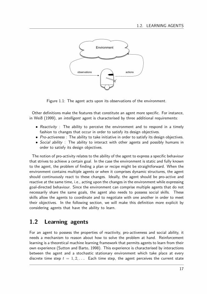
Although this definition still remains very broad, the principle components of an agentstructure are clear, i.e., the agent observes the environment it is operating in and selectsan action, which in its turn can change the state of the environment, as illustrated inFigure 1.1.
16
1.2. LEARNING AGENTS
actionsobservations
Environment
Figure 1.1: The agent acts upon its observations of the environment.
Other definitions make the features that constitute an agent more specific. For instance,in Weiß (1999), an intelligent agent is characterised by three additional requirements:
• Reactivity : The ability to perceive the environment and to respond in a timelyfashion to changes that occur in order to satisfy its design objectives.
• Pro-activeness : The ability to take initiative in order to satisfy its design objectives.• Social ability : The ability to interact with other agents and possibly humans in
order to satisfy its design objectives.
The notion of pro-activity relates to the ability of the agent to express a specific behaviourthat strives to achieve a certain goal. In the case the environment is static and fully knownto the agent, the problem of finding a plan or recipe might be straightforward. When theenvironment contains multiple agents or when it comprises dynamic structures, the agentshould continuously react to these changes. Ideally, the agent should be pro-active andreactive at the same time, i.e., acting upon the changes in the environment while expressinggoal-directed behaviour. Since the environment can comprise multiple agents that do notnecessarily share the same goals, the agent also needs to possess social skills. Theseskills allow the agents to coordinate and to negotiate with one another in order to meettheir objectives. In the following section, we will make this definition more explicit byconsidering agents that have the ability to learn.
1.2 Learning agentsFor an agent to possess the properties of reactivity, pro-activeness and social ability, itneeds a mechanism to reason about how to solve the problem at hand. Reinforcementlearning is a theoretical machine learning framework that permits agents to learn from theirown experience (Sutton and Barto, 1998). This experience is characterised by interactionsbetween the agent and a stochastic stationary environment which take place at everydiscrete time step t = 1, 2, . . .. Each time step, the agent perceives the current state
17
CHAPTER 1. INTRODUCTION
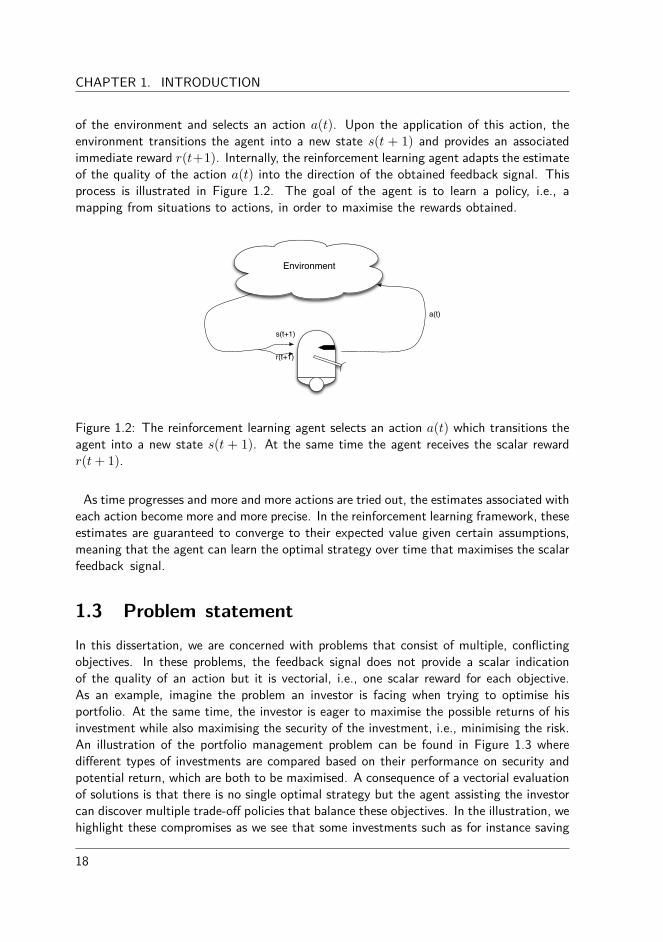
of the environment and selects an action a(t). Upon the application of this action, theenvironment transitions the agent into a new state s(t + 1) and provides an associatedimmediate reward r(t+1). Internally, the reinforcement learning agent adapts the estimateof the quality of the action a(t) into the direction of the obtained feedback signal. Thisprocess is illustrated in Figure 1.2. The goal of the agent is to learn a policy, i.e., amapping from situations to actions, in order to maximise the rewards obtained.
a(t)
s(t+1)
r(t+1)
Environment
Figure 1.2: The reinforcement learning agent selects an action a(t) which transitions theagent into a new state s(t + 1). At the same time the agent receives the scalar rewardr(t + 1).
As time progresses and more and more actions are tried out, the estimates associated witheach action become more and more precise. In the reinforcement learning framework, theseestimates are guaranteed to converge to their expected value given certain assumptions,meaning that the agent can learn the optimal strategy over time that maximises the scalarfeedback signal.
1.3 Problem statementIn this dissertation, we are concerned with problems that consist of multiple, conflictingobjectives. In these problems, the feedback signal does not provide a scalar indicationof the quality of an action but it is vectorial, i.e., one scalar reward for each objective.As an example, imagine the problem an investor is facing when trying to optimise hisportfolio. At the same time, the investor is eager to maximise the possible returns of hisinvestment while also maximising the security of the investment, i.e., minimising the risk.An illustration of the portfolio management problem can be found in Figure 1.3 wheredi�erent types of investments are compared based on their performance on security andpotential return, which are both to be maximised. A consequence of a vectorial evaluationof solutions is that there is no single optimal strategy but the agent assisting the investorcan discover multiple trade-o� policies that balance these objectives. In the illustration, wehighlight these compromises as we see that some investments such as for instance saving
18

1.3. PROBLEM STATEMENT
bonds (a) and precious metals (b) are very secure but o�er only small profit margins.A counter example is the stock market (d) that has the potential of a high return ofinvestment while at the same time a high probability in money losses as well. Real estateproperties (c) o�er a more balanced compromise between the two objectives. Since thereare no solutions improving these four investments on any of the two objectives, thesefour approaches are said to be optimal trade-o�s which the agent can discover. However,there are also solutions that are not optimal. Consider for instance, the investment intechnological devices, such as computers (e), and cars (f), which rapidly devalue and takeo� in valuation.
Secu
rity
Possible return
(a)
(b)
(c)
(d)
(e)
(f)
Figure 1.3: The trade-o� between security and the potential return in a portfolio man-agement problem. The optimal solutions (a) to (d) are denoted by black dots while thedominated solutions, such as (e) and (f) are white dots. The goal of the agent optimisingthe investment problem would be to discover the optimal compromise solutions (a) to (d).
Internally, the agent needs a mechanism to evaluate these multi-objective solutions basedon the preferences of the investor. In some cases, these preferences can be very clear andthe possible solutions can be totally ordered to select the best solution. For instance, thepreference could be to maximize the possible return, regardless of the security objective.Hence, the agent would only suggest solution (d), i.e., the stock market. In other cases,when the preferences are unclear (or possibly even unknown), only a partial order can beretained. The mechanism that evaluates solutions while taking into account this preferenceinformation is called a scalarisation function. Based on the specific instantiation of thescalarisation function, di�erent properties arise. Each of these properties will be coveredin Chapter 3.
In general, multi-objective reinforcement learning approaches that learn these compromisesolutions can be characterised based on two aspects. In Section 3.4, we provide a detailed
19

CHAPTER 1. INTRODUCTION
taxonomy, but for now it is su�cient to characterise the approaches based on (1) whetherone or more solutions are returned and (2) whether these solutions are situated in aconvex or non-convex region of the objective space.
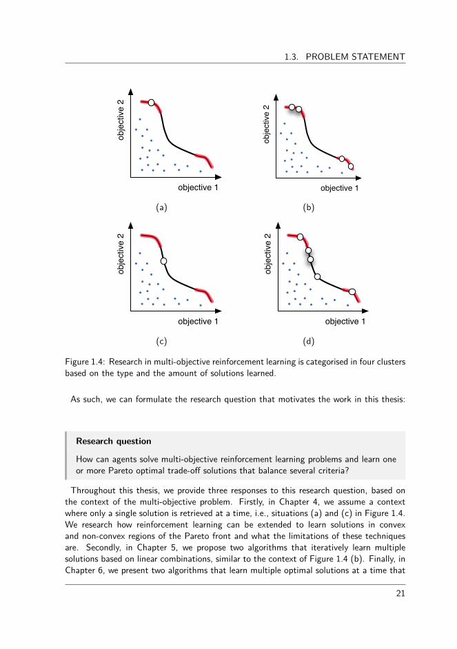
A first and simple category of approaches learns a single, convex solution at a time.Since the solution is located in a convex region, mathematical formulas guarantee thatthe solution can be retrieved by a linear, weighted combination of the objectives. Thee�ectiveness of this category is represented in Figure 1.4 (a) where both objectives needto be maximised. The blue dots represent dominated solutions while the set of optimalsolutions, referred to as the Pareto front, is depicted in black. The areas in red denote asubset of the Pareto front that can be discovered by convex combinations. In this red area,the white dot represents a possible solution the techniques in this category would learn.
A second category represents a collection of techniques that learn a set of multiple,convex solutions. These mechanisms exploit the same mathematical properties of thealgorithms of the first category, but this time to retrieve a set of trade-o� solutions. Eachof these solutions then lies in convex areas of the Pareto front, as depicted in Figure 1.4(b). Ideally, this category of algorithms would aim to discover the entire set of solutionscovering the red areas.
Although a significant amount of research in reinforcement learning has been focussingon solving problems from the viewpoint of these situations (Vamplew et al., 2010; Roijerset al., 2013), only a subset of the Pareto front is retrievable, leaving potential fruitfulparts of the objective space untouched. A large part of this dissertation addresses theproblem of discovering solutions that cannot be defined by convex combinations. In thatsense, we analyse the theoretical and the empirical performance of reinforcement learningalgorithms for retrieving optimal solutions, that lie in both convex and non-convex partsof the Pareto front. This constitutes the third and fourth category. The third categoryencompasses algorithms that learn a single convex or non-convex solution at a time, asdepicted in Figure 1.4 (c).
The fourth category involves algorithms for learning multiple solutions simultaneously.These algorithms then retrieve a set of both convex and non-convex solutions as presentedin Figure 1.4 (d). In essence, these algorithm are genuine multi-policy algorithms thatcan discover the entire Pareto front of optimal solutions, as they are not limited to aspecific subset.
20
1.3. PROBLEM STATEMENT
obje
ctiv
e 2
objective 1
obje
ctiv
e 2
objective 1
(a) (b)
obje
ctiv
e 2
objective 1
obje
ctiv
e 2
objective 1
(c) (d)
Figure 1.4: Research in multi-objective reinforcement learning is categorised in four clustersbased on the type and the amount of solutions learned.
As such, we can formulate the research question that motivates the work in this thesis:
Research question
How can agents solve multi-objective reinforcement learning problems and learn oneor more Pareto optimal trade-o� solutions that balance several criteria?
Throughout this thesis, we provide three responses to this research question, based onthe context of the multi-objective problem. Firstly, in Chapter 4, we assume a contextwhere only a single solution is retrieved at a time, i.e., situations (a) and (c) in Figure 1.4.We research how reinforcement learning can be extended to learn solutions in convexand non-convex regions of the Pareto front and what the limitations of these techniquesare. Secondly, in Chapter 5, we propose two algorithms that iteratively learn multiplesolutions based on linear combinations, similar to the context of Figure 1.4 (b). Finally, inChapter 6, we present two algorithms that learn multiple optimal solutions at a time that
21

CHAPTER 1. INTRODUCTION
are located in both convex and non-convex regions of the Pareto front. These approachesrelate to Figure 1.4 (d).
1.4 ContributionsWhile answering the research question, we have made several contributions to the fieldof multi-objective reinforcement learning. We summarise the main achievements in thefollowing list:
• We provide an overview of the foundations and the history of standard, single-objective reinforcement learning. We closely examine the theoretical characteristicsof the reinforcement learning framework and explicitly describe all the componentsthat compose a reinforcement learning problem.
• We provide a taxonomy of multi-objective reinforcement learning research based onthe type of scalarisation function used in the decision making process and the amountof solutions learned.
• We highlight the advantages and limitations of current state-of-the-art approacheswithin this field. We argue that there is a need for algorithms that go beyond theexclusive search for convex solutions. We show that these solutions only represent asubset of the Pareto front, leaving other optimal trade-o� solutions undiscovered.
• We propose a framework for single-policy algorithms that rely on scalarisation func-tions to reduce the dimensionality of the multi-objective feedback signal to a scalarmeasure. In this framework, the knowledge representation of the agent is extendedto store a vector of estimates and the scalarisation function is employed in the actionselection process.
• In that same framework, we argue that the choice of the scalarisation function iscrucial since it has a huge impact on the solution the reinforcement learning techniqueconverges to. In this respect, we theoretically and empirically analyse a linear andnon-linear scalarisation function on their e�ectiveness in retrieving optimal trade-o�solutions.
• We analyse how the weight parameters of the linear scalarisation function relate tospecific parts of the objective space. We highlight that the mapping from weightspace to objective space is non-isomorphic, meaning that it is far from trivial todefine an appropriate weight configuration to retrieve a desired trade-o� solution.
• In this regard, we propose two adaptive weight algorithms (AWA) that iterativelyadjust their weight configurations based on the solutions obtained in previous rounds.These algorithms have the ability to adaptively explore both discrete and continuousPareto fronts.
• We surpass single-policy scalarisation functions by investigating algorithms that sim-ultaneously learn a set of Pareto optimal solutions. We first propose MO-HOO, analgorithm that is tailored for single-state environments with a continuous actionspace. Internally, MO-HOO constructs and refines a tree of multi-objective estim-ates that cover the actions space. For multi-state environments we propose Pareto
22
1.5. OUTLINE OF THE DISSERTATION
Q-learning, which is the first temporal di�erence based multi-policy algorithms thatdoes not employ a linear scalarisation function. The main novelty of Pareto Q-learning is the set-based bootstrapping rule which decomposes the estimates intotwo separate components.
• We go beyond academic benchmark environments and analyse the multi-policy MO-HOO algorithm on a simulation environment of a wet clutch, a transmission unitthat can be found in many automotive vehicles. In this setup, the goal is to find anengagement that is both fast and smooth, which are conflicting criteria.
1.5 Outline of the dissertationIn this section, we provide an outline of the content of each of the chapters of thisdissertation:
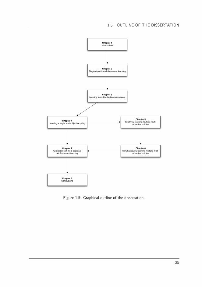
In Chapter 2, we introduce the foundations of single-objective reinforcement learning.We present its history and foundations, which lie in the fields of psychology and optimalcontrol theory. Additionally, we define the components that comprise a reinforcementlearning setting such as value functions and policies. We also describe the notion of aMarkov decision process, which is a mathematical framework to model the environmentthe agent is operating in. Furthermore, we emphasise the synergies and the di�erencebetween model-based and model-free learning for sequential decision making problems.Since the remainder of this dissertation is focussed on model-free learning, we pay particularattention to the Q-learning algorithm, which is one of the foundations of the studies inthe following chapters.
In Chapter 3, we present the idea of learning in environments that require the optim-ising multiple criteria or objectives. We introduce the general concepts of multi-criteriadecision making and we provide a survey of the theoretical foundations of multi-objectiveoptimisation. With special care, we describe the characteristics of the Pareto front andthe articulation of the preferences of the decision maker. In this regard, we categor-ise multi-objective reinforcement learning algorithms based on a taxonomy that classifiesthese techniques based on the type of scalarisation function, i.e., a linear or a more gen-eral monotonically increasing scalarisation function, and the amount of solutions learned,i.e., single-policy or multi-policy. We situate the current state-of-the-art reinforcementlearning algorithms within this problem taxonomy, together with our contributions withinthis dissertation.
In Chapter 4, we elaborate on multi-objective reinforcement learning algorithms thatemploy a scalarisation for learning a single policy at a time. We first present a generalframework for single-policy reinforcement learning, based on the Q-learning algorithm. Inthis framework, we analyse the established linear scalarisation function and we draw at-tention to its advantages and limitations. Additionally, we elaborate on an alternativescalarisation function that possesses non-linear characteristics. This is the Chebyshev scal-arisation function, which is well-known in the domain of multi-objective optimisation. We
23

CHAPTER 1. INTRODUCTION
stress the lack of convergence guarantees of the Chebyshev function within the frame-work on reinforcement learning on a theoretical level. Furthermore, we investigate to whatdegree this limitation holds in practice on several benchmark instances.
In Chapter 5, we explore the relation between the weight configuration, which incorporatespredefined emphasis of the decision maker, and the learned policy in the objective space.Based on this mapping, we investigate how single-policy algorithms can be augmented toobtain multiple solutions by iteratively adapting this weight configuration. We propose twoalgorithms that rely on tree structures to produce a series of weight configurations to obtaina set of optimal solutions. The first algorithm is specifically tailored for Pareto fronts witha discrete amount of solutions while the second algorithm is capable of retrieving solutionswith a high degree of diversity in continuous Pareto fronts.
In Chapter 6, we present two distinct algorithms for learning various compromise solu-tions in a single run. The novelty of these algorithms lies in the fact that they can retrieveall solutions that satisfy the Pareto relation, without being restricted to a convex subset.A first algorithm is the multi-objective hierarchical heuristic optimisation (MO-HOO) al-gorithm for multi-objective X -armed bandit problems. This is a class of problems where anagent is faced with a continuous finite-dimensional action space instead of a discrete one.MO-HOO is a single-state learning algorithm that is specifically tailored for multi-objectiveindustrial optimisation problems that involve the assignment of continuous variables. Asecond algorithm is Pareto Q-learning (PQL). PQL extends the principle of MO-HOO to-wards multi-state problems and combines it with Q-learning. PQL is the first temporaldi�erence-based multi-policy MORL algorithm that does not use the linear scalarisationfunction. Pareto Q-learning is not limited to the set of convex solutions, but it can learn theentire Pareto front, if enough exploration is allowed. The algorithm learns the Pareto frontby bootstrapping Pareto non-dominated Q-vectors throughout the state and action space.
In Chapter 7, we go beyond the academic benchmark environments and apply a collec-tion of our algorithms on a real-life simulation environment. This environment simulatesthe filling phase of a wet clutch which are used in shifting and transmission systems ofautomotive vehicles. We analyse the application of a multi-policy reinforcement learningalgorithm. More precisely, we apply the multi-objective hierarchical optimistic optimisa-tion (MO-HOO) algorithm on the simulation environment in order to approximate itsPareto front.
In Chapter 8, we conclude the work presented in this dissertation and we outline avenuesfor future research.
A graphical outline of the dissertation is provided in Figure 1.5. The arrows indicatethe recommended reading order.
24
1.5. OUTLINE OF THE DISSERTATION
Chapter 1Introduction
Chapter 2Single-objective reinforcement learning
Chapter 3Learning in multi-criteria environments
Chapter 4Learning a single multi-objective policy
Chapter 6Simultaneously learning multiple multi-
objective policies
Chapter 5Iteratively learning multiple multi-
objective policies
Chapter 7Applications of multi-objective
reinforcement learning
Chapter 8Conclusions
Figure 1.5: Graphical outline of the dissertation.
25


2
| Single-objectivereinforcement learning
In reinforcement learning (RL), the agent is faced with the problem of taking decision inunknown, possibly dynamic environments. In the standard single-objective case, the overallgoal of the agent is to learn the optimal decisions so as to maximise a single, numericalreward signal. These decisions are in essence actions that have to be selected in certainstates of the environment. This environment is usually defined using a Markov DecisionProcess. This is a mathematical framework used to model the context of the problem theagent is solving. We describe this framework in Section 2.2. As the environment itself maybe evolving over time, the consequence of a particular action on the resulting behaviourmight be highly unpredictable. Also, the e�ect of the actions might not be direct butdelayed. Therefore, the agent has to learn from its experience, using trial-and-error, whichactions are fruitful.
In this chapter we introduce some preliminary concepts on single-objective reinforcementlearning that we use as a basis throughout this dissertation. Firstly, we elaborate on thehistorical background of reinforcement learning which lies in the field of animal learningand optimal control. We also explain the theoretical foundations of reinforcement learningand explicitly define all the components that compose a reinforcement learning problem.We will focus on both stateless as well as stateful problems. Subsequently, this generalintroduction will be augmented with an experimental analysis of several action selectionstrategies in a classical reinforcement learning problem. In the end, we conclude thechapter by summarising the most important aspects.
27

CHAPTER 2. SINGLE-OBJECTIVE REINFORCEMENT LEARNING
2.1 History of reinforcement learningReinforcement learning is learning from interaction with an unknown environment in orderto take the optimal action, given the situation the agent is facing (Sutton and Barto,1998). The agent is not supported by a teacher pointing out the optimal behaviour orcorrecting sub-optimal actions, but it is solely relying on itself and its past experience inthe environment. This experience is quantified by the agent’s previously selected actionsin the states of the environment and the observed reward signal. This principle of learningdates back to two main research areas which evolved rather independently from each other.These two tracks are animal learning and optimal control.
Psychologists observing animals have already found out over a hundred years ago thatthese creatures exhibit learning behaviour. A first experiment was conducted by EdwardL. Thorndike, where he placed a cat in a wooden box and let it try to escape (Thorndike,1911). In the beginning, the cat tried various approaches until it accidentally hit themagical lever that allowed it to flee. When Thorndike later put the cat again in this cage,it would execute the correct action more quickly than before. The more Thorndike repeatedthis experiment, the faster the cat escaped the box. In essence, the cat executed a type oftrial-and-error learning where it would learn from its mistakes and its successes (Schultzand Schultz, 2011). These mistakes and successes are then quantified by a feedbacksignal, i.e., in the case of the cat, this signal would reflect if the action led to the cat’sfreedom or not. Sometimes the e�ect of an action can be direct, like in the case ofthe cat, but in some situations the outcome can also be delayed. For instance, in thegame of chess, the true influence of a single move may not be clear at the beginningof the game, as only at the end of the game a reinforcement is given for winning orlosing the game. Hence, the delayed reward needs to be propagated in order to favour ordisfavour the course of actions in case of winning or losing the game, respectively. Anotherdistinctive challenge that characterises reinforcement learning is the so-called exploration-exploitation trade-o�. This trade-o� comprises one of the major dilemmas of the learningagent: when has it acquired enough knowledge in the environment (exploration), beforeit can use this information and select the best action so far (exploitation), given thatthe environment is stochastic and perhaps even changing over time? It is clear that if theagent explores too much, it might unnecessarily re-evaluate actions that it has experiencednumerous times to result in poor performance. When the agent explores too little, it is notguaranteed that the action the agent estimates to be the best policy is also the best policyin the environment. In Section 2.4.2, we will elaborate on some established techniquesfor dealing with this issue.
The second research track that is a foundation of reinforcement learning is the disciplineof optimal control. In optimal control, the goal is to find a sequence of actions so as tooptimise the behaviour of a dynamic system over a certain time period. One of the principaldiscoveries within this field was the Bellman equation (Bellman, 1957). The Bellmanequation defines a complex problem in a recursive form and serves as a foundation of manyDynamic Programming (DP) algorithms (Bertsekas, 2001a,b). Dynamic programming isa mechanism for solving a complex problem by breaking it apart into many subproblems
28
2.2. MARKOV DECISION PROCESSES
and will be covered in more detail in Section 2.4.1. First, we describe a mathematicalframework that serves as a model for sequential decision making. This framework is aMarkov decision process.
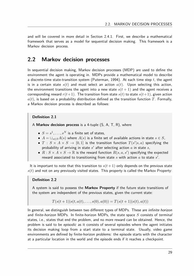
2.2 Markov decision processesIn sequential decision making, Markov decision processes (MDP) are used to define theenvironment the agent is operating in. MDPs provide a mathematical model to describea discrete-time state-transition system (Puterman, 1994). At each time step t, the agentis in a certain state s(t) and must select an action a(t). Upon selecting this action,the environment transitions the agent into a new state s(t + 1) and the agent receives acorresponding reward r(t+1). The transition from state s(t) to state s(t+1), given actiona(t), is based on a probability distribution defined as the transition function T . Formally,a Markov decision process is described as follows:
Definition 2.1
A Markov decision process is a 4-tuple (S, A, T, R), where
• S = s1, . . . , sN is a finite set of states,• A = fisœSA(s) where A(s) is a finite set of available actions in state s œ S,• T : S ◊ A ◊ S æ [0, 1] is the transition function T (sÕ|s, a) specifying the
probability of arriving in state sÕ after selecting action a in state s,• R : S ◊ A ◊ S æ R is the reward function R(s, a, sÕ
) specifying the expectedreward associated to transitioning from state s with action a to state sÕ.
It is important to note that this transition to s(t + 1) only depends on the previous states(t) and not on any previously visited states. This property is called the Markov Property:
Definition 2.2
A system is said to possess the Markov Property if the future state transitions ofthe system are independent of the previous states, given the current state:
T (s(t + 1)|s(t, a(t), . . . , s(0), a(0)) = T (s(t + 1)|s(t), a(t))
In general, we distinguish between two di�erent types of MDPs. These are infinite horizonand finite-horizon MDPs. In finite-horizon MDPs, the state space S consists of terminalstates, i.e., states that end the problem, and no more reward can be obtained. Hence, theproblem is said to be episodic as it consists of several episodes where the agent initiatesits decision making loop from a start state to a terminal state. Usually, video gameenvironments are defined by finite-horizon problems: the episode starts with the characterat a particular location in the world and the episode ends if it reaches a checkpoint.
29

CHAPTER 2. SINGLE-OBJECTIVE REINFORCEMENT LEARNING
In some situations, the exact length of the agent’s lifetime might not be known inadvance. These problems are referred to as infinite-horizon problems since they have gota continuous nature. An example of such a problem is the cart pole problem (Sutton andBarto, 1998). In this problem, a robot tries to balance a pole on a cart by applying forceto that cart. Based on the angle of the pole and the velocity of the cart, the robot has tolearn when to move left or right along a track. Clearly, for this problem it is not possibleto state beforehand where or when the agent’s lifespan comes to a halt.
The overall goal of the agent is to learn a policy, a mapping from states to actions. Weare not just interested in any policy, but in an optimal policy, i.e., a policy that maximisesthe expected reward it receives over time. A formal definition of a policy will be providedin Section 2.3 where we present general notations of reinforcement learning. We concludethe definition of MDPs by presenting an illustrative example.
Example 2.1
In this example, we consider the Tetris game, a puzzle-based game released the 1980sby Alexey Pajitnov that is still very popular today . In Tetris, geometric shapes, calledTetriminos, need to be organised in the matrix-like play field (see Figure 2.1 (a)),called the wall. There are seven distinct shapes that can be moved sideways androtated 90, 180 and 270 degrees. A visual representation of the di�erent Tetriminoscan be found in Figure 2.1 (b). These shapes need to be placed in order to form ahorizontal line without any gaps. Whenever such a line is created, the line disappearsand blocks on top of the horizontal line fall one level down. Many versions of theTetris game exist, including di�erent levels and di�erent game speeds, but the goalof the Tetris game in this example is to play as long as possible, i.e., until a pieceexceeds the top of the play field. This game can be modelled in terms of an Markovdecision process as follows:
• The states in the MDP represent the di�erent configurations of the play fieldand the current Tetriminos being moved. The configuration can be describedby the height of the wall, the number of holes in the wall, di�erence of heightbetween adjacent columns and many more (Gabillon et al., 2013; Furmstonand Barber, 2012).
• The actions in the MDP are the possible orientations of the piece and thepossible locations that it can be placed on the play field.
• The transition function of the MDP define the next wall configuration de-terministically given the current state and action. The transitions to the nextTetrimino are given by a certain distribution, e.g., uniformly over all possibletypes.
• The reward function of the MDP provides zero at all times, except when theheight of the wall exceeds the height of the play field. In that case, a negativereward of ≠1 returned.
30

2.3. NOTATIONS OF REINFORCEMENT LEARNING
(a)
(b)
Figure 2.1: The Tetris game (a) and its seven geometrical shapes called Tetriminos (b).
2.3 Notations of reinforcement learningIn the previous section, we have presented a definition of the environment the agent isoperating in. The next part of the puzzle is to define the goal of the agent in that environ-ment, that is, to act in such a way in order to maximise the reward it receives over time.In this section, we formally describe this goal in mathematical terms. Subsequently, wealso specify how the agent gathers knowledge on the fruitfulness of its action and how thisknowledge evolves over time. We present two distinct types of learning, i.e., model-basedand model-free learning, depending on whether a model of the environment is available tothe agent or not. In this dissertation, we concentrate on model-free learning. Therefore,in Section 2.4.2, we present some additional techniques on how to gather knowledge inan incremental manner and how to tackle the exploration-exploitation problem, discussedearlier in Section 2.1.
In reinforcement learning problems, the agent is in a certain state of the environments(t) and has to learn to select the action a(t) at every time step t = 0, 1, . . .. In return,the environment transitions the agent into a new state s(t + 1) and provides a numericalreward r(t + 1) representing how beneficial that action was. It is important to note thatthe transition to s(t + 1) and the observed reward r(t + 1) are not necessary (and also notlikely) to be deterministic. On the contrary, these are usually random, stationary variables.This means they are random with respect to a certain distribution, but the distribution isnot changing over time.
31

CHAPTER 2. SINGLE-OBJECTIVE REINFORCEMENT LEARNING
Definition 2.3
In a stationary environment, the probabilities of making state transitions or receivingreward signals do not change over time.
A schematic overview of the RL agent is given in Figure. 2.2.
a(t)
s(t+1)
r(t+1)
Environment
Figure 2.2: The reinforcement learning model, based on (Kaelbling et al., 1996).
The goal of this agent is to act in such a way that its expected return, Rt, is maximised.In the case of a finite-horizon problem, this is just the sum of the observed rewards. Whenthe problem consists of an infinite-horizon, the return is an infinite sum. In this case,a discount factor, “ œ [0, 1[, is used to quantify the importance of short-term versuslong-term rewards. Consequently, the discount factor ensures this infinite sum yields afinite number:
Rt =
Œÿ
k=0“krt+k+1. (2.1)
When “ is close to 0, the agent is myopic and mainly considers immediate rewards. Instead,if “ approaches 1, the future rewards are more important. For finite-horizon MDPs, thesum might be undiscounted and “ can be 1.
In order to retrieve this return, the agent needs to learn a policy fi œ �, where � is thespace of policies. A policy is a function that maps a state to a distribution over the actionsin that state. Several types of policies exist, depending on the type of distribution and onthe information it uses to make its decision. Here we distinguish between two properties,i.e., (1) deterministic or stochastic and (2) stationary or non-stationary. Each of thesetypes of policies will be defined in the following paragraph.
A deterministic policy is a policy that deterministically selects actions.
32
2.3. NOTATIONS OF REINFORCEMENT LEARNING
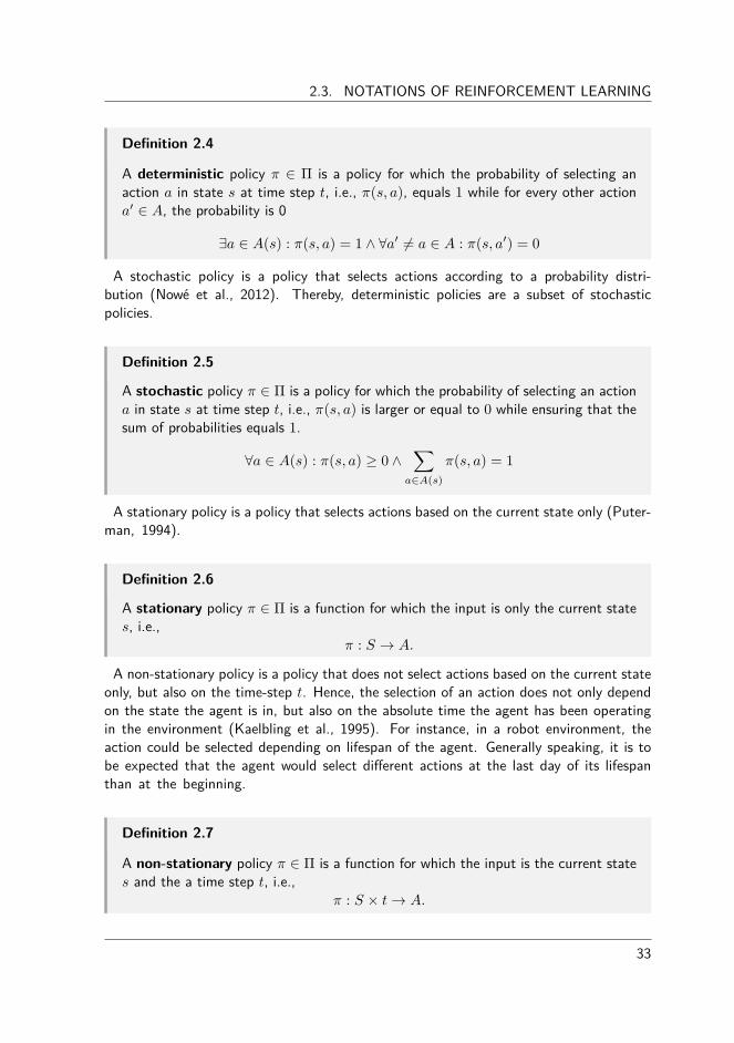
Definition 2.4
A deterministic policy fi œ � is a policy for which the probability of selecting anaction a in state s at time step t, i.e., fi(s, a), equals 1 while for every other actionaÕ œ A, the probability is 0
÷a œ A(s) : fi(s, a) = 1 · ’aÕ ”= a œ A : fi(s, aÕ) = 0
A stochastic policy is a policy that selects actions according to a probability distri-bution (Nowé et al., 2012). Thereby, deterministic policies are a subset of stochasticpolicies.
Definition 2.5
A stochastic policy fi œ � is a policy for which the probability of selecting an actiona in state s at time step t, i.e., fi(s, a) is larger or equal to 0 while ensuring that thesum of probabilities equals 1.
’a œ A(s) : fi(s, a) Ø 0 ·ÿ
aœA(s)fi(s, a) = 1
A stationary policy is a policy that selects actions based on the current state only (Puter-man, 1994).
Definition 2.6
A stationary policy fi œ � is a function for which the input is only the current states, i.e.,
fi : S æ A.
A non-stationary policy is a policy that does not select actions based on the current stateonly, but also on the time-step t. Hence, the selection of an action does not only dependon the state the agent is in, but also on the absolute time the agent has been operatingin the environment (Kaelbling et al., 1995). For instance, in a robot environment, theaction could be selected depending on lifespan of the agent. Generally speaking, it is tobe expected that the agent would select di�erent actions at the last day of its lifespanthan at the beginning.
Definition 2.7
A non-stationary policy fi œ � is a function for which the input is the current states and the a time step t, i.e.,
fi : S ◊ t æ A.
33

CHAPTER 2. SINGLE-OBJECTIVE REINFORCEMENT LEARNING
In standard, single-objective reinforcement learning (SORL), an optimal policy fiú œ � ofthe underlying MDP is a deterministic stationary policy (Bertsekas, 1987). In the upcomingchapters of this dissertation we will see that this is not the case when the reward signalis composed of multiple objectives.
Based on the stationary principle in SORL, the agent can learn a policy that is globallyoptimal, i.e., over multiple states, by taking actions locally for each state individually. Thenotion of the value function is important for this matter.
Definition 2.8
The value function V fi(s) specifies how good a certain state s is in the long term
according to the policy fi. The function returns the expected, discounted return tobe observed when the agent would start in state s and follow policy fi:
V fi(s) = Efi{Rt|s(t) = s}
= Efi
; Œÿ
k=0“ krt+k+1 | s(t) = s
<
The value of an action a in a state s under policy fi œ � is represented by a Qfi(s, a).
This is called a Q-value, referring to the quality of an action in a state and can be definedas follows.
Definition 2.9
The value of an action a in a state s, Qfi(s, a) is the expected return starting
from s, taking action a, and thereafter following policy fi:
Qfi(s, a) = Efi{Rt|s(t) = s, a(t) = a}
= Efi
; Œÿ
k=0“ krt+k+1 | s(t) = s, a(t) = a
<
In the previous sections, we have introduced a theoretical framework that forms the basis ofreinforcement learning. We have formally defined the environment the agent is operating inand how the agent represents its knowledge. In the following sections we will describe howwe can learn the optimal Q-values, Qú, which will be used to learn the optimal policy, fiú.
2.4 Learning methodsTwo main categories of learning approaches exist. These are model-based and model-freetechniques. In model-based learning, an explicit model of the environment is used tocompute the optimal policy fiú. This model can either be available a priori to the agentto exploit or it can be learned over time. In the former case, dynamic programming is
34
2.4. LEARNING METHODS
the advised solution technique, while in the latter case dyna architecture methods, whichconcise an integrated architecture for learning, planning, and reacting, can be used (Sutton,1991). Model-based approaches will be discussed in Section 2.4.1.
In model-free learning, no explicit model of the environment is considered, but the agentlearns the optimal policy in an implicit manner from interaction. As we will see in Sec-tion 2.4.2, model-free learning uses the same mathematical foundations as model-basedlearning.
2.4.1 Model-based learningIn a model representation of the environment the knowledge on the transition functionT (sÕ|s, a) and the reward function R(s, a, sÕ
) are explicit. When these aspects of the en-vironment are known to the agent, dynamic programming methods can be used to computethe optimal policy fiú. Dynamic programming will be explained in the subsequent sections.
Dynamic programming
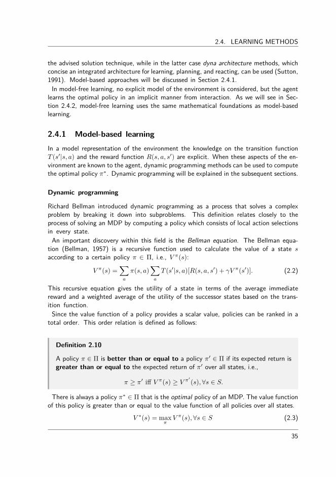
Richard Bellman introduced dynamic programming as a process that solves a complexproblem by breaking it down into subproblems. This definition relates closely to theprocess of solving an MDP by computing a policy which consists of local action selectionsin every state.
An important discovery within this field is the Bellman equation. The Bellman equa-tion (Bellman, 1957) is a recursive function used to calculate the value of a state saccording to a certain policy fi œ �, i.e., V fi
(s):
V fi(s) =
ÿ
a
fi(s, a)
ÿ
a
T (sÕ|s, a)[R(s, a, sÕ) + “V fi
(sÕ)]. (2.2)
This recursive equation gives the utility of a state in terms of the average immediatereward and a weighted average of the utility of the successor states based on the trans-ition function.
Since the value function of a policy provides a scalar value, policies can be ranked in atotal order. This order relation is defined as follows:
Definition 2.10
A policy fi œ � is better than or equal to a policy fiÕ œ � if its expected return isgreater than or equal to the expected return of fiÕ over all states, i.e.,
fi Ø fiÕi� V fi
(s) Ø V fiÕ(s), ’s œ S.
There is always a policy fiú œ � that is the optimal policy of an MDP. The value functionof this policy is greater than or equal to the value function of all policies over all states.
V ú(s) = max
fiV fi
(s), ’s œ S (2.3)
35

CHAPTER 2. SINGLE-OBJECTIVE REINFORCEMENT LEARNING
Similar to the definition of the optimal value function of a state, we can also define theoptimal state-action value function Qú over all states and all actions:
Qú(s, a) = max
fiQfi
(s, a), ’s œ S, a œ A(s). (2.4)
This equation gives us the expected return for selecting an action a in state s and thereafterfollowing the optimal policy fiú. Hence,
Qú(s, a) = Efi{r(t + 1) + “V ú
(s(t + 1))|s(t) = s, a(t) = a}. (2.5)
Since V ú(s) is the value of a state under the optimal policy, it is equal to the expected
return for the best action of that state. This is referred to as the Bellman optimalityequation of a state s and is defined as follows.
V ú(s) = max
aœA(s)Qfiú
(s, a)
= max
aœA(s)Efiú{Rt|s(t) = s, a(t) = a}
= max
aœA(s)Efiú
; Œÿ
k=0“kr(t + k + 1)|s(t) = s, a(t) = a
<
= max
aœA(s)Efiú
;r(t + 1) + “
Œÿ
k=1“kr(t + k + 1)|s(t) = s, a(t) = a
<
= max
aœA(s)E{r(t + 1) + “V ú
(s(t + 1))|s(t) = s, a(t) = a}
= max
aœA(s)
ÿ
sÕ
T (sÕ|s, a)[R(s, a, sÕ) + “V ú
(sÕ)]
(2.6)
The Bellman optimality equation for state-action pairs, Qú, is defined in a similar way:
Qú(s, a) = E{r(t + 1) + “ max
aÕQú
(s(t + 1), aÕ)|s(t) = s, a(t) = a}
=
ÿ
sÕ
T (sÕ|s, a)[R(s, a, sÕ) + “ max
aÕQú
(sÕ, aÕ)].
(2.7)
Algorithms that solve this equation to calculate the optimal policy are called dynamicprogramming algorithms. Over the years many dynamic programming algorithms havebeen proposed, but the two main approaches are policy iteration and value iteration.Policy iteration uses an alternation of evaluation and improvement steps to calculate thevalue of the entire policy. Value iteration does not need a separate evaluation step but isable to compute the value of a policy iteratively using a simple backup scheme. For moreinformation on these two principle dynamic programming algorithms, we refer to (Bellman,1957; Puterman, 1994; Bertsekas, 2001a,b).
Note: It is important to note that the Bellman equation is based on the property ofadditivity, meaning that passing the sum of two variables through a function f isequal to summing the result of f applied to the two variables individually.
36

2.4. LEARNING METHODS
Definition 2.11
A function f is additive if it preserves the addition operator:
f(x + y) = f(x) + f(y)
This is a basic, but an important requirement as we will see once we equip multi-objectivelearning algorithms with scalarisation functions in Chapter 4.
2.4.2 Model-free learningIn the previous section we have examined techniques to compute the optimal policy when amodel of the environment is available. In this section, we explore the model-free approach,i.e., the agent does not have at its dispense a model of the environment, but it has to learnwhat to do in an implicit manner through interaction. This is referred to as learning fromexperience. In this section, we will present a well-known algorithm, called Q-learning,that does exactly this.
Q-learning
One of the most important advances in reinforcement learning was the development of theQ-learning algorithm (Watkins, 1989; Watkins and Dayan, 1992). In Q-learning, a tableconsisting of state-action pairs is stored. Each entry contains a value for ˆQ(s, a) whichis the learner’s current estimate about the actual value of Qú
(s, a). In the update rule,the Q-value of a state-action pair is updated using its previous value, the reward and thevalues of future state-action pairs. Hence, it updates a guess of one state-action pair withthe guess of another state-action pair. This process is called bootstrapping. The ˆQ-valuesare updated according to the following update rule:
ˆQ(s, a) Ω (1 ≠ –(t)) ˆQ(s, a) + –(t)[r + “ max
aÕˆQ(sÕ, aÕ
)], (2.8)
where –(t) œ [0, 1] is the learning rate at time step t and r is the reward received forperforming action a in state s. The pseudo-code of the algorithm is listed in Algorithm 1.
In each episode, actions are selected based on a particular action selection strategy, forexample ‘-greedy where a random action is selected with a probability of ‘, while thegreedy action is selected with a probability of (1 ≠ ‘). Upon applying the action, theenvironment transitions to a new state sÕ and the agent receives the corresponding rewardr (line 6). At line 7, the ˆQ-value of the previous state-action pair (s, a) is updated towardsthe reward r and the maximum ˆQ-value of the next state sÕ. This process is repeated untilthe ˆQ-values converge or after a predefined number of episodes.
To conclude, Q-learning and general model-free learning possess a number of advantages:
• It can learn in a fully incremental fashion, i.e., it learns whenever new rewards arebeing observed.
37

CHAPTER 2. SINGLE-OBJECTIVE REINFORCEMENT LEARNING
Algorithm 1 Single-objective Q-learning algorithm1: Initialise ˆQ(s, a) arbitrarily2: for each episode t do3: Initialise s4: repeat5: Choose a from s using a policy derived from the ˆQ-values (e.g., ‘-greedy)6: Take action a and observe sÕ œ S, r œ R7: ˆQ(s, a) Ω ˆQ(s, a) + –t(r + “ max
aÕˆQ(sÕ, aÕ
) ≠ ˆQ(s, a))
8: s Ω sÕ
9: until s is terminal10: end for
• The agent can learn before and without knowing the final outcome. This means thatthe learning requires less memory and that it can learn from incomplete sequences,respectively, which is helpful in applications that have very long episodes.
• The learning algorithm has been proven to converge under reasonable assumptions.Provided that all state-action pairs are visited infinitely often and a suitable evolutionfor the learning rate is chosen, the estimates, ˆQ, will converge to the optimal values,Qú (Tsitsiklis, 1994).
At first sight, visiting all state-action pairs infinitely often seems hard and infeasible inmany applications. However, the amount of exploration is usually reduced once the Q-values have converged, i.e., when the di�erence between two updates of the same Q-valuedoes not exceed a small threshold. In the next section, we will discuss some well-knowntechniques for balancing exploration and exploitation in model-free environments.
Action selection strategies
As we have already discussed in Section 2.1, the exploration-exploitation trade-o� is oneof the crucial aspects of reinforcement learning algorithms. This dilemma is the issue ofdeciding when the agent has acquired enough knowledge in the environment (exploration),before it can use this information and select the best action so far (exploitation). Below,we elaborate on the four main techniques that leverage a certain trade-o� of explorationand exploitation.
• Random action selection : This is the most simple action selection strategy. In thiscase, the agent does not take into account its ˆQ-estimates, but it selects an actiona randomly from the set A(s). It is obvious that this action selection strategy is nota mechanism to let the agent obtain high-quality rewards (exploitation), but it is asimple technique to let the agent explore as it selects uniformly between the actionsin a state.
• Greedy action selection : In this strategy, the agent selects the action that it believesis currently the best action based on its estimate ˆQ. However, if the agent follows
38

2.5. REINFORCEMENT LEARNING IN STATELESS ENVIRONMENTS
this strategy too early in the learning phase, this estimate might be inaccurate andthe resulting policy might be sub-optimal.
• ‘-greedy action selection : This mechanism is a simple alternative to acting greedyall the time. In an ‘-greedy action selection, the agent selects a random action witha probability of ‘ and a greedy action with a probability of (1 ≠ ‘). It is importantto note that the ratio of exploration and exploitation is static throughout the entirelearning phase.
• Softmax action selection : In order to leverage this ratio of exploration and exploit-ation, a probability distribution can be calculated for every action at each actionselection step, called a play. The softmax action selection strategy selects actionsusing the Boltzmann distribution. The probability of selecting an action a in states is defined at follows:
P (a) =
eQ(s,a)
·
qaÕœA(s) e
Q(s,aÕ)·
, (2.9)
where · œ R+0 is called the temperature. In the case of high values for · , the
probability distribution of all actions are (nearly) uniform. When a low value isassigned to · , the greedier the action selection will be. Usually, this parameter ischanged over time where in the beginning of the learning phase a high value for ·will be chosen which is being degraded over time.
2.5 Reinforcement learning in stateless environmentsAfter we explained the theoretical foundations of reinforcement learning, it might be ap-propriate to evaluate these techniques in a practical context. Therefore, we turn ourselvesto a classical problem in reinforcement learning, called the multi-armed bandit problem.In the multi-armed bandit problem, or also called the n-armed bandit problem, a gambleris faced with a collection of slot machines, i.e., arms, and he has to decide which leverto pull at each time step (Robbins, 952). Upon playing a particular arm, a reward isdrawn from that action’s specific distribution and the goal of the gambler is to maximisehis long-term scalar reward.
This problem is a stateless problem, meaning that there is no state in the environment.1Therefore, we do not need an implementation of the entire Q-learning algorithm of Sec-tion 2.4.2, but we can use a simpler updating rule. We can update the estimate ˆQ using thesample average method. The ˆQ(a)-value, representing the estimate of action a is given by:
ˆQ(a) =
r(0) + r(1) + . . . + r(k)
k, (2.10)
where r(i) is the reward received at time step i and k is the number of times action a hasbeen selected as yet. Initially, the ˆQ-value of each action is assigned 0. Once the agentperforms an action selection, called a play, the episode is finished.
1or only a single state, depending on the viewpoint
39

CHAPTER 2. SINGLE-OBJECTIVE REINFORCEMENT LEARNING
Although this problem seems trivial, it is not. The multi-armed bandit problem provides aclear mapping to the exploration-exploitation dilemma of Section 2.1; the agent has to tryto acquire new knowledge while at the same time use this knowledge to attempt to optimisethe performance of its decisions. Extensive research has been conducted for this problemin the field of packet routing (Awerbuch and Kleinberg, 2008), ads placement (Pandeyet al., 2007) and investment and innovation (Hege and Bergemann, 2005).
2.5.1 Experimental evaluationIn this section, we experimentally compare the action selection strategies of Section 2.4.2on the multi-armed bandit problem. More precisely, we analyse the following strategies:
• Random action selection• Greedy action selection• ‘-greedy, ‘ = 0.1• ‘-greedy, ‘ = 0.2• Softmax, · = 1
• Softmax, · = 0.1• Softmax, · = 1000 ú 0.9play
• Softmax, · = 1000 ú 0.95
play
We will analyse their behaviour on a 4-armed bandit problem. The expected reward ofeach arm is given below in Table 2.1. The rewards are drawn from a normal distributionwith mean Qú
a and the variance equal to 1. Furthermore, the initial Q-values are assignedto zero and we averaged the performance of the action selection strategies over 1000 trialsof each 1000 plays.
Action Qúa
action #1 1.7action #2 2.1action #3 1.5action #4 1.3
Table 2.1: The Qúa for each action of the multi-armed bandit problem.
We first depict the behaviour of the action selection strategies in terms of three criteria:(1) the probability over time of selecting the optimal action, which is in this case action#2, (2) the average reward received over time and (2) the number of times each actionis selected. These results are presented in Figures 2.3, 2.4 and 2.5, respectively. Wesummarise the results for each of the traditional action selection strategies below.2
2For n-armed bandits also more specialised action selection strategies exist that analyse the upperconfidence bound of each arm (Auer et al., 2003; Audibert et al., 2009)
40

2.5. REINFORCEMENT LEARNING IN STATELESS ENVIRONMENTS
0 100 200 300 400 500 600 700 800 900 1000
0
0.2
0.4
0.6
0.8
1
Play
Pro
ba
bili
ty o
ptim
al a
ctio
ns
Random
ε−greedy, ε=0
ε−greedy, ε=0.1
ε−greedy, ε=0.2
Softmax, τ=1
Softmax, τ=0.1
Softmax, τ=1000*0.9play
Softmax, τ=1000*0.95play
Figure 2.3: The probability of selecting optimal actions for each of the action selectionstrategies in the multi-armed bandit problem.
• Random action selection : As this strategy does not consider the obtained knowledgein the ˆQ-values and selects actions uniformly at random, the probability of selectingthe optimal action is 1
4 as there are 4 actions in this environment (see Figure 2.3and Figure 2.5). Because the strategy is very naive and not exploiting, the averagereward obtained over time in Figure 2.4 is also very low.
• Greedy action selection : Selecting the greedy action all of the time is also not anideal strategy. In Figure 2.3, we see that the greedy action is always stuck and neverfinds the best action. As, we see in Figure 2.5, action #1 is selected all of the times,because the algorithm never explores other levers than the one it selected the firsttime. Hence, only for this action the ˆQ-value approaches the Qú-value, while for theother actions, the ˆQ-value remains its initial value.
• ‘-greedy action selection : Introducing the ‘-parameter clearly allows us up to someextent to balance exploration and exploitation. In Figure 2.3, we see that introducingan ‘ parameter of 0.1 allows us in the end to reach a performance of 84%. Utilisinga higher probability for random actions with ‘ = 0.2 degrades the performance interms of the optimal actions and the average reward compared to ‘ = 0.1.
• Softmax action selection : We see that the algorithms with · = 0.1 and · = 1 donot perform well. With a high · value, the algorithm is exploring a lot while a low· value makes the algorithm behave greedily and it gets stuck in a local optimum.Therefore, it is recommended to let the temperature parameter degrade over time.This idea is implemented when assigning · = 1000ú0.9play and · = 1000ú0.95
play.From the figures, we see that the strategies explore a lot in early learning phaseswhile exploiting more at the end. For this particular case, we see that when assigning· = 1000ú0.9play yields the best performance in terms of selecting the optimal actionand the obtained reward.
41

CHAPTER 2. SINGLE-OBJECTIVE REINFORCEMENT LEARNING
0 100 200 300 400 500 600 700 800 900 10001.6
1.65
1.7
1.75
1.8
1.85
1.9
1.95
2
2.05
2.1
Play
Ave
rage r
ew
ard
Random
ε−greedy, ε=0
ε−greedy, ε=0.1
ε−greedy, ε=0.2
Softmax, τ=1
Softmax, τ=0.1
Softmax, τ=1000*0.9play
Softmax, τ=1000*0.95play
Figure 2.4: The average reward obtained for each of the action selection strategies in themulti-armed bandit problem.
The total accumulated reward obtained for each of the action selection strategies ispresented in Table 2.2. This statistic also shows that the softmax strategy found thebest compromise between explorative and exploitative behaviour over the entire learningperiod. The ‘-greedy strategies approach its performance due to their rapid increase inearly learning phases, but this does not su�ce to surpass the performance of the softmaxalgorithm.
Strategy Cumulative rewardRandom 1649.8Greedy 1698.3‘-greedy, ‘ = 0.1 1950.1‘-greedy, ‘ = 0.2 1947.6Softmax, · = 1 1737.6Softmax, · = 0.1 1644.4Softmax, · = 1000 ú 0.9play 1976.5Softmax, · = 1000 ú 0.95
play 1903.1
Table 2.2: The total accumulated reward for each of the action selection strategies in themulti-armed bandit problem.
Even in this simple, stateless example, we have seen that it is crucial to find a goodbalance between exploration and exploitation. Behaving too greedily and exploiting tooearly tends to lead to suboptimal performance at the end of the learning task, whileunnecessary exploration does not allow to obtain a lot of reward during learning. Althoughthe softmax algorithm provided the best performance for this learning task, this result
42

2.6. SUMMARY
1 2 3 40
100
200
300
400
500
600
700
800
900
1000
Action Number
Tim
es
Random
ε−greedy, ε=0
ε−greedy, ε=0.1
ε−greedy, ε=0.2
Softmax, τ=1
Softmax, τ=0.1
Softmax, τ=1000*0.9play
Softmax, τ=1000*0.95play
Figure 2.5: The number of times each action is selected for each action selection strategy.
cannot be generalised. Up to this day, there is no general answer to solving the exploration-exploitation dilemma as it requires tuning that is problem-specific (Auer et al., 2002). In thefollowing chapter, we will analyse the additional di�culties that arise when the environmentis no longer single-objective, but when multiple reward signals are supplied to the agent.
2.6 SummaryIn this chapter, we introduced the foundations of single-objective reinforcement learning.We presented its history, which lies in the fields of psychology and optimal control theory.We explained the crucial aspects that define a reinforcement learning problem and de-scribed all its components, such as the Markov decision process and definitions of a policyand a value function. We paid special attention to the Bellman equation which is thefoundation of many reinforcement learning methods. We also emphasised the synergiesand the di�erences between model-based and model-free learning for sequential decisionmaking problems, i.e., situations where the model is either known or unknown to theagent. For model-free learning approaches, the Q-learning algorithm was one of the majorbreakthroughs in the late 1980s.
Furthermore, we introduced di�erent action selection strategies that allow to balance theexploration towards uncharted territory and the exploitation of the acquired knowledge.These mechanisms were tested on a simple, single-state problem, called the n-armedbandit problem.
43


3
| Learning in Multi-CriteriaEnvironments
Many real-world problems require the simultaneous optimisation of multiple criteria orobjectives. These objectives can be either correlated, conflicting or independent. In thischapter we present several characteristics for learning in these environments. We intro-duce the general concepts of multi-criteria decision making and we provide a survey of thetheoretical foundations of multi-objective optimisation. With special care, we introduceevolutionary multi-objective (EMO) algorithms that use population-based principles too�er a wide range of advantages in multi-objective environments. Many of these EMO al-gorithms have also inspired research to solving multi-objective problems with reinforcementlearning techniques. This research area is called multi-objective reinforcement learning(MORL) and is the topic of this dissertation. We formally specify the di�erences betweensingle-objective reinforcement learning and MORL in Section 3.3 and highlight why spe-cific MORL algorithms are required for solving this particular set of problems. Finally, wepresent an overview of MORL research that is categorised by two aspects and we highlightour main contributions in Section 3.4.
3.1 IntroductionMany real-world decision making problems are inherently too complex to be described bya single aspect or criterion. Restricting ourselves to these one-dimensional approacheswould be a simplification of the problem at hand which would result in unrealistic andsuboptimal decisions. Usually, these decision making problems deal with the systematicand simultaneous optimisation of a collection of objectives (Coello Coello et al., 2006;Tesauro et al., 2008; Hernandez-del Olmo et al., 2012). These objectives can be correlated
45
CHAPTER 3. LEARNING IN MULTI-CRITERIA ENVIRONMENTS
or independent, but usually they are conflicting, i.e., an increase in the performance of oneobjective implies a decrease in the performance of another objective and vice versa. Forexample, in the area of portfolio management, the manager wants to maximise the returnswhile at the same time reduce the risks. It is clear that a risky policy has the potentialof a high return of investment while at the same time a high probability in money lossesas well (Hassan, 2010). In vehicle routing, the goal is to generate a tour on a networkthat minimises the overall distance of the route, the workload of the driver, the customersatisfaction and many more (Jozefowiez et al., 2008). Additionally, in a wireless sensornetwork the packets need to be routed in such a way that both energy consumption andlatency is optimised (Gorce et al., 2010).
In such cases, there is no single optimal solution, but the idea is to come up with trade-o�or compromise solutions that balance one or more objectives. As such, we are dealing witha multi-criteria decision making (MCDM) problem. MCDM is a process that analysescomplex problems that possess multiple, possible conflicting objectives (Zionts, 1979). Inthe following section, we will accurately define the fundamental components of MCDM.
3.1.1 Definitions of Multi-Criteria Decision MakingIn this section, we will formally introduce multi-criteria decision making (MCDM) andmulti-objective optimisation, which define the key foundations of problem solving in mul-tiple dimensions. Belton and Stewart define MCDM as follows (Belton and Stewart,2002):
Definition 3.1
MCDM is an umbrella term to describe a collection of formal approaches which seekto take explicit account of multiple criteria in helping individuals or groups exploredecisions that matter.
In other words, MCDM is concerned with the development of methodologies to solvecomplex decision making problems involving multiple goals of conflicting nature. AlthoughMCDM problems have been typical and relevant for all problems of mankind, research inthe area was relatively minimal until the last 40 years. Up to today, MCDM is a vividresearch track that has generated significant amount of methods and techniques for multi-criteria problems (Stewart, 1992; Figueira et al., 2005; Tzeng and Huang, 2011; Aruldosset al., 2013).
3.1.2 Multi-Objective OptimisationMulti-objective optimisation (MOO) is a subarea of MCDM where each objective can bedefined by means of a mathematical equation and constraints. Without loss of generalityit can be assumed that these objectives are to be maximised. A general multi-objective
46

3.1. INTRODUCTION
optimisation problem can be formulated by an objective function F :
max F(x) = (f1(x), f2(x), . . . , fm(x)), (3.1)
where m is the number of objectives and x = (x1, x2, . . . , xk) is the decision vector inthe decision space X. The decision vector x then defines the input to the optimisationproblem. The objective function fi evaluates the decision vector on objective i and assignsit a real value, i.e., fi : X æ R. Thus, the objective function F provides an objectivevector (y1, y2, . . . , ym), where each index i contains the value of fi(x). Furthermore,constraints might be specified on the objective functions that define a minimal thresholdfor the objective function value fi for objective i. In order to find a feasible solution tothe problem, this constraint should be met. The constraint function g : X æ R, whereg(x) Æ 0 is to be satisfied. Usually, multi-objective optimisation problems - and also theworks presented in this dissertation - deal with problems where m œ {2, 3}. In the caseof m > 3, we speak of many-objective optimisation. This is a separate research trackaimed at solving problems with very high dimensionality that require specific multi-criteriasolution methods (Deb and Jain, 2014; Jain and Deb, 2014).
Defining optimal solutions
So far, we have formalised the components that define a MOO problem. The goal of solvingsuch a problem is to identify a decision vector x œ X such that ’x
Õ œ X, F(x
Õ) ª F(x).
Therefore, it is crucial to define a binary relation ª on the objective space. In a single-objective problem, defining such a relation is easy; the solutions are evaluated by a singlescalar value which entails that we can totally order the solutions as in Figure 3.1 (a).However, in the multi-objective case, we are no longer optimising in a single-dimensionbut the objective function provides a vectorial evaluation of a solution. Therefore, typically,there is no single global solution in MOO problems, but there exist a set of solutions thatmeet a certain optimality criterion (see Figure 3.1 (b)). The traditional relation thatcompares two solutions is the Pareto dominance relation (Pareto, 1896).
A solution (strictly) Pareto dominates another solution if it is strictly better on at leastone objective of another solution xÕ, while not being strictly worse on the other objectives:
Definition 3.2
A solution x œ X strictly Pareto dominates another solution x
Õ œ X, i.e., x
Õ ª x
whenx
Õ ª x ≈∆ ÷j : fj(x) > fj(x
Õ) · ’ i ”= j : fi(x) ⌅ fj(x
Õ). (3.2)
This binary relation possesses a few properties:
• Irreflexive: The Pareto dominance relation is not reflexive since it does not hold thata solution x Pareto dominates itself.
47

CHAPTER 3. LEARNING IN MULTI-CRITERIA ENVIRONMENTS
objective 1 objective 1
obje
ctiv
e 2
(a) (b)
Figure 3.1: In the single-objective case in (a), the solutions of the problem can be totallyordered. In the case of two or more dimensions, the solutions are vectorial and no longertotally ordered. The Pareto relation specifies a partial order. The optimal solutions aredenoted by black dots in both figures.
• Asymmetric: The Pareto dominance relation is not symmetric since x ª x
Õ does notimply x
Õ ª x.• Antisymmetric: Since the Pareto dominance relation is not symmetric, it cannot be
antisymmetric.• Transitive: The Pareto dominance relation is transitive as when x ª x
Õ and x
Õ ª x
ÕÕ,then x ª x
ÕÕ also holds.
The definition of strict Pareto dominance can be relaxed. A solution x weakly Paretodominates another solution x
Õ, i.e., x
Õ ∞ x when there does not exist an objective wherex
Õ is better than x.
Definition 3.3
A solution x œ X weakly Pareto dominates another solution x
Õ œ X, i.e., x ∞ x
Õ
whenx
Õ ∞ x ≈∆ ’j : fj(x) Ø fj(x
Õ). (3.3)
The Pareto relation defines a partial order amongst the solutions. Two solutions x andx
Õ are incomparable if x does not Pareto dominate x
Õ and vice versa:
Definition 3.4
Two solutions x, x
Õ œ X are incomparable, i.e., x Î x
Õ when
x Î x
Õ ≈∆ x ⌃ x
Õ · x
Õ ⌃ x. (3.4)
48

3.1. INTRODUCTION
A solution x is non-dominated by another solution x
Õ if it is either Pareto dominatingor incomparable with that solution:
Definition 3.5
A solution x œ X is non-dominated by another solution x
Õ œ X, i.e., x ⌃ x
Õ when
x ⌃ x
Õ ≈∆ x
Õ ª x ‚ x
Õ Î x. (3.5)
The goal of solving MOO problems is to come up with solutions that are Pareto optimal,i.e. the solutions that are non-dominated by any other solution:
Definition 3.6
A solution x œ X is Pareto optimal i� it is non-dominated by any other solutionx
Õ œ X:x is Pareto optimal ≈∆ ’x
Õ œ X : x ⌃ x
Õ. (3.6)
The set of decision vectors that define Pareto optimal solutions is called the Pareto op-timal set, while the set of objective vectors of these solutions is called the Pareto front. InFigure 3.1 (b), the white dots represent solutions that are dominated by the black dots,which define the Pareto front. The Pareto dominance is a commonly accepted optimalitycriterion for multi-objective problems (Bäck, 1996; Knowles and Corne, 2002; Vamplewet al., 2010). Nevertheless, also other optimality criteria exist, such as ‘-dominance (Lau-manns et al., 2002), ordering cones (Batista et al., 2011), etc. Especially in multi-objectivereinforcement learning, these alternatives play a crucial role. For more information on op-timality criteria, we refer to Section 3.1.2.
Characteristics of the Pareto front
The Pareto optimal set and the Pareto front are closely related and possess some interestingcharacteristics that can have an impact on the multi-criteria decision making process. Inthis section, we highlight the main properties of the Pareto front, which are the range,the shape and the size.
The range of the Pareto front represents the dimensions of the Pareto front. For instance,in a two-dimensional environment, the range can provide details on the width and the heightof the area that holds the Pareto optimal solutions. This area can be represented by twopoints, i.e., the ideal point and the nadir point:
49

CHAPTER 3. LEARNING IN MULTI-CRITERIA ENVIRONMENTS
Definition 3.7
Let Y ™ X be the set of Pareto optimal solutions of a maximisation problem. Theideal point z = (z1, z2, . . . , zm) œ Rm of this problem is then defined as:
zi = max
yœYfi(y). (3.7)
Definition 3.8
Let Y ™ X be the set of Pareto optimal solutions of a maximisation problem. Thenadir point z = (z1, z2, . . . , zm) œ Rm of this problem is then defined as:
zi = min
yœYfi(y) (3.8)
In Figure 3.2, we depict a graphical representation of both points. Based on these coordin-ates, the decision maker has more knowledge of the area and size of the objective space thatcontains the optimal solutions, which can be helpful for example in interactive optimisationprocesses, where the user can interactively steer the search process (Deb et al., 2006).
obje
ctiv
e 2
objective 1
Figure 3.2: The Pareto front of a maximisation problem. The back dots denote the Paretofront that dominate the white dots. The red and green dots depict the nadir and idealpoint, respectively.
The size of the Pareto front can also have an impact on the optimisation process. Whenthe size of the Pareto front is relatively large, traditional techniques might have a di�culttime approaching the entire set of optimal solutions. The number of objectives of aproblem also directly relates to the size of the Pareto front. As proven in Winkler (1985),the number of Pareto incomparable solutions increases with the number of objectives.
The shape of the Pareto front is another important property that influences the optim-isation process. The form of the Pareto front reflects how strongly the optimal solutions
50

3.1. INTRODUCTION
obje
ctiv
e 2
objective 1
a
obje
ctiv
e 2
objective 1
a
obje
ctiv
e 2
objective 1
a
(a) (b) (c)
Figure 3.3: When the internal angle a of all indentations in the Pareto front is eithersmaller, bigger or equal to 180 degrees, the shape of the Pareto front is convex (a),concave (b) or linear (c), respectively. Both objectives are to be maximised.
are correlated. We di�erentiate between a discrete and a continuous decision space. Ifthe decision space is discrete, the set of Pareto solutions is not contiguous and containsa finite number of elements as in Figure 3.2. When the decision space is continuous, theshape of the Pareto front represents a line that connects all optimal solutions without anygaps (Ehrgott, 2005). Since the shape of the Pareto front also influences the e�ectivenessof particular MORL algorithms that rely on (linear) scalarisation functions, as we will seein Section 4.2.2, it is appropriate to review this property below. We distinguish betweenfive principal types of Pareto fronts, depending on their shape:
• Convex shape : A Pareto front is convex in shape if the shape of the Pareto front isbulging outwards. Another way to determine the shape is to look at the internal anglethat is defined by every three adjacent vectors as denoted in Figure 3.3 (a). Whenno internal angle is greater than 180 degrees, the Pareto front is convex (Yaochu,2003). An example of a convex Pareto front can be found in Figure 3.4 (a). Moreformally, a Pareto front is convex if a normalised linear combination of two of itselements y1 and y2 is always lower than a normalised third element y3:
Definition 3.9
Let Y ™ X be the set of Pareto optimal solutions of a maximisation problem.The Pareto front is convex if :
’y1, y2 œ Y · ’0 Æ ⁄ Æ 1, ÷y3 œ Y : ⁄Îy1Î + (1 ≠ ⁄)Îy2Î Æ Îy3Î. (3.9)
• Concave shape: A Pareto front is concave in shape if the shape of the Pareto front isbulging inwards. Alternatively, it should also hold that there are indentations wherethe internal angle is greater than 180 degrees, as shown in Figure 3.3 (b). 1 Anexample of a concave Pareto front can be found in Figure 3.4 (b). Mathematically
1Concave or non-convex are synonyms.
51

CHAPTER 3. LEARNING IN MULTI-CRITERIA ENVIRONMENTS
speaking, a Pareto front is concave if a normalised linear combination of two of itselements y1 and y2 is always larger than a normalised third element y3:
Definition 3.10
Let Y ™ X be the set of Pareto optimal solutions of a maximisation problem.The Pareto front is concave if :
’y1, y2 œ Y · ’0 Æ ⁄ Æ 1, ÷y3 œ Y : ⁄Îy1Î + (1 ≠ ⁄)Îy2Î Ø Îy3Î. (3.10)
• Linear shape: A Pareto front is linear if the line representing the Pareto front canbe analytically defined by m · x + b, where m is the slope of the line and b is theintercept. Logically, the internal angle is then equal to 180 degrees for every tripleof vectors (Figure 3.3 (c)). An example of a linear Pareto front can be found inFigure 3.4 (c). Technically, a Pareto front is linear if a normalised linear combinationof two of its elements y1 and y2 is equal to a normalised third element y3:
Definition 3.11
Let Y ™ X be the set of Pareto optimal solutions of a maximisation problem.The Pareto front is linear if :
’y1, y2 œ Y · ’0 Æ ⁄ Æ 1, ÷y3 œ Y : ⁄Îy1Î + (1 ≠ ⁄)Îy2Î = Îy3Î. (3.11)
• Disconnected shape: In some problems, the Pareto front might not be continuous butdiscontinuous, i.e., there might exist gaps as in Figure 3.1 (d). Problems that retaina disconnected Pareto front are particularly di�cult for multi-objective optimisationtechniques as these methods no longer guarantee to converge to the global Paretofront if it contains gaps (Huband et al., 2006).
Pareto fronts can also contain combinations of the above shapes. For instance, in Fig-ure 3.4 (e), we depict a Pareto front that contains a mixture of both convex and concaveshapes.
52

3.1. INTRODUCTION
obje
ctiv
e 2
objective 1
obje
ctiv
e 2
objective 1
(a) (b)
obje
ctiv
e 2
objective 1
obje
ctiv
e 2
objective 1
(c) (d)
obje
ctiv
e 2
objective 1
(e)
Figure 3.4: Several Pareto fronts with di�erent shapes.
Other characteristics of the Pareto front are not listed here. The interested reader can finda more comprehensive discussion of other properties in Ehrgott and Gandibleux (2002);Figueira et al. (2005).
To conclude, we denote a practical MOO problem in an illustrative manner. This is theproblem of acquiring a new vehicle.
53

CHAPTER 3. LEARNING IN MULTI-CRITERIA ENVIRONMENTS
Example 3.1
When a person is looking to buy a vehicle, he might be interested in a vehicle thatis both cheap and speedy. In other words, the person would like to find a vehiclethat maximises the speed objective and minimises the cost objective. In Figure 3.5,we depict 12 vehicles and their performance in terms of these two objectives. Wenote that in this example, there is no single vehicle that is both the fastest and thecheapest, but there are several trade-o� solutions: vehicles that balance the speedand cost objective in a certain way. In our example, we clearly see that vehicle (f) isnot an ideal solution as every other vehicle is better in terms of speed. This solution,together with the other solutions denoted by white dots are Pareto dominated by theblack dots. These five vehicles are Pareto optimal and mutually incomparable as theyprovide an optimal trade-o�. These vehicles then define the Pareto optimal set whiletheir evaluations on the speed and cost level define the Pareto front.
Depending on the specific trade-o� the person is interested in, e.g., preferring costover speed or vice versa, the optimal decision would be to acquire one of these fivevehicles.
Spee
d (m
ax)
Cost (min)
(a)
(b)
(c)
(d)
(e)
(f)
Figure 3.5: Vehicles can be evaluated on several criteria. The vehicles (a) to (e), denotedby a black dot, possess optimal combinations of speed and cost, while the white dots, suchas vehicle (f), are not optimal, but dominated.
Articulation of preferences
So far, we have presented the principal theoretical concepts of multi-criteria optimisation,such as the Pareto optimal set and the Pareto front. We now introduce another major
54

3.1. INTRODUCTION
part of the MCDM process, more precisely the role of the decision maker. The decisionmaker possesses preferences or opinions concerning the solutions in the objective space.These opinions reflect the relative importance of the di�erent objectives, e.g, the preferredbalance between speed and cost in Example 3.1. Whether deliberately or not, thesepreferences are applied in the mind of the decision maker to evaluate the results obtainedby the optimisation process, in order to finally select a single solution in the executionphase. In literature, we discover three distinct ways how the preferences of the decisionmaker can be used in the optimisation process to select a single solution in the objectivespace. These are a priori, a posteriori and interactive articulation of preferences. Wewill highlight these types of preferences which will be used to introduce the algorithmicnotions of single-policy and multi-policy categories.
In the case of a priori articulation of preferences, the decision maker provides its pref-erences before the optimisation process takes place. Many of these a priori methodsincorporate preferences in the form of parameters that steer the search process to solu-tions that satisfy these preferences. Usually, a scalarisation function is employed thatreduces the original multi-objective problem to a single-objective problem, taking into ac-count the preferences of the decision maker as constraints to refine the optimality criterion.A scalarisation function f is a function that projects a vector to a scalar, given a certainweight vector:
Definition 3.12
A scalarisation function f is a function that projects a vector v to a scalar:
vw
= f(v, w), (3.12)
where w is a weight vector parameterising f .
Many implementations of scalarisation functions exist, such as the weighted global criterionmethod, the weighted sum, the Chebyshev scalarisation functions (Dunford et al., 1988)and lexicographic methods, where an order exists among the objectives, similar to howwords are ordered in the alphabet. As the preferences of the decision maker are knownbeforehand, there is no need to approximate the entire Pareto front of optimal solutions.For instance, in Example 3.1, if the decision maker would know its preferred alignmentof speed and cost, this information could be used to seed the search process. Since theweight vector w specifies the compromise solution the user is interested in ahead of time,there is no need to learn a set of trade-o� solutions. This way, one can reuse establishedsingle-objective solution methods as the dimensionality of the problem is reduced to one.The class of solution techniques that adopt this principle are called single-policy algorithmsas each execution of the optimisation process yields only a single solution as presented inFigure 3.6. In the upcoming chapters, we will more closely investigate these functions anddetermine their performance once combined in a reinforcement learning setting.
55

CHAPTER 3. LEARNING IN MULTI-CRITERIA ENVIRONMENTS
MOOProblem Provision of preferences
explicit
MOOAlgorithm
single-policy
single solution
Preference articulation phase Optimization phase Execution phase
Figure 3.6: In a priori optimisation, the decision maker first supplies its preferences inan explicit format in the articulation phase. In the optimisation process, this explicitpreference information is employed in a single-policy algorithm in order to obtain the bestcompromise solution according to the decision maker.
In some cases, the decision maker might not succeed to express its preferences beforethe optimisation process is initiated. This could be the case when the decision maker isunfamiliar with the problem at hand or because he might have a hard time explicitly statingits preferences. For instance, in Example 3.1, someone with no experience in automotivevehicles might have a hard time to formally describe its preferences a priori. Anotherexample could be the situation where the government has to decide on where to build anew airport. For this type of problem, the government could quite accurately estimatethe monetary costs associated to the build, but it would be much harder to specify aweight vector that evaluates solutions based on other criteria. For example, the increaseof noise, tra�c and pollution in the area and the social cost of expropriating familiesfrom their houses are qualitative rather than quantitative cost functions. In these cases,it is appropriate to o�er a palette of trade-o� solutions which the decision maker canchoose from once he has a clearer view on what solutions appeal to him. The class ofalgorithms that obtain a set of trade-o� solutions rather than a single solution are calledmulti-policy algorithms. How the decision maker finally picks a single solution from thisset is defined by a preference articulation process. In this selection process the user caneither supply specific weights to define an explicit representation of its preferences or useother, less-quantifiable preferences that allow a more implicit representation. This principleis called a posteriori preference articulation as it makes use of a generate-first-choose-laterapproach (Messac and Mattson, 2002). We depict the process in Figure 3.7.
Provision of preferences
explicit implicit
MOOProblem
MOOAlgorithm
multi-policy
single solution
Optimization phase Preference articulation phase Execution phase
Figure 3.7: In a posteriori optimisation, a multi-policy algorithm first proposes a set oftrade-o� solutions. In the next step, the decision maker can select a single solution fromthis set according to its explicit or implicit preferences.
56

3.1. INTRODUCTION
In the two previous approaches, the role of the decision maker was minimal, i.e., hesupplied his preference information explicitly or implicitly either before or after the multi-objective optimisation algorithm is initiated. However, the decision maker may also interactwith the optimisation process in an iterative manner. For instance, when the set of trade-o� solutions obtained by an a posteriori optimisation process is too large or when too manyobjectives are present, the decision maker might have a hard time choosing its preferredcompromise solution. In that case, interactive methods can help to incorporate the possiblysubjective and implicit preferences of the decision maker during the optimisation processitself. This interactive setting allows the decision maker to gradually specify its area ofinterest within the objective space, even if this area was not entirely clear to the decisionmaker itself at the start of the process. Several approaches are possible to interact withthe optimisation process. Firstly, the decision maker can opt to interactively redefinethe parameters of the scalarisation function, traditionally used for single-policy methods,to steer the search towards a desired compromise solution (Alves and Climaco, 2000;Sakawa and Kato, 1998; Sakawa and Shibano, 1998). Secondly, instead of evaluating asingle solution at a time, the decision maker can also interactively evaluate a finite setof alternative solutions. Each run of the multi-policy algorithm, the decision maker canselect the solutions that it finds appealing. The interactive algorithm then takes thispartial and limited preference knowledge into account to refine the search to regions inthe objective space that match this information. In the end, the decision maker needs toselect a single solution in a similar manner as the a posteriori approach to end up withthe best trade-o� solution (see Figure 3.8). Examples of this principle are the light-beammethods (Jaszkiewicz and S≥owiÒski, 1994, 1995; Kalyanmoy and Abhay, 2007).
MOOProblem Provision of preferences MOO
Algorithmsingle
solution
Preference articulation phase Optimization phase Execution phase
explicit implicit single-policy multi-policy
Provision of preferences
Preference articulation phase
explicit implicit
Figure 3.8: In interactive optimisation, the user can first define partial and rough preferenceinformation in an implicit or explicit form which the optimisation algorithm uses to suggesta single solution or a set of solutions. In an alternating fashion, the user can redefine andreassign more accurate preference information to steer the search process. In the end, thesame principle can be employed to select a single solution for the selection phase.
In this section, we have provided an overview of di�erent scenarios of the decision makerand how preference information influences the search process. We have introduced thetwo classes of multi-objective optimisation algorithms, called single-policy and multi-policyalgorithms. In the following section, we describe some evolutionary multi-objective optim-isation algorithms that are particularly suited for multi-policy optimisation.
57

CHAPTER 3. LEARNING IN MULTI-CRITERIA ENVIRONMENTS
3.2 Evolutionary Multi-Objective OptimisationSo far, we have seen that multi-objective solution methods can be characterised by whetherthey learn a single policy or multiple policies at the same time. Single-policy methodsmay not be very exotic as the function they optimise is usually a scalarisation functionapplied on the problem’s original objective functions. Hence, single-policy techniques relateclosely to standard, single-objective solution methods. Moreover, multi-policy algorithmsmight arouse more excitement as they simultaneously optimise multiple objectives ando�er a set of trade-o� solutions in a single run. In this regard, evolutionary algorithms(EA) are of great interest for multi-policy optimisation as their internal mechanisms areintrinsically coupled to the principle of supplying a set of solutions. In this section, wewill more closely elaborate on EAs since they provide foundations to some concepts inmulti-objective reinforcement learning.
Evolutionary algorithms are inspired by natural systems and apply the principles of bio-logical evolution to design algorithms for problem solving (Bäck, 1996). Evolutionaryalgorithms consist of an initially random population of individuals that evolves over aseries of generations until a termination criterion is met. Each generation, a principlebased on the survival of the fittest is mimicked to determine which candidates of theprevious generation can seed the next generation based on an evaluation, selection, re-combination and mutation steps (Spears, 2000). We describe these components in moredetail in the following paragraph.
1. In the evaluation step, the current population is evaluated given a certain objectivefunction that assesses its quality.
2. In the selection step, this fitness is used to determine which candidates of the cur-rent population are chosen for mating. These candidates will become parents thatproduce o�spring.
3. In the recombination step, the information of two or more selected parents is com-bined in order to produce o�spring.
4. In the mutation step, the o�spring undergoes mutation, i.e., small perturbations, inorder to maintain genetic diversity from one generation to another.
5. In the reinsertion step, it is determined which elements of the old population andthe new o�spring are to be inserted in the new population. This step is based onthe size of the newly generated o�spring and their fitness evaluation.
This process is repeated until the fitness of a candidate solution exceeds a certain thresholdor after a predefined number of iterations. An overview of the di�erent steps that comprisean evolutionary algorithm is depicted in Figure 3.9.
58

3.2. EVOLUTIONARY MULTI-OBJECTIVE OPTIMISATION
Initialise population Evaluate population Is termination criterion met?
Selection
RecombinationMutation
Reinsertion
Start End
Figure 3.9: An overview of the di�erent components of an evolutionary algorithm.
Due to the fact that evolutionary algorithms evolve a population of solutions rather thana single solution, they are particularly suited for problems involving multiple and conflictingobjectives. With this in mind, researchers in the 1980s grew a rapidly increasing interest inthe area of evolutionary multi-objective (EMO) algorithms (Scha�er, 1985; Van Veldhuizenand Lamont, 1998; Coello Coello, 1999). As a result of their principal characteristics, EMOalgorithms are inherently powerful multi-policy algorithms that yield a set of candidatesolutions in a single run.
In this thesis, we focus on sequential decision making under uncertainty. The reasonswhy we consider reinforcement learning instead of EMO algorithms are as follows:
• Traditionally EMO algorithms are focussed on problems involving a single state. Al-though workarounds are possible for multi-state environments (Goh and Tan, 2009),they are merely ad-hoc solutions. The reinforcement learning framework is specific-ally tailored for dealing with multiple states.
• The applications that we believe can benefit from this work in the near future arerobotic problems. In these problems, the learning speed and the sampling costare crucial aspects. Intrinsically, reinforcement learning is concerned with theseproperties.
• On a theoretical side, the performance and the power of evolutionary algorithmsare argued by Holland’s schema theorem (Holland, 1992). However, this theorem isnot a formal convergence proof. For some reinforcement learning algorithms, suchas for instance for the Q-learning algorithm in Section 2.4.2, convergence proofs
59

CHAPTER 3. LEARNING IN MULTI-CRITERIA ENVIRONMENTS
exist (Tsitsiklis, 1994). This is why we find it more appropriate to focus on rein-forcement learning in this dissertation.
3.3 Definitions of Multi-Objective RLIn the previous section, we have described the theoretical foundations of multi-objectiveoptimisation and all the components that comprise a MCDM problem. In this section, weproceed to the main topic of this dissertation, i.e., multi-objective reinforcement learning(MORL). We characterise the key components that comprise a MORL environment whichis a multi-objective Markov decision process. Subsequently, we also categorise the di�erentMORL algorithms in a problem taxonomy. We will analyse two di�erent types of problemtaxonomies, i.e., an axiomatic and a utility approach.
3.3.1 Multi-Objective Markov Decision ProcessIn Section 2.2, we have seen that a Markov decision process is the principal structure todefine the environment the reinforcement learning agent is operating in. In the case ofa multi-objective problem consisting of m objectives, the environment is modelled as amulti-objective Markov decision process (MOMDP). Formally, a MOMDP is described asfollows:
Definition 3.13
A multi-objective Markov decision process is a 4-tuple (S, A, T, R), where
• S = s1, . . . , sN is a finite set of states,• A = fisœSA(s) where A(s) is a finite set of available actions in state s œ S,• T : S ◊ A ◊ S æ [0, 1] is the transition function T (sÕ|s, a) specifying the
probability of arriving in state sÕ after selecting action a in state s,• R : S ◊ A ◊ S æ Rm is the reward function R(s, a, sÕ
) specifying the m-dimensional expected reward vector associated to transitioning from state swith action a to state sÕ.
From the definition, we can see that the only di�erence compared to standard MDPs isthe reward function. Instead of a single, scalar reward, the reward function now returnsan m-dimensional vector in case of a problem with m objectives:
R(s, a, sÕ) = (R1(s, a, sÕ
), R2(s, a, sÕ), . . . , Rm(s, a, sÕ
)) (3.13)
The agent is in a certain state of the environment s(t) and has to learn to select the actiona(t) at every time step t = 0, 1, . . .. In return, the environment transitions the agent intoa new state s(t + 1) and provides a vectorial reward r(t + 1) representing how beneficialthat action was. A schematic overview of the RL agent is given in Figure 3.10.
60

3.3. DEFINITIONS OF MULTI-OBJECTIVE RL
a(t)
s(t+1)
r(t+1)
Environment
Figure 3.10: The multi-objective reinforcement learning environment returns a vectorialfeedback signal r(t + 1) upon the selection of a particular action a(t).
Due to this vectorial reward function, also other reinforcement learning definitions changein the case of multi-objective environments. In the case of a MOMDP, the goal of theagent is to act in such a way that its expected vectorial return, Rt, is Pareto optimal:
Rt =
Œÿ
k=0“k
rt+k+1 (3.14)
Additionally, the state-dependent value function of a state s is now vectorial:
Definition 3.14
The value function V
fi(s) specifies how good a certain state s in the long term
according to the policy fi œ �. In a MOMDP, the function returns the expected,discounted vectorial return to be observed when the agent would start in state s andfollow policy fi:
V
fi(s) = Efi{Rt|s(t) = s}
= Efi
; Œÿ
k=0“ k
rt+k+1 | s(t) = s
<
For the sake of completeness, we review the optimality criterion that we previously definedin Section 3.1.2 now also for multi-objective reinforcement learning. A policy fi (strictly)Pareto dominates another policy if it is strictly better on at least one objective of anotherpolicy fiÕ, while not being strictly worse on the other objectives over all states:
61

CHAPTER 3. LEARNING IN MULTI-CRITERIA ENVIRONMENTS
Definition 3.15
A policy fi œ � strictly Pareto dominates another policy fiÕ œ �, i.e., fiÕ ª fi when
fiÕ ª fi ≈∆ ÷j : V fi(s)j > V fiÕ
(s)j · ’ i ”= j : V
fi(s)i ⌅ V
fiÕ(s)i, ’s œ S. (3.15)
A policy fi weakly Pareto dominates another policy fiÕ, i.e., fiÕ ∞ fi when there does notexist an objective where V
fi(s) is better than V
fi(sÕ
) over all states.
Definition 3.16
A policy fi œ � weakly Pareto dominates another policy fiÕ œ �, i.e., fi ∞ fiÕ when
fiÕ ∞ fi ≈∆ ’j : V
fi(s)j Ø V
fiÕ(s)j . (3.16)
Two policies fi and fiÕ are incomparable if V
fi(s) does not Pareto dominate V
fiÕ(s) over
all states and vice versa:
Definition 3.17
Two policies fi œ � and fiÕ œ � are incomparable, i.e., fi Î fiÕ when
fi Î fiÕ ≈∆ fi ⌃ fiÕ · fiÕ ⌃ fi. (3.17)
A policy fi is non-dominated by another policy fiÕ if it is either Pareto dominating orincomparable with that solution:
Definition 3.18
A policy fi œ � is non-dominated by another policy fiÕ œ �, i.e., fi ⌃ fiÕ when
fi ⌃ fiÕ ≈∆ fiÕ ª fi ‚ fiÕ Î fi. (3.18)
The goal of solving MOMDPs by MORL is to come up with policies that are Paretooptimal, i.e. the policies that are non-dominated by any other policy:
Definition 3.19
A policy fi œ � is Pareto optimal i� it is non-dominated by any other policy fiÕ œ �:
fi is Pareto optimal ≈∆ ’fiÕ œ � : fi ⌃ fiÕ. (3.19)
62

3.4. PROBLEM TAXONOMY
3.4 Problem taxonomySo far, we have elaborated on the multi-objective reinforcement learning framework andits foundations in multi-objective optimisation. We have discussed three types of pref-erence articulation in multi-criteria decision making and we have presented the notionof scalarisation functions. In this section, we present a problem taxonomy that categor-ises MORL algorithms according to the type of scalarisation function and the amount ofpolicies learned, i.e., single-policy or multi-policy. Within this taxonomy, we classify relatedwork on MORL and emphasise the main contributions of this dissertation. In literature,two types of problem taxonomies for MORL algorithms exists, i.e., an axiomatic and autility-based. We begin by describing the axiomatic approach and emphasise why it ismore appropriate in this work than the utility-based approach in Section 3.4.2.
3.4.1 Axiomatic approachIn Figure 3.11, we depict the major MORL algorithms that are published in literature.The approaches in red are the contributions of this dissertation. In the following subsec-tions, we will analyse in more depth each category of related work and briefly outline ourimprovements to the MORL research field.
monotonically increasing scalarization
linear scalarization
single-policy multi-policy
- MO-MCTS- White's algorithm- CONMODP- Pareto Q-learning- MO-HOO
- Parellel Q-learning- CHVI- Lizotte's algorithm- MOFQI
- Thresholded lexicographic Q-learning- MDRL algorithm- W-learning- Policy-gradient methods (CPGRL)- Chebyshev scalarization Q-learning
- Linear scalarization Q-learning- Qlp- Hybrid RL
- Castelletti et al- Natarajan and Tadepalli- AW algorithms
Figure 3.11: An overview of multi-objective algorithms for learning and planning settings.We categorise these approaches on two factors: whether or not they learn a single policy ormultiple policies and whether or not the scalarisation function is a linear or a monotonicallyincreasing combination of the objectives. The approaches in red are the contributions ofthis dissertation.
63

CHAPTER 3. LEARNING IN MULTI-CRITERIA ENVIRONMENTS
Single-policy algorithms with a linear scalarisation function
In Section 3.1.2, we have provided a general description of a scalarisation function asa function that projects a vector to a scalar. In the case of MORL, we can make thisdefinition a bit more specific (Roijers et al., 2013):
Definition 3.20
A scalarisation function f is a function that projects the multi-objective value V
fi
to a scalar value:V fi
w
= f(V
fi(s), w), (3.20)
where w is a weight vector parameterising f and V
fi is the value function in state s.
Thus, the scalarisation function maps the multi-objective value function in a state toa scalar value. In this way, a traditional reinforcement learning setting is created as theenvironment becomes one-dimensional. We di�erentiate between two types of scalarisationfunctions. i.e., a linear or a monotonically increasing scalarisation function. When fcomputes a linear combinations of the values of a vector given a weight vector w, f isin essence linear. This linear combination is simply a weighted sum of the values foreach objective with the corresponding element in w. Following the notation in Roijerset al. (2013), the linear scalarisation function can be formalised by the following definition.
Definition 3.21
A linear scalarisation function f computes the inner product of a vector-valuedvalue function V
fi and a weight vector w
V fiw
= w · V
fi, (3.21)
where w is a positive weight vector parameterising f and V
fi is the value function ina state s.
Each element of the weight vector w specifies the relative importance of each objectiveand should satisfy the following equation:
mÿ
o=1wo = 1. (3.22)
The linear scalarisation function possesses some interesting properties. For starters, itis a simple and classical approach that requires few modifications to standard solutionmethods. Also, it is proven that the linear scalarisation function converges to a Paretooptimal solution (Vamplew et al., 2010). However, the linear scalarisation function alsohas downsides. For instance, it is not always clear how to specify the weights in order
64

3.4. PROBLEM TAXONOMY
to find a desired trade-o� between solutions. Additionally, as the scalarisation functioncomputes a linear combination of the objectives, only a subset of the Pareto front can belearned as we will see in Chapter 4.
We begin this overview in the simplest category of MORL algorithms, i.e., algorithmsthat employ a linear scalarisation function to obtain a single policy. These algorithmare particularly tailored for the scenario with an a priori articulation of preferences inSection 3.1.2, where a single policy is to be obtained that is optimal for a given weightvector. Incorporating the linear scalarisation function in MORL is relatively easy as onecan apply the scalarisation function on the vectorial reward function to obtain a scalarisedfeedback signal or one can learn a vectorial value function and apply the scalarisationfunction in the action selection strategy. The latter is found to be more appropriate in thecase of function approximation as the scalarised value might be harder to learn than thevalues for each of the objectives individually (Roijers et al., 2013; Tesauro et al., 2008).Therefore, learning a single policy through linear scalarisation is not exceptionally di�cultas highlighted in Vamplew et al. (2010) where a linear scalarised Q-learning algorithm isproposed that is a trivial extension to the single-objective version of the algorithm.
Although there is no specific need for specialised algorithms for this category, MORLalgorithms involving a linear scalarisation function have been an active research topic formany years (Natarajan and Tadepalli, 2005; Castelletti et al., 2010; Vamplew et al., 2010;Roijers et al., 2013). For instance, in Perez et al. (2009), a method is developed forthe provision and the allocation of computational resources. The authors use a linearscalarisation function to reduce the dimensionality of the multi-objective feedback signalto obtain a single, scalar reward. In Castelletti et al. (2002), a reinforcement learningalgorithm is developed for the operational management of a water system. The solutionmethod is a Q-learning variant, called Qlp, that tries to regulate the provision of waterto downstream agricultural users that live near Lake Como in Italy while also providingflood protection on the lake shores. The same authors extended the fitted Q-iterationalgorithm or multiple objectives in Castelletti et al. (2010). Fitted Q-iteration is a batch,model-free reinforcement learning algorithm that learns an approximation of the optimalQ-function. Each iteration of the algorithm consists of a single application of the standardQ-learning update rule in Equation 2.8 for each input sample, followed by the execution ofa supervised learning method in order to train the next Q-function approximation (Ernstet al., 2005). In Tesauro et al. (2008), the hybrid RL algorithm is proposed for balancingpower consumption and the response time to user requests in computing servers by linearcombinations.
In this dissertation, we analyse the advantages and the limitations of the algorithms of thiscategory in Chapter 4. In the same chapter, we propose a framework for these algorithms,where the scalarisation function can be seen as a parameter. In this framework, theknowledge representation of the agent is extended to store a vector of estimates and thescalarisation function is employed in the action selection process.
65

CHAPTER 3. LEARNING IN MULTI-CRITERIA ENVIRONMENTS
Single-policy algorithms with a monotonically increasing scalarisation function
Although the linear scalarisation function is common and its use is widespread (Vamplewet al., 2010), it may not su�ce to express every user preference. In that case, non-linear preferences might be more appropriate. Scalarisation functions belonging to thisclass of algorithms are called monotonically increasing scalarisations functions. The set ofmonotonically increasing functions is a superset of the linear functions, i.e., they are lessspecific than linear functions and can be defined as follows.
Definition 3.22
A scalarisation function f is monotonically increasing if:
’ i, V
fii Ø V
fiÕ
i =∆ ’w, f(V
fi, w) Ø f(V
fiÕ, w) (3.23)
where w is a positive weight vector parameterising f and V
fi is the value function ina state s.
In layman’s terms, this means that the scalarisation function preserves the weakly Paretodominance relationship. As highlighted in Roijers et al. (2013), monotonically increasingfunctions are a broad class of functions. For example, the Pareto relation, the Chebyshevfunction (Dunford et al., 1988) and lexicographic orderings (Gábor. et al., 1998) aremembers of this class of functions.
Due to specific preference relations of the decision maker, single-policy algorithms with amonotonically increasing scalarisation function also achieved significant attention in MORLresearch. Humphrys (1997) models a mind with internal tension and competition betweenselfish behaviours in a decentralised manner by constructing a multi-agent system. Toaccommodate for intelligent action selection, W-learning is proposed. In W-learning di�er-ent parts of the mind modify their behaviour based on whether or not they are succeedingin getting the body to execute their actions (Humphrys, 1997). The thresholded lex-icographic Q-learning (TLQ) algorithm is another example of a non-linear scalarisationfunction (Gábor. et al., 1998). In TLQ, constraints should be met for all but the last ob-jective. These constraints define a minimal threshold level for the values of the objectives,which can be ordered in a lexicographic fashion. For example, in stock markets, the TLQcould find a policy that maximises the return on investment while not exceeding a certainlevel of risk. While constraints and thresholds are a specific type of preference information,it is also possible to define an area of interest in the objective space as being preferred bythe decision maker. This area can then gradually scale and move in an interactive manneras the algorithm proceeds. In Mannor and Shimkin (2002), this idea is proposed in themultiple directions reinforcement learning (MDRL) algorithm. MDRL o�ers a possibilityto steer the average reward vector towards a target set using so-called approaching policies.Although these approaching policies employ a standard linear scalarisation function, themechanism to steer the policies uses a selection strategy that is non-linear. This concept isextended for episodic tasks as well in Vamplew et al. (2009) where stochastic combinations
66

3.4. PROBLEM TAXONOMY
are constructed of optimal policies that are obtained through linear scalarisation. In Uchibeand Doya (2007), a policy-gradient algorithm is proposed that learns in a direct and it-erative manner a single policy satisfying predefined constraints. This algorithm is calledconstrained policy gradient reinforcement learning (CPGRL) as it iteratively updates thepolicy in the direction of a gradient satisfying one or more constraints. Similar to the pre-vious approaches, mixture policies are constructed with non-linear scalarisation functions.
In Chapter 4, we will more closely analyse monotonically increasing scalarisation func-tions and their performance in multi-objective reinforcement learning. We argue that thechoice of the scalarisation function is crucial since it has a huge impact on the solutionthe reinforcement learning technique converges to. In this respect, we theoretically andempirically compare the linear and the non-linear Chebyshev scalarisation function on theire�ectiveness in retrieving optimal trade-o� solutions.
Multi-policy algorithms with a linear scalarisation function
Multi-policy algorithms that employ a linear scalarisation function aim to learn policies thatare optimal for linear combinations of a weight vector and the vector-valued value function.This set of policies represents the convex hull, which is a subset of the Pareto front. 2 Theconvex hull defines a set of policies for which the linear combination of the value of policyfi, V
fi, and some weight vector w is maximal (Roijers et al., 2013).
Definition 3.23
The convex hull (CH) of a set of policies � = {fi1, . . . , fik} is a set of policies forwhich there exists a w which linear combination with the vector-valued value functionin a state s is maximal
CH(�) = {fi œ �|÷w œ Rm, ’fiÕ œ � : w · V
fi(s) Ø w · V
fiÕ(s)} (3.24)
where w is the weight vector satisfying Equation 3.22 and V
fi is the vectorial valuefunction of policy fi in a state s.
In Figure 3.12 (a), white dots denote the Pareto front of a bi-objective problem and inFigure 3.12 (b) the red line represents the corresponding convex hull.
Several algorithms have been proposed that follow this principle. One of the most import-ant contributions is the convex hull value-iteration (CHVI) algorithm which computes thedeterministic stationary policies that are on the convex hull of the Pareto front (Barrett andNarayanan, 2008). From batch data, CHVI extracts and computes every linear combina-tion of the objectives in order to obtain all deterministic optimal policies. CHVI bootstraps
2Do note that in mathematics and geometry, the term ‘convex hull’ has a di�erent meaning than inMORL. In geometry, the convex hull of a set of points S is the minimal subset of C µ S so that everypoint in S can be expressed by a convex combination of the points in C. In MORL, the convex hull isconsidered the upper envelope of the points in C, i.e., those points whose convex combinations are Paretodominating all other points in S.
67
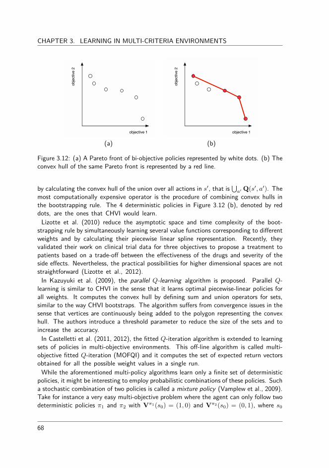
CHAPTER 3. LEARNING IN MULTI-CRITERIA ENVIRONMENTS
objective 1
obje
ctiv
e 2
objective 1
obje
ctiv
e 2
(a) (b)
Figure 3.12: (a) A Pareto front of bi-objective policies represented by white dots. (b) Theconvex hull of the same Pareto front is represented by a red line.
by calculating the convex hull of the union over all actions in sÕ, that ist
aÕ Q(sÕ, aÕ). The
most computationally expensive operator is the procedure of combining convex hulls inthe bootstrapping rule. The 4 deterministic policies in Figure 3.12 (b), denoted by reddots, are the ones that CHVI would learn.
Lizotte et al. (2010) reduce the asymptotic space and time complexity of the boot-strapping rule by simultaneously learning several value functions corresponding to di�erentweights and by calculating their piecewise linear spline representation. Recently, theyvalidated their work on clinical trial data for three objectives to propose a treatment topatients based on a trade-o� between the e�ectiveness of the drugs and severity of theside e�ects. Nevertheless, the practical possibilities for higher dimensional spaces are notstraightforward (Lizotte et al., 2012).
In Kazuyuki et al. (2009), the parallel Q-learning algorithm is proposed. Parallel Q-learning is similar to CHVI in the sense that it learns optimal piecewise-linear policies forall weights. It computes the convex hull by defining sum and union operators for sets,similar to the way CHVI bootstraps. The algorithm su�ers from convergence issues in thesense that vertices are continuously being added to the polygon representing the convexhull. The authors introduce a threshold parameter to reduce the size of the sets and toincrease the accuracy.
In Castelletti et al. (2011, 2012), the fitted Q-iteration algorithm is extended to learningsets of policies in multi-objective environments. This o�-line algorithm is called multi-objective fitted Q-iteration (MOFQI) and it computes the set of expected return vectorsobtained for all the possible weight values in a single run.
While the aforementioned multi-policy algorithms learn only a finite set of deterministicpolicies, it might be interesting to employ probabilistic combinations of these policies. Sucha stochastic combination of two policies is called a mixture policy (Vamplew et al., 2009).Take for instance a very easy multi-objective problem where the agent can only follow twodeterministic policies fi1 and fi2 with V
fi1(s0) = (1, 0) and V
fi2(s0) = (0, 1), where s0
68

3.4. PROBLEM TAXONOMY
denotes the start state. If one would follow policy fi1 with probability p and policy fi2 withprobability (1≠p), the average reward vector would be (p, 1≠p). Thus, although there areonly two deterministic policies for the original problem, a mixture policy implicates that wecan sample the entire convex hull of policies by combining the deterministic policies witha certain probability. Hence, stochastic combinations of the policies of the Pareto front inFigure 3.12 (a) can represent every solution on the red line in Figure 3.12 (b). However,mixture policies might not be appropriate in all situations, as highlighted in Roijers et al.(2013). For instance, in the setting of Lizotte et al. (2010), clinical data is analysed topropose a treatment to patients based on a trade-o� between the e�ectiveness of the drugsand severity of the side e�ects. Consider the case where only two policies exist that eithermaximise the e�ectiveness and the severity of the side e�ects and vice versa. While theaverage performance of the mixture policy of these two basic policies might yield goodperformance across a number of episodes, the policy itself might be unacceptable in eachepisode individually, i.e., for each patient independently.
Single-policy algorithms for multiple policies In the above subsection, we have dis-cussed on specific and elaborate algorithms that retrieve multiple policies simultaneously. Asimpler and straightforward alternative is to run a single-policy algorithm multiple times andto collect the resulting policies in a set. For instance, one can run the linear scalarisationalgorithm many times for varying weights to approximate the Pareto front. Neverthelessthe approach, being basic and relatively ine�cient, is implemented in many settings (Cas-telletti et al., 2002; Vamplew et al., 2008, 2010). In order to increase the e�ciency, amethod is also proposed that does not need to learn from scratch but which allows toreuse policies obtained in previous runs of the algorithms (Natarajan and Tadepalli, 2005).
Strictly speaking, this iterative principle is an intermediate approach compared to genuinemulti-policy algorithms that learn these policies simultaneously. This is why we choose toplace these techniques in between the single and multi-policy setting in Figure 3.11.
In Chapter 5, we analyse how the weight parameters of the linear scalarisation functionrelate to specific parts of the objective space. We highlight that the mapping from weightspace to objective space is non-isomorphic, meaning that it is far from trivial to definean appropriate weight configuration to retrieve a desired trade-o� solution. In this light,we propose two adaptive weight algorithms (AWA) that iteratively adjust their weightconfigurations based on the solutions obtained in previous rounds. These algorithms havethe ability to adaptively explore both discrete and continuous Pareto fronts.
Multi-policy algorithm with a monotonically increasing scalarisation function
Because of the properties of linear scalarisation functions, sum and union operators can bequite straightforwardly defined on convex hulls. The downside is that only a subset of thePareto front will be retrieved, leaving potentially interesting trade-o� solutions inaccessibleto the decision maker. In White (1982), a dynamic programming (DP) algorithm computesa set of Pareto dominating policies. White’s algorithm bootstraps the Pareto dominatingQ-vectors of the next state to the set of the current state-action pair. The idea is that,
69
CHAPTER 3. LEARNING IN MULTI-CRITERIA ENVIRONMENTS
after the discounted Pareto dominating rewards are propagated and the ˆQset’s converge toa set of Pareto dominating policies, the user can traverse the tree of ˆQset’s by applying apreference function. As highlighted in Section 2.3, a deterministic stationary policy su�cesfor single-objective reinforcement learning. In the case of MORL, White (1982) showedthat deterministic non-stationary policies, i.e., policies that do not only condition on thecurrent state but usually also on the time step t, can Pareto dominate the best deterministicstationary policies. As a result, in infinite horizon problems with large values for thediscount factor, the number of non-stationary policies increases exponentially and thereforeit can lead to an explosion of the sets. In order to make the algorithm practically applicable,Wiering and de Jong (2007) proposed the CON-MODP algorithm which solves the problemof non-stationary policies by introducing a consistency operator, but their work is limitedto deterministic transition functions. Monte Carlo tree search is also extended for multipleobjectives in the MO-MCTS method to learn a set of solutions (Wang and Sebag, 2012,2013). In MCTS, a search tree is incrementally built and explored simultaneously (Coulom,2007). The nodes of the tree represents visited states and branches represent actions. Atthe end of an episode, the nodes are weighted according to the outcome of the episodein order to bias the action selection in future plays. In MO-MCTS, the upper confidencebounds of the actions are scalarised in either of two distinct manners. One possibilityis to apply the hypervolume quality indicator on the combination of their estimates andthe set of Pareto optimal policies computed so far. Because the hypervolume measure iscostly to compute, as an alternative, it is also possible to simply determine whether a treewalk obtained a non-dominated reward or not in a boolean fashion. This way, scalarisedmulti-objective value functions are constructed that ease the process of selecting an actionwith vectorial estimates.
Up to this moment, there are no on-line reinforcement learning methods for learningmultiple policies that lie on the Pareto front. As quoted twice in Roijers et al. (2013), thisis a specific need for this type of algorithms although the setting is far from straightforward:
. . . MORL methods that can work with nonlinear scalarisation functions are ofsubstantial importance. Unfortunately, coping with this setting is especiallychallenging . . .
. . . we are not aware of any methods that use a value function approach tolearn multiple policies on the PCS. When stochastic policies are permitted, theproblem is easier [. . . ] However, when only deterministic policies are permitted,the problem is more di�cult.
Because of the challenging nature of this setting, a large part of this dissertation focusseson the development of multi-policy methods for learning Pareto optimal policies. To thisextent, we propose two algorithms in Chapter 6. These are the multi-objective hierarchicaloptimistic optimisation (MO-HOO) and the Pareto Q-learning algorithm.
The MO-HOO algorithm is applicable in multi-objective X -armed bandit problems. Thisis a class of problems similar to a standard bandit problem where an agent is faced witha continuous finite-dimensional action space instead of a discrete one as the example of
70

3.4. PROBLEM TAXONOMY
Section 2.5. The goal of the agent is to discover ranges in the continuous action spacethat provide Pareto optimal rewards. Our algorithm builds a binary tree where each noderepresents an optimistic estimate of the corresponding area in the objective space. Moreprecisely, each node stores a set of optimistic estimates of the Pareto front attainablefrom sampling its subtree.
In the Pareto Q-learning (PQL) algorithm, we further refine the idea of the MO-HOOalgorithm and extend it for multi-state environments. PQL is the first temporal di�erence-based multi-policy MORL algorithm that does not use the linear scalarisation function.Internally, Pareto Q-learning incrementally updates sets of vectorial estimates based onthe obtained rewards and the set of Pareto non-dominated estimates of the next state. Asa result, the algorithm is not limited to the convex hull, but it can learn the entire Paretofront of deterministic non-stationary policies, if enough exploration is provided.
3.4.2 Utility approachThe axiomatic problem taxonomy assumes the Pareto front is the optimality criterion.Recently, a utility-based problem taxonomy was proposed where the optimality criterionis not assumed but derived (Roijers et al., 2013). In that taxonomy, it is argued thatthere are more suitable solution concepts than the Pareto relation to denote the set ofoptimal policies in MORL. The utility-based taxonomy derives the optimality criterionbased on three properties. These properties are (1) the fact if the decision maker requiresa single policy or multiple policies, (2) the type of scalarisation function, being linear ormonotonically increasing and (3) whether deterministic or stochastic policies are allowed.The utility-based taxonomy is comprehensive and provides justification for the optimalitycriterion, specialised for the specific context.
In this dissertation, we limit ourselves to deterministic policies as stochastic policiesrepresent a specific type of policies that we do not envisage having a significant potential inreal-life engineering applications. Therefore, in the axiomatic taxonomy, we could reducethe utility-based taxonomy by one category. Similar to the utility-based taxonomy, wecluster research based on the number of policies required and the type of scalarisationfunction. However, we do not agree with the statement in Roijers et al. (2013) thatthe scalarisation function is publicly stated by the decision maker at the beginning ofthe MCDM process. In the utility-based approach, they assume the implicit or explicitscalarisation function employed by the decision maker is known and provided beforehandto the optimiser which can then exploit the properties of the scalarisation function athand. For instance, they assume that in the case of an a posteriori scenario the multi-objective optimiser knows that the decision maker will use a linear scalarisation functionin its thought process once the agent has provided a set of solutions. In this regard, thealgorithm only needs to retrieve policies on the convex hull as others will be disregardedby the linear scalarisation function once the decision maker discloses its desired weights.In our opinion, the authors then assume there are two articulations of preferences insteadof only a single articulation when the weights are provided. We do not agree with thefact that the scalarisation function is always predefined knowledge to the multi-criteria
71

CHAPTER 3. LEARNING IN MULTI-CRITERIA ENVIRONMENTS
optimiser or even known by the decision maker before initiating the optimisation process.From our point of view, there should be only a single articulation of preferences wherethe decision maker reveals its desired scalarisation function and weights at the same time.Therefore, we hold on to the fact that the Pareto front is the only optimality criterionin the general MCDM case. In the case where the scalarisation function can be assumedbefore initiating the process, a utility-based taxonomy could be employed.
3.5 SummaryIn this chapter, we introduced general concepts for learning in multi-criteria environments.We have defined multi-criteria decision making, the umbrella term for describing a collec-tion of approaches which seek to take explicit account of the multiple objectives in orderto facilitate and improve decision making. Multi-objective optimisation is an importantbranch of MCDM which solves these problems by means of mathematical equations. Gen-erally speaking, by solving MCDM problems, one needs to find solutions that are Paretooptimal. Because this optimality criterion entails a partial order, there usually exists nosingle optimum solution as in the case of single-objective optimisation. In this case, thereexists a set of optimal trade-o� solutions, called the Pareto front. We have drawn atten-tion to the role of the decision maker in the MCDM process and how it can articulateits preferences. We have highlighted three di�erent types of preference articulation whichinfluence the flow of the optimisation process and how the decision maker and the multi-criteria solver interact.
Evolutionary multi-objective optimisation is an important class of algorithms that areparticularly suited for multi-objective problems as they evolve a set of solutions in a singlerun. These techniques are intrinsically multi-policy algorithms as they obtain a set ofsolutions instead of a single solution, as single-policy algorithms do.
After carefully introducing the foundations of multi-objective optimisation, we focussedon the main topic of this dissertation, which is multi-objective reinforcement learning. Wehave defined multi-objective Markov decision processes and what constitutes an optimalpolicy. In the end, a problem taxonomy is provided which classifies MORL research on 4categories, i.e., the number of policies obtained (single or multi-policy) and whether thescalarisation is linear or monotonically increasing. In the following chapter, we will moreclosely analyse di�erent types of scalarisation functions for MORL and to what degree theycan be used to approximate the set of optimal trade-o� solutions.
72

4
| Learning a SingleMulti-Objective Policy
Multi-objective reinforcement learning algorithms that employ a scalarisation function toobtain a single multi-objective policy have been omnipresent in research (Gábor. et al.,1998; Vamplew et al., 2008; Perez et al., 2009; Van Mo�aert et al., 2013b). Most com-monly, a linear scalarisation function is used to transform the multi-objective nature ofthe problem to a standard single-objective RL problem (Castelletti et al., 2002; Tesauroet al., 2008), although non-linear scalarisation functions could potentially solve a few of itslimitations (Roijers et al., 2013). In this chapter, we will both theoretically and empiricallyanalyse the linear scalarisation function and the non-linear Chebyshev scalarisation func-tion. We will elaborate on the advantages and the limitations of each scalarisation functionand highlight how these scalarisation functions can be incorporated in a general framework.
In more detail, we will present the following contributions in this chapter:
• Present a general framework for scalarised MORL• Investigate the usefulness of the linear scalarisation function and its limitations• Research on a theoretical and empirical level whether the Chebyshev scalarisation
function can also be applied in MORL
This research has been published in Van Mo�aert et al. (2013b,a,c).
4.1 A framework for scalarised MORL algorithmsBefore we analyse the specifics of linear and non-linear scalarisation functions, we expand onhow the higher dimensionality of the reward signal influences the knowledge representationof the agent. Traditionally, in single-objective reinforcement learning, the agent keeps
73
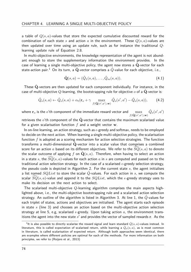
CHAPTER 4. LEARNING A SINGLE MULTI-OBJECTIVE POLICY
a table of Q(s, a)-values that store the expected cumulative discounted reward for thecombination of each state s and action a in the environment. These Q(s, a)-values arethen updated over time using an update rule, such as for instance the traditional Q-learning update rule of Equation 2.8.
In multi-objective environments, the knowledge representation of the agent is not abund-ant enough to store the supplementary information the environment provides. In thecase of learning a single multi-objective policy, the agent now stores a ˆ
Q-vector for eachstate-action pair.1 On its turn, a ˆ
Q-vector comprises a ˆQ-value for each objective, i.e.,
ˆ
Q(s, a) = (
ˆQ1(s, a), . . . , ˆQm(s, a)). (4.1)
These ˆ
Q-vectors are then updated for each component individually. For instance, in thecase of multi-objective Q-learning, the bootstrapping rule for objective o of a ˆ
Q-vector is:
ˆQo(s, a) Ω ˆQo(s, a) + –t(ro + “ max
f(Q(sÕ,aÕ),w)ˆQo(sÕ, aÕ
) ≠ ˆQo(s, a)), (4.2)
where ro is the o’th component of the immediate reward vector and max
f(Q(sÕ,aÕ),w)ˆQo(sÕ, aÕ
)
retrieves the o’th component of the ˆ
Q-vector that contains the maximum scalarised valuefor a given scalarisation function f and a weight vector w.
In on-line learning, an action strategy, such as ‘-greedy and softmax, needs to be employedto decide on the next action. When learning a single multi-objective policy, the scalarisationfunction f is adopted as a scoring mechanism for action selection strategies. The functiontransforms a multi-dimensional ˆ
Q-vector into a scalar value that comprises a combinedscore for an action a based on its di�erent objectives. We refer to the ‰SQ(s, a) to denotethe scalar outcome of applying f on ˆ
Q(s, a). Therefore, when having to select an actionin a state s, the ‰SQ(s, a)-values for each action a in s are computed and passed on to thetraditional action selection strategy. In the case of a scalarised ‘-greedy selection strategy,the pseudo code is depicted in Algorithm 2. For the current state s, the agent initialisesa list named SQList to store the scalar ˆQ-values. For each action in s, we compute thescalar ‰SQ(s, a)-value and append it to the SQList, which the ‘-greedy strategy uses tomake its decision on the next action to select.
The scalarised multi-objective Q-learning algorithm comprises the main aspects high-lighted above, i.e., the multi-objective bootstrapping rule and a scalarised action selectionstrategy. An outline of the algorithm is listed in Algorithm 3. At line 1, the ˆQ-values foreach triplet of states, actions and objectives are initialised. The agent starts each episodein state s (line 3) and chooses an action based on the multi-objective action selectionstrategy at line 5, e.g, scalarised ‘-greedy. Upon taking action a, the environment trans-itions the agent into the new state sÕ and provides the vector of sampled rewards r. As the
1It is also possible to directly scalarise the reward signal and learn standard Q(s, a)-values instead. Inliterature, this is called expectation of scalarised return, while learning a Qo(s, a), as is most commonin literature, is called scalarisation of expected return. Although both approaches seem identical, thereare examples where di�erent policies are optimal for each of the methods. For more information on bothprinciples, we refer to (Roijers et al., 2013)
74
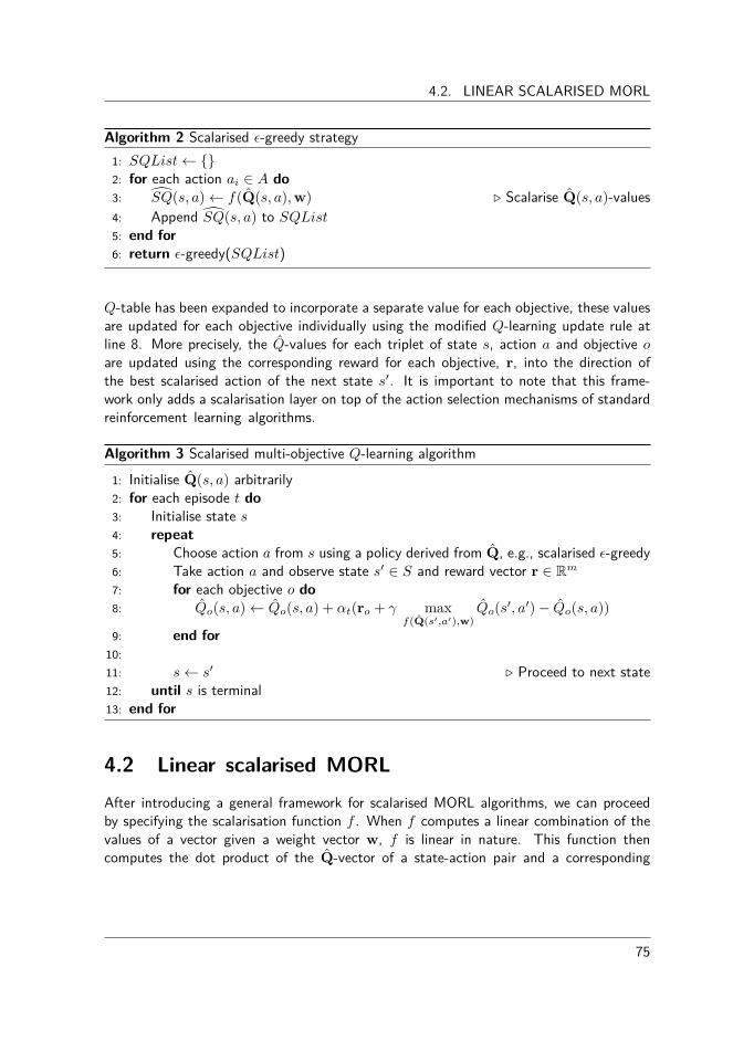
4.2. LINEAR SCALARISED MORL
Algorithm 2 Scalarised ‘-greedy strategy1: SQList Ω {}2: for each action ai œ A do3: ‰SQ(s, a) Ω f(
ˆ
Q(s, a), w) Û Scalarise ˆ
Q(s, a)-values4: Append ‰SQ(s, a) to SQList5: end for6: return ‘-greedy(SQList)
Q-table has been expanded to incorporate a separate value for each objective, these valuesare updated for each objective individually using the modified Q-learning update rule atline 8. More precisely, the ˆQ-values for each triplet of state s, action a and objective oare updated using the corresponding reward for each objective, r, into the direction ofthe best scalarised action of the next state sÕ. It is important to note that this frame-work only adds a scalarisation layer on top of the action selection mechanisms of standardreinforcement learning algorithms.
Algorithm 3 Scalarised multi-objective Q-learning algorithm1: Initialise ˆ
Q(s, a) arbitrarily2: for each episode t do3: Initialise state s4: repeat5: Choose action a from s using a policy derived from ˆ
Q, e.g., scalarised ‘-greedy6: Take action a and observe state sÕ œ S and reward vector r œ Rm
7: for each objective o do8: ˆQo(s, a) Ω ˆQo(s, a) + –t(ro + “ max
f(Q(sÕ,aÕ),w)ˆQo(sÕ, aÕ
) ≠ ˆQo(s, a))
9: end for10:11: s Ω sÕ Û Proceed to next state12: until s is terminal13: end for
4.2 Linear scalarised MORLAfter introducing a general framework for scalarised MORL algorithms, we can proceedby specifying the scalarisation function f . When f computes a linear combination of thevalues of a vector given a weight vector w, f is linear in nature. This function thencomputes the dot product of the ˆ
Q-vector of a state-action pair and a corresponding
75

CHAPTER 4. LEARNING A SINGLE MULTI-OBJECTIVE POLICY
non-negative weight vector:‰SQ(s, a) =
ˆ
Q(s, a) · w
=
mÿ
o=1
ˆ
Qo(s, a) · wo,(4.3)
where w is a weight vector specifying the relative importance of each objective. Theweight vector itself should satisfy the following equations:
’o œ [1, m] : 0 Æ wo Æ 1. (4.4)
mÿ
o=1wo = 1. (4.5)
4.2.1 Optimality of linear scalarised MORLOne important advantage of the linear scalarisation function is its property of additivity.In essence, this means that the result of the scalarisation function applied on the vectorialvalue function of a policy fi is equal to applying the scalarisation function in the learningprocess directly:
f(V
fi(s), w) = V
fi(s) · w
= Efi{Rt|s(t) = s} · w
= Efi
; Œÿ
k=0“ k
rt+k+1 | s(t) = s
<· w
= Efi
; Œÿ
k=0“ k
w · rt+k+1 | s(t) = s
<
= Efi
; Œÿ
k=0“ kf(rt+k+1, w) | s(t) = s
<
(4.6)
Hence, the single-objective MDP that was obtained by applying the linear scalarisationfunction on the original MDP has additive returns. As a result, the linear scalarisationfunction in combination with the Bellman equation, and thus RL in general, is proven toconverge to the optimal policy fiú for the weight vector w. Subsequently, this optimalpolicy is also optimal in the original objective space:
Theorem 4.1
If f is a linear scalarisation function and V
fiú is the vector-valued value function ofthe converged and optimal policy fiú, then fiú is also Pareto optimal.
fi œ � · ’ fiÕ œ � : V
fi · w Ø V
fiÕ· w =∆ fi is Pareto optimal.
76

4.2. LINEAR SCALARISED MORL
For insights in the proof of this theorem, we refer to Nakayama et al. (2009).
4.2.2 Convexity of linear scalarised MORLSo far, we have seen that the linear scalarisation function is theoretically proven to con-verge to a Pareto optimal solution in the objective space of the original problem. In thissection, we will analyse whether the inverse also holds, i.e., is every Pareto optimal solutiondiscoverable by employing a linear scalarisation function or not?
In Das and Dennis (1997), this research question is answered by examining the influenceof the weights in the objective space. For simplicity reasons, the authors analysed thematter for a problem with two objectives f1 and f2, but it could be generalised for m-objective environments as well. The authors argue that the weight space of the linearscalarisation can be considered a goniometric circle with a radius of 1 in order to satisfyEquation 4.5. A visual representation of the process is provided in Figure 4.1 where thePareto front is entirely convex. The weights of the two objectives can then be representedby w1 œ [0, 1] and w2 = 1 ≠ w1. The goal of the optimisation process is then to findthe solution x œ X so that:
max
xœX
w1f1(x) + (1 ≠ w1)f2(x). (4.7)
In the goniometric circle, this equation can be rewritten by considering the angle ◊ œ [0, fi2 ]:
max
xœX
sin ◊
sin ◊ + cos ◊f1(x) +
cos ◊
sin ◊ + cos ◊f2(x). (4.8)
The utilisation of the weights can be seen as a transformation of the original axis of eachof the objectives, i.e., f1 and f2 to f1 and f2 in Figure 4.1. The rotated f1 and f2 axescan be found by an elementary coordinate transformation:
5f1f2
6=
5cos ◊ sin ◊
≠ sin ◊ cos ◊
6◊
5f1f2
6(4.9)
77

CHAPTER 4. LEARNING A SINGLE MULTI-OBJECTIVE POLICY
θ
w11
1 - w11
f1
f2
P
!1
!2
Figure 4.1: The linear scalarisation function can find any solution on the Pareto front withan appropriate weight vector if it the Pareto front has a convex shape.
Therefore, the goal is to find the solution maxxœX
f1, with f1 = f1 cos ◊ + f2 sin ◊. InFigure 4.1, this maximisation can be regarded as a parallel translation of f2 to itself until ithits the curve of the Pareto front (Das and Dennis, 1997). In this case, the point P is thesolution that is discovered by the linear scalarisation function employing a weight vectorof (w1, 1 ≠ w1) as f2 is tangent to the Pareto front at that point. Since the Pareto frontin this example is convex, it is equal to the convex hull and every element of the Paretofront can be discovered by varying the ◊ angle, and thus the weight vector.
Theorem 4.2
If the value function V
fi of a policy fi lies on the convex hull of the Pareto front,then there exists a weight vector w for which V
fi · w is maximal:
fi œ CH(�) =∆ ÷w œ Rm · ’fiÕ œ � : V
fi · w Ø V
fiÕ· w.
78
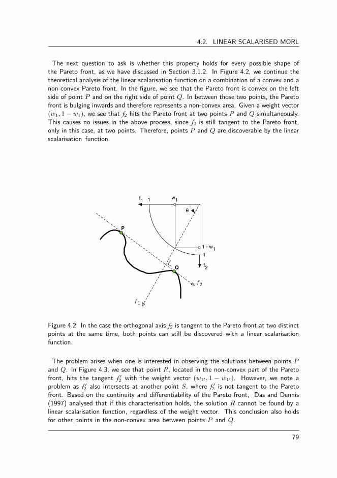
4.2. LINEAR SCALARISED MORL
The next question to ask is whether this property holds for every possible shape ofthe Pareto front, as we have discussed in Section 3.1.2. In Figure 4.2, we continue thetheoretical analysis of the linear scalarisation function on a combination of a convex and anon-convex Pareto front. In the figure, we see that the Pareto front is convex on the leftside of point P and on the right side of point Q. In between those two points, the Paretofront is bulging inwards and therefore represents a non-convex area. Given a weight vector(w1, 1 ≠ w1), we see that f2 hits the Pareto front at two points P and Q simultaneously.This causes no issues in the above process, since f2 is still tangent to the Pareto front,only in this case, at two points. Therefore, points P and Q are discoverable by the linearscalarisation function.
θ
w11
1 - w11
f1
f2
!1
P
Q
!2
Figure 4.2: In the case the orthogonal axis f2 is tangent to the Pareto front at two distinctpoints at the same time, both points can still be discovered with a linear scalarisationfunction.
The problem arises when one is interested in observing the solutions between points Pand Q. In Figure 4.3, we see that point R, located in the non-convex part of the Paretofront, hits the tangent f Õ
2 with the weight vector (w1Õ , 1 ≠ w1Õ). However, we note a
problem as f Õ2 also intersects at another point S, where f Õ
2 is not tangent to the Paretofront. Based on the continuity and di�erentiability of the Pareto front, Das and Dennis(1997) analysed that if this characterisation holds, the solution R cannot be found by alinear scalarisation function, regardless of the weight vector. This conclusion also holdsfor other points in the non-convex area between points P and Q.
79
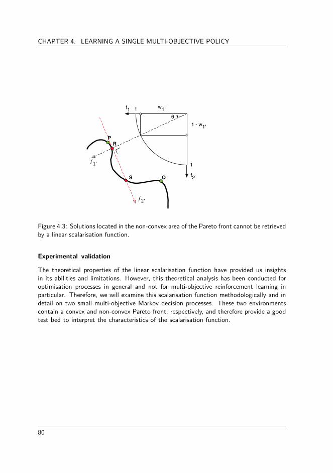
CHAPTER 4. LEARNING A SINGLE MULTI-OBJECTIVE POLICY
θ
w1'1
1 - w1'
1
f1
f2
!1'
P
Q
R
S
!2'
Figure 4.3: Solutions located in the non-convex area of the Pareto front cannot be retrievedby a linear scalarisation function.
Experimental validation
The theoretical properties of the linear scalarisation function have provided us insightsin its abilities and limitations. However, this theoretical analysis has been conducted foroptimisation processes in general and not for multi-objective reinforcement learning inparticular. Therefore, we will examine this scalarisation function methodologically and indetail on two small multi-objective Markov decision processes. These two environmentscontain a convex and non-convex Pareto front, respectively, and therefore provide a goodtest bed to interpret the characteristics of the scalarisation function.
80
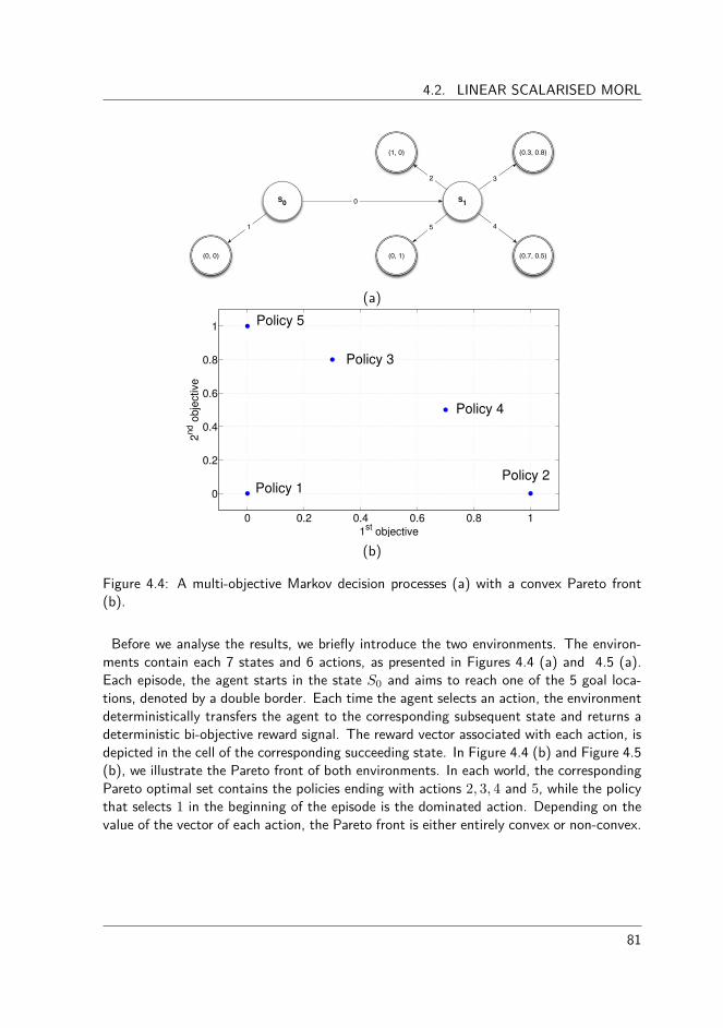
4.2. LINEAR SCALARISED MORL
S0 S1
(0, 0)
(1, 0) (0.3, 0.8)
(0.7, 0.5)(0, 1)
0
1
2 3
45
(a)
0 0.2 0.4 0.6 0.8 1
0
0.2
0.4
0.6
0.8
1
1st objective
2n
d o
bje
ctiv
e
Policy 5
Policy 3
Policy 1
Policy 4
Policy 2
(b)
Figure 4.4: A multi-objective Markov decision processes (a) with a convex Pareto front(b).
Before we analyse the results, we briefly introduce the two environments. The environ-ments contain each 7 states and 6 actions, as presented in Figures 4.4 (a) and 4.5 (a).Each episode, the agent starts in the state S0 and aims to reach one of the 5 goal loca-tions, denoted by a double border. Each time the agent selects an action, the environmentdeterministically transfers the agent to the corresponding subsequent state and returns adeterministic bi-objective reward signal. The reward vector associated with each action, isdepicted in the cell of the corresponding succeeding state. In Figure 4.4 (b) and Figure 4.5(b), we illustrate the Pareto front of both environments. In each world, the correspondingPareto optimal set contains the policies ending with actions 2, 3, 4 and 5, while the policythat selects 1 in the beginning of the episode is the dominated action. Depending on thevalue of the vector of each action, the Pareto front is either entirely convex or non-convex.
81

CHAPTER 4. LEARNING A SINGLE MULTI-OBJECTIVE POLICY
S0 S1
(0, 0)
(1, 0) (0.5, 0.2)
(0.1, 0.4)(0, 1)
0
1
2 3
45
(a)
0 0.2 0.4 0.6 0.8 1
0
0.2
0.4
0.6
0.8
1
1st objective
2n
d o
bje
ctiv
e
Policy 3
Policy 2Policy 1
Policy 4
Policy 5
(b)
Figure 4.5: A multi-objective Markov decision processes (a) with a non-convex Paretofront (b).
In Figures 4.6 (a) and (b), we depict the outcome of linear scalarised MORL algorithmon both environments. The results were obtained after learning the ˆ
Q-vectors of eachstate-action pair until the bootstrapping rule in Equation 4.2 did not incur any updateslarger than a small � to the value of each objective.
82

4.2. LINEAR SCALARISED MORL
0 0.2 0.4 0.6 0.8 1
0
0.2
0.4
0.6
0.8
1
w1
f(V
π(S
0),
w)
Policy 1Policy 2Policy 3Policy 4Policy 5max f(Vπ(S
0), w)
(a)
0 0.2 0.4 0.6 0.8 1
0
0.2
0.4
0.6
0.8
1
w1
f(V
π(S
0),
w)
Policy 1Policy 2Policy 3Policy 4Policy 5max f(Vπ(S
0), w)
(b)
Figure 4.6: The optimal actions for each weight vector using the linear scalarisation func-tion on environments with a convex and a non-convex Pareto front, respectively.
For the environment with the convex Pareto front in Figure 4.6 (a), we depict a list oflinear functions, one for each policy. Each of these lines can be represented by a list oftrade-o�s, i.e., di�erent values of w1 œ [0, 1] while w2 = 1≠w1, together with a list of theircorresponding scalarised value function values from the start state S0, i.e., f(V
fi(S0), w).
The set of policies that are optimal for some w1 œ [0, 1] are the policies whose linerepresentation lies on the upper convex envelope of the scalarised value functions (Lizotteet al., 2010). This representation allows us to discover which policies are optimal forwhich weight vector, i.e., the policies that lie on the black line in Figure 4.6 (a). In thisfigure, we see that policy 1 is never optimal as its line does not intersect with the blackline. We also note that polices 2, 4 and 5 are optimal for a relatively large portion of theweight space. Although, it is hardly noticeable on the figure, the linear scalarised MORL
83

CHAPTER 4. LEARNING A SINGLE MULTI-OBJECTIVE POLICY
algorithm also successfully identified policy 3 as being optimal, albeit only for a very smallpart of the weight space. These results correspond to the Pareto front in Figure 4.4 (b)and, therefore, they also confirm that the linear scalarisation function can discover everyelement on the convex hull.
For the non-convex Pareto front, we highlight the results in Figure 4.6 (b). Althoughwe know that four policies in this environment are Pareto optimal, the linear scalarisedMORL algorithm has only identified two regions of the weight space where two policies areoptimal. In this non-convex environment, the scalarised value functions of the other policiesare always lower than the scalarised value functions of the policies with returns (1, 0) and(0, 1). The linear scalarised MORL algorithm is only able to discover the extremes of thenon-convex Pareto front, i.e., the knots in the Pareto front where the curve starts to bulgeinwards. Depending on the weight vector, either of these extreme policies are retrieved,leaving the other, also Pareto optimal, policies undiscovered.
We can conclude the section on the linear scalarisation function by emphasising its sim-plicity and usability in MORL. We have seen it is theoretically proven to converge to aPareto optimal policy. However, only policies on the convex hull, a subset of the Paretofront, can be discovered, leaving the optimal solutions in the concavities of the Paretofront undiscovered. In the next section, we will both theoretically and empirically analysean alternative scalarisation function that overcomes the limitations the linear scalarisationfunction imposes.
4.3 Chebyshev scalarised MORLSo far we have seen that the linear scalarisation function fits well into the reinforcementlearning framework as it preserves additivity. As a result, the linear scalarisation functionin combination with MORL is guaranteed to converge to a policy on the convex hull ofthe Pareto front (Das and Dennis, 1997). Nevertheless, the convex hull is only a subsetof the Pareto front which might not match the preferences of the decision maker. Inorder to account for every possible preference the decision maker might yield, we are inneed for methods that are able to discover the entire set of optimal trade-o� solutions.To overcome these limitations, researchers have been focussing on non-linear scalarisationfunctions (Humphrys, 1997; Mannor and Shimkin, 2002). Some successful approacheswithin this field employ a thresholded lexicographic order on the objectives (Gábor. et al.,1998; Issabekov and Vamplew, 2012). In these approaches, a minimal threshold levelshould be met for the values of each of the objectives, which can then be ordered in alexicographic order. Nonetheless, the scalarisation functions in these algorithms are stillvery specific and tuned to the problem at hand. More precisely, they lack simplicity in theirformulation which is one of the main contributions to the success of the linear scalarisationfunction. In this prospect, we investigate an alternative non-linear scalarisation functionwhich has proven its e�ciency and e�ectiveness in the general multi-objective optimisation
84

4.3. CHEBYSHEV SCALARISED MORL
domain. This scalarisation function is the Chebyshev scalarisation function, named afterthe Russian mathematician Pafnuty Lvovich Chebyshev.2
4.3.1 Formal definitionThe Chebyshev scalarisation function is an alternative scalarisation function based on Lp
distance metrics (Dunford et al., 1988). These metrics measure the distance between twovectors a = (a1, . . . , am) and b = (b1, . . . , bm), where m is the dimensionality of thevector space. The Lp distance between points a and b is then defined as:
Lp(a, b) = Îa ≠ bÎp
=
! mÿ
o=1|ao ≠ bo|p
"1/p.
(4.10)
In the case where p = 1, the distance metric is:
L1(a, b) = Îa ≠ bÎ1
=
mÿ
o=1|ao ≠ bo|.
(4.11)
This distance metric calculates the sum of the absolute di�erences of the coordinates ofeach vector. This principle alludes to the distance one would need to walk in a big city toreach point b starting from point a, since one cannot cross through buildings but needs tostay on the streets. Therefore, it is also known as the taxicab or Manhattan distance.Themost common Lp metric is the Euclidean distance with p = 2. The Euclidean distanceis defined as the square root of the sum of the squares of the di�erences between thecorresponding coordinates of the points a and b.
L2(a, b) = Îa ≠ bÎ2
=
ııÙmÿ
o=1(ao ≠ bo)
2.(4.12)
In the case of p = Œ, the metric results in the LŒ or the Chebyshev metric. The Cheby-shev metric is defined as the greatest distance between a and b along any dimension (Xuet al., 2013). Its mathematical equation is defined as:
LŒ(a, b) = Îa ≠ bÎŒ
= max
o=1...m|ao ≠ bo|. (4.13)
The best way to compare the di�erent distance metrics is to consider their unit spheres.A unit sphere is a set of points that lies at a distance of one from a fixed central point.
2His name can be alternatively transliterated as Chebychev, Chebyshe�, Chebyshov, Tchebychev,Tchebyche�, Tschebyschev, Tschebyschef or Tschebysche�
85

CHAPTER 4. LEARNING A SINGLE MULTI-OBJECTIVE POLICY
Depending on the distance metric used, this sphere will be of a particular shape. Below, inFigure 4.7 (a), (b) and (c), one can find and compare the unit spheres for the Manhattan,Euclidean and Chebyshev distance metrics, respectively.
(a) (b) (c)
Figure 4.7: The unit spheres of the L1, L2 and LΠdistance metrics.
From the figure, we see that each shape intersects each axis at distance one from thecentral point. We also note that the smaller the p-value, the smaller the size of theunit sphere.
4.3.2 Scalarisation with the Chebyshev functionNow that we have properly introduced the Lp distance metrics, we research how they canbe used as a scalarisation function in multi-objective optimisation. The observant readermight have already noticed that the L1 distance metric is very similar to the equation of thelinear scalarisation function. Actually, when one introduces weight vectors in Equation 4.11and when b = (0, . . . , 0), the function becomes:
L1(a, b) = w1|a1 ≠ 0| + . . . + wm|am ≠ 0|= w1|a1| + . . . + wm|am|= w · a,
(4.14)
which is equivalent to the formula of the linear scalarisation function if the necessaryconstraints of Equation 4.4 and 4.5 are satisfied for w.
The Chebyshev distance metric can also be transformed to serve as a scalarisation functionin multi-objective optimisation (Bowman and Joseph, 1976). In these approaches, theChebyshev norm is used to scalarise a given vector a by calculating the Chebyshev distancefrom that point to an attraction point z
ú œ Rm. This attraction point serves as a pointof interest to guide the vector a to certain areas of the objective space. In Steuer andChoo (1983), this idea is pursued by interactively redefining the attraction point to attaincertain solutions in the objective space. In more traditional approaches, the attractionpoint acts as an ideal point, as described in Section 3.1.2. In this case, z
ú is a parameter
86

4.3. CHEBYSHEV SCALARISED MORL
that is constantly being adjusted during the optimisation process by recording the bestvalue so far for each objective o, plus a small negative or positive constant · , dependingwhether the problem is to be minimised or maximised, respectively (Klamroth and Jørgen,2007; Dächert et al., 2012).
One of the main advantages of the Chebyshev scalarisation function in general multi-objective optimisation is that every Pareto optimal solution can be discovered by appro-priately varying the weights and/or the attraction point. For a formal proof, we referto Miettinen (1999). Nevertheless, it remains hard to specify appropriate values for the w
and z
ú parameters in order to discover a desired trade-o� solution (Marler and Arora, 2004).
4.3.3 Convergence issues in MORLIn the previous sections, we have introduced the foundations of the Chebyshev scalarisa-tion function and its ability to discover every Pareto optimal solution. This property istheoretically proven to hold in the general topic of multi-objective optimisation. In thissection, we will verify whether this property also holds in MORL.
Before we can test the assumption, we need to specify how we can incorporate theChebyshev function in the scalarised MORL framework of Section 4.1. To accommodatefor a new scalarisation function, we only need to specify how one calculates the scalarised‰SQ(s, a)-value given the Q-vector of that same state-action pair. Utilising the Chebyshevfunction in this process gives us:
‰SQ(s, a) = ≠ max
o=1...mwo · | ˆ
Qo(s, a) ≠ z
úo|, (4.15)
with w satisfying both Equation 4.4 and 3.22. Note that the Chebyshev formula is negatedto account for a maximisation problem.
However, for a scalarisation function to be suitable in reinforcement learning, it needsto preserve additivity. Therefore, for any choice of w œ Rm and z
ú œ Rm, it needsto hold that
f(V
fi, w) = Efi
; Œÿ
k=0“ kf(rt+k+1, w)
<. (4.16)
As analysed by Perny and Weng (2010), this equation does not hold if f is the Cheby-shev formula. To highlight this, consider the following situation described by Roijers et al.(2013). In an episode, the agent follows a policy fi that selects two actions which cor-responding rewards are r1 = (0, 3) and r2 = (3, 0). Hence, when the discount factor“ = 1, then V
fi= (3, 3). If we now apply the Chebyshev function with z
ú= (3, 3) and
w = (0.5, 0.5) on the vector-valued value function, we get on the one hand
f(V
fi, w) = ≠ max(|0.5 ◊ (3 ≠ 3)|, |0.5 ◊ (3 ≠ 3)|)= ≠ max(|0.5 ◊ 0|, |0.5 ◊ 0|)= 0
(4.17)
87

CHAPTER 4. LEARNING A SINGLE MULTI-OBJECTIVE POLICY
While on the other hand, when applying f throughout the learning process, we see
Efi
; Œÿ
k=0
“ kf(rt+k+1, w)
<= “ 0f(r1, (0.5, 0.5)) + “ 1f(r2, (0.5, 0.5))
= ≠ max(|0.5 ◊ (0 ≠ 3)|, |0.5 ◊ (3 ≠ 3)|≠ max(|0.5 ◊ (3 ≠ 3)|, |0.5 ◊ (0 ≠ 3)|)
= ≠ max(|0.5 ◊ ≠3|, |0.5 ◊ 0| ≠ max(|0.5 ◊ 0|, |0.5 ◊ ≠3|)= ≠ max(1.5, 0) ≠ max(0, 1.5)
= ≠1.5 ≠ 1.5
= ≠3
”= f(Vfi, w)
(4.18)
This inequality has important consequences in reinforcement learning. As a result of thelack of additivity of the non-linear Chebyshev function, the Bellman equation no longerholds and the Chebyshev function in combination with a learning algorithm is not provento converge to the optimal policy (Perny and Weng, 2010; Roijers et al., 2013). Thisis an important disadvantage of the Chebyshev scalarisation function since it would havebeen a powerful alternative to overcome the limitations of the linear scalarisation functionas it could potentially discover every Pareto optimal solution. Nevertheless, it serves asan attractive research question to investigate the impact of this theoretical limitation onsome practical exercises.
4.3.4 Experimental validationTo verify the empirical performance of the Chebyshev MORL algorithm, we focus ontwo environments with similar characteristics. These are the Deep Sea Treasure and theBountiful Sea Treasure environments. In the following subsections, we will empiricallyanalyse the e�ectiveness of the Chebyshev scalarised MORL algorithms in attaining thePareto optimal solutions for specific configurations.
Deep Sea Treasure world
The Deep Sea Treasure (DST) is proposed by Vamplew et al. (2010) and is a standardMORL benchmark instance. The problem concerns a deterministic episodic task wherean agent controls a submarine, searching for undersea treasures. The world consists of a10◊11 grid where 10 treasures are located, with larger values as the distance from thestarting location increases. A visualisation of the environment is depicted in Figure 4.8.At each time step, the agent can move into one of the cardinal directions, i.e., up, down,left and right.
88

4.3. CHEBYSHEV SCALARISED MORL
124
74
8
24
2
3
50
165
1
Figure 4.8: A visual representation of the Deep Sea Treasure world
The goal of the agent is to minimise the time needed to reach the treasure, while max-imising the treasure value.3 In this environment, a Pareto optimal policy is a path to atreasure that minimises the Manhattan distance to each of the 10 treasures. Given thereward signal of the environment, the Pareto front is entirely non-convex and presentedin Figure 4.9.
−20 −18 −16 −14 −12 −10 −8 −6 −4 −2 00
20
40
60
80
100
120
140
Time objective
Tre
asu
re o
bje
ctiv
e
Pareto front
Figure 4.9: The Pareto front of the Deep Sea Treasure world
To thoroughly analyse the performance of the Chebyshev scalarised MORL algorithm, weinvestigate the converged policy after 10.000 episodes for di�erent parameter configura-tions. For each configuration, we specify a weight vector w œ [0, 1] and a static attractionpoint z
ú œ Rm. We evaluate which policy the algorithm converges to for 11 weightvector and 30 ◊ 140 attraction points. Therefore, in total we evaluate 46200 possibleconfigurations. In Figure 4.10, we depict on the x and y-axis the first and the second
3Traditionally, single-objective reinforcement learning solves a maximisation problem. If the problemat hand concerns a minimisation of one of the objectives, negative rewards are used for that objective totransform it also into a maximisation problem.
89

CHAPTER 4. LEARNING A SINGLE MULTI-OBJECTIVE POLICY
coordinate of the z
ú vector, respectively. The z-axis represents the corresponding weightused for the time objective, i.e., w1, while the second objective, i.e., the treasure objective,is w2 = (1 ≠ w1). Eventually, the colour of the dot represents which of the 10 Paretooptimal policy has been retrieved when following a greedy policy at the end of the learningphase. In case the retrieved policy was not Pareto optimal, no dot is displayed.
Figure 4.10: A parameter sweep for di�erent weight vector and attraction points in theDeep Sea Treasure world
From the figure, we see di�erent trends emerging. For starters, we see that for specificconfigurations every possible Pareto optimal policy has been learned as all the possiblecolours are present. To some degree, this result confirms the findings of the Chebyshevscalarisation function in general multi-objective optimisation also in MORL. Secondly,we see that the weight vector, usually employed by the decision maker to emphasise aspecific trade-o� between solutions, does not provide an explicit bias to specific parts ofthe objective space. For instance, when the weight for the time objective is 0, we finddi�erent Pareto optimal solutions. On the contrary, when the weight is equal to 1, almostregardless of the value of the attraction vector, the policy that retrieves the smallesttreasure is learned. Thirdly, for di�erent combinations of weight vector and attractionvector, we see several areas emerging where particular solutions are optimal. When theseareas become more obvious also the space that separates these areas and where no Paretooptimal policy is discovered, becomes more distinctive. This can easily be noticed whencomparing the areas for weights 0.5 and 1.
90

4.3. CHEBYSHEV SCALARISED MORL
0 0.1 0.2 0.3 0.4 0.5 0.6 0.7 0.8 0.9 10
0.1
0.2
0.3
0.4
0.5
0.6
0.7
0.8
0.9
1
Weight
Pe
rce
nta
ge
1
2
3
4
5
6
7
8
9
10
Figure 4.11: The retrievable policies for di�erent weights in the Deep Sea Treasure world
In Figure 4.11, we approach this analysis from a di�erent viewpoint. In this stacked barchart, we investigate for each of the 11 weights the occurrence of each Pareto optimalpolicy. With this representation, we can straightforwardly analyse in what percentage ofthe cases the Chebyshev MORL algorithm does not converge to an optimal solution. Wesee that for weights w1 from 0 to 0.6, the percentages of occurrence of each of the Paretooptimal solutions remain relatively identical. We note that for these weights also over30% of the time no Pareto optimal solution was learned, which is remarkable. Only forthe larger weights, we see a decrease in the amount of dominated policies but also in thediversity of the optimal solutions, i.e., for weight w1 = 1 in 90% of the cases the optimalpolicy towards the smallest treasure is learned.
From the previous figures, one could argue that certain weights, such as w1 = 0.4, o�era relatively good setting to obtain various Pareto optimal trade-o� solutions, if one playsaround with the values of the reference point. However, the robustness of these parametersettings is also crucial, i.e., with the same configuration, do we always retrieve the samesolution of the policy space. In the next experiment, we repeat 11 runs of the Chebyshevalgorithm while keeping w1 = 0.4 fixed and varying the reference point z
ú. In Figure 4.12,we then denote the configurations that consistently yield the same Pareto optimal policythroughout the 11 runs. As we see, only for some very specific parameter configurations,the Chebyshev algorithm consistently learns the same policies. More specifically, this isthe case in only 9.59% of the 4200 configurations examined. Therefore, this demonstra-tion clearly shows the huge amount of variability of the Chebyshev single-policy MORLalgorithm, which will become a constant factor in each of the subsequent experiments.
91

CHAPTER 4. LEARNING A SINGLE MULTI-OBJECTIVE POLICY
−40
−20
0
−20020406080100120140
0.4
We
igh
t
Solution
0
1
2
3
4
5
6
7
8
9
10
Time
Treasure
Figure 4.12: The variability of the Chebyshev single-policy MORL algorithm over multipleruns with w1 = 0.4 is very large. In only 400 out of 4200 parameter configurations, thesame Pareto optimal policy is returned. In the other configurations, the results varied andthe algorithms converged to a di�erent policy.
Bountiful Sea Treasure world
Before we proceed to formulating conclusions on the Chebyshev scalarised MORL al-gorithm, it is fruitful to investigate its e�ectiveness also on another environment withother characteristics. The Bountiful Sea Treasure environment is a variation to the DeepSea Treasure environment where the reward signal is altered to accommodate for a convexPareto front. A visual representation of the environment and its Pareto front with 10elements is provided in Figure 4.13 and Figure 4.14, respectively.
175
173
145
163
80
120
166
150140
5
Figure 4.13: A visual representation of the Bountiful Sea Treasure world
92

4.3. CHEBYSHEV SCALARISED MORL
−20 −18 −16 −14 −12 −10 −8 −6 −4 −2 0
20
40
60
80
100
120
140
160
180
Time objective
Tre
asu
re o
bje
ctiv
e
Pareto front
Figure 4.14: The Pareto front of the Bountiful Sea Treasure world
Since both environments only di�er from one another in their reward signal, it is verysuitable to run a similar parameter sweep. In Figure 4.15, we depict the learned policies forthe same elements in the weight space and the space of attraction points. What strikes usimmediately is the fact that the diversity of the policies has disappeared compared to theprevious experiment. In a lot of cases, the extreme policies, denoted by red and blue dots,are learned almost regardless of the weight parameter and the attraction point. However,closely examining the results teaches us that still every Pareto optimal policy is beinglearned, albeit for some policies only for a very restricted set of configurations.
93
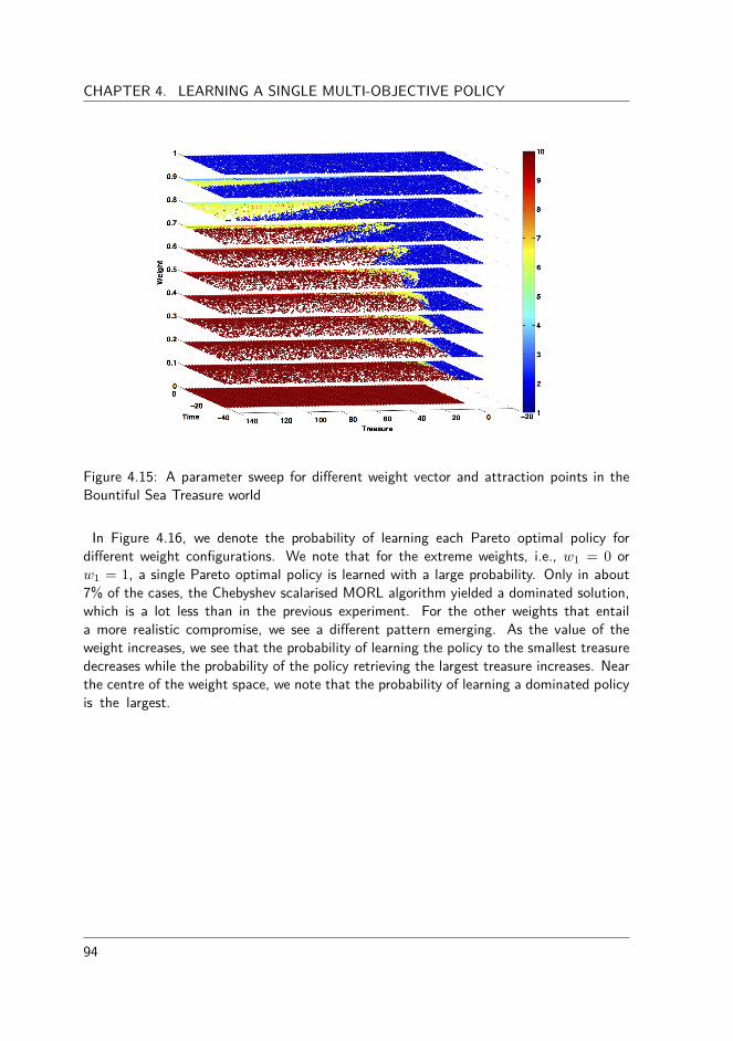
CHAPTER 4. LEARNING A SINGLE MULTI-OBJECTIVE POLICY
Figure 4.15: A parameter sweep for di�erent weight vector and attraction points in theBountiful Sea Treasure world
In Figure 4.16, we denote the probability of learning each Pareto optimal policy fordi�erent weight configurations. We note that for the extreme weights, i.e., w1 = 0 orw1 = 1, a single Pareto optimal policy is learned with a large probability. Only in about7% of the cases, the Chebyshev scalarised MORL algorithm yielded a dominated solution,which is a lot less than in the previous experiment. For the other weights that entaila more realistic compromise, we see a di�erent pattern emerging. As the value of theweight increases, we see that the probability of learning the policy to the smallest treasuredecreases while the probability of the policy retrieving the largest treasure increases. Nearthe centre of the weight space, we note that the probability of learning a dominated policyis the largest.
94

4.4. BENCHMARKING LINEAR AND CHEBYSHEV SCALARISED MORL
0 0.1 0.2 0.3 0.4 0.5 0.6 0.7 0.8 0.9 10
0.1
0.2
0.3
0.4
0.5
0.6
0.7
0.8
0.9
1
Weight
Pe
rce
nta
ge
1
2
3
4
5
6
7
8
9
10
Figure 4.16: The retrievable policies for di�erent weights in the Bountiful Sea Treasureworld
In both environments, we have performed an in-depth analysis of the Chebyshev scalarisedMORL algorithm for several parameter configurations. We can now present two statementson the e�ciency and the e�ectiveness of the scalarisation function in combination withthe MORL framework.
In terms of e�ectiveness, we have seen that in both environments every Pareto optimalpolicy was retrieved using a specific parameter configuration. However, especially in theconvex environment, the frequency of some of the optimal solutions is very low, makingit especially di�cult to define a good weight vector and attraction point to retrieve aspecific trade-o� between objectives.
The e�ciency of the Chebyshev scalarised MORL algorithm is relatively low, i.e., we havenoted that in both environments in 10 to 30 percent of the situations, the algorithm did notsucceed in finding a Pareto optimal solution. The reason for this behaviour can be found inthe fact that the Chebyshev scalarisation function does not preserve the additivity relation.In this example, we see that this means that the scalarisation function is not guaranteedto converge to a Pareto optimal solution in every run of the algorithm. This is a seriouslimitation as the decision maker is not concerned in retrieving suboptimal solutions. In thecase where the decision maker prefers robustness and consistency over the e�ectivenessof the solution, he might opt employing a MORL algorithm with a linear scalarisationfunction instead of the same algorithm with a non-linear Chebyshev scalarisation function.In the following section, we will more closely compare both scalarised MORL algorithmon several benchmark environments.
4.4 Benchmarking linear and Chebyshev scalarised MORLTo properly benchmark the two scalarised MORL techniques, it is necessary to obtainsimulation environments where the set of optimal policies in known. Given this information,
95

CHAPTER 4. LEARNING A SINGLE MULTI-OBJECTIVE POLICY
we can then determine how close the learned policies approach the Pareto front of optimalpolicies. The environments used for benchmarking the performance of both scalarisationfunctions are the Deep Sea Treasure, Mountain Car and Resource Gathering environments.Before we proceed to the empirical evaluation, we present a distance metric that allows tocompare the quality of the learned policies to their optimal values.
4.4.1 Performance criteriaIn single-objective optimisation, the return of a policy can easily be compared to its optimalvalue since the rewards are scalar. A result of this sole dimensionality of the reward signal,there exists only a single optimal policy or multiple optimal policies but with an identicalreturn. In the multi-objective case, the rewards are vectorial and usually not one, butmultiple, optimal policies exist. Therefore, researchers have been investigating into qualityindicators that analyse the obtained multi-objective solutions on multiple criteria as well.The two most important criteria are the degree of optimality and the spread. Moreover,the decision maker is interested in solutions that approach the Pareto front as closely aspossible but also in solutions that are diverse in the objective space to o�er a disperseset of trade-o� solutions.
Many quality indicators exist, but the one that is the most interesting for our context isthe hypervolume indicator (Zitzler et al., 2003a; Van Mo�aert et al., 2013a). The hyper-volume measure is a quality indicator that evaluates a particular set of vectorial solutionsby calculating the volume with respect to its elements and a reference point (Figure 4.17).As the goal is to maximise the hypervolume, this reference point is usually defined by de-termining the lower limit of each objective in the environment. The hypervolume indicatoris of particular interest in multi-objective optimisation as it is the only quality measureknown to be strictly increasing with regard to Pareto dominance and it can be used forenvironments with an m-dimensional objective space.
4.4.2 Parameter configurationWe use the same parameter configuration for both scalarised MORL algorithms in order toinvestigate how closely their learned policies approach the Pareto front of the environment.Therefore, we need to retrieve a set of learned policies first. A simple and straightforwardapproach is to run the single-policy algorithm multiple times and to collect the resultingpolicies in a set. For instance, one can run the linear scalarisation algorithm many timesfor varying weights to approximate the Pareto front (Castelletti et al., 2002; Vamplewet al., 2010, 2008). In this experiment, we employ a naive but standard scheme to varythe weights which consists of a fixed step size of 0.1. In a bi-objective environment, theweights of the first objective w1 are a consecutive sequence of 0, 0.1, 0.2, . . . , 1.0, whilethe corresponding weight of the second objective is (1 ≠ w1) to satisfy Equation 3.22.Therefore, there are 11 weights in a bi-objective environment and 64 possible weights inan environment with 3 objectives. In Chapter 5, we investigate more complex schemes
96

4.4. BENCHMARKING LINEAR AND CHEBYSHEV SCALARISED MORL
ref
S1
S2
S3
objective 1
obje
ctiv
e 2
Figure 4.17: Illustration of the hypervolume calculator. It calculates the area of a set ofnon-dominated policies, i.e., S1, S2 and S3, in the objective space with a given referencepoint ref.
that take into account the shape of the Pareto front the previously obtained solutions todetermine the next weight.
For the Chebyshev scalarisation function, the attraction point is an additional parameterthat needs to be specified. A common approach is to adjust the parameter during thelearning process to continuously regulate the direction of search (Klamroth and Jørgen,2007; Dächert et al., 2012). In practice, we redefine the attraction point every episode byanalysing the highest return for each objective individually, plus a small positive constant.In our experiments, this constant was assigned to 1.
To accurately benchmark the performance of single-policy scalarised MORL algorithms,we propose a train and test setting for each iteration. In the train setting, we learn for asingle episode with a specific weight parameter and an ‘-greedy action selection strategywith ‘ > 0. In the test phase, we analyse the policy the agent currently has converged to bydetermining the result of a greedy policy (‘ = 0). Each iteration, the return of this greedypolicy for a particular weight is then stored in a set. We name this set the approximation setas it contains learned policies that aim to approximate the Pareto front of the environment.In earlier work, Vamplew et al. (2010) propose to employ the hypervolume indicator onthis approximation set. The hypervolume of the approximation set can then be comparedto the hypervolume of the true Pareto front, i.e., the set of Pareto optimal policies ofthe environment. The value of the reference point of the hypervolume metric is usuallydefined by determining the lower limit of each objective in the environment. Therefore,the value for the reference point of the hypervolume indicator is environment-specific andcan be found in Table 4.1
97

CHAPTER 4. LEARNING A SINGLE MULTI-OBJECTIVE POLICY
Parameter ValueDeep Sea Treasure (-25, 0)Mountain Car (-350, -250, -500)Resource Gathering (-50, -10, -10)
Table 4.1: The value for the hypervolume indicator used to evaluate the policies for eachof the environments.
The Q-values are initialised optimistically to encourage exploration. We average theresults over 50 independent trials and depict the 95% confidence interval every 300 itera-tions. The other parameter settings such as the learning rate, the discount factor and the‘ parameter can be found in the table below.
Parameter Value– 0.1“ 0.9‘ 0.1
Table 4.2: The parameter settings for the linear and Chebyshev scalarised MORL algorithm.
4.4.3 Deep sea treasure worldWe compare both scalarised MORL algorithms on a familiar environment, that is the non-convex Deep Sea Treasure world. In Figure 4.18, we depict the learning graphs for the linearand Chebyshev scalarised MORL algorithms. As the optimal policies in the environmentform a non-convex Pareto front, the linear scalarisation function is struggling to approachthe Pareto front. After around 100 iterations, the algorithms exclusively learns the twoextreme policies of the Pareto front. Hence, a static hypervolume value with zero deviationis denoted in the figure. The Chebyshev scalarised MORL algorithm is able to improve thequality of its learned policies over time and surpasses the performance of its linear variant.However, in the end, not every Pareto optimal policy has been learned as its line does notcoincide with the line of the Pareto front. This is merely a result of our naive and restrictedset of weight parameters and reference point values as we have seen in Section 4.3.4.
98
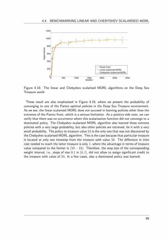
4.4. BENCHMARKING LINEAR AND CHEBYSHEV SCALARISED MORL
0 500 1000 1500 2000 2500 30000
200
400
600
800
1000
1200
Iteration
Hyp
erv
olu
me
Pareto front
Linear scalarized MORL
Chebyshev scalarized MORL
Figure 4.18: The linear and Chebyshev scalarised MORL algorithms on the Deep SeaTreasure world
These result are also emphasised in Figure 4.19, where we present the probability ofconverging to one of the Pareto optimal policies in the Deep Sea Treasure environment.As we see, the linear scalarised MORL does not succeed in learning policies other than theextremes of the Pareto front, which is a serious limitation. As a positive side note, we canverify that there was no occurrence where this scalarisation function did not converge to adominated policy. The Chebyshev scalarised MORL algorithm also learned these extremepolicies with a very large probability, but also other policies are retrieved, be it with a verysmall probability. The policy to treasure value 24 is the only one that was not discovered bythe Chebyshev scalarised MORL algorithm. This is the case because that particular treasureis located at only one timestep from the treasure with value 50. The di�erence in timecost needed to reach the latter treasure is only 1, where the advantage in terms of treasurevalue compared to the former is (50 ≠ 24). Therefore, the step size of the correspondingweight interval, i.e., steps of size 0.1 in [0, 1], did not allow to assign significant credit tothe treasure with value of 24. In a few cases, also a dominated policy was learned.
99

CHAPTER 4. LEARNING A SINGLE MULTI-OBJECTIVE POLICY
1 2 3 5 8 16 24 50 74 124 Dom.0
0.1
0.2
0.3
0.4
0.5
0.6
0.7
Policy (Treasure value)
Pro
babili
ty
Linear scalarized MORL
Chebyshev scalarized MORL
Figure 4.19: The retrieved policies for the linear and Chebyshev scalarised MORL al-gorithms on the Deep Sea Treasure world
4.4.4 Mountain car worldThe single-objective Mountain Car world is a famous benchmark for reinforcement learningalgorithms. In this world, a car is required to escape a one-dimensional valley. As the car’sengine is less powerful than gravity, the vehicle must perform a series of acceleration andreversal actions to build enough potential energy to escape the valley. A visual representa-tion of the environment can be found in Figure 4.20. The state space of the environmentis a continuous domain of velocity and position coordinates. Traditionally, one would usefunction approximation techniques to deal with the continuous state space, such as forinstance tile coding (Sutton and Barto, 1998). To simplify the setting, we discretised bothcontinuous domains into a 6 ◊ 6 grid. The action space consists of three actions: fullthrottle forward, full throttle backward, and zero throttle. The multi-objective version ofthis benchmark is challenging as it consists of three objectives that are to be optimised.The three objectives are (1) the time required to escape the valley and (2) the number ofacceleration and (3) reversal actions, which are all to be minimised. The Pareto optimal setcontains 470 dominating policies and the maximum amount of steps allowed to reach thegoal location is 500 steps (Vamplew et al., 2010). It is important to note that the shapeof the Pareto optimal set has a significant portion of locally convex and non-convex areas.
100
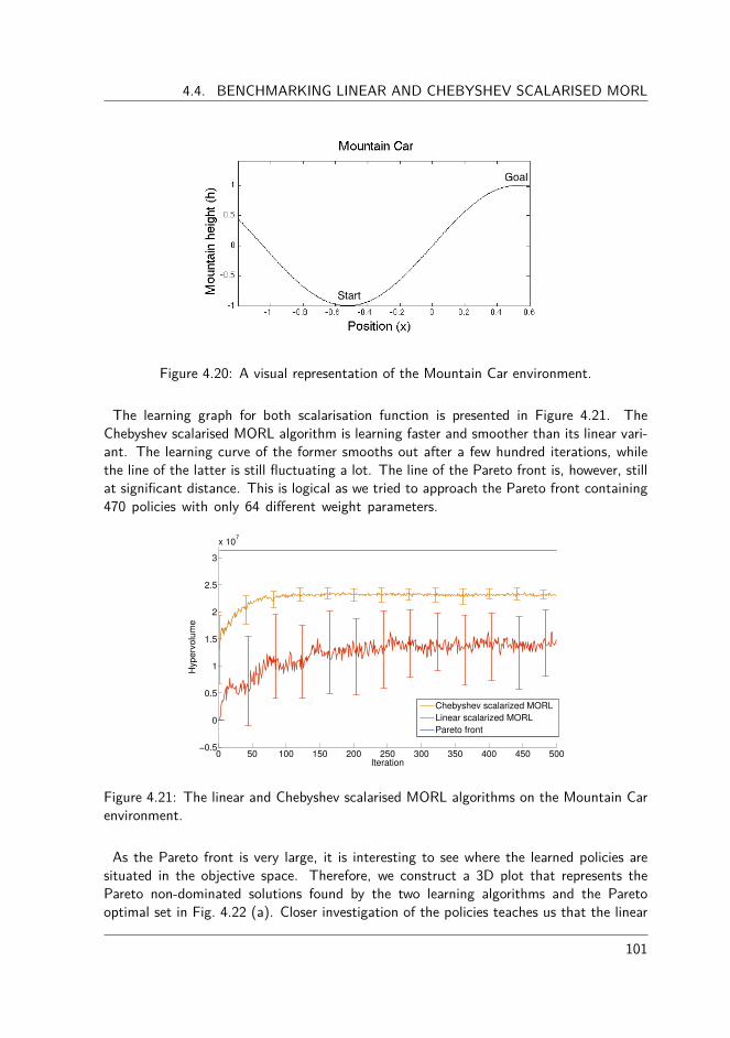
4.4. BENCHMARKING LINEAR AND CHEBYSHEV SCALARISED MORL
magnitude bias.7 We slightly modify the formulation from [32], byranking Q-values, instead of policy probabilities, i.e. let r : D�A �N be the ranking map of a demon. Then rd(a) > rd(a�), if and onlyif Qd(s, a) > Qd(s, a�). The combination or ensemble policy actsgreedily w.r.t. the cumulative preference values P :
P (st, a) =
|D|�1�
d=1
rd(a), �a � A (10)
In the next section we validate our approach on the typical moun-tain car benchmark and interpret the results.
5 Experiments
In this section we give comparison results between the individuals inour ensemble, and the combination policy. We remind the reader thatwhile all policies eventually arrive at the same (optimal) solution, ourfocus is the time it takes them to get there.
We focus our attention to a classical benchmark domain ofmountain car [24]. The task is to drive an underpowered car upa hill (Fig. 2). The (continuous) state of the system is composedof the current position (in [�1.2, 0.6]) and the current velocity(in [�0.07, 0.07]) of the car. Actions are discrete, a throttle of{�1, 0, 1}. The agent starts at the position �0.5 and a velocity of0, and the goal is at the position 0.6. The rewards are �1 for everytime step. An episode ends when the goal is reached, or when 2000steps8 have elapsed. The state space is approximated with the stan-dard tile-coding technique [24], using ten tilings of 10 � 10, witha parameter vector learnt for each action. The behavior policy is auniform distribution over all actions at each time step.
Figure 2: The mountain car problem. The mountain height h is givenby h = sin(3x).
In this domain we define three intuitive shaping potentials. Eachis normalized into the range [0, 1].
Right shaping. Encourage progress to the right (in the direction ofthe goal). This potential is flawed by design, since in order to getto the goal, one needs to first move away from it.
�1(x) = cr � x (11)
7 Note that even though the shaped policies are the same upon convergence –the value functions are not.
8 Note the significantly shorter lifetime of an episode here, as compared toresults in Degris et al. [5]; since the shaped rewards are more informative,they can get by with very rarely reaching the goal.
Height shaping. Encourage higher positions (potential energy),where height h is computed according to the formula in Fig. 2.
�2(x) = ch � h (12)
Speed shaping. Encourage higher speeds (kinetic energy).
�3(x) = cs � |x|2 (13)
Here x = �x, x� is the state (position and velocity), and c =�cr, ch, cs� is a vector of tuned scaling constants.9
Thus our architecture has 4 demons: < d0, d1, d2, d3 >, where d0
learns on the base reward, and the others on their respective shapingrewards. The combination policy is formed via rank voting, whichwe found to outperform majority voting, and a variant of Q-valuevoting on this problem.
The third (speed) shaping turns out to be the most helpful univer-sally. If this is the case one would likely prefer to just use that singleshaping on its own, but we assume such information is not avail-able a priori, which is a more realistic (and challenging) situation.To make our experiment more interesting we consider two scenarios:with and without this best shaping. Ideally we would like our combi-nation method to be able to outperform the two comparable shapingsin the first scenario, and pick out the best shaping in the second sce-nario.
We used � = 0.99. The learning parameters were tuned and se-lected to be � = 0.4, � = 0.0001, � = �0.1, 0.05, 0.1, 0.1�, where� is the trace decay parameter, � the step size for the second set ofweights in Greedy-GQ, and � the vector of step sizes for the valuefunctions of our demons.10 We ran 1000 independent runs of 100episodes each. The evaluation was done by interrupting the off-policylearner every 5 episodes, and executing each demon’s greedy policyonce. No learning was allowed during evaluation. The graphs reflectthe average base reward. The initial and final performance refer tothe first and last 20% of a run.
Table 1: Results for the scenario with two comparable shapings. Thecombination has the best cumulative performance. In the initial
stage it is comparable to the right shaping, in the final – to the heightshaping (each being the best in the corresponding stages), overalloutperforming both. The results that are not significantly different
from the best (Student’s t-test with p > 0.05) are in bold.
PerformanceVariant Cumulative Initial FinalNo shaping -336.3 ± 279.5 -784.7 ± 385.9 -185.1 ± 9.9Right shaping -310.4 ± 96.9 -378.5 ± 217.4 -290.3 ± 19.3Height shaping -283.2 ± 205.2 -594.2 ± 317.0 -182.3 ± 7.5Combination -211.2 ± 94.2 -330.6 ± 179.5 -180.2 ± 1.5
The results in Fig. 3, and Tables 1 and 2 show that individual shap-ings alone aid learning speed significantly. The combination methodmeets our desiderata: it either statistically matches or is better thanthe best shaping at any stage, overall outperforming all single shap-ings. The exception is the final performance of the run in Scenario 2,where the performance of the best shaping is significantly different
9 The scaling of potentials is in general a challenging problem in rewardshaping research. Finding the right scaling factor requires a lot of a priorituning, and the factor is generally assumed constant over the state space.The scalable nature of Horde could be used to lift this problem, by learningmultiple preset scales for each potential, and combining them via either avoting method like the one described here, or a meta-learner. See Section 6.
10 These were tuned individually, as the value functions differ in magnitude.
4
Figure 4.20: A visual representation of the Mountain Car environment.
The learning graph for both scalarisation function is presented in Figure 4.21. TheChebyshev scalarised MORL algorithm is learning faster and smoother than its linear vari-ant. The learning curve of the former smooths out after a few hundred iterations, whilethe line of the latter is still fluctuating a lot. The line of the Pareto front is, however, stillat significant distance. This is logical as we tried to approach the Pareto front containing470 policies with only 64 di�erent weight parameters.
0 50 100 150 200 250 300 350 400 450 500−0.5
0
0.5
1
1.5
2
2.5
3
x 107
Iteration
Hyp
erv
olu
me
Chebyshev scalarized MORL
Linear scalarized MORL
Pareto front
Figure 4.21: The linear and Chebyshev scalarised MORL algorithms on the Mountain Carenvironment.
As the Pareto front is very large, it is interesting to see where the learned policies aresituated in the objective space. Therefore, we construct a 3D plot that represents thePareto non-dominated solutions found by the two learning algorithms and the Paretooptimal set in Fig. 4.22 (a). Closer investigation of the policies teaches us that the linear
101

CHAPTER 4. LEARNING A SINGLE MULTI-OBJECTIVE POLICY
scalarised MORL algorithm retrieved only 25 distinct Pareto non-dominated policies, whichare not necessarily members of the Pareto front. On the contrary, the Chebyshev scalarisedMORL algorithm obtained 38 distinct non-dominated solutions. Note that both algorithmswere run only 64 times, i.e., using 64 weight tuples. We also observe that the policiesobtained by the linear scalarisation method are, as expected, located in convex areas ofthe Pareto optimal set, while the Chebyshev function learned policies that are situated inboth convex and non-convex regions.
Next to optimality, the goal of a MORL algorithm is to ensure a significant spread inthe solution space. Ideally, when the obtained results are scattered across the objectivespace, the decision maker has a larger choice amongst very di�erent policies. On thecontrary, when policies are clustered into particular areas, often the di�erences betweenthose policies are minimal and they do not provide the decision maker with a diverse setof choices. In Figure 4.22 (b), (c) and (d), we present a sliced representation of the 3Dplot where we focus on only two objectives at a time. Note that the Chebyshev methodobtains a larger spread in the objective space, where the results of the linear scalarisationfunction are clustered into particular regions.
−250−200
−150−100
−500
−100
−50
0−400
−300
−200
−100
AccelerationsReversals
Tim
e
Chebyshev Q−learning
Linear scalarized Q−learning
Pareto front
−250 −200 −150 −100 −50 0
−80
−70
−60
−50
−40
−30
−20
−10
0
Accelerations
Reve
rsals
Chebyshev scalarized MORL
Linear scalarized MORL
Pareto front
(a) (b)
−200 −180 −160 −140 −120 −100 −80 −60 −40 −20 0−400
−350
−300
−250
−200
−150
−100
Accelerations
Tim
e
Chebyshev scalarized MORL
Linear scalarized MORL
Pareto front
−90 −80 −70 −60 −50 −40 −30 −20 −10 0−400
−350
−300
−250
−200
−150
−100
Reversals
Tim
e
Chebyshev scalarized MORL
Linear scalarized MORL
Pareto front
(c) (d)
Figure 4.22: The policies in the objective space of the linear and Chebyshev scalarisedMORL algorithms on the Mountain Car environment.
102

4.4. BENCHMARKING LINEAR AND CHEBYSHEV SCALARISED MORL
4.4.5 Resource gathering worldIn this final experiment, we analyse the performance on an entirely convex environment,named the Resource gathering task. In this environment, adapted from Barrett andNarayanan (2008), the agent goes on a quest to bring gold and gems to its home site.Upon returning to its starting location, the goods he acquired are analysed. The possiblegathering outcomes are bringing home nothing, gold, gems or gold and gems. A visualrepresentation of the environment is provided in Figure 4.23. The three objectives aretime, gold, and gems, and there are 4 Pareto optimal policies in this environment, i.e.,
1. a policy that returns to the home site as fast as possible without carrying anything,
2. a policy that gathers the gold and returns as fast as possible,
3. a similar one for the gems objective,
4. and a policy that gathers both resources as fast as possible.
These optimal policies are all located on the convex hull of the Pareto front as depictedin Figure 4.24.
Figure 4.23: A visual representation of the Resource Gathering environment.
103
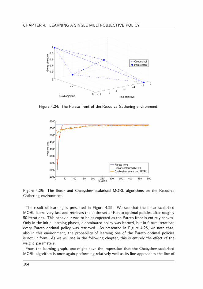
CHAPTER 4. LEARNING A SINGLE MULTI-OBJECTIVE POLICY
−12−10
−8−6
−4−2
0
0
0.5
10
0.2
0.4
0.6
0.8
1
Time objectiveGold objective
Gem
s obje
ctiv
e
Convex hull
Pareto front
Figure 4.24: The Pareto front of the Resource Gathering environment.
0 50 100 150 200 250 300 350 400 450 5002000
2500
3000
3500
4000
4500
5000
5500
6000
Iteration
Hyp
erv
olu
me
Pareto front
Linear scalarized MORL
Chebyshev scalarized MORL
Figure 4.25: The linear and Chebyshev scalarised MORL algorithms on the ResourceGathering environment.
The result of learning is presented in Figure 4.25. We see that the linear scalarisedMORL learns very fast and retrieves the entire set of Pareto optimal policies after roughly50 iterations. This behaviour was to be as expected as the Pareto front is entirely convex.Only in the initial learning phases, a dominated policy was learned, but in future iterationsevery Pareto optimal policy was retrieved. As presented in Figure 4.26, we note that,also in this environment, the probability of learning one of the Pareto optimal policiesis not uniform. As we will see in the following chapter, this is entirely the e�ect of theweight parameters.
From the learning graph, one might have the impression that the Chebyshev scalarisedMORL algorithm is once again performing relatively well as its line approaches the line of
104
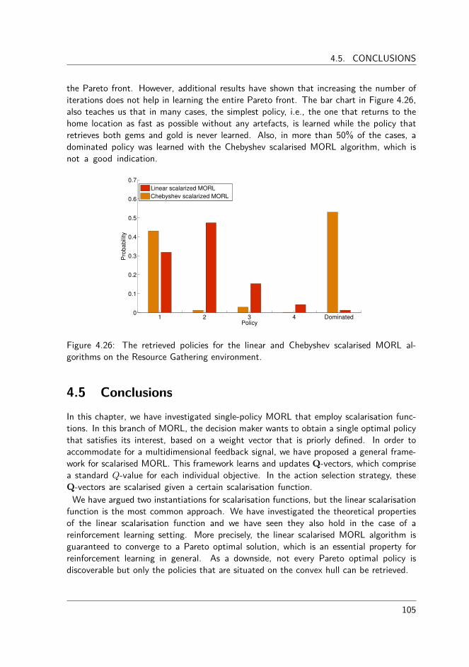
4.5. CONCLUSIONS
the Pareto front. However, additional results have shown that increasing the number ofiterations does not help in learning the entire Pareto front. The bar chart in Figure 4.26,also teaches us that in many cases, the simplest policy, i.e., the one that returns to thehome location as fast as possible without any artefacts, is learned while the policy thatretrieves both gems and gold is never learned. Also, in more than 50% of the cases, adominated policy was learned with the Chebyshev scalarised MORL algorithm, which isnot a good indication.
1 2 3 4 Dominated0
0.1
0.2
0.3
0.4
0.5
0.6
0.7
Policy
Pro
ba
bili
ty
Linear scalarized MORL
Chebyshev scalarized MORL
Figure 4.26: The retrieved policies for the linear and Chebyshev scalarised MORL al-gorithms on the Resource Gathering environment.
4.5 ConclusionsIn this chapter, we have investigated single-policy MORL that employ scalarisation func-tions. In this branch of MORL, the decision maker wants to obtain a single optimal policythat satisfies its interest, based on a weight vector that is priorly defined. In order toaccommodate for a multidimensional feedback signal, we have proposed a general frame-work for scalarised MORL. This framework learns and updates Q-vectors, which comprisea standard Q-value for each individual objective. In the action selection strategy, theseQ-vectors are scalarised given a certain scalarisation function.
We have argued two instantiations for scalarisation functions, but the linear scalarisationfunction is the most common approach. We have investigated the theoretical propertiesof the linear scalarisation function and we have seen they also hold in the case of areinforcement learning setting. More precisely, the linear scalarised MORL algorithm isguaranteed to converge to a Pareto optimal solution, which is an essential property forreinforcement learning in general. As a downside, not every Pareto optimal policy isdiscoverable but only the policies that are situated on the convex hull can be retrieved.
105

CHAPTER 4. LEARNING A SINGLE MULTI-OBJECTIVE POLICY
In general multi-objective optimization, the Chebyshev scalarisation function is proven tobe able to discover every Pareto optimal solution, regardless of the shape of the Paretofront. However, researchers have analysed that this property does not hold in MORL. Inthis chapter, we empirically investigate to what degree this theoretical limitation e�ectsthe behaviour of the learning agent in practice. After thoroughly investigating both scal-arisation functions on three benchmark instances, we have seen that in most cases, theChebyshev scalarised MORL performs acceptably and is able to find policies the linearscalarised MORL algorithm does not manage to retrieve. As a drawback, this performanceis very parameter-specific and in a significant amount of cases, the Chebyshev scalarisedMORL indeed converges to a suboptimal policy. As a conclusion we could state that theChebyshev scalarised MORL algorithm does not solve all the limitations of the linear scal-arisation function but it has the potential to significantly improve its performance in termsof the optimality of the solution and their spread in the objective space. In its strictestform, one could state that non-linearity and MORL inherently exclude each other due thelack of additivity. However, the search for non-linear scalarisation functions that can beused to enhance the performance of single-policy optimisation should not take a halt atthis point. We highlight three scenarios where non-linear scalarisation function can stillbe employed and that can potentially guide future research.
For starters, one could combine temporal di�erence learning with a non-linear scalarisationfunction in pure form, that is without any refinement or restrictions. In such case, thescalarisation function should be used as a heuristics that is not founded on any theoreticalprinciples but that can guide the search to potential fruitful areas of the objective space.The work in Van Mo�aert et al. (2013b,a,c) falls in this category.
Secondly, it is possible to combine temporal di�erence learning with a non-linear scal-arisation function, be it in a more restricted form. To solve the issue of non-additivity,one can alter either the learning algorithm itself or its state representation (Geibel, 2006).Nevertheless, this approach remains very specific and complex. Additionally, as mentionedby Roijers et al. (2013), the speed of learning su�ers from this workaround. Yet, it wouldundoubtedly be of great interest to further investigate this path.
Thirdly, one could investigate the use of non-linear scalarisation functions also outsidethe temporal di�erence setting. Instead of adopting a value-iteration approach wherea value function is learned, one could learn a policy directly. These are policy-searchmethods which directly and iteratively update a single policy without learning a valuefunction first. In that facet, policy-gradient methods for MORL have also been proposed.In Uchibe and Doya (2007), a policy-gradient algorithm is proposed that learns in a directand iterative manner a single policy satisfying predefined constraints. This algorithm iscalled constrained policy gradient reinforcement learning (CPGRL) as it iteratively updatesthe policy in the direction of a gradient satisfying one or more constraints. As CPGRLdoes not learn in a temporal di�erence manner, it poses no problem in combining it witha non-linear scalarisation function.
106

4.6. SUMMARY
4.6 SummaryIn this chapter, we investigated single-policy MORL that rely on scalarisation functionsto transform the dimensionality of the reward signal to a single dimension. We haveproposed a framework that allows to reuse standard reinforcement learning algorithmsin a multi-objective setting by employing a scalarisation function in the action selectionstrategy. We have theoretically and empirically analysed the linear and the non-linearChebyshev scalarisation function and emphasised their advantages and limitations. Wehave seen that non-linearity and temporal di�erence learning do not synthesise well due tothe lack of additivity of the scalarised returns. However, we have illuminated several pathsfor future research that can boost the development of learning algorithms that handle anon-linear scalarisation function.
107


5
| Iteratively learningmultiple multi-objective
policies
In the previous chapter, we have investigated into MORL algorithms that employ a scalar-isation function and a weight vector to discover a single trade-o� solution. In this chapter,we explore how this single-policy setting can be augmented to obtain multiple policiesby adaptively varying the weight vector. The main question to research is then how toconsecutively redefine the weight vector in other to find a diverse set of trade-o� solutionstaking into account the relation between the weight vector and the slope of the Paretocurve. As pointed out in Das and Dennis (1997), this relation is non-isomorphic, meaningthat the mapping from the weight space to the converged solution in the objective spaceis unclear. In this chapter, we will dig deep into this problem and highlight the reasonsfor this relation. We will propose two tree-based mechanisms that allow to define adapt-ive weights in the case of a discrete and continuous Pareto front. These techniques areexperimentally validated on several benchmark problems and conclusions are formalised.
In more detail, we will present the following contributions in this chapter:
• Analyse how single-policy algorithms can obtain multiple policies• Investigate the non-isomorphic mapping from weight to objective space• Propose an adaptive weight algorithm that can e�ciently explore discrete Pareto
fronts• A similar set of algorithms that can e�ciently explore continuous Pareto fronts
This research has been published in Van Mo�aert et al. (2014a) and in Van Mo�aertet al. (2013).
109

CHAPTER 5. ITERATIVELY LEARNING MULTIPLE MULTI-OBJECTIVE POLICIES
5.1 Iteratively learning an archive of trade-o� solutionsOver the years, a few mechanisms have been proposed to obtain a set of trade-o� solutionswith single-policy algorithms. Usually, a single-policy algorithm is run multiple times andits resulting policies are collected in an archive or approximation set, denoted by A. Forinstance, one can run the linear scalarisation algorithm many times for varying weightvectors to approximate the convex hull of the Pareto front (Castelletti et al., 2002; Vamplewet al., 2008, 2010). In the case the Pareto front is continuous, it is both impossible andunnecessary to retrieve every Pareto optimal solution. In this respect, the idea is to findan archive that is both (i) (close to) optimal and (ii) diverse, using a predefined numberof weights. Diversity is a very important aspect as it is important to guarantee that thepolicies are not clustered into particular areas of the objective space, but that they identifydiverse trade-o�s that the decision maker can choose from. In Figure 5.1 (a), we depicta poor archive since some policies tend to be clustered in specific areas while leavingother regions of the objective space uncharted. In Figure 5.1 (b), the policies are morewidespread and, therefore they define a better approximation.
0.2 0.4 0.6 0.8 10
0.2
0.4
0.6
0.8
1
Objective 1
Ob
ject
ive
2
0.2 0.4 0.6 0.8 10
0.2
0.4
0.6
0.8
1
Objective 1
Ob
ject
ive
2
(a) (b)
Figure 5.1: A poor approximation of a continuous Pareto front is shown in (a), while in(b) the policies are more diverse and spread across the objective space.
A common strategy is to uniformly and evenly divide the weight space in chunks of equalsize and to collect the results. Nevertheless the approach, being simple and intuitive, isproven not to provide an even spread of solutions in the objective space. Moreover, aspointed out by Das and Dennis (1997), only for very specific shapes of the Pareto front, aneven spread in the weight space provides an even spread in the objective space. Basically,without any prior knowledge on the shape of the Pareto front, it is impossible to foreseewhat point in the objective space a certain weight vector will yield. In layman’s terms,learning with a weight vector of (0.8, 0.2) does not guarantee that the solution obtainedwill compromise 80% of the best solution for the first objective and 20% of the best
110
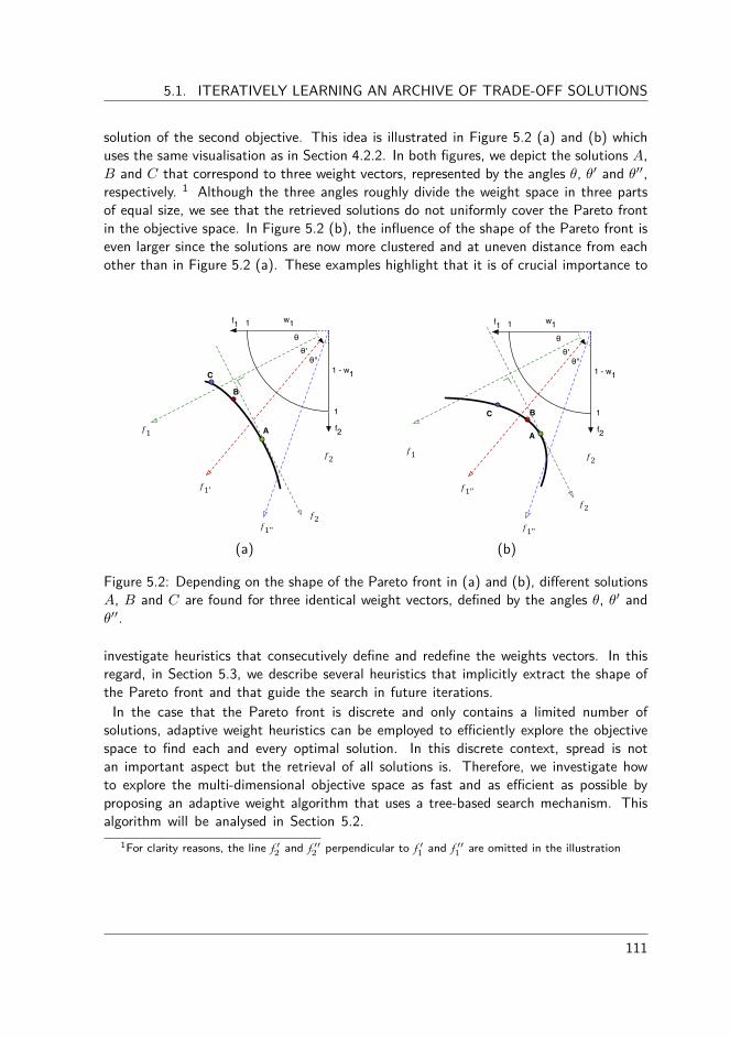
5.1. ITERATIVELY LEARNING AN ARCHIVE OF TRADE-OFF SOLUTIONS
solution of the second objective. This idea is illustrated in Figure 5.2 (a) and (b) whichuses the same visualisation as in Section 4.2.2. In both figures, we depict the solutions A,B and C that correspond to three weight vectors, represented by the angles ◊, ◊Õ and ◊ÕÕ,respectively. 1 Although the three angles roughly divide the weight space in three partsof equal size, we see that the retrieved solutions do not uniformly cover the Pareto frontin the objective space. In Figure 5.2 (b), the influence of the shape of the Pareto front iseven larger since the solutions are now more clustered and at uneven distance from eachother than in Figure 5.2 (a). These examples highlight that it is of crucial importance to
θ
w11
1 - w1
1
f1
f2
B
!1
!2
!1'
!1''
θ'θ''
A
C
!2
θ
w11
1 - w1
1
f1
f2
B
!1 !2
!1''
!1''
θ'θ''
A
C
!2
(a) (b)
Figure 5.2: Depending on the shape of the Pareto front in (a) and (b), di�erent solutionsA, B and C are found for three identical weight vectors, defined by the angles ◊, ◊Õ and◊ÕÕ.
investigate heuristics that consecutively define and redefine the weights vectors. In thisregard, in Section 5.3, we describe several heuristics that implicitly extract the shape ofthe Pareto front and that guide the search in future iterations.
In the case that the Pareto front is discrete and only contains a limited number ofsolutions, adaptive weight heuristics can be employed to e�ciently explore the objectivespace to find each and every optimal solution. In this discrete context, spread is notan important aspect but the retrieval of all solutions is. Therefore, we investigate howto explore the multi-dimensional objective space as fast and as e�cient as possible byproposing an adaptive weight algorithm that uses a tree-based search mechanism. Thisalgorithm will be analysed in Section 5.2.
1For clarity reasons, the line f Õ2 and f ÕÕ
2 perpendicular to f Õ1 and f ÕÕ
1 are omitted in the illustration
111

CHAPTER 5. ITERATIVELY LEARNING MULTIPLE MULTI-OBJECTIVE POLICIES
5.1.1 Related WorkSeveral researchers have attempted to define adaptive weighting schemes in the case ofgeneral optimisation problems. For continuous Pareto fronts, Dubois-Lacoste et al. (2011)proposed a series of algorithms that alter the weight of a linear scalarisation function witha so-called dichotomic scheme to specify the direction of search. As the optimisationalgorithm relies on a linear scalarisation of objectives, only solutions on the convex hullof the Pareto front are retrieved, as we have seen in Section 4.2. These adaptive weightalgorithms are created specifically for stochastic local search algorithms. Internally, theycombine interesting techniques such as divide-and-conquer by either progressively explor-ing finer levels or by moving the search towards solutions that comprise the largest gapaccording to several metrics.
In Das and Dennis (1998), the normal boundary intersection (NBI) algorithm is proposed.NBI is able to produce an evenly distributed set of solutions given an evenly distributedset of parameters. In its internal workings, NBI breaks the original problem down into aset of subproblems, each with a specific scalarisation scheme. This scalarisation scheme isindi�erent of the relative scales of objective functions but it is not guaranteed to retrieveoptimal solutions in non-convex regions of the Pareto front.
To overcome the limitation of the linear scalarisation function concerning non-convexity,Kim and de Weck (2005) suggest to combine an adaptive weighting scheme with ad-ditional inequality constraints. Their algorithm divides the original problem into severalsubproblems that each focus on particular regions of the objective space. By continuouslyrefining these regions, the algorithm is able to discover an even spread of solutions in bothconvex and non-convex regions of the Pareto front.
These approaches have proven their usefulness in general optimisation processes involvingstate-less and usually deterministic problems. However, they are not ideal for sequentialmulti-objective reinforcement learning problems where the state space can be large andwhere both the transition function as the reward signal can be stochastic. In Section 5.2and 5.3, we propose two mechanisms that allow to repeatedly use single-policy MORLalgorithms to obtain multiple policies in both discrete as well as continuous Pareto fronts.
5.2 Adaptive weight algorithms for discrete Pareto frontsIn some situations the system engineer might have some insights in the solution spaceof the problem. For instance, in case the dynamics of in the environments are ratherdeterministic and the number of actions limited, the number of optimal solutions in theobjective space usually restricted. However, for the system engineer to find the appropriateweight configurations that retrieve all solutions with minimal computational e�ort is nottrivial. To stress this statement, one can investigate the correspondence of the weight spaceto the objective space of the Bountiful Sea Treasure environment, previously introducedin Section 4.3.4. The objective space of the environment contains 10 Pareto optimalsolutions that are each retrievable with a certain weight vector. In Figure 5.3 (a), we
112

5.2. ADAPTIVE WEIGHT ALGORITHMS FOR DISCRETE PARETO FRONTS
denote an exhaustive sweep of the weight space and the converged policy in the objectivespace. On the x-axis, we depict the weight w1 assigned to the first objective while theweight of the second objective is w2 = 1 ≠ w1. We see that several areas in the weightspace emerge that each converge to the same solutions. However, it is clear that somepolicies correspond to a much larger set of weights than others, e.g., the blue policy occursmuch more frequently than the yellow policy. Additionally, some policies correspond tosuch a restricted set of weights that (1) a uniform sampling of the weight space will bebiased towards particular policies and (2) it is unrealistic that the system engineer wouldever find it by purely guessing the weights. This aspect is highlighted in Figure 5.3 (b)where we depict a zoomed-in portion of a particular area of Figure 5.3 (a). We notethat the interval of weights that converge to the green policy is very narrow and locatedbetween the yellow and turquoise policies. Subsequently, when the number of objectivesincreases, also the number of decision variables, i.e., the weights, increases, which makesthe problem of retrieving all optimal solutions even harder.
Therefore, we elaborate on an algorithm that e�ciently explores the weight space of anym-dimensional problem in order to find every optimal solution with as minimal computa-tional e�ort as possible. This algorithm will be unveiled in the upcoming section.
0 0.1 0.2 0.3 0.4 0.5 0.6 0.7 0.8 0.9 1Weight W
1
Policy
0 0.02 0.04 0.06 0.08 0.1 0.12Weight W
1
Policy
(a) (b)
Figure 5.3: In (a), we depict the mapping of weight space to objective space of theBountiful Sea Treasure environment. In (b), we present a zoomed-in area of (a) and wenote that some policies are only retrievable for a very restricted set of weights.
5.2.1 The algorithmThe algorithm we propose is a tree search algorithm that can be incorporated with anunderlying single-policy MORL algorithm, such as the linear scalarised MORL algorithmof Section 4.2. The tree search algorithm incrementally supplies a sequence of weightconfigurations to e�ciently explore the weight space. In computer science, searching isoften performed with tree-like structures as their hierarchical composition makes themvery e�cient for searching purposes.
113

CHAPTER 5. ITERATIVELY LEARNING MULTIPLE MULTI-OBJECTIVE POLICIES
Our tree search algorithm exploits two properties of convex linear combinations. First,we know that the weight space for linear scalarisation is always (m≠1)≠dimensional, withm the number of objectives. This is due to the fact that all weights must sum to 1, andtherefore setting all but one weight is enough to also fix the value for the last weight.Selecting a specific weight assignment w = (w1, w2, . . . , wm) transforms the MOMDPinto a standard MDP where the optimal policy is also the Pareto optimal policy of theoriginal MOMDP.
Another important aspect of convex Pareto optimal sets is that the set of policies that isoptimal for a weight wo œ [0, 1] are precisely those policies whose line-representations lieon the upper convex envelope of the Q-functions (Ehrgott, 2005), i.e., if for two di�erentweight assignments w and w
Õ the same policy is optimal, it is also optimal for the weightassignments between w and w
Õ.The aim of our method is to take benefit from these properties and exploit the structure of
convex hulls to identify the weight space regions that are associated with a particular Paretooptimal policy, and specifically by recursively refining the boundaries of these regions.
0 1w1
0 10.5w1
(a) Tree level 1 (b) Tree level 2
0 10.25w1
0 10.375w1
(c) Tree level 3 (d) Tree level 4
Figure 5.4: A visualisation of the exploration of the weight space of a bi-objective problem.In this case, the weight w1 (x-axis) is the only decision variable, since w2 = 1 ≠ w1.Di�erent symbols and colours identify di�erent Pareto optimal policies.
Initially, the algorithm starts by solving the MOMDP using the linear scalarised MORLalgorithm of Chapter 4 with the weight combinations that define the boundaries of theentire weight space. For instance, for a bi-objective problem, the two extrema are (w1 =
0, w2 = 1) and (w1 = 1, w2 = 0). As a running example, we visualise the search process fora bi-objective toy problem in Figure 5.4 (a), with di�erent symbols and colours identifyingdi�erent Pareto optimal policies. If the discounted cumulative rewards of the convergedpolicies are identical, our search stops since we can conclude that there is only one Pareto
114
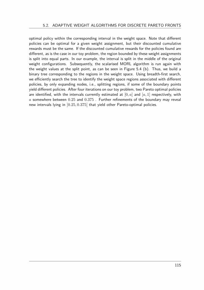
5.2. ADAPTIVE WEIGHT ALGORITHMS FOR DISCRETE PARETO FRONTS
optimal policy within the corresponding interval in the weight space. Note that di�erentpolicies can be optimal for a given weight assignment, but their discounted cumulativerewards must be the same. If the discounted cumulative rewards for the policies found aredi�erent, as is the case in our toy problem, the region bounded by these weight assignmentsis split into equal parts. In our example, the interval is split in the middle of the originalweight configurations. Subsequently, the scalarised MORL algorithm is run again withthe weight values at the split point, as can be seen in Figure 5.4 (b). Thus, we build abinary tree corresponding to the regions in the weight space. Using breadth-first search,we e�ciently search the tree to identify the weight space regions associated with di�erentpolicies, by only expanding nodes, i.e., splitting regions, if some of the boundary pointsyield di�erent policies. After four iterations on our toy problem, two Pareto optimal policiesare identified, with the intervals currently estimated at [0, a] and [a, 1] respectively, witha somewhere between 0.25 and 0.375 . Further refinements of the boundary may revealnew intervals lying in ]0.25, 0.375[ that yield other Pareto-optimal policies.
115
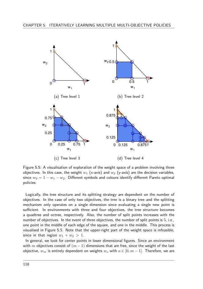
CHAPTER 5. ITERATIVELY LEARNING MULTIPLE MULTI-OBJECTIVE POLICIES
10
1
w1
w2
10
1
0.5
0.5w1
w2
(a) Tree level 1 (b) Tree level 2
10
1
0.75
0.25 0.75
0.25
w1
w2
10
1
0.125 0.875
0.125
0.875
w1
w2
(c) Tree level 3 (d) Tree level 4
Figure 5.5: A visualisation of exploration of the weight space of a problem involving threeobjectives. In this case, the weight w1 (x-axis) and w2 (y-axis) are the decision variables,since w3 = 1 ≠ w1 ≠ w2. Di�erent symbols and colours identify di�erent Pareto optimalpolicies.
Logically, the tree structure and its splitting strategy are dependent on the number ofobjectives. In the case of only two objectives, the tree is a binary tree and the splittingmechanism only operates on a single dimension since evaluating a single new point issu�cient. In environments with three and four objectives, the tree structure becomesa quadtree and octree, respectively. Also, the number of split points increases with thenumber of objectives. In the event of three objectives, the number of split points is 5, i.e.,one point in the middle of each edge of the square, and one in the middle. This process isvisualised in Figure 5.5. Note that the upper-right part of the weight space is infeasible,since in that region w1 + w2 > 1.
In general, we look for center points in lower dimensional figures. Since an environmentwith m objectives consist of (m ≠ 1) dimensions that are free, since the weight of the lastobjective, wm is entirely dependent on weights wo with o œ [0, m ≠ 1]. Therefore, we are
116

5.2. ADAPTIVE WEIGHT ALGORITHMS FOR DISCRETE PARETO FRONTS
iterating through geometrical hypercubes lower than dimension (m ≠ 1), i.e., dimension1 (points) to dimension (m ≠ 2). Moreover, we know that a hypercube of dimension zcontains 2
z vertices, e.g., a cube has 8 vertices. Each of these vertices of the z-dimensionalfigure plays a role in one or more lower dimensional figures of dimension (z ≠ 1). Forinstance, a vertex of a cube is part of three faces of dimension 2. Therefore, we can usethe combinatorial binomial coe�cient to know how many times a vertex in a space with(m ≠ 1) dimensions can be used in a space with only k < (m ≠ 1) dimensions. This is!m≠1
k
". Of course, we are counting some doubles, so we have to subtract 2
k. In the formulabelow, we calculate the sum of lower dimensional figures by iterating with k. Additionally,we also add one point, this is the center point of the (m ≠ 1) dimensional figure itself.
1 +
m≠2ÿ
k=12
m≠1≠k
3m ≠ 1
k
4= 1 +
m≠2ÿ
k=12
m≠1≠k (m ≠ 1)!
k!(m ≠ 1 ≠ k)!
. (5.1)
For example, for an environment with four objectives, the tree structure is an octree andthe geometrical figures we are splitting are cubes. In that case, the number of split pointsto be evaluated is equal to the number of edges, i.e., one split point in the middle of eachedge, plus the number of faces, i.e., one split point in the middle of each face, plus 1split point for the middle of the cube:
1 + 12 + 6 = 19. (5.2)
5.2.2 Experimental evaluationIn this section, we will perform an empirical evaluation of di�erent weight schemes onseveral MORL benchmark instances.
5.2.3 The Bountiful Sea Treasure worldWe first analyse the tree-based algorithm on the standard Bountiful Sea Treasure (BST)environment of Section 4.3.4. The correspondence of the weight space to the objectivespace of that environment is already depicted in Figure 5.3. In the experiments, we compareour algorithm to two alternative weight schemes that are often employed in literature. Thefirst scheme is a predefined sequence of weights that divide the weight space in chunks ofequal size. The second scheme is an unbiased, uniform random weight selection strategy.We analyse the results by investigating the cardinality, i.e., the number of optimal elementsobtained over time compared to the size of the Pareto front.
117
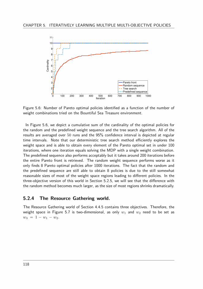
CHAPTER 5. ITERATIVELY LEARNING MULTIPLE MULTI-OBJECTIVE POLICIES
0 100 200 300 400 500 600 700 800 900 10001
2
3
4
5
6
7
8
9
10
11
Iteration
Ca
rdin
alit
y
Pareto frontRandom sequenceTree searchPredefined sequence
Figure 5.6: Number of Pareto optimal policies identified as a function of the number ofweight combinations tried on the Bountiful Sea Treasure environment.
In Figure 5.6, we depict a cumulative sum of the cardinality of the optimal policies forthe random and the predefined weight sequence and the tree search algorithm. All of theresults are averaged over 50 runs and the 95% confidence interval is depicted at regulartime intervals. Note that our deterministic tree search method e�ciently explores theweight space and is able to obtain every element of the Pareto optimal set in under 100iterations, where one iteration equals solving the MDP with a single weight combination.The predefined sequence also performs acceptably but it takes around 200 iterations beforethe entire Pareto front is retrieved. The random weight sequence performs worse as itonly finds 8 Pareto optimal policies after 1000 iterations. The fact that the random andthe predefined sequence are still able to obtain 8 policies is due to the still somewhatreasonable sizes of most of the weight space regions leading to di�erent policies. In thethree-objective version of this world in Section 5.2.5, we will see that the di�erence withthe random method becomes much larger, as the size of most regions shrinks dramatically.
5.2.4 The Resource Gathering world.The Resource Gathering world of Section 4.4.5 contains three objectives. Therefore, theweight space in Figure 5.7 is two-dimensional, as only w1 and w2 need to be set asw3 = 1 ≠ w1 ≠ w2.
118

5.2. ADAPTIVE WEIGHT ALGORITHMS FOR DISCRETE PARETO FRONTS
Figure 5.7: The four Pareto optimal policies in the Resource Gathering world and itsassociated locations in the weight space.
From this figure, we can clearly see the four large, distinct regions, which should ease thediscovery of the four Pareto optimal policies. In Figure 5.8 we summarise the performanceon this benchmark instance. We notice that, although there are no huge di�erencesin size between the various regions, the random sequence on average needs up to 50iterations. The predefined weight sequence is doing a bit better although still 22 weightconfigurations are tried before every solution is found. We also see that the performanceof this scheme is often stagnating and plateaus are formed where a lot of weights are oftenretrieving policies that were found in previous iterations. Obviously, this is because thescheme provides weights that are at a predefined distance from one another rather thandetermined adaptively. Finally, the tree-based search algorithm only requires 5 iterationsat minimum cost of resources.
119

CHAPTER 5. ITERATIVELY LEARNING MULTIPLE MULTI-OBJECTIVE POLICIES
5 10 15 20 25 30 35 40 45 500.5
1
1.5
2
2.5
3
3.5
4
Iteration
Card
inalit
y
Pareto frontRandom sequenceTree searchPredefined sequence
Figure 5.8: The number of Pareto optimal policies identified as a function of the numberof weight combinations tried for di�erent search algorithms on the Resource Gatheringworld.
5.2.5 The Bountiful Sea Treasure 3D worldAdditionally, we extend the two-dimensional BST by adding a third objective, namely the
pressure objective. This objective relates to the depth of the submarine and a penaltyis given linear to this depth, i.e., at every step, the agent receives a reward of ≠depth.As a result, the Pareto optimal set still consists of 10 optimal policies, but instead ofallowing for any shortest path to a treasure, the submarine must travel as long as possiblein the shallowest water before making its descent to a particular treasure. Therefore, theBountiful Sea Treasure 3D world is the most challenging environment of the three discussedhere. As is clear from the weight space in Figure 5.9 (a), a single policy is optimal in 95%of the space, while the other optimal policies are only obtained for a very specific set ofweights (see the zoomed-in representation in Figure 5.9 (b)). Even using a brute-forceexploration of the weight space, while trying all weight combinations with increments of0.001, only allowed to discover 7 of the 10 Pareto optimal policies. This again shows thatuniformly sampling the weight space to identify the convex parts of the Pareto optimalset can be a very ine�cient procedure indeed.
120
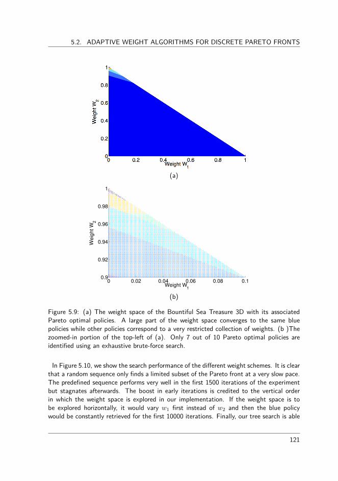
5.2. ADAPTIVE WEIGHT ALGORITHMS FOR DISCRETE PARETO FRONTS
(a)
0 0.02 0.04 0.06 0.08 0.10.9
0.92
0.94
0.96
0.98
1
Weight W1
Weig
ht W
2
(b)
Figure 5.9: (a) The weight space of the Bountiful Sea Treasure 3D with its associatedPareto optimal policies. A large part of the weight space converges to the same bluepolicies while other policies correspond to a very restricted collection of weights. (b )Thezoomed-in portion of the top-left of (a). Only 7 out of 10 Pareto optimal policies areidentified using an exhaustive brute-force search.
In Figure 5.10, we show the search performance of the di�erent weight schemes. It is clearthat a random sequence only finds a limited subset of the Pareto front at a very slow pace.The predefined sequence performs very well in the first 1500 iterations of the experimentbut stagnates afterwards. The boost in early iterations is credited to the vertical orderin which the weight space is explored in our implementation. If the weight space is tobe explored horizontally, it would vary w1 first instead of w2 and then the blue policywould be constantly retrieved for the first 10000 iterations. Finally, our tree search is able
121
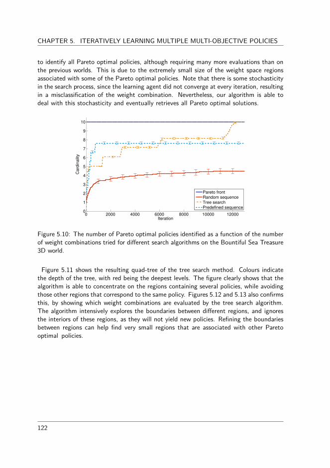
CHAPTER 5. ITERATIVELY LEARNING MULTIPLE MULTI-OBJECTIVE POLICIES
to identify all Pareto optimal policies, although requiring many more evaluations than onthe previous worlds. This is due to the extremely small size of the weight space regionsassociated with some of the Pareto optimal policies. Note that there is some stochasticityin the search process, since the learning agent did not converge at every iteration, resultingin a misclassification of the weight combination. Nevertheless, our algorithm is able todeal with this stochasticity and eventually retrieves all Pareto optimal solutions.
0 2000 4000 6000 8000 10000 120000
1
2
3
4
5
6
7
8
9
10
Iteration
Card
inalit
y
Pareto frontRandom sequenceTree searchPredefined sequence
Figure 5.10: The number of Pareto optimal policies identified as a function of the numberof weight combinations tried for di�erent search algorithms on the Bountiful Sea Treasure3D world.
Figure 5.11 shows the resulting quad-tree of the tree search method. Colours indicatethe depth of the tree, with red being the deepest levels. The figure clearly shows that thealgorithm is able to concentrate on the regions containing several policies, while avoidingthose other regions that correspond to the same policy. Figures 5.12 and 5.13 also confirmsthis, by showing which weight combinations are evaluated by the tree search algorithm.The algorithm intensively explores the boundaries between di�erent regions, and ignoresthe interiors of these regions, as they will not yield new policies. Refining the boundariesbetween regions can help find very small regions that are associated with other Paretooptimal policies.
122
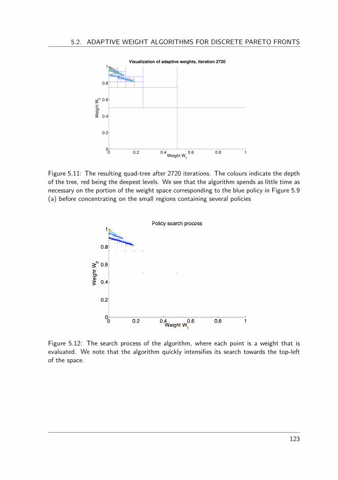
5.2. ADAPTIVE WEIGHT ALGORITHMS FOR DISCRETE PARETO FRONTS
0 0.2 0.4 0.6 0.8 10
0.2
0.4
0.6
0.8
1
Weight W1
Weig
ht W
2
Visualization of adaptive weights, iteration 2720
Figure 5.11: The resulting quad-tree after 2720 iterations. The colours indicate the depthof the tree, red being the deepest levels. We see that the algorithm spends as little time asnecessary on the portion of the weight space corresponding to the blue policy in Figure 5.9(a) before concentrating on the small regions containing several policies
Figure 5.12: The search process of the algorithm, where each point is a weight that isevaluated. We note that the algorithm quickly intensifies its search towards the top-leftof the space.
123

CHAPTER 5. ITERATIVELY LEARNING MULTIPLE MULTI-OBJECTIVE POLICIES
Figure 5.13: A zoomed-in portion of Figure 5.12. We clearly see that exploration isfocussed on the boundaries between regions.
5.2.6 Advantages and limitationsWe showed that a uniform sampling of the weight space often does not lead to a uniformsampling of the convex parts of the Pareto optimal set. Therefore, the decision makershould not only rely on intuition when tuning weights by hand, since it wastes significantamounts of computation power. To overcome these problems, the decision maker should beassisted with adaptive weight algorithms. In this regard, our algorithm performs breadth-first search on a tree-based partitioning of the weight space, and explores those regionsthat contain the boundaries between already identified policies. Even though the numberof split points of the tree structure increases exponentially in the number of objectives,it is still preferable over non-adaptive schemes since sampling high-dimensional spaces isnotoriously more complex. We experimentally showed it to outperform a uniform randomsampling of the weight space, and that it can automate the process of tuning weightsto find policies that achieve a desired trade-o� between the di�erent objectives. In someoccasions a predefined weight sequence might show acceptable results but this performanceis not guaranteed as the order in which the sequence followed is crucial to avoid plateauperformance.
The tree-search algorithm serves as a simple and useful mechanism to learn multiplepolicies by repeatedly executing single-policy optimisation algorithms with di�erent weights.Because the search strategy and the optimisation algorithm are inherently two distinctivecomponents, the principle can also be combined with other optimisation techniques thanMORL, such as for instance local search. The strategy is extendible to environments witha high number of objectives as only the structure of the tree changes. Another alternativeto the process described here, is to use k-d trees, instead of quadtrees, octrees, etc. Since
124

5.3. ADAPTIVE WEIGHT ALGORITHMS FOR CONTINUOUS PARETO FRONTS
k-d trees do not split regions symmetrically, but based on an inspection of the boundingweight assignments and the neighbouring regions, the search process could be sped up.
In case the environment is roughly deterministic and contains a discrete amount of optimalpolicies, the tree search algorithm will perform well. However, if a lot of stochasticity ispresent, the equality operator on which the search strategy is based to accentuate or ignoreparticular areas should be relaxed. In that case, a distance metric could be employed. Ifthe distance between the policies then does not exceed a certain threshold, the policiesare said to be roughly equal and the strategy should not emphasise their correspondingarea in the weight space.
5.3 Adaptive weight algorithms for continuous Paretofronts
In the previous section, we assumed the Pareto front contains a discrete amount of policies.However, in real-life applications, this assumption might no longer hold and the Paretofront could be continuous. If we would naively apply the tree-based strategy in this context,the algorithm would perform splits at every single level since the equality operator is toostrict. Therefore, continuous Pareto fronts require the use of heuristics to yield an archiveof solutions that is both optimal and well-spread. In the subsequent section, we willdescribe in more detail what these properties entail.
5.3.1 Defining good approximation setUsually, a good archive is considered to contain solutions of high quality and that are well-spread to o�er a diverse set of trade-o�s. To formally specify these properties, one needsdistance metrics to measure the space between the archive and the true Pareto front, ifavailable. Currently, there is no single best measure available to evaluate the quality ofan archive, but researchers often use quality indicators to asses its performance (Knowlesand Corne, 2002; Zitzler et al., 2003b). Quality indicators usually transform a set ofm-dimensional vectors into a real number:
Definition 5.1
A (unary) quality indicator is a function I : A æ R, which assigns each vector(A1, A2, . . . , Ap) of a set of m-dimensional elements to a real value I(A1, . . . , Ap)
So far in this dissertation, we have already dealt with one specific quality indicator. Re-member the hypervolume measure of Section 4.4.1, which is also a quality indicator as ittakes a set of vectors as input and provides a real number representing the volume of thatset in the objective space. Other typical quality indicators are:
125

CHAPTER 5. ITERATIVELY LEARNING MULTIPLE MULTI-OBJECTIVE POLICIES
• Generational distance : A measure that calculates how far the elements in thearchive, generated by the optimisation algorithm, are from those in the Paretofront (Van Veldhuizen and Lamont, 1998). Internally, the average Euclidean dis-tance dist from the elements of the archive A to the Pareto front PF is calculated.The lower the GD value, the closer the obtained elements are to the Pareto front:
GD(A, PF ) =
1
|A|
1 |A|ÿ
i=1dist(Ai, PF )
22
. (5.3)
• Inverted generational distance : This variant of the generational distance indicatorcalculates the distance from the viewpoint of the Pareto front (Van Veldhuizen andLamont, 1998). In essence, IGD(A, PF ) = GD(PF, A):
IGD(PF, A) =
1
|PF |
1 |P F |ÿ
i=1dist(PFi, A)
22
. (5.4)
• Generalised spread : A measure of diversity that calculates the extent of spreadamongst the obtained solutions (Aimin et al., 2006). It calculates the ratio of theEuclidean distance from the extremes of the archive to the Pareto front to the meandistance between each point and its nearest neighbour. This way, one gets an ideaof the density of the solutions in the archive.
Often not a single indicator is used in the performance assessment process but rather acombination of multiple quality indicators before conclusions are drawn. To be theoreticallycorrect, Zitzler et al. (2003b) state that an infinite number of unary set measures is neededto detect in general whether one approximation is better than another one.
5.3.2 Existing adaptive weight algorithmsIn Dubois-Lacoste et al. (2011), a series of adaptive weight algorithms (AWAs) is proposedto steer the search process. These algorithms are analysed in combination with two-phase local search (TPLS) optimisers. TPLS is a powerful algorithmic framework thatcomprises two phases and focusses exclusively on bi-objective problems. In a first phase,a single-objective local search algorithm obtains a high-quality solution for one of theobjectives, while in the second phase this solution serves as a starting point for a sequenceof future weight configurations. In the end, the goal of TPLS is to find an archive of highquality yet diverse trade-o� solutions. Some TPLS variants use a predefined sequence,while others select the new weight as a function of the solutions previously discovered,and their coverage of the Pareto front. We summarise these existing variants in thefollowing paragraph.
• TPLS: The standard procedure defines a sequence for w1 ranging from 0 to 1 withsteps of 1
Nscalar, where Nscalar determines the step size. The weight for the other
126

5.3. ADAPTIVE WEIGHT ALGORITHMS FOR CONTINUOUS PARETO FRONTS
objective, i.e., w2 is calculated by w2 = 1 ≠ w1 for the bi-objective case. However,although the method performs a uniform sampling of the weight space, there is noguarantee that the resulting solutions will yield a uniform spread in the objectivespace as we have seen earlier in this chapter. Another crucial aspect of TPLS is thesequential order of weights. When TPLS is stopped prematurely, it will not havesampled the latter part of the weight space, potentially leaving a part of the Paretofront uncharted. Hence, TPLS does not produce solutions as good as possible asfast as possible, i.e., it has poor anytime behaviour.
• RA-TPLS: To overcome these problems, the Regular Anytime TPLS algorithm (RA-TPLS) is proposed (Dubois-Lacoste et al., 2011). The algorithm explores the weightspace in a divide-and-conquer manner by progressively exploring finer levels k. RA-TPLS starts at evaluating w1 = 0 and w1 = 1 at level 0. At the next level, whenk = 1, w1 œ {0.5}. At level k = 2, w1 œ {0.25, 0.75} and so forth. As the searchcontinues, the coverage of the weight space is refined. Therefore, at any time, thesearch e�ort is (almost) evenly distributed across the possible weight settings.
• AN-TPLS: The previous two methods generate weights in a predefined manner.However, sometimes the shape of the Pareto front is irregular and the search directionshould be adapted by taking into account the actual shape of the Pareto front.Adaptive Normal (AN) TPLS defines a metric to identify the largest gap in thecoverage of the Pareto front (Dubois-Lacoste et al., 2011). Between all the currentlyobtained trade-o�s, the pair with the largest gap according to the metric specified(Euclidean distance in this variant) is used to calculate the next weight, aiming tofill this largest gap. The new weight w1 is perpendicular to the line between theobjective function F of solutions s1 and s2 defining the largest gap in the objectivespace, assuming s1 and s2 are normalised (Dubois-Lacoste et al., 2011):
w1 =
F2(s1) ≠ F2(s2)
F2(s1) ≠ F2(s2) + F1(s2) ≠ F1(s1)
(5.5)
• AN-TPLS-HV: An extension to the standard adaptive TPLS algorithm of above usesan alternative metric to specify a distance measure. The hypervolume measure isemployed to measure the size of the gap in the Pareto front (Dubois-Lacoste et al.,2011). Given two solutions s1 and s2, the hypervolume measure calculates therectangle defined in the objective space:
HV (s1, s2) = |(F1(s1) ≠ F1(s2)) · (F2(s1) ≠ F2(s2))| (5.6)
Although these methods are developed with local search algorithms in mind, they canbe adapted to interact with other optimisation algorithms, such as reinforcement learning.In order to assess their performance, we proceed to an experimental evaluation of theseexisting techniques, before we propose some alternatives of our own.
127

CHAPTER 5. ITERATIVELY LEARNING MULTIPLE MULTI-OBJECTIVE POLICIES
5.3.3 Experimental evaluationBefore we proceed to the results, we depict the properties of the existing AWAs in a sim-ulation environment, mimicking a distributed smart camera network. This environment isnamed CamSim. Afterwards, in Section 5.3.4, we propose novel extensions that overcomemost of the limitations of the current AWAs.
Simulation environment
CamSim (Esterle et al., 2013) simulates a distributed smart camera network. 2 Smartcameras are fully computationally capable devices endowed with a visual sensor, and typic-ally run computer vision algorithms to analyse captured images. Where standard camerascan only provide plain images and videos, smart cameras can pre-process these videos andprovide users with aggregated data and logical information, such as the presence or notof an object of interest. Since smart cameras are designed to have a low energy footprint,their processing capabilities are also low. Communication between cameras allows thenetwork as a whole to track objects in a distributed fashion, handing over object trackingresponsibilities from camera to camera as objects move through the environment. In oneapproach (Esterle et al., 2014), cameras exchange object tracking responsibilities throughauctions, sending auction invitations to other cameras, who may then bid to buy objects.The cameras use pheromone-based on-line learning to determine which other cameras theytrade with most often. This neighbourhood relationship graph (the vision graph), enablesthem to selectively target their auction invitations and achieve higher levels of e�ciency.In Lewis et al. (2013), six di�erent behavioural strategies are available to cameras, whichdetermine the level of marketing activity they undertake, given the learnt vision graph.Some strategies incurred higher levels of communication overhead but typically obtainedhigher levels of tracking confidence; other strategies obtained the opposite results. How-ever, the trade-o� realised by each strategy is found to be highly scenario dependent;as camera positions varied and object movements di�ered, the relative benefits of thestrategies is greatly influenced.
Although cameras make decisions based on local information, we are primarily interestedin performance at the global level. This consists of two network-level objectives:
1. Tracking confidence: the achieved tracking confidence during a small time windowfor each object by the camera tracking that object, summed over all objects. Thisobjective is to be maximised.
2. Number of auction invitations: the number of invitations sent by all cameras as aresult of auction initiations, during a small time window, a proxy for communicationand processing overhead. This objective is to be minimised.
The camera agents are single-state independent learners and can choose between sixmarketing strategies defining each agents behaviour. The scalarised reward rtotal is a
2The CamSim software is open-source and retrievable at https://github.com/EPiCS/CamSim
128

5.3. ADAPTIVE WEIGHT ALGORITHMS FOR CONTINUOUS PARETO FRONTS
camera-specific reward and is a weighted-sum of the utility reward rutility and the negativeauction invitation reward rauction, given w1 for the first objective and (1 ≠ w1) for thesecond objective:
rtotal = w1 ◊ rutility + (1 ≠ w1) ◊ ≠rauction. (5.7)
The utility reward of a camera i is calculated by
rutility =
ÿ
jœOi
[cj · vj · „i(j)] ≠ p + sp. (5.8)
Here, vj is a visibility parameter which is determined by the distance and angle of theobserved object to the observing camera. The tracking performance is estimated by aconfidence value cj . Both values cj and vj are between 0 and 1 as soon as the observedobject is within the field of view of a camera, 0 otherwise. In addition to utility earned bytracking objects, a camera b may make a payment to another camera s in order to ‘buy’the right to track an object from that camera. This requires that the ‘selling’ cameras already itself owns the object. If an exchange is agreed, then the object is removedfrom the inventory of camera s and added to camera b. Moreover, p denotes the sum ofall payments made in trades in that iteration, and sp conversely denotes the sum of allpayments received (Esterle et al., 2011).
The rauction reward denotes the number of auction invitations sent by this camera atthe current time step. Our aim is to minimise the number of auction invitations, buttraditionally, RL concerns a maximisation problem. Therefore, we want to maximise thenegative number of auction invitations in Equation 5.7. The agents use a softmax actionselection strategy with · equal to 0.2. For more information on the details behind thesemarketing strategies, we refer to Lewis et al. (2013).
Simulated data In our simulation, a scenario comprises a set of cameras with associatedpositions and orientations, along with a set of objects and their movement paths throughthe environment. We simulate and evaluate configurations within 11 qualitatively di�erentscenarios using the open source CamSim software. We also acquired video feed data froma real smart camera network, which gives us a twelfth scenario. All simulated scenariosare depicted in Figure 5.14, where a dot represents a camera and the associated trianglerepresents its field of view.
Real-life data Figure 5.15 shows snapshots from each camera at five di�erent pointsin time. Each camera captured 1780 frames, looped four times to create a total of 7120
frames, each with a resolution of 640 ◊ 480.
129

CHAPTER 5. ITERATIVELY LEARNING MULTIPLE MULTI-OBJECTIVE POLICIES
(a) Scen 1 (b) Scen 2 (c) Scen 3 (d) Scen 4
(e) Scen 5 (f) Scen 6 (g) Scen 7 (h) Scen 8
(i) Scen 9 (j) Scen 10 (k) Scen 11
Figure 5.14: The scenarios tested with the CamSim simulation tool. A dot represents acamera, the associated triangle represents its field of view.
Figure 5.15: Shots from five participating cameras tracking a single person.
Results I
We will now present the results of applying the adaptive two-phase weight schemes incombination with reinforcement learning agents in CamSim. There are two main sidemarks. First, note that we do not use local search techniques as in the original TPLSproposals (Dubois-Lacoste et al., 2011) so therefore we refer to these implementationsas two-phase reinforcement learning or TPRL. Secondly, in the current setup, the weightparameter used in each iteration of the simulation is the same for all agents in the scenario.
130
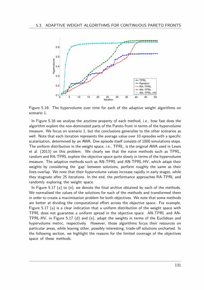
5.3. ADAPTIVE WEIGHT ALGORITHMS FOR CONTINUOUS PARETO FRONTS
0 5 10 15 20 25 30 35 40 45 500.1
0.2
0.3
0.4
0.5
0.6
Iteration
Hyp
erv
olu
me
TPRLRandomRA−TPRLAN−TPRLAN−TPRL−HV
Figure 5.16: The hypervolume over time for each of the adaptive weight algorithms onscenario 1.
In Figure 5.16 we analyse the anytime property of each method, i.e., how fast does thealgorithm explore the non-dominated parts of the Pareto front in terms of the hypervolumemeasure. We focus on scenario 1, but the conclusions generalise to the other scenarios aswell. Note that each iteration represents the average value over 10 episodes with a specificscalarisation, determined by an AWA. One episode itself consists of 1000 simulations steps.The uniform distribution in the weight space, i.e., TPRL, is the original AWA used in Lewiset al. (2013) on this problem. We clearly see that the naive methods such as TPRL,random and RA-TPRL explore the objective space quite slowly in terms of the hypervolumemeasure. The adaptive methods such as AN-TPRL and AN-TPRL-HV, which adapt theirweights by considering the ‘gap’ between solutions, perform roughly the same as theirlines overlap. We note that their hypervolume values increase rapidly in early stages, whilethey stagnate after 25 iterations. In the end, the performance approaches RA-TPRL andrandomly exploring the weight space.
In Figure 5.17 (a) to (e), we denote the final archive obtained by each of the methods.We normalised the values of the solutions for each of the methods and transformed themin order to create a maximisation problem for both objectives. We note that some methodsare better at dividing the computational e�ort across the objective space. For example,Figure 5.17 (a) is a clear indication that a uniform distribution of the weight space withTPRL does not guarantee a uniform spread in the objective space. AN-TPRL and AN-TPRL-HV, in Figure 5.17 (d) and (e), adapt the weights in terms of the Euclidean andhypervolume metric, respectively. However, those algorithms focus their resources onparticular areas, while leaving other, possibly interesting, trade-o� solutions uncharted. Inthe following section, we highlight the reasons for the limited coverage of the objectivesspace of these methods.
131

CHAPTER 5. ITERATIVELY LEARNING MULTIPLE MULTI-OBJECTIVE POLICIES
0 0.2 0.4 0.6 0.8 10
0.2
0.4
0.6
0.8
1
Auctions
Confidence
0 0.2 0.4 0.6 0.8 10
0.2
0.4
0.6
0.8
1
Auctions
Confidence
0.2 0.4 0.6 0.8 10
0.2
0.4
0.6
0.8
1
Auctions
Confidence
(a) TPRL (b) Random (c) RA-TPRL
0 0.2 0.4 0.6 0.8 10
0.2
0.4
0.6
0.8
1
Auctions
Co
nfid
en
ce
0 0.2 0.4 0.6 0.8 10
0.2
0.4
0.6
0.8
1
Auctions
Confidence
0 0.2 0.4 0.6 0.8 10
0.2
0.4
0.6
0.8
1
Auctions
Co
nfid
en
ce
(d) AN-TPRL (e) AN-TPRL-HV (f) AN-TPRL-OHV
0 0.2 0.4 0.6 0.8 10
0.2
0.4
0.6
0.8
1
Auctions
Co
nfid
en
ce
0 0.2 0.4 0.6 0.8 10
0.2
0.4
0.6
0.8
1
Auctions
Co
nfid
en
ce
0 0.2 0.4 0.6 0.8 10
0.2
0.4
0.6
0.8
1
Auctions
Co
nfid
en
ce
(g) RA-TPRL-DIST (h) RA-TPRL-HV (i) RA-TPRL-OHV
Figure 5.17: The Pareto fronts obtained after 50 iterations for each of the adaptive weightalgorithms on Scenario 1.
132

5.3. ADAPTIVE WEIGHT ALGORITHMS FOR CONTINUOUS PARETO FRONTS
5.3.4 Novel adaptive weight algorithms for RLAlthough the adaptive weight algorithms have served their purpose on a number of testdomains (Dubois-Lacoste et al., 2011; Lust and Teghem, 2010), there are still some openquestions on their performance in MORL. This doubt is based on the following reasons.
Firstly, the AWAs of Section 5.3.2 are tailored for stochastic local search algorithms thatcan be seeded using particular solutions to provide the optimisation algorithm with a goodinitial position in the search space. The AWAs make extensive use of this property to biasthe search direction to fruitful and uncharted areas of the Pareto front. However, seedingthe reinforcement learning agent in such a way is not possible as most problems tend tobe episodic and consist of multiple stages that the agent has to go through. Secondly, thedichotomic scheme in Equation 5.5 uses the segment between two solutions s1 and s2 tocalculate the new weight. However, the equation does not guarantee that the resultingsolution obtained by the calculated weight will lie between the interval of the two parentsolutions, i.e., between s1 and s2.
The solution that we propose is to combine the properties of RA-TPLS and AN-TPLS,meaning that we use the layered-division of the weight space where deeper layers intensifythe search process to particular areas of RA-TPLS together with an adaptive ordering ofthe elements of the di�erent layers, based on the aspects of the Pareto front currently beingexplored. Similarly to AN-TPLS we use di�erent metrics, such as the Euclidean distanceand the hypervolume indicator, to qualify the di�erence between solutions. By mergingboth procedures, we combine the best of both worlds, i.e., the layered approach allowsus to explore the rough outline of the Pareto front in initial iterations of the algorithmand secondly, we do not rely on the dichotomic scheme in Equation 5.5 which does notscale well to general application domains. Subsequently, we no longer require specificseeds that bias the search direction and eventually also the performance of the obtainedsolutions. We call this algorithm RA-TPRL-DIST and RA-TPRL-HV with the Euclideanand hypervolume metric, respectively. An outline of the procedure for the bi-objective caseis given in Algorithm 4. The algorithms starts by examining the bounds of the Pareto front,i.e., we evaluate the optimisation algorithm, in this case RL(), with weights w1 = 0 andw1 = 1. The solutions s1 and s2 and their corresponding weights are added to a tree-likedata structure that stores the segments of the weight space (line 4). Every iteration, thelargest segment, according to a metric (Euclidean distance or hypervolume), that is notexplored yet is determined (line 6) and the new weight is calculated to be in the middleof that segment (line 7). Subsequently, the reinforcement learning algorithm is run withthat weight and 2 new segments are added to the tree. i.e., the segment connectingthe left solution and the middle solution and another segment from the middle to theright solution. (lines 9 and 10). Eventually, the Archive stores the set of multi-objectivesolution acquired throughout the run.
We also see opportunities for trying out an alternative metric. The hypervolume measurein AN-TPLS-HV is an interesting indicator that calculates the surface that two solutionsoccupy in the two-dimensional objective space. Although the hypervolume measure inEquation 5.6 works well for calculating the volume of two solutions in the objective space,
133

CHAPTER 5. ITERATIVELY LEARNING MULTIPLE MULTI-OBJECTIVE POLICIES
Algorithm 4 An Improved AWA1: s1 Ω RL(0)
2: s2 Ω RL(1)
3: Add s1, s2 to Archive4: tree Ω new Tree(new Segment(0, s1, 1, s2))
5: while stopping criteria not met do6: Segment lg Ω tree.getLargestGap()
7: w Ω lg.weights1 +lg.weights22
8: sÕ Ω RL(w)
9: tree.add(new Segment(lg.weights1 , lg.s1 , w, sÕ))10: tree.add(new Segment(w, sÕ, lg.weights2 , lg.s2))11: Add sÕ to Archive12: end while13: return Archive
it is not the common hypervolume formula. An alternative hypervolume calculation takesinto account a particular reference point ref to measure the volume of a given set ofsolutions, for any number of elements. It is clear that some solutions in the set willhave less or more contribution to the final performance because the rectangles, defined bythe reference point to each of the solutions, will have significant overlaps. Therefore, itmight be interesting to consider the degree of overlap between solutions directly and tominimise this overlap. We call this metric the overlapping hypervolume (OHV) measure(Figure 5.18). The measure calculates the ratio of the overlap and the unique hypervolumeof the two solutions (Equation 5.9 and 5.13).The idea is to order the solutions using thismeasure in order to intensify the search to segments with the smallest overlap first.
Note that our test environment only considers two objectives, but we believe this al-gorithm could be generalised to more objectives quite easily, since both distance measuresare applicable in m-dimensional spaces.
overlap = |(ref1 ≠ min(F1(s1), F1(s2)) · (ref2 ≠ min(F2(s1), F2(s2))| (5.9)
surfs1 = |(F1(s1) ≠ ref1) · (F2(s1) ≠ ref2)| (5.10)
surfs2 = |(F1(s2) ≠ ref1) · (F2(s2) ≠ ref2)| (5.11)
total = surfs1 + surfs2 ≠ overlap (5.12)
OHV (s1, s2) =
overlap
total(5.13)
134

5.3. ADAPTIVE WEIGHT ALGORITHMS FOR CONTINUOUS PARETO FRONTS
overlap
ref
F (s1)
F (s2)
Figure 5.18: The overlapping hypervolume (OHV) measures the percentage of overlapbetween two solutions s1 and s2 in the objective space.
Results II
Next, we analyse and compare the former adaptive weight selection mechanisms of Sec-tion 5.3.2 and 5.3.4 on both simulated and real-life scenarios. We focus on the speed atwhich these methods approximate the Pareto front as measured by the quality indicatorsof Section 5.3.1.
First we investigate the anytime property of each of the methods. The results in Fig-ures 5.19 extend the results of Figure 5.16 by including our novel methods. We notethat the combination with the overlapping hypervolume metric (AN-TPRL-OHV) doesnot manage to improve a lot after the initial iterations as it reaches similar performance toTPRL on scenario 1. The best combination of speed of learning and final performance isobtained by our RA-TPRL-HV and RA-TPRL-OHV, while the Euclidean distance metric(RA-TPRL-DIST) learns significantly slower. For scenario 7 in Figure 5.20, similar con-clusions can be formed except that AN-TPRL-OHV is now amongst the best performingalgorithms, leaving TPRL far behind. In general, the naive methods and RA-TPRL-DISTare the slowest learners of the pack, while the adaptive methods reach similar performancein the end. In initial stages, the AN-TPRL and AN-TPRL-HV methods learn a bit faster,but this di�erence is negligible.
135

CHAPTER 5. ITERATIVELY LEARNING MULTIPLE MULTI-OBJECTIVE POLICIES
0 5 10 15 20 25 30 35 40 45 500.1
0.2
0.3
0.4
0.5
0.6
Iteration
Hyp
erv
olu
me
TPRLRandomRA−TPRLRA−TPRL−DISTRA−TPRL−HVRA−TPRL−OHVAN−TPRLAN−TPRL−HVAN−TPRL−OHV
Figure 5.19: The hypervolume over time for each of the adaptive weight algorithms onscenario 1.
In Figure 5.17 the 50 solutions of the archive are depicted for each of the methods. Wesee that TPRL, although providing promising results in previous work on CamSim (Lewiset al., 2013), clearly lacks at exploring every part of the Pareto front as it leaves particularareas uncovered. On the third row of Figure 5.17, the methods that combine RA-TPRLwith the distance, hypervolume and overlapping hypervolume metrics improve these resultsin terms of spread in the objective space, while minimising the gaps by taking into accountthe limited number of iterations. Other results using quality indicators that quantify thesegaps in the Pareto front are presented in Table 5.1. We note that our RA-TPRL-HVmethod obtains the best results in terms of spread in the 10 scenarios. The best methodin terms of generational (inverted) distance di�er a lot for each scenario but in generalthe di�erences between the methods are minimal.
136
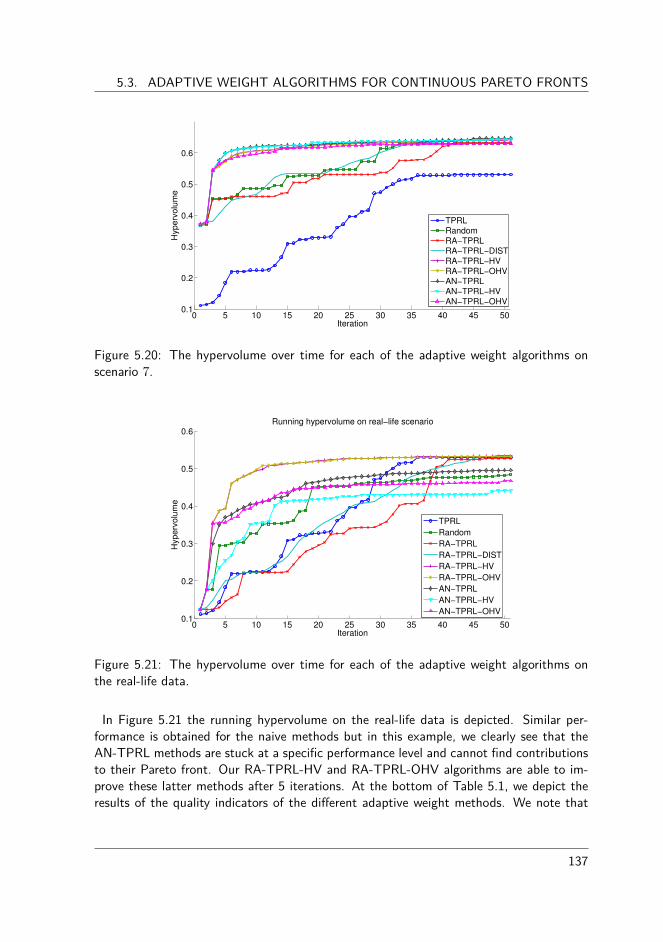
5.3. ADAPTIVE WEIGHT ALGORITHMS FOR CONTINUOUS PARETO FRONTS
0 5 10 15 20 25 30 35 40 45 500.1
0.2
0.3
0.4
0.5
0.6
Iteration
Hyp
erv
olu
me
TPRLRandomRA−TPRLRA−TPRL−DISTRA−TPRL−HVRA−TPRL−OHVAN−TPRLAN−TPRL−HVAN−TPRL−OHV
Figure 5.20: The hypervolume over time for each of the adaptive weight algorithms onscenario 7.
0 5 10 15 20 25 30 35 40 45 500.1
0.2
0.3
0.4
0.5
0.6
Iteration
Hyp
erv
olu
me
Running hypervolume on real−life scenario
TPRL
Random
RA−TPRL
RA−TPRL−DIST
RA−TPRL−HV
RA−TPRL−OHV
AN−TPRL
AN−TPRL−HV
AN−TPRL−OHV
Figure 5.21: The hypervolume over time for each of the adaptive weight algorithms onthe real-life data.
In Figure 5.21 the running hypervolume on the real-life data is depicted. Similar per-formance is obtained for the naive methods but in this example, we clearly see that theAN-TPRL methods are stuck at a specific performance level and cannot find contributionsto their Pareto front. Our RA-TPRL-HV and RA-TPRL-OHV algorithms are able to im-prove these latter methods after 5 iterations. At the bottom of Table 5.1, we depict theresults of the quality indicators of the di�erent adaptive weight methods. We note that
137
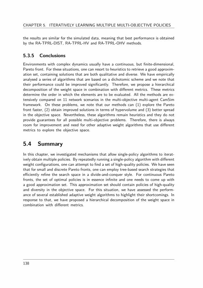
CHAPTER 5. ITERATIVELY LEARNING MULTIPLE MULTI-OBJECTIVE POLICIES
the results are similar for the simulated data, meaning that best performance is obtainedby the RA-TPRL-DIST, RA-TPRL-HV and RA-TPRL-OHV methods.
5.3.5 ConclusionsEnvironments with complex dynamics usually have a continuous, but finite-dimensional,Pareto front. For these situations, one can resort to heuristics to retrieve a good approxim-ation set, containing solutions that are both qualitative and diverse. We have empiricallyanalysed a series of algorithms that are based on a dichotomic scheme and we note thattheir performance could be improved significantly. Therefore, we propose a hierarchicaldecomposition of the weight space in combination with di�erent metrics. These metricsdetermine the order in which the elements are to be evaluated. All the methods are ex-tensively compared on 11 network scenarios in the multi-objective multi-agent CamSimframework. On these problems, we note that our methods can (1) explore the Paretofront faster, (2) obtain improved solutions in terms of hypervolume and (3) better spreadin the objective space. Nevertheless, these algorithms remain heuristics and they do notprovide guarantees for all possible multi-objective problems. Therefore, there is alwaysroom for improvement and need for other adaptive weight algorithms that use di�erentmetrics to explore the objective space.
5.4 SummaryIn this chapter, we investigated mechanisms that allow single-policy algorithms to iterat-ively obtain multiple policies. By repeatedly running a single-policy algorithm with di�erentweight configurations, one can attempt to find a set of high-quality policies. We have seenthat for small and discrete Pareto fronts, one can employ tree-based search strategies thate�ciently refine the search space in a divide-and-conquer style. For continuous Paretofronts, the set of optimal policies is in essence infinite and one needs to come up witha good approximation set. This approximation set should contain policies of high-qualityand diversity in the objective space. For this situation, we have assessed the perform-ance of several established adaptive weight algorithms to highlight their shortcomings. Inresponse to that, we have proposed a hierarchical decomposition of the weight space incombination with di�erent metrics.
138

5.4. SUMMARY
TPRL Random RA-TPRL RA-TPRL-DIST RA-TPRL-HV RA-TPRL-OHV AN-TPRL AN-TPRL-HV AN-TPRL-OHVScenario 1
GSpread 0.97501 0.91959 0.95257 0.80777 0.81487 0.8076 1.00112 1.00059 1.04571HV 0.60384 0.66785 0.66347 0.6732 0.67332 0.67311 0.65238 0.65446 0.53106
GDistances 2.99143 2.98875 2.96057 2.92172 2.91005 2.92752 2.92267 2.95842 2.94144IGDistance 14.20181 14.07198 14.07761 14.07234 14.07109 14.07234 14.07971 14.07675 14.14254
Scenario 2GSpread 0.90053 0.92837 0.92312 0.93271 0.87589 0.92952 0.95014 1.00981 0.91466
HV 0.66331 0.66783 0.67734 0.67008 0.67916 0.67087 0.6792 0.68073 0.65541GDistances 2.83976 2.82884 2.74931 2.9209 2.87788 2.91765 3.02818 3.1312 2.74639IGDistance 12.95593 12.95081 12.90369 12.95266 12.97541 12.95451 12.96075 12.98492 12.93109
Scenario 3GSpread 0.89829 0.92254 0.88001 0.90019 0.85584 0.88654 0.95599 1.05615 0.97401
HV 0.55002 0.54008 0.54899 0.54764 0.5553 0.54865 0.58074 0.53527 0.52907GDistances 3.03947 3.04809 2.98084 2.99027 2.9913 2.99857 3.10163 3.20551 3.02713IGDistance 13.99183 14.1615 14.03292 14.2017 14.10126 14.18741 14.08196 14.17774 14.05668
Scenario 4GSpread 0.90403 0.92403 0.92751 0.88937 0.87291 0.87961 0.9389 1.02157 0.96905
HV 0.46702 0.45717 0.46915 0.47347 0.47403 0.47481 0.46587 0.45524 0.44411GDistances 3.11392 3.11126 3.06278 3.08443 3.08056 3.07423 3.15675 3.22976 3.15611IGDistance 14.81707 14.7147 14.8793 14.84748 14.89994 14.81748 14.85078 14.85685 14.88275
Scenario 5GSpread 0.89728 0.93505 0.93387 0.8638 0.83163 0.85699 0.9592 1.02245 0.98591
HV 0.7239 0.70845 0.73191 0.73584 0.73768 0.73611 0.72231 0.71118 0.61485GDistances 2.8878 2.8815 2.84129 2.8124 2.81807 2.83094 3.00157 3.06383 2.94756IGDistance 13.20978 13.28262 13.16021 13.16986 13.16021 13.17839 13.21716 13.26455 13.31449
Scenario 6GSpread 0.89975 0.90772 0.90297 0.92098 0.8757 0.92804 0.95141 1.04161 0.91413
HV 0.35623 0.31604 0.33999 0.32833 0.34209 0.32689 0.34858 0.33307 0.32476GDistances 3.23164 3.4249 3.15232 3.27144 3.36656 3.40051 3.49461 3.61006 3.37513IGDistance 14.84423 14.60966 14.63511 14.63258 14.63511 14.62701 14.63511 14.63511 14.62822
Scenario 7GSpread 0.88941 0.91815 0.91261 0.87262 0.86677 0.87676 0.92367 1.02515 0.92114
HV 0.6351 0.63149 0.63461 0.64238 0.64151 0.64271 0.64698 0.64234 0.63078GDistances 2.91725 2.91555 2.85605 2.89079 2.88499 2.8822 2.98927 3.08699 2.94745IGDistance 13.56464 13.60138 13.62932 13.60277 13.60277 13.62932 13.52138 13.56219 13.50574
Scenario 8GSpread 0.89045 0.89952 0.92083 0.87468 0.8426 0.85821 0.94294 1.00346 0.90937
HV 0.67929 0.67015 0.70277 0.69972 0.69903 0.70077 0.68043 0.6726 0.64769GDistances 2.87852 2.86679 2.81096 2.86095 2.87561 2.858 2.99304 3.0593 2.90116IGDistance 13.32639 13.12466 13.25595 13.29731 13.2644 13.27501 13.23966 13.25307 13.27036
Scenario 9GSpread 0.98498 0.97623 0.9948 0.85214 0.84111 0.8635 1.01375 1.00589 1.01342
HV 0.77092 0.72027 0.76646 0.77816 0.77854 0.77773 0.75198 0.74881 0.71142GDistances 2.86232 2.87269 2.8102 2.76207 2.755 2.77794 2.84333 2.90014 2.92109IGDistance 13.12838 13.17884 13.11477 13.11224 13.11206 13.11371 13.15331 13.17327 13.18997
Scenario 10GSpread 0.94538 0.97646 0.95739 0.94302 0.91827 0.93815 1.00365 1.06029 1.00073
HV 0.62974 0.63441 0.63944 0.63959 0.63967 0.63957 0.63652 0.64938 0.63766GDistances 2.80424 2.79834 2.7291 2.73846 2.75131 2.73696 2.95668 3.00213 2.82691IGDistance 12.79585 12.72557 12.74433 12.74441 12.74441 12.74441 12.74441 12.74229 12.73365
Scenario 11GSpread 0.94689 0.96702 0.95472 0.92537 0.90926 0.91007 0.98978 1.05081 0.99617
HV 0.56738 0.56372 0.56865 0.57189 0.57219 0.57197 0.5778 0.58042 0.56247GDistances 2.94136 2.94263 2.88296 2.90703 2.91029 2.90481 2.99781 3.05835 3.00429IGDistance 13.93518 13.93155 13.93476 13.93734 13.93801 13.93734 13.99275 13.95814 13.95763
Real-life scenarioGSpread 0.8974 0.90369 0.89542 0.86498 0.85507 0.85358 0.94972 1.016 0.95567
HV 0.53053 0.48302 0.52724 0.53287 0.53401 0.5332 0.49554 0.44196 0.46728GDistances 3.10149 3.12013 3.09672 3.05587 3.05963 3.06153 3.09171 3.17102 3.11861IGDistance 14.9041 15.24093 14.98453 14.77806 14.77806 14.77806 14.96315 15.17256 15.12926
Table 5.1: Quality indicators on 12 di�erent scenarios in CamSim
139


6
| Simultaneously learningmultiple multi-objective
policies
In the previous two chapters, we focussed our attention on single-policy reinforcementlearning algorithms, i.e., algorithms that obtain a single policy at each run. Perform-ing repeated runs of these algorithms might act as a suitable but primitive approach todiscover a set of trade-o� solutions. In this chapter, we investigate algorithms that re-trieve various compromise solutions simultaneously. Hence, they are called multi-policyalgorithms. In this chapter, we propose two multi-policy algorithms that each cover aparticular topic of MORL.
A first algorithm is the multi-objective hierarchical heuristic optimisation (MO-HOO) formulti-objective X -armed bandit problems. This is a class of problems similar to a standardbandit problem. Only in this case, the agent is faced with a continuous, finite-dimensionalaction space instead of a discrete one. MO-HOO evolves a tree of Pareto non-dominatedestimates that explores the continuous action space in a hierarchical manner. As a result,the algorithm is specifically tailored for multi-objective industrial optimisation problemsthat involve the assignment of continuous variables.
A second algorithm is Pareto Q-learning. Pareto Q-learning (PQL) combines the prin-ciples of MO-HOO with Q-learning to make it applicable in multi-state problems. PQLis the first temporal di�erence-based multi-policy MORL algorithm that does not use thelinear scalarisation function. Pareto Q-learning is not limited to the convex hull, but it canlearn the entire Pareto front of deterministic non-stationary policies, if enough explorationis provided. The algorithm learns the Pareto front by bootstrapping Pareto non-dominatedQ-vectors throughout the state and action space. As we will see, one of the crucial as-pects of this algorithm is its bootstrapping process, i.e., how to update a set of Q-vectors
141

CHAPTER 6. SIMULTANEOUSLY LEARNING MULTIPLE MULTI-OBJECTIVEPOLICIES
with another set of Q-vectors, bearing in mind that both sets might not contain the samenumber of elements.
In more detail, we will present the following contributions in this chapter:
• Analyse related work on multi-policy MORL• Propose and evaluate a multi-policy MORL algorithm for multi-objective X -armed
bandit problems• Propose and evaluate a multi-policy temporal-di�erence MORL algorithm for multi-
objective sequential decision making problems
This research has been published in Van Mo�aert et al. (2014b), Van Mo�aert and Nowé(2014) and Van Mo�aert et al. (2015).
6.1 Related work on simultaneously learning multiplepolicies
Over the years, several algorithms have been proposed that simultaneously retrieve multiplemulti-objective policies. Usually, these algorithms fall into two separate categories, i.e.,algorithms that employ either linear scalarisation functions or monotonically increasingscalarisation functions, such as the Pareto dominance relation.
Most algorithms that learn multiple policies belong to the first category. Because ofthe properties of linear scalarisation functions, sum and union operators can be quitestraightforwardly defined on convex hulls. One of the most important contributions is theconvex hull value-iteration (CHVI) algorithm which computes the deterministic stationarypolicies that lie on the convex hull of the Pareto front (Barrett and Narayanan, 2008). Frombatch data, CHVI extracts and computes every linear combination of the objectives in orderto obtain all deterministic optimal policies. CHVI bootstraps by calculating the convexhull of the union over all actions in sÕ, that is
taÕ Q(sÕ, aÕ
). The most computationallyexpensive operator is the procedure of combining convex hulls in the bootstrapping rule.Lizotte et al. (2010) reduce the asymptotic space and time complexity of the bootstrappingrule by simultaneously learning several value functions corresponding to di�erent weightsand by calculating their piecewise linear spline representation. They validated their work onclinical trial data for two objectives to propose a treatment to patients based on a trade-o�between the e�ectiveness of the drugs and severity of the side e�ects. Nevertheless, thepractical possibilities for higher dimensional spaces are not straightforward (Lizotte et al.,2012). In Kazuyuki et al. (2009), the parallel Q-learning algorithm is proposed. ParallelQ-learning is similar to CHVI in the sense that it learns optimal piecewise-linear policiesfor all weights. It computes the convex hull by defining sum and union operators forsets, similar to the way CHVI bootstraps. The algorithm su�ers from convergence issuessince vertices are continuously being added to the polygon representing the convex hull.To overcome this, the authors introduce a threshold parameter to reduce the size of thesets and to increase the accuracy. In Castelletti et al. (2011, 2012), the fitted Q-iteration
142
6.2. LEARNING MULTIPLE POLICIES IN SINGLE-STATE PROBLEMS
algorithm is extended to learn sets of policies in multi-objective environments. This o�-linealgorithm is called multi-objective fitted Q-iteration (MOFQI) and it computes the set ofexpected return vectors obtained for a series of weight vectors in a single run.
The second category comprises algorithms that employ monotonically increasing functionswhich are more general than the linear scalarisation function. A typical member of thisclass would be the Pareto dominance relation. How it can be combined into a learningparadigm has been a subject of research for many decades. In White (1982), a dynamicprogramming algorithm simultaneously computes a set of Pareto non-dominated policies,i.e., a ˆQset. The algorithm bootstraps the Pareto non-dominated Q-vectors of the nextstate to the set of the current state-action pair. The idea is that, after the discountedPareto non-dominated rewards are propagated and the ˆQset’s converge to a set of Paretonon-dominated policies, the user can traverse the tree of ˆQset’s by applying a preferencefunction. Wang and Sebag (2012, 2013) propose a multi-objective Monte Carlo tree search(MO-MCTS) algorithm to learn a set of solutions. In MCTS, a search tree is incrementallybuilt and explored at the same time (Coulom, 2007). The nodes of the tree represent visitedstates and branches represent actions. At the end of an episode, the nodes are weightedaccording to the outcome of the episode in order to bias the action selection in futureplays. In MO-MCTS, the upper confidence bounds of the actions are scalarised in eitherof two distinct manners. One possibility is to apply the hypervolume quality indicator todetermine which path of vectorial estimates in the tree introduces the largest hypervolumecontribution w.r.t. the policies that are already retrieved. Because the hypervolumemeasure is costly to compute, as an alternative, it is also possible to simply determinewhether or not a tree walk obtained a non-dominated return in a boolean fashion. Thisway, a scalarised multi-objective value function is constructed that eases the process ofselecting an action with vectorial estimates.
As highlighted by Roijers et al. (2013), there is a specific need for on-line reinforcementlearning algorithms that are able to discover the Pareto front although the setting is farfrom straightforward. To fill this gap, we will research this problem from two distinctviewpoints. Moreover, in the case of (1) single-state problem involving a continuous butfinite dimensional action space in Section 6.2 and (2) for multi-state sequential decisionmaking problems in Section 6.3.
6.2 Learning multiple policies in single-state problemsIn the classical bandit problem, described in Section 2.5, a gambler wants to maximisehis reward by selecting the best possible action from a finite set of arms with unknownreward distributions. The on-line aspect of this problem is very important, i.e. in orderto maximise his gain, the gambler needs to find a balance between exploring unchartedterritory and exploiting his current knowledge.
Recently, this problem is generalised to environments where the action space is con-tinuous but finite-dimensional. In this case, the gambler is faced with an continuous setof arms. This problem is called an X -armed bandit problem B consisting of a pair of
143
CHAPTER 6. SIMULTANEOUSLY LEARNING MULTIPLE MULTI-OBJECTIVEPOLICIES
B = (X , M), where X is a measurable space of arms and M determines the distribu-tion of rewards associated with each arm (Bubeck et al., 2010). This problem has astrong resemblance to operational research and control applications that involve the calib-ration of several parameters. Examples of such applications are the tuning of hydrostaticdrive-train controllers (Van Vaerenbergh et al., 2014) and the adjustment the temperaturelevels to maximise a chemical reaction (Cope, 2009). One of the algorithms that e�ect-ively solves a X -armed bandit problem is the hierarchical optimistic optimisation (HOO)strategy (Bubeck et al., 2010) which will be explained in the subsequent section.
6.2.1 Hierarchical Optimistic OptimisationThe HOO strategy iteratively constructs a binary tree over the action space X . A nodein the binary tree represents an area over X and is represented by (h, i), where i is theindex of the node at depth h. Hence, the root node is represented by (0, 1). Following theterminology of Bubeck et al. (2010), (h+1, 2i≠1) and (h+1, 2i) refer to the child nodesof the node located at (h, i). Let Ph,i µ X be the area of the action space correspondingto node (h, i), given these two conditions:
P0,1 = X (6.1)
Ph,i = Ph+1,2i≠1 fi Ph+1,2i, ’h Ø 0 and 1 Æ i Æ 2
h. (6.2)A node stores an optimistic estimate of the quality of its subtree, i.e. a U-value. TheUh,i(n)-value is an initial estimate of the maximum value of the pay-o� function in thecorresponding region of the action space X and is defined as follows:
Uh,i(n) =
Iµh,i(n) +
Ò2 ln n
Th,i(n) + ‹1flh, if Th,i(n) > 0
+Œ, otherwise,
where µh,i(n) is the mean estimate of the subtree of node n and the other two terms expressa standard optimistic exploration value and the maximum possible variation of the pay-o�function, defined by the ‹1 and flh parameters. When the action is not sampled before, itreceives the highest optimistic value, i.e. +Œ. As we are interested in sampling near themaxima of the pay-o� function, the HOO strategy focusses on estimating this functionnear its maxima while leaving the other, less interested parts of the function, less explored.
Given the U-value of a node n, its B-value is computed by taking into account its ownU-value and the B-values of its two child nodes. The B-value is designed to put a tighterupper-bound on the best possible value that can be obtained in that region of X . TheB-value estimate is:
Bh,i(n) Ω min {Uh,i(n), max{Bh+1,2i≠1(n), Bh+1,2i(n)}} . (6.3)
Thus, the root node stores an (optimistic) estimate of the quality of the entire actionspace, where its left child stores a more accurate estimate for the interval [inf(X ), sup(X )
2 ]
144

6.2. LEARNING MULTIPLE POLICIES IN SINGLE-STATE PROBLEMS
of the action space, i.e. between the infimum of X and half of its supremum giventhe divide-and-conquer approach. Similarly, the right child of the root stores equivalentinformation for [
sup(X )2 , sup(X )]. Selecting an action is performed by traversing the subtree
with the largest B-value until a leaf value is reached. Thereafter the action is sampled andthe estimates of the nodes on the traversed path are updated and refined by consideringthe observed reward and the number of times the subtree is visited in previous plays. Anoutline of the algorithm can be found in Algorithm 5.
Bubeck et al. (2010) prove this algorithm to converge to the mean pay-o� function aroundits maxima if the function’s smoothness is conform to being locally Lipschitz continuous.In short, a function is said to be Lipschitz continuous if a small change in the function’sinput values signifies a mild change in the corresponding function values of that function,which is a reasonable assumption in many engineering problems.
6.2.2 Multi-Objective Hierarchical Optimistic OptimisationTransforming the single-objective HOO strategy to multi-objective environments requiresseveral adjustments to the algorithm’s internal workings. Below, we tackle the requiredmodifications for constructing the Multi-Objective Hierarchical Optimistic Optimisation(MO-HOO) algorithm into four di�erent categories.
Sampling purpose
A first crucial aspect that arises when transforming a single-objective on-line algorithm toa multi-objective environment is defining its purpose. In the standard problem the goal ofthe agent is to maximise the average reward being received, which is the logical approachas there is a total order between the scalar rewards. In the case of multiple objectives,the Pareto dominance relation only supplies a partial order, i.e. only non-dominated anddominated vectors can be compared but non-dominated vectors are incomparable amongsteach other. As a consequence, if one would average the reward vectors being obtained bythe agent, we are not guaranteed that the average is an actual attainable solution for theproblem. Take for instance, a very easy multi-objective problem where the agent can onlytake two action a and b where the deterministic rewards are (1, 0) and (0, 1), respectively.If one would take action a with probability x and action b with probability p = (1 ≠ x),the average reward vector would be (x, 1 ≠ x). Thus, although there are only two possibleoutcomes for the problem, considering average reward vectors implicates that we are nolonger sampling on the Pareto front but on the convex hull of the Pareto front, similarto the stochastic mixture policies of Section 3.4.1. Therefore, averaging vectorial rewardsdoes not represent actual solution points in the objective space.
In control problems we are not interested in stochastic mixture policies obtained fromthe convex hull of the Pareto front, but rather in sampling a genuine trade-o� in everyexecution of the policy. This means that we want to identify actually realisable controlpolicies that lie on the Pareto front that o�er a fixed trade-o� between the di�erent controlobjectives. However, despite the fact that our main goal is to identify the Pareto front, we
145

CHAPTER 6. SIMULTANEOUSLY LEARNING MULTIPLE MULTI-OBJECTIVEPOLICIES
Algorithm 5 The HOO strategyParameters: Two real numbers ‹1 > 0 and fl œ (0, 1), a sequence (Ph,i)hØ0,1ÆiÆ2h of subsetsof X satisfying the conditions (6.1) and (6.2).
Auxiliary function Leaf(T ): outputs a leaf of T .
Initialization: T =
)(0, 1)
*and B1,2 = B2,2 = +Œ.
1: for n = 1, 2, . . . do Û Strategy HOO in round n Ø 1
2: (h, i) Ω (0, 1) Û Start at the root3: P Ω {(h, i)} Û P stores the path traversed in the tree4: while (h, i) œ T do Û Search the tree T5: if Bh+1,2i≠1 > Bh+1,2i then Û Select the “more promising” child6: (h, i) Ω (h + 1, 2i ≠ 1)
7: else if Bh+1,2i≠1 < Bh+1,2i then8: (h, i) Ω (h + 1, 2i)
9: else Û Tie-breaking rule10: Z ≥ Ber(0.5) Û e.g., choose a child at random11: (h, i) Ω (h + 1, 2i ≠ 1)
12: end if13: P Ω P fi {(h, i)}14: end while15: (H, I) Ω (h, i) Û The selected node16: Choose arm X in PH,I and play it Û Arbitrary selection of an arm17: Receive corresponding reward Y
18: T Ω T fi {(H, I)} Û Extend the tree19: for all (h, i) œ P do Û Update the statistics T and µ stored in the path20: Th,i Ω Th,i + 1 Û Increment the counter of node (h, i)
21: µh,i Ω!1 ≠ 1/Th,i
"µh,i + Y/Th,i Û Update the mean µh,i of node (h, i)
22: end for23: for all (h, i) œ T do Û Update the statistics U stored in the tree24: Uh,i Ω µh,i +
(2 ln n)/Th,i + ‹1flh Û Update the U–value of node (h, i)
25: end for26: BH+1,2I≠1 Ω +Œ Û B–values of the children of the new leaf27: BH+1,2I Ω +Œ28: T Õ Ω T Û Local copy of the current tree T29: while T Õ ”=
)(0, 1)
*do Û Backward computation of the B–values
30: (h, i) Ω Leaf(T Õ) Û Take any remaining leaf
31: Bh,i Ω min
ÓUh,i, max
)Bh+1,2i≠1, Bh+1,2i
*ÔÛ Backward computation
32: T Õ Ω T Õ \)
(h, i)*
Û Drop updated leaf (h, i)33: end while34: end for
146

6.2. LEARNING MULTIPLE POLICIES IN SINGLE-STATE PROBLEMS
do not want to neglect the sampling e�ciency of our method. Our motivating assumptionhere is that sampling policies inherently has a certain cost associated with it, either intime, in resources or both. Often these costs are associated with evaluating a controlstrategy on a real system. Furthermore, we assume that solutions which lie far from thePareto front are suboptimal in at least one of the objectives and thus typically have highercosts associated with them, e.g., because they are less e�cient, they take longer to reacha goal, or they might even violate safety constraints. Therefore, our goal is to develop ane�cient method for identifying the Pareto front, which minimises the amount of samplingperformed in regions far from the Pareto front.
Averaging over subtrees
In the original implementation of the HOO strategy, the U-value of a node stores an estim-ate of the average reward of a subtree together with some additional statistics. However,as we are dealing with multiple objectives at the same time, there is no point in averagingmultiple reward vectors into a single value for each objective. Together with the fact thatin the HOO strategy, one does not sample the same action more than once, but rather itsleft or right child node, we no longer consider the U-values in their original form. There-fore, in the multi-objective case, we only propagate the U -vector of leaf nodes as they aresamples that are not averaged out over subtrees.
Knowledge representation
Recall that in the single-objective HOO strategy, the agent’s goal is to maximise the scalarreward obtained by sampling close to the optimum of the pay-o� function. Therefore, thealgorithm propagates an estimate of the maximum of the pay-o� function from leaf nodesto the root node in terms of B-values. In a multi-objective problem, however, there usuallyis no single-optimum but there are multiple Pareto non-dominated solutions. Thus, a scalarestimate or B-value is insu�cient to store the quality of a region of the pay-o� function.The solution we propose is to consider sets of estimates, i.e., B-sets. The elements of thesets are B-vectors that store an estimate for each objective. The most optimistic upperbound is now a vector u that is always a member of the Pareto front without excludingother Pareto optimal vectors, e.g. u = (≠Œ, +Œ) for an environment with two objectives.
Information propagation
In Equation 6.3, the HOO strategy performs a backward computation to adjust the estim-ate of a node by taking into account its U-value and the B-value of its two child nodes.To determine the B-value of a node, the algorithm determines the highest upper bound ofits child nodes by a max operator. In the multi-objective variant, we replace this operatorby the operator ND(
tB(Bh+1,2i≠1(n), Bh+1,2i(n)) which yields every non-dominated B-
vector of the left and right child of node n. The min operator in Equation 6.3 assures atighter bound of the B-value of node n. As we are not focussing on the average Pareto
147

CHAPTER 6. SIMULTANEOUSLY LEARNING MULTIPLE MULTI-OBJECTIVEPOLICIES
front or convex hull, we no longer consider the U-value of non-leaf nodes. However, as theU -vectors of leafs are recalculated at every iteration, the additional statistics introduce alevel of robustness in the case of noisy environments.
If one would not be interested in the actual trade-o� achieved in every execution of thepolicy, but rather in the average sampling performance, a multi-objective min operatorshould be proposed. The specification of a multi-objective min operator could place astricter bound on the B-vectors in order to make them less optimistic. However, definingsuch a min operator that would work in a multi-objective setting with multiple incom-parable solutions is currently an open question as it is not clear to determine the logicaloutcome of applying a min operator on a set of non-dominated B-vectors of child nodesand a U -vector since there is no total order.
An algorithmic outline of the MO-HOO strategy for an m-objective problem can befound in Algorithm 6.
148

6.2. LEARNING MULTIPLE POLICIES IN SINGLE-STATE PROBLEMS
Algorithm 6 The MO-HOO strategyParameters: Two real numbers ‹1 > 0 and fl œ (0, 1), a sequence (Ph,i)hØ0,1ÆiÆ2h of subsetsof X satisfying the conditions (6.1) and (6.2).
Auxiliary function Leaf(T ): outputs a leaf of T .
Initialisation: T =
)(0, 1)
*and B1,2 = (+Œ, . . . , ≠Œ) and B2,2 = (≠Œ, . . . , +Œ).
1: for n = 1, 2, . . . do Û Strategy MO-HOO in round n Ø 1
2: (h, i) Ω (0, 1) Û Start at the root3: P Ω {(h, i)} Û P stores the path traversed in the tree4: Brand œ Bh,i Û Select random Pareto dominant B-vector5: while (h, i) œ T do Û Search the tree T6: if Brand œ Bh+1,2i≠1 then7: (h, i) Ω (h + 1, 2i ≠ 1)
8: else9: (h, i) Ω (h + 1, 2i)
10: end if11: P Ω P fi {(h, i)}12: end while13: (H, I) Ω (h, i) Û The selected node14: Choose arm X in PH,I and play it Û Arbitrary selection of an arm15: Receive corresponding reward vector Y16: T Ω T fi {(H, I)} Û Extend the tree17: for all (h, i) œ P do Û Update the statistics T and µ stored in the path18: Th,i Ω Th,i + 1 Û Increment the counter of node (h, i)19: ˆ
µh,i Ω!1 ≠ 1/Th,i
"ˆ
µh,i+Y/Th,i Û Update the mean vector ˆ
µH,I of node (h, i)
20: end for21: for all (h, i) œ T do Û Update the statistics U stored in the tree22: Uh,i Ω ˆ
µh,i +
(2 ln n)/Th,i + ‹1flh Û Update the U–value set of node (h, i)
23: end for24: BH+1,2I≠1 Ω (+Œ, . . . , ≠Œ) Û m-ary incomparable B–vectors to leaf’s children25: BH+1,2I Ω (≠Œ, . . . , +Œ)
26: T Õ Ω T Û Local copy of the current tree T27: while T Õ ”=
)(0, 1)
*do Û Backward computation of the B–values
28: (h, i) Ω Leaf(T Õ) Û Take any remaining leaf
29: if Bh,i is Leaf(T ) then Û If node is leaf in original tree30: Bh,i Ω Uh,i
31: else32: Bh,i Ω ND
tB
!Bh+1,2i≠1, Bh+1,2i
"Û Backward computation
33: end if34: T Õ Ω T Õ \
)(h, i)
*Û Drop updated leaf (h, i)
35: end while36: end for
149
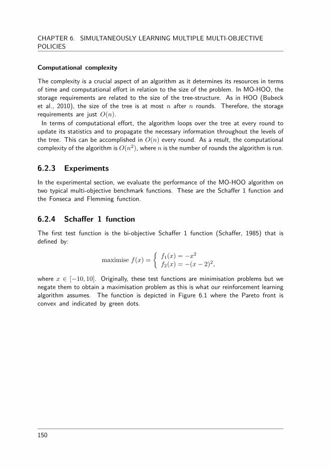
CHAPTER 6. SIMULTANEOUSLY LEARNING MULTIPLE MULTI-OBJECTIVEPOLICIES
Computational complexity
The complexity is a crucial aspect of an algorithm as it determines its resources in termsof time and computational e�ort in relation to the size of the problem. In MO-HOO, thestorage requirements are related to the size of the tree-structure. As in HOO (Bubecket al., 2010), the size of the tree is at most n after n rounds. Therefore, the storagerequirements are just O(n).
In terms of computational e�ort, the algorithm loops over the tree at every round toupdate its statistics and to propagate the necessary information throughout the levels ofthe tree. This can be accomplished in O(n) every round. As a result, the computationalcomplexity of the algorithm is O(n2
), where n is the number of rounds the algorithm is run.
6.2.3 ExperimentsIn the experimental section, we evaluate the performance of the MO-HOO algorithm ontwo typical multi-objective benchmark functions. These are the Scha�er 1 function andthe Fonseca and Flemming function.
6.2.4 Scha�er 1 functionThe first test function is the bi-objective Scha�er 1 function (Scha�er, 1985) that isdefined by:
maximise f(x) =
;f1(x) = ≠x2
f2(x) = ≠(x ≠ 2)
2,
where x œ [≠10, 10]. Originally, these test functions are minimisation problems but wenegate them to obtain a maximisation problem as this is what our reinforcement learningalgorithm assumes. The function is depicted in Figure 6.1 where the Pareto front isconvex and indicated by green dots.
150

6.2. LEARNING MULTIPLE POLICIES IN SINGLE-STATE PROBLEMS
−100 −90 −80 −70 −60 −50 −40 −30 −20 −10 0−70
−60
−50
−40
−30
−20
−10
0
Objective 1
Obje
ctiv
e 2
Schaffer1
Schaffer 1 Pareto front
Figure 6.1: The objective space of the Scha�er 1 function. The Pareto front of the functionis denoted by green dots.
In Figure 6.2 the sampling performance of the MO-HOO strategy is compared to arandom sampling strategy. Recall that our goal is to sample as fast as possible as close aspossible on the Pareto front. As the Pareto front is in this case continuous, we determinewhether the vector valued return of the sampled action is within a distance of ” of adiscrete approximation of the true Pareto front. In all our experiments, ” is set to 0.2and the results are averaged over 50 independent runs. This discrete approximation of thetrue Pareto front is obtained by collecting the Pareto non-dominated outcomes of manyindependent random runs of the algorithm. From the figure, we note that the MO-HOOstrategy gradually increases its performance by sampling closer to the Pareto front as thelearning time increases. After 500 iterations, the probability of sampling a Pareto optimalaction approaches 1. The random strategy only achieves a performance of 18% to 20%.
0 50 100 150 200 250 300 350 400 450 5000
0.1
0.2
0.3
0.4
0.5
0.6
0.7
0.8
0.9
1
Iteration
% P
are
to o
ptim
al a
ctio
ns
sam
ple
d
RandomMOHOO
Figure 6.2: The sampling performance MO-HOO is compared to a naive random strategy.We note that the probability of the MO-HOO strategy of sampling Pareto optimal solutionsapproaches 1 as time increases.
151

CHAPTER 6. SIMULTANEOUSLY LEARNING MULTIPLE MULTI-OBJECTIVEPOLICIES
In Figure 6.3, we plot three graphs that provide additional insights in the behaviour ofthe MO-HOO strategy. In a first subplot, we denote the sampled action at each timestep in the normalised action space. The MO-HOO strategy is exploring in early stagesof the process and afterwards it is exploiting its knowledge quite rapidly. In a secondsubplot, we show the depth of the tree in relation to the action space. Subtrees thatare more expanded have a greater depth and focus on a finer part of the action spacecompared to small subtrees. Where we note that the MO-HOO strategy roughly exploressome parts of the actions space, whereafter it focusses on the region corresponding tothe Pareto optimal area in the objective space. The third subplot depicts the sampledpoints in the objective space. The colour of the points indicates the iteration number,where red dots denote points obtained in later iterations. The MO-HOO samples thePareto optimal region after just a few iterations. We also see that the MO-HOO strategydiscovers a wide and diverse set of optimal solutions. This is a result of the optimisticterm added to the estimates. Imagine the case where multiple estimates are optimal andtherefore equally good. The algorithm then selects one and follows it down the tree untilit arrives in an untouched leaf node. In the event that this action selection also retrievesan optimal reward vector, its estimate (plus the optimistic term) is propagated to the rootnode. Because the leaf is located deeper in the tree, this optimistic term will be less thanfor the other estimates that were originally present at the root node. Therefore, in thenext iteration, the algorithm will not select the same action in the action space, but itwill go for one of its original non-dominated estimates. As a result, a set of wide-spreadand optimal solutions is retrieved.
152

6.2. LEARNING MULTIPLE POLICIES IN SINGLE-STATE PROBLEMS
0 50 100 150 200 250 300 350 400 450 5000
0.5
1
iteration
act
ion
Sampled points in action space
action
0 0.1 0.2 0.3 0.4 0.5 0.6 0.7 0.8 0.9 10
5
10
15
20
action space
depth
Tree depth
action
−100 −90 −80 −70 −60 −50 −40 −30 −20 −10 0−80
−60
−40
−20
0
objective 1
obje
ctiv
e 2
Obtained points in objective space
Figure 6.3: The MO-HOO strategy quickly retrieves the area in the action space thatcorresponds to the Pareto optimal area of the deterministic Scha�er 1 function (subplot1 and 3). In subplot 2, we note that the algorithm first roughly explores the function atrandom and thereafter it focusses specifically and exclusively on the optimal part of theaction space.
In Table 6.1, we present the average cardinality of all sampled policies during the learningprocess for each of the strategies. Recall that the cardinality indicators simply counts thenumber of Pareto non-dominated elements. Based on the results, we note MO-HOOacquires more than 6 times the amount of Pareto non-dominated solutions obtained bythe random method. After 500 action selections, MO-HOO is able to retrieve on average436.2 non-dominated points while the random strategy only obtained 69.5.
Strategy CardinalityRandom 69.5MO-HOO 436.2
Table 6.1: The cardinality indicator on the Scha�er 1 function for random exploration andMO-HOO. The goal is to maximise the number of Pareto optimal points.
153

CHAPTER 6. SIMULTANEOUSLY LEARNING MULTIPLE MULTI-OBJECTIVEPOLICIES
6.2.5 Fonseca and Flemming functionThe second problem is the Fonseca and Fleming function Fonseca and Fleming (1993):
maximise f(x) =
If1(x) = ≠(1 ≠ e≠
qn
i=1(xi≠ 1Ô
n)2
)
f2(x) = ≠(1 ≠ e≠qn
i=1(xi+ 1Ô
n)2
),
where x is a two-dimensional input vector with xi œ [≠4, 4] for input i. This bi-objectivefunction contains a large and an entirely non-convex Pareto front which makes it especiallyappealing to assess an algorithm’s ability to find a close and uniform approximation of thePareto front. The function and its corresponding Pareto front can be found in Figure 6.4.While the previous optimisation function is entirely deterministic, we added Normal noisewith ‡ = 0.1 to the values of each of the objectives.
−1 −0.9 −0.8 −0.7 −0.6 −0.5 −0.4 −0.3 −0.2 −0.1 0−1
−0.9
−0.8
−0.7
−0.6
−0.5
−0.4
−0.3
−0.2
−0.1
0
Objective 1
Obje
ctiv
e 2
F. and F. function
F. and F. Pareto front
Figure 6.4: The objective space of the Fonseca and Flemming function. The Pareto frontis highlighted by green dots.
In this environment the input vector itself is multi-dimensional. Therefore, we adjust theimplementation of a node in the tree to take into account a multi-dimensional interval,i.e., one interval for each input variable. In this implementation, the tree splits the intervalof the first variable for nodes located at uneven depth in the tree. In the case the node isat an even tree depth, the interval represented by the second variable is split.
In Figure 6.5, we depict the sampling performance of the MO-HOO strategy on thisnoisy function. As this function is significantly harder than the previous pay-o� function,the probability of sampling the Pareto front increases more slowly than is the case for theScha�er 1 function. When the learning process stopped after 1000 iterations, MO-HOOsamples Pareto optimal actions in 88% of the cases. The naive random strategy reacheda performance of only 20%.
154
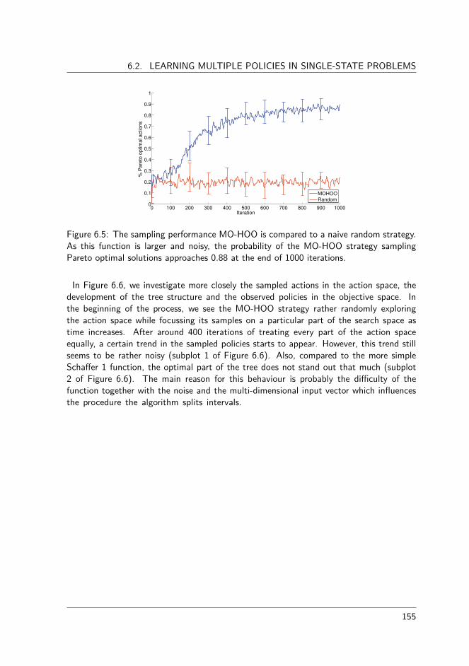
6.2. LEARNING MULTIPLE POLICIES IN SINGLE-STATE PROBLEMS
0 100 200 300 400 500 600 700 800 900 10000
0.1
0.2
0.3
0.4
0.5
0.6
0.7
0.8
0.9
1
Iteration
% P
are
to o
ptim
al a
ctio
ns
MOHOORandom
Figure 6.5: The sampling performance MO-HOO is compared to a naive random strategy.As this function is larger and noisy, the probability of the MO-HOO strategy samplingPareto optimal solutions approaches 0.88 at the end of 1000 iterations.
In Figure 6.6, we investigate more closely the sampled actions in the action space, thedevelopment of the tree structure and the observed policies in the objective space. Inthe beginning of the process, we see the MO-HOO strategy rather randomly exploringthe action space while focussing its samples on a particular part of the search space astime increases. After around 400 iterations of treating every part of the action spaceequally, a certain trend in the sampled policies starts to appear. However, this trend stillseems to be rather noisy (subplot 1 of Figure 6.6). Also, compared to the more simpleScha�er 1 function, the optimal part of the tree does not stand out that much (subplot2 of Figure 6.6). The main reason for this behaviour is probably the di�culty of thefunction together with the noise and the multi-dimensional input vector which influencesthe procedure the algorithm splits intervals.
155

CHAPTER 6. SIMULTANEOUSLY LEARNING MULTIPLE MULTI-OBJECTIVEPOLICIES
0 100 200 300 400 500 600 700 800 900 10000
0.5
1
iteration
act
ion
Sampled points in action space
actionaction
0 0.1 0.2 0.3 0.4 0.5 0.6 0.7 0.8 0.9 10
10
20
30
action space
depth
Tree depth
actionaction
−1.4 −1.2 −1 −0.8 −0.6 −0.4 −0.2 0 0.2−1.5
−1
−0.5
0
0.5
objective 1
obje
ctiv
e 2
Obtained points in objective space
Figure 6.6: Subplots 1 and 2 depict that the MO-HOO strategy needs a bit more timeon the Fonseca and Flemming function to explore the fruitful areas. We see that thealgorithm needs around 400 iterations before it had clear idea on which parts to furtherexplore.
The consequence of this practice is that the MO-HOO strategy did not entirely cover thecontinuous Pareto front as there are still some uncharted gaps. Table 6.2, we see that over50 runs, MO-HOO obtained on average a set containing 16.22 solutions that o�er an non-dominated balance between the two objectives. The random strategy obtained on averagea set containing 8.1 non-dominated elements. However, as the results of Figure 6.6 denote,the non-dominated solutions of the MO-HOO strategy are much closer to the Pareto frontand they clearly dominate the solutions obtained by the random strategy.
Strategy CardinalityRandom 8.1MO-HOO 16.22
Table 6.2: The cardinality indicator on the Fonseca and Flemming function for randomexploration and MO-HOO.
6.2.6 DiscussionIn this section, we have presented our first multi-policy algorithm for learning multiplepolicies in a simultaneous manner. We name this strategy the multi-objective hierarchicaloptimistic optimisation algorithm as it builds a tree of vectorial estimates that include
156

6.3. LEARNING MULTIPLE POLICIES IN MULTI-STATE PROBLEMS
some statistics on the variance of the samples. This algorithm is particularly suited forreal-life control problems that involve the optimisation of continuous parameters.
In the experimental section, we have seen that MO-HOO is an appropriate strategy todiscover a set of non-dominated solutions at once and to sample accordingly. Althoughthe pay-o� functions in this setting only consider two objectives, the principles of theunderlying tree-based algorithm can easily be extended to environments with more thantwo objectives. However, when increasing the number of objectives in the pay-o� function,also the number of Pareto incomparable solutions increases. Therefore, the problem alsogets harder for the optimisation algorithm and probably more running time is needed forthe algorithm to discover the Pareto optimal regions.
To possibly improve the algorithm, one could investigate how to consider the U -vectorsof non-leaf nodes in the backward computation to the root node. For each node, U -vectors store statistical information on the average quality of the subtree starting fromthat node. As this U -vector averages multiple reward estimates into a single estimate, wedid not find it beneficial to be included in the backward computation. If it would su�cefor the decision maker to sample the convex hull of the Pareto front, the U -vectors couldprovide supplementary guidance. Additionally the robustness of the MO-HOO strategywould also increase as the U -vectors provide average information over subtrees which ismore resilient to noisy rewards.
So far, to the best of our knowledge, MO-HOO is the first multi-objective multi-policyX -armed bandit solver. This has the advantage that it makes MO-HOO a very noveloptimisation algorithm that still includes a lot of uncharted research questions. However,a rigorous experimental comparison of the algorithm is still needed. Due to time constraintsour experimental evaluation is limited to a comparison with a naive random strategy. Apossibility would be to perform an experimental study to genetic algorithms that also evolvea population of solutions, as presented in Section 3.2. However, these algorithms rarelyconsider the sampling cost and are often less suitable if the environment is stochastic.
In order to make MO-HOO an acceptable solution mechanism for control problems itwould be of great importance to investigate its performance on some environments thatare close to the real world. In Chapter 7, we take a first step and perform an initialexperiment on a realistic simulation environment of the filling phase of a wet clutch.
6.3 Learning multiple policies in multi-state problemsIn the previous section we have investigated a multi-policy MORL algorithm for single-statelearning. In the case of a multi-state environment, the task at hand is a genuine sequentialdecision making problem. Over the years, a few multi-policy algorithms (Barrett andNarayanan, 2008; Lizotte et al., 2010, 2012) have been proposed that are all based on thesame principle of the algorithm of White (1982). In that paper, a dynamic programmingalgorithm is proposed that computes a set of Pareto non-dominated policies. The dynamic
157

CHAPTER 6. SIMULTANEOUSLY LEARNING MULTIPLE MULTI-OBJECTIVEPOLICIES
programming function is as follows:
ˆQset(s, a) = R(s, a) ü “ÿ
sÕœS
T (sÕ|s, a) V ND(sÕ
) (6.4)
where R(s, a) is the expected reward vector observed after taking action a in state s andT (sÕ|s, a) is the corresponding transition probability of reaching state sÕ from (s, a). Werefer to V ND
(sÕ) as the set of non-dominated vectors of the ˆQset’s of each action in sÕ,
as denoted in Eq. 6.5. The ND operator is a function that removes all Pareto dominatedelements of the input set and returns the set of non-dominated elements.
V ND(sÕ
) = ND(fiaÕ ˆQset(sÕ, aÕ
)) (6.5)
The ü operator performs a vector-sum of a vector v and a set of vectors V . Summing twovectors can be performed simply by adding the corresponding components of the vectors.
v ü V =
€
v
ÕœV
(v + v
Õ) (6.6)
The idea is that, after the discounted Pareto dominating rewards are propagated andthe ˆQset’s converge to a set of Pareto dominating policies, the user can traverse the treeof ˆQset’s by applying a preference function. As highlighted in Section 2.3, a determin-istic stationary policy su�ces for single-objective reinforcement learning. In the case ofMORL, White (1982) showed that deterministic non-stationary policies, i.e. policies thatdo not only condition on the current state but usually also on the timestep t, can Paretodominate the best deterministic stationary policies. Although we omit the theoretical proofbehind this theorem, the process is easily justified by considering the environment in Fig-ure 6.7. In the example, adapted from Roijers et al. (2013), there is a single state S andthree actions a1, a2 and a3 that leave the state of the environment unchanged.
S
(4, 0) (0, 4)
(1,1)
a1a2
a3
Figure 6.7: Deterministic non-stationary policies can Pareto dominate deterministic sta-tionary policies.
158
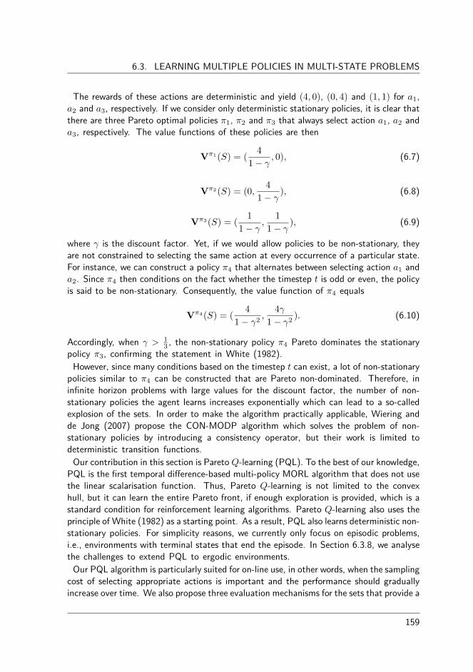
6.3. LEARNING MULTIPLE POLICIES IN MULTI-STATE PROBLEMS
The rewards of these actions are deterministic and yield (4, 0), (0, 4) and (1, 1) for a1,a2 and a3, respectively. If we consider only deterministic stationary policies, it is clear thatthere are three Pareto optimal policies fi1, fi2 and fi3 that always select action a1, a2 anda3, respectively. The value functions of these policies are then
V
fi1(S) = (
4
1 ≠ “, 0), (6.7)
V
fi2(S) = (0,
4
1 ≠ “), (6.8)
V
fi3(S) = (
1
1 ≠ “,
1
1 ≠ “), (6.9)
where “ is the discount factor. Yet, if we would allow policies to be non-stationary, theyare not constrained to selecting the same action at every occurrence of a particular state.For instance, we can construct a policy fi4 that alternates between selecting action a1 anda2. Since fi4 then conditions on the fact whether the timestep t is odd or even, the policyis said to be non-stationary. Consequently, the value function of fi4 equals
V
fi4(S) = (
4
1 ≠ “2 ,4“
1 ≠ “2 ). (6.10)
Accordingly, when “ > 13 , the non-stationary policy fi4 Pareto dominates the stationary
policy fi3, confirming the statement in White (1982).However, since many conditions based on the timestep t can exist, a lot of non-stationary
policies similar to fi4 can be constructed that are Pareto non-dominated. Therefore, ininfinite horizon problems with large values for the discount factor, the number of non-stationary policies the agent learns increases exponentially which can lead to a so-calledexplosion of the sets. In order to make the algorithm practically applicable, Wiering andde Jong (2007) propose the CON-MODP algorithm which solves the problem of non-stationary policies by introducing a consistency operator, but their work is limited todeterministic transition functions.
Our contribution in this section is Pareto Q-learning (PQL). To the best of our knowledge,PQL is the first temporal di�erence-based multi-policy MORL algorithm that does not usethe linear scalarisation function. Thus, Pareto Q-learning is not limited to the convexhull, but it can learn the entire Pareto front, if enough exploration is provided, which is astandard condition for reinforcement learning algorithms. Pareto Q-learning also uses theprinciple of White (1982) as a starting point. As a result, PQL also learns deterministic non-stationary policies. For simplicity reasons, we currently only focus on episodic problems,i.e., environments with terminal states that end the episode. In Section 6.3.8, we analysethe challenges to extend PQL to ergodic environments.
Our PQL algorithm is particularly suited for on-line use, in other words, when the samplingcost of selecting appropriate actions is important and the performance should graduallyincrease over time. We also propose three evaluation mechanisms for the sets that provide a
159
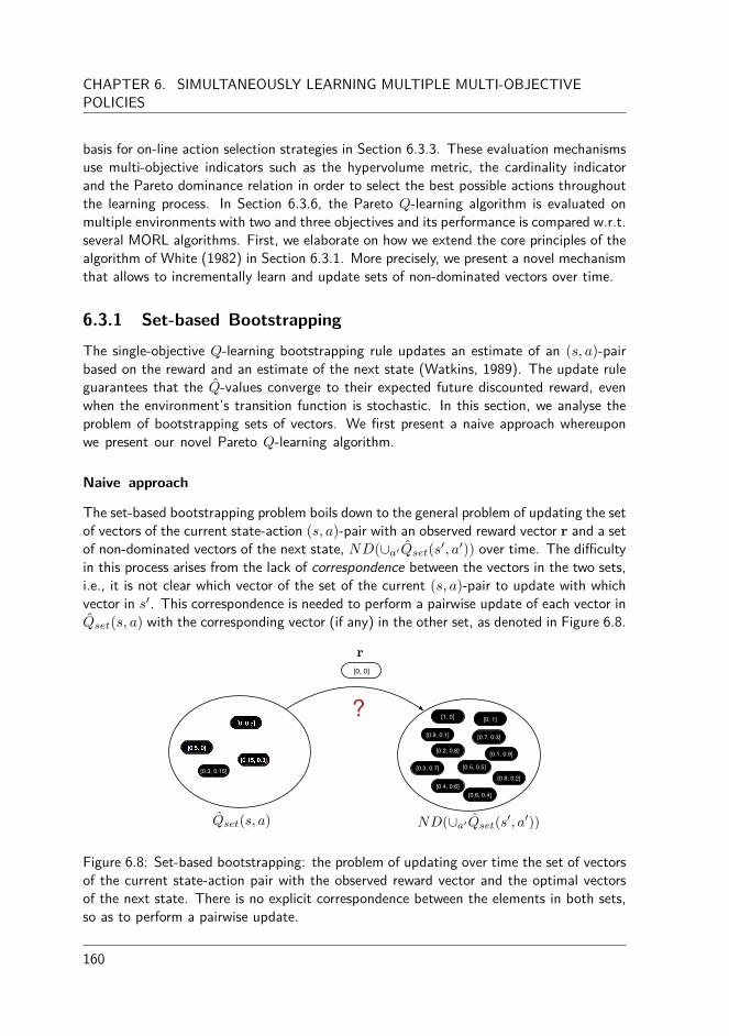
CHAPTER 6. SIMULTANEOUSLY LEARNING MULTIPLE MULTI-OBJECTIVEPOLICIES
basis for on-line action selection strategies in Section 6.3.3. These evaluation mechanismsuse multi-objective indicators such as the hypervolume metric, the cardinality indicatorand the Pareto dominance relation in order to select the best possible actions throughoutthe learning process. In Section 6.3.6, the Pareto Q-learning algorithm is evaluated onmultiple environments with two and three objectives and its performance is compared w.r.t.several MORL algorithms. First, we elaborate on how we extend the core principles of thealgorithm of White (1982) in Section 6.3.1. More precisely, we present a novel mechanismthat allows to incrementally learn and update sets of non-dominated vectors over time.
6.3.1 Set-based BootstrappingThe single-objective Q-learning bootstrapping rule updates an estimate of an (s, a)-pairbased on the reward and an estimate of the next state (Watkins, 1989). The update ruleguarantees that the ˆQ-values converge to their expected future discounted reward, evenwhen the environment’s transition function is stochastic. In this section, we analyse theproblem of bootstrapping sets of vectors. We first present a naive approach whereuponwe present our novel Pareto Q-learning algorithm.
Naive approach
The set-based bootstrapping problem boils down to the general problem of updating the setof vectors of the current state-action (s, a)-pair with an observed reward vector r and a setof non-dominated vectors of the next state, ND(fiaÕ ˆQset(sÕ, aÕ
)) over time. The di�cultyin this process arises from the lack of correspondence between the vectors in the two sets,i.e., it is not clear which vector of the set of the current (s, a)-pair to update with whichvector in sÕ. This correspondence is needed to perform a pairwise update of each vector inˆQset(s, a) with the corresponding vector (if any) in the other set, as denoted in Figure 6.8.
[0.9, 0.1]
[0, 1]
[0.3, 0.7]
[0, 0]
[0.5, 0]
[0.15, 0.3]
[0, 0.5]
[0.3, 0.15]
[0.1, 0.9]
? [1, 0]
[0.2, 0.8]
[0.4, 0.6][0.6, 0.4]
[0.8, 0.2]
ND([a0Qset(s0, a0))Qset(s, a)
[0.7, 0.3]
[0.5, 0.5]
r
Figure 6.8: Set-based bootstrapping: the problem of updating over time the set of vectorsof the current state-action pair with the observed reward vector and the optimal vectorsof the next state. There is no explicit correspondence between the elements in both sets,so as to perform a pairwise update.
160

6.3. LEARNING MULTIPLE POLICIES IN MULTI-STATE PROBLEMS
A possible solution is to make this correspondence explicit by labelling or tagging thevectors in the two sets. When vectors in the sets of (s, a) and sÕ are tagged with the samelabel or colour, the bootstrapping process knows that these vectors can be updated in apairwise manner. More precisely, the process would be as follows: when sampling an actiona in s for the first time, the vectors in the set of the next state ND(fiaÕ ˆQset(sÕ, aÕ
)) arelabeled with a unique tag. Next, the bootstrapping process can continue for each vectorin sÕ individually and the tag is copied to the set of (s, a). This process is illustrated inFigure 6.9 (a) for a bi-objective environment. Subsequently, when action a is sampled infuture timesteps, we would possess an actual correspondence between the vectors in thetwo sets and we can perform a pairwise update for each objective of each vector with thesame label (Figure 6.9 (b)). However, the main problem with this naive solution is thatthese sets are not stable but can change over time. We highlight two main cases thatcan occur in a temporal-di�erence setting:
• It is possible that the set of (s, a) is updated with vectors from sÕ at timestep t, whileactions in sÕ that are previously unexplored are sampled at timestep t + 1. Then,possibly new non-dominated vectors may appear in ND(fiaÕ ˆQset(sÕ, aÕ
)). When, infuture episodes, the set of (s, a) is to be updated again, there are elements in sÕ thatare not bootstrapped before and the correspondence between the sets is incomplete(Figure 6.9 (c)).
• As estimates are being updated over time, it is very likely that vectors in sÕ that werenon-dominated at timestep t may become dominated by other vectors at timestept + 1. In Figure 6.9 (d), we see that in that case the correspondence no longerholds, i.e., di�erent labels appear in the two sets. As a consequence, learning wouldhave to begin from scratch again for those vectors. Especially in early learningcycles, the vectorial estimates can repeatedly switch between being non-dominatedand dominated. Hence, this naive updating process would waste a lot of samplesbefore the vectors mature.
It is clear that such a naive updating procedure would become even more cumbersomeand complex in environments with stochastic transitions. As a result, it would not begenerally applicable to a wide range of problem domains.
161

CHAPTER 6. SIMULTANEOUSLY LEARNING MULTIPLE MULTI-OBJECTIVEPOLICIES
ND([a0Qset(s0, a0))Qset(s, a)
[0, 1]
[0.7, 0.2]
[0, 0]
r
ND([a0Qset(s0, a0))Qset(s, a)
[0, 1]
[0.7, 0.2]
[0, 0.5]
[0.35, 0.1]
[0, 0]
r
(a) (b)
[1, 0]
[0, 1][0.2, 0.7]
[0.7, 0.2]
[0, 0.5]
[0.3, 0.1]
?
?
[0, 0]
ND([a0Qset(s0, a0))Qset(s, a)
r
[1, 0]
[0.2, 0.7]
[0, 0.5]
[0.3, 0.1]
[0, 0]
?
ND([a0Qset(s0, a0))Qset(s, a)
r
(c) (d)
Figure 6.9: Several situations can occur when updating a set with another set over time.In (a), we would naively label the vectors of sÕ with a certain colour when sampling actiona in s for the first time. In (b), we note that the labeled and coloured vectors of sÕ
are now bootstrapped and present in (s, a). As the colours are also copied in (s, a), thecorrespondence between the vectors in (s, a) and sÕ is explicit and in future timestepsthe vectors can be updated in a pairwise manner. Illustrations (c) and (d) highlight thedi�erent situations one should account for as the sets are not stable but can change overtime. For instance, new vectors can appear in sÕ (c) or estimates that were non-dominatedcan become dominated (d). We refer to Section 6.3.1 for more details.
Our approach: Learning immediate and future reward separately
In the presentation of our updating principle, we first limit ourselves to environments withdeterministic transition functions. We then proceed to highlight the minimal extensionsto the algorithm to also cover stochastic transitions.
In standard, single-objective Q-learning, ˆQ-values store the sum of the estimated valueof the immediate reward and the future discounted reward as presented in Section 2.4.2.Our idea consists of storing this information separately. We use R(s, a) to denote theaverage observed immediate reward vector of (s, a) and NDt(s, a) to represent the set ofnon-dominated vectors in the next state of s that is reached through action a at timestept. The next state of s is determined by observing the transitions during learning. Bystoring R(s, a) and NDt(s, a) separately, we allow them to converge separately as well.This way, no explicit correspondence between the two sets is required and the current setof non-dominating policies at timestep t, NDt(s, a) is allowed to evolve over time. TheˆQset of (s, a) can be calculated at run time by performing a vector-sum over the average
162

6.3. LEARNING MULTIPLE POLICIES IN MULTI-STATE PROBLEMS
immediate reward vector and the set of discounted Pareto dominating future rewards:
ˆQset(s, a) Ω R(s, a) ü “NDt(s, a) (6.11)
Whenever the action a in s is selected, the average immediate reward vector R(s, a) isupdated and the NDt(s, a) list is updated using the non-dominated ˆ
Q-vectors in the ˆQset
of every action aÕ in sÕ, i.e., ND(fiaÕ ˆQset(sÕ, aÕ)).
We present an algorithmic outline of the Pareto Q-learning algorithm in Algorithm 7.The algorithm starts by initialising the ˆQset’s as empty sets. In each episode, an actionis selected using a particular action selection strategy (line 5). How we actually performthe action selection based on the ˆQset’s will be presented in the subsequent section.Afterwards, the environment transfers the agent to state sÕ and provides the reward vectorr. In state sÕ, the non-dominated ˆ
Q-vectors for each action are retrieved at line 8 andare discounted. At line 9, the average immediate reward for each objective, R(s, a), isiteratively updated given the new reward r and the number of times that action a issampled, denoted by n(s, a). The algorithm proceeds until the ˆQset’s converge or aftera predefined number of episodes.
Algorithm 7 Pareto Q-learning algorithm1: Initialise ˆQset(s, a)’s as empty sets2: for each episode t do3: Initialise state s4: repeat5: Choose action a from s using a policy derived from the ˆQset’s6: Take action a and observe state sÕ œ S and reward vector r œ Rm
7:8: NDt(s, a) Ω ND(fiaÕ ˆQset(sÕ, aÕ
)) Û Update ND policies of sÕ in s
9: R(s, a) Ω R(s, a) +
r≠R(s,a)n(s,a) Û Update average immediate rewards
10: s Ω sÕ Û Proceed to next state11: until s is terminal12: end for
The updating principle can also be extended to stochastic environments, where the trans-ition probability T (sÕ|s, a) ”= 1 for some next state sÕ, given state s and action a. In thecase of stochastic transition functions, we store the expected immediate and future non-dominated rewards per (s, a, sÕ
)-tuple that is observed during sampling, i.e., R(s, a, sÕ)
and NDt(s, a, sÕ), respectively. By also considering the observed frequencies of the oc-
currence of next state sÕ per (s, a)-pair, i.e., F sÕ
s,a, we estimate T (sÕ|s, a) for each (s, a).Hence, we learn a small model of the transition probabilities in the environment, sim-ilar to Dyna-Q (Sutton and Barto, 1998), which we use to calculate a weighted pairwisecombination between the sets. To combine a vector from one set with a vector from theother set, we propose the C-operator, which simply weighs them according to the observed
163
CHAPTER 6. SIMULTANEOUSLY LEARNING MULTIPLE MULTI-OBJECTIVEPOLICIES
transition frequencies:
C(
ˆ
Q(s, a, sÕ), ˆ
Q(s, a, sÕÕ)) =
F sÕ
s,aqsÕÕÕœS F sÕÕÕ
s,a
ˆ
Q(s, a, sÕ) +
F sÕÕ
s,aqsÕÕÕœS F sÕÕÕ
s,a
ˆ
Q(s, a, sÕÕ) (6.12)
6.3.2 Notions on convergenceIn this section, we sketch a convergence proof of the Pareto Q-learning algorithm. Asketch of the convergence of the algorithm can be accomplished by imitating the processof the proof of the single-objective Q-learning algorithm. This algorithm is a recursivealgorithm that, in each stage, updates its estimates based on newly acquired informationof the environment. Since the correction terms of each update are random, Tsitsiklis(1994) combines ideas from stochastic approximation and convergence theory of parallelasynchronous algorithms to prove the convergence of Q-learning. In essence, Tsitsiklis(1994) argues the update rule of the Q-learning algorithm in Equation 2.8 is a contraction.Let us say that this update rule is a function G which takes as input a vector q œ Rn, thenG(G(G(G(...G(x))))) converges to a fixed-point for all x œ Rn. This means that regardlessof the initialisation of the Q-values, the update rule makes these values converge to theiroptimal Qú-values under acceptable conditions. Basically, G is a contraction mappingw.r.t. maximum norm || ||Œ. This means that the more times G is applied on a Q-value,the closer the estimate will become to its optimal value Qú.
In the case of Pareto Q-learning, the situation is more complex because of two reasons.Firstly, we learn Q-vectors instead of Q-values. Secondly, and more importantly, we learna set consisting of multiple vectors. Therefore, a traditional norm such as || ||Œ is notapplicable in this context. Luckily, the Hausdor� distance can be used to measure thedistance between sets of vectors. The Hausdor� distance between two sets X and Y ofdiscrete elements can be calculated as follows:
dH(X, Y ) = max{ min
’xœX,’yœYd(x, y), min
’yœY,’xœXd(y, x)}. (6.13)
Basically, the metric simply calculates the longest shortest distance between elements ofthe two sets.
Although we do not provide a formal theoretical proof on the convergence of PQL, itsconvergence can be argued by the following experiment. In Figure 6.10, we calculate ateach timestep the Hausdor� distance between the learned set and the elements of thePareto front. At first we note that the initial learned set only contains a null element andthe distance to the optimal set is large. As the Pareto Q-learning update rule is appliedmore and more, the distance between the sets gradually decreases. Eventually, the distancebecomes zero, meaning that the learned sets becomes identical to the Pareto front andall the optimal policies are learned.
164

6.3. LEARNING MULTIPLE POLICIES IN MULTI-STATE PROBLEMS
Figure 6.10: The Hausdor� distance between the learned set to the Pareto front overtime. At first, the distance is large but the update rule of Pareto Q-learning decreases thedistance until it becomes zero. Hence, eventually, the learned set becomes equal to thePareto front and all the optimal policies are learned.
6.3.3 Set evaluation mechanismsIn reinforcement learning, the on-line performance is crucial. Therefore, it is interesting tosee how the standard exploration strategies, such as ‘-greedy, can be applied on the ˆQset’sduring learning. In this section, we propose three evaluation mechanisms that obtain ascalar indication of the quality of a ˆQset. These scalar evaluations are used in actionselection strategies to balance exploration and exploitation. We name these techniquesset evaluation mechanisms.
Hypervolume set evaluation
The first set evaluation mechanism we propose uses the hypervolume measure of Sec-tion 4.4.1 to evaluate the ˆQset’s. Recall that the hypervolume indicator is well-suited fortwo reasons: (1) it is the only quality indicator to be strictly monotonic with the Paretodominance relation and (2) it provides a scalar measure of the quality of a set of vectors.An outline of the evaluation mechanism is given in Algorithm 8. First, we initialise the listwhere the evaluations of each action of s will be stored. At line 4, we calculate the ˆQset
for each action and we compute its hypervolume which we append to the list. The list ofevaluations can then be used in an action selection strategy, similar to the single-objectivecase. For instance, when selecting an action greedily, the action corresponding to the ˆQset
with the largest hypervolume is selected. When the ˆQset’s are empty, the hypervolume
165
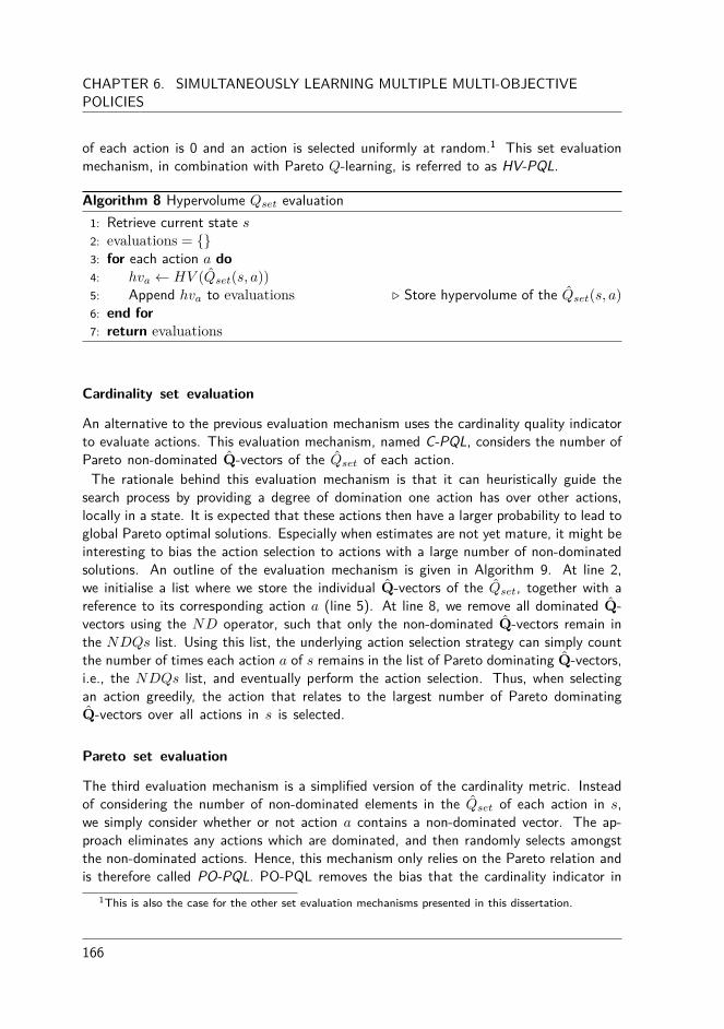
CHAPTER 6. SIMULTANEOUSLY LEARNING MULTIPLE MULTI-OBJECTIVEPOLICIES
of each action is 0 and an action is selected uniformly at random.1 This set evaluationmechanism, in combination with Pareto Q-learning, is referred to as HV-PQL.
Algorithm 8 Hypervolume Qset evaluation1: Retrieve current state s2: evaluations = {}3: for each action a do4: hva Ω HV (
ˆQset(s, a))
5: Append hva to evaluations Û Store hypervolume of the ˆQset(s, a)
6: end for7: return evaluations
Cardinality set evaluation
An alternative to the previous evaluation mechanism uses the cardinality quality indicatorto evaluate actions. This evaluation mechanism, named C-PQL, considers the number ofPareto non-dominated ˆ
Q-vectors of the ˆQset of each action.The rationale behind this evaluation mechanism is that it can heuristically guide the
search process by providing a degree of domination one action has over other actions,locally in a state. It is expected that these actions then have a larger probability to lead toglobal Pareto optimal solutions. Especially when estimates are not yet mature, it might beinteresting to bias the action selection to actions with a large number of non-dominatedsolutions. An outline of the evaluation mechanism is given in Algorithm 9. At line 2,we initialise a list where we store the individual ˆ
Q-vectors of the ˆQset, together with areference to its corresponding action a (line 5). At line 8, we remove all dominated ˆ
Q-vectors using the ND operator, such that only the non-dominated ˆ
Q-vectors remain inthe NDQs list. Using this list, the underlying action selection strategy can simply countthe number of times each action a of s remains in the list of Pareto dominating ˆ
Q-vectors,i.e., the NDQs list, and eventually perform the action selection. Thus, when selectingan action greedily, the action that relates to the largest number of Pareto dominatingˆ
Q-vectors over all actions in s is selected.
Pareto set evaluation
The third evaluation mechanism is a simplified version of the cardinality metric. Insteadof considering the number of non-dominated elements in the ˆQset of each action in s,we simply consider whether or not action a contains a non-dominated vector. The ap-proach eliminates any actions which are dominated, and then randomly selects amongstthe non-dominated actions. Hence, this mechanism only relies on the Pareto relation andis therefore called PO-PQL. PO-PQL removes the bias that the cardinality indicator in
1This is also the case for the other set evaluation mechanisms presented in this dissertation.
166

6.3. LEARNING MULTIPLE POLICIES IN MULTI-STATE PROBLEMS
Algorithm 9 Cardinality Qset evaluation1: Retrieve current state s2: allQs = {}3: for each action a in s do4: for each ˆ
Q in ˆQset(s, a) do5: Append [a, ˆ
Q] to allQs Û Store for each ˆ
Q-vector a reference to a6: end for7: end for8: NDQs Ω ND(allQs) Û Keep only the non-dominating solutions9: return NDQs
C-PQL might have for actions with a large number of non-dominated vectors over actionswith just a few. The rationale behind this mechanism is to have a more relaxed evaluationof the actions and to treat every non-dominated solution equally.
6.3.4 Consistently tracking a policyThe set evaluation mechanisms in Section 6.3.3 provide the necessary tools to performaction selection during learning, i.e., balancing the exploration towards uncharted areas ofthe state space and the exploitation of non-dominated actions. However, at any moment intime, it might be necessary to apply the learned policies. In single-objective reinforcementlearning, the learned policy can be easily tracked by applying the arg max-operator over allactions in each state, i.e., applying greedy action selection. In the case of a multi-policyproblem, we are learning multiple policies at the same time which requires an adapteddefinition of a greedy policy in MORL.
Because of the nature of multi-policy setting, one needs to select actions consistentlyin order to retrieve a desired policy based on the ˆ
Q-vectors. If one would select actionsbased on local information about the ‘local’ Pareto front attainable from each action, thenthere is no guarantee that the cumulative reward vectors obtained throughout the episodewill be globally Pareto optimal. This process is highlighted in Figure 6.11 (a) where thestate space is an 8◊8 grid and three global Pareto optimal policies exist, each given adi�erent colour. In Figure 6.11 (b), we select actions that are locally non-dominated, i.e,non-dominated within the current state. The black policy is a sequence of locally optimalactions, as it always overlaps with one of the coloured lines, however, the resulting policyis not globally Pareto optimal. To conclude, when in a state where multiple actions areconsidered non-dominated, and thus incomparable, one can not randomly select betweenthese actions when exploiting a chosen balance between criteria. Instead, actions needto be selected consistently.
167

CHAPTER 6. SIMULTANEOUSLY LEARNING MULTIPLE MULTI-OBJECTIVEPOLICIES
S
G
S
G
(a) (b)
Figure 6.11: (a) In this environment, there is a green, yellow and red Pareto optimal actionsequence that is globally optimal. (b) Selecting actions that are locally non-dominatedwithin the current state does not guarantee that the entire policy is globally Pareto optimal.Hence, the information about the global Pareto front has been lost in the local Pareto front.
Globally greedy policy
In order to solve the problem of locally optimal actions that are globally dominated, wedefine a greedy policy as a policy fi that consistently follows or tracks a given expectedreturn vector V
fi(s) from a state s so that its return equals V
fi(s) in expectation. There-
fore, we need to retrieve fi, i.e., which actions to select from a start state to a terminalstate. However, due to the stochastic behaviour of the environment, it is not trivial toselect the necessary actions so as to track the desired return vectors. Let us consider thesmall bi-objective MDP with deterministic transitions in Figure 6.12.
168

6.3. LEARNING MULTIPLE POLICIES IN MULTI-STATE PROBLEMS
S0 S1a
b
c
d
Action R(s, a) NDt(s, a)
ˆQset(s, a)
a (0.2, 0.0)!(0.9, 0.5), (2.0, 0.4), (0.0, 0.6)
" !(1.1, 0.5), (2.2, 0.4), (0.2, 0.6)
"
b (0.9, 0.5) () (0.9, 0.5)c (2.0, 0.4) () (2.0, 0.4)d (0.0, 0.6) () (0.0, 0.6)
Figure 6.12: A small multi-objective MDP and its corresponding Qset’s. As we storethe expected immediate and future non-dominated vectors separately, we can consistentlyfollow expected return vectors from start to end state.
When the agent reaches a terminal state, denoted by a double circle, the episode isfinished. Assume that the discount factor “ is set to 1 for simplicity reasons. Once theQset’s have converged separately, we can identify three Pareto optimal policies in the startstate s0. These policies have corresponding expected reward vectors (1.1, 0.5), (2.2, 0.4)
and (0.2, 0.6). When one is for instance interested in following the policy with an expectedreward vector of (2.2, 0.4), the agent should select action a as the vector (2.2, 0.4) is anelement of the ˆQset of action a (and there is no other option). But, once in the next state,the next action to select is not clear when one only stores the converged Qset’s. Hence,should the agent select action b, c or d to acquire a return of (2.2, 0.4) at the end of theepisode? The approach we propose to solve this issue is based on the separation of theaverage immediate and future rewards, i.e., we can simply subtract the average immediatereward from the expected return we are targeting, in order to retrieve the next action toselect. This way, we can consistently follow the expected return from state s, V
fi(s),
throughout the entire state space. In the example, the agent should select the action thatcontains (2.2, 0.4)≠ (0.2, 0) = (2.0, 0.4) in its Qset, i.e., action c. The pseudo-code of thetracking algorithm for environments with deterministic transitions is listed in Algorithm 10.The agent starts in a starting state s of the environment and has to follow a particularpolicy so as to obtain the expected value of the policy from that state, i.e., V
fi(s), at the
end of the episode. For each action of the action set A, we retrieve both the averagedimmediate reward R(s, a) and NDt(s, a), which we discount. If the sum of these twocomponents equals the target vector to follow, we select the corresponding action and
169
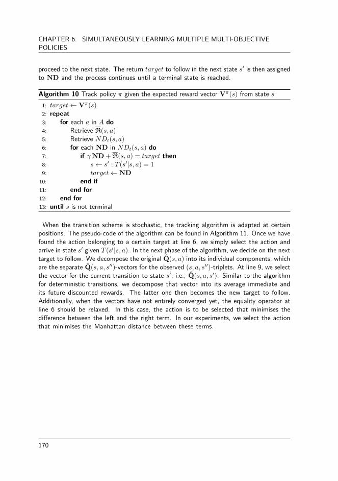
CHAPTER 6. SIMULTANEOUSLY LEARNING MULTIPLE MULTI-OBJECTIVEPOLICIES
proceed to the next state. The return target to follow in the next state sÕ is then assignedto ND and the process continues until a terminal state is reached.
Algorithm 10 Track policy fi given the expected reward vector V
fi(s) from state s
1: target Ω V
fi(s)
2: repeat3: for each a in A do4: Retrieve R(s, a)
5: Retrieve NDt(s, a)
6: for each ND in NDt(s, a) do7: if “ ND + R(s, a) = target then8: s Ω sÕ
: T (sÕ|s, a) = 1
9: target Ω ND
10: end if11: end for12: end for13: until s is not terminal
When the transition scheme is stochastic, the tracking algorithm is adapted at certainpositions. The pseudo-code of the algorithm can be found in Algorithm 11. Once we havefound the action belonging to a certain target at line 6, we simply select the action andarrive in state sÕ given T (sÕ|s, a). In the next phase of the algorithm, we decide on the nexttarget to follow. We decompose the original ˆ
Q(s, a) into its individual components, whichare the separate ˆ
Q(s, a, sÕÕ)-vectors for the observed (s, a, sÕÕ
)-triplets. At line 9, we selectthe vector for the current transition to state sÕ, i.e., ˆ
Q(s, a, sÕ). Similar to the algorithm
for deterministic transitions, we decompose that vector into its average immediate andits future discounted rewards. The latter one then becomes the new target to follow.Additionally, when the vectors have not entirely converged yet, the equality operator atline 6 should be relaxed. In this case, the action is to be selected that minimises thedi�erence between the left and the right term. In our experiments, we select the actionthat minimises the Manhattan distance between these terms.
170

6.3. LEARNING MULTIPLE POLICIES IN MULTI-STATE PROBLEMS
Algorithm 11 Track policy fi given the expected reward vector V
fi(s) from state s
1: target Ω V
fi(s)
2: repeat3: for each a in A do4: Retrieve ˆQset(s, a)
5: for each Q in ˆQset(s, a) do6: if Q = target then7: s Ω sÕ
: T (sÕ|s, a) ”= 1
8: Knowing that Q = C(
ˆ
Q(s, a, sÕ), . . .) using Equation 6.12
9: and that ˆ
Q(s, a, sÕ) = R(s, a, sÕ
) + “ ND
10: Retrieve R(s, a, sÕ)
11: Retrieve ND
12: target Ω ND
13: end if14: end for15: end for16: until s is not terminal
6.3.5 Performance assessment of multi-policy algorithmsBefore we analyse the experiments, we first discuss the general challenges in assessing theperformance of on-line multi-policy MORL algorithms. In single-objective reinforcementlearning, an algorithm is usually evaluated by its average reward accumulated over time.The curve of the graph then indicates both the speed of learning and the final perform-ance of the converged policy. In multi-objective reinforcement learning, the performanceassessment is more complex because of two main reasons: (1) the reward signal is vectorialand not scalar and (2) there exists no total ordering of the policies but there is a set ofincomparable optimal policies.
For scalarised MORL algorithms that converge to a single policy, Vamplew et al. (2010)propose to employ the hypervolume indicator on the approximation set of policies, i.e., thepolicies that are obtained after applying a greedy policy for a range of experiments withvarying parameters in the scalarisation functions. The hypervolume of the approximationset can then be compared to the hypervolume of the true Pareto front, i.e., the set of Paretooptimal policies of the environment. Each experiment then represents an individual run of ascalarised MORL algorithm with a specific weight vector w. In the case of tracking globallygreedy policies, we can adopt the mechanism by Vamplew et al. (2010) and calculatethe hypervolume of the cumulative reward vectors obtained by the tracking algorithm ofSection 6.3.4 for each of the non-dominated vectors in the ND(fia
ˆQset(s0, a)), wheres0 is the start state. The hypervolume of each of these vectors should then approachthe hypervolume of the Pareto front. It is important to note that in this way, we willevaluate and track as many policies as there exist non-dominated ˆ
Q-vectors in the startstate for all actions.
171

CHAPTER 6. SIMULTANEOUSLY LEARNING MULTIPLE MULTI-OBJECTIVEPOLICIES
6.3.6 Benchmarking Pareto Q-learningIn this section, we analyse the performance of the Pareto Q-learning algorithm on two testproblems for each of the three set evaluation mechanisms, i.e., with either the hypervolume,cardinality or Pareto evaluation mechanism. The algorithms are tested on several bench-mark environments with a linear, convex and non-convex Pareto front. All the experimentsare averaged over 50 runs and their 95% confidence interval is depicted at regular intervals.
The Pyramid MDP
The Pyramid MDP is a new and simple multi-objective benchmark environment. A visualrepresentation of the world is depicted in Figure 6.13. The agent starts in the down-leftposition, denoted by a black dot at (0, 0), and it can choose any of the four cardinaldirections (up, down, left and right). The transition function is stochastic so that with aprobability of 0.95 the selected action is performed and with a probability of 0.05 a randomtransition is executed to a neighbouring state. The red dots represent terminal states. Thereward scheme is bi-objective and returns a reward drawn from a Normal distribution withµ = ≠1 and ‡ = 0.01 for both objectives, unless a terminal state is reached. In that case,the x and y position of the terminal state is returned for the first and second objective,respectively. The Pareto front is therefore linear as depicted in Figure 6.14.
0 10 20 30 40 50 60 70 80 90 1000
10
20
30
40
50
60
70
80
90
100
X−axis
Y−
axis
Non−terminal states
Terminal states
Start state
Figure 6.13: The Pyramid MDP: the agent starts in the down-left position and can selectactions until a terminal state is reached, denoted by a red dot.
172

6.3. LEARNING MULTIPLE POLICIES IN MULTI-STATE PROBLEMS
−20 0 20 40 60 80 100−20
0
20
40
60
80
100
Objective 1
Obje
ctiv
e 2
Figure 6.14: The corresponding linear Pareto front of the Pyramid MDP.
As we are learning multiple policies simultaneously, which potentially may involve dif-ferent parts of the state space, we found it beneficial to employ a train and test setting,where in the train mode, we learn with an ‘-greedy action selection strategy with de-creasing epsilon.2 In the test mode of the algorithm, we perform multiple greedy policiesusing Algorithm 10 for every element in ND(fia
ˆQset(s0, a)) of the start state s0 and weaverage the accumulated returns along the paths. Each iteration, these average returnsare collected and the hypervolume is calculated.
In Figures 6.15 and 6.16, we present the results of learning and sampling Pareto optimalpolicies in the Pyramid MDP environment for the train and test phases, respectively.
2At episode eps, we assigned ‘ to be 0.997eps to allow for significant amounts of exploration in earlyruns while maximising exploitation in later runs of the experiment.
173

CHAPTER 6. SIMULTANEOUSLY LEARNING MULTIPLE MULTI-OBJECTIVEPOLICIES
0 50 100 150 200 250 300 350 400 450 5000
1000
2000
3000
4000
5000
6000
7000
Iteration
Hyp
erv
olu
me
Hypervolume of vectors in start state
PO−PQL
C−PQL
HV−PQL
Pareto front
Figure 6.15: We depict the hypervolume of the estimates in the start state of the stochasticPyramid MDP and we note that the entire Pareto front is learned very quickly during thelearning phase.
0 50 100 150 200 250 300 350 400 450 5000
1000
2000
3000
4000
5000
6000
7000
Iteration
Hyp
erv
olu
me
Hypervolume of tracked policies of start state
PO−PQL
C−PQL
HV−PQL
Pareto front
Figure 6.16: We track the estimates learned in Figure 6.15 through the state space anddenote that the hypervolume of their average returns approaches the Pareto front as well.
In Figure 6.15, we depict the hypervolume over time of the estimates in the start states0.3 Hence, for each iteration, we calculate HV (fia
ˆQset(s0, a)). We see that each ofthe set evaluation mechanisms guide the Pareto Q-learning algorithm very well as thehypervolume of the learned estimates approaches the hypervolume of the Pareto front (“
3In the Pyramid MDP, the reference point for the hypervolume calculation in both HV-PQL and theperformance assessment is specified to (≠20, ≠20) after observing the reward scheme.
174

6.3. LEARNING MULTIPLE POLICIES IN MULTI-STATE PROBLEMS
is set to 1). Based on the graph, we see that each of the set evaluation mechanisms hasvery similar performance in early stages of the learning process. After around hundrediterations, however, we note a small distinction in performance between C-PQL and HV-PQL on the one hand and PO-PQL on the other hand. Closer investigation of the resultstaught us that this di�erence is caused by the fact that, once the estimates become stable,C-PQL and HV-PQL still create a total order out of the set of Pareto optimal estimates,even though they are incomparable. That is why, in later iterations of the learning phase,C-PQL and HV-PQL provide a (too) large bias towards particular areas of the state andaction space and therefore some estimates are no longer updated. Hence, the very close,but not coinciding curves of their learning graphs. PO-PQL does not provide a totalorder, but keeps the partial order that the multi-objective nature of the problem entails.Therefore, it treats every Pareto optimal solution equally and the estimates are updatedmuch more consistently.
In Figure 6.16, we depict the results of the tracking algorithm of Section 6.3.4 thatglobally follows every element of the start state in Figure 6.15 (a). We see that thehypervolume of the average returns of each the estimated ˆ
Q-vectors in ND(fiaˆQset(s, a))
is very similar to the learned estimates themselves. We see that tracking the estimatesobtained by PO-PQL allows to sample the entire Pareto front over time.
0 10 20 30 40 50 60 70 80 90 1000
0.1
0.2
0.3
0.4
0.5
0.6
0.7
Number of times the policy is tracked
Ma
nh
att
an
dis
tan
ce
Manhattan distance from sampled average to estimate
Manhattan distance
Figure 6.17: The performance of the tracking algorithm for a specific estimate. We seethat the Manhattan distance of the running average of the return vector approaches thetracked estimate over time.
In Figure 6.17, we see the tracking algorithm at work to retrieve the policy of a specificvectorial estimate from the start state. In the figure, we denote the Manhattan distanceof the running average return to the estimate after learning. We see that averaging thereturn of the policy obtained by the tracking algorithm over time approaches the estimatepredicted at the start state, i.e., the distance becomes zero in the limit.
175

CHAPTER 6. SIMULTANEOUSLY LEARNING MULTIPLE MULTI-OBJECTIVEPOLICIES
The Pressurised Bountiful Sea Treasure environment
In order to evaluate the Pareto Q-learning algorithm on an environment with a largernumber of objectives, we analyse its performance on the Pressurised Bountiful Sea Treasure(PBST) environment of Section 5.2.5. This environment is very similar to the standardDeep Sea Treasure (DST) environment (Vamplew et al., 2010) with the slight modificationof an additional objective.
100
101
102
103
0
0.5
1
1.5
2
2.5
3
3.5
4x 10
5
Iteration
Hyp
erv
olu
me
Hypervolume of vectors in start state
PO−PQL
C−PQL
HV−PQL
Pareto front
Figure 6.18: The results on the PBST environment. We depict the hypervolume over timeof the learned estimates in the start state. As time progresses, the vectors in the startstate approach their true values.
176

6.3. LEARNING MULTIPLE POLICIES IN MULTI-STATE PROBLEMS
100
101
102
103
0
0.5
1
1.5
2
2.5
3
3.5
4x 10
5
Iteration
Hyp
erv
olu
me
Hypervolume of tracked policies of start state
PO−PQL
C−PQL
HV−PQL
Pareto front
Figure 6.19: We see that the hypervolume of the tracked policies in the PBST environmentis very similar to the hypervolume of the learned policies, which means that the learnedpolicies are also retrievable.
The results on the train and test phases are depicted in Figures 6.18 and 6.19, respect-ively.4 In Figure 6.19, we depict the hypervolume of the tracked policies of the start stateby applying the greedy policies. As the environment has both deterministic reward andtransition schemes, the performance of the di�erent set evaluation mechanisms is almostidentical. The tracking algorithm performs very well and the graph is almost identical toFigure 6.18 as in the previous environment.
6.3.7 Experimental comparisonIn the previous section, we analysed the performance of Pareto Q-learning in combinationwith the three set evaluation mechanisms. In this section, we conduct an empirical com-parison of the algorithms to several single-policy and multi-policy MORL algorithms. Weconduct this experimental comparison on the Deep Sea Treasure environment.
The Deep Sea Treasure environment
The Deep Sea Treasure (DST) is a standard MORL benchmark instance that has been thesubject of many performance evaluations in MORL. A general description of the environ-ment can be found in Section 4.3.4. In Figure 6.20, we denote the hypervolume duringthe test phase of the algorithm with Pareto, cardinality and hypervolume set evaluations,
4In the PBST environment, the reference point for the hypervolume calculation in both HV-PQL andthe performance assessment is specified to (≠25, 0, ≠120) after observing the reward scheme.
177

CHAPTER 6. SIMULTANEOUSLY LEARNING MULTIPLE MULTI-OBJECTIVEPOLICIES
i.e., PO-PQL, C-PQL and HV-PQL, respectively. The reference point for the hypervolumecalculation is specified to (≠25, 0).
Furthermore, we also evaluate a naive random strategy, a multi-policy algorithm and twosingle-policy algorithms. The multi-policy algorithm is the multi-objective Monte-Carlotree search algorithm by Wang and Sebag (2013). Recall that this algorithm incrementallybuilds and explores a search tree of optimistic vectorial estimates. We implemented MO-MCTS-DOM, i.e., the version that relies on the Pareto dominance relation to scalarize themulti-objective value function, since this alternative is the best choice in terms of runtimeand performance (Wang and Sebag, 2013). The two single-policy algorithms employ thelinear and Chebyshev scalarisation functions of Chapter 4. These single-policy algorithmsare evaluated using the configuration specified in Section 6.3.5. In the following paragraph,we highlight the performance of each algorithm individually.
Random The first algorithm we analyse is a random strategy. This algorithms servesas a baseline since it does not use any learning principles but naively applies a randompolicy. As expected, this algorithm learns slowly and reaches a hypervolume of 316. The95% confidence interval of this algorithm is remarkably low since it always tends to findthe same solutions, more precisely, the policies that are located close to the start state.The treasures that are far away are usually not discovered.
Linear scalarised MORL Since the environment contains 10 Pareto optimal solutions,the linear scalarised MORL algorithm is run with 10 uniformly distributed weight vectorsto allow for a fair comparison to the multi-policy algorithms. More precisely, the con-tinuous weight range of [0, 1] is uniformly discretised with steps of 1
10≠1 while satisfyingqmo=1 wo = 1. Each of these weights is then used in an individual execution of the scalar-
isation algorithm and its results are collected in order to obtain a set of sampled policies inthe test phase. Thus, every 10 iterations (episodes), we calculate the hypervolume of the10 greedy policies of each of those iterations. We note that, although we have a uniformspread of weights, the algorithm only manages to retrieve a hypervolume of 768 which is incorrespondence with our results from Chapter 5. When we take a closer look at the resultsobtained, we see that the algorithm learns fast but after 800 iterations, only the optimalpolicies with return (≠1, 1) and (≠19, 124) for the time and treasure objectives, respect-ively, are sampled. This is shown by the 95% confidence intervals that become zero. Thisis to be expected as the Pareto front is non-convex and, hence, a linear combination ofthe objectives then can only di�erentiate between the extreme policies of the Pareto front,as highlighted in Section 4.2. Therefore, the linear scalarised MORL algorithm convergesto either of the optimal policies with return (≠1, 1) or (≠19, 124).
Chebyshev scalarised MORL This non-linear scalarisation function is equipped withthe same set of weight vectors as the linear scalarisation function. As we see in the graph,the Chebyshev scalarised MORL algorithm learns slower than the linear scalarised MORLalgorithm but is able to surpass its performance after around 1700 iterations. However,
178

6.3. LEARNING MULTIPLE POLICIES IN MULTI-STATE PROBLEMS
as we have seen in Section 4.3, the Chebyshev scalarisation function is not guaranteed toconverge to a Pareto optimal policy in a value-iteration approach. Nevertheless, we seethat the algorithm performs acceptably in practice as it learns almost at the same speedas the linear scalarised MORL algorithm and attains a bigger hypervolume of 860.36. Thisis a confirmation that this scalarisation function, despite its lack of theoretical guarantees,can be successful in MORL when employed as a heuristic. Possibly, a higher hypervolumevalue could be reached, if we would equip the algorithm with more intelligent weightparameters. In this regard, the mechanisms of Chapter 5 could act as a starting point.
MO-MCTS-DOM The multi-policy MO-MCTS algorithm that utilises the Pareto dom-inance relation learns fast in the first 500 iterations but is, generally speaking, slowercompared to the single-policy strategies. Earlier results of the algorithm indicate that thesearch tree algorithms requires substantial amounts of training time before a large set ofpolicies is retrieved. This is because the algorithm builds an archive of non-dominatedtree walks and, in the best case, appends only one solution at the end of every iteration.Therefore, the algorithm intrinsically only learns multiple policies in an implicit manner,while wasting information on explicit trade-o�s as the interaction with the environmentprogresses. In the experiments in Wang and Sebag (2013), around 15600 iterations areneeded for MO-MCTS-DOM to converge to the set of optimal solutions, which is signi-ficantly large for this environment. Therefore, considering 3000 iterations, allowed us onlyto slowly reach a final performance comparable to the Chebyshev scalarisation function.
Pareto Q-learning So far, no algorithms managed to sample the entire Pareto front.This was a result of either the shape of the Pareto front, the assignment of the weightvectors or an ine�cient use of the available samples. Pareto Q-learning is not biased bythe first two aspects, but treats every Pareto optimal solution equally in the bootstrappingprocess. Additionally, it explicitly learns multiple policies in a simultaneous fashion toallow for an e�cient use of the available samples. Taking these principles into account,we see that in early learning phases, i.e, iteration 0 to 450, regardless of the set evaluationmechanisms, Pareto Q-learning learns notably faster than the other MORL algorithms.This is because PQL can simultaneously combine and store information about multipleoptimal policies while the single-policy learners look only for an individual policy thatmatches its a priori preferences, thereby discarding considerable amounts of information. Inthe end, regardless of the set evaluation mechanisms used, Pareto Q-learning surpasses theperformance of the other MORL algorithms. In this experiment, the Pareto set evaluationmechanism performs a bit better than the other set evaluation mechanisms and samplesevery element of the Pareto front.
179
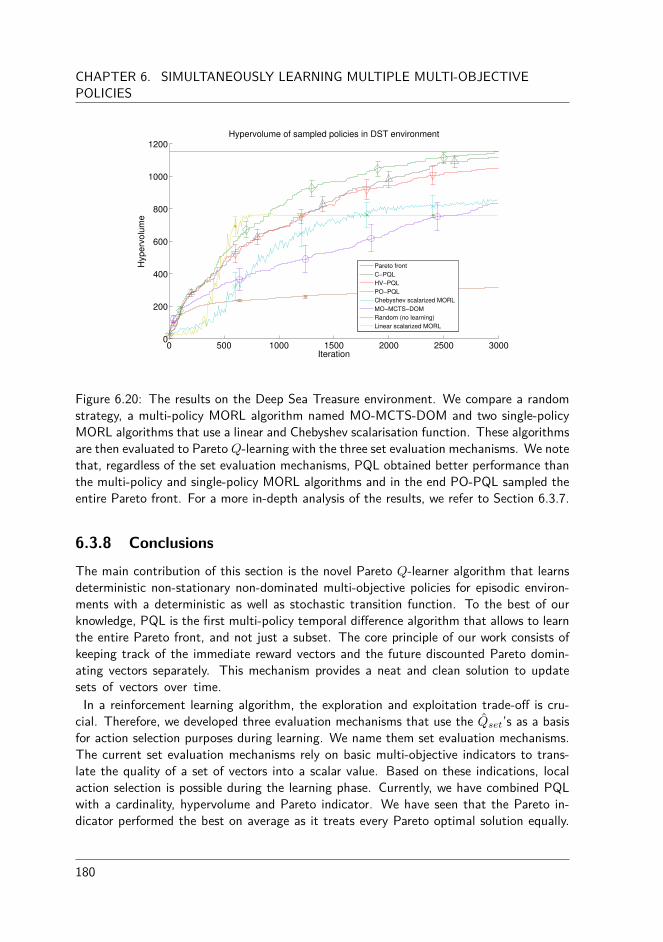
CHAPTER 6. SIMULTANEOUSLY LEARNING MULTIPLE MULTI-OBJECTIVEPOLICIES
0 500 1000 1500 2000 2500 30000
200
400
600
800
1000
1200Hypervolume of sampled policies in DST environment
Iteration
Hyp
erv
olu
me
Pareto front
C−PQL
HV−PQL
PO−PQL
Chebyshev scalarized MORL
MO−MCTS−DOM
Random (no learning)
Linear scalarized MORL
Figure 6.20: The results on the Deep Sea Treasure environment. We compare a randomstrategy, a multi-policy MORL algorithm named MO-MCTS-DOM and two single-policyMORL algorithms that use a linear and Chebyshev scalarisation function. These algorithmsare then evaluated to Pareto Q-learning with the three set evaluation mechanisms. We notethat, regardless of the set evaluation mechanisms, PQL obtained better performance thanthe multi-policy and single-policy MORL algorithms and in the end PO-PQL sampled theentire Pareto front. For a more in-depth analysis of the results, we refer to Section 6.3.7.
6.3.8 ConclusionsThe main contribution of this section is the novel Pareto Q-learner algorithm that learnsdeterministic non-stationary non-dominated multi-objective policies for episodic environ-ments with a deterministic as well as stochastic transition function. To the best of ourknowledge, PQL is the first multi-policy temporal di�erence algorithm that allows to learnthe entire Pareto front, and not just a subset. The core principle of our work consists ofkeeping track of the immediate reward vectors and the future discounted Pareto domin-ating vectors separately. This mechanism provides a neat and clean solution to updatesets of vectors over time.
In a reinforcement learning algorithm, the exploration and exploitation trade-o� is cru-cial. Therefore, we developed three evaluation mechanisms that use the ˆQset’s as a basisfor action selection purposes during learning. We name them set evaluation mechanisms.The current set evaluation mechanisms rely on basic multi-objective indicators to trans-late the quality of a set of vectors into a scalar value. Based on these indications, localaction selection is possible during the learning phase. Currently, we have combined PQLwith a cardinality, hypervolume and Pareto indicator. We have seen that the Pareto in-dicator performed the best on average as it treats every Pareto optimal solution equally.
180
6.4. SUMMARY
The cardinality and hypervolume set evaluation measures rate the actions also on addi-tional criteria than the Pareto relation to provide a total order. We have seen that inmore complex environments, these set evaluation mechanisms bias the action selectiontoo much in order to learn the entire Pareto front. Nevertheless, it could be that the useris not interested in sampling the entire Pareto front but is looking for particular policiesthat satisfy certain criteria. For instance, other quality indicators such as the spread in-dicator (Van Veldhuizen and Lamont, 1998) could be used to sample policies that areboth Pareto optimal and well-spread in the objective space. This can straightforwardlybe incorporated in our framework.
Additionally, we also conducted empirical evaluations on a benchmark instance and wecompared Pareto Q-learning’s performance to several single-policy MORL algorithms. Wehave seen that selecting actions that are locally dominating does not guarantee that theoverall combination of selected actions in each state, i.e., the policy, is globally Paretooptimal. As a solution, we proposed a mechanism that tracks a given return vector, i.e.,we can follow a selected expected return consistently from the start state to a terminalstate in order to collect the predicted rewards.
To summarise, we note that PQL (1) can learn the entire Pareto front under the assump-tion that each state-action pair is su�ciently sampled, (2) while not being biased by theshape of the Pareto front or a specific weight vector. Furthermore, we have seen that (3)the set evaluation mechanisms provide indicative measures to explore the objective spacebased on local action selections and (4) the learned policies can be tracked throughoutthe state and action space.
6.4 SummaryIn this chapter, we investigated multi-objective reinforcement learning algorithms for sim-ultaneously learning multiple policies. In this light, we have proposed two algorithmsfor both single state as well as multi state environments. The first algorithm is themulti-objective hierarchical optimistic optimisation algorithm that constructs a binary treeover a continuous actions space. The second algorithm extends standard Q-learning fordiscovering multiple trade-o� policies at once for sequential decision making problems.Both algorithms share commonalities in the fact that they operate on sets of Pareto non-dominated vectorial estimates.
181


7
| Applications ofmulti-objective
reinforcement learning
The contributions of the previous chapters concentrated on theoretical foundations ofsingle-policy and multi-policy MORL. we will now investigate how we can apply thesealgorithms on a simulation environment, representing a real-life application. This environ-ment simulates the filling phase of a wet clutch which is used in shifting and transmissionsystems of automotive vehicles.
In this chapter, we will analyse the application of the multi-objective hierarchical op-timistic optimisation (MO-HOO) algorithm on the simulation environment in order toapproximate its Pareto front. Before we proceed to the details of this practical exercise, itis necessary to properly introduce the details of this application domain in Section 7.1.
In more detail, we will present the following contributions this chapter:
• Analyse the simulation environment of the filling phase of a wet clutch• Evaluate the performance of MO-HOO for multi-policy learning in the environment• Outline directions for further research
This research has been published in Van Mo�aert et al. (2014b).
7.1 The Filling Phase of a Wet ClutchThe problem considered in this paper is the e�cient engagement of a wet clutch, i.e., aclutch where the friction plates are immersed in oil in order to smooth the transmissionand increase the lifetime of the plates. Wet clutches are typically used in heavy duty
183
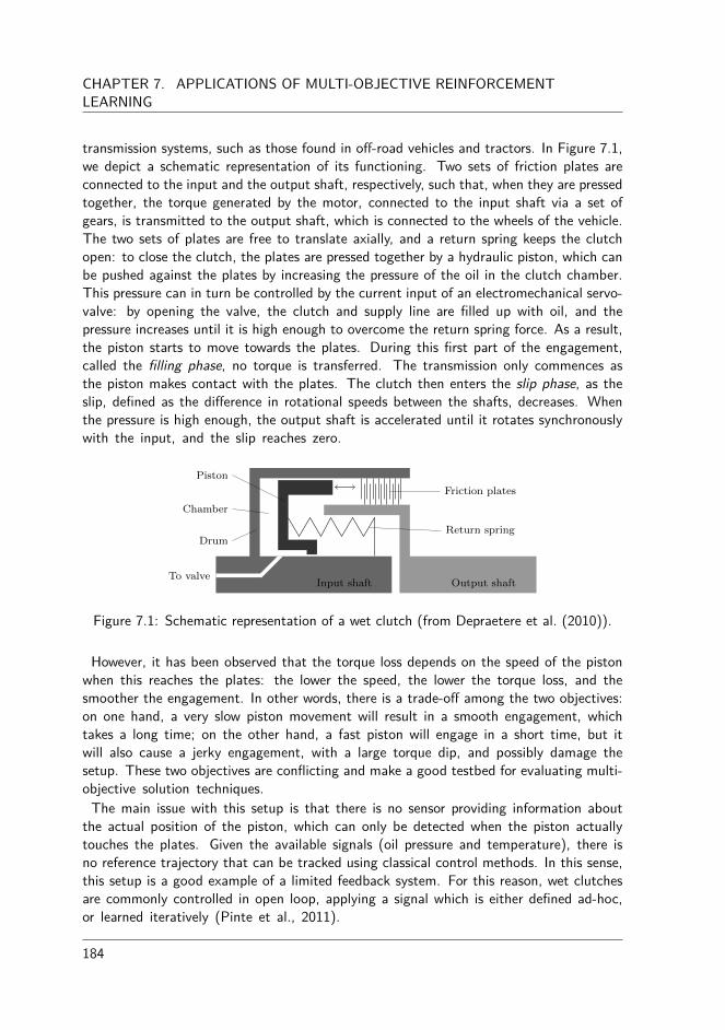
CHAPTER 7. APPLICATIONS OF MULTI-OBJECTIVE REINFORCEMENTLEARNING
transmission systems, such as those found in o�-road vehicles and tractors. In Figure 7.1,we depict a schematic representation of its functioning. Two sets of friction plates areconnected to the input and the output shaft, respectively, such that, when they are pressedtogether, the torque generated by the motor, connected to the input shaft via a set ofgears, is transmitted to the output shaft, which is connected to the wheels of the vehicle.The two sets of plates are free to translate axially, and a return spring keeps the clutchopen: to close the clutch, the plates are pressed together by a hydraulic piston, which canbe pushed against the plates by increasing the pressure of the oil in the clutch chamber.This pressure can in turn be controlled by the current input of an electromechanical servo-valve: by opening the valve, the clutch and supply line are filled up with oil, and thepressure increases until it is high enough to overcome the return spring force. As a result,the piston starts to move towards the plates. During this first part of the engagement,called the filling phase, no torque is transferred. The transmission only commences asthe piston makes contact with the plates. The clutch then enters the slip phase, as theslip, defined as the di�erence in rotational speeds between the shafts, decreases. Whenthe pressure is high enough, the output shaft is accelerated until it rotates synchronouslywith the input, and the slip reaches zero.
Input shaft Output shaftTo valve
Piston
Drum
Friction plates
Return spring
Chamber
Figure 7.1: Schematic representation of a wet clutch (from Depraetere et al. (2010)).
However, it has been observed that the torque loss depends on the speed of the pistonwhen this reaches the plates: the lower the speed, the lower the torque loss, and thesmoother the engagement. In other words, there is a trade-o� among the two objectives:on one hand, a very slow piston movement will result in a smooth engagement, whichtakes a long time; on the other hand, a fast piston will engage in a short time, but itwill also cause a jerky engagement, with a large torque dip, and possibly damage thesetup. These two objectives are conflicting and make a good testbed for evaluating multi-objective solution techniques.
The main issue with this setup is that there is no sensor providing information aboutthe actual position of the piston, which can only be detected when the piston actuallytouches the plates. Given the available signals (oil pressure and temperature), there isno reference trajectory that can be tracked using classical control methods. In this sense,this setup is a good example of a limited feedback system. For this reason, wet clutchesare commonly controlled in open loop, applying a signal which is either defined ad-hoc,or learned iteratively (Pinte et al., 2011).
184

7.1. THE FILLING PHASE OF A WET CLUTCH
A parametric form of such a signal (Zhong et al., 2011) can be found in Figure 7.2.First, a large current pulse is sent to the valve, in order to generate a high pressure levelin the oil chamber of the clutch, which will allow the piston to overcome the resistance ofthe preloaded return spring, and accelerate towards the friction plates. After this pulse, alower constant current is sent out, in order to decelerate the piston as it approaches thefriction plates: before reaching this low value, the current decreases shortly to an evenlower value, creating a small dent in the signal, which should act as a ‘brake’, limiting thespeed of the piston. Finally, the current signal grows following a ramp with a low slope,closing the clutch smoothly. The signal is parametrised as follows: the first parameter (a)controls the duration of the initial peak, whose amplitude is fixed at the maximum level,while the last (d) controls the low current level, just before the engagement begins. Theremaining parameters (b, c) control the shape of the ‘braking’ dent, while the final slopeduring the engagement phase is fixed. In our setting the signal consists of two parameters,i.e., only a and c are free, while b = 0, and d = c.
Figure 7.2: Parametric input signal from Zhong et al. (2011), with four parameters(a, b, c, d). All parameter ranges are mapped to the unit interval [0, 1]. In this setting,only two parameters can be controlled.
There currently is no reliable model of the whole engagement. However, an approximatebut deterministic model is available for the filling phase, until the piston touches theplates. 1 Nonetheless, this model does not comprise the slip phase, which would allowto simulate and optimise the resulting torque loss. But, torque loss has been observedto depend on the speed of the piston upon engagement, and we can therefore minimisepiston velocity in simulation.
1Developed in Simulink R� by Julian Stoev, Gregory Pinte (FMTC), Bert Stallaert and Bruno Depraetere(PMA, Katholieke Universiteit Leuven).
185

CHAPTER 7. APPLICATIONS OF MULTI-OBJECTIVE REINFORCEMENTLEARNING
7.2 Multi-policy analysis with MO-HOOIn this section, we analyse the MO-HOO algorithm of Section 6.2 on the wet clutchenvironment. Since the model of the wet clutch consists of a single state with a continuousbut finite dimensional action space, the MO-HOO algorithm is a perfect fit for the job.
Before we continue to the actual results, it is necessary to have an intuition of the sizeand the shape of the Pareto front of this environment. In contrast to the relatively simpleScha�er 1 and Fonseca and Flemming functions of Section 6.2.3, where the identificationof the continuous Pareto front is relatively easy, this is not the case for the wet clutchenvironment. In Figure 7.3, we denote the policies that are discovered through an ex-haustive parameter sweep. First, we normalise both reward signals and transform themfor maximisation purposes:
rv = v, (7.1)
rt = (3 ≠ t)/3. (7.2)We note that many of the parameters lead to dominated policies located in clusteredsuboptimal areas of the objective space. These dominated policies are denoted by ared colour. Additionally, we also see that some regions in the objective space are moredense than others. This is an indication of the level of di�culty of the problem since smallchanges in the decision space, i.e., the parameter values, imply big changes in the objectivespace. The exhaustive search only discovered 8 Pareto non-dominated policies, denotedby black squares, which are located in the top-right corner of the objective space. Sincethe Pareto front is continuous, there should exist other non-dominated policies connectingthe black dots. The question is how to find them without wasting extensive resources onthe dominated areas of the objective space.
0 0.1 0.2 0.3 0.4 0.5 0.6 0.7 0.8 0.9 10
0.1
0.2
0.3
0.4
0.5
0.6
0.7
0.8
0.9
1
Velocity objective
Tim
e o
bje
ctiv
e
Dominated pointsDominating points
Figure 7.3: An exhaustive search of the parameter space of the wet clutch simulationenvironment discovered only 8 non-dominated policies.
186
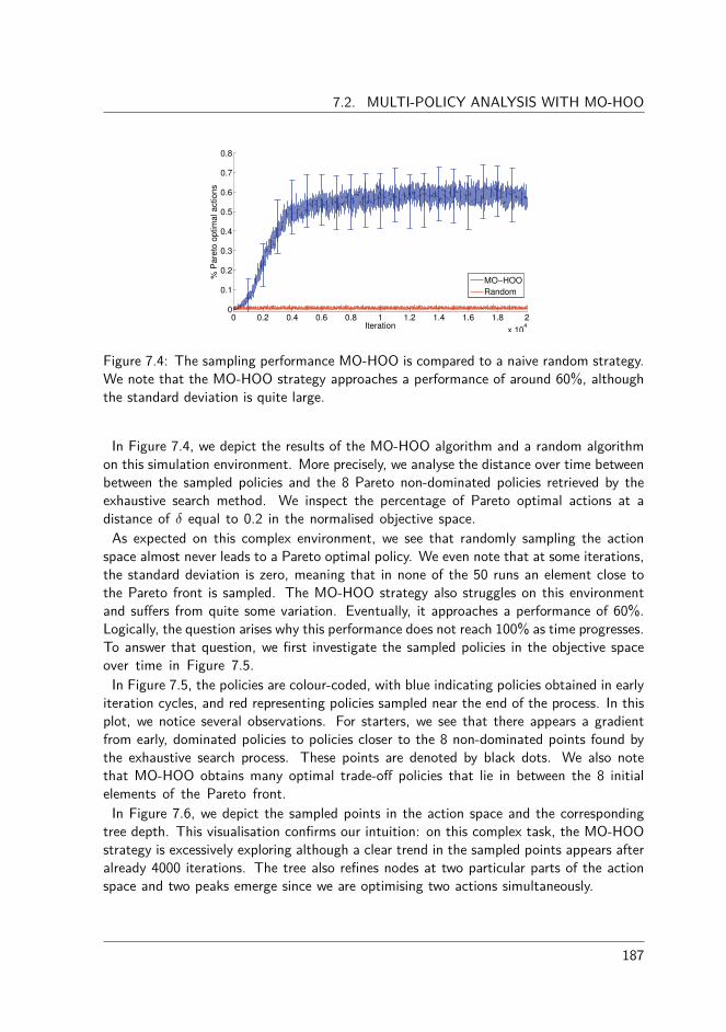
7.2. MULTI-POLICY ANALYSIS WITH MO-HOO
0 0.2 0.4 0.6 0.8 1 1.2 1.4 1.6 1.8 2
x 104
0
0.1
0.2
0.3
0.4
0.5
0.6
0.7
0.8
Iteration
% P
are
to o
ptim
al a
ctio
ns
MO−HOO
Random
Figure 7.4: The sampling performance MO-HOO is compared to a naive random strategy.We note that the MO-HOO strategy approaches a performance of around 60%, althoughthe standard deviation is quite large.
In Figure 7.4, we depict the results of the MO-HOO algorithm and a random algorithmon this simulation environment. More precisely, we analyse the distance over time betweenbetween the sampled policies and the 8 Pareto non-dominated policies retrieved by theexhaustive search method. We inspect the percentage of Pareto optimal actions at adistance of ” equal to 0.2 in the normalised objective space.
As expected on this complex environment, we see that randomly sampling the actionspace almost never leads to a Pareto optimal policy. We even note that at some iterations,the standard deviation is zero, meaning that in none of the 50 runs an element close tothe Pareto front is sampled. The MO-HOO strategy also struggles on this environmentand su�ers from quite some variation. Eventually, it approaches a performance of 60%.Logically, the question arises why this performance does not reach 100% as time progresses.To answer that question, we first investigate the sampled policies in the objective spaceover time in Figure 7.5.
In Figure 7.5, the policies are colour-coded, with blue indicating policies obtained in earlyiteration cycles, and red representing policies sampled near the end of the process. In thisplot, we notice several observations. For starters, we see that there appears a gradientfrom early, dominated policies to policies closer to the 8 non-dominated points found bythe exhaustive search process. These points are denoted by black dots. We also notethat MO-HOO obtains many optimal trade-o� policies that lie in between the 8 initialelements of the Pareto front.
In Figure 7.6, we depict the sampled points in the action space and the correspondingtree depth. This visualisation confirms our intuition: on this complex task, the MO-HOOstrategy is excessively exploring although a clear trend in the sampled points appears afteralready 4000 iterations. The tree also refines nodes at two particular parts of the actionspace and two peaks emerge since we are optimising two actions simultaneously.
187
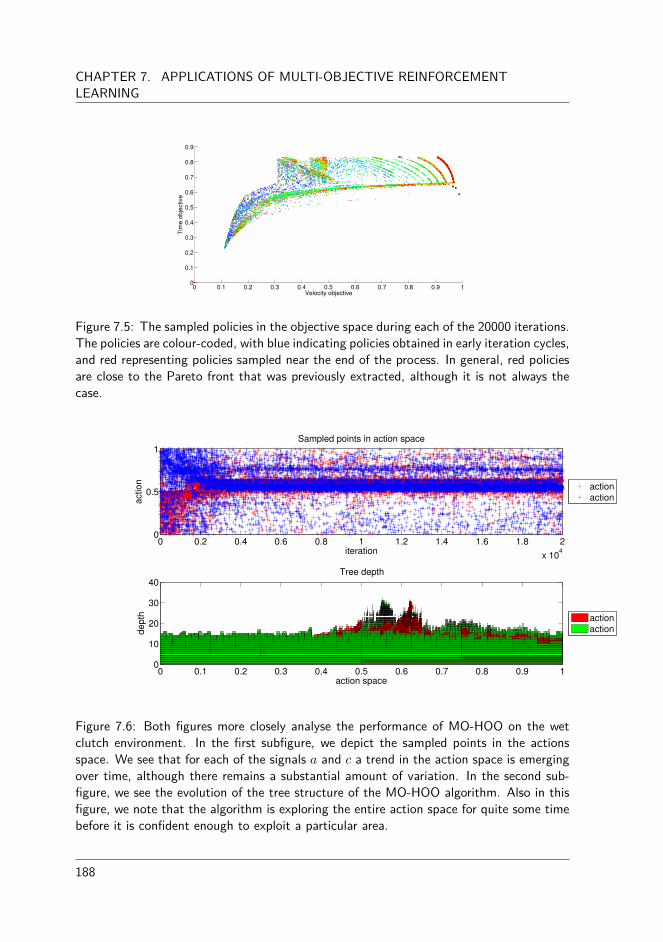
CHAPTER 7. APPLICATIONS OF MULTI-OBJECTIVE REINFORCEMENTLEARNING
0 0.1 0.2 0.3 0.4 0.5 0.6 0.7 0.8 0.9 10
0.1
0.2
0.3
0.4
0.5
0.6
0.7
0.8
0.9
Velocity objective
Tim
e o
bje
ctiv
e
Figure 7.5: The sampled policies in the objective space during each of the 20000 iterations.The policies are colour-coded, with blue indicating policies obtained in early iteration cycles,and red representing policies sampled near the end of the process. In general, red policiesare close to the Pareto front that was previously extracted, although it is not always thecase.
0 0.2 0.4 0.6 0.8 1 1.2 1.4 1.6 1.8 2
x 104
0
0.5
1
iteration
act
ion
Sampled points in action space
actionaction
0 0.1 0.2 0.3 0.4 0.5 0.6 0.7 0.8 0.9 10
10
20
30
40
action space
de
pth
Tree depth
actionaction
Figure 7.6: Both figures more closely analyse the performance of MO-HOO on the wetclutch environment. In the first subfigure, we depict the sampled points in the actionsspace. We see that for each of the signals a and c a trend in the action space is emergingover time, although there remains a substantial amount of variation. In the second sub-figure, we see the evolution of the tree structure of the MO-HOO algorithm. Also in thisfigure, we note that the algorithm is exploring the entire action space for quite some timebefore it is confident enough to exploit a particular area.
188

7.3. CONCLUSIONS AND FUTURE OUTLOOK
The cause for this behaviour is not very clear and might have multiple sources. First, thewet clutch environment is a combination of multiple complex interacting systems whichimpedes the analysis of the underlying optimisation function. In contrast to the standardbenchmark settings, such as the Scha�er 1 function, the wet clutch function is hard tograsp and to visualise. Therefore, it is possible that the function does not satisfy theassumption of the HOO strategy, which is that it should be locally Lipschitz di�erentiable.Another possibility is that the MO-HOO strategy itself is exploring too much since itsestimates are too optimistic. This could be resolved by carefully tuning the fl and ‹1parameter values which define the level of optimism added to each estimate. A possibilitywould be to employ the F-Race algorithm (Birattari et al., 2010) to find the best values forthese parameters that steer the quantity of exploration. Finally, it could also be an issuewith the bounds the algorithm itself places on the estimates. Since there is no mechanism,i.e, no min operator, to bound the estimates and as a result the algorithm keeps exploringparameters that are suboptimal. A thorough analysis of the underlying function of thewet clutch could possibly identify the issue.
To conclude, we still note that the MO-HOO strategy discovers a wide set of non-dominated trade-o� solutions since it obtained on average 357.21 Pareto non-dominatedsolutions at each run of the algorithm. As expected, the random strategy obtained only asmall set of 7.66 non-dominated solutions out of 20000 samples, as depicted in Table 7.1.
Strategy CardinalityRandom 7.66MO-HOO 357.21
Table 7.1: Cardinality indicator for random exploration and MO-HOO.
7.3 Conclusions and future outlookIn this chapter, we analysed to which extent the theoretical algorithms behave on a complexand real-world application. This application comprises the filling phase of a wet clutch,which is a crucial part in a wide range of automotive vehicles.
We applied the MO-HOO strategy of Section 6.2 on a simulation environment, repres-enting this setup. We have seen that the algorithm was struggling to find a good trade-o�between exploring uncharted territory and exploiting its knowledge near the end the of theoptimisation process. As a result, the results had a larger variation than on the bench-mark environments but the algorithm still performed acceptably. Eventually, MO-HOOdiscovered no less than 357 non-dominated elements on average in each run, o�ering awide and diverse set of compromise solutions to the decision maker. We believe thata closer investigation of the internals of the wet clutch environment could be beneficialto find better values for the configuration parameters of the MO-HOO strategy itself,although this remains an unanswered question for now.
189


8
| Conclusions
Reinforcement learning is the study of intelligent systems that learn to take optimal de-cisions in unknown and dynamic problem environments. Traditionally, this study aims tolearn the optimal actions so as to maximise a single, numerical reward signal. In thislight, we have illustrated some standard approaches such as the Q-learning algorithm inChapter 2. As we have seen, reinforcement learning provides a rigorous theoretical frame-work for learning systems. However, this framework is based on the assumption that everyaction can be evaluated by a single, scalar feedback signal. As we have seen in Chapter 3,many real-world problems involve the simultaneous optimisation of multiple, possibly con-flicting, objectives. An example is the optimisation of the return and its risk in portfoliooptimisation for stock markets (Hassan, 2010). It is clear that a risky policy has the po-tential of a high return of investment while at the same time a high probability in moneylosses as well. Therefore, there is no single optimal solution but a set of equally optimalcompromise solutions that balance these objectives. This set is referred to as the Paretofront. In this case, the problem the agent tries to solve is considered a multi-objectivereinforcement learning problem.
In this dissertation, we study the development and the evaluation of MORL algorithmsthat extend the standard, single-objective framework to discover a number of trade-o�solutions. In Section 8.1, we highlight our main contribution, presented throughout thisthesis. Subsequently, in Section 8.2, we formalise additional remarks and limitations ofour newly developed algorithms which on their turn serve as a starting point for outlooksfor future research in Section 8.3.
8.1 ContributionsIn this section, we summarise the main contributions of this dissertation. To thoroughlyunderstand the research domain, we presented a necessary overview of the foundations of
191
CHAPTER 8. CONCLUSIONS
standard, single-objective reinforcement learning in Chapter 2. This background is neededto support the reader to fully comprehend the domain of multi-objective reinforcementlearning in Chapter 3. In that chapter, we discussed current state-of-the-art strategies formulti-objective reinforcement learning and we proposed a taxonomy that classifies thesestrategies on two main aspects. The first aspect considers whether the algorithm retrievesa single solution or a set of solutions. As a result, the algorithm is either a single-policy ora multi-policy approach. The second aspect is based on the type of scalarisation functionused in the process, i.e., is the function linear or merely monotonically increasing. In thefollowing paragraphs, we highlight our principal contributions that surpass the state-of-the-art in the field of MORL.
In Chapter 4 we considered MORL algorithms that learn only a single trade-o� solutionat a time. These algorithms use scalarisation functions to reduce the dimensionality ofthe multi-objective feedback signal to a single, scalar measure. To accommodate for thesefunctions, we have presented a general framework for scalarised MORL algorithms. Inthis framework, the traditional Q-values are extended to Q-vectors that store an estimatefor every objective separately. In the action selection phase, the scalarisation function isapplied on the Q-vectors to acquire a single, scalarised estimate for a state-action pair.This scalarised estimate can on its turn be used for action selection purposes, such as forinstance ‘-greedy. Although the idea is relatively simple, the choice of the scalarisationfunction is crucial. We have elaborated on the standard linear scalarisation function andinvestigated why it is guaranteed to converge to a Pareto optimal solution and why itcannot retrieve every Pareto optimal solution. Additionally, we have researched to whatdegree the monotonically increasing Chebyshev scalarisation function can also be applied inMORL. In both a theoretical and empirical analysis we have seen that the Chebyshev func-tion lacks additivity, which is a crucial requirement for reinforcement learning algorithmsthat rely on the Bellman equation. However, the Chebyshev scalarisation function can stillbe used as a heuristic without possessing any convergence guarantees. We compared bothscalarisation functions on three commonly accepted benchmark environments on severalperformance measures.
Subsequently, in Chapter 5, we analysed how the weight parameters of the scalarisationfunctions relate to specific parts of the objective space. We have seen that the mappingfrom weight space to objective space is non-isomorphic, meaning that it is far from trivialto define an appropriate weight vector that retrieves a desired compromise solution. Inthis regard, we have proposed two classes of algorithms that adaptively explore bothdiscrete and continuous Pareto fronts. The algorithm that can be used in a discretesetting constructs a tree over the weight space. Each iteration the tree is iteratively refinedto cover finer parts of the weight space until all solutions are found. This algorithm isevaluated on two testing environment with two to three objectives. In the case the Paretofront is continuous and, in essence, infinite, the goal is to find as fast as possible adiverse set of optimal solutions that provide a careful coverage over the Pareto front.This adaptive weight algorithm (AWA) can be combined with several distance metrics,such as the hypervolume measure and a gap distance. This mechanism, together with all
192

8.2. REMARKS
its variants, is tested on a smart camera environment where the goal is to maximise thetracking confidence of moving objects while minimising the computational overhead.
In Chapter 6 we presented the pinnacle of our contributions. In this chapter, we no longeruse scalarisation functions to reduce the dimensionality, and hence also the di�culty ofthe problem. Instead, we extend the core principles of reinforcement learning frameworkto simultaneously learn a set of trade-o� solutions. The first algorithm we proposed in thiscontext is the multi-objective hierarchical optimistic optimisation (MO-HOO) algorithmwhich is tailored for single-state environments with a continuous action space, as is thecase in a lot of engineering applications. The MO-HOO algorithm builds a tree of op-timistic estimates over the action space and propagates a set of Pareto non-dominatedestimates to the root node. Based on these estimates, the algorithm continues the searchto promising parts of the action space that result in optimal and diverse solutions in theobjective space. This algorithm is tested on two optimisation functions, commonly usedin evolutionary multi-objective optimisation. For multi-state environments that require abootstrapping procedure, we proposed the Pareto Q-learning algorithm. Pareto Q-learningis the first temporal di�erence-based multi-policy algorithm that does not employ a linearscalarisation function and can therefore learn the entire Pareto front and not just a sub-set. The main novelty of the Pareto Q-learning algorithm is the set-based bootstrappingrule that separates the average immediate reward and the set of Pareto non-dominatedvectorial estimates. Pareto Q-learning can be combined with several quality measures toaccommodate for action selection strategies, such as the hypervolume and the cardinalityquality indicators.
In Chapter 7, we moved beyond the academic benchmark environments and tested multi-policy MORL algorithms on a simulation environment of a real-world problem. Thisproblem concerns the filling phase of a wet clutch, a transmission unit that can be foundin many automotive vehicles. In this setup, the goal of the agent is to find an engagementthat is both fast and smooth, which are in essence conflicting objectives. We evaluatedthe MO-HOO algorithm to learn a set of trade-o� solutions at once. We have seen thetask introduces an amplified level of complexity but the algorithm still managed to obtainon average 357 trade-o� solutions in a single run.
8.2 RemarksThroughout this thesis, we have presented several algorithms for learning in multi-criteriaenvironments. Many of these algorithms are novel in their specific field and requiredchanges to the theoretical reinforcement learning framework on a detailed conceptual level.For instance, the MO-HOO algorithm of Chapter 6 is, to the best of our knowledge, thefirst multi-objective X -armed bandit solver. On the one hand side, this algorithm extendsthe boundaries of the MORL field but on the other hand side, the novelty of the algorithmcomplicates a rigorous experimental comparison to other, specific algorithms for the sametype of problems. One possibility is to improve the experimental evaluation of the algorithmis to compare it to evolutionary multi-objective algorithms. However, for the comparison to
193

CHAPTER 8. CONCLUSIONS
be fair, one needs to take into account some aspects. For instance, evolutionary algorithmsinherently evolve a population of solutions. Therefore, they mimic a multi-agent principlewhere agents can cooperate to improve the overall quality. Additionally, the size of thepopulation plays a crucial role in the process and influences the performance as well.
A second remark is related to the convergence guarantees of the MO-HOO algorithm.In that algorithm, we adjusted the internal mechanisms of the HOO tree to propagatePareto non-dominated estimates to the root node. Since our estimates are not averagedover subtrees and there is no alternative multi-objective min operator, we cannot assumeMO-HOO to have the same convergence rate and upper bounds for the regret as the HOOstrategy. Although the algorithm seems to perform well on the three experiments we carriedout in this dissertation, a thorough theoretical analysis of the mechanism is still needed.
Thirdly, due to time constraints, we did not perform a rigorous
8.3 Outlooks for future researchFinally, we conclude the thesis by listing outlooks for future research that can open thedoor to new advances in the multi-objective reinforcement learning domain:
• Alternative distance metrics for AWA algorithms: In Chapter 5, we have proposedseveral distance measures that can be used to guide the search to optimal and well-spread solutions. Although, the list of possible distance measures is quite elaborate,there is no single best metric that will be the ideal solution approach for everyapplication domain. A possible next step would be to directly incorporate the genuinemulti-objective quality indicators such as the spread indicator (Van Veldhuizen andLamont, 1998) directly in the internal workings of the adaptive weight algorithm.
• Sampling the Pareto front with AWA algorithms: One could extend the reach ofthe adaptive weight algorithms by extending the scalarisation principle. As thismechanism currently relies on a convex combinations of the objectives, only policieson the convex hull are retrievable. To also empower the discovery of policies in non-convex regions of the Pareto front, one could try to combine AWAs with the adaptiveweighted sum principle in Kim and de Weck (2005) and Yliniemi and Tumer (2014),where the objective space of the original problem is transformed to a convex shape.In this transformed Pareto front, the linear scalarisation function can find solutionsthat correspond to solutions in non-convex parts of the original objective space.
• Tighter bounds on MO-HOO: the MO-HOO algorithm of Chapter 6 is based onthe HOO algorithm which uses a combination of traditional min and max operatorto place bounds on the level of optimism of the estimates. In MO-HOO, the max
operator is replaced by a union operator that filters out the Pareto non-dominatedestimates. No multi-objective variant is found for the min operator and as a result,the estimates might become too optimistic, resulting in an algorithm that explorestoo much. In future work, the specification of a multi-objective min operator couldplace a stricter bound on the B-vectors in order to make them less optimistic.
194

8.3. OUTLOOKS FOR FUTURE RESEARCH
However, it is not clear to determine what would be the logical outcome of applyinga multi-objective min operator on a U -vector and a set of non-dominated B-vectors.Since there is no total order, defining a min operator that can deal with multiplePareto incomparable vectors remains an open research question.
• Alternative action evaluation indicators for Pareto Q-learning : In the Pareto Q-learning algorithm of Chapter 6, three di�erent action evaluation mechanisms areproposed. These are the hypervolume, cardinality and the Pareto set evaluationmechanisms which quantify the quality of a set of Q-vectors. These mechanismswere designed to treat every Pareto optimal solution equally (to a certain extent).However, it could be that the decision maker is not interested in sampling the entirePareto front but that he is looking for particular policies that satisfy certain criteria.For instance, other quality indicators such as the spread indicator (Van Veldhuizenand Lamont, 1998) could be used to sample policies that are both Pareto optimaland well-spread in the objective space. In future research, alternative set evaluationmechanisms could be investigated to steer the search process.
• Pareto Q-learning for infinite-horizon problems: In Pareto Q-learning, the Qset’sgrow according to the size of the Pareto front. Therefore, Pareto Q-learning isprimarily designed for episodic environments with a finite number of Pareto optimalpolicies. To make the algorithm practically applicable for infinite horizon problemswith a large value for the discount factor, we have to consider that all states canbe revisited during the execution of an optimal policy. Upon revisiting a state, adi�erent action that is optimal w.r.t. other criteria can be chosen. As explainedin Mannor and Shimkin (2001), this o�ers a possibility to steer the average rewardvector towards a target set using approaching policies. Alternatively, we could reducethe number of learned policies by using a consistency operator to select the sameaction during each revisit of some state, similar to the work of Wiering and de Jong(2007) for multi-criteria dynamic programming.
• Pareto Q-learning on continuous states: Currently, Pareto Q-learning is limited to atabular representation where each state-action pair stores a Qset. In order to makePareto Q-learning applicable to real-life problems or ergodic environments, these setsshould also be represented through function approximation. A possible idea is to fitthe elements in each set through a geometric approach, such as for instance ordinalleast-squares. If the environment would consist of two or three objectives, we wouldbe fitting the vectors on a curve or a plane, respectively. In that case, we would belearning the shape of the Pareto front through local interactions that each updateparts of this geometric shape. Therefore, this research direction could pave the wayfor multi-policy MORL in real-world problem environments.
• Risk-sensitive learning with Pareto Q-learning : Although Pareto Q-learning is primar-ily designed for multi-objective problems. It could also be employed to augmentstandard single-objective problems. Through a principle called multi-objectivisation,additional, artificial objectives can be constructed to improve the performance on theoriginal objective, as measured by solution quality, time to solution, or some othermeasure (Knowles et al., 2001). In this way, one could solve a practical problem of
195

CHAPTER 8. CONCLUSIONS
reinforcement learning in real-world applications, i.e., in those cases, algorithms thatsolely focus on maximising the mean return might be inappropriate as they do notaccount for the variability of their solutions. Thereby, a variability measure couldbe included to accommodate for a risk-sensitive setting, where the decision makercan explicitly define the tolerated level of deviation of the observed return from theexpected return. In Van Mo�aert et al. (2015), we scratched the surface of thisidea by learning a set of optimal trade-o� policies that balance mean reward and itsvariance.
• Many-objective optimisation: The algorithms presented throughout this dissertationwere developed for multi-objective problems. In practice this means the environ-ments deal with two to three objectives. Many-objective optimisation is anotherresearch topic that moves beyond this point and deals with the optimisation of fouror more objectives (Deb and Jain, 2014; Jain and Deb, 2014). This branch posesgreat challenges to the classical approaches since the number of Pareto incomparablesolutions grows when the number of objectives increases as well (Winkler, 1985).Nonetheless, the underlying mechanisms of our algorithms, such as the hypervolumeand the Pareto dominance relation, are without adaptation also theoretically ap-plicable in these many-objective environments. However, a huge amount of Paretoincomparable solutions will unquestionably a�ect the running time of the algorithmsin practice since the space of possible solutions can become very large. In futurework, researchers could investigate to what degree these algorithms scale up tomany-objective problems. A possible idea to shrink down the huge solution spacewould be to employ user-defined preference functions that emphasise certain partsof the objective space.
8.4 OverviewIn this dissertation, we have presented several multi-objective reinforcement learning al-gorithms for many di�erent situations. For the sake of clarity, in Figure 8.1, we summariseour algorithmic contributions based on three aspects. These aspects are (1) whether thedecision maker wants to learn a single or multiple policies, (2) whether or not convex solu-tions su�ce (or are also non-convex solutions of interest?) and (3) whether the problemconsists of a continuous or a discrete action range.
196

8.4. OVERVIEW
Single-policy?
Convex solutions suffice?
Convex solutions suffice?
Linear scalarisationChapter 4
Monotonically increasing scalarisation
Chapter 4
Pareto Q-learningChapter 6
Continuous actions?
Adaptive weight algorithms (AWA)
Chapter 5
MO-HOOChapter 6
Yes No
Yes No Yes No
Yes No
Figure 8.1: An overview of the di�erent algorithmic contributions in this dissertation,depending on the type of problem and whether convex solutions su�ce for the decisionmaker.
197


List of Selected Publications
International Journals and Lecture Notes1. K. Van Mo�aert, A. Nowé. Multi-Objective Reinforcement Learning using Sets of
Pareto Dominating Policies. Journal Of Machine Learning Research, vol. 15, 2014,p 3483-3512.
2. K. Van Mo�aert, M. M. Drugan, A. Nowé. Hypervolume-based Multi-ObjectiveReinforcement Learning. In Proceedings of the 7th International Conference onEvolutionary Multi-Objective Optimization (EMO), 2013, Lecture Notes in Com-puter Science 7811, 2013, p 3483-3512.
Proceedings of Conferences with International Referees1. K. Van Mo�aert, K. Van Vaerenbergh, P. Vrancx, A. Nowé. Multi-Objective X-
Armed Bandits. In Proceedings of the IEEE World Congress on ComputationalIntelligence (WCCI), 2014, p 2331-2338.
2. K. Van Mo�aert, T. Brys, A. Chandra, L. Esterle, P. Lewis, A. Nowé. A NovelAdaptive Weight Selection Algorithm for Multi-Objective Multi-Agent ReinforcementLearning. In Proceedings of the IEEE World Congress on Computational Intelligence(WCCI), 2014, p 2306-2314.
3. K. Van Mo�aert, M. M. Drugan, A. Nowé. Scalarized Multi-Objective ReinforcementLearning: Novel Design Techniques. In Proceedings of the IEEE Symposium onAdaptive Dynamic Programming and Reinforcement Learning (ADPRL), 2013, p191-199.
199

List of Selected Publications
4. K. Van Mo�aert, Y. M. De Hauwere, P. Vrancx, A. Nowé. Reinforcement Learningfor Multi-Purpose Schedules. In Proceedings of the 5th International Conference onAgents and Artificial Intelligence (ICAART), 2013, p 203-209.
Extended abstracts1. T. Brys, K. Van Mo�aert, M. M. Drugan, A. Nowé, M. Taylor. Adaptive Objective
Selection for Correlated Objectives in Multi-Objective Reinforcement Learning. InProceedings of the 13th International Conference on Autonomous Agents and Multi-Agent Systems (AAMAS), p 1349-1350.
2. K. Van Mo�aert, M. M. Drugan, A. Nowé. Learning Sets of Pareto Optimal Policies.In Proceedings of the AAMAS 2014 Workshop on Adaptive and Learning Agents(ALA), 2014.
3. K. Van Mo�aert, M. M. Drugan, A. Nowé. Multi-Objective Reinforcement Learn-ing. In Proceedings of the European Workshop on Reinforcement Learning (EWRLDagstuhl Seminar 13321), 2013, p13-14.
200

List of abbreviations
AI Artificial intelligenceAN-TPLS Adaptive normal two-phase local searchAN-TPRL Adaptive normal two-phase reinforcement learningAN-TPLS-HV Adaptive normal two-phase local search using the hyper-
volume distanceAN-TPRL-HV Adaptive normal two-phase reinforcement learning using the
hypervolume distanceAN-TPRL-OHV Adaptive normal two-phase reinforcement learning using the
overlapping hypervolume distanceAWA Adaptive weight algorithm
BST Bountiful Sea Treasure environment
CH Convex hullCHVI Convex hull value iterationCON-MODP Consistent multi-objective dynamic programmingC-PQL Pareto Q-learning using cardinality-based action selection
DST Deep Sea Treasure environmentDP Dynamic programming
EMO Evolutionary multi-objective optimization
GD Generational distance
201

List of abbreviations
HOO Hierarchical optimistic optimizationHV HypervolumeHV-PQL Pareto Q-learning using hypervolume-based action selection
IGD Inverted generational distance
MCTS Monte-Carlo tree searchMDP Markov decision processMOFQI Multi-objective fitted Q-iterationMOMDP Multi-objective Markov decision processMO-MCTS Multi-objective Monte-Carlo tree searchMO-HOO Multi-objective hierarchical optimistic optimizationMORL Multi-objective reinforcement learning
ND Non-dominated operator
PF Pareto frontPGPE Policy gradient with parameter explorationPO-PQL Pareto Q-learning using Pareto dominance-based action se-
lectionPQL Pareto Q-learning
RA-TPLS Regular anytime two-phase local searchRA-TPRL Regular anytime two-phase reinforcement learningRA-TPRL-DIST Regular anytime two-phase reinforcement learning using the
Euclidean distanceRA-TPRL-HV Regular anytime two-phase reinforcement learning using the
hypervolume distanceRA-TPRL-OHV Regular anytime two-phase reinforcement learning using the
overlapping hypervolume distanceRL Reinforcement Learning
TD Temporal di�erenceTPLS Two-phase local searchTPRL Two-phase reinforcement learning
OHV Overlapping hypervolume
202

List of symbols
Single-objective reinforcement learninga(t) Selected action at timestep tA(s) Action set in state s– Learning rate“ Discount factor‘ Exploration parameter of the ‘-greedy action selection
strategyt Timesteps(t) State at timestep tS = s1, . . . , sN Set of statesr(t + 1) Observed immediate reward at timestep t + 1
T (sÕ|s, a) Probability of arriving in state sÕ after selecting action a instate s
R(s, a, sÕ) Expected reward associated to transitioning from state s
with action a to state sÕ
· Temperature parameter of the Softmax action selectionRt The return up to timestep tfi Policyfi(s, a) Probability of selecting an action a in state s� Space of policiesV fi
(s) The value of state s under policy fiV ú
(s) The value of state s under an optimal policyQfi
(s, a) The value of action a in state s under policy fiQú
(s, a) The value of action a in state s under an optimal policyˆQ(s, a) The estimated value of action a in state s
203

List of symbols
Multi-objective reinforcement learningF Multi-objective optimization functionm Number of objectivesX The space of decision vectorsª Strict Pareto dominance∞ Weak Pareto dominanceÎ Pareto incomparable⌃ Pareto non-dominatedR(s, a, sÕ
) Expected reward vector associated to transitioning fromstate s with action a to state sÕ
V
fi(s) The vector value of state s under policy fi
V
ú(s) The vector value of state s under an optimal policy
Q
fi(s, a) The vector value of action a in state s under policy fi
Q
ús, a The vector value of action a in state s under an optimalpolicy
ˆ
Q(s, a) The estimated vector value of action a in state sSQ(s, a) The scalarized value of action a in state sCH(�) The convex hull of a set of policies �
PF (�) The Pareto front of a set of policies �
z
ú The attraction point of the Chebyshev scalarisation functionw The weight vector of a scalarisation functionX The continuous action space of an X -armed bandit problem(h, i) A node of the tree of the HOO strategy at index i and
depth hPh,i The area of the action space corresponding to node (h, i)Uh,i(n) The U -value of node n located at index i and depth hUh,i(n) The U-vector of node n located at index i and depth hBh,i(n) The B-value of node n located at index i and depth hBh,i(n) The B-vector of node n located at index i and depth hµh,i(n) The estimated average reward of node n located at index i
and depth hTh,i(n) The number of times node n located at index i and depth
h is sampledˆQset(s, a) A set of Q(s, a) vectorsR(s, a) The average immediate reward of taking action a in state
sNDt(s, a) The set of Pareto non-dominated vectors of the state
reached after selecting action a in state sn(s, a) The number of times action a is selected in state sF sÕ
s,a The observed frequency of reaching state sÕ after selectinga in state s
204

Bibliography
Z Aimin, J. Yaochu, Z. Qingfu, B. Sendho�, and E. Tsang. Combining model-based andgenetics-based o�spring generation for multi-objective optimization using a convergencecriterion. In Evolutionary Computation, 2006. CEC 2006. IEEE Congress on, pages 892–899, 2006. doi: 10.1109/CEC.2006.1688406.
M. J. Alves and J.N. Climaco. An interactive method for 0-1 multiobjective problems usingsimulated annealing and tabu search. Journal of Heuristics, 6(3):385–403, 2000.
M. Aruldoss, T.M. Lakshmi, and V.P. Venkatesan. A survey on multi criteria decisionmaking methods and its applications. American Journal of Information Systems, 1(1):31–43, 2013. doi: 10.12691/ajis-1-1-5. URL http://pubs.sciepub.com/ajis/1/1/5.
J.-Y. Audibert, R. Munos, and C. Szepesvári. Exploration-exploitation tradeo� using vari-ance estimates in multi-armed bandits. Theor. Comput. Sci., 410(19):1876–1902, April2009. ISSN 0304-3975. doi: 10.1016/j.tcs.2009.01.016. URL http://dx.doi.org/10.
1016/j.tcs.2009.01.016.
P. Auer, N. Cesa-Bianchi, and P. Fischer. Finite-time analysis of the multiarmed banditproblem. Mach. Learn., 47(2-3):235–256, May 2002. ISSN 0885-6125. doi: 10.1023/A:
1013689704352. URL http://dx.doi.org/10.1023/A:1013689704352.
P. Auer, N. Cesa-Bianchi, Y. Freund, and R. Schapire. The nonstochastic multiarmedbandit problem. SIAM J. Comput., 32(1):48–77, January 2003. ISSN 0097-5397. doi:10.1137/S0097539701398375. URL http://dx.doi.org/10.1137/S0097539701398375.
B. Awerbuch and R. Kleinberg. Online linear optimization and adaptive routing. J. Comput.Syst. Sci., 74(1):97–114, February 2008. ISSN 0022-0000. doi: 10.1016/j.jcss.2007.04.
016. URL http://dx.doi.org/10.1016/j.jcss.2007.04.016.
205
BIBLIOGRAPHY
T. Bäck. Evolutionary Algorithms in Theory and Practice: Evolution Strategies, Evolu-tionary Programming, Genetic Algorithms. Oxford University Press, Oxford, UK, 1996.ISBN 0-19-509971-0.
T. Bäck. Evolutionary algorithms in theory and practice - evolution strategies, evolutionaryprogramming, genetic algorithms. Oxford University Press, 1996. ISBN 978-0-19-509971-3.
L. Barrett and S. Narayanan. Learning all optimal policies with multiple criteria. InProceedings of the 25th international conference on Machine learning, ICML ’08, pages41–47, New York, NY, USA, 2008. ACM. ISBN 978-1-60558-205-4. doi: 10.1145/
1390156.1390162.
L.S. Batista, F. Campelo, F.G.. Guimar„es, and J.A. Ramírez. Pareto cone ‘-dominance:Improving convergence and diversity in multiobjective evolutionary algorithms. In R.H.C.Takahashi, K. Deb, E.. Wanner, and S. Greco, editors, Evolutionary Multi-CriterionOptimization, volume 6576 of Lecture Notes in Computer Science, pages 76–90. SpringerBerlin Heidelberg, 2011. ISBN 978-3-642-19892-2. doi: 10.1007/978-3-642-19893-9_
6. URL http://dx.doi.org/10.1007/978-3-642-19893-9_6.
R. Bellman. Dynamic Programming. Princeton University Press, Princeton, NJ, USA, 1edition, 1957.
V. Belton and T. Stewart. Muliple Criteria Decision Analysis: An Integrated Approach.Kluwer Academic, Dordrecht, 2002.
D. P. Bertsekas. Dynamic Programming: Deterministic and Stochastic Models. Prentice-Hall, Inc., Upper Saddle River, NJ, USA, 1987. ISBN 0132215810.
D. P. Bertsekas. Dynamic Programming and Optimal Control, Vol. I, 2nd Ed. AthenaScientific, Belmont, MA, 2001a.
D. P. Bertsekas. Dynamic Programming and Optimal Control, Vol. II, 2nd Ed. AthenaScientific, Belmont, MA, 2001b.
M. Birattari, Z. Yuan, P. Balaprakash, and T. St tzle. F-race and iterated f-race:An overview. In T. Bartz-Beielstein, M. Chiarandini, L. Paquete, and M. Preuss,editors, Experimental Methods for the Analysis of Optimization Algorithms, pages311–336. Springer Berlin Heidelberg, 2010. ISBN 978-3-642-02537-2. doi: 10.1007/
978-3-642-02538-9_13. URL http://dx.doi.org/10.1007/978-3-642-02538-9_13.
V. Bowman and Jr. Joseph. On the relationship of the tchebyche� norm and the ef-ficient frontier of multiple-criteria objectives. In H. Thiriez and S. Zionts, editors,Multiple Criteria Decision Making, volume 130 of Lecture Notes in Economics andMathematical Systems, pages 76–86. Springer Berlin Heidelberg, 1976. ISBN 978-3-540-07794-7. doi: 10.1007/978-3-642-87563-2_5. URL http://dx.doi.org/10.1007/
978-3-642-87563-2_5.
206

BIBLIOGRAPHY
S. Bubeck, R. Munos, G. Stoltz, and C. Szepesvári. X-armed bandits. CoRR,abs/1001.4475, 2010.
A. Castelletti, G. Corani, A.E. Rizzoli, R. Soncini, and S.E. Weber. Reinforcement learningin the operational management of a water system. In IFAC Workshop on Modeling andControl in Environmental Issues, pages 325–330, 2002.
A. Castelletti, S. Galelli, M. Restelli, and R. Soncini-Sessa. Tree-based reinforcementlearning for optimal water reservoir operation. Water Resources Research, 46, 2010.doi: 10.1029/2009WR008898.
A. Castelletti, F. Pianosi, and M. Restelli. Multi-objective fitted q-iteration: Pareto frontierapproximation in one single run. In Networking, Sensing and Control (ICNSC), 2011IEEE International Conference on, pages 260–265, April 2011. doi: 10.1109/ICNSC.
2011.5874921.
A. Castelletti, F. Pianosi, and M Restelli. Tree-based fitted q-iteration for multi-objectivemarkov decision problems. In Proceedings International Joint Conference on NeuralNetworks (IJCNN 2012), 2012.
C.A. Coello Coello. A comprehensive survey of evolutionary-based multiobjective op-timization techniques. Knowledge and Information Systems, 1(3):269–308, 1999.ISSN 0219-1377. doi: 10.1007/BF03325101. URL http://dx.doi.org/10.1007/
BF03325101.
C.A. Coello Coello, G.B. Lamont, and D.A.V. Veldhuizen. Evolutionary Algorithms forSolving Multi-Objective Problems (Genetic and Evolutionary Computation). Springer-Verlag New York, Inc., Secaucus, NJ, USA, 2006. ISBN 0387332545.
E. Cope. Regret and convergence bounds for immediate-reward reinforcement learning withcontinuous action spaces. IEEE Transactions on Automatic Control, 54(6):1243–1253,2009.
R. Coulom. E�cient selectivity and backup operators in monte-carlo tree search. InProceedings of the 5th International Conference on Computers and Games, CG’06,pages 72–83, Berlin, Heidelberg, 2007. Springer-Verlag. ISBN 3-540-75537-3, 978-3-540-75537-1. URL http://dl.acm.org/citation.cfm?id=1777826.1777833.
K. Dächert, J. Gorski, and K. Klamroth. An augmented weighted tchebyche� method withadaptively chosen parameters for discrete bicriteria optimization problems. Comput.Oper. Res., 39(12):2929–2943, December 2012. ISSN 0305-0548. doi: 10.1016/j.cor.
2012.02.021. URL http://dx.doi.org/10.1016/j.cor.2012.02.021.
I. Das and J. E. Dennis. A closer look at drawbacks of minimizing weighted sums ofobjectives for pareto set generation in multicriteria optimization problems. Structuraland Multidisciplinary Optimization, 14:63–69, 1997. ISSN 1615-147X.
207

BIBLIOGRAPHY
I. Das and J. E. Dennis. Normal-boundary intersection: A new method for generating thepareto surface in nonlinear multicriteria optimization problems. SIAM J. on Optimiza-tion, 8(3):631–657, March 1998. ISSN 1052-6234. doi: 10.1137/S1052623496307510.URL http://dx.doi.org/10.1137/S1052623496307510.
K. Deb and H. Jain. An evolutionary many-objective optimization algorithm usingreference-point-based nondominated sorting approach, part i: Solving problems withbox constraints. Evolutionary Computation, IEEE Transactions on, 18(4):577–601, Aug2014. ISSN 1089-778X. doi: 10.1109/TEVC.2013.2281535.
K. Deb, J. Sundar, N. Udaya Bhaskara Rao, and S. Chaudhuri. Reference point basedmulti-objective optimization using evolutionary algorithms. In International Journal ofComputational Intelligence Research, pages 635–642. Springer-Verlag, 2006.
B. Depraetere, G. Pinte, and J. Swevers. Iterative optimization of the filling phase ofwet clutches. In The 11th International Workshop on Advanced Motion Control (AMC2010), pages 94–99. IEEE, 2010. ISBN 978-1-4244-6668-9.
J. Dubois-Lacoste, M. López-Ibáñez, and T. Stützle. Improving the anytime behavior oftwo-phase local search. Annals of Mathematics and Artificial Intelligence, 61(2):125–154, 2011. ISSN 1012-2443. doi: 10.1007/s10472-011-9235-0. URL http://dx.doi.
org/10.1007/s10472-011-9235-0.
N. Dunford, J.T. Schwartz, W.G. Bade, and R.G. Bartle. Linear Operators: General theory.Part. I. Linear Operators. Interscience Publishers, 1988. ISBN 9780470226056.
M. Ehrgott. Multicriteria Optimization. Lectures notes in economics and mathematicalsystems. Springer, 2005. ISBN 9783540213987.
M. Ehrgott and X. Gandibleux. Multiple Criteria Optimization. State of the art annotatedbibliographic surveys. Kluwer Academic, Dordrecht, 2002.
D. Ernst, P. Geurts, and L. Wehenkel. Tree-based batch mode reinforcement learning.Journal of Machine Learning Research, 6:503–556, April 2005.
L. Esterle, P.R. Lewis, M. Bogdanski, B. Rinner, and Xin Yao. A Socio-Economic Ap-proach to Online Vision Graph Generation and Handover in Distributed Smart CameraNetworks. In Proceedings of the Fifth ACM/IEEE International Conference on Distrib-uted Smart Cameras, pages 1–6. IEEE Press, 2011.
L. Esterle, P.R. Lewis, H. Caine, X. Yao, and B. Rinner. CamSim: A distributed smartcamera network simulator. In Proceedings of the 7th IEEE Conference on Self-Adaptiveand Self-Organizing Systems Workshops (SASOW). IEEE Press, 2013. In press.
L. Esterle, P.R. Lewis, X. Yao, and B. Rinner. Socio-economic vision graph generation andhandover in distributed smart camera networks. ACM Transactions on Sensor Networks,10(2), 2014.
208

BIBLIOGRAPHY
J. Figueira, S. Greco, and M. Ehrgott. Multiple Criteria Decision Analysis: State of theArt Surveys. Springer Verlag, Boston, Dordrecht, London, 2005.
C. M. Fonseca and P.J. Fleming. Genetic algorithms for multiobjective optimization:Formulationdiscussion and generalization. In Proceedings of the 5th International Con-ference on Genetic Algorithms, pages 416–423, San Francisco, CA, USA, 1993. MorganKaufmann Publishers Inc. ISBN 1-55860-299-2. URL http://dl.acm.org/citation.cfm?
id=645513.657757.
T. Furmston and D. Barber. A unifying perspective of parametric policy search methods formarkov decision processes. In F. Pereira, C.J.C. Burges, L. Bottou, and K.Q. Weinber-ger, editors, Advances in Neural Information Processing Systems 25, pages 2717–2725.Curran Associates, Inc., 2012.
V. Gabillon, M. Ghavamzadeh, and B. Scherrer. Approximate dynamic programming fi-nally performs well in the game of tetris. In C.J.C. Burgesv, L. Bottou, M. Welling,Z. Ghahramani, and K.Q. Weinberger, editors, Advances in Neural Information Pro-cessing Systems 26, pages 1754–1762. Curran Associates, Inc., 2013.
Z. Gábor., Z. Kalmár, and C. Szepesvári. Multi-criteria reinforcement learning. In J.W.Shavlik, editor, ICML, pages 197–205. Morgan Kaufmann, 1998. ISBN 1-55860-556-8.
P. Geibel. Reinforcement learning for mdps with constraints. In J. F rnkranz, T. Sche�er,and M. Spiliopoulou, editors, Machine Learning: ECML 2006, volume 4212 of LectureNotes in Computer Science, pages 646–653. Springer Berlin Heidelberg, 2006. ISBN978-3-540-45375-8. doi: 10.1007/11871842_63. URL http://dx.doi.org/10.1007/
11871842_63.
C.K. Goh and K.C. Tan. Evolutionary Multi-objective Optimization in Uncertain Environ-ments: Issues and Algorithms. Studies in Computational Intelligence. Springer, 2009.ISBN 9783540959755.
J.-M. Gorce, R. Zhang, K. Ja�rès-Runser, and C. Goursaud. Energy, latency and capacitytrade-o�s in wireless multi-hop networks. In Proceedings of the IEEE 21st InternationalSymposium on Personal, Indoor and Mobile Radio Communications, PIMRC 2010, pages2757–2762. IEEE, 2010.
G.N.A. Hassan. Multiobjective Genetic Programming for Financial Portfolio Managementin Dynamic Environments. University College London (University of London), 2010.
U. Hege and D. Bergemann. The Financing of Innovation: Learning and Stopping. RANDJournal of Economics, Vol.36,n¶4:pp.719–752, 2005.
F. Hernandez-del Olmo, F. H. Llanes, and E. Gaudioso. An emergent approach for thecontrol of wastewater treatment plants by means of reinforcement learning techniques.Expert Syst. Appl., 39(3):2355–2360, 2012.
209
BIBLIOGRAPHY
John H. Holland. Adaptation in Natural and Artificial Systems: An Introductory Analysiswith Applications to Biology, Control and Artificial Intelligence. MIT Press, Cambridge,MA, USA, 1992. ISBN 0262082136.
S. Huband, P. Hingston, L. Barone, and L. While. A review of multiobjective testproblems and a scalable test problem toolkit. Trans. Evol. Comp, 10(5):477–506,October 2006. ISSN 1089-778X. doi: 10.1109/TEVC.2005.861417. URL http:
//dx.doi.org/10.1109/TEVC.2005.861417.
M. Humphrys. Action selection methods using reinforcement learning. PhD thesis, Uni-versity of Cambridge, Computer Laboratory, June 1997. URL http://www.cl.cam.ac.
uk/techreports/UCAM-CL-TR-426.ps.gz.
R. Issabekov and P. Vamplew. An empirical comparison of two common multiobjectivereinforcement learning algorithms. In Proceedings of the 25th Australasian Joint Con-ference on Advances in Artificial Intelligence, AI’12, pages 626–636, Berlin, Heidelberg,2012. Springer-Verlag. ISBN 978-3-642-35100-6. doi: 10.1007/978-3-642-35101-3_53.URL http://dx.doi.org/10.1007/978-3-642-35101-3_53.
H. Jain and K. Deb. An evolutionary many-objective optimization algorithm usingreference-point based nondominated sorting approach, part ii: Handling constraintsand extending to an adaptive approach. Evolutionary Computation, IEEE Transactionson, 18(4):602–622, Aug 2014. ISSN 1089-778X. doi: 10.1109/TEVC.2013.2281534.
A. Jaszkiewicz and R. S≥owiÒski. The light beam search over a non-dominated surfaceof a multiple-objective programming problem. In G.H. Tzeng, H.F. Wang, U.P. Wen,and P.L. Yu, editors, Multiple Criteria Decision Making, pages 87–99. Springer NewYork, 1994. ISBN 978-1-4612-7626-5. doi: 10.1007/978-1-4612-2666-6_10. URLhttp://dx.doi.org/10.1007/978-1-4612-2666-6_10.
A. Jaszkiewicz and R. S≥owiÒski. The light beam search - outranking based interact-ive procedure for multiple-objective mathematical programming. In PanosM. Pardalos,Yannis Siskos, and Constantin Zopounidis, editors, Advances in Multicriteria Analysis,volume 5 of Nonconvex Optimization and Its Applications, pages 129–146. SpringerUS, 1995. ISBN 978-1-4419-4748-2. doi: 10.1007/978-1-4757-2383-0_9. URLhttp://dx.doi.org/10.1007/978-1-4757-2383-0_9.
N.R. Jennings, K. Sycara, and M. Wooldridge. A roadmap of agent research and develop-ment. Autonomous Agents and Multi-Agent Systems, 1(1):7–38, January 1998. ISSN1387-2532. doi: 10.1023/A:1010090405266. URL http://dx.doi.org/10.1023/A:
1010090405266.
N. Jozefowiez, F. Semet, and E.-G. Talbi. Multi-objective vehicle routing problems.European Journal of Operational Research, 189(2):293 – 309, 2008. ISSN 0377-2217.doi: http://dx.doi.org/10.1016/j.ejor.2007.05.055.
210
BIBLIOGRAPHY
L. Kaelbling, M. Littman, and A. Cassandra. Partially observable markov decision pro-cesses for artificial intelligence. In Ipke Wachsmuth, Claus-Rainer Rollinger, and WilfriedBrauer, editors, KI-95: Advances in Artificial Intelligence, volume 981 of Lecture Notesin Computer Science, pages 1–17. Springer Berlin Heidelberg, 1995. ISBN 978-3-540-60343-6. doi: 10.1007/3-540-60343-3_22. URL http://dx.doi.org/10.1007/
3-540-60343-3_22.
L. Kaelbling, M. Littman, and A. Moore. Reinforcement learning: A survey. Journal ofArtificial Intelligence Research, 4:237–285, 1996.
D. Kalyanmoy and K. Abhay. Light beam search based multi-objective optimization usingevolutionary algorithms. In IEEE Congress on Evolutionary Computation, pages 2125–2132, 2007. doi: 10.1109/CEC.2007.4424735.
H. Kazuyuki, Y. Manabu, and M. Taketoshi. Parallel reinforcement learning for weightedmulti-criteria model with adaptive margin. Cognitive Neurodynamics, 3(1):17–24, 2009.ISSN 1871-4080. doi: 10.1007/s11571-008-9066-9. URL http://dx.doi.org/10.1007/
s11571-008-9066-9.
I.Y. Kim and O.L. de Weck. Adaptive weighted-sum method for bi-objective optimization:Pareto front generation. Structural and Multidisciplinary Optimization, 29(2):149–158,2005. ISSN 1615-147X. doi: 10.1007/s00158-004-0465-1. URL http://dx.doi.org/
10.1007/s00158-004-0465-1.
K. Klamroth and T. Jørgen. Constrained optimization using multiple objective program-ming. Journal of Global Optimization, 37(3):325–355, 2007. ISSN 0925-5001. doi:10.1007/s10898-006-9052-x. URL http://dx.doi.org/10.1007/s10898-006-9052-x.
J. Knowles and D. Corne. On metrics for comparing nondominated sets. In EvolutionaryComputation, 2002. CEC ’02. Proceedings of the 2002 Congress on, volume 1, pages711–716, May 2002. doi: 10.1109/CEC.2002.1007013.
J. Knowles, R. Watson, and D. Corne. Reducing local optima in single-objective problemsby multi-objectivization. In Evolutionary Multi-Criterion Optimization, pages 269–283.Springer, 2001.
M. Laumanns, L. Thiele, K. Deb, and E. Zitzler. Combining convergence and diversityin evolutionary multiobjective optimization. Evol. Comput., 10(3):263–282, September2002. ISSN 1063-6560. doi: 10.1162/106365602760234108. URL http://dx.doi.org/
10.1162/106365602760234108.
P.R. Lewis, L. Esterle, A. Chandra, B. Rinner, and X. Yao. Learning to be di�erent:Heterogeneity and e�ciency in distributed smart camera networks. In Proceedings ofthe 7th IEEE Conference on Self-Adaptive and Self-Organizing Systems (SASO), pages209–218. IEEE Press, 2013.
211

BIBLIOGRAPHY
D. J. Lizotte, M. Bowling, and S. A. Murphy. E�cient reinforcement learning with multiplereward functions for randomized controlled trial analysis. In Proceedings of the Twenty-Seventh International Conference on Machine Learning (ICML), pages 695–702, 2010.
D. J. Lizotte, M. Bowling, and S. A. Murphy. Linear fitted-q iteration with multiple rewardfunctions. Journal of Machine Learning Research, 13:3253–3295, 2012.
T. Lust and J. Teghem. Two-phase pareto local search for the biobjective traveling salesmanproblem. Journal of Heuristics, 16(3):475–510, 2010. ISSN 1381-1231. doi: 10.1007/
s10732-009-9103-9. URL http://dx.doi.org/10.1007/s10732-009-9103-9.
S. Mannor and N. Shimkin. The steering approach for multi-criteria reinforcement learning.In T. G. Dietterich, S. Becker, and Z. Ghahramani, editors, NIPS, pages 1563–1570.MIT Press, 2001.
S Mannor and N. Shimkin. The steering approach for multi-criteria reinforcement learn-ing. In T.G. Dietterich, S. Becker, and Z. Ghahramani, editors, Advances in NeuralInformation Processing Systems 14, pages 1563–1570. MIT Press, 2002.
R.T. Marler and J.S. Arora. Survey of multi-objective optimization methods for engin-eering. Structural and Multidisciplinary Optimization, 26(6):369–395, 2004. ISSN1615-147X. doi: 10.1007/s00158-003-0368-6. URL http://dx.doi.org/10.1007/
s00158-003-0368-6.
A. Messac and C. Mattson. Generating well-distributed sets of pareto points for engineeringdesign using physical programming. Optimization and Engineering, 3(4):431–450, 2002.ISSN 1389-4420. doi: 10.1023/A:1021179727569. URL http://dx.doi.org/10.1023/
A%3A1021179727569.
K. Miettinen. Nonlinear Multiobjective Optimization. International Series in OperationsResearch & Management Science. Springer US, 1999. ISBN 9780792382782.
H. Nakayama, Y. Yun, and M. Yoon. Sequential Approximate Multiobjective Optimiz-ation Using Computational Intelligence. Vector Optimization. Springer, 2009. ISBN9783540889106.
S. Natarajan and P. Tadepalli. Dynamic preferences in multi-criteria reinforcement learning.In Proceedings of the 22Nd International Conference on Machine Learning, ICML ’05,pages 601–608, New York, NY, USA, 2005. ACM. ISBN 1-59593-180-5. doi: 10.1145/
1102351.1102427. URL http://doi.acm.org/10.1145/1102351.1102427.
A. Nowé, P. Vrancx, and Y-M. De Hauwere. Game theory and multi-agent reinforcementlearning. In M. Wiering and M. van Otterlo, editors, Reinforcement Learning: State-Of-The-Art, volume 12 of Adaptation, Learning, and Optimization, pages 441–470.Springer, Heidelberg, Germany, 2012. doi: 10.1007/978-3-642-27645-3_3.
S. Pandey, D. Chakrabarti, and D. Agarwal. Multi-armed bandit problems with dependentarms. In Proceedings of the 24th International Conference on Machine Learning, 2007.
212

BIBLIOGRAPHY
V. Pareto. Cours d’Economie Politique. Droz, Genève, 1896.
J. Perez, C. Germain Renaud, B. Kégl, and C. Loomis. Responsive Elastic Computing.In 2009 ACM/IEEE Conference on International Conference on Autonomic Computing,pages 55–64, Barcelone, Spain, June 2009. ACM. doi: 10.1145/1555301.1555311.
P. Perny and P. Weng. On finding compromise solutions in multiobjective markov decisionprocesses. In H. Coelho, R. Studer, and M. Wooldridge, editors, ECAI, volume 215 ofFrontiers in Artificial Intelligence and Applications, pages 969–970. IOS Press, 2010.ISBN 978-1-60750-605-8.
G. Pinte, J. Stoev, W. Symens, A. Dutta, Y. Zhong, B. Wyns, R. De Keyser, B. Depraetere,J. Swevers, M. Gagliolo, and A. Nowé. Learning strategies for wet clutch control. In15th International Conference on System Theory, Control and Computing — ICSTCC2011, pages 467–474. IEEE, 2011. ISBN 978-973-621-322-9.
M. L. Puterman. Markov Decision Processes: Discrete Stochastic Dynamic Programming.John Wiley & Sons, Inc., New York, NY, USA, 1st edition, 1994. ISBN 0471619779.
H. Robbins. Some aspects of the sequential design of experiments. Bulletin of the AmericanMathematical Society, 58(5):527–535, 952.
D. M. Roijers, P. Vamplew, S. Whiteson, and R. Dazeley. A survey of multi-objectivesequential decision-making. J. Artif. Intell. Res. (JAIR), 48:67–113, 2013.
M. Sakawa and K. Kato. Interactive decision-making for multiobjective linear fractionalprogramming problem with block angular structure involving fuzzy numbers. Fuzzy Setsand Systems, 97(1):19–32, 1998.
M. Sakawa and T. Shibano. An interactive fuzzy satisficing method for multiobjective0-1 programming problems with fuzzy numbers through genetic algorithms with doublestrings. European Journal of Operational Research, 107(3):564–574, 1998.
J.D. Scha�er. Multiple objective optimization with vector evaluated genetic algorithms.In Proceedings of the 1st International Conference on Genetic Algorithms, pages 93–100, Hillsdale, NJ, USA, 1985. L. Erlbaum Associates Inc. ISBN 0-8058-0426-9. URLhttp://dl.acm.org/citation.cfm?id=645511.657079.
D. Schultz and S. Schultz. A History of Modern Psychology. Cengage Learning, 2011.ISBN 9781111344979.
W.M. Spears. Evolutionary Algorithms: The Role of Mutation and Recombination. NaturalComputing Series. Springer, 2000. ISBN 9783540669500.
R.. Steuer and E. Choo. An interactive weighted tchebyche� procedure for multiple object-ive programming. Mathematical Programming, 26(3):326–344, 1983. ISSN 0025-5610.doi: 10.1007/BF02591870. URL http://dx.doi.org/10.1007/BF02591870.
213

BIBLIOGRAPHY
T.J. Stewart. A critical survey on the status of multiple criteria decision making theoryand practice. Omega, 20(5?6):569 – 586, 1992. ISSN 0305-0483. doi: http://dx.doi.
org/10.1016/0305-0483(92)90003-P.
R. Sutton. Dyna, an integrated architecture for learning, planning, and reacting. SIGARTBull., 2(4):160–163, July 1991. ISSN 0163-5719. doi: 10.1145/122344.122377. URLhttp://doi.acm.org/10.1145/122344.122377.
R. S. Sutton and A. G. Barto. Reinforcement Learning: An Introduction. AdaptiveComputation and Machine Learning. Mit Press, 1998. ISBN 9780262193986.
G. Tesauro, R. Das, H. Chan, J.O. Kephart, D.W. Levine, F. Rawson, and C. Lefurgy.Managing power consumption and performance of computing systems using reinforce-ment learning. In J.C. Platt, D. Koller, Y. Singer, and S.T. Roweis, editors, Advances inNeural Information Processing Systems 20, pages 1497–1504. Curran Associates, Inc.,2008.
E.L. Thorndike. Animal Intelligence: Experimental Studies. The animal behaviour series.Macmillan, 1911.
J. N. Tsitsiklis. Asynchronous stochastic approximation and q-learning. Journal of MachineLearning, 16(3):185–202, 1994.
G.H. Tzeng and J.J. Huang. Multiple Attribute Decision Making: Methods and Applica-tions. A Chapman & Hall book. Taylor & Francis, 2011. ISBN 9781439861578.
E. Uchibe and K. Doya. Constrained reinforcement learning from intrinsic and extrinsicrewards. In Development and Learning, 2007. ICDL 2007. IEEE 6th International Con-ference on, pages 163–168, July 2007. doi: 10.1109/DEVLRN.2007.4354030.
P. Vamplew, J. Yearwood, R. Dazeley, and A. Berry. On the limitations of scalarisation formulti-objective reinforcement learning of pareto fronts. In Proceedings of the 21st Aus-tralasian Joint Conference on Artificial Intelligence: Advances in Artificial Intelligence,AI ’08, pages 372–378, Berlin, Heidelberg, 2008. Springer-Verlag. ISBN 978-3-540-89377-6.
P. Vamplew, R. Dazeley, E. Barker, and A. Kelarev. Constructing stochastic mixturepolicies for episodic multiobjective reinforcement learning tasks. In Ann E. Nicholsonand Xiaodong Li, editors, Australasian Conference on Artificial Intelligence, volume 5866of Lecture Notes in Computer Science, pages 340–349. Springer, 2009. ISBN 978-3-642-10438-1.
P. Vamplew, R. Dazeley, A. Berry, R. Issabekov, and E. Dekker. Empirical evaluationmethods for multiobjective reinforcement learning algorithms. Machine Learning, 84(1-2):51–80, 2010.
K. Van Mo�aert and A. Nowé. Multi-objective reinforcement learning using sets of paretodominating policies. Journal of Machine Learning Research, 15:3483–3512, 2014.
214

BIBLIOGRAPHY
K. Van Mo�aert, Brys, and A. Ann Nowé. E�cient weight space search in multi-objectivereinforcement learning. Technical Report AI-TR-14-69, Computational Modeling Lab,Department of Computer Science, Vrije Universiteit Brussel, Belgium, 2013.
K. Van Mo�aert, M. M. Drugan, and A. Nowé. Hypervolume-based multi-objective rein-forcement learning. In R. Purshouse, P. Fleming, C. Fonseca, S. Greco, and J. Shaw,editors, Evolutionary Multi-Criterion Optimization, volume 7811 of Lecture Notes inComputer Science, pages 352–366. Springer Berlin Heidelberg, 2013a. ISBN 978-3-642-37139-4.
K. Van Mo�aert, M. M. Drugan, and A. Nowé. Scalarized multi-objective reinforcementlearning: Novel design techniques. In ADPRL, pages 191–199. IEEE, 2013b. ISBN978-1-4673-5925-2.
K. Van Mo�aert, M. M. Drugan, and A. Nowé. Scalarized multi-objective reinforcementlearning: Novel design techniques. In K. Hindriks, M. de Weerdt, B. van Riemsdijk, andM. Warnier, editors, Proceedings of the 25th Benelux Conference on Artificial Intelli-gence, BNAIC 2013, Delft, the Netherlands, pages 360–361, Delft, The Netherlands,November 2013c. Delft University of Technology.
K. Van Mo�aert, T. Brys, A. Chandra, L. Esterle, P.R. Lewis, and A. Nowé. A novel ad-aptive weight selection algorithm for multi-objective multi-agent reinforcement learning.In Neural Networks (IJCNN), 2014 International Joint Conference on, pages 2306–2314,July 2014a. doi: 10.1109/IJCNN.2014.6889637.
K. Van Mo�aert, K. Van Vaerenbergh, P. Vrancx, and A. Nowé. Multi-objective X -armedbandits. In Neural Networks (IJCNN), 2014 International Joint Conference on, pages2331–2338, July 2014b. doi: 10.1109/IJCNN.2014.6889753.
K. Van Mo�aert, T. Brys, and A. Nowé. Risk-sensitivity through multi-objective reinforce-ment learning. In 2015 Congress of Evolutionary Computation, pages 2331–2338, May2015. doi: 10.1109/IJCNN.2014.6889753.
K. Van Vaerenbergh, P. Vrancx, Y.-M. De Hauwere, A. Nowé, E. Hostens, and C. Lauwerys.Tuning hydrostatic two-output drive-train controllers using reinforcement learning.Mechatronics, 24(8):975 – 985, 2014. ISSN 0957-4158. doi: http://dx.doi.org/10.
1016/j.mechatronics.2014.07.005.
D. A. Van Veldhuizen and G. B. Lamont. Multiobjective Evolutionary Algorithm Research:A History and Analysis. Technical Report TR-98-03, Department of Electrical and Com-puter Engineering, Graduate School of Engineering, Air Force Institute of Technology,Wright-Patterson AFB, Ohio, 1998.
W. Wang and M. Sebag. Multi-objective monte-carlo tree search. In S. Hoi and W.L.Buntine, editors, Proceedings of the 4th Asian Conference on Machine Learning, ACML2012, Singapore, Singapore, November 4-6, 2012, volume 25 of JMLR Proceedings,pages 507–522. JMLR.org, 2012. URL http://jmlr.org/proceedings/papers/v25/.
215
BIBLIOGRAPHY
W. Wang and M. Sebag. Hypervolume indicator and dominance reward based multi-objective monte-carlo tree search. Machine Learning, 92(2-3):403–429, 2013. ISSN0885-6125. doi: 10.1007/s10994-013-5369-0.
C. Watkins. Learning from Delayed Rewards. PhD thesis, University of Cambridge, Eng-land, 1989.
C. J. C. H. Watkins and P. Dayan. Q-learning. Machine Learning, 8(3-4):279–292, 1992.doi: 10.1023/A:1022676722315.
G. Weiß, editor. Multiagent Systems: A Modern Approach to Distributed Artificial Intel-ligence. MIT Press, Cambridge, MA, USA, 1999.
D. J. White. Multi-objective infinite-horizon discounted Markov decision processes. Journalof Mathematical Analysis and Applications, 89(2), 1982.
M. A. Wiering and E. D. de Jong. Computing Optimal Stationary Policies for Multi-Objective Markov Decision Processes. In 2007 IEEE International Symposium onApproximate Dynamic Programming and Reinforcement Learning, pages 158–165. IEEE,April 2007. ISBN 1-4244-0706-0.
P. Winkler. Random orders. Order, 1(4):317–331, 1985. ISSN 0167-8094. doi: 10.1007/
BF00582738. URL http://dx.doi.org/10.1007/BF00582738.
G. Xu, Y. Zong, and Z. Yang. Applied Data Mining. CRC Press, 2013. ISBN9781466585843.
J. Yaochu. Advanced fuzzy systems design and applications., volume 112 of Studies inFuzziness and Soft Computing. Physica-Verlag, 2003. ISBN 3-7908-1537-3.
L. Yliniemi and K. Tumer. PaCcET: An objective space transformation to iteratively con-vexify the pareto front. In The Tenth International Conference on Simulated EvolutionAnd Learning (SEAL 2014), Dunedin, New Zealand, December 2014.
Y. Zhong, B. Wyns, R. De Keyser, G. Pinte, and J. Stoev. Implementation of genetic basedlearning classifier system on wet clutch system. In 30th Benelux Meeting on Systemsand Control — Book of Abstracts, page 124, Gent, Belgium, 2011. Universiteit Gent.ISBN 978-90-9026089-1.
S. Zionts. Mcdm? if not a roman numeral, then what? Interfaces, 9(4):94–101, 1979.doi: 10.1287/inte.9.4.94. URL http://dx.doi.org/10.1287/inte.9.4.94.
E. Zitzler, L. Thiele, M. Laumanns, C. M. Fonseca, and V. Grunert da Fonseca. Per-formance Assessment of Multiobjective Optimizers: An Analysis and Review. IEEETransactions on Evolutionary Computation, 7(2):117–132, 2003a.
E. Zitzler, L. Thiele, M. Laumanns, C.M. Fonseca, and V.G. da Fonseca. Performanceassessment of multiobjective optimizers: an analysis and review. Evolutionary Com-putation, IEEE Transactions on, 7(2):117–132, April 2003b. ISSN 1089-778X. doi:10.1109/TEVC.2003.810758.
216

Index
AAction selection . . . . . . . . . . . . . . . . . . . 38, 77
‘-greedy . . . . . . . . . . . . . . . . . . . . . . . . . 39Greedy . . . . . . . . . . . . . . . . . . . . . . . . . . .39Random . . . . . . . . . . . . . . . . . . . . . . . . . 38Softmax . . . . . . . . . . . . . . . . . . . . . . . . . 39
Adaptive Normal TPLS . . . . . . . . . . . . . . 127Adaptive Normal TPLS Hypervolume . 127Adaptive weights . . . . . . . . . . . . 69, 112, 125Additivity . . . . . . . . . . . . . . . . . . . . . 36, 78, 90Agent . . . . . . . . . . . . . . . . . . . . . . . . . . . . . . . . 16
Intelligent . . . . . . . . . . . . . . . . . . . . . . . . 17Learning . . . . . . . . . . . . . . . . . . . . . . . . . 17
AN-TPLS . . . . . see Adaptive-normal TPLSAN-TPLS-HV . . . . . . . see Adaptive-normal
TPLS HypervolumeAnytime . . . . . . . . . . . . . . . . . . . . . . . . 127, 135Artificial intelligence . . . . . . . . . . . . . . . . . . 16Attraction point . . . . . . . . . . . . . . . . . . . . . . 89
BBandits
X -armed bandits . . . . . . . . . . . . . . . . 143n-armed bandits . . . . . . . . . . . . . . . . . .39
Bellman equation . . . . . . . . . . . . . . . . . . . . . 35Bootstrapping . . . . . . . . . . . . . . . . . . . . . . . . 37
Set-based . . . . . . . . . . . . . . . . . . . . . . . 161
CCamSim . . . . . . . . . . . . . . . . . . . . . . . . . . . . .128Cardinality . . . . . . . . . . . . . . . . . . . . . .117, 154
Set evaluation . . . . . . . . . . . . . . . . . . .167Concave . . . . . . . . . . . . . . . . . see Non-convexConvex hull . . . . . . . . . . . . . . . . . . . 20, 68, 79
DDistance metrics . . . . . . . . . . . . . . . . . . . . . . 87
Lp metrics . . . . . . . . . . . . . . . . . . . . . . . 87Chebyshev metric . . . . . . . . . . . . . . . . .87Euclidean metric . . . . . . . . . . . . . . . . . 87Manhattan metric . . . . . . . . . . . . . . . . 87
Dyna-Q . . . . . . . . . . . . . . . . . . . . . . . . . . . . . 165Dynamic programming . . . . . . . . . . . 35, 159
GGeneralised spread . . . . . . . . . . . . . . . . . . . 126Generational distance . . . . . . . . . . . . . . . . 125
HHierarchical optimistic optimisation . . 144,
146HOO . . . . . . . . . . . . . . . . . . . . see Hierarchical
optimistic optimisationHypervolume . . . . . . . . . . . . . . . . . . . . . .97, 98
Set evaluation . . . . . . . . . . . . . . . . . . .166
217

INDEX
Hypervolume indicatorOverlapping hypervolume . . . . . . . . 134
IIdeal point . . . . . . . . . . . . . . . . . . . . . . . . . . . .49Inverted generational distance . . . . . . . . 126
LLearning methods . . . . . . . . . . . . . . . . . . . . . 34
Model-based . . . . . . . . . . . . . . . . . . . . . 35Model-free . . . . . . . . . . . . . . . . . . . . . . . 37Multi-policy . . . . . . . . . . . . . . . . . . . . . . 67Single-policy . . . . . . . . . . . . . . . . . . . . . 64
MMarkov . . . . . . . . . . . . . . . . . . . . . . . . . . . . . . . 29
Decision Process . . . . . . . . . . . . . . . . . 29Multi-objective decision process . . . 61Property . . . . . . . . . . . . . . . . . . . . . . . . . 29
MO hierarchical optimistic optimisation 145,149
MO-HOO . . . . . . . . . . . . see MO hierarchicaloptimistic optimisation
Multi-objective . . . . . . . . . . . . . . . . . . . . . . . .46Evolutionary optimisation . . . . . . . . . 58Optimisation . . . . . . . . . . . . . . . . . . . . . 47Reinforcement learning . . . . . . . . . . . 60
Multi-objective hierarchical optimistic optim-isation . . . . . . . . . . . . . . . . . . . . . 186
NNadir point . . . . . . . . . . . . . . . . . . . . . . . . . . . 50
OOverlapping hypervolume . . . . . . . . . . . . 134
PPareto
Front . . . . . . . . . . . . . . . . . . . . . . . . . . . . 49Incomparable . . . . . . . . . . . . . . . . . . . . .48Non-dominated . . . . . . . . . . . . . . . 49, 63Optimality . . . . . . . . . . . . . . . . . . . 49, 63Relation . . . . . . . . . . . . . . . . . . . . . . 47, 49Set evaluation . . . . . . . . . . . . . . . . . . .168Strict dominance . . . . . . . . . . . . . 47, 62
Weak dominance . . . . . . . . . . . . . 48, 62Pareto Q-learning . . . . . . . . . . . . . . . 159, 165Pareto front . . . . . . . . . . . . . . . . . . . . . . . . . 110
Continuous . . . . . . . . . . . . . . . . . . 51, 125Discrete . . . . . . . . . . . . . . . . . . . . . 50, 113
Policy . . . . . . . . . . . . . . . . . . . . . . . . . . . . . . . . 32Deterministic . . . . . . . . . . . . . . . . . . . . .33Mixture . . . . . . . . . . . . . . . . . . . . . . . . . . 69Non-stationary . . . . . . . . . . . . . . 33, 160Optimal . . . . . . . . . . . . . . . . . . . . . . . . . 35Stationary . . . . . . . . . . . . . . . . . . . . . . . 33Stochastic . . . . . . . . . . . . . . . . . . . . . . . 33
PQL . . . . . . . . . . . see Pareto Q-learning159Preference articulation . . . . . . . . . . . . . . . . 55
A posteriori . . . . . . . . . . . . . . . . . . . . . . 56A priori . . . . . . . . . . . . . . . . . . . . . . . . . . 56Interactive . . . . . . . . . . . . . . . . . . . . . . . 57No preference . . . . . . . . . . . . . . . . . . . . 58
ProblemFinite Horizon . . . . . . . . . . . . . . . . . . . . 29Infinite Horizon . . . . . . . . . . . . . . . . . . .30
QQ-learning . . . . . . . . . . . . . . . . . . . . . . . . . . . . 37Q-set . . . . . . . . . . . . . . . . . . . . . . . . . . .159, 164Q-value . . . . . . . . . . . . . . . . . . . . . . . . . . . . . . 34Quality indicator . . . . . . . . . . . . . . . . . 97, 125
RRA-TPLS . . . . . see Regular-anytime TPLSRegular anytime TPLS . . . . . . . . . . . . . . . 127Reinforcement learning . . . . . . . . . . . . 17, 31
Multi-objective . . . . . . . . . . . . . . . . . . . 60Multi-policy . . . . . . . . . . . . . . . . . . . . . 141Single-objective . . . . . . . . . . . . . . . . . . 34Single-policy . . . . . . . . . . . . . . . . . . . . . 75
SScalarisation function . . . . . . . . . . . . . . . . . 64
Chebyshev . . . . . . . . . . . . . . . . . . . . . . . 86Linear . . . . . . . . . . . . . . . . . . . . . . . . 65, 77Monotonically increasing . . . . . . . . . . 66
Set . . . . . . . . . . . . . . . . . . . . . . . . . . . . .147, 159Bootstrapping . . . . . . . . . . . . . . . . . . .161
218
INDEX
Evaluation mechanisms . . . . . . . . . . 166Shape . . . . . . . . . . . . . . . . . . . . . . . . . . . . . . . . 50
Convex . . . . . . . . . . . . . . . . . . . . . . . . . . 51Disconnected . . . . . . . . . . . . . . . . . . . . .52Linear . . . . . . . . . . . . . . . . . . . . . . . . . . . 52Non-convex . . . . . . . . . . . . . . . . . . . . . . 52
Smart cameras . . . . . . . . . . . . . . . . . . . . . . 128
TTPLS . . . . . . . . . see Two-phase local searchTracking . . . . . . . . . . . . . . . . . . . . . . . . . . . . 168Tschebysche� . . . . . . . . . . . . . see ChebyshevTwo-phase local search . . . . . . . . . . . . . . . 127
VValue function . . . . . . . . . . . . . . . . . . . . 34, 62
WWet clutch . . . . . . . . . . . . . . . . . . . . . . . . . . 183
Model . . . . . . . . . . . . . . . . . . . . . . . . . . 185
219