CRITERIA POLLUTANTS - IN.gov

INDIANA DEPARTMENT OF ENVIRONMENTAL MANAGEMENT

SOUTHWEST INDIANA - Criteria Pollutants Air Quality Trends Analysis Report - May 2012

CRITERIA POLLUTANTS

Air Quality Trend Analysis Report

(1980-2010)

SOUTHWEST INDIANA

Indiana Department of Environmental Management

__________________________________________________________________________________________________

Office of Air Quality

This page was intentionally left blank.

i

Table of Contents Introduction ........................................................................................................... 1

Improvements in Air Quality .................................................................................. 6

National Controls ................................................................................................... 6

Regional Controls .................................................................................................. 8

State Emission Reduction Initiatives ................................................................... 11

Local Controls ..................................................................................................... 11

Southwest Indiana Emission Inventory Data ....................................................... 12

Top Ten Emission Sources ................................................................................. 13

Air Quality Trends................................................................................................ 15

Air Monitoring and Emissions Data ..................................................................... 15

Carbon Monoxide (CO) ....................................................................................... 15

Fine Particles (PM2.5) .......................................................................................... 20

Lead... ................................................................................................................. 30

Nitrogen Dioxide (NO2) ........................................................................................ 33

Ozone .................................................................................................................. 39

Particulate Matter (PM10) ..................................................................................... 48

Sulfur Dioxide (SO2) ............................................................................................ 53

Total Suspended Particulate (TSP) ..................................................................... 61

Future of Air Quality ............................................................................................ 64

Conclusions ......................................................................................................... 64

ii

Figures

Figure 1: Map of Southwest Indiana Counties and Monitors .............................. 2

Figure 2: Map of Southwest Indiana Top Ten Sources .................................... 14

Tables

Table 1: Southwest Indiana County Population Information ............................... 3

Table 2: Southwest Indiana Vehicle Miles Traveled (VMT) Information ............. 4

Table 3: 2009 Southwest Indiana Commuting Patterns ..................................... 5

Table 4: Southwest Indiana Top Ten Sources Data (Tons per Year) ............... 13

Table 5: Southwest Indiana 1-Hour CO 2nd High Value Monitoring Data Summary ............................................................................................................. 17

Table 6: Southwest Indiana 8-Hour CO 2nd High Value Monitoring Data Summary ............................................................................................................. 18

Table 7: Southwest Indiana Annual Arithmetic Mean PM2.5 Monitoring Data Summary ............................................................................................................. 22

Table 8: Southwest Indiana Annual PM2.5 Three-Year Design Value Monitoring Data Summary .................................................................................................... 23

Table 9: Southwest Indiana 24-Hour 98th Percentile Value PM2.5 Monitoring Data Summary .................................................................................................... 24

Table 10: Southwest Indiana 24-Hour PM2.5 Three-Year Design Value Monitoring Data Summary ................................................................................... 25

Table 11: Southwest Indiana Lead Quarterly Average Monitoring Data Summary ............................................................................................................. 31

Table 12: Southwest Indiana Lead Three-Month Rolling Average Monitoring Data Summary .................................................................................................... 32

iii

Table 13: Southwest Indiana Annual Arithmetic Mean NO2 Values Monitoring Data Summary .................................................................................................... 35

Table 14: Southwest Indiana 1-Hour NO2 98th Percentile Values Monitoring Data Summary .................................................................................................... 36

Table 15: Southwest Indiana 1-Hour Three-Year Design Value NO2 Monitoring Data Summary .................................................................................................... 37

Table 16: Southwest Indiana 1-Hour Ozone Annual 4th High Value Monitoring Data Summary .................................................................................................... 40

Table 17: Southwest Indiana 1-Hour Ozone 4th High Value in Three-Year Period Monitoring Data Summary ....................................................................... 42

Table 18: Southwest Indiana 8-Hour Ozone 4th High Values Monitoring Data Summary ............................................................................................................. 43

Table 19: Southwest Indiana 8-Hour Ozone Three-Year Design Value Monitoring Data Summary ................................................................................... 44

Table 20: Southwest Indiana Annual Arithmetic Mean PM10 Values Monitoring Data Summary .................................................................................................... 50

Table 21: Southwest Indiana 24-Hour PM10 2nd High Values Monitoring Data

Summary ............................................................................................................. 51

Table 22: Southwest Indiana Annual Arithmetic Mean SO2 Values Monitoring Data Summary .................................................................................................... 55

Table 23: Southwest Indiana 24-Hour SO2 2nd High Values Monitoring Data

Summary ............................................................................................................. 56

Table 24: Southwest Indiana 1-Hour 99th Percentile SO2 Monitoring Data Summary ............................................................................................................. 57

Table 25: Southwest Indiana 1-Hour SO2 Three-Year Design Values Monitoring Data Summary ................................................................................... 58

Table 26: Southwest Indiana Annual Geometric Mean TSP Values .................. 62

Table 27: Southwest Indiana 24-Hour TSP 2nd High Values .............................. 63

iv

Graphs

Graph 1: Southwest Indiana 1-Hour CO 2nd High Values ................................... 16

Graph 2: Southwest Indiana 8-Hour CO 2nd High Values ................................... 17

Graph 3: Southwest Indiana CO Emissions ....................................................... 18

Graph 4: Southwest Indiana Annual Arithmetic Mean PM2.5 Values ................... 22

Graph 5: Southwest Indiana Annual PM2.5 Three-Year Design Values .............. 23

Graph 6: Southwest Indiana 24-Hour PM2.5 98th Percentile Values.................... 24

Graph 7: Southwest Indiana 24-Hour PM2.5 Three-Year Design Values ............ 25

Graph 8: Southwest Indiana PM2.5 Emissions .................................................... 27

Graph 9: Southwest Indiana SO2 Emissions ...................................................... 28

Graph 10: Southwest Indiana NOx Emissions .................................................... 29

Graph 11: Southwest Indiana Lead Highest Annual Quarterly Values ............... 31

Graph 12: Southwest Three-Month Rolling Average Values .............................. 32

Graph 13: Southwest Indiana Annual Arithmetic Mean NO2 Values .................. 35

Graph 14: Southwest Indiana 1-Hour NO2 98th Percentile Values ..................... 36

Graph 15: Southwest Indiana 1-Hour NO2 Three-Year Design Values .............. 37


Graph 17: Southwest Indiana 1-Hour Ozone 4th Highest Value in Three-Year Period………….. ................................................................................................. 42

Graph 18: Southwest Indiana 8-Hour Ozone 4th High Values ............................ 43

Graph 19: Southwest Indiana 8-Hour Ozone Three-Year Design Values .......... 44


Graph 21: Southwest Indiana VOC Emissions ................................................... 47

v

Graph 22: Southwest Indiana Annual Arithmetic Mean PM10 Values ................. 49

Graph 23: Southwest Indiana 24-Hour 2nd High PM10 Values ............................ 50

Graph 24: Southwest Indiana PM10 Emissions ................................................... 52

Graph 25: Southwest Indiana Annual Arithmetic Mean SO2 Values ................... 54

Graph 26: Southwest Indiana 24-Hour SO2 2nd High Values .............................. 55

Graph 27: Southwest Indiana 1-Hour SO2 99th Percentile Values ...................... 57

Graph 28: Southwest Indiana 1-Hour SO2 Three-Year Design Values .............. 58

Graph 29: Southwest Indiana SO2 Emissions .................................................... 59

Graph 30: Southwest Indiana Annual Geometric Mean TSP Values ................. 62

Graph 31: Southwest Indiana 24-Hour 2nd High TSP Values ............................. 63

Charts

Chart 1: Southwest Indiana CO Emissions ...................................................... 19

Chart 2: Southwest Indiana PM2.5 Emissions ................................................... 27

Chart 3: Southwest Indiana SO2 Emissions ..................................................... 28

Chart 4: Southwest Indiana NOx Emissions ..................................................... 29



Chart 7: Southwest Indiana VOC Emissions .................................................... 47

Chart 8: Southwest Indiana PM10 Emissions .................................................... 52

Chart 9: Southwest Indiana SO2 Emissions ..................................................... 60

vi

Appendix

Southwest Indiana County-Specific Emissions Inventory Data (1980-2009)…….A1- A11

Acronyms/Abbreviation List

CAA Clean Air Act

CAIR Clean Air Interstate Rule

CO carbon monoxide

CSAPR Cross-State Air Pollution Rule

D.C. District of Columbia

EGUs electric generating units

FR Federal Register

I interstate

IAC Indiana Administrative Code

IDEM Indiana Department of Environmental Management

MWe megawatt electrical

NAAQS National Ambient Air Quality Standard

NEI National Emissions Inventory

NO2 nitrogen dioxide

NOx nitrogen oxides

NSR New Source Review

PM2.5 particulate matter less than or equal to 2.5 µg/m3 or fine particles

PM10 particulate matter less than or equal to 10 µg/m3 or particulate matter

ppb parts per billion

ppm parts per million

RACT Reasonably Available Control Technology

vii

SIP State Implementation Plan

SO2 sulfur dioxide

SUVs sport utility vehicles

TSP total suspended particulate

U.S. EPA United States Environmental Protection Agency

µg/m3 micrograms per cubic meter

VOC volatile organic compound

VMT vehicle miles traveled

This page intentionally left blank.

1

Introduction

The Southwest Indiana area is composed of eleven counties. The counties represented in the area shown in Figure 1 are: Daviess, Dubois, Gibson, Knox, Martin, Perry, Pike, Posey, Spencer, Vanderburgh, and Warrick. Two major interstates pass through the Southwest Indiana area, Interstate (I)-64 through Perry, Posey, Spencer, Vanderburgh, and Warrick counties. Interstate (I)-164, in Vanderburgh County, is only 21 miles in length and wraps around the east side of the City of Evansville.

There are currently 19 criteria pollutant monitoring sites in Southwest Indiana collecting data for carbon monoxide (CO), fine particles (PM2.5), nitrogen dioxide (NO2), ozone, particulate matter (PM10), and sulfur dioxide (SO2). The map in Figure 1 reflects only the monitors that are currently in operation. Monitoring data for the years 2000 through 2010 for Southwest Indiana are included in the tables for each regulated criteria pollutant, if available. Monitoring data prior to the year 2000 are available upon request. Trend graphs of historical data for the years 1980 through 2010 are also provided.

The largest emission sources within the Southwest Indiana area include Indiana Michigan Power - Rockport and Indianapolis Power Light - Petersburg Generating Station. Emission trend graphs and pie charts are included for the precursors for each regulated criteria pollutant. Emission information by county is available upon request.

2

Figure 1: Map of Southwest Indiana Counties and Monitors

3

Table 1: Southwest Indiana County Population Information

COUNTY COUNTY SEAT LARGEST CITY

2010 NUMBER

OF HOUSE-HOLDS

1980 POPU-

LATION

1990 POPU-

LATION

2000 POPU-

LATION

2010 POPU-

LATION

POPULATION PERCENT

DIFFERENCE BETWEEN 1980 AND

2010

DAVIESS WASHINGTON WASHINGTON 12,471 27,836 27,533 29,820 31,648 14%

DUBOIS JASPER JASPER 17,384 34,238 36,616 39,674 41,889 22%

GIBSON PRINCETON PRINCETON 14,645 33,156 31,913 32,500 33,503 1%

KNOX VINCENNESS VINCENNESS 17,038 41,838 39,884 39,256 38,440 -8%

MARTIN SHOALS LOOGOOTEE 4,786 11,001 10,369 10,369 10,334 -6%

PERRY TELL CITY TELL CITY 8,495 19,346 19,107 18,899 19,338 0%

PIKE PETERSBURG PETERSBURG 5,735 13,465 12,509 12,837 12,845 -5%

POSEY MOUNT VERNON MOUNT VERNON 11,207 26,414 25,968 27,061 25,910 -2%

SPENCER ROCKPORT SANTA CLAUS 8,872 19,361 19,490 20,391 20,952 8%

VANDERBURGH EVANSVILLE EVANSVILLE 83,003 167,515 165,058 171,922 179,703 7%

WARRICK BOONVILLE BOONVILLE 24,203 41,474 44,920 52,383 59,689 44%

Table 1 shows that Warrick County has had the highest percent growth in population between 1980 and 2010, increasing by 44%. Not all counties had increases in population between 1980 and 2010. An increase or decrease in population within the counties in the Southwest Indiana area can largely be attributed to changes in the job market and the location of jobs in the Southwest Indiana area. Changes in population size, age, and distribution affect environmental issues ranging from basic needs such as food and water to atmospheric changes such as an increase in emissions from vehicle miles traveled (VMT), area sources, and the demand for electricity. Generally, increases or decreases in population will result in higher or lower area source and mobile emissions. Examples of area sources that increase with higher populations include household paints, lawnmowers, and consumer solvents. In addition, higher or lower population figures indicate a secondary effect on increasing or decreasing VMT if the change in population occurs away from the employment centers.

4

Table 2: Southwest Indiana Vehicle Miles Traveled (VMT) Information

COUNTY

2010 NUMBER OF ROADWAY

MILES

2009 NUMBER OF REGISTERED

VEHICLES

Back Casted 1980 DAILY

VMT 2010 DAILY

VMT

PERCENT DIFFERENCE BEWTEEN 1992 AND

2010 DAILY VMT

DAVIESS 999 31,873 688,406 838,000 22%

DUBOIS 962 51,170 902,077 1,204,000 33%

GIBSON 1,245 38,085 1,028,300 1,406,000 37%

KNOX 1,209 40,637 1,315,137 1,265,000 -4%

MARTIN 480 12,590 421,209 365,000 -13%

PERRY 695 21,525 644,799 692,000 7%

PIKE 691 16,250 446,435 503,000 13%

POSEY 886 32,784 871,283 943,000 8%

SPENCER 2,066 26,166 725,381 889,000 23%

VANDERBURGH 1,232 167,853 1,695,209 3,976,000 135%

WARRICK 987 64,118 903,119 1,588,000 76%

Table 2 illustrates that Vanderburgh and Warrick counties had the highest increase in daily VMT since 1980. The daily VMT for 9 of the 11 counties in the Southwest Indiana area have increased over time. Daily VMT data are only available as far back as 1992, prior to that year data were not collected in a comparable manner. However, the annual change between 1992 and 2010 was applied for the years 1980 to 1992 to approximate the VMT for 1980. The United States Environmental Protection Agency (U.S. EPA) estimates that motor vehicle exhaust is a major source of emissions of CO, PM2.5, and ozone precursors (volatile organic compounds (VOCs) and nitrogen oxides (NOx)). Generally, increases in VMT result in subsequent increases in emissions of CO, VOCs, and NOx from mobile sources. These increases in VMT also result in increased evaporative emissions from more gasoline and diesel consumption. Each of these factors may be somewhat offset by fleet turn-over where newer, cleaner vehicles replace older, more polluting ones.

5

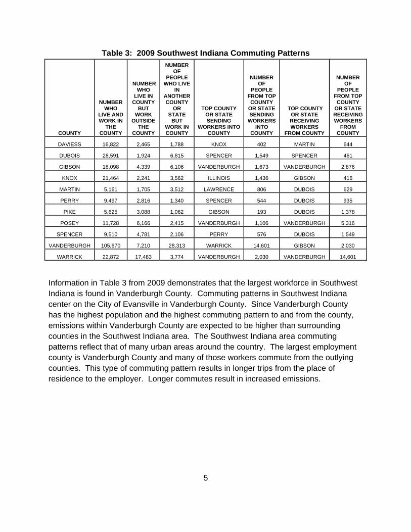
Table 3: 2009 Southwest Indiana Commuting Patterns

COUNTY

NUMBER WHO

LIVE AND WORK IN

THE COUNTY

NUMBER WHO

LIVE IN COUNTY

BUT WORK

OUTSIDE THE

COUNTY

NUMBER OF

PEOPLE WHO LIVE

IN ANOTHER COUNTY

OR STATE

BUT WORK IN COUNTY

TOP COUNTY OR STATE SENDING

WORKERS INTO COUNTY

NUMBER OF

PEOPLE FROM TOP COUNTY

OR STATE SENDING

WORKERS INTO

COUNTY

TOP COUNTY OR STATE RECEIVING WORKERS

FROM COUNTY

NUMBER OF

PEOPLE FROM TOP COUNTY

OR STATE RECEIVING WORKERS

FROM COUNTY

DAVIESS 16,822 2,465 1,788 KNOX 402 MARTIN 644

DUBOIS 28,591 1,924 6,815 SPENCER 1,549 SPENCER 461

GIBSON 18,098 4,339 6,106 VANDERBURGH 1,673 VANDERBURGH 2,876

KNOX 21,464 2,241 3,562 ILLINOIS 1,436 GIBSON 416

MARTIN 5,161 1,705 3,512 LAWRENCE 806 DUBOIS 629

PERRY 9,497 2,816 1,340 SPENCER 544 DUBOIS 935

PIKE 5,625 3,088 1,062 GIBSON 193 DUBOIS 1,378

POSEY 11,728 6,166 2,415 VANDERBURGH 1,106 VANDERBURGH 5,316

SPENCER 9,510 4,781 2,106 PERRY 576 DUBOIS 1,549

VANDERBURGH 105,670 7,210 28,313 WARRICK 14,601 GIBSON 2,030

WARRICK 22,872 17,483 3,774 VANDERBURGH 2,030 VANDERBURGH 14,601

Information in Table 3 from 2009 demonstrates that the largest workforce in Southwest Indiana is found in Vanderburgh County. Commuting patterns in Southwest Indiana center on the City of Evansville in Vanderburgh County. Since Vanderburgh County has the highest population and the highest commuting pattern to and from the county, emissions within Vanderburgh County are expected to be higher than surrounding counties in the Southwest Indiana area. The Southwest Indiana area commuting patterns reflect that of many urban areas around the country. The largest employment county is Vanderburgh County and many of those workers commute from the outlying counties. This type of commuting pattern results in longer trips from the place of residence to the employer. Longer commutes result in increased emissions.

6

Improvements in Air Quality

Indiana’s air quality has improved significantly over the last 30 years. The majority of air quality improvements in Southwest Indiana have stemmed from the national, regional, and local controls outlined below. These programs have been or are being implemented and have reduced monitored ambient air quality values in Southwest Indiana and across the state.

National Controls Acid Rain Program

Congress created the Acid Rain Program under Title IV of the 1990 Clean Air Act (CAA). The overall goal of the program is to achieve significant environmental and public health benefits through reduction in emissions of SO2 and NOx, the primary causes of acid rain. To achieve this goal at the lowest cost to the public, this program employs both traditional and innovative, market-based approaches to controlling air pollution. Specifically, the program seeks to limit, or “cap,” SO2 emissions from power plants at 8.95 million tons annually starting in 2010, authorizes those plants to trade SO2 allowances, and while not establishing a NOx trading program, reduces NOx emission rates. In addition, the program encourages energy efficiency and pollution prevention.

Tier II Emission Standards for Vehicles and Gasoline Sulfur Standards

In February 2000, U.S. EPA finalized a federal rule to significantly reduce emissions from cars and light duty trucks, including sport utility vehicles (SUVs). This rule requires automakers to produce cleaner cars, and refineries to make cleaner, lower sulfur gasoline. This rule was phased in between 2004 and 2009 and resulted in a 77% decrease in NOx emissions from passenger cars, an 86% decrease from smaller SUVs, light duty trucks, and minivans, and a 65% decrease from larger SUVs, vans, and heavier duty trucks. This rule also resulted in a 12% decrease in VOC emissions from passenger cars, an 18% decrease from smaller SUVs, light duty trucks, and minivans, and a 15% decrease from larger SUVs, vans, and heavier duty trucks.

7

Heavy-Duty Diesel Engines

In July 2000, U.S. EPA issued a final rule for Highway Heavy-Duty Engines, a program that includes low-sulfur diesel fuel standards. This rule applies to heavy-duty gasoline and diesel trucks and buses. This rule was phased in from 2004 through 2007 and resulted in a 40% decrease in NOx emissions from diesel trucks and buses.

Clean Air Nonroad Diesel Rule

In May 2004, U.S. EPA issued the Clean Air Nonroad Diesel Rule. This rule applies to diesel engines used in industries such as construction, agriculture, and mining. It also contains a cleaner fuel standard similar to the highway diesel program. The engine standards for nonroad engines took effect in 2008 and resulted in a 90% decrease in SO2 emissions from nonroad diesel engines. Sulfur levels were also reduced in nonroad diesel fuel by 99.5% from approximately 3,000 parts per million (ppm) to 15 ppm.

Nonroad Spark-Ignition Engines and Recreational Engine Standards

This standard, effective in July 2003, regulates NOx, VOCs, and CO for groups of previously unregulated nonroad engines. This standard applies to all new engines sold in the United States and imported after the standards went into effect. The standard applies to large spark-ignition engines (forklifts and airport ground service equipment), recreational vehicles (off-highway motorcycles and all terrain vehicles), and recreational marine diesel engines. When all of the nonroad spark-ignition engines and recreational engine standards are fully implemented, an overall 72% reduction in VOC, 80% reduction in NOx, and 56% reduction in CO emissions are expected by 2020.

8

Regional Controls Nitrogen Oxides (NOx) Rule

On October 27, 1998, U.S. EPA published the NOx State Implementation Plan (SIP) Call in the Federal Register (FR), which required 22 states to adopt rules that would result in significant emission reductions from large electric generating units (EGUs)1, industrial boilers, and cement kilns in the eastern United States (63 FR 57356). The Indiana rule was adopted in 2001 at 326 Indiana Administrative Code (IAC) 10-1. Beginning in 2004, this rule accounted for a reduction of approximately 31% of all NOx emissions statewide compared to previous uncontrolled years.

Twenty-one other states also adopted this rule. The result is that significant reductions have occurred within Indiana and regionally due to the number of affected units within the region. The historical trend charts show that air quality has improved due to the decreased emissions resulting from this program.

On April 21, 2004, U.S. EPA published Phase II of the NOx SIP Call that established a budget for large (emissions of greater than one ton per day) stationary internal combustion engines (69 FR 21604). In Indiana, the rule decreased NOx emissions statewide from natural gas compressor stations by 4,263 tons during May through September. The Indiana Phase II NOx SIP Call rule became effective in 2006 and implementation began in 2007 (326 IAC 10-4).

Clean Air Interstate Rule (CAIR)

On May 12, 2005, the U.S. EPA published the following regulation: “Rule to Reduce Interstate Transport of Fine Particulate Matter and Ozone (CAIR); Revisions to Acid Rain Program; Revisions to the NOx SIP Call; Final Rule” (70 FR 25162). This rule established the requirement for states to adopt rules limiting the emissions of NOx and SO2 and provided a model rule for the states to use in developing their rules in order to meet federal requirements. The purpose of CAIR was to reduce interstate transport of PM2.5, SO2, and ozone precursors (NOx).

Generally, CAIR applied to any stationary, fossil fuel-fired boiler or stationary, fossil fuel-fired combustion turbine, or a generator with a nameplate capacity of more than 25 megawatt electrical (MWe) for sale. This rule provided annual state caps for NOx and SO2 in two phases, with Phase I caps for NOx and SO2 starting in 2009 and 2010,

1 An EGU is a fossil fuel fired stationary boiler, combustion turbine, or combined cycle system that sells any amount of electricity produced.

9

respectively. Phase II caps were to become effective in 2015. U.S. EPA allowed limits to be met through a cap and trade program if a state chose to participate in the program.

In response to U.S. EPA’s rulemaking, Indiana adopted a state rule in 2006 based on the model federal rule (326 IAC 24-1). IDEM’s rule includes annual and seasonal NOx

trading programs and an annual SO2 trading program. This rule required compliance effective January 1, 2009.

SO2 emissions from power plants in the 28 eastern states and the District of Columbia (D.C.) covered by CAIR were to be cut by 4.3 million tons from 2003 levels by 2010 and by 5.4 million tons from 2003 levels by 2015. NOx emissions were to be cut by 1.7 million tons by 2009 and reduced by an additional 1.3 million tons by 2015. The D.C. Circuit court’s vacatur of CAIR in July 2008, and subsequent remand without vacatur of CAIR in December 2008, directed U.S. EPA to revise or replace CAIR in order to address the deficiencies identified outlined by the court. As of May 2012, CAIR remains in effect.

Cross-State Air Pollution Rule (CSAPR)

On August 8, 2011, U.S. EPA published a rule that helps states reduce air pollution and meet CAA standards. The Cross-State Air Pollution Rule (CSAPR) replaces U.S. EPA’s 2005 CAIR, and responds to the court’s concerns (76 FR 48208).

CSAPR requires 27 states in the eastern half of the United States to significantly reduce power plant emissions that cross state lines and contribute to ground-level ozone and fine particle pollution in other states.

On December 30, 2011, the U.S. Court of Appeals for the D.C. Circuit stayed CSAPR prior to implementation pending resolution of a challenge to the rule. The court ordered U.S. EPA to continue the administration of CAIR pending resolution of the current appeal. This required U.S. EPA to reinstate 2012 CAIR allowances which had been removed from the allowance tracking system as part of the transition to CSPAR. The federal rule is on hold pending resolution of the litigation.

10

Reasonably Available Control Technology (RACT) and other State VOC Rules

As required by Section 172 of the CAA, Indiana has promulgated several rules requiring Reasonably Available Control Technology (RACT) for emissions of VOCs since the mid 1990's. In addition, other statewide rules for controlling VOCs have also been promulgated. The Indiana rules are found in 326 IAC 8. The following is a listing of statewide rules that assist with the reduction of VOCs in Southwest Indiana:

326 IAC 8-1-6 Best Available Control Technology (BACT) for Non- Specific Sources

326 IAC 8-2 Surface Coating Emission Limitations

326 IAC 8-3 Organic Solvent Degreasing Operations

326 IAC 8-4 Petroleum Sources

326 IAC 8-5 Miscellaneous Operation

326 IAC 8-6 Organic Solvent Emission Limitations

326 IAC 8-8.1 Municipal Solid Waste Landfills

326 IAC 8-10 Automobile Refinishing

326 IAC 8-14 Architectural and Industrial Maintenance Coatings

326 IAC 8-15 Standards for Consumer and Commercial Products

New Source Review (NSR) Provisions

Indiana has a longstanding and fully implemented NSR program. This is addressed in 326 IAC 2. The rule includes provisions for the Prevention of Significant Deterioration permitting program in 326 IAC 2-2, and emission offset requirements for nonattainment areas in 326 IAC 2-3 for new and modified sources.

11

State Emission Reduction Initiatives

Outdoor Hydronic Heater Rule

Rule 326 IAC 4-3, effective May 18, 2011, regulates the use of outdoor hydronic heaters (also referred to as outdoor wood boilers or outdoor wood furnaces) designed to burn wood or other approved renewable solid fuels and establishes a particulate emission limit for new units. The rule also includes a fuel use restriction, stack height requirements, and a limited summertime operating ban for existing units.

Reinforced Plastic Composites Fabricating and Boat Manufacturing Industries Rule

Rules 326 IAC 20-48, effective August 23, 2004 and 326 IAC 20-56, effective April 1, 2006, regulate styrene emissions from the boat manufacturing and fiberglass reinforced plastic industries. The state rules implement the federal NESHAP for each of these source categories with additional requirements that were carried over from the Indiana state styrene rule (326 IAC 20-25) adopted in 2000 and now repealed.

Local Controls

Local control measures that have helped reduce motor vehicle emission and other types of emission values in the Southwest Indiana area are outlined below and include:

The Evansville Environmental Protection Agency (Evansville EPA) has worked with the community to identify and implement a number of locally enforceable control measures via ordinance. These ordinances address the following subjects:

County City Subject

Chapter 8.12 Section 3.30.214 Burning Regulations

Chapter 19.08 Section 3.30.248 Gasoline Dispensing Regulations

Chapter 19.12 Section 3.30.249 Automobile Refinishing

Chapter 19.16 Section 3.30.250 Pollution Prevention and Education Program

12

Southwest Indiana Emission Inventory Data

Emission trend graphs and pie charts for each criteria pollutant are included in this report. Emission trend graphs and pie charts for any precursors that lead to the formation of a criteria pollutant are also included. Indiana’s emission inventory data are available for 1980 through 2009 for CO, PM2.5, NO2, PM10, SO2, and VOC. These emission estimates are reflective of U.S. EPA methodologies found in the National Emissions Inventory (NEI) Air Pollutant Emissions Trends Data. Some of the fluctuations found in the trends inventory are due to U.S. EPA not incorporating state reported data until after the submission of the 1996 Periodic Emission Inventory1. Further, U.S. EPA acknowledges that changes over time may be attributable to changes in how inventories were compiled2.

The emissions have been broken down into contributions from the following individual source categories: point sources (including electric generating units (EGUs)), area sources, onroad sources, and nonroad sources. There are twelve EGU facilities in the Southwest Indiana area, eight of which are top ten emitters in the area. Emissions data for each county in Southwest Indiana are available upon request.

Point Sources

Point sources include major and minor sources, including EGUs that report emissions through Indiana’s emission reporting program. Examples include steel mills, manufacturing plants, surface coating operations, and industrial and commercial boilers.

Area Sources

Area sources are a collection of similar emission units within a geographic area that collectively represent individual sources that are small and numerous and have not been inventoried as a specific point, mobile, or biogenic source. Some of these sources include activities, such as dry cleaning, vehicle refueling, and solvent usage.

11http://www.epa.gov/ttn/chief/trends/trends98/trends98.pdf 2 http://www.epa.gov/air/airtrends/2007/report/particlepollution.pdf

13

Onroad Sources

Onroad sources include cars and light and heavy duty trucks.

Nonroad Sources

Nonroad sources typically include construction equipment, recreational boating, outdoor power equipment, recreational vehicles, farm machinery, lawn care equipment, and logging equipment.

Top Ten Emission Sources

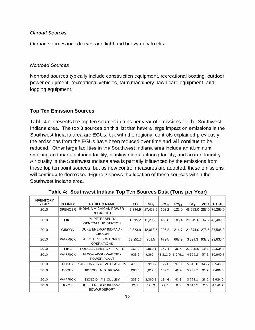
Table 4 represents the top ten sources in tons per year of emissions for the Southwest Indiana area. The top 3 sources on this list that have a large impact on emissions in the Southwest Indiana area are EGUs, but with the regional controls explained previously, the emissions from the EGUs have been reduced over time and will continue to be reduced. Other large facilities in the Southwest Indiana area include an aluminum smelting and manufacturing facility, plastics manufacturing facility, and an iron foundry. Air quality in the Southwest Indiana area is partially influenced by the emissions from these top ten point sources, but as new control measures are adopted, these emissions will continue to decrease. Figure 2 shows the location of these sources within the Southwest Indiana area.

Table 4: Southwest Indiana Top Ten Sources Data (Tons per Year)

INVENTORY YEAR COUNTY FACILITY NAME CO NOx PM10 PM2.5 SO2 VOC TOTAL

2010 SPENCER INDIANA MICHIGAN POWER-ROCKPORT

2,394.9 27,468.9 303.2 122.0 45,693.0 287.0 76,269.0

2010 PIKE IPL PETERSBURG GENERATING STATION

1,395.2 11,206.8 688.8 185.4 29,845.6 167.2 43,489.0

2010 GIBSON DUKE ENERGY INDIANA - GIBSON

2,323.9 12,018.5 796.2 214.7 21,874.0 278.6 37,505.9

2010 WARRICK ALCOA INC. - WARRICK OPERATIONS

23,251.5 208.5 679.5 663.9 3,899.3 932.8 29,635.4

2010 PIKE HOOSIER ENERGY - RATTS 163.3 1,860.1 147.4 36.4 21,308.0 19.6 23,534.6

2010 WARRICK ALCOA APGI - WARRICK POWER PLANT

632.8 9,395.4 1,312.0 1,078.1 4,365.2 57.2 16,840.7

2010 POSEY SABIC INNOVATIVE PLASTICS 470.8 1,990.2 122.6 97.8 5,516.0 346.7 8,543.9

2010 POSEY SIGECO - A. B. BROWN 265.3 1,612.6 162.5 42.4 5,291.7 31.7 7,406.3

2010 WARRICK SIGECO - F.B.CULLEY 233.9 2,390.6 154.6 43.5 3,776.1 28.2 6,626.9

2010 KNOX DUKE ENERGY INDIANA - EDWARDSPORT

20.9 571.9 22.0 8.8 3,516.5 2.5 4,142.7

14

Figure 2: Map of Southwest Indiana Top Ten Sources

15

Air Quality Trends

An area meets the standard when the monitoring values for a regulated criteria pollutant meet the applicable National Ambient Air Quality Standards (NAAQS). All counties in the Southwest Indiana area meet the historic NAAQS. New 1-hour NAAQS were introduced in 2010 for NO2 and SO2. The 1-hour NO2 monitoring data in Southwest Indiana, as well as elsewhere in the state, are well below the new 1-hour NO2 NAAQS. There are three counties with monitor violations of the new 1-hour SO2 NAAQS in Southwest Indiana at the close of 2010. States are required to develop SIPs to show attainment of the 1-hour SO2 NAAQS by 2017.

Air Monitoring and Emissions Data

All counties in the Southwest Indiana area have an ambient air quality monitor located within the county boundaries except Martin County. Monitoring data for the years 2000 through 2010 for Southwest Indiana are included in the tables in this report for each criteria pollutant, if available. Monitoring data prior to the year 2000 are available upon request. A historical trend graph of all available data for the years 1980 through 2010 is also provided. The data were obtained from the U.S. EPA’s Air Quality System.

Emission trend graphs and pie charts for the criteria pollutants and precursors that lead to the formation of a criteria pollutant are outlined in this report. Indiana’s emission inventory data are available for 1980 through 2009 for CO, PM2.5, NOx, PM10, SO2, and VOC. The data were obtained from the U.S. EPA’s National Emissions Inventory (NEI). An appendix is attached that includes county-specific emissions data for each county from 1980 through 2009.

Carbon Monoxide (CO)

There is one monitoring site within Southwest Indiana, located in Vanderburgh County that measures CO levels. The trend data shown in Graphs 1 and 2 reflect the 2nd highest concentration for 1-hour and 8-hour CO. The 2nd high values are not the highest monitored concentration at a given monitoring location, rather the 2nd highest measured value. These values (2nd highs) are used to determine attainment of the

16

primary 1-hour CO standard at 35 ppm and the primary 8-hour CO standard at 9 ppm. The primary 1-hour and primary 8-hour CO standards were first established in April 1971. There are no secondary standards for 1-hour or 8-hour CO. While there are occasional spikes in the monitoring values for both 1-hour and 8-hour CO concentrations, a downward trend over time can be seen in Graphs 1 and 2. Monitoring values have historically been below both the 1-hour and the 8-hour primary CO standards. CO monitoring data fluctuated between the years of 1986 and 2005 due to variability in the motor vehicle fleet. CO correlates closely with vehicle traffic and emissions from motor vehicles, which can lead to variability in the data.

The data shown in Tables 5 and 6 reflect the 2nd highest concentration values for 1-hour and 8-hour CO from 2000 to 2010. Historical data prior to the year 2000 are available upon request for both 1-hour and 8-hour CO. Monitoring data in Table 5 are compared to the primary 1-hour CO standard of 35 ppm. Attainment is determined by evaluating the 2nd highest 1-hour high concentration. Monitoring data in Table 6 are compared to the primary 8-hour CO standard of 9 ppm. Attainment is determined by evaluating the 2nd highest 8-hour concentration. There are no monitor violations in the Southwest Indiana area for the 1-hour or 8-hour CO reflected.

Graph 1: Southwest Indiana 1-Hour CO 2nd High Values

0

5

10

15

20

25

30

35

40

1980 1985 1990 1995 2000 2005 2010

Concentration (ppm)

Year

1‐Hour CO 2nd High ValuesSouthwest Indiana

1‐Hour 2nd High Values 1‐Hour CO Standard (35 ppm) Trendline

17

Table 5: Southwest Indiana 1-Hour CO 2nd High Value Monitoring Data Summary

County Site # Site Name

1-Hour 2nd High Value (ppm)

2000 2001 2002 2003 2004 2005 2006 2007 2008 2009 2010

Vanderburgh 181630015 Evansville-Water Pumping Station 4.3 6.1 5.9 3.7

Vanderburgh 181630019 Evansville-3013 N 1st Ave 3.5 5.0 3.3 3.9 2.5 1.8 2.4

Vanderburgh 181630022 Evansville-10 S 11st St 2.4 5.5

Highlighted red numbers are above the 1-hour CO standard of 35 ppm

Graph 2: Southwest Indiana 8-Hour CO 2nd High Values

0

2

4

6

8

10

1980 1985 1990 1995 2000 2005 2010

Concentration (ppm)

Year

8‐Hour CO 2nd High ValuesSouthwest Indiana

8‐Hour 2nd High Values 8‐Hour CO Standard (9 ppm) Trendline

18

Table 6: Southwest Indiana 8-Hour CO 2nd High Value Monitoring Data Summary


8-Hour 2nd High Value (ppm)

2000 2001 2002 2003 2004 2005 2006 2007 2008 2009 2010

Vanderburgh 181630015 Evansville-Water Pumping Station 3.0 3.2 3.0 2.5

Vanderburgh 181630019 Evansville-3013 N 1st Ave 1.9 2.7 2.1 2.2 1.6 1.1 1.7

Vanderburgh 181630022 Evansville-10 S 11st St 1.8 4.3

Highlighted red numbers are above the 8-hour CO standard of 9 ppm

U.S. EPA’s NEI contains emissions information for CO which is used for Graph 3 and Chart 1. Graph 3 illustrates the emissions trend for CO in Southwest Indiana and Chart 1 shows how the average emissions are distributed among the different source categories.

Graph 3: Southwest Indiana CO Emissions

0

50,000

100,000

150,000

200,000

250,000

300,000

350,000

400,000

450,000

1980

1981

1982

1983

1984

1985

1986

1987

1988

1989

1990

1991

1992

1993

1994

1995

1996

1997

1998

1999

2000

2001

2002

2003

2004

2005

2006

2007

2008

2009

Emissions (tons/year)

Year

Southwest Indiana ‐ CO Emissions

Point Area Onroad Nonroad EGU

19

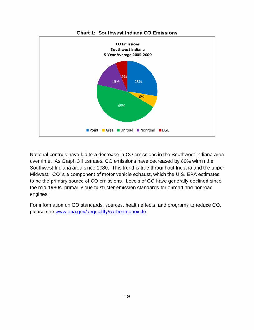
Chart 1: Southwest Indiana CO Emissions

National controls have led to a decrease in CO emissions in the Southwest Indiana area over time. As Graph 3 illustrates, CO emissions have decreased by 80% within the Southwest Indiana area since 1980. This trend is true throughout Indiana and the upper Midwest. CO is a component of motor vehicle exhaust, which the U.S. EPA estimates to be the primary source of CO emissions. Levels of CO have generally declined since the mid-1980s, primarily due to stricter emission standards for onroad and nonroad engines.

For information on CO standards, sources, health effects, and programs to reduce CO, please see www.epa.gov/airqualilty/carbonmonoxide.

28%,

6%

45%

15%6%

CO EmissionsSouthwest Indiana

5‐Year Average 2005‐2009


20

Fine Particles (PM2.5)

There are six monitors within Southwest Indiana, two in Vanderburgh County and one each in Dubois, Gibson, Knox, and Spencer counties currently measuring PM2.5 levels. The Evansville–Post Office monitoring site was discontinued in early-2011. The trend data in Graphs 4 and 6 reflect the annual arithmetic mean (the method used to derive the central tendency of the monitoring values) for annual PM2.5 and the 98th percentile (the method used to determine the value below which a certain percent of monitored observations fall) for 24-hour PM2.5 for each year in the Southwest Indiana area for the years 2000 through 2010. The annual arithmetic mean values for annual PM2.5 and 98th percentile values for 24-hour PM2.5 are not used to compare to the primary and secondary annual or 24-hour PM2.5 standards. A three-year average, also known as the design value, is used to compare to both the primary and secondary annual PM2.5 standards of 15.0 micrograms per cubic meter (µg/m3), as well as the primary and secondary 24-hour PM2.5 standards of 35 µg/m3, but the annual arithmetic mean and 98th percentile for each year do provide a good indication of annual and 24-hour PM2.5 trends over time. The primary and secondary 24-hour PM2.5 standards were first established in July 1997 of 65 µg/m3. U.S. EPA revised the primary and secondary 24-hour PM2.5 standards and lowered them to 35 µg/m3 in October 2006.

For both annual and 24-hour PM2.5, the secondary standard is the same as the primary standard. Attainment of the annual primary and secondary PM2.5 standards is determined by evaluating the design value of the annual arithmetic mean from a single monitor, which must be less than or equal to 15.0 µg/m3. An exceedance of the annual PM2.5 standards occurs when an annual arithmetic mean value is equal to or greater than 15.0 µg/m3. A violation of the annual PM2.5 standards occurs when the design value of the annual arithmetic mean value is equal to or greater than 15.05 µg/m3. A monitor can exceed the annual PM2.5 standards without being in violation. Attainment of the 24-hour PM2.5 standards is determined by evaluating the design value of the 98th percentile of the 24-hour concentrations at each population-oriented monitor within an area, which must not exceed 35 µg/m3. An exceedance of the 24-hour PM2.5 standards occurs when the 98th percentile is equal to or greater than 35 µg/m3. A violation of the 24-hour PM2.5 standards occurs when the design value of the 98th percentile is equal to or greater than 35.5 µg/m3. A monitor can exceed the 24-hour PM2.5 standards without being in violation.

21

The trend data in Graph 5 reflect the three-year design value of the annual arithmetic mean for annual PM2.5 for each year in the Southwest Indiana area for the years 2000 through 2010. The trend data in Graph 7 reflect the three-year design value of the 98th percentile values for 24-hour PM2.5 for each year in the Southwest Indiana area for the years 2000 through 2010.

While there is some variability in the monitor values for both annual PM2.5 and 24-hour PM2.5, a downward trend over time can be seen in Graphs 4 and 5. The design value of the annual arithmetic mean is used for comparison to the primary and secondary annual PM2.5 standards at 15.0 µg/m3; therefore, the one-year values shown in Graph 4 are not a true comparison to the annual PM2.5 standards and the values in the years that are above the red line are not a violation of the primary and secondary annual PM2.5 standards. The values in Graph 4 reflect the annual arithmetic mean and the highest value from all of the monitors in the Southwest Indiana area are plotted on the graph for each year.

The design value of the 98th percentile is used for comparison to the 24-hour PM2.5 standards; therefore, the one-year values shown in Graph 6 are not a true comparison to the 24-hour PM2.5 standards and the values in the years that are above the red line are not a violation of the primary and secondary 24-hour PM2.5 standards. The values in Graph 6 reflect the 98th percentile and the highest value from all of the monitors in the Southwest Indiana area is plotted on the graph for each year.

The data in Tables 7, 8, 9, and 10 are from the monitoring sites that measured annual and 24-hour PM2.5 from 2000 to 2010. Statewide monitoring for PM2.5 began in 2000; all available data for both annual and 24-hour PM2.5 for the Southwest Indiana area are shown in the tables. Monitoring data for both annual and 24-hour PM2.5 show a downward trend over time.

Monitoring data in Table 7 show the annual arithmetic mean for annual PM2.5 for the years 2000 through 2010. Monitoring data in Table 8 show the design value of the annual arithmetic mean for annual PM2.5 for the years 2000 through 2010, which are compared to the primary and secondary annual PM2.5 standards of 15.0 µg/m3. Monitoring data in Table 9 show the 98th percentile for 24-hour PM2.5 for the years 2000 through 2010. Monitoring data in Table 10 show the design value of the 98th percentile for 24-hour PM2.5 for the years 2000 through 2010, which are compared to the primary and secondary 24-hour PM2.5 standards of 35 µg/m3.

22

Graph 4: Southwest Indiana Annual Arithmetic Mean PM2.5 Values

Table 7: Southwest Indiana Annual Arithmetic Mean PM2.5 Monitoring Data Summary

County Site # Site Name Annual Arithmetic Mean (µg/m3)

2000 2001 2002 2003 2004 2005 2006 2007 2008 2009 2010

Dubois 180372001 Jasper - Post Office 17.16 16.54 16.34 15.72 14.42 16.92 13.54 14.26 12.93 12.49 13.65

Gibson 180510012 Oakland City 11.33 11.00 12.17

Knox 180830004 Southwest Ag Center 13.87 13.39 14.20 13.96 12.62 15.66 13.20 13.79 11.58 11.41 12.34

Spencer 181470009 Dale 16.32 14.52 14.06 14.63 12.16 16.76 12.78 14.13 12.03 11.77 12.99

Vanderburgh 181630006 Evansville - Civic Center

16.17 15.45 15.36 14.93 13.23 16.49 13.72 13.91 12.58 11.98

Vanderburgh 181630006/20

Evansville Combined (Civic Center & Post

Office) 12.32

Vanderburgh 181630020 Evansville - Post

Office 12.28 13.40

Vanderburgh 181630012 Evansville - Mill Rd 16.17 15.15 15.27 15.27 13.46 16.29 14.05 14.23 12.70 12.16


Evansville Combined (Mill Rd & Buena

Vista) 12.28

Vanderburgh 181630021 Evansville - Buena

Vista 12.41 12.83

Vanderburgh 181630016 Evansville - Univ of

Evansville 15.70 16.16 15.24 15.09 13.68 16.67 14.15 14.21 12.53 12.49 13.40

0

2

4

6

8

10

12

14

16

18

20

2000 2001 2002 2003 2004 2005 2006 2007 2008 2009 2010

Concentration (µg/m³)

Year

Annual Arithmetic Mean PM2.5 ValuesSouthwest Indiana

Annual Arithmetic Means Annual PM₂.₅ Standard (15 µg/m³) Trendline

23

Graph 5: Southwest Indiana Annual PM2.5 Three-Year Design Values

Table 8: Southwest Indiana Annual PM2.5 Three-Year Design Value Monitoring Data Summary

County Site # Site Name Three-Year Design Value (µg/m3)

00-02 01-03 02-04 03-05 04-06 05-07 06-08 07-09 08-10

Dubois 180372001 Jasper - Post Office 16.7 16.2 15.5 15.7 15.0 14.9 13.6 13.3 13.0


Knox 180830004 Southwest Ag Center 13.8 13.9 13.6 14.1 13.8 14.2 12.9 12.3 11.8

Spencer 181470009 Dale 15.0 14.4 13.6 14.5 13.9 14.6 13.0 12.6 12.3

Vanderburgh 181630006 Evansville - Civic Center 15.7 15.2 14.5 14.9 14.5 14.7 13.4 12.8

Vanderburgh 181630006/20 Evansville Combined (Civic Center & Post Office)

12.9 12.8

Vanderburgh 181630020 Evansville - Post Office 12.3 12.9

Vanderburgh 181630012 Evansville - Mill Rd 15.5 15.2 14.7 15.0 14.6 14.9 13.7 13.0

Vanderburgh 181630012/21 Evansville Combined (Mill Rd & Buena Vista)

13.1 12.6

Vanderburgh 181630021 Evansville - Buena Vista 12.4 12.6

Vanderburgh 181630016 Evansville - Univ of Evansville 15.7 15.5 14.7 15.1 14.8 15.0 13.6 13.1 12.8

Red highlighted numbers are above the annual PM2.5 standard of 15.0 µg/m3

0

5

10

15

20

00‐02 01‐03 02‐04 03‐05 04‐06 05‐07 06‐08 07‐09 08‐10


Year

Annual PM2.5 Three‐Year Design ValuesSouthwest Indiana

Three‐Year Design Values Annual PM₂.₅ Standard (15 µg/m³) Trendline

24

Graph 6: Southwest Indiana 24-Hour PM2.5 98th Percentile Values

Table 9: Southwest Indiana 24-Hour 98th Percentile Value PM2.5 Monitoring Data Summary

County Site # Site Name Daily 98th Percentile Values (µg/m3)

2000 2001 2002 2003 2004 2005 2006 2007 2008 2009 2010



Knox 180830004 Southwest Ag Center 34.5 33.0 38.6 34.8 29.9 41.8 36.2 30.9 23.5 23.1 27.6

Spencer 181470009 Dale 43.4 28.2 27.8 34.6 25.2 39.7 27.7 31.4 22.9 24.3 26.7

Vanderburgh 181630006 Evansville - Civic Center

37.3 36.4 46.7 34.5 28.3 42.5 30.5 33.6 27.2 21.9

Vanderburgh 181630006/20 Evansville Combined (Civic Center & Post

Office) 26.2

Vanderburgh 181630020 Evansville - Post Office 30.8 26.4

Vanderburgh 181630012 Evansville - Mill Rd 34.3 34.2 44.9 34.1 27.6 41.5 27.9 29.9 24.7 25.1

Vanderburgh 181630012/21 Evansville Combined

(Mill Rd & Buena Vista) 27.7

Vanderburgh 181630021 Evansville - Buena Vista

27.7 30.4

Vanderburgh 181630016 Evansville - Univ of

Evansville 33.5 37.9 46.2 35.9 28.3 37.0 29.5 31.5 26.5 25.5 29.2

0

10

20

30

40

50

60

70

2000 2001 2002 2003 2004 2005 2006 2007 2008 2009 2010


Year

24‐Hour PM2.5 98th Percentile ValuesSouthwest Indiana

24‐Hour Maximum 98th Percentile Values 1997 24‐Hour PM₂.₅ Standard (65 µg/m³)

2006 24‐Hour PM₂.₅ Standard (35 µg/m³) Trendline

25

Graph 7: Southwest Indiana 24-Hour PM2.5 Three-Year Design Values

Table 10: Southwest Indiana 24-Hour PM2.5 Three-Year Design Value Monitoring Data Summary

County Site # Site Name Three-Year Design Value (µg/m3)

00-02 01-03 02-04 03-05 04-06 05-07 06-08 07-09 08-10

Dubois 180372001 Jasper - Post Office 38 38 35 37 34 35 30 28 26

Gibson 180510012 Oakland City 25 25 25

Knox 180830004 Southwest Ag Center 35 35 34 36 36 36 30 26 25

Spencer 181470009 Dale 33 30 29 33 31 33 27 26 25

Vanderburgh 181630006 Evansville - Civic Center 40 39 37 35 34 36 30 28

Vanderburgh 181630006/20 Evansville Combined (Civic Center & Post Office)

29 27

Vanderburgh 181630020 Evansville - Post Office 31 29

Vanderburgh 181630012 Evansville - Mill Rd 38 38 36 34 32 33 28 27

Vanderburgh 181630012/21 Evansville Combined (Mill Rd & Buena Vista)

27 28

Vanderburgh 181630021 Evansville - Buena Vista 28 27

Vanderburgh 181630016 Evansville - Univ of Evansville 39 40 37 34 32 33 29 28 27

Prior to 2006, highlighted red numbers are above the 24-hour PM2.5 standard of 65 µg/m3

Beginning in 2006, highlighted red numbers are above the 24-hour PM2.5 standard of 35.0 µg/m3

0

10

20

30

40

50

60

70

00‐02 01‐03 02‐04 03‐05 04‐06 05‐07 06‐08 07‐09 08‐10


Year

24‐Hour PM2.5 Three‐Year Design ValuesSouthwest Indiana

Three‐Year Design Values 1997 24‐Hour PM₂.₅ Standard (65 µg/m³)

2006 24‐Hour PM₂.₅ Standard (35 µg/m³) Trendline

26

Tables 7, 8, 9, and 10 demonstrate that the annual and 24-hour PM2.5 values for the Southwest Indiana area correlate with each other over time, meaning that when one monitoring site trends upward or downward, the other sites do also. Annual PM2.5 values in Southwest Indiana had been above the primary and secondary annual PM2.5 standards until the end of 2005, but have remained below the standards since then. 24-hour PM2.5 values in Southwest Indiana had been above the primary and secondary 24-hour PM2.5 standards until the end of 2007, but have remained below since then. The Jasper –Post office site in Dubois County has historically registered the highest PM2.5 values in Southwest Indiana. This is expected since it is downwind from some of the larger PM2.5 emitters in the Southwest Indiana area.

While fluctuations in monitoring data are shown in Graphs 4, 5, 6, and 7, monitoring data for both annual PM2.5 and 24-hour PM2.5 indicate a downward trend over time. PM2.5 is influenced by meteorology (wind speed, temperature, stagnant air, etc.). Meteorological conditions can have an episodic effect on PM2.5 concentrations as seen in 2005 (Graphs 4, 5, 6, and 7), when three of the four quarters of the year had high PM2.5 values which drove the annual PM2.5 values higher for the year. The annual value is calculated from the average of the year’s four quarterly averages. A quarterly average is the average of all available data from the respective quarter. The upper Midwest experienced several episodes of unusually high PM2.5 concentrations in 2005 caused by unusual confluences of meteorological factors. Several times during 2005 high pressure systems were held in place by jet streams which lead to a persistent, highly stable atmosphere with calm winds. Atmospheric mixing was suppressed and pollutants that form PM2.5 were trapped near the surface and high values were measured. The longest and most wide spread episode happened during the first week of February 2005 which lasted for nine days and affected the upper Midwest and southern Ontario where daily PM2.5 values exceeded 70 µg/m3.

PM2.5 is emitted directly into the air, but is also created by a chemical reaction between SO2 and NOx. U.S. EPA’s NEI contains emissions information for PM2.5, SO2, and NOx and is used for Graphs 8, 9, and 10 and Charts 2, 3, and 4. Graphs 8, 9, and 10 illustrate the emissions trend for PM2.5 and its precursors (SO2 and NOx) in Southwest Indiana. Charts 2, 3, and 4 show how the average emissions are distributed among the different source categories.

27

Graph 8: Southwest Indiana PM2.5 Emissions

Chart 2: Southwest Indiana PM2.5 Emissions

0

5,000

10,000

15,000

20,000

25,000

30,000

35,000

40,000

45,000

1980

1981

1982

1983

1984

1985

1986

1987

1988

1989

1990

1991

1992

1993

1994

1995

1996

1997

1998

1999

2000

2001

2002

2003

2004

2005

2006

2007

2008

2009


Year

Southwest Indiana ‐ PM2.5 Emissions


14%

28%

1%2%

55%

PM2.5 EmissionsSouthwest Indiana



28

Graph 9: Southwest Indiana SO2 Emissions

Chart 3: Southwest Indiana SO2 Emissions

0

100,000

200,000

300,000

400,000

500,000

600,000

700,000

800,000

900,000

1980

1981

1982

1983

1984

1985

1986

1987

1988

1989

1990

1991

1992

1993

1994

1995

1996

1997

1998

1999

2000

2001

2002

2003

2004

2005

2006

2007

2008

2009


Year

Southwest Indiana ‐ SO2 Emissions


5%

0%

0%

0%

95%

SO2 EmissionsSouthwest Indiana



29

Graph 10: Southwest Indiana NOx Emissions

Chart 4: Southwest Indiana NOx Emissions

0

50,000

100,000

150,000

200,000

250,000

300,000

1980

1981

1982

1983

1984

1985

1986

1987

1988

1989

1990

1991

1992

1993

1994

1995

1996

1997

1998

1999

2000

2001

2002

2003

2004

2005

2006

2007

2008

2009


Year

Southwest Indiana ‐ NOX Emissions


5%

1%

8%

11%

75%

NOX EmissionsSouthwest Indiana



30

National controls, such as engine and fuel standards, as well as regional controls, such as the NOx SIP Call, have led to a decrease in PM2.5 values over time. As Graphs 8, 9, and 10 illustrate, PM2.5, SO2, and NOx emissions have decreased by 8%, 74%, and 71%, respectively, within the Southwest Indiana area since 1980. This trend is true for the key precursors of PM2.5 throughout Indiana and the upper Midwest.

Nationally, average SO2 concentrations have decreased by more than 70% since 1980 due to the implementation of the Acid Rain Program. Reductions in Indiana for SO2 are primarily attributable to the implementation of the Acid Rain Program, as well as federal engine and fuel standards for onroad and nonroad vehicles and equipment.

For information on PM2.5 standards, sources, health effects, and programs to reduce PM2.5, please see www.epa.gov/air/particlepollution.

Lead

There are no monitoring sites within the Southwest Indiana area currently measuring lead levels. The Evansville–Post Office monitoring site was discontinued in early-2011. The primary and secondary lead standards were first established in October 1978 at 1.5 µg/m3. Attainment was determined by evaluating each calendar quarter arithmetic average, which must not exceed 1.5 µg/m3 over a three-year period. U.S. EPA replaced the primary and secondary 1978 lead standards with new primary and secondary lead standards of 0.15 µg/m3 in October 2008. Attainment of the primary and secondary 2008 lead standards is determined by evaluating the rolling three-month average. Any three consecutive monthly averages (January-March, February-April, March-May, etc.) must not exceed 0.15 µg/m3 within a three-year period. The trend data in Graph 11 reflect the highest annual quarterly arithmetic mean. The trend data in Graph 12 show the highest three-month rolling average. Lead values in the Southwest Indiana area have been steady over time and are well below both the 1978 and 2008 lead standards.

The data in Tables 11 and 12 are for the monitors that measured lead from 2000 to 2010. Historical lead data prior to the year 2000 are available upon request. Monitoring data in Table 11 are compared to the primary and secondary 1978 lead standards which were 1.5 µg/m3. Monitoring data in Table 12 are compared to the primary and secondary 2008 lead standards.

31

Graph 11: Southwest Indiana Lead Highest Annual Quarterly Values

Table 11: Southwest Indiana Lead Quarterly Average Monitoring Data Summary


Quarterly Average (µg/m3)

1Q 2000

2Q 2000

3Q 2000

4Q 2000

1Q 2001

2Q 2001

3Q 2001

4Q 2001

1Q 2002

2Q 2002

3Q 2002

4Q 2002


Evansville-Civic Center/Post Office 0.00 0.00 0.00 0.00 0.01 0.01

County Site # Site Name 1Q

2003 2Q

2003 3Q

2003 4Q

2003 1Q

2004 2Q

2004 3Q

2004 4Q

2004 1Q

2005 2Q

2005 3Q

2005 4Q

2005


Evansville-Civic Center/Post Office 0.00 0.00 0.00 0.01 0.01 0.01 0.01 0.00 0.01 0.01 0.01 0.01

County Site # Site Name 1Q

2006 2Q

2006 3Q

2006 4Q

2006 1Q

2007 2Q

2007 3Q

2007 4Q

2007 1Q

2008 2Q

2008 3Q

2008 4Q

2008


Evansville-Civic Center/Post Office 0.01 0.01 0.01 0.00 0.00 0.01 0.00 0.00 0.01 0.01

Highlighted red numbers are over the 1978 lead standard of 1.5 µg/m3

*The monitor at the Evansville Civic Center was moved to the Evansville Post Office in 2009. These two sites are considered to measure the same air mass, thus the data are combined.

0.00 0.01 0.01 0.01 0.01 0.01 0.01 0.01

0

0.2

0.4

0.6

0.8

1

1.2

1.4

1.6

2001 2002 2003 2004 2005 2006 2007 2008


Year

Lead Highest Annual Quarterly ValuesSouthwest Indiana

Lead Values 1978 Lead Standard (1.5 µg/m³) Trendline

32

Graph 12: Southwest Three-Month Rolling Average Values

Table 12: Southwest Indiana Lead Three-Month Rolling Average Monitoring Data Summary


Three-Month Averages (µg/m3)

11/07-01/08

12/07-02/08

01/08-03/08

02/08-04/08

03/08-05/08

04/08-06/08

05/08-07/08

06/08-08/08

07/08-09/08

08/08-10/08

09/08-11/08

10/08-12/08

Vanderburgh* 181630006/20 Evansville-Civic Center/Post Office

0.00 0.00 0.00 0.00 0.01 0.00 0.00 0.00 0.00 0.00 0.00 0.01

County Site # Site Name 11/08-01/09

12/08-02/09

01/09-03/09

02/09-04/09

03/09-05/09

04/09-06/09

05/09-07/09

06/09-08/09

07/09-09/09

08/09-10/09

09/09-11/09

10/09-12/09


0.01 0.01 0.01 0.01 0.00 0.01 0.01 0.01 0.00 0.00 0.01 0.01

County Site # Site Name 11/09-01/10

12/09-02/10

01/10-03/10

02/10-04/10

03/10-05/10

04/10-06/10

05/10-07/10

06/10-08/10

07/10-09/10

08/10-10/10

09/10-11/10

10/10-12/10


0.01 0.00 0.00 0.00 0.01 0.01 0.01 0.00 0.00 0.00 0.00 0.00

Highlighted red numbers are rolling three-month averages above the 2008 Lead standard of 0.15 µg/m3

*The monitor at the Evansville Civic Center was moved to the Evansville Post Office in 2009. These two sites are considered to measure the same air mass, thus the data are combined.

0.00

0.02

0.04

0.06

0.08

0.10

0.12

0.14

0.1611/07 ‐01/08

12/07 ‐02/08

01/08 ‐03/08

02/08 ‐04/08

03/08 ‐05/08

04/08 ‐06/08

05/08 ‐07/08

06/08 ‐08/08

07/08 ‐09/08

08/08 ‐10/08

09/08 ‐11/08

10/08 ‐12/08

11/08 ‐01/09

12/08 ‐02/09

01/09 ‐03/09

02/09 ‐04/09

03/09 ‐05/09

04/09 ‐06/09

05/09 ‐07/09

06/09 ‐08/09

07/09 ‐09/09

08/09 ‐10/09

09/09 ‐11/09

10/09 ‐12/09

11/09 ‐01/10

12/09 ‐02/10

01/10 ‐03/10

02/10 ‐04/10

03/10 ‐05/10

04/10 ‐06/10

05/10 ‐07/10

06/10 ‐08/10

07/10 ‐09/10

08/10 ‐10/10

09/10 ‐11/10

10/10 ‐12/10


Year

Lead Three‐Month Rolling ValuesSouthwest Indiana

Lead Three‐Month Rolling Values 2008 Lead Standard (0.15 µg/m³) Trendline

33

Historically, the majority of lead emissions came from motor vehicle fuels. As a result of U.S. EPA's regulatory efforts to remove lead from motor vehicle gasoline, emissions of lead from the transportation sector declined by 95% between 1980 and 1999, and levels of lead in the air decreased by 94% between 1980 and 1999. As can be seen in Graphs 11 and 12, lead levels in Southwest Indiana are well below the current standard and will continue to do so as new federal controls are adopted.

For information on lead standards, sources, health effects, and programs to reduce lead, please see www.epa.gov/air/lead.

Nitrogen Dioxide (NO2)

There is one monitoring site within the Southwest Indiana area, located in Vanderburgh County that measures NO2 levels. The trend data in Graph 13 reflect the annual arithmetic mean NO2 values. The annual arithmetic mean is used to compare to the primary and secondary annual NO2 standards at 53 parts per billion (ppb). The secondary annual NO2 standard is the same as the primary NO2 standard. Attainment of the annual NO2 standards is determined by evaluating the annual arithmetic mean concentration in a calendar year, which must be less than or equal to 53 ppb. U.S. EPA added a primary 1-hour NO2 standard in February 2010 at 100 ppb. Attainment of the 1-hour NO2 standard is determined by evaluating the design value of the 98th percentile of the daily maximum 1-hour averages at each monitor within an area, which must not exceed 100 ppb averaged over a three-year period.

The trend data in Graph 14 show the 98th percentile of the 1-hour NO2 values, which are provided for reference purposes only, because they were collected prior to the implementation of the current standard. The design value of the 98th percentile is used for comparison to the primary 1-hour NO2 standard; therefore, the one-year values shown in Graph 14 are not a true comparison to the primary 1-hour NO2 standard. The values in Graph 14 reflect the highest 98th percentile from all of the monitors in the Southwest Indiana area which is plotted on the graph for each year. The 1-hour NO2 standard at 100 ppb is only listed for the year 2010 on this graph since it was not established until February 2010. Attainment of the primary 1-hour NO2 standard is determined by evaluating the design value of the 98th percentile values of the daily maximum 1-hour averages at each monitor within an area, which must not exceed 100 ppb averaged over a three-year period. An exceedance of the primary 1-hour NO2 standard occurs when a 98th percentile value is equal to or greater than 100 ppb. A

34

violation of the primary 1-hour NO2 standard occurs when the three-year design value of the 98th percentile is equal to or greater than 100 ppb. A monitor can exceed the standard without being in violation.

NO2 data are presented from 2000 to 2010 in this report; however, historical monitoring data for annual NO2 for all monitors in Southwest Indiana are available upon request. Monitoring data for annual NO2 show a downward trend over time and the monitor values for Southwest Indiana have historically been below the primary and secondary annual NO2 standards. While fluctuations in monitoring data are shown in Graphs 13, 14, and 15, monitoring data for both annual and 1-hour NO2 indicate a downward trend over time. NO2 monitors are located in close proximity to major sources in the area and data fluctuate based on variability in facility operations and meteorology

The data in Tables 13, 14, and 15 are from the monitoring sites that measured NO2 from 2000 to 2010. Historical data prior to the year 2000 are available upon request for both annual and 1-hour NO2. Monitoring data in Table 13 are compared to the primary and secondary annual NO2 standards at 53 ppb. Monitoring data in Table 14 show the 98th percentile of the 1-hour NO2 values for the years 2000 through 2010. Monitoring data in Table 15 are compared to the primary 1-hour NO2 standard at 100 ppb. The 1-hour NO2 data prior to 2010 was not compared to any standard and the 98th percentile values and the design values from 2000 to 2007 are included for reference purposes only. NO2 values in Southwest Indiana are well below both the annual and 1-hour NO2 standards.

35

Graph 13: Southwest Indiana Annual Arithmetic Mean NO2 Values

Table 13: Southwest Indiana Annual Arithmetic Mean NO2 Values Monitoring Data Summary

County Site # Site Name Annual Mean (ppb)

2000 2001 2002 2003 2004 2005 2006 2007 2008 2009 2010

Gibson 180510010 Princeton-CR 550 S 10 10 9 9 9

Spencer 181470008 CR 750 N 7 6

Vanderburgh 181630012 Evansville-W Mill Rd 14 13 11 12 12 10 9 10 9

Vanderburgh 181630021 Evansville-Buena Vista 9 11

Highlighted red numbers are above the annual NO2 standard of 53 ppb

The 2009 annual mean value is West Mill's 6 months mean of 8 and Buena Vista's 6 months mean of 9 averaged together. The Buena Vista monitor replaced the West Mill Road monitor in June 2009

0

10

20

30

40

50

60

1980 1985 1990 1995 2000 2005 2010

Concentration (ppb)

Year

Annual Arithmetic Mean NO2 ValuesSouthwest Indiana

Annual Arithmetic Means Annual NO₂ Standard (53 ppb) Trendline

36

Graph 14: Southwest Indiana 1-Hour NO2 98th Percentile Values

Table 14: Southwest Indiana 1-Hour NO2 98th Percentile Values Monitoring Data Summary

County Site # Site Name Daily 98th Percentile Values (ppb)

2000 2001 2002 2003 2004 2005 2006 2007 2008 2009 2010


Spencer 181470008 CR 750 N 40 40

Vanderburgh 181630012 Evansville-W Mill Rd 49 43 36 39 41 39 32 36 37

Vanderburgh 181630021 Evansville-Buena Vista 321 41

1The 98th percentile for 2009 was calculated by using the first 6 months of data from the West Mill Rd monitor and the last 6 months of data from the Buena Vista monitor.

0

20

40

60

80

100

120

1980 1985 1990 1995 2000 2005 2010

Concentration (ppb)

Year

1‐Hour NO₂ 98th Percentile ValuesSouthwest Region

1‐Hour 98th Percentile Values 1‐Hour NO₂ Standard (100 ppb) Trendline

37

Graph 15: Southwest Indiana 1-Hour NO2 Three-Year Design Values

Table 15: Southwest Indiana 1-Hour Three-Year Design Value NO2 Monitoring Data Summary

County Site # Site Name Three-Year Design Value (ppb)

00-02 01-03 02-04 03-05 04-06 05-07 06-08 07-09 08-10


Spencer 181470008 CR 750 N 40 40

Vanderburgh 181630012 Evansville-W Mill Rd 43 39 39 40 37 36 35

Vanderburgh 181630021 Evansville-Buena Vista 35 1 37 2

Highlighted red numbers are above the 1-hour NO2 standard of 100 ppb

1 The 3 year daily site design value is calculated by using the West Mill Road monitor for 2007 through 2008 and the combination of the West Mill Road monitor and the Buena Vista monitor for 2009.

2 The 3 year daily site design value is calculated by using the West Mill Road monitor for 2008, the combination of the West Mill Road monitor and the Buena Vista monitor for 2009, and the Buena Vista monitor for all of 2010.

U.S. EPA’s NEI contains emissions information for NOx and is used for Graph 16 and Chart 5. NOx emissions data are used as a surrogate for NO2 in conjunction with the NO2 NAAQS. Graph 16 illustrates the emission trends for NOx in Southwest Indiana and Chart 5 shows how the average emissions are distributed among the different source categories.

0

20

40

60

80

100

120

00‐02 01‐03 02‐04 03‐05 04‐06 05‐07 06‐08 07‐09 08‐10

Concentration (ppb)

Year

1‐Hour NO2 Three‐Year Design ValuesSouthwest Indiana

Three‐Year Design Values 1‐Hour NO₂ Standard (100 ppb) Trendline

38



0

50,000

100,000

150,000

200,000

250,000

300,000

1980

1981

1982

1983

1984

1985

1986

1987

1988

1989

1990

1991

1992

1993

1994

1995

1996

1997

1998

1999

2000

2001

2002

2003

2004

2005

2006

2007

2008

2009


Year



5%

1%

8%

11%

75%




39

National and regional controls, such as the Acid Rain Program, engine and fuel standards, and the NOx SIP Call have led to a decrease in NO2 values over time. As Graph 16 illustrates, NO2 emissions have decreased by 71% within the Southwest Indiana area since 1980. This trend is true throughout Indiana and the upper Midwest. According to U.S. EPA, average NO2 concentrations have decreased by more than 40% nationally since 1980.

For information on NO2 standards, sources, health effects, and programs to reduce NO2, please see www.epa.gov/airquality/nitrogenoxides/.

Ozone

There are seven monitoring sites within Southwest Indiana, one each located in Perry and Posey counties, two in Vanderburgh County, and three in Warrick County, that measure ozone levels. Primary and secondary ozone 1-hour ozone standards were first established in April 1979 at 0.12 ppm. Based on U.S. EPA’s published data guidelines, values above 0.124 ppm were deemed to be in violation of the standard. The trend data in Graph 17 reflect the 4th highest monitored concentration for 1-hour ozone within a given three-year period from all of the monitors in the Southwest Indiana area is plotted on the graph for each year. These values were used to determine attainment of the primary and secondary 1-hour ozone standards before they were revoked in June 2005.

In July 1997, U.S. EPA established the primary and secondary 8-hour ozone standards at 0.08 ppm. Based on the U.S. EPA’s data handling guidelines, values above 0.084 ppm were deemed to be in violation of the standard. U.S. EPA lowered the primary and secondary 8-hour ozone standards to 0.075 ppm in March 2008. Attainment of the primary and secondary 8-hour ozone standards is determined by evaluating the design value of the 4th highest 8-hour ozone concentration measured at each monitor within an area over each year, which must not exceed 0.075 ppm. An exceedance of the standards occurs when an 8-hour ozone value is equal to or greater than 0.075 ppm. A violation of the standards occurs when the design value of the three-year average of the 4th highest 8-hour ozone value is equal to or greater than 0.076 ppm. A monitor can exceed the standards without being in violation.

40

The trend data in Graph 18 reflect the 4th high and the highest 4th high concentration for 8-hour ozone from all of the monitors in the Southwest Indiana area for each year. The design value of the three-year average of the 4th highest 8-hour ozone values is used for comparison to the 8-hour ozone standard; therefore, the one-year values in Graph 18 are not a true comparison to the primary and secondary 8-hour ozone standards. The values in Graph 19 reflect the design value of the three-year average of the 4th highest 8-hour ozone values from the monitors for each year.

The data in Tables 16 and 17 are from all of the monitoring sites in the Southwest Indiana area that measured 1-hour ozone from 2000 through 2010. Monitoring data in Table 16 show the four highest annual concentrations for 1-hour ozone for the years 2000 through 2010. Monitoring data in Table 17 show the 4th highest concentration for 1-hour ozone in a three year period for the years 2000 through 2010. The data in Tables 18 and 19 are from all of the monitoring sites in the Southwest Indiana area that measured 8-hour ozone from 2000 through 2010. Monitoring data in Table 18 show the 4th highest concentration for 8-hour ozone in a three-year period for the years 2000 through 2010. Monitoring data in Table 19 show the design value of the three-year average of the 4th highest 8-hour ozone values for the years 2000 through 2010, which are compared to the primary and secondary 8-hour ozone standards at 0.08 ppm.

Table 16: Southwest Indiana 1-Hour Ozone Annual 4th High Value Monitoring Data Summary


1-Hour Ozone Value (ppm) 1st

High 2000

2nd High 2000

3rd High 2000

4th High 2000

1st High 2001

2nd High 2001

3rd High 2001

4th High 2001

1st High 2002

2nd High 2002

3rd High 2002

4th High 2002

Gibson 180510011 Princeton 0.077 0.076 0.076 0.073 0.082 0.077 0.076 0.074 0.091 0.091 0.089 0.088

Perry 181230009 Leopold

Posey 181290003 St. Phillips 0.116 0.097 0.094 0.093 0.093 0.093 0.090 0.089 0.121 0.109 0.108 0.107

Vanderburgh 181630012/21 Buena Vista 0.098 0.093 0.091 0.088 0.091 0.087 0.087 0.085 0.118 0.112 0.109 0.105

Vanderburgh 181630013 Inglefield 0.088 0.084 0.082 0.081 0.089 0.089 0.083 0.080 0.107 0.107 0.102 0.096

Warrick 181730002 Yankeetown 0.088 0.086 0.085 0.085 0.097 0.095 0.091 0.091 0.132 0.110 0.106 0.105

Warrick 181730008 Boonville 0.084 0.083 0.083 0.081 0.096 0.091 0.091 0.089 0.117 0.109 0.108 0.104

Warrick 181730009 Lynnville 0.094 0.089 0.088 0.085 0.096 0.090 0.087 0.084 0.107 0.104 0.102 0.101

Warrick 181730011 Dayville

41


1st High 2003

2nd High 2003

3rd High 2003

4th High 2003

1st High 2004

2nd High 2004

3rd High 2004

4th High 2004

1st High 2005

2nd High 2005

3rd High 2005

4th High 2005

Gibson 180510011 Princeton 0.095 0.090 0.089 0.084 0.086 0.085 0.083 0.082

Perry 181230009 Leopold 0.088 0.087 0.086 0.084 0.107 0.100 0.098 0.098




Warrick 181730002 Yankeetown 0.119 0.096 0.095 0.092 0.085 0.085 0.082 0.081



Warrick 181730011 Dayville 0.093 0.090 0.086 0.083


1st High 2006

2nd High 2006

3rd High 2006

4th High 2006

1st High 2007

2nd High 2007

3rd High 2007

4th High 2007

1st High 2008

2nd High 2008

3rd High 2008

4th High 2008

Gibson 180510011 Princeton

Perry 181230009 Leopold 0.102 0.092 0.090 0.088 0.100 0.098 0.092 0.092 0.091 0.086 0.083 0.081




Warrick 181730002 Yankeetown



Warrick 181730011 Dayville 0.091 0.089 0.088 0.084 0.091 0.090 0.087 0.086 0.074 0.070 0.067 0.067


1st High 2009

2nd High 2009

3rd High 2009

4th High 2009

1st High 2010

2nd High 2010

3rd High 2010

4th High 2010

Gibson 180510011 Princeton

Perry 181230009 Leopold 0.085 0.081 0.075 0.073 0.095 0.092 0.091 0.089

Posey 181290003 St. Phillips 0.087 0.081 0.079 0.075 0.087 0.080 0.077 0.077

Vanderburgh 181630012/21 Buena Vista 0.071 0.071 0.071 0.066 0.078 0.074 0.072 0.070

Vanderburgh 181630013 Inglefield 0.090 0.082 0.079 0.076 0.092 0.083 0.079 0.077

Warrick 181730002 Yankeetown

Warrick 181730008 Boonville 0.078 0.072 0.072 0.072 0.091 0.086 0.084 0.080

Warrick 181730009 Lynnville 0.080 0.075 0.074 0.070 0.081 0.080 0.078 0.077

Warrick 181730011 Dayville 0.073 0.068 0.067 0.066 0.088 0.084 0.081 0.081

42

Graph 17: Southwest Indiana 1-Hour Ozone 4th Highest Value in Three-Year Period

Table 17: Southwest Indiana 1-Hour Ozone 4th High Value in Three-Year Period Monitoring Data Summary


4th High Value in Three-Year Period (ppm)

00-02 01-03 02-04 03-05 04-06 05-07 06-08 07-09 08-10

Gibson 180510011 Princeton 0.088 0.088 0.088

Perry 181230009 Leopold 0.098 0.098 0.092 0.092 0.089

Posey 181290003 St. Phillips 0.107 0.107 0.107 0.089 0.089 0.090 0.090 0.090 0.079

Vanderburgh* 181630012/21 Buena Vista 0.105 0.105 0.105 0.091 0.091 0.092 0.092 0.092 0.083

Vanderburgh 181630013 Inglefield 0.096 0.096 0.096 0.082 0.089 0.096 0.096 0.096 0.078

Warrick 181730002 Yankeetown 0.105 0.105 0.105

Warrick 181730008 Boonville 0.104 0.104 0.104 0.091 0.095 0.095 0.095 0.091 0.080

Warrick 181730009 Lynnville 0.101 0.101 0.101 0.085 0.085 0.088 0.088 0.088 0.077

Warrick 181730011 Dayville 0.086 0.086 0.086 0.081

*Vanderburgh County - Evansville ozone monitor was moved from Mill Road to Buena Vista on July 10, 2010. The 2008-2010 value is calculated from both monitoring sites.

0.060

0.070

0.080

0.090

0.100

0.110

0.120

0.130

0.14081‐83

83‐85

85‐87

87‐89

89‐91

91‐93

93‐95

95‐97

97‐99

99‐01

01‐03

03‐05

05‐07

07‐09

Concentration (ppm)

Year

1‐Hour Ozone 4th Highest Value in Three‐Year PeriodSouthwest Indiana

4th High Value in Three‐Year Period 1‐Hour Ozone Standard (0.12 ppm)

Trendline

43

Graph 18: Southwest Indiana 8-Hour Ozone 4th High Values

Table 18: Southwest Indiana 8-Hour Ozone 4th High Values Monitoring Data Summary


4th Highest Ozone Value (ppm)

2000 2001 2002 2003 2004 2005 2006 2007 2008 2009 2010

Perry 181230009 Leopold 0.078 0.086 0.079 0.080 0.073 0.065 0.072

Posey 181290003 St. Phillips 0.085 0.079 0.097 0.077 0.071 0.077 0.058 0.080 0.069 0.067 0.069

Vanderburgh 181630012/21 Buena Vista 0.081 0.073 0.095 0.081 0.072 0.080 0.075 0.085 0.074 0.061 0.064

Vanderburgh 181630013 Inglefield 0.075 0.072 0.086 0.075 0.058 0.056 0.081 0.088 0.072 0.068 0.071

Warrick 181730002 Yankeetown 0.077 0.081 0.094 0.082 0.074

Warrick 181730008 Boonville 0.073 0.078 0.091 0.076 0.073 0.080 0.078 0.083 0.071 0.064 0.071

Warrick 181730009 Lynnville 0.077 0.075 0.090 0.078 0.066 0.076 0.070 0.080 0.064 0.064 0.070

Warrick 181730011 Dayville 0.077 0.078 0.076 0.060 0.057 0.070

0.020

0.040

0.060

0.080

0.100

0.120

1980 1985 1990 1995 2000 2005 2010

Concentration (ppm)

Year

8‐Hour Ozone 4th High ValuesSouthwest Indiana

8‐Hour 4th High Values 1997 8‐Hour Ozone Standard (.085 ppm)

2008 8‐Hour Ozone Standard (.075 ppm) Trendline

44

Graph 19: Southwest Indiana 8-Hour Ozone Three-Year Design Values

Table 19: Southwest Indiana 8-Hour Ozone Three-Year Design Value Monitoring Data Summary


Three-Year Design Value (ppm)

00-02 01-03 02-04 03-05 04-06 05-07 06-08 07-09 08-10

Perry 181230009 Leopold 0.081 0.081 0.077 0.072 0.070

Posey 181290003 St. Phillips 0.087 0.084 0.081 0.075 0.068 0.071 0.069 0.072 0.068

Vanderburgh* 181630012/21 Buena Vista 0.083 0.083 0.082 0.077 0.075 0.080 0.078 0.073 0.066

Vanderburgh 181630013 Inglefield 0.077 0.077 0.073 0.063 0.065 0.075 0.080 0.076 0.070

Warrick 181730002 Yankeetown 0.084 0.085 0.083

Warrick 181730008 Boonville 0.080 0.081 0.080 0.076 0.077 0.080 0.077 0.072 0.068

Warrick 181730009 Lynnville 0.080 0.081 0.078 0.073 0.070 0.075 0.071 0.069 0.066

Warrick 181730011 Dayville 0.077 0.077 0.077 0.071 0.064 0.062

Prior to 2008, highlighted red numbers are above the 8-hour O3 standard of 0.085 ppm

Beginning in 2008, highlighted red numbers are above the 8-hour O3 standard of 0.075 ppm *Vanderburgh County - Evansville ozone monitor was moved from Mill Road to Buena Vista on July 10, 2010. The 2008-2010 Design Value is calculated from both monitoring sites.

0.060

0.065

0.070

0.075

0.080

0.085

0.090

00‐02

01‐03

02‐04

03‐05

04‐06

05‐07

06‐08

07‐09

08‐10

Concentration (ppm)

Year

8‐Hour Ozone Three‐Year Design ValuesSouthwest Indiana

Three‐Year Design Values 1997 8‐Hour Ozone Standard (.085 ppm)

2008 8‐Hour Ozone Standard (.075 ppm) Trendline

45

While fluctuations in monitoring data can be seen in Graphs 17, 18, and 19, monitoring data for both 1-hour and 8-hour ozone indicate a downward trend over time. Because ozone is formed by the secondary reaction of precursor pollutants, it is heavily influenced by meteorology (wind speed, temperature, stagnant air, etc.) and during an ozone season when peak meteorology conditions exist it is not unusual to see an increase in ozone. The high spikes in ozone in 1983, 1988, 1995, 2002, 2005, and 2007 shown in Graph 18 can be traced back to high temperatures and stagnant weather conditions during the ozone seasons of those years.

Tables 16, 17, 18, and 19 demonstrate that the 1-hour and 8-hour ozone values for the Southwest Indiana area correlate with each other over time, meaning that when one monitoring site trends upward or downward, the others do as well. Monitor values for 1-hour and 8-hour ozone in Southwest Indiana were in violation of the 1-hour and 8-hour ozone standards, but are now below the standards. The Inglefield 8-hour ozone monitoring site has historically registered the highest 8-hour ozone values in Southwest Indiana. This is expected since it is downwind of the core metropolitan area. Downwind monitors are usually the last to attain the standard because ozone and ozone precursors from the most densely populated areas and emission sources have more time for photochemical reactions to build to peak levels.

Ozone is not emitted directly into the air, but is created in the lower atmosphere by a chemical reaction between NOx and VOC in the presence of sunlight. U.S. EPA’s NEI contains emissions information for NOx and VOC and is used the following graphs and charts. Graphs 20 and 21 illustrate the emissions trend for the ozone precursors in Southwest Indiana and Charts 6 and 7 show how the average emissions are distributed among the different source categories.

46



0

50,000

100,000

150,000

200,000

250,000

300,000

1980

1981

1982

1983

1984

1985

1986

1987

1988

1989

1990

1991

1992

1993

1994

1995

1996

1997

1998

1999

2000

2001

2002

2003

2004

2005

2006

2007

2008

2009


Year



5%

1%

8%

11%

75%




47

Graph 21: Southwest Indiana VOC Emissions

Chart 7: Southwest Indiana VOC Emissions

0

10,000

20,000

30,000

40,000

50,000

60,000

70,000

1980

1981

1982

1983

1984

1985

1986

1987

1988

1989

1990

1991

1992

1993

1994

1995

1996

1997

1998

1999

2000

2001

2002

2003

2004

2005

2006

2007

2008

2009


Year

Southwest Indiana ‐ VOC Emissions


17%

57%

16%

8%

3%

VOC EmissionsSouthwest Indiana



48

National controls, such as engine and fuel standards, as well as regional controls, such as the NOx SIP Call, have led to a decrease in ozone precursor emissions over time. As Graphs 20 and 21 illustrate, NOx and VOC emissions have decreased by 71% and 60%, respectively, within the Southwest Indiana area since 1980. This trend is true for the key precursors of ozone throughout Indiana and the upper Midwest. Reductions in NOx and VOC emissions are also attributable to the implementation of the federal engine and fuel standards for onroad and nonroad vehicles and equipment, the NOx SIP Call beginning in 2004, and to local controls that were necessary in reducing emissions in the Southwest Indiana area. Nationally, average ozone levels declined in the 1980’s, leveled off in the 1990’s, and showed a notable decline after 2004 with the implementation of the NOx SIP Call.

For information on ozone standards, sources, health effects, and programs to reduce ozone, please see www.epa.gov/air/ozonepollution.

Particulate Matter (PM10)

Currently there are two monitoring sites, one each located in Dubois and Vanderburgh counties that measure PM10 data in Southwest Indiana. The trend data in Graph 22 reflect the annual arithmetic mean which is used to compare to the primary and secondary annual PM10 standards of 50 µg/m3. The highest value from all of the monitors in the Southwest Indiana area is plotted on the graph for each year. The annual PM10 standard was revoked in October 2006. The trend data in Graph 23 reflect the 2nd highest 24-hour PM10 concentration, which is used to compare to the primary and secondary 24-hour PM10 standards of 150 µg/m3. Attainment of the primary and secondary 24-hour PM10 standards is determined by evaluating the 2nd highest 24-hour concentrations and is attained when the number of days per year with a 24-hour average above 150 µg/m3 is equal to or less than 1 per year in a three-year period. The highest 2nd high concentration from all of the monitors in the Southwest Indiana area is plotted on the graph for each year.

49

While there is some variability in the monitoring data for both the annual and 24-hour PM10 values, a downward trend over time is demonstrated in Graphs 22 and 23. The monitoring data in Southwest Indiana have been below both the primary and secondary annual PM10 standards, as well as the primary and secondary 24-hour PM10 standards. PM10 monitors are located in close proximity to major sources in the area and data will fluctuate based on variability in facility operations and meteorology.

The data shown in Tables 20 and 21 include the monitoring sites that measured annual and 24-hour PM10 from 2000 through 2010. Monitoring data for both annual and 24-hour PM10 prior to the year 2000 are available upon request. Monitoring data in Table 20 are compared to the primary and secondary annual PM10 standards of 50 µg/m3 and show that the Southwest Indiana area has always been below the standards. Monitoring data in Table 21 are compared to the primary and secondary 24-hour PM10 standards of 150 µg/m3 and show that the Southwest Indiana area has always been below the standards.

Graph 22: Southwest Indiana Annual Arithmetic Mean PM10 Values

0

10

20

30

40

50

60

1984 1986 1988 1990 1992 1994 1996 1998 2000 2002 2004 2006 2008 2010


Year

Annual PM10 Maximum ValuesSouthwest Indiana

Annual Maximum Values Annual PM₁₀ Standard (50 µg/m³) Trendline

50

Table 20: Southwest Indiana Annual Arithmetic Mean PM10 Values Monitoring Data Summary

County Site # Site Name Annual Arithmetic Mean (µg/m3)

2000 2001 2002 2003 2004 2005 2006 2007 2008 2009 2010

Daviess 180270004 Washington 23.0 19.9 18.5 18.8


Perry 181230006 Tell City - Old Brush Fork Rd 30.4 26.1 28.3 24.9 26.6 28.1 23.8 34.3 26.9 13.6

Perry 181230006 Tell City - Waupaca Foundry 26.8 24.2 21.9 23.2 20.4 25.9 23.8 27.0 21.8 14.5

Vanderburgh 181630006 Evansville - Civic Center 27.4 24.8 24.6 24.8 22.8 28.3 22.7 25.0 21.0

Vanderburgh 181630012 Evansville - Mill Rd 26.3 22.1 27.0 23.3 25.2 18.7 15.3

Vanderburgh 181630014 Evansville - Illinois St 18.5 27.7 26.7 27.5

Vanderburgh 181630021 Evansville - Buena Vista 20.2 19.8

Highlighted red numbers are over the annual PM10 standard of 50 µg/m3

Graph 23: Southwest Indiana 24-Hour 2nd High PM10 Values

0

20

40

60

80

100

120

140

160

1984 1987 1990 1993 1996 1999 2002 2005 2008


Year

24‐Hour PM10 2nd High ValuesSouthwest Indiana

24‐Hour 2nd High Values 24‐Hour PM₁₀ Standard (150 µg/m³) Trendline

51

Table 21: Southwest Indiana 24-Hour PM10 2nd High Values Monitoring Data

Summary


24-Hour 2nd High Value (µg/m3)

2000 2001 2002 2003 2004 2005 2006 2007 2008 2009 2010

Daviess 180270004 Washington 60 46 36 29

Dubois 180372001 Jasper - Post Office 62 44 37 43 41 55 34 48 35 36 36

Perry 181230006

Tell City - Old Brush Fork Rd 75 54 88 56 88 65 54 79 68 17

Perry 181230006

Tell City - Waupaca Foundry 68 52 46 49 42 49 48 54 42 21

Vanderburgh 181630006

Evansville - Civic Center 68 54 50 48 42 58 52 51 45

Vanderburgh 181630012 Evansville - Mill Rd 47 42 55 52 48 37 25

Vanderburgh 181630014 Evansville - Illinois St 66 54 50 44


Evansville - Buena Vista 40 37

Highlighted red numbers are over the 24-hour PM10 standard of 150 µg/m3

Tables 20 and 21 demonstrate that the annual and 24-hour PM10 values for the Southwest Indiana area correlate with each other over time, meaning that when one monitoring site trends upward or downward, the other sites do also.

U.S. EPA’s NEI contains emissions information for PM10 and is used in Graph 24 and Chart 8. Graph 24 illustrates the emissions trend for PM10 in Southwest Indiana and Chart 8 shows how the average emissions are distributed among the different source categories.

52

Graph 24: Southwest Indiana PM10 Emissions

Chart 8: Southwest Indiana PM10 Emissions

0

10,000

20,000

30,000

40,000

50,000

60,000

70,000

80,000

90,000

100,000

1980

1981

1982

1983

1984

1985

1986

1987

1988

1989

1990

1991

1992

1993

1994

1995

1996

1997

1998

1999

2000

2001

2002

2003

2004

2005

2006

2007

2008

2009


Year

Southwest Indiana ‐ PM10 Emissions


12%

60%0%

1%

27%

PM10 EmissionsSouthwest Indiana



53

National controls, such as engine and fuel standards, as well as regional controls, such as the NOx SIP Call, have led to a decrease in PM10 values over time. As Graph 24 illustrates, total PM10 emissions in the Southwest Indiana area have decreased by 1% since 1980.

Sulfur Dioxide (SO2)

Seven monitoring sites within Southwest Indiana measure SO2 levels, one each in Daviess, Pike, and Warrick counties, and two in Gibson and Vanderburgh counties. The trend data in Graph 25 reflect the annual arithmetic mean which was used to compare to the primary annual SO2 standard at 0.03 ppm. Attainment of the primary annual SO2 standard was determined by evaluating the annual arithmetic mean which could not exceed the standard. U.S. EPA revoked the primary annual SO2 standard in June 2010 and replaced it with a 1-hour SO2 standard. The highest annual arithmetic mean from all of the monitors in the Southwest Indiana area is plotted on Graph 25 for each year.

The trend data in Graph 26 reflect the 2nd highest 24-hour SO2 concentrations, which were used to compare to the primary 24-hour SO2 standard at 0.14 ppm. Attainment of the primary 24-hour SO2 standard was determined by evaluating the 2nd highest 24-hour concentration, which could not exceed the standard. U.S. EPA revoked the primary 24-hour SO2 standard in June 2010 and replaced it with a 1-hour SO2 standard. The highest of the 2nd high 24-hour values from all of the monitors in the Southwest Indiana area is plotted on Graph 26 for each year. The trend data in Graph 27 show the 99th percentile of the 1-hour SO2 values, which are provided for reference purposes only, because they were collected prior to the implementation of the current standard. The design value of the 99th percentile is used for comparison to the primary 1-hour SO2 standard; therefore, the one-year values shown in Graph 27 are not a true comparison to the primary 1-hour SO2 standard. The values in Graph 27 reflect the highest 99th percentile from all of the monitors in the Southwest Indiana area which is plotted on the graph for each year. The 1-hour SO2 standard at 75 ppb is only listed for the year 2010 on this graph since it was not established until June 2010. Attainment of the primary 1-hour SO2 standard is determined by evaluating the design value of the 99th percentile values of the daily maximum 1-hour averages at each monitor within an area, which must not exceed 75 ppb averaged over a three-year period. The values in Graph 28 reflect the design value of the 99th percentile of the daily maximum 1-hour average values for the years 2000 through 2010 from all of the monitors in the Southwest

54

Indiana area is plotted on the graph for each year. An exceedance of the primary 1-hour SO2 standard occurs when a 99th percentile value is equal to or greater than 75 ppb. A violation of the primary 1-hour SO2 standard occurs when the three-year design value of the 99th percentile is equal to or greater than 75.5 ppb. A monitor can exceed the standard without being in violation.

The data in Tables 22, 23, 24, and 25 include the monitoring sites that measured annual, 24-hour, and 1-hour SO2 from 2000 through 2010. Monitoring data for SO2 prior to the year 2000 are available upon request. Monitoring data for all graphs display a downward trend over time. The monitor values for Southwest Indiana have always been historically below the primary annual and 24-hour SO2 standards.

Monitoring data in Table 22 show the annual arithmetic mean for the years 2000 through 2010 which were compared to the primary annual SO2 standard of 0.03 ppm. Monitoring data in Table 23 show the 2nd highest 24-hour value for the years 2000 through 2010 which was compared to the primary 24-hour SO2 standard of 0.14 ppm.

Monitoring data in Table 24 show the 1-hour 99th percentile values for the years 2000 through 2010. Monitoring data in Table 25 show the design value of the 99th percentile for the years 2000 through 2010 which are compared to the new primary 1-hour SO2 standard at 75 ppb. In Tables 22, 23, and 25 values above the standards have been highlighted. The 1-hour SO2 data prior to the 2008-2010 design value were not compared to any standard and the 99th percentile and design values from 2000 to 2007 are included for reference purposes only.

Graph 25: Southwest Indiana Annual Arithmetic Mean SO2 Values

0.000

0.005

0.010

0.015

0.020

0.025

0.030

0.035

1980 1985 1990 1995 2000 2005 2010

Concentration (ppm)

Year

Annual Arithmetic Mean SO2 ValuesSouthwest Indiana

Annual Arithmetic Means Annual SO₂ Standard (0.03 ppm) Trendline

55

Table 22: Southwest Indiana Annual Arithmetic Mean SO2 Values Monitoring Data Summary

County Site ID Site Name

Annual Arithmetic Mean (ppm)

2000 2001 2002 2003 2004 2005 2006 2007 2008 2009 2010

Daviess 180270002 West off of SR 57 0.007 0.007 0.006 0.007 0.006 0.007 0.006 0.005 0.005 0.004 0.005

Gibson 180510001 E - SE of Plant 0.005 0.003 0.002 0.003 0.003 0.004 0.004 0.004 0.003 0.004 0.003

Gibson 180510002 Gibson Coal Rd 0.006 0.006 0.006 0.007 0.007 0.006 0.008 0.006 0.004 0.005 0.004

Perry 181230006

Tell City - Old Brushy Fork Rd 0.004 0.007 0.007 0.006 0.006

Perry 181230007

Tell City - Waupaca Foundry 0.007 0.007 0.007 0.006 0.007

Pike 181250005 E Arda Lane 0.008 0.012 0.010 0.008 0.007 0.007 0.007 0.007 0.008 0.007 0.008

Spencer 181470002 Highway 245 0.008 0.006

Vanderburgh 181630012/21 Evansville - Buena Vista 0.004 0.003 0.003 0.003 0.004 0.004 0.003 0.003 0.004 0.002 0.002

Vanderburgh 181631002 Roth Rd 0.003 0.003 0.003 0.003 0.004 0.005 0.001 0.001 0.003 0.000 0.001

Warrick 181730002

200 Yards S of S 650 & 1/4 Mile E of W 400 0.015 0.014 0.013 0.012 0.012 0.006 0.007 0.003 0.003 0.003 0.002

Highlighted red numbers are above the annual SO2 standard of 0.03 ppm

Graph 26: Southwest Indiana 24-Hour SO2 2nd High Values

0.000

0.020

0.040

0.060

0.080

0.100

0.120

0.140

0.160

1980 1985 1990 1995 2000 2005 2010

Concentration (ppm)

Year

24‐Hour SO2 2nd High ValuesSouthwest Indiana

24‐Hour 2nd High Values 24‐Hour SO₂ Standard (0.140 ppm) Trendline

56

Table 23: Southwest Indiana 24-Hour SO2 2nd High Values Monitoring Data

Summary


2nd High Value (ppm)

2000 2001 2002 2003 2004 2005 2006 2007 2008 2009 2010

Daviess 180270002 West off of SR 57 0.035 0.030 0.032 0.034 0.039 0.026 0.036 0.025 0.036 0.026 0.026

Gibson 180510001 E - SE of Plant 0.019 0.032 0.015 0.027 0.023 0.025 0.020 0.020 0.012 0.015 0.013

Gibson 180510002 Gibson Coal Rd 0.070 0.062 0.054 0.124 0.048 0.030 0.086 0.042 0.019 0.023 0.021

Perry 181230006

Tell City - Old Brushy Fork Rd 0.021 0.038 0.036 0.036 0.026

Perry 181230007

Tell City - Waupaca Foundry 0.030 0.040 0.034 0.033 0.028

Pike 181250005 E Arda Lane 0.029 0.053 0.050 0.069 0.033 0.027 0.029 0.037 0.047 0.032 0.037

Spencer 181470002 Highway 245 0.028 0.023

Vanderburgh 181630012/21 Evansville - Buena Vista 0.020 0.025 0.017 0.026 0.018 0.017 0.015 0.016 0.012 0.006 0.005

Vanderburgh 181631002 Roth Rd 0.010 0.010 0.010 0.024 0.022 0.023 0.009 0.018 0.013 0.004 0.007

Warrick 181730002

200 Yards S of S 650 & 1/4 Mile E of W 400 0.084 0.053 0.054 0.065 0.056 0.034 0.038 0.026 0.024 0.012 0.008

Highlighted red numbers are over the 24-hour SO2 standard of 0.14 ppm

57

Graph 27: Southwest Indiana 1-Hour SO2 99th Percentile Values

Table 24: Southwest Indiana 1-Hour 99th Percentile SO2 Monitoring Data Summary


99th Percentile Values (ppb)

2000 2001 2002 2003 2004 2005 2006 2007 2008 2009 2010

Daviess 180270002 West off of SR 57

120 119 119 107 131 91 135 112 122 138 115

Gibson 180510001 E - SE of Plant 103 106 86 82 135 122 101 103 56 44 45

Gibson 180510002 Gibson Coal Rd 279 203 194 266 226 154 265 136 90 65 74

Perry 181230006 Tell City - Old Brushy Fork Rd

124 201 157 147 147

Perry 181230007 Tell City - Waupaca

125 178 148 179 123

Pike 181250005 E Arda Lane 107 155 130 183 151 119 161 172 205 194 211

Spencer 181470002 Highway 245 86 78

Vanderburgh 181630012/21 Evansville - Buena Vista

97 82 64 85 72 66 67 69 41 17 1 19

Vanderburgh 181631002 Roth Rd 33 33 33 45 79 60 21 27 43 14 18

Warrick 181730002 200 Yards S of S 650 & 1/4 Mile E of W 400

253 233 202 217 238 143 199 103 111 38 18

1 The 4th high value for 2009 was found by using the first 6 months of data from West Mill Rd (163-0012) and the last 6 months of data from Buena Vista (163-0021)

050

100150200250300350400450500550600

1980 1985 1990 1995 2000 2005 2010

Concentration (ppb)

Year

1‐Hour SO2 99th Percentile ValuesSouthwest Indiana

1‐Hour 99th Percentile Values 1‐Hour SO₂ Standard (75 ppb) Trendline

58

Graph 28: Southwest Indiana 1-Hour SO2 Three-Year Design Values

Table 25: Southwest Indiana 1-Hour SO2 Three-Year Design Values Monitoring Data Summary

County Site ID Site Name Three-Year Design Value (ppb)

00-02 01-03 02-04 03-05 04-06 05-07 06-08 07-09 08-10

Daviess 180270002 West off of SR 57 119 115 119 110 119 113 123 124 125

Gibson 180510001 E - SE of Plant 98 91 101 113 119 109 87 66 48

Gibson 180510002 Gibson Coal Rd 225 221 229 215 215 185 164 97 76

Perry 181230006 Tell City - Old Brushy Fork Rd

161 168 150 147 147

Perry 181230007 Tell City - Waupaca Fo ndr

150 168 150 151 123

Pike 181250005 E Arda Lane 131 156 155 151 144 151 179 190 203

Spencer 181470002 Highway 245 82 78

Vanderburgh 181630012/21 Evansville - Buena Vista

81 77 74 74 68 67 59 43 2 26 3

Vanderburgh 181631002 Roth Rd 33 37 52 61 53 36 30 28 25

Warrick 181730002 200 Yards S of S 650 & 1/4 Mile E of

229 217 219 199 193 148 138 84 56

Beginning in 2010, highlighted red numbers are above the 1-hour SO2 standard of 75 ppb

2 The (07-09) 3-yr design value of the 4th high value was calculated by using West Mill Rd (163-0012) for 2007, 2008 and West Mill Rd and Buena Vista (163-0021) for 2009

3 The (08-10) 3-yr design value of the 4th high value was calculated by using West Mill Rd (163-0012) for 2008, West Mill Rd and Buena Vista (163-0021) for 2009 and Buena Vista for all of 2010

0

50

100

150

200

250

00‐02 01‐03 02‐04 03‐05 04‐06 05‐07 06‐08 07‐09 08‐10

Concentration (ppb)

Year

1‐Hour SO2 Three‐Year Design ValuesSouthwest Indiana

Three‐Year Design Values 1‐Hour SO₂ Standard (75 ppb) Trendline

59

As shown in Graphs 25 and 26, both annual and 24-hour SO2 values for the Southwest Indiana area have historically been below their respective standards. In addition, monitoring data shown in Graph 27 indicate a downward trend in 1-hour SO2 monitoring values over time. SO2 monitors are located in close proximity to major sources in the area and data will fluctuate based on variability in facility operations and meteorology.

While 1-hour SO2 values illustrated in Graph 27 for the Southwest Indiana area have been trending downward over time, the area’s three-year design value in Graph 28 is currently over the new 1-hour primary standard. It is expected that 1-hour, 24-hour, and annual SO2 values will continue to decline in the Southwest Indiana area in the future and the area will comply with the 1-hour primary SO2 standard when CSAPR or equivalent replacement rule is implemented.

U.S. EPA’s NEI contains emissions information for SO2 and is used in Graph 29 and Chart 9. Graph 29 illustrates the emissions trend for SO2 in Southwest Indiana and Chart 9 shows how the average emissions are distributed among the different source categories.

Graph 29: Southwest Indiana SO2 Emissions

0

100,000

200,000

300,000

400,000

500,000

600,000

700,000

800,000

900,000

1980

1981

1982

1983

1984

1985

1986

1987

1988

1989

1990

1991

1992

1993

1994

1995

1996

1997

1998

1999

2000

2001

2002

2003

2004

2005

2006

2007

2008

2009


Year

Southwest Indiana ‐ SO2 Emissions


60

Chart 9: Southwest Indiana SO2 Emissions

National and regional controls, such as the Acid Rain Program, engine and fuel standards, and the NOx SIP Call have led to a decrease in SO2 values over time. As Graph 29 illustrates, SO2 emissions have decreased by 74% within the Southwest Indiana area since 1980. This trend is true throughout Indiana and the upper Midwest. Nationally, average SO2 concentrations have decreased by more than 70% since 1980 due to implementation of the Acid Rain Program.

For information on SO2 standards, sources, health effects, and programs to reduce SO2, please see www.epa.gov/air/sulfurdioxide.

5%

0%

0%

0%

95%

SO2 EmissionsSouthwest Indiana



61

Total Suspended Particulate (TSP)

All available TSP data for Southwest Indiana are from monitors that were located in Dubois and Vanderburgh counties. The trend data in Graph 30 reflect the annual geometric mean values, which were used to compare to the primary and secondary annual TSP standards of 75 µg/m3. The highest annual geometric mean from all of the monitors in the Southwest Indiana area is plotted on the graph for each year. The trend data in Graph 31 reflect the 2nd highest 24-hour TSP concentrations which were used to compare to the primary 24-hour TSP standard of 260 µg/m3. The highest 2nd high 24-hour value from all of the monitors in the Southwest Indiana area is plotted on the graph for each year.

Both the primary and secondary annual TSP standards, as well as the primary and secondary 24-hour TSP standards, were revoked in 1987. TSP monitoring sites were discontinued across Indiana in 1995 because TSP was replaced by PM10. Monitoring data for both annual and 24-hour TSP show a downward trend over time. Annual TSP monitoring values violated the primary and secondary annual TSP standards in 1980 and 1981, but afterwards remained below the annual TSP standards for the Southwest Indiana area. While occasional spikes can be seen in the 24-hour TSP values, the monitor values for Southwest Indiana have been below the primary and secondary 24-hour TSP standards. TSP monitors were located in close proximity to major sources in the area and data fluctuate based on variability in facility operations and meteorology.

The data in Tables 26 and 27 are from the monitoring sites that measured annual and 24-hour PM2.5 from 1980 through 1988. All available data for both annual and 24-hour TSP for the Southwest Indiana area are shown in the tables. Monitoring data for both annual and 24-hour TSP show a downward trend over time.

Monitoring data in Table 26 show the annual geometric mean for annual TSP for the years 1980 through 1988 which are compared to the primary and secondary annual PM2.5 standards of 75 µg/m3. Monitoring data in Table 27 show the 2nd highest 24-hour TSP concentrations for the years 1980 through 1988, which are compared to the primary 24-hour TSP standard of 260 µg/m3.

62

Graph 30: Southwest Indiana Annual Geometric Mean TSP Values

Table 26: Southwest Indiana Annual Geometric Mean TSP Values


Annual Geometric Mean (µg/m3)

1980 1981 1982 1983 1984 1985 1986 1987 1988 1989 1990 1991

Dubois 180372001 Jasper Post Office 91 83 60 62 62 62 56 58 45


NW Martin Luther King Junior Blvd 56 66 51 52 50 52 55 50 50

Vanderburgh 181630010 University of Evansville 60 61 45 44 43 47 47 51 46

Vanderburgh 181630011 N. St. Joseph Avenue 77 86 63 61 59

Vanderburgh 181630012 W. Mill Road 63 61 47 42 44 44 45 44 43

Vanderburgh 181630014 W. Illinois Street 56 66 69 57 53

Highlighted red numbers are above the Annual TSP Standard of 75 µg/m3

0

20

40

60

80

100

1980 1981 1982 1983 1984 1985 1986 1987 1988


Year

Annual Geometric Mean TSP ValuesSouthwest Indiana

Annual Geometric Means Annual TSP Standard (75 µg/m³) Trendline

63

Graph 31: Southwest Indiana 24-Hour 2nd High TSP Values

Table 27: Southwest Indiana 24-Hour TSP 2nd High Values


2nd High Values (µg/m3)

1980 1981 1982 1983 1984 1985 1986 1987 1988 1989 1990 1991

Dubois 180372001 Jasper Post Office 155 137 117 152 171 129 114 124 68


NW Martin Luther King Junior Blvd 75 105 117 118 135 116 112 116 112

Vanderburgh 181630010 University of Evansville 141 121 116 110 104 94 114 107 103


N. St. Joseph Avenue 145 162 125 116 136

Vanderburgh 181630012 W. Mill Road 111 100 98 82 104 92 90 94 85

Vanderburgh 181630014 W. Illinois Street 130 152 174 115 105

Highlighted red numbers are above the 24-Hour TSP Standard of 260 µg/m3

0

50

100

150

200

250

300

1980 1982 1984 1986 1988


Year

24‐Hour TSP 2nd High ValuesSouthwest Indiana

24‐Hour 2nd High Values 24‐Hour TSP Standard (260 µg/m³) Trendline

64

Future of Air Quality

U.S. EPA is required by the CAA to review each criteria pollutant standard to evaluate whether it adequately protects public health. If a criteria pollutant standard is lowered in the future, the Southwest Indiana area may monitor violations of the new standard simply because the standard could be set lower than current monitored values. However, as new air programs are implemented in the future, the Southwest Indiana area will continue to see declines in monitor and emission values, which will help it meet the threshold for any new criteria pollutant standards that are implemented.

Conclusions

Although overall population and VMT has been on the increase over time, the Southwest Indiana area's monitored air quality and emission values have been trending downward and will continue to improve into the future. The overall decrease in emissions in the Southwest Indiana area can be attributed to a variety of clean air programs put in place nationally (i.e. the Acid Rain Program, Tier II Emission Standards for Vehicles and Gasoline Sulfur Standards, Heavy-Duty Diesel Engine Program, and the Clean Air Nonroad Diesel Rule), regionally (i.e. the NOx SIP Call, CAIR, and state rules), and locally through local ordinances (i.e. open burning regulations, outdoor wood-fired heating devices, and vehicle or engine operations) over the past 30 years. It is expected that this downward trend will continue as existing clean air programs continue and new programs such as CSAPR and recently adopted state rules are implemented (e.g. the Outdoor Hydronic Heater Rule, the Consumer and Commercial Products Rule, the Architectural and Industrial Maintenance Coatings Rule, the Automobile Refinishing Operations Rule, and the Stage I Vapor Recovery Rule).

Appendix

Southwest Indiana County-Specific Emission Inventory Data

(1980-2009)

This page intentionally left blank.

A-1

Daviess County Emissions (Tons per Year)

Year CO NOx PM2.5 PM10 SO2 VOC

1980 20,195.60 2,084.71 1,425.23 4,574.20 772.29 2,432.56

1981 19,694.74 2,057.88 1,411.01 4,625.68 750.10 2,419.93

1982 19,193.89 2,031.05 1,396.79 4,677.15 727.91 2,407.31

1983 18,693.03 2,004.22 1,382.57 4,728.63 705.91 2,394.68

1984 18,192.18 1,977.39 1,368.35 4,780.11 684.06 2,382.06

1985 17,691.37 1,950.56 1,354.13 4,831.58 662.21 2,369.43

1986 17,190.67 1,923.73 1,339.91 4,883.06 640.36 2,356.81

1987 16,689.98 1,896.90 1,325.69 4,934.54 618.51 2,344.19

1988 16,189.29 1,870.07 1,311.47 4,986.02 596.66 2,331.56

1989 15,688.60 1,843.24 1,297.25 5,057.04 574.81 2,318.94

1990 13,705.12 1,638.73 1,295.12 5,409.29 923.38 2,104.24

1991 13,560.32 1,651.97 1,289.31 5,433.40 784.38 2,147.93

1992 13,415.52 1,665.20 1,283.50 5,457.52 645.39 2,191.61

1993 13,270.72 1,678.44 1,277.68 5,481.64 506.40 2,235.30

1994 13,125.92 1,691.68 1,271.87 5,505.75 367.40 2,278.99

1995 12,981.12 1,704.91 1,266.05 5,529.87 228.41 2,322.67

1996 12,836.32 1,718.15 1,260.24 5,553.99 89.41 2,366.36

1997 12,348.04 1,709.60 1,045.57 4,522.12 91.00 2,355.54

1998 11,982.42 1,668.33 1,061.52 4,607.76 91.82 2,311.35

1999 11,291.25 1,627.66 1,073.53 4,721.04 328.11 2,236.45

2000 11,340.65 1,621.41 1,084.84 4,721.05 326.25 2,254.03

2001 10,752.57 1,541.86 1,030.81 4,593.39 327.81 2,236.96

2002 10,963.54 1,822.42 1,140.70 6,945.34 331.69 2,613.96

2003 10,181.12 1,760.97 1,147.96 6,957.40 329.20 2,583.37

2004 9,398.70 1,699.53 1,155.22 6,969.46 326.71 2,552.77

2005 8,616.27 1,638.08 1,162.48 6,981.52 324.22 2,522.18

2006 6,731.21 1,355.33 1,142.14 6,406.05 301.27 2,299.41

2007 4,846.15 1,072.58 1,121.81 5,830.58 278.32 2,076.64

2008 2,961.09 789.83 1,101.47 5,255.11 255.37 1,853.88

2009 2,954.13 780.02 1,078.58 5,152.69 226.27 1,816.26 %Change

1980 to 2009 -85.37% -62.58% -24.32% 12.65% -70.70% -25.34%

A-2

Dubois County Emissions (Tons per Year)


1980 36,334.51 9,195.27 3,076.23 5,253.83 2,354.47 7,109.21

1981 35,374.26 8,953.05 3,065.92 5,283.56 2,350.55 7,039.25

1982 34,414.01 8,710.82 3,055.61 5,331.69 2,346.63 6,969.29

1983 33,453.77 8,468.60 3,045.30 5,379.81 2,342.70 6,899.34

1984 32,493.52 8,226.38 3,035.00 5,427.94 2,338.78 6,829.38

1985 31,533.27 7,984.15 3,024.69 5,476.07 2,334.86 6,759.43

1986 30,573.02 7,741.93 3,014.38 5,524.20 2,330.93 6,689.47

1987 29,612.77 7,499.71 3,004.07 5,572.33 2,327.01 6,619.52

1988 28,652.53 7,257.49 2,993.76 5,620.45 2,323.08 6,549.56

1989 27,692.43 7,015.26 2,983.45 6,181.11 2,319.16 6,479.61

1990 25,661.13 6,827.42 2,849.87 5,712.52 4,022.45 6,657.57

1991 24,864.26 6,497.10 2,800.38 5,852.51 3,569.34 6,472.24

1992 24,067.40 6,166.77 2,750.90 5,992.50 3,116.24 6,286.91

1993 23,270.54 5,836.45 2,701.41 6,132.49 2,663.13 6,101.58

1994 22,473.67 5,506.13 2,651.93 6,272.48 2,210.02 5,916.25

1995 21,676.81 5,175.80 2,602.44 6,412.47 1,756.92 5,730.92

1996 20,879.94 4,845.48 2,552.95 6,552.46 1,303.81 5,545.59

1997 20,168.95 4,763.00 2,587.90 6,874.86 1,024.39 5,656.28

1998 19,552.56 4,658.84 2,639.95 7,082.08 1,207.97 4,586.49

1999 18,813.65 5,512.12 2,632.59 7,186.38 1,278.85 6,536.83

2000 18,315.86 5,494.92 2,656.96 7,176.88 1,147.65 6,350.54

2001 17,927.64 5,664.90 2,654.97 7,118.80 1,694.29 6,675.87

2002 17,920.49 3,816.99 1,485.40 6,979.09 2,164.39 6,079.53

2003 16,527.73 3,498.19 1,482.41 6,959.26 1,989.23 5,783.76

2004 15,134.97 3,179.39 1,479.42 6,939.44 1,814.06 5,488.00

2005 13,742.21 2,860.59 1,476.43 6,919.61 1,638.90 5,192.23

2006 10,812.67 2,590.88 1,465.93 6,326.67 2,605.60 5,056.17

2007 7,883.14 2,321.17 1,455.42 5,733.74 3,572.30 4,920.12

2008 4,953.60 2,051.46 1,444.91 5,140.80 4,539.00 4,784.06

2009 4,998.68 2,088.22 1,442.46 5,048.37 4,539.00 4,742.86 %Change

1980 to 2009 -79.23% -77.29% -53.11% -3.91% 92.78% -33.29%

A-3

Gibson County Emissions (Tons per Year)


1980 38,355.86 90,517.16 4,559.10 8,076.67 321,879.53 4,825.51

1981 37,300.02 88,132.99 4,506.16 8,044.62 313,708.13 4,770.14

1982 36,244.18 85,748.83 4,453.23 8,012.58 305,536.73 4,714.77

1983 35,188.35 83,364.66 4,400.29 7,980.53 297,365.33 4,659.39

1984 34,132.51 80,980.49 4,347.35 9,171.42 289,193.93 4,604.02

1985 33,076.67 78,596.32 4,294.41 9,139.38 281,022.53 4,548.82

1986 32,020.83 76,212.16 4,241.47 10,643.53 272,851.13 4,493.83

1987 30,965.00 73,827.99 4,188.54 12,147.67 264,679.73 4,438.83

1988 29,909.16 71,443.82 4,135.60 13,651.82 256,508.33 4,383.83

1989 28,856.14 69,059.65 4,082.66 15,209.59 248,336.93 4,328.84

1990 29,102.56 65,645.46 9,314.73 18,479.79 272,787.37 4,211.53

1991 27,524.38 62,661.32 9,412.63 18,046.33 253,358.74 4,163.48

1992 25,946.20 59,677.17 9,510.52 17,612.86 233,930.12 4,115.42

1993 24,368.02 56,693.03 9,608.41 17,179.40 214,501.50 4,067.37

1994 22,789.84 53,708.88 9,706.31 16,745.94 195,072.87 4,019.32

1995 21,211.66 50,724.73 9,855.63 16,312.48 175,644.25 3,971.26

1996 19,633.48 47,740.59 10,028.70 15,879.01 156,215.62 3,923.21

1997 19,138.66 53,950.49 10,563.06 16,701.90 152,998.91 3,943.27

1998 18,669.70 50,538.30 10,821.48 16,980.65 169,674.91 3,868.98

1999 17,797.45 52,447.04 10,134.09 16,795.52 159,372.59 3,674.00

2000 17,722.90 50,764.71 11,115.10 17,676.02 171,970.79 3,679.31

2001 17,132.17 46,937.68 10,202.52 16,733.00 148,809.06 3,686.09

2002 17,036.58 40,934.61 6,265.85 13,412.18 127,933.67 3,830.92

2003 15,984.82 38,189.37 6,467.04 13,582.38 136,891.94 3,824.17

2004 14,933.05 35,444.14 6,668.22 13,752.57 145,850.20 3,817.43

2005 13,881.29 32,698.90 6,869.41 13,922.77 154,808.47 3,810.68

2006 11,233.19 26,413.66 6,334.74 13,061.57 126,739.99 3,437.36

2007 8,585.08 20,128.42 5,800.07 12,200.36 98,671.51 3,064.05

2008 5,936.98 13,843.18 5,265.40 11,339.16 70,603.03 2,690.73

2009 5,925.13 13,768.16 5,217.29 11,234.91 70,611.20 2,608.17 %Change

1980 to 2009 -77.16% -84.79% 14.44% 39.10% -78.06% -45.95%

A-4

Knox County Emissions (Tons per Year)


1980 37,438.29 5,814.47 1,903.43 5,880.76 9,553.55 4,974.90

1981 36,362.58 5,728.00 1,882.92 5,947.71 9,452.96 4,897.77

1982 35,286.88 5,641.53 1,862.42 6,014.66 9,352.36 4,820.63

1983 34,211.17 5,555.06 1,841.92 6,081.62 9,251.77 4,743.50

1984 33,135.46 5,468.59 1,821.42 6,148.57 9,151.17 4,666.36

1985 32,059.75 5,382.12 1,800.91 6,229.37 9,050.58 4,589.23

1986 30,984.05 5,295.65 1,780.41 6,296.32 8,949.99 4,512.09

1987 29,908.34 5,209.18 1,760.20 6,568.54 8,849.39 4,434.96

1988 28,832.63 5,122.71 1,741.07 6,846.80 8,748.80 4,357.83

1989 27,756.93 5,036.24 1,870.91 7,119.58 8,648.20 4,280.69

1990 25,162.76 3,913.56 1,866.36 7,582.75 5,665.42 4,036.89

1991 24,379.41 4,010.45 1,888.68 7,455.16 6,144.98 3,992.22

1992 23,596.06 4,107.35 1,911.00 7,327.57 6,624.54 3,947.56

1993 22,812.71 4,204.24 1,933.32 7,199.97 7,104.10 3,902.89

1994 22,029.35 4,301.13 1,955.64 7,072.38 7,583.65 3,858.22

1995 21,246.00 4,398.03 1,979.23 6,944.78 8,063.21 3,813.56

1996 20,462.65 4,494.92 2,002.86 6,817.19 8,542.77 3,768.89

1997 19,618.84 5,328.32 2,272.09 7,421.34 10,736.52 3,729.36

1998 19,002.15 4,922.95 2,189.13 7,417.66 9,500.91 3,613.74

1999 18,001.40 5,676.46 2,159.93 7,420.60 11,585.53 3,629.89

2000 17,904.19 5,586.60 2,229.51 7,389.38 11,067.13 3,613.70

2001 17,355.54 5,252.97 2,017.00 7,082.65 9,403.33 3,617.69

2002 15,378.52 4,460.39 1,656.52 9,034.11 8,485.46 3,532.93

2003 14,043.42 4,235.06 1,624.78 8,996.80 8,130.19 3,396.81

2004 12,708.33 4,009.72 1,593.04 8,959.49 7,774.93 3,260.69

2005 11,373.23 3,784.39 1,561.30 8,922.18 7,419.66 3,124.57

2006 8,693.77 2,987.63 1,488.53 8,154.44 5,604.95 2,868.61

2007 6,014.31 2,190.88 1,415.77 7,386.70 3,790.24 2,612.66

2008 3,334.85 1,394.12 1,343.00 6,618.96 1,975.52 2,356.70

2009 3,296.37 1,394.12 1,343.00 6,618.96 1,975.52 2,187.47 %Change

1980 to 2009 -86.03% -76.02% -29.44% 12.55% -79.32% -56.03%

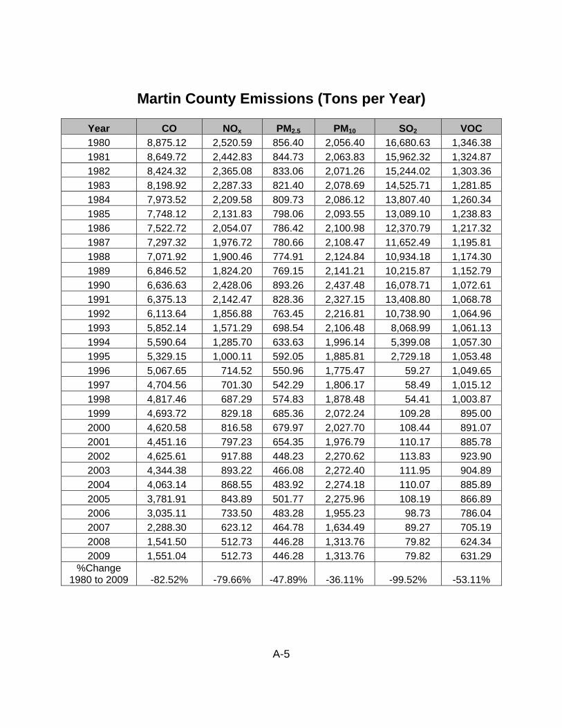
A-5

Martin County Emissions (Tons per Year)


1980 8,875.12 2,520.59 856.40 2,056.40 16,680.63 1,346.38

1981 8,649.72 2,442.83 844.73 2,063.83 15,962.32 1,324.87

1982 8,424.32 2,365.08 833.06 2,071.26 15,244.02 1,303.36

1983 8,198.92 2,287.33 821.40 2,078.69 14,525.71 1,281.85

1984 7,973.52 2,209.58 809.73 2,086.12 13,807.40 1,260.34

1985 7,748.12 2,131.83 798.06 2,093.55 13,089.10 1,238.83

1986 7,522.72 2,054.07 786.42 2,100.98 12,370.79 1,217.32

1987 7,297.32 1,976.72 780.66 2,108.47 11,652.49 1,195.81

1988 7,071.92 1,900.46 774.91 2,124.84 10,934.18 1,174.30

1989 6,846.52 1,824.20 769.15 2,141.21 10,215.87 1,152.79

1990 6,636.63 2,428.06 893.26 2,437.48 16,078.71 1,072.61

1991 6,375.13 2,142.47 828.36 2,327.15 13,408.80 1,068.78

1992 6,113.64 1,856.88 763.45 2,216.81 10,738.90 1,064.96

1993 5,852.14 1,571.29 698.54 2,106.48 8,068.99 1,061.13

1994 5,590.64 1,285.70 633.63 1,996.14 5,399.08 1,057.30

1995 5,329.15 1,000.11 592.05 1,885.81 2,729.18 1,053.48

1996 5,067.65 714.52 550.96 1,775.47 59.27 1,049.65

1997 4,704.56 701.30 542.29 1,806.17 58.49 1,015.12

1998 4,817.46 687.29 574.83 1,878.48 54.41 1,003.87

1999 4,693.72 829.18 685.36 2,072.24 109.28 895.00

2000 4,620.58 816.58 679.97 2,027.70 108.44 891.07

2001 4,451.16 797.23 654.35 1,976.79 110.17 885.78

2002 4,625.61 917.88 448.23 2,270.62 113.83 923.90

2003 4,344.38 893.22 466.08 2,272.40 111.95 904.89

2004 4,063.14 868.55 483.92 2,274.18 110.07 885.89

2005 3,781.91 843.89 501.77 2,275.96 108.19 866.89

2006 3,035.11 733.50 483.28 1,955.23 98.73 786.04

2007 2,288.30 623.12 464.78 1,634.49 89.27 705.19

2008 1,541.50 512.73 446.28 1,313.76 79.82 624.34

2009 1,551.04 512.73 446.28 1,313.76 79.82 631.29 %Change

1980 to 2009 -82.52% -79.66% -47.89% -36.11% -99.52% -53.11%

A-6

Perry County Emissions (Tons per Year)


1980 22,298.05 3,810.98 1,095.59 3,921.43 951.07 3,109.35

1981 21,715.76 3,764.79 1,069.89 3,840.74 927.09 3,037.98

1982 21,133.46 3,718.60 1,044.20 3,760.06 903.11 2,966.60

1983 20,551.17 3,672.42 1,018.51 3,679.38 879.13 2,895.23

1984 19,968.88 3,626.23 992.82 3,598.70 855.15 2,831.46

1985 19,386.58 3,580.04 967.12 3,518.02 831.17 2,767.95

1986 18,804.29 3,533.86 941.43 3,437.34 810.24 2,704.44

1987 18,222.00 3,487.67 915.74 3,356.65 791.27 2,640.93

1988 17,639.70 3,441.48 890.05 3,275.97 772.31 2,577.42

1989 17,057.41 3,395.30 864.36 3,225.97 753.35 2,513.92

1990 15,495.77 3,052.23 903.42 3,575.74 943.40 2,460.47

1991 15,119.75 3,076.67 852.70 3,341.82 846.39 2,387.99

1992 14,743.72 3,101.10 801.98 3,107.89 749.37 2,315.51

1993 14,367.70 3,125.54 751.26 2,873.96 652.36 2,243.03

1994 13,991.68 3,149.97 700.88 2,640.03 555.35 2,170.54

1995 13,615.65 3,174.40 671.47 2,406.11 458.33 2,098.06

1996 13,239.63 3,198.84 642.67 2,172.18 361.32 2,025.58

1997 12,613.34 3,181.09 627.43 2,193.92 363.40 1,989.19

1998 12,399.47 3,135.54 667.03 2,372.52 365.08 1,847.40

1999 12,961.52 3,171.65 799.40 2,596.26 761.21 2,021.13

2000 12,677.34 3,111.86 796.05 2,541.25 772.13 1,983.45

2001 12,735.23 3,102.41 754.87 2,448.39 788.87 2,017.74

2002 12,597.44 3,328.93 580.22 2,567.75 621.28 2,023.13

2003 11,895.98 3,118.97 587.16 2,588.13 534.92 1,963.16

2004 11,194.52 2,909.01 594.10 2,608.52 448.56 1,903.19

2005 10,493.05 2,699.04 601.05 2,628.90 362.20 1,843.22

2006 8,568.68 2,490.17 587.96 2,245.73 412.04 1,653.14

2007 6,644.30 2,281.29 574.87 1,862.55 461.88 1,463.07

2008 4,719.93 2,072.41 561.78 1,479.38 511.71 1,272.99

2009 4,575.94 2,061.07 540.74 1,423.68 478.16 1,204.31 %Change

1980 to 2009 -79.48% -45.92% -50.64% -63.69% -49.72% -61.27%

A-7

Pike County Emissions (Tons per Year)


1980 14,065.23 40,120.27 1,224.52 2,681.84 170,329.82 1,670.77

1981 13,716.75 39,328.38 1,215.31 2,697.68 165,404.81 1,650.53

1982 13,368.27 38,536.58 1,206.09 2,774.68 160,479.81 1,630.30

1983 13,019.79 37,744.79 1,196.88 2,790.52 155,554.80 1,610.06

1984 12,671.32 36,953.00 1,187.67 3,135.13 150,629.79 1,589.82

1985 12,322.84 36,161.21 1,178.45 3,479.74 145,704.79 1,569.59

1986 11,974.36 35,369.42 1,169.24 3,824.35 140,779.78 1,549.35

1987 11,625.88 34,577.63 1,160.03 4,168.96 135,855.03 1,529.11

1988 11,277.41 33,785.84 1,150.81 4,513.57 130,930.29 1,508.88

1989 10,943.82 32,994.05 1,141.82 4,859.79 126,005.55 1,488.64

1990 9,536.89 31,430.60 2,135.91 5,414.25 138,193.40 1,311.38

1991 9,471.68 30,613.11 2,309.34 5,491.64 128,581.34 1,332.90

1992 9,406.48 29,795.61 2,482.76 5,569.03 118,969.27 1,354.41

1993 9,341.27 28,978.12 2,656.19 5,646.42 109,357.21 1,375.93

1994 9,276.06 28,160.62 2,829.61 5,723.82 99,745.14 1,397.45

1995 9,210.86 27,343.12 3,003.04 5,801.21 90,133.08 1,418.96

1996 9,145.65 26,525.63 3,176.47 5,878.60 80,521.01 1,440.48

1997 8,810.46 24,835.52 3,486.36 6,372.48 62,987.82 1,422.70

1998 8,768.80 28,859.26 3,682.61 6,631.50 68,999.51 1,433.69

1999 8,463.49 25,151.48 3,441.01 6,426.14 67,580.92 1,435.38

2000 8,086.13 28,268.44 3,846.28 6,803.09 65,307.50 1,393.77

2001 7,811.92 28,567.26 3,733.27 6,780.57 63,626.09 1,381.40

2002 6,791.14 25,136.69 2,949.42 6,511.52 65,285.36 1,307.47

2003 6,520.67 23,087.73 2,855.98 6,418.07 61,140.65 1,308.92

2004 6,250.20 21,038.76 2,762.54 6,324.63 56,995.95 1,310.38

2005 5,979.73 18,989.80 2,669.09 6,231.19 52,851.24 1,311.84

2006 4,992.21 17,772.36 2,743.04 5,963.23 47,783.73 1,179.79

2007 4,004.70 16,554.93 2,816.99 5,695.26 42,716.22 1,047.74

2008 3,017.18 15,337.50 2,890.94 5,427.30 37,648.71 915.69

2009 3,016.87 15,308.79 2,864.92 5,352.95 37,653.58 906.15 %Change

1980 to 2009 -78.55% -61.84% 133.96% 99.60% -77.89% -45.76%

A-8

Posey County Emissions (Tons per Year)


1980 38,259.49 18,562.03 2,487.29 12,400.07 26,290.60 7,994.30

1981 37,539.87 18,272.57 2,447.09 12,155.71 25,882.80 7,790.09

1982 36,820.26 17,983.12 2,406.88 11,917.29 25,475.01 7,585.89

1983 36,100.64 17,694.09 2,366.67 11,672.93 25,067.21 7,381.95

1984 35,381.02 17,413.06 2,334.80 11,455.87 24,659.41 7,179.30

1985 34,661.40 17,132.03 2,302.92 11,294.73 24,251.62 6,976.64

1986 33,941.78 16,851.01 2,271.04 11,111.30 23,843.82 6,773.99

1987 33,222.16 16,569.98 2,239.17 10,961.56 23,470.78 6,571.33

1988 32,502.55 16,288.96 2,207.29 10,928.76 23,102.23 6,368.68

1989 31,795.04 16,007.93 2,346.46 10,895.95 22,733.67 6,166.03

1990 20,409.81 14,456.46 2,922.24 13,878.38 20,067.46 5,847.75

1991 22,861.30 14,338.13 2,838.16 12,839.82 20,188.72 5,652.26

1992 25,312.79 14,219.80 2,754.07 11,801.26 20,309.98 5,456.78

1993 27,764.28 14,101.47 2,669.99 10,762.70 20,431.25 5,261.30

1994 30,215.76 13,983.14 2,585.90 9,724.13 20,552.51 5,065.81

1995 32,667.25 13,864.81 2,505.63 8,685.57 20,673.77 4,870.33

1996 35,118.74 13,746.48 2,444.56 7,647.01 20,795.03 4,674.84

1997 35,407.06 14,450.15 2,490.90 7,678.94 25,109.01 4,747.20

1998 35,037.01 13,723.54 2,542.16 8,014.78 24,183.04 4,685.04

1999 26,077.24 15,924.86 2,494.72 7,931.84 22,079.96 4,690.35

2000 25,874.74 14,395.86 2,417.51 7,692.72 17,610.83 4,405.47

2001 25,668.35 14,866.20 2,405.83 7,640.00 18,714.76 4,439.53

2002 24,565.46 14,944.47 1,968.79 9,132.62 14,165.61 3,712.89

2003 22,975.10 13,883.97 1,900.29 8,971.97 15,655.22 3,521.50

2004 21,384.73 12,823.48 1,831.78 8,811.31 17,144.82 3,330.10

2005 19,794.37 11,762.99 1,763.28 8,650.66 18,634.43 3,138.71

2006 17,310.11 10,093.19 1,826.71 8,107.45 16,917.01 2,913.64

2007 14,825.84 8,423.38 1,890.14 7,564.24 15,199.59 2,688.58

2008 12,341.58 6,753.58 1,953.58 7,021.03 13,482.17 2,463.51

2009 10,895.82 5,736.23 1,812.06 6,680.52 11,688.68 2,452.54 %Change

1980 to 2009 -71.52% -69.10% -27.15% -46.13% -55.54% -69.32%

A-9

Spencer County Emissions (Tons per Year)


1980 32,700.29 40,967.77 2,271.06 5,240.03 69,754.28 4,279.36

1981 31,818.34 40,552.25 2,238.31 5,214.98 69,218.96 4,190.42

1982 30,936.38 40,136.72 2,205.55 5,189.94 68,683.63 4,101.48

1983 30,054.42 39,721.20 2,172.80 5,164.89 68,148.31 4,012.84

1984 29,172.46 39,305.68 2,140.04 5,139.85 67,612.98 3,924.32

1985 28,290.50 38,892.51 2,107.29 5,114.80 67,077.65 3,835.79

1986 27,408.54 38,480.96 2,074.53 5,089.76 66,542.33 3,747.27

1987 26,526.58 38,069.42 2,041.78 5,064.71 66,007.00 3,658.75

1988 25,648.62 37,657.87 2,009.02 5,039.67 65,471.68 3,570.23

1989 24,770.69 37,246.32 1,976.27 6,092.97 64,936.35 3,481.71

1990 23,271.35 28,847.60 1,908.59 6,168.52 54,772.84 3,379.53

1991 22,465.21 30,155.76 1,938.69 6,049.61 56,809.08 3,282.16

1992 21,659.08 31,463.92 1,968.78 5,930.69 58,845.32 3,184.79

1993 20,852.95 32,772.08 1,998.88 5,811.77 60,881.57 3,087.43

1994 20,046.81 34,080.24 2,034.02 5,692.85 62,917.81 2,990.06

1995 19,240.68 35,388.40 2,069.33 5,573.93 64,954.05 2,892.69

1996 18,434.54 36,696.56 2,106.37 5,455.02 66,990.29 2,795.32

1997 17,810.13 41,076.11 2,070.76 5,392.06 66,014.42 2,773.88

1998 17,379.86 42,750.27 2,253.81 5,977.17 67,820.73 2,664.36

1999 16,369.83 41,587.38 3,063.29 7,341.95 67,452.10 2,647.91

2000 15,923.85 40,530.56 3,105.04 7,402.47 64,000.44 2,629.89

2001 15,952.17 38,521.22 5,282.08 12,463.97 57,983.55 2,676.06

2002 14,698.23 37,558.82 1,757.73 6,215.47 53,720.62 2,365.90

2003 13,733.80 32,993.44 1,758.93 6,217.74 58,313.17 2,299.11

2004 12,769.36 28,428.06 1,760.14 6,220.00 62,905.72 2,232.32

2005 11,804.93 23,862.68 1,761.35 6,222.27 67,498.27 2,165.53

2006 9,611.49 24,060.20 3,184.30 8,428.17 57,115.59 1,960.52

2007 7,418.04 24,257.71 4,607.25 10,634.06 46,732.91 1,755.51

2008 5,224.60 24,455.23 6,030.21 12,839.96 36,350.23 1,550.50

2009 5,211.73 24,378.28 5,936.83 12,588.04 36,347.53 1,501.88 %Change

1980 to 2009 -84.06% -40.49% 161.41% 140.23% -47.89% -64.90%

A-10

Vanderburgh County Emissions (Tons per Year)


1980 120,641.49 12,380.24 4,737.45 13,426.52 9,517.34 22,468.66

1981 117,409.00 12,160.96 4,688.29 13,317.46 9,187.44 21,922.07

1982 114,176.52 11,941.68 4,639.13 13,208.40 8,857.54 21,375.49

1983 110,944.03 11,722.41 4,589.97 13,099.34 8,527.64 20,828.90

1984 107,711.55 11,503.13 4,540.80 12,990.29 8,197.75 20,282.31

1985 104,479.07 11,283.86 4,491.64 12,881.23 7,867.85 19,735.72

1986 101,246.58 11,064.58 4,442.48 12,772.17 7,537.95 19,189.13

1987 98,014.10 10,845.30 4,393.32 12,663.12 7,208.05 18,642.54

1988 94,781.62 10,626.03 4,344.16 12,554.06 6,878.15 18,095.95

1989 91,549.13 10,406.75 4,295.00 13,102.12 6,548.25 17,549.36

1990 69,247.97 8,239.78 4,272.56 12,628.20 8,844.62 15,038.06

1991 70,962.06 8,471.97 4,251.63 12,303.19 7,760.76 14,982.68

1992 72,676.14 8,704.17 4,230.70 11,978.18 6,676.89 14,927.31

1993 74,390.23 8,936.36 4,209.77 11,653.18 5,593.03 14,871.94

1994 76,104.32 9,168.55 4,189.23 11,328.17 4,509.16 14,816.56

1995 77,818.40 9,400.75 4,194.93 11,003.16 3,425.29 14,761.18

1996 79,532.49 9,632.94 4,201.53 10,678.15 2,341.43 14,705.81

1997 76,534.68 9,740.74 4,019.82 10,087.60 2,379.38 14,646.94

1998 76,372.72 9,701.94 4,438.47 11,703.68 2,396.12 14,183.08

1999 72,410.46 10,119.08 4,013.88 10,130.99 1,399.75 13,791.90

2000 70,111.28 9,930.68 3,916.30 9,997.82 1,392.87 13,545.65

2001 65,917.14 9,537.88 3,720.55 9,563.36 1,421.46 13,426.78

2002 53,880.26 8,504.06 1,991.72 10,532.04 2,141.42 9,660.26

2003 48,433.21 7,922.03 1,983.96 10,522.57 2,057.82 9,196.27

2004 42,986.16 7,339.99 1,976.19 10,513.10 1,974.21 8,732.27

2005 37,539.11 6,757.96 1,968.43 10,503.64 1,890.60 8,268.27

2006 28,856.52 5,705.79 1,941.44 9,509.45 1,869.63 7,472.64

2007 20,173.93 4,653.62 1,914.46 8,515.26 1,848.67 6,677.01

2008 11,491.34 3,601.45 1,887.48 7,521.08 1,827.70 5,881.38

2009 11,482.93 3,590.39 1,807.07 7,423.46 1,797.62 5,918.48 %Change

1980 to 2009 -90.48% -71.00% -61.86% -44.71% -81.11% -73.66%

A-11

Warrick County Emissions (Tons per Year)


1980 46,880.32 54,995.77 5,973.19 7,090.29 212,633.57 5,980.93

1981 46,040.48 53,591.78 5,919.64 7,043.50 207,345.85 5,881.41

1982 45,895.03 52,187.78 5,866.09 6,996.71 202,058.13 5,781.89

1983 45,749.58 50,783.78 5,812.54 6,949.93 196,770.41 5,682.37

1984 45,604.13 49,379.78 5,758.99 6,903.14 191,482.69 5,582.84

1985 45,458.68 47,975.79 5,721.17 6,856.35 186,194.97 5,483.32

1986 45,313.23 46,571.79 5,711.83 6,809.57 180,907.25 5,383.80

1987 45,200.78 45,167.79 5,702.49 6,774.66 175,619.52 5,298.88

1988 45,098.30 43,763.80 5,695.01 6,727.88 170,331.80 5,216.88

1989 44,995.83 42,359.80 5,687.53 12,013.79 165,044.08 5,134.88

1990 29,113.74 39,762.27 5,617.13 12,756.94 176,195.98 4,130.21

1991 33,324.41 38,100.85 6,101.97 12,876.69 163,560.27 4,280.73

1992 37,535.09 36,439.44 6,586.81 12,996.44 150,924.55 4,431.25

1993 41,745.76 34,778.02 7,071.65 13,116.19 138,288.84 4,581.78

1994 45,956.43 33,116.60 7,556.49 13,235.94 125,653.13 4,732.30

1995 50,167.11 31,455.19 8,041.34 13,355.69 113,017.41 4,882.82

1996 54,377.78 29,793.77 8,590.91 13,475.44 100,381.70 5,033.34

1997 54,952.96 35,393.71 8,480.74 13,479.81 126,228.65 5,044.51

1998 54,013.53 35,177.58 9,258.75 14,333.59 123,006.90 4,936.71

1999 51,752.81 31,126.93 10,178.74 15,064.00 135,131.51 5,046.91

2000 51,638.78 30,478.94 8,303.41 13,136.50 107,391.24 4,965.93

2001 52,671.78 28,646.49 8,076.70 12,755.71 102,203.24 5,020.44

2002 47,426.55 28,629.17 8,345.02 16,497.83 109,699.36 4,256.16

2003 45,665.32 25,105.55 8,726.11 17,427.79 103,992.78 4,087.13

2004 43,904.10 21,581.92 9,107.19 18,357.74 98,286.21 3,918.09

2005 42,142.87 18,058.29 9,488.28 19,287.69 92,579.63 3,749.05

2006 37,851.84 15,898.95 7,943.19 16,014.75 79,647.39 3,355.47

2007 33,560.80 13,739.61 6,398.11 12,741.80 66,715.15 2,961.88

2008 29,269.77 11,580.28 4,853.02 9,468.85 53,782.92 2,568.30

2009 28,366.74 11,635.40 4,839.90 8,393.05 53,782.92 2,522.08 %Change

1980 to 2009 -39.49% -78.84% -18.97% 18.37% -74.71% -57.83%

CRITERIA POLLUTANTS - IN.gov

Documents

Transcript of CRITERIA POLLUTANTS - IN.gov