
Multi-objective Optimization of Industrial Ammonia Synthesis
153
Western University Western University Scholarship@Western Scholarship@Western Electronic Thesis and Dissertation Repository 4-10-2017 12:00 AM Multi-objective Optimization of Industrial Ammonia Synthesis Multi-objective Optimization of Industrial Ammonia Synthesis Stanislav Ivanov, The University of Western Ontario Supervisor: Ajay Kumar Ray, The University of Western Ontario A thesis submitted in partial fulfillment of the requirements for the Doctor of Philosophy degree in Chemical and Biochemical Engineering © Stanislav Ivanov 2017 Follow this and additional works at: https://ir.lib.uwo.ca/etd Part of the Catalysis and Reaction Engineering Commons Recommended Citation Recommended Citation Ivanov, Stanislav, "Multi-objective Optimization of Industrial Ammonia Synthesis" (2017). Electronic Thesis and Dissertation Repository. 4489. https://ir.lib.uwo.ca/etd/4489 This Dissertation/Thesis is brought to you for free and open access by Scholarship@Western. It has been accepted for inclusion in Electronic Thesis and Dissertation Repository by an authorized administrator of Scholarship@Western. For more information, please contact [email protected].
-
Upload
khangminh22 -
Category
Documents
-
view
1 -
download
0
Transcript of Multi-objective Optimization of Industrial Ammonia Synthesis

Western University Western University
Scholarship@Western Scholarship@Western
Electronic Thesis and Dissertation Repository
4-10-2017 12:00 AM
Multi-objective Optimization of Industrial Ammonia Synthesis Multi-objective Optimization of Industrial Ammonia Synthesis
Stanislav Ivanov, The University of Western Ontario
Supervisor: Ajay Kumar Ray, The University of Western Ontario
A thesis submitted in partial fulfillment of the requirements for the Doctor of Philosophy degree
in Chemical and Biochemical Engineering
© Stanislav Ivanov 2017
Follow this and additional works at: https://ir.lib.uwo.ca/etd
Part of the Catalysis and Reaction Engineering Commons
Recommended Citation Recommended Citation Ivanov, Stanislav, "Multi-objective Optimization of Industrial Ammonia Synthesis" (2017). Electronic Thesis and Dissertation Repository. 4489. https://ir.lib.uwo.ca/etd/4489
This Dissertation/Thesis is brought to you for free and open access by Scholarship@Western. It has been accepted for inclusion in Electronic Thesis and Dissertation Repository by an authorized administrator of Scholarship@Western. For more information, please contact [email protected].

Abstract
Ammonia is widely used in different applications - as an intermediate product in produc-
tion of agricultural fertilizers, inorganic salts and explosives, or used directly as a solvent
or refrigerant. The broad domain of applications, especially its importance for agricul-
ture, puts ammonia synthesis in the basis of chemical industry. However, the process is
mature and well developed, the improvements to be made towards it are still significant
due to growing demand.
The use of mathematical models in chemical engineering has been extensively applied
towards optimization of industrial process and proven itself to be an efficient technique.
If done properly, it allows for finding best process conditions avoiding timely and costly
experiments.
The objective of this thesis work is to perform optimization study of industrial am-
monia synthesis and discover operational and/or design modifications to be done in order
to improve performance of the process. Two parts of industrial ammonia synthesis have
been considered - the converter carbon dioxide removal from process gas.
Firstly, the mathematical model for simulation of the industrial converter was de-
veloped. In order to fit main model parameters, the large array of industrial data was
studied by means of cluster analysis. It allowed to extract the smaller subset of data to
perform model fitting followed by validation. The simulations showed a good consistency
between model and observed instrumentation reading from the ammonia plant. Further,
few case studies were performed in order to find optimal set of process parameters allow-
ing for improved performance. The main controlling parameters are temperature of feed,
converter pressure, ratio of quenching stream to primary feed and catalyst distribution
of among beds.
Secondly, an optimization of carbon dioxide removal stage from process gas was per-
formed. The aim was to improve solvent recovery and boost carbon dioxide liberation.
Ranking of major process controlling parameters was performed with random forest al-
i

gorithm and Boruta. It allowed to narrow down the number of model parameters from
more than 10 to 4. Further optimization search allowed for finding the best combination
of these parameters to achieve better solvent regeneration.
Keywords: Ammonia synthesis, Modelling, Multi-objective optimization
ii

Co-Authorship statement
The work presented in the current thesis is collaboratively done by the author, Dr. Ajay
Kumar Ray and plant engineers from the company the author and Dr. Ray worked with -
Scott Link, Brian Bloxam and Bratin Ghosh. The personal contribution described below
applies to the content of every chapter presented in the thesis.
The author did a literature review and study of a theoretical background, research
methods and performed data retrieval from the plant. Also, the author developed all
modelling work - incorporated the model equations found in literature, derived missing
equations and developed a code to solve them. Additionally, the author performed simu-
lation and interpretation of obtained optimization results. All chapters are solely written
by the author.
Dr. Ajay Kumar Ray did a supervision of the entire thesis work, consulted on every
step of model development and its applicability towards the existing plant. Also, he
advised on results interpretation and their delivery to the plant engineers.
Material on the optimization methods in chemical engineering was partly published
as book chapter in Catalytic reactor ed. by Basu Saha (2016). Chapters 2,3 will be sub-
mitted a single paper entitled “Modelling and multi-objective optimization of industrial
ammonia converter”. Chapter 5 will be published as “Multi-objective optimization of
industrial ammonia converter under catalyst deactivation”.
iii

”...where was no one who knew for certain what happiness is and what exactly is themeaning of life. And they had accepted as a working hypothesis that happiness lies inthe constant cognition of the unknown, which is also the meaning of life.”
”Monday Begins on Saturday”, Arkady and Boris Strugatsky
iv

Acknowlegements
Dedicated to my entire family, in its widest sense possible.
To my lovely wife:Without your support and patience I would not be able to make it.
To my grandfather:You always believed in me and made me who I am now. You have started this journey
with me but did not see how it’s ended. You are always in my heart. I love you,grandpa!
To my grandmother:Thanks for being fun and supportive, for long-lasting discussions and your endless
wisdom.
To my mom:I am endlessly grateful for your patience, love and for permanently covering my back!
To my dad:Appreciate your advice even when I disagree with you.
To my other mom and dad:I have been honoured to be the part your family all these years. I hope you are not
disappointed with me and will never be.
To my friends:Thanks for always being around, your jokes and a helping hand whenever I needed it.
To Scott Link, Brian Bloxam and Bratin Ghosh:I appreciate all the help, advice and support you gave me during my research project.
To Dr. Ajay Kumar Ray:I will never be able to express how grateful I am to you for giving me a chance to studyat Western and work with you personally. Thank you for giving me freedom of choiceand decision making, forging me into much more independent and responsible thinkerthan I was.
v

Contents
Abstract i
Acknowlegements v
List of Figures ix
List of Tables xi
1 Introduction 11.1 Preface . . . . . . . . . . . . . . . . . . . . . . . . . . . . . . . . . . . . . 31.2 Overview of Industrial Ammonia Synthesis . . . . . . . . . . . . . . . . . 4
1.2.1 Ammonia properties and synthesis reaction . . . . . . . . . . . . . 41.2.2 Ammonia synthesis technology . . . . . . . . . . . . . . . . . . . . 7
1.3 Overview of optimization methods . . . . . . . . . . . . . . . . . . . . . . 91.3.1 Multi-objective optimization . . . . . . . . . . . . . . . . . . . . . 111.3.2 MOO methods . . . . . . . . . . . . . . . . . . . . . . . . . . . . 13
No-preference methods . . . . . . . . . . . . . . . . . . . . . . . . 14A priori methods . . . . . . . . . . . . . . . . . . . . . . . . . . . 14A posteriori methods . . . . . . . . . . . . . . . . . . . . . . . . . 17
1.3.3 Genetic algorithms . . . . . . . . . . . . . . . . . . . . . . . . . . 18About binary-coded variables . . . . . . . . . . . . . . . . . . . . 19Simple Genetic Algorithm . . . . . . . . . . . . . . . . . . . . . . 20Use of GA in MOO . . . . . . . . . . . . . . . . . . . . . . . . . . 21Constraint handling in GA . . . . . . . . . . . . . . . . . . . . . . 23
1.3.4 Simulated annealing . . . . . . . . . . . . . . . . . . . . . . . . . 24
2 Converter modelling 302.1 Introduction . . . . . . . . . . . . . . . . . . . . . . . . . . . . . . . . . . 322.2 Overview of ammonia synthesis . . . . . . . . . . . . . . . . . . . . . . . 342.3 Converter modelling . . . . . . . . . . . . . . . . . . . . . . . . . . . . . 37
2.3.1 Ammonia synthesis reaction . . . . . . . . . . . . . . . . . . . . . 382.3.2 Intraparticle diffusion . . . . . . . . . . . . . . . . . . . . . . . . . 392.3.3 Mass and energy balance of catalyst bed . . . . . . . . . . . . . . 402.3.4 Interchanger model . . . . . . . . . . . . . . . . . . . . . . . . . . 402.3.5 Model overview . . . . . . . . . . . . . . . . . . . . . . . . . . . . 42
2.4 Results and Discussion . . . . . . . . . . . . . . . . . . . . . . . . . . . . 43
vi
2.4.1 Model validation . . . . . . . . . . . . . . . . . . . . . . . . . . . 432.4.2 Sensitivity analysis . . . . . . . . . . . . . . . . . . . . . . . . . . 442.4.3 Effect of process parameters . . . . . . . . . . . . . . . . . . . . . 45
2.5 Summary and conclusion . . . . . . . . . . . . . . . . . . . . . . . . . . . 48
3 Multi-objective optimization 533.1 Introduction . . . . . . . . . . . . . . . . . . . . . . . . . . . . . . . . . . 553.2 Ammonia synthesis and model summary . . . . . . . . . . . . . . . . . . 583.3 Multi-objective optimization of converter operation . . . . . . . . . . . . 613.4 Multi-objective optimization of converter design . . . . . . . . . . . . . . 643.5 Results and discussion . . . . . . . . . . . . . . . . . . . . . . . . . . . . 653.6 Conclusions . . . . . . . . . . . . . . . . . . . . . . . . . . . . . . . . . . 68
4 Carbon dioxide removal 764.1 Introduction . . . . . . . . . . . . . . . . . . . . . . . . . . . . . . . . . . 774.2 Process description . . . . . . . . . . . . . . . . . . . . . . . . . . . . . . 804.3 Process modelling . . . . . . . . . . . . . . . . . . . . . . . . . . . . . . . 814.4 About clustering . . . . . . . . . . . . . . . . . . . . . . . . . . . . . . . 844.5 Model training and validation . . . . . . . . . . . . . . . . . . . . . . . . 854.6 Variable selection and ranking . . . . . . . . . . . . . . . . . . . . . . . . 874.7 Results and discussion . . . . . . . . . . . . . . . . . . . . . . . . . . . . 894.8 Model validation . . . . . . . . . . . . . . . . . . . . . . . . . . . . . . . 894.9 Operation optimization . . . . . . . . . . . . . . . . . . . . . . . . . . . . 924.10 Conclusions . . . . . . . . . . . . . . . . . . . . . . . . . . . . . . . . . . 94
5 MOO with catalyst deactivation 1005.1 Introduction . . . . . . . . . . . . . . . . . . . . . . . . . . . . . . . . . . 1015.2 Overview of converter model . . . . . . . . . . . . . . . . . . . . . . . . . 102
5.2.1 Reaction kinetics . . . . . . . . . . . . . . . . . . . . . . . . . . . 1045.2.2 Intraparticle dissuion . . . . . . . . . . . . . . . . . . . . . . . . . 1045.2.3 Mass and energy balance . . . . . . . . . . . . . . . . . . . . . . . 105
5.3 Industrial data analysis . . . . . . . . . . . . . . . . . . . . . . . . . . . . 1055.4 Data and methods . . . . . . . . . . . . . . . . . . . . . . . . . . . . . . 1105.5 Results and discussion . . . . . . . . . . . . . . . . . . . . . . . . . . . . 111
5.5.1 Data cleaning . . . . . . . . . . . . . . . . . . . . . . . . . . . . . 1115.5.2 Model fitting and validation . . . . . . . . . . . . . . . . . . . . . 114
5.6 Multi-objective optimization . . . . . . . . . . . . . . . . . . . . . . . . . 1185.6.1 MOO results . . . . . . . . . . . . . . . . . . . . . . . . . . . . . 119
5.7 Summary and conclusions . . . . . . . . . . . . . . . . . . . . . . . . . . 122
6 Conclusion 1326.1 Conclusions . . . . . . . . . . . . . . . . . . . . . . . . . . . . . . . . . . 1336.2 Recommendations and future work . . . . . . . . . . . . . . . . . . . . . 135
A Heat transfer model for interchanger 136
vii

6.1 Curriculum Vitae . . . . . . . . . . . . . . . . . . . . . . . . . . . . . . . 139
viii

List of Figures
1.1 Applications of ammonia1 . . . . . . . . . . . . . . . . . . . . . . . . . . 31.2 Ammonia molecule configuration . . . . . . . . . . . . . . . . . . . . . . 51.3 Ammonia synthesis loop . . . . . . . . . . . . . . . . . . . . . . . . . . . 81.4 Two principle designs of industrial ammonia converters . . . . . . . . . . 91.5 Overall economic effect of heat insulation . . . . . . . . . . . . . . . . . . 101.6 Parallel reaction scheme . . . . . . . . . . . . . . . . . . . . . . . . . . . 101.7 Effect of temperature on concentration of species in parallel reaction scheme 111.8 Pareto set for two conflicting objectives . . . . . . . . . . . . . . . . . . . 131.9 Mapping continuous variable into binary . . . . . . . . . . . . . . . . . . 191.10 Genetic algorithm operator: crossover . . . . . . . . . . . . . . . . . . . . 201.11 Genetic algorithm . . . . . . . . . . . . . . . . . . . . . . . . . . . . . . . 21
2.1 Ammonia synthesis loop . . . . . . . . . . . . . . . . . . . . . . . . . . . 352.2 Schematic representation of a catalytic bed in ammonia converter . . . . 352.3 Internals of the ammonia converter . . . . . . . . . . . . . . . . . . . . . 362.4 Heat transfer along tube wall . . . . . . . . . . . . . . . . . . . . . . . . 412.5 Simulation procedure for the ammonia converter . . . . . . . . . . . . . . 422.6 Comparison between simulated and observed temperatures along reactor 442.7 Effect of process parameters on ammonia production . . . . . . . . . . . 472.8 Effect of process parameters on heat recovery . . . . . . . . . . . . . . . 47
3.1 Ammonia converter schematic . . . . . . . . . . . . . . . . . . . . . . . . 593.2 Comparison between simulated and observed temperatures along reactor 613.3 Response surfaces for process objectives . . . . . . . . . . . . . . . . . . . 633.4 Pareto optimal set of solutions for Case 1 . . . . . . . . . . . . . . . . . . 663.5 Pareto optimal set of solutions for Case 2 . . . . . . . . . . . . . . . . . . 673.6 Comparison of catalyst loading distributions . . . . . . . . . . . . . . . . 68
4.1 Process flow diagram for carbon dioxide removal . . . . . . . . . . . . . . 804.2 Single variable generic case for linear regression of industrial data . . . . 834.3 Example of real industrial data . . . . . . . . . . . . . . . . . . . . . . . 844.4 SOM coding vectors . . . . . . . . . . . . . . . . . . . . . . . . . . . . . 864.5 Variable importance test with Boruta: a) XD−1
H2
, b) XD−1CO2
, c) QtopS−1 . . . . 88
4.6 Cluster size vs. RMSE: a) XD−1H2
, b) XD−1CO2
, c) QtopS−1 . . . . . . . . . . . . 90
4.7 Validation plot: a) XD−1H2
, b) XD−1CO2
, c) QtopS−1 . . . . . . . . . . . . . . . . 91
4.8 Effect of number of variables on RMSE: a) XD−1H2
, b) XD−1CO2
, c) QtopS−1 . . . 92
ix

4.9 Process parameters vs. objectives. a) XD−1CO2
, b) QtopS−1 . . . . . . . . . . . 94
5.1 Ammonia converter schematic . . . . . . . . . . . . . . . . . . . . . . . . 1035.2 Industrial data processing sequence . . . . . . . . . . . . . . . . . . . . . 1075.3 MAD filter . . . . . . . . . . . . . . . . . . . . . . . . . . . . . . . . . . . 1085.4 PCA transformation . . . . . . . . . . . . . . . . . . . . . . . . . . . . . 1095.5 Process data . . . . . . . . . . . . . . . . . . . . . . . . . . . . . . . . . . 1125.6 Effect of Min-max cut off and MAD filter on process data . . . . . . . . . 1135.7 WCCS reduction with number of clusters . . . . . . . . . . . . . . . . . . 1145.8 Effect of clustering on data cleaning . . . . . . . . . . . . . . . . . . . . . 1155.9 Ammonia catalyst deactivation over time . . . . . . . . . . . . . . . . . . 1165.10 Simulated and experimental temperatures within ammonia converter . . 1175.11 Pareto optimal set of solutions for case fresh . . . . . . . . . . . . . . . . 1205.12 Pareto optimal set of solutions for case old . . . . . . . . . . . . . . . . . 1215.13 Comparison for “middle” points in pareto sets . . . . . . . . . . . . . . . 122
A.1 Heat transfer along tube wall . . . . . . . . . . . . . . . . . . . . . . . . 137
x

List of Tables
1.1 Equilibrium fraction (% mol.) of ammonia in stoichiometric mixture H2:N2 5
2.1 Comparison between simulated and experimented gas composition . . . . 442.2 Sensitivity analysis . . . . . . . . . . . . . . . . . . . . . . . . . . . . . . 452.3 Simulation range . . . . . . . . . . . . . . . . . . . . . . . . . . . . . . . 46
3.1 Comparison between simulated and experimented gas composition . . . . 613.2 Single objective maximums . . . . . . . . . . . . . . . . . . . . . . . . . . 64
4.1 Performance criteria of carbon dioxide removal unit used in the modelling 874.2 Performance criteria of carbon dioxide removal unit used in the modelling 874.3 Performance criteria of carbon dioxide removal unit used in the modelling 93
5.1 Comparison between simulated and experimental gas compositions . . . . 117
xi

Chapter 1
Introduction
1
2 Nomenclature
Nomenclature
DM decision maker
g inequality constraint
G goal in goal programming method
GA genetic algorithm
h equality constraint
I objective function
J number of equality constraints
K number of inequality constraints
lstr length of binary string
MOO multi-objective optimization
n number of objectives
R penalty parameter
S decision domain
SA simulated annealing
SGA simple genetic algorithm
SOO single-objective optimization
x decision vector

Greek letters 3
Greek letters
δ deviation
ǫi constraint
Ω penalty term
1.1 Preface
Ammonia is one of major chemicals produced in the industry. It has a variety of appli-
cations: for manufacturing of inorganic salts, polymer fibers, explosives, etc. (Fig. 1.1)
Especially, it is essential chemical in production of agricultural fertilizers: as an interme-
diate in urea synthesis or used directly as liquid. It is hard to diminish the importance of
ammonia for agricultural sector all over the world, and in North America in particular.
Figure 1.1: Applications of ammonia1
Ammonia is produced all over the world. Largest gross producers are Asian countries
and former Soviet Union. Middle East and North America are not far behind. However,

4 Greek letters
not all the regions are self-sustainable supply-wise. North America, even having a large
production, is still net importer of ammonia.
Moreover, ammonia market is continuously growing. Total world ammonia demand
has been steadily increasing over last decade at rate of 2.2 % per annum.2 In order to
satisfy for the demand of an already deficit market it is imperative to go both ways
simultaneously - build new facilities as well as intensify production at existing ones.
We put planning, design and development of new production facilities outside of the
scope of this work, while focusing on enhancements in ammonia synthesis. As with any
chemical engineering process, there is a vast number of ways to improve performance of
an industrial process. Regardless of the objectives for improvement, this may be done
through, among others, physical modelling, data analysis and data-based modelling, first-
principle mathematical modelling and numerical optimization.
One can not neglect the power of process modelling and numerical optimization for
chemical engineering processes. Developing robust models allows for accurate process
simulation. Therefore, one can perform a comprehensive study of a process without
expensive physical modelling and/or use the model for the numerical optimization to
boost up process performance.
Moreover, since major chemical engineering plants introduced digital process control
for continuous operation a large amount of data has become available. It is wise to take
advantage of the fact to assist for development of more accurate and relevant models or
improve existing ones.
1.2 Overview of Industrial Ammonia Synthesis
1.2.1 Ammonia properties and synthesis reaction
Ammonia is a chemical compound formed by one nitrogen and three hydrogen atoms.
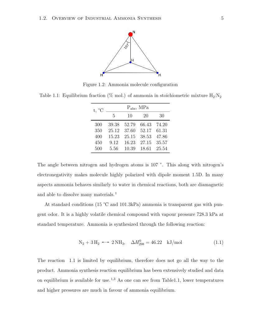
Geometrically, ammonia molecule is a tetrahedron with atoms in its apices (Fig. 1.2).
1.2. Overview of Industrial Ammonia Synthesis 5
Figure 1.2: Ammonia molecule configuration
Table 1.1: Equilibrium fraction (% mol.) of ammonia in stoichiometric mixture H2:N2
t, °CPabs, MPa
5 10 20 30
300 39.38 52.79 66.43 74.20350 25.12 37.60 52.17 61.31400 15.23 25.15 38.53 47.86450 9.12 16.23 27.15 35.57500 5.56 10.39 18.61 25.54
The angle between nitrogen and hydrogen atoms is 107 °. This along with nitrogen’s
electronegativity makes molecule highly polarized with dipole moment 1.5D. In many
aspects ammonia behaves similarly to water in chemical reactions, both are diamagnetic
and able to dissolve many materials.1
At standard conditions (15 °C and 101.3kPa) ammonia is transparent gas with pun-
gent odor. It is a highly volatile chemical compound with vapour pressure 728.3 kPa at
standard temperature. Ammonia is synthesized through the following reaction:
N2 + 3H2 2NH3, ∆H0298 = 46.22 kJ/mol (1.1)
The reaction 1.1 is limited by equilibrium, therefore does not go all the way to the
product. Ammonia synthesis reaction equilibrium has been extensively studied and data
on equilibrium is available for use.1,3 As one can see from Table1.1, lower temperatures
and higher pressures are much in favour of ammonia equilibrium.

6 Greek letters
However, the reaction is kinetically slow. Therefore, elevated temperatures are nec-
essary to provide significant yield and make synthesis process somehow efficient. So
equilibrium-wise, Eq.1.1 is carried out in such conditions that compromise between high
thermodynamic equilibrium ammonia concentration and fast reaction rate. Also, the
reaction’s exothermicity plays a role as liberated heat slows it down at any process con-
ditions.
Even though, the reaction is exothermic and supposed to react spontaneously, it
does not happening due to high energy input required to overcome activation barrier.
One of major reason is that nitrogen as a molecule is highly inert and does not easily
involved into chemical interactions. Energy of its dissociation is around 941 kJ/mol. The
activation energy itself for homogeneous reaction of nitrogen and hydrogen is reported
in the range 230-420 kJ/mol. In order to overcome this barrier the temperatures of
650-1000 °C are necessary.1 However at this conditions, yield of ammonia is low due to
reaction equilibrium. Therefore, in order to make process feasible at reasonable industrial
condition the presence of catalyst is necessary to reduce energy barrier of reaction4.
Activation energy of ammonia synthesis over heterogeneous catalysts is fairly lower -
around 100-160 kJ/mol. This drastically reduces reaction temperature down to 250-400
°C. Historically, the synthesis catalysts used for industrial scale production have predomi-
nantly been iron-based with promoters from non-reducible oxides (i.e. CaO,Al2O3,MgO,SiO2).
Iron is used in forms of Fe(II)-Fe(III) oxides mixtures in about even ratio. Later genera-
tions of catalysts have been based on ruthenium as an active metal. Ru-based catalysts
appeared to be more active and able to reduce process temperature and pressure even
further. However, majority of ammonia plants nowadays are still utilizing Fe-based cat-
alysts.
Ammonia synthesis is a mature process and extends back over decades, but theres
still no consensus about reaction mechanism on the surface of catalyst. There have been
many studies conducted to investigate mechanism of reaction 1.1 on heterogeneous solid
1.2. Overview of Industrial Ammonia Synthesis 7
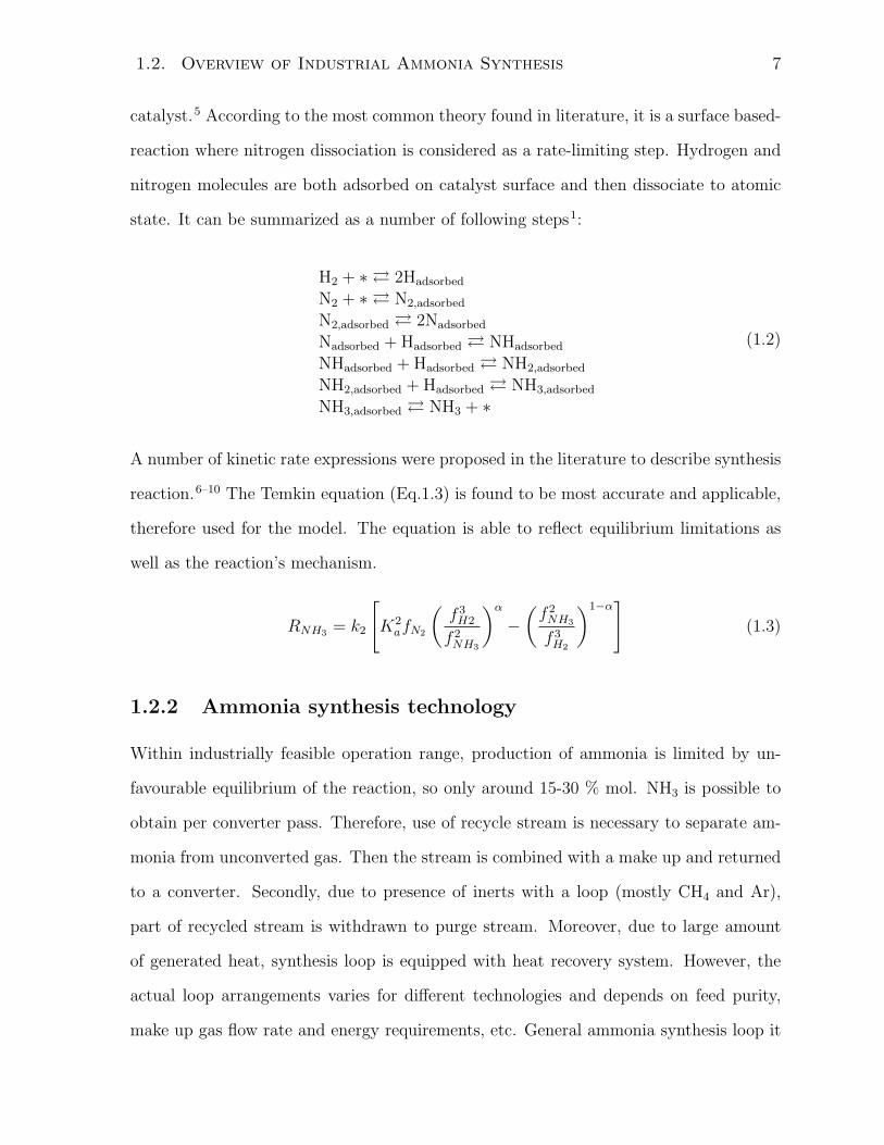
catalyst.5 According to the most common theory found in literature, it is a surface based-
reaction where nitrogen dissociation is considered as a rate-limiting step. Hydrogen and
nitrogen molecules are both adsorbed on catalyst surface and then dissociate to atomic
state. It can be summarized as a number of following steps1:
H2 + ∗ 2Hadsorbed
N2 + ∗ N2,adsorbed
N2,adsorbed 2Nadsorbed
Nadsorbed +Hadsorbed NHadsorbed
NHadsorbed +Hadsorbed NH2,adsorbed
NH2,adsorbed +Hadsorbed NH3,adsorbed
NH3,adsorbed NH3 + ∗
(1.2)
A number of kinetic rate expressions were proposed in the literature to describe synthesis
reaction.6–10 The Temkin equation (Eq.1.3) is found to be most accurate and applicable,
therefore used for the model. The equation is able to reflect equilibrium limitations as
well as the reaction’s mechanism.
RNH3= k2
[
K2afN2
(
f 3H2
f 2NH3
)α
−
(
f 2NH3
f 3H2
)1−α]
(1.3)
1.2.2 Ammonia synthesis technology
Within industrially feasible operation range, production of ammonia is limited by un-
favourable equilibrium of the reaction, so only around 15-30 % mol. NH3 is possible to
obtain per converter pass. Therefore, use of recycle stream is necessary to separate am-
monia from unconverted gas. Then the stream is combined with a make up and returned
to a converter. Secondly, due to presence of inerts with a loop (mostly CH4 and Ar),
part of recycled stream is withdrawn to purge stream. Moreover, due to large amount
of generated heat, synthesis loop is equipped with heat recovery system. However, the
actual loop arrangements varies for different technologies and depends on feed purity,
make up gas flow rate and energy requirements, etc. General ammonia synthesis loop it

8 Greek letters
Figure 1.3: Ammonia synthesis loopA: make up gas compressor, B: ammonia synthesis converter with heat recovery network, C:
ammonia separation and refrigeration.
arranged as shown on Fig.1.3.1
Converter is a heart of the system, as it mainly defines operating conditions and
provides yield of ammonia. Converter-wise, a number of different designs have been
developed. They can be divided into two groups - with internal bed cooling (Fig. 1.4(a))
and adiabatic bed (Fig. 1.4(b)) converters with external heat exchange.1 In former, a cold
medium - usually make up gas - is running through the tubes to remove excess heat from
the bed as well as to pre-heat feed and bring it up to the reaction temperature. Converters
of these design have been widely used decades ago and more suitable for smaller scale
production. Converters with multiple adiabatic beds are more wide spread in industry.
Mainly, they can be divided into two groups based on method of heat removal. First is
quench cooling, where hot gas effluent from each bed is cooled down by direct injection
of colder stream. Second, indirect cooling of hot stream in separate waste heat boilers in
order to generate steam needed for operation at ammonia plant or in heat exchanger to
preheat converter feed. They are usually comprised of 2-4 beds and utilize axial or radial
flow pattern. Beds with axial flow are more widely found, but on a number of modern
plants converters have been redesigned into radial gas flow. It allows to reduce pressure
drop across a bed and increase converter throughput within the same unit geometry.11

1.3. Overview of optimization methods 9
(a) Internal bed cooling (b) Adiabatic bed
Figure 1.4: Two principle designs of industrial ammonia converters
1.3 Overview of optimization methods
Optimization in engineering is aimed for the search of the “best” solution for a specific
problem. Criteria to determine whether the solution is the “best” or not are varied widely
and defined by an engineer (researcher) based on their experience, problems objectives,
common sense, etc. For example, while optimizing performance of synthesis reactor its
often desired to maximize possible yield of final product; or in the case of equipment
design, it is common to reduce the total cost while keeping units performance at the
desired level.
Engineering optimization can be classified by the number of objectives into single ob-
jective optimization (SOO) and multi-objective optimization (MOO). SOO approach has
longer history. Essentially, it is based on formulation of unified function which represents
the overall effect. Most of objective functions in SOO are related to economic efficiency
of the process or unit. A classical example is optimization of insulation thickness. In-
sulation saves money through reduced heat losses but insulation can be highly costly at
the same time. One has to compare total cost of insulation with savings from energy
losses to find optimal thickness; the ratio between these two factors can be an objective

10 Greek letters
Insulation thickness
Overall c
ost
cost from heat loss
insulation cost
overall cost
Figure 1.5: Overall economic effect of heat insulation
A
B
C
k1
k2
Figure 1.6: Parallel reaction scheme
function to be minimized (Fig. 1.5 ). It can be said that SOO methods are mainly aimed
for search of an extreme point (minimum or maximum) in a search space.
However it is not always possible to formulate single objective for a particular problem
which can adequately represent a meaningful optimal solution. MOO methods arise to
overcome this drawback. One can deal with more than one objective and these objectives
are not necessarily economic-related parameters. For example, consider a very common
reaction engineering problem simultaneous yield maximization of goal (desired) product
and minimization of undesirable side product. Such case is quite common for oil refining,
petrochemical and polymer industry, organic synthesis, etc. Consider a simple parallel
reaction, where we are targeting species B (desired) while species C is a side product
(undesired) (Fig. 1.6):
Operating conditions might have similar effect on yield of both products, e.g. in-
crease in process temperature increase percentage of both, desired and side, products in
outflow. Plotting this trend (concentration vs. temperature) (see Fig. 1.7), it is possible
to visualize conflictive nature of our objectives, that is one cannot increase concentration
of B (desired) and decrease concentration of C (undesired) simultaneously. If we apply

1.3. Overview of optimization methods 11
temperature
co
ncen
trati
on
B
C
Figure 1.7: Effect of temperature on concentration of species in parallel reaction scheme
a classical single-objective approach, we would probably formulate objective function in
some way relating price of production to concentrations of species. But, this type of
objective function (cost minimization or profit maximization) usually is time- and/or
site- specific. The cost of raw material or revenue generated from selling a product is site
dependent (price varies from one region to another around the globe) and time dependent
(price varies from year to year).
Application of MOOmethods allows for solving such problem wherein one can directly
treat product concentrations as objectives instead of single objective function expressed
in terms of economic effect (cost minimization or profit maximization). This is why
multi-objective approach is superior to classical Single objective approach.
Below, we will briefly consider the general ideas and concepts in use for MOO, de-
scribe methods, especially more recent and state-of art ones and make a review of their
applications in chemical reactor engineering.
1.3.1 Multi-objective optimization
Concept of Multi-objective optimization
Multi-objective optimization (MOO) concept originates from economics and was de-
veloped by Italian economist, engineer and philosopher Vilfredo Pareto. At first let us
consider the definition of multi-objective optimization of minimization problem (here

12 Greek letters
and throughout the chapter we will discuss minimization MOO problems, since any
maximization problem can be converted into minimization one easily):
minimizex∈S
I(x) = [I1(x), I2(x), ..., In(x)]
subject to
gk(x) ≤ 0, i = 1, 2...K
hj(x) = 0, j = 1, 2...J
(1.4)
General solution for such optimization problem is set of points, not a single one unlike
in SOO problem. However, in some special cases, single point solution is also possible,
this is a trivial case and is not considered. The set of points is called Pareto set (front
or distribution).
Definition of Pareto Optimal Point: A point x is called Pareto optimal point if and
only if there does not exist such point x∗ in a search space that Ii(x*) is better than
Ii(x) for all objectives simultaneously. By better it is necessary to assume mathematical
operators or depending on particular problem formulation.
Pareto set can be presented in terms of decision variables (set of x) or objectives (set of
I (x)). For better understanding lets illustrate Pareto concept on two objective function
problem. (Fig. 1.8) If the problem requires simultaneous maximization of both objectives
A and B, Fig. 1.8 describes Pareto set obtained with respect to decision variable limits
and equality and inequality constraints. If we move from point 1 to point 2, objective A
is increasing (desired) while objective B is decreasing (undesired). It is said that these
two points like any other points on the curve are non-inferior (non-superior or equally
good) to each other. If we move from point 3 in the direction of Pareto, one can see that
both objectives A and B are improving, thus point 3 is not a Pareto point.

1.3. Overview of optimization methods 13
Objective AO
bje
cti
ve B
1
2
3
Pareto front
Figure 1.8: Pareto set for two conflicting objectives
1.3.2 MOO methods
Once solution for MOO problem in the form of Pareto set is defined, let turn one’s
attention to methods utilized for its search. There are number of different techniques;
later the accepted classification will be provided for better understanding.12–14 The clas-
sification is based on decision makers (DM) role in optimization search. Here DM is a
person familiar with formulated problem; he/she can impact on preference of objectives
or solutions. Therefore, methods are divided into:
• no-preference
• a priori
• a posteriori
• interactive
The first group excludes any influence of DM on search of Pareto points while next
two take it into account. The latter case is a group of currently developing methods
where DM is directly involved in optimization search and able to alter preferences until
the best solution is found. Just note here as a remark that the classification is not strict
because the same methods can be referred to by more than one group, this will be shown
later. From here we provide further a concise review of introduced methods.

14 Greek letters
No-preference methods
If preferences are hard or impossible to define by DM, no-preference methods can be ap-
plied. They allow finding average solution regardless of any preference; no extra knowl-
edge has to be provided by DM to solve such MOO problem.
Neutral compromised solution
Neutral compromised solution method allows finding optimal solution somewhere in
the middle of Pareto set. To apply this technique it is required to define the norm
in objective domain, which will be a measure of distance for middle solution, select
a reference point from which the distance shall be minimized.15 However we can say
that DM expresses preferences by choosing the norm and reference point, but he/she
is not doing it in explicit way. For MOO problems it is necessary for all objectives to
be of the same dimension or dimensionless. The commonly used norms are p-norm,
Chebyshev norm or augmented Chebyshev norm. The following problems are to be
minimized respectively:
minimizex∈S
[
n∑
i=1
|Ii,up − Ii|p
|Ii,up − Ii,low|p
]1/p
, 1 < p < inf
minimizex∈S
max1≤i≤n|Ii,up − Ii|
|Ii,up − Ii,low|
minimizex∈S
max1≤i≤n|Ii,up − Ii|
|Ii,up − Ii,low|+ ǫ
n∑
i=1
|Ii,up − Ii|
|Ii,up − Ii,low|
(1.5)
Also, the Method of global criterion is one of such methods but will be considered in
section of a priori methods below with some remarks.
A priori methods
A priori methods require DM to state his preference in MOO problem. This has to be
done prior to determining the Pareto set. One can specify the priority of objectives (or
aims) to be achieved. Since a DM is a person familiar with particular problem sometimes
1.3. Overview of optimization methods 15
it becomes possible to single out more important objectives or put them in preference
order.
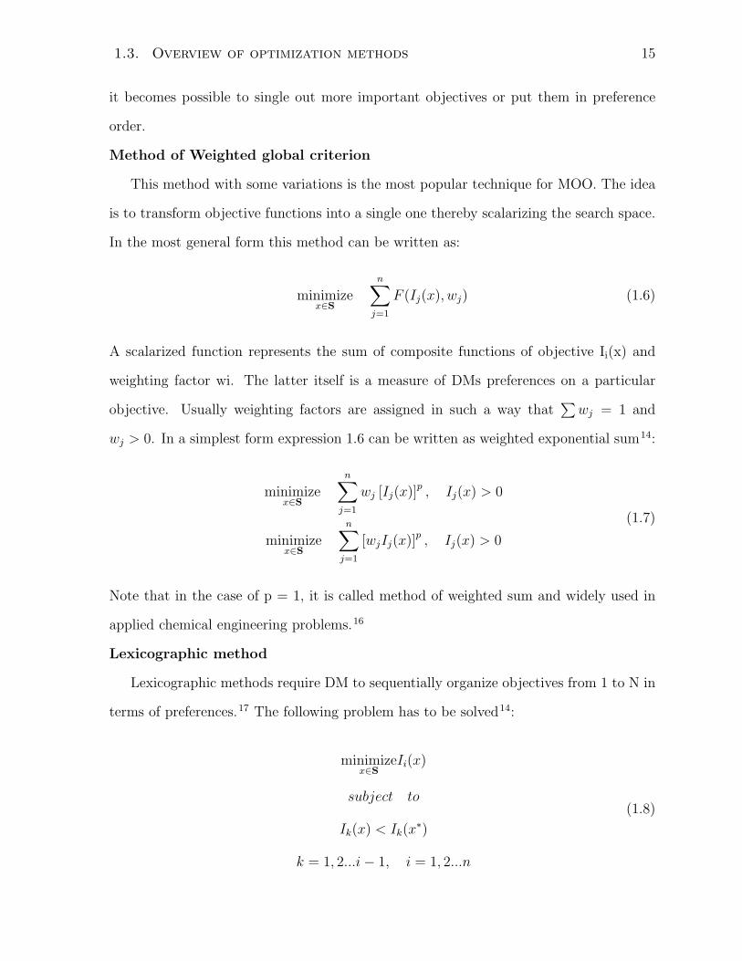
Method of Weighted global criterion
This method with some variations is the most popular technique for MOO. The idea
is to transform objective functions into a single one thereby scalarizing the search space.
In the most general form this method can be written as:
minimizex∈S
n∑
j=1
F (Ij(x), wj) (1.6)
A scalarized function represents the sum of composite functions of objective Ii(x) and
weighting factor wi. The latter itself is a measure of DMs preferences on a particular
objective. Usually weighting factors are assigned in such a way that∑
wj = 1 and
wj > 0. In a simplest form expression 1.6 can be written as weighted exponential sum14:
minimizex∈S
n∑
j=1
wj [Ij(x)]p , Ij(x) > 0
minimizex∈S
n∑
j=1
[wjIj(x)]p , Ij(x) > 0
(1.7)
Note that in the case of p = 1, it is called method of weighted sum and widely used in
applied chemical engineering problems.16
Lexicographic method
Lexicographic methods require DM to sequentially organize objectives from 1 to N in
terms of preferences.17 The following problem has to be solved14:
minimizex∈S
Ii(x)
subject to
Ik(x) < Ik(x∗)
k = 1, 2...i− 1, i = 1, 2...n
(1.8)

16 Greek letters
where k is a function order in preference list, Ik(x∗k) is constraints limit received at kth
step. First objective in the list should be minimized with the original constraints. If the
DM obtains single solution one can accept it as an optimum. If not, the new constraint
Ik(x∗k) has to be accepted to keep the kth objectives optimal values. The procedure
continues with next objective function (e.g. second function in a list, third function in a
list, etc.), until the optimum is reached.
In reality it is often difficult for DM to distinctly organize objectives in order of im-
portance on account of MOO problem complexity. Another drawback with this technique
is that in unique solution is often found before the best optimal solution is reached. It
means that some of objectives are not taken into consideration at all.13
Goal programming
This method was developed by Charnes and Cooper.18 The DM defines a set of
goals G which should be achieved for each objective, Ii(x). Even if all these goals are
unattainable simultaneously, it is still desired to approximate as close as possible. It is
proposed to minimize the distance between vectors I(x) and G. Weighted GP problem
formulation is written as:
minimizex∈S
n∑
i=1
wiδi
δi = Ii(x)− gi, i = 1, 2...n
(1.9)
The formulation of goal programming problem doesnt necessary require the solution to
be Pareto optimal. The solution obtained can be referred to (a) efficient, (b) inefficient
or (c) unbounded solution. Efficient solution belongs to Pareto front while inefficient
solution can be improved for two or more objectives simultaneously. The latter case is a
solution located too far from Pareto front.19
Setting goals to attain is clear approach for DM (unlike, for example, use of utopia
point in global criterion method). However, the further procedure for optimum search is
not necessarily easy, e.g., weights assignment can be more difficult. Some GP methods
are combined with lexicographic method, where deviations are structured in preference

1.3. Overview of optimization methods 17
order and then minimized. The DM has to be aware of all drawbacks of GP methods
and choose proper technique for finding optimal solution.
A posteriori methods
In contrast to other methods discussed so far, a posteriori method generates Pareto set
first, when the DM is given the opportunity to choose acceptable ones. It is reasonable if
the DM is unsure about his/her preferences or problem definition is vague about relative
importance of objectives.
ǫ-Constraint Method
The ǫ-constraint method is a non-scalarizing approach. Original idea was reported
by Yacov Haimes.20 The more comprehensive explanation is provided at Chankong and
Haimes.21 It is proposed to solve the following n-objective problem 1.4 to define Pareto
set:
minimizex∈S
Ii(x)
subject to :
Im(x) ≤ ǫm, i = 1, 2...n m 6= i
gk(x) ≤ 0, i = 1, 2...K
hj(x) = 0, j = 1, 2...J
(1.10)
Note that any of the objective functions can be chosen to be minimized. Varying ǫm the
Pareto set can be reached. It is reported by authors that current method can deal with
non-convex problems. However, drawbacks still exist. The choice of ǫm is not easy for
DM as well as the technique significantly increases computation time if total number of
equations (objectives and constraints) is relatively high.
Interactive methods
As it follows from the name interactive methods require some sort of interaction be-
tween the DM and MOO algorithm. Initially, no a priori information is required, and
the DM specifies some objective-related preference information during a search process.

18 Greek letters
Solutions in interactive methods move iteratively providing the DM with some new so-
lution(s) and allowing re-specifying his/her preferences, if needed. Interactive methods
outcome is one or more Pareto optimal solutions, but not the entire Pareto set. Generally,
many other variations exist, which are kind of extension of classical methods described
here with the way how DM should interact with algorithm. There is variety of such meth-
ods and we will not discuss it here providing only references on some original sources and
reviews.
• Interactive Surrogate Worth Trade-off (ISWT)21
• Reference point methods22
• Non-differentiable Interactive Multi-objective Bundle-based Optimization System
(NIMBUS)23
• Step method (STEM)24
1.3.3 Genetic algorithms
Genetic algorithms (GAs) are currently one of the most developing groups of methods
in MOO. They are based on the mechanics of natural selection and natural genetics.25
Here we would like to emphasize the power of GA and discuss it in more details. While
genetic algorithms belong to a posteriori methods; we discuss GA in an individual sub
chapter on account of its fundamental difference from methods discussed above.
Original idea was proposed by Holland26 as an adaptation concept. Thereafter, Gold-
berg evolved this theory and formulated general regulations of GAs.25 GAs has been de-
veloped intensively in recent years, but the main principles remain the same. As indicated
by Goldberg, main distinctions from classical methods are:
• GA works with number of points (population) instead of a single one
1.3. Overview of optimization methods 19
0000 1111- 0001 - 0010 - ............................-
Xmin Xmax
2 = 164
π
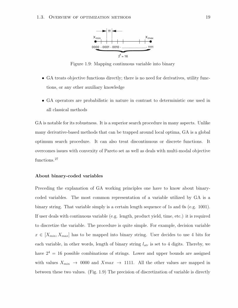
Figure 1.9: Mapping continuous variable into binary
• GA treats objective functions directly; there is no need for derivatives, utility func-
tions, or any other auxiliary knowledge
• GA operators are probabilistic in nature in contrast to deterministic one used in
all classical methods
GA is notable for its robustness. It is a superior search procedure in many aspects. Unlike
many derivative-based methods that can be trapped around local optima, GA is a global
optimum search procedure. It can also treat discontinuous or discrete functions. It
overcomes issues with convexity of Pareto set as well as deals with multi-modal objective
functions.27
About binary-coded variables
Preceding the explanation of GA working principles one have to know about binary-
coded variables. The most common representation of a variable utilized by GA is a
binary string. That variable simply is a certain length sequence of 1s and 0s (e.g. 1001).
If user deals with continuous variable (e.g. length, product yield, time, etc.) it is required
to discretize the variable. The procedure is quite simple. For example, decision variable
x ∈ [Xmin, Xmax] has to be mapped into binary string. User decides to use 4 bits for
each variable, in other words, length of binary string lstr is set to 4 digits. Thereby, we
have 24 = 16 possible combinations of strings. Lower and upper bounds are assigned
with values Xmin → 0000 and Xmax → 1111. All the other values are mapped in
between these two values. (Fig. 1.9) The precision of discretization of variable is directly
20 Greek letters
1 1 1 1
0 0 0 0
1 1 0 0
0 0 1 1
parents daughters
crossover
point
Figure 1.10: Genetic algorithm operator: crossover
dependent on the string length; more the length is, more binary variables can be mapped
between lower and upper limit. Precision may be calculated as25:
π =xmax − xmin
2lstr − 1(1.11)
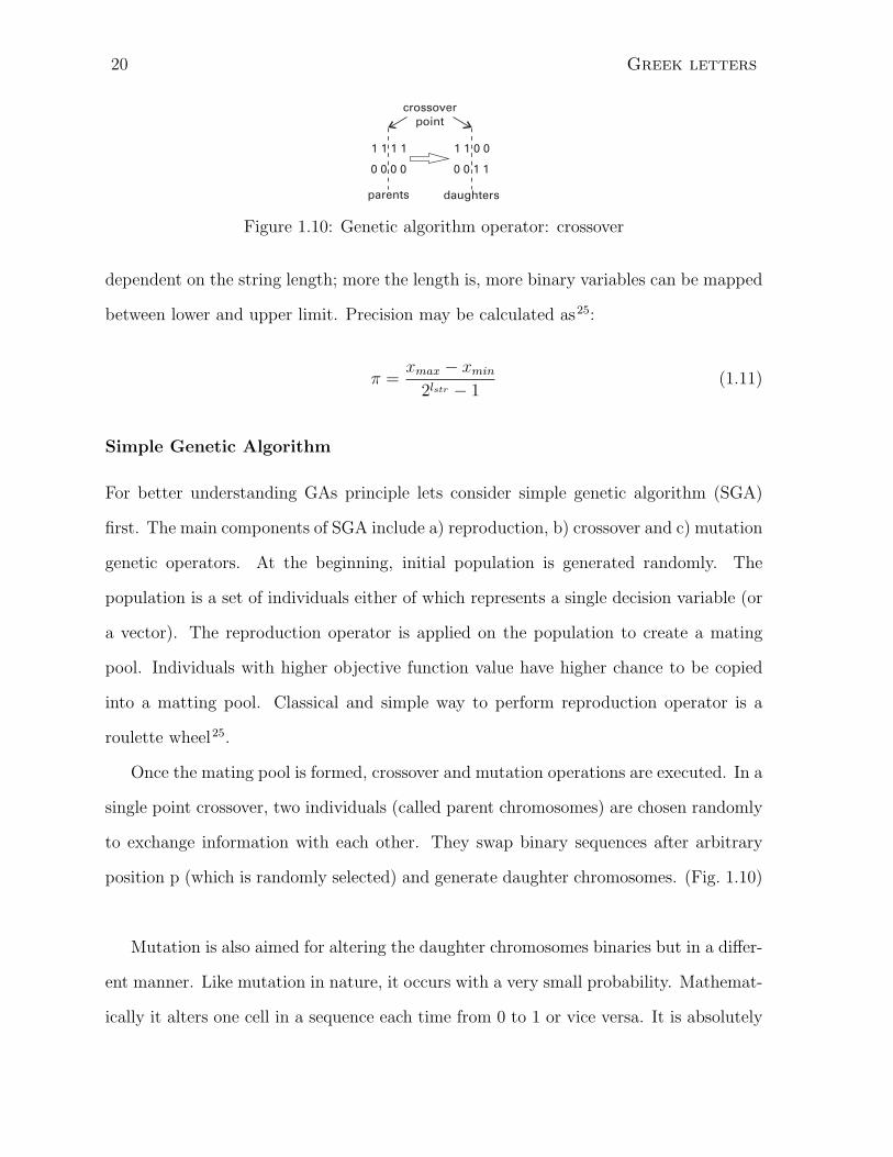
Simple Genetic Algorithm
For better understanding GAs principle lets consider simple genetic algorithm (SGA)
first. The main components of SGA include a) reproduction, b) crossover and c) mutation
genetic operators. At the beginning, initial population is generated randomly. The
population is a set of individuals either of which represents a single decision variable (or
a vector). The reproduction operator is applied on the population to create a mating
pool. Individuals with higher objective function value have higher chance to be copied
into a matting pool. Classical and simple way to perform reproduction operator is a
roulette wheel25.
Once the mating pool is formed, crossover and mutation operations are executed. In a
single point crossover, two individuals (called parent chromosomes) are chosen randomly
to exchange information with each other. They swap binary sequences after arbitrary
position p (which is randomly selected) and generate daughter chromosomes. (Fig. 1.10)
Mutation is also aimed for altering the daughter chromosomes binaries but in a differ-
ent manner. Like mutation in nature, it occurs with a very small probability. Mathemat-
ically it alters one cell in a sequence each time from 0 to 1 or vice versa. It is absolutely

1.3. Overview of optimization methods 21
0001
00100101
0111
1110
Crossover
10 10
00 00
10 00
00 10
Mutation
Selection of the
“best” individuals1 010 0 010
with probability Pcros with probability Pmut
Population of N individuals
Random generation
Pareto optimal
front
Termination?
Evaluation
of objectives
and selection
Yes
No
Figure 1.11: Genetic algorithm
necessary to keep diversity in population.28 For example, lets assume a case where all
individuals in population have 0 at kth position, under this conditions crossover operator
cannot create 1 there. Mutation allows overcoming this issue.
The best n daughter individuals are taken to form a new mating pool where crossover
and mutation are carried out again. This procedure repeats until termination criterion
is satisfied. Below we provide generalized scheme of SGA. (Fig. 1.11)
Use of GA in MOO
If one have SOO problem, it is easy to choose best solutions from the population by
comparing single objective values of individuals. When one deals with multiple objectives,
it becomes not clear how to compare them. To deal with this Goldberg introduces the
concept of non-dominated vectors.25 Vector a is said to be less than vector b if and only
if these two conditions are satisfied simultaneously:
• all components of a are less or equal to corresponding components of b
• at least one component of a is strictly less than corresponding element of b
or in other words (for a minimization MOO problem) - a dominates a . If for the vector
a theres no such vector c that dominates it, vector a is called non-dominated. From this
point of view a Pareto set is a non-dominated set.

22 Greek letters
I would like to emphasize one of the state-of-the-art algorithms non-dominated sorting
genetic algorithm II (NSGA-II). Reader can note that this algorithm was used in majority
of MOO problems solved in literature (Tab. 1). After development by Deb29, it has been
widely propagated in optimization problems for chemical engineering as well as for many
other fields. NSGA-II is notable for its characteristics, especially ability to find diverse
solutions close to real Pareto set and speed of convergence29. Here are elements which
contribute to its high performance.
1. This algorithm uses concept of elitism. After mating pool formation, N parents
and N daughters chromosomes are united into a single group of 2N. Selection is
carried out over this pool and not only from the original mating pool. If parents
are better than their daughters, it permits not to exclude them from population,
but carry on in the next generation. This allows diversity.
2. Non-dominated Sorting Approach is used as a selection procedure. It divides entire
population into groups of non-dominated individuals (non-dominated fronts). Any
solution in front 1 is superior to any solution in front 2, and so on.
3. To maintain diversity of population, authors introduced crowding distance. If some
region in objective domain is too populated with individuals it is reasonable to ex-
clude some of them from population. Crowding distance of point i represents an
average side length of n-dimensional cuboid in objective space, drawn out around
point i where two neighbouring points are taken as vertices. The higher the crowd-
ing distance the less crowded a region. Points from the same front but with less
values of this parameter have less chance to carry on into next generation. Step-
by-step guide to execute NSGA-II, performance of algorithm in test problems or
other characteristics can be found in elsewhere27,29
1.3. Overview of optimization methods 23
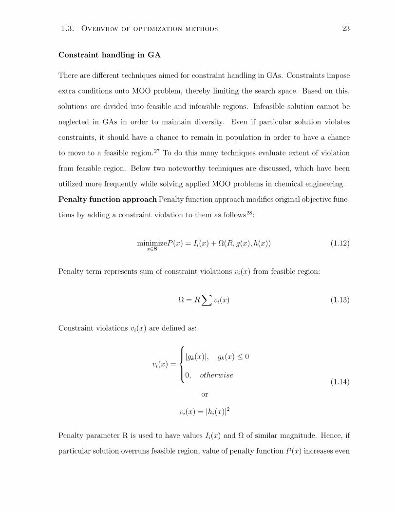
Constraint handling in GA
There are different techniques aimed for constraint handling in GAs. Constraints impose
extra conditions onto MOO problem, thereby limiting the search space. Based on this,
solutions are divided into feasible and infeasible regions. Infeasible solution cannot be
neglected in GAs in order to maintain diversity. Even if particular solution violates
constraints, it should have a chance to remain in population in order to have a chance
to move to a feasible region.27 To do this many techniques evaluate extent of violation
from feasible region. Below two noteworthy techniques are discussed, which have been
utilized more frequently while solving applied MOO problems in chemical engineering.
Penalty function approach Penalty function approach modifies original objective func-
tions by adding a constraint violation to them as follows28:
minimizex∈S
P (x) = Ii(x) + Ω(R, g(x), h(x)) (1.12)
Penalty term represents sum of constraint violations vi(x) from feasible region:
Ω = R∑
vi(x) (1.13)
Constraint violations vi(x) are defined as:
vi(x) =
|gk(x)|, gk(x) ≤ 0
0, otherwise
or
vi(x) = |hi(x)|2
(1.14)
Penalty parameter R is used to have values Ii(x) and Ω of similar magnitude. Hence, if
particular solution overruns feasible region, value of penalty function P (x) increases even
24 Greek letters
if the value of original objective function Ii(x) is small. The solution becomes inferior
and has higher chance to be excluded from population. One of the main drawbacks of
this method is that penalty function distorts Pareto front of original function which cause
difficulties finding true Pareto set.
Constrained Tournament Method
Constrained tournament method is a methods developed for use with GAs only. The
approach can treat constraints directly instead of using any objective function transfor-
mation. It modifies the tournament selection of individuals for formation of mating pool.
Now solutions are checked for constraint violation in addition to dominance. Between
two infeasible solutions the one chosen is the one with less constraint violation. When
two individuals are picked for tournament selection, the following constraint-domination
rules have to be kept:
• Feasible individual is always superior to infeasible
• Between two infeasible individuals the one with smaller constraint violation should
be given priority
• If both individuals are feasible the regular (non-constraint) approach should be
applied
The generic constraint-domination principle can be used with any GA and does not
require extra computational time27.
1.3.4 Simulated annealing
Simulated annealing (SA) is another stochastic-based method of search and, like GAs,
belongs to a posteriori methods. The procedure mimics the behaviour of molten metals
cooling. At high temperatures, metals behave like a liquid where atoms are in chaotic
motion. When the cooling is started, atoms lose mobility and begin to form crystalline
lattice of solid metal. The rate of cooling strongly affects the structure of crystal, the

1.3. Overview of optimization methods 25
slower the rate, the more uniformed the structure. Uniformed mono-crystalline structure
has more stable (i.e. has minimum energy).
SA for optimization was first considered in Kirkpatrick et al. 30 . They applied prin-
ciples of statistical mechanics of systems in thermal equilibrium to solve optimization
problem. The main principle is based on Boltzmann probability distribution function.
At given temperature T the probability of system to have energy E1 is proportional
to exp(−E1/kT ), where k is the Boltzmann constant. In this context probability for a
system to move from state 1 to state 2 is given as:
state1
state2= exp(
−(E2 − E1)
kT) (1.15)
Hence if E2 is lower than E1 when system definitely turns to state 2. At the same
time, if E2 − E1 ≥ 0 finite probability for transition from 1 to 2 still exists. The higher
temperatures T correspond to higher probabilities of state 2 to exist. For energies in
Boltzmann distribution equations, the reader has to consider objective values. SA in the
simplest form can be described in the following way: the algorithm starts with an initial
point x0 (usually random). The random point x1 is generated in the neighbourhood of
x 0 and the objective values are compared at these points. If a new point improves our
objectives, it is accepted instead of x0. If not, the point x1 is accepted with the probability
exp((E2 − E1)/kT ). During the search, the temperature T is slowly decreased (cooling)
which reduces the probability of a new point with worse objective being accepted. The
search continues until some termination criteria are reached, for example, it can be an
error between points in subsequent iteration or minimal temperature. One run of SA
yields one Pareto optimal solution. Thus multiple simulations are required to obtain a
Pareto set.
The same principle with some modifications can be applied for MOO problems.31? –33
Algorithms could differ in probability functions or stopping criteria, or they have some

26 Greek letters
operators for a better Pareto distribution. The current technique is less popular than
GAs but still has a significant interest in modern MOO applications.
Bibliography
[1] M. Appl. Ammonia : principles and industrial practice. Wiley-VCH, Weinheim ;
New York, 1999.
[2] Incitec Pivot Limited. Louisiana Ammonia Plant Presentation, 2013. URL
papers2://publication/uuid/52721835-95E4-4EF5-9735-A3D29BBE2DB5.
[3] L. J. Gillespie and J. A. Beattie. The thermodynamic treatment of chemical equi-
libria in systems composed of real gases. I. An approximate equation for the mass
action function applied to the existing data on Haber equilibrium. Physical Review,
36:743–753, 1930.
[4] H. Liu. Ammonia synthesis catalysts: Innovation and practice. Beijing : Chemical
Industry Press ; New Jersey : World Scientific, 2013.
[5] J. R. Jennings. Catalytic Ammonia Synthesis. Springer US, 1991.
[6] A. Nielsen, J. Kjager, and B. Hansen. Rate Equation and Mechanism of Ammonia
Synthesis at Industrial Conditions. Journal of Catalysis, 3:68–79, 1964.
[7] D. C. Dyson and J . M. Simon. A Kinetic Expression with Diffusion Correction for
Ammonia Synthesis on Industrial Catalyst, 1968. ISSN 0196-4313.
[8] D. Y. Murzin and A. K. Avetisov. Kinetics of Ammonia Synthesis Close to Equilib-
rium. Society, (3):4779–4783, 1997. ISSN 08885885.
[9] I. Rossetti, N. Pernicone, F. Ferrero, and L. Forni. Kinetic study of ammonia synthe-
sis on a promoted Ru/C catalyst. Industrial and Engineering Chemistry Research,
45(12):4150–4155, 2006. ISSN 08885885. doi: 10.1021/ie051398g.

BIBLIOGRAPHY 27
[10] W. D. Seider, J. D. Seader, and D. R. Lewin. Ammonia case study. In Product &
Process Desing Principles: Synthesis, Analysis and Design, pages 341–361. Wiley,
2008.
[11] V. Pattabathula and J. Richardson. Introduction to ammonia production. Chemical
Engineering Progress, 112(9):69–75, 2016.
[12] K. Miettinen. Nonlinear Multiobjective Optimization. 1998.
[13] J. Branke, K. Deb, K. Miettinen, and R. Slowinski. Multiobjective Optimization.
Interactive and Evolutionary Approaches. Springer-Verlag Berlin Heidelberg, 2008.
[14] R. T. Marler and J. S. Arora. Survey of multi-objective optimization meth-
ods for engineering. Structural and Multidisciplinary Optimization, 26(6):
369–395, 2004. ISSN 1615-1488. doi: 10.1007/s00158-003-0368-6. URL
http://dx.doi.org/10.1007/s00158-003-0368-6.
[15] A. Wierzbicki, M. Makowski, and J. Wessels. Model-based decision support method-
ology with environmental applications. Boston: Kluwer Academic Publishers, 2000.
[16] V. Bhaskar, S. K. Gupta, and A. K. Ray. Applications of multiobjective optimization
in chemical engineering. Reviews in Chemical Engineering, 16(1):1–54, 2000. ISSN
0167-8299. doi: 10.1515/REVCE.2000.16.1.1.
[17] P.C. Fishburn. Lexicographic Orders, Utilities and Decision Rules: A Survey. Man-
agement Science, 20(11):1442–1471, 1974.
[18] A. Charnes and W. W. Cooper. Management models and industrial applications of
linear programming. New York : Wiley, 1961, 1961.
[19] M. Tamiz, D. Jones, and C. Romero. Goal programming for decision making: An
overview of the current state-of-the-art. European Journal of Operational Research,
(111):569–581, 1998.

28 Greek letters
[20] Y. Haimes. On a bicriterion formulation of the problems of integrated system iden-
tification and system optimization. IEEE transactions on systems, man, and cyber-
netics, pages 296–297, 1971.
[21] V. Chankong and Y. Haimes. Multiobjective decision making :theory and methodol-
ogy. Dover Publications, New York: North Holland, 1983.
[22] A. Wierzbicki. The use of reference objectives in multiobjective optimization. In
G. Fandel and T. Gal, editors, Multiple Criteria Decision Making Theory and Ap-
plication, pages 468–486. Berlin: Springer Berlin Heidelberg, 1980.
[23] K. Miettinen and M. M. Makela. Interactive bundle-based method for nondifferen-
tiable multiobjeective optimization: nimbus. Optimization, (34):231–246, 1995.
[24] R. Benayoun, J. de Montgolfier, J. Tergny, and O. Laritchev. Linear programming
with multiple objective functions: Step method (stem). Math Program, (1):366–375,
1971.
[25] D. E. Goldberg. Genetic algorithms in search, optimization, and machine learning.
Reading, Mass. ; Don Mills, Ont. : Addison-Wesley Pub. Co., 1989.
[26] J. H. Holland. Adaptation in natural and artificial systems :an introductory analysis
with applications to biology, control, and artificial intelligence. 1st MIT Press ed.,
1992.
[27] K. Deb. Multi-objective optimization using evolutionary algorithms, volume 1. John
Wiley & Sons, Chichester, England ;; New York, 2001. ISBN 047187339X.
[28] K. Deb. Optimization for engineering design: Algorithms and Examples. PHI Learn-
ing Private Limited, New Delhi, 1995.
[29] K. Deb, A. Pratap, S. Agarwal, and T. Meyarivan. A fast and elitist multiobjective

BIBLIOGRAPHY 29
genetic algorithm: NSGA-II. Ieee Transactions on Evolutionary Computation, 6(2):
182–197, 2002. ISSN 1089-778X. doi: 10.1109/4235.996017.
[30] S. Kirkpatrick, C. D. Gelatt, and M. P. Vecchi. Optimization by Simulated An-
nealing. Science, 220(4598):671–680, 1983. ISSN 0036-8075. doi: 10.1126/sci-
ence.220.4598.671.
[31] P. Czyzzak and A. Jaszkiewicz. Pareto simulated annealinga metaheuris-
tic technique for multiple-objective combinatorial optimization. Journal of
Multi-Criteria Decision Analysis, 7(1):34–47, 1998. ISSN 1099-1360. doi:
10.1002/(SICI)1099-1360(199801)7:1¡34::AID-MCDA161¿3.0.CO;2-6. URL
http://dx.doi.org/10.1002/(SICI)1099-1360(199801)7:1<34::AID-MCDA161>3.0.CO
2-6.
[32] B. Suman. Study of simulated annealing based algorithms for multiobjective op-
timization of a constrained problem. Computers & Chemical Engineering, 28(9):
1849–1871, 2004. ISSN 0098-1354. doi: 10.1016/j.compchemeng.2004.02.037.
[33] B. Suman. Study of self-stopping PDMOSA and performance measure in multiob-
jective optimization. Computers & Chemical Engineering, 29(5):1131–1147, 2005.
ISSN 00981354. doi: 10.1016/j.compchemeng.2004.12.002.

Chapter 2
First principle modelling of an
industrial ammonia converter
30

Nomenclature 31
Nomenclature
α constant parameter for reaction equation
αi convection heat transfer coefficient for interchanger [W/m2K]
νi stoichiometric coefficient in Eq. 2.1 for component i
χ nitrogen conversion
ω dimensionless distance from pellet center to interior point
∆HR enthalpy of reaction [kJ/kmoleK]
ǫ bed voidage
φi fugacity coefficient of component i
η effectiveness factor
C total concentration of components [kmol/m3]
Cp specific heat capacity [kJ/kgK]
Die effective diffusivity of component i [m2/s]
fi fugacity of ith component
FN2molar flow rate [mol/s]
K overall heat transfer coefficient [W/m2K]
k2 kinetic constant of reverse reaction [kmol/m3 · h]
Ka equilibrium constant
L interchanger length [m2]
l length coordinate for interchanger [m2]
mi mass flow rate [kg/s]
P pressure [Pa]

32 Nomenclature
Qi volumetric rate [m3/s]
ri tube radius [m]
RNH3rate of ammonia formation [kmol/m3 · h]
Rp radius of catalyst particle [m2]
T temperature [K]
V bed volume [m3]
Xi molar fraction of component i
2.1 Introduction
Ammonia is one of major chemicals produced in the industry. It has a variety of appli-
cations: for manufacturing of inorganic salts, polymer fibers, explosives, etc. Its biggest
role it plays for agricultural fertilizers: as an intermediate in urea production or used
directly as liquid. It is hard to diminish the importance of ammonia for agricultural
sector all over the world.1
Moreover, ammonia market is continuously growing. Total world ammonia demand
has been steadily increasing over last decade at rate of 2.2 % per annum. One of the
ways to satisfy for the demand is to boost up the performance of existing units through
the comprehensive optimization.
One possible way this to be done is through first-principle mathematical modelling and
numerical optimization. Developing robust models allows for accurate process simulation.
Therefore, one can perform a comprehensive study of a process without expensive physical
modelling and/or use the model for the numerical optimization to boost up process
performance.
Modelling of ammonia synthesis has been drawing attention over the years and a
number of attempts has been made. Baddour et al. 2 developed a simple one-dimensional
plug-flow model for autothermal ammonia converter. They studied effect of process

2.1. Introduction 33
parameters such (i.e. feed temperature and composition) on ammonia production rate
and temperature profile along catalyst bed. Shah 3 discussed two-bed adiabatic model
with recovery heat exchange for the process control. He found best stable operating point
as balance between heat generation and consumption. Gaines 4 used mathematical model
for adiabatic bed with empirical correlation for effectiveness factor to perform analysis on
model parameters. Singh and Saraf 5 modelled converters with both types - adiabatic and
non-adiabatic - catalytic beds. They used pseudo homogeneous model with effectiveness
factor based on reactants diffusion. Mansson and Andresen 6 did an optimization study
for tubular ammonia converter with one-dimensional pug low model aiming to maximize
ammonia content in the effluent and obtain optimal temperature profile. Elnashaie et al. 7
compared the performance of homogeneous and heterogeneous models for auto-thermal
converter showing advantages and better accuracy for the latter. In the consequent works
of Elnashaie et al.8–10 they incorporated rigorous model for intraparticle diffusion and
obtained more accurate solution for the effectiveness factor. They validated the model
with data of Singh and Saraf 5 . Later, Upreti and Deb 11 performed a design optimization
study with genetic algorithm by maximizing overall economic return of the synthesis
having total converter length as a major decision variable. Babu and Angira 12 performed
a similar study but could obtain more stable model solution in wider temperature range.
Summarizing, one can say that, firstly, it is evident that the topic still bears its
value and importance. Models vary in complexity: some works consider broader range
of units (as converters and product separators) in a model while others mainly consider
converter itself. Secondly, models for different converter designs have been done (auto-
thermal or adiabatic catalyst beds with different type of heat exchange). Each of studies
shows that converters of different design distinct in optimal operating parameters, thus
each particular converter arrangement bears different behaviour and requires independent
investigation for the best results. Thirdly, some works focus on modelling for investiga-
tion of the process parameters effect on process performance while others perform more

34 Nomenclature
comprehensive optimization studies striving for higher ammonia production or least cost.
However, none of the works, to the best of the author’s knowledge, utilizes multi-objective
optimization principles and performs optimization search for more than one objective.
Hence, it could be beneficial for the complex system as industrial converter.
In this work we develop a first-principle mathematical model of an industrial ammonia
synthesis converter with design not reported before. The model incorporates heteroge-
neous reaction kinetics with intra-particle diffusion resistances. As process being highly
exothermic, the heat recovery model is also embedded into the overall converter model.
The model is able to predict gas temperature and concentration profiles along con-
verter’s bed, and the amount of heat which is recovered from a gas stream and recycled
to supply for the pre-heat.
2.2 Overview of industrial ammonia synthesis and
converter internals
Industrial ammonia synthesis is done through Haber process (see more detailed descrip-
tion below). There are a number of different technologies available for commercial ap-
plication (i.e. Kellog, Haldor Topsoe, etc.). Regardless of any particular one, ammonia
is produced through stoichiometric reaction of hydrogen and nitrogen (Eq.2.1). The re-
action is slow at ambient conditions as well as limited by equilibrium, thus to achieve
significant yields is carried out in a presence of catalyst under elevated temperatures (350
- 500 °C) and pressure (100-250 atm.)
Typical ammonia synthesis loop is presented on Fig. 2.1. Makeup gas coming from
upstream units passes through loop compressor and forward to a synthesis converter. As
hydrogen usually being produced upstream by steam conversion of methane, the makeup
gas contains inert components (as methane, argon). Along with others, minor part of
ammonia is also present among reactants. An ammonia-rich converter effluent (15-20 %

2.2. Overview of ammonia synthesis 35
Figure 2.1: Ammonia synthesis loop
vol. ammonia) is sent to a separator where ammonia is separated into product stream
while unconverted gases are recycled back to the compressor.
An ammonia converter is comprised of multiple (usually, three) fixed catalytic beds.
Pre-heated gas stream enters a catalyst bed (Fig. 2.2). The synthesis reaction occurs
on a surface and inside the pores of catalyst. While gas mixture heats up while passing
along a bed. To prevent catalyst from exposure to high temperatures and shift reaction
equilibrium the excess heat is removed. It is done in many ways: quenching, indirect
heat exchange with cooling water or product stream, etc. Therefore, it is necessary to
consider all those steps in order to develop an accurate mathematical model.
Figure 2.2: Schematic representation of a catalytic bed in ammonia converter

36 Nomenclature
The ammonia converter to be modelled in this work is a three bed converter with
heat interchanger and quenching. The converter’s layout is provided in Fig. 2.3. Pre-
heated and compressed synthesis gas is split into two flows - for main inlet and quench
- in ratio tentatively 60/40.1 The main feed enters from the bottom of reactor into
annular space between outer shell and inner bed casing. It flows upwards to shell-side
inlet of interchanger where the gas heats up to the reaction temperature by indirect heat
exchange with effluent from second bed. The heated gas travels through the gap between
interchanger and catalyst baskets up and enters first bed. The converter has the ability
to quench prior to the first bed, but usually is done at start up only. At steady-state
operation first bed quenching is relatively low or completely off. After first bed the main
stream is quenched and enters next bed. The effluent from second bed passes through
the tube-side of the interchanger into the third bed and out of the converter.
Figure 2.3: Internals of the ammonia converter

2.3. Converter modelling 37
2.3 Converter modelling
Considering the process description and converter layout, the following assumption are
made for converter modelling:
1. Steady state operation
2. Adiabatic catalyst bed The converter and catalyst basket are well insulated,
therefore the heat transfer from reaction zone towards the gas flow is negligible.
3. Negligible heat and mass transfer resistance at boundary of bulk and
catalyst pellet due to high gas velocities and bulk thermal conductivity.
4. Significant diffusion resistances inside catalyst pellet
5. Constant temperature inside catalyst pellet Due to high heat conductivity
of catalyst support, the temperature profile inside a pellet can be assumed flat.
6. One-dimensional plug flow model Radial dispersion of mass and heat can be
neglected for the well-insulated beds as well. Moreover, since we are not aiming
to rigorously study gas flow patterns inside catalyst bed, it is reasonable to use
one-dimensional model for global optimization of converter performance3.
7. No axial dispersion term Ammonia converter bed is a gas solid system. Gas
velocities are quite high and bulk viscosity is relatively low resulting in high Peclet
number. Therefore, dispersion term can be neglected as well13.
8. Converter pressure is constant along converter As reported in literature and
observed by author from industrial data, the actual pressure drop along one bed
is approximately 0.2 atm. Considering high loop pressures (100-250 atm.) this
difference is negligible.

38 Nomenclature
2.3.1 Ammonia synthesis reaction
Industrially ammonia is synthesized through the exothermic reaction of nitrogen and
hydrogen in presence of catalyst (most often, iron-based) as shown by reaction:
N2 + 3H2 2NH3, ∆H0298 = −46.22 kJ/mol (2.1)
Even though the process has a long history and been extensively studied, there is
still no consensus regarding the mechanism of the reaction over the catalyst. Therefore,
a number of mechanisms as well as kinetic equations are found in the literature.14–18
The Temkin equation (Eq.2.2) is found to be most widely used due to its accuracy and
applicability:
RNH3= k2
[
K2afN2
(
f 3H2
f 2NH3
)α
−
(
f 2NH3
f 3H2
)1−α]
(2.2)
where RNH3- rate of ammonia formation [kmol/m3·h], k2 - kinetic constant of reverse
reaction [kmol/m3 · h], Ka - equilibrium constant, fi - fugacity of ith component, α -
constant number. The respective value for α = 0.559 while k2 is estimated with industrial
data. The expression for equilibrium constant Ka is taken from19 (Eq. 2.3):
logKa = −2.691122logT − 5.519265× 10⁻⁵T+
1.848863× 10⁻⁷T 2 + 2001.6/T + 2.6899 (2.3)
where T - process temperature [K].
Fugacity of i th component is found as:
fi = φiXiP (2.4)
where φi - fugacity coefficient of i th component, Xi - molar fraction of i th component in
gas stream, P - loop pressure [Pa].

2.3. Converter modelling 39
2.3.2 Intraparticle diffusion
Industrially ammonia is synthesized over a variety of catalysts. Historically, first catalysts
have been iron based and constitute majority of catalysts in use until now1, however
Ru-based catalysts have been commercialized in past decades, being more active yet
expensive20. Whichever catalyst type is loaded in converter, it is usually in a form
of pellets 4-10 mm in diameter. In order to provide larger surface, active component
is immobilized on Al2O3 support. Due to porous structure of the support, diffusional
resistances inside pores play significant role in integral synthesis reaction rate, therefore
it has to be accounted for21.
Assuming Fick-type diffusion, the mass balance for species i in spherical catalytic
particle can be written as:
d2Xi
dω2−
(
2
νi + 2Xi
)(
dXi
dω
)2
+2
ω
dXi
dω=
−
[
R2p
CDie
(νi + 2Xi)
]
RNH3(X, T, P )
1− ǫ(2.5)
subject to boundary conditions:
ω = 0 :dXi
dω= 0
ω = 1 : Xi = Xi(bulk)
where νi - corresponding stoichiometric coefficient in synthesis reaction (Eq. 2.1), ω -
dimensionless distance from pellet center to interior point, Rp - pellet radius [m2], C -
total concentration [kmol/m3], Die - effecitive diffusivity [m2/s], ǫ - bed voidage.
The Eq. 2.5 is solved using orthogonal collocation method22 using 4 collocation points.
The solution yields a concentration profile for the reactants. Therefore, one can calculate
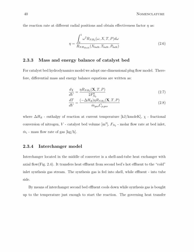
40 Nomenclature
the reaction rate at different radial positions and obtain effectiveness factor η as:
η =
∫ 1
0
ω2RNH3(ω,X, T, P )dω
RNH3bulk(Xbulk, Tbulk, Pbulk)
(2.6)
2.3.3 Mass and energy balance of catalyst bed
For catalyst bed hydrodynamics model we adopt one-dimensional plug flow model. There-
fore, differential mass and energy balance equations are written as:
dχ
dV=
ηRNH3(X, T, P )
2F 0N2
(2.7)
dT
dV=
(−∆HR)ηRNH3(X, T, P )
mgasCp,gas
(2.8)
where ∆HR - enthalpy of reaction at current temperature [kJ/kmoleK], χ - fractional
conversion of nitrogen, V - catalyst bed volume [m3], FN2- molar flow rate at bed inlet,
mi - mass flow rate of gas [kg/h].
2.3.4 Interchanger model
Interchanger located in the middle of converter is a shell-and-tube heat exchanger with
axial flow(Fig. 2.4). It transfers heat effluent from second bed’s hot effluent to the “cold”
inlet synthesis gas stream. The synthesis gas is fed into shell, while effluent - into tube
side.
By means of interchanger second bed effluent cools down while synthesis gas is bought
up to the temperature just enough to start the reaction. The governing heat transfer

2.3. Converter modelling 41
Figure 2.4: Heat transfer along tube wall
equation for the interchanger is:
Shell side : (2.9)
dTshell
dl=
2πK(Ttube − Tshell)
mshellCpshell
(2.10)
Tube side : (2.11)
dTtube
dl= −
2πK(Ttube − Tshell)
mtubeCptube
(2.12)
K =
[
1
αtuberinner+
1
λ
1
αshellrouter
]−1
(2.13)
subject to boundary conditions:
l = 0 : Tshell = T inletbed1
l = L : Ttube = T outletbed2
where K - overall heat transfer coefficient [W/m2K], αi - convective heat transfer coeffi-
cient towards tube wall from shell or tube side [W/m2K], ri - inner or outer interchanger
tube radius [m], λ - thermal conductivity of interchanger material [W/mK], l - length
coordinate for interchanger integration [m], L - interchanger length [m]. Detailed model
derivation for interchanger for a given geometry can be found in appendix A.

42 Nomenclature
Figure 2.5: Simulation procedure for the ammonia converter
2.3.5 Model overview
The intraparticle diffusion is boundary-valuer problem and solved through transformation
of equation into set of non-linear equation by orthogonal collocation with 4 collocation
points. Then the system is solved by the Newton method. The catalyst bed mass and
heat balance equations are solved as initial value problem using Runge-Kutta 5th order
method. The interchanger model is a boundary-value problem and solved using mono-
implicit Runge-Kutta method (based on subroutine “bvptwpc”23). The simulation is
carried out as shown on Fig. 2.5. The initial guess is set on inlet temperature for first
bed, then the model is run in series for two quenching and beds followed by interchanger
and checked whether shell side temperature at interchanger outlet matches initial guess.
If error is below 10−5 then simulation follows to calculate the outcome of the third bed.
Thus, the model yields temperature and gas composition profile along the converter
length.
2.4. Results and Discussion 43
2.4 Results and Discussion
2.4.1 Model validation
As kinetic parameters of catalyst remain unknown, they were estimated using industrial
data. In reality, the catalyst in each bed is a layered mixture of few catalyst brands of dif-
ferent activity and size in certain ratio. Therefore, the kinetic parameters in each bed are
averaging the individual kinetic parameters of each of the catalysts. The sum of squared
distances between observed and simulated temperatures for each bed is minimized in
order to do model fitting:
min3
∑
i=1
(T simulatedbedi
− T observedbedi
)2 (2.14)
To assess validity, one can compare temperatures between simulated profile and on bed
boundaries, measured by thermocouples. One can find that the model proved a good
overall match. The error for the most cases lies within few °C. Especially notable that
simulated temperature for the first bed inlet is very close to measured one. Considering
that the model of interchanger was excluded from fitting stage (see 2.14), but validation
was carried out with interchanger on, it, first of all, validates assumption that heat losses
from catalyst basket towards gas stream inside converter are negligible. Secondly, it en-
sures the validity of interchanger model as well, since we are unable to validate it directly
and independently from the whole converter. The only largest observed error is for inlet
into the third bed. This discrepancy might result from the fact that this temperature
is not measured directly in a gas flow but taken as an average of three thermocouples
located inside the third bed (Fig. ??). Moreover, one can look into comparison of gas
compositions in Table 2.1. Even though components concentrations were not included
into fitting, but along with temperatures they have a close match.

44 Nomenclature
Figure 2.6: Comparison between simulated and observed temperatures along reactor
Gas stream composition [% mol.]N2 H2 NH3 CH4 Ar
simulated 23.53 56.38 13.31 5.08 1.70experimental 23.10 56.50 13.56 5.08 1.71
Table 2.1: Comparison between simulated and experimented gas composition
2.4.2 Sensitivity analysis
The sensitivity analysis of the model was performed in order to a) check that model
performs “as expected” (i.e. with agreement of thermodynamics, reaction kinetics, engi-
neering sense) and b) evaluate effect of parameters onto process performance (Table 2.2).
The analysis performed as follows: the most important process parameters were chosen
and fixed at reference value (denoted by “-” sign). Then, parameter varies one at a time
around reference in order to quantify its effect on performance indicators. The chosen
process control parameters are: feed temperature Tfeed, volumetric flow rate for converter
inlet and quenches Qi, loop pressure P , second bed’s quench-to-feed ratio Qquench2/Qfeed.
As performance indicators the following are used: outlet temperature from each bed T outi ,
conversion per bed χi, ammonia content in converter outlet XNH3, temperature change
across interchanger from tube side ∆Ttube. The latter is chosen as a measure of heat
recovery in the system, since it is proportional to the value. Thus, it is indirect measure
of heat recovery efficiency.
The increase in feed temperature shows an increase in total ammonia production

2.4. Results and Discussion 45
Table 2.2: Sensitivity analysis
Parameter Value T outbed1 T out
bed2 T outbed3 ∆Ttube χbed1 χbed2 χbed3 XNH3
+10% 266.26 457.03 ↑ 468.44 ↑ 411.81 ↑ 98.60 ↓ 5.53 ↑ 9.04 ↓ 5.41 ↑ 13.40 ↑Tfeed - 242.06 443.38 463.58 393.57 107.80 5.22 9.58 4.89 13.31
-10% 217.85 247.31 ↓ 456.77 ↓ 372.82 ↓ 116.03 ↑ 4.79 ↓ 10.08 ↑ 4.16 ↓ 13.04 ↓+10% 65.56 434.52 ↓ 461.72 ↓ 389.30 ↓ 107.96 ↑ 4.67 ↓ 9.62 ↑ 4.59 ↓ 13.01 ↓
Qfeed - 59.6 443.38 463.58 393.57 107.80 5.22 9.58 4.89 13.31-10% 53.64 452.62 ↑ 464.60 ↑ 397.89 ↑ 106.91 ↓ 5.82 ↑ 9.52 ↓ 5.21 ↑ 13.61 ↑+10% 96.83 457.99 ↑ 473.27 ↑ 405.22 ↑ 112.31 ↑ 6.12 ↑ 9.55 ↓ 5.75 ↑ 14.12 ↑
P - 88.03 443.38 463.58 393.57 107.80 5.22 9.58 4.89 13.31-10% 79.22 423.61 ↓ 447.82 ↓ 378.86 ↓ 100.37 ↓ 4.21 ↓ 9.32 ↓ 4.03 ↓ 12.29 ↓+10% 38.49 442.41 ↓ 460.17 ↓ 392.78 ↓ 104.10 ↓ 5.19 ↓ 9.73 ↑ 4.75 ↓ 13.25 ↓
Qquench2 - 34.99 443.38 463.58 393.56 107.80 5.22 9.58 4.89 13.31-10% 31.49 443.64 ↑ 466.37 ↑ 393.98 ↑ 111.34 ↑ 5.22 9.38 ↓ 5.04 ↑ 13.34 ↑+10% 3.4987 431.95 ↓ 459.67 ↓ 392.51 ↓ 103.87 ↓ 4.77 ↓ 9.84 ↑ 4.75 ↓ 13.24 ↓
Qquench1 - 0 443.38 463.58 393.56 107.80 5.22 9.58 4.89 13.31more 1.31 450.45 ↑ 457.04 ↓ 396.12 ↑ 98.51 ↓ 5.77 ↑ 9.90 ↑ 4.88 ↓ 13.48 ↑
Qquench2/Qfeed - 1.70 443.38 463.58 393.56 107.80 5.22 9.58 4.89 13.31less 2.86 432.69 ↓ 469.72 ↑ 389.25 ↓ 118.41 ↑ 4.53 ↓ 9.13 ↓ 4.89 ↓ 13.01 ↓
(XNH3) as a result of higher reaction rate on average, however individual conversions over
bed does not simultaneously follow the increase. The second bed has lower conversion,
but total increase is reached by means of first and third beds. At the same time, it
lowers the efficiency of interchanger shown by lower ∆Ttube due to lower temperature
gradient between tube and shell sides. Higher feed flow rates on opposite reduce space
time hence reducing XNH3. But as in case with T , it is not reflected identically in all
beds’ conversion. On contrary, second bed gives boost in conversion while other two
drop while counter effect is done on ∆Ttube. Higher pressure like feed temperature boosts
up reaction rate yielding higher ammonia in reactor effluent. Higher quench like higher
feed flow rate - either to first or second bed - both have similar effect on every process
indicator due to reduction of space time. Notable, that heat recovery efficiency ∆Ttube
and XNH3are showing different trends - if one increases other decreases and vice versa.
2.4.3 Effect of process parameters
One can note that among considered process parameters, the largest effect on process
indicators is delivered by three process parameters: Tinlet, P and Qquench,bed2/Qfeed, while
others have smaller impact. Although Qfeed also has large effect, but engineering-wise

46 Nomenclature
it is not easy to vary feed flow rate since it involves complicated alteration of operation
mode on preceding series of units. Thus we had been mainly focused on these three
to estimated their effect on process performance. Firstly, to carry out simulations have
established decision domain in accordance with industrial practice. To set the range we
have studied the process history for over 10 years and extended the range by 40 °C for
feed temperature, by 10 % for quench-to-feed ratio, for pressure - we chose one value to
represent lower and upper range(Table 2.3).
Table 2.3: Simulation range
Variable Lower UpperTinlet 220 300
Qquench,bed2/Qfeed 0.3 0.5P 85 91
Simulation results for effect on ammonia production and heat recovery are shown
in Fig. 2.7 and Fig. 2.8 respectively. Firstly, one can see that for a given loop pressure
variation of Tinlet and Qquench,bed2/Qfeed allow for wide range production rate - 12 to 13.8%
and 13 to 14.2 % for 85 and 91 atm. respectively. Usually, acceptable production lies
above 13% of ammonia in converter effluent, thus improper control might significantly
drop XNH3below acceptable significantly reducing process efficiency. Secondly, Tinlet has
a pronounced maximum for ammonia production (i.e. convex surface). More, at higher
pressure (Fig. 2.7b) the convex peak is steeper. So, if higher production is needed a
careful attention has to be taken for adjusting feed temperature. The effect of quench
is mostly monotonous, favouring higher ammonia production at higher quench-to-feed
ratios.
There is a different picture if one to take a look onto effect on heat recovery within
the converter. Firstly, variation of these parameters allows for ∆Ttube change in range
70 to 120 °C. It is a significant variation of 40 %. Especially, considering the large scale
of production this results in high absolute values for heat recovery. However, there’s
no engineering requirements for heat recovery during production, this is important to

2.4. Results and Discussion 47
(a) P=85 atm. (b) P=91 atm.
Figure 2.7: Effect of process parameters on ammonia production
consider because it is able to reduce overall heat duty for the converter. Secondly, heat
recovery is more sensitive to quench-to-feed ratio than ammonia production. Although,
there’s an also convex maximum with respect to Tfeed at higher ratio, but the heat
recovery is more monotonous at lower quench and higher pressure. Moreover, in contrast
to ammonia production, higher heat recovery is favoured by lower quench.
(a) P=85 atm. (b) P=91 atm.
Figure 2.8: Effect of process parameters on heat recovery

48 Nomenclature
Therefore, a better process performance for ammonia production can be done by
controlling three main parameters: Tinlet, P and Qquench,bed2/Qfeed. They can cover
a wide range of process operation and it is possible to improve performance by their
proper adjustment. If one needs to increase ammonia content in converter effluent XNH3,
then it is needed to find a “sweet spot” in controlling feed temperature. It is possible to
significantly improve XNH3even without changing a loop pressure if for an engineering
purpose it has to be kept constant. Quenching can also help to improve production,
however its most effect it can influence on heat recovery. Unfortunately, higher heat
recovery corresponds to lower ammonia production, thus it is necessary to decide on
which mode is acceptable and efficient to properly set process control parameters for
best outcome.
2.5 Summary and conclusion
Firstly, in this work we considered a model development for simulation of an industrial
ammonia converter. Model includes four major parts: reaction kinetics, diffusion of
reactants inside solid catalytic particle, model for fixed hydrodynamics and model for
heat interchanger. The model was tested on a large scale industrial ammonia converter:
model fitting and validation were performed using design parameters and operation data.
The model found to have a good agreement with industrial data. From model sensitivity
analysis we were able to conclude the most important parameters for process performance
improvement. They are: feed temperature Tinlet, loop pressure P and quench-to-feed ratio
Qquench,bed2/Qfeed. We evaluated their effect on ammonia production XNH3and heat
recovery within interchanger ∆Ttube. It was found that variation of these three allows
for wide range of performance solutions. By their proper adjustment it is possible to
achieve improved production rate or heat recovery. However, both performance indicators
are in conflict - one cannot improve them simultaneously, hence needs to compromise.

BIBLIOGRAPHY 49
Therefore, engineering judgment and/or additional performance priorities are needed to
make a final decision about operational conditions.
Bibliography
[1] M. Appl. Ammonia : principles and industrial practice. Wiley-VCH, Weinheim ;
New York, 1999.
[2] R. F. F. Baddour, P. L. T. Brian, B. A. Logeais, and J. P. P. Eymery. Steady-state
Simulation of an Ammonia Synthesis Converter. Chemical Engineering Science, 20
(4):281–292, 1965. ISSN 0009-2509. doi: 10.1016/0009-2509(65)85017-5.
[3] Shah. Control simulation in ammonia production. Industrial and Engineering Chem-
istry, 59(1):72–83, 1967.
[4] L. D. Gaines. Ammonia synthesis loop variables investigated by steady-state sim-
ulation. Chemical Engineering Science, 34(1):37–50, 1979. ISSN 00092509. doi:
10.1016/0009-2509(79)85176-3.
[5] C. P. P. Singh and D. N. Saraf. Simulation of Ammonia-Synthesis Reactors. In-
dustrial & Engineering Chemistry Process Design and Development, 18(3):364–370,
1979. ISSN 0196-4305. doi: 10.1021/i260071a002.
[6] B. Mansson and B. Andresen. Optimal Temperature Profile for an Ammonia Re-
actor. Industrial & Engineering Chemistry Process Design and Development, 25:
59–65, 1986. ISSN 0196-4305. doi: 10.1021/i200032a010.
[7] S. S. E. H. Elnashaie, A. T. Mahfouz, and S. S. Elshishini. Digital Simulation of an
Industrial Ammonia Reactor. Chemical Engineering and Processing, 23(3):165–177,
1987.

50 Nomenclature
[8] S. S. E. H. Elnashaie and F. M. Alhabdan. A computer software package for
the simulation and optimization of an industrial ammonia converter based on a
rigorous heterogeneous model. Mathematical and Computer Modelling, 12(12):
1589–1600, 1989. ISSN 08957177. doi: 10.1016/0895-7177(89)90335-X. URL
http://www.sciencedirect.com/science/article/pii/089571778990335X.
[9] S. S. E. H. Elnashaie, M. E. Abashar, A. S. Alubaid, and A. S.
Al-Ubaid. Simulation and optimization of an industrial Ammo-
nia Reactor. Industrial & Engineering Chemistry Research, 27(8):
2015–2022, 1989. ISSN 08885885. doi: 10.1021/ie00083a010. URL
http://pubs.acs.org/doi/abs/10.1021/ie00092a024.
[10] S. S. E. H. Elnashaie, M. E. E. Abashar, and A. S. Al-Ubaid. Non-
monotonic behaviour of the effectiveness factor along a catalyst bed.
Chemical Engineering Science, 44(7):1581–1585, 1989. ISSN 0009-
2509. doi: http://dx.doi.org/10.1016/0009-2509(89)80034-X. URL
http://www.sciencedirect.com/science/article/pii/000925098980034X.
[11] S. R. Upreti and K. Deb. Optimal design of an ammonia synthesis reactor using
genetic algorithms. Computers & Chemical Engineering, 21(1):87–92, 1996. ISSN
00981354. doi: 10.1016/0098-1354(95)00251-0.
[12] B. V. Babu and R. Angira. Optimal design of an auto-thermal ammonia synthe-
sis reactor. Computers and Chemical Engineering, 29(5):1041–1045, 2005. ISSN
00981354. doi: 10.1016/j.compchemeng.2004.11.010.
[13] S. S. E. H. Elnashaie and S. S. Elshishini. Modelling, simulation, and optimization
of industrial fixed bed catalytic reactors. Gordon and Breach Science, elnashaie1
edition, 1993.

BIBLIOGRAPHY 51
[14] A. Nielsen, J. Kjager, and B. Hansen. Rate Equation and Mechanism of Ammonia
Synthesis at Industrial Conditions. Journal of Catalysis, 3:68–79, 1964.
[15] D. C. Dyson and J . M. Simon. A Kinetic Expression with Diffusion Correction for
Ammonia Synthesis on Industrial Catalyst, 1968. ISSN 0196-4313.
[16] D. Y. Murzin and A. K. Avetisov. Kinetics of Ammonia Synthesis Close to Equilib-
rium. Society, (3):4779–4783, 1997. ISSN 08885885.
[17] I. Rossetti, N. Pernicone, F. Ferrero, and L. Forni. Kinetic study of ammonia synthe-
sis on a promoted Ru/C catalyst. Industrial and Engineering Chemistry Research,
45(12):4150–4155, 2006. ISSN 08885885. doi: 10.1021/ie051398g.
[18] W. D. Seider, J. D. Seader, and D. R. Lewin. Ammonia case study. In Product &
Process Desing Principles: Synthesis, Analysis and Design, pages 341–361. Wiley,
2008.
[19] L. J. Gillespie and J. A. Beattie. The thermodynamic treatment of chemical equi-
libria in systems composed of real gases. I. An approximate equation for the mass
action function applied to the existing data on Haber equilibrium. Physical Review,
36:743–753, 1930.
[20] A. Logadottir and J. K. Nørskov. Ammonia synthesis over a Ru(0001) surface studied
by density functional calculations. Journal of Catalysis, 220(2):273–279, 2003. ISSN
00219517. doi: 10.1016/S0021-9517(03)00156-8.
[21] S. Charcoal. Diffusion and reaction rate in porous synthetic ammonia catalysts.
Journal of Physical Chemistry, 57(1):471–476, 1954.
[22] J. V. Villadsen and W. E. Stewart. Solution of boundary-value problems by or-
thogonal collocation. Chemical Engineering Science, 50(24):3981–3996, 1995. ISSN
00092509. doi: 10.1016/0009-2509(96)81831-8.

52 Nomenclature
[23] K. Soetaert, J. Cash, and F. Mazzia. bvpSolve, 2015. URL
https://cran.r-project.org/web/packages/bvpSolve/index.html.
Chapter 3
Surrogate-based multi-objective
optimization of the industrial
ammonia converter with NSGA-II
53
54 Nomenclature
Nomenclature
∆HR enthalpy of reaction [kJ/kmoleK]
AIC Akaike information criterion
bed refers to catalyst bed
C total concentration of components [kmol/m3]
Die effective diffusivity of component i [m2/s]
fi fugacity of ith component
FN2molar flow rate [mol/s]
feed refers to process gas feed into the converter
HR heat recovered through heat recovery system
k2 kinetic constant of reverse reaction [kmol/m3 · h]
Ka equilibrium constant
mi mass flow rate [kg/s]
out refers to a catalyst bed out
P converter pressure [atm.]
Q volumetric rate [m3/s]
QFR quench-to-feed ratio
quench refers to converter quench
RNH3rate of ammonia formation [kmol/m3 · h]
Rp radius of catalyst particle [m2]
T gas temperature [°C]
V bed volume [m3]

Greek letters 55
Xi molar fraction of component i
Greek letters
α constant parameter for reaction equation
νi stoichiometric coefficient in Eq. 3.1 for component i
χ nitrogen conversion
ω dimensionless distance from pellet center to interior point
ǫ bed voidage
φi fugacity coefficient of component i
3.1 Introduction
Ammonia is one of major chemicals produced in the industry. It has a variety of appli-
cations: for manufacturing of inorganic salts, polymer fibers, explosives, etc. Its biggest
role it plays for agricultural fertilizers: as an intermediate in urea production or used
directly as liquid. It is hard to diminish the importance of ammonia for agricultural
sector all over the world1.
The use of rigorous mathematical models in process design and optimization has
been extensively used for a large-scale chemical engineering processes. Model simula-
tions allows for fast and accurate investigation of the decision domain providing an engi-
neer/researcher with valuable knowledge on a process behaviour while avoiding expensive
and time consuming lab scale or industrial experiments. Therefore, one can perform a
comprehensive study of a process for the numerical optimization to boost up process
performance.
Conceptually, there are two approaches in optimization - single and multi-objective
(SOO and MOO respectively). The former formulates a sole objective function to be
optimized into a single point solution, while latter treats two or more objective objective

56 Greek letters
functions to find (likely) a set of equally good solutions.
However, SOO approach is still extensively used, but MOO has gained its popularity
in chemical engineering. Large-scale industrial processes are very complex system, so
often it is troublesome to single out the only objective. Thus, it is especially beneficial
to use multi-objective approach for optimization of industrial processes.
Multi-objective optimization has been successfully performed in a number of works,
especially in oil refining processes2–7, steam reforming8–13, polymer manufacturing14–19
and hydrogen production20–23. All these works evidently showed advantages of multi-
objective approach applied to industrial problems. The most common objectives are
related to: a) production of the desired product, b) production of side or undesired prod-
ucts and c) utilities. Constraint-wise, problems usually have a few (mostly one to three)
additional requirements for process conditions (i.e. upper or lower cap for stream tem-
perature or composition). Problems are solved predominantly with multi-objective opti-
mization methods, such as multi-objective genetic algorithms (e.g. NSGA-II24), multi-
objective simulated annealing25, however, some other problems are formulated through,
for example, ǫ-constraint or objective sum method and solved as single-objective prob-
lem. The main outcome of the problem solution is obtained set (known as Pareto set)
of non-dominating points, which resemble best solution with respect to all objectives.
Additionally, they reflect the trade-off between objectives, thus illustrating whether one
can significantly improve one objective while not worsening other beyond reasonable.
However, theoretically one can handle infinitely many objectives and constraints, the
problems solved in the literature are mostly two and sometimes three objective. Firstly,
it is worthwhile in terms of results interpretation as easier to visualize and analyze. Sec-
ondly, definition of overly complicated multi-objective optimization problem is excessive
as one usually willing to find practically feasible solution. In industrial processes it is
quite often not possible to adjust some parameters or measure process performance with
high accuracy. Thus two or three objective problems are sufficiently enough in major-

3.1. Introduction 57
ity of cases in order to obtain a good set of solutions. If required to account for more
objectives, they can be included as constraints.
Few attempts has been made to perform optimization study for an industrial ammonia
synthesis by a number of authors(Mansson and Andresen 26 , Elnashaie and Alhabdan 27 ,
Upreti and Deb 28 , Babu and Angira 29). They aimed towards maximization of ammonia
production or overall economic profit. To the best of authors knowledge, none of the
works available in open literature treats the problem in multi-objective manner.
There is one more major problem related to process optimization. In order to perform
numerical optimization one requires to run a number (and often quite large) of model
simulations. Sometimes even a single simulation is computationally expensive, thus total
optimization search will result in a large time. Imagine one uses NSGA-II with 100
individuals and 100 generations (however, in real search much larger number generations
is needed). In case if a single simulations takes 1 minute, the most conservative estimate
will be around 166 CPU-hours, and that excluding algorithm itself, taking into account
simulations only. One of the possible ways would be a code optimization either for model
or optimization algorithm. Firstly, the optimization is time consuming itself, and time
spent may not be payed off by results of the search. As famous saying declare “premature
optimization is a root of all evil”, thus one shall not strive for it without dire need.
Secondly, one can run model or optimization search in parallel thus decreasing elapsed
time. It is efficient way, however, like in previous case, development-wise is also time con-
suming. One may need to find places within a model which can be efficiently parallelized.
Also, parellelizing optimization search can boost up time while keeping the model’s code
untouched. For example, any genetic algorithm requires a number of independent model
evaluations at each generations. Thus, one can parallelize a model up to the number
of available cores. In case of derivative-based optimization, one will be limited by the
number of derivatives regardless of cores available. This all making an improvements in
code performance non-trivial task, therefore one shall carefully decide if it is a worthwhile

58 Greek letters
to do.
An alternative solution is to use surrogate model instead of original one for the op-
timization. Surrogate is a regression model obtained from a simulation data of original
model30,31. With required accuracy it is resembled in behaviour but computationally
much cheaper. Therefore, it can be used with existing optimization codes without any
alteration, thereby saving development time. An optimization run even on a single-core
will be much more faster. Optimization with surrogates have been successfully applied
for chemical engineering problems. A number of works available in open literature solv-
ing optimization problems for chemical engineering tasks, e.g. optimization of distillation
columns32, design and optimization of chemical engineering units under uncertainty33,
flow sheet optimization34, etc. It was shown that with use of proper surrogate it is pos-
sible to substitute original with proper regression model without loss of accuracy and
obtain effective and feasible solution.
In this work, we utilize a developed first-principle model for an industrial ammonia
converter. The model was validated with industrial data and showed a satisfactory accu-
racy. After, we trained a surrogate model with Eureqa® 35,36. Then obtained regression
model was coupled with optimization algorithm and few two-objective optimization cases
have been solved. One can find a broad range of optimal solutions with a trade of between
objectives.
3.2 Ammonia synthesis and model summary
Regardless of particular technology, industrial ammonia synthesis is done through Haber
process. The ammonia is produced through the reaction of hydrogen and nitrogen:
N2 + 3H2 2NH3, ∆H0298 = 46.22 kJ/mol (3.1)
The reaction is carried out under elevated temperature and pressure to suffice significant
yield. The Eq. 3.1 is a gas-solid reaction occurring in presence of iron or ruthenium

3.2. Ammonia synthesis and model summary 59
Figure 3.1: Ammonia converter schematic
catalyst. The catalytic ammonia converter is made of few packed beds. The reaction
mixture is sequentially fed into beds to produced ammonia in steps. The intermediate
cooling is essential as the reaction 3.1 is exothermic. To prevent catalyst from exposure
to high temperatures and shift reaction equilibrium the excess heat is removed between
beds.
The object of study is a three bed ammonia converter. The simplified layout is
provided at Fig. 3.1. The synthesis gas is split into two flows - for main feed and quench.
The main feed enters prior the first bed, while quenching is done in between. The process
gas passes though a bed and experiences a temperature rise. This is where quenching
and heat recovery is used - to remove the excess heat from the gas stream.
The main steps of ammonia synthesis in this reactor include:
1. Reaction kinetics
2. Intraparticle diffusion
3. Fixed bed hydrodynamics model
4. Heat recovery model
The four following steps were implemented in the model. The reaction rate is modelled

60 Greek letters
by a Temkin equation:
RNH3= k2
[
K2afN2
(
f 3H2
f 2NH3
)α
−
(
f 2NH3
f 3H2
)1−α]
(3.2)
where RNH3- rate of ammonia formation [kmol/m3·h], k2 - kinetic constant of reverse
reaction [kmol/m3 · h], Ka - equilibrium constant, fi - fugacity of ith component, α -
constant number. Intraparticle diffusion is derived through mass balance assuming Fick
diffusion37:
d2Xi
dω2−
(
2
νi + 2Xi
)(
dXi
dω
)2
+2
ω
dXi
dω=
−
[
R2p
CDie
(νi + 2Xi)
]
RNH3(X, T, P )
1− ǫ(3.3)
subject to boundary conditions:
ω = 0 :dXi
dω= 0
ω = 1 : Xi = Xi(bulk)
where νi - corresponding stoichiometric coefficient in synthesis reaction (Eq. 3.1), ω -
dimensionless distance from pellet center to interior point, Rp - pellet radius [m2], C -
total concentration [kmol/m3], Die - effective diffusivity [m2/s], ǫ - bed voidage. The
catalyst bed hydrodynamics is assumed to be a one-dimensional plug flow with no axial
dispersion:
dχ
dV=
ηRNH3(X, T, P )
2F 0N2
(3.4)
dT
dV=
(−∆HR)ηRNH3(X, T, P )
mgasCp,gas
(3.5)
where ∆HR - enthalpy of reaction at current temperature [kJ/kmoleK], χ - fractional
conversion of nitrogen, V - catalyst bed volume [m3], FN2- molar flow rate at bed inlet,
mi - mass flow rate of gas [kg/h].
Due to proprietary reasons authors cannot provide a layout for the heat recovery
system in the converter, thus making it impossible to disclose details of the heat recovery

3.3. Multi-objective optimization of converter operation 61
model as well. So this part will remain unknown for the reader, however one will not
experience any unclarity of the work flow or loose generality of this work.
The model was validated with industrial data of the converter operation. Authors
performed a comparison between simulated and measured temperatures (Fig. 3.2) and
feed compositions (Table 3.1). One can see a close match between simulated temperature
profile within catalyst beds and measured by thermocouples at beds’ edges. The error
lies with range of few °C. Moreover, prediction of stream composition are also very close
to the experimental results. Thus, the model has a good accuracy to be further used for
converter simulation and optimization.
Figure 3.2: Comparison between simulated and observed temperatures along reactor
Gas stream composition [% mol.]N2 H2 NH3 CH4 Ar
simulated 23.53 56.38 13.31 5.08 1.70experimental 23.10 56.50 13.56 5.08 1.71
Table 3.1: Comparison between simulated and experimented gas composition
3.3 Multi-objective optimization of converter oper-
ation
The converter’s operation is a complex process. It has a number of control and perfor-
mance parameters which has to be taken in to account in order to operate the unit or

62 Greek letters
perform multi-objective optimization. Proper study of the converter’s layout, consul-
tation with process engineers and preliminary model simulations allowed us to narrow
down process control parameters for operation to three major: feed gas temperature
Tfeed, quench-to-feed ratio QFR and process pressure P .
The most important industrial criteria of the ammonia converter efficiency is ammonia
production. Other objective of engineering importance is the amount of heat recovered
within the system. The more heat can recovered the less is needed to provide into the syn-
thesis gas. Firstly, we performed few model simulation to visualize the objective domain
for up mentioned process parameters (shown at Fig. 3.3 (a) and (b)). Both objective
spaces are convex surfaces with individual maximums located within box-constrained
region leading to non-linear optimization problem.
Secondly, the developed model is inconveniently expensive computation-wise taking
around 5 minutes of CPU time for a sole simulation. Therefore, an optimization search
requiring a large number of model evaluations will result in lengthy runs. So we performed
60 model simulations and used this data to train surrogate models with Eureqa®. A
surrogate model was obtained minimizing AIC as goodness-of-fit measure as more robust
metrics38. As Eureqa® yields a set of models compromising accuracy vs. complexity,
we choose one model for each objective which we found to have satisfactory accuracy for
MOO.
The obtained models are shown on Fig. 3.3 (c) and (d) for XoutNH3
and HR respectively.
One can find some discrepancy between figures a) and c) in the area of low Tfeed and
QFR, while the other regions show good consistency. However, as it will be shown in
Results and Discussion, the obtained optimum lies far from the discrepancy region. Thus,
the regression models by Eureqa® can adequately represent original objective functions.
Case 1 : The two objective discussed above were included into two-objective opti-
mization problem. The optimization problem is constrained by maximum bed tempera-
ture as it is limited by catalyst manufacturer in order to prevent damaging the catalyst

3.3. Multi-objective optimization of converter operation 63
a) b)
c) d)
Figure 3.3: Response surfaces for process objectivesFigures a), b) are obtained by simulation of original model, figures c), d) - by surrogate
simulation.

64 Greek letters
Table 3.2: Single objective maximums
Objective Optimum Other objective Tfeed Qquench
XoutNH3
0.1354 85.06 249.98 0.45HR 105.31 0.1310 230.04 0.33
and loss of activity. Industrially feasible domain for process parameters is a subject to
minimum and maximum bounds as decided in accordance with industrial practice. The
MOO problem is summarized as:
maximize I1(x) = XoutNH3
maximize I2(x) = HR
subject to:
T outbed ≤ Tmax for each bed
x = Tfeed, Qquench, P ∈ [min;max]
Prior to MOO, corresponding SOO problem was solved with only one objective
to be maximized. Individual maximums of the objectives were found with COBYLA
method39(Table 3.2). Firstly, one can find individual maximums of both objectives.
Secondly, it is evident that both objectives cannot be satisfied simultaneously. In case
of conflicting objectives, the optimal solution should be a Pareto optimal set of points.
Therefore, the MOO problem was solved with NSGA-II24 which allows to treat the prob-
lem directly as formulated.
3.4 Multi-objective optimization of converter design
Case 2 : Also, we considered MOO problem involving converter’s design parameters.
Beside ammonia production, another important process parameters is a total catalyst
loading within converter and it distribution among beds. Therefore, another multi-

3.5. Results and discussion 65
objective optimization problem to to investigate possibility to lower total catalyst volume
in reactor while keeping ammonia production high to be solved as follows:
maximize I1(x) = XoutNH3
minimize I2(x) =3
∑
i=1
Vi i = 1− 3
subject to:
T outbed ≤ Tmax for each bed
x = Tfeed, Qquench, Vi ∈ [min;max]
3.5 Results and discussion
Case 1. Pareto set of optimal solution for Case 1 was obtained for two different con-
verter pressures. As the converter pressure being the parameter not easily changeable
in industry (contrary to feed temperature and quench-to-feed ratio), we solved Case 1
for 85 and 91 atm. independently. Former pressure is found to be most common for the
converter, while latter is intended to show the potential changer in converter operation
and possible to achieve within the unit. The results are shown in Fig. 3.4. Overall, higher
temperatures and QFR favour higher ammonia production. If this is the objective one
is striving for, it is necessary to control both parameters simultaneously to stay near
optima. However, at higher pressure the impact of quenching is becoming less important
thus more attention has to be paid for feed temperature.
One can note that higher pressure is much in favour of higher ammonia production.
Any point of 91 atm. set is providing higher molar fraction of ammonia in product.
On contrary, lower pressure on average allows for higher heat recovery within converter.
Moreover, it also provides a wider range of Pareto optimal solutions for both objectives.
If one willing to come from low to high heat recovery (i.e. from most right to most
left point at 85 atm.), it will allow for 8% in heat saving. Considering large scale of
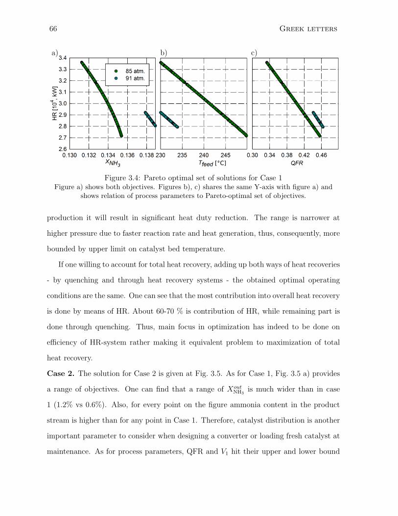
66 Greek letters
a) b) c)
Figure 3.4: Pareto optimal set of solutions for Case 1Figure a) shows both objectives. Figures b), c) shares the same Y-axis with figure a) and
shows relation of process parameters to Pareto-optimal set of objectives.
production it will result in significant heat duty reduction. The range is narrower at
higher pressure due to faster reaction rate and heat generation, thus, consequently, more
bounded by upper limit on catalyst bed temperature.
If one willing to account for total heat recovery, adding up both ways of heat recoveries
- by quenching and through heat recovery systems - the obtained optimal operating
conditions are the same. One can see that the most contribution into overall heat recovery
is done by means of HR. About 60-70 % is contribution of HR, while remaining part is
done through quenching. Thus, main focus in optimization has indeed to be done on
efficiency of HR-system rather making it equivalent problem to maximization of total
heat recovery.
Case 2. The solution for Case 2 is given at Fig. 3.5. As for Case 1, Fig. 3.5 a) provides
a range of objectives. One can find that a range of XoutNH3
is much wider than in case
1 (1.2% vs 0.6%). Also, for every point on the figure ammonia content in the product
stream is higher than for any point in Case 1. Therefore, catalyst distribution is another
important parameter to consider when designing a converter or loading fresh catalyst at
maintenance. As for process parameters, QFR and V1 hit their upper and lower bound

3.5. Results and discussion 67
a) b) c)
A
B
C
Figure 3.5: Pareto optimal set of solutions for Case 2Figure a) shows both objectives. Figures b) shares the same Y-axis with figure a) and showsrelation of feed temperature to Pareto-optimal set of objectives. QFR is at upper bound, V1 is
at lower bound.
respectively. The relation of other process parameters to Pareto optimal points is given
on Fig. 3.5 b) and c). Feed temperature and two other bed volumes are experiencing more
complex relations in order to stay Pareto optimal. Firstly, higher total catalyst volume
will allow for lower inlet temperature due to higher space times. Secondly, the major
decrease in feed temperature ( 20 °C) and rise in ammonia (0.8 %) is achieved through
the increase in third bed catalyst loading. The further boost in ammonia ( 0.4%) is
through increase of the loading in second bed, while keeping Tfeed and V3 constant.
To take a closer look into importance of catalyst distribution on converter perfor-
mance, one can consider three cases from Fig. 3.6 a) highlighted as. A and C correspond
to marginal cases with minimum and maximum loading while B depicts solution “in the
middle”. In fact, total loading of catalyst at point B is the same as in the converter
studied but with different distribution. The existing catalyst distribution is labelled as
“original” at Fig. 3.6. Firstly, one can note a major contribution of the first and second
beds into overall ammonia production. While first bed loading remains constant, the
change in other two can drastically improve ammonia production. Secondly, even lowest
catalyst loading provides higher ammonia production by far (“original” vs. A). Needless
to say that if one can properly redistribute existing amount of catalyst among beds, it
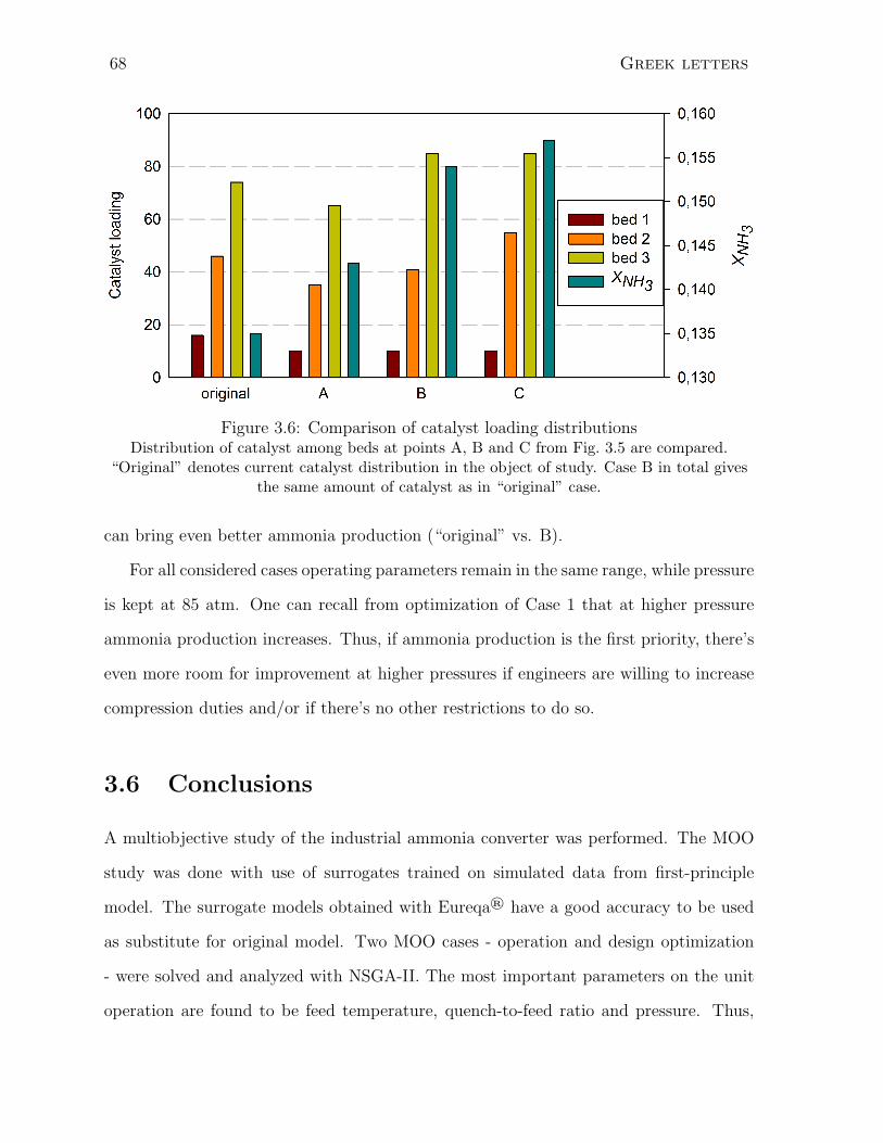
68 Greek letters
Figure 3.6: Comparison of catalyst loading distributionsDistribution of catalyst among beds at points A, B and C from Fig. 3.5 are compared.
“Original” denotes current catalyst distribution in the object of study. Case B in total givesthe same amount of catalyst as in “original” case.
can bring even better ammonia production (“original” vs. B).
For all considered cases operating parameters remain in the same range, while pressure
is kept at 85 atm. One can recall from optimization of Case 1 that at higher pressure
ammonia production increases. Thus, if ammonia production is the first priority, there’s
even more room for improvement at higher pressures if engineers are willing to increase
compression duties and/or if there’s no other restrictions to do so.
3.6 Conclusions
A multiobjective study of the industrial ammonia converter was performed. The MOO
study was done with use of surrogates trained on simulated data from first-principle
model. The surrogate models obtained with Eureqa® have a good accuracy to be used
as substitute for original model. Two MOO cases - operation and design optimization
- were solved and analyzed with NSGA-II. The most important parameters on the unit
operation are found to be feed temperature, quench-to-feed ratio and pressure. Thus,

BIBLIOGRAPHY 69
former case yielded a Pareto set of solutions compromising between ammonia production
and heat recovery depending on these parameters. The latter case showed that for any
point in Pareto set for design MOO ammonia production is higher that in operation MOO.
Therefore one can benefit even more with change of total catalyst loading in the converter
and/or proper distribution of catalyst among beds. The total ammonia production at
any point of Pareto set for design optimization was higher that for operation case even
for lower total catalyst loading in converter.
Bibliography
[1] M. Appl. Ammonia : principles and industrial practice. Wiley-VCH, Weinheim ;
New York, 1999.
[2] R. B. Kasat, D. Kunzru, D. N. Saraf, and S. K. Gupta. Multiobjective Optimization
of Industrial FCC Units Using Elitist Nondominated Sorting Genetic Algorithm.
Industrial & engineering chemistry research, 41(19):4765–4776, sep 2002. ISSN 0888-
5885. doi: 10.1021/ie020087s.
[3] R. B. Kasat and S. K. Gupta. Multi-objective optimization of an industrial fluidized-
bed catalytic cracking unit (FCCU) using genetic algorithm (GA) with the jumping
genes operator. Computers & Chemical Engineering, 27(12):1785–1800, 2003. ISSN
00981354. doi: 10.1016/S0098-1354(03)00153-4.
[4] B. Sankararao and S. K. Gupta. Multi-objective optimization of an industrial
fluidized-bed catalytic cracking unit (FCCU) using two jumping gene adaptations of
simulated annealing. Computers & Chemical Engineering, 31(11):1496–1515, 2007.
ISSN 00981354. doi: 10.1016/j.compchemeng.2006.12.012.
[5] H. Weifeng, S. Hongye, M. Shengjing, and C. Jian. Multiobjec-
tive Optimization of the Industrial Naphtha Catalytic Reforming Pro-

70 Greek letters
cess. Chinese Journal of Chemical Engineering, 15(1):75–80, feb
2007. ISSN 10049541. doi: 10.1016/S1004-9541(07)60036-6. URL
http://linkinghub.elsevier.com/retrieve/pii/S1004954107600366.
[6] M. R. Rahimpour, D. Iranshahi, E. Pourazadi, and A. M. Bahmanpour. Boosting
the gasoline octane number in thermally coupled naphtha reforming heat exchanger
reactor using de optimization technique. Fuel, 97:109–118, 2012. ISSN 00162361.
doi: 10.1016/j.fuel.2012.01.015.
[7] E. Pourazadi, R. Vakili, D. Iranshahi, a. Jahanmiri, and M. R. Rahimpour. Opti-
mal design of a thermally coupled fluidised bed heat exchanger reactor for hydrogen
production and octane improvement in the catalytic naphtha reformers. Cana-
dian Journal of Chemical Engineering, 91(1):54–65, 2013. ISSN 0008-4034. doi:
10.1002/cjce.20687.
[8] J. K. Rajesh, S. K. Gupta, G. P. Rangaiah, and A. K. Ray. Multiobjective Op-
timization of Steam Reformer Performance Using Genetic Algorithm. Industrial
& engineering chemistry research, 39(3):706–717, mar 2000. ISSN 0888-5885. doi:
10.1021/ie9905409.
[9] A. D. Nandasana, A. K. Ray, and S. K. Gupta. Dynamic Model of an Industrial
Steam Reformer and Its Use for Multiobjective Optimization. Industrial & en-
gineering chemistry research, 42(17):4028–4042, aug 2003. ISSN 0888-5885. doi:
10.1021/ie0209576.
[10] B. Sankararao and S. K. Gupta. Multiobjective optimization of the dynamic opera-
tion of an industrial steam reformer using the jumping gene adaptations of simulated
annealing. Asia-Pacific Journal of Chemical Engineering, 1(1-2):21–31, oct 2006.
ISSN 19322135. doi: 10.1002/apj.4. URL http://doi.wiley.com/10.1002/apj.4.
[11] A. Alizadeh, N. Mostoufi, and F. Jalali-Farahani. Multiobjective Dynamic Optimiza-

BIBLIOGRAPHY 71
tion of an Industrial Steam Reformer with Genetic Algorithms. International Journal
of Chemical Reactor Engineering, 5(1), 2007. ISSN 15426580. doi: 10.2202/1542-
6580.1356.
[12] A. Behroozsarand, H. Ebrahimi, and A. Zamaniyan. Multiobjective Optimization of
Industrial Autothermal Reformer for Syngas Production Using Nonsorting Genetic
Algorithm II. Industrial & engineering chemistry research, 48(16):7529–7539, aug
2009. ISSN 0888-5885. doi: 10.1021/ie900259n.
[13] H. Ebrahimi, A. Behroozsarand, and A. Zamaniyan. Arrangement of pri-
mary and secondary reformers for synthesis gas production. Chemical Engi-
neering Research and Design, 88(10):1342–1350, 2010. ISSN 02638762. doi:
10.1016/j.cherd.2010.02.021.
[14] K. Mitra, K. Deb, and S. K. Gupta. Multiobjective dynamic optimization of an
industrial nylon 6 semibatch reactor using genetic algorithm. Journal of Applied
Polymer Science, 69(1):69–87, 1998. ISSN 0021-8995. doi: 10.1002/(SICI)1097-
4628(19980705)69:1¡69::AID-APP9¿3.0.CO;2-K.
[15] M. Ramteke and S. K. Gupta. Multiobjective optimization of an indus-
trial nylon-6 semi batch reactor using the a-jumping gene adaptations of ge-
netic algorithm and simulated annealing. Polymer Engineering & Science, 48
(11):2198–2215, nov 2008. ISSN 00323888. doi: 10.1002/pen.21165. URL
http://doi.wiley.com/10.1002/pen.21165.
[16] F. B. Zhou, S. K. Gupta, and A. K. Ray. Multiobjective optimization of the continu-
ous casting process for poly (methyl methacrylate) using adapted genetic algorithm.
Journal of Applied Polymer Science, 78(7):1439–1458, 2000. ISSN 0021-8995. doi:
10.1002/1097-4628(20001114)78:7¡1439::AID-APP150¿3.0.CO;2-7.
[17] V. Bhaskar, S. K. Gupta, and A. K. Ray. Multiobjective optimization of an industrial
72 Greek letters
wiped-film pet reactor. AIChE Journal, 46(5):1046–1058, 2000. ISSN 00011541. doi:
10.1002/aic.690460516. URL http://doi.wiley.com/10.1002/aic.690460516.
[18] V. Bhaskar, S. K. Gupta, and A. K. Ray. Multiobjective optimization of an industrial
wiped film poly(ethylene terephthalate) reactor: some further insights. Computers
& Chemical Engineering, 25(2):391–407, 2001. ISSN 00981354. doi: 10.1016/S0098-
1354(00)00665-7.
[19] B. V. Babu, J. H. S. Mubeen, and P. G. Chakole. Simulation and optimization of
wiped-film poly-ethylene terephthalate (PET) reactor using multiobjective differen-
tial evolution (MODE). Materials and Manufacturing Processes, 22(5-6):541–552,
2007. ISSN 1042-6914. doi: 10.1080/10426910701319266.
[20] J. K. Rajesh, S. K. Gupta, G. P. Rangaiah, and A. K. Ray. Multi-objective optimiza-
tion of industrial hydrogen plants. Chemical Engineering Science, 56(3):999–1010,
2001. ISSN 00092509. doi: 10.1016/S0009-2509(00)00316-X.
[21] P. P. Oh, A. K. Ray, and G. P. Rangaiah. Triple-objective optimization of an
industrial hydrogen plant. Journal of Chemical Engineering of Japan, 34(11):1341–
1355, 2001. ISSN 0021-9592. doi: 10.1252/jcej.34.1341.
[22] P. P. Oh, G. P. Rangaiah, and A. K. Ray. Simulation and multiobjective opti-
mization of an industrial hydrogen plant based on refinery off-gas. Industrial &
Engineering Chemistry Research, 41(9):2248–2261, 2002. ISSN 0888-5885. doi:
10.1021/ie010277n.
[23] M. M. Montazer-Rahmati and R. Binaee. Multi-objective optimization of an indus-
trial hydrogen plant consisting of a CO2 absorber using DGA and a methanator.
Computers & Chemical Engineering, 34(11):1813–1821, 2010. ISSN 00981354. doi:
10.1016/j.compchemeng.2010.01.001.

BIBLIOGRAPHY 73
[24] K. Deb, A. Pratap, S. Agarwal, and T. Meyarivan. A fast and elitist multiobjective
genetic algorithm: NSGA-II. Ieee Transactions on Evolutionary Computation, 6(2):
182–197, 2002. ISSN 1089-778X. doi: 10.1109/4235.996017.
[25] A. Suppapitnarm, K. A. Seffen, G. T. Parks, and P. J. Clarkson. A simulated
annealing algorithm for multiobjective optimization. Engineering Optimization, 33
(1):59–85, 2000. ISSN 0305-215X. doi: 10.1080/03052150008940911.
[26] B. Mansson and B. Andresen. Optimal Temperature Profile for an Ammonia Re-
actor. Industrial & Engineering Chemistry Process Design and Development, 25:
59–65, 1986. ISSN 0196-4305. doi: 10.1021/i200032a010.
[27] S. S. E. H. Elnashaie and F. M. Alhabdan. A computer software package for
the simulation and optimization of an industrial ammonia converter based on a
rigorous heterogeneous model. Mathematical and Computer Modelling, 12(12):
1589–1600, 1989. ISSN 08957177. doi: 10.1016/0895-7177(89)90335-X. URL
http://www.sciencedirect.com/science/article/pii/089571778990335X.
[28] S. R. Upreti and K. Deb. Optimal design of an ammonia synthesis reactor using
genetic algorithms. Computers & Chemical Engineering, 21(1):87–92, 1996. ISSN
00981354. doi: 10.1016/0098-1354(95)00251-0.
[29] B. V. Babu and R. Angira. Optimal design of an auto-thermal ammonia synthe-
sis reactor. Computers and Chemical Engineering, 29(5):1041–1045, 2005. ISSN
00981354. doi: 10.1016/j.compchemeng.2004.11.010.
[30] N. V. Queipo, R. T. Haftka, W. Shyy, T. Goel, R. Vaidyanathan, and P. K. Tucker.
Surrogate-based analysis and optimization. Progress in Aerospace Sciences, 41(1):
1–28, 2005. ISSN 03760421. doi: 10.1016/j.paerosci.2005.02.001.
[31] A. I. J. Forrester and A. J. Keane. Recent advances in surrogate-based optimiza-

74 Greek letters
tion. Progress in Aerospace Sciences, 45(1):50–79, 2009. ISSN 03760421. doi:
10.1016/j.paerosci.2008.11.001.
[32] N. Quirante, J. Javaloyes, and J. Caballero. Rigorous Design of Distillation Columns
Using Surrogate Models Based on Kriging Interpolation. AIChE Journal, 61(7):
2169–2187, 2015. doi: 10.1002/aic.14798.
[33] U. Abubakar, S. Sriramula, and N. C. Renton. A Hybrid Method for
Stochastic Performance Modeling and Optimization of Chemical Engineering
Processes. Chemical Engineering Communications, 202:217–231, 2015. doi:
10.1080/00986445.2013.838159.
[34] I. Sharma, A. Hoadley, S. M. Mahajani, and A. Ganesh. Methodology for Surro-
gate Assisted Multi-Objective (MOO) Optimization for Computationally Expensive
Process Flowsheet Analysis. Journal of Chemical Information and Modeling, 45:
349–354, 2015. ISSN 1098-6596. doi: 10.1017/CBO9781107415324.004.
[35] M. Schmidt and H. Lipson. Distilling Free-Form Natural Laws from Experimental
Data. Science, 324(5923):81–85, 2009.
[36] M. Schmidt and H. Lipson. Eureqa, 2014. URL www.nutonian.com.
[37] S. S. E. H. Elnashaie, M. E. Abashar, A. S. Alubaid, and A. S.
Al-Ubaid. Simulation and optimization of an industrial Ammo-
nia Reactor. Industrial & Engineering Chemistry Research, 27(8):
2015–2022, 1989. ISSN 08885885. doi: 10.1021/ie00083a010. URL
http://pubs.acs.org/doi/abs/10.1021/ie00092a024.
[38] A. Cozad, N. V. Sahinidis, and D. C. Miller. Learning surrogate models for
simulation-based optimization. AIChE Journal, 2014. ISSN 15475905. doi:
10.1002/aic.14418.

BIBLIOGRAPHY 75
[39] M. J. D. Powell. A view of algorithms for optimization without derivatives. Math-
ematics Today-Bulletin of the Institute of . . . , 43(5):1–12, 2007. ISSN 1361-2042.
URL http://www.damtp.cam.ac.uk/user/na/NA papers/NA2007 03.pdf.

Chapter 4
Data-Based Modelling And
Optimization Of Carbon Dioxide
Removal From Process Gas
76

Nomenclature 77
Nomenclature
A− 1 absorption tower
abs absorbent
C− 1 cooler
D− 1 desorber
L liquid level
Nclust number of clusters
ni number of points in ith cluster
P pressure
p refers to point in cluster
P− 1 solvent pump
Q volumetric flow rate
RMSE root mean squared error
S− 1 separator
SOM self-organizing maps
T temperature
X molar fraction
4.1 Introduction
Carbon dioxide occurs as an undesired flow component in a number of chemical engineer-
ing processes, such as industrially mature natural gas treatment ammonia production1
or power generation, or more modern as biogas production2, etc. The purpose of CO2
removal may vary, from gas pre-treatment to its further conversion. Depending on the
required extent of carbon dioxide removal, scale of production or other process features
78 Nomenclature
there are a number of technologies available nowadays. Carbon dioxide is removed by
chemical or physical absorption using selective solvents or solids3,4, pressure swing ad-
sorption5or membrane separation.6 Some of these ways have long history and wide spread
among industries, while others are more modern.
In the large scale processes, the use of physical and chemical solvents is more common.
Conventionally, the process undergoes through two stages. Firstly, carbon dioxide cap-
ture occurs in a contact unit through direct gas-liquid contact. Later, captured carbon
dioxide is released in a solvent-regeneration unit. This absorption-desorption loop allows
carbon dioxide removal unit to operate in a continuous mode.
There is significant number of works published in the literature dedicated to the
modelling of industrial carbon dioxide removal units. Robinson and Luyben 7 performed
a modelling of carbon dioxide removal unit as a part of a large scheme of integrated
gasification combined cycle (IGCC). CO2 along with other contaminants occur there as
a result of fuel combustion. They developed a dynamic model using Aspen Dynamics.
Optimal equipment design was selected based on desired product purity; and dynamic
simulation was performed to evaluate performance of the IGCC plant under disturbing
conditions.
Similarly to previous work, Bhattacharyya et al. 8 performed a steady-state simulation
of IGCC plant with Aspen Plus. Conceptual way was illustrated in how to optimize IGCC
plant, what parameters should be accounted for and how to utilize them while solving
optimization problem. However, it was not applied to any existing plant. They used the
model for overall three-phase plant optimization while targeting CO2 capture as one of
objective functions. They came up with various scenarios for best plant design decisions.
Kapetaki et al. 9 authors are striving to achieve higher carbon dioxide removal effi-
ciency than the authors of two previous researches. They used Honeywell UniSim for
steady state modelling of carbon dioxide removal unit. They investigated two differ-
ent process operating modes under different operating conditions (e.g. unit pressure,

4.1. Introduction 79
absorbent flow rate) onto process performance (i.e. carbon dioxide capture, power con-
sumption).
Mores et al. 10 performed modelling and optimization study of carbon dioxide removal
with monoethanol amine solvent. Their model was implemented with General Algebraic
Modeling System. The model underlies complex heat and mass transfer equations with
a significant number of process parameters and technological constraints. This work is
mainly focused on improvement to be made in solvent regeneration from CO2. To do so
two objective functions were proposed: to minimize heat duty in reboiler and to minimize
ratio (heat duty in reboiler/CO2 removal).
The object of this study is an industrial solvent-based carbon dioxide absorber. In
this work authors intend to utilize different approach for modelling of the latter. Firstly,
we are performing the study of real operating unit aimed for synthesis gas purification
in the ammonia production chain. Carbon dioxide has to be removed there up to certain
percentage in order to avoid catalyst poisoning downstream. While carbon dioxide re-
moval itself on this unit is efficient enough and practically does not raise any optimization
problem, but solvent regeneration bears a room for improvement. Therefore, authors are
focusing on quality of solvent regeneration. The requirements which constitute qual-
ity will be addressed below in process description. Thirdly, we are willing to utilize vast
amount of available industrial data. It covers a quite long time span of the unit operating
history. This work is done in collaboration with plant engineers, thus their engineering
judgment is taken into high consideration. Overall, they are quite satisfied with the
mode of the unit operation and quality of treated gas. However, throughout this work
we intend to determine most important parameters to be used in process performance
improvements having minor interference with the current operation mode. Note: due to
proprietary reasons all the data used throughout this paper related to the real operating
conditions of the industrial unit is provided in dimensionless form.

80 Nomenclature
Treated gas
Leanabsorbent
Recycle gas Recovered CO2
A-1 D-1
S-1
P-1C-1
Desorbingagent
2
CO rich gas2
Figure 4.1: Process flow diagram for carbon dioxide removal
4.2 Process description
One of the most conventional technologies for ammonia synthesis uses natural gas as
a feedstock. Overall description of ammonia synthesis from natural gas can be found
elsewhere.1 Briefly, the process gas is mainly (80-90 % mol.) made of hydrogen and
nitrogen in the ration close to stoichiometric (3:1). The remaining gases are unconverted
methane, argon, carbon dioxide and carbon monoxide. Remaining carbon oxides in the
gas originate from steam reforming reaction followed by gas shift reaction. A gas stream
contains 10-15% mol. of carbon dioxide at the inlet of the treatment unit. If not removed,
carbon dioxide will act as a catalyst poison downstream in the ammonia converter.
Thus, carbon dioxide removal unit serves for process gas purification. Untreated gas
from shift conversion enters to the bottom of to the packed bed absorber A− 1 (Fig. 4.1).
Lean absorbent is supplied through the top of A-1 where CO2 removal occurs through
gas-liquid absorption in a counter-current fashion. However, absorbent is selective to
CO2, but all of the process gasses are getting captured but in a lesser amount. A second
most captured gas is hydrogen. The treated gas leaving from the top of A-1 contains
10-1000 ppm. of carbon dioxide. The actual concentration highly depends on solvent
and process operating conditions.

4.3. Process modelling 81
Further, the solvent is freed from captured gases through two stages desorption.
Firstly, CO2-rich solvent leaves from the bottom of A− 1 to the cooler C− 1 where
its temperature drops down. When cooled, it flows into separator S− 1. Prior to en-
tering S− 1 flow pressure is dropped and absorbed gases are partially released from top
(Recycle gas). Recycle gas is mainly carbon dioxide and hydrogen with minor part of
other gases from the gas stream. Then, half-rich CO2 solvent flows to the desorber D− 1.
Similarly to A− 1, the desorber D− 1 is a packed bed contact unit there remaining gases
are stripped away fully regenerating lean solvent. Remaining gases are stripped from the
top of a column. Lean absorbent is compressed in the pump P− 1 up to operating
pressure and recycled back to the absorber.
4.3 Process modelling
The instrumentation and chromatography analysis data obtained from industrial carbon
dioxide recovery unit was used for the modelling. The data covers a time span for several
years of the unit operation. It includes process instrumentation readings such as from
pressure or temperature indicators, flow meters, etc., as well as chromatography analysis
of gas flows at the unit. The entire set of original data was pre-treated to remove irrelevant
information which could occur due to indicators failure and malfunction, a human error
or errors of any kind.
Firstly, data inspection was done visually appealing to common sense and engineering
judgment of the authors and plant engineers. Then, it was clustered using self-organizing
maps (SOM) (described below) in order to determine outlying groups of data. After pre-
screening was accomplished, the post-treated data set contained around 350 points.
Operating range of real industrial unit is quite narrow, i.e. process parameters cannot
vary in wide range due to some engineering restrictions. Hence, the correlations between
inputs and outputs can assumed to be linear, therefore linear regression to be used.

82 Nomenclature
As with majority of data-based models, during training one may face over-fitting
problem. To resolve the faced problem with models training, one may take a closer look
into the operation of a large scale industrial unit and, particularly, the instrumentation
readings. The carbon dioxide removal unit is a continuously operating unit serving for
the only purpose to provide treated gas of a certain quality for its further downstream
conversion. This quality has to be maintained all the time for stable plant operation.
As with many large scale continuous units, the object of this study is operating in the
steady state most of the time. It is worth to admit that in reality the instrumentation
readings and analysis during a steady state operation are obviously not constant, they are
subject to random noise, fluctuations in feedstock quality and feed rate, malfunctioning,
etc. Transition between the states occurs when engineers decide to change operating
conditions and shift unit into a new state.
At the same time, the instrumentation readings and gas analysis occur on the regular
basis and are almost evenly distributed in time. Thus, the longer the unit was in state
a the more data points are retrieved from the system. When the unit changed its state
into state b for a shorter time, we end up with fewer points for the new state. However,
this points deliver for us useful information about units performance. This is happening
several times during the entire unit operation (state c, etc.). Lets consider a generic
uni-variate case of such unit operation (Fig. 4.2).
Imagine we have three real states a unit have been into over observed period of time.
They are marked in solid black circles. If we were able to measure these values, applying
least square method we would get an ideal regression model (black line). No doubt it is
impossible to achieve it with real data because all the measurements are subject of noise
and uncertainty.
Lets compare two independent cases. In the case 1 measurements are done rarely,
so we have just a few points representing each true state (green dots). In the case 2,
measurements were more frequent and more observation points were gathered (red dots).

4.3. Process modelling 83
Figure 4.2: Single variable generic case for linear regression of industrial data
Since time spans of true states are differ time, we have more points representing state
2 and less for states 1 and 3. If we apply least square regression to both cases, we
can conclude that if we have bigger data cloud for state 2 (i.e. case 2), it causes more
significant deviation from ideal case than having less points (i.e. case 1). So we obtain
distortion of results if we dont account for that. Thus, it is necessary to diminish impact
of data clouds onto regression model.
If we apply least square regression to both cases, we can conclude that if we have
bigger data cloud for state 2 (i.e. case 2), it causes more significant deviation from ideal
case than having less points (i.e. case 1). So we obtain distortion of results if we dont
account for that. Thus, it is necessary to diminish impact of data clouds onto regression
model.
If we take a closer look onto industrial data, we can find that there are some denser
regions, while some other are scattered or even few points at all (Fig. 4.3). Lets do
not forget that real problem is multivariate and similar effects can be observed in other
dimensions. If we disregard this phenomena we obtain regression model which tends
to deviate more from real units performance. Authors understand that perception of

84 Nomenclature
13.4
13.5
13.6
13.7
10 11 12 13
Variable
Re
sp
on
se
Figure 4.3: Example of real industrial data
whether the model underestimates or overestimates the real performance is unclear and
subjective. Thus, the criteria to decide about models ability to describe units performance
was based on common sense and long-time experience of plant engineers who were able
to provide us with a reliable feedback on model performance.
To diminish impact of dense regions we are going to incorporate least square regression
with clustering algorithm. Clustering will allow for aggregation points within dense
regions and diminish effect of large clusters. To clarify, by this means we do not intend
to explicitly divide data into the exact number of steady states in which unit has been
operated. We just willing to account for the impact of big data clouds, thus mitigating
their distortion effect and cutting through the clusters.
4.4 About clustering
Clustering is a general word to describe a number of methods aimed for grouping data.
The criteria for grouping as well as techniques vary widely.11 For the sake of clarity, one
can say that points within a particular cluster bear more resemblance to each other than

4.5. Model training and validation 85
to points belonging to another cluster. For example, similarity between data points can
be expressed as metric distance, e.g. Euclidean distance in K-means clustering12 or some
other cases of Minkowski distance is used in hierarchical clustering13.
In the purpose of this work, authors used a self-organizing maps also known as Ko-
honen maps (SOM).14 SOMs provide mapping of multi-dimensional variables into two-
dimensional space. One pre-defines SOM topology first (i.e. type of grid). Each node in
the grid is referred as a codebook vector. Then SOM learning algorithm maps original
data into discrete locations around codebooks. Thus to be said that each codebook vec-
tor is representation of group of data points (cluster) gathered around it. The entire set
of them in the SOM grid depicts structure of entire data set. More detailed description
of learning algorithm can be found elsewhere.14,15
Fig. 4.4 shows the example of codebook vectors obtained with SOM while clustering
industrial data. Values of data points within each cluster are in the close proximity with
values of codebook vectors. Coloured leaves with each sub diagram illustrate relative
values of each process parameter. For example, counting row-wise from top left corner,
one can say cluster three has larger values of QA−1 and XA−1H2
or cluster seven has higher
values of Qabs than others, etc. Thus, SOM mapping provides one, firstly, with intuitive
sense of the data structure. It is worth to note that from a practical point of view it
a convenient way for outlier screening in the raw data. One can cluster data first and
then check out clusters with outstanding values. Secondly, SOM mapping provides one
directly with clusters of data assigning each point to a particular coding vector.
4.5 Model training and validation
The following assumptions have been made prior to the modelling. Firstly, absorber
A− 1 operates in steady state under the same conditions, i.e. feedstock flow conditions
and unit operating conditions are constant. Thus, flows leaving A− 1 from top and

86 Nomenclature
QA-
XH
A-
XCO
A-
PS-
LS-
TC-
TP-
Qabs
Figure 4.4: SOM coding vectors
bottom are also have constant conditions, i.e. composition, temperature, pressure, etc.
We find it a reasonable assumption, because the plant operates at constant production
rate and it is crucial to maintain the quality of treated gas over time to provide stable
operation of ammonia synthesis reactor. As it was confirmed by distribution of operating
conditions over considered time span.
Secondly, we assume a feed rate of stripping agent constant since no flow meter is
installed on the line to retrieve this data. Thirdly, as we mainly interested in two most
absorbed components CO2 and H2 we dont consider remaining components separately,
but as lump of. Summarizing, to perform modelling and evaluate performance of carbon
dioxide removal unit authors selected to predict 3 response properties (Table 4.1) based
on the defined set of variables. Any other needed flow properties within the unit can be
calculated from mass balance of the process.
Original data set was divided into training and validation sets. The former was
used for model fitting and the latter for evaluating model performance. The training
procedure was as follows. The training data was clustered into Nclust clusters with each

4.6. Variable selection and ranking 87
Table 4.1: Performance criteria of carbon dioxide removal unit used in the modelling
Response Description
QtopS−1 Volumetric feed rate of recycle gases from S− 1
XD−1CO2
Mole fraction of CO2 in top gas from D− 1
XD−1H2
Mole fraction of H2 in top gas from D− 1
Table 4.2: Performance criteria of carbon dioxide removal unit used in the modelling
Variable Description
LS−1 Liquid level in separator S− 1PA−1 Pressure in absorber A− 1PD−1 Pressure in desorber D− 1PS−1 Pressure in separator S− 1TC−1 Temperature of CO2 reach absorbent after cooler C− 1TP−1 Temperature of lean absorbent after pump P− 1Qin
A−1 Volumetric feed rate of gas into absorber A− 1Qabs Volumetric feed rate of absorbent in CO2 removal loopXA−1
CO2
Mole fraction of CO2 in feed gas to A− 1
XA−1H2
Mole fraction of h2 in feed gas to A− 1
cluster having ni points. Point pji is given weight of 1/ni. Thus points within bigger
clusters are assigned smaller individual weights and clusters have even impact on the
regression. Then least square linear regression model is fitted over weighted data, and
models performance is evaluated with validation data. For validation score root mean
squared error (RMSE) is used. The procedure is repeated for different Nclust and the one
with least RMSE score is chosen.
4.6 Variable selection and ranking
Prior to modelling, one needs to be explained with procedure of variable selection for
modelling. We selected all process parameters which are a) aimed for control of process
performance, b) parameters which affect process performance thermodynamic-wise and
c) which are stored in the industrial data base in a sufficient amount. List of selected
variables is given in Table 4.2.

88 Nomenclature
a)
b)
c)
Figure 4.5: Variable importance test with Boruta: a) XD−1H2
, b) XD−1CO2
, c) QtopS−1
Then variables were tested and ranked for relative importance onto each of the re-
sponse parameters. Boruta method16 was used for feature selection. The method ranks
variables based on the Z-score of Random Forest.17 In addition, it creates a number of
random attributes and compares their Z-cores with scores ones of real attributes. Real
attributes only with Z-scores higher than maximum the Z-core of random attributes are
considered as relevant for prediction of the response. Fig. 4.5(a-c) shows the ranking of
accepted variable for each of three responses.

4.7. Results and discussion 89
4.7 Results and discussion
Carbon dioxide unit model is developed in R language.18 Additional R packages caret19,20
are used for data pre-processing and clustering respectively, package Boruta21 is used for
variable ranking.
4.8 Model validation
Self-organizing maps of rectangular topology are used for clustering, since they have
shown good performance in clustering industrial data on the data pre-processing stage.
However, authors believe that the use of other clustering methods will not change the
approach significantly.
Firstly, one can conclude from Fig. 4.6 that fewer number of clusters allows for RMSE
reduction better than more clusters. Maximum SOM topology 6 by 6 SOM was chosen
since mapping 350 points into larger number of clusters is not reasonable.
Secondly, one can admit that in some cases the proposed method works better than
in others. Thus, in case of XD−1CO2
and QtopS−1 and XD−1
H2
(Fig. 4.6a,c) we obtain evident
solution for the SOM size depending on RMSE values. In case XD−1CO2
it was not clear
which SOM topology to choose, thus for consistency with two other cases we selected 3
by 3. Table 3 shows RMSE obtained on validation data set. Fig. 4.7 depicts validation
plots for property prediction.
On the next step, we attempted to reduce a number of variables used for regression.
Since not all of them are possible to include into optimization problem due to technolog-
ical constraints, we intend to limit their number only to the most industrially important
ones. We took Z-score of Boruta test as a measure of relative importance and fitted the
model removing less important variables one by one (i.e. from left to right on Fig. 4.5.
Fig. 4.8 shows the effect of number of variables on RMSE. It is observed that by use of

90 Nomenclature
a)
b)
c)
Figure 4.6: Cluster size vs. RMSE: a) XD−1H2
, b) XD−1CO2
, c) QtopS−1
less number of variables (comparing to the original ones, i.e. number of removed variables
= 0) it is possible to further reduce cross validation error.
While selecting the finalized number of variables for regression, authors compromised
between the minimum RMSE score and practical importance of the variables. The final-
ized variables are given in Table 4.3.
Here it is worth to notice one fact about chosen process variables. Liquid level in sep-
arator LS−1 has the highest Z-score among other variables for all responses, thus having
significant effect towards process performance. Industrially-wise, it is relatively simple
to control liquid level in the vessel rather any other parameters, such as temperature
or pressure. The variations in the latter might be restricted due to design, safety or

4.8. Model validation 91
a)
b)
c)
Figure 4.7: Validation plot: a) XD−1H2
, b) XD−1CO2
, c) QtopS−1
other engineering reasons. Should we apply conventional first principle modelling for
carbon dioxide removal in the unit, it would be problematic to account for that process
parameter as a decision variable for modelling and optimization. Authors believe that
this phenomenon might happen due to change in the residence time of absorbent in the
vessel. The hypothesis makes sense, since higher residents time favour separation of ab-
sorbed gases. However, the exact reason for this fact has to be established in the further
research, which might involve CFD modelling and simulation.

92 Nomenclature
Figure 4.8: Effect of number of variables on RMSE: a) XD−1H2
, b) XD−1CO2
, c) QtopS−1
4.9 Operation optimization
Out of 5 process parameters used for modelling (Table), two were selected to be used as
decision variables (Qabs and LS−1), while others are keep constant at their industrially
feasible values. Values of TC−1 and PS−1 are taken at the designed values. TP−1 cannot be
controlled directly, thus the average value for the observed period of time is taken. Upper
and lower bounds for Qabs and LS−1 are chosen in accordance with industrial values.
Objectives for optimization were established as 1) to achieve carbon dioxide flow from

4.9. Operation optimization 93
Table 4.3: Performance criteria of carbon dioxide removal unit used in the modelling
Response Number of removed variables Variables RMSE
XD−1H2
4
TC−1
0.6200PS−1
Qabs
LS−1
XD−1CO2
4
TC−1
0.0673PS−1
Qabs
LS−1
QtopS−1 4
Qabs
2.4635TP−1
PS−1
LS−1
desorber D− 1 of a given purity and 2) to recover more hydrogen from S− 1. One can
summarize optimization problem as follows:
I1 : XD−1CO2
= X targetCO2
I2 : maximizeQS−1h2
subject to :
min ≤ Qabs, LS−1 ≤ max
TC−1, PS−1, TP−1 = constant
(4.1)
Fig. 4.9 depicts the response surface between decision variables and either of objec-
tives. Firstly, one can note that two objectives are not in conflict. Either of decision
parameters favouring one of objectives favours another one as well. Industrial-wise, it is
an advantageous phenomenon. It is possible to satisfy both objective at the same time,
thus avoiding any compromising solution. Thus it is needed to increase the liquid level
LS−1 in S− 1 and lower absorbent circulation rate in the system to improve gas recovery.
Secondly, there is a vast possibility for process performance improvement. The yellow
line shows the current operating values for XD−1CO2
and QS−1H2
. One the one hand, it is
possible to reach the goal of I1, because the point lies within the plane. However, at that

94 Nomenclature
a) b)
Figure 4.9: Process parameters vs. objectives. a) XD−1CO2
, b) QtopS−1
Yellow lines are representing intersection of current operation plane with the response surface.Green dot indicates the goal value for XD−1
CO2
point decision variables both hit its bounds (LS−1 reach upper while Qabs reach lower).
Even though it is not always possible to completely minimize absorbent circulation rate
(e.g. due to unexpected overflow of synthesis gas to A− 1), but the unit still has capacity
to operate with improved performance. Operation-wise, it is relatively easy to change
liquid level in the vessel with regard to other process conditions. Increase in the level
alone provides significant performance boost even when QS−1H2
is not at the minimum.
4.10 Conclusions
In this work data-based modelling approach is utilized in order to optimize the recovery
of valuable gases of carbon dioxide removal unit. Carbon dioxide removal technology in-
formation, process flow diagram and description as well as data for several years of plant
operation are used for modelling. Linear relations between process and performance pa-
rameters are assumed due to narrow operation range and engineering limitations. Data-
based model was built as conjunction of self-organizing maps with least square linear
4.10. Conclusions 95
model. Model validation was done with industrial data. It has achieved satisfactory
performance in order to solve the proposed optimization task. The number of relevant
process parameters were narrowed down with Boruta algorithm (i.e. liquid level in sep-
arator and absorbent circulation rate). The model revealed significant room for process
performance improvements. It is possible to reach the goal of optimization task within
the process bounds.

96 Nomenclature
Nomenclature
A− 1 absorption tower
abs absorbent
C− 1 cooler
D− 1 desorber
L liquid level
Nclust number of clusters
ni number of points in ith cluster
P pressure
p refers to point in cluster
P− 1 solvent pump
Q volumetric flow rate
RMSE root mean squared error
S− 1 separator
SOM self-organizing maps
T temperature
X molar fraction
Bibliography
[1] M. Appl. Ammonia : principles and industrial practice. Wiley-VCH, Weinheim ;
New York, 1999.
[2] A. Arya, S. Divekar, R. Rawat, P. Gupta, M. O. Garg, S. Dasgupta, A. Nan-
oti, R. Singh, P. Xiao, and P. A. Webley. Upgrading Biogas at Low Pres-

BIBLIOGRAPHY 97
sure by Vacuum Swing Adsorption. Industrial & Engineering Chemistry Re-
search, 54(1):404–413, 2015. ISSN 0888-5885. doi: 10.1021/ie503243f. URL
http://pubs.acs.org/doi/abs/10.1021/ie503243f.
[3] C.-H. Yu. A Review of CO2 Capture by Absorption and Ad-
sorption. Aerosol and Air Quality Research, pages 745–769,
2012. ISSN 16808584. doi: 10.4209/aaqr.2012.05.0132. URL
http://www.aaqr.org/Doi.php?id=7 AAQR-12-05-IR-0132&v=12&i=5&m=10&y=2012.
[4] Y. E. Kim, J. A. Lim, S. K. Jeong, Y. I. Yoon, S. T. Bae, and S. C. Nam. Comparison
of carbon dioxide absorption in aqueous MEA, DEA, TEA, and AMP solutions.
Bulletin of the Korean Chemical Society, 34(3):783–787, 2013. ISSN 02532964. doi:
10.5012/bkcs.2013.34.3.783.
[5] S. Cavenati, C. A. Grande, and A. E. Rodrigues. Removal of carbon dioxide from
natural gas by vacuum pressure swing adsorption. Energy and Fuels, 20(6):2648–
2659, 2006. ISSN 08870624. doi: 10.1021/ef060119e.
[6] E. Sjoberg, S. Barnes, D. Korelskiy, and J. Hedlund. MFI membranes for separation
of carbon dioxide from synthesis gas at high pressures. Journal of Membrane Science,
486:132–137, jul 2015. ISSN 03767388. doi: 10.1016/j.memsci.2015.03.041. URL
http://www.sciencedirect.com/science/article/pii/S0376738815002197.
[7] P. J. Robinson and W. L. Luyben. Integrated Gasification Combined Cy-
cle Dynamic Model: H2S Absorption/Stripping, WaterGas Shift Reactors, and
CO2 Absorption/Stripping. Industrial & Engineering Chemistry Research, 49
(10):4766–4781, 2010. ISSN 0888-5885. doi: 10.1021/ie901549s. URL
http://pubs.acs.org/doi/abs/10.1021/ie901549s.
[8] D. Bhattacharyya, R. Turton, and S. E. Zitney. Steady-State Simula-
tion and Optimization of an Integrated Gasification Combined Cycle Power

98 Nomenclature
Plant with CO 2 Capture. Industrial & Engineering Chemistry Research,
50(3):1674–1690, 2011. ISSN 0888-5885. doi: 10.1021/ie101502d. URL
http://dx.doi.org/10.1021/ie101502d.
[9] Z. Kapetaki, P. Brandani, S. Brandani, and H. Ahn. Process simulation of a dual-
stage Selexol process for 95% carbon capture efficiency at an integrated gasifica-
tion combined cycle power plant. International Journal of Greenhouse Gas Con-
trol, 39:17–26, aug 2015. ISSN 17505836. doi: 10.1016/j.ijggc.2015.04.015. URL
http://www.sciencedirect.com/science/article/pii/S1750583615001589.
[10] P. Mores, N. Scenna, and S. Mussati. CO2 capture using monoethanolamine
(MEA) aqueous solution: Modeling and optimization of the solvent
regeneration and CO2 desorption process. Energy, 45(1):1042–1058,
sep 2012. ISSN 03605442. doi: 10.1016/j.energy.2012.06.038. URL
http://www.sciencedirect.com/science/article/pii/S0360544212004896.
[11] R. Xu and Donald Wunsch II. Survey of clustering algorithms. IEEE Transactions on
Neural Networks, 16(3):645–678, 2005. URL http://arxiv.org/abs/0912.2303.
[12] C. M. Bishop. Pattern Recognition and Machine Learning, vol-
ume 4. 2006. ISBN 9780387310732. doi: 10.1117/1.2819119. URL
http://www.library.wisc.edu/selectedtocs/bg0137.pdf.
[13] P. Filzmoser and F. Group. Kurt Varmuza. 2008. ISBN 9781420059472.
[14] T. Kohonen. The self-organizing map. Proceedings of the IEEE, 78(9):1464–1480,
1990. ISSN 0018-9219. doi: 10.1109/5.58325.
[15] R. Gentleman, K. Hornik, and G. Parmigiani. Use R ! 2008. ISBN 978-0-387-78170-
9. doi: 10.1007/978-0-387-78171-6.

BIBLIOGRAPHY 99
[16] M. B. Kursa and W. R. Rudnicki. Feature Selection with the Boruta Package.
Journal Of Statistical Software, 36(11):1–13, 2010. ISSN 15487660. doi: Vol. 36,
Issue 11, Sep 2010. URL http://www.jstatsoft.org/v36/i11/paper.
[17] L. Breiman. Random forest. Machine Learning, 45:1–35, 1999. ISSN 0885-6125.
doi: 10.1023/A:1010933404324.
[18] R Core Team. R: A Language and Environment for Statistical Computing, 2015.
URL http://www.r-project.org/.
[19] M. Kuhn. Caret, 2015. URL https://cran.r-project.org/web/packages/caret/index.html.
[20] R. Wehrens. kohonen: Supervised and Unsupervised Self-Organising Maps, 2015.
URL https://cran.r-project.org/web/packages/kohonen/index.html.
[21] M. B. Kursa and W. R. Rudnicki. Boruta: Wrapper Al-
gorithm for All-Relevant Feature Selection, 2015. URL
https://cran.r-project.org/web/packages/Boruta/index.html.

Chapter 5
Multi-objective optimization of the
industrial ammonia converter with
respect to catalyst deactivation
100

5.1. Introduction 101
5.1 Introduction
Ammonia synthesis has a major importance for chemical industry. It has been one of
the first processes commercialized at industrial scale. Ammonia has been used widely in
different areas - from direct application and manufacturing of agricultural fertilizers (e.g.
urea, ammonium nitrate) to production of polymer fibers and explosives.1
The way to improve performance of ammonia synthesis in the existing units is pro-
cess simulation using comprehensive mathematical models followed by numerical opti-
mization. Having a valid model is essential for accurate representation of an industrial
system. The subject has been continuously drawing attention over the years as a num-
ber of works are present in the literature. Models have been developed for converters
of different designs, e.g. for autothermal converters2–4, with multiple adiabatic catalyst
beds5–7. Models differ in their complexity, from simple plug flow to more comprehensive
heterogeneous ones accounting for species transport in catalyst pores. Application of
heterogeneous models to industrial converter modelling showed a very good consistency
with industrial data and to be more robust.6,8
Also, attempts have been made towards optimization of converter performance. Most
of works have maximization of ammonia production as the main objective6,9, while other
maximize overall economic return of the process.4,10 However, none of the works to
the best of authors knowledge, use multi-objective approach for converter optimization
(MOO). As the industrial ammonia converter being a complex system, it is beneficial
to include more than one objective into consideration. MOO has been successfully ap-
plied for a number of industrial processes. Many works have been reported for MOO of
oil refining processes11–16, polymer manufacturing17–22, hydrogen plants23–26, and many
others. Therefore, there’s no doubt that applying MOO is beneficial and able to provide
better operating conditions for ammonia converter.
Another side of converter optimization that has not been addressed is account for cat-

102 Chapter 5. MOO with catalyst deactivation
alyst deactivation. It is the case with many solid catalysts that their performance drops
with time.27 Therefore, it is important to optimize converter performance with respect to
changing activity of catalyst.28 Ammonia catalyst deactivation can be happening due to
absorption of oxygen compounds (i.e. CO, CO2, H2O) and non-metallic compounds(i.e.
sulphur or arsenic) if any present in the process gas stream. However, absorption of poi-
sonous compounds on catalyst surface is reversible, but poisoning is stable and activity
does not return to it original state.29 Even though short-term operation-wise catalyst
deactivation is not the most crucial issue as catalyst lifetime is quite long (reaching up to
several years1), but in a long run optimal operating conditions are still different. There-
fore, it is necessary to adjust them with respect to catalyst deactivation at real process
conditions.
In this work, we perform multi-objective optimization study of industrial ammonia
converter. We use first principle mathematical model of catalytic converter. It accounts
for heterogeneous gas-solid reaction over catalyst and utilizes model for heat recovery sys-
tem used in the object of study. The model was used to estimate catalyst deactivation
rate and kinetic parameters of catalyst at different lifetimes. In order to do estimation,
we propose a method to treat industrial data and extract valuable information from it.
Finally, the MOO of converter performance was done with respect to catalyst deactiva-
tion.
5.2 Overview of converter model
In the Haber process ammonia is produced through the reaction of hydrogen and nitrogen
(Eq. 5.1). The reaction is carried out under elevated temperature and pressure to suffice
significant yield. The Eq. 5.1 is a gas-solid reaction occurring in presence of iron or
ruthenium catalyst. The catalytic ammonia converter is made of few packed beds. The
reaction mixture is sequentially fed into beds to produced ammonia in a number of

5.2. Overview of converter model 103
Figure 5.1: Ammonia converter schematic
steps. The intermediate cooling is essential as the reaction 5.1 is exothermic. To prevent
catalyst from exposure to high temperatures and shift reaction equilibrium the excess
heat is removed between beds.
The object of study is a three bed ammonia converter. The simplified layout is
provided at Fig. 5.1. The synthesis gas is split into two flows - for main feed and quench.
The main feed enters prior the first bed, while quenching is done in between. The process
gas passes through a bed and experiences a temperature rise. This is where quenching
and heat recovery is used - to remove the excess heat from the gas stream.
The model mainly consist of four parts covering phenomena occurring during am-
monia synthesis. They are reaction kinetic, intraparticle species diffusion, catalyst bed
hydrodynamics and model of heat recovery system. The detailed description can be
found below.
Note. This work was done on existing ammonia converter and real industrial data
was used. Due to proprietary reasons authors cannot disclose full layout of converter and
model details. Therefore, heat transfer system and catalyst bed arrangement will remain
unknown for the reader. Also, all numbers related to process operating conditions are
given in dimensionless form. However, reader will not loose generality of the work flow
as we are mainly focusing on process optimization and relative trends in variables.
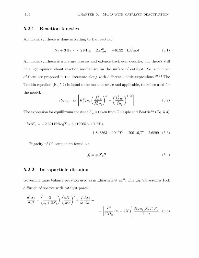
104 Chapter 5. MOO with catalyst deactivation
5.2.1 Reaction kinetics
Ammonia synthesis is done according to the reaction:
N2 + 3H2 2NH3, ∆H0298 = −46.22 kJ/mol (5.1)
Ammonia synthesis is a mature process and extends back over decades, but there’s still
no single opinion about reaction mechanism on the surface of catalyst. So, a number
of them are proposed in the literature along with different kinetic expressions.30–34 The
Temkin equation (Eq.5.2) is found to be most accurate and applicable, therefore used for
the model:
RNH3= k2
[
K2afN2
(
f 3H2
f 2NH3
)α
−
(
f 2NH3
f 3H2
)1−α]
(5.2)
The expression for equilibrium constantKa is taken from Gillespie and Beattie 35 (Eq. 5.3):
logKa = −2.691122logT − 5.519265× 10⁻⁵T+
1.848863× 10⁻⁷T 2 + 2001.6/T + 2.6899 (5.3)
Fugacity of i th component found as:
fi = φiXiP (5.4)
5.2.2 Intraparticle dissuion
Governing mass balance equation used as in Elnashaie et al. 8 . The Eq. 5.5 assumes Fick
diffusion of species with catalyst pores:
d2Xi
dω2−
(
2
νi + 2Xi
)(
dXi
dω
)2
+2
ω
dXi
dω=
−
[
R2p
CDie
(νi + 2Xi)
]
RNH3(X, T, P )
1− ǫ(5.5)

5.3. Industrial data analysis 105
subject to boundary conditions:
ω = 0 :dXi
dω= 0
ω = 1 : Xi = Xi(bulk)
Solving the following equation one can find concentration profile in radial direction of
catalyst particle and then incorporate it as effectiveness factor η:
η =
∫ 1
0
ω2RNH3(ω,X, T, P )dω
RNH3bulk(Xbulk, Tbulk, Pbulk)
(5.6)
5.2.3 Mass and energy balance
For catalyst bed hydrodynamics model we adopt one-dimensional plug flow model. There-
fore, differential mass and energy balance equations are written as:
dχ
dV=
ηRNH3(X, T, P )
2F 0N2
dT
dV=
(−∆HR)ηRNH3(X, T, P )
mgasCp,gas
(5.7)
5.3 Industrial data analysis
Industrial process control has been broadly upgraded over last decades. It has turned
digital with all the sensors connected into a sole database. This allows for continuous
monitoring of the system and non-stop gathering of process history. With hundreds of
sensors serving a single unit and sending readings a number times per second, this fact
made large arrays of data for researchers and engineers to analyze and benefit from.
Ammonia synthesis is a continuous large scale process. As with majority of industrial
units, most of the time on line operation is in (pseudo) steady state, i.e. control and
performance parameters are time-independent. But considering long time run, these
process parameters do no remain constant entire time. Usually, the unit changes its

106 Chapter 5. MOO with catalyst deactivation
steady states through operation. Quite often, transition from one steady state to another
is controlled by process operators. When needed, they change one or more process control
parameters thus affecting the performance. For example, this might be necessary when
feed stock is changed in terms of quality or rate, some auxiliary equipment experienced
failure and immediate reaction is needed, etc. The list of reasons is limitless due to
different complexity of processes.
The time needed for transition from one steady state to another is usually quite
smaller than the time unit spends in either of steady states. Therefore, the majority of
instrumental reading will be reflecting the steady states of unit operation rather then
transition information. Also, those reading do not genuinely depict true states due to
short term fluctuations of process parameters, sensor noise, failures and misreading.
Thus, any data entry at time t is an approximation of corresponding unit state. More
important, a data entry might be a bad approximation if signal at the moment was
subject to large deviation for any up mentioned reason. And not least important, since
data arrays are large and sometimes cover time span of few years, it is impossible to
genuinely recover time points when did steady state transitions happen. Quite often
other non-numeric details of unit operation are lost, since process operators and engineers
are rotating, forget things, thus unable to provide all auxiliary information. Thus the
one willing to analyze this data is faced with problem of approximation of steady state
history and recovery of information from raw data. The specific features of data is as
follows:
• Data is a time series, i.e. sensor readings vs. time
• Data covers a time span of several years
• Data is multidimensional, as reading from a number of control sensors are consid-ered
• Data is taken as it is, covering everything that has been recorded, i.e. cold and hotstart-ups, urgent and scheduled shutdown, sensors failures and other uncertainties
• Time location for state shifts, unit shutdowns, etc. is unknown

5.3. Industrial data analysis 107
Min-maxcutoff
MAD PCA ClusteringCluster
”centering”
Figure 5.2: Industrial data processing sequence
So below we are proposing a way to recover information about steady states of in-
dustrial ammonia converter operation from data for several years. In order to clean it
from uncertainties, it is treated both ways - with respect to the process history (as time-
series), and regardless of it. So, in order to single out the steady state from the data of
a given quality, we have done the procedure shown on Fig. 5.2. The data is sequentially
fed through the following step in order to get cleaner process data.
Min-max cutoff. It constitutes the most basic preliminary data cleaning. For some
sensors one can define a “feasible” range of measurements as minimum and maximum
values. Beyond this range the readings no doubt will be irrelevant to normal unit op-
eration. For example, if unit pressure is around atmospheric, it means that likely unit
has been shutdown and depressurized for maintenance thus any reading at that time has
can be safely neglected. The same can be defined for temperature, as catalyst operation
range is define by manufacturer and know.
MAD. Median absolute deviation (MAD) filter is a technique widely used in signal
processing to deal with burst signal disturbances. In given time series data set x, for
point xt at time t one can define a window of width k and find corresponding median
µ (Fig. 5.3). Then an absolute deviation for each point within a window from median
is calculated (MAD). If point xt deviates from median of median further than some
threshold value, then it is treated as outlier and shall be removed36. The moving window
is applied to entire time series data for each sensor independently. This way allows for
removal of data points which were unable to be detected by min-max cutoff.
PCA. Principal component analysis (PCA) is a method of data transformation based
on variance in original data. PCA projects original data set Dm×n (m data entries of

108 Chapter 5. MOO with catalyst deactivation
sign
alx
xt
window
2MAD
threshold
µ
Figure 5.3: MAD filter
dimensionality n) onto new set of orthogonal basis vectors ui, often called as principal
components, such that the variance of projected data is maximized37. Therefore, each
original data point can be exactly given as linear combination of principal components.
The detailed description can be found elsewhere38. Thus, each original data point can
be approximated as a linear combination of first d principle components ((5.8)). By
doing this, one is able to reduce dimensionality of data while preserving the most of its
information. Also, it help to reduce noise and correlations in original data.
xi ≈ xi =d
∑
i=1
βniui, d < n (5.8)
For example, let us have a data set of two variables (Fig. 5.4). The original axis are given
in black. Applying PCA, one can rotate original axis such that new axis PC1 will be
directed along with maximal variance in data, PC2 will be orthogonal to PC1 and with
second largest variance (in green). Knowing the transformation rule it is always possible
to restore original data from principal components. Therefore, after moving to a new
basis, one can just use PC1 to approximate a point in 2D space. For higher dimensional
case, one can select first d principal components based that cover required variation in
data space.
Clustering. Clustering is a process of splitting a data set into number of groups based

5.3. Industrial data analysis 109
variable 1
variab
le2
PC1PC
2
variance 1
varian
ce2
variance P
C1
variancePC2
Figure 5.4: PCA transformation
on their proximity to each other39. The measure of “proximity” can be defined differently
depending on data domain using different metrics38. Therefore, one can say that points
with a particular cluster are more resemble to each other than to any point in other clus-
ter. Thus, after data was cleaned from outliers and correlated noises over three previous
steps, this approach can be applied towards splitting a process history data points based
on their affiliation with different steady states. As process conditions belonging to the
same state will be closer to each other, one can use Euclidean distance to define proximity
of points ((5.9)). A vast number of clustering methods The number of clusters k can be
found by minimization of within cluster sum of squares (wcss ) - sum of distances from
each point in cluster xki to its center among all clusters xk
center ((5.10)).
dx1−x2=
√
√
√
√
n∑
i=1
(x1i − x2
i )2 (5.9)
wcss =k
∑
j=1
pj∑
i=1
dxji−xj
center(5.10)
where n - dimensionality of data point, pj - number of points in ith cluster. Obviously,
the minimum for (5.10) will be when number of cluster is equal to number of data

110 Chapter 5. MOO with catalyst deactivation
point (k = m) and is exactly equals to zero. So the number of clusters is found when
incremental reduction of wcss is becoming negligible with increasing number of clusters.
Thus, one can calculate wcss for k = 1 to m, and stop search when reduction in wcss
is less than 10%. In this work we used and compared two clustering methods - kmeans
and kmedoids. Detailed description can be found elsewhere.
Cluster drop off. As we are striving to find major distinction and isolate steady
states from cluster data, the intention of this is to find some “middle ground” in cluster
structure. This is done by removing points located “far away” from cluster center. Thus,
for each point in cluster i one can calculate Euclidean distance to the center and drop off
the upper quantile q from consideration as being the most ouliering points in the group
((5.11)). Authors used a = 0.5, thus removing upper half of points.
D = dxji−xj
center for i = 1− pj
q(a) = d | Pr[D ≤ d] = a
(5.11)
5.4 Data and methods
In this work we used industrial data collected from the ammonia plant for the period of 14
years. All instrumentation data is taken as daily average yielding the raw data set with
5000 observations. Catalyst bed temperature originally was measured by three termocou-
ples located radially either at bed’s entrance or exit, but average of three measurements
was used in the model fitting. Gas chromatography (GC) analysis were performed every
3-4 days. At model fitting stage, entire processed data set was used, but on validation
stage - only those days with GC analysis were selected.
The converter model is implemented using R language40. The diffusion equation (2.5)
is solved using orthogonal collocation method for spherical geometry41. Mass and energy
balance equations ((5.7)) soled with Runge-Kutta 5th order. Industrial data analysis
procedure is also developed in R. MAD filter is taken from pracma package as function

5.5. Results and discussion 111
hampel 42.From stats package: PCA as function prcomp, kmeans clustering as function
kmeans, partitioning around medoids are function pam.
5.5 Results and discussion
5.5.1 Data cleaning
In order to analyze process performance authors chose five main converter control pa-
rameters - feed temperature, process pressure, volumetric feed rate, volumetric flow rate
for quenches - having 5 in total. Using examples from few sensors we are willing to
illustrate the contribution of each stage to data cleaning. Fig. 5.5(a) shows untreated
industrial data over years for the three control parameters - Tfeed, P , quench. Fig.5.5(b)
shows results of data cleaning from all stages. One can see that points are less scattered
and grouped in accordance with proximity to each other, thereby resembling a steady
state modes of operation. It is evident that data in Fig. 5.5(b) is cleaner and more clear.
Moving from (a) to (b) one can easily distinguish operation modes at which the unit was
operating over a period of time.
Now we provide more in-depth explanation of each step and its contribution into data
cleaning. Fig. 5.6(a) shows untreated industrial data. Min-max cut off allow for points
remove which are obviously does not correspond with process conditions at steady states.
Fig. 5.6(b) show removing lower portion of data corresponding with non-operational
times. However, some singleton points are still presented in the graph. Then, applying
MAD filter one can remove those points as well, which correspond to short-time changes
in sensor signal due to failure, unexpected start up and so on. Fig. 5.6(c) depicts data
after MAD cleaning where those points are removed.
Notably, that if one does not use either of two step, the effect would be unreachable.
For example, if one excludes min-max cut off, it would be impossible to remove portion of
data, which corresponds to the long time sensor failure and shown in red rectangle at the

112 Chapter 5. MOO with catalyst deactivation
01
00
20
03
00
40
0
Tfe
ed
01
00
20
03
00
40
0
Tfe
ed
02
04
06
08
0
P
02
04
06
08
0
P
2004 2006 2008 2010 2012 2014 2016
01
00
20
03
00
40
0
time
qu
en
ch
(a) Raw sensor signal
2004 2006 2008 2010 2012 2014 2016
01
00
20
03
00
40
0
time
qu
en
ch
(b) Cleaned and clusterized data
Figure 5.5: Process data

5.5. Results and discussion 113
05
10
15
time
P
(a) Raw pressure data
05
10
15
time
P
(b) After min-max cut off
05
10
15
time
P
(c) After MAD filter
Figure 5.6: Effect of Min-max cut off and MAD filter on process data
top of Fig. 5.5(a) for Tfeed, by MAD filter only. On opposite, if one only uses min-max
cut off, one will not be able to remove data in blue rectangle on the same figure. Since
those points have higher values than group of points in green rectangle and belonging to
feasible operation range. Thus, they will remain untreated.
Once data was treated from outliers, we applied PCA to the remaining data points,
and performed clustering of first two principal components. We used two popular clus-
tering algorithms - kmeans 36 and partitioning around medoids or kmedoids43. In order
to find the number of clusters, we evaluated reduction in wcss with increasing k. Firstly,
we used kmeans algorithm for number of clusters 1 to 100 (Fig. 5.7 (a)). However, it did
not perform well enough to determine number of clusters. One can see that reduction
in wcss is uneven and non-monotonous with increasing k. From Fig. 5.7(b) one can see

114 Chapter 5. MOO with catalyst deactivation
0 20 40 60 80 100
365
370
375
380
385
number of clusters
WC
SS
0 10 20 30 40 50
370
380
390
400
number of clusters
WC
SS
Figure 5.7: WCCS reduction with number of clusters
that kmedoids converges better than kmeans. Reduction in wcss is more distinct and
monotonous, and approximately after k ≈ 20 is becoming negligible. The final number
of clusters 21 is chosen for further analysis.
The data for quench before and after clustering is shown at Fig.5.8(a) and (b) respec-
tively. The effect of clustering is especially notable with process parameters which has
been changing more frequently and data points look scattered, as shown in the figure.
One can see that quenching values has been widely fluctuating with time, so any lengthy
steady periods are barely distinguishable. One can see data points grouped by colouring
after clustering was applied. Further, Fig.5.8(c) shows only points left after removal of
the upper 0.5 quantile. One can see that data became less scattered with distinguishable
operating modes. This drop off within a cluster allows for removal of outliering points,
therefore determining points “around the center” as the best representation of steady
state.
5.5.2 Model fitting and validation
The clean industrial data was further used for model fitting and validation. In order to
do it, authors minimized the sum of squared distances between measured and simulated
temperatures for each bed ((5.12)) as function of kinetic constant. The model fitting

5.5. Results and discussion 115
01
02
03
0
time
qu
en
ch
(a) Before clustering
01
02
03
0
time
qu
en
ch
(b) After clustering
01
02
03
0
time
qu
en
ch
(c) After cluster centering
Figure 5.8: Effect of clustering on data cleaning
was done for a groups of point taken over distant time periods. As loaded catalyst is a
mixture of several different sub brands in certain ratio, we obtain three kinetic constant
being a representation of each bed independently.
min f(k1, k2, k3) =3
∑
i=1
(T simulatedbedi
− T observedbedi
)2 (5.12)
Results of model fitting vs. catalyst life time are shown in Fig. 5.9. One can see that
catalyst activity is gradually decreasing over time. The most of deactivation is occurring
within first few years of operation. Unfortunately, due to unavailability of the data with
that time span (years 0 to 6), we cannot specifically determine the rate of deactivation.

116 Chapter 5. MOO with catalyst deactivation
year0 2 4 6 8 10 12 14
kine
tic k
onst
ant
0.3
0.4
0.5
0.6
0.7
0.8
0.9
1.0
1.1
(a) Bed 1
year0 2 4 6 8 10 12 14
kine
tic c
onst
ant
0.5
0.6
0.7
0.8
0.9
1.0
1.1
(b) Bed 2
year0 2 4 6 8 10 12 14
kine
tic c
onst
ant
0.6
0.7
0.8
0.9
1.0
1.1
1.2
(c) Bed 3
Figure 5.9: Ammonia catalyst deactivation over time
However, it is evident that apparent value of kinetic constant in the beginning of catalyst
cycle is higher than the ones closer to an end. Comparing catalyst deactivation among
different beds we can say that deactivation rate is decreasing with increasing bed number.
After first few years of reduction in catalytic activity, it reaches plateau and remain
constant. If for beds 1 and 2 it takes more than a half of total cycle length to reach it,
but for catalyst in bed 3 it is happening sooner. Results show no significant changes in
kinetic constant k3 over latter time span (years 6 to 12). However, actual deactivation
might still be happening, it is hardly unnoticeable within industrial unit and the data
does not reflect those changes.

5.5. Results and discussion 117
The model validity was asses by comparing experimental and simulated temperature
profiles at catalyst bed inlet and outlet. It was found that model is in good agreement
with industrial data (Fig. 5.10). The error for temperature is around 4%. Moreover, one
can compare between simulated and experimental feed compositions (Table 5.1). The
model gives a good match in stream composition as well. The product gas composition
was not used in the fitting, but it showed a very good consistency with experimental
data. It provides enough assurance in model quality and its applicability to process
optimization.
Figure 5.10: Simulated and experimental temperatures within ammonia converter
Gas stream compositionN2 H2 NH3 CH4 Ar
simulated 3.77 9.02 2.13 - -experimental 3.70 9.04 2.17 - -
Table 5.1: Comparison between simulated and experimental gas compositions

118 Chapter 5. MOO with catalyst deactivation
5.6 Multi-objective optimization of ammonia con-
verter with catalyst deactivation
In order to conduct a multi-objective optimization one needs to identify a) industrially
important objectives, b) select key process control parameters and c) define a search
domain, i.e. box-constraints for controls (upper and lower bounds) or other constraints
on process performance parameters if any.
Definitely, one of the most important criteria of converter operation is ammonia pro-
duction. The efficiency of ammonia production is expressed in its molar fraction if con-
verter effluent XNH3. Ammonia synthesis reaction (2.1) is highly exothermic, generating
large amounts of heat per bed pass. Depending on converter design and unit layout, the
heat can be removed through feed pre-heat, quenching, stream generation, etc. As actual
process scheme remains unknown to the reader, we are introducing another performance
criterion of converter operation as amount of regenerated heat HR - heat which was re-
covered within the unit. This performance criterion is a measure of heat efficiency, as
more heat is not wasted and used elsewhere on a plant.
Control-wise, through model sensitivity analysis and engineering consultations we
chose three parameters with largest contribution into process performance. They are:
feed temperature Tfeed and quench-to-feed ratio QFR, also converter pressure P has a
great impact on XNH3, but it is not as easily changeable as other two. Minimum and
maximum bounds for control parameters are set in accordance with industrial practice.
Pursuantly with catalyst specification, we also add constraints for each bed maximum
temperature in order to prevent catalyst from damaging.
Thus, we will consider two MOO cases to investigate possibilities for process perfor-
mance improvement. Especially, we will consider effect of catalyst activity. As has been
shown above, the deactivation occurs more rapidly within first few years, while staying
relative constant in second half of lifetime. Thus, we will consider two catalyst stages -
5.6. Multi-objective optimization 119
fresh and old. Former being a representation of fresh catalyst, just loaded into converter,
while latter - being close to the end of cycle.
The formulation of MOO problem is the same for both cases as show in (5.13). The
difference is in control parameters. For case fresh we use Tfeed and QFR as main variables
and solve MOO at two different pressures. The pressures are chosen that lower one is
a representation of the most common loop pressure obtained from process history and
more specific for operation with fresh catalyst. The higher one is chosen to illustrate an
opportunity to alter loop pressure to boost up ammonia but still remains within feasible
range.
MOO formulation: In summary, one can formulate multi-objective optimization
problem for up mentioned cases as follows:
maximize I1(x) = XoutNH3
maximize I2(x) = HR
(5.13)
subject to:
T outbed ≤ Tmax for each bed
x = Tfeed, QFR ∈ [min;max]
5.6.1 MOO results
The Pareto optimal set for fresh case is shown in Fig.5.11. One can see the wide range of
compromising solution to select the best operating conditions to serve his/her purpose.
Relative variation in heat recovery is around 7, while ammonia production ranges at 0.08.
Generally, high temperatures and QFR are favourable for ammonia production. A
proper control of both parameters at the same time will allow the unit to operate at
the optimal state. Moreover, the same conditions at higher pressures are able to provide
more ammonia. The entire Pareto set for higher pressure is on the right from lower
having any point in it with better XNH3.

120 Chapter 5. MOO with catalyst deactivation
Figure 5.11: Pareto optimal set of solutions for case freshFigure a) shows both objectives. Figures b), c) shares the same Y-axis with figure a) and
shows relation of process parameters to Pareto-optimal set of objectives.
However, higher pressure provide much lower range of optimal solutions. Contrary to
ammonia production, higher pressure on average provide lower heat recovery possibilities.
The is due to faster reaction rates at higher pressure, when more heat is produced and
temperature constraints come in greater effect. Also, quenching effect is becoming less
noticeable and major adjustments in converter operation has to be done with Tfeed.
Further one can look into Pareto set of solutions for case with old catalyst (Fig. 5.12).
Evidently, one can note that on average converter performance decreases by the end of
catalyst life - both production and heat recovery wise. Ammonia production is between
1.88 - 1.97 and heat recovery - 21 - 30 (vs. 2.08 - 2.22 and 29 - 35 for fresh respectively).
However, if one consider only high pressure, the range increases comparing with case.
Firstly, pressure increase is essential for less active catalyst to boost up ammonia
production. Comparing tow cases at pressure 10, one can see that relative reduction is
over 10%. This is significant drop, thus in shall be compensated with not only Tfeed and
QFR, but with system pressure as well. Also, since XNH3is decreasing with time, the
HR should be of a lesser concern as it is becoming more important to keep sufficient
ammonia.
Secondly, the optimal feed temperature increases drastically from 20.8 - 22.8 to 23.7 -

5.6. Multi-objective optimization 121
XNH3
1.84 1.88 1.92 1.96
HR
[°C
]
20
22
24
26
28
30
32
1015
Tfeed23.5 24.0 24.5 25.0 25.5 26.0
QFR4.2 4.8 5.4 6.0 6.6 7.2 7.8
Figure 5.12: Pareto optimal set of solutions for case old
26.1. Noticeably that ranges do not overlap, thus making it almost impossible to maintain
sufficient ammonia production or heat recovery at the same feed conditions.
Notably that at case old, shift from pressure 10 to 15 improves both objectives and
Pareto correspondingly shifts to the right. Contrary, the opposite effect can be seen
with fresh catalyst, when Pareto shift to the left. It can be explained as with less active
catalyst one still have room to increase reaction rate without violating constraint, while
with more active catalyst increase in converter pressure has to be compensated with lower
Tfeed.
QFR range is a wider for old catalyst (4.2-7.4 vs 4.8-7.0). However, optimal quench-
to-feed ratio is almost the same for two different pressure as difference is quite negligible.
Thus for old catalyst, temperature has to be adjusted with higher attention that quench
when increasing pressure loop.
Therefore, the main process operation features with respect to catalyst life are (Fig.5.13):
• Ammonia catalyst is slowly but steadily deactivating, reducing production by 10%
• One can compensate for reduction of activity by proper adjustment of P , Tfeed and
QFR
• Converter pressure has to be increase along with catalyst life

122 Chapter 5. MOO with catalyst deactivation
Figure 5.13: Comparison for “middle” points in pareto sets
• Proper pressure for the fresh catalyst has to be adjusted carefully as one may face
excessively high temperatures inside bed
• Feed temperature increase is also essential with time as it is impossible to keep
sufficient ammonia production
5.7 Summary and conclusions
In this work authors performed a multi-objective optimization study of an industrial
ammonia converter. We used a developed first-principle mathematical model in order
to a) estimate apparent kinetic constant of the catalyst at industrial conditions and b)
perform simulations for MOO. Catalyst kinetics were estimated using industrial data for a
time span of several years. Since original industrial data is subject to noise, uncertainties,
etc., it cannot be used directly and has to be cleaned. We proposed a method of industrial
data treatment around steady states of converter operation. By doing this we were able
to estimated catalyst deactivation with respect to time.

5.7. Summary and conclusions 123
Results of MOO showed the necessity of both feed temperature and pressure increase
by the end of catalyst life. Without either it is impossible to keep sufficient ammonia
production, thus proper control of these two parameters is essential. For fresh catalyst,
it is possible to utilize lower unit pressure thus saving on compression and self-supplied
heat. Contrary for old catalyst ammonia production is of higher importance, therefore
optimal range of operation in Pareto has to be shifted towards it.

124 Nomenclature
Nomenclature
AIC Akaike information criterion
bed refers to catalyst bed
C total concentration of components [kmol/m3]
Cp specific heat capacity [kJ/kgK]
Die effective diffusivity of component i [m2/s]
feed refers to process gas feed into the converter
fi fugacity of ith component
FN2molar flow rate [mol/s]
HR heat recovered through heat recovery system
K overall heat transfer coefficient [W/m2K]
k2 kinetic constant of reverse reaction [kmol/m3 · h]
Ka equilibrium constant
l length coordinate for interchanger [m2]
L interchanger length [m2]
MAD median absolute deviation
mi mass flow rate [kg/s]
out refers to a catalyst bed out
P converter pressure [atm.]
q quantile
Q volumetric rate [m3/s]
QFR quench-to-feed ratio
Greek letters 125
quench refers to converter quench
ri tube radius [m]
RNH3rate of ammonia formation [kmol/m3 · h]
Rp radius of catalyst particle [m2]
T gas temperature [°C]
t time
V bed volume [m3]
wcss within cluster sum of squares
Xi molar fraction of component i
Greek letters
α constant parameter for reaction equation
µ median value
νi stoichiometric coefficient in Eq. 2.1 for component i
χ nitrogen conversion
ω dimensionless distance from pellet center to interior point
∆HR enthalpy of reaction [kJ/kmoleK]
ǫ bed voidage
φi fugacity coefficient of component i
η effectiveness factor
Bibliography
[1] M. Appl. Ammonia : principles and industrial practice. Wiley-VCH, Weinheim ;
New York, 1999.
[2] R. F. F. Baddour, P. L. T. Brian, B. A. Logeais, and J. P. P. Eymery. Steady-state
126 Greek letters
Simulation of an Ammonia Synthesis Converter. Chemical Engineering Science, 20
(4):281–292, 1965. ISSN 0009-2509. doi: 10.1016/0009-2509(65)85017-5.
[3] S. S. E. H. Elnashaie, A. T. Mahfouz, and S. S. Elshishini. Digital Simulation of an
Industrial Ammonia Reactor. Chemical Engineering and Processing, 23(3):165–177,
1987.
[4] S. R. Upreti and K. Deb. Optimal design of an ammonia synthesis reactor using
genetic algorithms. Computers & Chemical Engineering, 21(1):87–92, 1996. ISSN
00981354. doi: 10.1016/0098-1354(95)00251-0.
[5] Shah. Control simulation in ammonia production. Industrial and Engineering Chem-
istry, 59(1):72–83, 1967.
[6] S. S. E. H. Elnashaie and F. M. Alhabdan. A computer software package for
the simulation and optimization of an industrial ammonia converter based on a
rigorous heterogeneous model. Mathematical and Computer Modelling, 12(12):
1589–1600, 1989. ISSN 08957177. doi: 10.1016/0895-7177(89)90335-X. URL
http://www.sciencedirect.com/science/article/pii/089571778990335X.
[7] C. P. P. Singh and D. N. Saraf. Simulation of Ammonia-Synthesis Reactors. In-
dustrial & Engineering Chemistry Process Design and Development, 18(3):364–370,
1979. ISSN 0196-4305. doi: 10.1021/i260071a002.
[8] S. S. E. H. Elnashaie, M. E. Abashar, A. S. Alubaid, and A. S.
Al-Ubaid. Simulation and optimization of an industrial Ammo-
nia Reactor. Industrial & Engineering Chemistry Research, 27(8):
2015–2022, 1989. ISSN 08885885. doi: 10.1021/ie00083a010. URL
http://pubs.acs.org/doi/abs/10.1021/ie00092a024.
[9] B. Mansson and B. Andresen. Optimal Temperature Profile for an Ammonia Re-

BIBLIOGRAPHY 127
actor. Industrial & Engineering Chemistry Process Design and Development, 25:
59–65, 1986. ISSN 0196-4305. doi: 10.1021/i200032a010.
[10] B. V. Babu and R. Angira. Optimal design of an auto-thermal ammonia synthe-
sis reactor. Computers and Chemical Engineering, 29(5):1041–1045, 2005. ISSN
00981354. doi: 10.1016/j.compchemeng.2004.11.010.
[11] R. B. Kasat, D. Kunzru, D. N. Saraf, and S. K. Gupta. Multiobjective Optimization
of Industrial FCC Units Using Elitist Nondominated Sorting Genetic Algorithm.
Industrial & engineering chemistry research, 41(19):4765–4776, sep 2002. ISSN 0888-
5885. doi: 10.1021/ie020087s.
[12] R. B. Kasat and S. K. Gupta. Multi-objective optimization of an industrial fluidized-
bed catalytic cracking unit (FCCU) using genetic algorithm (GA) with the jumping
genes operator. Computers & Chemical Engineering, 27(12):1785–1800, 2003. ISSN
00981354. doi: 10.1016/S0098-1354(03)00153-4.
[13] B. Sankararao and S. K. Gupta. Multi-objective optimization of an industrial
fluidized-bed catalytic cracking unit (FCCU) using two jumping gene adaptations of
simulated annealing. Computers & Chemical Engineering, 31(11):1496–1515, 2007.
ISSN 00981354. doi: 10.1016/j.compchemeng.2006.12.012.
[14] H. Weifeng, S. Hongye, M. Shengjing, and C. Jian. Multiobjec-
tive Optimization of the Industrial Naphtha Catalytic Reforming Pro-
cess. Chinese Journal of Chemical Engineering, 15(1):75–80, feb
2007. ISSN 10049541. doi: 10.1016/S1004-9541(07)60036-6. URL
http://linkinghub.elsevier.com/retrieve/pii/S1004954107600366.
[15] M. R. Rahimpour, D. Iranshahi, E. Pourazadi, and A. M. Bahmanpour. Boosting
the gasoline octane number in thermally coupled naphtha reforming heat exchanger

128 Greek letters
reactor using de optimization technique. Fuel, 97:109–118, 2012. ISSN 00162361.
doi: 10.1016/j.fuel.2012.01.015.
[16] E. Pourazadi, R. Vakili, D. Iranshahi, a. Jahanmiri, and M. R. Rahimpour. Opti-
mal design of a thermally coupled fluidised bed heat exchanger reactor for hydrogen
production and octane improvement in the catalytic naphtha reformers. Cana-
dian Journal of Chemical Engineering, 91(1):54–65, 2013. ISSN 0008-4034. doi:
10.1002/cjce.20687.
[17] K. Mitra, K. Deb, and S. K. Gupta. Multiobjective dynamic optimization of an
industrial nylon 6 semibatch reactor using genetic algorithm. Journal of Applied
Polymer Science, 69(1):69–87, 1998. ISSN 0021-8995. doi: 10.1002/(SICI)1097-
4628(19980705)69:1¡69::AID-APP9¿3.0.CO;2-K.
[18] M. Ramteke and S. K. Gupta. Multiobjective optimization of an indus-
trial nylon-6 semi batch reactor using the a-jumping gene adaptations of ge-
netic algorithm and simulated annealing. Polymer Engineering & Science, 48
(11):2198–2215, nov 2008. ISSN 00323888. doi: 10.1002/pen.21165. URL
http://doi.wiley.com/10.1002/pen.21165.
[19] F. B. Zhou, S. K. Gupta, and A. K. Ray. Multiobjective optimization of the continu-
ous casting process for poly (methyl methacrylate) using adapted genetic algorithm.
Journal of Applied Polymer Science, 78(7):1439–1458, 2000. ISSN 0021-8995. doi:
10.1002/1097-4628(20001114)78:7¡1439::AID-APP150¿3.0.CO;2-7.
[20] V. Bhaskar, S. K. Gupta, and A. K. Ray. Multiobjective optimization of an industrial
wiped-film pet reactor. AIChE Journal, 46(5):1046–1058, 2000. ISSN 00011541. doi:
10.1002/aic.690460516. URL http://doi.wiley.com/10.1002/aic.690460516.
[21] V. Bhaskar, S. K. Gupta, and A. K. Ray. Multiobjective optimization of an industrial
wiped film poly(ethylene terephthalate) reactor: some further insights. Computers
BIBLIOGRAPHY 129
& Chemical Engineering, 25(2):391–407, 2001. ISSN 00981354. doi: 10.1016/S0098-
1354(00)00665-7.
[22] B. V. Babu, J. H. S. Mubeen, and P. G. Chakole. Simulation and optimization of
wiped-film poly-ethylene terephthalate (PET) reactor using multiobjective differen-
tial evolution (MODE). Materials and Manufacturing Processes, 22(5-6):541–552,
2007. ISSN 1042-6914. doi: 10.1080/10426910701319266.
[23] J. K. Rajesh, S. K. Gupta, G. P. Rangaiah, and A. K. Ray. Multi-objective optimiza-
tion of industrial hydrogen plants. Chemical Engineering Science, 56(3):999–1010,
2001. ISSN 00092509. doi: 10.1016/S0009-2509(00)00316-X.
[24] P. P. Oh, A. K. Ray, and G. P. Rangaiah. Triple-objective optimization of an
industrial hydrogen plant. Journal of Chemical Engineering of Japan, 34(11):1341–
1355, 2001. ISSN 0021-9592. doi: 10.1252/jcej.34.1341.
[25] P. P. Oh, G. P. Rangaiah, and A. K. Ray. Simulation and multiobjective opti-
mization of an industrial hydrogen plant based on refinery off-gas. Industrial &
Engineering Chemistry Research, 41(9):2248–2261, 2002. ISSN 0888-5885. doi:
10.1021/ie010277n.
[26] M. M. Montazer-Rahmati and R. Binaee. Multi-objective optimization of an indus-
trial hydrogen plant consisting of a CO2 absorber using DGA and a methanator.
Computers & Chemical Engineering, 34(11):1813–1821, 2010. ISSN 00981354. doi:
10.1016/j.compchemeng.2010.01.001.
[27] Gilbert F. Froment and Kenneth B. Bischoff. Title Chemical reactor analysis and
design. Wiley, New York ; Toronto, 1990.
[28] S. S. E. H. Elnashaie and S. S. Elshishini. Modelling, simulation, and optimization
of industrial fixed bed catalytic reactors. Gordon and Breach Science, elnashaie1
edition, 1993.

130 Greek letters
[29] W. Arabczyk and K. Kalucki. New model of deactivation of iron catalyst fro am-
monia synthesis. In New Frontiers in Catalysis, 1993.
[30] A. Nielsen, J. Kjager, and B. Hansen. Rate Equation and Mechanism of Ammonia
Synthesis at Industrial Conditions. Journal of Catalysis, 3:68–79, 1964.
[31] D. C. Dyson and J . M. Simon. A Kinetic Expression with Diffusion Correction for
Ammonia Synthesis on Industrial Catalyst, 1968. ISSN 0196-4313.
[32] D. Y. Murzin and A. K. Avetisov. Kinetics of Ammonia Synthesis Close to Equilib-
rium. Society, (3):4779–4783, 1997. ISSN 08885885.
[33] I. Rossetti, N. Pernicone, F. Ferrero, and L. Forni. Kinetic study of ammonia synthe-
sis on a promoted Ru/C catalyst. Industrial and Engineering Chemistry Research,
45(12):4150–4155, 2006. ISSN 08885885. doi: 10.1021/ie051398g.
[34] W. D. Seider, J. D. Seader, and D. R. Lewin. Ammonia case study. In Product &
Process Desing Principles: Synthesis, Analysis and Design, pages 341–361. Wiley,
2008.
[35] L. J. Gillespie and J. A. Beattie. The thermodynamic treatment of chemical equi-
libria in systems composed of real gases. I. An approximate equation for the mass
action function applied to the existing data on Haber equilibrium. Physical Review,
36:743–753, 1930.
[36] David C. Hoaglin, Frederic Mosteller, and John W. Tukey, editors. Understanding
Robust and Exploratory Data Analysis. New York; Toronto : Wiley, 1983.
[37] R. Gentleman, K. Hornik, and G. Parmigiani. Use R ! 2008. ISBN 978-0-387-78170-
9. doi: 10.1007/978-0-387-78171-6.

BIBLIOGRAPHY 131
[38] C. M. Bishop. Pattern Recognition and Machine Learning, vol-
ume 4. 2006. ISBN 9780387310732. doi: 10.1117/1.2819119. URL
http://www.library.wisc.edu/selectedtocs/bg0137.pdf.
[39] R. Xu and Donald Wunsch II. Survey of clustering algorithms. IEEE Transactions on
Neural Networks, 16(3):645–678, 2005. URL http://arxiv.org/abs/0912.2303.
[40] R Core Team. R: A Language and Environment for Statistical Computing, 2015.
URL http://www.r-project.org/.
[41] J. V. Villadsen and W. E. Stewart. Solution of boundary-value problems by or-
thogonal collocation. Chemical Engineering Science, 50(24):3981–3996, 1995. ISSN
00092509. doi: 10.1016/0009-2509(96)81831-8.
[42] H. W. Borchers. pracma: Practical Numerical Math Functions, 2016. URL
https://cran.r-project.org/package=pracma.
[43] A. P. Reynolds, G. Richards, B. de la Iglesia, and V. J. Rayward-Smith.
Clustering Rules: A Comparison of Partitioning and Hierarchical Cluster-
ing Algorithms. Journal of Mathematical Modelling and Algorithms, 5(4):
475–504, 2006. ISSN 1572-9214. doi: 10.1007/s10852-005-9022-1. URL
http://dx.doi.org/10.1007/s10852-005-9022-1.

Chapter 6
Conclusion
132
6.1. Conclusions 133
6.1 Conclusions
Multi-objective optimization approach is an effective tool for improvement of process
performance in chemical engineering. It is especially efficient in application towards
industrial processes as they usually bare more than one conflicting objective. Therefore,
it allows to account for a number of them often yielding a more efficient solution.
Throughout the thesis, multi-objective optimization study of industrial ammonia syn-
thesis converter is considered.The work was done in collaboration with plant engineers
and operators who provided me with valuable guidelines on plant operation. As a result,
accurate first-principle mathematical model for ammonia converter was developed and
used in multi-objective optimization context to investigate ways of the plant improve-
ment.
In chapter 1, the model development for converter is described. The converter of
this particular design has not been reported in the literature before. Thus a proper
investigation of plant and unit layout, process data was required to provide a valid model.
The model combines heterogeneous gas-solid diffusion reaction in porous catalyst with
one-dimensional plug flow. Also, heat transfer between process gas and converter feed
in interchanger is modelled as well. Important to note that the model and its part are
able to be used for different converters. The applicability range requires converters to be
with recycle and have some ammonia in the feed to avoid numerical errors in kinetic rate
equation. Also, if it happends that for some catalyst support has low heat conductivity,
isothermal effectiveness factor no longer apples and one has to add one more equation
for heat transfer within catalyst pellet. Lastly, model best work for beds with behavious
close to plug flow. Thus, they have to operate under high gas velocities and have greater
lenght than diameters.
The model was validated with industrial data and showed good consistency with
experimental results. The sensitivity analysis has followed to estimated effect of process
134 Chapter 6. Conclusion
parameters on process performance and find most important ones.
In chapter 2, two MOO case studies on the converter was performed. All results
were achieved using Eureqa® as surrogate model trainer paired with NSGA-II as on
optimization method. In first case, higher ammonia production and better heat recovery
in the unit was targeterd. Results yielded a Pareto set showing possible option to choose
operating conditions from. It was revealed that along with increased ammonia production
it is also possible to introduce some heat savings through better heat recovery and bring
converter’s inlet feed temperature down.
Chapter 3 considers an attempt to approach industrial process data and its use for
modelling. Carbon dioxide removal from ammonia synthesis gas within Selexol unit
wastudieds. Real industrial data was used to provide statistical model and use it for
process optimization. Process modelling was done based on weighted linear regression
in conjunction with data clustering. It was possible to select the most relevant feature
which affect performance of carbon dioxide removal unit and propose better operating
point for Selexol recovery. The method of data modelling showed itself efficient to some
extend, however, still suffers from outliers present in data.
In chapter 4, optimization study of ammonia converter under catalyst deactivation
is considered. The same model as in chapter 1 was utilized for simulation. Preceding
optimization study, the method of data analysis from chapter 3 was reconsidered and
improved to be used along with first principle model to estimated catalyst kinetics.
The method was significantly improved and allowed to provide good results. Catalyst
degradation was observed from industrial data and the model was fitted with it in order
to estimate catalyst kinetics at different time periods. The converter optimization with
respect to catalyst deactivation yielded Pareto optimal solution which indicated decay
in converter performance. Still it was possible to maximize losses due to deactivation
as well as provide ways to decrease heat duty of converter at earlier stages of catalyst
operation.

6.2. Recommendations and future work 135
6.2 Recommendations and future work
Considering promising outcome of the work, it is neccessary to do some more in depth
studies to justify feasibility as follows:
• Economic evaluation of Pareto optimal solutions to find better operational point
business-wise
• Modefy bed model from axila to radial flow and inestigate possibilities for improve-
ment through changing converer design
• Perform CFD modelling of flow pattern inside catalyst bed to have more accurate
knowledge about radial temperature distribution
• Modify model fitting procidure trough creating a feedback from the model to the
quality of data points selected by the cleaning algorithm
• Create automatic surrogate generation and exclude one from doing it manually
Appendix A
Heat transfer model for interchanger
136

137
Figure A.1: Heat transfer along tube wall
Th following boundary problem is solved:
Shell side :
dTshell
dl=
2πK(Ttube − Tshell)
mshellCpshell
Tube side :
dTtube
dl= −
2πK(Ttube − Tshell)
mtubeCptube
K =
[
1
αtuberinner+
1
λ
1
αshellrouter
]−1
subject to boundary conditions:
l = 0 : Tshell = T inletbed1
l = L : Ttube = T outletbed2
where K - overall heat transfer coefficient [W/m2K], αi - convective heat transfer coeffi-
cient towards tube wall from shell or tube side [W/m2K], ri - inner or outer interchanger
tube radius [m], λ - thermal conductivity of interchanger material [W/mK], l - length
coordinate for interchanger integration [m], L - interchanger length [m].

138 Chapter A. Heat transfer model for interchanger
With αi for either side found as:
αi =Nu× k
dpipe
where, Nu - Nusselt number, k - thermal conductivity for fluid [W/mK], d - corresponding
pipe diameter [m]. Nusselt number:
αi =Nu · k
dpipe
Heating :Nu = 0.0243Re0.8Pr0.4
Cooling :Nu = 0.0265Re0.8Pr0.3
Re =vdeρ
µ
Pr =Cpµ
k
where Re - Reynolds number, Pr - Prandtl number, Cp - heat capacity of fluid [J/molK],
µ - dynamic viscosity [Pa · s], v - linear flow velocity, de - equivalent diameter of tubes,
ρ - flow density [kg/m3].

139
Curriculum Vitae
Stanislav Ivanov
______________________________________________________________________
HIGHLIGHTS
Overall 6 years of experience in developing models for chemical processes and plants, performing
simulations and conducting operation and design optimization
Experience in model development using commercial simulators as well as creation of custom modelling
tools with programming languages
Extensive practical skills and knowledge in mathematical methods used in process modelling and
numerical optimization along with their applications towards chemical processes
Experience in dealing with large multidimensional data, performing analysis, data mining and various
statistical methods, data visualization
Strong analytical and troubleshooting thinking
Outstanding track record in communication with academic and engineering audience
Excellent team player with demonstrated leadership skills
EDUCATION AND RELATED EXPERIENCE
PhD in Chemical Engineering, Western University, London, Canada
Supervisor: Dr. Ajay K. Ray, Professor and Department Chair
January 2013 – April 2017
Thesis: Multi-objective optimization of an industrial ammonia synthesis
• Developed first principle model for a gas phase catalytic industrial converter in collaboration with CF
Industries (Sarnia, ON). Model encompasses gas-solid reaction with diffusional resistances, heat transfer
model for converter design and catalyst deactivation
• Developed statistical method for study of catalyst deactivation from industrial data
• Implemented software package for the converter simulation and optimization
• Performed several optimization studies aiming to increase converter performance
• Used methods of statistics and machine learning to model operation of packed bed absorber and
troubleshoot its performance
Visiting graduate student, University of Waterloo, Waterloo, Canada
May – June 2015, Dr. Ali Elkamel’s research group
• Received a training in machine learning methods and chemometrics
• Worked on a project for biodegradability prediction of chemical compounds
Teaching Assistant in Chemical Plant Design course
September 2014 – PRESENT
• Supervised groups of undergraduate students
• Assisted in process flow diagram, P&ID development
• Consulted students for equipment design, i.e. catalytic reactors, distillation columns, heat-exchangers,
etc.

140
• Assisted in process simulation and optimization with Aspen HYSYS and VMGSim
MSc in Chemical Engineering, Tomsk Polytechnic University, Tomsk, Russia
September 2010 – June 2012
Thesis: Process modelling for regeneration of Pt-catalysts for naphtha reforming and alkanes
dehydrogenation
• Developed thermodynamic model of oxidative chlorination of Pt-catalyst
• Implemented software for regeneration monitoring, control and optimization
• Troubleshot catalyst regeneration at naphtha reforming unit resulted in successful star up and long
catalyst life
• Participated in kinetic model development for catalytic reactors at linear alkylbenzene plants - Pacol,
DeFine processes
• Registered software patent for water supply optimization program
Engineering Intern, HF Alkylation Unit, PO Kirishinefteorgsintez Ltd., Kirishi, Russia
July – August 2011
• Collected data and analyzed unit operation for development of mathematical model
• Performed unit simulation and optimization studies
Engineering Intern, Platforming Unit, Gazpromneft, Omsk, Russia
June – July 2009
BSc in Chemical Engineering, Tomsk Polytechnic University, Tomsk, Russia
September 2006 – 2010
Field of study: Petroleum refining and petrochemistry
PUBLICATIONS
1. Stanislav Y. Ivanov and Ajay K. Ray Multi-objective optimization of industrial ammonia converter under
catalyst deactivation. Ready for submission
2. Stanislav Y. Ivanov and Ajay K. Ray Modelling and multi-objective optimization of industrial ammonia
converter. Ready for submission
3. Stanislav Y. Ivanov, Irena O. Dolganova, Evgeniya V. Frantsina, Elena N. Ivashkina, Emiliya D.
Ivanchina Increasing the Selectivity of Synthesis Stages for Linear Alkyl Benzenes, Current Organic
Synthesis, vol. 14 (3), pp. 353-364, 2017
4. Stanislav Ivanov, Natalia Belinskaya, Emilia Ivanchina, Galina Nazarova, Elena Ivashkina The Increase
in the Yield of Light Fractions During the Catalytic Cracking of C13-C40 Hydrocarbons, Current Organic
Synthesis, vol. 14 (3), pp. 342-352, 2017
5. Matthew J. Palys, Stanislav Y. Ivanov, Ajay K. Ray Conceptual Approach in Multi-Objective
Optimization of Packed Bed Membrane Reactor for Ethylene Epoxidation Using Real-coded Non-
Dominating Sorting Genetic Algorithm NSGA-II International Journal of Chemical Reactor Engineering,
2016
6. Zhefu Liu, Linzhou Zhang, Ali Elkamel, Dong Liang, Suoqi Zhao, Chunming Xu, Stanislav Y. Ivanov
and AjayY K. Ray Multiobjective Feature Selection Approach to Quantitative Structure Property
Relationship (QSPR) for Predicting the Octane Number of Compounds Found in Gasoline. Under review

141
7. Zhe F. Liu, Hedia Fgaier, Stanislav Y. Ivanov, Ali Elkamel, Xiang H. Meng, and Suo Q. Zhao A Novel
Hybrid Feature Selection Methods and Prediction for Ready Biodegradibility of Chemicals Using Random
Forests and Boruta International Journal of Technical Research and Applications, 2015
8. Stanislav Y. Ivanov, Ajay K. Ray Application of multi-objective optimization in the design of industrial
catalytic reactors. Chapter in Catalytic Reactors. Edited by B. Saha. DeGruyter, 2016
9. Stanislav Y. Ivanov, Ajay K. Ray Multiobjective Optimization of Industrial Petroleum Processing Units
Using Genetic Algorithms, Procedia Chemistry, 2014, Vol. 10, p.7-14
10. Stanislav Y. Ivanov, Igor K. Zanin, Elena N. Ivashkina, Emilia D. Ivanchina, Anatoly V. Kravtsov
Regeneration process modeling of Pt-catalysts for naphtha reforming and dehydrogenation of higher
paraffins, Bulletin of Tomsk Polytechnic University, 2010, Issue 319, Vol. 3, p. 96-99
HONORS, AWARDS AND CERTIFICATES
Excellence in teaching Western University 2016
Runner up Research Bridges Conference 2016
Finalist, 3rd award All-Russian Exhibition of Students Research Projects 2011
Scholarship Government of Russian Federation 2011
Software licence certificate 2011
TECHNICAL SKILLS
Proficient in programming. Languages: R, C/C++, LaTeX
Experienced in using various engineering software such as Aspen HYSYS and VMGSim, AutoCAD,
ChemOffice, SigmaPlot
Advanced user of MS Office and Corel Draw
Highly proficient in spoken and written English and Russian
COMMUNICATION
Drafted and revised research manuscripts in a team effort. Prepared and published a book chapter covering
mathematical methods for optimization of catalytic reactors
Prepared and delivered 5 oral and 1 poster presentations for academic and engineering audiences,
including talks at AIChE 2016 and CSChE 2016
Wrote several technical reports and presented results to plant engineers and management
Experienced in communicating effectively and professionally with individuals from a wide variety of
disciplines and career levels
Maintained confidentiality, and worked with proprietary information and documentation such as PFDs,
P&ID, equipment drafts, etc.