ARTICLE IN PRESSComputers & Operations Research ( ) --

Contents lists available at ScienceDirect

Computers &Operations Research

journal homepage: www.e lsev ier .com/ locate /cor

A robust transportation signal control problem accounting for traffic dynamics

Satish V. Ukkusuria,∗, Gitakrishnan Ramaduraib, Gopal Patilba4032 Jonsson Engineering Center, Rensselaer Polytechnic Institute, Troy, NY 12180, USAb4002 Jonsson Engineering Center, Rensselaer Polytechnic Institute, Troy, NY 12180, USA

A R T I C L E I N F O A B S T R A C T

This article is dedicated in honor of ProfessorRobert Paaswell on his 70th birthday for hisoutstanding contributions to transportationresearch and leadership

Keywords:Robust optimizationDynamic traffic assignmentSignal controlCell transmission model

Transportation system analysis must rely on predictions of the future that, by their very nature, containsubstantial uncertainty. Future demand, demographics, and network capacities are only a few of theparameters that must be accounted for in both the planning and every day operations of transportationnetworks. While many repercussions of uncertainty exist, a primary concern in traffic operations is to de-velop efficient traffic signal designs that satisfy certain measures of short term future system performancewhile accounting for the different possible realizations of traffic state. As a result,uncertainty has to beincorporated in the design of traffic signal systems. Current dynamic traffic equilibrium models accountingfor signal design, however, are not suitable for quantifying network performance over the range of possiblescenarios and in analyzing the robust performance of the system. The purpose of this paper is to pro-pose a new approach—robust system optimal signal control model; a supply-side within day operationaltransportation model where future transportation demand is assumed to be uncertain. A robust dynamicsystem optimal model with an embedded cell transmission model is formulated. Numerical analysis areperformed on a test network to illustrate the benefits of accounting for uncertainty and robustness.

© 2009 Elsevier Ltd. All rights reserved.

1. Introduction

Transportation system analysis has been traditionally concernedwith supply and demand analysis in some nominally `typical' con-ditions. However, since traffic volume and capacities continue tochange both within day and day to day, dynamic models account-ing for time varying conditions have recently been developed. Inaddition, the rapid advances in real-time sensors and informationtechnology have provided us the ability to capture the inherent un-certainty and opportunities to apply robust optimization approachesto transportation problems. These opportunities have begun to chal-lenge the idea of planning for `nominal' conditions. While the initialimpetus has been realized in the context of natural disasters—suchas earthquakes [3,15]—affecting the `connectivity' of a road network,recent thinking has focused on broadening this definition to bothplanning and operational decision making [29,30,5].

The main focus of this work is to develop a robust dynamicsignal optimization formulation that integrates both dynamic traf-fic assignment and signal control. Because the transportation net-work performance depends on the control devices such as trafficlights, variable message signs, etc., and influences the `optimal path'

∗ Corresponding author. Tel.: +15182766033; fax: +15182764833.E-mail addresses: ukkuss@rpi.edu (S.V. Ukkusuri), ramadg@rpi.edu

(G. Ramadurai), patilg@rpi.edu (G. Patil).

0305-0548/$ - see front matter © 2009 Elsevier Ltd. All rights reserved.doi:10.1016/j.cor.2009.03.017

available for routing, an integrated model is highly beneficial to op-timize the entire transportation network. In addition, there is alsouncertainty in the total number of vehicles that will move from agiven origin to a destination pair in a time interval. Estimates of howmuch of demand will move is forecasted for each O–D pair, but theseestimates are at best educated guesses. Based on the realization ofthe demand, the signal control will vary at each intersection and theoptimal routing pattern for vehicles would appropriately be differ-ent. In addition, the design of signal control should be resilient for allrealizations of demand. Such resilient control mechanisms will im-prove the overall transportation network performance. Most of thepast work account for this by using static user/stochastic user equi-librium models. These models are however not applicable because:(1) they are not applicable for real-time management; (2) they donot account for traffic dynamics and (3) they do not account for un-certainty and robustness.

The core question addressed in this analysis is: How should thetraffic signal control settings be designed optimally over time to bestmeet the requirements of the transportation network performance,given uncertainties in point to point demand over time and the needto account for robustness, recognizing that there are constraints thatlimit the cycle times, green times at intersections and restrictions incapacities and jam densities on the road network?

To address this core question, we develop a robust optimiza-tion model of the dynamic system optimal signal control problemthat focuses on developing optimal signal times at intersections. To

Please cite this article as: Ukkusuri SV, et al. A robust transportation signal control problem accounting for traffic dynamics. Computers and OperationsResearch (2009), doi: 10.1016/j.cor.2009.03.017

2 S.V. Ukkusuri et al. / Computers & Operations Research ( ) --

ARTICLE IN PRESS

correctly reflect the uncertainties in the O–D demand, and the re-sulting implications on network performance, the optimization mustinclude uncertainty in the structure of some of its constraints. Inaddition to accounting for robustness, the objective function shouldmeasure the resiliency of the network. We have included this`structural uncertainty' in the definition of discrete scenarios anddevelop a discrete two stage robust formulation. We are focusedmore on finding `robust' solutions to the optimization problem, us-ing the core concepts discussed in [30,23]. This robust optimizationformulation allows us to study the tradeoff of different objectiveswith varying levels of system risk in the solutions that are acceptedby the network manager.

Although, the main focus of this work is demonstrating the needto account for robustness in traffic signal control on simple trans-portation networks, the developed model can be extended to solvelarge scale networks by using efficient algorithms for the robustoptimization model. The paper is organized as follows. Section 2discusses the previous literature on robust optimization and appli-cations in transportation problems. Section 3 describes the formula-tion of the robust signal control problem and discusses the intuitionof the objective function and the constraint sets. Computational re-sults on a test network are presented in Section 4. Section 5 focuseson discussing the insights obtained from the analysis and Section 6concludes the paper with recommendations for future work.

2. Background

A common tool for modeling uncertainty is a two-stage stochasticprogram where the decision variables are partitioned into two sets.First stage variables are those that have to be decided before theuncertain parameters are realized. For transportation planning, thesewould be equivalent to any infrastructure added to the networkbefore future demand is realized. The second stage (also referredto as recourse) variables represent decisions that are made aftersome uncertainty has been realized. The second stage problem can beviewed as an operational decisionmaking problem following the firststage plan. It is important to realize that the second stage objective isto minimize the expected value of a function of the random secondstage costs. This concept has been applied in linear, integer and non-linear programming problems. A compact formulation of a generalstochastic linear programming is given in [13,7].

Waller and Ziliaskopoulos [31] proposed a dynamic network de-sign model as a two stage stochastic linear programming problemwhere the cell transmission model (CTM) [10] is the embedded traf-fic flow model in the second stage and the demand was modeled asa random variable. Lo and Tung [21] discuss a chance-constrainedreliability formulation of the traffic equilibrium problem under mi-nor network disruptions. Their primary focus was on developinga probabilistic user equilibrium model under the assumption thatusers minimize the expected travel time and the flows would settleinto equilibrium in the long term. In these formulations, minimiz-ing expected costs often fails to appropriately account for extremeoutcomes which are resilient to future variations. In other words,although the first stage variables will optimize the mean of the ob-jective function, there may be scenarios for which the network per-forms poorly although on average it performs quite satisfactorily.

Long-term demand uncertainty can be accounted for usingstochastic optimization methods with either a recourse or a chance-constrained formulation as demonstrated in [31]. In transportation,uncertainty has been primarily studied in terms of capacity relia-bility of a network [12]. `Capacity reliability' has been defined indifferent ways by different researchers. A comprehensive reviewof these definitions is given in [2]. Chen et al. [8] defined capacityreliability as the probability that the network can accommodatea certain demand at a given service level. The studies were done

on small networks, extending these studies for larger networks isa computationally intensive task. Du and Nicholson [11] proposeda conventional equilibrium approach with variable demand to de-scribe flows in a network with degradable link capacities. Lo andTung [22] define capacity reliability as a maximum flow that thenetwork can carry, subject to link capacity and travel time reliabilityconstraints.

The problem of robustness has been closely examined in the areaof financial investment and is often addressed by including the vari-ance of future cost as a measure for analysis (for example, referto [23]). This approach minimizes variance as part of the objectivefunction so that highly volatile solutions are discouraged. An effi-cient frontier is achieved by varying the weights on the expectedvalue and volatility of network performance in the objective func-tion. This approach is appropriate if input parameters are uncertainwith known distributions, or if there exist multiple bounded randominput parameters with unknown distributions. The model presentedin [23] extends the volatility to higher norms of the random variablesand has been extensively used in practice [24]. One drawback, how-ever, is that it requires symmetrically distributed random variables.A second approach is based on the von Neumann–Morganstern ex-pected utility models [14]. This presents a more general frameworkfor handling risk aversion, the primary advantage being the abilityto handle asymmetries in random variables. These models can alsobe extended to model multi-period planning problems. In our workwe use this definition of robustness to model the minimization ofnetwork wide travel times.

A more recent definition of robustness is given in [6]. A robustsolution is defined at an aggregate level as one that guarantees thefeasibility of the solution if, for a given number i, less than i con-straint coefficients change. Further, a probabilistic guarantee thatthe robust solution will be feasible is given if more than i coeffi-cients change. Ben-Tal and Nemirovski [4] proposed a second-ordercone programming approach to overcome the conservative solutionsof Soyster [28]. The formulation is a non-linear program and has adifficult solution algorithm in the size of constraints and variables.This definition of robustness however converts our problem into theworst case problem [28].

3. Model formulation

In this section, we define the basic variables and the math-ematical formulation for developing the robust signal controlproblem. The formulation utilizes an embedded cell transmis-sion model [9,10], a mesoscopic traffic flow model to capture thevehicle movement in the network. CTM [9,10] provides a conver-gent numerical approximation to Lighthill and Whitham [16] andRichards' [25] (LWR) hydrodynamic model to simple differenceconstraints by assuming a piecewise linear relationship betweentraffic flow and density for each cell (or segment). The CTM approx-imates the fundamental diagram of flow-density shown in Fig. 1aby a piecewise linear model shown in Fig. 1b. The basic relation-ships of the cell transmission model are extensively discussed in[9,10,20,18,32]. To facilitate cross-reference, we adopt similar no-tation as in [32,29]. The CTM as proposed by Daganzo [9,10] doesnot explicitly model signalized intersections; however, the samebasic building blocks can be extended to capture traffic realism.Beard and Ziliaskopoulos [1] develop an improvised CTM that canexplicitly model intersection movements not accounting for thedemand uncertainty. The intersection cell configuration adoptedin this paper is similar to the one by Beard and Ziliaskopoulos[1] and is briefly described here. Each turning movement on eachapproach at the intersection is designated a separate single cell.Each cell uniquely handles a turning movement. The set of cellsthat represent all the movements at an intersection are together

Please cite this article as: Ukkusuri SV, et al. A robust transportation signal control problem accounting for traffic dynamics. Computers and OperationsResearch (2009), doi: 10.1016/j.cor.2009.03.017

ARTICLE IN PRESSS.V. Ukkusuri et al. / Computers & Operations Research ( ) -- 3

kjDensity k

qmax

Flow q

kjDensity k

qmax

Flow q

-wv

kj1v +

vk

qmax

w(kj − k)w1

Fig. 1. (a) q–k diagram in LWR. (b) q–k diagram in CTM.

designated as intersection cell (CI). A single diverging upstream cell(∈ CD—the set of diverging cells) transmits vehicles to the intersec-tion cells. All turning movements feeding to a downstream direc-tion of motion discharge the vehicles into a merge cell. Beard andZiliaskopoulos [1] adopt a convenient numbering scheme forintersection cells that is consistent with the National Electrical Man-ufacturers Association (NEMA) numbering convention. The samenumbering scheme is retained here for comparison. The first digitof intersection cell number represents the intersection number.The second and third digit denote NEMA signal phase numbers.For example, left-turn cells on the major street at intersection 1are numbered 101 and 105 while the through movement cells onthe major street arenumbered 102 and 106. Right turns are num-bered 109–112. A complete numbering scheme for a test networkis shown in Fig. 3.

The robust system optimal signal control (RO-SOSC) problem fora general traffic network is formulated as a linear program in thispaper. Traffic flow ismodeled using linear relationshipswhile a linearpositive deviation measure accounts for robustness of the solution.

The notations used in the RO-SOSC are listed below. The lettersshown in bold represent the decision variables that are to be deter-mined by the RO-SOSC model.

� discretization time interval (60 s)T set of discrete time intervalsC set of cells—CO: ordinary, CD: diverging, CM: merging,

CR: source, CS: sink, CI: intersection and CIS : {CI ∪�−1(i) ∪ �−1(�−1(i)) : i ∈ CI} set of intersection cellsand cells close to intersections which are used forcomputing number of stops and intersection delays.

xodti number of vehicles in cell i during current time inter-val t oriented from source cell o to sink cell d

Nti jam density (maximum number of vehicles that can

be accommodated) of cell i at time tyodtij number of vehicles moving from cell i to cell j during

current time interval t oriented from source cell o tosink cell d

Qi maximum number of vehicles that can flow into orout of cell i (saturation flow rate)

qti maximum number of vehicles that can flow into orout of cell i between time intervals t to t + 1

�ti ratio of forward to backward propagation speed for

cell i at current time interval t; �ti : =1

�(i) set of successor cells to cell i�−1(i) set of predecessor cells to cell iI set of intersectionsd̃odt demandfrom cell o to cell d at current time interval t,

o ∈ CR and d ∈ CS� the set of demand realizationswt

i fraction of green time for cell i in time interval t

Gmin duration of minimum green phase� arbitrarily large constant�1, �2, �3 weights for different performance measures in objec-

tive function—total system travel time, intersectiondelay and number of stops, respectively. �1 =1, �2 =2or 0 and �3 = 4� or 0.

In addition, the following letters will be used as indices: i, j, kfor cells, od for origin–destination pairs, t for time steps and � fordemand scenario realizations. The model uses a set of discrete timeintervals indexed by t {t = 0, 1, 2, 3, . . . , T} and the network is repre-sented by a set of discrete cells. The length of a time period is fixedat 60 s while the length of each cell is the distance traveled by avehicle at free-flow speed.

Mathematical formulation of RO-SOSC problem:Objective function:

Min∑�∈�

[�p�z�(x, y) + (1 − �)p��(z�(x, y), z̄(x, y)) + �z�4 ], (1)

where z̄(x, y) is the expected value given by∑

�∈�[p�z�(x, y)],

�(z�(x, y), z̄(x, y)) is a deviation measure defined thus: �(z�(x, y),z̄(x, y)) = Max(z�(x, y) − z̄(x, y), 0), z�(x, y) is a weighted perfor-mance measure, z�(x, y) = �1z�1 (x, y) + �2z�2 (x, y) + �3z�3 (x, y) where�i's are weights and z�i 's represent the following: z�1 is the mea-sure of total delay in network for a realization � ∈ � given by∑

i∈C\CS∑

∀t�(∑

∀od xodti (�)), z�2 the measure of intersection de-

lays for a realization � ∈ � given by∑

i∈CIS∑

∀t�(∑

∀od(xodti (�) −∑

j∈�(i)yodtij (�)). The delay in each cell at each time interval in the

network may be specified as [19] �∑

∀od(xodti (�) − ∑

j∈�(i)yodtij (�)).

The sum of this delay over all cells that are `close' to the in-tersection provides the intersection delay. The sum over all in-tersections over all time provides the total intersection delay inthe network. z�3 the measure of number of stops for a realiza-tion � ∈ �. The number of stops can be approximated as [17]( 12 ) ∗ ∑

j∈CIS∑

t∑

∀od|∑

k∈�(j)yodtjk (�) − ∑

i∈�−1(j)yodtij (�)|.

Constraints: The RO-SOSC should satisfy the following constraints.Each of the following constraints must hold for each � ∈ �.

Flow conservation equations:

xodti (�) − xodt−1i (�) −

∑k∈�−1(i)

yodt−1ki (�) +

∑j∈�(i)

yodt−1ij (�)

={d̃odt−1(�) if i = o,0 otherwise,

(2)

∀o ∈ CR, ∀d ∈ CS, ∀i ∈ C, ∀t ∈ T.Demand satisfaction constraint:

∑t

∑i∈�−1(d)

yodtid (�) =∑t

d̃odt(�) ∀o ∈ CR, ∀d ∈ CS. (3)

Please cite this article as: Ukkusuri SV, et al. A robust transportation signal control problem accounting for traffic dynamics. Computers and OperationsResearch (2009), doi: 10.1016/j.cor.2009.03.017

4 S.V. Ukkusuri et al. / Computers & Operations Research ( ) --

ARTICLE IN PRESS

Flow propagation constraints:∑

∀j∈�(i)

yodtij (�) − xodti (�)�0 ∀o ∈ CR, ∀d ∈ CS, ∀i ∈ C, ∀t ∈ T, (4)

∑∀od

∑∀j∈�(i)

yodtij (�)�qti ∀i ∈ C, ∀t ∈ T, (5)

∑∀od

∑∀i∈�−1(j)

yodtij (�)�qtj ∀j ∈ C, ∀t ∈ T, (6)

∑∀od

∑∀i∈�−1(i)

yodtij (�) +∑

∀o∈CR

∑∀d∈CS

�tj x

odtj (�)��t

jNtj ∀j ∈ C, ∀t ∈ T. (7)

Non-negativity and initialization constraints:

xodti (�)�0 ∀i ∈ C, ∀t ∈ T, ∀o ∈ CR, ∀d ∈ CS, (8)

yod0ij (�) = 0 ∀(i, j) ∈ E, ∀o ∈ CR, ∀d ∈ CS, (9)

yodtij (�)�0 ∀(i, j) ∈ E, ∀t ∈ T, ∀o ∈ CR, ∀d ∈ CS. (10)

Constraints restricting the maximum flow:

qti ={wt

iQi ∀ i ∈ CI , ∀t ∈ T,Qi otherwise.

(11)

Constraints to ensure correct coordination between different sig-nal phases:

wti+p = wt

i+p+4 ∀i ∈ I, p ∈ {1, 2, 3, 4}, ∀t ∈ T, (12)

4∑p=1

wti+p�1 ∀i ∈ I, ∀t ∈ T, (13)

wti+2p = wt

i+p+8 ∀i ∈ I, p ∈ {1, 2, 3, 4}, ∀t ∈ T. (14)

The total green time for any phase should at least equal the min-imum green time:

wti �Gmin ∀i ∈ CI , ∀t ∈ T. (15)

The objective function (1) is composed of three terms. � is theweight for term 1 and p� is the probability of realizing scenario� ∈ �. The first term �p�z�(x, y) is a weighted measure of theexpected value of performance measure function z�(x, y). The per-formance measure function z�(x, y) is a weighted combination ofthree different performance measures—the total system (network)travel time, delay at intersections and the number of stops. It is as-sumed that �1 = 1,�2 = 2 and �3 = 4�. That is, intersection delayscontribute an additional disutility of twice the delay time, whilethe additional disutility of a stop is 4� (that is 4� units of traveltime has the same disutility as a single stop). The reader wouldnote that these weights are arbitrary and have been chosen for il-lustration purposes only—estimates based on real data should beused in real-life application of this model. The second term in theobjective—(1 − �)p��(z�(x, y), z̄(x, y))—is a measure of the positivedeviation of the weighted performance measure function from itsexpected value; negative deviations do not affect the objective. Therationale for ignoring negative deviations is that travel times whichare lesser than the expected values are always considered favorable;users view as unfavorable only those travel that takes longer thanusual. Further, the adopted deviation measure retains the linearityof the objective function (the Max function may be removed by in-troducing an additional non-negative variable that is always at leastas large as the difference between weighted performance measurefunction and the expected value). The final term in the objectivefunction �z�4 ensures vehicles are not held back at the origin cells.This term may be computed as z�4 = ∑

t∑

∀od∑

j∈�(o)tyodtoj .

Constraints (2) represent the flow conservation relationships ata cell i. The number of vehicles from origin o to destination d in celli at time t(xodti ) is equal to the number of vehicles at time t − 1 plus

the difference between inflow into and outflow from the cell. Thesame equation applies for the different types of cells. If the cell is anorigin cell, there are no predecessor cells (�−1(o)=∅) therefore inflowfrom others cells is zero. However, origin cells get inflow from thedemand generated at time t − 1 at cell o(d̃odt−1). On the other hand,destination cells have no successor cells (�(d)=∅) and therefore zerooutflow. Constraint (3) is the demand satisfaction constraint at thedestination. Ignoring this constraint will result in all flow from anorigin being routed to the nearest (based on travel time) destination.These constraints, however, are not required if the indices o, d foreach cell are based on whether or not that cell lies on a path joiningcells o and d.

Flow propagation is controlled by constraints (4)–(7). Constraint(4) restrict the outflow from a cell to its current occupancy; (5)and (6) restrict the outflow and inflow to the flow capacity of thesending and receiving cells, respectively. Constraint (7) restrict theinflow into the downstream cell to the available capacity. Constraints(8)–(10) are the non-negativity and initialization constraints. Initialoccupancy and flow have been assigned to zero.

Flow restrictions at an intersection are modeled as reduced flowcapacity. For example, if the fraction of green for a particular turningmovement at time t is 0.3, the maximum flow out of the cell is 0.3Qifor the time period t. Constraints (11) control these flow restrictions.The approximation for intersection flow restriction used here doesnot account for start-up delay and gap acceptance behavior (whichweremodeled in [1]). However accounting for these behaviors wouldrequire integer variables and therefore result in a significantly morecomplex problem. The present approximation was therefore adoptedbecause of the significantly reduced computational burden.

Coordination between the different signal phases are controlledby constraints (12)–(14). Constraints (12) ensure that the left andthrough movements on the street share the same fraction of greentimes while constraint (14) ensures that there is synchronization ofthe right turn green times with the corresponding through greentimes (that is, `No turn on Red'). Constraint (13) ensures that thegreen time fractions of independent phases add-up to 1. Finally, con-straints (15) enforces a minimum green duration for each phase.The decision variables in this model are all constrained to be non-negative, but we do not explicitly impose integer restrictions. Thegreen times are generally large enough for each phase that simplyrounding a linear programming solution is quite acceptable in prac-tice.

4. Test network and experimental setup

To illustrate the application of the model developed in Section3, we implement the formulation on a test network (Fig. 2). In thissection, the test network characteristics and the experimental setupare discussed and in the next section we provide key insights thatare obtained from the RO-SOSC model for the test network. The testnetwork and data are generally representative of the typical trans-portation network with signals, although the particular network ordata used do not reflect actual values of any particular real trans-portation network.

The primary goals in conducting the analysis are to:

• measure the value of accounting for uncertainty in the signalcontrol problem,

• understand the value of accounting for robustness (at differentlevels of risk) in the signal control problem and

• investigate the potential to develop signal timing plans for dif-ferent levels of demand accounting for robustness.

The test network comprises of 45 cells with one intersection(numbered from 1 to 33 and 12 intersection cells numbered from

Please cite this article as: Ukkusuri SV, et al. A robust transportation signal control problem accounting for traffic dynamics. Computers and OperationsResearch (2009), doi: 10.1016/j.cor.2009.03.017

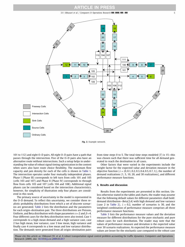
ARTICLE IN PRESSS.V. Ukkusuri et al. / Computers & Operations Research ( ) -- 5

2 3

11 10

4 5

9 812

6

105

102

109

111

106

101

1

7

28

30

29

31

26

27

25

32

33

14

15

23

22

16

17

21

20

24

18

103 108 112

110 104 107

13

19

Freeway Cells

Intersection Cells

Sink Cells

Source Cells

Ordinary Cells

Fig. 2. Example network.

101 to 112) and eight O–D pairs. All eight O–D pairs have a path thatpasses through the intersection. Five of the O–D pairs also have analternative route without intersections. Such a setup helps in under-standing the value of robust signal timing optimization in the contextwhen users also have route choice flexibility. The maximum flowcapacity and jam density for each of the cells is shown in Table 1.The intersection operates under four mutually independent phases.Phase I (Phase III) corresponds to left turn from cells 101 and 105(cells 103 and 107) and Phase II (Phase IV) corresponds to throughflow from cells 103 and 107 (cells 104 and 108). Additional signalphases can be considered based on the intersection characteristics,however, for simplicity of illustration only four phases are consid-ered in this work.

The primary source of uncertainty in the model is represented inthe O–D demand. To reflect this uncertainty, we consider three re-alistic probability distributions from which a set of discrete scenar-ios are generated. Table 2 lists the distribution and the parametersfor each origin–destination pair. The three distributions are Poisson,Uniform, and Beta distribution with shape parameters =2 and �=4.Four different cases for the Beta distribution were also tested. Case 1corresponds to a high mean demand and a high variance case, case2 has high mean, low variance, case 3 low mean, high variance andfinally case 4 corresponds to a low mean and low variance distribu-tion. The demands were generated from all origin–destination pairs

from time steps 0 to 5. The total time steps modeled (T) is 15—thiswas chosen such that there was sufficient time for all demand gen-erated to reach the destination in all cases.

Other factors that were varied in the experiments include theweight factor for the expected value and deviation measure in theobjective function (� = {0, 0.1, 0.2, 0.3, 0.4, 0.5, 0.7, 1}), the number ofdemand realizations (1, 5, 10, 20, and 30 realizations), and differentperformance measure functions.

5. Results and discussion

Results from the experiments are presented in this section. Un-less otherwise stated in the tables and charts, the reader may assumethat the following default values for different parameters shall hold:demand distribution—Beta(2,4) with high demand and low variance(case 2 in Table 2), � = 0.2, number of scenarios is 30, and theweighted combination of performance measure comprises all threeperformance measure functions.

Table 3 lists the performance measure values and the deviationmeasure for different distributions for the pure stochastic and purerobust cases for each distribution. The reader may note that thevalues of performance measure and deviation is the expected valueover 30 scenario realizations. As expected the performance measurevalues are lesser for the stochastic case compared to the robust case

Please cite this article as: Ukkusuri SV, et al. A robust transportation signal control problem accounting for traffic dynamics. Computers and OperationsResearch (2009), doi: 10.1016/j.cor.2009.03.017

6 S.V. Ukkusuri et al. / Computers & Operations Research ( ) --

ARTICLE IN PRESS

Table 1Maximum flow capacity and jam density.

Cell number Max. flow capacity Jam density

1 120 99992 30 1203 30 1204 30 1205 30 1206 120 99997 120 99998 30 1209 30 12010 30 12011 30 12012 120 999913 120 999914 30 12015 30 12016 30 12017 30 12018 120 999919 120 999920 30 12021 30 12022 30 12023 30 12024 120 999925 30 48026 30 48027 60 96028 60 96029 60 72030 60 96031 60 96032 60 72033 60 720101 30 120102 30 120103 30 120104 30 120105 30 120106 30 120107 30 120108 30 120109 30 120110 30 120111 30 120112 30 120

where the objective is to minimize the deviation measure only. Thedeviations areminimized at the expense of recording very high traveltimes and intersections stops and delays. These results are consistentacross the three different distributions. A possible reduction of thehigh values of performance measures may be achieved by assuminga value of �>0.

Table 4 presents the signal time values for the different distribu-tions for both the pure stochastic and pure robust cases. The valuespresented for each phase (P1–P4) are the average percent green, theminimum value and the maximum value of percent green over thetime intervals when there was non-zero flows from the intersectioncells (typically this interval ranged from the 3rd time interval to the12th/13th (10th/11th for low demand cases) time interval). The lastcolumn indicates the % of vehicles that choose the freeway route.The signal timing splits for the Poisson and Uniform distributions donot vary for the different time intervals; however, for the Beta distri-bution the splits show differences. The differences could be becauseof `true' benefits that may be realized by adopting a dynamic signaltime splits or may be `false' bias introduced due to insufficient sam-ple size. The effects could not be isolated and identified because ofmemory restrictions (problems were solved using CPLEX solver ona computer with 1GB RAM) that did not allow us to run larger than30 scenarios or 15 time intervals. The signal timing differences ap-

pear only minor from these results. Apart from the observation thatthe RO-SOSC provided solutions along expected lines for differentdistributional assumptions of demand, no conclusive results can bedrawn on the impact of distribution on signal timing.

A related factor of interest is the performance of RO-SOSC forvarious levels of mean demand and variance. The Poisson distribu-tion cannot be used in the experiment since its' coefficient of vari-ance term is always 1. Between the Uniform and Beta distributions,the Beta distribution is chosen given the greater flexibility it affordsin terms of varying shapes (for example, asymmetry). Four combi-nations arising from two different values (high and low) each formean and variance were tested (see Table 2). The results are shownin Tables 5 and 6. The performance and deviation measures for thepure stochastic and pure robust cases are again along expected lines.In terms of the signal timings (Table 6) we again observe variationover time intervals (dynamic signal times). More pronounced is thevariation between the stochastic and robust signal timing plans par-ticularly for the low demand case. These variations are a result ofgreater flexibility in routing arising from excess unused capacity inthe network. When the demand is high, there is less recourse inrouting and therefore the signal timings of the stochastic and ro-bust cases are close. This argument is further strengthened by thefreeway route choice percentages—for the high demand case the dif-ference between stochastic solution and robust solution is less than5% while it is 20% for the low demand case. A greater proportionof the vehicles under low demand are routed through the freewayin the robust solution—perhaps, a result of the reliable travel timesthat freeways provide compared to the more unpredictable inter-sections. These results provide strong motivation to analyze the RO-SOSC problem, especially if the objective is to provide reliable serviceat low demands.

Given the importance of analyzing the RO-SOSC problem an im-portant question facing the analyst is the degree or level of robust-ness in the objective function. To better understand the dependenceof the solutions to varying levels of robustness, the RO-SOSC is solvedby varying the value of � from 0 to 1. This analysis was conducted ata high demand level, low variance, with # of scenarios equal to 30.As expected, there is a trade-off between the expected value of totalsystem travel time (E(TSTT)) and the deviation measure (Fig. 3). Asthe weight on the risk factor increases it is observed that a conserva-tive solution is obtained in terms of E(TSTT). However, there appearsa value of � ≈ 0.4 beyond which any more increase in � does notresult in substantial changes in the performance measures. The par-ticular value of � obtained is expected to be dependent on severalfactors and may not be generalizable. The choice of the appropriatevalue of � would depend on the level of risk that the analyst/planneris willing to accommodate. In terms of the signal timings, minordifferences were observed for different values of lambda. Howeversubstantial differences or noticeable trends were not observed. Aninteresting future extension would be to observe the results underlow demands since signal timings were found to be sensitive to thelevel of demand (Table 6).

The analysis reported till now were carried out with 30 scenariosfor each case. This was the maximum number of scenarios that couldbe analyzed while solving the problem in CPLEX 9.0 on a personalcomputer running Windows XP operating system with 1GB of RAM.Efficient decomposition and variable storage techniques could allowthe analysis of larger networks with greater number of realizations.An interesting question in this context is whether 30 scenario real-izations is enough to obtain reliable results. To test the sensitivityof solutions to number of scenarios different runs were carried outvarying the number of replication. 1, 5, 10, 20 and 30 scenarios wereanalyzed. The value of the different performance measures and thedeviation measure is plotted in Fig. 4. Given the multiplicity of solu-tions that are possible in system optimal problem formulations, the

Please cite this article as: Ukkusuri SV, et al. A robust transportation signal control problem accounting for traffic dynamics. Computers and OperationsResearch (2009), doi: 10.1016/j.cor.2009.03.017

ARTICLE IN PRESSS.V. Ukkusuri et al. / Computers & Operations Research ( ) -- 7

Table 2Origin–destination demands.

O–D pair Poisson dist. Uniform dist. Beta(2,4) Range

Mean Range Case 1 Case 2 Case 3 Case 4

(1,6) 7 (0,14) (0,14) (3.5,10.5) (0,7) (1.75,5.25)(1,18) 25 (0,50) (0,50) (12.5,37.5) (0,25) (6.25,18.75)(7,12) 25 (0,50) (0,50) (12.5,37.5) (0,25) (6.25,18.75)(7,24) 25 (0,50) (0,50) (12.5,37.5) (0,25) (6.25,18.75)(13,12) 15 (0,30) (0,30) (7.5,22.5) (0,15) (3.75,11.25)(13,18) 25 (0,50) (0,50) (12.5,37.5) (0,25) (6.25,18.75)(19,6) 7 (0,14) (0,14) (3.5,10.5) (0,7) (1.75,5.25)(19,24) 25 (0,30) (0,30) (7.5,22.5) (0,15) (3.75,11.25)

Table 3Performance measure values for different distributions.

Distribution Objective function TSTT No. of stops Intersection delay Deviation measure

Poisson Stochastic (� = 1) 328888.00 74.21 18936.60 12120.20Robust (� = 0) 457512.00 306.08 30808.50 0.00

Uniform Stochastic (� = 1) 352163.00 100.21 24624.80 15560.60Robust (� = 0) 464536.00 347.79 36010.90 0.00

Beta Stochastic (� = 1) 201876.00 19.29 2279.00 6970.47Robust (� = 0) 316800.00 280.73 18047.00 0.00

Table 4Signal times and route choice split for different distributions.

Dist. Objective function Avg. % green for phase Avg. % of veh. freeway route

P1 P2 P3 P4

P S 10.0 (10.0,10.0) 37.1 (37.1,37.1) 15.9 (15.9,15.9) 37.0 (37.0,37.0) 55.35R 14.7 (14.7,14.7) 32.4 (32.4,32.4) 15.9 (15.9,15.9) 37.0 (37.0,37.0) 54.47

U S 11.3 (11.3,11.3) 23.3 (23.3,23.3) 20.3 (20.3,20.3) 45.0 (45.0,45.0) 56.50R 11.3 (11.3,11.3) 23.3 (23.3,23.3) 20.3 (20.3,20.3) 45.0 (45.0,45.0) 56.62

B S 10.0 (10.0,10.0) 26.7 (26.7,26.7) 19.2 (17.5,31.7) 44.1 (31.7,45.8) 53.41R 10.0 (10.0,10.0) 27.3 (16.7,33.3) 18.8 (16.7,20.0) 0.44 (36.7,53.3) 58.70

Table 5Performance measure values for different demand levels.

Demand level (mean, var.) Objective function TSTT No. of stops Intersection delay Deviation measure

High, high Stochastic (� = 1) 201876 19.29 2279 6970.47Robust (� = 0) 316800 280.73 18047 0

High, low Stochastic (� = 1) 256921 20.45 3251 5107.87Robust (� = 0) 386262 338.70 18967.5 0

Low, high Stochastic (� = 1) 94510 0.3 18 2668.93Robust (� = 0) 164909 187.71 9035 0

Low, low Stochastic (� = 1) 119234 0.1 6 1461.33Robust (� = 0) 203578 192.92 10222.5 0

interpretations have to be cautious. Nevertheless the figures suggestthat a minimum of 5 realizations are required to obtain reasonablystable performance measures while at least 20 realizations are re-quired to obtain reasonable deviation measures. It is important toinvestigate whether the trends observed with 20 and 30 realizationscontinue for a greater number of realizations to conclusively answerthe question on scenario sample size (Table 7).

Trading off different objectives—total delay, number of stops andintersection delay: because different objectives are possible for therobust signal control problem, it will be interesting to examine howthe solution changes with the different parameters for �1, �2 and�3 are varied. Table 8 shows the performance measure values fordifferent objective functions. It is observed that the network wide

total travel time objective influences the greatest in the robust signalcontrol problem as compared to the other objective functions. Inother words, in the design of signal control systems, it is importantto consider system wide impacts as opposed to local objectives suchas intersection delays and number of stops.

Tables 9 and 10 present the value of robust system optimal sig-nal design. This experiment is performed by evaluating the solutionsobtained by the deterministic, stochastic and robust problems. Thedeterministic problem was solved as an expected value problem. Tomeasure the value of robust design, the signal timings obtained fromsolving the deterministic, stochastic, and robust problems are takenas input to the system optimal dynamic assignment problem. Traf-fic assignment is then done assuming a purely stochastic objective

Please cite this article as: Ukkusuri SV, et al. A robust transportation signal control problem accounting for traffic dynamics. Computers and OperationsResearch (2009), doi: 10.1016/j.cor.2009.03.017

8 S.V. Ukkusuri et al. / Computers & Operations Research ( ) --

ARTICLE IN PRESS

Table 6Signal times and route choice split for demand levels.

Demand level (mean, var.) Objective function Avg. (min, max) % green for phase Avg. % of veh. freeway route

P1 P2 P3 P4

High, high S 10 (10,10) 26.7 (26.7,26.7) 19.3 (17.5,31.7) 44.1 (31.7,45.8) 53.4R 10 (10,10) 27.2 (16.7,33.3) 18.8 (16.7,20) 43.9 (36.7,53.3) 58.7

High, low S 13.9 (10,45) 29.8 (28.3,35) 17.4 (10,18.3) 38.9 (10,43.3) 54.8R 10.5 (10,13.3) 29.9 (26.7,30.1) 17.1 (16.7,18.3) 42.4 (41.7,42.5) 57.4

Low, high S 10 (10,10) 35.7 (33.3,36.7) 14.3 (13.3,16.7) 40 (40,40) 42.0R 14.5 (10,36.7) 23.6 (10,55) 35.5 (10,55) 26.4 (25,30) 62

Low, low S 10 (10,10) 36.7 (36.7,36.7) 13.3 (13.3,13.3) 40 (40,40) 40.5R 13.3 (10,20) 27.7 (10.4,65) 27.6 (11.7,69.6) 31.8 (10,50) 59

Int. Delay

TSTT

0

50000

100000

150000

200000

250000

300000

350000

400000

450000

0

2000

4000

6000

8000

10000

12000

14000

16000

18000

20000

0

TST

T

Inte

rsec

tion

Del

ay

λ

Dev. Measure

No. of stops

0

50

100

150

200

250

300

350

400

0

1000

2000

3000

4000

5000

6000

0

No.

of

stop

s

Dev

eati

on M

easu

re

λ

0.2 0.4 0.6 0.8 1 1.2

0.2 0.4 0.6 0.8 1 1.2

Fig. 3. Performance measure values for various robustness weights.

function or a weighted robust objective function. The value of totalsystem travel time, number of stops, intersection delay, and the de-viation measure are then compared. This comparison is repeated fortwo levels of demand: mean demand levels of high and low, with lowvariance in both cases. The assignment as well as the signal timingdetermination is based on the objective of minimizing the weightedmeasure of all three performance measures. The following insightsare noteworthy:

• Robust assignment of traffic even when the signal times are setto deterministic or stochastic solutions provides deviation values

(2106.01 and 2139 in high demand and 576 and 512 for low de-mand) that are within 10% of the deviation measure obtained inthe pure robust case (1962.57 in high demand and 515.11 in lowdemand). This suggests that even if the signal timings are not opti-mized the deviation can be minimized substantially if at least theassignment of traffic is performed with a robust objective function.

• The deviation measures are high for robust signal times if theassignment objective is the pure stochastic problem. This suggeststhat it is not sufficient to determine signal times based on therobust problem to ensure risk minimization but that real time

Please cite this article as: Ukkusuri SV, et al. A robust transportation signal control problem accounting for traffic dynamics. Computers and OperationsResearch (2009), doi: 10.1016/j.cor.2009.03.017

ARTICLE IN PRESSS.V. Ukkusuri et al. / Computers & Operations Research ( ) -- 9

255000

256000

257000

258000

259000

260000

261000

262000

263000

264000

265000

0

1000

2000

3000

4000

5000

6000

30

TST

T

Inte

rsec

tion

Del

ay

Int. delay ETSTT

No. of Scenarrio

0

5

10

15

20

25

30

0

500

1000

1500

2000

2500

3000

30

No.

of

stop

s

Dev

eati

on M

easu

re

Dev. measure No. of stops

No. of Scenario

20 10 5 1

20 10 5 1

Fig. 4. Performance measure values for various number of scenarios.

Table 7Signal times and route choice split for various robustness weights.

Value of � Avg. % green for phase Avg. % veh. freeway

P1 P2 P3 P4

� = 0 10.5 (10.0, 13.3) 29.9 (26.7, 30.8) 17.1 (16.7, 18.3) 42.4 (42.5, 41.7) 57.44� = 0.1 10.7 (10.0, 16.3) 30.3 (29.6, 32.7) 20.1 (16.7, 47.2) 38.9 (10.0, 43.7) 56.41� = 0.2 14.8 (10.0, 53.3) 30.2 (20.0, 31.4) 16.7 (16.7, 16.7) 38.3 (10.0, 41.9) 56.28� = 0.3 14.3 (10.0, 49.2) 30.0 (30.0, 30.0) 16.8 (10.8, 17.5) 38.9 (10.0, 42.5) 55.33� = 0.4 10.0 (10.0, 10.0) 29.6 (29.6, 29.6) 17.6 (17.6, 17.6) 42.8 (42.8, 42.8) 57.53� = 0.5 10.0 (10.0, 10.0) 30.2 (29.2, 33.9) 20.9 (17.8, 46.1) 38.8 (10.0, 43.1) 55.71� = 0.75 10.0 (10.0, 10.0) 29.6 (28.7, 35.4) 17.9 (17.9, 17.9) 42.5 (36.7, 43.3) 57.22� = 1.0 13.9 (10.0, 45.0) 29.8 (28.3, 35) 18.3 (18.3, 18.3) 42.5 (36.7, 43.3) 54.83

Table 8Performance measure values for different objective functions.

Objective function includes TSTT No. of stops Intersection delay Deviation measure

TSTT only 262149 78.44 7039.27 1135.14TSTT and intersection delay 261743 46.97 4073.84 1902.07TSTT and # of stops 263075 21.86 3944.33 1326All three terms 263660 21.88 3689.95 1962.57

control based on the robust objective function has to be enforcedin order to minimize deviation.

• The expected values of performance measures are in generalhigher for the stochastic assignment of traffic when the signaltimings are based on deterministic or robust problem compared

to when signal timings are based on the stochastic problem (par-ticularly for high demand case). In conclusion, traffic assignmentprovides some flexibility to work around when signal timingsare not optimized for the same objective function as the assign-ment objective. The best results are obtained when both signal

Please cite this article as: Ukkusuri SV, et al. A robust transportation signal control problem accounting for traffic dynamics. Computers and OperationsResearch (2009), doi: 10.1016/j.cor.2009.03.017

10 S.V. Ukkusuri et al. / Computers & Operations Research ( ) --

ARTICLE IN PRESS

Table 9Value of robustness—high demand.

Signal timing objective function Traffic assignment objective function TSTT No. of stops Intersection delay Deviation measure

Deterministic Deterministic (� = 1) 244800 0 0 0

Deterministic Stochastic (� = 1) 257146 21.57 3705.99 4874.73Robust (� = 0.2) 263200 21.97 3793.99 2106.01

Stochastic (� = 1) Stochastic (� = 1) 256921 20.45 3251 5107.87Robust (� = 0.2) 264274 22.43 3472.16 2139

Robust (� = 0.2) Stochastic (� = 1) 256944 21.08 3489.69 4845.48Robust (� = 0.2) 263660 21.8813 3689.95 1962.57

Table 10Value of robustness—low demand.

Signal timing objective function Traffic assignment objective function TSTT No. of stops Intersection delay Deviation measure

Deterministic Deterministic (� = 1) 113760 0 0 0

Deterministic Stochastic (� = 1) 120028 0 0 1549.07Robust (� = 0.2) 122500 0.03 6.0 576

Stochastic (� = 1) Stochastic (� = 1) 119234 0.1 6 1461.33Robust (� = 0.2) 121608 0.2 12 512

Robust (� = 0.2) Stochastic (� = 1) 119230 0.16 10.89 1458.68Robust (� = 0.2) 121588 0.21 14.25 515.11

optimization and assignment are done with the same objectivefunction.

5.1. Summary

In summary, the main results of the experiments conducted onthe test network are as follows:

• The introduction of uncertainty in the demand in the robust trafficcontrol problem has a significant effect on the solution. The de-terministic optimization using `nominal' values for the input datayields conservative solutions and underestimate the network wideperformance measures.

• The robust optimization solution is significantly different from thestandard stochastic programming and the deterministic solutionespecially at low demand levels. It is observed that the signal tim-ings are different for the robust and the stochastic cases.

• It was observed that the optimization problem is not overtly sen-sitive to the two objectives—total intersection delay and numberof stops. The main important objective was the total system traveltime. This states that signal setting design should consider networkwide impacts and account for intersection delays and number ofstops as secondary objectives.

• The number of stops and the intersection delay increases withincreasing the value of robustness in the optimization problem.

• It is observed that the deviation can be minimized substantiallyif at least the assignment of traffic is performed with a robustobjective function even when the signal controls are obtained bya different objective.

• High quality results are obtained when both the signal design ob-jectives and the traffic assignment objectives are similar.

• The quality of solution changes with the increase in number ofscenarios. In the computational results considered in this work, themaximum scenarios we could implement with the AMPL/CPLEXsolver was 30 scenarios. It was observed that the solution is notstable. There is no conclusive evidence on the optimal number ofscenarios required for robust signal design.

6. Conclusions

Accounting for uncertainty and robustness in the optimal signalcontrol problem is an important illustration of the need to developrobust signal plans considering uncertainty. The signal plans have tobe optimized for the intersection considering network wide impacts,traffic dynamics and the uncertainty in the O-D demand. One of thesignificant contributions of this paper is that we have developed arobust mathematical programming formulation of this problem thatprovides ample opportunity to explore the impact of uncertainty androbustness in optimal signal control.

Other contributions of the paper include: (i) embedding a meso-scopic traffic flow model (cell transmission) which captures shock-wave and link spillover in traffic networks and (ii) accounting fortraffic dynamics where the demand changes over time of day withinthe operation period of the traffic network. Further, the developedmodel can be extended to incorporate gap acceptance behavior ofdrivers, thereby developing more complicated signal phases at theintersection. This can be achieved by introducing a binary variablefor each phase movement and restricting the flow of vehicle basedon the turn movements. However, this transforms the problem froma linear program to an integer program for which efficient solutionalgorithms are unavailable. Our preliminary analysis with the inte-ger version of the problem significantly reduces the problem sizethat can be solved with this formulation. Positive deviation mea-sure of the travel time is used as a measure of risk in the robustoptimization formulation. The risk term allows the examination ofthe tradeoffs of the risk against the expected value term. Extensivecomputational results on a test network illustrate that the introduc-tion of the robust term is important in determining optimal signaltimings that determine overall network performance. A tradeoff alsoexists between the signal timings obtained from the stochastic androbust problem. Evaluation of the deterministic, stochastic and ro-bust problems are conductedwith different weights' for the objectivefunction.

In general, the multiobjective nature of the analysis facilitatedby the model provides significantly greater insight into the trade-offs that are available to traffic operations managers than would bethe case if we focused on simply using the deterministic version or

Please cite this article as: Ukkusuri SV, et al. A robust transportation signal control problem accounting for traffic dynamics. Computers and OperationsResearch (2009), doi: 10.1016/j.cor.2009.03.017

ARTICLE IN PRESSS.V. Ukkusuri et al. / Computers & Operations Research ( ) -- 11

minimizing the expected costs. The robust optimization frameworkhas substantial value in this regard.

Future research extending the current model should focus onsolving large scale instances of the problem. Quite clearly, the devel-oped formulation is computationally intensive and the addition ofinteger and binary variables will further add to the complexity of theproblem. Enhancements related to variable reduction should be ex-plored in future research. Further, more efficient solution techniquesthat exploit the structure of the formulation and utilize decomposi-tion based approaches should be explored. Large scale instances ofthe problem can be solved by developing specialized sampling tech-niques.

Another direction of enhancement is to extend the model to in-corporate different measures of risk. The current model used thepositive deviation as a measure of risk, however the penalty parame-ters associated with this positive deviation were not calibrated. Thisextension can be explored by some of the recent advances in mod-eling risk measures, such as the conditional variance of risk [26,27].

Finally, further work in this area should explore the use of themodels like this for informing policy makers to arrive at networkwide control strategies. By providing policy makers with explicitneed to account for robustness and the impact of uncertainty on traf-fic systems, it may be possible to identify technology based solutionsthat reduce the levels of uncertainty and also satisfy the concerns ofother stakeholders.

Acknowledgements

This reserach is partly supported by the first author's BlitmanCareer Development Chair at Rensselear Polytechnic Institute. Theauthor's would also like to thank the constructive comments of thethree anonymous reviewers. Any opinions, findings and conclusionsare the responsibility of the authors alone.

References

[1] Beard C, Ziliaskopoulos A. A system optimal signal optimization formulation.In: Proceedings of transportation research board annual meeting, Washington,DC; 2006.

[2] Bell MGH, Cassir C. Reliability of transport networks. Research Studies PressLimited; 2000.

[3] Bell MGH, Iida Y. Transportation network analysis, chapter network reliability.New York: Wiley; 1997.

[4] Ben-Tal A, Nemirovski A. Robust solutions of linear programming problemscontaminated with uncertain data. Journal of Mathematical Programming2004;88(3):411–24.

[5] Berdica K. An introduction to road vulnerability: what has been done, is doneand should be done. Transport Policy 2002;9:117–27.

[6] Bertsimas D, Sim M. The price of robustness. Operations Research 2004;52(1):35–53.

[7] Birge JR, Louveaux F. Introduction to stochastic programming. New York:Springer; 1997.

[8] Chen A, Yang H, Lo HK, Tang WH. A capacity related reliability for transportationnetworks. Journal of Advanced Transportation 1999;33(2):188–200.

[9] Daganzo CF. The cell transmission model: a simple dynamic representationof highway traffic consistent with the hydrodynamic theory. TransportationResearch B 1994;28:269–87.

[10] Daganzo CF. The cell transmission model ii: network representation.Transportation Research B 1995;29:79–93.

[11] Du ZP, Nicholson A. Degradable transportation systems: sensitivity andreliability analysis. Transportation Research B 1997;31:225–37.

[12] Iida Y, Wakabayashi H. An approximation method of terminal reliability of aroad network using partial minimal path and cut set. In: Proceedings of thefifth WCTR, Yokohama; 1989. p. 367–80.

[13] Kall P, Wallace SW. Stochastic programming. 2nd ed, New York: Wiley; 1994.[14] Keeney RL, Raiffa H. Decisions with multiple objectives: preferences and value

tradeoffs. 1976 ed, New York: Wiley; 2000.[15] Kim YS, Elnashai A, Spencer BF, Ukkusuri SV, Waller ST. Seismic performance

assessment of highway networks. In: Proceedings of the national earthquakeengineering conference (NEEC), Los Angeles; 2006.

[16] Lighthill MJ, Whitham JB. On kinematic waves, i: flow movement in long river;ii: a theory of traffic flow in long crowed roads. Proceedings of the RoyalSociety A 1955;229:281–345.

[17] Lin WH, Wang C. An enhanced 0-1 mixed-integer linear program formulationfor traffic signal control. IEEE Transactions on Intelligent Transportation Systems2004;5(5):238–45.

[18] Lo H, Szeto YWYW. A cell-based variational inequality formulation ofthe dynamic user optimal assignment problem. Transportation Research B2002;36:421–43.

[19] Lo HK. A cell-based traffic control formulation: strategies and benefits ofdynamic timing plans. Transportation Science 2001;35(2):148–64.

[20] Lo HK, Chang E, Chan YC. Dynamic network traffic control. TransportationResearch A 2001;35(8):721–44.

[21] Lo HK, Tung YK. Network with degradable links: capacity analysis and design.Transportation Research B 1993;37:345–63.

[22] Lo HK, Tung YK. A chance constrained network capacity model. In: Bell M, CassirC, editors. Reliability of transport networks. Baldock, Hertfordshire, England:Research Studies Press Limited; 2000. p. 159–72.

[23] Mulvey JM, Vanderbei RJ, Zenios SA. Robust optimization of large-scale systems.Operations Research 1995;43(2):264–81.

[24] Paraskevopoulos D, Karakitsos E, Rustem B. Robust capacity planning underuncertainty. Management Science 1991;37(7):787–800.

[25] Richards PI. Shock waves on the highway. Operations Research 1956;4:42–51.[26] Rockafellar RT, Uryasev SP. Conditional value at risk for general loss

distributions. Journal of Banking & Finance 2002;26:1443–71.[27] Uryasev SP, Rockafellar RT, Zabarankin M. Deviation measures in risk analysis

and optimization. Research Report, 2002-7, University of Florida; 2002.[28] Soyster AL. Convex programming with set-inclusive constraints and applications

to inexact linear programming. Operations Research 1973;21(5).[29] Ukkusuri S. Accounting for uncertainty, robustness and online information in

transportation networks. PhD thesis, The University of Texas at Austin; 2005.[30] Ukkusuri SV, Tom VM, Waller ST. Robust transportation network design under

demand uncertainty. Computer-Aided Civil and Infrastructure Engineering2007;22:9–21.

[31] Waller ST, Ziliaskopoulos AK. The stochastic dynamic network design problem.Transportation Research Record 2001;1771:106–13.

[32] Ziliaskopoulos A. A linear programming model for the single destinationsystem optimum dynamic traffic assignment problem. Transportation Science2000;34(1).

Please cite this article as: Ukkusuri SV, et al. A robust transportation signal control problem accounting for traffic dynamics. Computers and OperationsResearch (2009), doi: 10.1016/j.cor.2009.03.017