TRANSPORTATION RESEARCH RECORD 6 91

Process Control in the Construction Industry

TRANSPORTATION RESEARCH BOARD

COMMISSION ON SOCIOTECHNICAL SYSTEMS NATIONAL RESEARCH COUNCIL

NATIONAL ACADEMY OF SCIENCES WASHINGTON, D.C. 1978

Transportation Research Record 691 Price $3.60

modes 1 highway transportation 3 rail transportation 4 air transportation

subject areas 11 administration 31 bituminous ma tcrials and mixes 33 construction 34 general materials 35 mineral aggregates

Transportation Research Boa rd publica1ions arc available by order· ing dircc1ly from the board . They may also be obtained on a regular basis through organizational or indi ,·1dunl support ing membership In the board; members or library ·ubscribcrs arc eli1?iblc for substantial discoun1s. For further informatio n, wri1c 10 1hc TrJnsporfation Re­search Board , National Academy ofSc.:iencc, 2101('on1i1u1ion Avenue, N.W., Washington, DC 20418.

Notice The papers in this Record have been reviewed by and accepted for publication by knowledgeable persons other than the authors ac· cording to procedures approved by a Report Review Comminee consisting of members of 1hc National Ac;1dcm)' of Science , the National Academy of Engincer111!!. and the lnstitulc of Medicine.

The views c:-.prcssed in 1hc c papers arc 1hosc of the au tho rs and do no1 necessarily rcnec1 1ho c of the sponsoring committee, the Transportalion Research Board, the National Academy of Sciences or the sponsor~ of TRB activi1ic .

To eliminate a ba<:kJog of publica tions and to make possible earlier, more timely publiea 1ion of reports given al ii mcctinl!S. the Transponation Rcsc:i.rch Board ha , for a trial period, adopted less stringent editorial standards for cn;iin dasses of publ ished material. The new standards apply only to papers and reporl that are clearly attributed 10 specific atuhors and 1h a1 have been accepted for publication after committee review for technical con­tent. Wilhin brood limits, the syntax and style of the published version of 1hese reports arc th sc of 1hc author(s).

The papers in this Record were treated according to the new s1andard .

Library of Congress Cataloging in Publication Data National Research Council. Transportation Research Board.

Process control in the construction industry.

(Transportation research record; 691) 1. Road construction- Quality control - Addresses, essays,

lectures. 2. Process control-Addresses, essays, lectures. 3. Road construction industry-Management-Addresses, essays, lectures. I. Title. II. Series. TE7.H5 no. 691 [TE155) 380.5'08s [658.5'6] ISBN 0-309-02837-X 79-16974

Sponsorship of the Papers in This Transportation Research Record

GROUP 2-DESIGN AND CONSTRUCTION OF TRANSPORTA­TION FACILITIES Eldon J. Yoder, Purdue University, chairman

Construction Section JJavid S. <Jedney, Federal Highway Administration, chairman

Committee on Earthwork Construction Richard P. "/i1mer, Hor11itz Company, chairman Joseph D'Angelo, Edward N. Eiland, David S. Gedney, JVi'lliam Brya11 Greene, lllilbur M. Haas, Erling Henrikson, William P. Hof mam1, Andl'e ii lully, W. F. Land, Charies H. Shepard, valter ' Waidelich

General Materials Section Roger V. LeClerc, Washington State Department of Transporta·

lion, chairman

Committee on Mineral Aggregates T. C. Paul Teng, Misslsslppi State Highway Departmem, chairman Gra/lf J. Allen, Gordon W. Beecroft, John C. Cook, J. T. Corkill, Ludmila Dolar-Ma11tua11i, Karl 11. Dunn, Stepl!e11 W. Forster, Richard D. Gaynor. Dorm E. Hancher, Robert F. Hinshaw, William W. llotaling, Jr. , Richard H. Howe, Eugene Y. Huan.g, William B. Ledbetter, Donald W. Lewls, Charles R. Marek, Johll E. McCllord, Jr., Andy M1111oz, Jr., Jerry G. Rose, N. Thomas Stephe11s. Hollis N. Walker. Richard {). llla/kP.r

Evaluations, Systems, and Procedures Section Donald R. Lamb, University of Wyoming, chairman

Committee on Quality Assur.ince and Acceptance Procedures Garland W. Steele, West Virginia Departmem of Ht"gfnvays, chair·

man Robert M. Nicotera, Pennsylvania Department of Transportation,

secretary Edward A. Abdui1-Nur, Ke1111etlt C. Afferto11, Ill. H. Ames, Doyr Y. Bolli11g, Fronk J. Bowery, Jr., E. J. Breckwoldt, Miles E. Byers, Richard L. Davis, Clarence E. Deyoung. C. S. Hughes, Ill, John T. Molnar, Frank P. Nichols, Jr., Donald J. Peters, Nnrlta11 L. Smith, Jr., Peter Smith, DaJiid G. T111111icliff. Warren B. Warden , Jack fl. Wille11brock , William A. Yrja11so11

William G. Gunderman and Bob H. Welch, Transportation Re­search Board staff

Sponsorship is indicated by a footnote at the end of each report. The organizational units and officers and members are as of De­cember 31, 1977.

300404

300405

30010f)

300-1'07

300108

300109

300110

300411

300112

300413

30041·1

Contents

CONTROLLING THE QUALITY OF CONSTRUCTION AGGREGATES THROUGH PROCESS CONTROL

Reid H. Brown . . . . . . . . . . . . . . . . . . . . . . . . . . . . . . . . . . . . 1

PROCESS QUALITY CONTROL IN THE CRUSHED-STONE INDUSTRY

Frank P. Nichols, Jr. . . . . . . . . . . . . . . . . . . . . . . . . . . . . . . . 4

DEVELOPMENT OF PROCESS CONTROL PLANS FOR QUALITY ASSURANCE SPECIFICATIONS

Jack H. Willenbrock and James C. Marcin . . . . . . . . . . . . . . . . . . 7

DEVELOPMENT OF A HIGHWAY CONSTRUCTION ACCEPTANCE PLAN

Jack H. Willenbrock and Peter A. Kopac . . . . . . . . . . . . . . . . . . . 16

CONTRACTOR CONTROL OF ASPHALT PAVEMENT QUALITY

David G. Tunnicliff ........... . . .. .. .. . . . . . ......... 22

EQUITABLE GRADUATED PAY SCHEDULES: AN ECONOMIC APPROACH

Richard M. Weed ...... . ..... ... .. ..... ..... ...... . . 27

CONSTRUCTION INDUSTRY RESPONSE TO A STATISTICALLY BASED BITUMINOUS CONCRETE SPECIFICATION IN NEW JERSEY

Frank Fee . . . . . . . . . . . . . . . . . . . . . . . . . . . . . . . . . . . . . . . 30

PROCESS CONTROL OF MINERAL AGGREGATES John T. Molnar .................. .. . .. . ............ 37

PROBABILISTIC MODEL OF AGGREGATE PLANT · • PRODUCTION SYSTEMS

Donn E. Hancher and Ping Kunawatsatit . . . . . . . . . . . . . . . . . . . . 42

APPLICABILITY OF CONVENTIONAL TEST METHODS AND ,~TERIAL SPECIFICATIONS TO COAL-ASSOCIATED

WASTE AGGREGATES Mumtaz Usmen, David A. Anderson, and Lyle K. Moulton . . . . . . . 49

IMPLEMENTATION OF QUALITY ASSURANCE SPECIFICATIONS FOR EXCAVATION AND

•EMBANKMENT CONSTRUCTION IN WEST VIRGINIA

Berke L. Thompson . . . . . . . . . . . . . . . . . . . . . . . . . . . . . . . . . 58

iii

Controlling the Quality of Construction Aggregates Through Process Control Reid H. Brown, Vulcan Materials Company, Birmingham, Alabama

The Georgia Department of Transportation and the Georgia Crushed Stone Association have worked together to develop a functional quality assurance system that requires the producer of construction aggregates to be responsible for process control and to certify to the state compli­ance with specifications. A state acceptance program maintains a check on the effectiveness of the program. A quality control program de­veloped by the Vulcan Materials Company in support of the state pro­gram is described. This support program not only provides for proper sampling and testing but also includes a well-managed system of collect­ing and statistically analyzing test data through the computer, which can be used as an effective management tool. Eight computer printout re­ports are generated. Histograms provide valuable insight into the mag­nitude and causes of variations in product quality.

Historically, most contracting agencies have had speci­fications that provide for inspection and testing to be ad­ministered directly by the agency itself for controlling the quality of construction aggregates. Generally, these specifications have been punitive; thus, inspection and testing have become policing functions rather than a man­agement tool to effect product quality. These types of specifications fail to provide the necessary incentives to aggregate suppliers to motivate them to accept their re­sponsibility to effect aggregate quality through process control.

Although construction aggregates are a manufactured product and usually represent the greatest quantity of any material used on a project, they are uniquely different from other materials. Because of economic considera­tions, aggregates must be provided from local resources. Thus, once an aggregate resource has been selected through proper geological and engineering evaluations, the inherent physical properties (specific gravity, abra­sion loss, s ulfate loss, and s o on) and chemical proper­ties of the aggregates produced are essentially fixed. There are a few deposits in which selective mining and special processing procedures are required to improve the properties and upgrade the quality of the aggregate. These special considerations are not considered in this paper; rather, it is limited primarily to control of ag­gregate gradations and cleanliness. Fortunately, many of the concepts that apply to gradation control are also applicable to the control of other properties.

During the past few years, the construction industry, particularly the highway segment, has recognized the merits of the "end-result" specification concept, ac­cording to which the responsibility for quality control lies with the contractor and material suppliers. Through quality assurance concepts, criteria and methods are es­tablished by contracting agencies to assure them that the products they receive are produced under properly con­trolled conditions and in compliance with specifications. For a contractor to successfully operate under an end­result specification, he or she must be furnished from a reliable source with materials of the right quality. Thus, the concept of process control becomes very workable and necessary to an aggregate producer's operation when material is produced for a project under end-result spe­cifications.

The Georgia Department of Transportation and the Georgia Crushed Stone Association have worked closely together to develop a functional quality assurance system for furnishing aggregates for use in state work. The

system requires the producer to be responsible for pro­cess control and to certify to the state compliance with specifications. The state has established a quality ac­ceptance program to maintain a check on the effective­ness of the producer's program.

Vulcan Materials Company, a major producer of con­struction aggregates, has developed a quality control program in support of the state program. The purpose of this paper is to describe this support program and some of the benefits that have resulted since it has been implemented.

BACKGROUND

The aggregate industry has traditionally been an unso­phisticated business. The nature of the business, in general, is local because of the high transportation costs associated with the movement of materials and the low unit value of aggregate. Most of the existing aggregate processing plants have grown from small, family-owned businesses that were generally concerned with "how to get it out of the ground." The responsibility for sam­pling, testing, and accepting material was left to the customer-the highway department. Frequently, the highway department was required to resort to rather thorough inspection and testing programs to ensure ac­ceptable quality and compliance with specifications. As a result, they found themselves in the position of run­ning the aggregate business for the producer. This, of course, was undesirable and awkward for all concerned. Testing and inspection were costly to the state and, under such conditions, not too effective. For example, during the early 1970s, the state of Georgia had over 400 per­sonnel assigned to aggregate testing.

Several years ago the aggregate industry was chal­lenged to develop and implement an effective quality con­trol program to effect better process control. It has taken considerable effort and encouragement by a few of the more progressive highway departments and the Fed­eral Highway Administration to interest the industry in the concept.

QUALITY ASSURANCE BY THE STATE

The Georgia quality assurance program was developed through a cooperative effort between the Georgia Depart­ment of Transportation (DOT) and the Georgia Crushed Stone Association and was implemented in February 1975. The program is strictly voluntary, and partici­pation by the producer is optional. Since its beginning, all producers of coarse aggregate have elected to par­ticipate. Since sand plants are generally much smaller and mostly operated by local contractors, only about 25 percent have elected to participate. If producers elect not to participate in the program, their material is sam­pled and tested by the state at the plant and project sites as it was before. To qualify for participation in the pro­gram, the source of material and the quality control pro­gram must meet the following criteria:

1. A mutually agreeable quality control program, between the DOT and the producer, must be established for each plant based on the characteristics of that plant

1

2

and its deposits as well as past performance. 2. Each plant must have an approved laboratory.

Laboratory equipment and facilities must be certified. 3. Sampling and testing personnel must be trained

and certified. 4. To ensure uniformity of testing between the DOT

and the producer, one sample per quarter is tested at the producer's laboratory and then shipped to the state's laboratory for comparison testing.

5. Correct load-out of materials, including clean­liness of all haul units and accurate identification of products, are recognized as producer responsibilities and are considered an integral part of the quality con­trol program.

6. Delivery of aggregate from a source that has an approved quality control program is certified by the pro­ducer to comply with the specification and need not be tested at the project or at the plant before use unless nonuniform or nonspecification material is suspected by the DOT.

7. To substantiate the quality of the material ac­tually incorporated in the work and to evaluate the quality assurance program, certain evaluation procedures are followed. The DOT samples and tests on a regular but random basis at the source of production and on occasion at the project site. Sampling and testing are done as often as required to evaluate the effectiveness of the pro­t!ucer' i; qualily cu11L1·ul prug1·aw.

8. The producer is required to sample and test at an agreed frequency for each type of material being fur­nished to the DOT. Producer certification is made on an approved DOT form. The producer's records are sent to the DOT for their records, F:ach load of material need not be tested, but the shipments represented by a particular sample should be indicated on the reports by a project number and other necessary identification.

9. The producer is responsible for keeping separate, if necessary, the different materials used for different purposes by the DOT, such as material for asphalt con­crete, portland cement concrete, graded aggregate base, and other mixtures.

10. Regular samples are taken at the project at fre­quencies prescribed by the DOT.

11. Certification of facilities and personnel is the responsibility of the DOT. ·Certification is made at the request of the producer. Subsequent recertification is required annually or based on personnel changes or prob­lems detected in the system.

This is a summary of what is required by the Georgia DOT for a producer to participate in a product certifica­tion program. This system thus far has been most ef­fective. As previously mentioned, before implementa­tion the DOT had approximately 400 people sampling, testing, and inspecting aggregates in the state of Georgia; now there are 12. In addition, before implementation the state experienced frequent problems with material that did not meet specifications; since implementation, the number of problems has been rP.d11cP.d si~nificantly.

PROCESS CONTROL BY THE PRODUCER

Initially, the producers were somewhat reluctant to par­ticipate in the program because they felt they were being required to add personnel to their staff to inspect and maintain a quality control program for the state, thus adding to their operating costs. Experience has shown that it takes about 1 person/909 000 l\1g (1 person/ 1 000 000 tons) of capacity to properly maintain a quality control program. Depending on the size of an operation, the cost to a producer will be between $0.01 and $0.02/ l\1g (ton). This is a significant cost and a very tangible

one, and any good business would require a justification before such an expenditure was approved. Unfortunately, the benefits of a producer quality control program are not readily apparent, and some are intangible in nature, much like technical services or research and develop­ment activities.

However, soon after the Georgia program had been implemented, the industry recognized that the program offered many advantages that certainly overshadowed the costs of the program. The most significant contribution was that the responsibility of producing quality, and therefore the mechanisms to effect quality, were given to the producer. Flexibility of plant operation, less re­jected material, technical ~ervices, and goodwill are but a few of the advantages that have emerged from this program. Obviously, the quality of the material has to be controlled at the plant, and the producer is in the best position to perform this function.

VULCAN QUALITY CONTROL PROGRAM

During the early 1960s, when Vulcan was emerging as a leader in the aggregate industry, its management recog­nized that a research and development capability merited attention. Thus, they formed one of the first research and development groups in the industry. A part of the defined function of the newly formed research and de­velopment section was quality control, but it was not un­til 1972 that this program became fully functional. The program has assisted measurably in improving the qual­ity of material being produced in those divisions that are using it. The development of Vulcan's quality control program has been closely related to and associated with the evolution of the certification and end-result specifi­cation program of the Georgia DOT.

Vulcan's program has had the support and encourage­ment of its top management, which is an essential aspect of the success of a quality control program. The follow­ing items have been identified as contributing to a good, functional quality control system:

1. Qualified personnel; 2. A well-planned, written system approved by man­

agement; 3. Good housekeeping and preventive maintenance

practices; 4. Correct sampling and testing procedures; 5. Proper data analysis; and 6. Use of the results in engineering and management

decisions.

Vulcan has now implemented its quality control pro­gram in about one-third of its plants. It is functioning in those states in which highway departments encourage producers to maintain their own quality control programs. In three of these states, the highway departments now accept product certification from the producer in lieu of state testing.

At each of the participating plants, an adequately equipped laboratory is maintained and manned by a trained quality control technician. This technician is under the supervision of the quality control manager, who, in turn, reports to division management. All quality control activities are overseen and monitored by the cor­porate quality control manager, who is a professional engineer.

More than a policing activity was desired. One of the basic premises of the program was that information de­veloped from testing, if obtained and analyzed correctly, could be a valuable asset to management.

To assist in the management of Vulcan's quality con­trol program, a computerized statistical quality control

system was developed. The system consists essentially of input data collected from the sampling and testing ac­tivities of the plants. The information is routed to the computer on a routine basis, and at defined points in time the data are statistically analyzed and reduced to a usable format. Currently, access to eight different reports is available each month. A brief description of each report follows.

Exception Report

The exception report is prepared as a tool to enable man­agement to make a quick assessment of any significant problems. It lists all tested samples of a product that are outside specification limits and provides, through statistical concepts, information on potential problems that may require corrective attention.

Frequency of Sampling Report

The sampling report provides information on the total number of samples tested at a plant by day and by month for each product.

Time-Sequenced Values Report

The values report is basic. It shows all the samples tested at a plant as well as the date, time of day, and gradation for each product.

Product Uniformity Report

The report on product uniformity provides information for comparing the quality of a particular product from one plant to another. It may be used to compare the uni­formity of the mean percentage passing and standard de­viation for a given product between plants and to com­pare the monthly performance of a plant with year-to­date performance.

Control Chart Limits Report

The control chart limits report provides data for the pur­pose of preparing quality control charts that are used by the inspector and superintendent at the plant to control quality during production.

Average Gradation Analysis and Standard Deviation Report

The report on average gradation analysis and standard deviation provides for sales personnel and customers a listing of mean percentage passing and standard devia -tion for all products produced at a plant.

Yearly Statistical Comparison Report

The yearly statistical comparison report lists the aver­age gradations and standard deviations by month for all products sampled during the previous 12 months. Sea­sonal patterns and fluctuations can thus be identified and anticipated.

Histograms

For each sampled product for which sufficient data are available, a histogram is plotted for each sieve size tested. If samples are properly selected and tested, a "bell-shaped" curve is generated. If the plots do not ap­proach such a shape, it is an indication that some pro­cedure may be incorrect and corrective action may be required.

3

Information obtained from these reports is providing valuable insight into the type and cause of variation that occurs in the various products. For example, it has been found, as would be expected, that the point of sam­pling makes a considerable difference in the magnitude of the variation. If an ASTM No. 57 aggregate (typical concrete-sized coarse aggregate) is sampled from the production belt just before it is discharged into stock or a loading bin, the variation on the 13-cm (0.5-in) control screen may be as low as 2 to 4 percent. If this same material is sampled under controlled conditions from a railcar or a truck, the variation will be in the range of 4 to 6 percent. If it is sampled from a stockpile, it can be as high as 10 percent. We believe that this type of information is extremely valuable in establishing speci­fication limits, methods of sampling, and tolerances in specifications and in assisting in the mix design for portland cement concrete, asphaltic concrete, and crushed-stone base.

SUMMARY

Vulcan's statistical quality control system has been a very effective aid in controlling quality and in knowing what is being produced. It is a valuable management tool. Among the advantages the program provides are the following:

1. It documents in a concise and orderly manner the quality of all products;

2. It satisfies the record-keeping requirements of state highway departments that are using or considering product certification programs in lieu of their present inspection procedures;

3. It optimizes the amount and timing of sampling; 4. It provides effective information to sales per­

sonnel and services to customers; 5. It reduces the amount of material shipped that

does not meet specifications; 6. It provides a valuable library of information that

may be adapted to research and development programs; 7. It provides an effective tool for operating, main­

taining, and upgrading plant control; 8. It makes it possible to identify and anticipate

seasonal fluctuations; 9. It maximizes product quality commensurate with

operations, sales, and marketing conditions; and 10. It provides a more competitive atmosphere in the

construction materials industry.

Vulcan's system has been designed to provide depend­ability and accuracy. It ensures a high probability of valid data and is flexible and adaptable to all aggregate plants operated within the company. Simplicity and clar­ity have been prime considerations throughout the de­velopment of the quality control system.

Even though significant progress has been made by a few states in the implementation of producer quality con­trol systems and product certification, several factors are still deterring the concept from being widely ac­cepted by highway departments and producers. l\1any producers see the program as costing them money and feel that there are no ways for them to recover incurred costs. Quality control is one of those functions that are somewhat intangible: The cost and effort of the activity are easily identifiable but the benefits are not. These obstacles can be overcome only by educating the pro­ducers and through experience.

It is important that the program be simple to admin­ister and require a minimum of paperwork. An effective program need not be complicated and bureaucratically burdensome. A producer is much more receptive and

4

responsive to a program that is simple to administer and that keeps costs down.

Producer-managed quality control and product certi­fication have proved to be effective methods of improving product quality and reducing inspection and testing costs. Vulcan believes that quality control can be an effective

cost control activity and that it will, if properly admin­istered, bring a profitable return to the company on its investment.

Publication of this paper sponsored by Committee on Quality Assurance and Acceptance Procedures.

Process Quality Control in the Crushed-Stone Industry Frank P. Nichols, Jr., National Crushed Stone Association, Washington, DC

Selected producers of crushed stone were surveyed on their attitudes to­ward setting up structured quality control systems that might largely re­place much of the conventional testing of aggregates by state inspectors. Their responses are summarized. The overall response was clearly in favor of the concept . Most producers felt that such e system would eliminate many problems and pay off in terms of customer confidence. The essen­tials of workable, statistically valid specifications that would be appro­priate to the producer control concept are outlined . Such specifications should define acceptable variations from approved target gradations for given end uses but should permit considerable latitude to the producer in establishing the target gradation. Good gradation control requires careful processing; the desired consistency is seldom if ever found in ma­terials taken from natural deposits with little or no processing. The im­portance of close adherence to sound, standardized sampling techniques is emphasized. Both process control samples and samples monitored by state or other agencies should be taken from the "as-produced" material. Test portions for monitoring should be split from routine process control field samples to provide a valid statistical comparison of the producer's control program.

The crushed-stone industry is clearly in favor of speci­fications based on concepts that recognize the fact that bulk materials are inherently variable and that place realistic limits on the degree of variability that is ac­ceptable. The old, outmoded practice of acceptance or rejection is no longer used in most areas of the country. Specifications must define reasonable limits within which the great majority of qualily m~asunm1ents should fall. However, in view of the many sources of variation in test results, it is unrealistic to expect every sample to "pass" in all respects.

Specifications should also require a measurable de­gree of consistency in gradation. The old axiom, ''We can use a wide variety of gradations, but we cannot tolerate too much variation," should be recognized. This is more important in some end uses than in others.

Specifications for crushed-stone base material, sim­ilar in principle to ASTM D 2940, exemplify this con­cept. They establish a rather wide master range and give producers considerable leeway in selecting a grada­tion that best fits their operations but require a job mix formula that places more strict limits on deviations from the target gradation selected.

Consistent gradations are important in the case of aggregate base materials, which rely on good compaction and accurate measurement of compaction for maximum load-supporting power. They are extremely important in the case of bituminous mixtures, where variability may affect not only compaction but also void content, both of which strongly influence stability and durability, and in the case of portland cement concrete, where

variability may affect water demand to achieve a given slump and thus also affect strength and yield. But in none of these cases is it necessary to require that every aggregate producer who bids on a given job meet a single, narrow gradation band.

Commercial producers of aggregate have found that good quality control programs pay off in a number of ways, especially in producing aggregates to meet this type of specification. Because they produce aggregates that are consistent in gradation and other important characteristics, their products are sought and are more readily accepted by contractors who work in the private sector and for public agencies. In recognition of the fact that crushed stone is generally processed under good quality control procedures, a number of state agencies are reducing their emphasis on sampling and testing of stone by state personnel. The growing ten­dency is to place greater reliance on the producer's quality control records as the basis for routine accep­tance.

On learning that the Federal Highway Administration (FHWA) has been pursuing research in its federally coordinated program (FCP) to "promote the takeover by producers of the job of process cont r ol" and thus relieve stat e inspector s of much of theil· testing l oad (1 ), the National Crushed Stone Association (NCSA} under took a survey of its members to determine the attitude in the industry toward such a development. The membership was advised that a shift from state test data to pro­ducers' data as the basis for quality assurance might involve making available to the state all quality control records on the specified materials. The following sec­tions summarize the responses from NCSA member companies.

SURVEY OF INDUSTRY ATTITUDE

Members of NCSA represent a wide range of company sizes as well as quarry sizes. At some quarries, highly sophisticated plants may be found that are designed to produce annually millions of megagrams of stone of a wide variety of sizes and blends. Other quarries are operated only intermittently, and portable plants are moved in and out to produce just enough material for a specific project or a year's supply of maintenance stone. With very few exceptions, all members who responded to the survey showed a favorable attitude toward the concept of producer control as the basis for quality as­surance. Some, in fact, urged that this paper reflect an NCSA policy of actively promoting the concept al-

though this policy has not been formally adopted by NCSA.

Statements of this sort characterize typical responses to the survey:

1. It is good business to make our test data available to our customers, both public and private.

2. This company has maintained its own quality con­trol system for 12 years, and it has resulted in minimal rejection. We are highly in favor of making reasonable reports to various agencies to facilitate acceptance.

3. Preacceptance of stone at the source should add value to offset the cost of a quality control program.

4. Though the cost of quality control is significant, benefits are well worth the cost in terms of customer confidence, up-to-the-minute information on "how well we are doing," and the ability to pinpoint and solve prob­lems.

5. In a state that has used producer control as the basis for acceptance since early 1975, the system has not hurt small operators.

6. We favor the system as described if it is confined to routine gradation and wash-loss tests. Abrasion and soundness testing is still best done by the state.

7. The system would offer no problems if acceptance were granted at the plant or plant stockpile before the material passed from the producer's control. The cost of the system can be determined, but the results may be intangible.

8. Costs should be recoverable even in the private sector. NCSA should assist local associations in estab­lishing workable systems that are not burdened by too much bureaucratic paperwork.

Minority responses to the survey took the following tone:

1. The present system is preferable. Our company furnishes very little stone for highway construction. We doubt that a company quality control system could be justified.

2. We would object to more government intrusion into company operations and question whether the sys­tem would eliminate overlapping inspection by state, county, and city representatives.

3. A producer-operated system would be acceptable for specified items. We would object to making all test data public, including data on nonspecification materials sold to private customers (this point was emphasized by several respondents).

4. If clear guidelines for the type and frequency of testing were supplied and if record keeping were kept simple, we would have no objection. We would object to allowing government agencies to inspect each and every test report in the producer's files.

Although some of the respondents expressed doubts that a workable system of producer control could be de­fined to the complete satisfaction of both buyer and seller, it is believed that such systems are evolving and that in a very few years commercial aggregate sources will be certified in much the same manner as many other manufacturing operations are. In short, effective quality control by the producer will be the basis for quality assurance by the consumer.

ROLE OF STATISTICS IN PROCESS CONTROL AND ACCEPTANCE

If possible, it would be desirable to establish guidelines that could be followed by production personnel who have had no training in statistics. With this in mind, the fol-

5

lowing practical considerations are offered. A fully workable, statistically valid aggregate specifi­

cation, from both the practical and the legal viewpoint, should describe

1. What characteristics are needed by the aggregate for particular end uses;

2. What tests will be made to evaluate these charac­teristics;

3. How the material will be sampled, by whom, at what stage in the production process, and how frequently;

4. The size of the lot (or sublot) to be represented by a sample or a specific number of samples (a lot, in the case of aggregate, should refer to an isolated spe­cific quantity of specific size of a given product from a given plant produced by a given, unchanging process);

5. The extent to which a sample or samples may fall outside a target range without being rejected; and

6. The formula for determining whether a given lot is in reasonably close conformity with specified limits and acceptable at full price or at clearly defined price adjustments.

Probably the greatest obstacles to the development of fully reliable producer quality assurance systems for processed aggregates relate to the inadequacy of certain test methods and common sampling practices. As noted earlier, gradation testing lends itself best to producer control. ASTM standard method C 136 (AASHTO T 27) for sieve analysis is reasonably pre­cise and should pose few problems when sampling is done properly. Other tests, particularly ASTM C 88 (AASHTO T 104) for soundness by use of sodium or magnesium sulfate, may be so imprecise as to be com­pletely impossible to apply under specifications of the type considered here.

The importance of sampling cannot be overempha­sized. When the producer's control records are to be the basis for acceptance, subject to occasional monitor­ing by the state, all samples must be taken in a statis­tically sound manner. ASTM standards D75-Methods of Sampling Aggregates-and C702-Methods for Reduc­ing Field Samples to Testing Size-outline the principles involved. The field sample should consist of "at least three approximately equal increments, selected at ran­dom, from the unit being sampled," such as the amount in or needed to fill a haul truck, and these increments should be mtxed together thoroughly and split or quartered to test portion size (obviously, the reduction to test portion size should be performed at the sampling site).

The unit to be sampled should be neither too small nor too large. A single increment of aggregate taken from a single spot on a conveyor belt, in a truckload, or from a stockpile merely accentuates unimportant within­batch variations and tells nothing about the characteris­tics of a unit of any significant size. But even three or more increments taken over widely separated intervals of production and mixed together may not reveal unde­sirable batch-to-batch variations. ASTM D 2940 gives the sound advice that acceptance decisions be based on average results from samples taken in accordance with ASTM D 75 from "at least 3 units or batches picked at random" within a lot of not more than 2700 Mg (3000 tons) of graded aggregate. A unit is defined as "the amount of material required to fill at least one normal sized haul truck."

Where the producer's records form the principal basis for acceptance, care must be taken in monitoring the accuracy of the producer's testing program. Runkle and Hughes (2) have described a statistically sound monitoring system for pug-mill-mixed aggregates. Weekly comparisons are made between the producer's

6

Figure 1. Control chart for aggregate base material produced to comply with ASTM 02940. LCL

-------- · --- __________________ IJ.L..

• • • • • • • - -·--- - - ------------LL

CHANGE IN

JOB MIX

UCL ---- ~ ----.-- -- -. ----.- -- - - - - - - - - - - - - - - - - -L L

• . --;-.---- -. - --- . - - --.. -r--__ ._ - - - - -- -- - - -- _____ .LI.CJ

ti J l

J I 11 11 1 1

w (.)

z <:(

0: w _J

0 f--

x ~

al 0 ,

I I I I I I I I I I I I I I I I I I I I I I J I I I I I I I I 5 10 15 20 25 30

test results and monitoring test results for all data ac­cumulated since the job mix formula was established for a given material. Statistical tests are made to de­termine whether either the mean values (x) or standard deviations (er) determined from monitoring tests differ significantly from those determined from the producer's tests. Proper account is taken of the fact that far fewer monitoring test results than production test results are available on which to compute standard deviations; therefore, the standard deviations from the monitoring tests are normally higher than those from the produc­tion tests. How much higher they are determines whether there is a significant difference.

Samples for either production or monitoring tests should always be obtained by the procedure described above. To give the state a more valid statistical com­parison for checking the accuracy of the producer's con­trol program, the monitoring test portion and the pro­duction test portion should preferably be split from the same field sample.

If variability in gradation is to be held at a minimum, careful processing is essential. Consistent gradations are seldom if ever noted in unprocessed aggregates taken directly from natural deposits. Frequent grada­tion checks can best be and should be made by the pro­ducer so that variability can be detected and promptly corrected. FHWA' s FCP Project 4F (1 )includes an inves­tigation of a number of short-cut, rai)id methods of checking gradation. One of the best of these is gap sieving-checking the percentage passing only one or two key control sieves at frequent intervals and running the complete sieve analysis only on every fourth sample or so. This and a number of other short-cut procedures have been reported (3), are being evaluated, and should be carefully considered in establishing producer control systems.

RECORD KEEPING

Although most stone producers do exercise good quality control, feeling that it adds value to the final product commensurate with its cost, some producers have def­inite reservations about being required to maintain

LOT NUMBER

voluminous records in order to be certified as an ac­ceptable source. It is recognized that variability must be minimized and that records must be complete to document compliance with specifications that penalize variability beyond reasonable limits; nonetheless, it is felt that these records need not be so complex as to be unduly burdensome.

Probably the simplest way to record the results of gradation tests and show trends in variability is by means of a control chart. Such charts may be used to record either (a) percentages passing all specified sieves for each lot tested or (b) percentages passing only one or two key sieves for each lot and percentages passing any other sieves for every fourth or fifth lot only.

Figure 1 shows one use of the control chart. The example relates to base material production for com -pliance with ASTM D 2940. Results for the first few lots are recorded for all sieves, after which only those for the minus 4. 75-mm (no. 4) sieve are determined and recorded routinely. As a check, however, the complete gradation is recorded for every fourth lot. Note that, as a trend toward a coarser gradation was noted, a new job mix formula was submitted and approved.

Some specifications require computation of standard deviations as a measure of variability over a period of time, often for the entire quantity of a given type of ma­terial on a project. In Virginia, for example, penalties may be assessed for deviations from job mix tolerances on base materials lot by lot, and a further penalty may be assessed for excessive standard deviation over the entire project including lots already penalized.

Although standard deviations are easy to compute and are statistically "pure," it is felt that control chart records that show either average test results for indi­vidual lots or "moving averages" for the most recent four or five tests should provide an adequate picture of variability.

Whenever a change in the basic job mix formula is requested and allowed, new upper and lower control limits must be plotted on the control charts; if standard deviations must also be recorded, a separate population of test values should be established to document the de-

gree of control obtained with respect to the new formula. Note in Figure 1 that the "master" or design ranges

under D 2940 merely define the limits of the job mix target values for the respective sieve sizes and that the full tolerances apply even though individual test results may fall beyond these limits.

The California Department of Transportation (DOT) (4) has used the moving average concept in specifying aggregate gradations for many years, applying fairly wide limits to individual tests and a narrower tolerance to the average of the most recent four or five tests. The California DOT also gives the contractor some leeway in selecting target values x for the percentage passing certain intermediate sieve sizes. Control charts can be used to record both individual test results and moving averages.

The various methods of defining a lot for acceptance purposes or establishing schedules of penalties for non­compliance are outside the scope of this paper. The Virginia system, mentioned earlier and widely publi­cized through FHWA pilot courses held at numerous lo­cations since late 1976, bases acceptance on the results of four tests per lot of a designated size but, as noted, places the producer in double jeopardy by the threat of additional penalties where variability between lots is judged to be excessive. Whatever method is chosen, compliance can be judged at least as well from process control chart records as from voluminous test reports issued by state personnel.

CONCLUSIONS

1. The crushed- stone industry has practiced quality control in one form or another for years, and most pro­ducers feel it to be well worth the effort and cost. The industry generally would approve the concept of a struc­tured quality control system, the records from which could largely replace the voluminous test reports now filed by state inspectors as the basis for acceptance.

2. Producers of stone would cooperate with user agencies by making quality control test data available for incorporation in project records; however, many would object to disclosing test data on miscellaneous sales of unspecified materials to private customers.

3. It should be expected that government agencies

7

would wish to take occasional check samples to monitor the effectiveness of the producers' control. With this in mind, it is important that both producer and inspector use an identical, sound sampling technique-the monitored samples preferably being a portion of a regular produc­tion sample.

4. All samples in a producer control system, either regular or monitoring, should be taken from the ma­terial as produced; the effectiveness of a producer's control cannot be judged from samples taken after the material has been rehandled one or more times before it finds its way into the work.

5. Record keeping should be kept simple; control charts are preferable to stacks of indi victual test reports and complex forms for statistical computations.

6. Specifications should place a premium on product uniformity and permit only minimal deviations from a job mix formula but should provide considerable latitude to the producer in establishing a formula that best fits the producer's operation and requires little or no waste of fractions of usable size.

REFERENCES

1. 1976 Federally Coordinated Program of Highway Research and Development: Project 4F-Develop More Significant and Rapid Test Procedures for Quality Assurance. Offices of Research and Devel­opment, Federal Highway Administration, 1976.

2. S. N. Runkle and C. S. Hughes. Monitoring Program for Pugmill Mixed Aggregates and Bituminous Con­crete. Virginia Highway and Transportation Research Council, Charlottesville, interdepartmental rept., Aug. 1977.

3. Investigation of Present Aggregate Gradation Control Practices and the Development of Short-Cut or Al­ternative Test Methods. Offices of Research and Development, Federal Highway Administration, Rept. FHWA-RD-77-53, 1977.

4. Standard Specifications. California Department of Transportation, Jan. 1975.

Publication of this paper sponsored by Committee on Quality Assurance and Acceptance Procedures.

Development of Process Control Plans for Quality Assurance Specifications Jack H. Willenbrock and James C. Marcin, Pennsylvania State University

Statistically based quality assurance specifications, such as the restricted performance bituminous specification of the Pennsylvania Department of Transportation, provide a clear delineation between the acceptance re­sponsibilities and the process control responsibilities of the highway agency and the contractor or material supplier. They also usually require that a process control plan be submitted for approval before the commence­ment of work. Because the available technical literature has favored the acceptance phase, there is currently little guidance available to these parties when they prepare such a plan. The need for such guidance is illustrated by presenting the two extreme approaches that may be taken

to meet the requirements of the Pennsylvania Department of Transpor­tation. The first case illustrates the "ideal" process control plan that can be developed if a literal interpretation of the specification is made. This plan clearly requires excessive documentation. It is contrasted with the process control plans currently being submitted to the Pennsylvania De­partment of Transportation, which do not provide enough detail to allow a determination of adequacy. A need is thus indicated for the industry to develop technical information that provides guidance in the develop­ment of plans that are somewhere between these extremes.

8

The final quality of a highway is to a large degree a function of the care and concern that is exercised by the material suppliers and the contractors who provide and place the materials used in its construction. If haphazard and inefficient control is exercised, these parties will suffer economically because of either ex­cessive rejection rates or process overreaction (i.e., the use of more cement than is required to avoid rejec -tion of the material).

Interest in process quality control has grown as more state highway agencies have adopted statistically based quality assurance specifications that require contractors and material suppliers to submit process control plans to qualify for consideration on projects. The objective of this paper is to indicate that the highway construction industry, through its trade and contractor associations, must take the lead in providing guidance and technical advice to its members with regard to the development of such plans.

First, a brief background of statistically based quality assurance specifications is provided, and then some of the aspects of the restricted performance specification for bituminous concrete implemented by the Pennsylvania Department of Transportation (PennDCYI') (1) are ex­amined. An "idealized" approach to the development of a proce5Hil control plan that interprets tho statements in that specification in a literal fashion is then presented. This is followed by the presentation of some examples of actual process control plans that have been submitted in response to that specification . These two extremes indicate that the development of practical, well-defined plans that provide the maximum benefit to material suppliers and contractors in terms of efficient control of their processes is still experiencing growing pains .

BACKGROUND OF QUALITY ASSURANCE SPECIFICA TlON

Quality assurance, broadly interpreted, refers to the total system of activities that is designed to ensure that the quality of the construction material is accept­able with respect to the specifications under which it was produced. It addresses the overall problem of ob­taining the quality level of a service, product, or facility in the most efficient, economical, and satisfactory manner possible. The scope of the total quality as­surance system (regardless of the type of matex·ial specification used) encompasses portions of the activi­ties of planning, desi~n, development of plans and specifications, advertising, awarding of contracts, construction, and maintenance.

Types of Specifications

At the heart of such a quality assurance system are practical and realistic specifications for construction materials. A practical specification is one that is de­signed to ensure the highest achievable quality of the resulting construction. A realistic specification is one that recognizes the fact that (a) there is a cost as­sociated with every specification limit and (b) the char­acteristics of all products, processes, and construction are by their very nature variable.

In highway construction, the three most common types of specifications are (a) end r esult, (b) material and methods, and (c) statistically based quality as­surance.

End Result

A pure end-result specification places the entire re­sponsibility for supplying an item of construction or

material of specified quality on the contractor or producer (2, p. 3 5). This type of specification places no restrictions on the materials to be used or the methods of incorporating them into the completed product. The responsibility of a highway agency is therefore reduced to either accepting or rejecting the final product or applying a penalty system that accounts for the degree of noncompliance.

Material and Methods

Most highway agencies have traditionally used the ma­terial and methods type of specification. It is more frequently referred to as the reasonable conformity or substantial compliance type of specification. In this type of specification, the contractor or producer is directed to combine specific materials in definite proportions, use specific types of equipment, and place the material or product in a prescribed way. Each step is controlled and in many cases directed by a representative of the highway agency. By specifying the procedure, the highway agency has obligated itself to a great degree to accept the end product even though there is no assurance that it will meet the performance requirements. The statement that the contractor is responsible for the end result under this type of specifi­cation is of questionable legalily if lhe contractor has met the materials and methods requirements.

Statistically Based Quality Assurance

As noted by Bolling (3 , p . 17.13) and the National Co­operative High.way Research Program (; p. 38), a num­ber of state highway agenc ies have already partially adopted statistically based specifications in some of their material specifications.

Generally speaking, the quality assurance specifica­tion bridges the gap between the two types of specifica­tions mentioned above. In basic intent, it is perfor­mance oriented. The distinguishing elements of a quality assurance specification are

1. Performance-oriented acceptance criteria; 2. Use of s tatistical techniques for the purpose of

(a) ensuring unbiased quality information, (b) effective and timely process control, (c) objective evaluation of quality characteristics in terms of both central tendency and dispersion, and (d) making acceptance decisions on a rational basis; and

3. Clear delineation of responsibilities with respect to (a) process contr ol by the contr actor and (b) ac­ceptance sampling, testing, and inspection by the owner (the state highway agenc y).

Reference to the two elements in item 3 is made in the form of a process control plan and an acceptance plan.

Cons tr uction Subsystem in Quality Assurance Specifications

An analysis of the construction subsystem within a statistically based quality assurance system will in­dicate how this type of specification differs from end­result and materials and methods specifications. There are two independent parties involved in the subsystem: the highway agency and the contractor. It is a funda­mental requirement that the responsibility for quality be assigned commensurably according to the role each party performs in the construction subsystem. The contractor (or material supplier) has the most direct and profound effect on the quality of the work and should

therefore be responsible for exercising process control. The highway agency acts as the legal agent of the buyer­the taxpayer-and is therefore intensely interested in the final quality of the product it buys. The highway agency therefore performs the acceptance sampling, testing, and inspection to make sure it is receiving the specified level of product quality.

Figure 1. Two-party relation of quality control and acceptance plans.

Penn DOT

Buyer

Assure they

obtain It by

Acceptance

Plans

Result is exchange of

Compensation

End product

Contractor

Seller

Describe whet he will make

$ Assures he

produces it by

Quality

Control

Figure 2. Three-party relation of quality control and acceptance plans.

Penn DOT

Specifies what no wants by o

Supplier

Describe what they wont by

Describe what

tie will produce by

Assures contractor

he supplies it by

Assures they obtain ii by

Acceptance

Plans

Process

Seller Buyer

Assures he

produces it by

Quality

Control

Compensation

End Product

Assures he

obtains it by

Acceptance

Pion

Quality Control

Product

Compensolion

9

Statistically based quality assurance specifications provide a clear division of responsibility for these two roles. In fact, for this type of specification, it might be stated that quality assurance (QA) is equal to process control (PC) plus acceptance sampling, testing, and inspection (AST&I) [i.e., QA = PC + AST&I (4, p. 2)]. In this equation, PC represents all those activities that are primarily carried out by the contractor or producer of a given product for the purpose of maintaining product quality at some specified standard. AST&I represents all those activities associated with the owner's (state highway agency's) efforts to determine that they received that for which they contracted.

It should be noted that the material supplier also occupies an extremely important position with regard to process control since in most instances the material supplier initiates process control activity.

RESTRICTED PERFORMANCE SPECIFICATION FOR BITUMINOUS CONCRETE

PennDOT currently has a restricted performance specifi­cation for bituminous concrete that is incorporated as a special provision on bituminous concrete contract projects that meet the following criteria:

1. The estimated quantities for each course of main­line paving must be a minimum of 2721 Mg (3000 tons) .

2. The thickness of the surface course must be 3.8 1 cm (1. 5 in) or greater.

3. Paving must be carried out on a properly prepared, stable base.

Figure 1 shows the relation that is envisioned when only PennDOT and a contractor are involved, and Figure 2 shows the relation when a material supplier is added to the picture. It should be noted that quality assurance specifications normally require fewer material charac­teristics to be tested for acceptance purposes than for process control purposes. This fact is illustrated below for the PennDOT specification.

Acceptance Testing

The PennDOT specification states that acceptance tests for bituI}1inous concrete be performed at the mixing plant for percentage of bituminous content and at the com­pleted pavement for compaction (ultimately, thickness and smoothness will also be incorporated in the ac­ceptance criteria) .

At the batch plant, acceptance is made on a lot-by­lot basis. The specification (!,p.1.4) states:

A lot shall consist of a minimum of 2721 metric tons (3000 tons) and shall be divided into 5 approximately equal sublots. Acceptance of the mixture by extraction shall be on the basis of bitumen results of five consecutive random samples for each lot. One random sample shall be taken from each sublot. Acceptance of the mixture by printed tickets from automated and recordated plants shall be based on the bitumen results of five consecutive random printed tickets for each lot. One random printed ticket shall be taken from each sublot.

The percentage bitumen content of the lot is expected to meet the approved job mix formula within the tolerances shown in the specification for either extrac­tion tests or the printed tickets from automated recordated plants. A determination of the acceptability and the level of payment (i.e., whether a full or adjusted price is paid) of the lot of material in terms of bitumen content is made by calculating the estimated percentage of material Within the allowable specification limits (!; E_, Session 20; ~ '.!_; !!.).

10

Acceptance of the completed pavement is also made on a lot-by-lot basis. As noted in the specification (1, p. 1.9), -

A lot shall consist of not more than 1524 m. (5000 linear feet) of pav­ing lane or 5601 sq. m. (6700 sq. yds.), whichever is lesser, of each layer or course but shall not exceed one day's construction. A lot will be sub divided into 5 approximately equal sublots. Readings for each nuclear density test will be taken at a random location (selected as prescribed in PTM No. 1) on each of the 5 sublots, except thnt nn rP.nrlings shnll hP. taken within two feet from the edge of the pavement ....

The in-place density of the compacted mixture (wearing or binder course) shall be equal to or greater than 98 percent of a control-strip density that has been pre­viously determined. If the results of the density tests on a lot indicate that less than 85 percent of the material has been compacted to the specified density, the lot will be paid at an adjusted price (!; §., Session 20 · ~; '!_; ~ · For payment purposes, the plant Lot [2721 Mg (3000 tons)], defined for acceptance of paving mixtures at the mixing plant, and the project lot [1524 m (5000 linear ft) or 5601 me (6 700 yd2

), whichever is less], defined for acceptance of completed pavement in place, are in­dependent of one another. Nonconforming lots are paid for at an adjusted contract unit price by considering bitumen and density individually.

ProcP.ss Control Testing

In a pure end-result specification, the contractor and material supplier would be left to their own devices with regard to the number of other bituminous concrete char­acteristics that they felt should be controlled. This situation does not exist with the PennDOT specification, however, because both a set of required process con­trol activities and a set of additional recommended process control activities are incorporated in the specification.

The required activities can be described as follows:

1. Control of aggregates-After the job mix formula is approved, the contractor must control the aggregates so that the hot-bin gradations meet the approved job mix formula within the tolerances shown in the specifications as determined by the contractor's quality control tests. A minimum of one hot-bin gradation analysis shall be made from each sublot.

2. Control of the completed mixture-The specifica­tion indicates that the completed bituminous mixture shall be sampled at random intervals at the plant as directed by the engineer. At least one Marshall test shall be made from each sublot. Each Marshall test shall consist of the average of three test portions prepared from the same sample increment. Testing shall be done in accordance with Pennsylvania Test Method (PTM) 705. If the results of any three con­secutive Marshall tests of any property do not conform to the requirements in the specification, the contractor shall take immediate corrective action.

3. Control of completed mix temperatures-The specification indicates that the temperature of the aggre­gate shall be so controlled that the temperature of the completed mixture taken at the plant shall be as specified within the tolerances shown in the specification. The temperature of the completed mixture shall be deter­mined by inserting a quick-reading dial thermometer at different locations in the truckload of bituminous mix­ture. A minimum of two temperature measurements shall be taken.

In addition to the above required process control activi-

ties, it was noted earlier that a set of suggested process control activities is incorporated in the specification. The most important aspects of these suggested guidelines are outlined below (units of measurement are given in U.S. customary units):

A. All types of plants 1. Cold bins

a. Determine aggregate gradation of each bin b. Determine gate settings of each bin to

ensure compliance with job mix formula 2. Hot bins

a. Determine aggregate ~i-adation of each bin b. Determine overrun in coarse aggregate bins c. Determine theoretical combined grading

3. Bituminous mixture a. Ross count b. Aggregate gradation c. Percentage of bitumen d. Mixing temperature

B. Weight batch increment type plant 1. Batch weights

a. Determine percentage used and weight (lb) of each bin to ensure compliance with job mix formula

C. Continuous volumetric proportioning plant 1. Hot bins

a. Determine gate calibration chart for each bin

b. Determine gate settings of each bin to ensure compliance with job mix formula

2. Bituminous material a. Determine gailons per revolution or gal­

lons per minute to ensure compliance with job-mix formula

D. Weight scales and asphalt pumps 1. Calibrate scales and pumps 2. Check calibration of scales and pumps

Dilemma of Contractor and Material Supplier

The above presentation and the outline given indicate the dilemma that faces the contractor or material supplier. From the bituminous supplier's viewpoint, for instance, a process control plan must be developed that incor­porates the following testing elements:

A. Acceptance testing-percentage bitumen content, 2721-Mg (3000-ton) lot, five sublots

B. Process control testing (required) 1. Hot-bin gradations-a minimum of one grada­

tion analysis per sublot 2. Marshall test-a minimum of one test per

sublot 3. Completed mix temperature-a minimum of

two temperature tests per truckload C. Process control testing (suggested)

1. Cold-bin gradations-no minimum testing requirements

2. Hot-bin gradations-no minimum testing re­quirements stated

3. Bituminous mixture (Ross count, aggregate gradation, percentage bitumen, mixing temperature)-no minimum testing require­ments stated

The plant technician must be provided with a random sampling schedule that allows all of these tests to be taken in an efficient manner. This schedule must reflect a decision about how the acceptance sampling requirements are overlayed onto the process control

Figure 3. X and R combined hot-bin gradation control charts [percentage passing 0.074-mm (no. 200) sieve] .

B

' ~ :rfiit&fl:::::::: 0

5 10 15 20 5.0

4 .0

~ 3.0 _g

' . y 2.0 a::

1.0

JI I \

y I/

5

A /\ . ~ \I .

10 Subgroup Number

,........ Fi · 1. 21 -...

15 20

activities. A decision must be made about whether the size of sublots, the number of tests in a sublot, and so on will conform to PennDOT acceptance sublots, for example, or whether acceptance testing and process control testing should be designed as independent sys­tems. The method of documenting the test information must .also be determined.

Very little information is currently available to the individual material supplier who is seeking guidance in making these types of decisions. The complexity that is involved will become more evident as proposed plans that represent reactions to the requirements are pre­sented in the remainder of this paper.

PROCESS CONTROL TECHNIQUES

The underlying intent of process control from the view­point of a contractor or material supplier is to ensure that the material is accepted without penalties. The contractor or supplier should be able to tell before the acceptance phase whether the proper level of quality is being furnished by establishing and maintaining a prac -tical process control system that has been designed based on his or her own needs.

Some material characteristics can be adequately controlled by merely providing a tabulation of results. A given process, however, is typically considered to be "in control" if both the central tendency and the dispersion (i.e., variability) of the process are con­trolled. The sources of variability that influence a process are

1. A system of chance causes that, because they are inherent in the process, cannot be eliminated and

2. A system of assignable causes that represent errors and mistakes that must be recognized and re­moved if a process is to stay in control.

The technique that allows the central tendency and the dispersion of a particular material characteristic to be "charted" as the material is being produced and at the same time identifies when either chance causes or as­signable causes are acting on the process is called a statistical control chart.

Statistical Control Chart

Background

According to Duncan ~' p. 316),

11

A control chart is a device for _describing in concrete terms what a state of statistical control is; second, a device for attaining control; and, third, a device for judging whether control has been attained.

This is accomplished by establishing X as well as R control charts, as shown in Figure 3. Each chart has three horizontal lines. The central line corresponds to the average or target value of the measurable char­acteristic (i.e., the job mix formula for the X chart and the average range for the R chart). The extreme lines represent the upper and lower control limits (UCL and LCL); the LCL for the R chart is 0. These limits are established so that values that fall between them are assumed to be attributable to a system of chance causes.

To plot the control chart, samples of size n are randomly selected from the process. It is important to note that all concepts that underlie statistical control charts are based on random sampling. The more preferred control charts from a statistical viewpoint (i.e., so that a normal distribution assumption is valid) are those with subgroup sizes of n > 1. This also allows both the X and the range for each subgroup to be plotted. It has been found, however, that because of economics there is a great reluctance on the part of contractors and material suppliers to use subgroup sizes n > 1. Whereas from the statistical standpoint the ideal subgroup size in an industrial situation may be 4 or 8 or 16, such sample sizes probably would not be practical in a high­way situation. Therefore, it may be necessary to use smaller subgroup sizes, possibly even n = 1, and fewer total number of observations (N) in estimating the values of X' and cr' in highway construction applications.

When plotted points fall outside the control limits, a problem that may necessitate a change in the process is indicated. When a trend of points inside the control limits is identified, an adjustment in the process may also be necessary. The closer the plotted values are to the central line, the better is the control of the product.

Types

There are two general types of statistical control charts. The first is a control chart for attributes. Attributes are usually visually inspected properties such as cracks, scratches, missing parts, or materials inspected by "go or no go" gauges. No actual measurements are recorded. The characteristic under inspection is merely classified qualitatively as conforming or not conforming to a specified requirement.

The second type of control chart is the control chart for variables. A variable control chart records the actual measured quality (or the average subgroup quality) of the characteristic. Although more effort is usually required in taking and retaining a measurement, the greater information supplied by variable sampling enables a desired level of sensitivity to be obtained with fewer samples than the attribute approach requires.

Types of Variable Control Charts

The Manual on Quality Control of Materials of the American Society for Testing and Materials (ASTM) (11) indicates that many different types of variable control charts have been developed for the industrial setting. The most readily adaptable control chart techniques for use in highway construction are, however, probably limited to the following types:

1. Control chart for individual observations­Possibly the simplest control chart is that in which in­dividual observations (i.e., n = 1) are plotted one by one

12

(11 ). This type of control chart is often used when sampling and testing are expensive, time-consuming, or destructive in nature.

2. Control chart for moving range between in­dividual observations-This type of chart is often used in conjunction with the first type of chart to obtain some measure of variability.

3. Trend indicator chart-This control chart is also often used in conjunction with a control chart for in­dividualA. 8nmP.timeA callP.d a control chart for moving averages (12), this type of chart smooths out the normally expected point-to-point fluctuations of individual test results. It achieves this effect by plotting the moving average of several test results.

4. Shewhart control charts-This technique was originally developed by Shewhart of Bell Telephone Laboratories in the early 1930s (12) and has proved to be very effective in identifying thepresence of as­signable causes. It requires grouping test results into subgroups of size n > 1. All interpretations are based on the normal distribution. The Shewhart technique re­quires using two control c'harts . The first is the con­trol chart for averages (X cha:rt), which controls the central tendency of the process by examining the change in process average between subgroups. The second type of chart is the control chart for ranges (R chart), which controls the dispersion of the process by examin­ing the variablllty within the subgroups. Either a con­trol chart for ranges (R chart) or a control chart for standard deviation (a chart) could be used for this pur­pose. The range chart is recommended because it is probably more easily understood by field personnel.

Presentations of the development of the equations for these types of control charts are given in the ASTM publication (11), by Willenbrock (5), and in most standard textbooks on statistical quality control.

Establishing Control Limits

The key element in the use of statistical control charts is the proper designation of the control limits for a given process. To establish control limits, the population mean X' and standard deviation a' are needed. There are two wn:ys in which these para.meters may be ob­tained: (a) X' and a' are known (for a well-defined process), and (b) X' and a ' are estimated (this requires a preliminary data collection phase).

In either case, however, it should be noted that the process data should be used to describe the process in terms of X' and a' as well as the UCL and LCL if true process control is to be achieved. It is these values, and not those imposed by the toleraµces in a specifica­tion, that determine whether a process is truly in con­trol. A control charting technique that uses specifica­tion tolerances as the UCL and LCL will not be able to identify when assignable causes are acting on the pro­cess. It should be noted that, if a material producer keeps the process in control with respect to the UCL and LCL and these limits are tighter than the specifica­tion tolerances, the producer will never be in a penalty situation even if the process is slightly out of control. A producer may even want to relax process control ac­tivities a little in such a case.

IDEAL PROCESS CONTROL PLAN FOR PennDOT SPECIFICATIONS

A pilot research project was undertaken at Pennsylvania State University in 1975 to provide a set of process con­trol guidelines for bituminous plants in Pennsylvania that would be operating under the new PennDOT specifi-

cation (10). The report attempted to look at the specifi­cation through the eyes of a material supplier who was seriously trying to develop a process control plan that would be of value to his or her operation and would also satisfy PennDOT requirements.

The study was restricted to the production of ID-2A wearing mix at a manually operated bituminous batch plant located in central Pennsylvania (hereafter called plant A). The plant had the following characteristics: (a) 1.8-Mg (2-ton) capacity and capability of producing 907 Mg (1000 tons) of base, binder, or wearing course per day; (b) 45.35-Mg (50-ton) capacity cold bins (2B, lB, and fine aggregates); (c) 16.33-Mg (18-ton) capacity hot bins (manual proportioning); (d) adequate testing equipment and one laboratory technician; and (e) Marshall mix design procedure. The control tests typically performed under the traditional bituminous inspections included (a) cold-feed gradation analysis (minimum of once per day per each type of mix), (b) hot-bin gradation analysis (minimum of once per day per each type of mix), (c) temperature tests (use of temperature gauges throughout process), (d) extraction test of completed mixture to determine bitumen content and gradation (minimum of once per day per each type of mix), and (e) Marshall test (minimum of once per day per each type of mix).

Recommended Procedure

The PennDOT report (10) identified the following steps that a bituminous material supplier should follow to de­velop a workable process control plan:

1. Assign responsibility for process control, 2. Review the quality assurance specifications, 3. Develop· a sampling and testing plan, 4. Select documentation techniques, 5. Devise a format for recording data, 6. Select and establish control limits, 7. Select interpretation criteria, 8. Investigate and eliminate assignable causes, and 9. Evaluate the system.

A brief outline of steps 2 through 4 will demonstrate what a contractor's interpretation of the specification might indicate with regard to process control [an explanation of the remaining steps can be found in the PennDOT specification (10)].

Step 2-Review of Quality Assurance Specifications

A review of the specifications might indicate that the characteristics given below must be controlled for the ID-2A wearing course process:

Process Control Activity

Hot-bin gradation Combined bins Individual bins

Fine aggregate Coarse aggregate

Cold-feed gradation Fine aggregate Coarse aggregate

Extraction analysis Asphalt content Gradation

Completed mix temperature Marshall criteria

Stability Flow

Number of Characteristics

B

7 3

7 3

1 B 1

Process Control Activity

Voids Voids filled with asphalt

Total

Number of Characteristics

42

It should be noted that the number of characteristics that must be controlled depends on the particular cir­cumstances at the plant being studied.

Step 3-Development of Sampling and Testing Plan

Once the characteristics to be controlled have been identified, the next step includes a decision about the sampling and testing plan that will be used. The con­tractor must make basic decisions related to

1. Criteria for the frequency of sampling and testing, including (a) available manpower and testing equipment, (b) type of material, and (c) randomizing on the basis of megagrams or time; and

2. Criteria for subgroup size and designation, in­cluding (a) the method of subgrouping (n samples at one point in time or over a period of time) and (b) cost and time for performing the test (for long test procedures, n = 1, and for short test procedures, n = 2, 3, and so on).

The schedule given in Table 1 was developed for plant A when these factors were considered.

A basic assumption related to process control is that all sampling should be done on a random basis. Super­visory personnel must therefore become involved in preselecting the random times at which samples will be taken by using an appropriate random number table or other device.

Step 4-Selection of Documentation Techniques

The schedule in Table 1 does not appear to be very different from current practices at plant A since it re­quires roughly four hot-bin gradation tests, four cold­feed gradation tests, two Marshall tests, and two ex­traction tests per day in addition to a number of temperature tests. The problem appears to lie in the necessary documentation that is required so that the data can be effectively used for process control purposes.

The most informative process control system would require the use of statistical control charts for every one of the material characteristics given previously. Clearly, this system would provide the maximum as­surance of high-quality material. It is recognized, however, that it would involve burdensome paperwork for the technician. For this reason, the partial use of tabulation techniques for monitoring less important con­trol characteristics was suggested. The following plan resulted.

Control charts would be used for the most important process control characteristics, including

1. Extraction tests (for bitumen content and selected sieve sizes),

2. Hot-bin gradation tests (for selected sieve sizes), 3. Cold-feed gradation tests (for selected sieve

sizes), and 4. Temperature tests of the completed mix.

The control charts used would be X and R charts when n > 1, X and moving range charts and trend indicator charts when n = 1. Tabulation techniques would be used

13

for the less important process control characteristics, including

1. Hot-bin gradation (for the remaining sieve sizes), 2. Cold-feed gradation of coarse aggregates, 3. Extraction tests (for the remaining sieve sizes),

and 4. Marshall properties.

If it can be assumed that this approach is valid, then a total of 38 separate control charts and separate tabu­lated results must be maintained, as given in Tables 2 (10, p. 96) and 3 (.!Q, p. 98).

It should be noted that, once the control limits for each characteristic have been determined, the main­tenance of the control charts is a relatively simple task that only requires that a single point be placed on the chart after the required number of test results are ob­tained. Even with this simplification in mind, the in­dicated requirements of documentation clearly become a factor to be reckoned with by the producer.

To put this problem in its proper perspective, how­ever, it must also be noted that several other com­plicating factors also enter the picture. The first is that the level of documentation discussed above only applies to one mix; if several mixes are produced in the same period, the requirements are greatly com­pounded. In addition, the fact that testing must be done on a random basis requires the development of random schedules for each test for each mix. In a practical situation in which day-to-day problems arise, this could present a major bookkeeping problem for the technician. The final factor that must be considered is that the process control plan must be developed in conjunction with the acceptance testing requirements of PennDOT. Ideally, separate lot and sublot designa­tions must therefore be kept for acceptance and process control characteristics.

Need for Guidance

We are not suggesting that PennDOT's bituminous specification requires such an extensive process control system. PennDOT's basic philosophy is that the details of the process control plan should be defined by the con­tractor or the material supplier. What is suggested in Tables 2 ·and 3, however, is that it is quite possible for a contractor or material supplier, with no available guidance, to assume that there is a need to maintain as many as 38 control charts and 24 tabulated characteris­tics for each type of mix. If the above information identi­fies the need for the industry as a whole, through its as­sociations, to give some very serious consideration to what the guidelines for process control should be, we will have achieved our objective.

EXAMPLES OF PROCESS CONTROL PLANS SUBMITTED

If the ideal process control plan discussed in the previous section can be considered an extreme case, then current practices can be compared with this case by briefly dis­cussing several actual plans that were submitted by bituminous suppliers who had contracted for projects under PennDOT's restricted performance specifications.

Plan A

One material supplier reacted to PennDOT's guidelines and requirements by submitting a plan that was a verbatim reproduction of the suggested guidelines. He supplied no specific details of the type given in the ideal

14

Table 1. Proposed process control frequency schedule for plant producing ID·2A wearing course material.

Characteristic Frequency of Sampling and Testing

Extraction ( n = 1) Asphalt content MIA gi·aUalluH

Marshall criteria (n = 1) Stability Flow Voids VFA

Hot-bin gradation (n = 2) Individual bins Combined bins

Cold-feed gradation (n = 2), individual bins Completed mix temperature 0 (n = 3)

Note: 1 Mg= 1. 1 tons.

aFrtQuency deflm::d by specification(.£). bMlnlmum freq1Jil!ln(:Y in specification is 1 test/544-Mg sublet

Every. 544 Mg'

Every 544 Mg"

Every 363 Mg"

Every 544 Mg Every three trucks

csubgroup consists of three temperature readings, one taken from each of three consecu · tive trucks_

Table 2. Proposed process control activities usiny control charts.

Charts Number of

Process Control Activity Characteristics Type Number

Completed mix temperature X, R (n = 3) 2 Hot-bin gradation

Combined bins X, R (n = 2) 16 Individual bins

Rin 2, 2 .:rn-mm sieve X, R, X, (n = 2) Bin 1

0.075-mm sieve X, R (n = 2) 2 2 .38-mm sieve X, R (n = 2) 2

Cold-feed gradation Coarse aggregate, 2.38- X, R (n = 2) i

mm sieve Fine aggregate

0.075-mm sieve X, R (n = 2) 2.38-mm sieve X, R (n = 2)

Extraction analysis Asphalt content X , R, X5 (n = 1) Gradation

0.075-mm sieve X, R (n ~ 1) 2.38-mm sieve X,R(n ; l)

Total 18 38

Notes: 2.38- and 0.075-mm sieves== no~ 8 and no. 200 sieves respectively . Shewhart control charts are identified as X, trend indicator charts as Xi, and charts for

individuals as X.

Table 3. Prupusell process cuntrul activities usiny tabulation techniques.

Number of Type of Process Control Activity Characteristics Tabulation

Individual hot-bin gradations Bin 2 (4.75- and 9.52-mm sieves) 2 X, R (n = 2) Bin 1 (0.15-, 0.3-, 0.6-, 1.18-, and 5 X, R (n = 2)

4. 75-mm sieves) Cold-feed gradations

Coarse aggregate (4. 75- and 9.52- 2 X, R (n = 2) mm sieves)

Fine aggregate (0.15-, 0.3-, 0.6-, X, R (n = 2) 1.18-, and 4.75-mm sieves)

Extraction gradations (0.15-, 0.3-, 0.6-, X, R (n = 1) 1.18-, 4. 75-, and 9.52-mm sieves)

Marshall properties (stability, flow, 4 X, R (n = 1) voids, voids filled with asphalt)

Total 24

Note: 0.15-, 0 ,3-, 0~6-, 1 18-, 4.75-, and 9.52-mm sieves== no , 100, no. 50, no. 30, no . 16, no. 4, and 0.375-in sieves respectively .

process control plan (Tables 1, 2, and 3) and therefore provided no basis on which his plan could realistically be evaluated. It might, therefore, be assumed that he either (a) developed a workable plan but was not willing to share this information with PennDOT or (b) gave very little thought to process control planning because he was not convinced that it could provide him with financial benefits.

Plan B

Another plan indicated the frequencies for each test but did not specify the size of the process characteristic sublot, the subgroup size, the randomizing process, or the types of control charts that would be used. The following exnmple for the bituminous mLnure tests in­dicates how these factors were conveniently glossed over:

1. Ross count is run every year before production is started. Ross count figures are on hand in district office for your inspection. The necessary mixing time was found to be 30 s/wet cycle time.

2. Aggregate gradation extraction method will be the immerex method. The aggregate gradation will be found from this test method, and a work sheet will be kept with the plant inspector for PennDOT inspection. Graphs will be kept for aggregate gradation and will be on file at the asphalt plant.

3. Bitumen content will be found from the extraction test and plotted on graph paper and kept on file at the plant.

4. We will be shooting for a mixing temperature of 149°C (300"F). Temperatures will be taken every fifth load to ensure proper mixing temperature control.

It should again be pointed out that if such a plan were accepted very little information would be supplied to PennDOT that would allow an evaluation of the adequacy of the process control system to be used.

Plan C

Plan C, as shown in the excerpt for bituminous mixtures reproduced below, attempts to supply some of the infor­mation required. Note, however, that such details as size of sublot, size of subgroups, and method of evaluat­ing the UCL and LCL are still missing:

A. Percentage bitumen (one per sublot, plot value) 1. Sampling location-off truck 2. Truck to be sampled determined by PTM 1,

Table 2 (tonnage) B. Aggregate gradation

1. Taken from same sample used to determine percentage bitumen

2. Plot all values (sieves) C. Marshall properties

1. Sample taken from same truck as sample for determining percentage bitumen

2. Average of three molds-plot (a) stability (b) Flow (c) Percentage voids (d) Percentage voids filled with asphalt

D. Mixing temperature-Two tests taken on first five trucks each day, then two tests on every third truck thereafter

E. Ross counts taken at beginning of job to deter­mine mixing time and additional taken at any time it would become visibly necessary

Plan D

After revisions suggested by PennDOT were included, plan D provided the following description for the bituminous mixture and documentation portions.

Bituminous Mixture

1. Ross counts will be taken at the start to confirm

mix time in accordance with PTM 736 and also when mix time is changed or when an amount of uncoated stone can be seen on a loaded truck.

2. A sample of completed mixtures will be taken and extracted at random and in accordance with our process control system and for acceptance.

3. Mixing temperatures will be obtained from our inspected asphalt affidavit and will be maintained within the tolerance limits stated in form 408.

4. Truck temperatures will be taken on the first tbree trucks of the day and every third truck thereafter for the entire sublot.

Documentation

Straight-line analysis charts will be kept on all raw aggregates, hot-bin gradations, and extractions. Hot­bin gradations and extractions will be taken once per sublot. Sieve sizes will be kept on charts [for hot bins according to PennDOT specification (!,Table 401-1)).

Item

Raw aggregate Fine aggregate 1·8 limestone 1·8 gravel 2·8 limestone

Hot bins Binder

Wearing

200 mesh (to be deter­mined by PTM 100)

Evaluation

Sieve Sizes (mm)

0.074, 0.15, 0.3, 0.6, 1.18, 2.36, 4.75, 9.52 2.36, 4.75, 9.52, 12.5

2.36, 4.75, 9.52, 12.5, 19, 25

0.074, 0.15, 0.3, 0.6, 1.18, 2.36, 4.75, 12.5, 25

0.074, 0.15, 0.3, 0.6, 1.18, 2.36, 4.75, 9.52, 12.5

Some of the specific details alluded to in the earlier plans are also missing in plan D. The notation regard­ing documentation, for instance, notes that "straight­line" analysis charts will be kept for various material characteristics. It must be assumed that the subgroup size of n = 1 will be used throughout although, as noted in the discussion of the ideal plan, subgroups of size n = 2 or 3 provide a better indication of the true nature of the capability of the process. An indication of how the UCL and LCL will be determined is also missing from the plan.

SUMMARY

The ideal process control plan discussed in this paper is clearly unrealistic from the standpoint of documenta­tion. Examples of submitted process control plans are also clearly deficient because they do not indicate that the correct statistically based process control decisions have been made. A need for additional guidance to in­dividual contractors and material suppliers is thus in­dicated. If the process control plan is to clearly outline a system that will aid these parties, more information must appear in the literature regarding this facet of statistically based quality assurance specifications. In fact, it might be stated that, if these types of specifica­tions are to gain wider adoption and support in the future, it is necessary that the benefits that have been achieved by use of well-defined process control plans must be shared within the industry.

15

ACKNOWLEDGMENT

The contents of this paper reflect our views, and we are responsible for the facts and the accuracy of the data presented. The contents do not necessarily reflect the official views or policies of the Pennsylvania Depart­ment of Transportation or the Federal Highway Ad­ministration. This paper does not constitute a standard, specification, or regulation.

REFERENCES

1. Restricted Performance Specifications for Bitu­minous Concrete. Bureau of Materials, Testing, and Research, Pennsylvania Department of Trans­portation, Harrisburg, Publ. 143, March 1977.

2. Statistically Oriented End-Result Specifications. NCHRP, Synthesis of Highway Practice 38, 1976.

3. D. Bolling. Quality Assurance Overview. In A Manual for Statistical Quality Control of Highway Construction (J. H. Willenbrock, ed.), Federal Highway Administration, U.S. Department of Transportation, Vol. 2, Ch. 17, Jan. 1976.

4. C. L. Miller. West Virginia's Quality Assurance Program (An Evolution of Engineered Systems). Federal Highway Administration, U.S. Department of Transportation, Training Course for Highway Engineers, Feb. 1976.

5. J. H. Willenbrock and others. A Manual for Sta­tistical Quality Control of Highway Construction in Pennsylvania. Bureau of Materials, Testing, and Research, Pennsylvania Department of Transpor­tation, Harrisburg, Dec. 1974.

6. J. H. Willenbrock and P. A. Kopac. A Methodology for the Development of Price Adjustment Systems for Statistically Based Restricted Performance Specifications. Pennsylvania Transportation In­stitute, Pennsylvania State Univ., Oct. 1976.

7. J. H. Willenbrock and P. A. Kopac. The Develop­ment of Operating Characteristic Curves for PennDOT's Restricted Performance Bituminous Concrete Specifications. Pennsylvania Transporta­tion Institute, Pennsylvania State Univ., Oct. 1976.

8. J. H. Willenbrock and P. A. Kopac. The Develop­ment of Tables for Estimating Percentage of Ma­terial Within Specification Limits. Pennsylvania Transportation Institute, Pennsylvania State Univ., Oct. 1976.

9. A. E. Duncan. Quality Control and Industrial statistics. Richard D. Irwin, Inc., Homewood, IL, Rev. Ed., 1959.

10. J. H. Willenbrock and J. C. Marcin. A Procedural Guideline for the Development of a statistically Based Process Control System for Bituminous Concrete Plants in Pennsylvania. Department of Civil Engineering, Pennsylvania state Univ., Con­struction Management Research Series, Rept. 7, July 1975.

11. Manual on Quality Control of Materials. ASTM, Special Technical Publ. 15-C, Jan. 1951.

12. E. I. Grant and R. S. Leavenworth. Statistical Quality Control. McGraw-Hill, New York, 4th Ed., 1972.

Publication of this paper sponsored by Committee on Quality Assurance and Acceptance Procedures.

16

Development of a Highway Construction Acceptance Plan Jack H. Willenbrock, .l:'ennsylvania State Umversity Peter A. Kopac, Federal Highway Administration

Acceptance plans are being developed for highway construction inspec­tion that require that the quality of a lot submitted by a contractor for acceptance be estimated by caicuiating the percentage that meets speci­fication limits. This type of acceptance plan was initially developed in the early 1950s for use in Military Standard 414 for the inspection by variables of government procurement. The theory that underlies such ac­ceptance plans is presented. Tables developed to facilitate the estima­tion of lot quality from small sample sizes are given. Four cases are con­sidered: (a) Population mean X' and populatjon standard deviation o' are both known, (b) X' is known and a' is unknown, (c) X' is unknown and a' is known, and (d) X' and a' are both unknown. In the fourth case, the one that most often applies in construction situations, two methods of estimation are possible: the range method and the standard deviation method. Although the range method has been used exclusively in highway construction, it is suggested that consideration be given to using the standard deviation method.

This paper presents the development of percentage wilhin ::;pecificalion limits (PWL) tables for acceptance plans that require that an estimate be made of the per­r.P.nt.fl gP. of Ruhmit.t.P.cl mflt.P.rfal t.hf!t. mP.P.t.R RpP.r.ifir.8t.ion limito. One advantage of ouch acceptance plano in that the estimate of quality that is used is a more meaning­ful and concise index than either central tendency or central tendency and dispersion, two indexes that have been used almost exclusively in other acceptance plans. Central tendency, of course, tells nothing about the variability of the material and is therefore limited in its application in highway construction to those rare cases in which it can be assumed that the variability is known. Central tendency and dispersion, on the other hand, must be evaluated together in order to adequately describe the material in question; however, any com­parison among several lots of different quality requires that these two measures be converted into a single per­centage that meets specification limits.

Many highway agencies have been reluctant to adopt the PWL type of acceptance plan. A primary reason appears to be that specification writers do not have at their disposal a clearly defined path through the develop­ment of the underlying theory. The basic acceptance tables can be found in Military Standard 414 (1), but this standard presents the end product ratherl:han the developmental rationale that is needed to Mly under­stand the acceptance plans.

The purpose of this paper, therefore, is to summa­rize the theory that underlies the PWL type of accep­tance plan to make it more convenient for those who might be interested in incorporating such a plan into their specifications. This paper should assist specifi­cation writers by filling the gaps that presently exist and thereby make it possible for adaptations of Military Standard 414 to highway construction to reach their maximum potential. A complete discussion of these acceptance plans can be found elsewhere (~, ~' j).

ESTIMATION OF PWL

In estimating the quality of a lot of material, four cases can be considered. These cases are a function of the amount of information that is known or that can be as­sumed about the lot of material being submitted by a contractor or material supplier for acceptance. These

cases may be iisted as foliows:

1. Population n1 ean X' and population standard de-viation a' are known,

2. X' is known and cr' is unknown, 3. x' is unknown and a' is know11, and 4. x' and a' a r e bo h unknown.

Military Standard 414 refers only to cases 3 and 4. Although case 4 is by far the most common in highway construction, the development of an estimate of quality is more complicated in this case because two parameters are unknown. Case 4 can best be understood if the theory is presented in steps starting with the simpler case 1.

Case 1

Case 1 presents no problem in highway construction be­cause ifX' and a' are both known there is no need for an acceptance plan. In other words, if one knew the con­tractor's or material supplier's X' and a', there would be no need to take a sample because the quality of the lot could easily be calculated. Assuming that the ran­dom variable (i.e., the quality characteristic) is nor­mally distributed, the percentage meeting the specifi­cation limits is simply 100 percent minus the percent­age of area under the normal distribution curve that is outside the lower specification limit L or outside the upper specification limit U or both. Thus, for double­limit specifications,

PWL' = I 00 - I 00 [1 (L-X ')/o' f(z)dz] - I 00 [ ( +: , f(z)dz J (I)

- J~~~ where f(z) = standard normal density = (1/2vfr) exp (-z2 /2) or

[ f (L-X ')/a' f +- J (PWL' /I 00) = I - f(z)dz + -, , f(z)dz

-- (U-X )/a

(2)

Note that in this case a prime appears above the PWL notation to denote a population parameter. In all other cases, the PWL notation without the prime is used.

As an example of the use of Equation 2, it is assumed that a lot of bituminous concrete has a mean a sphalt content X' = 6 .0 pe rcent with a standard deviation a'= 0. 25 percent. If asphalt contents between L = 5 .6 per­cent and U = 6 .4 percent meet the specification limits, then Equation 2 can be used to find the actual percentage of the lot that meets specification limits. Thus,

PWL' /I 00 = I - f(z)dz + f(z)dz [i (5 ,6-6 ,0)/0.25 1. +- J -- (6.4-6 .0)/0 .2 5

Thus, PWL'/100 = 1 - (0.0548 + 0.0548) = 0.8904, or PWL' = 89.04 percent.

Case 2

WhenX' is known but a' is unknown, sampling inspec-

(3)

Table 1. Factors for making unbiased estimates of a or R.

Number of Number of Observations Observations i~ subgroup c, d, i1! Subgroup C2 d, n Factor Faclor n Factor Factor

0 .5642 1.128 14 0.9353 3.407 3 0 . 7236 1.693 15 0.9490 3 .472 4 0. 7979 2.059 16 0.9523 3 .532 5 0.8407 2.326 17 0.9551 3 .588 6 0.8686 2.534 18 0.9576 3 .640 7 0.8882 2.704 19 0.9599 3 .689 8 0.9027 2.847 20 0.9619 3.735 9 0. 9139 2.970 25 0.9696 S,931

10 0.9227 3.078 30 0.9748 4.086 11 0.9300 3. 173 50 0.9849 4 .498 12 0.935 9 3 .258 100 0. 9925 5.0 15 13 0. 9410 3.336

Table 2. d~ factor for various numbers of subgroups of size n'.

Number ~f Subgroups di Number ~f SUbgroups d,* of Size n = 5 Factor of Size n = 5 Factor

1 2.474 8 2.346 2 2.405 10 2.342 3 2.379 12 2.339 5 2.358 20 2.334 6 2.353 35 2.331 7 2.349 2.326 = d,

tion is necessary to obtain an estimate of the quality of a lot. Since the only unknown term on the right side of Equation 2 is a', the first inclination might be to esti­mate a' from the sample data and substitute t hat esti­mate into Equation 2. It is not that easy, however, be­cause the value of standard deviation or range that would be obtained from a small sample (i.e., n < 30) would provide a biased estimate of a'. It has been shown ~' pp. 350-352) that the sample standard devia-

tion s = ~ r; (X -X)2 l (n- 1), the root-mean-square devia­

tion a= .Jr; (X-X)2ln, and the sample range Rare all biased estimators of a'.

To correct for this bias, one might use a table simi­lar to Table 1 (5, p. 644). In Table 1, C2 (a'= a I C2) is the unbiasing factor associated with the range. To use the table, one must understand that a sample (of size n > 1) can be thought of as consisting of one subgroup of size n or several subgroups of size n '. If m equals the number of subgroups, then n = mn'. The use of more than one subgroup is sometimes advantageous, especially if the sample range R is used to es timate a'. The unbiased estimates can be based on calculating a, s, or R from the entire sample when o_!!ly one subg1·oup is available or on calculating a, s, or R (i.e., the aver­age a, s, or R obtained from m individual subgroups). The unbiased estimates of cr' can the1·efore be ol Cl , sl c2'1n/(n- l), or Rl di whenever the sample consists of one subgroup of size n, or they can be al c2,

sl c2.Jn1(n' - 1), or RI di when m subgroups of size n' are used.

It should be noted that the factor to be used in making estimates fro m the sample range (R or R) must be chosen with caution. Although di (cr' = RI cb) is the cor­rect unbiasing factor, it has been found that for a small number of subgroups (i.e., m < 20) a slightly larger factor (dt) will give better precision even though the estimate of a' will be somewhat biased. Although Mili­tary Standard 414 uses the symbol c in place of dt , the d~ designation is used by most statisticians and is used in this paper. · Unlike cb, dt varies with the number of subgroups. Data given in Table 2 ~' p. 93) show the effect of the

17

number of subgroups on dt for a subgroup of size n' = 5. Note in Table 2 that dt becomes essentially a con­

stant (di) when the sample contains about 20 or more subgroups.

It should also be noted that, although the c2 and cl:! fac­tors given in T able 1 correct the bias in the estimate of a', the mere substitution of an unbiased estimate of a' in Equation 2 does not result in an unbiased estimate of PWL '. (This can be seen in Equation 1. If the true value of a' in a certain situation is 3, for instance, the average pWI} obtained by using CJ

1 estimat es of 2, 3, and 4 i s not equal to t he PWL' obtained with cr' = 3 .) Although it is biased, the estimate of pWI} obtaine.d t hrough the substitution for cr' is nonethel ess a good es­timate. The unbiased estimate of cr' that is preferred for the s ubstitution into Equation 2 is al C2 (or a I c2) since a is the maximum likelihood estimate of a' (6, p. 257). In the case of one subgroup of size n that represents a particular lot of material, the estimated PWL can thus be obtained by using the following equation, which is analogous to Equation 2:

[J c2(L·X' ) o f +- J PWL/ 100 =I - f(z)dz + _ f(z)dz

.- c2(U-X')/a

(4)

As an example to demonstrate the use of Equation 4, it is ass umed that an asphalt content sampl e of s i ze n = 5 taken from a lot that has a knownX' of 6.0 per cent indicates a root-mean-square deviation a= 0.25 percent. For a specification that has L = 5.6 percent and U = 6.4 percent, the estimated quality then becomes

[ f 0.8407(5.6-6.0)/0.25

PWL/ 100= 1- f(z)dz

i ·- J + ~~dz .8407 (6.4-6.0)/0 .25

Thus, PWLllOO = 1 - (0.0885 + 0.0885) = 0.8230, or PWL = 82.30 percent .

(5)

It should be noted that a sample statistic C2 (L - X') l a or c2(U - X')/cr m ust be calculated to obtain the estimate. This sample statistic follows a normal distribution; however, as will be seen in case 4, not all sample sta­tistics provide this convenience. Further, it should be noted that the Equation 4 estimate is a function of a (since a is the only unknown term and is calculated from sample data)". As indicated, other estimates are pos­sible-for example, those that are a function of s or R. No matter which estimate is used, however, the only information to be used from the sample data in case 2 is a measure of variability.

Case 3

As in case 2, numerous equations are pos sible for es­timating PWL' when a' is known. All of these estimates should be based on a sample statistic that is a function of central tendency. The statistic selected for use in

Military Standard 414 is ~n/(n - 1) (L -X)l a' or

.Jnl (n- 1) (U -X) l a'. Additional information regarding the development of this statistic is available elsewhere (_'.0. , As the statistic is develop~d, the best estimate of PWL when X is unknown and a is known can be ex­pressed as

[f J n/(n· l) (L-X)/o'

PWL/100 =I - - f(z)dz

f .... J + f(z)dz .Jn/(n· I ) (U·X)/a'

(6)

18

Figure 1. Symmetrical beta distributions (o: = il) .

f(y)

4 /a= 1/4, B = 1/4

2

0

Figure 2. Incomplete beta function ratio .

f(y)

0 x

Ix (a, 8) = shaded area

aroa under Beta distribution (equals 1)

v

where PWL is an estimate that is a function of the sam­ple meanX.

Equation 6 is very similar to Equation 2, the most

obvious difference being the ..fn/(n- 1) factor, which is introduced in_Equation 6 because X' is not known but is estimated by X. The larger the sample, the better is the estimate of X. Hence, as n app1·oaches "', -./11/(n - I) tends to become 1. It may also be noted that Equalion 6 is also similar to Equation 4.

As an example to show the use of Equation 6, it is as­sumed that an asphalt content sample of size n = 5, taken from a lot that has a known cr' of 0.25 percent, shows a sample mean X ~ 0 .0 percent. For a spec;ificaliun Lhat has L = 5.6 percent and U = 6.4 percent, the estimated quality then becomes

[ i 1.118(5.6·6 .0)/0.25

PWL/ I 00 - I - f(z)dz

l +~ ] + f(z)dz .118 (6 4·6.0)/0.25

Thus, PWL/ 100 = 1 - (0.0367 + 0.0367) = 0.9266 or PWL = 92.66 percent.

Case 4

(7)

The above discussion has set the pattern for case 4. As in cases 2 and 3, to obtain an estimate of PWL' a sample of size n > 1 must be taken on which measurements of

Table 3 . Incomplete beta function ratio Ix (o:, il) for parameters of standard deviation method.

et=8 = 0.5 Ct 2 ~ = 1,0 ex.= 8 = 1.5 cx. = 8 = 2.0 "' 8 ~ 2 .5 x' (n = 3) (n 4) (n = 5) (n = 6) (n - 7)

0 .01 0.063 76B 6 0.010 000 0 0.001 692 6 0.000 298 0 0.000 053 7 0.02 0.090 334 5 0.020 000 0 0.004 772 8 0.001 184 0 0.000 300 7 u . u~ U.l!U 824 7 O.U3U 000 0 0.008 741 4 0.002 646 0 0.000 819 8 0.04 0.12B !BB 4 0.040 000 0 0.013 417 1 0.004 672 0 0.001 664 5 0.05 0.143 566 3 0.050 000 0 O.OlB 693 0 0.007 250 0 0.002 875 8 0.06 0.157 542 4 0 .060 000 0 0.024 496 3 0.010 36B 0 0.004 4B6 1 0.0'1 U.l'IU4ti34 U.070 UUU U U.U30 772 2 0 .014 014 0 0 .006 521 B 0.0B 0. 1B2 554 9 0 .0BO 000 0 0.037 478 0 O,O!B 176 0 0.009 004 2 0.09 0.193 973 4 0.090 000 0 0.044 578 4 0.022 B42 0 0.011 950 6 0. 10 0.204 B32 B 0 . 100 000 0 0.052 044 0 0.02B 000 0 0.015 374 7 0.11 0.2152Hl0 0.110 coo a 0.0:59 349 4 0 .033 G38 0 0.019 287 G 0.12 0.225 198 9 0.120 000 0 0.067 972 4 0.039 744 0 0.023 697 5 0. 13 0.234 825 5 0 . 130 000 0 0.076 393 4 0.046 306 0 0 .028 610 3 0.14 0.244 141 8 0 . 140 000 0 0.085 094 6 0.053 312 0 0.034 029 9 0.15 0.253 1B3 3 0. 150 000 0 0.094 060 2 0.060 750 0 0.039 95B 3 0.16 0.261 979 8 0. 160 000 0 0.103 275 5 0.068 608 0 0.046 395 9 0.17 0 .270 556 3 0 . 170 000 0 0.112 727 0 0.076 B74 0 0.053 341 1 O.lB 0.278 934 3 0.180 000 0 0.122 402 3 0.085 536 0 0.060 791 3 0.19 0.287 132 6 0.190 000 0 0.132 2B9 7 0.094 5B2 0 0.06B 742 2 0.20 0.295 167 2 0.200 000 0 0.142 37B 5 0.104 000 0 0.077 188 0 0 .21 0.303 052 5 0.210 000 0 0.152 658 3 0 . 113 778 0 0.086 123 8 0.22 0.310 BO! 1 0.220 000 0 0. 163 119 4 0.123 904 0 0.095 540 2 0. 23 0.3 lB 424 2 0.230 000 0 0.173 752 7 0.134 366 0 0.105 429 I 0.24 0.325 931 9 0.240 000 0 0.184 549 4 0.145 152 0 0.115 780 0 0.25 0.333 333 3 0.250 000 0 0.195 501 1 0 .1562500 0. 126 585 0 0.26 0.340 636 7 0.260 000 0 0.206 599 9 0.167 64B 0 0, 137 830 I 0.27 0.347 B49 4 0.270 000 0 0.217 838 1 0.179 334 0 0. 149 504 1 0.28 0.354 97B 4 0.2BO 000 0 0.229 208 1 0.191 296 0 0.1615940 0.29 0.362 030 1 0.290 000 0 0.240 703 0 0.203 522 0 0.1740B64 0.30 0.369 010 1 0.300 000 0 0.252 315 8 0.216 000 0 0.1B6 967 0 0 31 0.375 924 0 0.310 000 0 0 .264 039 7 0 ,228 718 0 0.200 220 9 0.32 0.3 82 776 7 0.320 000 0 0.275 868 2 0.241 664 0 0.213 8n 8 0.33 0.389 572 9 0.330 000 0 0.287 795 0 0,254 B26 0 0.22'1 '18~ 8 0.34 0.396 317 1 0.340 000 0 0.299 813 9 0.268 192 0 0.242 066 4 0.35 0.403 013 3 0.350 000 0 0.311 918 B 0.281 750 0 0.256 654 8 0.36 0 409 665 5 0.360 000 0 0.324 103 B 0.295 48B 0 0.271 534 7 0.37 0.416 277 4 o.~70 ooo o 0 ~~fi ~fi~ 1 0 ~OH ~94 0 0 ?.BG GBB 4 0.3B 0.422 B52 6 0.3BO 000 0 0.348 691 0 0.323 456 0 0.302 097 7 0 ,39 0.429 ~94 3 0.390 000 0 03610B18 0.337 662 0 0.3177444 0.40 0 .435 905 8 0. 400 000 0 0.3 73 530 0 0.352 000 0 0.333 609 0 0.41 0.442 390 2 0.410 000 0 0.386 030 3 0.366 458 0 0.349 6'14 q

0.42 0.448 B50 6 0.420 000 0 0.39B 577 1 0.3Bl 024 0 0.365 919 5 0 .43 0.455 2B9 7 0.430 000 0 0.411 165 2 0.395 6B6 0 0.3B2 325 5 0 .44 0.461 710 5 0.440 000 0 0.423 7B9 4 0. 410 432 0 0.398 872 6 0. 45 0.468 115 7 0.450 000 0 0. 436 444 3 0 .425 250 0 0 .415 541 J 0.46 0.474 508 0 0 . 460 000 0 0.449 124 8 0 .440 128 0 0.432 311 0 0.47 0.480 B89 9 0 . 470 000 0 0.461 B25 7 0 .455 054 0 0.449 162 0 0. 48 0.487 264 2 0.4BO 000 0 0.474 542 0 0 .470 016 0 0.466 074 1 0.49 0.493 633 4 0.490 000 0 0. 4B7 26B 5 0. 4B5 002 0 o.483 026 a 0 .50 0.500 000 0 0.500 000 0 0.500 000 0 0.500 000 0 0.500 000 0

"The value I,. (~./J) for x greater than 0 .50 is the complement of that for 1 - x For exa mple, when a. = (3 = 2.5, the value of I~ (a., (I) for 0.61 is obtained by subtracting the value 0 317 744 4 for 0 39 from 1; i.e., 1 - 0.317 744 4 = 0.682 255 6

a quality characteristic arc made. A statistic that is known to follow a certain distribution is then omputed. The estimate of PWL' can then be obtained by finding the appropriate area under the distribution being considered.

In accordance with the procedure outlined in Military Standard 414, two methods of estimating quality are pre­sented for case 4: (a) the stanclai·d deviation method and (b) the range method. It is important to realize before these two methods are discussed that the normal distri­bution cannot be used in case 4 since matters have be­come more complicated now that X' and cr' are both un­known. As developed elsewhere (7), the sample statis­tics that are used to provide the best estimate of PWL' in this case follow a symmetrical beta distribution. An explanation of the reason for using the beta distribution can be found in a paper by Lieberman and Resnikoff (8). The discussion that follows will provide a brief introduc­tion to the beta distribution and will also provide a table of this distribution, which is often difficult to obtain.

A random variable v is said to be distributed as the beta distribution if the density function is given by

f(v) = crco: + {J)/r(o:)r({J)] v~·I (I -v)~·I 0 ... v ... I

with parameters a and (3, both of which are positive constants. When a is equal to (3, the distribution is symmetric as shown in Figure 1.

(8)

19

Figure 3. Representation of the estimate of PWL'using double specification limits when PWL is a function of X and s (X' and a' unknown),

BETA DISTRIBUTION WITH PARAMETERS a= B = 1.5

!!\'lh = l-2(.0204) = .9592 ·100

0.5

1/2-[(U -XI Yo J = .053 2•(n - l)

0.5

112-[ (X-L) Vn J = .053 2s(n-l)

Table 4. Values of d~ and v for use in range Size of Subgroups (n') method estimate of case 4. Subgroups

(rn) Factor

di 1.41 v 1.00 cti 1.28 ,, 1.92 di 1.23 v 2.82 ct,* 1.21 v 3. 71 cti 1.19

4.59

r in Equation 8 is the symbol for a gamma function. The gamma function r(A) is defined by

(9)

It can be shown-as, for example, by Miller ~)-that if A is a positive integer, r(A) = (A-1)!. If B is a posi­tive half-integer greater than 1 (i.e., 1.5, 2.5, 3.5, and so on), one may write B = m + 0.5 where m is an inte­ger, and it can be shown that r(B) = (B -1), (B - 2), (B - 3), ... , (B - m) r(0.5) where r(0.5) = 'IT.

In working with the beta distribution, the incomplete beta function ratio is normally used. The incomplete beta function ratio I, (QI, {3) is defined by

(10)

As Figure 2 shows, the incomplete beta function ratio gives an area under the beta distribution from v = 0 to v = x.

I.(a, {3) has been tabulated by Pearson (10) for QI and f3 values of integers and half-integers less than or equal to 50. Although Pearson's tables are extensive, only values of QI = f3 are required to solve the equations that apply for case 4. It will be shown below that the parameters QI and f3 of the beta distributions developed for the standard deviation method are (n/2) - 1; there­fore, QI and f3 are al ways half-integers for that method.

Table 3 (10) is a table of the incomplete beta function ratio for thestandard deviation method parameters. Table 3 was obtained from Pearson's tables. Only those beta distributions that are required for n = 3 through n = 7 are tabulated.

Standard Deviation Method

The equation for estimating PWL' by using the standard deviation method of case 4 is

6 9 10 15

1.91 2 24 2.48 2 .67 2 .83 2,96 3,08 3. 18 3 ,55 1.98 2,93 3,83 4.68 5. 48 6.25 6.98 7.68 10,8 1.81 2. 15 2.40 2 ,60 2 . 77 2,91 3.02 3.13 3 .51 3.83 5. 69 7. 47 9. 16 10.8 12 .3 13 .8 15. 1 21.3 1. 77 2. 12 2.38 2 .58 2 . 75 2, 89 3,01 3. 11 3 ,50 5.66 8.44 11.1 13 .6 16.0 18 ,3 20 ,5 22.6 3 1.9 1. 75 2. 11 2 ,37 2 .57 2 .74 2. 88 3.00 3.10 3.49 7.49 11.2 14.7 18. 1 21 .3 24.4 27.3 30.1 42 .4 1.74 2. 10 2.36 2,56 ?. , 73 2, 87 2.99 3. 10 3.49 9.31 13 .9 18.4 22 .6 26 .6 30 .4 34.0 37 .5 52 .9

( i maxlo,(I/2). [(U-X)v~/2s(n·l)J)

PWL/100= 1- d{l[(n/2)-1] 0

J: max{0,(1/2)-[(X·L)Vo/2s(n·l)J) )

+ d{l [ (n/2) - 1] 0

(11)

where PWL is an estimate that is a function of both X and s and d/3 [(n/2) - 1] is a symmetrical beta density function with parameters QI and /3 both equal to [(n/2) - 1].

A symmetrical beta distribution that has parameters QI and B greater than 1 (i.e., n > 4) is similar in appear­ance to the normal distribution (Figure 1); however, whereas the normal random variable z is continuous over an infinite range, the beta random variable v is contin­uous over a range from 0 to 1. Figure 3 shows the estimate of PWL' obtained by means of Equation 11 for the case of an asphalt content sample of size n = 5 that yields a sample meanX = 6.0 percent and a sample standard deviation s = 0 .25 percent for a specification that has L = 5.6 percent and U = 6.4 percent. This esti­mate is

[ r m"'(0,0.053) r max(0,0 .053) J

PWL/100=1- Jo d{l(l.5)+J0

d{l(l.5) (12)

Thus, PWL/100 = 1 - (0.0204 + 0.0204) = 0.9592, or PWL = 95.92 percent.

Range Method

The equation for estimating PWL' by using the range method of case 4 is

( f max{o,(1/2)-[d;(U-X)vv+1/2Rvll

PWL/100= 1- d{l{[(v+ 1)/2] -1} 0

+ i maxi 0,(1/2)-[d;(X·L).JV+]/2Rvl}

x dfl{[(v+ 1)/2] -1} ) (13)

20

where PWL is an estimate that is a function of both X and R, d/3 ( [(11 + 1)/2] - 1} is a beta density function with parameters of a and /3 both equal to [(11 + 1)/2] - 1, and

d~ = factor from Table 2 or Table 4; 11 = degrees of freedom [see Table 4, modified from

Nelson (11)); and R = average range of subgroups (R = R where only

one subgroup is used).

Table 5. Incomplete beta function ratio Ix (a, m for parameters of range method.

oi = B = 0,467 oi = ~ = 0 .998 oi = ~ = 1.414 oi = B = 1.84 oi = ~ = 2.25 x· (n = 3) . (n = 4) (n = 5) (n = 6) (n = 7)

0.01 0 .072 396 8 0,02 0.100 241 0 0.03 0.1213476 0.04 0.139 030 2 0.05 0 . 154 580 0 0.06 0 . 168 616 2 0.07 0.181 525 6 0.08 0 ,193 553 5 0.09 0.204 868 9 0, 10 0.215 594 7 0, 11 0,22 5 823 0 0. 12 0.235 625 3 0.13 0.245 058 1 0.14 0.254 107 2 0. lS 0,202 990 1 0.16 0.271 558 4 0.17 0.2798981 O. JR 0.288 0~2 D 0 ,19 0.295 981 3 0.20 0.303 761 0 0.21 0.311 386 4. 0.22 0.318 871 0 0.23 0 .326 226 5 0.24 0, 333 463 3 0.25 0.340 591 0 0,26 0 .347 618 0 0.27 0.354 552 2 0.28 0 .361 400 5 0.29 0 .368 169 1 0.30 0 .374 865 6 0.31 0. 381 493 9 0.32 0 .388 059 , 0.33 0 .394 567 0 0.34 0 .401 022 9 0 35 0 .407 428 ~ 0.36 0 .413 790 1 0.37 0 .420 110 3 o.38 o .426 ~92 n 0.39 0 .432 641 5 0.40 0 .438 859 •I 0.41 0 .445 049 8 0.42 0. 451 215 6 0,43 0. 457 359 0 0.44 0 .463 485 4 0.45 0.469 59b ~ 0.46 0.475 691 1 0.47 0 .481 777 7 0.48 0.487 856 0 o.49 o .493 929 a 0.50 0. 500 000 0

0.010 072 5 0.0201172 0.030 151 7 0.040 179 G O ~ OGO 202 5 0.060 221 7 0 .070 237 6 0.080 251 1 0.090 262 2 0 , 100 271 2 0.110 278 5 0 ,120 284 2 0. 120 388 4 0 ,140 291 3 O, lSO 293 1 0. 160 293 8 0.1702934 0 lAO ?.9?. 1 0.1902899 0.200 286 9 0.210 283 2 0.220 278 7 0.230 273 7 0.240 268 0 0.250 261 7 0.260 254 9 0.270 247 6 0.280 239 8 0.290 231 7 0.300 223 0 0.310 214 0 0.320 204 7 0.330 195 1 0,340 185 1 0.350 174 8 0,360 164 3 0.370 153 5 0 ~80 142 5 0.390 131 2 0.400 119 9 0.410 108 3 0.420 096 6 0.430 084 7 0.440 072 9 U.4bU UoU 8 0.460 048 7 0.470 036 5 0.480 024 2 0.490 Oil 9 0.500 000 0

0.002 289 5 0. 006 086 0 0. 010 771 1 0 ,0lG 137 0 0 .022 069 3 0.028 487 8 0 .035 336 2 0 ,042 571 0 0. 050 156 5 0.058 063 7 0 .066 267 7 0 ,074 747 3 0 .083 483 6 0 ,092 400 0 0 .101 661 6 0 ,111 074 9 0 . 120 687 5 o 1 ~o 488 ~ 0. 140 466 6 0. 150 612 9 0. 160 918 0 0. 1713731 0 . 181 971 I 0.192 703 5 0.203 563 3 0.2145436 0.225 638 I 0.236 840 3 0.248 144 2 0.259 544 0 0.271 033 9 0.282 608 9 0.294 263 4 0.305 992 3 0.317 790 7 0.329 653 6 0.341 576 5 0 .3 53 554 5 0.365 583 1 0.377 658 0 0 .389 774 6 0.401 928 4 0.414 115 4 0.426 331 3 U.438 571 Y 0.450 832 9 0 .463 110 3 0.475 400 0 0 .487 697 8 0.500 000 0

0.0005179 0.001 843 9 0.003 866 8 0.00G G20 G 0.009 788 1 0.013 612 5 0.017 974 1 0.022 849 0 0.028 215 2 0,034 052 9 0.040 343 7 0,047 070 4 0.054 216 6 U.UUl 'IUU Y 0.069 706 4 0.078 020 9 0.086 696 6 o 095 no 1 0.105 078 4 0 . 114 759 0 0, 124 749 5 0.135 037 8 0.1456121 0.156 460 9 0.167 572 7 0 , 178 936 2 0.190 540 5 0 ,202 374 5 0.214 427 6 0.226 689 0 0.239 148 2 0.251 794 8 0.264 618 4 0 .277 608 7 0.290 755 6 0,304 049 0 0.317 478 8 03310350 0 ,344 707 7 0.358 487 2 0.372 363 ~ 0 .386 326 0 0.400 367 0 0 .414 475 0 0 .428 640 8 0 .442 854 8 0 .457 107 3 0.471 368 8 0 ,485 689 5 0 .500 000 0

0.000 126 3 0.000 595 3 0 .001 469 4 0.002 782 2 0.004 555 8 0.006 804 9 0.009 539 4 0.012 765 7 0.016 487 4 0 .020 705 7 0.025 420 3 0.030 628 9 0.036 328 1 U.U4i o 13 3 0.049 178 7 0.056 318 0 0.063 923 4 n 071 986 9 0.080 499 8 0.089 452 3 0.098 834 7 0. 108 636 3 0. 118 846 1 0, 129 452 7 0.140 444 0 0.151 808 I 0.163 532 1 0.175 603 3 0. 188 008 4 0.200 734 0 0.213 766 2 0.227 091 1 0.240 694 5 0.254 561 9 0.268 678 8 0.283 030 3 0 .297 601 5 0 .312377J 0 .327 342 0 0.342 481 g U.357 77Y 6 0.3 73 220 4 0.3 88 788 6 0.404 468 1 0.420 243 4 0.436 098 7 0.452 017 Ii 0.467 985 ' 0.183 981 f> 0. 500 000 0

8 The value I,. (O',µ) tor x greater than 0,50 is the complement of that for 1 - x, For example, when O' = (3 = 2,25, the value I,. (o:,J'.J) for 0~61 is obtained by subtracting the value 0.327 342 6 for 0.39 from 1; i.e ., 1 - 0,327 342 6 = 0,672 657 4

Table 5 (3, pp. 103-105), a table of the incomplete beta function ratio for some commonly used parameters of the range method, can now be used to solve the fol­lowing example. If an asphalt content sample of size n = 5 yields a sample meanX = 6.0 percent and a sample range R = 0.6 percent for a specification that has L = 5.6 verceut aml U = 6 .4 verceut, then au estimate uf Pwrl can be computed from Equation 13. Using v = 3 .828 and d~ = 2.474, the estimate becomes

[ r max(0,0.027)

PWL/100=1- Jo d{l(l.414)

f max(0,0.027) J

+ d{l(l.414) 0

(14)

Thus, PWL/100 = 1 - (0.0094 + 0.0094) = 0.9812, or PWL = 98.12 percent. This estimate is shown in Fig­ure 4.

Equations 11 and 13 can now be used to develop tables that will simplify the estimating process. These tables are based on the fact that the Pwrl estimate for case 4 is constant for a given sample size n and given values of either (U -X)/s and CX-L)/s !or EquaUon 11 or (U-X)/ R an.d <X :._L)/R for Equation 13. If it is designated that Qu =- (U - X)/s alid QL = (X - L)/s in Equation 11 and Qu - (U - X) / R and QL - (,X - L)/R in Equation 13, then tables such as Table 6 (!, pp. 68-69), for the Equation 11 standard deviation method, and Table 7 (3, pp. 56-57), for the Equntion 13 r anse method, can be developed.

Tables 6 and 7 are different from those that are cur­rently used by state highway agencies that have the PWL type of acceptance plans. First, to avoid potential prob­lems of interpretation, the tables are accurate to four decimal places (the tables commonly used by state high­way agencies are accurate to two decimal places and may result in two different estimates from the same Qu or QL value). Second, the only tables that have until now been readily available to state highway agencies are tables based on the range method. The biggest advantage of the range method is the ease of calculating R from the sample data. The advent of pocket calculators and computer programs developed to determine the contrac­tor's payment is, however, increasing the attractiveness of the standard deviation method, which requires the calculation of s from the sample data . The two methods may give slightly different cstimntes of PWL'; the stan­dard deviation estimate is the more accurate. For this reason, and because a smaller sample size can be used to achieve the same accuracy, it is recommended that highway agencies consider using the standard deviation method and Table 6 .

Figure 4. Representation of the estimate of PWL: using double specification limits when PWL is a function of X and R (X'

BETA DISTRIBUTION WITH PARAMETERS a = fJ = 1.414

and a' unknown). PWL liio 1-2 1.00941 = .9B12

0 1 0.5 v 1.0 0.5 1.0

112-[ d; (U-XJ- f.\J+t J . v y .. = .027

2ii '\} 1/2-[ d; ('i._-LJ~J = .027

ZR -V

21

Table 6. Estimation of percentage within Negative Values of Q. or Q .. Positive Values of Q, or Ql specification limits by standard deviation method. PWL n = 3 n = 4 n = 5 11 = 6 n = 7 PWL n = 3 n = 4 n = 5 n =6 n = 7

50 0.0000 0.0000 0.0000 0.0000 0.0000 99 1.1510 1.4701 1.6719 l.8016 1.8893 45 o. 1806 0 . 1500 0.1406 0.1364 0.1338 98 1. 1476 1.4401 1.6018 l.6990 I. 7615 40 0 .3568 0 .3000 0.2823 0.2740 0.2689 97 1.1439 l.4101 l.5428 1.6190 1.6662 39 0.3912 0.3300 0.3106 0.3018 0.2966 96 1. 1402 1.3801 1.4898 1.5500 1.5868 38 0 ,4252 0.3600 0 .3392 0.3295 0.3238 95 1. 1367 l.3501 1.4408 1.4892 1.5184 37 0.4587 0.3900 0.3678 0.3577 0.3515 94 1.1330 1.3201 1.3946 l.4332 1.4562 36 0.4917 0.4200 0.3968 0.3859 0.3791 93 1.1263 1.2901 l.3 510 l.3813 1.3990 35 0. 5242 0.4500 0.4254 0.4140 0.4073 92 1.1170 1.2601 1.3091 1.3328 t.3465 34 0 .5564 0.4800 0.4544 0.4426 0.4354 91 1.1087 l.2301 l.2683 1.2866 1.2966 33 0.5878 0. 5101 0.4837 0.4712 0.4639 90 !.0977 1.2001 1.2293 l.242 l 1.2494 32 0.6187 0.5401 0.5131 0.5002 0.4925 89 1.0864 l.1701 l.1911 l.200 l 1.2045 31 0.6490 0 .5701 0.5424 0.5292 0.5211 88 1.0732 J.1401 1.1538 l.1592 1. 1615 30 0.6788 0.6001 0.5717 0.5586 0.5506 87 1.0596 1.J 10 l 1.1174 1.1196 1. 1202 29 0. 7076 0.6301 0.6018 0.5880 0.5846 86 1.0446 1.0801 1.0819 l.0813 1.0798 28 0 . 7360 0.6601 0 .6315 0.6178 0 .6095 85 1.0286 l.0501 l.0469 1.0437 1.0413 27 0 . 763 5 0.6901 0.6619 0.6480 0.6395 84 1.0118 1.020 l l .0125 1.0073 1.0032 26 0 . 7905 0. 7201 0.6919 0.6782 0.6703 83 0 .9940 0.9901 0. 9782 0 .9718 0 .9673 25 0.8164 0.7501 0. 722 7 0. 7093 0.7011 82 0.9748 0.9601 0. 9453 0 .9367 0.9315 24 0.8416 0. 7801 0. 753 5 0. 7403 0. 7320 81 0 .9555 0.9301 0, 9123 0.9028 0 .8966 23 0.8661 0.8101 0. 7846 0. 7717 0. 7642 80 0 .9342 0.9001 0.8798 0.8693 0 ,8626 22 0.8896 0.8401 0.8161 0. 8040 0. 7964 79 0.9122 0.8701 0.8479 0.8363 0 ,8290 21 0 .9122 0.8701 0 .8479 0. 8363 0 .8290 78 0. 8896 0.8401 0.8161 0.8040 o. 7964 20 0.9342 0.9001 0. 8798 0.8693 0 .8626 77 0.8661 0.8101 0. 7846 0. 7717 0. 7642 19 0.9555 0.9301 0. 9123 0.9028 0 ,8966 76 0 .8416 0. 7801 0. 7535 0. 7403 0. 7320 18 0.9748 0.9601 0. 9453 0.9367 0. 9315 75 0. 8164 0. 7501 0.7227 0. 7093 0 .701 l l 7 0.9940 0.9901 0.9782 0.9718 0 .9673 74 o. 7905 0.7201 0.6919 0.6782 0.6703 16 l ,0118 l.0201 1.0125 l .0073 t.0032 73 0. 7635 0.6901 0.6619 0.6480 0 .6395 15 l.0286 l.0501 1.0469 1.043 7 1.0413 72 0. 7360 0 .6601 0.6315 0.6178 0.6095 14 l .0446 l.0801 1.0819 l.0813 1,0798 71 0. 7076 0.630 1 0.6018 0.5880 0. 5846 13 1.0597 l.1101 l.1174 1.1196 l.1202 70 0 .6788 0.6001 0.5717 0.5586 0 .5506 12 1.0732 1.1401 1. 1538 1.1592 l.1615 69 0.6490 0. 5701 0.5424 0.5292 0 .5211 11 1.0864 l.1701 1.1911 1.2001 1.2045 68 0 .6187 0 .5401 0.5131 0 .5002 0 .4925 10 l.0977 1.2001 1.2293 1.2421 1.2494 67 0 .5878 0.5101 0.4837 0.4712 0.4639 9 l.1087 l.2301 1.2683 1.2866 l.2966 66 0.5564 0.4800 0 .4544 0.4426 0 .4354 8 1.1170 1.260 I l.3091 l.332 8 1.3465 65 0.5242 0.4500 0.42 54 0.4140 0.4073 7 1.1263 1,290 I l.3510 1,3813 1.3990 64 0.4917 0.4200 0.3968 0 .3859 0 .3791 6 l , 1330 1.3201 1.3946 l.4332 l.4562 63 0.4587 0.3900 0.3678 0.3577 0.3515 5 l.1367 l.3501 l.4408 1.4892 1.5184 62 0.4252 0.3600 0.3392 0.3295 0.3238 4 1.l 402 l.3801 1.4898 l.5500 l.5868 61 0.3912 0.3300 0.3106 0.3018 0.2966 3 1, 1439 l.4101 l.5428 1.6190 1.6662 60 0.3568 0.3000 0.2823 0.2740 0.2689 2 l.1476 1.4401 1.6018 l .6990 l. 7615 55 0.1806 0.1500 0. 1406 0.1364 0.1338 1 1.1510 1. 4701 1.6719 l.8016 l.8893 50 0.0000 0.0000 0.0000 0.0000 0.0000

Table 7. Estimation of percentage within Negative Values of Q. or Q .. Positive Values of QJ or QL specification limits by range method.

PWL n = 3 n = 4 11 = 5 n = 6 11=7 PWL n = 3 n = 4 n = 5 n = 6 n = 7

50 0.0000 0.0000 0.0000 0 .0000 0.0000 99 0 .5895 0.6574 0 .6642 0 .6611 0.6534 45 0.0970 0.0672 0.0573 0.0515 0.0477 98 0.5879 0.6440 0.6387 0.6264 0.6124 40 0.1911 0.1343 0.1149 0.1034 0.0957 97 0 .5863 0 .6307 0.6166 0.5983 0.5811 39 0.2093 0.1477 0.1265 0.1139 0. 1055 96 0 ,5847 0 .6173 0.5966 0.5744 0.5550 38 0.2274 0.1611 0 . 1382 0.1243 0. 1152 95 0 .5830 0.6039 0.5777 0.5530 0. 5319 37 0.2451 0, 1747 0.1497 0. 1349 0.1252 94 0 .5814 0 .5905 0 .5600 0.5330 0.5110 36 0.2625 0.1881 0.1614 0.1455 0. 1351 93 0 .5797 0.5771 0.5431 0.5143 0.4916 35 0.2798 0.2015 0.1732 0. 1562 0.1450 92 0.5762 0 . 5638 0.5267 0.4968 0,4735 34 0.2965 0.2149 0.1835 0. 1668 0.1549 91 0,5719 0.5504 0.5108 0 .4800 0.4564 33 0.3131 0.2283 0.1968 0. 1777 0.1649 90 0 .5677 0. 5370 0.4955 0.4640 0.4402 32 0.3293 0.2417 0.2086 0.1884 0. 1752 89 0 .5621 0 .5236 0.4808 0.4485 0.4249 31 0.3450 0.2551 0.2206 0, 1995 0.1854 88 0 .5564 0 .5 101 0.4657 0.4337 0.4099 30 0 .3604 0.2685 0.2325 0.2104 0. 1957 87 0 .5499 0.4967 0.4514 0.4191 0.3957 29 0.3754 0.2820 0 .2446 0,2215 0 .2061 86 0.5432 0.4833 0.4373 0 .4050 0.3817 28 0.3901 0.2954 0.2567 0 .2327 0.2166 85 0.5355 0.4699 0.4234 0.3913 0 .3683 27 0.4041 0.3088 0.2689 0.2440 0.2273 84 0 .5275 0.4565 0.4097 0.3778 0.3552 26 0.4179 0.3223 0.2811 0.2554 0 .2380 83 0.5189 0.4431 0.3962 0 .3647 0.3424 25 0.4311 0.3358 0.2935 0.2669 0.2489 82 0. 5098 0.4297 0.3829 0.3517 0.3300 24 0.4439 0 .3492 0.3059 0.2785 0.2599 81 0.5001 0.4162 0.3697 0.3391 0.3177 23 0.4560 0.3626 0.3184 0.2902 0.2712 80 0.4889 0.4028 0.3567 0.3266 0.3058 22 0.4679 0.3760 0.3311 0.3023 0.2825 79 0.4791 0.3 894 0.3438 0.3144 0.2941 21 0.4791 0.3894 0.3438 0.3144 0.2941 78 0.4679 0.3760 0.3311 0,3023 0.2825 20 0.4899 0.4028 0.3 567 0.3266 0.3058 77 0.4560 0.3626 0.3184 0.2902 0.2712 19 0.5001 0.4162 0.3697 0.3391 0.3177 76 0 .4439 0.3492 0.3059 0.2 785 0.2599 18 0.5098 0.4297 0.3829 0 .3517 0.3300 75 0.4311 0.3358 0.2935 0.2669 0.2489 17 0. 5189 0.4431 0 .3962 0.3647 0.3424 74 0.4179 0.3223 0.2811 0.2554 0.2380 16 0. 5275 0.4565 0.4097 0.3778 0.3552 73 0.4041 0.3088 0.2689 0.2440 0.2273 15 0.5355 0.4699 0.4234 0.3913 0.3683 72 0.3901 0.2954 0.2567 0.232 7 0.2166 14 0 .5432 0.4833 0.4373 0.4050 0.3817 71 0.3754 0.2820 0.2446 0.2215 0.2061 13 0.5499 0.4967 0.4514 0.4191 0.3957 70 0.3604 0.2685 0.2325 0.2104 0.1957 12 0. 5564 0. 5101 0 .4657 0.4337 0. 4099 69 0.3450 0.2551 0.2206 0.1995 0. 1854 11 0.5621 0 .5236 0.4808 0.4485 0.4249 68 0.3293 0.2417 0.2086 0.1884 0. 1752 10 0.5677 0.5370 0 .4955 0.4640 0.4402 67 0.3131 0.2283 0.1968 0.1777 0.1649 9 0.5719 0.5504 0 .5108 0.4800 0.4564 66 0.2965 0.2149 0 . 1835 0.1668 0.1549 8 0 .5762 0 ,5638 0 .5267 0.4968 0.4735 65 0.2798 0.2015 0.1732 0.1562 0.1450 7 0.5797 0.5771 0 . 5431 0.5143 0.4916 64 0.2625 0.1881 0.1614 0.1455 0 . 1351 6 0.5814 0 .5905 0 .5600 0.5330 0.5110 63 0.2451 0.1747 0.1497 0.1349 0.1252 5 0. 5830 0 .6039 0 . 5777 0.5530 0.5319 62 0,2274 0.1611 0.1382 0.1243 0 . 1152 4 0.5847 0.6173 0 . 5966 0.5744 0.5550 61 0.2093 0 . 1477 0.1265 0.1139 0.1055 3 0.5863 0.6307 0 .6 166 0.5983 0.5811 60 0.1911 0.1343 0.1149 0.1034 0.0957 2 0.5879 0.6440 0 . 6387 0.6264 0.6124 55 0.0970 0.0672 0.0573 0.0515 0.0477 1 0.5895 0.6574 0 .6642 0.6611 0.6534 50 0.0000 0.0000 0.0000 0.0000 0.0000

22

SUMMARY

The complete development of a PWL type of acceptance plan is founded on complex statistical theory. It is not necessary to understand the theory to use a PWL ac­ceptance plan since estimation tables can easily be modi­fied from Military Standard 414. However, if flexibility in adapting the standard to highway construction specifi­cations is desired, a knowledge of the underlying theory is certainly helpful. Although one adaptation of Military Standard 414 plans-the range method-has gained a foot­hold in statistically based highway construction specifi­cations, we believe that PWL plans are not being used to their fullest potential. It is hoped that the summary presented in this paper of the basic theory that underlies PWL acceptance plans will better equip highway agencies to develop acceptance plans specifically suited to their needs.

ACKNOWLEDGMENT

The contents of this paper reflect our views, and we are responsible for the facts and the accuracy of the data presented herein. The contents do not necessarily re­flect the official views or policies of the Pennsylvania Department of Transportation or the Federal Highway Administration. This paper does not constitute a stan­dard, specification, or regulation.

REFERENCES

1. Military Standard 414-Sampling Procedures and Tables for Inspection by Variables for Percent De­fective. U.S. Government Printing Office, 1957.

2. J. H. Willenbrock and P. A. Kopac. A Methodology for the Development of Price Adjustment Systems for Statistically Bai;ed Rei;tricted Performance

Specifications. P ennsy 1 vania Transportation In­stitute, Pennsylvania State Univ., Oct. 1976.

3. J. H. Willenbrock and P. A. Kopac. The Develop­ment of Tables for Estimating Percentage of Ma­terial Within Specification Limits. Pennsylvania Transportation Institute, Pennsylvania State Univ., Oct. 1976.

4. J. H. Willenbrock and P. A. Kopac. The Develop­ment of Operating Characteristic Curves for Penn­OOT's Restricted Performance Bituminous Concrete Specifications. Pennsylvania Transportation In­stitute, Pennsvlvania State Univ., Oct. 1976.

5. E. I. Grant a~d R. S. Leavenworth. Statistical Quality Control. McGraw-Hill, New York, 4th Ed., 1972.

6. R. V. Hogg and A. T. Craig. Introduction to Mathematical Statistics. Macmillan, New York, 3rd Ed., 1970.

7. Mathematical and Statistical Principles Underlying Military Standard 411. Office of the Assistant Sec­retary of Defense (Supply and Logistics), 1958.

8. G. J. LiebermanandG. J. Resnikoff. Sampling Plans for Inspection by Variables. Journal of American Statistical Association, Vol. 50, 1955, pp. 457-516.

9. K. S. Miller. Partial Differential Equations in Engineering Problems. P 1•entice-Hall, New York, 1953.

10. K. Pearson. Tables of the Incomplete Beta Func­tion. Biometrilm Office, University College, Lum.luu, 1934.

11. L. S. Nelson. Use of the Range to Estimate Vari­ability. Journal of Quality Technology, Vol. 7, Jan. 1975, pp. 46-48.

Publication of this paper sponsored by Committee on Quality Assurance and Acceptance Procedures.

Contractor Control of Asphalt Pavement Quality David G. Tunnicliff, Warren Brothers Company, Cambridge,

Massachusetts

Warren Brothers Company builds asphalt pavements in seven states that use statistically based end-result specifications that require contractor control of quality. Company experiences with these seven different spec­ifications are described, and control systems developed to comply with the specifications are exµlained. Problems and their sulutiuns are dis­cussed, and contractor costs and benefits are tallied. On balance, com­pany experience with end-result specifications has been favorable. It is shown that end-result specifications can be workable for contractors, and imµruvements that would be beneficial to both contractors and agen­cies are suggested.

Over approximately the past 10 years, several state highway agencies have adopted end-result specifications for asphalt paving that encourage, if not require, con­tractor control of quality (1). All of these specifications are statistically oriented to some degree. There has been a high degree of interest in statistically oriented end-result specifications for about 20 years, but in

spite of that interest implementation has been slow . One reason cited for the slow pace of implementation has been contractor resistance to change (1). This paper is concerned with the experiences and practices of one con­tractor-Warren Brothers Company, a division of Ash­land Oil-with modern end-result specifications and qual­ity control systems for asphalt paving.

HISTORICAL PERSPECTIVE

Contractor control of quality is not a new concept. In fact, early pioneers in bituminous paving such as Abbott, DeSmedt, and the Barber Asphalt Paving Company had their own quality control systems 100 years ago (2, 3). They had to have their own systems because nobody e lse knew how, but they had learned that control was neces­sary in order to duplicate successes.

Warren Brothers is no newcomer to quality control.

When Warren Brothers began building patented pave­ments in 1901, a quality control sys tem was developed (4). This system was used successfully for over 40 years wherever Warren pavements were built.

Although contractors had control systems, paving specifica tio11s that 11equired certain controls were in use before 1900 (2) . By 1920, control by specification rather than by contractor was prefer r ed (5).

Today, Warren Brothers Company operates 175 as­phalt plants in 21 states and places pavements in 25 states. Annual production is about 13 000 000 Mg (14 000 000 tons) of asphalt concrete. Of these, 44 plants operate in seven states that use end-result spe­cifications. A few plants located near state lines oper­ate under both end-result and specification control. More than 10 years ago, the company began to partici­pate in trials in these and otl)er s tates.' Overall company experience with modern end-result specifications is broad and varied, and it is from this multifaceted per­spective that modern experiences are viewed.

MODERN END-RESULT SPECIFICATIONS

Acceptance Systems

Agencies in the seven states that use end-result specifi­cations use seven different acceptance systems. The differences among the systems are significant and do not allow generalization. The requirements specified by these agencies are given below:

Requirement

Aggregate gradation

Number of Agencies

7 Number of sieves (typical surface mi x) 8 1

4 1 1 7 7 4 2 1 5 4 2

7 4 3

Asphalt content Mix temperature Marshall stability Marshall flow Air voids Roadway density Smoothness Thickness

All seven agencies specify aggregate gradation, asphalt content, and mix temperature. One or more agencies specify up to six additional requirements. Agencies that do not specify density and smoothness have requirements for these items that are not included in their end-result specifications.

In addition to the number of requirements, the re­quirements themselves differ among agencies. The table above indicates that aggregate gradation is accepted on the basis of various numbers of sieves. More differ­ence among grading requirements is illustrated below by a tabulation of requirements for one sieve:

Number of To lerance for Agency Tests per Lot Average Result

1 5 . 2.2 2 4 ±4.3 3 2 • 6.0 4 Unspecif ied • 3.0 5 5 • 2.5 6 5 ±4.7 7 4 • 4.5

Similar differences are found for other sieves, asphalt contents, and requirements.

23

Acceptance is based on the lot-a specified unit of production-and a specified frequency of testing . Lot size can be one day' s production (three cases), various a mounts of mate rial (three cases), or unspecified (one case). In some cases, pr ovision is made to handle un­usually large or small lots. The frequency of testing is shown in the table above where the indicated frequency is applicable to other requirements also. In some cases, mixture production lots and testing frequency are dis­tinct from roadway lots and testing frequency.

Although it is not strictly a part of acceptance re­quirements, the job mix formula is an important con­sideration because it is the target that forms the basis of acceptance . In all seven cases, the contractor is re­quired to submit a job mix formula that must then be ap­proved by the agency. Approval involves duplicate test­ing in some cases and accepting the contractor's docu­mentation in others.

Control Systems

One concept that has encouraged the adoption of end­result specifications is that, if end results are specified, control requirements can be eliminated entirely. This dream has not yet been realized. Many provisions of previous construction specifications have been retained and acceptance requirements simply added. This prac­tice is correct because the previous specifications did not include explicit acceptance requirements. However, when new controls accompany the acceptance require­ments, the net effect is an increase in control require­ments.

Among the seven state agencies, the most elaborate new control system provides that the contractor furnish an agency-certified technician to perform all acceptance testing. Facilities and equipment for sampling and test­ing are specified. Acceptance tests are the basis of con­trol. Altogether, test results for 10 mixture and pave­ment characteristics are reported on each sublot. All test results are recorded and plotted on control charts. Another agency has similar requirements for control but performs acceptance testing itself. Evidence of satis­factory control is, however, required.

Some controls are recommendations rather than re­quirements. One agency performs its own acceptance testing and recommends a control system for the con­tractor's consideration. Various random sampling plans are recommended for both acceptance and control, but none is specified. In general, it has appeared prudent for contractors to follow these recommendations as if they were requirements .

In some cases, no new control requirements are used. The contractor is free to do whatever he or she wants to ensure that the process is under control.

Complicating Factors

When end-result specifications are implemented, con­tractors are faced with a new acceptance system and must at least consider establishing a new control sys­tem. Frequently, there are additional considerations.

New acceptance systems are often accompanied by new requirements. For example, master ranges of ag­gregate gradation and asphalt content have been changed enough so that satisfactory mixtures that had been pro­duced for many years would no longer be acceptable . Other examples of new requirements include Marshall stability and related criteria, density, and smoothness, all of which have been either new or applied in new ways with end-result specifications.

When considering a new control system, a contractor must also consider local aggregates. The control sys-

24

tern at an asphalt plant to control aggregate gradation may range from almost nothing where aggregate pro­ducers have good control systems to a very intensive testing program where aggregate producers have poor control systems .

Local markets must also be considered. In addition to the local state agency, paving contractors also work for other government agencies, various authorities, private customers, and other contractors who purchase mixtures FOB. Some plants produce more than 20 job mixes and work with up to 10 aggregate sizes to comply with the various specifications. The contractor must make an end-result specification with new acceptance and control requirements compatible with the remainder of his or her operation or vice versa.

CONTRACTOR CONTROL SYSTEMS

Contractor control systems for end-result specifications begin with the specified controls. This includes many of the plant and construction controls from previous speci­fications and may include additional control tests . The next step is to establish whatever other controls may be needed to satisfy particular local conditions and still comply with the new acceptance requirements.

With Specified Controls

When additional control tests have been specified, test results for from 8 to 11 mixture and pavement charac­ter istics are required on each sublot. Usually, there are four or five sublots per day . Test results are re­corded and plotted on control charts as required.

This much work is a full-time job for one very good technician at one plant. Where required, the technician is agency certified. Because the technician's time is fully occupied with specified control testing, he or she does not perform other control work and is not expected to. The technician's job is to sample, test, and report as required-in other words, to produce the required evidence of control.

Evidence of control may be all that is needed to con­trol the process. Minor adjustments of batch weights, cold-fP.ed settings, burner temperature, and roller pat­terns, for example, can be accomplished on this basis before the process gets out of control.

Although this much evidence of control is certainly not too little, sometimes it is too late. In lhat case, additional personnel must be assigned to perform other control work to supplement but not duplicate the required control testing. Supplemental control testing concen­trates on problem areas at a particular plant and should always occur at a point earlier in the process than the required control testing. Aggregates present the most frequent need for supplemental testing and may be tested at hot bins, cold feed, or the source as circumstances require.

Personnel requirements for supplemental control work vary, but someone must spend at least part time on it when it is needed. Sometimes supervisory personnel can perform the necessary work, but more often it has to be assigned to a technician who can concentrate on it. Rarely, however, does supplementary control work re­quire a full-time technician when a plant already has a technician who works on required control tests.

Without Specified Controls

When contractor control testing and procedures are not specified, agency acceptance testing becomes the basis for control. There can be no other basis because it would be useless (even though possible) for a contractor

to establish a control system that is incompatible with the acceptance system. In other words, if the control system indicates good control, the acceptance system should indicate an acceptable product.

Although control testing and procedures are not speci­fied, an agency-certified technician usually is. Whether specified and certified or not, competent contractor per­sonnel should be assigned to perform necessary control work. Full cooperation with the inspection personnel of the agency is per haps the most essential aspect of the control technician's duties.

In addition to heing the basis of control, agency ac­ceptance testing can also serve as control testing. In these cases, control personnel do not have to do any­thing beyond monitoring test results and adjusting pro­cesses. However, more effective use of these personnel can be made, often depending on agency preferences. In some cases, inspection and control personnel work to­gether on all aspects of the acceptance system. When sampling locations are selecled by random numbers or some other device, both are present and both know that there is no bias. They obtain samples together and, if possible, each tests specimens of the same sample or in some way checks the other's testing. Test results are recorded, and control charts are plotted together. Dis­crepancies are investigated and corrected. In this way, both know with cerlaluly that test results, whether good or bad, are correct. The duplication that characterizes this system may be wasteful, but it p1·ovides a very high degree of confidence for both pai"lies a nd practically eUminates any possibility of dispute. Duplication can be advantageous: One of the two people performing the job-the contr a ctor's technician- can find time for s up­plemental control work and thereby reduce or eliminate personnel requirements for this purpose.

In other cases, the agency prefers to work alone on acceptance, and the contractor's control is an entirely separate operation. Acceptance and control personnel work closely together , but control personnel are free to concentrate on the most troublesome areas. The con­trol system is established to satisfy the demands of the local situation a nd may include duplication of the accep­tance sys tem, supplemental control tes ts, or some com­bination of the two. In p ractice , s upplemental control tests have received the most attention because they allow concenlrat (:ld effort where it is needed. 1"requently, ran­dom sampling plans, s tandard tes t methods , control charts, and other necessar y aspects of statistical quality control are not used because they do not help to solve the problem that the control testing is trying to overcome.

A situation in which agency acceptance testing was not useful in some way for control purposes has not been encountered. Some agency acceptance testing is more useful than others, and the contractor's control system must be established accordingly.

When no control system is specified, whatever sys­tem is established must be well documented. Sample locations must be pinpointed, and all test results-good and bad-must be recorded. Control charts can be use­ful and should be used when appropriate data are obtained. Control technicians do not find control charts to be par­ticularly valuable because the technician knows the con­trol situation when he or s he obtains the test res ult; how­ever, the charts are valuable to contractor supervisory personnel and agency personnel. All control records and charts and other control information, such as plant recordation, must be open and available to agency per­sonnel at all times. The need for complete and open documentation of control cannot be overemphasized be­cause these documents form the basis for appeal when acceptance testing indicates an inferior product. Er­roneous acceptance testing has been discovered and cor-

rected in this way. This feature of control documenta­tion is to the contractor's advantage because it has al­ways been used to correct indications of inferior products and never to correct indications of acceptable products.

PROBLEM AREAS

A great variety of problems have been encountered through the years with the several systems. IBtimately, the major problems revolve around acceptance testing identifying inferior products.

Difficult Requirements

Compliance with certain acceptance requirements has been difficult, if not impossible, in some cases. These experiences suggest that the acceptance requirements may not be realistic. For example, a table given pre­viously reveals different tolerances for one mixture characteristic. Even when allowance is made for the number of tests, it is difficult to avoid the conclusion that all tolerances cannot be right and some may be un­realistic. An unrealistic tolerance could be either too small or too large. Too small results in frequent non­compliance and is the difficult requirement. Too large is not difficult but results in acceptance of inferior products, an unfavorable situation for both agency and contractor.

Most difficult requirements are in some way new re­quirements that had to be established based at least partly on engineering judgment. Aggregate gradation, which the table on tolerances illustrates, is a time­honored, traditional basis for control and acceptance, but the use of random sampling and statistical procedures is new. Thus, tolerances for this and for other tradi­tional characteristics as well required judgment. Ex­perience suggests that many of these tolerances may be realistic for major paving operations in which continu­ous operation is possible but unrealistic for bridge ap­proaches, intersections, and other irregular areas that are a part of nearly all paving contracts and require stop-and-go, low-production operation. Experience also suggests that tolerances that appear to be realistic for surfaces are unrealistic for bases, but one set of tol­erances is applicable to both.

New, difficult requirements have also been encoun­tered with respect to pavement smoothness, thickness, and density. In the past, these items were controlled mostly by method requirements rather than result. Ex­perience shows that full compliance with these new re­quirements has not been possible in some cases when the old methods were used and in other cases no matter what methods were used. A majority of paving contracts involve leveling or base courses or both, but the new ac­ceptance requirements appear to be reasonably applica­ble only to surface courses and then only if the contract provides enough leveling so that a smooth, dense sur­face can be built.

Feedback

It has already been noted that acceptance requirements are the basis for control and that acceptance testing can be used for control. Either way, prompt reporting of acceptance test results to the contractor is essential. Otherwise, the contractor does not know where he or she stands no matter what quality control system is used because acceptance tests are the bottom line. Delay ap­pears to serve no useful purpose, and it does prolong undesirable situations that could be corrected. Prompt and timely reporting of acceptance test results is the practice in many cases. No overwhelming reason is

25

known for not practicing it in all cases.

Number of Requirements

Most agencies use approximately 10 acceptance require­ments, and some require an equal number of controls. If the probability of acceptance of one requirement is 0 .99, most statisticians would agree that the process is under very good control with respect to that requirement. When there are 10 such requirements, the probability that their combination is acceptable is 0.99 10 or 0.90. If the requirements are not mutually exclusive, which is usually the case with paving requirements, the proba­bility is less than that. Even though there is ample evi­dence that actual processes are under good control, the number of requirements makes full compliance with all requirements all of the time unlikely. Yet, a process under good control should be able to comply.

Reproducibility

Two or more laboratories are often involved in mix de­sign, control, and acceptance. The reproducibility of the results of most of this testing is judged to be poor. Discrepancies between laboratories in excess of specified tolerances is expected. Mix designs that cannot be pro­duced have been required, and mix designs that another laboratory could not duplicate and therefore accept when produced have been required.

When control testing is specified, the problem is not reproducibility because the laboratories test different materials. However, some sort of agreement between laboratories is required and is often unattainable within specified tolerances. When control testing is not speci­fied, the problem does not exist even though laboratories do not agree because the objective of control testing is control rather than agreement.

Judgment

In theory, statistically based end-result specifications require no judgment in application because all decisions were made when the specifications were written. In practice, experience shows that judgment is needed. Be­cause of the variety of circumstances encountered in pavement construction, it is unlikely that all situations can be anticipated. Decisions made in the field are nec­essary and often advantageous to all parties,

EVALUATION OF CONTROL AND ACCEPTANCE SYSTEMS

Contractor Costs

In every case in which responsibility for quality control has passed from the agency to the contractor, there has been an increase in contractor costs. These costs vary with circumstances and stem from several sources. Whatever they add up to, these costs must be included in bids.

Qualified personnel must be made available. In a few cases, qualified quality control personnel were already present and only needed to assume new duties. The work that they had been doing still needed to be done and had to be assigned to others but with a minimum of new hir­ing. In most cases, additional quality control personnel must be hired. One technician per plant is not always required. Multiplant operations can be handled by a team of technicians who concentrate their efforts where needed.

Training of personnel is an additional cost. Because an agency-certified technician is required in most cases, training is not optional. Where agency certification is

26

required, more training than necessary appears to be desirable even though expensive. Supervisors and plant foremen have been trained so that the required presence of a certified technician is ensured. Additional training by the contractor usually follows depending on the ex­perience :rnrl h::ickermmrl of the perRnnnel.

Laboratory facilities and equipment represent another cost. In some cases, this has amounted to practically nothing because suitable laboratories were already present . Minor repair and replacement costs have been incurred. In other cases, new equipment and buildings have been necessary. l•..lthough these costs are high, they are depreciated over several years, which results in substantial but not excessive annual costs.

The final cost item is the penalties that are part of every statistically based end-result specification. Al ­though alarming penalties have occasionally been as­sessed, generally penalties have not been excessive. Where penalties have been large, the cause has been found and corrected. More often than not, the cause was the specification. Today, penalties amount to a small fraction of 1 percent of contract prices, which is re­garded as about as good as possible. Bids must bear the cost of penalties, but a separate item for penalties is not included in cost estimates.

There are also hidden costs of penalties. When a penalty is assessed, it would be folly not to investigate it. This may involve supervisors, planl and slreel crews, and estimators in addition to control personnel. Although such an investigation may pay significant divi­dends either immediately or in the future,- it does cost time and effort.

The most significant cost of penalties is poor psy­chology. One supervisor reported that he was not deal­ing with an end-result system but a penalty system. Anolher slated that penalties were very rare but too often too close for comfort. Both were working to avoid penalties and could do a better job working toward in­cenlives. Penalties, even though only occasional and small, must be explained by quality control personnel. With an incentive system, the same personnel would oc­casionally be praised and would not have to explain any­thing.

Contractor Benefits

Although there are costs associated with contractor con­trol of quality, there are also benefits that at least partly offset the costs.

All end-result specifications require contractors to submit mix designs. Contractor mix designs are often more economical and easier to produce than agency mix designs because the contractor's knowledge of materials is different from the agency's knowledge of the same ma­terials. If the same mixture can be used by other cus­tomers, significant cost reductions are possible.

Control personnel are not fully occupied all of the time on control of agency jobs. Their free time can be devoted to mix design, concentrated effort on problem areas, helping other customers with quality control, and a variety of related work. Experience shows that con­trol personnel can always be used effectively even though required agency work may occupy less than half of their time.

Other personnel, such as plant and laydown crews, can be used more effectively to control quality. They can make minor, previously prohibited adjustments. Any adjustment must be reported to control personnel, but it can be made when it is needed. Timely, minor adjust-

ments can eliminate problems before they become ser,i­ous. When personnel can make such minor adjustments, they develop an improved attitude toward quality.

In most cases, cooperation between contractor and agency has improved. Lines of authority and responsi­bility are more diRtinct :inrl lngic::il. AdverR::iry rel:i­tionships that sometimes existed have disappeared. A side benefit is improved relations with other customers who have been ready and willing to accept contractor control even though their specifications do not provide for it.

Most benefits of contractor control are intangibles that are not readily reduced to bookkeeping entries. Whether or not the costs outweigh the benefits cannot be deter­mined. However, even if costs exceed benefits, con­tractor control appears to be worth the cost in most cases.

FUTURE IMPLEMENTATION

On balance, company experience with modern end-result specifications and contractor control of quality has been favorable. Major difficulties have been corrected either internally or through agency cooperation. Accordingly, further implementation can be expected in the future.

Future end-result specifications can be improved if quality can be ensured by more realistic requirements and procedures. The areas to be considered include tolerances, number of requirements, reproducibility, feed!Jack, and penallies. Of these, realistic tolerances and fewer requirements will probably be the most diffi­cult to achieve. Penalties can be replaced by incentives. Reproducibility and feedback problems are not present in some existing systems and could probably be elimi­nated from all.

Even more improvement could be expected if, in­stead of one end-result specification per agency, there were just one end-result specification. A standard end­result specification used by all would be easier for everyone to understand. Contractors, who have been accused of resisting the adoption of end-result specifi­cations, would resist less and perhaps not at all if they were faced with a specification that contained realistic, understandable requirements. Agencies could communi­cate with each other better and learn more from each other's experiences. The machinery for developing such a standard already exists in the American Society for Testing and Materials. That machinery can be used to everyone's benefit.

REFERENCES

1. Statistically Oriented End-Result Specifications. NCHRP, Synthesis of Highway Practice 38, 1976.

2. D. G. Tunnicliff, R. W. Beaty, and E. H. Holt. A History of Plants, Equipment and Methods in Bitu­minous Paving. Proc., Association of Asphalt Pav­ing Technologists, Vol. 43A, 1974.

3. C. Richardson. The Modern Asphalt Pavement. Wiley, New York, 2nd Ed., 1908.

4. D. G. Tunnicliff. Quality Control of Bituminous Paving From the Beginning. Proc., Association of Asphalt Paving Technologists, Vol. 42, 1973.

5. A. H. Blanchard. Bituminous Concrete Pavements. In American Highway Engineers Handbook (A. H. Bla nchard, ed.), Wiley, New York, Section 16, 1919.

Publication of this paper sponsored by Committee on Quality AssurancR and Acceptance Procedures.

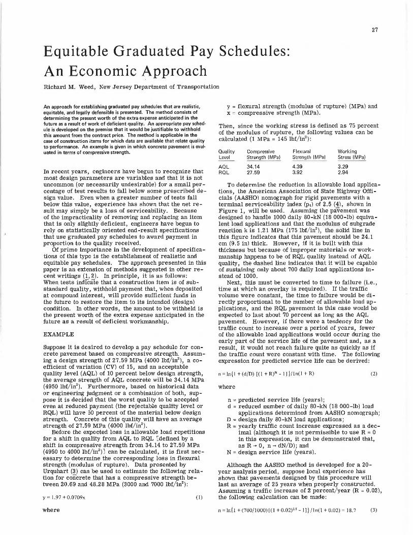
27

Equitable Graduated Pay Schedules: An Economic Approach Richard M. Weed, New Jersey Department of Transportation

An approach for establishing graduated pay schedules that are realistic, equitable, and legally defensible is presented. The method consists of determining the present worth of the extra expense anticipated in the future as a result of work of deficient quality. An appropriate pay sched· ule is developed on the premise that it would be justifiable to withhold this amount from the contract price. The method is applicable in the case of construction items for which data are available that relate quality to performance. An example is given in which concrete pavement is eval· uated in terms of compressive strength.

In recent years, engineers have begun to recognize that most design parameters are variables and that it is not uncommon (or necessarily undesirable) for a small per­centage of test results to fall below some prescribed de­sign value. Even when a greater number of tests fall below this value, experience has shown that the net re­sult may simply be a loss of serviceability. Because of the impracticality of removing and replacing an item that is only slightly deficient, engineers have begun to rely on statistically oriented end-result specifications that use graduated pay schedules to award payment in proportion to the quality received.

Of prime importance in the development of specifica­tions of this type is the establishment of realistic and equitable pay schedules. The approach presented in this paper is an extension of methods suggested in other re­cent writings (1, 2). In principle, it is as follows: When tests indicate that a construction item is of sub­standard quality, withhold payment that, when deposited at compound interest, will provide sufficient funds in the future to restore the item to its intended (design) condition. In other words, the amount to be withheld is the present worth of the extra expense anticipated in the future as a result of deficient workmanship.

EXAMPLE

Suppose it is desired to develop a pay schedule for con­crete pavement based on compressive strength. Assum­ing a design strength of 27.59 MPa (4000 lbf/ in2

), a co­efficient of variation (CV) of 15, and an acceptable quality level (AQL) of 10 percent below design strength, the average strength of AQL concrete will be 34.14 MPa (4950 lbf/ in2

). Furthermore, based on historical data or engineering judgment or a combination of both, sup­pose it is decided that the worst quality to be accepted even at reduced payment (the rejectable quality level or RQL) will have 50 percent of the material below design strength. Concrete of this quality will have an average strength of 27.59 MPa (4000 lbf/ in2

).

Before the expected loss in allowable load repetitions for a shift in quality from AQL to RQL [defined by a shift in compressive strength from 34.14 to 27.59 MPa (4950 to 4000 lbf/ in2

)] can be calculated, it is first nec­essary to determine the corresponding loss in flexural strength (modulus of rupture). Data presented by Urquhart (3) can be used to estimate the following rela­tion for concrete that has a compressive strength be­tween 20.69 and 48.28 MPa (3000 and 7000 lbf/in2

):

y = 1.97 + 0.0709x (I)

where

y = flexural strength (modulus of rupture) (MPa) and x = compressive strength (MPa).

Then, since the working stress is defined as 75 percent of the modulus of rupture, the following values can be calculated (1 MPa = 145 lbf/ in2

):

Quality Level

AOL ROL

Compressive Strength ( M Pa)

34.14 27.59

Flexural Strength (MPa)

4.39 3.92

Working Stress (MPa)

3.29 2.94

To determine the reduction in allowable load applica­tions, the American Association of State Highway Offi­cials (AASHO) nomograph for rigid pavements with a terminal serviceability index (pt) of 2.5 (4), shown in Figure 1, wilf be used. Assuming the pavement was designed to handle 1000 daily 80-kN (18 000-lb) equiva­lent load applications and that the modulus of subgrade reaction k is 1.21 MPa (175 lbf/in2

), the solid line in this figure indicates that this pavement should be 24.1 cm (9. 5 in) thick. However, if it is built with this thickness but because of improper materials or work­manship happens to be of RQL quality instead of AQL quality, the dashed line indicates that it will be capable of sustaining only about 700 daily load applications in­stead of 1000.

Next, this must be converted to time to failure (i.e . , time at which an overlay is required). If the traffic volume were constant, the time to failure would be di­rectly proportional to the number of allowable load ap­plications, and the RQL pavement in this case would be expected to last about 70 percent as long as the AQL pavement. However, if there were a tendency for the traffic count to increase over a period of years, fewer of the allowable load applications would occur during the early part of the service life of the pavement and, as a result, it would not reach failure quite as quickly as if the traffic count were constant with time. The following expression for predicted service life can be derived:

n = ln{l + (d/D) [(I+ R)N - I) }/In(!+ R) (2)

where

n = predicted service life (years); d = reduced number of daily 80-kN (18 000-lb) load

applications determined from AASHO nomograph; D = design daily 80-kN load applications; R = yearly traffic count increase expressed as a dec­

imal (although it is not permissible to use R = 0 in this expression, it can be demonstrated that, as R ... O, n ... dN/ D); and

N =design service life (years).

Although the AASHO method is developed for a 20-year analysis period, suppose local experience has shown that pavements designed by this procedure will last an average of 25 years when properly constructed. Assuming a traffic increase of 2 percent/year (R = 0.02), the following calculation can be made:

n =In{!+ (700/1000)[(1+0.02)25 -1]) / In(!+ 0.02) = 18.7 (3)

28

Figure 1. AASHO design chart for rigid pavements. DAILY LOAD APPLICATIONS

100

500

1000

RQL

Thus, with an increase in traffic of 2 percent/year, a pavement that has been determined to be capable of sus­taining about 70 percent as many load applications by use of the AASHO nomograph is seen to have a service life about 18. 7/ 25 = 75 percent as long as would nor­mally be expected.

In this example, the RQL pavemeul will require an overlay after 19 years-6 years sooner than the AQL pavement. To determine the present worth of the ex­tra cost of this premature failure, basic engineering­economlcs formulas (Q.l are used along with the follow­ing data (1 m2 = 1.2 yd2

; 1 cm= 0.39 in):

Item

In-place cost of concrete In-place cost of overlay Interest rate Inflation rate

Amount

$21.52/m2

$0.54/cm/m2

5 percent 4 percent

In the calculations, the depreciation of an overlay is assumed to be proportional to the length of time it has been in service. For example, if the expected life of an overlay is 10 years, after 7 years its salvage value is considered to be 30 percent of the cost of installing a new overlay at that time.

For this example, it will be assumed that the over­lay on the RQL pavement will have to be about 7.6 cm (3 in) thick (because of such factors as cracking and faulting) and that it will have an expected life of 10 years. This overlay will be required 19 years in the future, and at t11at time its cost will be •1. 62 x $0. 54 x (1 + 0.04)1.!I = $8.67/m2 ($7.27/ yd2

). If the interest rate of 5 percent/ year, compounded monthly is used, the value of this money at the 25th year (6 years later) would be $8.67 x [1 + (0 .05/ 12)]12x6 = $11.70/m2 ($9.81/ yd2

). At that time, the overlay will have a 40 percent salvage value, which is 0.4 x 7.6 x $0.54 x (1 + 0.04)25 = $4.38/ m2 ($3.68/ yd2

). The extra cost incurred as a re­sult of deficient quality will be the difference between these last two values, or $11. 70 - $4.38 = $7.32/ m2

($6 .13/ yd2). To convert this back to present worth, the

following expression is used: $7.32/( l + (0.05/ 12 ))1ix,, = $2 .10/ m2 ($1.76/ yd2

).

Since this is the amount of money that must be in­vested at compound interest at the time of construction to pay for the future cost of restoring the pavement to its intended (design) condition, it would seem equitable to withhold this amount from the contract price. How­ever, before this result can be ufled to ca1culate an ap­propriate pay schedule, it is necessary to consider the following factors not included in the economic analysis:

WORKING PIVOT STRESS LINE

(~!Pa) (psi)

300

.....--: ~00--

PAVEMENT 1li!CKNESS

(cm) (in)

?R 11

26 IO 24

22

20

SUBGRAOE MODULUS

(MPa) (psi)

100

200

300

400

1. There will be administrative costs involved in preparing for the premature repair of poor-quality pave­ments.

2. There will be a cost to the motoring public for earlier and more frequent disruption of traffic to make the necessary repairs.

3. A section of poor-quality pavement will almost certainly make it necessary to overlay a larger section of pavement. For example, if one lane fails, all adja­cent lanes will receive an overlay. Similarly, practical considerations will often make it necessary to overlay an entire length of pavement even though only a portion of it has failed.

4. Premature failures, which necessitate additional unanticipated rehabilitation work, could severely re­strict the priority-setting capabilities of a highway agency.

Attempts to include item 1, administrative costs, as some fixed percentage of construction costs show this to have little effect on the pay schedule that is ultimately developed. Item 2, the costs associated with inconve­niences and delays to the motoring public, is extremely difficult to quantify but does suggest that some increase in expected costs is warranted. Item 3 can be approxi­mately quantified and is seen to have a very significant effect. If a failed section in one lane causes just one adjacent lane to be overlaid, this immediately doubles the cost while providing very little additional benefit. Furthermore, if a failed section (or sections) causes a lengthier section to be overlaid, this cost might easily be doubled again, resulting in a fourfold increase. Fi­nally, if many early !allures were tu occur, item 4 in­dicates that some very serious scheduling difficulties might arise. Since fixed appropriations are allotted for maintenance work, the occurrence of several pavement failures might lead to substantial delays in making the necessary repairs. If increased appropriations were not forthcoming, these delays could become prolonged, which would further accelerate tile deterioration, cause driving conditions to become more hazardous, and makP. subsequent repairs even more costly.

Because of the potentially devastating effect of the occurrence of many substandard construction projects, plus the fact that it should be the highway agency's goal to build quality pavements that do not fail prematurely, it is felt that the reduced pay factor for RQL (truly in­ferior) construction should be set low enough to ensure that the buyer (i.e., lhe Laxpayer) gels his money's worth and that sufficient incentive is provided for the contrac­tor to produce quality workmanship. Since item 3 by it­self indicates that the estimated costs of future repairs

should be multiplied by a factor of 2 or more, it is felt that a multiplication factor of at least 3 should be used to account for all unquantified items. The present worth of the cost to repair RQL quality pavement is then estimated to be 3 x $2.10 = $6.30/ m2 ($5.28/ yd2

) and tbe appropriate percentage payment, based on the bid price of $21.52/m2 {$18.00/yd2

), is ($21.52 - $6.30)/$21.52 = 70. 7 percent, which, for practical purposes, is rounded off to 70 percent.

The next step is to develop an acceptance procedure and a graduated pay schedule that, on the average, will award 70 percent payment for RQL-quality concrete. In an earlier paper (6), it was demonstrated that the aver­age pay factor actually received for RQL-quality con­crete will be substantially higher than the minimum value in the pay schedule. This is true because many RQL lots will receive pay factors higher than the minimum value and these, in turn, bring the average up. More recent work by the author has shown that a minimum pay factor of 50 percent will produce an average pay factor between 70 and 80 percent for truly rejectable concrete. Based on this, a minimum pay factor of 50 percent is judged to be appropriate.

Once the minimum pay factor for RQL-quality con­struction has been established, it remains to develop a series of graduated pay factors that correspond to qual­ity levels between the AQL and the RQL. If one recog­nizes that the consequences of deficient concrete become much greater as the deficiency increases, it would seem reasonable to graduate the pay schedule in a nonlinear fashion so that concrete that is only slightly below the AQL would receive nearly full payment. One possible pay schedule that uses five steps and an RQL pay factor of 50 percent would be as follows:

Quality

AOL

RQL

Pay Factor (%)

100 95 85 70 50

In addition to this, most agencies would want to reserve the option to require removal and replacement of any material found to be at or below the RQL.

It is not U1e purpose of this paper to discuss the de- / -, velopment of the acceptance procedure by which the a'c­tual quality of a product is estimated. This information may be obtained from many sources (7, 8, 9). When this is completed, it would be wise to use computer simula­tion (10) or other means to confirm that the expected pay factors for various levels of quality are reasonable and equitable.

SUMMARY

The intent of this paper is to present by example a ra­tional and logical method for determining the value of an item of substandard quality to provide solid justifica­tion for the use of statistically oriented end-result spe­cifications with graduated pay schedules. It is suggested that the present worth of the additional future cost antic­ipated as a result of construction of deficient quality is a sound basis for the determination of an equitable pay

29

reduction. It is recognized that this method is appro­priate only for items for which there are data that re­late quality to performance (or expected life), but it is believed that there are a sufficient number of such cases to warrant serious consideration of this approach.

The example presented concerns the development of a pay schedule for concrete pavement based on compres­sive strength. By using the same AASHO nomograph, it would also be possible to develop a pay schedule based on pavement thickness and, in fact, these two param­eters of quality-strength and thickness-could be used jointly. Similarly, a pay schedule based on thickness could be developed for flexible pavements.

It is believed that the information needed to apply this procedure is readily available within most state highway agencies although it is recognized that the choice of specific interest and inflation rates requires the assumption that these rates can be accurately pro­jected some distance into the future. The values used in the example were chosen for purposes of illustration and, as would be expected, slightly different input val­ues will produce slightly different results. Users of this method are cautioned that care should be taken to determine appropriate input values for the agency for whom the specification is being developed.

ACKNOWLEDGMENT

The findings and opinions presented in this paper are mine and do not necessarily reflect the views of the New Jersey Department of Transportation.

REFERE~CES

1. Statistically Oriented End-Result Specifications. NCHRP, Synthesis of Highway Practice 38, 1976.

2. J. H. Willenbrock and P. A. Kopac. Development of Price-Adjustment Systems for Statistically Based Highway Construction Specifications. TRB, Trans­portation Research Record 652, 1977, pp. 52-57.

3. L. C. Urquhart. Civil Engineering Handbook. McGraw-Hill, New York, 1962.

4. AASHO Interim Guide for Design of Pavement Struc­tures. American Association of State Highway Of­ficials, 1972.

5. R. S. Burington. Handbook of Mathematical Tables and Formulas. Handbook Publishers, 4th Ed., 1965.

6. R. M. Weed. Basic Techniques and Examples of Computer Simulation. TRB, Transportation Re­search Record 613, 1976, pp. 44-50.

7. Military Standard 414-Sampling Procedures and Tables for Inspection by Variables for Percent De­fective. U.S. Department of Defense, 1952.

8. J. H. Willenbrock. Statistical Quality Control of Highway Construction. Federal Highway Adminis­tration, Vol. 2, 1976.

9. S. B. Hudson. Handbook of Applications of Statis­tical Concepts to the Highway Construction Industry. National Technical Information Service, Pt. 2, 1971.

10. R. M. Weed. An Introduction to Computer Simula­tion. Federal Highway Administration, 1976.

Publication of this paper sponsored by Committee on Quality Assurance and Acceptance Procedures.

30

Construction Industry Response to a Statistically Based Bituminous Concrete Specification 1n New Jersey J:<'rank Fee, West Bank Oil, Inc., Pennsauken, New Jersey

The evolution of a statistically based specification for bituminous mix in New Jersey is reviewed. How five producers of asphalt mix dealt with the specification and their various attitudes and approaches toward de· sign and quality control are discussed. An overview is presented of studies by the New Jersey Department of Transportation of projects run under the specification. Parti1:ular problems with the specific~tion en· countered by both the producer and the state are cited. Revisions to the specification that were used in an effort to correct the various problems are outlined. Finally, a critique is given of the specification as it evolved and as it stands today.

Before 1968, virtually all bituminous mix design and testing in New Jersey was performed by state highway department personnel. The 1961 Standard Specification for Road and Bridge Construction was still the basic specification in use. The salient provision of this spec­ification related to bituminous concrete (specifications cited in this paper refer to U.S. customary units of measurement; therefore, no SI equivalents are given):

Formula for Job Mix. The composition limits for every mixture as pre­scribed in [Table 1] are extreme ranges that must not be exceeded.

The Laboratory will establish a job mix formula for each mixture to be supplied for the Project. The job mix formula shall be in effect until modified by the Laboratory. The job mix formula for each mixture shall establish a single definite percentage of mineral aggregate to be weighed from each bin, a single definite percentage of bituminous mate­ria I to be added to the aggregate, the percentage or amount of any other ingredient that may be required, and the temperature at which the mix­ture is to leave the plant, all within the ranges of the specifications for the specific type of mixture. Should a change in sources of materials be made, a new job mix formula may be established before the mixture containing the new materials is produced.

After the job mix formula was established for a mix­ture as prescribed in Table 1, all mixtures of that type furnished for the project were to conform within the fol­lowing tolerances:

Material

Coarse aggregate, bottom course (total retained on no. 10 sieve)

Coarse aggregate, top course (total retained on no. 10 sieve)

Bitumen content for type SA top course

Tolerance (%)

±5

±4

±0.5

Essentially, the producer was required to manufacture a mix lhal t:unformed to the master range of the grada­tion table and an asphalt content within a specified tolerance of design. With the exception of the bitumi­nous stabilized base course, no Marshall testing was specified for any mix. All acceptance testing (and most quality control testing) was performed by state highway personnel.

In 1967 several factors were operating to move the New Jersey Department of Transportation (DOT) to re­vise their bituminous concrete specifications. From the viewpoint of industry, there was concern about the

specifications for raw aggregate. It was felt that the fine aggregate requirement not only was difficult to meet (thus limiting sources of supply) but also con­tributed to unstable mixes. The coarse aggregates that were specified on the basis of percentage retained through sieves with round openings were also often dif­ficult to obtain. In addition, the state's northern pro­ducers, who were involved with several different agen­cies (e.g., New York State, New York City, port author­ity), wanted to obtain a more standru·dized specification.

From thP. viewpoint of the state DOT, there was grow­ing concern about the legal position in relation to proj­ects in whkh material was found to be defective. Since personnel of the department had been responsible for both the design and quality control of the mixes, the de­purlmcnl could not be considered totally free of respon­sibility should the material not meet specifications. There was also a desire to adopt a more standardized specification consistent with the national trend at that time.

It was in this atmosphere that the first "Addenda A" (revision to the standard specification for bituminous concrete) was conceived. The department felt that the specification should contain the following basic provi­sions:

1. A shift of responsibility for design and quality control of mixes from the state DOT to the producer,

2. Partial end-result specification in that there would be no gradation requirement for raw aggregates or hot bins at the plant so long as the producer could meet the finished mix parameters,

3. A more standardized specification basically molded after ASTM D 1663-67,

4. A reduced payment schedule for material deemed not in conformance with minimum performance require­ments, and

5. Statistically based sampling and testing concepts that would provide some solid basis for item 4 above.

The producers were in favor of the first three items but not the last two. In January of 1968, the department published an interim revision that incorporated the first three concepts. This interim specification, termed "pink Addenda A," could be used as an alternate during this period by any producer who opted to do so.

The initial reaction of most p1·ouucers lu pink Auuemla A was favorable. Although some added costs were in­curred for mix design and quality control services, most felt that this was more than offset by the use of other, less costly raw materials and the ability to design and control their own mixes. The first adverse reaction on the part of the producer did not come until after the pub­lishing of the November 1968 revision of Addenda A, which was the first statistically based specification (in­corporating the last two provisions in the list above). From this time on, the_ Addenda A specification was

31

Table 1. Requirements for hot-mixed Total Aggregate Percentage by Weight bituminous concrete and sheet asphalt from 1961 specifications. Passing Retained On Mix 1 Mix 2 Mix 3 Mix 4 Mix 5 Mix 6 Mix 7

Screen, in Screen, in 1.5 1 0-35 0-25 1 0.5 25-70 20-45 8-25 0-10 0-5 0.5 0. 75 0-20 10-25 20-45 12-40 20-35 0-10

Sieve 0. 75 No. 10 0-15 5-15 5-25 8-30 15-30 8-25 0-5 Sieve

No. 10 No. 30 1-11 2 -14 2-14 2-17 8-22 3-20 4-25 No. 30 No. 50 2-15 5-18 5-18 4-24 4-15 8-30 10-35 No. 50 No. 80 2-14 4-18 4-18 6-22 3-15 10-28 12-33 No. 200 0-5 4-8 4-8 4-8 4-8 4-10 10-15

Total retained on no. 10 sieve 55-85 45-65 45-65 30-60 40-55 15-30 0-5 Bitumen content (solubility in 4-6 5-7 5-8 5.5-9 5-8 8-11 9-11.5

benzol)

Notes: All screens 0.75 in and larger are round openings. Aggregate to be used for the following pavement courses: mix 1-all bottom courses; mix 2-CA-BC-1, CA-BC-2, top; mix

3-MA-BC-1, MA-BC-2, top; mix 4-FA-BC-1, FA-BC-2, top; mix 5-SM-1, SM-2, top; mix 6-SP-1, SP-2, top; and mix 7-SA, top.

viewed with disdain and skepticism by many producers. The pertinent provision of the November 1968 Addenda

A can be found in Figure 1. Essentially, it calls for a lot of five samples to be taken for each 1500 tons of finished mix. A random number table was used to se­lect the precise ton that was to be sampled in each sub­lot of 300 tons. Five quality parameters were selected for evaluating samples of mixtures taken at the plant. Three parameters were concerned with gradation, one with asphalt content, and the last with Marshall stability. The sixth parameter involved air voids, which were de­termined by using core samples taken from the finished pavement. The producer had to have a quality control technician present during all productions for state proj­ects.

Tables of tolerances for gradation and asphalt con­tent were included based on statistical analysis of cen­tral laboratory extraction data (primarily of road cores dating back to 1961). The tolerances in the first table were based on two standard deviations. This was ap­plicable to single samples and was intended to control the range between individual samples in the lot. The tolerances in the second table were based on one stan­dard deviation and applicable to the lot average.

Under this specification, there were two sets of re­quirements for the Marshall properties: First, a mini­mum stability was required for mix designs; second, a lower "control" standard was specified for a set of three specimens molded at the producer's laboratory from a material used for one of the five composition samples in a lot. For air voids, a wider range was again used for control than for design. In this case the control air­void requirement was applicable to indiVidual core·s taken for approximately every 2000 yd2 of pavement.

In line with the department's concern about enforce­ment of the new specifications, provisions for payment reduction were incorporated for the five parameters to encourage producers to make every effort to comply. The November 1968 revision was a substantial change, then, from the standard 1961 specifications. Even though the rate of sampling and the tolerances had re­mained about the same, the shifting of responsibility for design and quality control, the increase in the number of parameters, and the inclusion of Marshall property requirements made the transition somewhat involved and difficult.

In 1968, very few producers had quality control per­sonnel. With this in mind, the New Jersey DOT and the New Jersey Asphalt Paving Association jointly con­tracted with a consultant to give a 2-week course on mix design and quality control of asphalt pavement. This program was first held in February 1968 and was at-

tended equally by both department personnel and em­ployees of producers. Many other producers hired out­side consultants to do their mix designs and quality con­trol work. Very little if any in-house design or quality control of asphalt mixes was carried on by the producers before the new specifications were issued. Virtually all endeavors at a statistically based quality control program were a direct result of the requirements of the new spec­ifications. All parties concerned were novices at this time, and much of the work was done by the trial-and­error method.

The response of five producers to the new specifica­tions is detailed below. They are intended to be a fairly representative cross section of New Jersey producers.

PRODUCER A

Located in north-central New Jersey, producer A owns four asphalt plants in two locations and one quarry. Be­fore 1968, there was one full-time quality control em­ployee. His primary responsibility was the quarry and, although he performed some limited control on the as­phalt mixes, the majority of this activity was taken care of by the state inspector. After 1968, one additional quality control person was hired.

Mix designs formulated by the quality control person­nel represented basically the same mixes as those used under the old specifications. Because of a high rate of production and therefore of sampling, the technician had little time to do anything except acceptance testing. Raw aggregate or hot-bin gradation data were not normally collected-only the information required by the specifica­tion. The only additional test run was for "stone con,­tent," which consists of soaking the hot mix in gasoline, burning off the asphalt cement, and running a gradation on the stone retained above the no. 8 sieve. This test was used with some regularity as a quick check on the mix gradation. Only one specification parameter (amount passing the no. 8 sieve) could be checked by means of this test. No graph or chart of data was used. Most control was based on single extraction samples taken within a lot. In many cases, an entire lot of ma­terial-Le., 1360 Mg (1500 tons)-would be produced in 1 d. Since the New Jersey DOT extraction test proce­dures were more involved than normal (requiring that the gradation on the aggregate after extraction be a washed gradation, which usually adds approximately 1 h to the normal test time), a competent technician could not normally be expected to run more than five extrac­tions in an 8-h day. This meant that there was no time for additional quality control testing and therefore con­trol judgments had to be based on acceptance samples.

32

Figure 1. Provision of November 1968 Addenda A revision to specifications for bituminous concrete.

GRADATION HIX!!(!. 1 1 4 5 6

5IE'IE ms

<lllADINO OP TOTAL AOORlnATB (OOAllS& PLUS l''lNt, PLUS !'ILLER IF Rl!QUIRm). NflUNTS fTI!!iR Tt!AI! EACH LA!lQllATORJ SIM (5gU/JlE OP!lllHO). \l!:!C!I!!' PE!!C!l!T.

2" 100 1-i" 90-100 100 l" 90-100 100 J/4" 60-100 90-100 100 1/2" 60-80 90-100 100 J/8" 60-80 90-100 100 No. 4 25-60 25-60 35-65 45-70 60-80 80-100 100 No. 8 20-50 15-45 20-50 25-55 35-65 65-100 95-100 Nu. 16 40-80 85-100 No. JO -~5 70-95 No. 50 8-JO J-18 5-20 5-20 6-25 7-40 45-75 No. 100 5-20 20-40 lfo. 200 J.-12 1-7 l-10 L-10 1.-lO 4=10 9-29

ASPHALT C!ME!IT, \l!:!Glfr PEllCENT OF TOTAL MIXTURES

3.5-8 4-8.5 4-9 4.5-9.5 5-10 7-12 8.5-12

Formul.ft- !OJ" job 1:1.b: . Tha Cont.mat.or ahall outait ror t.hD £.ne:lnaer• J'.I:

eppro'val. on fol"flllt n:uppUed kf1' the dopll.rlaent, 11 Job Dix foniul.1111 for t!lil1oh mixture roquirod for th• p!'Ojoot., ft l'rt&toc:wtnt nWns tho "ourae or ench component , ftnd " Hport. 1thovillg tho rcun.tl.tJt ot the applicable t.est.1:1 llJIOOif!r. in a tabl• )-11. fl'he job a b tonsul.4, including t.ho tolorancH ohovn in toblo J-A(l , =".hall bo \tU.hlD th• M•t.er ranp spec.lied in table J tor the pa.rUCular t.ypo of b1t\tlllinou11 cont!rot...

L\DL& l-AI l l TOl.ffl.11/CES f!!QH JOB llIX ft!Rllllol! roR IHPMQIAL SAl!!'!n! GRADATION

ml~m ~ "- ~ ~ ~er. [rJO!:i..l!B ~ll!D.~l l'll!!im!lA~= 1

Ho. g 8 6 > 5 s 8 No. 50 5 4 I, 4 4 4 8 HD 2!lD ,z.Q z.a za 2 D 20 2 il z ll 6J!P!W,t .6 " s ~ ~ s s

TABLE J-A( 5 ) TOLERANCES FROM JOB llIX FORMULA FOR AVIRAGE OF 5 SAMPLES

GRADATION

~'ZE l!l~~ !wi& !!B H!!!!lsI t!!l!&t1!Ll~E 2

No. 8 4.0 J.O 2,5 2.5 >. S 1 .. 0 No. 50. 2.5 >.O 2.0 2.0 2.0 =i.o 2.0 llQ 2ml J,Q lQ & SI &.a l !l 1 Q l.g Mifl:!.!.LI ,]Q lQ 2~ 25 25 2S .2~

'I' AlltE )-11. llESHlll Allil <XlMTOOL fll'4lll\IJW;l'S

HlX NllMllER l 4 6 7

CNm!I El!li GRlVl'l. fW LOOj'S

ll!SUlll STABILm , LBS. MIH. 1500 1100 1200 1400 lJOO 1200 CONTROL STABILITY, LBS. MIH. 1200 800 900 1100 1000 900 FLOW VALUE • 01 6-18 6-18 6-18 6-16 6-16 6-16 DESIGN AIR VOIDS % (NOTE 2) J-7 J-7 J-7 J-6 J-6 J-6 J-8 J-6 COHTlllL AIR VOIDS P!MJlltTAGE 2-10 2-10 >-10 2-10 2-10 2-10 2-12 2-10

!llOTES 1 61!!! il l FOR ANY I.OT OF BITUMINOUS CONCRETE WlllCH IS NECESSARILY LESS THAN 1500

TOHS, THE TEST llSSUt.TS OF THE INDMOOAL SAHl'L&S SHALL <XlKroRH TO THE JOB MIX FOflHUW. WITHlH Tllli TOLl!KAllC.~ Ul' 'fAl!Ll: J-A( l). Wlll:JI ANY SUUH LOT Will NOt OOl!l'L'I llU1l TIUS R!l<UIR»IENT, THE PAil!lllT QUANTITY FOR THAT LOT SHALL BE R&OOCED BY ~.

DEVIATION OF 5-SAl!PLE AVERAGE, PERC!JIT OF TOLERANCES REOOCTIOH OF PAIHENT QUANTITY PEI\ I.OT,

PERCENT l!! WJ!.E H(5l

0 to 100 101 to 150 151 to 200 OVER 200 (See Note 2)

NOHE 5

10 15

NOTE 1 - 1111ERE HlRE THAN ONE ADJUSTHENT OF PAY!mlT QUANTITIES FROM THE ABOVE TABLES IS APPLICABLE TO A I.OT, USE ONLY THE GREATEST SINGLE ADJUSTHENT FOR NON­CONroRHANCE TO THE JOB.J<IX FORMULA.

NOTE 2 - THE EHGINEER MAY ORDER THE ROOVAL, AT THE OONTllACTOR•S EXPEJ!s&, OF ANY MATERIAL SUBJ&CT TO THE MAXIMUM ADJUS'l'IIDIT OF PAY!mlT QUANTITY SIDWH IN TABLE J-C,

CONroRHANCE TO THE CONTROL STABILITY R!l<UIRDIENTS SPECIFIED IN TABLE J-B SHALL BE ASCERTAINED FROM ONE STABILITY DETERMINATION FOR EACH I.OT OF MATEllIAL. THE MATEllIAL FOR THE STABILITY DETERllINATION SHALL BE OBTAINED AT THE MIXING PLANT AT THE SAME TIME THAT ONE OF THE RAlllXlH SAMPLES IS TAKEN.

TABLE J-D ADJUSTMENT OF PAIHl!JIT QUANTITIES PER LOT OF BITUllillOUS OONCRE17l !XIE TO l!lHQOl!Fll!!!!Al!C& l!;l STl.BILilX llf.'Q!JIRIJ!!Z!TS.

DEVIATION OF I.OT STABILITY BWlW REDUCTION OP' PAI!!ENT QUANTITY CONTROL STABILITY OF TABLE J-B (LBS) (PERCENT)

0 to 100 101 to 200 OVER 200

5 10 20

CONroRHANCE TO THE OOHTROL AIR VOIDS SPECIFIED IN TABLE J-B SHALL BE DETERllIHED ON THE BASIS OF OHE AIR VOIDS MEASUR!MENT FOR EACH I.OT OF APP!lOXI!!ATELI 2000 SijUAlll: YAHOO A SINGLE RAJIOOH CORE FRO!I THAT LOT,

TABLE J-E

HIX Dl.VIAT[ON OP I.OT, AOOVE DEVIATION OF LOT, REDUCTION lil.P.mEll OO!i:rlllL AIR VOIDS BWlW OONTlllL AIR VOIDS OF

EAXH!JIT QUAJn'l'l'I [I!&!!lf.l!II !fm&f.l!Il lfEl!gf.l!Il

l AHO 2 0,0 to O.? ----- ---- 5 0.8 to 1.5 o.o to 0,5 10 ovm 1.5 ovm 0.5 20

),4,5,6,

""" ? 0.0 to 1.0 ···------ 5 1.1 to 2.0 0,0 to 0.5 10 OVER 2,0 OVER 0,5 20

PRODUCER B

Producer B is located in central New Jersey and has six hot-mix plants at three locations and two quarries. Be­fore the new specifications, there was one quality con­trol employee whose primary function was control of the quarry operations. In 1967, a new asphalt testing lab­oratory was constructed and, over the next 2 years, an additional four employees were hired. All state mixes at this time were produced with bank-run sand and quarried stone. Trial mix designs were set up based on the new specifications and used the unprocessed quarry screenings (stone sand). These mixes were used in all commercial work. Raw-aggregate, hot-bin, ex­traction, and Marshall data were collected. Standard deviations were developed for the commercial mixes in production. These deviations were beyond those set out in the November 1968 Addenda A. Efforts were made to correct this problem. Attempts were made to better control both the gradation and the feeding of raw ma­terials at the plant. A more elaborate sampling tech­nique was tried. A program to "reeducate" plant opera­tors was begun. Emphasis was placed on consistent cold-feed control and improved methods of storing and handling raw aggregate. An automatic compactor and a larger extractor were purchased for the laboratory. As a result, the standard deviation was reduced in 1969, but material was still often found to be outside the limits of the new specifications.

PRODUCER C

Producer C is located in south-central New Jersey. They had three asphalt plants at two locations and a natural sand pit. They had no quality control employees; in­stead, all work was contracted out to a consultant. Thus, quality control work was performed only when the project required it. This producer ran one of the few large jobs [approximately 136 078 Mg (150 000 tons)] under the January 1968 Addenda A. A new 3.6-Mg (4-ton) plant and a new laboratory were built for this job. The mix designs were set up with quarried stone and bank-run sand from the producer's pit located adjacent to the mix plant. Since the only sampling specified at this time was one roadway core (for composition thickness, and density) for every 3000 yd2

, the consultant set up his own sampling program at the plant as follows:

1. Minimum of one set of raw-aggregate gradation daily,

2. Minimum of one set of hot-bin gradation daily, 3. Minimum of two extractions daily, and 4. Minimum of two sets (three plugs) of Marshall

specimen daily.

The daily rate of production for the plant was between 1089 and 1633 Mg (1200 and 1800 tons). The mix was considered under control if the results fell within the tolerance for individual samples. Since this earliest specification had no averaging or penalty provision, no consideration was given at this time to statistical con­trol.

Three major problems became apparent as the job progressed. The first was a lack of management super­vision of plant operation. A relatively inexperienced operator was left to manage the plant by himself. Cold­feed calibration settings were rarely followed. An un­supervised loader operator allowed cold-feed bins to run out of material. Little or no action was taken by the supervisor-dispatcher when quality control problems were reported. In one instance, the plant ran in an "out-of-control" situation with variable carryover of

33

12.7-mm (0.5-in) material in bin 4 for 3 d before the general superintendent appeared and discovered the hole between the bin 3 and bin 4 compartments. The state inspector was not concerned since he considered this an end-result specification in that cores taken from the road would have to fail before the material would be con­sidered unacceptable.

The second problem to develop during the course of the job was the variability of the bank-run sand. Al­though some borings of the pit had been taken, either a rational mining plan was never established by the pro­ducer or the material was too inherently variable. The end result was high variability on all three of the ac­ceptance sieves [2.36, 0.3, and 0.075 mm (no. 8, no. 50, and no. 200)] in the final mix.

The third problem concerned the metering of mineral filler into the mix. Either the filler delivery system was too large, or the electromechanical control was too coarse. In any case, sample-to-sample variance outside the 2.0 percent tolerance of the specification was common on the 0.075-mm (no. 200) sieve.

The variances on the 2.36- and 0.3-mm (no. 8 and no. 50) sieves were equally high. Initially, the consultant followed the standard procedures of "quartering" the mix sample to reduce it to testing size. When high variance was found on the 2.36-mm sieve, the "grab" method of sampling was tried simultaneously as an alternative. In this case, one pan of material was taken from the truck from three levels of conical pile by using small shovels. A grab sample was carefully taken from the pan in a large grain scoop. Then the same pan of material was quartered in the usual way, and another sample was taken. Extractions were run on both samples. Sample­to-sample variance on the 2.36-mm sieve for the grab samples was about half as great as that for the quar­tered sample.

Although the use of the grab method reduced the vari­ance on the 2.36-mm sieve, samples would still fall out­side the tolerance with some regularity. This was usually attributable to raw-aggregate and cold-feed variances that were well beyond the tolerances and in many cases out of control. At times, the bank-run sand would alternate over a range more than twice the toler­ance during the course of a single day. Although efforts were made to monitor and control this material, it was often out of control.

Producer C had another, older plant located in their central yard that produced material under the November 1968 specifications during this period. This plant used a bank- run sand from another source and was under the direct supervision of the chief superintendent. During this same period, this plant produced material with a sample-to-sample variance on the 0.3- and 0.075-mm (no. 50 and no. 200) sieves about half that of the newer plant. The same consultant was used for mix design and quality control in both plants.

PRODUCER D

Located in the southern part of the state, producer D operated one asphalt plant and a natural sand pit. Before 1968, they had no quality control run on their material other than that performed by the state inspector. With the advent of the new specifications a consultant was hired to do the mix design and quality control work. The only time quality control testing was performed was when the plant was supplying a state project. The mix designs were very similar to those under the old specifi­cations. The producer's own bank-run sand and a quarried stone and mineral filler were used. The same daily testing program established by the consultant for producer C was again implemented here. Since most

34

work for this plant came under the November 1968 re­vision of Addenda A (which included the statistical con­cepts), additional extractions were run on each lot sam­ple. These extraction results soon became the primary data for quality control because of the penalty provision in the specifications. The problems encountered at this plant were twofold: first, the lack of respect for the quality control process on the part of the owners; and second, the variability of the bank-run sand. The owner would generally ten the batch man to run "light on filler and heavy on sand." The more expensive items in the mix in this case were filler and stone , This made effec­tive quality control by the consultant quite difficult since no meaningful mix changes could be implemented until the owner was convinced it was necessary. Another common practice was to "top" trucks (i.e., mix only the final top loads in the truck according to design). On several occasions, the plant ran out of mineral filler and yet continued to ship material to the job. The bank-run sand, although fairly consistent, did tend to shift enough over time to require design revisions on the amount passing the 0.3-mm (no. 50) sieve.

PRODUCER E

Located in southeastern New Jersey, p1·oducer E oper­ates one asphalt plant. Before 191i8, this company had no quality control personnel. The mixes at this time were designed with natural sand, which was readily available. With the coming of Addenda A, a consultant was hired for the design and quality control work. In this case, the owner and plant superintendent took a strong interest in the quality control program. Sugges­tions made by the consultant were acted on promptly. Yard personnel and operators were given an understand­ing of what the quality program was about and materials were purchased with some consideration as to their quality.

Basically, the same quality control program outlined previously for producer C was again used here. In this case, control charts were used for the raw materials and mix analysis. A desired range for the raw materials was established based on the mix design and, when trends outside the range became apparent, calls were made to the suppliers to correct the problem. As deviations from the job-mix mean became apparent, small adjustments were made in the mix formula.

The only serious problem the consultant found was in the variance between the field and the central laboratory. In one instance, when the central laboratory reported a lot failure, the consultant witnessed the running of the "referee" sample at the central laboratory. Under this system, the mix sample was divided at the plant into three portions. The first went to the central laboratory for analysis and was considered the sample of record. The second was run by the producer's quality control person at the plant. The third was tagged, sealed, and stored as a referee sample.

The central laboratory had a policy of running only one ash correction per lot of material on their centrifuge extraction. When ash corrections were run on all sam­ples in the lot, all passed and conformed fairly closely with the results obtained at the plant.

This producer succeeded in running several medium­sized [36 360-Mg (40 000-ton)) jobs without penalties under the new specification.

SUMMARY OF 1968-1970 PERIOD

In summary, it seemed that during this period only a few producers fully comprehended the ramifications of the new specifications and most felt they could get by without

any changes in their basic operations. Quality control data were generally viewed with skepticism by the few producers who could comprehend it. Generally speak­ing, the few comprehensive quality control programs (those including raw-aggregate and hot-bin data and reg­ular visual plant inspection) fell prey to the demands of the end-result process. The extraction sample of record (::mcl, to a IP.RRP.r clP.grP.P., thP. Marshall Rample) bP.c.amP. the dominant indicator of mix quality. In the beginning, there was generally a poor understanding at the field level of the statistically based two-tolerance system. Most quality control personnel soon realized that mixes had to be controlled on the lot tolerance (average of five) and not on the individual tolerances.

Extractions run in the field were often considered ac­ceptable if they fell within the tolerance for individual samples (which was twice as wide as that for the lot average). On several early jobs it seemed that passing results were being obtained, but at the end of those jobs it was found that the lot failed on the basis of the average of five.

In spite of this, few if any charts were kept of process control data. In fact, when the department distributed control charts in 1970 and required their use, there was so much resistance on the part of both producers and state personnel that the program faded uut uf existence a year later. The only significant collecting and pub­lishing of data were done by the department in the job printout, an example page of which is shown in Figure 2. Most process control continued to be based on the vari­ances of the individual samples in a lot. Technicians generally reviewed the individual sample result and made "judgment calls" as to whether the formula needed to be adjusted. Depending on the technician, these judgment calls may have been based on overall plant operations (variance in raw aggregate and screening problems) or simply the results of the last extractions.

Inlatel969, theNewJerseyDOT did astudyofprojects completed under the new specification (1). It found that 17 of the 35 lots included in the study failed to comply and were subject to penalties. Approximately 75 per­cent of the failures were for composition, and the re­maining failures were equally divided between core air voids and Marshall stability. An evaluation of the aver­age standard deviations for the projects showed that they were equal to or less than those used in developing the specification. Thus, the state concluded that excessive variance was not the cause of the failures but rather multilaboratory testing variance and the inability of the producer's quality control process to keep his process average target on the job mix. This was amply demon­strated by the fact that central laboratory results showed a consistent variation from producers' laboratory results on duplicate samples. At the same time, the producers' own results showed that they often failed to meet the average of five sample tolerances based on their own de­sign. In the area of composition testing, most samples failed because they missed the target values and not be­cause they were excessively variable. The state attrib­uted this to the lack of experience of the producers' quality control personnel or "inexactness in the design­ing of the mix" or both.

From the producer's viewpoint, there appeared to be several problem areas with the new specification. First, there was the problem of the difference between the sam­ple run at the plant laboratory, on which all quality con­trol was based, and the sample run at the department's centr11l l11boratory, on which all payments were based. Next, there was the problem of adjusting the mix design for variations in raw materials. Under the 1968 Addenda A, the lengthy process of submitting a new design was the only method of making adjustments [this was partic-

35

Figure 2. Page from New Jersey Department of Transportation job printout.

l0•29-b9 NEW JERSEY STATE DEPARTMENT OF TRANSPORTATION PAGE Z ·-o "tv rs·1 ufnrni"AffiffAL - ------·-- -

------------------------------~S~ltNV~E""'ANALVS!S RE~~OR~T.__ ______ _.._ __________________________ _ 8 IT IJiITROlJSifArrl\J A

; ccNTR DL SECTI ON 324

': HUTUR £: ~,.....c>'-J-f------~----·~-

iUiiofrnrRvS"ElffALNOifBE-R ---9o<iT24 ___ 909~---S--"90"98S~0985 7 9098 58

~m-tAI 0 6 -4-69 6 -5=69 6 -5-69 6 -5-69 6 -b-b'1

rt clNl JrACTOl{- ---uS"""----i.rs-------i 15 115 ~------ - - ~--·

il'lfOiJU"t~ ·-· j B ltf--~,.,...------- ·

, rvrnu~r-, SPEC r-~C.{ffN S "ANll- !lfEVES- usrn- - - ------ -- - - - ------=-1.ERCENT----~-==---=-=== IOLl:RAN'C~ I PASSJ NG 1/ 2 IN 100 .0 100.0 100.0 100,0 l OO , O 100.0-l OO,O ·~·AS'~1r,t-~f8 .. 1N ~-- 911--::0-·--·'>~-=-~-va .o 9"tt;"o 9·>.0 --·---g o.<Froo ~ o iP ASS I NG NO . 4 74. 0 75 .0 75.0 b~ . o 1>3 . 0 b 0.0- eo.o m~o. a sa . o• s2.o ss.o.!I' 49 . o 41.0 42.0- s2.o ; P ASSI i'<G NO . 50 21. 0 20 .0 24.0• 21.0 20.0 15.0- 23.0 f P~5STNG-- NO:<Ov -- - ----·- -- -6:·0--,.-~-o.cr----.r.rr-- -5~. 3-;4:---,;4-

i ~ ~~~~~~~~·l11~~~-~~T. _________ ~-···--®-·----~~ 5.~ siti ~ s.1- b,l I

~ITIJTE"S~ll:UITT: OF A PARTICULAR SARl'LE At 1RAI PAR I I COLAR SCREEN SIZE I NOICAI ED

':ir tv rnrnN! t-ITHE--S-Ailrc:-f!Ail.At:TERTSTTCllf--roR' "RQ"i(Ell<t) IVl DIJ~LTAHPl~STRG"""Nir;-a------5 PERCEN T RED UCT ION - - - ---·-------- - - -

SAMPLE SPEC AVG. ; c:ll.HfiS---c ·srEVE>lJS-EU== - - - - :.---==i>cRCENT="---- - i'IVG-;----TO[ERANtclOlERANCE >~SSING NU. e 53.0 52.0 55.0 49.0 47.0 51. 20 Z.50 44.50- 49.50 ~A~o. so 21.0 20.0 24;-o 21. 0 20.0 21. 20 2. oo-rr;uo~u-PASSll!G N0.200 b.O 5.5 6.e e,1 5,4 6.31> 1.00 4.40- 6.40 BITUMINOUS· c:ONT.ENl·----· - -5;-i. . ----s;-r---- ---s-.4·----- 5;·-r---· --:;;-i;--~-;3e---u;-z 5 -~;35---·-s. 85

DEVIATION UF 5~-AHP[tliVG"~--l'A'S-S1NC>NO·;--ii---11FP"ERCENT--P.EDIJCTTOi.---- ----- ---·-------·-OEVlAl JON OF 5-SAMPLE AVG. PASSlNG NU. 50 5-PERCENT REOUCTION

ularly applicable on the 0.3-mm (no. 50)sieve]. Next, there was .a general feeling that the tolerances were not broad enough to contain normal variation, a desire to have more than just the three plugs per lot on the stabil­ity determination, and a desire for a modification in the basic gradation tables to allow the use of a wider variety of raw materials.

Shortly after the completion of the 1969 study, the department began to allow the acceptance of "retroactive designs." These could be submitted by the producer after he reviewed the lot data from the central labora­tory. Retroactive designs could be submitted on a lot­to-lot basis and were intended to compensate for multi­laboratory testing variance. This required nothing more than a letter requesting a numerical change on a particular sieve.

In September 1970, a new revision of the 1968 Addenda A was published. Known as the "yellow Addenda A," it contained the following revisions:

1. Changes in the basic gradation tables; 2. An i ncrease in the gl'adation and asphalt cement

(AC) tolerance for both the individual and average (in addition, the penalty provision for failing to comply with the individual sample tolerance was removed);

3. Plant acceptance, i.e., the final acceptance of ma­terial for gradation, AC content, and Marshall stability based on the plant technician's field results (these tests had to be carefully documented on forms supplied by the department and witnessed by the state inspector);

4. A tightening up of the air-void limits for both de­sign and field core samples;

5. An increase in the number of specimens used for

the Marshall stability criteria (one plug would be made and tested for each of the sublot samples, and the aver­age of fi ve would have to meet the minimum specified for control);

6. A reduction in the amount of the penalty for non­conformance; and

7. A limitation on the use of unwashed natural fine aggregates.

Also included in the yellow Addenda A was a detailed description of the various testing procedures to be fol­lowed.

The above changes seemed to resolve most of the problems that had plagued the first Addenda A. Although the policy of allowing retroactive design changes elimi­nated many composition penalties, the department was less than enthusiastic about this approach. It was felt that this policy encouraged an even greater lack of con­trol by the producer. Thus, late in 1971, the depart­ment changed its policy and allowed design changes only at the beginning of a lot.

The inclusion of a natural sand requirement that ef­fectively eliminated the use of bank-run sands disturbed most of the producers in the South Jersey area. The de­partment's action was the result of several pavement failures attributed to clay "pop-outs" in mixes that used bank-run sand.

With the advent of "plant acceptance," many pro­ducers' technicians seemed to have more confidence in the statistical specification since the results they got were now considered record. Further confidence was gained as a result of the wider tolerances and the rela-

36

Table 2. Summary of average composition parameters under Addenda A.

Average Standard Deviation ("')

1969 1970-1971 1971 Mixture Green Green Yellow Current Characteristic Addenda Addenda Addenda Tolerance a.

Mix 1 8ieve

No. 8 3. 75 3.34 3 .31 4.0 No. 50 2 .01 2.08 1.93 2.5 No. 200 1.18 0.96 1.10 1.0

Average composition 0.35 u . ~~ 0 .34 o.~5

Mix 2 Sieve

No . 8 2.91 2.90 2 . 77 3.00 No. 50 1.87 1.67 1. 58 2.00 No. 200 0. 99 0.82 0.89 1.00

Average composition 0.34 0.32 0.25 0.35

Mix 5 Sieve

No. 8 3.28 2. 74 2. 70 3.0 No. 50 2 ,42 2.28 1.92 2.5 No. 200 1. 13 0.95 1.10 LO

Average composition 0.30 0.26 0.26 0.30

J Average of five samples b 197 i

tivc case of adjusting designs for normal variation in raw materials.

Process control in the average asphalt plant was not affected, however. Since most technicians were already normally sampling and testing the duplicate record sam­ple under the "green Addenda A," the control process continued to be based on the extractions taken for rec­ord. Control at the plant may indeed have become some­what more lax. Since the plant technician's samples were the sample of record, he could now run closer to the limits of the tolerance and not fear that the sample run in the central laboratory might be out. He could also make mix adjustments that would compensate for samples that fell outside the limit. Since there was no longer any limitation on the individual samples, he could intentionally make material out of tolerance to bring the average of five in range.

Again in 1972, the department reviewed the results of Addenda A. Afferton (2) observed that there was gen­erally a decrease in variability since the 1969 study (Table 2). He pointed out that in spite of this one out of seven lots was still penalized. As in Lhe earlier study, he attributed this to the producer's inability to meet his or her own job mix formula. Although some increase was observed in the producer's ability to hit the target value, Afferton generally discounted this as the result of the shift in testing laboratories. He further observed (2) that "marked changes in the produc;:er's ability to evaluate stockpile aggregate and use statistical tech­niques would be needed to effect . . . improvement." He felt that this would be a difficult and time-consuming process that may not be necessary since historical data suggest that the current differences in the job mix mean are comparable in magnitude to those that occurred be­fore Addenda A when the department had complete con­trol of plant production. As a result, a wider tolerance range was proposed for mixture composition.

Finally, in May 1973, another version of Addenda A was released. The changes represented by "blue Ad­denda A" were as follows:

1. Deletion of the tolerance for individual samples, 2. Inclusion of "tolerances for the range of five

samples," and 3. An increase in all of the tolerances for the aver­

age of five samples.

Average Absolute Standard Deviation Plus Difference in Job Difference" ( ~) Mix Mean("') Recommended

Rounded New Specification 1969 1971 to Account Tolerance for Green Yellow for Toot Five-Sample Addenda Addenda Calculated Precision Average (1-)

1.69 1.26 0.39 0.Jl

1.91 1.21 0.51 0.13

0.36 0.81 0.44 0.11

1.10 4.41 4 .5 4,5 0.47 2.40 2.5 3.0 0.25 1.35 1.4 1.4 0.017 0.41 0.40 0.45

0.92 3.69 3.5 4.0 1.10 2.68 2.5 3 .0 0.37 1.26 1.3 1.4 0.12 0.37 0.35 0 ,45

0.00 3.50 3 .5 4.0 0 . 90 2. 82 3 .0 3 .0 0.18 1.28 1.3 1.4 0. 17 0.43 0.45 0.45

These changes seemed to have effectively corrected the problem outlined above.

CONCLUSIONS

Because Addenda A changed so many things all at once, it is difficult to isolate the effects of the statistical pro­cess control aspect of the new specification. Ensuring that the changes in requirements for gradation and raw aggregates had a substantial effect on the asphalt mixes (whether for better or worse) would be a subject for another paper. One thing appears certain: After the ap­plication of the first penalties, nearly all producers took a keen interest in the Addenda A specification. Some were inherently skeptical and continuously sought to find defects in the specification rather than defects in the product. A few were more willing to accept the system and generally strove to control the product better. The latter seem to have fared rather well even under the earlier, more restrictive version of Addenda A.

In any event, the producer's attitude toward process control is critical tu its effective application. If the producer is not convinced of the necessity or the desira­bility of the system, it is virtually impossible to effec­tively carry out a good program. No matter how com­petent and enthusiastic the technician may be, he can only do what the rest of the organization is geared to do.

As in any good system of process control, testing error must be kept in line with the limits allowable by the tolerance. In addition, a standardized and practical testing procedure must be published and understood by the technicians. A certain level of confidence must be established and maintained between quality control test­ing and acceptance testing.

It is essential, therefore, that careful consideration be given to the establishment of realistic tolerances and penalties. Since the person who pays the penalty often has little or no understanding of testing or quality con­trol technology, that person tends to quickly judge the system in black-and-white terms. He or she generally has neither the time nor the inclination to determine why samples pass or fail. If a produc.er suddenly finds that he or she is being penalized often and that fellow producers are in the same position, then the credi­bility of the system will soon be in question. Once this occurs, it becomes very difficult for the technician ef-

fectively to keep the products under control within the system. If at the same time the technician lacks con­fidence in the testing and acceptance procedures, the system virtually disintegrates.

Under these circumstances, when the acceptance point is at the plant, the propensity for graft is greatly increased. When the acceptance is more distant (as in the case of cores taken from the finished product and tested in central laboratories), more involved legal battles are often encountered. In any event, the theory and practice of good statistically based quality control are completely undermined. I feel that this was the status of the Addenda A specification just before the release of the 1970 yellow Addenda A.

It is important that good delineation and coordination be established between acceptance testing and quality control testing. A good quality control program should be somewhat independent of the acceptance system. Un­der the existing Addenda A, acceptance testing dominates and indeed, in most cases, overpowers what I consider to be good quality control testing. In plants that have lower rates of production, there is a tendency not to do any testing until a "lot sample is due" because of the strong emphasis on acceptance samples. Indeed, if tolerances were properly established and confidence in correlation with central laboratory testing was ensured, I would rather see acceptance testing performed by the central laboratory from field samples. However, I do not wish to minimize the problem of developing such a

37

system (especially the problem associated with a central laboratory type of operation such as that used in New Jersey in recent years). If such a system could beef­fectively developed, however, a more comprehensive quality control program could be used at the plant where the technician could monitor the entire operation and not just some narrow aspect of it.

Essentially, a statistically based quality control pro­gram is a vast improvement over the typical one-sample (pass or fail) system of the past. If it is to be truly ef­fective in maintaining the quality of the product, confi­dence in the system must be upheld by the establishment of realistic tolerances and testing methods. It is essen­tial that all of the involved parties thoroughly under­stand the theory and application of the system.

REFERENCES

1. K. Afferton. New Jersey Department of Transpor­tation Standard Specification Analysis-1969 Addenda A. New Jersey Department of Transportation, Jan. 1970.

2. K. Afferton. Composition and Air Void Require­ments for Bituminous Mixtures. New Jersey De­partment of Transportation, Memorandum Rept., July 7, 1972.

Publication of this paper sponsored by Committee on Quality Assurance and Acceptance Procedures.

Process Control of Mineral Aggregates John T. Molnar, Standard Slag Company, Youngstown, Ohio

An aggregate process control program currently used by a multiplant ag­gregate producer is described. The success of the program is credited to the rapid feedback of test data directly to plant management. The pro­gram uses district and plant laboratories staffed with from one to three technicians for conducting daily tests for gradation control and a central laboratory for determining other important properties of aggregates and the products in which they are used. Benefits of the program-including savings that result from minimizing rejections, improved customer rela­tions, and other services performed by the responsible department-are emphasized. The importance of a working knowledge of basic statistical concepts by both aggregate technicians and plant management is stressed.

The process control system described in this paper is used to control the quality of aggregates at 21 plants of the Standard Slag Company. These include 11 blast furnace slag plants, 5 limestone plants, and 5 sand and gravel plants. The program is directed by the Materials Control and Research Department with a staff of 20 full­time and 5 part-time employees. Testing facilities in­clude six district and plant laboratories, each staffed with from one to three technicians and equipped to con­duct daily determinations for gradation and unit weight, and a central laboratory equipped for determining most physical and chemical properties specified for the ag­gregates as well as the performance of the finished products in which the aggregates are used.

Since gradation is the primary aggregate property over which the plant manager has control and since failure to comply with the specified gradation is the primary cause for rejecting aggregate from approved sources, this paper

deals primarily with the control of aggregate gradation during production, handling, and recovery from stock.

The founders of our organization realized more than 50 years ago the benefits of producing quality aggregates in terms of a favorable return on investment and repeat sales. During our first encounter with statistical or end-result specifications during the late 1960s, it be­came apparent that increasing the effectiveness of our process control system would be a sound investment in terms of minimizing costly rejections and product lia­bility claims and improving customer relations by sup­plying aggregates that have a minimal variation in speci­fied properties. Accomplishing this meant devising a system of rapid testing and reporting that would provide immediate feedback of production control test results to plant management so that process adjustments, when necessary, could be implemented and checked for their effectiveness before a sizable quantity of nonspecifica­tion material was produced. The system now in effect was presented to the company's executive committee and received their total support.

The basic procedure used for gradation control is shown in Figure 1. Basically, each aggregate size pro­cessed in each operation is sampled in accordance with a prescribed sampling plan that stipulates sampling frequency and location and the minimum sample size. If the gradation of the sample complies with that speci­fied, no adjustment is made. If the first sample fails to comply, a second sample is immediately selected to verify the results of the first and, at the same time, to

38

Figure 1. Procedure for gradation control. Figure 2. Responsibilities of district laboratory technicians.

RE SAMPLE

~ TEST

YES

ADVISE PLANT SUPT.

ADJUST PR OCESS

l RESAMPLE

i TEST

YES NO

CONTINUE PRODUCTION AS IS

Figure 3. Plant aggregate report.

EACH SIZE PROCESSED

SAMPLE IN ACCORDANCE WITH SAMPLING PLAN

\ TEST

I CALCULATE RESULTS

PREPARE DAILY PLANT REPORTS

KEEP OWN COPY UNTIL COMPLETE

OR END OF MONTH

j _CALCULATE: X,S,F,X MOVING ,.........____!

PL NT SUPT.

CENTRAL OFFICE

t SUGGEST ACTION

IF NECESSARY

USE DATA FOR MONTHLY AND ANNUAL

REPORTS, FILE

j COPY

GENERAL MANAGER,

OPERATIONS

PLOT DATA ON CONTROL CHARTS

SUPERINTENDENT'S COPY DISCUSS RESULTS

WITH SUPT,, LEAVE COPY

j END OF MONTH

OR CHART COMPLETE

l _ CALCULATE: x,s,F,X MOVING

DISTRICT MANAGER,

OPERATIONS

DISTRICT SALES REP.

Report No . __ _,l.,,;22~--~=------- Date DECEMBER 21 , l 977 Material A C B. SLAG Plant 5 Sampled by R Tested by R.J.M

~ · .... '" lv<l< Source

(mill or stock) M M M M Sample No. 243 I , •• I i4~ , .. I I .JlZe No. 57 I S7 <•<~ I 8 8 I •n<r I Sieve Size Total Percent Passino Sauare Qnonina < ;ouo•

4" Jli" 3" 2lf" 2" lJ, 100 rnn rnn l" 96 91 90- If

3/4" 1/2" 42 45 25-60 inn 11 inn 3/8" ......9A....... 93 B~Q

No. 4 4 5 0-10 ?1 1R 10-30 No. 6 No. 8 2 2 0-5 4 3 0-10 No. 10 No. 16 ? 1 0-~ No. 20 No. 30 No. 40 No. 50 No. 60 No. 80 No. 100 No. 200 F .M. tU>ohjM• 0.6 1. 0

I/eight, lb/cu ft Loose 78 76 Compact (Dry) i-;;,;o...-+---+---l---1-i.;;...-1---+---1----.i-- -1----1

Loose ( Campa ct Damp)

% Mai sture t----t---t---+---t---+---t----t--- i---i----1

Samp.l e l/t. , l bs_t=34~_,lr..,..;3"'1,---+----1t---t-rnl8.__11,..;ln;;5-+---t---+---+----t Approx . tons rep. 250 250 UO Im

Shipped Vfa ' I REMARKS '------------------------------

Figure 4. Control chart .

PLANT: _ __ 2~~-S I ZE NO,: 57

5 10 15 20 TEST NO' I I I I I I I I I I I I I I I I I I I

SIEVE H"

l"

6 0

5

a ~ -~~ .:.:J~ 7- ,__

l/j\ ,q: d ~I ~ · · · ·' · - - i?''

-t-·)....~ -· ·J.... j

98 0 . 7 0

~ 112" O·\

· -·,:v .(.IL!

x = 50

s = 4 . 5

F = 1. 3 :;:

_J

Cl ,,, u..

u ,,, 0..

"'

NO,

4 0

- - - - - - -0

2 0

- - - - - - - - - - - - CAUTloN­BAND

x = 6 ) 10~·~· s = 2 . 1

4L 0~ F = 2 . 9

NO. s[1

J:UJfQ™4JJUJJ x = 3 s = 0 . 9 F = 1. 8

~~ ::f 11 1 1 t 1 1 11 t 1111 I 111 t ~ ':ltl I lfiTI I t 1 111 i#H

reduce sampling or testing error. If the second sample also fails to comply with the specified gradation, the technician advises the plant superintendent that an adjust · ment in the process is necessary. Once the adjustment is made, the aggregate is resampled to confirm that the adjustment corrected the condition. If it did not, the adjustment process is continued until compliance with the specified gradation is achieved.

Figure 2 shows an outline of the responsibilities of the district laboratory technicians. It should be noted that sampling and testing encompass all of the steps out­lined in Figure 1.

District technicians are responsible for calculating the test data and preparing two reports. The daily plant report (Figure 3) is a comparison of tP,e gradations of current production with the specified gradings (because the reports cited here use U.S. customary units of mea­surement, no SI equivalents are given). To provide im­mediate feedback of test results, the technician discusses the results and supplies the plant superintendent with his or her copy immediately after completing the daily tests. The technician also sends a copy to the central office for further action and distribution as shown in Figure 2. In addition, immediately after completing the daily tests, the technician brings the control charts up to date. The control charts (Figure 4) show up to 25 sieve analyses of a given aggregate size and provide the plant superin­tendent with a running account of the variation of each size processed.

Again, to provide the necessary immediate feedback of test results to the plant superintendent, the technician keeps the superintendent's copies of the control charts in a looseleaf binder in the plant office and brings them

39

Figure 5. Sampling procedure for central laboratory tests.

EACH SIZE PROCESSED

SAMPLE IN ACCORDANCE WITH SAMPLING PLAN

SHIP TO CENTRAL LABORATORY

TEST FOR PROPERTIES NOT DETERMINED AT DISTRICT LABS

REPORT

I CENTRAL OFFICE

DATA CHECKED AND RECOMMENDATIONS MADE

LAB REPORT TYPED AND COPIED

USE GEN. DIST, PLANT DIST. DIST, DATA FOR MGR. MGR. SUPT. SALES LAB

MONTHLY AND OPERA- OPERA- REP, TECH,

ANNUAL REPORTS, TIONS TIONS

Fl LE

up to date on the day the tests are conducted. The tech­nician also brings his or her own copies up to date at the same time. Note that, besides the upper and lower specification limits for each sieve, caution bands are included to alert the superintendent that he or she may be operating too close to the specified limits.

In preparing the control charts, a circle is plotted for each test result. Also, starting with the fifth test result, a square is plotted on the control sieve to rep­resent the moving average of five results. The moving average reduces the variation of individual test results and is used to predict causes of potential problems, such as wear of production components.

At the end of each month, the technicians calculate the average, standard deviation, and potential failure for each sieve specified based on a normal curve. These figures are shown at the right of each plot. Each tech­nician is provided with a statistical calculator for ease in determining these parameters. The technicians then send their copies to the central office (Figure 2) where if necessary, further action is suggested. Copies are ' then distributed to the general manager of operations, the district manager of operations, and the district sales representative.

District technicians also select samples of all sizes produced at each operation at prescribed intervals and ship these to the central laboratory (Figure 5) to be tested for specified properties not determined at the dis­trict level. A typical laboratory report is shown in Fig­ure 6.

The quality control program generates five reports. In addition to the daily plant report, the laboratory re­port, and the control charts already mentioned, the in­formation from the daily plant i·eports are tabulated by the department secretaries on a monthly r eport (Figure 7). The average, standard deviation, minimum, max­imum, range, and potential percentage of failure are computed by using a tape-programmed calculator. Dur­ing December of each year, the data from the monthly

40

Figure 6. Interoffice aggregate report.

""m""' No. ,,.. ,,., JUA

-No. R I 11'.l ~•n 11!.VI' AN~L'f.18. '1'0 T AL. ,.IUt Cl'.HT ~A.SllNG

4-..... 3- 1.1 1.1 ...... z-l"Jll 100 r 89

'l'4 71 'f2 100 52 ~ 92 100 39 ~amp1e No. 1146 I

N9. 3(1,(,. -,

No.4 lHc 99 23 Gradln1 Lo• Ang. Abraaion

% Lon Jilo.6 ~ 24 . 2 I No.8 3 83 17 I No.10 16 I No.16 2 60 14 I No. 20 No.30 44 12 No.40 37 11 Cru1hed P1ecea No.50 32 In N0.60 NO.•~ 22 9 NO. LUU 15 . 7 7.2 ~•mp11 ""· t.•. 1111

93.8 109.6

1'1<11 sture uens1 tY M2thOd n•m<

W4l Sample No. lJqH

>taD1 I ty Good Good bs/fto Wet 142.4 152.8

Boll i..m.11 '1f> Dry 13~.o 140,q Umonltn l>OllOI \ii>

""""' 9'o tr; Molst. 5.~ ~ . l Tobllo;.-r % _,.,...,.,.

11>

!ihal• ~ 0 4 CM••na uanne · ~ .......,.ruq ... Th1o & F l nno~t•d ~ 16 .5

Mgr., Materials Control and Research Dept.

Figure 7. Monthly gradation report.

PLANT: 3 SIZE: 57

95- },00

26 100 100 80 44 18 2 6.0 27 100 98 74 42 17 1 28 100 98 72 40 13 2 29 100 99 82 44 16 3 2 1.2 30 100 99 67 34 14 2 31 100 99 81 35 15 7 32 100 99 83 40 18 3 33 100 100 88 41 18 1 34 100 99 85 39 17 1 35 100 99 86 43 13 4 2 6.0 1. 5

7-25 36 100 99 79 25 11 3 3

x 100 99 79 41 21 3 2 6 , 0 1.4 s 0 0.6 4.5 8.8 8.0 2.3 0 . 5 0 . 7 0.2 F 0 0 5 0 0 HI 100 100 88 53 38 8 3 7 . 0 1.6 LO 100 98 67 34 11 0 2 5 . 0 1. 2 R 0 2 21 19 27 8 1 2.0 0.4

N = ( 36) (36) (36) (36) (36) (36) (4) (5) (4)

Figure 8. Annual aggregate report.

PLANT:

Material Size Physical Properties

Unit Weight, lb/ft3 Dry Loose Dry Compact

Specific Gravity, Bulk Dry

Absorption, % Moisture as Rec'd., %

Hi

87.8 98.0

2. 52 3.80 7 .0

LIMESTONE

MATERIAL SOURCE:

1

..21_ I 8 Low Avge · 1 !!.!_ Low Avge.

83.6 i 85.7 82.0 80.2 81.2 93.6 195.6 • 91.8 3g,6 90.7

2.45 I 2.49 1 2.48 2.42 2 . 46 2.93 , 3.27 4.55 . 3.75 4 . 12 4.o s.6 ! 8.o I 5.o 6.1

Chem lea l

Constituents

Si Oz Al 203 cao MgO

Properties ~I I 8

Totif lC byWt. 3.30 3.28 0 . 19 0.19

33.77 34.63 16.85 16.96

Los Angel es Abrasion, % Loss B Grading

s 0.084 0.100

C Grading Soundness, % Loss Shale, % Thin & Elongated, %

Average Gradation Sieve Size ~

l 1/2" 100 I'' 95-100 3/4" 1/2" 25-60 3/B" #4 0-10 NB #16

~/ash Loss, % 200 Si eve

31.3 1 26.3 I

5. 5 1. 5 0 0 3.2 1.6

57 N ~ 220 Avge. T""'Ri_ Low

100 100 JOO 99 100 95 79 99 66 42 59 26 18 43 5 2 9 0

l 1.1 l.3 1 0. 7

28.6

3. 6 0 2.4

!'.. 0 5

33 33 38

9

: 31. 5 6. 7

I 0 I 9 .3

: i I

I i o I I 0.9 I : 4.6 I : 6. 2 I . 5. 8

1. 2

27. 7 2.S 0 5.0

129.3

5 . 1

I ~ .s

f ~ 0 0

I 100 I 85-lQQ ' 10-30

0-10 0-5

Fe20J 0.12 0.15 Ign. Loss 44 .6 l 44. 38

8 N ~ 108 ~ Tl1_i_ Low !'.. i

I I I

100 100 I 100 0 0 95 99 88 10 I. 7 17 25 I 9 14 3.1 3

~J 2 3 1.0

1 I 0 0

1.0 0.5

TOTAL PERCENT PASSING

Figure 9. Example control charts used in training sessions.

NUMBER OF TESTS

60.--.-.-.-+--.--.,---.-...... .....,0.'"""T,--.,--.,--.,-;1,~.--.--.-.....-~

AVERAGE: TOO CLOSE TO L.L, VARIATION! LOW

} OUT OF 3 SAMPLES FAIL

NUMBER OF TES TS

60 ~~--.--f--,--..--.--._,,Jn._,__,__,__,_,,1s"-i_.,---,---,--,20

~ 50 ;;:

AVERAGE: NEAR LOWER Lltlll VARIATION: LOW

EXCELLENT CONTROL

NUMBER OF TESTS

AVERAGE: NEAR MID-POINT OF LIMITS VARlATION: MODERATE

x = 31

s = 2 ,q

F = 33, 7

x = 36

s = 2 ,q

F = Q, 5

x = q5

s = 6. 5

F = 2.Q

Figure 10. Example stockpile-recovery training aids used in training sessions.

INCORRECT

f

0 0 2 0 0

41

42

repo1·ts are used to construct an annual report for each plant (Figure 8). This report, which shows the yearly average and the variation of properties of each size ag­gregate processed at each plant, provides valuable data to the marketing, operations, and plant engineering de­partments as well as a comparison of the capability of each operation to maintain or upgrade the quality of its products.

As u meuns of continuully upgruding the quulity con­trol program, all technicians and other members of the Materials Control and Research Department are requir ed to annually attend a 21/.-d seminar conducted at the cen­tral laboratory that includes s e s s ions on new· and pro­posed aggregate specifications, sampling and testing techniques, and basic statistics and reporting techniques. The technicians also attend seminars sponsored by state aggregate associations and qualify as registered tech­nicians in those states that require certification.

So that the test data that result from the program are thoroughly understood, several half-day seminars that are conducted annually by personnel of the Materials Control and Research Department are held on a district basis for operating personnel and cover such areas as understanding control charts and stockPile recovery to minimize Regregation. Typical training aidR used in these sessions are shown in Figures 9 and 10.

In an effort to reduce sampling and testing timfl, we have incorporated automatic sampling and tP.sting in our largest operat ion, which loads aggregate into lake ves­sels at 1090 Mg/ h (1200 tons/bl . At the touch of a but­ton, a sample tha t weighs approximately 227 kg (500 lb) is sliced from a conveyor-belt transfer point, conveyed to a testing tower, split, sieved, and weighed in separate size fractions. In less than 10 min from the time the sample is taken, thfl tP.chnician has a printout of the gradation. In several of our district laboratories, we dry fine aggregate samples by using microwave ovens that reduce the drying time to about one-third of that re­quired when an electric oven is used. We have recently incorporated the pycnometer method for deter mining the material fine r than the 0.075-mm (No. 200) sieve , which eliminates the necessity for drying the aggregate and saves considerable time.

At this point, the question probably arises, What re­turn on investment can I expect from an efficient process control program? Our experience has demonstrated that the cost of this program ranges between $0.02 and $0.03/ Mg ($0.018 and $0.027/ton). After recently reviewing

the program, the chairman of the board of the Standard Slag Company stated that "quality control is the most economic insurance we can purchase."

If a quantity of aggregate is rejected because of fail­ure to comply with the specified gradation after it is in­corporated in a project, the aggregate producer could at least incur the cost of production, transportation to the project, placement, and removal. These costs could well exceed the selling price of the aggregate by five or more times. On the other hand, applying process con­trol to one of our plants that produced a large riprap order last yeru: resulted in our technicians handling and testing samples that weighed 2727 kg (6000 lb) or rnore, but als o resulted in shippiJig more than 272 700 Mg (300 000 tons) of this material without a single rejection.

Additional savings result from having process control personnel perform other services within the organiza­tion, such as the following:

1. Testing of equipment performance, which would include analyzing the input and output of crushers to de­termine their effectiveness in size reduction and reduc­tion of deleterious material to provide the necessary par­ticles with one or more fractured faces and to produce the desired particle shape;

2. Analyzing material from prospective deposits; 3. Providi.ne tP.chni.cial service for customers; and 4. Management of air and water quality.

In summary, an effective process control program in a corporation must have at least the following essential elements:

1. The total backing of top management, 2. The cooperation of plant production personnel who

should immediately report malfunctions in production or loading components since it is not possible for the ma -terials technician to be at all points of production or loading at one time, and

3. Hapid sampling, testing, and reporting procedures to provide immediate feedback of test results to the plant superintendenl so Lhal when a p1·ocess adjustment is necessary the superintendent can rapidly determine whether the adjustment produced the desired effect.

Publication of this paper sponsored by Committee on Quality Assurance and Acceptance Procedures.

Probabilistic Model of Aggregate Plant Production Systems Donn E. Hancher, School of Civil Engineering, Purdue University Ping Kunawatsatit, Chulalongkorn University, Bangkok

A probabilistic model that could be used to evaluate the product charac­teristics of an aggregate processing plant was developed by combining several theories and mathematical models. The model interest was con­fined to cru6hing and screening gubsy5tems. The final model is in the form of a computer programming model that is ready for application to similar plant systems. The computer model will store and compile a series of subroutines; each subroutine performs a specific function, and the whole model analysis procedure is controlled by a main program.

A simulator is used to generate desired data to provide for the evalua­tion of the statistical nature of the output products. Through the use of the high-speed computer , parameters of plant production control­&uch a& raw material feed rate, cru&her &ettings, screen mesh sizes, com· bining and splitting of certain production flow streams, and appropriate production demand schedules-can be easily evaluated. By varying the data on raw feed material, the model evaluates the tonnage and grada­tion of the flow streams in the production plant as well as variability.

The program analyses used in the proposed model are logical and com­patible with those used in the aggregate production industry. Extensive experimental data are still required to ensure the validity of the model .

The aggregate production industry is a growing industry. Through an evaluation of the present growth rate of aggregate consumption, it has been estimated that 1. 76 billion Mg (1. 9 billion tons) of crushed stone will be needed by 1986 (1). The increasing demand for con­struction aggregates will necessitate the design and development of new aggregate processing plants and the expansion of existing plants.

The study discussed in this paper was concerned with the analysis of crushed-stone plant production systems that include the crushing, screening, transporting, and storing of the material. Although the system as a whole looks simple, the processes themselves are very com­plicated. Of all the subsystems in the aggregate plant production system, crushing and screening are the most important and the most complicated ones. More attention has to be paid to these two subsystems since they not only control the production capacity of the plant but also affect such characteristics of the product as size dis­tribution and shape.

It was the purpose of this study to evaluate several theories and mathematical models so as to develop a probabilistic model that could be used to evaluate the product characteristics of an aggregate processing plant. The model interest was confined to the crushing and screening subsystems. The final model is in the form of a computer programming model that is ready for applica­tion to similar plant systems. The computer model will store and compile a series of subroutines; each sub­routine performs a specific function, and the whole model analysis procedure is controlled by a main pro­gram. A simulator is used to generate desired data to provide for the evaluation of the statistical nature of the output products.

CRUSHING MODEL

Early techniques for predicting crusher performance, which used the concept of mathematical models of com­minution theories, were developed by Rittinger in 1867, Kick in 1885, and Bond in 1951. These "laws" were used to predict the energy spent in crushing or grinding material from one average size to another. All of these laws do not predict the output size distribution of crushers under given conditions, which is particularly important in aggregate plant production. This is especially critical when the subsequent process-either crushing or screening-is significantly affected by changes in feed particle size. Thus, the efficiency of the whole production system is intimately linked with the efficient interaction of the various subsystems. It is necessary to develop a crushing model that is capable of predicting the size distribution of plant flow streams and that thus enables the overall system to be optimized.

Several persons have developed methods for predict­ing the product size distribution of rock breakage. Broadbent and Callcott's approach for evaluating the crushing process (2) has been adapted in this study where the selection functiOn P and the breakage function B are considered.

The selection function is said to be directly propor­tional to the particle size. The larger the feed particle is with respect to the crusher setting, the higher is the probability of breakage (3): P1 = 1 for all x1 ~ SET and P 1 = k.,x, for all x1 < SET-(0,; P1 ,; 1), where P1 is the matrix element of the selection matrix P, which de­scribes the probability that particle size ~ will break in

43

the crushing process; k0 is a constant suggested by Guadin and Meloy (3) for given crushing conditions, and x1 is the feed particle size.

The breakage function B(x0 xJ) usually expresses a cumulative frequency distribution function, for which B(x1 , xJ) is the mass fraction of crushed material be­tween xJ and xJ+i where x 3 is the product particle size. The breakage function is said to be characterized by the material and is easier to evaluate for crushing machines when expressed in terms of the dimensionless parameter x/x1 •

It is necessary to assume a mathematical form for the breakage function to make an analytical solution pos­sible. Schuhmann's equation (4) is used in this study because of its simplicity and because it has been verified by other authors (5, 6). The Schuhmann equation can be expressed by - -

(!)

Hence,

(2)

In terms of discrete form, the fraction of mass be­tween size xJ and xJ+i is equal to

(3)

The value of the modulus of distribution (N) has been found to be unity for brittle solids (7) and in the range of 0.90 to 0.95 for quartz (5). In the evaluation of limited crushing data in connection with this study, it was found that the average value of N is equal to 0.8 for a Pioneer roll crusher and 0. 9 for a Telsmith 1.2-m (4-ft) standard cone crusher under certain given conditions.

SCREENING MODEL

The proposed screening model has been constructed around the probability of a particular size of particle passing through the screen opening. The probability of a particle size x1 passing through the screen open­ings has been found to be a function of the size of the particle and the size of the screen opening. If S is given as a screening matrix, its matrix elements can be expressed by

- I -Ci 1 - (X[/k 1 CLOTH) IR Sj - - e

and, for x1 ~ k; CLOTH, s 1 = 0, where

s1 probability of particle size x1 passing through the screen opening;

e base of the Napierian logarithm, 2. 718; x1 particle size;

CLOTH size of the screen opening;

(4)

k1 = a constant usually set equal to 0.875; and C and R = constants that control the screening model

and can be obtained through experimenta­tion (if no data are available, values for C of 2.5 to 5.0 and values for R of 60 to 100 are reasonable assumptions).

ANALYSIS OF PLANT FLOW STREAM

The computer model evaluates the tonnage rate and gradation analysis of each stream of material in the flow diagram of the plant that is being analyzed (the model discussed in this paper is calibrated in U.S. customary

44

Figure 1. Flow-stream numbering system for sample aggregate plant.

Figure 2. STREM array . 12 u

8"

"' 6"

" 4" c: -300.0 300 0 0.0 100. 0 100.0 o.o 70.0 70.0 0.0 60. 0 60_0 0.0

+

"' ft i II

" >

"

60.0 7.4 52.6

M "' ~ T11 1:; lltl IUNNAGL ( TPH I OF

PARTICLES IN STREAM" J" OF A

SIZE GREATER THAN OR EQUAL

"' LI.I TO SIEVE SIZE "i" AND LESS THAN

N SIEVE SIZE "l minus l 11.

"' 30.0 3.7 26.3 ( "i" inereoses from lop lo bottom;

LI.I 40M 20.0 2.5 17.5 while "j" increases from lefl lo > LI.I

50M 20.0 2.5 17.5 right. )

"' IOOM 10 .0 1.2 8.8

200M 10 .0 1. 2 8.8 FINES 40.0 4 .9 35.1

2 3 ljj li

STREAM NUMBER

units of measurement). Therefore, the importance of carefully drawing and individually numbering the flow streams of the plant layout cannot be overemphasized. Each time the characteristics of a flow stream are changed by plant processing-for example, when the stream flows into a crusher, passes onto a screen, or combines with another stream-the old stream should be terminated and a new stream or streams, with new identification numbers, should be initiated. An example of this identification process is shown in Figure 1.

In addition to the plant flow diagram, it is necessary to identify the operating properties of each crusher and screen; these properties are essential information for the computer analysis and are identified when the crush­ing and screening subroutines of the program are called. The basic input data include the sieve sizes to be used to describe the product gradation, the size of the sieves in inches, the rate of raw feed flow into the plant, the gradation of the raw feed, and the estimated standard deviation of each feed size range.

Once the raw feed information has been read into the computer, the analysis of each flow stream in the plant model can be requested by calling the appropriate sub­routine. As a basic rule, no stream can be called for analysis until all the streams that directly precede it have been analyzed. For instance, in Figure 1 neither stream 8 nor stream 9 can be determined unless the contents of stream 7 are known; likewise, stream 7 can­not be analyzed until streams 5 and 6 have been deter­mined.

Flow-stream data are stored in a two-dimensional

49 50

array called STREM, shown in .figure 2. l!:ach column of the array contains the information for one stream. The array is currently set up to handle a maximum of 50 streams but could easily be expanded to handle more. Information will only be stored, of course, in the columns that correspond to the stream numbers in­cluded in the plant analysis .

Each row in the array corresponds to a different sieve size. The array is set up to handle 20 rows of information; the first 19 rows represent designated sieve sizes, and the last row represents all material finer than the nineteenth sieve. The designation of the dif­ferent sieve sizes to be used for the gradation analyses is optional; however, since these sizes are used to establish the gradations of all streams in the plant, careful consideration should be given to their selec-tion.

Each block in the STREM array represents the tonnage of material, for the stream represented by the column, that is contained between the sieve size des­ignated by the row and the next larger sieve size. By using the information in this format, the percentage retained between sieves, the cumulative percentage retained on each sieve, plus the total stream tonnage can easily be calculated for each stream.

A similar array, ST, has been set up in the com -puter model to store the standard deviation of each sieve size of material for each flow stream being analyzed. This two-dimensional array is exactly the same size as the STREM array.

HONPI AGGREGATE PLANT PRODUCTION MODEL

A comprehensive aggregate plant production model de­veloped in 1972 by Hancher (8 )-set up as a computer model called HONDO-was developed to simulate the crushing and screening operations in aggregate plants. By giving certain characteristics of the feed material and the setup of plant facilities, the computer model evaluates the capacity and size distribution of any in­termediate flow stream as well as the final end product in the plant flow system. However, no method was in­cluded to predict variation in plant processes.

The HONDO computer model consists of a series of

Figure 3. Essential subroutines of HONPI computer model. I ~~ain Controlling Program

I Utility Subroutines

Feeds

Lists

Addst

Splts

I Crushing Subroutines

Compression type

crushing model

- Impact type

crushing model

- Gauss

I Screening Subroutines

- Screen capacity

- Screening model

Gauss

Figure 4. Flow diagram of plant operation.

I

45

subroutines, each of which simulates a certain type of operation in the plant. The total plant analysis is con­trolled by the main program, which dictates and directs the subroutine analyses to predict the quantities and size distributions of the required products. Regression models for both the crushing and screening models were set within the subroutines for specific types of equipment and were derived from the results of a compilation of various guidance and experimental data from machine manufac­turers. The model has been deemed reasonably satis­factory for several analyses of aggregate-producing plants.

The proposed HONPI computer model has been de­veloped by using existing theories for breakage and screening and the HONDO computer model. It has been directed toward the development of a simple and more practical method for predicting the performance of aggregate plant systems and expanded to a probabilistic prediction model. The probable prediction parameters for both crushing and screening were estimated on the basis of what was considered a reasonable extrapolation from a limited amount of available data, and a simulator function was used to generate random data for estimating the statistical nature of plant flow streams. The prob-

Table 1. Operating characteristics of Ward Stone Plant facilities .

Item

Feed material

Primary crusher

Screen 1

Secondary crusher

Scr een 2

Scr een 3

Tertiary crusher

Operating Characteristics

Limestone: 1613 kg/m 3, dry quarried material, blocky

particle shape 76- by 106-cm jaw c rusher (NTYPE = 1): 11.4-cm closed

side setting, 227-Mg/h esti mated capacity 1.5- by 3,6-m double -dec k vibrating screen: 3.8-cm top

deck of square wo·ven wire mesh, 3. 8-cm bottom deck of square woven wire mesh, 15c s lo1>e

1.2-m standard cone (NTYPE = 3): 3,8-cm closed side set­ting, 204-Mg/h estimated capacity

1.5- by 3.6-m triple-deck vibrating screen: 3-cm top deck of square woven wire mesh, 1.3- cm second deck of square woven wire mesh, 0.47-cm third deck of square woven wire mesh, 15° s lope

1.5- by 3 .6 -m triple-deck vibra ting screen: 5.7-cm top deck of square woven wir e mesh, 3.8-cm second deck of :.qunrc woven wire mesh, 1.3- cm third deck of square woven wire mcslt, 15° s lope

76- by 106.6-cm roll (NTYPE = 2): 1.3-cm setting, 136-Mg/h estimnlcd capacity

0.9-m short head cone (NTYPE = 3): 1.9-cm closed side setting, 136-Mg/h estimated capacity

Note: 1kg/m3 =0 062 lb/ft3 ; 1cm=0 39 in: I Mg = 1.1tons;1m=3 3 ft

46

Figure 5. Basic input data for analysis "f Ward Stone plant.

Figure 6. Computer setup for plant analysis.

4 1/2 4 3 1/2 2 1/2 1 1/2 1 3/4 1/2 3/8 4M BM 16M 40~1 SOM SOM 100 200

Elements of the Matrix "SIEVE" (19A4)

4.S 4.0 3.S 3.0 2.S 2.0 l.S 1.0 . 7S .so .37S .1870938046901740117007000S90029

Element s of the Matrix "SIZES" (19F4.4)

200 .17. 227 .144 . 654. 364. 372. 678. 586. 690. 092. 994. 396. 697. 998. 599. 5100 .100 .100.100.

'!'PH (F4 .4)

Cumulative Percent Ret~ined nn Each Sieve S1ze ll~l--'4 4 J

6.805. 984 .123. 945 .484. 471. 612. 082. 051 .190. 750. 740. 630. 240 .000 .000. 000. 000 .oo

Standard Deviation of Cum. Percent Retained on Each Si eve (19F4.4)

PROGRA H HONPI I! ~PUT, OUTPUT, TA PoZ=I NPUT, TA Pf3=OUTPUT1 ............ . • ..... . . INTEGER CARO,PRINT ~OHHON SHEHIZO,~DI ,WORKl 1201, WOR<212C 1,surs11"91 -. ------

COHHON CO~HON

• -· CO .. HON C0"1110N

ST IZ0,601 STE~IZO.~DI PCT 12),&0I

s l EV~ _119 I , CAR~~I_!I!._ ..... _ .......... - .. ---·- ·

STl1AXCZDt f10I , S T 11IH12:0,f.~I VIZO,&Ol,CON9, C Z Oo01rl"·~-~--~~----------~ ---·--ca11.'10N

CAP.Del PJUNT•l

10 ~[AO ICAP.0, 1a1 SIEVE FO~HAT ll')A~ I PC:AQCCAR.1,201 SIZ~S

ZD -- F'O~M.1T<l 1F'" .. ,ltl 0:1 35 K=l,50

100

2S '

00 31+ J•l,50 ST f.l, l( J =.J. ~ -ST R!:H(J,l(J ;'110.3 CONTitlUE WR:r;::cPR.lNT,1.t.JJ F"OR11AiTt10X,:tS!l"IUL4TION OF W~QL) STnNE: P.ANffJ c.:..'-L FEC: J S C21 CALL sce.. 0 11i;.:,1z,1.s,1r;,1,z,3,,.,1.o,1.o.1.c.1,o,1.o.cAPvt CALL SCk:::N I 1, l, r; ,z t J, It ,C"'PY, 7J,O,lt, i, t Ct. LL SC~Py l'J(!, 12' \I. 7c; ,1i; ,z .... r;,6, 1.c' 1. a, 1. 0' 1.0 ,1.0.cAPY J CALL SCA. :,'. ~(2,3,7t;,c.,s,~.CA.PY,10.,i.;~n -----· - - - ------CALL CRUSHC3tl•c;,7,3,zz5,, CALL AOll ~ Tl'i,7,81

CHL LISTscal NP :.<;'::1 (l:'l lS I z: t, r. W~IT£C 0R•riT 1 1~01 t.fPLSS FOP."t'1TC1"41 ,111,'l•••••STARTlNG PAS> NO, i,11,tTHRCUGH CLCSEO•Cilf.CUI

1T o\NALYS!:5•••••#,///J CA'-'- LISTS 181 CALL •oosrce,zs,1a> CALL LISTS 12'1 CALL LISTS Uul CALL SPLTSc1:;,,r;o,11,1e1 CALL LISTS C111 CALL LISTS ClOI CALL ~CA Py cr,i:; ,12' t.2s,1s,1,11,12,13, 1. il,1. 0 .1. t;, 11 J,1.0 ,CO.PY) CALL SCR:.N C 1,1,zr; t 11, 12'113 ,CADY, 7J,, 3, 01 CALL SCA.F>Y u;i:, 12' o. 5~' ts' 2, 13, lit ,p; .i. u' 1. 0 .1. 0 .1. 0 ,1. 0 ,CAPY)- - -­CALL SC Oc ~ N c z, o. ~c t1 l ,1r., l'i1CAP'f' 7J. ';J, a) CA LL SC£PY CJ;O,ll t .1 er' ts tl t lS t16, 17' t. :J, 1. 0 .1. o, 1. 0,1.0 ,CAPYJ CALL SCRC:"I c .J,a .16 7 t lS ,1,. ,17,CAPY, 7 ~. 'l. 01 CALL SCA PY C&O, 12, z, 2 S, tS, 1118, 19, Z O, 1, 0 1 1. 0, 1• 0, 1, 0 ,1, 0 ,C.C.PYI -- -­CALL SCR. ~ "I Cl .z. z:;, 1e' 19' zo .CAPY '7J. '3, Ot CALL SCA PY f liC, 12' l. 50 ,1-;' 2. 2~ .21,z z,1. i)' 1. 0 ,1.--ut :r.-a .-1 ·~ a fCA-PY) ___ , CALL Stft~tl fZ,1.s. 2Q '21, 2Z ,CAPY, ro. ,3 .o I CALL SCA PY C60' 12, o. 1;c:' 1S '3, 22,z ... z J, l. il, 1. 0' i.o '1. 0 ,1. 0 ,CAPYI CALL SCR£1rit U,ll,;Q, 22, lfl 1 ZJ 1 CAPY 1 7J,, 3, Dt CALL ADDST uz,19,z51 CALL LISTS IZSI

CALL CRUSHfZS,o,1s,z1,3,1150.> CALL l.ODSTU1t 1 21t,?9• CALL LISTS 1291 .,,_.,, ____ .,, _ ___ • _ __ , ....... .. .

CALL CftUiH(29,o,so.2&,2,1sg., CALL ADDSTIZ•.z1,2u-- .. ·-NPASS.aNPASS+1 CONTINUE .... ....... .. ............ ... _ ............. ...... • CALL LISTS c2e1

" THIS IS THE £ND"OF THt· ANALYS"IS'" " _,,_ ... ., ......... .. ... ...................... . CALL EXIT STOP · .. _ · ----··-£ND

abilistic approach is considered here because it coincides with real operating situations in which the feed ma­terial and the output products are almost always fluctuating.

Subroutines

FEEDS Subroutine

Figure 3 shows the essential subroutines of the HONPI computer model. The individual subroutines are de­scribed below.

The FEEDS subroutine is used to read in the information about the raw feed material where the number of the feed stream in the plant flow system is specified. The input for raw feed material must consist of

Figure 7. Computer results of plant analysis.

47

HED STREAM • READ FRCM CARD

STREAM NUMBER z zaa. a TONS P!:R HOUR •ll2 4 !l/Z ! · Zl/Z · z ll/Z - l - JJ•" llZ - Jll - . · 4"-"1•-ulf"-40ir-5W-8G~-111u--zrr-ltt.4t 1'9.a 3'i.o 1CJ.tt zo.a 1r..6 12.6 l~.,. '·' s.a t.a "·6 z.6 1,2 2.0 1.c o.o a.o o.o o.: TPH 11.2 g,g u.s g,7 10.0 e.! 6,J 1,1 s.• 2,g 1,• 2.! 1,J ,6 1.c ~s · c.a u.O a.c · •;o PCT .... 17.2 z1.1 ...... Sit,! 61t,l 7Z.6 79,9 86,6 9013 9219 91t.:J 961f. 97.'i 9a.s 9~.510C.J1QO.Ci1CO.J1CO.C1~0.0 CUP1 RETr4 e2.e tz,g ss,tt ,.5,7 Js.1 21.i. 21.1 13,c. 1:1.0 1.1 s.r :s,,. 2.1 1.s - ,-;-- .o ·.a ·· .o ·-· .o · .a · cu" P.:.::is &,ea 15 .. CJa ~-12 !•CJ,. s.-.e .. ,._, 1,,,1 2.oe z.as. 1.19 ·'~-- -'~!~ .. t-~--~ 2,. o.t~~ o.~o ~~~~~~.:!_~oc.sto.ot:\I.

STREAM NO, Z SCREEllED OVC:R 1.SG INC~ CLOTH 60 INC~ES 8Y l2 FEET OVERSIZE TO STREAM ! UtlDC:RSIZE TO STREAM • DECK l tAP~CIH na.~s TP• - c~~RYl"C z~o.oa TPH - IS .. SS,72 PE~ CENT lOADC:O . DLCl(lOPEl\AlING _A_T86,CJPC:R.CE~T EF~ICI~ NCY --- -·-- -· __

STRfA" NWt9~~ ! 16-), It TO~S Pi;~ HOUR •ll2 • ll/2 l 21/Z 2 11/Z I 3,. l/2 318 "" a" 1•• i.:11 i;.111 8~" :cu zi; 35. z 20. a J•.e 2l,6 l9,Z ,.,, 7 ll. 7 '·. .1 • 1 .. c.c a. c o. 0 D, G 3, c c. o ;.i o.a c. • .:: TPH 20. 8 u. ! 20. s 12.1 u.J g.9 6,9 ••• .6 . . .z D..J c.a c.o - ~.o o.c a. a ,., J,c C. 0 ' PCT 20.e 33.l .,. 6 66,l 11.1 67. s ;i.,,. ~8. I 99,. 99, u:c. uoo. J 10 0. ~ 13c.a100. o 10o.o1oa.1i1c o. 01cu. o 1i:C. ~ CUN P<i.T N 79,Z u.g .. 6.lrt !!, 7 22,J 1z.s 5,6 1. 2 .6 • 2 a. o 0 .~ o.o J •• J,O c. 0 ~. c O,J •• c a .c cu" ?A~S &.12 s.-. 5, DJ s.za -. •. a 3. i;9 1. re ,42 .21 .u .ou ,OD , DD • .a • 00 , OD ,O D • D3 .c!J .Dt.STO.o~v.

z.r 2.s 2. 3 2.4 1.a l. 6 •• .2 .1 • 0 .a .a 'G -.o • 0 . ~ • 0 " .~ ·.cco~1F9s

J!. ! •l.l &1.z 75, 8 as. 2 CJ1t. a 9 7,S 99.S 9q. 810G. 0100. 0100.1100 . 0100.0100. 01.lO. 0100. DH c. ,j 1C~. a 10 :i .c '1 ix,PC.T. ~ST. -- ,.i 21.a· 46,! S4.2 ra.! 11. 7 93,a 96, c ·ga,·1 99;61oe. Ula lr.'G100. a 1oa~ 010 0. l: 10G; Gl"OG". c fCJ:.; l~U.li 1t ~· tl'tlN ~PC T"~Rrr;--

STREAM HU"lBi:~ " 3a, 6 TO~S PER HOU~ ·-·--·-·····-'•112 • ll/2 l 2112 2 1112 I 3,. 11 2 318 "" SH lnH •D• SCH a :i 11 IC~ 2UU a.a D, I a. o 0 .o o. 0 a, o a. o 1,. •• s •• J ?. i; ••• 2.2 1,. 1.q 1. c a.~ ~ . " 0. c a. o TPH o.a a.a a.a a.a o.a a, D a, D Z•, 3 u.1 13, g 6, D 1 i..] 1. 2 •• 1 6.3 3.1 c.a ~.; c.c c.o PCT

- ·· o.o · o.o--a.a- · o. ~ · a.a - 'Q , G" ·a.0 · 21t,J 4Z.l 56. 3 61t.] 78. r sc;. e 90, 6 . % • 9lllc-. auc. a 10 o. >no;o·1aa;·o CUK-RCTrr--100 .ou o .ouo, 01oo.a10a.o10 a. a lD o. a 1s. 1 sr.1 ltJ, 7 JS, 7 21.3 l•· 2 q,. 3 .1 .a • D ·" .c .o CUM ~ASS

O. DD a. co Q, DD 0 ,Q Q 0 ,c D a. 3D (j. 0 0 5, 32 7, 6! 7. ! J e." s. 56 ••SJ z.zi. • 53 , Gt , 3C .OJ ,DC .~-:::s10.o,11. -a.a o.a a.a a.a a. a c. D a.c 2 ... 3,• J,S 3,7 2. s 2. a 1. 0 • 2 .o .. ·" • 0 , (.~ (oifgi a.a a.a · o. 3 c.o o. 3 o, D a.o l•. 2 S8, 1 &6 ... 7~. 9 87,li SJ, 1 9ft. c 97, 710G,C1CC.C1G C.: 10 J. 0 lilC .:OH~X.PCT .R~ • a.o a.a o.o o. 0 o.o a,o a.a 13. z z5, 2 31, a .. , • 8 6q, 7 77,ft 81\,lt 9'>, 9100. t1UG, G HC. Ol~U, G 1t ~. C 11IN.PCT, ,;,.::i. - -·- . --- · - •k- .. ·-- - - - .. - - ----· ------- - ·- ----

----·--· - ·-.----STREA" NO. • SCREENED OH~ .1~ INCH CLOTH 60 JNCH!S &Y 1Z FEET OVHSIZE TO STU AN 5 UHDERSI ZE TO STREAM • DECK Z CAPACITY 269,91 TP• • CARRYING Jl,64 TP• • U U,35 PU CENT LOADED 0£Ck20P!AATIN( ATH,DPERCENT EFrICIEJICY - .. .. -··-··-··· · ····· ---· ·

---·- . ------ - --- ·-. ~· · ·-- ·-- ------------ --------STREAM ~U"BEllt s l7. l TONS PER HOUR

'112 • !111 ! Zll2 l lllZ l JH lll !18 '" e• 1&• •D• 5C M a DM ICO ZD3 c .o o.o o. 0 a.a o .a c.o a. c r,• s •• J,. ,9 Q, J o. 0 ~.o c. ~ a. o o. 0 c~ J ~.a a.c TPH 0 .o o.o a, D o.a 0. 0 ;, ::J c, c •3. 5 !lo 0, 19.6 s,s o.o a.o a.a o.o J; 0 o.o · 11.1- o.o- .. o.o -Per· - ---0 .o o.o a. o o.o a.o c. 0 o. 0 .Iii], s ,,.. 9 94, HOO, OlDD. llOC, D l~J. D 10 C, 0 lOC, 010D, D lOC, HGO. J ltD,C CU-. R::T N

100.o10C, ( 100, ~ 10 O, 0100•010G, iJ1C C, t '>&, s zs.1 s. s , a .o • c ,g .o • c • c ·' .J .c CUM PA ~S G. ca o.oo a.ao O, DO o.,. a.a i 0. co 9,9510.a. !." • co 'c~ • co .oo .oo • tt ,;g .o; ,CD , liOSTO.OE'I •

o.o o.o a.o a.a o.o o, a a.o •• s •• s lo 6 •a .o • 0 .o • 0 . .o 'D • J .o ,QCCNF9S o.o o.o o. 0 0 .o o.o o. 3 o.o , ..... g5,7 99. c.u;o. 010 c. 01oa. a 10:1. 0100. 01GG. 0100. c lt Cl, iJ 1\liJ .c 100. CHA)( .PCT. fi.ET. -- ••11 er.a- ·a;r-a·.--o ·o;o· a, o Q, 0 · 30,·! 51 •• .... UDO .0110;0100; 01U.Ol0t ;0100;0100-. on a; :na;i; lGT.t'NI"·""' •• d.

. n.s TONS PER HOUR

ftl/2 • 31/? J 21/2 2 11/2 ll• l/ 2 H5 4K 8H 1611 ·~~ SJ H a :N C. D o.o G, C ],3 c. c 1-a u ZJC c. c c.c "· c Q, D lol 1,6 •• 2 z.5 1.J 1.8 .9 ,, .c TPH 0 .c o.c c, 0 D, D 0. D J. J .. .. 0. ~ c.o a. o a.• 11. 7 31, c H.7 9.9 D. D o. a o.o o.o o.o o. a o.c o. 0 o." u .• 6.a • .o ,J . ", 0 .. - ._D PCT

·1co.aoo.0100. o100.0100. 0100, ao a. 01oc, c 100. a e, • 2~. z s1.1 o.a 19.1 93, 21oa. a 100. HD o. c lUO, c 1co.o CUM ~ET N

91,6 7~ •• •e.1 · 30,2 21.3 - .... . . • a. a - , 3"" , o- •'. G CUN ?ASS " --a.co o.oo o.oa o.aa o.ao o.oo o.oo o.ao a.oa l16S 9, 6! 1, 90 s.a6 s.i.i 1.10 • oc .oo ,JQ , DO • OOSTO , o;; y, a.o a.a o.o o.o a.a i.o o.a o.o a.a l. 6 ... , !.~ · Z.6 ' 1.S ,'I' .. ; 0 • o .o •. ; 0 • oOC CNF9S " • ·••· • a.o o.o o.o o.o a.a c.o o.o o.o o.o lS, 2 ".o ~3.J 10 .o as.1 9S • 0100, 0100, C 1Ho~ 100, C 1 0~.GHU,PCT .RET, o.o a.a a.a a.a ·o.o o.a o,b o.o · a.a 'I 7, 7 !7.0 sa.2 13;a 9l. 3Ui!, aua-. DUl. Ho:. 0 100.'lHl>l.PCr;Rtr; · · ·

STREA• NO, !CRUSHED n 1,so1-CH SETTINC ANO P~lOUCT FEO TO STl<EAH NO, · 7· -- - ---·------

STREAM NU•8ER 1 l61.• TO'f~ Pf:5' MOUllt •11z ,. !1/Z J Zl/2 z 1112 I ,,. llZ l/8 ·~ BH l6N •DH SD M . 8oH IDD . ZDD o.o o.c o.o o.o o.o !Q, ~ 20 •• i.2. 9 u.s 19, 0 9.S llo8 ~.I l •• 2.2 .. ,] .1 .2 .1 TPH a.o · a.o o. Q a. a o, D l&.l 12.l H,J 11. 5 11. z s, ~ 8, 1 •• o - 2.0 1.r --; z- ·,2- ,; - .1·-- .1--pc;r---- -c .o 0 .o a. o ~.a a.a la, I JO .1 5~ •• 61. 3 71\, z !!, 8 n.; -;~.c 93.D 99,J 9» 6 99, a 59.8 99,91oi.~ CUN ~!TN

lCO, D 100, 0100, 0100 .OlOD, 0 u. ~ ~3. 9 .. ,.,i; !J,J 21. ~ 1~. z a.a •• o 2. 0 .7 .. .z .2 .1 -.o CU• P.C.~S

Do GO o.oo o. 00 O.OO Q,JD lo 13 J,22 ~. ~2 1.l6 ·'" ,;a .n • l• ,g1 .oz .az .a .a .DC ,Q(;STD.D~'f'.

o.~o o.oo o.aa o.oo o.oo .ar l.•5 .73 .52 .33 , Z6 .1! • 06 , Dl , G 1 .a . " • ill , OD , GZC 1Nf95 · .. o.o a.1 1.a o. 0 a. o zz. 0 !6, 7 59, ! &9,IJ aa,z e5,.,. 92.1 ''·" 9,,2 H.• 'H,6 99, I 91.d 9~.91~0.a"'x P::r Ri: T aoo · · o-.1r-~1.o-a • ..-n.r n.~· u. 2 ''· , . 11; 1- eJ. cr--91·.-.. - 95;9· "97 .,..... 9,, '3"--vi", s-91J, r 99.-s--99, nat ,JHI H PC I ctE I

STREA" NUMBER • Sl6oS TONS PER HOUR •11z • Jl/Z '! 'Zl/Z z ll/2 l !'- l/Z 11a •K '" l6H •DH SCH !DH lOO ' ZDD ---·- · ---- -·- -o.o ••• a.a o.o a.o !D, & 20 ·" sc •• 2•• 9 2z ... 10 •• 13 ... •·• ! •• 2.2 .. • J ol .2 .1 TPH . . a.o a.a - o.o-a,J"- a.a 16 ••. ll.C 21. 0 llo! a. a S,6' 1.•-•;T--i·;1--1;.z-~2 .. -.'2 -,v--.1-·~-PC o.o ••• o.a a.a 1.0 , .... 27 ... s •• 4 67. 7 79, 7 as., 9z, 1 96.• ga,z u •• U,6 n.a gg,a 99,9100.a CUM RETN

s oo .osae.asoa, 0111.uoo.o 13.6 72.6 45,6 JZ,J 20. ! lit, 7 - 7. ] ' 1., -- , •• ---· ·' •• --;z ·- --.'z·-- -.-1 -- a.o CUff PASS ..... a.aa .... a.11 .... .... _l~l.! __ 3.22 J,93 tteS! 1 ... 2 ,41 • Z9 ol4 .11 .oz .oz .u .u , OD ,QOSTD,DEYo ·- --·-------- .. . ••-•..-.. - ··- • --• • • • • • •• • •....., .... • - • •·• .. ~ •••••• r••••-•••••• •• • • • ••••••••-••-•

48

Table 2. Comparison between analytical results and observed results.

Cumulative Percentage Retained

Observed HON PI HONDO Sieve Size a Standard Standard Standard

Stream (mm) Mean Deviation Mean Deviation Mean Deviation

115 18.6 7 .23 19. 7 5.71 21.4 NA 100 27. 9 7.09 34.5 5.90 33. 7 NA 90 41.8 9.38 G4 . 1 4.G2 GG.G NA 75 52.8 8.04 65.8 3 .88 67.6 NA 64 71.4 6 . 14 78. 7 5. 79 80.8 NA 50 83 ,9 4.67 88.2 5.40 90.3 NA 37.5 92.9 3.53 96.3 1.03 98.2 NA 25 99.6 0.30 99.9 0.03 99.4 NA 19 99.7 0.22 100.0 0.00 100.0 NA 12.5 99.7 0.23 100.0 0.00 100.0 NA 9.5 99.7 0.23 100.0 0.00 100.0 NA 4 . 75 99. 7 0.23 100.0 0.00 100.0 NA 0 .425 99. 7 0.23 100.0 0.00 100.0 NA

37.5 21.8 7. 10 28.5 3.05 40.5 NA 25 54 .0 9.47 54.8 2.12 67.0 NA 19 67.1 8.92 66.2 1.59 77.5 NA 12.5 77.1 7. 16 77.5 1.06 85.8 NA 9.5 81.6 5 93 83.1 0.79 89,0 NA 4. 75 88. 7 3. 76 91.6 0.39 92.5 NA 0.425 95. 7 2.63 95. 8 0.20 93.9 NA

No10~ Ni\ .. no c 11.1i1".11h11hM

• corresponding sieve sizes: 4 5, 4, 3 5, 3, 2,5, 2, 1.5, 1, 0 75, 0.5, and 0.375 in, no, 4, no , 40,

1. The estimated flow rate of the raw feed material in tons per hour,

2. The size distribution of the raw feed material in the specified particle size ranges, and

3. The estimated standard deviation of each particle size of the raw feed material.

LISTS Subroutine

The LISTS subroutine is used to list all necessary infor­mation on the flow rate and gradation, as well as the standard deviation, of any specified flow stream in the aggregate plant production system.

ADDST Subroutine

The ADDST subroutine is used when two flow streams are merged into a single stream or a portion of one stream combines with a portion of another stream in the aggregate plant system.

SPLITS Subroutine

The SPLTS subroutine is used when any flow stream in the aggregate plant system is split into two separate streams. This subroutine can be revised in case it splits into more than two separate streams.

SCAPY Subroutine

The SCAPY subroutine is used to estimate the capacity of a vibrating screen. Many factors are known to affect screen capacity; various estimated factors proposed by manufacturers of screening equipment have been sum­marized. The screen capacity that was used in this subroutine is based primarily on the formula for vibrating screen capacity presented by the Iowa Manufacturing Company (9); two more variables-E and M-were added. The formula for screen capacity is

CAPY = AREA x B x E x S x I x M x D x 0 x H x G x A x L x W (5)

where

CAPY capacity of the vibrating screen deck, ex-

pressed as tons per hour of feed material that the screen can handle at the specified screening efficiency and under a certain set of conditions;

AREA net effective screening area, equal to the width times length of the screen less the deck part and frames that reduce the open­ing of the screen;

B basic capacity of the screen, usually ex­pressed as tons per hour of feed ma­terial per square foot of square opening screen cloth for a material that weighs 100 ib/ft3 with 25 percent oversize, 40 percent half size, 50 percent open area, and 90 percent efficiency;

E efficiency factor; S = particle shape factor; I = screen slope or incline factor;

M = material factor; D dee k factor; 0 = oversize factor; H = half size factor; G = weight factor; A = open area factor; L slotted opening factor; and

W wet screening factor.

SCREN Subroutine

The SCREN subroutine analyzes by probability analysis the size separation where the feed stream to the screen is divided into two new streams; the oversize material is restrained by the screen opening and remains on the screen surface, and the amount of undersize material that passes through the screen opening is evaluated by stratification, selection, and probabilistic processes. The probability of a particular size of particle passing through the screen opening follows the formula pre­viously proposed for the screening model. A simulator is used to generate 20 estimates of the feed stream, and these are averaged out to a final estimated stream before screening is evaluated.

CRUSH Subroutine

The CRUSH subroutine is used to predict the crushed product gradation when the feed gradation is known. This subroutine has been constructed by using the proposed crushin~ model described previously. The only parameter used in this subroutine is the value of N, which is the distribution modulus according to Schuhmann's equation (4). The value of N will vary according to the type or crushing machine used. The result of evaluation of the available plant data is an estimated average value of N for Telsmith's 1.2-m (4-ft) standard cone crusher of 0.9 and 0.8 for a Pioneer roll crusher. The value of N is set equal to 1.0 for any compression type of crusher if no average value of N has been preevaluated. For the impact type of crushing machine, for which speed is the controlling criterion for required product gradation, the setting equivalent used is based on tables from the Iowa Manufacturing Company. A simulator is used to gen­erate 20 estimates of the feed stream, and these are averaged out to a final estimated stream before crush­ing is evaluated.

Sample Analysis of Plant Production

To demonstrate the use of the HONPI computer model to evaluate plant production, a sample analysis is done for part of the Ward Stone Plant. A flow diagram of the

plant operation is shown in Figure 4. The operating characteristics of the plant facilities are given in Table 1. The computer model set up for the plant is similar to the one proposed by Hancher (8). The basic input data for the feed to the plant are shown in Figure 5. Figure 6 shows the computer statement sequence required for the partial plant analysis. The results of the computer model analysis are shown in Figure 7.

Comparison between the proposed model (HONPI) and the existing model (HONDO) predictions for test samples collected at the plant has shown a certain degree of improvement of the HONPI model for aggregate plant analysis. Table 2 gives the results of the prediction of flow stream 7-the crushed product from a Telsmith 1.2-m (4-ft) standard cone crusher-and flow stream 3-the oversize material from the second deck of the first screen unit. Considerably more testing is required to evaluate the true capabilities of the model.

SUMMARY AND CONCLUSIONS

The primary objective of this research study was to de­velop a probabilistic prediction model for aggregate production plants. Through the use of available crush­ing and screening theories, Hancher's computer model (8 ) has been r evised, and statistical devices have been added for the development of this proposed probabilistic model. Preliminary testing of the new proposed crush­ing and screening models has been confirmed by the manufacturer's recommended crushed product output and available screening data.

The probabilistic model proposed in this study will be a useful tool in the design and development of new aggregate plants as well as the expansion of existing plants . Although it does not purport to be a compre­hensive model of the entire aggregate processing sys­tem, it does permit the user to seek, where appropriate, proper planning and optimization of his or her own de­sign data for the data postulated in the basic model.

The analysis techniques used in the proposed model are compatible with those used in the aggregate industry in the United States. The use of such a model greatly facilitates the evaluation of many more plant arrange­ments, raw-feed compositions, and equipment settings than it is now possible to evaluate. It is also much

49

easier, by using this model, to evaluate closed-circuit plant analyses (introduction of such material was omitted from this paper because of considerations of length).

Extensive experimental data would be required to ensure the validity of this model; however, collection of such data was not feasible in this study because of a lack of funding. It is believed that, after additional study and development, satisfactory, proven probabilistic prediction models might emerge.

REFERENCES

1. R. A. Grancher and E. W. Stearn. The Year Ahead 1977. Rock Products, Dec. 1976, pp. 45-52.

2. S. R. Broadbent and T. G. Callcott. A Matrix Analysis of Processes Involving Particle Assemblies . British Coal Utilization Research Association, April 1956.

3. A. M. Guadin and T. P. Meloy. Model and a Com­minution Distribution Equation for Repeated Frac -ture. Trans., AIME, Vol. 223, March 1962, pp. 43-46.

4. R. Schuhmann, Jr. Principles of Comminution: 1-Size Distribution and Surface Calculations. Trans., AIME, No. 1189, July 1940, pp. 1-11.

5. D. F. Kellsall and K. J. Reid. The Derivation of a Mathematical Model for Breakage in a Small, Con­tinuous, Wet Ball Mill. Institution of Chemical Engineering, 1965.

6. L. G. Austin and R. P. Gardner. Simulation of Grinding. Industrial and Engineering and Chemistry Symposium Series, 1970.

7. J. J. Gilvary and B. H. Bergstorm. Fractures and Comminution of Brittle Solids (Theory and Experi­ment). Trans., AIME, Vol. 30, 1961.

8. D. E. Hancher. A Mathematical Model of Aggregate Plant Production. Purdue Univ., PhD dissertation, June 1972.

9. Cedarapids Reference Book. Iowa Manufacturing Co., Cedar Rapids, 8th Pocket Ed., 1975.

Publication of this paper sponsored by Committee on Mineral Aggregates.

Applicability of Conventional Test Methods and Material Specifications to Coal-Associated Waste Aggregates Mumtaz Usmen, Department of Civil Engineering, Ege University, Izmir, Turkey David A. Anderson, Department of Civil Engineering, Pennsylvania state University Lyle K. Moulton, Department of Civil Engineering, West Virginia University

The applicability of standard test procedures and specifications to non­conventional, coal-associated materials such as bottom ash, boiler slag, and coal mine refuse is evaluated. Test procedures for specific gravity, Los Angeles abrasion, degradation resistance, soundness, deleterious ma­terials, weak particles, and leachate quality were performed. Asphaltic mixtures were analyzed for Marshall stability and flow, density, voids,

and degradation. It was found that, because of the unique characteris­tics of bottom ash, boiler slag, and coal mine refuse, application of con­ventional test methods and specifications is often inappropriate and that effective use of such materials requires the development of new test methods or modifications to existing methods and specifications. Application of existing test methods and specifications may result in

50

the acceptance of a questionable material or arbitrary rejection of an acceptable material.

Natural aggregates such as crushed rock, sands, and gravels have been used in highway construction for many years . Based on extensive laboratory and field ex­perience, a variety of test methods., specifications, and design and constnLction procedures have been developed to ensure that they provide adequate performance. In recent years, there has been considerable interest in the use of synthetic aggregates and waste materials, and it has been pointed out by several authors that these "new" materials exhibit properties and behavior that may be quite different from that of conventional aggre­gates (1,2,3).

Severii. approaches can be taken to test methods and specifications for these new materials:

1. They can be specified by applying the existing test methods and specifications and rejecting those materials that do not meet existing criteria.

2. Existing test methods and specifications can be modified to accommodate the new materials .

3. The unique properties of these new materials can be recognized and, where necessary, new test methods and opccificntions and dei;iign :a.nd construction procedures can be developed.

Research on coal-associated wastes has shown that the first approach given above is often inappropriate. Existing test methods and specifications developed for conventional aggregates often fall short of properly characterizing and evaluating coal-associated wastes. Adoption of standard test method8 and specifications can lead to the acceptance of a questionable material or the arbitrary rejection of a suitable material. This implies that the second and third approaches ai·e often more realistic for new materials such as coal-associated wastes.

In this paper, the applicability of selected test methods to coal-associated wastes is discussed in rela­tion to the use of these materials in bituminous mix­tures. Although the discussion in the paper applies to coal-associated wastes, similar problems may be en­countered with other new materials such as incinerator residue, pyrolysis residue, various industrial slags, and recycled pavement materials.

MATERIALS

For the purposes of this paper, coal-associated wastes are defined as the solid wastes that arise from the mining, preparation, or burning of coal. Included in this definition are coal mine refuse, fly ash, bottom ash, and boiler slag (!, !)· To understand property the nature and behavior of these materials , it is important to know how they are produced and subsequently handled. Factors such as coal source, plant production operations, and disposal practices exert a significant influence on material properties and behavior (2).

Power plant ashes ru·e produced-by burning coal at high temperatures in steam-generating boilers or furnaces. The finer portion of the ash residue that is carried up the stack by combustion gases is called fly ash, and the coarser portion of the ash that is rejected by the stack is called bottom ash (4). The bottom ash irom "dry bottom" boilers that burn pulverized coal over open grates iB called dry bottom ash, bottom ash, or cinders. The ash produced by "wet bottom" 'boilers is called wet bottom boiler slag or boiler slag. Whereas dry bottom ash solidifies before it drops from the

furnace, boiler slag is tapped irom the furnace as a molten slag and dropped into water where it is quencheq to an angular, glasslike material. Dry bottom ash is typically well graded and may contain varying qua.ntities of popcornllke pai•ticles, which are loosely sintered agglomerates of coarse fly ash . The individual particles are vesicular and irregularly shaped and have a rough, gritty texture. Boiler slag, in contrast, is one-sized [predominantly 4. 75- to 1.18-mm (no . 4 to no. 16) mesh), smooth-textured, and angulru·. Some vesic ul:u·ity may be present, paxticularly in the coarser sizes (2).

Coal mine refuse represents the rejected rock, -carbonaceous and pyritic shales and slates, waste ·o;:i 1, and other impurities produced during mine development and operation and during the coal-cleaning process. The refuse is generally composed of dark grey, Hat, angular, shalelike particles graded from 80 to 50 mm (3 to 2 in) to 0.075-mm (no. 200) mesh. Poor resistance to weathering-Le., slaking-is also a prominent char­acteristic of coal mine refuse (5). Coal washings, or slurries, are typically less than 1 mm (0.04 in) and are not considered in this paper.

A description of the study materials is given in Tables 1 and 2. The materials were selected to represent typiCRl bituminous coal sources, production operations, and disposal practices in the Appalachian region. TeHls were performed on these materials in strict accordance with the stl'lnc!Rrd AmP.rican Society of Testing and Ma­terials (ASTM) procedures to (a) evaluate the suitability of the test methods and (b) observe the behavior of the material during the testing procedures.

AGGREGATE TESTS

Specific Gravity

Hubbard and Jackson (6) discussed the early definitions and test methods for s'Pectiic gravity that have remained relatively unchanged for the past 40 years (7). The cur­rently used satui·ated, surface-dry concept \'ASTM C 127) has long been used for coarse aggregates (6), but it was fow1d to be unsatisfactory for sands nnd so the present "cone method" (ASTM C 128) was developed (7). Various researchers have disagreed about the appropriateness of these tests, particularly as a measure of absorption (8, 9). - Representative speciilc grav ity and absorption

values for coal-associated wastes are given in Table 1. A comparison of specific gravity data for coal-associated wastes with those for conventional materials indicates that the ash particles, because of their vesicular nature, tend to be lighter in weight than natural aggregates. The fine Iraotion of BS mate1·ial is an exception because it is dense and nonvesicular. In general, the coarser ash fractions h:we a lower specific gravity than the fine fractions because they are more vesicular. The high absorption obtained for the BA-1 coarse agw:egate is caused by the presence of soft friable agglomerates that become satw·ated when soaked. It was found that, when satw-ated, such particles may contain in excess of 30 percent moisture . It was also noted that, because the pores are large, the absorbed water drained off fairly quickly when the particles WP.re removed from water. Therefore, the actual water that can be held in the pores may be considerably in excess of the 13 .1 percent given in Table 1. In terms of determining the saturated, surface -dry condition, it is difficult to ob­serve the disappearance of the surface sheen on both the irregularly textured bottom ash surface and the black glassy boiler slag particles.

Achieving a true saturated, surface-dry condition in the sand-size BA-1 and BA-2 particles also presents

51

Table 1. Properties of coal·associated wastes selected for study and ASTM test methods.

ASTM C 127 and C 128 ASTM C131, Los Angeles ASTM C 142,

Water ASTM C88, Abrasion ASTM C 123 , Clay Lumps Absorption Soundness so~ Lightweight and Friable

Material G1iu1t. G~•·r (") Loss Value Grading pH (mg/ L) Particlesb Particles ('-l

BA-1 Coarseb 1.549 1.942 13.1 16.6 50 D 9.2 49 67 Finee 2.192 2.225 0 .7 24.4 80

BA-2 Coarse 2.164 2.266 2 . .1 0.3 38 B 3.8 375 14 0.2 Fine 2.417 2.468 0.8 9.8 25 0 .2

BS Coarse 2.210 2.301 1.8 29.1 46 B 9.4 31 13 0 ,2 Fine 2.575 2 .654 1.2 7.1 0.4

CMR-1 Coarse 2.549' 68.9 37 A 7.5 1750 16 27 Fine 17 37

CRM-2 Coarse 2.459' 82 .7 26 B 7.9 725 9 70 Fine 18 76

Notes: 1 mg.IL "' 0.000 13 oz/gal Coarse = passing 50.8 mm (2 in) and retained on 4 ,75 mm (no. 4); fine= passing 4 ,75 mm {no. 4) and retained on pan.

aAprrnrent specific gravity . 0 Liquid spec ific gravity== 2.0 CASTM D 854.

Table 2. Gradation of as-sampled materials . Percentage Passing Sieve Sizea

50.8 25 .4 12 . 7 4. 75 2.36 1.18 0.60 0.30 0.15 0.075 Material mm mm mm mm mm mm mm mm mm mm

BA-1 100 100 98 90 79 65 50 35 19 7.0 BA-2 100 98 91 66 49 33 22 13 6 1.9 BS 100 98 90 71 38 9 3 2 1 0.4 CMR-1 100 86 61 35 23 13 9 6 4 3.2 CMR-2 100 78 46 7 2 1 0.3

aCor responding U S sieve sizes: 2, 1, and 0.5 in and nos 4, B, 16, 30, 50, 100, and 200

difficulties. The 25 tamps in the sand cone compacted the samples to a state in which, because of the rough, irregular surface texture, the particles would hold together without slumping despite a dry appearance. This effect, plus the draining of water from the larger pores, gives anomalously low values of water absorp­t ion . Therefore, the bulk specific gravity and absorp­tion values given in Table 1 are suspect.

The values for specific gravity of solids reported in Table 1 for the samples of coal mine refuse (CMR-1 and CMR-2) were determined by the soils procedure (ASTM D 854). Bulle specific gravity and percentage absorption determined by standard aggregate procedures were found to be inappropl'iate for these materials be­cause of the slaking tendency of the refuse. The low values of specific gravity reflect the porous nature of the unslaked particles and the presence of lightweight coal pieces.

Los Angeles Abrasion

The Los Angeles Abrasion test procedure (10) was devised by the city of Los Angeles in 1916 and sub­sequently adopted by the California Division of Highways. The specification limits (40 to 50) have changed little from t hose originally suggested i11 the late 1930s. The percentage of "wear" is considered to be an indicator of overall aggregate quality and is associated with mechanical strength and degradation during construction and service.

Values for percentage of wear for BA-1, BA-2, BS, CMR-1, and CMR-2 are given in Table 1. The test value reported for BA-1 is quite high and reflects the presence of a degradable "popcorn" type of material. On the other hand, BA-2 shows better tou~hness as in­dicated by the lower percentage value. BS has an in­termediate percentage of wear.

The fines produced from the bottom ash and the boiler slag were intermediate in size and appeared as small,

broken pieces of the larger particles with sharp edges and porous surfaces. This implied that the mechanism of degradation in the ash materials was primarily a fractur i.ng process. In contrast, the fine material produced from the coal mine refuse was much finer and typical of abrasion or wearing action. This was verified by the rounded and smooth appearance of the refuse particles at the end of the test.

At the end of the test it was possible to identify in the BA-1 material some popcorn particles that could be easily crushed between one's fingers. Two mechanisms are believed to contribute to this anomalous behavior. The first is a possible "cushioning effect" that results from degraded material and the relatively large volume of the test ~pecimen that results from batching the light­weight bottom ash on a weight basis. A second mecha­nism may be the lower inertia of the lightweight particles, which causes them to roll more slowly to the bottom of the drum during the test.

The coarse fraction of the bottom ash and boiler slag is more vesicular than the fine fraction, and vesicularity affects strength. Therefore, the Los Angeles values obtained on the coarse fraction are not representative of the composite sample. This is especially true for the boiler slags. Although the standard Los Angeles test does not break down all the popcorn particles and in that sense is a mild test, it is perhaps too severe for the denser slaglike particles that degrade by fracturing (11). A modification of the test is needed-a reduced sampie size adjusted for volume to account for the popcorn particles and fewer revolutions or lighter balls to account for the fracturing.

Because of its tendency to slake, the degradation of the coal mine refuse is much more pronounced in the presence of moisture than when it is dry. Thus, the standard Los Angeles abrasion test performed on a dry refuse will give a poor indication of the level of degrada­tion that might occur under moist conditions in the field during construction or in service.

52

Figure 1 . Gradations produced by degradation of mixture Sieve Opening in Millimeters

BA·1bymoditiedLosAngetes,mortarandpestle,and o.074 o.149 o.297 0.595 1.19 2.38 4. 76 9 .51

kneading compaction procedures. 100

90

80

70

.. 60 !l . m m "' so " ~ u 40 M ~

"' 30

20

• Initial

e L.A. Abraoion

• Mortar 6 Pestle

A Kneading

#100 150 #JO 116

S'lwe !lEe

Figure 2. Gradat ions produced by degradation of mixture Sievliil Opening 1n M11 l !meters

CMR-2 by modified Los Angeles, mortar and pestle, and 0.074 0.149 0. 297 0.595 1.19 2. 38 4. 76 9.51 19 .0 kneading compaction procedures. 100

90

80 • Initial

0 L.A. Abrasion Wet

70 • L.A. Abrasion Dry

• Mortar & Peetle & Kneading

60

.. s 50 . m m

"' " 40 ~ ~ 0 M ~ 30 "'

20

10

0 '200 #100 150 fJO H6 18 14 3/8" ls" 3/4"

Nonstandard Degradation

The degradation ch.aracleristics of bottom ash, boiler slag, and coal mine refuse were studied by using three different testing procedures, performed both wet and dry: (a) a modified Los Angeles abrasion test, (b) a mortar and pestle test, and (c) a kneading compactor test. The test procedures, which are described else­where (12), were chosen to demonstrate different mechanisms of degradation. The Los Angeles test was modified by adjusting the weight of the specimen based on apparent specific gravity to give a constant sample volume. A washed sieve analysis and Atterberg limits test were performed at the end of eac h test. The mortar and pestle test was performed with 75 hand strokes of a rubber-tipped pestle for each 15- to 20-g portion of

Sieve Size

a 200- to 250-g sample. This level of effort was just sufficient to crush the friable popcorn particles in the BA-1 material. The lmeading compaction was per­formed on a dry sample sandwic11ed between two 0.64-cm (0.25-in) rubber discs in a 10-cm (4-in) diameter mold by using 150 blows at a pressure of 3.45 MPa (500 lbf/ in2

) . The same gradation was used for each test but was chosen for each material to be representa­tive of the as-produced materials.

The results of the degradation testing on the BA-1 material are shown in Figure 1. The modified Los Angeles teat produced much severer degradation than the mortar and pestle and kneading compactor proce­dures. Although ·tbe level of degradation produced by the kneading and the mortar and pestle a.re very similar, the nature of the degradation is quite di!fel'ent. After

testing, samples from the kneading and the modified Los Angeles abrasion tests contained soft and friable particles that could be crushed either by one's fingers or by the mortar and pestle . The fines produced in the Los Angeles and kneading tests included some of the crushed popcorn agglomerates as well as fractured cor­ners from the more dense, slaglike particles. The fines produced by the mortar and pestle test contained mostly broken popcorn agglomerates.

Th mortar and pestle test adequately identifies the popcorn and highly vesicular friable particles. The Los Angeles and kneading tests reflect both fracture of corners from the denser, slaglike particles and the breaking of friable popcorn particles . As in the case of refuse, surface wear is not present because of the hai'd and brittle nature of the glass that comprises the ash. For bottom ash and boiler slag, the Los Angeles test is considered too severe to represent degradation as it might occur in the field because of the natm·e of the degradation mechanisms, the single-size gradation of the test sample, and the lack of confinement in the test. This is also true of the kneading test performed on a sample with a one-size gradation except that con­finement is provided in the mold. Wet (versus dry) degradation had little effect on the bottom ash and boiler slag materials.

The results of degradation testing for CMR-2 ma­terial, including the modified Los Angeles abrasion test performed wet are shown in Figure 2. Significant surface wearing of the refuse in the dry test is evident in the percentage of minus 0.0'75-mm (no. 200) mesh material produced and in the rounded appearance of the coai·ser particles. The wet degradation is significantly higher, principally because of slaking. The mortar and pestle is relatively ineffective in degrading the refuse. The Los Angeles abrasion test may be more representative of field degradation, but the quantity of water added to the specimen must be representative of field conditions.

Degradation in bottom ashes and refuse can also ob­scure the results of some of the other standard tests. One such test is the wet sieve analysis (ASTM C 117) in which constant degradation .of the particles under rigorous agitation complicates the establishment of a termination point for the test.

Soundness

The use of salt crystallization tests to evaluate soundness dates back to 1826 when Brandt devised a test procedure in France that used a sodlum sulfate solution (13) . Sul­fate tests of soundness have remained controversial over the years, particularly in relation to bituminous con­struction (!!). The sulfate tests have been considered relatively ineffective for synthetic lightweight aggre­gates because of the presence of large pores in the coarse aggregate particles (15).

A summary of sodium sulfate soundness losses (ASTM C 88) is given in Table 1. The BA-1 material shO\vs significantly higher losses than the BA-2 material. This is attributed to the presence of the highly porous and weak BA~l popcorn particles, which disintegrate not only as a result of the expansive forces of the salt crystals but also as a result of rigorous shaking in the sieves after the soaking and drying cycles. In a com­parison of the soundness losses for BA-1 and BA-2 materials with the associated absorption data, the more absorptive coarse particles exhibit a smaller loss of soundness. This reverse effect is caused by the drainage of the salt solution from the larger voids in the coarse particles. In fact, some of the coarse BA-1 particles that could be broken with the fingers still remained at

53

the end of the soundness test. The BS material behaved in the opposite manner: The

coarser, more porous particles exhibited the greater loss of soundness. The voids in the coarse BS material are smaller than those in the BA-1 and BA-2 materials so that the salt solution was retained before drying. The coarser fraction of BS, which is necessary to make up the standard gradation for performing the test, is not representative of the larger portion [minus 4 . 76 mm (no. 4)) of the boiler slag, and its inclusion gives an anomalously high soundness value for the composite sample. For heterogeneous materials the SOWldness or Los Angeles abrasion test samples must be repre­sentative of the grading of the material as it will be used if the test data are to be representative of the tested material.

The coal mine refuse exhibited very large soundness losses (Table 1). The severity of the standard sulfate soundness test on shale materials has been recognized by Shamburger, Patrick, and Lutton (16). This is caused in part by the slaking that occurs during wetting and drying, whicb overshadows the exj>ansive forces produced by salt crystallization. Splitting along the bedding planes and complete disintegration into a fine powder were observed in the W1SOund particles of the refuse specimens.

Deleterious Materials

Various materials have been found to have an adverse effect on the performance of paving mixtures. Most of the literature that deals with deleterious materials emphasizes the effect of unsound and weak particles on the durability of portland cement concrete: e .g., soft and friable particles · clay lumps; coal and lignite (17, 18); chert and porous absorbent sandstones (~ 20); and surface coatings (21). Thin and elongated pieces, vegetation, shale, softparticles, clay lumps, and clay coatings have been cited as objectionable substances in aggregates in bituminous mixtures (23). A number of different procedul.'es for determiningdeleterious ma­terials in aggregates are described in the literature (!1, ..!.!!,, _!!. ~ 22). Currently, a wide variety of del­eterious materials are covered in the material specifi­cations.

Lightweight Particles

The results of an evaluation for clay lumps and friable particles (ASTM C 123 and C 146) are presented in Table 1. Because of its nonvesiculru:ity, the fine frac­tion of the boiler slag contains few lightweight particles in contrast to its coarse fraction and ashes BA-1 and BA-2. The coal mine refuse contains relatively high percentages of lightweight particles-mostly coal frag­ments.

A visual examination of the particles that floated on the heavy liquid indicated that the major factor that affects the test results is particle vesicularity. Most of the popcorn particles in BA-1 material were floaters. Although the majority of the bottom ash particles that floated were vesicular and lightweight, not all of these particles were necessuily weak. A good portion of the refuse particles that floated were coal pieces, but appreciable quantities of shale pieces, which comprise the bulk of the material, also floated. No appreciable slaking was evident in the refuse specimen when it was agitated in the heavy liquid but, when it was brought in contact with water after testing, slaking occurred. The portions of the refuse that sank to the bottom were com­pletely shalelike, but these pieces displayed as much slaking as the shale particles that floated. Although the

54

test of lightweight particles is used to identify shale in conven't'ional aggregates, the usefulness of this test on coal mine i·efuse, which is almost entirely composed of a carbonaceous shale, is open to question.

Weak Particles

The results of the tests for clay lumps and friable pm·ticles (Table 1) indicn:te that, although RA-2 ma­terial has minor quantities of soft, friable particles that can be crushed with the fingers, BA-1 material has appreciable amounts of such particles. The pop­cornlike agglomerates present in the BA-1 material showed little resistance to pressure applied with the fingers and disintegrated into individual grains of fly ash. The particles classified as friable in BS were thin and porous pieces. These pieces were brittle and could be easily broken between the fingers; however, this was not a disintegration phenomenon as in the case of bottom ashes. No clay lumps in the literal sense were encountered in any of the power plant aggregates tested.

The abnormally high percentages of clay lumps and friable particles reported for the coal mine refuse ma­terials CMR-1 and CMR-2 reflecl Lhe slaking of these materials when they are soaked in water. The values given in Table 1 are arbitrary in that it was not possible to run the test on these materials in a meaningful manner because of continuous slaking and subsequent disintegration. In addition, most of the "nonfriable" pieces were coal fragments that had low resistance to breaking with the fingers but were still retained on the 0.075-mm (no. 200) sieve after washing.

The standard test procedure for clay lumps and friable particles {ASTM C 146) can be effectively per­formed on bottom ash and boiler slag. This test identi­fies the soft, popcornlike particles that are subject to degradation under compaction and traffic. Bottom ashes are free oI clay lumps that can degrade into deleterious plastic fines, which suggests that higher percentages of friable particles thnn those customarily specified could be allowed in bottom ashes. However, excessive quantities of friable particles will ui1doubtedly hinder performance .

Leachate Tests

Although coal-associated wastes generally do not contain the types of deleterious materials that are found in con­ventional materials, in some instances they contain other deleterious elements that are potentially detri­mental to their performance. For example, the presence of pyrites and other r eactive salts in some of these ma­terials can adversely affect pavement performance and may, in some extreme cases, be unacceptable from an environmental standpoint.

Table 1 gives pH values and the sulfate (SO.i) contents iu milligrams per liter of water leachate. As pre­viously reported by Anderson, Usmen, and Moulton ~), no direct correlation appears to exist between pH and sulfate content. All of the materials tested except BA-2 have leachates that are neutral or slightly alkaline in character. The acidic nature of the BA-2 leachate is attributable to the pyrite particles present in this ma­terial. The leachate water in this case was reddish­brown in color (iron oxide) and, on evaporation, left stains on the particle surfaces. The highest quantities of sulfate are observed in the CMR-1 and CMR-2 leachates. White salt crystals were seen on the particle surfaces of the refuse particles after the evaporation of the leachate water. Although they are not identified in

Table 1, soluble salts other than sulfates are also pres­ent in ashes and refuse (2).

These considerations indicate that appropriate test methods and accompanying specification criteria de­signed to identify and exclude unacceptable material. are definitely needed in the case of coal-associated wastes. A leachate analysis such as that reported iu this paper and discussed by others (!, 12) should be considered if high pyrite contents are suspected. The sulfate content test suggested by Sherwood and Ryley (23) should also be considered. -

INFLUENCE OF AGGREGATE PROPERTIES ON BITUMINOUS MIXTURES

The influence of the properties of bottom ash and boiler slag on bituminous mixtui·es was evaluated by Marshall mixture design procedures in which both Marshall (ASTM D 1559) and kneading compaction (ASTM D 1561) were used. The bottom ash was used at its as-sampled gradation (Table 2) but, based on earlier experience, the boiler slag was blended with a limestone sand to improve stability . Fly ash was added as a mineral fille1·, and an AC-20 ~1sphalt cement was used in the mixture design. Gradations for the mixtures are given in Table 3.

Mixture Properties

Marshall stability and flow were measured in accordance with ASTM D 1560. ulk specific grnvity was deter-mined by ASTM D 2726 by using saturated, surface-dry specimens and tne maximum specific gravity of the loose mixtures was determined by ASTM D 2041 by using the bowl method. Mixture properties are given in Table 3. The Marshall stability and flow values for mixtures prepared with BA-1, BA-2, and BS materials by using kneading compaction are shown in Figure 3.

The Marshall stabilities of the BA-1 and BA-2 ma­terials peak at relatively high asphalt contents, which reflects the absorptive nature of the vesicular bottom ash particles. The BA-1 and BA-2 mixtures appeared extremely dry at lower asphalt contents because of in­complete particle coating. The BA-1 popcorn particles were difficult to coat except at high a.spbalt contents. This incomplete particle coating may account for the double peak in the Marshall stability curve of the BA-1 material (Figure 3), whlch is similar to the double peak encountered in the moisture density curve for clean sands. Bituminous mixtures of bottom ash generally yield low flow vah1 s, particularly at low asphalt con­tents, because of the irregular sliape and gritty surface texture of the ash particles. More detailed discussions of the properties oI bottom ash and boiler slag mixtures are given elsewhere (~, g ~ 25).

The specific gravities for the BA-1, BA-2, and BS mixtures are given in Table 4. The effective specific gravity is consistently greater than the apparent specific gravity. This is attributed to the difficulty in perform­ing the tests for bulk specific gravity oI the ash and the maximum specific g1·avity of the mixture. In the latter case, the difficulty is associated with lhe deter­mination of the saturated, surface-dry condition on the "coated" (loose) mixtures, which absorb water during the test. It was observed that the large pores present in the coated particles allowed the drainage of water fairly quickly during the surface drying process. The effective specific gravity of the aggregate is calculated from the maximum specific gravity of the mixture, and any inconsistency in the effective specific gravity is

Table 3. Gradation of materials used in bituminous mixtures .

Per centage Passing Sieve Size"'

12 . 7 9.5 4. 75 2.36 1.18 0.60 0.30 0. 15 0 .075 Malerial m m mm mm m m m m mm mm mm mm

BA-I 100 100 93 83 68 53 38 22 9 BA-2 100 91 74 56 39 28 18 II 6 BS 100 96 74 51 27 17 II 7 6

•corresponding U,S sieve sizes: 0.5 and 0 375 in and nos. 4, B, 16, 30, 50, 100, and 200

Figure 3 . Marshall stability and flow curves for mixtures BA-1, BA-2, and BS.

907

"" -"'

i;' ·« ... ·« .0

:l 680 Ul ... ... "' ~ ~

>'! 454

11

% AC

11 l5 19 23

7. AC

reflected in the calculated air voids and voids in mineral aggregate. Further, any degradation that occurs during compaction opens new pores, and this alters both the bulk specific gravity of the aggregate and the maximum specific gravity of the mixture . Based on these observations, the validity of customary voids ana lys es and the standard test procedures are suspect relative· to the more vesicular bottom ash and boiler slag mixtures .

Effect of Water on Marshall Stability

Two tests were performed to determine the effect of water on the stability of the mixtures . The first test was the immersion-Marshall test, and the second was a modified immersion-Marshall test in which the 24 h of soaking were replaced by five wet-dry cycles. Each cycle consisted of 12 h of soaking at 60°C (140"F) fol­lowed by 12 h of air drying at room temperature. The results of the tests, which are given .n Table 4, were performed at "optimum" asphalt contents and lower asphalt contents that were considered economically compatible with conventional mixtures. Only the lower

55

Table 4. Properties of bituminous mixtures that incorporate bottom ash and boiler slag.

Aggregate

Mixture Glrn1~ G,.11 G,1'1'

BA- I 2. 134 2.235 2.205

BA-2 2.341 2 .421 2 .404

BS 2.561 2 .652 2.643

11 Percentage retained stability at 60°C ( 140"'F) l>Optimum asphalt content (Marshall) cToo weak to test •

Asphalt ('-)

9.0 11.0 13.0 17.0 23. 7'

6.5 8.0 9.5

11.0 11.3' 4.0 5.0 6.0 6.9' 7.0

Mixture

R, (~)"

F ive Air VMA 24-h Wet -Dry ( ~) (~) Soak Cycles

28.6 38 .5 89. 2

22 .0 38.4 15. 7 39.0

100 + -. 13.9 23.6 10.5 23.3

84. 7 72. I 4. 7 23 . 7

95. 7 9.8 15.7 7.1 15.3

85. 7 83 .1 98.0

2. 4 15.4

asphalt contents were used in the modified immersion­Marshall tests.

The index of s tability retention (R,) values given in Table 4 indicates that all of the mixtures tested ex­hibited satisfact ory moisture -durability characteristics {75 pe1·cent stability r etention was considered adequate). Although it is not shown, kneading compact ion gener ally improves r es istance ·to water because of a reduction in voids.

The more severe exposure conditions in the wet-dry cycles have resulted in a reduction of stability retention (Table 4). The most drastic reduction is observed in mixture BA-1. Although this mixture retained 100 per­cent of its stability in the 24-h soak of the immersion­Marshall test, it was weakened considerably on extended immersion and drying. The weakening was manifested as cracking of the specimens after the third cycle and complete deterioration in the subsequent cycles. Al­though such deterioration was not observed in the specimens of the other mixtures, some reddish-brown stains were visible on the surfaces of t he specimens of mixture BA-2 a long with a few pop-outs . T he pre sence of i·eactive ele ments, such as pyrite and other s oluble salts , clearly explains the behavior of the specimens of mixtures BA-2 in the immersion tests. Although stain­ing may or may not be significant with respect to stability retention on immersion, the pop-outs are believed to be detrimental to mixture durability.

The 24-h soak immersion-Marshall test can be ap­plied t o the compacted bituminous mixtures that in­co1·porate bottom ash and boiler s lag without any tech­nical difficulties . However, the duration of the ex­posure in this test may be too short to identify some of the potential problems associated with bottom ash. This test must be modified so that it can identify the reactivity or stripping proble ms proper ly. A wet-dry c ycle test s hould be us ed as a guideline for developing a proper s et of exposure condi tions, and test methods s uch as those suggested by Schmidt (26) and Lottman and others (27) should also be considered. -

Mixture Degradation

Because of the inherently low particle strength of bottom ash and boiler slag, c onsider able degradation takes place under both laboratory and field compaction (2) . The degradation of bituminous mixtures that incorporate bottom ashes BA- 1 and BA- 2 and boiler slag BS under

56

Sieve Opening in Millimeters Figure 4. Extracted gradations of bituminous mixtures BA-1 and BS after drop-hammer compaction. 0 . 149 o. 297 0.595 l.19 2.38 4. 76 9 .51 19 .o 0.074

lOOr--~~,.-~~---.~~~,.-~~-,~~~,-~~-,~~:-;o..--~~-.

90

80

: Initial

• • Extracted

70

60

/ /

/ /

/

U2oo #100

Table 5. Summary of applicability of conventional tests to coal· associated wastes.

Coal Bottom Boiler Mine

Test Methot! Ash Slag Refuse

Gradation ASTM C 136 A A A ASTM C 117 NA A NA

Specific gravity ASTM C 127 NA NA NA ASTM C 128 NA Q NA

Unit weight, ASTM C29 A A A Deleterious materials I I I

ASTM C 123 Q Q Q ASTM C 146 A A NA

Los Angeles abrasion, ASTM C 131 Q Q Q Soundness, ASTM C 88 NA Q Q Marshall method of mix design NA Q -Bulk specific gravity, ASTM D 2726 A A -. Marshall stability and !low, ASTM D 1560 A A -Maximum specific gravity, ASTM D 2041 NA Q -Note: A"' applicable, NA= not applicable, Q = questionable applicability, and I• test results

insurficient to characterize the material 3 NOt studied

d1·op-hammer and kneading compaction was s tudied by comparing the gradations oI the mixture before and alter compaction. Exh·action tests were used to re­cover the aggregate. The r esults of the studies on mix­tures BA-1 and BS in which drop-hammer compaction was used are shown in Figure 4. It was found that kneading compaction, which is not shown in the figure, results in slightly higher levels of degradation.

The derp.·adation in the bituminous mixtures (Figure 4) is less severe than that in the previously discussed degradation tests performed on aggregate specimens (Figure 1). Some popcorn particles of the extncted BA-1 mixture did not experience excessive degradation during the laboratory compaction. Clearly, there is a potential for mechanical degradation in bottom ash and boiler slag, but a dense gradation and proper confine­ment will reduce this potential. As long as the stresses imposed by traffic do not break down the matrix of the mixture, t he so1ter friable particles may escape deg­radation (~).

/

/ / "'

1150

/ /

/ /

1130

SUMMARY

1116 llB 114 3/8" ':!" 3/4"

Sieve Size

A summary of the assessment of the applicability of selected conventional tests to three coal-associated wastes is given in Table 5. The surface textm·e and pore structure of bottom ash and boiler slag and the slaking of coal mine refuse complicate the determination of bulk specific gravity and absorption. The Los Angeles abrasion and sulfate soundness tests do not give a good indication of the mechanical integrity of the coal­associated wastes and fall short of representing the field conditions. '!'he deleterious materials present in coal-associated wastes are not of the same origin and nature as those found in conventional materials and are thus not properly accounted for by the existing test methods and material specifications. The unit weight and dry sieve analysis are acceptable test procedures, but wet sieve analysis produces suspect test results because of degradation during sieving.-

The unique properties of coal-associated wastes (i.e., pore structure and slaking) also obscure the test re­sults on paving mixtui·es that in<;o.rporate these ma­terials. An example of such a case is the voids analysis of bituminous mixtures prepared with power plant ashes . Existing methods of assessing moisture damage in bituminous mixtures are not sufficient to identify properly the potential problems associated with bottom ash. The degradation of the ash mixtures is also not properly evaluated by any of the current test methods.

CONCLUSIONS

Many of the existing test methods and associated specifi­cation criteria were not applicable to the three coal­associated wastes described in this paper, and modifica­tions and additions to existing test methutli,; and sveciii­cation criteria are needed to enhance effective use of such materials. The considerations presented in this paper are not confined to coal-associated wastes but are pertinent to many other non.conventional materials. The specialized test methods and materials specifications developed for synthetic lightweight aggregates (28) illustrate this point. The following questions should be

raised relative to the use of any new material in highway construction:

1. What are the physical and chemical properties of the product and what is its variability ?

2. How do these properties affect design, construc­tion, and performance?

3. How can the existing tests and specifications be used to assess properties and predict performance?

4. What modifications to the methods and criteria are needed?

5. What performance data are available as guide­lines to modify or verify steps 1 through 4 above?

It should be clear from the information presented here that the assessment of new materials on the basis of conventional tests and specifications may lead to the approval of a questionable material or an arbitrary rejection of a suitable material. The experience and judgment of the materials engineer will be of increasing importance and value as new materials are proposed for use in highway construction .

REFERENCES

1. B. M Gallaway. Aggregates for Bituminous Pave­ments. Symposium on Asphalt Paving for the Seventies, Proc., AAPT, 1971, pp. 262-272.

2. D. A. Anderson, M. Usmen, and L. K. Moulton. Use of Power Plant Aggregate in Bituminous Con­struction. TRB, Transportation Research Record 595, 1976, pp. 18-24.

3 . C. R. Marek and others. Promising Replacements for Conventional Aggregates for Highway Use. NCHRP, Rept. 135, 1972.

4. L. K. Moulton, R. K. Seals, and D. A. Anderson. Utilization of Ash From Coal Burning Power Plants in Highway Construction. HRB, Highway Research Record 430, 1973, pp. 26-39.

5. L. K. Moulton D. A. Anderson, R . K. Seals, a nd S. :(VI. Hussain. Coal Mine Refuse: An Engineering Material. Proc., Coal and t he Envil;onment Tech­nical Conference, Louisville, KY, Oct. 1974, pp. 1-25.

6. P. Hubbard and F. H. Jackson. The Specific Gravity of Non-Homogeneous Aggregates. Proc., ASTM, Vol. 16, Pt. 2, 1916, pp. 378-402.

7. D. 0. Woolf. The Cone Method of Determining the Absorption by Sand. Proc., ASTM, Vol. 36, Ft. 2, 1936, pp. 411-425.

8. B. P. Hughes and B. Bahramian. An Accurate Laboratory Test for Determining the Absorption of Aggre,gates. Materials Research and Standards, 1967, pp. 18-23.

9 . P. S. Kandhal and D. Y. Lee. An Evaluation of the Bulk Specific Gravity for Granula1· Materials . HRB, Highway Research Record 307, 1970, pp. 44-55.

10. D. 0 . Woolf. Results of Coope1·ative Tests Using the Los Angeles Abrasion Machine. Proc., 16th Annual Meeting, HRB, 1936, pp. 174-180.

11. D. 0. Woolf. The Relation Between Los Angeles Abrasion Test Results and the Service Records of Coarse Aggregates. Proc., 17th Annual Meeting, HRB, 1937, pp. 350-359.

12. M. Usmen. A Critical Review of the Applicability of Conventional Test Methods and Material Specifi-

57

cations to the Use of Coal-Associated Wastes in Pavement Construction. West Virginia Univ., PhD dissertation, 1977.

13. L. V. Garrity and H. F. Kriege. Studies of the Accelerated Soundness Tests. Proc., 15th Annual Meeting, HRB, 1935, pp. 237-260 .

14. T. D. Larson and P. D. Cady. Identification of Frost-Susceptible Pai·ticles in Concrete Aggregates. NCHRP, Rept. 66, 1969.

15. B. M. Gallaway and W. J. Ifarper. Laboratory and Field Evaluation of Lightweight Aggregates as Coverstone for Seal Coats and Surface Treatments. HRB, Highway Research Record 150, 1966, pp. 25-81.

16. J. H. Shamburger, D. M. Patrick, and R. J. Lutton. Design and Construction of Compacted Shale E.mhankments: Volume 1-Survey of Problem Areas and Current Practices. Federal Highway Administration, U.S. Department of Transporta­tion, Rept. FHWA-RD-75-61, Aug. 1975.

17. S. Walker and C. E. Proudly. Shale in Concrete Aggregates. Proc., 12th Annual Meeting, HRB, 1933 pp. 273-304.

18 . D. 0. Woolf. Methods of Determination of Soft Pieces in Aggregates. Proc., ASTM, Vol. 47, 1947, pp. 321-340.

19. C. E. Wuerpel and E. P. Rexford. The Soundness of Chert as Measured by Bulk Specific Gravity and Absorption. Proc., ASTM, Vol. 40, 1940, pp. 1021-1054.

20. D. W. Lewis and E. Venters. Deleterious Con­stituents of Indiana Gravels. HRB, Bulletin 94, 1954, pp. 1-10.

21. T. A. Goldbeck. The Nature and Effects of Surface Coatings on Coarse Aggregates. Proc., 12th Annual Meeting, HRB, 1933, pp . 305-319.

22. H. A. Wallace and J . G. Martin. Asphalt Pave­ment Engineering. McGraw-Hill, New York, 1967.

23 . P. T. Sherwood and M. D. Ryley . The Effect of Sulphates in Colliery Shale on Its Use in Road­making. Transport and Road Research Laboratory, C1·owthorne, England, Rept. LR 324, 1970.

24. Mix Design Methods for Asphalt Concrete and Other Mix Types. Asphalt Institute Manual Series 2 (MS-2), 4th Ed., March 1974.

2 5. T. S. Shuler and L. E. Wood. The Effects of Bottom Ash Upon Bituminous Sand Mixtures. Annual Meeting, AAPT, San Antonio, TX, Feb. 1977.

26. R. J. Schmidt. Effect of Temperature , Freeze­Thaw, and Vai·ious Moisture Conditions on the Resilent Modulus of Asphalt Treated Mixes. TRB, Tl.'ansportation Researc ll Record 515, 1974, pp. 27-39 .

27. R. P. Lettman, R. P. Chen, K. S. Kumar, and L. W. Wolf. Laboratory Test System for Predic ­tion of Asphalt Concrete Moisture Damage. TRB, Transportation Research Record 515, 1974, pp. 18-26.

28. W. B. Ledbetter. Synthetic Aggregates From Clay and Shale: Recommended Criteria for Evaluation. HRB, Highway Research Record 430, 1973, pp. 9-15.

Publication of this paper sponsored by Committee on Mineral Aggregates.

58

Implementation of Quality Assurance Specifications for Excavation and Embankment Construction in West Virginia Berke L. Thompson, West Virginia Department of Highways

Current West Virginia quality assurance specifications for excavation and embankment construction are the result of a research demonstration project that was constructed and evaluated in 1971 and 1972. The tests required of the contractor and their frequencv and evaluation are do· scribed. The current specifications are not end-result specifications in that, rather than requiring that a total project be built and presented for acceptance, they require the cont rector to present parts or segments of a project as lots fo r individual acceptance. They also require the con· tractor to perform his or her own quality control testing and allow the contractor to manage 01Jerntions more efficiently. Acceptance by the West Virginia Department of Highways is bared on the percent;ige of a lot that is within the specifiC<ltlnn~ . Ar.cepmnce ol individual lots can be based on departmental testing or on tests parformed by the contrac· tor. Lot-by·lot acceptance allows the reworking of Individual lots to bring tham within the specifications. All density testing by the contrac· tor and the highway department is done by nuclear methods, and re· porting is done on computer mark-sense forms.

The objective of the quality assurance specifications of the West Virginia Department of Highways is to provide realistic limits and tolerances that will ensure an ac­'ceptable level of quality in completed construction. This type of specification enables the contracting authority to estimate the percentage of material that is within speci­fication tolerances. The acceptance procedures can be tailored to measure the uniformity of the material and produce a low risk of rejecting acceptable material or accepting substandard material.

SCOPE OF SPECIFICATIONS

If quality assurance specifications are to accomplish their purpose at the most appropriate level or construc­tion, it is imperative that the contractor have an adequate quality cont1·01 program. These specifications define the contractor's responsibility for the quality conh'ol of the product and its construction as well as the buyer's re­sponsibility for acceptance testing. It is important that the contractor describe his or her method of quality con­trol to ensure an adequate and acceptable level of quality by filing a quality control plan before the start of work. It is the intent of the specifications to allow the contrac­tor as much leeway as possible so as not to restrict new methods and ideas. It is necessary, however, to specify a minimum of measurements and testing so that a real­istic estimate of quality can be made.

The current West Virginia specifications, which are in the process of being implemented, require that the contractor control the quality of the unclassified exca­vation to be used to form the embankment and subgrade. This quality control includes the density, percentage of organic content, lift thicknes s, and, to a certain degree, placement of material. Although the specifications do not classify the material from the excavation into differ­ent pay items, the specifications do require that a cer­tain quality of material be placed at designated locations, such as select embankment for drainage purposes, which consists of limestone or sandstone with a limit of 15 per-

cent of other suitable random material. After the con­tractor has placed a "measured amount of specified ma­terial"-the definition for one lot of embankment or sub­grade material-and has performed quality control tests, the lot is offered to the highway department for accep­tance.

EXPERIMENTAL PROGRAM

Initial Research

Current quality assurance specifications for embankment and 8ubgrade in West Virginia are based on experience and knowledge gained from research that included a demonstration construction project (1). The demon­stration project accompanied the construction of RS-S-733(3), a two-lane, controlled-access connector between US-21 and I-77 in Kanawha County. Construction began on January 12, 1971.

The project was 3.38 km (2.1 miles) long and had 690 244 m3 (902 805 yd3

) of unclassified excavation. The unclassified excavation consisted of A-2-4 to A-6 soil and bedrock of sandstone and various grades of shale. The project was completed and opened to traffic in No­vember 1972, and the completed project carried all of the southern terminus traffic for I-77 for 2 years until the next segment of the Interstate was completed into Charleston, West Virginia.

Testing and Lot Size

The contractor elected to use both procedures of the American Association of State Highway and Transporta­tion Officials (AASHTO) and materials procedures (MP) of the West Virginia Department of Highways, depart­mental forms, and a nuclear moisture-density gauge of the direct transmission type for testing. All test s ites were selected on a random basis, and the contractor conducted approximately one test for each 1538 m 3 (2000 yd3

) of embankment and subgrade as specified by the con­tract documents. The lot size of embankment and sub­grade material that the specifications suggested be used te present material to the highway department for ac­ceptance waR 2508 m2 (3000 yd 2

). The lot size could be increased if production were greater than 8360 m1/d (10 000 yd2/d). The contract documents approved for the research project allowed the department to select any lot size. As a result, highway department lot sizes did not always coincide with the contractor's lots. The lot sizes offered by the contractor actually varied from 670 to 6690 m?. (800 lo 8000 yd2

). The lot size selected by the department varied from 926 to 10 786 m2 (1108 to 12 900 yd'°).

Contractor Quality Control

The contractor's quality control program for the re-

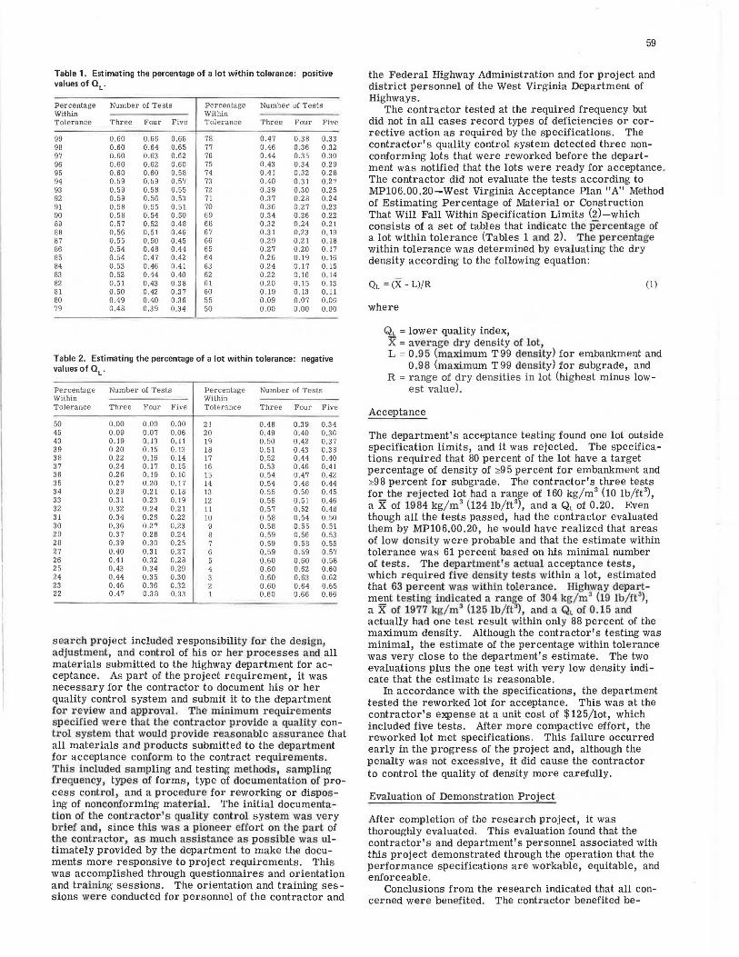
Table 1. Estimating the percentage of a lot within tolerance: positive values of QL.

Percentage Number of Tests Percentage Number of Tests Within Within Tolerance Three Four Five Tolerance Three Four Five

99 0.60 0.66 0.66 78 0.47 0.38 0.33 98 0.60 0.64 0.65 77 0.46 0.36 0.32 97 0.60 0.63 0.62 76 0.44 0.35 0.30 96 0.60 0.62 0.60 75 0.43 0.34 0.29 95 0.60 0.60 0.58 74 0.41 0.32 0.28 94 0.59 0.59 0.57 73 0.40 0.31 0.27 93 0.59 0.58 0.55 72 0.39 0.30 0.25 92 0.59 0.56 0.53 71 0.37 0.28 0.24 91 0.58 0.55 0.51 70 0.36 0.27 0,23 90 0.58 0.54 0.50 69 0.34 0.26 0.22 89 0.57 0.52 0.48 68 0.32 0.24 0.21 88 0.56 0.51 0.46 67 0.31 0.23 0.19 67 0.55 0.50 0.45 66 0.29 0.21 0.16 86 0.54 0.48 0.44 65 0.27 0.20 0.17 85 0.54 0.47 0.42 64 0.26 0.19 0.16 84 0.53 0.46 0,41 63 0.24 0.17 0.15 83 0.52 0.44 0.40 62 0.22 0. 16 0.14 82 0.51 0.43 0.38 61 0.20 0.15 0.13 81 0.50 0.42 0.37 60 0.19 0.13 0.11 80 0.49 0.40 0.36 55 0.09 0.07 0.06 79 0.48 0.39 0.34 50 0.00 0.00 0.00

Table 2. Estimating the percentage of a lot within tolerance: negative values of QL.

Percentage Number of Tes ts Percentage Number of Tests Within Within Tolerance Three Four Five Tolerance Three Four Five

50 0.00 0.00 0.00 21 0.46 0.39 0.34 45 0.09 0.07 0.06 20 0.49 0.40 0.36 40 0.19 0. 13 0. 11 19 0.50 0.42 0.37 39 0.20 0.15 0.13 18 0.51 0.43 0.38 38 0.22 0.16 0.14 17 0, 52 0.44 0.40 37 0 .24 0.17 0.15 16 0.53 0.46 0.41 36 0.26 0. 19 0.16 15 0.54 0.47 0.42 35 0.27 0.20 0.17 14 0.54 0.48 0.44 34 0.29 0.21 0.18 13 0.55 0.50 0.45 33 0.31 0.23 0.19 12 0.56 0.51 0.46 32 0.32 0.24 0.21 11 0. 57 0.52 0.48 31 0.34 0.26 0.22 10 0.58 0.54 0.50 30 0.36 0.27 0.23 9 0.58 0.55 0. 51 29 0.37 0.28 0.24 8 0.59 0.56 0.53 28 0.39 0.30 0.25 7 0.59 0.58 0.55 27 0.40 0.31 0.27 6 0. 59 0.59 0.57 26 0.41 0.32 0.28 5 0.60 0.60 0.58 25 0.43 0.34 0.29 4 0.60 0.62 0.60 24 0.44 0.35 0.30 3 0.60 0.63 0.62 23 0.46 0.36 0.32 2 0.60 0.64 0.65 22 0.47 0.38 0.33 I 0.60 0.66 0.66

sea r ch pr oject included responsibility for the design, adjus tment, and control of his or her processes a nd all materials submitted to the highway department for ac­ceptance. As part of the project requirement, it was necessary for the contractor to document his or her quality control system and submit it to the department for review and approval. T he minimum r equir ements specified were tha t the contractor provide a quality con­trol system that would pr ovide i·easonable assurance that all materials and products submitted to the department for acceptance conform to the contract requirements . This included sampling and testing methods , sampling fr equency , types of forms, type of docun1.entation of pro­cess control, and a procedure for reworking or dispos ­ing of nonconforming mater ial . The initial documenta­tion of the contr a ctor's quality control system was very brief and, s ince this was a pioneer effort on the par t of t he contractor, as much assistance as possible was ul­timately provided by the department to make the docu­ments more responsive to project requirements. This was accomplis hed through questionnaires and orientation and trai ning sessions. The orientation and training ses­sions were conducted for personnel of the contractor and

59

the Federal Highway Administration and for project and district personnel of the West Virginia Department of Highways.

The contractor tested at the required frequency but did not in all cases record types of deficiencies or cor­rective action as required by the specifications . The contractor's quality control system detected three non­conforming lots that were reworked before the depart­ment was notified that the lots were ready for acceptance. The contractor did not evaluate the tests according to MP106.00.20-West Virginia Acceptance Plan "A" Method of Estimating Percentage of Material or Construction That Will Fall Within Specification Limits (2)-which consists of a set of tables that indicate the per centage of a lot within tolerance (Tables 1 and 2). The percentage within tolerance was determined by evaluating the dry density according to the following equation:

QL = (X - L)/R (1 )

where

QL = lower quality index, X = average dry dens ity of lot , L = 0 .95 (maximum T99 dens ity) for embankment and

0.98 (maximum T99 density) for subgrade, and R = range of dry densities in lot (highest minus low­

est value).

Acceptance

The department's acceptance testing found one lot outside specification limits, and it was rejected. The specifica­tions required that 80 percent of the lot have a target percentage of density of ;;,9 5 percent for embankment and <:98 percent for subgrade . The contractor's three tests for the r ejected lot had a range of 160 kg/m 3 (10 lb/ ft 3

),

a X of 1984 kg/ m 3 (124 lb/ ft 3), and a QL of 0.20. Even though all the tests passed, had the contractor evaluated them by MP106.00.20, he would have realized that areas of low density were probable and that the estimate within tolerance was 61 percent based on his minimal number of tests. The departme nt' s actual acceptance tests, which required five dens ity tests within a lot, estimated that 63 percent was within tolerance . Highway depa rt­ment testing indicated a ran~e of 304 kg/m3 (19 lb/ft3), a X of 1977 kg/m3 (12 5 lb/ft ), and a Q L of 0 .15 and actually had one test result within only 88 percent of the maximum density. Although the contractor's testing was minimal, the estimate of the percentage within tolerance was very close to the department's estimate. The two evaluations plus the one test with very low density indi­cate that the estimate is reasonable.

In accordance with the specifications, the department tested the reworked lot for acceptance. This was at the contractor's expense at a unit cost of $125/lot, which included five tests. After more compactive effort, the reworked lot met specifications . This failure occurred early in the progress of the project and, although the penalty was not excessive, it did cause the contractor to control the quality of density more carefully.

Evaluation of Demonstration Project

After completion of the research project, it was thoroughly evaluated. This evaluation found that the contractor's and department's personnel associated with this project demonstrated through the operation that the performance specifications are workable, equitable, and enforceable.

Conclusions from the research indicated that all con­cerned were benefited. The contractor benefited be-

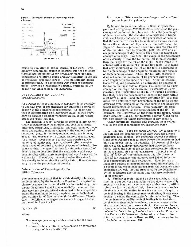
60

Figure 1. Theoretical estimate of percentage within tolerance.

% OFDFN51TY

105 'j':978

97 o-:409

96

96

95

" SIMILAR SIZE LOTS

~ OFlENSITY

x• 96.8 98

tr•l .64 98

91'

91'

94

R•4

0-0.45

cause he was allowed better control of his work. The highway department benefited because this type of speci­fication has the potential for producing more uniform compaction and allows much greater flexibility in the use of available inspecting forces. The statistically based acceptance plan, in conjunction with random sampling plans, provided a r easonably accurate estimate of the density for embankment and subgrade.

DEVELOPMENT OF CURRENT SPECIFICATIONS

As a result of these findings, it appeared to be feasible to use this type of specification for statewide control of density in U1e standard specifica.tions. To adopt this type of specification on a statewide basis, i t was neces­sary to consider whether variation in materials would affect the specifications.

The bedrock in West Virginia is composed almost en­tirely of sedimentary rock units that consist of shale, siltstone, sandstone, limestone, and coal; some of these units axe slightly metamorphosed in the eastern part of the state. l:ihale is the predominant rock type in many areas. The topography is almost entirely mountainous. As a result, mrn:;l pi·ojects of any size require large volumes of earthwork. The earthwork often contains many types of soil and a variety of types of bedrock. Be­cause of this, the specifications for statewide control of density had to cons ider that the materials would vary conside1·ably withln a given project and could vary within a given lot. The1·efore, instead of using the value for dry density to determine the quality index it was neces­sary to use the percentage of density.

Determination of Percenlage of a Lot Within Tolerance

The pe1·centage of a lot that is within density tole1·ance, as determined by the formula in Equation 1, required a change because the material within a lot could vary. Al­though Equations 1 and 2 are essentially the same, the data used for the statistical value::; had to be cha nged be ­cause the maximum density required for an individual test within a lot of five tests might be different. There­fore, the 'following changes we1·e made in regard to tho data used in Equation 1:

QL =(X-L)/R

where

X = average percentage of dry density for the five tests,

(2)

L = lower tolerance limit in percentage or target per­centage of dry density, and

R = range or difference between largest and smallest percentage of dry density.

QL is used to enter the tables in West Virginia De­pai'tment of Highways MP106.00.20 to determine the per­centage of the lot within tolerance . L is the percentage of density on which the decision of acceptance is based and is not to be confused with the percentage of density that the contractor may try to achieve to ensure that the lot has the minimum of 80 percent within tolerance. In Figure 1, two examples are shown in which the lots are of s imilar size. In this example both lots have an av­erage percentage of dry density (ID above the target per­centage of density. However, the range of the percentage of dry density (R) for the lot on the left is much greater than the 1·ange for the lot ·on the i·ight. When Table 1 is entered with a QL value of 0.28 and five tests, it is found that only 74 percent oI the lQt on the left is estimated to have a percentage of the required maximum dry density of 95 percent 01· above. Thus, the lot fails because it does not meet th minimum of 80 percent within toler­ance required in the specifications. After the calcula­tions Ior Ql are performed, an estimated 87 percent of the lot on the i·ight side of F igure 1 is densified to a per­centage of the required maximum dry density of 95 or granter . The illustration on lhe left in Figure 1 exempli­fies that, when the percen.tage of density for tests within a lot have a large Rand standard deviation (a), it i1:1 po1:1-sible for a relatively high percentage of the lot to be sub­standard even though all of the test l·esults are above the target percentage of density. This no1·mally indicates poor quality control of the densification of the lot. In contrast, the illustration on the right of the f_!$1Jre, which has a smaller R and a, can tolerate a lower X and an ac­tual test below the target percentage of dry density.

Other significant changes that resulted from evalua­tion of the research project are described below:

1. Lot size-In the research project, the contractor's lol s ize and the department's lot size were not always analogous and, iurthel', the research project specifica­tions often resulted iu a lot size where the r.ontractor had only one or two tests. In actuality, 63 percent of the lots offered to the highway department had three or fewer tests. Since the size of the lot has considerable influence on the financial risk to the contractor, a sublot size of 1910 m3 (2500 yd3

) for embankment and 120 linear m (400 ft) for subgrade was selected and judged to be the best compromise for this evaluation. Each lot has at least five sublots of approximately equal dimensions. As a result of the expe1·ience gained from the r esea1·ch dem­onstration project, the lots presented to the department by the cont1·acto1· ru:e the same lots that are evaluated for acceptance.

2. Number of tests-Based on the research, at least five tests per lot were desirable to provide a reasonably accurate estimate of the percentage oI dry density within tolerance for an individual lot. Because it was also de­sirable to have the option to use the contractor's quality control testing in the acceptance evaluation, it was nec­essary to revise Uie contractor's minimum testing. Thus, tJ1e contractor's quality control testing is to include at least one nuclear moisture-density measurement made at a random location in each sublot. The random loca­tions are selected in accordance with MP712.27.26-Pro­cedure for Determining Random Locations for Compac­tion Tests on Embankment, Subgrade and Base. For lots that consist of more than one lift, the contractor is to include testing on each lift.

Test Methods

Moisture Control

The lots of embankment and subgrade material are re­quired (as in the research project) to be within the spec­ified moisture tolerance of 4 percent below optimum to 3 percent above optimum. This tolerance was evaluated and adopted as a result of a study conducted before 1968. Moisture tolerance has proved to be a suitable control for most soil material found in West Virginia. The only exception is soil that has a high silt content. The speci­fications and procedures for this material require that moisture be controlled at optimum or below until pump­ing has been checked. This type of soil, however, is not commonly encountered in current construction in West Virginia. The percentage of moisture is deter­mined in conjunction with density testing by using MP712.21.25 and MP300.0l.01 and the nuclear gauge.

Density Testing

Soil that has less than 3 5 percent retained on the 19-mm (O. 75-in) sieve is tested in accordance with the depart­ment's MP712.21.25-Nuclear Field Density Test for In-Place Density for Compacted Soils, Soft Shales, or Random Material Layers Having Less Than 35 Percent Retained on the [19-mm] %-Inch Sieve and Soil Cement Stabilization-which uses a direct-transmission type of nuclear gauge. No laboratory testing is normally re­quired since a table of maximum density and optimum moisture values is used in conjunction with the one-point Proctor test to determine AASHTO T 99 optimum moisture and maximum density. Only one determination of optimum moisture and maximum density is required for individual lots in cases in which the material remains uniform.

For soil material that has 35 percent or more retained on the 19-mm (O. 75-in) sieve, the research project found that very little of the material from the excavation could be tested by the highway department's roller pass pro­cedure because of the nonuniform nature or the nominal particle size of the material. This procedure required that the material remain uniform and somewhat homo­geneous. In addition, the method for determining the maximum density used in the researcJ1 project was quite time consuming. Only one lot of 2470 m 2 (2950 yd 2

), or less than 1 percent of the excavation, was tested.

Because of the excessive settlement observed in vari­ous areas of the state in many embankments formed of shale and lifts that contained combinations of soil and bedrock (3), it was decided to initiate and document con­trol of compaction on these embankments. The nuclear testing equipment currently owned by the West Virginia Department of Highways has a maximum depth reading in the direct-transmission mode of 305 mm (12 in). The department allows loose lifts that vary from 200 to 610 mm (8 to 24 in) in placing shale. Since the quality of the shale can vary from soil to rocklike material, it was de­cided to adapt the specifications to this type of material instead of processing the material to accommodate methods of testing.

Two methods of compaction control are used for ma­terial (other than rock lifts) that has 35 percent or more retained on the 19-mm (0. 75-in) sieve:

1. MP300.0l.Ol-Method of Test for Quality Assur­ance of Compaction of Untreated and Stabilized Aggre­gate and Granular Embankment Material by Roller Pass Method-a new and less time-consuming roller pass test, is used for soil that is relatively uniform in gradation and is composed of particles of a nominal 254 mm (10 in)

61

or less. The material is controlled to a target percent­age of dry density of 9 5 percent. In part 1 of the mate­rials procedure, the maximum density is developed in the field by the contractor's equipment by using a specified minimum compactive effort (roller weight) and a growth curve. The growth curve is evaluated after a specified number of passes have been conducted on the test sec­tion. The required maximum density is considered to be achieved when a minimum change of 32 kg/m3 (2 lb/ ft 3

) or less occurs after two passes of the roller. The two passes normally evaluated are numbers 13 and 14. The method is normally used on subgrade material that is specified to be natural or synthetic mineral aggre­gate-e.g., broken or crushed rock, gravel, or slag that can be incorporated in a 200-mm (8-in) loose-depth lift. It may also be applicable to some embankment material.

2. Material that either has a nonuniform gradation or includes particles larger than a nominal 250-mm (10-in) top size or both is proof rolled by making two or more passes over the entire area at a speed of not more than 8 km/ h (5 mph) with a 45-Mg (50-ton) roller. All unstable areas or soft spots that are disclosed are to be corrected before placement of overlying lifts.

Documentation of Results of Density Tests

All test results for MP712.21.25 and MP300.0l.Ol are recorded on computer mark-sense forms. This includes tests performed by the contractor and the highway de­partment. The original of these forms is submitted by project personnel to the central office of the West Vir­ginia Department of Highways. The data on the forms are evaluated for completeness and correctness by the computer. If errors or missing data are found, they are identified and printed out. After corrections have been made, the data are permanently stored on magnetic tape. Various subroutines are used to evaluate the data. Two of the most significant ones are (a) a statistical analysis of the percentage of density for the project on a timed sequence and on the completed project, which includes an evaluation of the uniformity of the embank­ment and subgrade density, and (b) an analysis of mois­ture control on a timed sequence and on the final project.

Organic Test

Organic material contained in the material used to form the embankment and subgrade is limited to 7. 5 percent by weight. At this limit, the possibility exists that the or­ganic matElrial could occupy as much as 15 percent of the volume of the material being placed. Should the per­centage exceed that specified, it could result in excess consolidation or an adverse effect on the strength of the material or both. Test method MP716.04.20-Deter­mination of the Organic Content of Soils by the Dry Com­bustion Method-determines the organic content at a con­trolled temperatw·e of 440°C (824°F) for 5 h (!).

Lift Thickness

Lift thickness must be measured three times per lift and documented by the contractor.

Quality Control

MP717.04.21-Guide for Quality Control and Acceptance Plan for Embankment and Subgrade-is specified in the contract documents and is intended to be used by the contractor for designing his or her quality control sys­tem. It requires that the contractor's plan be submitted at the preconstruction conference, and it defines the ac­ceptable test procedures. A direct-transmission type

62

Figure 2. Procedure for acceptance of embankment and subgrade.

CONTF?ACTVR ff1E5EIVTS

l(JT TD D£PAF?TMENT

FOR ACCEPTANCE

I DEPARTMENTS OPTION FOR EVALUATICIV I

I I 01/WlffTON OF LOT EVALUAnON OF LOT EVALUATION OF LOT

UTILIZING THE UnLIZING THE unl/ZING TESTING

CONTRACTORS CONTRACTOR "S CONDUCTED

TESTING WITHOUT TESTING WITH BY DEPARTMENT

DEPARTMENTS DEPARTMENTS

OBSfflVATION OBSERVATION

OF TESTING OF TESTING

I T

ACCEPTANCE REJECTION

I I I l

REWORK CONTINUE CONSTRUCT-

LOT ION WITH NEXT LOT

(BB::CMES MW LOT) i..-

of nuclear gauge is required for density testing. The minimum number of tests, reports, and measurements per lot is indicated for the several types of gradation in the material placed. The reports for proof rolling are to include the make, size, and compactive force of the roller and the number of rolls performed on each lift. The plan is also to include the time schedule and distri­bution of data.

The document is to include the names of the con­tractor's personnel who are responsible for quality con­trol and liaison and the personnel who are conducting the tests and measurements. It is recommended that per­sonnel who conduct the density tests be certified com­paction technicians. The West Virginia Department of Highways has beim conducting a certification program for departmental personnel for 9 years. This program, which includes a written and practical examination, has been extended to industry personnel in conjunction with the Contractors' Association of West Virginia. The de­partment also conducts a training program that has been extended to industry personnel. The· training program includes programmed instruction, lectures, and prac­tical exercises. Audiovisual tape instructions are also used where "hands-on" training is not practical.

Lots Offered for Acceptance

Acceptance of a Lot

The highway department has the option of acceptance of the contractor's lots according to the methods shown in Figure 2. Say the percentage of a lot within a tolerance of 80 percent has been retained. An analysis of the data finds that the department has approximately a 6 percent probability of accepting substandard material that is evaluated by five density tests. Although the contractor's actual risk cannot be determined before he or she per-

forms the work because the risk is dependent on con­trol by the contractor, an average value can be esti­mated. Therefore, based on historical data from the research project that were used to determine an average quality of density, a contractor with adequate control could expect to have approximately a 3 percent proba­bility of rejection on acceptably densified material. It should be noted that a very important feature of the ac­ceptance plan used is that, if the contractor's quality control of density is poor, his or her risk is greatly in­creased.

A recent evaluation of the demonstration project that was constructed by using these controls shows that the project has performed satisfactorily for 5 years with negligible settlement or pavement failure. The evalu­ation of the percentage within tolerance indicated that, had a value greater than 80 percent been used, it would have been necessary for the contractor to have a much smaller range in dry density per lot or a higher average density or both; otherwise, as indicated by the perfor­mance of the project, many more lots would have been unnecessarily rejected.

Rejection of a Lot

When a lot fails to meet the specifications , reworking is required before another lot can be placed on it (Figure 2). Testing of the reworked lot for acceptance is done at the expense of the contractor if the highway department con­ducts the testing. The unit cost for testing of a reworked lot when tests are conducted by the department is pub­lished in MP109.00.20-Basis of Charge for Additional Testing. The amounts are updated to reflect current testing costs. The cost is for five tests since that is the minimum acceptable for evaluation. Since reworking a lot in effect produces a new lot, the reworked lot is eval­uated only by the five tests conducted after reworking.

SUMMARY AND CONCLUSIONS

Current quality assurance specifications in West Vir­ginia have been reviewed by industry personnel, and in­formative seminars have ueen given for industry man­agement. The specifications have been received quite favorably to date. During the first 6 months of the cer­tification program for industry personnel, 68 people have entered the program and 24 have been certified.

The cost of this type of specification for embankment and subgrade can only be evaluated after several years of use. The cost would normally be reflected in the unit price bid for the unclassified excava tion. That cost was $1. 54/m3 ($1.18/yd3

) for the research project. The average cost for all types of roadways and construction for unclassified excavation in 1970, the year the project was bid, was $1.67/m3 ($1.28/yd3

). It was anticipated that the bid might be high because of uncertainty on the part of the contractor about this type of specification and because it was the fir s t time the highway department had required this type of quality control on ea1'thwork. It would appear, however, that for the research project the required quality control did not materially affect the con­tractor's bid.

The current specifications require thal the contractor be responsible for quality control of the embankment and the subgrade. This is quite appropriate since the con­tractor has the fundamental control of the work process. The current specifications for embankment and subgrade are not true end-result specifications because of the na­ture of the material placement.

As determined by the research demonstration project, the quality assurance specifications discussed here do offer a level of quality control and acceptance that inter-

feres as little as possible with the contractor's manage­ment of his or her processes. Further, the research demonstration project and the current specifications ac­cept the premise that there will be a certain percentage of material that will fall below a given standard. The method of acceptance makes reasonable estimates of substandard material. These estimates are used to keep nonspecification material to a minimum. Because the method of acceptance requires control of variance in the quality control of density, it encourages a more uni­form density in the final product.

REFERENCES

1. S. B. Hudson, F. J. Bowery, and F. T. Higgins. Determination of Statistical Parameters for Highway Construction. Materials Research and Development

63

Division, Woodward-Clyde Consultants, West Vir­ginia Research Project 18, July 1976.

2. G. W. Steele, S. B. Hudson, and C. J. Vantil. Sta­tistical Approach to Realistic Highway SPecifications. Proc., 25th Annual Convention of Southeastern Asso­ciation of State Highway Officials, Sept. 1966.

3. G. H. Bragg, Jr., and T. W. Zeagler. Design and Construction of Compacted Shale Embankments. Federal Highway Administration, U.S. Department of Transportation, Rept. FHWA-RD-75-62, Sept. 1975.

4. A. Arman. Engineering Classification of Organic Soils. HRB, Highway Research Record 310, 1970, pp. 75-89.

Publication of this paper sponsored by Committee on Earthwork Con· struction.