
SHRP-S-657.pdf - Transportation Research Board
382
SHRP-S-657 Electrochemical Chloride Removal and Protection of Concrete Bridge Components: Laboratory Studies Jack Bennett, Thomas J. Schue, Kenneth C. Clear, David L. Lankard, William H. Hartt, and Wayne J. Swiat Strategic Highway Research Program National Research Council Washington, DC 1993
-
Upload
khangminh22 -
Category
Documents
-
view
0 -
download
0
Transcript of SHRP-S-657.pdf - Transportation Research Board

SHRP-S-657
Electrochemical Chloride Removaland Protection of Concrete Bridge
Components: Laboratory Studies
Jack Bennett, Thomas J. Schue, Kenneth C. Clear,David L. Lankard, William H. Hartt, and Wayne J. Swiat
Strategic Highway Research ProgramNational Research Council
Washington, DC 1993

SHRP-S-657Contract C-102A
Program Manager: Don M. HarriottProject Manager: Marty LaylorProduction Editor: Marsha Barrett
Program Area Secretary: Carina S. Hreib
June 1993
key words:anode
bond strengthbridgescathode
chlorideremoval
concretecorrosion
electrochemistryelectrolyte
hydrogen embrittlementpolarizationreinforcing steel
Strategic Highway Research ProgramNational Academy of Sciences
•2101 Constitution Avenue N.W.
Washington, DC 20418
(202) 334-3774
The publication of this report does not necessarily indicate approval or endorsement of the findings, opinions,conclusions, or recommendations either inferred or specifically expressed herein by the National Academy ofSciences, the United States Government, or the American Association of State Highway and TransportationOfficials or its member states.
© 1993 National Academy of Sciences
350/NAP/693

Acknowledgments
The research described herein was supported by the Strategic Highway Research Program(SHRP). SHRP is a unit of the National Research Council that was authorized by Section128 of the Surface Transportation and Uniform Relocation Assistance Act of 1987.
We wish to acknowledge the contribution of those who contributed to this work. Dr. DavidR. Lankard of Lankard Materials Laboratory, Inc. was responsible for the preparation of allconcrete specimens, petrographic examinations and ASR studies. Dr. Lankard also conductedSEM/EDS, porosity, permeability, and compressive strength studies. Kenneth Clear ofKenneth C. Clear, Inc. was responsible for concrete-reinforcing steel bond strength studiesand long-term remigration studies, which included test yard monitoring of treated specimens.Dr. William H. Hartt of Florida Atlantic University was responsible for hydrogenembrittlement studies. Wayne J. Swiat of Corrpro Companies, Inc. was responsible for designconcepts for chloride removal field trials. The authors would also like to thank Mr. James E.Barnhart, Dennis Bunke, and Tom Fox of the Ohio DOT for their cooperation with testsconducted on the Marysville, Ohio bridge deck.
Work at ELTECH Research Corporation was conducted principally by John E. (Jack) Bennett,Thomas J. Schue, and Thomas R. Turk.
iii

Contents
Abstract .......................................................... 1
Executive Summary .................................................. 3
1 Introduction ...................................................... 7
2 Background Studies ................................................ 11Chloride Analyses ............................................. 11Test Specimen Concrete ......................................... 12
Compressive Strength ..................................... 13Concrete Evaluations ........................................... 14Evaluation of Previous FHWA Chloride Removal Studies ................. 15
Kansas Chloride Removal Study .............................. 15Battelle - MarysviUe Bridge Deck History ....................... 16
3 Hydrogen Embrittlement ............................................ 21Preliminary Constant Extension Rate Testing .......................... 21
Constant Extension Rate Test Specimen ......................... 21Constant Extension Rate Determination ......................... 22
CERT Testing at Expected Chloride Removal Conditions .................. 26CERT Testing at Varying Current Densities ...................... 26CERT Testing at Varying Chloride Concentrations ................. 27
Smooth Specimen Testing ....................................... 28Ductility Recoverability .................................... 30
CERT Testing on Mortared Specimens ............................... 32Conclusions ................................................. 35
4 Concrete-Rebar Bond Strength Study ................................... 37Specimen Preparation ........................................... 38Power Application ............................................. 40Concrete-Rebar Bond Test ....................................... 42Results and Discussion .......................................... 44
The Ultimate Bond Stress ................................... 47
Bond Stress at 0.01" Loaded-End Slip .......................... 50Bond Stress at 0.001" Free-End Slip ........................... 53Non-Salty Control ........................................ 55Overall ................................................ 55
v

Conclusions ................................................. 58
5 Transference Numbers .............................................. 61
6 Anode Studies ................................................... 67Sacrificial Anodes ............................................. 67Inert Anodes ................................................. 69Steel Anode ................................................. 72Anode Selection .............................................. 73
7 Other Testing .................................................... 75Supplemental Cathodes ......................................... 75Concrete Depth-of Cover Effects on Current Distribution .................. 83Effects of Concrete Cracks on Current Distribution ...................... 84
8 Chloride Removal and Distribution ..................................... 85
Preliminary Testing ............................................ 85Laboratory Concrete Slab Specimens ................................ 86
Pre-Treatment Data ....................................... 89Static Half-Cell Potentials ............................. 89Macrocell Currents .................................. 89Corrosion Rate Measurements .......................... 89
Slab Treatment .......................................... 90
Post-Treatment Core Analyses ............................... 93Post-Treatment Chloride Distribution ...................... 95SEM/EDS Examination ............................... 96Petrographic Examination ............................. 101Porosity and Permeability ............................. 101Compressive Strength ................................ 103
Field Cores .................................................. 103
9 Chloride Removal Electrolytes ........................................ 107Anion Exchange Resins ......................................... 107Manganese Sulfate Additions ..................................... 108High pH Electrolyte ............................................ 110
Buffer Solution Electrolytes ................................. 110Borate Buffer Electrolyte .............................. 111
Alkali-Silica Reactions .......................................... 112
Effect of Chloride Removal on ASR-prone Aggregates .............. 113Lithium Borate Electrolyte .................................. 115
10 Long-Term Slab Study ............................................. 117Chloride Remigration ........................................... 118Post-Treatment Corrosion Studies .................................. 128
Half-Cell Potential ........................................ 128Junction Potential Error ............................... 132
Laboratory Slab Confnumtion Tests ................. 134
vi

Macrocell Current ........................................ 1353LP Corrosion Rate ....................................... 141
Conclusions ................................................. 143
11 Concurrent Protection ............................................. 145
Specimen for Electro-Migration Studies .............................. 146Impregnants and Complexing Materials .............................. 146Electrophoretic Coatings ......................................... 147
Low Molecular Weight Materials ............................. 147High Molecular Weight Materials ............................. 148Quatemized Monomeric Acrylates ............................. 148
Corrosion Inhibitors ............................................ 148
Electro-Emplacement of TEP* Ion Corrosion Inhibitor ............... 148Petrographic Analyses of TEP* Treated Samples .............. 150
Conclusions ................................................. 152
12 Equipment and Procedure Development ................................. 153Design Concepts for Field Trials ................................... 153
Deck Design ............................................ 157Column Design .......................................... 157
Anode Blanket Assembly ........................................ 157Blanket Testing Under Electrochemical Conditions ................. 163
13 Major Conclusions ............................................... 165
Appendix A Pre-Treatment Data of Laboratory Slabs ......................... 169
Appendix B Post-Treatment Corrosion Data of Laboratory Slabs ................. 183
References ....................................................... 199
vii

List of Figures
2-1. Half-Cell Potential Data on "Treated Area" of Marysville Bridge Deck ........ 18
2-2. Half-Cell Potential Data on "Untreated Area" of Marysville Bridge Deck ....... 19
3-1. Constant Extension Rate Specimen Design ............................ 22
3-2. Load to Failure vs Extension Rate .................................. 23
3-3. Notched Specimen CERT Tests at 1500 Microamp/cm 2 (1.5 A/ft2) ........... 24
3-4. Notched Specimen CERT Tests at 5000 Microamp/cm 2 (5 A/ft2) ............. 24
3-5. CERT Tests - 1500 vs 5000 Microamp/cm 2 (1.5 vs 5 A/ft2) ................ 25
3-6. Fracture Load vs Current Density at 4.76 x 10⁻⁶cm/sec ................... 26
3-7. Fracture Load vs Chloride Concentration at 4.76 x 10.4 crrgsec .............. 27
3-8. Reduction in Area vs Current Density in Air and Environment .............. 28
3-9. Time to Failure vs Current Density in Air and Environment ................ 29
3-10. Reduction in Area of Smooth Specimens vs Precharging Time .............. 29
3-11. Effect of Rest Time on Reduction in Area ............................ 31
3-12. Effect of Rest Time on Time to Failure .............................. 31
3-13. Electrochemical Cell Used for Mortaxed Specimens ...................... 33
3-14. Reduction in Area vs Current Density for Mortared Smooth Specimens ........ 33
3-15. Time to Failure vs Current Density for Mortared Smooth Specimens .......... 34
3-16. Reduction in Area vs Off Potential for Mortared Smooth Specimens .......... 34
4-1. Modified Stub-Cantilever Beam Specimen Configuration .................. 39
ix

4-2. Bond Test Specimen Setup for Power Application ....................... 40
4-3. Photographs of Rebar Bond Strength Test Setup ........................ 43
4-4. Specimens Just After Power for 200 A-hr/ft 2 at 5000 mA/ft_ ................ 45
4-5. Effect of Currant on Ultimate Bond Stress ............................ 48
4-6. Effect of Total Applied Charge on Ultimate Bond Stress .................. 48
4-7. Effect of Current Density on Bond Stress at 0.01" Loaded-End Slip .......... 51
4-8. Effect of Total Applied Current on Bond Stress at 0.01" Loaded-End Slip ...... 51
4-9. Effect of Current on Bond Stress at 0.001" Free-End Slip ................. 54
4-10. Effect of Total Applied Charge on Bond Stress at 0.001" Free-End Slip ....... 54
4-11. Comparisons of Bond Stress at Various Current Density Levels ............. 56
4-12. Comparisons of Bond Stress at Various Total Applied Charge Levels ......... 62
5-1. Schematic of Transference Number Test Setup ......................... 60
5-2. Transference Number as a Function of Chloride Content .................. 63
5-3. Transference Number as a Function of Temperature ..................... 63
5-4. Transference Number as a Function of Currant Density ................... 63
6-1. Test Cell for Sacrificial Anode Testing .............................. 66
6-2. Chlorine Efflciencies of EC-100 at Various Chloride Concentrations .......... 69
6-3. Chlorine Efficiencies of Inert Anode Coatings .......................... 69
7-1. Schematic of Supplemental Cathode Test Setup ........................ 75
8-1. Laboratory Chloride Removal Test Slab Specimen ...................... 87
8-2. 2-Ft x 2-Ft Slab Chloride Removal Efficiency ......................... 92
8-3. Core N_ 1-1 Showing Broad Band Of Persistent Wemess ................... 94
8-4. Core N_ 1-1 Showing Fracture Plane at Top Layer of Steel .................. 94
8-5. EDS Spectrum of Virgin Columbia Type I Portland Cement Paste ........... 97
x

8-6. EDS Spectrum of Cement Paste Contacting Top Rebar of Core N° 1-1 ........ 98
8-7. SEM Photograph of Cement Paste Contacting Top Rebar of Core N° 1-1 ....... 99
8-8. EDS Spectrum of Cement Paste 1/4-Inch from Top Rebar of Core N° 1-1 ...... 100
8-9. EDS Spectrum of Cement Paste of Core N° 1-1 with Liquid Phase Intrusion .... 100
8-10. Mercury Porosimetry Data Obtained on Mortar Samples of Core N_ 1-1 ....... 102
8-11. SEM Photograph of Core N° 1-1 Cement Paste Showing Open Porosity ....... 102
9-1. Schematic of Ion Exchange Resin Test Setup .......................... 108
9-2. Slab Operation with MnO:_-Coated Inert Anode ................. ........ 109
9-3. Relative Longevities of Various Chloride Removal Electrolytes ............. 111
9-4. Borate Buffer Electrolyte Longevity ................................. 112
9-5. Wearing Surface of Opal Aggregate Concrete Specimen .................. 114
10-1. Crossing Reinforcing Steel Top Imprint Chloride Content; pH Maintenance .... 120
10-2. Crossing Reinforcing Steel Bottom Imprint Chloride Content; pH Maintenance .. 121
10-3. Single Reinforcing Steel Bar Top Imprint Chloride Content; pH Maintenance ... 122
10-4. Single Reinforcing Steel Bar Bottom Imprint Chloride Content; pH Maintenance . 123
10-5. Crossing Reinforcing Steel Top Imprint Chloride Content;Without pH Maintenance ........................................ 124
10-6. Crossing Reinforcing Steel Bottom Imprint Chloride Content;Without pH Maintenance ........................................ 125
10-7. Single Reinforcing Steel Bar Top Imprint Chloride Content;Without pH Maintenance ........................................ 126
10-8. Single Reinforcing Steel Bar Bottom Imprint Chloride Content;Without pH Maintenance ........................................ 127
10-9. Quarterly Average Half-Cell Potential Results .......................... 129
10-10. Half-Cell Potential Data Taken from Bottom of Holes .................... 131
10-11. Post-Treatment EDS Analysis of Slabs Na 9 and N° 12 ................... 133
xi

10-12. Cumulative Charge Passed Data Summary; All Slabs ..................... 137
10-13. Cumulative Charge Passed Data Summary; Excluding Control Slab N° 2 ....... 138
10-14. MacroceU Current Linear Regression Analysis (Slab No 2) ................. 139
10-15. Cracking on Control Slab (Slab N° 2) ............................... 140
10-16. Quarterly 3LP Corrosion Rate Data Summary .......................... 142
11-1. EDS Spectrum on Quartz Aggregate Concrete for P+ ..................... 150
11-2. EDS Spectrum at Re'mforcing Steel-Concrete Interface for P+ ............... 151
11-3. EDS Spectrum At and Near Wearing Surface for P+ ..................... 151
12-1. Conceptual Layout of Deck Configuration ............................ 154
12-2. Conceptual Layout of Land Column Configuration ...................... 155
12-3. Conceptual Layout of Marine Column Configuration ..................... 156
12-4. Flow Test Setup for Anode Blanket Evaluations ........................ 159
12-5. Flow Rate Tests with Polyfelt TS-1000 Outer Blanket .................... 160
12-6. Flow Rate Tests with GTF 350 EX Outer Blanket ....................... 161
xii

List of Tables
2-1. Concrete Mix for C-102A Research ................................. 12
2-2. Fresh Concrete Property Data of Compressive Strength Specimens ........... 13
2-3. Compressive Strength Gain ....................................... 14
2-4. Dimensional and Physical Data of MarysviUe Bridge Deck Cores ............ 17
2-5. Corrosion Rate Measurements on MarysviUe Bridge Deck ................. 20
3-1. Load to Failure for Notched Steel Specimens .......................... 22
4-1. Basic Concrete Properties of Rebar Bond Test Specimens ................. 39
4-2. Concrete-Rebar Bond Strength Study Matrix ........................... 41
4-3. Powering and Testing Schedule for Different Variables ................... 41
4-4. Summary of Rebar-Concrete Bond Test Results ........................ 46
4-5. Summary of Average Ultimate Bond Stress ........................... 47
4-6. Summary of Average Bond Stress at 0.01" Loaded-End Slip ............... 50
4-7. Summary of Average Bond Stress at 0.001" Free-End Slip ................. 53
4-8. Bond Stress Data Summary for All Variables for Salty Specimens Only ....... 58
5-1. Concrete for Transference Number Tests ............................. 61
5-2. Transference Numbers Corrected for Diffusion ......................... 64
6-1. Concrete Properties of Sacrificial Anode Test Specimens .................. 68
6-2. Sacrificial Anode Data .......................................... 69
7-1. Concrete Composition for Supplemental Cathode Test Blocks ............... 76
to*
Xlll

7-2. Supplemental Cathode Testing: Block A ............................. 79
7-3. Supplemental Cathode Testing: Block B .............................. 80
7-4. Supplemental Cathode Testing: Block C .............................. 81
7-5. Current Distribution vs Concrete Depth of Cover ....................... 83
7-6. Effects of Concrete Cracks on Current Distribution ...................... 84
8-1. Fresh Concrete Data for Chloride Removal Slab Specimens ................ 88
8-2. 2-Ft x 2-Ft Slab Test Status ...................................... 90
8-3. 2-Ft x 2-Ft Slab Treatment Summary ................................ 91
8-4. Chloride Ion Content of Electrochemical Removal Slab Cores .............. 95
8-5. Chemical Analysis of Project Portland Type I LA Cement ................. 96
8-6. Operating Data - Field vs Laboratory Cores ........................... 104
8-7. Concrete Chloride Analyses - Field Cores ............................ 105
10-1. Chloride Removal Process Parameters ............................... 117
10-2. Chloride Analysis Results ........................................ 119
10-3. Post-Treatment cr Analyses of Slab N= 9 and Slab N= 12 ................. 132
10-4. 2-Ft x 2-Ft Slab Conf'trmation Tests Using 6-Inch Diameter Cylinders ......... 134
10-5. Post-Treatment Data of 6-Inch Diameter Specimens ...................... 134
10-6. Static Potentials of Specimens - pH vs No pH Maintenance ................ 135
10-7. Corrosion Data Summary for Each Individual Slab ...................... 136
11-1.. Concretes Used to Prepare Reinforced Concrete Specimens ................ 146
11-2. Half-CeU Potential Data for Specimens Treated with _ Inhibitor .......... 149
12-1. Performance and Cost Data for Anode Blanket Materials .................. 158
12-2. Percent Surface Contact of Anode Blanket Materials ..................... 159
12-3. Decision Matrix for Anode Blanket Materials .......................... 162
xiv

Abstract
The feasibilty of electrochemical chloride removal and concurrent protection as arehabilitation option for concrete bridge structures was investigated. Chloride removalprocess procedures were developed, and the effects of the process on structure concreteintegrity and reinforcing steel were studied. This report discusses the laboratory evaluationsof this process.

Executive Summary
Corrosion is recognized today as one of the major contributors to the deterioration of steelreinforced concrete structures. This corrosion is induced primarily by chlorides introduced inthe form of de-icing salts or seawater. A secondary source is chlorides in the concretematerials and admixtures. One technique for dealing with this corrosion is the removal ofoffending chlorides from the concrete. The electrochemical removal of chloride fromconcrete structures is accomplished by applying an anode and electrolyte to the externalconcrete surface, and passing direct current between this anode and the reinforcing steelwhich acts as a cathode. Since anions (negatively charged ions) migrate toward the anode, itis possible to migrate chloride ions toward the anode and out of the structure.
Under this SHRP contract, the feasibility of chloride removal from reinforced concrete bridgecomponents was examined, first in laboratory and test yard studies, and finally in fieldvalidation studies. The laboratory and test yard studies are in this report, and field validationstudies in Volume II.
Laboratory and test yard studies conducted under this contract clearly show chloride removalto be an effective technique for arresting chloride-induced corrosion of reinforcing steel.Results of chloride removal conducted on 2-ft x 2-ft (0.6-m x 0.6-m) test yard slabs wereparticularly impressive. Treatment of these slabs was conducted at a varietyof currentdensities and charges, yet none show any tendency to return to corrosive condition 3_ yearsafter treatment. By contrast, the control slab, which was not treated, is badly delaminated anddeteriorated.
Initial testing focused on fundamental electrochemical properties not previously reported. Thetransference number of chloride ion (a measure of the fraction of current carried by that ion)was established under various conditions. This study showed that the transference number ofchloride increases with increasing concentration and temperature, but is independent ofcurrent density. In a chloride removal process, chloride removal efficiencies are initiallyabout 40%, but decrease as the treatment progresses. Overall current efficiencies on a fieldstructure could be expected to be about 20%. In other words, the passage of each amp-hr ofcharge will remove about 0.25 gm of chloride.
The actual amount of chloride removed was rather disappointing, and early technical targetswere not met. Even very heavy treatments removed only 40 to 55% of the total chloridepresent. But further test results indicate that more complete removal may not be necessary.The chloride left in the concrete was positioned between and behind the reinforcing bars, andremained well away from the steel. Chloride contents around the top reinforcing steel were
3

greatly reduced by the treatment, and show no significant change after 40 months. It is alsoclear that in addition to removing chloride away from the bars, the treatment results in abuild-up of hydroxide ions at the steel surface. This undoubtedly plays an important role inarresting corrosion, since corrosion is more dependent on chloride/hydroxide ratio rather thanchloride concentration alone. Examination of rebars removed from treated slabs show onlyvery slight rusting, whereas bars from the untreated control were heavily corroded.
The effectiveness of the treatment was also demonstrated by several other measurements.The macroceU current (current flowing between top and bottom mats of steel) was reducedfrom an average of 0.42 mA to very near zero by the treatment. Macrocell currents remainnear zero 3_ years after chloride removal. Half-cell potentials of the steel on the control slabwere very corrosive, whereas steel potentials on treated slabs were very non-corrosive. Thisstudy also offered dramatic evidence of the errors which can occur when measuring potentialson the top surface of treated slabs. These errors, which can be as great as 200 mV, exist as aresuk of junction potentials due mainly to differences in pH. This study had the additionalbenefit of improving our understanding of the magnitude and nature of junction potentialerror.
Work under this contract also addressed several concerns which arise as a result of the
passage of large amounts of current through concrete. Reinforcing steel-concrete bondstrength was measured over the full range of current and charge experienced for both chlorideremoval and cathodic protection. The application of a very high current density (5000 mA/ft 2,50 A/m 2) and/or high amount of total charge (200 A-hr/ft 2, 2000 A-hr/m 2) did result in areduction of bond strength when compared to controls containing salt. The use of eitherlower current density or lower charge, however, had no adverse effect. Even at the highestcurrent density and charge, bond strength was reduced only to the values equal to those of no-salt control specimens.
Concrete compressive strength was not reduced at lower current densities, but concrete treatedat high current (2.0 A/ft 2, 20 A/m 2) for long periods of time (500 A-hr/ft 2, 5000 A-hr/m 2) didexperience a softening of the cement paste around the reinforcing steel. This softening isprobably also responsible for the loss of bond strength of severely treated specimens. Thisstrong treatment also caused one slab to crack and delaminate. For these reasons the currentregime used in previous studies (up to 2000 mA/ft_, 20 A/m s) was judged to be excessive,and more modest treatment conditions were used for field trials.
The possible hydrogen embrittlement of conventional reinforcing steel was also studied.Although a slight, temporary loss of ductility was noted on smooth specimens, this loss wasdetermined to be not structurally significant.
The generation of chlorine gas from the anode, which could present a safety hazard, was alsostudied. It was decided that the electrolyte should be maintained at a basic pH to preventgeneration of chlorine gas. Several buffers were studied for this purpose, and a sodiumborate buffer was found to be the most effective and practical. Control of the electrolyte pHin this way also prevented any etching or acid attack of the concrete surface.
4

Other studies have shown that this electrochemical treatment of concrete causes an increase in
the alkali cation concentration in the vicinity of the reinforcing steel. This study confirmedthese results, and demonstrated that serious damage could result if the chloride removalprocess were used on concrete containing alkali-reactive aggregate. But it was also found thatthe presence of lithium ion in the electrolyte could be used to mitigate this problem. Wherealkali-sensitive aggregate is present, the use of lithium borate buffer is recommended.
Based on the laboratory and test yard results, a chloride removal treatment process wasdefined which results in effective removal of chloride without any damage to the concrete orreinforcing steel. Treatment current density is limited to less than 500 mA/ft 2 (5 A/m 2) ofconcrete. System voltage is also limited by OSHA to less than 50 volts for safety reasons.Under these conditions, treatment time for chloride removal can be expected to be 2 to 4weeks. Typical applied charge will be 80 to 120 A-hr/ft 2 (800 to 1200 A-hr/m2). Treatmenttimes and charges greater than these will probably yield little additional benefit in terms ofchloride removed or corrosion prevented. This treatment is probably more suitable for abridge substructure rather than a deck, which would require closure to traffic for a relativelylong period of time.
The chloride removal system proposed consists of an inert catalyzed titanium anode, which isapplied to the surface of the concrete together with a blanket material which serves to containelectrolyte. The blanket is a composite of a reusable geotextile outer blanket and an innerwater-absorbent layer. The anode/blanket composite is fixed to the outer surface of thestructure, and may be prefabricated for standard bridge members. An electrolyte ofapproximately 0.2 molar sodium (or lithium) borate buffer is then continuously circulated tothe top of the chloride removal system. From there the electrolyte flows by gravity down theblanket and back to a sump compartment. This chloride removal system and its performanceare further described in Volume II of this report.
From this study, the process of chloride removal from reinforced concrete bridge componentsis judged to be both feasible and technically practical. At this time it is difficult to judgehow long the treatment will be effective. All that can be said with certainty is that it isextremely effective at arresting corrosion for a period of 3_ years. It also appears fromextrapolation of macrocell corrosion charge that the treatment is likely to remain effective forseveral years. Post-SHRP monitoring of test yard slabs and field structures is highlyrecommended for this reason.
The cost of the chloride removal treatment process is difficult to judge until a greater database of experience is logged. Different types of concrete members, as well as differentlocations, are expected to have significant impact on treatment costs.
In summary, the chloride removal process, as defined in this study, appears to be technicallysound and commercially viable. It is hoped that further field studies will serve to gain furtherexperience in the practice of chloride removal.
5
1
Introduction
The massive highway system that has been constructed in the United States has been animportant element in the economic development of the nation. A key component of thisinfrastructure is reinforced concrete. A primary reason for the good long-term performance ofconcrete is an alkaline environment which causes the reinforcing steel in the concrete to"passivate", or become covered with a protective oxide film 1.
Unfortunately, with the advent of a widespread bare pavement policy in the early 1960s andsignificant coastal construction, a widespread corrosion problem began to occur at anincreasing rate. In spite of the alkalinity of the concrete, it was determined that chloride ions,contained in deicing salt, in seawater, or in the fresh concrete, could destroy the concrete'sability to keep the reinforcing steel in a passive state. Hausmann 2 reported that if chloride tohydroxyl ion ratios exceed 0.6, embedded steel corrosion could occur, and such has beenconfirmed in recent investigations 3. For bridge structures, it has generally been found that aconcrete chloride content in the range of 1.0 to 1.4 pounds chloride per cubic yard (0.6 to 0.8kg per cubic meter) is critical because at values above this threshold, corrosion of reinforcingsteel in concrete can occur. 4'5'6 The resukant corrosion products occupy more volume than thesteel and this exerts tensile stresses on the surrounding concrete. When these stresses exceedthe tensile strength of the concrete, cracking develops. This cracking often interconnectsbetween reinforcing bars and the common undersurface fracture, or delamination, develops.As corrosion continues, the concrete cover breaks up and a pothole or spall is formed. Thisis frequently accelerated by additional stress from freezing and thawing and traffic pounding.
Several practices which have the potential to extend the useful life of new highway structureshave been studied and implemented. Higher quality concrete, improved constructionpractices, increased concrete cover over the reinforcing steel, surface sealers, waterproofmembranes, coated reinforcing steel, specialty concretes, corrosion inhibiting admixtures andother preventive or corrective strategies have been evaluated and used extensively. It isgenerally agreed that new reinforced concrete structures constructed using selected strategieswill exhibit a longer service life. Many structures built prior to the 1980's are saltcontaminated and continue to deteriorate at an alarming rate.
7

Two electrochemical solutions have been suggested for rehabilitation of structures which arealready salt contaminated and experiencing corrosion. These solutions are cathodic protectionand chloride removal. Both of these techniques are possible since concrete is an ionicconductor and capable of supporting a small flow of electric current.
The first of these solutions, cathodic protection, was first applied by R. F. Straffull and co-workers in the California Department of Transportation on the Sly Park Road Bridge in June,19737. Since those early days many advances have been made in cathodic protection systemcomponents and test procedures, and cathodic protection is today an accepted technique s. A1988-89 survey conducted by Battelle indicated that more than 275 bridge structures in theUnited States and Canada have been cathodically protected, and that the total concrete surfaceunder cathodic protection was about nine million square feet (840 000 square meters) 9.
The second solution, chloride removal, has not been studied or used as extensively ascathodic protection. Chloride removal was the subject of two major studies conducted underUS DOT Federal Highway Administration. Both of these studies, as well as follow-upreports have concluded that electrochemical migration is a promising technique for theremoval of chloride ions from salt con_minated concrete.
Cathodic protection and chloride removal are actually quite similar in principle. It isrecognized that the corrosion of reinforcing steel in concrete is an anodic process. Ittherefore follows that if the reinforcing steel can be made more electronegative (cathodic),corrosion will be reduced. This is accomplished in practice by incorporating into thestructure an anode, where anodic reactions can take place without detriment. A relativelysmall flow of direct current between this anode and the reinforcing steel is used to cause thereinforcing steel to become more cathodic. The amount of current which is used is quitemodest, about 1 mA/ft 2 of concrete (10 mA/m2), and power consumed is on the order of 2-20wattll000 ft2 (20-200 watt/1000 m2). It is important to remember that cathodic protection is apermanent installation and is intended to rem:_in in place for the life of the structure. Assuch, maintenance is required for a cathodic protection system on a regular basis. Thisrequirement for ongoing maintenance has caused some problems 9.
Chloride removal is similar to cathodic protection in that direct current is passed between thereinforcing steel and a surface applied anode, but there are two important differences. First,the surface anode for chloride removal is temporary, and remains in place only for theduration of the process. Second, the amount of current used for chloride removal is muchhigher than that for cathodic protection. Current levels determined to be practical for chlorideremoval range from about 100 to 500 mA/ft _ of concrete (1000 to 5000 mA/m_). This is over100 times that used for cathodic protection. The total charge applied by cathodic protectionover a 20 year period will be about 200 A-hr/ft z (2000 A-hr/m2). For chloride removal, thissame amount of charge is used, but is applied in a shorter period of time. This concept isattractive to many highway agencies, since the need for ongoing, long-term, relativelycomplex maintenance is eliminated.
Conduction of direct current through concrete is accomplished by the movement of chargedions. Since anions (negatively charged ions) migrate toward the anode, it is possible tomigrate chloride ions away from the steel and to an anode outside the concrete structure.
8

Only a portion of the total applied current will be carded by chloride ions moving toward theanode, however. The balance of the current will be carded by any other ions which arepresent. These include primarily hydroxide, calcium, sodium and potassium ions. Therelative concentration of these ions is a major factor in determining the percentage of currentcarded by chloride, and therefore the efficiency for chloride removal. If the removalefficiency was 100%, then one Faraday of charge (28.8 A-hr) would remove one mole (35.5g) of chloride. But since many other ions are carrying charge as well, practical currentefficiencies for chloride removal are typically only 10-30%.
The electrochemical removal of chloride from concrete structures is accomplished by applyingan anode and electrolyte to the structure surface, and passing direct current between thisanode and the reinforcing steel which acts as a cathode. Since anions migrate toward theanode, it is possible to migrate chloride ions away from the reinforcing steel and out of theconcrete structure. The speed at which this process is accomplished is largely dependent onthe magnitude of the applied current. An additional benefit of charge passed is the buildup ofhydroxide ions at the surface of the reinforcing steel. This further prevents the corrosion ofreinforcing steel since corrosion is more dependent on chloride/hydroxide ratio than onchloride concentration itself.
This simple movement of ions through concrete does not appear to have any deleteriouseffects for the concrete. Changes occur at the surface of both the anode and the reinforcingsteel which raise a number of concerns, however. These changes are the result ofelectrochemical reactions which take place whereever current enters or leaves the concrete.Generally speaking, oxidation reactions take place at the anode which results in a loss ofelectrons. Such reactions will involve the generation of oxygen, acid (H+), and possiblychlorine. The acid (H+) generated at the anode must be neutralized or controlled in some wayto prevent etching of the concrete surface. Conditions which allow the evolution of hazardousquantities of chlorine gas must be avoided.
Even more importantly, reduction reactions take place at the cathode which result in anincrease in alkalinity and the evolution of hydrogen gas. These reactions may result in asoftening of the cement paste surrounding the reinforcing steel, and in a loss of concrete-reinforcing steel bond strength. The evolution of hydrogen may cause hydrogenembrittlement of the reinforcing steel, and may exert a tensile stress on the concrete.
These concerns were addressed in this contract, and conditions were identified under whichthe chloride removal process can be conducted safely and effectively. Corroding steel can bereturned to a passive non-corroding state using this technique. Questions still exist regardingthe useful life of this method and cost of the process in different situations.
Research studies under SHRP Contract C-87-102A, "Electrochemical Chloride Removal andProtection of Concrete Bridge Components", are contained in Volumes I and II of this report.This report (Volume I) contains the results of laboratory and test yard work, and Volume IIcontains the results of field validation trials. A separate study is reported in "Evaluation ofNORCURE TM Process for Electrochemical Chloride Removal from Steel-Reinforced ConcreteBridge Components", SHRP Report No. SHRP-C-620, 1992, by Jack Bennett and Thomas J.Schue, ELTECH Research Corporation. A "Chloride Removal Implementation Guidance
9

Manual" suitable for use by operating agencies has also been prepared. It contains adescription of equipment and procedures used to implement the chloride removal process.
10

2
Background Studies
Pertinent chloride removal background information was assembled from available literature.Background information on chloride removal included the following:
• FH A chloride removal contract work at Kansas DOT a°'n).
• FHWA chloride removal contract work conducted at Battelle (n'_3).
• Two unpublished FHWA reports from Kenneth C. Clear, Inc. on follow-up ofthe Battelle chloride removal trial at Marysville, Ohio.
• Information regarding the nature, effect and analysis of chloride in concrete.
• Information regarding the movement of ions in concrete under the influence ofapplied potential.
This background information was considered in developing analytical methods, concretespecimens, and chloride removal procedures.
Chloride Analyses
Chloride ion analyses were conducted in both aqueous electrolyte and concrete. Liquidelectrolytes were fn'st analyzed using both ion chromatography and ion selective electrode.Analyses by ion selective electrode were inconsistent and scattered while analyses by ionchromatography were consistent and accurate. Ion chromatography was therefore used for allsubsequent analyses of chloride ion in electrolytes.
Concrete samples were analyzed for total chloride ion according to AASHTO T 260-84,Procedure A, by ion selective electrode. Standard control specimens were analyzed at threelaboratories, ELTECH Research Corp., Kenneth C. Clear, Inc., and Lankard MaterialsLaboratory, Inc., to insure precision and reproducibility. Free chloride was not measured.
11

For this contract it was assumed necessary to remove total chloride, both free and bound withtricalcium aluminate, from the concrete in the vicinity of the reinforcing steel. Results laterconftrmed that this could be accomplished.
Test Specimen Concrete
The concrete developed for all of the specimens for this research conformed to the OhioDepartment of Transportation (ODOT) specifications for Class C concrete. 14 This concretewas typical bridge deck concrete used by the ODOT. It was chosen because of its historicaluse in the early chloride removal work, and because it was anticipated that at least one fieldtrial would be conducted in Ohio. These specifications have the concrete mixture propertiesand proportions shown on Table 2-1.
Table 2-1. Concrete Mix for C-102A Research
Concrete Constituent lb/yd 3 kg/m 3
Cement: Columbia Type I LA Portland 612 363
Fine aggregate: Frank Road Sand (SSD) 1310 777
CoarseAggregate:ColumbusLimestoneNo. 57 (SSD) 1662 986
Water 306 182
Air-EntrainingAdmixture 1 oz/cwt 0.65 ml/kg(Sika AEA- 15)
Slump = 2-I/4 inches (5.5 cm)Air Content = 6.0%Water Cement Ratio = 0.50
Theoretical Unit Weight = 144.1 Ib/ft3 (2308 kg/m 3)
The cement for this concrete was Type I LA portland cement, acquired from a singleshipment from Columbia Portland Cement Company, Zanesville, Ohio, to ensure uniformity.A chemical analysis was done on the Columbia Type I LA cement by ConstructionTechnology Laboratories, Inc. using the x-ray fluorescence procedure per ASTM C 114-85.The cement met the standard chemical requirements for a Type I LA portland cement asdef'med in ASTM C 150-86, the standard specification fo_"portland cement. The total alkalicontent, as Na20, was 0.40%, well below the ASTM specified maximum limit of 0.60% forlow alkali cement.
The coarse aggregate was a crushed limestone produced by American Aggregates, Columbus,Ohio conforming to ASTM C 33-86 size No. 57, 1 inch nominal maximum size. The specificgravity (SSD) was 2.73 and absorption was 1.85%.
12

The fine aggregate was a natural sand produced by American Aggregates, Columbus, Ohioand identified as Frank Road Sand. The sand had a bulk SSD specific gravity of 2.68, anabsorption of 2.56%, a fineness modulus of 2.93, and conformed to the requirements ofASTM C 33-86.
The air-entraining admixture was Sika Chemical Corporation's AEA-15.
Some concrete specimens required the addition of chloride ion. Chloride additions were madeas sodium chloride, reagent grade manufactured by Mallinckrodt, Inc., Paris, Kentucky.
All reinforcing steel was obtained from a single source (Brown Steel Corporation, Columbus,Ohio) and included No. 6, No. 5, No. 4, and No. 2 bars. All bars except the No. 2 bars weredeformed.
Compressive Strength
The compressive strength results were used as a possible indication of the effects of chlorideremoval effects on the strength of the concrete. Baseline measurements of the project's baseconcrete are necessary for future comparisons.
Fifteen 4-in. (10-cm) diameter x 8-in. (20-cm) long cylinder specimens were prepared fromConcrete Batches No. 1, No. 2, and No. 3 of the concrete with three different chloridecontents to provide for baseline compressive strength measurements at 7, 28, 90, 180, and 365days. Property data obtained in the fresh state on these batches are shown in Table 2-2. Thecompressive strength data is shown in Table 2-3.
Table 2-2. Fresh Concrete Property Data of Compressive Strength Specimens
Concrete Unit AirBatch Weight, Content,
Number lb/fts % Slump,in. #Cl'/yd3
1 145.0 4.4 3.25 0.72 145.4 4A 2.5 7.53 145.4 4.4 2.5 17.1
kg/m3concrete= 16 * lb/fP concrete; kg Cl/m3concrete= 0.6 * _Cl/yd3 concrete
13

Table 2-3. Compressive Strength Gain
Concrete Chloride UniaxialCompressiveBatch Content, Strengthca),psi
Number _Cl-/yd3 7 Day 28 Day 90 Day 180 Day 365 Day
1 0.7 3895 5240 5930 6860 7375
2 7.5 4500 5585 6650 7000 7925
3 17.1 4865 6185 7040 7140 7865
(a) Averageof test resultson three4-in.diameterx 8-in. long concretecylinderspecimensstoredat 100%RH/74°F prior to testing. Compressiveslrengthtests run inaccordancewith ASTM C 39-86.
The data from the compressive strength gain results indicate it is representative of the fieldbridge structure concrete. There is confidence that data obtained in laboratory evaluationswill not be affected by concrete quality variations.
Concrete Evaluations
The concept of electrochemically removing chloride ions from concrete involves theapplication of an electrical potential difference in the concrete with a subsequent migration ofnegatively charged chloride ions to an external (to the concrete) anode. Accompanying themovement of chloride ions are other anions present in the free water phase of the concreteincluding hydroxyl (OH) and sulfate (SO42) and possibly carbonate (CO32"),and silicates(SiOx). Moving in the direction opposite to the flow of anions, cations are expected tomigrate to the cathode (the steel rebar). Cations present in the free water phase of concreteinclude Ca2+,K •_, and Mg++. Post-treatment concrete evaluations include:
• Develop qualitative and quantitative information on the redistribution of ionicspecies in the treated concrete.
• Identify the effect of the ionic movement on the mineralogical/chemicalmakeup of the concrete.
• Identify the effect of the ionic redistribution on the porosity/permeability of theconcrete.
• Identify the effect of the ionic redistribution on the integrity of the hydratedportland cement phases.
• Identify the effect of the ionic redistribution on the integrity of the aggregatephases.
14

• Identify any mechanical distress features (cracking) relating to the effects of theelectrochemical treatment.
Procedures were developed for characterizing the microstructure and chemistry/mineralogy ofconcretes that had been subjected to electrochemical chloride removal treatments. Themethodology used for this characterization was based on standard petrographic techniques, pHmeasurements, scanning electron microscopy (SEM) techniques combined withenergy-dispersive x-ray rEDS) analyses, and porosity and permeability measurements. Thesecharacterization methods are more specifically stated as follows:
• Standard petrographic techniques including transmitted light microscopy on thinsections and powder immersions and reflected light microscopy onpolished/lapped surfaces and fresh fracture surfaces.
• pH measurements made at specific sites using microelectrodes and on amacroscale using colorometric pH indicators (such as phenolphthalein andindicator papers).
• Ion redistribution measured at specific sites using miniaturized ion-selectiveelectrodes and on bulk samples using x-ray fluorescence and/or wet chemicaltechniques.
• Physical microstructural features examined using scanning electron microscopeprocedures.
• Porosity/permeability measurements made using mercury porosimetrytechniques (on relatively small samples) and on bulk samples using theAASHTO Rapid Permeability procedure (AASHTO T 277-83) andconventional permeability procedures.
Evaluation of Previous FHWA Chloride Removal Studies
The remigration of chloride remaining in the concrete after chloride removal is likely to be aslow process, possibly taking several years to complete. Therefore, this investigation placed apriority on the analysis of long-term effectiveness of chloride removal on the slabs andstructures used in previous studies.
Kansas Chloride Removal Study
The electrochemical chloride removal study performed by the Kansas DOT utilized asacrificial copper anode for the impregnation of monomers into bridge deck and laboratoryslabs. 1°'1x This study concluded that electro-osmotic chloride removal results in a markedincrease in concrete permeability, making it subject to rapid future ingress of chloride.
15

The slabs used in the Kansas study were still in the possession of the Bureau of Materials andResearch, Kansas DOT. However, these slabs, which had been impregnated by furfurylalcohol, were nearly totally destroyed after thirteen years of freeze-thaw damage, and it wasconcluded that no information could be obtained by further study.
Battelle - Marysville Bridge Deck History
An electrochemical chloride removal study was performed by Battelle on ODOT Bridge No.UNI-33.1138-R located on southbound S.R. 33, about 1/4 mile (0.4 kin) north of S.R. 36 Eastnear Marysville, Ohio. This trial, conducted in April, 1975, utilized an inert anode and ionexchange resin to adsorb chloride ions as they migrated out of the concrete. 12'13The studyreported no significant re-initiation of corrosion for at least two years after the chlorideremoval treatment. According to the report, the bridge was treated in five, 40-ft2 (4-m 2)zones. Two zones were treated for 12 hours at a current density averaging roughly 2.3 A/ft2(23 A/m 2) for a total charge of 28 A-hr/ft _ (300 A-hr/m2). The other three zones were treatedfor 24 hours at a current density of roughly 2.5 A/ft2 (25 A/m 2) for a total charge of 60 A-hr/_ (600 A-hr/m2). All treatment was done at a constant voltage of 100V.
Aquisition and characterization of core specimens from the Marysville, Ohio bridge deck weredone to obtain insight on remigration of chloride on a field structure following the chlorideremoval process. The bridge received an LMC overlay in 1986 which may have changed thecharacteristics of chloride remigration, but the SHRP Project Team decided that valuableinformation could still be gained from the samples obtained from the treated portion of thebridge deck.
In the present work, a 200 ft_ (20 m2) section of the north end of the southbound lane wasdesignated as the "treated area". On 10/27/88, a 200 ft2 (20 m 2) section on the south end ofthis lane was selected as the "untreated area". Delamination soundings were made in the"treated area" and "untreated area" on two-foot centers. Delamination was indicated in the"treated area" covering a section of approximately 25 ft2 (3 m2). No delamination wasdetected in the "untreated area". Results are indicated in Table 2-4 and Figures 2-1 and 2-2.
Half-cell potential measurements were made on two-foot centers with a Cu/CuSO4 referenceelectrode per ASTM C 876-87, "Standard Test Method for Half-Cell Potentials of UncoatedReinforcing Steel in Concrete". Of the sixty-six measurements made in the "treated area",four were more negative than -350 mV, indicating active corrosion. Of the sixty-sixmeasurements made in the "untreated area", seven were more negative than -350 inV.Results are indicated in Table 2-4 and Figures 2-1 and 2-2.
16

Table 2.4. Dimensional and Physical Data of Marysville Bridge Deck Cores
LMC Reinforcins S,.reel Half-Cell I)e]_.rlonCore Core Core Overlay PCC Depth Core Potential Icc_ Condi_on
Num_ Diameter, Length, Thickness, Thickn_s, Size frtxn Condition Condition at Coring at Coring at Coringin. in. in. in. Surface Site Site Site
1A 4 7-1/4 3 4-1/4 No.6 3-3/8 Corrosion 1 pcs, nocrack, spaU 177 0.35 NoVisible or delam.
1B 4 7-1/4 3-1/4 4 None None None Same as 1A 177 0.35 No
Corrosion 2 pes, Sel_r. @ 394 0.81 Yes2A 4 7 3 4 No. 6 3-1/2 Visible LMC/I:_CCinterface
2B 4 7 2-1/2 to 3 4 to 4-1/2 None None None Same as 2A 394 0.81 Yes
3A 4 7-1/4 2-3)4 to 3- 3-1/2 to 4- No.6 3-1/4 Ccxrosion 3 pcs, separ.@ rebar, 417 0.27 Yes3/4 1/2 Visible LMC crack
3B 4 4-1/4 4-1/4 Rubble None None None 1 pes, LMC 417 097 Yesw/delaminations
No 2 pes, sepal'. @ rebar 399 0.15 No4A 4 7-1/4 1-3/8 5-7/8 No. 6 4-1/2 Corrosion in PCC
No lpcs, no crack, 1 span 399 0.15 No4B 4 7-1/4 1-1/4 6 No. 6 3-5/8 Corrosion (coring)
2 pcs, separ, through5A 4 7-3/4 1-5/8 6-I/8 None None None PCC 396 0.49 No
1-1/2 to 1-5B 4 7-1/4 5-3/4 to 6 None None None Same as 5A 396 0.49 No
3/4
5C 4 I 7-3/4 1-5/8to3- 4-1/4to6- No.6 3-3/4 Corrosion 2pes, separ.@rebar 396 0.49 No1/2 1/8 Visible
14and 4- Corrosion 3 pcs, separ.@ 26A 4 8-1/2 2 to 3-1/2 5 to 6-1/2 No. 6 491 0.43 No3/4 Visible rebars
6B 4 8 1-1/4 6-3/4 1'4o.6 3-7/8 Ccxrosion 2pcs, separ.@rebar, 491 0A3 NoVisible LMC crack
7A 4 8-1/4 1-1/4 to 2 6-1/4 to 7 No. 6 4-1/4 Corrosion 2 pes, separ. @ rebar 376 0.47 NoVisible through PCC
7B 4 8-1/4 2 6-1/4 None None None 1 pes, no crack, spall 376 0.47 Noor delam.No
8A 4 7-3/4 1-1/2 6-1/4 No. 6 4-5/8 Same as 7B 238 0.26 NoCorrosion
8B 4 7-1/2 1-5/8 5-7/8 None None None Same as 713 238 0.26 No
17

Figure 2-1. Half-Cell Potential Data on "Treated Area" of Marysville Bridge Deck
Ex )anslon Plate/ / / / / / / / / o
- 10'10" to deck edge_
-_ 8 -2z4 -,_oo -zze -zee -s_:8 2
N -2 P6 -180 -194 -S_ -Z t4 4
-8 = - -_o -zso -_oo -,-r4 6
/"--zoo 2_',, -_s -2_o B
,/...x" \\
Berm _ r""-_....
Core and -2_' -zo6 -_.g6 -_a -,,,ass -a,o 14r_
• 3LP Sites<.)
..... Delaminations -a z _m_ -ass -zeo -zsz -_ bo 16
Potentials axemV vs. Cu/CuSO_
-2 ,0 -310 -348 -,,_97 -350 -S ,0 18
4AI_4B
-_ 4- -337 -280 -386 _ -P. ;9 _0
Ohio Bridge No.UNI-33.1138-R -_ _ -_so --a_o -_9 -_s -z sz 22
0 2 4 6 8 10
Distance Across Deck, ft
18

Figure 2-2. Half-Cell Potential Data on "Untreated Area" of Marysville Bridge Deck
Distance Across Deck. ft
0 2 4 6 8 10
' 10'10" to deck edge , 5A-8 -Z04 -2Z3 -3_ -889 - 22
5C_5B
N-2 '8 -238 -280 -243 -844 -3 |6 20
I -2 ;6 -236 "-_0 -_4 -294 -3 S8 18
-2 "3 -,,,,84,8 _ -401. -38e ,-,301 -a L4 1 6
6A_6B
-z _ _ -242 --340 -37s -8 z 14
Berm _7A7B ._o
-:__5 -zz;_ -z15 .-_8 -zes -8 o 12 ¢_Untreated
o
Core and -a o -_ -_3 -z07 -zs8 -2 5 10e
3LP Sites
-z m -2_ -:_+m -P.ez -,'.5 -, _ 8
Potentialsaxe
mV vs.Cu/CuSO,-,++o -_o_ _o.r -;.,8 -v+5 -,, _. 6
-2 3 -260 -235 -P.53 -270 -2 4 4
8SOe8A
Ohio Bridge No.UNI-33.1138-R -_ z -2w -_z -Me -_ -_ _6 2
/ / / / / / / / oExpansion Plate
19

Corrosion rate measurements using a 3-electrode linear polarization technique (3LP) weremade at four sites in each area, most were previously indicated as "hot" during the half-ceUpotential measurements (more negative than -350 mV). There was a disappointing lack ofcorrelation between the 3LP corrosion rate measurements and static potentials. Corrosion ratevalues are listed in Table 2-5. Site locations are indicated in Figures 2-1 and 2-2.
Table 2-5. Corrosion Rate Measurements on Marysville Bridge Deck
Measurement I,_ Mils/Site mA/ft_ Year
1 0.35 0.12 0.81 0.33 0.27 0.14 0.15 0.05 0.49 0.26 0.43 0.27 0.47 0.28 0.26 0.1
Two 4-inch (10-cm) diameter cores were taken by the ODOT at each of the sites wherecorrosion rates were measured. Dimensional and physical characterization data on all thecores are found in Table 2-4. Cores 1A through 4B were taken in the "treated area", andcores 5A through 8B were taken in the "untreated area".
Observations on the corrosion and core characterization data reveal no major differencesbetween the "treated" and "untreated" areas investigated. Distribution of half-ceU potentialswas nearly identical on the two areas. Linear polarization measurements indicate very littlecorrosion is occuring in either area. Visual and petrographic examinations showapproximately the same amount of corrosion on reinforcing steel taken from both areas. Thetreated area was about 10% delaminated, but this did not appear to be a result of morecorrosion in that area, and may have been related to the treatment result.
In summary, the treated and untreated areas appeared not to be significantly different. Itshould be noted, however, that neither area could be characterized as corrosive, and that thechloride removal treatment applied was relatively light.
20

3
Hydrogen Embrittlement
It is generally recognized that hydrogen is evolved at cathodic metal surfaces in aqueouselectrolytes, including concrete pore water, and that a portion of this hydrogen which isadsorbed on the surface may enter the steel and contribute to embrittlement. Thephenomenom is most important for high strength steels, 15but may manifest itself as loss ofductility and associated notch brittleness in structural grades such as reinforcing steel.
Because hydrogen ion reduction occurs only at potentials more negative than about -1.0 V vs.Cu/CuSO4 (actually this potential is pH dependent), the effect should occur only at currentdensities higher than those used for cathodic protection. Hydrogen embrittlement of low-strength steel is therefore a concern only in instances of overprotection and for the chlorideremoval process. Although hydrogen embrittlement of low-strength conventional reinforcingsteel is not as serious a concern as with high strength steel, it was considered prudent toassess the possibility of the high current density electrochemical chloride removal processaffecting the structural properties of steel.
Slow strain rate testing, also known as constant extension rate testing (CERT), was used forthese evaluations.
Preliminary Constant Extension Rate Testing
Constant Extension Rate Test Specimen
One hundred feet of #2 smooth bar and 200 feet of #4 deformed bar was obtained from
Brown Steel Corporation, Columbus, Ohio for stock material to manufacture hydrogenembrittlement test specimens. A notched specimen for constant extension rate testing wasdesigned and manufactured from the reinforcing steel. Grips on the slow strain rate testdevice were modified to accommodate the specimens. The specimen design is shown inFigure 3-1.
21

Figure 3-1. Constant Extension Rate Specimen Design
,_..- 90 o
! +' 9.00"
Notch Diam_eter = 0.069 +0.001"Notch Root Radius = 0.010 ±0.001"
Constant Extension Rate Determination
Tests were conducted on the notched reinforcing steel specimens to determine a suitableextension rate for further CERT tests. For this investigation, the specimens were cathodicallypolarized at a current density of 3.15 milliamp/cm 2 (3 A/ft2). The electrolyte was deaerated,saturated calcium hydroxide at a pH of 12.5. These conditions are identified in the results asthe "environment". Control tests were also conducted in air for comparison. Six differentextension rates were used as shown in Table 3-1 and plotted in Figure 3-2.
Table 3-1. Load to Failure for Notched Steel Specimens
Load to Failure Time to FailureExtensionRate (pounds) (hours)
(cm/sec) Air Environment Air Environment
1.176x 10"s 709 724 1.67 1.37
8.23 x 10.6 673 689 2.00 1.87
6.11 x 10.6 729 714 2.77 2.47
4.76 x 10.6 679 824 4.97 4A0
3.06 x 10"_ 724 819 5.70 5.43
2.35 x 10.+ 668 809 7.37 7.67
22

Figure 3-2. Load to Failure vs Extension Rate
9OO
[] Air• Environment --
850
600
(n
_" 750
0Q.
"I00 []0 700
._J
r'1
Q
650
600 ' ' ' 1 ' ' ' 1 ' ' ' I ' ' ' I _ ' '2.00-006 4.0e-006 6.0e-006 8.0e-006 J.00-005 1.2e-005
Extension Rate (cm/sec)
Additional tests were conducted to determine CERT effects at current densities surroundingthe current density already used. Nine different CERT experiments were conducted onnotched specimens at both 1500 microamps/cm 2 (1.5 AJft2) and 5000 microamps/cm 2 (5A/ft2). Tests were also conducted in air as controls at those nine different extension rates.The data obtained at 1500 microamps/cm 2 (1.5 AJft2) are plotted in Figure 3-3, and the 5000microamps/cm 2 (5 A/ft2) data are plotted in Figure 3-4. No significant reduction in fractureload was observed in the electrolyte compared to air at either current density. However, thefracture loads at a current density of 5000 microamp/cm 2 (5 A/ft2) were, in general, lowerthan for 1500 microamp/cm _ (1.5 AJft 2), as shown in Figure 3-5.
Based on the above tests, an extension rate of 4.76 x 10.6 cm/sec was selected for furtherexperiments due to the relative stability of the fracture load curves at that point.
23

Figure 3-3. Notched Specimen CERT Tests at 1500 Microamp/cm 2 (1.5 A/ft 2)
900
o Air• Environment
85O
"oc 800
0(3-
"0 750O0
-J
_- 700
.4.-u ..... ---" []0 [3 o
650
o
600 ' ' ' ' _ '' '1 ' ' ' ' ' '' '1 ' ' ' ' ' ' ' '
I 0-7 I 0-6 I 0 -5 I 0 -4
Extension Rate (cm/sec)
Figure 3-4. Notched Specimen CERT Tests at 5000 Microamp/cm 2 (5 A/ft z)
800
o Air• Environment-
,_, 750 •
-(3 •r-
0e_
"0 700
o[3 .-4 ..--- .I "" /--I
fot
o 650 ..----0
la.A
0
600 ' ' ' ' ' ' ' ' 1 ' ' ' ' ' ' ' '
10-6 10 -5 10 -4.
Extension Rate (cm/sec)
24

Figure 3-5. CERT Tests - 1500 vs 5000 Microamp/cm z (1.5 vs 5 A/ft 2)
9oo I a 1500 microamp/cm 2
sso_ • 5000 microamp/cm 2
D
"I0= soo \•-, /o \o. /
"O 750 A_ S _ Q
o /
G)700 / •
- /0 u
L= 650
600 ' ' ' ' ' ' ' ' I ' ' ' ' ' ' ' '
10 -$ 10-S 10 -4
Extension Rate (cm/sec)
25

CERT Testing at Expected Chloride Removal Conditions
CERT Tests at Varying Current Densities
Tests were conducted at current densities ranging from 1500 to 7000 microamps/cm2. Thesecurrent densities correspond to 1.4 to 6.5 amps/ft2 on the steel or 0.8 to 4 amps/ft2 ofconcrete, current densities expected during the chloride removal process. The data obtainedare plotted in Figure 3-6. The effect of current density in the above range does not seem tobe significant, since a fairly consistent reduction in area and time to failure results wereobserved.
Figure 3-6. Fracture Load vs Current Density at 4.76 x 10"_cm/sec
90O
850
D
e- 800
oo.
-10 750
0 0 _ ;'
..J
-- 700
0L
" 650
600 ' I ' I ' I ' I ' I ' I '
1000 2000 3000 4000 5000 6000 7000 8000
Current Density (microamp/cm 2)
26

CERT Tests at Varying Chloride Concentrations
The chloride concentration at rebar level in a concrete structure can vary and may have aneffect on embrittlement. Tests were also performed on notched specimens varying thechloride concentration from 0 to 2.5% in calcium hydroxide solution at an extension rate of4.76 x 10-6 cm/sec. The steel current density was constant at 5.0 amps/ft 2 (5 mA/cm 2) and thepH was 12.5. These data, plotted in Figure 3-7, show that there is no reduction in fractureload compared to air tests.
Figure 3-7. Fracture Load vs Chloride Concentration at 4.76 x 10_ era/see
1000
900
_" 800"0
°g o
,, --[uo 600
" Air
_- 500oU
400
500 ' ' ' I ' ' ' I ' ' '
0.00 1.00 2.00 3.00
ChlorideConcenfrafion (%)
27

Smooth Specimen Testing
No negative effect (fracture load reduction) was apparent from the testing of notchedspecimens. Hence, CERT experiments were performed at an extension rate of 4.7 x 10⁻⁶cm/sec on smooth specimens machined from steel conforming to ASTM A 36. Currentdensity was constant for a given specimen and in the range of 5 to 6000 mi]liamp/ft2 (5 to6000 l.tA/cmZ).Figures 3-8 and 3-9 present the results of these experiments as plots ofreduction in area (RA) and time to failure (proportional to fracture strain), respectively, as afunction of current density. Collectively, the data show little or no environmental effectbelow about 10 milliamp/ft 2 (10 I.tA/cm2), followed by a regime of relatively high ductilityloss between 10 and 100 mi!liamp/ft2 (10 and 100 lxA/cm2) and, lastly, a progressive, lesserductility reduction with increased current density above 100 milliamp/ft 2 (100 _tA/cm2).
Smooth specimens were then precharged for different durations ranging from 5 to 25 hours toput hydrogen into the system before beginning the mechanical testing. The specimens werethen tested while being dynamically charged. The extension rate was again 4.76 x 10.6cm/sec, the pH was constant at 12.5, and the steel current density was 5000 microamp/cm 2 (5A/ft2). All the tests showed reduction in ductility as shown in Figure 3-10. There is nocorresponding change in reduction in area with respect to varying precharging time.
Figure 3-8. Reduction in Area vs Current Density in Air and En_ronment
00
9O
80+
70
o 60t
5o .:_ Air._
e" 4O.00 50
"C
°e_
I0
O ' ' ' ' ' '''1 ' ' ' ' '_"1 ' ' ' ' '_1 ' _ _ ' '_"
10 0 101 10 2 10 5 10 4.
Curren_ Density (milliamp//ft 2)
28

Figure 3-9. Time to Failure vs Current Density in Air and Environment
10
9
s _--Air
? ,oe- 6
o_- 5
,I
u 4i,
0_ 3
I.-
1
0 I I I I I I_I I I I I [ I I II I I I i t I _ll I _ I I I I I I
10 0 101 10 2 10 3 10 4.
Current Density (rnilliamp/ft 2)
Figure 3-10. Reduction in Area of Smooth Specimens vs Precharging Time
100
90
80i
70 "N
I:1 60o
50 _- Airo__ -
C 400
"*d 3o•,_ -• 20e_
1Q
0 _ ' ' ' I ' ' ' ' I ' ' ' ' I ' ' L , I ' _ ' ' I ' ' ' '0 5 10 15 20 25 30
Ourofion of Precharging (hours)
29

The consequence of embrittlement of conventional reinforcing steel due to the chlorideremoval process appears to be limited to plasticity, or reduced reduction in area, of the steelrather than its ultimate fracture load. Figure 3-3 presented fracture load of reinforcing steelspecimens in air as a function of extension rate. Comparison of these data with those inFigure 3-6 indicates that cathodic current densities as high as 7 mA/cm 2 (7 A/ft2) had little orno effect on fracture load. On the other hand, Figure 3-8 indicates that an eighty percentreduction in specimen cross-sectional area occurred for this same current density compared totests in air. Similarly, Figure 3-9 shows a 30% decrease in time to fracture, which isconsidered to correspond to an equivalent reduction in specimen strain-to-fracture for'the highcurrent density compared to air test conditions. In other words, the cathodic current densitiesinvolved here have reduced plastic properties of the material, as represented by area reductionand strain-to-fracture, but have not influenced strength.
Ductility Recoverability
A second set of experiments was conducted in order to determine whether the ductility lossshown in Figures 3-8 and 3-9 was recoverable. Smooth specimens were precharged at 5000milliamp/_ (5 mA/cm 2) in the environment (calcium hydroxide solution) for 10 hours. Thespecimens were then maintained without cathodic charging for different durations from 0 to48 hours. CERT experiments were then performed to failure at 4.7 x 10⁻⁶cm/sec. The dataare shown in Figures 3-11 and 3-12 as plots of reduction in area and time to failure,respectivily, versus rest time. All the tests showed that ductility was recovered to within 90%of the air values.
30

Figure 3-11. Effect of Rest Time on Reduction in Area
100
9O
8O
.-_ 70
u 6O
50 -
._
c 40 Airo .
ca 30
-1320rY
1o
o ' ' ' ' I ' ' ' ' I ' ' ' ' I ' ' ' ' I ' ' ' '
0 10 20 30 40 50
Resf Time (hours)
Figure 3-12. Effect of Rest Time on Time to Failure
10
9
• < Air8
m 7I...:30
..¢: 6
(D_- 5
on
0 4
o"_- 3
E "_. 2
.
1
0 ' ' ' ' I ' ' ' ' I ' ' ' ' I ' ' ' ' I ' ' ' '
10 20 50 40 50
Rest Time (hours)
31

CERT Testing on Mortared Specimens
CERT experiments were performed on reinforcing steel specimens while cathodicallypolarized in mortar to obtain data in an environment more similar to that found in a structure.Specimens were made using cement mortar (1:2 cement:sand) with a water-to-cement ratio of0.5. Mortar was cast covering the reduced section of the smooth specimen. Platinum wirewas used as the primary anode with a moist coke backfill to assure uniform current densityaround the specimen. Moisture inside the test cell was controlled. Figure 3-13 provides aschematic illustration of the specimen configuration and test cell.
An experimental procedure appropriate for constant extension rate testing of tensile mortarcovered reinforcing steel specimens was developed. CERT experiments were carded out atcurrent densities ranging from 0.005 to 5.00 amps/ft 2 (0.005 to 5.00 mA/cm 2) of steel surfaceand were compared with data obtained in saturated calcium hydroxide solutions.
Ductility data for the testing are presented as plots of reduction in area (R.A) at fracture andtime-to-failure (Tt) by Figures 3-14 and 3-15, respectively. The general trend here is thesame as reported previously for a saturated Ca(OH) 2 electrolyte. This reveals RA wasessentially the same as in air for current densities <10 mA/ft 2 (< 10 gA/cm2). However,elongation, assumed to be proportional to Tf, was reduced compared to air at even the lowestcurrent density, 5 mA/ft 2 (5 I.tA/cm2). In the range of the highest current density investigated,5 A/ft2 (5 mA/cm2), RA was approximately 50% of the air value. This contrasts with theCa(OH) 2 solution results, where the ductility loss was 70%. Figure 3-16 presents this sameRA data on a potential (current-off) basis.
32

Figure 3-13. Electrochemical Cell Used for Mortared Specimens
Platinum Anode Wire Mortared Specimen
l Reference Electrode
ItI I
-++,.,l'J,
., • ':."[.",., '..:. _."._..?.:-
Coke Backfill
Figure 3-14. Reductionin Areavs Current Densityfor MortaredSmoothSpecimens
1O0
90
80
70
60o)
'<_ 50 I._ Air¢- 40
.o_ 3o
"o20 nQ::
10
100 101 102 103 10+
Curren_ Denstfy (rnA/ff 2)
33

Figure 3-15. Time to Failure vs Current Density for Mortared Smooth Specimens
10.
9 < Air
8 0
• _ o
oe- 6
"5 4o
"*" 5
E "
1
0 ........ 1 ' ' ' ' ''"l ' ' ' ' ''"l ' ' ' ' '''
100 101 102 103 104
Current Densify (mA//ff 2)
Figure 3-16. Reduction in Area vs Off Potential for Mortared Smooth Specimens
• 100
90
80
70
0 60
L '_ 0
< 50 ].c " Airr- 40
oo 30
-1o - 13• 20ty . o
10
0 ' i , I ' I ' I , I ' I ' I , I '
-0.2 -0.4 -0.6 -0.8 -1.0 -1.2 -1.4 -1.6 -1.8 -2.0
Current-Off Potential (V vs SCE)
34

Conclusions
A significant long-term loss in ductility could be important since this may affect themaximum overload that may be placed on bridge decks. Because of the structuralimplications of these tests, Dr. R. M. Barnoff, consulting and structural engineer, wasconsulted for an opinion. After reviewing the available data, Dr. Bamoff concluded:
"In my opinion, if large current densities are applied to existingbridge decks for chloride removal ...... the modest loss ofductility will not create any significant problems ...... a modestreduction in ductility will not adversely affect the useful life ofthe bridge decks"?
Experiments indicated that the loss of ductility for mortared specimens was even less thanthat in the calcium hydroxide solution. The ability of mild steel specimens to recover quicklyis evidence that there should be no long-term adverse effects to the reinforcing steel in thestructure. Therefore, there is no evidence that the chloride removal process will adverselyaffect the reinforcing steel of the structure within the limits tested.
_Part of a technical opinion by Dr. R. M. Bamoff of R. M. Barnoff & Associates, Inc.,PA
35

4
Concrete-Rebar Bond Strength Study
Previous studies have indicated a slight decrease in bond strength between reinforcing steeland concrete with increasing ampere-hours of applied direct current I_'17,presumably arisingfrom interface modification due to:
a. migration of ions within the concrete in association with flow of direct current and/or
b. depletion of cathodic reactants and accumulation of reaction products.
Extensive bond studies were performed in NCHRP Project 12-13 using salt-free concrete,which was stored in 1% NaC1 solution before and after power application, many morenegative than the hydrogen overvoltage which is -1.11 to -1.25 V vs Cu/CuSO4, and currentdensities similar to those used in chloride removal, 48 to 960 mA/ft 2 (0.48 to 9.6 A/m2)16. Itwas concluded that:
"The application of a cathodic-protection current to reinforcing bars inconcrete can result in a decrease in bond strength between steel and theconcrete.
It should be noted, however, that the 6920 amp-hr/ft _ of current that wasapplied in this study, which was done to observe the effects of excessiveamounts of current, is far in excess of any reasonable level of cathodicprotection current that would be applied to a bridge structure. The 6920 amp-hr/f-t_ is equivalent to about 75 years of protection at a very high level ofcurrent density.
Bond stresses generally are not critical in the design of the reinforced-concreteslabs of bridge decks because the span-to-depth ratios of the slabs arerelatively large. In fact, the AASHTO specification does not require thecomputation of bond stresses in the design of bridge decks. Therefore, amoderate decrease in ultimate bond stress, such as 10 percent or possibly 20percent, should not jeopardize the ultimate safety of the deck slab.
37
In the case of bond stress to produce a 0.01 in. loaded-end slip (30 specimens),no statistically significant relationships of dependent variables to theindependent were found."
Bureau of Standards (now National Institute of Standards and Technology) tests in 1913 f'n'stshowed that TMa definite softening of the concrete occurred near the cathode when the
reinforcing steel was made cathodic. This softening was reportedly due to the gradualconcentration of sodium and potassium ions near the cathode by passage of the current.Additionally, it is noted in reference 18 that tests by the U.S. Army Corps of Engineersshowed measurable loss of bond at 20 mA/ft 2 (200 mA/m2), whereas at 2 and 5 mA/ft 2 (20and 50 mA/m2), there was no damage for the 54-month duration of the test.
Work by the Jersey Production Research Company showed that 17the bond strength betweenhigh strength concrete and deformed reinforcing bars did not depend on applied voltage orcurrent, but on the total applied ampere hours per square foot of embedded steel surface. TheNCHRP 12-13 study confn'med the above and stated a6 "when the effect of current density onultimate bond strength is considered, the loss in bond strength is much less with increasingcurrent density than with an increasing total ampere hour per square foot of applied current".
This study was performed to provide additional quantitative data on the effect of cathodiccurrents on reinforcing steel-concrete bond. Reinforcing steel bar will subsequently bereferred to as rebar.
Specimen Preparation
The concrete-rebar bond strength test specimen was a modification of the typical beam-endtype of pull-out specimen with dimensions of 4-in. (10-cm) thick by 7-in. (18-cm) wide by14-in. (36-cm) long. One #4 black steel reinforcing bar (Grade 40, manufactured by BrownSteel of Columbus, OH) was placed in the center of the beam along the longitudinal direction.Plastic tubes, a 5-in. (13-cm) long on one end and a 4-in. (10-era) long on the other end, wereplaced on the reinforcing steel in the beam so that only the central 5-in. (13-era) portion ofthe rebar would be bonded with concrete. For testing, steel frames and slip gauges wereattached to the specimens as shown in Figure 4-1. The test method used was consideredsuperior to that used in ASTM C 234, "Comparing Concretes on the Basis of the BondDeveloped with Reinforcing Steel."
38

Figure 4-1. Modified Stub-Cantilever Beam Specimen Configuration
t¢I5_ gmbedment 4" I
1-Beam Beam
I
Elevation _nd View
A total of 30 specimens were cast, twenty-eight with salty concrete and the other two withsalt-free concrete. The admixed chloride content for the salty concrete was 7.5 lb/yd 3 (4.5kg/m3). The basic concrete properties are in Table 4-1.
Table 4.1. Basic Concrete Properties of Rebar Bond Test Specimens
CompressiveConcrete Slump, Air Content Unit Weight StrengthBatchNo. inches % lb/ft3 @ 28 days,psi
9 (Salt-Free) 2.0 6.0 144.4 5,24010(Salty) 3.0 6.0 144.6 5,585
kg/rn3 concrete= 16* lb/ftz concrete;kg Cl'/m3concrete= 0.6 * #Cl/yd3concrete
The specimens were cured in a fog room with tb.e molds remaining in place for 10 days.They were then removed from the fog room and the finished surface was sealed using plasticsheet and tape to prevent moisture loss during shipping. At 28 days they were demolded andstored at 73°F(23°C) and 50% humidity (typical laboratory environment).
On September 20, 1988, some of the specimens were inadvertently wetted as a result of roofleakage during an unusual storm. To ensure an equal moisture content for all the testspecimens, they were all soaked in saturated limewater for 7 days (from 9/23/88 to 9/30/88)and then placed in lab air storage (73°F and 50% RH) for 28 days (until 10/28/88) on woodsupports to allow air flow between the specimens.
39

Power Application
On October 28, 1988, the specimens were removed from lab air storage and installed in thepower application setup (Figure 4-2) to ensure all the specimens were exposed to the sametemperature and relative humidity. Loresco DWl coke was used as the backfill material toensure uniform and stable temperature, humidity, and current distribution (in the case ofpowered specimens). Water was initially sprayed on the coke backfill material to provideinitial moisture, and the lower portion of each container was filled with water as a moisture
supply. The water level was checked frequently and topped as necessary. All the specimensremained in the setup until the time for the bond strength test regardless of whether they wereunder power or not.
Figure 4-2. Bond Test Specimen Setup for Power Application
To l_ectifler (-)
Opentugs for Air Flow
To Rectifier (+)
Non-Conduct2ve Cont_ner
i'__i_Plastic _resh Covered
. With CheeseclothBond Specimens
Openings for Wood Supports
Water
The concrete-rebar bond strength study matrix was designed to cover the representative valuesof the current density and the total applied current which were appropriate for use in the fieldfor chloride removal and cathodic protection. The variables examined in this study are inTable 4-2 where the numbers in the matrix refer to the number of specimens tested.
40

Table 4-2. Concrete-Rebar Bond Strength Study Matrix
CurrentDensitymA/ft_ Total Applied CurrentTA-hr/ft2
0 20 50 2000 8<I_ .........2 --- 7_2_ 3c3_ ---
100 ...... 3 35000 ...... 3 3
Note: (1) Two of the eight specimens were Non-Salty Controls.(2) Four of the seven specimens accidentally received a current density of
43.12 mA/ft2 for 6 days. The total applied current was corrected byreducing the total exposure time.
(3) All three specimens accidentally received a current density of 43.12mA/ft2 for 6 days.
The power was applied by a filtered Hewlett Packard DC Power Supply in a current controlmode. Currents were monitored three times a week and adjusted when necessary to assure
that a relatively constant current was being applied to the specimens. The remaining
specimens were powered in such a manner that all the tests could be completed in two sets.The dates of powering and testing for all the variables are presented in Table 4-3.
Table 4-3. Powering and Testing Schedule for Different Variables
Bucket Specimen Current Density Total Applied Current Date DateNo. No. mA/ft2 steel A-hr/ft2 steel Powered Tested
2 4 to 7 2 20 11/22/88 09/12/895 16 to 18 2 20 10/11/90 12/02/911 1 to 3 2 50 11/22/88 09/30/913 8 to 10 100 50 08/22/89 09/15/894 14 & 15 5000 50 09/12/89 09/19/896 19 5000 50 09/12/89 09/19/893 11 100 200 06/'21189 09/14/894 12 & 13 100 200 06/21/89 09/14/896 20 to 22 5000 200 09/10/89 09/21/89
7 23 Salty Control --- N/A 09/13/8924 09/14/89
7 25 Non-Salty Control --- N/A 09/14/8926 09/19/89
8 27 Salty Control --- N/A 09/21/898 28 to 30 Salty Control --- N/A 09/30/91
mA/ft2= I.tA/cm2;,A-hr/ft 2 * 10 = A-brimz
41

Specimens 1 to 7 accidentally received 43.12 mA/ft 2 (43 l.tA/cm2) instead of the desired 2mA/ft _ (2 IxA/cm2) for 6 days. For Specimens 4 to 7, the total applied current was correctedby reducing the total exposure time. To evaluate the effect, if any, of the current surge, anadditional set of 3 specimens (No. 16, 17, and 18) were powered at 2 mA/ft 2 (2 _A/cm 2) for20 A-hr/ft 2 (200 A-hr/m2).
Concrete-Rebar Bond Test
The pull-out concrete-rebar bond test equipment was designed and assembled as shown inFigure 4-3. 2 The concrete-rebar bond strength test and calculations were performed inaccordance with NCHRP Report 1801_. A horizontal jack, exerting a tensile force recorded bya load cell, was connected to the reinforcing bar by a clamping mechanism. Three dialindicators, for measuring longitudinal movements of the rebar with respect to the concrete,were supported by the steel frames which were attached to the concrete specimen and thesides of the reinforcing steel. The dial indicator most remote from the jack measured thefree-end slip of the bar. The loaded end movement of the rebar was obtained by averagingthe reading from the other two dial indicators, which were mounted on both sides of therebar. The loaded-end slip was calculated as the difference between the measured loaded-endmovement and the theoretical stretching of the bar, in accordance with Hooke's law, betweenthe beginning of the bar embedment and the point on the bar where the measurements weremade.
During each test, the top of the beam was maintained horizontal (as indicated by a carpenter'slevel) by pumping the vertical jack at the outer end of the specimen. This prevented anytendency for dowel action of the reinforcing bar to split the concrete, and, consequently,resulted in the attainment of levels of bond stress considerably higher than generally observedin bond testing 16(Figures 4-1 and 4-3).
2Designed by Dr. R. M. Barnoff of R. M. Barnoff & Associates, Inc., PA and assembledby KCC INC, Virginia.
42

Figure 4-3. Photographs of Rebar Bond Strength Test Setup
43

All the specimens were tested for concrete-rebar bond strength at room temperature, within afew hours after completion of power application. Any change in moisture content of thespecimen was minimized by testing the specimen within 45 minutes after being removed fromthe power application set up, except for specimens powered at a current density of 5,000mA/ft 2 steel (5 mA/cm 2 steel) which required 3 to 4 hours to cool to room temperature.
The data reduction involved examining the three most significant parameters of the bondtests: the ultimate bond stress, the bond stress at the 0.01 in. loaded-end slip (which wouldcorrespond to a maximum tolerable crack of 0.02 in. resulting from bond stress in an actualstructure), and the bond stress at the 0.001 in. free-end slip. The bond stress was computedas a value equal to the appropriate load divided by the embedded area of the steel. Theultimate bond stress was calculated based on the maximum load recorded just beforeconcrete-rebar bond failure.
The apparent loaded-end slip was affected by a slight bending of the reinforcing steel as itwas gripped by the test apparatus at the beginning of loading. Therefore, the origin of thebond stress vs loaded-end slip plot was assumed to be the point of intersection of the linethrough the straight line portion of the curve and the slip axis.
Results and Discussion
The specimens that were powered at a current density of 5,000 mA/ft 2 (5 mA/cm 2) showed ablack powder deposit at the concrete-rebar interface. The three specimens which werepowered to 200 A-hr/_ steel (0.2 A-hr/cm 2) displayed a color variation (Figure 4-4) on thesurface which was noticed when the specimens were removed from the power applicationsetup. No other specimen showed any visual effect of the power application. The bond testresults for all the specimens are given in Table 4-4. The inadvertent current surge forSpecimens 1 to 7 (discussed earlier) does not appear to have had any significant effect on thestudy findings.
44

Figure 4-4. Specimens Just After Power for 200 A-hr/ft 2 at 5000 mA/ft 2
45

Table 4-4. Summary of Rebar-Concrete Bond Test Results
TotalApplied Bond Stress,psi,Bond Stress,psi, Ul_mateSpecimen Charge AppliedAs at0.01inch at0.001inch Bond Stress
A-hrlsq.ft. Loaded-EndSlip Free-EndSlip psi4 971 815 1,8845 20 2 mA/sq, ft. for 287 days & 1,359 1_22 1,3756 43.12 mA/sq, ft. for 6 days 886 662 1,1597 970 560 1,553
16 1,171 1,273 1,27317 20 2 mA/sq,ft.for417 days 1,074 1,120 1,12018 I,063 637 1,171
1 1,174 1,502 1,5022 50 2 mA/sq, ft. for 1036 days & 1,072 1,579 1,6813 43.12 mA/sq, ft. for 6 days . 1,019 1T019 lt0198 924 1,171 1,4779 50 100 mA/sq, ft. for 21 days 987 815 1,324
10 1,069 841 1,65511 930 866 1,68112 200 I00mA/sq,ft.for84 days 1,171 866 1,19713 785 713 1,63014 1,053 509 1,22215 50 5000 mA/sq, ft. for 10 Hrs. 719 611 1,57919 898 713 1,83320 716 357 1,32421 200 5000 mA/sq, ft. for 40 Hrs. 415 255 1,40122 328 357 1,22223 1,432 1,171 1,47724 Salty Control No Applied Current 1,067 1,120 1,83327 lr043 1,070 1,37525 No Salt No Applied Current 459 357 1,32426 Control 390 430 1,63828 1,036 1,732 1,73229 Salty Control No Applied Current 1,250 1,261 1,55330 1,480 1,023 1,630
46

The Ultimate Bond Stress
The average values of the ultimate bond stress for all the specimens tested are summarized inTable 4-5. They are also graphically presented in Figures 4-5 (vs current density) and 4-6 (vs
total applied current) with the maximum and minimum values.
Table 4-5. Summary of Average Ultimate Bond Stress
Current Ultimate Percentage Total Current Ultimate PercentageDensity Bond Stress of Applied Bond Stress ofmA/ft2 psi Reduction A-hr/ftz psi Reduction
0 1600 0 16002 1374 -14% 20 1362 -15%
100 1494 -7% 50 1477 -8%5000 1430 -11% 200 1409 -12%
0 (No Salt) 1481 -7% 0 (No Salt) 1481 -7%
mA/ft z = la.A/cm2;A-hr/ft2 * 10 = A-hr/m2
47

Figure 4-5. Effect of Current on Ultimate Bond Stress
2OOO
18oo T _'1600 _ m
i 1400• lS74 _i_/__i_ 1430
j i_/_i_i_i_iiiiiii_iiii_i_iii_iiiii__ ii :_::_i_i_i_i_::_::_i_i_:_::_:_i_::_i_::_::_i_::_i_::_::12oo ..... _................._**: ;i::iiiii::!::i::i::iiiiiii::i::iii!ili::i!i::ii}ii::i::--
:::::::::::::::::::::::::::::::::::::::::::::::::::::::::::::::::::::::::::::::::::::::::::::::::::::::::::::::::::::::::::::::::::::::::
] ...........................................i!iiiiiiii!iiii!ili!i_iiiiiii!ilUii!iiiiiilUMiiiiiiiiiiiiii!Uiiiii-looo iilM!iiMiMUi}iiiUiiiiiiiiiil:::::::::::::::::::::::::::::::::::::::::::::::::::::::
.... :::::::::::::::::::::::::::::::::::::::::::::::::::::::::::::':............................................'i::!::iiiiiiiiii::!::_i_::_::_i_::_i_::_::_iiiii::iii::i_:::::::::::::::::::::::::::::::::::::::::::::::::::::::::::::::::::::::::::::::::::::::::::::::::::::::::::::::::::::::::::::::::::::::::::::::::::::::::::::::::::::::::::::::::::::::::::::::::::::::::::::::::::::::::::::::::::::::::::::::::::::::::::::::::::::::::::::::::::::::i_iii;ii_i_!;iii_i_i_iiiii_iisiiiiiisiiis
...................... :::::::::::::::::::::::::::::::::::::::::::::::::::::::::::::::i::i::ii)iiii::?iiii::i::i::i::iiiii::i::i::i::i::i::i::il;ii!ii!i!;!;!i!i!iii!}!iiii!!i!i!i!i!i!i)i!il:::::::::::::::::::::::::::::::::::::::::::::::::::::::::::::i_i_::_i_i_i_::_i_i_::_::_::_::_i_::_::_i_i_i_::_::_::_::!iiiii!i!i!i!i!i!i!!;i?i!i!i)!iii}!iii!!!!::::::::::::::::::::::::::::::::::::::::::::::::::::::::::::::::::::::::::::::::::::::::::::::::::::::::::::::::::::::::::::::::::::0 ::::::::::::::::::::::::::::::::::::::::::::I ..................... I ' •"-''.'-'.',','.'•".'.''.'.','"." I :::::::::::::::::::::::::::::::::::::::::::::I ':':'":':':':':':':':-:-:':-:':':+:-:':':
0 2 100 5000 0 (No Salt) .
Current Density, mA/sq, ft.
I[] • Maximum O MinimumAverage
Figure 4-6. Effect of Total Applied Charge on Ultimate Bond Stress
2OOO
_' •1800
_6oo '1' 1:'611600 i _ I 1477 14091400 • . 1_2 iiiiiiiii!iliiiiiii!!i!i!i!i!i!iii!i!i!iii -
.............................' _ ' i ! ' :_i_!_!_!_i_!_!_!_!_!_i_i_i_!_i_i_!_i_!_i_!_i_,.....................] ,00o _!!iiiiiiiiiiiiiiiiiiiiiiiiiii!iiiiiiiiiiill.... iiiii!iiiilMiliiiiii!!iiiii!iiiiiiiiiiii_iliiiiiiililililililiiii!;ii!ii!iiiiii!!iii!ii_i_i_i_i_i_i_i_!_i_i_i_i_i_i_i_i_i_i_i_i_i_i!ili!i!i!!!i!iiiii!i!iiiiiiiiiiiii!iiiiiiil
._- _00" ii!iii!i!iiiii!iii!iii!i!i!i!i!i!i!iii!i!i!!i.iiiii_iii_ii_i_iiiii_i_iiiiiii_i_i_iiiii_ii.,i_iiiiii!!ii!i!!!!!i!_!_!_!_ii!_!_i_!ii_i_!_.,_!_i_i_!_i_i_i_i_!_i_i_i_!_i_i_:.,i_!_i_!_!_!_!_!_!_!_i_i_i_i_!_!_!_i_i_!-!i!!!!!!!i!_i!i!_ii_iiiiiiii!iii!iii!ii?ii
• iiiiiiiiiiiiiiiiiiiiii.... :..........................................--iiiiiiiiiiiiiiiii;iiiiiiiii;i!iiiiiii!iii!ii!......................................................................................... :..........................................
4°°' iiiiii!iiiiiiiiiiiiMiiiiiiiiiiiiiiiiii!i:.!iiiiiiii!iiiiilili!iUiiiiiiiiiiiiiiiiiiiiil.• ,iiiiii!iiiiiiiiiiiiii-200 • ' i!iiiiiiiiiiiiiiiiiiiiiii!iiiiiiiiiiiiiiiiii_i'
0 ::::::::::::::::::::::::::::::::::::::::::::n :::::::::::::::::::::::::::::::::::::::::::::I ,....................., I I :::::::::::::::::::::::::::::::::::::::::::::
0 20 50 200 0 (No Salt)
Total Cm_ent Applied, A-Hrs/sq. ft.
[] Average @ Maximum O Minimum II
48

Data analysis indicated that:
• Applying current on the reinforcing steel reduced the rebar-concrete ultimatebond stress somewhat (6.6% to 15% reduction) in comparison to the saltyconcrete controls (unpowered).
• The average ultimate bond stress for all powered specimens was 1422 psi, whichrepresented a reduction of 11% as compared to the salty control specimens to whichno current was applied.
• The variations of the bond test results were quite large for powered specimens. Allthe results for the control specimens were in the range of the results for the poweredspecimens.
• As compared to salty control specimens, no-salt control specimens showed a7% reduction in ultimate bond stress. It is also notable that the averagecompressive strength of the no-salt concrete was 6% less than that of the saltyconcrete.
Analysis of variance showed that there was no statistical difference between the reductions ofultimate bond strength due to current density or total applied current.
In NCHRP Report 18016(the final report on NCHRP Study 12-13), it was concluded that atotal applied current of 3460 A-hr/ft 2 (34,600 A-hr/m2), applied at current densities as high as960 mA/ft 2 (9.6 A/m2), produced about a 10% reduction in ultimate bond stress; and therewas relatively little effect shown between the applied current density and the ultimate bondstrength up to 960 mA/ft_ (9.6 AJm2). In this study, no significant reduction in ultimate bondstress was observed for total applied current up to 200 A-hr/ft 2 (2000 A-hr/m2), and forcurrent density up to 5,000 mA/ft_ (50 A/m2). These findings are in agreement with what wasconcluded in the NCHRP 12-13 study.
49

Bond Stress at 0.01" Loaded-End Slip
The average values of the bond stress at a 0.01" loaded-end slip are summarized in Table 4-6for all the variables. These values are also plotted in Figures 4-7 (vs current density) and 4-8(vs total applied current) with the maximum and minimum values. Statistical analysis(ANOVA) showed that a significant reduction in bond stress at 0.01" loaded-end slip occurredafter the specimens were powered at different current density levels and different total appliedcurrents.
Table 4-6. Summary of Average Bond Stress at 0.01" Loaded-End Slip
Current BondStress@ Percentage TotalCurrent BondStress @ PercentageDensity .01"L.E. Slip of Applied .01" L.E. Slip ofmA/ft2 psi Reduction A-hr/ft2 psi Reduction
0 1218 0 12182 1078 -11% 20 1073 -12%
100 978 -20% 50 990 -19%5000 688 -44% 200 724 -41%
0 (No Salt) 425 -65% 0 (No Salt) 425 -65%
mA/ft2 = IJA/cm2;A-hr/ft2 * 10 = A-hr/m2
50

Figure 4-7. Effect of Current Density on Bond Stress at 0.01" Loaded-End Slip
1600 "
14oo I ,$ 1218
1200
_!Jiii_iiiiil"" ':::::::::::::::::::::::::: 6ss• ::::::::::::::::::::::::::::::::::::::::::::::::::::::::::::i_i_i_i_i_i_i_
o :::::::::::: !!iii!iiiiiii!i!i!!}ili!i!i!iiiiiiiiiiiiiiiiiiii_i_i_i_i_@iii_ii_i_i@ii_iii@_o 600 !!!iii!i!i!i!i!i!i!i!iiiii!iiiiiiiiiiiiiiii
_ . ,i!_!i:;:i::i::i::i::i::_!i::_::_::_::_::_!_!_::_!_:;:_!@i!!!::!::?:ili!i@::i::?:!::i::!::i!ii?:i!!,. --4oo., ::::::::::::::::::::::::::::::::::::::::::::::::::::::::::::::::::::::::::::::::::::::::!i!i_!_iiiii_i_i_ii_i!;!i!}!}_i_i_i_iI ::::::::::::::::::::::::::::::::::::::::::::::::::::::::::::::::::::::::::::::::::::::::::::::::::::::::::::::::::::::::::::::::::::::::::::::::::::::::::::::::::::::::::::::::::::::!i!iii!!ii!i!ii!!i!_!_!!!i!_!_i!_i_!!i_ii :::::::::::::::::::::::::::::::::::::::::::::::::::::::::::::::::::::::::::
::::::::::::::::::::::::::::::::::::::::::::::::::::::::::::::::::::::::::::::::::::::::::::::::::::::::::::::::::::::::::::::::: _................._:,_,
:::::::::::::::::::::::::::::::::::::::::::::::::::::::!_i_@@_i!;_ii!_i_i_i_i_i_i_i_?_;_ii0 _:_:_:_:;:_:_:_:_:_:_:_:_:_:_:;:_:_:_:_:!:_:I _ ::::::::::::::::::::::::::::::::::::::::::::T I
0 2 100 5000 0 (NoSalt)
Current Density, mA/sq, ft.
l [] Average O MaximumO Minimuml
Figure 4-8. Effect of Total Applied Current on Bond Stress at 0.01" Loaded-End Slip
1600
°_' 1400
1218
_ iii_iiiii"°1000 _i_: ............_......................
_ i',i',i',i',!',!',!!ii_}__iiiiiiiiii= 800 ii!!i!!!!!!!_!!!iii!ii!i!i:i:!:i: ::::::::::::::::::::::::::::::::?:?:::::::}:::::::::::::::724:::::::::::::::::::::::::::::::::::::::::::::
• : i::i::@i::i::i::i::i::;iiiiiiiiiiiii;!i!i!ii_!_...............:......
_° _ iiliiiii!iii!;i __, _ ii_ii?i?::?i?iiilli?ii!iiiiiii?i?i!!iiii!iii?i_ I0
0 20 50 200 0 (No Salt)
Total Current Applied, A-Hrs/sq. ft.
[] Average @ Maximum 0 Minimum
51

It was also noticed that:
• At the lower current densities, 2 and 100 mA/ft a (20 and 1000 mA/m2), thereduction was not very significant (a reduction less than 20%). However, at ahigh current density of 5,000 mA/ft2 (50 Ajm2), the reduction became verysignificant (as high as 44% reduction).
• A similar behavior was observed with the increase of the total applied current.The higher total applied charge, 200 A-hr/ft a (2000 A-hr/m 2) yielded areduction of 41% for the bond stress at 0.01" loaded-end slip.
• Compared to the salty control, no salt control specimens showed a reduction of65% in bond stress at 0.01" loaded-end slip. This reduction was greater thanany reduction caused by power application.
Further statistical analysis (Newman-Keuls Test) t9 showed that, other than no salt controls,this reduction was significant only when the current was applied at a current density of 5,000mA/ft a (50 A/m 2) to a total applied charge of 200 A-hr/ft a (2000 A-hr/m2). It is notable thatboth of the following showed no significant reduction:
• 5000 mA/ft 2 (50 A/m 2) to a total applied charge of 50 A-hr/ft 2 (500 A-hr/m2), and
• 100 mA/ft a (1 AJm2) to a total applied charge of 200 A-hr/fta (2000 A-hr/m2).
Thus, it is only the combination of 5000 mA/fta (50 A/m 2) and 200 A-hr/ft a (2000 A-hr/m 2)which yielded a significant reduction. For the above analyses, all salty control specimenswere included (3 were tested in 1989 and 3 others were tested in 1991). The 1991 controldata are only slightly higher than those tested in 1989 (about 5%).
In the NCHRP 12-1316study, it was found that there was no apparent relation between thebond stress required to produce a 0.01" loaded-end slip and the application of cathodicprotection at a current density up to 960 mA/fta (9.6 A/m 2) and total applied current up to6920 A-hr/ft 2 (69,200 A-hr/m2). This study revealed that when current was applied at veryhigh current density, 5,000 mA/ft a (50 A/m2), to a high level of total applied current, 200 A-hr/ft 2 (2000 A-hr/m2), the bond stress at 0.01" loaded-end slip was significantly reduced.
52

Bond Stress at 0.001" Free-End Slip
The average values of the bond stress at 0.001" free-end slip are summarized in Table 4-7 forall the variables. These values are also plotted in Figures 4-9 (vs current density) and 4-10(vs total applied current) with the maximum and minimum values noted.
Table 4-7. Summary of Average Bond Stress at 0.001" Free.End Slip
Current Bond Stress @ Percentage Total Current Bond Stress @ PercentageDensity .001" F.E. Slip of Applied .001" F.E. Slip ofmA/ft 2 psi Reduction A-hr/ft2 psi Reduction
0 1230 0 12302 1039 -16% 20 898 -27%
100 879 -29% 50 973 -21%5000 467 -62% 200 569 -54%
0 (No Salt) 394 -68% 0 (No Salt) 394 -68%
mA/ft2= _adcm2; A-hr/ft2 * 10 = A-hr/m2
53

Figure 4-9. Effect of Current Density on Bond Stress at 0.001" Free-End Slip
1800
T1600
1400m
1200 -- l1039
1000 Iii:.i!iiii_i_!!::iil;:!::_!_;:i!_::ii_::_::i::!::i!l; ii::_::i::_i_i_ii::_ii::_................. 879
800i:Y::::::i!!:i:i:i!L:i!iig'/:iii::i::!ilili _o !':!!!!i::i::!::ii!!!_?;_?:!i!::i!!_!_i_!_!!}•
]
.......,.,.,,....,....,,.......,,.......,...::::::::::::::::::::::::::::::::::::::::::::::::::::::::::::::::::::...,,..,............,.,................,....__ ' ::i::i::i::i!i_:i::!::!::i::!::!ii_ilili::i_i::i::i::i::?:';_iii:_ii?_iiiiiiii!:.:.:iiiiiiiiiiii!ili;!ii ::i::!::!::_!_iii_i_i_::!:/:!ii::!::ii_iii!::_::iii!i:::::::::::::::::::::::::::::::::::::::::::::::::::::::::::::::::::::::::::::::::::::::::::::::::::::::::::::::::::::::::::::::::::::::::::::::::::::::::m 2oo - :::::::::::::::::::::::::::::::::::::::::::::::::::::::::::::::::::::.:::::i::iiiii::i::i::!::i::i_iiiiiii!iii::i::i::iii::iii. -
...................... :::::::::::::::::::::::::::::::::::::::::_ !!i!_!_!!!!!!!!i!ii!_!_!!ii_!!_!i!_!i!
:::::::::::::::::::::::::::::::::::::::::::::::::::::::::::::::::::::::::::,_ii!iiii_i_!_i_!ii!!i!_iii_:i_!!!ii!!i!!!!i!iiiiiiiiiii!!ili!!i!!!ii'_i'_i'_i'_i'_iii'_ili_i_iii_i_ili',i'_iiiii'_iiiii:':':':':':':':':':':':':':':':':':':':':':"I I I ::::::::::::::::::::::::::::::::::::::::::::I0
0 2 loo 5000 0 (No Salt)
Current Density, mA/sq, ft.
I_ @ Maximum 0 MinimumAverage
Figure 4-10. Effect of Total Applied Current on Bond Stress at 0.001" Free-End Slip
1800
i 1600
_1400
x_so _,
: I000 898 _giii::_::ii_::_ii::_i_gi:::::::::::::::::::::::::::::
i 8oo ::ii::ii::_iii_::!ili:::::::.iiii!iiiiiiiiiiiii_i_i_i_iiiii!iii_iii_i_
::::::::::::::::::::::::::::::::i:i:i:i,!:i:i:i............ i!::_!ii!::!!i::i::i::!::!
eoo _ . .iiii_iiiii_i_i_i_iiiii!!!iiiiiiiiiiliiiiii__ ss9
• . .iiiiiiiiiiiiiiiiiiiiiiiiiiiiiiiiiiii._.oo ..... ::::::::::::::::::::::::::::::::::::::::::::, , _
o .............................................' i_i_i_i_i_i_i_i_i_!_i_i_i_i!_i_i_, _._.:.;._.:_:_.._:_:_:.:_:_._:_..!i!_ii!iiii_i!_iiiiiiii_!_!i_iii_iii!i!i_, , ii_ii_i_i_i_i_i_i_!_i_i_i_i_:i!i0 20 50 200 0 (No Salt)
Total Current Applied, A-Hrs/sq. ft.
[[] Average Maximum M_n!mum
O
54

The statistical analysis (ANOVA and Newman-Keuls Test with a 95% confidence level)showed that:
• A significant reduction in bond stress at 0.001" free-end slip occurred when thecurrent was applied at the current density of 5,000 mA/ft 2 (to the total applied currentof either 50 or 200 A-hr/ft2).
• A significant reduction in bond stress at 0.001" free-end slip occurred when thetotal applied current was 200 A-hr/ft 2 (applied at the current density of either100 or 5,000 mA/ft2).
• As compared to the salty concrete controls, no salt control specimens showedan average reduction of 68% in bond stress at 0.001" free-end slip. Again, thisreduction was greater than any reduction caused by power application.
The bond stress at 0.001" free-end slip seems to be influenced more by the power applicationthan the bond stress at 0.01" loaded-end slip. The bond stress at 0.01" loaded-end slip wasonly reduced by the power application at high current density and high total applied current,5,000 mA/ft 2 (50 A/m s) and 200 A-hr/ft z (2000 A-hr/m2); and the bond stress at 0.001" free-end slip was reduced by the power application either at a high current density, 5,000 mA/ft _(50 A/m 2) or to a high total applied current density, 200 A-hr/ft 2 (2000 A-hr/m2). NCHRP12-1316 study did not include the bond stress at 0.001" free-end slip as an examing parameter.Therefore, no comparison can be made.
Non-Salty Control
The non-salty control specimens (no power applied) exhibited significantly lower loads to0.01" loaded-end and 0.001" free-end slips than the salty control specimens, but about thesame ultimate load. This possibly is the result of resting bars in the salty control specimensincreasing the concrete-reinforcing steel bond. Visual examination of the bars from the saltedcontrol specimens revealed only light rusting which was not greatly different in appearancefrom the light rust on the bars from the non-salty control specimens. At present, the cause ofthe significant difference in performance between the salty and non-salty control specimens isnot known.
Overall
The ratios of the bond stress at 0.01" loaded-end slip and the bond stress at 0.001" free-endslip to the ultimate bond slress were calculated and plotted in Figures 4-11 and 4-12 for allthe variables. The results showed that, for the salty control specimens, the bond stress ateither 0.01" loaded-end slip or 0.001" free-end slip were about the same, and about 24%lower than the ultimate bond stress. As the total applied current increased, the reductionbecame larger, especially for the bond stress at 0.001" free-end slip. This was the same whenthe applied current density increased. This reduction was more obvious in the case ofincreasing current density.
55

Figure 4-11. Comparisons of Bond Stress at Various Current Density Levels
2OOO
1800
1600
1600 _@_i_!_ 1494 1481izi!i!!!i!i!!!!!i! 14301400 i!!iiii!!i!i!!!ii! 1374 _ ............................. ............
• _:!:_:!:_:_:_:!:!: :::::::::::::::::: :_:_:!:i:_:_:_:_:_: _:_:_:_:i:_:_:_:_:
m @ii!i!iiii!it2181230 !i!i!i!iiiiiiiiiii iiiiiiiiiiiiiiiiiii @!!!ii!i!i!!1200 iiiiiiiiiiiiiiiiii iii@iiiiiiii ................... _:_:_s_:_s_:
!iiii!i!!i!!ii!i!i !_iiii!iiiiiiiilli10781039 i:!:!:!:ss!si:i :!:!:i:i:!:i:!:i:!........................... _igii_iii_i;ii_i !!iii!!i!iiii!!!ii::::::::::::::::::
1000 .................. !!ii!i!iiiiiiiiiii ...................978 ii!i!!!!!!!!!!!!!!
80o @Fill i!@!i!!!i!i......... iiiiiii!iiiiiiiiiil iiiii_i!iiiiiii_ii:::::::::......... +:+:.:.:+:.: ,:.:+:+:,:+:, ..........-,.,....
•_ iiiiiiiiiiiiiiiiii _i_i_i_i_i_i_i_i_i iiiiiiiii_i_i_iii!i iii!i!iiiiiiiii!ii688:::::::::::::::::: :::::::::::::::::: :::::;:::::::::::::
600 !@#!i!_!! i_i!_;!!_i!_i i!_;;!_!_!_;_i_!•................. :.:.:.:.:.:-:.:,:. .:.:.:.:.:+:+:,
400 iii!i!iiiiiiiiiill _i_i_i_i_i_i_i_i_i @ii!@ii
ii!ili_iii!iii_ili_ .................. ' ........
•:.:.:.:.:.:.:.:.: ......... :::::::::::::::::::
0 i:i!i!i_i_!ii_i!i! iiii_:iii_i;ifi: , i_i_i:i_i_ili_i;i i
0 2 i00 5000 0 (No Salt)
Current Density, mA/sq, ft.
[] UltimateBondStress [] Bond Stress@ 0.01"Loaded- [] Bond Stress@ 0.001"Free-End Slip End Slip
"_'""'" ::::::::::::::::: !:!:!:!:i:!:!:!:!: ::::::::::::::::::: !!!_!i!i!i!!i:i:i:100% ::::::::!:::@:iii:: _!_i_::_::f:!!ii_!_ !@_;_!_ _;_@;_ ..................
::::::::::::::::::::::::::::: _;_;;_i ;;;;;_i_!;_i ................... ".................® 9o_ i!ii!ii!i!!ii!i!!ii?:ii@i:Si s_:_s_s_ ::::::::::::::::::::::::::::ilili!ili!!i!iiiil
80% 78% 76%
70% 65%
0 2 100 5000 0 (No Salt)
Current Density, mA/sq, ft.
[] UltimateBond Stress [] Bond Stress@ 0.01"Loaded- [] Bond Stress@ 0.001"Free-End Slip End Slip
56

Figure 4-12. Comparisons of Bond Stress at Various Total Applied Charge Levels
2000
1800
1600
1600 '_ 1477 L491'1_!I 1862 _ 1409
L 1200 . '..............
i 10OO
800 724O
600
400
200
0
0 20 50 200 0 (No Salt)
Total Charge Applied, A-hrs/sq. ft.
[] Ultimate Bond Stress [] Bond Stress @0.01" Loaded- [] Bond Stress @0.001" Free.
End Slip End Slip
100%
90%
4M
0 20 50 200 0 (No Salt)
Total Charge Applied, A-hrs/sq. ft.
[] Ultimate Bond Stress [] Bond Stress @0.01" Loaded- [] Bond Stress @0.001" Free-
End Slip End Slip
57

As described in the section of "Power Application", the test matrix was incomplete.Therefore, the interaction of the current density and total applied current could not beevaluated. When evaluating the possible effects of the total applied current on the bondstresses, the possible effect of the current density was also involved since the same currentdensity was not applied to all the total applied current levels. The same situation existedwhen evaluating the possible effects of the current density. To estimate the possibleindividual effect of either current density or the total applied current, the bond stress datawere rearranged in Table 4-8.
Table 4-8. Bond Stress Data Summary for All Variables for Salty Specimens Only
Current Density TotalAppliedCurrent,A-hr/ft_mA/ft2 steel 0 20 50 200
0 1600/1218/1230 .........2 --- 1362/1073/898 1401/1088/1367 ---
100 ...... 1485/993/942 1503/962/8155000 ...... 1545/890/611 1316/486/323
Note: The numberin the tablerepresent the bondstresses in the followingorder(psi):Ultimate BondStress/BondStress @ 0.01" L.E. Slip/BondStress@ 0.001"F.E. Slip
mA/ft_ = laA/cmZ;A-hr/ft2 * 10= A-hr/m2
From Table 4-8, it was noted that, at lower current densities of 2 and 100 mA/ft_ (20 mA/m 2and 1000 mA/m2), increasing total applied current did not reduce all three types of bondstress; however, at high current density of 5,000 mA/ft 2 (50 A/m2), increasing the total appliedcurrent reduced the ultimate bond stress slightly and bond stresses at either 0.01" loaded-endslip or 0.001" free-end slip significantly. At a lower total applied current level of 50 A-hr/ft 2(500 A-hr/m2), increasing current density did not reduce the ultimate bond stress, but didreduce the bond stress at 0.01" loaded-end slip slightly and the bond stress at 0.001" free-endslip significantly. When the total applied current level was high, 200 A-hr/f_ (2000 A-hr/m2),increasing current density reduced all three types of bond stress.
Again it is necessary to point out that the above observations were made based on the testmatrix used in this study. Therefore, a full scale statistical analysis could not be done.
Conclusions
From the above discussion, the following conclusions could be reached:
• Ultimate bond stress was not significantly affected by applying current of up to200 A-hr/ft 2 (2000 A-hr/m 2) at current densities as high as 5,000 mA/ft 2 (50AJm2);
• Applying current at a high current density, 5,000 mA/ft2 (50 A/m2), and to ahigh total applied current level, 200 A-hr/ft 2 (2000 A-hr/m2), produced a
58

significant reduction in the bond stresses at 0.01" loaded-end slip (about 40%)as compared to the salty control specimens, but no reduction as compared tothe non-salty controls;
• Applying current either at high current or to a high total applied current levelyielded a significant reduction in the bond stress at 0.001" free-end slip ascompared to the salty control specimens, but no reduction as compared to thenon-salty controls;
• Applying current either at a lower current density, less than 100 mA/ft 2 (1A/m2), or to a lower total applied current level, less than 50 A-hr/ft 2 (500 A-hr/m2), did not significantly reduce the bond stress at both 0.01" loaded-endslip (less than 20%) and 0.001" free-end slip (less than 30%) as compared tothe salty control specimens;
• Even at the highest current density, 5,000 mA/ft 2 (50 A/m2), for the longesttime, 200 A-hr/ft 2 (2000 A-hr/m2), the measured bond stresses were reducedonly to values about equal to those of the non-salty control specimens (nopower applied);
• It is not possible to determine whether current density or total applied CUlrentis the most important parameter based on the test matrix used in this study.
59

5
Transference Numbers
The transference or transpot number of an ion is a measure of the fraction of total currentcarried by that ion in an electrochemical process. 2° Determination of transference numbers ofchloride and other relevant ions encountered in the chloride removal process was one of theobjectives of this research. This information made it easier to predict the migration ofchloride and other ions in concrete structures under various conditions.
Thiry-six, 1.0-in. (2.5-cm) thick x 4-in. (10-cm) diameter concrete disc specimens wereprepared for transference number measurements. Twelve specimens contained 3 #Cl/yd 3 (2kg/m3), twelve contained 8 #Cl'/yd3 (5 kg/m3), and twelve contained 18 #Cl'/yd3 (11 kg/m3).The composition of the concrete used is shown in Table 5-1. The sides of the concrete testdiscs were coated with epoxy to prevent possible water loss.
Table 5-1. Concrete for Transference Number Tests
Concrete Unit AirBatch Weight, Conten
Number Ib/ft3 % Slump,in. _Cl/yd3
5 144.1 6.0 2.125 7.66 144.1 6.0 2.125 18.17 145.3 6.0 2.0 2.7
kg/m3concrete= 16 * lb/fPconcrete;kg Cl'/m3concrete= 0.6 * _Cl/yd3concrete
Modifications on the cell used in the AASHTO T-277 method, Rapid Determination ofChloride Permeability of Concrete, were made to enable its use with transference numberdeterminations. The cell chambers accommodate approximately 200 milliliters of electrolyte.They are separated by a concrete disc specimen. A zinc plate was used as the anode toprevent chlorine gas evolution. Titanium was used as the cathode. A schematic of thetransference number test setup is shown in Figure 5-1.
61

Figure 5-1. Schematic of Transference Number Test Setup
Concrete Specimen4" Diameter, 1" Thick
Year Year
LI .., ._ II
, • .._
I 4... I IXi1:." _" KI
zn _o_e % I ' ""1 _'_• ° Titanium CathodeI", ,.'I
F..... I _'-I .....]
1 I_ 1_ "., ".._t II N C, l lI Thermocouple U i
I II II Ii t[ + Po_rer Supply - I
L5 A, 150 V
Transference numbers are determined by passing a known amount of current across theconcrete disc specimen and determining ion concentration changes in the electrolytes on eachside of the specimen. The change in concentration relates to a fraction of the total currentpassed according to Faraday's Law.
Preliminary tests were performed to develop the test and analytical procedures. Initially, testswere done using an inert mixed-metal coated titanium anode with KNO3 and limewateranolytes. However, analyses were complicated since the anolyte, regardless of the electrolytecomposition, saturated with dissolved chlorine and other chloride-containing oxidants. Theacids created dissolved the limestone aggregate in the concrete disc specimens. Zincsacrificial anodes were used for the remainder of the tests to prohibit acid production.
62

Tests were performed at various temperatures and current densities. Transference numberdeterminations were made at concrete current densities of 0.1 A/ft: (1 A/m2), 1.0 A/ft2 (10A/m2), and 5.0 A/ft2 (50 A/m 2) for each of the discs of different chloride concentrations.These tests were performed at temperatures of 0°C, 40°C, and 80°C. This was accomplishedby conditioning the test system (cell, electrolyte, and concrete disk) in a controlledtemperature chamber. Test times were kept as short as possible (equivalent to 2.5 A-hr/ft 2) toprevent temperature rises due to IR-drop, and transport changes due to ion concentrationdepletion. A 0.1M KNO3 solution was used as the supporting electrolyte to avoidinterferences with Ca_, Na •CI concentration determinations.
The anolyte was analyzed for chloride ion concentration change by ion chromatography. Thecatholyte was analyzed for Ca_ and Na changes by inductively coupledplasma(ICP). K not be determined due to the high initial concentration in theelectrolyte and significant concentration change from the concrete could not be detected.Effects of ion diffusion vs operating time, temperature, and specimen chloride content wereobtained without current flow and subtracted from the results obtained during current flow.Transference numbers corrected for diffusion are shown in Table 5-2.
63

Table 5-2. Transference Numbers Corrected for Diffusion
Initial Current Trans. Trans. Trans.
Cylinder Temp. Density Cell Number Number Number_Cl/yd 3 °C Amp/ft2 Volts Cl" Na+ Ca++
3 0 0.1 6.0 0.6 3.7 12.58 0 0.1 5.2 0.0 13.5 3.3
18 0 0.1 3.8 15.2 14.7 0.0
3 0 1.0 38.1 1.2 6.6 25.88 0 1.0 49.1 1.8 27.8 10.1
18 0 1.0 42.1 9.2 27.2 5.43 0 5.0 95.0 0.0 4.8 21.88 0 5.0 108.0 1.9 23.7 20.1
18 0 5.0 83.0 *0.0 "5.1 2.0
3 40 0.1 2.2 2.0 11.9 10.88 40 0.1 2.2 1.2 12.9 0.0
18 40 0.1 1.5 13.4 *0.0 0.03 40 1.0 15.7 2.4 11.9 24.08 40 1.0 14.5 2.5 21.9 *33.9
18 40 1.0 9.6 11.4 18.3 0.03 40 5.0 52.9 1.0 10.5 18.48 40 5.0 62.8 1.4 18.5 15.4
18 40 5.0 41.4 8.9 24.2 3.7
3 80 0.1 1.6 6.0 11.9 0.58 80 0.1 1.4 18.6 16.2 0.0
18 80 0.1 1.0 40.0 20.4 0.03 80 1.0 13.0 7.1 17.5 6.48 80 1.0 10.6 2.1 24.4 4.4
18 80 1.0 4.2 47.2 32.2 0.03 80 5.0 56.0 4.9 18.3 8.98 80 5.0 50.5 6.3 22.4 * 13.5
18 80 5.0 29.0 40.2 44.5 3.2
• - transference numbers considered to be in error
kg Cl/m 3 concrete = 0.6 * _Cl'/yd3 concrete; A/ft 2 * 10 = A/m z
Results show that chloride and sodium transference numbers increase with increasingtemperature and concrete chloride content. Calcium transport decreases with increasingtemperature and concrete chloride content. This is expected since a smaller percentage ofcalcium is available with increasing chloride concentrations due to NaC1 addition. Figures 5-2, 5-3, and 5-4 show some of the relationships of ion transference number to temperature,current density, and concrete chloride content.
Figure 5-4 indicates that in a chloride removal process, at least for the initial stages, chlorideremoval efficiencies would be approximately 40%. As the process continues and chloride ionin the concrete is decreased, chloride removal efficiencies would also decrease according to
Figure 5-2.
64

Figure 5-2. Transference Number as a Function of Chloride Content
50
4s 80°C0.1 A/ff 2 CI-
"_ 40 0
I..35
.13E-,1 30Z
25o Na +¢.
_- 20 •,,- 0
r. 15o
io
o
5 Ca++
o i i T-I I l J 'r i i i J i , i i i ? i0 1 2 3 4 5 6 7 8 9 10 11 12 15 14 15 16 17 18 19 20
Concrete Chloride Concentrofion (_CI-/yd 3)
Figure 5-3. Transference Number as a Function of Temperature
50
4s 18 #Cl-/yd3,-, O.1 A/fF CI-
40 0
35 .
= 30 .
_ 2s
_ 2o _Na10
s Ca++
o , , i ' i ' I , I' ' I ' I ' I , 'I' ' I '0 10 20 30 40 50 60 70 80 90 100
Temperature (°C)
65

Figure 5-4. Transference Number as a Function of Current Density
50
• 0
__ CI-• 35
E " e"
"_ 30
Z
25
" /yd® 18 _Cl- 3z. 20 J•,_ . 80occ 15{3I,,,.
I,-10
5
_v Ca ++0 T --i i ; ! i ! i ! i i | i i | i i
i0 -I 100 101
Current Density (A/ft =)
66

6
Anode Studies
A major milestone of this study was the selection of the anode to be used in the chlorideremoval process. The choice was initially between the sacrificial anode and the inert anode,with or without the use of an ion exchange resin. Experiments were conducted in thelaboratory to measure sacrifical anode efficiencies (charge delivered per unit weight), depth ofmigration of sacrificial metal cations, and extraction efficiency and regeneration of anionexchange resins. This work is an expansion of the work done by Kansas and Battelle.
As work progressed, the use of steel as an anode was recognized. This was prompted by theemergence of the NORCURE TM chloride removal process, and is discussed in the SHRPReport No. SHRP-C-620, "Evaluation ofNORCURE TM Process for Electrochemical ChlorideRemoval from Steel-Reinforced Concrete Bridge Components", 199221.
Once the anode selection is made, specifics of the chloride removal process can be focussedupon.
Sacrificial Anodes
Sacrificial anodes are consumed by electrochemical dissolution as well as chemical parasiticcorrosion. Three anode candidates for this study were 99.999% pure (5-9s) aluminum, analuminum alloy (containing 0.1% In and 0.05% Ga) known to possess low parasitic corrosionrates, and 99.99% pure zinc. Copper was not investigated since, if Cu++ions reach anddeposit on the reinforcing steel, it would cause galvanic corrosion of the steel.
Forty, 4-in. (10-cm) diameter x 6-in. (15-cm) long cylinder specimens containing 16.6 #Cl/yd 3of concrete were cast in rigid plastic molds. Following initial set of the concrete, a 2-inch (5-cm) thickness of moisture-saturated sponge was placed in the molds on top of the concreteand sealed with plastic caps. These specimens were prepared from Concrete Batch No. 8which had the properties shown in Table 6-1.
67

k
Table 6-1. Concrete Properties of Sacrificial Anode Test Specimens
Concrete Unit Air
Batch Weight, Content,Number lb/ft 3 % Slump_ in. "Cl/yd 3
8 145.7 5.3 2.0 16.6
kg/m 3 concrete = 16 * Ib/ft3 concrete; kg Cl/m 3 concrete = 0.6 * "Cl/yd 3 concrete
The cell designed for transference numbers determinations was used for these evaluations.The test setup for evaluation of the sacrificial anodes is shown in Figure 6-1. A steel cathodewas attached to the bottom of the cylinder and the anode was ponded in an electrolyte on thetop of the cylinder.
Figure 6-1. Test Cell for Sacrificial Anode Testing
.
SacrificialI Anode Vent
iII Luggin
[ -- -- -J-- ProbeI
Limewater
[ ".
I 4. "_' .'_ 4" Diameter, 1" Thick
Power Supply . .." .: _.. ........ _ . . . ..1.5 A, 200 V 4" _. ,'. .,. ". ........ Concrete Specimen
[ I [IiIIi Steel Cathode
h
Each anode candidate was tested at 10, 20, and 50 A-hr/ft 2. Cell operating voltage, anodehalf-cell potential, and anode consumption were determined. Results are shown in Table 6-2,and show that approximately three times the weight of zinc was used per unit charge passedthan either the aluminum or aluminum alloy.
68

Table 6-2. Sacrificial Anode Data
AluminumT5-9s
Total charge, A-hr/ft2 50 20 10Current density, A/ft2 1 1 2.5Time, hr 50 20 4Volts 44-92 53-92 107-121Half-Cell Potential vs SCE -1.62 -1.62 -1.12pH 12.8-4.1 12.8-4.3 12.8-4.6Wt loss, g 0.9106 0.4330 0.1631Precipitate, g 1.5326 0.9117 0.4310
AluminumAlloy
Total charge, A-hr/ft2 50 20 10Current density, A/ft2 1 1 2.5Time, hr 50 20 4Volts 49-76 39-178 117-122Half-Cell Potential vs SCE -1.74 -1.74 -1.53
, pH 12.8-4.0 12.8-4.2 12.8-4.3Wt loss, g 1.1319 0.5249 0.2341Precipitate, g 2.1222 0.9940 0.6727
Zinc
Total charge, A-hr/ft2 50 20 10Current density, A/ft2 1 1 3Time, hr 50 20 4Volts 54-194 53-137 119-163Half-Cell Potential vs SCE i.73 1.73 1.99pH 12.8-6.1 12.7-6.8 12.7-7.0Wt loss, g 3.4613 1.3784 0.9481Precipitate, g 3.7308 1.6972 1.0917
mA/ft2= gA/cm2;, A-hr/ft2 * 10 = A-hr/m2; SCE is saturated calomel electrode
Cell operating voltage showed no large differences between anode types. However, cell
voltages in all sacrificial anode tests increased significantly as precipitate accumulated on the
surface of the concrete. If any of these sacrificial anodes are selected for the chloride
removal process, steps will need to be taken to recirculate the electrolyte and remove theprecipitate during operation. Even so, cell voltages may be very high due to scale formationnear the concrete surface.
Inert Anodes
Inert anodes were investigated for their use with electrochemical chloride removal systems.Inert anodes have the advantage of being stable and offering the possibility of multiple uses.
Also, there are no corrosion products or staining to deal with when using inert anodes. The
major concern with inert anodes is the possible evolution of chlorine gas. Chlorine gas
69

evolution is a possibility with inert anodes since they operate at more anodic potentials thando most sacrificial anodes. This encourages chlorine evolution over the other competinganodic reaction, oxygen evolution. The United States Occupational Safety and HealthAdministration (OSHA) lists a maximum time weighted average (8 hour work day, 40 hourwork week) for chlorine of 1 part per million with a 3 milligram per cubic meter ceilingwhich must not be exceeded even instantly 22.
Because of the above regulations it was concluded that chlorine must not be evolved. Themethods investigated to prevent chlorine evolution include the following:
• Use an anion exchange resin to absorb all chloride ions as they emerge from theconcrete.
• Use a highly selective catalyst for oxygen evolution.
• Maintain electrolyte pH high enough to encourage only oxygen evolution.
The use of an anion exchange resin to absorb chloride ions, and therefore prevent chlorineevolution, was the approach taken by Battelle in their early study of chloride removal lz13. Areview of the field trial conducted by Battelle at Marysville, Ohio shows that this approachwas not effective. Despite the use of anion exchange resin at Marysville, authors reportsignificant corrosion of equipment due to evolved chlorine. Also, feasibility studiesconducted in the present contract show that anion exchange resin is incapable of absorbingchloride ion to the degree necessary to avoid chlorine gas evolution.
Several tests were conducted in an effort to define a selective catalyst which would preventthe evolution of chlorine during the chloride removal process. This is a difficult task sincethe electrolyte surrounding the anode may be acidic and normally contains large amounts ofchloride ion.
A cell configuration and test were developed to measure chlorine evolution under conditionswhich simulate those which occur during chloride removal. The cell contained a membraneto simulate the concrete surface and separate the anode from the products of the cathodereaction. The gas vent from the cell was connected to a caustic scrubber to collect anychlorine gas that was evolved. The membrane used was a sulfonic/carboxylic acid laminateconstruction which exchanges only cations. Both scrubber and anolyte solutions wereanalyzed for chlorine and chlorine products (available chlorine). Chlorine efficiency isdefined as the percentage of current expended to generate chlorine relative to the total current.
Two catalyzed titanium anodes were supplied for this study by Electrode Corporation ofChardon, Ohio. The first anode was supplied with a typical catalyst coating, identified as EC-100. The second anode was supplied with a more oxygen selective catalyst, identified as EC-600. Tests were conducted in solutions containing 0.3, 3, and 30 gin/liter sodium chloridesolution, and operated at current densities equivalent to 0.1, 1 and 10 amps/ft 2 (1, 10, and 100A/m 2) of concrete. Results are shown on Figures 6-2 and 6-3.
70

Figure 6-2. Chlorine Efficiencies of EC-100 at Various Chloride Concentrations
100J
9o -_1.2 A/ff =
80 0.1 2 A/ft =25*C
-- 70E¢i• 60o
>" 50¢3C
'6 40 f30 gpl NaCI
te-MJ
v 30
o 2O" 3 gpl NaCl(3
io - -_ _. ____-_:;..... _--_ ----_-. _ .0 ' ' ' I ' ' ' I '
200 300 400 500 600 700 800 900
Coulombs Passed
Figure 6-3. Chlorine Efficiencies of Inert Anode Coatings
°.
100
--EC-IO0
90 _ m EC-600
- - - MnO2-Coated EC-100,--, 80 12 A/ft = 50 gpl NaCl, 25°C
-- 70E _
o>" 500
c 1.2 A/ft =.__.o 40 " .,_ . ._.,,, - 12 A ft =.l /_) 30r.t=.
o 20
o10
....................... 120 A/fi _
o ' ' ' I ' ' ' I ' ' ' I ' ' ' I ' ' ' I ' ' ' I ' ' ' I ' ' 'O0 200 300 400 500 600 700 800 900
Coulombs Passed
71

Chlorine efficiencies were strongly dependent on chloride concentration, ranging from about70% in 30 gm/liter chloride solution to about 10% in 0.3 gin/liter chloride solution. There isno significant difference between the two catalyst coatings tested. These efficiencies areclearly unacceptable, since this would result in the release of large amounts of chlorine gas inthe field.
Another coating was then tested which is known to be highly specific for oxygen evolution.This is a coating of manganese dioxide (MnOz), which is formed on site during the process.Efficiencies were measured in 30 grn/liter sodium chloride solution, and are shown on Figure6-3. Even though efficiencies for chlorine evolution were 10-20% lower than those for theother anodes, significant chlorine was still generated. Very low chloride efficiencies arerealized for this anode only at higher current densities z3, which are not appropriate for thechloride removal process. Also, this anode coating is known to be very fragile, and will falloff whenever the anode is not anodicaUy polarized. This would lead to the need to regenerateit frequently in the field.
As a result of the above tests it was determined that inert anodes were incapable of operationwithout evolving too much chlorine from acidic chloride containing solutions. If inert anodeswere to be used, it was decided that the pH of the electrolyte must be maintained above 7 toprevent any evolution of chlorine gas. This option is discussed more fully in Chapter 9 ofthis report.
Steel Anode
Steel was also evaluated as a consumable anode. Steel has the advantage that it will notoperate at a potential anodic enough to evolve chlorine gas. Instead, steel will dissolve toform iron oxide or hydroxide (rust). This reaction will cause the electrolyte to becomeprogressively acidic down to a pH of about 6. At this point the anode reaction will beoxidation of iron to ferrous ion, and the electrolyte pH will not become more acidic. Thisrelationship can easily be seen on a standard Pourbaix diagram, which relates electrodepotential to pI-1"_.
A 1.75-inch (4-cm) thick, 4-in. (10-cm) diameter disc was cut from a concrete cylindercontaining 15 #C1-/yd3 (9 kg Cl'/m3). The chloride content of this disc was estimated at 3.2grams. A steel anode was placed in a limewater (saturated calcium hydroxide solution)electrolyte, and operated at a concrete current density of 0.2 A/ft2 (2 A/m2). A cellulose matwas placed between the anode and the concrete surface to collect the steel corrosion productsand minimize concrete staining. The pH of the solution decreased to 4.5 by the end of therun. The surface of the concrete was checked after a total charge of 70 A-hr/fd (700 A-hr/m2) of concrete was passed. There was minimal staining and there appeared to be no acidattack on the aggregate. The electrolyte was analyzed for chloride content and approximately1.1 gm of chloride had been removed from the concrete. Operation was continued and after200 A-hr/ft 2 concrete (2000 A-hr/m 2) of total charge was accumulated, a total of 1.64 gramsof chloride was removed from the disc. This removal rate is nearly identical to that obtainedwith an inert anode and pH maintenance (See Chapter 9).
72

After completion of the test, staining of the surface of the concrete was somewhat minimizedby the cellulose fiber but was still unsightly. This staining is an unavoidable consequence ofthe anodic reaction of iron to iron oxides and hydroxides.
Based on these laboratory data, the evaluation of the NORCURE TM chloride removal process,which normally uses a steel anode, became desirable to provide further insight to the selectionof the anode and chloride removal system to be used on this project. This evaluation isdetailed separately in SHRP Report SHRP-C-620.
Anode Selection
The choice of anodes for the chloride removal process was to be made nine months after thestart of the research. Zinc, aluminum, and aluminum alloy sacrificial anodes produced largequantifies of insoluble oxide and hydroxide precipitates. These precipitates formed anon-conductive layer at the surface of the concrete and caused the voltage to increase. Thismeans that an involved electrolyte management scheme due to the precipitate formationmakes these conventional sacrificial anodes undesirable.
A steel sacrificial anode was acceptable, but it did produce undesirable staining of theconcrete surface.
The inert catalyzed titanium anode was selected for this research. This anode is readilyavailable, easy to fit in any configuration, and clean to use. The relatively high initial cost ofthe material can be amortized since it is reusable. Also, chlorine evolution can be avoided bymaintaining the electrolyte basic with a pH buffer, as described in Chapter 9.
73

7
Other Testing
Supplemental Cathodes
A supplemental cathode was conceived of as a technique for significantly reducing theamount of current density on the reinforcing steel. If successful, hydrogen embrittlement,cement paste deterioration, and reduced bond can be avoided. This concept offers not onlythese advantages during removal, but possible concurrent protection schemes involvingelectrochemical injection of inhibitors can be aided.
This type of cathode would attach to the underside of a bridge deck and carry most of thecurrent for chloride removal. Two methods of attaching a supplemental cathode to thebottom of a concrete specimen were investigated: grout and an ionically conductive gel. Bothmethods were initially successful; however, after a short period of time, the cell potentialacross a 6-inch (15-cm) thick cylinder increased to over 100 volts at a current density of 1A/ft 2 (10 A/m2). This increase was traced to the cathode side of the cell where a drying-outeffect was observed.
A third method of conducting current from a supplemental cathode to the concrete wasinvestigated. A water-saturated, cellulose sponge was placed between the cathode and theconcrete surface and kept wet with water. Voltage escalation was minimized in that the poresof the sponge allowed gas to escape while the sponge absorbed water toward the cathode.The inconvenience with this method in field practice is that the sponge must always be keptwet with a conductive solution such as limewater, and this may prove to be difficult at times.
The supplemental cathode study was conducted on 1-ft x 1-ft x 8-in. (40-cm x 40-cm x 20-cm) concrete block specimens containing two levels of reinforcing steel. The specimenscontained three lifts of the base concrete. No chloride was added to the bottom lift of 3.25
inches (8 cm). The middle lift of 3.25 inches (8 cm) contained 7 #Cl'/yd3 (4 kg Cl/m3). Thetop lift of 1.5 inches (4 era) contained 18 #Cl/yd 3 (11 kg Cl'/m3). Concrete properties forthese blocks are shown in Table 7-1.
75

Table 7-1. Concrete Composition for Supplemental Cathode Test Blocks
Concrete Unit Air
Batch Weight, Content, ConcreteNumber lb/ft 3 % Slump, in. "Cl'/yd3 Location
23 143.4 6.5 2.75 0.8 Bottom 3.25 in.Blocks A and B
24 143.4 6.5 2.75 7.6 Middle 3.25 in.Blocks A and B
25 143.4 6.5 2.75 17.9 Top 1.5 in.Blocks A and B
26 145.5 5.7 3.0 0.6 Bottom 3.25 in.Blocks C and D
27 145,5 5.7 3.0 6.6 Middle 3.25 in.Blocks C and D
28 145.5 5.7 3.0 17.8 Top 1.5 in.Blocks C and D
kg/m 3 concrete = 16 * Ib/ft3 concrete; kg Cl/m 3 concrete = 0.6 * _Cl/yd 3 concrete
The reinforcing steel configuration was typical of Ohio bridge deck construction; the top matwas on 7-in. (18-cm) centers with #6 bar crossing on top of #4 bar, and the bottom mat wason 7-in. (18-cm) centers with all #5 bar, crossing. The bottom mat remained 1 inch (2.5 era)from the bottom for each block; however, the distances from the top mat to the top of theblock were 0.5 inch (1.3 cm) for Block A, 1.0 inch (2.5 cm) for Block B, 2.0 inches (5 era)for Block C, and 3.0 inches (7.6 cm) for Block D. This was done to encompass the range ofconcrete cover thicknesses encountered in the field, which may affect the resistance requiredbetween the steel mats and the supplemental cathode.
The sides of the blocks were coated with epoxy to minimize moisture loss.
Each of the specimens was fitted with a dam to pond approximately 1/2 inch (1 cm) oflimewater electrolyte on the concrete surface. An inert mesh anode was placed in the anolyteand rested on the concrete surface. The bottom of the concrete block was placed in a traycontaining approximately 1/2 inch (1 era) of limewater electrolyte. A steel meshsupplemental cathode with diamond size 1/4- x 1-in. (0.6- x 2.5-cm) was placed between thebottom of the block and the tray. Electrical connections were made to the reinforcing steel,anode, and supplemental cathode with 1 ohm resistors in each of the lines for current flowand distribution measurements. A schematic of the experimental test setup is shown in Figure7-1.
76

Figure 7-1. Schematic of Supplemental Cathode Test Setup
Inert Anode
t Ohm l- x l-Ft Concrete Block
V----'2-22222U2222-----22-22222'-2222:"2U2-2-2222---_- "-" t o_,,,
Ste Cathode i I Ohm ,_ Ohm**
+ 300 V, 1.5 A -
The test blocks were soaked in the ponded electrolyte for several hours before testmeasurements were made. This was done to allow moisture replenishment of the concretethat may have dried out from air exposure. AC resistance measurements were taken initiallyand after 1 and 4 hours of soak time to check moisture replenishment. A soak rime of onehour was sufficient. Current distribution was measured to the top steel mat, bottom steel mat,and supplemental cathode at operating current densities ranging from 2 to 1000 mA/ft _ (0.02to 10 AJm 2) of concrete surface area. The lower current densities were investigated, with andwithout the use of the supplemental cathode.
At low current densities without the supplemental cathode, at least 80% of the current wascarried by the top mat of rebar. All current distribution and AC resistance measurement
results am shown in Tables 7-2, 7-3, and 7-4 for Blocks A, B, and C, respectively. Datafrom Block D could not be obtained due to discontinuous steel problems.
With the resistance ORin Figure 7-1) in the open condition, the reinforcing steel mats becamea bipolar element; current would enter the top mat from the anode, pass through thereinforcing steel, and leave through the bottom mat to the supplemental cathode. Both matsexperienced the same amount of current but the top mat was cathodic and the bottom mat wasanodic. An anodic condition on the reinforcing steel was detrimental in that corrosion occurred.
77

With the resistance fll) at zero, approximately 90% of the current was carried by the top matof steel at chloride removal current densities. Less than 3% was carried by the supplementalcathode.
The amount of current carried by the supplemental cathode could be controlled with a finiteresistance for R. As the resistance was increased, more current would be carried by thesupplemental cathode but the bottom mat would become more anodic. As the resistance wasdecreased to make the bottom mat of rebar just cathodic, most of the current would then becarried by the top mat of rebar.
The data show that electrical contact must be made to the reinforcing steel or significantanodic corrosion to the bottom steel mat will occur. The data also show that a resistance
must be placed between the supplemental cathode and the reinforcing steel within theconcrete structure or 90% of the current will be observed by the top mat of steel. However,in order to maintain both mats of reinforcing steel net cathodic and prevent anodic corrosion,the resistance needed was so low that only 3% of the current was forced to the supplementalcathode.
78
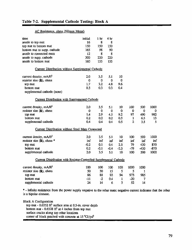
Table 7-2. Supplemental Cathode Testing: Block A
AC Resistance_ ohms (Nilsson Meter)
time initial 1 hr 4 hr
anode to top mat 16 8 8top mat to bottom mat 150 150 150bottom mat to supp. cathode 165 98 90anode to connected mats 12 8 8
anode to supp. cathode 300 220 220anode to bottom mat 160 155 155
Current Distribution without Supplemental Cathode
current density, mA/ft 2 2.0 3.5 5.1 10resistor size 0g), ohms 0 0 0 0
top mat 1.7 3.2 4.8 9.6bottom mat 0.3 0.3 0.3 0A
supplemental cathode (none)
Current Distribution with Supplemental Cathode
current density, mA/ft 2 2.0 3.5 5.1 10 100 500 1000resistor size (R), ohms 0 0 0 0 0 0 0
top mat 1.4 2.9 4.5 9.2 97 490 982bottom mat 0.2 0.2 0.2 0.3 1 6.5 13
supplemental cathode 0.4 0.4 0.4 0.5 2 3.5 5
Current Distribution without Steel Mats Connected
current density, mA/ft z 2.0 3.5 5.1 10 100 500 1000resistor size 0g), ohms * inf inf inf inf inf inf inf
top mat -0.2 0.1 0.4 2.5 79 430 870bottom mat 0.2 -0.1 -0.4 -2.5 -79 -430 -870
supplemental cathode 2.0 3.5 5.1 10 100 500 1000
Current Distribution with Resistor-Controlled Supplemental Cathode
current density, mA/ft z 100 100 100 100 1000 1000resistor size 0g), ohms 50 30 15 5 5 1
top mat 86 88 92 94 973 985bottom mat -11 -2 0.4 1 -20 7
supplemental cathode 24 14 6 3 52 14
• - infinite resistance from the power supply negative to the rebar mats; negative current indicates that the rebaris a bipolar element.
Block A Configuration
top mat - 0.6552 ftz surface area at 0.5-in. cover depthbottom mat - 0.6528 ft_ at 4 inches from top matsurface cracks along top rebar locationscomer of block patched with concrete at 15 #Cr/yd 3
79

Table 7-3. Supplemental Cathode Testing: Block B
AC Resistance_ohms(Nilsson Meter); Block B
time initial 1 hr 4 hranode to top mat 78 42 38top mat to bottom mat 140 140 140bottom mat to supp. cathode 135 89 80anode to connected mats 71 42 38anode to supp. cathode 320 230 230anode to bottom mat 190 170 165
Current Distribution without Supplemental Cathode
current density, mA/ft2 2.0 3.5 5.1 10resistor size 011),ohms 0 0 0 0
top mat 1.6 3.0 4.4 9.0bottom mat 0.4 0.5 0.6 1.0
supplemental cathode (none)
Current Distribution with Supplemental Cathode
current density, mA/ft2 2.0 3.5 5.1 10 100 500 1000resistor size 011),ohms 0 0 0 0 0 0 0
top mat 1.3 2.8 4.3 8.8 92 470 942bottom mat 0.3 0.3 0.3 0.5 5 24 48
supplemental cathode 0.4 0.4 0.5 0.7 3 6 10
Current Distribution without Steel Mats Connected
current density, mA/ft2 2.0 3.5 5.1 10 100 500 1000resistor size 011),ohms * inf inf inf inf inf inf inf
top mat -0.2 0.3 0.4 2.5 75 410 830bottom mat 0.2 -0.3 -0.4 -2.5 -75 -410 -830
supplemental cathode 2.0 3.5 5.1 10 100 500 1000
CurrentDistributionwith Resistor-ControlledSupplementalCathode
current density, mA/ft2 100 100 100 100 1000 1000resistor size (R), ohms 50 30 15 8 50 5
top mat 82 86 90 92 897 936bottom mat -9 -2 1 4 -250 5supplemental cathode 27 16 9 4 356 62
* - infinite resistance from the power supply negative to the rebar mats; negative current indicates that the rebaris a bipolar element.
Block B Configurationtop mat - 0.6552 ft2surface area at 1-in. cover depthbottom mat - 0.6528 ft2 at 3.5 inches from top matsurface cracks along top rebar locations
80

Table 7-4. Supplemental Cathode Testing: Block C
AC Resistance, ohms(Nilsson Metcr)]Block C
time initial 1 hr 4 hranode to top mat 97 76 67top mat to bottom mat 92 96 96bottom mat to supp. cathode 130 84 75anode to connected mats 100 75 67
anode to supp. cathode 270 220 205anode to bottom mat 170 160 155
Current Distribution without Supplemental Cathode
current density, mA/ft: 2.0 3.5 5.1 I0resistor size OR),ohms 0 0 0 0
top mat 1.8 3.2 4.6 9.0bottom mat 0.2 0.3 0.5 1.0
supplemental cathode (none)
Current Distribution with Supplemental Cathode
current density, mAJft_ 2.0 3.5 5.1 10 100 500 1000resistor size OR),ohms 0 0 0 0 0 0 0
top mat 1.5 3.0 4.4 8.6 89 452 909bottom mat 0.3 0.3 0.4 0.8 8 38 77supplemental cathode 0.2 0.2 0.3 0.6 3 10 17
CurrentDistributionwithout Steel Mats Connected
current density, mA/ftz 2.0 3.5 5.1 10 100 500 1000resistor size OR),ohms * inf inf inf inf inf inf inf
top mat -0.6 0 0.1 0.6 65 373 763bottom mat 0.6 0 -0.1 -0.6 -65 -373 -763supplemental cathode 2.0 3.5 5.1 10 100 500 1000
Current Distribution with Resistor-Controlled Supplemental Cathode
current density, mA/ftz 100 100 100 100 1000 1000resistor size OR),ohms 50 30 15 15 8 5
top mat 78 82 87 882 893 899bottom mat -5 -0.4 2 -38 12 37
supplemental cathode 29 20 12 159 96 67
* - infinite resistance from the power supply negative to the rebar mats; negative current indicates that the rebaris a bipolar element.
Block C Configurationtop mat - 0.6552 ft2 surface area at 2-in. cover depthbottom mat - 0.6528 ftz at 2.5 inches from top matsurface cracks along top rebar locations
81

A practical problem is that many bridge decks in the field are constructed with permanentsteel pan forms. In this case the use of a supplemental cathode applied external to theconcrete structure would not be possible. Difficulty would also arise from the presence ofexposed steel chairs on the bottom of the bridge decks. These are sites for direct shortsbetween the supplemental cathode and the reinforcing steel. In this case the vast majority ofcurrent would flow directly to the reinforcing steel and the supplemental cathode would notaccomplish its purpose.
It was therefore concluded that supplemental cathodes were not feasible for use inelectrochemical chloride removal from concrete bridge components. This emphasizes the
importance of the hydrogen embrittlement and bond strength studies carried out in thiscontract since the existing reinforcing steel must be used as the system cathode.
82

Concrete Depth-of-Cover Effects on Current Distribution
If variations in current density are high, several problems can arise. Portions of the
reinforcing steel structure could actually be operating at too high of a current density and
result in softening of the cement paste at the concrete-steel interface. Other areas of thereinforcing steel could see nearly no current and leave the chloride in place to causecorrosion.
Three blocks with different depths-of-cover, 1, 2, and 4 inches (2.5, 5, and 10 cm), were
electrically connected in parallel to simulate variation on a bridge deck. A limewaterelectrolyte was ponded on the surface of the concrete which contained an inert mesh anode.
These blocks were operated at 0.1 and 0.5 amps/ft 2 (1 and 6 A/m s) of concrete per block.Results are summarized in Table 7-5.
Table 7-5. Current Distribution vs Concrete Depth of CoverI I IIII
System Target C.D. System Block Amps]ft2Conditions Amps A.mps/ft2 V..olts 1" Cover 2" Cover 4" Cover
initial 0.3 0.1 6.4 0.14 0.10 0.06>24 hrs 0.3 0.1 5.6 0.16 0.09 0.05
initial 1.8 0.6 28.4 0.87 0.57 0.36>24 Ins 1.8 0.6 24.7 0.93 0.56 0.31>48 hrs 1.8 0.6 30.3 0.69 0.68 0.43>72 hrs 1.8 0.6 39.6 0.67 0.63 0.50
Mfta * 10 = Mm 2I I| II I I
These data show that, initially, when the concrete was not saturated with electrolyte, only
60% of the intended current was received by the high depth-of-cover block. However, afterthree days of electrolyte contact nearly 85% of the intended current was received by this
block and even more was expected if it was allowed to operate longer. The low
depth-of-cover block did not experience a current density greater than 1.0 amps/ft 2 (10 A/m2).
Based on these tests, variation in depth-of-cover does not pose a current distribution problem.
83

Effects of Concrete Cracks on Current Distribution
Evaluation of the effects of cracks over the reinforcing steel on current distribution wasinvestigated. Even though the cracks seemed large, approximately 0.5 millimeter, and werevisible with the naked eye, there was no significant current distribution shift at the initialenergizing. However, as time passed, the cracked block received 135% of its intended currentdensity. A thick, white precipitate of high pH began to form at the cracks and eventuallyseemed to fill them. It is felt that this is a result of the production of high hydroxyl ionconcentration at the rebar and the hydrogen bubbling action bringing these hydroxyls to thesurface forming Ca(OH)2. The current distribution returned to the intended values after 30hours on line. Data are shown in Table 7-6.
Table 7-6. Effects of Concrete Cracks on Current DistributionI
System Target C.D. System Block Amps/ft"zConditions Amps Amps/ft 2 Volts Cracked Untracked
initial 1.2 0.6 20.9 0.59 0.61>6 hrs 1.2 0.6 18.3 0.81 0.39>24 hrs 1.2 0.6 33.0 0.63 0.57>30 hrs 1.2 0.6 33.0 0.60 0.60
A]ftz * 10 = Aim2I
The white precipitate is unsightly and is not desired. It was recommended that all largecracks, spaUs, and potholes be repaired prior to the removal process.
84

8
Chloride Removal and Distribution
Laboratory chloride removal experiments on concrete slab specimens were necessary todevelop criteria for electrochemical chloride removal and to determine completion of theprocess. The questions of how to monitor and when to stop the process were answered.Chloride removal efficiency, chloride removal threshold, and chloride distribution followingtreatment were determined. Analysis of concrete cores taken from existing chloridecontaminated bridge decks was conducted to conf'u'm results from the laboratory slabscontaining cast-in chloride.
Preliminary Testing
Preliminary testing was conducted on the 1-ft x 1-ft (30-cm x 30-cm) supplemental cathodespecimens (See Chapter 7) as a prelude to chloride removal on the 2-ft x 2-ft (60-cm x 60-cm) test slabs. This preliminary testing was necessary to identify conditions that may have anadverse effect on the slab specimens. High-temperature operation was investigated and amaximum current density limit was set.
Previous investigations by Battelle in the 1970's measured rate of removal, chloridedistribution, and chloride threshold values. Electrochemical removal was performedpotentiostatically at constant voltage. ELTECH experiments were performed galvanostaticaUyat constant current. With this technique, an accurate measure of the amount of charge passedcan be made, and through Faraday's Law, ion transport and efficiency are easily determined.
Transference number testing showed improved chloride ion mobility at higher temperaturesand relative insensitivity to current density. The test blocks used for supplemental cathodetesting were used to verify this. Block C was operated at 0.2 A/ft2 (2 A/m s) and 25°C, andBlock D was operated at 0.2 A/f-t2 (2 A/m 2) and 80°C. Temperature wells were installed toobtain internal block temperatures. Data were not accurate in either case due to leakage ofthe ponded electrolyte, but confirmation of improved chloride removal at the highertemperature was obtained. Data also indicated that approximately 400 to 500 A-hr is neededto remove the majority of chloride from these blocks, based on their initial chloride contents.
85

Block B was operated at 3 Alfd (30 A/m 2) and 80°C with external heating but it had only oneinch (2.5 cm) of concrete cover, and within a day, surface cracks appeared over thereinforcing steel resulting in a cell voltage of only 15V. Data from this test was thought tobe unreliable.
Block D was then operated at 3 A/fd (30A/m 2) to obtain the high current density data withoutexternal heating. This block had 3 in. (7.5 cm) of concrete cover. After seven hours ofoperation, the block reached a voltage of 157V (from an initial 100V) and a temperature of94°C. Current density decreased to 0.8 A/ft2 (8 A/m2) due to the rectifier 180V voltage limit.It was speculated that the area around the reinforcing steel cathode had dried out and createda high resistance situation. The same phenomenon occurred when the block was operated at2 Mft 2 (20 A/m2).
A gradual current density increase was done to avoid these high voltage runaways. At 1 A/ft2(10 A/m2), Block D operation held steady for two days at 100V and an internal blocktemperature of 40°C. At 1.5 Mft 2 (15 A/m2), operation was steady at 75V and 50°C.However, after a day of operation the current distribution to the bottom mat of steel increasedfrom approximately 5% to 15%. Current was increased to 2 A/fd (20 A/m 2) where operationsteadied at 70V and 65°C. One day later a large crack was noticed completely around theblock at the level of the top mat of steel. Surface cracks were also noticed after the blockwas shut down. It was believed that the cracking occurred due to pressure buildup from theinability of hydrogen gas to diffuse away from the reinforcing steel cathode surface. At acurrent density of 2 AJft2 (20 Mm2), hydrogen gas is formed at the rate of about a liter perhour. The block was separated at the crack, and a high pH region around the reinforcingsteel was found.
These tests show that operation at higher current densities can achieve temperatures sufficientfor improved chloride transfer. However, current densities as high as 2 A/ft2 (20 A/m 2) mayinflict serious damage and are to be avoided.
Laboratory Concrete Slab Specimens
Twelve 2-ft x 2-ft x 8-in. thick (60- x 60- x 20-cm) test slabs were prepared for chloride ionremoval and distribution tests. Ohio DOT specifications for bridge deck concrete and rebarschedules were used. A schematic of these 2-ft x 2-ft (60-cm x 60-cm) test slabs is shown inFigure 8-1.
86

Figure 8-1. Laboratory Chloride Removal Test Slab Specimen
• • °
• • ° , • ° °
• "l_]
............... ° ° ° .............
J J
1.5" (4 era) of 15 Ibs/yd 3 Chloride
3.25"(8 o)of 7 ib/y 3 Chlo idNo Chloride Added
The specimens contained two mats of reinforcing steel. The top mat consisted of #6 barscrossing over #4 bars. There were 2 in. (5 cm) of concrete cover over the #6 bars. Thebottom mat consisted of crossing #5 bars. There was 1 in. (2.5 cm) of concrete below thebottom #5 bar. All bars were located on 7-inch (18-cm) centers.
The specimens contained three lifts of the concrete. No chloride was added to the bottom liftof 3.25 in. (8 cm). The middle lift of 3.25 in. (8 cm) contained 7 #Cr/yd3 (4 kg/m3). The toplift of 1.5 in. (4 cm) contained 15 #Cl/yd s (9 kg/m3). Data on the fresh concrete used in thepreparation of these slab specimens are shown in Table 8-1.
87

Table 8-1. Fresh Concrete Data for Chloride Removal Slab Specimens
Concrete Unit Air
Batch Weight, Content, Concrete
Number lb/ft 3 % Slump, in. #Cl/¥d 3 Location
11 143.0 6.5 2.75 0.5 Bottom 3.25 in.
Slabs 1,2,3
12 143.0 6.5 2.75 7.7 Middle 3.25 in.
Slabs 1,2,3
13 144.1 6.2 4.0 16.0 Top 1.5 in.Slabs 1,2,3
14 143.2 6.4 3.5 0.6 Bottom 3.25 in.Slabs 4,5,6
15 143.2 6.4 3.5 7.4 Middle 3.25 in.Slabs 4,5,6
16 145.9 5.4 "3.0 12.5 Top 1.5 in.Slabs 4,5,6
17 141.1 8.0 4.0 *N.D. Bottom 3.25 in.
Slabs 7,8,9
18 141.1 8.0 4.0 *N.D. Middle 3.25 in.
Slabs 7,8,9
19 145.5 5.8 3.25 *N.D. Top 1.5 in.Slabs 7,8,9
20 142.0 7.8 4.0 0.7 Bottom 3.25 in.
Slabs 10,11,12
21 142.0 7.8 4.0 6.7 Middle 3.25 in.
Slabs 10,11,12
22 145.2 5.8 3.5 15.5 Top 1.5 in.Slabs 10,11,12
* Not Determined
kg/m 3 concrete = 16 * lb/fP concrete; kg Cl'/m 3 concrete = 0.6 * _Cl'/yd3 concreteI
88

Pre-Treatment Data
Static half-cell potentials, macroceU currents, and corrosion rate measurements were taken onthe twelve 2-ft x 2-ft (60-cm x 60-cm) chloride removal slabs to be compared to post-treatment testing and provide a means for evaluating the treatment. Pre-treatment test dataare shown in Appendix A, Figures A-1 through A-12.
Static Half-Cell Potentials
Forty static half-cell potentials were taken per slab; all but eight of the 480 measurementswere more negative than -0.350 V vs Cu/CuSO4, indicating active corrosion. Thesemeasurements were taken with uncoupled top and bottom reinforcing steel mats.
Macrocell Currents
Macrocell corrosion currents between the top and bottom mats were taken after the top andbottom mats were coupled for 16 hours to establish corrosion. MacroceU currents rangedfrom 0.3 to 0.7 mA, indicating active corrosion of the top mat of reinforcing steel.
Corrosion Rate Measurements
Corrosion rate measurements with uncoupled top and bottom mats of reinforcing steel wereobtained with the three electrode linear polarization (3LP) technique? Six measurementswere taken on each slab. Initially, these measurements were to be taken at the 3 mostnegative cross bar sites and 3 most negative straight bar sites as determined by the staticpotential measurements. However, measurements taken in this way would have beenclustered around a single location and would not have provided a representative sampling ofthe entire slab. Instead, one of the most negative sites was selected fn'st with the remaining 5sites spread out but still being of the more negative group. 3LP corrosion rates ranged from4 to 26 mA/fta of steel (2 to 13 mil/yr) and averaged about 12 mA/ft a of steel (6 mil/yr).Based on these 3LP data, damage of the concrete due to corrosion could be expected to occurin two years or less.
The static potentials and corrosion rate measurements were repeated at select locations withthe mats coupled and were found to be similar to those taken uncoupled.
3Measurements were made with the KCC INC 3LP Device.
89

Slab Treatment
The status of the twelve 2-ft x 2-ft (60-cm x 60-cm) test slabs is shown in Table 8-2.
Table 8-2. 2.Ft x 2.Ft Slab Test Status
Slab No. .Status
2 Control1,3,4,5,10,11,12 Chlorideremovalwith high pH electrolyte
7,8,9 ChlorideremovalwithouthighpH electrolyte(NORCURE_')6 Spare
Seven of the twelve slabs were treated by the same process. A 2-inch (5-cm) highpolypropylene wall was sealed to the top surface of the slabs with polyurethane caulk to forman electrolyte ponding dam. The ponding dam was filled with 1-1/2 inches (4 cm) of 0.1MNaOH solution as the electrolyte. An inert catalyzed titanium mesh was placed in theelectrolyte as the anode.
The electrolyte pH was monitored daily with a handheld pH meter. The pH was maintainedat or above 12 to prevent chlorine gas evolution, and therefore enabling accurate monitoringof the removal of chloride ion. When the electrolyte pH decreased to 12, an addition of solidNaOH pellets was made to increase the pH. This was necessary every two or three days.
Operation was monitored for electrolyte pH, electrolyte chloride concentration, cell voltage,and current distribution to the top and bottom mats.
Two major criteria were to be determined from results of the laboratory treatment of theseslabs. First, the highest operating current density without detrimental effects must bedetermined. This is desirable since a high current density will result in a shorter treatmenttime. The closing of a bridge deck or the existence of traffic control should be kept at aminimum. Second, the duration of treatment or total charge must be determined. A summaryof the treatment of the slabs together with data for the untreated control slab are shown inTable 8-3. Operating voltages for these trials were 25 to 30 volts.
90

Table 8-3. 2-Ft x 2.Ft Slab Treatment SummaryI I Ill
Current Total TotalDensity Charge Chloride Chloride Chloride
Slab No. A/ft2. A-hr/ft 2 Removed, g Possible, g Removed 1% Comment
1 2.0 495 139.1 253.5 55 cracked at top mat
2 0 0 0 253.5 -- control slab
3 0.6 60 55.1 253.5 22 partial removal /
4 0.6 60 65.1 218.6 30 partial removalf'"
5 0.6 302 114.7 218.6 53 heavy removal
I0 0.6 302 125.7 231.1 54 heavy removal
11 0.2 302 123.5 231.1 53 heavy removal
12 0.2 302 109.6 231.1 47 heavy removal
mA/ft2 *10 = Mm2; A-hr/ft2 * 10 = A-hr/m2
Figure 8-2 shows plots of each slab's overall chloride removal efficiency as a function of thetotal charge passed. Chloride removal efficiency is def'med as the amount of chloride actuallyremoved relative to the amount of chloride which would have been removed ff 100% of the
current was carried by chloride ion. It can be seen that after approximately 100 A-hr/ft 2
(1000 A-hr/m 2) of total charge is passed, the overall efficiency is the same regardless of
current density.
91

Figure 8-2. 2-Ft x 2-Ft Slab Chloride Removal Efficiency
55 _. O Slab I1 - 0.2 A/ft=
50 _/ • Slab 12 - 0.2 A/ft=Z_ Slab 5 - 0.6 A/f1 ="" 45 - • Slab 10 - 0.6 A/ft z>- " O O Slab 5 - 0.6 A/ft I
C 4.0 _ • Slab 4 - 0.6 A/ft=,----. . _\ v Slab 1 - 2.0 A/ft=
..,.-.2_-__>oEo® 55302520 "." __'_'(j 15 ..
p 10- V-- V---------- V _ v
> 5O
0 .... I .... I .... 1 .... I .... I .... i .... I .... a .... I ....
0 50 100 150 200 250 300 350 400 450 500
Total Charge Passed (A-hr/ft 2)
Even though chloride removal is faster at higher current densities, there is still an uppercurrent density limit that must be set based on the damage experienced by Slab N* 1. Asindicated in Table 8-3, Slab N_ 1 was operated at 2.0 A/ft2 (20 A/m 2) of concrete for 495A-hr/ft 2 (4950 A-hr/m2). The slab fractured at the top mat of reinforcing steel. This samedamage occurred with a smaller slab at the same current density (see Preliminary Testing,this chapter). It is believed that this fracture occurred because of the generation of molecularhydrogen at a rate which was faster than that which could diffuse through the surroundingconcrete. Based on the detriment of Slab N° 1, maximum treatment current density andduration was reduced to 0.6 A/ft_ (6 AJm2) of concrete for 300 A-hr/ft _ (3000 A-hr/m2).There was a concern that even removal at 0.6 A/ft2 (6 A/m 2) of concrete may be detrimentalto the concrete structure.
According to Figure 8-2, a leveling of the curves occurs at approximately 150 A-hr/ft 2 (1500A-hr/m 2) of total charge passed. This indicates that after 150 A-hr/ft 2 (1500 A-hr/m 2)relatively little chloride is being removed for the amount of energy used to remove it. Sinceall of the chloride is not going to be removed anyway, the economics of further treatmentbecome questionable. It is likely that the maximum necessary treatment will be set at about150 A-hr/ft 2 of concrete (1500 A-hr/m 2) of total charge.
92

Post-Treatment Core Analyses
Slab No1 was delaminated over 100% of its horizontal area at the end of its quite severetreatment, 2.0 amps/ft 2 (20 A/m 2) of concrete for 495 A-hr/ft 2 (4950 A-hr/m 2) of concrete.The delamination plane was coincident with the top levels of reinforcing steel and wasparallel to the top surface of the slab. The delamination crack was apparent to the unaidedeye on the side surfaces and had a maximum width of around 0.015 inches (15 nail). Thiscrack appeared to be the only distress feature relating to the electrochemical treatment. Athorough examination of the slab wearing surface with a 10X hand lens revealed no verticallyoriented cracks.
Even within the confines of the polyethylene sheet wrapping used for shipment, someevaporation of surface moisture took place. However, wetness persisted on the concrete coresurface in a relatively broad band coplanar with the top level of reinforcement as shown inFigure 8-3.
Observations/measurements of the concrete core slab are as follows:
• The cement paste phase adjacent to the top layer of reinforcing steel had undergone asoftening relative to the cement paste at lower depths in the core.
• The pH of the altered phase around the top layer of reinforcing steel was 14 comparedwith a pH of 12.5 at lower depths in the core.
• Some f'me aggregate particles within an inch or so of the top reinforcing steel haveundergone a softening degradation.
• The delamination described above passed through the entire section of Core No. 1-1 asshown in Figure 8-4.
• The fracture plane typically passed around rather than through the coarse aggregateparticles.
• There was an absence of corrosion product on either the top or bottom bars.
93

Figure 8-3. Core N_ 1-1 Showing Broad Band of Persistent Wetness
Figure 8-4. Core N_ 1-1 Showing Fracture Plane at Top Layer of Steel
b3
U_C
c_2J
94

Post-Treatment Chloride Distribution
Chloride analysis of concrete cores removed from treated slabs is summarized on Table 8-4.
The mix concentration of chloride is shown on Figure 8-1.
Table 8-4. Chloride Ion Content of Electrochemical Removal Slab Cores
Slab Density Charge Sample Post-Treatment InitialCored Amp/ft2 Amp-hr/ft2 Depth, in. %C1"¢_) lb Cl/yd 3°' lb Cl/yd 3c_
1 2 500 0 to 3/8 0.175 6.85 16.0without 2 500 7/8 to 1-1/4 0.210 8.22 16.0steel 2 500 1-3/8 to 1-3/4 0.094 3.68 10.4c')
1 2 500 0 to 3/8 0.037 1.45 16.0with 2 500 7/8 to 1-1/4 0.028 1.10 16.0steel 2 500 1-5/8 to 2 0.024 0.94 7.7
5 0.6 300 0 to 3/8 0.070 2.74 12.5with 0.6 300 5/8 to 1 0.045 1.76 12.5steel 0.6 300 1-1/2 to 1-7/8 0.036 1.41 7.4
12 0.2 300 0 to 3/8 0.080 3.13 15.5with 0.2 300 3/4 to 1-1/8 0.042 1.64 15.5steel 0.2 300 1-3/8 to 1-3/4 0.033 1.29 9.6<'_
(a) Based on dry concrete weightCo)Based on concrete unit weight of 145 lb/ft_(c) Value calculated from Table 8-1 data
Chloride removed from the three cores containing steel is seen to be quite complete.Chloride removed from these cores ranged from about 80% at a charge of 300 A-hr/ft2 (3000A-hr/m2) to 89% at a charge of 500 A-hr/ft2 (5000 A-hr/m2). These data can be misleading,however, since chloride removal is much more complete over the reinforcing steel where thecurrent flow is concentrated. The core taken between bars on Slab N° 1 shows chloride
concentrations indicating only 46% of chloride removed. It is clear from these and other data
that chloride removal is thorough close to and directly over the reinforcing steel, but notbetween bars.
The data also imply that about 0.9 lb/yd 3 (0.5 kg/m 3) of chloride cannot be removed by thetreatment. This is consistent with the Battelle study in 1975 which indicated that 0.8 lb/yd 3
(0.5 kg/m 3) of chloride could not be removed. In the present study, about 0.6 lb/yd 3 (0.4kg/m 3) of chloride was present in the concrete with no chloride added (see Table 8-1), and
this was likely the bound chloride which could not be removed under any circumstances.
Because of the complexities involved in analysis of concrete following treatment, total
chloride removed is better determined from solution analysis (data in Table 8-3).
95

SEM/EDS Examination
Mortar samples were carefully excavated from around both the top and bottom rebar in CoreN° 1-1. the cement paste contacting the reinforcing steel was examined, as well as fracturesurfaces located about 1/4-inch (0.6-era) from the reinforcing steel/concrete interface.
For comparative purposes, an SEM/EDS analysis was done on the Type I LA cement used in
the subject concrete. A major portion of the alkalies present in this cement is represented by
potassium. An analysis of the cement, as conducted by Construction TechnologyLaboratories, is presented in Table 8-5.
Table 8-5. Chemical Analysis of Project Portland Type I LA CementI
Analyte Weight %
SiO2 20.57A1203 4.58Fe203 3.62CaO 63.74
MgO 3.21SO3 2.35NazO 0.09g_o 0.46TiO2 0.26P205 0.08Mn203 0.11SrO 0.08L.O.I. 0.93
TOTAL 100.08
Total Alkalies as NazO = 0.40
Calculated Compounds(perASTM C 150-85a) Weight %
c_s 58c2s 15C3A 7C,AF 11ss<C,AF+C_-3 0
The EDS spectrum obtained on a two-day-old hydrated paste sample is shown in Figure 8-5.The principal constituent is calcium followed by silicon with lesser amounts of iron, sulfur,
potassium, aluminum, and magnesium. This spectrum is considered to be representative ofthe Type I LA portland cement that has not been subjected to any chemical alteration.
96

EDS spectrum for the cement paste touching the bottom reinforcing steel (not shown) and thecement paste about 1/4-inch (0.6-cm) from the bottom reinforcing steel are virtually identicalto that of the "normal" cement paste shown in Figure 8-5. This indicates that theelectrochemical removal had virtually no effect on the overall chemistry of the cementsurrounding the bottom reinforcing steel despite the fact that measurements indicate that somecurrent passed through the bottom bars during the treatment.
Figure 8-5. EI)S Spectrum of Virgin Columbia Type I Portland Cement Paste
CA
[ AL_A S K "M G ,,±._t__ , .,_ _ _- ._FE ! __2.0 4.0 6.8 8. E1 1El. El
EHEF'gY (t::EU)
The electrochemical removal caused significant changes in the distribution of the ionic speciesin the cement paste phase near the top reinforcing steel. The initial chloride ion content ofthe concrete surrounding the top reinforcing steel at the start of the electrochemical removaltreatment was 7 #C1-/yd3 (4 kg/m 3) concrete. Following the electrochemical treatment, nochloride ion was detected by EDS, either immediately adjacent to or 1/4-inch (0.6-cm) awayfrom the reinforcing steel. The EDS spectrum of the paste touching the top reinforcing steelis shown in Figure 8-6. A high level of iron/manganese is indicated. Relative to "normal"Type I LA portland cement paste, the cement paste around the top reinforcing steel showedextremely high levels of potassium with abnormally high amounts of sodium and sulfur aswell.
97

Figure 8-6. EDS Spectrum of Cement Paste Contacting Top Rebar of Core N_ 1-1
• " f_t-1
FE
K
o2.0 4.0 6.0 E:.O 10.0
EIqEF'GY (KEU)
The presence of high levels of sulfur at the reinforcing steel/concrete interface wasunexpected. The sulfur in portland cement was derived from gypsum_ which was added as aset-controlling material, z_ The gypsum subsequently reacts with calcium aluminate phases toform calcium sulfoaluminates. Thus, in "normal" cement pastes, most of the sulfur is tied upas sulfate in solid phases. In the concrete in the treated area of Slab Na 1, the SEM/EDSevidence suggests that sodium and potassium hydroxides (particularly sodium) has attackedthe sulfate-bearing phases yielding an aqueous solution rich in sodium sulfate. Figure 8-7, anSEM photograph of the cement paste surface contacting the top rebar in Slab N_ 1, showsevidence of the movement of sodium sulfate solutions in the paste adjacent to the reinforcingsteel.
98
Figure 8-7. SEM Photograph of Cement Paste Contacting Top Rebar of Core Na 1-1
The relief areas in the microstructure of the paste have been f'dled in with a phase that, at onerime, was liquid (right side of photograph). The EDS spectrum in this area shows high levelsof sodium and sulfur (as well as some calcium). There was considerable evidence in theSEM examination of sodium/sulfur-rich solutions moving into void volumes in themicrostructure of the paste adjacent to the top reinforcing steel. The EDS spectrum of thecement paste about 1/4-inch (0.6-era) away from the top reinforcing steel is shown in Figure8-8 (shot at around 20X). Overall, the spectrum looks reasonably "normal" with theexception of relatively high levels of sodium and sulfur. Chlorine (around 2.6 KEV) is absentfrom the spectrum.
The liquid material intruding the concrete microstructure discussed above (shown in Figure 8-7) was also observed in the cement paste material 1/4-inch (0.6-cm) away from thereinforcing steel/concrete interface. An EDS analysis of this material (at 10,000X) is shownin Figure 8-9. This analysis shows extremely high levels of sodium and sulfur suggestingthat the intruding material is principally sodium sulfate solution.
99

Figure 8-8. EDS Spectrum of Cement Paste l/4-Inch from Top Rebar of Core No. 1-1
CA
__.,_- - - _._,,N, _,-,-_u.,..... _- :-'-'--__" -7-.:,- :- ::"':_::---_ ......2..0 4.0 6.0 E'.O 10.0
EI-IEF:GY ,: KEU )
Figure 8-9. EDS Spectrum of Cement Paste of Core No. 1-1 with Liquid Phas_ Intrusion
H14A
2.0 4.0 ,g.O 8.0 lO.OEI'4EF:GY ( ICEU )
I
100

Petrographic Examination
Petrographic examinations (ASTM C 856-83) were made on polished surfaces and on freshfracture surfaces of the concrete from Core N° 1-1, taken at a crossbar site. This examination
revealed that the concrete adjacent to, and above the top reinforcing steel level was adverselyaffected by the high level of electrochemical removal treatment in Slab N_ 1. The effect onthe cement paste is a softening which is most severe immediately adjacent to the bar,diminishing in its effect as the distance from the reinforcing steel increases. Some aggregatetypes are also adversely affected (softened) by contact with the aggressive, high pH solutions.To date, rock types that have been identified as susceptible to this softening include shales,porous cherts, and porous limestone. In this concrete, all of these rock types were present inthe fine aggregate. The aggregate-softening phenomenon was conf'med to the regionimmediately adjacent to the reinforcing steel. At distances of 1/2-inch (1-cm) or more fromthe reinforcing steel, the aggregate particles were unaffected.
In cores taken from Slab N_ 1, the portions of the concrete that have undergone significantchemical changes can be easily identified by their darker appearance (see Figure 8-3) which isdue to the hygroscopic nature of the altered paste at high pH levels.
Porosity and Permeability
Mercury porosimetry was considered as a means of measuring the changes in concreteporosity _. Small 3- to 4-gram samples of paste, representing the In'st 1/4-inch (0.6-cm) ofmaterial adjacent to the top and bottom reinforcing steel, were subjected to mercuryporosimetry measurements. These results are shown in Figure 8-10. The ordinate value ofthe graph in this figure, Cumulative Intrusion, is the amount of mercury that is forced underpressure into the open pore volume of the sample. It is seen that the paste adjacent to the topreinforcing steel has a significantly higher amount of porosity in the 1- to 10-micron porediameter range. A conftmaation of this result is provided by a comparison of the SEMphotomicrographs of the paste from the two areas (Figure 8-11). Void volumes in the 1- to10-micron range are obvious in the paste taken from regions near the top reinforcing steel inCore Na 1-1. It is presumed that the electrochemical treatment produced these results througha dissolution of previously solid material.
101

Figure 8-10. Mercury Porosimetry Data Obtained on Mortar Samples of Core N° 1-1
0.10
_: e_e
_ e Cement Paste Adjacent to Top Steelu • A Cement Paste Adjacent to Bottom Steel
° \.o_
Top
® \.\ *.>.4"
__o -\ •
= • \E \ Q
= _\ \.C3 •
Bottom" _ _e
\ \
10-3 10 -2 10 -1 10 0 101 10 2 10 3
Pore Diameter _micrometers)
Figure 8-U. SEM Photograph of Core No. 1-1 Cement Paste Showing Open Porosity
102

Compressive Strength
The compressive strength of the untreated concrete represented by Slab N" 1 was around 8,000psi, as determined on a retained 4-inch (10-cm) diameter x 8-inch (20-cm) long cylinderspecimen prepared from the same batch as Slab N° 1. It is expected that whatever the sourceof stress, the concrete represented by Core N° 1-1, if unaffected by any deteriorationmechanisms, should show mostly an intra-aggregate form of fracture.
As a measure of the effect of the electrochemical treatment on the compressive strength of theproject concrete, impact hammer readings (ASTM C 805-85, Standard Test Method forRebound Number of Hardened Concrete) were taken on Slab N_ 1 on the outside surfaces atthe top and bottom reinforcing steel levels. The results of these measurements showed anaverage rebound number of 49 for the concrete at the top rebar level and bottom reinforcingsteel levels. These averages are based on a total of 30 readings at each level. The actualcompressive strength at the time of the test was around 7,800 psi (as measured on cylinderspecimens per ASTM C 39-86, Standard Test Method for Compressive Strength ofCylindrical Concrete Specimens). It is assumed that the actual compressive strength ofconcrete at the lower reinforcing steel level, where participation in the electrochemicalreactions is minimal, would be at or near the 7,800 psi level. On this basis, the similarity ofthe rebound hammer values in the top and bottom of the slab suggest that, as a bulk concreteproperty, the compressive strength of the concrete was not significantly adversely affected bythe large amount of charge passed, 500 A-hr/ft z (5000 A-hr/m2), at the high current density, 2A/ft2 (20 A/mZ).
Field Cores
All the work in the laboratory phase of this contract was conducted on specimens preparedwith cast-in chloride. This caused concern since chloride originally present in the concretemix may be "absorbed" during the curing process by incorporation into essentially insolublecompounds with the tricalcium aluminate present in the concrete. Thus, chloride incorporatedin this way may be tightly bound, and not as available for chloride removal as chloride whichis introduced as deicing salt after the concrete is fully cured. For this reason it was decidedto conduct chloride removal from cores obtained from structures contaminated by deicing salt.This was considered an important step to take prior to the field validation phase of thiscontract.
Six field cores were obtained from the Rt. 2 bridge over E. 361st St. in Eastlake, Ohio nearCleveland. The concrete of these cores was intended to be similar to the 2-ft x 2-ft (60-cm x60-cm) slabs, but this was unexpectedly not the case. The deck had previously been repairedwith an LMC overlay. The overlay was 1 to 2 in. (2.5 to 5 cm) thick resulting in a concretethickness over the reinforcing steel of 4 in. (10 cm) in places. The presence of the LMCoverlay caused concern, but since initial tests showed the overlay to be heavily contaminated(see Table 8-7), and have a reasonable electrical resistance, it was decided to proceed withchloride removal testing.
103

Two cores were to be operated at 0.6 A/ft_ (6 A/m 2) in NaOH electrolyte with pHmaintenance, the same manner in which the 2-ft x 2-ft (60-cm x 60-cm) slabs were operated.Due to the relatively high electrical resistivity of the 2-in. (5-cm) thick LMC overlay, acurrent density of only 0.2 A/ft2 (2 A/m 2) was achieved. Starting voltages were 71V and126V. After 60 A-hr/ft _ (600 A-hr/m 2) of total charge was passed, the voltages decreased to49V and 55V and then down to approximately 25V by the end of the treatment at 300A-hr/f-t2 (3000 A-hr/m2). Removal efficiency from the field cores was only slightly lowerthan from the 2-ft x 2-ft (60-cm x 60-cm) slabs. Data are shown in Table 8-6 with similar2-ft x 2-ft (60-cm x 60-era) slab data.
Table 8-6. Operating Data - Field vs. Laboratory Cores
Total Charge Voltage Percent Removal EfficiencyA-hr/ft 2 Core 3 Core 4 Field Cores 2-ft x 2-ft Slabs
0 71 126 ..........60 49 55 15 25150 34 35 7 12300 22 24 4 8
A-hr/ft2 * 10= A-hr/m2
The removal efficiencies shown on Table 8-6 imply that there is little difference betweenspecimens with cast-in chloride and those from the field. It is likely that the bound chlorideis in eqoilibriuim with soluble chloride which allows it to be removed over the long period oftime used for treatment. Chloride analys'.'s of concrete powder samples taken before and aftertreatment are shown in Table 8-7 along with similar data from one of the 2-ft x 2-ft (60-era x60-cm) treated slabs.
Treatment of these cores also shows that removal is possible from structures with LMCoverlays, but with initially higher voltage and longer times. If the low voltage requirement(50 VDC) stands for the entire treatment, structures of this type may not be able to be treatedin a reasonable period of time. Based on the operating differences encountered with the fieldcores, it is recommended that cores from every candidate structure be operated in thelaboratory to identify probable field operating parameters for that structure.
104

Table 8-7. Concrete Chloride Analyses - Field Cores
_Cl'/yd3 _Cl'/yd3Depth from Before Treatment After TreatmentSurface, in. Core 3 Core 4 Core 3 Core 4
0.125-0.875 18.0 15.6 8.5 4.2
1.125-1.875 6.1 4.5 2.5 1.72.125-2.875 4.0 3.4 1.9 1.23.125-3.875 1.7 1.7 1.3 0.8
............. -BAR .............
4.125-4.875 0.9 0.5 1.0 0.6
Slab N° 12 Slab Na 12Before Treatment After Treatment
0.000-0.375 15.0 3.10.750-1.125 15.0 1.61.375-1.750 9.0 1.3
.............. BAR ...............
kg Cl/m 3 concrete = 0.6 * _Cl/yd 3 concrete
105

9
Chloride Removal Electrolytes
As discussed in Chapter 6, several anode types were evaluated for use with the chlorideremoval process. Based on this work it was decided to use an inert anode. When an inert
anode is used in chloride-containing electrolytes, chlorine gas may be evolved. Threepossible electrolyte procedures, anion exchange resins, manganese sulfate addition, and pHmaintenance, were studied to eliminate chlorine evolution. These are discussed separatelybelow.
Anion Exchange Resins
The use of anion exchange resin to adsorb chloride ion during electrochemical removal ofchloride from concrete structures was the approach used by Battelle in their mid-1970'sstudy 12'13.Complete adsorption of all chloride ions would prevent chlorine evolution at theinert anode. This study was done to determine the exchange efficiency, resin stability, andease of resin handling to incorporate the use of anion exchange resin with inert anodes.
Anion exchange resin appropriate for this study is commercially available in two forms: CI"and OH'. Several resins were obtained from Dow and Rohm & Haas, two major producers ofion exchange resins. For this study, the Rohrn & Haas resin IRN-78 was chosen since it wasalready in the hydroxide form, eliminating the initially required step of conversion to thechloride form. It has an exchange capacity of 1.1 meq/ml which corresponds to 0.039 gmCl/ml of resin.
Tests were performed using 4-in. (10-cm) diameter x 3-in. (8-cm) long cylinders. Theschematic of the test setup is shown in Figure 9-1. Resin was ponded in limewaterelectrolyte between the concrete surface and an inert mesh anode. Air was sparged into theanolyte chamber to help transport the gases produced at the anode to the caustic scrubberwhere any chlorine could be scrubbed and analyzed. The catholyte, 0.1 M NaOH, wascirculated past a steel cathode to prevent a build-up of hydrogen bubbles.
107

Figure 9-1. Schematic of Ion Exchange Resin Test Setup
[Inert Chlori._e Scrubbe
J Anode
, --,.i . _ _I L__ Air Sparge
[[ I IonExchAnge
Resin
I �.<."• o ..
Power Supply . _..4"" . .:_ .:" 4 ..._ 4" 4 4" Diameter, 1" Thick..._ • , .._" . .: " ,1.5 A, ZOO V ._. "" Concrete Specimen
• + " "+"'"+"---_:_ II
Ut II it HtI o.IM[ Steel Cathode NaOH
1 LPI[ Pump
Tests were performed at 0.1, 1, and 2.5 amps/ft2 (1, 10, and 25 AJm 2) WithOUtpH control.Resin depth ranged between 0.1 and 0.3 in. (0.3 and 1 cm). The electrolyte became acidic inevery case and significant chlorine evolution resulted. It was indicated that during theBattelle treatment of the Marysville, Ohio bridge, the odor of chlorine was detected eventhough anion exchange resin was used.
A technical representative from the resin manufacturer, Rohm & Haas, was contacted andsuspected that the resin would not adsorb the chloride ion the basic pH needed to minimizechlorine evolution with the use of an inert anode. Basic solutions are used to regenerate the
resin. The use of ion exchange resin was not feasible and therefore abandoned.
Manganese Sulfate Additions
Previous investigations at ELTECH identified MnO2 coating on an inert mesh anode to act asa diffusion-barrier type coating and prevent chloride ions from reaching the anode surface andevolve chlorine gasz_. A pre-coated anode was unsuccessful, so its use was investigated insitu.
10g

The chlorine gas concentration above a ponded anode was first determined. A catalyzedtitanium inert mesh anode was placed in a pond of limewater on a 2-ft x 2-ft x 8-in. (60-cm x60-cm x 20-cm) slab and energized at 0.2 amps/ft 2 (2 A/m 2) of concrete. The pH of theelectrolyte was allowed to become acidic to enable chlorine evolution at the anode. Baselineconcentrations of chlorine in stagnant air 1 in. above the electrolyte was measured with aDrtiger Gas Detector. Values ranged from 0.9 to 1.0 parts per million (ppm). OSHA lists amaximum time weighted average (8 hour work day, 40 hour work week) of 1.0 ppm. 22 Sincethe chlorine values obtained were near this OSHA limit, there was supporting evidence thatchlorine evolution must be prevented.
While the chloride removal process is energized, 150 ppm of manganese (as manganesesulfate) was added to the electrolyte. This resulted in a MnO 2 coating that iselectrochemically deposited on the anode. Further chlorine concentration measurements abovethe electrolyte detected no chlorine as shown in Figure 9-2. (This method of eliminatingchlorine evolution was tested during the initial inert anode testing but was ineffective due tothe presence of extremely high amounts of chloride ion. These concentrations of chloride ionin the electrolyte would never be reached during a chloride removal treatment.) However,when the power was interrupted, labeled "upset" in Figure 9-2, the coating fell off andchlorine was again evolved. Chlorine-free operation could be recovered by simply addingmore manganese ion. The disadvantage to this method is that manganese sulfate must beadded every time current is interrupted, and this can be quite often in the field. Chlorideremoval using this anode-electrolyte system was encouraging and considered as a possiblemethod.
Figure 9-2. Slab Operation with MnO2-Coated Inert Anode
2.0 / 75 ppm Mn
1.8 -_ No Air Flow Addition
1.6 - 1" Above Eleefrolyfe __/1.4-
1.2 - 150 pprn Mn"-- AdditionC_ j,
1.0- _o- -o o/_..//E•
_0.8 -
0.6 - Upsef
0.4-0.2- •
\ .0 7 14 21 28 35 42 49
Days on LTneaf 0.2 A/ff 2
109

High pH Electrolyte
In aqueous solutions containing chloride, the evolution of oxygen and chlorine compete at theanode. At low pH, both reactions will occur and significant amounts of chlorine will beevolved. At high pH, the thermodynamic potential for oxygen is less anodic (59 mV per pHunit), and oxygen evolution is favored. Above pH 7, there is virtually no evolution ofchlorine gas.
The 2-ft x 2-ft (60-cm x 60-cm) slabs were treated using an electrolyte of 0.1M NaOH at pH13. Acid forms at the anode during operation and consumes the available hydroxide in theelectrolyte and lowers the pH. NaOH pellets were added to the pond at a rate of 1.5 gramsper A-hr to counter the acid formed and prohibit the undesirable evolution of chlorine at theanode. This method is not feasible in the field due to the extremely high rate at which theNaOH would be consumed, resulting in nearly continuous maintenance.
A less severe electrolyte additive would be calcium hydroxide. Chlorine evolution tests wereconducted with a catalyzed titanium inert anode in a saturated Ca(OH)2 solution (limewater)containing 30 g/1 NaC1. The initial solution pH was approximately 12. As the pH decreasedduring the runs, chlorine production increased. Additional tests were conducted using excessCa(OH) 2 to maintain a high pH during chloride removal with an inert anode. Results werepromising, with < 5% of the current contributing to chlorine evolution.
The test was repeated using a concrete cylinder with an embedded reinforcing steel cathode.Application of an excess 5 g/1 Ca(OH)2 to the limewater electrolyte was insufficient tomaintain pH. When 25 g/1 Ca(OH)2 was added, settling of the powder on the surface of theconcrete in an unagitated condition created an extremely large resistance and greater than300V cell voltage. The use of a "pillow" to contain the Ca(OH) 2 powder was tried to preventthe plugging of the pores of the concrete surface. When the pH decreased to between 2 and3, the cement at the concrete surface began to dissolve. The solution had to be agitated towork effectively.
Buffer Solution Electrolytes
Post-treatment data on the 2-ft x 2-ft (60-cm x 60-cm) chloride removal slabs indicated thatthose slabs that did not use a sodium hydroxide electrolyte showed very positive (non-corrosive) post-treatment steel potential measurements. One possibile explanation for thisresult is that ingress of sodium ion from the electrolyte may be responsible for the poorpost-treatment corrosion data. A possible solution to reducing the electrolyte Na+ content(and possibly less desirable post-treatment corrosion data) is by using a buffer solutionelectrolyte. An additional advantage for this testing was to identify an electrolyte that wasnot environmentally hazardous and could easily be maintained at a desired pH to preventchlorine evolution.
Several buffer solutions were tested as a possible electrolyte for the chloride removal process.Electrochemical titrations of 0.1M Na2CO3,0.1M Na3PO 4,12HzO, 0.1M Na4SiO4 and 0.1MNa3BO3 were done to determine their relative lifetimes. The pH of the anolyte was monitored
110

against the total charge passed, and plots in Figure 9-3 show the solutions' serviceability.The electrolytes used in previous chloride removal treatments, 0.1M NaOH and limewater(saturated Ca(OH)2 solution), are also shown.
All buffer solutions are relatively similar in cost (bulk prices), 5 to 6 cents to prepare eachgallon of 0.1M solution. Electrolyte maintenance at a pH of 6 to 7 was being targeted toprevent C12gas evolution. Figure 9-3 shows the sodium borate (Na3BO3) electrolyte toprovide a buffering effect for a significarit amount of charge passed as well as being theeasiest to maintain at a pH of 7. Additions of NaOH will replenish the buffer once the pHbecomes too low.
Figure 9-3. Relative Longevities of Various Chloride Removal Electrolytes
14 :_ --- _ot. Co(OH)2I3 _z-ra-m.
!!_ill,li_mi_:_._ • o.1M NaOH12 -'."9"...<>.o m=B'":_:_'i:_-
i_ _, "o, m, %ua__, • 0 1td Na2CO_11 -e l <> ¶ \ _
" • I <> I • O
10 -" e_, ' 'e mOo-ran.- a 0.1M No4SiO 4- wt Ox e.
_o. 9 -: _ _ I "•'e D o 0.1M No.PO.-12H.O
• _ 0 | "e. e8 -" w _ ' -• 0 ......
: I_ _ "e., • O.1 M Na3uu 3
, "...: _ "e <bO "**
5- I • ".'_, •
3 :: _ • o o o 0.<>._> *.•..2 I I I , Im_lq • I ' I I I I "I I ] l I Ii i _ i n i i i i i i n i ] i
0 10 20 30 40 50 60 70 80 90 100 110 120 130 140 150160 170 180
Total Charge (A-hr/ft z)
Borate Buffer Electrolyte
Three 4-in. (10-cm) diameter concrete core specimens containing a single #4 reinforcing steelbar were treated for chloride removal. Three different buffer solutions were prepared and
used as electrolytes: 0.2M Li3BO3, 0.3M N%BO_, and 0.2M Na3BO3. The Li3BO3 electrolytewas tried since Li+ was reported to be an an alkali-silica reaction (ASP,.) inhibitor for concretewhere ASR-susceptible aggregate is used 4 (see next section, Alkali-Silica Reactions). Thespecimens were operated at 0.6 A/f# (6 AJm2) for 300 A-hr/ft 2 (3000 A-hr/m2). Plots of thesolution pH during the treatments are shown in Figure 9-4.
4Personal Communication with David Stark, Contruction Technology Laboratory, Skokie,Illinois.
111

Figure 9-4. Borate Buffer Electrolyte Longevity
13 _ _a.....o"-II_ e _a
12-_ _11
[]
o ,9 l_ _w_-_O II..,..O..."
o. 8 _m0
.._ I.--. 1
o \m 6. • 0.2M LisBO5
s \• 0.2M N%BO3 \
4a O,3M Na3BO3 \
3
2 ' ' I ' ' I ' ' I ' ' I ' ' 1 ' ' I ' ' 1 ' ' I ' * I ' '
0 30 60 90 120 150 180 210 240 270 _00
Total Charge (A-hr/ft 2)
A total of 225 A-hffft2 (2250 A-hx/m2) was surpassed before replenishment of the 0.2__MNa3BO3 buffer solution was necessary to prevent chlorine evolution. A total of 35 g/ft 2 (350g/m2) Na+ was contained in this electrolyte for the entire treatment. Comparing this to the2-ft x 2-ft (60-cm x 60-cm) slabs that operated for 300 A-hr/ft 2 (3000 A-hr/m 2) with 275 g/ft2(2.8 kg/m 2) of Na+ addition, a reduction of sodium ion concentration to almost 10% wasaccomplished with the use of this borate electrolyte.
Figure 9-4 indicates that the use of a 0.3_.MNa3BO3 buffer solution electrolyte can last theentiretreatmentwithoutNaOH additionstorenewthebuffersolution,thussignificantlyreducingNa+ additions.However,thisconcentrationwas tooclosetosaturationandprecipitate interferences arose. Additional tests found that the serviceability of the buffersolution was dependent upon the chloride content of the concrete. At higher concrete chloridelevels, more cr is removed from the concrete than OH, increasing the need to renew thebuffer solution.
Alkali-Silica Reactions
It was shown that the electrochemical removal treatment caused a redistribution of cations and
anions in the vicinity of the participating reinforcing steel. An increase in the alkali cationconcentration (sodium and potassium) in the concrete adjacent to the reinforcing steel raisesthe possibility of the ASR activity at these locations zT'zz_'9'3°'31'32.
112

The pertinent findings were:
• Concretes subject to ASR experience a rapidly increasing electrical resistivity withincreasing curing time relative to concretes not experiencing ASR.
• Diffusion of alkali ions under the influence of an electrical potential gradient mayaccelerate alkali-aggregate reaction.
• An increased concentration of alkali ions in the vicinity of reinforcing steel mayinitiate ASR.
For the present study, a gel fluorescence procedure developed at Cornell University foridentifying alkali-silica reaction products in concrete was used 33'_4.
Effect of Chloride Removal on ASR-Prone Aggregates
Szmples of known potential reactive aggregates, a reactive chert from Missouri and a reactiveopal from Nevada, were obtained from Geosciences Resources, Burlington, North Carolina.The ASR aggregates were received as 1-in. x 2-in. (2.5-cm x 5-cm) pieces that were crushedto yield a gradation conforming to the requirements of ASTM C 33 for free aggregate forconcrete.
Specimens for electrochemical treatment were prepared using chert and opal fine aggregate aswell as a non-reactive quartz fine aggregate. The same Type I portland cement (ColumbiaType I) was used in all of the concretes. The concretes prepared for these tests all contained3/4-in. (2-cm) quartz aggregate as the coarse aggregate as well as 6 #Cl/yd 3 (4 kg/m 3)concrete. The water requirement to cast the concrete containing the opal fine aggregate wassomewhat higher than that to cast the concretes containing the quartz or chert free aggregate,w/c = 0.59 (opal) vs 0.50 (quartz and chert). The specimens were 4-in. (10-era) diametercylinders, 3 in. (8 cm) high and contained a #4 reinforcing steel bar 2 in. (5 cm) below thewearing surface. Following hardening of the concrete, the interface between the concrete andthe plastic cylinder mold was sealed with silicon caulk. Electrochemical treatment was doneon the specimen contained in the cylinder mold.
Following a two-month storage period, treatment of the specimens was done at 0.6 A/ft2 (6A/m 2) for 300 A-hr/ft 2 (3000 A-hr/m 2) in 0.3M sodium borate electrolyte. All specimensoperated at a higher than expected voltage. The electrolyte in the specimen with the opalaggregate became acid and needed to be pH adjusted several times while the electrolytes ofthe chert specimen and quartz control specimen required no pH adjustments. The specimenswere examined petrographically and direct evidence for alkali-silica reaction was sought usingthe gel fluorescence technique developed at CorneU University _3.
In the case of the quartz aggregate mortar and the chert aggregate mortar, no ASR activitywas detected in either the treated or untreated specimens. In the untreated opal aggregate
concrete, a slight amount of ASR activity was indicated over the two-month storage period ofthe specimens. The activity was manifested as a slight amount of discontinuous cracking
113

within the matrix phase of the concrete. No alkali-silica gel was observed and only a veryfew opal aggregate particles exhibited rimming and/or cracking.
The effect of the electrochemical removal treatment on the opal aggregate concrete wasdramatic (see Figure 9-5). Extensive cracking parallel to the wearing surface developed inthe concrete sample, principally in the area between the cathode (rebar) and the anode. Largeamounts of alkali-silica gel were formed and numerous individual opal aggregate particlesshowed extensive dissolution to the point that some aggregate particles were completelyconsumed by the reaction.
Figure 9-5. Wearing Surface of Opal Aggregate Concrete Specimen
The conclusion derived from this work is that the electrochemical removal treatment can
hasten the onset of alkali-silica reactivity in concretes containing certain ASR-proneaggregates, especially opal aggregate. This phenomenon can occur even in concretescontaining a portland cement having a total alkali content (Na20 equivalent) of less than 0.6percent.
114

Lithium Borate Electrolyte
The sodium borate electrolyte has been shown to be a very good electrolyte with non-reactiveaggregates, but is detrimental with reactive aggregates. The use of Li3BO 3 is as effective asNa3BO3 for a buffer electrolyte in chloride removal treatments. The interest in lithium wasdue to its reported effectiveness in mitigating alkali-silica reaction in concrete.
To test this, a specimen containing opal aggregate was treated using 0.1M LiOH electrolytefor a total charge of 300 A-hr/ft 2 (3000 A-hr/m 2) at a current density of 0.6 A/f-t_ (6 A/m2).The pH of the electrolyte was maintained at 11 to 12 with periodic additions of LiOH.Preliminary visual examination indicates a dramatic mitigation of alkali-silica reaction as aresult of the presence of lithium ion in the electrolyte. Petrographic analysis showed noindication of ASR activity due to the chloride removal treatment.
The results of this study strongly suggest that for concrete structures being considered forelectrochemical chloride removal, cores from the structure should be subjected to testing todetermine whether conditions exist for cement aggregate reactivity. Petrographicexaminations could be done on the concrete to identify potential reactive aggregates. If
suspicious aggregates are identified, additional tests could be conducted to determine whetherthe concrete is currently experiencing alkali-silica or alkali-carbonate reactions. Inquestionable cases, cores from a treated structure could also be analyzed to ascertain theeffect of the treatment on the cement-aggregate reactions.
Various electrolytes have been used in the laboratory with the chloride removal process.Differences in post-treatment analyses of concrete slabs treated with the different electrolyteshave indicated that a single electrolyte will not be used for all treatments. The ASRinvestigation reveals Li to inhibit ASR. Lithium borate should be the buffer electrolyteused when potentially reactive aggregates are involved.
115

10
Long-Term Slab Study
Electrochemical chloride removal was performed on nine 2-ft x 2-ft (60-cm x 60-cm)
laboratory slabs as discussed in Chapter 8 of this report. Various electrolytes, anode
materials, operating current densities, total applied currents, and pH values of electrolyte were
investigated. The variable combinations are presented in Table 10-1.
Table 10-1. Chloride Removal Process Parameters
Current TotalDensity Charge
Slab Na mA/ft2 A-hr/ft2 Electrolyte AnodeType
3 & 4 600 60 0.1 M NaOH Inert anode coatingon a titanium substrate
5 & 10 600 300 0.1 M NaOH Inert anode coatingon a titanium substrate
11 & 12 200 300 0.1 M NaOH Inert anode coatingon a titaniumsubstrate
9 200 300 Limewater Inert anode coatingon a titanium substrate
7 93 196 Limewater, horizontal Std. #1 gauge concrete reinforcing steelmesh with strands at 3-in. spacing
8 93 196 Limewater and cellulose Std. #1 gauge concrete reinforcingfiber, vertical steel mesh with strands at 3-in. spacing
117

Chloride Remigration
After the chloride removal operation was completed, the top surface of each slab was lightlysandblasted and Hydrozo 650 penetrating sealer was applied at the rate of 110 ft2/gallon (2.5m2/liter). The slabs were stored on above-groung racks and subjected to long-term outdoorexposure and monitoring in the Northern Virginia climate.
Four sets of cores (three sets for Slabs N° 7, Ng 8, and N° 9) were collected at various times forprocurement of powdered concrete samples for chloride analysis and thus determine chlorideremigration trends. For each coring, three cores were taken on each slab. The core locationswere randomly selected so that one core contained crossing reinforcing steel, one corecontained a single reinforcing steel bar, and one core contained no reinforcing steel. Thecores were obtained using minimal amounts of water to alter the concrete composition as littleas possible. The inside surface of the core holes in the slabs were coated with a 100% solidsepoxy, and cut reinforcing bars were reconnected as necessary to maintain continuity.Separate powdered concrete samples were taken from the top imprint and bottom imprint ofthe top mat reinforcing steel. In the case of crossing reinforcing steel locations, the powderedsamples were taken from the top imprint of the crossing top bars and the bottom imprint ofthe bottom crossing bars. Total chloride analyses were performed on all the collectedsamples per AASHTO T 260, and the results are presented in Table 10-2 and in Figures 10-1through 10-8.
For the control slab without chloride removal treatment, the top mat reinforcing steel imprintchloride contents were much higher than those of the treated slabs at the start of the exposure.However, it showed a decreasing trend over a period of 40 months (as would be expected asthe higher top chloride migrated deeper in the slab in accordance with Fick's law ofdiffusion). By the end of 40 months, this difference became much less except for the topimprint chloride content (at crossing rebar locations) which was about triple that for treatedslabs.
For the slabs subjected to chloride removal treatment, the reinforcing steel imprint chloridecontents were greatly reduced after the treatment, and showed no significant change up to 40months. The slabs treated with the highest total charge, 300 A-hr/ft 2 (3000 A-hr/m 2)exhibited lower chloride contents at both the top and bottom imprints than the other treatedslabs. It is also notable that for most chloride removal treated slabs, the chloride levelsaround the bottom of the top reinforcing steel bars were higher than those around the top ofthose bars; and for the untreated control slab, the bottom imprint chloride content was lessthan the top imprint chloride content.
However, after treatment chloride levels around the top reinforcing steel were still, in mostinstances, above the commonly accepted corrosion threshold. Nevertheless, the analysisresults showed no evidence of remigration of the chloride remaining after treatment.Examination of the reinforcing steel bars removed from the slabs subjected to chlorideremoval showed only very light rusting, whereas some bars from the untreated control slabwere heavily corroded.
118

Table 10-2. Chloride Analysis Results

Figure 10-1. Crossing Reinforcing Steel Top Imprint Chloride Content; pHMaintenance
I I I I I I I I I o
•p_C"uo/sq! '_uo_uoc) opLxolqo
120

Figure 10-2. Crossing Reinforcing Steel Bottom Imprint Chloride Content; pHMaintenance
121

Figure 10-3. Single Reinforcing Steel Bar Top Imprint Chloride Content; pHMaintenance
I I I I I I I I I _
•p_ "no/sql '_,uavuoo opl.xolqo
122

Figure 10-4. Single Reinforcing Steel Bar Bottom Imprint Chloride Content; pHMaintenance
1 1 I I I I I I I
I--I _ i--i l--I
•p_ "no/sql '_u_uoo _plzolqo
123

Figure 10-5. Crossing Reinforcing Steel Top Imprint Chloride Content; Without pHMaintenance
i
fe_
•
, _"_1_ _ _ _1_, _ _ _ -_'II F._
!
|
.II
1 I I I I I I I I _
•p,t "no/sq_ '_uo_,uoo op_o[qo
124

Figure 10-6. Crossing Reinforcing Steel Bottom Imprint Chloride Content; Without pHMaintenance
t_¢ej
g
' t4,o
|
I I I I I I I I I _
•p.¢ "uo/sql '_,uo_,uoo _plzolqo
125

Figure 10-7. Single Reinforcing Steel Bar Top Imprint Chloride Content; Without pHMaintenance
!
[ L [ I I I [ 1 IOO cad ,_4 Cq _ O0 ¢,D ,_4 ¢_v-I _-I v-.4 v...I v-4
•p,¢ "m)/sq! '_uo_uo;:) opT_oIqo
126

Figure 10-8. Single Reinforcing Steel Bar Bottom Imprint Chloride Content; WithoutpH Maintenance
0
u
0
t_
I l I I I I I I 1
_N] v-I v-4 _ v-I v-I
•p_[ "no/sqI ':_ue_uo3 oppolq3
127

Post-Treatment Corrosion Studies
The corrosion performance of treated slabs was evaluated by measuring the half-cellpotentials, macrocell currents, mat-to-mat AC resistances, and 3LP corrosion rates. Themacrocell currents and mat-to-mat AC resistances data were collected monthly, and the half-cell potential data were collected quarterly (as weather permitted). The 3LP data werecollected from two data points monthly and from six data points quarterly (as weatherpermitted). The data collected are presented in Tables B-1 through B-10 of Appendix B foreach individual slab.
Half-Cell Potential
Initial half-cell potential data were collected from 40 data points on the top surface of eachslab. Each coring eliminated two half-cell potential data points. The average of eachquarterly data are presented in Tables B-1 through B-10 of Appendix B with the standarddeviation, maximum, and minimum values. The quarterly average half-cell potentials are alsopresented in Figure 10-9.
As the study progressed, the half-cell potential data were divided into three groups. For thecontrol slab (Slab N° 2) subjected to no chloride removal treatment, the half-cell potentialswere very negative, overall average potential was -453 mV vs Cu/CuSO4 (with a standarddeviation of 44 mV), indicating active corrosion. The quarterly average half-cell potentialshowed a slight tendency to become more negative over the 40-month period.
128

Figure 10-9. Quarterly Average Half-Cell Potential Results
129

For the slabs treated with pH maintenance, the quarterly average half-cell potentials weremuch more positive than those of the control slab. The overall average half-cell potential wasabout -270 mV vs Cu/CuSO4 (with a standard deviation of 22 mV), indicating an uncertaincorrosion status by conventional interpretation standards. The quarterly average half-ceUpotential remained at about the same levels for the 40-month test period. The half-ceUpotentials showed no significant difference for the slabs treated at different current densitiesand total applied current levels.
For the slabs treated without pH maintenance, all the quarterly average half-cell potential datacollected were positive, and remained at about the same levels for a period of about 35months. These slabs were treated 5 months after those with pH maintenance, resulting in the35-month test period. The overall average was about 55 mV vs Cu/CuSO4 (with a standarddeviation of 67 mV). The rebar corrosion status for these slabs would generally be judged aspassive by conventional standards. The cause for this difference among the treated specimenswas initially unknown.
To study this phenomenon, the following special program was developed and conducted oneach quarterly data collection:
1. On each of the ten slabs, select four locations where the most negative half-cellpotential was measured during the last quarter data collection;
2. Take half-cell potentials from the top of the slab at one of the four selectedlocations;
3. Drill 1/2 inch (1 cm) down from the top of the slab at the location where thetop potential was taken in step 2, and take the half-cell potential from thebottom of the hole;
4. Repeat steps 2 and 3 at all four selected locations for all ten slabs and then f'illthe drill holes with grout. Steps 2 and 3 must be completed at the same timefor each location.
The findings from this program are presented in Tables B-11 through B-14 of Appendix B. Itwas found that for the slabs treated without maintaining pH, the potentials taken from thebottom of the holes were in the passive range (less negative than -200 mV), but much morenegative than the values taken from the slab top. For all other slabs, the potentials takenfrom the bottom of the holes were less negative than from the slab top. It was also shownthat the potential differences between the slabs treated with and without pH maintenance weresignificantly reduced, and no positive potentials were observed (as shown in Figure 10-10).
130

Figure 10-10. Half-Cell Potential Data Taken from Bottom of Holes
131

Junction Potential Error
Post-treatment corrosion data showed that Slabs No 7, N° 8, and N° 9 had low static potential andcorrosion rate values as shown on Figures 10-9 and 16. Cores taken from Slab N2 9 coreswere chosen for detailed comparison to cores taken from Slab No 12 which did not show thelow static potentials and corrosion rate values. Both of these slabs were treated with acurrent density of 0.2 A/ft2 (2 A/m 2) and a total charge passed of 300 A-hr/ft 2 (3000 A-hr/mZ).The only difference between the two slabs was that a high electrolyte pH was maintainedwith NaOH on Slab N° 12 but not on Slab No 9. Table 10-3 shows the post-treatment chlorideanalysis data over a top reinforcing steel in Slabs No 9 and N2 12. As expected, thepost-treatment chloride distribution is quite similar in the two slabs.
Table 10-3. Post-Treatment CI Analyses of Slab No 9 and Slab No 12
Slab-Core Sample Core TakenNumber Depth_in. %C1"Ce _Cl/ydTM Over Rebar
0 to 3/8 0.080 3.1312-14 3/4 to 1-1/8 0.042 1.64 Yes
1-3/8to 1-3/4 0.033 1.29
0 to 3/8 0.074 2.909-1 7/8 to 1-1/4 0.058 2.27 Yes
1-5/8to 2 0.042 1.64
(a) Basedon dry concreteweight(b) Basedon concreteunit weightof 3915 lb/yd3
Figure 10-11 shows EDS analyses of cement paste contacting the top reinforcing steelfollowing the electrochemical treatment of Slabs N_ 9 and N_ 12. These EDS spectra show thechemical species expected (and in the amounts expected) for a "normal" hydrated portlandcement paste for both slabs. Thus, there are no unusual chemical features in the Slab Na 9concrete to explain the significant difference observed in its post-treatment corrosionbehavior. Similarly, the petrographic examination failed to yield any microstrucnnal featuresthat would explain the difference.
132

Figure 10-11. Post-Treatment EDS Analyses of Slabs Na 9 and Na 12
C:
Slab 12 Top Bar Interface (40X)
0.2 A/ft 2
300 A-hr/ft 2
pH Control
SI
1L!K+LM G FE• +..._ ....... __..... .:.....,.. ..... ! _i___":" E_ 4 El 6 El 8 0 1 0 E++._ .... .
ENERGY ( KEU )
CA
Slab 9 Top Bar Interface (60X)
0.2A/ft 2300 A-hr/ft 2
NO pH Control
SI
° ,-- .
! !+
2 . E1 4 . E1 E, . E1 8 . E1 1 _ . E1EI"tERGY ( KEU )
133

Laboratory Slab Confirmation Tests Since petrographic examinations did not yield anexplanation for the discrepancy in corrosion data for slabs with and without pH maintenance,
additional tests were performed to identify the effect of the electrolyte pH and composition onpost-treatment corrosion rates and static potentials in electrochemically treated concrete slabs.
Six-inch (15-cm) diameter concrete specimens were made similar to the original 2-ft x 2-ft
(60-cm x 60-cm) slabs to minimize differences while conf'urning previous treatment results.
However, quartz aggregate was used because it is totally inert from a chemical point of view
in concrete and would contribute no misleading ions to interfere with petrographic analyses.
Table 10-4 summarizes the test conditions and purpose for the evaluations to conf'n'mcorrosion data obtained on the 2-ft x 2-ft (60-cm x 60-cm) chloride removal slabs.
Table 10-4. 2-Ft x 2-Ft Slab Confirmation Tests Using 6-Inch Diameter Cylinders
current
densityA/ft 2 electrolyte pH maintenance specimen # - purpose
0.2 limewater no 1 - simulate Slab Na 9 treatment
0.6 limewater no 2 - repeat of 1 at higher current density0.2 0.1M NaOH yes 3 - simulate Slab N_ 12 treatment0.6 0.1M NaOH yes 4 - repeat of 3 at higher current density
Post-treatment half-cell potentials and corrosion rate data are shown in Table 10-5. These
results confirm those obtained for the 2-ft x 2-ft (60-cm x 60-cm) chloride removal slabs, thus
indicating that the results are real and some reason other than concrete compostion differences
is the cause for the discrepancies.
Table 10-5. Post-Treatment Data of 6-Inch Diameter Specimens
StaticSpecimen# pH Maintenance Potential 3LPCorrosionRate
1 no +69 mV 0.3 rnA/ft22 no +67 rnV 0.0 mA/ft23 yes -333 mV ---4 yes -255 mV 1.2 rnA/ft2
The apparent discrepancy which exists between Slabs Na 9 and Na 12, and between corespecimens 1 (or 2) and 3, are due to junction potential error. This error exists close to the
concrete surface as shown by steel potential data taken on the concrete surface, and at various
depths within the concrete. These data are shown in Table 10-6.
134

Table 10-6. Static Potentials of Specimens - pH vs. No pH Maintenance
Electrolyte/ StaticPotentials,mV vs Cu/CuSO4CurrentDensity On 1" Above Level to 1"Below
in A/ft2 Surface Rebar Rebar Rebar
limewater/0.6 11 -130 -145 -159limewater/0.2 26 -134 -162 -166
0.1 M NaOH/0.6 -227 -195 -182 -1800.3M Na3BOJ0.2 -204 -202 -192 -195
AJft2 *10 = Mm 2
Junction potential exists because of concentration differences in ions which carry current.Specifically, if the anionic and cationic species have very different mobilities, and if there areregions of very different concentrations, then an electrochemical potential will be establishedat the concentration boundary. There is no known way to take a potential measurementwithout inclusion of this junction potential error. Errors will be most significant whenmeasuring across a boundary separating different pHs. This work shows that junctionpotential errors over 200 mV may commonly exist in concrete.
Errors may be especially high when measuring steel potentials from the surface of carbonatedconcrete, or concrete which has been subjected to chloride removal treatment without pHcontrol Data from Figures 10-9 and 10-10 can be compared to show the change in potentialsdue to junction potential error.
Macrocell Current
The macrocell current between the top and the bottom mat steel in each slab was monitoredmonthly (as weather permitted). The data obtained are presented in Tables B-1 through B-10of Appendix B for each individual slab and are summarized in Table 10-7. The "initial" dataon Table 10-7 are pretreatment data, and the "average" data are for the entire period tested.The macrocell current data were also converted into cumulative charge passed. The resultsare presented in Figures 10-12 and 10-13, and the cumulative charge passed for the 40months after treatment is summarized in Table 10-7.
For the untreated control slab (Slab Na 2), the macrocell current remained high and showed aslight increasing trend over a period of 40 months (see Figure 10-14). The correlationcoefficient between time (x) and macrocell current (y) was 0.41 (r2 = 0.17). There was nooutlier analysis. The average macrocell curent density was 0.16 mA/_ (1.6 Aim2) of topreinforcing steel surface. It was found that the cumulative charge passed was very high,0.685 mA-year/ft 2 (6.85 mA-yr/m 2) for a period of 40 months. Cracking over one of the topreinforcing steel bars was fh'st observed for the untreated control slab (27 months afterfabrication including 15 months of outdoor exposure) when the cumulative charge passed wasabout 0.21 mA-year/ft 2 (2.1 mA-year/m 2) (see Figure 10-15).
135

Table 10-7. Corrosion Data Summary for Each Individual Slab
Aeemnnlative
Slab # Half-Cell Potentlal, V vs CSE Macro Cell Current, mA Macrocell CurrentInieiM [ Average Minimum Maximum Initlal Average Minimum [Max-lm,,m mA-year/sq, i_.
#2 -406 -453 -611 -275 0.500 0.420 0.160 1.000 0.6849
#3 -413 -288 -439 -179 0.500 0.011 0.000 0.040 0.0183
#4 -422 -265 -397 -190 0.600 0.012 0.000 0.060 0.0192
#5 -403 -266 -364 -163 0.300 0.012 -0.010 0.050 0.0198
#10 -410 -278 -370 -199 0.300 0.012 -0.020 0.030 0.0218
#11 -430 -285 -365 -192 0.500 0.010 0.000 0.040 0.0171
#12 -426 -288 -391 -192 0.300 0.010 0.000 0.060 0.0162
#7 -401 065 -185 168 0.500 0.008 0.000 0.040 0.0085
#8 -382 041 -225 179 0.300 0.008 0.000 0.030 0.0076
#9 -392 059 -098 171 0.400 0.010 0.000 0.030 0.0119
136

Figure 10-12. Cumulative Charge Passed Data Summary; All Slabs
0.7
• 0.6 - //"+
_o.5 -- /+/+
/0.3 -- /+/+/= /
i0.2 ,'L-,=_Ob,--',,,d /+"- S/
0.i - /+/+.+//0
0 200 400 600 800 1,000 1,200
Days after Chloride Removal Treatment ....
o------Slab 3 -- Slab 4 o Slab 5 = Slab 10 o Slab 11
¢ Slab 12 A Slab 7 A Slab 8 )K Slab 9 I Slab 2
137

Figure 10-13. Cumulative Charge Passed Data Summary; Excluding Control Slab N= 2
0.02
0.018
0.016
_ 0.014
_ 0.012
0.01
_ 0.008
i 0.006
0.004
0.002
o I I I0 200 400 600 800 1,000 1,200
Days after Chloride Removal Treatment
o Slab 3 = Slab 4 _ Slab 5 = Slab 10 o Slab 11
¢ Slab 12 z_ Slab 7 A Slab 8 --x Slab 9
138

Figure 10-14. Macrocell Current Linear Regression Analysis (Slab Na 2)
1 •
0.9 -
0.8 •
0.7 - •
0.8 -
0.5 - •
k0 0.4 - _
°a • @ • •
o_ • • • •0.3 --• •
• •
0.2 -- •
0.1 -
o I I I t I L
32600 32800 33000 33200 33400 33600 33800 34000
Time
• Data Point -- Regression Line
139
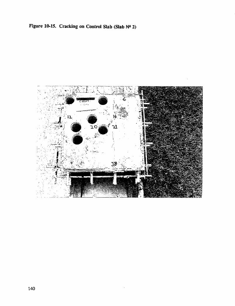
Figure 10-15. Cracking on Control Slab (Slab No 2)
140

After chloride removal treatment, the macroceU current was reduced from an average of 0.40mA to about 0.01 mA or less for all treated slabs. The average macroceU current densitymeasured over the period of 35 to 40 months was about 0.0038 mA/ft 2 (0.038 mA/m 2) of topmat steel for all the treated slabs as compared to 0.1604 mA/_ (1.604 mA/m 2) for theuntreated control slab. There was no significant difference among the treated slabs. Thecorrelation coefficient between cumulative macroceU current and A-hr/ft 2 of chloride removal
treatment was only 0.01, indicating no relationship between these variables. The averagecumulative charge passed for all treated specimens was 0.0156 mA-year/ft 2 (0.156 mA-year/m2), 35 to 40 months after chloride removal treatment. No cracking was observed onany of the treated slabs through the 40-month test period. The cumulative charge passed, asshown on Figure 10-12, imply that it will be a very long time before sufficient charge ispassed to crack the treated slabs.
3LP Corrosion Rate
The 3LP corrosion rate data were collected quarterly on six pre-selected test points, andmonthly on the two most negative points of the six pre-selected test points. The average 3LPcorrosion rates collected are presented in Tables B-1 through B-10 of Appendix B and inFigure 10-16 (quarterly data only).
It was found that the 3LP corrosion rate decreased significantly within two months afterchloride removal treatment for all treated slabs. However, the untreated control slab alsoshowed a similar decrease. Afterward, 3LP corrosion rate only decreased slightly up to 40months after treatment. It was also noticed that for the untreated control slab, the 3LPcorrosion rate was only slightly higher than that for the slabs treated with pH maintenance.These f'mdings contradict the macroceU current findings. It is believed that the 3LP data arenot accurate for the treated slabs, but the reason for this behavior is not fully understood.Additional study is needed in this area.
141

Figure 10-16. Quarterly 3LP Corrosion Rate Data Summary
25.00 ,
20.00
¢_ 15.00
i "j •
m •
w •
10.00 "o,
5.00 ° -. . . " • -
-.|-=.....=- - oI
0.00
0 100 200 300 400 500 600 700 800 900
Days after Chloride Removal
¢ #2 -- o-- #3 -" #4 -- m-- #5 " #10
-- _-- #11 A #12 _ #9 o #7 _#8
142 .

Conclusions
From the above results, the following conclusions can be drawn.
• For the untreated control slab (Slab N_ 2), reinforcing steel corrosion remained activefor a period of about 40 months, even though the rebar imprint chloride contentssignificantly decreased from the initial value. Half-ceU potentials remained verynegative and macrocell current increased with time. Cracking over one of the top matreinforcing steel was first observed when the cumulative charge passed was 0.21 mA-year/ft 2 (2.1 mA-year/m2).
• Chloride removal resulted in a dramatic change in the treated slabs. No significantremigration and redistribution of the residual chloride was observed through 40 monthsafter the chloride removal process, 60 to 300 A-hr/ft 2 (600 to 3000 A-hr/m2). Nocorrosion-induced cracking was observed on any treated slab.
• No large performance differences were discemable for the slabs treated at differentamounts of charge and current density, < 0.6 A/ft2 (6 A/m2).
• After treatment chloride levels around the top rebar imprint were stiU, in mostinstances, above the commonly accepted corrosion threshold.
• The macrocell corrosion process was greatly decreased by the chloride removalprocess. The average macrocell cumulative charge passed for the chloride removalslabs was only 2.4 percent of that for the untreated control during the 35- to 40-monthexposure.
• Half-cell potentials, as taken using a top surface reference electrode, appeared to bemuch more passive when the electrolyte pH was not maintained basic. This isconsidered to be a manifestation of junction potential error.
• 3LP measurements taken on treated slabs do not reflect the passive state of thereinforcing steel. The reasons for this phen6menon are not understood.
143

11
Concurrent Protection
The chloride removal treatment of a concrete structure will move chloride ions away from the
reinforcing steel and halt the corrosion process. Since the chloride is not completely removedfrom the concrete structure, protection against remigration of the chloride to reinifiatecorrosion is obviously desirable. Therefore, sealers or corrosion inhibitors that can deeplypenetrate the concrete and be placed between the reinforcing steel and migrated chloride ionare necessary.
True "corrosion inhibitors" that have actually been used in concrete are relatively few innumber. Calcium nitrite is currently being marketed by W.R. Grace Corporation as acorrosion inhibiting admixture for fresh concrete. Researchers at the Stanford ResearchInstitute (SRI), working under SHRP Project C-102C, have identified an inhibitor,tetraethylphosphonium (TEP) nitrite, which has been claimed to move into hardened concreteunder the influence of an electrical potential difference. Domtar Chemicals Group in Canadais currently marketing a corrosion inhibiting deicer for concrete identified as "TCr'. Thiscorrosion inhibitor is included in deicing salt mixtures and allegedly enters the concrete alongwith the chloride solutions and maintains steel passivity. Other than the SRI work, there havebeen relatively few research investigations conducted to electrochemically move impregnantmaterials into hardened concrete. Pioneering work in this area was conducted by the KansasDepartment of Transportation in the 1970s in conjunction with electrochemical chloride ionremoval experiments.
There is a large body of technical information dealing with sealants for concrete. 35 It seemsobvious, however, that conventional sealants penetrate to relatively shallow depths, less thanl/8-inch (0.3-era), and require a pre-applicafion drying period to achieve even these depths.
This research investigates the electrochemical application of deep sealing agents and corrosioninhibitors to be used as a concurrent protection scheme to prevent future reinforcing steelcorrosion from remigrafion of chloride ions after the chloride removal process. Othermethods of introducing sealers and corrosion inhibitor, i.e., surface applications or admixtures,are not investigated in this research, but are covered in the C-103 research.
145
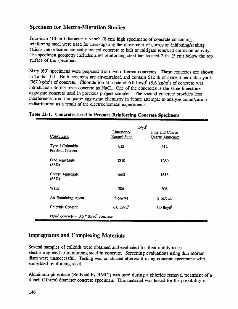
Specimen for Electro-Migration Studies
Four-inch (10-cm) diameter x 3-inch (8-cm) high specimens of concrete containingreinforcing steel were used for investigating the movement of corrosion-inhibiting/sealingcations into electrochemically treated concrete to halt or mitigate renewed corrosion activity.The specimen geometry includes a #4 reinforcing steel bar located 2 in. (5 cm) below the topsurface of the specimen.
Sixty (60) specimens were prepared from two different concretes. These concretes are shown
in Table 11-1. Both concretes are air-entrained and contain 612 lb of cement per cubic yard(367 kg/m 3) of concrete. Chloride ion at a rate of 6.0 lb/yd 3 (3.6 kg/m 3) of concrete wasintroduced into the fresh concrete as NaC1. One of the concretes is the same limestone
aggregate concrete used in previous project samples. The second concrete provides lessinterference from the quartz aggregate chemistry in future attempts to analyze anion/cationredistribution as a result of the electrochemical experiments.
Table 11-1. Concretes Used to Prepare Reinforcing Concrete Specimens
lb/yd3Limestone/ FineandCoarse
Constituent NaturalSand QuartzAggregate
TypeI Columbia 612 612PortlandCement
FineAggregate 1310 1260(SSD)
CoarseAggregate 1662 1613(SSD)
Water 306 306
Air-EntrainingAgent 2 oz/cwt 2 oz/cwt
ChlorideContent 6.0 lb/yd3 6.0 lb/yd3
kg/m3concrete= 0.6 * lb/yd_ concrete
Impregnants and Complexing Materials
Several samples of colloids were obtained and evaluated for their ability to beelectro-migrated to reinforcing steel in concrete. Screening evaluations using thin mortardiscs were unsuccessful. Testing was conducted afterward using concrete specimens withembedded reinforcing steel.
Aluminum phosphate (Refbond by RMCI) was used during a chloride removal treatment of a4-inch (10-cm) diameter concrete specimen. This material was tested for the possibility of
146
complexing the aluminum with the chloride ion to form insoluble chloroaluminatecompounds, rendering the chloride harmless to initiate corrosion at the reinforcing steel.There was also the potential for corrosion-inhibiting activity of the phosphate complexes.Within 4 hours of the beginning of the treatment process, the pores at the surface of theconcrete were plugged, resulting in excessive voltage and system shutdown. Another Zn2+complexing material reacted in the same manner. This same effect was noticed when usingaluminum, zinc, and magnesium as anodes during sacrificial anode testing.
Colloidal silica (Nalcoag 1140 by Nalco) was also tested with unfavorable results. Silicagelled in the electrolyte pond and did not enter the concrete at all.
Two corrosion inhibitors marketed for concrete reinforcing steel, manufactured by CortecCorporation were obtained. However, the manufacturer data indicate these samples, MCI1337 (injection type) and MCI 1608 (overlay additive type), are not to be used in anoxydizing environment.
It appears that electrochemical migration of deep sealing agents is not possible. Either theelectrolyte or the concrete composition itself precipitates the prospective agent at or near thesurface of the concrete.
Electrophoretic Coatings
Discussions were conducted with PPG Industries, Inc., Research and Development Center inAllison Park, Pennsylvania concerning electrophoretic coatings. They felt quite confident thatthey could provide substances small enough to migrate through pores of the size found inconcrete. This process would involve the migration of cationic substances, now the standardin the electrodeposition of coatings, to the reinforcing steel followed by a polymerization step.The substances they have in mind need to withstand the high pH of concrete and also resistcoagulation before the migration to the reinforcing steel is complete.
Low Molecular Weight Materials
Two samples of electrophoretic coating materials were obtained from PPG Industries, Inc.,Research and Development Center in Allison Park, Pennsylvania. The exact composition ofthese low molecular weight polymer samples, WEQ-1900 and WET-5747, was proprietary.They contained 60%-65% by weight solids and dilution to 2%-10% by weight solids wasrecommended. The solution was used as the electrolyte during chloride removal treatment on4-in. (10-era) diameter cylinders with 2-in. (5-cm) thick concrete cover. These cylinders wereoperated to a total charge of 300 A-hr/_ (300 A-hr/m 2) at 0.6 A/ft2 (6 A/m2). The concretespecimens were analyzed for the location of the material by detecting nitrogen, a majorcomponent. Nitrogen was detected only in the top 1/2-inch (1-cm) in excess of that found ina control specimen, indicating only minimal migration of the coating and nothing reaching thereinforcing steel as needed.
147

High Molecular Weight Materials
Three additional samples were obtained from PPG: CR-500, CR-600 and CR-640. Thesehigher molecular weight materials were tested in the same manner as the first set of samples.After several days of operation all materials polymerized at currents less than half of thatdesired and at high voltages, >150 V. These higher molecular weight materials are less stableat a high pH and it is felt that the concrete pH as well as high temperature produced by thehigh resistivity solution promoted premature polymerization. The PPG high molecular weightCR-640 material was retested at a lower solution concentration (5% solids by weight) in anattempt to avoid the premature polymerization obtained with the 36% solids solution.However, polymerization and high voltage occurred after only 4 hours of operation.
Quaternized Monomeric Acrylates
Samples of quaternized monomeric acrylates were obtained from PPG. These materialsrepresent quaternary ammonium salts of the lowest possible molecular weight which can stillbe expected to cure and form a polymer. Their hydrodynamic radius is one-fifth that of thematerials previously tested. According to PPG, the polymerization of these monomeric quats,Concoat-6 (modified methacrylate) and Concoat-9 (acrylate monomer), can be expected tooccur under anaerobic or basic conditions. Hence, polymer formation should occur once themonomers have diffused into the concrete.
Electrolytes for chloride removal were made from these samples in a 50% by volome mixwith deionized water. The starting pH of the solutions were approximately 4. Treatment of6-in. (15-era) diameter concrete cylinder specimens was performed for 300 A-hr/ft 2 (3000 A-hr/mz) of total charge using these electrolytes. To the contrary of previous samples,polymerization in the electrolyte did not occur and system voltage did not increase throughoutthe duration of the treatment. The pH of the electrolyte changed to approximately 7 within aday after treatment started and remained there without any electrolyte pH adjustments for theremainder of the treatment. After shutdown, inspection of the specimen showed severe acidattack of the concrete surface. This was deemed unacceptable.
Corrosion Inhibitors
Electro-Emplacement of TEP �IonCorrosion Inhibitor
As part of the SHRP C-102C Research, SRI International claimed, through their tests TEWnitrite to inhibit corrosion of reinforcing steel in concrete. As part of the SHRP C-102AResearch, ELTECH was to identify and evaluate corrosion inhibitor candidates for concurrentprotection practices in conjunction with electrochemical chloride removal.
The cost of the TEP + corrosion inhibitor in the nitrate form was viewed as too expensive tobe economically feasible in the chloride removal process. TEW in the base chloride form,
148

prior to its conversion to the nitrite form through ion exchange, was alternately tested byELTECH. These tests were performed with the reinforced concrete specimens containing asingle #4 reinforcing steel bar. Chloride removal was performed in limewater at a currentdensity of 0.6 A/ftz (6 A/m 2) of concrete for 300 A-hr/ft 2 (3000 A-hr/m2). Not only does thistreatment regime fit the range of previously determined chloride removal treatment times andduration, but the total amount of charge passed to emplace the corrosion inhibitor, asdetermined by SRI, is satisfied. One specimen was treated without the concurrentemplacement of TEP + as a control. Two specimens were treated with the presence of the SRIrecommended TEP + concentration of 0.05 molar or a total of 0.0077 moles. One of these
specimens used the embedded reinforcing steel bar as the cathode, thus simulating actualpractice. Previous tests show that the chloride removal treatment alone will shift reinforcingsteel static potentials to the non-corroding state after depolarization is complete. Therefore,the other specimen was treated using a supplemental cathode below the reinforcing steel barto migrate the TEP + cation into the vicinity of the reinforcing steel bar without altering thebar through polarization. Before and after treatment half-ceU potential data to date are shownin Table 11-2.
Table 11-2. Half-Cell Potential Data for Specimens Treated with TEP + Inhibitor
Days After Static Potentials, mV vs Cu/CuSO4Treatment #10 #12 #14 #16 #18
TEW conc. control .05M .10M .05M .10M
before -266 -319 -340 -261 -2617 -1130 -1140 -1150 -268 -258
16 -910 -1096 -1120 -197 -20823 -270 -928. -1090 -193 -20342 -240 -273 -287 -190 -20474 -269 -325 -347 -289 -382
These data show depolarization after treatment takes approximately 4 to 6 weeks after acurrent density of 0.6 A/ftz (6 A/m 2) is applied for 300 A-hr/ft 2 (3000 A-hr/m2). This is inline with the 2-ft x 2-ft (60-cm x 60-era) slab results. Specimens #16 and #18 were treatedusing a supplemental cathode to prevent polarization during treatment. Even though the staticpotentials have been shifted in the right direction to indicate a decrease in rebar corrosion,corrosion rate measurements taken at 42 days were 15 to 25 mA/ft2 (7 to 12 nail) of steel,about three times higher than the original rates. It does not appear that simply observingstatic potentials is going to indicate the success of TEW as a corrosion inhibitor. The highconcentration specimens were cut in half during petrographic analysis and mapped forphosphorus to find the location of the TEP +.
149

Petrographic Analyses of TEP + Treated Samples
Specimens 13552-95-14 and 13552-95-18 were subjected to petrographic and SEM/EDSexaminations. The only difference in the two samples was that a supplemental cathode wasused with the 13552-95-18 specimen and not with the other.
Fresh fracture surfaces of the concrete specimens were were used in the SEM/EDSinvestigation. A 20 mm thickness of the wearing surface was subjected to examination aswell as the 10 mm thickness of concrete surrounding the top reinforcing steel bar. Figure11-1 shows the EDS spectrum (1400X) on the 13552-95-14 sample 3 mm below the concretewearing surface. No phosphorus was found at this level. Figure 11-2 shows the EDSspectrum (1400X) in the 13552-95-14 specimen at the top reinforcing steel interface. Nophosphorus was found in the concrete surrounding the reinforcing steel bar. Phosphorus wasdetected in the 13552-95-14 specimen only in the top 0.1 mm thickness of the wearingsurface. No phosphorus was found in any of the concrete at levels below the 0.1 rnm level.
Figure U-1. EDS Spectrum on Quartz Aggregate Concrete for P+
CA
13552-95-14
3 mm below wearing surface
. i
L IPLMG SAL K FE
2.13 4.£I 6.0 8.0 10.OENERGY < KEU )
Figure 11-3 shows the presence of phosphorus (P) in the top 2- to 3-_t thickness of thewearing surface of specimen 13552-95-14. A similar result was obtained for specimen13552-95-18 (i.e., phosphorus only present in the top 0.1 mm thickness of the wearingsurface).
Electro-emplacement of the TEl_ corrosion inhibitor, at least in the chloride form wasunsuccessful as a concurrent protection scheme.
150

Figure U-2. EDS Spectrum At Reinforcing Steel-Concrete Interface for P+
CA
13552-95-14
At rebar interface surface
2 in. below wearing surface
I sx I I
2.e _.e 6._, 8.e _e.eENERCY ,'.KEU)
Figure 11-3. EDS Spectrum At and Near Wearing Surface for P+
SI
13552-95-14
Below wearing surface
2-3u (dots)3 mm (bars)
151
Conclusions
• Colloids, hoped to penetrate deep into the concrete and complex with chloridesremaining in the concrete after chloride removal treatment, only slightly entered theconcrete surface.
• Electrophoretic coatings, expected to be migrated near the reinforcing steel wherepolymerization would result in deep sealing, actuany polymerized at the surface of theconcrete.
• Possible corrosion inhibitors also showed only slight penetration during electro-emplacement attempts.
• Based on the experiments performed in this research, application of concurrentprotection through electrochemical means does not appear to be possible.
152

12
Equipment and Procedure Development
Information gained from laboratory studies was used to develop chloride removal processprocedures. Specific equipment was identified in order to carry out these procedures in fieldvalidation trials. Different field structure configurations also required different equipment.Conceptual designs of various field trial configurations were developed, and, based on theseconcepts, equipment and procedures were further developed.
Design Concepts for Field Trials
Conceptual layouts for three different field trial configurations were developed. These designconcepts are for: (1) Deck (Figure 12-1), (2) Land Column (Figure 12-2), and (3) MarineColumn (Figure 12-3). These are the three most common concrete bridge elements thatwould be subjected to chloride removal treatments.
153

Figure 12-1. Conceptual Layout of Deck Configuration
Water _ +
Reservoir Rectifier
[Pump _orValve Anode
I /
ReinforcingDeck Steel
154
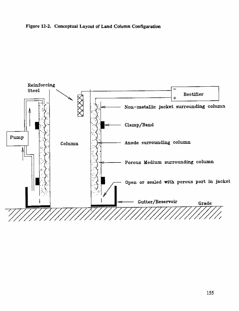
Figure 12o2. Conceptual Layout of Land Column Configuration
155

Figure 12-3. Conceptual Layout of Marine Column Configuration
Reinforcing
Steel __ _ !.l:i ]+RectifierI
IiI,::, . .... , ° ° , • " ° " ..... . , • ° ...... . ...
• , , , ." ,, • • o., .... . • " "
i "" High Tide
..." "...... ......... . .Low Tide• . • . • . . , . .... . • •• . , ." . , . . •
l _ [__ Open or sealed with porous port in jacket
156

Deck Design
The bridge deck treatment concept was to construct a wooden perimeter dam as was done byBattelle in the 1970s. The catalyzed titanium inert anode mesh would be embedded in a sandbackfill over the treatment area. Most decks slope from the centerline to the edge whichwould enable electrolyte to be pumped from a reservoir electrolyte distribution system. Theelectrolyte would move through the sand and over the anode by gravity to a gutter collectionnetwork at the edge of the deck, and channeled back to the reservoir.
An alternate deck concept was very similar to the method used to treat the 2-ft x 2-ft (60-cmx 60-cm) laboratory slabs. A dam would be built around the perimeter of the treatment areato contain the electrolyte. Sand would not be used to allow for convective electrolyte mixing.This would obviously be the less expensive, less complex system. Consideration was givento a temporary riding surface since treatment times of at least three weeks are expected. Itwas eventually realized that the expense would be prohibitive.
Column Design
The column treatment concept utilizes an anode-blanket assembly that is wrapped around thecolumn and pinned, banded, or otherwise held in place during the treatment. For a columnlocated on land, electrolyte would be contained in a reservoir on the ground. The electrolytewould be pumped to the top of the system, flow by gravity over the anode, and return to thereservoir. The marine column concept is similar but has the advantage of constant freshseawater electrolyte feed and no reservoir.
Anode Blanket Assembly
Development of the anode-blanket assembly was the major challenge with the column designconcepts. The design had three components: the anode mesh, an outer blanket, and an innerblanket. The anode selected by laboratory testing, was ELGARD 300 titanium mesh withEC-100 coating. The selection of the blanket material(s) was based on its physical andchemical properties. A variety of blanket materials for the assembly, including cellulose,polyurethane, and open-cell foam rubber were evaluated.
The blanket characteristics examined were:
Physical PropertiesNon-metallic materialSaturation rateVertical flow rateThickness
WeightShear strength
157
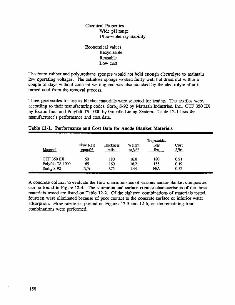
Chemical PropertiesWide pH rangeUltra-violet ray stability
Economical values
RecycleableReusableLow cost
The foam rubber and polyurethane sponges would not hold enough electrolyte to maintainlow operating voltages. The cellulose sponge worked fairly well but dried out within acouple of days without constant wetting and was also attacked by the electrolyte after itturned acid from the removal process.
Three geotextiles for use as blanket materials were selected for testing. The textiles were,according to their manufacturing codes, Sorbx S-92 by Matarah Industries, Inc., GTF 350 EXby Exxon Inc., and Polyfelt TS-1000 by Grundle Lining System. Table 12-1 lists themanufacturer's performance and cost data.
Table 12-1. Performance and Cost Data for Anode Blanket Materials
TrapezoidalHow Rate Thickness Weight Tear Cost
Material gpm/fta mils oz/yd2 lbs $/fta
GTF 350 EX 50 180 16.0 180 0.21Polyfelt TS-1000 65 160 16.2 155 0.19Sorbx S-92 N/A 375 1.44 N/A 0.52
A concrete column to evaluate the flow characteristics of various anode-blanket compositescan be found in Figure 12-4. The saturation and surface contact characteristics of the threematerials tested are listed on Table 12-2. Of the eighteen combinations of materials tested,fourteen were eliminated because of poor contact to the concrete surface or inferior wateradsorption. Flow rate tests, plotted on Figures 12-5 and 12-6, on the remaining fourcombinations were performed.
158

Table 12-2. Percent Surface Contact of Anode Blanket Materials
Percent Saturationafter 4 min. of Percent Concrete Percent Surface
Inner Blanket 0.25 gpm feeding Surface Saturation Contact
GTF 350 EX 100 100 75
Polyfelt TS-1000 30 60 30Sorb x S-92 100 100 100
Figure 12-4. Flow Test Setup for Anode Blanket Evaluations
Pressure Gauge
Trouh?-oo o-2
Soaker _ o_ o n-_ Geotex%ile
Reinforcing _ " - ' .._ "" '4'Steel "'-'. ." i ....:.
_...... .o...: :.. _ '_• 4 .° 4"_" " "
Concrete . . . .. _a.'.. 4'
Column ----'-' "--_' "" ' " ""
3' _ ...: " ..'_. _': w_•". "4. . . . _ /14, High . .. . FastenersDiameter ., _... '._ ._."_ . 4"" 4'
" _. .'. ". • l_• .. "4'..4 4": .,_: , -'"
Support ..- . _. L* _ _
-- -- -- rAssembly
Trough _ _ J Inner Blanket -- "
159

Figure 12-5. Flow Rate Tests With Polyfelt TS-1000 Outer Blanket
S / " / /" I
0.25 gpm ." , / /// IPolyfelf . / . _/ /
,/ "-- - ,,_--,2"- _, _- - ;,_ - -
5
/ /"4 ............ I_'- ---
/ J /
"_ / " / / " "" -_ -/ "//_E]/'- -3 ............... _ - %- - -p" ............L / / .• ,'/
/-4-- • / •
2 ........ • -7,0- - - _0 ..... ,'_- ................
/ •
1 .... =_'- -_ -=O-% - - -._ ................
// -°
0 5 10 15 20 25Time (minutes)
P - Polyfelf1"3-1000Composite: P-A-E-S P-A-S--S P-A-E-E P-A--S-E P-A-P-P
Temperature: B0OF 67OF 69OF 80OF 690F A - Anode,Inert[3 -_-- -O - -<>-- --I-.
E - Exxon GTF 350 EX
S - Sorb x S-92
160

Figure 12-6. Flow Rate Tests With GTF 350 EX Outer Blanket
6
0.25 gpm J /,z-/
GTF 350 EX /,_/'/
......... --_,_....../d-s .................... LA---,,,
i,'-/ /
,j./ ,-4 ................. A,, _,'- - - _ .......
_ J
? ,,:/ .g ,'/ /
h" "--- /J
o ..... _.._ ..............r_ 3 ................ "_ -
0 1
_: 2 ........ ._,__.;..4.................
•I f • t
.j<;>"
0 5 10 15 20 25Time (minutes)
A - Anode, InertComposite: E-A-E-E E-A-S-E E-A-S-S E-A-E-S
Temperature: 80°F 68OF 79OF 70OF E - ExxonGTF350 EXn -,_- -O - -O-
S - Sorbx S-92
161

A decision matrix was constructed from the top four combinations, and is shown in Table12-3.
Table 12-3. Decision Matrix for Anode Blanket Materials
Water Inner Vertical Outer Sum
Retention Surface Flow Tear Assembly of Average PriorityAssembly Time Contact Rate Strength Reuse Cost %s Percent Listing
P-A-E+S 100% 100% 78% 100% 75% 100% 553% 93% I
4.17 rain. 0A0 gpm 155 lbs $.92/ft_
P-A-S+S 90% 100% 78% 100% 50% 75% 493% 82% III
3.75 rain. 0.40 gpm 155 lbs $1.23/ft2
E-A-S+S 95% 100% 62% 73% 50% 74% 454% 76% IV
3.98 min. 0.50 gpm 110 lbs $1.25/_
E-A-E+S 86% 100% 100% 73% 75% 98% 532% 89% II3.57 min. 0.31 gpm 110 lbs $.94/ft2
P = Polyfelt TS-1000A = Anode ELGARD 300 titanium meshE = GTF 350 EX
S = Sorbx S-92 (not reusable)
The anode-blanket assembly selected for the field trims was:
Outer Blanket - Polyfelt TS-1000
Anode - ELGARD 300 Mesh with EC-100 Coating
Inner Blanket - GTF 350 EX
This blanket will be pre-assembled and is expected to be reusable. In addition to the anode
blanket, an inner layer (between the assembly and concrete surface) would be Sorbx S-92 that
is not reusable. To reduce evaporation, a plastic wrap covering the complete assembly will
be necessary. The actual size of the pre-assembly will be based on the dimensions of thestructures to be treated.
Prior to the identification of Polyfelt TS-1000 as a strong outer blanket material, a method to
attach a unitized chloride removal system (anode, electrolyte holding medium, support frame)
to a concrete structure was investigated. Adhesive samples from Avery International, Fasson
Industrial Division in PainesviUe, Ohio were evaluated. These adhesive samples, only 5 rail
thick, were applied between the anode assembly and concrete in strips, to allow for ionic
movement since the adhesive is not ionically conductive. Attempts were unsuccessful due totheir lack of ability to withstand the moisture and pH extremes from the electrolyte.
162

Blanket Testing Under Electrochemical Conditions
A 1-ft (30-cm) wide x 3-ft (90-cm) high vertical concrete test column was prepared to test theanode-blanket assembly while removal currents were being passed. This test system wasfitted with a continuous wetting system where electrolyte is pumped to the top of the columnand distributed along the top. The electrolyte then returns to the sump by gravity through theanode blanket. This eliminates daily wetting of this medium.
The system was operated for 300 A-hr/ft 2 (3000 A-hr/m 2) at 0.6 A-hr/ft 2 (6 A/m 2) withsodium borate electrolyte. Post-treatment inspection of the anode blanket materials showedno problems. The surface of the concrete was only slightly etched, and it appeared that thissystem will be satisfactory for field trials.
Other chloride removal treatment component equipment (i.e., pumpsize, water requirements,electrolyte reservoir, rectifier) are dependent upon the treatment areas.
163

13
Major Conclusions
• Electrochemical chloride removal is a feasible technique for the rehabilitation ofconcrete structures suffering from chloride induced corrosion. The term "chlorideremoval" is not fully descriptive of the process since the beneficial effect is alsolargely due to a large increase in alkalinity at the surface of the steel. It is bestapplied to structures which are chloride contaminated and undergoing active corrosion,but which have not undergone significant deterioration.
• Only a minor percentage of the total applied current contributes to the electromigrationof chloride ion. This percentage is independent of current density, voltage gradient,and temperature (below 40°C). It is, however, directly dependent on chlorideconcentration. The current efficiency for the removal of chloride ion is relativelyhigh, typically 30-40%, near the beginning of the process, but will decrease to verylow values near the end of treatment. The overall current efficiency for chlorideremoval for the entire treatment is typically 10-20%.
• The total charge required for an effective treatment is typically 150 A-hr/ft 2 (1500 A-hr/m 2) of concrete surface area. Current density during treatment may range from 100to 500 mA/ft 2 (1 to 5 A/m 2) of concrete, depending on the resistivity of the concrete.It is recommended to maintain system voltage below 50V for safety reasons. Currentdensities higher than 500 mA/fd (5 A/m 2) of concrete may result in damage to theconcrete and the structure. This treatment regime will typically result in treatmenttimes of 2 to 8 weeks.
• The total chloride removed from the structure by the treatment described above willtypically be 40-50% of that originally present. The majority of chloride whichremains will be in regions where the flow of current is lowest, such as between andbehind reinforcing bars. Following treatment, the concentration of chloride within ahalf inch (1 era) of the steel can be expected to be below 1 lb/yd 3 (0.6 kg/m 3) ofconcrete (0.16 % by weight of cement).
165

• The best indicator of corrosion rate following a chloride removal treatment conductedon test slabs was found to be macrocell corrosion current (current flowing between topand bottom mats of reinforcing steel). Macrocell corrosion current dropped from anaverage of 0.105 mA/ft 2 (1.05 mA/m _) of steel before treatment to 0.002 mA/ft 2 (0.02mA/m 2) a few days after treatment. Nine test yard slabs show almost no tendency toreturn to corrosive conditions three and one half years after treatment. Over thisperiod of time a control slab, which received no treatment, accumulated 0.685 mA-yr/ft2 (6.85 mA-yr/m 2) of macrocell current charge, and cracked at 0.21 mA-yr/ft 2 (2.1mA-yr/m2). The nine treated slabs have accumulated only 0.015 mA-yr/ft 2 (0.15 mA-yr/m 2) of macrocell current charge, and none exhibit any cracking.
• Half-cell potentials taken on slabs prior to treatment averaged -417 mV vs acopper/copper sulfate (CSE) reference electrode, indicating a high probability of activecorrosion. Four months after chloSde removal treatment, however, potentials hadimproved to an average of -271 mV vs CSE, 98% were more positive than -350 mV,indicating a dramatic reduction in steel corrosion. Slabs which were treated with anacidic electrolyte exhibited artificially positive half-cell potentials when measured fromthe top of the concrete slab. A significant result of this work was a betterunderstanding of this error in measurement, which is due to junction potentials set upas a result of differences in ionic concentrations. Junction potential error can exceed200 mV in some cases.
• Linear polarization resistance data taken on treated slabs was inconclusive. It appearsthat this technique is not appropriate for the measurement of corrosion rate of steelsubjected to a chloride removal process. The reason for this observation is not known.
• Testing of notched specimens revealed no effect on the fracture load strength ofconventional reinforcing steel under any conditions of electrochemical chlorideremoval. Following these results, further testing of smooth specimens did reveal ashort-term loss in ductility within the range of current density appropriate for chlorideremoval. After reviewing the available data, it was concluded that this modest loss ofductility will not create any significant problems or adversely affect the useful life ofconcrete structures.
• Concrete-rebar bond strength was evaluated for treated specimens by measuringultimate bond stress (maximum load just before failure), bond stress at 0.01 inchloaded-end slip, and bond stress at 0.001 inch free-end slip. Ultimate bond stress wasnot affected by any treatment process, up to the maximum current density of 5 A/ft 2(50 A/m 2) and charge of 200 A-hr/ft 2 (2000 A-hr/m 2) of steel. Loaded-end slip, whichis probably the most important parameter, was reduced about 40% for the specimensubjected to both the highest current and charge, but not for either one appliedindependently. Free-end slip, considered less important, was reduced significantly forspecimens subjected to either the highest current density or the highest charge. Thesereductions are reported relative to salt-contaminated control specimens, which had amuch higher bond strength than specimens prepared without salt. In summary, thechloride removal process as recommended in this report, less than 500 mA/ft2 (5 A/m s)and about 150 A-hr/ft 2 (1500 A-hr/m2), is expected to have little or no effect on rebar
166

bond strength. In view of these results, higher current densities and higher chargesshould not be used.
• No cracking, acid attack or change in compressive strength was recorded as a result ofthe chloride treatment process recommended in this report. Severe cracking,delarnination and softening of the concrete was noted for slabs subjected to highcurrent density, 2 A/ft2 (20 A/m2), and high charge, 500 A-hr/ft 2 (5000 A-hr/m2).Again, current densities and charges above those recommended in this report shouldnot be used.
• Petrographic examination, SEM/EDS and porosity analysis show no significant adverseeffects as a result of the chloride removal process conducted as recommended in thisreport. Analyses of slabs treated at a current density of 2 A/ft2 (20 A/m 2) and acharge of 500 A-hr/ft _ (5000 A-hr/m 2) show a damp hygroscopic layer around the topmat of reinforcing steel. SEM/EDS analysis showed this layer to be extremely high insodium, potassium and sulfur, and petrographic examination revealed a softening ofboth cement paste and aggregates in this region. The porosity of the cement paste wassignificantly higher in the 1- to 10-Ix pore diameter range. This confirms, togetherwith the concrete rebar bond strength studies and visual observation of cracks, thatcun'ent densities above 500 mA/ft 2 (5 A/m 2) and very high values of total chargeshould not be used.
• The evolution of chlorine gas can be avoided by maintaining pH greater than 7. Thisis best accomplished by using a captive electrolyte of sodium borate. Other techniquesdesigned to prevent the evolution of chlorine gas, including the use of anion exchangeresin and special anode formulations and treatments, were unsuccessful.
• The chloride removal process can hasten the onset or increase the severity of alkali-silica reactivity in concretes containing aggregates which are prone to ASR. Thisphenomenon can be mitigated by the use of a lithium borate electrolyte. Although thiswork has conf'mued the effectiveness of lithium ion in this regard, additional work isneeded to optimize its use.
• Electromigration of species designed to seal the concrete following chloride removalwas unsuccessful. Colloids, hoped to penetrate deep within the concrete, only slightlyentered the concrete surface. Electrophoretic coatings, expected to migrate near thereinforcing steel followed by polymerization, polymerized at the surface of theconcrete.
• The design concept developed as a result of this work consisted of a reusableanode/blanket composite which was strapped or otherwise held onto the concretesurface during the treatment process. The anode of choice was a catalyzed titaniummesh designed to last several treatments. The electrolyte was a captive sodium orlithium borate buffer which was continuously circulated. Other design concepts, suchas an electrolyte pond or an electrolyte of sprayed cellulose fiber, are also viableconcepts.
167

Appendix A
Pre-Treatment Data of Laboratory Slabs
169

Figure A-1. Pre-Treatment Data for Slab Na 1
Sta_c Pot. 3LP Static Po_ 3LPLoc. vs Cu/CuSO_ mA/f_ _ ZLC_U/_C_U_mA/f_
1 -.353 21 -.4332 -.378 22 -.3823 -.353 23 -.3984 -.384 17.0 24 -.4025 -.373 25 -.4276 -.375 26 -.4227 -.358 27 -.412 15.98 -.389 28 -.3939 -.395 29 -.388
10 -.409 30 -.41_ %011 -.396 31 -.37812 -.389 32 -.39113 -.389 33 -.36514 -.401 15.5 34 -.41215 -.421 35 -.40016 -.427 13.3 36 -.39617 -.394 37 -.39018 -.401 38 -.38819 -.406 39 -.37520 -.428 16.9 40 -.385
170

Pre-Treatment Data for Slab N" 2
! ! !i! i! i! !i
II It
II II II '1
!i i! !! ii
II II II II
I I I I ,I i I I I
II II
========================================
MacroceU Current = 0.5AC Resistance, 25°C = 21 ohms
Sta_c Pot. 3LP Sta_c Pot. 3LPLoc. _F_.Cu!CuS04 mA/f_ Loc..W Cu/C_S0_ mA!f@
1 -,333 21 -.448 43.92 -,349 22 -.4033 -.390 23 -.4104 -.407 24 -.4045 -.417 25 -.4046 -.392 25.2 26 -.4227 -.419 27 -.4338 -.400 28 -.4349 -.391 29 -.40910 -.381 30 -.41011 -.380 31 -.39712 -.404 9.6 32 -.40713 -.400 33 -.38514 -.417 34 -.39915 -.445 35 -.40116 -.440 20.8 36 -.40917 -.416 37 -.41618 -,398 38 -.404 11.819 -.416 39 -.40920 -.416 36.9 40 -.416
171
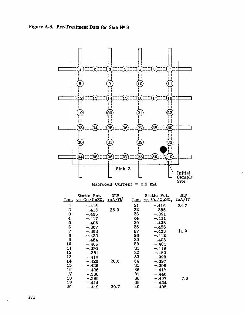
Figure A-3. Pre-Treatment Data for Slab N° 3
n n nI I ! I
! I _ L I 1 l II I t I I I I t
II ......
:::::::::::::::::::::::::::::::::::!i [[ ii [1
1 1 | i
_' 11 II ,,| a
I l | I I I I
:::
SiteMacrocell Current = 0.5 mA
Sta_c Pot. 3LP Sta_c Pot. 3LPLoc. vs Cu/CuS0 ! mA/f_ Loe. vs Cu/CuS0_ mA/f_
1 -.416 21 -.416 24.72 -.418 26.0 22 -.3883 -.435 23 -.3914 -.417 24 -.4115 -.405 25 -.4386 -.367 26 -.4567 -.393 27 -.433 11.98 -.422 28 -.4129 -.434 29 -.403I0 -.405 30 -._01II -.395 31 -.41912 -.381 32 -.46013 -.416 33 -.39814 -.420 20.6 34 -.39715 -.436 35 -.39B16 -.426 36 -.41717 -.380 37 -.44018 -.398 38 -.407 7.819 -.414 39 -.42420 -.419 20.7 40 -.405
172t

Pre-Treatment Data for Slab N_ 4
I C | !
ii il ii i!
| I I l I I
@ ® @ @=====================================--_
[i [[ ii [
| I I I I II I I I I l
===================================--SampleSite
_[aerocellCurrent = 0.6 mA
Sta_c Pot. 3LP Sta_c Pot. 3LPLoe, vs Cu/CuS0_ mA/f_ LOC. vs Cu/CuS0_ mA/f_
1 -.410 21 -.442 22.72 -.407 22 -.4053 -.386 23 -.4204 -.425 24 -.4305 -.433 25 -.4676 -.407 26 -.451 41.27 -.393 27 -.4688 -.410 28 -.4239 -.401 29 -.415I0 -.397 BO -.41911 -.396 31 -.429 24.212 -.402 32 -.45913 -.403 33 -.42814 -.413 13.2 34 -.40715 -.441 35 -.42416 -.411 12.9 36 -.43017 -.420 37 -.44018 -.400 38 -.431 10.019 -.412 39 -.43620 -.467 40 -.428
173

Figure A-5. Pre-Treatment Data for Slab No 5
I II I I I L I
I III '' II
II II II II
1 I t 1 I I I I
II II i, III I
1I I I l I I
/ i ii ii Qi!=================================:-SampleSite
_iacrocell Current = 0.3 mA
Static Pot. 3LP Static Pot. 3LPLoc. VS Cu/CuS0_ mA/f_ Loc. VS Cu/CuS0_ mA/f_
1 -.410 21 -.4092 -.439 21.1 22 -.3983 -,416 23 -.4074 -.405 24 -.4125 -.387 25 -.421 18.16 -.358 26 -.4107 -.364 27 -,3998 -.430 28 -.3899 -.441 29 -.398
10 -,414 30 -.428 9.111 -.376 31 -.40112 -.405 32 -.414 14.313 -.429 33 -.39414 -.448 16.4 34 -.37615 -.432 35 -.39316 -.420 17.7 36 -.38217 -.377 37 -.38618 -.382 38 -.38319 -.411 39 -.37920 -.423 40 -.359
174

Figure A-6. Pre-Treatment Data for Slab Na 6
:_ :: ii ilt tt t I _ t t
I t I I
'' II
il ii ii :_
II II II
=======================================
=================================
Sa_mpleSite
Macrocell Current = 0.7 mA
Sta_c Pot. 3LP Sta_c Pot. 3LPLo_ _ _ Loo._ mA/fe
i -.368 21 -.4372 -.321 22 -.3703 -.332 23 -.3754 -.363 24 -.3755 -.397 25 -.396 6.56 -.379 26 -.3767 -.365 27 -.4288 -.380 28 -.395 17.99 -.380 8.8 29 -.380
10 -.413 30 -.36211 -.341 31 -.38712 -.393 6.4 32 -.431 8.513 -.364 33 -.36214 -.403 34 -.34215 -.420 35 -.363i6 -.434 7.4 36 -.38517 -.380 37 -.36918 -.377 38 -.41119 -.358 39 -.39420 -.398 40 -.385
175

Figure A-7. Pre-Treatment Data for Slab Ng 7
i il ii i
::::::::::::::::::::::::::::::::::::
,,il IS ii 1
i ii i! W:,
==================================:
Site_faerocell Current = 0.5 mh
Static Pot. 3LP Static Pot. 3LPLoe. vs Cu/CttSO¢ mA/ft2 Loc. vs Cu/CuSO¢ _aA/ft2I -.398 21 -.40B2 -.360 22 -.424 10.93 -.410 23 -.4224 -.379 24 -.4285 -.365 25 -.445 18.36 -.302 26 -.4197 -.350 27 -.418 II.38 -.393 28 -.3929 -.410 29 -.391
10 -.370 30 -.452 10.1ii -.331 31 -.43112 -.450 8.5 32 -.39013 -.415 33 -.37514 -.427 34 -.43215 -.407 35 -.42516 -.387 36 -.43117 -.381 37 -.429 I1.718 -.389 38 -.40619 -.415 39 -.38320 -.436 40 -.372
176

Pre-Treatment Data for Slab Na 8
i! ii !i ii
® @ @ ®I I t I I 1I I I I I
'' II ' I
SampleSite
Macrocell Current = 0.3 mA
Sta_c Pot. 3LP Static Pot. 3LPLoc. vs Cu/CuSO_ mA/f_ _oc. _ mA/f_
1 -.354 21 -.413 16.32 -.366 22 -.3883 -.373 23 -.3674 -.373 24 -.3835 -.376 6.4 25 -.3996 -.370 26 -.3987 -.376 27 -.4048 -.361 28 -.3999 -.380 29 -.394 6.6
tO -.380 30 -.36711 -.372 31 -.37912 -.374 32 -.36213 -.382 33 -.39314 -.403 34 -.36015 -.393 35 -.36916 -.397 36 -.37017 -.390 37 -.37018 -.384 6.6 38 -.37619 -.377 39 -.384 13.320 -.415 18.4 40 -.389
177

Figure A-9. Pre-Treatment Data for Slab No 9
N ni! i! il il
! I L I I ! I II !,, II '',° III I I I ! ! I I
=======================================ii [[ !i ii
II II II III I I I I I I I
======================================
® @ @InitialSampleSite
_facroeellCurrent -- 0.4 niA
Sta_e Pot. 3LP Static Pot. 3LPLoc. vs Cu/CuS04 mA/f_ LoC. vs Cu/CuS0_ mA/f_1 -.397 21 -.408 14.12 -.389 12.5 22 -.3773 -.376 23 -.4114 -.385 24 -.4035 -.388 25 -.406 8.96 -.377 26 -.3997 -.370 27 -.3968 -.412 28 -.3749 -.395 29 -.370
10 -.405 30 -.39311 -.380 31 -.40712 -.413 32 -.37513 -.400 33 -.37314 -.414 11.7 34 -.39215 -.410 35 -.39116 -.408 10.9 36 -.39417 -.393 37 -.38218 -.376 38 -.37619 -.398 39 -.37220 -.418 10.8 40 -.386
178

Pre-Treatment Data for Slab I_i_ 10
II II II L.'
i! i! !i !i
'' II| I
II II II
r-----.-.-_--:z_--::_'--_--:-_.:--_]]__
® @ @ @/
r--_--I I ........ I I ........ I I .....
SampleSite
Macrocell Current = 0.3 mA
Static Pot. 3LP Sta_c Pot. 3LPLoc. VS Cu/CuS0_ mA/f_ LOC. Vs Cu/CuS0_ mA/f_
1 -.420 21 -.460 41.52 -.421 22 -.4043 -.416 23 -.4124 -.410 26.2 24 -.4135 -.393 25 -.415 10.06 -.391 26 -.4177 -.380 27 -.4158 -.433 17.5 28 -.4119 -.433 29 -.402 6.5
10 -.402 30 -.40411 -.391 31 -.40212 -.432 32 -.40013 -.435 33 -.40114 -.450 20.7 34 -.39615 -.429 35 -.39616 -.415 36 -.39517 -.405 37 -.39218 -.395 38 -.36919 -.426 39 -.39020 -.430 40 -.383
179

Figure A-11. Pre-Treatment Data for Slab No ]11
H n ,!_-:::::::::::::::::::::::::::::::::::::
ii i! ii !!
=======================================!! !i i! !! --
=.::::::::::::::::::::::::::::::::::::.... _[::,_
I t
ii U SampleSite
Hacrocell Current = 0.5 mA
Sta_c Pot. 3LP Sta_c Pot. 3LPLoc. vs Cu/CuS0_ mA/f_ Loc. Vs Cu/CuS0_ mA/f_
1 -.416 21 -.4692 -.411 22 -.4253 -.413 23 -.4254 -.431 10.3 24 -.4265 -.431 25 -.440 8.36 -.422 26 -.4477 -.411 27 -.4628 -.414 28 -.445g -.429 2g -.423
10 -.452 30 -.402II -.411 31 -.42212 -.436 32 -.459 12.013 -.431 33 -.41214 -.442 8.5 34 -.39815 -.452 35 -.39816 -.473 10.4 36 -.41217 -.444 37 -.42016 -.425 38 -.43919 -.448 9.1 39 -.42820 -.433 40 -.412
180

Pre-Treatment Data for Slab N Q 12
II II
===================================Site
Macrocell Current = 0.3 n_A
Static Pot. 3LP Static Pot. 3LP
Loc. vs Cu/CuS0_ mA/f_ Lo_. vs Cu/CuSO_ mA/f_
1 -.418 21 -.4282 -.425 22 -.4163 -.437 9.2 23 -.443 6.84 -.440 24 -.4355 -.443 25 -.4326 -.430 26 -.4337 -.415 27 -.4168 -.431 28 -.412 16.99 -.444 29 -.404
10 -.446 13.0 30 -.439ii -.416 31 -.4_212 -.435 4.3 32 L.41013 -.439 33 -.40314 -.442 34 -.426i5 -.445 35 -.42516 -.428 36 -.40717 -.427 37 -.41318 -.414 38 -.40319 -.436 39 -.40220 -.443 12.4 40 -.396
181

Appendix B
Post-Treatment Corrosion Data of Laboratory Slabs
183

Table B-1. Post-Treatment Corrosion Data for Slab Na 2
184

Table B-2. P0st-Treatment Corrosion Data for Slab N2 3
_ I_ _ _l_J_ _ _-_ _ __ _ _'_ _ _r'¸_
!
i_ [._ 0 i J _'
_ _"_ , , , , , _ , , , , ...... : : i j
_ > o ooo o o o oiolo o o o o c _ _ _ _ _:_ _ _ _ _ _ O:_ _ _ _ -_
_0_ 0 0 O0 d o o od dd old oc_ ddl_ ¢_clo cld oi_ od cic_ cic_ c_
_ ° e,-_o o _ o oo o o _ o o _ _._7 0 '_§
o_ _ _:_
_ __ ' i_.J
,,, !i __ __-_r-., _ _ _ _ _ _0 _ .._ -,.__ . _ _, , _ _ _. __
-,_-_ _< _-o _'-_o.-. o _...- s _ _o _o._ _°-_°_s_o§__ _z
185

Table B-3. Post-Treatment Corrosion Data for Slab Na 4
186

Table B-4. Post-Treatment Corrosion Data for Slab No 5
187

Table B-5. Post-Treatment Corrosion Data for Slab N° 10
188

Table B-6. Post-Treatment Corrosion Data for Slab No 11
189

Table B-7. Post-Treatment Corrosion Data for Slab Na 12
190

Table B-8. Post-Treatment Corrosion Data for Slab Na 9
191

Table B-9. Post-Treatment Corrosion Data for Slab Na 7
" _ .
• " ' " ' o,-q 66666 _
....... ol;
i °°°°°°° ::_
- o_
_o _
"7 , "- " V , "6_'_
0 l _ 8 g _
--_ _ ^O-
_,,,'_ __-_-__ ___ ! ____.__
Z l _ _ _ I 0 _ _ _ _ _ _ _ _
192

Table B-10. Post-Treatment Corrosion Data for Slab N_ 8
193

Table B-11. Comparison of Potential Dam: Surface vs Bottom of Holes on 4-1-92
I I I "n"a"mVO+"ak'°a'I ISlab # Location Top of Slabs J Bottom of Holes Difference
2 11 -544 -475 - 6922 -527 -459 - 6827 -519 -443 - 7640 -520 -459 - 61
AVERAGE -528 -459 - 69
3 7 -372 -303 - 6919 -320 -259 - 6126 -325 -I 90 -I 3530 -366 -232 -I 34
AVERAGE -346 -246 -100
4 30 -258 -23635 -285 -193 - 9239 -296 -220 - 76
40 -320 -247 - 73AVERAGE -290 -224 - 66
5 21 -290 -224 - 66
25 -313 -237 - 7628 -284 -257 - 2732 -305 -253 - 52
AVERAGE -298 -243 - 55
10 I -222 -166 - 56
3 -223 -167 - 5625 -281 -158 -123
31 -219 -156 - 63AVERAGE -236 -162 - 76
11 19 -220 -165 - 5520 -243 -165 - 7825 -252 -I 52 -I 0031 -228 -157 - 71
AVERAGE -236 -160 - 76
12 10 -227 -166 - 6111 -219 -170 - 4927 -226 -195 - 3134 -215 -185 - 30
AVERAGE -222 -179 - 43
7 8 99 - 70 1699 86 - 75 16115 106 - 67 173
30 99 - 70 169AVERAGE 98 - 71 168
8 2 -150 -104 - 463 -145 -106 - 39
4 -136 - 31 -1055 -138 - 90 - 48
AVERAGE -142 - 83 - 60
9 4 - 14 30 -4416 - 80 - 94 14
20 14 -102 11621 - 15 - 89 74
AVERAGE - 24 - 64 40
194

Table B.12. Comparison of Potential Data: Surface vs Bottom of Holes on 6-25.92
I I P°tentlal (mV CSE)Taken at: iSlab # Location lop of Slabs I Bottom of Holes Difference
2 6 -530 -445 - 857 -515 .474 - 418 -457 .401 - 5632 ..522 -493 - 29
AVERAGE -506 -453 - 53
3 7 -355 -314 - 4111 -331 -288 - 4330 -275 -269 634 -333 -270 - 63
AVERAGE -324 -285 - 38
4 24 -326 -221 - 10531 -293 -208 - 85
39 -294 -252 - 4240 -320 -296 - 24
AVERAGE -308 -244 - 64
5 25 -298 -232 - 6632 -287 -239 - 4833 -293 -238 - 5540 -297 -231 - 66
AVERAGE -294 -235 - 59
10 2 -255 -153 -10219 -241 -186 - 55
23 -303 - 188 -11525 -219 -183 - 36
AVERAGE -255 -178 - 77
11 11 -222 -165 - 5713 -211 -170 - 4120 -259 -173 - 8625 -245 -173 - 72
AVERAGE -234 -170 - 64
12 1 -256 -186 -3 -257 -180 - 775 -228 -173 - 5523 -238 -172 - 66
AVERAGE -245 -178 - 67
7 3 - 18 - 5 - 135 5 3 827 11 5 1629 4 4 8
AVERAGE 1 4 5
8 2 -131 - 74 - 57
3 -134 - 86 -
6 -197 -103 - 94
7 -216 -110 -106AVERAGE -170 - 93 - 76
9 3 41 -I I0 151
16 - 85 -106 2118 62 -101 16321 -44 -94 50
AVERAGE 7 -103 96
195

Table B-13. Comparison of Potential Data: Surface vs Bottom of Holes on 9-14-92
J P°tenflal (mV CSE)Taken at: 1 ISlob # Location Top of Slobs I Bottomof Holes Difference
2 7 -520 -448 - 7219 -429 -369 - 6022 -523 -449 - 7431 -473 -375 - 98
AVERAGE .486 -410 - 76
3 4 -288 -199 - 8919 -334 -230 -10422 -337 -215 -122
38 -,346 -283 - 63AVERAGE -326 -232 - 95
4 8 -315 -171 -14411 -220 -I 11 -I 0917 -271 -123 -14835 -351 -205 -146
AVERAGE -289 -153 -137
5 7 -193 -158 - 3521 -206 -176 - 3034 -226 -166 - 6035 -225 -205 - 20
AVERAGE -213 -176 - 36
10 12 -272 -208 - 6418 -281 -197 - 84
28 -250 -206 - 4433 -293 -206 - 87
AVERAGE -274 -204 - 70_111 i_)li_till_ll[l_llI_lll[_!_.llI_IiI_Ig_llliI_l!_l1]_.t[[lllt!l__(lIjIlll_i[llil[ll_ll!I]_fl_JIllIill IlJ_l_,*][ffl!_l_(lII_I[Iti__[!l_[ll))]llI!l_II!Ill]I[l!!lll[_!!I!Lffi]!llIi_I_II!!ll_]i!!i_II_[ll_tIEI_lllI]f!i!_[_l((_l!I!]l]l[lil!ffl_!tIIl_llfill_i1!1])!il_J_lllIJlilll]ll_JllIltllll[Itlltllll_lilllJJIl_ll!Ili_]j1fl_]I!tll[[l[[itl_I[
11 3 -239 -208 - 3120 -239 -185 - 5422 -252 -183 - 6938 -259 -181 - 78
AVERAGE -247 -189 - 58
12 18 -242 -194 - 4819 -261 -196 - 65
22 -239 -185 - 5434 -263 -184 - 79
AVERAGE -251 -190 - 62
7 4 22 - 87 1097 -102 -111 927 - 47 -105 5834 85 -I02 187
AVERAGE - 11 -101 91
8 6 -106 -117 1132 74 -101 17533 93 - 78 171
38 - 19 - 88 69AVERAGE 11 - 96 107
9 2 85 -89 174
9 71 - 95 16628 135 - 82 217
37 101 - 80 181AVERAGE 98 - 87 185
196

Table B-14. Comparison of Potential Data: Surface vs Side on 9-14-92
I I ,o ,o. s,ooIT!M_h# [_'_'__.,'_on TopofSlab , L_" Down from Top , I_" DownfromTop ,
2 -475 -358 -362 -37519 .-506 -411 -421 -442
2 22 -506 -423 -417 -40235 -519 -325 -386 -424
AVERAGE -502 -379 -397 ..411III1131]llJlllNilIII_[tlllllillll_l_lll_lllll1111111IltlI_11_llllti[lllli[[131II1_11111[1_111_[lIl[ll_llllII[[lll_liillll]11[llKIlllilllllllllllI[lll!ililllilllIlllI[l[tl[lllJiIIlllilllJll[illiilllJ[iilhll[ll[ill[ll]lllliilliilll;llillilll_iliIIhI[Ii[l[lllliIli[iliilffilllllillI[lllIhl]l]l]llllhlllltlIlilli]illllllllIILIIl[I]lllIIIll[hillIIllIIJI[lltltllllllll[llLl[[llltllllIl[llllil
4 -341 -198 -209 -2363 19 -358 -250 -267 -285
22 -286 -195 -231 -230
37 -269 -197 -214 -229
AVERAGE -314 -210 -230 -245
4 -258 -166 -176 -I 164 19 -294 -176 -180 -198 :.
22 -266 -202 -214 -18639 -326 -235 -240 -233
AVERAGE -286 -195 -203 -183
4 -258 -204 -208 -1985 19 -327 -216 -216 -251
22 -301 -209 -216 -23335 -311 -225 -253 -224
AVERAGE -299 -214 -223 -227l]_ilttIllIIII_ [II[liililll!II[lil[[l[_lllll!!!]]lil;l[_ll[[lllZE[1.11iii111111lltl;l[Ill!llillllllillliII)llli[lt!lllllllll[lillEIIiIll[11;1Ilill!!lllitil!l[liil[I[I;l_l!]ililllliil!ll[tlltl_l!lltll!llI![[il_ll!!II[lilli]l;[lll;lill!llII[[[llilliilllll!!l[I111[l[[l[llill]ll[illIIl[lIIlitIIi]l[l[illIIIt[iltlIIi111_[111]I111111111!1]I[ltllJl lililil[IIIIl[llll]]lIIIll[lIililIlIil(illlilllllilli[i_
6 -289 -185 -212 -I 7910 19 -285 -181 -216 -188
22 -297 -204 -218 -19637 -246 -176 -180 -169
AVERAGE -279 -187 -207 -183
6 -227 -209 -182 -17611 8 -289 -224 -179 -148
22 -234 -203 -172 -18030 -260 -179 -194 -175
AVERAGE -253 -204 -182 -170I[[ill:[_llli_,ii[11!!11]]111Till!Illll_liil]ill[lll[Ililllttltl]lllll[i!l!lll]l[Ip41!IIlii_.I_l[lll!lll[llll![1111]lll[ll[lll]!llll[llll[llllll[illli!llltI[[[llli![tll[l[lllllll[]l]lllllllltt]llllllllllilllllllI! !llllfl!_ll[!_lllIlllll]lll[llltltlllllll[llll IIIlllhllllllt[lililllll![[l[ltl[iIII[IBIiliiii1!1[111111_lllZlll]l]ll111111]1ill IIllI[I]1]1111111111]ill[l[l[l]ll[ll[ll[!liiiltlLili_
2 -240 -213 -189 -17812 6 -2..46 -204 -186 -183
19 -292. -210 -185 -17822 -289 -186 -180 -190
AVERAGE -267 -203 -185 - 182_!_`_i_I_h_]_L_h_i!__[t_[_]_;;_L_]!__!_[_!_Z_!_]_[_]_!_!_!_!!_]!!_
References
1. Mayne, J.E.O. and M.J. Pryor. "The Mechanism of Corrosion of Iron by SodiumHydroxide Solution," J. Chem. Soc., (1950): p. 3229.
2. Hausmann, D.A. "Steel Corrosion in Concrete," Materials Protection, November1967.
3. Clear, K.C. "Chloride at the Threshold - Comments and Data," American ConcreteInstitute Convention Debate, Anaheim, California, March 1983.
4. Clear, K.C. and R.E. Hay. "Time to Corrosion of Reinforcing Steel in Concrete Slabs,Volume 1: Effect of Mix Design and Construction Parameters," Federal HighwayAdministration Report FHWA-RD-73-32, April 1973.
5. Chamberlain, W.P., R.J. Irwin, and D.E. Amsler. "Waterproofing Membranes forBridge Deck Rehabilitation," Research Report No. 52, New York State Department ofTransportation, May 1977.
6. Clear, K.C. and Y.P. Virmani. Research Update: Methods and Materials. Presentedat National Association of Corrosion Engineers Conference: "Solving Rebar CorrosionProblems in Concrete," September 1982.
7. StratfuU, R.F. "Experimental Cathodic Protection of a Bridge Deck," TransportationResearch Record No. 500, (1974): pp. 1-15 and Federal Highway AdministrationReport No. FHWA-RD-74-31, January 1974.
8. Federal Highway Administration. "1991 Status of the Nation's Highways and Bridges:Conditions, Performance and Capital Investment Requirements," July 2, 1991.
9. Han, M.K., M.J. Snyder, P.D. Simon, G.O. Davis, and B. Hindin. "CathodicProtection of Concrete Bridge Components," Quarterly Report SHRP-87-C-102B,April 1989.
10. Morrison, G.L., et. al., "Chloride Removal and Monomer Impregnation of BridgeDeck Concrete by Electro-Osmosis," Kansas Department of Transportation, FHWAReport No. FHWA-KS-RD. 74-1, April 1976.
199

11. Jayaprakash, G.P., et. al., "Electro-Osmotic Techniques for Removal of Chloride fromConcrete and for Emplacement of Concrete Sealants," Kansas Department ofTransportation, FI-tWA Report No. FHWA-KS-82-2, August 1982.
12. Lankard, D.R., et al., "Neutralization of Chloride in Concrete," Battelle ColumbusLaboratories, FHWA Report No. FHWA-RD-76-6, September 1975.
13. Lankard, D.R., et. al., "Development of Electrochemical Techniques for Removal ofChlorides from Concrete Bridge Decks," Battelle Columbus Laboratories, FHWAReport No. DOT-FH-11-9026. June 1978.
14. Specification for Class C Bridge Deck Concrete, State of Ohio Department ofTransportation, Construction and Maintenance Specifications, Columbus, Ohio,January 1, 1986.
15. Scannel, W.T. and W.H. Hartt. "Cathodic Polarization and Fracture PropertyEvaluation of a Pretensioned Steel Tendon in Concrete," Paper No. 127 presented atCORROSION/87, San Francisco, March 9-13, 1987.
16. Vrable, J.B. "Cathodic Protection for Reinforced Concrete Bridge Decks - LaboratoryPhase," NCHRP Report 180, 1977.
17. Ewing, S.P. "Effect of Cathodic Current on Bond Strength Between Concrete andReinforcing Steel," Report WC-IR-60, Jersey Research Company, January 1960.
18. Rose, E.B., B. McCoUum, and O.S. Peters. "Electrolysis in Concrete," TechnicalPapers No. 18, National Bureau of Standards, 1913.
19. Anderson, V.L. and R.A. McLean. "Design of Experiments - A Realistic Approach,"Marcel Dekker, Inc., New York, pp. 10-12,.
20. Glasstone, S. and D. Lewis. "Elements of Physical Chemistry," D. Van NostranCompany, New York, April 1960.
21. Bennett, J.E. and T.J. Schue. "Evaluation of NORCURE Process for ElectrochemicalChloride Removal from Steel-Reinforced Concrete Bridge Components," ELTECHResearch Corp., SHRP Report No. SHRP-C-620, January 1993.
22. Encyclopedia of Occupational Health and Safety, Int. Labor Organization, Geneva,Switzerland, 1983.
23. Bennett, J.E.U.S. Patent No. 4,180,445. "Oxygen Selective Anode," December 25,1979.
24. Pourbaix, M. Atlas of Electrochemical Equilibria in Aqueous Solutions, NationalAssociation of Corrosion Engineering, Houston, 1974.
200

25. Lea, F.M. Chemistry of Cement and Concrete, London, 3_t Ed. 1970, p. 727.
26. Nyame, B.K. and J.M. Illston. "Effect of Air on the Hydraulic Conductivity ofConcrete," Durability of Building Materials and Components, ASTM STP 691,American Society for Testing and Materials, 1980.
27. Moore, A.E. "Effect of Electric Current on Alkali-Silica Reaction" in Ion Effects ofAlkalies in Cement and Concrete, pp. 69-72, Purdue University, West Lafayette,Indiana, 1978.
28. Nixon, P.J. and I.P. Gillson. "An Investigation Into Alkali-Silica Reaction in ConcreteBases at An Electricity Substation at Drakelow Power Station, England" in ConcreteAlkali-Aggregate Reactions, Patrick Grattan-Bellew, Editor, pp. 173-177, NoyesPublications, New Jersey, 1987.
29. Ozol, M.A. "Alkali-Silica Reaction of Concrete in Electrical Substation PiersAccelerated by Electric Currents" in Symposium on Petrography Applied to Concreteand Concrete Aggregates, B. Erlin and D. Stark, Editors, ASTM STP-1061, ASTM1990.
30. Tashiro, C. and Y. Katsuo. "Study of Relationship Between Alkali-AggregateReaction and Electrical Resistivity," 8th International Conference on Alkali-AggregateReaction, pp. 381-384, Kyoto, Japan, 1989.
31. Natesaiyer, K. and K.C. Hover. "investigation of Electrical Effects on Alkali-Aggregate Reaction" in Concrete Alkali-Aggregate Reactions, Patrick Grattan-BeUew,Editor, pp. 466-472, Noyes Publications, New Jersey, 1986.
32. Natesaiyer, K. "The Effect of Electric Currents on Alkali-Silica Reaction inConcrete," a Ph.D. Dissertation, Graduate School of Cornell University, Ithaca, NewYork, January 1990.
33. Natesaiyer, K. and K.C. Hover. "In-Situ Identification of ASR Products in Concrete,"Cement and Concrete Research, Volume 18, No. 3, March 1988, pp. 455-463.
34. Stark, D. "Handbook For the Identification of Alkali-Silica Reactivity in HighwayStructures," Strategic Highway Research Program Publication No. SHRP-C/FR-91-101,pp. 1-49, 1991.
35. Pfeifer, D.W. and M.J. Scali. "Concrete Sealers for Protection of Bridge Structures,"NCHRP Program Report 244, 1981, pp. 1-134.
201

Acknowledgments
The research described herein was supported by the Strategic Highway Research Program
(SHRP). SHRP is a unit of the National Research Council that was authorized by section 128of the Surface Transportation and Uniform Relocation Assistance Act of 1987.
iii

Contents
1. Introduction ............................................. 1
2. The Purpose of the Study ..................................... 1
3. Methods of Locating the Initial and Final Points of TDR Traces ............. 1
4. Comparative Study of Different Methods of Reading TDR Traces andSelection of a Recommended Method .............................. 3
5. Calculation of Soil Moisture Content Using Empirical Equationsand Recommendation for Monitoring a Specific Road Test Section ............ 5
6. Conclusions ............................................. 6
References ............................................. 14
List of Appendices ........................................ 15
Tables ................................................. 7
Appendices ............................................. 17

1. Introduction
Time domain reflectometry (TDR) is a relatively new method for determining soil moisturecontent under road pavements from the measurement of the soil's dielectric permitivity.1
TDR equipment consists of a pulse generator, a sampler that produces a low frequencyoutput, and an oscilloscope for the display of the sampler output. 2 Electromagnetic pulses inthe range from 1 Mhz to 1 Ghz are applied through a transmission line ending in awaveguide which is embedded in the soil. When a pulse enters the soil, the change ofimpedance at the air/soil interface causes part of the pulse to be reflected. The travel time ofthe pulse can be measured on an oscilloscope and is a function of the relative permitivity ofthe soil surrounding the sensors. This permitivity is in turn strongly dependent on soilmoisture content since the relative values of the dielectric constant for water, dry soil, andair are 80, 4, and 1, respectively.
2. The Purpose of the Study
The purpose of this study is to evaluate time domain reflectometry method and equipmentused for seasonal monitoring of soil moisture content. The study is based on data collectedbefore and during the installation of instrumentation 4, as well as seasonal data collected overa period of three months in 1992 at a Strategic Highway Research Program (SHRP) testsection in Boise, Idaho. 3
More specifically, the study has the following objectives:
a) To evaluate existing methods for reading TDR traces and recommend a method specific tothe type of TDR waveguide used.
b) To compare soil moisture values obtained using various empirical equations. 5'6,8
c) To calculate and represent graphically the effective seasonal moisture content for the testsection studied.
3. Methods for Locating the Initial and Final Points of a TDR Trace
Three methods have been suggested for determining the locations of the initial and finalpoints of TDR traces: the Method of Peaks, the Method of Diverging Lines, and the Methodof Tangents. A typical TDR trace rises smoothly to a local maximum and then fallssmoothly to a local minimum. Figures 1, 2, and 3 depict typical TDR traces and illustratethese methods, which require the construction of various tangents and determination oflocations where tangents intersect or where trace and tangent diverge.

a) The Method of Peaks
In Figure 1, the initial poim ("A") is located on the TDR trace at the imersection of tangentsdrawn on either side of the local maximum. The final point ("B") is located on the trace atthe intersection of tangents drawn on either side of the local minimum.
I
_m- 165041 _w|mgll¢
Fig.1. Method of Peaks, suggested for locating the initial and final points of a typical TDRtrace.
b) The Method of Diverging Lines
In Figure 2, "A" is located where the trace diverges from the local maximum's positivelysloped tangent. "B" is located where the trace diverges from the local minimum's negativelysloped tangent.
o o / o o6 I f t" r"-..--., _
i ' ' IIII . I Irz_ I ,__! y i i I :, ,,,
f',_l 'ii _-i " ,' : ' , ' '' _1111. - -- _ . : Jl | ,
,1111 1 !1 1, i" ' I !",_ /": - i iI-Ii-I-I -tl.,hl - ,-.I , i. ! -, . _4 .. -" .J- . i 11
Fig.2. The Method of Diverging lines, for locating the initial and f'mal points of a typical TDRcurve.
2

c) The Method of Tangents
In Figure 3, "A" is located at the intersection of the horizontal and negatively slopedtangents to the trace's local maximum value. "B" is located at the intersection of thehorizontal and positively sloped tangents to the trace's local minimum value.
d) The Alternative Method of Tangents (AMT)
In Figure 4, "A" is located at the intersection of the horizontal and positively sloped tangentsto the trace's maximal value. "B" is located at the intersection of the horizontal and
negatively sloped tangents to the trace's local minimum value.
4. Comparative Study of Different Methods of Reading TDR Traces andSelection of a Recommended Method
Lengths (i.e., time) from "A" to "B" have been determined graphically from TDR tracesand compared statistically to select a recommended method of reading field measurementtraces.
These traces were obtained from measurements made in February through April 1992 atSHRP General Pavement Study (GPS) Test Section 163203 in Boise, Idaho for Boreholes #2and #3.
Taking into consideration the small quantity of data available, the non-parametric Wilcox'ssigned-rank test was used. 9 This test considers both the direction and magnitude ofdifferences between pairs of observations.
Appendix 1 contains the TDR traces taken at Borehole #2 using 7.5" fiat-prongedwaveguides. The initial and final points of the traces have been determined using all threemethods. Table 1 lists the lengths between "A" and "B".
Appendix 2 contains the TDR traces taken at Borehole #3 using 12.0" curved-prongedwaveguides. Again, the initial and final points have been determined using the threemethods. Table 2 lists the lengths between "A" and "B".
Appendix 3 contains the detailed statistical approach implied by the non-parametric Wilcox'ssigned-rank test. Table 3 lists the statistical comparisons made between pairs of TDRreadings and suggests that the Method of Peaks leads to higher results than the Method ofDiverging Lines.
The "t-Student test" has been used to investigate the meaning of these differences. 9 This testassumes normality of the data and requires that all pairs of data be observed under the sameconditions. It yields more information than is achievable using Wilcox's signed-rank test.

= : i ! i i i _ i
. lln,u pol.t(Po,.,tA] !° i'I | I. mmimi. , ¢1 o
q_X,M• . I'.......... 'I.......... ,-I-.......... 1.......... -i'........... ti O0 0 • 0 • 0 Oo • 0 o o iI
o Ii " 0 0 0 0e8 o • e • o oo e o o o •(i e _ e
!' i' TON trade o! ,,4000" : .........
" I °° I I I °
' z : _ | i I
3500" : " i ' : =i oo _ ! i i
• • _ o
• • • o °e
: l • I l I Il | 0 I I I. 8 i : oo :: : I l I o° o: : i i _ i
2500............l..,........; .........>.........._... _..........+..........!: : ° ' i ° _ :I I i l i I I
: I i i ; i _ °• ' i i i _ ii: l l
I-'iT v.," " ' : : °° :i ra el timel ' ,-t ,.:., _,' '_ '; , i . : : of T.R prou_,Poin,B/' : l ' !1500
5 30 55 80 105 130 155 180 205 230
Fig.3. The Method of Tangents, for locating the initial and f'mal points of a typical TDR trace.
Fig.4. The Alternative Method of Tangents for locating the initial and f'mal points of a typicalTDR curve.

Calculating the means and standard deviations of the resulting differences for each pair ofdata and analyzing their significance, one may establish confidence limits for thesedifferences (see Appendix 5). These confidence limits are given in Table 4.
The influence of the average confidence limit d,avg = 0.18 ft. on soil moisture contentdetermined with flat and curved sensors was studied (see Appendix 8) and found to be lessthen 1% for curved and 2 % for flat sensors. Thus, the influence of the method of readingTDR curves is negligible in the case of curved sensors. When flat-pronged sensors are used,the Method of Diverging Lines is recommended.
The Method of Tangents has not been studied in detail, but a rough comparative examination(see Appendices 1 and 2) shows that this method produces lengths somewhat smaller thenthose obtained by the Method of Diverging Lines.
From this statistical study, it appears that the data obtained with the Method of DivergingLines fits well between the data obtained with the other two methods and is the most suitableone for future use.
5. Calculation of Soil Moisture Content Using Empirical Equations andRecommendation for Monitoring of a Specific Road Test Section
Considering soil as composed of three constituent materials, air, dry solids, and water, forwhich the dielectric constants are as follows:
K(air) = 1K(dry soil) = 3 to 6K(water) = 79 to 82
the dielectric constant of a moist soil (Ka) will be somewhere in the range from 6 to 82 andcan be calculated from the formula:
Ka = (L/VP) 2
where L is the trace length, V is the phase velocity, and P is the probe length.
Topp has developed an empirical relationship between a soil's volumetric moisture content(X) and its dielectric constant (Ka):
X = -0.053 + (0.0292)Ka- (0.00055)Ka 2 + (0.0000043)Ka 3
where 0 < X < 1. This equation is known as Topp's Universal Equation. 1° Despite itsminor limitations for clay materials, in which the soil and water interact chemically andphysically, this equation has been proved to be valid in most cases. 6"7'8'1°
5

The explicit Universal Equation has been compared with two implicit equations:
X3 - (198.8/417.3)X 2- (30.08/417.3)X- (3.91-Ka)/417.3 = 0
X3 - (146/76.7)3( 2 - (9.3/76.7)X- (3.03-Ka)/76.7 = 0
for gravel and soil, respectively, 11and has produced more pertinent results (see Appendix 9,Borehole #3, February 1992).
The use of existing tabulated values for the solutions of these two implicit equations wasfound to be slow and burdonsome. To remove these deficiencies, a Lotus-based spreadsheetroutine was developed and used. This routine, described in Appendix 10, permits the user toselect with equal ease any of the three equations to calculate the soil moisture content.
Except for the case of Borehole #3, February 1992, for which all three equations were used,the Universal Equation was used to calculate soil mositure content for all seasonal testsperformed on the Idaho test section. The volumetric moisture contents thus obtained werethen transformed into moisture contents by weight using the dry density values of the soildetermined during the installation of the TDR sensors.3 These calculations are contained inAppendix 9.
The final worksheet of Appendix 9 presents the seasonal average soil moisture content underthe road pavement and related statistical values characterizing its variability (standarddeviation and coefficient of variation). These figures illustrate the change in moisturecontent with depth and time.
6. Conclusions
1. Both the Method of Diverging Lines and the Alternative Method of Tangents arerecommended for the interpretation of TDR traces obtained using 7.5" flat sensors fordetermining soil moisture content (MC) under road pavements.
2. Use of the other two methods studied requires corrections as follows:
a) Method of Peaks: MC = MC(Peaks) - 1.8
b) Method of Tangents: MC = MC(Tangents) + 1.8
3. Any of the three methods for interpreting traces obtained using 12.0" curved sensorscould be used without correction.
4. This statistical study could be repeated to evaluate more fully the Method of Tangentsusing the data in Appendices 1 and 2.
6

5. Curved TDR sensors produce more reliable results than shorter flat probes.
6. Topp's Universal Equation is recommended for calculating moisture content fromexperimental data.
7. The Lotus-based spreadsheet routine developed for determining soil moisture contentfrom any of the three equations studied is recommended.
Table 1. The lengths of TDR traces, graphically determined through the use of differentmethods on Borehole No. 2, from measurements taken in February, March, and April,1992, at Boise Test Section 163023.
Table 1, Part 1. Measurements Taken During February, 1992.
Wire Depth Prong Vrt. Hrz. "Peaks" "Div. "Tangents"(No.) (in.) (No.) mp/d ft/d (ft.) Lines" (ft.)
(ft.)
1-01 12 3 10 1 1.40 1.40 1.30
10 1 1.37 1.48 1.30
1-02 17 2 10 1 1.72 1.60 1.53
t-03 22 3 50 1 1.75 1.79 1.69
20 1 1.65 1.67 1.66
1-04 27 2 20 1 2.16 1.88 2.10
1-05 33 3 50 1 2.25 2.00 2.20
1-06 39 2 10 1 1.68 1.60 1.52
5 1 1.65 1.67 1.55
1-07 45 3 50 1 1.72 1.81 1.49
20 1 1.65 1.60 1.52
1-08 57 2 20 1 2.12 1.84 2.09
1-09 69 3 50 1 2.77 2.45 2.85
1-10 81 2 50 1 2.60 2.39 2.70
3.10 2.22 3.79

Table 1, Part 2. Measurements Taken During March, 1992.
Wire Depth Prong Vrt Hrz "Peaks" "Div. "Tang."(No.) (Ins.) (No.) mp/d ft/d (ft.) Lns." (ft.)
(ft.)
1-01 12 3 10 1 1.42 1.38 1.30
10 1 1.47 1.40 1.10
1-02 17 2 5 1 1.60 1.60 1.10
1-03 22 3 20 1 1.89 1.82 1.72
20 1 1.90 1.90 1.80
1-04 27 2 20 1 2.08 1.78 2.00
1-05 33 3 50 1 2.29 2.51 2.22
50 1 2.18 2.02 2.20
1-06 39 2 20 1 1.73 1.60 1.60
1-07 45 3 20 1 1.72 1.49 1.63
20 1 1.75 1.45 --
1-08 57 2 20 1 2.02 1.77 2.05
20 1 2.07 1.98 2.05
1-09 69 3 50 1 2.88 2.40 3.07
50 1 2.80 2.26 3.90
1-10 81 2 50 1 2.80 2.40 3.40
50 1 2.50 2.1 3.70
8

Table 1, Part 3. Measurements Taken During April, 1992.
Wire Depth Prong Vrt. Hrz. "Peaks" "Div. "Tang."(No.) (Ins.) (No.) mp/d ft/d (ft.) Lns" (ft.)
(ft.)
1-01 12 3 50 1 1.60 1.67 1.40
1-02 17 2 5 1 1.68 1.62 1.57
1-03 22 3 50 1 1.90 1.88 1.82
1-04 27 2 20 1 2.04 1.78 2.12
1-05 33 3 50 1 2.21 2.10 2.23
1-06 39 2 5 1 1.72 1.65 1.58
1-07 45 3 50 1 1.77 1.59 1.65
1-08 57 2 20 1 2.10 2.00 2.20
1-09 69 3 50 1 2.80 2.15 3.16
1-10 81 2 50 1 2.60 2.54 3.79
9

Table 2. The lenomthsof TDR traces, graphically d_rmined using three differem methods onBorehole No. 3 (12-inch curved-prong semors) from measuremems taken in February, March, andApril, 1992, at Boise, Idaho Test Section 163023.
Table 2 Part 1. Measurements Taken During February, 1992.
Wire Depth Prong VrL Hrz. "Peaks" "Div. "Tango"(No.) (ins.) (No.) mp/d ft/d (fto) nns." (ft.)
(ft.)
0-01 12 3 10 1 1.69 1.66 1.03
5 1 1.47 1.69 1.05
0-02 17 2 20 1 2.44 2.43 2.03
10 1 2.44 2.43 2.03
5 1 2.44 2.34 2.05
0-03 22 3 20 1 4.12 3.05 2.78
0-04 27 2 20 1 3.00 2.90 2.90
0-05 33 3 10 1 '2.49 2.19 1.90
5 1 2.45 2.04 2.03
0-06 39 2 20 1 2.50 2.39 2.11
0-07 45 3 100 1 2.40 2.74 -
0-08 57 2 10 1 2.38 2.50 2.11
0-09 69 3 50 1 3.55 3.45 3.65
0-10 81 2 20 1 3.30 2.66 3.15
10

Table 2 Part 2. Measurements Taken During March, 1992.
Wire Depth Prong Vrt. Hrz. "Peaks" "Div. "Tang."(No.) (Ins.) (No.) mp/d ft/d (ft.) Lns" (ft.)
(ft.)
0-01 12 3 10 1 2.02 1.90 1.68
0-02 17 2 10 1 2.40 2.40 2.08
0-03 22 3 20 1 2.98 2.29 2.90
50 1 3.05 2.58 2.90
0-04 27 2 20 1 2.95 2.97 2.95
0-05 33 3 10 1 2.60 2.48 2.48
10 1 2.63 2.40 2.50
0-06 39 2 10 1 2.46 2.40 2.05
0-07 45 3 50 1 2.79 2.53 2.60
50 1 2.76 2.58 -
0-08 57 2 10 1 2.36 2.35 2.35
0-09 69 3 50 1 3.63 3.37 3.85
0-10 81 2 20 1 3.05 2.35 3.15
11

Table 2 Part 3. Measurements Taken During April, 1992.
Wire Depth Prong Vrt. Hrz. "Peaks" "Div. "Tang."(No.) (ins.) (No.) rnp/d ft/d (ft.) _ns" (ft.)
(ft.)
0-01 12 3 50 1 2.17 2.10 2.60
0-02 17 2 10 1 2.29 2.38 2.29
0-03 22 3 50 1 3.00 2.40 3.16
0-04 27 2 20 1 2.93 2.85 2.48
0-05 33 3 20 1 2.70 2.58 2.30
0-06 39 2 10 1 2.45 2.38 2.30
0-07 45 3 50 1 2.72 2.63 2.64
0-08 57 2 10 1 2.33 2.28 2.72
0-09 69 3 50 1 3.62 3.00 4.05
0-10 81 2 20 1 3.15 2.63 3.30
Table 3. Statistical Comparison Between Pairs of TDR Readings Obtained by Using the "Methodof Peaks" and the "Method of Diverted Lines."
Month Annex W Wcr Relation Conclusion
A) Borehole No. 2, 7_-inch flat prongs:
February 31 24 25 W < Wcr DifferentResults
March 32 7 35 W < Wcr DifferentResults
April 32 3.5 8 W < Wcr DifferentResults
B) Borehole No. 3, 12-inch curved prongs:
February 41 32.5 25 W > Wcr SimilarResults
March 42 2 7 W < Wcr DifferentResults
April 43 5.5 8 W < Wcr DifferentResults
12

Table 4. Confidence limits for the differences (di) between the reading of typical TDR curves,utilizing the method of "Peaks" and the method of "Divided Lines" in the hypothesis:
TDR(Peaks)- TDR(Div.Lns) + di
Confidence limits for di (ft.)
Probability d,min d,max d,avg(e%)
95 0.06 0.29 0.18
90 0.09 0.26 0.18
80 0.12 0.23 0.18
60 0.15 0.22 0.18
13

References
1. D. Esch, "Pavement Sections Instrumented for Seasonal Strength Variation Studies.Water, Winter, and Warm Weather," FOCUS (ISSN 1060-6637), February 1992.
2. L.J. Nieber and M. J. Baker, "In-Situ Measurement of Soil Water Content in thePresence of Freezing/Thawing Conditions," US Army Corps of Engineers�ColdRegions Research & Engineering Laboratory Report 98-23, page 52.
3. E.G. Elkins, "Seasonal Instrumentation Pilot Study. Instrumentation Installation onSection 16302," Nichols Consulting Engineers, Inc., 1991.
4. E.G. Elkins, "Technical Memorandum on Instrumentation Data Collected on thePilot Test Section," Nichols Consulting Engineers, Inc., 1992.
5. B. Henderson, S. Turay, and S. Comstock, "Time Domain Reflectometry andFrequency Domain Principles in Estimating Soil Moisture Content," working paper,1992.
6. B. Henderson, S. Turay, and S. Comstock, "Time Domain Reflectometry Principle inEstimating Soil Moisture Content," working paper, 1991.
7. S. Zegelin, PAYELAB TDR SYSTEM. An Introduction, CSIRO, Australia, 1992.
8. G.B. Look and N. I. Reeves, "The application of Time Domain Reflectometry inGeotechnical Instrumentation," working paper.
9. E.R. Walpole and H. R. Myers, Probability and Statistics for Engineers andScientists, Third Edition, Macmillan Publishing Company, New York, 1985,p.529-544.
10. C.C. Topp and A. L. Davis, "Time Domain Reflectometry (TDR) and ItsApplication to Irrigation Scheduling," Advances in Irrigation, Vol. 3, 1985.
11. D.E. Paterson and N. W. Smith, "The Use of Time Domain Reflectometry forMeasurement of Unfrozen Water Content in Frozen Soils" Cold Reg. Sci. Technol.3:205-210.
12. M.G. Dalvadori and K. S. Miller, The Mathematical Solution of EngineeringProblems, Columbia University Press, New York, 1953, p. 107-110.
14

List of Appendices
1. Plots of TDR traces obtained from field seasonal measurements in February, March,and April 1992 in Borehole #2, using flat prongs 7.5" long and different graphicalmethods of reading.
2. Plots of TDR traces obtained from field seasonal measurements in February, March,and April 1992, in Borehole #3, using curved prongs 12" long and different graphicalmethods of reading.
3. Application of the Wilcox's Signed-Rank Test, for pairs of TDR readings, obtained inBorehole #2, by using different graphical methods of reading.
4. Application of the Wilcox's Signed-Rank Test, for pairs of TDR readings, obtainedon Borehole #3, by using different graphical methods of reading.
5. Testing the significance of the differences between pairs of TDR readings, obtainedby using different methods of reading.
6. Evaluation of the confidence levels for the average differences, di, between pairs ofTDR readings, obtained by using different methods of reading.
7. Synthesis of confidence limits for the average differences, di, between the lengthvalues of TDR traces, evaluated according the procedures from Appendix 6
8. Estimation of the influence of the differences in reading TDR traces on the finalmoisture content values.
9. Evaluation of soil moisture contents from TDR readings, graphically determined, byMethod of Diverging Lines. Worksheets and graphical representation.
10. Instructions for use of Lotus-based spreadsheet routine for calculation of volumetricmoisture content (VMC) from TDR experimental data using various empiricalequations.
15

Appendix I.
Plots of TDR traces obtained from field seasonal measurements in February, March, andApril 1992 in Borehole #2, using flat prongs 7.5" long and different graphical methods ofreading.
17

Appendix 1.
Plots of TDR traces obtained from field seasonal measurements in February, March, andApril 1992 in Borehole #2, using flat prongs 7.5" long and different graphical methods ofreading.
aaa) "Method of Tangents", Borehole #2/February 1992
19


_!--t-!I! I 1-! .
!,-i-.- I t---t--r--I--!....i-!I l !-t--t--t--t-i--i--t---!....i- _ l i_.i._.i_...l__t____y.,__ii t!---t i....I-!-!-- .
, t---t..... ,---i.......-!-----t '_'......... rl ............!-'
_--p-t--i-i --i---_ rl -_---_-t......t I '- i I I ' I i IP-----l--,-!.--i 1 ' '_
li --_, I 1 I i il--'---_I -- I _ _---4---i[__ !--I [
"-@-I

Appendix 1.
Plots of TDR traces obtained from field seasonal measurements in February, March, andApril 1992 in Borehole #2, using fiat prongs 7.5" long and different graphical methods ofreading.
bbb) "Method of Diverging Lines", Borehole #2/February 1992
25


I
..... .i--l---+ ---I--_

----4--I---
__io
iI
I
i---t---P-4-_--t--_--I...., _ ,


Appendix 1.
Plots of TDR traces obtained from field seasonal measurements in February, March, andApril 1992 in Borehole #2, using flat prongs 7.5" long and different graphical methods ofreading.
ccc) "Method of Peaks", Borehole #2/February 1992
31

_q

f I "° .._
t
].i" _ ; ! 7 _ I-I :....
.tb-i-i _-_-,t-i _---!
- • .b-f--,-"r'_L_--!--l---i.[ _ ' '' ._.l[ • I 11 i t -.,., ,I
i _ lid It /t I I
[ t /' l' I
i It/li
! 1"=I'_;_ 1 1 I l -i ........' _'_',.,._I
I _ I II I l II t _".-.
l !I I
- _ !I t! ti [
, "- t j I il,, _11 I I
_ .... ! , II}I,, ,i II 1 7
-_-+-_ It ' ''1-_ _ t j itJ 1
ti ! 3'iJ i I1 |i _ t.- !
, 111
il;i---f-i--, II1 Ji I
i ii _ !
II_-_'_+-_-._---,-e.-_
'_ 1-7.,-t--_L--i,_,_ .{_--: i,-i--4.,-_-,7-.L-I
i---f--t-#.-._-.-i--+--i..... _ <I_"_I---t---i--G----t.--t----tt It_' 1 7...... t-f-, _

__k--l-.-i.:.-i....!.-.I..I-I [_--,l...._---l-,--I--I:---:i F---I---_....I-i--]"-L-"I-j _tU_ '. _ _, " i .
r_---i---!....!....i--+-I-_. _--_ _,.f-+-1--l--i--l---_._---I i.I,......-:-__---I.... ,r-
_ [ J 1 | [F--l--r- ,--T-- , I_
-t L_I4___iLlll
' I _ I [ I _E--,- ,,, , J , "'L ,Ri
I I_ I ] l ! I [ I
i
! . --} --_ l I I J [ l--.--I i 'i.i\_ I I I I . _*-i I\ t [ , I I,, ! 1_ , f i , L_I
l l\i _ -- I I• X
l l _ I\ I I _i. i _ I _ _ j ! i . _ ._',,,_! ...
. : 7" _ I I '1 1_-.., _- ",-'_ _ T --_.*_
-_' ' ,-4-_,._-_'-_.
.,, ! ,,i.,,, __ _ _ '_
l ] 1 1 ]_ I I ! I "',"/I .
:.-i I I lilll * _,/, 'i I _ 1 _L.. 1 j _ -- i I 11 _ iI i I _ _-I---'F'_..., _ J X , i, ] j l j I 1 I I I __, 1 _._
_:' _ ' ' _ ' --.-_-_-.i-,-_,-+-__,,.__- , .._-_--_ I., -
_,_ _ _Jl_._i_., , .... _i- _
I-+--i.--4-+,'_ 'I- , , _ i _ .._J_._.L_I.__.__.L..4__',. _ I
' ., ----I--I....i--r-_--T- ,! .., .! I t .t i •
r _ l], i'-']-_,- _ i , , __, t, I ! i1'
1 I 1 l
i. r,_ l _,..] I _ " 1. ', -&..-".-i-__- - "_ -:
--' _)i I 1 i.: -._,..__ -.= ! _ I / I
'q--l--r-': I-.....I
, .--l---i
---i


t ' , ' , ''l | , , ] , . , . ,_ .i -'l" iri---t--t-._-:--_---;---u-,, + . , r_--I ....,_---+....' t - i--T +--_--i....!....' ' , ,,.I__ .' ' ' t--t,, '--i--i-
.i " I _, i i I l _ 7.---__, I - I--4--P,-|'-I-- I I I Ii--- _ t - . I
. i [ [ ! t ' [ I i I i--4--+-+-+--_I , ' 1 t.I .i I 1 _] i [ + : [i i l "I, [l, I i-- i l_ ' J- .! I=- I ' ..'. I I _ i
rl! t i ,i ' ....' it I '
,I i I
I+ i I i l-- l _ I t q- li--" , ,! , t ! ! i t I-- l
I l i iI-- I ' I
--_'4c-i--!----f--_t--_ _t : . i; , ' f , i
,_ I_I i _ , ! l ' ! I t I '"l:_ ,I1 I •
-,,., , i _ I I I . , _ , .i iti_, , + i ,+ r , i' I t I i ! i ,
I ! o I ; I i/I 1I ! I I ,/ ,
# _ t' ,' ,' _" ,-_'' "< _- _ I-4--/---_-_---i i !/_ i _ i - --l i ..Ift" 1 I , __ +,+ __, ,,____
+ _- - -/'d-d-7-u-- --r---, ' _'-_--i-,i--¢d--, f _ ; -- 1-.-.-' . . ' ' !'
-+.--.f--.-ff-! H_+/,_.__.f_._ii i i --+_ __....4+-_g.,,._,I j i_ t--_L-,-f-i-+--t-+ + ,.-, ,_..+__u___F--F--I",Z ,-T--t--r---T-'G ! I _ ! I --.4--I_.LJ\ : I I i I , i I i I
• ' _-+-_--i-. -_----i_ ' ! i.-i--:.¢-z¢.,--,i--.+..-:-+.-l--.-t_ ,/,, , . ,. ' ;.ii- -,--7---r---i , --'4-#-4.....I--t-t-:
I 4--t ' i I ': _ __."_-I_!'__ -i-d _i--C-_---_ I ] l/ I , ! II, I ..1 I , t .i r'--f---l--r--i I 'l--J l I i +
1 i ! .' i i--t.... -__---I-- I ',,,,_ J -,.,,I i ,,i . --
I I l""- i I _ 1 _ I i.__l_,_l_. L _ i +,,,.,,_,_.i_ p -
, --. , ,,.,-',,-'-_ _-i-<9.+-_-_, ,,_i i ll-l -]_ d- ,: _ , -.-+_._ . - i-_:-}-_-+_--.'!':_ i i +., L__-- r---_.,-p-,--c__ --- 7 C-_-t--t....I-:f-Fi ->- LI - .......j
. ,_+,,, _-r--_ i I " _-t- !. _.4-t.-t-+t-.+-f-._+-1--- t--!--!-,-! '-_' ,,t + I--"--1-,---,--'. , r-t-! i-q--t---" _-t----;,t--l-f--t t------t---l-----t-',I !_ i- 1 i __,.--F-I,! ....r f-I-:----|----+,i....t--t I---f-l---f-.---I,--F-t--_ --!-.;'-t 'f ::t-----!"_--t---+-.i---t--t---',

Appendix 1.
Plots of TDR traces obtained from field seasonal measurements in February, March, andApril 1992 in Borehole #2, using fiat prongs 7.5" long and different graphical methods ofreading.
aaa) "Method of Tangents", Borehole #2, March 1992
37
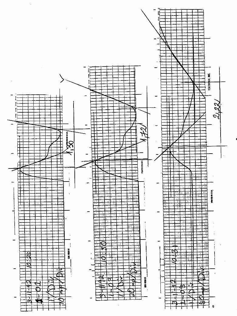

II ,!.
|
II

- /
-- - i|
I
i
_! ,' _ 'i '
! • ,,'t,, :: ' t!
, .i_l
' , . ' , ,, ' ."
" '... I I ! ,;_!I
-- , ...... ,i!lI, I _I l'l.ll ,
' ' " ' "_.' I
I!

II
i •
i
• ." , !


|

j :1: I: I
1
I i'
I I • I...I !
' ] ' II ! i
' i I• i
i
I

Appendix 1.
Plots of TDR traces obtained from field seasonal measurements in February, March, andApril 1992 in Borehole #2, using flat prongs 7.5" long and different graphical methods ofreading.
bbb) "Method of Diverging Lines", Borehole #2/March 1992
45

!
\

- i

\
Fi o
'l _._ I i . 'I • I
' ,I ,,, I,k I I
--- I 17I
" I1
_l. I J
/IN _ I %1
, 1!_ ,-?--l-_--i_i_!.// , ,i.V7
|#l i I l ." l
P I I l.ar I - I• r i _Iw I ol_
-- ar l 1 i'l I
I v ( I ,fl Ii i,,'1 I I
' \ _ " ,I I --- 1%1 L--'I i
kI I I-- • 1 1 I
-- - ._1:\ I I I
-I :I I I I- I : I I .!!! '1 ',_ I , I" ti_ I " I. I
.1 j1_ ...... " I ': :, I I ._ :., :1
• . . , I I "_ _ I I I :i, ,' I ,_1 _ '"1 ._ 1 _ , I',;-- ,. .,., I :_I '_', fix l , ' I .I_
' ' I .'1; " -'_ l! - : :_l ; ' I ,i_• I,,. , I':,1:. 'i'.: _ '- ,i..' "'" i. !_
l:.. I ,,I ._: _ ' • ,'1":• I 1 _' : ' : I. _ 1' '
I,. 1 I ' '=; 1 :I I.1 : :" '; ', 'u
- I i i,i .'. I ' I .'.
l..i .I I :,'. i .,I..' I I ," .i ' ,_
I I _ '1._ , '1 ,
- :-, I .t ' - -.--: I, i ,.,,--]"_ " i.... II, 1 : :,! ,i_" I --" l , .I :_,
_ _. ,_i _ ---'" ij._ i,,,iI I ', l:_.t ', ! ,I ;;
' I _1 _.1
r_. i.I -' -" .:1- ,,___+I<.,- I.I "_- ""--_ _-_-'t'_
_ "" _.. . 1 _ _2."!1 ,,. " .lilt
- I--_--"b-"4.----i"-' ' -I- -----_B-- tier%
; _ • ,i¢_ _! ill ,, _,.I>-"

!
- i
mI
I
!


Appendix 1.
Plots of TDR traces obtained from field seasonal measurements in February, March, andApril 1992 in Borehole #2, using flat prongs 7.5" long and different graphical methods ofreading.
ccc) "Method of Peaks", Borehole #2/March 1992
53


,....
°I
, "! "_II - ,
I II I
, _I! •
'fl


!


i
I
iiiI I :I I
• !
_ I'I'_'
, t_• I! i
I
LI
'"I--- I .I, I 'I"
-I -I _'I:
-! ! - b, ._i I_,!
-- .--

Appendix 1.
Plots of TDR traces obtained from field seasonal measurements in February, March, andApril 1992 in Borehole #2, using fiat prongs 7.5" long and different graphical methods ofreading.
aaa) "Method of Tangents", Borehole #2, April 1992
61

t
i!!
I
ii
tq
_ !
z_
I


I

m
Ii
11
!F-
-i-l !I r--
•l -E----'i' I
-! I •
| -- .
--1

Appendix 1.
Plots of TDR traces obtained from field seasonal measurements in February, March, andApril 1992 in Borehole #2, using flat prongs 7.5" long and different graphical methods ofreading.
bbb) "Method of Diverging Lines", Borehole #2/April 1992
67

1o.
,s
f
;- [I
-i
||

\
t |.L |
:[[
1
tI
i
I
! _.
i


Appendix 1.
Plots of TDR traces obtained from field seasonal Measurements in February, March, andApril 1992 in Borehole #2, using flat prongs 7.5" long and different graphical methods ofreading.
ccc) "Method of Peaks", Borehole #2/April 1992
73


I
i• --
• , ._

\

Appendix 2.Plots of TDR traces obtained from field seasonal measurements in February, March, andApril 1992, in Borehole #3, using curved prongs 12" long and different graphical methods ofreading.
aaa) "Method of Tangents", Borehole #3, February 1992
79

I, , t I • + I ' | ;
' _-ti I̧ I .......i.+'+' f ...... i...._ , .+--.t--i t --t--_--t-,'t---!--b' + u.__..
...._-_- +,,_--_-i J ' "_ ' ' "; :t_ i It i+i+l + _ t _" ,-,- • '[ -t..---i---I-_ t --4---i -.i-- --!--; , ---- -t :--_....-!-._--,-._..... i---
.__j _ t i--+-+-=_ .--,--
.+ + ++-- +,+,_ / !I,,_, _
- ! -iil}i}}i +--J!+-".I -.++-+_ t --+-._-I+++::++:-:-.t--i-++_--__-+,---+-i _-.+ [ -_--_--,_-_--_--i___._.+.......+_:___-__._• ' .___. _ • ' ' _ I _
' '--+--_.--+-.-+--I---+-_--_---I' -:--J , t_l-- .....+---.I,+ ;----I--u ...... ' +-': " _ , I _ - + +-)-b-l---I --_
__I -I---I + I +--- "--, : , . .u_.
[ .__L.1
+t I
I
•!.-. , [t 1____._._ [
_ tI" I
i.--+.
i J '' +I ! I
i .+ I i
i ' ,G
,_ i.. _ -I 11 t--i-
!i' .... . I ! i _i { I I ' , _j ,. + . _+_..,+ _ ,---+--
--i-l--_-i .--+--_I I +
+ ! i + i + +___. +_+ \ �+ +!---V_
' ! I
!-_--,-.t-_+--+--_ .--+,_-+-;-+ I. i' ' ' ' ' ' + .... -!-i-
! _ I I + I ! _ ' -'I. , , i-.+,-_++_.-Ii, , .-]--r-_, i--_ .'--+-I!--i-:-i -.'"...i-l--+--4--_--t--_ ' ' "' " ' --I.- _-.+:+-I_ --u-.I-.--+--_-+--i-_ +':I +-----+:--.++ I_ _Y.._i....l..+.+_.l.l_+.Jr__- --+--,-++ i-!--_:_ _ ';i' _ : ' ' --.-I---_.+-i!-I '+'
..__,-___.+___"._,+,, ,., I +--,,--i!--b-+.... __I-_V-A-,_._,,,---_ __.+_+_..,__.i+..+...i__L4--4" +-_ + I'_,.+.L_.++ + 1--':--+"+ _ t + + i.-!-.-,:.-y--t---T---t-_
_!t .... +' 'I H-_--,'---L_-_-_• , ----if-i-t--_---F-t--t-"_-.--i.-_,'_-I _-_ -_ I , _ _ .. ],,+,, _
;_G+___,..__i_ ____+ _-+-i--i.-_--1--i-I _---+,---+!_--+- --- ' -_.r_-+-.7.._--I-_ - _.__+----+ _", -t--_,. _,--v-i--l::+--i--_;
_ . _ , _-+----I--,+_-t "s,,:
! +---,t+_-.',A--+-F-t-_• c.e,+,,_--+---"_-.,t+-_---.._,..-._._l-V-i-:+-i-4---i_ " i _" -,-_ : ,-._-+--t-
" : + , i , + ' ;_ I I t'!+| +
+i+--
! ,
,--- i ': _- J --t-.i i
I f I
I


-t_-- l---I---_I....I--[
[[[I
I
_ t
-- , . i ! ' t"N

Appendix 2.Plots of TDR traces obtained from field seasonal measurements in February, March, andApril 1992, in Borehole #3, using curved prongs 12" long and different graphical methods ofreading.
bbb) "Method of Diverging Lines", Borehole #3, February 1992
87
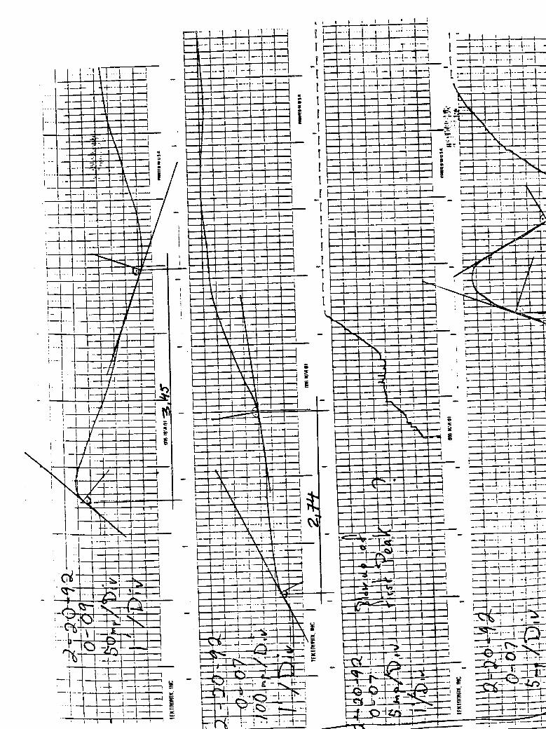
l i I t , I ! t ! ;
----i I -!--il '1 1.'-] ...... ' : : ' ' *
---tl-'i---t--7.--! I --I---i-I. i...... i--q---4 ' ' .-_--t_-tH--_...t-_.... ,.-- _,4-fl..-:i-t._..-t-_ _.... ___ '
- --t4--t_-_---i....I- -- i ....... +-f--i-' i -t/--:....I--i-!---i--t--
i ' C'-Ii i '_--:.:-t.- I'%. ! .. 1.
i- -i , t "_tH-'_k-_.........
" _ " I _- i ,i __-_ • t / / !
:--I _ ' I I .=_--- _r -+--7--i--_ , ! i--i----i--.-:q"i-'_" ""I'_ `-+-4-1-.i- _ i i_
tt [I- { 7li, I 1
'--144" - ' -: 'i l .__,__
1 --+-y+=_4---- 'l • il I
• I %t !1 1:i J ,I i
:. 1 ! %_i I1 ' i
1 i I 1% i '- I [ ' ill:
'# 1 I i i
' ' i r, ' _ I
1 i _\l , 1 t _ t
_ 1 ' _ .}._.]i_...i__! i.
--1-k+_--i-:i'_-I--:i_ _ ,.,..,. _- t ---.1. _-..!. _ ..;• -_ ;-
--l--_"_ -r-_ , .t-i-. i-:!-!. -
, : _+_,++,i, %i_ ,, , . _--;--i-;--+--1 i _ , _ i I :"-i i I I _ _-"-i--i-
i_l i i
' I --1- ._ -J
..__ I --'r 1--}--'_-- ."-,_'" _ '' --1


k" : !..!_.__.._ , ._
:...._ I _ l i--.t-t---._- _--r--i-,......Jr-. _--t---t...._-it_I, -k-\-++ i....
--k-t-_:k--t-1
-HN
__-1:_ ,, iq---x<-t J I ''4_ _ .. l I J '%1 I 1 - I 1 •
I
,_ f _ •
- t1 ,--..it ] it i j J.I '#it, r! I I i .• I _


Appendix 2.Plots of TDR traces obtained from field seasonal measurements in February, March, andApril 1992, in Borehole #3, using curved prongs 12" long and different graphical methods ofreading.
ccc) "Method of Peaks", Borehole #3, February 1992
93


Appendix 2.Plots of TDR traces obtained from field seasonal measurements in February, March, andApril 1992, in Borehole #3, using curved prongs 12" long and different graphical methods ofreading.
aaa) "Method of Tangents", Borehole #3, March 1992
99

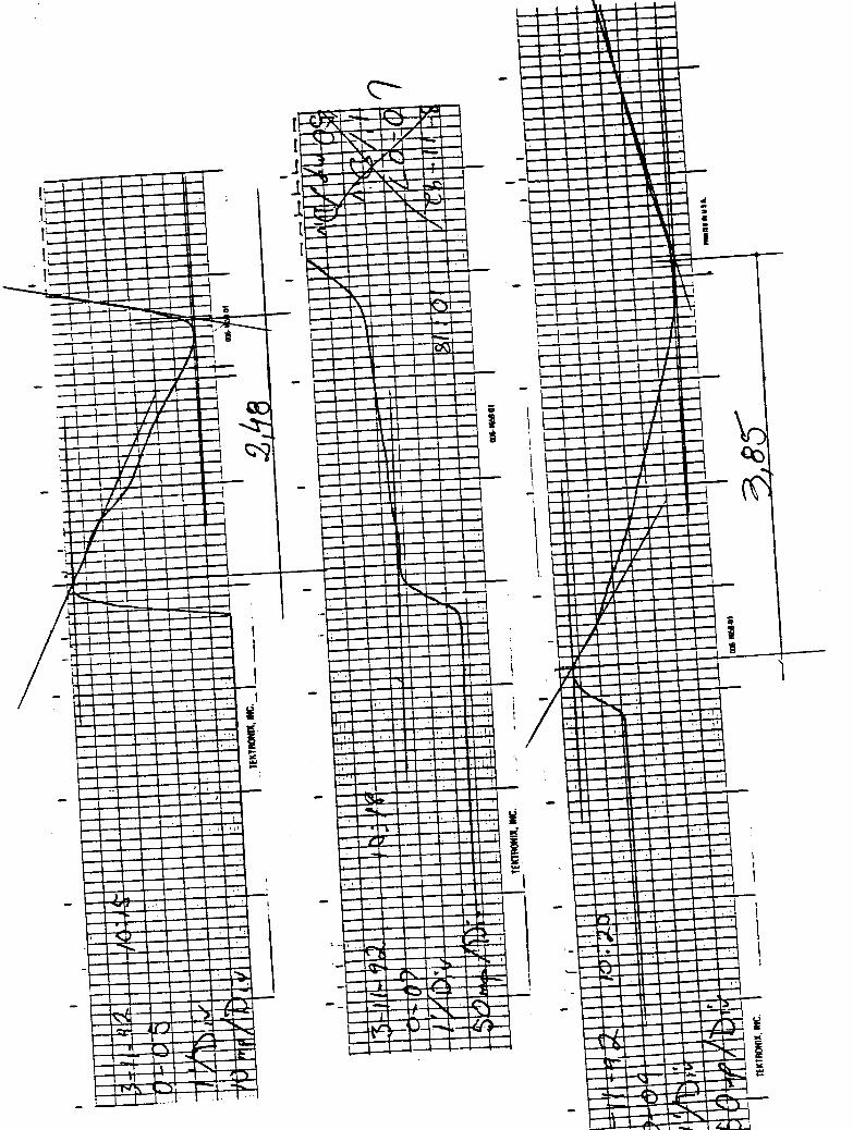


.
i!I

Appendix 2.Plots of TDR traces obtained from field seasonal measurements in February, March, andApril 1992, in Borehole #3, using curved prongs 12" long and different graphical methods ofreading.
bbb) "Method of Diverging Lines", Borehole #3, March 1992
105

I
t
S
!I
- - "I'--I .- El
--!
-. _ : _
i , J


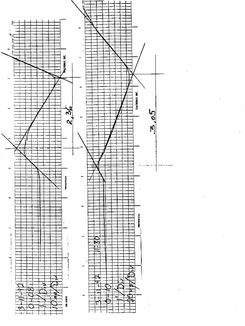


u• _o

Appendix 2.Plots of TDR traces obtained from field seasonal measurements in February, March, andApril 1992, in Borehole #3, using curved prongs 12" long and different graphical methods ofreading.
ccc) "Method of Peaks", Borehole #3, March 1992
113

i Jl| 1 I
I i _I ] II _I I I _I I ql I I
I I _ I I:
' l I' i' l I -li
' .I -LI I II I, I II I
- -I t t II II I I_ I_
t 1 I I I"-,,I I I 1 I |
' I I I I I
- I I I I Il I l I I
] |t

I
! -II

I
i ,' i! •
i
I
ii •i
-II ,:I I
I
i •
|§

I
- ||


Appendix 2.Plots of TDR traces obtained from field seasonal measurements in February, March, andApril 1992, in Borehole #3, using curved prongs 12" long and different graphical methods ofreading.
aaa) "Method of Tangents", Borehole #3, April 1992
119
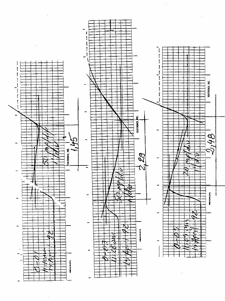


Appendix 2.Plots of TDR traces obtained from field seasonal measurements in February, March, andApril 1992, in Borehole #3, using curved prongs 12" long and different graphical methods ofreading.
bbb) "Method of Diverging Lines", Borehole #3, April 1992
125


Appendix 2.Plots of TDR traces obtained from field seasonal measurements in February, March, andApril 1992, in Borehole #3, using curved prongs 12" long and different graphical methods ofreading.
ccc) "Method of Peaks", Borehole #3, April 1992
131

\

I


i -ttttLt

Appendix 3.
Application of the Wilcox's Signed-Rank Test, for pairs of TDR readings, obtained inBorehole #2, by using different graphical methods of reading.
137
ANNEXE.31
Statistical comparison between pairs of TDR readings obtained byusing :
(I) method of peaks{2) method of diverted lines
A) DATA: Idaho,Boise, Test Section 163023, Borehole #2, flatprongs /7.5"length, February 1992. Values of TDR
lengths are those ,given in the Annexe 1 and Table 1.
B) THE PROBLEM:
Using the Wilcoxon singned-rank test for pairedobservations ,test the hypothesis ,at the 0.05 level ofsignificance ,to determine wether the two different methods usedfor reading the TDR experimental traces ,lead to simillar ordifferent results.
C) SOLUTION:
Let ml and m2 represent the mean TDR readings ,obtainedby using the methods (1) and (2),respectivelyo Following the sixstep procedure one may have:
1.The null hypothesis, H0: ml=m2
2.The alternative hypothesis, HI: ml><m2
3.The significance level, a: 0.05
4.The critical region: Since the number of pairs ofobservations is 15, from the Table AI6 (Walpole, 1985),for n=15and a =0o05,one may find the critical region to be : Wcr<=25

/.
5. Computations:
Pair Method(l) Method (2) Di/Rank Wi+ Wi-
1 1.40 1.40 0/I 1
2 1 •37 i. 48 -0.11/8 8
3 1.72 1.60 0.12/9 9
4 1.75 1.79 -0.04/4 4
5 1.65 I. 67 -0.02/2.5 2.5
6 2.16 1.88 0.28/12.5 12.5
7 2.25 2.00 0.25/11 11
8 1.68 1.60 0.08/6 6
9 1 •65 I. 67 -0.02/2.5 2 •5
i0 I. 72 I. 81 -0.09/7 7
11 1.65 1.60 0.05/5 5
12 2.12 1.84 0.28/12.5 12.5
13 2.77 2.45 0.32/14 14
14 2.60 2.39 0.21/10 i0
15 3.10 2.22 0.88/15 15
Total 96 24
W+=96
W-=24
W=24

6.Conclusion:
As the computed value, W=24 is less than the critical value Wcr<=25gone
have to reject the null hypothesis, H0, and to conclude that the
TDR readings,obtained by using the two investigated methods
mentioned above are significantly different. Also one may observe
that this assertion is not decissive,because the Computed value,
W is situated very near the up-limit of the critical region o

ANNEXE, 32
Statistical comparison between pairs of TDR readings obtained byusing :
(I) method of peaks(2) method of diverted lines
A) DATA: Idaho,Boise, Test Section 163023, Borehole #2, flatprongs /7.5"length, March 1992. Values of TDR
lengths are those ,given in the Annexe 1 and Table 1.
B) THE PROBLEM:
Using the Wilcoxon singned-rank test for pairedobservations ,test the hypothesis ,at the 0.05 level ofsignificance ,to determine wether the two different methods usedfor reading the TDR experimental traces ,lead to simillar ordifferent results.
C) SOLUTION:P
Let ml and m2 represent the mean TDR readings ,obtainedby using the methods (1) and (2),respectively. Following the sixstep procedure one may have:
1.The null hypothesis, H0: ml=m2
2.The alternative hypothesis, HI: ml><m2
3.The significance level, a: 0.05
4.The critical region: Since the number of pairs ofobservations is 17, from the Table A16 (Walpole, 1985),for n=17and a =0.05,one may find the critical region to be : Wcr_=35

5 oComputations:
Pair Method(l) Method (2) Di/Rank Wi+ Wi _
1 1.42 1o38 0.04/1 1
2 1.47 1o40 0.07/2.5 2o5
3 1.60 1.60 0
4 1o89 1.82 0.07/2.5 2°5
5 1.90 1.90 0
6 2.08 1 o78 0o 30/10.5 I0o 5
7 2.29 2o51 -0.22/7 7
8 2.18 2.02 0o 16/6 6
9 i. 73 i. 60 0.13/5 5
10 1.72 1.49 0.23/8 8
11 1 .75 1 .45 0 .30/10 .5 i0 .5
12 2.02 i. 77 0.25/9 9
13 2.07 1o 98 0o 09/4 4
14 2.88 2°40 0..44/14 14
15 2.80 2.26 0.54/15 15
16 2.80 2 o48 0o 32/12.5 12 o5
P
17 2.50 2.18 0.32/12.5 12.5
Total 111 7 ==
W+=III
W-=7
W=7

6.Conclusion:
As the computed value, W=7 is less than the critical value
Wcr<=35, one have to reject the null hypothesis, H0, and to
conclude that the TDR readings,obtained by using the two
investigated methods mentioned above are significantly different.

ANNEXE.33
Statistical comparison between pairs of TDR readings obtained byusing z
(l) method of peaks(2) method of diverted lines
A) DATA: Idaho,Boise, Test Section 163023, Borehole #2, flatprongs /7.5"length, April 1992. Values of TDR
lengths are those ,given in the Annexe 1 and Table i.
B) THE PROBLEM:
Using the Wilcoxon singned-rank test for pairedobservations ,test the hypothesis ,at the 0.05 level of
significance ,to determine wether the two different methods used
for reading the TDR experimental traces ,lead to simillar ordifferent results.
C) SOLUTION:
'Let ml and m2 represent the mean TDR readings ,obtained
by using the methods (i) and (2),respectively. Following the six
step procedure one may have:
l.The null hypothesis, H0: ml=m2
2.The alternative hypothesis, HI: ml><m2
3.The significance level, a: 0.05
4.The critical region: Since the number of pairs of
observations is i0, from the Table AI6 (Walpole, 1985),for n=10
and a =O.05,one may find the critical region to be : Wcr-=8

5. Computations:
Pair Method(l) Method (2) Di/Rank Wi+ Wi-
1 i. 60 i. 67 -0.07/3.5 3.5
2 i. 68 i. 62 0.06/2 2
3 1.90 1.88 0.02/1 1
4 2.04 i. 78 0.26/8 8
5 2.21 2.10 0.11/6 6
6 1.72 1.65 0.07/3.5 3.5
7 1.77 i. 59 0.18/7 7
8 2. i0 2. oo o. 10/5 5
9 2.80 2.15 o. 65/10 i0
i0 2.60 2.14 0.46/9 9
Total: 51.5 3.5
W+=51.5
W-=3.5
W=3.5
6.Conclusion:
As the computed value, W=3.5 is less than the critical value
Wcr<=8, one have to reject the null hypothesis, H0, and to conclude
that the TDR readings,obtained by using the two investigated
methods mentioned above are significantly different.

Appendix 4.
Application of the Wilcox's Signed-Rank Test, for pairs of TDR readings, obtained onBorehole #3, by using different graphical methods of reading.
147

ANNEXE.41
Statistical comparison between pairs of TDR readings obtained byusing
{Z) method of peaks(2) method of diverted lines
A) DATA: Idaho,Boise, Test Section 163023, Borehole #3,curvedprongs /12"length, February 1992. Values of TDR
lengths are those ,given in the Annexe 2 and Table 2o
B) THE PROBLEM:
Using the Wilcoxon singned-rank test for pairedobservations ,test the hypothesis ,at the 0.05 level ofsignificance ,to determine wether the two different methods usedfor reading the TDR experimental traces ,lead to simillar ordifferent results.
C) SOLUTION:P
e
Let ml and m2 represent the mean TDR readings ,obtained
by using the methods (I) and (2),respectively. Following the sixstep procedure one may have:
loThe null hypothesis0 H0: ml=m2
2oThe alternative hypothesis, HI: ml><m2
3oThe significance level, a: 0°05
4oThe critical region: Since the number of pairs ofobservations is 15, from the Table AI6 (Walpole0 1985),for n=15and a =0.05,one may find the critical region to be : Wcr<=25

5. Computations :
Pair Method(l) Method (2) Di/Rank Wi+ Wi-
1 1.69 1.66 0.03/2 2
2 1.47 1.69 -0.22/9 9
3 2.44 2.43 0.01/i 1
4 2.44 2.44 0
5 2 •44 2.34 0.10/4.5 4.5
6 4.12 3.05 i. 07/14 14
7 3.00 2.90 0.10/4.5 4.5
8 2 •49 2.19 0.30/10 i0
9 2.45 2.04 0.41/12 12
i0 2 .50 2.39 O. 11/7 7
11 2.40 2.74 -0.34/11 ii
12 i. 25 1.35 -0.10/4.5 4.5
13 2.38 2.50 -0.12/8 8
14 3.55 3.45 0.10/4.5 4.5
15 3.30 2.66 0.64/13 13
Total 62.5 32.5
W+=62.5
W-=32.5
W=32.5
6.Conclusion:
As the computed value, W=32o5 is higher than the critical value
Wcr<=25,one have to accept the null hypothesis, H0, and to conclude
that the TDR readings,obtained by using the two investigated
methods mentioned above are not significantly different.

ANNEX _ .42
Statistical comparison between pairs of TDR readings obtained by
using :(1) method of peaks(Z) method of diverted lines
A) DATA: Idaho,Boise, Test Section_163023, Borehole #3, curved
prongs /12"length, March 1992. Values of TDR
lengths are those ,given in the Annexe 2 and Table 2.
B) THE PROBLEM:
Using the Wilcoxon singned-rank test for paired
observations ,test the hypothesis ,at the 0.05 level of
significance ,to determine wether the two different methods used
for reading the TDR experimental traces ,lead to simillar ordifferent results.
C) SOLUTION:!
'Let ml and m2 represent the mean TDR readings ,obtained
by using the methods (I) and (2),respectively. Following the six
step procedure one may have:
l.The null hypothesis, H0: ml=m2
2.The alternative hypothesis, HI: ml><m2
3.The significance level, a: 0.05
4.The critical region: Since the number of pairs of
observations is 13, from the Table AI6 (Walpole, 1985),for n=13
and a =0.05,one may find the critical region to be : Wcr_=17

5. Computations :
Pair _ Method(l) Method (2) Di/Rank Wi+ Wi-
1 2.02 lo90 0.12/5 5
2 2.40 2°40 0
3 2.98 2o 29 0o 69/12 12
4 3,05 2 o58 0o 47/11 ll
5 2.95 2°97 =0°02/2 2
6 2.60 2°48 0.14/6 6
7 2.63 2 o40 0 o06/8 8
8 2.46 2°40 0.06/3 3
9 2.79 2 o53 0.26/9 o5 9 °5
i0 2.76 2 .58 0.18/7 7
ii 2 .36 2 .35 0 .01/I 1
12 3 .63 3.37 0 o26/9.5 9.5
13 3.05 2.35 0.10/4 4
Tota i 76 2
W+=76
W-=2
W=2

6.Conclusion:
As the computed value, W=2 is less than the critical value
Wcr<=17, one have to reject the null hypothesis, H0, and to
conclude that the TDR readings,obtained by using the two
investigated methods mentioned above are significantly different.

ANNEX o43
Statistical comparison between pairs of TDR readings obtained byusing z
(I) method of peaks(2) method of diverted lines
A) DATA: Idaho,Boise, Test Section 163023, Borehole #3, curved
prongs /12"length, April 1992. Values of TDR
lengths are those ,given in the Annexe 2 and Table 2o
B) THE PROBLEM:
Using the Wilcoxon singned-rank test for pairedobservations ,test the hypothesis ,at the 0.05 level of
significance ,to determine wether the two different methods used
for reading the TDR experimental traces ,lead to simillar ordifferent results.
C) SOLUTION:
Let ml and m2 represent the mean TDR readings ,obtained
by using the methods (I) and (2),respectively° Following the sixstep procedure one may have:
l.The null hypothesis, H0: ml=m2
2.The alternative hypothesis, HI: ml><m2
3.The significance level, a: 0°05
4.The critical region: Since the number of pairs of
observations is I0, from the Table AI6 (Walpole0 1985),for n=10
and a =0.05,one may find the critical region to be : Wcr<=8

5. Computations :
Pair Method(l) Method (2) Di/Rank Wi+ Wi-
1 2.17 2.10 0.07/2.5 2.5
2 2.29 2.38 -0.09/5.5 5.5
3 3.00 2.40 0.60/8 9
4 2.93 2.85 0.08/4 4
5 2.70 2.58 0.12/10 7 6
2.45 2.38 0.07/2.5 2.5
7 2.72 2.63 0.09/5.5 5.5
8 2.33 2.28 0.05/1 l
9 3 .62 3 .00 0.62/9 I0
i0 3.15 2.63 0.52/7 8
Total 40.5 5.5
W+=40.5
W-=5.5
W=5.5
6.Conclusion:
As the computed value, W=5.5 is less than the critical value
Wcr<=8, one have to reject the null hypothesis, H0, and to conclude
that the TDR readings,obtained by using the two investigated
methods mentioned above are significantly different.

Appendix 5.
Testing the significance of the differences between pairs of TDR readings, obtained by usingdifferent methods of reading.
157

Annexe 5 Testing the differences between the TDR values
obtained by using different methods for readingTDR traces
Brhl#3 Brhl#2
Crt. Annexe Annexe annexe Annexe Annexe Annexe
No. 41 42 43 31 32 33
io00 0.03 0.12 0,07 0.00 0.04 °0°07
2.00 -0.22 0.00 -0.09 -0.ii 0.07 0°06
3.00 0.01 0.69 0.60 0.12 0.00 0°02
4.00 0.00 0.74 0.08 -0.04 0.07 0°26
5.00 0.10 -0.02 0.12 -0.02 0.00 0oli
6.00 1.07 0.14 0.07 0.28 0.30 0°077.00 0.10 0.06 0.09 0.25 -0.22 0.188.00 0.30 0.26 0.05 0.08 0.16 0o109.00 0.41 0.18 0.62 -0.02 0.13 0.65
10.00 0.11 0.01 0.52 -0.09 0.23 0°461.1.00 -0.34 0.26 0.05 0.3012.00 -0.10 0.10 0.28 0.2513.00 -0.12 0.47 0.32 0.0914.00 0.10 0.21 0.4415.00 0.64 0.88 0.5416.00 0.32
17.00 0.32
SUM (FT) 2.09 3.01 2.13 2.19 3.04 1.84
AVG (ft) 0.14 0.23 0.21 0.15 0.18 0.18
STD 0.34 0.24 0.25 0.24 0.18 0.21
N 15.00 13.00 10.00 15.00 17.00 10.00
t 1.58 3.45 2.73 2.35 4.09 2.80
Sign.
Appendix 6.
Evaluation of the confidence levels for the averagedifferences, di, between pairs of TDR readings, obtained by using different methods ofreading.
159

Test 31 : Analysys of the average differences,related with datafrom Annex 31 :n=15; Avg=0.15, Std=0,24
P% t t*s/n'0.5 dmin dmax
60 0.54 0.0334 0.1165 0.1834
80 0.87 0.0539 0.0960 0.2039
90 1.35 0.0836 0.0663 0.2336
95 1.76 0.1090 0.0409 0.2590
97.5 2.15 0.1332 0.0167 0.2832
99 2.62 0.1623 -0.012 0.3123
99.5 2.98 0.1846 -0.034 0.3346
99.95 4.14 0.2565 -0.106 0.4065

Test 32:Analysis of the average differencese,related with datafrom Annexe 32:n=17; Avg=0.18;Std=0.18
P% t t*s/n'0.5 dmin dmax
60 0.535 0.0233 0.1566 0.2033
80 0.865 0.0377 0.1422 0.2177
90 1.337 0.0583 0.1216 0.2383
95 1.746 0.0762 0.1037 0.2562
97.5 2.12 0.0925 0.0874 0.2725
99 2.583 0.1127 0.0672 0.2927
99.5 2.921 0.1275 0.0524 0.3075
99.95 4.015 0.1752 0.0047 0.3552

Test 33: Analysis of average differences,related with data
fom Annexe 33 : n=10; Avg=0.18; Std=0.21
PZ t tes/n'0.5 dmin dmax
60 0.543 0.0360 0.1439 0.2160
80 0.893 0.0593 0.1206 0.2393
90 1.383 0.0918 0.0881 0.2718
95 1.833 0.1217 0.0582 0.3017
97.5 2.262 0.1502 0.0297 0.3302
99 2.821 0.1873 -0.007 0.3673
99.5 3.25 0.2158 -0.035 0.3958
99.95 4.781 0.3174 -0.137 0.4974

Test 41:Analysis of average differences related with
data from Annexe 41 : n=15; Avg=0.14; Std=0.34
P_ t t_s/nA0.5 dmin dmax
60 0.537 0.0471 0.0928 0.1871
80 0.868 0.0761 0.0638 0.2161
90 1.345 0.1180 0.0219 0.2580
95 1.761 0.1545 -0.014 0.2945
97.5 2.145 0.1883 -0.048 0.3283
99 2.624 0.2303 -0.090 0.3703
99.5 2.977 0.2613 -0.121 0.4013
99.95 4.14 0.3634 -0.223 0.5034

Test 42: Analysis of average differences related with da
from Annexe 42: n=13; Avg=0.23; Std=0.24
P% t t*s/nA0.5 dmin dmax
60 0.538 0.0358 0.1941 0.2658
80 0.87 0.0579 0.1720 0.1979
90 1.35 0.0898 0.1401 0.2298
95 1.771 0.1178 0.1121 0.2578
97.5 2.16 0.1437 0.0862 0.2837
99 2.65 0.1763 0.0536 0.3163
99.5 3.012 0.2004 0.0295 0.3404
99.95 4.221 0.2809 -0.050 0.5109

Test 43. Analysis of the average differences related with data
from Annexe 43: n=10; Avgffi0.21;Std=0.25
PZ t t*s/nA0.5 dmin dmax
60 0.543 0.0429 0.1670 0.2529
80 0.893 0.0705 0.1394 0.2805
90 1.383 0.1093 0.1006 0.3193
95 1.833 0.1449 0.0650 0.354997.5 2.262 0.1788 0.0311 0.3888
99 2.821 0.2230 -0.013 0.4330
99.5 3.25 0.2569 -0.046 0.4669
99.95 4.781 0.3779 -0.16/ 0.5879

Appendix 7.
Synthesis of confidence limits for the average differences, di, between the length values ofTDR traces, evaluated according the procedures from Appendix 6.
167

Table 4. Confidence levels for the average differences , di,between the lenth values of TI)R traces
obtained by using different methods of reading
P%: 60 80 90 95 97.5 99 99.5 99.95 n Avg Std
dmin
test:
31 0.12 0.1 0.07 0.04 0.02 0 0 -0.i 15 0.15 0.24
32 0.16 0.14 0.12 0.i 0.08 0.07 0.05 0 17 0.18 0.18
33 0.14 0.12 0.09 0.06 0.03 0 -0.04 -0.13 I0 0.18 0.21
41 0.09 0.06 0.02 -0.01 -0.05 -0.09 -0.12 -0.22 15 0.14 0.34
42 0.19 0.17 0.14 0.12 0.09 0.05 0.02 -0.05 13 0.23 0.24
43 0.17 0.13 0.1 0.07 0.03 -0.01 -0.04 -0.17 10 0.21 0.25
Avg 0.145 0.12 0.09 0.063 0.033 0.003 -0.02 -0.11 13.33 0.181 0.243Std 0.033 0.034 0.038 0.041 0.045 0.050 0.054 0°072 2.624 0.031 0.049
Cv% 22.78 28.46 42.55 66.15 137.1 1526. -250. -65.2 19.68 17.23 20.22
dmax
te_t
31 0.18 0.2 0.23 0.26 0.28 0.31 0.33 0.41
32 0.2 0.22 0.24 0.25 0.27 0.29 0.31 0.36
33 0.22 0.23 0.27 0.3 0.33 0.37 0.4 0.5
41 0.19 0.22 0.25 0.29 0.32 0.37 0.4 0.542 0.27 0.2 0.22 0.26 0.28 0.32 0.34 0.51
43 0.25 0.28 0.32 0.35 0.38 0.43 0.46 0.59
Avg 0.218 0.225 0.255 0.285 0.31 0.348 0.373 0.478Std 0.032 0.026 0.033 0.034 0.038 0.047 0.051 0.074
Cv% 14.82 _11.96 12.95 11.94 12.35 13.50 13.80 15.52

Appendix 8.
Estimation of the influence of the differences in reading TDR traces on the final moisturecontent.
169

Annexe8
Influence of differences in reading TDR traces
TDR flat prongs curvedprongs
TDR k VMC MC DifMC k VMC MC DifMC
ft V% wt% % V% wt% %
1 2.612 -0.04 -0.02 3.104 1.02 -0.5 -0.25 -2.46
1.25 4.081 5.934 3.082 2.843 1.54 -5.24 -2.72 2.155
1.5 5.877 11.40 5.925 2.445 2°296 -1.09 -0.56 0.566
1.75 7.995 16.11 8.371 2.3092 10.44 20.56 10.68 2.259 4.081 5.939 3.085 1.849
2.25 13.22 24.91 12.94 2.256 5.165 9.5 4.935 1.6232.5 16.32 29.25 15.19 2.273 6.377 12.62 6.558 1.517
2.75 19.75 33.63 17.47 2.311 7.716 15.54 8.075 1.4603 23.50 38.08 19.78 2.365 9.183 18.35 9.536 1.429
3.25 27.58 42.63 22.14 2.434 10.70 21.10 10.96 1.413
3.5 31.99 47.32 24.58 2.520 12.49 23.82 12.37 1.423
3.75 36.37 52.17 27.10 2.625 14.38 26.57 13.80 1.3944 41.79 57.22 29.72 16.32 29.25 15.19
Avg 2.479 1.124Std 0.251 1.191
Cv% 10.14 105.9
For an average differance di=0.18 ft,the average difMC is:
Avg 1.785 0.809

Appendix 9.
Evaluation of soil moisture contents from TDR readings, graphically determined, by Methodof Diverging Lines. Worksheets and graphical representation.
171

rY _
i--
,=In
C-(33Cq .............................................
Oo..... Io°°_ rl_
.4--c-_
_I .. 10-
(/3_'_ I
- ./r
0 ,,:_
-I--
E 4-_3 I I I I I I I
O -0 '
-I--- .r-,. ,- N _ "_I- U*) r_ I"-. _I) (:r_ 0
Z3 ..c-II--.
I,I _ ED

Evaluation of soil moisture content from TDR readin
Idaho,Boise,Test Section 163023,Borehole #2,February i
Wire Depth Phase Probe TDR Dielec VMC Dry De MCNo. velocilengthreadinconst.Univers.
ins ft/sec ft ft k Equation
% vol.g/cm3 %wt
o-01 12 0.99 0.625 1.4 3.919 5.326 2.163 2.462
0.99 0.625 1.37 3.594 4.504 2.163 2.082
o-02 17 0.99 0.625 1.72 8.929 16.69 1.929 8.655
o-03 22 0.99 0.625 1.75 9.569 17.98 1.924 9.346
0.99 0.625 1.65 7.562 13.82 1.924 7.184
0-04 27 0.99 0.625 2.16 22.20 37.13 1.924 19.30
0-05 33 0.99 0.625 2.25 26.14 41.13 1.921 21.41
0-06 39 0.99 0.625 1.68 8.127 15.03 1.923 7.816
0.99 0.625 1.65 7.562 13.82 1.923 7.188
o-07 45 0.99 0.625 1.72 8.929 16.69 1.917 8.709
' 0.99 0.625 1.65 7.562 13.82 1.917 7.210
o-08 57 0.99 0.625 2.12 20.60 35.28 1.927 18.30
o-09 69 0.99 0.625 2.77 60.06 64.84 1.918 33.80
0.99 0.625 2.6 46.62 54.86 1.918 28.60
o-i0 81 0.99 0.625 3.1 94.22 141.2 1.92 73.57


R Evaluation of soil moisture content from TDR readingsIdaho ,Boise,Test Section 163023,Borehole #2,March 1992
Wire Depth Phase Probe TDR Dielect VMC Dry Den MC
No. velocitlength readingconst. Univers.
ins ft/sec ft ft k Equation
vol. g/cm3 Zwt
o-01 12.00 0.99 0.63 1.38 0.76 -3.12 2.16 -1.44
0.99 0.63 1.40 2.00 0.32 2.16 0.15
o-02 17.00 0.99 0.63 1.60 2.61 1.96 1.93 1.02
o-03 22.00 0.99 0.63 1.82 3.38 3.96 1.92 2.06
0.99 0.63 1.90 3.68 4.73 1.92 2.46
0-04 27.00 0.99 0.63 1.78 3.23 3.58 1.92 1.86
0-05 33.00 0.99 0.63 2.51 6.43 11.31 1.92 5.89
0.99 0.63 2.02 4.16 5.93 1.92 3.09
o-06 39.00 0.99 0.63 1.60 2.61 1.96 1.92 1.02
0-07 45.00 0.99 0.63 1.49 2.27 1.04 1.92 0.54
0.99 0.63 1.45 2.15 0.72 1.92 0.37
o-08 57.00 0.99 0.63 1.77 3.20 3.49 1.93 1.81
0.99 0.63 1.98 4.00 5.53 1.93 2.87
o-09 69.00 0.99 0.00 2.40 5.88 10.05 1.92 5.240.99 0.63 2.26 5.21 8.48 1.92 4.42
o-10 81.00 0.99 0.63 2.48 6.28 10.96 1.92 5.71

E
.i
_ _ ........................................................ w _om
0.... • .... • .......... °......... ° ..... i ..... ,..... i°,o_
: : :
_- _o____°°_ _o
N
I,I _

R Evaluation of soil moisture content from TDR readingsIdaho,Boise,Test Section 163023,Borehole #2,April 1992
Wire Depth Phase Probe TDR Dielect VMC Dry Den MCNo. velocitlength readingconst. Univers.
ins ft/sec ft ft k Equation% vol. glcm3 Zwt
o-01 12.00 0.99 0.63 1.67 7.28 13.22 2.16 6.11o-02 17.00 0.99 0.63 1.62. 6.85 12.27 1.93 6.360-03 22.00 0.99 0.63 1.88 9.23 17.31 1.92 9.000-04 27.00 0.99 0.63 1.78 8.28 15.34 1.92 7.97o-05 33.00 0.99 0.63 2.10 11.52 21.69 1.92 11.29o-06 39.00 0.99 0.63 1.65 7.11 12.84 1.92 6.68o-07 45.00 0.99 0.63 1.59 6.60 11.71 1.92 6.11o-08 57.00 0.99 0.63 2.00 10.45 19.69 1.93 10.22o-09 69.00 0.99 0.63 2.15 12.07 22.69 1.92 11.83o-i0 81.00 0.99 0.63 2.14 11.96 22.49 1.92 11.72

Evaluation of soil moisture content from TDR readings
Idaho,Boise,Test Section 163023,Borehole #3,February 1992
Wire Depth Phase Probe TDR Dielec VMC VMC VMC Dry De MC MC MCNo. velocilengthreadinconst.UniverEqu. 1 Equ. 2 univ. Equ. 1 Equ.2
ins ft/sec ft ft k Equation equ. gran. soil
% vol.%vol %vol g/cm3 %wt %wt %wt
o-01 12.0 1.0 1.0 1.7 2.9 2.8 -5.9 2.2 1.3 -2.70
1.0 1.0 1.5 2.2 0.9 -5.7 2.2 0.4 -2.64
o-02 17.0 1.0 1.0 2.4 6.1 10.5 5.5 1.9 5.4 2.83
1.0 1.0 2.4 6.1 10.5 5.5 1.9 5.4 2.83
1.0 1.0 2.4 6.1 10.5 5.5 1.9 5.4 2.83
o-03 22.0 1.0 1.0 4.1 17.3 31.0 30.6 1.9 16.1 15.88
o-04 27.0 1.0 1.0 3.0 9.2 17.2 18.4 1.9 8.9 9.54
o-05 33.0 1.0 1.0 2.5 6.3 ii.i 12.5 1.9 5.8 6.51
1.0 1.0 2.5 6.1 10.6 12.0 1.9 5.5 6.26
o-06 39.0 1.0 1.0 2.5 6.4 11.2 12.6 1.9 5.8 6.56
o-07 45.0 1.0 1.0 2.4 5.9 I0.0 11.4 1.9 5.2 5.95
1.0 1.0 1.3 1.6 -0.8 -5.5 1.9 -0.4 -2.87
o-08 57.0 1.0 1.0 2.4 5.8 9.8 11.2 1.9 5.1 5.79P
o-09 69.0 1.0 1.0 3.6 12.9 24.1 24.4 1.9 12.5 12.71
o-i0 81.0 1.0 1.0 3.3 11.1 20.9 21.7 1.9 10.9 11.28


Evaluation of soil moisture content from TDR readingsIdaho, Boise,Test Section 163023,Borehole #3,March 1992
Wire Depth Phase Probe TDR Dielect VMC Dry Den MCNo. velocitlength readingconst. Univers.
ins ft/sec ft ft k Equation
% vol. g/cm3 Zwt
o-01 12.00 0.99 1.00 1.90 3.68 4.73 2.16 2.19
0-02 17.00 0.99 1.00 2.40 5.88 10.05 1.93 5.21
0-03 22.00 0.99 1.00 2.29 5.35 8.81 1.92 4.58
0.99 1.00 2.58 6.79 12.13 1.92 6.32
0-04 27.00 0.99 1.00 2.97 9.00 16.84 1.92 8.75
0-05 33.00 0.99 1.00 2.48 6.28 10.96 1.92 5.71
0.99 1.00 2.40 5.88 10.05 1.92 5.23
0-06 39.00 0.99 1.00 2.40 5.88 10.05 1.92 5.23
0-07 45.00 0.99 1.00 2.53 6.53 11.54 1.92 6.02
0.99 1.00 2.58 6.79 12.13 1.92 6.33
0-08 57.00 0.99 1.00 2.35 5.63 9.48 1.93 4.92
0-09 69.00 0.99 1.00 3.37 11.59 21.82 1.92 11.38
o-10 81'.00 0.99 1.00 2.95 8.88 16.59 1.92 8.64

I,I _ o,
"I::a.

Evaluation of soil moisture content from TDR readings
Idaho,Boise,Test Section 163023,Borehole #3,April 1992
Wire Depth Phase Probe TDR Dielect VMC Dry Den MC
No. velocitlength readingconst. Univers.
ins ft/sec ft ft k Equation
Z vol. E/cm3 Zwt
o-01 12.00 0.99 1.00 2.10 4.50 6.76 2.16 3.13
0-02 17.00 0.99 1.00 2.38 5.78 9.82 1.93 5.09
o-03 22.00 0.99 1.00 2.40 5.88 10.05 1.92 5.22
0-04 27.00 0.99 1.00 2.85 8.29 15.37 1.92 7.99
o-05 33.00 0.99 1.00 2.58 6.79 12.13 1.92 6.31
o-06 39.00 0.99 1.00 2.38 5.78 9.82 1.92 5.11
o-07 45.00 0.99 1.00 2.63 7.06 12.72 1.92 6.63
o-08 57.00 0.99 1.00 2.28 5.30 8.70 1.93 4.52
o-09 69.00 0.99 1.00 3.00 9.18 17.21 1.92 8.97
o-i0 81.00 0.99 1.00 2.63 7.06 12.72 1.92 6.62

0" DOrY"
F--
-I_ 'E
0
-4-- ::I:1::
-_ ..................................................._•.4--. O "5:
2"0 :,. . S,._l,ml • • .._
:_. _.:_ : _>..o" ..... :..._., ". .... : ...... , .........
: : _ _: :
"4- : |:; _-:._L II ' ": _ "
0 _-."::_ _r' _: _ .. i" -__i; t:. • . ,_i _ :o i_a.i • _:_' .... _'L,,,,_: :. •
E .E :_:_'_i _ " _ ! ! :El t.h,'e I I -I' I ! I | 0
0-o°_ "- 0 0 0 0 0 0 0 0 0 0 0 .r.
"3 v E
E] r- =e:> CL
I,I ¢_ P
i.,.


Seasonal "average " moisture content
under road pavements
Depth Borehole #2 Borehole #3
Ins February March April February March April
12 2.65 0.15 6.11 0.85 2.19 3.13
17 8.65 1.02 6.36 5°4 5.21 5.09
22 8.26 2.26 9 16.1 5.45 5.2227 19.3 1.86 7.97 8.9 8.75 7.99
33 21.41 4.59 11.29 5.65 5.47 6.3139 7.5 1.02 6.68 5.8 5.23 5.11
45 7.86 0.46 6.11 5.2 6.17 6.63
57 18.3 2.34 10.22 5.1 4.92 4.52
69 31.2 4.83 11.83 12.5 11.38 8.97
81 73.57 5.71 11.72 10.9 8.64 6.62
Sum 198.7 24.24 87.29 76.4 63.41 59.59
Avg 19.9 2.4 8.7 7°6 6.3 5.9
Std 19.7 1.9 2.3 4.2 2,4 io6
Cv% 98.9 79.1 26.4 55.3 38.1 27.1
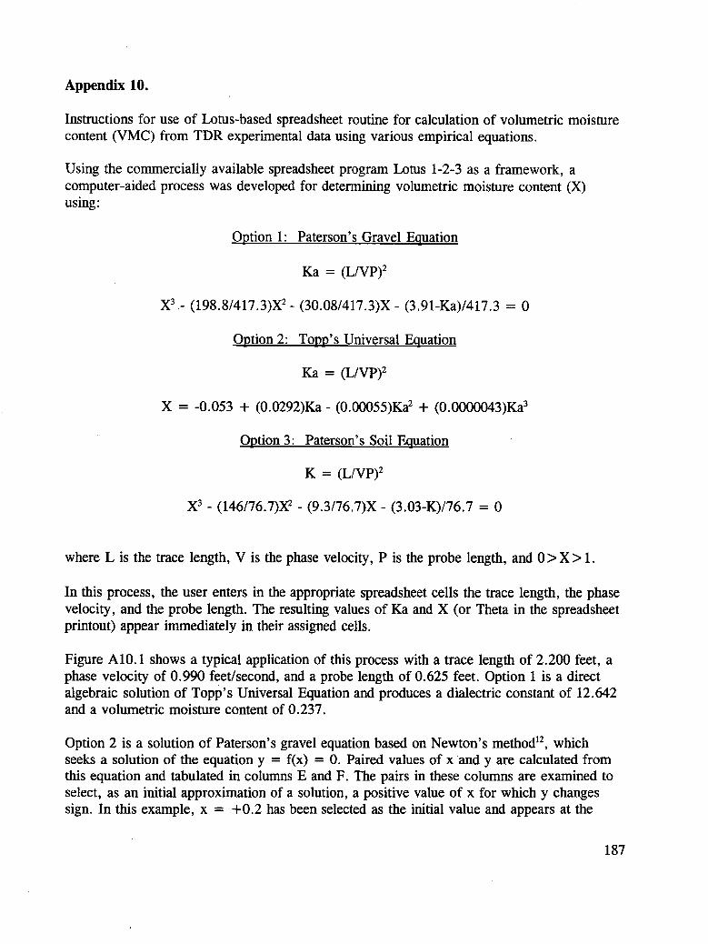
Appendix 10.
Instructions for use of Lotus-based spreadsheet routine for calculation of volumetric moisturecontent (VMC) from TDR experimental data using various empirical equations.
Using the commercially available spreadsheet program Lotus 1-2-3 as a framework, acomputer-aided process was developed for determining volumetric moisture content (X)using:
Option 1: Paterson's Gravel Equation
Ka = (L/VP) 2
X3- (198.8/417.3)X 2- (30.08/417.3)X- (3.91-Ka)/417.3 = 0
Option 2: Topp's Universal Equation
Ka = (L/VP) 2
X = -0.053 + (0.0292)Ka- (0.00055)Ka 2 + (0.0000043)Ka 3
Option 3: Paterson's Soil Equation
K = (L/VP) 2
X3 - (146/76.7)X 2 - (9.3/76.7)X- (3.03-K)/76.7 = 0
where L is the trace length, V is the phase velocity, P is the probe length, and 0 > X > 1.
In this process, the user enters in the appropriate spreadsheet cells the trace length, the phasevelocity, and the probe length. The resulting values of Ka and X (or Theta in the spreadsheetprintout) appear immediately in their assigned cells.
Figure A10.1 shows a typical application of this process with a trace length of 2.200 feet, aphase velocity of 0.990 feet/second, and a probe length of 0.625 feet. Option 1 is a directalgebraic solution of Topp's Universal Equation and produces a dialectric constant of 12.642and a volumetric moisture content of 0.237.
Option 2 is a solution of Paterson's gravel equation based on Newton's method 12,whichseeks a solution of the equation y = f(x) = 0. Paired values of x and y are calculated fromthis equation and tabulated in colunms E and F. The pairs in these columns are examined toselect, as an initial approximation of a solution, a positive value of x for which y changessign. In this example, x = +0.2 has been selected as the initial value and appears at the
187

head of a column of figures in column G. An examination of this column, which tabulatessucceeding trial values of x in this iterative method, shows that convergence to a volumetricmoisture content of 0.169 is achieved in four cycles.
Option 3 is a solution of Paterson's soil equation also based on Newton's method. It followsthe same form as Option 2 and shows convergence in five cycles to a volumetric moisturecontent of 0.240.
In Options 2 and 3, if the values of x in column G do not converge, the user can enter adifferent starting value at the head of column E, check succeeding values, and repeat theprocess (i.e., enter a new starting value) until convergence is achieved.
188

"TDR01": A VMC CALCULATOR BY A. ROBERT RAAB, SHRP SENIOR STAFF OFFICEROPTION i: SOIL VMC CALCULATION USING PETERSON'S GRAVEL EQUATION
FUNCTION PLOT SOLUTION BY NEWTON'S METHOD
INPUT X y X=Theta Y=f(X) dY/dXTrace L= 2.200 -0.50 -0.19 0.2000000000 -0.0045473872 -0.1426407860
Ph Vel= 0.990 -0.40 -0.09 0.1681200072 0.0000932223 -0.1474727812
Probe L= 0.625 -0.30 -0.03 0.1687521398 0.0000000114 -0.1474362283
-0.20 0.01 0.1687522173 0.0000000000 -0.1474362237
OUTPUT -0.i0 0.02 0.1687522173 -0.0000000000 -0.1474362237
Ka= 12.642 0.00 0.02 0.1687522173 -0.0000000000 -0.1474362237
0.I0 0.01 0.1687522173 -0.0000000000 -0.1474362237
SOLUTION 0.20 -0.00 0.1687522173 -0.0000000000 -0.1474362237
Theta= 0.169 0.30 -0.02 0.1687522173 -0.0000000000 -0.1474362237
Theta %= 16.88 0.40 -0.02 0.1687522173 -0.0000000000 -0.1474362237
0.50 -0.01 0.1687522173 -0.0000000000 -0.1474362237CHECK 0.60 0.02 0.1687522173 -0.0000000000 -0.1474362237
Kac= 12.642 0.70 0.08 0.1687522173 -0.0000000000 -0.1474362237
Kec-Ka= 0.000 0.80 0.17 0.1687522173 -0.0000000000 -0.1474362237
0.90 0.30 0.1687522173 -0.0000000000 -0.1474362237
1.00 0.47 0.1687522173 -0.0000000000 -0.1474362237

OPTION 2: SOIL VMC CALCULATION USING TOPP'S UNIVERSAL EQUATION
INPUT
Trace L= 2.200
Ph Vel= 0.990
Probe L= 0.625
OUTPUT
Ka= 12.642
Theta= 0.2369
Theta %= 23.693

OPTION 3: SOIL VMC CALCULATION USING PETERSON'S SOIL EQUATIONTRACE DATA SOLUTION BY NEWTON'S METHOD
INPUT x y X=Theta Y=f(X) dY/dXTrace L= 2.200 -0.50 -0.41 0.2000000000 0.0329279701 -0.7626597132
Ph Vel= 0.990 -0.40 -0.19 0.2431751796 -0.0023494043 -0.8696268631
Probe L= 0.625 -0.30 -0.04 0.2404735562 -0.0000085884 -0.8632615838
-0.20 0.07 0.2404636074 -0.0000000001 -0.8632380625
OUTPUT -0.i0 0.12 0.2404636073 -0.0000000000 -0.8632380622
Ka= 12.642 0.00 0.13 0.2404636073 -0.0000000000 -0.8632380622
0.i0 0.i0 0.2404636073 -0.0000000000 -0.8632380622
SOLUTION 0.20 0.03 0.2404636073 -0.0000000000 -0.8632380622Theta= 0.240 0.30 -0.06 0.2404636073 -0.0000000000 -0.8632380622
Theta %= 24.046 0.40 -0.16 0.2404636073 -0.0000000000 -0.8632380622
0.50 -0.29 0.2404636073 -0.0000000000 -0.8632380622
CHECK 0.60 -0.42 0.2404636073 -0.0000000000 -0.8632380622
Kac= 12.642 0.70 -0.55 0.2404636073 -0.0000000000 -0.8632380622
Kac-Ka= 0.000 0.80 -0.68 0.2404636073 -0.0000000000 -0.8632380622
0.90 -0.80 0.2404636073 -0.0000000000 -0.8632380622
1.00 -0.90 0.2404636073 -0.0000000000 -0.8632380622


te
Cr-_r,,l..," .a_,r4als K-* ._t/,.Jo.olP,_,, * ,'_P_,, -,//;..I
K& T_¢t& l& "rhd_. & K& 7t, et& K& Tl',et & k& _het_
4.._,_(_ |. (_| | 4.._'_ l |. • | ;." 4.".£. cl J,@|4 4.440 _-, |]( 4, 51."; |.G|I
,;. 5E,_ I_. e.2£ 4. _.e. t_. G-'2 4. ?,_ t G. e;_4 ,;. t!9 l,. e2( 4. I_,e.• t_. _2_
_.f_,.r., (_.i_',._ 5.¢,=.._ :e.l_',,2 (..._4_; G.q)54 E. "4_ 6.E'_.(. f,.2';2 t_.1_',,.It:. _4G _:. (_{'._ (...a: 4G _, (_G_ (..• ,'r.4G C_.('f'4 i_. (.41 e. E'_'¢ ¢.74_ I_. E'Gt¢.G4_ _, G,"C'. £. ©.r.1. e.. GT-" T ...,,¢,'" _.e?4 ";'. I_I _... _?G 7 .2¢.E e.. e ,"_T._Tr.. e, E_¢.:C" 7.4E'_ e. _.£:2 7. _c,=. _. ,_£._ ";',762 G.E.E:¢ 7. i_12. e. _i:',":.92_ G;_._(: E:._._5 e._-_2 (:.l,;E e..O?4 f_.2(l e.e.._._ $.$74 _.(,9_1_.4_.. • I_.._(,C_ l:._;e4 I_..I_" _..T]. _. I_..1(14 _..8_;. _,]GF, _.?_;- e.]_l.r..,q_(r,. e. 22 C'. .c.. I 8E E'. 21:' .r-.._ C-.,r, t_.114 .c,. ¢2_ G. 111_ )..8.42 q_. ".,1:9. f.(.1 e. ]_:c S..-f_a e.. __-'. $.._o: _. 1:'-_ ]0. (-2_ B. ]_. le. _,:_ e._;,
• Oe r . . _. . * ....;i_.,I_T_ _..14_: le..e,.., e.14_ I .!*C. e.1,;4 ]1 _z.. _.:4( ,1 ._c_ e.|,l; ].4_,: e. '. 5;' ],..(]_ i_. _ _;" ll.T_ _.154 I I. t_',,( e.15_ ] 1.98£, e.l'.A1;¢, _.e:_ G.]_ ] ; _ ;:2(; .e. ](_ |2,3_s I_. 1(_ |;.473 _.]¢_ 12.59(; e. I(.,4.2. ?'1 ¢. _,ITG 1._'. _42 1_. l ,"2 1_'. _,£4 6.17_ ] _. _f:? G. !7(. 13.210 I). 17_]'.:'. ?$2 e. IE._ 1 ._. • .'.4 . _. lS;: :2.'_7( e.. 1_4 15._97 e. :_:_ I_:. _17 e. I (_sl_.S,;_ "_..'.¢(_ 1._.GF.,_. e.l$;_ !_.!£.; ?.:.¢4 1_:.3e] e,:_.6 1c.42_.. e.jsl$ t'r, _,,__• ('. 2_ " I 4 • (.-".E_ _. ;1_.2 34.." ?T _.. ;_a. !4. _.S5 (s. _(. |_._12 1_.2_!"-_..12S" l_.21e 15.2a( :e.21; 15._.(_: .I).21g" l._..#,,", " _.21_ ¢ 1_ _¢; 1_ :It:.'r, ?E_ _.. 2;.'_, l "... £:2_ I_. 222 ] .".. S3_ e._24 1E. O4_, E.. _2{ 1(.. 15_ E,. ;,2);_..=¢_ e..:,._e ;_._,"£: " e,;232 ;(.4_._ e.2.'a_; l_.L,.s.t, e.2._ 1(..7¢',_ e,;_]t'..e:: _..;:z_ _¢._1f: "_(_;242 17.1__ e.;:4z. _.7;12r_ e.;4( 17.£_:Z e.2a::7,_2¢ G.2"-._ _7.¢,_r . _..2,".2 _7.,_. _.2,_¢ l.",.(_ e.2,',.(- l?,?_';" e.'r-',_;;;._:-.'. e._e ,"...,_?;" e.2_;.. ]¢._2,'.: e.2_.z Is:. ]2_ _.;_£_ ]_.2_: e.2_;!
.,S. ] ";".. e. 2'._ • : F. 254.. _. 2$2 ] S. 3.'.:;: E.294 I .¢. 4G.c, G.. 29(: ,..c;. 4£'T e.27_
. **e * - * * ° •
2:1_,.4 _ _. _. 2:('_. 5_E: e. ?_2' 2_. _Ezf G.$34 ,I'E'. f..":.l G. ::.,_:( _:C"..£;T_, G._, c2t:.T:7 e._q. ;.,£, _r-. e._c," 2C..7a5 e.".,._¢ 2G ¢_-'- 2.._4£. _I_._(_.- e._4I2e.,e..¢_; e,_;r.._ 2_._:e. e.3"-,2 2_.s_..¢ B._r4 2_..s'B_ 8,356 _l,Bl] _..3-'._