Travel demand models - Transportation Research Board
65
TRANSPORTATION RESEARCH RECORD 775 • ,, .. Travel Demand Models: Application, Limitations, and Quantitative Methods TRANSPORTATION RESEARCH BOARD COMMISSION ON SOCIOTECHNICAL SYSTEMS NATIONAL RESEARCH COUNCIL NATIONAL ACADEMY OF SCIENCES WASHINGTON, D, C. 1980
-
Upload
khangminh22 -
Category
Documents
-
view
0 -
download
0
Transcript of Travel demand models - Transportation Research Board

TRANSPORTATION RESEARCH RECORD 7 7 5 •
,, ..
Travel Demand Models: Application, Limitations, and Quantitative Methods
TRANSPORTATION RESEARCH BOARD
COMMISSION ON SOCIOTECHNICAL SYSTEMS NATIONAL RESEARCH COUNCIL
NATIONAL ACADEMY OF SCIENCES WASHINGTON, D, C. 1980

Transportation Research Record 775 Price $6.20 Edited for TRB by Naomi Kassabian
modes 1 highway transportation 2 public transit
subject areas 12 planning 13 forecasting
Library of Congress Cataloging in Publication Data National Research Council. Transportation Research Board.
Travel demand models.
(Transportation research record; 77 5) Reports presented at the 59th annual meeting of the Transpor
tation Research Board. 1. Choice of transportation-Mathematical models--Addresses,
essays, lectures. 2. Transportation-Planning-Mathematical modelsAddresses, essays, lectures. I. National Research Council (U.S.). Transportation Research Board. II.' Series. TE7.H5 no. 775 [HE336.C5] 380.5s 81-3950 ISBN 0-309-03119-2 ISSN 0361-1981 (380.5'22) AACR2
Sponsorship of the Papers in This Transportation Research Record
GROUP I-TRANSPORTATION SYSTEMS PLANNING AND ADMINISTRATION Leon M. Cole, Library of Congress, chairman
Transportation Forecasting Section George V. Wickstrom, Metropolitan Was·~·•ngton Council of Govern
ments, chairman
Committee on Passenger Travel Demand Forecasting David S. Gendel/, Federal Highway Administration, chairman Moshe E. Ben-Akiva, Daniel Brand, David J. Dunlap, Robert T. Dunphy, Raymond H. Ellis, Robert E. Gall, Thomas F. Golob, Walter G. Hansen, David T. Hartgen, Thomas J. Hillegass, Joel L. Horowitz, Stephen M. Howe, Lidia P. Kostyniuk, T. Keith Lawton, Steven Richard Lerman, Eugene J. Lessieu, Frederick A. Reid, Martin G. Richards, Gordon W. Schultz, Gordon A. Shunk, Bruce D. Spear, Anthony R. Tomazinis, Edward Weiner, Yacov Zahavi
James A. Scott, Transportation Research Board staff
The organizational units, officers, and members are as of December 31, 1979.

Contents
STUDY OF THE TRANSPORTATION CORRIDOR BETWEEN RIO DE JANERIO, SAO PAULO, AND CAMPINAS
Valerio J. Bertucci, Hsu Y. H. O'Keefe, Paulo A. R. Lago , and Weider G. Soubhia .... ... . . .. . .
SIMPLE EQUILIBRIUM ANALYSIS OF THE DEDICATION OF A FREEWAY LANE TO EXCLUSIVE BUS USE
Y osef Sheffi . . . . . . . . . . . . . . . . . . . . . . . . . . . . . . . . . . . . . . . . . . . . . . . . . . . . . . . . . . . . . . . . . . . 7
CAR-OWNERSHIP FORECASTING TECHNIQUES IN GREAT BRITAIN A. D. Pearman and K. J. Button . .. .. ... . .. .. .. . . . . .. . . . . .. . . . ... . . . . . . . . . . . . .. .. . . . 11
STRATEGY STUDIES FOR URBAN TRANSPORT IN THE NETHERLANDS Aad Ruhl . . . . . . . . . . . . . . . . . . . . . . . . . . . . . . . . . . . . . . . . . . . . . . . . . . . . . . . . . . . . . . . . . . . . . 1 7
USE OF INCREMENTAL FORM OF LOG IT MODELS IN DEMAND ANALYSIS Ashok Kumar ... .... . .. .. ... . . .. . . . .... . . ... . . .. . . . . .. ... .. ... . .......... . . . ... 2 1
MODEL SPECIFICATION, MODAL AGGREGATION, AND MARKET SEGMENTATION IN MODE-CHOICE MODELS: SOME EMPIRICAL EVIDENCE
Youssef Dehghani and Antti Talvitie ........... . ............ .. . ... . . . ..... .. . . . .... . 28
NONRESPONSE PROBLEM IN TRAVEL SURVEYS: AN EMPIRICAL INVESTIGATION
Werner Brog and Arnim H. Meyburg . .............. .. .. ..... . .. ... . ... . . . .. ...... .. . 34
ASSESSMENT OF LAND-USE AND SOCIOECONOMIC FORECASTS IN THE BAL TIM ORE REGION
Antti Talvitie, Michael Morris, and Mark Anderson ............. ....... .. . . . . .. ...... .. . 38
COMPONENTS OF CHANGE IN URBAN TRAVEL Gerald S. Cohen and Michael A. Kocis ... . ................ ... . . .. . . . . ... ... .... ... .. .42
TRAVEL DEMAND FORECASTING BY USING THE NESTED MULTINOMIAL LOGIT MODEL
Kenneth L. Sobel .. ..... .. .. . . .. ..... . . . . . ..... . . . ... .. . . .. .. . . . . .. .. .. . . ....... 48
NETWORK EQUILIBRATION WITH ELASTIC DEMANDS Nathan H. Gartner ...... . . . ........... . .. ... · . . . .. .. .. . .. . ... . . . ... .. .. .. . ...... . 56
iii

Authors of the Papers in This Record
Anderson, Mark, Department of Civil Engineering, State University of New York at Buffalo, 3435 Main Street, Buffalo, NY 14214
Bertucci, Valerio J., Transportation Systems Department, Promon Engenharia S.A., Avenida 9 de Julho 4939, Sao Paulo, SP 01407, Brazil
Brog, Werner, Socialdata GmbH, Hans-Grassel-Weg 1, Miinchen 70, West Germany Button, Kenneth J., Department of Economics, Loughborough University, Loughborough, LEl 1 3TU, England Cohen, Gerald S., Planning and Research Bureau, New York State Department of Transportation, 1220 Washington Avenue,
Albany, NY 12232 Dehghani, Youssef, Department of Civil Engineering, State University of New York at Buffalo, Parker Engineering Building,
Buffalo, NY 14214 Gartner, Nathan H., Civil Engineering Department, University of Lowell, Lowell, MA 01854 Kocis, Michael A., Planning and Research Bureau, New York State Department of Transportation, 1220 Washington Avenue,
Albany, NY 12232 Kumar, Ashok, Northeast Ohio Areawide Coordinating Agency, 1501 Euclid Avenue, Cleveland, OH 44115 Lago, Paulo A.R., Transportation Systems Department, Promon Engenharia S.A., Avenida 9 de Julho 4939, Scio Paulo,
SP 01407, Brazil Mey burg, Arnim H., School of Civil and Environmental Engineering, Cornell University, Ithaca, NY 1485 3 Morris, Michael, Department of Civil Engineering, State University of New York at Buffalo, 3435 Main Street, Buffalo, NY
14214 O'Keefe, Hsu Y.H., Transportation Systems Department, Promon Engenharia S.A., Avenida 9 de Julho 4939, Sao Paulo,
SP 01407, Brazil Pearman, Alan D., School of Economic Studies, University of Leeds, Leeds, LS2 9JT, England Ruhl, Aad, Ministry of Transportation and Public Works, Postbus 20901, The Hague 2500 EX, Netherlands Sheffi, Yosef, Department of Civil Engineering, Massachusetts Institute of Technology, Cambridge, MA 02139 Sobel, Kenneth L., Cambridge Systematics, Inc., Kendall Square Building, 238 Main Street, Cambridge, MA 02142 (associated
with Cambridge Systematics in the Netherlands when this paper was prepared) Soubhia, Weilder G., Transportation Systems Department,Promon Engenharia S.A., Avenida 9 de Julho 4939, Sao Paulo,
SP 01407, Brazil Talvitie, Antti, Department of Civil Engineering, State University of New York at Buffalo, Parker Engineering Building,
Buffalo, NY 14214
iv

Transportation Research Record 775 1
Study of the Transportation Corridor Between Rio de Janeiro, Sao Paulo, and Campinas VALERIO J. BERTUCCI, HSU Y. H. O'KEEFE, PAULO A. R. LAGO, AND WEIDER G. SOUBHIA
In this paper the passenger-demand studies and the preliminary economic eval· uation of policies to meet the passenger travel demand within the Rio de Janeiro-Sao Paulo-Campinas Corridor are summarized; particular attention is paid to the introduction of a high·speed train service. Existing methods for travel-demand forecasting were not judged suitable, both because of their cross· elasticity problems and because of the volume of data required to calibrate them. Accordingly, a new direct-demand model was developed centered on a multilevel multinomial·logit mode-split formulation. By applying this meth· odology, the main results of the evaluation of high-speed train service showed that it is unlikely to be economically justified for the whole corridor. How· ever, it appears to be warranted for part of the corridor-the Siio Paulo· Campinas link-under all hypotheses adopted.
• The 500-km corridor between Rio de Janeiro and Sao Paulo had in 1975 a population of about 21 million that increases at an annual growth rate of 2.7 percent. For this study, the towns in the corridor were grouped into 12 level-! zones surrounded by B level-2 zones (with 4 million inhabitants in 1975). Four more external zones were considered since they contribute a large amount of freight that goes through the corridor. The entire study was carried out by Promon Engenharia S.A., a Brazilian private consulting company, for the Brazilian Transport Planning Agency (GEIPOT).
This study investigated three policies to meet the travel demand in the area:
l. frees
2. 3.
Transfer of freight from road to rail, which the road system for passenger use; Transfer of passengers from road to rail; and Introduction of a high-speed train.
The study was made up of three separate substudies: a passenger-demand study (which included a study of land use within the corridor), a review of available high-speed rail technology (which included estimates of capital and operating costs as well as a route-location study), and a preliminary economic evaluation.
This paper presents only the method used in the transportation studies and in the economic evaluation as well as the results obtained.
METHOD
The aim of the study was to evaluate alternative ways of meeting travel demand within the corridor between Rio de Janeiro, Sao Paulo, and Campinas. These alternatives included operational measures, such as the partial regulation of freight transport, as well as alternatives that require large capital expenditure, such as a high-speed train (TAV), which would provide a new mode that has characteristics quite different from those of the existing ones.
In addition, the corridor is expected to experience a period of strong population and income growth during the next 20 years, particularly in the Rio de Janeiro-Sao Paulo section, and it was necessary to take this into account in evaluating the alternatives.
A model was therefore required that was capable of responding to changes in the operational characteristics of existing modes, to the introduction of new modes that had characteristics different
from those of the existing ones, and to changes in population and income distribution.
A particularly important requirement was that the model adopted be one in which the demand for travel was responsive to the supply, i.e., that, as the cost and time of travel by various modes changed and as new modes were introduced, both the total volume of travel and the proportions of persons who travel by the various modes respond to such changes. Figure 1 shows the major stages in the modeling process; the demand, supply, and evaluation phases are identified separately •
The modeling approach adopted was therefore one in which a direct-demand submode! is linked with a submode! of the transport network to provide an integrated representation of the transport system in the corridor. It should be noted that, since the demand for travel is a function of the system that satisfies that demand and since the level of service is conversely a function of the demand for travel, the modeling procedure adopted is an interactive one in which the results of the demand submode! are input to the supply submode!, and vice versa, until equilibrium is reached.
There are several methods available for forecasting the demand for travel. They can be summarized in four main groups: growth factors and allied techniques (Fratar expansion), traditional four-step models, direct-demand models, and disaggregate models.
Each of the above methods was considered for use in the present study. Since the central problem is one of mode split and possible trip generation, it was thought that a technique should be selected that was strong from the point of view of mode split and trip generation. This suggested a direct-demand formulation. However, existing specifications were not judged suitable both because of their crosselastici ty problems and because of the volume of data required to calibrate them Clrll· Accordingly, a new direct-demand model was developed centered on a multilevel multinomial logi t mode-split formulation C11!l.
The model used has two important features that distinguish it from earlier direct-demand models. First, the multilevel mode-split formulation allows the clustering of modes into subgroups that contain modes that are relatively close substitutes for each other <!l. Second, the linking of mode-split and trip""9eneration characteristics via the composite utility (U) ensures that cross-elasticities are always positive, if the parameters satisfy certain simple conditions (,i).
The supply submode! concerns the transport networks for the various options and years considered in the study. The approach adopted is a conventional one (i): the main steps can be summarized as (a) the construction of a multirnode network; (b) the calculation of speeds and times for each link of the network; (c) the extraction of subnetworks (called reduced networks) for each mode; (d) the calculation of minimum paths, costs, and times by mode between all pairs of zones; and (e) the assignment of the flows that are output from the demand submode! to the network constructed above.

-.
2
Figure 1. Transport model flow chart. r -------..., I SUPPLY I
I TAI 1 I TRANSPORT I NETWORK I
I l I I ~ I I CATPAA~~TY I I RESTRAINT I I l I I I I R;~u
9
c~D I NETWORK I
L_
TAS4
MINIMUM
PATH
I TAS6
TRAFFIC
ASSIGNMENT
I I I I I
I I I I I
__ I
Transportation Research Record 775
. -----------1 I . DEMAND
I I I I
I I I
I
XPGM
BASE YEAR
FLOWS
GROWTH
FORECAST YEAR
FLOWS
TAS5
MODAL
SPLIT
L __
GENER
TRIP GENERATION
AND SUPRESSION
I I I I I I I I
_ __ _J , --- - - --- --------,
I EVALUATION I I OPCOST SURPLUS I
OPERATION USER
I STATISTICS BENEFITS ! L ___________ _i
'£here are two points in this process at which there is interaction with the demand submodel: (a) in the second step, the speeds and times in the network, particularly on the road links, are a function of the amount of traffic and (b) the output of the fourth step, the minimum costs and times, is input to the demand submodel.
The main purpose of an economic evaluation is to provide a measure of the value to society of the different options being considered.
This study has adopted the more-conventional efficiency approach in which individuals provide their own valuation of their costs and benefits. However, it should be pointed out that in a country such as Brazil, in which there are large income differentials both between different parts of the country and different groups in the same region, care is required in comparing different projects since efficiency evaluations inevitably favor those projects that help the richer members of society.
The calculation of the net present value (NPV) of costs and benefits provides the main economic indicator for choice between alternatives. Breakdown of this NPV by user income group and by organization gives useful additional information on the distribu-
tional impact of the change. indicators may be regarded information to be assessed reached.
Some other performance as useful additional
before a decision is
The structure adopted is given in Figure 2, which shows the different categories of costs and benefits (labeled A-K) and their distribution among the three groups--users, transport operators, and government (1). Certain costs and benefits that accrue to a particular group do not accrue to all the groups together.
DEMAND SUBMODEL
Three types of travel demand were identified:
1. Passenger travel among the 20 internal study zones (levels 1 and 2) i
2. Freight traffic among the 24 study zones (levels 1, 2, and 3) i and
3. The remaining traffic, made up of passenger travel between the study area and the rest of Brazil, as well as all passenger and freight traffic internal to a single study zone. (This traffic was judged to be unaffected by any of the options con-

Transportation Research Record 775
Figure 2. Economic evaluation structure.
r - - -------- - - - -- -A
USER NET
BENEFIT
B TRIP
DISUTILITY
c CAR
OPERATIONAL COST
3
TOLLS
1 I I I
--~::· ___ B -: ... 11 ._ _____ __,,
______ _ ______ _J L--------- --- - -
1---~----~-----~------- -. -----1
I + CJ ECONOl\illC TAXES OPERATORS I
I FARES - OPERATIONAL AND I
COSTS TOLLS
L---------------------~-------~ ,...- ------------- ----, I I I J I I + TOLL REVENUES ROAD GOVERNMENT I I AND TAXES MAINTENANCE I L ______________ _ _ J
r --------- - - - -1 I K I '1 CAPITAL INVESTMENT :
I COST I L ____ _ _ ________ J
sidered in this study and hence could be treated as constant for any given year.)
The first two groups of demand were estimated by using origin-destination (0-D) models. The third group was estimated on a link basis as the difference between the assigned flows of the first two groups and the average traffic flows recorded on each link.
The study considered total trips subdivided by income group and car ownership, since these are important factors in mode choice, which lies at the heart of the work. In an ideal world, separate models would therefore be estimated for each of the market groups. However, in the present study, information on the income and, to a lesser extent, the car ownership, of travelers was severely limited. It was therefore necessary to estimate models for business and leisure travelers as a whole and to then subdivide the matrices in a manner that was consistent with the aggregate data available.
Based on the above, separate trip models were estimated for
1. Business and nonbusiness trips and 2. Pairs of centers connected by commercial ties
(hereafter termed functionally related) and those that are not (hereafter termed unrelated).
The business and nonbusiness models have the same specification in terms of variables, but the specifications are different for functionally related centers and unrelated centers.
A final point concerns the influence of income on trip making, specifically interurban trip making. The results clearly demonstrate the strong influence of income on this type of travel, and it was thus important that this variable be included in the
moael. However, there were no data available on incomes at the required level of detail, so the model used car ownership instead, which is a good proxy for expenditure on this type of trip over the range of data considered.
The model used for mode split was a multi level multiple-logit model. Such models are comparatively new; they first appeared in the literature about 1976 Q_,ll and are developments of the simple logit model that seeks to recognize the different sensitivi~ies of different travel decisions.
The model used is set within a utility maximization framework, which assumes that each individual associates a utility Ui with each choice i and then makes the choice that has the highest utility (~). In practice, individuals attach different utilities to the same choice, either because they perceive the attributes of the choice in different ways or because they attach different weights to the different attributes. In either case, the utility Wi thus becomes a random variable and may be written (2,) as follows: Wi = Ui + Xi (Ui is the measurable utility of choice and Xi is a random variable). The exact form of the choice model depends on the distributions assumed for the random variable. The normal multiple-logit model results if they are assumed to be Weibull (]).
Under this assumption it can be shown that Var (Wj - Wil = 11 2 /31- 2 , where A is the parameter associated with the Weibull distribution and Var(Wj - Wi) is the va r iance of the difference between two choices; however , this will not be the same for all pairs of choices. For example, in the "red-bus, blue-bus" paradox, estimates of the utility of the red bus relative to the blue bus will be almost constant: If passengers like the red bus, they will like the blue bus, and vice versa. Thus, in this situation the variance of the utility

4
differences will be very small and A should be large. By contrast, in considering car and bus, it does not follow that a particular person's attitude to bus travel can be predicated by his or her attitude toward car travel; in this case the variance will be large and A should be small.
The formal structure of the mode-choice model used in the study is given below. The model considers five modes: car, bus, conventional rail, air, and TAV.
The model is defined as follows:
where
number of person trips between i and j by mode m in year t; composite utility between i and j for forecast-year network; total number of person trips between
(I)
Pijm t
i and j in year t, assuming the base-year network cost and times, when the composite utility Uij = Uij'; proportion of trips between i and j by mode m in year t; and
k calibration constant.
Each of these modes has a utility Uj k attached to it defined as follows:
(2)
where
a utility of the jth mode for the kth market;
• constant (mode-specific constant) ,
bjk• Cjk'• Cjk2, Cjk' = constants that use the
same notation as Ujk' g "' cost,
tv = time in vehicle, ta access time, and tw wait and transfer time.
Define composite utilities w1 and W2 for bus and train and air and TAV (dropping the subscript k) a s follows:
exp(X1 W1) = exp(X1 U2) + exp(X1 U3)
exp(X1 W2) = exp(X2W4) + exp(X2W5)
and define a composite ut ility U ove r all modes by
exp(U) = exp(U 1) + exp(W1) + exp(W2)
Then, if Pm is the probability of choosing mode m,
P1 = exp(U 1 )/exp(U)
P2 = [exp(W1 )/exp(U)] x [exp(A.1 U2)/exp(X1 W1 )]
PJ = [exp(W1)/exp(W)] x [exp(X1U3)/exp(X1W 1)]
P4 = [exp(W2)/exp(W)] x [exp(X2 U4)/exp[X2W2)]
Ps = [exp(W2)/exp(W)] x [exp(X2U5)/exp(X2W2)l
(3)
(4)
(5)
(6)
(7)
(8)
(9)
The model assumed that the choices between bus or train and air or TAV are both second-order decisions compared with the choices among car, bus, or air and thus that both A 1 and A 2 were greater than unity. The parameter estimates and comparison of the modeled results with original data are given in Tables 1 and 2.
The term exp(kUijl/exp(kUij') in the model
Transportation Research Record 775
generates and suppresses trips according to changes in the composite utility Uij, which is output from the mode- spl it model. As a function of composite utility it reflects the pure generation effect of changes in the transport network, net of any switching between modes.
The estimates of k that were derivable from the cross-sectional models are approaching or are greater than unity. This confirms the view expressed above that the estimates of k are too large.
However, realistic estimates of k can be obtained by consideration of the following air cost and time elasticities between Rio de Janeiro and Sito Paulo: business: k = 0.2; nonbusiness: high income, k 0.3; medium income, k = 0.5, and low income, k 0.7.
SUPPLY SUBMODEL
The supply submodel represents the networks for the various options and years considered, provides inputs to the demand models, and then assigns the trips that are output from the demand model to the network.
A different network was constructed for each year and each option, although some of the them were physically identical and only different in terms of systems parameters such as operating costs. Four modes (road, bus, train, and air) were used for all runs except those that involved TAV, in which a fifth mode was introduced. However, in order to facilitate the evaluation, the road was split into two submodes--car and truck.
Operating costs were also input to the model at the network-construction stage. These costs are the costs as perceived by the user and hence include perceived motoring costs, fares, tolls, and parking charges.
The selection of minimum paths was handled by using a standard program that identifies the minimum paths between each pair of zones for each mode and calculates the appropriate costs and times. The minimum path was calculated as the path that had the lowest generalized cost. This study considered four groups that had very different values of time and theoretically, therefore, different minimum paths should have been calculated for each group. However, such a process would have been prohibitively expensive in computer time, and it is unlikely that significantly different paths would have emerged from the sparse networks used in the study. The minimum paths were therefore in general calculated by using a value of $1.35/h (1979 U.S. dollars), as had been used by another study (§).
The study used the all-or-nothing assignment, since the lack of route choice over much of the network meant that the potential improvement from using a probabilistic assignment would be very small. The assignment procedure loaded each of the modes separately into their subnetworks and then recombined them, thus amalgamating all the road flows by the different modes.
ECONOMIC EVALUATION
This study analyzed alternative transport investments in the corridors between Campinas and Siio Paulo and Sao Paulo and Rio de Janeiro and the effects that different transport policies might have on the volume of traffic by the various modes. Three options were considered:
l. Transfer of freight from road to rail by using the existing rail system more intensively and thus freeing the road system for passenger use,

Transportation Research Record 775
Table 1. Parameter estimates for mode-split model.
Parameter Estimates
Timein Market Mode Constant Cost Vehicle
Business Car -0.53 -0.0072 -0.52 Bus -0.0130 -0.36 Train -0.38 -0.0130 -0.36 Air -0.78 -0.0130 -0.36
Nonbusiness High income Car 1.12 -0.0052 -0.29
Bus -0.0130 -0.20 Train -1.06 -0.0130 -0.20 Air 0.75 -0.0130 -0.20
Medium income Car 0.21 --0.0052 -0.10 Bus -0.0130 -0.07 Train -0.84 -0.0130 -0.07 Air -0.26 -0.0130 -0.07
Low income Car -0.44 -0.0052 -0.04 Bus -0.0130 -0.03 Train -0.74 -0.0130 -0.03 Air -1.40 -0.0130 -O.D3
Global Car 0.26 -0.0052 -0.22 Bus -0.0130 -0.16 Train -0.74 -0.0130 -0.16 Air 0.07 -0.0130 -0.16
Table 2. Comparison of estimated and modeled flows.
Flow (thousands of passengers per year)
Sao Paulo-Rio de Sao Paulo-Campinas Janeiro
Market Mode Observed Modeled Observed Modeled
Business Car 747 730 184 187 Bus 835 801 511 530 Train 126 177 39 17 Air __ o __ o 659 659 Total 1708 1708 1393 1393
Nonbusiness High income• Car 974 959 272 273
Bus 280 284 208 213 Train 15 26 11 5 Air __ o __ o ----26.. ----26.. Total 1269 1269 549 549
Medium incomea Car 202 212 57 52 Bus 181 168 87 89 Train 27 30 9 11 Air __ o __ o __ 4 __ 5 Total 410 410 157 157
Low income3 Car 6 5 6 4 Bus 6 7 12 12 Train 2 2 0 2 Air __ o 0 _ _ o __ o Total 14 ---i4 18 18
Total nonbusinessb Car 1182 1176 336 338 Bus 800 797 608 611 Train 148 151 46 40 Air __ o _ _ o -1.1. --11 Total 2101 2101 1045 1045
8Car owners only. blncludes those Vllho do not own cars.
2. Transfer of passengers from road to the existing rail system by improving the services offered but without prejudicing the carriage of freight traffic in that system, and
3. Construction of TAV link between Rio, sao Paulo, and Campinas.
The study adopted two rates of growth per capita for real income throughout the study period: 2 percent and 4 percent per year. Of these two values, 4 percent per year was selected as the primary forecast for the study, and the TAV option
5
Utility
Access Transfer Rio de Time
-0.52 -0.52 -0.52 -0.52
-0.29 -0.29 -0.29 -0.29 -0.10 -0.10 -0.10 -0.10 -0.04 -0.04 -0.04 -0.04 -0.22 -0.22 -0.22 -0.22
Time Janeiro Campinas
-0.52 -4.46 -1.72 -1.04 -3.42 -1.53 -l.04 -5.17 -2.26 -1.04 -3.19
-0.29 -2.15 0.17 -0.57 -2.39 -0.99 -0.57 -4.24 -2.17 -0.57 -3.69 -0.10 -1.85 -0.32 -0.21 -1.24 -0.47 -0.21 -2.40 -1.34 -0.21 -4. 18 -0.04 -2.07 -0.83 -0.08 -0.83 -0.28 -0.08 -1.72 -1.02 -0.08 -5. 13 -0.22 -2.58 -0.51 -0.44 -l.98 -0.80 -0.44 -3.34 -1.63 -0.44 -4.10
was also examined by using the lower rate of growth. A per-capita income growth of 4 percent per year
was selected as the basic hypothesis on the grounds that, if options proved infeasible for this assumption, the conclusion would also hold under a lower rate of income growth and thus eliminate the need for sensitivity tests. This proved to be the case for both the forced-freight and conventional-trainimprovement options.
The main economic evaluation results are presented in Table 3, which presents an approximate evaluation on a sectional basis. The sections are described below:
User Passengers Length Benefits per Kilo-
Section Jill !%! meter !%! sio Paulo-Campinas 93 43 36 Sao Paulo-Cruzeiro 209 44 43 Cruzeiro-Rio de
Janeiro 198 ....!l --1! Total 500 100 100
All costs and benefits in Table 3 are relative to the base case and are expressed in 1979 U.S. dollars discounted to 1990 U.S. dollars at 12 percent per year. The study period extends from 1979 to 2010, giving a 20-year period of operation for TAV if it is opened in 1990.
It shows that under the high-attraction hypothesis, the section from Cruzeiro to Rio de Janeiro does not appear to be viable. Under the low-attraction hypothesis, this conclusion is of course reinforced, and the existence of the Cruzeiro-Sao Paulo section is also in doubt.
CONCLUSION
Total passengers per kilometer within the study area is forecast to increase from 43. 5 million/day in 1975 to 221.l million/day in 2000. The figures are based on a 4 percent per-capita rate of income growth and on increases in operating costs based on a rise in the price of crude oil to $30/barrel by 2000. The cost increases fall more heavily on some modes than on others, and the limited capital

6
Table 3. Economic evaluation of hypotheses of attraction.
Costs and Benefits ( 1979 U.S. $000 OOOs)
Section Ll(A - B) Ll(C + G + J)
High-Attraction Hypothesis
Sao Paulo-Campinas Siio Paulo-Cruzeiro Cruzefro-Rio de Janeiro Total
8 076 8 263 2 441
18 780
Low-Attraction Hypothesis
Sao Paulo-Campinas Sao Paulo-Cruzeiro Cruzeiro-Rio de Janeiro Total
2 875 2 942
___[Q,,2 6 686
783 936 457
2176
318 380
-1.ll.!i. 884
Note: A, 8, C, G, J, and Kare as defined in Figure 2. 8 Data are from Daly and Jachary (LI·
LlK" Net Benefits
1028 6 265 2310 5 017 2189 -205 5527 11 077
1076 I 481 2418 144 ll2!. -I 608 5785 17
expenditure assumed causes traveling speeds on some stretches of road to be comparatively slow by 2000.
Freight transport in the study area is forecast to grow at about 7 percent per year; road freight is forecast to grow more slowly than rail freight. Road freight nevertheless increases at about 6 percent per year throughout the study period. This increase in freight ton kilometers is not translated directly into trucks, since the size of trucks is forecast to increase over the period in which the average payload (including running empty) increases to 10 tons by 2000.
Three broad options were considered in the study, as discussed below.
Transfer of freight to Rail
The study assumed that under this policy all bulk ores and 10 percent of the general freight would be carried to rail in areas in which a rail link was available. This policy reduces interurban road freight vehicle kilometers by about 20 percent and increases the rail freight on the Sao Paulo-Barra Mansa link to about 50 million tons/year. Although such a policy is clearly not viable, the results from the transport model show that, even if it were, the impact either on road travel times or on travel demand would be very slight. The study also shows that, even if such a policy were considered from the point of view of pure efficiency, its economic merits depend crucially on the comparative haul costs by road and by rail. The data used in this study suggest that, although rail is more efficient for bulk commodities, road is more efficient for general freight for the typical distance carried within the corridor.
Imp rovemen t of Existing Passenge r Serv ices
This option was a difficult one to formulate and was eventually modeled in a form that implied a level of frequency, reliability, and punctuality that is competitive with existing bus services. As buses, by their very nature, will always provide a higher frequency of service than the larger-capacity trains, this is a very generous assumption, and the forecasts for this option therefore represent an upper limit. The forecast volume of freight for the link between Rio de Janeiro and Sao Paulo is such that this policy, like the forced transfer of freight, is not feasible in that corridor. The study has not been able to estimate in detail the effects of such a policy on the Sao Paulo-Campinas stretch, but it is probable that an augmented
Transportation Research Record 775
service could be incorporated on that link without undue difficulty. However, increasing it to a level competitive with the existing bus service (with, say, 10-min departures in the peaks) would certainly create capacity problems. Although this option shows significant benefits, they are mostly caused by the undefined improvements in the rail service assumed in order to make rail a "bus on rail tracks." Although the study ruled out capital investment, it is clear that very little improvement could be made without at least some injection of capital, and this has not been included in the evaluation. It must be noted that the costs developed for this study indicate that rail passenger services do not cover their avoidable costs, and this option must therefore be considered in that light. The results of the option with a fare level that covered avoidable costs would be much less encouraging.
Introduction of TAV
This option was examined in detail; four fare levels were analyzed in addition to two different assumptions on the attraction of the mode relative to the bus. The results show that TAV gains at the expense of all modes but principally air and bus and that, particularly at the lower fare levels, TAV is also a generator of traffic. The figures hide the very different responses to these changes in the Sao Paulo-Campinas and Sao Paulo-Rio de Janeiro corridors. While TAV is competing only with car, train, and bus in the Campinas corridor, it also faces competition from air for the Rio de Janeiro link and thus loses passengers to air as TAV fares approach air fares. Since there are a number of intermediate stations, the volume given for each section of the TAV system is the maximum loading within it. Analysis of these results shows that the fare that maximizes net revenue (i.e., net of variable operating costs) from Sao Paulo to Rio de Janeiro is about $0.11/km (1979 U.S. dollars) more than the $0.15/km (1979 U.S. dollars) for the remainder of the system. It should be noted that air fares for the year 2000 were forecast to be about $0.15/km (1979 U.S. dollars). In addition to being more sensitive to price, the Rio de Janeiro travelers do not generate the benefits, either per capita or per kilometer, that the remainder of the system generates. This again is due to the fact that TAV competes with air and does not provide a completely new alternative.
The evaluation of this option indicates that it can be divided into three sections for analysis.
1. The Rio de Janeiro-Cruzeiro section is unlikely to be economically justified for many yers, even with a high rate of income growth. The area through which the line passes is in general sparsely settled, and through traffic from Sao Paulo suffers from competition from air services. In addition, this is the most expensive part of the line to construct, since it contains extensive tunnels and earthworks.
2. The Cruzeiro-Sao Paulo section (more particularly the Taubate-Sao Paulo section) is justified under a high rate of income growth but not under a low one. This section passes through the Paraiba Valley, which is densely settled and has a link with Sao Paulo that will be severely congested by the end of the century. The ultimate viability of this link would be subject to any future decisions regarding any upgrading of Dutra.
3. The Sao Paulo-Campinas link appears warranted under both high and low rates of income growth. However, a substantial portion of these benefits

Transportation Research Record 775
comes from travelers from outside Campinas proper, and this may not be substantiated under closer examination. Nevertheless, the results from both the demand model and the evaluation indicate that this link warrants further examination at a greater level of detail.
ACKNOWLEDGMENT
We are indebted to GEIPOT for their permission to present this work and to Marcial Echenique and Partners for their technical support. We gratefully acknowledge the help and advice provided by Richard G. Bullock for this work.
REFERENCES
1. R. Gronau and R. E. Alcaly. The Demand for Abstract Modes: Some Misgivings. Journal of Regional Science, Vol. 9, No. 1, 1969.
2. R. E. Quandt and K. H. Young. Cross-Sectional Travel Demand Models: Estimates and Tests. Journal of Regional Science, Vol. 9, No. 2, 1969.
3. A. J. Daly and S. Jachary. Improved MultipleChoice Model. In Behavioral Demand Modelling (D.
7
A. Hensher and M. Q. Dalvi, eds.), Heath, Lexington, MA, 1978.
4. H. C. w. L. Williams. On the Formation of Travel-Demand Models and Economic Evaluation Measures of User Benefit. Environment and Planning A, Vol. 9, 1977, pp. 285-344.
5. Promon Engenharia S.A. Estudo Preliminar do Transporte de Passageiros no Eixo Rio de Janeiro-Sao Paulo-Campinas. In Empresa Brasileira de Planejamento de Transportes. GEIPOT, Brazil, 1979.
6. Sistema de Planejamento de Transportes. Secretaria dos Transportes do Estado de Sao Paulo, Brazil, 1978.
7. L.. B. Lave. The Demand for Intercity Passenger Transportation. Journal of Regional Science, Vol. 12, No. 1, 1972.
8. M. L. Manheim. Fundamentals of Transportation Systems Analysis. Urban Transportation Laboratory, Massachusetts Institute of Technology, Cambridge, 1974.
9. M. E. Ben-Akiva. Structure of Passenger Travel Demand. Massachusetts Institute of Technology, Cambridge, 1973.
Simple Equilibrium Analysis of the Dedication of a Freeway Lane to Exclusive Bus Use YOSEF SHEFFI
In this paper. the dedication of an existing freeway lane to exclusive (with· flow) bus 'use is critically examined. A simple equilibrium analysis by means of a logit mode-choice model and typical volume-delay curves indicates that such projects might bring about the expected benefits only under extreme congestion. The benefits are measured in terms of the ratio of total person hours before to those after the implementation.
One of the many methods suggested in order to increase transit ridership is the dedication of a freeway lane for exclusive use by high-occupancy vehicles or buses. The rationale behind the so-called "diamond lane" is that by shifting the right number of users from private automobiles to buses, everyone would be better off. The automobile users, who are faced with higher congestion on a reduced-capacity freeway (and, it is hoped, who envy the free-flowing buses on the dedicated lane) would shift to transit. Naturally, it is hoped that there would not be a shift of so many users to transit that congestion would develop on the diamond lane. (It is reasonable to assume that the travel time on the diamond lane should be no longer than the travel time on the remaining lanes.)
The above-mentioned scenario seems to be a part of the underlying rationale for several diamond-lane projects throughout the country--for example, the Southeast Expressway in Boston and the Santa Monica Freeway in Los Angeles. In both of these projects no capacity was added to the system, but rather existing automobile lanes were reserved for high-occupancy vehicles. Neither of these projects achieved sufficient diversion to high-occupancy vehicles, possibly because they were terminated at an early stage for other reasons.
Obviously, many local factors, such as enforce~ent, marketing, and geometric design, have contributed to the early termination of such projects. However, this paper suggests that such projects might not be beneficial even if the flows are allowed to stabilize, due to the equilibrium characteristics of the problem. At the new equilibrium point, the total travel time (in person hours) might be higher than it was before.
The analysis offered here is very simplistic and the actual results in a particular case would naturally depend on the actual demand and congestion functions involved. However, it seems that only under conditions of quite high congestion would benefits be realized.
A detailed analysis of priority lanes had been performed by May and others at the University of California in Berkeley <l-il by using simulation methods. Such methods can obviously handle many more factors and considerations and (unlike the analysis presented here) are suited for a detailed design or a feasibility study.
Our analysis assumes two modes only (buses and cars) on one freeway segment. It can be extended to aaditional modes and more-realistic conditions at the expense of somewhat complicating the analysis. with the present scope of the analysis, the reader can follow the formulas and results with the aid of a pocket calculator.
The paper is organized as follows: The next section presents the equilibrium framework and the model from which the total travel time (before and after the implementation of the exclusive lane) can be computed. The performance measure and analysis of

8
Figure 1. Flow versus travel-time curves for three- and two-lane highway segment 1 km long (T0 = 1 min/km, J = 1 /2).
7
6 -
2
2 3 4 5 6 X CTHOUSAND VEH/ HRl
some numerical examples are presented in the following section.
THE MODEL
Consider a three-lane freeway segment of length L miles that leads from Residence City to the central business district (CBD). Let the volume-delay curve associated with this freeway segment be as follows:
where
Tc automobile travel time per kilometer (h), q flow of vehicles (in private-car units)
(thousands of cars/h),
(l)
J parameter of the volume-delay function, and T0 free-flow travel time (min/km).
[All quantities, such as car and bus travel times, flows, and occupancy factors, referred to in this paper are averages for the analysis period (say, peak) over a sufficiently large number of days.) Equation l has been suggested as a model of congestion by Davidson (2_) and an estimation procedure has been reported by Taylor (2). This curve is shown in Figure l. It is based on three lanes of freeway, each of which has an absolute capacity of 2000 vehicles/h. In Figure l we have assumed J = 1/2, L = 1 km, and T0 = l min/km.
We assume that the flow of vehicles consists of a flow of cars (Fe) and a flow of buses (Fb). If we denote the flow of car users by Xe and the flow of bus users by Xb, the vehicles and occupants flows are connected through the occupancy factors Oc and Ob for the cars and buses, respectively. In other words, Fe Xc/oc, and Fb Xb/Ob. Let the total flow of users of the road segment under study be denoted by N, i.e., N Xb + Xe• In Equation 1, we assume that q aFb + Fe, where a is the equivalent of a bus in private-car units (typically 1.5 - 3.0).
In mixed-mode traffic, the bus travel time (Tb) equals the car travel time plus additional collection-distribution time (Ts). Thus Tb Tc + Ts·
Let us assume that the mode split between the cars and buses is given by a legit mode-choice function. If we define the measured utility of the
Transportation Research Record 775
car and bus modes as Ve and Vb, respectively, the share of car users is given by
(2)
where it is assumed that we are dealing with an aggregate mode-choice model or, alternatively, that the naive aggregation approach is used. [The legit function as a demand model is discussed by Domencich and McFadden (1), by Richards and Ben-Akiva (~), and by many other authors. The aggregation problem and in particular the naive aggregation approach have been discussed by Koppelman (~) and by Bouthelier and Daganzo (10).) Assume that a mode-choice model has been estimated for the problem under consideration and the resulting parameters are as follows:
(3a)
(3b)
In this model, e is the coefficient of the (generically specified) travel-time variable, and ~ includes all other parameters and variables in the model. It is reasonable to expect o/ to be strictly positive since, at equal travel time, we expect the car share to be more than half. In fact, o/ can be expressed in terms of the existing flows and the product of 0 and Ts. By using the logi t formula with the definitions of Equations 3, it is not difficult to see that
(4)
Now consider the dedication of one of the freeway lanes for exclusive bus use. Since congestion on the two remaining freeway lanes would increase, some users would divert to the bus, and the system would reach another equilibrium point.
The volume-delay curve that corresponds to a two-lane highway is given by
(5)
The primed variable refers to the values of all the previously defined components after the introduction of the exclusive lane. The function given in Equation 5 is depicted in Figure l for J = 1/2, L = l km, and T0 = l min/km.
The third lane is reserved for buses, which operate at constant (not flow-dependent) speed. We assume that the bus travel time equals the free-flow car travel time plus some collection-distribution time; i.e., Tb' = T0 +Ts•
In order to keep the analytics trivial, we assume that the total number of person trips (N) remains fixed and so do the vehicle occupancy factors. The first assumption is reasonable for work trips, whereas the second assumes the typical behavior of a bus operator, i.e., keeping the load factor constant.
Thus, the total travel time before the introduction of the exclusive lane is given by
(6)
or, substituting Equation l for Tc,
(7)
Substituting q = Fb + Fe and the definitions of Fb and Fe in terms of xb and Xe, respectively, the total travel time (in person minutes) becomes

Transportation Research Record 775
Tt = (Xe +Xb) · L ·T0 ({6-(1-J) (a(Xb/Ob) +(Xc/Oc)J}/
{6 - [Q(Xb /Ob) + (Xc/Oc)J }) + Xb · Ts (8)
The total travel time with the exclusive lane is given by
(8a)
Substituting Tc' and Tb' Equation 6, the total minutes) becomes
as in travel
the derivation of time (in person
T,' =Xe' · L · T0 {14 - (1 - J)(Xc'/Oc)J / (4 - (Xc'/Oc))}
+ (N - Xc')(T0 L + T, )
where (N - Xe') replaces Xb'•
(9)
In the last equation, Xe'• the equilibration flow of car users, is unknown. However, the equilibrium condition (Equation 2) holds after introduction of the exclusive lane as well and can be used to find Xc'i i.e.,
x:/N= l/[l +exp(V~ -v;)J = l/{l +exp (EJ(T:-T~)-wl} (JO)
Substituting for Tc' and Tb'• one obtains
Xe'= N ·{ 1 +exp [0.(LT0 { [4 -(1 -J)(X~/Oc) J /(4 - (X~/Oc)J} - (T0 L+ T,))- >Ir)}-1 (11)
Equation 11 is a simple fixed-point problem in the equilibrium car flow Xe'· The equation can be easily solved numerically (by using, say, a programmable c alculator) for Xe' , given the values of L, N, e , J , Oc, T0 , Ts , and '!'. I ns t ead of using '!', o ne can a lternatively use {log ((N
Xb)/Xb] - 0Tsl (s ee Equation 4), thus introducing the "bef ore " bus-users' flow (or share) as a parameter in the model. In order to evaluate Equation 8, the parameters Ob and a must be specified as well.
We now examine the total travel time in the system before and after the introduction of the exclusive bus lane.
ANALYSIS
This section analyzes the mode split and the total travel time before and after the institution of the exclusive bus lane. We also change parametrically the values of all inputs to Equations 8, 9, and 11 in order to determine the ranges in which the exclusive bus lane is advantageous . The criterion used here is the ratio of the total travel time after the introduction of the bus lane to the total travel time before. Let R denote this ratio: i.e.,
(12)
where Tt and Tt' are given by Equations 8 a nd 9, respectively. Note that the ratio specif icat ion eliminates L from Equation 12. It only enters
9
These parameters can be thought of as site specific. We will now investigate the dependency of the ratio R on the total volume of users (N) . In conjunction with the investigation of this function, we conduct a sensitivity analysis on the demand-model parameters (e and'!').
Figure 2 depicts R as a function of N for e = 0.05 and '!' = 0.5, 1.0, 2.0, and 2.5. (Some of the values on which Figure 2 is based are given in Table 1.) Since R is defined as the ratio of total travel time after the implementation of the bus lane to the total travel time before, R > 1 indicates that the exclusive lane worsens the level of service. The lane exhibits net benefits only for R < 1.
As seen from Figure 2, the ratio is rising at moderate levels of congestion, peaking, and decreasing as the total population increases. Beyond a certain level of congestion, the exclusive lane becomes favorable. As congestion increases (N increases), one can note two competing effects. Even though the share of car users drops with increasing N (and relative to the car share before), as is evident from Table l, the number of users increases with N. Those car users are realizing conditions that are worse than before. It is reasonable to believe that the last effect is stronger than the former one, thus explaining the increase in R. The parameter that controls this effect in the demand
Figure 2. Ratio of total travel time before and after instituting preferential lane versus total flow for different values of W.
14 B·0.05
Table 1. Predicted statistics before and after the project as >Ir and N vary.
N x· c Xe T' c Tc R
0.5 1 0.714 0.731 21.746 21.172 1.010 2 1.379 1.462 24.032 22.655 1.021 3 1.972 2.193 26.973 24 .592 1.027 4 2.464 2.924 30.548 27.229 1.014 5 2.841 3.655 34.506 31.030 0.966
1.0 1 0.802 0.818 22.006 21.310 1.020 2 1 .558 1.635 24.805 23 .015 1.045 3 2.231 2.453 28.687 25.326 1.069 4 2.773 3.270 33.685 28.633 1.069 5 3.158 4.088 39.225 33.7 62 1.007
through Equation 11, in which only the product e • L 2.0 l 0.916 0.924 22.357 21.485 1.034
affects the result. Let us assume the following values of the model's
parameters:
20 km, 1 min/km, 0.5, 3 private-car units, 1.2 persons/car, 40 persons/bus, and 10 min.
2 1.801 1.848 26.003 23.488 1.089 3 2.61 l 2.772 31.927 26.337 1.169 4 3.244 3.697 40.857 30.713 1.233 5 3.621 4.621 50.700 38.289 l.152 6 3.8 17 5.545 58.825 54.605 0.873
2.5 1 0.947 0.953 22.457 21.533 1.039 2 J .872 J.905 26.392 23.620 1.105 3 2.7 36 2.858 33.253 26.630 1.216 4 3.416 3.810 44.679 31.348 1.337 5 3.785 4.763 57 .27 9 39.804 1.258 6 3.95 5 5.715 66.808 59.351 0.907
Note : L - 20, T0 - 1, J • 0.5, Oc - t.2, T8 = 10, a= 3, Ob = 40, and 8 = 0 .05; variables are defined in text ,

10
function is !, which can be interpreted as the pure car bias. This now also explains why, in Figure 2, R increases with increasing !.
Nevertheless, beyond a certain point (given 0 and!), the number of car users stabilizes and the
Figure 3. Ratio of total travel time before and after instituting preferential lane versus total flow for different values of e.
2.2 li=O "'= 2
2.0
l\·00' 1.8
f \ 1.6
R I .4
1.2
I. I ~,,,. 1.0
2 3 6 8 N
0.8 [THOUSAND PERSONS/ HRJ
0 .6
Table 2. Predicted statistics before and after project as E> and N vary.
e N X' c Xe T ' c Tc R
0.01 I 0.889 0.891 22.272 21.430 1,027 2 1.770 1.782 25.843 23.337 1.078 3 2.636 2.673 32.176 26.008 1.178 4 3.454 3.564 45.647 30.017 1.399 5 4.099 4.455 78.485 36.702 1.846 6 4.397 5.345 129.098 50.096 2.005 7 4.502 6.2263 171.095 90.452 1.319
0.05 1 0.916 0.924 22.357 21.485 l.034 2 1.801 1.848 26.003 23.488 1.089 3 2.611 2.772 31.927 26.337 1.169 4 3.244 3.697 40.857 30.713 1.233 5 3.621 4.621 50.700 38.289 1.1522 6 3.817 5.545 58.825 54.605 0.873
0.10 1 0.940 0.953 22.436 21.537 l.040 2 l.831 l.905 26.168 23.620 1.100 3 2.586 2.858 31.680 26.630 1.160 4 3.080 3.810 37 .912 31.348 1.134 5 3.344 4.763 42.971 39.804 0.960
Note: L = 20, T0 = 1, J = 0.5, Oc = 1.2, T, = 10," = 3, 0 1 ~ 40, and 'l' = 2; variables are defined in text .
Figure 4. Regions of demand-function parameters in which exclusive-lane project is advantageous.
2 5
2.0 ..... ..._..._ Xs IN "0,05
...... , ..... ..... 1. 5
' -... X 8 /N"O15
' 10
' ' ---~"4
.... , 05
0 05 010 0 ,15 8
Transportation Research Record 775
fact that more and more users choose the bus causes the ratio to start decreasing. Note, however, that no congestion on the exclusive lane is included in the model, and thus the R-values for the congested part of the figure are somewhat biased in favor of the exclusive-lane proposition.
When the values of ! are very low, this second effect is more pronounced. A low value of 'l' means that users react principally to travel-time differences. Our example would correspond in this case to fixing the travel time on an existing highway lane at (Ts + LT0 ) and eliminating congestion effects on this lane. This, of course, is an unrealistic scenario. By using Equation 4, one can get a feeling for which values of 'l' are associated with different pre implementation mode-split levels. For e = 0.05, a bus share of between 25 and 5 percent is associated with values of 'l' between 0. 6 and 2.4, respectively. For such values, the exclusive lane is appropriate only for N between 4.5 and 5.7. Such a use level of the facility corresponds to congestion that approximately doubles to triples the free-flow travel time.
We now turn to investigate the model's sensitivity to the values of e. Figure 3 depicts R versus N for ! = 2 and e = 0.01, 0.05, and 0.10. (Table 2 gives some of the values on which Figure 3 is based.)
The general shape of the curves is similar to that in Figure 2. A low value of e means that travel time is not a major determinant in the mode-choice decision. The associated values of the ratio R would be high, since individuals . would keep choosing the automobile mode even though the car travel time is growing as congestion grows. At the extreme (8 = 0), the curve would not have a downward-sloping part at all.
At higher values of e, users respond more and more to the travel-time differences and the share of bus riders growsi this leads to a reduction in R. (This effect was discussed in the context of Figure 2. ) From Figure 3 one can see that for ! = 2, the exclusive lane becomes appropriate for N = 4800 users/h (which corresponds to e = 0.10) and N = 7300 users/h (which corresponds to e = 0.01). These values correspond to travel times on the remaining two car lanes that are between two and nine times the free-flow travel times.
Figure 4 shows regions of values of the demand-model parameters e and 'l' in which the exclusive-lane project would be warranted. (The values of the rest of the variables are identical to those fixed in Tables 1 and 2.) In general, for a given number of total person trips, the project would be favorable when e is high and 'l' is low. '.l'hus, for a given N, the project is favorable when the values of e and 'l' are located to the right and below the corresponding N-value curve.
The dashed lines in Figure 4 indicate combinations of 8 and 'l' in which the preproject bus mode share (Xb/N) is 5, 15, and 25 percent. Based on these shares and the total volume, one can get an idea of the probability of success of the exclusive lane, given the values of all the rest of the mode parameters as defined in the beginning of this section •
DISCUSSION OF RESULTS
In this paper, we have tried to show that, under general assumptions, dedicating a freeway lane for bus use yields net benefit only under conditions of relatively heavy congestion .
So far, only the sensitivity of our model to the demand-function parameters was discussed. The other parameters of the problem were fixed at the values

Transportation Research Record 775
presented analysis. determined
at the beginning of the section The effect of these parameters can
from the model's equations. This discussed next.
on be is
Increasing the segment length (L) or the free-flow travel time would have an effect that is quite similar to the effect of increasing e, i.e., a lower R-value and favoring the project at lower volumes. This can be seen from Equation 11. The effect of increasing the collection-distribution times (Ts) is similar to the effect of increasing '!', which is contrary to the effect of incr.easing 0 . The effects of the car-occupancy parameter (Oc) and the congestion-curve parameter (J) are similar; both cause the congestion curves to be effectively lower. Lowering the congestion curves has a similar effect to using lower volumes to enter these curves and thus the exclusive lane would be less favorable if either Oc or J is increased, all other parameters being equal. The private-car-unit parameter (a) and the bus-occupancy parameter <<>ri> would not substantially affect the results. In general, as a/Ob increases, the flow (in private-car units) in the base case, for a given N, is larger. Thus the ratio R would tend to be lower and the project more favorable.
The model presented in this paper is very simple and does not pretend to capture the subtleties of the real situation. However, it is suggested only as a framework for a more-complete analysis on the subject, which should precede the implementation of a similar bus project. Such a simple analysis can capture, in many cases, the important elements of equilibrium attained through the interaction of demand and performance (supply) relationships and be used for a first-cut or sketch-planning tool in other contexts. In the context of bus priority lanes, such analysis should indicate that a more-comprehensive in-depth study should be carried out since the benefits of such projects as bus priority lanes are not obvious.
The model presented in this paper can be trivially extended to include a carpooling model and a lane for high-occupancy vehicles rather than a lane for buses. One should also include a calibrated demand model and congestion function as well as a more-accurate aggregation method. This, however, extends the analysis and one would require more than a programmable calculator to carry out the model estimation, aggregation, and equilibration.
In closing, we note that extending the analysis
11
method to include carpooling on the high-occupancyvehicle lane would mean that our no-congestion assumption on the exclusive lane would become questionable, especially at the high congestion levels at which the project seems attractive. Note also that at higher congestion levels there is more accident potential, a fact that was not included in our model but whose effect would be to make the exclusive lane an even less-desirable project.
REFERENCES
1. M. P. Cilliers, A. D. May, and R. Cooper. Development and Application of a Freeway Priority-Lane Model. TRB, Transportation Research Record 722, 1979, pp. 16-25.
2. G. A. Sparks and A. D. May. A Mathematical Model for Evaluating Priority Lane Operation on Freeways. HRB, Highway Research Record 363, 1971, pp. 27-42.
3. A. Stock. A Computer Model for Exclusive Bus Lanes on Freeways. Institute of Transportation Engineering, Univ. of California, Berkeley, 1969.
4. A. D. May. A Mathematical Model for Evaluating Exclusive Bus Lane Operations on Freeways. Institute of Transportation Engineering, Univ. of California, Berkeley, 1966.
5. K. Davidson. A Flow Travel Time Relationship for Use in Transportation Planning. Proc., Australian Road Research Board, Vol. 3, No. 1, 1966.
6. M. Taylor. Parameter Estimation and Sensitivity of Parameter Values in Flow-Rate/Travel-Time Relation. Transportation Science, Vol. 11, No. 4, 1977.
7. T. Domencich and D. McFadden. Urban Travel Demand: A Behavioral Approach. North-Holland, Amsterdam, the Netherlands, 1975.
B. M. Richards and M. Ben-Akiva. A Disaggregate Travel Demand Model. Saxon House, Westmead, England, 1975.
9. F. Koppelman. Guidelines for Aggregate Travel Prediction Using Disaggregate Choice Models. TRB, Transportation Research Record 610, 1976, pp. 19-24.
10. F. Bouthelier and C. Daganzo. Aggregation with Multinomial Probit and Estimation of Disaggregate Models with Aggregate Data: A New Methodological Approach. Transportation Research, Vol. 13B, 1979, pp. 133-146.
Car-Ownership Forecasting Techniques in Great Britain A. D. PEARMAN AND K. J. BUTTON
The prospect of continuing changes in the relative prices of different energy sources and of energy as a whole with respect to the general price level has heightened interest in the forecasting of car ownership and use. In Great Brit· ain, two main schools of thought exist concerning aggregate forecasting techniques. The longer-established of these uses straightforward projections from a logistic curve of car ownership per capita calibrated mainly on the basis of national-level time-series data. This technique, however, has lately been subject to increasing criticism. As a result, a second approach, closer to recent Ameri· can work and based largely on cross-sectional calibration, has now emerged and is increasingly finding favor in government circles. The developments that
have taken place in Great Britain in national·level forecasting techniques are described and assessed. Then recent advances in local-level forecasting are de· scribed and particular reference is made to a detailed study of 10 000 house· holds in the West Yorkshire conurbation. Special emphasis is placed on the role of family structure and employment status in influencing car ownership and also on the importance of accessibility to facilities by public transport. In the final section, those areas in which further work is particularly needed and the importance of intrahousehold interaction and the relations among accessibility, public transport provision, multicar ownership, and energy prices are discussed.

12
Reliable car-ownership forecasts have always been of considerable technical importance to the urban transportation planner because of the sensitivity to the level of car ownership of subsequent elements in the conventional transportation planning process, notably trip generation and mode split. More recently, the prospect of continuing changes in the relative prices of different forms of energy and of energy as a whole with respect to the general price level has heightened interest in car ownership and use. The strong interdependence among car-ownership levels, the provision of public transport, and the planning of urban areas has been particularly highlighted.
The importance of car-ownership forecasts has led, both in Britain and in the United States, to increased efforts to provide more-accurate and more theoretically satisfying forecasting models. The extent to which these efforts have been coordinated is, perhaps, not as great as it should have been, and one of the purposes of this paper, therefore, is to give an up-to-date account of British work so as to facilitate interchange of ideas in the future. In the first main section, a description is given of the development of the two main British schools of thought. The longer-established of these uses straightforward projections from a logistic curve of car ownership per capita calibrated mainly on the basis of national-level time-series data. This technique, however, despite being the subject of progressive refinement, has been increasingly criticized. As a result, a second school of thought, which is closer to American ideas and depends mainly on cross-section calibration by using disaggregated data, has come into being. The latter approach has found increasing favor in government circles, although not al? yet to the extent of ousting timeseries projections altogether.
At the same time that cross-sectional models have been increasingly used to guide national forecasts, work has been going on to gain a fuller understanding of the localized factors that influence the car-ownership decisions of individual households. This is described in the second main section of the paper with particular reference to a detailed study of 10 000 households in the West Yorkshire conurbation. Special emphasis is placed on the role of family structure and employment status in influencing car ownership and also on the importance of accessibility to facilities by public transport.
In the final section of the paper, an attempt is made to contrast British work with current developments in the United States and to speculate on those areas in which further work is particularly needed. Further understanding of the importance of intrahousehold interactions in determining car ownership and use appears to be particularly important and so (in Great Britain at least) does the interaction among accessibility, public transport provision, multicar ownership, and energy prices.
CAR-OWNERSHIP MODELING IN GREAT BRITAIN
Since World War II, two broad schools of car-ownership forecasting have developed in Great Britain. The longer-established of these, which until recently formed the basis for official forecasts at both the local and national levels, is the logistic-curve procedure developed at the U.K. Transport and Road Research Laboratory (TRRL) (,!). Initially, the model used was a pure logistic time extrapolation that can be fitted if the following parameters are known: car ownership per person in year zero (Co), rate of growth of C at year zero [ (l/Col (dC0/dt) J (g0 ), and saturation level to which C is asymptotic as t increases (S). It can
Transportation Research Record 775
be shown that for the logistic curve
where a is a constant. The solution to Equation 1 is
Ct= S/[I + b exp(-aSt)]
where b is a constant of integration. g 0 = a(S - Col and c0 = S/(l + b), so 2 becomes
Ct= S/{I + [(S -C0 )/C0 ] exp[-g0 St/(S- C0 )])
(!)
(2)
At t = O, Equation
(3)
Consequently, if Co, go, and S are known, Ct can be calculated. In pr act ice, however, s is not known with any degree of certainty and must be estimated. In their early work, the procedure adopted by TRRL to try to solve this problem involved the use of data from two cross sections of English counties to estimate first the linear relationship:
(4)
which can be derived from Equation 1. Hence s can be identified as -a/S, since in Equation 4, when gt = O, Ct must equal S, the saturation level. In addition, however, supplementary evidence from the United States and other sources guided the final choice of s. Thus the value chosen for this very influential parameter depended strongly on the judgments of the analysts concerned.
Between 1958 and the early 1970s, TRRL produced a series of forecasts by using the basic logistic method, accompanied, however, by increasing public skepticism about the long-term accuracy of the method as it began to become apparent that consistent overprediction was occurring. Initial attempts at , rectification (£) consisted of the incorporation of income and motoring-cost variables into the basic relationship:
(5)
where the ki are constan~s, Yt is income per capita at fixed prices, a.nd Pt is cost of motoring at fixed prices.
This modified version, however, only partially solved the problems. For example, it allows income and motoring costs to affect the rate of growth of car ownership but not its ultimate saturation level. The determination of the saturation level is a problem inherent in the logistic format, which stems in part from the difficulty of even defining what is meant by saturation. Three types of saturation level may in fact be identified.
1. It may be taken merely as a statistical parameter for a sigmoid growth curve never intended to approach its upper asymptote during the period under consideration. When there is certainty about the model form, external evidence about saturation level of the kind used by TRRL can be employed. However, it is dangerous practice to supe.rimpose even correct external data on a model form that may itself be wrong. In these circumstances it may be preferable to treat S as nothing more than an endogenously determined parameter rather than potentially to distort forecasts by forcing S to take an externally conceived value.
2. It may be defined as the ceiling level of car ownership, which will never be exceeded. Since it is sometimes claimed that income acts as the dominant influence on car ownership, this concept of

Transportation Research Record 775
saturation has been described as a money-no-object saturation level (3).
3. Last, it -may be taken as the average long-term level of car ownership consistent with the model as the independent variables follow their hypothesized courses over time. There are two distinctive features of this notion: First, there may be a variety of factors other than income that influence the saturation level (for example, fuel prices and extent of road provision). This implies the view that government policy can exert real influence over eventual levels of car ownership. Second, it implies that different groups in the population (for example, spatial or social) may have markedly different levels of car ownership even when there is no budgetary constraint operative. In this case, changes, say, in spatial or social structure may affect levels of car ownership, and specific long-term planning for those who will be disadvantaged in terms of transportation is suggested.
One of the fundamental problems with early TRRL forecasts was that no clear distinction was made among these three concepts of saturation. In addition, the cross-sectional estimation technique by using data from the English counties, which TRRL used as a major determinant of s, has been criticized by J,G.U. Adams of the Department of Geography, University College, London, on econometric grounds. The principal objection is that inadequate allowance was made for the possibility that different groups of counties might be heading for quite different saturation levels; the result would be that a cross-sectional estimate is unlikely to be an unbiased estimator of the true overall saturation level. Kirby (1) suggests that time-series estimation of s may be statistically preferable.
In addition to the difficulties caused by the partial exogeneity of S, in Equation 5 the coefficients associated with motoring cost and income also result from external calculations. The implication, however, that there exists reliable information about the income and motoring-cost demand elasticities of car ownership is questionable. Empirical evidence on income elasticity, for example, has produced a wide range of estimates [see Button and Pearman <!, Table 1)).
After the oil crisis in the mid-1970s, it appeared that the symmetric growth path of the logistic curve might not reflect the iikely trend in car ownership. As a response, TRRL put forward a power growth curve (2_):
Ci= Sf( I + {(Co/(S - Co)J 1'" +at+ b log(YtfY 0)·+ c log(P1/P0)}-n} (6)
where a, b, c, and n are constants. As n tends to infinity Equation 6 tends to the logistic, but for finite n, the relationship of g against C is not linear as in Equation 4 but convex to the origin and thus tends to saturation more slowly. The intention is to avoid the previous short-term overprediction, but most of the other problems already identified in the context of the logistic curve remain, particularly the use of exogenous parameters.
At about the same time that TRRL was beginning to revise their forecasting methods, the central government was independently exploring an alternative approach as part of a much wider exercise concerned with the whole process of modeling national traffic flows. This developed into the Regional Highway Traffic Model (RHTM). The car-ownership component of the overall model (~) is more firmly based in behavioral theory than are the TRRL models and is similar in concept to a number of disaggregate car-ownership models developed in the
13
United States, for example (1). It parallels the approach used in many local urban transportation studies, which relate car ownership specifically to a set of causal spatial, social, and economic variables. Cross-sectional data collected at the household level are used for calibration. The functional forms employed are log logistic for the proportion of households that own one or more cars [P (l+) I and simple logistic for the proportion of households that own two or more cars [P(2+/l+)J.
At the national level, the models are fitted with only one independent variable--income:
P1(1 +) = S(I + )/ j! + exp [-a,1 (t)J Ytl-b 1 (t)J}
P1(2+/ I+) = 8(2+/ l + )/ {I + exp [-a2 (t) - b2 (t)YiJ f
(7)
(8)
where S(l+) is the saturation level of P(l+), S (2+/l+) is the saturation level of P(2+/l+), and the ai(t) and bi(t) are estimated coefficients for the equations that have data for year t. At other levels of aggregation, it proved desirable to supplement income with other causal variables (.!!.), notably residential density.
This approach offers both advantages and disadvantages when compared with the earlier TRRL models. One of the clear advantages is the fact that all parameters except S are estimated within the model; thus the potential for inconsistency is minimized. The theoretical framework is also consistent with the models of disaggregate trip distribution and mode split that now form the basis of much traffic forecasting. By working with data at the household level, not only are the possibilities of aggregation bias diminished but the analysis is in terms of what is widely regarded as the basic decision-making unit. Further, by distinguishing single-car from multicar households, a clear identification is made of two household groups that have markedly different trip-making characteristics.
As with the logistic models, however, significant practical difficulties remain. The reliance on spatial and economic explanatory variables compounds the problem inherent in the latei:- TRRL models that there is a need to have accurate projections of each explanatory variable used. There is thus a clear trade-off, which may have been underemphasized, between theoretical acceptability and practicality. This has been highlighted particularly by the form of the income variable chosen for the RHTM approach. In order to obtain consistent parameters when the same model form is fitted to cross sections in consecutive years, it is necessary to adjust the basic income variable to reflect changes in motoring costs. This is achieved by deflating income by an index of the cost of car purchase. Such an approach, however, imposes serious restrictions on the underlying relationship between income and car price in much the same way as the often-used generalized cost variable imposes restrictions on the time and money cost elasticities of travel (2.l. The underprediction of car-price changes over the past two or three years has resulted in serious overprediction of ownership levels by means of the RHTM approach. Nevertheless, despite these problems, the recent Leitch Committee report on trunk road assessment (10) strongly favored the use of causal models of the RHTM type and, although at present the official government forecasts are in a state of flux, it would be surprising if models of this type did not substantially replace time-trend-based models in the near future. Indeed, the U.K. Department of Transport has recently instigated additional research based on the RHTM work and aimed at incorporating measures of accessibility so

14
as further to increase the realism of the forecasts obtained.
CAR OWNERSHIP IN WEST YORKSHIRE
Car-ownership modeling at the local level in Great Britain has recently developed along lines similar to those followed by the car-ownership component of the RHTM. The emphasis has been on causal modeling that employs similar functional forms but incorporates a wider range of variables to reflect more localized influences. One of the largest studies (11) has used data provided by the West Yorkshire Transportation Study, based on nearly 10 000 household interviews carried out in 1975. Two broad lines of analysis were followed. Initially, category analysis was used to provide preliminary insights into the data (12), but the main analysis has used log-logi t models to develop
Table 1. Notation for variables used in West Yorkshire car-ownership study.
Variable
c P(O) P(l) P(2)
y E H
z
Definition
Aveiage number of cars or vans available per 1000 households Households that have no cars or vans available(%) Households that have one car or van available (%) Households that have two or more cars or vans available (%)
Household income (£) Employed residents in the household Household residents Household-structure code:
1 = 0 employed residents and 1 nonemployed resident 2 = 0 employed residents and 2+ nonemployed residents 3 = 1 employed resident and 0 or 1 nonemployed resident 4 = 1 employed resident and 2+ nonemployed residents 5 = 2+ employed residents
Zone-type code: 1 = urban or suburban 2 = dormitory or rural 3 =other
D Residential density cgde: four roughly equal groups by increasing density
G Mean reduction in generalized time cost to households in that res-idence zone from having > 0.6 car available per driving license compared with being dependent on public transport, assuming a typical distribution of journeys to work and coded into four equal groups:
1 = gain .;; 18. 2 generalized cost minutes 2 =gain 18.2-20. 7 generalized cost minutes 3 =gain 20.7-27.4 generalized cost minutes 4 = gain > 2 7.4 general.ized cost minutes
Transportation Research Record 775
causal relationships. A particular concern was to examine the role played by different policy-sensitive variables, for example, public transport accessibility and land-use features.
The variables explored fall into two groups-those that reflect the socioeconomic characteristics of households and those that may be broadly termed policy sensitive. Both average ownership levels and the distribution of households among no-car, onecar, and multicar groups were investigated. The dependent and independent variables used are shown in Table l.
An outline of car availability relative to some of the major socioeconomic variables is given in Table 2. Car availability rather than car ownership is modeled because of the significant number of cars in Great Britain not financed by private income but by employers. It is apparent that the expected positive relationship between car availability and household income exists. Further, it is clear from examining the breakdown of car ownership by either H or E that anticipated variations in car availability generally do take place. However, the combination of E and H produces interesting results. The column headed All Incomes implies that, with H fixed, C increases with E, but this is largely a consequence of increased employment that provides households with larger income, since, when H and Y are held constant, C more often than not falls as E increases. In view of these findings, more-detailed investigations of measures of household structure were undertaken, and on this basis the structure variable preferred was that termed s 2 in Table 1.
One fact that this type of analysis highlights is that small, low-income households tend to exhibit quite different patterns of behavior from the others. It thus cannot simply be assumed that future increases in income for these groups will cause them to behave like more-typical households of today. It seems that such households are likely to be atypical in many ways and that different types of models may be required if reliable car-ownership forecasts are required for them.
In addition to investigating household-structure variables, an examination by category analysis of different policy-sensitive variables was undertaken. Some attention was given (13) to classification according to general area type (Z) and also to population density (D) but in both cases, since the degree of control that the transport planner can
Table 2. Observed average number of cars per 1000 households analyzed by household size, employed residents, and income.
Y(£)
H E <1041 1041-2080 2081-3120
All 43 176 566 0 33 140 417 1 197 192 571
2 All 144 284 597 0 125 220 647 1 220 328 595 2 391 592
3 All 211 476 658 0 91 341 1 273 439 661 2 566 660 3 923 621
4+ All 100 380 675 0 0 172 1 429 700 2 413 641 3+ 263 684
Note: Variables are defined in Table 1.
3121-4160 4161-5200 5201-6240
630
692
832 908 1219
897 917 813 906 1215
845 986 1424
1000 1160 1286 845 958 1667 639 936 1286
823 1034 1230
952 1192 1500 813 1053 1288 645 909 983
6241-7800 >7800
1317 1519
1400 1750 1333 1286
1382 1679
1312 1562 1308 2000
1371 1843
1500 2235 1480 1852 1293 1667
All Incomes
133 50
353
503 209 512 762
771 282 698 852 943
809 253 806
0
807 924

Transportation Research Record 775
Table 3. Observed car availability analyzed by household income and accessibility.
Y(£)
G <1041 1041-2080 2081-3120 3121-4160 4161-5200
Average Number of Cars per 1000 Households (C)
1 75 294 590 765 902 2 48 288 586 716 928 3 68 306 637 833 982 4 99 368 737 986 1130
Percentage of Households with No Car Available [P(O)]
All 93.8 71.1 42.2 29.5 21.7 1 92.7 71.9 48.7 31.3 26.5 2 95.2 72.7 44.8 36.5 21.6 3 93.7 72.7 41.7 30.4 21.9 4 93.5 66.4 33.8 20.6 17.8
Table 4. Parameter estimates for log-logit models of P(O) against household income analyzed by household structure and accessibility.
G
S2 3 4 All
Estimates of b0 (Constant)
I 2.30 1.72 2.67 3.80 2.72 2 2.02 2.84 2.88 3.06 2.80 3 2.29 2.41 3.04 1.74 2.70 4 2.23 2.50 2.76 3.64 2.97 5 2.06 1.55 1.84 1.87 1.99 All 2.42 2.46 2.78 2.94
Estimates of b 1 (Income Coefficient)
I -1.56 -0.78 -1.88 -3.07 -1.81 2 -1.52 -2_33 -2.26 -2.56 -2.25 3 -1.70 -1.86 -2.35 -1.45 -2.12 4 -1.85 -2.03 -2.33 -3.10 -2.49 " 5 -1.60 -1.24 -1.52 -1.62 -1.61 All -1.87 -1.91 -2.20 -2.45
Estimates of Income(£) at Which P0 = 0.5
1 3926 20 989 3439 2235 4121 2 2753 2 160 2425 2022 2284 3 2854 2 579 2572 2047 2427 4 2094 2 194 1979 1930 2025 5 2521 2 334 2089 1838 2233 All 2544 2 531 2353 2063
hope to have over these variables is limited, more attention was paid to G, a variable that measures the generalized time costs of accessibility to different types of work (Table 3). The results obtained with this variable were plausible and, in view of its obvious policy relevance, it was decided to use G as the main policy-sensitive input to the logit-analysis phase of the study.
The approach adopted here was to use the log-logit form to relate P(O) to income for 14 income groups, five household types (S2), and four accessibility bands (G). Although there are a number of statistical problems associated with the approach (.!l_), so that the individual coefficients bo and b1 in the log-logi t formulation vary widely, their ratio, which permits the estimation of the income level at which P(O) is exactly 0.5, behaves consistently (Table 4). The equiprobable income is negatively related to the accessibility index (G) so that the greater the generalized cost gain on work trips through car availability, the lower the level of income at which a household is just as likely as not to own a car. Subdivision by household type leads to less-unambiguous results, but in general there is a tendency for the
15
5201-6240 6241-7800 >7800 All Incomes
1104 1214 1556 496 906 1235 1828 481
1476 1513 1656 565 1440 1529 1855 689
13.9 9.4 5.9 54. l 16.9 14.3 13.9 58 .0 26 .6 14.7 3.4 57.9
8.5 7.7 6.2 54.1 8.0 2.0 1.8 46.4
equiprobable income to be lower for large households. The coefficients bo and b1 are not so readily
open to interpretation, but for all households they generally increase in absolute value as accessibility gains from car availability increase. This suggests that the income elasticity of car ownership increases as opportunities for generalized cost savings from car use become available. Confirmation depends on the application of improved calibration methods to a more-detailed set of variables abstracted from the initial data base, which is the subject of current research.
CONCLUSIONS
The intention here has been to give a brief account of the development of the two main types of car-ownership model commonly used in Great Britain, with an emphasis on recent developments in causal modeling, especially at the local level. It is clear that British work is now close in spirit to much of what is going on in the United States, although there is probably less emphasis on economic theory and more on demonstrable predictive capacity. This may well be due to the strong influence of the central government on much British work in this area and its concern with the politics of building interurban trunk roads in an age of increasing environmentalist criticism of such proposals.
However, it seems that the most pressing need in Great Britain is now for more-thorough work at the microscopic level to provide a more-sophisticated guide than hitherto for the many difficult urban transport planning questions that will have to be answered in the 1980s. These are questions the answers to which are only secondarily technological and in which behavioral insights are going to be of the greatest importance. In this respect, the work of Heggie and Jones (14), for example, is noteworthy; it stresses the complex structure of social interactions within households and the interdependence of their transportation requirements with structure. The major hurdle to be overcome with this strand of work is that between the descriptive and the predictively operational. At present, the idiosyncrasies of each household seem to be so dominant that to get a sufficiently detailed prediction of reaction to a proposed change in transport provision appears only to be possible through direct questioning of the family about that change. In an era of restricted budgets for transportation studies, the drawbacks to this approach are self-evident.

16
In Great Britain, another question of real concern is how households are likely to behave with respect to multiple-car ownership. Until recently, it would have been reasonable to surmise that British development would follow that of the United States, but the increased energy consciousness that is now ar1s1ng throws some doubt on this. A particularly British difficulty in this respect is the provision by many firms of free or subsidized cars for their employees, thus making the household's second car the first one for which it has to bear the brunt of the financial burden. However, it seems likely that this practice (which is in large part a tax-avoidance device) will be curtailed by government policy changes. Thus not only will the second car become a less-attractive proposition in terms of running cost because of diminishing energy resources, but it will also require significant capital outlay. Likely changes of this kind throw into doubt the British tendency to use in their forecasting models combined variables (such as car-purchasing income) rather t;han separate variables, as is more common in the U.nited States. If major changes in transport structure are probable, it is undesirable to develop models that are constrained by the use in fixed form of complex combinations of explanatory variables.
The final major question that appears to deserve particular attention is the concept of accessibility in relation to its influence on car ownership and use decisions. In this area, work in both Britain and the United States seems rather crude. There is some interdependence here with the kind of questions that Heggie is addressing. Whether attractors of enough importance are sufficiently inaccessible to justify car purchase is intimately bound to the ways in which households arrange their lives. To expect the very general measures of accessibility now used to go far in explaining travel behavior is overly optimistic. If there is one area common to U.S. and British researchers in which progress really is needed, it is in understanding the interaction between the locations a household wishes to visit and the transportation requirements that these wishes engender.
ACKNOWLEDGMENT
This paper is the result of work undertaken as part of a research project carried out under the auspices of a grant from the Social Science Research Council. The computational work was undertaken by Tony Fowkes at the University of Leeds. We have benefitted greatly from discussions about the car-ownership forecasting problem with him and with Chris Nash of the University of Leeds Institute for Transport Studies.
REFERENCES
l. J.C. Tanner. Long-Term Forecasting of Vehicle
Transportation Research Record 775
Ownership and Road Traffic. Journal of the Royal Statistical Society, Vol. 141A, 1978, pp. 14-41.
2. J.C. Tanner. Forecasts of Vehicles and Traffic in Great Britain: 1974 Revision. U.K. Transport and Road Research Laboratory, Crowthorne, Berkshire, England, TRRL Rept. LR650, 1974.
3. H. R. Kirby. The Saturation Level of Car Ownership: Estimation Problems and a Regional Time-Series Analysis. In Transportation Models: Proc., Summer Annual Meeting, Planning and Transport Research and Computation Co., London, England, 1976, pp. 169-185.
4. K.J. Button and A.D. Pearman. The Theory and Practice of Car Ownership Forecasting. In Transport Decisions in an Age of Uncertainty (E.J. Visser, ed.), Martinus Nijhoff, the Hague, 1977.
5. J.C. Tanner. Car Ownership Trends and Forecasts. U.K. Transport and Road Research Laboratory, Crowthorne, Berkshire, England, TRRL Rept. LR799, 1977.
6. J.J. Bates, H.F. Gunn, and M. Roberts. A Disaggregate Model of Household Car Ownership. Department of Transport, London, Res. Rept. 20, 1978.
7. L.D. Burns, T.F. Golob, and G.C. Nicholaidis. "rheory of Urban-Household Automobile-Ownership Decisions. TRB, Transportation Research Record 569, 1976, pp. 56-75.
8. J.J. Bates, H.F. Gunn, and M. Roberts. A Model of Household Car Ownership. Traffic Engineering and Control, Vol. 19, 1978, Part I: pp. 486-491; Part II, pp. 562-566.
9. A. Gray. The Generalised Cost Dilemma. Transportation, Vol. 7, 1978, pp. 261-280.
10. Department of Transport. Report of the Advisory Committee on Trunk Road Assessment. Her Majesty's Stationery Office, London, 1978.
11. K.J. Button, A.D. Pearman, and A.S. Fowkes. Car Ownership Modelling and Forecasting. Gower Publishing Co., Farnborough, England (in preparation).
12. K.J. Button and A.D. Pearman. Some Problems in Forecasting Car Ownership in Urban Areas. In Integration of Traffic and Transportation Engineering in Urban Planning (A.S. Hakkert, ed.), ITE, Tel-Aviv, Israel, 1979.
13. A.S. Fowkes. Initial Investigation of the WYTCONSULT Household Survey Data for Illustrating Methods of Car Ownership Forecasting. Institute for Transport Studies, Univ. of Leeds, Rept. WP96, 1977.
14. I.G. Heggie and P.M. Jones. Defining Domains for Models of Travel Demand. Transportation, Vol. 7, 1978, pp. 115-125.

Transportation Research Record 775 17
Strategy Studies for Urban Transport in the Nether lands
AAD RUHL
A strategy study is described that was undertaken in the Netherlands in order to develop and test transport policies. The transport context was that of the decline of the traditional Dutch bicycle mode, since trip distances have increased, and the growth of car use, which has led to more-dangerous and congested traveling conditions. Promotion of bicycling and public transport and restraint of car use were therefore policy objectives. In the most recent study completed for preparation of policies for the early 1980s, a demand model was employed that used disaggregate data from the Amsterdam area collected in 1976. Several different strategies were investigated for shifting traffic from car to bicycle or public transport. Particular care was taken to ensure that policies tested were both technically and economically feasible. The findings indicate a number of interesting policy considerations. Aggregate study tests showed a considerable sensitivity to bicycle disutility; i.e., quicker or morepleasant conditions caused a considerable shift toward the mode. Changes in the quality of public transport did not generally show much potential increase in demand, with the exception of one area of deficiency in Amsterdam in which improvements in the network produced a 10 percent increase in public transport use but car traffic decreased only 2 percent. The study indicated that an important influence on car use might be the introduction on an extensive scale of company buses, vanpools, and other similar arrangements. The economic feasibility of this option was not tested, however. The results of the study have to be looked at with some care, given some doubts as to the explanatory power of the models used. It is hoped that in future strategy studies a model can be used that will be based on a real understanding of the decision processes.
Short-distance passenger transport in the Netherlands has traditionally relied on the bicycle as its main mode. Even now, 53 percent of all vehicular work journeys less than 4 km are made by bicycle, as well as 46 percent of other home-based journeys in the same distance category (1, pp. 18 and 37).
Car ownership has been increasing rapidly during the past 20 years and often results in use of this mode for most trips.
A more-important factor, however, has been the change in land use. The population density of cities has decreased considerably. This is largely explained by the demand for better housing and the trend toward smaller family units (more single people are occupying dwellings that were formerly occupied by families). The big cities have grown to the extent that now some journeys inside the agglomeration are too long for bicycling and therefore people have changed to public transport or, in most cases, car. Also many people have moved out of the cities even though they continue to work there and, for these journeys, the bicycling mode could only attract a ' few enthusiasts.
Government policy could not prevent people who work in cities from occupying much of the new housing in small villages and for them the difference in quality between public and private transport has been such that the private-car mode is predominant. Even between planned new towns, which are well served by public transport, and the main cities, an appreciable share of traffic is by car. The reason is the convenience of this mode and the fact that destinations (jobs, shops, etc.) are sometimes at considerable distances from the city center.
These developments have greatly increased the number of cars on city streets, which results in strong competition among bicycle, car, and public transport for road space. Bicycling has become more dangerous and also slower because of the introduction of traffic lights that give a green wave to cars and a red wave to bicycles. Trams and buses are held up in traffic and also hindered by traffic lights, and this makes this mode less
attractive to passengers and more costly to operate. During the early 1970s, transport policy
gradually changed from a following-demand approach (i.e., one responsive to the demands of users) to selective policies that introduced restraint on car use. Long-term parking was restricted by the introduction of parking meters. Also, priority schemes for trams and buses, which includes segregated tracks for trams and lanes for buses, were introduced and bicycle routes were constructed to promote this least costly energy-efficient mode of transport (_£, p. 49).
After a short period of metro (heavy rapid transit) construction, the central government realized that this mode was not justified in cities the size and structure of the large Dutch cities, and attention was given to extension of the existing tram (light rapid transit) networks. In Utrecht, the fourth-largest city in the Netherlands, trams will be reintroduced on a new suburban line.
EARLIER STRATEGY STUDIES
During the preparation of the first Medium-Term Passenger Transport Plan (MPP) for 1976-1980, studies were made of alternative transport strategies for the urban areas in and around Amsterdam, Rotterdam, and Tilburg.
The purpose of these studies was to obtain information on the possibilities of influencing car use where undesirable side effects, such as occupation of too great a proportion of the available space, deterioration of road safety, pollution, noise, and road congestion, made the unlimited use of the car undesirable or even impossible.
The following is a summary of the Amsterdam study, for which a report is available in English (]).
The main part of the strategy study is concerned with the estimation of the influence on demand for passenger transport of a number of alternative policies. The demand model used belonged to the family of models first used in the SELNEC study (i) with minor adaptations to take account of the Dutch situation. The results of a household survey in 1966 provided the main data for this adaptation.
Travel impedance was expressed in generalized time or generalized cost divided by the coefficient of in-vehicle time. An exponential function of the general form [exp (-Sc)] was used in a two-way mode split--first for car owners, to obtain the split between bicycle and car plus public transport, and then for the split between the latter two. For those who do not own cars, of course, only one split was needed. Distribution was done on the basis of a log sum, which combined car and public transport impedances. Five strategies were tested: (a) doing nothing; (b) having a higher cost of car use or more congestion (since monetary cost and travel time are combined in one generalized time function, a higher value of this function can stand for a rise in money cost, a longer travel time, or a combination of both) ; (c) having better urban public transport; (d) the same as (c) but also with higher fares; and (e) the same as (d) combined with higher cost of car use [but less than in (b)].
It was found that providing better public transport could not by itself produce any

18
significant shift from car to public transport. This could only be brought about by either higher costs of car use or a combination of higher car cost and better public transport. This was an important conclusion since it ran counter to the argument put forward earlier (and even now) that people would be glad to leave their cars at home if only public transport would give them better service.
In line with the results of this study, the MPP 1976-1980 contained a package of measures that aimed at selective restraint of car traffic by an active parking policy that favored short-term parkin~, very few improvements to the urban road system, and only limited extensions of the main roads around the larger agglomerations; thus a deterioration in traffic conditions was accepted.
A rise in the price of gasoline was planned but could not be brought into effect in view of the effects at the borders. Road pricing was mentioned as a subject for study, but even though calculations of the effects of an area-licensing scheme for Amsterdam were made (~), no action in this field has been undertaken so far.
The quality of service of public transport should be raised by providing more tram and bus lanes and new lines to serve the expansion areas of cities and new towns; elsewhere, the level of service should be adapted to respond to changes in demand .
NEW STRATEGY STUDY
When the preparations for a new MPP, which would include 1980-1984, were started, the possibility of making new strategy studies was considered. The reason for this was not so much that doubt was cast on the conclusions of the earlier studies but that, since 1975, new model estimations had been made that aimed at a policy-sensitive demand model for the Amsterdam area by using data collected in 1976 (!rll· This model had the advantage over the earlier one of being based fully on data collected within the study area and of using estimation techniques that were considered to be the best available.
Another advantage was that the traditional distinction between those who do and those who do not own cars was replaced by a car-availability factor. For home-based work trips, this was calculated as a proportion between workers who had a driver's license and cars in the household. For other home-based trips, a car-remaining factor was calculated and, if all cars in the household were used for work trips, the other home-based trips made during working hours were put in a separate category for persons who owned a car but whose car was not available. In this way a change in mode choice for the journey to work has an influence on mode choice for other journeys.
A program was set up that consisted of the development of a base strategy (no change in transport policy) and the calculation of the traffic flows to be expected in the study area--road and public transport loadings derived from total trip matrices by mode and travel purpose. A certain number of general policy options were then to be considered for the whole study area and the consequences calculated for the sample of trips that were used for estimations. Finally, one or two options were to be developed into a realistic network to provide better public transport on a selective basis, i.e., where a potential demand existed that was not sufficiently catered to for the base network. These networks were then to be used for new forecasts of traffic flows. It was intended that the additional costs and revenues of providing better public transport should also be calculated.
Transportation Research Record 775
Unfortunately, the model, estimated on a disaggregate basis, proved difficult to use for the calculation of a matrix of trips for the study area. It is not the purpose of this paper to tell the sad story of what has been called aggregate validation (1,8,9). This process is comparable to traditional ~alibration, the main difference being that it had to be done with far fewer data. After a lengthy process, it was eventually possible to use the new models for aggregate forecasting, with the exception of the home-based work-destination choice model, which was considered to be weak as a result of the aggregate validation (10).
The delay incurred made it impossible to complete the studies in time to use the results for the preparation of MPP 1980-1984, and abandoning the project altogether was considered. However, it was decided to proceed with a limited program, which was to be ready in time for the discussion of the plan in Parliament. This decision was promoted by remarks made by a member of Parliament stating that an active policy of providing better public transport should be followed to attract people away from use of their cars, a statement contrary to the conclusions of the first strategy study. It was of course worthwhile to see whether this conclusion would still hold when the new model was used.
BASE STRATEGY
The base strategy was formulated for 1985. This year was chosen mainly for practical reasons: The land-use and other data that are necessary for a run of the model had already been collected for that year, and a year some five years away seemed realistic for medium-term planning.
The networks were based on the existing situation and included those additions that had already been planned. Parking capacity was based on the traffic circulation plan for Amsterdam, which severely limits the number of long-term parking spaces available to workers throughout the agglomeration.
Modal probabilities were calculated by using the travel disutility derived from the Stadsgewestelijk Individueel Geschat Model [Individually Estimated Conurbation Model (SIGMO)J study and were then applied to an existing home-based work matrix. Next, the number of cars that remained was calculated and applied in a full run of the other SIGMO home-based model. This process is equivalent to the application of the SIGMO models described in an earlier paper on the use of these models for railway investment decisions (§).
The demand forecast for the base strategy was used not only as a basis for comparison with other strategies to be tested, but also as the starting point for the development of these strategies. They were meant to be realistic, that is, both technically and economically feasible.
Technical feasibility of a change in the public transport system can only be guaranteed if changes in the network are determined individually by the introduction of new infrastructure or public transport lines; by changes in the speed of the car, bicycle, or transit traffic; or by changes in frequency of public transport.
On railways and the metro, speed is given by the technical characteristics of the network and rolling stock. On many tram and bus routes, speeds are already at the highest possible level; on others, however, the introduction of tram or bus lanes and regulation of traffic lights so as to give priority to public transport vehicles is feasible. A higher frequency on a line that already has a very high one does not make . sense or may not even be technically

Transportation Research Record 775
possible because of restrictions in line or terminal capacity.
Economic feasibility means that there should be a demand for better service: It is not sensible to provide good public transport between areas in which there is low traffic demand, because it can in no way influence car traffic appreciably.
Analysis started by studying sector-to-sector relations on a nontraditional basis. Normally the full matrices that result from destination-choice and mode-split calculation are condensed in matrices containing at the most 19 sectors. Each of these sectors consists of a combination of adjacent zones that can easily be printed and inspected. In this case, a distinction was made between zones near railway stations and zones far away from railway stations, and relative differences in mode choice were studied.
Unfortunately, this analysis was not very conclusive. The reasons for this might be not only an inappropriate combination of zones into sectors, but also the values of the coefficients in the disutility (generalized cost) function. In fact, coefficients for walking and waiting times are very high compared with in-vehicle time (5-10 times the latter, instead of the usual 2-3). This makes the relatively slow bus, which is available anywhere, attractive compared with the fast trains that generally have a longer access time.
Another analysis was directed to find areas or routes in which public transport probabilities were low compared with those of the car. The results of this analysis will be mentioned below.
AGGREGATE STRATEGIES
As a side product of the SIGMO study, a sample enumeration system was developed that can be used to calculate quickly the impact of general changes in the independent variables of the model on destination and mode choice of the trips that are in the 1976 sample for Amsterdam (11).
A general change in car speeds was not a policy to be tested, since it was expected that the diminishing capacity of long-term parking would keep traffic flows reasonably within the available road capacity. Use of traffic congestion to limit road use is not being considered by the present government and, even if there is a tendency to raise the variable cost of using a car, this would not show any change in the outcome of at least the home-based work model, since this contains no coefficient for monetary cost.
As has been said earlier, bicycle traffic is being slowed down by traffic lights and road congestion; moreover, many people consider bicycling to be too dangerous. A test was therefore undertaken in which bicycling times were reduced by 30 percent. Bicycle use appeared to be very elastic: Bicycling from home to work went up by 36 percent and from home to other destinations (excluding school) by 41 percent. The following table gives further details about the mode split after the test:
Trip Type and Mode
Home-based work (excluding walking)
Bicycle Car Transit
Change (%)
+36 -12 -22
Percentage of Total Trips ~ After
29 32 28
40 28 22
19
Percentage of Trip Type Total TriJ:!S and Mode Change l'l ~ After
Home-based other
Bicycle +41 37 53 car -13 26 22 Transit -32 35 23
A change of 30 percent in bicycling time may seem considerable. It has, however, already been said that in many cases a series of traffic lights can slow down bicycle traffic considerably. Also, one-way schemes and large-scale layout of junctions, both meant to facilitate car traffic, make bicycle trips longer. Furthermore, we should realize that the propensity to use a bicycle is dependent not only on the bicycling time, but also on the coefficient of this time, which is the negative value to personal well-being of a minute of bicycling. This value is influenced by a number of factors, and recently a study was started to determine which factors are most important for determining attitudes toward bicycling. For example, if many find bicycling dangerous, providing protected bicycle paths may influence the negative value of bicycling time.
The main purpose of the study was to see to what extent better public transport could promote a shift from car to transit. In the SIGMO study, the coefficients for out-of-vehicle time were, at least for the journey to work, far higher than those for invehicle time. It was therefore natural to consider strategies that produced a lower out-of-vehicle time.
Three options were open:
1. Shorter access and egress times, to be realized by a denser networki
2. Shorter waiting time1 and 3. Elimination of interchanges.
The last was chosen: Transfer waiting times were eliminated. In practice this can be realized by offering a through service to all passengers or by providing planned interchanges; i.e., a vehicle of a connecting line leaves immediately after the arrival of the vehicle that makes the connection.
Public transport home-based work trips increased by 12 percent and home-based other trips by 21 percent. If these changes are compared with the relevant trips (that is, those trips with at least one interchange), then the influence will of course be greater. The table below gives the details:
Percentage of Trip Type Total Tri2s and Mode Change l'l Before After
Home-based work Transit +12 28 32 .t:licycle -5 29 28 Car -6 32 30
Home-based other Transit +21 35 42 Bicycle -17 37 31 Car -3 26 25
NETWORK STRATEGIES
In reality, changes in the quality of the transport system will never be of the same proportion throughout the network. Technical and economic contingencies will cause the changes to vary from none when there already is good service or no demand to very considerable when there is a missing link in the network.
In general, the quality of service on the public

20
transport system of the base strategy proved to be very satisfactory, and few possibilities were available to speed up services. Apart from a few isolated links, there was a general deficiency in quality of service only in a region southwest of Amsterdam. New services were introduced and frequencies changed on order to cater more effectively to the demand in this area.
Following the promising outcome of the SIGMAT test for the elimination of transfer waiting times, the public transport assignment of the base strategy was searched for important transfer movements between two lines or directions, and through services were introduced where appropriate. In some cases it was possible to link two lines that terminated at the same place, and sometimes lines were diverted, with possibly a loss of frequency or even of an existing through service. As a result of these changes in the network, the overall share of public transport for the journey to work rose by more than 10 percent, with a corresponding fall in car traffic of only 2 percent. The modifications would of course have been more important if they had been compared only with trips between zones that were affected by changes in the network.
The SIGMO model distinguished only walk, bicycle, public transport, and car as available modes for the journey to work. Shared ride or carpool, minibus, company bus, subscription bus, and similar intermediate forms of transport are not included. In fact, group transport (buses provided by the employer) is used to an important extent by workers at Schiphol and at Hoogovens (the blast furnaces and steel works at Velsen) in the two outer areas of these underserviced zones. These forms of transport are less frequent to other destinations but far from nonexistent.
It was therefore decided to study the effect of giving the opportunity of using these forms of transport to all workers who live outside the agglomeration, since they provide better service than the normal public transport network of the base strategy. Workers who live in Amsterdam were considered to have sufficient traditional public transport services available.
This was done by using the highway network as a spider network for company buses after having scaled down the speeds by 20 percent to allow for the lower speeds of buses versus cars and the stops and detours to pick up passengers. A walk link that averaged between 5 and 10 min was introduced between the zone centroids and the highway network (since it cannot be expected that every worker will be picked up in front of his or her home) and a waiting time of 10 min (one way only) to allow for irregular running of the buses.
The coefficients of the public transport mode were applied to the walk, wait, and in-vehicle time obtained from this network, which implies that traveling in a company bus is considered to be as unpleasant as traveling in a public service vehicle. This hypothesis of course needs to be tested on the basis of appropriate data before any conclusions from this research can be transferred to actual policy.
"Parabus," as the hypothetical system was called, proved to be more attractive than traditional public transport for more than 60 percent of the trips generated outside the agglomeration. Substituting parabus disutili ties for those of public transport gave an increase in use of the combined modes of 76 percent, with a corresponding drop in car traffic of 13 percent. One should realize, however, that the calculations were made on the hypothesis that parabus was always available. In practice, however, this form of transport can only be provided if a
Transportation Research Record 775
group travels on a route at approximately the same time. But even if this mode could only be made available to 20 percent of the workers, its effect would already be stronger than that of either a better public transport network or the elimination of transfer waiting times. It may be of interest to start a feasibility study of a parabus system.
These and other ancillary calculations can, however, be made later.
CONCLUSIONS
The strategy studies show that there are several options available to promote the use of public transport. However, the conclusion of the first strategy study that provision of better public transport could not by itself produce a significant shift from car to public transport has not been refuted, since the influence on car traffic is very limited.
The parabus system may be a more-successful means of reducing car traffic than providing better public transport, but this provisional conclusion needs to be studied further to determine (a) where and for which commuters parabus can be provided in practice and (b) the disutili ty or generalized cost of this mode, or at least the validity of the hypothesis that the coefficients of this mode are similar to those of public transport.
Unfortunately, a procedure followed in the model estimated for trips generated in Amsterdam has not been followed in the estimation for trips generated outside the agglomeration: In determining car availability for home-based other trips, the fact that all the cars available to the household are already on a work trip has been accounted for and therefore the effect of fewer people who use their cars for the journey to work in this mode or for other journeys can only be determined for trips generated in the agglomeration.
The importance of the validation coefficients introduced after the estimation of the model can give rise to serious doubts as to the explanatory power of the model. The functional form itself (multinomial legit) is sometimes criticized, and the disutility functions have some strange elements--no cost factor and extremely high coefficients for out-of-vehicle time in the home-based work model and a positive coefficient for in-vehicle time of more than 20 min in the home-based-other model for trips outside the agglomeration, to cite just a few very striking examples.
If a third series of strategy studies is ever undertaken, it is hoped that a model can be used that will be based on a real understanding of the decision processes that determine behavior. From this better understanding, relevant factors for the decision of users may be identified, so that data can be collected and analyzed that will have sufficient variability in these factors. Also, model building should be based on the theories of the behavioral sciences and not on mathematical considerations, as is now often the case. Developing this type of model will provide the experts with a great deal of work that, to some extent, will require different skills than those now being applied in the field.
ACKNOWLEDGMENT
The strategy studies have of course been the work of many people. I cannot mention them all. My thanks go in particular to George Dobson, Grahame Wood, and Christopher Noon of Computation Research and Development London, who not only did the calculations with the network model but also contributed their
--

Transportation Research Record 775
ideas to the formulation of strategies and the organization of the study; to John Hoekwater of the Project Bureau for Integrated Transport Studies for his many ideas and his great experience; and to Erik Mackinlay of the project studies department, Ministry of Transport and Public Works, for his careful review of the paper. Its contents, and in particular its conclusions, are my thoughts and not the opinions of my employer. Copies of reports mentioned in the reference section may be obtained by writing to me.
REFERENCES
l. Computation Research and Development. SIGMO Models: Aggregate Validation Report. Project Bureau, Ministry of Transport and Public Works, the Hague, Netherlands, 1979.
2. I. Illich. Energie et Equite. Editions du Seuil, Paris, 1973.
3. Report on the Study of Traffic and Transport Strategy in Greater Amsterdam. Project Bureau, Ministry of Transport and Public Works, the Hague, Netherlands, Jan. 1975.
4. A.G. Wilson, A.F. Hawkins, G.J. Hill, and D.J. Wagon. Calibration and Testing of the SELNEC Transport Model. In Regional Studies, Volume 3, Pergamon Press, New York, 1969, pp. 337-350.
21
5. Supplementary Licensing Project Report. Computation Research and Development, London, 1975.
6. A.I.J.M. van der Hoorn and J. Vogelaar. SIGMO: Disaggregate Models for the Amsterdam Conurbation. In Transportation Models: Proc., Summer Annual Meeting, Planning and Transport Research and Computation Co., London, England, 1978, pp. 87-102.
7. SIGMO Study Reports, Parts 1-4. Project Bureau, Ministry of Transport and Public Works, the Hague, Netherlands, 1977.
8. A. Ruhl, A. Daly, and G.G. Dobson. The Use of Disaggregate Models for Railway Investment Decisions in Holland. In Transportation Models: Proc., Summer Annual Meeting, Planning and Transport Research and Computation Co., London, England, 1977, pp. 293-306.
9. Ring Rail Study: Model Validation Report. Computation Research and Development, London, 1978.
10. SIGMO Study Report, Part 3: Home-Based Work Trips. Project Bureau, Ministry of Transport and Public Works, the Hague, Netherlands, 1977.
11. SIGMO Study Report, Part 6 (SIGMAT). Ministry of Transport and Public Works, the Hague, Netherlands (in preparation).
Use of Incremental Form of Logit Models in
Demand Analysis
ASHOK KUMAR
Many transportation systems management policies are geared toward making minor changes in the level of service (LOS) provided by transportation networks in an urban area. Estimation of changes in travel demand is usually prerequisite to assessing the costs and benefits associated with such policies. The pivot·point technique, which uses the incremental logit model, is especially suited for this type of analysis. This procedure predicts revised travel behavior based on existing travel behavior and changes in LOS experienced by a trip maker. The major advantage of this procedure is that no knowledge of detailed existing LOS data on all relevant alternatives available to a trip maker is required. Only estimates of existing market shares and proposed changes in modal disutilities are necessary. Based on the values of the coefficients of travel time and travel cost reported in transportation literature, default values of the coefficients of in-vehicle travel time, out-of-vehicle travel time, and outof-pocket travel cost have been suggested. These coefficients can then be used to calculate the changes in modal disutilities due to changes in travel time, travel cost, or both. The use of this technique is discussed by using a case study.
More and more, transportation planners are being asked to consider low-capital short-range transportation system management (TSM) solutions prior to justifying transportation improvements such as fixed-guideway transit facilities and limited-access highways in an urban travel corridor to alleviate traffic congestion. Some of the management strategies for shifting motorists to public transportation modes involve consideration of changes in headway, routing, and fare structure; preferential treatment; signal preemption; and express service and route
extensions. Operating strategies for discouraging the use of the automobile on the highway system may include consideration of preferential treatment for high-occupancy vehicles and, at certain locations, parking restrictions, parking-fee surcharges, or both. Such strategies should also be analyzed in the preparation of a state implementation plan for the attainment of air-quality standards and of an energy contingency plan. Transportation analysts are invariably asked to assess the impacts associated with such changes. Assessing changes in travel demand for the subject mode and competing modes is usually prerequisite to estimating impacts on energy consumption, air and noise pollution, fare-box revenues, and operating expenses.
It is usually difficult to estimate the changes in travel demand by using the classical Urban Transportation Modeling System (UTMS). Many binary mode-choice modeling techniques developed during the 1960s (1) have proved to be ineffective in computing the changes in travel demand. These techniques were primarily designed for system-level transportation and land-use studies and could not easily split the travel demand among the several competing transit and automobile mode choices usually present in a large metropolitan area. Since these models cannot adequately simulate the equilibrium flows along competing transit routes, changes in travel demand due to minor changes in level of service (LOS) cannot be accurately estimated.

22
Multinomial logit models (1,ll enable analysis of multiple transit and highway options simultaneously. In addition, the incremental form of a multinomial logi t model is especially suited for analyzing the shifts in market shares of competing modes if the LOS for one of the modes is changed. The following sections describe the structure and application of an incremental logi t model in estimating changes in travel demand due to LOS changes.
INCRF.MENTAL LOGIT MODEL
This procedure predicts revised travel behavior based on existing travel behavior and changes in LOS (such as travel time and travel cost) experienced by a trip maker. The major advantage of this procedure is that no knowledge of detailed existing LOS data [such as parki:ng fees paid in the central business district (CBD) and travel times) on all alternatives available to a trip maker is required. Only existing probabilities (market shares) and proposed changes in the LOS are necessary. The incremental form of the logit model is used to pivot about an existing situation. The use of this technique in transportation systems analysis has been pioneered by the Rand Corporation (il and by Cambridge Systematics (.2_).
This procedure has also been discussed in a recent National Cooperative Highway Research Program report (6). - 'l'he incremental form of the logi t model (2.l is
expressed
pA (i :A) = [P(i:A) exp(L'IU; )]/[~ P(m:A) exp(L'.U,,J J (I)
where
pA(i:A) =revised market share of alternative i out of A possible alternatives available to a trip maker,
P(i:A) original market share of alternative i, change in disutility (travel time, travel cost, or both), and
m summation index.
For example, assume that for a given community there are the following three modes available to commute to the CBD: express bus, rail rapid transit, and automobile. The existing market shares of these modes are expressed Pbus, Pr ail, and Pauto • Further, assume that the travel time and travel cost associated with these modes are changed so that the changes in disutili ty associated with these modes are given by 6Ubus• 6Urail• and 6Uauto·
By using the incremental form of the logit model, the revised market shares are then expressed as follows:
Pbus A =Pb us exp(L'.Ubus)
+ [Pbus exp(L'.Ubus) + Prail exp(L'.Ureu) + Pauto exp(L'.Uauto)J (2a)
Prau J\ = Prau exp(L'IU,ail)
+ [Pbus exp(L'.Ubus) + Prail exp(L'.U,8 n) + Pauto exp(L'.Uaut0 )] (2b)
Pauto A= Pauto exp(L'.Uauto)
+ [Pb us exp(L'.Ubus) +Pr ail exp(L'IU,.11) + Pauto exp(L'.Uauto)J (2c)
It is customary to express the disutility associated with any mode as a weighted combination of travel time and travel cost associated with that mode:
(3)
Transportation Research Record 775
where
disutility associated with mode i to travel to any specific destination j, travel time associated with mode i to travel to destination j,
cost1 = travel cost associated with mode i to travel to destination j, and
A1,A2 weights associated with travel time and travel cost that show their relative importance.
Travel-behavior studies also indicate that time spent walking and waiting (out-of-vehicle time) is perceived differently from time spent traveling (in-vehicle time). In addition, trip makers who have different socioeconomic characteristics (income, occupation, etc.) attach different values to traveltime and travel-cost coefficients. Therefore, Equation 3 is modified and rewritten as follows:
U; =Ao• [out-of-vehicle time] + A1• [in-vehicle travel time]
+ A2 • [out-of-pocket travel cost] + A3.income
or
Ui =Ao• [out-of-vehicle time] + A1 [in-vehicle travel time]
+ (A2 /income)* [out-of-pocket cost]
(4a)
(4b)
It should be noted that these are just a few of the mathematical forms of utility expression. Other forms of utility expression used in travel-demandmodeling studies are discussed in a publication prepared by the Federal Highway Administration (FHWA) (ll.
The changes in the disutility expression due to change in travel time, travel cost, or both by using Equation 4a can be expressed as follows:
L'IU1 = Ao• [change in ou I-of-vehicle time]
+ A 1, [change in in-vehicle travel time]
+ A2 • [change in out-of-pocket travel cost] (5)
In order to use the incremental form of the logi t model (Equation 1), one must specify the existing market shares; the changes in travel time, trave'l cost, or both; and weight coefficients Ao, Ai, and A2• Existing market shares can usually be approximated by first estimating total person trips between the origin-destination (0-D) pair in question and then by using the results of recent on-board surveys, base-year 0-D surveys, U.S. Bureau of Census journey-to-work data <.!V, and all other data sources available for a study area on mode choice. Changes in travel time, travel cost, or both can be easily related to the systems management policy under consideration. If multinomial logit models have been calibrated for the study area under consideration, values of weight coefficients Ao• A1 , and A2 can readily be substituted in Equation 1. However, if the calibrated models are not available, it becomes necessary to borrow these values from other study areas. For several metropolitan areas, the values of the coefficients for in-vehicle travel time, out-of-vehicle travel time, and out-of-pocket cost have already been estimated. Table 1 shows these values for the mode-choice models calibrated for the metropolitan areas of San Diego <1>, Minneapolis and St. Paul (Twin Cities) (.2_), Washington, D.C. (10), and Chicago (11). The values vary somewhat depending on other socioeconomic variables used in formulating the utility expressions for these areas. The utility expressions used for calibrating mode-choice models for San Diego, Twin Cities, and Chicago are similar

Transportation Research Record 775
Table 1. Coefficients for in-vehicle and out-of-vehicle travel times and out-ofpocket cost in logit models.
In-Vehicle Study Travel Time
Home-to-Work Trips
San Diego 0.0563 Twin Cities 0.032 Washington, D.C. 0.0308
Chicago 0.040
Home-to·Nonwork Trips
TMn Cities Chicago
0.007 0.0054
Out-of-Vehicle Travel Time
0.0916 0.044 0.320 + travel
distance (miles)
NA
0.018 NA
Out-of-Pocket Cost
0.0106 0.014 S 7 .6 + annual
household income($)
0.010
0.011 0.014
to Equation 4a, whereas the utility expressions employed in calibrating mode-choice models by using Washington, D.C., travel-survey data (10) are much more complex. Variables such as the number of automobiles per licensed driver in the household, the household income after mandatory expenses, the dummy variable that indicates whether the worker is a major breadwinner in the household, the dummy variable that indicates whether the worker is a civilian employee of the federal government, the number of workers in the household, and the employment density at the work zone have been used in specifying the utility expressions for work-trip mode choice. Although these causal variables improve the overall statistical predictive ability of mode-choice models, stratification of trips by such detailed socioeconomic characteristics usually cannot be easily achieved by using conventional transportation-planning data. Therefore, if it becomes necessary to borrow the values of logit coefficients from other studies, it is suggested that the analyst assume that existing choice probabilities· (market shares) for modes under consideration are governed by utility expressions such as Equation 4a. Transferability of individual choice models to urban areas other than the one used for model calibration has been reported (~,12).
Based on the values shown in Table 1 and limited validation performed for the case study to be presented later, the following default values of the coefficients for in-vehicle travel time, out-of-vehicle travel time, and out-of-pocket cost are recommended:
Variable In-vehicle travel time Out-of-vehicle travel
time Out-of-pocket travel
cost
Home-to-Work Trips 0.032
0.052
0.010
Aggregation and Market s.egmentation
Home-to-Nonwork Trips 0.007
0.018
0.010
Prior to the application of Equation 1 to calculate revised market shares of competing modes, it is necessary to specify the assumptions related to aggregation and market segmentation. Note that, although Equation 1 actually holds for an individual trip maker, for planning purposes the choice probabilities should be estimated by traffic zones, political units, or both. The use of Equation 1 for a group of individuals rather than for a single individual does not cause bias provided the group of individuals has
23
1. Identical sets of choices available to complete the journey, i.e. , choice of bus, rail, and automobile;
2. Identical values of travel-time and travelcost components; and
3. Identical socioeconomic characteristics.
Several schemes to facilitate aggregation and market segmentation have been proposed by Talvitie (13) and by Koppelman (14). The simplest of the aggregation techniques is the naive approach, which assumes that the choice probabilities computed at the mean values of the explanatory variables in the utility expression represent average choice probabilities for that group. In other words, by using the naive approach, the aggregate mode splits can be computed for an 0-D pair by simply substituting in the utility expressions zonal means of socioeconomic data (such as mean household income and mean zonal parking fee) and zone-to-zone time and distance skims obtained by using standard Urban Transportation Planning System (UTPS) and FHWA PLANPAC software. However, due to the nonlinear relationship between choice probability and model disutility implied in the logit formulation, average choice probability computed by using the naive approach may be significantly biased. To circumvent this problem, Talvitie (13) suggested using the approximate aggregate utility function obtained by using a Taylor-series expansion about the mean values of the explanatory variables in the utility expression and truncating the series after variances and covariances of the distribution of independent variables have been incorporated. By using this approach, it is possible to derive the aggregate form of the incremental logi t model. However, computation of variances of variables such as walking distance to the transit stop, parking fees, and other discrete socioeconomic variables used in the utility expression usually poses a problem and therefore this procedure is difficult to use.
Koppelman and Ben-Akiva (15) have suggested a classification approach to reduce the bias introduced in the naive approach. In this procedure the decision makers are classified into a set of relatively homogeneous groups by virtue of choice-set availability, socioeconomic characteristics, LOS experience, or all three characteristics. For example, trip makers can be classified by availability of automobile and transit mode or modes, income, distance to the transit stops, or all three. For each group, the mean choice probabilities are computed by u.sing the naive approach and aggregate probability is computed as the weighted sum of group probabilities. Usually, in practical planning applications, determination of homogeneous groups with respect to choice-set availability, socioeconomic characteristics, and LOS becomes a formidable task, especially if the utility expressions use several socioeconomic variables, e.g., the utility expressions used for the U.S. Department of Energy' S·
State Energy Conservation Program <i>· Therefore, in practice, groups are determined either on the basis of choice-set availability or LOS experience. If the classification approach is the aggregation procedure chosen, it appears most prudent to calibrate the mode-choice models by using simpler utility expressions (for example, Equations 4a or 4b) and to determine choice-set availability on the basis of automobile availability and dichotomized distance to the transit stop (that is, acceptable versus unacceptable walking distances to the transit stop) • I will discuss issues related to determination of automobile availability again later in this paper.
Two other approaches used in aggregate predictions from disaggregate models are the

24
Figure 1. Southern Height• Corridor.
- - - COlllUDOll 80UNOAllY
Note: 1 mile= 0.62 km .
sample-enumeration and pseudosample-enumeration procedures. In the sample-enumeration technique, before-and-after choice probabilities are computed after the utility expressions have been modified to reflect the policy under consideration for a sample of households for which detailed socioeconomic, LOS, and choice-set availability data exist. Calculated changes in the choice probabilities of the sample are then used to draw inferences about the entire population. Examples of this approach can be found in the work of Cambridge Systematics (2_,16). The sample-enumeration procedure can provide accurate predictionsi however, this procedure is not feasible for TSM-type project-level planning due to the unavailability of special household survey samples from the project market area. Use of this technique also relies on the availability of and the familiarity with special computer programs designed for this purpose (16) • The pseudosample-enumeration technique relies on the synthetic household samples constructed by randomly sampling from the postulated distributions of LOS and socioeconomic data. These synthetic samples are then used to compute beforeand-after choice probabilities and to draw inferences about the proposed policy. Examples of the use of the pseudosample-enumeration technique to perform aggregation may be seen in several reports (16,17). Like the sample-enumeration technique, this procedure is also tied to the use of special computer programs.
Applicability of the aggregation techniques described above is dictated to a great extent by the availability of transportation-planning data (especially the type of data that were collected during the on-board surveys) , the analytical capabilities of the analyst, and the other components of the modeling system developed by the Metropolitan Transportation Planning Study. Invariably, the naive approach adjusted for the choice-set availability is the most practical way to estimate aggregate market shares. It has been further shown by Koppelman (18) that changes in market shares estimated by using the
Transportation Research Record 775
pivot-point procedure tend to have minimal aggregation bias.
A case study presented below further illustrates the application of incremental logit models in transportation planning.
Case Study
Figure 1 shows the major freeway and arterial highway network that provides access to the Cleveland CBD in the eastern half of the Cleveland metropolitan area. It also shows the general corridor location of the proposed Interstate 290. However, due to anticipated adverse social, economic, and environmental impacts of the freeway construction, project planning for I-290 has been dropped. Figure 2 shows the rail facilities available in the metropolitan area. An extensive rail network is also available to provide line-haul and feeder service within Cuyahoga County. Many planning studies have proposed the easterly extension of the Shaker Green Line from its current terminus at the Shaker Green--West Green Road stop to the I-271 overpass at Shaker Boulevard (Figure 2). The proposed project is about 2.25 km (1.4 miles) long and can be accommodated within the median of Shaker Boulevard (Figure 1). Besides extending the Shaker Green Line, a proposal has also been made to construct a new parking lot in the vicinity of the I-271 and Shaker Boulevard overpass and to build special ramps from I-271 to provide exclusive access to this parking facility. To discourage through traffic, automobile access between local streets and the parking facility or I-271 would not be permitted. To serve the local communities, a proposal has been made to build a station and a small parking lot at Richmond Road. A feasibility study is currently under way to determine the cost-effectiveness of this proposal along with three other alternatives, namely, do nothing, expand the existing parking lot at Green Road, and build an autoway. The autoway alternative
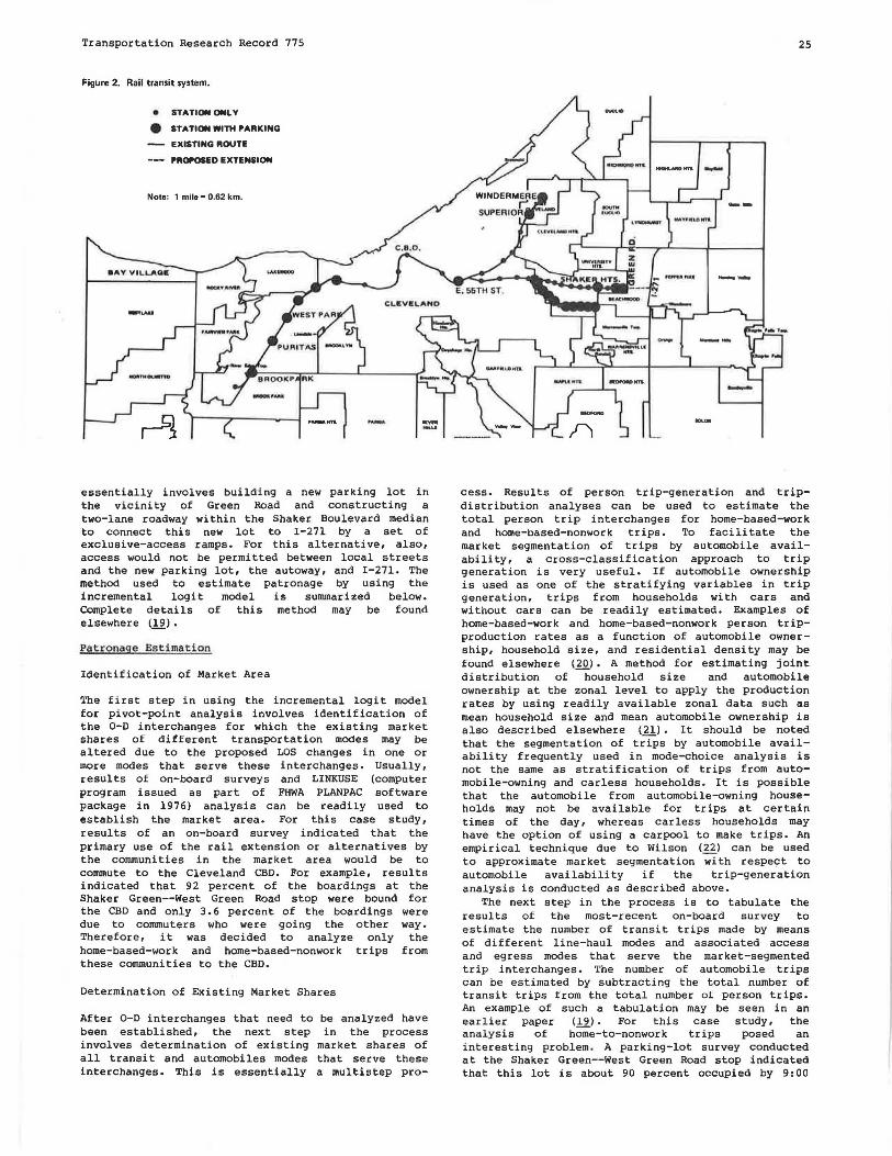
Transportation Research Record 775
Figure 2. Rail transit system.
e STATIONONLY
• STATION Wint ,ARKING
EXISTING ROUTE
,ROl'OSED EXTENSION
Note: 1 mile= 0.62 km.
..... ......
essentially involves building a new parking lot in the vicinity of Green Road and constructing a two-lane roadway within the Shaker Boulevard median to connect this new lot to I-271 by a set of exclusive-access ramps. For this alternative, also, access would not be permitted between local streets and the new parking lot, the autoway, and I-271. The method used to estimate patronage by using the incremental logit model is sullllnarized below. Complete details of this method may be found elsewhere (19) •
Patronage Estimation
Identification of Market Area
The first step in using the incremental logi t model for pivot-point analysis involves identification of the 0-D interchanges for which the existing market shares of different transportation modes may be altered due to the proposed LOS changes in one or more modes that serve these interchanges. Usually, results of on-board surveys and LINKUSE (computer program issued as part of FHWA PLANPAC software package in 1976) analysis can be readily used to establish the market area. For this case study, results of an on-board survey indicated that the primary use of the rail extension or alternatives by the co11Ununities in the market area would be to co11Unute to the Cleveland CBD. For example, results indicated that 92 percent of the boardings at the Shaker Green--West Green Road stop were bound for the CBD and only 3. 6 percent of the boardings were due to co11Unuters who were going the other way. Therefore, it was decided to analyze only the home-based-work and home-based-nonwork trips from these co11Ununities to the CBD.
Determination of Existing Market Shares
After 0-D interchanges that need to be analyzed have been established, the next step in the process involves determination of existing market shares of all transit and automobiles modes that serve these interchanges. This is essentially a multi step pro-
25
cess. Results of person trip-generation and tripdistribution analyses can be used to estimate the total person trip interchanges for home-based-work and home-based-nonwork trips. To facilitate the market segmentation of trips by automobile availability, a cross-classification approach to trip generation is very useful. If automobile ownership is used as one of the stratifying variables in trip generation, trips from households with cars and without cars can be readily estimated. Examples of home-based-work and home-based-nonwork person tripproduction rates as a function of automobile ownership, household size, and residential density may be found elsewhere (20) • A method for estimating joint distribution of household size and automobile ownership at the zonal level to apply the production rates by using readily available zonal data such as mean household size and mean automobile ownership is also described elsewhere (21). It should be noted that the segmentation of trips by automobile availability frequently used in mode-choice analysis is not the same as stratification of trips from automobile-owning and carless households. It is possible that the automobile from automobile-owning households may not be available for trips at certain times of the day, whereas car less households may have the option of using a carpool to make trips. An empirical technique due to Wilson (22) can be used to approximate market segmentation with respect to automobile availability if the trip-generation analysis is conducted as described above.
The next step in the process is to tabulate the results of the most-recent on-board survey to estimate the number of transit trips made by means of different line-haul modes and associated access and egress modes that serve the market-segmented trip interchanges. The number of automobile trips can be estimated by subtracting the total number of transit trips from the total number of person trips. An example of such a tabulation may be seen in an earlier paper (19) • For this case study, the analysis of home-to-nonwork trips posed an interesting problem. A parking-lot survey conducted at the Shaker Green--West Green Road stop indicated that this lot is about 90 percent occupied by 9: 00

26
a .m., whereas a 1963 home 0-D survey showed that about 60 percent of the nonwork person trips to the CBD are made between 9:00 a.m. and 4:00 p.m. Therefore, it became apparent that there is a latent demand for additional park-and-ride facilities. In order to determine the magnitude of this latent demand, use of parking spaces at the Brookpark, Puritas, and Westpark stops (Figure 2) was studied. The maximum occupancy of parking spaces at these stops is currently about 42 percent. Therefore, it was assumed that communities served by these stops do not experience any parking shortages during any time of the day. Results of an on-board survey showed that about 7 percent of the home-to-nonwork trips to the CBD from these communities are made by using the rapid transit and park-and-ride mode of access. Communities served by the Shaker Green--West Green Road stop showed that only 3.S percent of the nonwork trips to the CBD were made by using the Shaker Green Line and park-and-ride mode of access. I assume that, if there were no shortage of parking space at the Shaker Green--West Green Road lot, 7 percent of the nonwork trips would have been made by using rail rapid transit; the unconstrained number of park-and-ride trips was derived by factoring the observed number of trips by 2. O. Once the number of trips along all possible modes that serve an 0-D pair had been determined, aggregate market shares were calculated by dividing the modal trips by total person trips.
Determination of Changes in Modal Disutilities
Changes in modal disutilities can be calculated first by expressing the proposed policy in terms of changes in travel time and travel cost and then by multiplying these changes by the appropriate coefficient values presented earlier. For this case study, the impact on the number of boardings at the Shaker Green--West Green Road stop was analyzed for (a) possible reduction in automobile access time to the stop due to the construction of new ramps (autoway and rail-extension alternatives) and (b) possible increase in automobile operating cost due to the gasoline-price increase. Three possible scenarios for automobile operating cost increases were developed: 25, SO, and 100 percent increase in automobile operating cost per mile.
Determination of Revised Market Shares
Once the existing market shares have been estimated and changes in modal disutilities calculated, revised market shares can be obtained by using Equation 1. At times the revised market share may indicate trips on a certain mode that are not physically possible due to the supply constraint. For example, in the present case study, the do-nothing option cannot accommodate additional park-and-ride trips. However, if the pivot-point procedure is applied by assuming increase in automobile operating expense and no change in transit fare, more trips may be assigned to the Shaker Green Line than are physically possible. To avoid this situation, a shadow price can be calculated to artificially increase the disutili ty of the mode in which equilibrium between supply and demand has to be maintained.
For this case study, the shadow price was calculated as follows. Let Prail a, Prail 0 ,
Pbus• and Pauto be the existing market shares of rail with automobile access (park-and-r ide), rail with access modes other than automobile (walk, feeder bus, kiss-and-ride), express bus, and automobile, respectively. Let 6Uauto denote the change in disutili ty of the automobile mode. Then,
Transportation Research Record 775
by using the incremental logit model, the revised market share of rail that has the automobile access mode (Frail a) can be expressed as follows:
(6)
Now, if the impact of change in disutili ty of the automobile mode (that is, 6Uauto> is such that Prail a > Prail a but it is not physically possible to satisfy this additional demand due to supply constraint, a shadow price (6C) can be imposed on the rail alternative that has automobile access to ensure that Prail a = Prail a The numerical value of this shadow price can be calculated by using Equation 6 as follows:
Praila = Prai1 86C/[P,0 i1 8 6C + Prail 0 + Pbus + Pauto exp(6Uauto)J (7)
This expression can be rearranged to yield
6C = lPrai1° +Pb us + Pau to exp(6Uau 10)] /(I - Prai13) (8)
The revised other than (Pbus>, and by using the
market shares of rail that has access by automobil~ (Frai l 0 ), express bus automobile fPauto> can be calculated
following equations:
1\uto = Pauto exp(6Uauto>
_,_ [Prail'6C + Prai1° + Pbu s + Pauto exp(6Uauto)J (I I)
where 6C is first calculated by using Equation 8.
Numerical Example
For the city of Mayfield Heights, data related to home-based work trips to the CBD are as follows: total person trips to the CBD = 793, trips made by using the Shaker Green Line = 141, and trips made by using express bus = 186. Network analysis indicated that redu~tion in access travel time by automobile to the Shaker Green--West Green Road lot due to the construction of an autoway alternative would be 3. 4 min. If the automobile operating cost per mile increases by SO percent, change in travel cost for a trip to the CBD will be 33¢. To determine the number of new rides on the Shaker Green Line from this community, we use the following calculations:
Pshaker = 141/793 = 0.178, 0.234, Pauto = 466/793 3.4 min, 6Cauto = 33¢.
Pbus 186/793 = O.S88, 6tshaker =
By using Equation 1 and the default values of the coefficients for in-vehicle travel time and travel cost, the revised market share of the Shaker Green Line is calculated as follows:
Pshaker = [0.178 x exp(0.032 x 3.4))/(0.17 x exp(0.032 x 3.4) + 0.234 + O.S88 x exp(-0.01 x 33)) = 0.232.
Therefore, new rides on the Shaker Green Line 0.232 x 793 - 141 = 43.
Changes in market shares for home-to-nonwork trips to the CBD were analyzed in a similar manner. Changes in ridership due to non-home-based trips and destinations other than the CBD were estimated by using suitable factors for the home-based-work and nonwork trips (12,).

Transportation Research Record 775
Table 2. Projected new rides on the study alternatives.
Assumed Automobile Operating Cost per Mile (cunts)a
Study Alternative 6 7.5 12
Do nothing 0 250 520 1126 Expand Green Road parking lot 638 1912 2888 5016
Build autoway 1224 2208 3236 5538 Extend rail line 1932 2938 3998 6370
a At the time of this study, the prevailing perceived out-of-pocket cost for operating the automobile was assumed to be Gd/mile.
RESULTS
The results obtained by using pivot-point analysis and base-year (1975) market shares are summarized in Table 2.
CONCLUSION
Changes in travel demand due to changes in LOS on one or more transportation modes that serve an urban area can be readily estimated by using pivot-point analysis. This technique is much less cumbersome to use than traditional mode-split models. Many policy issues related to fare structure, headway, automobile operating cost, etc., can be quickly analyzed by using this procedure. This paper also illustrates the use of pivot-point analysis for specific project-level planning in addition to its use for the quick order-of-magnitude analyses described in the literature (2_,16).
ACKNOWLEDGMENT
The preparation of this paper was financed through a grant for technical studies from the Urban Mass Transportation Administration and the Federal Highway Administration of the u.s. Department of Transportation with joint sharing in the cost by Cuyahoga, Geauga, Lake, Lorain, and Medina counties and the municipalities within them.
REFERENCES
1 . M. J. Fertal, E. Weiner, A. J. Balek, and A. F. Sevin. Modal Split: Documentation of Nine Methods for Estimating Transit Usage. Bureau of Public Roads, U.S. Department of Commerce, 1967.
2. Peat, Marwick, Mitchell and Co. Implementation of the N-Dimensional Logit Model. Comprehensive Planning Organization, San Diego, CA, 1972.
3. D. McFadden. Conditional Logit Analysis of Qualitative Choice Behavior. .!.!!. Frontiers in Econometrics (P. Zarembka, ed.), Academic Press, New York, 1973.
4. Rand Corporation. A Policy-Oriented Urban Transportation . Model: The San Diego Version. Office of Environmental Management, County of San Diego, Santa Monica, CA, 1973.
5. Cambridge Systematics. Guidelines for
27
Travel-Demand Analysis of Program Measures to Promote Carpools, Vanpools, and Public Transportation. u.s. Department of Energy, 1976.
6. G. v. Wickstrom and A. B. Sosslau. Travel Estimation Procedures for Quick Response to Urban Policy Issues. NCHRP, Rept. 186, 1978.
7. B. D. Spear. Application of New Travel-DemandForecasting Techniques to Transportation Planning. Urban Planning Division, Federal Highway Administration, U.S. Department of Transportation, 1977.
8. Census Data and Urban Transportation Planning. TRB, Special Rept. 145, 1974.
9. R. H. Pratt and Associates and DTM, Inc. Development and Calibration of Mode-Choice Models for the Twin Cities Metropolitan Council. Minneapolis, MN, 1976.
10. T. J. Atherton, J. H. Suhrbier, and W. A. Jessiman. Use of Disaggregate Travel-Demand Models to Analyze Carpooli ng Policy Inc~nti ves. TRB, Transportation Research Record 599, 1976, pp. 35-40.
11. M. F. Wigner. Disaggregated Modal-Choice Models of Downtown Trips in the Chicago Region. HRB, Highway Research Record 446, 1973, pp. 49-65.
12. T. J. Atherton and M. E. Ben-Akiva. Transferability and Updating of Disaggregate Travel-Demand Models. TRB, Transportation Research Record 610, 1976, pp. 12-18.
13. A. P. Talvitie. Aggregate Travel-Demand Analysis with Disaggregate or Aggregate Travel-Demand Models. Proc., Transportation Research Forum, Vol. 14, No. 1, 1973.
14. F. s. Koppelman. Methodology for Analyzing Errors in Prediction with Disaggregate Choice Models. TRB, Transportation Research Record 592, 1976, pp. 17-23.
15. F. s. Koppelman and M. E. Ben-Akiva. Aggregate Forecasting with Disaggregate Travel-Demand Models Using Normally Available Data. Presented at World Conference on Transport Research, Rotterdam, the Netherlands, 1977.
16. Cambridge Systematics. Urban Transportation Energy Conservation: Case City Applications of Analysis Methodologies, Volume 3. U.S. Department of Energy, 1978.
17. Urban Systems. Aggregation Procedure--The Monte Carlo Simulation. Northeast Ohio Areawide Coordinating Agency, Cleveland, 1978.
18. F. s. Koppelman. Guidelines for Aggregate Travel Prediction Using Disaggregate Choice Models. TRB, Transportation Research Record 610, 1976, pp. 19-24.
19. A. Kumar. Mode-Mixer Feasibility Study: Patronage Estimates. Northeast Ohio Areawide Coordinating Agency, Cleveland, 1979.
20. A. Kumar. Trip-Generation Analysis: Calibration of Trip Production Models. Northeast Ohio Areawide Coordinating Agency, Cleveland, 1980.
21. A. Kumar. Trip-Generation Analysis: Methodology for Estimating Joint Distribution of Household Size and Automobile Ownership. Northeast Ohio Areawide Coordinating Agency, Cleveland, 1980.
22. A. G. Wilson. Urban and Regional Models in Geography and ~lanning. Wiley, New York, 1974.

28 Transportation Research Record 775
Model Specification, Modal Aggregation, and Market
Segmentation in Mode-Choice Models: Some Empirical Evidence
YOUSSEF DEHGHANI AND ANTTI TALVITIE
Multinomial logit models that have four, five, and seven alternatives are de· scribed for work-trip mode choice. The most satisfactory overall specification is based on treating travel-time components as a single variable in additive and generic form and also on equating three,rail alternative-specific constants (in the seven-alternative models) as a result of statistical tests. A simplistic method is used to aggregate rail and bus modes in the five- and four-alternative models, respectively. The resulting coefficients of corresponding variables among all the models are all consistent since they are statistically equal and numerically very close. Statistical tests show that at least alternative-specific constants, which account for over two-thirds of the total explanatory power of the models, are valued differently for the following markets: (a) one- versus two-car households, (b) commuters bound for the central business district versus others, and (c) low· and high-income households that also value service attributes unequally. Finally, coefficients estimated by means of observation of level-of· service attributes or by means of network models that estimate these attributes are also compared.
A series of multinomial logit models for work-trip mode choice that have four, five, and seven alternatives is described. The four basic alternatives are drive alone, shared ride, bus, and rail. In the five-alternative model, the bus mode is separated into local-bus and express-bus modes and, in the seven-alternative model, rail is further divided into the modes of rail that has walk access, rail that has bus access, and rail that has car access. The data used in this study were originally collected by the Urban Travel Demand Forecasting Project (UTDFP) at the University of California at Berkeley in 1975.
A number of alternative model specifications were tested, and the results of these tests were analyzed. The model specification that was considered to be the most satisfactory overall is based on treating travel-time components (in-vehicle and excess times, i.e., wait and walk times) as a single variable in additive and generic form. Alternative-specific constants for the three rail modes (in the seven-alternative model) were found to be statistically equal for the models calibrated that had observed service attributes. This refined and simplified model specification is used to analyze the effect of market segmentation on model coefficients. Three market segments are used--oneversus two-car households, low- versus high-income households (annual household income of $13 000 was used as the point of division between high and low income), and commuters bound for the central business district (CBD) versus others.
The results are presented in the following order. First, some model-specification issues are discussed. This is followed by a discussion and analyses on aggregation of alternatives. Third, market segmentation is studied. Last, the models with observed and network level-of-service (LOS) data are compared.
MODEL SPECIFICATION
Travel Time
Previous studies by Talvitie and Dehghani (J)
suggest that, statistically speaking, the travel-time components are valued equally, at least when the observed LOS data are used. The folklore of mode-choice models divides travel time into excess and line-haul componentsi the former has a value two to three times that of the latter.
The following explanatory variables are used in the models:
Variable INVT
WALKT
TRANSFERS WAI'rT
TTIME
COST/INC
DR CARS/DR
EMPD
WACCESS
CBD
CONST
LOG(N)
Definition In-vehicle time or time spent inside a
vehicle when traveling from origin to destination, door to door (round-trip time) (min)
Walk time to and from bus stop or Bay Area Rapid Transit (BART) station, in transfer, or to and from car's parking place (min)
Number of transfers Sum of wait times of all transit
vehicles, normally one-half of first headway [headway of first transit vehicle boarded on a trip (min)] plus sum of wait times of second, third, etc., transit vehicles at transit transfer points (min)
Sum of in-vehicle time, walk time, and wait time (determined in same way as WAI TT)
Out-of-pocket travel cost divided by household income (dollars)
Number of driverq in household Number of cars owned divided by number
of drivers Employment density in neighborhood
(employees per acre) Walk access to transit facility (takes
value of 1.0 if transit-mode stop or station is within 0.60 mile from residence)
Dummy variable constructed to differentiate trips destined to CBD from these destined to other locations (takes value of 1.0 if EMPD is greater than 120.0, zero otherwise)
Constant (takes value of 1.0 for specified alternative, zero otherwise)
Natural log of number of transit-access modes (N) accessible (available)
The null hypothesis that the excess and line-haul components are valued equally was accepted for both the observed and the network LOS datai these two types of data are defined in Table 1, which gives the models that have the segmented travel times. The supporting statistics for Table 1 are as follows [L(S*) is log likelihood at maximum, the success index is the weighted average of differences in correct predictions between the full model and the model that used only alternative-specific constants, and prediction success is that percentage attrib-

Transportation Research Record 775
Table 1. Model specification and coefficients with segmented travel times.
Type of LOS Datab
Alterna- Network Observed live
Variable Entered" Coefficient !-Value Coefficient !-Value
INVT 1-7 -0.0198 2.21 -0.021 5 2.29 WALKT l-7 -0.047 3 1.90 -0.018 2 2.66 WAITT l-7 -0.034 5 3. 16 -0.020 8 1.95 TRANSFERS 2-6 0.176 1.79 -0.050 0.30 COST/INC l-7 -8.438 l.20 -38.56 3.10 DR 1,7 0.454 2.90 0.082 3 0.42 CARS/DR I 2.369 4.43 l.824 2.73
7 l. I 85 2.42 0. 760 78 l.22 EMPD l -0.001 32 2.89 -0.001 53 2.81 WACCESS 2,4,5 0.852 2.89 0.679 2.03 CBD 1,7 -l.096 3.30 -1.039 8 2.42
4-6 2.270 3.8 l 0.895 1.84 CONST 1 -1.747 2.34 -0.252 0.31
3 -0.807 2.10 -0.561 1.61 4 -3. 799 4.97 - l.878 3.10 5 -3.749 5.46 -l.578 2.76 6 -2.260 3.77 -l.085 2 2.13 7 - l.787 2.54 -0.785 1.07
a Alternatives: 1 = drive alone, 2 =local bus, 3 =express bus, 4 "' BART with walk access, 5 = BART with bus access, 6 = BART with car access, and 7 = shctred ride.
bNetwork LOS data are zone-to-zono travel times and cost obtained from standard coded networks by using the Urban Transportation Planning System (UTPS) or its equivalent. Observed LOS data \/Vere obtained by direct observation, measurement of travel times and costs for a door-to-door trip, or both (l l.
Table 2. Model specification and coefficients with one rail-mode constant.
Type of LOS Data
Alterna- Network Observed tive
Variable Entered Coefficient t-Value Coefficient !-Value
TTIME l-7 -0.021 9 4.67 -0.021 0 4.78 COST/INC 1-7 -8.842 1.2 l -38.609 3.10 DR 1,7 0.466 3.00 0.082 0.42 CARS/DR l 2.367 4.45 1.823 2.74
7 1.187 2.45 0.759 l.22 EMPD 1 -0.001 31 2.83 -0.001 53 2.81 WACCESS 2,4,5 0.862 2.95 0.635 1.96 CBD l,7 -1.228 3.77 -l.073 2.59
4-6 2.324 3.90 0.883 l.84 CONST I - 1.306 2.04 -0.238 2.95
3 -0.554 1.87 -0.599 l.76 4 -4.098 5.98 - l.744 3.39 5 -3.549 5.48 -1.626 3.10 6 -2.179 3.70 - l.058 2.13 7 -l.326 2.30 -0.777 l.03
Note: Alternatives are same as in Table 1.
Table 3. Model specification and coefficients with three rail-mode constants.
Type of LOS Data
Alterna- Network Observed tive
Variable Entered Coefficient !-Value Coefficient t-Value
TTIME 1-7 -0.027 7 6.84 -0.024 5 6.16 COST/INC 1-7 -9.663 1.31 -37.325 3.00 DR l,7 0.437 2.82 0.063 5 0.32 CARS/DR I 2.345 4.40 l.813 2.70
7 l.189 2.41 0.760 1.21 EMPD I -0.00 l 29 2.80 -0.00 I 54 2.83 WACCESS 2,4,5 0.404 l.60 0.397 l.46 CBD 1,7 - l.275 3.90 -l.094 2.62
4-6 2.249 3.81 0.845 l.75 CONST I - l.779 2.82 -0.57 0.73
3 -0.836 3.00 -0.764 2.42 4-6 -3.!34 5.72 -l.457 3.35 7 -l.762 3.10 -l.074 l.47
Note: Alternatives are same as in Table 1.
29
utable to variables other than alternative-specific constants] :
Statistic L(ll*)
Percent right (maximum utility classification)
Success index Successful predic-
t ion (%) Prediction success
due to other than modal constants (%)
Network -583.927
63.40 0.097
49.6
20(= 9.7/49.6)
Observed -478.36
66.80 0.152
54.3
28
It may be seen that, in the network model, the ratio of the coefficients of excess time to in-vehicle time has the customary value of about 2: for the model that has observed travel times, this ratio has a value of 1. Again, statistically speaking, the travel-time components are valued equally. This result is adopted for further analyses in this paper. It is also a result that one can live with fairly comfortably, considering the accuracy of the travel-time data. Briefly, studies by Talvitie and Dehghani (1) and Talvitie and Anderson Ill show that the excess-time components are poorly approximated by the network models, but the total travel time (at least for car and bus modes) is calculated quite well by the network models.
Modal Constants
These have a totally different function from that of the other variables. If the variables included in the modal utility functions fully explain mode-choice behavior, then the modal constants should equal zero. Thus, with a perfect model specification and with perfect data, it can be argued that no constants are necessary. However, estimating a model without constants is not reconunended in practice because the estimated values of the coefficients of the variables included are seriously affected if those variables do not fully explain the observed behavior. The constants, therefore, represent the effect of those variables that influence mode choice but are not included explicitly in the model. This effect was found empirically to be substantial (1) and accounts for more than two-thirds of the total explanatory power of the model.
In the seven-alternative models developed in this study, the alternative-specific constants for rail were found to be statistically equal at the 0. 05 level of significance by using observed service attributes. However, when the network-based service attributes were used, statistical equality of the rail mode's modal constants was rejected. The relevant models are shown in Tables 2 and 3. The supporting statistics are shown below [L (OJ is log likelihood at zero] for Table 2:
Statistic L(O)
L( B*) Percent right (maxi
mum utility classification)
Sample size Success index Successful predic-
tion (%)
Prediction success due to other than modal constants (%)
Network -1005.987 586.155
62.43 626 0.096
49.5
19
Observed -724.633 -478.547
66.67 567 0.152
54.3
28

-.
30
and for Table 3:
Statistic Network Observed L(O) -1005.987 -724.633 L (a*) -597.235 -480.118 Percent right (maxi-
imum utility classification) 61.98 66.84
Sample size 626 567 Success index 0.091 0.152 Successful predic-
tion (%) 48.9 54. 2 Prediction success
due to other than modal constants (%) 19 28
For three reasons, the results of one modal constant for rail mode are adopted for further work. First, summary indices of predictive accuracy for the model that has one rail-mode constant are not materially worse than those for the model that has three rail-mode constants (Tables 2 and 3). Second, the model with one modal constant enables easier aggregation of alternatives. Last, the observed LOS data are more reliable than the network data and that model suggests that one modal constant for rail is enough. It is further evident that the modal constant for express bus is no different from that for rail. This finding enables the application of a model developed for the express-bus mode to be used for a new rail-mode situation.
Other Specification Issues
The models in Table 3 indicate that the variable DR is insignificant in the model that uses observed LOS data but has strong significance in the network-based model. A model estimated without both variables DR and CARS/DR is shown in Table 4. The supporting statistics are shown below:
Statistic Network Observed L(O) -1005.987 -724.633 L(a*J -609.425 -484.438 Percent right (maxi-
mum utility classification) 62.62 67.20
Sample size 626 567 Success index 0.083 0.149 Successful predic-
tion (%) 48.2 53.9 Prediction success
due to other than modal constants (%) 17 28
Table 4. Model specification and coefficients estimated without variables DR and CARS/DR.
Type of LOS Data
Alterna- Network Observed tive
Variable Entered Coefficient !-Value Coefficient t-Value
TTIME 1-7 -0.029 I 6.30 -0.024 5 6.21 COST/INC 1-7 -10.241 1.35 -38.306 3.10 EMPD I -0.001 22 2.64 -0.001 47 2.70 WACCESS 2,4,5 0.463 1.87 0.399 1.47 CBD 1, 7 -1.217 3.86 -1.091 2.51
4-6 2.246 3.84 0.903 1.88 CONST I 0.787 2.40 0 .984 2.56
3 -0.825 3.00 -0.762 2.41 4-6 -3.219 5.94 -1.514 3.50 7 -0.177 0.60 -0.413 I 1.10
Note: Alternatives are same as in Table 1.
Transportation Research Record 775
Prediction-success indicators show that the network-based model lost more in predictive power than the model based on observed LOS data. Future work will study in more detail whether this pattern and the surprisingly small loss in predictive power will also hold when models are transferred to other locations. Clearly, forecasting errors in the variables CARS and CARS/DR might be more detrimental to forecasting accuracy than errors due to excluding these variables from the model altogether.
AGGREGATION OF ALTERNATIVES
Most of the modes actually represent a group of modes: For example, several bus lines or carpooling arrangements may be available. In the seven-alternative model, the bus and rail modes are separated into their various components. Model simplification would be accomplished if the components of bus and rail modes could be represented by two modes or one composite mode--for example, bus and rail or simply transit. In this section a method for aggregating alternatives is studied.
McFadden (ll has shown that if there are J choice groups and Mj components (submodes) within each group (mode) and if each component has a utility function of the form Vjm o 'Yj + ll 'Xjm• where Yj represents attributes common to the group and Xjm• attributes specific to the component, then the choice probability for a group is
(I)
(2)
If there is no variation in the attributes of the component alternatives, Xjm = O and Wj (l ojl logMj. If the unobserved attributes of the component alternatives are uncorrelated, the parameter s oj are equal to zero and the usual MNL form is obtained. If. Cl j = l, the unobserved attributes are perfect.ly correlated and the term vanishes.
In this study we assumed that the variation in the component attributes (Xjml was very small and calculated the group attributes (y jl for BART (rail) by using the fol lowing conventions:
1. BART that has walk access was used if the residence location was within 0. 60 mile of a BART station,
2. BART that has automobile access was used if the household owned at least two cars, and
3. BART that has bus access was used otherwise.
For bus, the group attributes were calculated by using the following:
1. Express bus was used if the service existed and was accessible and
2. Local bus was used otherwise.
Model-estimation results showed that the parameters a j were not statistically different from zero. At the same time, t he addition of logMj to the model brought at least some degree of stability to the values of the modal constants regardless of whether seven, five, or four alternatives were used. This procedure of using a somewhat maximum mode to represent the group also facilitates partitioning the results into access-mode levels.

Transportation Research Record 775
The estimated models are shown in Tables 5 and 6 for five and four alternative modes, respectively. The supporting statistics follow for Table 5:
Statistic L(O) L (6 *)
Percent right (maximum utility classification)
Sample size Success index Successful predic-
Network -922.937 -561. 275
63.61 621 0.099
t ion (%) 50.4 Prediction success
due to other than modal constants (%) 20
Observed -637.543 -430.055
69.29 560 0.165
56.6
29
Table 5. Model specification and coefficients with five alternative modes.
Type of LOS Data
Alterna- Network Observed tive
Variable Entered Coefficient !-Value Coefficient !-Value
TTIME 1-5 -0.022 3 4.99 -0.017 8 3.88 COST/INC 1-5 -10.790 1.42 -37.943 3.04 DR 1,5 0.586 3.64 0.292 1.41 CARS/DR I 2.799 5.02 2.326 3.38
5 1.591 3.02 1.208 1.86 EMPD 1 -0.001 25 3.66 -0.001 49 2.71 WACCESS 2,4 0.173 0.65 0.130 0.42 CBD 1,5 -1.335 4.00 -0.947 2.22
4 1.698 3.30 0.829 1.63 CONST .l -2.182 3.20 -1.105 1.26
3 -0.901 3.24 -0.87 2.74 4 -2.340 4.98 -1.246 2.81 5 -2.189 3.50 -1.613 1.97
LOG (N) 4 1.0 1.0
Note: Alternatives: 1 = drive alone, 2 • local bus, 3 =express bus, 4 = BART, and 5 =
shared ride.
Table 6. Model specifica.tion and coefficients with four alternative modes.
Type of LOS Data
Alterna- Network Observed tive
Variable Entered Coefficient !-Value Coefficient !-Value
TTIME 1-4 -0.023 8 5.20 -0.016 7 3.70 COST/INC 1-4 -9.399 1.30 -37.452 3.00 DR 1,4 0.581 3.60 0.305 1.47 CARS/DR I 2.792 4.98 2.322 3.36
4 1.588 2.98 1.198 1.84 EMPD l -0.001 28 2.72 -0.001 51 2.72 WACCESS 2,3 0.123 0.50 -0.015 6 0.05 CBD 1,4 -1.294 3.86 -0.936 2.70
3 1.718 3.30 0.878 1.72 CONST I -2.552 3.77 -1.351 • 1.56
3 -2.024 4.33 -0.998 2.28 4 -2.531 4.10 -1.859 2.29
LOG(N) 2,3 1.0 1.0
Note: Alternatives: 1 = drive alone, 2-= local and express bus, 3 = BART, and 4 =shared ride.
Table 7. Alternative·specific constants of the rail mode .
Observed LOS Data Network LOS Data
With Without With Without Model logMj logMj logMj logMj
Seven alternatives -1.457 -1.457 -3.134 -3.134 Five alternatives -1.246 -0.488 -2.340 -1.618 Four alternatives -0.998 -0.809 -2.024 -1.983
and for Table 6:
Statistic L(O) L (6*) Percent right (maxi
mum utility classification)
Sample size Success index Successful predic-
tion (%) Prediction success
Network -757.727 -508.942
65.86 621 0.115
52.7
due to other than modal constants (%) 22
Observed -545.876 -388.489
71.01 545 0.179
59.1
30
31
Table 7 contains a comparison of alternativespecific constants. Note that the coefficients of other variables, notably those of WACCESS, have also changed due to modal aggregation.
Statistical tests of coefficients are an incomplete means of assessing the similarity of forecasts by different models. When model specification is changed, all the coefficients change to some degree but not really substantially. The most troublesome changes are those in the alternative-specific constants. There is an ongoing study to determine empirically whether the method of modal aggregation reported here is as useful in making forecasts as it seems to be in achieving regularity in coefficients.
MARKET SEGMENTATION
Three variables were defined to divide the travelers into market segments. These were (a) car ownership--one versus two or more cars per household (there were too few carless households to allow analyses of that segment of the market), (bl CBDbound commuters versus others, and (c) income--less than $13 000 per year versus more than $13 000 per year.
The results are summarized as follows. The carownership models for the one- and two-car families were statistically equivalent when f.i ve- or fouralternati ve model structures were used, regardless of whether the service attributes were obtained from the networks or coded manually. On the basis of visual examination, the inclusion of carlese households in the models did not affect the coefficients.
When the seven-alternative model was used, the alternative-specific constants were different but other coefficients were equal. From a visual examination, it seems that the walk-access variable has a very strong positive effect on transit ridership for car less and one-car households; this variable has a reverse influence for transit use for two-car households. Not surprisingly, it is the rail mode's constant that causes these problems. Apparently, there is interaction among car ownership, location of residence, and availability of transit to work that is not captured by the model as specified here.
For the CBD and non-CBD travelers, the results depend on whether network or observed LOS data are used. When the observed values of service variables are used, the models for CBD and non-CBD travelers are equivalent if separate CBD dummies are used for rail and automobile modes. However, when networkbased service variables are used, the coefficients for both the socioeconomic and service variables are different regardless of the number of alternatives in the model. We will discuss the reasons for the ambiguous results later.
The division of travelers by rather clear results: The modal
income produced constants and

32
coefficients of the service variables are different, but the coefficients of the socioeconomic variables are equivalent for the two market segments regardless of the number of alternatives used in the model. The models for the two income groups are shown in Tables 8 and 9. The supporting statistics are shown below for Table 8:
Statistic L(O) L(t>*) Percent right (maxi
mum utility classification)
Sample size Success index Successful predic-
tion (%)
Prediction success due to other than modal constants (%)
and for Table 9:
Statistic L(O) L(6*) Percent right (maxi-
mum utility classification)
Sample size Success index Successful predic-
tion (%) Prediction success
due to other than modal constants (%)
Network -406.225 -254.654
62.11 256 0.110
47.3
23
Network -599.762 -317.235
63.51 370 0.093
52.7
18
Observed -304.915 -192.116
68.53 232 0.195
55.9
35
Observed -419. 718 _;261.531
67.16 335 0.139
56.2
25
It is seen from Tables 8 and 9 that there are clear differences in the coefficients for one income group. Surprisingly, the low-income travelers are less elastic with respect to cost. At average values, the cost elasticities are -0.03 to -0.23 for the low-incom~ and -0.50 to -0.60 for the high-income travelers. In general, seems to be more applicable than to high-income travelers.
however, the to low-income
model rather
COMPARISON OF MODELS THAT USE NETWORK AND OBSERVED LOS VARIABLES
An earlier study by Talvitie and Dehghani (1) found that models developed by using network and observed LOS variables resulted in differing coefficients for modal constants and service variables for the two types of data. In the current model specification, travel-time components and rail modal constants have been consolidated.
With this new model specification, the models that use network and observed LOS variables are statistically equivalent except for the sevenalternative model, in which the modal constants are still different for the two types of data. It is noted that the cost coefficient alone is borderline: The t~statistic for the test of the equality is 1.92; the critical value is 1.96. Table 10 gives the results.
The results of Table 10, although encouraging, must be checked against the forecasting and transferability aspects of the models. As seen from Table 3, the cost coefficient is four times higher when observed data are used than it is when network data are used. There are also substantial differences in the CBD dummy and rail-mode constant. Also troublesome is the fact that the two types of data yield different models for the CBD and non-CBD
Transportation Research Record 775
Table 8. Model specification and coefficients for low-income households.
Type of LOS Data
Alterna- Network Observed tive
Variable Entered Coefficient t-Value Coefficient !-Value
TTIME 1-7 -0.031 2 4.0 -0.010 9 1.79 TRANSFERS 2-6 0.279 2.3 0.063 1 0.40 COST/INC 1-7 -2.773 0.40 -23.477 1.63 DR 1,7 0.572 2.54 0.550 1.50 CARS/DR 1 1.427 1.88 1.614 1.45
7 1.010 1.4 1.238 1.20 EMPD 1 -0.001 41 1.80 -0.001 38 1.74 WACCESS 2,4,5 0.694 2.10 0.818 2.15 CBD 1,7 -0.909 2.0 -1.229 1.90
4-6 2.811 2.56 2.205 2.10 CONST 1 -1.497 1.73 -0.069 7 0.05
3 -1.256 3.30 -0.930 2.22 4-6 -4.389 4.20 -3.067 2.94 7 -2.157 2.73 -1.423 1.15
Note: Alternatives are same as in Table 1.
Table 9. Model specification and coefficients for high-income households .
Type of LOS Data
Al tern a- Network Observed tive
Variable Entered Coefficient t-Value Coefficient t-Value
TTIME 1-7 -0.032 1 3.20 -0.037 7 5.13 TRANSFERS 2-6 -0.028 2 0.20 -0.064 7 0.32 COST/INC 1-7 -80.214 3.60 -107 .52 4.32 DR 1,7 0.090 9 0.34 -0.086 9 0.31 CARS/DR 1 3.513 4.23 2.439 2.67
7 1.777 2.32 0.715 0.84 EMPD 1 -0.000 572 l.O -0.001 56 1.92 WACCESS 2,4,5 0.025 3 0.06 0.315 0.70 CBD 1,7 -1.558 2.80 -0.584 0.88
4-6 1.540 1.98 0.637 0.89 CONST 1 -0. 749 0.74 -0.834 0.74
3 -0.076 8 0.20 -0.002 54 0.005 4-6 -1.938 2.60 -0.345 0.52 7 -0.630 0.70 -0.993 0.93
Note: Alternatives are same as in Table 1.
travelers. This and other issues are discussed in the next section.
DISCUSSION OF RESULTS AND CONCLUSIONS
The issues studied in the previous four sections are interrelated and really cannot be studied separately. Because of the complexity of the subject, the attempted separation of tasks can be defended on the grounds of clarity of presentation. In this section we try to make some amends.
It its appropriate to start the discussion with the measurement of travel-time and cost variables. The discrepancy in the cost coefficient depending on whether network or observed LOS data were being used is disturbing. The explanation for this discrepancy most probably involves the way in which parking costs have been calculated. The coded networks assign travelers the zonal parking cost. This figure is misleading. Surveys that have asked about the parking cost show that few drivers actually pay for parking. There is also a large variance in parking costs for those who pay. This is because, by walking a longer distance, one can normally park for less and because, for many zones, available parking spaces vary greatly in cost.
There are even-greater problems in assigning parking costs for transit users' potential automobile trips. Do the transit users know what the

Transportation Research Record 775
Table 10. Chi-square statistics for tests of coefficient equality.
Seven Alternatives
Accept Critical X2 or
Null Hypothesis x2 (0.05 level) Reject
Equality of alternative-specific constants 10.412 9.48" Reject Equality of coefficients of service variables 2.508 7.80 Accept
Equality or coefficients of socioeco· nomic variables 10.212 9.48' Reject
Equality or coefficients of service varia· bles given unequal alternative-specific consta nts 3.630 7.80 Accept
Equality of coefficients of socioeco· nomic variables given unequal alterna-live-specific constants 2.768 9.48 Accept
8This statist ic is 11 .16 at the 0.025 level ,
parking charges will be? Would current transit users be eligible for parking privileges available to current drivers? There are also fundamental problems in assigning car costs. Should automobile-ownership costs be included and how should they be divided between work trips and other trips?
How costs are calculated appears to have a significant effect on coefficient values, and there are no clear answers. It is safe to say that it is untenable to assume a zonal parking cost that is equal for all travelers.
The problem with the travel-time variable seems to be in not consolidating all travel-time components. Studies by Talvitie and Dehghani (l) and Talvitie and Anderson (£.) show that networks estimated poorly the excess time components but provided rather good approximations for total trip time. The analyses in this paper show that, statistically speaking, trip components are valued equally by travelers and there is no need for separating travel time into excess and line-haul components. This is a fortunate result.
There are also other data problems that begin to interact with model-specification issues. These are (a) the use of the walk-access variable and its interaction with the car-ownership and income variables, (b) definition and use of the CBD dummies and market segmentation in general, and (c) specification of the shared-ride mode. These are discussed next.
The models developed in this paper show that walk access to transit significantly increases the chances that transit will be chosen for carless or one-car households and for low-income households. For two-car families, walk access to transit has a negative effect on choice of transit. Three or four factors are interacting here. The first factor is one of tastes and values. Some prefer to use transit and live near transit lines to be able to do so. Others prefer to use cars even if transit is nearby. The second factor is income. Households that have a higher income can well afford to own two or more cars and, if their tastes favor the car, they will use it. The third factor has to do with the needs of the other household members. The present model specification does not explicitly incorporate notions of household decision making.
The effect of the CBD dummy variables and their definition presents another complex problem for the modeler. It was seen that the CBD variables do have an independent effect. If the network variables were used, this effect was particularly annoying because it established the CBD commuters as their own market segment. Undoubtedly, CBD parking costs and other zonal variables that assign their disaggregate
33
Five Alternatives Four Alternatives
Accept Accept Critical X2 or Critical x 2 or
x2 (0.05 level) Reject x2 (0.05 level) Reject
4.971 9.48 Accept 3.566 7.80 Accept
3.507 7.80 Accept 3.2548 7.80 Accept
5.091 9.48 Accept 4.024 9.48 Accept
effect on socioeconomic variables are at work here. This was concretely shown by the fact that the models that used observed LOS values were equivalent for CBD- and non-CBD-bound travelers. Nevertheless, the CBD variables are problematic. They interact strongly with the rail-mode constants and their definition is ambiguous. The CBD variables may act as proxies for tastes and for occupation. A better variable that represents (or at least is correlated with) the causes now captured by the CBD variables is needed.
The data are not plentiful enough to draw firm conclusions regarding market segmentation. The data suggest that there are income effects that a single model cannot capture. There probably are also carownership effects not captured by a single market model. The indications from Tables 8 and 9 are also that models for a specific income level may need fewer variables than a single model for the entire market does. Several issues must be addressed before such a conclusion can be made definitive. For example, what relative errors will be committed in developing a model that has fewer variables but ones that must be made income specific? Surely the price variables are not the same for each income group. Is there really a substantial gain in forecasting accuracy from doing this?
The specification problems of mode-choice models are indeed pervasive. In particular, there is need for the specification of the utility function for the shared-ride mode. In current models, 80 percent of the shared-ride mode's explanatory power is in the modal constant. And, in general, the dummy variables assume too large a share of the explanatory power; at most one-third of the explanatory power can be attributed to variables other than the modal constants. If the CBD variables were included in the list of constants, this figure would be even less. The price variables, as included in the model, assume a minuscule part in explaining mode-choice behavior.
A direct outgrowth of these considerations is that travel forecasting by using disaggregate-choice models is subject to substantial uncertainties. These uncertainties are due to both data inaccuracies and model specification. There appear to be no quick remedies available. An honest user of these models must convey to both planners and decision makers the existence of these uncertainties in predictions. Otherwise these models are only a tool to justify those decisions that a group that has strong influence may want. Even then, the opportunities for misuse and what one might call unethical behavior (for whatever good reason) are numerous.

34
ACKNOWLEDGMENT
This research was supported by the Federal Highway Administration, U.S. Department of Transportation.
REFERENCES
1. A. Talvitie and Y. Dehghani. Comparison of Observed and Coded Network Travel Time and Cost Measurements. TRB, Transportation Research Record 723, 1979, pp. 46-51.
Transportation Research Record 775
2. A. Talvitie and M. Anderson. Comparison of the Observed, Network, and Reported Travel Times and Costs. State Univ. of New York at Buffalo, Working Paper 782-05, 1979.
3. D. McFadden, A. Talvitie, and others. Demand Model Estimation and Validation. Univ. of California, Berkeley, UTDFP Final Rept., Vol. 5, 1977.
Nonresponse Problem in Travel Surveys: An Empirical Investigation
WERNER BROG AND ARNIM H. MEYBURG
The effects in survey sampling of nonadherence to the assumption that all elements of a selected sample provide the desired information are investigated. On the basis of a thorough survey sample that had four follow-up reminders (77 percent return rate) and a subsequent survey of nonrespondents, it is shown that substantial misrepresentations of mobile households, trip frequencies, mode-choice distributions, and certain trip purposes become evident. A number of precautions and remedies are suggested to deal with this problem in order to improve the quality of the information input used for the analysis of travel behavior. Not only is the nonresponse bias for low response rates substantially greater, but it also affects the trip structure (frequency, choice, purpose, and destination) more than Is the case in a more-exhaustive survey sample. It is demonstrated that a systematic bias arises due to the underrepresentation of nonmobile persons. It is therefore essential to take steps that will Increase the willingness of the nonmobile persons to respond to such surveys and that will generate more cost-effective methods to accomplish this objective. It is still necessary to aim for as large a response rate "' possible, since the systematic nonresponse bias cannot be compensated for by sociodemographic weighting. A reduction In the follow-up reminders cannot be recommended.
In general, empirical surveys are based on the assumption that the survey of a sample will provide sufficiently precise information about the total population from which the sample was drawn. The significance tests used to prove and control the results are based on a further assumption, namely, that every sample point selected provides the desired relevant information. Of course, it is known from experience that this condition is practically never met in survey sampling <.!.>·
In order to be able to make statistically sound statements about the survey population in better-quality surveys, an attempt is made to estimate the effect of this nonresponse factor on the population estimates. This nonresponse factor can seriously distort the results of investigations into travel behavior and can cause inappropriate investments into transportation facilities or services.
BACKGROUND
The research reported in this paper is based on a household travel survey conducted in West Berlin in the spring of 1976. By means of a carefully administered mail-back questionnaire supplemented by four follow-up reminders at one-week intervals, a total return rate of 77 percent was reached. In spite of the excellent return rate, the question
remained of what influence the 23 percent nonresponse rate had on the population estimates for that particular investigation of travel behavior.
The existence of any nonresponse component in a survey sample leads to the undesirable, yet often disregarded, fact that the principles of the theory of survey sampling are only applicable with certain limitations. Only when information about every element of the sample is available can the statistical computations of sampling theory be indeed precise.
In general, there are four different approaches used in order to deal with this nonresponse problem. First is the naive approach, in which one simply ignores the problem and proceeds with the .computation of statistical significance and population values.
The second approach, the so-called "technocratic approach," compares selected sociodemographic data of the survey sample with corresponding secondary statistics and makes adjustments by means of weighting factors in case of observable deviations. The better strategy in this case is the use of cell adjustments rather than column and row adjustments. The results of the survey can only be improved in cases in which there exists a correlation between the phenomenon under investigation and the sociodemographic variables used.
The scientific approach replicates, by means of substantial effort, the selection principles used for the construction of the original survey sample and combines them into a procedure called "free grossing up" (estimation of population values). It is generally overlooked that nonresponses to survey questions are subject to systematic bias caused by the interrelationships among the survey administrator, the phenomenon under investigation, and the interviewee.
Finally, in the problem-oriented approach, one attempts to gain some basic selection of information for the nonrespondent about the subject under investigation. For th.at purpose it is generally necessary to conduct so-called "nonresponse investigations." These investigations are guided by the consideration that it might be better to obtain relevant qualitative information for at least a subset of the survey elements than to obtain possibly irrelevant quantitative data from all elements.

Transportation Research Record 775
Again, the influence of the nonresponse problem can only be estimated.
RESEARCH APPROACH USED
The approach used in the investigation on which this paper is based represents a combination of the technocratic and the problem-oriented approaches. This approach implied that the sociodemographic structure of the nonrespondents was obtained by means of correcting the corresponding variables for the respondents on the basis of secondary statistical information. A second task was to determine the travel behavior (the phenomenon under investigation) of the nonrespondents by a nonresponse investigation. The travel behavior of the remaining hardcore nonrespondents was to be determined by using the response speed of the respondents as a measure of their willingness to participate in the survey.
The stratification of respondents according to their willingness to respond can generally only be performed for mail-back surveys. It should also be noted that it is essential for a meaningful nonresponse investigation that the main survey and the nonresponse survey be performed during the same season in order to avoid the occurrence of seasonal bias in travel behavior.
The basis for this investigation is the Continuous Travel Survey (KONTIV) (~) performed in West Berlin in 1976. The results of that survey were stratified by their different return phases and evaluated according to their return speed. The nonrespondents were the subjects of a special nonresponse investigation.
RESPONSE GROUPS IN MAIN SURVEY
The respondents to the main travel survey and its four follow-up steps can be stratified as follows:
Group 1: Prompt respondents, who answered on the specified survey date;
Group 2: Respondents to the first reminder (a postcard) ;
Group 3: Respondents to the second reminder (a postcard);
Group 4: Respondents to the third reminder (a second copy of the questionnaire) ; and
Group 5: Respondents to the fourth reminder (a postcard).
Table 1 gives the results of the main survey by response group. The results of each subsequent follow-up naturally decreased in size. Nevertheless, these reminders contributed substantially to the overall response rate. Each reminder can also be viewed as a separate survey that has a separate gross sample size.
Smaller households tended to show slightly respond to the travel average household size of the four follow-up
greater survey. increased actions.
willingness to The cumulative in the course
Overall, it wa·s found, however, that the
Table 1. Response groups and response rates in the main survey.
Gross Sample Response Group Size Responses
1 918 265 2 631 148 3 470 88 4 369 67 5 288 30
Note: Response groups are defined in the text.
Response Rate per Response Group (%)
29 23 19 18 10
35
distribution of individual household characteristics was virtually identical for these four response phases. This confirms the assertion that the willingness to respond to travel surveys (at least in Germany) has very little relationship to the socioeconomic characteristics of the population. Rather, the personal interest in the phenomenon under investigation is of decisive importance in determining both the willingness and the speed of response.
The trip structure (represented by trip length and duration, trip purpose, and mode choice) showed an equally uniform picture for the groups of respondents as did the sociodemographic structure. If the degree of mobility is considered, however, rather than the trip structure, the results are substantially different. The cumulative average trip frequency decreased by 4 percent between the main survey date and the last response phase after the fourth reminder. The reason for this reduced mobility lies in the fact that completely nonmobile persons are very reluctant and slow to respond, since they tend to assume that their responses are unnecessary for an investigation into travel behavior. These results facilitate the investigation into the nonresponse problem. The relevant problem to be investigated is the question whether the mobility of the nonrespondents differs significantly from that of the respondents.
NONRESPONSE INVESTIGATION
In order to solicit responses from nonrespondents, it is often advisable to change the survey method. Of course, different survey methods will also affect the results of the survey. In order to maintain full compatability with the main survey, the mail-back approach was also used in the investigation of nonresponses. The problem is that this method will not lead to a 100 percent return rate. In this project the final hard-core nonrespondents were contacted by specially trained interviewers in order to find out whether and to what degree genuine nonresponses (e.g., change of residence or death) existed among the nonrespondents and whether there were any genuinely nonmobile persons in that last group.
The target group for this nonresponse investigation consisted of 209 households out of a gross total of 984 households (Table 2). This survey of nonresponses consisted of a main survey followed by two written reminder notices. In the course of the survey, 30 households were found to be genuine nonrespondents, whereas 59 completed questionnaires were received. The remaining households were visited by trained interviewers, during which time additional genuine nonrespondents and nonmobile households were identified. Table 2 shows that the nonresponse survey added substantially to the information of this travel survey, which led to the result that statements about travel behavior could be made for 95 percent of the original survey samplel The remaining 5 percent constitute the hard core of project-specific nonrespondents. All percentage values presented in Table 2 represent uncorrected gross values that relate to the original survey sample. Information was obtained about all households; yet this must not be equated with a true response rate. For the true response rate, we started from 984 original sample elements; 178 households were genuine nonrespondents, which left a corrected sample of 806 households, of which 699 were respondents. This represents a return rate of 86. 7 percent.
Table 3 represents the cumulative response rates for the six groups of respondents (groups 1-5 were

36
Table 2. Summary of response rates for main travel survey and nonresponse survey.
Main Travel Survey Mail-Back Nonresponse (N = 984) Survey (N = 209)
Category No. Percent No. Percent
Respondents 598 61 59 28 Genuine nonrespondents 128 13 30 14 Other nonrespondents 49 5 4 2 Total households for which information was obtained 775 79 93 44
Households for which no information was obtained• 209 21 116 56
8 Basis for computations in the next column.
Table 3. Cumulative response rates and mobility values.
Cumulative Average Mobility Cumulative Mobility Return (trips per person Values (trips per
Response Group Rates(%) per day) person per day)
1 32.9 2.72 2.72 2 51.2 2.31 2.57 3 62.2 2.27 2.51 4 70.5 2.22 2.48 5 74.2 2.21 2.46 6 86.7 1.46 2.32
Table 4. Trend extrapolation for computing mobility by response group.
Computed Return Increment
First tenth Second tenth Third tenth Fourth ten th Fifth tenth Sixth tenth Seventh tenth Eighth tenth Ninth tenth Tenth tenth
Computed Cumulative Average Mobility (trips per person per day)
2.77 2.73 2.68 2.65 2.58 2.53 2.47 2.40 2.34. 2.29•
8 Values computed from the trend estimation. bTrend estimate.
Change
-0.07 -0.07 -0.05 -0.06 -0.07 -0.06b -o.05b
defined earlier; group 6 contains respondents in the nonresponse survey). It also depicts the average and cumulative mobility per person per day.
A number of approaches, either intuitively simple or statistically sophisticated, are available to estimate the mobility of the nonresponse group. Examples of the former approaches are trend extrapolation, a minimum-maximum method (averaging procedure), and a qualitative estimation. Simple methods were used here since we are dealing with an estimate of mobility that remained obvious only by means of a simple estimation procedure. Another argument in support of simple approaches is that they a"re easily tractable by the analyst.
Trena Extrapolation
In the trend extrapolation of the cumulative mobility values, the return rates were subdivided into 10 equal increments and values were estimated for the last 1. 5 tenths. Table 4 shows the values computed for this procedure. By using this method, an average trip frequency of 2.29 for the total population was obtained.
Minimum-Maximum Method
In the minimum-maximum method, we ignored response
Transportation Research Record 775
Interview Nonresponse Combined Main and Nonresponse Survey (N = 116) Surveys (N = 984)
No. Percent No. Percent
42 36 699 71 20 17 178 18
2 2 55 6
64 55 932 95
52 45 52
group 1, since persons in this group are particularly interested in the subject of the investigation (i.e., travel), and it can be assumed that they almost all will have answered. This leaves 2.21 (group 5) as the lowest and 2.31 (group 2) as the highest mobility values among response groups 2-5; this results in a weighted average of 2.29 trips per person per day. Computing the highest and lowest mobility alternately for the nonresponse group, averaging the two values, and inserting that value into the cumulative analysis results in a mobility value of 2.32 trips per person per day.
Qualitative Estimation
In the qualitative-estimation approach, the individual response groups were subjected to a qualitative analysis and the mobility value was used of that group most similar to the nonresponse group. After the characteristics of all response groups (in terms of their socioeconomic characteristics) had been investigated, it was concluded that the structure of the nonresponse group (group 6) was most similar to the last two groups of the main survey (groups 4 and 5), whose average mobility was 2.22 and 2.21 trips per person per day, respectively. On the other hand, the values derived from the nonresponse survey seemed to stabilize at about 1.46 trips per person per day. It seemed reasonable to conclude that the mobility of the remaining nonrespondents would tend to be lower than that of the comparison group.
The average value of the comparison group lies at 2. 22 trips per person per day and would have to be adjusted downward to an average trip frequency of 1.83 trips per person per day. Inserting this value into the cumulative computation results in an estimated average value of 2.26 trips per person per day.
The results of the three simple estimation methods differed only insignificantly. The final value would have to lie somewhere between 2. 26 and 2.32 trips per person per day, namely, an estimated trip frequency value of 2.29.
ANALYSIS OF RESULTS OF NONRESPONSE ANALYSIS
In general, the ultimate objective of an investigation into nonresponse is not the detailed analysis of the nonrespondents; rather, it is the determination of the changes that would have occurred in the survey results had the opportunity existed of securing a response from every element of the survey sample. Since survey results are generally weighted, we can reformulate this objective as investigating whether such weighting will have already provided sufficiently corrected results for the phenomenon under investigation.
For this investigation the weighting of the main survey sample (taken as 100) resulted in a reduction

Transportation Research Record 775
Table 5. Mobility and trip-frequency indices.
Cumulative Share Cumulative Trip Cumulative Trip of Mobile Persons Frequency for All Frequency for
Item in Survey Survey Elements Mobile Persons
Response group 1 107 111 103 2 103 104 101 3 101 102 101 4 101 101 100 5• 100 100 100 6 95 94 100
Weighted values for main survey 96 96 99
Final estimates 92 93 100
8 The unV\eighted overall results of the main survey were set to 100.
Table 6. Comparison of indices from low-response survey sample with those of main survey sample.
Group 1 Main Survey Respondents
Variable (unweighted) Unweighted Weighted
Mobile persons Share 116 109 l04 Overall 119 107 103 Mobility 103 100 99
Mode choice Walk 103 100 103 Bicycle or mo-
torized bicycle 100 100 75 Automobile
driver 100 101 97 Automobile
passenger 114 103 100 Public transit 89 94 104
Trip purpose Work 97 97 100 School 92 100 85 Shopping 116 104 112 Social or recrea-
ti on 100 100 100 Other 88 100 100
Trip length Average duration 100 100 100 Average distance 100 100 100
8 The final estimated values were set to 100 for the index computation.
of the average mobility, as shown below:
Item
Main survey Unweighted Weighted
Final estimated value
Average Mobility (trips per person per day)
2.46 2.36
2.29
Final Estimated Values•
100 100 100
JOO
100
100
100 100
100 100 100
100 100
100 100
104 100
97
It turned out that the direction of the correction (which included nonresponse considerations) performed through the weighting process was correct but not pronounced enough. If we set the typical result of a household survey (weighted according to sociodemographic characteristics) equal to 100, we have to suspect that nearly 50 percent of the actually required correction is not accomplished by such a weighting. This result confirms the fact that the correlation between sociodemographic characteristics and travel behavior is not sufficiently strong to provide a corrected picture of travel behavior that can be obtained by means of weighting through demographic characteristics.
TRAVEL CHARACTERISTICS OF MOBILE VERSUS NONMOBILE RESPONDENTS
37
It is significant to determine how many of the survey respondents participated in an activity outside the home during the survey date and what the trip frequency of this mobile group was. As is evident from an inspection of Table 5, the portion of mobile persons was too high in the early phases of the survey compared with the share of mobile persons in the whole survey population. The degree of representativeness of the mobile persons (those who participated in an activity outside the home) improved within subsequent response groups. Nevertheless, at the end of the survey there remained a discrepancy between the expected share in the total population and the share evident in the survey sample.
On the other hand, it was found that the average trip frequency of the mobile persons was almost independent of the return rate. The value was a little too high with the first response group, but it reached the final results of the survey very quickly. Furthermore, this result is not affected by the results of the nonresponse survey. The observed reduction in overall mobility in later response groups can therefore be attributed exclusively to the underrepresentation of nonmobile persons in early response groups. A further investigation of the relationship among response speed and choice of mode, trip purpose or destination, and trip length (time and distance) revealed that the nonresponse investigation did not result in any changes from the unweighted values of the main survey. In most cases, the results were already stable after the first response phase; i.e., they were free from any nonresponse influences. On the other hand, the results obtained by weighting according to socioeconomic characteristics do not show this homogeneous picture. The sociodemographic weighting procedure did not lead to any improvements in the results, since the relatively small portion of mobile persons in the nonresponse group cannot lead to such a change in the trip structure. On the contrary, sociodemographic weighting in part led to deterioration of the survey sample results.
IMPLICATIONS FOR SURVEY PRACTICE
It is not uncommon for survey analysts and administrators to work with return rates of about 30 percent without attempting to obtain any additional information about the remainder of the sample. This research has shown what consequences such a strategy has on the quality of the collected travel data. The data of such a survey correspond to the 32.9 percent of group l respondents identified in the main survey in this paper. Table 6 permits a comparison of survey results for that group (response rate of 32.9 percent) with those of the
main (complete) survey (response rate of 74. 2 percent) • The major results of using such a low response rate are likely to be as follows:
l. Overestimation of mobile persons (those who pursue activities outside the home on the survey day),
2. Overestimation of trip frequencies per person per day,
3. Poor representation of the mode-choice distribution, and
4. Serious overestimation of shopping trips (although social and recreational trips are represented correctly).

38
In sununary, it can be stated that the nonresponse bias for low response rates not only is substantially greater but also affects the trip structure (frequency, choice, purpose, and destination) more than is the case in a more-exhaustive survey sample . As a consequence, the nonresponse error certainly cannot be compensated for by a correction of the share of mobile versus nonmobile persons.
The survey procedure (which includes the main survey and the nonresponse survey) was obviously quite cost-intensive, mainly because of the various follow-up phases. The question arises how these costs can be reduced while essentially the same data quality is maintained. The insights into the response behavior provided by this research might provide the prerequisite for meeting such a goal. It was demonstrated that a systematic bias arises due to the underrepresentation of nonmobile persons. It is therefore essential to take steps that increase the willingness of the nonmobile persons to respond to such surveys and that generate more cost-effective methods to accomplish this objective. It is still necessary to aim for as large a response rate as possible, since the systematic nonresponse bias cannot be compensated for by sociodemographic weighting. A reduction in the follow-up reminders cannot be recommended. At the moment, cost savings might be suggested
Transportation Research Record 775
(assuming that the results of this research are transferrable) by means of correcting the portion of mobile persons on the basis of the research results presented in this paper prior to the sociodemographic weighting of results. Another procedure would be to determine the ratio of mobile to nonmobile persons on the basis of a subsample of nonrespondents. This approach would be justifiable on the basis of this research, since the .trip structure is practically unaltered by the nonrespondents.
ACKNOWLEDGMENT
We gratefully acknowledge the support of the Ministry of Transport, Federal Republic of Germany, and the city of West Berlin. We also owe special thanks to Otto G. F6rg, Bernhard Schwertner, and Anke-Jutta Bergob for their extensive efforts in the data preparation that supports this research.
REFERENCES
1 . P.R. Stopher and A.H. Meyburg. Survey Sampling and Multivariate Analysis for Social Scientists and Engineers. Heath, Lexington, MA, 1979.
2. w. Br()g. Continuous Travel Survey (KONTIV). Ministry of Transport, Federal Republic of Germany, Munich, 1975-76.
Assessment of Land-Use and Socioeconomic Forecasts in
the Baltimore Region ANTTI TALVITIE, MICHAEL MORRIS, AND MARK ANDERSON
Acc:uracy of forecasts for population, labor force, employment, and car own· enhip from 1962 to 1975 in the Baltimore area are examined. Comparisons are made at three levels of zonal aggregation-city and suburbs, traffic districts, and traffic zones. The lack of information about household size and household income made inferences from the results incomplete. The results show that regionwide forecasts were accurate for all the variables except population. However, allocation of these forecasts between city and suburbs, to traffic districts, and to traffic zones was quite inaccurate. The correlation coefficient between predicted and actual changes varied from 0.93 to 0.17 for the city zones and from 0.28 to 0.02 for the suburban zones. The corresponding ranges at the traffic-district level were from 0.86 to 0.61 and from 0.36 to 0.30, respectively. The results in the paper point toward large errors and uncertainties in the independent variables of traditional traveldemand models.
The importance of socioeconomic and land-use variables to travel forecasts requires no elaboration. Forecasts of population, labor force, employment, car ownership, income, and other such variables are routinely made for 15-20 years into the future.
In spite of the popularity of hindsight, the accuracy of forecasts of land-use and socioeconomic variables is rarely examined. In fact, we know of no other study that has reported on the matter.
In this paper, forecasts of Baltimore-area population, labor force, employment, and car ownership by traffic zone made in 1962 for 1980 are interpolated for 1975 and compared with the actual 1975 figures as given by the Baltimore Regional Planning Council.
The comparison is made at three levels of zonal
aggregation--city and suburbs, traffic districts (68), and traffic zones (484). These levels of aggregation were chosen to pinpoint the location of inaccuracy in forecasts., It is noted that 14 zones or 2 districts were eliminated from the analysis because of lack of 1962 data. These areas were on the very outskirts of Baltimore.
DATA AND METHOD
Three things need to be said about the data and method. First, the data pertain to the Baltimore area. In the 1962 study, this area was divided into 796 traffic zones. Some time later, the traffic zones were redefined, which resulted in 498 traffic zones. Equivalency between the . old and the new traffic zones is achieved by means of a zone-equivalency table that assigns certain percentages of the old zones to new zones. This introduces a source of error. Percentage allocations of old zones to new zones cannot be done in a faultless manner. This problem will be examined briefly later in the paper.
Second, the 1980 forecasts were interpolated for 1975 by using both linear and logarithmic mathematical forms. The former provided better agreement for areawide figures for population, labor force, and employment (jobs). The latter provided a better match for car ownership [Table 1 (1)), Thus, the linearly interpolated figures are chosen as the basis of comparison for population, labor force, and

Transportation Research Record 775
employment, and the logarithmic interpolation was used for car ownership.
Third, forecasts will be evaluated in terms of both absolute numbers and change from 1962 to 1975.
As a comment to Table 1, it is noted that it is unfortunate that predicted figures for household size are not available. Thus, it is not clear whether population projections are off because fewer households moved to the area than were predicted or because household size declined. If fewer households have moved to the area, labor-force participation rate and household car ownership have increased from the projections made in 1962. On the other hand, it is possible that family size has gone down and that household car ownership and labor-participation rates have been predicted correctly. It is not known which of these two sources of error is more important.
ANALYSES AND RESULTS
Allocation of Activities Between City and Suburbs
To begin, the predictions for city and suburban areas are compared with the situation that existed in 1975. The data are shown in Table 2 Cll· Again, linear-interpolation figures are used for all the variables except cars, which is interpolated by using the logarithmic form.
It is seen from Table 2 that the total (normalized) population is allocated reasonably well between the city and the suburbs. Car ownership is
Table 1. Actual and forecast values for Baltimore in 1975.
Interpolation of 1980 Forecast
Actual Error Error Variable 1975 Linear (%) Logarithmic (%)
Population 1749125 2 000 592 +14 2 079 342 +19 Cars 693 627 643 974 -7 693 508 0 Labor force 773 522 777 496 +I 816 295 +6 Employment 776 765 763 464 -2 816 690 +5
Table 2. Actual and forecast values for city and suburbs of Baltimore, 1975.
City Zones Su bur ban Zones
Error Variable Actual Forecast (%) Actual Forecast
39
overpredicted in the city and underpredicted in the suburbs. The same applies more strongly to labor force and jobs. In fact, the location or relocation of jobs into the suburbs is substantially underpredicted.
The data in Table 2 are brought into a sharper focus when the forecasts are viewed as changes from 1962 to 1975. These changes are shown in Table 3 Cl>·
It can be seen from Table 3 that changes in the number of cars and in the labor force have a low percentage of error for the suburban areas, whereas other changes have been poorly predicted. In particular, the drop in labor force in the city was much larger than anticipated and the number of jobs created in the city was only half what was anticipated i also, the increase in car ownership in the city was much less than was predicted.
In general, the total change was predicted quite well except for population. This total change was inaccurately divided between the city and suburbs. The misallocation may mas k important and interesting demographic changes that were not foreseen in 1962, Key information on income, household size, unemployment, and labor-participation rates would be desirable to make speculations about these unforeseen changes worthwhile.
Tables 2 and 3 are , of course, important from the point of view of travel-demand forecasting. According to these tables, population is the only variable that is substantially mispredicted as a total. However, predictions of allocation of activities between the city and the suburbs resulted in significant mispredictions, not only for population but also for employment and labor force. Because travel demand is directly dependent on these variables, travel forecasts may be critically affected by geographic misallocation of activities. The allocation of activities into geographic areas smaller than the city and the suburbs is examined next.
Allocation of Activities into Traffic Districts
The quality of the forecasts deteriorates rapidly when allocation to geographic areas smaller than the
Actual Totals Error (%) 1975 1962
Population 845 035 942 813 +12 904 090 I 057 779 +17 I 749 125 I 624 138 Cars 227 165 238 461 +5 466 462 455 047 -2 693 627 438 564 Labor force 357 420 379 748 +6 416 102 397 748 -4 773 522 616 659 Employment 417 015 462 970 +11 359 750 300 494 -16 776 765 542 692
Population (normalized) 845 035 824 304 -2 904 090 924 821 +2
Table 3. Actual and forecast changes from 1962 to 1975 for city and suburbs of Baltimore.
City-Zone Change Suburban-Zone Change Total Change
Error Error Error Variable Actual Forecast (%) Actual Forecast (%) Actual Forecast (%)
Population -106 641 -8 863 -92 23 l 628 ' 375 637 +62 124 987 366 774 +193 Cars 22 748 34 044 +50 232 315 220 902 -5 255 063 254 946 0 Labor force -23 760 -1 432 +94 180 623 162 269 -JO 156 863 160 837 +3 Employment 41 955 87 910 +110 192 118 132 862 -31 234 073 220 772 -6
Population (normalized) -106 641 -3 020 231 628 128 073 124 987 124 987

-.
40
city and the suburbs is required. Table 4 (ll shows the average absolute error, the
correlation coefficient (p) , and the Theil u coefficient between the actual and forecast values for population, cars, labor force, and employment at the traffic-district level.
It may be seen from Table 4 that total predictions for the city districts are quite good. Forecasts for the suburban districts are still fairly good, but their overall accuracy is about one-half that of the city districts. It may be noted that allocation of jobs, especially to suburban districts, has been predicted poorly; on average, they are 50 percent off.
Again, when the allocation of changes from 1962 to 1975 is considered, the quality of the forecasts drops. The average absolute error remains the same, but correlations between the predicted and actual changes are about one-half of those between the totals. Interestingly (and unlike the prediction of the totals), the prediction of changes is only slightly (if at all) better for the city districts than for the suburban districts.
Of course, the use of average-error figures can be misleading. More accurately, many districts are reasonably well predicted and few districts have been predicted very poorly. For example, one suburban district had a population of about 5000 in 1975; in 1962 it had been predicted to have a population of more than 23 000. Another suburban district had been predicted to have about 2500 jobs in 1975; in reality it had nearly 21 000 jobs. Based on visual observation, 5-10 percent of the city districts (one to two districts) was predicted poorly, whereas 15-20 percent of the suburban districts (seven to nine districts) was predicted quite poorly.
It is not surprising that allocation of activities to the city districts is predicted better than allocation of activities to the suburban districts. The city districts had already been built at the time of the forecast. Knowledge existed about population and employment, and trends of change may also have been known. The situation is different in the case of the suburban districts. Often a fair amount of suitable vacant land exists for development to take place. It is always difficult to predict which tracts will develop, since this depends on choices of many individuals and firms. It is left for further studies to show how sensitive travel forecasts are to errors in
Table 4. Statistics for total forecasts and forecast changes at traffic-district level. City Districts (N = 26)
Absolute Variable Error Pl
Population 5341 0.98 Cars 1070 0.94 Labor force 2172 0.94 Employment 3708 0.98
Transportation Research Record 775
input data. Nonetheless, a guess is made that prediction of changes in travel demand is subject to substantial uncertainty.
Allocation of Activities into Traffic Zones
The same pattern of accuracy observed at the district level holds for zonal-level predictions except that, relatively speaking, at the zonal level the errors are much larger than at the traffic-district level. Table 5 <±l gives the same statistics as Table 4 for the zonal level.
The prediction of totals for the city zones is made with half the precision of the prediction of totals for the suburban zones. The exception that confirms this rule is employment, which is done equally poorly for both the city and the suburban zones.
When only the allocation of forecast changes is considered, these forecasts are wholly inaccurate for both city and suburban zones. Theil's u coefficient is nearly equal to 1, except for the labor force in city zones, for which the value is 0.35. This observation was confirmed by plotting actual versus forecast changes on graph paper. Such plots showed that if a dozen well-predicted zones were removed--zones that gave direction to the plots--the plots formed a circle. This shape indicates a completely random pattern of predictions. The plot for labor force also suggested that the reason for the good correlation coefficient and low Theil U value was due to a single well-predicted zone. Without that extreme value, the plot was effectively a circle.
The numbers of both origins and destinations of trips are dependent on variables shown in Table 5; some variables, such as income and household size, are still missing. Because of such direct dependency and because of substantial uncertainty in allocating activity changes to the traffic-zone level, prediction of changes in travel demand must be subject to large errors, since changes from the base line are bound to occur even if the region is not experiencing growth or decline.
Comparison of District- and Zone-Level Forecasts
Traffic zones have traditionally been used in transport planning for pinpointing origins and destinations of trips and thus for defining trips. Most of the summary information relevant to
Suburban Districts (N = 42)
Absolute P2 U1 Uz Error Pl P2 U1 Uz
0.61 0.13 0.73 6928 0.85 0.36 0.24 0.62 0.40 0.12 0.65 3743 0.79 0.30 0.27 0.52 0.86 0.15 0.47 3140 0.85 0.31 0.24 0.54 0.64 0.13 0.58 3787 0.74 0.36 0.41 0.72
Notes: The Theil U coefficient is equal to 0 for perfect predictions and has an upper bound of 1, The subscript 1 refers to the total forecast and subscript 2 to the forecast changes.
Table 5. Statistics for total forecasts and forecast changes at traffic-zone level. City Zones (N = 205) Suburban Zones (N = 279)
Absolute Absolute Variable Error Pl P2 U1 Uz Error Pl P2 U1 Uz
Population 1217 0.87 0.41 0.22 0.81 2106 0.36 0.28 0.46 0.78 Cars 331 0.89 0.40 0.23 0.75 982 0.24 0.02 0.51 0.79 Labor force 538 0.80 0.93 0.27 0.35 855 0.39 0.03 0.46 0.80 Employment 1151 0.77 0.17 0.36 0.91 948 0.71 0.17 0.49 0.88

Transportation Research Record 775
transport decision making is provided at the traffic-district level. The information for the traffic-district level is obtained by adding the zonal figures that make up the traffic district. For this reason, it is of interest whether traffic districts could be used directly for predicting travel demands and especially whether this is warranted on the basis of accuracy of predictions of the socioeconomic and land-use forecasts.
Table 6 summarizes the relevant statistics of forecasting accuracy at the zonal and district levels for total forecasts and for changes from 1962 to 1975. These include the statistics given in previous tables and the actual and predicted means and the root-mean-square error (RMSE).
The data in Table 6 suggest that the prediction of totals at the district level is more accurate than it is at the zonal level. Theil' s U coefficient for districts is about one-half that for the zones, and the RMSE, as a percentage of the mean, is also twice as much for the zones as for the districts. The activity levels in city zones or districts are predicted better than in suburban zones and districts; actually, the accuracy of predictions for city zones is quite comparable to the accuracy of predictions for suburban districts.
The data on changes also show that changes from 1962 to 1975 are allocated better at the district level than they are at the zonal level. The advantage that district-level allocations of changes have over the zonal-level allocations is, however, less pronounced than is the allocation of totals. This is in part due to the general inaccuracy in allocating changes even at the most aggregate level of city versus suburbs.
At any rate, Table 6 suggests a general conclusion that the district-level allocations are superior to the zonal-level allocations in the suburban areas and the allocation of employment in the city is substantially better accomplished at the district rather than at the zonal level. Because of the importance to travel demand of the location of jobs, the problem whether traffic zones or districts
41
should be used from the point of view of accuracy of travel forecasts merits serious consideration and study.
REDEFINITION OF ZONES AS SOURCE OF ERROR
Between 1962 and 1975 the traffic-zone structure was changed in the Baltimore area. In 1962 there were about BOO zones; these were consolidated into approximately 500 zones in 1975 by percentage allocation of old zones to new zones. From 1962 to 1975, 5B city zones and BO suburban zones remained unchanged. It is therefore of interest whether the redefinition of zones alone introduces a substantial error.
Table 7 (ll lists some summary statistics for all zones and for the zones unaffected by the redefinition of zone boundaries. It can be seen from Table 7 that the allocation of activities to the zones unaffected by zone redefinition is done more accurately than it is to all zones. The exception is allocation of jobs to suburban zones, in which the unaffected zones fare less well.
So the results in Table 7 give a new twist to the results obtained earlier. At least some of the allocation error by zone must be attributed to the redefinition of zones. On the other hand, the lack of redefinition of these zones may imply that they are well-defined and well-established areas and, as such, easier to make predictions for than other zones. There may also be other reasons for forecasting success for these few zones. To pursue detailed analysis of such causes would require a good knowledge of the area and its historical development for such analysis to be of value. Due to lack of such knowledge, the matter was not researched further.
CONCLUSIONS
The conclusions of this paper are tentative and quickly stated. First, regionwide forecasts for cars, labor force, and employment were made with
Table 6. Comparison of relevant statistics of forecasting accuracy at zonal and district levels.
Total Forecasts Changes in Forecast
City City Suburban Suburban City City Suburban Suburban Variable Zones Districts Zones Districts Zones Districts Zones Districts
Population Mean
Actual 4122 32 501 3240 24 955 -520 -4102 830 5515 Predicted 4599 36 262 3757 21 526 -43 -341 1346 8944
RMSE 1619 7420 2772 9452 1621 7452 2773 9439 Correlation coefficient 0.87 0.98 0.36 0.85 0.41 0.61 0.28 0.36 Theil U 0.22 0.13 0.46 0.24 0.81 0.73 0.78 0.62
Cars Mean Actual 1108 8737 1672 11 106 Ill 875 833 5531 Predicted 1163 9172 1631 10 835 166 1309 792 5260
RMSE 480 1691 1482 5067 479 1692 1482 5071 Correlation coefficient 0.89 0.94 0.24 0.79 0.40 0.39 0.02 0.30 Theil U 0.23 0.12 0.51 0.27 0.75 0.65 0.79 0.52
Labor force Mean
Actual 1747 13 747 1491 9907 -116 -914 647 4300 Predicted 1852 14 607 1426 9470 -7 -55 582 6918
RMSE 859 3444 1165 3985 859 3453 1165 3982 Correlation coefficient 0.80 0.94 0.39 0.85 0.93 0.86 0.03 0.31 Theil U 0.27 0.15 0.46 0.24 0.35 0.47 0.80 0.54
Employment Mean
Actual 2034 16 039 1289 8565 205 1614 689 4574 Predicted 2258 17 807 1077 7155 429 3381 476 3163
RMSE 1652 5181 1825 6891 1654 5194 1824 6889 Correlation coefficient 0.77 0.98 0.71 0.74 0.17 0.64 0.17 0.36 Theil U 0.36 0.13 0.49 0.41 0.91 0.58 0.88 0.72

42 Transportation Research Record 775
City Zones (N" = 5 8) Suburban Zones (N" = 80) Table 7. Summary statistics for all zones and zones unaffected by redefinition of boundaries. Absolute Absolute Absolute Absolute
Variable Error
Population 0.30 Cars 0.30 Labor force 0.31 Employment 0.57
Error3
0.19 0.24 0.23 0.40
p
0.87 0.89 0.80 0.77
0.96 0.94 0.92 0.92
Error Error3 p p"
0.65 0.35 0.36 0.62 0.59 0.37 0.24 0.64 0.57 0.34 0.39 0.68 0.74 0.73 0.71 0.38
aZones unaffected by redefinition of zone boundaries.
good accuracy1 however, population was substantially overpredicted. Second, allocation of these forecasts to traffic districts and zones was inaccurate. Statistical indicators showed that the allocation of activities to districts was more accurate than their allocation to traffic zones. The allocation of predicted changes was especially inaccurate; at the zonal level it was essentially random. This conclusion is tempered because of the redefinition of zones that occurred during the forecasting period. Because of the grave inaccuracy in those zonal projections, research should be undertaken to examine whether traffic districts could be successfully used to predict travel demands without unduly increasing the uncertainty in travel-demand predictions. Third and last, it needs to be mentioned that progress has been made since 1962 in methods for allocating activities to geographic areas. The use of present methods in 1962 might have resulted in better allocations and forecasts. By the same token, the world is more complex and uncertain now than it was in 1962, and
we doubt that we are really more knowledgeable now than we were in 1962 of the many causes that affect spatial choices. The uncertainty in forecasts of socioeconomic and land-use variables, whether at the zone or district level, is large and, with certainty, here to stay.
ACKNOWLEDGMENT
This research was supported by a U.S. Department of Transportation contract from the Federal Highway Administration to the State University of New York at Buffalo.
REFERENCE
1. A. Talvitie, M. Morris, and M. Anderson. An Assessment of Land Use and Socioeconomic Forecasts in the Baltimore Region. State Univ. of New York, Buffalo, Working Paper 782-04, June 1979.
Components of Change in Urban Travel
GERALDS. COHEN AND MICHAEL A. KOCIS
Home-interview travel surveys in two upstate New York areas-Buffalo and Rochester-were conducted in the early 1960s and repeated in the early 1970s. An analysis of the changes in travel and household characteristics for both areas shows some surprising patterns as well as many that support the current theories of urban growth. Travel increased 8 percent and 37 percent in Buffalo and Rochester, respectively, over an 11-year period. However, average trip rates and trip lengths remained relatively constant over time, whereas automobile-ownership levels, number of households, and average travel time increased. In general, the increase in person kilometers of travel over time resulted primarily from an increase in the number of households rather than from increasing trip rates or lengths. The theory that travel-time budgets are stable holds for travelers and, to a lesser extent, for households. New highway construction does not appear to have generated large numbers of new trips but has had a greater impact on trip origins and destinations. Analyses of various stratifications of the data showed generally similar results.
How do area and household trip rates and trip lengths change over time? Do area characteristics or system investme nts cause the changes? What sort of similarities and differences emerge when one looks at two different areas? Trip rates and lengths are inputs to the computer-simulation process, and temporal instability must be adjusted if future forecasts are to have validity. If results are transferable from one area to another, a literature search may reduce the need for a local
survey. In an attempt to answer such questions, we describe travel patterns observed in Buffalo and Rochester, New York, over an 11-year period.
Many cities in the United States have conducted comprehensive travel home-interview surveys at two different times. However, the growth in the areas surveyed often makes comparison over time difficult. Atlanta, Georgia, for example, had a comprehensive survey in 1961 that covered an area of 588 km2 (227 miles2 ), whereas the area surveyed in 1972 was 6068 km2 (2117 miles 2
) (1). The Niagara Frontier region of New York--Buffalo and Niagara Falls--conducted home-interview and cordon-line surveys in 1962 and 1973. Rochester, New York, conducted similar surveys in 1963 and 1974. The type of information obtained was similar for both areas. The survey design for the more-recent surveys permits direct comparison with the earlier surveys, since the area of the first survey is a major subset of the later survey. Thus, the analyst is able to compare travel changes in two cities over time and to note differences between the two areas.
Examination of results in different areas suggests that areas should be treated on an individual basis and that trip rates, in general, are not transferable (!.). The study of travel changes in
-.

Transportation Research Record 775
the Chicago area over the period 1956-1970 was one of the most extensive. particular interest <l>· a significant decrease destination, and the importance.
Some of the results are of The city of Chicago showed in importance as a trip
suburban areas gained in
The 1970 survey results showed that two-person households made approximately twice as many trips as one-person households. But, as household size increased, each additional person was associated with fewer extra trips. There was a decline in trip rates for car less households. Trip lengths increased very slightly, from 6.75 to 6.92 km (4.2-4.3 miles), during the 1956-1970 period. Work trips generally grew longer and trip lengths for other purposes showed little or no change.
In Washington, D.C., between 1955 and 1968, there was a 21. 4 percent increase in households but only an 11. 7 percent increase in population (3). Household size (persons per household) decreased -in all 14 districts studied.
Single-person households increased as a proportion of all households (from 15 to 22 percent), whereas the proportion of three- to four-person households fell from 38 percent to 33 percent.
Zahavi 's Washington, D.C., study (1) found that travel time per household was 2. 29 h in 1955 and 2.27 h in 1968, which suggested that this variable remains constant over time. Average trip time was approximately 0.41 h for both years. Trip rates per household were also constant over time; trip rates for automobile users increased slightly and trip rates for transit users decreased. Trip rates per person increased slightly. Trip lengths did show an increase over time from 6.45 km (4.01 miles) in 1955 to 7.88 km (4.90 miles) in 1968. There was a decrease in the proportion of work trips and an increase in the proportion of shopping trips.
In addition to his study of Washington, Zahavi's study of several other areas (,i) showed that the average daily travel time per automobile is approximately the same in all areas. This concept explains the expansion of influence of an urban area by noting that an increase in the speed of the transport modes enables one to live farther from the city and still travel the same number of minutes per day. Zahavi suggests that automobile drivers appear to trade travel time savings for more trips and that trip makers' daily travel-time budgets are affected by their location, income, and modes selected.
Zahavi's recent work for the Federal Highway Administration (2_) studied the stability and change in travel components over time in Washington, D.C., and in the twin cities of Minneapolis and St. Paul. He found that the daily travel time of approximately 1.1 h per average car driver was stable over time and in both locations. The paper discusses the implication of this result for forecasting purposes and suggests that models might be calibrated on the constraints under which decisions are made rather than on the decisions themselves. If a household budget is known, McLynn and Spielberg (~) show how a graphical approach can be used to determine the response to changes in transportation policies.
Recent research by Smith and Schoener <1> also supports the theory that travel-time budgets exist. They studied the impact of highway construction on mobility and found that highway construction did not seem to generate increased trips or vehicle hours per household. However, there was a significant increase over time in vehicle kilometers of travel per household.
BACKGROUND
Standard home-interview surveys were conducted in
43
Buffalo in 1962 and again in 1973. The 1973 Buffalo survey was a stratified multistage sample of approximately 2000 households, apportioned equally over 12 large subareas of the region (8). Previous surveys, including the 1962 surveys, - had samples drawn proportionately to households. This decreased reliability in certain areas. The study area was unchanged from that used in the 1962 survey. The 1962 Buffalo survey consisted of approximately 13 000 households that made approximately 103 000 trips, a truck and taxi survey that included approximately 2800 interviews, and a roadside survey that included approximately 36 000 interviews (2.l·
In Rochester, surveys were conducted in 1963 and 1974. The 1963 survey had truck and taxi and external surveys as well as a home-interview survey. The procedure was a 5 percent sample from a land-use inventory. Of the 9701 interviews attempted, 7809 completed interviews were obtained. The survey was conducted in May, June, and July. Within the cordon of the 1963 survey, the 1974 survey covered approximately 2500 households (10).
Table 1 shows the changes in travel parameters by automobile ownership, family size, and location of residence. For both Buffalo and Rochester, significant increases in the number of households were found but very small changes in trip rates and trip lengths for the data sets as a whole. This seems to suggest that the increase in travel is due primarily to the increase in the number of households. In Buffalo, the number of households increased by 17.6 percent and the area population by less than 8 percent. This seems to suggest that the bulk of the increase in number of households was in one- and two-person households. As we see when we examine Table 1, this assumption is correct.
To determine the components of this change, let us define calculated person kilometers of travel (PKT) by using the following formula:
PKT = (number of households) x (trips per household) x (trip length per trip).
This will generally differ from the PKT given in Table 1 because of the rounding error associated with the two-place accuracy for trip lengths and trip rates.
By using elementary calculus, it can be shown that the percentage change in PKT is approximately equal to the sum of the percentage changes in the key input variables. Thus, the main contribution to the change in PKT is associated with the input variable that changes the most.
CHANGES IN TRAVEL BY AUTOMOBILE OWNERSHIP
In Table 1 the travel parameters stratified by automobile-ownership categories over the 11-year period show that the more automobiles a household owns, the more likely it is that the household will make more trips. However, for each automobileownership category, fewer trips were made in the 1970s than in the 1960s. Both cities showed an increased proportion of households that owned more than one automobile.
Trip rates (trips per household) showed a decrease for all automobile-ownership categories in Buffalo and a small decrease (-5.8 percent) for the whole data set. In Rochester there was an increase in trip rates for the carless households, whereas households that owned one or more cars showed a decrease but generally a smaller one than that seen in Buffalo. Overall, the average trip rate increased only 1.9 percent.
Rochester's greater growth in households and its small but positive changes in trip length and trip

44 Transportation Research Record 775
Table 1. Changes in travel by automobiles owned, family size, and location.
Trip Rate (trips per Variable Number of Households household)
Buffalo 1962 1973 6(%) 1962 1973
Automobiles owned 0 73 222 74 889 +2.3 2.4 1.6 I 214 243 208 917 -2.5 8.4 6.9 2 54 967 106 293 +93.4 12.8 11.5 3 5 760 15 251 +164.8 16.8 13.6 4+ __fill_ ---2...QlB_ +646.8 27.0 18.8 Total 348 864 410 369 +17.6 8.0 7.5
Family size I 34 826 88 280 +153.5 1.9 2.0 2 91 724 114 908 +25.3 5.0 5.0 3 67 911 68 407 +0.7 7.8 8.5 4 63 696 59 332 -6.9 10.0 l 1.2 5 44 477 39 169 -11.9 11.5 13.2 6 25 227 21 859 -13.3 11.8 12.9 7+ 21 00~ 1a~m -12.3 13.4 15.9
Total trips 2 785 677 3 085 837 +10.7 District group
1 216 525 217 464 +0.43 6.8 6.1 2 96 763 137 899 +42.5 10.0 9.0 3 27 072 42 839 +58.2 9.9 9.6 4 8 504 12 166 +43.l 10.0 9.3
Rochester 1963 1974 6(%) 1963 1974
0 35 571 37 874 +6.5 1.9 2.2 1 106 052 104 988 -1.0 8.l 7. l 2 34 190 76 267 +123.1 12.4 l l.1 3 3 935 12 213 +210.3 14.9 14.2 4+ 445 2 836 +537.3 21.3 12.9 Total 180193 234 178 +30.0 7.9 8.0
Family size 1 28 946 38 726 +33.8 2.1 2.3 2 48 870 70 201 +43.6 5.3 5.6 3 30 000 40 213 +34.0 8.1 8.3 4 31 098 35 631 +14.6 10.7 11.1 5 21 387 23 751 +I I.I 12.2 13.2 6 10 667 13 556 +27.l 12.5 13.6 7+ 9 225 12 110 +31.3 14.0 14.4
Total trips I 420 906 1882119 +32.5 District group
I 104 279 102 569 -1.6 6.2 5.9 2 58 748 89 400 +52.2 10. 1 9.4 3 8 562 23 731 +177.2 11.2 10.4 4 8 604 18 488 +l 14.9 10.3 10.6
rates led to a 36. 9 percent increase in PKT over time. In contrast, Buffalo's smaller increase in the number of households and reductions in trip rates and average trip lengths generated only an 8.4 percent increase in PKT over the 11-year period.
CHANGES IN TRAVEL BY FAMILY SIZE
In Table 1, family size concerns all members and those visitors who are more than 5 years old; all trips that ended in the study area made by study-area residents more than 5 years old were included in the analysis. Trip length in this study is the zone-to-zone centroid airline distance. There was a significant change over time in the distribution of households by family size for the Buffalo area. Although only 10 percent of all households in 1962 consisted of one person, this percentage grew to 21.5 percent of all households by 1973. In Buffalo, trip rates for all household sizes increased but, because of the shift to smaller households, the overall trip rate was slightly lower. The phenomenon of increased trip rates for a given household size held true for Rochester but, because there was less shift to one- and two-person households, in which trip rates are lower, the overall average trip rate showed a small increase.
Trip Length (km) PKT
6(%) 1962 1973 6(%) 1962 1973 6(%)
- 33.0 6.0 4.6 -24.0 1 041 121 543 488 -47.8 -17.8 5.9 5.8 - l.4 10 574 984 8 356 269 -21.0 -10.0 6.6 6.2 -6.l 4 658 828 7 606 455 +63.3 -18.7 6.6 6.8 +2.9 636 023 I 409 770 +121.7 -30.4 7.1 5.8 -18.4 128 866 546 704 +324.2
-5.8 6.1 6.0 -2.l 17 039 823 18 462 686 +8.4
+5.7 6.2 6.0 -3.4 415 139 I 074 263 +158.8 0 6.5 7.0 +8.4 2 978 864 4 033 909 +35.4
+7.8 6.1 6.4 +4.5 3 246 312 3 685 691 +13.5 +12.0 6.1 S.7 -6.3 3 896 706 3 811 391 -2.2 +14.5 5.6 S.3 -6.0 2 882 586 2 730 915 -5.3
+8.8 6.0 S.2 -14.6 1 804 800 I 452 515 -19.5 +19.0 6.5 5.7 -11 .5 1 815 413 I 673 998 -7.5
-10.1 5.5 5.0 -9.3 8 078 258 6 625 197 -18.0 -10.4 6.3 5.8 -6.7 6071593 7 231 972 +19.1 -2.5 7.8 8.4 +8 .3 2 080 099 3 470 395 +66.8 -6.9 9.5 10.0 +5.3 809 872 I 135 122 +40.2
6(%) 1963 1974 6(%) 1963 1974 6(%)
+16.l 5.1 4.7 -6.9 337 814 388 211 +14.9 -12.9 5.6 5.8 +3.4 4 848 584 4 329 605 -10.7 -10.4 6.0 6.0 +0.3 2 538 868 5 072 918 +99.8 -5 .0 7.0 6.9 -1.4 410 129 I 189 915 +190.l
-39.l 6.6 6.7 +0.5 ~' B~Q 244 307 +288.7 +1.9 5.8 6.0 +3.4 8 198 247 11 224 957 +36.9
+8.5 6.3 6.4 +2.0 385 657 570 837 +48.0 +4.9 6.3 6.5 +3 .6 1631540 2 541 393 +55.8 +2.2 5.8 6.1 +4.9 1 426 899 2 049 327 +43.6 +3.5 5.8 5.6 -3.8 1 941 171 2212897 +14.0 +8.6 5.4 6.1 +12.5 1 412 444 1912888 +35.4 +8.5 5.4 5.5 +1.5 726 043 1017592 +40.2 +3.4 5.2 5.3 +0.6 674 489 919 987 +36.4
-4.7 4.9 4.8 -0.7 3 145 080 2932159 -6.8 -7.1 6.1 5.8 -5.5 3 620 871 4 830 721 +33.4 -7.0 7.0 7.4 +5.5 665 902 1813357 +172.3 +2.3 8.6 8.4 -2.1 766 394 l 648 718 +l 15.l
CHANGES IN TRAVEL BY RESIDENCE LOCATION
In Table 1, travel characteristics and patterns in Buffalo and Rochester are shown by location of household in one of four district groups. For Buffalo, district group l represents the cities of Buffalo, Niagara Falls, Lockport, Lackawanna, Tonawanda, and North Tonawanda; district group 2, stable suburbs; district group 3, growing suburbs; and district group 4, rural areas. The definition of the last three categories was based on the judgment of the metropolitan planning organizations and the New York State Department of Transportation. The district groups for Rochester are similar in character. District group l is Rochester proper; group 2, stable suburbs; group 3, growing suburbs; and group 4, rural areas. The suburbs and rural portions of both the Rochester and Buffalo study areas grew substantially more than the respective cities. In Rochester, there were actually fewer households in district group l (-1.6 percent), whereas the city portions of the Buffalo area gained a small number of households (0. 43 percent). The stable suburbs of Buffalo showed a 42.5 percent increase, and those of Rochester showed 52.2 percent increase in the number of households. The areas classified as growing suburbs showed a 58. 2 percent increase in households in Buffalo and a 177.2 percent increase in Rochester. The number of

Transportation Research Record 775
Table 2. Changes in travel time.
Travel Time per Trip (min)
Variable
Automobiles owned 0 1 2 3 4+
Family size I 2 3 4 5 6 7+
District group I 2 3 4
Total data set
Buffalo
1962 1973
26.4 27.2 17.3 I 8.1 17. 1 I 8.9 15.5 18.0 16.1 17.8
21.3 19.4 17.8 17.3 16.6 17.1 17.7
18.3 17. I 17,0 18.0 17 .7
20.1 19.5 17.8 17.3 18.9 20.0 19.8
18.8 17.8 20.4 21.7 18.8
Table 3. Daily travel time per traveler.
6(%)
+3.0 +4.6
+10.5 +16. 1 +10.6
-5.6 +0.5
0.0 0.0
+13.9 +17 .0 +11.9
+2.7 +4.1
+20.0 +20.6
+6.2
Rochester
1963 1974
24.9 28.6 17.4 19.1 17.4 19.9 20.3 21.3 17.4 19.5
20.0 19.2 18.6 17 .5 16.6 17.6 16.5
18. 1 17.6 17. l 18.6 17.9
21.8 20.0 20.l 19.0 18.4 21.3 23.6
20.9 19.6 18.9 21.3 20.1
Travel Time per Traveler (min)
Buffalo Rochester
Variable 1962 1973 1963 1974
Automobiles owned 0 66 .9 63.5 63.4 70.6 l 68.0 66.4 68.2 69.5 2 75.8 74.1 73.2 76.4 3 72.1 63.1 82. l 85.3 4+ 85.2 78 . l 86.8 69.0
District group I 69. l 67. 7 68.1 73.3 2 70.6 67.1 71.8 74.4 3 70. l 77.9 68.4 74.4 4 75.7 79.5 73.2 73.1
Average 69.8 69.1 69.9 73.9
6(%)
+14.8 +9.8
+!4.5 +4.9
+12.3
+8 .8 +4.2 +7 .8 +8 .9
+!0.9 +20.9 +42.7
+15 . 1 +! 1.4 +10.6 +14.7 +12 .5
households in rural areas increased 43.l percent in Buffalo and 114. 9 percent in Rochester. In Buffalo, trip rates decreased only for growing suburbs and rural areas. PKT decreased only for city households in Rochester. Although trip rates decreased for all but rural households, trip lengths in Rochester showed an increase only for growing suburbs. It should be stressed that the satellite cities in the Buffalo area, namely, Niagara Falls, Lackawanna, etc., are larger than the satellite cities of Rochester, such as Brockport and Spencerport.
CHANGES IN TRAVEL TIME
Table 2 shows average trip time in minutes for Buffalo and Rochester. Trip time is defined as door-to-door time elapsed. In Buffalo, average travel time has increased by slightly more than l min (6 percent) over the time period. This result is surprising in view of the 2 percent decrease in average trip length as seen in Table L Increased congestion is a possible explanation. Calculating speed changes, we note a 1.6-km/h (l-mile/h) decrease. The largest increase in travel time is for residents of the growing suburbs and rural areas: these groups also show a gain in trip length.
Since trip rates in Buffalo decreased 5.8 percent and, as shown in Table 2, trip times increased 6.2
45
percent, we can conclude that the average household spent approximately the same time traveling in 1973 as it did in 1962. This constancy of the traveltime budget has been noted in several cities (Chicago, Washington). Zahavi (4) noted that both the trip makers' and households' travel-time budgets changed little over time in Washington. This result appears to be confirmed, as shown in Tables 2 and 3. Average trip time for carless households is much longer than it is for households that own one or more cars. This is because many of the trips are by transl t and such factors as wait time and access time are much longer for transit trips than they are for automobile trips. Presumably, the much longer travel time needed for transit trips is one reason for the long-term decline in transit use.
The results in Rochester give less support to Zahavi 's theories. Households' travel-time budgets increased by 20 min and the budget for trip makers increased by approximately 4 min.
In both Buffalo and Rochester, we notice a trend toward longer travel times--by 6.2 and 12.5 percent, respectively. In the base years, the two cities experienced very similar travel times for the parameters automobile ownership, residence location, and family size. Travel times in Rochester increased by a greater margin, due in part to an increase in trip length, lower speeds, increased congestion, and a smaller increase in roadway capacity. The highway networks used for planning purposes show an increase in vehicle kilometers of capacity for the Buffalo area of approximately 10.8 million km (6. 7 million miles) --an increase of 27. 5 percent. Rochester showed an increase of approximately 5.5 million km (3.4 million miles)--an increase of 17. l percent. These numbers represent the increase in vehicle kilometers of capacity (capacity times link length) for roads of the minor-arterial functional class and for higher classes. During the same time, PKT increased 36.9 percent in Rochester and 8. 35 percent in Buffalo, which presumably led to increased congestion. It should be noted that, as shown in Table 4, the average PKT decreased slightly over time in both areas.
IMPACT OF TRIP PURPOSE
Table 5 shows the changes over time and by area in trip length as stratified by trip purpose. It is noteworthy that, whereas there are large percentage changes in certain trip-purpose categories, overall there is a small decrease in Buffalo trip lengths and a small increase in Rochester trip lengths. One should also note that the percentage changes over time by categories are somewhat similar for both areas. For example, both areas show large increases in trip lengths to work and to dine and large decreases in trip lengths for social and recreational purposes and for changes in mode.
An examination of Table 6 suggests some reasons for the lack of long-term growth in trip rates in spite of possible population shifts. There has been a shift over time in trip purposes to trip types that have relatively short trip lengths (such as personal business and dining) and away from trip purposes th~t are relatively long (such as work and social and recreational trips). For example, work trips as a proportion of all trips decreased from 16.2 to 14 percent in Buffalo and 17.2 to 16 percent in Rochester. Similarly, social and recreational trips declined from 11.5 to 6.9 percent in Buffalo and 9.2 to 7 percent in Rochester. A factor in the increase in the proportion of school trips in both areas and a decrease in the proportion of social and recreational trips is the time of year when the

46
Table 4. Daily PKT.
PKT(km)
Buffalo Rochester
Variable 1962 1973 1963 1974
Automobiles owned 0 15.3 10.8 12.9 11 .9 1 23.2 21.4 22.0 21.2 2 29.3 24.3 25.l 23.2 3 30.6 23.8 28.2 27.7 4+ 37.5 25.4 33.I 24.l
District group I 20.9 18.1 18.3 17.2 2 25.9 22.0 24.9 22.0 3 32.0 32.2 27.8 29.I 4 40.I 36.7 33.9 29.l
Average 24.I 22.0 22.5 22.0
Table 5. Trip length by destination or purpose.
Trip Length (km)
Buffalo Rochester Destination or Purpose 1962 1973 fl(%) 1963 1974 fl(%)
Home 6.0 6.0 -1 5.8 5.9 +l Work 6.8 8.0 +17 6.1 7.9 +29 Shopping 4.0 4.3 +7 3.8 4.6 +21 School 3.8 4.2 +8 3.5 4.6 +30 Social or recreational 9.3 7.6 -18 9.2 6.7 -27 Dining 5.2 7.1 +35 5.0 6.1 +21 Personal business 4.9 5.4 +10 5.5 5.6 +3 Serve passenger 4.7 4.8 +3 4.4 4.9 +II Change in mode 13.3 6.5 -50 14.3 7.5 -47 Ride 6.0 6.0 +I 5.1 5.0 -2 Total data set 6.1 6.0 -2 5.8 6.0 +3
Table 6. Shift in trip purposa.
Percentage of All Trips
Buffalo Rochester Destination or Purpose 1962 1973 1963 1974
Home 37.0 39.0 37 .5 39.2 Work 16.2 14.0 17 .2 16.4 Shopping 11.0 10.3 9.3 8.9 School 2.9 7.7 4.0 7.8 Social or recreational 11.5 6.9 9.2 7.0 Dining 2.2 2.9 2.3 2.6 Personal business 6.6 8.0 8.1 7.4 Serve passenger 7.3 7.8 7.8 7.8 Change in mode 0.6 0.6 0.6 0.6 Ride 4.7 2.8 4.0 2.3
survey was made. The surveys in the 1960s were held in part during the summer months, when there were few school trips and many social and recreational trips, whereas the surveys in the 1970s were held in the fall during the school year.
CHANGES IN MODE CHOICE
Similar mode-choice patterns exist in Buffalo and Rochester for both years for the different automobile ownership and trip-purpose categories. Generally, as automobile ownership increases, the percentage of trips by automobile driver increases. Carless households rely more heavily on the bus as a means of transport for all purposes.
There appears to be a difference in the magnitude of the changes in share of the trip modes. The
Transportation Research Record 775
share of bus trips declined by 62 percent in Buffalo and by 30 percent in Rochester. The share of automobile driver trips increased by 10 percent in Buffalo and by 5 percent in Rochester.
ROLE OF DOWNTOWN AREA
The central business district (CBD) has declined in importance as a trip attractor in both Buffalo and Rochester. This is particularly true for shopping trips, for which the decline was 62 percent and 56 percent in Rochester and Buffalo, respectively. For all trips, the decline was 33 percent and 27 percent. In the rest of the cities, the decline has been almost as precipitous. These results coincide with the trend in the declining number of households in district group 1.
SUMMARY AND CONCLUSIONS
It is important to recognize that the sample sizes of the surveys, although large enough for planning purposes, are not so large as to reduce the sampling error to insignificant levels. Thus, caution should be used when attempting to draw conclusions from small changes in travel patterns. Nevertheless, most of the trends observed in this study have been seen in other areas, and generally the magnitude of the change leaves no doubt that events have occurred as described.
For both areas, growth trends are confirmable by the census and other sources. Confirmation of automobile ownership levels in Buffalo and Rochester can be found by using data from the New York State Department of Motor Vehicles (Form MV 213). Number of automobiles registered increased at a more rapid rate than did number of households, which led to an increase in the level of automobiles per household.
This trend of increasing automobile ownership levels has been noted in studies of other areas. The largest difference between the growth patterns of Rochester and Buffalo was the striking trend toward smaller households in Buffalo, a trend that occurred to a much smaller degree in Rochester. Both areas show a greater degree of growth in the suburbs than in the city. Although this growth is probably due to migration from the city, the study did not obtain the type of data that would confirm this hypothesis.
Trip rates were down slightly in Buffalo but up slightly in Rochester. Changes are of a magnitude that casts some doubt on the precise nature of the trend. The data sets stratified by automobile ownership show a decrease in all categories for Buffalo and in all categories but carless households for Rochester. In contrast, trip rates are up for all categories when one looks at family size. This appears to result from the increase in automobile ownership. A family of a given size is likely to own more automobiles in the 1970s than it did in the 1960s, and increased automobile ownership leads to more trips. When the trend in trip rates by district group is examined, the long-term trend appears to be down. There is, however, greater growth in the areas in which trip rates are higher, and this is the major factor that leads to the increase in trip rates for Rochester.
There is a long-term trend toward increases in trip length in Rochester and decreases in Buffalo. Generally, trends are small. It appears that the growth in the suburbs does not necessarily lead to longer trips, possibly as a result of increased commercial and industrial development outside the city. This hypothesis is supported by the far smaller share of shopping trips with a destination in the city. Changes in trip-purpose patterns over

Transportation Research Record 775
time have also led to a smaller increase in trip lengths than might have been expected to arise from increased suburban migration. Trip length in this study is zone-to-zone centroid airline distance rather than distance by highway. The error introduced is not significant in the small zones of the city, but lengths for trips that ended in the suburbs or rural areas are probably underestimated. Since there are a greater proportion of these trips in the 1973 and 1974 surveys, the decline in trip lengths indicated for Buffalo is probably not so large as stated, and the increase in trip lengths for Rochester is in actuality probably somewhat larger. Similarly, the actual decline in average speed is probably smaller than our study shows.
The growth in PKT over time of 8. 4 percent for Buffalo is due almost entirely to the growth in households. In Rochester, the 37 percent PKT growth is due mainly to the increase in number of households, although there were small increases in trip lengths and rates. The results seem to suggest that the highways that have been constructed in the areas have not necessarily resulted in the generation of vast numbers or lengths of additional trips but may have had a more-profound influence on the origin and destination of these trips.
Our studies of trends in average travel time suggest an increase in congestion in both areas. Although trip lengths in kilometers for Buffalo showed a decrease over time, there was a small (6 percent) increase in average travel time. Average travel time in Rochester showed an even larger increase (12 percent). There was a good deal of highway construction in both areas. Buffalo's somewhat greater investment to reduce congestion--a 27 percent increase in vehicle kilometers of capacity compared with a 17 percent increase in vehicle kilometers of capacity for Rochester--is a partial explanation for the larger increase in travel time in the Rochester area. More significant is the much greater growth in PKT for Rochester. The additional travel presumably leads to greater congestion. Average speeds decreased slightly in both areas.
Although some of the trends noted confirmed, travelers' travel-time Rochester were not stable over household travel time changed little increased 14.6 percent in Rochester.
by Zahavi were budgets in
time. Total in Buffalo but
Over the period of time covered by the surveys, transit use declined in both Buffalo and Rochester. Transit use declined in Buffalo from 7 percent in 1962 to 3 percent in 1973; in Rochester it declined from 6 percent in 1963 to 4 percent in 1974. Increased levels of automobile ownership, higher fares, and reduced service (11) are all contributing factors.
Over time, the proportion of trips that had a destination in the CBD declined in both Rochester and Buffalo. Work trips showed the smallest decline, whereas the CBD' s loss of shopping trips was particularly significant.
This study has attempted to quantify changes in travel patterns for the two upstate New York areas of Buffalo and Rochester. The importance of the study is that the trends discovered appear to confirm several (but not all) of the current beliefs of transportation planners about the nature of travel. In particular, some doubt is cast on the theory that construction of highways will generate large amounts of additional travel and on the theory that travel-time budgets are stable both geographically and over time. The loss in importance of the CBD, the decline in average family size, and the increased level of automobile
47
ownership are all trends that have been seen not only in this study but in most localities. Thus, although the numbers themselves are probably not transferable to other areas, the patterns exhibited suggest trends that have probably occurred in many similar areas.
ACKNOWLEDGMENT
We would like to acknowledge the valuable assistance provided by many staff members of the New York State Department of Transportation and the metropolitan planning organizations of Buffalo and Rochester, New York. Particular thanks are due Paul Griffen and James McDermott, who provided computer-programming assistance; Martha Bernhardt, who performed many of the needed calculations; and William Holthoff, Bernd Schatz, Robert Scholl, and Duane Wright, who were able to provide valuable information about the study areas and the original survey files. We are indebted to Brenda Van Buskirk for the typing of this paper.
REFERENCES
1. !TE Technical Council Committee 6F-12. Consistency of Origin-Destination (O-D) Characteristics Through Time. ITE Journal, Vol. 49, No. 10, Oct. 1979, pp. 32-39.
2. Summary of Travel Characteristics. Chicago Area Transportation Study; Northwestern Illinois Regional Planning Commission, Chicago, IL, Aug. 1977.
3. Y. Zahavi. Initial Review of the Comparison of Travel Behavior in Washington, D.C., for 1955 and 1968. Creighton Hamburg and Associates, Inc., Bethesda, MD, May 1975.
4. Y. Zahavi. Travel Time Budgets and Mobility in Urban Areas. Federal Highway Administration, U.S. Department of Transportation, Rept. FHWA PL-8183, May 1974.
5. Y. Zahavi. Travel over Time. Federal Highway Administration, U.S. Department of Transportation, Rept. FHWA PL-79-004, Feb. 1979.
6. J.M. McLynn and F. Spielberg. Procedures for Demand Forecasting Subject to Household Travel Budget Constraints. In Directions to Improve Urban Travel-Demand Forecasting, Conference Summary and White Papers, Federal Highway Administration, U.S. Department of Transportation, 1978.
7. M.E. Smith and G.E. Schoener. Testing for Significant Induced Trip Making and Travel in Providence, Rhode Island. TRB, Transportation Research Record 673, 1978, pp. 152-157.
8. D.T. Hartgen, ed. 1973 Buffalo Travel Survey: Design, Conduct, and Processing. Planning Research Unit, New York State Department of Transportation, Albany, Prelim. Res. Rept. 82, Aug. 1975.
9. Niagara Frontier Transportation Study. The Basis of Travel. New York State Department of Transportation, Albany, Final Rept., Vol. 1, Aug. 1964.
10. D.T. Hartgen and J. Knoll. Design for the Genesee Transportation Study Travel Survey, Fall 1974. Planning Research Unit, New York State Department of Transportation, Prelim. Res. Rept. 64, Albany, July 1974.
11. Evaluation and Recommendations for Transit Operating Assistance, Volume 2: Technical Documentations Report. Basic Research Unit, New York State Department of Transportation, Albany, Dec. 1974.

48 Transportation Research Record 775
·Travel Demand Forecasting by Using the Nested
Multinomial Logit Model KENNETH L. SOBEL
A considerable amount of recent travel demand research has highlighted the limiting assumptions of the multinomial logit model, particularly its property of being independent of irrelevant alternatives. Nevertheless, because of its tractability, the multinomial logit formulation is likely to remain the most important of disaggregata·analysis techniques. This paper points out that, although the axiom of the independence of. irrelevant alternatives is a property of the simple multinomial logit model, a generalization of that model has been developed that is virtually free from that limitation, has been shown to be effective and economically usable in practical studies, and provides a simple diagnostic capability for assessing the validity of the assumption of independence of irrelevant alternatives in any given situation. The generalized logit modelreferred to here as the nested multinomial logit model-has been reported in the literature for several years, but awareness of its properties and even axis- _ tence seems to be very slight. This paper provides a background on the development of the nested multinomial logit model, presents its structure (with guidelines for its use), and reports on current research that uses the nested formulation as the analysis tool.
In recent years, disaggregate approaches to analyzing travel demand have exhibited very promising characteristics, and a wide variety of advances have been achieved. Models have been developed to study not only the traditional problems of mode choice for work trips (!.), but also the full range of travel decisions: frequency, time of day, destination, etc. <1-il. There are two primary rationales for the disaggregate approach--efficiency of data requirements and validity of results. Unlike models that rely on zonal averages, disaggregate models do not require analysts to discard the majority of the information that describes the distribution of important variables prior to the statistical estimation of model parameters (f). This enables development of models that exhibit high statistical validity by using only a small portion of the data otherwise necessary. Second, because travel decisions and factors that influence travel decisions are measured and analyzed at the level of the household or the individual, it seems more plausible that actual behavioral relationships may be reflected in successful models rather than in the simple exploitation of ecological correlations in the data <!l. This provides increased confidence in forecasts (which of course requires some degree of faith in the behavioral representations of the models).
Most disaggregate models have been formulated from the concept of random utility, which assumes that individuals' evaluation of available alternatives and their attributes can be conceptually described by utility functions and that the choice process can be conceptually described as the selection of the alternative that has the greatest utility (1) • However, it has also been explicitly recognized that all the important components of utility functions cannot be observed or measured, so that in practice the utility functions (U) of alternative i are typically represented by a deterministic portion (V) and a (usually additive) random portion {E):
(I)
The deterministic portion of the utility function is composed of the observable characteristics of the alternatives and the decision maker and measures the average (systematic) tastes of decision makers within each category of socioeconomic descriptors. The random portion of the utility function contains
the unobservable attributes of the alternatives and the decision maker, which includes idiosyncratic variations in taste that may be present in the population of decision makers (also called random taste variation).
The popular multinomial logit (MNL) model is based on the assumptions that the random components of the utility function are independently and identically distributed by means of the negative reciprocal exponential distribution:
Prob(ei .;;c) = exp[-exp(-c)] (2)
This is equivalent to assuming that random taste variation within a population of interest does not exist and that the effects of unobservable attributes of individuals and alternatives are uncorrelated across individuals or alternatives. Specifying the random components of the utility in this fashion allows for the derivation of the simple MNL model (!!):
A P1 = exp(Vi)/!: exp(V1)
I (3)
where Pi is the probability that a decision maker will choose alternative i from the set of A possibilities and Vi is the deterministic portion of the utility function of alternative i.
In recent years, the assumptions of the MNL model (lack of random taste variation and uncorrelated disturbance terms across alternatives and individuals) have been criticized as being overly restrictive and, in some cases, blatantly counter to observed behavior. This has been especially true insofar as these assumptions have led to the notorious property of independence of irrelevant alternatives (IIA) (9-ll). The IIA property states that the relative "Odds that an individual will select one alternative from an available pair of alternatives is independent of the presence or absence of any other alternatives. Although this property may be quite reasonable in many cases and in fact is useful for the prediction of demand for a new alternative, it is also easy to construct examples in which the IIA property yields false results.
Consider the infamous problem of the red bus versus the blue bus: A given market is initially served by two modes--automobile and a bus line with red buses. The automobile mode has two-thirds of the market, so the ratio of automobile to bus probabilities is 2:1. If blue buses are introduced into the bus line (with relevant characteristics identical to those of red buses), we would expect the new market shares to be two-thirds for automobile and one-sixth for each bus mode (red or blue). However, because of the IIA property, the MNL model will predict the automobile's new mar~et share to be only twice that of the red bus, not four times as large. Further, because the relevant characteristics of the red and blue bus modes are identical, their market shares will be predicted to be equal. Thus, the ratio of market shares predicted by the MNL for automobile to red bus to blue bus is 2:1:1, or one-half to one-fourth to one-fourth.

Transportation Research Record 775
With the recent development of improved methods of statistically estimating multinomial probit models (12-14), many researchers have shifted attention to that model, because of its ability to represent explicitly random taste variation within a sample population and especially because of its ability to account explicitly for covariance among the unobserved attributes of the alternatives' utility functions, thereby overcoming the IIA restriction inherent in the MNL model (10). The added flexibility of the multinomial probit model is not gained without paying a price: Its generality is derived by the estimation of many more parameters than are necesary (or possible) when the logit model is applied. For example, one empirical comparison test of equivalent log it and pr obit models required the estimation of 34 probi t parameters and only 7 logit parameters (12). This suggests that the statistical efficiency of each of the coefficient estimates may be lower in probit models than in logit models, which yields greater standard errors of estimates or requires larger data samples (12). Of course, it is a reasonable criticism to state that, when two models require the estimation of 34 and 7 parameters, they can hardly be considered equivalent. In the case cited, however, the key to the comparison lies in testing the probi t model's added flexibili ty--this flexibility is provided by the additional estimated coefficients. Therefore, to restrict the number of parameters to be equal for the two models would def eat the purpose of the comparison. Also, the computational requirements of estimation appear to be between 2 to 10 times as great for probit models as for logit models (10), a factor that may have practical importance in the production environment of ongoing studies. In addition, there is reported experience that the estimation properties of multinomial probi t models may not be well behaved (their likelihood functions may exhibit multiple local optima) , which possibly would confound attempts to solve for the the maximum-likelihood coefficient estimates in some circumstances (15) •
One rationale of this paper concerns the frequent statement that the MNL model cannot account for interdependence among alternatives. In fact, this statement is only completely valid for a restricted variation of MNL models, called the simple MNL model. In addition to the simple MNL model, the more-general nested MNL logit (also called the structured or hierarchical MNL model by some authors) retains many of the desirable characteristics of simple MNL formulations but also explicitly represents many of the possible correlations of observed attributes across alternatives and does not therefore suffer from the restrictions of the IIA axiom in situations in which it is not warranted. Furthermore, the model also provides an explicit statistical diagnostic of the appropriateness of assuming independence across alternatives. Therefore, when the purpose is to transcend the limitations inherent in the IIA property of the simple MNL model, to represent interalternative correlations of the utility function's disturbance terms, or to test whether either of the above possibilities is valid, it is not necessary to abandon the advantageous computational properties of the MNL model. Instead, one can accomplish those more-general investigations with the nested MNL model. Of course, for situations in which it is desirable to represent or test for the existence of significant random taste variation, the nested MNL model will not be the appropriate analysis tool; fully generalized multinomial probit approaches will probably be required instead. However, many multinomial probit analyses have been performed that have restricted probit ap-
49
proaches, which themselves do not permit the measurement of random taste variation (16).
Although the nested MNL model has been presented in the literature, derived, and explored in the last few years, its properties (and even its existence) are not widely known. This is true in part because, in the United States, the nested MNL model has usually been applied to problems of representing multidimensional choice contexts, e.g., separate nests for mode and destination choice (!_,~), even though the IIA property can also create problems within the context of a single choice dimension (several destinations may be perceived as similar to each other by travelers). One purpose of this paper is to add to the dissemination of knowledge about the nested MNL model so that unnecessary sacrifices of mathematical convenience and tractability can be avoided.
NESTED MNL MODEL STRUCTURE
To best present the nested MNL structure, it is useful to first reexamine the simple MNL model to highlight their differences. Figure 1 illustrates the model portrayed by Equation 3, in which A, the number of alternatives, equals 3. For purposes of exposition, the alternatives have been identified as bus, train, and automobile. Conceptually, each alternative is evaluated by individuals according to utility functions ub, Ut, and Uai furthermore, individuals are conceptualized as selecting the alternative that has the greatest value of utility. However, since the Ui 's cannot be completely observed, they are written as in Equation 1. Given suitable assumptions about the distribution of the ci's, Equa tion 3 is der i ved.
If there are reasons to believe that the alternatives are not completely independent, one can postulate that a particular nested structure applies or, alternatively, one can test the validity of all possible nested structures as well as the simple (MNL) structure. Figure 2 shows one nested structure that seems to be a likely candidate for
Figure 1. Simple MNL model.
auto bus train
Figure 2. NoodMNL~d•I. /\
transit auto
bus train

50
testing. In this situation, each individual is again conceptually assumed to evaluate each of the alternatives that has the same utility function as specified by the simple MNL model. However, there is also a composite utility of the nest, which in this case represents public transit. The composite utility includes the expected value of the maximum utility of the members of the nest, given by
N lb 1 = E(max(Ui)] = n ~ exp(Vi)
' il (4)
where lb t is the expected maximum utility of the members ~f the public-transi t nest, N is the number of available alternatives in the nest (N < A), and all other symbols are as defined previously.
The nest's composite utility is then written as
(5)
where e is an estimated coefficient, g_ is a vector of estimated coefficients, and wb,t is a vector of attributes common to all members of the nest.
The nested MNL model shown in Figure 2. can be estimated by using standard log it estimation software in two stages: First a simple binary legit model between bus and train is estimated; the results allow the calculation of the expected maximum utility of the nest Ib,t according . to Equation 4. This value is then entered as a typical independent variable that has the ~rt va riables and the characteristics of automobile into a second-level simple binary logi t model between the public-transit nest and automobile.
For prediction, the first-level logi t model yields P(blb,t) and P(tlb,t), the conditional probabilities of the bus or train given that the choice is constrained to public transit. The second-level legit model yields P(b,t) and P(a), the marginal probabilities of public transit and automobile, respectively. To calculate bus and train choice probabilities, Equations 6 and 7 are invoked:
Pb = P(blb,t)·P(b,t) (6)
P1 = P(tlb,t)·P(b,t) (7)
The automobile choice probability (Pal is given directly by the second legit model.
A critically important feature of the model concerns acceptable values of e, the coefficient of the expected maximum utility of the nest. It can be proved [see the report by Williams and Ortuzar (17)] that e must satisfy O < e ~ l and that, -if e < O or e > l, pathological forecasts may result. If e < O, then improving the utility of one member of a nest (say, Vb) can decrease the choice probability of selection Pb of that alternative. If a = 0, then an improvement in the utility of one or both members of a nest will not change the choice probability of the nest. If e > l, then improving the utility of one member of a nest (say, Vb) will not only improve its choice probability Pb b u t may also improve the choice probability of other members o f the nest (here, Ptl. If e = l, t hen the choice-probabili ty calculations yield algebraically equivalent results to those of the simple MNL model.
The concept of separable logi t models linked by measures of inclusive utility is not new. Even the particular formulation of Equation 4 as the functional form of the linking measure was tested as early as 1973 <l>· However, in the early tests, the consistency of Equation 4 with the underlying utility maximization theory was not recognized. This is
Transportation Research Record 775
shown by the selection of other composition rules or by the rejection of any composition rule as unfounded (2.,4,18,19). Soon afterward, however, the behavioral- consistency of the composition rule embodied by Equation 4 was formally derived and proved by several researchers almost simultaneously (lQ.-2.3).
NESTED MNL MODEL ISSUES
Structural Alternatives and Diagnosis
Use of the nested MNL model results in a new degree of freedom in the problem of specifying a model. Not only must the analyst (a) specify the functional form of the choice probabilities (legit, probit, etc.), (b) identify the available choice set for the members of the relevant population, (c) select the appropriate set of explanatory variables, and (d) define the functional form of the utility functions, but also he or she must decide on or test the structure of the model a priori. Figure 3 displays a number of feasible structures for the cases of two, three, and four fundamental choice alternatives (a-d) • Clearly the number of structural alternatives increases much faster than the number of choice alternatives. Furthermore, the selected structure may interact with the desirable variable specification, so that, when a satisfactory set of variables is tested in the context of one structure, it may .prove to be unsatisfactory when imbedded in another structure. This, of course, would considerably increase the complexity of searching for the best model for a given choice context.
As described earlier in this paper, there is an important restriction on the values that the coefficients of the expected maximum utilities (the e ' s) can take. Specifically, e must satisfy O < ei .s_ 1, where ei represents the coefficient of the expected maximum utility of the ith-level nest. Furthermore, if ei = 1, then the linked nest at level i is mathematically equivalent to the simple MNL model at that level. (As an example, referring to the four-alternative case of Figure 3, if the e that corresponds to the expected maximum utility Ia,b,c of structure 2.1 is equal to 1, then structure 2.1 is mathematically equivalent to structure 11.) Clearly, structure 1 (the simple MNL structure) is the special case of all other structures when all possible e's have values of 1.
These properties suggest a technique by which an analyst can statistically test whether particular structures can be rejected and whether the !IA property is appropriate for the situation that is being examined. Each feasible structure (after prescreening to eliminate theoretically unreasonable structures) can be estimated in turn. The tested structure is rejected if e does not satisfy the constraint O < e .::_ 1, and, if is not very different from 1, its nest and structure can be evolved into a less-general form. If all e's equal 1, then the IIA property cannot be rejected (alternatives cannot be empirically indicated to be interdependent) and the simple MNL model is likely to be appropriate.
When an estimate for results in a value of approximately 1, it is preferable to reestimate the model without the separate nest. Although the mathematics of a nested MNL model with e = 1 is equivalent to a simple MNL model, the statistical results of the two formulations may not be identical for three reasons. First, the values of the coefficients of the lower-level logi t model (which are used to calculate the value of the nest's expected maximum utility I) are not known with certainty. Their errors create an additional source

Transportation Research Record 775 51
Figure 3. Nested MNL structural alternatives. # Alternatives Possible Nested Structures
2 : l
(\ 3: 2 3 4
!l\ I> I> ~ a b c
4 :
of measurement error in the value of I; this measurement error affects the estimated coefficients of the higher-level logit model. This problem would be eliminated if all the nested MNL coefficients were estimated in one step. Second, since the same amount of data is used to calibrate either the simple or the nested MNL model, the estimates of the coefficients of the simple MNL model will be statistically more efficient since there is one less coefficient that requires estimation (there is no e). Third, only a subset of the full data set is used to estimate the coefficients of the utility functions of the members of the (lower-level) nest of the nested MNL model, although the complete data set is used for estimating all coeffici-ents of the simple MNL model. This more-complete use of data results in statistically better coefficient estimates.
The computational advantage of nested logit estimation when compared with probit estimation loses its importance when the process of structural testing is considered. Although any given probit estimation may require 2-10 times the computational resources of logit estimation (10), the probit results show the degrees of interdependence between all pos-
a b a c b c
sible pairs of alternatives. In contrast, a single nested MNL model estimation measures only as many sets of interdependencies as there are e 's in the model; many nested MNL model estimations may be required to yield most of the information that results from one (albeit complex) probit estimation.
Goodness-of-Fit Measures
Goodness-of-fit measures for logit models depend on the values of the logarithm of the models' likelihood function when the coefficients assume various values. In general, the value of the likelihood function (L) is given by
L=IlP··N;; •· lj IJ (8)
wher e Pij is t he probability that j would choose alte rnative i , and Nij equals 1 if individual j was observed to choose a lternative i, 0 otherwise. ~ij is found from Equation 3. The logari thm of L is usually denoted L* The value of L* when all the coefficients in V are set to zero is written L* (0) and represents the maximum amount of uncertainty

52
that can be removed by developing a perfect model; L*(O) corresponds to an initial state of information that all alternatives are equally likely. Because of the way in which it is defined, L*(O) is a large negative number. When the coefficients in Vi are set to their maximum-likelihood estimated values, the result is L* (a), a smaller negative number [a value of 0 for L*'(a) would indicate a perfect model] • L* (6) corresponds to a final state of information about the likelihood of alternatives when the information in V is fully known. Most logit estimation software packages routinely report both L* (0) and L* (6) as part of their output. When all coefficients in V are set to zero except the coefficients of a full set of alternative-specific constant terms, the result is L*(C), a negative number that lies withinthe range L*(O) ~L*(C) ~L*(S). L* (C) corresponds to a second initial state of information that alternatives are as likely to be chosen by any individual as are their aggregate market shares.
The value of L* (C) can also sometimes be calculated without the estimation of a restricted model. A formula for L* (C) for a binary model has already been reported (l!), and the following equation generalizes that result for a model among N alternatives in which all individuals have all N alternatives available to them or in which the unavailability of alternatives is independent across individuals:
N L*(C) = ~ x; [ln(X;/Y;)]
l=J (9)
where Xi equals the number of observations in the estimation data set that have selected alternative i, and Yi equals the total number of observations in the estimation data set that had alternative i available (including those that selected alternative i).
Because the dependent-variable observations of logit models are discrete, or qualitative (e.g., bus, automobile), a coefficient of determination (R2
) cannot be calculated as is done with regression analysis. Statistics similar to R2 are constructed from the values of L* given above and are called p 2 (J!.,1,!l • In particular,
p2 =I - [L*(ll)/L"(O)]
Pc 2 =I - [L*(ll)/L*(C)]
(10)
(11)
Both lie between 0 and 1, although the corrected <Pc2 l allows comparisons between models estimated with observation sets that have different market shares.
At first glance, the development of overall measures of goodness of fit for linked sequential estimated logit models appears to be a complicated task. In reality, measures equivalent to p 2 suggested by McFadden <!l and the Pc 2 suggested by Tardiff (1,!) can easily be constructed. The corresponding equations are as follows:
p2
= I - { [L1 *(fl)+ L2 *(fl)+ ... + L/(ll)) / [L1 *(O) + L2 *(O)
+ ... + L/(O)) I (12)
Pc 2 =I - { [L1 "(fl)+ L2*(/l) + ... + L/(il)) /[L1 *(C) + L2 *(C)
+ ... + L;"(C)) I (13)
where the subscripts 1 through j refer to the j simple MNL models in the structure of interest.
Simultaneous or Sequential Choice
Clearly, as described in this paper and elsewhere,
Transportation Research Record 775
the estimation process that uses nested MNL models has so far been sequential: Lower-level choices are estimated first, then inclusive utilities of nests are calculated, and last upper-level choices are estimated. (These estimations could be done simultaneously, and more is mentioned on this issue later.) The forecasting process that uses nested MNL models is also sequential, although the direction of sequence is less clear. First, lower-level models are applied to calculate conditional choice probabilities and inclusive utilities (moving up the tree); then marginal choice probabilities and trip volumes are calculated (moving down the tree).
These sequences notwithstanding, the fundamental question whether nested MNL models imply a particular sequence of individual decisions may not be meaningful. When there is a clear reason to presuppose a particular sequence (say, one nest is the mode choice for shopping trips and the higher nest represents residential location), then the nested MNL can be used to represent a choice sequence (1,.2_). On the other hand, if the nests are intended to represent varying degrees of closeness among alternatives (one nest represents access mode and the higher nest models line-haul mode), the nested MNL can clearly be interpreted as a model of simultaneous choice broken into steps merely for reasons of computational convenience (21).
PLANNING APPLICATION
As part of a larger currently ongoing regionalplanning study of the Rotterdam-Hague metropolitan area (25), mode-choice models are being developed to represent travelers' decisions among the six fundamental alternatives: automobile driver (D), automobile passenger (P), public transit (Tl, walk (W), bicycle (B) , and moped (M) • Among the preliminary mode-choice models estimated for travel to work, there were two models that had identical specifications in all respects except for structure. Figure 4 illustrates the two nested structures: (a) the four-alternative structure A, made up of the combined D and P alternatives and the slow modes (the w, B, and M alternatives), and (b) the three-alternative structure B (automobile (D and P), T, and the slow modes]. The approximate split of travel in the study area among these modes is D, 22 percent; P, 8 percent; T, 6 percent; w, 33 percent; B, 28 percent; and M, 3 percent; or 30 percent for automobile, 6 percent for transit, and 64 percent for the slow modes.
The four-alternative model (structure A) shown in Figure 4, which was based on 726 observations, had an overall Pc2 of 0.321. The coefficient of the slow-mode expected maximum utility was 0.4131 the t-ratio was 1.44. (Note that, when calculated by many of the standard MNL estimation software packages, t-ratios at upper levels of a nested structure are biased upward. Examples cited in this paper have not been corrected for such bias.) The slow-mode expected maximum utility variable was calculated from a lower-level submode-choice model of work travel that had 21 variables (Table 1) and the upper-level main mode-choice model included 33 other variables as well (Table 2).
Structure A in Figure 4 was converted to structure B by estimating a second lower-level submode-choice model between the automobile alternatives (D or Pl. The nine variables used in structure A and associated with the D and P alternatives formed the specification of the automobile submodechoice model (Table 3), which was used to compute the expected maximum automobile utility variables for the main mode-choice model (Table 4). The other
Transportation Research Record 775
Figure 4. Nested mode-choice structures. Structure A:
Structure B:
AUTO
/\ DRIVE PASSENGER
Table 1. Submode-choice model for slow modes.
Coefficient Variable Value I-Ratio
W-constant (=I) l.25 2.53 W-distance
0-1 km -l.74 -3.32 >l km -0.558 -4.60
W-1 If age <25 years -0.549 -2.07 If lunch-time trip -O.I84 -0.8 IO If income > $10 500 -1.62 -6.20
M-constant (=I) -3.86 -9.71 M-distance 0-9km 0.273 5.16 >9km 0.0876 I.I I
M-1 if age <20 years 1.17 3.74 25-45 years -0.626 -2.03
M-1 if departure before 8:00 a.m. 0.818 2.87 W-1 if unfixed destination 0.333 0.911 M-1 If unfixed destination -0.390 -0.696 If white collar -0.472 -l.37
W-1 if blue collar -0.991 -3.13 M-1 If blue collar 0.467 l.56 If no driver's license 1.01 3.41
M,W-1 if part-time or commercial worker 0.665 2.91 W-1 if service worker 0.436 1.23 W-population density, origin 0.000 082 l 3.28
25 variables previously used in structure A were left unchanged in the three-alternative model (structure B), which was then estimated with 765 observations of work-travel modes. The overall Pc2 for structure B was O. 333. The coefficient of the slow-mode expected maximum utility was 0.384; the t-ratio was 1.36. The coefficient of the automobile-mode expected maximum utility was 0.477; the t-ratio was 2.7.
53
WALK BICYCLE MOPED
TRANSIT SLOW
WALK BICYCLE MOPED
Table 2. Structure-A main mode-choice model .
Coefficient Variable Value t-Ratio
!).constant(=!) -1.34 -2.05 T-constant (=I) 0.150 0.243 P-constant (=l) -1.12 -1.89 S-expected maximum utility 0.41 3 1.44 D,P, T-in-vehicle time -0.005 17 -0.551 D,P,T-cost -0.0875 -0.945 T-final walk time -0.003 94 -0.401 T-outbound headway -0.0481 -2.97 T-return headway -0. 109 -3.90 T-1 if Rotterdam destination 0.694 1.94 S-distance
0-IOkm -0.355 -7.32 10-25 km 0.315 3.62 >25 km -0.742 -1.85
S-1 If departure after 5:30 p.m. -0.376 -1.13 If lunch-time trip 0.395 If age <30 years 0.304 1.28 If male 0.920 2.67 If Hague destination 0.940 2.71
!).number of cars 0.812 2.36 !).!
If male 1.59 4.06 If parking cost > 0 and arrival after
9:00 a.m. 1.23 I.OS P-distance 0.004 76 1.29 P-parking cost 0. 168 0.940 P-household density, origin -0.000 194 -1.28 P-employment density, destination -0.000 066 9 -0.532 P-1 if unfixed destination 0.103 0.212 D,P-1 If male -0.220 -0.442 If age > 55 years -1.05 -2.78
D,P-number of cars per license If I car 0.728 1.75 If 2+ cars 0.261 0.639
D,P-1 If parking cost >0 and arrival after 9:00 a.m. -1.14 -0.926
If no driver's license -2.32 -6.07 If white collar -0.508 -2.25 If peak-period trip -0.866 -2.84

54
Clearly, the value of ijA in structure B is sufficiently and significantly unequal to l.O to indicate the lack of independence between the D and P modes, which helps to explain the improved summary statistics of the structure-B model despite its use of a seemingly lower number of variables.
For Tables 1-4, it should again be stressed that these were preliminary models, already superseded by revisions typically necessary in the course of an ongoing study (25) • The modal symbols preceding each variable description (B-, w-, M-, T-, etc.) show the alternative (i.e., utility function) with which that variable is associated. Table 5 summarizes the statistics for each of the models compared.
FUTURE RESEARCH
Three areas for future research will be mentioned; they are areas likely to yield high payoffs or quick results and insights or both. In reality, the nested MNL model is simply a special case of a class of generalized extreme value (GEV) models (22). However, to my knowledge, it is the least-res tr ict ive form of GEV model implemented in an operational sense thus far. Other GEV models should be pursued through at least the proof-of-concept stage, especially insofar as they may be made to represent random taste variation within a mathematically convenient framework.
Futher investigation into the numerical solution of probit models should be pursued with two goals:
Table 3. Submode-choice model for automobile models.
Coefficient Variable Value I-Ratio
D-constant (=I) 0.0995 0.177 D-number of cars 1.29 3.32 D-1 If male 0.930 2.78 If parking cost >0 and arrival after
9:00 a.m. 2.65 2.13 P-distance 0.009 31 4.01 P-parking cost 0.390 2.99 P-household density, origin -0.000 413 -2.75 P-employment density, destination -0.000 251 -1.89 P-1 if unfixed destination -0.653 -1.60
Table 5. Summary statistics for models. Model
Submode Choice for
Statistic Slow Modes•
Structure A
L*(O) -802.44 L*(C) -643.66 V(JJ) -469.06 p1 0.415 p 2 0.198 p';_'i 0.271
Structure B
L*(O) -802.44 L*(C) -643.66 L;(~) -469.06 p 0.415
Prr1} 0.198 Pc 0.271
Transportation Research Record 775
to learn about the potentially pathological behavior of the probi t' s likelihood function (15) and to reduce further the computational burden associated with evaluating the likelihood function. Research into the comparison of probit and logit models (for example, the report by Horowitz (10)) should be expanded to consider nested MNL models so as to draw more-meaningful conclusions.
Finally, accessible and user-oriented software should be developed to allow for the simultaneous estimation of all levels of coefficients of a nested MNL model. Although this presents no new theoretical problems, the computer programming may be quite complex. Nevertheless, the consequence of
Table 4. Structure-B main mode-choice model.
Coefficient Variable Value t-Ratio
A-constant (= 1) -l.61 -2.94 T-constant (= 1) -0.222 -0.376 A-expected maximum utility 0.477 2.70 S-expected maximum utility 0.384 1.36 A,T-in-vehicle time -0.006 94 -0.770 A,T-cost -0.108 -l.21 T-final walk time -0.004 77 -0.512 T-outbound headway -0.0313 -2.28 T-return headway -0.0977 -4.05 T-1 if Rotterdam destination 0.826 2.33 S-distance
< lOkm -0.363 -7.66 1().25 km 0.326 3.88 > 25 km -0. 780 -1.71
S-1 If departure after 5: 3 0 p. m. -0.464 -1.41 If lunch-time trip 0.365 1.54 If age <30 years 0.270 l.16 If male 0.822 2.44 If Hague destination 0.885 2.59
A-1 If male 0.346 0.870 If age >55 years -0.987 -2.64
A-number of cars per license If I car 1.81 4.98 If 2+ cars 1.07 2.98
A-1 If parking cost >0 and arrival aFter
9:00 a.m. -I.OD -1.42 If no license -l.97 -3.47 If white collar -0.454 -2.05 If peak-period trip -0.755 -2.55
Submode Choice For Main Mode Overall Corrected Overall Automobileb Choice0 Structure Structured
-868.56 -1671.00 -1241.67 -740.85 -1384.51 -1041.61 -470.71 . -939. 77 -686.83
0.458 0.438 0.447 0.147 0.171 0.161 0.365 0.321 0.341
-765.93 -747.59 -2315.96 -1345 46 -263.56 -711.22 -1618.44 -1078.40 -231.56 -379.08 -1079.70 -659.31
0.697 0.493 0.534 0.510 0.656 0.049 0.301 0.198 0.121 0.467 0.333 0.389
a Number of observations by mode Mro as follows: wnlk, 146; bicycle, 480: moped, 107 {total "" 733). bNumber of observations by mode: driver, 1034 ; fJ8'5SfJngor. ·11 (total= 1 1051. c Number of 9bservations by mode: lUUcture A.-dtlvor, 313; p4s.son9er, '1 l ; lransit, 89; slow, 283 (total = 726); structure
B- outomobile, 354; slow, 322; transit, 89 (total • 765). dAdju.atmtmts made to correct for inconsistencies due to varying sample sizes.

Transportation Research Record 775
sequential estimation is a loss of statistical efficiency, which may be severe.
ACKNOWLEDGMENT
Grateful thanks are due Andrew Daly for many hours of enlightening discussions and for a careful review of an earlier draft of this paper. Further benefits have come from talks with Moshe Ben-Akiva and correspondence with Yehuda Gur, Frank Koppelman, Juan de Dios Ortuzar, and Timothy Tardiff. James Berkovec, Douglas Bell, and Andrew Daly each played a major role in developing the sample application given here. Thanks are also due the Netherlands Ministry of Transport and Public Works for supporting some of the work represented here and for permitting preliminary results to be disseminated. Any errors in fact and all opinions are my sole responsibility and do not necessarily reflect the views of the Netherlands Ministry of Transport and Public Works or of Cambridge Systematics.
REFERENCES
1. s. L. Warner. Stochastic Choice of Mode in Urban Travel. Northwestern Univ. Press, Evanston, IL, 1962.
2. M. E. Ben-Akiva. Structure of Passenger Travel Demand Models. Department of Civil Engineering, Massachusetts Institute of Technology, Cambridge, Ph.D. thesis, 1973.
3. The SIGMO Study Methodology, Volume 2. Cambridge Systematics, Cambridge, MA: Netherlands Ministry of Transport and Public Works, the Hague, 1977.
4. A Disaggregated Behavioral Model of Urban Travel Demand. Charles River Associates, Cambridge, MA: U.S. Department of Transportation, 1972.
5. E. R. Ruiter and M. E. Ben-Akiva. System Structure, Component Models, and Application Procedures. TRB, Transportation Research Record 673, 1978, pp. 121-128.
6. c. R. Fleet and S. R. Robertson. Trip Generation in the Transportation Planning Process. HRB, Highway Research Record 240, 1968, pp. 11-31.
1. D. Brand. Travel Demand Foundations and a Review.
Forecasting: Some In Urban Travel De-
mand Forecasting, HRB, Special Rept. 143, 1973, pp. 239-282.
8. D; McFadden. Conditional Logit Analysis of Qualitative Choice Behavior. In Frontiers in Econometrics (P. Zarembka, ed.), Academic Press, New York, 1974.
9. Charles River Associates. Disaggregate Travel Demand Models. NCHRP, Project 8-13, Phase 1, Vol. 2, 1976.
10. J. Horowitz. The Accuracy of the Multinomial Logit Model as an Approximation to the Multinomial Probit Model of Travel Demand'. U.S. Environmental Protection Agency, 1979.
11. D. McFadden, K. Train, and w. Tye. An Application of Diagnostic Tests for the Independence
55
from Irrelevant Alternatives Property of the Multinomial Logit Model. TRB, Transportation Research Record 637, 1977, pp. 39-46.
12. R. L. Albright, s. R. Lerman, and c. F. Manski. Report on the Development of an Estimation Program for the Multinomial Probi t Model. Cambridge Systematics, Cambridge, MA: U.S. Department of Transportation, 1977.
13 , c. F. Daganzo, F. Bouthelier, and Y. Sheffi. Multinomial Probit and Qualitative Choice: A Computationally Efficient Algorithm. Transportation Science, Vol. 11, 1977, pp . 339-358.
14. J. A. Hausman and o. A. Wise. A Conditional Probit Model for Qualitative Choice: Discrete Decisions Recognizing Interdependence and Heterogeneous Preferences. Econometrica, Vol. 46, 1978, pp. 403-426.
15. C. F. Daganzo. Calibration and Prediction with Random Utility Models: Some Recent Advances and Unresolved Questions. Presented at- 4th International Conference on Behavioral Travel Modeling, Eibsee, Germany, 1979.
16. F. Bouthelier and C. F. Daganzo. Aggregation with Multinomial Probit and Estimation of Disaggregate Models with Aggregate Data: A New Methodological Approach. Transportation Research, Vol. 13B, 1979, pp. 133-146.
17. H. C. w. L. Williams and J. D. Ortuzar. Behavioral Travel Theories, Model Specification, and the Response Error Problem. In Transportation Models: Proc., Summer Annual Meeting, Planning and Transport Research and Computation Co., London, England, 1979, pp. 231-262.
18. M. E. Ben-Akiva. Structure of Passenger Travel Demand Models. TRB, Transportation Research Record 526, 1974, pp. 26-42.
19. T. A. Domencich and D. McFadden. Urban Travel Demand: A Behavioral Approach. North-Holland, Amsterdam, the Netherlands, 1975.
20. M. E. Ben-Akiva and s. R. Lerman. Disaggregate Travel and Mobility Choice Models and Measures of Accessibility. Presented at 3rd International Conference on Behavioral Travel Modeling, Tanunda, Australia, 1977.
21. A. J. Daly and s. Zachary. Improved Multiple Choice Models. In Transportation Models: Proc., Summer Annual Meeting, Planning and Transport Research and Computation Co., London, England, 1976, pp. 1-17.
22. D. McFadden. Qualitative Methods for Analyzing Travel Behavior of Individuals: Some Recent Developments. Urban Travel Demand Forecasting Project, Univ. of California, Berkeley, Working Paper 7704, 1977.
23. H. c. w. L. Williams. On the Formation of Travel-Demand Models and Economic Evaluation Measures of User Benefit. Environment and Planning A, Vol. 9, 1977, pp. 285-344.
24. T. J. Tardiff. A Note on Goodness-of-Fit Statistics for Probit and Logit Models. Transportation, Vol. 5, 1976, pp. 377-388 .
25. A. Daly. Zuidvleugel Study Report 1: Proposed Model Structure. Cambridge Systematics, Cambridge, MA: Netherlands Ministry of Transport and Public Works, the Hague, 1978.

56 Transportation Research Record 775
Network Equilibration with Elastic Demands NATHAN H. GARTNER
Elastic-demand equilibration (assignmend is an analytical model for travel forecasting in homogeneous and multimodal transpo.rtation networks in which the demand for travel between each origin-destination (0-0) pair is an elastic function of the service level offered by the network. The problem was formulated as a mathematical optimization program in 1956 and, since that time, a variety of iterative schemes have been proposed for its solution. In this paper, the mathematlcel·programming formulation of the network-assignment problem (NAP) with elastic demands is examined, an economic rationale for its optimization objective is derived, and an efficient method for its solution is presented. The method is based on modeling the NAP as an equivalent:assignment problem in an expanded network. The variable-demand NAP is thus transformed into a fixed-demand NAP that has a trip table that consists of the potential 0-0 travel demands and can therefore be solved by any fixed-demand assignment procedure available.
Conventional traffic assignment--the final phase in the travel-forecasting procedure--calculates loadings on a network of transportation facilities given the predicted interzonal travel demands. The result of the assignment is an estimate of user volumes and associated performance measures on each segment of the transportation network. The interzonal demands are usually assumed to be fixed and are estimated by earlier stages of the analysis. In the traditional urban transportation planning method, these stages consist of trip generation, trip distribution, and modal split. The user volumes may be determined by the number of vehicles, the number of persons, the number of transit riders, or any other measure that has an origin, destination, and some quantifiable trip-interchange characteristic (ll·
A large variety of assignment techniques have been developed; those most frequently used are based on heuristic procedures, such as capacity restraint or probabilistic multipath assignment (_£). During the last decade, a number of assignment methods have been introduced that are based on mathematical programming. In general, these methods model the assignment problem as a multicommodity convex costminimization problem in which each origin-destination (0-D) flow is considered to be a different commodi~y. Reviews and discussion of the methods may be found in papers by Gartner <ll and by Nguyen (,i).
The main advantage of these methods is that they provide access to efficient network-optimization techniques that are both mathematically rigorous and computationally predictable and therefore offer improved analysis capabilities.
A more-general class of problems in transportation-network analysis (one that has a sounder behavioral foundation) is to equilibrate (assign) traffic with elastic demands. The basic premise is that trips are undertaken by persons who (a) have a range of choices available to them and (bl are motivated by economic considerations in their decisions. Thus, the total amount of travel between any 0-D pair and the mode chosen for the travel are considered to be a function of the perceived benefit (or disbenefi t) to the potential travelers between this o-o pair. The problem was originally described in 1956 in a seminal study on the economics of transportation (2_) in which it was also formulated as an equivalent mathematical optimization program. Over the years, this problem has attracted considerable attention, since it was recognized to have a wide range of applications in the analysis of transportation networks <i>· A number of specialized techniques have been proposed for solution of the
problem, all of which are based on various iterative schemes for equilibration of demand and supply in a network. I do not dwell in this paper on the various possible applications of the problem. Its main application recently has been in the development of multimodal equilibrium models in which the demand for each mode is an elastic function of the service levels offered by the mode <l-10). My purpose is to encourage use of the models and develop new applications through improved understanding of their formulation and the development of more-efficient computational techniques for their implementation.
In this paper, the formulation of the network-assignment problem (NAP) with elastic demands as a mathematical optimization program is reexamined, an economic found<1tion for its optimiza tion objective is identified , and an eff icient method for its solution is presented. The method is based on reformulating the problem as an equivalent-assignment problem in a modified network. The variable-demand NAP is thus converted into a fixed-demand NAP in which there is a trip table given by certain (fixed) potential demands. As a consequence, any technique available for fixed-demand network assignment becomes dh:ectly applicable to the more-general NAP with elastic dema nds.
MATHF.MATICAL FORMULATION
In this section the NAP with elastic demands is formulated as a mathematical optimization problem. A transportation network is considered that consists of N nodes and L links. Some of the nodes represent centroids, i.e., origins and destinations of traffic. Between each o-o pair (i,k) there exist, in general, Pik distinct possible paths. M denotes the set of all 0-D trip interchanges (i, k) in the network. The following variables are used:
f· =flow on link j; cj (fj1 = average cost of travel (or, in
general, the level of service) on link j; marginal cost of travel on link j; trip rate from i to k; flow on path p; average path travel cost from i to k; demand function for travel from i to k, i.e., trip rate as function of interchange travel cost; and Gik- 1 (Cik) = inverse of demand function, i.e., interchange travel cost as a function of trip rate.
The following integral functions are defined:
f f·
Zi =
0
J ci(z)dz
If, for convenience, a link-path formulation is used, the elastic-demand NAP consists of the following equivalent mathematical optimization program.

Transportation Research Record 775
Determine link flows fj and 0-0 trip rates gik so that
(J)
is subject to
(2)
The link flows are related to the path flows by means of
(3)
where ajp.= 1 if link j is on path p, or 0 otherwise. Accora1ng to the theory of mathematical
programming, an optimal solution to the NAP (indicated by an asterisk) is characterized by the Kuhn-Tucker necessary conditions:
(4)
(5)
Equation 4 represents the network-equilibrium condition that corresponds to Wardrop• s first principle: i.e., travel costs on all routes used between any o-o pair are equa l to o r l ess tha n t hose on unused routes . Wik* is t he c os t (leve l of service ) that generates the demand 9ik* that , at optimality, has to be equal to the a verage path costs. When the objective function is convex, the necessary conditions are also sufficient. Commonly used link performance functions (such as the Bureau of Public Roads volume-delay function) and 0-0 demand functions (such as those of the simple
Figure 1. Market equilibrium paradigm.
w ::::> ...J
"' > w
"'
d R
;i N ..,.,.,.,.,<+ ,~ w > "'
w ::::> ...J g
F
0
u
...J 5
"' l-o /-
0
d
M D
I I -------r -- --1
CONSUMER I UTILITY
M p
A-
QUANTITY
8 .
QUANTITY
57
gravity type) are, in general, convex with respect to cost.
If demand is inelastic (i.e., if it is given by a fixed value rather than by a function), the first term in expression l is a fixed quantity and can be eliminated from the optimization objective. The fixed-demand NAP objective is then simply minEjZj• The term "user optimization" has been coined for this problem (11).
INTERPRETATION OF OPTIMIZATION OBJECTIVE
Several economists have studied the effects of transportation costs on equilibrium prices in spatially separated markets in the early 1950s, notably Nobel laureates Koopmans and Samuelson. However, Beekmann, McGuire, and Winsten (BMW) (~l
adapted their results to the travel market" by considering trip making itself as the commodity that is traded. They discuss the computational aspects of their mathematical formulation but neglect to furnish an economic justification for the optimization objective. This has led some analysts to argue that there is no such justification and that the formulation is an artificial construct (12), whereas other analysts (l0,!11 14) believe that the equilibrium-NAP objective implies the maximization of consumer surplus. BMW specifically warn against the adoption of this simple interpretation, which is valid only in capacity-free networks, i.e., when link costs are independent of volumes, a rather restrictive assumption that is of little practical value. In this section, the BMW formulation is reexamined and it is shown that its optimization objective can be rationalized on the basis of accepted economic criteria.
Market EgUilibrium
The equilibrium market price is where the demand (d-d) and supply (s-s) curves intersect (point E, Figure la). At this point, consumers buy and producers supply quantity OM at price ON. If we assume that money provides a firm measuring rod of utility, the areas in Figure l represent the following values:
OMEN = total revenue paid by consumers to producers,
OMER = total use to consumers, OMEF = total cost to producers,
NER = OMER - OMEN = consumer surplus, NEF = OMEN - OMEF = producer surplus •
economic rent, and OMER - OMEF NER + NEF = social surplus.
It is easy to verify that, at equilibrium,
Social surplus = consumer surplus + producer surplus = consumer utility - producer cost,
which is maximized with respect to the rate of consumption (see Figure lb).
An analogy is now drawn in a transportation system with d ue consideration for the i nherent differences bet ween the consumer-product market and the distribution of trips among given facilities of a transportation system. A major difference is that traffic routing is a short-term problem that has an objective of optimal use of facilities that already exist and not a long-term one that has an objective of optimal investment. (Therefore, the notion of performance rather than supply should be used.) Travel costs are presumed to include only those short-term costs that users perceive in deciding whether or not to transport, when and how to do so,

58
which mode and route to use, and so forth. Those costs paid by users but considered by them only on some longer-term basis are not included. The period considered is also a short one, e.g., a typical daily peak period. Thus, the operators of the system do not expect to recover investments by affecting routing, and fixed costs can be disregarded in the analysis.
Transport Network Equilibrium
A simple transportation system is considered below that consists of one link (j l and a single 0-D pair (i,k); it is related to the paradigm described above. Complex networks can be similarly analyzed when the summations over links and 0-D pairs are restored. As stated in the section on mathematical formulation, Yik represents the total utility to travelers between i and k measured by the maximal cost they are willing to expend for making the trip.
Figure 2. Demand-performance equilibration in a transportation system.
d m(f)
c( f I
d
0 M FLOW
Figure 3. Surplus maximization in a two-route network.
f-Ul 0 u
w
"' <l Q'. w > <l
Ill f-Ul 0 u ...J <!. f--0 f--
0 N M
A.
Co
B.
O'
Transportation Research Record 775
The user surplus (which replaces consumer surplus) aggregates the excess of this utility over the actual costs incurred in making the trips. The notion of social surplus is also replaced by system surplus, while the optimized quantity that corresponds to producer surplus will be given a new interpretation. In analogy to market equilibrium, the NAP objective corresponds to the maximization (with respect to flow) of
SS (system surplus)= US (user surplus)+ Q (6)
where Q is given by
Q = fc(f) ~ r c(z)dz (7)
The marginal travel cost is defined as follows:
m(f) = (d/df) [fc(f)] = c(f) + fc'(f) (8)
i.e., it is equal to the average (private) cost plus the increment in cost to all other users imposed by an additional user, which is termed the marginal social cost (MSC). When Equations 7 and 8 are combined, the following results:
Q =i f m(z)dz -i r c(z)dz =i f zc' (z)dz (9)
Economists believe that economic efficiency is achieved when every user pays the full social cost of his or her travel. Therefore, the cost increment fc' (f) should be charged as a toll by the operators of the transportation system. This argument is critical to this analysis; however, I shall not elaborate on it here, since it has been discussed extensively in the literature (_?.,15). By using the terms of economists, Equation 9 aggregates the difference between the social costs and the private costs when flows are considered incrementally, i.e., the summation of the MSC. If no tolls are charged, the value of Q represents an undercharge to the users or, equivalently, a lost revenue for the operators. The assigned flow pattern maximizes this quantity together with US, as indicated by Equation 6. Economists also suggest another meaning for Q: Since the existence of congestion creates an obligation to pay, the failure to price the social costs of congestion amounts to an outright subsidy to motorists (16, p. 49). This reinforces the notion of user optimization for describing equilibrium flows in a transportation network.
The concepts discussed here are illustrated in Figure 2 for the single link. The Q-value is represented by area AEF, which (according to Equation 9) is equal to area AEH, the congestion undercharge. Since area AEK is common to both quantities, the two triangular areas AFK and HEK are equal.
Example
Consider a system of two parallel links a and b that have flows fa and fb and connect one o-o pair (illustrated in Figure 3). Total demand is represented by the baseline OO' (assumed to be of variable length). At user equilibrium the flow distribution is determined by the intersection of the two average link-cost functions at point E. Average travel cost on each link is then ME (Figure Jal and the system surplus is maximal at M (Figure 3bl. US is calculated as the difference between the total utility (a fixed quantity) and the travel cost
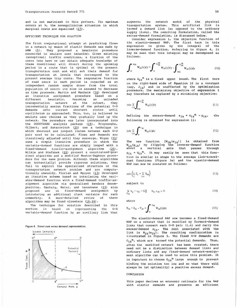
Transportation Research Record 775
and is not maximized in this pattern. Its maximum occurs at N, the nonequilibrium situation in which marginal costs are equalized (]]).
EFFICIENT TECHNIQUE FOR SOLUTION
The first computational attempt at predicting flows in a network by means of elastic demands was made by BMW (i). They proposed a heuristic procedure conceived to emulate user behavior: Given existing (nonoptimal) traffic conditions, a fraction of the users (who have or can obtain adequate knowledge of these conditions) will divert during the upcoming period to a route that is optimal at the present transportation cost and will set their demand for transportation at levels that correspond to the present average trip costs. The responsive fraction of road users in each period is regarded as an independent random sample drawn from the total population of users: its size is assumed to decrease as time proceeds. Martin and Manheim (18) developed an iterative assignment procedure based on a different heuristic. Assuming an unloaded transportation network at the outset, they incrementally assign fractions of the potential 0-D demands onto current shortest routes until equilibrium is approached. This, too, is believed to emulate user choices as they gradually load up the network. The procedure was later incorporated into the DODOTRANS analysis package (!2_). Bruynooghe, Gilbert, and Sakarovitch (1.Q_) use a technique in which shortest and longest routes between each 0-D pair need to be calculated. Flows and demands are iteratively adjusted until they converge. Wigan (21) uses a simple iterative procedure in which the variable-demand functions are simply looped with a fixed-demand traffic-assignment algorithm (20). Wilkie and Stefanek (ll) present a constrained-gradient algorithm and a modified Newton-Raphson procedure for the same problem. Although these algorithms can (potentially) provide rigorous solutions, they fail to exploit the specialized structure of the transportation network problem and are computationally unwieldy. Florian and Nguyen (13) developed an iterative scheme based on interlacing the variable-demand function with a fixed-demand traffic-as-
decomalso
by
signment algorithm via generalized Benders position. Dantzig, Maier, and Lansdowne (~)
proposed use of fixed-demand assignment introducing an additional slack variable for each commodity. A more-detailed review of these algorithms may be found elsewhere (.!.§_,~).
The technique for solution described in this section is based on representing the 0-D variable-demand function by an auxiliary link that
Figure 4. Travel cost versus demand representation.
Excess Demond. e
Gm o' 0
!:
"' 0 u
~ 0
.=
0
Demand Rate, g
59
augments the network model of the physical transportation system. This artificial link is termed a demand link (as opposed to the ordinary supply links). The resulting formulation, called the excess-demand formulation, is discussed below.
Consider expression 1, the objective function of the elastic-demand NAP. The first term in this expression is given by the integral of the inverse-demand function. Heferring to Figure 4, it may be seen that this integral may be decomposed as follows:
(10)
where Gikm is a fixed upper bound. The first term
on the right-hand side of Equation 10 is a constant (say, Jik) and is unaffected by the optimization procedure. The maximizing objective of expression l may therefore be replaced by a minimizing objective:
Defining the excess-demand eik = Gikm - gik•
following is obtained for expression 11:
[
eik
min ~ W;k(z)dz i ,k 0
(I I)
the
(12)
The new wik(gikl about a
function [Wik (eik) I is obtained from by flipping the inverse-demand function
vertical axis that passes through
gik = Gikm. It may easily be seen that this func
tion is similar in shape to the average link-travelcost functions (Figure 3a) and the elastic-demand NAP can now be restated as follows:
(13)
subject to
(14)
where
(15)
The elastic-demand NAP now becomes a fixed-demand NAP on a network that is modified by forward-demand links that connect each 0-D pair (i,k) and carry the excess -demand eik • The cost associated with the link is Wik(eik). The resulting configuration is illustrated in Figure 5. 'l'he fixed o-o demands are
Gikm, which are termed the potential demands. Thus,
after the modified network has been created, there need not be a distinction between demand links and ordinary links and any fixed-demand network-assignment algorithm can be used to solve this problem. It
is important to choose Gikm large enough to prevent
binding the solution too low and so that there will always be (at optimality) a positive excess demand .
CONCLUSION
This paper derives an economic rationale for the NAP with elastic demands and presents an efficient

60
Figura 6. Equivalent network for excess-demand formulation.
I Origin
Demand Link ,,_ ___.._ / ...........
/ .........
/ '
---.---Demand Link
Destination k,
Destination
k2
method for its solution. The optimization objective of the NAP implies the maximization of user surplus + Q, in which Q represents an undercharge to the users due to the social costs of congestion. The method of solution is based on modeling the problem as an equivalent network in which the elastic-demand functions are represented by appropriate demand links. This transforms the variable-demand NAP into an equivalent fixed-demand NAP that has the (fixed) 0-D trip table given by the potential 0-D demands.
The equivalent network model has the obvious advantages of convenient representation and efficiency in data handling, which thereby renders unnecessary the specialized iterative schemes inherent in all other methods of solution. The model is amenable to solution by efficient fixed-demand network-assignment algorithms without modification to those algorithms. Most important, in terms of computation, the model requires no additional nodes in the expanded network. Since network-assignment algorithms, which are based on the calculation of shortest-path trees, are more sensitive to the nwnber of nodes in the network than to the number of links (25) , this model requires only a moderately larger computational effort than that for a fixed-demand assignment on the same physical network. This effort is estimated to be only 25-75 percent larger than a comparable fixed-demand assignment. The most important conclusion, however, is that there are no inherent computational differences between fixed-demand and elastic-demand network-assignment problems, and the same algorithms can be used in both cases.
As noted above, the method described in this paper can be extended to consider more-general demand (cost) functions and is also applicable to other transportation analysis problems that involve choice situations that can be modeled as an equivalent-assignment (path-choice) problem in an expanded network. Such problems include, for example, the combined distribution-assignment problem (which involves origin or destination choice) and assignment in multimodal transportation networks (which may also include simultaneous modal choice).
ACKNOWLEDGMENT
Preparation of this paper was supported by an Intergovernmental Personnel Act Research Fellowship from the Office of Research, Federal Highway Administration (FHWA), Washington, D.C. The contents of this paper reflect mY views and not necessarily those of FHWA.
Transportation Research Record 775
REFERENCES
1. FHWA Computer Programs for Urban Transportation Planning. Federal Highway Administration, U.S. Department of Transportation, July 1974.
2. Comsis Corporation. Traffic Assignment. Federal Highway Administration, U.S. Department of Transportation, Aug. 1973.
3 . N.H. Gartner. Analysis and Control of Transportation Networks by Frank-Wolfe Decomposition. Seventh International Symposium on Transportation and Traffic Theory, Institute of Systems Science Research, Kyoto, Japan, 1977.
4. s. Nguyen. A Unified Approach to Equilibrium Methods for 'l'raffic Assignment. In Traffic Equilibrium Methods (M. Florian, e~ Lecture Notes in Economics and Mathematical Systems, Vol. 118), Springer Verlag, New York, 1976, pp. 382-295.
5. M.J. Beckmann, C.B. McGuire, and C.B. Winsten. Studies in the Economics of Transportation. Yale Univ. Press, New Haven, CT, 1956.
6. M.J. Beckmann. On the Theory of Traffic Flow in Networks. Traffic Quarterly, Vol. 21, Jan. 1967, pp. 109-117.
7. M. Florian. A Traffic Equilibrium Model of Travel by Car and Public Transit Modes. Transportation Science, Vol. 11, 1977, pp. 166-179.
8 . M. Florian, R. Chapleau, S. Nguyen, C. Achim, L. James-Lefebvre, S. Galarneau, J. Lefebvre, and C. Fisk. Validation and Application of an Equilibrium-Based Two-Mode Urban Transportation Planning Method (EMME). TRB, Transportation Research Record 728, 1979, pp. 14-23.
9. I. Hasan and A. Talvitie. An Equilibrium Mode-Split Model of Work Trips Along a Transportation Corridor. Proc., 3rd world Conference on Transportation Research, Martinus Nijhoff, the Hague, Netherlands, 1977, pp. 129-136.
10. D. McFadden and others. Demand Model Estimation and Validation. Univ. of California, Berkeley, Rept. UCB-ITS-SR-77-9, June 1977.
11. s.c. Dafermos and F.T. Sparrow. The Traffic Assignment Problem for a General Network. Journal of Research of the National Bureau of Standards, Vol. 73B, 1969, pp. 91-118.
12. G.F. Newell. Traffic Flow on Transportation Networks. MIT Press, Cambridge, MA, 1980.
13. M. Florian and s. Nguyen. A Method for Computing Network Equilibrium with Elastic Demands. Transportation Science, Vol. 6, 1974, pp. 321-332.
14. L.J. LeBlanc. The Use of Large-Scale Mathematical Programroing Models in Transportation Systems. Transportation Research, Vol. 10, 1976, pp. 419-421.
15. J.R. Meyer and M.R. Straszheim, eds. Techniques of Transport Planning, Volume 1: Pricing and Project Evaluation. Brookings Institution, Washington, DC, 1971.
16. Traffic Congestion as a Factor in Road-User Taxation. HRB, Highway Research Record 47, 1964.
17. N.H. Gartner. Optimal Traffic Assignment with Elastic Demands: A Review. Transportation Science, Vol. 14, 1980, pp. 174-208.
18. B.V. Martin and M.L. Manheim. A Research Program for Comparison of Traffic Assignment Techniques. HRB, Highway Research Record 88, 1965, pp. 69-84.
19. M.L. Manheim and E.R. Ruiter. DODOTRANS I: A Decision-Oriented Computer Language for Analysis of Multimode Transportation Systems. HRB, Highway Research Record 314, 1970, pp. 135-163.
. .

Transportation Research Record 775
20. .M. Bruynooghe, A. Gilbert, and M. Sakarovitch. Une Methode d'Affectation du Traffic. In Beitrage zur Theorie des Verkehrsflusses (W. Leutzbach and P. Baron, eds.), Strassenbau and Strassenverkehrstechnik Heft 86, Bonn, 1969, pp. 198-204.
21. M.R. Wigan. Benefit Assessment for Network Traffic Models and Application to Road Pricing. U.K. Transport and Road Research Laboratory, Crowthorne, Berkshire, England, Rept. LR 417, 1971.
22. D.F. Wilkie and R.G. Stefanek. Precise Determination of Equilibrium in Travel-Forecasting Problems Using Numerical Optimization Techniques. !UlB, Highway Research Record 369, 1971, pp. 239-252.
61
23. G.B. Dantzig, S.F. Maier, and Z.F. Lansdowne. The Application of Decomposition to Transportation Network Analysis. Control Analysis Corporation, Palo Alto, CA, Rept. DOT-TSC-OST-76-26, Oct. 1976.
24. E.R. Ruiter. The Prediction of Network Equilibrium--The State of the Art. Proc., International Conference on Transportation Research (Bruges, Belgium, June 1973), Transportation Research Forum, pp. 717-726.
25. s.E. Dreyfus. An Appraisal of Some Shortest-Path Algorithms. Operations Research, Vol. 17, 1969, pp. 395-412.