Activity-based travel demand modeling

Citation for published version (APA):Ettema, D. F. (1996). Activity-based travel demand modeling. Technische Universiteit Eindhoven.https://doi.org/10.6100/IR471498

DOI:10.6100/IR471498

Document status and date:Published: 01/01/1996

Document Version:Publisher’s PDF, also known as Version of Record (includes final page, issue and volume numbers)

Please check the document version of this publication:

• A submitted manuscript is the version of the article upon submission and before peer-review. There can beimportant differences between the submitted version and the official published version of record. Peopleinterested in the research are advised to contact the author for the final version of the publication, or visit theDOI to the publisher's website.• The final author version and the galley proof are versions of the publication after peer review.• The final published version features the final layout of the paper including the volume, issue and pagenumbers.Link to publication

General rightsCopyright and moral rights for the publications made accessible in the public portal are retained by the authors and/or other copyright ownersand it is a condition of accessing publications that users recognise and abide by the legal requirements associated with these rights.

• Users may download and print one copy of any publication from the public portal for the purpose of private study or research. • You may not further distribute the material or use it for any profit-making activity or commercial gain • You may freely distribute the URL identifying the publication in the public portal.

If the publication is distributed under the terms of Article 25fa of the Dutch Copyright Act, indicated by the “Taverne” license above, pleasefollow below link for the End User Agreement:www.tue.nl/taverne

Take down policyIf you believe that this document breaches copyright please contact us at:openaccess@tue.nlproviding details and we will investigate your claim.

Download date: 29. Jan. 2022

ACTIVITY ·BASED TRAVELDEMAND MODELING

D. EHema

44

ACTIVITY-BASED TRA VEL

DEMAND MODELING

Dick Ettema

ACTIVITY-BASED TRAVEL

DEMAND MODELING

PROEFSCHRIFT

ter verkrijging van de graad van doctor aan de Technische Universiteit Eindhoven, op gezag van de Rector Magnificus, prof.dr. M. Rem, voor een commissie aangewezen door het College van Dekanen in het openbaar te verdedigen op

vrijdag 29 november 1996 om 14.00 uur

door

Dick Ettema

Geboren te Tilburg

Dit proefschrift is goedgekeurd door de promotoren:

prof.dr. H.J.P. Timmermans

en

prof. dr. R. Kitamura (University of Kyoto)

Technische Universiteit Eindhoven, Faculteit Bouwkunde, Vakgroep Architectuur, Urbanistiek en Beheer

ISBN 90-6814-544-4

TABLE OF CONTENTS

Table of Contents

List of Tables

List of Figures

Preface

INTRODUCTION

I Shifting Paradigms in Travel Demand Modeling

II Activity-Based Modeling

Hl Aim and Layout of the Thesis

CHAPTER 1 A THEORY OF ACTIVITY SCHEDULING BEHA VlOR

AND ACTIVITY PATTERNS

1.1 Introduetion

1.2 The Activity-Based Approach: Fundamentals

1.3 A Theory of Activity Scheduling and Activity Patterns

1.3.1 Long-term mobility and lifestyle decisions

1.3.2 Activity scheduling 1.3.3 Activity participation and rescheduling

1.4 Activity-based Modeling

1.5 Conclusions and Outline

CHAPTER2 ACTIVITY-BASED MODELSIN GEOGRAPHY

AND URBAN PLANNING

2.1 Introduetion 2.2 Chapin's Theory of Activity Patterns

vii

i x

x i

2 5

9 10

12 13 16 17 19 20

23

24

TABlE OF CONTENTS

2.3 Applications of Chapin's theory 2.4 Hägerstrand's Space-Time Geography 2.5 Activity Pattem Feasibility Models 2.6 Related Approaches

2. 7 Conclusions

CHAPTER3 M!CRO-ECONO:MIC MODELS OF TIME ALLOCATION

3 .1 Introduetion 3.2 Micro-Economie Consumer Theory 3.3 Time Allocation Models

3.4 Applications of Time Allocation Models in Transportation 3.5 Conclusions

CHAPTER4 ACTIVITY-BASED DISCRETE CBOICE MODELING

4.1 Introduetion 4.2 Theoretica! Foundations of Discrete Choice Models

4.2.1 Deterministic choice models 4.2.2 Strict utility models 4.2.3 Random utility models

4.3 Probit and Logit Models 4.3.1 Probit models 4.3.2 Logit models 4.3.2.1 Joint logit models 4.3.2.2 Universa! logit models 4.3.2.3 Nested logit models

4.4 Stated Preferenee and Choice Techniques 4.5 Activity-Based Choice Modeling

4.5.1 Joint choice models of complete activity patterns 4.5.2 Simultaneous nested logit models 4.5.3 Sequential activity/destination choice models 4.5.4 Recursive models based on prospective utility

4.6 Conclusions

ii

26 29 31

35 38

39 40 43 45 52

55 56 56 58 59 61 61 62 62 65 65 68 71 72 76 78 80 82

TABIE OF CONTENTS

CHAPTER5 CONTRIBUTIONS FROM COGNITIVE PsYCHOLOGY AND ARTIFICIAL INTELLIGENCE

5.1 Introduetion 5.2 The Symbolic Search Space Paradigm

5.2.1 Foundations 5.2.2 Production systems 5.2.3 Applications to activity scheduling

5.3 The Connectionist Paradigm 5. 3.1 Foundations of the connectionist approach 5.3.2 Applications of neural networles to activity scheduling

5.4 Conclusions

CHAPTER6 AN EVALUATION OF ÁCTIVITY-BASED TRA VEL DEMAND MODELS

6.1 Introduetion 6.2 Criteria for the Evaluation of Activity Based Models

6.2.1 Comprehensiveness 6.2.2 Flexibility 6.2.3 Interdependencies 6.2.4 Stage in the decision mak:ing process 6.2.5 Opportunities for statistica! tests 6.2.6 Theoretica! contribution

6.3 An Evaluation of Activity-Based Models 6.3.1 Joint logit models 6.3.2 Simultaneous nested logit models 6.3.3 Sequentia! (nested) logit models 6.3.4 Prospective utility mode\s 6.3.5 Production system models and neural networks 6.3.6 Micro-economie time allocation models 6.3.7 Activity patterns feasibility model

6.4 Conclusions

83 84 84 89 91 95 95 99

102

103 104 105 105 106 106 106 107 107 108 111 113 114 115 116 116 117

iii

TA.BLE OF CONTENTS

CHAPTER 7 SMASH (SIMULATION MODEL OF

ACTIVITY SCHEDULING HEURISTICS)

7.1 Introduetion 121

7.2 Aim of the Model 122 7.3 Theoretica! Considerations 123

7 .3.1 Aetivity seheduling phase: dependent and independent variables 123

7.3.2 A deseription of aetivity seheduling behavior

7.4 Model Specification

126

135 141

142

144

7.5 Statistica! Considerations 7.6 Applîcation Areasof the Model

7.7 Conclusions

CHAPTER8 COMRADE (COMPETING RISK MODEL OF

ACTIVITY DURATION AND EXECUTION)

8.1 Introduetion 145

8.2 Aim of the Model 146 8.3 Theoretica! Considerations 147

8.3.1 Execution phase of activity patterns: explanatory and dependent 147

variables

8.3.2 Deseription of activity patterns as a continuous decision-mak:ing 150 process

8.4 Hazard models 155

8.4.1 Introduetion 155

8.4.2 Fundamentals of hazard models 156 8.4.3 Parametrie and semi-parametrie hazard models 164

8.4.4 Competing risk models 166

8.5 Model Specifieation 168

8.6 Statistica! Considerations 171 8. 7 Application Areas of the Model 174 8.8 Conclusions 175

iv

TABU: OF CONTENTS

CHAPTER9

9.1 Introduetion

MAGIC (METHOD OF ACTIVITY GUIDED INFORMATION

COLLECTION): DESIGN AND APPLICATION

9.2 Data Collection Issues 9.2.1 Questionnaire versus diary 9.2.2 Form of administration 9.2.3 Form of instrument 9.2.4 Diaries: effects of data collection method 9.2.5 Starting points for developing a data collection procedure

9.3 Design of the Data Collection Procedure MAGIC 9.3.1 Data requirements and general structure of MAGIC 9.3.2 Module 1: recording the activity and travel environment 9.3.3 Module 2: activity scheduling task 9.3.4 Module 3: personal and household data 9.3.5 Module 4: revealed activity pattern

9.4 .Results of the Data Coneetion Procedure 9.4.1 Sampling frame 9.4.2 Response rate 9.4.3 Representativeness 9.4.4 Description of the sample 9.4.4.1 Travel and activity behavior of the sample 9.4.4.2 Travel and activity behavior by gender 9.4.4.3 Travel and activity behavior of groups with different

marital status 9.4.4.4 Travel and activity behavior of groups with different

education level 9.4.4.5 Activity and travel behavior of groups with different

main occupations 9.5 Conclusions

CHAPTER 10 CALmRATION AND EMPIRICAL TEST OF SMASH

10.1 Introduetion 10.2 Estimation Procedure 10.3 Estimation Results

10.3.1 Add model

177

178 179 182 183 187 189 190 190 194 198 203 204 207 207 207 208 209 209 209 211

213

215

216

219 219 225 226

V

TABIE OF CONTENTS

10.3.2 Delete model

10.3.3 Reschedule model

10.3.4 Model of choice of operation

10.4 Test of Model Validity

10.4.1 Test procedure

10.4.2 Simulation procedure

10.4.3 lnternal validity

10.4.4 External validity

10.4.5 Predictive validity

10.5 Conclusions

CHAPTER 11 CALIBRATION AND ILLUSTRATIONS OF COMRADE

11.1 Introduetion

11.2 Estimation Procedure

11.3 Estimation Results

11.3.1 Distributions

11.3.2 Parameter estimates

11.4 Illustrations of Hazard Function

11.4.1 The effect of current activity

11.4.2 The effect of time of day

11.4.3 The effect of opening hours

11.4.4 The effect of travel time 11.5 Conclusions

CHAPTER 12 CONCLUSIONS AND DISCUSSION

BIBLIOGRAPHY

AUTHOR INDEX

DUTCH SUMMARY (SAMENVATTING)

CURRICULUM VITAE

vi

227

228

229

231

231

232 234

236

237

239

241

241

245

245

246

250

250

251 254

256

258

261

269

281

285

297

LIST OF TABLES

Table 4.1

Table 5.1

Table 6.1

Table 7.1

Table 7.2

Table 7.3

Table 7.4

Table 8.1

Table 8.2

Table 8.3

Table 9.1 Table 9.2

Table 9.3

Table 9.4

Table 9.5 Table 9.6

Table 9.7

Table 9.8

Table 9.9

Table 9.10

Table 9.11

Table 9.12

Table 10.1

Table 10.2

Table 10.3

Table 10.4

Table 10.5

Table 10.6

Table 10.7

Table 10.8

Table 10.9

Example of a Profile

Example of Truth Table

Evaluation of Activity-Based Modeling Approaches

Factors Influencing the Activity Scheduling Process

Decisions Involved in the Activity Scheduling Process

Activity Scheduling Decisions I

Activity Scheduling Decisions ll

Factors lnfluencing the Execution of Activity Patterns

Decisions lnvolved in the Execution of Activity Patterns

The Effect of Various Factors on Choice Probabilities

Motivations with Respect to the Design of the Modules of MAGIC

Range Checks

Actlvities Used in the Experiment

Pre-Coded Answer Categones

Response Rate

Comparison of Distributton of Characteristics of the Sample and the

Popu/ation

Distributton of Diary Days across the Week

Average Activity and Travel Characteristics

Activity and Travel Characteristics by Gender

Activity and Travel Characteristics by Marltal Status

Activity and Travel Characteristics by Education Level

Activity and Travel Characteristics by Main Occupation

Example of Activity Schedule

Example of Activity Program

Example of Lower Nest Alternatives

Attributes included in the Add, Delete and Reschedule Models

Parameter Estimates of the Lower Level Add, Delete and Reschedule

Mode Is Higher Level Model (/) Higher Level Model (11)

Overview of Validity Tests

Characteristics of Simulated and Observed Schedules

vii

Table 10.10 Table 10.11 Table 11.1 Table 11.2 Table 11.3 Table 11.4 Table 11.5 Table 11.6

viii

Characteristics of Simulated Schedules and Observed Activity Patterns Comparison of Original and Simulated Schedules Goodness-of-Fit Measures of Different Distributional Assumptions Parameter Estimates Log-Normal Model Covariates of Current Activities Covariates of Competing Risks I Covariates of Competing Risks // Covariates of Competing Risks ///

LIST OF FIGURES

Figure 1.1

Figure 2.1

Figure 2.2

Figure 2.3

Figure 2.4

Figure 2.5

Figure 4.1

Figure 4.2

Figure 5.1

Figure 5.2

Figure 6.1

Figure 7.1

Figure 7.2

Figure 7.3

Figure 7.4

Figure 7.5 Figure 7.6 Figure 7.7

Figure 7.8

Figure 8.1

Figure 8.2

Figure 8.3

Figure 8.4

Figure 8.5

Figure 8.6

Figure 8. 7 Figure 8.8

Figure 8.9

Figure 8.10

Figure 8.11

A Theory of Activity Scheduling Behavior and Activity Pattems

Chapin 's Theory of Activity Pattems

Example of a Space-Time Path

Coupling Constraints

Space-Time Prisms

Relationship between Long-Termand Short-Term Choices (Cullen, 1978)

Nested Structure of Destination and Mode Choice

Structure of Nested Logit Model (Ben-Aldva and Bowman, 1997)

Neuron with inputs via Weighted Links

Examples of Neural Networks

Behaviaral Principlesof Various Modeling Approaches

The Activity Scheduling Stage

The Activity Scheduling Process as a Stepwise Adaptation Process

The Application of Subsequent Scheduling Decisions

Examples of Adding, Deleting and Rescheduling

The Application of Subsequent Scheduling Decisions and Evaluations

A State Space Representation of the Activity Scheduling Process

Nested Logit Model Structure of 1ntegrated Evaluation and Scheduling

Decisions

The Application of Subsequent 1ntegrated Evaluation-Scheduling

Decisions

The Execution Phase of Activity Patterns

The Activity Pattem in Terms of Activity, Travel and Waiting Time

Choice Sets as a Function of Time of Day

The Effect of Time-Constraints on Choice Sets

Weibull p.d.f (À = 1, (3 = 3)

Weibull Cumulative Probability Function (À = 1, (3 = 3)

Weibull Survivor Function (À = 1, (3 = 3)

Weibull Hazard Function (À = 1, (3 = 3)

Examples of Different Hazard Functions

Proportionaf Hazard Functions

Accelerated Time Hazard Functions

ix

Figure 9.1 Figure 9.2 Figure 9.3 Figure 9.4 Figure 9.5 Figure 9.6 Figure 9.7 Figure 9.8 Figure 9.9 Figure 9.10 Figure 9.11 Figure 9.12 Figure 10.1 Figure 11.1 Figure 11.2 Figure 11.3 Figure 11.4 Figure 11.5 Figure 11.6 Figure 11.7 Figure 11.8

x

Sequence of Different Modules of MAGJC Input Screen for Activity Data Input Screen for Destinafton Data Input Screen for Travel Times Selecting an Activity from the Agenda Selecting a Destination Selecting the Position in the Schedule Selecting a Travel Mode Specifying Start and End Times of Activfties Organization of Module 2 Input Screen Personaf and Household Data Activity Diary Used in Module 4 Stepwise Simulation Process Different Hazard Functions Hazards for t'P 9.00 AM Hazards for t'P = 1.00 PM Hazards for t'P = 7.00 PM Hazards if Shops are open until5.()() PM Hazards if Shops are open until 9.()() PM Hazards if Travel Times are 30 Minutes Hazards if Travel Times are 60 Minutes

PREFACE

This thesis is the result of the research that I have conducted over the last five years at

Eindhoven University of Technology, as a memher of the Urban Planning Group. This

period has been very rewarding for me in a several ways. First, working in the Urban Planning Group has shaped me as a researcher and bas given me the opportunity to acquire much theoretica! knowledge and many practical skilis involved in doing research. In addition, during the past years I have had the opportunity to meet many people inside and outside the university, from whom I learned a lot and who all enriched my personal

and professional life. It goes without saying that a project like this cannot be completed without the

support of others. I thank everyone who, in one way or another, has helped me completing this research. However, there are some that I want to acknowledge

specifically for their contribution. First of all, I want to thank Harry Timmermans, my primary advisor. After I

graduated at Eindhoven University, he offered me a position as a PhD student at the Urban Planning Group. During my research he has been a very stimulating advisor, giving me every opportunity to develop my ideas and eneauraging me to present my work at conferences and in journals. Discussing my work with him learned me a lot about how

to conduct scientific research. During the last hectic months before finishing this thesis,

Harry managed to find time in bis busy schedule to carefully review the manuscript, which contributed considerable to the quality of this work. Working with Harry over the past years bas been a real pleasure.

I am also grateful to my second advisor, Aloys Borgers. He bas taught me many aspects of travel behavior research, and always provided valuable comments, which

improved the quality of my work. He was always prepared to help me out with any questions I had regarding my research. It bas been a real pleasure working with him as

wel!. I am also indebted to Ryuichi Kitamura, my second promotor. He provided

valuable comments on my research and on the manuscript, which significantly added to

its quality. I also thank Toon van der Hoorn for reviewing the manuscript as a memher of

the committee.

x i

PREFACE

S.R.O., the Social and Environmental Research Foundation, is gratefully acknowledged for funding the last two years of this research project. Furthermore, they provided travel grants, enabling me to meet with colleagues in the field.

Over the past years, I have had the pleasure to collaborate with other researchers

in the field of transportation research. First, Tommy Gärling should be mentioned. He invited me several time to Göteborg, to work on research projects in the context of

activity scheduling. This collaboration and the discussions we have had, have been important sourees of inspiration for my research, for which I am grateful. I also was invited to the Royal Institute of Technology by Christer Lindh, to work with him and my former colleague Benedict Dellaert on a research project regarding overnight long­distance trip making. This collaboration also was arewarding and challenging experience.

During the organization of a conference regarding activity-based approaches, I had the pleasure to work with Kay Axhausen, Eric Pas and Andy Harvey as memhers of the steering committee. Working with all these people bas been very rewarding and enjoyable for me.

Of course, the success of this research project bas very much depended on the people that I have worked with on a daily basis over the past years. I am grateful to my colleagues at the Urban Planning Group for providing an informal and pleasant

atmosphere that enabled me to finish this work successfully. Each member has contributed in his or her unique way to the completion of this research. Furthermore, I

thank my colleagues at Hague Consulting Group for their flexibility and moral support during the final stages of finishing this thesis.

Last but not least, I want to thank my wife Miranda. Her continuous support has been very important in finishing this thesis. I dedicate this work to her.

Dick Ettema Eindhoven, October 19%

xii

INTRODUC110N

INTRODUCTION

I SHIFTING PARADIGMS IN TRAVELDEMAND MODELING

Over the last decades the theoretica! underpinnings and practice of travel demand modeling have experienced significant shifts, invoked by new issues that became salient in

transportation policy at a particular time. The first generation of travel demand models was developed in the nineteen sixties when a rapid increase in car ownership and car use emerged in the US and Western Europe. This increase necessitated major public investment in new road infrastructure. In order to assess the impact of these investments, models that could be used to predict travel demand on the long run (say iwenty to thirty years ahead) were deemed critica! in evaluating (ex ante) alternative investment decisions. This resulted in the development of aggregate, gravity type models, predicting traffic

flows between traffic zones (Jones et a/.,1983; Stopher et al., 1981). These predicted flows were then used to determine future road capacity needs. In particular, travel was

assumed to be the result of four subsequent decisions which were modeled separately. It was assumed that individuals first decide whether or not to travel (trip generation). Then,

they were assumed to choose a destination for a specific trip (trip distribution), foliowed by the choice what metbod of transportation to use (mode choice) and the choice which

route to follow (route choice). The implication of this concept was that each consecutive deelsion was treated as an isolated phenomenon. Furthermore, alternatives were

considered to be easily substitutable, which led to the belief that, for example, car traffic could be fairly easily reduced by increasing public transport capacity.

In the seventies, these aggregate four-step models were increasingly criticized. Often, model forecasts turned out to be very unreliable and failed to assess the effects of policy measures correctly. In addition, the focus of policies shifted from long-term investment strategies to short term market-oriented solutions. This resulted in a need for models that could predict behavloral responses to policy measures more directly.

In responsetothese changing needs, a new type of model was developed in the early seventies. It described individual behavior rather than aggregate traffic flows and mode shares. These disaggregate travel demand models were based on developments in micro­economie and psychological research on individual choice behavior. Consequently, the

INTRODUCflON

weak theoretica! basis of the gravity model which relied on an analogy to gravity and

entropy concepts in physics, could be replaced by theories about utility-maximizing behavior and individual choice behavior. These discrete choice models have the advantage

that individual choice behavior can be modeled directly, so that responses to market­oriented polides could be better assessed. Furthermore, these models require smaller data sets for calibration and can potentially incorporate a wider range of explanatory variables. These attractive features have made disaggregate travel demand models the core of

transportation modeling practice from the mid seventies onwards. Nevertheless, disaggregate models did not escape criticism either. In partienlar, the

behavloral underpinnings of these models, although based on principles of human behavior, is limited in the sense that they regard travel as a demand in its own right, and neglect the question why people travel and undertake trips. Consequently, they offer a

limited insight into the relationship between travel and non-travet aspects. In addition, the

models can be criticized for descrihing travel decisions separately. For instance, trips in a trip chain or diffeTent home-based trips are modeled as being independent of each other, whereas in reality interdependencies exist between these trips. These criticisms have become more relevant in light of social, technological and behavioral developments, which

have led to increasingly complex individual travel and activity patterns. At the same time, new policy measures, such as telecommuting, flexible work hours or time specific pricing mechanisms, will likely induce more complex responses than simpte changes in mode choice ordeparture time choice of just one trip. Thus, models that allow the assessment of

complex responses to new policy measures in terms of complex behavloral patterns are required to better reflect such relationships in travel and activity patterns.

ll ACTIVITY -BASED MODELING

Activity-based models have been developed in response to these needs since the early eighties. In the United States, for example, the development of activity-based models was stimulated by the Clean Air Act Amendments (CAAA) of 1991 and the Intermodal Surface Transportation Efficiency Act (ISTEA) of 1992. These pieces of legislation implied a major change in US transportation planning, involving an increased concern for environmental issues, such as air quality, and congestion reduction. Proposed policies include ridesharing, HOV lanes, telecommuting, congestion pricing and IVHS. CAAA and ISTEA explicitly stimulated the development of activity-based models as the most appropriate tooi for forecasting the potentially complex effects of these policies. An important outcome of this development is the Travel Model Improvement Program (TMIP) of the US Department of Transportation that aims at the introduetion of activity-

2

/NTRODUC110N

based models in applied transportation planning practice.

Activity-based models aim at predicting travel behavior as a derivative of activities.

That is to say, by predicting which activities are performed at particular destinations and

times, trips and their timing are implicitly forecasted. Thus, these models strongly

emphasize individuals' activity scheduling behavior. An important goal of activity-based

modeling is to disentangle the decision mechanisms that individuals use to decide about

the activities they perform and the trips they make when integrating many different

decisions regarding separate actlvities and trips into a single activity schedule.

To date, different approaches have been taken in the development of activity-based

models. The first attempts in activity-based modeling were based on Hägerstrand's space­time geography. Based on this theory, models such as PESASP (Lenntorp, 1978),

CARLA (Jones et al., 1983) and BSP (Huigen, 1986), that systematically identify the set

of feasible activity patterns, given existing land use patterns, time constraints and the

available transportation options, were developed. This approach is very useful for the

evaluation of the possibilities to implement specific activity programs in constrained

spatio-temporal settings. However, in most applied situations, individuals have a

considerable set of response options by which the can adapt their activity pattem to

specific policies. The models then give little information regarding the behavioral response

that can be expected.

In addition, some activity-based models rely on discrete choice theory to describe the choice of activity patterns. For instance, the ST ARCHILD model (Recker and

McNally, 1986a, 1986b), which can be considered as the most complex activity-based

model from the late 1980s, describes the choice of complete activity patterns. As such, the

model accounts for interdependencies between different decisions that are integrated in the

overall pattern. However, the model assumes that individuals make their final choice out

of a limited set of distinct patterns. This implies that the number of behavioral responses

described by the model is rather small, thereby limiting the flexibility of the model.

Furthermore, the way in which household activity programs are derived from observed

activity patterns suggests that not all relevant alternatives may be included in the model.

Other models in the discrete choice tradition (e.g., Van der Hoorn, 1983) have used

discrete choice models to describe the choice of consecutive activities. In this respect, the

consecutive choices are assumed to be made independent of each other. Thus, this model

is more flexible in that it allows for the description of every possible activity pattern,

based on a rather comprehensive set of activities. However, as the model assumes

subsequent activities throughout the day to be the outcome of separate decisions, it does not fully account for the dependencies that may exist between the choice of different

activities and trips throughout the day.

Another approach involves the use of time allocation models based on micro-

3

lNTRODUCTION

economie theory, that describe how individuals allocate time to actlvities and travel, such

that their total utility is maximized. These models are very useful in descrihing individuals' time expenditures. However, the incorporation of travel behavior in these

models in terms of origin destination pairs is still very problematic. For instance, RDC's (1994) model describes the time allocation to activities, but it does not incorporate the timing and sequencing of activities and the destination and mode choice associated with trips that are part of an activity pattern.

Finally, artificial intelligence and cognitive science techniques have been used to build activity-based models. These models are very well capable of descrihing activity

scheduling in terms of human reasoning processes. However, they are qualitative models, which makes it difficult to calibrate and apply them in a real world context. For instance, the model suggested by Hayes-Roth and Hayes-Roth (1979) includes a variety of deelsion rules, accounting for many policy-related variables and decision variables. However, as

the model is based on a think aloud protocol, which contains very specific individual data, the model cannot be readily transferred to other individuals or contexts.

The above examples indicate that activity-based modeling typically involves trade­offs between comprehensiveness (including all relevant variables), flexibility and the opportunity to account for interdependencies, as the mathematica! formalation of the models usually does not allow one to combine all these characteristics into one single model. In addition, one has to balance the complexity of the model carefully against data needs and computational difficulties in estimating the models and applying them for predictions.

Another problem of activity-based modeling has been its eclectic character. That is to say, a wide variety of modeling techniques has been applied to model a variety of responses. The approach has consequently lacked a unifying behavloral framework, in which different approaches can be embedded. Such a framework would allow one to determine which behavloral variables and which stages in the decision-making process are affected by a specific policy and, consequently, which modeling offers the best opportunity to predict the impact of the policy.

Finally, it should be noted that all current activity-based models have failed to account for the highly dynamic nature of activity participation. It is increasingly

recognized that activity patterns are the outcome of a continuous decision-making process, in which individuals may at each point in time decide to switch from their current activity to another one, possibly implying a trip to another destination. Especially, in order to describe the duration and timing of actlvities and trips, the development of more dynamic models is deemed increasingly important.

4

INTRODUCTION

ill AIM AND LAYOUT OF THE THESIS

Given these shortcomings of existing activity-based models, the aim of this thesis is

threefold. First, it offers a unifying behavioral framework of activity and travel patterns,

that incorporates different stages of decision-making, different decision dimensions and

different policy variables. This framework can be used to determine the domain in which

current activity-based models can be applied. Furthermore, it can be used to assess the

shortcomings of different activity-based approaches and may serve as a reference point for

the further development of activity-based models. Secondly, the aim is to develop an

activity-based model that is comprehensive, flexible and can account for interdependencies

between various decision dimensions. To date, a model combining these properties has not

been reported in the literature. Specific attention is given to the choice of the most

promising modeling technique for this purpose, the ioclusion of behavioral and policy

variables in the model and the empirica! test of the model. Finally, the aim is to

incorporate the dynamic character of activity patterns in activity-based models.

Specifically, a modeling technique is introduced that better than existing models accounts

for the dynamic nature of activity patterns. Based on this technique, an activity-based

model will be developed.

In line with most activity-based models described in the literature, the emphasis is

on models that describe one-day activity scheduling. That is to say, models are developed

that describe the activities and trips planned or performed by an iudividual on a single day. Ideally, activity-based models in their most complete form should address the

decisions what activities to perform, at what locations to perform these activities, when to

start and end activities, in what sequence to perform activities, with whom to perform the

activities, how to travel between the locations of subsequent activities (mode choice) and

when to depart at a specific location to travel to the next one. However, the models

described in this thesis each put an emphasis on specific decisions while ignoring others.

This thesis is organized as follows. Chapter 1 first provides a theory of complex

travel and activity decision-making. In particular, it is assumed that the process leading to

the performance of activity patterns entails long-term life style and mobility decisions, a

pre-trip activity scheduling phase and a phase in which the activity schedule is executed. For each stage, the relevant policy and decision variables are identified and

interdependencies between different stages are identified. Then, to allow the reader to assess the contribution of the present thesis to the state­

of-the-art, Chapters 2 to 5 summarize and discuss various activity-based models that have

been developed lately or are still under development. Each chapter discusses a different

modeling approach. For each approach, we discuss the theoretica! foundations underlying

the model, the technica! and statistica! characteristics of the model and the applicability of

5

INTRODî!CI10N

the model for the evaluation of policy measures. The following modeling approaches are distinguished. Chapter 2 discusses models of activity behavior developed in geography and urban planning. These models go back to the theories of Chapin and Hägerstrand, which

wil! be briefly discussed. The models typically are concerned with the constraints, set by the environment, to activity patterns. Attention is paid to operational models, such as

CARLA, PESASP and BSP, which have been developed in this tradition. Another class of models, described in Chapter 3, are micro-economie models of time allocation. These roodels are based typically on micro-economie consumer theory and regard activity scheduling as an allocation problem guided by utility maximization. The chapter discusses some fundamental principles, the application to time expenditures as developed by Becker and applications to transportation and activity scheduling. Chapter 4 reviews activity-based models which are based on discrete choice theory. These models can be considered as the

logica! successors of the discrete choice models that currently constitute the core of transportation modeling. These models typically describe activity scheduling as the outcome of a (series of) discrete choice(s). In particular, trip chaining models and models of activity pattem choice are considered. A fourth approach to activity-based modeling, described in Chapter 5, is based on the application of psychology and artificial intelligence to travel decisions. These modeling approaches are closely related to theories of human decision-making, which will be discussed to the extent necessary for understanding these

models. Specifically, two directions can be identified: the symbolic search space paradigm, on which computational process models are based, and the connectionist paradigm, which has led to the development of neural networks. Applications of CPMs and neural networks to activity scheduling will be discussed.

The review of existing models is foliowed by an evaluation framework, which is described in Chapter 6. Specifically, the models described in the previous chapters will be matebed against the theory of travel decision-making described in Chapter 1, to establish the extent to which they succeed in incorporating various dimensions and factors of travel decision-making. In particular, the models are evaluated with respect to the decision variables they describe, the policy variables that are included, the phase in the decision­making process that is described, the flexibility of the model and the possibility to account for interdependencies between different decision dimensions. Based on the evaluation, it wil! be argued that existing activity-based models are characterized by two major shortcomings: (i) they fail to take into account all relevant decision and explanatory

variables while maintaining sufficient flexibility and the possibility to account for interdependencies between various decision dimensions, and (ii) they Jack sophistication in

representation of the timing and duration of activities.

In an attempt to overcome these shortcomings, the second part of this thesis describes the development and test of two activity-based models. Chapter 7 presents

6

INTRODUeTION

SMASH, a model of activity scheduling that combines production system modeling and discrete choice modeling techniques. This model is developed to combine comprehensiveness, flexibility and the capability to account for interdependencies into one

single model. Another activity-based model, COMRADE, is described in Chapter 8.

COMRADE was developed to account for the dynamic nature of activity patterns. It applies a competing risk hazard model to describe simultaneously the choice duration and timing of activities. Given the complexity of the models, the issue of data collection

requires special attention. We will argue that the commonly used diaries are inappropriate

to collect data on activity patterns. We will defend the notion that interactive computer experiments are the most reliable method to collect data on activity scheduling. A computer program MAGIC, developed to support such interactive data collection, is

described in Chapter 9. The estimation results of the two models are described in the

following chapters. Chapter 10 addresses the estimations results of SMASH. Parameters will be presented and interpreted. Further tests of the model involve simulation experiments to test whether the model is capable of reproducing the estimation data and

scenario based data. Chapter 11 discusses the estimation results of COMRADE. The parameters estimated for the covariates of the model are discussed as wel\ as the

characteristics of the baseline hazard function. The estimation results are illustrated by predictions of different scenarios. Finally, Chapter 12 draws conclusions regarding the

state-of-the-art in activity-based modeling, the models presented in th!s thesis, the data collection methods that should be used to support activity-based modeling efforts and fruitfut directions for future model developments.

7

CHAPTER 1

A THEORY OF ACTIVITY SCHEDULING BEHA VlOR AND

ACTIVITY PATIERNS

1.1 INTRODUCTION

Over the last couple of years, the activity-based approach has received increasing attention

among transportation researchers. Specifically, researchers have relied on activity-based approaches in order to overcome some of the shortcomings of disaggregate travel demand

models. First, the activity-based approach has been used to provide a better theoretica! underpinning of travel behavior research as it addresses the questions why people travel

and how decisions regarding trips are made. Specifically, it is assumed that travel is not a demand in its own right, but a demand which is derived from activity participation. This implies that travel is best understood in the broader contèxt of individual activity patterns.

Research which has been carried out along these lines of thinking has revealed much of the underlying factors of travel behavior (see for instance: Jones et al. 1983; Carpenter and Jones, 1983; Jones, 1990).

Based on these theoretica! insights, attempts have also been made to develop travel

demand models which better than the traditional disaggregate travel models reflect the driving and constraining factors underlying travel behavior . These so called activity-based models do not describe single-dimensional decisions concerning one trip, but rather address complex decisions concerning multiple dimensions of various trips and activities. Specifically, they describe what activities are performed during a specific period, at what destinations, at what times and in which sequence. Such activity sequences imply trips with a specific origin and destination, which are made at a specific time of day using a

specific mode. Hence, travel behavior is described in an implicit way as a derivative of activity participation at different destinations.

The development of activity-based models has become increasingly important in light

of increasingly complex travel patterns and the introduetion of policies such as telematics, information technologies and time policies, which may lead to complex changes in activity

and travel patterns. To date, however, activity-based models are far from common practice in applied travel behavior research as the models that have been introduced to

date still have many theoretica! and practical problems. This thesis introduces alternare modeling approaches which can overcome these problems, based on an assessment of

9

CHAPTER 1 A THEORY OF AC17V1TY SCHEDUUNG BEHAVlORAND AC17V1TY PATTERNS

current activity-based models and their shortcomings. To facilitate an assessment of current models and provide a base for the development

of the models outlined in this thesis, this chapter presents a theory of travel decision mak.ing which encompasses subsequent stages in decision making, the decisions made in

each stage and the factors influencing these decisions. Specifically, the theory addresses activity scheduling (the decision making process in which it is decided what activities and trips are performed during a fixed period of time) and the performance of activity patterns. The theory adopts the theoretica! notions of the activity-based approach, but focuses specifically on the decision making process. The theory is used in this thesis to position and evaluate different modeling approaches to highlight their differences and

shortcomings and formulate the requirements of new modeling approaches. The structure of this chapter is as follows. Section 1.2 first introduces some basic

concepts underlying the activity-based approach in transportation research. Section 1.3 then presents a theory of activity scheduling behavior. Th is theory describes how travel decision making proceeds through the subsequent stages of long-term decision making, activity scheduling and activity pattem performance. This section furthermore gives definitions of concepts that are used throughout this thesis. Section 1.4 briefly introduces some activity-based modeling approaches that have been developed and that will be discussed in greater detail in Chapters 2 to 5. Finally, section 1.5 draws conclusions regarding individual activity scheduling behavior and approaches to model this phenomenon.

1.2 THE ACTIVITY-BASED APPROACH: FuNDAMENTALS

Although the activity-based approach has gained momenturn in transportation research since the mid-eighties, many of its concepts were developed earlier in other disciplines. Especially scholars in geography and urban planning have, from the sixties onwards, contributed significantly to the development of theories and empirica! descriptions of activity patterns. The emphasis in these disciplines has primarily been on the effect of land

use patterns on individuals' opportunities to participate in activities and on how urban planning processes should meet the demands invoked by individuals' activity patterns. A detailed discussion of activity-based approaches in geography and urban planning is given

in Chapter 2. Transportation researchers have extended this approach by specifically emphasizing the relationship between activities and travel behavior. This has led to the formulation of a number of assumptions in the context of trip making and activity participation, which can be considered the starting points of activity-based research in transportation (see Jones et al., 1983).

10

CHAPTER 1 A THEORY OF AC17VITY SCHEDUUNG BEHAVlORAND AC17VITY PATTERNS

The first assumption made is that travel is a derived demand. That is to say, in most

cases travel is not an independent demand, but takes place in order to participate in

activities which take place at different destinations. As a consequence, characteristics of

activities will strongly influence individual travel behavior. What activities are performed depends on an individual's physiological, economie and social needs and the roles he has

to fulfil in a household, profession, etc. Lifestyle, which can be defined as a combination of roles, is an important issue in this respect (Havens, 1981). Hence, someone's lifestyle essentially determines which activities he pursues and which trips he makes accordingly. However, activities usually have different priorities (Cullen and Godson, 1975). One may, for instance, distinguish between obligatory activities, such as work, and more

discretionary activities, such as leisure. A trade-off between the time and costs required

for activities and their priorities will therefore determine which activities are performed. Furthermore, activities may be related in the sense that they have to appear in a specific

order. For instance, cooking necessarily has to preeede having supper. Both priorities and

sequence constraints have an impact on the activities that can be performed and the travel that is required to participate in the activities.

A second important notion of the activity-based approach is that activity performance depends on the availability of specific facilities, which sets limitations to the possibilities

of performing activities. First, activities can usually take place at only a limited number of destinations. For instance, work is fixed at the work location and for grocery shopping one is dependent upon the availability of shops. Furthermore, the availability of facilities may be limited to particular hours, such as fixed work hours and opening hours of shops. However, limitations may also arise from more informal appointments that are made, for

instanee between household memhers to have dinner at a specific time. The need for facilities also has a spatial dimension, which accounts for the derived nature of traveL As facilities are only offered at specific destinations, travel is required to access them. As a

consequence, the relative position of facilities determines the amount of travel needed for activity participation and may impose constraints on the opportunity to engage in them. Hence, the duration of activities and constraints with respect to their sequence, the available facilities, the hours at which they are accessible and the travel times between facilities affect which activities can eventually be performed. Specifically, such limitations

are termed space-time constraints. They are at the focus of Hägerstrand's (1970) space­time geography, which will be discussed in detail in Chapter 2. Travel can thus be considered a space-shifting mechanism, subject to space-time constraints and enabling people to take part in successive activities at different sites. Furthermore, trip generation

and distribution are the outcome of activity and site trade-offs. A third important issue in the context of the activity-based approach is the emphasis

on the household as the decision-making unit. As most households consist of multiple

11

CHAPTER 1 A THEORY OF ACTTVITY SG11EDUUNG BEHAVlORAND AC11VJTY PA11ERNS

persons, interpersonal linkages influence activity patterns. One example is the effect of

activities which are performed together by the household members, such as eating meals.

In this case, constraints to individual activities arise from appointments that are made with

other household members. Alternatively, individual constraints may affect the behavior of

other household members. For instance, if one person has fixed working hours, this limits

the possibilities for joint leisure activities. Another type of interpersonal linkage arises

from the allocation of resources within the household. If, for example, only one car is

available within the household, the allocation of this car affects the actlvities that can be

pursued in the context of the spatial configuration of facilities.

A fourth principle of the activity-based approach is that travel should be regarded in

the context of activity patterns, consisting of multiple actlvities and trips. This implies that

interdependencies (space-time linkages) exist between independent events throughout the

day. Partly, this is the result of the available limited time budget: if more time is spent on

one activity or at one site, less time is available for others. Furthermore, the sites at

which different activities take place may be linked, for example such that travel distance is

minimized. Furthermore, linkages exist between travel and non-travel behavior. For

instance, for an activity which requires carrying of many goods, one may decide to choose

the car instead of bicycle or public transport.

As a final note, it is mentioned that travel and activities can be considered the

outcome of a scheduling process, in which activity demands are matebed against a supply

side which is defined by the available facilities, time windows and transportation options.

Modeling this scheduling process is a specific focus of this thesis as the scheduling

process determines individual travel and activity behavior.

1.3 A THEORY OF ACTIVITY SCHEDULING AND ACTIVITY PATTERNS

The aim of this section is to describe in greater detail how individuals make decisions

regarding their travel and activity behavior. Without specifically addressing the cognitive

mechanisms underlying the decision making process, different stages in the decision

making process will be addressed in terms of the independent and the dependent variables

that are relevant in each stage. Following Ben-Akiva et al. (1994), the following stages in

the decision-making process are distinguished:

i) Long-term lifestyle and mobility decisions, such as for instanee residential choice,

choice of work place, the decision whether or not to buy a car and the choice which

activities to perform at regular intervals. These decisions, which are made for Jonger

periods, determine the general travel and activity conditions which remain stabie for a Jonger time.

12

CHAPTER 1 A 11/EORY OF AC17VI1Y SCHEDUUNG BEHAVlORAND AC17VI1Y PA1TERNS

ii) Daily activity scheduling decisions, such as the deelsion which actlvities and trips to

perform in a specific period, the sequencing and timing of trips and actlvities and

durations of activities. These decisions thus refer to the implementation of actlvities

and trips in a specific situation and are made in response to the specific situation at

that time.

iii) Activity rescheduling. This phase refers to the ongoing process of monitoring the

execution of the plan made in phase ii, and adapting it in response to unforeseen

events or additional information.

For each stage, the decision dimensions, plus the factors that affect the various decisions

are identified. This is done building on the theoretica! work of Havens (1981), Root and

Recker (1983), Gärling et al., (1989), Ben-Akiva et al. (1994) and Ettema et al. (1995).

The subsequent stages, decision dimensions and factors are displayed in Figure 1. 1.

1.3.1 Long-term mobility and Ufestyle decisions

The basic explanatory variabie of long-term lifestyle and mobility decisions can be

considered an individual's lifestyle, as elaborated by Havens (1981). According to his

conceptual model, travel is a derived demand of activity participation, aiming at the

fulfillment of certain needs. These needs are clustered into a smaller number of groups,

which can be defined as roles. Roles may, for instance, include household/family,

work/career, interpersonallsocial and leisure/recreation. The roles are divided among

memhers of a houschold and consequently gulde the activities of individual household

members. It should be noted that roles include both the actlvities themselves and the

person's attitude towards the activities. A lifestyle is now defined as a combination of

rol es held by a single household memher. A lifestyle thus encompasses the actlvities

aiming at the fulfillment of needs and attitudes towards the activities. An important

implication of the role and lifestyle concept is the temporal stability of activity programs.

That is, once an activity is part of a lifestyle it tends to remain part of it as a result of

three factors. The first factor involves interpersonal factors. That is, other people involved

in an activity may stabilize roles and activities by their expectations, cooperation and

reinforcement SeconQly, socia\ norms and institutions will reinforce activities that are part

of the role and sanction activities that are opposed to the role. Finally, the temporal

stability of lifestyles sterns from temporal and spatlal factors. As activities usually form

part of habitual patterns, the options to insert new activities in the schedule are limited

because of spatio-temporal constraints. For the same reason, people may be reluctant to

shift activities.

Lifestyle decisions are thus very important factors determining travel and activity

behavior over a long period. Particularly, they influence an individual's long-term

calendar (Gärling et al., 1993), which contains general information regarding activities

13

LONG -TERM DECISIONS SCHEDULING PHASE

DECISION AND PREFERENCE STRUCTURE

EXECT.ITION PHASE

DECISION AND PREFERENCE STRUCTURE

Figure 1.1: A Theory of Activity Scheduling Behavior and Activity Pattems

CHAP1ER 1 A lliEORY OF AC17VJTY SCHEDUUNG BEHAVJOR AND AC17VJTY PATJERNS

that an individual performs with certain regularity. For instance, information can be stored

regarding the frequency at which an activity is performed, the average duration of an

activity, the attitude towards the activity and the available destinations and times at which

the activity can be performed. In addition constraints pertaining to activities, such as costs, distance or household interactions, are stored in the long-term calendar. The

contents of the long-term calendar is largely acquired by experiences of prior activity

engagements, which may lead to the development of certain attitudes toward activities

(Golledge et al., 1994). For example, one's attitude toward activities which are harmful to the environment may change as a result of information regarding these negative effects. In

addition, prior engagements may lead to the accumulation of knowledge regarding activities, such as available times and destinations. It should, furthermore, be noted that

lifestyle may lead to a limitation of the activity space which goes beyond pure functional

considerations, as lifestyles imply attitudes toward activities (Havens, 1981). For instance, a lifestyle may be associated with visiting only particular shops, restaurants or recreation facilities and participating in activities which are exclusively part of a particular lifestyle.

Lifestyle decisions not only affect the long-term calendar, but they may furthermore guide decisions that are made concerning the circumstances under which activities and

travel take place. For instance, the decisions where to live, where to work, the composition of the vehicle fleet and the buying of information equipment set important

limits to activities that can be performed and trips that can be made. Especially, the choice

of the home location in relation to the accessibility of the transportation network and the location of facilities will have an effect on the available activity space. Knowledge regarding the environment is stored in the cognitive map, a memory representation that individuals have of their environment. Specifically, the cognitive map contains information

regarding destinations and their opening hours, the available routes connecting these

destination, and travel times associated with these routes for different modes. Similar to the long-term calendar, the contents of the cognitive map is acquired by prior experiences

of the environment, which may lead to knowledge of routes, travel times and destinations. Finally, long-term lifestyle decisions affect a household's resources, which enable

one to participate in activities. For instance, the decision where and how many hours to work will result in available monetary and time budgets to spend on activities and traveL Ben-Akiva et al. (1994), furthermore, point to the increasing importance ofinformation technology in making the above decisions. For instance, in choosing where to live one

may be willing to accept a Jonger commuting distance if tele-commuting enables the commute trip to be made less frequently. Similarly, tele-services may lead to a choice of

residence more remote from physical service points. Hence, the choice whether or not to buy electronic appliances of various kinds, such as radio, TV or a computer with Internet

connection, can also be considered a long-term mobility decision. Similarly, decisions

15

CHAPTER 1 A THEORY OF AC17VITY SCliEDUUNG BEHAVlORAND AC11VITY PA'ITERNS

made for a limited period, which imply the access to services, may also be considered as lifestyle decisions (Axhausen, 1994). In this respect, one can think, for instance, of season

tickets for the theater, health club or public transport.

1.3.2 Activity scheduling In order to fulfil individual and household needs, activities which are part of the long-term

calendar have to be implemented at a specific day and in a specific context. This implementation entails the formation of a plan or schedule, specifying how the activities are implemented. The processof conceiving such a plan, activity scheduling, entails that a

number of decisions are taken. One has to decide what activities to perform, where to perform the activities, in what sequence toperfarm the activities, at what time to perform

activities, for how long to perform each activity, with whom to perform the activities, which routes to follow between destinations and which modes to use for each trip.

The time horizon of such decîsions may vary. For instance, a professional appointment may be planned a couple of weeks ahead, whereas the decision to purebase a good that has run out of supply may be implemented immediately. The time horiron depends on the availability of persons and facilities required for the activity. Planning actîvities wiJl result in schedules for different time spans. For instance, individuals have schedules for the activities to perform in the coming year, the next month, the next week,

the next day and even the next coup Ie of hours. Obviously, the level of detail and the number of dimensions that is involved increases with a shorter time span. This thesis focuses on daily activity scheduling, i.e. the formation of a detailed scheme of activities to

perform during one day, including their timing, sequencing, location and travel modes

used. A full schedule thus consists of activities and trips. Following Axhausen (1994), we define an activity as the main business carried out at a location including waiting time before or after the actual activity. A trip is defined as the movement between two destinations at which activities take place. A trip may encompass multiple movements made by different modes. In addition, we define a trip chain as a sequence of trips, starting and ending at the same destination.

With respect to the factors affecting the activity scheduling process, we distinguish between general conditions that remain stabie over long periods, and conditions that hold specifically for the day for which the schedule is made. It is obvious that activîty scheduling decisions are made subject to the general conditions that are the result of long­term lifestyle and mobility decisions: the long-term calendar, the environment as stored in

the cognitive map and available resources. These factors have in common that they remain stabie over a Jonger period of time. However, there may be other factors that specifically apply to the period for which the schedule is made. For example, in addition to the long­term calendar, there exists an activity agenda, which applies to a specific day. The agenda

16

CHAPTER 1 A 11IEORY OF AC17V1TY SCllEDUUNG BEHAVIOR AND AC17V1TY PAITERNS

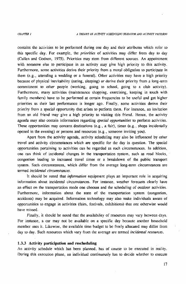
contains the activities to be performed during one day and their attributes which refer to

this specific day. For example, the priorities of actlvities may differ from day to day

(Cullen and Godson, 1975). Priorities may stem from different sources. An appointment

with someone else to participate in an activity may give high priority to this activity.

Furthermore, some activities derive their priority from a moral obligation to participate in

them (e.g., attending a wedding or a funeral). Other activities may have a high priority

because of physical inevitability (eating, sleeping) or derive their priority from a long-term

commitment to other people (working, going to school, going to a club activity).

Furthermore, many activities (maintenance shopping, exercising, keeping in touch with

family members) have to be performed at certain frequencies to be useful and get higher

priorities as their last performance is longer ago. Finally, some activities derive their

priority from a special opportunity that arises to perform them. For instance, an invitation

from an old friend may give a high priority to visiting this friend. Hence, the activity

agenda may also contain information regarding special opportunities to perform activities. These opportunities may concern destinations (e.g., a fair), times (e.g., shops incidentally

opened in the evening) or persons and resources (e.g., someone inviting you).

Apart from the activity agenda, activity scheduling may also be influenced by other

travel and activity circumstances which are specific for the day in question. The special

opportunities pertaining to activities can be regarded as such circumstances. In addition,

one can think of incidental changes in the transportation system, such as road blocks, ·

congestion leading to increased travel times or a breakdown of the public transport

system. Such circumstances, which differ from the average long-term circumstances are

termed incidental circumstances. It should be noted that information equipment plays an important role in acquiring

information about incidental circumstances. For instance, weather forecasts clearly have

an effect on the transportation mode one chooses and the scheduling of outdoor activities. Furthermore, information about the state of the transportation system (congestion,

accidents) may be acquired. lnformation technology may also make individuals aware of

opportunities to engage in activities (fairs, festivals, exhibitions) that one otherwise would

have missed. Finally, it should be noted that the availability of resources may vary between days.

For instance, a car may not be available on a specific day because another household

memher uses it. Likewise, the available time budget to be freely allocated may differ from

day to day. Such resources which vary from the average are termed incidental resources.

1.3.3 Activity participation and rescbeduling An activity schedule which has been planned, has of course to be executed in reality.

During this execution phase, an individual continuously has to decide whether to execute

17

CHAPTER 1 A THEORY OF ACI7VlTY SCHEDUI.lNG BEHAWOR AND ACI7VlTY PAITFJINS

the activities as scheduled or to adjust and reschedule them in response to unforeseen and

unexpected circumstances. Decisions to adjust the schedule are termed activity rescheduling decisions. Such decisions may concern the execution of activities that were not planned, deleting planned activities, changing locations to visit, changing the sequence in which activities are performed, or changing the timing and duration of activities. Furthermore, changes may be made with respect to trips that were planned: modes may be changed, different routes may be foliowed and departure times may be adjusted. Thus, the decisions are principally the same as in the scheduling phase, but now they are taken in

the context of monitoring an existing schedule. Similarly to activity scheduling decisions, activity rescheduling decisions are made

subject to the same factors, such as the long-term calendar, the cognitive map of the environment, the available general and incidental resources, the activity agenda and incidental circumstances. However, the performance of activities and the decision whether to reschedule also depend on the outcome of the scheduling phase, that is, the activity schedule. For instance, someone working on a tight schedule may need to reschedule

more than someone working on a less tight schedule. By nature, the rescheduling phase entails decisions whether or not to maintain the

planned schedule, and if not, how to adjust it. There are several possible reasons why individuals may decide to divert from their original schedule. First, the experienced outcome of scheduled activities and trips may give rise to changes. For instance, activities and trips taking more or less time then expected or requiring more money than expected,

so that other activities have to be cancelled or postponed. Secondly, outside information regarding changes in the travel and activity environment or the activity agenda may play a

role. For instance, information about congestion or the pubtic transportation system may lead someone to change bis schedule. However, also information about activities (a concert that is cancelled, a friend calling to invite you for a drink or asking your help) may cause a change in priorities of activities and a revision of the schedule. Thirdly, motivations and attitudes may change internally. For instance, one may feel less eager to

perform an activity that was originally scheduled and decide to postpone it. Another possibility is that, one experiences fatigue while performing an activity and decides to end the activity earlier than expected. Finally, one's physical condition may be a reason to divert from the original schedule. For instance, a sudden toothache or illness may prevent one from going to work or sleepiness may cause one to go to bed instead of doing other activities in the evening.

Finally, it should be noted that the rescheduling phase is a continuous process: once

the schedule is changed, this results in a revised schedule, which in turn is subject to the same monitoring process and may be further adjusted. What results is a revealed activity pattem of executed activities and trips which may be different from the one that was

18

CHAPTER 1 A 'IHEORY OF AGnVITY SCHFDUUNG BEHAVlORAND AGnV!TY PA1TERNS

originally planned. To what extent the planned and the executed activity pattern differ, of course depends on the level of detail at which a plan is made and the risks of diverting from the original schedule.

1.4 ACTIVITY-BASED MODELING

As noted earlier, by examining travel in the context of the activity scheduling process and

the activity pattern, a comprehensive framework of travel decision making is obtained. This framework encompasses responses to a wide range of policies such as telematics,

information technology and planning induced changes in the travel environment. As a

consequence, roodels which describe activity scheduling or the execution of activity patterns are potentially useful tools for predicting travel behavior. This thesis presents new activity-based roodels based on an assessment of existing models. Specifically, a state-of­

the-art review is provided which allows the identification of the key issues in developing new activity-based models. The state-of-the-art review includes activity-based roodels which account for a comprehensive description of one-day activity scheduling or one-day activity patterns. As a consequence, roodels which are limited to partial aspects of the

total pattern, such as work-related trip ebains are not included. Existing activity-based roodels differ in a number of respects.

First, different nwdeling techniques have been applied. Discrete choice theory,

micro-economie consumer theory, normative approaches and artificial intelligence techniques have been applied to model daily activity scheduling. Secondly, the modeling

approaches differ with respect to the stages in the decision rnaking that they address.

Some models focus specifically on the scheduling stage, whereas others focus on the execution of activity patterns. Thirdly, the roodels also differ with respect to the decision­making strategies that are assumed to underlie activity scheduling. For example, utility­maximization approaches assume that individuals act rationally in that they have complete information about all available choice alternatives and are able to maximize the utility gained from any of these alternatives. In contrast, artificial intelligence techniques assume that human decision-making is of a satisficing nature and that the outcome of decisions is

not necessary optima!. Fourthly, the different modeling techniques imply different possibilities to perform statistical tests of the significanee and the performance of the models. Some roodels allow for the derivation of statistica! goodness-of-fit measures,

which can be used to test different model specifications and calculate confidence intervals of estimated parameters. Other roodels rely on more qualitative methods to derive the best model specification. Furthermore, roodels may differ with respect to the variables, both dependent and independent, that are included in the model. In this respect, the

19

CHAP1ER 1 A lliEORY OF ACTTVIIT SCHEDUUNG BEHAV/OR AND AC11VITY PAT1ERNS

independent variables are an indication of the possibilities to assess specific policies. For instance, models which include mode choice as an endogenons variabie can better predict the effect of changes in the infrastructure than models which regard mode choice as an exogenous variable. The dependent variables can then be interpreted as the behavioral responses a model can account for. In a similar vein, models differ with respect to the dependendes between the dependent variables that they account for. For instance, the extent to and the way in which different activities or trips that are made or planned are

linked in the model structure is an important characteristic of different model types. This issue is related to the flexibility that models have to account for a wide range of behavioral responses. For instance, some models describe behavioral responses only in the terms of changes of destination and mode choice within a stabie activity sequence, whereas other models also allow for the substitution of activities and changes in the sequence. Clearly, the greater the flexibility, the more useful a model is for assessing policies.

1.5 CONCLUSIONS AND 0UTLINE

This chapter has demonstrated the importance of the activity-based approach in travel demand modeling. The activity-based approach does not consider travel as a demand in its own right, but rather as a demand derived from activity participation at different destinations. This implies that travel should be treated in the context of total activity patterns. Along these lines of thinking, the activity-based approach emphasizes dependencies between travel and non-travel, linkages between different trips and activities throughout the day and household interactions. Furthermore, the existence of space-time constraints is an important characteristic. Due to the increasing complexity of individual activity patterns and new policies such as telernatics and information technology, an activity-based approach to travel demand modeling becomes increasingly important.

To facilitate an assessment of current activity-based travel demand models and to give a rationale for the new approaches presented in this thesis, a theory of travel decision making in the context of the activîty-based approach was presented in this chapter. The theory assumes that travel decision-making is the outcome of long-term mobility lifestyle decisions, daily activity scheduling and the execution of a schedule. The outcome of a longer-term deelsion can in this respect serve as explanatory variabie of a shorter term decision. The theory identifies the decision dimensions and the explanatory variables in each stage. It can be concluded that long-term factors, such as the long-term calendar, the cognitive map and the available resources affect activity scheduling and the execution of activity patterns. However, also shorter term factors which hold for a specîfic day, such as the activity agenda and incidental circumstances and resources may be of importance.

20

CHAPTER 1 A THEORY OF AC17VITY SCHEDUUNG BEHAVlORAND ACnVITY PATJERNS

The role of information technology to bring these circumstances to travelers' attention is

emphasized. The Chapters 2 to 5 provide an overview of modeling approaches in the area of

activity scheduling and activity patterns. The applied modeling technique is chosen as the

organizing principle of the chapters, as many of the other issues or to some extent typical

for a specific model type. Specifically, Chapter 2 addresses space-time mode Is which have been developed in geography and urban planning based on the theories of Chapin (1974) and Hägerstrand (1970). Chapter 3 focuses on time allocation models, which are rooted in

micro-economie consumer theory. Discrete choice models, which are related to micro­

economie models, but also bear relationship to psychological choice theories, are discussed in Chapter 4. Finally, Chapter 5 discusses modeling techniques developed in

artificial intelligence. In particular, production system models and neural networks are

addressed. Each chapter first presents the theoretica! notions underlying the modeling

techniques, and then gives some examples of applications in the field of activity scheduling and activity patterns. Each chapter will furthermore address the aforementioned

issues of decision strategies, decision-making stages, dependent and independent variables and flexibility of the model. Based on the review of existing models, Chapter 6 assesses the capability of existing models to account for the effect of policies in the field of

transportation and travel behavior. Furthermore, a rationale is given for the new models which are presented in this thesis.

21

22

CHAPTER2

ACTIVITY-BASED MODELS IN GEOGRAPHY AND URBAN

PLANNING

2.1 INTRODUCTION

As noted in Chapter l, many concepts of the activity-based approach in travel behavior

research were originally developed in geography and urban planning. Since the 1960s, a

continuous stream of research in geography and urban planning has examined human

activity patterns and their associated traveL This direction emerged as a reaction to the

more traditional approaches in this field, which, at that time, focused specifically on

aggregate urban developments. This traditional approach was criticized for ignoring the

individual processes underlying these aggregate developments. Furthermore, the search was for models and paradigms that relaxed the strong assumptions on which the classica!

economie approach relied. These concerns gave rise to >the development of what is called

behavioral research, which focuses on the individual as the central unit of research.

Hence, urban development processes are not considered as autonomous processes, but instead are considered to be the sum of many, mutually dependent, individual behaviors.

However, within this behavioral stream of research, most researchers made the

simplifying assumption that decisions made by an individual are independent of each

other, thereby ignoring interdependencies that exist between different activities that are

pursued within a household. A more integrated approach, based on the analysis of activity

patterns, was initialized by the pioneering work of Chapin and Hägerstrand. Their theories can be considered complementary to each other. Whereas Chapin focused specifically on

the motivations that drive individuals to participate in various activities, Hägerstrand emphasized the factors which limit an individual's options to perform activities. Both

approaches are relevant to transportation modeling. The relevanee of Chapin's work lies

in the enhanced understanding of the factors that underlie activity patterns by which travel

is evoked. Hägerstrand's work, on the other hand, offers a conceptualization of human

activity spaces which can be directly incorporated into transportation models. For this

reason, we wil! discuss both approaches in this chapter.

Chapin's theory is discussed in section 2.2. Section 2.3 gives examples of

descriptive studies in the Chapin tradition. Hägerstrand's space-time geography is outlined

23

CHAPTER 2 AC11Vl'IT-BASED MGDELS lN GEOGRAPHY AND URBAN PLANNING

in section 2.4. Based on Hägerstrand's work, several models have been developed which systematically describe individuals possibilities to perform activity patterns in a specific spatio-temporal setting. The models are briefly discussed in section 2.5. Section 2.6 discusses some extensions of Chapin's and Hägerstrand's work. Section 2.7 finally concludes the chapter by drawing some conclusions regarding the relevancy of the approaches for activity-based travel behavior modeling.

2.2 CHAPIN'S THEORY OF ACTIVITY PATTERNS

One of the first researchers to recognize the importance of time and space in urban planning was Chapin (1974). He emphasized the importance of activity patterns as the building blocks of the use of time and urban space. According to Chapin, activity patterns determine the demand for housing, employment and facilities at particular times and places. Urban planning processes should therefore be based on a thorough understanding of the determinants and evolution of activity patterns.

According to Chapin, activity patterns should be analyzed at the level of individual daily routines. If regularities in activity patterns are understood at this level, the scope can

be broadened to aggregate distributions of activities in time and space, which can give an indication of the impact of policy interventions. The daily activity pattem consists of activities of different kinds. Some are necessary, biologically determined activities, such as sleeping and eating. Others are still ob Iigatory, but are more socially than biologically determined, such as working or buying groceries. Finally, there are discretionary activities such as reading or watching TV. To answer the question how individuals decide about the activities to perform, Chapin distinguishes between four driving forces by which activities are determined (Figure 2.1). First, a propensity will invoke the performance of the activity and secondly, the opportunity for the activity has to be present. Furthermore, an appropriate situation has to arise and activity performance is also influenced by the environmental context.

With respect to propensity, Chapin distinguishes motivational and constraining factors. The motivational factors are related to the fulfillment of basic needs on the levels of security (sleep, food, intake), affection (activities with relatives and friends),

achievement and status (getting ahead in your job, obtaining prestigious goods) and self­fulfillment (doing things for the enjoyment of doing them). However, propensity is also affected by constraints such as personal characteristics (sex, stage in the Iife cycle and health status) and rol es that society assigns to persons (e.g., the fact that male partners are assumed to fulfil the breadwinning role in western society).

24

CHAPTER 2 AC11VITY-BASED MGDELS lN GEOGRAPHY AND URBAN PLANNlNG

appropriate tilring 1. outcome of

earlier activ~ies 2. prior cammi­

menis 3. institutionalized

schedules

appropriate i

oircurrstances 'I

1. right persons 2. n.qui~e props S. suitable weather i

appropri e situallen

-----.. probability . high activity is \--T---1 9/J

oongeniality of surroundings foractivity

0

accessibleplace ancHaoility of acceptable quality lor an activity

high

unlil~on

changes

unlil

Figure 2.1: Chapin 's Theory of Activity Patterns

individu al engsges in activity

Opportunity is associated with physical and spatial variables affecting the probability

of choosing an activity. In this respect, Chapin mentions the example of a restrained

housing market that prohibits people to choose their dwelling at such a place that they can pursue all the activities they would like. Thus, opportunity principally retlects the availability and spatial location of facilities needeel to perform specific activities.

A third factor in activity performance is the appropriateness of timing and circumstances. The timing of an activity may for instanee depend on if one has been engaged in the activity before, commitments one has made for the activity or other activities and time schedules of shops and other institutions (schools, firms, etc.). The appropriateness of timing not only implies that there needs to be opportunity for the

activity to occur at a certain time, but also that the activity can be performed for its full duration, also with respect to the timing of other activities. Appropriate circumstances may depend on various factors such as the availability of certain 'props' (e.g., bringing

your bank pass if you go to a bank, bringing sports clothes along if you go sporting) or

25

ACT/VlTY-BASED MODELSIN GEOGRAPHY AND URBAN PlANNING

suitable weather. However, circumstances may also be enforced on someone by external factors (e.g., a friend dropping in unexpectedly).

Finally, activities are influenced by the , environmental context which provides

facilities and opportunities. The environmental context encompasses all non-physiological factors affecting an individual's activities. Of specific interest is that Chapin's theory describes how the environmental context is changed by external and internat sources. The

external sourees by which the environment is constantly changed include technological, economie, cultural and social developments. lnternal sourees of change are represented by four feedback loops, representing how individuals react to the outcome of activities by changing the environmental context. First, the execution of activities may lead to a change in the constraints stemming from personal characteristics. Secondly, the outcome of activities may lead to a change in attitude and motivations towards activities. A third internal souree of change is that the outcome of activities motivates people to modify opportunities to perform activities, for instanee by moving to a place with a higher density of various facilities. Finally, individuals may react by adapting the timing of activities until the right timing and circumstances occur.

In his empirica! work, Chapin emphasizes the propensity side of his model, focusing

especially on the effect of needs and roles on activity performance. Hence, the opportunity side, which accounts for spatial factors such as the location of facilities, and temporal factors, such as the appropriate timing, are somewhat neglected. Neverthe\ess, Chapin's theory can be considered a milestone in urban planning, as it is the first to relate

activities, time and space in urban planning in a single coherent theory.

2.3 APPLICATIONS OF CHAPIN'S THEORY

An important implication of Chapin's theory is that both the motivational and the constraining dimension of propensity partially determine how individual activity patterns evolve. Both dimensions coincide with personal characteristics such as age, life cycle, sex, income etc., which are related to roles and motivations. Consequently, this notion has led to a stream of research efforts, which aim at descrihing activity patterns of predefined socio-demographic groups to identify how characteristics of each group affect travel and activity behavior. Although these approaches do not involve predictive models in the sense that they use a mathematica\ formulation to predict behavior based on a set of predietor variables, they provide valuable information regarding the effects of personal characteristics on activity patterns. This section therefore discusses some of the studies in this tradition that have been reported in the literature.

Based on a 1968 data collection, Chapin (1978) investigated how · participation rates

26

CHAFIER 2 AClTVJTf.BASED MODELSIN GEOGBAPHY AND URBAN PLANNING

and hours allocated to different activities varied across racial and income groups. He

found, among other things, that blacks did not participate in social activities as much as non-blacks. A similar result was found for low income groups as compared to higher income groups. When looking at time allocation, it was found that blacks spend more time

on working, recreation and hobbies, watching TV and resting and relaxing than non­

blacks. A similar results was found for low-income groups compared to high-income groups. However, high-income groups spend more time on shopping and out-of-home

activities in generaL Chapin's results furthermore confirm the intuitively plausible hypothesis that peopie who do not work full time spend more time on social activities, watching TV and resting and relaxing.

Van Knippenberg et al. (1990) analyzed the activity patterns of non-traditional households in the Netherlands, basedon a 1982 data collection. 58% of the women in the sample worked part-time, whereas 98% of the men worked full-time. There appeared to

be only minor differences between working men and women with respect to the number of trips, time spent travelling and mode choice. Children were found to have an effect on

activities and travel behavior. On average, men with children were found to work 1 hour less then men without children. However, their travel time was not affected. Women with children, on the other hand, worked 2.5 hours less then women without children. Their

trip pattern is also different in the sense that they make more home-work trips in order to prepare lunch for their children, they travel for shorter distances and more often combine their work trip with other purposes. The younger the children, the more complex the trips are and the more often the car is used. Moreover, they found that single mothers work

more hours than married mothers and have Jonger travel times due to lower car

availability rates. Part- time working women, finally, make less home-work trips and combine less activities intheir trips as compared to full-time working women.

The activity patterns of non-traditional households have also been addressed by Vijgen and Van Engelsdorp Gastelaars (1990). In a comparative study based on activity

diaries taken in the Netherlands in 1985 and 1987, they investigated the activity patterns of nine household categories. All time expenditures below are given per person. i) Single starters, such as students. They have much free time (7 hours per day). They

also spend much time on study (3 hours) and little on housekeeping.

ii) Single workers with relatively little free time (5.5 hours). They spend on average 6.5 hours per day on professional work and 1.5 hours on housekeeping.

iii) Working couples without children have a behavior that is quite identical to that of

single workers. They have more free time (6 hours) and spend a little more time

(1.75 hours) on housekeeping. They spend 6.25 hours per day on work. iv) Parents in traditional one-worker households spend on average more time on

housekeeping (3.5 hours per day), have more free time (6.5) hours and less time on

27

CHAPTER 2 ACTIVITY-BASED MODELSIN GEOGRAPHY AND URBAN PlANNING

work (3.5 hours). It should be noted, however, that the distribution across busband and wife is not equal.

v) Dual earner families with children spend more time on work (5 hours) in comparison to traditional families. Logically, they have less free time (6 hours) and

spend less time on housekeeping (3 hours). vi) The time allocation of single mothers living on welfare is quite different. They

spend 8.5 hours per day on housekeeping and 4.5 hours per day on free time. vii) Working single parents spend on average 4.5 hours per day on work and 3.5 hours

on housekeep ing. They have 6 hours of free time per day. viii) Retired people are found to have very much free time (9.5 hours per day) and also

spend relatively much time on housekeeping (4 hours). Comparing the groups, Vijgen and Van Engelsdorp Gastelaars (1990) conclude that

shortage and fragmentation of time are the most serious problems in time allocation faced by particular groups. Especially households in which all adults have a job have little net free time as they also have to perform the housekeeping task. Consequently, many free time activities can only be performed in the weekends. Fragmentation of free time is especially relevant to households with children as they have to catch up and take care of their children at a number of fixed times per day. This wiJl limit their possibilities of staying away from home for Jonger periods and participate in certain activities. Moreover, the difficulty of brioging children along to certain facilities {theaters, cafés, restaurants, other people) is a further limitation for outdoor activity participation.

Another way of testing the differences in behavior of different socio-demograpbic groups is to regress characteristics of the activity pattem on socio-demograpbic characteristics, as was done by Pas (1984). His results suggest that higher educated people have activity patterns with more multi-stop trips, whereas less educated people make more single-stop trips, especially for maintenance. Furthermore, people with children under 12 appeared to make more single-stop trips around noon. People without children under 12 more often make multi-stop trips, aimed at various activities and trips in the evening. Furthermore, married people make more single-purpose trips in the evening aiming at leisure. Single people in general make more multi-purpose trips for all activities. Also people living in areas with a low residential density turn out to make more multi-purpose trips.

The applications described in this section clearly illustrate the implications of Chapin's theory for transportation research. Individuals with different socio-demograpbic characteristics, living in different settings have very different activity and trip pattems. On the one hand this is caused by differences in needs and objectives, which cause them to pursue different types of activities. On the other hand, the opportunities and constraints of individuals differ widely which has an impact on both activities and traveL This implies

28

CHAP1ER 2 ACTIVITY-BASED MODELSIN GEOGRAPHY AND URBAN PLANNING

that in order to develop adequate activity-based transportation models one has to account

for both spatio-temporal constraints and socio-demograpbic differences. With respect to the latter, one should preferably include individual activity agendas in order to represent

different neects and objectives. If this is not possible, socio-demograpbic variables can be

used to distinguish segments with typica1 activity patterns.

2.4 IIÄ.GERSTRAND'S SPACE-TIME GEOGRAPHY

As noted in Chapin's theory, activity performance is affected by spatial opportunity,

which is related to the availability of facilities, and the appropriate timing, necessary for

each activity. However, the spatial and temporal dimensions are treated separately in his

theory. An approach which incorporates both space and time in a coherent framework is the space-time geography of the Lund school of which Hägerstrand (1970) is the founding

father. Space-time geography systematically explores the opportunity to unfold activity

patterns in a specific spatio-temporal environment. It is assumed that time and space are

scarce goods and that, consequently, daily activity patterns are largely determined by space-time constraints. Similar to Chapin, Hägerstrand points out that activities are

invoked by basic neects such as security and self-fulfillment. An activity can furthermore

be described in terms of a certain duration and location. A sequence of activities then

implies a path through space and time that is foliowed by an individual. This activity path

consists of stations where activities take place, and transportation ebains between the

activities. Such a space time path can be represented in three dimensions as shown in

Figure 2.2. Obviously, not all paths through space and time are feasible in everyday life.

Hägerstrand identifies three basic types of constraints to which activity patterns are subject.

The first of these are capability constraints, referring to physical limitations. An

important limitation, for instance, is the neect to spend a considerable time of the day

sleeping and eating. Furthermore, individual indivisibility and limits to the maximum

speeds of different transport modes imply that activities that are too remote in space

cannot be part of one space-time path.

Hägerstrand also distinguishes coupling constraints, which basically define "where,

when and for how long the individual has to join other individuals, tools and materials in·

order to produce, consume and transact (Hägerstrand, 1970)". Due to coupling

constraints, the paths of individuals and tools may form bundies at a fixed location for a

certain duration (see Figure 2.3). Bundies are, for example, formed by colleagues at the

workplace, worker and machine and salesman and customer in a shop. Bundies may be formed according to fixed time tables, such as for instanee factory workers. Another

29

CHAPTER 2 ACTIV/TY-BASED MODELSIN GEOGRAPHY AND URBAN PLANNING

time

24.00 t-l't=:.tttF====:::!=:::a:;-1"

18.00

12.00 space

6.00

0.00

0 available time window

path through space and time

Figure 2.2: Example of a Space-Time Path

possibility to form bundies is by allowing random access, which is the case for shops and banks. Furthermore, bundies may form only occasionally as a result of unique appointments. Hägerstrand also points at the possibility of remote bundles, which are made possible by modern communication tools. For instance, two individuals having a telephone conversation have to stick to their telephones, and are thus subject to coupling constraints, although their paths can be spatially remote.

Another category of constraints are authority constraints, which prohibit the use of facilities at certain times. Hence, they define certain domains that exist for activities at

certain times. Such domains may be caused by power of custom (e.g., a favorite chair or a place in a queue) or have astrong legal status (the home place, that is not accessible for outsiders, shops that are closed at certain times). The constraints may furthermore hold fora very long time (e.g., nation states) or may be temporary (a seat in a theater).

How the above constraints affect the individual activity space is illustrated by the time-space prism concept. Suppose that two activities are fixed in time and space. The

30

CHAPTER 2 AC11VITY-BASED MODELSIN GEOGRAPHY AND URBAN PLANNING

time

space

Figure 2.3: Coupling Constraints

possible space time path that can be performed between the acnvttles can then be displayed by a prism (see Figure 2.4). The size of the prism is detennined by the speed at which one can traveL For instance, the prism of a car driver will be much wider than a cyclist's prism. If other fixed points are introduced along the space-time path, this results in splitting up the large prism into a number of smaller prisms which illustrate the limiting

effect of constraints on possible activity patterns. Hägerstrand's theory thus clearly illustrates the relationship that exists between the transportation system, the location of facilities and the possibility to perform activity and travel patterns. Furthermore, it opens the opportunity to theoretically assess the activity patterns that an individual can perform, given the locations at which he can perfarm certain activities, the transport facilities available to him and the current coupling and authority constraints. The relevancy of Hägerstrand's theory for transportation modeling thus lies in its opportunity of integrating both spatial and temporal aspects which determine individuals' travel patterns.

2.5 ACTIVITY PATTERN FEASmiLITY MODELS

Obviously, the main difference between Hägerstrand's and Chapin's approach is the identification of various kinds of constraints influencing behavior. Based on Hägerstrand's

31

CHAPTER 2 AC11VlTY-BASED MODE!.S lN GEOGRAPHY AND URBAN PlANNING

! time

a b c distance

Figure 2. 4: Space-Time Prisms

theory, a stream of research, which emphasizes constraints as the basic determinant of human behavior, bas evolved. In this respect, it is typically assumed that the impact of constraints on behavior outweighs the effect of preferences that lead individuals to make certain choices. In this context, much attention has been devoted to studying the possibi!ities offered by the spatio-temporal environment to realize specific activity programs. Various roodels have been developed. They have in common their main objective of identifying feasible activity schedules as a function of observed constraints. That is, they typically have been developed and applied to demonstrate that particular activity patterns could no Jonger be performed as a result of (planned) policies that affect various constraints. For example, ciosure of schools results in Jonger travel distances, which in turn may imply that certain activity patterns cannot be implemented any Jonger. Similarly, Jonger opening hours may induce shifts in activity patterns.

These roodels thus typically examine whether particular activity patterns can be realized within a specified time-space environment. These roodels require activity programs, which describe a set of actlvities of a certain duration which can be performed at certain times as input. Usually, these programs are derived from observations of activity patterns. The space-time environment is defined in terros of locations, their attributes, available transport modes and travel times between locations per transport mode. Typically, one of the attributes of interest is the opening hours of that location. To examine the feasibility of a certain activity program, a combinatorial algorithm is typically used to generate all possible activity sequences. Then, the feasibility of each sequence is tested by (i) checking whether the interval between the end time of the previous activity

32

CHAPTER 2 AC11V/TY-BASED MODELSIN GEOGRAPHY AND URBAN PLANNING

and the start time of the next activity is sufficient to perform the activity plus the

associated travel time; (ii) testing whether the activity can start after the earliest possible start time and be finished before the latest possible end time; (iii) checking whether

conditions about the sequencing of activities are not violated. The number of feasible activity schedules is often used as a measure of flexibility of the time-space environment.

One of the first models in this tradition is Leuntorp's (1978) PESASP model. The starting point of this model is a set of activities that has to be performed by an individual.

Given that · each activity can be performed at a certain number of locations, an exhaustive

listing of sequences· of activities, performed at specific locations, can be generated. However, in a specific setting not all sequences are feasible, due to constraints set by the environment. PESASP reduces the set of all possible sequences by checking for their feasibility in terms of a set of predefined constraints. That is, given activity durations,

travel times by various modes and opening hours of facilities, it checks whether a certain sequence can be executed. Hence, the rules of Hägerstrand's space-time geography are applied to determine to what extent the three types of constraints limit the possibility to

perform activity patterns. PESASP in this respect takes an exhaustive approach by evaluating all possible sequences. In the feasibility check, the time needed for parking and

for walking to and from public transport facilities is also taken into account. PESASP typically imposes an activity program onto all possible home-work constellations in an area in order to exhaustively obtain an impression of the possibilities of the spatio­temporal environment in facilitating specific activity programs. Hence, the activity

programs are not derived from observed activity patterns, but defined a priori. As PESASP is primarily used to test the feasibility of activity programs based on residence/work place pairs across a total study area, the output of the model gives an impression of the accessibility at each point within the area. For instance, the model can assess the effect of an improverneut of public transport services in terms of the additional number of work places accessible from each residential zone.

A similar model, developed in the field of transportation, is CARLA (Jones et al., 1983), which is basically a combinatorial algorithm for generating feasible activity

patterns. It is based on two important underlying principles. First, alternative activity arrangements are generated in an ordered way to avoid wasting time on testing obviously infeasible patterns. Secondly, beuristic rules are applied to the scheduling process to reduce as far as possible the number of alternatives examined. CARLA, which stands for a Combinatorial Algorithm for Rescheduling Lists of Activities, first generates. activity

schedules according to the principles of back-track programming which relies on building up the schedules according to a tree structure. Intermediate nodes in the tree represent incomplete schedules, and the terminal nodes represent the set of possible complete

schedules. This tree-Iike representation allows one to identify whole sections of the tree

33

CHArTER 2 AC17Vl1Y-BASED MODELSIN GWGRAPHY AND URBAN PLANNING

which contain only infeasible schedules and which therefore need not be examined at all.

In this respect CARLA differs from PESASP, which exhaustively examines all possible configurations. The number of permutations examined is limited by applying constraints to the times at which partienlar activities may take place. Such constraints stem from supply side constraints (e.g., shops are only open at certain hours) and behavioral rules (e.g.,

householcts are unlikely to reschedule their meal times by more than, say, 45 minutes). The algorithm requires as input a list of activities to be scheduled, their durations

and the times of day between which each is allowed to take place. The output produced is a list of all the 'feaSible' permutations of those activities, where feasible means that the

schedule does not contradiet any of a number of rules which are either implicit in the design of the algorithm, or are explicitly stated in the model input. Many different rules represent the constraints. For example, logica! rules are incorporated in the design of the algorithm; environmental rules are represented by those temporal constraints, which limit

the supply of facilities for certain activities to certain times of day; scheduling rules reflect people's habits and routines and are represented by other types of temporal constraints (i.e. those which limit the time by which activities may move from their observed positions).

Another combinatorial algorithm, BSP, was proposed by Huigen (1986). This program is similar to CARLA in that it evaluates the options to maintain the current

activity pattem in a changed spatio-temporal setting. However, as PESASP, it does so by

exhaustively evaluating all possible sequences of activity/destination combinations. Furthermore, BSP differs somewhat with respect to the way constraints are incorporated. lt offers the option that different trips in a trip chain are made by different modes and allows for the simulation of cycling from and to pubtic transport facilities. Different from CARLA and PESASP, BSP furthermore defines available time windows specifically for destinations and not for activities. For instance, instead of defining time constraints for shopping in genera!, as PESASP and CARLA do, BSP opens the option to define different opening hours for different shops. With respect to the output, BSP offers an additional

option to evaluate the feasible activity patterns on a number of criteria, which give an impression of the quality of the feasible patterns. For instance, BSP gives information about the travel distance of each feasible pattern, the time spent in-home and out-of-home, the number of visited locations and zones. lf, in a specific spatio-temporal setting, no feasible activity patterns were found, BSP indicates the critica! factors that prohibit execution of the given activity program.

The above discussion indicates that PESASP, CARLA and BSP are especially valuable in situatîons where one wishes to demonstrate the potentlal impact of policies affecting the time-space environment on activity patterns. For example, CARLA has been applied to assess the consequences of the dîscontinuation of a bus service in the British

34

CHAPTER 2 AcnVITY-BASED MODELSIN (',EOGRAPHY AND URBAN PLANNING

countryside (Van Knippenberg and Splinter, 1983). Likewise, BSP (Huigen, 1986) has been used to simulate the effects of school ciosure on students' travel times. These simulation models provide a valuable policy evaluation tool, as long as it is realized that

the predicted activity schedules do not necessary reflect actual patterns. Compared to

many other models, to be discussed in later chapters, these mode\s Jack the necessary

mechanisms to predict adjustment behavior of individuals. When faced with a changed time-space environment, individuals are Iikely to adjust/reschedule their activity programs.

Consequently, policies may often have less dramatic social impacts as these models may suggest. This is especially true in urban contexts where often many potential activity

patterns can still be conducted, even after the number of choice alternatives has been reduced. The models discussed in this section may have oversold the notion of constraints and neglected that individuals often still do have substantial choices in (re)scheduling their

activities, even when their typical activity patterns are no Jonger feasible. They may

decide to perform certain activity at other times and/or other locations; activities may be combined in different manners; they may decide to use different transport modes to relax time constraints; activities may be reallocated to other memhers of the household; the duration of activities may change the optima! time allocation in a given time-space environment; and, finally, discretionary activities with lower priorities may be substituted for other ones to maximize, or at the very least satisfy, the individual's or household's

basic needs and desires.

2.6 RELATED APPROACHES

The above theories of Hägerstrand and Chapin can be considered as the foundation of activity-based theory, research and modeling in geography and urban planning. These theories have been the basis for further developments in geography and urban planning, but also in other disciplines, which have refined and elaborated specific aspects of Chapin's and Hägerstrand's work. Some of these developments are discussed in the remainder of this section.

An approach that integrates Chapin's and Hägerstrand's theory but places more emphasis on the individual planning process has been developed by Cullen and Godson (1975). The relevancy of Cullen and Godson's work is that it integrates the propensity and opportunity approach of Chapin, the constraints-based approach of Hägerstrand and a

description of the decision-making process underlying daily activity and travel patterns. In

this respect, Cullen and Godson's theory is one of the first comprehensive behavioral theories of activity and travel decision-making. Many aspects of Cullen and Godson's work have later been incorporated into the behavioral models described in the next

35

CHAPTER 2 AC17VITY-BASED MGDELS IN GEOGRAPIJY AND URBAN PLANNING

chapters. Cullen and Godsou distinguish six factors that affect individuals' activity patterns.

Related to Hägerstrand's theory is the notion that the action space is limited by economie,

physical, institutional, conventional and accessibility constraints. The physical and accessibility constraints in this respect refer to Hägerstrand's capacity constraints, whereas

institutional and conventional constraints are comparable to the authority constraints defined by Hägerstrand. An important contribution is the introduetion of economie constraints, implying that also limited monetary budgets set limits to the possibilities to participate in activities.

Another factor, which is closely related to the propensity and opportunity factors identified by Chapin, is the definition of an individual's action space. The action space is

a framework that is fundamentally structured by physical patterns and needs. This framework is nowadays institutionalized by the availability of facilities and norms, expectations and habits acquired by the individual.

Building on the above, Cullen and Godson introduce the concept of priorities, which is an extension of Hägerstrand's and Chapin's theories. They state that individuals select amongst possible alternative activities by an order of priorities, based on their attributes. The time horizon of the priorities differs between actlvities that should be performed immediately (e.g., answering the phone) to actlvities that have to be performed

some time in the future (e.g., a meeting scheduled some weeks ahead). The priorities may depend on their importance in financial, strategie, physical or other terms, the involvements of others and their characteristics, the order in which actlvities are planned, the role of routines and preferences for certain activities.

Other extensions to Chapin's and Hägerstrand's work concern the decision-making process by which individuals arrive at the activity patterns that can be observed in everyday live. First, they conceive of activity patterns as organized behavior, where activities are performed with a certain purpose. However, the strength of the purpose may vary as some actlvities are almost instinctive, whereas others are carefully thought out. It is furthermore noted that actlvities occur in recurrent patterns, which are well organized and highly structured, although maybe notperfect rational.

Secondly, Cullen and Godson emphasize the importance of the flexibility of activities. It is argued that the freedom to choose activities is highly dependent on the degree of commitment towards the activity. As different degrees of commitment are distinguished arranged activities, routine activities, planned activities and unexpected activities.

Finally, activity patterns are the outcome of a scheduling process aiming at the synchronization of activities and saving time. The scheduling may be more automatic or more deliberate for different parts of the activity pattern. The highly prioritized activities

36

CHAPTER 2 AC11VITY-BASED MODELSIN GEOGRAPHY AND URBAN PlANNiNG

in this respect serve as pegs around which the other activities are scheduled, subject to

theîr flexibility.

LONG TERM BEHAVlOR

SHORT TERM BEHAVlOR

Figure 2.5: Relationship between Long-Termand Short-Term Choices (Cullen, 1978)

Further research by Cullen (1978) extends the theory of the decision-making

process of activity patterns to include also long-term choice behavior. In this respect,

decisions regarding the long-term context in which daily activity patterns take place are

emphasized. Examples of such decisions are decisions to move to another residence or to

change jobs. Cullen emphasizes that for a better onderstanding of such long-term choices,

it is necessary to have insight in individuals' daily activity patterns. The crucial

assumption he makes is that long-term decisions regarding the spatia-temporal context are

taken such that the stress caused by the performance of daily activity patterns within that

context is minimized. Thus, as indicated by Figure 2.5, daily activity patterns not only

depend on the long-term context in which they are made. They also, via the accumulated

experience of daily activity patterns, have an effect on the long-term choices affecting the

context.

37

CHAPTER 2 AC17VITY-BASED MODELSIN GEOGRAPHY AND URBAN PlANNING

2. 7 CONCLUSIONS

This chapter has reviewed theories and models of individual activity patterns, which have

been developed in geography and urban planning and which are potentially relevant for transportation modeling. The approaches that have been developed in this field differ substantially with respect to their underlying assumptions. Chapin's theory primarily focuses on the propensities and driving forces that motivate individual activity

participation. Empirica! studies in this tradition indicate that propensities primarily stem

from personal characteristics. Therefore, they provide valuable information regarding personal characteristics that should be incorporated into models of activity and travel patterns.

Hägerstrand's space-time geography, in contrast, has emphasized the relationship

between time and space in relation to human activity patterns by defining the forma! constraints set by the environment to the available activity space. The theory has been operationalized in the form of activity pattern feasibility models. These models can be applied to determine the opportunities to perform an activity program in a specific spatio­

temporal setting. The effect of policy measures can therefore be assessed in terms of the change in the number and quality of feasible patterns. These models are also relevant for transportation modeling, as they describe the theoretica! boundaries within which trip patterns have to take place. However, a major drawback of the models is that they assume constraints to be the main determinants of human behavior. In reality, however, individuals often have a variety of options to respond to changes in their environment,

even if their spatio-temporal setting appears relatively constrained at first sight. This suggests that travel demand models should not only include constraints, but also individual choices and preference, in order to predict which of multiple response options is selected by an individual.

Thus, although the activity pattem feasibility models offer a useful contribution to policy evaluation in constrained environments, the most important contribution of the research described in this chapter seems to be the identification of factors affecting activity and travel behavior, which have been incorporated in more advanced predictive models, basedon behavioral theories.

38

CHAPTER3

MICRü-ECONOMIC MODELSOF TIME ALLOCATION

3.1 INTRODUCTION

Activity scheduling can be viewed as an allocation problem. The problem then is how to

allocate time and money available for a one-day period to activities and traveL In this

respect, micro-economie theory offers an attractive framework for descrihing and modeling activity scheduling as an allocation procedure. Originally, micro-economie theory typically addressed the question how individuals decide about the quantities of different goods to consume such as to best meet their preferences and desires, given their available budget.

However, the theory can also be used to describe how other resources, such as for instanee time, are allocated to the consumption of goods, or, more generally, activity participation. Hence, micro-economie models can be used to describe the quantities of time that are spem on the consumption of activities such that an activity pattem is obtained

which is optima! given time and money budgets. Time allocation models, which are obtained in this way, were first introduced in this area in the pioneering work of Becker (1965). Since then, several improvements and refinements of the models have been proposed.

Time · allocation models are potentially useful for modeling activity patterns and activity scheduling, as the time that is allocated to activities is highly related to the choice of activities and their durations. However, micro-economie models have only seldom been applied in travel demand modeling. This is typically caused by the fact that the emphasis is especially on the temporal dimension of activity patterns and not so much on the spatial dimension, which invokes traveL The only applications of time allocation models to date have been models which describe mode choice as the allocation of travel time to one out of a set of alternative modes.

This chapter reviews micro-economie models in the field of time allocation and activity and travel patterns. The chapter is structured as follows. Section 3.2 first summarizes the underlying principles of micro-economie theory in generaL Micro­economie models of time allocation are then reviewed in section 3.3. Extensions of the time allocation models which include spatial components and which can therefore be used to describe travel patterns are discussed in section 3.4. Conclusions regarding the use of

39

CHAPTER 3 MICRO-ECONOMIC MODELSOF 11ME ALLOCATION

micro-economie models in activity-based modeling are drawn insection 3.5.

3.2 MICRO-EcONOMIC CONSUMER THEORY

Mièro-economic consumer theory basically deals with the mathematica! description of the relationship between an individual's needs and desires and his consumption of commodities and services (Ben-Akiva and Lerman, 1985). Individual consumption is

operationalized by means of a consumption bundie Q, specifying the quantity q1,

consumed of any good l:

(3.1)

this formulation implies that consumer behavior is measured in terms of continuous variables. Hence, consumer behavior is depicted as allocation behavior rather than discrete choice behavior, which is addressed by the models to be described in the next chapter.

Obviously, an individual has the choice between an infinite number of bundles. The set of available bundies is, however, limited by the constraints that are set by the available

income. Given that p1 is the fixed price associated with commodity l, the budget constraint is:

(3.2)

where I is the available income. Given a constrained set of consumption bundles, the question is then how individuals

decide which consumption bundie to choose. According to micro-economie theory, consumer choice is guided by the preferences consumers have for particular bundles. A number of assumptions is typically made regarding these preferences. First, it is assumed that a consumer, when faced with any two consumption bundles, can decide whether they prefer one or the other bundie or whether they are indifferent between them. Furthermore,

it is assumed that a consumer's preferences are transitive, so that if a consumer prefers A to B and B to C, he also prefers A to C. Finally, it is assumed that a consumer always prefers more of a commodity to less. That is to say, by consuming more of a commodity, the utility derived from the consumption of that commodity always increases.

Closely linked to the concept of preferenee is the concept of utility, which can be

regarded as the level of satisfaction derived from a particular consumption bundle. In this respect, it is assumed that a consumer always prefers one bundie to another if he derives a higher utility from that bundle. The crucial assumption underlying micro-economie theory,

40

CHAPTER 3 MICRO-ECONOMIC MODELSOF 17ME AILOCA170N

however, is that consumers act rationally in the sense that they maximize their utility.

However, given their individual tastes and budgets, optima! bundies of different

individuals may have a different content. Furthermore, due to misperceptions and

miscalculation of prices, deviations from the optimum may be observed in practice.

Finally, it is assumed that a consumer is capable of evaluating all possible alternative

consumption bundles.

Given the above assumptions, there exists a rank order of bundies according to their

utility, which reflects a consumer's preferenee order. The utility of a bundie is specified

as a function of the quantities consumed of various goods l:

(3.3)

Thus, if a consumption bundie i is preferred to bundie j, this is expressed as:

(3.4)

The choîce of a consumption bundie is now depicted as an optimlzation problem, as

illustrated by the following example. Assuming two commodities, a general utility function may be given by:

(3.5)

Given that individuals act rationally in the sense that they max1m1ze their utility, the

decision which consumption bundie to choose is formulated as the following optimization problem:

{3.6)

If the parameters /30 , /31 and /32 are known, the demand functions of the commodities q1,

given known prices and incomes can be derived using the Lagrange multiplier technique

(Varian, 1978). The demand functions give the amount of each good for which an optima!

utility is derived from the consumption bundle, given fixed prices and income and given

model parameters. In this example they are given by:

41

CHAF'I'ER 3 M/CRO-ECONOMIC MODELS OF TIME ALLOCATION

(3.7)

It is easily shown that by substituting the demand functions into utility function (3.5), the

maximum achievable utility is expressed as:

(3.8)

In the above we have discussed the ideal case of micro-economie models, in which

individuals would optimize their consumption of commodities according to utility­

maximization. However, in real life, behaviors would be observed which deviate from

optima! behavior as predicted by the model. This may be due to individual taste differences, which cause individual optimization 'errors'. The deviations may also be

caused by measurement errors or unobserved factors not included in the model. To

account for such deviations, a random error term is usually introduced.

Micro-economie models of the above type are particularly useful in analyzing the

forces underlying the demand for goods in a market and the calculation of market

demands and equilibrium prices (Mansfield, 1985). The models have primarily been

applied at an aggregate level to assess public polides in the market sector. Over the past decades, several extensions have been developed, aiming at facilitating

the application of micro-economie models to specific areas. One stream of research has

aimed at developing models that do not describe economie behavior in terms of price

equilibria and market shares, but in terms of individual choices. In this respect, it is

typically assumed that utilities can be formulated for separate commodities, based on a set of attributes (Lancaster, 1966). This theory has played an important role in the

development of discrete choice models, which are at the focus of Chapter 4. Another

development has emphasized that consumption of goods, or, more generally speaking,

activity participation, is not only constrained by money budgets but also by time budgets.

In this respect, it is typically assumed that individuals maximize utility by allocating time

and money budgets to the consumption of goods and the participation in activities. The

latter class of models will be further explored in the remaioder of this chapter.

42

CHAPTER 3 MICRO-ECONOM/C MODFLS OF 11ME A/.LOCA170N

3.3 TIME ALLOCATION MODELS

One of the first attempts to integrate time allocation and micro-economie theory was made

as early as 1965 by Becker. Specifically, Becker assumes the maximization of utility as a function of the time spent on activities and the consumption of goods during the activities. Noteworthy is the use of commodities, which require the input of time and the consumption of market goods. Becker's model assumes the maximization of utility, which

is expressed a:s a function of commodities:

Max U(Z) U[f(X,T)]

Subject to constraints that stem from the limitation of time and money budgets:

L:T;+W=T i

Lp x= IF + w w . J J

J

(3.9)

(3.10)

(3.11)

where T; is the time spent on actlvity i, JÇ is the amount of market good j that is

consumed, ~is the commodity associated with market good j, Ij is the price of good j, IF is the fixed income, W is the total work hours, w is the wàge rate and r is the total time available. An important feature of Becker's model is that "time can be con_verted into

goods". For instance, by working more hours, the price constraint is relaxed, so that more money can be spent on the consumption of goods. According to Becker's model, working hours can be chosen freely and are not incorporated in the utility function as such. As a consequence, the optima! salution to the time allocation problem is determined irrespective of how many time is spent on work. This is clearly an unrealistic assumption which may cause problems in the interpretation of the results.

A more general model, accounting for some of these shortcomings is given by De Serpa (1971). In his formulation, utility depends on the time necessary for the consumption of market good i and the amount of good i consumed. Constraints stem from the available income, the available overall time and the time needed for the consumption of a certain amount of good i. In formula:

Max U(X,T) (3.12)

subject to:

(3.13)

43

CHAPTER 3 MICRO-ECONOMIC MODELS OF 1lME ALLOCA1lON

(3.14)

T ~a X V. l i l l

(3.15)

where I is the fixed income, and a, is the time needed for consumption of good X,. De Serpa's model has the important implication that by the consumption rate a1, the time devoted to consumpiion of good X" the utility derived from consumption of goods and time and the income constraint are connected in a straightforward way. In this respect,

equation 3.15 is added as an additional technical constraint, compared to Becker's model.

The effect of this function is that it limits the number of possible solutions to the optimization problem of equation 3.12 (Truong and Hensher, 1985). Using this additional constraint, De Serpa operationalizes the value of saving time: by saving time on one activity i (i.e. by obtaining a smaller value of the coefficient a1}, more time remains for other activities to increase utility. However, saving time only results in a higher utility in case of time shortage (Jara-Diaz, 1994). De Serpa points out that the model can be generalized to encompass work commodity, pure time rommodities and negative prices.

An even more general model was proposed by Evans (1972), who formalized utility as a function of the time spent on various activities. Associated with each activity are goods and prices. The allocation of time is subject to time and income constraints, which are formulated in a very flexible way. In formula:

Max U(T) (3.16)

subject to:

(3.17)

BT -5, 0 (3.18)

(3.19)

(3.20)

where T is a vector with time expenditures, P is a matrix with prices of goods, Q is a

44

CHAPTER 3 MICRO-ECONOMIC MODELSOF 11ME AUOCATION

matrix specified the amount of goods required per time unit for an activity and B is a matrix specifying dependendes between the amounts of time spent on different activities.

Equation 3.17 specifies oost constraints with respect to activity participation, taldng into

account both the amount of goods per time unit needed for an activity (Q) and the price of one unit of a good (P). This formulation accounts for the fact that multiple goods may be involved in one activity and that multiple activities may involve the same good. Equation

3.18 implies that the time devoted to one activity can be technically related with the time spent on another activity. An advantage of the model is that goods are not incorporated in the utility function. Consumption of goods is secondary as a means to enjoy time, which

allows a more general formulation of constraints and seems a conceptually correct

approach. Similar to De Serpa's approach, the model allows for the inclusion of pure time commodities, which may have positive or negative costs. Hence, by introducing more interdependencies to the roodels with respect to the input rates of time and goods into

activities, an even more constrained model is obtained as compared to De Serpa's model. According to Jara-Diaz (1994), Evans' model gives the most complete relationship

between time and goods as it specifies the combinations of goods necessary to perform a set activities.

3.4 APPLICATIONS OF TIME ALLOCATION MODELSIN TRANSPORTATION

The above roodels can be considered as useful tools to better understand the allocation of time and money to activities and the consumption of goods. A flaw, however, is the complete absence of spatial factors, which may also influence time allocation and the

consumption of goods. The fact that certain goods or services can only be consumed or purchased at particular locations implies that time allocation is also affected by the spatial setting in which an individual participates in activities of various kinds. Specifically, it can be assumed that individuals when allocating time and money to activities and goods also take into account the amounts of time and money needed for travel in order to get access

to the goods and services required. This section discusses extensions of the time allocation roodels described in the previous section that incorporate spatial aspects in their decision and/or explanatory variables, and are therefore potentially useful for applications in

transportation modeling. These models assume that the utility function is not only a function of the time spent on activities and the consumption of goods, but also of the distance or time traveled in order to participate in activities. Similar to the roodels in the previous section, the utility-maximization problem m~y be constrained by time and budget

constraints. However, the use of constraints differs between different models. Furthermore, the models differ with respect to technica! constraints that may be imposed

45

CHAPTER 3 MICRO-ECONOMIC MODELS OF 11ME AlLOCATION

in order to link the consumption of goods to the available time or the distribution of trips.

A first example is the model proposed by RDC (1994). They propose a model which involves the optimization of the sum of the utilities derived from all activities performed

during the day:

(3.21)

where,

u. is the utility derived from activity episode a; UH is the utility derived from the time between coming home in the evening and leaving

home the next morning, which serves as the reference activity in this study. Hence, other than the models described in section 3.3, this model does not describe the total time allocated to all activity episodes of one activity type, but the duration of subsequent activity episodes. The utility of an activity episode is defined as:

where,

k(a) is the activity type k of episode a;

rk1a1 is the density of opportunities for activity k(a);

s. is the travel time associated with episode a;

Ta is the duration of episode a;

(3kfali is a parameter associated with attribute j of activity typekof episode a;

a is a scale parameter; e. is an i.i.d. random error term.

(3.22)

Thus, it is assumed that individuals maximize the sum of the utilities of all episodes they engage in, where each utility depends on the duration of the episode, the density of

opportunities and the associated travel time. Thus, in contrast to the models proposed by

Becker (1965), De Serpa (1971) and Evans (1972), the consumption of goods does not appear in the utility function. The decision variables include the number of episodes to

engage in, the duration of each episode and the associated travel time. This last variabie gives some indication of destination choice and individual travel behavior.

However, the maximizing behavior expressed by equation 3.21 is not unconstrained. In particular, it is assumed that maximization is subject to:

46

CHAPTER 3 MICRO-ECONOMIC MODELS OF 11ME AUOCA110N

(3.23)

where r is the total time available. Thus, the major technica! constraint posed upon the

maximization problem is that the total time spent on activities and travel should not exceed

the theoretica! upper level. The roodels provides a useful tooi for evaluating the effect of

temporal and spatial policies on activity patterns in terms of welfare measures. However,

if the objective is to develop predictive travel demand models which describe activities

and trips in time and space, it may be necessary to include more technica! constraints in

the model to account for the effect of the costs of trips and activities and the consumption

rates and prices of goods.

Another approach is proposed by Kraan (1995). H~r model assumes that individuals

maximize the utility derived from the allocation of time to utilities, the travel distance

associated with activities and the frequency with which an activity is performed. Thus,

equivalent to RDC's (1994) model, the model assumes that activity durations and travel

distauces are the decision variables. However, activity frequencies are also included as

decision variables.

The total utility derived from all activities is expressed as an additive function of the

utilities derived from (i) the time spent on activities i, (ii) the time spent on travel

associated with activities i, (iii) the time spent home, and (iv) the amount of money spent

on goods:

(3.24)

The maximization is assumed to be subject to time and budget constraints. This results in

the following model:

s.t.

T;, d;, J; ;;:: 0 'rl i TH, G 2: 0

(3.25)

47

CHAPTER3 M/C1W-ECONOMIC MODELS OF 11ME AUOCA110N

where, T1 is the time spent on activity i; d1 is the travel distance associated with activity i; /; is the frequency at which activity i is performed; v1 is the average speed associated with activity i; c1 is the cost associated with activity i; Th is the time spent home;

G is the amount of money spent on goods; IF is the available ·fixed income.

Compared to the models formulated by De Serpa and Evans, Kraan's model does not take into account interdependencies that arise from the time necessary for the

consumption of goods and the price associated with various goods and activities. The model can thus be considered a Becker type model, in the sense that hours spent on activities can be chosen freely without consictering the time needed for the consumption of

goods X1 associated with an activity i. A limitation of the model is that most of the decision and explanatory variables

appear independently of each other in the utility function and in the technica! constraints. Por instance, the money spent on goods is not related to activity participation as one would expect. Furthermore, frequencies and travel distances associated with an activity can be chosen freely according to the model, which is theoretically not appealing. Given that activities can usually be performed only at a limited number of locations, one would expect a relationship between the number of times an activity is performed and the total

travel distance for that activity. An additional problem of Kraan's model is that travel time does not appear in the

utility function of the model, but only in the time constraint. Hence, the utility derived directly from traveling is not incorporated in the model, which makes it impossible to investigate how individuals trade off travel time against the time spent on a specific activity.

Although Kraan (1995) and RDC (1994) include the trade off between travel and activities in their models, their approaches suffer from some serious limitations with

· respect to the possibility to forecast travel demands. First, their models do not directly describe why trips with a specific origin and destination are made in the context of the daily activity pattern. That is to say, travel is in their models not directly associated with

visiting destinations at which goods or services can be consumed. Secondly, the models describe the amount of time that is allocated to an activity but they do not directly

describe activity participation as the outcome of a discrete choice. Hence, apart from deciding how much time to spent on an activity, individuals also decide whether to

48

CHAPTER 3 MlCRO-ECONOMlC MODELS OF 71ME ALLOCA710N ·

participate in an aetivity or not. This latter ehoice is not incorporated in the abovemodels.

An attempt to incorporate trips with a speeific origin and destination in time allocation models was made by Jara-Diaz (1994). His model assumes that individuals maximîze the time spent on all activities, including work and the travel time of specific

trips made by specifie modes. The decision variables include the time allocated to , different activities, the number of trips made, the modes used for eaeh trip and the amounts of various goods to purebase in specific destination zones. Especially the ehoice

of specific destinations is an important improvement in the context of travel demand modeling. The maxîmization process is eonstrained by time and ineome eonstraints.

Additional constraints are added to account for the time T; needed for the eonsumption of good ~ and to link the trips to the purebase of goods at specific destinations. The model is given by:

s.t.

L Ti + wv + WF + L L l3,nk t""' T · mEMkk (3.26)

F(X,T) 2: 0

LL P ~d + L L l3mk Cmk = IF + wWv j d kmEMk

R B(X)

where,

T; is the time spent on activity i in period 7;

tmk is the travel time of trip k by mode m; R is the number of trips made in period 7;

omk is 1 if trip k is made by mode m; 0 otherwise; F is technica! transformation function, specifying the time T needed for consumption of

good X;

~a is the amount of good j bought in zone d; ~a is the price of good j in zone d;

cmk is the cost of a trip k made by mode m; Wv are variabie work hours; w is the wage rate;

M. is the set of modes available for trip k;

B(X) is a funetion linking trips to the purebase of goods j in zone d.

49

CHAP1ER 3 MlCRO-ECONOMIC MODELSOF 11ME AILOCA110N

Jara-Diaz' model implies that time spent on activities and travel and trips made by various

modes are allocated such that utility is optimized, in relation to goods consumed in different zones. An important assumption in the context of travel behavior is that the

number of trips is only sensitive to the purebase of goods at different destinations, which

is represented by function B(X). As clearly indicated by equation 3.26 the model can be

considered an Evans type model, which takes into account the time needed for the

consumption of goods by a transformation function F. Furthermore, mode choice is

included in the model by the allocation of time to trips made by a particular mode, which

should obey money and time constraints. Thus unlike Kraan's model travel time by mode

is incorporated dîrectly in the utility function, which seems a more plausible solution. The

spatial setting affects time allocations by the fact that goods can be purchased at different

destination zones at different prices. The choice of different destination zones is therefore

subject to a price constraint which includes the oost of traveling to a destinatîon and the

price of a good X at a specific destination. The choice of number of trips is sensitive to

the choice of destinations X, as indicated by the function B(X). The decision variables are,

according to the model, time allocated to activities, mode choices for each trip, the

amount of goods to be bought at each destination, variabie work hours and the number of trips. Thus, unlike Kraan's model, the model proposed by Jara-Diaz (1994) integrates

decisions regarding time location with decisions regarding trips to make to particular

destinations in order to perform particular activities. However, the notion of activity

participation as a discrete choice is not incorporated.

An approach incorporating discrete choice of activities with time allocation is the model proposed by Kitamura (1984a). Basically, Kitamura's approach assumes that

individuals maximize the total utility of time spent on a set of activities. The utility of activity i is in this respect defined as:

(3.27)

where ~; is a random variable, t; is the time spent on activity i,[; is a function of variables

X; and 'Y; is a parameter greater than 0. Given that constraints stem only from the available time budget, the allocation problem can be formulated as:

Max. U(T) (3.28)

subject to:

Et.= T I (3.29)

50

CHAPTER 3 MlCRO-fXONOMlC MODELS OF nME ALLOCAnON

where T is the total available time. If time is allocated to all activities, the optimal time

allocation to any activity i, t;* is given by:

• f.;Y; J;(!:;) t- =--·-- T ' EF,. .y. !.(x.)

1 J J J

(3.30)

However, these optimum time expenditures do not hold if not all activities are chosen.

Nevertheless, in reallife situations, this is often the case. For instance, if the optima! time

expenditure, as given by equation 3.30 is insufficient to perform the activity, one may

decide not to participate in the activity at all, so that no time is allocated to it. Hence, the

discrete choice whether or not to participate in an activity should be incorporated in time

allocation models as well. This case is elaborated by Kitamura (1984a) for the case of two

activities, one of which is discretionary and the other one is obligatory. First, the utility of

an activity is redefined such that the utility is zero if no time is allocated to it:

U. = F,..y. •Jx.) In t~ i1 t. > 0 l I IJ;\: i I ':J l

= 0, if ti 0 (3.31)

Furthermore, the time allocated to the discretionary activity is given by td, whereas the

time spent on the obligatory activity is t0 • If only the obligatory activity is performed, to

equals T, so that the utility equals:

(3.32)

lf both the discretionary and the obligatory activity are performed the total utility U

equals:

(3.33)

Assuming that individuals maximize their total utility, the discretionary activity is only performed if:

(3.34)

Kitamura (1984a) shows that there exists a threshold value /, which is a function of

attributes x and T, determining whether or not the discretionary activity is performed:

51

CHAPTFJ/3

where,

I

{3j

x

MICRO-ECONOMIC MODELS OF 71ME AUOCA710N

I= f(T, x)

td 0 if I ~ 0

:E {J. y + e if I > 0 jE! J I

is a threshold value for performance of the discrete activity;

are parameters associated with attribute j of an activity.;

(3.35)

are independent variables affecting the threshold value /, associated with the

discretionary activity, the obligatory activity or the individual;

y are independent variables affecting td, associated with the discretionary activity,

the obligatory activity or the individual;

T is the total time available for the two activities; e is an error term.

Kitamura's (l984a) model incorporates discrete act1v1ty choice into time allocation

models. However, the model in this form only accounts for two different activity types.

The extension of the model to account for more activity types oornes at the cost of a rapid

increase in complexity. The model was applied to describe the time allocation of workers to work and the choice of and time allocation to discretionary out-of-home activities.

Explanatory variables included, among others, the work trip length and the work trip

duration. In this respect, the model gives some information regarding travel behavior in

relation to time allocation and activity choice. However, the model does not directly account for spatial aspects of activity partièipation, such as trip making between specific

origins and destinations. In this respect, the criticism as expressed for the models developed by Kraan (1995) and RDC (1994), holds for Kitamura's model as well.

3.5 CONCLUSIONS

Some important insights can be gained from micro-economie theories of time allocation.

First, the approach illustrates that individuals do not only decide about separate activities,

but derive utility from an activity pattem containing multiple activities. This implies that

trade-offs have to be made between the amounts of time and money that are spent on various activities and traveL At the same time, this clearly shows the interdependencies

that exist between different activities which stem from limitations of time and money

budgets, time needed for the consumption of goods and prices per unit of goods and

52

CHAYFERJ MK'RO-ECONOM/C MODELSOF 17ME ALLOCA170N

services. Especially the introduetion of costs of both travel and actlVIties is a useful

improverneut compared to other activity-based travel demand models. The models offer particularly interesting options to model how activities can be substituted by others in case of price shifts and travel time shifts.

lt can, however, also be concluded that, notwithstanding the insightful conceptuali­

zation of travel and time allocation, micro-economie models have major shortcomings as far as the modeling of activity scheduling is concerned. First, the micro-economie approach faits to take into account the timing of activities and trips over the day and offers

a limited representation of the effect of durations. For instance, according to the micro­economie approach, performing an activity one time for one hour or three times for twenty minutes wiJl give the same utility, which is an unrealistic assumption. Also, the

time of day, which has an effect on the utility derived from activities is not taken into account. Furthermore, opening hours of facilities are not included in the models as they assume that, within the limitations of the total time budget, time can be allocated freely. However, opening hours do strongly influence the timing of activities.

A second shortcoming of the models is that they do not take into account the effects of the spatial setting in which activities are performed. In particular. destination choices

are usually not included in the model. Only secondary indices of travel behavior, such as travel time expenditures, are included in the models. As the location of facilities is an

increasingly important tooi for influencing travel and activity patterns, this can be considered a major shortcoming.

Although this chapter has introduced models accounting for some of the above shortcomings, one can generally conclude that time allocation models cover only a limited part of the decisions involved in the scheduling and implementation of activities.

53

54

CHAPTER4

ACTIVITY-BASED DISCRETE CHOICE MODELING

4.1 INTRODUCTION

Choice models have constituted the core of transportation modeling since the mid­seventies. They typically describe how individuals choose one alternative from a set of alternatives, each of which is characterized by a number of attributes. Models of this type

have been used to describe and model a wide range of travel related choices, such as mode choice, route choice and destination choice. However, choice models have also been

applied to describe how individuals decide about their daily activity pattem and schedule activities and trips across the day. In this respect, different applications have assumed different conceptualizations of the activity scheduling process. Th is chapter discusses the theory underlying discrete choice modeling in generaL It also reviews several applications in the field of activity-based modeling and discusses their advantages and disadvantages.

The chapter is organized as follows. Section 4.2 discusses the theoretica) foundations of choice modeling. In this respect, we distinguish between two developments. First, we discuss discrete choice models, which are estimated from revealed choice data. Several classes of discrete choice models, such as deterministic models, probabilistic strict utility models and random utility models are discussed. Two specifications of the random utility model, the probit and the logit model, are discussed in greater detail in section 4.3, as they are the most widely applied travel demand models. Special attention in this respect is given to the nested logit model, which is frequently applied in activity-based transportation modeling. In transportation research, most of the applications have relied on revealed

preferenee data to calibrate mode, destination, route and activity-pattern choice models. lt is important to note, however, that discrete choice models are a family of statistica!

models, which can be applied to describe different types of data. Thus, discrete choice models can also be derived from stated choice data, and in fact, as we wil! discuss later,

considerable progress in developing discrete choice models of trip chaining and activity patterns using stated choice data has recently been made. These stated choice approaches are discussed in section 4.4.

Section 4.5 then discusses the application of discrete choice models to modeling

activity patterns. In this respect, four different conceptualizations are distinguished. First, we discuss models which regard the choice of an activity pattem as one simultaneous

55

CHAPTER4 AC11VIIT-BASED DfSCRETE CHOICE MODEUNG

choice. Two subclasses can be distinguished: i) joint logit models, which regard decisions

about different dimensions as an integral part of one simultaneous choice, and ii)

simu.ltaneous nested logit models that assume that decisions about different aspects are

taken at different hierarchical levels. Furthermore, models which describe the choice of

consecutive activities during the execution of activity patterns are discussed. Again, two

subclasses can be distinguished: iii) models which regard activity scheduling as repeated choices in a sequence, which are conceptualized as independent events, and iv) models

which view activity sclleduling as consecutive choices which are conceptualized in terrus

of prospective utilitj. Section 4.6 finishes the chapter with some conclusions regarding

activity-based discrete choice modeling in generaL

4.2 THEORETICAL FOUNDATIONS OF DISCRETE CHOICE MODELS

This section introduces the basic concepts of discrete choice modeling. Discrete choice

models are the outcome of developments in micro-economy and psychology, which will be

discussed. Specifically, it will be shown how different behaviaral assumptions lead to

deterministic models, probabilistic strict utility models or random utility models

respectively.

4.2.1 Deterministic choice models An important theoretica! basis of discrete choice theory is provided by micro-economie

theory. As described in Chapter 3, micro-economie consumer theory typically assumes

that individual consumer behavior is represented by consumption bundles, which describe

the amount that is consumed of each good. Individuals derive a certain utility from a

consumption bundle, depending on their preferences, their available budget and the prices

of goods. It is assumed that individuals rationally allocate their available resources to

different goods, such that their utility is maximized. Based on this theory, demand

functions, which specity the amount of each good that is consumed under specific price

and budget conditions, are derived.

However, because classic micro-economie theory concerns continuons consumption,

it is inappropriate to describe discrete choices between mutually exclusive alternatives. In

case of discrete choices, resources cannot be freely allocated to different alternatives,

implying that the methods to derive demand functions cannot be applied. Ben-Akiva and

Lerman (1985) formulated this problem as follows. Consider a mode choice between three

alternatives 1, 2 and 3. A utility tunetion of the consumption bundie descrihing the

allocation of resources to these alternatives can now be written as:

56

CHAPTER 4 ACTfVITY-BASED D/SCREJE CHO/CE MODEUNG

(4.1)

where q. denotes the amount of resources allocated to mode n. However, as a mutually exclusive choice has to be made (a trip can be made by only one mode) there are only three possible solutions to the optimization problem, with the

following utility functions:

U(l, 0, 0), U(O, 1, 0), U(O, 0, 1) (4.2)

Hence, the micro-economie allocation problem reduces to a discrete choice problem, entailing a choice out of a number of mutually exclusive alternatives. The possible choice alternatives together constitute the choice set.

According to Ben-Akiva and Lerman (1985), micro-economie models do not suffice

to analyze discrete choice behavior as they are based on the assumption that budgets can be freely allocated to various products. To overcome this problem, Lancaster (1966) proposed that utility is not derived from the amount of each product that is consumed, but from characteristics of products. An alternative can bedescribed as a bundie of attributes. Consequently, utilities can be determined for each alternative separately as a function of the attributes of the alternative. The utility of alternative i can then be expressed as follows:

(4.3)

where xin is the n-th attribute of alternative i. Lancaster's (1966) theory states that an individual will always chose the alternative with the highest utility. Thus, referring to the above mode choice problem, mode I will be chosen if and only if:

(4.4)

An important implication of the model is that individuals' choices are transitive. That is to say, if alternative 1 is chosen over alternative 2 and alternative 2 is chosen over alternative 3, then alternative 1 is also chosen over alternative 3. This transitivity follows directly from the ranking of the utilities. Given equation 4.4, U1 > U3 also bas to hold.

As the alternative with the highest utility is always chosen, this leads directly to the

property of transitivity. In addition, it should be noted that individual choice behavior is described in terms of a deterministic choice mechanism. Hence, it is assumed that an

57

CHAP1ER 4 ACnVITY-BASFI> DISCRETE CHOICE MODEUNG

individual, when faced with an identical situation, always makes the same choice.

4.2.2 Strict utility models The assumption that choice behavior is deterministic is often probiernatie in applied

contexts and it could be argued that individual choice behavior is probabilistic in nature. One way of incorporating the probabilistic character of choice behavior into choice roodels is strict utility theory (Luce, 1959). This theory states that the utility an individual derives

from an alternative, given the values of the attributes, is fixed. That is, when faced with an identical alternative, an individual wiJl always derive exactly the same utility from that alternative. However, based on these strict utilities, the chance that an alternative is chosen is expressed as a probability. Luce (1959) assumed a probability function in which

the choice probability of an alternative is proportional to its utility and inversely proportional to the total utility of all alternatives in the choice set:

p(i) (4.5)

It can be easily shown that in Luce's model the odds of the choice probabilities of two alternatives are not affected by the composition of the choice set. Consider two choice sets C1 and C2 , and two alternatives i and j. The choice probabilities for each alternative in each choice set can now be expressed as:

p(iiCz) ui

uk kEC2

(4.6)

p(j ICz) ~_!i_ E uk

kEC2

He nee:

(4.7)

Th is property is called the independenee of irrelevant alternatives (IIA) property.

Alternative specifications of strict utility roodels can be formulated, the familiar logit model being a wel! known example:

58

CHAPTER 4

p(i) exp (U;)

exp (U)

Atî1VITY-BASED DlSCRETE CHO/CE MODEUNO

(4.8)

It can be shown that the IIA property also holds in this specification:

p(iiC2)

PUIC2)

exp (U;)

exp (Uj) (4.9)

Although strict utility theory results in a probabilistic model which can account for

the possibility of inconsistent and transitive choice behavior, it is still based on the

rigorous assumption of a deterministic utility function, whereas individual choice behavior

is more likely to be stochastic.

4.2.3 Random utility models An alternative approach to account for the probabilistic nature of choices is random utility

theory. Strictly speaking, random utility roodels can be related to several different

theoretica! approaches, but unfortunately in most publications, different approaches and

interpretations are combined. As a strict account is not crucial to this thesis, we will

follow this practice in this section.

Random utility theory accounts for non-deterministic choice behavior. For instance, choices may be inconsistent in the sense that individuals, when faced twice with an

identical choice set, choose different alternatives. Furthermore, individuals' choices have

been found to be intransitive. Finally, inconsistencies may arise if choices of multiple

individuals are observed. lt may then occur that individuals with identical choice sets and

socio-demograpbic characteristics still choose different choice alternatives.

Hence, inconsistent choices, violation of the assumption of transitivity of preferences

and heterogeneity may be observed in reality. There are a number of possible explanations

for these inconsistencies and violations (Manski, 1973). They may be due to unobserved

attributes, which affect behavior but are not included in the model. They may be caused

by unobserved taste variations, which imply that individuals, even with identical

characteristics and faced with an identical choice set, may have different preferences.

Furthermore, there may be measurement errors with respect to both dependent and independent variables, which may lead to behavior that is inconsistent with the model.

Finally, human behavior may be inherently probabilistic, implying that even if all relevant

factors could be included and perfectly measured, behavior can still not be described in

deterministic terms.

59

CHAPTER4 ACflVIIT-BASEJJ DJSCREJE CHOICE MODEllNG

To account for the above phenomena, random utility theory regards utilities as random variables, which cannot be precisely measured, due to observational deficiencies on the part of the analyst. Similar to deterministic choice theory, random utility theory assumes that the alternative with the highest utility is always chosen. However, the utility U1 of an alternative is treated as a random variable, which consists of a deterministic part

V; and a random component e1:

where the structural utility V; is a (usually additive) function of a set of attributes X:

v, = E f3j xij j

(4.10)

(4.11)

and e1 follows some statistica! distribution. The random component accounts for various sourees of error in the measurement of dependent and independent variables (Manski, 1973). First, error may occur due to unobserved attributes, which affect behavior, but are not included in the model. Secondly, error may occur as a result of unobserved taste variations. In this case, individuals with identical characteristics and faced with an identical choice set, may derive different utilities from an identical alternative. The above sourees of error imply that the utility that is measured deviates from the real utility. The error term is used to represent this deviation. Given the probabilistic formulation of the

utility, the probability that an alternative i is chosen from a choice set C can now be formulated as:

= Pr (v; + e1 > lj + s), V j-:F-i

Pr (v; lj > ei s;), V j-:F-i

(4.12)

Equation 4.12 shows that, although a deterministic decision rule is assumed, a probabilistic choice model results because of the random nature of the utility.

Furthermore, it can be seen that the probability of choosing alternative i does not only depend on the attributes of the alternatives in the choice set, but also on the distribution that is assumed for the error terms e.

The actual choice probabilities then depend on the assumptions one is willing to

make about i) the distributional form of the error term and ii) the variance-covariance structure. of the error term. As far as distributional form is concerned, researchers have typically assumed a normal distribution, leading to the family of probit models, or a

60

CHAPTER4 ACTlVITY-BASED DISCRETE CHOICE MODEUNG

Gumbel distribution, leading to logit models. The assumed variance-covariance structure

has direct implications for the properties of the models. IIA models can be derived by

assuming independently distributed error terms (that is, all covariances are equal to zero), while the inclusion of covariances results in non-HA models. Timmermans and Borgers (1985) provide further details.

4.3 PROBIT AND LOGIT MODELS

4.3.1 Probit models Probit models are derived from the assumption that the error terms of each alternative i are normally distributed, with zero mean and a specific varianee a;. For the binary case,

the probability that alternative i is chosen over alternative j equals:

p(i) Pr (J?; + s; ~ Vj + s)

Pr (V; Vj ~ si - s;) (4.13)

Because the term ej - e; is also normally distributed with zero mean and r? af + aJ - 2n ij, the probability of choosing i can be expressed as:

(V- V)

p(i) ~ tP ' a 1 (4.14)

The factor 11 a serves to set the scale of the utility function. The scale of the utility function does not change the outcomes of the model, as multiplication of {3 and a by any

constant does notaffect the choice probabilities. However, for the limiting cases of a (a-+

oo and a -+ 0) the properties of the model change, to reflect extreme decision rules. If u -+

0, a deterministic choice model without any bias is obtained. If u-+ oo, on the other hand, a pure random choice model is obtained, with equal probabilities for each alternative.

The probit model can be extended to the multinomial case by assuming that each

alternative i has a utility U;, containing an error term e; with zero mean and varianee a7 . Hence, variances of different error terms may differ in magnitude. Moreover, covarianees between the distributions of the error terms may be assumed. The most restricted form of the probit model is obtained by assuming that the error terms of different alternatives have the same varianee and that all covariances are equal to zero. In this case, an IIA model

results. Non-HA models can be obtained by assuming that covariances are not equal to

zero or that the variances of the error terms of different alternatives differ in magnitude.

61

CHAPTEk4 AC71VITY-BASED DISCRETE CHOlCE MODEUNG

Given that the covariance between two alternatives is u!i, there exists a systematic

correlation between the alternatives. The correlation coefficient is then calculated as

pij = aii I ..ja7 aJ. In this respect, a larger positive covariance between two alternatives

implies larger choice probabilities of other alternatives. As a consequence, the odds of the

choice probabilities of two alternatives may be affected by the composition of the choice

set, depending on whether one of the two alternatives has a positive covariance with other alternatives. In case the variances are not equal, the alternative with the Jarger varianee

will draw a larger market share.

A major disadvantage of multinomial probit models, which severely limits their

applicability to demand forecasting, is that the calculation of choice probabilities of J alternatives involves a J-1 dimensional numerical integral, which cannot be solved

analytically. This problem may be overcome by approximating the normal distribution. A

common metbod is the Clark-approximation. However, alternative approximations have been proposed. Recently, McFadden (l989) proposed a metbod of simulated moments, which approximates the normal distribution by means of stochastic simulation techniques.

4.3.2 Logit models

4.3.2.1 Joint logit models. If the assumption of independently and identically normal

distributed error terms is replaced by the assumption of independently and identically Gumbel distributed error terms, the independent probit model is replaced by the

multinomial logit model of the following form:

p(i) exp (1-L~)

j exp (1-L~) (4.15)

where,

p(i) is the probability of choosing alternative i; V; is the structural utility of alternative i; fJ. is a scale parameter.

The scale parameter fJ. is arbitrary and is usually given the value of 1. The behavior of the logit model is affected by the value of fJ.· lf fJ. _.,.<:x>, a choice model is obtained in which

the alternative with the greatest deterministic utility component has a choice probability 1

and the other alternatives have a choice probability zero. If fJ. _.,. 0, on the other hand, a

pure random choice model is obtained, with equal probabilities for each a\ternative. The obvious advantage of the multinomial logit (MNL) model is its closed form,

implying that choice probabilities can be derived analytically. Th is is probably the main

62

CHAPTE114 ALïlVITY-BASED [)JSCRETE CHOICE MODELING

reason why the model has become the most widely applied choice model.

However, the MNL formulation also bears some serious limitations, the most

important of which is the independenee of irrelevant alternatives (IIA) property, which

follows from the assumption that the error terms of separate alternatives are identically

and independently distributed (liD). That is, the variances of all error terms are equal,

and no systematic correlations exist between them. The IIA property of the logit model is

easily shown by calculating the choice probabilities of alternatives i and j in different

choice sets:

p(iiCt) exp ui

p(iiCz) exp U;

exp uk E exp uk kEC1 kEC2

(4.16)

p(j I Cl) exp uj

p(jiC2) =, exp

E exp uk E exp uk kEC1 kEC2

He nee:

p(iiCl) p(iiCz) exp ui ----

p(j I Cl) p(j ICz) exp uj (4.17)

Thus, the odds of the choice probabilities of two alternatives are not affected by the

composition of the choice set. The IIA-property is especially undesired if it is expected

that choice probabilities of alternatives may be affected by the presence and/or

characteristics of other alternatives. A famous example this situation is the red bus-blue

bus case, where a violation of HA is expected as a result of the similarity between

alternatives. Assuming that consomers are indifferent between car and bus, the following

choice probabilities would be observed if individuals choose between car and bus:

p(car) 1 1 2, p(bus) =

2 (4.18)

If a new bus service is introduced which is identical to the existing one, except for its

color, one would intuitively expect that the two buses (e.g., blue and red) are treated as

identical alternatives, giving the following choice probabilities:

p(car) 1 -, p(red bus) 2

1 -, p(blue bus) 4

1 4

(4.19)

63

CHArrER4 AL11V1TY-BASED DISCRETE CHOICE MODEUNG

However, the MNL model gives the following choice probabilities:

p(car) 1 1 3. p(red bus) = 3, p(blue bus)

1 3

(4.20)

Thus, the similarity effect that is expected in this case cannot be accounted for by the

multinomial logit model. Another situation in which the IIA-property may be undesirable, is when modeling

multidimensional choices such as combined mode and destination choice. One way of

approaching this problem is to treat the combined choice as one simultaneous choice.

Hence, the utility of a destination/mode combination is assumed to be a function of the

attributes of both destination and mode, characterized by a single error term:

where,

Uàm is the overall utility of a destination mode combination;

vm is the strict utility derived from attributes of mode m;

vd is the strict utility derived from attributes of destination d; edm is an error term associated with attributes of both the mode and the destination.

(4.21)

A model of this type, descrihing a multidimensional choice as one simultaneous choice is

termed a joint logit model. The disadvantage of this model is illustrated by the following

example. Consider a destination which is only accessible by one mode (d1m1) and a second

destination which is accessible by two modes, giving two combined alternatives (dtn1 and

dtn-d. If consumers have equal preferences for all destinations and modes, the joint model predièts the following choice probabilities:

1 3

(4.22)

However, if we assume that the choice of destination is the predominant choice and that

mode choice is only of secondary importance, we would expect the following choice probabilities:

1

64

1 4'

1 4

(4.23)

CHAPTER 4 At17VITY-BASEJJ DISCRETE CHOJCE MODEUNG

Hence, as in the red-bus blue bus example, it is expected that alternatives sharing common

characteristics (in this case a dimension) are more similar to each other, resulting in a

violation of IIA.

4.3.2.2 Universa/ logit models. In order to develop models which combine the

computational ease of logit models with the possibility of modeling non-IIA behavior,

different methodologies have been developed. One approach is to include characteristics of (the presence of) competing alternatives in the utility function of a particular choice

alternative. The effects of attributes .of other alternatives on the utility of i are termed

cross-effects (Louviere, 1988a). Dummy variables can be included to represent the

presence or absence of competing specific alternatives. These effects are termed

availability-effects (Anderson et al., 1992; Ettema, 1991). Logit models which incorporate

these cross or availability effects are called mother logit or universa/ logit roodels

(Timmermans et al., 1991). They can be regardedas a generalization of a test of the IIA

property, originally suggested by McFadden et al. (1977). Given a choice set J,

containing j alternatives, a full universa! logit model of alternative i can be formulated as:

(4.24)

where,

D,. is a dummy denoting the presence of alternative i; cx1 is a parameter, indicating the effect of the presence of alternative i; xik is the k-th attribute of alternative i; (3il< is a parameter denoting the effect of the k-th attribute of alternative i; 'YJi is a parameter, indicating the effect of the presence of alternative j on alternative i; o1,." is a parameter denoting the effect of the k-th attribute of alternative j on alternative

i; e; is a Gumbel distributed error term.

Note that the error term is still assumed to be identically and independently distributed.

The cross and availability effects, however, allow the modeling of non-IIA behavior.

4.3.2.3 Nested logit models. An alternative approach of relaxing IIA is the use of the

nested logit model. This model is especially used to describe multi-dimensional choices, where different alternatives may have shared components corresponding to particular

choice dimensions. For instance, suppose a model of combined mode-destination choice.

The utility of a mode-destination combination can then be defined as:

65

CHAP'IER 4 AC11VITY-BASED DISCRETE CHOK'E MODELING

UJ ~V +VJ+VJ +e +eJ+eJ m m m m m

where,

Udm is the overall utility of destination mode combination dm; vm is the strict utility derived from attributes of mode m;

Vá is the strict utility derived from attributes of destination d; Vám is the strict utility derived from attributes of both mode m and destination d; e"' is an error terni associated with attributes of mode m; eá is an error term associated with attributes of destination d;

eám is an error term associated with attributes of both mode m and destination d.

(4_25)

The main implication of this formulation is that the distributions of error terms for each

dimeosion or combination of dimensions may have a different scale factor p..

Consequently, if all error components are independent, the covariance between two

alternatives that share a common dimeosion can be simply specified. For instance, the

covariance between two alternatives with an identical destination can be formulated as:

cov (Udm'Udm,) cov (em +SJ + eJm' Sm'+ SJ + sJm')

var (sJ) (4.26)

Hence, by allowing for scale differences of the distributions of the errortermsof different

dimensions, dependendes between different choice alternatives can be represented. Nested

logit models depiet multidimensional choice as a hierarchical choice, with a nested

structure of choice dimensions. For instance, in the mode-destination choice example such

a nested structure can be assumed as displayed in Figure 4.1. The nested logit model then

gives the choice probabilities at separate levels by:

exp [1-L'"(V:n + V~)] p(m)

L exp [J.tm(V111

t + V~;)] m;

(4.27)

with

(4.28)

and

66

CHAPTER4 ACT!VITY-BASED f)/SCRETE CHOICE MODEUNG

p(dlm)

DESTINATION 1

exp [JLd (Vdm + Vd)]

L exp [JLd (Vdlm + vd,)J dl

DESTINATION Z

I CAR BUS BICYCLE CAR BUS MCYCLE

Figure 4.1: Nested Structure of Destination and Mode Choice

(4.29)

For a detailed derivation of the model, the reader is referred to Ben-Akiva and Lerman

(1985). At this stage, we confine ourselves to highlighting some implications of the nested

logit model. First, the term V'm can be considered to represent the expected maximum

utility of any alternative at the lower nest. This expected maximum is Gumbel distributed

with parameter p.d. It can be shown that the fraction p.m/p.d should fall in the interval [0, 1]

if utility-maximizing choice behavior is assumed. Parameters outside this range are

indicative of a violation of the assumption of utility-maximizing behavior. In common practice, the parameter p.m is usually assumed to have a value of 1. The term 1/p.d is then

estimated as a parameter indicating the effect of the logsum lnf.d exp fl (Vd + V"J]. This term indicates the contribution of the lower level choice options to the utility of the higher

order alternatives. The term 1/p.d also represents the ratio of the scale parameters at both

levels. If 1/p.d equals 1, the model reduces to a joint logit model, implying that no

systematic correlation exists between any pair of alternatives that are identical at a particular dimension. If theta is 0 on the other hand, the model reduces to a simple MNL

model at the higher level, while all probabilities at the lower level are equal. Hence, the

choice at the lower level is then made randomly and does not affect the higher level

choice. As shown by Ben-Akiva and Lerman (1985), the correlation between any pair of

67

CHAPTER 4 ALTIVlTY-BASED DISCRETE CHOJCE MOOELING

alternatives that share a common dirneusion equals (1 - (p."'/p.df).

Theoretically, the nested logit approach can be extended to choices with more than

two dimensions in a straightforward way. However, limitations of the available data set

and estimation procedures usually limit the number of dimensions that can be incorporated

in practical applications.

4.4 STATED PR.EFERENCE AND CHOICE TECHNIQUES

Discrete choice models constitute a family of statistica! models, that can be used to

describe individual choice behavior as a function of the attributes of a set of exclusive alternatives. They have been widely applied over the last decades to describe a variety of

travel related choice behavior. Usually, the models have been derived from choice data

observed in real life situations. That is to say, the model parameters are estimated from

observed choices and the attribute values of the alternatives in a concrete situation.

Models derived from real life choice data have been termed revealed preferenee models in

the transportation literature. However, revealed preferenee models are not without drawbacks. Following

Oppewal (1995), the following problems can be mentioned. First, attributes in real life situations may often be highly correlated. For instance, prices and levels of services of

public transport services are often positively correlated. Such correlations may lead to less

efficient parameter estimates. In addition, the parameter estimates can only be interpreted

in the context of the set of predietor variables that was used to estimate the model. Also, subjects usually provide information about one choice, which leads to relatively high costs of data collection. Furthermore, the specification of choice sets may cause a problem. If

the choice set is not correctly specified, large biases in parameter estimates can occur, especially if non-HA effects are present in the data. In addition, the models describe

behavior in the domain of the current attribute values. If one is interested in the effect of

new alternatives, one is forced to rely on ad hoc extrapolations. Finally, revealed

preferenee models typically have low internat and construct validity.

Stated preferenee and choice models offer possibilities to avoid these problems of

revealed preferenee models. Stated preferenee and choice models typically derive preferenee/utility functions from ratings or choice data collected in experimentally

controlled situations. In stated preferenee experiments, subjects are asked to express their

preferenee for hypothetical, experimentally designed alternatives. The alternatives are

described by their scores on a number of attributes, that are potentially relevant for policy

evaluation. Attributes are represented in terms of a limited number of attribute levels. For example, a public transport service can be described by its price, travel time and comfort.

68

CHAPTER4 At11VITY·BASED DISCRETE (1/0ICE MODELING

If three levels are distinguished for each attribute, an alternative or profile can be

described as shown in Table 4.1. Subjects are requested to evaluate a number of profiles that is presented to them. This can be done by rating each profile on a pre-defined scale, or by ranking the set of profiles in order of preference. In both cases. analytica! tools are

available to estimate the parameters that represem the part-worth utility associated with an attribute level.

Table 4.1 : Example of a Profile

attribute value alt5native valnes

.. cQSts

········ ··•···. US$ 5 [3. 7 1

travel tmle . ; 30 minutes [20,40)

·. • ·•···. romfort ·.·

••. < medium flow, high]

The profiles that are presented to individuals are constructed according to an experimental design. For instanee, if alternatives have three two-level attributes, 23 or 8 different profiles can be created. This is called a full factorial design. If subjects rate or rank all profiles, all parameters associated with main effects and all interaction effects can be estimated in an unbiased way. If the number of attributes and/or levels increases, the number of possible profiles increases as well, as the design involves all possible

combinations of attribute levels. However, if one is primarily interested in main effects,

only a fraction of the full factorial design is needed to estimate such effects. Thus, as subjects can only be presenred a limited number of profiles, the actual number of profiles presented to subjects is determined by the selected number of attributes and attribute levels, and the number of interactions the analyst wishes to include in the model.

An advantage of stated preferenee models over revealed preferenee models is that all relevant effects can be estimated in a statistically efficient way. Furthermore, multiple observations can be obtained from subjects, which reduces the oost of data collection. However, a potential drawback of stated preferenee experiments is that it is not readily

evident that the behavior of subjects under experimental conditions is the same as their behavior in real life. Another potential disadvantage of stated preferenee models is that, if one wishes to predict choice behavior, ad hoc assumptions have to made regarding the relationship between preferences and choices.

The latter disadvantage has partly been overcome by stated choice experiments. These experiments typically involve observations of choice behavior under experimentally controlled conditions. Subjects are typically presented choiee sets, containing a number of alternatives, which are described by the levels of their relevant attributes. Subjects are

then requested to choose one alternative from each choice set or to allocate a fixed budget

69

ClJAPTER 4 AC71VTTY-BASED D/SL"RETE CHOKE MODEUNG

among the alternatives in each choice set. The resulting choice behavior is analyzed using

a choice model. Essential in this respect is that the experimental design satisfies the necessary and sufficient conditions to estimate the choice model of interest. Often a MNL model is applied as this involves less strict assumptions: choice sets can be constructed by simple randomization procedures. More complex models, such as the universa! logit

models, require a more sophisticated design strategy (for details see Louviere, 1988b; Anderson and Wiley, 1992).

The use of stated choice experiments offers some advantages over stated preferenee experiments. First, choice task:s are more natura! and easier than rating and ranking tasks, and they better resembie real life choice behavior. Furthermore, the use of choice tasks avoids the need to assume an ad hoc decision rule to predict choice behavior. A disadvantage is the greater complexity of stated choice models in terms of the experimental design and the analyses that are needed tö derive model parameters, especially if non-IIA effects are to be included.

A point of concern remains the external validity of stated choice models as one still has to prove that experimental choice behavier is systematically related to real world choice behavior. However, over the years, stated choice experiments have been successfully used to describe travel-related choices in real-world situations (e.g., Kroes et

al., 1990; Andersen et al., 1992; Bates, 1994). An important application of stated choice techniques in the field of activity patterns

and activity scheduling involves the development of trip chaining models. Most trip chaining models are estimated from activity diary data, which record activity type and trip chains. Attributes such as time of day and history of the present and previous activity

ebains are extracted from these diaries. A disadvantage of such datá however is that the researcher does not have any control over the data points. Timmermans and his co-workers therefore experimented with stated or conjoint preferenee and choice models of trip chaining. First, Timmermans {1988) showed how a model of trip-chaining could be developed from experimental choice data. The model however had the same disadvantage

as models based on travel diaries: dependendes between consecutive choices in the chain are not explicitly modeled. In a more recent study, Timmermans and van der Waerden (1993) therefore showed how universa) logit models can be used to estimate such

dependencies. This model outperformed a conventional multinomia1 logit model. Later, Timmermans (1996) showed that the suggested design strategy and generic model specification can be generalized to build alternative-specific models. A disadvantage of this approach however is that it can only be applied to chains that are limited in terms of number of stops. Dellaert, Arentze, Borgers and Timmermans (1997) therefore developed

a stated choice alternative to their revealed choice model of trip chaining behavior involving many stops, and showed under which circumstances it can be given a

70

CHAPTER 4 AC:flVlTY-BASEIJ DlSCRETE CHOICE MODEIJNG

u til ity-maximizing interpretation.

Alternatively, stated choice approaches have been applied to model other aspectsof activity pattern choice. For instance, Khattak, Koppelman and Schofer (1992) and Abdel­

Aty, Kitamura and Jovanis (1995) used stated choice data to calibrate models of departure

time and mode diversion. Explanatory variables in their models were whether or not a freeway was used, ATIS pre-trip information about length of delay, type of congestion, travel time, commute distance, familiarity with the route and habitual travel patterns. In the experiment, these factors were systematically varied to generate different departure

time and mode choièe options. Subjects were then requested to indicate their preferred departure time and mode.

It can be concluded that stated preferenee methods offer a valuable tooi for

analyzing certain aspects of activity patterns, such as trip chaining, departure time choice and mode choice for separate trips or trip chains. However, their applicability to modeling

complex activity patterns is not without problems. The main difficulty in this respect is to include all necessary decision variables and explanatory variables in the stated choice experiment. Activity patterns typically are characterized by a set of attributes that are to

some extent correlated, as they are inherent to a certain pattern. For example. travel time implied by an activity pattem and time spent on out-of-home activities are closely related to each other. If such attributes are varied according to an experimental design, unrealistic combinations, which cannot be combined into one activity pattern, may occur. In addition,

many attributes, such as the number of activities of different types, can take many different values, implying that an enormous number of profiles would be necessary to represem the full range of possible activity patterns. Thus, notwithstanding the

possibilities of stated choice experiments, they are less suitable to describe full activity patterns, which is the primary goal of this thesis.

4.5 ACTIVITY-BASED CHOICE MODELING

Having brietly summarized the main principles underlying discrete choice models, we can now review how these models have been applied to predict activity schedules. To

understand the specific modeling approaches, it should be realized that a primary

characteristic of activity-based modeling is the complexity of the behavior to be modeled. This complexity concerns two dimensions. First, it involves a number of decisions on different dimensions. For instance, a model of activity pattem generation involves

decisions about destinations, activities, travel modes, departure times, company and

activity durations. Moreover, such decisions need to be made multiple times. For instance, departure times have to be decided for all trips that are made during the day.

71

CHAPTER4 ACTIVITY-BASElJ DISCRETE CHOJCE MODEUNG

Consequently, activity-based model ing requires that many decisions are integrated in the

model structure. Although several developments in choice modeling, such as nested logit models and dynamic mod.els, imply increasingly greater complexity, the complexity of

everyday activity patterns is still such that it is practically impossible to incorporate all

involved decisions simultaneously as endogenous variables into a single coherent modeL

Hence, if choice models are applied to modeling activity patterns, one necessarily has to make many simplifying assumptions with respect to the number of dimensions and

interdependencies included in the model structure. Activity-based choice models can

therefore be classifiea according to the dimensions they describe and the extent to which

they account for interdependencies between decisions. Furthermore, they differ with

respect to the assumed decision-making process that underlies the modeL Specifically, we

distinguished between the following conceptualizations. which are discussed in subsequent

sections.

First we discuss models which regard the choice of an activity pattem as a single

simultaneous choice. In this respect, two different model types can be distinguished: joint logit models, which regard decisions about different dimensions as an integral part of one

simultaneous choice, and simultaneous nested logit models which assume that decisions

about different aspect are taken at different hierarchical levels. Furthermore, models

which describe the choice of consecutive activities during the execution of activity patterns

are discussed. Again, two types of models can be distinguished. First, models which regard activity scheduling as repeated choices in a sequence as independent events are

described. Secondly, models which regard activity scheduling as consecutive choices

which are conceptualized in termsof prospective utility are reviewed.

4.5.1 Joint choice modelsof complete activity patterns The most straightforward way of modeling activity patterns is to regard them as the outcome of a single choice. Hence, by choosing an activity pattern, individuals implicitly

decide about activity choices, destination choices, sequencing and timing of trips, as well as route and mode choices. Two approaches have been described in the lirerature that have adopted this representation of activity pattem choice. Adler and Ben-Akiva (1979) argued

that three factors affect travel behavior: the household, the transportation system and the

activity system. They also argued that many travel decisions are interdependent, such as the organization of trips within a tour or the modes used for various trips. Furthermore,

trips are made subject to overall travel budget constraints. The interdependency between

travel decisions justifies the conceptualization of activity pattern choice as one joint

choice. Specifically, it is assumed that householcts choose between alternative patterns according to the principle of utility-maximizing behavior. In this respect, the utility of an

activity pattem depends on the following considerations. First, scheduling convenience

72

CHAPTER4 ACTIVITY-BASE!J DISL"RETE CHOICI': MODI':UNG

plays a role. This concept refers to the choice of destinations such that each activity is performed at its most suitable location, ensuring that the conditions for performing the activity are met. Furthermore, it refers to the organization of trips into tours. It is argued

that convenience increases if more single-purpose trips are made. Apart from scheduling

convenience, the choice of a pattem is assumed to be affected by the amount of time spent at destinations, the remaining income after travel expenses, the attributes of visited destinations and socio-economie characteristics of the household.

Adler and Ben-Akiva's model is operationalized as a multinomial logit model in

which the following · attributes are used to represent the considerations mentioned above:

the number of tours, the number of trips per tour, the fraction of tours comprising work activity, the total travel time, the remaining income after travel, the number of cars owned and remaining during work time, fraction of trips made by various modes, retail and

seniice employment density in visited zones, the fraction of land are devoted to parking in

visited areas, fraction of trips made to the CBD, a no-travel constant, the household income, the number of non-workers in the household and the retail, service and parking

conditions in the residential zone. The model was estimated using trip diary data. Choice sets for estimation were created by drawing activity patterns from a pool of patterns

chosen by other households in the sample. Although the estimation results indicate that the model has a satisfactory goodness­

of-fit and that the parameter estimates generally are significant and have the expected sign, some questions can be raised regarding the model. First, the model assumes that all travel decisions are made simultaneously and that a single error term characterizes the choice process. However, it can be argued that the choice of a travel pattern consists of multiple

decisions of major and minor importance, which can be represented by a set of conditional choices. Adler and Ben-Akiva (1979) argued that no sequence of choices can be considered to be the natoral sequence teading to the choice of an activity pattern and that therefore a joint choice model provides the best description. However, it seems reasonable

that different error terms with different scales pertain to different dimensions of the activity pattern, which may result in non-IIA choice behavior. This cannot be tested by the multinomial logit model.

An alternative model system which falls into the same class of joint choice models is STARCHILD (Simulation of Travei/Activity Responses to Complex Household Interactive Logistic Decisions: Recker et al, l986a, l986b). The choice of an activity pattem is

described in simHar terms as used by Adler and Ben-Akiva. However, more attention is paid to the choice set generation process. First, it is assumed that for each individual an

activity program P exists, which is spawn by the househeld activity program. The activity

program P represents the activities allocated to an individual that have to be completed during a fixed time interval. To imptement the activity program, a set of activity

73

CHAPTER4 A(71V/TY-BASED DISCRETE CHO!CE MODEUNG

scheduling decisions D is available. The application of a subset of these decisions d, eventually results in an activity pattem AP, which specifies the sequence of activities and trips during the target period. In formula:

(4.30)

However, the set of decisions is limited to those decisions that result in feasible activity

patterns. The set of feasible patterns, termed the opportunity set F, is determined by constraints such as transportation supply, time constraints and coupling constraints. However, it is argued that if the number of feasible patterns is very large, individuals will not evaluate each separate alternative. Instead, activity patterns which are similar on

certain dimensions may be indistinguishable and are therefore treated as a single alternative. A classification reduction process 1/; wil! therefore result in a smaller subset C, containing a small number of distinct activity patterns. This subset is called the perceived choice set. In formula:

C = lJ.r · F (4.31)

The choice of a pattem from the perceived choice set is assumed to be based on the

principle of utility-maximization. In this respect, utility is derived from planned activities and the potential participation in unplanned activities. The utility derived from · planned activities is formulated as:

where, U(D1)

l'i E{•}

is the utility of time D1 spent on planned activity j; is the probability that sufficient time is available for activity j;

denotes the expected value.

(4.32)

The utility derived from the potential to participate in unplanned activities is represented by:

where,

UiV)

74

(4.33)

is the utility of the potential V to participate in unplanned activity j at location k;

CHAPTER4

UlD) P,(kiJJ P,(j)

AC'nVITY-BASED [)/SCRETE CHO/CE MODEUNG

is the utility of time D spent on unplanned activity j at location k;

is the probability that unplanned activity j is performed at location k at time t; is the probability that unplanned activity j occurs during time t.

STARCHILD bas been operationalized in the form of a model system consisting of

roodtlies that represent successive stages in the activity pattem choice process. First, the

module TROOPER derives individual activity programs from observed activity and travel

diaries. Specifically, personal characteristics, activity data (performed activities, durations,

locations, spatio-temporal constraints), modal availability data, coupling constraints and

distance data are derived. A second module, SNOOPER, then applies a combinatorial

algorithm to generate all feasible activity patterns in terms of activity sequences and mode

choice for the resulting trips. The timing of activities is determined by rules of thumb. A

third module, GROOPER, uses classification technîques to reduce the set of feasible

patterns into a smaller set of distinct patterns. This set is further limited by the module

SMOOPER, which removes inferior patterns based on a set of decision objectives. The

resulting set is used for model estimation. Specifically, a multinomial logit model was

estimated. It included the following attributes: the travel time to very important activities,

the travel time to discretionary in-home activities, the time spent at home with other

household members, the potential to participate in unplanned activities and the risk of not

being able to participate in important planned activities. The successive modules were

applied using the 1979 Windham Regional Travel Survey, which provided the necessary

information regarding revealed activity patterns, personal and household characteristics

and spatio-temporal constraints.

The MNL model performed satisfactory in terms of fit measures and parameter significance. However, again the question can be raised whether the choice of activity

patterns can be considered an HA process. As it clearly concerns a multi-dimensional

choice process, one would expect that alternatives sharing a common dimeosion are

correlated. A model allowing for scale differences between different dimensions could yield important insights into the dependendes that exist between choices on different

dimensions.

However, the way in which choice sets are generated offers advantages as compared

to Adler and Ben-Akiva's approach. First, the choice set represents distinct patterns that

cover a wide range of response options and display low correlations in their attributes. As

a consequence, more reliable parameter estimates will be obtained. Furthermore, as the

formation of the choice set is based on the limitations invoked by the transportation

system, the land use pattem and spatio-temporal constraints, the effects of policies affecting these constraints can be more easily predicted. This does, however, not

necessarily imply that a model specification that was derived under one set of constraints

75

CHAPTER 4 AC71V/rY-BASEIJ DISCRETE CllOICE MODEUNG

can be extrapolated to other sets of constraints.

4.5.2 Simultaneons nested logit models As noted earlier, a disadvantage of modeling activity pattem choice as a joint choice is

that no insight is gained into the dependencies that exist between decisions made on

different dimensions. One way of overcoming this shortcoming is by breaking down the

activity scheduling process into a number of partial decisions, which are imbedded in a

hierarchical nested decision structure. Hence, similar to the models proposed by Adler and

Ben-Akiva (1979) and Recker et al. (1986a, 1986b), it is assumed that the choice of an

activity pattem is made at one point in time. A difference, however, is that the model

specifies the extent to which decisions about different aspects of the pattem are

interrelated. This approach is foliowed by Ben-Akiva and Bowman {1997), who

distinguish the following decisions made on different hierarchical levels.

The first decision regards the type of daily activity patterns is chosen. This choice

entails the decision about the primary activity of the day (home, work, school, other) and

the structure of the primary tour. For instance, in case of work as the primary activity,

structures may include HOME-WORK-HOME, HOME-WORK-HOME-WORK-HOME,

'HüME-WORK-OTHER-WORK-HOME, etc. It also invo!ves a decision about the number

and purpose of secondary tours, which are defined as additional home-based trips made

for the purpose of lower priority activities. Explanatory variables for this choice are

alternative specific constauts for each alternative and personal characteristics.

A second decision concerns the choice of the primary tour time of day. This

decision involves the departure times of both the trip from home to the activity and the

trip from the activity back home. Specifically, the day is divided into four time zones which serve as alternatives. Explanatory variables of this choice are constauts for different

alternatives and dummies which represem characteristics of the activity pattern.

A third choice involves the destination and mode choice of the primary tour. With

respect to mode, Ben~Akiva and Bowman (1997) define six alternatives: drive alone by

car, shared car trip, combined transit and car trip, combined transit and walk trip, walk

and bicycle. The destination alternatives can be located in any zone where the primary

activity can be performed. Explanatory variables of this choice are alternative-specific

constants, travel times and costs, some socio-demograpbics and characteristics of the activity pattern.

Another choice relates to the choice of the secondary tour time of day, with the

same explanatory variables as the choice of primary tour time of day. The last choice to

be made is the choice of secondary tour destination and mode, with the same explanatory

variables as choice of primary tour destination and mode. These decisions are imbedded in

a hierarchical decision structure as displayed in Figure 4.2.

76

CHAPTER 4 AC17VITY-BASED DISCRETE CHOICE MODELJNG

Ben-Akiva and Bowman (1997) assumed a nested logit model to describe the above

choices. Hence, they assume that the choice made at one level is influenced by the

expected maximum utility derived from any alternative at the level below, which is

operationalized as the logsum of the utilities at the lower level. The parameter estimated

for this inclusive value is indicative of the ratio of the scale factors at both levels.

daily activity pattem

primary tour time of day

primary tour destination and mode

secondary tour time of day

secondary tour destination and mode

Figure 4.2: Structure of Nested Logit Model (Bèn-Akiva and Bowman, 1997)

The model offers an attractive framework for modeling primary and secondary tours

through the day which can account for many aspects of travel decision-making.

Nevertheless, it is questionable whether the model can be viewed as a complete activity

pattern model. One weakness of the model in this respect seems to lie in the way in which

time is incorporated in the model. By only including four time periods, the temporal component of activity patterns is represented in a very limited way only. Activity pattern

choice entails decisions concerning timing and duration of activities and trips, which are

not reflected in the model. As a result, it is unclear how the model may serve to predict

the effect of changes in temporal constraints or changes in travel times.

A second criticism concerns the way in which trip-chaining behavior is accounted

for by the model. In particular, if a complex primary tour is selected, the destination and

mode choice for the secondary activity in this tour are not specified. Hence, the

sequencing of trips in order to reduce travel may not be adequately represented. A third

77

CliAPTER 4 ACUVTTY-BASED [)ISCRETE CHO!CE MODEUNG

point of concern is the limited number of response options implied by the model. Due to

its hierarchical structure, the model can only account for 54 different activity patterns, whereas in most cases the number of possible activity patterns is much larger. Especially

the number of activities that can be included and the destinations that can be selected is

limited. Problems also arise with respect to the estimation of the model. As reported by

Ben-Akiva and Bowman (1997), logsums could not be included in the model at all levels because the estimated parameter exceeded the theoretica! range of 0 to I.

Summarizing, it can be concluded that Ben-Akiva and Bowman's model offers

attractive opportunitiès to break down the complex activity pattem choice process into a

number of partial choices. This has the advantage that a straightforward decision framework is obtained which describes the choice of activity patterns. while remaining

traetabie due to the limited number of alternatives per choice. Consequently, this model

can be easily applied. A danger, however, is that, if too many decisions at different levels

are incorporated, the nested structure becomes too complex to estimate and apply for demand forecasting. The crucial point in applications of these models therefore seems to

be to choose a breakdown such that the most important decisions are included while maintaining a traetabie model. The model structure may thus depend on the specific

'setting in which the model is applied. Nevertheless, the timing and duration of activities remains a weak point of this model type.

4.5.3 Sequential activity/destination choice models Another type of models does not describe the choice of complete activity patterns, but rather the sequentia! choice of separate activities or trips that form part of a chain. An

important difference with the models discussed in the two previous sections is that the choice of an activity pattem is not made at a single point in time. Instead, decisions

regarding a trip or an activity are made after completion of the previous one. Thus, the decision process proceeds during execution of the activity pattern. One approach in this

stream of research is the so-called Oerman approach of simulating activity ebains (Axhausen and Herz, 1989; Axhausen, 1990). An operational model in this tradition is

VISEM (Fellendorf et al., 1995). The approach basically uses Monte Carlo techniques to

simulate the choices made at successive stages of an activity chain by drawing from

empirica! distributions or probability functions. Originally, activity ebains were simulated for each individual in a sample. In this respect, it is assumed that activity sequences

remain unchanged, but that decisions within the sequence. such as destination and mode

choice, may differ. These decisions are described by separate models. The destination

choice is described by a spatial interaction model and the mode choice by a MNL model. The first full activity-chain model was developed by Poeck and Zumkeller (1976) for the

Nürnberg Regional Transport study. This study did not account for coupling constraints

78

CHAPTER4 AC71VTTY-BASED DISCRETE CliO/CE MODEUNG

between household members, but this shortcoming was later avoided in the study by

Zumkeller (1983), and also in Menz (1984). Many different versions exist. For example, Sparmann (1980) added mode choice constraints to the basic model, but did not

incorporate a check on the acceptabîlity of travel times. Swiderski (1983) tried to incorporate mental maps to link activities to locations. Schmiedel (1984) looked in more

depth into the problem of the duration of the activities. A problem of this approach concerns its intensity. Individuals are simulated and this

has a tremendous impact on the time required to run these models. Therefore, more recently, aggregate roodels based on homogeneous groups with the same location and

activity chain have been developed (e.g., Kutter, 1984; Küchler. 1985 and PTV, 1987). The VISEM model (Fellendorf et al., 1995} first draws an activity chain from a pool of

chains derived from travel diaries. This is done for a set of homogeneous groups per residential zone. The activity chains are then converted into separate trips. For each trip to

an activity, the timing is drawn from an empirica! distribution. The destination is then drawn from a probability function based on a deterrence function accounting for the

attractiveness of zones for a specific activity and transport related data. Mode choice is simulated according to a logit probability function, in which travel time, access and egress

time, distance and cost serve as explanatory variables. Although the approach provides an attractive framework for modeling activity

chains, some questions can be raised from a conceptual point of view. First, if one wishes to evaluate policies, one should consider the possibîlity that the marginal distribution from which activity ebains are drawn, is affected by these policies. For example, time policies

relating to opening hours of stores, may lead to changes in the distribution of ebains in a population segment. Of course, one could formulate scenarios for the future and translate

these into new distributions (see for example Van Beek et al., 1995), but this involves ad hoc and untestable assumptions. A second issue concerns the independenee between partial decisions. Timing, destination and mode choice are modeled as independent decisions, although mode choice is conditional on the chosen destination. However, the inherent

dependency that may exist between the decisions is not accounted for. Especially the independenee of time of day choice from destination choice is not realistic in the context of trip-chaining behavior. To what extent these shortcomings affect aggregate model

predictions is not clear. However, the theoretica! and methodological shortcomings of these roodels should be kept in mind when they are applied for policy assessment. A more

elaborate discussion of these issues is given in Timmermans et al. (1995). The roodels developed by Van der Hoorn (1983) and Kitamura and Kermanshah

(1983, 1984) accountforsome of the shortcomings of the German approach. Both roodels describe successive choices of activity/location pairs, which together form activity

patterns. The roodels offer some attractive properties compared to the German approach.

79

CHAP1ER4 AC11VITY-BASED l>ISCRETE CHOICE MOJ)EUNG

First, it is not assumed that activity sequences are given beforehand. Instead, it is assumed

that individuals, after completion of an activity, will choose the next activity and its destination, based on the previous activity engagements of that day. This seems to be a much more natura! conceptualization of activity patterns, which allows to model history dependence. That is, the effect of previous activity engagement on the choice of the next activity and destination can be included. Another attractive property of the models is the application of a nested logit model to describe simultaneously activity and destination choice_ In this respect, the location choice is nested under the activity choice. Thus, the

availability and attraètiveness of locations, represented in the inclusive value, affects the

choice of the next activity. The incorporation of activity and des ti nation choice in one model is an important improverneut over the German approach, where both decisions are considered to be independent. The models differ somewhat with respect to their use of explanatory variables. Both models use the following attributes in the activity choice model: history of the preceding activity pattem and the logsum of available destinations. Kitamura and Kermanshah (1984) use time of day and socio-demograpbics as explanatory variables, whereas Van der Hoorn (1983) uses the available time budget and the number of permitted starting periods as attributes representing the effects of time constraints. Both models include characteristics of the destination and travel time as attributes in the destination choice sub-modeL An attractive feature of Kitamura and Kermanshah's model (1984) is that they also use time of day and activity history as attributes of the destination choice. The models developed by Van der Hoorn (1983) and Kitamura and Kermanshah (1984) can be considered the first models to incorporate many aspects of activity pattern choice into a flexible framework that accounts for many different behavioral responses. The sequential decision structure can represent many different activity and destination sequences, relating to possible response options in different spario-temporal settings. One shortcoming of the models, however, is that they do not account for the dependency that exists between the choice of the next activity and the possibility to perform other activities afterwards. For instance, individuals may choose the destination of a shopping trip such as to minimize the travel time involved in visiting other shops afterwards. These effects are not captured by the models discussed in this section.

4.5.4 Recursive models based on prospective uti1ity To overcome the shortcoming of not accounting for the effect of future activities on the choice of the next activity, Kitamura (1984b) introduced the concept of prospective utility. The notion of prospective utility implies that the utility of a trip to a destination does not

only depend on characteristics of the trip and the destination, but also on the probability that other trips to other destinations. from which one derives a certain utility, are made afterwards. This can be expressed as:

80

CHAPTER4 AC17VlTY-BASED DlSCRETE CHOJCE MODEUNG

(4.34)

where,

~ is the total utility of traveling to destinationj;

Vf is the utility derived solely from attributes of destination j;

qik is the probability of traveling from kafter visitingj;

~k is the travel distance from j to k; 0 is a distance deèay parameter.

As the utility U appears on both sides of the equation, the model structure is recursive. lt

allows one to capture the effects of future trips on current destination cboice. Tbe model was empirically verified by Kitamura (1984b), who found that the prospective utility of future trips contributed considerably to the current destination choice. Notwitbstanding its

attractive features, tbe model is not without problems. To estimate tbe model, some unrealistic assumptions regarding distributions of various error terms have to be made, wbich lead in Kitamura's case to the exclusion of the home location from the model. In addition, the model, being already quite complex in its current formulation, is likely to

become untractable if one would try to expand it to describe activity choice in addition to destination choice.

This condusion is supported by Arentze, Borgers and Timmermans (1993), who

generalized Kitamura's (1984b) model to the case of multi-purpose, multi-stop shopping bebavior. In their model, the utility of a trip from i to j in order to purebase a good of

order g equals:

U/ = V/+ E (pj' Vj") h

(f:d .. lj

where,

Vfg is tbe utility of buying a good of order g at destination j; h Pij is tbe probability that a lower order good h is purchased at destination j;

()!! is a good specific distance decay parameter.

(4.35)

Thus, the utility of visiting a destination in order to purebase a particular good is

influenced by the possibility of buying lower order goods at tbe same destination as well. The probability of buying a lower order good at the same destination depends on tbe

attractiveness of the current and other destinations and the oost of travel to other locations.

The model gives an elegant description of the destination choices of different order

shopping trips, which are determined by characteristics of tbe supply at the various

81

CHAPTER 4 AC17VITY-BASED DISCRETE CHOIL'E MODEllNG

destinations. In principle, instead of modeling goods of order g, activities could be modeled. It would immediately make the model, however, much more complex, as the

size of g would be much higher. Consequently, it is unclear at this stage how the model could be extended beyond shopping . trips to describe destination choices of various

purposes in a hierarchical recursive structure. Another problem of the prospective utility models concerns the incorporation of timing of actlvities and time constraints. Due to the recursive structure, these factors cannot be readily related to specific activities, so that the timing of actlvities cannot be exactly prediered and the effect of time polides cannot be

accounted for.

4.6 CONCLUSIONS

This chapter has discussed the theoretica! underpinnings and specification of choice models and their application to activity-based modeling. lt can be concluded that, although

discrete choice models tend to become more complex, they cannot account for the full complexity of the activity scheduling process. Simplifying assumptions have to be made with respect to the factors and dependendes represented by the model. The assumptions made in this respect mainly determine the strong and weak points of the various model

types that have been developed over the last decade. Stated choice models perform well to describe specific aspects of activity patterns,

but cannot include all relevant attributes of activity patterns in the experimental design. Models which describe the choice of an activity pattem as one joint choice incorporate most of the relevant deelsion variables and interdependendes, but require unrealistic assumptions to reduce an almost infinite choice set to one of acceptable size. Nested logit models of complete activity patterns describe interactions between multiple activity and destination choices very well, but have problems in modeling the timing and duration of activities. Models which describe the next activity/destination in a sequence can adequately account for the sequencing of actlvities and trips, but are limited to the predierion of the next activity and destination. In contrast, models which use prospective utility implicitly take such dependendes into consideration, but they describe only a limited set of actlvities and cannot adequately account for spario-temporal constraints.

Hence, it can be concluded that different models of activity pattern choice each have attractive and less attractive features. Which type to apply therefore strongly depends on the context of the situation in which analyses and predictions are carried out and the goals and objectives of the project.

82

CHAPTER5

CONTRIBUTIONS FROM COGNITIVE PSYCHOLOGY AND

ARTIFICIAL INTELLIGENCE

5.1 INTRODUCTION

Research in cognitive psychology and artificial intelligence has, over the last three decades, focused on the development of theories and models which describe human

intelligence. Intelligence in this respect entails such mental processes as recognition, association and reasoning by which humans or computers perform problem-solving tasks

of various kinds. An important starting point of this discipline is the analogy between the

human brain and the computer in terms of data processing and storage. It is believed that a computer memory can be organized such that it can perform similar operations as human brains, and can thus display intelligent behavior. Consequently, the computer offers an excellent opportunity for simulating intelligent processes, which may enhance the

insight into human reasoning processes. An important objective of artificial intelligence has therefore been to develop

operational models that can simulate and perform problem-solving tasks in different

domains. This aspect is relevant to activity-based modeling, in that the models that have been developed can also be applied to activity scheduling behavior.

Within the artificial intelligence and cognitive science community, two paradigms, that have been the object of a considerable competition between scholars (Partridge, 1991), can be distinguished. One paradigm, the "symbolic search space paradigm",

assumes that a symbolic representation of the world, the search space, offers a base for

intelligent processes. This search space consists of a set of possible states in which the system can be. Each state in this respect matches a situation in the real world. The search

space is highly structured, usually represented by a tree structure, to allow a top down search process. An important impHeation of this paradigm is the use of heuristic search in

problem-solving processes. That is, by applying algorithmic procedures, acceptable solutions are found without exhaustively exploring the search space. The symbolic search

space paradigm has been the dominant paradigm in artificial intelligence fora considerable

time and has provided the base for the development of expert systems. Production system

models or computational process models that are able to describe human reasoning

83

CHAPTERS CONTRIBU170NS FROM COGNl17VE PSYCHOLOGY AND AR17FICIAL INTEI.llGENCE

processes in termsof beuristic statespace search have been developed in this tradition. Alternatively, since about ten years, the connectionist paradigm receives increasing

attention. This approach assumes that intelligent behavior is based on a network of subsymbolic units, connected by weighted links. Clearly, this representation is based on the physical structure of the huroan brain in which the interaction between neurons

constitutes human brain activity. Intelligent processes in connectionist networks take place by passing around activation through the network. Consequently, not the units in the network themselves, but patterns of activated units represent meaningful concepts, which relate to the outside world. The connectionist paradigm bas been operationalized in the form of neural networks, which can be considered as forma! descriptions of neurons and the links connecting them. Problero-solving by neural networks is not based on algorithms, as in the symbolic paradigm. lnstead, they have to be trained in order to establish the weight of links and determine frring rules of each unit, in order to perform

problem-solving tasks by generating patterns of activated neurons. As the scope of this thesis is limited to modeling activity scheduling, I will not get

involved in the aforementioned competition between the two paradigms, which to some extent seems to be descriptions of the same processes using different conceptualizations. For detailed discussions of the two paradigms, the reader is referred to Papert (1988), Dreyfus and Dreyfus (1988), Boden (1994) and Partridge (1991).

In this chapter, applications of production systems and neural networks in the field of activity scheduling will be discussed. Specifically, the chapter is organized as follows. Section 5.2 discusses in more detail the symbolic search space paradigm. Section 5.2.1 in this respect introduces and explores the concept of beuristic search. The operationalization of this concept in the form of production system roodels is discussed in section 5.2.2. Section 5.2.3 finally discusses applications of symbolic theory and roodels to the field of transportation and activity scheduling. Section 5.3 subsequently focuses on the connectionist paradigro. Specifically, 5.3.1 introduces some fundamentals of connectionist

theory and neural networks. Section 5.3.2 then discusses an application of neural net modeling to the domain of activity scheduling. Section 5.4, finally, draws some conclusions regarding the application of both paradigms to roodeling travel behavior in general and activity scheduling in partienlar.

5.2 THE SYMBOLIC SEARCH SPACE PARADIGM

5.2.1 Foundations

As noted in the introduction, models that are based on the symbolic search space paradigm, involve a symbolic representation of the real world. This representation

84

CHAPTER5 CONTRIBU110NS FROM COGNmVE PSYCHOLOGY AND AR11FlClAL lNTEWGENCE

constitutes the search space in which a solution is to be found for a particular problem. The search space consists of initia! states, from which the search starts, goal states, which match acceptable solutions for the current problem, and intermediate states. In this

representation, intelligent behavior consists of efficiently moving through the search space

from an initia! state via intermediale states, until a goal state is reached. A set of operators which can be applied to move from one state to another is available. How operators are subsequently applied and how the search process consequently takes places is guided by

beuristic rules. Such ~euristics typically determine what will be the best or most promising direction for further search. The crucial point in beuristic search is to achieve the right

pruning to avoid exhaustive search and ensure that a goal state is reached. The concept of beuristic search in human problem-solving has been introduced and

elaborated by Simon. According to Sirnon (1990), the use of beuristics is made necessary by the limited computational capability of the human mind combined with the complexity

of many everyday tasks, such as planning a day's errands. Finding the optima! salution to such everyday probieros would already require the evaluation of a giant number of alternative configurations, which simply goes beyond human computational capability.

Consequently, approximate methods, which reduce the amount of information that needs to be processed, have to be used. The use of approximate methods, however, implies that the resulting solution is not necessarily optima!, although it is likely to be sufficient. The extent to which behavior is intelligent, therefore, depends on the efficiency of the beuristic

procedure and the quality of the solutions that are obtained. According to Sirnon (1990), the beuristics applied to a complex problem depend on

the structure of the task domain and the computational skilis of the decision-maker. Computational skilis are determined by physiological computational capability on the one

hand, but also by the availability of knowledge about the task domain and about successful

search strategies. The difference between experts and novices can be primarily explained from the difference in knowledge about strategies and the task domain. However, both

experts and novices apply, in principle, the same kind of approximate mechanisms. One mechanism involved in approximate decision-making is recognition. Reacting on

cues that are stored in the long-term memory and that are recognized in the task environment, information is retrieved directly that can be used for solving the problem

associated with the cue. In this way, solutions can be found in a few secouds without conscious analysis. For instance, Alterman (1988) describes how a planner, when planning

activities, may take advantage of the habitual nature of a planning situation by retrieving a pre-stored plan from memory and, if necessary, adjust it to the present situation. In many instances, the daily activity pattern, or at least parts of it, will match a habitual pre-stored

plan, implying that conscious planning is not necessary.

However, some problems cannot be resolved by recognition but require conscious

85

CHAPTER5 CONTRIBU110NS FROM COGNI17VE PSYCHOLOGY AND AR11FICIAL INTEWGENCE

analysis. For instance, the scheduling of a number of activities which take place at

specific locations but which are not fixed in time (e.g., multi-purpose shopping) requires deliberate planning in order to obtain an effective schedule which saves time. In this

respect, activity scheduling is closely related to the traveling salesman problem of determining the shortest route between N destinations.

To deal with such complex everyday problems individuals apply beuristic rules,

which can be regarded as rules of thumb that are likely to yield a satisfactory solution without requiring extensive data manipulations. Which beuristics are applied typically depends on the specific task domain in which the search takes place. If the task is well structured, task-specific heuristics, which systernatically lead to the goal state, may be

applied. For instance, in determining the extremes of a mathematica! function, a well defined algorithm, which leads to the solution in a straightforward way, can be followed. However, often the task domain is less structured, as is, for example, the case when

alternatives have multiple attributes that are hard to compare or when the outcorne of a solution is uncertain. In these cases, so-called weak methods, which help to identify the most proruising direction in which to continue the beuristic search, are applied. Examples of weak methods, which have found to be representative of human problem-solving are satisficing and means-ends analysis (Rich and Knight, 1991). Weak methods are typically used if a very large number of solutions is possible and the task domain is so ill-structured

that all solutions would have to be evaluated to identify the best solution. Especially if there are no clear-cut criteria to determine the best solution, weak methods are used to

find a solution that rneets a set of minimum requirements. As all these conditions typically apply to activity scheduling processes, weak methods seem to offer a potentially valuable

approach to descrihing and modeling this behavior. Rich and Knight (1991) identified a number of weak search techniques which apply

to search in a state space tree. That is, starring from the initia! state, more specific and more elaborate solution states are reached by continuously branching down until a

satisfactory state is reached. In this search process, a beuristic function is used to evaluate a specific state. This evaluation may encompass characteristics of the state, which give an

indication of how well it matches the goal state, and the cost of reaching the state in terms of the preceding search history. Based on this beuristic function, the most proruising direction for further search is determined or, alternatively, a decision to stop searching is made.

Weak beuristics can be classified according to two criteria. A first distinction can be made between reactive and deliberate planning techniques. In deliberate planning processes, a whole sequence of operations leading toa solution is planned before actually performing the first operation. Reactive processes, in contrast, take one step at a time.

The .result of a move is evaluated and based on its outcome the next operation is setected.

86

CHAPTER5 CON1RIBU110NS FROM COGNJ11VE /'SYCHOLOGY AND AR11FICIAL lNTEWGENCE

The system thus reacts on clues from the new situation. Given the computational limitations of the human mind, we hypothesize that reactive systems better match human

decision-making. A second classification can be made into exhaustive and selective heuristics.

Exhaustive beuristics typically evaluate all possible solutions and consequently they are guaranteed to find the optima! solution. Selective heuristics, on the other hand, do not require evaluation of all solutions, but are likely to yield a good, albeit perhaps not the best solution. An important characteristic of selective beuristics is that they have to decide at each point of the search process whether to stop the search and accept a solution or to

keep searching foraneven better one. Rich and Knight (1991) discuss some examples of selective and reactive heuristics.

The generate-arui-test heuristic randomly creates candidate solutions. That is, a search path is foliowed to some point in the state space. This state is evaluated to see if it meets the requirements of a solution. If so, the search is successfully ended; if not, other candidates are created until they match the salution state. The simple hill climbing beuristic starts from an initia! state and generates a successar state. The successar is

evaluated according to a beuristic function, which gives an estimate of how well the solution matches the goal state. lf a successor perfarms better than the initia! state, this state is set to the current state. lf it doesn't, new successors are generated until one performs better than the current state. Once a new current state has been found, the

procedure is repeated. This iterative process continues until a state matches the goal state or no further impravement is possible. The steepest aseent hili climbing beuristic differs from simple hili climbing in that all possible successors are generated and evaluated. The successar with the best performance is then set to the current state. Another example is

the simulated annealing heuristic, which is largely identical to simple hili climbing, but

differs in that a transition to a less favorable state may in some instances be accepted. The idea is that by accepting less favorable state a local optimum can be left and a better salution may be reached afterwards. The probability of accepting a state which is worse than the current state is defined as:

p e -AEIT (5.1)

where,

p is the probability that a transition to a less favorable state is made; !JE is the difference in the values of the beuristic function for the current and the

successar state; T is a sealing factor.

87

CHAPTER5 CONTRIBU110NS FROM COGNITIVE PSYCHOLOGY ANI> ARTIFICIAL INTEWGENCE

In case a worse state is set to the current state, the parent state is kept as the best-so-far state, which can be chosen as a solution if no further improverneut is reached during the subsequent search process. This approach is especially appealing as it introduces a form of stochastic search, which is related to the stochastic nature of decision-making assumed in choice theory.

The above search strategies can all be regarded as special cases of depth-first strategies. That is, a single branch of the state space tree is pursued until a solution is found or the path terminates. In the latter case, backtracking occurs. The most recent state

from which alternative moves are possible is revisited and the search continues from there. Breadth-first strategies, on the other hand, first evaluate all solutions on one level, before moving to a lower level. A combination of depth-first and breadth-first search is

the best-first algorithm. This search technique always sets the most proruising state from which no successors were generated to the current state. After all successors of this most promising state have been generated and evaluated, the most promising state is determined again. This may be a state that was generated in an earlier stage, but from which no

successors have been generated yet. In this case, back-tracking wiJl occur. The procedure implies that a descent in performance of the current state is accepted. To determine which state is the most promising, a beuristic function of the following form is applied:

f' = g + h I (5.2)

where,

[1 is the score indicating how promising a certain state;

g is the oost of reaching a state (the number of moves); h 1 is the expected oost of reaching a solution.

If the symbolic state space paradigm is applied to modeling human behavior, it is assumed that individuals internally represent a particular problem in terms of a forma! symbolic search space. In addition, it is assumed that forma! logic is applied to background

knowledge to determine the subsequent moves through the state space. Some scholars have argued that this is an unrealistic representation as human thought processes are not structured in this way. According to Partridge (1991), the reason why artificial intelligence scientists have so much trouble extracting the symbolic rules that experts are believed to use is simply that experts do not use such rules. On the other hand, one could argue that the structured representation of human problem-solving allows one to obtain insight into the strategies that are followed, which is not the case for the connectionist · roodels which are discussed insection 5.3

88

CHAPTER 5 CONTR/BU110NS FROM COGNI77VE PSYCHOLOGY AND ARllFICIAL lNTELIJGENCE

5.2.2 Production systems The symbolic symbol structure paradigm has been operationalized in terms of production systems or computational process models, which conceptualize choices as the outcomes of heuristics. Underlying these models is the theoretica! notion that individuals' choices are based on their cognition of the environment. From their earlier experiences with the

environment, individuals collect and constantly update their information about the environment, resulting in opinions and cognitions. These are stored in their long-term memory, which contains a memory representation of the environment. Part of the information, which is imperfect and limited, is stored in the short-term memory, which

contains a subset of imperfect information about the environment and sets of heuristics. In its most basic form, a production system can be formulated as a set of IF-THEN rules (or production rules), a short-term memory and a mechanism for controlling which rule to apply in a given context. Thesetof IF-THEN rules takes the form:

IF (condition = X1) THEN (perform action Y1)

IF (condition =X.) THEN (perform action Y.)

The short-term memory represents the current state (or context) of the system and takes a form similar to that of a condition in the IF-THEN rul es. The control mechanism matches

the short-term memory against the condition side of the production rules and chooses the rule the condition side of which best matches the short-term memory so that its action can

be executed. A specific action generally leads to a change in the state of the system and therefore in the contents of the short-term memory. The basic cycle of matching the rules against the short-term memory and carrying out the most appropriate action continues to occur in an iterative manner until the system reaches some terminal state.

The modeling approach assumes that decision-making processes can be described as sequences of state-action (S-A) pairs in which the state S represents a possible state of both the individual and the decision-making process, whîle the action A represents the

decision taken in that state. An individual's state at any time may be represented in terms of a conjunction of values over a set of N variables {X1, i = 1, ... ,N}. Hence a sequence of decision-making behavior may be represented in terms of a sequence of S-A pairs, each having the form:

(5.3)

89

CHAPTER 5 CON7RIBU110NS FROM COGNI11VE PSYCHOLOGY AND AR11FICIAL lNTEJ.llGENCE

where, X1 denotes one of the state variables; x1 denotes the conesponding value;

A represents the logica! conjunction connective; ::> connects the state to an applicable action; N is the number of variables; a is the action observed to be taken in the given state.

Each distinct action Óf an individual may be expressed as a production rule in terms of a simple logica! language known as disjunctive normal form. lt represems the conditions under which each of the available actions is feasible. In particular, for each distinct action

a1 (i = 1, ... , K), a rule can be formulated as a set of L disjunctions of conjunctions of se lectors:

A A

V

A A

V (5.4)

V

A ...• A

where Xy refers to the state of the system with respect to characteristic j appearing in disjunctive term i and Xij refers to the value of the j-th characteristic that should be met. The above disjunctive rul es are particularly simp Ie examples of IF-THEN rules comprising a general production system. A production system operates by camparing the selectars in the various conditions of the disjunctive rules with the selectars in the short­term memory. The rule providing the best match is selected for execution and the

corresponding action is taken. Hence, in case multiple rules are met, some conflict resolving rule is used to determine which condition is best matebed and which is consequently executed.

90

CHAPTER 5 CONTRIBII170NS FROM COGNI11VE PSYCHOLOGY AND AR11FIGAL lNIEWGENCE

The relationship between production systems and state space search is

straightforward. The short-term memory refers to the current state in the search process.

The set of productions and conflict resolving rules represents the beuristic search

procedure. In this respect, both very specitïc and more genera!. weak beuristics can be

represented in the cognitive architecture. Very specific rules can be formulated directly in

a conditional form: for example IF < it is Monday morning > THEN <go to work >. To

operationalize more general rules, a conditional form could be formulated as: IF <action

x applies to the current state> THEN < perform action x>. As this usually results in a large number of actions applying to the situation, a conflict resolving rule is used to

determine which action is taken.

Finally, it should be noted that the action side may not only affect the contents of

the short-term memory, but may also serve to change existing productions or add new

productions. Additional goals may also be formulated. Furthermore, as the architecture

has a highly modular structure, production systems have the property that changes in one

production do not affect the performance of the total system dramatically. Th is property

reflects the behavior of human cognitive systems. It can be concluded that production systems constitute a flexible representation of

human decision-making. A drawback of the models, however, is the difficulty of

calibrating the models. That is, it is difficult to derive productions and conflict resolving

rules based on observed behavior. Two approaches have been taken in this respect. One

involves the use of think-aloud protocols to reveal the beuristics and rules individuals apply in problem-solving. This approach is useful to derive very task specific beuristics

(e.g., Hayes-Roth and Hayes-Roth, 1979). Alternatively, experimental interactive

approaches have been used, where decision variables and applied operators are monitored

during tbe search process (Smitb, Clark and Cotton, 1984). This approach is especially

suitable for deriving weak heuristics, based on the evaluation of a beuristic function.

Although both methods may reveal useful insights, they do not allow statistica! tests of

model validity.

5.2.3 Applications to activity scbeduling Theories of beuristic search and production system models have been applied to describe

various aspects of the activity scheduling process preceding the execution of activity

patterns. Research on the spatio-temporal sequencing of activities has been conducted by

Gärling et al. (1986). In this study, students were requested to plan the shortest route

through a number of well known locations in the town where tbey lived. The planned

routes were analyzed to find out whether tbey corresponded to specific sequencing

heuristics. Their findings suggested that a nearest neighbor beuristic is frequently applied

to schedule spatially dispersed activities. This beuristic states that, starting from one

91

CHAPTER 5 CONTRIBUT/ONS HWM COGNtnVE PSYL110LOGY AND AR1IFICIAL INTEWOENCE

location, tbe nearest location is selected. Tben. in the next step the location is selected

wbicb is nearest, and so on. However, depending on the number of locations that has to

be scbeduled and the additional information one has, individuals may also try to minimize

the overall distance travelled. Hirtle and Gärling (1992) tested bow the application of

certain beuristics depended on the spatlal configuration of locations. They found that, in actdition to tbe nearest neighbor beuristic, the straight line heuristic, cluster beuristic and

zigzag beuristic were used .. Tbe nearest neighbor heuristic implies that, starting from one

location, the ciosest location is always chosen as the next location to visit. The straight

line beuristic implies tbat consecutive locations are most likely to be situated along a

straight line. The cluster beuristic implies that locations are first clustered into spatially

concentrated groups of locations. These clustered locations are then further sequenced,

using anotber beuristics as, for example, a nearest neighbor heuristic. The zigzag beuristic implies that an individual first determines tbe start and end location, wbicb are the two

most remote locations. The locations inbetween are sequenced by first choosing the

location with the longest distance to the end location, tben the location with second longest

distance to the end location etc. Tbis procedure often results in a zigzag pattern. One of

tbeir findings is that if more locations have to be visited, the cluster beuristic is more

often applied. Tbe above example illustrates that simplified forms of activity scheduling

can be cbaracterized by a number of beuristic rules. It also illustrates that individuals

evaluate only a small part of a large searcb space when scbeduling their activities. However, real life activity scheduling is a much more complex problem than the

sequencing of actlvities only as it also involves the choice whicb activities to perform, for

bow long, at what times and bow to travel between locations. In this respect, a number of

complex space-time constraints, sucb as opening hours of facilities, schools and work places, etc., have to be met. Hayes-Roth and Hayes-Roth (1979) suggested a description

of tbe activity scheduling process, in which individuals make decisions at different levels

and in which they frequently change between these levels. Specifically, they assumed the

presence of many different "specialists", wbich are defined as modules that each can make decisions influencing different aspects of the plan. Each "specialist" delivers its decisions

in a common data base, called the blackboard. The specialists are operationalized in the

form of IF < condition > THEN < action > rul es, that react to cues found in the

information in the blackboard by modifying the contents of tbe blackboard or generating new IF < condition > THEN < action > rul es. The blackboard is partitioned into five

planes to distinguish different types of decisions: plan, plan-abstractions, knowledge base,

executive and metaplan. It should be noted that the framework offered by Hayes-Roth and

Hayes-Roth (1979) is a full decision-making framework incorporating both a description of problem-solving strategies and a cognitive architecture of data storage and retrieval. Following tbe operationalization of specialists, the model is operationalized as a

92

CHAPTER 5 CONJRIBU170NS FROM COGNJ71VE PSYL7iOWGY ANJJ AR17FK1AL lNTEillGENCE

production system. The model uses as its input a list of activities that have to be

performed, a map of the environment with the available activity sites and available time

slots for various activities. A set of specia\ists were operationalized by IF < condition >

THEN <action> rules. These rules referred tor instanee to the priority of activities, spatial proximity of activities, checks of the reality and implied waiting time of the

schedule. The model produces a sequence of activities performed at specified locations,

and the route foliowed between locations.

A conceptual model of activity scheduling. SCHEDULER. based on Hayes-Roth and Hayes-Roth's work, is described by Gärling et al. (1989). The SCHEOULER

framework assumes that a beuristic search procedure is foliowed in the scheduling

process. An individual is supposed to select a set of activities to be performed from the

so-called long-term calendar. Also, information is sought about when and where activities can be performed. On the basis of temporal constraints, the activities are first partially

sequenced. This sequence is then optimized using a nearest-neighbor heuristic. Next,

starring with the first activity, the schedule is mentally executed. This means that a more

detailed schedule is formed in which mode choice, activity durations, travel times and

waiting times are determined. In the stage of mental execution, the first sequence formed

may be altered if contlicts between activities (e.g., overlapping starring and finishing

times) occur. Other possibilities are the reptacement of an activity with an activity of

lower priority or the adding of activities from the LTC when open time slots are present

in the schedule. When the mental execution is finished, the first activity is carried out. It

is important to note that the scheduling process continues during the execution of the

schedule. The schedule can be revised if it cannot be executed as initially expected. The

model is a clear example of a conceptualization of activity scheduling as a reactive

beuristic process, in which a preliminary plan is adapted in response to the outcome of

previous decisions.

SCHEDULER has been operationalized in the form of a production system, which

chooses the activities that are subsequently performed at partîcular locations. lt starts by choosing the first activity to perform. then the second and so on. Hence. the model

describes activity choice, destination choice and the timing of activities. To choose the

consecutive activities, a beuristic function which incorporates activity type, travel time,

time pressure due to available time slots, wait times, attractiveness of locations and activity durations is applied. Consequently, consecutive activîty choices are made

independent of each other, apart from the history of the preceding choices. That is to say,

the effect of the current choice on the possibility to perform other actlvities at a later stage

is not incorporated in the activity choice. The input data for the model consists of an

activity agenda, in which a set of activity durations, available locations and available time

slots are defined. Furthermore, travel distances between locations and travel speeds of

93

CHAPTER 5 CONTRJBunONS FROM COGNI11VE I'SYCHOLO(iY ANlJ AR11FICIAL INTEWGENCE

various transport modes are assumed to be known. The model has been applied to predict the activity patterns of commuters after the introduetion of tele-commuting (Golledge,

Kwan, Gärling, 1994). In this study, a GIS was used to generate input data in the form of

available loeations and travel times between various locations. An alternative rule-based model of activity seheduling proeess has been proposed

by Vause (1995) who focused on the type of rules involved in various activity-seheduling

decisions. He argues that the decision-making process is driven by deelsion rules of two

kinds. First, rules are applied to restriet individuals' choice set depending on the deeision­

making context. An example in the case of mode choice would be: if the person has no

Iicense, then the car is no option. In addition to restrictions, actual choices can be

modeled by simple decision rules. Vause (1995) argues that when the attractiveness of an

alternative is evaluated in terms of a set of attribute values, four types of strategies can be distinguished: i) dominance: an alternative is dominant with respect to another if it is

better on at least one attribute and not worse on all other attributes; ii) satisfaction: for

every attribute, a satisfaction criterion is defined and alternatives that do not meet the criterion are eliminated; iii) lexicographic rules: the attributes are ordered by their level of importance and the chosen alternative is the one that is most attractive on the most

important attribute; iv) utility: the attractiveness of an alternative is expressed in terms of

some tunetion of its attributes and the alternative with the highest utility is chosen. It should be noted that these deelsion rules are only a subset of many alternative rules

(Timmermans, 1984; Payne et al., 1988) to represent decision strategies. Once the

number of alternatives has been restricted, the next step is to sort the remaining

alternatives remaining choose the alternative with the highest rank.

Rule-based models may produce partlal solutions and incoherences. The rule base does not necessarily create a total order of the restricted universe, but rather a partial one. Moreover, the rule base may contain incaherences in that rule x may state that solution i is preterred to solution j, but rule y states the opposite, Vause (1995) uses a topological

sorting algorithm to completely order the graph of decisions. Incoherences can be removed by, for example, applying a minimal decyclization algorithm, which finds the

smallest set of edges and/or nodes of the graph, the removal of which destroys all cycles

of the graph. Alternatively, one can weigh the edges of the graph by the number of rules

that ereare this edge. Then, in case of conflict, the edge with the highest weight is kept, while edges with lower weights are removed.

Another problem of these models concerns the generation of all possible

combinations of alternatives, which often results in a enormous number of alternatives.

Vause (1995), therefore, decided to split the decision-making process into a set of more

elementary decision-making modules: choice of the activities to be performed, choice of the person(s) who will perform the activity, choice of the activity locations, choice of the

94

CHAPTER 5 CONTRIBUTTONS FROM CO(;Nf11VE PSYCHOLOGY AND AR'llFICIAL INTEWOENCE

activtty beginning time, choice of the activity duration, choice of the order of the

activities, choice of the mode, choice of the itinerary and choice of parking. Meta-rules are used to simulate how these elementary decisions are combined into activity patterns.

Vanse's approach offers an attractive classification of the decisions implied by an activity-scheduling process and of the type of rules that may drive various decisions. However, the model has not yet been operationalized and tested in an empirica! setting to

find out whether the description of the scheduling process is correct.

5.3 THE CONNECTIONIST PARADIGM

5.3.1 Foundations of the connectionist approach Connectionist theories and models in cognitive science differ from symbolic search systems in that they do not assume that intelligent behavior is based on a representation of the world as a symbolic search space. Instead, it is assumed that human decision-making is based on networks of subsymbolic units, which are connected by weighted links. Operational models based on this assumption are usually denoted as neural or connectionist networks. The building blocks of neural networks are nodes, which can be either activated or non-activated. This conceptualization is obviously closely related to the physical structure of the brain. As has become apparent from neuroscience, the human brain consists of about 1011 neurons, which are each connected to thousands of other neurons. The exchange of electric activity in the form of short pulses constitutes the core of human thought processes.

The use of subsymbolic units implies that the nodes in the network do not correspond directly to meaningful concepts in real life. Instead, patterns of activated nodes

in the network are considered representations of concepts which are the solution to a

partienlar task. Changes in the activation state of nodes are typically the result of the spread of activity through the network in a parallel distributed way. Th is depietion is in sharp contrast with the symbolic search space representation. According to the symbolic search space paradigm, intelligent behavior is the outcome of a reductionist process, where a problem is partitioned into a set of partial problems which can be traeed analytically. That is, although the solutions that are found may be suboptimal, the search is based on logical inference rules. This process is supposed to take place in a highly­structured task environment, the formulation of which is already an important step in

solving the problem. Connectionist networks, on the other hand, describe human reasoning as a much more associative process, in which recognition and matching of current and goal states plays an important role. Similarly, whereas symbolic search methods are based on algorithms, the connectionist approach relies on the capacity of

95

CHAPTER5 CONTR1Blf110NS FROM COGN!11VE PSYCfJOLOOY AN[) AR11FICIAL INTEWOENCE

neural networks to learn and acquire experience. An important implication of this

characteristic is that a connectionist network needs to be trained before it can be applied

for modeling purposes. This training takes place by p~esenting training tasks to the

network, which serveto determine the link weights and firing rules of the system. Neural networks can formally be described as a set of interrelated 'adaptable

nodes'. Typically, a node is able to receive inputs (from other nodes or external stimuli)

and generates, based on its input, an output. Both inputs and outputs. which can be

regarded as manifestations of activity in the network, are usually defined in a binary way, such that 0 denotes nó activation and 1 denotes the presence of activation. Whether or not

a node will fire (that is, generate output activity) can be described by a truth table. For

instance, given a node with three inputs X1, X2 and X3, the firing rule for the output F

could be given by the truth tab ie displayed in Table 5. I.

Table 5.1: Example of Truth Table

The truth table implies that the node fires when each of the following sets of inputs

(0,0,1), (0,1,0), (1,0,0) are provided. According to the same principle, the node can be

taught to produce a particular output for particular input by modifying the truth table.

A somewhat more complicated description of nodes is obtained if inputs are modified by the weight of the specific input link. A threshold then determines whether or not a node will fire. For instance, consider a node with two inputs X1 and X2 and weight

links W1 and W2 as displayed in Figure 5.1. The firing rule can then be formulated as:

F=l if

F=O if

where T is some threshold value.

X1W1 + X2W2 > r X1W1 + X2W2 < r

In order to train a neuron and establish the correct weights and threshold values,

Widrow (1962) suggested the delta rule. This rule states that the weights can be

determined in an iterative process of producing outputs, checking them against the desired

output, adjusting the weights, etc. Specifically; the new weights are determined by using a

96

CHAPTER 5 CONTRIBimONS FROM COGN/17VE PSYCHO/-C)(;y AND ARTlFIC'IAL INTEWGENCE

correction factor of the magnitude (E + e)*d, where E is the error made in the prediction

of the output, d is the proportion of the error to be removed and e is the amount by which

to surpass the threshold value.

Ft gure 5.1: Neuron with Inputs via Weighted Links

Apart from studying the characteristics of separate nodes, the emphasis in

connectionist research is of course on the interaction between nodes in a network. A

network consists of a number of interconnected nodes, where the output of one node may serve as input of another node. However, also external stimuli may serve as input for the

nodes. Along these lines of thinking, a number of different network types can be

identified. A first type is the feed-forward (or associative) network (Figures 5.2a and

5.2b). In this type of network, input patterns and output patterns are linked in one direction only. That is to say, closed loops do not appear in the network. Feed forward

networks may furthermore be single-layered (Figure 5.2a), in which case inputs are linked

to outputs by only one intermediate node, or multi-layered (Figure 5.2b), in which case

multiple sequentially chained nodes are passed between input and output. The layers which are not directly linked to input or output are termed hidden layers in this respect. Another

type of network is the feedback network (see Figure 5.2c). In this network type, closed

loops within the network appear, implying that nodes mutually exchange inputs and

outputs. If a feedback net is not fed with external input, which is linked to external outputs, a network is said to be auto-associative (see Figure 5.2d). Both in the training

and operational phase, the network associates a pattem with itself.

97

CHAPTER5 CONTKIBli170NS f'ROM COGNl11VB f'SYCHOLO(;y AND AR17FICIAL INTBWGENCE

a. single layer, feed-forward network

·z-r ~·J •.

c. leedback network

b. multi-layer, feed-forward netwerk

,Á, l \_{ ). \

I) '~-)-.-..,1 y

d. auto assooiative network

Figure 5.2: Examples of Neural Networks

net work node

• external input

• intemal eonneetion

To describe the flow of activation in neural networks, the work of Hopfield (1982)

bas been of utmost importance. The mechanism assumed by Hopfield is the same as that underlying the McCulloch-Pitts model. That is, the firing rules for separate nodes depend

on link weights and threshold values. However, Hopfield goes one step further by assuming that the firing of nodes takes place at a specific rate. Consequently, the passing

of activity can be considered a stochastic process, based on the probability that a node will

fire within a period S. Based on this notion, the probabilities that the network transfers

from one activation state to another can be calculated. The activation state of the system is in this context defined as the configuration of all nodes being in a specific activation state.

Hopfield furthermore introduced the concept of energy in networks. The energy depends

on the activation state of each neuron, the threshold value for each neuron to fire and the

strength of the conneetion between each pair of neurons. The implication of Hoptield's theory is that if a node changes its state, a loss of energy of that node results. In addition,

the probabilistic process is such that after some time, the network will settie down in a

steady state which has a probability 1 of reproducing itself and is at least a local minimum in terms of total energy.

Hinton and Sejnowski (1986) further refined Hoptield's theory by changing the

deterministic firing rule into a probabilistic one. which takes the form:

98

CHAPTER S L'ONTRJBU110NS FROM COGN/11VE I'SYL'HOLOGY IJNlJ AR11F/Cl!JL INTEWGENCE

p(l) 1 + exp( AlT)

(5.5)

where, p(l) is the probability that a neuron wiJl fire;

A is the activation state of the neuron;

T is an arbitrary constant (the temperature).

This probabilistic function, which is an analogy of the work of Boltzmann in physics,

overcomes the problem of pure Hopfield models of landing in a local minimum and is

more capable of coping with learning problems. lt should be noted that the temperature T that is chosen affects the firing rule. For low temperatures, the firing rule resembles the deterministic rules proposed by McCulloch and Pitts, for higher temperatures the firing

rule becomes more random.

5.3.2 Applications of neural networks to activity scheduling To date, neural networks have been applied in travel behavior modeling only at a small

scale. Applications in the domain of activity-scheduling have, to my knowledge, been

limited to AMOS, which stands for Activity and MObility Simulator (Pendyala et al.,

1995). However, AMOS is nota pure neural network model as it also applies rule based production system techniques. The model is part of the modeling system SAMS, which

also contains a socio-demograpbic simulator, an urban system simulator, a veiliele

transactions simulator, a dynamic network simulator, and an emissions module. The

Socio-Economie and Demograpbic Simulator is a stoellastic microsimulator of the socioeconomie and demograpbic evolution of households and firms. The household

component follows the progression of a household through the life-cycle stages. The

business component of this model simulates the birth, growth and death of firms in terms

of variables such as number of employees, size and location. The Urban System Simulator is a dynamic, market-based microsimulator of urban evolution representing the household,

commercial/ industrial, and developer sectors where land prices and rents are

endogenously forecasted through a market-based land transactions simulation. The Vehicle

Transactions Simulator addresses the problem of vehicle holdings of households. It is a

dynamic, stochastic microsimulator of the time-path of vehicle fleet rejuvenation based on

models of decisions to acquire, dispose and replace vehicles, and the choice of vehicle

types. The Dynamic Network Simulator operates on a continuous 24-hour time axis to

provide temporal variations in traffic flow characteristics.

The core of the system is AMOS, which describes the adaptation process by which

individuals adapt their current activity and travel pattem to a new situation brought about

99

CHAPTER 5 CONTRJBIJTIONS f1WM COI;N/17VE PSYCHOWUY AND AR'flFICIAL INTEWGENCE

by policy measures. Specifically, this process is hypothesized to be a process consisring of

two consecutive stages, which are each modeled by different modules.

The first stage, the response option generator. concerns the decision of the basic

response mode in reaction to the introduetion of a policy. This decision is described by a

feed forward neural network model, which involves 45 input nodes. that are linked to

information regarding the current travel conditions, the coming policy measure and

personal characteristics. The input nodes are connected to 8 output nodes, conesponding

to as many principal response modes, through two hidden layers. These output nodes are changing departure ti.me to off-peak period, using public transport to go to work, using

car- or van pool to go to work, cycling to work, walking to work, working at home,

doing nothing different or doing sarnething else. Given the state of activation of the input

nodes, activation is spread through the network as follows. Each node in a layer receives

an input which is determined by the output of nodes in a previous layer and the weights of

the conneering links:

where,

; ~ ii SJ Xn = L Wn-l n-l

x.i is the activation of the i-th neuron of the n-th layer;

s:_1 is the output signa! of the j-th neuron of layer n-1:

(5.6)

w :!..1 is the weight applied to the signa! from the j-th neuron in layer n-1 to the i-th neuron in layer n.

The output of each node is then determined hy a firing rule:

(5.7)

The network was trained using stated preferenee data. Specifically, input in the training phase consisted of current personal and travel characteristics and a hypothetical scenario in

which a travel demand management measure was described. The output consisted of

responses specified by subjects in terrus of one of the eight basic response modes. As

described by Pendyala et al. (1995). the network was capable of reproducing 70% of the responses correctly. However, how the network perfarms on data other than the training data is not described.

The outcome of the response option generator serves as the input for the

activity/travel pattem modifier stage. The input consists of the baseline travel pattern, the

transportation network, land use patterns and socio-demographic characteristics. In this stage, the basic response is applied to the base pattern. This process is described by a

100

CHAPTER 5 CONTRJBU710NS FROM C()(;N/11VI:. PSYLHOWGY AND AR77f1CIAL INTEWGENCE

rule-based system which can reschedule the baseline pattem by changing modes assigned

to trips, changing destinations of activities, changing time of day at which actlvities are

performed or changing the sequence in which actlvities are performed. The rules now

represent constraints that limit the possibilities to adapt the pattem and heuristics whîch

serve to identify how the baseline pattem is adapted. These rules stem from six different

sources: rules represemlog spatio-temporal constraints. rules representing physiological

needs, rules representing institutional constraints. rules representing household

responsibilities and interdependencies, rules with respect to the avaîlability and operational

characteristics of travel modes and rules with respect to prioritization of activities. A

detailed description of how the rule-based system is implemented is presented in Pendyala

et al. (1995).

Once the base pattem is adapted, it is evaluated to see if it meets some minimum

requirements. In this respect, a utility function is applied which includes the following

factors: the length of activity episodes in the adapted pattem, the density of opportunities

for a specific activity, the travel time associated with an activity episode and individual

characteristics. If the utility meets some threshold value, the adaptation is accepted and the

process is terminated. However, if the adaptation is not acceptable, the process restarts the

pattern modification phase to conceive a new implementation of the base response mode

which is then further evaluated.

The structure of AMOS is conceptually appealing as it relates to the associative

structure of human decision-making which has bec01ne evident in cognitive science. At the

same time, the rule-based system represents a more analytica! implementation phase which

is related in a straightforward way to the spatio-temporal constraints influencing activity

scheduling. Furthermore, the cyclic trial-and-error procedure implies a satisficing process,

which is also representative of human problem-solving. Another attractive feature of the

model is that policy measures are direct input to the model, which increases the

probability that reliable responses are measured. On the other hand, it implies a limitation

as only a limited number of pre-defined responses, related to the work trip, can be

modeled. Other responses, such as substitution between non-work activities. cannot be

accounted for by the model.

Given the Jack of empirica! evidence, it is still uncertain to what extent the model

can be generalized. This problem was already raised in the context of production system

modeling, but applies even more to neural networks as the causa! relationships are much

harder to trace and test than in the case of rule-based systems. It is particularly

cumhersome to develop a calibration procedure for a model combining a neural network

and rule-based modules and assess its reliability and validity.

101

CHAPTER5 CONTRIBUT/ONS FROM COONI11VE PSYCf/O[{)(;y ANlJ ARITFICIAL lNTEillGENCE

5.4 CONCLUSIONS

In this chapter, two different theories of intelligent behavior developed in cognitive

psychology and artificial intelligence have been discussed. The first. described as the symbolic search space paradigm, describes human problem-solving as a beuristic search

procedure in a symbolic search space, which is a conceptualization of the real world.

Operational models based on this paradigm are production system models, which are rule­

based systems, driven by a set of IF < condition > THEN < action > rul es. The second. connectionist theory,- describes human thought processes as the flow of activation in a

network of subsymbolic units. Neural networks. which have been developed as an

implementation of connectionist theory, formally describe the flow of activation. Procedures to calibrate the networks by learning tasks have been developed through the

years.

Both production systems and neural networks have been applied to the problem of activity scheduling. They both provide flexible tools for modeling activity scheduling in an

intuitively appealing way. That is to say, they both represem the suboptimal way in which

humans deal with complex problems such as activity scheduling. The representation given

by the symbolic search space paradigm is more structured as it is based on algorithms that

are used to solve problems analytically, whereas the connectionist paradigm emphasizes

recognition and learning. Both modeling approaches eau describe activity scheduling in its full complexity and incorporate many mutually dependent deelsion dimensions. A problem

of the models, however, concerns the difficulty of assessing their construct validity.

102

CHAPTER6

AN EVALUATION OF ACTIVITY-BASED TRAVEL DEMAND

MODELS

6.1 INTRODUCTION

In the preceding chapters, we reviewed different models that all, albeit using very

different conceptualizations, described daily activity scheduling and activity patterns. The

models differ with respect to a number of aspects. First, the decision-making mechanisms

they assume to underlie activity scheduling may be of a deterministic, utility-maxiruizing

or satisficing nature. Furthermore, they may either address the pre-trip scheduling stage or

the execution of activity patterns. Other aspects in which the models differ concern the

behavioral responses that are included and the factors that are assumed to influence the

decision-making process. The latter aspect is especially important as it determines which

polides can be evaluated. Finally, the flexibility of the models and the possibilities to

perform empirica! tests may differ considerably. The great diversity of models raises the

question to what extent the different models can be used to assess effects of policies on

travel and activity behavior. A related question is whether additional models need to be

developed to address specific questions which cannot be answered by existing models.

This chapter gives an assessment of existing models in terms of their capability to

address certain policies. It is based on a set of criteria, which are derived trom the

activity-scheduling theory that was developed in Chapter 1. These criteria concern the

policy and decision variables included in the models, the stage in the decision-making

process that is involved, the dependendes between partial decisions that are modeled, the

flexibility of the models and statistica! properties of the model. The assessment is used to

provide a rationale for the models presented in the remainder of this thesis.

The chapter has the following structure. Section 6.2 defines the criteria that are used

to evaluate current modeling approaches. Then, in section 6.3, an evaluation of the

different modeling approaches is given. Based on this evaluation, section 6.4 draws some

general conclusions regarding the state-of-the-art of activity-based modeling and future

developments.

103

CHAPTER6 AN EVALUA110N OF AC11VITY-BASElJ TRAVEL DEMAIVD MODELS

6.2 CRITERIA FOR THE EVAWATION OF ACTMTY-BASED MODELS

6.2.1 Comprehensiveness Based on the theoretica) framework developed in Chapter 1, criteria can be formulated

that serve to evaluate different modeling approaches. One obvious criterium is that

activity-based models should ideally include all variables that were identified in the

framework. This criterium is termed comprehensiveness. In this respect, a distinction can

be made between the decision variables and the explanatory variables. Decision variables

are the possible response options by which individuals adapt their activity pattem to their

specific circumstances. Explanatory variables, on the other hand, represent the

circumstances under which activity and travel patterns take place, and can be influenced

by transportation and infrastructure planning, land use policies and time policies.

The theoretica! framework distinguishes the following decision variables: what activities to perform, where to perform the activities, in what sequence to perform the activities, at what time to perform activities, for how long to perform the activity, with whom to perform the activities, which routes to follow between destinations and which modes to use for each trip. Clearly, the more decisions are incorporated in a model, the

more useful it is for policy evaluation, especially if policies may invoke very different responses. Models which include multiple decision dimensions are a pre-requisite to

evaluate such policies. Specific attention in this respect is required for decisions regarding the timing and duration of actîvities. These decision dimensions have largely been overlooked in current activity-based modeling, but may be very relevant to predict the timing of trips. For instance, policies such as changing opening hours of facilities affect when and for how long people will shop, recreate, etc. Models incorporating timing and duration of activities are necessary to evaluate such policies.

With respect to the explanatory variables, it should be kept in mind that the main objective of an activity-based travel demand model is to evaluate the impact of transportation planning policies, land use planning and time policies. Transportation planning affects the road infrastructure, the public transport network and fixed and variabie costs of traveL Land-use planning affects the availability of facilities at specific destinations as well as the situation of dwellings relative to these facilities. Time policies determines at what times facilities or travel options are available. These three policy areas are reflected in the explanatory variables, which coincide with the theoretica! framework outlined in Chapter 1.

The theoretica! model suggests that the following (groups ot) variables should be included in the model. First, models should include individuals' long-term calendar. The long-term calendar entails such variables as the activities to be performed, the available

104

CHAPTER 6 AN EVALUATION OF ACT/V/11'-BASFJJ TRAVELDEMAND MODELS

destinations, the times at which activîties can be performed, the average duration of the

activities and constraints with respect to their sequence or preserree of other persons. Specifically, activity programs should be identified for different socio-demograpbic

groups. Secondly, explanatory variables should include the average travel and activity

conditions as stored in the cognitive map, such as the spatial position of facilities, their attributes, routes and their attributes, travel times by different modes, pubtic transport time tables and opening hours of facilities.

A third type of explanatory variables concerns the availability of resources needed

for activity participation or travel, such as the composition of the vehicle fleet, the available time and money budget and the possession of information equipment. The fourth

type of policy variabie is the activity agenda fora specific day, which gives information regarding the priority of activities and special opportunities or obligations.

A fifth kind of explanatory variabie concerns încidental changes in the transportation system, opening hours of facilities and available destinations. Examples of such variables

are incidental shopping openings and fairs and festivals. In addition, this category includes circumstances such as road blocks, congestion and dîsruptîons in public transport systems.

Because options to find out about such circumstances are rapidly increasing due to new information technology, these factors increasingly affect travel and activity scheduling.

Finally, explanatory variables should include incidental changes in the availability of resources such as, for instance, another houschold member using the car. Models which

include these factors may significantly contribute to 11n increased insight in travel and activity decision-making.

6.2.2 Flexibility Another criterium is that activity-based models should be flexible. This implies that models should be able to describe many different types of activity schedules and patterns in response to policy measures. For instance, the models should ideally be able to represent both typical work-related patterns and home-making related patterns, which

differ with respect to the number of activities and trips included. This flexibility is

required in order to assess the effect of policies for different socio-demograpbic groups with essentially different activity and travel patterns. In addition, flexibility refers to the ability of modeling different response types, varying from simply changing the mode used

for one trip to completely rescheduling the complete activity pattern by substituting activities, changing destination, timing and sequences. This flexibility is required to obtain a good impression of the impact of a policy.

105

CHAPTER 6 AN EVALUA110N OF ACf/VITY-BASED TRAVELDEMAND MGDELS

6.2.3 Interdependencies A third criterium is to what extent interdependencies between decisions are taken into account. Interdependencies may exist between different dimensions of an activity or trip.

For instance, activity and destination choice may be highly interdependent. A model accounting for such interdependencies can probably better assess the effects of policies

affecting activity and destination choice. Alternatively, interdependencies may exist between activities and trips. Clearly, destination choices of consecutive trips are interrelated as individuals will try to minimize travel by effective trip-chaining (Kitamura, l984b). Models accóunting for these linkages become increasingly important as activity and travel patterns become more complex. In this respect, different models take different positions. For instance, some models assume that decisions made regarding activities and

trips are only affected by activities and trips that have already been made. Other models, on the other hand, assume that activities and trips that are planned later may affect a specific activity or trip. Preferably, a model should take into account both these interdependencies as daily activity-schedulîng involves space-time linkages between

activities and trips. Also, in order to assess unexpected and/or undesired side effects of polîcies, the incorporation of interdependencies is of prime importance (Jones et al., 1990). Such side affects could, for instance, concern the effect that a rednetion of car use for one trip purpose results in an increase in car use for other purposes.

6.2.4 Stage in the decision·making process A fourth criterium concerns the stage in the decision-making process that is addressed. Some models describe the scheduling process preceding travel and activities, whereas other models describe the execution of successive activities, resulting in activity patterns. What option is preferabie depends on the context in which the model is used and the research questions under study. However, care should be taken that the behavioral assumptions underlying the model reflect the stage in the decision process that is addressed.

6.2.5 Opportunities for statistica( tests Another criterium, which was touched upon in Chapter 5, is the need to perform

statistica! tests of the model. lf the model can be calibrated on observed or experimental data, and if goodness-of-fit measures and significanee levels of the estimated parameters can be determined, this gives valuable information regarding the factors that have a significant impact on travel and activity decision-making and, depending upon the model

type, the degree to which decisions regarding different dimensions and activities are interrelated. For example, if a nested logit model is estimated, the parameter that is

estimated for the inclusive value gives an indication of the extent to which decisions at

106

CHAPTER 6 AN EVALUAllON OF AC17Vl1Y-BASED TRAVELDEMAND MOOELS

different hierarchical levels are interrelated.

6.2.6 Theoretica! contribution A final criterium is the insight that is gained in the decision-making process. Each model calibration is, in essence, a test of the theory from which the model is derived. However, these theories differ with respect to the assumptions they make regarding human travel

decision-making. In this respect, a model is regarded to yield more insight if its structure

corresponds more to the data storage and processing mechanisms that have been emphasized by cognitive psychological research.

6.3 AN EVALUATION OF ACTIVITY-BASED MODELS

The modeling approaches that were discussed in the previous chapters can now be evaluated according to the above criteria. In the previous chapters, the following model types were distinguished:

Joint logit models. Modelsof this type (e.g., Adler and Ben-Akiva, 1979; Recker et al., 1986) conceptualize the choice of an activity pattem as a one-dimensional choice. He nee, activity, destination and mode choices implied by the activity pattem are simultaneously made as integral parts of activity pattem choice.

Simultaneous nested logit models. As the joint logit models, these models (e.g., Ben­Akiva and Bowman, 1997) conceptualize the choice of an activity pattem as a single

simultaneous choice. However, different choices about dimensions are assumed to be represented by different hierarchical levels, characterized by specifically distributed error terms. In this way, lower level decisions are nested under more higher level decisions.

Sequential (nested) logit models. Models of this type (e.g., Van der Hoorn, 1983; Kitamura and Kermanshah, 1984; Fellendorf et al., 1995) predict how activities, destinations and modes of specific trips are chosen during the execution of activity patterns. Some of these dimensions (activities and destinations) may be integrated in a nested logit structure, with the activity choice being made at the higher level.

Prospective utility models. These roodels (e.g., Kitamura, 1984b) describe the choice of consecutive destinations during the execution of an activity pattern. However, the effect of the possibility to visit other destinations at a later stage in the trip chain is included in a recursive model structure.

Production system models. These models involve rule-bases, which describe the pre­travel scheduling process. The rules use background information regarding the activity and

travel ciccumstances to modify the contents of a short-term memory in which the activity schedule is stored.

107

CHAPTER 6 AN EVALUA170N OFAC17VITY-BASED TRAVELDEMAND MODEl}.'

Micro-economie time allocation models. These models (Becker, 1965; Jara-Diaz,

1994) describe how time, being a continuous variable, is allocated to particular activity

classes. The allocation is assumed to be the outcome of a utility-maximization process

under time and budget constraints. according to micro-economie consumer theory. Feasible pattem generation models. Models of this type (Lenntorp, 1978; Jones et

al., 1983; Huigen, 1986) apply a combinatorial algorithm to systematically list all feasible

activity patterns, given an activity program, time constraints, land use patterns and the

state of the transportation system Table 6.1 summarizes the results of the evaluation procedure. Each model type is

evaluated on a three point scale (-, 0, +), indicating how well it performs on a specific

criterium. The table also gives an impression of the decision variables and the explanatory

variables included in each model type. It should be realized that the evaluation is based on current applications of the various model types and not on the optima! or perhaps possible specifications of each type. Hence, it is possible that, although certain effects can

relatively easily be incorporated into a particular model type, they are not included in

current applications. The evaluation procedure then regards these effects as not accounted for by the models of that type. In addition, the various model types are represented in

Figure 6.1 by numbered solid arrows. The arrows indicate the behavioral response that is

modeled in terms of a specific stage of decision-making.

6.3.1 Joint logit models Joint logit models typically conceptualize the choice of an activity pattem as a single­

dimensional decision, which suggests that the models describe the pre-trip activity scheduling process. The choice of an activity pattem is modeled according to the utility­maximization principle. Hence, optimizing behavior is assumed to underlie this choice. These models are estimated from data on revealed activity pattems, assuming that the scheduling and the execution phase are identical. Hence, no insight is gained into the

nature of the rescheduling and execution process. This implies, for instance, that the models cannot be used to assess the effects of information provision on trip and activity

rescheduling. Furthermore, the joint logit structure is simplifying in that it ignores the fact that different decisions underlying activity scheduling may be taken at different levels. In

this respect, the contribution of his type of model to the understanding of travel decision­making is limited.

With respect to the decision variables of models of this kind, it can be concluded

that joint logit models usually encompass most relevant variables such as activity choices,

destination choices, mode choices and sequencing of trips. However, the choice of company during trips and activities and the duration and timing of activities are not explicitly incorporated. Specifically, duration and timing are usually treated as exogenous

108

LONG-TERM DECISIONS SCHEDULING PHASE

DECISION AND PREFERENCE STRUCTURE

I

I

Figure 6.1: Behavioral Principles of Various Modeling Approaches

E)ffiCUTION PHASE

DECISION AND PREFEREN CE STRUCTURE

Table 6.1: Evaluation of Activitv-Based Modeling Approaches

joint logit simul· sequential prospec- produc- time activity models taneous nested tive tion alloca- ~attem

nested logit utility system ti on easibi· logit models models models models lity

models models

Pl!ASE execution execution execution execution scheduling execution

.DEClSlQN VARIABLES:· + + + 0 + 0

.. itc~ivio/ cltoic~ + + + + + -destmatiO:n chmc.e implied implied explicit explicit explicit -

seque11cmg - - 0 - + -timil)g - - - - - 0

duration - - - - 0 -

company - - - - 0 -routes + + 0 - + -modes

LONG-1ERM CALEND AR: + + + 0 + + +

activities + - - - 0 - + durations - - - - - - -attitudes + + + + + - +

destinations + - 0 - + - + times + - 0 - + - +

wnstraints

COGNITIVE MAP; + + + + + - +

destinations - + - 0 + - + routes + + + + + - +

travel titnes/inode + - + - + - + openîng houis .

RESOURCES: modes . ·• - + + - + - + money 0 - - - - + -

infomrntion - - - - 0 - -time + - + - + + +

ACTIVITY AGENDA: 0 0 0 - + - -prioriti~~ + 0 0 - + - -

opporturnnes

INCIDENTAL CIRCUMST. 0 0 0 0 0 - -

routes 0 0 0 0 0 - -

travel titnes 0 0 0 - 0 - -openîng hours

ACTIVITY - - - 0 -SCHEDULE

history dependency

- - + - -

tlexibility + - + + + 0 +

dependendes 0 + - + + + 0

statistical tests + + + 0 - +

theoretica). - 0 0 0 + - 0 contributión

CHAPTER6 AN EVALUA110N OF AC11VITY-BASED TRAVELDEMAND MODELS

variables or determined according to an ad hoc imposed rule. The flexibility of the models

is considerable as the choice set that is used can, in principle, contain many different types of activity patterns. Hence, the formulation of the choice set that is used during

calibration and prediction primarily determines the flexibility of the model. lf many

different response options are included in the choice set, the models can account for many activity and travel patterns in response to policy options.

With respect to the interdependencies, it can be concluded that interdependencies are only implicitly accounted for. For instance, the interdependencies between destination choices may be accounted for by a parameter for the total travel time of the schedule.

However, a precise description of such interdependencies is not given. Hence, it is

assumed that interdependencies are accounted for by individuals in their evaluation of the

total activity pattern. Th is assumption, however, ignores the fact that decisions taken with respect to different dimensions may be of a very different nature, which may be retlected

in the error term pertaining to each separate decision. How the different dimensions affect each other is not explicitly incorporated by models of this kind.

With respect to the explanatory variables included in the models, joint logit models differ somewhat. Adler and Ben-Akiva's (1979) model regards activity patterns as

invariable with respect to the included activities and their sequence. However, STARCHILD (Recker et al., 1986a, 1986b) includes a long-term calendar which specifies

the activities typically performed by an individual from a specific socio-demograpbic group. This calendar specifies activity durations, available time windows, available destinations and sequence constraints. In this respect, a cognitive map specifying the geographical location of destinations is assumed to underlie the choice process. Both joint

logit models include long-term travel and activity circumstances, operatîonalized as travel

times of trips by varîous modes over the road/rail network. However, these trips are not specified by the chosen route. At the individual level, they take into account the availability of resources such as the availability of travel modes and the monetary budget. Adler and Ben-Akiva's model also uses travel costs as a policy variable. An activity agenda for a specific day, representing priorities of activities as a result of incidental obligations or appointments, is not included in the models of this type. lncidental changes in the transportation system, destination or opening times can in principle be represented by the input variables of the models, similar to the average travel and activity conditions.

A specific advantage of joint logit models is that they allow for statistica! tests of the model performance and the significanee of model parameters. However, as noted before, statistica! tests of înterdependencies between partial decisions cannot be performed.

6.3.2 Simultaneons nested logit morleis Simultaneous nested logit models descrihing the choice of a complete activity pattern.

111

CHAPTER 6 AN EVALUAT10N OF AGTIVITY-BASEJ) TRA VELDEMAND MODEl",\'

Similar to joint logit models, nested logit models regard the choice of an activity pattem as a choice made at one point in time. The models are also estimated on revealed activity patterns implying that the same criticism as for the joint logit models holds: simultaneous

nested logit models do not give insight in the nature of the execution and rescheduling phase. Furthermore, the fact that the choice of a complete pattem is described prohibits the prediction of rescheduling in response to (information regarding) unexpected events in the course of day. However, nested Jogit models are theoretically more appealing in the

sense that they assume that different decisions are made at different hierarchical levels. Furthermore, the dependency that exists between different levels can be tested. For instance, insight can be gained to what extent destination choice of secondary activities

affects the choice of primary activities. Nevertheless, the choice of an activity pattem is assumed to be the outcome of optimizing behavior.

Simultaneous nested logit models are very similar to joint logit models as far as the

comprehensiveness of the models is concemed. Activity choices, destination choices and mode choices are modeled explicitly, whereas sequencing is only implicitly modeled as the outcome of the choice of primary and secondary tours at certain times of day. Compared to joint logit models, however, activity classes are very crudely defined as only four classes are distinguished. Timing is also treated in a more superficial way, in the sense that the model describes the time window in which an activity is performed. These time windows are defined in terms of rather broad time intervals as opposed to the exact starting time. Typical of simultaneous nested logit models is that the duration of activities is treated as an exogenous variable. Another potential limitation is that the flexibility of

nested logit models is limited as the assumed hierarchical structure largely determines the activity pattems that can be modeled. For instance, Ben-Akiva and Bowman's (1997) model accounts for only 54 different activity patterns, whereas empirica! evidence

suggests this number to be much larger in reality. On the other hand, dependendes are taken into account by the nested logit structure. That is, the parameters that are estimated for the inclusive values at different levels give an indication of the extent to which higher level decisions depend on the expected outcome of lower level decisions.

With respect to the explanatory variables included in the models, nested logit models of this type typically include a long-term calendar which specifies the activities

and their priorities and available destinations. Similar to the joint logit models, models of this type include long-term travel circumstances, operationalized in terms of travel times between origins and destinations by various modes. In addition, they take into account the availability of resources such as the availability of a travel mode. An activity agenda for a specific day, representing priorities of activities as a result of incidental obligations or

appointments is not included in the models of this type. However. incidental changes in the transportation system, destination or opening times can be represented by the input

112

CHAPTER 6 AN EVAL!JATION OF AG/fVITY-BASED TRAVELDEMAND MODELS

variables of the models, similar to the average travel and activity conditions. A drawback of this model type is that time constraints are not incorporated in the explanatory variables.

Finally, it should be noted that the nested logit model offers attractive possibilities to

test not only the model performance and significanee of parameters, but also the

dependencies between choices on different levels.

6.3.3 Sequential (nested) logit roodels Sequentia! (nested) logit models describe the consecutive choice of activities and locations

and can therefore be considered as models of the execution of activity patterns. However, because these models do not start from an existing schedule, it is difficult to consicter them as rescheduling models. They do not provide insight into the rescheduling process as

such. In principle, they could be used, however, to model how individuals proceed with their activity and travel pattern in response to information provided about changes in their travel and activity environment. As their decision structure is rather simplified, because the effects of activities that are performed later on earlier activities are not incorporated, their contribution to the theory of travel decision-making is limited in this respect.

Sequentia! nested logit models primarily describe subsequent activity and destination choices and, as a consequence, include sequencing and timing of activities. However,

some models (Fellendorf et al., 1995) assume that a sequence of activities is given, implying that only consecutive destination choices remain to be modeled. Mode choice is

sametimes included in models of this class (Fellendorf et al., 1995). Hence. the models are rather comprehensive in that activity choice, destination choice, sequencing and timing

are included. However, not all relevant decision variables are included. For example, duration is considered an exogenous variable. Route choice is not incorporated in the models of this type either, although assignment procedures have been used to translate

origin destination rnatrices into traffic flows on the road network.

An attractive property of sequentia! nested logit models is that they are very flexible, as, in principle, many sequences can be reproduced. In contrast, the models give only limited information regarding dependendes between consecutive activity and destination

choices because the model structure regards all activity/destination choices as independent. Only the effect of activities performed earlier is taken into account by the explanatory variables.

With respect to the explanatory variables included, sequentia! nested logit models use a long-term calendae, specifying the available activities and destinations for each activity. Activities may be defined more (Van der Hoorn, 1983) or less (Kitamura and

Kermanshah, 1984) specific and destinations may be more precisely (Kitamura and Kermanshah, 1983) or approximately (Van der Hoorn, 1983) identified. In principle, all

113

CHAPTER 6 AN EVALUA110N OF AC11VITY-BASED 'IRA VELDEMAND MODELS

models are based on a transportation system specifying travel times between destinations by one or more modes. Mode availability is only included in Fellendorf et al. 's (1995) model, whereas information regarding temporal constraints is only incorporated in Van

der Hoorn's (1983) model. Similar to the joint and simultaneous nested models, sequentia! nested logit models do not use information that holds for a specific day such as opening hours of facilities. However, incidental changes in the transportation system, destination or opening times can be represented by the input variables of the models.

Sequentia! nested logit models allow for statistica! tests of how wel! separate decisions (combined activity destination choices) are predicted. The mutual relationship between these decisions falls outside the scope of these models. However, the relationship between destination and activity choice at each stage can be tested by a nested logit structure.

6.3.4 Prospective utility models Prospective utility models also describe the sequentia! choice of the next activity/ destination. However, unlike sequentia! nested logit models, they take into account the utility and travel costs of destinations that are visited later in the trip chain. In this sense. the models use a property of activity schedules as an explanatory variabie and provide insight into the scheduling process and the effect of longer-term scheduling considerations

on the current choice. In this respect, the models contribute more to the theory of travel decision-making than sequentia! nested logit models.

With respect to the decision variables of prospective utility models, it can be

concluded that they describe only consecutive destination choices and thereby the sequencing of destinations. Activity choice is only accounted for in Arentze et al.' s (1993) model, but their model is limited to shopping trips of different orders. It is not readily evident how their model can be generalized to different kinds of activities, unless a solution is found for the hierarchical property of their model. Mode choice and the timing

of trips are not explicitly modeled. Hence, these models are not very comprehensive. Having said this, within these limitations the models are rather flexible in that they account for many different sequences of destinations. Moreover, dependendes between later and current destination choices are accounted for by their model structure. On the other hand, the effect of past behavior on the execution of the activity pattem is neglected.

With respect to the explanatory variables included in the model, the models of this

type do not depart from long-term agendas which specify individuals' activities because activity choice is not a primary focus of these models. Only data regarding travel times

between various destinations and characteristics of destinations are included. Opening hours are not considered in the model. Hence, long-term travel and activity circumstances are only partially represented. With respect to factors pertaining specifically to the

114

CHAP1ER 6 AN EVALUA170N OF AC17V/TY-BASED TRAVELDEMAND MODEL.\'

scheduling day, prospective utility models do not include an activity agenda. lncidental

changes in the transportation system, destination or opening times can in principle be

represented by the input variables of the models.

Prospective utility models can be statistically tested. That is to say, goodness-of-fit

measures and significanee levels of parameters can be derived. Furthermore, it can be

statistically tested to what extent the probability of making subsequent trips affects the choice of the current destination choice.

6.3.5 Production system models and neural networks Production system (PS) models and neural networks describe the activity scheduling

process preceding the execution of the schedule. As they incorporate heuristic rules and

suboptimal problem-solving, which have been found to be representative for human

decision-making, tests of these models, for instanee by think-aloud protocols or other

experimental techniques, can give insight into human reasoning processes in the context of activity scheduling. Therefore, production system models make a significant contribution

to the theory of activity scheduling behavior.

With respect to the models' comprehensiveness, many behavioral responses, such as

activity choice, destination choice, mode choice, sequencing and timing of activities, are

usually included in the models. Duration of activities is, on the other hand, usually

regarded as an exogenous variable. Production systems and neural networks are flexible in

the sense that they are capable of generating many different schedules. For instance, the

number of activities included in a schedule, the type of activities and the number of visited

destinations can vary considerably as a result of the stepwise, flexible model structure of

most production systems. Dependencies between decisions are accounted for by feed-back

loops which occur in most production systems. For instance, the interdependency between

destination choices may be represented by the option to adjust the destination of an

activity in response to the destination chosen for another activity. Hence, production

systems combine flexibility with the opportunity to model interdependencies. The explanatory variables in production system models include a long-term calendar,

containing general information regarding activities and their available destinations and

times. General data such as land use patterns and travel distances implied by the

transportation system are furthermore incorporated in these models. Moreover, the data is

organized at an individual basis by the definition of individual activity agendas. Additional

information such as the priority of activities or household interaction constraints can also

be defined on an individual basis. Also, incidental changes in the transportation system,

destination or opening times can in principle be represented by the input variables of these

mode Is.

A drawback of production systems and neural networks concerns the Jack of

115

CHAPTER 6 AN EVALUA170N OP ACflVlTY·BASE[) TRAVELDEMAND MODELS

statistica! calibration methods available to derive model parameters such as threshold

values. Production systems are typically validared by oomparing the outcome of predictions with observed scheduling behavior. Obviously, this process is much less

rigorous than the statistica! estimation procedures typically used for competing models of

activity behavior.

6.3.6 Micro-economie time allocation models Micro-economie time allocation models predict the allocation of time and money to the

activities to be performed during a fixed period. They can be considered as models of

activity scheduling, as they give insight in trade-offs that are made between time and money expenditures. However, time allocation models ignore the spatial dimension of

activity patterns and the existence of spatio-temporal constraints. Therefore, their

contribution to the theory of travel decision-making is limited.

As a consequence, time allocation models are not very comprehensive: only time

allocation under budget constraints is modeled. Activity choices and durations can only be partially derived from such time allocation. Destination choices and timing and sequenèing of activities are not incorporated into these models. Within these narrow boundaries, time

allocation models are flexible as an infinite number of allocation bundies is possible. Furthermore, as these models involve trade-offs between time expenditures to different

activities, interdependencies between these expenditures are taken into account. With respect to the explanatory variables included in these models, time allocation

models do not include a long-term calendar which specifies optional activities and their

available destinations and times. Only a classification of activities is used to distinguish different classes of time allocation. Furthermore, general characteristics of the travel and activity environment such as land use patterns and transportation options and travel times

are not taken into account. Only money budgets and the costs of travel and goods are used

as explanatory variables. An activity agenda for a specific day, representing priorities of

activities as a result of incidental obligations or appointments, is not included in these models. Incidental changes in thè transportation system. destination or opening times cam1ot be represented by the input variables of these models. Hence, time allocation

models primarily aim at predicting general long- term time allocation patterns in response

to average price and cost levels.

Finally, micro-economie models can be estimated by means of statistica! estimation techniques, implying that statistica! tests of model performance and the significanee of

parameters are possible.

6.3. 7 Activity patteros feasibility models

Activity pattem feasibility models hold a special position as they do not directly predict a

116

CHAPTER 6 AN EVALUATION OF ACTIVITY-BASED TRAVELDEMAND MODELS

behavioral response, but rather describe the limits that are posed upon possible activity patterns. Based on the general spatio-temporal setting, these models describe the set of possible activity patterns from which an individual can choose in a particular situation.

Their contribution to the understanding of travel behavior concerns the impact of various

kinds of constraints on the feasibility of activity patterns. It can be argued that the models

are comprehensive as they can be used to assess the feasibility of full activity patterns, entailing activity choices, destinations, specified modes and timing of activities. In addition, they can be considered as flexible, given that they generate all possible

configurations of actlvities and destinations. Such feasibility checks can be performed

based on a long-term calendar, specifying the activities to be performed, the available destinations and time windows. Furthermore. travel times implied by the transportation system and the availability of modes are specified. In actdition to examining the feasibility

of a long-term calendar, these mode Is can also be applied to assess the impact of more

specific circumstances such as disruptions of the transportation system or incidental congestion levels. In addition, an activity agenda can be assumed that specifies the

actlvities to be performed on a specific day. As noted before, activity pattem feasibility models do not describe behavior, but the

theoretica) boundaries posed upon behavior. As a consequence of their descriptive nature, these models do not require statistica! tests. In addition, they do not give information

about the dependendes that possibly exist between decisions concerning different dimensions.

6.4 CONCLUSIONS

In this chapter, the stronger and weaker aspects of various models of activity scheduling or activity patterns have been discussed in terrus of their comprehensiveness, flexibility, ability to account for interdependencies and the opportunity for performing statistica! tests. Several conclusions can be drawn regarding the applicability of different model types for policy evaluation.

First, some models are clearly inferior to other models for policy evaluation. Activity pattern feasibility models cannot be considered a realistic option as they do not actually describe travel and activity behavior, but only the limitations that are posed upon

behavior by the environment. Although this may be a useful approach to assess the effect of changes in minimum service levels, the approach is certainly insufficient if many choice options are available to an individual. To assess individuals' responses to policies,

it is necessary to have insight into their preferences for available activity and travel options and into their adaptive strategies. Likewise, micro-economie time allocation

117

CHAPTFJ?6 AN EVALUA170N OF AC17VlTY-BASED TRAVELDEMAND MODELS

models are not very attractive for policy evaluation, as many relevant decision and

explanatory variables are not considered. Jn particular, transportation options, land use patterns and time constraints are not incorporated. Furthermore, sparial choices inducing travel and timing of activities and trips are not modeled. Prospective utility models cannot be considered realistic alternatives in the context of policy evaluation either, because some

relevant decision variables such as activity and mode choice are not incorporated, although the latter choice dimeosion can probably be included in a straightforward manner. Moreover, their model structure is very complex, which may cause data availability and computational problems in applications.

The remaining four roodels all have their specific shortcomings and opportunities. The main advantage of joint logit models is that they (i) cover most of the explanatory and decision variables involved in the decision-making process, (ii) are flexible and (iii) offer the opportunity of statistica! model calibration. A drawback, however, is that the models do not explicitly specify the dependencies that exist between decisions on different dimensions and the absence of a specific activity agenda. They are mainly applicable to

predict shifts in long- term activity patterns. Simultaneous nested logit models prediering the choice of a complete activity pattem

have the advantage that they (i) account for most decision and explanatory variables, (ii) describe the interdependencies between various activity and trip decisions and (iii) can be

estimated using statistica! estimation techniques. Major drawbacks of the models, however, are (i) their limited flexibility, (ii) the weak representation of some key variables, such as the timing of activities and trips, and (iii) the lack of an activity agenda. They are especially useful to predier behavioral responses in restricted temporal settings.

Sequentia! nested logit models prediering the next activity destination in a chain, have the advantage that they (i) are very flexible, (ii) account for the sequencing of activities, and (iii) allow the use of statistica! estimation techniques. A drawback of the models, however, is that they do not include mode choice and that some relevant dependendes are ignored. They are primarily applicable to the predierion of the sequencing of activities if space-time constraints play a minor role.

Production systems have the advantage that they (i) cover most of the relevant decision variables, (ii) account for all explanatory variables, including the activity agendas, (iii) are very flexible, (iv) account for interdependencies in the decision-making

process, and (v) unlike utility based models, can describe both the scheduling and the execution and rescheduling phase. The major drawback of the models is, however, that they cannot be estimated by means of statistica! estimation techniques. They are especially useful to predict complex behavioral, involving rescheduling of the complete activity pattern.

A major criticism to all these models concerns their property to treat the duration of

118

L11APTER 6 AN EVALIJAT/ON OF AC'nVf7Y-BASED TRAVEL l>EMAND MGDELS

activities as an exogenous variable. This is due to the fact that all models describe discrete

choices. Therefore. they cannot easily deal with continuous variables such as time and

duration. Nevertheless, the duration of actlvities is relevant for travel demand modeling,

as it determines the timing of trips.

Based on the above evaluation, it can be concluded that further development of

activity-based models is necessary in order to develop models that combine

comprehensiveness, flexibility and interdependencies with the opportunity to use statistica!

estimation techniques. Especially in light of new policies. such as telernatics and

information technologies, such models are required to predict complex behavloral

responses. A combination of principles underlying existing models may be a proruising

approach to combine the attractive features of these models into a single model structure.

For instance. combining principles of utility-maximization and beuristic search may offer

an opportunity to develop comprehensive and flexible models that can be estimated using

statistica! estimation techniques. The development of such models is especially important as activity and travel patterns have become more complex over the past decades, implying

that more interrelated decisions regarding various aspects of the activity pattem have to be

taken in response to new policies. Heuristic search models offer proruising opportunities

for modeling the decision-mechanisms used by individuals to make satisfactory decisions

in complex situations. These decision-mechanisms provide the flexibility to cover many

different response options. Combining these models with utility-maximization models

creates options to perform statistica! tests of model performance and significanee of model

parameters. Such information is cruelal if the models are to be used in applied transportation planning situations.

Another condusion is that the duration of activities should be included in new

activity-based models as this decision variabie is related to the timing of trips. This may

be hard to achieve using the existing, static models structures. Hence, a more dynamic

modeling approach may be necessary to develop activity-based models that can account for

the duration of activities and the timing of activities and trips.

119

120

CHAPTER 7

SMASH (SIMULATION MODEL OF ACTIVITY SCHEDULING

HEURISTICS)

7.1 INTRODUCTION

The previous evaluation of existing models suggests that a variety of modeling approaches

exists, each with their specific opportunities and limitations. Depending on the included variables and the behavioral responses, each of the existing models can be applied to

. forecast the effects of changes in the travel and activity environment to specific policy areas. Each model addresses specific aspects of the decision process teading to activity patterns, as reviewed in the theory discussed in Chapter 1. To date, most of the models

have focussed on the execution phase of activity patterns (Adler and Ben-Akiva, 1979; Van der Hoorn, 1983; Kitamura and Kermanshah, 1984; Recker et al., 1986a, 1986b). In contrast, the phase preceding the execution of activity patterns, the activity scheduling phase, has received only minor attention in transportation modeling. Models of activity

scheduling that are described in the literature are qualitative models (Hayes-Roth and Hayes-Roth, 1979, Golledge et al., 1994) that are difficult to apply to policy evaluation. Nevertheless, it can be argued that the activity scheduling phase is crucial in activity and travel decision-making, as in this phase very salient decisions regarding the contents and structure of the activity pattem are taken. Models addressing the scheduling phase could therefore significantly enhance our understanding of travel and activity decision-making,

and could yield potentially better policy forecasts. In this chapter, a model of the activity scheduling process is therefore outlined.

SMASH (Simulation Model of Activity Scheduling Heuristics) is based on recent theories of activity scheduling behavior, which have been developed in psychology. It allows for the satisficing nature of the scheduling process and the use of beuristic search. The model

combines production system modeling techniques and discrete choice modeling techniques to describe activity choice, destination choice and activity and trip sequencing. The model is developed such that it offers a flexible tooi for policy evaluation accounting for

interdependencies between various trips and activities. In addition, the model structure provides opportunities to empirically verify the assumptions underlying the model.

The chapter is organized as follows. Section 7.2 outlines the aim of the model.

121

CHAPTER 7 SMASH iSIMULAllON MODEL OF ACllVITY SCHEDUUNG HEURISllCSi

Section 7.3 then discusses the theoretica! framework underlying the model. Th is framework is based on recent research in cognitive science regarding the nature of

activity scheduling processes. Section 7.4 discusses the model itself. The model specification as well as the input and output data of the model are discussed. Section 7.5 addresses statistica! considerations in the context of model estimation. Possible application areas of the model are discussed in section 7.6. The chaptet is concluded by section 7.7, which draws conclusions regarding the behavior of the model, its contribution to the

literature and its applicability for policy assessment.

7.2 AlM OF THE MODEL

The aim of the model is to describe individual activity scheduling behavior. That is, it describes the decision-making process preceding the actual execution of activity patterns,

resulting in an activity schedule, which forms the guideline for the execution of the activity pattern. The reason for this is that the scheduling phase is often the phase in

which the most salient decisions regarding activities and travel are made. In this phase, individuals decide about the activities to be performed, the destinations to be visited and the global structure of the activity schedule. Along this line of thinking, the execution

phase can be considered as a monitoring process invalving minor adaptations of the schedule that has already been worked out. Hence, modeling the scheduling process gives crucial information about activity and travel decision-making, which may lead to potentially better policy forecasts.

In developing an activity scheduling model we have carefully tried to combine comprehensiveness, flexibility and the capacity to account for dependencies into a single model. The model should be oomprehensive in light of complex behaviaral responses that can be expected in response to the introduetion of new policies. Hence the explanatory variables should be able to assess many different policies. The dependent variables should be able to predict many different basic response options. such as choosing other activities, changing the timing of activities, changing the sequence of activities, etc. Flexibility is

required to model many different behaviaral responses. In this respect, the model should be able to generate many different activity sequences, many different combinations of

activities and schedules which differ with respect to the number of activities. Finally, the model should account for interdependencies between various activities and trips given their relevanee for travel and activity decision-making. Especially during the scheduling process, decisions regarding destinations and sequencing of actlvities are taken such that the resulting schedule is satisfactory. Th is implies that decisions regarding separate actlvities in the schedule will be interdependent.

122

CHAPTER 7 SMASH (SIMUI.AT10N MODEL OF ACT!Vl1Y SCHE!JUUNG HEURJST1CS)

7.3 THEORETICAL CONSIDERATIONS

7.3.1 Activity scheduling phase: dependentand independent variables As described in Chapter 1, the activity scheduling phase can be considered an intermediate

phase between long-term mobility and lifestyle decisions and actual, executed activity patterns. Basically, the activity scheduling phase entails the formulation of an elaborated

scheme, the activity schedule, which entails information regarding the activities and trips to perform on a specific day. This schedule is based on an individuals' long-term mobility

and lifestyle situation and on circumstances that hold for a specific day. The activity

pattem that is eventually executed is, in turn, largely based on the schedule conceived in the scheduling phase (Figure 7.1).

long-term mobility and lifestyle situation

activity pattem

specific cueurnstances

Figure 7.1: The Activity Scheduling Stage

The following long-term factors are assumed to influence the scheduling process (Table 7.1). First, the long-term calendar contains the activities to be performed by an

123

CHAPTER 7 SMASH (SlMUU170N MODEL OF ACl1VlTY SCHEDUUNG HEURIS17CS}

individual with certain regularity. The long-term calendar is assumed to define, in principle, the possibilities for generating and substituting activities. For each activity, the following information is stored in the long-term calendar: the duration, the available destinations for the activity and the available time window, specifically for each destination. Importantly, the long-term calendar is assumed to contain both in-home and out-of-home activities, as it is hypothesized that the choice, duration and timing of out-of­home activities and their associated trips depend on the planning of in-home activities. The

long-term calendar d~fines activity ciccumstances at a very detailed level to represent very specific, individual situations.

Table 7.1: Factors Influencing the Activity Scheduling Process

durations

destinations

time windows

geographical

location

travel distances

travel modes priori ties,

incidental durations,

opening times

and destinations

changes in

transp. network

special

opportunities

Secondly, the cognitive map is assumed to contain a representation of the spatial and temporal characteristics of the activity and travel environment. In particular, it specifies the geographical location of destinations, the travel distances between destinations by various modes and the hours at which destinations are accessible. 1t is assumed that individuals use this information to assess the spatial effects of their activity and destination choices, such as the travel time implied by a sequence of destinations. These implied mobility effects are assumed to play an important role in individuals' activity scheduling processes.

Third\y, it is assumed that the availability of resources plays an important role in

activity scheduling. The most salient resource in this respect is the availability of modes. In particular, as shown by Hägerstrand (1970), mode availability is an important factor that determines the destinations that can be visited in a specific period of time. These limitations are assumed to be taken into account by individuals when planning their daily activity schedule.

In addition, a number of specific circumstances is assumed to determine the activity scheduling process (Table 7.1). First, an activity agenda, containing characteristics of activities that hold for a specific day, is assumed to affect the decision-making process.

124

CHAPTER 7 SMASH (SIMUU170N MODEL OF AC17VITY SCIIEDUUNG llEURIS17CS)

Especially, the priority of activfties is a variabie defined in the activity agenda. However,

also deviations from the average value of duration and opening times, along with additional destinations are specified in the activity agenda. Following Axhausen {1994), it

is argued that circumstances that hold for a specific situation often have a significant impact on travel and activity decision-making.

Secondly, incidental circumstances are assumed to influence the decision-making­

process. Special opportunities pertaining to activities can be regarded as such circumstances. In a4dition, one can think of incidental changes in the transportation system, such as road blocks, congestion teading to increased travel times or a breakdown

of the public transport system.

Table 7.2: Decisions lnvolved in the Activity Scheduling Process

choice of activities destination choice

sequencing timing of activities

mode choice route choice

company

Besides assumptions about the explanatory variables, SMASH is based on assumptions regarding the decision variables involved with activity scheduling (Table 7.2).

First, it is assumed that activity scheduling involves decisions regarding activity choice. Individuals have to decide which activities they plan to perform and which are therefore included in their activity schedules. The activities are chosen such that they best satisfy an individuals' needs and obligations. It is assumed that highly prioritized activities or daily activities are more likely to be included in the schedule than less prioritized or incidental activities. In addition, individuals' activity choice is assumed to be based on a priori

preferences that they have for eertaio activities, such as hobbies. Secondly, it is assumed that activity scheduling involves decisions regarding

destination choice. On the one hand, the choice of destinations may influence how well an activity satisfies one's needs. For example, shopping at different shops may be more or less satisfactory. On the other hand, destination choice implies decisions regarding trips that have to be made to reach destinations and regarding the implied travel distance. Both

aspects are considered by individuals when choosing the destinations of activities. Thirdly, activity scheduling involves decisions regarding the sequencing of activities.

125

CHAPTER 7 SMASH iSIMULAT10N MODEL OF AC71VTTY SCHEDUUNG HEUR/ST1CS)

Sequencing decisions are assumed to be based on several considerations. First, there may be practical reasons for scheduling activities in a certain sequence. For example, cooking necessarily has to preeede having supper, instead of following it. Another example may concern the decision to buy groceries on the way home from work, instead of on the way

to the work place, as it is inconvenient to store groceries at the work place. In addition, considerations may arise from temporal constraints. For example, opening times of shops or other facilities may simply prohibit certain sequences, or may imply such long waiting times that certain sequences are inferior. Finally, sequencing decisions may be guided by

the spatial effects of destination choices. By visiting destinations in a partienlar sequence, the implied travel distance may be less than in other sequences. Thus, by sequencing the activities in a specific order, a schedule with acceptable travel time is obtained. These three aspects are assumed to affect sequencing decisions.

A fourth decision of activity scheduling concerns the timing. Given the limited time windows that exist for many activities, the timing of activities may often flow from the sequencing of activities. However, decisions regarding the exact start time of activities are also assumed to be important to avoid waiting times, or to coordinate activities which require cooperation of other persons. As for the sequencing of activities, timing decisions are assumed to be based on practical considerations, avoiding waiting times, reducing travel and coordinating activities with others.

A fifth aspect of scheduling concerns the choice of company for an activity. In this respect, the company may be obligatory for functional reasons, for example if one has to

cooperate with someone else. Alternatively, the choice of company may depend on social considerations if leisure activities are concerned.

Another activity scheduling decision involves mode choice. It is assumed that by choosing travel modes for specific trips, individuals try to optimize their scheduling in terros of the same considerations that hold for sequencing and timing. Hence, travel time and waiting time are assumed to be minimized and convenience will play an important role. For example, for activities that require carrying of heavy goods, the car is usually preferred to public transport for reasons of convenience. However, these factors are

balanced against the costs of a travel mode and possible other considerations, such as environmental concern.

Finally, activity scheduling involves route choice of separate trips. The route choice is assumed to be guided by distance minimization, avoidanee of congestion and safety.

7.3.2 A description of activity scheduling behavior

The fact that SMASH addresses the activity scheduling phase has major implications for the conceptualization of the model. Following Gärling et al. (1989), activity scheduling behavior is regarded as a satisficing process, consisting of a number of subsequent

126

CHAPTER 7 SMASH (SIMUlA110N MODEL OF AC11V/TY SCHEDUUNG HEURIS11C'S)

decisions, which concern specific aspects of the activity schedule. Specifically, it is assumed that activity scheduling is a cyclic process in which some preliminary activity schedule is stepwise adapted (Figure 7.2).

I smrt aoWHy I . scheduling process i

~ adaptation of

..

nt activity schedule

l i !

evaluation of Sl

I activity schedule ~

schedule stllfaclory

execution of

I activity schedule

.. Fzgure 7.2 : The ActlVIty Schedulmg Processas a Stepwcse Adaptatwn Process

After each adaptation, the schedule is evaluated against a set of criteria to check if it meets certain minimum requirements. lf this is the case, the schedule is accepted in its current form. If not, it is subject to further adaptations. The outcome of this process is an

activity schedule, specifying what actlvities are peiformed, at which destinations, in which sequence, at what times, which modes are used to travel between subsequent locations and

which routes will be followed. As discussed in the previous theoretica! sections, the schedule could be extended with a 'with-whom' dimension, but this was not attempted in

the present case. The dimensions of the activity schedule are summarized in Table 7.2. An activity schedule thus consists of actlvities of a specific type a, which are performed at a destination l. Furthermore, p represents the position in the schedule, f the start time of .

127

CHAPTER 7 SMASH (SIMUU170N MODEL OF AC17VITY SCHEDUllNG HEURIS17CS)

the activity, m the mode used to travel to the activity and r the route foliowed to the

destination of the activity. In the remainder of this section we will only use those subscripts that are relevant in a specific case.

This process can be formalized as follows. First, an activity program is defined as a set AP of activities. This set contains all activities that an individual might possibly pursue. For each activity, certain information that is required in the scheduling process, is available. This information may either be stored in the long-term calendar or in the

activity agenda. In particular, it is assumed that AP consists of A activities and that for each activity a, the priority R11 and the duration Da are defined. For each activity a, a set of available destinations La is defined. If a1 denotes the activity a performed at destination

l, a time window can be defined, indicating the earliest start time <ta~) and the latest end

time (t!;;} for performing a at l. Let SS0 denote the initial state of the scheduling process. In this state, some

decisions regarding the activity schedule may already be taken. For example, if the schedule concerns a regular work day, large parts of the schedule wiJl be pre-determined and do not require conscious scheduling. However, in less standardized situations, such as a non-working day at which several special activities are performed, there may be little to none fixed elements, implying that the scheduling process starts with an 'empty' schedule SS0 •

It is now assumed that the activity scheduling process consists of a number of

subsequent scheduling decisions sd., where s refers to the s-th step of the scheduling process. Each decision sd, results in a new schedule, SS, (Figure 7.3). Thus, the schedule SS,.1, resulting from sds_1, is transformed by sd, into schedule SS,:

(7.1)

To conceptualize the activity scheduling process we further define SD, as the set of scheduling decisions, that can be applied at stage s. These decisions may concern various aspects of activity scheduling. First, scheduling decisions may involve the choice which activities to perform. These decisions are denoted as SD 0

• In addition, scheduling decisions which involve the choice of destinations are denoted as SD 1

• Sequencing and

timing decisions are denoted as SD P and SD 1 respectively. Finally, scheduling decisions may concern mode choice (SD m) or route choice (SD '). It should be noted that one

scheduling decision SD. may consist of various of the above aspects. For instance, if one decides to perform an activity, one also has to decide about its destination, its timing and its position in the sequence of activities that are performed during the day. In addition, if

128

CHAPTER7 SMASH (SlMUlA170N MODEL OF AC17VTTY SCHEDUUNG HEURlS11CS}

schedule s+ 1

scheduling decision s

scheduling ~- decision s+~/

Figure 7.3: The Application of Subsequent Scheduling Decisions

ADD: activityA destination B position2 start time 14.00 mode: car

23.00 23.00

21.00 21.00

19.00 19.00

17.00 I activity A 17.00

15.00 15.00

13.00 13.00

!1.00 11.00

9.00 9.00

7.00 7.00

DELETE: activity A position 2

I activityY

~] activity A

~ activity X

23.00

21.00

19.00

17.00

15.00

13.00

11.00

9.00

7.00

RESCHEDULE: activilyA position 2 -+ 3 destination B -+ C start time 13.00-+20.00 mode: car- bicycle

Figure 7.4: Examples of Adding, Deleting and Rescheduling

129

CHAPTER 7 SMASH (S/MULATION MODEL OF ACTIV/TY SCHEDUUNG HEURISTICS)

the activity invokes a trip, mode and route choice become of interest. Although one does not necessarily has to decide about all these aspects directly, it is apparent that activity scheduling decisions can involve multiple aspects.

Table 7.3: Activity Scheduling Decisions I

In particular, we define the foll()wing composite scheduling decisions by which the activity schedule may be adapted (Table 7.3). SD"dd implies that an activity from the activity program is added to the schedule. In addition, the destination is selected and decisions regarding the position in the existing sequence and the timing are made. With respect to the position in the existing sequence, it is important to note that the activity is not necessarily added as the last activity in the sequence, but can also be used to fill a gap

between two other activities. Furthermore, if the activity requires a trip the mode and route are decided. An example of an ~ decision is displayed in Figure 7.4. SIY"'"' implies that an activity is removed from the existing schedule. However, no changes are made to other activities with respect to destinations, sequence, timing, travel modes and routes. Hence, this decision only involves the decision which activities to perform (Figure 7.4). Finally, SD'eschedule implies that an activity from the schedule is rescheduled. That is

to say, an activity remains part of the schedule, but its destination, position in the sequence, timing, mode and route choice are chosen again. Rescheduling may be applied by individuals to integrate an activity in the schedule in a more advantageous way. Thus, apart from activity choice, rescheduling involves all scheduling decisions (Figure 7.4).

From the above definition, it is apparent that in many cases there will be many alternative scheduling decisions S~, SUU1 and SDreschedul•. However, not each scheduling

decision sd, may be feasible at stage s. Therefore, two sets of scheduling constraints are defined, which check the outcome of a scheduling decision for its feasibility. The set SC""'qchecks whether no sequence constraints are violated if the decision is taken. For each pair of activities, a constraint scse~ pertaining to activities a and af is used to

aa define if activity a can be performed before activity a '. Thus, it is assumed that for each pair of activities, it is known whether or not they can be performed in a given sequence. In addition, a set of constraints SC' is defined, which checks whether the resulting

130

CHAPTER 7 SMASH (SIMULA770N MODEL OF AC77VITY SCHEDUUNG HEURISTJCS)

schedule can be executed given activity durations, time windows, travel distances and the

given sequence of activities. Thus, if aP is the p-th activity in the schedule, then the

following constraints hold for each activity in the schedule:

where,

t s is the start time of activity aP; "IJ

t. is the end time of activity aP;

t & is the earliest possible start time of activity aP; "ti! t. is the latest possible end time of activity aP;

t1 ~ is the travel time between destinations d and d' by modem; p-p>l

D a is the duration of activity ar p

(7.2)

Thus, the set of feasible scheduling decisions at stage s, FSDs, is a subset of the set SD., subject to time and sequence constraints. This can be expressed as:

FSDS c SD, (7.3)

Let FSDs denote the set of feasible scheduling decisions at the s-th stage in the scheduling process. Each scheduling decision sd, that is taken is then assumed to be the outcome of a

choice process, that can be described as a utility-maximization process. If sds; denotes the

i-th alternative for scheduling decision s, scheduling decision sd,1 is chosen only if:

(7.4)

where U(sd,J is the utility of scheduling decision sd,1• The utility of a scheduling decision is regarded as a function of a set of explanatory variables:

(7.5)

where X51 is a set of attributes associated with the implementation of sd51 • Based on the discussion of the decision and explanatory variables, it is assumed that the following

attributes determine the utility of the scheduling decision. First, convenience issues (X'),

for instanee referring to the sequence in which activities are performed, are assumed to

play a role. In addition, the travel distance implied by the schedule (X") and waiting time

131

CHAPTER 7 SMASH (SlMULA710N MODEL OF AC71VlD' SCliEDUUNG liEURlS71C'S)

implied by the schedule (X") affect the utility of a scheduling decision. Finally, the priority (_KI'~ and the a priori preferenee for eertaio activities (_KI'j included in the

schedule are assumed to affect the utility of a scheduling decision.

schedule s-1

schedule s+ 1

Figure 7.5: 1he Application of Subsequent Scheduling Decisions and Evaluatioils

In addition to the choice of subsequent scheduling decisions, the activity scheduling process also involves the decision whether to accept the current schedule as acceptable or whether to further adapt the schedule. Following each activity scheduling decision sd,, a evaluation function E, is performed, which evaluates schedule SS, against a set of criteria

to determine whether it is satisfactory and the scheduling process is stopped or whether it is necessary to add, delete or reschedule activities (Figure 7.5). The different options are

in general terms described as e,j. Each option is assigned a utility, which is a function of the characteristics of the ctment schedule and the number and type of decisions taken in previous scheduling steps:

132

CHAPT'ER 7

where,

U(e,;)

SMASH (S/MULA770N MODEL OF AC17VlTY SCHEDUUNG HEURIS77CS)

U(e .. ;) = f(SS,, Nadd,, Ndeletes, Nreschedules) (7.6)

is the utility of evaluation option e;, referring to adding, deleting, rescheduling

or stopping at stage s;

SSs is the schedule resulting from scheduling decision sds; Nesi is the number of times option e; (referring to adding, deleting or rescheduling,

bas been applied in previous stages of the scheduling process.

Option es; is now chosen only if it yields the highest utility:

(7.7)

An important implication of the use of Nadd, Ndelete and Nreschedule is that the utility of stopping, adding, deleting and rescheduling, is not constant throughout the scheduling

process. Specifically, it is assumed that the utility of stopping increases with increasing

Nadd, Ndelete and Nreschedule. This effect has been demonstrated by various studies in the area of cognitive science, and reflects the propensity of individuals to trade off the quality of the solution to the effort that is required to obtain it.

lt should be noted that the above conceptualization of activity scheduling has some

important implications. First, it should be noted that, although subsequent scheduling decisions are each made according to the utility-maximization principle, the total outcome

of the scheduling process may be suboptimal in terms of the utility function:

(7.8)

This is due to the use of Nadd, Ndelete and Nreschedule, which account for the effort

required to obtain a solution. Thus, if finding the optima! solution would take too much effort, an individual is likely to accept a suboptimal solution, which can be obtained with less effort. The suboptimal behavior has been found to be typical for human problem­

solving processes such as activity scheduling. A second impHeation of the above conceptualization is that it depiets activity

scheduling as a beuristic search procedure. In particular, the activity scheduling process can be described as a beuristic search process in a state space tree. Starting from the

initia! state SS0 , and given the available activity scheduling decisions sd; at each step, a combinatorial algorithm can be used to represent all sequences of scheduling decisions in a state space tree (Figure 7.6). As the above representation of the activîty scheduling

133

CHAPJER 7 SMASH (SlMUU110N MODEtOF AC11Vl'IY SCHEDUUNG HEURlS'flL'S)

process assumes that the best decision, in terms of utility, is selected at each stage, it can be considered as a reactive, steepest aseent hili climbing algorithm.

• endstate

() initia! state

ACTIVITY AGENDA:

activities A B

locations 1,2 3,4

()

84

Figure 7.6: A StateSpace Representation of the Activity Scheduling Process

lt should furthermore be noted that the above conceptualization of the activity scheduling process is very flexible. The fact that the solution space entails each sequence of scheduling decisions implies that the model can reproduce each feasible activity schedule. As a consequence, the conceptualization can in principle account for very different behavioral responses to changes in the activity and travel environment.

The stepwise, reactive mechanism of the model furthermore implies that the above conceptualization captures the interdependencies that may exist between separate scheduling decisions. In genera!, the conceptualization suggests that when adjusting the

schedule in step s, the current state of the schedule, SS" is taken into account. For instance, when adding an activity to the schedule, the destination of this activity is likely to be chosen such that distance is minimized in relation to the destinations of the activities

134

CHAPTER 7 SMASH (S/MUlA710N MODEL OF AC71VlTY SCHEDUUNG HEURIS71CS)

already scheduled. Alternatively, the destinations of actlvities specified in schedule SS,

may be changed in response to the destination of a newly added activity. An important final note regarding the theoretica] underpinnings of the model is that

it combines beuristic search techniques with utility-maximization techniques. As a consequence, the model offers the opportunity to combine attractive features of both

techniques, and to overcome their potential shortcomings. First, thê beuristic search procedure offers the advantage of flexibility, comprehensiveness and the opportunity to

account for interdep~ndencies between various scheduling decisions. The use of utility­maximization techniques offers the opportunity of using statistica! estimation techniques. Most importantly, however, the model gives a description of activity scheduling that is in line with recent findings regarding human problem-solving.

7.4 MODEL SPECIFICATION

The input data of the operational model consists of an activity program, which is defined

as a set AP of activities. For each activity a the following information is available: the

frequency FRa, average duration Da, the available destinations La and the available time window per destination W,uJ). In addition, the travel times between all destinations by various travel modes, t' M'm are assumed to be known,

Table 7.4: Activity Scheduling Decisions 11

The model assumes that individuals start from an initia! schedule SS0 , which does not contain any activities. lt can be argued that activity scheduling usually does not start

trom a blank schedule, but that instead a framework of fixed activities exists, around which other activities are scheduled (Cullen and Godson, 1975). However, SMASH is

capable of distinguishing routine actlvities from incidental activities, for instanee by using frequency as an explanatory variable. As a consequence, SMASH is capable of first

scheduling the fixed activities such as work, school, meals etc. and placing other activities around these anchor points. Hence, in this way, SMASH effectively uses the same

135

CllAPTER 7 SMASH (SIMULA110N MODEL OF AC11VTTY SCHEDUUNG HEURJS11CS)

scheduling metbod as described by Cullen and Godson. Schedules are in the operational model specified as sequences of activities, of which the destinations are specified. Hence, the timing of actlvities and mode and route choices are not incorporated in the operational model (Table 7.4). With respect to timing, it is argued that given the limited time windows that exist for many activities, the timing of activities largely flows from the sequencing of activities. As the most important aim of the model is to get an impression of the trips made by time of day and not to gain information regarding the exact timing of activities, timing is derived from the sequencing of activities, and not explicitly modeled. With respect to mode choice, it should be noted that the main objective of the model is to describe the mobility effects arising from the generation and substitution of activities. Therefore, less attention is paid to the mode choice made for separate trips. In particular, it is assumed that individuals choose out of their set of personal available modes the mode for a trip that gives the shortest travel time. In addition, it should be noted that mode choice can be included in a straightforward way by introducing an additional dimension by which different scheduling decisions can be identified. This issue is further discussed in the final chapter of this thesis. However, as mode choice has been one of the main subjects in transportation research for many years, we decided to emphasize other aspects

that have received much less attention. lnclusion of route choice in the model was not considered as necessary as the model

describes the main mobility effects of policies by means of trips made between available origins and destinations by time of day. If the travel times of these trips are known, a good impression of the mobility effectscan be obtained. The allocation of trips to links of the road network is not accounted for by the model. However. it is suggested that

allocation algorithms can be easily used to translate the output of the model to segments of the road network.

In principle, the model described in this section can be formulated as a special case of the theoretica! framework described before. Starting from the initia! schedule SS0 ,

individuals start to stepwise adjust tbe schedule. However, as timing, mode and route choice are not included in the model, the scheduling decisions only affect activity and

destination choice and sequencing of activities. Hence, the set of decisions SD encompasses the subclasses SD a, SD 1 and SD P. However, as for the theoretica! model, a

set of basic response modes can be distinguished, that may consist of multiple scheduling decisions (Table 7.4). SfY"'d implies adding an activity from the agenda to the schedule.

The activity can be inserted on every place in the sequence. Furthermore, the destination at which the activity takes place is specified. Alternatively, the add operation may also imply inserting a trip home between two out of home activities. SDdel implies deleting an activity from the schedule. S!Yeschedute implies changing the destination of an activity in the

schedule or changing the sequence of actlvities in the schedule by putting one activity on

136

CHAPTER 7 SMASH (SJMUIA170N MODEL OF AC17VITY SCHEDUUNG HEURJS17CS)

another place.

To distinguish the set of feasible scheduling decisions at stage s, FSD., the set of all scheduling decisions SDS is subject to three sets of constraints. scseq checks whether the

schedule SSs resulting from scheduling decision sds does not lead to violation of sequence constraints. In this respect, the set of constraints sc•eq specifies for each pair of activities,

whether they may occur in a particular sequence. These constraints are derived from activity sequences in observed activity schedules. The set of constraints SC ' checks

whether the sequence of activities specified in schedule SSs can be performed, given

activity durations, available time windows and implied travel times, which are all

specified in the input data. In this respect the same conditions hold as described in

equation 7.2. Finally, an additional set of constraints SC"' is defined, stating that if a schedule contains an activity that is performed twice or more at the same location, this episodes should not be scheduled immediately after each other, i.e. with no other activity

or trip between them.

ACTIVITY SCHEDUUNG DECISION

ADD RESCH STOP

~~r\\ I I \ \

I i \\ I I \ \

add1, ... , addN resch1, ... , reschN

Figure 7. 7: Nested Logit Model Structure of lntegrated Evaluation and Scheduling Decision

The choice of the scheduling decision sds and the evaluation function Es are in the operational model integrated into a hierarchical nested logit model. The higher nest

contains the principle decision whether to stop the scheduling process and accept the current schedule SSs as satisfactory, or whether to add, delete or reschedule an activity.

137

L1JAPTER 7 SMASH !SlMUlAITON MODEL OF ACliVlTY SCHEDUUNG llEl!RISITCS)

The lower nest describes the choice of specific add, delete and reschedule options (Figure7.7). Thus, the scheduling process in the operational model can be defined as a.

sequence of integrated scheduling and evaluation decisions(Figure 7.8). It is assumed that this process ends if the decision to stop scheduling is taken in the higher nest, resulting in the final schedule SSp The higher level choice is similar to the evaluation function Es, which matches the utility of the current state against a threshold value that reflects the

state of the scheduling process. It is assumed that the decision whether to stop scheduling or whether to add, delete or reschedule an activity, is based on characteristics of the current schedule SS5 , the history of the decision-making process and the expected

maximum utility of any alternative of the lower nest. Thus, instead of serving as a threshold value, the history of the scheduling process is directly incorporated in the utility

function. The utilities of adding, deleting, rescheduling and stopping at stage s are defined as:

where,

V(e,;) 2: {3k Xs-t.k + L: y m ys-l,m + 9(e;) !(es;) k m

J

I(e.) = In L exp V(sdsij) jol

VSTOP 0

V(e,i) is the utility of a specific operation e; at stages;

x.k is the k-th attribute of schedule S,; Y,111 is the m-th characteristic of the scheduling process up to stages;

(7.9)

l(e.;) is the inclusive value, representing the expected maximum utility derived from any alternative of nest e; at stage s;

O(eJ is a parameter representing the proportion of the scales of the disturbance terms between the higher level choice and the lower level choice of a specific action of type e;; is the utility of the j-th scheduling decision in nest e; at stage s.

Based on the theoretica! considerations, the utility of alternatives at the upper nest is

assumed to be determined by the following attributes Xsk· First, the total time spent on activities is assumed to affect the utility. It is hypothesized that individuals try to optimize the time spent on activities during the day. The variabie is calculated by summing he

durations of activities included in the schedule as specified in the activity agenda. Secondly, the total travel time implied by the schedule is assumed to influence the utility.

It is assumed that individuals also aim at optimizing the amount of travel during the day. With respect to the history of the search process, the following attributes Ysk are

138

CHAPTER 7 SMASH (SIMUIA110N MODEL OF AC11VITY SCHEDUI.JNG HEURJS11CS)

schedule s-1

and

. adaptation s-1 , > /

//~-- ~

l_s_c_h_ed_u~I-e_s __ r: ---y;:::~

, adaptation s ,

/~/'

schedule s+l

Figure 7.8: The Application of Subsequent lntegrated Evaluation-Scheduling Decisions

considered to be relevant. First a constant effect, representing the a priori preferenee for adding, deleting or rescheduling an activity is involved. Secondly, the utility is affected by

the number of preceding stages in the scheduling process. This variable, which takes the

value s-1, gives an indication of the scheduling effort involved in the decision process so far. It is hypothesized that the effort is traded off against other attributes of the current schedule and of schedules resulting from further modifications.

The utility of alternatives in the lower nests in stage s is considered as a function of attributes of schedule SS., resulting from the implementation of a scheduling decision sd,. Thus, the lower level choice is comparable to the choice of a scheduling decision sd, in the theoretica! model. This is expressed as:

where, V(sdsj)

V(sd.) = E ~k JÇjk k

is the utility of scheduling decisionj at stages;

(7.l0)

139

CHAPTER 7 SMASH (SlMUlA170N MODEL OF AC17Vl1Y SCJ/EDULING HEURIS17CS}

Xsik is the k-th attribute of schedule SSs resulting from scheduling decision sdsj·

In particular, the attributes Xsjk first include the frequency of the activity that is added, deleted or rescheduled. This attribute reflects the intuitive notion that activities that are more frequently performed are more likely to be added and less likely to be deleted. It is recognized that, to some extent, frequency can be regarded as an endogenous variable, as the frequency at which activities are performed is the outcome of activity choices made over a Jonger period _of time. As such, the choice of frequency can be considered a long­term mobility and lifestyle decision. Therefore, in the model described here, frequency

represents the effect of long-term decisions on daily activity scheduling, as described in the theory outlined in Chapter l. Although SMASH, as presented in this thesis, is estimated based on an exogenous measure of activity frequency, it is in principle possible to derive frequency from predictions made by SMASH, and use them in dynamic forecasting exercises. In addition, the total travel time implied by the schedule resulting

from the specific operation is included. Thirdly, a constant associated with the activity type that is added, deleted or rescheduled. In this respect, in-home leisure activities, in­home task activities, out-of-home task activities, shopping and out-of-home personal activities are distinguished. Finally, the time spent on each of the activity types mentioned above and the change in the timespent on each activity type are used as attributes.

It should be noted that a straightforward relationship exists between the explanatory variables of the model as outlined above and the concepts of "long-term calendar" and "cognitive map" described in the theory of Chapter 1. First, the available activities from which an individual is assumed to choose is defined in the long-term calendar. The possible destinations at which activities can be performed are stored in the cognitive map. Furthermore, the long-term calendar and cognitive map define characteristics of activities and destinations that are stabie over a longer time and which serve as variables in the model, such as the average activity duration, the frequency of an activity and the travel time between destinations.

The use of a nested logit model to describe for each stage in the scheduling process simultaneously the evaluation of the current schedule and the choice of a scheduling decision has some implications. First, the nested logit model implies a stoellastic beuristic search procedure, in which random error terrus are included to account for taste variation, variables not included in the model, etc. This is a step away from the deterministic beuristic rules that are usually applied in beuristic search algorithms. Discrete choice models are based on theories of human decision-making, and they incorporate an error theory which specifies what part of the variation in observed behavior is explained by. the

model and which part is due to random disturbances. At the same time, this opens the opportunity to test the model empirically by deriving model parameters according to

140

CllAPTER 7 SMASH (S/MULATION MODEL OF ACTIVITY SCilEIJUUNG llEURISTICS)

statistica] estimation techniques. By doing so, the model performance and the significanee

of model parameters can be tested as well. Another important impHeation of the nested logit model is that the evaluation

function and the choice of the scheduling deelsion by which to adapt the schedule, are

now incorporated into a single utility-maximization framework. Thus, it is assumed that individuals maximize their utility in terms of characteristics of the schedule and characteristics of the scheduling process itself. However, the utility may be suboptimal if expressedas a function of the attributes of the schedule only. In this way. the nested logit

model can be used to account for satisficing behavior, which is typical for human

problem-solving. Finally, it should be noted that the nested logit model allows for testing the

relationship that exists between the higher and the lower level choice. If () is between

theoretica! boundaries of 0 and 1, the model follows the assumptions underlying the nested logit model. That is, it is assumed that the higher and lower level alternatives share one or more unobserved attributes, the error terms of the higher and lower level choices are independent for all alternatives and the varianee of the error term of the higher level choiee is smaller than the varianee of the error term of the lower level choice. Moreover, it is assumed that the multi-dimensional choiee behavior is of a utility-maximizing nature, such that the alternative yielding the highest utility on both dimensions is chosen. In this study, a small value of 8 would imply that the possible scheduling decisions does not strongly affect the decision whether to stop scheduling, add an activity, delete an activity

or reschedule an activity. A value close to 1 would suggest that the possible scheduling decisions directly intluenee the higher level decision.

7.5 STATISTICAL CONSIDERATIONS

It was argued above that the use of a discrete choiee model to describe separate scheduling steps opens the opportunity totest the model statistically. The approach that was foliowed in this respect has been to regard each planning step as an independent choice, so that a choice model is estimated that describes separate planning steps. This approach implies

that in principle all choices taken during the scheduling process (i.e. the path foliowed through the state space) need to be observed. Hence, it has to be observed which

adaptations are subsequently made to the schedule, and which alternatives were available.

In addition, the relevant attributes of each option should be known. To this end, an

interactive data collection procedure has been developed which will be discussed in detail in chapter 9. The fact that the scheduling process usually encompasses multiple choices of adaptation options may cause problems, as correlations may be expected between the

141

CHAPTER 7 SMASH (SIMUl.A710N MODEL OF ACTIV!TY SCHEDUUNG HEURIS71CS)

choices made by one person. In estimating the model, it is assumed, however, that there are no systematic correlations in the error terms of multiple choices made by one person. Hence, all choices observed for all subjects are simply combined into one data set that is used for estimation. However, by using the nested logit model, we account for the correlation between alternatives that have one dirneusion in common.

It should be noted that the calibration of the model takes place at the level of separate scheduling steps. This implies that measures of the model performance should be interpreted at this level. Hence, model performance indicators only give information regarding how well separate scheduling steps are described and not how well activity schedules are reproduced. An insight in the latter question can be gained by simulating sequences of scheduling steps leading to complete activity schedules. These schedules can then be compared with the schedules conceived by subjects.

7.6 APPLICATION AREAS OFTHE MODEL

The fact that SMASH combines comprehensiveness and flexibility in its structure and can account for interdependencies between various decisions implies that it can be applied to

evaluate various policy measures. First, it can be applied to time policies. In this respect, one can think of a wide range of policies that relax the time constraints posed upon activities such as shopping, working, leisure and other actlvities that require the availability of certain facilities. In addition, policies affecting public transport time tables or times at which television programs are broadcasted can also be considered as time policies. In the Netherlands, time policy is increasingly regarded as a promising tooi for facilitating opportunities for activity participation (Beckers and Raaymakers, 1991). For instance, by allowing shops to be opened in the evening and on Sundays, additional

opportunities are created for individuals to combine work and shopping. Similarly, by introducing flexible work hours, the possibility for household merobers to coordinate time schedules increases. Time policy primarily aims at relieving the stringent time constraints that cause probieros for particular socio-demograpbic groups such as single workers, double income pareuts and working single mothers who have to combine multiple tasks in a household such as working, housekeeping and education.

Studies by Tacken (1988), Tacken and Mulder (1986) and Tacken and De Boer

(1990) indicate that flexible work hours and opening hours of stores may have an effect on the timing and number of trips associated with these trip purposes. However, as indicated by a study of changed bus schedules (Jones et al., 1983) time policy may lead to more complex responses, which result in a rescheduling of complete activity patterns such that also actlvities and trips at which the policy is not directly aimed are affected. For

142

CHAPTER 7 SMASH (SlMUlA170N MODEL OF AC11VITY SLtiEDI!llNG HEURIS17CS)

instance, Jones et al. found that if school times were advanced by half an hour, this

induced additional trips and activities in the late afternoon and evening. As SMASH

includes the choice and sequencing of activities in their mutual coherence, subject to temporal constraints, it is very well capable of actdressing exactly such indirect and unintended consequences of time policies at the activity pattem level.

A second application area concerns land use policies. Similar to time use policy, land use planning is increasingly regarded as a tooi for affecting travel behavior. For instance, the Dutch ABC policy (Ministry of Housing Planning and Environment, 1988,

1990) aims at allocating offices to zones with different levels of public transport accessibility according to the number of expected visitors. Specifically, offices with many

visitors are allocated to locations with high rail and bus accessibility (e.g., railway stations), whereas offices with Iess visitors are located at locations which are primarily

accessible by car. The policy aims at reducing emissions by reducing the number of car trips and increase the number of trips made by public transport. Also, in the context of residential planning, there Is a tendency to locate residential areas at locations which are

well accessible by public transport. There is an increasing concern to establish land use patterns which reduce car

mobility by increasing the accessibility of services by public transport. The principle tools in this respect are the planning of residential areas and facilities. However, simHar to time policies, the effect of land use patterns on travel behavior should be evaluated at the level of complete activity patterns. The relationship between land use patterns and activity patterns has been well established in the literature. Pas (1984), for instance, found that individuals living in low density areas made more multi-purpose trips as compared to urban residents. Similarly, Jorritsma (1990) found significant differences in the number

and length of trips between rural and urban residents. An indication of the complexity of the behavioral response to changes in land use patterns is given by research carried out by

Golledge et al. (1994), who investigated workers' activity patterns before and after the introduetion of tele-commuting. The study indicated that on telework days considerable shifts in the regular pattem occurred which also affected non-work related activities and

trips. As destination choice of different activities in their mutual coherence is the focus of SMASH, the model can be applied to assess complex responses in return to land use policies.

A third application area of SMASH are policies affecting the public transportation system or the road network. These policies constitute the more traditional means by which

to affect travel behavior. An extensive number of examples of such policies are described in the literature. These policies range from constructing new roads (Bovy et al., 1990), changing the characteristics of car trips (Bates, 1994; Noland and Small, 1995) or changing the public transportation system (Kroes et al., 1990). lt goeswithout saying that

143

CHAPTBR 7 SMASH (S!MUIATTON MODEL OF ACTTVITY SCHEDUUNG HEURJSTTCS)

any transportation demand model should include the possibility to evaluate such policies. SMASH regards the transportation system explicitly as a means of making trips in the context of the total activity pattern. Consequently, the model is capable of descrihing responses to transportation policies in terros of the total activity and travel pattern.

7. 7 CONCLUSIONS

This chapter introduced a simulation model of activity scheduling heuristics. This model addresses the activity scheduling phase preceding the actual execution of activity patterns,

as it is assumed that in this phase the most salient decisions regarding activities and trips are made. Furthermore, the model aims specifically at assessing complex responses to time policies, land use policies and changes in the transportation system. In this respect, responses are supposed to take place on the activity pattem level, implying substitution and generation of activities and trips. To assess the responses adequately, the model includes the choice of activities and destinations throughout the day and the sequencing of

activities. The above policies can be evaluated based on a set of input variables which include the long-term calendar, the cognitive map, the activity agenda and the available resources, which basically define the state space in which solutions to the activity scheduling problem are to be found. To describe how individuals choose an activity pattem according to their preferenee structures, a stepwise model, in which consecutive steps in the activity scheduling process are described by a discrete choice model, is used.

SMASH provides flexibility and can potentially account for many different types of activity schedules and responses to policies. Furthermore, the stepwise structure of the model can capture dependendes that exist between various activity and destination choices. As the model also reflects the satisficing nature of activity scheduling and offers opportunities for deriving the model parameters according to statistica! estimation procedures, it can be concluded that the model offers a promising tooi for evaluating policies of the above kind. The calibration of the model and tests of the model performance are described in chapter 10.

144

CHAPTER8

COMRADE (COMPETING RISK MODEL OF ACTMTY

DURATION AND EXECUTION)

8.1 INTRODUCTION

In the previous chapter, SMASH was introduced as a model addressing the act1v1ty

scheduling phase which preeerles the actuaJ, implementation of activity patterns. In this

respect, it overcomes the shortcoming of existing activity-based models that have largely

ignored the activity scheduling phase. Another limitation of existing activity-based

approaches is that they have failed to provide an adequate description of how individuals

decide about the duration and timing of their activities. Nevertheless, the duration and

timing of activities is an issue of increasing importance in light of increasingly more

flexible time schedules. From a transportation point of view, the timing and duration of

activities is very relevant to predict the timing of trips to specific destinations.

The model described in this chapter, COMRADE, not only describes the choice and

sequencing of activities and destinations, but also their timing and duration. It is different

from any other activity-based model in that it conceptualizes the execution of activities and

trips as a dynamic process, in which decisions about the duration of the current activity

and the timing of future activities and trips can be taken at each point in time.

Specifically, a competing risk hazard model is used to describe the choice, timing and

duration of subsequent trips as well as their destinations. Although a few examples of the

use of simpte hazard models exist in largely unpublished work, the application of the more

powerfut and more advanced competing risk hazard models to activity duration and

execution is still unexplored in the literature.

The chapter is structured as follows. Section 8.2 will briefly elaborate on the

objectives of COMRADE. Based on these objectives, section 8.3 addresses some

theoretica! considerations that have guided the specification of the model. As hazard

models have not often been applied to activity-based modeling, section 8.4 discusses the

principles of this modeling technique. Section 8.5 then presents an operational model

based on the hazard modeling technique that accounts for the theoretica! considerations

discussed in 8.3. Section 8.6 addresses statistica! considerations with respect to the model.

145

CHAPTER 8 COMRADE (COMPE7ING I?JSK MODEL OF AC7IVTTY lJURA7ION AND EXECl!7ION)

Areas of application are discussed in section 8.7. The chapter is finished by some

concluding remarks made insection 8.8.

8.2 AlM OF THE MODEL

COMRADE specifically aims at dynamically descrihing the execution phase of activity

patterns. In this respect, it should be realized that, in principle, the execution phase of

activity patterns is a continuous decision-making process in which individuals at every

stage during the execution of activities may decide whether to continue with the current

activity or to switch to another activity, possibly implying that a trip has to be made.

Existing activity-based models fail to account for this fully dynamic aspect of travel and

activity decision-making, as they assume that the duration of activities is determined

before the start of an activity. Hence, they assume that the execution of activity patterns

involves only a limited number of decision moments. In reality, however, duration is not

pre-determined before the start of an activity. Individuals may respond to opportunities for

other activities and changes in the environment arising during the execution of the current

activity. Especially in light of the increasing importance of telernatics in acquiring

information regarding the travel and activity environment, it becomes relevant to account

for the continuous nature of travel and activity decision-making. The model tries to

accomplish this by assuming that the execution of activity patterns is a continuous

decision-making process. Thus, by modeling activity patterns as the outcome of a

continuous decision-making process potentially better policy forecasts of -the timing and

duration of activities and the timing of trips may be obtained.

In developing COMRADE, an additional aim was to combine comprehensiveness,

flexibility and the capacity to account for dependencies into a single model.

Comprehensiveness is required to assess policies in terms of possible complex behavioral

responses. Hence, whereas the explanatory variables should be able to assess many

different policies, the dependent variables should be able to predict many different basic

response options, such as choosing other activities, changing the timing of activities,

changing the sequence of activities, etc. The model should be flexible in that it can predict

many different activity sequences, many different combinations of activities, and schedules

which differ with respect to the number of activities. Finally, an objective of the model is

to describe dependencies that exist between decisions regarding choice, timing and

duration of various activities throughout the day.

146

CHAPTERB COMRADE (COMPE17NG RISK MODEL OF AC17VITY DURA170N AND EXECU170N)

8.3 THEORETICAL CONSIDERATIONS

8.3.1 Execution pbase of activity patterns: explanatory and dependent variables Underlying COMRADE is the assumption that decisions regarding activity timing and

duration can only to some extent be taken during the scheduling phase. As a consequence, important decisions regarding timing and duration of activities are supposed to be taken during the execution of the activity pattern. For this reason, the model addresses the

execution phase of activity patterns. Hence, it describes how activities are subsequently

performed during the day in terms of a set of relevant decision dimensions. As outlined in Chapter 1, the execution of activity patterns is determined by a number of factors, which are displayed in Figure 8.1.

~- long-term I

I mobility and lifestyle

r-­specttïc . 1

cJrcumstances i

activity schedule

J::ryof ] activity pattem

1 situation :

~\.____L_i __ ~ execution of 1

activities

i

Figure 8.1: The Execution Phase of Activity Patterns

The factors that determine the execution of activity patterns first involve long-term

travel and activity circumstances such as the long-term calenáar, individuals' cognitive map and the availability of resources (Table 8.1). The long-term calenáar defines the possibilities for generating and substituting activities in terms of the activities that are performed by an individual with certain regularity. For each activity, the available

destinations and the available time window, specific for each destination, are assumed to

be specified. The cognitive map contains a representation of the spatial and temporal characteristics of the travel environment. It specifies the geographical location of destinations, the travel distauces between destinations by various modes and the hours at

147

CHAPTER8 COMRADE (COMPE'flNG RISK MODEL OF AC'flVITY DURA'llON AND EXECU'flON)

which destinations are accessible. This information is necessary to determine the sparial effects of activity and destination choices and to calculate the travel time implied by the choice of the next destination. Furthermore, the temporal information stored in the cognitive map may set limits to the timing and duration of activities. With respect to the availability of resources, the most salient resource is the availability of modes. It is assumed that to each individual a set of travel modes is available. It is furthermore assumed that travel times between pairs of locations specified in the cognitive map are

known for all travel !Uodes. Thus, the availability of modes determines the accessibility of certain destinations and the travel time needed to reach those destinations.

Factors that determine the execution of activity patterns furthermore involve circumstances that hold for a specific day, such as the activity agenda and incidental circumstances (Table 8.1). The activity agenda contains characteristics of actlvities pertaining to a specific situation. Such characteristics may for instanee refer to the priority of an activity for a specific day, an incidental change in the hours at which an activity can be performed or a change in the destinations at which the activity can be performed. In this way, deviations from the average circumstances in terms of priorities and spatial or temporal opportunities are accounted for. lncidental circumstances may refer to the transportation network, such as incidental rongestion or roadblocks. It is assumed that individuals take these incidental ciccumstances into account when deciding about the actlvities to perform, and the destinations to visit.

Table 8.1: Factors lnjluencing the Execution of Activity Pattems

durations, geographical

destinations, location,

time win- travel dis-

dows tances

travel

modes

priori ties,

incidental

durations,

opening times,

destinations

cltanges in

transp. net­

work, special

opportunities

planned

activities

and trips

(timing,

sequence,

modes,

routes)

previous dedsions

previons

activities

and trips

In actdition to long-term and specific circumstances, the execution of activities is also assumed to be affected by the outcome of the activity scheduling phase, the activity schedule. The activity scheduling theory outlined in Chapter 1 suggests that the execution of activity patterns is based on an elaborated schedule that is the outcome of the

148

CHAP1ER8 COMRADE (COMPE17NG RISK MODEL OF ACT!VlTY DURA110N AND EXECU110N)

scheduling phase. This would imply that the decisions underlying the schedule have to be

confirmed in the form of activity and destination choices during the execution. Thus, decisions made during the execution phase to execute activities and travel to destinations are guided by a framework that was conceived in the scheduling phase.

Finally, it is assumed that the outcome of travel and activity decisions that are made earlier on the day, affect decisions pertaining to the remainder of the day. In particular, the propensity to engage in a certain activity will strongly depend on the fact if one has already been engaged in the activity earlier that day and on the length of engagement.

The execution phase involves a number of different decision dimensions, by which

individuals decide about the characteristics of their travel pattem (Table 8.2). First of all,

individuals decide about the activities that are subsequently performed. The choice of actlvities will depend on long-term circumstances, such as the long-term calendar, but also

on the incidental circumstances, such as the priority of an activity for a specific day or a special opportunity to engage in an activity. Generally spoken, activities to perform will be chosen such that an individual's needs, as indicated by the activity agenda and the long-term calendar, are best met. A second decision involved is the destination choice. Each activity has to be performed at a specific destination. The choice of the destination is assumed to be based on considerations of implied travel time and attractiveness of the destination. The implied travel time should not exceed the amount of time that an individual is prepared to traveL Furthermore, enough time should remain for participation

in other activities, given activity duration and the implied travel time.

Table 8.2: Decisions Involved in the Execution of Activity Patterns

choice of activities destination choice

sequencing timing of activities

duration of activities mode choice route choice

Thirdly, by performing subsequent activities, individuals decide about the sequencing of activities. Sequencing decisions are assumed to be based on several considerations. First, there may be practical reasons for scheduling activities in a certain sequence. For example, cooking necessarily has topreeede having supper, instead of following it. Thus, after having cooked the next activity that is chosen will automatically involve having

149

CHAPTER8 COMRADE (COMPE11NG RJSK. MODEL OF ACI1VJTY DURA170N AND EXECU170N)

supper. In addition, travel time considerations are assumed to affect the choice of the next

activity. For instance, if one has purchased a good at a shopping center, it is attractive to perform another shopping activity afterwards at the same center, in order to save travel time. Finally, sequencing decisions may be affected by temporal constraints. For instance,

if shopping has a high priority, but only little time remains for shopping, the probability is high that shopping wil! be chosen as the next activity.

A fourth decision made during the execution phase of activity patterns involves the

timing of activities. Given the time that the previous activity has ended, the individual has to decide when to start the next activity. Decisions regarding the exact start time of activities are assumed to be important to avoid waiting times, or to coordinate activities which require cooperation of other persons. Similar to the sequencing of activities, the timing is also assumed to be based on practical considerations, avoiding waiting times and minimizing traveL

Another decision taken during the execution phase concerns the duration of activities. Although some activities may have relatively fixed durations, or some decisions regarding the duration have already been taken during the scheduling phase, individuals are assumed to decide about activity durations also during the execution phase. Given the specific circumstances, or given the outcome of earlier activities, individuals may decide to engage in an activity for a shorter or Jonger time than initially planned. For instance, if the preceding activities took more time than expected, one may decide that the duration of the next activity should be shorter. Also during the execution of activities, individuals may

decide to stop earlier or later than planned, due to a change in motivation or fatigue. In addition, a change in the travel and activity circumstances may affect the duration of activities. Por instance, if one hears about congestion on the route to the next activity, one may decide to stop the current activity earlier than planned in order to be in time for the next activity.

Yet another decision involves mode choice. It is assumed that the choice of the mode for the trip associated with the next activity is guided by travel time and convenience. For example, for activities that require carrying of heavy goods, the car is usually preterred to public transport for reasons of convenience. However, these factors are balanced against the costs of a travel mode and possible other considerations, such as environmental concern.

Finally, the execution of activities involves route choice if the execution of the activity involves a trip. The route choice is assumed to be guided by distance minimization, avoidanee of congestion and safety.

8.3.2 Description of activity patterns as a continuous decision-making process Given the above explanatory and decision variables, the execution phase of activity

150

CHAPTER 8 COMRADE (COMPE77NG RISK MODEL OF AC77Vl7Y Dl!RA770N AND EXEClf770N)

pattems can be conceptualized as follows. First, it is assumed that a one-day period is

described by a continuous variabie t, denoting the time of day. At each time t, an

individual may either be engaged in an activity, making a trip or be waiting to start an

activity. A daily activity pattem is defined as a series of activities with a specific destination, start time, duration and sequence, involving trips made by specific modes and

routes. Thus, a daily activity pattem consists of activities of various types a, performed at destination l, the position in the schedule p. In addition, t denotes the time of engagement

in the activity, m the_ mode used to travel to the activity and r the route foliowed to the destination of the activity. In the remaioder of this section, we will only use those subscripts that are relevant to describe the execution of activity patterns.

23.00

21.00

19.00

17.00

15.00

13.00

11.00

9.00

7.00

Tt9.oo = true

A11_00 = true - activity

~ travel

waiting

Figure 8.2: The Activity Pattem in Termsof Activity, Travel and Waiting Time

Let A1• T, and W, be Boolean variables, denoting whether an individual is at time t

involved in an activity, travel or waiting at a destination until a new activity can start,

respectively (Figure 8.2). It is then assumed that if T1 is true, an individual finishes this trip and is not involved in any decision-making process until the trip is finished. Similarly, if one has to wait until an activity can start (e.g., until the shops open) it is assumed that noother activities are undertaken within this, usually short, waiting period.

151

CHAP'rERB

23.00

21.00

COMRADE !COMPE17NG RISK MODEL OF AC17VITY DURA170N AND EXECU170N)

17.00

15.00

13.00

11.00 Cu.oo = {al,l,lt.oo• •.... , am.11.oo}

9.00

7.00

Figure 8.3: Choice Sets as a Function of Time of Day

If A, is true, however, it is assumed that an individual is involved in a continuous decision-making process. In particular, at each time t, an individual has the option to

continue the current activity, or to stop the current activity and start the execution of another activity. Associated with each activity a is a destination l, implying that the various choice options at time t can be denoted as a1,. Both the continuation of the current activity or a switch to another activity can be defined in terms of an activity performed at a specific destination a1,. It is possible, however, that different options a1, share a similar activity or destination. It should be noted that a switch from the current activity a to

another activity a' may involve a trip, if the destination of a' is different from the current destination. In addition, if one arrives at the destination of a' too soon, it is possible that one has to wait for some time before the activity can be started. It is assumed that during this implied travel or waiting time, an individual takes no further decisions regarding the

execution of activities until the execution of a' has started. Thus, given that A, holds, and one is involved in activity a1., the choice set C, for each time t can be defined as:

(8.1)

where A is the number of activities and La the number of possible destinations to conduct a specific activity. Thus, the choice set contains both the current and alternative activities

152

CHAPTER 8 GOMRADE (COMPE'flNG RISK MODEL OF AC'flVITY DURA'flON AND EXECUUON)

and destinations. Examples of choice sets C, are displayed in Figure 8.3. The exact

composition of the choice set, however, depends on an individual's specific situation and

on the time of day t. The activities a and destinations l are assumed to be included in an

individual's long-term calendar. Based on the long-term calendar, an activity program AP is defined as a set of activities that an individual might possibly pursue. Of each activity,

certain information that is used by an individual to decide about the duration of the current

activity and the choice of the next activity and destination, is avai\able. This information

may either be stored in the long-term calendar or in the activity agenda. In particular, it is

assumed that AP conslsts of A activities and that for each activity a, the frequency FR. and

time since the activity was last performed, LPa are defined. For each activity a, a set of

available destinations La is defined. If a1 denotes the activity a performed at destination l,

a time window W.1 can be defined, indicating the earliest start time and the latest end time

for performing a at l. Thus, there may be some activities, such as shopping, that can only

be performed at particular times of day. It then depends on t, if they are included in the

choice set (Figure 8.4).

23.00

21.00

19.00

. 17.00

15.00

13.00

11.00

9.00

7.00

shopping ~ c18.00

SHOPS CLOSE AT 18.00

shopping E C11.oo

Figure 8.4: The Effect of Time Constraints on Choice Sets

Having defined the choice alternatives that are available at each time t, it is assumed

that each alternative is characterized by a choice probability Pr{ } , which holds

153

CHAPTER8 GOMRADE (COMPE17NG RiSK MODEL OF ACflVITY DffRA'flON AND EXECUTTON)

specifically for time t and which specifies the probability of choosing an activity at a

specific destination at time t given the activity and destination at time t-1, immediately

preceding t . It is assumed that each probability Pr{} is determined by the value of t, the

attributes of all choice alternatives a1, and attributes of the current activity a 11.,_1• Thus:

(8.2)

where Xa1, denotes a set of attributes associated with alternative a1,.

In the remaioder of this section, Pr{a1,1 a 1r1_1} is used to denote the probability of a

switch from activity a' at des ti nation l' to activity a at destination l at time t, and

Pr{a1,l a11_1} is used to denote the probability of continuing activity i at destination I at time

t. With respect to the effect of t, it is assumed that the probability of continuing the

activity, Pr{a1,ja1,_1}, decreases with increasing t, reflecting the intuitive notion that activities have only a limited duration. In contrast, Pr{a11 I a 1r1.} is assumed to increase

with t, implying that the probability of ending the current activity by switching to another

activity increases. However, t may also reflect the inherent effect of time of day. For instance, some activities are usually performed at particular times of the day _ The choice

probability of these activities will be relatively high during these times, and relatively low

during other times. The effect of t is summarized in Table 8.3.

With respect to the attributes X011 of a11 , the followîng attributes are considered to influence the choice probability Pr{a11 i a 1

['1.} (Table 8.3). First, the nature of activity a

may affect the choice probability Pr{a1,i a 1r,.1}. For instance, if activity a involves an

incidental activity, this implies a lower probability of choosing this activity in general as compared to more frequent activities. Thus, the frequency of the activity a is assumed to have an effect. In addition, the available time window of activity a affects the choice probability _ If less time remains for the execution of the activity, it becomes more urgent,

resulting in a higher probability of switching from the current activity to this activity and a sharper increase with t. Another possible attribute of activity a affecting the choice probability is the last time the activity was performed. It is hypothesized that, the Jonger

ago an activity was performed, the greater the need to perform it again, and the higher the

probability of switching to this activity. The travel time implied by activity a and

destination I is also assumed to have an effect on the choice probability. On the one hand, it can be assumed that the Jonger the travel time, the more urgent it is to start traveling,

so that the choice probability of a increases more sharply with t. On the other hand, one may argue that individuals have an aversion against long travel distances, suggesting that

the choice probability remains Jow for t. Finally, the time already spent on activity a is

assumed to affect the choice probability Pr{ a1,l a 11'1_1}. I f one assumes the existence of time budgets for particular activities, this would imply that the more time is spent already

154

atAPTERB COMRADE (COMPET1NG RISK MODEL OF ACT1VlTY DURAT10N AND EXECUT10N)

budgets for partienlar activities, this would imply that the more time is spent already on a, the less likely one is to perform it again, implying a lower probability of choosing activity a again.

Table 8.3: The Effect of Various Factors on Choice Probabilities

+

+

+

+ +

+I-

With respect to the attributes X01,_1 of the current activity, the effect is primarily on the

probability Pr{ au I a1,.1} of continuing the current activity. However, a Jarger probability of continuing the current activity automatically implies a smaller probability of switching to any other activity a. The following attributes are assumed to have an effect on the choice

probability Pr{a1,!au_1} (Table 8.3). First, there may be an inherent effect of the type of activity. If the current activity in general has a short duration, the probabilities of continuing the current activity a wil! decrease much faster with t than if it concerns an

activity with a long duration. Furthermore, the frequency of the current activity is

assumed to affect the choice probabilities. lt is assumed that if the current activity is more often performed, it is more likely that it has a shorter duration, implying that the

probability of a switch to activity a1 takes place for small t. Finally, it is hypothesized that

if it is Jonger ago that the current activity was performed one is likely to perform it for a

Jonger time, implying a smaller decrease in the choice probability Pr{a1,l a1,_1} with increasing t.

8.4 HAzARD MODELS

8.4.1 Introduetion In order to describe the above continuons decision-making process, a rnadeling technique

is required that accounts for the dynamic nature of travel and activity decision-making.

Discrete choice models of various types, production system models and micro-economie time allocation models have been discussed and evaluated in Chapters 2 to 6. However,

155

CHAPTER8 COMRADE (COMPEITNG RISK MODEL OF ACITVIIY DURAITON AND EXECUITON)

none of these modeling techniques suffices to achleve a fully dynamic model of activity participation and traveL Discrete choice roodels by nature describe choices between mutually exclusive alternatives. In this concept, the continuous nature of time and duration can hardly be incorporated. In a similar vein, production system roodels are formalized in the form of logica! expresslons which result in making discrete moves in the state space or making discrete choices, similar to discrete choice models. Time is treated as a continuous variabie in time allocation models, however, not according to a continuous time axis. That is to say, the amount of time that is allocated to an activity is not related to the timing and duration of separate activities. Therefore, time allocation roodels cannot be considered as roodels of continuous decision-making either.

To overcome this general shortcoming of existing activity-based models,

COMRADE is basedon the hazard modeling technique. Hazard roodels have been applied for several decades in disciplines such as medical science, engineering and labor market economics to model duration processes such as patient survival times under different medications, machine faihi.re times and unemployment periods. Hazard roodels can account for the dynamic nature of activity and travel decision-making as they describe the probability of ending an activity conditional on the length of involvement in the activity. More specifically, hazard roodels describe the probability of occurrence of a certain event {machine failure, death, finding a job) within a time interval [t,t+Ll.t], given that it has not

occurred up to time t. This conditionality can be considered the key concept of hazard modeling and offers a natura! framework for descrihing durations and intervals between

the occurrence of events. For instance, in the case of activity duration, the probability of stopping an activity will be small when it has just started and wiJl gradually increase with the time of execution. Hazard roodels offer the statistica! tools to describe travel decision­making as a continuous decision-making process, in which travel decisions are dependent on a continuous variabie t, as described in the theoretica] model. In addition to the description of activity durations, hazard roodels can be extended to account for the choice of activities. These competing risk hazard roodels describe the probabilities of ending an activity by transitions to various other activities. COMRADE is based on competing risk roodels to describe transition probabilities from one activity to another as a continuous function of time, thereby accounting for the duration of the current activity and the choice of the next activity and destination. This section further introduces the concept of hazard modeling. The application of hazard roodels to modeling the execution of activity patterns is discussed insection 8.5.

8.4.2 Fundamentals of hazard models Hazard roodels describe the probability that an event will happen at time t, given that it has not happened up to time t, or equivalently, the probability that a duration process will

156

CHAPTER 8 GOMRADE (COMPE11NG RISK MODEL OF AC11V/1Y DURA110N AND EXECU170NJ

exit at time t given that it has been ongoing until that time. For instance, in the case of

activity durations one could model the probability of ending the activity at time t

conditional on the fact that it has already lasted until t. Underlying hazard models is a probability density function f(t) of durations or

lifetimes T. For example, one can think of this distribution as referring to a distribution of

durations of a certain activity a observed in a population. The probability density function f(t) giving an unconditional distribution of durations T within a population can be defined

as:

J(t) ~ lim P(t s T < t ;t- át) dt->0 At

(8.3)

for example, a Weibull p.d.f. can be formulated as:

(8.4)

The p.d.f obtained for À=l and {j=3 is displayed in Figure 8.5. The example indicates that the most common duration of the activity a is 1, and that durations vary between 0

and approximately 2.

Figure 8.5: Weibull p.d.f (A=l, {j=3)

Based on the probability density function, it is possible to determine the cumulative

distribution that an event will occur before time t or that the duration of a process will be

157

CHAPTERB GOMRADE (COMPET1NG RiSK MODEL OF ACT1VITY DURAT10N AND EXECUT10N)

shorter than t. Basically, the cumulative dis tribution function F(t) is derived from the

probability density function by computing the integral of f(t) up to t. Hence, the total

probability is obtained by summing the probabilities over all small intervals ó.t in between

0 and t. The probability that in a specific case the event will occur before time t is then:

F(t) = P(T < t) f f(u) du (8.5) 0

It logically follows thatf(t) is the first derivative of F(t) with respect to time. Basedon the

Weibull p.d.f of equation 8.3 the cumulative probability function F(t) is expressed as:

F(t) = 1 exp(-À tf3) (8.6)

0.8

0.6 8 u.

0.4

0.2

0 2 3

Figure 8.6: Weibull Cumulative Probability Function (1..=1, {3=3)

The Weibull cumulative probability function for À=l and {3=3 is displayed in Figure 8.6.

It can be seen that the probability of occurrence before t gradually increases. For t-+oo,

the probability asymptotically approaches l. In the previous example of activity duration

a1, the example would imply that shortly after starting the activity the share of individuals

that has stopped the activity stays relatively low for some time. However, as t approaches

the mean the share sharply increases. For higher values of t, the share of individuals

having stopped the activity further increases slowly to 1.

A key function in hazard modeling is the survivor function S(t). The survivor

158

CHAPTER 8 GOMRADE (COMPE11NG RISK MODEL OF AC11Vl1Y DURA110N AND EXECU110N}

S(t) 1 - F(t) (8.7)

Hence, whereas the cumulative probability function gives the expected share of a

population that has dropped out at t, the survivor function gives the share that is still

operational. Thus, in terms of activity participation this function gives the probability that

someone is still involved in an activity after time t. From equations 8.5 and 8. 7 the

survivor function can be derived as:

S(t) 1 F(t) ~ P( T?:. t) f .f(u)du (8.8)

The survivor function basedon a Weibull p.d.f. is expressed as:

S(t) = exp(- À t~') (8.9)

The survivor function basedon a Weibull p.d.f. with À= 1 and {3=3 is displayed in Figure

8. 7. It is easily seen that the survivor function is the inverse of F(t). Hence, it starts from

1, indicating that the whole population is still engaged in activity a. With increasing t, the

share that is still involved in the activity decreases to asymptotically approach 0.

The hazard function h(t) is now defined as the probability that a process will exit,at

time t, conditionat on the fact that it has survived up to time t, consirlering the total

number of survivors up to t. The importance of this conditional concept is easily

illustrated by an example. For instance, the number of individuals stopping the activity a at t=2 is much smaller than the number of individuals stopping at t=l, as is easily seen

from the p.d.f. However=2 and the total number of survivors up to t=l, one finds that at

t=2 the probability to stop the activity within the next period I:J.t is much higher than it is

at t=l. Clearly, to calculate the probability of stopping, the number of individuals stopping at t=2 should be related to the small share of survivors up to t=2. In terms of

the above formulas, the hazard rate h(t) is obtained by relating the p.d.f. f(t), which gives

information on the share of the population exiting at t, to the share of the population

surviving up tot, as described by the survivor function S(t):

h(t) lim P(t :s; T < t + t!.t 1 T ?:. t) 1M .-,. 0 t!.t

Basedon the Weibull p.d.f., the hazard can be derived as:

h(t) ~ À f3 (À t)~' l

.f(t) S(t)

(8.10)

(8.11)

159

CHAPTER8 COMRADE (COMPE11NG RISK MODEL OF ACI1VlTY Dl!RA110N AND EXECU110N)

h(t) = À {1 (À t)f' - I (8.11)

0.8

0.6

~ 0.4 +------- --·--···-- ---- --------\- ----------·----· ----------------------------- ------ -------- ------. -1

0.2

2 3

Figure 8. 7: Weibull Survivor Function (À=l, fJ=3)

The hazard as derived from a Weibull p.d.f. with À=l and fJ=3 is displayed in Figure

8.8. It is easily seen that the Weibull p.d.f. used in this example implies a monotonically increasing hazard. Thus, with increasing t, the probability of stopping the activity within the next interval At increases.

In principle, the shape of hazard functions may take many different forms to represent the specific nature of different duration processes (Figure 8.9). For instance, the hazard can be monotonically increasing (a). This case can be found in product faiture time curves or demograpbic processes. It typically implies that the longer a machine is

operational the higher the probability of dropping out or in case of human life times, the longer a person lives, the higher the probability of dying. Alternatively, a U-shaped (b) hazard can be observed, which is decreasing in the beginning and increasing for higher

t's. The U-shaped curve accounts for infant mortality. That is to say, the weak individuals or badly manufactured products drop out early in the beginning of the process, indicated by an initially high hazard rate. Removal of the weak individuals leads then to a lower

hazard rate for some time. However, as time proceeds individuals or products become worn out, resulting in an increasing hazard. Depending on the character of the product, the hazard may also be constant (d), as in the case of engine fans (Nelson, 1982). This implies that the failure rate does not differ between new and old products. Finally, Nelson

160

CHAPTER 8 COMRADE (COMPE11NG RISK MODEL OF AC11VlTY DURA110N AND llXECU110N)

(1982) notes that some products, such as semiconductor devices, may even have monotonically decreasing (c) hazard rates, implying a continuous burn in process during the observation period. Hence, the shape of the hazard function yields very important information about the nature of the process under study.

30,----------------~-----~-------

25 ... .. . . .... ·~~

I 2 0 +--·· ................. ~ ..... -·~~·~~-·~ -·~~-~~~. ·~-~-..

1 0 + ~~ ~ .... ~. -~- -~~ .. ~~~. ~~~. ··~· ~~~~~~~ ·~~~·~~~~· ~~~ ·~~~~ ·~"?-'~~~ ~~-~~ ~·~-~. .... . ........... -~ ... ... i

5 +····------· ·--~· ........................ :---''"""~-~·~-~ .... ~ ................... ~ ... -~ ................ i

Figure 8.8: Weibull Hazard Function {X=l, fJ=3)

With respect to activity durations, one typically finds monotonically increasing hazard functions (Mannering et al., 1994). That is to say, with increasing duration, the probability of ending the activity increases. This finding is consistent with the intuitive

notion that actlvities wil! only have a limited duration. However, the survival curve is

usually S-shaped, as shown by Niemeier and Morita (1994). This implies that the drop out rate is typically low in the beginning of the process. However, if t approaches the mean value of activity duration, the number of exits sharply increases and hence the survivor rate sharply falls. For higher values of t, the survivor rate then gradually decreases to zero. The S-shaped survival curve thus suggests that there exists an average preferred

duration of actlvities around which most of the exits are centered. It was noted before that underlying a hazard function is a p.d.f. of lifetimes or

failure times. In this respect, a number of different distributions can be chosen for the

p.d.f., resulting in different hazard functions, which are typical for a specific duration

process. Some distributions and their related hazard functions are Iisted below.

161

CHAP1ER8 COMRADE (COMPETING RiSK MODEL OF ACTIVITY DURATION AND EXECUTION)

h(t)

t(dulllllon)

Figure 8.9: Examples af Different Hazard Functions

(i) exponential distribution:

h(t) À: '

t ~ 0 (8.12)

(ii) Weibull distribution

À, f3 > 0 (8.13)

iii) log-normal distribution

(8.14)

(iv) log-logistic distribution

h(t) (8.15)

(v) gamma distribution

162

CHAPTER8

h(t)

GOMRADE (COMPE11NG RISK MODEL OF AC11VITY DURA110N AND EXECU110N)

Ä(Ä tt-Ie-Àt

f(k) À t

1 - _l_J k-Ie- JLdu r (k) o JL

(8.16)

Equation 8.12 suggests that the exponential p.d. f. results in a constant hazard function. In

the context of activ~ty durations, this would imply that irrespective of the length of involvement in the activity, the probability of stopping would always be the same, which

seems a bold assumption. A Weibull p.d.f. results in a monotonically increasing hazard function for {3 > 1,

and in an monotonically decreasing hazard for {3 < 1. Por {3 = 1, the Weibull model

reduces to an exponential model implying a constant hazard rate. Hence, a Weibull p.d. f with {3 > 1 seems a good candidate to describe activity durations.

The log-normal hazard is zerofort = 0 and then increases toa maximum. However for t -oo, the hazard rate decreases and approaches 0. Hence, for modeling activity

durations, this hazard does in principle nothave attractive properties. However, depending

on the range of t involved in an analysis, the distribution may be useful if only that range of t is used for which the hazard rate increases.

The log-Jogistic model is a good approximation for the log-normal except in the

extreme tails. However, the mathematica! formulation is rnuch simpler than for the log­

normal case. It should be noted that the model is identical to the Weibull model except for the denominator 1 + (À t)ll. The log-Jogistic hazard is monotonically decreasing from oo

if {3 < 1 and monotonically decreasing from À if {3 = 1. Por {3 > 1, it increases form zero toa maximum at ({3- 1)1

- 11/À and then decreases to zero.

The Gamma distribution is the most flexible one and encompasses the exponential and Weibull models as special, limited cases. As a consequence, the model can describe many different duration processes adequately, if the right parameter values are used.

Hence, it can be concluded that the Weibull, log-normal, log-Jogistic and Gamma

model may all provide useful descriptions of activity duration processes, provided that their shape and scale parameters are chosen such that they result in monotonically

increasing hazards for the relevant range of t. To test which dis tribution best describes a duration process under study, the different

hazard functions have to be calibrated on observed duration data. That is, by optimizing

the shape and scale parameters, the best-fitting hazard function can be determined. In this

way one can decide about both the p.d.f. underlying the hazard and the magnitude of the shape and scale parameters. Prom this information, important information is gained with

respect to the nature of the duration process under study.

163

CHAPTER8 GOMRADE (COMPE17NG RISK MOlJEL OF AC11Vl1Y DURATlON ANI> EXEClmON)

8.4.3 Parametrie and semi-parametrie hazard models In the above, it was assumed that different hazard functions are the outcome of different

underlying p.d.f.s that characterize a specific duration process. However, in order to

derive models for policy evaluation, it is necessary to incorporate explanatory variables,

that reflect the travel and activity environment or personal characteristics. in the model.

Typically, this is achieved by assuming that the underlying p.d.f. is similar for all individuals. Based on this p.d.f., the baseline hazard, which is identical for all

individuals, can be derived. The baseline hazard can be considered to give information

regarding the generar nature of the duration process under study. In particular, the shape

of the hazard curve is defined by the baseline hazard. However, this baseline hazard is influenced by characteristics of individuals and the environment, resulting in different

hazard functions in specific cases. Typically. the baseline hazard is adjusted according toa

correction factor which is a function of a set of covariates.

There are two ways of incorporating covariates in the model. The first is known as the proportional hazard model, which takes the form:

(8.17)

where,

X is a vector of explanatory variables;

ho(t) is the baseline hazard function.

The baseline hazard thus is the hazard function assuming that all covariates X have value

0. g(X) is usually defined as exp (f3X), where {3 is a vector of parameters, that has to be

estimated on observed duration data. The function g thus acts multiplicatively on the

baseline hazard. This causes the property of proportionality, implying that the ratio of

hazards for specific sets of covariates (h/h2) remains constant over time. Figure 8.10 clearly illustrates the effect of proportionality. It can easily be seen that different hazards

are obtained for different sets of covariates. However, the shape of the hazards is identical

except for the sheer magnitude of the hazards. However, the assumption of proportionality can in some cases be undesirable. For

instance, Popkowski Leszczyc and Timmermans (1996) found that inter-shopping trip

times differed depending on the store chains that were visited. In the present research,

different duration processes may be expected tor different types of activities. For instance,

the mean duration of different activities may vary considerably, implying different shapes

of the hazard, which are not proportional (see Figure 8.11). Accelerated lifetime roodels

can be used to describe such cases. These models are loglinear for T:

164

CHAPTER8

s .I::

100 ----

80

60

40

20

0

COMRADE (COMPE1ING RISK MODEL OF AC71VTTY DURA710N AND EXECU710N)

2 t

3 4

Figure 8.10: Proportionaf Hazard Functions

logT=X/3+€ (8.18)

The hazard function in this case can be shown to be:

h(t I X) h0(t e -X.B) e -x.e (8.19)

Thus, the effect of the covariates X is on t rather than on the baseline hazard. Hereby, the models are not proportional and offer greater flexibility in modeling durations of alterna­tive processes. Two accelerated lifetime hazards, based on the same base line hazard are displayed in Figure 8.1 1. This figure illustrates clearly that the hazards differ in size, but

also with respect to their development over time. For instance, the hazard rate of function 2 increases more rapidly than hazard I to reach its maximum forsmaller t.

A third option to estimate the effect of covariates on the hazard is by using a semi­parametrie model. Semi-parametrie models are based on the principle that a model is estimated using only a limited part of the information available in the data. Hence, the full joint distribution of the data is not parametrically specified. The metbod is useful to make

useful inferences in the presences of many nuisance parameters (Kalbfleisch and Prentice, 1982). Also, if there is little or no theoretica! guidance for specification of some parts of

the model, semi-parametrie models are applicable (Lancaster, 1990). In case of hazard models, no assumptions are made regarding the distribution of the baseline hazard. The covariates are then estimated according to partial likelibood techniques. Semi-parametrie

165

CJIAPTER 8 GOMRADE ICOMPET!NG RISK MODEL OF AC11VlTY DURATION AND EXECUTION)

0.003

~ 0.002 +--1------··--·----·----·-----------··--·----····--·--··--· ::::::·::·::.:c:::.::"='''~"-'1

60

Figure 8.11: Accelerated Time Hazard Functions

or Cox hazard roodels have frequently been applied in the context of proportional hazard modeling. The reader is referred to Kalbtleisch and Prentice (1980) and Lancaster (1990) for extensive discussion of assumptions and estimation techniques.

Hence, estimating hazard roodels to describe duration processes implies first of all the choice whether to apply a proportional hazard, an accelerated time model or a Cox model, depending on theoretica! considerations of the process under study. Secondly, the covariates to be included in the model have to be selected. Usually, this selection is based on the policies one intends to evaluate. Finally, model parameters are to be estimated on observed duration data.

8.4.4 Competing risk models Section 8.4.3 illustrates the potential usefulness of hazard models in descrihing activity durations. However, according to the model requirements, an activity-based travel demand model should not only describe activity durations but also the choice of activities and destinations during the day. To this end, a competing risk hazard model was applied to

describe simultaneously the duration of the current and the choice of the next activity. Competing risk roodels are based on the assumption that a duration process may

have different exits. For instance, in biomedical science, human life can be ended by dying from different diseases. In terms of activity participation, the concept of competing

risks implies that an activity can end by starting various other activities at different destinations. Such different exits are termed competing risks. Competing risk roodels not only describe the duration of the current event, but also the probabilities of transitions to

166

CHAP'IER 8 COMRADE (COMPE17NG RISK MODEL OF AC17V!TY DUR,.JnON AND EXECU170N)

different competing risks as a function of time. In this study competing risks can thus be

defined as a1, denoting a transition to activity a at destination l. Important is that

competing risk roodels describe exits to different risks as mutually exclusive events. That

is to say, it is assumed that if an exit takes place at time t, no other exits have taken place

before t. In analysis of duration data, the transitions that did not occur are explicitly taken

into account. This distinguishes the competing risk approach from the hazard roodels

described in 8.4.3. A competing risk hazard function, descrihing the rate at which exits to

a1 occur, is given by:.

P(t :5 T < t + àt , Ba Jim I

11 T;:::: t) (8.20)

~~-o àt

is the probability that risk a1 is chosen in a short interval t+ t:.t; is a dummy variabie indicating whether or not risk a1 was chosen.

The relation between hazards and survival functions for specific exits and joint hazard and

survival functions is given simply by:

h(t) ~ 2: Eha,<t) dt A L.

(8.21)

(8.22)

Parametrie versions of the proportional and accelerated time type are written as follows:

(8.23)

(8.24)

where different distributional assumptions can be made for h0, the baseline hazard.

The probability that, if an exit is chosen, this exit will be a1, can be calculated as follows:

167

CHAPTER8 GOMRADE (COMPE71NG RISK MODEL OF AC71VITY DURA710N AND EXECU710N)

7r01

js(s) ha/s) ds (8.25)

0

8.5 MODEL SPECIFICATION

Competing risk hazard models offer attractive opportunities for operationalizing the

model outlined in section 8.3. The model assumed that at each time t, individuals can

decide whether to continue the current activity or whether to stop the current activity in

order to pursue another activity, possibly at a different destination. These probabilities are

assumed to be some function of time t and the attributes of the current and alternative

activities. As a consequence, individuals are involved in a continuous decision process

regarding the duration of the current activity and the choice of the next activity and

destination. Competing risk hazards describe transition rates from the current activity to a

set of other activities, which serve as competing risks, as a continuous tunetion of time.

These transition rates could for instanee be observed in a sample as the outcome of the

choice probabilities defined in the theoretica! model. Thus, by modeling the transition

rates hetween activities, a good impression is obtained of the factors that affect the

transition rates and choice probabilities. However, competing risk hazard functions are not

a function of the time of day, as in our theory, but a function of the time past since the

start of the current activîty. Thus, t does not refer to time of day, as in our theory, but to

the duration of the current activity. Given that the current activity starts at t=O, an

individual can each time t decide to end the current activity and start a new activity at a

specific destination. Hence, the competing risks that are cortsidered, are activities

performed at a specific destination. The transition rates from the current activity to

another activity/destination combinations at time t are described by COMRADE.

An important issue in the development of a competing risk hazard model concerns

the choice between a proportional hazard or an accelerated lifetime formulation. An

important consideration in this respect is that the proportion of transition probabilities to

different activities may vary over time. For instance, consider an activity which can be

performed during the whole day and an activity that can only be performed during a short

period. It is likely that the transition rate to the first activity steadily increases for all t, whereas the transition rate to the second activity rises sharply before the possible time of

execution and decreases sharply afterwards. Thus, in order to reflect the different spatio­

temporal characteristics of different activities, it is necessary to allow the proportions of

different transition rates to vary. To account for such effects, an accelerated time model

specification was used, allowing the shares of probabilities to vary over time. Thus, the

168

CHAPTER 8 GOMRADE {COMPE11NG RISK MODEL OF ACTIV11Y DURA110N AND EXECU110N)

model is specified as follows:

(8.26)

where,

t refers to the time since the start of the current activity;

haP) is the hazard function specific for a transition to activity/destination pair al;

XQ1 is a vector of covariates of the transition to activity/destination pair al; f3a1 is a vector of parameters for activity/destination pair al;

haft) is the baseline hazard function.

With respect to the distributional assumptions underlying the baseline hazard, it may be expected that the distribution is such that it is monotonically increasing for the range of t

observed in the sample. As Weibull, log-normal, log-logistic and Gamma life time distributions all can yield hazards that are monotonically increasing for a specific range, it

is not necessary to make a priori distributional assumptions. By estimating models based

on different distributional assumptions, one can decide which distribution best matches the data. However, when interpreting the data, the theoretica! necessity of a monotonically increasing hazard should be kept in mind.

The choice of the covariates X used in the model is based on the factors identified in the theory section, reflecting aspects of the long-term calendar, cognitive map and activity agenda. Specifically, spatio-temporal constraints, travel times and activity priorities are

used as explanatory variables in the model. The following variables are defined. In the below definitions, the subscript p is used to denote the current activity, whereas p+ 1 denotes the activity involved in the competing risk.

First, the constant effect of the current activity, aP, is taken into account by a dummy variable. This covariate represems differences in the average durations of activities. Specifically five subclasses of activities were distinguished which are expected have typical duration processes. The subclasses include in-home leisure activities, in-home

task activities, work/education, shopping and personal business out-of-home (not work/education or shopping).

Secondly, the constant effect of the next activity, ap+J• associated with a competing risk is represented by a dummy variable. These dummies account for the effect that

transitions to some activities are more likely to occur than transitions to other activities. The same classification of activity types was used as for the current activity. However, an

addition category was used, denoting the end state in which no further activities are

executed. A third covariate involves the start time of the current activity in minutes, t;. It is

169

CHAPTeR 8 GOMRADE (COMPETING RISK MODEL OF ACTIVITY DUl?ATION AND EXECUTION)

assumed that the time of day at which activities start may influence the probability of transition to another activity. For instance, the probability of switching to leisure actlvities may be larger at the end of the day, while switching to work is more likely at the beginning of the day.

A . fourth covariate involves the time until the next activity can end at latest in minutes, M:. This factor represems the effect of closing times or the end of fixed hours for certain activities. The effect can be twofold: if less time remains for the execution of an activity, it becomes more urgent so that transition to this activity is more likel y to take place. However, if too little time remains for the execution of an activity a transition wil!

become less likely. If t;:1 is the latest possible end time of next activity, M: is calculated A D le lf le A D • 0 . as 1..11.:. = tp+l - t. t > tr1 , .:.u;, ts set to .

A fifth covariate is the frequency of the current activity, FRP, expressed as the number of times per month the activity is performed. Th is co varia te is used to represem the difference in the duration process between regular and incidental activities. The

frequency of the next activity, FRp+l• expressed as the number of times per month the activity is performed, is included to represent differences in transition probabilities to regular and incidental activities.

Similarly to SMASH, it is recognized that, to some extent, frequency can be regarcled as an endogenous variable, as the frequency at which actlvities are performed is the outcome of activity choices made over a Jonger period of time. However, also in COMRADE, frequency represents the effect of long-term decisions on daily activity scheduling, as described in the theory outlined in Chapter 1. It is in principle possible to derive frequency from predictions made by COMRADE and use them in dynamic forecasting exercises.

The last time the current activity was performed, LPP, expressed as the number of

days ago, is used as another covariate to account for the effect of the interval between executions of one activity on its duration. In addition, LPP+l' the last time the next activity was performed, expressed as the number of days ago, is used. This covariate represents the effect of the interval between two performances of an activity on the transition rate to this activity.

Another covariate includes the travel time between the destinations of the current and next activity in minutes, t'n. This factor represents the distance decay over time of switching to different activities.

Finally, the time spent on the next activity type at earlier occasions the same day in minutes 'f.Tp+l is used as a covariate. This factor represems history dependenee and the

effect of time budgets. That is to say, it accounts for the effect that the amount of time spent on an activity earlier on the day is likely to influence the probability of switching to the activity once more. lt is recognized that this variabie is in a way endogenous, as the

170

CHAPTER8 COMRAJJE {COMPE11NG RISK MODEL OF ACflVITY DURA110N AND EXECU110N)

history of the activity pattem depends on previous activity choices and durations, which

are described by COMRADE. Thus, COMRADE describes the choice and timing of

activities depending on the outcome of previous choices and durations. It is not assumed that the possible outcome of activities to be performed later at the day affects the choice and timing of the current activity. In this depietion of activity performance the history

variabie serves as a proxy of state dependence. The relationship between the explanatory variables of the model as outlined above

and the concepts of "long-term calendar" and "cognitive map" described in the theory of

Chapter 1 is similar as for SMASH. First, the available activities from which an individual is assumed to choose is defined in the long-term calendar. The possible destinations at which activities can be performed are stored in the cognitive map.

Furthermore, the long-term calendar and cognitive map define characteristics of activities and destinations that are stabie over a Jonger time and which serve as variables in the model, such as the average activity duration, the frequency of an activity and the travel time between destinations.

The above model accounts for many decision variables such as activity choice,

destination choice, timing and sequencing of activities and trips and duration of activities.

Therefore, COMRADE is cap.able of predicting complex responses to policies, including substitution and generation of activities and trips. In addition, the model is very flexible

and can account for many different types of activity patterns. It can be considered more flexible than any existing model in the sense that the duration of activities is also

incorporated as a decision variable. The most important consequence of the model, however, is that the execution of activity patterns is modeled as a continuous decision­making process in which time is treated as a continuous variable. This implies that travel

and activity decision-making are modeled dynamically to account for activity duration.

8.6 STATISTICAL CONSIDERATIONS

COMRADE describes the duration of the current activity and the choice of the next

activity/destination. This implies that a calibration procedure only tests how well the model describes these decisions. Hence, no information is gained of how well the model

prediets complete activity patterns. The model is estimated based on observed transitions between activities. In particular, for each activity that is executed the following data

should be known: the duration, type, frequency of the activity and the last time it was

performed. Furthermore, for each possible activity/destination pair to which a transition

can take place, the frequency, type, the last time the activity was performed, the travel time to the destination and the time spent on the specific activity previously should be

171

CHAPTER8 COMRADE: (COMPE:1ING 81SK MODeL OF AC1IVlTY DURA110N AND EXECU'flON)

known. One-day actiVIty diaries were used to collect the data for model estimation.

However, this implies that multiple transitions are typically observed for one individual. To estimate the model it is necessary to make the following assumptions. First, it is

assumed that there exist no systematic correlations between the underlying p.d.f.s of different risks. Secondly, it is assumed that different activity durations observed for one

subject are independent. Finally, activity durations are assumed to be independent between individuals. U nder these assumptions it is possible to estimate a competing risk model by

maximizing the following likelibood function:

N Ai Cai

L TI TI TI fc(tia I xial'= Sc(tia I xiact d.." (8.27)

i"l a4 c 1

where:

N is the number of individuals in the sample; A1 is the number of activities performed by individual i; C.1 is the number of possible risks for activity a of individual i; fc is the p.d. f. of duration times for risk c;

Sc is the survivor function for risk c,· t;a is the time at which activity a of individual i is ended;

xiac is a vector of covariates associated with risk c from activity a of individual i; du.c is a dummy variabie indicating whether or not risk c was chosen from the a-th

activity of individual i.

In the above formula, a risk c involves the choice of a 1 as the p+ 1-th activity in a sequenee, following the p-th activity a. For the ease of notation, the locations associated with activities a and a 1 are omitted here. However, estimating the model under these assumptions, the following issues should be taken into consideration. First, the independenee between risks can be questioned. Competing risk models fall in the class of

models with multivariate Jifetime distributions, with different distributions of lifetimes Ta~

according to the competing risks. If information on all lifetimes Ta1 is available, one can test for independenee of the various lifetime distributions. However, in the case of

competing risks only min (F11 " .. , T AJJ is observed so that the assumption of independenee cannot be tested. This is caused by the fact that it is impossible to discriminate between

different multivariate distributions f(t11 , .. • ,tAJ) that give rise to the same cause specific hazard functions based on min (F11 , ... , TAJ) only (Lawless, 1982). Recently, Han and

Rausman (1990) introduced a proportional hazard model that allows for testing of

independenee among risks. In their approach, time is divided into T discrete periods and a proportional hazard model is formulated in an ordered logit or ordered probit form.

172

CHAPTER 8 COMRADE (COMPEITNG RISK MODEL OF ACITVITY DURAITON AND EXECUITON)

Interdependency can then be incorporated by correlations in the stochastic terrus of the model.

A second issue that should be addressed is the problem of unobserved heterogeneity

within the sample. Unobserved heterogeneity exists when unobserved characteristics of

subjects in the sample (e.g., motivations, tastes and preferences) correlate with the

observed behavior. Not accounting for heterogeneity may lead to biased results. The effects of ignoring heterogeneity in duration models are, however, not clear cut. Studies

by Hensher (1994) and De Jong, Kitamura and Klooster (1994) seem to suggest that neglecting heterogeneÎty does not have a dramatic effect on the parameter estimates of the

explanatory variables, but has a larger impact on the shape and scale parameters of the distribution of the baseline hazard. An additional complication arises when multiple observations for a single subject are included in the sample. When such muiti-speil duration data are used, one typically observes multiple successive duration processes for

one person. For example, an activity diary, which reveals durations of consecutive activities can be considered as muiti-speil data. If heterogeneity exists, the observations of one subject wil! be interdependent. In particular, if multiple observations of one individual

are used the error terms pertaining to different observations of one individual rnay be correlated (Meurs, 1991). Usually, this problem is treated by assuming separate error terrus pertaining to within-observation and across-observation effects. Such models, accounting for serial correlation, have been developed and tested for linear models.

However, models accounting for serial correlation between consecutive duration processes are much more difficult to develop and still require extensive research. It should however be kept in mind that by treating the observations as independent, one can easily overestimate the effects of state and time dependenee and habit persistenee (Hensher and Mannering, 1994).

To account for heterogeneity in proportional hazard models usually a heterogeneity term is introduced, which is a random variabie with a certain (often Gamma) distribution (e.g., Lancaster, 1990; Hensher, 1994). Lancaster (1990) and Sueyoshi (1992) extended

the inclusion of a mixing distribution to the competing risk case. By specifying mixing distributions for competing risks, the joint distribution can be used to account for interdependency between risks. However, in the case of accelerated time models,

introduetion of a heterogeneity term is not possible due to identification probieros (Ridder, 1990).

As apparent from the above discussion, proportional hazard models offer the

opportunity to test the assumption of independenee between risks and to account for

heterogeneity. However, they have the unattractive feature that the proportion of hazards

for different risks remains constant over time. Therefore, we let the tlexibility of accelerated time models prevail over the incorporation of interdependencies and

173

CHAPTER8 COMRADE (COMPEITNG RISK MODEL OF ACITVITY DURAITON AND EXECU110N}

heterogeneity.

8.7 APPUCATION AREAS OFTHE MODEL

COMRADE is capable of assessing the effect of policies in terms of complex behaviaral

responses. That is to say, as the model includes activity and destination choice as well as

the sequencing, timing and duration of activities, it prediets the effects of policies in terms

of substituting, retiming and resequencing activities and trips. In this respect, it can evaluate time policies, land use policies and changes in the transportation system. An

important and attractive property of the model is that these policies are not only assessed

in terms of changes in the choice and sequencing of activities and destinations but also in

terms of changes in the duration of activities and the timing of activities and trips. The importance of assessing time policies has increased because the number of

people having to combine tasks (work:/house-keeping/education) has significantly increased

over the past decades, due to socio-demograpbic developments (Knuist and Schoonder­

woerd, 1983). Existing time regimes, such as opening hours of shops, school hours and

fixed work hours often pose important limitations on the possibilities to schedule activities

across the day. Relieving the existing time constraints may not only affect the decision

whether or not to participate in activities, but also their duration. For instance, an

extension of opening hours of shops may lead to staying Jonger at work because shopping

can be done in the evening. The relationship between work duration and household tasks

such as shopping is indicated by Van Knippenberg et al. (1990).

It can be concluded that the flexibility in the timing of activities increases, for

instanee due to increased flexibility of work hours, extension of opening hours of shops in

the evenings and Sundays and the accessibility of recreation facilities at day time. At the

same time, the increased fragmentation of time spent on activities may negatively affect

the quality of activity and travel patterns. In the light of these developments, the inclusion of activity duration and timing, which in turn affect the timing of trips, is a significant

improverneut compared to existing activity-based models.

Apart from time policies, also land use policy may affect the duration and timing of

activities and trips. For instance, Niemeier and Morita (1994) found that shopping

duration was significandy affected by the location of the home and work place. However,

also the travel induced by an activity affects activity duration. For instance, Dijst (1995)

found a positive correlation between travel time to a destination and the duration of a leisure activity at that destination. Hence, the inclusion of activity timing and duration is

also a relevant contribution to assess the effects of land use policy on travel behavior.

Finally, the transportation system may affect activity duration similar to land use

174

CHAPTER8 COMRADE {COMPEI7NG RISK MODEL OF AC71VlTY DURA710N AND EXEClmON)

patterns by means of the implied travel time of activities. An indication of this effect can

be found in Knippenberg et al. (1990), who showed significant differences in the duration

of activities of groups with different vehicle availability. The timing of activities and trips may also be affected by the state of the transportation system (Mahmassani, 1990). Thus, the inclusion of activity duration and timing is also a very relevant issue in assessing the

effect of changes in the transportation system. In addition, the increasing role of information technology is emphasized as a factor

that affects activity timing and duration., For instance, Mahmassani (1990) found that information regarding congestion levels affected the departure time of the commute trip

and the start of the work activity. Similarly, information regarding the state of the transportation system may affect the timing of the trip back home and the duration of the work activity. The increased flexibility of time regimes and the increased role of informa~

tion technologies, provide an additional reason for the incorporation of activity timing and

duration and travel demand models.

8.8 CONCLUSIONS

This chapter introduced COMRADE, a competing risk model of activity duration and execution. The model aims at descrihing the execution of activity patterns instead of the scheduling process. Tbe execution of activities is depicted as a continuous, dynamic

decision~making process during which an individual at each time may decide to end the current activity to switch toanother activity. The model encompasses the choice, sequenc~ ing and timing of activities and trips and can therefore account for complex responses on

the activity pattern level, including substitution and generation of trips. However, the model also addresses the duration of activities as a response option. In this respect, it is

one step ahead of existing activity-based models that all regard activity duration as an endogenous variable. In addition, it provides a flexible tooi for policy evaluation in that it can model very different activity patterns in response to policy alternatives. As such, it

can assess the effects of time policies, land use policies and changes in the transportation system.

175

176

CHAPTER9

MAGIC (METHOD OF ACTIVITY GmDED INFORMATION

COLLECTION): DESIGN AND APPLICATION

9.1 INTRODUCTION

In Chapters 7 and 8, two new activity-based travel demand models, SMASH and COMRADE, were introduced. These chapters aiso briefly addressed the data requirements

of these models. lt can be concluded that these data requirements exceed the data that is usually collected in travel surveys in two respects. With respect to the dependent variables, the calibration of a model of activity scheduling behavior requires that

consecutive scheduling steps as well as the attributes that affect the subsequent scheduling decisions are observed. With respect to the policy variables, both models include variables that are often neglected in conventional travel surveys, such as available time windows

and the priorities of actlvities for individuals. These considerations lead to the more fundamental discussion what data is necessary to calibrate activity-based travel demand models and how these data are best collected. Especially the contents of diaries and questionnaires and the choice of the data collection instrument in relation to issues such as response rates, data quality and validity are extremely important issues in this regard. This

chapter will discuss such issues in the collection of activity and travel data. Based on this discussion, the data collection metbod MAGIC (Method of Activity Guided Information Collection), which was specifically designed to provide the data for estimating the two

models introduced previously, will be presented. Decisions with respect to the design of this method are imbedded in the more general discussion of data collection methods.

The chapter is structured as follows. Section 9.2 discusses the effects of data collection methods in generaL First, the effects of data collection by questionnaires is

discussed. Then, the effects of the data collection by activity and travel diaries is

discussed. Finally, attention is paidto interactive data collection methods. Section 9.3 then introduces MAGIC. Next, in section 9.4, the application of this tooi to provide the data required for model calibration is discussed. In particular, the sampling frame and sampling

method, the way of approaching respondents, the administration of the survey and the

results in terms of response rates and data quality are discussed. Furthermore, a

description of the sample and its activity and travel behavior is given. Specifically, socio-

177

CHAPTER 9 MAGIC (ME1HOD OF ACI7Vl1Y GUIDED INFORMA110N COUECI70N): DESIGN AND APPUCA110N

demographics, activity participation rates and mobility figures are discussed. Finally, section 9.5 draws some conclusions regarding the development and application of MAGIC as a means of data coneetion for activity analysis.

9.2 DATA COLLECTION ISSUES

The estimation of activity-based models requires different types of data. First, data may be

required regarding general travel and personal characteristics such as the contents of the activity agenda, the long-term calendae and socio-demographics. Secondly, data may concern individuals' activity and travel patterns, that is to say the activities they actually perform on a specific day. Finally, data may be needed regarding human reasoning

processes, such as the activity scheduüng process. Especially, the latter two data types are of a complex nature and involve that data on multiple dimensions and items is collected.

The collection of these types of data requires operational decisions regarding (i) the use of a questionnaire or a diary, (ii) the form of administration (self ádministered vs.

face-to-face interview vs. telephone interview), and (iii) the form of instrument (paper­and-pencil vs. computer assisted). Moreover, if a diary is chosen, operational decisions are required regarding the frequency, the use of an activity or trip diary, the time horizon, the reeall period, the timing, the use of fixed or open intervals, etc.

The first choice relates to questionnaire vs. diary. In case of a questionnaire, respondents are requested to report their average or typical time use on a set of activities.

lt is thus strongly based on respondents impressions and reealL A diary is a more systematic means of data collection in which respondents are requested to provide information about several aspects of their activities and related travel.

Both questionnaires and diaries can be administered in different ways ranging from self-administration to face-to-face interviews. These modes of administration differ in terms of interaction between respondents and interviewer and hence generate different response effects and may have a different data quality.

Finally, the survey instrument can be based on paper-and-pencil or on computers. Over the years, computer-assisted versionsof self-administered, telephone and face-to-face (CASI, CATI and CAPI) have been developed. Computer-assisted methods may have the advantage of improved data quality control but may also have the disadvantage of less flexibility in designing the survey instrument.

In order to develop MAGIC, it is thus pertinent to examine the available empirica! evidence on these operational decisions. The results are presented in the next sections. Section 9.2.1 discusses empirical evidence on the choice between a questionnaire and a diary and concludes that a diary is likely to produce better quality data. Then, in section

178

CHAPTER 9 MAGIC (MEIHOD OF AC11VITY GUIDED INFORMA110N COUEC110N): DESIGN AND APPUCA110N

9.2.2, the empirica! evidence on the effects of form of administration is presented. This is

followed, in section 9.2.3, by a discussion of the effects of form of instrument. Given the choice of the diary to collect data about activities and related travel some

further operational decisions need to be made. These are discussed insection 9.2.4.

9.2.1 Questionnaire versus diary The questionnaire is usually considered to be most appropriate when limited travel information is to be gathered. Mail questionnaires offer the advantages of low cost, and the opportunity to be. completed at the respondents' convenience. Personal interviews are

appropriate when the geographic distribution of the population is not extremely great and sufficient resources are available to obtain information about an entire household's travel

behavior. In addition, the personal interview also allows the incorporation of more advanced and sophisticated methods of eliciting factors and conditions of travel behavior.

It has been argued however that .a questionnaire format with a focus on an average

day may result in an under-reporting of trips. Evidence from the United Kingdom suggest that even after adjustment, there were differences of up to 100 percent between home­based vehicle trips reported in-home-interview surveys and those observed at external

cordon points. A study in Sydney conducted in 1971 shows that whereas underreporting occurred throughout the day, it was most significant in the middle of the day off peak

between 9:00 a.m. and 4:00 p.m. This discrepancy was attributed to the acceptance of proxy responses on trip data. Although household memhers were frequently aware of most household movements in the morning and evening, non-home based trips characterized by a general irregularity were often not known. In the subsequent 1981 survey, personal interviews involving a diary were therefore conducted with all memhers of the sampled

householcts 15 years of age and over. The results supported the hypothesis that because

travel is reported directly by the traveller, results would more closely approximate reality and the number of reported trips would increase.

In the German context, some interesting numbers are reported by Meyburg and Brög (1981). They found that for intercity vacation and personal travel, the recollection of trips

decreases up to 14.3 percent for train travel and 18.1 percent for automobile travel ondertaken more than 9 months ago. Apparently, the more unique the transport mode, the less probieros with under-reporting. They concluded that in general the reporting of other

personal trips is even less reliable. Robinson (1985) concluded from experimentally studies that the 24-hour reeall diary is a reasonably valid instrument, based on the observation that there was no significant difference between the 24-hour reeall diary and

other, presumably more valid methods, in the distribution of time use. It was also significantly superior to survey questions about time spent in various activities during various past periods.

179

CHAPTER9 MAG/C (ME77IOD OF AC/1V/TY GUIDED INFORMA170N COUEC/10N): DESIGN AND APPUCA170N

These findings have been reinforeed by many other studies conducted in different countries. All these studies concluded, often in a comparative analysis of survey and diary data, that survey data were highly incomplete in terms of the reported number of trips. Moreover, the degree of incompleteness also seems to vary by transport mode, activity/trip purpose and trip Iength. For example, Vidakovic (1986) compared the questionnaire with the diary metbod in three neighborhoods in Amsterdam. The results of his study indicated that reported trip frequencies were 45 - 50 % lower for the questionnaire compared to the diary method. Moreover, he found that the questionnaire under-reported the number of activities out-of-home. Finally, he observed some relationship between incompleteness and trip characteristics. The data collection metbod did not seem to have a significant impact on the reported Jonger ( > 2 km) trips. Differences between the two methods especially occurred for the shorter trips (walking and by bike). Consequently, there is some impact on the type of destination: the largest difference was found for shopping destinations: the questionnaire recorded no more than 30% of the trips. In contrast, less differences were found for school and work. Sîmilar conclusions were reached by Dijst (1993) and Koppelman (1981).

Although this did not involve any comparative research, Houbeo's (1980, 1981, 1984) analysis of the Dutch Mobility Survey indicated that especially walking trips are under­reported. He also found some impact of level of education, respondents with lower education levels under-reporting trips. Age had an effect in that children between 15 and 18 and respondents older than 65 years of age forgot to report trips more often. Widdershoven (1979) in a pre-test also found that particular types of trips were under­reported: trips that are not considered important (e.g., a walk during lunch break or a visit to the corner shop), and routine-Iike trips (e.g., shopping).

Stopher (1992) argues that an activity diary outperfarms a travel diary and travel surveys in that short, non-home-based trips are no Jonger under-reported: This is consistent with the findings of Clarke et al. (1981) who reported that the activity survey indicated a significantly higher level of trip making than the travel survey. (13-16% higher). Compulsory trip purposes do not vary significantly between the surveys. lt is the discretionary trips which show the greatest differences. Also, differences were found in the walk/cycle mode.

These differences in degree of reporting have also been found in time use studies. Niemi (1993) romparing data based on surveys carried out by Statistics Finland showed that measurement error varied considerably between population groups. Activities clearly distinctive from other activities, such as employment out of the house, produced the most accurate data in direct survey questions. Everyday activities that do not clearly stand out from other uses of time, such as home-based eroptoyment are difficult to reeall and produce a lot of biasing measurement errors. Thus, it may be concluded that the diaties

180

CHAPTER 9 MAGIC (MElliOD OF AC17VITY GUIDED INFORMA170N COUEC170N): DESIGN AND APPUCA170N

offer the more valid information.

Nevertheless, diaries are also not perfect as, for example, exemplified by the study conducted by Golob and Meurs (1986) who found a systematic under-reporting of walking

trips and an under-reporting of walking segments on trips involving more than one mode

in diary data. People who continue to report each day's travel, tend to overlook short, non-vehicular trips with increasing incidence during the diary period. Murakami and Watterson (1992) reported similar effects for the Puget Sound Transportation Panel.

There is also evidence on differential non-response by socio-demographic variables. For example, Kuzmyak and Prensky (1979) discussing the problems of measuring travel

patterns of the elderly argue that substantial variation in travel and memory problems require frequent visits and the collection of minimum information: origin, destination,

mode, purpose, and start time. Kuzmyak and Prensky (1979) also report the results of a

disaggregate data set pilot test by the State University of New York at Buffalo. Presumably because of the Jack of incentive and the absence of surveillance, the survey suffered from a low level of success. Roveri (1992), discussing experience from the ltalian time use survey, concluded that the level of non-response for time diaries is higher

than for conventional questionnaires, evidences a differential non-response by socio­

economie groups and location, but in general these patterns of non-response are similar to those obtained for conventional questionnaires. Dowling and Colman (1995) reported a

higher non-response for lower income groups in San Francisco, while Sen et al. (1995) found for the Chicago region that managerial and professional educations had higher

response rates than blue collar workers. Also, larger householcts were found to have lower response rates as have single-member households. Finally, householcts with vehicles are

more likely to respond. Thus, the available Iiterature seems to suggest that the diary outperforms the

questionnaire in terms of the validity of trip and activity data. It is also a richer souree of information that allows different kinds of analysis. However, collecting diary data also

seems to be quite demanding for respondents which tends to result in lower response rates and differential non-response and hence in higher costs and policy bias. Especially the

latter problem can be very serious: respondents who cannot afford the time to fill out the

diary might also be the people who travel a lot. If this example can be taken to be representative, it can be concluded that reasonably significant incentives are required to stimulate participation in diary data collection and avoid significant non-response. In

addition, surveillance, either in the form of an appointment to piek up the travel diary or

repeated visits or calls seems essential. Finally, the user-friendly design of the diary,

combined with as simple as possible and explicit instructions seems to be a prerequisite for successful data collection.

181

CHAPTER9 MAGIC (METHOD OF AC11VlTY GUIDED /NFORMAITON COLLECITON): DESIGN AND APPUCAITON

9.2.2 Fonn of administration Questionnaires and diaries can be administered by mail, telephone or face-to-face. These different forms of administration each have certain advantages and disadvantages. With respect to the population and sample control the literature (Dillman, 1991; De Leeuw, 1992) suggests that the home interview offers the greatest potential in studying the general

behavior of the population, as no detailed sampling frame is required. That is to say, no individuals are a priori excluded from the sample, for instanee because they do not have a phone or do not appear on an address list. As elderly or students have less access to a phone, these groups tend to be under-represented in telephone interviews. As mailing lists are often based on telephone directories, mail-back interviews potentially suffer from the same problem.

Another relevant issue relating to the type of interview is the opportunity to include questions of varying complexity in the questionnaire. Clear\y, home interviews are the

most flexible way of collecting data. The presence of an interviewer makes it possible to

ask rather complex questions. In particular, the interviewer can assist the respondent by explaining the task, stimulating excitement and presenting visual data. Telephone

interviews are the least flexible form in this respect. As one has to rely on verbal communication only, the length of the questionnaire is usually limited and complex questions have to be avoided. Typically, factual questions using a simp ie categorical scale are used in this type of interview. Mail-back interviews allow the ioclusion of rather

complex tasks and questions, provided that the interview is well tested. However, as there is no interviewer present to provide explanation or help if required, complex skip and branch patterns and adjusting the order of questions should be avoided.

Furthermore, studies are reported in the litera:ture that focus on the effect of the data collection metbod on the quality of the data. There is agreement in the literature (Aneshensel et al., l982a, 1982b; Cannell et al., 1982; Groves and Kahn, 1987) that distributions of survey answers were similar when collected face-to-face or over the phone, suggesting comparable data quality between the two modes. However, Groves and Kahn (1987) and Jordan et al. (1980) reported a higher frequency of missing data, less

numerous answers to open-ended questions and a lower response rate for telephone interviews. Also, if more sensitive questions are considered, differences between data collection modes may arise, especially between self-administered and interviewer­administered modes. In this respect, it can be argued that self-administered interviews provide the greatest anonymity, whereas face-to-face modes provide a better way to convince respondents of the confidentiality of the data. In line with this consideration, Aquilino (1994) found that admission of drug and alcohol use was highest in self­administered face-to-face interviews. Similarly, in case of attitudinal questions, the presence of an interviewer may lead to an underreporting of socially undesirable answers

182

CHAPTER 9 MAGIC (ME1HOD OF AC11VITY GU!DED INFORMA110N COUEC110N): DESIGN AND APPUCA110N

(Krysan et al., 1994). In a similar vein, the use of self-administered computer interviews

seems to lead to less underreporting of socially undesirable answers. Hence, face-to-face interviews outperform other forms of administration in terms

of obtaining a representative sample, complexity of diaries and questionnaires and data quality. These findings hold for questionnaires and diaries alike. However, the literature

also reports findings with respect to the effect of form of administration which apply specifically to the collection of diary data. First, the literature suggests that there is little difference between telephone or personal interviews in terms of time use (Klevmarken, 1982) but that telephone interviews are less costly. Comparing telephone and self

completed mail-back interviews Stopher (1992) found that mail back interviews were more

complete, but telephone interviews gave a higher response rate. Personal interviews seem

to yield higher response rates then mail back interviews (Ampt, 1989), and have the additional advantage that interviewers can help and motivate respondents. An advantage of mail back interviews is that respondents can fill them out in their own time. Hence, in the

case of diary surveys the advantage of face-to-face interviews over mail back interviews is less clear cut. However, if detailed information is needed or if complex tasks are to be completed by the respondent, face-to-face interviews are preferred.

9.2.3 Form of instrument Data can be recorded by paper-and~pencil or computer-assisted methods. The use of computerized data collection procedures has some advantages, as reported in the literature

(Rowley et al., 1986; Perlman, 1985). First, as data are directly entered into the computer, the need for data preparation, coding and entry is avoided, implying that costs

are reduced and production errors, which can occur in this phase, are avoided. This saving of time and money furthermore implies that larger samples can be interviewed. In addition, money is saved as paper questionnaire forms are not necessary and do not have to be duplicated. The use of a computer is also convenient as data can be more easily

transported. Particularly, data is notsent by mail, but can besent electronically. Computers can also have a positive effect on the data colteetion procedure in itself,

by assisting the respondent (Saris, 1991). For instance, the computer can be used to

present information, answer categories and instructions, to check answers and to route the

respondent through questionnaires which use complex branching. By building intelligence

into the computer program, range checks can be carried out, the answer can be checked against existing knowledge, previous answers can be substituted and questions and answer categories can be randomized. In all these respects, computer interviews outperform

paper-and-pencil methods. On the other hand, some limitations of computer interviews should also be realized

(Saris, 1991; Groves and Nicholls, 1986). The most important disadvantage of computer

183

CHAPTER 9 MAGIC (METHOD OF AC17VlTY GUIDFJ) lNFORMA110N COUEC170N}: DESIGN AND APPUCA110N

procedures mentioned in the literature is that the computer screen represents a limitation compared to paper forms as computer sereens are smaller and can contain less information. As a consequence, respondents may loose track of the purpose of questions and the structure of the interview, which has a negative impact on the quality of the data. Furthermore, making corrections often implies going back to a previous screen, which reduces concentration and therefore the quality of the data.

A specific advantage of a computer instrument is that it allows the collection of data in an interactive way. Specifically, by incorporating some intelligence in. the computer program, it can be used to investigate respondents' reactions to scenario-based or rule-based conditions. Doing so, data can be collected in an interactive way. It should be noted that interactivity can be incorporated in different ways.

A frrst way of incorporating interactivity is by retrieving information recorded previously and present this to the respondent in a different, scenario-based context. An example of this approach is described by Bradley, Jones and Ampt (1987). They used a computer program to perform a stated preferenee experiment, in which respondent were requested to choose between different options to adjust their activity and travel pattem to changes in the environment. In the first stage, the computer was used to record the daily activity pattern. The computer in this stage served to check whether journey attributes were logica! and whether time constraints were obeyed. Based on the activity pattem that was recorded in this way, stated preferenee options were described, which were customized to the current pattern by the computer program. That is to say, ranges of attributes were in the observed range and response options were translated by the computer into adapted activity patterns. This interactive way of gatbering data considerably added to the realism of the respondents' task and helped them understanding the impact Óf specific response options. The instrument was tested on several occasions and proved to perform wel!.

Another interesting option is the use of computerized interactive data collection tools for collecting information regarding human decision-making processes. To allow quantitative analyses of the decision-making process, standardized approaches can be used, in which mental operations are regarded as discrete choices made out of a set of predefined options. One such approach in the context of residential choice is described by Smith, Clark and Cotton (1984). They used a computer program which allowed respondents to take a limited number of action in their search process. For instance, they could request information about submarkets, request a recommendation from an agent, or perform different types of search with the help of new or familiar agents. All actions were assigned costs, and respondents were instructed to maximize the amount of money left from the amount they were given at the start of the interview. The computer program was interactive in that respondents, at each time in their choice process, are confronted with

184

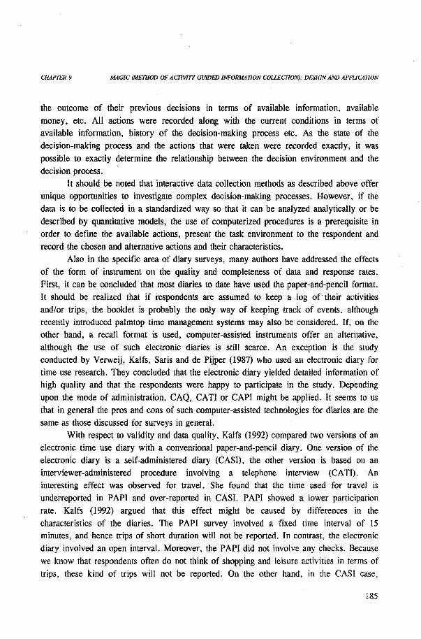
CHAPTER9 MAGIC (METHOD OF ACTIVITY GUlDED lNFORMA110N COUEC110N): DESIGN AND APPUCA110N

the outcome of their previous decisions in terms of available information, available

money, etc. All actions were recorded along with the current conditions in terms of available information, history of the decision-making process etc. As the state of the

decision-making process and the actions that were taken were recorded exactly, it was

possible to exactly determine the relationship between the decision environment and the

decision process.

It should be noted that interactive data collection methods as described above offer

unique opportunities to investigate complex decision-making processes. However, if the

data is to be collected in a standardized way so that it can be analyzed analytically or be

described by quantitative models, the use of computerized procedures is a prerequisite in

order to define the available actions, present the task environment to the respondent and

record the chosen and alternative actions and their characteristics.

Also in the specific area of diary surveys, many authors have addressed the effects

of the form of instrument on the quality and completeness of data and response rates.

First, it can be concluded that most diaries to date have used the paper-and-pencil format.

It should be realized that if respondents are assumed to keep a log of' their activities

and/or trips, the hooklet is probably the only way of keeping track of events, although

recently introduced palmtop time management systems may also be considered. If, on the other hand, a reeall forrnat is used, computer-assisted instruments offer an alternative,

although the use of such electronic diaries is still scarce. An exception is the study

conducted by Verweij, Kalfs, Saris and de Pijper (1987) who used an electronic diary for

time use research. They concluded that the electronic diary yielded detailed information of

high quality and that the respondents were happy to participate in the study. Depending

upon the mode of administration, CAQ, CATI or CAPI might be applied. It seems to us

that in general the pros and cons of such computer-assisted technologies for diaries are the

same as those discussed for surveys in generaL With respect to validity and data quality, Kalfs (1992) compared two versionsof an

electronic time use diary with a conventional paper-and-pencil diary. One version of the

electronic diary is a self-administered diary (CASI), the other version is based on an

interviewer-administered procedure involving a telephone interview (CATI). An

interesting effect was observed for traveL She found that the time used for travel is

underreported in PAPI and over-reported in CASL PAPI showed a lower participation

rate. Kalfs (1992) argued that this effect might be caused by differences in the

characteristics of the diaries. The PAPI survey involved a fixed time interval of 15 minutes, and hence trips of short duration will not be reported. In contrast, the electronic

diary involved an open interval. Moreover, the PAPI did not involve any checks. Because

we know that respondents often do not think of shopping and leisure activities in terms of

trips, these kind of trips will not be reported. On the other hand, in the CASI case,

185

CHAPTER9 MAGJC (MEI1:/0D OF ACTIVITY GUIDED INFORMA110N COUECI70N): DESIGN AND APPUCA110N

respondentsoften recorded shopping and leisure as one activity, and not as three.(the two trips to and from the location, plus the activity itselt). The time use for the activity was added to the travel time, and hence this resulted in higher estimates. A more detailed

analysis further supported these findings. In another publication, Kalfs (1994) examined the effects of form of instrument

(CASI vs. PAPI) in terms of data quality as measured by (i) the total number of different primary activities, (ii) the number of different primary activities, (iii) the duration of primary activities, an_d (iv) the number of mistakes in the data. The paper-and-pencil diary

involved a pre-coded list of 106 activities, Actlvities were recorded in fixed intervals of 15 minutes and secondary activities were ignored. The electronic diary involved tree-structured questionnaire of 368 activities with an open time interval. Respondents were requested to report their activities that lasted for at least ten minutes, with the exception of traveL They were also asked whether they liked the activity and whether they performed another activity simultaneously. The tree structure implied that they were first asked what they were doing in more general terms, then what exactly and then perhaps even more details. Because of these differences, the lists of activities was converted into a common list of 75 activities as judged by four different researchers. The results indicated that a higher mean number of total actlvities was obtained for the PAPI. On average, the respondents in the paper-and-pencil survey reported two to nearly three more primary activities than the respondents in the CASI survey. The same result was obtained for the number of different actlvities per day, although as one would ex peet the deviation was

smaller. On the other hand, the number of activities lasting more than four hours was less in the paper-and-pencil diary and the mean duration was also shorter. Mistakes were assessed in terms of coding errors. Consistent with our theoretica! expectations, the CASI diary involved significantly less coding errors, although the errors in the PAPI survey were also smal!.

In another paper, Kalfs (1995) discussed the results of a study conducted to

compare paper-and-pencil and computer-assisted (CASI and CATI) instrument for time use data. She found that, as found in the general literature, the response rate is highest for CA TI. The time required to complete the survey as measured by interviewers' time and assistance and coding and editing time, in contrast, was lowest for CASI. The

paper-and-pencil instrument yielded the most detail, but also more mistakes, while the computer-assisted instruments yielded less errors (especially CASI). Social desirability effects were highest for CATI. Kalfs (1995) also reported differences in estimated time use between the form of instruments, although these results might be largely influenced by differences in the design of the instrument and cannot be necessarily attributed to the mode of administration. Time use was underreported in the paper-and-pencil instrument and over-reported in the CASI instrument. The paper-and-pencil instrument, however, had

186

CIIAPTER9 MAGIC (ME1HOD OF AC11VJTY GUIDED INFORMA110N COUEC110N): DESlGN AND APPUCA110N

a fixed time interval, implying that short trips could not be reported. Kalfs (1995) also warned that the findings for CASI may be due to incorrect interpretations of the respondents.

Thus, although the evidence is not quite convincing, it seems that computer­

assisted methods should improve data quality, especially when intelligent systems would

be used. Moreover, interactive computer experiments are a valuable means of collecting data on response to planned change or on beuristics individuals may use in scheduling or rescheduling their activities.

9.2.4 Diaries: effects of data colleedon metbod Although the previous considerations, in principle, hold for both questionnaires and

activity diaries, there are also some specific considerations with respect to the use of diaries. Diaries can be designed in different ways and several operational decisions need to be made. In this section we will discuss these considerations to derive guidelines for the design of MAGIC.

A frrst consideration is whether activities or trips should be the unit of observation. In case of an activity diary, one bas to decide whether only out-of-home activities or all

activities are recorded. If a trip diary is used, the leading question relates to trips and other information is linked to the trips. In case of an activity diary, the Ieading question refers to activities that respondents have engaged in. The lirerature favors the use of activity diaries as more, especially shorter, non-home based trips, are recalled (Clarke et al., 1981; Stopher, 1992). With respect to the inclusion of in-home activities, no significant increase in triprates was found. It should furthermore be noted that if the data

is to be used for the estimation of activity-based travel demand models, the use of activity diaries is a necessity by definition.

Another consideration is to ask respondents for their past behavior or to record

their future behavior (time lwrizon). Thus, respondents may be asked to reeall the activities and/or trips they made the day before the interview. Alternatively, an activity diary may be left with the respondent with the request to fill it out for a day in the future.

After this day, the respondent is visited by an interviewer who checks the diary for completeness and consistency and, if necessary, requests additional information or clarification from the respondent. The diary can also be retrieved by phone. In case of a

reeall procedure, respondents are asked, with or without prenotification, to reeall their activities and trips performed during the previous day. There appears to be some evidence that a leave bebind diary leads to better data quality, especially in that more trips and activities are reported (Survey Research Center, 1984). However, the difference is rather

small and usually does not warrant the cost difference, given that leave bebind diaries are 1.5 to 4 times more expensive (Juster, 1986). If a mixed mode approach is used, this

187

CHAPTER 9 MAGIC (METHOD OF AC11VITY GUIDED INFORMA110N COUEC110N): DESIGN AND APPUCA110N

might be of less concern. Another decision dirneusion in collecting diary data is the observation period that is

used. The literature on this issue suggests that the observation period should preferably

not exceed 48 hours, as empirica! evidence suggests that the number of reported activities (Niemi, 1983) and trips (Golob and Meurs, 1986) steadily decreases after the second day.

Apparently, tendencies to skip activities or trips or to report inaccuracies are likely to increase over time. Furthermore, response rates deercase with increasing duration (Survey Research Center, 19~4). However, other authors (e.g., Pas, 1994) have argued that Jonger observation periods should be used, as many activities and trips occur in weekly or monthly cycles. Balancing both considerations, Kievmarken (1982) and Harvey (1993)

reeommend the use of two day activity or trip diaries. If longer periods are used, special attention has to be given to the survey administration (e.g., multiple contacts) to ensure data quality over a longer period.

With respect to the timing of diary days, Harvey (1993) reeommencis that diaries are colleeted for all seven days of the week and that a designated rather than a random day of the week is used. This is to ensure that all days of the week' are adequately represented in the sample, which is a necessity as structural differences exist, not only

between weekdays and weekends, but also between different weekdays. ldeally, diaries should also be held at different times of the year to account for seasonal effects. There exists proof in the Iiterature that designated days yield a higher representativeness and better estimates of time expenditures as compared to the use of convenience days ( Juster, 1985).

If a reeall diary is used, one has to decide about the reeall period, that is to say the period between the day for which a diary is reported and the day it is recorded. The findings reported in the literature are somewhat conflicting in this regard. Some studies (e.g., Juster, 1985) suggest that depending on the diary day, there is either no deterioration or only a small deterioration as the reeall period increases. Other studies (Clarke et al., 1981) indicate that respondents have problems recalling the trips they made

the day before yesterday. Based on these findings a maximum reeall period of two days seerns preferable.

With respect to the recording of activities, two approaches can be followed. Fixed time interval diaries use fixed, usually 15 minute time slots. Respondents then have to specify the main activity performed in each period. Open time intervals, on the other hand, require that the begin and end time of all activities is specified. An important drawback of fixed interval diaries is that activities and trips with a short duration may be

underreported (Harvey and Gmnmo, 1986). Moreover, using fixed interval diaries, the effect of time constraints may be overestimated in modeling efforts. Hence, for transportation applications, the use of open interval diaries is clearly preferred.

188

CHAPTER 9 MAGlC (METHOD OF AC11VITY GUlDED lNFORMA nON COU.ECnON): DESIGN AND APPUCAnON

Yet another issue of concern is whether to use precoded activfties or whether to have respondents formulate activities in their own words. The literature on time use

research (Harvey, 1993) recommends the use of the latter option, as it allows greater flexibility in recording and analyzing and is less demanding for respondents (Arangio­Ruiz, 1984). However, precoded categories may be useful to record other aspects of the

activity such as location. In transportation contexts, one often requires less detailed

activity classifications, implying that precoded categories become more convenient.

Moreover, in case of computerized data collection, the use of precocled categoTies is to be preferred.

With respect to fonn of prompting, the most realistic options are to ask respondents to fill out the questionnaire immediately after completion of an activity or trip or at fixed times, such as the end of the day. Although the first option is theoretically desirable, it

imposes a heavy burden upon respondents and as a consequence they may be expected to miss certain events. In addition, filling out the diary at the end of the day seems to be a

perfectly acceptable way of prompting (Ettema et al., 1996).

9.2.5 Starting points for developing a data coneetion procedure Based on the above literature review, some conclusions can be drawn regarding the collection of activity, travel and personal data. These conclusions provide a base for the development of a data collection procedure that can be used to collect the data that is necessary to calibrate SMASH and COMRADE.

Personal and household characteristics, which can be recorded by factual questions,

should preferably be collected using a computerized questionnaire for several reasons. First, a computerized questionnaire improves the data quality by performing range checks and randomizing the sequence in which questions are posed. Furthermore, a computerized procedure makes the respondent's task easier by routing him through the questionnaire so that irrelevant questions are avoided, substituting previous answers and presenting

information. Finally, the use of a computerized procedure has the advantage that the data that is entered can be stored directly in a format that can be input into analytica! software or other computerized data collection tools. With respect to the form of administration, face-to-face interviews are preferred. They have the advantage of offering the greatest potential for obtaining a representative sample, as no individuals are a priori excluded from the sample, because they do not have a phone or do not appear on an address list. In addition, an interviewer may help interviewers and stimulate interest, making it possible to

use an extensive and quite complex questionnaire in this module.

Activity and travel data should be collected using a dairy rather than a questionnaire. Compared to questionnaires, diaries provide more complete information

regarding the activity and travel pattern. As the data is used to model activities and trips

189

CHAPTER 9 MAGIC (METHOD OF AC11VITY GUIDED INFORMA110N COUECI10N): DESIGN AND APPUCA110N

in their mutual dependency, a diary is preferred to a questionnaire. With respect to the

form of instrument, the literature suggests that computerized methods are preferred as the

offer a tooi to improve the data quality by performing range checks, checking for item

non-response and inconsistencies in the data. Furthermore, the computerized procedure

can be used to present answer categories in random order, or to substitute previous

answers. However, it is argued that a paper-and-pencil mail-back approach mayalso serve well, provided that respondents are motivated and well instructed. With respect to the

form of administration, the lirerature suggests that face-to-face interviews are preferred, as they offer the opportunity to give better instructions, raise commitment and help the

respondents providing the data.

A final note concerns the use of interactive data collection procedures to collect

data regarding complex decision-making processes, needed to collect data for the

calibration of SMASH. The lirerature clearly shows the advantages of computerized interactive methods in this respect. They are especially useful in presenting the decision­

making environment to the respondent and providing him with feedback of previous

decisions. With respect to the form of administration of such interactive methods, face-to­

face interviews are clearly preferred. As interactive computerized tasks are rather complex, respondents are expected to have problems in fully understanding the task and

handling the computer program. The presence of an interviewer is considered necessary to

explain respondents about the scheduling task and to assist them to record the data using the computerized procedure. Furthermore, the interviewer can stimulate respondents to complete the rather demanding task.

9.3 DESIGN OF THE DATA COLLECTION PROCEDURE MAGIC

9.3.1 Data requirements and general structure of MAGIC The model of activity scheduling SMASH assumes that activity scheduling is a stepwise

decision-making process, consisting of subsequent schedulîng decisions. Each decision in this respect entails the choice how to proceed the beuristic search process, based on the

current schedu!e and the attributes of alternatives that are available. Specifically, at each

step an individual can adapt the preliminary schedule by adding, deleting or rescheduling

an activity. A nested logit choice model is used to describe how subsequent scheduling decisions are made.

This implies that to calibrate the model it is necessary to monitor an individual's

activity scheduling process. That is to say, one has to observe which scheduling decisions

are subsequently taken, and what operations were available for each decision. This requires that respondents are requested to perform an activity scheduling task in a task

190

CHAPTER 9 MAGIC (METHOD OF ACTlVITY GUIDED INFORMATION COILECTION): DESIGN AND APPIJCATION

environment that corresponds to the state space assumed by the model. Furthermore,

during the scheduling task one has to record which operations were performed, which operations were available and the attributes of these operations.

The attributes may refer to the existing schedule, such as the number of trips

implied by the schedule, the travel time implied by the schedule and the total time spent on activities in the schedule. Alternatively, the attributes may refer to the outcome of an alternative scheduling operation, such as the number of trips implied by the schedule, the

travel time implied by the schedule and the total time spent on specific activities in the

schedule. Finally, attributes may refer to the (history of the) scheduling process, such as the type of decision (adding, deleting, rescheduling or stopping) or the number of preceding scheduling stages. Some of these attributes, such as the number of activities and trips, can be derived directly from the schedule. Others, like the implied travel time and time expenditures, require information concerning travel times between specific destinations and activity durations respectively. These pieces of information are stored in the long-term calendar.

Unlike SMASH, COMRADE describes the execution of activity patterns. Specifically, it describes the ·duration of the current activity and the choice of the next

activity and destination. This implies that the model is to be estimated on revealed data regarding activity participation and duration. The model requires the following data for

each activity that is performed by an individual: the duration of the current activity, the next activity and its destination and the possible activities that could have foliowed the

activities (the competing risks). In addition, information about the values of the covariates pertaining to each competing risk is required. This involves knowledge regarding the type of the current and next activity, travel times between different destinations, possible start

and end times for activities, activity frequencies and the history of the activity pattern. These data are typically stored in the long-term calendar and the activity agenda.

Hence, it can be concluded that four different types of data are required:

information regarding the scheduling process, observation of the actual activity pattem, information about the long-term calendar and the activity agenda and data regarding

personal characteristics. MAGIC has been developed to collect these data in a systematic way. lt consists of

four modules, corresponding to the four types of data that are needed. For each module,

several operational decisions had to be taken regarding the form of instrument, form of administration, form of prompting, etc. These decisions and their underlying motivations are summarized in Table 9.1. The remainder of this section discusses these decisions

pertaining to each module, based on the previous literature review. First, the general

structure of MAGIC is discussed in terms of the instrument and form of administration of each module and the interdependency between the modules. Then, each module is

191

CHAI'TER 9 MAGIC (ME1HOD OF AC11VITY GUIDED INFORMATION COUEC110N): DESIGN AND APPIJCAT!ON

discussed in detail.

module 1: activity program

Figure 9.1: Sequence of Different Modules of MAGIC

The sequence of the four modules is displayed in Figure 9.1. First, data is collected regarding the long-term calendar, the activity agenda and the cognitive map. These data

are first collected to identify an individuals' choice options in both the scheduling and the execution phase. Furthermore, it provides the data regarding the explanatory variables driving decisions made in both phases. The data is collected by a questionnaire that prompts respondents to reeall data regarding their activity and travel environment.

Table 9.1: Motivations with Respect to the Design of the Modules of MAGIC

sampling, explanation, stimulation

sampling, explanation, stimulation

sampling, stimulation

costs,

experience and motivation of respondents

!DRil back

instruction, stimulation

The second module involves an interactive experiment, in which respondents have

to perform an activity scheduling task concerning the day after the interview. This module

192

CHAPTER 9 MAGIC (MElliOD OF AC17VTTY GUIDED INFORMA110N COUEC110N): DESIGN AND APPIJCATJON

logically follows the first one, as the specification of the scheduling task is based on the

data regarding the long-term calendar, activity agenda and cognitive map that was recorded in the first module. With respect to the choice of instrument, the use of a

computerized procedure was evident, given the complex, interactive nature of the task. First, the activity agenda that was specified serves as the starting point for the scheduling

task, and has therefore to be presented to respondents. This can be best achieved by a computerized procedure, which can easily store and display the agenda such that the information can easily be retrieved by respondents. Furthermore, the procedure is

interactive, in that thé task environment is structured according to previous decisions taken in the scheduling process. As this requires the presentation of the state in the scheduling process in response to previous decisions adequately, accurately and without loss of time, a computerized approach seems to be the only viabie way to retrieve the requested data.

In addition, the use of a computer offers the opportunity of performing range checks to improve the quality of the data and providing choice options in random order to avoid order bias. Finally, the use of a computerized procedure is helpful in routing the respondent and providing information regarding the task.

The third module involves a short questionnaire, asking respondents about their personal and mobility situation. This module is scheduled after the two previous ones, as these are considered to provide the crudal information that is needed for model estimation and are more complex. To avoid fatigue effects, it was decided to schedule the relatively

short and easy questionnaire as the third module. lt was decided to use a computerized questio1111aire, because of the possibil ity to perform range checks and because answer categories can be easily presented. An additional advantage is that the data can be directly stored in a format, that can be accessed by analytica! software. With respect to the form of administration, a face-to-face interview is preferred, so that an interviewer can assist

the respondent in entering the data and stimulate the respondent in completing the task. The fourth module involves the recording of the activity pattem that was actually

performed at the target day. As this can only be done after the day of concern, it logically follows the first three modules, that, with exception of the third one, have to be performed before the day of concern. A paper-and-pencil mail-back diary was used to collect these data. Respondents were requested to list for each activity that they performed on the target day the type of activity, the destination, the start and end times, the travel

mode and the travel time needed to travel from the previous to the current destination.

The four modules were integrated into one data collection procedure. The first three modules were incorporated in a computerized data collection procedure that was

programmed in PASCAL (Ettema et al., 1993a). Laptop computers were used to conduct face-to-face home interviews with this instrument. The data was entered by the interviewer, although the respondent was encouraged to take advantage of the information

193

CHAPTER 9 MAGIC (METHOD OF AC17VlTY GIJIDED INFORMATJON COU.ELllON): DESIGN AND APPUCATlON

displayed on the computer screen while providing the data. Hence, a CAPI procedure was

used to collect the data involved with the first three modules. Following the home interview, respondents were handed out the questionnaire and given a short instruction.

After fitling out the diary, respondents returned the diary in a pre-stamped envelope. In the following (sub-) sections, the modules will be discussed in greater detail.

9.3.2 Module 1: recordiug the activity and travel environment This module consists of two parts. The first part collects data regarding a respondent's

long-term calendar and activity agenda, the second regarding the cognitive map. The first part is based on a list of 32 activities about which information has to be provided for a target day which in the present case was the day after the interview. The recorded items concern (i) will the activity be performed on the planning day according to an arrangement in which other people are involved (yes/no); (ii) what was the last time the activity was performed (days ago); (iii) what is the average frequency of performance of the activity (times per month); (iv) how long does is take to perform the activity (average time in minutes); (v) how likely is it that the activity wil! be performed on the target day (on a 0-10 scale); (vi) for each location at which an activity can take place the name of the location, the hours at which the respondent would consider to perform the activity at this location, the attractiveness of the location on a 0-10 scale, indicating how pleasant the

location is to stay at and the address of the location.

Table 9.2: Range Checks

> : . · ~ODt!LEl ',,··.· .. ,. MODULE2 M0J)ULE3.

start time < end time start time p-tb activity < age < 100 minimum duration s end time p-tb activity age <:: 18

average duration end time (p-1 )-tb activity s number of children s 6 average duration s start time p-tll activity number of cars s 3

maxitnum duration end time p-tll activity s number of licenses s 8 frequency s 100 start time (p+ l)-th probability s 100 activity

The program uses an input screen for each activity (Figure 9.2). The input of destinations takes place in a pop-up window (Figure 9.4). During the completion of this part of the module, respondents can move back and forth through the list in order to make corrections if it is realized that a previous activity was not specified correctly. The computerized procedure presents the activities in random order to avoid any order bias. It should be noted that the computerized procedure requires that all information regarding an

194

CHAPTER 9 MAGIC (ME1HOD OF ACJIVITY GU/DEIJ INFORMATION COUECTION): DESIGN AND APPUCATION

activity is entered before one can move forward or backward to another activity. In this

way, item non-response is avoided.

The computer program includes several checks to improve the quality of the data

(Table 9.2). The begin and end times of activities and minimum, average and maximum

durations are checked against each other in order to avoid inconsistencies. Also, monthly

frequencies and probabilities are limited to upper bounds.

Furthermore, the program helps respondents by providing default answers. For

instance, for in-home activities such as preparing food, cleaning, etc., the home location

appears as the default location, which saves typing effort. lf the address of a location has

been entered once, it appears as default the next time the location is mentioned as a

possible activity site. In addition, the computerized procedure is used for automatic

branching to avoid irrelevant questions. In case of an incidental and unplanned activity

such as visiting a doctor the frequency is not asked for. Also, for daily activities like

having breakfast asking for frequency is avoided. The computerized data coneetion offers

the opportunity to shortcut such cases and customize the questions to the specific situation.

Figure 9.2: Input Screen for Activity Data

An important issue arising in the development of the procedure is the number and

specification of activities for which these data have to be supplied. One consideration has

been that the activities should ideally cover the full range of activities people perform in

everyday life. This is specifically important as the activities are also used in the second

195

CHAPTER9 MAGlC (MElliOD OF AC11VITY GUIDED INFORMA110N COUEC110N): DESIGN AND APPUCA110N

module in which a daily activity schedule is conceived by respondents. Axhausen (1994)

stresses the importance of using detailed activity categories in order to properly

understand and model travel behavior. In addition, the list should contain both in-home

and out-of-home activities as the scheduling of out-of-home activities may be related to the

scheduling of in-home activities in terms of constraints and substitution of out-of-home by

in-home activities may take place. On the other hand, the list should not be too long in

order to avoid fatigue. Balancing comprehensiveness and user convenience, a list of 32

activities, based on a study conducted by Knuist and Schoonderwoerd (1983), was

compiled (Table 9.3). Specifically, the 223 categories used in their study were grouped

into 32 categories such as to reflect the full range of daily activities. This list proved to be

acceptable both with respect to length and comprehensiveness in a pilot study (Ettema et al., 1994). As discussed before, the use of pre-coded activitîes may imply a loss of

information, if individuals pursue activities which do not exactly fall in one of the 32

categories. However, the use of a standardized list is necessary to provide a standardized input format for the scheduling task in module 2. Furthermore, as special attention is

given to the comprehensiveness of the list, it also serves as a check! ist to eosure that

respondents supply information about all their daily activities without ignoring or

forgetting some. · It should be noted that in the analysis stage, the activities are grouped

into five broader groups for reasons of convenience and insight. The distribution into five

categories is also displayed in Table 9.3.

Figure 9.3: Input Screen for Destination Data

196

CHAPTER 9

• study • breakCast • prepare food • lunch • ironing • disbwasbing • dinner

MAGIC (ME11:10D OF ACITVlTY GUIDED INFORMA110N COUECTION;: DESIGN AND APPUCA170N

• bobbies • reading • watching TV • baving visitors

• education • worklvolnntary

job

• buying groceries • buying clothes/

shoes • getting food

(snackbar) • specialty shop

Figure 9.4: Input Screen for Travel Times

·out.-ofiliome ~Dal

• post office/bank •sports • watch sports

match • sightseeing trip • visiting someone • club activity • library • museum/

exhibition • theater/concert/

movies • deliver a parcel • bring/get

someone • cafe/bar/

restaurant • doctor/dentist • strollinglbiking

197

CHAPTE119 MAGlC (METHOD OF ACfTVlTY Gl!lDED INFORMATlON COUEcnON): DESIGN AND APPllCATlON

In the second part of the module, the respondent is asked to enter the travel times between pairs of destinations that were mentioned according to bis cognition of the planning area. Travel times are asked for all transportation modes that the respondent can reasonably use for a trip. One screen is used per pair of destinations (see Figure 9.4). Although the program offers the opportunity to enter travel time for eight different modes, respondents only have to specify the travel times by the modes that they can reasonably use. It is possible to move back and forth through the list of trips in order to check the entties and correct ~em if necessary. A respondent can only move to another trip, however, if the travel time for at least one mode is specified. This is done to avoid item non-response in the sense that travel times for each trip are known.

All information on activities, possible locations and travel times is stored in a

standard format in data files which are used in the secoud module of MAGIC.

9.3.3 Module 2: activity scheduling task The secoud module of the data collection procedure serves to record the decisions made by respondents during their activity scheduling. Specifically, respondents are asked to complete a one-day scheduling task for a specified target day. Typically, this is the day after the experiment to reflect the short time horizon of daily activity scheduling. The scheduling task is based on the activity agenda specified in module 1. Respondents are asked to construct the schedule for this day as realistically as possible.

The computerized task environment is designed as follows. On the left side of the screen an agenda with activities to perform on the target day is Iisted. This agenda contains the same 32 activities that were presented to the respondent in the previous part of the procedure. By offering a set of activities, which adequately covers respondents' daily activities and which consists of in-home and out-of-home activities, the daily activity scheduling process is represented in a realistic way, including trade-offs between in-home and out-of-home activities implying traveL As the list is too long to be fully displayed on the screen, respondents can scroll through the list in order to retrieve their desired activities. The order in which activities are listed may affect the outcome of the scheduling. For instance, activities in the top of the list may have a higher probability of being included as they are more easily detected. To avoid such biases across respondents, the activities are listed in random order. The locations at which the activities can be, performed are the same that were entered in the first part of the experiment. The scheduling task is thus adjusted to the specific situation of the respondent to obtain realistic information about the scheduling process.

Given this agenda, the respondent can then start to construct the schedule, thereby applying the same response modes that are included in the model. The operations ffadd",

"delete", "reschedule" and "stop" can be activated by specific function keys. In case of

198

CHAPTER 9 MAGlC (ME1HOD OF ACIIVITY GU/DED lNFORMA170N COlLF.C170N): DESIGN AND APPUCA'J10N

adding an activity, the activity can be selected from the agenda using arrow keys (Figure

9.5). Once an activity is selected, the available destinations as specified in module 1 are

Iisted. Furthermore, the options to choose ~unknown" and to specify another destination

by name and address are offered. The preferred option is again selected by means of arrow keys (Figure 9.6). This is also the case for the selection of the place of insertion in

the schedule (Figure 9. 7). If insertion of the activity invokes a trip, the program also asks

to specify the travel mode for this trip (Figure 9.8). Deleting an activity also takes place

by selecting the activ_ity to be deleted by means of arrow keys. Finally, rescheduling an

activity is done by selecting the activity to be rescheduled in the same way as deleting an

activity. The destination, place of insertion and, if necessary, travel mode are specified in

the same way as adding an activity.

The schedule under 'construction is always displayed at the right side of the screen.

Hence, after each operation, the schedule is updated to represent the current state of the

scheduling process which may then be further modified by applying new operations. Each

operation that is applied by a respondent is recorded with respect to all relevant decision

dimensions. This information, together with the data collected in module 1, can be used to

define choice sets and choice data pertaining to the subsequent scheduling decisions.

According to this procedure, the respondent continues adjusting the schedule until no

further adjustments are feit necessary. This implies that a full activity schedule is not

necessary if the respondent, for instance, wants to maintain a degree of flexibility.

Once the scheduling is completed, the respondent is 3;5ked tQ, specify st:af! and end

times for each activity (Figure 9.9). This sequence of different activity scheduling

decisions (first sequencing, tben timing) is in line with recent theories of activity

scheduling (Gärling et al., 1989) that postulate that activity schedules are first sequenced

and then checked to ensure that start and end times are not overlapping and time

constraints are not violated. An open time interval format is used to record activities and

their start and end times. Underlying this decision is the consideration that the activity is

the natura! unit by which respondents construct their scbedules, for instanee by actding or

deleting activities. It is hypothesized that the timing of activities largely flows from their

sequencing. A procedure in which respondents specify their schedule by, for instance, 15

minute periods throughout the day would reflect activity scheduling behavior less well

than open time intervals. Furthermore, fixed time intervals may result in less reliable start and end times and might lead to underreporting of activities with a short duration. The

program checks whether all start and end times are consistent. That is to say eacb activity

bas to end later than it starts and can only start after the previous activity bas ended

(Table 9.2). If an inconsistency is detected, it is not possible to proceed with the

procedure unless tbe inconsistency is solved. The respondent can go back to the

sequencing phase if conflicting start and end times are detected and adjust the schedule

199

CHAPTER9 MAGIC (METHOD OF ACITVITY GUIDED INFORMATION COUECT!ON): DESIGN AND APPUCA170N

(Figure 9.10). The final schedule, including activities, destinations, modes, start and end

times, is recorded in a data file.

Once a schedule has been created for the target day, the respondent is presented

with a rescheduling task. That is to say, the final schedule is presented, together with a

description of a hypothetical situation. This hypothetical situation is presented by an

additional information screen. The hypothetical situation typically refers to the

implementation of a specific policy. The respondent is now asked to modify his schedule

to this changed situation, thereby using exactly the same operations as in the original

scheduling phase. The input sereens are identical as in the original scheduling task.

Similar to the original scheduling task, all operadons and their relevant dimensions and

the final schedu\e are recorded. The information collected for the rescheduling phase can

be used to investigate how individuals adapt their habitual patterns to changed situations and to test how well the model of activity scheduling performs in assessing the effect of

policies. The rescheduling task is a good example of the opportunities offered by

interactive data collection tools. By collecting background information about an

individual's activity and travel pattem and recording his activity schedule, hypothetical

policies can be presented in a way that is very similar to decision-making processes in real

life. The hypothetical question is, as much as possible, customized to an individual's

specific circumstances at a specific day, resulting in potentially more reliable responses.

Figure 9.5: Selecting an Activity from the Agenda

200

CHAPTER 9 MAGIC (METH(J[) OF ACflVITY GUIDED INFORMA'IION COUEC'IION): DESIGN AND APPUCA'IION

Figure 9.6: Selectinga Destination

Figure 9. 7: Selecting the Position in the Schedule

201

CHAPTER9 MAGIC (MElliOD OF AC77VITY GUTDED INFORMA170N COUEC170N): DESIGN AND APPUCA170N

Figure 9.8: Selectinga Travel Mode

Figure 9.9: Specifying Startand End Times of Actlvities

202

CHAPTER9

'

MAGIC (ME1110D OF ACTIVITY GUlDED INFORMA170N COUEC170N): DESIGN AND APPLICA170N

activity choice destination choice sequencing modechoice

~t scenario 1

···············'···· scenario 2

scenario 3 ' '

······-···-···

startand end times

,

·~ ' '

Figure 9.10: Organization of Module 2

9.3.4 Module 3: personal and household data The third module consists of a short questionnaire in which the following personal data

are recorded. The questionnaire consists of a number of open-ended questions concerning respondents' age, number of children, and the number of cars and \icenses in the

household. In addition, for a number of questions precoded answer categories are used. These questions concern gender, marital status, education level, main occupation. personal

and household car ownership, personal and household driving license possession. The precoded categories used in these questions are listed in Table 9.4.

In case pre-coded categories were used or a dichotomous answer was requested, the answer could be picked from a pop-up menu using arrow keys (Figure 9.11). In case

of a numerical response the correct answer has to be typed in and the program performs a range check. The upper and lower levels of these range checks are displayed in Table 9.2. The computer program requires that each item is filled out before the module can be finished. Thus, item non-response is avoided in this way.

203

CHAPTER 9 MAGlC (MEWOD OF AC17111TY GUIDED /NFORMA170N COUEC170N}: DESIGN AND APPUCA170N

Figure 9.11: Input Screen Personaf and Household Data

Table 9.4: Pre-Coded Answer Categones

male elementary school single wort

female high school married education

university unmarried couple houseteeping

divareed other

widowed

other

9.3.5 Module 4: revealed activity pattem The calibration of COMRADE requires information regarding the activity pattem actually

performed by a respondent. These data were collected by means of an activity diary.

When conducting an activity diary survey, several options are available with respect to the

design and organization of the diary. In section 9.3.1 the choice of a paper-and-pencil

mail-back diary was already discussed.

Another operational decision concerns the use of free form or pre-coded activity

categories. Based on the literature in this field it was decided to use a free form diary,

204

CHAPTER 9 MAGIC (ME1110D OF ACflVITY GUIDED lNFORlvfA170N COUECflON): DESIGN AND APPUCA170N

because of greater flexibility in the analysis stage and the less heavy burden for

respondents. With respect to the time horizon of the diary, there seems to be agreement in the

literature (Ettema et al., 1996) that leave bebind diaries provide higher quality diaries then

reeall diaries. As this procedure well coincides with the practical administration of the data collection (the diary can be left bebind when modules 1 to 3 have been performed), a

leave bebind approach was chosen. A third issue concerns the time of filling out the diary. In this respect, it was

decided that respondénts should fill out the diary at the end of the target day. Th is

procedure implies a short reeall period and is also less demanding than filling out the diary each time an activity or trip is completed.

Finally, with respect to the use of open or fixed time intervals, the same consideration holds as for the activity scheduling task. Using open time intervals, more

detailed information is obtained regarding the start and end times of activities. In addition, activities with short duration are less likely to be ignored. Forthese reasons, an open time interval was used.

The above consideration led to the use of a paper-and-pencil mail-back activity diary as displayed in Figure 9.12. Respondents are requested to specify for each activity a

description of the activity, the destination of the activity. the travel time to the destination of the activity, the mode used to travel to the destination and the start and end time of the activity. In additiori respondents were requested to specify their home address to enable the linkage with the computerized modules.

The fourth module, the paper and pencil diary, was checked on completeness during the analyses of the data. Of all diaries, all activities were checked on completeness with respect to the following issues: location, start time, end time, travel time and travel

mode. Some simple rules were used to reconstruct missing data. lf the mode of a return trip was not specified, it was assumed that the same mode was used as for the away trip.

If the destination was not specified, the location was coded as home for all in-home activities. For all out-of-home activities, the location was assumed to be similar to that of the previous activity. If start or end times were not specified, they were derived from the start time of the next activity or the end time of the previous one, taking into account the required travel time. If travel times were not specified, they were, if possible, derived

from the activity agenda recorded in the computerized procedure. If this was not possible, the travel time was determined based on the difference between the start and end times of

the two activities between which the travel took place and the geographical locations of

the two activities.

205

CHAPTER9 MAGIC (METHOD OF AC17VITY GUlDED INFORMA110N COLLEC710N): DESIGN AND APPUCA710N

ACTIVITY DIARY FOR ............ DAV ...... SEPTEMBER

ACTIVITY LOCATION/ START- END- TRAVEL TRAVEL ADDRESS TIME TIME MODE TIME

1 hr hr hr min

12 hr hr hr min

3 hr hr hr min

4 hr hr hr min

5 hr hr hr min

6 hr hr hr min

7 hr hr hr min

8 hr hr hr min

9 hr hr hr min

10 hr hr hr min

111 hr hr hr min

12 hr hr hr min

13 hr hr hr min

PLEASE Flll OUT YOUR HOME ADDRESS:

Street and number

Zipcode

PLEASE RETURN THE QUESTIONNAIRE FORM IN THE PRE-STAMPED ENVELOPE. THANK YOU!

Figure 9.12: Activity Diary Used in Module 4

206

CHAPTER 9 MAGIC (MEIHOD OF ACTIVITY GUIDED INFORMA110N COLU:C110N): DESIGN AND APPUCA110N

9.4 REsULTS OF THE DATA COLLECTION PROCEDURE

9.4.1 Sampfing frame The data was collected in Veldhoven in September/October 1994. The city of Veldhoven was partitioned into 10 areas of approximately equal size and a total of 40 interviews was held in each of these areas, using the random walk method. Thus, the data collection involved a total of 400 interviews. The random walk metbod implies that within a certain area, streets and the_ number of interviews per street are randomly selected and that interviewers are requested to select the addresses to visit in each street at random. At each address, interviewers asked the household memher whose birthday was due first to participate in the data collection. However, only respondents older than 18 years were sampled. If this household memher was not home or refused to participate, the next memher who would be first to have bis/her birthday was asked to participate. If no participant was found or if nobody was home, another address was selected. Interviews were held from Monday through Sunday, implying that schedules and diaries were obtained for all days of the week. Hence, both weekdays and weekend days are included in the sample. Those respondents who agreed to participate in the interview received a smal! gift (a purse) as a sign of appreciation. For each diary that was left bebind, it was checked whether the diary form was sent back. If respondents did not return the diary within four days, up to four attempts were made to contact them by phone and persuade them to return the diary.

9.4.2 Response rate The response rate is shown in Table 9.5. A total of 2090 addresses was visited to conduct the requested 400 interviews. At 1150 of these, nobody was home. Of the remaining 940 addresses, 540 people refused to cooperate or no respondent older than 18 years was home. All respondents were requested to mail back the leave bebind diary. In reality, 320 of them did, which represents a response rate of 80%. Unfortunately, due to missingor

Table 9.5 : Response Rate

2890

400

320

228

207

CHAPTER9 MAG/C (ME1HOD OF AC17Y1TY GUIDED INFORMA110N COUEC110N): DESIGN AND APPIJCA110N

incomplete addresses, only 228 of these 320 diaries could be linked to the data recorded by computer. These cases were used to estimate both models.

9.4.3 Representativeness Table 9.6 describes the distribution of the sample with respect to various personal characteristics. It clearly demonstrates that the distribution of the sample matches the distribution of the population well with respect to age and gender. Only a slight undersampling of rnales can be observed, possibly because they are more often away from home during daytime than women. A x2-test indicated that the difference in the distribution of age between the sample and the population is not statistically significant at the 5% probability level (critica! value = 0.103 with 2 degrees of freedom). However, the difference in the distribution of gender proved to be significant at the 5% confidence level.

50.6%

50.2%

49.5%

0.028

With respect to the distribution of diary days over the days of the week, Table 9.7 suggests that most days are adequately represented. An underrepresentation of Sundays and Mondays can be observed. Apparently, as these days correspond with interviews held on Saturdays and Sundays, less interviews were held in the weekends, or respondents were less likely to cooperate during the weekend. A x2 of 40.70 indicates that it cannot be concluded at the 5% confidence level that the distri bution of diary days across the week is similar for all days (critical value = 1.635 with 6 degrees of freedom).

Table 9. 7 : Distribution of Diary Days across the Week

ednesday: Friday SatUJ'day Suuday

25.0% 17.1 14.5% 12.7% 7.0%

208

CHAPTER 9 MAGIC (MElliOD OF AC11VITY GUIDFD INFORMA710N COI.lEC770N): DESIGN AND APPUCA710N

9.4.4 Description of tbe sample Because population data were only available for age and gender, the representativeness of

the sample could only be assessed in those terms. To better understand the nature of the sample and their behavior, the distribution of some other variables will be described in this section. In particular, the following characteristics of respondents' activity patterns, as recorded in module 4, will be discussed. First, the total time spent on activities per day

exclusive of resting, sleeping and travel time is considered. Then, the total time

expenditures per day to in-home leisure, in-home task activities, out-of-home task activities, shopping and out-of-home personal activities are described. Following the

classification described in Table 9.3, each activity listed in the diary was assigned to one

of these categories. Detailed activities were grouped into these classes to obtain a better insight into the time expenditures of different segments of the sample and to correspond to the classification that is used for the estimation of the models.

Finally, the behavior is also described in terms of the total time spent on travel per day and the travel time lJy various modes per day, the number of activities performed on the target day, the number of trips made and the number of different locations that was visited. In actdition to descrihing the average behavior of the sample, the above characteristics were also used to illustrate differences in the behavior of different

subgroups in the sample.

9.4.4.1 Travel and activity behavior of the sample. Table 9.8 illustrates the average activity and travel behavior in the sample. The figures indicate that the total time spent on activities (excluding sleepand travel) is on average 13 hours and 16 minutes. Of this time,

the largest share is spent on in-home leisure and task activities. Of the out-of-home activities most time is spent on task and personal activities. It should be noted that the total activity time does not vary much among respondents as indicated by a small standard

deviation. The time spent on specific activity types, especially out-of-home activities varies much more across respondents. On average, 11.53 activities are performed per day. The smallest amount of time is spent on shopping. The total time spent on travel is 1.10 hours. The travel, on average, consists of 4.99 trips, and involves 3.53 different locations. With respect to travel modes used, the car is the predominant mode, foliowed by bicycle

and walking. The other modes are only marginally used.

9.4.4.2 Travel and activity behavior by gender. Table 9.9 indicates the differences

between sexes with respect to activity and travel behavior. The figures suggest that rnales

spend significantly more time on out-of-home task activities, whereas females spend significantly more time on in-home task activities. These time expenditures reileet the

traditional division of tasks in the household, where the male is mainly responsible for the

209

CHAI'TER 9 MAGIC (MEWOD OF ACTIVITY GUlDE!> /NFORMA110N COUECTION): DESIGN AND APPUCA110N

Table 9.8: Average Activity and Travel Characteristics

mean

796.04 167.68

246.07 173.68

238.43 159.55

130.99 203.42

44.55 60.94

135.14 144.61

11.53 3.76

70.21 52.02

34.79 43.38

19.13 29.37

1.43 11.33

2.21 21.09

0.13 1.99

12.52 24.96

3.53 1.50

4.99 2.86

household iocome and spends more time working. The female traditionally fulfills the housekeeping task, implying more in-home task activities. Males spend significantly more total time on activities.

Females perform significantly more different activities than males. Apparently, the

tendency is that rnales perform less activities of Jonger duration whereas feiTiales perform more activities of shorter duration. With respect to travel behavior, differences were not

significant at the 5% probability level. However, the nearly significant differences suggest that females make more trips and visit more different locations. However, the time spent on traveling does not differ significantly between sexes. Apparently, females make more short trips in the vicinity of their homes.

210

Cl:IAPTER 9 MAG/C (METilOD OF ACllVlTY GUIDED /NFORMATION COUECllON): DESIGN AND APPUCATION

Table 9.9: Activity and Travel Characteristics by Gender

male f.emale

825.63 770.78 2.48

256.39 237.26 0.83

186.40 282.85 -4.74

197.19 74.47 4.75

51.l0 -1.76

124.21 1.26

12.74 -5.50

71.38 69.22 0.31

37.84 32.19 0.98

17.83 20.23 -0.61

0.76 1.99

3.52 1.10

0.24

11.40 13.46 -0.62

3.44 3.59 -0.78

4.76 5.19 -l.l2

105 123

9.4.4.3 Travel and activity behavior of groups with different marital status. Table 9.10 gives information regarding the differences in activity and travel behavior of people with different marital status. An F-test was performed to test whether group means differences were statistically significant. The test results indicate that significant differences between groups arise with respect to the time spent on in-home task activities, out-of-home task activities and the number of activities that is performed.

An interesting way of interpreting the results is by comparing single and divorced

people and married and unmarried couples. In this respect, 'single' only refers to single people who have not been married before. lt can be concluded that single and divorced

people, although both living alone, have rather different characteristics. Both groups spend relatively much time on in-home leisure and out-of-home personal activities. However,

211

CBAPTER 9 MAGIC (MEIHOD OF AC11VlTY GUlDE[) !NFORMATION COUECJ70N): DESIGN AND API'UCATION

whereas divorced people spend much time on in-home task activities and shopping, single

people spend more time on out-of-home task activities such as education and work, while

spending little time on in-home task activities.

Table 9.10: Activity and Travel Characteristics by Marital Status

··················i··································/··············

i:Lit:.>J •· .. \ ' .. . ·• · .. · ..

;·· .. < \ . > •• :rrrr ...... un• . . divor.- widow• otbe~ IJ p

••• • ••••••••••••••••••••• married eed ed i•. ... .. . ... .····

······· · .. ··•••··············· .... .. \ ...... couples ·:

; . • <:. ty ~ill!el 757.74 801.58 778.50 876.00 697.50 747.57 0.95 0.44

·····=.-.~·····"··· ·•···· .... ·.· .. •·· ....... 273.63 253.23 156.00 246.75 211.25 114.29 1.57 0.17

····· i~t.alik

. •·• . .. .. 110.68 257.28 192.50 308.75 171.25 124.00 4.52 0.00

·~@(~~·~····· 188.94 112.50 240.00 78.75 140.00 347.86 3.01 0.01

···'· ~. ....

:.) 30.00 45.35 49.00 73.l3 23.75 36.43 . 0.70 0.63 ...... .. . _;;,. ~·-.. 154.47 l32.29 141.00 150.63 143.75 125.00 0.11 0.99

•••••••••••• .···· _"",. . >

. .. \:: ...... · .u... . • ;,;.;.. •· .•

9.68 11.96 10.90 10.63 10.75 7.57 2.84 0.02 ) •... { .. , .. .i> i

...... ,·. . >~i:-· 75.68 69.54 82.30 53.88 73.50 72.14 0.31 0.90 """'"

•·· : < ; .. ,:.·······•··• . .:•.·········~·~- 34.89 35.30 34.00 24.63 56.00 22.14 0.40 0.85 :':"".: ~

·····~veltt~.by 19.58 17.87 38.10 6.63 17.50 38.57 1.84 0.11 lllçJid~ .•·

trt~Vellinte ~y ~~. 3.94 1.33 0.00 1.25 0.00 0.00 0.25 o.94 1

[• ··•···.· < ,, .. 0.79 2.44 0.00 0.00 0.00 7.14 0.14 0.98

i\;< ~~· i~ •.••.. •.··· ···.. \ .. · . . . .

1.00 I ~tihieby / 0.00 0.17 1.00 0.00 0.00 0.00 0.05

·~· ,r··· , .. .. i' ..••..•.•• !c·.i>"' 16.47 12.43 10.20 21.38 0.00 4.29 0.66 0.65

l••·•· .. j.h1~L_,, ..

3.52 3.53 4.20 3.13 2.50 3.43 0.91 0.48

•••• i;; ..... , •••••·••• .···• 5.10 4.98 6.00 4.37 4.00 4.71 0.43 0.83 ~~·~~·F:• .. · .

. ~. . .. .. _.:..~~i 19 180 10 8 4 7

212

CHAPTER 9 MAGIC (ME11lOD OF AC11VITY GUIIJED INFO/IMA770N COUEC170N): Dlü1GN AND APPUCA110N

The differences with respect to in-home task activities and out-of-home task

activities are statistically significant. A possible explanation is that single people are

usually younger people having work or education (students) as their primary occupation.

Divorced people are usually older and do not participate in the labor force as often as

single people.

Comparing married and unmarried couples, it can be seen that unmarried couples

spend more than twice as much time on out-of-home task activities. Married couples

spend more time at home. A possible explanation is that in the case of unmarried couples. both partners participàte in the work force and still socialize as if they were single. In the

case of married couples, the female often has stopped working or works less hours. for

instanee because of child care. The presence of children may also lead them to more time

spent at home and to less time spent on out-of-home personal business. Again, the differences with respect to in-home task activities and out-of-home task activities are

statistically significant. Widowed people's time expenditures fall somewhere inbetween the

other groups.

A significant difference also arises with respect to the number of activities. It can

be concluded that married people perform relatively many activities, whereas single

people perform relatively few different activities.

With respect to the mobility behavior of various groups, the figures do not differ

significantly. However, nearly significant differences at the 5% confidence level suggest that travel time of tinmarried couples is relatively high, whereas divorced people spend

less time on traveL Unmarried couples also visit the most locations and make the most trips. Remarkable is the small number of trips made and locations visited by widowed

people, although their travel time is comparable to orher groups. Apparently, they make

few trips of relatively long distance. However, the very small number of observations

does not warrant general conclusions to be drawn for this group. With respect to travel

modes used by different groups, it can be concluded that divorced people travel less by

car. This is possible due to smaller car ownership rates for this group. The time spent walking by this group is relatively high. Widowed people, on the other hand, travel more

by car than the average. This is possibly due to the fact that widowed people are generally

older and are therefore reluctant to use other modes.

9.4.4.4 Travel and activity behavior of groups with different education level. Table 9.11

displays the activity and travel characteristics of groups with different education levels. In

this table, low refers to elementary school and lower levels of vocational and general

education, medium refers medium levels of vocational and general education whereas high refers university levels. The F-test indicates that significant differences between groups are

not observed with respect to any characteristic. Hence. travel and activity behavior for our

213

CHAPTER 9 MAGIC (ME11JOD OF AC71VITY GUIDED lNFORMA110N COUEC710N): DESIGN AND APPUCA110N

sample does not seem to depend on education.

Table 9.11: Activity and Travel Characteristics by Education Level

.....• ·}).·.·.·.

778.66 800.70 820.96 1.35 0.26

239.70 237.80 270.56 0.67 0.53

236.61 219.90 270.28 1.65 0.19

119.95 153.19 117.21 0.74 0.48

47.ll 48.75 33.37 1.15 0.32

133.93 140.44 129.25 0.21 0.81

11.75 11.38 11.35 0.28 0.76

67.06 73.06 71.65 0.31 0.73

34.79 33.18 37.29 0.14 0.87

17.69 19.15 21.77 0. 0.72

2.60 0.94 0.00 1.01 0.37

0.00 2.06 6.54 1.63 0.20

0.31 0.00 0.00 o.69 1 o.s1

11.67 17.74 6.06 3.63 0.28

3.45 3.79 3.27 2.28 0.11

5.02 5.26 4.52 1.07 0.34

96 80 52

Keeping in mind that differences are not statistically significant, the figures suggest that higher educated people spend more time on activities. However, the number of different activities they perfarm is smaller. With respect to specific activity types, the tendency seems to exist that the higher someone's education, the more time is spent on in­home leisure and in-home task activities. Highly educated people furthermore spend Iess time on shopping. It can also be concluded that people with a medium education level

spend the least time on in-home task, and the most time on out-of-home task activities ooropared to the other groups.

214

CHAPTER 9 MAGIC (ME1HOD OF AC11VITY GUIDED /NFORMA110N C0ll.EC110N): DESIGN AND APPIJCA110N

With respect to mobility figures, only minor differences can be observed. Highly

educated people appear to make less trips and visit less locations than other groups, although their travel time is comparable. Apparently, they make less trips of relatively

long distance. This is reflected in their choice of travel mode. They spend more time traveling by car and train and less time walking.

Table 9.12: Activity anà Travel Characteristics by Main Occupation

I ·.· > • i >. •··•· workeJ'S students homelilakerS otber F P .. I (. . •... · ..•. ·: ... > ···.·•· •. · .•.••

... · i·.······. . i . .··••··. . .•...•. ··.·.·.··· . . ~~vijyti~(!JQ .. ~)) 808.90 763.75 774.97 835.29 1.535 0.206

I · · >> "< • 198.so 304.50 246.77 323.42 s.188 0.002

174.85 156.75 303.02 224.76 12.342 0.000 ·:.··<: . ..~,. x ..

..........

283.46 126.66 47.50 39.08 32.220 0.000

28.05 58.33 49.15 61.97 3.443 0.018

123.53 117.50 127.73 184.08 1.805 0.147

9.64 9.67 13.07 11.92 15.074 0.000 · .. -·:·.-..... _ .. ·. · .. ,.,;·,.

••••·• t(lta]tra.~ii~(bmiutcis) ·.· .... 78.45 72.50 62.17 73.76 1.526 0.209

49.32 23.75 25.71 32.37 4.918 0.003 • '' ---- "'·'·"·''- i .. -- .... -.. '--

······~faY~···~~···I)1·"!J!~y~é···(~~è!il•··· 11.40 28.75 22.06 24.26 3.029 0.030

1.15 6.25 1.60 0.00 0.947 0.419

····"'~•·tim~••b)'JrnUt (rotniJt~)· 5.64 5.41 0.00 0.00 1.290 0.279

. ~iárlêbt~(Uij .. td~) 0.00 0.00 0.30 0.00 0.423 0.736

10.94 8.33 12.50 17.13 0.646 0.586

··. •··. . .·· .•.•. ., Df fo~ti()llS 3.46 3.25 3.56 3.66 ~ ••.•••. ·.··••·•··•···•••····•···· •·· ~~ftl'i~. ••••

4.69 4.33 5.11 5.50 0.953 0.416

78 12 100 38 <·•·····•·· •······•········••········ ,.s~···· .... ······· ....

9.4.4.5 Activity anà travel behavior of groups with different main occupations. Finally, groups with different main occupations can be compared with respect to their mobility and

activity behavior. In this respect, the following groups were distinguished: workers, having work as their main occupation, students, having education as their main

215

CHAnER9 MAG/C (MEmOD OF AC17V/TY GI![J)EJJ !NFORMA770N CO!D~C770N): DE~1GN AND APPUCA170N

occupation, and homemakers, having houschold tasks as their main occupation. The F-test

indicates significant differences between groups with respect to in-home leisure and task activities, out-of-home task activities, shopping, the number of activities and the travel

time by car and bicycle. As indicated by Table 9.12, it can be concluded that workers logically spend more

time on out-of-home task activities. Of all groups. students spend the most time on in­

home leisure. They spend little time on in-home task activities. They have much free time

and little household responsibilities. However, of all groups, they also spend the most time on shopping. Homemakers spend much time on in-home task activities and shopping,

as one would expect. However, they also spend much time on in-home leisure activities. Homemakers perform considerably more different activities than the other groups.

These are different in-home task activities or shopping activities at different destinations.

Indicative of the latter is the relative high number of trips made by this group, although

their travel time is relatively low. With respect to mode choice, workers spend more time

traveling by car, whereas students and homemakers travel more by bicycle.

9.5 CONCLUSIONS

This chapter has introduced a computerized data collection method called MAGIC which has been developed to provide the data necessary to calibrate and test SMASH and

COMRADE. The estimation of these models requires data about the activity scheduling

process, the actual activity pattern and background information regarding the activity and travel environment. Based on a review of the relevant literature, we have argued that the collection of data by means of computer-assisted methods has the advantage that (i) the data quality is improved by performing range and consistency checks, randomization of

questions and pre-coded answers, (ii) more complex questions and tasks can be presented

to respondents, and (iii) the respondent can be helped by routing him through the questionnaire, substituting previous answers and providing information about the task.

Especially for the collection of activity scheduling data, which requires an interactive data collection procedure, the use of computerized methods is inevitable in order to present the

task environment in response to previous decisions made by the respondent. In addition, it

has been argued that a face-to-face interview is the preferred form of administration, as an interviewer can assist respondents in performing the rather complex tasks and stimulate interest.

MAGIC has been designed along these lines. It comprises four modules. The first

module collects data regarding the activity agenda and the long-term calendar. The second module collects data on the activity scheduling process, by recording subsequent

216

CHAPTER9 MAGIC (MElliOD OF AC17VliT Gff/DEJJ INFOI?MA170N COL/EC110N): OESJ(;N AND APPUCA110N

scheduling steps, the alternatives at each step and the relevant attributes of alternatives.

The third module collects data on personal and household characteristics. The three

modules are foliowed by a fourth one entailing a paper-and-pencil activity-diary that has to

be filled out the day after the interview and then mailed back. The data was collected by

face-to-face home interviews, during which the computerized modules were completed and

an instruction was given to fill out the activity diary of module 4.

The results indicate that respondents did nor have any major problems in

completing the computerized procedure. Apparently, the activity scheduling task is a

realistic representation of the activity scheduling process. This implies that the use of

interactive computer experiments is a promising approach of collecting data about complex

travel and activity decision-making. Furthermore. it can be concluded that the data

collection was successful in obtaining a sample that was representative of the population

with respect to gender and age. With respect to the time allocation and travel behavior of

the sample, it can be concluded that considerable differences exist between time expenditures and mobility figures between individuals of different sex, marital status, and

ma in occupancy. ldeally, therefore, any modeling attempt should incorporate these socio-economie

and socio-demograpbic variables into the specification of the model, or include

heterogeneity. The actual sample size of the present study prevenred such disaggregation.

Therefore, the results reported in the next chapters are based on aggregate data. When assessing the results, one should keep in mind that even better results are likely to be

obtained when the sample size would allow for at least some degree of segmentation.

217

218

CHAPTER 10

CALmRATION AND EMPIRICAL TEST OF SMASH

10.1 INTRODUCTION

This chapter describes the calibration procedure and validity tests of SMASH, which are

both based on the data collection described in the previous chapter. The model is a model

of activity scheduling behavior that involves adding, deleting or rescheduling an activity at

each stage of the scheduling process or stopping the process. A nested logit model has

been developed to describe these successive steps. It implies that one test of the model can

be derived from these scheduling data. The results indicate how successful the model is in

representing the successive steps. However, even if it is relatively successful, it does not

necessary mean that full activity patterns are also successfully represented. Therefore, a

second test of model performance involves simulating full activity patterns and oomparing

the simulated results with observed patterns.

This chapter is structured as follows. Section 10.2 describes the estimation

procedure that was used to estimate the nested logit model. Section 10.3 then discusses the

estimation results. A behavioral interpretation of the results is given in the context of

activity scheduling. Section 10.4 describes the design, application and results of a

procedure that was developed to test how well full activity patterns are predicted by

SMASH. Based on the tests, section 10.5, draws some conclusions regarding model

performance and validity.

10.2 EsTlMATION PROCEDURE

As described in Chapter 7, a nested logit model has been proposed to describe the choice

of subsequent scheduling decisions. In particular, it has been assumed that each scheduling

decision sd., made at stage s of the scheduling process, is the outcome of a decision

comprising of two dimensions. The higher nest represents the choice whether to add,

delete or reschedule an activity or to stop the scheduling process and accept the current

219

CHAP7ER JO CALIBRA170N AND EMPlRJCAL TEST OF SMASH

state as a satisfactory solution. The lower nest represents the choice (if one decides not to

stop the scheduling process) how an activity is added, deleted or rescheduled to further

modify the schedule (see Figure 7.7). In case of adding, this decision involves the choice

of an activity and destination and the position in the schedule of this activity. In case of

deleting, the decision involves the choice of the activity to be deleted from the schedule.

In case of rescheduling, the decision involves the choice of an activity from the schedule

to be rescheduled, and the choice of the destination and position in the schedule of this

activity. The utilities of the higher level choice alternatives at stages are defined as:

where,

V(e.;) = :E {3k Xs-l.k + :E y m Ys-l,m + O(e;) I(e.;) k m

J

l(e.;) = ln :E exp V(sd.;) j=l

VSTOP = 0

V(es;) is the utility of a specific operation e; at stage s;

Xsk is the k-th attribute of schedule Ss; .

Ysm is the m-th characteristic of the scheduling process up to stage s;

(10.1)

!(es;) is the inclusive value, representing the expected maximum utility derived from

any alternative of nest e; at stage s;

O(eJ is a parameter repcesenting the proportion of the scales of the disturbance

terms between the higher level choice and the lower level choice of a specific _

action of type e;;

is the utility of the j-th scheduling decision in nest e; at stage s.

The utility of alternatives at the upper nest is assumed to be determined by the following

attributes Xsk· First. the total timespent on activities is assumed to affect the utility. lt is

hypothesized that individuals try to optimize the time spent on activities during the day.

That is to say, they wish tospendat least a minimum amount of time on activitiès, but not

exceed some upper limit. Hence, it is expected that the total time spent on activities has a

negative effect on adding an activity and a positive effect on deleting an activity. The

effect on rescheduling is not clear. A possible effect is that rescheduling is more attractive

if more activities are scheduled and if more time is spent on activities, according to the

schedule. This would imply a positive effect on rescheduling. The variabie is calculated

by summing the durations of activities included in the schedule as specified in the activity

220

CHAP'fER JO CAUBRAllON AND EMI'IR/CAL TEST OF SMASH

agenda.

Secondly, the total travel time implied by the schedule is assumed to influence the

utility. It is assumed that individuals also aim at optimizing the amount of travel during

the day. Again, it can be argued that if the schedule implies more travel time. one is less

inclined to add another activity as this may result in additional travel time. In contrast,

deleting may become more attractive with more travel time as deleting may reduce the

implied travel time. In a similar veîn, rescheduling is assumed to be more attractive with

more travel time as it may lead to reduced travel time. Thus, the effect is expected to be

negative on adding and positive on rescheduling and deleting.

With respect to the hîstory of the search process, the following attributes Ysk are

considered to be relevant. First a constant effect. representing the a priori preferenee for

adding, deletingor rescheduling an activity is involved. Secondly, the utility is affected by

the numher of preceding stages in the scheduling process. This variable, which takes the

value s-1, gives an indication of the scheduling effort involved in the decision process so

far. It is hypothesized that the effort is traded-off against other attributes of the current

schedule and against the expected utility of schedules resulting from further modifications.

Thus, it is assumed that with an increasing number of preceding stages, the utility of

adding, deleting and rescheduling decreases.

The utility of alternatives in the lower nests in stages is considered to be a function

of attributes of schedule SS5 , resulting from the implementation of a scheduling decision

sd,. Thus, the lower level choice is comparabte to the choice of a scheduling decision sd, in the theoretica! model. This is expressed as:

where,

V(sd,;)

xsijk

(10.2)

is the utility of scheduling dec is ion j of type i at stage s;

is the k-th attribute of schedule SSs resulting from scheduling decision sdsu·

In particular, the attributes Xsjk include the frequency of the activity that is added, deleted

or rescheduled. This attribute reflects the intuitive notion that activities that are more

frequently performed are more likely to be added and less likely to be deleted. Hence.

frequency is expected to have a positive effect on utility if an activity is to be added, and

a negative effect if an activity is to be deleted. In case of rescheduling, one may expect a

negative effect, as regular activities. which have a higher frequency, often serve as fixed

221

a/APTER 10 CAUBRA110N AND EMPIRJCAL TEST OF SMASH

points in the schedule and are not easily rescheduled. In addition, the total travel time

implied by the schedule resulting from the specific operation is used as an explanatory

variable. It is expected that any add, delete or reschedule option gives a higher utility if

the travel time resulting from that option is less. Hence, a negative effect is expected in

all cases. Thirdly, a constant associated with the activity type that is added, deleted or

rescheduled. In this respect, in-home leisure activities, in-home task activities, out-of­

home task activities, shopping and out-of-home personal activities are distinguished. This

constant gives an indication of the a priori preferenee that individuals have for adding,

deleting or rescheduling an activity. Finally, the time spent on each of the activity types

mentioned above and the change in the time spent on each activity type are used as

attributes. These attributes reflect time budgets that exist for each of the activity types and

that may guide the decision which activity to add, delete or reschedule.

The nested logit model describes separate scheduling steps and consequently the

model structure does not account for relationships that may exist between subsequent

decisions made by an individual. As a consequence, each scheduling step is considered a

single, independent observation in the estimation procedure. In the context of possible

heterogeneity in the sample, this may give rise to systematic correlations between the

decisions made by individuals, which are not accounted for by the model. However, this

effect is, at least partly, mitigated by the use of very detailed input data that accounts for

interpersonal differences.

To estimate the model, a data set was constructed containing all scheduling decisions

made by all subjects in the sample. That is to say, each scheduling decision recorded by

the interactive scheduling task included in MAGIC is used as an independent observation.

For each scheduling decision, choice sets for the choices made at the higher and lower

nests are constructed by listing all available alternatives. At the higher nest, there are at

most four alternatives (adding, deletîng, rescheduling and stopping). However, not all

alternatives are feasible. Adding an activity is an alternative only if the activity can be

added such that time and sequence constraints are not violated. In this respect, two sets of

scheduling constraints, which check the outcome of a scheduling decision for its feasi­

bility, are defined. The set SC seq checks whether no sequence constraints are violated if

the decision is taken. For each pair of activities, a constraint SCijeq pertaining to actlvities

a, and ai is used to define if activity ai can be performed before activity ai. Thus, it is

assumed that for each pair of activities, it is known whether or not they can be performed

in a given sequence. In addition, a set of constraints SC' is defined, which checks whether

the resulting schedule can be executed given activity durations, time windows, travel

222

CHAPTER JO L'ALlflllA110N AND EMI'lRlCAL TEST OF SMASH

distances and the given sequence of activities. Thus, if aP is the p-th activity in the

schedu\e, then the following constraints hold for each activity in the schedule:

is the start time of activity aP;

is the end time of activity aP;

is the earliest possible start time of activity aP;

is the latest possible end time of activity aP;

is the travel time between destinations LP and lp+J by modem;

is the duration of activity aP.

(10.3)

Deleting an activity is only possible if the schedule contains at least one activity.

Rescheduling is only feasible if at least one activity can be rescheduled such that time and

sequence constraints, as specified above, are met.

Table 10.1: Example of Activity Schedule

lth A p

2nd B R

Finally, a set of constraints scnv prohibits that activities are performed twice at the same

location without another intermediate activity being performed inbetween.

Choice sets for the lower nest are constructed by listing all feasible ways to

implenient the higher level choice. Thus, if the higher level choice was to add an activity,

the lower level choice set contains all feasible adding alternatives. To assess the

feasibility, it is checked whether a schedule. resulting from a lower nest scheduling

decision meets the time and sequence constraiilts defined above. For instance, consider

the schedule specified in Table lO.l and the activity program specified in Tablè 10.2.

Ignoring time and sequence constraints, two activities (A and B) can be added, each at

223

CHAPTER JO CALIIJRATION ANi> EMPlRICAl. TEST OF SMASH

two destinations (A at P or Q, B at R or S), and at three positions in the schedule (before

A, between A and B and after B). As the schedule contains two activities, there are two

ways of deleting an activity. That is to say, either A or B can be deleted. In addition, two

activities (A and B) can be rescheduled. Each of these can be assigned a new destination,

a new position in the schedule, or both, resulting in six different rescheduling alternatives.

Alllower nest alternatives are listed in Table l0.3.

Table 10.2: Example of Activity Program

ACTJVITY PROGRAM

possible activities possible destinations

A P,Q

B R,S

According to this procedure, 2617 choice sets were constructed, representing the

scheduling decisions made by 228 subjects. Of these 2617 scheduling decisions, 2253 involved adding an activity, 94 involved deleting an activity 50 involved rescheduling an

activity. Furthermore, there were 228 scheduling decisions involving the stop option.

The nested logit model was estimated using a sequentia! estimation procedure. That

is to say, a multinomial logit model was estimated to describe the lower level choice of

adding, deleting or rescheduling an activity. The parameter estimates obtained in this way

are then used to calculate the inclusive value that is incorporated in the estimation of the model on the higher level. The higher and lower nest models are all estimated as one­

dimensional multinomial logit models, using a maximum likelihood estimation procedure.

It is realized that a full information procedure (Daly, 1987) would be preferabie in estimating a nested logit model. In case of a full information estimation, both the upper

and lower level model are estimated simultaneously to ensure identification of the best

fitting model. A full information estimation is therefore likely to yield more optima! results as compared to the stepwise sequentia! estimation procedure. However, in this

study a full information estimation procedure did not reach convergence if all relevant

variables were included in the model. possibly because of the complexity of the problem.

It should be noted that three different scale parameters are to be estimated, and that each

nest contains a large number of alternatives. In addition. the number of alternatives in

each nest varied considerably, depending on the stage in the scheduling process that was

described. Therefore, it was decided to apply a sequentia! estimation procedure. The

estimation results are described in the next section.

224

CHAPTER JO CAUBRATION AND EMPIRICAL TEST OF SMASH

Table 10.3: Example o/Lower Nest Alternatives

I• .···• ~giÏ~ ;;~. "'";.~~ / li·····i•··•·•··•·•···•··•·•••···· ~~~t•·•••••···•·•·······•·•••·.•r

i > ; ,•c..; ..•..•• : ... d. i> .... ·.. .. . .··

I .·~~~ion• · ... · .. 1

add A p 1

i add A p 2

add A p 3

add A Q 1

add A Q 2

add A Q 3

add B R 1

add B R 2

add B R 3

add B s 1

add B s 2

add B s 3

delete A

delete B

rescbedule ··.c: p 2

reschedule A Q 1

rescbedule A Q 2

rescbedule B R 1

reschedule B s 1

reschedule B s 2

10.3 ESTIMATION RESULTS

The sequentia! estimation procedure first involves the estimation of the three lower level

models, descrihing the choice of specific add, delete and reschedule options. The

explanatory variables that were included in the estimation are listed in Table 10.4. The

estimation results of the lower level models are summarized in Table 10.5. In the

estimations, the constant utility of adding an out-of-home task activity was fixed at value

zero, so that other activity classes can be interpreted relative to this activity type.

225

CHAPTER JO C4llBRA170N AND EMPIRJCAL TEST OF SMASH

Table I 0. 4: Attributes included in the Add, Delete and Reschedule Models

variabie explanation

c., a constant, indicating wilether tht: operation involves activity x

·TIMEx the time spent activity x atier the operation

/:!i. TIME~ dte change in time spent on activity x after the operation

1·· TRAVTJME the travel time implied by tht: scht:dule after the operation

·FiÉQ i the frequency at which au activity is performed. In case of adding, this value is fixed at

zero if the activity bas already bt:en included in tht: schedule.

10.3.1 Add model

The p2 of the model is 0.17 {L(O) = -5006.9, L(/3) = -4313.5), implying that the

goodness-of-fit of the model is satisfactory. With respect to the parameter estimates, it can

be concluded that adding an activity a priori yields a lower utility than adding an out-of­

home task activity. This is understandable as out-of-home task activities encompass core

activities such as working, going to school, etc., which are obligatory, and therefore have

a high utility. The a priori least attractive activities are in-home leisure activities and

shopping. More attractive to add to the schedule are in-home task and out-of-home

personal activities. The effect of the constant utility can be modified by the time

expenditure to various activity classes. This effect appears to be strongest for in-home­

leisure and out-of-home personal activities. Apparently, these activities become more

attractive to add if they result in more time spent on the relevant activity class. In other

words, the Jonger the duration of the activity. the more attractive it is to add it. Th is

effect is also observed for the other activities, but not to the same ex tent. Apparently, if

the duration of activity is more or less fixed, such as for in-home and out-of-home task

activities and shopping, time expenditures do not have a strong impact. If the duration is

more flexible, such as for in-home leisure and out-of-home personal activities, time

expenditures are more important.

The parameter estimated for travel time is negative and highly significant. This

suggests that adding an activity is less attractive if it results in more additional travel time.

A positive and significant parameter, finally, is found for FREQ, implying that if an

activity is not yet included in the schedule, it is more likely to be included the higher the

frequency at which at is performed. This finding reflects the intuitive notion that for

instanee everyday activities are most likely to be included in the daily activity schedule.

Hence, the expected effects of travel time and frequency are confirmed by the parameter

:226

CHAPTER JO CAU/11111 TION ANlJ EMPlRJCAL TEST OF SMASH

estimates of the add model.

Table 10.5: Parameter Estimates of the Lower Level Add, Delete and Reschedule Models

delete resehedule • i •· ..... .

-2.24 (-3.04) 0.099 (0.149)

-1.32 (-2.38) 0.78 (1.25) ..

-2.79 (-17 .66) -0.98 ( -0.82} -0.99 (-0.86)

· .. -1.08 (-8.35) -0.039 (-0.04) 2.26 (3.37)

0.30 (5.32)

. . i'IMB18 .• ~.··· .. .·· .··· .··. •· 0.16 (2.91)

0.15 (4.73)

0.15 (0.87)

0.23 (4.02)

-0.67 (-2.23) . . ... 4'11M'flfl;~· .. ·· .· ...... · .... · -0.043 (-0.17)

· ·.. ATIMB ·•·· ..•...•.•...••. . -~ ..•... 0.55 (3.87)

2.31(0.75)

0.70 (1.26)

!·•••·············· "'::i·i:·:.~:::.······.··i···. -0.90 (-9.95) -0.51 (-0.95) -2.65 (-2.68)

0.027 (17.29) -O.Ol7 (-1.40) -0.030 H.86)

... •· ..... Jl 0.17 0.17 0.15

10.3.2 Delete model The delete model has a p2 of 0.17 (L(O) -117.4. L(~) = -97.6), implying that the

model performs equally well as the add model. With respect to the delete model, the

estimation results seem to suggest that individuals are more reluctant to delete any type of

activity compared toanout-of-home task activity, which serves as a base alternative. This

holds especially for in-home activities (both task and leisure) for which significant

negative parameters are obtained. Apparent! y, in-home activities are not easily deleted

from a schedule. However, Iooking at the effect of the change in time expenditures to

various activity types, it can be concluded that the disutility of deleting out-of-home

227

CHAPTF:R 10 CAllBRA170N AND EMPlRJCAL TEST OF SMASH

activities also depends on their duration. Especially, in the case of out-of-home task

activities, the positive parameter indicates that if deleting causes a decrease in the time

spent on out-of-home task activities, the utility also decreases. Thus, whether or not out­

of-home activities are deleted strongly depends on their duration. This effect is also

observed for shopping and out-of-home personal activities, although the estimated

parameters are not significant, probably due to the small sample size. However, if an in­

home leisure activity is deleted, the decrease in time yields a positive utility, as indicated

by the negative parameter. This would imply that individuals, when scheduling their

activities, try to reduce the amount of time spent on in-home leisure. The negative

parameter for travel time ind1cates that more utility is gained from deleting an activity if

this results in a reduction of travel time. This finding oorresponds to the negative value of

time that was also found in the case of adding and to the expectations described

previously. Finally, the negative value of FREQ suggests that an activity is less likely to

be deleted, if it is more often performed. This finding suggests that everyday activities

such as having meals, working etc. are regarded as fixed elements of the daily activity

schedule and are not easily removed. This finding also oonfirms the theoretica!

oonsiderations expressed before.

10.3.3 R.eschedule model The reschedule model has a p 2 of 0.15 (L(O) = -105.2, L(IJ) = -89.5), implying that the

model performs almost equally well as the add model. The reschedule model did not

concern time expenditures or changes in time expenditures as rescheduling does not bring

about any such changes. However, a constant effect of rescheduling was inoorporated.

The estimated parameters suggest that all activity types give a higher utility if rescheduled

than rescheduling out-of-home personal activities, which served as a base alternative. The

exception is shopping, but the estimated parameter is not significant. Especially out-of­

home personal activities are likely to be rescheduled. This may be caused by the fact that

these activities are the most flexible to be planned. Another explanation may be that they

are more optiç:mal than the other activities. As a consequence, they are scheduled around

the other mandatory activities which serve as pegs. A negative and significant parameter

was estimated for travel time. This implies that, as expected, travel minimization is a

major motivation for rescheduling, as indicated by the magnitude of the parameter that is

greater than the ones obtained for deleting and adding. Finally, a negative and nearly

significant parameter was found for FREQ. Similar to the delete model, this finding

suggests that everyday activities such as having meals, working etc. are regarded as fixed

228

CHAPTER JO CAUBRA110N ANl) EMPIRJCAL TEST OF SMASH

elements of the daily activity schedule. This finding confirms the hypothesis that was

formulated before.

10.3.4 Model of choice of operation

The parameter estimates of the lower level models were used to calculate the logsums l""d'

ldeie~e and lrescheduie that were used in the estimation of the higher level model, descrihing the

choice whether to apply an add, delete or reschedule operation or to stop scheduling. A

multinomial logit model was estimated to describe the higher level choice, using a

maximum likelibood estimation procedure. The parameter estimates are summarized in

Table 10.6. As the stop option is given a utility value of zero by definition; the parameter

estimates of the other alternatives can be interpreted relative to the stop option.

First, a model without the inclusive values of the specific operations was estimated.

The p2 of this model is 0.69 (L(O) = -3231.4, L((j) = -990.4), suggesting that it

describes the higher level choice of operations very well. lt can be concluded that adding

an activity gives a much higher utility than all other operations. This finding reflects the

propensity of individuals to participate in activities and therefore include them in their

schedules. The utility of deleting or rescheduling is less than zero, implying that these

options are less attractive than stopping the scheduling process. However, the parameter

estimated for the delete option was not statistically significant.

All operations beoome less attractive compared to the stop option if the number of

preceding operations increases. In other words, stopping becomes relatively more

attractive as the scheduling process proceeds. The parameters are significant for the add

and delete option. This finding is in line with the hypothesis that was formulated on the

basis of theoretica! considerations. It suggests that individuals limit the amount of effort

that is put into the scheduling process.

With respect to the total travel time, a significant parameter was found only for the

reschedule operation. The positive parameter suggests that rescheduling is more attractive

if the travel time of the current schedule is higher. This is in line with the finding of the

lower level reschedule model that utility increases sharply with decreasing travel time in

case of rescheduling. Finally, with respect to the total time spent on activities in the

current schedule, a significant parameter was estimated only for the add operation. The

negative parameter indicates that adding becomes less attractive if the total time spent on

activities increases. This finding is consistent with the notion that individuals can spend

only a limited amount of time per day on activities, and confirms our theoretica!

expectations.

229

CHAPTER JO C'AIJBRA110N AND EMP/RJC'AL '!EST OF SMASH

Table 10.6: Higher Level Model (I)

• add delete reschedWe "

....... " .. .. • ..

.. .. "

I· amstant 4.21 (23.94) -4.41 (-1.56) -0.89. (-2.47)

munber .of actloos .......... -o.t5 (-10.27) -0.044 (-1.99) -0.057 (-1.85)

• travel timë · 0.040 (0.43) 0.049 (0.36) 0.38 (2.87) ...

I ~-· .. · ....... -0.046 (-2.48) 0.011 (0.37) -0.059 (-1.17)

In actdition to the above model, a model which incorporated the inclusive values of

the lower level choice alternatives was estimated. The p2 of this model was 0. 70,

suggesting a small increase in the goodness-of-fit as a result of the inclusive values. As

shown in Table 10.7, the parameter estimated for the inclusive value of the delete option

falls in the theoretically correct range between zero and one. This would imply that there

is a systematic correlation between any delete alternative with a magnitude of 1 - (0.098)2

= 0.990.

However, for the add and reschedule option, negative parameters were estimated,

which is not consistent with the assumptions underlying the nested logit model. There is

no straightforward explanation for the negative parameter estimates. Nevertheless, the

negative values suggest that the relationship between the higherand lower level choices, at

least for the add and delete option, cannot be explained in terros of the utility-maximizing

principle. In line with our theoretica! framework, it can be concluded that the evaluation

phase and the adaptation phase can be regarded as independent decisions and that the

expected utility over both dimensions is not necessarily maximized. For this reason, we

decided to use the model without the logsums for the simulations that will be presented in

section 10.4.

Table 10. 7: Higher Level Model (11)

............. ••

....... . .... add delete reschedule >

"· .. ··

! .. • ............ • .. ··" constam

" .. s. 74 (16.84} -0.26 (-0.97) -0.63 (-1.72)

ÎU~rnber ohdit'lns · .. ·:. -0.13 (-7.79) -0.044 ( -1.98) -0.047 ( -1.54)

trá\'ettimë -0.50 (·4.09) -0.0022 (-0.02) 0.045 (0.29)

totaHime 0.029 (1.25) -0.051 (-1.38) -0.049 (-1.01) ..

~pil~tl~·· .... -0.53 (-5.53) 0.098 {2.11) -0.15 (-2.40)

230

CHAPTER JO CAUBRA110N AND EMP/RICAL TEST OF SMASH

10.4 TEST OF MODEL V ALIDITY

10.4.1 Test procedure

As noted before, the calibration of SMASH provides insight in how well the model

describes separate scheduling steps. However, no insight is gained in how well activity

schedules are described as the outcome of a series of scheduling steps. For this purpose,

additional tests were performed, which are described in this section.

These tests encompass the simulation of activity schedules for each individual in the

sample. The simulations were performed for different sets of input data. First, simulations

were run based on the activity agenda and the cognitive map recorded in modules 1 and 2

of MAGIC. These data, denoted as the base scenario, represent the current activity and

travel circumstances, pertaining to the target day. Secondly, simulations were run based

on a set of input data that were modified to represent different opening hours of shops.

Hence, the input data is similar to the base scenario, except for the opening hours of

shops, which are opened until 10.00 PM. These data are denoted as the extended shopping scenario.

Table 10.8: Overview of Validity Tests

~~~~j~iliji~ ·. · ·•· ·· .. ··•· •·· ~dèr eitenclèd •• .. ···.··.·.· .· .· :·:·:··· .·. :··.· ...

sh~P~iïlg s~o •.· base scenario

external validity

predictive validity

The simulation results can be compared to different sets of observed behavior,

resulting in different validity tests (Table 10.8). First, the simulations based on the base

scenario can be compared to the activity schedules conceived by subjects for the target

day, which are based on the same activity and travel circumstances. This comparison can

be considered as a test of the model's intemal validity as it gives an indication how wel!

the model reproduces respondents' activity schedules.

The simulations based on the base scenario can furthermore be compared to the

activity patterns that were actually performed by individuals in the sample on the target

231

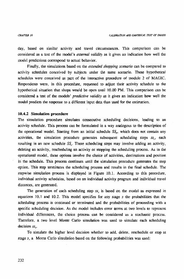
CHAPTER JO CA11BRA110N AND EMPIRICAL TEST OF SMASH

day, based on similar activity and travel circumstances. Th is comparison can be

considered as a test of the model's e.xternal validity as it gives an indication how well the

model predictions correspond to actual behavior.

Finally, the simulations basedon the extended shopping scenario can be compared to

activity schedules conceived by subjects under the same scenario. These hypothetical

schedules were conceived as part of the interactive procedure of module 2 of MAGIC.

Respondents were, in this procedure, requested to adjust their activity schedule to the

hypothetical situation that shops would be open until 10.00 PM. This comparison can be

considered a test of the models' predictive validity as it gives an indication how well the

model prediets the response to a different input data than used for the estimation.

10.4.2 Simulation procedure

The simulation procedure simulates consecutive scheduling decisions, leading to an

activity schedule. This process can be formulated in a way analogous to the description of

the operational model. Starting from an initial schedule SS0 , which does not contain any

activities, the simulation procedure generates subsequent scheduling steps sss, each

resulting in an new schedule SSs. These scheduling steps may involve actding an activity,

deleting an activity, rescheduling an activity or stopping the scheduling process. As in the

operational model, these options involve the choice of activities, destinations and position

in the schedule. This prooess continues until the simulation procedure generates the stop

option. This step terminates the scheduling process and results in the final schedule. The

stepwise simulation process is displayed in Figure 10.1. According to this procedure,

individual activity schedules, based on an individual activity program and individual travel

distances, are generated.

The generation of each scheduling step sss is based on the model as expressed in

equations 10.1 and 10.2. This model specifies for any stage s the probabilities that the

scheduling process is continued or terminated and the probabilities of proceeding with a

specific scheduling decision. As the model includes error terms at two levels to represent

individual differences, the choice process can be considered as a stochastic process.

Therefore, a two level Monte Carlo simulation was used to simulate each scheduling

decision SS5 •

To simulate the higher level decision whether to add, delete, reschedule or stop at

stages, a Monte Carlo simulation basedon the following probabilities was used:

232

CHAFIER 10 CAUBRA710N AND EMP/RJCAL TEST OF SMASH

schedule s-1

( simulation step s

schedule s

schedule s+ 1

Figure 10.1: Stepwise Simulation Process

(10.4)

(10.5)

exp(V r=Jwdule,s) (10.6)

233

CHAnER JO CAUBRA110N AND EMPIRICAL TEST OF SMASH

Pstop,< ---:::-::---:------:::-:--e_xp_(_V=sto::L'P:.:-:c") ______ _ exp(V add")+exp(V delete")+exp(V """hedule,.)+exp(V.top)

(10.7)

V add,s• V4•1eze,s• V reschedule,s and Vstop.s are calculated based on characteristics of the previous

schedule sss-1• resulting from simulation step ss,_[ and the history of the search process,

according to equation 10.1. To calculate utilities, the parameters described in section

10.3.4 vvere used.

lf the outcome of the higher nest simulation is to add, delete or reschedule an

activity, the choice of a specific operation made at the lovver level is simulated by a Monte

Carlo simulation based on the follovving probabilities. If the outcome is to add:

(10.8)

lf the outcome is to delete:

(10.9)

If the outcome is to reschedule:

exp (V re!'Ciuldule ,.;)

Presc!Uidule,<i = ~ (V ) "-- exp re!'Ciulduie ,.i

(10.10)

)

V add,sl V del,s1 V reschedule,si are calculated based on the characteristics of the schedule SS,,

resulting from the implementation of simulation step ss., according to equation 10.2_ To

calculate utilities, the parameter estimates described insection 10.3 are used.

10.4.3 IntemaJ validity

To test the models' internal validity, vve compared the characteristics of the simulated

schedules vvith those of the schedules conceived by the subjects themselves based on the

base scenario. This comparison gives an indication of hovv vvell the model reproduces

individuals' activity schedules_ The characteristics refer to time expenditures to different

234

CHAPTER JO CA1JBRA170N AND EMPlRJCAL TEST OF SMASH

activity classes, the travel time and number of trips included in the schedule and the

number of activities and locations. Tab ie lO. 9 gives the means of these characteristics

aggregated across all individuals and simulation runs.

Table 10.9: Characteristics of Simulated and Observed Schedules

317.7 281.4 3.97

263.2 262.6 0.09

251.8 226.9 1.92

26.6 39.3 -5.28

152.4 67.7 11.33

10.9 11.7 -4.50

91.2 0.69

3.0 -3.09

5.0 -8.95

The simulation results suggest that, in genera!, time expenditures are reasonably well

predicted, although the total time spent on activities is somewhat underpredicted. A t­

value of 8.02 indicates that this difference is significant. However, the time expenditures

on in-home task, in-home leisure, out-of-home task activities and travel are rather

accurately predicted, with t-values of 3.97, 0.09, 1.92 and 0.69 respectively. In contrast,

significant differences were found with respect to out-of-home personal activities

(t=ll.33) and shopping (t=-5.28). Whereas the first is seriously underpredicted, the

latter is overpredicted by about 50%. A possible explanation is the importance of

frequency as an explanatory variabie in the ADD and DELETE models. This variabie

implies that everyday activities, such as shopping, are more likely to be scheduled and

less Jikely to be deleted than more occasional activities such as out-of-home personal

235

CHAPIER JO CAIJIJRA170N AN1J EMPIRJL'AL TEST OF SMASH

activities. This is reflected in the time expenditures predicted for both activity types.

With respect to the other indices, it can be concluded that the number of different

activities is somewhat underpredicted as is the number of visited locations. The t-values of

-4.5 and -3.09 suggest that the differences are significant. A more serious difference,

however, is observed with respect to the number of trips made. This figure is significantly

higher (t=-8.95) in the simulated schedules than in the original schedules. Keeping in

mind that the amount of time spent traveling is wel! predicted, this implies that more but

shorter trips are made in the simulated schedules. This may be a result of the

overprediction of shopping and the underprediction of out-of-home personal activities.

Usually, shops are located nearer to the residence than out-of-home personal trip

destinations. Consequently, this suggests that, given a more or less fixed travel time

budget, more single-purpose trips instead of a smaller number of multi-purpose trips are

made.

10.4.4 External validity To test the models' external validity, the activity schedules were compared to observed

activity patterns. The comparison gives an indication how wel! the model prediction

corresponds to actual activity and travel behavior. The characteristics of simulated activity

schedules and actual activity patterns are displayed in Table 10.10.

It is evident that there are some differences between predicted schedules and

observed activity patterns. First, the overall time expenditures of the observed patterns are

lower than in the simulated schedules (t=-6.04). Although this is to some extent due to an

over-prediction of in-home leisure (t=-5.13) and in-home task (t=-2.04) activities, the

main reason lies in the overprediction of out-of-home task activities by almost 100% (t =

-10.02). Also when comparing the actual patterns to the schedules created by subjects

themselves a similar difference is observed. Apparently, individuals tend to seriously

overestimate the amount of time they are going to spend on out-of-home task activities.

This tendency is reflected by SMASH. A reverse tendency can be observed with respect

to shopping and out-of-home personal activities, to which more time is devoted than

predicted by SMASH. t-values of 1.97 for shopping and 9.64 for out-of-home personal

activities indicate that these differences are significant. If actual behavior is compared to

the original schedules, the time allocated to out-of-home personal activities is in the same

order of magnitude, implying that SMASH seriously underpredicts this time allocation.

However, the difference with respect to shopping is even larger. Thus, with respect to

out-of-home personal activities, the predictions of SMASH are much too low whereas they

236

CHAPTER 10 CALIBRAT70N ANIJ EMI'!RlCAL TEST OF SMASH

give a somewhat better impression of the time spent on shopping. The time spent traveling

is less in reality than predicted by SMASH. This difference was significant (t=-5.48).

Table 10.10: Charaderistics of Simulated Schedules and Observed Activity Patterns

281.4 236.7 -5.13

262.6 246.1 -2.04

226.9 122.8 -10.02

39.3 45.2 1.97

67.7 131.2 9.64

11.7 11.4 -1.65

91.2 70.5 -5.48

3.0 3.5 7.67

5.0 5.0 -0.32

Looking at the other indices, it can be concluded that the number of activities (t = -1.65) and trips (t=-0.32) are predicted very well, but the number of locations is

significantly underpredicted (t=7.67). When actual behavior is compared to the schedules

created by the subjects, a difference in the number of locations and the number of trips is

observed. Apparently, in reality more and shorter trips are made than planned, implying

that more locations are visited and more single-purpose trips are made.

10.4.5 Predictive validity

To test the models' predictive validity, the simulations under the extended shopping

scenario were compared to schedules conceived by respondents under the assumption that

shops would be open untillO.OO PM. However, diversions from the base scenario were

also analyzed for both simulated schedules and schedules. conceived by subjects. These

comparisons give an indication of the predictive validity of the model, as the model

237

CHAPTER JO CAU/Il?A170N AND EM/'/R/L"AL TEST OF SMASH

predictions based on different data than used for the estimation can be tested. Simulated

and real schedules under the base and the extended shopping scenario are displayed in

Table 10.11.

Table 10.11: Comparison of Original and Simulated Schedules

1020.6

317.7 317.7 281.4 272.0

263.2 264.8 262.6 283.7 yes

251.8 250.3 226.9 236.3 110

26.6 27.7 39.3 40.1 yes

152.4 152.4 67.7 58.9

10.9 10.9 11.7 11.6

94.7 94.7 91.2 87.5

2.8 2.8 3.0 2.8

3.8 3.8 5.0 4.8

When oomparing observed and simulated schedules under the extended shopping

scenario, it is first concluded the total time spent on activities is somewhat underpredicted

(t=6.86). This seems to be primarily the result of the underprediction of out-of-home

personal activities (t= 11.59). Similar to the base scenario, in-home leisure {t=4. 92)

activities, in-home task activities (t=-2.38) and out-of-home task activities (t= 1.00) are

rather accurately predicted, whereas shopping (t=-4.38) is seriously overpredicted. Also,

the time spent on travel (t= 1.36) and the number of visited locations (t= 1.08) are

correctly predicted. However, the number of performed activities (t =-3.38) and the

number of trips (t=-7.05) are significantly overpredicted. Thus, SMASH prediets more

238

CJJAnER JO CAlllJRAnON AND EMPIRJCAL TEST OF SMASH

and shorter trips for the same travel budget. Hence, the simulation results in more single­

purpose trips to closer destinations than observed in reality.

Another way of testing the predictive validity is by c01nparing the change in time

expenditures and other indices as a result of the extended shopping hours in both observed

and simulated schedules. In this respect, the observed schedules do not display a real

change in the time spent on activities or traveL This is reflected by the simulation results,

which do not seem to be very much affected by this policy. However, where a minor

change is visible in the observed schedules, the change in the simulated schedules has the

right sign, with the exception of out-of-home task activities.

The observed schedules furthermore show that the number of activities included in

the schedule remains stable, which is reflected by the simulations. Finally, whereas the

number of activities and locations are not affected in the observed schedule, they deercase

in the schedules predicted by SMASH. Apparently, t11e relaxation of space-time

constraints is used by SMASH to create more efficient schedules with more multi-purpose

trips.

10.5 CONCLUSIONS

This chapter outlined and discussed the empirica! test of SMASH based on the data

collected with MAGIC. First, a nested logit model, descrihing separate scheduling choices

was estimated. The estimation results suggest that activity scheduling can be regarded as a

beuristic search process, which is satisficing in nature instead of utility-maximizing. The

significant effect of state dependent variables on the search process suggest that

individuals trade off scheduling effort against the efficiency of the schedule. Furthermore,

the estimation results suggest that each activity scheduling step can be considered a

hierarchical choice. At the higher level, a choice is made wilether to add, delete or

reschedule an activity or to stop scheduling. This choice is affected by the preceding

search process and characteristics of the current schedule such as the total travel time and

time spent on activities. At the lower level, choices regarding the exact add, delete,

reschedule or stop operation are made. These choices are affected by time expenditures to

various activity classes, travel time and frequency at which activities are performed.

To determine how well SMASH prediets complete activity schedules, a series of

simulation studies was described. These simulations aimed at testing the internal, external

and predictive validity of SMASH. The internal validity of the model was tested by

239

CHAPTER JO CALIBRA110N A.NlJ EM!'lRJCAL TEST OF SMASH

investigating whether the model could reproduce the original schedules observed for the

sample. The external validity was tested by comparing simulated schedules to observed

activity patterns measured by time expenditures and travel characteristics. The predictive

validity was tested by simulations of activity schedules under the assumption of extended

opening hours of shops. Simulations for each person under each scenario were replicated

five times.

The simulation results suggest that SMASH prediets time expenditures to activities

and travel well, with the exception of shopping and out~of-home personal activities. Also,

the number of activities that is scheduled is accurately predicted. However, the model

tends to predict relatively many short single-purpose trips, whereas in reality more and

Jonger multi-purpose trips are made. A test of the predictive validity of the model was

successful in that the stability of activity schedules under a relaxation of space-time

constraints was reflected in the simulation results.

240

CHAPTER 11

CALIBRATION AND ILLUSTRATIONS OF COMRADE

11.1 INTRODUCTION

Chapter 8 introduced COMRADE, a competing risk hazard model, which described the

timing and choice of transitions from one activity to another. Based on the data collection procedure described in Chapter 9, the model has been calibrated on observed activity patterns. This chapter reports the results of an estimation of the model's parameters. Moreover, the illustrations of the model's behavior in different spatio-temporal settings

are presented. The chapter is organized as follows. Section 11.2 addresses the model estimation.

The organization of the data and the statistica! estimation procedure are outlined. Section

11.3 discusses the estimation results. Based on the shape and scale parameters of the underlying distribution, conclusions are drawn regarding the nature of the duration process. Furthermore, a behavioral interpretation of the parameter estimates associated with the model's covariates is given. Section 11.4 further explores the characteristics of the estimated competing risk model. Based on some examples, implications of different

space-time constellations on activity choice and duration are illustrated. Finally, section 11.5 draws conclusions regarding the insights that are provided by the model and possible applications of the model in policy contexts.

11.2 ESTIMATION PROCEDURE

COMRADE describes the probabilities .of a transitions from the current activity to other activities a1 as a function of time t. In particular, the following model was specified to

describe cause specific hazard functions h0

(t): I

(11.1)

refers to the time since the start of the current activity; is the hazard function specific fora transition to activity/destination pair a1;

241

CHAPTER 11 CAUBRATION AND EMPIRICAL TEST OF COMRADE

is a vector of covariates of the transition to activity/destination pair a;: is a vector of parameters for activity/destination pair a;: is the baseline hazard function.

The following covariates X, which refer to the current activity of the competing risk, were used in the model. In the below definitions, the subscript p is used to denote

the current activity, whereas p+ 1 denotes the activity involved in the competing risk. First, the constant effect of the current activity, cxP' is taken into account by a

dummy variable. This covariate represents differences in the average durations of activities. Specifically, five subclasses of activities were distinguished which are expected to have typical duration processes. The subclasses include in-home leisure activities, in­home task activities, work/education, shopping and personal business out-of-home (not

work/education or shopping). Secondly, the constant effect of the next activity. cxP,_1, associated with a

competing risk is represented by a dummy variable. These duromies account for the fact that transitions to some activities are more likely to occur than transitions to other activities. The competing risk activities are classified similar to the current activities. However, one category was added, denoting the end state in which no further activities are executed.

A third covariate involves the start time of the current activity in minutes, t;. It is

assumed that the time of day at which activities start may intluenqe the probability of a

transition toanother activity. For instance, the probability of switching to leisure activities may be larger at the end of the day, while switching to work is more likely at the beginning of the day.

A fourth covariate involves the time until the latest end time of the next activity in minutes, 413. This factor represents the effect of closing times or the end of fixed hours for certain activities. lt is not readily evident what the effect of this factor will be. The

effect may be twofold: if less time remains for the exec.ution of an activity, it becomes more urgent so that transition to this activity is more likely to take place. However, if too little time remains for the execution of an activity, a transition may become less likely. If

c;:_1 is the latest possible end time of next activity, 4E is calculated as 4E =t:.-1 - t. If t > t;:_1 , llE is set to 0.

A fifth covariate is the frequency of the current activity, FRP, expressed as the number of times per month the activity is performed. This covariate is used to represent

the difference in the duration process between regular and incidental activities. The

frequency of the next activity. FRP,_ 1, expressed as the number of times per month the

activity is performed, is included to represent differences in transition probabilities to

242

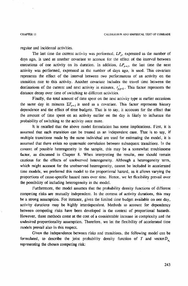
CHAPTER 11 CALIBRATION AND EMPIRICAL TEST OF COMRADE

regular and incidental activities.

The last time the current activity was performed, LPP, expressed as the number of

days ago, is used as another covariate to account for the effect of the interval between

executions of one activity on its duration. In addition, LPp+l• the last time the next

activity was performed, expressed as the number of days ago, is used. This covariate

represents the effect of the interval between two performances of an activity on the

transition rate to this activity. A nother covariate includes the travel time between the

destinations of the current and next activity in minutes, tP~.1 • This factor represents the

distance decay over time of switching to different activities.

Finally, the total amount of time spent on the next activity type at earlier occasions

the same day in minutes ETp+l is used as a covariate. This factor represents history

dependenee and the effect of time budgets. That is to say, it accounts for the effect that

the amount of time spent on an activity earlier on the day is likely to intluence the

probability of switching to the activity once more.

It is recalled that the above model formulation has some implications. First, it is assumed that each transition can be treated as an independent case. That is to say, if

multiple transitions made by the same individual are used for estimating the model, it is

assumed that there exists no systematic correlation between subsequent transitions. In the

context of possible heterogeneity in the sample, this may be a somewhat troublesome factor, as discussed in Chapter 8. When interpreting the results, one should remain

cautious for the effects of unobserved heterogeneity. Although a heterogeneity term,

which might account for the unobserved heterogeneity, cannot be included in accelerated

time models, we preferred this model to the proportional hazard, as it allows varying the proportions of cause-specific hazard rates over time. Hence, we let tlexibility prevail over

the possibility of including heterogeneity in the model.

Furthermore, the model assumes that the probability density functions of different

competing risks are mutually independent. In the .context of activity durations, this may

be a strong assumption. For instance, given the limited time budget available on one day,

activity durations may be highly interdependent. Methods to account for dependency

between competing risks have been developed in the context of proportional hazards.

However, these methods come at the costof a considerable increase in complexity and the

undesired proportionality assumption. Therefore, we let the tlexibility of accelerated time

models prevail also in this respect.

Given the independenee between risks and transitions, the following model can be

formulated, to describe the joint probability density function of T and vectorD al

representing the chosen competing risk:

243

CHAPTER IJ CALIBRA TION AND EMPIRICAL TEST OF COMRADE

(11.2)

with d = 1, if a1 was the next activity exit and d = 0 otherwise. Hence, the a1 a1

probability of a transition to a1 at time t is expressed as the joint probability that

transitions to other activities have not occurred up to t and the probability of a transition

to a1 occurring at t. A maximum likelibood estimation can then be performed to calibrate

the model, using the following log-likelibood function:

N A; Cai

L = rr rr rr fc(t;a I xiaf"c Sc(tia I xiact dia< (11.3) i=l a=l c = 1

where:

N is the number of individuals in the sample;

A; is the number of activities performed by individual i;

cai is the number of possible risks for activity a of individual i; fc is the probability density function of duration times for risk c;

Sc is the survivor function for risk c; tia is the time at which activity a of individual i is ended;

xiac is a vector of covariates associated with risk c fröm activity a of individual i;

diac is a dummy variabie indicating whether or not risk c was chosen for the a-th

activity of individual i.

The model describes transitions between pairs of activities. Hence, each pair of subsequent activities, performed by an individual and recorded in an activity diary, serves

as a separate case. To estimate the model, the following data are needed for each case.

First, the competing risk a1, to which a transition has taken place and the time of

transition t, have to be observed. These data can be directly derived from the activity

diary. Furthermore, it should be known which other competing risks could have been

chosen. These are derived from individuals' activity agendas, as recorded with MAGIC. It is assumed that each activity that is performed with a frequency greater than zero is a

competing risk. If multiple destinations are specified for an activity, each

activity/destination pair is considered a competing risk. Finally, the covariates of both the

chosen and non-chosen competing risks should be known. Some of these, such as frequencies and the time since the last performance, can be derived directly from the

activity agenda. Others, such as the start time, the time remaining for the execution of the

244

CHAPTER 11 CALIBRATION AND EMPIRICAL TEST OF COMRADE

next activity, the travel time and the time spent on the competing risk activity at earlier occasions, can be derived from the diary with additional information from the activity

agenda. Diaries from 228 respondents, which contained a total of 2866 transitions, were used. Thus, the average number of transitionsper respondent was 12.57.

It should be noted that the underlying probability density function of the baseline hazard has to be specified a priori. Hence, to test which probability density function best

matches the data, different models based on different probability density functions were estimated. By comparing the goodness-of-fit measures of these models, the best model can be selected.

11.3 ESTIMATION RESULTS

11.3.1 Distributions A first issue in the interpretation of the results is which underlying probability density

function best reflects the duration process of activities. As there exists little theoretica! evidence as to what distribution an activity duration probability density function should follow, it is assumed that the probability density function resulting in the best model fit is

most representative of activity durations. However, based on empirica! studies (Niemeier and Morita, 1994), it is expected that the overall hazard rate, being the sum of the cause­specific hazards, monotonically increases over time.

The competing risk hazard model was estimated based on different probability

density functions The goodness-of-fit measures of these models are displayed in Table

11.1. It can be concluded that the Jog-normal model gives the best fit and, consequently, is the best descriptor of activity duration processes.

With respect to the generàl behavior of the model, information is obtained from

the estimated scale parameters of the models. The exponential model implies a constant

hazard. As noted before, one would expect a monotonically increasing hazard, implying that the exponential hazard is not a good descriptor of activity durations and transitions.

This is confirmed by the relatively low goodness-of-fit of the exponential model. For the Weibull hazard model, the estimated scale parameter was 1.279, implying

a monotonically increasing hazard. For the log-Jogistic hazard model, a scale parameter of 1.727 was estimated. This implies a hazard function which is first increasing to reach its maximum and is then monotonically decreasing. However, for the range of time relevant to this study, a monotonically increasing hazard is obtained in the log-Jogistic

case, as displayed in Figure 11.1. Finally, the estimated scale parameter of the log­normal model was 3.69, which implies a monotonically increasing hazard. These findings are consistent with other findings (e.g., Niemeier and Morita, 1994; Mannering et al.,

245

CHAPTER 11 CALIBRATION AND EMPIRICAL TEST OF COMRADE

1994) that the hazard function of activity duration is monotonically increasing, reflecting the notion that activities cannot proceed infinitely.

Table 11.1: Goodness-of-Fit Measures of Different Distributional Assumptions

11.3.2 Parameter estimates The parameters estimated for the covariates are displayed in Table 11.2. Given the

specification of the model, the parameters can be interpreted such that a positive parameter corresponds to a Jonger duration of the current activity. A negative parameter indicates a shorter duration of the current activity, or, in other words, that a transition to a competing risk will occur earlier.

The constant effect of the current activity, aP, gives information about the average duration of the current activity. The parameter estimates thus indicate that out-of-home task activities have the longest duration. This is a plausible result, as this category includes many activities with a long duration, such as working, going to school or college, etc. The parameter estimates suggest that in-home leisure and out-of- home personal activities also have a relatively long duration. In-home task activities and

shopping generally have the shortest duration as these categories include short activities such as grocery shopping and small homemaking activities. All these constauts are highly significant.

With respect to the effect of the next activity type, ap+I• it can be concluded that a transition to any activity results in a shorter duration of the current activity as indicated by the negative parameter estimates. However, this effect is strongest for a transition to shopping. Hence, ceteris paribus, a transition to shopping is more likely to take place than transitions toother activities. Or, in other words, if the next activity is shopping, the

current activity is finished earlier. An example of this effect is that people stop working

earlier in order to be able to buy their groceries before closing time. The effect is also relatively strong for in-home task activities. An example of this case is that people stop

246

CHAI"fER 11 CALIBRA TION AND EMPIRICAL TEST OF COMRADE

working earlier toprepare dinner for their family members. The effect is the weakest for in-home leisure activities. Apparently, less responsible activities, which can be freely planned in time, do not have a major impact on the duration of preceding activities.

The parameters estimated for the tP' variables indicate the effect of start time of the current activity on the transition to another activity. The parameters suggest that the later the current activity starts, the longer a transition to another activity is postpOned or

the less likely it is to happen. This holds strongest for shopping, foliowed by out-of-home task activities. Apparently, these activities are less likely to be performed later on the day. This is a logica! finding in light of existing opening hours and working hours. The effect is smaller, but still significant for in-home leisure and task activities and out-of­

home personal activities. These findings tagether suggest that the later the time of day,

the less likely one is to pursue another activity. This is in line with the negative parameter

estimated for the end state, suggesting that the probability that the current activity is the last activity of the day increases if it starts later.

The parameters estimated for AE reflect the effect of the time remaining for execution of the next activity. The parameters were only significant for shopping and in­home leisure and task activities. The positive parameters suggest that if more time

remains for the activity, a transition to this activity is less likely to happen or takes place later. In other words, if there is less time left, the activity becomes more urgent and one is more likely to switch to these activities, as one would expect.

The effect of the frequency of the current activity is expressed by the parameters

estimated for FRr A positive parameter was estimated for all activities, except for out-of­home personal activities. The positive sign suggests that duration increases with increased frequency, although this effect is notsignificant for out-of-home task activities. In case of in-home task activities and shopping, the interpretation of this effect can be that individuals who have these activities as their main task and perform them more often,

also perform these activities with a Jonger duration. For instance, a housewife, who does the weekly grocery shopping needs more time for this activity as her working partner who

visits a shop to buy a single item. The negative parameter for out-of-home personal activities indicates that this activity type generally has a shorter duration the more often it is performed. A possible explanation is that individuals who have more out-of-home

activities and thus have a higher frequency, have to allocate their time to more activities, implying that the average duration is shorter.

The effect of the frequency of the next activity is expressed by the parameters

estimated for FRp+l' In this case, significant parameters are estimated for in-home leisure activities, out-of-home task activities and shopping. The negative parameter values suggest that if an activity is performed more often, a transition to this activity is more

247

CHAPTER 11 CALIBRAT10N AND EMPIRICAL TEST OF COMRADE

likely and occurs more often. This finding reflects the intuitive notion that if an activity is part of an individual's activity program and performed with a certain regularity, it is

more likely to be chosen by that individual. This effect is strongest for out-of-home task

activities, suggesting that working regularly has an important impact on the probability of

choosing workas the next activity.

The parameters estimated for LPP reflect the effect of the last time the current

activity was performed on the duration of the current activity. The only parameter that

comes close to significanee is estimated for in-home task activities. The positive sign

suggests that if it is longer ago that the activity was performed, its duration is generally

longer.

The parameters estimated for LPp+J reflect the effect of the last time the next

activity was performed. A significant and positive parameter was estimated for in-home

task activities and out-of-home task and personal activities. This suggests that the longer

ago one has participated in an activity of this type, the less likely one is to switch to this

activity. This effect is equivalent to the effect of frequency. If the last time the activity

was performed is Jonger ago, one pursues the activity less often, and it is less likely that

a transition to the activity wiJl take place. As a consequence, the duration of the current activity is longer.

The effect of travel time is indicated by the parameters estimated for t,"'. Significant and positive parameters are estimated for the in-home activities and shopping.

This suggests that if travel time from the current destination to the destination of the next

activity increases, one is less likely to switch to these activities, resulting in a Jonger

duration of the current activity. Alternatively, it can be argued that these activities are less likely to be performed if more travel is required to participate in them. Hence, the effect of travel time is that it restrains individuals from switching to an activity.

Finally, the effect of history dependenee is represented by the parameters

estimated for ETp+J· Significant parameters were only obtained for in-home-leisure activities and shopping. The negative sign for in-home leisure suggests that the more time

is spent on the activity in earlier episodes, the sooner a new transition takes place. This

finding may reflect a kind of habit persistence. If an individual tends to perform many

leisure activities and has already spent time on leisure before, he is Iikely to pursue

leisure activities even more in the remainder of the day. The opposite effect is observed

for shopping: the more time is spent on shopping al ready, the longer a transition to a new shopping episode is postponed. Apparently, shopping time is subjecttoa certain budget,

reflecting that only a limited amount of time is needed for shopping. Thus, the more this

amount is exceeded, the more unlikely it is that a transition to shopping takes place again.

248

CHAPTER 11 CALIBRATION AND EMPIRICAL TEST OF COMRADE

Table 11.2: Parameter Estimates Log-Normal Model .... •

... ·.• ... ·· .. ·. ···· .. ) i ~If'l.'l' c .'r .. l I TV' . ...• > < >x .i ... · .•.· .·.· · .... · . ... . .... ·. .· .. · ..... ··.·•.· ... .·•·· . • ..

·· .iJl-home ••• • :... :..#.: .. .• CL j}ot-of-bome endstate I T~~~k?' •.···· ••

· h:isure •••••

I •···. >i · .. . pel'sonai •.• • • •• ! < .. .·· ..

O:p,lliL: 6.48 (72.00)1

"inrr 5.78 (74.15)

O:p,()HT 7.39 (47.77)

~IJ .. 6.09 (47.87)

. ·• 6.47 (75.50)

............ «i+ -1.39 (-15.32) -1.90 (15.32) ·1.60 (5.15) -2.76 (-10.07) -1.66 (·7.76) 0.16 (1.19)

~~.tn. .... 0.05 (2.28)

. l,;mt ..... 0.09 (7.42)

· .•. · • 1;.,<frri: .. · 0.16 (5.40)

. "'ie •• 0.21 (8.75)

~ 0.09 (4.29)

-0.13 (·9.29)

0.07 (3.50) 0.02 (2.53) -0.03 (-1.11) 0.18 (6.66) 0.03 (1.15)

FRp;TBL 0.01 (2.77)

~mr 0.01 (7.85)

-~R~!~JI'i: .• ·· 0.01 (1.62)

.. Ji'RPi$~ 0.01 (5.96)

F.«,,()IJP -0.01 (-8.40)

FR":.;1 • -o.019 (-11.11) 0.002 (1.13) .0.042 (·6.00) -0.006 (-2.30) -0.003 (-1.14) -.·· ... ··

LP,,ÎHt. 0.010 (1.11}

:• LP•,mr 0.020 (1.95)

LPp,!)IJT -0.014 (-0. 75)

LP~· -0.011 (-1.27)

.1#~~111' -0.006 (-0.98)

· ...•. JJJ!,+1. 0.003 (0.72) 0.027 (3.67) 0.017 (2.01) 0.008 (1.45) 0.034 (4.51) -

·. <tG# • 0.19 (4.73) 0.12 (4.51) -0.02 (0.51) 0.23 (4.42) 0,02 (0.48) -0.05 (-1.88)

·-· •.. ~rrt~ < -o.os (2.92) 0,02 (1.01) -0.05 (0.92) 0.25 (3.34) O.o3 (0.42) -

........ : .. •• ··•>"'

1.07 (76.42)

t-valoes m parentheses

249

CHAPTER 11 CALIBRATION AND EMPIRICAL TEST OF COMRADE

11.4 ILLUSTRATIONS OF HAZARD FuNCTIONS

To illustrate the model's behavior and its possible application to policy evaluation, this section presents some examples of log-normal hazard functions that were calculated for specific spatio-temporal settings, based on the parameter estimates described in the previous section. The hazard functions illustrate the effect of the explanatory variables on

the behavior of the model. In this section, the subscript p is used to denote the current activity, whereas the subscript p+ 1 is used to denote a potenrial successor activity, associated with a competing risk.

11.4.1 Tbe effect of current activity The first mustration of the model's behavior concerns the hazard functions of different types of current activities. It is assumed that the next activity in each case is an in-home leisure activity (fable 11.3). Hence, in this case the hazards can be interprered as hazards

descrihing the duration of different activities. The start time t; of all activities is noon.

Table 11.3: Covarlates of Current Activities

leisure

9.00 AM 9.00 AM

12.00 PM 12.00 PM

lO lO

10 10 10 lO

10 10 10 10

10 10 10 10

0 30 30 30

0 0 0 0

The other covariates, which are displayed in Table 11.3, are chosen such that they

represent average conditions. The frequency of the current activity, FRP, and the next activity, FRp+~> is 10 times per month, and the last time the current and the next activity

were performed, LPP and LPp+I• is 10 days ago. The travel time tp.p+I of the out-of-home activities back home is 30 minutes. Finally, the time spent on previous occasions is assumed to be zero. The hazard curves under these conditions, as displayed in Figure

250

CHAPTER 11 CALIBRATION AND EMPIRICAL TEST OP COMRADE

11.1, indicate that with the exception of in-home task activities, all activities have

monotonically increasing hazards. Hence, with increasing duration, the probability of stopping these activities

increases. This finding is consistent with other studies of activity duration (Niemeier and

Morita, 1994; Mannering et al., 1994). However, in-home task activities usually have a short duration, as indicated by the high value of the hazard function. Therefore, the

observed durations fall in the increasing part of the hazard. The size of the hazards

reflects average durations of various activity types. Out-of-home task activities usually have the longest duration, foliowed by out-of-home personal activities, in-home leisure and shopping. In-home task activities have the shortest duration. It should furthermore be

noted that the relative proportions of hazards of different activities are not constant. This finding, which never could have been revealed using proportional hazards,· supports the

use of accelerated time hazard models in this study.

0.005 ,----------------,

0.004 -

0.003

0.001

0~~~======~~ 60 120 180 240 300 360

t (minutes)

Figure 11.1: Different Hazard Functions

11.4.2 Tbe effect of time of day A second mustration of the behavior of the model concerns the effect of time of day on the sizes of competing risks. In this example, it is assumed that the current activity is in­home-leisure and that this activity can be ended by transitions to a number of other

activities. Specifically, competing risks are defined as all five activity types used in this study, plus the end state, implying that no further activities are performed.

The covariate values are displayed in Table 11.4. However, the competing risks hazards are calculated for different start times fP of the current activity: 9.00 AM, 1.00

251

CHAPTER 11 CALIBRATION AND EMPIRICAL TEST OF COMRADE

PM and 7.00 PM. The other covariates are similar for each condition. The frequency of

the current activity, FRP, and the next activity, FRp+I• is 10 times per month, and the last time the current and the next activity were performed, LPP and LPp+l• is 10 days ago.

The travel time t'p,p+I to any out-of-home activity is 30 minutes and the time spent on

previous occasions l:Tp+I is assumed to be zero.

Table 11.4: Covariates of Competing Risks 1

leisure leisure leisure

9.00 AM/ 9.00 AM/ 9.00 AM/ 9.00 AM/

I.OOPM/ 1.00 PM/ 1.00 PM/ 1.00 PM/ 1.00 PM/

7.00 PM 7.00 PM 7.00 PM 7.00 PM 7.00 PM

6.00 PM 6.00 PM 12.00 PM 12.00 PM

10 10 10 10

10 10 lO 10

10 10 10 10 10

10 10 10 10 10

0 0 30 30 30 0

0 0 0 0 0 0

The competing risk hazards in the three situations are displayed in Figures 11.2 to

11.4. They are displayed cumulatively so that the sum of the competing risks reflects the general hazard function of the currem activity. A first conclusion that can be drawn is that with increasing start time the overall hazard increases more slowly. This would imply that the later an in-home leisure activity is started, the Jonger its duration wil! be. With

respect to the competing risks, it can be concluded that in the morning, out-of-home task activities (work, school) constitute the most important risks by which to end the in-home leisure activity. However, the risk associated with these activities, which is first

increasing, starts to decrease after about 4 hours, suggesting that if this risk is not chosen in the beginning of the duration process, it is unlikely that it wiJl be chosen at all. In the

afternoon, the probability of switching from in-home leisure to an out-of-home task activity is less and in the evening the probability has become really small. A similar tendency is observed for out-of-home personal and shopping activities. If the in-home

252

CHA.PTER ll CALIHRA'IlON AND EMI'IRICAL TEST OF COMRADE

leisure activity is started later on the day, the probability that a transition to out-of-home personal or shopping activities is made beoomes smaller. However, in-home leisure and

the end state become more important. Hence, this example illustrates that if an in-home leisure activity starts later on the day, it is more likely to be ended by in-home activities,

non-task activities or the end state.

0.014 ~---------···---,

0.012

0.01

~0.008 ::;t .c 0.006

0.004

0.002

0 60 120 180 240 300 360

t (minutes)

Figure 11.2: Hazards for t'P = 9.00 AM

0.01

0.008

~0.006 .c

0.004

0.002

0 60 120 180 240 300 360

t (minutes)

Figure 11.3: Hazards for t'P = 1. 00 PM

253

CHAPTER 11

0.01

0.008

~0.006 s::.

0.004

0.002

0

CALIBRATlON AND EMPIRICAL TEST OF COMRADE

60 120 180 240 300 360 t (minutes)

Figure 11.4: Hazards for fr = 7.00 PM

11.4.3 The effect of opening hours Another mustration concerns the effect of opening hours on competing risks. In this example, the current activity is again in-home-leisure. The competing risks are all activity

types and the end state, as in the previous illustration. In this illustration, competing risks are calculated based on different opening hours of shops. As displayed in Table 11.5, closing times can take the value of 6.00 PM and 9.00 PM respectively. The other covariates are similar tor both conditions. The start time of the current activity, t;, is

5.00 PM. The frequency of the current activity, FRP, and the next activity, FRp+I• is 10 times per month, and the last time the current and the next activity were performed, LPP and LPr+I• is 10 days ago. The travel time fp,p+I to any out-of-home activity is 30 minutes and the time spent on previous occasions ETp+I is assumed to be zero. The covariates are displayed in Table ll.5.

The competing risk hazards are displayed as in the previous example (Figures 11.5 and 11.6). The hazards functions indicate that the opening hours only affect the risk function of shopping. If shops close at 6.00 PM, implying a higher time pressure, there is a higher probability of switching from the current activity to shopping. However, as the

overall hazard is simply the sum of the competing risks, earlier closing times also imply a higher probability of ending the current activity, resulting inashorter duratîon.

In contrast, if shops close at 9.00 PM, a smaller probabilîty of switching from the current activity to shopping is observed. As a consequence, the probability of ending the current activity is smaller, so that its duration is likely to be Jonger.

254

CHAPTER 11 CALIBRATlON AND EMPIRICAL TEST OF COMRADE

Table 11.5: Covariates of Competing Risks /1

10

10

10

10

0

0

0.01

0.008

Ç' ":;[0.006 .s::.

0.004

0.002

0

out-of· shopping

in-home leisure leisl,lfe leisure

5.00 PM 5.00 PM 5.00 PM

12.00 PM 6.00 PM 6.00 PM/

9.00 PM

10 10 10

10 10 10

10 10 10

10 10 10

0 30 30

0 0 0

60 120 180 240 300 360 t (minutes)

in-home leisure

5.00 PM

12.00 PM

10

10

10

10

30

0

Figure 11.5: Hazards if Shops are open until 5.00 PM

in-home leisure

5.00PM

12.00 PM

10

10

10

10

0

0

255

CHAPTER 11 CALIBRA TION ANI> EMPIRICAL TEST OF COMRADE

0.01

0.008

~0.006 .c

0.004

0.002

0 60 120 180 240 300 360

t (minutes)

Figure 11.6: Hazards if Shops are open unti/9.00 PM

11.4.4 The effect of travel time A final illustration concerns the effect of travel time on competing risks. Again, the

current activity is in-home leisure and the competing risks are all activity types and the

end state.

Table 11.6: Covariates of Competing Risks lll

in-home in-home out~of- shopping out-ofc END

leisure task hometask home

personal

tufrent activity in-home in-home in-home in-home in-home in-home leisure leisure leisure leisure leisure leisure

start timeP . ·• noon noon noon noon noon noon

latest erUJ timep+I 12.00 PM 12.00 PM 6.00 PM 6.00 PM 12.00 PM 12.00 PM

frequency; 10 10 10 10 10 10

frequencyp+l 10 10 10 10 10 10

last peifontl4nceP 10 10 10 10 10 10

lastpeifontl4ncep+l 10 10 10 10 10 10

travel timep.p+I 0 0 30/60 30/60 30/60 0

!:Tp+I 0 0 0 0 0 0

In this example, travel time from the current. in-home activity to any out-of-home

256

CHAPTER 11

0.01

0.008

~0.006 .s::::

0.004

0.002

0

CALIBRA'I10N AND EMPIRICAL TEST OF COMRADE

60 120 180 240 300 360 t (minutes)

Figure 11. 7: Hazards if Travel Times are 30 Minutes

0.01

0.008

~0.006 .s::::

0.004

0.002

0 60 120 180 240 300 360

t (minutes)

Figure 11.8: Hazards if Travel Times are 60 Minutes

activity was varied. Competing risk hazards were calculated for the case that all travel

times are 30 minutes and the case that all travel times are 60 minutes.

The other covariates were similar for both conditions. The start time of the current

activity, t'P, is noon. The frequency of the current activity, FRP, and the next activity,

FRp+I• is 10 times per month, and the last time the current and the next activity were

performed, LPP and LPp+I• is 10 days ago. The travel time fp,p+I to any out-of-home

257

CHAPTER 11 CALIBRATION ANll EMPIRICAL TEST OF COMRADE

activity is 30 minutes and the time spent on previous occasions ETp+I is assumed to be

zero. The covariates of the competing risks are displayed in Table 11.6.

The competing risk hazard functions are displayed in Figures 11.7 and 11.8. The

hazards suggest that travel time does not affect the probability of switching to out-of­home task or personal activities. This is understandable as these activities are often the

outcome of an appointment, so that there is little flexibility in timing. However, shopping

is affected. If travel time to the shopping destination increases, the hazard of shopping

decreases. That is to say, if more travel is required, the probability of a transition to

shopping decreases, resulting in a Jonger duration of the current activity, as reflected by

the smaller size of the overall hazard function.

11.5 CONCLUSIONS

This chapter described the calibration of COMRADE, based on activity diary data. Specifically, the duration of the current activity, the activity to which a transition takes

place and alternative competing risks and their relevant covariates were derived from

activity diaries and data regarding individual activity agendas. Under the assumption of independenee between competing risks and subsequent events, a competing risk model

was estimated using a maximum likelibood estimation.

The estimation results imply that a model based on the log-normal distributed

probability density function best describes activity durations and probabilities of

transitions to other activities. An examinadon of the general behavior of this model suggests that hazards descrihing activity duration are monotonically increasing, at least in

the range under consideration. This finding is consistent with previous findings reported

in the literature. Factors that were found to intluence duration of the current and choice

of the next activity were the type of next activity, start time of the current activity,

closing times of facilities, activity frequencies, travel times and previous time expenditures. The estimation results confirmed the hypotheses that were formulated in the theoretica! framework.

Some examples were used to illustrate the effect of differences in spatio-temporal settings, using a log-normal hazard model. ln particular, the hazard model was used to

assess the impact of time of day. opening hours and travel times. The calculated hazard

functions were consistent with the effects that can be expected. Hence, it can be

concluded that the face validity of the model is satisfactory. The illustrations also demonstrate the usefulness of the model for assessing the effect of various types of

policies. Time policies can be assessed in terms of the time that is available for

performing different activities. In this way, not only changing opening hours of shops,

but also flexible work hours or changes in the opening hours of other facilities can be

assessed. The effect of travel time is related to both transportation policies and land use

258

CHAPTER 11 CAUBRA T10N AND EMPIR1CAL TEST OF COMRADE

policies. In particular, by changing the geographical location of activity sites, the level of

service of public transport facilities or the state of the road network, travel times can be affected. Hence, the model can assess both land use and transportation policies in terros

of the implied changes in travel time. Compared to existing models, COMRADE has the advantage that it does not only

predict the probability that an activity is made at a particular destination, implying a trip, but also the probability that this trip is made at a particular time of day. In this respect, the model offers a very flexible tooi for assessing the effect of time, land use and transportation policies in terros of some very critica! dimensions.

259

260

CHAPTER 12

CONCLUSIONS AND DISCUSSION

Over the past decades. it has been increasingly realized that transport plays a critica! role in developing sustainable cities from an economie, social and environmental perspective. Transportation is required to conduct activities and represents the backbone of healthy cities and regions. It has also been increasingly realized that transport policy alone will be insufficient to tackle the many problems associated with rapidly increasing transport volumes. A more integrative approach, in which transport policies are related to time and land use policies, is required.

This realization that a broader perspective is required to address more successfully

current transportation problems, has stimulated a renewed interest in activity-based transport forecasting models. Transportation demand is nothing but derived demand: it is in pursuing activities that a demand for transportation is generated. Moreover, even if the transportation system will remain exactly the same, time and land use policies may have

dramatic effects on the demand for transportation over time and space. Vice versa, transport policies will necessarily have an impact on land use patterns and the economie performance of a spatial system, and hence the assessment of such policies requires a wider perspective than the one traditionally used in the four-stage rnadeling approach. Activity-based models potentially provide this wider perspective but their inherently much more complex nature and their considerably higher data demands may restriet their use in applied transportation planning.

lt is against this specific background that in this thesis two alternative activity-based models have been introduced. The first, SMASH, is a model of activity scheduling behavior. It represents an original attempt to combine elements of production system

modeling and classica! utility-maximization theory. The activity scheduling process is viewed as a sequentia! decision-making process. In each step, individuals are assumed to add or delete activities to or from their schedule, reschedule activities or stop the

scheduling process. The latter is conceptualized as satisficing behavior in the sense that if an individual is satisfied with the sequence at a particular stage, the scheduling process is assumed to end. As long as this stage has not been reached, individuals are assumed to

maximize their utilities at each step of the scheduling process. The second model that has been developed, COMRADE, is a competing risk model

261

CHAPTER 12 CONCLUSfONS AND DiSCUSSfON

of activity choice, timing, sequencing and duration. The model represems an innovative

approach in activity-based forecasting in that the duration of an activity and the transition rates toother activities are conceptualized as competing risks. This implies that the choice

of an activity in every step of the execution of an activity schedule and its duration are simultaneously modeled as a function of a set of covariates.

These two models account for some of the shortcomings of current activity-based approaches in terms of behavioral responses or explanatory variables that are not

accounted for by current models. In particular, joint logit modelsof activity pattem choice do not explicitly specify the dependendes that exist between decisions on different dimensions and the absence of a specific activity agenda. Nested logit models descrihing the choice of a complete activity pattem only have limited flexibility as a result of

restrictions of the decision structure imposed by the nested logit structure. Furthermore, some key variables, such as the timing of activities and trips are only addressed in terms

of part of the day. Likewise, nested logit or joint logit models descrihing the next activity and destination in a chain do not include mode choice and some relevant dependencies,

such as the effect of the possibility to perfarm activities afterwards on the current activity. In particular, as separate activity and destination choices are modeled, the models do not

account for the effect that the choice of the next activity may be affected by the possibility to perform other activities later on the day. Production systems Jack a statistica! theory to estimate their parameters and test their inherent structure.

Thus, it can be concluded that the proposed models address some of the shortcomings of existing model systems. In particular, existing models are not concerned with the timing and duration of activities and do not account for dependendes between

various activity scheduling decisions while maintaining sufficient flexibility to account for many different response options.

Obviously, the calibration of the proposed models requires the availability of a comprehensive data set, containing not only information regarding space-time behavior in the form of actual activity patterns, but also information regarding opportunities and

constraints pertaining to activities and travel and adaptation strategies used by individuals. To address these data needs and collect data on individuals' reactive behavior to changes in their institutional, spatial or transportation environment, we have advocated the use of interactîve computer experiments and developed MAGIC, based on a review of the empirica! evidence on the effects of key decisions in the design of diaries, form of administration and form of instrument. lnteractive computer experiments offer an unobtrusive means of identifying sequencing decisions, constructing cognitive maps and to check the consistency and completeness of the information.

The data to estimate the models were collected using interactive computer

262

CHAPTER 12 CONCLUS/ONS AND DISCUSSION

experiments. The estimation results of SMASH suggest that the decision whether to stop

scheduling or add, delete or reschedule an activity is based on characteristics of the current schedule, such as the time spent on activities and the total travel time, but also on characteristics of the scheduling process, such as the number of preceding scheduling

decisions. This finding suggests that the outcome of the scheduling process may be suboptimal in terms of characteristics of the schedule, as the efficiency of the schedule is balanced against the cost involved in the scheduling process. Thus, the estimation results confirm existing theoretica! models that describe activity scheduling as a satisficing

process. The choice of a specific scheduling decision was found to be affected by the outcome of the decision in terms of the number of activities, time expenditures to various classes, implied travel time and the frequencies of activities included in the schedule.

COMRADE was estimated based on conventional activity diaries, implying that the

data needs of COMRADE are easier to meet than those of SMASH. The scale parameter that was estimated suggests that the hazard function of activities is monotonically increasing, reflecting the intuitive notion that activities are more likely to be ended if they

· have been going on for a Jonger time. Furthermore, the parameters estimated for the covariates suggest that the duration of the current activity increases with time of day and frequency. A switch to another activity becomes more likely if less time remains for performing the activity if it is performed more frequently, if the last time it was

performed is shorter ago and if travel time to the next activity is shorter. The amount of time already spent on a possible next activity has an ambiguous effect, depending on the

activity type. Thus, the model results suggest that characteristics of activities play an important role in the choice, timing and duration and should therefore be incorporated in transportation models. However, also service level variables such as travel time play an important role in activity and trip timing and destination choice.

Given these empirica! results, the question then is what these models contribute to the state-of-the-art in activity-based modeling and to transportation planning practice.

Moreover, how can they be further improved to increase their relevancy? At the very outset, we have developed an evaluation framework to critically assess the stronger and

weaker points of current activity-based models. lt only makes sense to apply this framework to SMASH and COMRADE alike.

If SMASH is evaluated in the terros of the evaluation framework described in Chapter 6, it can be concluded that SMASH is comprehensive with respect to decision

variables. The model includes activity and destination choice and sequencing of activities. By descrihing activity schedules as sequences of activities and destinations, the most important travel decisions (trip generation and distribution) can be predicted in an activity­

based context. Other travel decisions, such as activity duration, mode and route choice

263

CHAPTER 12 CONCU!310NS AND DISCUSSJON

and the timing of activities and trips, can be determined using beuristic rules or additional

models or are treated as exogenous variables. With respect to the policy variables, it can be concluded that many relevant policy variables are accounted for by the model.

Characteristics of activities, as stored in the long-term calendar and the activity agenda, are included and the cognitive map is represented by the travel distauces between pairs of

locations. It should be noted that the model describes the pre-trip scheduling process. As a consequence, history dependenee or real time informatîon regarding changes in the travel and activity environment are not included in the set of explanatory varîables. The model is very tlexible as, in principle, the model can generate all sequences of scheduling

decisions; leading to any feasible schedule. In addîtion, the model accounts for dependendes between separate decisions by feedback loops that are incorporated in the model. An important feature of the model is that the structured task environment allows the use of statistica! estimation techniques, given that specîfic data is available regarding

subsequent scheduling decisions. This can be considered an important improvement compared to production systems of activity scheduling, which are qualitative in nature.

Finally, SMASH makes a significant contribution to the theory in this area, as it not only gives insight in the factors that guide the scheduling process, but also allows for the

quantification of the effect of these factors. In this respect, the merit of SMASH lies in the combination of a weak beuristic search algorithm, representing tlexible and satisficing decision-making processes, with discrete choice models, which offer the statistica! tools for quantification of the factors guiding the scheduling process.

In terms of the evaluation criteria used in Chapter 6, COMRADE is comprehensive with respect to both behavioral and policy variables. The model includes activity choice,

destination choice, sequencing and timing of activities. Furthermore, it includes activity duration by adopting a dynamic modeling framework, depicting activity participation as a continuous decision-making process. In this sense, COMRADE is one step al1ead of other activity-based models. The inclusion of activity duration as a decision variabie is

especially important in the context of increasing flexibility of time regimes in order to predict how departure times of trips are adjusted to changes in the environment. The model does not include mode choice. Similar to SMASH. heuristic rules or additional models are required to determine this dimension. With respect to policy variables, COMRADE assumes that the long-term calendar, the activity agenda and travel times as stored in the cognitive map and incidental circumstances affect the activity pattern. Hence,

COMRADE is quite comprehensive in this respect. The model is very tlexible, as it allows for all activity and destination sequences and activity durations. With respect to dependendes between models. COMRADE only accounts for history dependence. That is,

the effect of previous decisions on the current deelsion is accounted tor. However, the

264

CHAPTER 12 CONCLUSIONS AND DISCUSSION

model does notaccount for prospective utility, repcesenting the effect of decisions to make at a later stage on the current decision. The model can be estimated using statistica! estimation techniques, implying that model performance and significanee of parameters

can be determined. Finally, the model contributes to the theory in this field in that it provides insight into the duration processes of different processes, depending on

characteristics of activities. The use of an accelerated time competing risk model also gives insight into the transition probabilities to other activities as a function of time as a

function of characteristics of activities and spatio-temporal circumstances. Although these two models make a contribution to the state-of-the-art in activity­

based modeling, there are a few aspects of these models that require further elaboration. In particular, the following avenues of further research, which may further improve the models described in this thesis can be identified.

As far as SMASH is concerned, a first issue concerns the satisficing nature of the activity scheduling process. We have attempted to account for satisficing behavior within a utility-maximizing framework by using state dependent variables, which represent the fact that individuals balance the amount of mental effort involved in activity scheduling against the efficiency of the schedule. Assuming that these variables account for the suboptimal nature of activity scheduling, one would expect the two-dimensional choice of a scheduling decision to be made according to utility-maximizing principles. However, the

estimation results, yielding a negative parameter for the inclusive value, suggest a violation of the utility-maximization principle. Further research should therefore address alternative decision strategies that may play a role in activity scheduling. Alternative decision rules, such as elimination-by-aspects, satisficing rules or lexicographic rules may be promising tools for descrihing complex decision-making processes and enhance and improve models such as SMASH. For instance, the combinatorial algorithm that generates

all feasible scheduling decisions for a specific state may stop generating schedules if a schedule is obtained which is satisfactory with respect to all relevant attributes. Alternatively, more intelligent combinatorial algorithms, which cut off complete branches if they are not expected to give acceptable solutions can be used. For instance, if actding an activity is infeasible anyway, it is no use creating all combinations of adding various activities at various destinations in various sequences. Apart from saving computational effort, such algorithms may reflect alternative decision-making strategies (as opposed to

utility-maximization) which may prove relevant to the topic at hand. A second aspect of SMASH that deserves further attention is the need to include

certain key decisions, such as mode and route choice, which are currently omitted. Neglecting these dimensions is a result of the emphasis in this thesis on modeling the decisions that, according to activity-based theory, invoke and to a large extent determine

265

CHAPTER 12 CONCLl!S/ONS AND DISCUSSION

travel, such as the choice and sequencing of activities and destinations. Nevertheless, it goes without saying that mode choice and route choice constitute key dimensions of travel decision-making, which are the target of transportation policy. Including mode and route choice would therefore be a significant improvement of SMASH.

A straightforward way of including mode choice in the model system would be to

add mode choice and route choice as extra dimensions of an add, delete or reschedule decision. Thus, in this view, adding an activity not only implies choosing an activity, destination and sequence, but also the choice of the mode and route of the invoked trip. A

drawback of such an approach clearly is that the number of alternatives rapidly increases,

causing problems in estimating the model. Furthermore, it cannot be assumed right away that alternatives that share a common dimension, such as an activity or destination or

mode, have identically and independently distributed error terms as suggested by such a

model. A more promising approach would, therefore, be the use of a nested logit model, in which mode choice is nested as an additional hierarchical level under the higher level add or reschedule decision. Such a model could be estimated using a sequentia! estimation procedure. First, a mode choice model is estimated, including the key service level variables of the system. This model could then be used to calculate the logsum of the

available mode choice alternatives, which can be used as an explanatory variabie in the higher level activity scheduling model. Such an approach would offer the opportunity of incorporating important service level variables, such as travel costs, travel times and

reliability into the activity scheduling model. In a similar vein, the effect of route characteristics such as road quality and

congestion levels could be incorporated in the model by adding route choice as a decision

dimension. The logsum of available routes that can be foliowed between origin and destination pairs generated by SMASH can be used as an explanatory variabie of higher level add or reschedule decisions. Thus, the above approach seems promising to incorporate mode and route choice into the model, so that actual travel volumes on specific links of the road network can be modeled, which is the ultimate goal of transportation modeling.

A third aspect of SMASH that needs further elaboration concerns the 'with whom' dimension. In principle, the choice with whom to perform activities or travel together implies that the activities and trips of multiple persons are mutually coordinated in time and space. The marketing literature (Davis et al., 1986; Molin et al., 1997) has described multi-person decision-making models, which describe how a group of individuals takes

decisions based on individuals' own utilities and the utilities they expect others to derive

from choice alternatives. Although these models are theoretically appealing and in principle apply to the decision-making process at hand, it is likely that the complexity of

266

CHAP1ER 12 CONt1J!SIONS AND DISCUSSJON

the activity scheduling process prohibits the use of multi-person decision-making models

to describe how individuals coordinate their schedules. A feasible approach, however, to represem interpersonal relationships may be to

derive rules from the activity agendas of the household members. For example, by

assuming that one individual is dominant over another individual, the activity schedule of the dominant person would result in space-time constraints for the other individual. In many cases, such as constraints stemming from fixed work hours of a individual, this will be a realistic assumption. Generally speaking, it can be assumed that, if an activity is performed by multiple persons, space-time constraints with respect to that activity are

transferred from one person to another. Given the importance of coupling constraints to

travel decision-making, further research is needed to investigate to what extent beuristic

rules as described above can be used to improve forecasting procedures. Similar to SMASH, COMRADE does not describe certain decisions, such as

mode and route choice. Again, this deelsion is justified by the need to model other aspects of activity scheduling that have to date received little or no attention in the literature. However, includlng mode and route choice would be an important improverneut of the

model. A straightforward way of doing so would be to define competing risks not only in terms of actlvities and destinations, but also in terms of modes and routes associated with a trip to a next activity. A drawback of this approach would be that the number of risks would perhaps rapidly increase, diminishing the applicability of the model and perhaps causing estimation problems. A more fundamental problem, however, concerns the assumption underlying competing risk models that the probability density functions of competing risks should be independently distributed. In case some competing risks share common dimensions, such as an activity, destination, mode or route, this assumption

becomes more unrealistic. Generally speaking, there is a need for further research and development of competing risk models that allow for dependendes between lifetime distributions of competing risks.

A final note concerns the relationship between SMASH and COMRADE. As we have noted before, both models describe different decision-making processes. Whereas

SMASH describes the mental process preceding the execution of activities, during which a schedule is conceived to coordinate the activities to be performed, COMRADE describes the actual execution of activities, during which one needs to decide at each point in time witether to proceed the current activity or witether to switch to another one. Both models

operate independently of each other. That is to say, COMRADE models the execution of activities from scratch, assuming that no schedule is available to guide the execution. It is plausible, however, that the execution of activities is preceded by a deliberate planning and coordination phase. To gain insight into the relationship between scheduling and

267

CHAPTER 12 C<JNCLUSIONS AND DISCUSSION

executing activities, it is a logica! step to try to link both models. This can be achieved in

different ways, depending on the flexibility that is allowed for in the execution phase. If it is assumed that the activity schedule is a fixed, sequence of activities and destinations, which is not changed during execution, hazard models could be used to model only the

duration of the subsequent activities. Such an approach would imply that a competing risk model is not necessary. However, it mayalso be assumed that individuals divert from the pre-specified sequence, destinations or activities. In that case, the schedule may serve as a guideline for execution, for instanee by assigning priorities to various activities in the

schedule. The use of a competing risk model would then leave open the possibility of choosing other activities and destinations than scheduled. Thus, in this approach, SMASH would provide the input needed by COMRADE to predict activity choice, timing and duration. In this way, the feasibility of activity schedules and space-time links that exist between activities can be better accounted for than by estimating and applying

COMRADE from scratch. Thus, further research is recommended to find out how models of scheduling and execution of activities can complement and improve each other.

Overall then, SMASH and COMRADE represem two potentially valuable models

that describe various aspects of activity scheduling and execution. Both models, however, are but a first step into this direction and both allow further improvement or, at least, the examination of alternative specifications. Moreover, both models have to be necessarily linked to other models to ultimately predict traffic volumes at various times of the day at the various links of a network or to predict average traffic volumes. Micro-simulation modeling seems the appropriate way to pursue, but should be subject of another study. Regardless of all these theoretical, statistica!, data and operational problems, the present

study suggests that activity-based models seem to gradually complement or replace the decades-old four-step transportation forecasting methodology. Hopefully, this thesis has made a contribution in tackling some of the problems that hitherto have prevenled policy­makers to invest in and use activity-based models.

268

BmLIOGRAPHY

Abdel-Aty M.A., R. Kitamura and P.P. Jovanis (1995), Route Choice Models Using GIS­Based Alternative Routes and Hypothetical Travel Time Information Input. Paper presented at the 74th Annual Meeting of he Transportation Research Board,

Washington D.C. Adler, T. and M. Ben-Akiva (1979), A Theoretica] and Empirica! Model of Trip Chaining

Behavior, Transportation Research, 13B, pp. 243-257. Alterman, R. (1988), Adaptive Planning, Cognitive Science, 12, pp. 393-421.

Ampt E. (1989), Comparison of Self-Administered and Personal Interview Methods for the Collection of 24-hour Travel Diaries, Proceedings of the WC1R, pp. 195- 206.

Anderson, O.A., A. Borgers, D. Ettema and H. Timmermans (1992), Estimating Availability Effects in Travel Choice Modelling: A Stated Choice Approach, Transportation Research Record,l351, pp. 51-65.

Anderson, D.A. and J.B. Wiley (1992), Efficient Choice Set Designs for Estimating Availability Cross Effects Models, Marketing Letters, 3, pp. 357-370.

Aneshensel, C.S., R.R. Frerichs, V.A. Clark and P.A. Yokopenioc (1982a), Measuring Depression in the Community: A Comparison of Telephone and Personal Interviews,

Pubtic Opinion Quarterly, 46, pp. 110-121.

Aneshensel, C.S., R.R. Frerichs, V.A. Clark and P.A. Yokopenioc (1982b), Telephone

versus In-Person Surveys of Community Health Status, American Joumal of Pub/ie HeaiJh, 72, pp. 1017-1021.

Aquilino, W.S. (1994}, Interview Mode Effects in Surveys of Drug and Alcohol Use: A Field Experiment, Pubtic Opinion Quarterly, 58, pp. 210-240.

Arangio-Ruiz G.G. (1984), Survey on Time Use in Italy. Paper presented at the Meetings of the International Group on Time Budgets and Social Activities, Helsinki, Finland.

Arentze, T., A. Borgers and H. Timmermans (1993), A Model of Multi-Purpose Shop­ping Trip Behavior, Papers in Regionat Science, 12, pp. 239-256.

Axhausen, K.W. (1990), A Simultaneous Simulation of Activity Chains and Traffic Flow.

In: P. Jones (ed.), New Developments in Dynamic and Activity Based Approaches, Gower Aldershot, pp. 206-225.

Axhausen, K.W. (1994), Travel Diaries: An Annotated Catalogue. Working paper, Imperia! College, London.

Axhausen K.W. and R. Herz (1989), Simulating Activity Chains: German Approach,

269

8/BUOORAPHY

Journat of Transportation Engineering, 12, pp. 324-341.

Bates, J. (1994), Modelling the Response of Non-Home-Based Trips to Congestion

Charges, PTRC Annual Meeting, University of Warwick, England.

Becker, G. (1965), A Theory of the Allocation of Time, Economie Journal, 75, pp. 493-

517.

Beek, P. van, N. Kalfs N. Aardoom and G. Roeleveld (1995), Future Activity Patterns. Paper presenred at the conference "Activity-Based Approaches: Activity Scheduling

and the Analysis of Activity Patterns", Eindhoven, The Netherlands.

Ben-Akiva, M. and J. Bowman (1997), An Activity Based Disaggregate Travel Demand

Model System with Daily Activity Schedules, to appear in Transportation Research. Ben-Akiva, M., J. Bowman and D. Gopinath (1994), Travel Demand Model System for

the Information Era, MIT. Ben-Akiva, M. and S.R. Lerman (1985), Discrete Choice Analysis: Theory and Applica­

tion to Travel Demand, MIT Press, Cambridge, Massachusetts. Boden (1994), Hourses of a Different Colour?. In: V. Honavar and L. Uhr (eds.),

Artificial lntelligence and Neural Networks: Steps Toward Principled Integration, Academie Press, Boston, pp. 3-20.

Bovy, P.H.L (1990), Effects of Opening the MlO Amsterdam Orbital Motorway,

Rijkswaterstaat, Transportation and Traffic Research Division, Rotterdam.

Bradley M., P. Jones and E. Ampt (1987), An Interactive Household Interview Method to

Study Bus Provision Policies. In: Transportation Planning Methods Volume P290,

Proceedings of Seminar C held at the PTRC Summer Annual Meeting, Bath, pp. 163-178.

Cannell, C.F. et al. (1982), An Experimental Comparison of Telephone and Personal Health Surveys, Institute for Social Research, Ann Arbor.

Carpenter, S. and P. Jones (1983), Recent Advances in TravelDemand Analysis, Gower, Aldershot.

Chapin, F.S. (1965), Urban Land Use Planning, University of Illinois Press, Urbana.

Chapin, F.S. (1974), Human Activity Patterns in the City, John Wiley and Sons, New

York. Chapin, F.S. (1978), Human Time Allocation in the City. In: T. Carlstein, D. Parkes and

N. Thrift (eds.), Human Activity and Time Geography (Volume 2), Edward Arnold, London, pp. 13-26.

Clarke M., M. Dix and P. Jones (1981), Error and Uncertainty in Travel Surveys.

Transportation, 10, pp. 105-126.

Cullen, I. (1978), The Treatment of Time in the Explanation of Spatial Behaviour. In: T.

270

Carlstein, D.N. Parkes and N.J. Thrift (eds.), Timing Space and Spacing Time. Volume 2: Hunwn Activity and Time-Geography, Edward Arnold, London, pp. 27-

BIBUOGRAPHY

38. Cul\en I. and V. Godson (1975), Urban Networks: The Structure of Activity Patterns,

Progressin Planning, 4, pp. 1-96. Daly, A. (1987), Estimating "Tree" Logit Models, Transportation Research, 21B, pp.

251-267. Davis, H.L, S.J. Hochand E.K.E Ragsdale (1986), An Anchoring and Adjustment Model

of Spousal Predictions, Joumal of Consumer Research, 13, pp. 25-37.

Dellaert, B.G.C, T.A. Arentze, A.W.J. Borgers and H.J.P Timmermans (1997), Consumer Activity Pattem Choice: Development and Test of Nested Conditional

Conjoint Choice Experiments, Joumal of Retailing and Consumer Services, to appear.

DeSerpa, A. (1971), A Theory of the Economics of Time, The Economie Joumal, 81, pp. 828-846.

Dijst M. (1993), Gewijzigde Opzet van Dagboekonderzoek Succesvol, OSPA, TU-Delft, Delft.

Dijst,. M. (1995), Het Elliptisch Leven: Actieruimte als Integrale Maat voor Bereik en Mobiliteit, Netherlands Geographical Studies, Delft.

Dillman D.A. (1991), The Design and Administration of Mail Surveys, Annual Review of Sociology, 17, pp. 225-249.

Dowling R.G. and S.B. Colman (1995), Effects of Increased Highway Capacity: Results of Household Travel Behavior Survey, Transportation Research Record, 1493, pp.

143-150. Dreyfus, H.L. and S.E. Dreyfus (1988), Making a Mind Versus Modeling the Brain:

Artificial Intelligence Back at a Branchpoint. In: S.R. Graubard (ed.), The Artificial lntelligence Debate: False Starts, Real Foundations, The MIT Press, Cambridge, Massachusetts, pp. 15-44.

Ettema, D. (1991), Vervoermiddelkeuze in de Vervoerregio Eindhoven: Een Gecombineerde Revealed Choice/Stated Choice Benadering, Eindhoven University of Technology.

Ettema, D., K. Axhausen and J. Polak (1995), Activities and Travel Behaviour: ModeHing and Data Issues. Paper presented at the ESF/EC Euroconference on European Transport and Communication Networks: Policies on European Networks, Espinho, Portugal.

Ettema, D., A. Borgers and H. Timmermans (1993a), Using Interactive Computer

Experiments for Investigating Activity Scheduling Behaviour, Proceedings of the PTRC 2lst Summer Annual Meeting, University of Manchester, P366, pp. 267-282.

Ettema, D., A. Borgers en H. Timmermans (1993b), A Simulation Model of Activity Scheduling Behaviour, Transportation Research Record, 1413, pp. 1-11.

271

BIBUOGRAPHY

Ettema, D., A. Borgers and H. Timmermans (1994), Using Interactive Computer

Experiments for Identifying Activity Scheduling Heuristics. Paper presented at the

Seventh International Conference on Travel Behaviour, Valle Nevado, Santiago,

Chile.

Ettema, D., A. Borgers and H. Timmermans (1995), Competing Risk Hazard Model of

Activity Choice, Timing, Sequencing and Duration, Transportation Research Record, 1493, pp. 101-109.

Ettema, D., A. Borgers and H. Timmermans (1997), SMASH (Simulation Model of

Acticity Scheduling Heuristics): Empirica! Tests, to appear in Transportation Research.

Ettema, D., H. Timmermans and L. van Veghel (1996), Effects of Data Collection

Metbod in Travel and Activity Research, European Institute of Retailing and

Services Studies, Eindhoven.

Ettema, D.F. and H.J.P. Timmermans (1997), Recent Advances in Activity Analysis, Pergamon Press, Oxford, to appear.

Evans, A. (1971), On the Theory of the Valnation and Allocation of Time, Scottish Joumal of Politica! Economy, 2, pp.l-17.

Fellendorf, M., T. Haupt, U. Heidl and W. Scherr (1995), VISEM: An A<::tivity Chain

Based Traffic Demand Model. Paper presented at the conference u Activity Based

Approaches: Activity Scheduling and the Analysis of Activity Patterns", Eindhoven,

The Netherlands.

Gärling, T., K. Brännäs, J. Garvill, R.G. Golledge, S. Gopal, E. Holmand E. Lindberg

(1989), Houschold Activity Scheduling. Paper presented at the Fifth World

Conference on Transport Research, Yokohama. Gärling, T., J. Säisä, A. Böök and E. Lindberg (1986), The Spatiotemporal Sequencing of

Everyday Activities in the Large-Scale Environment, Joumal of Environmental Psychology, 6, pp. 261-280.

Golledge, R.G., M.-P. Kwan and T. Gärling (1994), Computational Process ModeHing of

Travel Decisions, Papers in Regionat Science, 73, pp. 99-ll7. Golob T.F. and H. Meurs (1986), Biases in Response over Time in a Seven-Day Travel

Diary, Transportation, 10, pp. 163-181. Groves, R.M. and R.L. Kahn (1987), Surveys by Telephone, Academie Press, New York.

Groves R.M. and W.L. Nicholls ll (1986), The Status of Computer-Assisted Telephone

Interviewing: Part II - Data Quality Issues, Joumal of Official Statistics, 2, pp.

117-134.

Hägerstrand, T. (1970), What about People in Regional Science?, Papers of the Regional Science Association, 23, pp. 7-21.

Han, A. and J.A. Hausman (1990), Flexible Parametrie Estimation of Duration and

272

BfBUOGRAPIIY

Competing Risk Models, Joumal of Applied Econometrics. 5, pp. l-28. Harvey A.S. (1993), Guidelines for Time Use Data Collection, Social Indicators

Research, 30, pp. 197-228. Harvey A.S. and S. Gn:mmo {1986), Social Contact in Canada and Norway. In: A.

Dagfinn, A.S. Harvey, E. Wunk-Lipinsky and I. Niemi (eds.), Time Use Studies: Dimensions and Applications, Central Statistics Office of Finland, Helsinki.

Havens, J.J. (1981), New Approaches in Onderstanding Travel Behavior: Role, Life Style, and Adaptation. In: P.R. Stopher, A.H. Meyburg and W. Brög (eds.), New Horizons in Travel-Behavior Research, Lexington, Massachusetts/Toronto, pp. 269-

284. Hayes-Roth, B. and F. Hayes-Roth (1979), A Cognitive Model of Planning, Cognitive

Science, 3, pp. 275-310. Hensher D. (1994), The Timing of Change for Automobile Transactions: A Competing

Risk Multispell Specification. Paper presented at the Seventh International Conferen­ce on Travel Behavior, Valle Nevado, Santiago, Chile.

Hensher, D.A. and F.L. Mannering (1994), Hazard-Based Duration Models and their Application to Transport Analysis, Transport Reviews, 14, pp. 63-82.

Hinton, G.E. and T.J. Sejnowski (1986), Learning and Relearning in Boltzmann

Machines, Parallel Distributed Processing Vol/ and 2, MIT Press. Hirtle, S.C. and T. Gärling (1992), Heuristic Rules for Sequentia! Spatial Decisions,

Geoforum, 23, pp. 227-238. Hoorn, van der, A.I.J.M. (1983), An Empirica! Model of Travel and Activity Choice: A

Case Study for the Netherlands, University of Amsterdam. Hopfield, J.J. (1982), Neural Networks and Physical Systems with Emergent Collective

Computational Abilities, Proceedings of the National Academy of Sciences, 79, pp. 2554-2558.

Houben P.C.P. (1980), Validiteitsonderzoek April 1980. Report H5600-80-E4, Netherlands Central Bureau of Statistics, Heerlen.

Houben P.C.P. (1981), Doelsteling, Opzet, Uitvoering en Analyse van het Validiteits­

onderzoek April 1980. Nota H2632-81-E4, Netherlands Central Bureau of Statistics, Heerlen.

Houben P.C.P. (1984), Experiment Telefonisch - Schriftelijk Enqueteren bij het Onderzoek Verplaatsingsgedrag: Deel 2 Analyse van het Experiment. Nota Hl236-84-E4, Netherlands Central Bureau of Statistics, Heerlen.

Huigen, P.P.P. (1986), Binnen of Buiten Bereik? Een Sociaal-Geografisch Onderzoek in Zuidwest-Friesland, Geografisch Instituut, Utrecht.

Jara-Diaz, S.R. (1994), General Micro-Model of User's Behaviour: The Basic Issues. Paper presented at the Seventh International Conference on Travel Behaviour, V alle

273

BlBUOGRAPHY

Nevado, Santiago, Chile. Jones, P.M. (1979), 'HATS': A Technique for lnvestigating Household Decisions,

Environment and Planning A, 11, pp. 59-70.

Jones, P.M. (1990), Developments in Dynamic and Activity-Based Approaches to Travel Analysis, Avebury, Aidershot

Jones, P.M., M.C. Dix, M.l. Clarke and l.G. Heggie (1983), Understanding Travel Behavior, Gower, Aidershot

Jones, P., F. Koppelman and J.P. Orfèuil (1990), Activity Analysis: State-of-the-Art and

Future Directions. In: P. Jones (ed.), Developments in Dynamic and Activity-Based Approaches to Travel Analysis, Avebury, Aldershot, pp. 34-55.

De Jong, G., R. Kitamura and J. Klooster (1994), A Disaggregate Model of Vehicle

Holding Duration, Type Choice and Use. Paper presented at the Seventh Internation­

al Conference on Travel Behaviour, Valle Nevado, Chile. Jordan, L.A., A.C. Marcus and L.G. Reeder (1980), Response Styles in Telephone and

Household Interviewing: A Field Experiment, Pubtic Opinion Quarterly, 44, pp.

210-222.

Jorritsma, P. (1990), Over Tijd, Reizen en Verblijven. Nederlanders Gegroepeerd naar hun Dagelijkse Verplaatsingen, Geo Pers, Groningen.

Juster F.T. (1985), The Validity and Quality of Time-Use Estimates Obtained from Reeall

Diaries. In: F.J. Juster and F.P. Stafford (eds.), Time, Goods and Well-Being, lnstitute for Social Research, University of Michigan, Ann Arbor, pp. 63-91.

Juster F.T. (1986), The Effect of Reeall Period on the Quality of Time Diary Data. In: A.

Dagfinn, A.S. Harvey, E. Wunk-Lipinsky and I. Niemi (eds.), Time Use Studies: Dimensions and Applications, Central Statistics Office of Finland, Helsinki, pp. 149-175.

Kalbtleisch, J.D. and R.L. Prentice (1980), The Statistica! Analysis of Failure Time Data, Wiley and Sons, New Vork.

Kalfs N. (1992), Time Budget Research: Three Data Collection Modes. In: Time Use Methodology: Towards Consensus, ISTAT, Rome, pp. 283-285.

Kalfs N. (1994), The Construction of a New Electronic Diary. In: N. Kalfs and A.S.

Harvey (eds.), Fifteenth Reunion of the International Association for Time Use Research, NIMMO, Amsterdam, pp. 246-260.

Kalfs N. (1995), Effects of Different Data Collection Procedures in Time Use Research,

Transportation Research Record, 1493, pp. 110-117.

Khattak, A.J., F.S. Koppelman and J.L. Schofer (1992), Stated Preferences for Investigat­

ing Commuters' Diversion Propensity. Paper presented at the 71st Annual Meeting

of the Transportation Research Board, Washington D.C. Kitamura, R. (1984a), A Model of Daily Time Allocation to Discretionary Out-of-home

274

BlBUOGRAPHY

Activities and Trips, Transportation Research, 18B, pp. 255-266.

Kitamura, R. (1984b), Incorporating Trip Chaining into the Analysis of Destination

Choice, Transportation Research, 18B, pp. 67-81.

Kitamura, R. and M. Kermanshah (1983), Identifying Time and History Dependencies of

Activity Choice, Transportation Research Record, 944, pp. 22-30.

Kitamura, R. and M. Kermanshah (1984), Sequentia! Model of Interdependent Activity

and Destination Choices, Transportation Research Record, 987, pp. 81-89.

Kievmarken N.A. (1982), Household Market and Non-Market Activities: A Pilot Study, University of Goteborg, Department of Statistics.

Knippenberg, C. van, M. Koekelkoren and N. Korsten (1990), Travel Behaviour of Non­

Traditional Households. In: P. Jones (ed.), Developments in Dynamic and Activity Based Approaches to Travel Analysis, Avebury, Aldershot, England, pp. 123-144.

Knippenberg, C. van en J. Splinter (1983), De Relatie tussen Openbaar Vervoer en

Mobiliteit in Kleine Kernen, Verkeerskundig Studiecentrum Rijksuniversiteit

Groningen.

Knuist, W. and L. Schoonderwoerd (1983), Waar blijft de Tijd? Onderzoek naar de Tijdsbesteding van Nederlanders, Social Cultural Planningbureau, The Hague.

Koppelman F.S. (1981), Non-Linear Utility Functions in Models of Travel Choice

Behavior, Transportation, 10, pp. 127-146.

Kraan, M. (1995), In Search for Limits to Mobility Growth with a Model for the

Allocation of Time and Money. Paper presented at the conference "Activity Based

Approaches: Activity Scheduling and the Analysis of Activity Patterns", Eindhoven,

The Netherlands.

Kroes, E., R. Sheldon and C. Gore (1990), How Do Passengers Choose When to Travel?

A Stated Preferenee lnvestigation. In: P. Jones (ed.), Developments in Dynamic and Activity Based Approaches to Travel Analysis, Avebury, Aldershot, England, pp.

123-144.

Krysan M., H. Schuman, L.J. Scott and P.Beatty (1994), Response Rates and Response

Content in Mail Surveys versus Face-to--Face Surveys, Pubtic Opinion Quarterly, 58, pp. 381-399.

Küchler, R. (1985), Wegekettenorientierte Verkehrsberechnungsmodelle, Ph.D. disser­

tation, Technische Hochschule Darmstadt.

Kutter, E. (1984), Integrierte Berechnung Städtischen Personenverkehrs, Technische

Universität Berlin.

Kuzmyak, J.R. and S. Prensky (1979), Use of Travel Diaries in Collection of Travel Data

on the Elderly and Handicapped, Transportation Research Record, 701, pp. 36-38.

Lancaster, K.J. (1966), A New Approach to Consumer Theory, Joumal of Politica/ Economy, 74, pp. 132-157.

275

BlBUOGRAPHY

Lancaster, T. (1990), The Econometrie Analysis of Transition Data, Cambridge U niversity

Press, Cambridge. · Lawless, J.F. (1982), Statistica! Models and Methods for Lifetime Data, Wiley and Sons,

New York.

De Leeuw, E.D. (1992), Data Quaüty in Mail, Telephone and Face-to-Face Surveys, Ph.D. Thesis, Free University, Amsterdam.

Lenntorp, B. (1978), A Time-Geographic Simulation Model of Individual Activity

Programmes. In: T. Carlstein, D. Parkes and N.Thrift, Human Activity and Time Geography (Volume 2), Edward Arnold, London, pp. 162-180.

Linsky A.S. (1975), Stimulating Response to Mailed Questionnaires: A Review, Public Opinion Quarterly, 39, pp. 82-101.

Louviere, J.J. (1988a), Analyzing Deelsion Making, Metric Conjoint Analysis, Sage

Publications, Newbury Park.

Louviere, J.J. (l988b), Alternative Strategies for Designing Choice Experiments, University of Alberta.

Luce, R.D. (1959), Individual Choice Behavior: A Theoretica! Analysis, John Wiley and

Sons, New York.

Mahmassani, H.S. (1990), Dynamic Models of Commuter Behavior: Experimental

Investigation and Application to the Analysis of Planned Traffic Disruptions,

Transportation Research, 24A, pp. 465-484. Mannering F., E. Murikami and S-G. Kim (1994), Temporal Stability of Travelers'

Activity Choice and Home Stay Duration: Some Empirica! Evidence, Transporta­tion, 21, pp. 371-392.

Mansfield, E. (1985), Microeconomics: Theory and Applications, Norton, London. Manski, C. (1973), The Analysis of Qualitative Choice, MIT, Cambridge, Massachusetts.

McFadden, D. (1989), A Method of Simulated Moments for the Estimation of Discrete Choice Response models without Numerical lntegration, Econometrica, 57, pp. 995-

1026. McFadden, D., K. Train and W.B. Tye (1977), An Application of Diagnostic Tests for

the Independenee from Irrelevant Alternatives Property of the Multinomial Logit

Model, Transportation Research Record, 637, pp. 39-46.

Menz, H.J. (1984), Analyse von Verkehrsverhalten im Haushaltskontext, Technische

Universität Berlin, Berlin.

Meurs, H. (1991), A Panel Data Analysis of Travel Demand, Ph.D, dissertation, University of Groningen.

Meyburg A.H. and W. Brög (1981), Validity Problems in Empirica! Analyses of Non­

Home-Activity Patterns, Transportation Research Record, 807, pp. 46-50.

Ministry of Housing, Planning and Environment (1988), Vierde Nota over de Ruimtelijke

276

B/BUOGRAPHY

Ordening. Op Weg naar 2015, Staatsuitgeverij, Den Haag.

Ministry of Housing, Planning and Environment (1990), Vierde Nota over de Ruimtelijke Ordening Extra. Op Weg naar 2015, Staatsuitgeverij, Den Haag.

Molin, E., H. Oppewal and H. Timmermans (1997), Modeling Group Preferences using a

Decompositional Preferenee Approach, to appear in Group Decision and Negotia­tion.

Muraka.mi E. and W.T. Watterson (1992), The Puget Sound Transportation Panel after

Two Waves, Transportation 19, pp. 141-158.

Nelson, W. (1982), Applied Life Data Analysis, John Wiley and Sons, New York.

Niemeier D.A. and J. Morita (1994), Duration of Trip-Making Activities by Men and

Women: A Survival Analysis. Paper presented at the 73rd Annual Meeting of the

Transportation Research Board, Washington D.C.

Niemi I. (1983), The 1979 Time Use Study Method, Central Statistics Office of Finland,

Helsinki. Niemi I. (1993), Systematic Error in Behavioural Measurement: Comparing Results from

Interview and Time Budget Studies, Sociallndicators Research 30, pp. 229-244. Noland, R.B. and K.A. Smal! (1995), Travel Time Uncertainty, Departure Time Choice

and the Costof the Morning Commute. Paperpresentedat the 74th Annual Meeting

of the Transportation Research Board, Washington, D.C.

Oppewal, H. (1995), Conjoint Experiments and Retail Planning; ModeHing Consumer

Choice of Shopping Centre and Retailer Reactive Behaviour. Ph.d. dissertation, Eindhoven University of Technology.

Partridge, D. (1991), A New Guide to Artijïciallntelligence, Ablex, Norwood.

Papert, S. (1988), One AI or Many. In: S.R. Graubard (ed.), The Artiftciallntelligence Debate: False Starts, Real Foundations, The MIT Press, Cambridge, Massachusetts,

pp. 1-14.

Pas, E.I. (1984), The Effect of Selected Sociodemographic Characteristics on Daily

Travel-Activity Behaviour, Environment and Planning, 16, pp. 571-581. Pas E.I. (1994), Emerging Directions in Travel Demand Modelling: A New Role for

Time Use Studies?. In: N. Kalfs and A.S. Harvey (eds.), Fifteenth Reunion of the International Associationfor Time Use Research, NIMMO, Amsterdam, pp. 19-30.

Payne, J.W., J.R. Bettman and E.J. Johnson (1988), Adaptive Strategy Selection in

Decision Making, Joumal of Experimental Psychology Learning, Memory and Cognition, 14, pp. 534-552.

Pendyala, R., R. Kitamura, C. Lula, E. Pas and D. Reinke (1995), AMOS: A Transpor­

tation Planning Tooi that Focuses on Behavioral Adaptation and Satisfaction. Paper

presented at the • Activity-Based Approaches: Activity Scheduling and the Analysis

of Activity Patterns" conference, Eindhoven. The Netherlands.

277

BIBUOGIIAPHY

Periman G. (1985), Electrooie Surveys, Behavior Research Methods, lnstruments &

Computers, 17, pp. 203-205. Poeck, M. and D. Zumkeller (1976), Die Anwendung einer Mallnahmenempfindliches

Prognosemethode am Beispiel des GroBraums Nürnberg, DVWG Workshop Policy

Sensitive Models, Deutsche Verkehrswissenschaftliche Gesellschaft, Giellen.

Popkowski Leszczyc P.T.L. and H.J.P. Timmermans (1996), Consumer Store Choice

Dynamics: An Analysis of the Competitive Market Structure for Grocery Stores, to

appear in Environment and Planning A. PTV (1987), VISUM and V/SEM, Product Description, Karlsruhe. RDC (1994), Further Comparitive Analysis of Daily Activity and Travel Patterns &

Development of a Time-Activity-Based Traveler Benefit Measure, RDC, Davis,

California. Recker, W.W., M.G. McNally and G.S. Root (1986a), A Model of Complex Travel

Behavior. Part 1: Theoretica! Development, Transportation Research, 20A, pp. 307-

318. Recker, W.W., M.G. McNally and G.S. Root (1986b), A Model of Complex Travel

Behavior. Part 2: An Operational Model, Transportation Research, 20A, pp. 319-

330.

Rich, E. and K. Knight (1991), Artifïciallntelligence, McGraw-Hill, New York.

Ridder, G. (1990), The Non-Parametrie Identification of Generalized Accelerated Faiture­

Time Models, Review of Economie Studies, 51, pp. 167-182.

Robinson J.P. (1985), The Validity and Reliability of Diaries versus Alternative Time Use

Measures. In: F.J. Juster and F.P. Stafford (eds.), Time, Goods and Well-Being, Institute for Social Research, University of Michigan, Ann Arbor, pp. 33-62.

Root, G.S. and W. W. Recker (1983), Toward a Dynamic Model of lndividual Activity

Pattern Formulation. In: S. Carpenter and P. Jones (eds.), Recent Advances in TravelDemand Analysis, Gower, Aldershot, pp. 371-382.

Roveri L. (1992), Non-Response Patterns: Experience from the Italian Time Use Survey,

Time Use Methodology: Towards Consensus, ISTAT, Rome, pp. 301-309.

Rowley G., K. Barker and V. Callagban (1986), The Market Research Terminal and

Developments in Survey Research, European Joumal of Marketing, 20, pp. 35-39.

Saris W.E. (1991), Computer Assisted lnterviewing, Sage University Press, Beverly Hills. Schmiedel, R. (1984), Bestimmung Verhaltensähnlicher Personenkreise für die

Verkehrplanung, Universität Karlsruhe, Karlsruhe. Sen, A., S. Sööt, L. Yang and E. Christopher (1995), Household Travel Survey

Nonresponse Estimates: The Chicago Experience, Transportation Research Record, 1493, pp. 170-178.

Simon, H.A. (1990), Invariants of Human Behaviour, Annual Review of Psychology, 41,

278

BIBUOGRAPHY

pp. 1-19. Smith, T.R., W.A.V. Clark and J.W. Cotton (1984), Deriving and Testing Production

System Modelsof Sequentia! Decisîon-Making Behavior, Geographical Analysis, 16, pp. 191-222.

Sparmann, U. (1980), Ein Verhaltensorientiertes Simulationsmodell zur Verkehrsprog­

nose, Universität Karlsruhe, Karlsruhe.

Stopher P.R. (1992), Use of An Activity-Based Diary to Collect Household Travel Data,

Transportation, 19, pp. 159-176.

Sueyoshi, G.T. (1992), Semiparametrie Proportional Hazards Estimation of Competing

Risk Models with Time-Varying Covariates, Journat of Econometrics, 51, pp. 25-

58. Survey Research Center (1984), Proposal to the National Science Foundation for Support

of a 1985-1986 Study of Time Allocation Among American Households, University

of Michigan, Institute of Social Research, Ann Arbor.

Swiderski, D. (1983), A Model for Simulating Spatially and Temporally Coordinated

Activity Sequences on the Basis of Mental Maps. In: S. Carpenter and P. Jones

(eds.), Recent Advances in TravelDemand Analysis, Gower, Aldershot, pp. 314-344.

Tacken, M. (1988), Winkeltijden en Congestie, OSPA, Delft.

Tacken, M. and E. de Boer (1990), Spreiding van Werktijden, Spreiding van de Verkeersspits: Een Analyse van Condities en Gedrag, OSPA, Delft.

Tacken, M. and J. Mulder (1986), Arbeidstijdverkorting en Vervoerpieken: Een Prognose voor 1990, ISO, Delft.

Timmermans, H.J.P. (1984), Decompositional Multiattribute Preferenee Models in Spatlal

Choice Analysis: A Review of Some Recent Developments, Progress in Human Geography, 8, pp. 189-221.

Timmermans, H.J.P (1988), Multipurpose Trips and Individual Choice Behavior: An

Analysis Using Experimental Design Data. In: R.G Golledge and H.J.P.

Timmermans (eds.), Behavioural Modelling in Geography and Planning, Croom Helm, London, pp. 356-367.

Timmermans, H.J.P. (1996), A Stated Choice Model of Sequentia! Mode and Destination

Choice Behaviour for Shopping Trips, Environment and Planning A, 28, pp. 173-184.

Timmermans, H.J.P., T.A. Arentze, A.J.W. Borgers, B. Dellaert, D. Ettema and H.

Oppewal (1995), Modellen voor Keuzeprocessen en Activiteitenpatronen, European

Institute of Retailing and Services Studies, Eindhoven.

Timmermans, H.J.P. and A.W.J. Borgers (1989), Dynamic Modelsof Choice Behaviour:

Some Fundamentals and Trends. In: J. Hauer et al. (eds.), Urban Dynamics and Spatial Behaviour, Kluwer Academie Publishers, Dordrecht, pp. 3-26.

279

BIBUOGRAPHY

Timmermans, H.J.P., A.W.J. Borgers and P.J.H.J. van der Waerden (1991), Mother

Logit Analysis of Substitution Effects in Consumer Shopping Destination Choice,

Joumal of Business Research, 23, pp; 311-323.

Timmermans, H.J.P and P.J.H.J van der Waerden (1993), Modelling Sequentia] Choice

Processes: The Case of Two-Stop Trip Chaining, Environment and Planning A, 24,

pp. 1483-1490. Truong, P.T. and D.A. Hensher (1985), Measurement of Travel Time Values and

Opportunity Cost from a Discrete-Choice Model, The Economie Journal, 95, pp. 438-451.

Varian, H. (1978), Microeconomie Analysis, Norton, New York. Vause, M. (1995), A Rule Based Model of Activity Scheduling Behavior. Paper presented

at the "Activity-Based Approaches: Activity Scheduling and the Analysis of Activity

Patternsn conference, Eindhoven, The Netherlands.

Verweij M., N. Kalfs, W.E. Saris and M. de Pijper (1987), Tijdbestedings-Onderzoek

middels Tele-interviewing en de Mogelijkheden voor Segmentatie, Massa­communicatie, 4, pp. 253-369.

Vidakovic V. (1986), Vergelijking Huisenquête en Dagboekonderzoek, Verkeerskunde, 37, pp. 111-113.

Vijgen, J. and R. van Engelsdorp Gastelaars (1991), Een Gevarieerd Bestaan. Het

Gebruik van Tijd en Ruimte in het Dagelijks Leven van Enkele 'Oude' en 'Nieuwe'

Groepen Binnen de Nederlandse Bevolking, Stedelijke Netwerken, Werkstukken. 28,

Centrum voor Grootstedelijk Onderzoek, University of Amsterdam.

Widdershoven M. (1979), Eerste Diepte-Omderzoek in het O.V.G. 1980: Onderzoek naar

de Volledigheid van Geregistreerde Verplaatsingen, unpublished memo, Netherlands Central Bureau of Statistics, Heerlen.

Widrow, B. (1962), Generalization and lnformation Storage in Networks of ADALINE

Neurons. In: G.T. Yovits (ed.), Self-Organizing Systems, Spartan Books, New York.

Zumkeller, D. (1983), Are Persons or Households the Basic Unit of Travel Demand Simulation?, PTRC Conference Annual Meeting, Brighton, UK.

280

AUTHOR INDEX

Aardoom 79

Abdei-Aty 7l Adler 72, 73, 76, 107, 111

Alterman 85

Ampt 183, 184

Anderson 65, 70

Aneshensel 182

Aquilino 182 Arangio-Ruiz 189

Arentze 70, 79, 81, 114

Axhausen 13, 16, 78, 195

Barker 183 Bates 70, 143

Beatty 183

Becker 39, 43, 46, 108

Beek, van, 79

Ben-Akiva 12, 13, 15, 40, 56, 57, 67, 72,

73, 76, 77, 78, 107, 111

Bettman 94

Boden 84 Boer, de, 142

Böök 91

Borgers 61, 65, 70, 79, 81, 114, 193, 194

Bovy 143 Bowman 12, 13, 15, 76, 77, 78, 107

Bradley 184

Brännäs 13, 93, 126, 199

Brög 179

Callaghan 183

Cannell 182

Carpenter 9 Chapin 21, 24, 26

Christopher 181

Clark, V.A. 182

Clark, W.A.V. 91, 184

Clarke 1, 3, 9, 10, 33, 108, 142, 180,

187, 188

Colman 181

Cotton 91 184

Cullen 11, 17, 35, 37, 135

Daly 224 .

Davis 266 Dellaert 70, 79

DeSerpa 43, 46

Dijst 174, 180

Dillman 182 Dix 1, 3, 9, 10, 33, 108, 142, 180, 187,

188

Dowling 181

Dreyfus, H.L. 84

Dreyfus, S.E. 84 Engelsdorp Gastelaars, van, 27, 28 Ettema 13, 44, 46, 65, 70, 79, 189, 193,

194, 205, 206 Evans 44, 46

Fellendorf 78, 79, 107, 113, 114 Frerichs 182

Gärling 13, 15, 91, 92, 93, 126, 143, 199

Garvill 13, 93, 126, 199

Godson 11, 17, 35, 135

281

AUTHOR INDEX

Golledge 13, 15, 93, 126, 143, 199 Golob 181, 188 Gopal 13, 93, 126, 199 Gopinath 12, 13, 15 Gore 70, 143 Grönmo 188 Groves 182, 183 Hägerstrand 11, 21, 29 Han 172 Harvey 188, 189 Haupt 78, 79, 107, 113, 114 Rausman 172

Havens 11, 15 Hayes-Roth, B.4, 91, 92 Hayes-Roth, F.4, 91, 92 Heggie 1, 3, 9, 10, 33, 108, 142 Heidl 78, 79, 107, 113, 114 Hensher 44, 173 Herz 78 Hinton 98 Hirtle 92 Hoch 266 Holm 13, 93, 126, 199 Hoorn, van der, 3, 79, 80, 107, 113, 114 Hopfield, 98 Houben 180 Huigen 3, 34, 35, 108 Jara-Diaz 44, 45, 49, 50, 108 Johnson 94 Jones 1, 3, 9, 10, 33, 106, 108, 142, 180,

184, 187, 188 Jong, de, 173 Jordan 182 Jorritsma 143 Jovanis 71 Juster 187, 188 Kahn 182 Kalbfleisch 165, 166

282

Kalfs 79, 185, 186 Kermanshah 79, 80, 107, ll3 Khattak 71 Kim 161 245, 251 Kitamura 50, 51, 52, 71, 79, 80, 81, 99,

100, 101, 107, 113, 173 Kievmarken 183, 188 Klooster 173 Knight 86, 87 Knippenberg, van, 27, 35,174, 175 Knuist 174 Kokkelkoren 27, 174, 175 Koppelman 71, 106, 180 Korsten 27, 174, 175 Kraan 47, 48, 52 Kroes 70, 143 Krysan 183 Küchler 79 Kutter 79 Kuzmyak 181 Kwan 15, 143 Lancaster, K.J. 42, 57 Lancaster, T. 165, 166, 173 Lawless 172 Leeuw, de, 182 Lenntorp 3, 33, 108 Lerman 40, 56, 57, 67 Lindberg 13, 91, 93, 126, 199 Louviere 65, 70 Luce 58 Lula 99, 100, 101 Mahmassani 175 Mannering 161, 173, 175, 245, 251 Mansfield 42 Manski 59, 60 Marcus 182 McFadden 62, 65 McNally 3, 73, 76, 107, 111

AUTHOR INDEX

Menz 79

Meurs 173, 181, 188

Meyburg 179

Ministry of Housing, Planning and

Environment 143

Molin 266

Morita 161 174, 245, 251

Mulder 142

Murikami 161, 181, 245, 251

Nelson 160 Nicholls Il 183

Niemeier 161, 174, 245, 251

Niemi 180, 188 Noland 143

Oppewal 68, 79, 266

Orfeuil 106

Papert 84 Partridge 83, 91

Pas 28, 99, 100, 101, 143, 188

Payne 94

Pendyala 99, 100, 101 Periman 183

Pijper, de, 185

Poeck 78

Polak 13 Popkowski Leszczyc 164 Prensky 181

Prentice 165, 166

PTV 79

Ragsdale 266 RDC 4, 46, 47, 48, 52

Recker 3, 13, 73, 76, 107, 111

Reeder 182 Reinke 99, 100, 101

Rich 86, 87

Ridder 173

Robinson 179

Roeleveld 79

Root 3, 13, 73, 76, 107, 111

Roveri 181

Rowley 183

Säisä 91

Saris 183, 185

Scherr 78, 79, 107, 113, 114

Schmiedel 79

Schofer 71

Schoonderwoerd 174

Schuman 183

Scott 183

Sejnowski 98

Sen 181 Sheldon 70, 143

Sirnon 85

Small 143

Smith 91 184 Sööt 181

Sparmann 79

Splinter 35

Stopher 1, 180, 183, 187 Sueyoshi 173

Survey Research Center 187

Swiderski 79

Tacken 142 Timmermans 61, 65, 70, 79, 81, 94, 114,

164, 189, 193, 194, 205, 206, 266

Train 65

Truong 44 Tye 65

Varian 41

Vause 94

Veghel, van, 189, 205, 206

Verweij 185

Vidakovic 180

Vijgen 27, 28

Waerden, van der, 65, 70 Watterson 181

283

A IJ71l0R INDEX

Widdershoven 180

Widrow 96 Wiley 70

284

Yang 181

Y okopenioc 182 Zumkeller 78, 79

SAMENVA171NG

SAMENVATTING

De laatste jaren is de belangstelling voor de activiteitenbenadering in de verkeerskunde sterk

toegenomen. Deze toenemende belangstelling valt samen met een groeiend besef dat een

geïntegreerde benadering, die verkeerskundige maatregelen, ruimtelijke planning en

tijdsbeleid integreert, noodzakelijk is om de groeiende problemen wat betreft congestie en

bereikbaarheid het hoofd te bieden. De activiteitenbenadering biedt een theoretisch kader

voor een dergelijke geïntegreerde aanpak. Binnen de activiteitenbenadering zijn modellen

ontwikkeld om het verplaatsingsgedrag in de context van het complete activiteitenpatroon

beschrijven. Deze modellen zijn van toenemend belang om complexe reacties van individuen

op nieuwe beleidsmaatregelen, zoals tijdsbeleid en informatievoorziening, adequaat te kunnen

voorspellen. Er zijn echter nog veel onvoikomenheden met betrekking tot de bestaande

activiteitenmodellen, zoals het ontbreken van belangrijke beslissingsdimensies en

afhankelijkheden tussen de verschillende aspecten van activiteitenpatronen.

Dit proefschrift heeft tot doel problemen met betrekking tot bestaande activiteitenmodellen te inventariseren en, op basis hiervan, nieuwe modellen te ontwikkelen

die beter in staat zijn om bepaalde aspecten van verplaatsingsgedrag in de context van het activiteitenpatroon te beschrijven. Hiertoe wordt in de Hoofdstukken l tot en met 6 een

inventarisatie gemaakt van bestaande modellen, die op een aantal criteria beoordeeld worden.

Hoofdstukken 7 tot en met 11 beschrijven de ontwikkeling en empirische toetsing van twee

nieuwe modellen, alsmede een dataverzamelingsmethode die werd ontwikkeld om de

benodigde data voor de statistische toetsen te verzamelen.

Hoofdstuk 1 geeft een theoretische beschrijving van de totstandkoming van individuele

activiteitenpatronen, die als basis dient voor de evaluatie van bestaande en de ontwikkeling

van nieuwe activiteitenmodellen in latere hoofdstukken. Als eerste worden de uitgangspunten van de activiteitenbenadering samengevat. De activiteitenbenadering in de verkeerskunde gaat

uit van een aantal veronderstellingen. Ten eerste wordt verondersteld dat verplaatsingen een

afgeleide zijn van activiteiten. Dit houdt in dat eigenschappen van activiteiten zoals prioriteit

en beperkingen met betrekking tot volgorde, plaats en tijd ook invloed zullen hebben op verplaatsingen. Ten tweede benadrukt de activiteitenbenadering het belang van de locaties

waarop activiteiten kunnen plaatsvinden. Het feit dat sommige plaatsen maar op bepaalde

285

SAMENVA171NG

tijden toegankelijk zijn en de onderlinge situering van locaties ten opzichte van elkaar bepalen

of activiteiten en de bijbehorende verplaatsingen in een bepaalde volgorde en op bepaalde tijden kunnen worden uitgevoerd. Ten derde benadrukt de activiteitenbenadering het belang

van het huishouden met betrekking tot het verdelen van taken en middelen tussen gezinsleden

en de noodzaak om activiteiten samen uit te voeren. Tenslotte legt de activiteitenbenadering

de nadruk op verbanden die bestaan tussen verschillende activiteiten en verplaatsingen in een

activiteitenpatroon met betrekking tot locatie, volgorde en duur. De theorie met betrekking tot activiteitenpatronen gaat uit van drie fasen in het

beslissingsproces: (i) lange termijn beslissingen met betrekking tot leefstijl en

mobiliteitssituatie. In deze fase worden beslissingen genomen met betrekking tot zaken zoals de activiteitenkalender, werkplek, woonlocatie, werkuren, vervoermiddelbezit en de aanschaf

van informatietechnologie, (ii) het plannen van een activiteitenschema voor een bepaalde

periode (meestal een dag), waarin wordt vastgelegd welke activiteiten op bepaalde locaties

en tijden worden uitgevoerd, in welke volgorde, met wie, hoe lang en met welke vervoermiddelen en langs welke routes men zich verplaatst en (iii), het uitvoeren van het

activiteitenschema. Tijdens de uitvoering kunnen wijzigingen doorgevoerd worden met

betrekking tot activiteiten, locaties, tijden, volgordes, vervoermiddelen en routes en

gezelschap. Het besluit tot wijzigen kan genomen worden omdat het schema niet haalbaar blijkt, bijvoorbeeld op grond van later verkregen informatie over een wijziging in de

omstandigheden. Het bovenstaande proces wordt beschreven door activiteitenmodellen.

Hoewel deze gemeenschappelijk hebben dat ze verplaatsingen als afgeleide van activiteiten

beschouwen, verschillen ze onderling sterk wat betreft de fases die gemodelleerd worden, de model techniek, de mogelijkheden voor statistische toetsing, de verklarende en afhankelijke

variabelen en de mate waarin verbanden tussen deelbeslissingen meegenomen worden.

Hoofdstuk 2 beschrijft activiteitenmodellen zoals die in de geografie en ruimtelijke

planning ontwikkeld zijn. Een belangrijke theorie is geformuleerd door Chapin, die stelt dat

vier factoren kunnen leiden tot activiteiten. Ten eerste is er een geneigdheid tot een activiteit

die voort kan komen uit motivationele factoren (veiligheid, affectie, prestatie, status en zelfverwezenlijking) of beperkende factoren wals persoonlijke eigenschappen en rolpatronen.

Ten tweede is de gelegenheid van belang die verband houdt met ruimtelijke en fysieke kenmerken van de omgeving, zoals woonlocatie en transportsysteem. Ten derde dienen de

geschikte timing en omstandigheden zich voor te doen. Deze kunnen te maken hebben met

openingstijden van voorzieningen, timing en duur van andere activiteiten en de aanwezigheid

van noodzakelijke attributen. Tenslotte is de omgevingscontext van belang, die bestaat uit faciliteiten en omstandigheden.

Chapin's d1eorie ligt ten grondslag aan veel beschrijvend onderzoek naar

activiteitenpatronen, dat zich met name richt op de invloed van persoonlijke kenmerken op

activiteitenpatronen. Dit onderzoek wijst uit dat er belangrijke verschillen bestaan tussen de

286

SAMENVA111NG

activiteitenpatronen van mensen met verschillende persoonlijke kenmerken in termen van

tijdsbesteding en participatiegraad. Het effect van persoonskenmerken op verplaatsingsgedrag

blijft in deze onderzoeken echter vaak onderbelicht.

In tegenstelling tot Chapin legt Hägerstrand in zijn tijd-ruimte geografie de nadruk op ruimtelijke en temporele beperkingen. Volgens hem bepalen deze beperkingen in sterke

mate het gedrag, aangezien tijd en ruimte schaarse goederen zijn. Hägerstrand onderscheidt

drie typen beperkingen: capaciteitsbeperldngen, voortkomend uit het feit dat mensen tijd

moeten besteden aan activiteiten zoals eten en slapen en zich met beperkte snelheid kunnen

verplaatsen; koppelingsbeperldngen, voortkomend uit de noodzaak om op een bepaalde tijd

met bepaalde personen of apparatuur samen te zijn, en gezagsbeperldngen inhoudend dat

bepaalde locaties op bepaalde tijden niet toegankelijk zijn. Deze beperkingen bepalen in

belangrijke mate de mogelijkheden om activiteiten uit te voeren.

Op basis van Hägerstrand's theorie zijn modellen ontwikkeld die systematisch alle

mogelijke activiteitenpatronen in een tijd-ruimtelijke setting nagaan. Gegeven een

activiteitenprogramma worden in principe alle volgordes gevormd, die dan op hun

haalbaarheid (gezien reistijden, openingstijden en activiteitsduren) getoetst worden. Wat

resulteert is een set van mogelijke activiteitenpatronen die een indruk geven van de

mogelijkheden van een tijd-ruimte omgeving. Hoe mensen daadwerkelijk op een verandering

in hun omgeving zullen reageren kan echter niet voorspeld worden omdat de modellen geen keuzemechanisme bevatten.

Hoofdstuk 3 beschrijft micro-economische tijdsallocatie modellen. Deze modellen zijn afgeleid van de algemene micro-economische theorie. Deze gaat er van uit dat consumptie

geformuleerd kan worden in termen van consumptiebundels die aangeven hoeveel van een

bepaald goed geconsumeerd wordt. Aan de consumptiebundel wordt de beperking gesteld dat

de totale uitgaven, afhankelijk van de kosten per eenheid product en de hoeveelheid van ieder

product, de inkomsten niet overschrijden. Tevens wordt verondersteld dat individuen aan

iedere mogelijke consumptiebundel een zeker nut ontlenen en dat ze uiteindelijk de

consumptiebundel met het hoogste nut zullen kiezen. Het nut wordt gezien als functie van

de geconsumeerde hoeveelheden.

Deze algemene theorie is uitgebreid om de verdeling van tijd en geld aan activiteiten

te beschrijven. Een activiteit kost niet alleen tijd, maar door de consumptie van goederen ook

geld, zodat een activiteitenpatroon binnen de beschikbare tijd en geld budgetten moet blijven. Verschillende tijdsallocatie modellen verschillen in het al dan niet leggen van een verband

tussen de hoeveelheid tijd en geld die aan een activiteit wordt besteed. Verder kan de keuze

van werkuren meer of minder vrij zijn en kunnen in sommige modellen negatieve prijzen en consumptieratio' s voorkomen.

Slechts in enkele gevallen bevatten tijdsallocatie modellen elementen van

verplaatsingsgedrag. In het eenvoudigste geval betreft het modellen die de toedeling van tijd

287

SAMENVAmNG

aan verschillende vei'voerswijzen beschrijven. Meer geavanceerde modellen beschrijven

expliciet de toedeling van tijd en geld aan activiteitendeelname en verplaatsingen. Sommige

modellen houden hierbij rekening met de frequentie waarmee activiteiten uitgevoerd worden

of met de ruimtelijke dichtheid waarmee voorzieningen worden aangeboden. Een probleem

van tijdsallocatie modellen is dat de toedeling van reistijd niet gekoppeld is aan het bezoeken

van locaties voor activiteiten. Het gevolg hiervan is dat verplaatsingen niet in tijd en ruimte

voorspeld kunnen worden zodat ze als beleidsevaluatie-instrument voor bijvoorbeeld congestie

minder geschikt zijn.

Hoofdstuk 4 beschrijft de toepassing van discrete keuze modellen voor het beschrijven

van activiteiten- en verplaatsingspatronen. Discrete keuzemodellen zijn evenals tijds­

allocatiemodellen afgeleid uit de micro-economische theorie, echter onder de aanname dat

tijd maar aan één discreet alternatief toebedeeld kan worden. De keuze voor een bepaald

alternatief hangt af van het nut dat aan alternatief en aan andere alternatieven besteed wordt.

De meest gebruikelijke aanname in dit verband is dat het alternatief met het hoogste nut altijd

gekozen wordt. Aangezien het nut echter een toevalscomponent bevat, kan de keuze als een

kans geformuleerd worden. Het meest gebruikelijke model, dat uitgaat van een Weibull

verdeelde toevalscomponent, is het logit model.

Voor het beschrijven van activiteiten- en verplaatsingspatronen zijn discrete keuzemodellen veelvuldig toegepast. In grote lijnen zijn de volgende modellen te

onderscheiden. Een eerste benadering (joint logit) beschrijft activiteitenpatronen als de

uitkomst van één discrete keuze tussen alternatieve activiteitenpatronen. Het nut van een

activiteitenpatroon wordt hierbij uitgedrukt als functie van het geïmpliceerde

verplaatsingsgedrag, de kosten, tijdsbesteding en kenmerken van het huishouden.

Een tweede benadering beschrijft de keuze van complete activiteitenpatronen als een

hiërarchisch proces, waarbij per dagdeel activiteiten met verschillende activiteiten en de

bijbehorende verplaatsingsketens gekozen worden. Verklarende variabeien zijn hetzelfde ais voor de modellen uit de eerste categorie, maar tevens kunnen logsums van lagere orde keuzes

als verklarende variabele op hogere niveaus dienen. De hiërarchische modellen hebben als

voordeel dat ze afhankelijkheden tussen aspecten van het activiteitenpatroon beter kunnen

beschrijven dan de joint logit modellen. Een nadeel is dat ze door de geneste structuur

minder flexibel zijn om verschillende activiteitenpatronen te beschrijven. Met name de

beschrijving van de tijdstipkeuze is problematisch in dit verband.

Een derde type model (sequentieel logit model) beschrijft activiteitenpatronen als de

uitkomst van een sequentieel keuzeproces. De keuze van een activiteit en zijn locatie vinden

in deze optiek plaats na uitvoering van de vorige activiteit. Op deze manier worden zeer

flexibele modellen verkregen, die veel verschillende activiteitensequenties kunnen

voorspellen. Een nadeel is dat aspecten van de planning van activiteitenpatronen, zoals het effect van latere activiteiten op eerdere activiteiten niet in het model verwerkt zijn.

288

SAMENVAmNG

Een vierde categorie modellen houdt wel rekening met verbanden tussen activiteiten

door middel van een recursieve structuur, waarin het nut van de huidige activiteit beïnvloed

wordt door het nut van mogelijke vervolgactiviteiten. Deze modellen zijn echter erg complex

en in de praktijk vaak moeilijk toepasbaar. Bovendien worden niet alle relevante

beslissingsvariabelen, zoals activiteitkeuze en vervoermiddelkeuze, in het model

meegenomen.

De verschillende typen keuzemodellen kennen dus ieder hun sterke en zwakke punten

wat betreft volledigheid, flexibiliteit en de mate waarin deelbeslissingen geïntegreerd zijn.

Een sterk punt van alle modellen is de mogelijkheid om ze te toetsen op basis van

waargenomen gedrag volgens statistische methoden, zodat significanties van parameters en

goodness-of-fit maten berekend kunnen worden.

In hoofdstuk 5 worden modellen uit de cognitieve psychologie besproken. Deze

modellen sluiten nauwer dan andere modellen aan bij cognitieve processen die ten grondslag

liggen aan complexe beslissingen, waarbij op basis van een subset van de beschikbare

informatie een beslissing wordt genomen. Binnen de cognitieve modellen vallen twee

hoofdtypen te onderscheiden. De productiesysteem modellen gaan uit van een gestructureerde

oplossingsruimte voor complexe beslissingen (vaak in de vorm van een beslissingsboom). In

deze oplossingsruimte worden heuristische regels toegepast om snel een goede (maar niet per

se de beste) oplossing te vinden. Productiesystemen worden meestal geoperationaliseerd door

middel van IF < > THEN < > regels. Deze regels impliceren dat indien aan de

conditiezijde wordt voldaan, de bijbehorende actie wordt uitgevoerd die een verandering in

de cognitieve toestand (c.q. het beslissingsproces) teweegbrengt. In de literatuur worden

verschillende toepassingen van productiesystemen op de vorming van activiteitenpatronen

beschreven. Hoewel deze modellen sterk verschillen wat betreft de mate van specificiteit van

de productieregels en de afbeelding van het cognitieve proces hebben ze gemeen dat ze de

keuze van activiteitenpatronen beschrijven als een stapsgewijs, suboptimaal beslissingsproces.

Een alternatief voor de productiesystemen zijn neurale netwerken. Deze gaan niet uit

van een gestructureerde oplossingsruimte maar van een analogie van het menselijk brein,

waarin neuronen door verspreiding van energie door verbindingen met verschillende

weerstanden geactiveerd kunnen worden. Op deze manier kunnen op een associatieve manier

oplossingen in complexe situaties gegenereerd worden. Tot op heden wordt in de literatuur

maar één toepassing van neurale netwerken op het modelleren van activiteitenpatronen

beschreven, waarbij neurale netwerken gebruikt worden om de primaire reactie op

beleidsmaatregelen te modelleren. Hoewel het gebruik van productiesystemen en neurale

netwerken vanuit theoretisch oogpunt aantrekkelijk is omdat ze een theoretisch juiste

afspiegeling van het beslissingsproces bieden, hebben ze als nadeel dat ze niet op basis van

een statistische theorie op waargenomen gedrag te toetsen zijn.

Hoofdstuk 6 geeft een evaluatie van de in eerdere hoofdstukken beschreven modellen.

289

SAMENVAmNG

Voor de evaluatie werd een aantal criteria gehanteerd. Ten eerste wordt gelet op de

volledigheid van de modellen in termen van verklarende en afhankelijke variabelen. De afhankelijke variabelen dienen activiteitkeuze, bestemmingskeuze, keuze van volgorde en

tijdstip, activiteitsduur, keuze van gezelschap, vervoermiddelkeuze en route keuze voor iedere

verplaatsing te omvatten. De verklarende variabelen dienen de lange termijn kalender,

toestand van het transport systeem en openingstijden van voorzieningen, de beschikbaarheid

van vervoermiddelen en geld, de activiteitenagenda voor een specifieke dag en incidentele

omstandigheden te omvatten. Andere criteria zijn flexibiliteit (kunnen verschillende

activiteitenpatronen en respons opties beschreven worden), de mate waarin afhankelijkheden

tussen deelbeslissingen gemodelleerd kunnen worden, de mogelijkheid om de modellen

statistisch te toetsen en de bijdrage van de modellen aan de theorievorming.

De evaluatie van bestaande modellen geeft aan dat modellen die haalbare

activiteitenpatronen genereren slecht scoren, omdat ze geen keuzemechanisme bevatten, zodat

geen response voorspeld kan worden. Micro-economische modellen zijn evenmin erg aantrekkelijk voor het modelleren van activiteitenpatronen omdat de ruimtelijke component

in deze modellen vrijwel ontbreekt, zowel wat betreft afhankelijke als onafhankelijke

variabelen. Prospective utility modellen zijn eveneens geen aantrekkelijk alternatief. Deze

modellen missen enkele belangrijke beslissingsvariabelen en zijn door hun complexe beslissingsstructuur moeilijk in de praktijk toepasbaar.

De overige modellen hebben ieder hun voor- en nadelen. Joint logit modellen hebben

als voordeel dat ze veel afhankelijke en verklarende variabelen omvatten en flexibel zijn,

maar dat ze afhankelijkheden tussen deelbeslissingen niet expliciet meenemen. Hiërarchische logit modellen hebben als voordeel dat ze de meeste verklarende en afhankelijke variabelen

omvatten en afhankelijkheden tussen deelbeslissingen beschrijven, maar ze zijn niet erg flexibel. Sequentiële modellen hebben als voordeel dat ze flexibel en volledig zijn, maar

kunnen niet alle afhankelijkheden tussen activiteiten meenemen. Productiesysteem modellen omvatten alle relevante verklarende en afhankelijke variabelen, zijn flexibel en beschrijven

expliciet de afhankelijkheden tussen verschillende activiteiten. Een nadeel is echter dat deze

modellen niet statistisch te toetsen zijn. Een nadeel van alle modellen is dat ze tijd niet als

continue variabele behandelen, zodat tijdstipkeuze en duur van activiteiten niet adequaat beschreven kunnen worden.

Hoofdstuk 7 beschrijft een model voor activiteitenplanning, dat het beslissingsproces

voorafgaand aan de uitvoering van activiteitenpatronen beschrijft. De overweging hierbij is

dat in deze fase de belangrijkste beslissingen met betrekking tot het activiteitenpatroon genomen worden. Andere overwegingen bij de ontwikkeling van het model zijn dat het

volledig en flexibel moet zijn en dat het afhankelijkheden tussen deelbeslissingen moet

beschrijven.

Met deze doelstellingen werd SMASH (Simulation Model of Activity Scheduling

290

SAMENVA171NG

Heuristics) ontwikkeld, dat activiteitenplanning beschrijft als een beslissingsproces bestaande

uit een aantal opeenvolgende stappen. Deze weergave komt overeen met cognitieve theorieën omtrent het activiteitenplanning-proces, die stellen dat individuen een voorlopig

activiteitenpatroon als uitgangspunt nemen, dat ze in een cyclisch mentaal proces een aantal

malen aanpassen totdat het aan hun eisen voldoet. Op dezelfde wijze wordt in SMASH een

initieel activiteitenschema in een aantal opeenvolgende stappen aangepast tot het aan een stop criterium voldoet. Volgens het model kan een aanpassing op drie manieren plaatsvinden: (i)

door het toevoegen van een activiteit an het activiteitenpatroon, (ii) door het verwijderen van

een activiteit uit het activiteitenpatroon en (iii), door het herschikken van een activiteit binnen

het activiteitenpatroon. In alle gevallen worden beslissingen genomen met betrekking tot de keuze van activiteiten, locaties en de volgorde van activiteiten. De tijdstipkeuze van

activiteiten en verplaatsingen wordt in deze opzet beschouwd als een afgeleide van de

volgorde terwijl vervoermiddelkeuze verondersteld wordt door beperkingen of eenvoudige

beslissingsregels bepaald te worden.

In het operationele model worden afzonderlijke aanpassingsstappen door een nested

logit model beschreven. Op. het hoogste beslissingsniveau van het nested logit model wordt

de keuze tussen stoppen of doorgaan door middel van een van de drie basisbeslissingen

gemodelleerd. Verklarende variabelen van deze keuze zijn de kenmerken van het voorlopige schema, het aantal aanpassingen van verschillende typen dat al heeft plaatsgevonden en de

logsum van de alternatieven op het laagste niveau. De alternatieven op het laagste niveau zijn

de verschillende manieren om activiteiten toe te voegen, te verwijderen of te herschikken.

De keuze van de precieze aanpassing vindt plaats op basis van kenmerken van het patroon

na de aanpassing zoals reistijd, tijdsbesteding aan verschillende activiteiten en het aantal verplaatsingen en activiteiten.

Door de bovenstaande opzet wordt een discreet keuzemodel toegepast om heuristische

zoekprocedures in een gestructureerde beslissingsruimte te beschrijven. Door deze

gecombineerde opzet wordt een model gecreëerd dat flexibel is, veel g~ragsvariabelen en

verklarende variabelen omvat en statistisch te toetsen is. Wel verdient de verzameling van

gegevens die voor de calibratie nodig zijn speciale aandacht.

Hoofdstuk 8 beschrijft een activiteitenmodel COMRADE (Competing Risk Model of Activity Duration and Execution) dat, in tegenstelling tot SMASH, niet het planningsproces

voorafgaande aan activiteitenpatronen beschrijft, maar de uitvoeringsfase van activiteiten­

patronen. Uitgangspunt hierbij is dat de uitvoering van activiteitenpatronen als een continu

beslissingsproces beschouwd dient te worden, waarbij individuen op ieder moment kunnen beslissen of de huidige activiteit wordt voortgezet of dat overgegaan wordt naar een andere

activiteit, die mogelijk een verplaatsing inhoudt. De keuze voor wel of niet overgaan en de

keuze naar welke activiteit een overgang plaatsvindt, hangt af van prioriteit, duur, frequentie

en de laatste deelname aan de huidige en de volgende activiteit, en van de verplaatsing die

291

SAMENVA177Nfi

mogelijkerwijs nodig is.

Het bovengenoemde keuzeproces wordt door middel van hazard modellen beschreven.

Deze modellen beschrijven de kans op beëindiging van een proces (een activiteit) op een

bepaald tijdstip afhankelijk van de duur van het proces tot aan dat tijdstip. Deze

afhankelijkheid komt goed overeen met de aard van het beslissingsproces gedurende de

uitvoering van een activiteit. Hazard modellen worden afgeleid van een kansdichtheidsfunctie,

die een verdeling van te verwachten activiteitsduren weergeeft. Van deze verdeling kunnen

de cumulatieve kansfunctie, de overlevingsfunctie en de hazard functie afgeleid worden. De

kans op beëindiging hangt echter niet alleen af van de kansdichtheidsfunctie maar ook van

kenmerken van de specifieke situatie. Deze kenmerken kunnen op verschillende manieren in

het model verwerkt worden. In proportionele modellen zijn kenmerken zo verwerkt dat de

verhoudingen van overgangskansen in verschillende situaties op ieder tijdstip gelijk zijn. In

versnelde tijd modellen hoeft dit niet het geval te zijn. Voor COMRADE is een versnelde

tijd specificatie gekozen zodat de verhoudingen tussen overgangskansen naar verschillende activiteiten kunnen variëren in de tijd. Verder is voor een competing risk benadering

gekozen, hetgeen inhoudt dat tijdens de schatting ook informatie uit niet gekozen activiteiten

wordt meegenomen. De competing risks zijn alternatieve activiteiten die op een specifieke

locatie uitgevoerd worden. Het model beschrijft dus de duur van de huidige activiteit en de

keuze van de volgende activiteit en locatie. Het model wordt geschat door uitgaande van een

bepaalde kansdichtheidsfunctie een maximum likelihood schatting toe te passen. De

verklarende variabelen van het model zijn de frequentie van de huidige en volgende activiteit.

de laatste deelname aan de huidige en volgende activiteit, het type van de huidige en volgende activiteit, reistijd naar de locatie van de volgende activiteit, tijd van de dag,

tijdsbeperkingen en de tijdsbesteding aan eerdere activiteiten.

COMRADE is een flexibel model, dat redelijk veel afhankelijke en verklarende

variabelen omvat. Het grote voordeel is dat de deelname aan activiteiten als een dynamisch proces beschreven wordt, waardoor duur en tijdstipkeuze van activiteiten beter beschreven

kunnen worden. Door de competing risk formulering kunnen tevens discrete keuzes

gemodelleerd worden. Wel dient opgemerkt te worden dat COMRADE slechts twee

opeenvolgende activiteiten uit een activiteitenpatroon omvat zodat niet alle afhankelijkheden binnen een activiteitenpatroon meegenomen kunnen worden.

Hoofdstuk 9 beschrijft een gecomputeriseerde dataverzamelingsmethode MAGIC

(Method of Activity Guided Information Collection) die ontworpen is om de gegevens te

verzamelen waarop zowel SMASH als COMRADE getoetst kunnen worden. Op basis van een literatuurstudie zijn de belangrijkste beslissingen met betrekking tot het ontwerp van de

dataverzamelingsmethode, die ten grondslag ligt aan MAGIC, genomen.

Uit de literatuurstudie blijkt dat het gebruik van dagboekjes te prefereren is boven

enquêtes omdat op deze manier een completer beeld van het activiteitenpatroon met zijn

292

SAMENVA111NG

onderlinge samenhangen wordt verkregen. De dagboekjes zouden bij voorkeur activiteiten­

en geen verplaatsingsdagboekjes moeten zijn. Behalve dat de te calibreren modellen de keuze

van activiteiten beschrijven, leveren activiteitendagboekjes ook meer genoteerde

verplaatsingen op en zijn dus vollediger. De literatuur beveelt verder aan om een 'leave

behind' methode te gebruiken, een observatieperiode van 48 uur, dagen toe te wijzen aan

respondenten in plaats van ze vrij te laten, de periode tussen activiteiten en het invullen zo

kort mogelijk te houden en open categorieën voor start en eindtijden te gebruiken. Bovendien

wordt het gebruik van persoonlijke interviews en gecomputeriseerde methodes aangeraden

omdat deze de betrouwbaarheid van de gegevens vergroten.

Wat betreft de dataverzamelingsmethode die in hoofdstuk 9 wordt beschreven geldt als belangrijkste overweging dat voor SMASH informatie over opeenvolgende stappen van

het pJanningsproces nodig is, terwijl voor COMRADE informatie over uitgevoerde

activiteitenpatronen nodig is. Voor beide modellen is informatie nodig over het

activiteitenprogramma en persoonlijke eigenschappen. De informatie over het planningsproces dient vóór de uitvoering van het activiteitenpatroon verzameld te worden, terwijl het

activiteitenpatroon pas na de uitvoering kan worden geobserveerd.

Deze overwegingen leiden tot de volgende dataverzamelingsmethode. In een eerste

module worden gegevens geregistreerd met betrekking tot het activiteitenprogramma. Voor een lijst van activiteiten worden gegevens verzameld zoals de frequentie, duur, laatste

deelname en mogelijke locaties en openingstijden. Tevens wordt gevraagd naar de reistijden

tussen de verschillende locaties die genoemd zijn. De gegevens in deze module worden door

middel van een gecomputeriseerde vragenlijst verzameld.

Module 2 registreert het planningsproces door middel van een interactieve computer

procedure. Respondenten kunnen hun activiteitenschema stapsgewijs opbouwen door het

toevoegen, verwijderen en herschikken van activiteiten. Tijdens de taak krijgen respondenten

feedback over de stand van het planningsproces in de vorm van het voorlopige

activiteitenschema dat op het scherm wordt weergegeven .

. De derde module omvat vragen over persoonlijke en huishoudenskenmerken. De

eerste drie modules worden door middel van een persoonlijk interview uitgevoerd. Een

interviewer bezoekt hiertoe de respondenten thuis met een laptop. Tijdens het bezoek wordt

tevens de vragenlijst voor module 4 achtergelaten. Deze bestaat uit een pen-en-papier

dagboekje waarin activiteiten, locaties, begin- en eindtijden, vervoermiddelen en reistijden

genoteerd worden. Respondenten wordt gevraagd het dagboekje in een gefrankeerde envelop

terug te sturen. Bovenstaande procedure werd in september/oktober 1994 door middel van een random

walk methode in Veldhoven uitgevoerd. Van in totaal 2090 benaderde personen deden er 400

mee aan het interview. Van hen stuurden 320 personen het dagboekje terug, dat in 228

gevallen gekoppeld kon worden aan het computer interview. De steekproef was representatief

293

SAMENVAffiNG

wat betreft leeftijd en geslacht. Beschrijvende analyses vati de activiteitenpatronen lieten zien

dat er significante verschillen bestaan in tijdsbesteding en verplaatsingsgedrag tussen

respondenten met verschillend geslacht, bezigheden, opleidingsniveau en huishoudenstype.

Hoofdstuk 10 beschrijft de empirische toetsing van SMASH op basis van de hiervoor

beschreven dataverzamelingsprocedure. Hiertoe werd een nested logit model geschat dat de

keuze van opeenvolgende planningsstappèn beschrijft. Er is dus één generiek model geschat

voor alle opeenvolgende stappen. Alternatieven op het hoogste niveau zijn de opties

'toevoegen', 'verwijderen', 'herschikken' of 'stoppen', terwijl de alternatieven op het laagste

niveau specificaties van deze basisacties weergeven. De keuzeset werd geformuleerd door alle

acties, die onder gegeven tijd-ruimte en volgorde beperkingen mogelijk zijn, te genereren. Uit de schattingsresultaten blijkt dat de keuze voor een toevoeging op het laagste

niveau afhangt van een aantal factoren. A priori maakt een verplichte buitenshuis activiteit

de meeste kans toegevoegd te worden, gevolgd door verplichte binnenshuis activiteiten en

winkelen. Verder blijkt voor binnenshuis vrije tijd en buitenshuis persoonlijke activiteiten de tijd besteed aan deze activiteiten een belangrijke motivatie voor het toevoegen. Het nut

ontleend aan een extra minuut van deze activiteiten is het grootst. Activiteiten worden verder

eerder toegevoegd als ze minder reistijd teweegbrengen en als ze frequenter worden

uitgevoerd. Verplichte en persoonlijke buitenshuis activiteiten en winkelen maken het meeste kans om verwijderd te worden. Verder geldt dat binnenshuis vrije tijd activiteiten minder snel

uit het schema verwijderd worden àls ze een langere duur hebben. Activiteiten worden ook

eerder verwijderd naarmate dat een grotere reistijdbesparing oplevert. Het herschikken van

activiteiten vindt a priori het meest waarschijnlijk plaats voor buitenshuis persoonlijke activiteiten. Ook reistijd is een belangrijke overweging voor het herschikken van activiteiten.

De keuze op het hoogste niveau van de geneste modelstructuur wordt bepaald door kenmerken van het huidige schema en het aantal voorgaande planningsstappen. Volgens het

theoretische model moet de keuze tevens afhangen van de logsurn van de alternatieven op de lagere niveaus. Er konden echter geen parameters tussen de theoretische grenzen van 0 en

1 geschat worden. De geschatte parameters op het hoogste niveau geven aan dat a priori toevoegen het hoogste nut heeft. Het nut van alle acties neemt ten opzichte van de stop-optie

af bij een toenemend aantal stappen. Herschikken wordt aantrekkelijker bij een grotere

reistijd van het huidige schema terwijl toevoegen onaantrekkelijker wordt als meer tijd an activiteiten gealloceerd is.

Het gecalibreerde SMASH model beschrijft afzonderlijke planningsstappen. Om te

testen hoe goed het model complete activiteitenpatronen voorspelt als uitkomst van een

sequentie van beslissingen werd een Monte Carlo simulatie uitgevoerd, waarbij

opeenvolgende planningsstappen gesimuleerd werden, leidend tot een activiteitenschema.

Deze schema's werden vergeleken met de schema's die door respondenten werden

samengesteld. Deze procedure werd uitgevoerd voor de basissituatie en voor een scenario

294

SAMENVA177NG

waarin winkels tot 22.00 uur open zijn. In beide gevallen wijzen de conclusies met

betrekking tot de simulaties in dezelfde richting. Het blijkt dat de tijd besteed aan verschillende activiteitstypes goed wordt voorspeld. Uitzonderingen zijn winkelen, waaraan

minder tijd besteed wordt dan voorspeld en buitenshuis persoonlijke activiteiten, waaraan

meer tijd besteed wordt dan voorspeld. De tijd besteed aan verplaatsingen wordt wel goed

voorspeld, al worden in werkelijkheid meer gecombineerde verplaatsingen gemaakt dan in de gesimuleerde schema's. Vergelijking van de verandering in waargenomen en gesimuleerde

activiteitenschema's tussen de twee scenario's geeft aan dat de reactie op de verandering in

winkelsluitingstijden over het algemeen goed voorspeld wordt. Zowel in werkelijkheid als

in de simulaties treden nauwelijks veranderingen op. Uitzonderingen zijn verplichte

buitenshuis activiteiten, waarvan een toename voorspeld wordt, en persoonlijke buitenshuis

activiteiten, waarvan een afname voorspeld wordt. In beide gevallen treedt echter in werkelijkheid geen verandering op.

Hoofdstuk 11 beschrijft de empirische toetsing van COMRADE op basis van de

activiteitendagboekjes. Op basis van waargenomen activiteitensduren en overgangen tussen

activiteiten wordt een Iikelihoodsfunctie, gebaseerd op hazard en overlevingsfuncties van gekozen en niet-gekozen alternatieven, gemaximaliseerd. Hiertoe is het noodzakelijk een

kansdichtheidsfunctie te kiezen op basis waarvan het model geschat wordt. Een lognormale verdeling bleek hierbij de bestefit op te leveren. Dit suggereert een monotoon toenemende

overgangskans in het voor activiteiten relevante bereik. Verder werden parameters die het

effect van de specifieke situatie en alternatieven aangeven geschat. Allereerst werden

constanten geschat die het effect van het type activiteit weergeven. Deze geven aan dat ·a priori buitenshuis taak activiteiten de langste duur hebben en binnenshuis taak activiteiten de

kortste duur. Verder is een overgang naar winkelen waarschijnlijker dan naar andere

activiteiten en naar binnenshuis vrije tijd activiteiten onwaarschijnlijker. Parameters voor het

effect van de starttijd wijzen uit dat naarmate de activiteit later gestart is, het waarschijnlijker is dat het de laatste activiteit van de dag is. Andere parameters geven aan dat de kans op een

overgang naar een activiteit groter is als minder tijd voor deze activiteit resteert. Verder kan

geconcludeerd dat activiteiten langer duren naarmate ze vaker uitgevoerd worden. Alleen

voor buitenshuis persoonlijke activiteiten is dit verband omgekeerd. De kans op een overgang naar een activiteit, tenslotte, neemt toe naarmate deze activiteit vaker wordt uitgevoerd, korter geleden is uitgevoerd en een kortere verplaatsing vergt.

COMRADE wordt geïllustreerd door in verschillende tijd-ruimtelijke settings overgangskansen naar verschillende activiteiten als functie van de tijd te berekenen. Uit de rekenvoorbeelden blijkt dat de overgangskansen aanzienlijk verschillen voor verschillende

tijden van de dag, openingstijden en reistijden.

In hoofdstuk 12 worden conclusies getrokken met betrekking tot activiteiten modellen

in het algemeen en SMASH en COMRADE in het bijzonder. Met betrekking tot

295

SAMENVAmNG

activiteitenmodellen wordt geconcludeerd dat, nu eenvoudige en enkelvoudige

beleidsmaatregelen niet langer meer volstaan om bereikbaarheid en leefbaarheid te waarborgen, activiteitenmodellen een breder perspectief kunnen bieden voor de evaluatie van

beleidsmaatregelen die zowel activiteiten als verplaatsingen kunnen beïnvloeden.

Verschillende typen activiteitenmodellen die tot nu toe zijn ontwikkeld hebben alle hun voor­

en nadelen in termen van volledigheid, flexibiliteit, mogelijkheden voor statistische toetsing,

weergave van afhankelijkheden en theoretische bijdrage. Om problemen met betrekking tot

de huidige modellen op te lossen werden twee nieuwe modellen ontwikkeld een aanzet geven

tot de ontwikkeling van nieuwe activiteitenmodellen.

SMASH is ontworpen als een flexibel model met speciale aandacht voor het menselijk beslissingsproces, dat aspecten van productiesysteem modellen en discrete keuze modellen

in zich verenigt. Voordat SMASH als volwaardige toepassing voor verkeersvoorspellingen

kan dienen, moeten echter nog enkele problemen opgelost worden. Ten eerste dienen

dimensies als vervoermiddelkeuze en routekeuze in het model geïntegreerd te worden. Een mogelijkheid om dit te doen is het gebruik van discrete keuzemodellen om deze keuzes te

beschrijven. Door middel van logsums kunnen deze modellen dan in de totale model structuur

ingepast worden. Verder dient de vraag met wie activiteiten uitgevoerd worden verdere

aandacht te krijgen. Dit kan gebeuren door de activiteitenagenda's van verschillende individuen op elkaar af te stemmen, zodat de keuze van één individu als een beperking voor

een ander individu geformuleerd kan worden of gemeenschappelijke beperkingen geformuleerd kunnen worden.

COMRADE werd ontwikkeld als een model voor de uitvoeringsfase van activiteiten en benadrukt met name het dynamische aspect van beslissingen met betrekking tot

activiteitsduur en tijdstipkeuze. Evenals voor SMASH geldt voor COMRADE dat vervoermiddelkeuze en routekeuze niet in het model verwerkt zijn. Hoewel dit in principe

kan door extra dimensies aan de competing risks toe te voegen, speelt hierbij het probleem dat de competing risks waarschijnlijk niet onafhankelijk zijn, hetgeen aanleiding kan geven

tot vertekende resultaten. Verder onderzoek op dit punt is noodzakelijk.

Tenslotte wordt in hoofdstuk 12 aandacht besteed aan de koppeling tussen SMASH

en COMRADE. Een goede mogelijkheid zou zijn om SMASH een activiteitenschema te laten genereren en met COMRADE de uitvoering van het schema te simuleren. Hierbij kan de

vrijheid om van het schema af te wijken variëren van alleen de duur van activiteiten tot ook de keuze van activiteiten, locaties en vervoermiddelen.

296

CURRICULUM VITAE

CURRICULUM VITAE

Dick Ettema (l%7, Tilburg) is a consultant with Hague Consulting Group, The Hague,

The Netherlands. Previously, he bas been affiliated with the Urban Planning Group at Eindhoven University of Technology from 1991 to 1996.

Dick holds a Master of Science degree in Architecture, Building and Planning from Eindhoven University of Technology. He received bis secondary education (gymnasium B) at the St. Odulphus-lyceum in Tilburg (1985).

Dick has been involved in various research projects in the area of transportation

and tourism, including activity based modeling approaches, stated preferenee techniques, data collection issues and long distance traveL His current research interests are in applications of activity based models and stated preferenee techniques.

297

BOUWSTENEN is een publikatiereeks van de Faculteit Bouwkunde, Technische Universiteit Eindhoven. Zij presenteert resultaten van onde'rzoek en andere aktiviteiten op het vakgebied der Bouwkunde, uitgevoerd in het kader van deze Faculteit.

BOUWSTENEN zijn verkrijgbaar bij:

Publikatiewinkel 'Legenda' Hoofdgebouw 4.92 Faculteit Bouwkunde Technische Universiteit Eindhoven Postbus 513 5600 MB Eindhoven

of telefonisch te bestellen: 040-472293 040-472529

Kernredaktie Prof. dr dipl. ing. H. Fassbinder Prof. dr R. Oxman Prof. ir H.H. Snijder Prof. dr H.J.P. Timmermans Prof. ir J.A. Wisse

International Advisory Board

Prof. ir N.J. Habraken Massachusetts lnstitute of Technology Cambridge U.S.A.

Prof. H. Harms Techische Universität Hamburg Hamburg, Duitsland

Prof. dr G. Helmberg Universität lnnsbruck lnnsbruck, Oostenrijk

Prof. dr H. Hens Katholieke Universiteit Leuven Leuven, Belgie

Dr M. Smets Katholieke Universiteit Leuven Leuven, Belgie

Prof. dr F.H. Wittmann ETH- Zürich Zürich, Zwitserland

nr 37 Design Research in the Netherlands editors: Prof. dr R.M.Oxman, Prof. dr ir. M.F.Th. Bax, Ir H.H. Achten

nr 38 Communication in the Building lndustry Bauke de Vries

nr39 Optimaal dimensioneren van gelaste plaatliggers

nr40 Huisvesting en overwinning van armoede dr.ir. P.H. Thung en dr.ir. P. Beekman (red.)

nr41 Urban Habitat: The environment oftomorrow George G. van der Meulen, Peter A. Erkelens

nr42 A typology of joints John C.M. Olie

nr43 Modeling constraints-based choices for leisure mobility planning Marcus P. Stemerding

Stellingen behorende bij het proefschrift

Activity Based Travel Demand Modeling

DiekEttema Technische Universiteit Eindhoven

1. Tmditionele verkeersmodellen hebben het effect van tijd-ruimte constraints op verplaatsingsgedrag verwaarloosd.

2. Het ontbreken van een statistische theorie vormt een belangrijke beperking bij de toepassing van productie systemen voor beleidsevaluatie.

3. Het gebruik van een hiërarchisch stelsel van discrete keuzemodellen vormt ~ belangrijke verbetering ten opzichte van de traditionele vierstaps modellen, omdat verschillende deelbeslissingen met betrekking tot het activiteitenpatroon in onderlinge samenhang gemodelleerd worden.

4. Het schatten en toepassen van activiteitenmodellen vereist de beschikbaarheid van data die niet door middel van traditionele verplaatsingsdagboelijes verkregen kan worden.

5. De eenvoudige aanname dat verplaatsingen voortkomen uit de deelname aan activiteiten heeft geleid tot bijzonder complexe modelsystemen.

6. De overtuiging dat verplaatsingen voornamelijk te voorspellen zijn op basis van de beperkingen die aan het verplaatsingsgedrag gesteld worden is en schromeljke onderschatting van de vindingrijkheid en het aanpassingsvermogen van mensen.

7. Het feit dat verplaatsingsgedrag een afgeleide van activiteiten is impliceert dat niet­infrastructurele factoren, zoals economische en sociaal-culturele ontwikkelingen, een grotere invloed op het verplaatsingsgedrag hebben dan infrastructureel beleid.

8. In hoeverre activiteitenmodellen in de praktijk toegepast zullen worden, zal bepaald worden door de mate waarin de benodigde data en rekentijd beperkt kunnen worden.

9. . 'De waarde van een voorspelling is onafhankelijk van de uitkomst'

Tim Krabbé, 43 Wielerverha/en, zesde druk, p. 39, Bakker, Amsterdam.

10. Het toelaten van concurrentie in het openbaar vervoer kan bijdragen aan een verbetering van de service, een grotere differentiatie van het aanbod en een betere afstemming van het regionaal vervoer.

11. Het indienen van schadeclaims tegen sigarettenfabrikanten is een ontkenning van de eigen verantwoordelijkheid.

12. De crisis in Bosnië toont aan dat van een verenigd Europa nog lang geen sprake is.

13. Het formuleren van normen en waarden waaraan het beleid getoetst kan worden is een essentiële overheidstaak.

14. Het feit dat de hoeveelheid wetenschappelijk onderzoek die wordt verricht continu toeneemt doet vermoeden dat wetenschappelijk onderzoek meer vragen dan antwoorden oplevert.