No.1486 - Transportation Research Board
154
TRANSPORTATION RESEARCH RECORD No.1486 Soils, Geology, and Foundations; Materials and Construction Environmental Testing and Evaluation of Stabilized Wastes, Performance of Stabilized Materials, and New Aggregate Tests A peer-reviewed publication of the Transportation Research Board TRANSPORTATION RESEARCH BOARD NATIONAL RESEARCH COUNCIL NATIONAL ACADEMY PRESS WASHINGTON, D.C. 1995
-
Upload
khangminh22 -
Category
Documents
-
view
0 -
download
0
Transcript of No.1486 - Transportation Research Board

TRANSPORTATION RESEARCH
RECORD No.1486
Soils, Geology, and Foundations; Materials and Construction
Environmental Testing and Evaluation of Stabilized Wastes, Performance of
Stabilized Materials, and New Aggregate Tests
A peer-reviewed publication of the Transportation Research Board
TRANSPORTATION RESEARCH BOARD NATIONAL RESEARCH COUNCIL
NATIONAL ACADEMY PRESS WASHINGTON, D.C. 1995

Transportation Research Record 1486 ISSN 0361-1981 ISBN 0-309-06124-5 Price: $35.00
Subscriber Category IIIA soils, geology, and foundations IIIB materials and construction
Printed in the United States of America
Sponsorship of Transportation Research Record 1486
GROUP 2-DESIGN AND CONSTRUCTION OF TRANSPORTATION FACILITIES Chairman: Michael G. Katona, U.S. Air Force Armstrong Laboratory
Geomaterials Section Chairman: Raymond K. Moore, University of Kansas
Committee on Cementitious Stabilization Chairman: Mumtaz A. Usmen, Wayne State University
'Richard L. Berg, William N. Brabston, Dave Ta-Teh Chang, James L. Eades, Harry L. Francis, K. P. George, Khaled Ksaibati, Harold W. Landrum, Dallas N. Little, Larry Lockett, Kenneth L. McManis, Raymond K. Moore, Peter G. Nicholson, Robert G. Packard, Thomas M. Petry, Lutfi Raad, C. D. F. Rogers, Roger K. Seals, Doug Smith, Sam/. Thornton, Samuel S. Tyson, La Verne Weber, Anwar E. Z. Wissa
Committee on Chemical and Mechanical Stabilization Chairman: Daniel R. Turner, Florida Department of Transportation Bruce M. Bertram, Wen F. Chang, Braja M. Das, James A. Gall, George R. Glenn, George M. Hammitt II, Myron L. Hayden, Rajaram Janardhanam, M. Saleh Keshawarz, John B. Metcalf, James B. Nevels, Jr., Martin Prager, Robert B. Randolph
Committee on Mineral Aggregates Chairman: Stephen W. Forster, Federal Highway Administration Bernard D. Alkire, Michael E. Ayers, John S. Baldwin, George M. Banino, James R. Carr, Robert J. Collins, David W. Fowler, James G. Gehler, Richard H. Howe, Jan L. Jamieson, Rita B. Leahy, Kamyar C. Mahboub, Charles R. Marek, Vernon J. Marks, Richard C. Meininger, D. C. Pike, William 0. Powell, Charles A. Pryor, Jr., Norman D. Pumphrey, Jr., Stuart L. Schwotzer, Larry A. Scofield, Barbara J. Smith, Mary Stroup-Gardiner, Kenneth R. Wardlaw, Lennard J. Wylde
Transportation Research Board Staff Robert E. Spicher, Director, Technical Activities G. P. Jayaprakash, Engineer of Soils, Geology, and Foundations Nancy A. Ackerman, Director, Reports and Editorial Services Marianna Rigamer, Oversight Editor
Sponsorship is indicated by a footnote at the end of each paper. The organizational units, officers, and members are as of December 31, 1994.

Transportation Research Record 1486
Contents
Foreword v
Part 1-Environmental Testing and Evaluation of Stabilized Wastes Experimental Study of Leaching of Fly Ash 3 D. Andrew Church, Lutfi Raad, and Mark Tumeo
Leachate Characteristics of Fly Ash Stabilized with Lime Sludge 13 M. A. Gabr, Ellis M. Boury, and John f. Bowders
Environmental Characteristics of By-Product Gypsum 21 Ramzi Taha, Roger Seals, Marty Tittlebaum, and Donald Saylak
Leachate Generation from Raw and Cement Stabilized Phosphogypsum 27 Marty E. Tittlebaum, Harish Thimmegowda, Roger K. Seals, and Sarah Cooley Jones
Fly Ash-Cement Mixtures for Solidification and Detoxification 35 of Oil and Gas Well Sludges R. C. Joshi, R. P. Lohtia, and Gopal Achari
Influence of Void Change, Cracking, and Bitumen Aging on Diffusional 42 Leaching Behavior of Pavement Monoliths Constructed with MSW Combustion Bottom Ash T. Taylor Eighmy, Douglas Crimi, Shamim Hasan Xishun Zhang, and David L. Gress
Fly Ash in Cold Recycled Bituminous Pavements 49 Stephen A. Cross and Glenn A. Fager
Part 2-Performance of Stabilized Materials Sulfate Expansion of Cement-Treated Bases George Huntington, Khaled Ksaibati, and Warren Oyler
59

Investigation of Performance of Heavily Stabilized Bases 68 in Houston, Texas, District Prakash B. V. S. Kata, Tom Scullion, and Dallas N. Little
Evaluation of Calcareous Base Course Materials Stabilized with Low 77 Percentage of Lime in South Texas Jasim U. Bhuiyan, Dallas N. Little, and Robin E. Graves
Resilient Properties and Microstructure of Modified Fly Ash-Stabilized 88 Fine-Grained Soils Dave Ta-Teh Chang
Waste Fibers in Cement-Stabilized Recycled Aggregate Base Course Material 97 J. K. Cavey, R. J. Krizek, K. Sobhan, and W. H. Baker
Part 3-New Aggregate Tests Uses of Waste Foundry Sands in Civil Engineering 109 Sayeed Javed and C. W. Lovell
Assessment of Suitability of Some Industrial By-Products for Use in 114 Pavement Bases in the United Kingdom A. R. Dawson, R. C. Elliot, G. M. Rowe, and J. Williams
Evaluation of Textural Retention of Pavement Surface Aggregates 124 L. K. Crouch, Joel D. Gothard, Gary Head, and William A. Goodwin.
Evaluation of Specialized Tests for Aggregates Used in Hot Mix Asphalt 130 Pavements in Colorado Tim Aschenbrener and Richard Zamora
Recent Improvements in Quality of Steel Slag Aggr_egate 137 Bruce Farrand and John Emery
Calibrating Washington Hydraulic Fracture Apparatus 142 Thomas E. Alford and Donald J. Janssen

Foreword
The 18 papers in this volume are arranged in three groups. The first two groups of papers discuss issues related to stabilized materials, and the third group of papers relates to aggregate testing.
The seven papers in the first group describe investigations related to materials such as fly ash, AMD sludge, phosphogypsum, FGD gypsum, fluorogypsum, oil and gas well sludge, and MSW combustion bottom ash. The investigations focus on leaching behavior of the waste materials and what effects cement, lime, fly ash, and bitumen stabilization have on the characteristics of the leachates.
The second group of five papers presents information on laboratory characterization and field performance evaluation of stabilized bases. These papers provide information on causes of expansion in cement-treated bases, how to control shrinkage cranking in cement or lime stabilized bases, and beneficial effects of lime additions to caliche and limestone bases. Also presented is information on engineering properties of fine-grained soils stabilized with fly ash and lime or cement, and cementstabilized recycled concrete aggregate reinforced with strips of reclaimed plastic or tire wires and tire chunks.
The third group of six papers describes engineering properties of waste materials and natural aggregates. Useful information on new developments in performance-oriented aggregate testing is presented.
v


PARTl
Environmental Testing and Evaluation of Stabilized Wastes


TRANSPORTATION RESEARCH RECORD 1486 3
Experimental Study of Leaching of Fly Ash
D. ANDREW CHURCH, LUTFI RAAD, AND MARK TUMEO
Leaching of Alaskan coal fly ash was investigated to characterize the leachate generated and identify any toxic elements released in large amounts. Pressure was used to increase the rate of leaching in the column apparatus. Effects of compaction, freezing and thawing, curing, and cement stabilization on leaching were also investigated. Results indicate that high levels of barium are released from ash when rapidly leached with distilled water, although the Environmental Protection Agency Toxicity Characteristic Leaching Procedure test method did not identify this potential hazard. Stabilization of fly ash with portland cement reduces to the maximum concentration of barium leached.
Coal fly ash has traditionally been disposed in monofills or landfills, but as a result of increasing disposal costs, reuse is being explored to relieve pressure on disposal sites and to reduce disposal costs. Low-volume uses of coal fly ash, such as lime-fly ash-aggregate road bases and fly ash concrete, have been widely used. Highvolume uses continue to be investigated to use greater amounts of ash (J). Compacted fly ash road bases, containing no aggregate and little or no stabilizer, have performed adequately in demonstration projects performed in the last 15 years (2-4). The ash used in this study achieved a 28-day unconfined compressive strength (ASTM C39-88) of 7 ,930 kPa ( 1, 151 psi) without the addition of portland cement as a stabilizer. With 12 percent cement added, the ash achieved a 28-day compressive strength of 30,700 kPa (4,455 psi) (Figure 1).
Because fly ash is composed of most of the noncombustible elements present in coal, a major concern in the use of coal fly ash is the potential environmental hazard due to the leaching of heavy metals from the ash. Results of other leaching studies indicate a wide range of concentrations of heavy metals in coal fly ash leachate. This variability is due in large part to differences in (a) chemical composition of the source coal, (b) coal preparation and combustion, and (c) laboratory methods. In one extensive study, Ainsworth and Rai (5) conducted Paar bomb extractions on 34 fly ash samples using pressurized water and nitric acid at 105°C. The summary in Table 1 demonstrates the range of concentrations of various metals in leachate from different fly ashes. Values of the leachate concentration for some of the metals tested (As, Cr, and Pb) exceed Environmental Protection Agency (EPA) Toxicity Characteristic Leaching Procedure (TCLP) limits (Table 2).
Other extraction studies concentrated on specific metals and obtained varying results. Moretti et aL (6) focused on immobilization of arsenic in fly ash by adding lime or gypsum and found concentrations of arsenic as high as 1.5 ppm in control samples. Arsenic concentrations decreased to 0.1 ppm in extract from samples treated with lime. Grisafe et al. (7) found elevated levels of lead (2.7 ppm), chromium (2.8 ppm), arsenic (1.2 ppm), and selenium (0.64 ppm) in fly ash extract. Lower levels of arsenic (0.05 ppm) and
School of Engineering, University of Alaska, Fairbanks, Alaska 99775-5900.
lead (0.15 ppm) were found in an extraction study by Garcez and Tittlebaum (8).
Several column leaching studies on coal fly ash performed by Dudas (9) and Warren and Dudas (10) focused on describing leaching trends and mechanisms. They observed that calcium and sodium concentrations decreased while silicon, aluminum, iron, and magnesium concentrations increased during long-term leaching tests. In another study, Warren and Dudas (11) further described leaching behavior of many elements and linked minor and trace element leaching behaviors to those of major elements in the ash.
OBJECTIVES
The significant variabilities in the chemical and physical characteristics of coal ashes require investigation of ashes from individual coal sources and individual power plants. The leaching study reported herein is part of a larger study on the use of Alaskan fly ash as a road-base source material. Included in the larger study are investigations of the characteristics and strength properties of fly ashes from six power plants in interior Alaska, all burning coal from the Usibelli Coal Mine in Healy, Alaska.
This leaching study investigates the possible negative effects on the environment from the use of fly ash in road bases by accelerating the leaching of fly ash under various possible field conditions. Specifically, the objectives of the study are to (a) identify toxic elements that may be released from the ash under field conditions, (b) identify leaching trends of the major and minor elements that make up the ash, and (c) more completely describe the leachate produced.
EXPERIMENTAL WORK
Material Description
The fly ash sample used in this study was collected in August 1992 from the Golden Valley Electric Association (GVEA) power plant in Healy, Alaska. Approximately 400 kg (880 lb) of ash was collected from eight hoppers in 1 day and was combined to produce one composite sample. The power plant uses a pulverized-coal firing system and a fabric filter ash collection system. The coal burned at the plant is classified as a sub-bituminous coal with a heating _value of 20,900 kJ/kg (9,000 Btu/lb), with ash and sulfur contents of 11 and 0.05 percent, respectively (12). The fly ash sample, classified as alkaline calsialic (J 3) met the specifications of ASTM C618-91, Specifications of Fly Ash for Use as a Mineral Admixture in Portland Cement Concrete, for a Class C Fly Ash (Table 3). The ash sample was composed primarily of the oxides of silicon, aluminum, iron, and calcium, which together make up more than 90 percent of the ash. Less than 1 percent of the ash was unburned carbon.

Cement Content (")
+ 0 • 3 & 6 • 9 • 12
8000
-·; .9-
6000 .£:. -Ct c «> ... -UJ 4000 ~ > ·o; OJ ~ .... Q. 2000 E 0 0
30 60 90 120
Cure Time (days)
FIGURE 1 Compressive strength of comp.acted fly ash specimens with varying cement contents.
TABLE 1 Range of Concentrations in Leachate from 34 Fly Ash Samples (5)
Concentration (rng/l)
Element Water Acid Al 0.123-268 50.3-423 As <0.1-14.1 0.1-6.29 B 0.482-82.4 0.128-18.7 Ba 0.045-2.99 0.254-24.4 Ca 61.5-634 14.1-879 Cd <0.002-0.792 0.002-0.134 Cr <0.01-5.32 0.068-1.47 Cu <0.004-61.6 0.06-6.44 F- <0.1-4.25 a
K 0.715-307 1. 73-39 Mg 0.039-118 2.39-184 Mn <0.001-2.07 0.164-4.57 Mo 0.036-1.86 0.039-0.737 Na 1.87-2008 1.14-329 Ni <0.01-8.52 0.064-1.08 Pb <0.06-3.76 <0.06-9.16 S042- 32.1-4600 Sb <0.05-0.752 <0.05-0.715 Si <0.05-9.8 0.107-7.95 Sr 0.034-23.7 0.285-27.3 Zn 0.01-121.2 0.116-12.8
a no data available for dashed entries

----------
Church et al.
TABLE 2 Maximum Allowable Concentrations of Metal Contaminants in Leachate from TCLP Test (19)
Element Arsenic Barium Cadmium Chromium Lead Mercury Selenium Silver
Maximum (mg/l)
5.0 100.0
1. 0 5.0 5.0 0.2 1. 0 5.0
Fly .ash particles are typically hollow or solid spheres that form from molten residues in the boiler. Amorphous and rounded vesicular particles form when temperatures are insufficient to melt the ash matrix. Amorphous particles resemble precombustion particles, and rounded particles are partially combusted and typically contain vesicles of exhaust gases and unburned carbon (J 4). The particles range in size from less than I µm to greater than 100 µm (J 5). Seventy-eight percent of the particles in the ash sample used in this study passed the No. 325 sieve (45 µm).
5
Experimental Design
A column leaching apparatus was chosen over an extraction apparatus to better simulate leaching of fly ash under field conditions. Laboratory conditions differed from field conditions in two important ways: (a) laboratory influent pressures were increased to accelerate leaching and (b) laboratory temperatures, 21 °C (70°F), are significantly higher than average field leaching temperatures.
Columns were constructed of 4-in.-diameter Plexiglas tubing with attached . end plates fitted with couplings for influent solution and effluent leachate. Porous stones and filter paper were placed in the bottom of each column before the ash was compacted or placed (uncompacted) in the column. Distilled, deionized water was used for the leaching solution and was supplied to the cylinders via a pressurized metal tank equipped with a rubber bladder. The rubber bladder prevented the metal tank from contaminating the leaching solution. Because of the low hydraulic conductivity of the ash samples, pressure was used to force the solution through the samples to obtain sufficient volumes and to simulate long-term leaching (Figure 2). The influent pressure head was increased incrementally from 70 to 200 kPa (10 to 30 psi) during the study to maintain leachate volumes at levels sufficient for analysis.
TABLE 3 Results of ASTM C618-91, Specifications of Fly Ash for Use as Mineral Admixture in Portland Cement Concrete
Chemical Composition(%)
Silicon Dioxide Aluminum Oxide Iron Oxide
40. 71 16.31
6.95 Total
Sulfur Trioxide Calcium Oxide Moisture Conient Loss on Ignition Sodium Oxide Potassium Oxide Available Alkalies (as Na 20)
Physical Test Results:
Fineness Retained on #325 sieve, (%)
Strength Activity Index With Portland Cement, ( % )
Ratio to Control at 7 days Ratio to Control at 28 days
Pozzolanic Activity Index With Lime at 7 days (psi)
Water Requirement, % of Control Soundness
Autoclave Expansion (%) Drying Shrinkage
Increase at 28 days (%) Specific Gravity
0.37 0.55
63.97 0.44
27.90 0.06 0.40
0.73
22.10
75.3 85.3
1170 93.4
0.057
-0.004 2.52
Specifications Class C Fly Ash
50.0 Min 5.0 Max
3.0 Max 6.0 Max
1.5 Max
34 Max
75 Min
No Limit 105 Max
0.8 Max
0.03 Max

6
10-2
to 10-1 .....
E ..2 >- 10-4 -·s; +: 10-• () :::s ,, c 0 10-• 0
.2 10-'1 :; GI ... ,,
10-• >-J:
10-• 0
+ Compa ct ed
0
.. -- .. ~--~~---
2
Lncompacted
...
4
...
TRANSPORTATION RESEARCH RECORD 1486.
Stabilized
Freezelnaw
---g:---£.----0-.~
Freeze-Thaw
6 8 10
Pore Volumes
FIGURE 2 Variations in hydraulic conductivity of fly ash specimens.
Six groups of triplicate specimens were prepared to investigate leaching of fly ash under differing field conditions: compaction, curing, freeze-thaw, and cement stabilization (Table 4). Three groups of compacted specimens were prepared, each containing 2.8 kg (6.2 lb) of ash, with a dry density of 1700 kg/m3 (I 06 pcf). Group A, the control group, was leached continuously for 8 weeks. Groups B and C were leached continuously for 4 weeks, and then Group B was allowed to cure under saturated conditions for 4 weeks while the specimens in Group C were subjected to 12 freeze-thaw cycles. Each freeze-thaw cycle consisted of 24 hr at - l 8°C (0°F) followed. by 24 hr in a moist room at 21°C (70°F). Groups Band C were then leached for 4 more weeks. Groups D and E consisted of uncompacted ash, 2.8 kg (6.2 lb) and 2.1 kg (4.6 lb), respectively, with a dry density of 1280 kg/m3 (80 pcf). The leaching solution was not pressurized for Groups D and E because the hydraulic conductivity of these specimens was greater than the compacted specimens, and sufficient leachate volumes could be obtained from a 1-m influent elevation head. Groups D and E were leached continuously for 8 weeks. Group F contained compacted fly ash with 3 percent portland cement by dry weight of fly ash, for a combined weight of 2.8
kg (6.2 lb), with a dry density of 1700 kg/m3 (106 pcf). Group F was leached continuously for 4 weeks.
The compacted ash specimens were compacted in accordance with ASTM D1557-78 (modified Proctor), which produced specimens 20 cm (8 inJ high with a density of 1700 kg/m3 (106 pcf). The specimens were compacted at the optimum moisture content of 15 percent.
Leachate samples were taken after the first 24 hr of leaching and then at intervals of 1 week thereafter. The pH of the samples was measured and the samples were weighed and acidified before the chemical analysis was conducted. The leachate was analyzed by Inductively Coupled Plasma Atomic Emission Spectrophotometry (ICP-AES) for 15 elements (Al, Ba, Ca, Co, Cr, Cu, Fe, K, Mg, Mn, Na, Si, Sr, Ti, and V) and analyzed for mercury by cold vapor atomic absorption spectrophotometry. The leachate from Group F was analyzed only for barium using ICP-AES.
This experimental procedure was designed to create a worst-case scenario leaching of fly ash under various field conditions. The column setup was similar to that of Dudas (9) and Warren and Dudas (10) with several exceptions. This study included compacted ash
TABLE4 Summary of Experimental Design and Treatment of Specimen Groups
Grou2 Weight~kg~ Com2action Stabilizer Freeze-Thaw
A 2.8 Compacted None None B 2.8 Compacted None None c 2.8 Compacted None 12 Cycles D 2.8 Uncompacted None None E 2.1 Uncompacted None None F 2.8 Compacted 3% Cement None

Church eta!. 7
TABLES Averages of Concentrations of Calcium, Sodium, and Potassium in Fly Ash Leachate
Calcium Sodium Potassium Grou_t., Days ctverage SD average SD average SD
A 1 630 3.os 798 27.6 220 4.91 A 7 836 17.0 117 6.34 53.6 3.06 A 14 407 2.46 397 18.3 423 17 .4 A 21 344 2.14 385 8.08 450 14.8 A 28 298 7.66 415 15.6 492 18.7 A 35 242 11. 5 431 12.3 513 17.0 A 42 189 22.4 504 4.06 609 6.81 A 49 110 26.4 693 9.23 864 14.4
B 1 637 5.96 786 30.0 216 3.~6
B 7 843 24.4 110 13.7 59.9 11.4 B 14 394 35.0 427 152 381 68.3 B 21 352 18.9 370 22.5 427 22.7 B 28 311 25.6 394 33.9 468 37.5
c 1 627 27.0 780 15.9 206 8.40 c 7 865 2.21 97.3 4.35 59.8 3.84 c 14 436 16.6 365 21. 9 386 25.8 c 21 368 14.1 357 21. 7 403 26.1 c 28 337 22.3 366 35.0 435 37.7 c 65 245 54.3 309 21.1 378 24.1 c 77 78.2 65.0 265 167 342 230 c 92 51.2 62.0 260 453 336 73.3
D 1 587 32.4 2050 189 547 54.2 D 7 773 15.5 76.9 2.03 40.5 16.8 D 14 467 16.4 282 29.1 281 31.1 D 21 407 5.56 272 34.1 299 42.2 D 28 355 20.4 337 52.7 386 64.2 D 35 303 9.84 345 75.1 389 84.5 D 42 291 31.1 362 57.2 415 80.3 D 49 247 27.8 450 78.7 541 97.7
E 1 598 39.7 1570 205 414 54.8 E 7 776 15.6 74.4 5.07 32.8 3.92 E 14 468 56.4 213 16.4 208 9.82 E 21 378 24.8 246 34.1 257 44.2 E 28 346 30.8 325 43.4 358 49.8 E 35 282 31.2 339- 47.0 381 58.0 E 42 277 21. 6 340 26.5 391 32.9 E 49 228 18.4 407 40.9 487 50.8
Values presented in ppm followed by standard deviations.
specimens and used pressure to increase the production of leachate percent of the maximum allowable levels. The procedure used in in a relatively short time. No other studies were found in the litera- this study was developed to better simulate possible field condi-ture using compacted ash in a column apparatus. tions, road base, or fill material and to investigate the long-term
The EPA method of classifying wastes as toxic or nontoxic is leaching behavior of selected elements. TCLP, an extraction procedure using a distilled water leaching solu-tion adjusted to pH 3 or 5 with acetic acid. The solid waste is added to the solution at a ratio of 1 :20 and agitated in a zero headspace RESULTS AND DISCUSSION extractor for 18 hr. This method was designed to identify possible toxic elements that may be released from a waste under typical land- Sufficient leachate volumes for analysis were obtained from Groups fill conditions (16). A, D, and E through Week 7 of the study. No leachate samples could
The results of numerous TCLP tests of fly ashes from interior be obtained from Group B after the curing period, which occurred Alaska power plants show that the fly ash consistently passed the from Week 5 through 8. Samples taken from Group C after Week 8 TCLP test. Dissolved metal concentrations were typically below 10 were obtained without pressure by introducing 500 ml of leaching

8 TRANSPORTATION RESEARCH RECORD 1486
TABLE6 Averages of Concentrations of Magnesium, Silicon, and Aluminum in Fly Ash Leachate
Magnesium Silicon Aluminum Group Days average SD average SD average SD
A 1 0.200 0.020 o.466 o.412 o.955 0.063 A 7 0.512 0. 011 0.000 0.000 2.14 0.044 A 14 0.453 0.003 0.000 0.000 4.49 0.682 A 21 0.181 0.014 0.553 0.019 5.16 0.421 A 28 0.134 0.032 1. 07 0.187 5.01 0.948 A 35 0.166 0.014 0.904 0.012 5.45 1. 04 A 42 0.140 0.012 0.822 0.251 5.97 2.35 A 49 0.342 0.040 2.48 1. 08 8.17 3.33
B 1 0.244 0.001 0.220 0.197 1. 01 0 .131 B 7 0.526 0.023 0.000 0.000 2.09 0.106 B 14 0.478 0.034 0.000 0.000 4.85 0.089 B 21 0.201 0.006 0.488 0.022 5.49 0.220 B 28 0.144 0.027 1. 08 0.183 5.69 0 .119
c 1 0.250 0.014 0.000 0.000 1. 03 0.063 c 7 0.494 0.024 0.000 0.000 1. 91 0.097 c 14 0.430 0.022 0.000 0.000 4.54 0.297 c 21 0.169 0.013 0.287 0.042 5.40 0.267 c 28 0.160 0.008 0.981 0.047 5. 90- 0.197 c 65 0.227 0.043 1. 27 0.240 5.52 0.178 c 77 0.187 0.032 1. 07 0.064 5.44 1. 35 c 92 0.085 0.015 1.45 0.458 5.74 0.961
D 1 0.559 0.118 0.961 0.069 2.46 0.226 D 7 0.496 0.007 0.000 0.000 2.61 0.017 D 14 0.437 0.021 0.000 0.000 3.86 0.099 D 21 0.176 0.005 0.214 0.137 5.23 0.058 D 28 0.146 0.013 0.795 0.224 5.20 0 .511 D 35 0.154 0.026 0.720 0 .. 246 5.25 0.391 D 42 0.155 0.009 0.245 0.108 5.66 0.245 D 49 0.809 1. 07 1.15 0.177 6.08 0.378
E 1 0.615 0.009 0. 715 0.140 2.27 0.168 E 7 0.499 0.017 0.000 0.000 2.88 0.070 E 14 0.385 0.044 0.000 0.000 3.50 0.336 E 21 0.191 0.028 0.097 0.058 4.35 0.617 E 28 0.158 0.005 0. 779 0.042 4.86 0.122 E 35 0.175 0.033 0.602 0.078 5.15 0.349 E 42 0.150 0.005 1. 04 0.084 5.49 0.262 E 49 0.181 0. 011 1.21 0.050 6.35 0.250
Values presented in ppm followed by standard deviations.
solution each week. The leachate samples from Groups A through • An initial increase in concentration followed by a gradual E were analyzed for concentrations of 16 elements. Of these, the decrease, demonstrated by Ca, Ba, and Sr (Figure 3); concentrations of six elements (Cr, Co, Cu, Fe, Mn, and V) in the • An initial decrease followed by a gradual and then sharp leachate were near or below the detection limit. Thus, no results for increase, demonstrated by Na and K (Figure 4);
these elements are reported. A mercury analysis was performed on • A gradual increase with a more pronounced increase near the
a random group of 26 leachate samples. The maximum concentra- end of the study, demonstrated by Si and Al (Figure 5); and
tion of mercury in the leachate was found to be less than 2 ppb. The • No distinct leaching trend, demonstrated by Mg and Ti.
concentrations of the other nine elements (Al, Ba, Ca, K, Mg, Na, A decrease in dissolved metals was observed for the specimens Si, Sr, and Ti) are presented in Tables 5, 6, and 7. The leachate sam- of Group C after they were subjected to 12 freeze-thaw cycles. This ples from Group F (Table 8) were analyzed only for barium ·to decrease is most likely the result of the increase in hydraulic investigate the effect of cement stabilization on barium leaching. conductivity of the specimens due to visible cracks that developed
The leaching behavior of these nine elements may be classified during freezing and thawing. As a result of the increased hydraulic in one of four groups: conductivity, the contact time between the leaching solution and

Church etal. 9
TABLE7 Averages of Concentrations of Titanium, Barium, and Strontium in Fly Ash Leachate
Titanium Barium Strontium Group Days average SD average SD average SD
A 1 0.023 0.002 136 2.14 302 3.36 A 7 0.043 0.001 542 15.3 516 9.78 A 14 0.034 0.001 401 6.11 280 7.94 A 21 0.012 0.001 209 2.31 165 2.85 A 28 0.006 0.001 75.0 1. 64 101 4.03 A 35 0.017 0.005 34.5 1.40 73.7 4.99 A 42 0.010 0.000 16.5 1.15 48.6 3.64 A 49 0.024 0.004 4.46 0.19 26.9 3.24
B 1 0.028 0.001 141 2.94 310 5. 71 B 7 0.043 0.002 541 1.46 511 32.7 B 14 0.036 0.003 373 43.2 256 34.6 B 21 0.015 0.001 207 8.87 161 3.30 B 28 0.008 0.001 74.1 3.67 96.5 3.67
c 1 0.029 0.001 138 1. 77 0.0 5.29 c 7 0.041 0.002 529 7 .33 477 19.5 c 14 0.033 0.001 407 5.06 267 7.44 c 21 0. 013 0.002 212 2.00 158 6.91 c 28 0.009 0.001 78.6 2.43 "96 .1 4.24 c 65 0.016 0.006 7.05 5.13 13.3 5.65 c 77 0.012 0.002 0.00 0.00 2.8 2.24 c 92 0.007 0.001 0.00 0.00 6.5 9.26
D 1 0.050 0.006 0.15 0.20 0.0 21. 6 D 7 0.040 0.001 329 79.7 254 61. 5 D 14 0.034 0.002 456 27.5 314 9.56 D 21 0. 013 0.001 258 11. 6 179 29.2 D 28 0.009 0.000 91. 3 4.54 107 11. 8 D 35 0.013 0.003 38.9 2.03 77.7 10.7 D 42 0.012 0.001 24.2 3" .16 66.9 2.90 D 49 0 ~ 013 0.001 12.8 1. 51 48.2 0.83
E 1 0.056 0.001 0.00 0.00 0.0 2.21 E 7 0.042 0.001 360 17.4 260 6.38 E 14 0.030 0.002 415 40.2 276 8.30 E 21 0. 013 0.001 226 27.4 136 29.1 E 28 0.010 0.001 90.0 2.88 92.4 7.43 E 35 0. 011 0.001 38.0 1. 75 70.9 3.75 E 42 0. 011 0.001 31. 5 6.17 88.3 10.6 E 49 0. 011 0.000 11. 9 1.37 51. 9 108
Values presented in ppm followed by standard deviations.
the ash was greatly reduced. The ash surface area in contact with the solution was also greatly reduced because the solution passed through cracks in the material instead of permeating the specimen.
As observed in the specimens of Group C, the hydraulic conductivity of the material can have a great effect on the leaching of metals from the ash. Specimens of Groups D'and E, uncompacted, had higher hydraulic conductivity than those of Groups A, B, and C (before freeze thaw). The leaching trends in Groups D and E were similar to the compacted specimens but differed in magnitude. Higher concentrations of sodium and potassium were initially observed in the leachate from the uncompacted specimens (Groups D and E).
The hydraulic conductivity decreased in all specimens that were not subjected to freeze thaw. During the time period of the study, the decrease was approximately two orders of magnitude in the compacted specimens, from 8 X 10⁻⁷ to 1 X 10-s cm/sec, and one order of magnitude in the uncompacted specimens, from 8 X 10⁻⁵
to 8 X I o-6 cm/sec. The change in hydraulic conductivity of fly ash can be attributed to the pozzolanic reactions that occur in highcalcium fly ashes such as the one used in this study.
Portland cement was added to Group F specimens as a source of sulfate to precipitate barium as barium sulfate and reduce the leaching of barium. Portland cement was chosen as a source of sulfate because it increases the strength of the compacted material and is therefore likely to be used as a stabilizer in road bases. With the

10 TRANSPORTATION RESEARCH RECORD 1486
TABLE 8 Averages of Barium Concentrations in Cement-Stabilized Fly Ash Leachate
Grou:g Da:i:S Concentration ~mgOl F 1 61. 7 ± 5.37 F 7 190 ± 23.5 F 14 323 ± 38.0 F 21 287 ± 14 .1 a
F 28 63.7 ± 17 .1 a
a represents average of two samples
addition of 3 percent cement to the ash, the peak barium concentration (average of three samples) in the leachate was reduced by about 40 percent. The authors hypothesize that additional cement would further immobilize barium (Figure 6).
The leaching behavior of many of the elements analyzed in this study (Ca, Mg, Sr, Na, K, Si, and Al) were similar to those described by Dudas (9) and Warren and Dudas (10,11). Other elements, most notably barium, behaved differently than described by these researchers. Barium was not readily leached in a study by Warren and Dudas (J 1). They attributed this behavior to the presence of sulfate in the leaching solution from sulfuric acid that was used to adjust the pH. Warren and Dudas predicted that in the absence of sulfate, barium would exhibit a leaching behavior similar to calcium, as was observed in this study.
Of the metals with maximum concentration limits (MCL) specified in the EPA TCLP, only barium was observed in the leachate in levels exceeding the MCL (100 ppm). The maximum concentration of barium observed in this study was 542 ppm (the average for Group A, Week 1 ). The TCLP test was performed on the ash sample used in this study, and the concentration of barium in the leachate was found to be 2.1 ppm, equivalent to a release of 0.042
+ Calcium • 1000
e 800
Q. .s c 600 0 ·:= co ... ... c 400 4> (,) c 0 0
200
0 0 2
mg per gram of dry ash. The maximum release of barium from the ash in this column leaching study was 0.35 mg per gram of dry ash, nearly 10 times the release of barium in the TCLP.
The factors controlling the solubility of barium in the column and TCLP tests cannot be easily identified from these results. In the TCLP, barium may not have reached equilibrium. In an extraction study performed as part of this study, barium concentrations were still increasing in samples after 24 hr of agitation. The length of time required to reach equilibrium in an extraction study may be due to the heterogeneity of the ash particles. Certain elements are concentrated in the highly soluble outer layer of the particle; others are concentrated in the interior glass matrix (J 7). The availability of elements will therefore change as the particle surface dissolves. No chemical species can be identified from the results to explain the solubility of barium in the column leaching test. Barium carbonate and barium sulfate have low solubilities: solubility products 2.58 x 10⁻⁹ and 1.07 X 10- 10
, respectively (18). Sulfate and carbonate must therefore have been greatly limited in the leaching column. If sulfate or carbonate were available, barium would precipitate as barium sulfate or barium carbonate and would not be present in the leachate in the high concentrations observed .
Barium Strontium
4 6 8
Pore Volumes
FIGURE 3 Variation of concentrations of calcium, barium, and strontium in Group A leachate.

Church et al.
+
1000
e 800
a. .9 c 600 0
Sodium 0 Potassium
Ci) I I I J I I
<h I
- I
II
',6::
"' ... ... -~----e-----~---£-/ c 400 G) (,) c 0 0
~ 200 '\ '\
'\
" " ' 0 0
'/ I
I ...... __ .J?l
2
A
/. /,
/,
4
Pore Volumes
6 8
FIGURE 4 Variation of concentrations of sodium and potassium in Group A leachate.
SUMMARY AND CONCLUSIONS
Although fly ashes generally pass the TCLP, this test may not accurately predict worst-case field leaching. As observed in this study, barium leaching occurred to a much greater extent in the column study using distilled water than in the TCLP test, an extraction procedure using distilled water and acetic acid. Leaching of fly ashes containing barium may result in large releases of dissolved barium when sulfate and carbonate are unavailable. The addition of 3 percent portland cement to the ash as a source of sulfate reduced the
e a. .9 c 0 :; as ... -c G) (,) c 0 0
12
9
6
3
0 0
+ Silicon
2
peak concentration of barium in the leachate by about 40 percent. Increasing the cement content may further immobilize barium in the ash.
ACKNOWLEDGMENTS
This study was funded in part by a grant from the Alaska Science and Technology Foundation. The assistance of P.D. Rao and GVEA was greatly appreciated.
• Aluminum
4 6 8
Pore Volumes
FIGURE 5 Variation of concentrations of silicon and aluminum in Group A leachate.

12
c 0 ::: • J: c ., () c 0 0
800
600
400
200
0 0
+
I I
I I I •
Stabilized
,....-:i: ...... , / ' / .....
/ ' I '
I " I •
I " I '\ I
2
TRANSPORTATION RESEARCH RECORD 1486
• Control
4 6 8
Pore Volumes
FIGURE 6 Variation of concentration of barium in compacted unstabilized (Group A) and stabilized (Group F) specimens.
REFERENCES
1. Golden, D. M. EPRI Research To Develop Coal Ash Uses in the USA. Proc., Shanghai I99I Ash Utilization Conference, Report GS-7388, Electric Power Research Institute, Palo Alto, Calif., 1991.
2. Larrimore, C. L., and C. W. Pike. Use of Coal Ash in Highway Construction: Georgia Demonstration Project. Report GS-6175, Electric Power Research Institute, Palo Alto, Calif., 1989.
3. Usmen, M. A., and J. J. Bowders. Stabilization Characteristics of Class F Fly Ash. In Transportation Research Record 1288, TRB, National Research Council, Washington, D.C., 1990, pp. 59-69.
4. DiGioia, A. M., R. J. McLaren, D. L. Bums, and D. E. Miller. Fly Ash Design Manual for Road and Site Applications, Vol. 1. Report CS-4419, Electric Power Research Institute, Palo Alto, Calif., 1986.
5. Ainsworth, C. C., and D. Rai. Chemical Characterization of Fossil Fuel Combustion Wastes. Report EA-5321. EPRI, Palo Alto, Calif., 1987.
6. Moretti, C. J., K. R. Henke, and C. A. Wentz. Immobilization of Arsenic in Coal Combustion Fly Ash Leachates. Particulate Science and Technology, Vol. 6, 1988, pp. 393-404.
7. Grisafe, D. A., E. E. Angina, and S. M. Smith. Leaching Characteristics of a High-Calcium Fly Ash as a Function of pH: a Potential Source of Selenium Toxicity. Applied Geochemistry, Vol 3., 1988, pp. 601-608.
8. Garcez, I., and M. E. Tittlebaum. Investigation of Leachability of Lignite Fly Ash Enhanced Road Base Materials. Proc., 7th International Ash Utilization Symposium and Exposition. Report DOE/METC 85/6018, Vol. 1., U.S. Department of Energy, 1985.
9. Dudas, M. J. Long-Term Leachability of Selected Elements from Fly Ash. Environmental Science and Technology, Vol. 15, No. 7, July 1981, pp. 840-843.
10. Warren, C. J., and M. J. Dudas. Weathering Processes in Relation to Leachate Properties of Alkaline Fly Ash. Journal of Environmental Quality, Vol. 13, No. 4, 1984, pp. 530-538.
11. Warren, C. J., and M. J. Dudas. Leaching Behavior of Selected Elements in Chemically Weathered Alkaline Fly Ash. The Science of the Total Environment, No. 76, 1988, pp. 229-246.
12. Usibelli Coal Miner. Vol. 14, No. 3, Usibelli Coal Mine Inc., Fairbanks, Alaska, Sept. 1992.
13. Roy, W.R., and R. A. Griffin. A Proposed Classification System for Coal Fly Ash in Multidisciplinary Research. Journal of Environmental Quality, Vol. 11, No. 4, 1982, pp. 563-568. .
14. Fisher, G. L., B. A. Prentice, D. Silberman, J.M. Ondov, A. H. Biermann, R. C. Ragaini, and A. R. McFarland. Physical and Morphological Studies of Size-Classified Coal Fly Ash. Environmental Science and Technology, Vol. 12, No. 4, 1978, pp. 447-452.
15. Wark, K., and C. F. Warner. Air Pollution: Its Origin and Control, 2nd ed. Harper Collins, Inc., New York, 1981.
16. Philips, M. H. Stabilization/Solidification of CERCLA and RCRA Wastes: Physical Tests, Chemical Testing Procedures. Techn~logy Screening, and Field Activities. Report EPN625/2-89/022. Environmental Protection Agency, 1989.
17. M. J., Dudas, and C. J. Warren. Submicroscopic Model of Fly Ash Particles. Geoderma, No. 40, 1987, pp. 101-114.
18. D. R. Lide. CRC Handbook of Chemistry and Physics, 74th ed. CRC Press, Boca Raton, Fla., 1993.
19. 40 CFR, Part 1, Sec. 261.24. July 1, 1994.
Publication of this paper sponsored by Committee on Cementitious Stabilization.

TRANSPORTATION RESEARCH RECORD 1486 13
Leachate Characteristics of Fly Ash Stabilized with Lime Sludge
M.A. GABR, ELLIS M. BOURY, AND JOHN J. BOWDERS
Development of a particulate permeation grout consisting of ft y ash and acid mine drainage (AMD) treatment sludge was investigated. Results indicated that a mix consisting of 50 percent AMD sludge solids and 50 percent fly ash had the best characteristics with regard to flow reduction and pozzolan content. The measured hydraulic conductivity of the grout increased with increasing fly ash content and was on the order of 2 X 10⁻⁵ to 7 x 105 cm/sec. Effluent analysis indicated total alkalinity values, measured as CaC03, in the range of 12 to 97 mg/L. Total iron and manganese _were typically less than 1 mg/L for the remainder of the test period for all grout mix ratios. The aluminum concentration ranged from 1 to 1.8 mg/Land began to rise slowly as the testing proceeded. The highest value reached was between 3.6 and 4.0. The increases in aluminum concentrations closely followed the noted increases in alkalinity and pH. Results from bench scale testing indicated that grouting provided one to two orders of magnitude reduction in the hydraulic conductivity. This reduction was achieved by grouting 59 to 64 percent of the voids. Effluent analysis from the bench scale testing indicated a pH of 8.6 to 8.9 and iron, manganese, and aluminum of less than 1 mg/L for all samples collected during the testing period of approximately 2 months.
Currently, only 20 to 25 percent of approximately 50 million tons of fly ash generated each year is used (1). The remainder is disposed of mainly in landfills and slurry ponds (2). At the same time, the disposal of sludge generated from the treatment of the acid mine drainage (AMD) generated from the coalfields of the eastern and midwestern United States presents another waste management challenge. The treatment of mine water entails the addition of chemical agents, which produces large quantities of chemical floe in the form of sludge. Common chemicals added include calcium hydroxide, calcium oxide, sodium hydroxide, sodium carbonate, and ammonia (3,4). On-site treatment of AMD with calcium oxide produces an abundant supply of sludge with potentially desirable characteristics. The sludge contains some fraction of unreacted lime, which can act as a catalyst to enhance the pozzolonic reactions in fly ash material. The need to develop new uses for fly ash and to dispose of the AMD sludge provides a strong impetus to investigate the use of both, in combination, to develop economical and effective grouts for highway applications where mass use is possible. A mix of fly ash and AMD sludge can be used to develop particulate permeation grouts for filling interstitial voids and fissures in rock or soil. In highway applications, permeation grouting is commonly used to control seepage in granular soils and fractured rock, control seepage in excavations, increase the bearing capacity of granular soils and shattered rock, improve slope stability, and strengthen brick and masonry structures (5). ·
The leachate characteristics and hydraulic conductivity of particulate grouts consisting of fly ash and AMD treatment sludge are
M.A. Gabr and E.M. Boury, Department of Civil Engineering, West Virginia University, Morgantown, W.Va. 26506-6101. J.J. Bowders, Department of Civil Engineering, University of Texas, Austin, Tex. 787 I 2- I 076.
investigated. The grout mixes were comprised of Class F fly ash collected from a single source and sludge generated by treatment of AMD with calcium oxide ·(quicklime). Five mixes were studied using leaching columns 100 mm in diameter. An optimum mix ratio was determined by examining the hydraulic conductivity and leachate characteristics of the various mixes. A bench scale testing program was conducted using the optimum mix from the column testing phase. The bench scale testing was performed using columns 0.27 min diameter and mine spoil with grain sizes ranging from 0.3 to 30 mm. Leachate analyses included pH, total alkalinity, total acidity, total iron, manganese, and aluminum. The feasibility of forming grout material using fly ash and AMD sludge material is presented and discussed.
FLY ASH IN GROUT MIXES
Past investigations to evaluate use of fly ash to develop low permeability grouts were conducted, among others, by Hamric ( 6), Sharma (7), Almes (8), Harshberger (9), and Baker (10). These studies mainly used Class F fly ash and included stabilization with portland cement, lime; and amending agents, such as sand and clay.
Sharma investigated the use of fly ash grouts for mine subsidence control (7). Fly-ash-based grouts with differing proportions of portland cement were tested in the laboratory using rigid-wall, doublering permeameters and flexible-wall permeameters. Results indicated that a fly ash grout stabilized with 8.5 percent portland cement produced the lowest hydraulic conductivity with a value between 4 10-7 and 9 x 10⁻⁷ cm/sec. Higher values were found for grouts with only 4 percent portland cement. Hydraulic conductivity values
., ranged from 4 x 10⁻⁵ cm/sec to 2 x 10⁻⁶ cm/sec in those grouts. Eftelioglu and Bowders (11) also investigated the hydraulic conductivity of fly ash-cement grouts. They reported a minimum hydraulic conductivity of 8.7 X 10⁻⁷ cm/sec for a grout mix containing 8.5 percent of portland cement. The hydraulic conductivity increased to 3.5 X 10⁻⁶ cm/sec as the weight percentage of cement was reduced to 3 percent.
Harshberger tested 26 grout mixes in a laboratory column study (9). Parameters of interest were hydraulic conductivity of the grouts and effluent analysis. Stabilizing agents included fluidized bed combustion ash, scrubber sludge (with and without the stabilizer, calcilox), hydrated lime, Type I portland cement, and bentonite and kaolinite clay. Results indicated that the fly ash and portland cement grout mixture produced the lowest hydraulic conductivity with a value of 5.0 X 10⁻⁶ cm/sec.
Depending on the stabilizing agent, two mechanisms usually exert control over decreasing hydraulic conductivities of fly-ashbased grouts. Lime and cement additions rely on the pozzolanic activity of the fly ash to produce a hardened mass. Hydration prod-

14 TRANSPORTATION RESEARCH RECORD 1486
TABLE 1 Grout Mix Ratios and Physical Properties
Column ·Mix Ratio
Nq (% Slud~e:% Fly Ash)
(dry basis)
1 90: 10 2 70: 30 3 50: 50 4 30: 70 6 10: 90
ucts formed during curing tend to reduce the pore size within the stabilized matrix. On the other hand, amending agents, such as sand and clay, improve the grain size distribution, thus allowing a greater degree of compaction, decreasing pore size, and providing more tortuous flow paths. Clay particles within the amended mixtures may also swell during hydration, which decreases pore size. Compacted stabilized fly ash mixtures have produced hydraulic conductivity values as low as 10-7 cm/sec in the laboratory (JO).
HEIGJ:[T VAllIES
-t 23 cm
10 48 cm
I
112 cm
Ory Unit Specific Porosity Void
Weight Gravity (n) Volume
(pcf) (Gs) (cm3)
9.80 2.39 0.936 1727.82 12.31 2.42 0.925 1866.07 15.91 2.44 0.902 1903.47 21.96 2.47 0.861 . 2122.28 40.51 2.50 0.742 2905.15
FLY ASH AND AMD SLUDGE GROUT DEVELOPMENT
Morphologically, most fly ·ash is· made up of thin-walled glassy spheres, which can either be hollow (cenospheres), filled with small solid spheres (plerospheres), or filled with crystals. The remaining fraction is comprised of irregularly shaped particles (2). The chemical composition of fly ash includes a number of inert mineral
DISTILLED WATER
10.2 cm DIAMETER ---- SEWER AND DRAIN
PVC PIPE
GROUT MIX
POROUS STONE 10.2 cm DIAMETER
CLEAN-OUT PLUG
1000 ml GRADUATED
CYLINDER ---ill FIGURE 1 Column configuration used for grout development.

Gahr et al.
oxides, alkalies, and a small portion of trace elements. Hydraulic conductivities of compacted fly ash have been reported to range from 10-4 to 10-7 cm/sec (12).
Class F fly ash used in this study and obtained from the Hatfield power station in Pennsylvania was a low-calcium (1 to 2 percent CaO) ash with no appreciable self-hardening characteristics. The range and type of oxide composition of the fly ash include 45 to 50 percent SiOz, 22 to 28 percent Al20 3, 14 to 22 percent Fe20 3, 1.2 to 1.4 percent CaO, 1 to 1.2 percent MgO, and 1.2 to 1.4 S03. The specific gravity of Class F fly ash was between, 2.3 and 2.6 with a mean value of 2.4. Typically, the fly ash particles ranged in size from 5 to 100 microns in diameter, and 91 percent of the material passed a No. 200 sieve (0.074 mm).
The AMD sludge used in this study was generated by alkaline contact of AMD with quicklime (CaO) and was collected from an active AMD site. The total suspended solids (TSS) of the sludge material was approximately 32 g/L. The physical and chemical characteristics of AMD treatment sludge are highly variable and depend on the quality and quantity of AMD being treated, chemicals used for treatment, contact time, mixing, availability of oxygen, and sludge age as well as numerous other factors (4). The precipitate that makes up the sludge generally contains hydrated ferrous or ferric oxides, gypsum, hydrated aluminum oxide, and calcium carbonate and bicarbonate, with trace amounts of silica, phosphate, manganese, copper, and zinc (4).
Specimen Preparation and Testing
Five grout mixes were tested to determine their hydraulic conductivity and effluent characteristics. Mix proportions and grout physical properties are presented in Table 1. All grout mixtures were tested in 100-mm-inside-diameter and 1118-mm-long columns (Figure 1). Standard No. 4 filter paper was placed on top of the porous stone to limit the possibility of clogging the stone with fines. Mix ratios were based on the relative percentages of fly ash and sludge solids as determined by TSS. The sludge solids is the dry weight of solids as found using the TSS analysis procedure (13).
The amount of sludge was held constant for all mix ratios and the appropriate amount of fly ash was added to make the desired mix.
15
This procedure resulted in grout samples between 229 and 482 mm high. Distilled water was used to keep the grout specimens submerged.
Hydraulic Conductivity
The hydraulic conductivity of five grout mix ratios was evaluated using the rigid-wall, falling-head method. Distilled water was used as the permeant fluid, and outflow from the columns was measured with time. The initial set of grout columns was permeated continuously for 58 days. In all cases, the hydraulic conductivity reached a steady value within the first five pore volumes of flow. Temperatures were recorded whenever test measurements were obtained. Hydraulic conductivity values have been adjusted to reflect the viscosity of water at 20°C. Table 2 summarizes the hydraulic conductivity measurements for all grout trials. The hydraulic conductivity for the grout inixes varied from 2 X 10⁻⁵ to 7 X 10-s cm/sec. Values for a mix of 100 percent fly ash and a mix of 100 percent sludge were measured to be 2 X 10⁻³ cm/sec and 2 X 10-s, respectively.
Results indicated that as the percentage of fly ash increased, the hydraulic conductivity also increased (Table 2). To compare the hydraulic conductivity values of the different mixes, a ratio of the hydraulic conductivity of the mix to the hydraulic conductivity of the 50:50 mix was used. These ratios are also presented in Table 2. The ratios for the 90: 10 and 70:30 mixes are slightly greater than 1.0, which indicated that a slight difference in the hydraulic conductivity values existed. This ratio increased as the fly ash content reached 70 percent, and it approached 2.46 when the fly ash content reached 90 percent.
The 100 percent sludge mix resulted in a ratio of 0.87. This indicated that the hydraulic conductivity of the sludge alone is similar to the values of mixes that contain up to 50 percent fly ash content. However, using the hydraulic conductivity for the 100 percent fly ash content resulted in a ratio of 91.6. This indicated a hydraulic conductivity that is nearly two orders of magnitude higher than that of the 50:50 mix~ Consequently, as the fly ash content reached the 70 percent level, the hydraulic conductivity characten~tics of the fly ash began to dominate the flow pattern. This influence became more pronounced as the fly ash content continued to increase until the
TABLE 2 Average Hydraulic Conductivity Values for All Grouts
Column Trial Mix Ratio Hydraulic Ratio
No Number (% Sludge:% Fly Ash) Conductivity
(dry basis) (Steady- kx I kso:so
State
Average)
(cm/s) I I 90: IO 2.47 x10·=> 1.09 2 I 70: 30 2.62 xl0"5 1.15 3 I 50: 50 2.86 xIO·J 1
4 1 30: 70 3.69 xlO"' 1.63 6 I 10: 90 7.06 x10·=> 2.46
9 - 100: 0 1.97 x10·=> 0.87 IO . - 0: 100 2.08 xl0"3 91.6

. 16 TRANSPORTATION RESEARCH RECORD 1486
TABLE 3 pH of Grout Effiuent for Different Mix Ratios
Column Trial Mix Ratio
No No. Sludge:Fly Ash
(dry basis)
1 1 90: 10
2 1 70: 30
3 1 50: 50
4 1 30: 70
6 1 10: 90
hydraulic conductivity of the grout mix was similar to that measured for the fly ash alone. Results also indicated that the rate of increase of hydraulic conductivity became more rapid as the fly ash content increased beyond 50 percent. Based on these results, the 50:50 mix ratio was selected as the optimum grout mix. This mix provided the highest fly ash content while maintaining the lowest hydraulic conductivity value.
Grout Effiuent Analysis
The outflow from the columns was periodically analyzed. An initial sample was collected from each column after the outflow had begun (zero pore volumes). Sampling was typically performed after every two pore volumes in the initial stages. Outflow for effluent samples was collected in clean, 125-mL polyethylene containers. The containers were rinsed in a 10 percent nitric acid bath. The complete effluent analysis included pH, total alkalinity, total acidity, total iron, manganese, and aluminum.
The pH values of the effluents of all grout mixes ranged from 10.6 to 10.8. Table 3 summarizes the high, low, and average values of pH for each grout tested. The total alkalinity values fluctuated as
0
pH (High) pH (Low) pH (Avg)
11.1 10.2 10.7
11.1 10.0 10.6
10.9 10.1 10.6
10.8 10.4 10.6
10.8 10.4 10.7
sampling progressed. Figure 2 shows the general pattern of alkalinity in the effluent with time. The total alkalinity values ranged from a low of 12 to a high of 97 mg/L, which is measured as CaC03 as shown in Table 4. Typically, the initial alkalinity value was near the middle of the range of values measured for a particular mix. The values then slowly dropped to their lowest level "»1ithin approximately 10 days. The alkalinity values for each column then began to rise to their highest levels, which were reached at approximately 30 days. The higher levels continued until testing was terminated at 59 days.
Analysis of effluent samples for total iron revealed that a small amount of iron was released during the first sampling period. Afterward, the iron content dropped to less than 1 mg/L for the remainder of the test period for all grout mix ratios. The small amount of iron that was found when the initial samples were collected included a high value of 2A mg/L for one column. Remaining columns were between 1.8 and < 1 mg/L. Effluent analysis for manganese showed that the -concentration was less than 1 mg/L for all grout ratios throughout the testing period.
In the case of aluminum, the trend that was noted for the total alkalinity was generally repeated. The initial aluminum concentration ranged from 1 to 1.8 mg/L. During subsequent testing, the con-
50
Pore Volumes
FIGURE 2 Total alkalinity as function of effiuent pore volume.

Gahr etal. 17
TABLE 4 Total Alkalinity of Grout Effiuent
Column Trial Mix Ratio
No No. Sludge:Fly Ash
(dry basis)
1 1 90: 10
2 1 70: 30
3 1 50: 50
4 I 30: 70
6 1 10: 90
centrations of aluminum were less than or very close to 1 mg/L but began to rise slowly as testing proceeded. The highest values reached were between 3.6 and 4.0. The increases in aluminum concentrations closely follow the noted increases in alkalinity and pH. Figure 3 shows the change in aluminum concentration with time for the 50:50 sludge fly ash mix ratio. Comparing Figures 2 and 3 shows the coordination of the patterns between the two effluent characteristics.
The reason for the increase in aluminum concentration is not completely clear. However, the following explanation is submitted. Most of the aluminum precipitated from AMD is in the form Al(OH)3 as the pH is driven above approximately 6. This continues to be the predominant form until a pH of approximately 8 is reached. At a pH of 8, an increasing amount of aluminum precipitates in the form of Al(OH)4 which is a soluble form. As the pH rises above 9, Al(OH)4 formation predominates. The pH values for the grouts were all 10 or greater and generally increased with time. Therefore, as time proceeded, additional Al(OH)4 was formed. It is not known for certain whether the aluminum was from precipitated Al(OH)3 that was being converted to soluble Al(OH)4 or it was aluminum leached from the fly ash that became soluble when it was converted to the Al(OH)4 form. In the bench scale grouting trials,
Total Total Total
Alkalinity Alkalinity Alkalinity
(High) (Low) (Avg)
97 20 58
95 12 52
70 21 49
70 21 48
76 22 57
the pH of the grouted spoil matrix was low enough that the formation of soluble Al(OH)4 became insignificant.
After the completion of permeation testing, the grout specimens were extracted from the columns. The specimens were cut lengthwise and moisture content samples were taken from the upper, middle, and lower one-third of the length. Physical traits of the specimens were also noted. Each specimen had a gelatinous layer on top. The length of this layer varied but was close to one-third the length of each specimen. The remaining length of each specimen became more soil-like as the bottom of the· specimen was approached. The bottom of the specimens were somewhat similar to a clayey silt. The consistency varied between specimens primarily due to the wide range in moisture contents. The range of moisture contents was from 803 to 98 percent.
Figure 4 details the moisture content analysis. The upper portion of the 50:50 mix ratio was lost during specimen extrusion. The results indicate a wide range of moisture contents, both within the specimens and among different specimens. This can be seen more clearly in Figure 4. As a result of the high moisture contents, the grouts were prone to a great deal of shrinkage. No tests were performed to quantify the degree of shrinkage. However, a grout specimen extruded from a 3-in.-diameter column used in a screening pro-
! ! i I
4 --------------·---t·---·---··-··-·-·--··---···"f-···----·--·-·--o;-i-·-m-·-····-·-···-···v·-·-·-1-·····m-············-····-·-············· I I l 0 IB iii I : i :
I eim" m I • l1:ti. -----·------1--·-·-·--r------- 1· ------'-~1---------------1 .6.. I "" i I ! -. b. ! !
--------------t----O·--IB-·--t--x-·------"l·-----·----·----·f·--·-···-···-····--······--··--1 i i l ! o~ • ; ! ! ! ... 8/i ! ! i
--···-·--l--!l_.f__~!o.1 ~·--·----·~J.·:,-·-·- ! I f:tt. 10:9o\Fiy Ash:Sludge . 0 70:30\Fly Ash:Sludge
IB 30:70\Fly Ash:Sludge i i ! i
ND-4--ocl'"'°'--.!.,..~ll-'li----~----~-t-j--iL-.~·----5-0:-50\F-r-ly_A_sh-:S-lu_d-ge------.-------------1 90: I O\Fly Ash:Sludge
0 10 20 30 40 50
Pore Volumes
FIGURE 3 Aluminum concentration as function of eftluent pore volume.

18
1000------------....... Po""-...-------... i I • Upper 1/3
Middle 1/3
Lower 1/3 800--rt--+--~+ : ~ I ' I I ! 600 - -·--.....---··t--··--~·-··-·t---·---··--···-·t--···------·H1HHOHOHOOHH0HoOHHoHoo
• i • i i ! I : i ! !
400 - __ _: ___ -t·-··--·!-·---·f-·----'··---t------·---·-·-···i .. -... ·-·--·-·-······· I • i : ! ~ I I ! I l I i
200 - ·---···-·-··--··+---.. ···-·-··-·---·l----A----·t···-·-·-·~-···-······l·············~--·-······ I I I ~ ! ~ i I 11 ! i
0-'------~~-----.------....... ----•,------l 0 20 40 60 80 100
Fly Ash Content (%)
FIGURE 4 Post-permeation grout moisture contents.
cedure was left lying lengthwise and allowed to air dry. Upon drying, the specimen diameter had decreased by at least one-third, and a number of desiccation cracks had formed. Some of the dried specimen was submerged in a beaker of water and left for several weeks. After this period, no noticeable volume change had occurred, and the pieces of grout remained hard. The potential for shrinkage indicates that these grouts may be ineffective in the unsaturated zone.
BENCH SCALE TESTING
Bench scale testing. was conducted using three columns 0.27 m in diameter and 1 m long, filled with mine spoil material having grain size distribution as shown in Figure 5. The spoil material mainly consisted of pyritic shale and a small amount of coal. Table 5 summarizes the properties of the three spoil samples.
TRANSPORTATION RESEARCH RECORD 1486
Each column was fitted with a miniature grouting well that was left in place throughout testing. The wells were constructed using a schedule 40 PVC pipe 432 mm long and 37 mm in diameter. The hydraulic conductivity of the spoil columns was measured using the constant head test method and the specimens were permeated with distilled water. Effluent samples were collected as described during the grout development phase. Grouting was performed using the 50:50 mix ratio of sludge solids and fly ash by percentage of dry weight. The outflow lines of each column were opened, and the specimens were allowed to drain before grouting. Grouting was conducted with a surcharge load of 5.2 kPa and under a maximum grouting pressure of approximately 20 kPa. A summary of the grouting parameters is presented in Table 6.
Hydraulic Conductivity
The measured pregrouting hydraulic conductivity values are presented in Table 7. The dry unit weight and porosity of each specimen are also included. In general, the pregrouting hydraulic conductivity was on the order of 7 x 10⁻² to 10 x 10-2 cm/sec and decreased as the dry unit weight increased. Postgrout evaluation of the hydraulic conductivity was performed for all columns using distilled water as the permeant. The postgrouting hydraulic conductivities were approximately one to two orders of magnitude less than the pregrouting values and ranged from 3 X 10⁻³ to 6 X 10⁻³
cm/sec. This reduction was induced when at least 59 percent of the pore space was grouted.
Effiuent Analysis
Effluent samples were collected periodically before and after grouting and analyzed for pH_, total alkalinity, total acidity, total iron, manganese, and aluminum. Samples were collected at the onset of permeation, at the first two to three pore volumes of flow, and nearly
U.S. Standard Sieve Number
1 "3/4" 3/8" 4 20 40 60 140200 100 ...-....................... __ _... ........................ ~--~......,~........,~,--~.,.,.,~.......,n1-.-----,llT'llr"T"T"...-,.......,r--nrTTT"'T"'T""T"-r----i
i.M.l+.&..+-l~,__-ffM-'+4 ........ ~~-~;:J--ffM-'++-+--+-~H-Hf++.+-l~~-ff+++++-+--+--ii+H-t-t-t--11---1 10 \
75
' 50 i.&.U"'-'~1--1~-U"""'~--'--1--~l-l+~~~~-d-~~1-1++4~~-41+H+-l-+-+-~-H+f+i-t-t--11----t50
W.lu..&..LJL-..JL-~.L.1..1..L..1....&......&..~.u.&.1L.1..L-'-L-L---Ll.L.1..1~"'iCJ..L-~..LL1..LL..L....L...L-L.....---"U-Ll ........ ~-L-----'JOO
1000 500 JOO 50 10 5.0 0.5 0.1 0.05 0.01 0.005 0.001
GRAIN SIZE IN MILLIMETERS
UNIFIED COBBLES SILT or CLAY
FINE FlNE CLAY
COARSE MFDIUM MIT
FIGURE 5 Grain size distribution of spoil material used in bench scale testing.

Gahr et al.
TABLE 5 Properties for Bench-Scale Grouting Specimens
Column Spoil Consol
Number Type Method
10 Acidic 3 l l Acidic l 15 Acidic 2
Consolidation Methods:
Total Moisture Ydry Specific Porosity Void
Unit Content (pcf) Gravity (n) Volume
Weight (%) (Gs) (cm3)
(pcf) 71.7 l.9 70.4 1.92 0.413 6723 66.5 l.9 65.3 1.92 0.455 7900 68.8 l.9 67.5 l.92 0.426 7104
(l) No Consolidation: spoil placed loosely
(2) 3 Layers: rod each layer 15 times, apply 5 blows
(3) 5 Layers: rod each layer 25 times, apply I 0 blows
TABLE 6 Summary of Grouting Process and Parameters
Column Surcharge Grouting Volume Grout Grouted
Number Load Pressure of Voids (L) Take Void Space
(psi) (psi) (L) (%) 10 0.75 1.5 - 3.0 6.72 5.0 74
11 0.75 1.5 - 3.0 7.90 5.0 63
15 0.75 l.5 - 3.0 8.65 5.0 59
19
every pore volume thereafter during pregrout testing. Testing was carried out intermittently over a 9-day period. Samples were collected at the end of a selected flow cycle and when flow had been initiated for the first time on a given day. The samples collected at the end of a flow cycle are referenced as "flushed" values. The samples collected at the beginning of a day are referenced as "ponded"
values. Results of the effluent analysis for distilled water permeation of the ungrouted spoil are presented in Table 8.
The pregrout effluent concentration values were at their highest during the first few pore volumes of flow. During the next few pore volumes of flow, the values dropped to their lowest levels for both the flushed and ponded samples. All values stayed at the low levels
TABLE 7 Pre- and Postgrout Hydraulic Conductivity Values
Column Dry Unit Porosity Pre-Grout Grouted Post-Grout Ratio
No. Weight (n) Hydraulic Void Space Hydraulic kpostkpre
(pcf) Conductivity (%) Conductivity
(cm/s) (cm/s) 10 70.4 0.413 7.13 x 10-i 74 3.31x10"-' 0.05 11 65.3 0.455 9.85 x 10"2 63 4.32 x 10⁻³ 0.04 15 67.5 0.426 7.60 x 10⁻² 59 6.24 x 10⁻³ 0.08
TABLE 8 Pregrout Effiuent Values
pH Total Acidity Total Iron Manganese Aluminum
(mg/I) (mg/l) (mg/I) (mg/I)
(as CaC03)
Column Pond Flush Pond Flush Pond Flush Pond Flush Pond Flush
Number 10 2.7 3.0 460 125 70.4 8.5 3.3 <l 20.2 2.8
11 2.7 3.1 284 128 39.3 14.7 2.0 <l 9.5 2.6
15 2.7 3.0 300 127 43.5 10.8 2.3 <1 11.l 2.4

20
80 ZO Post-Grout rout DID Iron IJlil Iron ID Aluminum
~Manganese ~Manganese .Alkalinity
8BIA1uminum
::::;-60 .Alkalinity 15
Oh 5 c 40 10 0 ·~ ~ c <I)
20 (.) c 0 u
0 0 ~-10 11 15 10 11 15
FIGURE 6 Pre- and post-grouting concentration of iron, manganese, aluminum, and alkalinity-distilled water. permeation, pH = 8.9 (average values over 40 pore volumes of flow).
for the remainder of the test period. Average values for the characteristics of interest are reported for both flushed and ponded samples in Table 8. Total alkalinity remained below 1 mg/L throughout testing and therefore was not included in the table.
Postgrout effluent sampling was carried out over 40 to 50 pore volumes of flow. The pH of the effluent ranged from 8.6 to 8.9. Alkalinity values were highest at the beginning of the test period. The values remained steady for most of the test period and then dropped to about 7 mg/L for the final few sample periods. A comparison between pre- and postgrouting effluent analysis is shown in . Figure 6. Analysis of the iron, manganese, and aluminum revealed effluent levels of less than 1 mg/L for almost every sample during the test period. Occasional small spikes would appear of all three metals, but the concentrations were low and not persistent. These concentrations were generally in the range of 2 to 3 mg/L. At this stage of experimentation, this grout mix appears capable of reducing the hydraulic conductivity by about one order of magnitude.
SUMMARY AND CONCLUSIONS
The development of particulate permeation grouts consisting of fly ash and AMD treatment sludge was investigated. The results of a grout development study indicated that a mix consisting of 50 percent AMD sludge solids and 50 percent fly ash had the best charac~ teristics with regard to flow reduction and pozzolan content. In addition, a grout from this mix was relatively easy to handle and inject. On the basis of the results presented in this study, the following conclusions can be advanced:
• The hydraulic conductivity of the grout increased with increasing fly ash content. The rate of increase was not significant until a fly ash content of approximately 70 percent was reached.
• The total alkalinity values, measured as CaC03, for all grout tested ranged from 12 to 97 mg/L. The higher levels continued until testing was terminated at 59 days. Total iron and manganese were typically less then 1 mg/L for the remainder of the test period for all grout mix ratios.
TRANSPORTATION RESEARCH RECORD 1486
• The aluminum concentration ranged from 1 to 1.8 mg/L and began to rise slowly as testing proceeded. The highest values reached were between 3.6 and 4.0. The increases in aluminum concentrations closely followed the noted increases in alkalinity and pH.
• The sludge, and therefore the grout, undergoes significant, nonrecoverable shrinkage on drying. Visual measurements indicated as much as a one-third loss in volume. This area needs further investigation before the developed grout mixes are used in the field.
• Results from bench scale testing indicated that grouting provided one to two orders of magnitude decrease in the hydraulic conductivity. This reduction was achieved by grouting 59 to 64 percent of the voids.
• Effluent samples from the bench scale testing indicated a pH of 8.6 to 8.9, and iron, manganese, and aluminum of less than 1 mg/L for every sample during the test period.
REFERENCES
1. Coal Combustion By-Product Production and Consumption Fact Sheet for 1991. American Coal Ash Association, Inc., Washington, D.C., 1992.
2. Stylianou, C. The Leachability of Stabilized and Unstabilized Fly Ash. M.S. thesis. Department of Civil Engineering, West Virginia Univer-sity, Morgantown, 1989. ·
3. Watzlaf, G. R., and L. W. Casson. Chemical Stability of Manganese and Iron in Mine Drainage Treatment Sludge: Effects of Neutralization Chemical, Iron Concentration, and Sludge Age. Proc., 1990 Mining and Reclamation Conference and Exhibition, Volume I, Charleston, W.Va., April 1990, pp. 3-9.
4. Brown, H., J. Skousen, and J. Renton. Floe Generation by Chemical Neutralization of Acid Mine Drainage. Greenlands, (in preparation).
5. McLaren, R. J., and N. J., Balsamo. Fly Ash Design Manual for Road and Site Applications, Volume 2: Slurried Placement. Project 2422-2. Electric Power Research Institute, Oct. 1986, pp. 3-1 to 3-37.
6. Hamric, D.R. Hydraulic Conductivity of Stabilized Fly Ash for Use as a Liner Material. Problem Report. Department of Civil Engineering, West Virginia University, Morgantown, 1987.
7. Sharma, C. S. Development of Quality Grouts for Subsidence Control. M.S. thesis. Department of Civil Engineering, West Virginia University, Morgantown, 1990.
8. Almes, W. S. Development of an Amended Fly Ash Barrier for Suiface Infiltration Control Applications. M.S. thesis. Department of Civil Engineering, West Virginia University, Morgantown, 1991.
9. Harshberger, K. L. Fly Ash Grouts for Remediation of Acid Mine Drainage at Reclaimed Suiface Mines. M.S. thesis. Department of Civil Engineering, West Virginia University, Morgantown, 1991.
10. Baker, R. C. Engineering Evaluation of Amended Fly Ash for LowHydraulic Conductivity Barriers. M.S. thesis. Department of Civil Engineering, West Virginia University, Morgantown, 1994.
11. Eftelioglu, M., and J. J. Bowders. Permeability Testing on Fly Ash/Grout Specimens. Proc., Mediterranean Conference on Environmental Geotechnology, Cesme, Turkey, May 25-27, 1992, pp. 495-501.
12. DiGioia, A. M., R. J. McLaren, D. D. L. Bum, and D. E., Miller. Fly Ash Design Manual for Road and Site Applications. Project 2422-2, Electric Power Research Institute, 1986.
13. Standard Methods for the Examination of Wastewater, 17th ed., American Public Health Association, Washington, D.C., 1989, pp. 217-223.
Publication of this paper sponsored by Committee on Cementitious Stabilization.

TRANSPORTATION RESEARCH RECORD 1486 21
Environmental Characteristics of By-Product Gypsum
RAMZI TAHA, ROGER SEALS, MARTY TITTLEBAUM, AND DONALD SAYLAK
A family of by-product gypsum materials-such as flue gas desulfurization (FGD) gypsum, phosphogypsum (PG), fluorogypsum, titanogypsum, and disulfogypsum-is produced as a result of stringent environmental regulations or are inherent to the industrial processes themselves. From a mineralogical viewpoint, all these materials are calcium sulfate. However, they are produced as a result of different industrial processes. About 18 million Mg (20 million tons) of FGD gypsum and 54 million Mg (60 million tons) of PG are generated annually in the United States. Current stockpiled quantities of FGD gypsum and PG are about 136 and 726 million Mg ( 150 and 800 million tons), respectively. One major application for the use of these materials is in road base and subbase construction. Phosphogypsum, a by-product of phosphoric acid production, was investigated for the past 20 years in Florida, Louisiana, and Texas. However, as a result of the 1989 Environmental Protection Agency (EPA) regulations related to the disposal of phosphogypsum, limited research is being conducted on this material. FGD gypsum, a by-product of sulfur oxides emission control systems, is still being evaluated. Fluorogypsum, a coproduct of the production of hydrogen fluoride, is being successfully marketed as a base and subbase material in the Houston, Texas, area. There is little information about the use of titanogypsum and disulfogypsum. A summary of the ·mineralogical, morphological, physical, chemical, radiological, and leachate characteristics of PG, FGD gypsum, and fluorogypsum is presented. Where applicable, properties of these materials will be compared with EPA environmental standards.
Geographic shortages of quality construction materials, nsmg transportation costs, and increasing environmental awareness have spurred the need to develop more cost-effective construction methods and materials. Wastes and by-products generated by industry are among the materials currently receiving attention as partial or full replacement for aggregates. Many by-products are generated as a result of stringent environmental regulations or are inherent to the industrial processes themselves. In either case, the main obstacles for by-product reuse are economic and environmental. For the past 20 years, considerable work was conducted on a family of by-product gypsum materials, including flue gas desulfurization (FGD) gypsum, phosphogypsum (PG), and fluorogypsum.
FGD gypsum is a by-product of the recovery of sulfur oxides from the flue gases generated at power plants that burn coal. A natural contaminant of coal, sulfur is almost completely converted to sulfur oxide (SOx) when coal is burned. FGD processes result in SOx removal by inducing exhaust gases to react with a chemical absorbent as they move through a scrubber (1). The
R. Taha, Department of Civil and Environmental Engineering, Washington State University, Pullman, Wash. 99164-2910. R. Seals and M. Tittlebaum, Institute for Recyclable Materials, College of Engineering, Louisiana State University, Baton Rouge, La. 70803-6405. D. Saylak, Civil Engineering Department, Texas A&M University, College Station, Tex. 77843.
absorbent (limestone, calcium hydroxide, or calcium oxide) is dissolved or suspended in water, forming a solution or slurry that can be sprayed or otherwise forced into contact with the escaping gases. Pumped in a slurry form or stabilized with fly ash before stockpiling, this material consists predominantly of either calcium sulfite (CaS03) or calcium sulfate (CaS04) crystals. The latter is preferred for disposal and use. Excess air must be provided to the process to convert the scrubber residual to calcium sulfate. It has been estimated that 18 million Mg (20 million tons) of FGD gypsum are generated annually in the United States and has already created an inventory of 136 million Mg (150 million tons). It has been projected that this inventory will quadruple in 40 years (M. Golden, Electric Power Research Institute, personal communication).
Phosphogypsum is a solid by-product of wet process phosphoric atid production. Generally, finely ground phosphate rock, Ca10Fi{P04)6, is dissolved in phosphoric acid to form a monocalcium phosphate solution. Sulfuric acid, which is added to the slurry, reacts with the monocalcium phosphate to produce a hydrated calcium sulfate, which can then be separated from the phosphoric acid by filtration (2). The resulting filter cake containing the hydrated calcium sulfate is called phosphogypsum. As a general rule, 4 to 5 Mg ( 4.5 to 5.5 tons) of PG are produced for every ton of phosphoric acid produced (3). In the United States, phosphogypsum is currently being produced at a rate of 54 million Mg (60 million tons) per year. Long-term projections indicate that more than 1.4 billion Mg (1.54 billion tons) will be stockpiled in Florida, Louisiana, and Texas by 2000 (4).
Fluorogypsum is a coproduct of the production of hydrogen fluoride (HF). In the process, fluorspar (caleium fluoride) reacts with condensing sulfuric acid (H2S04) to form HF gas and calcium sulfate. The reacted fluorspar leaves the reactor as solid calcium sulfate and is pumped into a slurry tank where it is neutralized with lime and then pumped to settling ponds for storage (5).
As stockpiles continue to grow and environmental constraints become more stringent, widespread uses of by-product gypsum materials must be developed. One possible large-volume application for the use of these materials is in road base and subbase construction.
MATERIALS
FGDGypsum
The FGD gypsum used in this study came from the Texas UtilitiesElectric Sandow Power Station at the Alcoa Plant in Rockdale, Texas. The material consists mainly of calcium sulfate dihydrate (CaS04·2H20) crystals.

22
L (!)
c G:: ~~
c (!)
u L (!)
Q_
100
90
80
70
50
40
30
10
• Fluorogypsum (Slurry) o Fluorogypsum (Coarse)
" FGD Gypsum o Phosphogypsum
O+-....-r-rrrn~.,-,-,~~~-rn-n-r--;r-rTTTITI-r--;----rrTTTTil 10 -J 10 _, 10 _, 1 10 10'
- Groin Size (mm)
FIGURE 1 Typical grain size distribution curves for FGD gypsum, fluorogypsum, and phosphogypsum.
Phosphogypsum
The phosphogypsum used in the research program was collected from stockpiles at the Uncle Sam Plant of the Agrico Chemical Company in Louisiana. The company uses the dihydrate modification of the wet process to produce phosphate fertilizers. Therefore, the phosphogypsum crystals are in the dihydrate form (CaS04·2H20).
Fluorogypsum
Fluorogypsum is generated at the E.I. DuPont De Nemours & Company, Inc., HF Plant in LaPorte, Texas. The material is initially produced in the anhydrite form (CaS04). However, after neutralization with a lime slurry, the fluorogypsum will be converted primarily to the dihydrate form.
EXPERIMENTAL INVESTIGATION
The Texas Transportation Institute (TTI) at Texas A&M University, the Institute for Recyclable Materials (IRM) at Louisiana State University, and the Florida Institute of Phosphate Research (FIPR) at Bartow, Florida, took the lead in investigating the potential use of by-product gypsum materials. Laboratory and field studies were conducted to establish the potential use of these materials in high-
TRANSPORTATION RESEARCH RECORD 1486
way construction as well as other applications. This paper presents a summary of the mineralogical, morphological, physical, chemical, radiological, and leachate characteristics of phosphogypsum, FGD gypsum, and fluorogypsum.
Mineralogical and Morphological Characteristics
Mineralogical testing indicated the phosphogypsum, FGD gypsum, and fluorogypsum crystals are mainly calcium sulfate dihydrate (CaS04·2H20) with the presence of other minor elements. Morphological testing was conducted using optical and scanning electron microscopy (SEM). By-produ".t gypsum particles are generally radiating agglomerates of platelets. Some of the aged or weathered materials tend to be denser.
Physical Properties
FGD gypsum, phosphogypsum, and fluorogypsum are nonplastic materials consisting primarily of particles ranging in size from fine sand to silt. Based on the Unified Soil Classification System (USCS), these materials would be classified as ML. However, because of cementation, fluorogypsum samples excavated from the settling ponds tend to have coarser particle sizes. Figure 1 shows typical grain size curves for FGD gypsum, ph6sphogypsum, and fluorogypsum. The physical properties of these materials are listed in Table 1. Free moisture in the materials can be obtained by drying the samples at temperatures below 55°C (131°F). At temperatures above 70°C (158°F), all chemically or structurally bonded water will also be removed. This temperature regime is not sufficiently high to cause gypsum roasting, a phenomenon that would change the physico-chemical characteristics of the material. Results (6)
show that gypsum roasting occurs only at temperatures on the order of 800°C to 1000°c (1,472°F to l,832°F).
Chemical Properties
The chemical analysis of the three by-product gypsum materials is presented in Table 2. The materials consist mainly of calcium (Ca) and sulfate (S04) crystals. Also, a number of trace elements are present in FGD gypsum, phosphogypsum, and fluorogypsum. Typical concentrations of these elements are presented in Table 3. With the exception of the lead (Pb) concentration in phosphogypsum, the concentrations of the leachable metals from the three fresh byproduct gypsum materials are well below the Environmental Protection Agency (EPA) leachate standards.
TABLE 1 Results of Physical Analyses of By-product Gypsum Materials
Property
Free Moisture ( % )
Structural Moisture (%)
Specific Gravity
a Average of 90 Samples. bNA = Not Available.
FGD Gypsuma
14
26
2.30
Phosphogypsum Fluorogypsum
8-18 5-30
25-30 NAb
2.35 2.96

Taha et al. 23
TABLE 2 Results of Chemical Analyses of By-product Gypsum Materials
Constituent Content FGD Gypsum (%)
Cao 24.0
S04 54.0
Si02 2.7
C03 3.0
F NA•
P20s NA
Fe20 3 NA
Al20 3 NA
pH 7.0
3 NA = Not Available.
Radiological Testing
A radiological evaluation was conducted on 12 samples of FGD gypsum. The average Radium-226 content was about 0.92 pCi/g. This concentration is in the same range values (0.3 to 5 .3 pCi/g) for cement (8). There is no radioactivity associated with fluorogypsum. The average Radium-226 concentration in the Louisiana phosphogypsum is about 29 pCi/g (Scott and Zhang, unpublished data). The source of this radioactivity is the natural phosphate rock that contains approximately 45 rnicrocuries/ton of Radium-226. In the Florida and Louisiana cases, the phosphoric acid is produced using phosphate rock mined in central and southern Florida. In the wet process of manufacturing phosphoric acid, most of the Radium-226 is not dissolved by acidulation with sulfuric acid and thus remains
. with the phosphogypsum. Radon emanation studies are currently underway at the Insti
tute for Recyclable Materials (Zhang, unpublished data). These
Phosphogypsum Fluorogypsum (%) (%)
29-31 29.0
50-53 42.1
5-10 0.5
NA NA
0.3-1.0 NA
0.7-1.3 NA
0.1-0.2 0.2
0.1-0.3 0.08
2.8-5.0 11-12
studies encompass theoretical predictions and experimental measurements of radon emanation from raw and cementstabilized phosphogypsum. For 203.2 mm (8-in.) thick specimens, the results of these studies have indicated emanation rates of 10 pCi/m2/sec or lower for various combinations of cement content, relative compaction, compaction water content, degree of saturation, type and content of admixture, and curing time. EPA emission standards for radon emissions from phosphogypsum stacks limit flux to no more than 20 pCi/m2/sec. (A complete summary of the results of this study will be reported in a future paper.)
Leachate Testing
This section presents laboratory as well as field leachate data generated on phosphogypsum and FGD gypsum.
TABLE 3 Typical Trace Element Concentrations in By-product Gypsum Materials
Element FGD Gypsum (mg/l)
As < 0.01
Ba < 0.50
Cd < 0.01
Cr < 0.05
Pb < 0.05
Hg < 0.001
Se < 0.01
Ag < 0.05
S04 (%) 18.84
3 NA = Not Available. bND = Not Detected. cNR =. Not Required.
Phospho-gypsum (mg/I)
1-5
50
0.3-0.4
2-5
2-10
0.02-0.05
1
0.1-0.2
NA•
Fluoro- USEPA USEPA gypsum TCLP Drink. (mg/I) (mg/I) Water
(mg/I)
NDb 5.0 0.05
Trace 100 1.0
NA 1.0 0.01
0.001 5.0 0.05
0.04 5.0 0.005
0.13 0.2 0.002
NA 1.0 0.01
NA 5.0 0.05
NA NRC 0.03

24 TRANSPORTATION RESEARCH RECORD 1486
TABLE 4 Leachate Characteristics of Materials Used on 1992 Roadway Demonstration Project at Texas A&M University Riverside Campus (9)
Elem. FGD Dry Wet Gypsum Bottom Bottom (mg/1) Ash Ash
(mg/I) (mg/l)
As < 0.01 < o.oi < 0.01
Ba < 0.50 < 0.50 < 0.50
Cd < O.Ql < O.Ql < 0.01
Cr < 0.05 < 0.05 < 0.05
Pb < 0.05 < 0.05 < 0.05
Hg < 0.001 < 0.001 < 0.001
Se < 0.01 < O.Ql < 0.01
Ag < 0.05 < 0.05 < 0.05
S04 18.84 0.055 0.095 (%)
aNR = Not Required.
Laboratory Leachate Testing
On the basis of the toxicity characteristic leaching procedure (TCLP) test, IRM conducted a comprehensive study of the leachability of raw and cement-stabilized phosphogypsum (Thimmegowda, unpublished data). This study encompassed four different types of cement, two levels of relative compaction, and two cement contents. The results generally indicated that the leachability of cement-stabilized phosphogypsum was not significantly affected by relative compaction but that both cement content and type did produce a measurable effect. In general, chromium and barium leached in increased amounts compared to raw phosphogypsum. These increased amounts were attributed to the higher natural levels of these metals in the cements. However, in no case did the concentrations of the leached metals exceed EPA leachate standards.
Field Leachate Testing
In 1991 and 1992, two demonstration roadway projects using FGD gypsum were constructed at the Texas A&M Riverside Campus 24.2 km (15 mi) from the main campus. The 1991 road section was a two-lane, 91.5-m (300-ft) long test section. The pavement cross section consisted of 203.2 mm (8 in.) of FGD gypsum stabilized with 7 percent by dry weight of a high-sulfate-resistant cement. A Type D surface treatment was then placed over the base. The 1992 roadway project was identical to the 1991 test section. However, in this project, wet bottom ash (boiler slag) and dry bottom ash ( cinder ash) were added to the stabilized FGD gypsum mixtures as coarse fractions to improve their compacted density (9). The mixture design for the 1992 section consisted of 50 percent by weight FGD gypsum, 50 percent by weight bottom ash (75 percent of which is wet bottom ash and 25 percent is dry bottom ash), and 7 percent by dry weight high-sulfate-resistant cement.
Laboratory analyses of the five materials used in the 1992 roadway section were conducted for leachable metals and sulfates. Leachates were evaluated by means of equilibrium batch extraction and slurry techniques. The results are shown in Table 4 (10). The
Cement Job USEPA EPA (mg/I) Mix TCLP Drink.
(mg/l) (mg/I) Water (mg/1)
< o.oi < 0.01 5.0 0.05
< 0.50 < 0.50 100 1.0
< 0.01 < 0.01 1.0 0.01
0.125 < 0.05 5.0 0.05
< 0.05 < 0.05 5.0 0.005
< 0.001 < .001 0.2 0.002
< 0.01 < O.Ql 1.0 0.01
< 0.05 < 0.05 5.0 0.05
1.48 10.95 NRa 0.03
materials were extracted at solid:solution ratios of 1 :5, 1 :20, and 1: 100 for 24- and 72-hr equilibration times. EPA TCLP protocol requires a 1 :20 acidic extraction for 18 hr. Values from leachate tests for the 1992 job mix do not approach the maximum allowable limits for TCLP. Most of the metals were below the instrument detection limits.
To measure subsurface migration of chemical constituents during construction and weathering of the test pavement, six vacuum extraction soil moisture cups were used (see Figure 2). The cups· were installed in the unsaturated zone 3.05 m (10 ft) below the surface. They were positioned in the drainage ditches on each side of
TAMP
-scREENED BACKFILL
...,..........,__ ____ 200 MESH
SILICA-SAND
BENTON I TE
FIGURE 2 Vacuum extraction soil moisture cup.(9).

Taha et al.
1991 Test Section 91.5 m New Test Section Existing Road
22.9m
._T e B2 4.6ni
eBI
1 ft =.305 m
45.8 m 22.9 m 22.9 m
eA2 ec2
C.L.
e Al • Cl
FIGURE 3 Location of soil moisture collection cups (9).
the roadway about 4.6 m (15 ft) from the roadbed with a distance of 45.8 m (150 ft) between collection sites (see Figure 3). Sites A and B are located on the 1992 test section. Site C is located on the existing road 22.9 m (75 ft) from the experimental road to serve as a background sample for reference. A vacuum pressure of negative 60 centibars was applied to each moisture cup (J 0).
Water samples were collected from the surface and the soil moisture cups in November 1992 (0 months), February 1993 (3 months), January 1994 (9 months), and July 1994 (18 months). The test results for surface water and leachate analyses are presented in Tables 5 and 6 (J 0).
The surface water collected from the drainage ditches passes EPA drinking water standards for all metals, except lead. However,
25
the lead content is still much lower than the TCLP requirement of less than 5 mg/L. The total dissolved solids (TDS) for site Cl are 2556 mg/L, which is high for the drinking water standards, but over 5000 mg/L is acceptable for agricultural or runoff purposes. Water samples collected from sites Cl and Al indicate that there is very little difference between the two sections. The water contains low metal concentrations and is below allowable EPA drinking water standards. Table 6 indicates that sulfates concentration has increased from 3 mg/L at 3 months to 82 mg/L after 15 months. However, such concentration is still well below EPA drinking water standard of 250 mg/L. On the basis of the results presented, there was no adverse environmental impact created by the FGD gypsum and bottom ash road test section.
CONCLUSIONS
From an environmental perspective, the following conclusions are warranted about the environmental concerns associated with the use of by-product gypsum materials in road base and subbase construction:
• Unmodified or stabilized FGD gypsum poses a negligible environmental impact, except for areas that could affect drinking water. The main area of concern is sulfate concentration. This conclusion is also true for the use of raw or stabilized fluorogypsum in road base applications.
• The main issue of the use of phosphogypsum is the uncertainty about the possible health effects related to radon emanation from
TABLE 5 Surface Water Analysis of FGD Gypsum and Bottom Ash (1992 Test Section)
·Element 11/92 2/93 (mg/l) (mg/I)
As < 0.01 < 0.01
Ba < 0.50 < 0.50
Cd < 0.01 < 0.01
Cr < 0.05 < 0.05
Pb 0.38 < 0.05
Hg < 0.001 < 0.001
Se < 0.01 < 0.01
Ag NAb < 0.05
Al NA < 0.05
Cu NA < 0.05
Fe NA 0.18
Mn NA 0.04
Zn NA 1.92
S04 0.9 1.20
TDS3 45.5 54.60
ams = Total Dissolved Solids. bNA = Not Available. cNR = Not Required.
1/94 7/94 USEPA USEPA (mg/l) (mg/I) TCLP Drink.
(mg/I) Water (mg/I)
< 0.01 < o.oi 5.0 0.05
< 0.50 < 0.50 100.0 1.0
< 0.01 < 0.01 1.0 0.01
< 0.05 < 0.05 5.0 0.05
0.03 < 0.41 5.0 0.005
< 0.001 < 0.001 0.2 0.002
< 0.01 < 0.01 1.0 0.01
NA NA 5.0 0.05
< 0.08 < 0.05 NRC 0.20
< 0.05 < 0.05 NR NR
< 0.001 < 0.001 NR 0.30
< 0.0002 < 0.0012 NR 0.05
1.90 1.87 NR 5.0
0.80 0.7 NR 250
209 48.0 NR 500

26 TRANSPORTATION RESEARCH RECORD 1486
TABLE 6 Soil Leachate Analysis of FGD Gypsum and Bottom Ash (1992 Test Section)
Element 11/92 2/93 1/94 7/94 USEPA USEPA (mg/I) (mg/I) (mg/I) (mg/I) TCLP Drink.
As < 0.01 < o.oi < 0.01
Ba < 0.50 < 0.50 < 0.17
Cd < 0.01 < o.oi < 0.002
Cr < 0.05 < 0.05 < 0.003
Pb < 0.05 < 0.05 0.025
Hg < 0.001 < 0.001 < 0.002
Se < 0.01 < 0.01 < 0.01
Ag < 0.05 < 0.05 0.023
Al < 0.05 < 0.05 < 0.16
Cu NAb NA NA
Fe < 0.04 0.18 < O.Q17
Mn 0.03 0.02
Zn 0.024 0.026
S04 0.81 2.98
TDS2 256 Trace
3TDS = Total Dissolved Solids. bNA = Not Available. cNR = Not Required.
this material. Further studies must be directed at an improved understanding of the health-related risks associated with raw or stabilized phosphogypsum. The studies must consider the short-term exposure to construction workers and the long-term exposure to users of such facilities. In addition, further studies to assess the factors influencing the radon emanation rate are warranted. Sulfate concentration could be another area of concern where the quality of drinking water is important.
ACKNOWLEDGMENT
The authors thank M. Larry Schwarz of E.I. DuPont De Nemours & Company, Inc., for providing the data about fl.uorogypsum.
REFERENCES
I. Controlling Sulfur Oxides. Summary Report EPA-600/8-80-029, Environmental Protection Agency, Research Triangle Park, N .C., 1980.
2. Arnold, W. D., and F. J. Hurst. Uranium Control in Phosphogypsum. Proc., International Symposium on Phosphogypsum, Vol. 2, The Florida Institute of Phosphate Research, 1980, pp. 367-382.
0.009
0.007
81.6
396
(mg/I) Water (mg/I)
< O.Ql 5.0 0.05
< 0.50 100.0 1.0
< 0.01 1.0 0.01
< 0.05 5.0 0.05
< 0.05 5.0 0.005
< 0.001 0.2 0.002
< 0.01 1.0 0.01
< 0.05 5.0 0.05
< 0.05 NRC 0.20
NA NR NR
< 0.19 NR 0.30
0.009 NR 0.05
0.009 NR 5.0
7.2 NR 250
Trace NR 500
3. Opening Remarks, Proc., International Symposium on Phosphogypsum, Vol. 1, The Florida Institute of Phosphate Research, 1980.
4. May, A., and J. W. Sweeney. Assessment of Environmental Impacts Associated with Phosphogypsum in Florida. Proc., International Symposium on Phosphogypsum, Vol. 2, The Florida Institute of Phosphate Research, 1980, pp. 415-442.
5. Schultz, M. S., C. A. Rivette, and R. A. Doan. Calcium Sulfate: An Alternative Road Base Material. Presented at Texas Section of ASCE, Dallas, April 1984. .
6. Petrukhin, V. P., and V. V. Mikheev. Compaction and Roasting of Gypseous Soils. Proc., 8th European Conference on Soil Mechanics and Foundation Engineering, Helsinki, Finland, 1983, pp. 809-810.
7. Erdman, C. A., and G. M. Vasquez. A Radiological Evaluation of TUGCO Natural and Synthetic Gypsum. Nuclear Engineering Department, Texas A&M University, College Station, May 1984.
8. Schmier and Kolb. Natural Radioactive Substances in Building Materials, 1977.
9. Saylak, D., T. Scullion, and D. M. Golden. Applications for FGD ByProduct Gypsum. Proc., Symposium on the Recovery and Effective Reuse of Discarded Materials and By-Products for Construction of Highway Facilities, FHWA/EPA, Denver, Colo., Oct. 1993.
10. Saylak, D., G. Sorenson, A. Gadalla, C. W. Berryman, and S. Bhatt. Utilization of FGD Gypsum and Bottom Ash in Roadway and Building Construction. Final Report. Texas Transportation Institute, Texas A&M University, College Station, Aug. 1994.
Publication of this paper sponsored by Committee on Cementitious Stabilization.

TRANSPORTATION RESEARCH RECORD 1486 27
Leachate ·Generation from Raw and Cement Stabilized· Phos p ho gypsum MARTY E. TITTLEBAUM, HARISH THIMMEGOWDA, ROGER K. SEALS, AND
SARAH COOLEY JONES
The results of a study to determine the leaching characteristics of portland cement stabilized phosphogypsum mixtures developed for base course applications are presented. The study used the Environmental Protection Agency Toxicity Characteristics Leaching Procedure to investigate leaching of mixtures prepared using two cement contents, four cement types, and two levels of relative compaction. The stabilized mixtures were cured 28 days before testing. The results generally indicated higher levels of leaching for the stabilized mixtures for the metals investigated compared with the raw phosphogypsum. Increased relative compaction tended to reduce leached amounts. Type I portland cement usually resulted in increased leaching compared with Types II, III, and V.
A research study was conducted to determine the leaching characteristics of portland cement stabilized phosphogypsum (PG) mixtures developed for highway base course applications. PG is a member of the family of by-product gypsum materials produced by the minerals, agricultural chemicals, and power-generating industries. Specifically, PG is a residual from the production of phosphoriC acid from phosphate rock using the so-called wet process (1). On the average, approximately 5 tons of PG are produced for each ton of phosphoric acid. Thus, large quantities of PG have been produced and are being produced annually. This research study is part of a larger research program of the Institute for· Recyclable Materials, Louisiana State University, to develop and evaluate highvolume uses for PG. It represents only one of several environmentally related projects associated with the use of PG in various forms and applications.
The specific objective of this study was to determine the leaching characteristic of portland cement stabilized PG for a range of cement contents, cement types, and compaction states. The leaching characteristics of the mixtures were determined using the Environmental Protection Agency (EPA) Toxicity Characteristics Leaching Procedure (TCLP) test (2). The mixtures were prepared using two cement contents, four cement types, and two levels of relative compaction. Specimens of the stabilized mixtures were cured· 28 days before conducting the leaching tests.
BACKGROUND
As a by-product of wet process phosphoric acid production, PG forms as calcium sulphate dihydrate (CaS04 • 2H20) .. PG is the byproduct of the acidulation process where sulfuric acid is reacted with phosphate rock. The reaction products-phosphoric acid and
Institute for Recyclable Materials, College of Engineering, Louisiana State University, Baton Rouge, La. 70803.
PG-are then separated by a filtration process. PG is then slurried with water and pumped to the disposal stack where it is deposited in temporarily diked areas on top of the stack.
The major elements of PG are calcium, sulphur, and silica. Other elements present in quantities exceeding 0.1 percent by weight include fluoride, iron, phosphorus, and aluminum. In addition, traces of arsenic, barium, calcium, chromium, lead, mercury, selenium, silver, and other elements are found in PG. As a carryover from the phosphate rock, PG contains radium 226 and uranium 238. These are normally occurring radioactive materials present in the phosphate rock. However, approximately 86 percent of the uranium 238 is retained in the phosphoric acid stream, whereas about 80 percent of the radium 226 follows the PG. Principally . because of the radon 222 decay product of the radium 226 present in PG, EPA has regulated use of PG (3). Effectively, the regula...: tions limit the distribution of PG for commercial purposes by requiring PG to be disposed in stacks or abandoned phosphate rock mines. Permits for using PG for any purpose will be approved if it can be demonstrated that the proposed use will be at least as safe to human health and the environment as the previously indicated disposal methods.
Although the ·concentrations of trace elements present in PG are comparatively low, the leaching potential of these elements must be assessed for stabilized and unstabilized applications to assess potential environmental impacts. The former application is the subject of this· paper.
SUMMARY OF PREVIOUS RESEARCH
Several heavy metals in PG are included on the EPA list of potentially toxic elements. The main concern about contamination is that the heavy metals released or leached from the PG stacks may affect the environment and human health. The potential for significant contamination includes contamination of groundwater by the leaching of water vertically and laterally into the aquifer as well as the contamination of surface water.
Many studies have been conducted to determine whether PG contains toxic materials and whether leaching of these toxic materials from PG occurs at levels of concern ( 4). Samples of PG taken from existing stockpiles were evaluated using the EPA extraction procedure (EP), atomic absorption spectrophotometry, and physical and chemical tests. The results demonstrated that PG is not hazardous as defined by EPA criteria. Trace elements are not present in large quantities and are not leached in substantial amounts.
May and Sweeney (5) conducted an investigation of nine PG stacks in Florida to study the various physical and chemical characteristics of PG. Samples were cdllected from top to bottom and

28
across all nine stacks at IO-ft intervals for the entire thickness of the stacks. Analytical tests were conducted to characterize PG to assess its potential environmental impact. The total concentrations of trace elements in PG were considered fostead of only the toxicity due to leachable elements (5). Emission spectrographic analyses of the PG solids were used to find trace elements. The results of these analyses were correlated with the EPA leaching test criteria that are based on an extraction procedure to identify toxic elements likely to leach into the groundwater. The results of these analyses showed that (a) trace elements were distributed uniformly within the PG stacks and (b) the eight metals listed by EPA as toxic elements were detected at concentrations far less than the EPA limits. In addition to the spectrophotometric analysis of total metals content in phosphogypsum, the EPA EP was used to find the leachable inorganic contaminants in PG. The results presented in Table 1 indicate that all the EPA priority metals were found to be present in the extract at concentrations lower than EPA maximum contaminant level (MCL). This further confirms that the leaching of trace elements from PG stockpiles is not significant in introducing toxic materials into the environment.
A study by Naff (6) investigated the environmental aspects of PG produced at Mobil Mining and Minerals Co., La Porte, Texas, by conducting EPA EP tests. EP tests were conducted on three types of PG from the Mobil stacks: fresh, aged, and .stabilized. Fresh and aged PG was found to meet leachate and drinking water standards for the eight specified heavy metals listed by EPA as toxic elements. Sulfates and fluoride levels exceeded drinking water levels primarily because of the solubility of PG. The stabilized PG investigated was stabilized using cement and fly ash. The results showed that the stabilized PG forms a monolithic slab .containing insoluble compounds, which help bind the metals within the block. Thus, the impact of stabilized PG on ground- and drinking water was judged to be lower than the raw PG.
More recently, data from groundwater monitoring at four active phosphogypsum stacks were evaluated for possible leachate effects on groundwater as judged by the EPA Primary Drinking Water Standards (7). These studies investigated the mobility of trace metals within the surfacial aquifers (surfacial aquifers are the primary groundwater systems potentially contaminated by leachate from PG stacks). Influence contours were developed for the model site using exceedance distances tabulated for the seven Primary Drinking
TRANSPORTATION RESEARCH RECORD 1486
Water Standards and are presented in Figure 1. For the four PG stacks selected, down gradient concentrations of selenium, silver, and fluoride decreased very quickly and were less than the EPA MCLs with_in about 30 m (100 ft) from the source. Concentrations of other metals, including lead and arsenic, met the standards within 91.4 and 243.8 m (300 and 800 ft), respectively. Finally, chromium and cadmium exhibited the greatest mobility within the surfacial aquifer, requiring distances up to approximately 365 ( 1,200 ft) before falling below drinking water standards.
EXPERIMENTAL PROGRAM
Overview
The testing program for this study consisted principally of conducting TCLP tests on compacted specimens of portland cement stabilized PG after a 28-day curing period. In addition to these tests, the program encompassed elemental analyses of PG and the four cement types, a TCLP test of the raw PG, and TCLP tests of the various cements used in_ the study.
Materials
The PG used in this study was obtained from the Uncle Sam Plant of the Agrico Chemical Company near Donaldsonville, Louisiana. Although tqis material was produced in Louisiana, the feedstock phosphate rock was mined in central Florida. Representative samples of major and trace element composition of PG are provided in Tables 2 and 3, respectively. Types I, II, III, and V portland cement from three different sources were used. The chemical composition of these cements, as provided by the respective suppliers, is given in Table 4. Deioniz~d water was used to mold the specimens.
Specimen Preparation
For each mixture combination, duplicate statically compacted specimens were fabricated in a 5.1. cm (2-in.) diameter by 10.2 cm (4-in.) high mold at a relative compaction of 85 or 1-10 percent and
TABLE 1 Concentrations of Toxic Elements in Extract from EPA EP (2)
Sample Toxic element, mg/L
As Ba Cd Cr Pb Hg Se Ag
AL ............ 0.020 0.2 0.01 0.04 0.01 0.000 0.002 0.08 A2 ............ .019 .2 .01 .05 .03 .000 .003 .07 A3 ............ .029 .0 .02 .06 .00 .000 .005 .10 61 ............ .014 .0 .01 .07 .01 .000 .004 .01 62 ............ .011 .2 .01 .01 .00 .001 .003 .04 C1 ............ .016 .2 .02 .02 .00 .001 .005 .04 C2 ............ .007 .4 .03 .05 .00 .001 .003 .10 0 .............. .009 .0 .01 .11 .01 .001 .003 .09 E .............. .005 .2 .03 .03 .03 .001 .004 .06 F .............. .002 .1 .01 .01 .04 .001 .002 .05 G .............. .005 .3 .01 .01 .01 .001 .002 .08 H .............. .018 .3 .01 .05 .00 .001 .003 .04 1 ............... .019 .2 .01 .02 .01 .004 .002 .07
Ave: .......... .013 .2 .01 .04 .01 .001 .003 .06

Tittlebaum et al. 29
Gypsum Stack
PLAN
0 2000ft
Note: Arrows indicate seepage flow
Pond
a Plant Sile
DETAIL
N
100' 300'
800'
1200'
FIGURE 1 Plume migration model Primary Drinking Water Standards (7).
optimum moisture content (both based on standard Proctor compaction). The optimum moisture content varied slightly with type of cement but was approximately 20 percent, based on the combined dry weight of cement and PG, for the various combinations of cement type and content. Sixteen different combinations of cement type, cement content, and relative compaction were evaluated.
Elemental and Leachate Testing and Analysis
Determination of metal concentrations (bulk analysis) for cadmium (Cd), chromium (Cr), barium (Ba), lead (Pb), and silver (Ag) in the PG and four types of portland cement was accomplished using the EPA Method 3050 digestion procedure (2) followed by an inductively coupled argon plasma (ICAP) analysis. The EPA Method 7471 digestion procedure (2) was used for mercury followed by an
atomic absorption spectrophotometer analysis. Each elemental determination was conducted on triplicate analytes from duplicate samples.
Leachate tests were conducted in accordance with the standards for the EPA Toxicity Characteristics Leaching Procedure test (Method 1311) (2). The generated leachate was digested using EPA Method 3010 (2) to determine the metals using ICAP, a_nd EPA Method 7470 (2) was followed to analyze mercury. Leachate was generated using duplicate samples of the cement stabilized PG mixtures. The analysis of each leachate sample was triplicated.
Quality Control
The following quality control samples were included in each batch of digestion where a batch varied from five to eight extractions:
TABLE 2 Results of Chemical Analysis of PG (8)
Constituent Content(%)
Cao 29 - 31
50 - 53
5 - 10
F 0.3 ~ 1.0
0.7 - 1.3
0.1 - 0.2
0.1 - 0.3
pW 2.8 - 5.0
·pH: not measured as a percent.

30 TRANSPORTATION RESEARCH RECORD 1486
TABLE3 Trace Element Concentration in PG (8)
Element
As
Ba
Cd
Cr
Pb
Hg
Se
Ag
U30s
• Reagent blank-digested distilled water, • Reagent blank spike-the distilled deionized water was spiked
with analytes of interest and digested, and ·. • Sample spike-the representative leachate sample was spiked
with analytes of interest and digested.
The spiked solutions were added before the leachate samples were digested, and the final concentrations in the digested quality control samples \\'.ere maintained below the highest concentration of the calibration curve and within the range of interest. The purpose of the spike addition was to monitor the performance of the analytical methods used and to determine whether matrix interference exists (Method 1311) (2).
RESULTS AND DISCUSSION
Individual Materials
The· results of the bulk analysis for raw PG and the four types of portland cement are given in Table 5. These results indicate that, with the exception of mercury, the concentration of metals present in the four types of portland cement significantly exceed
Concentration (ppm)
1.0 - 5.0
50.0
0.3 - 0.4
2.0 - 5.0
2.0 - 10.0
0.02 - 0.05
1.0
0.1 - 0.2
5.0 - 10.0
those present in PG. However, the amount of portland cement present in the PG mixtures was equal to or less than 12 percent of the dry weight of the PG. Thus, in the mixture, the PG component generally contained the larger portion of each metal present.
The TCLP test results for raw phosphogypsum and the four types of portland cement are given in Table 6. By using the results of the bulk analysis for each material, the theoretical leachate concentration for 100 percent extraction of a given metal was calculated using the following equation:
TLC;= kC;
where
TLC; = theoretical 100 percent leachate concentration of metal (mg/L),
k = 0.05 = factor to· convert concentration based on mass to concentration based on volume (mass = 0.1 kg and volume= 2 L), and
C; =concentration of metal i from bulk analysis (mg/kg).
TABLE 4 Chemical Composition of Cement Used for Stabilization Study of PG (9)
Element Type I Type II Type Ill Type V
Si02 (%) 20.78 20.26 20.62 20.42
Al20 3 (%) 5.72 4.53 5,25 4.42
Fe20 3 (%) 2.82 3.84 3.71 5.30
cao (%) NA 64.61 Nil 64.87
Mg0(%) 0.99 0.86 0.97 0.84
$03 (%) 3.01 2.97 2.84 2.00
C3S (%) 58.10 62.89 61.50 62.89
C2S (%) 15.80 11.10 12.70 11.10
C3A (%) 10.40 6.67 7.70 3.97
C4AF (%) Nil 11.69 Nil 16.13
CaSQ4 (%) Nil 5.05 Nil 3.4

Titt!ebaum et al. 31
TABLE 5 Total Metals Present in PG and Cement (7)
Material Cd (ppm) Pb (ppm) Cr (ppm) Ba (ppm) Ag (ppm) Hg (ppb)
PG 0.02 15.70
Type I 2.20 30.50
Type II 2.30 . 29.90
Type·111 2.80 56.00
Type V 2.80 -36.30
When the concentration of each metal leached from raw PG was compared with the theoretical 100 percent leachate concentration of each metal determined from the equation, the leached amount did not exceed 26.8 percent. In the case of portland cements, with the exception of barium, the percentage of each metal leached for any given metal was less than 9.6 percent. Barium leached in an amount ranging from 49.4 to 63.9 percent of the theoretical 100 percent extraction value for the individual cements. Thus, if portlahd cement leached at the same level when contained in a mixture containing PG and 12 percent cement (by dry weight of PG), the concentration of a given metal contributed by the cement to the leachate could range from 0.07 percent (Cr for Type III cement) to 7.7 percent (Ba for type V cement) of the corresponding amount of that metal present in the cement alone. However, because of morphological changes, chemical reactions, and the change in the chemical environment that takes place during the cement stabilization process, the mixtures will not behave as simple physical mixtures.
1.60
36.20
37.30
100.00
25.30
31.50 16.20 194.00
84.10 51.00 96.50
85.17 51.30 75.00
152.00 54.90 91.50
114.90 49.60 75.00
Cement Stabilized Mixtures
The average results of the TCLP tests performed on the various mixtures are given in Table 7. An individual result represents the average of results of triplicated tests on leachate from duplicate molded specimens. Of the six metals considered, the concentrations of all the metals (excluding cadmium) in the leachate exceeded EPA drinking water standards. None of the metal concentration values exceeded EPA leachate standards. Cadmium was not detected at levels above the detection limit of 0.02 ppm.
The primary objective of the test program was to examine the effects of cement type and content and relative compaction on the leachate behavior of stabilized mixtures of PG. Because of the comparatively small amount of data as well as the variability of the data, a qualitative assessment method was used to investigate the effects of a given factor on the results. Thus, to assess the effect of cement content on the concentrations of metals in the leachate,
TABLE 6 Results of TCLP Average Leaching from PG and Cement: (top) Cd, Pb, and Cr; (bottom) Ba, Ag, and Hg (10)
Item Amount of Standard Amount of Standard Amount of Standard Cd Leached Deviation Pb Leached Deviation Cr Leached Deviation
(ppm) (ppm) (ppm) (ppm) (ppm) (ppm)
Raw Pg ND 0.210 0.087 0.009 0.000
Type I ND 0.092 0.044 0.018 0.001 Cement
Type II ND 0.143 0.004 0.012 0.001 Cement
Type Ill ND 0.134 0.024 0.030 0.001 Cement
Type V ND 0.137 0.003 0.024 0.001 Cement
Item Amount of Standard Amount of Standard Amount of Standard Ba Leached Deviation Ag Leached Deviation Hg Leached -Deviation
(ppm) (ppm) (ppm) (ppm) (ppb) (ppb)
Raw Pg 0.175 0.015 0.209 0.068 0.206 0.128
Type I 2.076 0.054 0.182 0.127 0.230 0.000 Cement
Type II 2.165 0.047 0.147 0.032 0.267 0.063 Cement
Type Ill 4.133 0.740 0.144 0.006 0.110 0.000 Cement
Type V 3.671 0.010 0.134 0.002 0.150 0.06 Cement

32 TRANSPORTATION RESEARCH RECORD 1486
TABLE 7 Concentration of Leached Metals from Cement-Stabilized PG Mixtures. (10)
%C R.C. Cement Type
Cd
85 I ND
II
Ill
4 IV
110 I ND
II
Ill
IV
85 I ND
II
Ill
IV
12 110 I ND
II
Ill
IV
"ppb
the results for a given metal for all cement types and each relative compaction were examined (see Table 7) to determine whether the larger cement content resulted in higher metal concentrations. Of the 40 data sets, 29 exhibited higher metal concentration values for the higher cement content. The most pronounced effect occurred at the lower relative compaction value where 17 out of 20 results exhibited increases. Only 60 percent of the results for the higher relative compaction value exhibited increases. Thus, it appears that increased dry density contributes to physical and chemical changes that somewhat inhibit leaching.
The data sets were examined to determine the qualitative response (increase or decrease) corresponding to the higher value of relative compaction for a given percentage of cement. Because the weight of the sample used for leaching was 100 gm, independent of the relative compaction value, the leachate concentrations should be unaff~cted by the value of relative compaction. This is borne out by an examination of the data that revealed that only 17 out of the 40 data sets exhibited increases. Of the two sets of relative compaction data, the set corresponding to the lower cement content value was more likely to exhibit an increase ( 11 out of 20 compared with 6 out of 20 for the higher cement content). When data is evaluated on this basis, it again appears that increased relative compaction (or increased dry density) contributes to the development of more physically and chemically stable mixture products.
To examine the possible contribution of cement type and content to leachate concentrations, a simple physical mixture model was developed to compare actual and theoretical leachate concentrations. To predict the theoretical leachate concentrations, the following process was followed:
Metals Concentration .(ppm)
Pb
.186
.198
.194
.157
.161
.238
.217
.164
.226
.204
·.101
.252
.205
.157
.101
0.96
Cr Ba Ag Hg*
.074 .329 .330 .225
.055 .273 .464 .020
.103 .265 .213 ND
0.51 .262 .182 .110
.065 .249 .462 .220
.048 .219 .203 .093
.090 .205 .248 .096
.103 .275 .184 .206
.152 .446 .544 .250
.115 .542 .326 ND
.191 .309 .402 .168
.050 .360 .203 .305
.133 .623 .255 .170
.092 .518 .147 .285
.204 .412 .125 .265
.090 .271 .147 .260
1. A hypothetical composite mixture of phosphogypsum, portland cement, and water having a total mass of 100 g was assumed.
2. By using a moisture content of 20 percent, the dry weights of PG and portland cement were calculated for the 4 and 12 percent cement treatments,
3. For both treatments, the mass of each metal present in the PG and portland cement components of the mixture was determined by multiplying the concentrations of each metal based on the bulk analysis by the respective mass of the component.
4. The calculated mass of each metal present in the PG and portland cement component was then multiplied by the respective leach ratios, considering type of material and metal.
5. The sum of the two values calculated in Step 4 for each component for a given metal was then added to yield the predicted leached mass from a mixture. This value was divided by two liters to derive an equivalent theoretical leachate concentration.
Once the theoretical leachate concentration values were predicted, they were used to calculate the ratio of actual to theoretical leachate concentration values. The actual concentration value represented the average of the values for the two relative compaction levels. These data are summarized in Table 8.
Overall, the results presented in Table 8 indicate no specific trend with respect to cement content. That is, a cured mixture can exhibit either higher or lower leachate concentrations than those predicted by a simple physical model. However, with the exception of chromium, the actual to theoretical leach concentrations for the metals ranged from 72 to 159 percent for both cement contents, giving an overall average of 120 percent. As noted in Table 8, the actual to predicted leachate concentrations (for all cement contents and types and the two relative compaction levels) for the metals are as follows:

Tittlebaum et al. 33
TABLE 8 Actual and Theoretical Leachate Concentrations for Variable Cement Content and Type
%C Cement Actual!Theoretlcal Leachate Concentration (%) Type
Pb Cr
I 103 868
Metal
Pb Cr Ba Ag Hg
II
4 Ill
v All
I
II
12 Ill
v All
Overall Average
Actual to Predicted Leachate Concentration(%)
106 1216
116 158 99
127 644
120 1206
94 962
111 920
131 1781
107 1294
60 2194
104 778
101 1512
106 1216
Thus, the addition of portland cement for physical stabilization of PG appears to selectively improve or degrade the leaching characteristics for specific metals in the mixture. The average actual to predicted leachate concentration of all metals combined for 4 percent cement (excluding chromium) is 114 percent, and the corresponding value for 12 percent cement (excluding chromium) is 132 percent.
Relative to the effect of cement type on leachate concentrations, it is difficult to define any specific trends. At the higher cement contents, 23 out of 30 data sets for the combined Type II, III, and V data exhibited lower leachate concentrations than the values corresponding to Type I cement. At the lower cement content, the corresponding comparison yielded 19 out of 30 data sets showing decreases. The observed differences by metal are given in Table 9. (The relative compaction data are combined so that "inc" represents an increased concentration for both relative compaction levels "dee" represents a decrease in values of concentration for both lev-
Ba Ag Hg
141 232 130
118 196 33
87 136 29
105 71 94
113 159 72
170 225 121
165 141 81
72 157 134
69 105 170
119 157 127
116 158 99
els ofrelative compaction, and "o" represents a data set with both a smaller and a larger value of concentration.) It is apparent that the Type II, III, and V cements generally produce decreased values of leachate concentrations relative to Type I cement when used to stabilize PG.
SUMMARY AND CONCLUSIONS
The results of this study have demonstrated that a simple physical mixture model is inadequate to describe the leaching behavior of cement-stabilized PG. For the metals considered, some leached in less-than-predicted amounts, but generally most leached in greaterthan-predicted amounts. The data clearly indicate that (Cr) was leached in far greater proportions than would be predicted. However, the leachate concentrations of all the metals from the cementstabilized PG mixtures were still well within EPA leachate standards. In general, increased dry density appears to have an overall beneficial effect relative to the leaching behavior of cementstabilized PG. Cement type also affects the leaching behavior of cement-stabilized PG, with Type I portland cement generally producing higher concentrations of leached metals. Because of the physical degradation requirements of the TCLP test, the possible influence of the improved physical stability of cement-stabilized PG at the higher cement content was probably minimized. Thus, a more
TABLE 9 Leaching Behavior Using Various Types of Cement Compared With Type I Cement
Leachate Concentration Compared to Type I
%C Cement Type Pb Cr Ba Ag Hg
II inc dee dee 0 dee 4 Ill inc inc dee dee dee
v 0 0 0 dee 0
II dee dee 0 dee 0
12 II dee inc dee dee 0
v 0 dee dee dee inc

34
realistic test methodology will have to be developed and used to predict possible environmental impacts resulting from the use of cement-stabilized PG and, perhaps, other cement-stabilized industrial residuals used for base course applications.
ACKNOWLEDGMENT
The authors acknowledge Freeport-McMoRan, Inc., of New Orleans, Louisiana, for providing funds to the Institute for Recyclable Materials, Louisiana State University, to support this study.
REFERENCES
1. Borris, D., and Boody, P. Phosphogypsum. Proc., International Symposium on Phosphogypsum, Florida Institute for Phosphate Research, Bartow, Nov. 1980.
2. Test Methods for Evaluating Solid Waste. Laboratory _Manual, SW-846, Vol. 1, 3rd ed., Environmental Protection Agency, 1986.
3. Final Regulatory Determination for Special Wastes from Mineral Processing (Mining Waste Exclusion). Environmental Protection
TRANSPORTATION RESEARCH RECORD 1486
Agency, 40 C.F.R., Part 261, Federal Register, Vol. 56, No. 114, June 13, 1991.
4. May, A., and J. W. Sweeney. Assessment of Environmental Impacts Associated with Phosphogypsum in Florida. Bureau of Mines Report of Investigation 8639, 1982.
5. May, A., and J. W. Sweeney. Evaluation of Radium and Toxic Element Leaching Characteristics of Florida Phosphogypsum Stockpiles. Bureau of Mines Report of Investigation 8776, 1983.
6. Naff, D. B. The Classification of Phosphogypsum for the Environmental Purposes. Proc., Fertilizer Institute's Environmental Symposium, The Fertilizer Institute, Kissimmee, Fla., 1984.
7. Bromwell, L., and R. Carrier. Phosphate Chemical Processing Facilities-Ground Water Chapters. Project, No. 7130, 1987.
8. Taha, R., and R. K. Seals. Preliminary Review of Phosphogypsum Laboratory Stabilization Study Conducted by Pittsburgh Testing Laboratory for freeport-McMoRan, Inc. Report No. 1-90-1. Feb. 1990.
9. Ong, S. Unconfined Compressive Strength of Cement Stabilized Phosphogypsum. M.S. thesis. Louisiana State University, Baton Rouge, 1993 ..
10. Thimmegowda, H. Generation and Evaluation of Raw and Cement Stabilized Phosphogypsum Leachates. Master's thesis. Department of Civil Engineering, Louisiana State University, Baton Rouge, 1993.
Publkatio'n of this paper sponsored by Committee on Cementitious Stabilization.
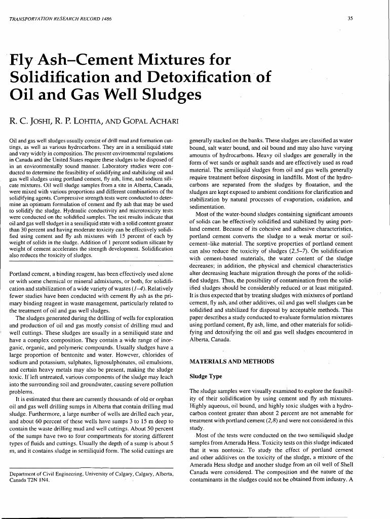
TRANSPORTATION RESEARCH RECORD 1486 35
·Fly Ash-Cement Mixtures for Solidification and Detoxification· of Oil and Gas Well Sludges
R. C. JOSHI, R. P. LOHTIA, AND GOPAL ACHARI
Oil and gas well sludges usually consist of drill mud and formation cuttings, as well as various hydrocarbons. They are in a semiliquid state and vary widely in composition. The present environmental regulations in Canada and the United States require these sludges to be disposed of in an environmentally sound manner. Laboratory studies were conducted to determine the feasibility of solidifying and stabilizing oil and gas well sludges using portland cement, fly ash, lime, and sodium silicate mixtures. Oil well sludge samples from a site in Alberta, Canada, were mixed with various proportions and different combinations of the solidifying agents. Compressive strength tests were conducted to determine an optimum formulation of cement and fly ash that may be used to solidify the sludge. Hydraulic conductivity and microtoxicity tests were conducted on the solidified samples. The test results indicate that oil and gas well sludges in a semiliquid state with a solid content greater than 30 percent and having moderate toxicity can be effectively solidified using cement and fly ash mixtures with 15 percent of each by weight of solids in the sludge. Addition of 1 percent sodium silicate by weight of cement accelerates the strength development. Solidification also reduces the toxicity of sludges.
Portland cement, a binding reagent, has been effectively used alone or with some chemical or mineral admixtures, or both, for solidification and stabilization of a wide variety of wastes (1-4). Relatively fewer studies have been conducted with cement fly ash as the primary binding reagent in waste management, partieularly related to the treatment of oil and gas well sludges.
The sludges generated during the drilling of wells for exploration and production of oil and gas mostly ,consist of drilling mud and well cuttings. These sludges are usually in a semiliquid state and have a complex composition. They contain a -wide range of inorganic, organic, and polymeric compounds. Usually sludges have a large proportion of bentonite and water. However, chlorides of sodium and potassium, sulphates, lignosulphonates, oil emulsions, and certain heavy metals may also be present, making the sludge toxic~ If left untreated, various components of the sludge may leach into the surrounding soil and groundwater, causing severe pollution problems.
It is estimated that there are currently thousands of old or orphan oil and gas well drilling sumps in Alberta that contain drilling mud sludge. Furthermore, a large number of wells are drilled each year, and about 60 percent of these wells have sumps 3 to 15 m deep to contain the waste drilling mud and well cuttings. About 50 percent of the sumps have two to four compartments for storing different types of fluids and cuttings. Usually the depth of a sump is about 5 m, and it contains sludge in semiliquid form. The solid cuttings are
Department of Civil Engineering, University of Calgary, Calgary, Alberta, Canada T2N IN4.
generally stacked on the banks. These sludges are classified as water bound, salt water bound, and oil bound and may also have varying amounts of hydrocarbons. Heavy oil sludges are generally in the form of wet sands or asphalt sands and are effectively used as road material. The semiliquid sludges from oil and gas wells generally require treatment before disposing in landfills. Most of the hydrocarbons are separated from the sludges by floatation, and the sludges are kept exposed to ambient conditions for clarification and stabilization by natural processes of evaporation, oxidation, and sedimentation.
Most of the water-bound sludges containing significant amounts of solids can be effectively solidified and stabilized by using portland cement. Because of its cohesive and adhesive characteristics, portland cement converts the sludge to a weak mortar or soilcement-like material. The sorptive properties of portland cement can also reduce the toxicity of sludges (2,5-7). On solidification with cement-based materials, the water content of the sludge decreases; in addition, the physical and chemical characteristics alter decreasing leachate migration through the pores of the solidified sludges. Thus, the possibility of contamination from the solidified sludges should be considerably reduced or at least mitigated. It is thus expected that by treating sludges with mixtures of portland cement, fly ash, and other additives, oil and gas well sludges can be solidified and stabilized for disposal by acceptable methods. This paper describes a study conducted to evaluate formulation mixtures using portland cement, fly ash, lime, and other materials for solidifying and detoxifying the oil and gas well sludges encountered in Alberta, Canada.
MATERIALS AND METHODS
Sludge Type
The sludge samples were visually examined to explore the feasibility of their solidification by using ce.ment and fly ash mixtures. Highly aqueous, oil bound, and highly toxic sludges with a hydrocarbon content greater than about 2 percent are not amenable for treatment with portland cement (2,8) and were not considered in this study.
.Most of the tests were conducted on the two semiliquid sludge samples from Amerada Hess. Toxicity tests on this sludge indicated that it was nontoxic. To study the effect of portland cement and other additives on the toxicity of the sludge, a mixture of the Amerada Hess sludge and another sludge from an oil well of Shell Canada were considered. The composition and the nature of the contaminants in the sludges could not be obtained from industry. A

36
few physical tests were conducted to characterize the sludge samples for their treatment with cement fly ash mixtures. The combined water and organic content of the sludge from Amerada Hess ranged from 120 to 220 percent. The solids content of the sludge was used as a base to express the amount of stabilizing agent used for the tests. The Amerada Hess sludge was designated as S 1• For toxicity tests, two composite samples marked S2 and"S3 were made using 90 and 80 percent Amerada Hess sludge and 10 and 20 percent high liquid (aqueous) Shell sludge, respectively. The Shell sludge was found to be highly toxic in its virgin state. The composite samples S2 and S3 thus had moderate toxicity and were in a semiliquid state and thereby amenable to treatment with cement-fly ash mixtures.
Materials Used.
Normal portland cement (ASTM Type 1 or CSA Type 10), Alberta fly ash obtained from the Forestburg power plant, and hydrated lime in various proportions were used as solidifying agents. Sodium silicate (water glass) was used as a dispersant for the cement. Dernineralized water and the necessary reagents and bacterial culture were used for rnicrotoxicity testing. The physical and chemical characteristics of the fly ash used are presented in Table 1.
The following combinations of materials were used to prepare trial mixes for solidification of the sludge:
1. Only portland cement at 20, 30, 40, and 50 percent by weight of solids in the sludge;
TABLE 1 Chemical Analysis and Physical Properties of Fly Ash (Undassified) from Forestburg Power Plant
Chemical Analysis
Silicon dioxide, Si02 Aluminum oxide, Al203 Iron oxide, Fe203 Total (Si02 + Al203 + Fe203) Sulphur trioxide, S03 Calcium oxide, CaO, total Available alkalies Loss on ignition Moisture content pH
Physical Properties
Fineness-Retained on 45µm (no. 325) sieve Strength Activity Index with cement: % of control at 7 days % of control at 28 days Strength Activity Index with. lime, MPa Specific Gravity Increase of drying shrinkage at 28 days Uniformity Requirements: - Specific gravity variation from average - Fineness, 45µm sieve, variation from average - Soundness: Autoclave expansion(%) - Quantity o_f Air-entraining Agent (%) Uniformity (%)
· - Reactivity with cement alkalies: Reduction at 14 days (%)
61.41 20.69 4.44 86.54 0.24 6.91 0.54 0.50
10.8
22.2
823 . 85.5
8.0 1.92 0.01%
-2.0% +2.4% 0.05 0.178 +20.3
73.1
TRANSPORTATION RESEARCH RECORD 1486
2. Portland cement as in A plus 1 percent lime by weight of solids in the sludge;
3. Portland cement as in A plus I percent sodium silicate by weight of the cement used (a mix with IO percent cement was also tried.);
4. Portland cement plus fly ash mixed in equal proportions ~y weight and the mixture at 20, 30, 40, and 50 percent by weight of solid material in the sludge; and . 5. Mixtures of lime and fly ash in proportions of I :5 by weight
at 10 to 50 percent by weight of solids in the sludge.
Table 2 describes the designations and details of the stabilizing mix-tures, reported in this study. .
Test Methods
The sludge samples for the tests were kept in properly sealed plastic pails. The combined water content plus organic content of the sludges was determined, and the solids content of the uniformly mixed sludge was computed. For solidification, predetermined quantities of the various stabilizing agents were thoroughly mixed with the sludge. No additional water was used for mixing. The details of the test procedures used in this study are described elsewhere (9, 10).
The sludge mixed with various stabilizing agents was tested to determine its compressive strength. Cylindrical specimens that were 25 mm in diameter and about 51 mm long were cast in plastic molds. The samples were air sealed with polyethylene sheet and cured in a fog room for 1, 3, 7, and 28 days. Before testing, the specimens were weighed and their length and diameter were measured. Compression tests were conducted with an INSTRON machine. After the test, the diameter of the failed specimen and the water content of the tested specimen were determined. For each test parameter, three samples were tested. As the test results were consistent, the average value was considered.
Two tests were conducted to determine the hydraulic conductivity, k, of the solidified sludge after 28 days of curing in a doublering fixed-wall perrnearneter (9) before commencement of water permeation. The height of the sample was 110 mm, and a hydraulic gradient of 20 was used for the permeability tests.
Microtoxicity tests were conducted in accordance with the Canadian standard procedures on untreated as well as solidified sludge samples with a Microtox Instrument. The following procedure was used to prepare s~rnples for rnicrotoxicity testing (J 1,12):
1. After the strength test on solidified sludge, a 1: 1 solution wt/ wt using dernineralized water of weight equal to that of the solid sample was prepared.
2. The I: 1 solution was shaken for 12 hr. 3. The sample was then centrifuged to clarify . 4. The pH of the sample was adjusted to lie in the range of 6.0 to
8.8, using 0.1 N H2S04 or 0.1 N NaOH. 5. The sample was then stored at 4°C. The rnicrotox test was
conducted within 72 hr of the sample preparation. 6. By using salt water bacteria (lurnin acid) and the rnicrotox
instrument, the value of EC 50, an index to measure the toxicity, was determined.
First, the microtox test was conducted on the raw sludge sample. If found toxic, the sludge was solidified using the stabilizing corn-

Joshi et al. 37
TABLE 2 Details of Stabilizing Mixtures and Solidifying Agents
Test series
A only normal
portJand cement
B c.ement+ Lime at 1 % by -
weight of solids in the sludge
c c.ement+sodium silicate at
1 % by weight of cement
D c.ement+fly ash in equal
proportion by weight
Solidifying agent
designation
A20 A30 A40 ASO
B20 B30 B40 B50
ClO
C20
C30
C40
cso
020 030 040 050
pounds. The microtox test was then conducted on the solidified material to assess the effectiveness of solidification on reducing the toxicity of the sludge.
RESULTS AND DISCUSSION
Compressive Strength
The resµlts of compressive strength tests on treated and solidified sludges are shown in Figures I through 4 and Tables 3 and 4.
The solidified sludge for effective disposal in a landfill should have some minimum strength to ensure that it can support the weight of the overburden placed on the top. Thus, a minimum compressive strength of about 140 kPa (20 psi) was adopted to meet the requirements (2).
It is observed from Figures 1 through 4 and Tables 3 and 4 that compressive strength increases with age and with an increase in the amount of the solidifying agent. The addition of lime to cement to improve the solidification is insignificant. However, the addition of sodium silicate at I percent by weight of cement accelerates the strength development at all the ages up to 28 days. The increase in strength with sodium silicate addition is even greater with richer mixes starting from the early age of 1 day. Sodium silicate gels rapidly by reacting with the calcium hydroxide released from hydration of portland cement. The rapid gelation of cement mixtures with sodium silicate stabilizes the sludge and prevents the deleterious materials in the sludge from affecting the setting and hardening of cement (2,13). Better dispersion of cement in the mix, with sodium silicate, leads to improved hydration, which results in higher
Amount of solidfying agent by weight of solids in the sludge
20% cement 30% cement 40% cement 50% cement
20% cement+ 1 % lime 30% cement+!% lime 40% cement+ 1 % lime 50% cement+!% lime
10%cement+0.01 %sodium silicate
20%cement+0.02%sodium silicate
30%cement+0.03%sodium silicate
40%cement +0.04%sodium silicate
50%cement + 0.05 %sodium silicate
10%cement+ 10%flyash 15 %cement+ 15 %flyash 20%cement + 20%flyash 25%cement+ 25%flyash
strength. Furthermore, the rapid gel formation from sodium silicate reduces the mobility of the substances present in the sludge that may interfere with cement hydration.
With the addition of fly ash, the early-age strength is considerably reduced. However, at28 days, the effect of pozzolanic action of fly ash becomes prominent as is evident by marked increases in 28-day strength of cement and fly ash mixtures compared with those of the corresponding mixtures with cement alone. The relative increase in the 28-day-strength sample, which contained 10,
en a.. ~ ..r::. Ci c: ~
U5
100
80 -
60
40
20
0 10
+ (A) cement only
x (B) cement+ 1% lime
• (C) cement+ 1% Na-silicate
o (0) cement + fly ash
20 30 40 50
Stabilizing Agent by wt. of Solids in Sludge (%)
FIGURE 1 1-day compressive strength versus amount of stabilizing agent mixed with sludge.
60

38
co a.. ~ .s= 0, c: ~ en
120
90
60
30
10
+ (A) cement only
x (B) cement+ 1% lime
• (C) cement+ 1% Na-silicate
o (D) cement + fly ash
20 30 40 50
Stabilizing Agent by wt. of Solids in Sludge(%)
FIGURE 2 3-Day compressive strength versus amount of stabilizing agent mixed with sludge.
60
15, 20, and 25 percent fly ash as cement replacement, is 12, 72, 34, and 67 percent, respectively. Alberta ashes are classified as Class F per ASTM C . 618. They possess pozz.olanic properties and are also somewhat self-cementitious. During cement hydration, calcium hydroxide is released, which reacts with fly ash to produce cementitious compounds similar to those produced by cement hydration. Pozzolanic reactions are relatively slow and depend on cement hydration. The ultimate strength or long-term strength of the sludge samples solidified with cement and fly ash would be higher than that of those solidified with cement alone (l,14).
A few trial tests, Series E, were conducted using lime and fly ash mixtures. These mixtures containing 1 :5 lime and fly ash did not solidify the sludges effectively, even after 7 days, and were not considered for further investigations. Similarly, preliminary tests on mixtures containing 5 percent cement and 5 percent fly ash as well as 10 percent cement alone by weight of solid material in the sludge were not found to be effective in solidifying the sludge sample. However, the addition of sodium silicate to the 10 percent cement mixture hardened the sludge within 24 hr.
200
160
co a.. 120 ~ .s= 0, c: ~ 80 en
40
0 10
+ (A) cement only
x (B) cement + 1 % lime
• (C) cement+ 1% Na-silicate
o (D) cement +fly ash
20 30 40 50
Stabilizing Agent by wt. of Solids in Sludge(%)
FIGURE 3 7-day compressive strength versus amount of stabilizing agent mixed with sludge.
60
TRANSPORTATION RESEARCH RECORD 1486
300
240
co a.. 180 ~ .s= 0, c: ~ 120 en
60
10
+ (A) cement only
x (B) cement + 1 % lime
• (C) cement + 1 % Na-silicate
o (D) cement+ fly ash
_______ ,,,,,..., ......
20 30 40 50
Stabilizing Agent by wt. of Solids in Sludge (%)
FIGURE 4 28-day compressive strength versus amount of stabilizing agent mixed with sludge.
60
Based on the strength results, the potential solidifying agents were identified as (a) mixtures containing 40 percent cement with or without lime and sodium silicate (A40, B40, and C40) and (b) cement and fly ash mixtures containing 10 percent cement and 10 percent fly ash (D20), 15 percent cement and 15 percent fly ash (D30), and 20 percent cement and 20 percent fly ash (D40) by weight of solid material in the sludge. · The compressive strength results of the composite samples, S2
and S3, 7 to 28 days, are given in Tables 3 and 4. As can be observed from the data in Tables 3 and 4, the strength values of the samples made from S2 sludge containing 90 percent Amerada Hess sludge and 10 percent Shell sludge are much higher than those made from S3 sludge containing 80 percent Amerada Hess sludge and 20 percent Shell sludge under similar conditions. For the sludge sample S2, all the solidifying agents identified and tried were found suitable. However, for the sludge sample S3, the solidifying agent that gave the specified strength of 140 kPa at 28 days was 20 percent cement and 20 percent fly ash. Even the mixture containing 15 percent cement and 15 percent fly ash, which solidified the sludge and imparted strength of 108 kPa, can be acceptable because with age the strength is anticipated to increase considerably because of the pozzolanic reactivity of fly ash.
Hydraulic Conductivity
The hydraulic conductivity test conducted on the 28-day cured and solidified samples of the composite sludge S3 using two solidifying agents-15 percent cement and 15 percent ft y ash (D30) and 20 percent cement and 20 percent fly ash (D40)-gave k values as 1.85 X
10-6 cm/sec and 2.01 X 10⁻⁶ cm/sec with D40 and D30 mixtures, respectively. A hydraulic conductivity, k, of about 1 o-6 cm/sec indi~ cates a fairly impervious material to control the migration of leachates (J 5).
Toxicity Tests
Toxicity of virgin and solidified sludge samples was considered on an overall basis per the Canadian Standards (J 1,12). Individual toxicants or contaminants were·not identified to define toxicity levels because of experimental constraints.

Joshi eta!. 39
TABLE 3 Compressive Strength Results of Composite Sludge Sample, S2, Containing 90 percent Amerada Hess Sludge and 10 percent Highly Liquid Shell Sludge
Solidifying Amount by weight of solid Compressive strength in kPa at Agent content in the sludge sample
Designation 7 days 28 days
A40 40% cement (;58.0 1221.0 B40 40% cement + 1 % lime 634.0 963.0 C40 40%cement+0.04% sodium 770.0 1157.0
silicate 020 10% cement + 10% fly ash 81.0 386.0 030 15% cement + 15% fly ash 149.0 648.0 040 20% cement + 20% fly ash 294.0 957.0
Microtox analyses of the untreated virgin sludge samples showed Amerada Hess sludge to be nontoxic and the liquid Shell sludge to be highly toxic. The results of Microtox analyses of the composite samples are presented in Tables 5 and 6. It is observed from the data in these tables that the sludge sample S2, wl)ich contained 90 percent Amerada Hess sludge and 10 percent highly liquid Shell sludge, showed slight toxicity in the virgin state. However, when solidified with the identified solidifying agents, no toxicity was observed, even after 7 days of curing.
The sludge sample S3, which contained 80 percent Amerada Hess sludge and 20 percent highly liquid Shell sludge, was quite toxic (EC 50 < 20) in the virgin state. After 7 days of curing, 40 percent cement mixtures containing (a) 40 percent cement (A40), (b) 40 percent cement and 1 percent lime (B40), and (c) 40 percent cement and 1 percent sodium silicate (C40) made the sample nontoxic. However, the sample treated with a cement-fly ash mixture consisting of I 0 and 20 percent each (D20-D40) retained the toxicity until 7 days after treatment. But after 28 days of curing, the sludge samples treated with cement and fly ash mixtures D30 and D40 were nontoxic, whereas slight toxicity was observed in the sample treated with the 10 percent mixture of cement and fly ash each (D20). Pozzolanic reactions are slow and they continue over a long period of time. It is, therefore, anticipated that with a further increase in curing age, even the stabilizing agent D20 will solidify and stabilize the sludge sample S3 to make it nontoxic.
TABLE 4 Compressive Strength Results of Composite Sludge Sample, S3, Containing 80 Percent Amerada Hess Sludge and 20 Percent Highly Liquid Shell Sludge
Solidifying Amount by weight of solid Compressive Agent content in the sludge sample strength in kPa at
Designation 7 14 28
days days days
A40 40% cement 91.0 105.3 134.0 B40 40% cement + 1% lime 77.0 85.5 112.0 C40 40%cement+0.04% sodium
silicate 92.5 100.7 131.~ 020 10% cement + 10% fly ash 19.0 29.7 45.9 030 15% cement + 15% fly ash 28.3 55.0 108.0 040 20% cement + 20% fly ash 32.7 70.2 183.5
CONCLUSIONS
On the basis of the results of the experiments conducted on oil and gas well sludge samples using cement and fly ash based materials, the following conclusions can be drawn:
• Oil and gas well sludges or drilling mud in the semiliquid state with a solids content greater than 30 percent and having moderate toxicity can be effectively solidified with cement and fly ash content.as low as 15 percent each by weight of solids in the sludge.
• The addition of 1 percent sodium silicate by weight of cement accelerates the strength development and also increases the strength of solidified sludge samples treated with cement as the stabilizing agent.
• At least 30 percent by weight of solids in the sludge is required to produce satisfactory stabilized products at a reasonable cost.
• The effect of lime addition at 1 percent by weight of solid content in the sludge before treatment with cement does not exhibit any significant effect on the strength of sludge treated with cement.
• The sludges solidified with cement and fly ash mixtures become reasonably impervious with a hydraulic conductivity, k, about 2.0 X 10⁻⁶ cm/sec.
• Solidification of the sludges also reduces toxicity. • Cement and fly ash mixtures, 1: I by proportion, at about 20 to
30 percent by weight of solids in the sludge may be used to stabilize and dispose oil and gas well sludges of moderate toxicity in a technically effective and environmentally sound manner. However, for a particular type of sludge, trial tests to obtain optimum formulation will be necessary.
ACKNOWLEDGMENTS
The authors thank Ken Putt of the Canadian National Research Council and Mike Pildysh of Pildysh and Assoc. Consultants Ltd. for useful discussions and suggestions at various phases of the 12roject. Significant help and cooperation were extended by Meri"L. Korchinski, Don C. Roberts of Energy Resource Conservation Board of Canada, and B. Mottle of the Environmental Research Centre, University of Calgary, Calgary, Alberta, Canada, in conducting the microtoxicity tests. The technical assistance of N.S. Ghali in conducting the tests is also gratefully acknowledged. Financial assistance for this project was provided by Pildysh and Assoc. Consultants Ltd., Calgary, under NRC-IRAP.

40 TRANSPORTATION RESEARCH RECORD 1486
TABLE 5 Results ofMicrotox Test on Sludge Samples S" S2, and S3 Before Solidifying
Sludge Sample EC" 50 in(%) Toxici~
Sl- Amerada Hess Sludge
S2- 90% Amerada Hess sludge + 10% highly liquid Shell sludge
S3- 80% Amerada Hess sludge + 20% highly liquid Shell sludge
• EC 50 value in % 0-50 50-90 > 90
Toxicity Toxic Slightly toxic Non toxic
>90 Non toxic
60 Slightly toxic
<20 Toxic
TABLE6 Results of Microtox Test on Solidified Samples of Sludge S2 and S3
EC 50 values in % and toxicity
Solidifying Amount by Sample S2
Agent weight of solid 7 day fog curing Designation content in the
sludge sample EC50 Toxicity
A40 40% cement >90 nontoxic
840 40cement+ >90 nontoxic 1%lime
C40 40% cement+ 0.04% sodium >90 nontoxic
silicate
020 10% cement+ >90 nontoxic 10% fly ash
030 15% cement+ >90 nontoxic
15% Oy ash 040 >90 nontoxic
20% cement+ 20% Oy ash
REFERENCES
L Barth, E. F. An Overview of the History, Present Status and Future Directions of Solidification/Stabilization Technologies for Hazardous Waste Treatment. Proc., 2nd Annual Symposium on Solidification/Stabilization Mechanisms and Applications, Golf Coast Hazardous Substance Research Center, Beaumont; Tex., Feb. 1990, pp. 1-5.
2. Adaska, W. S., S. W. Tresouthich, and P. B. West. Solidification and Stabilization of Wastes using Portland Cement. Portland Cement Association, Skokie, Ill., 1991.
3. Stegeman, J. A., and P. L. Cote. Investigation o/Test Methods for Solidified Waste Evaluation-A Cooperative Program. Report EP53/HA/8. Ottawa, Canada, Jan. 1991.
Sample S3
7 day fog curing 28 day fog curing
EC50 Toxicity EC50 Toxicity
>90 nontoxic >90 nontoxic
>90 nontoxic >90 nontoxic
>90 nontoxic >90 nontoxic
28 toxic 60 . slightly toxic
40 toxic >90 nontoxic
67 slightly >90 nontoxic toxic
4. Handbook for Stabilization/Solidification of Hazardous Wastes. Report EP A/540/2-86/00, Environmental Protection Agency, Cincinnati, Ohio, 1986.
5. Albino, V., R. Cioff, and R. Santoro. Stabilization/Solidification of a Residue of Municipal Solid Waste Incinerator by Combined Use of Coal Fly Ash and Chemical Gypsum. Proc., 10th International Ash Use Symposium, EPRI TR-101774, Project 3176, Vol. 1, Jan. 1993, pp. 8-1 to 8-12.
6. Process Design Manual for Sludge Treatment and Disposal. Report EPA 625/1-79-011. Environmental Protection Agency, 1979.
7. Montgomery, D. M., C. J. Sollar, and R. Perry. Cement Based Solidification for the Safe Disposal of Heavy Metal Contaminated Sewage Sludge. Waste Management and Research, No. 6, 1988, pp. 217-226.

Joshi et al.
8. Delched, S. Chemical Treatment: An Inexpensive Alternate to Handling Oil Sludge. Proc., 5th National Conference on Hazardous Wastes and Hazardous Materials, April 1988, pp. 85-88.
9. Joshi, R. C., J.P. A. Hettiaratchi, and G. Achari. Properties of Modified Alberta Fly Ash in Relation to Utilization in Waste Management Applications: Canadian Journal of Civil Engineering, Vol. 21, No. 3, 1994, pp. 419-426.
10. Joshi, R. C., R. P. Lohtia, G. Achari, S. N. Ghali, and M.A. Salam. Oil Well Sludge Solidifications. NRC-IRAP Project No. 234114 U-TE-18, Civil Engineering Department, University of Calgary, Canada, March 1994.
11. Standard Procedure for Microtox Analysis. Western Canada Microtox Users Committee, 1991.
·•
41
12. Rapid Toxicity Test using Luminescent Bacteria. Environment Protection, C and P, Environment Canada, Nov. 1992.
13. Falcone, J. S., R. W. Spencer, and E. P. Katsanes. Chemical Interactions of Soluble Silicates in the Management of Hazardous Wastes. Special Technical Publication No. 851 ASTM, 1983.
14. Joshi, R. C., and R. P. Lohtia. Types and Properties of Fly Ash. In Mineral Admixtures in Cement and Concrete, Vol. 4. ABI Books Pvt. Ltd., New Delhi, India, 1993, pp. 118-157. ·
15. Wentz, C. A., C. J. Moretti, K. R. Henke, 0. E. Manz, and K. U. Wiken. Use of Fly Ash as a Waste Minimization Strategy. Eni:ironmental Progress, Vol. 7, No. 3, 1988, pp. 198-206. ·
Publication of this paper sponsored by Committee on Cementitious Stabi-lization. · · -

42 TRANSPORTATION RESEARCH RECORD 1486
Influence of Void Change, Cracking, and Bitumen Aging on Diffusional Leaching Behavior of Pavement Monoliths Constructed with MSW Combustion Bottom Ash
T. TAYLOR EIGHMY, DOUGLAS CRIMI, SHAMIM HASAN XISHUN ZHANG, AND
DAVID L. GRESS
The evaluation of leaching behavior of monolithic forms containing waste materials requires the use of leaching tests that evaluate diffusional release mechanisms. This can be coupled to procedures that accelerate the aging of the monolith to better predict long-term leaching behavior. As part of a comprehensive demonstration project examining the use of municipal solid waste combustion bottom ash as an aggregate substitute in bituminous binder course, the diffusional leaching behavior of ash constituents was assessed as a function of pavement voids level (5, 7 .5, 10 percent), bitumen aging (none, medium, high), and monolith cracking (none, medium, high). Effective diffusion coefficients (D., m2/sec) were determined for some ash constituents that leach; values ranged from 10- 12 to 10- 16 m2/sec: These values are typical for ion diffusion in polymer systems. Species with small ionic radii (e.g., Na, Cl) were more diffusive than those with large ionic radii (e.g., Si, Zn). Monolith tortuosity values (-r) were found to be influenced only by monolith cracking. Diffusing specie chemical retention values (R) and effective diffusion coefficients were not influenced by voids, cracking, or aging. Bituminous pavement monoliths release ash constituents at very low fluxes. Modeled releases of chloride for 10 percent wetting ranged from 1.7 g Cl/m2/l.5 years to 54.9 g Cl/m2/100 years. These fluxes are considerably smaller than fluxes associated with road salting during a single snowfall. The tortuous, hydrophobic nature of the monolith system controls diffusion.
In the fields of waste stabilization and waste use, it is frequently desirable to produce monolithic forms from granular material. Examples include the solidification and stabilization of contaminated granular soils with portland cement and use of coal fly ash as filler in bituminous asphalt. In either case, the environmental performance of the product depends on the analysis of leaching behavior of monolithic instead of granular material.
In monolithic leaching scenarios (Figure 1 ), the very low specific surface area, permeability, and high structural integrity result in leaching regimes where diffusion is the dominant mass transfer mechanism. This differs dramatically from granular materials where solvent percolation and advection produce contaminant fluxes that are orders of magnitude larger than diffusional fluxes. Diffusional leaching involves diffusion into the monolith of solvents, such as H20, and diffusion out of the monolith of dissolving solutes such as cationic and anionic species. In the nuclear waste
Environmental Research Group, Al 15 Kingsbury Hall, University of New Hampshire, Durham, N.H. 03824.
disposal field, the ANSI/ ANS 16.1 monolith leach test (1) is used to assess diffusional release. In the hazardous waste disposal field, both the ANSI/ ANS 16.1 and ASTM single batch extraction test (2) can be used to assess diffusional release. Finally, in the field of waste use, the Dutch NEN 7345 monolithic tank diffusion leaching test (3) is used to examine diffusional leaching behavior. To accelerate leaching, flow-through triaxial devices ( 4) or pressure vessels (Van der Sloot, personal communication) can be used to speed up the influx of solvent into the monolith. In virtually all these cases, an effective diffusion coefficient (De in m2/sec) can be calculated and then used to model release as a function of geometry and application cycle of leachant.
The issue of monolith integrity plays an important role in evaluating diffusional leaching behavior. Improper solidified and stabilized (S/S) formulations, freeze or thaw, or wetting or drying phenomena can cause monolithic waste forms to spall, crack, or devitrify. When granular wastes or conventional materials are used in civil construction applications, the materials can undergo physical changes due to loading, temperature, and oxidation (02,
UV) that can also result in loss of monolithic integrity. The ability to induce such loss of integrity in the laboratory for a monolithic leaching scenario allows the prediction and modeling of
ADVECTIVE TRANSPORT
DIFFUSIVE TRANSPORT
Granular Diffusion
Diffusional Flux
Monolithic Diffusion
FIGURE 1 Advective and diffusive release (19).

Eighmy etal.
potential leaching behavior at the end of a design life of an app li ca ti on.
The authors are involved in a large demonstration project that examines the feasibility of using bottom ash from the combustion of municipal solid waste as an aggregate substitute in asphaltic binder course (5-10). A demonstration project involving the paving of a portion of Route 3 in Laconia, New Hampshire, has been underway since May 1993. To understand better the potential environmental behavior of monolithic pavement material over its 20- to 30~ year design life, the Dutch monolith tank leaching procedure was used to evaluate the potential effects of void change, cracking, and bitumen aging on the diffusional leaching of bottom ash constituents from asphaltic pavement monoliths.
This research has shown that the bottom ash constituents that leach from the pavement monoliths are Si, Ca, S04 , Mn, Cl, and Mg. The effective diffusion coefficients (De m2/sec), reported as their negative logs (pDe), are in the range of 12 to 16. These values are typical for ash constituent elements diffusing in polymer monoliths (7,11). The influence of monolith cracking was the only experimental variable to alter diffusional leaching behavior. Cracking reduces the diffusion path length from which diffusional release occurs. Void change and bitumen aging had no significant effects.
MONOLITH LEACHING FUNDAMENTALS
Figure 2 depicts the fundamental processes involved in leaching from monolithic specimens. The figure depicts the diffusive release of constituents via pathways of varying tortuosity, long-term dissolution of solid phase material at the monolith surface, and initial wash-off of material from the monolith surface. These phenomena exhibit different cumulative release behaviors (see Figure 3), as evidenced by plot slopes, on log-log cumulative release versus time plots.
Diffusion occurs by the random movement of individual molecules or ions. It is driven by the difference in chemical potential between the solid and the leachant (12). In a slightly porous solid, the i~n flux of a soluble contaminant in the pore water system is defined by Fick's Second Law, which relates the concentration of a diffusing substance to both space and time:
dC d 2C -=L-dt dx2
Bituminous Polymeric Matrix
• ~ Ash Particl~
• Monolith
FIGURE 2 Monolithic leaching behavior.
Tortuous Diffusion
Dissolution
Less Tortuous Diffusion
Wash-Off
Leachant
(1)
43
~
E -C'> ,§_ 100.0 w (/) c(
10.0 w ..... w a: w 1.0 > t:= ~ 0.1 :::> ~ :::> 0 1.0 10.0 100.0
TIME {days)
FIGURE 3 Hypothetical cumulative release plots.
where C is the concentration of the diffusing ion, and L is the leach constant, with units of a diffusion coefficient (m2/sec). In the case of one-dimensional diffusion, the leach constant, L, is obtained by applying the following relationship:
f 2 ·Do L=-
R·-r
where
f = available leachable fraction of element in material, D 0 = mobility of element in water (m2/sec), R = chemical retention factor of element (unitless), and. T = physical retardation or tortuosity factor (unitless).
(2)
When the leachable amount of the element equals the total amount of the element present in the material (i.e.,f = 1), the leach constant L equals the effective diffusion coefficient, which is diffusion modified for retention and tortuosity (13).
If Equation 2 is transformed to logarithmic values and the relationship pD0 = - log D0 is used, then the new relationship is as follows:
pL = pD0 + 2pj- pR - PT (3)
Because the available leachable fraction of the element may be obtained from analytical data and remains as a constant, Equation 3 may be simplified to:
pDe = pD0 - pR - PT (4)
where De is the effective diffusion coefficient (m2/sec) (13). This equation allows for the determination of the relative contributions of D0 , R, and T to the magnitude of De.
The mobility of an element within the monolithic pore space may be compared with its free mobility in water by determining the physical and chemical retardation factors of the product and the element, respectively. To calculate the physical retardation factor, it is necessary to choose an ion that does not chemically interact with the matrix (i.e., R = 1). In most studies, sodium is chosen and the physical retardation is calculated with the formula (13).

44
(5)
where DNa is the diffusion coefficient of sodium in water (pDNa = 8.88 m2/sec at 25°C) and De.Na is the effective diffusion coefficient of sodium in the monolith (m2/sec). The chemical retardation factor for the element is determined using the following formula:
(6)
where Dx is the diffusion coefficient for the element in water (m2/sec) and De.xis the.effective diffusion coefficient for the element in the monolith (m2/sec).
In monolith leach testing, the material is considered homogeneous and is immersed in a leachant that is renewed at regular intervals. The concentration of the element is uniformly distributed and the surface is maintained at a constant concentration. The solution to Equation 1 under such conditions is presented elsewhere (14).
C- C1 x =erf ... ~
Co - C1 2 V (D · t) (7)
where
C = element's concentration in monolithic material as function of place and time,
C1 = constant concentration at surface of monolith, Co = initial concentration of element in material, D = diffusion coefficient, and
erf = standard error function.
Because the leachant is regularly renewed during the leaching experiment, the surface concentration, Ci. is assumed to be zero (13), and the solution to Equation 7 under this assumption is
De= 4 d)2 t(Umax · (8)
where
B1 = cumulative release of element at time t (mg/m2),
Umax =maximum leachable quality of element from monolith (mg/kg), and
d = bulk_ density of monolithic material (kg/m3).
By plotting the cumulative release of an element leaching from the ash material as a function of time, it can be determined whether matrix diffusion or other leaching mechanisms, such as dissolution or surface wash-off, more common to granular materials, are occurring. The solubility of certain elements within the solid material can be significantly high, such that longer-term dissolution of the element at the surface proceeds faster than diffusion through the pores of the solid matrix. In addition, because of process conditions, a material may be covered with a soluble surface coating that is readily leached with initial leachant contact.
To determine which leaching mechanism is controlling release of the element from the monolith, Equation 8 is rearranged to yield the following (J 3):
(9)
TRANSPORTATION RESEARCH RECORD 1486
After log transformation, Equation 9 becomes
log(B1) = 1 h log(t) + log[ Umax dVcWehr)] (10)
From the monolith leach test results, the release of the element per time interval may be calculated using the formula (J 3)
where
B; = release of element per unit area in period i (mg/m2),
c; = concentration of element in ith period (µg/L), V; = volume of leachant (L), and A = surface area of monolithic material (m2
).
(11)
The cumulative release of the element for all N periods (N = 8) is calculated from
\ii Bu = B; ~ r: _ ~ r- for i = 1 to N
v t; v t;-1
where
(12)
B1,; =cumulative release of element for all periods (mg/m2),
t; = contact time after period i (sec), and t;- 1 =contact time after i-1 periods (sec) (13).
Eight leaching periods are usually used (0.25, 1, 2, 4, 8, 16, 32, and 64 days). This conforms to a time series relationship (renewal time of the nth period is equal to the square of the period sequence number times the renewal time of the first period) that is based on both leaching behavior and on data distribution in log (Br,;) - log(t;) plots.
If the logarithm of the cumulative release, B1,;, is plotted versus the logarithm of time, t,., for the eight periods; the slope of the resulting graph indicates the mechanism controlling the release of the element. Because the slope may change over different time intervals, the slope is examined over the following ranges (13):
• Total range-i = 1 to 8, • Initial range-i = 1 to 3, • Middle range-i = 3 to 6, and • Final range-i = 5 to 8.
The relevance of the change in slope at the different intervals is summarized as follows:
Slope
Range <0.35 0.35..,.().65 >0.65
Initial Surface washoff Diffusion Lag time/dissolution Middle Depletion Diffusion Dissolution Final Depletion Diffusion Dissolution
The effective diffusion coefficient for the element is then calculated from each period for the release per period (B;) using the data points where the slope is 0.50 ± 0.15 with a deviation of less than 50 percent, and the slope of the final range is smaller than 0.65 by

Eighmy et al.
(13)
where D . is the effective diffusion coefficient of element x calculated fro~xthe release in the ith period (m2/sec), and the other terms are as previously described.
MATERIALS AND METHODS
The purpose of the monolith leach test was to evaluate the effects of void content, aging, and cracking on monolith specimens generated from the job mix formula using the NEN 7345 monolith leach test procedure. The monolith leach test examines diffusive leaching mechanisms from monolith specimens. Estimates of monolith tortuosity (T), and chemical retention (R), via sorption or precipitation of diffusing solutes, were used with estimates of the effective diffusion coefficient (De) to model leaching.
A partial 33 + 6 factorial design experiment was conducted on 14 gyratory compacted specimens. The material used to make the specimens came from the actual production run for the full-scale demonstration (50 percent bottom ash, 7 percent asphalt content). Three degrees of voids (low, medium, high), aging (none, medium, high), and cracking (none, medium, high) were integrated into. the experimental design. Voids (5, 7 .5, 10 percent) were created during the compaction of the specimens using the gyratory testing method (GTM). Voids of 10, 7.5, and 5 percent were produced using 60, 110, and 300 cycles, respectively, on the GTM. Aging was simulated by heat treatment in the presence of forced hot air (107°C for 5 days for moderate aging and 107°C for 10 days for severe aging). The regimen was based on methods compiled by von Quintus et al. (15). An Instron machine was used to subject some of the samples to cyclical loading parallel to the direction of compaction to produce micro and macro cracking (i.e., moderate and high cracking levels). A load of 8.22 MPa at 2 cycles/sec was used. Moderate cracking was produced after 1,250 ::!::: 250 cycles. High cracking was produced after 1,750 ::!::: 250 cycles.
Each specimen was placed in a 3-L container filled with contact solution (5 times the specimen volume). Cqntact solution consisted of Nanopure ASTM Type II (double-deionized) water reduced to pH 4 using Baker Analyzed Ultrex II Ultrapure nitric acid. The leachate was filtered and analyzed periodically (0.25, 1, 2, 4, 8, 16, 32, and 64 days) to determine specified element concentrations leached per indicated time frame. After each filtration; new contact solution was added to the sample. Samples were analyzed using ion chromatography, graphite furnace atomic absorption spectrophotometry, and inductively coupled argon plasma atomic emission spectrometry. Monolith specimens were also ground to less than 300 µm and subjected to the Dutch total availability leaching procedure (NEN 7341) to determine Umm the fraction available for leaching.
RESULTS AND DISCUSSION
Results from preliminary evaluations (16) of the leaching behavior of the bottom ash before this study indicated the following general environmental behavior. Neutron activation analyses detected the presence of approximately 45 elements in the bottom ash. Although 45 elements are present in the bottom ash, only 16 con-
45
sistently leached from bottom ash ground to <300 µm when subjected to the total availability leach test: Cl, Ca, Zn, Cd, Mg, Cu, Mn, Pb, Sr, Si, Fe, Al, Na, K, Ba, and Cr. Lysimeter leaching data for the granular ( < 1.9 cm) bottom ash lysimeter showed that the bottom ash leached Cl, so~-. Ca, K, Mg, Na, Fe, Mn, Si, and Sr. Similar constituents were leached from a lysimeter containing pavement rubble containing bottom ash, but at much lower levels. Only seven constituents (Na, Cl, so~-. Ca, Si, Mg, and Zn) were routinely leached from the bottom ash test specimens during the monolith leach test.
In this study, monoliths that were ground to less than 300 µm were subjected to the Dutch availability leaching test (NEN 7434). The data, shown in Table 1, indicate that Ca, S04, K, Cl, Si, Na, Mg, and Al are the species with the largest potential to be released if the integrity of the monolith were to be severely compromised. Their availabilities range from 7860 to 200 mg/kg. These values are considered extremely low and reflect the role of the bitumen in coating ash particles and reducing surface area available for leaching (7). A number of additional species are alsp available for leaching but at low levels ( <200 mg/kg).
In monolithic form, however, leaching behavior is markedly different. The elements Ca, Pb, Mn, Si, Na, Zn, S04, Cu, Fe, Mg, and Cl were released from the monoliths in the factorial designed experiment. Only the elements Si, Ca, S04, Mn, Cl, Na, and Mg were routinely leached from the monoliths in accordance with diffusional
TABLE 1 Availability of Potentially Diffusing Species in Pavement Monoliths
Element/Specie Availability mg/kg
Al 221.8
As <2.02
Ba 20.2
B < 100.8
Cd < 1.01
Ca 7,860
Cr <2.02
Cu 102.8
Fe 137.1
Pb 98.8
Mg 362.9
Mn 98.8
Hg <0.60
Mo <20.2
K 1,008
Se <2.02
Si 766.2
Na 403.3
Sr <40.3
Zn 221.8
Cl 806.5
S04 3,630
Br <.201

46
• • NE 4 c, .§. w A en ~ <( w ..J • w . 0:: w 3 > t== ~ Specie Slope ::::> er 0.05 ::::?: • ::::> • sot 0.67 (.)
C) A Na• 0.46 0 ..J
2 4 5 6 7
LOG TIME (seconds)
FIGURE4 Cumulative release plots for CI, Soi-, and Na.
processes. The elements Pb, Zn, Cu, and Fe were leached sporadically. Some of the data could be modeled using diffusional modeling. Cr, Al, K, and Sr were seen in only a few of the 112 leachate samples that were analyzed during the experiment. As, Ba, B, Cd, Hg, Mo, and Se were never detected. Some of the elements that exhibited high relative availabilities, such as K, Na,.Mg, and Al, were not readily leachable from the monolith. Other elements that exhibited low relative availabilities, such as Mn, were readily leached. These behaviors can be attributed to pH effects and monolith integrity.
Some typical cumulative release plots are shown in Figure 4. The specie Cl shows wash-off behavior; the specie so~- shows dissolution behavior; and the specie Na shows diffusion behavior. These cumulative releases or fluxes are very low and close to that of control specimens containing bitumen and natural aggregates (7,16,17).
As shown in Figures 5 and 6, the influence of monolith void content and bitumen aging had little influence on monolith tortuosity and diffusion path length. However, as shown in Figure 7, the pres-
10000 • • • • ~ • c;; I 0
::::> ~1000 0 I .....
I • •
100 4· 6 8 10
VOID CONTENT (%)
FIGURES Influence of monolith void content on tortuosity.
~ c;; 0 ::::> .... 0:: 0 ....
TRANSPORTATION RESEARCH RECORD 1486
10000 • • • • • I
1000 I • • • •
100 ~--'--------''------'----' NONE MEDIUM HIGH
AGING
FIGURE 6 Influence of monolith · bitumen aging on tortuosity.
ence of micro and macro cracks dramatically reduced tortuosity (-r) values by reducing diffusion path length.
The effective diffusion coefficients that were calculated from the experiment are shown in Figure 8 (top). Diffusing species with small ionic radii usually were the most diffusive (De values of 10- 12
m2/sec or pDe values of 12). Diffusing species or anions with larger ionic radii were less diffusive (pDe values of 12 to 16). These values are similar to those reported by de Groot et al. (J 1) for asphalt paving blocks where MSW electrostatic precipitator ash was used as mineral filler and for earlier studies by the authors' group using the same bottom ash but at various substitution levels of 25, 50, and 75 percent (16,17). There were no strong relationships betweenpDe and the variables tested (voids, aging, and cracking). Some weak relationships may exist given the interdependence of pDe and tortuosity.
Reactivity (R) values are shown in Figure 8 (bottom). The values shown are typical (J 1, 16, 17) for bituminous asphalt systems gov~rned by hydrophobic surfaces where reaction is less likely. Diffusing species with a small likelihood of sorption or coprecipitation in the matrix exhibit reactivities close to Na. However, species with high sorption or coprecipitation potential, such as Pb, Mn, Zn, and Cu, show high values. There were no strong relationships between R and the experimental variables that were tested.
10000 ... • • • • ~ • c;; I 0 ::::> ~1000
I 0 .... I • •
100 NONE MEDIUM HIGH
CRACKING
FIGURE7 Influence of monolith cracking on tortuosity.

Eighmy et al.
10 -
g 10000.0
c 0 1000.0 -;; c .s Cl)
100.0 -0:: c;; 10.0 -CJ ·e Cl) 1.0 -.c 0
0.0 -
~,~ 6 ~ Mn Si ~ Zn ~ B ~ t ~ Ca g Cu Mg •
Na Cl
Diffusing Specie
~~~~~~~~~~~~~~~~~~-'
Diffusing Specie
FIGURE 8 Diffusing species for all monoliths versus (top). pDe and (bottom) chemical retention.
The reported effective diffusion coefficients are 104 to 105 times smaller than diffusion coefficients of these ions in water. The dramatic reduction is due to the difficulties associated with ion diffusion in a bituminous polymer matrix where pathways are tortuous and reaction sites on ash particles can interrupt the diffusion process.
The pDe values depend on both T and R. Given the large T values and the relatively low R values, it is apparent that the high degree of tortuosity provided by asphalt accounts for the very low fluxes occurring from such specimens. The maintenance of monolithic integrity is therefore one consideration for keeping fluxes of ash constituents at background levels.
47
The use of the diffusional modeling approach can be illustrative in estimating the release of constituents from monoliths (J 4, 18). The cumulative release of a diffusing constituent from a monolith can be described by (18)
( Det )o.s
M, = 2pUmax --;;-- (14)
where
M1 = cumulative mass of constituent released per unit surface area,
p = monolith density, u max = availability'
De = effective diffusion coefficient, and t = some time period of interest.
This equation assumes that the concentration of the diffusing constituent remains dilute at the surface boundary and that the concentration does not deplete in the monolith. The use of this equation can be further enhanced by correcting De for temperature and correcting the cumulative release for the degree of wetting the monolith (14,19).
Table 2 illustrates the use of Equation 14 in estimating cumulative release data for Cl for a hypothetical binder course asphalt pavement scenario where the pavement changes its voids content, bitumen polymer aging, and degree of cracking over time. A 10 per'" cent wetting time is assumed to mimic the potential release from the lower surface of a binder course. The 10 percent wetting time is based on an annual average best estimate of percentage of wetting from condensation of moisture vapor from the vadose zone on the lower binder surface; its use is illustrative and would require field verification.
Three relative time frames are used to illustrate the approach: 1.5, 20, and 100 years. The. fluxes are shown in Table 2. The largest modeled cumulative flux of 54.9 g Cl/m2 over a 100-year time frame is similar to the flux associated with road salting during a single snow storm in New Hampshire (20 g Cl/m2
) and less than that applied over a single season (500 g Cl/m2
). These calculations are to be used for simple order of magnitude comparisons only. In fact, the estimated .flux from the lower road surface interface is very conservative. Chloride, a nonreactive and mobile anion, would still have to move via diffusive processes through capillary water and
TABLE 2 Modeled Flux of Chloride from Pavement Monoliths as Function of Monolith Integrity and Time
Scenario Flux, g Cl/m2
Years•
1.5 20 100
New Pavementb 1.7 6.4 14.3 (Voids = 10%, Cracking = L, Aging = L)
Moderately Aged Pavementb 4.1 14.9 33.5 (Voids = 7.5%, Cracking = M, Aging = M)
Aged Pavementb 6.7 24.5 54.9 (Voids = 5%, Cracking = H, Aging = H)
a Based on an estimated 10% wetting time from condensation of vadose zone moisture vapor on the lower surf ace of the binder course.
b Based on conditions used in the monolith leach test.

48
condensate ·ephemerally present on soil particle surfaces a very large distance to the groundwater table via a tortuous, noncontiguous pathway. This diffusive process would be driven by a weak driving gradient. Given the preexisting chloride levels in RAP, roadside soils, and groundwater, this gradient could also be nonexistent. Nevertheless, the approach can allow order of magnitude comparisons of waste product leaching to background signals.
CONCLUSIONS
Monolith cracking was the only experimental variable influencing diffusional leaching behavior. Increased cracking decreased diffusional path lengths whereby release occurs. Void content and asphalt aging had little influence. The observed effective diffusion coefficients for those species exhibiting diffusional release are typical for diffusion in polymer systems. The results suggest that MSW bottom ash constituent leaching behavior is controlled by the tortuous hydrophobic nature of the bituminous polymer system in the pavement.
ACKNOWLEDGMENTS
This research was supported by Wheelabrator Environmental Systems, Inc., the Concord Regional Solid Waste/Resource Recovery Cooperative, the Environmental Protection Agency through Rutgers University, and the U.S. Department of Energy through the National Renewable Energy Laboratory.
REFERENCES
1. Measurement of the Leachability of Solidified Low Level Radioactive Wastes by Short Term Test Procedures. ANSI/ANS 16.1, American Nuclear Society, Chicago, Ill., 1986.
2. Single Batch Extraction Method for Wastes. ASTM D-5233-92. American Society for Testing and Materials, Philadelphia, Pa., 1992.
3. van der Sloat, H. A., D. Hoede, and P. Bonouvrie. Comparison of Different Regulatory Leaching Test Procedures for Waste Materials and Construction Materials. ECN-C-91-082, Petten, The Netherlands, 1991.
4. Butcher, E. J., C. R. Cheesman, C. J. Sollars, and R. Perry. FlowThrough Leach Testing of Solidified Waste Using a Modified Triaxial Cell. Environmental Technology, Vol. 14, 1993, pp. 113-124.
5. Gress, D. L., X. Zhang, S. Tarr, I. Pazienza, and T. Eighmy. Physical and Environmental Properties of Asphalt-Amended Bottom Ash. In Transportation Research Record 1345, TRB, National Research Council, Washington, D.C., 1992, pp. 10-18.
TRANSPORTATION RESEARCH RECORD 1486
6. Gress, D. L., X. Zhang, S. Tarr, I. Pazienza, and T. T. Eighmy. Municipal Solid Waste Combustion Ash as an Aggregate substitute in Asphaltic Concrete. In Waste Materials in Construction, (J. J. J. R. Goumons, H. A. van der Sloat, and Th.G. Albers, eds.) Elsevier, Amsterdam, The Netherlands, 1991.
7. Whitehead, I.E., T. T. Eighmy, D. L. Gress, and X. Zhang. An Environmental Evaluation of Bottom Ash Substitution in Pavement Materials. In Municipal Waste Combustion, Air and Waste Management Association, Pittsburgh, Pa., 1993.
8. Musselman, C. N., M. P. Killeen, D. Crimi, S. Hasan, X. Zhang, D.L. Gress, and T. T. Eighmy. The Laconia, New Hampshire Bottom Ash Paving Project. In Waste Materials in Construction, (J. J. J. R. Goumons, H. A. van der Sloat, and Th.G. Aalbers, eds.) Elsevier, Amsterdam, The Netherlands, 1994.
9. Musselman, C., T. Eighmy, D. Gress, M. Killeen, J. Presher, and M. Sills. The New Hampshire Bottom Ash Paving Demonstration (US Route 3). Proc., 1994 ASME National Waste Processing Conference, Laconia, N.H., ASME, New York, 1994, pp. 83-90.
10. Zhang, X., D. Gress, and T. Eighmy. Bottom Ash Utilization as an Aggregate Substitute in Hot Mix Asphalt. Proc., 2nd Annual Great Lakes GeotechnicaVGeoenvironmental Conference, 1994, pp. 132-157.
11. de Groot, G. J., H. A. van der Sloat, P. Bonouvrie, and J. Wijkstra. Karacterisering van het Uitlooggedrag, van Intacte Producten. MAMMOET deelrapport 09, ECN-C-90-007, Petten, The Netherlands, 1990.
12. Conner, J. R. Chemical Fixation and Solidification of Hazardous Wastes. Van Norstrand Reinhold, New York, 1990.
13. de Groot, G. J., and H. A. van der Sloat. Determination of Leaching Characteristics of Waste Materials Leading to Environmental Product Certification. In Solidification/Stabilization of Hazardous, Radioactive and Mixed Wastes, (T. M. Gilliam and C. C. Wiles, eds.) ASTM, Philadelphia, Pa., 1992. ·
14. Crank, J. The Mathematics of Diffusion. Oxford University Press, Oxford, England, 1975.
15. von Quintus, H. L., J. A. Scherocman, C. S. Hughes, and T. W. Kennedy. NCHR Program Report 338: Asphalt-Aggregate Mixture Analysis System. TRB, National.Research Council, Washington, D.C., 1991.
16. T. T., Eighmy, D. L. Gress, X. Zhang, S. Tarr, and I. Whitehead. Bottom Ash Utilization Evaluation for the Concord, New Hampshire Waste-to-Energy Facility. University of New Hampshire, Durham, 1992. .
17. Whitehead, I. E. An Environmental Evaluation of Bottom Ash Substitution in Pavement Materials. M.S. thesis. Department of Civil Engineering, University of New Hampshire, Durham, 1992.
18. Kasson, D. S., H. A. van der Sloat, and T. T. Eighmy. An Approach for Estimation of Contaminant Release During Utilization and Disposal of Municipal Waste Combustion Residues. Journal of Hazardous Materials, (in press).
19. An International Perspective on Characterization and Management of Residues from Municipal Solid Waste Incineration. International Ash Working Group, ECN, Petten, The Netherlands, 1994.
Publication of this paper sponsored by Committee on Cementitious Stabilization.
TRANSPORTATION RESEARCH RECORD 1486 49
Fly Ash in Cold Recycled Bituminous Pavements
STEPHEN A. CROSS AND GLENN A. FAGER
Since 1986, the Kansas Department of Transportation has been cold recycling about 80 to 160 km of bituminous pavements per year. All of the projects were completed in place, 100 mm in depth, using mostly an emulsified asphalt as an additive, and incorporated a thin surface overlay. However, the emulsified asphalt cold recycle projects can leave a pavement that is susceptible to moisture damage and rutting. Since 1990, fly ash was added to these mixes with and without an emulsified asphalt. Laboratory tests indicated that fly ash would reduce the potential for moisture damage and wheel path rutting. Four test pavements were built between 1990 and 1992. Two pavements incorporated a non-self-hardening fly ash and a Type C fly ash. Water with set retarder was the other additive used. On the basis of the results of this study, the conclusions are (a) fly ash decreases the permeability of the cold recycle mixes thereby increasing the resistance of the mix to the detrimental effects of moisture damage, (b) fly ash increases the strength of the mix and decreases its potential for wheel path rutting, (c) Jeffery ash (Type C) has lower permeabilities and higher strengths than Sunflower ash, and (d) fly ash-only cold recycle mixes have a tendency to ravel under construction traffic. A protective cover material (prime coat, seal, overlay) is necessary even on low-budget projects.
Since 1986 the Kansas Department of Transportation (KsDOT) has been cold recycling about 80 to 160 km (50 to 100 mi) of bituminous pavements per year. All the projects were completed in place, recycling the top 100 mm (4 in.) of the pavement, and using mostly an emulsified asphalt as an additive. A thin surface overlay or a seal coat is applied to protect the cold in-piace recycled (CIR) mix. For the most part, these projects appear to have minimum rutting and a life expectancy of 3 or more years. However, there is concern that as more emulsified asphalt is added to make the mix more resistant to cracking and moisture effects, the mix will become unstable and result in increased rutting.
BACKGROUND
Kansas has many miles of thermally cracked roads, primarily in the western half of the state. Distress includes small cracks at 4.5 to 6 m ( 15 to 20 ft) intervals on thin pavements to wider cracks with secondary cracking and depressions on thicker pavements. Conventional hot mix asphalt (HMA) overlays and hot recycling have not given the service life expected before the existing cracks reflect through the pavement. CIR has shown to be a cost-effectiye alternative for rehabilitating thermally cracked low-volume [less than 140 equivalent 80 kN (18-kip) single-axle loads per day] pavements in western Kansas.
The aggregates typically used in western Kansas are silicious sands and uncrushed gravels with a history of moisture susceptibility problems. As a result of the use of these sands and gravels and
S.A. Cross, Department of Engineering, 2006 Learned Hall, University of Kansas, Kans. 66045-2225. G.A. Fager, Kansas Department of Transportation, 2300 Van Buren, Topeka, Kans. 66611.
the higher in-place air void contents typically encountered in CIR mixes (J), CIR projects leave a pavement that is susceptible to moisture damage and rutting.
By adding fly ash instead of an asphalt emulsion to the CIR mix, the potential for moisture damage and wheel path rutting could be reduced. However, this could be at the expense of more cracking because the pavement system would become more of a rigid system. Fly ash could prove to be a viab~e additive if the moisture susceptibility and rutting problems could be reduced without causing an appreciable increase in pavement cracking.
OBJECTIVE
The objective of this study was to determine the effects of using fly ash as an additive in CIR mixes. It is believed that fly ash·will help prevent moisture damage to the CIR pavements. A typical CiR construction project is susceptible to moisture damage before it can cure· and be covered with a seal coat or a hot mix asphalt overlay (2,3). Another benefit would be the ability to incorporate a waste product (fly ash) into the old pavement. There is now a larger supply of fly ash than demand in Kansas, and some fly ashes are being deposited in landfills.
SCOPE
The Research section. of KsDOT Bureau of Materials and Researc.h conducted a laboratory study to evaluate the effects of using fly ash as an additive in CIR. In addition, four test sections were built between 1990 and 1992 to evaluate the performance and constructability of fly ash in CIR.
PLAN OF STUDY
Phase I
Fly ash was studied in the laboratory to determine its effect on cold recycled mixes. Test specimens were mixed and compacted in the laboratory with cold recycle millings and the following additives:
• Class C fly ash, • Class F fly ash, • hydrated lime, • HFMS-1 high-float asphalt emulsion, and • CMS-1 asphalt emulsion.
Material properties evaluated were resilient modulus, tensile and compressive strength, moisture susceptibility, and absolute perme-

50
................................... Maximum~--········ .................. . Average ~--· "'-Minimum
Sieve Opening (mm)
FIGURE 1 Typical RAP gradation.
ability. For the fly ash samples, the effects of time and temperature on the rate of setting were also investigated.
Phase II
The second phase involved incorporating fly ash into four test projects and monitoring the constructability and performance. The projects were located on US-56 in Haskell County, K-27 in Hamilton County, I-70 in Thomas County, and K-27 in Sherman and Wallace counties~ The first two test pavements contained test sections using fly ash, asphalt emulsion, and fly ash with asphalt emulsion as additives. I-70 in Thomas County used fly ash, asphalt emulsion, and asphalt emulsion with lime as additives. K-27 in Sherman and Wallace counties used fly ash, asphalt emulsion, and polymer modified asphalt emulsion as additives.
TEST RESULTS AND DATA ANALYSIS
Phase I··
Some of the first laboratory tests to be completed were sieve analyses of the cold recycled asphalt pavement (RAP). This was not
1.8
1.6
~ 1.4 ~ ~ - 1.2 :; ~ '8 ~ 1 ~~ ,m - 0.8 -en ~ 0.6
0.4
0.2
TRANSPORTATION RESEARCH REC.ORD 1486
0o 0.5 1.5 2 2.5 3 3.5 4 Asphalt Emulsion (% HFMS-1)
FIGURE 2 Resilient modulus .versus percentage of HFMS-1 emulsion.
an extracted gradation but the gradation of the RAP itself. The results of the typical gradation used in this study are shown in Figure 1. The high and low values are presented with the average RAP gradation. As can be seen, a small percentage of material passed the 75 µm (No. 200) sieve in the RAP gradation itself. In fact, a small percentage of material passed the 300 µm (No. 50) sieve.
All test samples were compacted in Marshall molds using 50 blows per side with a Marshall compaction hammer. Typical field unit weight measurements of Kansas CIR_ mixes are in the 18.8 to 20.4 kN/m3 (120 to 130 pcf) range, and previous work has shown that a 50-blow Marshall pill compacted at 43°C (l l0°F) would give laboratory unit weights that would be close to those found under normal field compaction operations.
The initial testing consisted of determining the stiffness and moisture susceptibility of CIR mixes with asphalt emulsions. Table· 1 shows the results of this phase of the laboratory testing. Resilient modulus tests (ASTM D4123) (4) were conducted on samples of laboratory-molded cold recycled material with increasing amounts of HFMS-1 asphalt emulsion. The results are shown in Figure 2. It is obvious that adding more asphalt decreases the resilient modulus. In addition, moisture sensitivity tests
TABLE 1 Results of Moisture Sensitivity and Modulus Testing
ROOT HFMS-1 UNCONDITIONED LOTTMAN TUNNICLIFF
(%)
0.0 296.8 0.5 287.0 1.0 229.8 2.0 178.7 3.0 118.7 4.0 NIT
NIT = Not Tested
TENSILE STRENGTH (kPa)
27.6 48.3 25.5 41.4 28.3 85.6 33.1 69.7 31.1 70.4 NIT NIT
100% RAP 75%RAP 25%CS-2
RESILIENT MODULUS (kPa * 1 CY'S)
18.27 12.34 N/T NIT 8.69 11.51 6.27 7.52 4.41 4.90 3.45 4.14

Cross and Fager
250
ca-22 200 ..r::. Ci c ~ 150
Ci5 j!2 ·u; c 100 ~
50
/ Unconditioned
O+-~~~~~~~~~~~~~
0 0.5 1.5 2 2.5 3 Asphalt Emulsion (% HFMS-1)
FIGURE 3 Moisture sensitivity of RAP HFMS-1 emulsion mixtures.
[AASHTO T283 (5)] were performed. The specimens were molded at 60°C (140°F) and cured for 24 hr at the molding temperature. The results are shown in Figure 3. The unconditioned indirect tensile strength substantially drop with increasing asphalt emulsion content but remain well above the conditioned samples. The results confirm the moisture sensitivity of the CIR and emulsion mixes. Based on the results of the resilient modulus and mois·ture susceptibility testing, it is questionable whether adding more asphalt emulsion to a CIR mix can really improve the overall quality of the mix.
The next step was to determine whether other additives would improve the moisture susceptibility of the CIR. HFMS-1 asphalt
TABLE2 Typical Fly Ash Composition
KsDOT TYPEC
51
emulsion, 1 percent hydrated lime, and fly ash were evaluated. The fly ashes were from the Jeffery Energy Facility (Type C) near Emmett, Kansas, and the Sunflower Generating Facility located near Garden City, Kansas. A third Type C fly ash, which was used in the I-70 test section, was obtained from the Gerald Gentleman Station near Sutherland, Nebraska. The properties of these three ashes are shown in Table 2. Throughout the remainder of this paper, the fly ash produced at the Garden City plant will be referred to as "Sunflower" fly ash and the Type C ashes as "Jeffery" and "Sutherland" ashes.
The results of the moisture sensitivity tests with the additives are shown in Table 3 and presented graphically in Figure 4. As can be seen in Figure 4, the highest after-conditioned tensile strengths occurred with the Jeffery ash. The highest tensile strength ratios were_ obtained with hydrated lime or fly ash. Table 3 shows that as the ash content is increased, the tensile strength ratio increases for the Jeffery and Sunflower ashes. _This could indicate that the ash is acting as a mineral filler, reducing the permeability and improving the tensile strength ratio. However, the Jeffery ash samples had twice the tensile strength ratio as the Sunflower ash for the same ash content. It appears that the free lime in the Jeffery ash is acting as an anti-strip additive as well.
The third phase of the laboratory portion of the study was to compare the strength [ASTM 04123 (4) and AASHTO T167 (5)], stiffness [ASTM D 4123 (4)], and absolute permeability [ASTM 03637 (4)] of mixes made with the Sunflower and Jeffery ashes, CMS-1 asphalt emulsion, and Sunflower ash with 1 percent hydrated lime. Marshall size cold recycled specimens were molded at 43 °C ( 110°F) and tested at room temperature. Different quantities of mixing water were added to each fly ash mix. The test results are presented in Table 4.
The results of the strength and stiffness tests are shown graphically in Figures 5 through 8. The Jeffery and Sunflower ash with 1 percent lime showed a definite increase in tensile strength (Figure 5) and compressive strength (Figure 6) when compared with the asphalt emulsion and Sunflower ash samples. The resilient modulus
JEFFERY SUTHERLAND SUNFLOWER SPECIFICATION ASH ASH ASH
COMPONENT (%) (%) (%) (%)
Chemical Calcium Oxide 25.0min 31.9 26.4 27.9 Suiter Trioxide 5.0max 3.1 2.8 11.7 Sum of Silicon Dioxide,
Aluminum Oxide, Iron Oxide 50.0min 55.2 61.8 48.3 Ignition Loss 6.0 max 0.2 0.2 4.3 Moisture Content 3.0max 0.00 O.Q1 0.60
Physical Fineness45 m Sieve 34max 24.2 20.2 18.9 Pozzolanic Activity Index
With Portland Cement @7 Days(% of control) 75min 110 101 0 @28 Days (% of control) 75min 108 108 83 Water Requirement (% of control) 105max 93 95 102
Soundness-autoclave expansion 0.8 max 0.09 0.04 -0.02 Density (g/cm"3) 2.78 2.59 2.38

52 TRANSPORTATION RESEARCH RECORD 1486
TABLE3 Moisture Sensitivity Results, Lottman Procedure, Using Additives
TENSILE STRENGTH
SAMPLE TENSILE STRENGTH (kPa) RATIO
NUMBER ADDITIVE (%) UNCONDITIONED CONDITIONED
1 0.8%HFMS-1 1.5%WATER
2 0.8%HFMS-1 1% HYO. LIME
3.2%WATER
3 10% SUNFLOWER 5%WATER
4 10%JEFFERY 5%WATER
5 5% SUNFLOWER 2.5%WATER
6 5%JEFFERY 2.5%WATER
sou 450-
400-
~ 350--=- I-
~ 300-
~ 250 U5 .--..!!:! 200 "<ii c 150-~ 1--
100-
n 50- l 0
~
1 2 3 4 5 6 Sample Number
I • Unconditioned D Conditioned I
SAMPLE ADDITIVE SAMPLE ADDITIVE
0.8% HFMS-1 4 10% JEFFERY ASH
1.5% WATER 5% WATER
0.8% HFMS-1, 5 5% SUNFLOWER
1% HYDRATED LIME, ASH, 2.5% WATER
3.2% WATER
10% SUNFLOWER ASH. 6 5% JEFFERY ASH,
5% WATER 2.5% WATER
FIGURE 4 Moisture sensitivity of RAP mixtures with various additives.
234.6
200.1
220.8
441.6
262.2
407.1
6.9 3
124.2 62
96.6 44
324.3 73
62.1 24
220.8 54
test (Figure 7) showed the highest mix stiffness for the Jeffery and Sunflower ash with 1 percent lime. The strength characteristics of the Sunflower fly ash are about equal to the asphalt emulsion specimens and less than those specimens with lime (Jeffery ash and Sunflower ash with 1 percent lime) as additives. From the results presented in Figures 5 through 8, it is apparent that much of the strength enhancements of the Jeffery ash are due to its self-reacting pozzolanic action.
The results of the absolute permeability tests are shown in Figure 8. Absolute permeability test results, reported in units of 10- 10
cm2, are classified by KsDOT as (a) over 1,000 is high, (b) 500 to 1,000 is medium, (c) 100 to 500 is low, and (d) 0 to 100 is very low. As shown in Figure 8, the absolute permeability of the asphalt emulsion mix was in the upper range of the medium category. The fly ash samples were all in the very low category, except the Sunflower ash at 10 percent mixing water. As shown by the unit weight of the Sunflower ash mixes in Table 3, 10 percent mixing water appears to be well over the optimum mixing water content. The low absolute permeability for the fly ash treated samples correlates with the higher Lottman conditioned strengths in that water was unable to penetrate and cause damage to the cold recycle specimens treated with fly ash. The Jeffery ash samples had a lower absolute permeability than the Sunflower ash. This reduced permeability could be because of the self-reacting pozzolanic action of the Jeffery ash.
When 1 percent hydrated lime was added to the Sunflower fly ash cold recycled mix, all strength characteristics increased and absolute permeability dropped to the very low category. However, it is recognized that adding two dry additives would create some field construction logistics problems. On the basis of laboratory testing, the best resistance to moisture damage and rutting occurred with the Jeffery (Type C) ash samples.

Cross and Fager 53
TABLE 4 Results of Strength, Stiffness, and Permeability Tests
MIXING UNIT RESILIENT MODULUS TENSILE COMPRESSIVE ABSOLUTE PERMEABILITY ( 1 CY'-1 O cm"2)
ADDITIVE WATER WEIGHT VERTICAL HORIZONTAL STA. STRENGTH (%) (kN/n'Y'3) (1CY'5 kPa) (10"5 kPa) (kPa) (kPa)
1%CMS-1 1.5 19.7 7.0 7.5% Jeffery 2.5 20.5 16.6 7 .5% Jeffery 5.0 20.7 19.2 7.5% Jeffery 7.5 20.1 15.0 7 .5% Jeffery 10.0 19.9 12.6 7.5% Sunflower 2.5 20.5 11.1 7.5% Sunflower 5.0 20.5 10.0 7.5% Sunflower 7.5 19.8 9.8 7 .5% Sunflower 10.0 19.5 8.1 7 .5% Sunflower 5.0 20.6 15.7
+Lime
N/T =Not tested.
The final phase of the laboratory portion was to investigate the time-temperature characteristics of the Jeffery (Type C) fly ash. Laboratory specimens were mixed and molded with 5 percent mixing water and 7.5 percent fly ash. Past KsDOT experience has shown that it takes approximately 30 min to mill and compact the old roadway; therefore, the time between mixing and molding was 0, 15, 30, 45, and 60 min. Four different temperatures-4.4°C, 15.6°C, 25°C, and 37.8°C (40°F, 60°F, 77°F, and 100°F)-were used. All samples were cured for 7 days at room temperature. For comparison, samples were made with 1 percent CMS-I asphalt emulsion with 1.5 percent mixing water. The results are shown in Table 5.
The results in table 5 show a decrease in strength as well as unit weight when the mixing time is increased. The results also indicate that as the temperature decreases, the unit weight and tensile strength decrease for the zero time delay. However, for the 15-, 30-, 45-, and 60-min mix and molding time delays, the unit weight and tensile strengths actually increase with decreasing temperatures. It was
600
I 7.5%Jetfery
500
cu-a.. 400 0 e. 7.5% Sunflower _,....., ..c 1%Lime 15> c ~ 300
U5 ..9:? ·c;; 7.5% Sunflower c 200 I ~
\EJ 100
O+---.-~---r-~-.----.-~--..-~-.--~~~---1
1 2 3 4 5 6 7 8 9 10 Water Content (%)
FIGURE 5 Tensile strength of RAP with various additives.
9.7 184.1 1276 963 51.2 497.8 3172 97 58.7 496.4 3192 2 35.2 337.2 2089 3 37.2 295.1 1862 3 20.8 217.9 1965 81 NIT NIT 1358 18 15.0 82.1 752 61 19.0 65.5 786 146 58.5 388.9 2730 6
believed that the field temperature for cold recycling with Type C fly ash could be substantially reduced, possibly as low as 4.4°C ( 40°F), and any decrease in unit weight due to reduced temperature could be negated by the additional time allowed for compaction at the lower temperatures.
Phase II
Test sections were constructed on four pavements during the 1990 to 1992 construction seasons. Two of the test sections used the Sunflower ash, and the others used the Type C fly ash from the Jeffery and Southerland plants. Constructability problems were documented during construction and draft Special Provisions to the standard specifications (6) were prepared. The results of crack surveys, rut depth measurements, and falling weight deflectometer (FWD) testing are shown in Table 6 and discussed in the following sections.
3500
3000 / j 7.5% Jeffery I
cu- 0 a.. 7.5% Sunflower / ~
~ 2500 15>
1%Lime
c ~
U5 2000 Q)
-~ (J) (J) I 7.5% Sunflower ~ 1500 E 0 ()
\MS-11 1000
soo-1--~-.--~~-.--~-.---.--~-.---r-__,.~--1
1 2 3 4·5 6 7 8 9 10 Water Content(%)
FIGURE 6 Compressive strength of RAP with various additives.

54
60
50 7'38_/ > 17.5% Jeffery I
C? a.. ~
b 40 1%Lime
..-en :J
30 :; "'O 0 :? E
20 ~ «n Q)
a: 10
I ,._ ICMS-11
0 1 2 3 4 5 6 7 8 9 10
Water Content(%)
FIGURE? Resilient modulus of RAP with various additives.
Sunflower Fly Ash
Two projects were constructed using the Sunflower fly ash. The first project was on US-56 in Haskell County and was constructed in 1990. This was the first CIR project in Kansas to use fly ash as an additive. The project incorporated 0.9 percent HFMS-1 asphalt emulsion, 5 percent Sunflower fly ash, and approximately 8 percent water. A small section was built without the emulsion, but it started to ravel under construction traffic; it was therefore, decided to continue adding asphalt emulsion. The fly ash from the Sunflower plant was slow to set, had very low strengths, and acted more like a mineral filler than a cementitious material. When rain fell on the pavement during construction, water penetration was reduced so that the stripping and stability problems typically associated with RAP and emulsion mixes were reduced. Permeability of the fly ash/RAP/emulsion mix appeared to be substantially reduced when compared with the RAP and emulsion mix. On the basis of the initial findings of this first project, it was decided to incorporate fly ash into additional projects.
TRANSPORTATION RESEARCH RECORD 1486
7.5% Sunflower ~
1+---.-~~~..---,-~-.-~,----,-~-.-~
1 2 3 4 5 6 7 8 9 10 Water Content(%)
FIGURE 8 Absolute permeability of RAP with various additives.
The second project was located on K-27 north of Syracuse in Hamilton County and was constructed in 1991. Three test sections were used: one containing 5 percent Sunflower fly ash, one containing 1 percent CMS-1 asphalt emulsion, and 5 percent fly ash with 1 percent CMS-1 asphalt emulsion as additives. A 38-mm (1.5-in.) HMA was placed over the test sections. Less water (3 percent), was added to the RAP/fly ash/emulsion mix. No major raveling or construction problems were encountered on this project. Crack survey results (shown in Figure 9) indicate more cracking in the fly ash sections. However, the cracks appear to be staying closed, without depressing. No unusual amounts of rutting were reported on any of the test sections.
Type C Fly Ash
Also in 1990, an 8-mi segment of I-70 in Thomas County was being reconstructed. A portion of the project used the Type C fly ash from Sutherland. The test sections contained 250 mm (10 in.)
TABLES Time Temperature Strength Characteristics, 7.5 Percent Jeffery Fly Ash, 5 Percent Water
MIXING TEMPERATURE (°C) 4.4 4.4 15.6 15.6 25 25 37.8 37.8
MIXING TENSILE UNIT TENSILE UNIT TENSILE UNIT TENSILE UNIT TIME STA. WEIGHT STA. WEIGHT STA. WEIGHT STA. WEIGHT (min) (kPa) (kN/111"'2) (kPa) (kN/111"'2) (kPa) (kN/111"'2) (kPa) (kN/111"'2)
0 427.5 19.22 434.4 19.22 496.5 19.31 531.0 19.84 15 427.5 19.27 462.0 19.31 482.7 19.52 351.7 18.51 30 448.2 19.45 372.4 19.24 262.0 18.17 289.6 18.37 45 441.3 19.36 296.5 18.77 268.9 17.95 275.8 18.25 60 386.2 19.24 248.2 18.31 213.8 17.78 268.9 18.19
1% CMS-1WITH1.5% MIXING WATER 0 69.0 17.45 69.0 17.29 96.5 17.75 179.3 18.51

Cross and Fager 55
TABLE 6 Results of Field Testing
TOTAL CRACKING (m/30.48 m) FWD PAVEMENT MODULUS (MPa) AFfER AFfER RUTTING AFfER AFTER AFTER
PROJECT/ ADDITIVE 12 MONTHS 24 MONTHS (mm) CONSTRUCTION 12 MONTHS 24 MONTHS
K-27 Hamilton Co. 5% Sunflower 5.2 8.9 <4 NIT NIT NIT CMS-1 1.0 5.7 <4 NIT NIT NIT 5% Sunflower + CMS 13.4 37.6 <4 NIT NIT NIT
K-27 Sherman-Wallace Co's. 13% Jeffery 0 NIA 3 1.98 1.17 NIA CMS-1 0 NIA 4 0.92 1.2 NIA CMS-150P 0 NIA 4 0.85 0.96 NIA
1-70 Thomas Co. 7% Sutherland 0 1.7 0 NIT 1.3 0.73 CMS-1 0 0 0 NIT 1.04 0.77 CMS-1 +Lime 0 0 0 NIT 1.81 1.22
NIA= Data not available, less than 24 months old. NIT= Not tested.
of RAP with (a) CMS-1 asphalt emulsion, (b) CMS-150P polymer modified asphalt emulsion, and (c) 7 percent fly ash with 8 percent mixing water. Each section was overlaid with 76 mm of a hot recycled mix and a 19-mm HMA friction course. The project was completed in 1991, and the available field test results are shown in Table 6.
The results in Table 6 show that, to date, the test sections have experienced minor rutting and cracking in each test section. Figure 10 shows the results of the FWD testing performed after construction and within 4 days of 1 year. The results are for the stiffness of the entire bound layer and indicate that the stiffness of each section is decreasing. The subgrade modulus also decreased. There were insufficient data to draw definite conclusions at the time of this writ-
c: 0 30-+-----------+'"+----l ~ (J) E 25+------------1:
~ g 20
<D 15 a.. ~
* 10 ~
5
0 6/3/92 5/26/93
Date of Survey
j• FlyAsh D CMS-1 I'~ :~;I Fly Ash/C
FIGURE'9 Crack survey for K-27, Hamilton County.
ing, but it appears that the pavement may be experiencing moisture damage.
The fourth test pavement is K-27 in Sherman and Wallace counties. The test sections contain 13 percent ft y ash, CMS-1, and CMS-150P, each with a 38-mm (1.5-in.) HMA overlay. The results of the field testing are shown in Table 6. The results indicate little or no cracking or rutting at this time. The FWD data are shown in Figure 11 and represent the stiffness of the entire bound layer. The results show that the fly ash section is experiencing a loss of stiffness with time where the emulsion sections are remaining constant or increasing. The magnitude of the stiffness of the sections are approximately equal at this time. The pavement modulus is being ~onito~~d to determine long-term trends:
2~------------~
1.8+----------cu ~ 1.6
~ 1.4+-----------
:g 1.2 0 ~ 1 'E ~ 0.8 ·c;; Q.l a: 0
~
0.6
0.4
0.2
0 7% Fly Ash CMS-1 Lime + CMS-1
Pavement Type
j • After 1 Year ~ After 2 Years
FIGURE 10 FWD pavement modulus for 1-70, Thomas County.

56
<?
2
1.8
~ 1.6
--;;; 1.4 :::::i ::; "8 1.2 ~ 1 c ~ 0.8 "(j) Q)
a: 0.6 0
~ 0.4
0.2
0 13% Fly Ash CMS-1 CMS-1 SOP
Pavement Type
I • Construction D After 1 Year
FIGURE 11 FWD pavement modulus for K-27, Sherman and Wallace counties.
CONCLUSIONS AND RECOMMENDATIONS
As a .result of the initial success of the above test sections and laboratory testing, four additional CIR fly ash projects were constructed during the 1992 construction season. The four projects used approximately 10,320 tons of Class C fly ash and a set· retarder (HP-5/Ammonium Lignosulfonate) at a rate of approximately 0.5 percent (based on the weight of fly ash) as additives. Three of the projects incorporated Type C fly ash at a rate of 7 percent, based on the weight of the RAP, and one smaller project used 13 percent fly ash. Each received a 38.1-mm (l.5-in.) HMA overlay. Water contents varied slightly but typically ranged from 5 to 7 percent (based on the weight of RAP + fly ash). No major construction-related
TRANSPORTATION RESEARCH RECORD 1486
problems were encountered on these projects, although there was a tendency for the mixture to ravel under traffic during construction.
On the basis of the results of this study, the following conclusions are drawn:
• Fly ash decreases the absolute permeability of the cold recy- -cled mixes, thereby increasing the resistance of the mix to the detrimental effects of moisture damage.
• Fly ash increases the strength of the mix and decreases its potential for wheel path rutting.
• Type C fly ash had lower permeability and higher strength than the Sunflower ash.
• Fly ash-only cold recycled mixes have a tendency to ravel under construction traffic. A protective cover material (prime coat, seal, overlay) is necessary, even on low-budget projects.
REFERENCES
1. Vollor, T. Pavement Recycling: Facilities Technology Application Test (FTAT) Demonstration, FY 84, Fort Gillem, Georgia. Technical Report GL-86-4, U.S. Army Corps of Engineers, Department of the Army, 1986.
2. Epps, J. A. NCHRP Synthesis of Highway Practice 160: Cold-Recycled Bituminous Concrete Using Bituminous Materials. TRB, National Research Council, Washington, D.C., 1990.
3. Kandhal, P. S., and W. C. Koehler. Cold Recycling of Asphalt Pavements on Low-Volume Roads. In Transportation Research Record 1106, TRB, National Research Council, Washington, D.C., 1987.
4. Road and Paving Materials, Pavement Management Technology, Vol. 04.03, Section 4-Construction, 1992 Annual Book of ASTM Standards, American Society for Testing and Materials, Philadelphia, Pa. 1992.
5. Standard Specifications for Transportation Materials and Methods of Sampling and Testing, Part II-Tests, 15th ed. American Association of State Highway and Transportation Officials, Washington, D.C., 1990.
6. Standard Specifications for State Road and Bridge Construction. Kansas Department of Transportation, Topeka, 1990.
Publication of this paper sponsored by Committee on Cementitious Stabilization.

PART2
Performance of Stabilized Materials


TRANSPORTATION RESEARCH RECORD 1486 59
Sulfate Expansion of Cement-Treated Bases
GEORGE HUNTINGTON, l<HALED KSAIBATI, AND WARREN OYLER
The causes of the destructive expansion and weakening of cementtreated bases (CTBs) on two sections of US-85 in northeastern Wyoming are examined. The research project was jointly conducted by the University of Wyoming and the Wyoming Department of Transportation. One-dimensional expansions, unconfined compressive strengths and X-ray analyses were performed to determine the causes behind the expansion of the CTBs. It was found that chemical reactions among clay, cement, and sulfate caused most of the deterioration.
The Wyoming Department of Transportation (WYDOT) has extensive experience in the design and construction of cement-treated bases (CTBs). Over the years, this type of construction has performed well and provided cost-effective service life. However, two recently built pavement sections on US-85 between Newcastle and Lusk have shown excessive deterioration. Shortly after construction, the CTB buckled substantially, requiring repeated millings to remove heaves in the road surface. Two years later the road was still expanding, and it was being milled to· lower the still-growing bumps. Although the initial bumps appeared at construction joints, subsequent bumps appeared between the construction joints. The road buckled and cracked at intervals as short as a few hundred feet. Figure 1 shows the deterioration of a representative pavement section. Some local truckers used unpaved county roads parallel to US-85 instead of traveling on the rough section.
The first section just north of Mule Creek Junction was constructed in summer 1991. Expansion was first noticed after asphalt was placed over the CTB. Initially this expansion was believed to be due to a flaw in the construction process. Therefore, more attention was given to the construction of expansion joints in the second section, which was built the following summer. Excessive expansions were later observed in the second construction project. To determine the causes of pavement deterioration and to prevent similar failures in the future, the University of Wyoming and WYDOT initiated a major research project. Some of the findings from that research study are presented in this paper.
BACKGROUND
Expansion of portland cement concrete (PCC) due to freeze/thaw and alkali-aggregate reactions has been researched extensively during the past 50 years. There has been less research dealing with sulfate expansion because low C3A cements have largely eliminated these problems (1).
Three sulfate sources may cause sulfate attack: the aggregate, the subgrade, and water in contact with the concrete or stabilized soil. Most problems associated with ordinary PCC sulfate attack are caused by constant or intermittent contact of concrete structures
G. Huntington and K. Ksaibati, University of Wyoming, P.O. Box 3295, University Station, Laramie, Wyo. 82071. W. Oyler, Wyoming Department of Transportation, P.O. Box 1708, Cheyenne, Wyo. 82002.
with water that contains sulfates. Consequently, most research on sulfate attack has focused on water-induced failure, particularly in marine environments. However, there is considerable evidence that sulfate-rich aggregates and soils may also be responsible for sulfatecaused expansion and weakening. This deterioration is more prevalent in cement and lime-stabilized soils, with problems being particularly common in the western United States (2,3).
Two factors may contribute to making CTBs more vulnerable to sulfate attack than ordinary PCCs. First, a higher cement content yields a higher resistance to sulfate damage (4). CTBs may be more vulnerable to sulfate attack than ordinary PCCs because of their lower cement contents. Second, ordinary PCC sulfate resistance is improved at lower water-to-cement (w/c) ratios (5). If one extrapolates to the CTB' s higher w/c ratios and lower cement contents, a potential problem exists with sulfate attack on CTBs.
Weakening and expansion of cement-stabilized soils is due primarily to sulfate, cement, and clay reactions instead of the sulfate and cement reactions that lead to the destruction of ordinary portland cements (6).
CTBs lie between cement-stabilized soils and ordinary PCC in composition. Determining which of the possible destructive mechanisms caused the CTB on US-85 in Wyoming to fail is critical in developing test procedures to prevent future failures.
EXPERIMENTAL DESIGN
This research project involved laboratory and field components. The main objective was to simulate field expansions in the laboratory and to identify the factors causing the expansion.
Laboratory mixes simulating CTBs were prepared for expansion and unconfined compressive strength (UCS). UCS specimens with a 101.6 mm (4.00 in.) height and 116.3 mm (4.58 in.) diameter were prepared and tested according to ASTM D 1633. Numerous 76.2 X
76.2 X 285.8 mm (3 X 3 X 11 1/4 in.) CTB bars were prepared and measured for one-dimensional expansion according to ASTM C 157, which specifies curing in lime-saturated water at 23°C (73°F). The laboratory testing also included X-ray diffraction studies of the aggregate and some of the CTB samples.
In addition to laboratory testing, a field evaluation was performed to estimate actual expansion. Construction records were also examined to identify any problems related to expansion. The laboratory and field data were then summarized in a computerized data base. A comprehensive data analysis was later performed to identify the factors causing expansion.
FIELD EVALUATION
Examination of the US-85 construction records revealed that the existing subgrade soil was classified as A-7-6. This soil was covered

60
FIGURE 1 Damaged pavement sections after milling.
with animpermeable plastic membrane during construction. A 254-mm (10-in.) CTB was placed on top of the membrane with 102 mm (4 in.) of hot plant mix asphalt overlain by 19 mm (3/4 in.) of wearing course. Figure 2 shows a typical pavement cross section. The geotextile membrane was placed on top of the sub grade to maintain a constant moisture content and prevent water-related expansion.
6'-8"
Slope 8:1
Impermeable Plastic Membrane
2'-8"
TRANSPORTATION RESEARCH RECORD 1486
Lateral.expansion of the CTB in the field caused the delineators to tilt outward. On the basis of this deflection and assumed geometries, the field expansion was estimated to be at least 0.7 percent.
Examination of the construction records also showed that the CTBhad only 2.8 MPa (400 psi) UCS after 7 days. This was partially corrected during the construction of the northern section by increasing the cement content from 7 to 9 percent. The increase in cement content did not resolve the expansion problem, though it improved the UCS.
X-ray diffraction studies were performed on cores taken from the US-85 CTB. Hydrated minerals, such as ettringite, were not found on the diffractograms of the CTB. This may have been the result of dehydration after the cores were removed from the road.
LABORATORY EVALUATION
The laboratory testing experimental design is presented in Figure 3. The effects of curing time, water concentration, clay type, aggregate type, and sulfate amount on expansion were examined. CTB bars and UCS cylinders were prepared, cured, and tested according to ASTM C 157 and ASTM D 1633 for each matrix. Bars exhibiting over 0.1 percent expansion were considered failed. Specimens with unconfined compressive strengths less than 3.45 MPa (500 psi) were also considered failed.
All laboratory mixtures had the same gradations as the average fieid CTB mix on US-85 except that no materials retained on the 19.05-mm (314 in.) sieve were included in the laboratory mix. Figure 4 shows the aggregate gradation used to prepare all CTB samples. The following sections describe the laboratory testing program and summarize its findings.
Materials Characterization
Aggregate
Several types of aggregate were used in this research. The first type was the LAK Pit aggregate, which caused expansion in the failed projects on US-85. Laboratory analysis discovered 6.7 percent gypsum (3.4 percent sulfate as S03) in the LAK Pit fines (passing a No. 200 sieve) as determined by a modified version of ASTM C 4 71. Sulfate was extracted with one volume of HCl (sp gr 1.19)
CL
20'-0" Paved Suriace
8'-0" 12'-0"
Shoulder Traveled Way
4" Hot Plant Mix Asphalt
3/4" Plant Mix Wearing Cours
FIGURE 2 Typical cross section of US 85.

Huntington et al.
FIGURE 3 Laboratory testing experimental design.
mixed with four volumes of water as described in ASTM C 471. The portion of the LAK Pit aggregate passing the No. 16 sieve and retained on the No. 30 sieve contained 4.3 percent gypsum (2.2 percent as S03). This aggregate was also analyzed using X-ray diffraction. It was found to contain quartz, calcite, gypsum, polyhalite, barite, possibly some native sulfur, and the clay minerals illite and kaolinite. Figure 5 shows the X-ray diffractogram for the LAK Pit aggregate. Hydrometer tests performed according to ASTM D 422 found that 6.1 percent of the LAK Pit aggregate is clay-sized particles smaller than 0.005 mm (0.0002 in.).
The second type of aggregate used in this experiment was scoria, which is a red mudstone used in more than 50 percent of Wyoming's CTB. It was used with a river-run filler. The scoria and its filler were analyzed with X-ray diffraction. The scoria was found to contain quartz and small amounts of smectite, illite, and kaolinite. The filler contains primarily quartz, with the fines containing substantial smectite, less kaolinite, and traces of illite.
The third type of aggregate used was a crushed limestone, which is common in Wyoming road construction projects. A similar riverrun filler was used with the crushed limestone.
% Passing
100.001
80.00 ~
60.00
40.00
20.00
61
Gypsum
In addition to the three aggregate types, a 95 percent pure gypsum (CaS04·2H20) from the Mountain Cement plant in Laramie, Wyoming, was used in this experiment.
Cement
Type 1-11 low-alkali portland cement manufactured at the Holnam, Inc., plant in Fort Collins, Colorado, was used to prepare all laboratory samples. This cement contains 6.9 percent tricalcium aluminate (C3A) and 11 percent tetracalcium aluminoferrite (C4AF).
Water
The water for all laboratory experiments was obtained from the South Fork of the Cheyenne River at the crossing of US-85. The same water source was used in the failed sections of US-85. This water flows over material similar to that of the LAK Pit quarry. Some of the Cheyenne River water was evaporated to half of its original volume to increase its sulfate concentration. Sulfate tests indicated that the sulfate concentrations were 0.15 percent (1500 ppm) and 0.28 percent (2800 ppm) as S03 in the natural and concentrated waters, respectively.
Clays
The following five clay types were included in this experiment: an Indiana ball clay (HTP), a Kentucky ball clay (KYS), two Georgia kaolins (KIN and ROG), and a Wyoming bentonite (BHB). Chemical and physical analyses of all five clay types are presented in Table 1. The clays were used to establish the effect of various clay types on expansion and UCS.
0.00--t,,--,,.-r-r~~r-~--r"T"",.-r-,r-r-~-.--,,_~~~~~~~~~~~~~~~~~
100.00 10.00 1.00 0.10 0.01
Particle Size, mm
FIGURE 4 Aggregate gradation of CTB mixes.

62
l
PS 216a.o I
I 1951.2]
1734.4
1517.6
1300.a
1084.0
867.2
650.4
433.6
216.B
a.pa
i
5
4.436 I
~ 'Gr
~
TRANSPORTATION RESEARCH RECORD 1486
2.f76 43" 100
90
BO
70
60
50
40
30
:a a I ~ l8 a I '1 20
10
oj
i i
~P~6s.o~. -~l~-----~:.!~~---_:.:.E__. __ ~J.:.5 __ . __ _:_J_:_s __ .. _~.+~~~1 \ . l ~ i ! 599. 4~ ~ soi
I : 1 I
532.e~ i- eo! ! ! I I
i 466.2~ I 1 · I
399.61
i 333.0i
266.4~
199.e-4
i 133.2"'1
j 66.6:
II
i ! :- 10:
I i
soJ
r- 40/ i !
~ 30i : I
~ 20!
i ! f- 10:
I i : i L---~~~·-·~~- ··-'6--.=r::·~1~ __ _J0 __ ~-~~----if1-~-.-·~=-·-_a.0_~=---:---~~,~-~~- ~j FIGURE 5 X-ray diffractogram of LAK Pit aggregate: (top) bulk sample; (bottom) fines <0.075 mm
Laboratory Testing Matrixes
Three test matrixes were prepared to examine the effect of different factors on CTB expansion and weakening. The objectives of the first matrix were to
• Reproduce the weakening and expansion experienced by US-85's CTB,
• Determine the percentage of LAK Pit aggregate that can cause excessive expansion and weakening, and
• Determine the effect of sulfate concentration in mixing water on expansion.
LAK Pit and limestone aggregate were mixed in proportions from 0 percent LAK Pit and 100 percent limestone to 100 percent LAK
Pit and 0 percent limestone at 20 percent increments. Duplicate specimens were prepared with natural and concentrated Cheyenne River water for each aggregate mixture.
The objectives of the second matrix were to determine the weakening and expansion caused by adding gypsum to the CTB prepared with limestone aggregate. Gypsum was added at the following percentages of the total aggregate weight: 0, 0.5, 1, 2, 3, 5, 8, and 11 percent. This allowed researchers to estimate expansion due to the effect of sulfate and cement chemical reactions.
The third matrix consisted of CTB samples prepared with scoria and limestone aggregates spiked with the five clay types and the three levels of gypsum. The gypsum levels were 0, 2, and 5 percent. Clay was added at 6.1 percent of the total aggregate weight, which is the same percentage found in the LAK Pit aggregate. This matrix's main objective was to esti-

Huntingtof} et al. 63
TABLE 1 Chemical and Physical Properties of Clays Used in Laboratory Testing
Clay Kingsley Rogers (KIN) (ROG)
Si02 44.8% 46.5%
Al 20 3 38.4% 37.5%
Fe20 3 0.39% 1. 00%
Ti02 1.64% 1. 30%
cao 0.09% 0.28%
MgO 0.04% 0.26%
K20 0.14% 0.26%
Na 20 0 .11% 0.12%
L.O.I. 13. 60% 13.20%
H20 -- --(crvstal) Plastic 33 34
Lirni t Liquid 58 76 Lirni t
PI 25 42 % <0.005 80% 95%
mm
mate CTB weakening and expansion in the presence of sulfate and clay.
RESULTS OF LABORATORY EVALUATION
Effect of Sulfate Concentration in Water on CTB Deterioration
Some of the specimens in the first matrix were prepared with the natural Cheyenne River water, while others were prepared with the concentrated Cheyenne River water. The expansions of all samples were measured and later analyzed statistically.
The differences in expansions due to water types were found to be significant at the 90 percent confidence level after 3, 7, and 14 days of curing. However, the differences were insignificant for all subsequent measuring times. Early chemical reactions causing expansion are affected by the composition of water used in mixing. However, with time, the expansion becomes dominated by the aggregate compositions. Thus the later expansions are not significantly affected by the mixing water's original composition.
Laramie tap water was used to prepare several bars of the 100 percent LAK Pit mix. The expansions for the tap water, natural Cheyenne River water, and concentrated Cheyenne River water. were similar.
Effect of LAK Pit Aggregate on CTB Deterioration
Figure 6 presents the CTB expansions for the limestone and LAK Pit matrix. The 100 percent LAK Pit mixes successfully reproduced the field expansions and showed 0.8 percent expansion after 90 days of curing. The bars showed expansion greater than about 0.1 percent when the destructive LAK Pit aggregate's
HTP Kentucky Black (HTP) Stone Hills
(KYS) Bond lBHB)
53.6% 67.2% 64.7%
32.0% 20.8% 17.6%
1.1% 1. 3% 4.4%
1. 4% 1. 4% 0.16%
0.3% . 0. 3% 1. 3%
0.3% 0.5% 1. 8%
0.7% 1. 3% 0.46%
0.1% 0.1% 2.5%
10.5% 7.1% --
-- -- 5.9%
31 29 --
74 58 --
43 29 --90% 70% 90%
concentration was 60 percent or greater. At 40 percent LAK Pit aggregate, the expansion was marginally destructive; at LAK Pit concentrations of 20 percent or less, the expansion was insignificant. These expansions were analyzed statistically to predict expansion based on the LAK Pit percentage and days of curing. The following statistical model with 95 percent R-square was obtained:
Exp = 0.11 + A2 [B(2.4 x 10⁻¹) + (yB) (7.8 x 10⁻⁶)
- (l.58 X 10-5)]
where
Exp = percentage of expansion, A = percentage of LAK Pit aggregate, and B = days of curing.
Figure 7 presents the UCSs of the limestone and LAK Pit matrix. All mixes containing 40 percent or more LAK Pit aggregate showed significant loss in strength. The 100 percent LAK Pit samples had 450 psi.and 400 psi UCS after 7 and 28 days, respectively. This loss of strength with time is due to continuing sulfate attack.
Effect of Sulfate-Cement Reaction on CTB Deterioration
The second matrix examined the effect of adding gypsum to lime-: stone CTB. The limestone was spiked with gypsum contents varying between 0 and 11 percent. As shown in Figure 8, none of the specimens expanded by more than 0.08 percent after 75 days of curing. The presence of gypsum without a significant amount of clay did not lead to failure in the CTB mixes.
The expansion results can be interpreted if one considers kinetic mechanisms of expansion due to the formation of ettringite

64 TRANSPORTATION RESEARCH RECORD 1486
g 0.600% ·;;; l6 Q.
in.
% Lake Pit
FIGURE 6 Laboratory linear expansion of LAK Pit and limestone mixes.
[Ca6(Al20 6) (S04) 3 ·32H20] and calcium monosulfate [Ca4(Al20 6)
(S04)· 12H20]. Havlica (7) reports that calcium monosulfate is only stable at a pH greater than 11.6, and ettringite is stable at a pH greater than 10.6. When ordinary PCC sets, ettringite forms early, consuming the available sulfate. With time, the ettringite decomposes to calcium monosulfate, a nonexpansive mineral (8). A postulated drop in pH may have caused the decomposition of calcium monosulfate, allowing later reformation of ettringite. Siedel et al. (5) have discussed similar primary and secondary ettringite formation in ordinary PCC.
The effects of spiking limestone CTB with gypsum on the 28-day unconfined compressive strengths are shown in Figure 9. It is clear from this figure that spiking CTB with variable percentages of gypsum causes losses in strength.
UCS. MPa
10.00
9.00
Effect of Sulfate, Clay, and Cement Reactions on CTB Deterioration
In the third testing matrix, limestone and scoria CTBs were spiked with clay and gypsum. Figure 10 shows the CTB expansion when the scoria CTB mixes were spiked with HTP clay and gypsum. It is clear that spiking the aggregates with clay alone produced little or no expansions. Expansions were significantly higher when gypsum was added to the clay and aggregate combination. The lack of expansion when clay is added to the CTB mix without gypsum indicates that clays alone do not cause destructive expansion in CTBs, and the combination of clay and gypsum can cause high expansions. It was interesting to note that 2 and 5 percent gypsum caused similar levels of expansions.
100%
FIGURE 7 Laboratory unconfined compressive strengths of the limestone and LAK Pit matrix.

Huntington et al.
E1<pansion
% Gypsum
FIGURE 8 Laboratory linear expansion of limestone and gypsum mixes.
Figure 11 shows the effect of spiking scoria aggregate with HTP clay and gypsum on the UCS after 28 days of curing. Again the clay and gypsum combination resulted in similar substantial losses in strength at 2 and 5 percent gypsum.
The same overall behavior described previously was observed when spiking the limestone and scoria aggregates with the other four clay types, although the expansion levels varied. The LAK Pit aggregate shows substantial weakening and expansion in CTB. The scoria and limestone CTBs became vulnerable to expansion and weakening after sulfate and clay were .added.
18.00
16.00
14.00
12.00
ca 10.00 a.. ~
en (.) 8.00 :::>
6.00
4.00
2.00
0.00
65
A major point of interest was to determine the effect of clay characteristics on expansion levels. The Al:Si ratio and the plasticity index (Pl) of the clays were statistically tested for their effect on expansion.
Aluminum was considered a possibly critical factor because it is a component of ettringite. If aluminum were in short supply, ettringite formation would be inhibited, so there would be less expansion. The Al:Si ratio was found to be insignificant, which indicates that excess aluminum was available to allow ettringite to form.
The PI is largely affected by surface area and highly correlated with the proportion of clay-sized ( <0.005 mm) particles. Greater surface area can allow the clays to react more quickly and completely. This mechanism may explain the significance of PI in predicting the expansion of CTBs. The following regression equation was developed for the limestone and scoria spiked with clay and gypsum:
%Exp= -1.33 + 0.42*(\!A) - O.l9*B + 0.77*C + 0.0072*B*D
where
A = days of curing, B = percent of gypsum, C = aggregate type (0 for limestone aggregate and 1 for scoria
aggregate), and D =PI of clay.
The R-squared value for this regression model is 65 percent. Clearly, clay of any type is a critical component in the ciestructive expansion of CTBs. However, the degree of this expansion appears to be correlated with the clay's PI.
0.0% 0.5% 1.0% 2.0% 3.0% 5.0%
% Gypsum
FIGURE 9 Laboratory 7-day unconfined compressive strengths of the limestone spiked with gypsum.

66
c:: 0 ·u; la a. >< w
0.700%
0.500%
0.400% \
TRANSPORTATION RESEARCH RECORD 1486
Days
% Gypsum
3
FIGURE 10 Laboratory linear expansion of scoria spiked with 6.1 percent HTP clay and gypsum.
CONCLUSIONS
This research project examined the causes of destructive expansion and weakening of CTBs on two sections of US-85 in northeastern Wyoming. One-dimensional expansions, unconfined compressive strengths, and X-ray analyses were performed to determine the causes behind the expansion and weakening of CTB. The following conclusions can be drawn from this study:
• Sulfate expansions in CTB can be simulated in the laboratory by using 76.2 X 76.2 X 285.8 mm (3 X 3 X 11 1/4 in.) bars soaked in lime-saturated water.
• CTB expansions are affected by the mixing water's sulfate concentration during the first 2 weeks of curing. Later expansions are controlled by aggregate compositions when the cement type and amount are constant.
9.00
8.00
7.00
6.00 .. a. 5.00 ~
ui 4.00 (.) :::>
3.00
2.00
1.00
0.00 0.0% 2.0%
• The presence of sulfate in a limestone aggregate without a significant amount of clay can cause relatively small expansion and moderate loss of strength in CTBs. Expansions of less than 0.1 percent were observed when spiking limestone specimens with gypsum only.
• CTB specimens spiked with clay or gypsum alone showed very small expansions; samples spiked with both clay and gypsum showed much larger expansions.
• Clays with higher Pis produced greater CTB expansions and losses in strength.
• Because clay is apparently an important factor in CTB deterioration, the actual destructive mechanism that causes weakening and expansion of CTBs is sulfate-:cement-clay reactions like those of cement-stabilized soils.
• The risk of future destructive CTB expansion can be greatly reduced by controlling the amounts of clay and sulfate in the CTB mix.
5.0%
% Gypsum
FIGURE 11 Laboratory 28-day unconfined compressive strengths of scoria spiked with 6.1 percent HTP clay and gypsum.

Huntington et al.
ACKNOWLEDGMENTS
This study was funded by WYDOT and FHW A. The authors express appreciation to all those who assisted with this project, particularly. Rick Harvey, Mike Farrar, and Steve Cook of WYDOT.
REFERENCES
1. Idorn, G. M. Expansive Mechanisms in Concrete. Cement and Concrete Research, Vol. 22, 1992, pp. 1039-1046.
2. Hunter, D. Lime-Induced Heave in Sulfate-Bearing Clay Soils. Journal of Geotechnical Engineering, Vol. 114, No. 2, Feb. 1988, pp. 150-167.
3. Petry, T. M., and D. N. Little. Update on Sulfate Induced Heave in Treated Clays; Problematic Sulfate Levels. Presented at 7lst Annual Meeting of the Transportation Research Board, ·Washington, D.C., 1992.
4. Harboe, E. H. SP 77-1 Longtime Studies and Field Experiences with Sulfate Attack. In George Verbeck Symposium on Sulfate Resistance of
67
Concrete. American Concrete Institute Publication SP-77, Detroit, Mich., 1982.
5. Siedel, H., S. Hempel, and R. Hempel. Secondary Ettringite Formation in Heat Treated Portland Cement Concrete: Influence of Different W IC Ratios and Heat Treatment Temperatures. Cement and Concrete Research, Vol. 23, 1993, pp. 453-461.
6. Sherwood, P. T. Effect of Sulfates on Cement- and Lime-Stabilized Soils. Bulletin 353, HRB, National Research Council, Washington, D.C., 1962, pp. 98-107.
7. Havlica, J., and S. Sahu. Mechanism of Ettringite and Monosulfate Formation. Cement and Concrete Research, Vol. 22, 1992, pp. 671-677.
8. Tikalsky, P. J., and R. L. Carrasquillo. The Effect of Fly Ash on the Sulfate Resistance of Concrete. Center for Transportation Research Report 481-5. Bureau of Engineering Research, University of Texas at Austin, Aug. 1989.
The authors are solely responsible for the contents of this paper, and the views expressed do not necessarily reflect the views of the research sponsors.
Publication of this paper sponsored by Committee on Cementitious Stabilization.

68 TRANSPORTATION RESEARCH RECORD 1486
Investigation of Performance of Heavily Stabilized Bases in Houston, Texas, District
PRAKASH B.V. S. KOTA, TOM SCULLION, AND DALLAS N. LITTLE
In situ strengths and performance of heavily stabilized bases in Houston, Texas, are evaluated. The falling weight deflectometer was used to evaluate in situ moduli. All sections had similar stabilizer contents (5 to 6 percent) and similar thicknesses (approximately 300 mm). The aim of the study was to (a) evaluate performance in flexible pavement systems and (b) if necessary, alter mix designs. Although similar designs were used in the pavements evaluated, the performance of the sections was dictated by the amount of shrinkage cracking that occurred. In fact, it appeared that the performance was inversely related to layer strength and stiffness. It was found that the cracking was largely influenced by the aggregate type used. In terms of structural strength, all sections were adequate. Recommendations include (a) limit the amount of stabilizer based on shrinkage criteria and (b) use a stress multiplication factor of 2 to account for cracking to predict the tensile stress under load.
The purpose of this study was to collect the performance and deflection data from inservice pavements in the Houston district of the Texas Department of Transportation (TxDOT) containing heavily stabilized bases and to develop appropriate guidelines for the design and use of such layers. Pavement performance is defined as the history of the pavement condition over time or with increasing axleload applications. This study was conducted in an effort to (a) measure the in situ stiffnesses of the stabilized layers, (b) evaluate their performance in terms of cracking, and(c) make general recommendations. Typical pavement sections in the Houston district consist of 75- to 100-mm thick hot mix asphalt concrete (HMAC), 225- to 400-mm thick cement-treated base (CTB) or lime-treated base (LTB), and 150-mm lime-treated subgrade (LTS) over a fin~ sandy loam to clayey soil. Data were collected from seven pavements with either cement- or lime-stabilized bases. These pavements represent a wide range of ages and traffic volumes. Table 1 presents detailed information about the pavement sections, including a description of each layer, layer thicknesses, type of aggregate in the stabilized base, type and amount of stabilizer, and the age of the pavement.
CURRENT TxDOT DESIGN PROCEDURES
Mixture Design
The cement-stabilized bases were designed on the basis of specifications for gradations in accordance with Item 27 4 of TxDOT and the percentage of stabilizer based on a minimum strength requirement of 4.48 MPa after 7 days of moisture curing at room temperature. Additional specifications about material passing the No. 40 sieve (known as "Soil Binder") are that the plasticity index should not exceed 10 and the liquid limit should not exceed 35. An exam-
T. Scullion and D.N. Little, Texas Transportation Institute, Texas A&M University, College Station, Tex. 77843. P.B.V.S. Kota, Texas Department of Transportation, 125 E. 1 lth Street_, Austin Tex. 78701-2483.
ple of TxDOT gradation specification ranges for cement-stabilized base material is provided in Table 2. The specifications allow for a tolerance of ± 5 percent from the values given in Table 2.
Thickness Design
Currently, the thickness of the stabilized base is designed using TxDOT FPS 11 software. The engineer supplies a stiffness coefficient for each layer with a minimum acceptable serviceability
. index. This current study was initiated partly because of concerns regarding this procedure. TxDOT hopes to move toward a mechanistic design procedure once this study is complete.
MECHANISTIC DESIGN CONCEPTS
Procedure
An acceptable mechanistic design procedure should be able to predict the performance of the pavement consistent with observed field experience. The mechanistic design criterion for stabilized bases in previous studies was based on the fatigue consumption of the stabilized layer resulting in the formation of longitudinal cracks. Research studies by Mayhew and Potter (1), Wang and Kilareski (2), Pretorious and Monismith (3) observed that the formation of longitudinal cracks that intersect transverse shrinkage cracks leads to the structural failure of the stabilized base.
Fatigue
The fatigue concept relates to crack initiation by developing small micro-cracks at the bottom of the stabilized material. But additional load repetitions are required for the crack to grow and propagate to the surface of the layer. Raad (4) suggested using shift factors (the ratio of the number of load repetitions for crack propagation to the surface to the numbe~ of load repetitions for crack initiation) to estimate the additional repetitions of load needed to propagate cracks in the field. Bofinger (5) reported that a higher cement content and an increase in the initial dry density increases fatigue life. Traditional layered elastic theory computer programs (e.g., Chevron five-layer program and BISAR) predict the pavement response by assuming axi-symmetric loading, which is equivalent to the interior loading case. The critical stress to consider for thickness design in this case is the maximum flexural stress at the bottom of the stabilized base course. This approach is valid as long as the pavement is uncracked.

Kata eta/. 69
TABLE 1 Details of Pavement Sections Investigated
Pavement Description Aggregate type Percent stabilizer Age Section
1
2
3
4
5
6
7
C =Cement L =Lime LS = Limestone
75 mm HMAC 350 mm CTB 150 mm LTS
75 mm HMAC 225 mm LTB 175mmLTS
75 mm HMAC 350 mm CTB 150 mm LTS
100 mm HMAC 275 mm CTB 150 mm LTS
75 mm HMAC 300 mm·CTB 150 rrim LTS
75 mm HMAC 300 mm CTB 150 mm LTS
75 mm HMAC 350 mm CTB 150 mm LTS
REB = Recycled Existing Base RG = River Gravel OS = Oyster shell
Cementitious base materials typically shrink, forming transverse shrinkage cracks. Research performed by Pretorious and Monismith (3) described the critical stress condition for the postcracked situation in stabilized bases as transitioning from the interior toward the edge loading. This, of course, results in increased tensile stresses in the stabilized base course. Depending on the width and the load transfer efficiency (LTE) across the crack, a critical loading condition equivalent to the edge loading may result. The ILLI-SLAB computer program was used to predict the response of the cracked pavement because this program can indirectly model the cracks of different load transfer efficiencies by specifying different aggregate interlock factors. The maximum flexural tensile stress occurs when the load is adjacent to the crack (6). This critical stress is at the bottom of the stabilized material layer and acts parallel to the crack. Thompson et al. (7) suggest increasing the stress calculated for the
(years)
LS C=6 7
REB L<4 7
LS C=6 3
REB C=6 3
RG C=6 7
LS C=6 4
OS C=6 5
interior loading case by a maximum of 50 percent to account for the edge loading conditions caused by cracking. To limit the early life fatigue consumption, it was recommended (8) providing adequate thickness or strength, or both, to limit the stress ratio to Jess than 0.6 to 0.65 before traffic loading.
Stabilized bases continue to gain strength with time. It can be conservatively estimated that portland cement stabilized bases will realize at least a 50 percent strength gain beyond the 28-day strength. Therefore, stress ratios for thickness design based on flexural fatigue will continue to decrease with age and additional strength gain.
One way to account for the reduction in stress ratio due to continued strength gain throughout the life of the stabilized base is to reduce the value of the traffic growth factor to account for the structural benefits of strength gain.
TABLE 2 TxDOT Specification for Gradation Requirement for Type-C Base Material
Sieve Size Percent Retained Percent Passing
45 mm 0 - 10 90 - 100
#4 45 - 75 25 - 55
#40 55 - 80 20 - 45

70
PROCEDURES TO ESTIMATE MODULI
Mechanistic design procedures use layer moduli or strength, or both, which may be based on laboratory and field tests. In the past decade, several researchers have raised concerns over the comparisons of laboratory-measured moduli with field-measured moduli, and it has been reported that they show little or no correlation. Houston et al. (9) explained in detail the advantages and disadvantages of laboratory and field testing procedures and recommended field testing. Nondestructive testing using the falling weight deflectometer (FWD) was selected for this study because of its very low operational costs and test efficiency, the nondestructive nature of the testing; and that it represents in situ conditions.
Field Testing
The following protocol of field testing was followed at all seven pavement sections investigated during this study:
1. A representative 150-m-long section was selected, and the pavement temperature was measured at a depth of 25 mm below the asphalt surface.
2. A visual survey of cracks and the condition of the pavement was conducted, and the width of the crack openings and their location on the asphalt concrete surface were recorded.
3. Samples of base, subbase, and subgrade were collected. Only the cores of the base could be obtained in an undisturbed state.
4. FWD and Dynamic Cone Penetrometer (DCP) tests were conducted.
5. The pavements were visited twice during the study period to investigate and record the seasonal effects on pavement strength.
TRANSPORTATION RESEARCH RECORD 1486
FWD Testing
The FWD drops a weight on the pavement surface generating an impulse load, and the deflections are measured with geophones. One geophone is located directly under the load, and six others are spaced outward from the point of loading at 0.30-m increments (Figure 1). The weight and distance of drop were adjusted to simulate the movement of the 80.1-kN axle.
The FWD load-deflection measurements were made at approximately 15-m intervals on a representative 150-m-long section of the road. Deflection basin measurements were obtained in the outer wheelpath with the load and sensors located between transverse shrinkage cracks, which is shown as configuration A in Figure 2. The LTE of transverse shrinkage cracks was also measured by placing the FWD load plate and associated sensor or geophone across the crack from the other sensors (geophones), which is shown as configuration B in Figure 2. This configuration was used by Uzan (JO). In this configuration the sensor positioned on the loaded side (the sensor at the center of the plate) is about 150 mm from the crack. The other sensors are positioned on the load-free side of the crack, and one of these sensors was positioned approximately 150 mm from the crack.
DCP Testing
The DCP, shown in Figure 3, was used to measure the in situ strength conditions of the stabilized layers with depth and also to help verify the presence of these layers. The test consists of driving a penetration cone through the pavement layers using a known weight dropped through a fixed (constant) height and thereby maintaining constant energy for each blow (drop of the weight). The basic philosophy is that stiffer (stronger) layers offer more resistance to
Geophones
FWD Load
Om 0.3m 0.6m 0.9m 1.2m 1.5m 1.Bm
Deflection Bowl
FIGURE 1 Geophone arrangement in FWD.

Kata eta!. 71
MEDIAN
T SHRINKAGE CRACKS
3.6m
DIRECTION OF TRAFFIC
3.6m
+ ®xxxxxx
®
3.0m SHOULDER
l_ FIGURE 2 Load and geophone positioning for (a) interior loading case, (b) load-transfer case.
cone penetration, so the average depth of penetration will be lower than that for the softer layers. The rate of penetration of the cone has been correlated with the California Bearing Ratio (CBR). The DCP is an excellent tool for routine pavement evaluation and is the only test available that measures both layer thickness and relative layer strength. The DCP also is excellent at complementing FWD data collected from a test section. In instances where the engineer conducting the backcalculation does not know the actual layer thicknesses or whether a stabilized subbase is present, the DCP data can be used to supplement this information. A _schematic of the number of blows versus depth of penetration is shown in Figure 4. The slope of the line is used to estimate the layer CBR, and the intercept of the upper and lower layer slopes is a measure of the layer thickness.
Laboratory Testing
The undisturbed cores of stabilized base were subjected to resilient modulus testing in accordance with Standard Test AASHTOT274-82 (Standard 1986). In this procedure, a cylindrical test specimen is subjected to a pulsating axial load, and the recoverable axial strain was measured after a spe~ified number of load repetitions. Because the testing is for a bound material, no confining pressure is applied. A preconditioning loading was applied to eliminate the effects of sample disturbance, which causes plastic strains to develop initially and then diminish. The cores were finally loaded to failure to determine the unconfined compressive strength.
Estimation of Layer Moduli-FWD Analysis
Asphalt Concrete -
Because the modulus of asphalt concrete changes with temperature, measured pavement temperatures were used to estimate the stiff-
ness of HMAC based on a model developed by Scullion (11). The asphalt layer modulus determined in this manner was corrected in the backcalculation process.
Stabilized Base
The layer moduli of the stabilized base, subbase, and subgrade were backcalculated using the MODULUS 4.2 backcalculation computer program developed by Uzan et al. (12). The results of the backcalculated layer moduli and laboratory testing are tabulated in Table 3.
Estimation of Load Transfer Efficiency
The deflection bowls measured across the cracks were used to calculate the L TE, which is defined as the ratio of second sensor deflection to the first sensor deflection. This ratio can never be one, even if there is perfect load transfer (LTE = 100 percent) because the sensors are at different distances (0 and 0.3 m) from the center of load drop. To account for this, the LTE ratio is divided by a similar ratio obtained for an interior loading case (without a crack) to determine the actual L TE.
Analysis of Pavement Sections
Two computer programs-BISAR and ILLI-SLAB-were used to analyze the pavement sections and predict the structural response. BISAR is a general-purpose layered elastic program for computing stresses, strains, and displacements in elastic multilayered systems subjected to one or more uniform loads (13). ILLI-SLAB, is a two-

- HANDLE
---- HAMMER (I kg)
E E
FIGURE 3 Dynamic cone penetrometer.
THE CONE
25 mm di.a. SLICING ROD
(4.05 kg)
CONE ANGLE I0°
ANVIL (ROOS SCREW TOGETHER)
MEASURING ROD
1' mm dia. STEEL ROD (2.!Skg)
CONE

Kota eta/.
Number of Blows
10 20 30 40 50 60 70 80 90
50
100
Depth 150
(mm) 200
250
300
FIGURE 4 Diagram of number of blows versus depth of penetration.
dimensional, finite element, multislab rigid pavement model that considers joints and cracks (14).
BISAR cannot model the postcracked phase because it was developed for the interior loading case only. The elastic modulus in the vertical direction is unaffected by the cracks, but the elastic modulus in the horizontal direction is affected and the pavement is no longer isotropic. ILLI-SLAB, was used to investigate the effect of the presence of cracks on pavement response.
The pavement sections were analyzed to determine their fatigue lives, closely following the conceptual methodology of Thompson et al. (8). The maximum flexural stress for a given base thickness was computed for an interior loading condition. But it was found, based on ILLI-SLAB analysis for different LTEs, that the maximum stresses corresponding to the postcracked situation were as much as 2.0 times the stresses obtained for the internal (uncracked) loading condition, depending on the effectiveness of load transfer at the crack. The fatigue life was predicted based on the relationship between the stress ratio (defined as the ratio of maximum postcracked stress to flexural strength of the material) and the fatigue life. The compressive strengths of the cores tested in the laboratory were used to calculate the stress ratio. The analysis showed that,
73
using the interior loading analysis, all the pavement sections were fatigue resistant and should not exhibit load-associated damage unless a significant LTE reduction occurs as the result of shrinkage cracking.
OBSERVED PERFORMANCE
The pavements examined in this study have been in service from 3 to more than 7 years as of summer 1994. Transverse shrinkage cracks of different widths were observed in all the pavement sections, except Section 7, which did not show any visible distress. None of the pavements showed any visible fatigue failure. Typical asphalt layer summer temperatures were from 95°F to l 15°F, and winter temperatures ranged from 25°F to 50°F. An FWD evaluation was performed along with the crack survey at each site to determine changes in LTE and modulus values with seasons.
The FWD deflection basins demonstrated that the structural capacity (determined based on maximum deflection and area within the basin) of all the pavements did not change from season to season. The variation in moduli of the bases relative to season were
. obtained from backcalculations from FWD response as tabulated in Table 3. Crack surveys included the location, length, and width of cracks. The crack widths and lengths are measurements that are obtained only on top of the HMAC layer, and they may not be the same as the crack as it exists in the base.
Cracks were classified into three main groups, hairline crack (difficult to measure width), moderate crack (width less than 2.5 mm), and severe crack (width greater than 2.5 mm). Cracks with widths greater than 6 mm were also noticed in Section 6. Crack spacing varied from 4.50 to 24.5 m, with the wider cracks corresponding to increased spacing. Table 4 summarizes data from the more severe cracks and the associated L TE across these cracks. A typical transverse crack is shown in Figure 5. Limited longitudinal cracking appeared in both inner and outer wheelpaths.
The L TE values decreased in winter as expected because of increased crack widths at lower pavement temperatures. Load transfer values varied from 35 to 97 percent, with an average of 70 p~rcent in winter. A typical LTE value for cracks wider than 2.5 mm
TABLE 3 Summary of FWD and Laboratory Test Results
Section# Modulus of Base (GPa) UCS of Cores
Back-Calculated from FWD From Lab (MP a)
Summer' Winter Testing
1 34.45 33.08 14.48 16.06
2 1.57 3.42 2.54 . 9.67
3 18.65 14.65 8.86 23.33
4 31.34 20.91 8.78 8.33
5 23.74 26.54 21.90 17.43
6 32.60 28.13 26.14 13.75
7 5.21 - 2.82 11.69

74 TRANSPORTATION RESEARCH RECORD 1486
TABLE 4 Summary of LTE and Crack Length (Severe Type)
Section# L TE (percent) Crack length®. (meter)
Summer Winter
Min Max Avg Min Max Avg Summer Winter
1 47.9 94.1 73.5 35.5 70.2 56.8 16.5 22.9
2 - - - 81.1 81.1 81.l - 1.5
3 67.5 95.9 80.3 53.0 88.6 76.9 15 18.9
4 73.7 91.5 87:0 66.4 88.3 75.4 5.8 15.5
5 68.7 97.6 89.6 48.8' 77.5 64.2 76.3 77.0
6 63.2 91.6 83.3 36.9 90.7 60.1 30.5 30.5
7 - - - - - - - ·-
@Length of severe type cracks (crack width> 2.5 mm) in 150 meter long section
was approximately 55 percent. The maximum pavement temperature difference between the winter and summer visits was only 22°F. The LTE values presented in Table 4 could be significantly lower under more extreme winter conditions and for colder climates. It is interesting to note that based on the last visit, new cracks were still developing in all the pavements, except in Sections 6 and
FIGURE 5 Typical transverse crack.
7. Some of the transverse cracks that were present for only a portion of the width of the pavement propagated to the full width of the pavement. Section 5, which had river gravel in the stabilized base, showed significantly more cracking. One of the best performing sections was the lightly stabilized lime-treated base. Although the in-place strengths and stiffnesses were relatively low (compared with the CTB), the section showed no significant cracking and the highest L TE.
After 3 years in service, Section 6 showed significant distress with pumping observed at many transverse shrinkage cracks. The distress took the form of transverse depressions in the wheelpath, approximately 300 mm wide initially, but eventually covering the entire travel lane. The depressions were centered on existing reflection cracks. The riding quality was noticeably reduced, and the section rides like a faulted concrete pavement. Coring indicated that the CTB layer was disintegrating in the problem areas. The primary cause was water entering the cracks and getting trapped under the base. Under the action of traffic, the hydraulic forces of pressurized water moving under the base caused the erosion and loss of fines
· through pumping. The failure was so serious that a separate investigation is under way to identify the causes of the premature distress and to make recommendations on how to avoid such failures in the future.
It is clear that the formation of wide shrinkage cracks was the origin for the observed distress. Cores collected in the distressed areas show clean coarse aggregate with no fines. On the other hand, cores collected in adjacent areas were intact, and unbroken with high average resilient moduli (26.14 GPa) and unconfined compressive strength (17.43 MPa) values. Figure 6 shows a core hole where solid cores were obtained. Figure 7 shows the core hole in the distressed area. Disintegration of the CTB can be clearly seen from this figure. It is interesting to note that even though the strength results obtained from solid cores suggest that the pavement is safe from fatigue, the pavement failed in a few years. The reason for this is that the mechanistic design procedures satisfied the interior load-based fatigue failure criteria and not the critical edge-loading condition. The findings here are consistent with the concern that poor performance of stabilized layers is caused by increased pavement deflection, decreased load transfer at cracks, and increased potential for subgrade erosion and pumping at transverse cracks (8).

Kora et al.
FIGURE 6 Core hole in solid area (intact cores were obtained).
DISCUSSION OF RESULTS
FWD test results and unconfined compressive strength test results from cores suggest that the stabilized base in pavement Section 6 has high strength but is still performing poorly because of wide shrinkage cracks. The performance of these pavements could have been better had the width of the shrinkage cracks been moderate to small.
Shrinkage crack widths can be reduced primarily by reducing the amount of the fine material and the amount of stabilizer used. An improved mixture design with more stringent limits on the amount of fine material or cement, or both, should help reduce transverse cracking and improve performance. Reducing the amount of stabilizer will lead to a reduction in the strength development, but the observed strengths of the pavements are so high that a reduction in strength requirement can still be permitted without failing to meet the fatigue criteria. Hence modifications to and possible reduction of the current strength requirement of 4.48 MPa based on 7 days of moist curing and incorporating shrinkage testing of the stabilized base material is being further investigated through field trials.
As explained before, the reduction in the stress ratio due to longterm strength gain of the stabilized material can be incorporated indirectly into the design by applying a reduction to the traffic growth factor used to calculate design equivalent single axle loads.
FIGURE 7 Core hole in distressed area.
75
CONCLUSIONS
• Transverse shrinkage cracks with widths greater than 2.5 mm significantly affect pavement performance. Minimum and typical load transfer efficiencies of 35 and 55 percent were noted for these wide cracks. These L TEs may even be less in lower-temperature periods of winter.
• Formation of wide shrinkage cracks in the pavement increases the critical flexural tensile stress for design by as much as two times the flexural (tensile) stress calculated for interior loading condition. A correction factor.of two is recommended for design.
• New cracks were still developing in all the pavements even 7 years after construction, and cracks present for a portion of the width of the pavement continue to propagate to the full width of the pavement.
• The unconfined compressive strength of stabilized base cores show that all the pavement sections tested had strengths in excess of the existing TxDOT minimum strength requirement of 4.48 MPa.
• Excessive transverse shrinkage cracking and pumping were observed as the primary mode of distress in the pavements evaluated.
• Performance of pavement Section 6 shows that the design of stabilized bases based only on fatigue criteria may result in permitting development of very high strengths in the stabilized bases, which may lead to premature failures. The strongest sections may not be the best performing sections.
• It is important to understand the limitation of the current mechanistic design procedures for stabilized bases because they may not always result in best performing designs. Performance of the stabilized pavements can be improved by additional considerations that lead to the reduction of the formation of wide shrinkage cracks.
• Bases with lower levels of stabilizer or that are less rigidly stabilized may perform better than those with higher stabilizer content. This point is illustrated by pavement Section 2 (Table 1). This pavement includes a recycled base stabilized with 4 percent lime. This layer provided adequate strength for durability as is evidenced by the level of performance and adequate stiffness for load distributing purposes. However, because the lime does not produce a rigid stabilized layer, shrinkage cracks are minimal.
REFERENCES
1. Mayhew, H. C., and J. F. Potter. Structural Design and Performance of Lean Concrete Roads. Proc., International Conference on Bearing Capacity of Roads and Airfields, Plymouth, England, 1986.
2. Wang, M. C., and W. P. Kilareski. Behavior and Performance of Aggregate-Cement pavements. In Transportation Research Record 725, TRB, National Research Council, Washington, D.C., 1979, pp. 67-73.
3. Pretorious, P. C., and C. L. Monismith. Fatigue Crack Formation and Propagation in Pavements Containing Soil-Cement Bases. In Highway Research Record 407, HRB, National Research Council, Washington, D.C., 1972,pp. 102-115.
4. L. Raad. Design Criterion for Soil-Cement Bases. Ph.D. thesis. University of California at Berkeley, Berkeley, 1976.
5. Bofinger, H. E. Further Studies on the Tensile Fatigue of Soil-Cement. Australian Road Research, Vol. 4, No. 1, Sept. 1969.
6. Otte, E. Analysis of a Cracked Pavement Base Layer. In Transportation Research Record 725, TRB, National Research Council, Washington, D.C., 1979, pp. 45-51.
7. Thompson, M. R., et al. Development of a Preliminary ALRS Stabilization Material Pavement Analysis System (SPAS). Technical Report ESL-TR-83-84. U.S. Air Force Engineering Services Center, Tyndall Air Force Base, Fla., Aug. 1984.

76
8. Thompson, M. R. A Proposed Thickness Design Procedure for High Strength Stabilized Base (HSSB) Pavements. Civil Engineering Studies, Transportation Engineering Series 48, Illinois Cooperative and Highway Research Program Series 216, University of Illinois at Urbana Champaign, May 1988.
9. Houston, W. N., M. S. Mamlouck, and R. W. S. Perera. Laboratory versus Nondestructive Testing for Pavement Design. Journal of Transportation Engineering, Vol. 118, No. 2, ASCE, March 1992.
10. Uzan, J. Rigid-Pavement Evaluation Using NOT-Case Study. Transportation Engineering Journal, Vol. 118, No. 4, ASCE, July/ Aug. 1992.
11. Scullion, T. Incorporating a Structural Strength Index into the Texas Pavement Evaluation System. Research Report 409-3F. Texas Transportation Institute, Texas A&M University, College Station, Dec. 1987.
TRANSPORTATION RESEARCH RECORD 1486
12. Uzan, J., T. Scullion, C.H. Michalak, M. Paredes, and R. L. Lytton. A Microcomputer Based Procedure for Backcalculating Layer Moduli from FWD Data. Research Report 1123-1. Texas Transportation Institute, Texas A&M University, College Station, Sept. 1988.
13. DeJong, D. J., M. G. F. Peutz, and A. R. Kornswagen. Computer Program BISAR, Layered Systems Under Normal and Tangential Surface Loads. Report AMSR 0006.73. Koninklijke/Shell Laboratorium, Amsterdam, The Netherlands, 1973.
14. Tabatabaie-Raissi, A. M. Structural Analysis of Concrete Pavement Joints. Ph.D. thesis, University of Illinois at Urbana, 1977.
Publication of this paper sponsored by Committee on Cementitious Stabilization.

TRANSPORTATION RESEARCH RECORD 1486 77
Evaluation of Calcareous Base Course Materials Stabilized with Low Percentage of Lime in South Texas
JASIM U. BHUIYAN, DALLAS N. LITTLE, AND ROBIN E. GRAVES
Two base course materials commonly used in South Texas-limestone and caliche aggregate-were tested extensively to examine the effect of carbonate cementation due to the addition of small percentages of hydrated lime Ca(OH)i. Testing included mineralogical analyses of the two materials, strength analyses in terms of Texas triaxial strength, Atterberg limits testing, scanning electron microscopy examinations, and resilient moduli determinations of the materials in the laboratory and in the field. Caliche and limestone base materials stabilized with either 1 or 2 percent hydrated lime were compared to control (unstabilized) materials in terms of the analyses listed previously. In addition, the falling weight deftectometer was used to backcalculate the moduli values of the pavement layers using the program MODULUS. The addition of 1 to 2 percent calcium hydroxide significantly increased compressive strength, as measured by the Texas triaxial test, and significantly increased resilient modulus over a wide range of deviatoric stress states. These engineering property improvements (measured in the laboratory were verified in the field through falling weight deflectometer testing.
The objective of this paper is to present the results of research designed to evaluate the effects of low concentrations of hydrated lime [Ca(OH)2] on calcareous aggregates. This research evolves from the work of Graves (1), who demonstrated the strength increase of calcareous Florida highway base course materials due to carbonate cementation induced by the addition of lime. According to Graves (1), the addition of 1 percent Ca(OHh to quartz and calcite sand mixes and cemented coquina base course materials increased strength by supplying more soluble Ca2+ ions, which caused the formation of carbonate cement.
Aggregate base courses have been stabilized with lime to upgrade the quality of marginal aggregates. For example, lime is often used in limestone aggregate base courses that have a significant plastic fines content. Caliche soil, which is also known as poor grade limestone, has also been stabilized in south Texas on a routine basis. Lime is used to (a) reduce the plasticity of the fines, stabilizing the consistency of the aggregate base over ranges of moisture fluctuation, and (b) improve strength and stability through pozzolanic reaction between the calcium-rich lime and the silicaterich and aluminate-rich clay. However, lime stabilization of base course materials is often performed with a low percentage of lime, such as 1 or 2 percent, which, in most cases, is not enough lime to induce significant pozzolanic reactions. Besides, pozzolanic
J. U. Bhuiyan and D. N. Little, Texas Transportation Institute, Texas A&M University, College Station, Tex. 77843. R.E. Graves, Chemical Lime Company, P.O. Box 127, BMI Complex, Henderson, Nev. 89015
reaction occurs in the presence of clay minerals that are normally not a significant component of limestone and caliche aggregates. It is supposed that the strength and stability increase due to the addition of a low percentage lime in calcareous aggregates with little or no clay content is the result of carbonate cementation. This paper investigates the effect of carbonate cementation due to the addition of small percentages of lime to base courses in south Texas.
-LITERATURE REVIEW
The literature typically classifies soil-lime reactions as being the result of the following mechanisms (2):
• Cation exchange, where sodium, magnesium, and other cations are replaced by the calcium cations in the lime;
• Flocculation and agglomeration, where flocculation of the clay particles increases the effective grain size and thus increases the strength of the matrix;
• Carbonate cementation, where lime reacts with carbon dioxide from the atmosphere to form calcium carbonate precipitates, which cement the soil particles; and
• Pozzolanic reaction, where the high pH environment created by lime solubilizes silicates and aluminates at the clay surface, which in turn react with calcium ions to form cementitious products primarily composed of calcium silicate hydrates or calcium aluminate hydrates, or both.
Carbonate cementation is of particular interest in this research because commonly used calcareous base course materials in south Texas contain few, if any, clay minerals and are normally stabilized with a low percentage of lime, which is often not sufficient for significant pozzolanic reaction. Calcium carbonate is known to be a natural cement. Because of constant fluctuation of chemical conditions in nature, calcium carbonate is dissolved and reprecipitated as a cementing agent (1). The reaction that takes place during the natural carbonate cementation process as suggested by Miller (3) is as follows:
This natural tendency toward the carbonation reaction can be enhanced by adding lime to the system, as was shown by Graves (1). In the experiments with different oase course materials, Graves added 1 percent hydrated lime to dry sand mixes of various quartz and calcite proportions. Compacted specimens of lime and sand
78
mixes were then soaked for various lengths of time and tested for Limerock bearing ratio (LBR). The LBR is used by the Florida Department of Transportation for strength measurements of various pavement materials. Cemented coquina materials were also mixed with 1 percent hydrated lime and then compacted, soaked, and tested for LBR strengths in a similar fashion. The LBR data showed significant strength increases of treated materials compared to untreated materials. However, it was observed that the strength gain was much higher for materials having a higher percentage of calcite and a lower percentage of quartz. Lime-treated high carbonate sands demonstrated strength increases as high as 450 percent following a 60-day soaking period. Using scanning electron microscopy (SEM), Graves (1) documented the presence of carbonate cement adhering to the carbonate particle surfaces and further demonstrated the lack of bonding of the carbonate material with the quartz particles.
Another experiment was conducted by Graves (1) to demonstrate the growth of calcite from a calcium hydroxide solution onto crystals of quartz and calcite. In this experiment, an SEM examination of quartz and calcite crystals (after they were placed in covered petri dishes with a calcium hydroxide solution, removed after 2 weeks, and dried) showed that the calcite precipitates nucleated on the calcite particle surfaces with an outward growth of scalenohedral crystals. On the other hand, the calcite precipitates did not nucleate onto the quartz crystal because the growth was not in contact with the quartz surface but instead nucleated from precipitation in the solution with small crystals growing downward and settling onto the quartz particle surface. This experiment (1) proved that the calcite cement formed as a result of carbonation reaction nucleates, which bonds to calcite particles, but not to quartz particles.
SCOPE
Two different base course materials commonly used in south Texas-limestone and caliche aggregate-were extensively tested in this research: The Texas triaxial test (Tex-117-E) was performed as a basic strength test on 48 samples using different lime contents and curing periods. The samples were cured in an environmentally controlled chamber where field conditions were simulated as closely as possible. Another 24 samples were tested for resilient modulus using AASHTO T-274-82. These samples were molded and cured in the same manner as those used for Texas triaxial testing. In addition, Atterberg limits, particle-size distribution, electron microscopy imaging, and X-ray diffraction analyses were performed in the laboratory on lime stabilized and unstabilized materials.
Field evaluation of stabilized and unstabilized base courses was also accomplished on representative pavement sections in two south Texas districts of the Texas Department of Transportation (TXDOT). Ten pavements were selected in these districts, which incorporated stabilized or unstabilized limestone, or stabilized caliche in the base course. No unstabilized cc;tliche base course, however, was available for evaluation in the districts. Nondestructive falling weight deflectometer (FWD) testing was performed to determine in situ layer moduli for the pavements. Deflection data
- obtained from the FWD test were evaluated and a backcalculation technique was used to predict layer moduli from the deflection basins through the use of a program called MODULUS ( 4) developed at Texas A&M University.
TRANSPORTATION RESEARCH RECORD 1486
MATERIALS
The two materials used in the study were limestone and caliche aggregates. Limestone was collected from a stockpile in Hearne, Texas, with an original source of Kosse, Texas. Caliche was collected from Corpus Christi, Texas. The two materials were tested in stabilized and unstabilized conditions. Commercially available hydrated lime was used as the stabilizer for both materials.
SPECIMEN PREPARATION AND LABORATORY PROCEDURES
The materials were oven dried at 60°C for 24 hr before moisturedensity relationships were determined on aggregate-lime mixtures incorporating 0, 1, and 2 percent lime in accordance with Texas test method, Tex 113-E.
Texas Triaxial
Texas triaxial compression test specimens were prepared at the optimum moisture contents previously determined. Lime was mixed with the dry materials at rates of either 1 or 2 percent by dry weight. Water was then slowly added until the optimum moisture content was reached. After the soil-lime mixtures were thoroughly mixed with water, they were left in bowls covered with wet cloths for 2 hr. This was necessary so that the materials would retain essential moisture and would be uniformly wetted. After a mellowing period, triaxial specimens were molded using an automatic compactor. A 4,540-g hammer was dropped 50 times on each layer of four 50-mm-thick layers to produce a 152-mm diameter and 216-mm-high sample. The specimen heights were maintained as close to 216 mm as possible.
After compaction, each specimen was extruded from the mold with the help of a hydraulic pump. Extreme care was taken during the extraction process to ensure that the specimens remained intact with a constant shape and size. Immediately after extraction, a latex rubber membrane was placed on each specimen, keeping only the top of the specimen open to the atmosphere. This was done with the assumption that during construction in the field, the carbonation reaction primarily occurs when C02 from the atmosphere diffuses into the lime stabilized layer through the surface.
The specimens were then placed in an environmentally con-· trolled chamber where a temperature of 25°C and a relative humidity of 80 percent were maintained throughout the entire curing period. Some specimens were cured for 28 days and some for 60 days to observe the effect of curing time and also to evaluate the rate of the carbonation cementation reaction. The specimens were subjected to overnight capillary wetting and were then tested in compression. The Texas triaxial test measures the compressive strength of the moisture conditional samples (through capillary rise) by applying a monotonic load at the rate of 0.38 m3/sec until compressive failure occurs.
Resilient Modulus
Resilient modulus test specimens were prepared in accordance with AASHTO T274-82 using the same optimum moisture

Bhuiyan et al. 79
TABLE 1 Particle Size Distribution and Calcite Content of Limestone and Caliche
Material Particle Size Distribution (nun) Type
Sand Silt Clay Calcite
(2-.0074) (.0074-.002) ( < .002)
Limestone 72.3 18.7
Caliche 55.5 15.7
contents and the same compaction energies as those used for the triaxial strength testing. The samples were cured in the same manner as those samples used for triaxial testing. The specimens were subjected to overnight capillary wetting before the resilient modulus test was performed using a materials testing system (MTS) machine, with 200 repetitions applied at each deviatoric stress.
Atterberg Limits
Liquid limits and plastic limits were determined on all stabilized and unstabilized materials following ASTM D4318-84.
Other Tests
Particle-size distribution analyses were performed at the Soil and Crop Science Department of Texas A&M University. In these analyses, bulk samples were dried in a forced-draft oven at 35°C and crushed between electric motor-driven wooden rollers. The soil fines were passed through a 2-mm diameter sieve and mixed, and a representative sample was stored in a liter cardboard carton. Any significant quantities of coarse fragments were soaked overnight in water and washed over a 2-mm sieve and then collected, dried, weighed and related back to the quantity of total aggregates as a percentage by dry weight (5). Particle-size distribution was determined in duplicate using the pipette method of Kilmer and Alexander (6). Ten gram samples were dispersed in 400 mL of distilled water, which contained 5 mL of 10 percent sodium hexametaphosphate by shaking overnight on a horizontal oscillating shaker. Aliquots of 5 mL were taken at a 5-cm depth following a settling time as given by the Stokes equation (7). The percentages of calcite and dolomite were determined using the gasometric procedure of Dreimanis (8).
9.0 31.1
16.9 23.2
X-ray Diffraction
X-ray diffraction (XRD) analyses were performed at the Geology Department of Texas A&M University. Sample preparation included grinding of material and fractionating into various sizes. Approximately 1 g of the clay-size fraction was applied to a slide with acetone. The XRD spectrum was evaluated to determine the presence of minerals, including calcite, quartz, and clay minerals.
Electron Microscopy
All SEM work was performed at the Electron Microscopy Center of Texas A&M University with a JEOL JSM-6400 Scanning Electron Microscope. The scope has a tungsten filament and a resolution of 3.5 nm, maximum magnification 300,000 X. All work was conducted in the secondary electron mode. Sample preparation included mounting samples on carbon double-stick tape on aluminum stubs. A carbon glue also was used to improve adhesion and conductivity. The samples were coated with 300 A of gold/palladium using a Hummer I Sputter Coater.
RESULTS
Mineralogical Analysis
Because the objective of this research was to investigate the strength increase due to carbonate cementation, a mineralogical analysis was performed on representative samples to check for.the presence of clay minerals. Particle-size distribution revealed that both materials contained claysize particles (Table 1 ). However, X-ray diffraction analyses showed that both limestone and caliche materials contained primarily calcite and quartz and no apparent clay minerals. Absence of definable clay minerals indicates that
TABLE 2 Atterberg Limit Test Results for Limestone and Caliche with 0, 1, and 2 Percent Lime
Percent Limestone Caliche Lime
Liquid Plastic Liquid Plastic Limit Limit PI Limit Limit PI
0 27.3 22.9 4.4 39.2 29.3 9.9
1 28.6 26.9 1.7 41.4 37.1 4.3
2 29. l 28.8 0.3 43.4 42.3 1.1 k PI = Plast1c1 ty Index

80 TRANSPORTATION RESEARCH RECORD 1486
TABLE 3 Texas Triaxial Strength Data for Limestone
Percent 28 Day Curing Period Lime
Strength, MPa
CP CP 0 KPa lOOKPa
0 0.65 1.16
1 1.10 1.50
2 0.80 1.60
TC= Texas triaxial classification CP = Confining Pressure c =Cohesion <I> = Angle of friction
c
0.15
0.25
0.17
<I>
41.2
39.9
47.0
there should be little, if any, pozzolanic reactions between the lime and aggregates.
Atterberg Limits
Atterberg limits test results are presented in Table 2. Liquid limits, plastic limits, and plasticity indexes were determined for limestone and caliche soil treated with 0, 1, and 2 percent lime. Liquid limits and plastic limits tend to increase with the increased percentage of lime, but plastic limits increase more than the liquid limits, resulting in reduced plasticity indexes.
Texas Triaxial Strength
Texas triaxial strength data show substantial strength increase due to lime stabilization. Triaxial strength data with the calculated cohesion and angle of friction for limestone and caliche bases are shown in Tables 3 and 4, respectively. The values for triaxial strength in both tables are the averages of two replicate specimens tested for each condition. Changes in triaxial strengths with percent lime for both limestone and caliche soil are shown graphically in Figures 1 and 2, respectively. Cohesion and angle of friction values were
TABLE 4 Texas Triaxial Strength Data for Caliche
Percent 28 Day Curing Period Lime
Strength, MP a
CP CP 0 KPa lOOKPa
0 0.14 0.78
1 0.48 1.11
2 0.63 1.53
TC= Texas triaxial classification CP = Confining Pressure c= Cohesion <I> = Angle of friction
c
0.03
0.09
0.10
<I>
45.9
46.5
53.3
60 Day Curing Period
Strength, MP a TC c <P TC
CP CP 0 KPa lOOKPa
3.2 0.23 1.13 0.04 52.4 3.2
2.0 1.10 2.00 0.18 53.6 2.0
2.0 0.87 2.00 0.13 55.9 2.0
determined by plotting a Mohr-circle diagram. Significant increases in cohesion and slight increases in angle of internal friction were observed in all stabilized specimens. The cohesion and internal friction values determined in Texas triaxial testing are not pure values. This is because test peculiarities, such as the stiffness of the membrane and the nature of confinement affect these parameters. However, the relative values can be effectively used to rank the performance of various materials.
SEM Examinations
SEM images of materials taken from the triaxial samples showed evidence of carbonate precipitates leading to bonding of particles in stabilized samples. Figures 3 and 4 show images of unstabilized and stabilized limestone. Figures 5 and 6 show images of unstabilized and stabilized caliche. All images shown in Figures 3 through 6 are of samples extracted from the triaxial test specimens, which were tested at the same confining pressure.
Resilient Modulus
Resilient moduli values from laboratory tests are summarized in Tables 5 and 6. A typical plot ofresilient modulus versus deviatoric
60 Day Curing Period
Strength, MP a TC c cl> TC
CP CP 0 KPa lOOKPa
3.7 0.21 0.81 0.04 44.7 3.7
3.2 0.32 1.07 0.06 48.6 3.2
2.5 0.64 1.57 0.10 53.3 2.5

2.5 -
2
..c. g1.5 ~ Ci)
ro ')( cu E .1 (/)
cu >< Q)
r-0.5
0
~····
0.5 1 Percent lime
1.5
FIGURE 1 Effect of lime stabilization on Texas triaxial strength of limestone.
cu 1.2 Cl.. ~
0.2
0 0.5
60 day, 0 KPa laleral
1 Percent lime
1.5
FIGURE 2 Effect of lime stabilization on Texas triaxial strength of caliche.
2
2

82
FIGURE 3 SEM image of unstabilized limestone (x370).
stress is shown in Figure 7. Plots showing the effect of change in deviatoric stress on resilient modulus have almost the same pattern for all specimens. Moduli values increased to a certain level of deviatoric stress and then decreased. Another plot showing the effect of stabilization on resilient modulus for both limestone and caliche soil is given in Figure 8.
Field data
In situ resilient moduli backcalculated from FWD data from 10 pavement sections with either lime-stabilized caliche, limestabilized limestone, or unstabilized limestone bases in the Yoakum and Corpus Christi districts are summarized in Table 7. Although the moduli values for all the layers of the pavements were backcalculated from the field data, only the base course moduli are shown in Table 7 because they are of primary interest. All of the caliche base courses have 200 mm of 4 percent lime stabi-
FIGURE 4 SEM image of stabilized limestone (x370).
TRANSPORTATION RESEARCH RECORD 1486
FIGURE 5 SEM image of unstabilized caliche (X370).
lized natural soil supporting them. On the other hand, two of the limestone base courses have 150 mm of lime stabilized natural soil supporting them, and the third is supported only by natural subgrade.
DISCUSSION OF RESULTS
It is evident that both of the base course materials tested have some very fine clay-sized particles and hence some degree of plasticity. But as the X-ray diffraction analyses reveal, clay minerals are not present. Therefore, pozzolanic reaction is not likely to occur in either material. The calcite contents of limestone and caliche are only 31.1 and 23.2 percent, respectively. According to the X-ray diffraction analyses, both materials are primarily composed of calcite and quartz minerals, and the percentage of quartz is much higher than calcite in both materials.
Carbonate cementation is substantially more effective with pure carbonate particles than with mixtures of calcite and quartz due to better bonding between carbonate particles and the carbonate cement (1). Even so, a significant strength increase is observed in Texas triaxial test data for both the quartz-rich limestone and
FIGURE 6 SEM image of stabilized caliche (x370).

Bhuiyan et al. 83
TABLES Laboratory Data of Resilient Modulus for Stabilized and Unstabilized Limestone
% Confining Resilient Modulus, MP a Lime Pressure Deviatoric Stress ( ud) , KP a
(KPa) 7 14 35
140 807 1040 1390
100 627 986 1250
0% 70 786 876 1220
35 655 765 1070
7 689 758 807
140 827 1180 1760
100 800 938 1740
1% 70 724 841 1590
35 745 1070 1590
7 689 910 1250
140 703 1080 1600
100 958 1120 1790
2% 70 945 1050 1700
35 862 1070 1670
7 883 993 1310
caliche aggregates tested in this study. From Figures 1 and 2, it is obvious that the strength increase of the stabilized limestone has a different trend than that of caliche soil. For limestone, the strength gain is approximately equal for 1 and 2 percent lime treatment levels. The caliche soil continued to gain strength with a higher percentage of lime.
None of the materials showed significant strength increases for the longer curing period, (e.g., a 60-day curing period compared with a 28-day curing period), except that limestone showed a higher strength for 60-day curing when lateral pressure was increased to 100 kPa. According to a work by Wissa and Ladd (9), artificial cementation increases the strength of sand due to a large increase in cohesion and a slight increase in friction. This appears to be well-supported by the calculated cohesion and angle of friction values from triaxial strength data. Determination of the Texas triaxial classification of stabilized and unstabilized material showed that stabilization changes poor base materials into fair base materials.
SEM images of unstabilized limestone and caliche soil in Figures 3 and 5 show scattered quartz particles with some calcite on the surface. Voids around the quartz particles indicate a low level of cohesion and friction in these materials. Because of a low percentage of
70 100 140 170 200
1630 972 200 159 138
1390 993 159 117 103
1280 345 124 97 90
579 110 90 69 76
103 69 55 48 48
2410 2490 2520 1770 558
2210 2300 1920 724 310
1750 1950 1280 359 221
1500 1030 407 179 145
1140 303 186 117 117
2670 2890 3590 3340 862
2430 3210 2990 2480 1050
2340 2780 2530 1980 738
2270 2500 2220 1700 579
1870 1950 1570 545 414
calcite, none of the materials experienced much self-cementation by carbonate reaction as self-cementation is directly proportional to the amount of calcite particles in the material (J). In Figures 4 and 6, however, the quartz particles are virtually covered with calcite deposits resulting in a denser matrix. Whereas some bonding might have occurred between the calcite particles and the calcite precipitate, cracks in the precipitate indicate unattached deposits of calcite onto the quartz particles. Thus, the increase in triaxial strength may have been dominated by filling the voids with the precipitate instead of by particle-to-particle cementing action. There is no evidence of fiber-like products of pozzolanic reaction in any of the images. This tends to confirm the strength increase by carbonate cementation only.
Lime-stabilized samples demonstrated laboratory-determined higher moduli than the unstabilized samples regardless of the material type. Backcalculated field moduli of the lime-stabilized limestone base course are higher than those of the two unstabilized base courses evaluated. Because there was no unstabilized caliche base tested, such a comparison is not possible, but the field data provide an idea of the range of moduli values for stabilized caliche base courses. The moduli values obtained were between 138 and 8410 MPa.
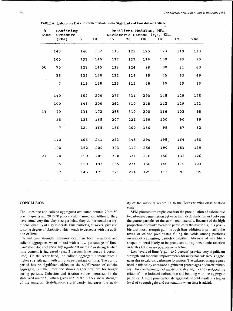
84 TRANSPORTATION RESEARCH RECORD 1486
TABLE6 Laboratory Data of Resilient Modulus for Stabilized and Unstabilized Caliche
% Confining Resilient Modulus, MP a Lime Pressure Deviatoric Stress ( C1 d) , KP a
(KPa) 7 14 35
140 140 152 135
100 133 145 137
0% 70 128 145 132
35 125 140 131
7 119 138 125
140 152 200 276
100 148 200 262
1% 70 131 172 255
35 138 165 207
7 124 165 186
140 165 241 283
100 152 200 303
2% 70 159 205 300
35 159 193 255
7 145 179 221
CONCLUSION
The limestone and caliche aggregates evaluated contain 70 to 80 percent quartz and 20 to 30 percent calcite minerals. Although they have some very fine clay-size particles, they do not contain a significant quantity of clay minerals. Fine particles, however, give rise to some degree of plasticity, which tends to decrease with the addition of lime.
Significant strength increases occur in both limestone and caliche aggregates when mixed with a low percentage of lime. Limestone does not show any significant increase in strength when lime content is increased (e.g., 2 percent lime versus 1 percent lime). On the other hand, the caliche aggregate demonstrates a higher strength gain with a higher percentage of lime. The curing period has no significant effect on the stabilization of caliche aggregate, but the limestone shows higher strength for longer curing periods. Cohesion and friction values increased in the stabilized material, which gives rise to the higher shear strength of the material. Stabilization significantly increases the qual-
70 100 140 170 200
129 125 123 119 110
127 116 100 93 90
124 98 90 81 69
119 95 75 53 49
115 48 45 39 36
331 290 145 129 125
310 248 142 129 122
310 200 136 102 98
221 159 100 90 89
200 150 99 87 82
345 290 195 164 150
317 256 190 151 139
331 218 158 135 126
234 160 140 110 103
214 125 113 95 85
ity of the material according to the Texas triaxial classification scale.
SEM photomicrographs confirm the precipitation of calcite due to carbonate cementation between the calcite particles and between the quartz particles of the stabilized materials. Because of the high proportion of quartz to .calcite particles in the materials, it is possible that most strength-gain through lime addition is primarily the result of calcite precipitates filling the voids among particles instead of cementing particles together. Absence of any fibershaped mineral likely to be produced during pozzolanic reaction indicates little or no pozzolanic reaction.
Low levels of lime (e.g., 1 to 2 percent) provide very significant strength and modulus improvements for marginal calcareous aggregates due to calcium carbonate formation. The calcareous aggregates used in this study contained significant percentages of quartz minerals. This contamination of parity probably significantly reduced the effect of lime-induced carbonation and bonding with the aggregate particles. A more pure carbonate aggregate should result in a higher level of strength gain and carbonation when lime is added.

2500 -··
f1. 2000 :2 vi :J ::;
~ I~
~ 1500
c
r~ '~
ISS!ffil "················! is:;:i ........ ·············!·· ...... ·············· ............... .
~ ~ ~ .iii
~ 1000 -
500
l . . I
0 -·--,. I
7 14 35 70 100 140 170 200 Deviatoric stress, KPa
I D 140 KP a m 100 KP a Im 70 KPa • 35 KPa IJI 7 KPa
FIGURE 7 Change of laboratory resilient modulus with deviatoric stress for limestone with 1 percent lime.
(iJ
0... :2 vi :J -s
4000 -.---------
3000
~ 2000
c ~ ·v; Q)
a::
1000 ..., ................... .
7 14
I •.~.·.·:.·:. ·:
'·
35 70 100 140 170 200 Deviatoric stress, KPa
lD LSO%L • LS1%L ~ LS2%L • CAO%L II CA1%L. CA2%L
FIGURE 8 Resilient moduli for stabilized and unstabilized limestone and caliche.

TABLE7 Backcalculated Moduli Values from FWD Data for Stabilized and Unstabilized Base Courses in Yoakum and Corpus Christi Districts of Texas
Description of Number of Average Modulus for
County Highway Base courses Deflection Basins Base Layers, (MPa)
Matagorda FM1468 200 mm limestone with 2% lime 33 483
Fayette SH71 150 mm limestone (unstabilized) 33 207
Nuces SH286 660 mm. limestone (unstabilized) 30 276
Refugio FM136 150 mm caliche with 1. 5% lime 30 138
Jim Wells US281 300 mm caliche with 1. 5% lime 30 207
San Pat. US77 150mm caliche, 125mm caliche with 1. 5% Lime 30 345
San Pat. FM1069 200 mm caliche with 1. 5% lime 30 8410
Nuces BS-44C 250 mm caliche with 1. 5% lime 30 621
Nuces SH357 200 mm caliche with 1. 5% lime 30 276
Nuces FM24 300 mm caliche with 1. 5% lime 24 207

Bhuiyan et al.
REFERENCES
1. Graves, R. E. Strength Developed From Carbonate Cementation in Silica/Carbonate Systems as Influenced by Cement-Particle Mineralogy. M.S. thesis. University of Florida, 1987.
2. Diamond, S., and E. B. Kinter. Mechanisms of Soil-Lime Stabilization. In Highway Research Record 92, HRB, National Research Council, Washington, D.C., 1965.
3. Miller, J.P. A Portion of the System Calcium Carbonate-Carbon Dioxide-Water with Geological Implications. American Journal of Science, Vol. 250, 1952, pp. 161-203.
4. Uzan, J., T. Scullion, C. H. Michalak, M. Paredes, and R. L. Lytton, A Micro-Computer Based Procedure for Backcalculating Layer Moduli from FWD Data. Research Report 1123-1. Texas Transportation Institute, Texas A&M University, College Station Sep. 1988.
5. Hallmark et al. Characterization Data for Selected Texas Soils. Texas Agricultural Experimentation Station, Department of Soil and Crop
87
Sciences, Soil Characterization Laboratory, Texas A&M University, 1983.
6. Kilmer, V. J., and L. T. Alexander. Methods of Making Mechanical Analysis of Soils. Soil Science Vol. 68, 1949, pp. 15-24.
7. Baver, L. D. Soil Physics. John Wiley and Sons, Inc., New York, 1965. 8. Dreimanis, A. Quantitative Gasometric Determination of Calcite and
Dolomite by Using the Chittick Apparatus. Journal of Sediment Petrology, Vol. 32, 1962, pp. 520-529.
9. Wissa, A. E. Z., and C. C. Ladd. Shear Strength Generation in Stabilized Soils. Research Report R65-l 7. Soils Publication No. 173, Department of Civil Engineering, Massachusetts Institute of Technology, Cambridge, Mass., June 1965.
Publication of this paper sponsored by Committee on Cementitious Stabilization.

88 TRANSPORTATION RESEARCH RECORD 1486
Resilient Properties and Microstructure of Modified Fly Ash-Stabilized Fine-Grained Soils ,
DAVE TA-TEH CHANG
A comprehensive study on the application of Class F fly ash for stabilizing subgrade soils in Taiwan is presented. Lime (or cement) was used with fly ash to enhance its self-cementing behavior in the study. Laboratory testing included using the plasticity index method to determine the optimum percentages of additive and fly ash. Through a resilient modulus (MR) test program, these percentages were confirmed. A section of test road with treated subgrade constructed on the West Coast Highway has been open to traffic for 40 months to date. A field investigation of this section was part of this study. Results from field California bearing ratio tests indicate that treatment of the subgrade soil had improved its properties by a factor of lO to I 5. Specimens obtained from the field were also evaluated through an MR test program, and the results were compatible with those for laboratorymade samples. Finally, a microstn.icture study is presented showing significant cementitious materials in laboratory and field specimens. Confidence about the future application of Class F fly ash for stabilizing subgrade soils in Taiwan and for handling this problematic waste material is provided.
Fly ash is causing serious disposal problems in Taiwan, where it occurs only in the Class F form as a by-product of electricity generation in thermal power plants. Recently, the use of fly ash as a stabilizer for subgrade soils has been the subject of much research. The project, sponsored by the Taiwan Electric Power Company and the Taiwan Highway Bureau, is recognized as the most complete study on this subject.
Hydrated lime was intentionally used as a modifier to enhance the self-cementing behavior of Class F fly ash; the modified fly ash (FA') yielded from this treatment process has been found (J) to exhibit behavior similar to Class C fly ash, which is a well-known stabilizer for problem soils. The preliminary study of this project evaluated the significance of improvements in terms of strength and durability. These were viewed as the best basis for determining the optimum FIL (fly ash/lime) ratios, as well as the optimum amount of FA' for use with fine-grained soils. The main program, which is presented in this paper, included an evaluation of the resilient modulus MR behavior for treated soils. The pavement-thickness design and layout of the test road were performed before the roadway was constructed, which at the time had been open to traffic for 40 months. The roadway subgrade was tested for its California bearing ratio (CBR) properties and sampled for further laboratory tests. Laboratory and field samples were tested for pH and MR and the microstructure of the FA' treated soils.
Civil Engineering Department, Chung Yuan University, Chung Li, Taiwan 32023,R.O.C.
BACKGROUND AND PRELIMINARY STUDY PROGRAM
Modification of the physicochemical properties of fine-grained soils with Class C fly ash results in improved strength and durability. Much has been reported about how Class C fly ash affects soil properties, but there has been little investigation in Taiwan into the effects of using Class F fly ash. Class F fly ash, which has low CaO content ( < 10 percent) and thus exhibits little or no self-cementing potential, has generally been considered waste in Taiwan, leading to pollution problems. In the study by Chang and Yu (J) on the use of Class F fly ash as sub grade-soil stabilization, FA' (Class F fly ash containing hydrated lime as an additive to enhance self-cementing behavior) was found to readily improve strength and reduce shrinkage-swelling potential. Following the pH method of Eades and Grim (2), Sabry and Parcher (3) succeeded in defining the Fly Ash Modification Optimum (F AMO) by using a similar pH measurement plot. This method was adopted as a means to select FA' percentages for improving engineering properties. The report (3) did not include recommendations for optimum ratios of FIL, because only two (8: 1 and 12: 1) were studied. The typical guideline for using fly ash, provided by the U.S. Department of Transportation and FHW A, requires improvement in strength and durability. Because fly ash is obtained at no cost in Taiwan, the limitation of strength of at least 400 psi may not be necessary. Thus, an applicability study based on the potential improvements in strength and durability was the first goal to be achieved with respect to using fly ash in Taiwan.
The preliminary program included index testing to evaluate the materials used and to determine the parameters for preparing compacted specimens. Next, specimens were prepared, using the Harvard Miniature Compaction Device, for the unconfined compression test. The specimens were then sealed with polyvinyl chloride (PVC) film to prevent moisture from escaping during the curing period. The lateritic soil (Soil L) and weathered mudstone (Soil M) used in this part of the study were obtained from the northwestern and the southwestern areas of Taiwan, respectively.
FIL ratios of 1, 2, 4, 6, 8, 10, and 12 were adopted for FA'. As determined by pH test analyses, results of F AMO for FA' s used in these soils are tabulated in Table 1. The quantity of FA' used for stabilization was preliminarily studied by using 0.5, 0.8, 1.0, 1.5, 2.0, 2.5, and 3.0 times their respective FAMO's (percent) to the soil by dry weight. This resulted in the use of a method based on unconfined compressive strength for the following test program: specimens using FA' with the amount of 1.5 X FAMO and 2.0 X
FAMO. For evaluating the improvement in terms of strength and durability behavior, 728 specimens were prepared and tested for

Chang 89
TABLE 1 Values of FAMO for FA' to Soil Land Soil M (2)
Soil Type FIL 1 2
FAMO 10 12 SoilL FA'/soil,%
FA I L s I 5 s I 4 FAMO 5 6
SoilM FA'/soil,%
FA I L 2.5 I 2.5 4 I 2
the proposed program (J). During the series of wet-dry tests, 1- and 12-cycle saturation treatments ( 4) were performed. For evaluation and comparison purposes, the ratio of strength of treated to strength of untreated specimens was determined and plotted against various percentages of lime compared with the sum of FA plus soil by weight [L/(FA + S)] for all treatments. The representation of L/(F A + S) was determined in the belief that for each treatment condition, a certain amount of lime would have a combined influence on the fly ash used (FIL) and the soil as FA'. Findings indicate that the optimum value of L/(FA + S) for lateritic soil and weathered mudstone are 3.5 and 2.0 percent, respectively. Because calcium (as a factor of FIL) plays an important role in the chemical reactions between FA and soil, the property of the clay particles reflected by plasticity may be a basis for quick determination of an optimum value for L/(FA + S). Therefore, for other finegrained soils, values of L/(FA + S) may be interpreted by PI, ranging from 12 to 34, with L/(FA + S) values of 2.0 and 3.5 percent, respectively. The ratios 4, 6, and 8 for FIL are recommended for other soils and could be used to determine the F AMO by the pH method. Knowing the L/(FA + S) in addition to the FIL and FAMO, the combination could be adapted as desired (Table 2). It is necessary to reiterate the limitations applicable when determining the desired combination:
• FIL ratios: 4, 6, 8. • Amount of FA': 1.5 and 2.5 times the FAMO. • Acceptable L/(FA + S) values: should be close to but defi
nitely no less than, the Interpreted value by Pl.
The following equation has been derived for obtaining the value of L/(F A + S) for other soils of these types:
3.5 - 2.0 L/(FA + S) =
34 _
12 (Pl - 12) + 2.0
= 0.07PI + 1.16
TABLE 2 Selection of FIL and Times ofFAMO Based on Optimum Values of L/(FA + S)
SoilL SoilM (L/(FA+S)=3.5%) (L/(FA+S)=3.5%)
FIL FA'/soil, % FIL FA'/soil, %
I.5XFAMO 1.5XFAMO 6 (17 %) 4 (8 %)
FA=l4.6, L=2.4 FA=6.4, L=l.6 1.5XFAMO 1.5XFAMO
8 (18 %) 6 (9%) FA=l6, L=2 F A=7. 7 , L=l.3
(1)
4 6 8 10 12
15 .. 17 18 19 20
12 I 3 14.~ 2.4 ''16 I 2 id 1.7 1s.511.5
8 9 10 11 12
6.4 I I.6 9.7 I 1.3 8.911.1 10 I I 1 ul o.9
Because the previous findings were to be directly used in the pavement thickness design for the test road, an MR testing program was subsequently completed at the H~ghway Bureau's request.
RESILIENT MODULUS PROGRAM
Because the FA' stabilized subgrade soil was to be applied to pavement thickness design, the next step was to verify the suitability of the strength-based formula by investigating MR characteristics. Of the two test roads (denoted A and B) provided by the Highway Bureau, the subgrade of Test Road A was classified as a CL soil, and it was included in the program. Research by Chang and Chang (5) indicates that portland cement provides the same results as lime when used as an additive for Class F fly ash and is relatively inexpensive. It was therefore incorporated for this section of the program. To facilitate differentiation, FA' containing lime is denoted as FA' land those containing cement as FA' c.
Modified MR Testing Device
The need to obtain reliable MR data for treated subgrade soil in the proposed program prompted the modification of the existing standard testing device. To control the testing and data-acquisition process, a computer program for determining MR of a fly ashtreated subgrade soil-MRSS II-was developed and revised from MRSS (6) (a program developed to control MR testing of subgrade soil) using an AID convertor for data processing. The software was capable of simulating various testin.g conditions, such as load duration, cycle duration, and varying repeated loads. For monitoring purposes, the software was written to plot the stress time _and deformation curves, which were found to res.emble the shape of a haversine curve, as shown in Figure I. Through the dynamic calibration procedure (7), the performance of this modified testing device was found to be reliable, accurate, and ready for the testing program.
Materials and Experimental Program
In this study, which focused. on fine-grained soils, the selected samples of the lateritic soil (Soil L) and weathered mudstone (Soil M) were the same as in the preliminary program. In addition, soil from the road subgrade of the test road was studied. This test road is located in Kaohsiung County on the Mituo section of the Highway Bureau's West Coast Highway project between kilometer marks 217 + 100and218 + 100,andisdesignatedsectionA,andthesoil

90
FIGURE 1 Typical stress-strain curve monitored by MRSS II software.
is designated as Soil A. The liquid limit of Soil A was 38 percent, and its plasticity index was 21 percent. So by the unified system, Soil A was classified as CL. Using the selected F/L ratios or fly ash/cement (F/C) ratios of 2, 4, 6, 8, and 10, pH tests were conducted. In terms of the FAMO values· for these soils, there were only slight differences between FA' containing a lime additive and those containing a cement additive. To facilitate analysis and comparison, the two were treated as providing the same values, as shown in Table 3. In accordance with the results explained above, the amount of FA' used was 1.5 X FAMO and 2.0 x FAMO.
MR tests were conducted in accordance with the procedures delineated in AASHTO T274-82 (8). Considering the stress behavior of higher tire pressures, the deviator stress was set at 82.8 kPa (12.0 psi) instead of 6.9 kPa (1.0 psi). Conditions of optimum moisture content (OMC) and maximum dry unit weight were adoptedfor preparing MR specimens. Specimens were molded by static compaction, sealed with PVC film and wax, and then cured in a moisture room for 7 days. The requirements for rapid curing (9) were adopted; therefore, the temperature was set at 38°C (100°F).
The MR testing procedures were conducted under two sets of conditions: the OMC state and a saturated state. Each cured specimen was placed in a triaxial cell for MR testing at the OMC s~ate. After this test was complete, back-pressure saturation was conducted for 24 hr to achieve the normal saturation requirement of 95 percent before carrying out the MR testing procedures. Reduction of back pressure (complete depressurization) had to be conducted in
TRANSPORTATION RESEARCH RECORD 1486
several stages with 30-min static intervals between each stage to avoid the adverse influence of excessive pore water pressure on MR behavior.
Results Analysis and Evaluation
Performance Differences from Fly Ash Additives
Because unconfined compressive strength had previously been adopted as a convenient index, MR properties were used in this study as an additional comparison and to verify the mutual conformity of the two. To ensure that the readings were conservative, MR values (JO) corresponding to ad= 41.4 kPa (6.0 psi) and the MR values corresponding to the stress transfer values of high tire pressures, ad= 82.8 kPa (12.0 psi) were also taken into consideration. These values are compared in Figure 2. In each case, the MR values corresponding to ad at 41.4 and 82.8 kPa are provided. To gain an understanding of the development potentials for these MR values and to simplify the results for analysis, all curves were drawn through points midway between the saturated and the unsaturated (OMC) values. Comparing the effect of saturation on MR values in Figure 2, it is apparent that its influence is not significant. In some cases the structure of the grains actually became more stable as sufficient water was provided for hydration purposes-a factor, which in durability terms, is positive indicator for stable applications of fly ash. Considering the situation for the influence of lime and cement additives, in only one case (Soil L) does the influence of lime slightly exceed that of cement. Lime is the preferred additive in this case because the relatively high PI of Linkou Lateritic Soil (Soil L; Pl = 34) means that there is a fairly high demand for CA+ during the initial phase of the cation exchange reaction. In those soils with lower PI values (the Pis for Soil Mand Soil A are 12 and 21, respectively), the ions required for the cation exchange reaction can be obtained in sufficient amounts from cement. Most of the soil-grain cementing agents are derived from the hydrating effect of the cement because these achieve earlier stability than the pozzolan effect of lime. This analysis is in complete correspondence with the chemical mechanisms of soil stabilization; therefore, the observed properties are credible.
Considering that local cement is cheaper than lime and that highly plastic soils are rarely encountered in Taiwan, it can be recommended that for practical applications for these soils cement would be the additive of choice.
Review of PI-Interpretation Method
Generally speaking the improved MR properties in Figure 2 allow one to combine the best parameters [L (or C)/FA + S] and ascertain
. TABLE 3 Values ofFAMO for FA' to Soil A
FIL orF/C 2 4 6 8 10
FAMO 8 11 13 14 15 FA'/soil, %
FA ILorC 5.3 12.1 8.8 12.2 11.111.9 12.411.6 13.611.4

Chang 91
400 Soil L Soil L
JSO - - = o-d =82.8 kpa - - : crd =82.8 kpa - : crd =41.4 kpa - : crd =41.4 kpa
JOO
• 0 & 250 ~ ~ I ~
~ ~ 200 ..
~ c. ..:.:
150 6 r.n L.:.J . I I 6 ::i .....) 100 < 400 2 3 3.5 4 2 3 3.5 > 0:: Soil M Soil M ~ J50
- - : crd =82.8 kpa - - : crd =82.8 kpa
JOO - : crd =41.4 kpa -: crd=41.4 kpa
250
~ I• a 200
~ ~· 150 f h ~ 0
100 I
400 2 2 J
350 Soil A Soil A - - : crd =82.8 kpa - - : crd =82.8 kpa
JOO - : crd =41.4 kpa - : crd =41.4 kpa
~ c. ..:.:
r.n 250 UJ .....) ;::::; 8 0
< 200 > 0:: ~ 150
• --i
100 1 2 2.6 J 4 2 2.6 J 4 5
L/fA+S,% L/fA+S,%
a.=41.4kPa CT.= 82.8 kPa
0 1.5 FAMO(Uns.) a 1.5 FAMO(Uns.)
• 1 .5 FAMO(Sot.) • 1.5 FAMO(Sat.)
• 2.0 FAMO(Uns.) • 2.0 FAMO(Uns.)
• 2.0 FAMO(Sat.) • 2.0 FAMO(Sat.)
FIGURE 2 Relationship of C (or L)/FA + S to the development of MR values.
rational and conservative values based on 1.5 and 2.0 times their FAMO's, respectively. The optimum values ofL/FA +Sand C/FA + S for Soil Lare all between 3.25 and 3.5 percent, and the values for Soil M are between 1.75 and 2 percent. Comparing the results obtained for unconfined compressive strength (2) (Soil L: 3.5 percent, Soil M: 2.0 percent) confirms the MR-based findings and provides almost the same conclusions (using upper limits). Use of Equation 1 for Soil A yields a result of 2.63 percent for L (or C)/FA + S. The figure of 2.6 percent that can be drawn from the results of Figure 2 conforms satisfactorily with the figures previously referenced and supports the suitability of the PI-interpretation method. The FAMO for Soil A in various ratios is known, and Table 4 shows the ideal combinations for modified fly ash as 1.5 and 2.0 times the
FAMO. For this method of calculation, see the procedures above for the PI-interpretation method. Thus the acceptable combinations are a ratio of 4 for FIL or F/C with an FA' of 1.5 times theFAMO (FA = 13.2 percent, Lor C = 3.3 percent, soil = 100 percent), or a ratio of 6 (FIL or F/C) with an FA' of 2.0 X FAMO (FA= 22.3 percent, Lor C = 3.7 percent, soil = 100 percent). The recommended combinations were incorporated in the design of test Road A.
Representation of MR Design Value
According to multilayer elastic criteria, MR values must be incorporated in the design in accordance with the relevant monthly

92
TABLE 4 Ratio and Amount of FA' Combination
Ratio l.SXFAMO 2.0XFAMO
FA'/S CIFA+S FA'IS C/FA+S
2 12 3.7 ... 16 4.8 ...
4 16.5 2.9 0 22 3.7 ...
6 19.5 2.4 T 26 3.0 0
8 21 1.9 T 28 2.5 T
10 22.5 1.7 T 30 2.1 T
.A: too high, not recommended; T: too low, not O: acceptable combination
moisture figures when calculating the appropriate thickness for the pavement structure. Hence an initial appraisal of the test results from this study was necessary as a basis for pavement-thickness design.
For FA' treated soils, where MR values and the u d used are concerned, the tire-pressure induced deformation should, as a rule, be within tolerance at a base-line ud of 41.4 and 82.8 kPa. Figure 2 shows that the MR values are approximately the same, allowing for some slight but tolerable differences. As stated previously, stability is excellent under unsaturated conditions. To ensure that conservative design figures are implemented, upper (unsaturated) and lower (saturated) limits should be established for design values. An overall analysis of Figure 2 reveals that 172.5 MPa (25 ksi) and 138 MPa (20 ksi) should be rational and somewhat conservative values for these three soils. Hence an MR value of 172.5 MPa is recommended for normal months and 138 MPa for wet months.
TEST ROAD
Design, Layout, and Arrangement of Test Road A
The pavement thickness was selected and designed for the test road on the basis of MR values. The layer-thickness design was varied in separate sections to evaluate the gravel equivalent factor value. (The layer coefficient of treated subgrade will be discussed further in a future study.) The details of the layout and arrangement are shown in Figure 3. Construction of the test road was completed in March 1989, and the field-investigation program was performed 2 years later. ·
Field Investigation Program and Results
A series of survey and evaluation operations began after the test road had been open to traffic for 2 years. Because of the space limitations of this paper, only evaluations for data related to the FA' -treated subgrade layers will be presented. The pH values for the treated layer are listed in Table 5, along with those measured for the treated layer during mixing in the construction process. Table 5 shows pH values decreasing over time, which is explained by the chemical mechanisms of soil stabilization. The pozzolan reactions .
TRANSPORTATION RESEARCH RECORD 1486
z17km 218km +700 • +780 +860 +940 +020.+100
1 F/L=6 F/L=6 F/C=6 F/C=6 ZSM Unt~eated1--__ ..__ __ +----'-------1
Section FA=25.7% FA=24.0% ' L=4.3%,~=100% C=4%,~=100%
I
: . • Opservation
T
FIGURE 3 Arrangement thickness layout of Test Road A.
use hydroxyl (OH) ions to form stable bonds, thus they are unavailable in the pore water, resulting in lower pH values. During the investigation program, field CBRs were conducted, and the results are tabulated in Table 6. From this table it can be seen that for the treated layer satisfactory performance was achieved because the strength increased by a factor of 10 to 15. The lowest layer of untreated subgrade had CBR values that were too low, most likely because of groundwater effects.
When the CBR program was completed, the treated layer was cut into large blocks, which were moved from the test pit to the laboratory. These specimens were cut into small blocks with a rock saw and finished to a final size [D = 5 cm (1.5 in.), H = 10 cm (3.94 in.)] with a knife and sandpaper. The trimmed specimens were then placed into the MR testing device. Because these specimens were extremely difficult to trim, only one set of tests was conducted for each section. Typical results are shown in Figure 4, along with the MR values for untreated samples. It is evident from Figure 4 that treatment was effective. The recommended design values (20 to 25 ksi), drawn from the results of indoor testing, were confirmed as being satisfactory. The slightly low performance of the first two sections may be attributed to the disturbance of the sampling and trimming processes. In summary, synthesis of the above items of field data confirms that Class F fly ash with cement (or lime) added produces satisfactory results as a stabilizer of these subgrade soils. Great confidence is justified in this method of dealing with the fly ash disposal problem. The results of another area of research, the rnicrostructure study, are further indicative of fly ash stabilization.
MICROSTRUCTURE EXAMINATION RESULTS
This portion of the project included investigation of the rnicrostructure of laboratory-made and field specimens. To facilitate comparison and explanation, the microstructures of laboratory-made spec-

Chang 93
TABLES pH Values for Soil A for Test Sections
Location 2l7km +740 217km +820 217km +900 217km +980 218km +060 (Untreated) (Treated) (Treated) (Treated) (Treated)
During 7.3,....,7.5 11.40,...., l l.5 l ll.57,....,11.71 11.68-11.78 i 1.45-11.60 Construction (Untreated)
36 months Untreated 9.48 9.50 9.68 9.59
40 months Untreated 8.93 8.51 8.92 8.65
TABLE6 Field CBR Test Results (Percent)
Location 217km +740 217km +820 (Untreated) (Treated)
Treated Layer None 84.8
Untreated Layer 15.0 4.2
imens for Soil L, Soil M, and Soil A are presented in Figure 5. Because Soil L consists of heterogeneous basic materials, it develops an anisotropic structure under influence of water pressure [Figure 5 (a)]. Soil M appears to induce marked erosion of the fly ash, so it forms consolidation of the mudstone quickly [Figure 5 (b)]. Figure 5(c) shows that Soil Mis dense in texture, hard, and bonds effectively (although cementing materials were distinct); newly developed faces effectively filled the fissures. Soil A is dense in texture; newly developed mineral faces consist of white encapsulated matter [Figure 5(d)]. The field samples for Soil A are shown in Figure 6. The items observed as results shown in Figure 5 are synthesized for comparison in Table 7.
Samples activated with cement (obtained from 217 km + 980 and 218 km + 060) were stronger in terms of mechanical properties and external appearance; they also presented a denser surface structure. In viewing these samples, one would notice a comparatively uniform appearance on cutting the surface open with a knife
400
350
300
0 250 a.. ~ 200 a:: ::I
150 .... _ -.... --100
50
0
217km +900 217km +980 218km +060 (Treated) (Treated) (Treated)
--
53.5 108.7 123.0
4.1 4.7 7.2
and a cross section that revealed a more uniform grain structure. Under observation with the microscope, as in Figure 5, the cementing materials presented tightly cross-linked interfaces in spite of their prominence, and the fly ash was joined strongly to the clay particles in its three-dimensional surroundings. These presented the densest structures of all the samples. Anisotropic arrangements resulting from trC;lffic loading were observed in some cross-sectional views. Furthermore, newly developed mineral faces, consisting of white encapsulated matter and trichome effectively filled the cracks along which they had developed, acting as excellent cementing agents (Figure 5).
Although the samples activated with lime in Figure 5 were strong in texture, surface clumps which had formed showed a tendency to peel off. Voids of approximately 30 to 60 µm existed between these clumps of grains. Their outer appearance and mechanical properties were similar to those of the samples activated with cement, and low clay content made the
•-•:217 +820 A-A:217km+900 •-•:217km+980 o-0:21a1cm+oso +-·+:UNTREATED
-... --.... --. 0 10 20 30 40 50 60 70 80 90 100
DEVIATOR STRESS .kPa
FIGURE 4 MR test results for specimen obtained from field.

94 TRANSPORTATION RESEARCH RECORD 1486
a c
b d
FIGURE 5 Microstructure from laboratory-made treated specimen.
grains clearly visible. The fly ash was not evenly mixed with the soil in these cases, and occasional large clumps were observed. The honeycomb structure that can be seen in the untreated soil was also observed in these samples, but in much lower proportions. From Figure 6 (a) and (b) it is evident that in terms of external appearance and unity, soils treated at the FIL ratio of 6 fell slightly short of the samples presented in Figure 6 (c) and (d), which had a cement additive. It is noted that the soils depicted in Figure 6 (c)· and (d), which had an F/C ratio of 6, have formed more newly developed mineral faces (trichome and white portions). The characteristics are slightly anomalous for samples of Soil A with FA' added at the ratios of F/C = 6 and FIL = 6. Both lime and cement appear more equal at an age of 4 years, which is what would be expected, because the cement will provide earlier strength gain and lime long-term strength gain.
CONCLUSION
On the basis of results from feasibility and applicability evaluations, this study was planned and conducted with a goal of simplifying design procedures and general applicability. The relevant results
and conclusions for the materials tested in the test-road program are as follows:
• The PI-interpretation method recommended for ascertaining the optimum percentage of additives and fly ash for these soils has been verified by the compatible results obtained through MR testing.
• A cement additive, as revealed in the microstructure study of 40-month-old specimens, is superior to lime, which is what would be expected because the cement will provide earlier strength gain and lime long-term strength gain. ·
• Microscopic analysis· confirms that the addition of lime or cement to Class F fly ash effectively induces beneficial reactions and significant improvements in strength and MR.
ACKNOWLEDGMENTS
This has been an extensive and long-term project in which too many people have participated to allow individual mention. The author expresses his appreciation to all concerned. The author also expresses his gratitude to the assistants and coordinators of the Taiwan Highway Bureau and to the Taiwan Electric Company, which provided funding, support, and the assistance of relevant personnel.

Chang 95
a c
b d
FIGURE6 Microstructure from field-treated specimen.
TA.BLE 7 Microstructure Analysis of Various FA' (FA' l or FA' c) Treated Soils
Pores Cementing Material Fine Cementing Silt General (solid particles)
outer curvature size degree of -shape difference sphericity
SoilL prominent good uniform
SoilM developed good not uniform distinct
Soil A developed good uniform distinct
Soil A (field specimem) d 1
d F A'l or F A'c eve ope good not uniform prominent
REFERENCES
I. Chang, T. T., and K. Yu. Study on Lime and Class F Fly Ash Stabilization for Linkou Lateritic Soils. (in Chinese) Report NSC 74-0414-Po033-0l, National Science Council, Taipei, Taiwan, R.O.C., 1986.
2. Eades, J. L., and R. E. Grim, A Quick Test to Determine Lime Requirements for Lime Stabilization. In Highway Research Board Record J 39, HRB, National Research Council, Washington, D.C., 1963, pp. 61-72.
<IO~tm Agent caves fissures
bundles
relatively poorly insufficient few developed
many many density
distinct observable full present few extremely developed dense
observable few easily many present acceptable observable
observable relatively
abundant many
many present poor
3. Sabry, M. M.A., and J. V. Parcher. Engineering Properties of SoilLime Mixes. Journal of Transportation Engineering, Vol. 105, No. 1, .ASCE 1979, pp. 59-70.
4. Standard Method for Wetting and Drying for Tests on Compacted SoilCement Mixtures. Report D559-82, Part IL American Society for Testing and Materials, Philadelphia, Pa., 1982.
5. Chang T. T., and C. Y. Chang. Application of Class Fly Ash for Subgrade Stabilization in Taiwan (/l)-Test Road. Final Report. Chung Yuan University, Chung Li, Taiwan, R.O.C., 1989.
6. Chang, T. T., C. Chiung, and C. Y. Chung. Modified Testing Device to

96
Evaluate MR Properties of Fly Ash Treated Subgrade Soils. Geotechnical Testing Journal, ASTM., 1991.
7. Chang, T. T., and Y. H. Liu. Resilent Modulus Property of Fly Ash Treated Fine-Grained Subgrade Soils. Journal of the Chinese Institute of Civil and Hydraulic Engineering, Vol. 4, No. 3, 1992, pp. 205-213.
8. AASHTO Materials: Methods of Sampling and Testing. American Association of State Highway and Transportation Officials, Washing
. ton, D.C., 1983, pp. 1157-1177.
TRANSPORTATION RESEARCH RECORD 1486
9. Soil Stabization Manual, Vol. II FHWA, U.S. Department of Transportation, 1979.
10. Soil Manual for Design of Asphalt Pavement Structures. MS-10. The Asphalt Institute, Md., March 1978, pp. 133-147.
Publication of this paper sponsored by Committee on Cementitious Stabilization .

TRANSPORTATION RESEARCH RECORD 1486 97
Waste Fibers in Cement-Stabilized Recycled Aggregate Base Course Material
J. K. CAVEY, R. J. KRIZEK, K. SOBHAN, AND W. H. BAKER
A coordinated laboratory and field study was undertaken to assess the suitability of producing an economically suitable pavement base course material by reinforcing cement-stabilized recycled concrete aggregate with strips of reclaimed plastic or tire wires and tire chunks from recycled scrap tires. The field program included constructing 12 test sections using different proportions of various waste materials. It was found that the addition of fibers exerted no measurable effect on field compaction, but the in-place mixing technique used was unsuccessful in distributing the fibers homogeneously throughout the full depth of the slab. Laboratory split tensile tests and beam flexural tests showed that reinforced specimens exhibited lower tensile and flexural strengths and no improvement in toughness compared with unreinforced specimens. The same basic recycled aggregate mix, when reinforced with a commercially available hooked-end steel fiber, showed that 28-day specimens with 4 percent fiber reinforcement exhibited a pseudo strain hardening behavior after the peak, accompanied by a modest increase in tensile strength and almost doubling in toughness. Notwithstanding the generally recognized benefits to be realized in a pavement system by an increase in toughness in one or more layers, the results of this study suggest that caution and careful investigation should be exercised when contemplating the incorporation of waste products in the component layers. Failure to do so may result in false
·economy whereby initial cost is reduced somewhat at the expense of increased life-cycle costs because the anticipated performance was not achieved.
In an effort to address growing national concerns for mitigating the solid waste disposal problem and conserving available landfill space, a number of studies have been conducted to identify waste products that can be effectively recycled and used in highway construction (1,2). One recent survey, which elicited responses from 44 state Departments of Transportation (DOTs) on current practice in the use of waste materials in highway construction, identified only 11 waste products (including recycled asphalt and portland cement concrete paving materials; building rubble; and other demolition debris, scrap tires, waste glass, recycled plastics, and various kinds of slags and ashes) that are being used by more than 7 percent (approximately three states) of the respondents (2). However, the use of most of these materials was reported to be still in the experimental stage.
Section 1038(b) of the Intermodal Surface Transportation Efficiency Act of 1991 requires the Secretary of Transportation and the Environmental Protection Agency to conduct studies to evaluate the economic, technical, and environmental factors associated with using recycled materials in highway construction. Although the concept of recycling is timely and desirable, caution must be exer-
J. K. Cavey, 1875 Mayfield Rd., Hayward Baker, Odenton, Md. 21113. R. J. Krizek and K. Sobhan, Department of Civil Engineering, Northwestern University, Evanston, Ill. 60208. W. H. Baker, 1728 Reynolds St., Geobase, Inc., Crofton, Md. 21114.
cised when incorporating recycled materials with unknown or questionable properties into a highway pavement system. Of particular concern is the use of materials for which there is limited knowledge about their long-term performance characteristics. The idealized goal of incorporating waste materials in highway pavements must not be satisfied at the expense of building an inferior (and ultimately uneconomical) pavement system, which will eventually contribute to the nation's already overwhelming infrastructure problems. Alternatively one must not aggravate the infrastructure problem by using highways as "linear landfills" to help solve the waste disposal problem. The use of recycled materials in highway constructi9n can be justified only if it results in a pavement system that is at least as serviceable and economical (with all factors considered) as the ones being built.
OBJECTIVE AND SCOPE
The objective of this study was to evaluate, through laboratory and field testing programs, the performance of a cement-stabilized base course material consisting of recycled concrete aggregate reinforced with either strips of reclaimed plastic or wires from old tires. In some cases, pieces of shredded tires were included in the mix. The primary motivations for this research were that (a) a fiber-reinforced, aggregate-cement composite has characteristic engineering properties that offer advantages for a pavement structure and (b) such a base course material is composed entirely of waste materials (except for a nominal cement content). The study is concerned mainly with (a) the mechanical characterization of the selected base course materials, (b) the benefits derived from incorporating waste fibers, and (c) the experience gathered from field mixing and the construction of test slabs. Evaluations of the environmental acceptability, economic feasibility, and frost susceptibility are beyond the scope of this investigation.
BACKGROUND OF CANDIDA TE WASTE PRODUCTS
Although several studies indicate that recycled crushed concrete aggregate is being used to construct or reconstruct various components of a pavement structure, only a limited number of successful field projects (many of which were experimental pavements) have been completed to date (1,3-5). Of the 30 state highway agencies that reported their experience with the use of waste tires in highway pavement systems (2), 50 percent considered their use uneconomical, 30 percent reported poor performance, and 9 percent were not confident about their future environmental acceptance. However, varying degrees of success have been claimed in several

98
experimental projects using tire products in geotechnical-related applications (2,6, 7). Recycled plastics have been used in hot mix asphalt concrete (3), in fence line and guardrail posts (8), as lightweight reinforcing inclusions in concrete (9), and as reinforcement in granular soils (JO). Efforts to use recycled fibers include waste nylon fibers (J J) and recycled carpet fibers (J 2) in portland cement concrete and recycled cellulose fibers as an asphalt modifier (J 3). No information was found in the literature on the mechanical behavior (toughness, in particular) of a material composed of a cement-stabilized, recycled aggregate and waste fiber, where shredded plastic bottles or reinforcing wires from scrap tires were used as fibers. Therefore, an evaluation of this particular composite material constitutes the focus of this study, which was conducted in three stages:
• Construction of test slabs and field testing, • Concurrent laboratory test program on field-prepared speci
mens, and • Series of controlled laboratory tests and a comparison study.
MATERIALS USED
Aggregates
The recycled concrete aggregate was obtained from two sources. For the Maryland field and laboratory study, the aggregate was obtained from the E.L. Gardner Concrete Company in Crofton, Maryland, and for the Illinois laboratory study, it was obtained from the R. I. Busse Corporation in Elk Grove, Illinois. The aggregate used met the CA-6 specifications for recycled concrete. The grain size distributions for four samples taken from different locations in the aggregate ·stockpiles of each of the sources are shown in Figure 1.
_,
""' ~ = ~· .... = ~ CJ
""' ~ ~
100
90
80
70
60
50
40
30
20
10
0 100
II
~ \ ~ ~' ~ \ ~ ~ I'
. 4~ '~ \ '
'
10
~~ ~ .....
~~ \ --~ ' ~~ ' I \.
,~ '\
l '~ ,, ~
\
~· -~
TRANSPORTATION RESEARCH RECORD 1486
Stabilizing Materials
Type II portland cement and several different types of waste materials were used to stabilize the aggregate. Three kinds of waste products from scrap tires were used. The first, termed "tire wire," is a waste product of the tire shredding process and consists of several strands of wire, generally 50 to 75 mm (2 to 3 in.) long, connected by small portions of rubber. The second, called "tire chips," was pieces of a tire 50 to 100 mm (2 to 4 in.) in width and length and about 13 mm (0.5 in.) thick containing wires. "Tire straps," the third type, were portions of a tire cross section 25 to 60 cm (10 to 24 in.) long. The recycled tire products were obtained from Sawyer Environmental Recycling Company in Hampden, Maine. The shredded plastic strips were derived from recycled soda bottles and were about 6 mm (0.25 in.) wide, 2.5 mm (0.1 in.) thick, and 50 to 100 mm (2 to 4 in.) long. The recycled plastic strips were supplied by Nikon Plastics in New York City. In addition, 75-mm (3-in.) long, 24-gauge galvanized steel wires were used to simulate the tire wires. To evaluate the performance of recycled fibers, a comparison study was conducted by reinforcing the cement-stabilized recycled aggregate with 60-mm (2.36-in.) long Dramix hooked-end steel fibers manufactured by the Bekeart Corporation.
FIELD CONSTRUCTABILITY TESTS
Using conventional construction techniques and equipment, a test pad consisting of 12 different test sections (each modeling a typical stabilized base course in a pavement section) was built in Crofton, Maryland, to (a) evaluate the effectiveness of in-place mixing of the stabilizing materials and the recycled aggregate, (b) determine the distribution of the fibers in the slab, and (c) quantify the effect of the fibers on the density of the roller-compacted test pads. The excavation and construction equipment included a Bobcat loader/dozer,
~ ~
~ '~ \ ~ l
" I ~~ ' .. , ,. ~ ~ )I
I--- • . ~ --1.0 0.10 0.01
Grain Size (mm)
FIGURE 1 Grain size distribution curves for recycled aggregate (solid symbols represent samples from Elk Grove, Ill.; open symbols, Crofton, Md.).

Cavey et al.
a BOMAG vibratory roller, and a REX in-place soil mixer. A nuclear density gauge was used for in-place density determinations.
Test Pad Construction
Each section of the test pad was approximately 2 m (6.5 ft) wide and 1.7 m (5.5 ft) long. The arrangement and numbering of the test sections, as well as the type and amount of reinforcement used in each section, are shown in Figure 2. The aggregate was transported with a Bobcat. Thirty-six bags of portland cement were distributed evenly on the surface of the test pad to provide an 8 percent cement mix. One test section was prepared with 12 percent cement. The cement was mixed dry to a depth of about 0.25 m (10 in.) using the REX mixer. A measured amount of water was added to the test pad and the designated fibers were placed on the wet pad in the proportions shown in Figure 2. The REX mixer then made a second pass, and the material was compacted with a vibratory roller, after which nuclear density gauge readings were taken at several locations in the compacted test pad. Seven days after construction, coring was attempted at 19 locations, but usable samples were obtained at only 6 locations. These cores were 100 mm (4 in.) in diameter and 100 to 150 mm (4 to 6 in.) long. Beam samples were sawed from the test pad after 14 days, but the quality of the resulting samples was poor. After 28 days, the test pad was broken into several pieces with a backhoe to evaluate the mixing of the cement and the distribution of the fibers in the aggregate-cement matrix.
Density Measurements
Nuclear gauge density determinations on a companion test pad consisting of only recycled aggregate showed that the average dry den-
32 Kg (2%>1 Control Control Tire Straps No Fibers No Fibers 5.5
8 Kg (0.5%)1
Two Extra Bags Control Shredded Plastic of Cement2 No Fibers 5.5
(12%)
. 1 64 Kg (4%f 32 Kg (2%)
1 32 Kg (2%)
Shredded Plastic Tire Chunks Tire Wire s.s
1 1 8 Kg {0.5%f 16 Kg (1 %) 16 Kg (1%)
Shredded Plastic Tire Chunks Tire Wire s.s
6.5 1 6.5 1 6.5
All dimensions are in feet Notes: 11ndicated percentages of inclusions are by weight
2All sections had 8% cement by weight, except this one
FIGURE 2 Composition of individual field test sections.
99
sity at a depth of about 0.3 m (12 in.) was 1786 kg/m3 (111.5 pcf) with a variation of ±59 kg/m3 (3.7 pcf) and the average moisture content was 12.1 percent with a variation of ±2.5 percent. Density measurements at the center of each test section to a depth of about 0.2 m (8 in.) indicated that at least 90 percent compaction (based on the laboratory-determined maximum Proctor dry density without cement or fibers) was achieved in all of the test sections. The average dry density was about 1800 kg/m3 (112.6 pcf) with a variation of ±48 kg/m3 (3.0 pcf), and the average moisture content was 13.7 percent with a variation of ± 1.7 percent. The measured densities indicate that the inclusion of fibers did not affect the densities attained in field compaction.
Distribution of Cement and Fibers
Based on visual observations of the cores (both successful and unsuccessful ones) and the broken pieces of the test pad, it was determined that the top 75 to 100 mm (3 to 4 in.) resembled concrete and the underlying aggregate-cement layer was granular with almost no cohesion. In addition, the plastic fibers, tire wires, and tire chunks were also located primarily near the surface in the top 50 to 100 mm (2 to 4 in.). Frequently the tire wires and chunks were observed to form clusters, thus preventing a more even distribution.
Lesson Learned
In this limited field exercise it was learned that the field mixing method employed did not produce an acceptably homogeneous mixture of the recycled aggregate, cement, and waste fibers or chunks used. Consequently, a satisfactory performance by the composite material could not be expected.
CONCEPT OF TOUGHNESS
Although a stabilized base course in a highway pavement is designed so that working stresses in the layer are generally lower than its ultimate tensile strength, many applications of traffic loads will cause fatigue cracking and eventually lead to failure. However, a properly designed fiber-reinforced layer will tend to resist the propagation of fatigue cracks under working stress levels because of its superior capacity for energy absorption. This capacity for energy absorption is termed toughness, and it is normally defined with reference to the post-peak responses associated with a singleload cycle going to failure. Because toughness is also a desirable property for enhancing material performance under conditions of repeated loading (fatigue) at applied stresses less than the peak strength, such as would be experienced by a highway base course material, it was a key material property measured in this study.
LABORATORY TESTS
As stated previously, two series of laboratory tests (denoted as the Maryland tests and the Illinois tests, the latter of which includes a program of comparison tests) were conducted to
• Identify candidate materials, fibers, and optimum mix proportions suitable for use in pavement base courses;

100
• Evaluate the effect of fiber type and proportion on the ultimate split tensile strength of specimens; and
• Determine the toughness characteristics and post-peak increase in ductility due to fiber inclusions.
The Maryland tests were performed on field-prepared specimens using the same materials and mixes incorporated in the various sections of the test pad. The Illinois test program included more sophisticated tests on specimens prepared with greater control. In addition, a different recycled aggregate and some different fibers were used.
Maryland Laboratory Tests
Simultaneous with constructing the field test pad, test cylinders 152 mm (6 in.) in diameter and 305 mm (12 in.) in length were prepared in the field for conducting laboratory split tensile (Brazilian) tests in accordance with ASTM C496. Four cylinders were prepared by conventional compaction techniques for each of the 12 sections; two were tested after 7 days and two after 28 days. The fiber types and quantities (measured by the weight percentage of the total dry weight) included tire wires (1, 4, and 8 percent), tire chunks (1 and 4 percent), and shredded plastic (0.5, 1, and 4 percent). Ten of the 12 sets had 8 percent cement, and the remaining two sets had 12 percent cement; the water-to-cement ratio was maintained at approximately 0.5. The inclusion of fibers affected the laboratory compaction and a constant density could not be achieved. The samples were stripped from their molds after 48 hr, wrapped in wet burlap, and cured at approximately 23°C (73°F).
Results
The ultimate tensile strengths for the 28-day specimens are plotted versus dry density in Figure 3 (although not shown, the 7-day results
TRANSPORTATION RESEARCH RECORD 1486
show the same pattern). These data show that the split tensile strength strongly depends on density; the 28-day tensile strength increased from 190 KPa (28 psi) at a dry density of 1712 kg/m3 ( 107 pcf) to-almost 1335 KPa (194 psi) at a dry density of 2010 kg/m3
(125 pcf). For the same type and amount of fiber, the strength generally increased with an increase in density. These data indicate that there is a slight increase in strength as a result of an increase in cement for specimens with no fibers. In general, however, there was a decrease in the tensile strength of specimens with fibers relative to the control specimens (no fibers).
Lesson Learned
Based on the experience gained during this phase of the study, it was learned that
• A procedure must be developed to prepare specimens with a controlled density,
• Fiber length should be controlled to reduce the number of variables, and
• Lateral deformation measurements should be incorporated into the test program to evaluate the post-peak response and the overall toughness of the material.
Illinois Laboratory Tests
The Illinois test program was undertaken in response to the foregoing dictates. The recycled aggregate used in this program was obtained from R. I. Busse Corporation in Elk Grove, Illinois. Shredded plastic fibers were used, but the lengths were cut to approxi-
1600 -------------..--------------. • 8% Cement, 0% Fiber
• 12% Cement, 0% Fiber
6. 0.5% Plastic
" 1% Plastic
1200 Cl 4% Plastic
= D 1% Tire Wire
~ <> 4% Tire Wire
~ ~ 8% Tire Wire
eii c 800 Q,I -Ct 1 % Tire Chunks
""' .... rlJ
A 4% Tire Chunks
.!! ·~ Q,I
~ y
400 * Cl
0 ..__ ........ _ __, __ ~ _ _.... _____ ...._ _____ ....._ _ _.... _ __.
1600 1700 1800 1900 2000 2100
Dry Density (Kg/m 3)
FIGURE 3 Split tensile strength versus dry density for 28-day specimens.

Cavey et al.
mately 75 mm (3 in.). Instead of tire wires, a galvanized smooth steel wire (cut into approximately 75-mm lengths) was used to simulate the tire wires. The test program included split tensile tests with lateral deformation measurements and flexural beam tests under third-point loading. To control the density, a simple static compactor consisting of a load frame and a hydraulic pump was developed. This apparatus worked well, and it was found that the desired density could be achieved consistently.
Split Tensile Tests
A closed-loop, servo-hydraulic testing machine (manufactured by MTS) was used to conduct the split tensile tests with lateral deformation measurements to capture the post-peak response of the specimens. As illustrated in Figure 4, two linear variable differential transformers (LVDTs) were attached to the specimen to measure the change in the horizontal diameter due to compression loading in the vertical direction. Sixteen cylinders with dimensions similar to those in the Maryland program were tested. The fiber percentages were 1 and 0.5 percent plastic and 1 percent steel, and four samples were made without fibers. The dry cement, aggregate, and fibers were mixed for 3 to 4 min in a concrete mixer, followed by another 5 min of mixing after the addition of water. The amount of water corresponded to approximately the optimum moisture content (in this case about 14 percent). The samples were cured for 7 or 28 days inside sealed containers. A relatively constant dry density of approximately 1715 kg/m3 (107 pcf) with a variation of :±: 32 kg/m3
(2 pcf) was achieved for all of the test specimens.
Beam Tests
Six beams [152 mm (6 in.) wide, 230 mm (9 in.) deep, and 915 mm (36 in.) long] were prepared (two with no fibers, two with 1 percent
Hydraulic Actuator Frame
FIGURE 4 Apparatus for splitting tensile test with lateral deformation measurement.
101
plastic fibers, and two with 1 percent steel fibers) at a predetermined dry density of approximately 1680 kg/m3 (105 pcf) by compaction with a modified Proctor hammer. The beams were removed from their mold after 7 days, wrapped with moist burlap, and cured for 28 days in the same room as the cylinders. They were tested in flexure by loading at the third points (as specified in ASTM C78-84) using a 220-kip capacity MTS hydraulic test machine. The midpoint deflection of the beams was measured with an L VDT as they were loaded with displacement control at a displacement rate of 0.05 mm/min (0.002 in./min).
Results
The results of 7- and 28-day split tensile tests and 28-day beam flexural tests are shown in Table 1. Figure 5 shows the tensile stress versus strain curves for the 28-day split tensile tests, and Figure 6 shows the load-deformation curves for 28-day beam flexural tests. For split tensile tests, the plotted symbols represent every 25th and 60th data point for unreinforced and fiber-reinforced specimens, respectively, whereas for unreinforced and fiber-reinforced specimens subjected to beam tests, symbols are shown for every 60th and lOOth data point, respectively. The split tensile strength of a specimen is calculated in accordance with ASTM C496 and is given by
2P T=-
7rld
where
T = split tensile strength, P = vertical compression load, l = specimen length, and
d = specimen diameter.
(1)
In this study, the energy absorption capacity or toughness of a split tensile test specimen is estimated from the area under the entire stress-strain curve up to a strain of 0.025 rn/m. A ratio termed the toughness index is calculated by dividing the areas for fiber-reinforced specimens by the area of the no-fiber specimen, and the values are summarized in Table 1. A toughness index value greater than unity indicates an overall increase in toughness or energy absorbing capacity, with resulting higher ductility in the post-peak region, relative to that of an unreinforced specimen. The data indicate that the average tensile strength of 7-day and 28-day specimens with plastic fibers (0.5 and 1 percent) decreased by approximately 40 and 20 percent, respectively, relative to the average strength of corresponding unreinforced specimens. In the case of the steel-wire fiber (1 percent) reinforced specimens, the decreases for the 7- and 28-day specimens were 19 and 4 percent respectively. There was a slight improvement in the toughness of the 7-day specimens with steel fibers, but the toughness decreased in all other cases involving the addition of fibers.
The ultimate flexural strength or the modulus of rupture of a beam specimen is calculated in accordance with ASTM C78-84 and is given by
Ps a=-
bh2 (2)
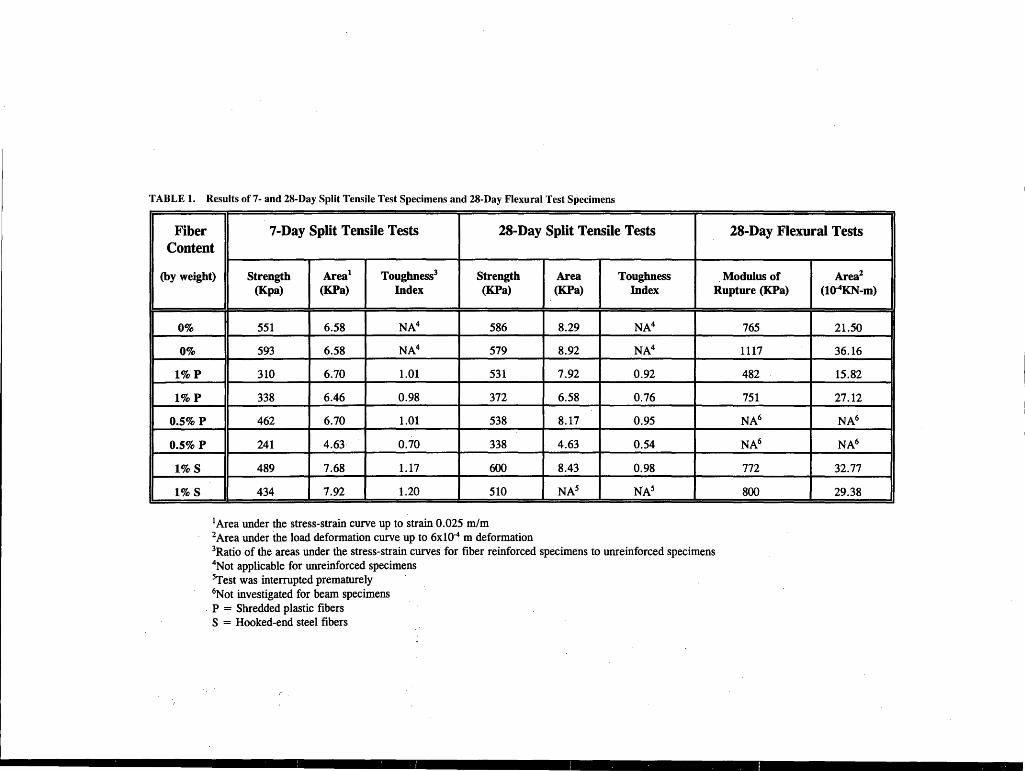
TABLE 1. Results of 7- and 28-Day Split Tensile Test Specimens and 28-Day Flexural Test Specimens
Fiber 7-Day Split Tensile Tests 28-Day Split Tensile Tests 28-Day Flexural Tests Content
(by weight) Strength Area1 Toughness3 Strength Area Toughness Modulus of Area2
(Kpa) (KPa) Index (KPa) (KPa) Index Rupture (KPa) (l04 KN-m)
0%
0%
1%P
1%P
0.5%P
0.5%P
1%S
1% s
551 6.58 NA4 586 8.29 NA4
593 6.58 NA4 579 8.92 NA4
310 6.70 1.01 531 7.92 0.92
338 6.46 0.98 372 6.58 0.76
462 6.70 1.01 538 8.17 0.95
241 4.63 0.70 338 4.63 0.54
489 7.68 1.17 600 8.43 0.98
434 7.92 1.20 510 NA5 NA5
1Area under the stress-strain curve up to strain 0.025 m/m 2 Area under the load deformation curve up to 6x10·4 m deformation 3Ratio of the areas under the stress-strain curves for fiber reinforced specimens to unreinforced specimens 4Not applicable for unreinforced specimens 5Test was interrupted prematurely 6Not investigated for beam specimens
. P = Shredded plastic fibers S = Hooked-end steel fibers
765 21.50
1117 36.16
482 15.82
751 27.12
NA6 NA6
NA6 NA6
772 32.77
800 29.38

Cavey et al.
700
600
500
~
~ 400 fll fll ~
""' ... Cl:J
..!! 300 ·~ ~ ~
200
100
0
-0.01
FIGURES
where
u = modulus of rupture, P = maximum applied load, s = length of span, b = average width of beam, and h = average depth of beam.
0 O.Ql 0.02
Strain (m/m)
__.__ 0%Fiber
--ft-- 0.5 % Plastic Fibers
_:s;;r.- 1 % Plastic Fibers
~ 1 % Steel Wire Fibers
0.03 0.04 0.05
103
Stress-strain curves for 28-day split tensile test specimens.
The results from the flexural tests show that one beam with no fibers, one with 1 percent plastic fibers, and the two with 1 percent steel fibers had approximately the same ultimate flexural strength or modulus of rupture [average of772 KPa (112 psi)]; one beam containing no fibers had the highest modulus of rupture [1117 KPa (162 psi)], and one of the beams containing I percent plastic fibers had the lowest modulus of rupture [482 KPa (70 psi)]. Relative to Beam 2 (the
12 r-~~~~~~~~~~~~~~~~~-.-~~~~~~~~----. ~ 0%Fiber
...Jfl-- 1 % Plastic Fiber
IO -B- 1 % Steel Wire Fiber
8
6
4
4
2
0 ..._~..___. ... ~..._~ ....... ~....i...~....i...~-1..~-i..~--1.~--1~---1'--~'--~.._____. -2 0 2 4 6 8 10 12
Deformation (10-4 m)
FIGURE 6 Load-deformation curves for 28-day flexural test specimens.

104
strongest unreinforced beam), there was a significant reduction (approximately 30 percent) in the average ultimate flexural strength· due to the inclusion of fibers; this is consistent with the previous results obtained from split tensile tests. The areas under the loaddeflection curves up to 0.6 mm (0.024 in.) deflection were calculated to estimate toughness (this method is typical for determining the toughness of a material subjected to a beam flexure test, in contrast to the strain criterion that was used for split tensile specimens). Although there was no meaningful change in toughness for any of the beams relative to that for Beam 2, there was a sharp drop in the load-carrying capacity of the unreinforced beams immediately after the peak load was reached. It is significant that these unreinforced beams manifested some modest level of post-peak load-carrying capacity, as represented by the recorded curves that are shown, until a brittle-type, catastrophic failure was encountered. On the other hand, the fiber-reinforced beams showed a relatively gradual decrease in their load-carrying capacity after the peak load was reached. These beams also sustained higher deformations than the unreinforced specimens, representing a more ductile type of failure.
Lesson Learned
Although the Illinois test program was conducted under reasonably well-controlled conditions (especially dry density and fiber length), the performance of the fiber-reinforced specimens suggests that the waste fibers used in this study are more likely to reduce, instead of enhance, the structural integrity and functional performance of a pavement system. Whereas the concept of toughness as a desirable attribute in a pavement system remains valid, the means to achieve it economically remains a challenge.
Comparison Study
To address the foregoing issue, a separate series of laboratory split tensile tests was conducted on specimens with the same basic mix design, except that they were reinforced with a commercially avail-
TRANSPORTATION RESEARCH RECORD 1486
able regular steel fiber commonly used in the concrete industry. The objective of this test program was to compare the performance of recycled fibers with that of a regular fiber and thereby attempt to explain the unsatisfactory performance of the recycled fibers, as observed during the field and laboratory tests. The fiber used in this study was a 60-mm (2.36-in.) long Bekeart Dramix hooked-end steel fiber with an aspect ratio of 75. Split tensile tests with lateral deformation measurements were performed on specimens with a dry density of approximately 1712 kg/m3 (107 pcf) and containing 1 and 4 percent steel fibers.
Results
The results of split tensile tests on 7-day and 28-day specimens are presented in Table 2. These data show that the average strength for 7-day specimens either remained the same (1 percent fiber) or decreased by approximately 10 percent ( 4 percent fiber) compared with that for unreinforced specimens, and the tensile strength of the 28-day specimens increased by approximately 15 percent (1 percent fiber) and 24 percent (4 percent fiber). The areas under the stressstrain curves up to a strain of 0.025 mlm showed a noticeable . increase in toughness for most of the specimens (with the exception of the 28-day specimens with 1 percent fibers). Figure 7 compares the performance of unreinforced specimens with those containing 4 percent fiber reinforcement, and a significant difference in behavior is observed; specifically, the toughness of a 28-day specimen with 4 percent fibers doubled relative to one with no fibers and a pseudohardening behavior was observed in the post-peak region. These specimens continued to carry load even when the lateral L VDTs reached their ultimate range and the tests were terminated (i.e., the specimens did not fail). This type of behavior is very desirable in a highway pavement system.
Lesson Learned
Significant improvement in the mechanical behavior (especially toughness) of a recycled aggregate mix can be achieved by incor-
TABLE 2. Results of7- and 28-Day Split Tensile Test Specimens with Hooked-End Steel Fibers
Fiber 7-Day Split Tensile Tests Content
(by weight) Toughness3
0%
0%
1%
1%
4%
4%
Strength Area1
(KPa) (KPa) Index
545 6.58 NA2
593 6.53 NA2
627 8.63 1.29
496 8.3 1.26
462 7.65 1.16
558 10.28 1.57
1 Area under the stress-strain curve up to strain 0.025 m/m 2Not applicable for unreinforced specimens
28-Day Split Tensile Tests
Strength Area Toughness (KPa) (KPa) Index
586 8.29 NA2
579 8.90 NA2
689 8.52 1.00
648 8.10 0.94
834 17.67 2.05
614 13.44 1.56
3Ratio of the areas under the stress-strain curves for fiber reinforced specimens to unreinforced specimens

-- - -------------
Cavey et al. 105
1000 ._._ 0%Fiber
900 ~ 4% Hooked-End Fiber
800
700
'i
~ 600
fll
~ ""'
500 .... 00 .! ·~ 400
~ 300
200
100
()
-0.01 () ().QI 0.02 0.03 0.04 0.05
Strain (rn/m)
FIGURE7 Stress-strain curves for 28-day split tensile tests with hooked-end steel fibers.
porating the correct amount of an appropriate fiber. It follows that the basic idea of fiber-reinforcement appears to have merit, and the unsatisfactory performance of the composite materials in the Maryland and Illinois studies was due to the inclusion of unsuitable waste fibers. Hence, careful evaluation is essential before using any waste product in highway construction, and studies are required to identify suitable candidate fibers and their optimum proportions within economical limits.
DISCUSSION OF RESULTS
The primary benefit obtained by adding fibers to a cement-based composite is to increase the energy absorption capacity or toughness (14). Higher toughness means higher fatigue strength and greater resistance to crack formation and propagation. A cementstabilized pavement layer is typically subjected to flexural (tensile) stresses in the slab, and this eventually leads to crack formation, crack propagation, and failure. If suitable fibers are incorporated in the pavement system in correct proportions, they can slow down the process of failure by effectively bridging the cracks and imparting a higher degree of tensile resistance to the material. Toughness is a measure of the effectiveness of the fibers in a composite; therefore, it is logical to expect that an improvement in this material property will enhance the flexural fatigue performance of a pavement system consisting of at least one layer of a fiber-reinforced composite. Accordingly, the material evaluations in this study were based primarily on the measured values of toughness.
Although there is perhaps little disagreement with the foregoing general concepts, incorporating fibers into pavement systems is limited by the cost of the fibers and the uncertainty of the benefit to be
achieved for this added cost. It follows that the economics would be significantly improved if low-cost or no-cost waste products could be used advantageously, and this is the principal motivating factor behind this study. Unfortunately, the recycled plastics and tire products in the forms and sizes described in this study not only afforded little or no improvement in material behavior, but also generally affected both the strength and toughness of the composite material adversely. Tire chunks, strands of tire wires, and strips of plastics acted more as defects in the composite system, instead of as beneficial additives. The unsatisfactory performance of the steel wires (which closely resemble "idealized" tire wires) suggests that, even if the tire wires could be economically separated from companion strands or tire chunks by complete removal of the rubber, they would still offer little benefit as fibers in a stabilized base course containing recycled concrete aggregate. The results of the comparison study indicated that recycled concrete aggregate would probably be suitable for use in a fiber-reinforced stabilized base course pavement system, provided the correct amount of an appropriate fiber is used. This use of recycled concrete aggregate would, of course, affect the economics and perhaps render the implementation unfeasible or unacceptable.
CONCLUSIONS
Although the basic concept of incorporating fiber-reinforcement in a highway base course to enhance the desirable property of toughness is generally accepted and appears achievable with a proper proportion of an appropriate fiber (even for the relatively low cement content of an economical cement-stabilized recycled concrete aggregate mix), the use of fibers from reclaimed waste products (shredded

106
plastic bottles and wires from scrap tires) did not produce the desired benefits. Instead, using fibers from waste products degraded the material properties relative to those of similar unreinforced mixes. Accordingly, notwithstanding the attractiveness of using waste materials from an environmental standpoint and from initial cost considerations, a careful evaluation of performance characteristics and life-cycle costs must be performed before any particular waste product is incorporated into a highway pavement system.
ACKNOWLEDGMENT
This study was supported financially by the Infrastructure Technology Institute at Northwestern University with funds received from the U.S. Department of Transportation.
REFERENCES
1. Proc., Recovery and Effective Reuse of Discarded Materials and Byproducts for Construction of Highway Facilities, Denver, Colorado, Environmental Protection Agency and FHWA, U.S. Department of Transportation, Oct. 19-22, 1993.
2. Ahmed, I., and C. W. Lovell. Use of Waste Materials in Highway Construction: State of the Practice and Evaluation of the Selected Waste Products. In Transportation Research Record 1345, TRB, National Research Council, Washington, D.C., 1992, pp. 1-9.
3. Ciesielski, S. K. A National Overview-The Use of Discarded Materials and By-Products in Hot Mix Asphalt Concrete Pavements. Proc., Recovery and Effective Reuse of Discarded Materials and By-products for Construction of Highway Facilities, FHW A, U.S. Department of Transportation and Environmental Protection Agency, Denver, Colo., Oct. 19-22, 1993, pp. 7-16.
4. Yrjanson, W. A. Recycling of Portland Cement Concrete Pavements. NCHRP Report 154: Synthesis of Highway Practice TRB, National Research Council, Washington, D.C., 1989.
5. Schutzbach, A. M. Recycling Old PCC Pavement-Peiformance Evaluation of FAl 57 Inlays. Physical Research Report No. 113, Illinois Department of Transportation, 1993.
6. Bosscher, P. J., T. B. Edil, and N. N. Eldin. Construction and Performance of a Shredded Waste Tire Test Embankment. In Transportation
TRANSPORTATION RESEARCH RECORD 1486
Research Record I 345, TRB, National Research Council, Washington, D.C., 1992,pp.44-52.
7. Humphrey, D. N., and R. A. Eaton. Tire Chips as Subgrade Insulation-Field Trial. Proc., Recovery and Effective Reuse of Discarded Materials and By-products for Construction of Highway Facilities, FHWA, U.S. Department of Transportation and Environmental Protection Agency, Denver, Colo., Oct. 19-22, 1993, pp. 55-68.
8. Smith, L. L., and R. M. Ramer. Recycled Plastics for Highway Agencies. In Transportation Research Record 1345, TRB, National Research Council, Washington, D.C., 1992, pp. 60-66.
9. Soroushian, P., A. Alhozaimy, and A. I. Eldarwish. Recycling of Plastics in Concrete To Enhance Toughness Characteristics and Resistance to Shrinkage Cracking.· Proc., Recovery and Effective Reuse of Discarded Materials and By-products for Construction of Highway Facilities, FHWA, U.S. Department of Transportation and Environmental Protection Agency, Denver, Colo., Oct. 19-22, 1993, pp. 41-53.
10. Benson, C. H., and M. V. Khire. Reinforcing Sand with Strips of Reclaimed High-Density Polyethylene. Journal of Geotechnical Engineering, Vol. 120, No. 5, American Society of Civil Engineers, 1994, pp. 838-855.
11. Groom, J.L., D. V. Holmquist, and K. Y. Yarbrough. Use of Waste Nylon Fibers in Portland Cement Concrete to Reduce Plastic Shrinkage Cracking. Proc., Recovery and Effective Reuse of Discarded Materials and By-products for Construction of Highway Facilities, FHW A, U.S. Department of Transportation and Environmental Protection Agency, Denver, Colo., Oct. 19-22, 1993, pp. 179-183.
12. Wang, Y., B-S Cho, and A-H Zureick. Fiber Reinforced Concrete Using Recycled Carpet Industrial Waste and Its Potential Use in Highway Construction. Proc., Recovery and Effective Reuse of Discarded Materials and By-products for Construction of Highway Facilities, FHWA, U.S. Department of Transportation and Environmental Protection Agency, Denver, Colo., Oct. 19-22, 1993, pp. 111-117.
13. Collins, J. H., and C. F. Usuda. Cellulose Fibers: An Abundant and Effective Asphalt Modifier for Highway Construction. Proc., Recovery and Effective Reuse of Discarded Materials and By-products for Construction of Highway Facilities, FHWA, U.S. Department of Transportation and Environmental Protection Agency, Denver, Colo., Oct. 19-22, 1993,pp. 119-124.
14. Balaguru, P. N., and S. P. Shah. Fiber-Reinforced Cement Composites. McGraw-Hill, Inc., 1992.
Publication of this paper sponsored by Committee on Chemical and Mechanical Stabilization.

PART3
New Aggregate Tests '


TRANSPORTATION RESEARCH RECORD 1486 109
Uses of Waste Foundry Sands in Ci vii Engineering
SAYEED JAVED AND C. W. LOVELL
Molds and cores for metal castings are normally sands with chemical or clay binders and other additives. After the casting is complete, the sand is disaggregated, and it is judged whether it is suitable for reuse. However, after several uses, the sand is no longer suitable and is designated as a waste foundry sand (WFS). Such waste has been disposed in landfills, public and private. Although some WFSs may contain excessive amounts of harmful heavy metals, those discarded after ferrous castings contain only iron, and this concentration is controlled by magnetic extraction from the waste. At this point, only WFSs from ferrous castings are thought to be environmentally acceptable. Through laboratory study of the ·mechanical and physical properties of WFSs from the greensand, shell, and chemically bonded processes for ferrous castings, a number of civil engineering uses have been identified: embankment fill, subgrade, flowable fill, and fine aggregate replacement in asphaltic concrete. The index properties of the WFSs and the appropriate test parameters for its various acceptable uses are described. The next step is to build demonstration and implementation projects to prove the practicality of the use and to provide long-term evidence of the absence of significant environmental effects.
Recent legislation in Indiana has intensified study of the use of industrial and domestic waste products in civil engineering, particularly in highways. The wastes given primary attention are scrap tires, coal combustion byproducts, destructed pavement materials and building demolition products, and spent foundry sands. This paper summarizes properties and potential uses of spent (waste) foundry sand.
The desire of Indiana foundries to reduce disposal costs led to the sponsorship of a 2-year study of waste foundry sand (WFS) in the School of Civil Engineering at Purdue University. The authors of this paper wrote the research report resulting from the study (J). The potential uses given greatest attention were WFS as embankment and subgrade material, fine aggregate in controlled low strength material (CLSM), (also called flowable fill), and fine aggregate in asphaltic concrete (3).
BACKGROUND
Sands have long been used for metal casting. They are chosen for several important reasons (3): they are readily available, inexpensive, highly refractory, and readily bonded by clays or other inorganic and organic material.
There are three types of molding processes: greensand, chemically bonded, and shell molded. In Indiana, the most commonly used process is greensand molding. The greensand mixture contains clay, combustible additives like seacoal, and water. The predomi-
S. Javed, Geotest Engineering, Inc., 5600 Bintliff Drive, Houston, Tex. 77036. C.W. Lovell, School of Civil Engineering, Purdue University, West Lafayette, Ind. 4 7907.
nant metal cast is gray iron. After a number of uses, the molding sands lose the desired qualities and are discarded. The foundry may operate a monofill for these wastes or may transport them to a municipal solid waste landfill. In either case, the disposal costs are significant, and the foundries are anxious to reduce them.
The grain size distribution of WFS is uniform, with most sizes within a narrow range between the No. 50 and No. 100 sieves. This means that they are finer than the materials generally specified for fine aggregates.
The greensands, with their additives of clay, demonstrate cohesive type behavior and the chemically bonded and shell-molded sands show cohesionless response. Consequently, greensand compaction curves show a definite dependence on compaction moisture content. The compacted unit weights of others is almost independent of that moisture content.
The results of standard heavy metal leaching tests, like the EPTOX and the Toxicity Characteristics Leaching Procedure (TCLP), depend on the metals cast because the WFSs are commonly contaminated by these metals. Much of the metal cast in Indiana is ferrous, and although limits are seldom exceeded, iron is occasionally present in concentrations above those stated. Chemically bonded and shell-molded WFSs contain chemicals and organics that may require special environmental assessment before routine use.
CHARACTERIZATION OF WFS
Experimental work on WFSs in the School of Civil Engineering, Purdue University, involved seven samples from greensand processes, two from chemically bonded processes, and one from a shell molding process. All of these involved ferrous castings.
Compactability of these sands is of considerable interest for embankment and subgrade applications. The WFSs from chemically bonded and shell-molded processes are cohesionless and respond best to vibratory compaction. The waste. greens ands are compacted best by impact (Pro.ctor) type processes: Figure 1 shows the moisture-density and moisture-California Bearing Ratio (CBR) relations for the raw sand (Rl) that comprises the casting sands. As is common for such materials, density varies little with compaction water content, although it is somewhat higher for a flushed condition. The soaked CBR is also maximized at this higher water content.
The WFSs from greensand casting for sample G 1 are illustrated in Figure 2. Unit weight ~trongly depends on moisture content, and soaked CBR is maximized at about the optimum moisture content. Note that the swell upon soaking is small arid that the soaked CBR values compare favorably with compacted natural soils.
Shear strength parameters were determined by performing direct shear tests on dry samples at various densities. The data are sum-
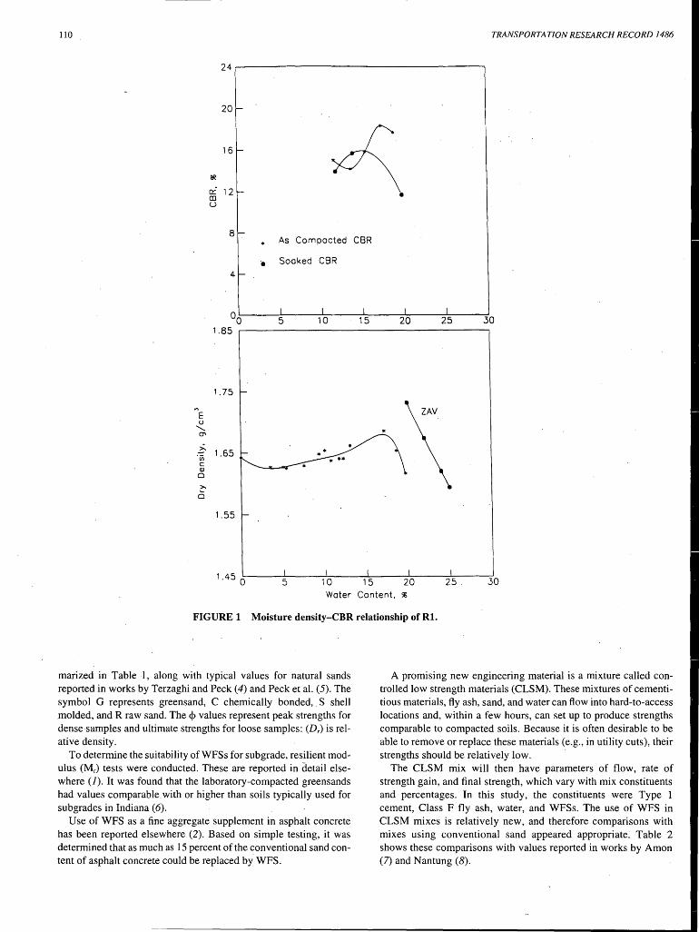
110 TRANSPORTATION RESEARCH RECORD 1486
24
20 -
16 >--
~
rY 12 ...... CD u
8-As Compacted CSR
• Soaked CSR
4-
00 I I I I I
5 10 15 20 25 30 1.85
1.75 .., E u
.......... O'
~ 1.65 "iii c <U 0
>-. a 1.55
1.45 0 5 iO 15 20 25 30 Water Content, %
FIGURE 1 Moisture density-CBR relationship of Rl.
marized in Table 1, along with typical values for natural sands reported in works by Terzaghi and Peck ( 4) and Peck et al. (5). The symbol G represents greensand, C chemically bonded, . S shell molded, and R raw sand. The <P values represent peak strengths for dense samples and ultimate strengths for loose samples: (Dr) is relative density.
To determine the suitability ofWFSs for subgrade,resilient modulus (Mr) tests were conducted. These are reported in detail elsewhere (1). It was found that the laboratory-compacted greensands had values comparable with or higher than soils typically used for subgrades in Indiana (6).
Use of WFS as a fine aggregate supplement in asphalt concrete has been reported elsewhere (2). Based on simple testing, it was determined that as much as 15 percent of the conventional sand content of asphalt concrete could be replaced by WFS.
A promising new engineering material is a mixture called controlled low strength materials (CLSM). These mixtures of cementitious materials, fly ash, sand, and water can flow into hard-to-access locations and, within a few hours, can set up to produce strengths comparable to compacted soils. Because it is often desirable to be able to remove or replace these materials (e.g., in utility cuts), their strengths should be relatively low.
The CLSM mix will then have parameters of flow, rate of strength gain, and final strength, which vary with mix constituents and percentages. In this study, the constituents were Type 1 cement, Class F fly ash, water, and WFSs. The use of WFS in CLSM mixes is relatively new, and therefore comparisons with mixes using conventional sand appeared appropriate. Table 2 shows these comparisons with values reported in works by Amon (7) and Nantung (8).

Javed and Lovell 111
28 0.4
• As Compacted CSR Soaked CBR
24 .-- 0 Swell -. '\
20 \ 0.3
!R 16 /~~
!R I ~ Ck'. 0.2 Q;
CD ~ ~ u 12 (/)
8 I
\
\ 0.1
i ·4
•
00 5 10 15 20 2SJ·O 1.85
1.80
1.75
..., E u 1.70
.......... O"I
~ 1.65 ·v; c:: QJ
Q
>-. 1.60 a
1.55
1.50
1 .45 0 I 5 10 15 20 25
Water Content, sg
FIGURE2 Moisture density-CBR relationship of G 1.
The WFSs are assumed to be free of charge and, within a short distance of source, produce CLSMs that are economical. Mix 3 is preferred within this set, but the use of WFS raises questions of porosity and permeability, as well as setting rate. These issues are being addressed in current research (9).
ENVIRONMENTAL CONCERNS
All of the WFSs tested in this study were from ferrous castings. Therefore, one would expect that the only elements present in the waste sand would be the additives and a small amount of iron. Because the principal additives in greensand are clay and seacoal, these materials would be expected to pass all reasonable environmental tests. The greensands pass the various leaching tests. Bio-
assay testing (a waste water technique) is also planned for these materials, but they are expected to pass.
There is no specific environmental testing for the chemicals and other inorganic or organic substances used in chemically bonded and shell-molded WFSs; therefore, more potential risk is involved. One also expects that greensand casting of other metals (e.g., aluminum), will yield a nonhazardous waste. Conversely, other castings, like brass, would be highly suspect.
Two use scenarios appear well-suited for demonstrating the use of greensand from ferrous casting:
• Well-drained situations like subgrades and embankmentsleachate in such situations is small and is further minimized by clayencasing layers on the sides. Some sort of growing layer would need to be placed at the sides, even without the encasement requirement.

TABLE 1 Results of Direct Shear Tests
Loose Dense Sample# Dr c (kPa) 0 (deg) Dr c (kPa) 0 (deg)
G1 29 4.13 32.4 90 . 9.92 36.6
G3 34 5.17 34.2 98 12.54 40.9
C2 22 0.41 30.4 94 7.17 34.9
Sl 31 0.41 30.8 94 4.75 36.5
Rl 32 0.21 30.4 88 1.17 33.8
Uniform Moderately 32-34 Very 35-38 medium sanda dense dense Sandb Loose 29-30 Dense 36-41
1.0 psi = 6.89 kPa a (4) b (5)
TABLE 2 Spread, Density, and Compressive Strength for Different Mixes
Mix No. 1 2 3 4 5 lN ES-lb
Cement (kg/m3) 78 74 59 33 45 47 37
Fly ash (kg/m3) 259 246 94 109 82 249 190
Water (kg/m3) 414 442 439 438 454 333 293
WFS or Sand (kg/m3) 1140 1080 1265 1262 1261 1503 1645
Spread (mm) 190.5 228.6 208.3 205.7 208.3 -c 127-i52
Density (kg/m3) 1890 1842 1858 1842 1842 -c 2147
Compressive strength (kPa) 3 - Day 296 282 248 59 165 -c 138
7 - Day 462 372 303 62 214 310 207
28 - Day 710 551 482 55 379 827 551
1.0 pcy = 0.593 kg/m3, 1.0 in = 25.4 mm, 1.0 pcf = 16.02 kg/m3 , 1.0 psi = 6.89 kPa
a (7) 1>(8) c Data not available

Javed and Lovell
• Stabilized mixtures like CLSMs-although these are wet and poorly drained situations (trenches, around pipes and tanks), the WFSs are reasonably well fixed in the mix. Porosity and permeability of the CLSM need to be given greater attention to increase confidence in this usage.
CONCLUSIONS
• The WFSs passed all environmental tests and demonstrated good physical and mechanical properties.
• Greensands from ferrous castings appear likely to pose very low environmental risk.
• Shell-molded and chemically bonded WFSs pass all existing leaching tests but warrant further study with respect to chemical and organic additives before use.
• Uses most favored for demonstration projects are (a) welldrained embankments and subgrades and (b) a fine aggregate in CLSMs.
• The WFSs are likely to be economically competitive when the project is close to a disposal source.
ACKNOWLEDGMENT
The research reported herein was funded by the Indiana Cast Metals Association, which has its headquarters in Indianapolis, Indiana.
113
REFERENCES
1. Javed, S., and C. W. Lovell. Use of Waste Foundry Sand in Highway Construction. Report JHRP/INDOT/FHW A-94/2. School of Civil Engineering, Purdue University, West Lafayette, July 1993.
2. Javed, S., C. W. Lovell, and L. E. Wood. Waste Foundry Sand in Asphalt Concrete. In Transportation Research Record 1437, TRB, National Res~arch Council, Washington, D.C., 1994, pp. 27-34.
3. Parkes, E., G. Westwood, and R. Grigg. Molding and Core Sands. In Applied Science in the Casting of Metals, (K. Strauss, ed.), Foesco International Limited, Permagon Press, Birmingham, Great Britain, 1970, pp. 313-360.
4. Terzaghi, K., and R. B. Peck. Soil Mechanics in Engineering Practice. John Wiley and Sons, Inc., New York, 1948.
5. Peck, R. B., W. E. Hanson, and T. H. Thornburn. Foundation Engineering. John Wiley and Sons, Inc., New York, 1974.
6. Lee, W. Evaluation of In-Service Subgrade Resilient Modulus with Con. siderations of Seasonal Effects. Ph.D. thesis, Purdue University, West Lafayette, Ind. 1993.
7. Amon, J. A. Controlled Low-Strength Material. Construction Specifier, Vol. 43, No. 12, Dec. 1990, pp. 98-101.
8. Nantung, T. Design Criteria of Controlled Low Strength Materials. Ph.D. thesis. Purdue University, West Lafayette, Ind. Aug. 1993.
9. Bhat, S. T., C. W. Lovell, C. F. Scholer, and T. E. Nantung. Flowable Fill Using Waste Foundry Sand. Proc., 1 lth/nternational Symposium on Use and Management of Coal Combustion By-Products, Vol. 2 (CCBs), EPRI TR-104657-V2, Project 3176, Orlando, Fla., Jan. 1995, pp. 39-1 to 39-14.
Publication of this paper sponsored by Committee on Cementitious Stabi/i.zation.

114 TRANSPORTATION RESEARCH RECORD 1486
Assessment of Suitability of Some Industrial By-Products for Use in Pavement Bases in the United Kingdom
A. R. DAWSON, R. C. ELLIOTT, G. M. ROWE, AND J. WILLIAMS
The increasing demand for materials and the increasing quantity of waste generated has created opportunities for the use of alternative materials in road construction. Industrial by-products for use in pavement bases are assessed. The objectives of the research were to (a) review industrial by-products for possible use in bound pavement bases in the U.K., (b) evaluate the structural properties and workability of selected materials identified in this review by laboratory and pilot scale pavement testing, and ( c) relate material performance to that of standard materials used in pavement bases. The work used not only conventional roadbase binders, such as cement and bitumen, but also self-cementing materials and mixtures incorporating alternative hydraulic binders, such as blast-furnace slag/lime and pulverized fuel ash/lime. The performance of all these mixtures is described.
The United Kingdom is well supplied with rock suitable for quarrying to produce high-quality aggregate for pavement construction. However, extraction is becoming increasingly difficult because of environmental and societal constraints. Thus it is inevitable that pavement engineers should turn to other sources for aggregate supplies. Among the most attractive sources are those secondary aggregates generated as by-products of various industries. The use of such aggregates may
• A void the problems of obtaining conventional aggregates, • Result in economic gains to the industry generating the by
products, and • Result in environmental gains to industry and society.
Against these positive benefits, the pavement engineer must set the uncertainties of behavior of the replacement aggregate. Often, there is little or no experience with the use of replacement aggregate, and it has observably different forms, which would appear likely to influence performance. Thus, extrapolation from conventional aggregate to by-product aggregate behavior appears imprudent.
To address these issues, after a desk review a research study of eight different by-products and recycled aggregates for use in pavement roadbases was performed by SWK Pavement Engineering for the U.K. Department of Transport. The University of Not-
A. R. Dawson, University of Nottingham, University Park, Nottingham NG7 2RD, United Kingdom. R. C. Elliott, SWK Pavement Engineering Ltd., 9 Faraday Building, Highfields Science Park, University Boulevard, Nottingham NG7 2QP, United Kingdom. G.M. Rowe, SWK Pavement Engineering Inc., Stonehouse Road, P.O. Box 211, Millington, N.J. 07946. J. Williams, Highways Agency, St. Christopher House, Southwark Street, London SEl OTE, United Kingdom.
tingham acted as principal subcontractor with many of the laboratory tests performed in its Civil Engineering Department laboratories.
OBJECTIVES
The objectives of the research were as follows:
• To review industrial by-products for possible use in bound roadbases in the U.K., taking into account the benefits, limitations, practical problems, likely performance, economics, environmental considerations, and existing specifications;
• To evaluate the structural properties and workability of selected materials, as identified previously in the description of the review objective, by laboratory and pilot scale pavement testing, and
• To relate material performance to that of standard materials used in pavement bases.
REVIEW OF CANDIDATE BY-PRODUCT AND RECYCLED AGGREGATES
A study conducted for the U.K. Department of Environment (J) identified the amount and geographical availability of a wide range of potential by-product, waste, and recycled aggregates. Omitting those arising or stockpiled in insignificant volumes or for which chemical uncertainties were identified (e.g., cement kiln dust, municipal solid waste incinerator ash), the following materials were considered in more detail.
China Clay Waste
Clay for high-quality pottery and paper glazing is extracted from partially decomposed granite in southwest England using highpressure water jets. A micaceous gravelly sand residue and a lessdecomposed granite are the principal waste materials. The former is candidate aggregate material as the washing process has cleaned it and imposed a fairly consistent grading (although finer than conventional aggregates). The coarser rock is a mixed material comprising large boulders, decayed rock, clay pockets, and so forth, and was not considered further in view of the likely processing cost and high wastage needed to produce a useful and consistent aggregate.

Dawson etal.
Slags
Steel and blast-furnace slags from the steel-making industry are available in several locations across the U.K. Blast-furnace slag is readily sold (as a cement modifier for example) whereas steel slag is less easily processed and less highly used. For these reasons, blast-furnace slag was identified as a potential binder (a relatively high-value, low-volume use) and steel slag as a potential aggregate.
Coal and Oil Shale Waste
Large volumes of rock incidentally excavated as part of the coal mining process are found in many parts of the U .K. In addition, in the Lothian region of Scotland, large stockpiles of shale from which oil was abstracted are available. The material is typically a weak rock, which when unburnt has a high carbonaceous content. Some of the coal waste, known as minestone, and all the oil shale waste have been burnt. This reduces the carbonaceous content and alters the shale to a less clayey and stronger form. However, the unburnt form is more widespread and is the only type currently arising. Thus this type of minestone was identified as a candidate · aggregate.
Slate Waste
In the past, slate was the principal roofing material used in the U.K. Some 90 percent of rock quarried to produce roofing slates is wasted, so huge stockpiles of broken slatey rock exist, which can be crushed to produce a conventional, if very flaky, aggregate. Such material is available in several locations on the western side of the U.K. and was an obvious material to include in this project.
Power Station Ash
Coal-fired power stations are common in the U.K. and generate coarse (furnace bottom) and fine (pulverized fuel) ash. The former is available in much lower quantities than the pulverized fuel ash (pfa) (sometimes known as fly ash) and is largely consumed by the construction industry as the principal ingredient of light-weight building blocks. For these reasons, orily pfa was selected as a potential material for study.
Demolition and Construction Waste
Crushed concrete and brick masonry provide an aggregate that is readily available in urban areas. At present, much is used as lowquality fill, but the material appears to have potential as an aggregate in engineered layers of the pavement. It is known (2) that unhydrated portland cement is liberated when concrete is crushed, giving fresh samples of crushed concrete the ability to self-cement and hence gain strength with time to generate a very high-quality pavement layer. A proportion of crushed bricks might dilute this effect but would permit greater volumes to be available. Thus, pure crushed concrete and a 50:50 mix of crushed concrete and crushed brick were selected for further study.
To use these materials in roadbases of pavements making the primary road network, prudence and limited past experience suggested
115
that all materials (except the potentially self-cementing demolition waste aggregate) should be used with portland cement, lime, slag, ash, asphalt cement, or bitumen emulsion cement.
MIX DESIGN
Selection of Combinations
Nine mixes were proposed for detailed study with conventional pavement roadbase material types. The basic components of the five hydraulically bound mixes (Mixes A through E) were selected on the basis of experience of similar mixes in the U.K., France, and the Netherlands. Four asphaltic mixes were chosen (Mixes F through I) using conventional asphalt cement, except for Mix I. This mix included crushed brick as part of the aggregate and used a cold-mix emulsion as the binder to overcome anticipated problems of bitumen adhesion. Mix I was a potential poor performer and by thus covering a range of performances, it was hoped to make subsequent interpretation of laboratory and pilot scale test results easier.
For control purposes three conventional mixes were also selected (Mixes J through L). One made up a conventional aggregate bound with portland cement, _one a conventional aggregate asphalt concrete, and one a conventional unbound aggregate. Each mix and its basis of selection is listed in Table 1.
Mix Proportioning
For Mixes A through I, the aggregate gradings were selected on the basis of those used in the reference roadbase mixes being "mirrored" by the new materials (see the last column of Table 1). Where the available material had a very different grading.from this reference material, the as-supplied grading was used to minimize processing and thus make the potential material more economic in routine use.
The ratio of the components used in Mixes. A through E was determined using tests appropriate for the particular mixture selected. Thus for the portland cement-bound· materials, cube compressive strength and density testing was important. For more lightly bound materials, stiffness assessment and maximum shear strength were determined in the triaxial test. Initially mix propor-
. tions were selected on the basis of similarity to reference roadbase mixes. Proportions were then varied to optimize density, compressive cube strength (Mixes A, B, C, D), triaxial compressive strength (Mixes C, D, E), and California bearing ratio (CBR) strength (Mixes C, E). Mix J was designed according to the relevant standard specification for lean-mix portland cement bound material (3). For Mixes Band J, the target cube crushing strength was 10N/mm2
at 7 days and for Mix A, 4N/mm2• For Mixes C, D, and E, slower
development of strength was anticipated, and hence the assessment of the mix-strength relationship was made on the basis of 28- and 60-day strength evaluations. A 28-day triaxial maximum deviator stress of 1500 kPa was required.
For the bituminous mixes (Mixes F through I), the Nottingham asphalt tester (NAT) was used to measure mechanical properties, particularly indirect tensile stiffness modulus (ITSM) and deformation resistance in the repeated load axial test (RLAT) (4). The proportions of materials in Mix F were optimized volumetrically and by determining the highest stiffness value in the ITSM while increasing the asphalt cement content from 3 to 6 percent in 0.5 per-

116 TRANSPORTATION RESEARCH RECORD 1486
TABLE 1 Mixes Selected for Detailed Evaluation
Mixture Aggregate Binder Notes Reference
Bound with Portland Cement or other Hydi:aulic Binder
A pfa Portland Cement Similar to a material supplied historically in the UK
B Slate Portland Cement Similar to a lean mix Portland concrete used in the UK but with non-standard aggregate
c Limestone Granulated Similar to Grave Laitier successfully used in Blastfumace Slag/ France
Lime
D Crushed None (Self- Successful experience in the Netherlands Portland cementing) with this material Cement
Concrete
E Selected pf a/Lime Similar to a material successfully used in Minestone France
Bound with Asphalt Cement
F "China Clay" Bitumen (Penetration Sand asphalt type material Sand Grade)
G Slate Bitumen (Penetration Asphalt concrete material with very flaky Grade) aggregate and mixture design based upon
volumetric parameters
H Steel Slag Bitumen (Penetration Assessment of slags with relatively high Grade) "free lime". Asphalt concrete design based
upon volumetric parameters
I Demolition Bitumen Emulsion Aggregate to be a 50/50 mix of brick and ·waste concrete waste.
Control Mixes
J Sand + Gravel · Portland Cement Conventional Lean Mix Portland Concrete
K ·Limestone Bitumen (Penetration Conventional Asphalt Concrete Grade)
L Limestone None
cent increments. Three percent lime was added to the as-supplied china clay sand to aid asphalt cement adhesion.
The slate-based asphalt concrete (Mix G) was proportioned using ·ITSM and RLAT assessments on a conventionally graded (3) mix with 2.5 to 7 .5 percent (again, in 0.5 percent increments) of 50 pen asphalt cement. The chosen mix shared the highest ITSM stiffness, good RLA T resistance to permanent deformation, and optimum volumetric composition. Additional tests in which nonstandard gradings were tried only indicated that the best performance was available from the standard grading even though the aggregate was more flaky than normal. However, this testing indicated that partial filler replacement by lime was beneficial.
The slag-based mix (Mix H) was used as supplied, having discarded the particles larger than 20 mm, and the asphalt cement composition optimized as before. Two pilot scale trials were conducted
Conventional Unbound Mix
with this material, the second with the binder content increased by 0.5 percent because of the premature failure of the first trial by cracking in the longitudinal wheelpath.
The demolition waste and bitumen emulsion mix (Mix I) was treated in a different manner. First, the aggregate was divided into seven fractions, and the (relatively high) water absorbency was determined for each. This showed that prewetting to 7 percent moisture content was required to obtain adhesion of the emulsion. The graded fractions were recombined to obtain a standard (3) asphalt concrete aggregate grading, and sufficient emulsion was added to provide 4.7 percent residual binder (the amount indicated by con~ ventional mix experience for this grading). Attempts were made to replace part of the natural filler with lime and to modify the grading, but no improvement in ITSM stiffness was detected. Testing for this mix was performed at 28 days for the emulsion to "break" and excess water to be lost.
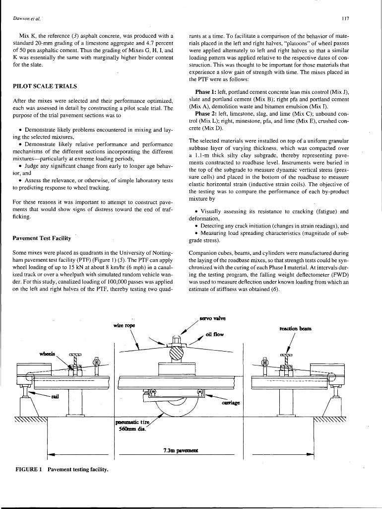
Dawson etal. ·
Mix K, the reference (3) asphalt concrete, was produced with a standard 20-mm grading of a limestone aggregate and 4.7 percent of 50 pen asphaltic cement. Thus the grading of Mixes G, H, I, and K was essentially the same with marginally higher binder content for the slate.
PILOT SCALE TRIALS
After the mixes were selected and their performance optimized, each was assessed in detail by constructing a pilot. scale trial. The purpose of the trial pavement sections was to
• Demonstrate likely problems encountered in mixing and laying the selected mixtures,
• Demonstrate likely relative performance and performance mechanisms of the different sections incorporating the different mixtures-particularly at extreme loading periods,
• Judge any significant change from early to longer age behavior, and
• Assess the relevance, or otherwise, of simple laboratory tests to predicting response to wheel tracking.
For these reasons it was important to attempt to construct pavements that would show signs of distress toward the end of trafficking.
Pavement Test Facility
Some mixes were placed as quadrants in the University of Nottingham pavement test facility (PTF) (Figure 1) (5). The PTF can apply wheel loading of up to 15 kN at about 8 km/hr (6 mph) in a canalized track or over a wheelpath with simulated random vehicle wander. For this study, canalized loading of 100,000 passes was applied on the left and right halves of the PTF, thereby testing two quad-
117
rants at a time. To facilitate a comparison of the behavior of materials placed in the left and right halves, "platoons" of wheel passes were applied alternately to left and right halves so that a similar loading pattern was applied relative to the respective dates of construction. This was thought to be important for those materials that experience a slow gain of strength with time. The mixes placed in the PTF were as follows:
Phase 1: left, portland cement concrete lean mix control (Mix J), slate and portland cement (Mix B); right pfa and portland cement (Mix A), demolition waste and bitumen emulsion (Mix I).
Phase 2: left, limestone, slag, and lime (Mix C); unbound control (Mix L); right, minestone, pfa, and lime (Mix E), crushed concrete (Mix D).
The selected materials were installed on top of a uniform granular subbase layer of varying thickness, which was compacted over a 1.1-m thick silty clay subgrade, thereby representing pavements constructed to roadbase level. Instruments were buried in the top of the subgrade to measure dynamic vertical stress (pressure cells) and placed in the bottom of the roadbase to measure elastic horizontal strain (inductive strain coils). The objective of the testing was to compare the performance of each by-product mixture by
• Visually assessing its resistance to cracking (fatigue) and deformation,
• Detecting any crack initiation (changes in strain readings), and • Measuring load spreading characteristics (magnitude of sub
grade stress).
Companion cubes, beams, and cylinders were manufactured during the laying of the roadbase mixes, so that strength tests could be synchronized with the curing of each Phase I material. At intervals during the testing program, the falling weight deflectometer (FWD) was used to measure deflection under known loading from which an estimate of stiffness was obtained (6).
servo valve wire rope
.__...........__~ oil flow
reaction beam
I
FIGURE 1 Pavement testing facility.
pneumatic tire S60mm dia . .
7.3m pavc:meot

118
By this means, all the hydraulically bound materials, the unbound base, and the cold mix bituminous emulsion bound material (which would exhibit low early strength) were tested at pilot scale under actual rotating tire loading, at realistic contact stresses, although at a somewhat reduced scale.
Slab Test Facility
The hot-mix asphalt materials that have early strength and for which time-dependent property changes were not expected were subjected to simulative wheel loading by the University of Nottingham slab test facility (STF). The STF is a small-scale wheel-loading apparatus in which trial slabs can be placed and subjected to simulated vehicle loading under controlled conditions. The loading system is servo hydraulic controlled.
Bidirectional tracking was used, with no traversing (lateral wander). The loading wheel was fitted with a pneumatic tire, which could be inflated to give a maximum contact pressure of around 650 kPa. Pavement temperature was maintained at a constant 20°C.
This device provides a realistic tire loading and contact stress but simplifies the pavement by using a 1 X 0.5 X 50 mm slab of asphaltic material supported on a rubber mat. The rubber simulates the support normally offered by the pavement subbase and subgrade. As the asphalt slab flexes, tensile strains are generated in the lower half, which are monitored by strain gauges fixed to the underside of the slab. Furthermore, surface rutting and fatigue cracking are induced. These can also be monitored and the materials' performance thereby assessed. Testing ceases when longitudinal surface cracking commences in the wheelpath.
Design of Trial Pavement Thicknesses
The design of the pilot scale trials involved performing analytical calculations to predict the tensile stresses and strains at the base of the bound roadbase layers. The PTF pavements were analyzed using an elastic analysis and relevant material properties for the hydraulically and bituminous bound materials. Critical input parameters to the analysis were as follows, with the total pavement structure (subbase and bound roadbase) assumed to be 300-mm thick:
Parameter Value Unit
Wheel load 10 kN Contact area 0.016 m2 Speed 6 km/hr E soil 40 MP a E subbase 100 MP a E roadbase 2,000-30,000 MP a Poisson ratio soil 0.45 Poisson ratio subbase 0.4 Poisson ratio roadbase 0.2, 0.3
The determined pavement thicknesses are shown in the following table:
Mixture Roadbase Sub base Estimated Life Reference Thickness (mm) Thickness (mm) (No. of Load repetitions)
B, J 75 210 104 A 130 155 104
C,D,E,L 185 100 104-105 I 110 175 104
TRANSPORTATION RESEARCH RECORD 1486
For the asphaltic mixtures (Mixes F, G, and H), a constant slab thickness of 50 mm was used in the STF, with the load level adjusted to produce a tensile strain level that would give an estimated life between 1()4 and 105 load repetitions. A slab thickness of 50 mm was also used for the control asphalt concrete (Mix K).
Construction
For the PTF, the subgrade was assessed as having a mean CBR of 4 percent. This was leveled, and the pressure cells installed in "pockets" and covered by a small amount of fines taken from the aggregate. Next, the sub-base, comprising a crushed diorite aggregate passing the 37.5-mm sieve, was placed as a 100-mm thick layer and compacted using a pedestrian vibrating roller with 20 passes. Additional aggregate, to bring the thickness to that of the design, was then placed, screeded to the correct thickness, and compacted as before. The strain coils were then placed on this prepared surface.
Above this foundation, Mixes A through E, I, J, and-L were placed and compacted, generally in two lifts of roughly equal thickness. The exact mixing and placing procedures varied a little with the material, but, in general, a 200-kg capacity concrete mixer was used to batch the mix, which was then gently tipped into position and raked and screeded to its proper final level. The same pedestrian roller was used as before, but the initial two passes were applied without vibratio~. This was then followed by 12 passes with vibration and, for the upper lift, completed by 2 passes without vibration to generate a smooth surface. Notable departures from this general approach were
• Mixes B and J (slate and conventional portland cement lean mix concretes)-laid in only one lift, and
• Mix L (conventional unbound aggregate)-no premixing.
Performance
As the mixes described were placed in the PTF or STF, companion specimens were cast for the portland cement and hydraulic bound materials. For the bituminous materials, cores were cut from companion roller compacted slabs (which used the same compaction procedure as for the STF slabs). Additional cores were removed from untrafficked parts of the PTF and STF after completion of the trial. loading. The recorded properties of the hydraulic, portland cement-bound and unbound materials' companion samples are summarized in Table 2. Those for the asphaltic materials are given in Table 3. The response of the pilot scale pavements to trafficking is summarized in Tables 4 and 5, with typical surface deformation and subgrade stress relationships shown in Figures 2 and 3.
Table 5 gives relevant data for the asphaltic materials, all except Mix I, being relevant to the slab test facility testing. In addition to the results illustrated in the figures and tables, FWD measurements were also taken on the PTF pavements.
DISCUSSION OF RESULTS
The reduced scale of the pilot scale trials and the large number of mixtures investigated inevitably means that the results must be interpreted somewhat subjectively, relying on comparison, where possible, instead of using numerical values as definitive absolutes. Nevertheless the results yield some interesting observations, allow-

Dawson et al.
TABLE 2 PTF Companion Specimens-Hydraulic Mixtures
Mixture Reference
A
B
c
D
E
J
L
Note: 1. 2. 3. 4. 5.
Cube Cube Compressive Triaxial Maximum Flexural E,,timated Test Age Density4 Strength (N/mm1) Deviator Stress1 Streogth5 Stiffness' (Days) (kg/m3) (N/mm1} (N/mm1) (MPa)
1750 12.5 - 7 1720 17.0 0.9 27 1730 22.0 - 60
2590 24.5 6 2570 32.5 5.0 27 2560 33.0 60
- 2.6 715 2 2430 5.5 4.4 980 28 2430 7.0 59
- 2.0 420 1 2110 2.0 2.81 780 28 2090 2.5 - - -..
- - 1.1 280 1 2200 4.5 3.5 1110 28 2170 6.0 - - 58
2450 9.5 - 7 2450 12.5 1.9 28 2440 14.0 - 60
2410 2.4 485 2 2410 - 2.9 725 28
28 day Triaxial data from Mixture D are actually from 14 day test (membrane leaked spoiling both 28 day tests). Triaxial Maximum Deviator Stress and Estimated Stiffness recorded at 200kPa confining pressure. Stiffness estimated during modified triaxial loading procedure. The. cube data are averages of two specimens. The beam data are averages of three specimens.
119
ing a gqod assessment as to the suitability or otherwise of the mixtures studied.
ilar response of the two mixtures is evident from the data in Tables 2 and 4, which show that wheelpath rutting is barely different and load spreading of the slate material is as efficient at reducing subgrade stresses, but its strength is better. The strain coil readings were subject to interference and have to be interpreted with caution. However, the strain levels in B and J appear to be similar and significantly lower than in other materials, indicating good load spreading. The back calculated stiffnesses from FWD testing showed that, although the conventional Mix J was
Mix B: Portland Cement Lean Concrete with Slate Aggregate
Mix B is the lean mix portland cement concrete containing slate aggregates in place of conventional crushed rock (Mix J). The sim-
TABLE 3 Companion Specimens-Asphaltic Materials
MixtureR Density (Mg/m3) Calculated ITSM Stiffness (MPa) ef. Air Voids
Bulk Maximum (%) 0°C 10°c 20°c
F 1.92 2.47 221 4970 2130 890
G 2.47 2.62 5.8 18250 7370 2660
H 2.91 3.03 4.0 22260 11520 4530
I 1.71 2.38 281 2510 1630 1040
K 2.45 2.48 3.2 21330 12460 5210
RLAT Test Age Permanent (Days) E,.., (%),at
40°C
3.0 90
1.8 n/a
1.0 n/a
>7.2 180
1.0 q/a
Note: 1. Calculated air voids based on measured maximum density according to ASTEM 02041. This procedure may not be valid for highly absorptive aggregates.
2. ITSM = Indirect Tensile Stiffness Modulus: RLA T = Repeated Load Axial test, both determined in Nottingham Asphalt Tester (NAT)

120 TRANSPORTATION RESEARCH RECORD 1486
TABLE 4 Comparison of Phase I and II PTF Studies
Mixture Number of Wheel Track Material Loss Subgrade Roadbase Estimated Ref. Wheel Passes Deformation from Stress Transient Longitudinal
(mm) Wheeltrack (kPa) Strain
A 100,000 4.5
B 100,000 1.5
I 100,000 15.3
J 100,000 0.2
c 100,000 5.0
D 100,000 11.0
E 100,000 2.0
L 100,000 8.7
stiffer after initial construction, stiffness loss was greater than that for B.
Mix C: Conventional Limestone Aggregate with Slag and Lime
The good performance of the lime and blast-furnace slag treated conventional aggregate (Mix C) is evident. This nonconventional binder gained initial strength slowly (Table 2), and perhaps as a consequence the material appeared susceptible to rutting in early life (Figure 2). However, subsequent rutting was insignificant, and after initial curing load spreading was excellent and subgrade stresses very small (Figure 3). In line with these findings, tensile strains at the bottom of the roadbase layer were small and the backcalculated FWD stiffnesses high.
Mix E: Minestone, Lime and pfa
Similar behavior was shown by Mix E, the minestone treated with lime and pfa. Although not quite as good in strength (Table 2) as
TABLE 5 Comparison of STF Performance
./
.I
x
./
x
./
./
x
(µt)
48 80
27 < 100
89 700
30 < 100
16 450
72 650
81 550
53 350
Mix C, giving higher tensile strain readings and not spreading stresses as well (Figure 3), Mix E showed better resistance to rutting (Figure 2). Slow improvement over the first weeks is evident (Figure 3).
Against this good pilot scale performance, the variability and low particle strength of the minestone must be set. Durability of the aggregates before treatment is known to be poor and may cause longterm problems in real roads exposed to the exigencies of weather.
Mix G: Slate Aggregate Asphalt Concrete
The slate aggregate asphaltic concrete (Mix G) is another good performer. The data in Table 3 show its high stiffness and low susceptibility to permanent deformation. The fatigue data from the Slab Test Facility tests also show its relatively long fatigue life (Table 5).
Mix A: pfa and Portland Cement
Mixes A, D, F, and I did not perform as well. Load spreading was not as good (Tables 4 and 5) for Mixes A, D, and I. Although Mix
Mixture Total Number of Wheel Passes when Distress Observations Ref. Wheel Passes Distress First
Observed
F 730,000 400,000 Longitudinal & Transverse Cracking
G 1,200,000 None
H 153,500 43,000 Longitudinal & Transverse Cracking
1Hl 420,000 186,000 Longitudinal & Transverse Cracking
K 1, 192,000 855,000 Transverse Cracking
Note: 1. Mix Hl was repeat of Mix Hat higher asphalt cement content (4.8% instead of 4.3% ).

Dawson etal.
i .._
8 ·.c
~ ~ Q
0
2
3
4
5
6
7
8 9
10
11
12
13 14
121
MixE
MixC
MixL
3k:N 12kN
MixD
15 0 10 20 30 40 50 60 70
Wheel Passes x103 80 90 100
FIGURE 2 Phase II PTF wheelpath surface deformation.
A (ash and cement) showed reasonable cube strength and stiffness values (Table 2), Mix D (recrushed portland cement concrete without additional binder) had low strengths, although it was able to resist rutting (Figure 2) comparably to Mix A (Table 4). However, the beam densities and flexural strength results from Mix A (Table 2) may be more representative of the installed material, which had a relatively low in situ density and exhibited some cracking. There was also practical difficulty in bonding the two lifts of the material during placement in the PTF. These problems may help to explain the poor load spreading, yet low apparent tensile strain readings and the low backcalculated stiffnesses from FWD testing.
Mix I: Demolition Waste and Bitumen Emulsion
The emulsion treated demolition waste (Mix I), however, was a uniformly poor performer. It rutted considerably, and this did
not stabilize with trafficking and time. It showed poor load spreading, and the companion specimen permanent deformation result was also large (Tables 3 and 4). In fact, this material was the only one to demonstrate true rutting; the other mixes lost material in the wheel path by erosion as a consequence of the decision not to use a surfacing layer. The self-cementing abilities of the Mix I do not appear to be significant. This is in apparent conflict to the work carried out in the Netherlands (2) and may warrant further study. The strain readings in Mix I were also much higher than that in other materials. This reflects the apparent differences in load spreading as indicated by the pressure cell readings, as discussed previously. A low stiffness reading was also deduced from FWD back-calculation. The high water absorption (approximately 8 percent)-compared with conventional aggregates (generally <2 percent)-and the consequent need for substantial wetting before applying the emulsion may mean the maximum performance cannot be expected for many months when full

122
drying has been achieved. This is likely to hinder the material's practical use.
Mix D: Recrushed Portland Cement Concrete
The pure crushed concrete (Mix D) performed somewhat better than the emulsion-treated concrete and brick mix, but not as well as experience suggested (2). Strain levels at the base of the roadbase were high as the subgrade stresses (Figure 3). FWD-deduced stiffnesses were also low. Thus the anticipated self-cementing does not appear to be taking place even though the material was placed within 48 hr of plant crushing. It is possible that rehydration had already taken place during this period. If so, this would emphasize the need to maintain a very dry aggregate until use and minimize the time delay between crushing and reuse.
Mix F: China Clay Sand Asphalt Concrete
Mix F (china clay sand and asphalt cement) did not perform as well as expected. It gave a low ITSM stiffness (Table 3), although permanent deformation behavior was good. There appear to be three possible explanations for its mo.derate performance.
• With no coarse aggregate particles, the mechanical contribution of the stone skeleton may be less significant than in conventional materials.
• Mix proportioning may require further optimization. • The high micaceous component of the aggregate may promote
delamination under loading.
Further work is currently under way with this mixture to address the first two explanations
Mix H: Steel Slag Asphalt Concrete
The steel slag asphalt concrete (Mix H) did not perform as well as expected. This mixture is a permitted option in the current U.K. specification (3), although it is rarely used in roadbases. Despite its high stiffness and resistance to permanent deformation (Table 3), Mix H performed poorly in the STF, exhibiting early distress (lon-
TABLE 6 Subjective Ranking of Mixtures Tested
Parameter
A B c Deformation 2 3 2
Stiffness/Strength 2 3 3
Buildability 1 2 3
Durability 2 3 3
I TOTALS I 7 I 11 I 11 I
TRANSPORTATION RESEARCH RECORD 1486
gitudinal and transverse cracking) even when the binder content was increased by 0.5 percent (Table 5). It is possible that the highly vesicular nature of the aggregate requires more binder than was used in this study to give adequate fatigue performance.
CONCLUSIONS
On the basis of the initial study of the available materials and the laboratory and the pilot scale testing, a subjective ranking of the material combinations tested has been made (Table 6). This ranking takes into account not only the mechanical performance but also the ease with which it is believed that good quality roadbase construction may be laid down (buildability).
It will be seen that the portland and asphalt cement bound slate materials (Mixes B and G) both score high, having performed comparably or better than their conventional mix partners (Mixes J and K). Mix C, which is similar to the French Grave Laitier using lime and blast-furnace slag as a binder with a conventional aggregate, is also a good performer. A good aggregate structure is required to ensure early life but, thereafter, as good or better performance than lean mix portland cement concrete may be obtained. This suggests that this binder combination with other aggregate (e.g., slate) might be a good combination.
The other materials did not perform as well. In some cases, this appears to be because of inherent problems with the material or the construction process. In several cases, additional time to allow strength and stiffness to develop (e.g., Mixes D and I containing demolition products) may be beneficial, although perhaps impossible in the context of modern practice. Refinement of the mix design process and a blending of different materials may also help improve mix performance, although there may be cost penalties in doing so.
The project has demonstrated that it is possible to use industrial by-products successfully, either as the aggregate component, the binder component, or, in certain cases, as both components of the bound roadbase layer. From a design point of view, some of the mixtures examined were found to be equivalent to conventional U.K. roadbases, whereas others did not easily fit into the U.K. design scenario and may require a different approach to design to realize their fulf effectiveness.
On the basis of the buildability and performance information, sufficient data have been obtained to draft specifications for mix
Mixture Ref.
D E F G H I
2 3 3 3 3 1
1 2 1 3 2 1
2 3 3' 2 2 2
1 2 2 3 1 1
6 I 10 I 9 I 11 I 8 I 5 I Note: Individual Code : 3 = Good, 2 = Moderate, 1 = Poor
Total Code : 12 = Excellent. ....... 3 = Very Poor

Dawson eta!.
production and construction practice for these secondary aggregate materials. This work will be the subject of a future paper.
ACKNOWLEDGMENTS
The authors thank their respective employers for supporting the production of this paper and for providing the facilities of the laboratories at SWK Pavement Engineering and the University of Nottingham. The work was funded by the Highways Agency of the U.K. Department of Transport.
REFERENCES
I. Whitbread, M., A. Marsay, and C. Tunnell. Occurrence and Utilization of Mineral and Construction Wastes. Department for Environment Report, HMSO, London, England, 1991.
0
123
2. Sweere, G. T. H. Re-use of Demolition Waste in Road Construction. Proc., International Road Fund Regional Conj for Europe, Vol. 2, Beograd, Yugoslavia, 1991, pp. 289-296.
3. Specification for Highway Works. Department of Transport, Vol. 1, Model Contract Document for Highway Works, HMSO, London, England 1992.
4. Brown, S. F., and K. E. Cooper. Simplified Methods for Determination of Fundamental Material Properties of Asphalt Mixes. Proc., SHRP Conference, The Hague, The Netherlands, Sept. 1993.
5. Brown, S. F., and B. V. Broderick. Nottingham Pavement Test Facility. In Transportation Research Record 810, TRB, National Research Council, Washington, D.C., 1981, pp. 67-72.
6. Brunton, J.M., S. F. Brown, and R. J. Armitage. Use of the Falling Weight Deftectometer for the Structural Evaluation of Pavements with Cement-Treated Bases. Proc., 5th Conference on Asphalt Pavements for South Africa, 1989, pp. III-I to III-8.
The views expressed herein are those of the authors and not necessarily those of the U.K. Highways Agency or Department of Transport.
Publication of this paper sponsored by Committee on Mineral Aggregates.

124 TRANSPORTATION RESEARCH RECORD 1486
Evaluation of Textural Retention of Pavement Surface Aggregates
L. K. CROUCH, JOEL D. GOTHARD, GARY HEAD, AND WILLIAM A. GOODWIN
Skid resistance of bituminous surface courses is related to the components of the mixture and construction procedures. An important element of the mixture is the aggregate surface texture and shape. Aggregates for use in these wearing courses must retain sufficient microtexture over time to contribute to a safe, skid-resistant pavement for the motoring public. The Tennessee textural retention method (TTRM) is used to characterize the aggregate particle shape initially and at various aging intervals to predict the aggregate's ability to retain its microtexture. The TTRM uses single-size aggregate (6.35 to 9.52 mm), the Los Angeles abrasion device, and a modified version of the National Aggregate Association's Particle Shape Tester (ASTM C 1252) to provide particle shape and texture data. In a preliminary evaluation, the TTRM was able to discern two proven performers from several other siliceous limestones. The test method appears to have excellent repeatability and is virtually operator insensitive. The method may be helpful in identifying potential aggregates for use in bituminous surface courses by predicting their ability to resist the polishing action of traffic.
The safety of the motoring public is the central objective in highway design. Among the many design considerations necessary to achieve this objective is the need for providing a skid-resistant roadway during wet weather. The economics of designing for wet pavement conditions, which occur only a small percentage of the time, have long been the subject of debate by highway engineers. The general conclusion drawn from this debate is that pavement design engineers should always use the most economical materials that provide the required level of performance. This concept is particularly important in the choice of aggregates for producing bituminous surface courses that exhibit adequate skid resistance during wet weather.
Skid resistance of a bituminous surface is a function of macrotexture and microtexture. Macrotexture controls the thickness of the water film developed on pavement surface and affects the length of time it remains there. Macrotexture is a function of mix properties as well as placement and compaction techniques. Microtexture is essentially the angularity and surface roughness of individual aggregate particles in the mix. Although adequate macrotexture and microtexture are essential to skid resistance, this project focused on laboratory evaluation of aggregate microtexture.
L. K. Crouch, Department of Civil and Environmental Engineering, Tennessee Technological University, Cookeville, Tenn. 38505. J.D. Gothard, S&ME, Inc., P.O. Box 1118 TCAS, 2153 Highway 75, Blountville, Tenn. 37617. G. Head, Tennessee Department of Transportation, Bureau of Operations, Division of Materials and Tests, 6601 Centennial Boulevard, Nashville, Tenn. 37209. W.A. Goodwin, Ten Mile Station, Box 31515, Knoxville, Tenn. 37930.
OBJECTIVES
This project was undertaken to achieve the following primary objectives:
• Ascertain what laboratory methods are currently available to prequalify aggregate polish-resistance for bituminous surface courses.
• Determine the relative effectiveness of the methods through a literature review.
• If no suitable methods are found, attempt to develop a test to characterize an aggregate's ability to retain microtexture over time. The test must also be inexpensive, repeatable, and not operator sensitive.
• Perform a preliminary evaluation of the new method.
QUESTIONNAIRE
To obtain information on laboratory test methods for characterizing aggregate polish-resistartce currently available or being developed, a survey (1) of state departments of transportation throughout the country, along with associated industry and academia, was conducted. Only three standardized laboratory tests were commonly used by the respondents, the Percent Insoluble Residue (ASTM D 3042), Petrographic Analysis (ASTM C 295), and British Polishing Wheel/Pendulum (BPW/BP ASTM D 3319 and ASTM E 303).
LITERATURE REVIEW
The Highway Research Center at Auburn University studied Alabama limestone aggregates for use in bituminous wearing courses. In this study, the BPW/BP method was used along with insoluble residue, loss-on-ignition, and petrographic analysis for evaluation. Thirty-two types of limestone and 12 types of gravel aggregates were studied. The aggregate frictional properties were characterized by British pendulum polishing value (PV) at 0, 3, 6, and 9 hr of aging on the British polishing wheel. Kandhal et al. (2) found that the PV of typical limestones declines in a hyperbolic manner with increasing polishing time. Initially, the PV declined rapidly. Then, over time, the curves became asymptotic, indicating that the aggregates will reach an ultimate PV. This behavior is similar to that of highway skid numbers (measured with the lockedwheel trailer, ASTM E 274) because the pavement is exposed to more traffic repetitions. This indicates that aggregates reach an ulti- -mate texture condition.

Crouch et al.
However, for routine testing, the British wheel, used with the British pendulum method, has several drawbacks. These include the time of testing, operator training, small sample size, and repeatability problems. Kulakowski et al. (3) found that there was considerable concern over the lack of agreement among the users of the British pendulum. The cause of the problem was considered to be the complex, cumbersome, and ineffective calibration procedure.
Kandhal et al. (2) also found that mineralogical methods such as percent insoluble residue (ASTM D 3042), Loss-on-Ignition Method [Tennessee Department of Transportation (TDOT)], and Petrographic Analysis (ASTM C 295) tend to reflect the general trend of later polishing values but concluded that polishing values could not be statistically predicted from these tests. Their results suggest that mineralogical composition, when used alone, cannot easily discern various levels of polishing resistance but may identify aggregates with a low probability of performing well.
Aggregate size has a large influence on skid resistance. Gramling ( 4) found that while accumulating field skid resistance research data, the coarse aggregate in bituminous mixtures was more influential in determining skid resistance than other mix constituents. Factors such as type of gradation held minimal influence on aggregate polishing; however, aggregate gradation might have a major influence on macrotexture of the pavement surface.
The physical shape of an aggregate also plays an important role in polish resistance and textural retention. Although strong, hard, and angular aggregates are almost always preferred, other types can offer good skid qualities. Softer particles can sometimes be interspersed within a stone having good skid qualities. These softer particles wear away on the outside, leaving the . harder particles exposed, while continuing to support those particles from the interior. Some types of aggregates, such as sandstones, tend to fracture instead of polish over time. Similarly, slag polishes away, but because of its vesicular nature, new and angular surfaces are constantly being exposed. Both types of aggregates offer a continually self-renewing, skidresistant surface over time (4).
DEVELOPMENT OF TENNESSEE TEXTURAL RETENTION METHOD (TTRM)
Rationale
Microtexture, as previously stated, dep.ends on the surface texture and angularity of aggregate particles. What is needed is a means to quantitatively determine these properties and the aggregate's ability to retain them in service. The National Aggregate Association's (NAA's) Uncompacted Voids in Fine Aggregate (recently approved as ASTM C 1252) appears to be a promising method for determining initial angularity and surface roughness. Theoretically, as angularity and surface roughness decrease, a sample of uncompacted aggregate will contain fewer voids. Thus, unit weight can be indicative of angularity and surface texture. In addition, ASTM C 1252 equipment could be easily modified to test the more important coarse aggregate fraction of most surface mixes (6.35, to 9.52 mm).
Desirable aggregates not only must have good initial angularity and surface texture but should retain these attributes while aging in service. In the laboratory, aging could be simulated by abrasion of the aggregates in a device such as the Los Angeles Abrasion Machine (ASTM C 13 I). It was surmised that the initial voids of a potential surface aggregate could be measured, and then the aggregate could be subjected to aging in the Los Angeles Abrasion device
125
and periodically tested in the NAA device. To ensure that no new particles in the size range to be tested would be created by fracture during aging, the sample would be made up of a single size and resieved after each.aging procedure to eliminate all finer particles.
If this rationale was sound, then a developed and tested procedure would have many advantages over traditional methods. Such methods are. expensive in initial equipment cost, labor intensive, time consuming, and operator sensitive, and typically have small sample sizes. This method has a much lower initial cost; almost every agency has Los Angeles Abrasion equipment, and the NAA device is priced below $200. The method is also rapid, requires minimal technician skills, and does not appear to be operator sensitive. Repeatability should improve because of the much larger sample size. Although the method should apply to any aggregate composition, carbonate aggregates would be given priority in this initial phase because of their abundance in Tennessee.
Equipment
The uncompacted void content (ASTM C I 252) apparatus consists of a reservoir to hold the aggregate and a funnel. The ASTM standard test apparatus was modified to test coarse aggregates (6.35 to 9.52 mm) by substituting a 101.6-mm diameter standard Proctor mold (ASTM D 698) for the nominal 100-mL cylindrical reservoir and by increasing the size of the funnel reservoir (see Figure 1). The approximate volume increase to the cylindrical reservoir was chosen by considering the present volume of the cylinder compared to the diameter of a No. 8 (2.38-mm) particle and by solving for the cylinder size needed to maintain the same proportion to a 9.52-mm particle. The funnel reservoir was chosen to have approximately the same shape of the standard funnel yet have a volume equal to twice that of the modified cylindrical reservoir. No significant adjustment was made to the height of free-fall of the particles.
Procedure
The funnel opening was blocked to allow the reservoir to fill. After filling, the aggregate was allowed to flow through the funnel opening, free-falling several centimeters into a cylindrical measure. The measure was then struck off, and the retained aggregate was weighed. That weight, along with the aggregate's specific gravity and volume of the measure, was used to calculate the void content. The equation for U is given as (ASTM C 1252)
v-(f) U= v * 100
where
U = percentage of uncompacted voids in material, V = volume of cylindrical measure (ml), F = net mass (g) of aggregate in measure (gross mass minus
mass of empty measure), and G = bulk dry specific gravity of aggregate.
Three 10-kg samples· of each aggregate were sieved to the gradation requirements of Table 1 and oven dried. Each sample was tested for initial particle shape using the modified uncompacted voids apparatus. After initial testing, the:sample was then subjected to 100 revolutions in the .Los Angeles Abrasion Machine. The combined

126
---1
135 mm I
48mm
TRANSPORTATION RESEARCH RECORD 1486
~ 123 mm
+ 116.4
101.Smm mm
FIGURE 1 Modified ASTM device.
actions of abrasion (attrition), impact, and grinding in a rotating steel drum containing eight standard steel spheres changed the particle shape and surface texture. The sample was then resieved to initial grading and tested in triplic~te using the modified uncompacted void content device. Triplicate samples were used to ensure repeatability.
This process was repeated for 12 cycles to compare change in shape and texture over time. A iO-kg sample size was chosen to allow sufficient sample left for triplicate testing to six cycles. After six cycles, the surviving portions of the three original 10-kg samples were combined to obtain a single sample. If the combined sample after six cycles exceeded I 0 kg, it was reduced by wasting to 10 kg.
PRELIMINARY EVALUATION
Materials
Twenty-five aggregates have been selected by the TDOT Steering Committee for the second phase of the study. Of these
TABLE 1 Testing Parameters
100 % Passing (sieve) 100 % Retained (sieve) Sample Size kg. (lbs) # of Spheres Test Fteq. (# rev's) Number of Testing Cycles Device
aggregates, 21 were siliceous limestones. The four remaining aggregates were noncarbonates. The aggregates selected included several aggregates approved by the TDOT and the Kentucky Transportation Cabinet for use in bituminous surface courses at various average daily traffic (ADT) levels, several aggregates believed to be poor performers, and several aggregates of unknown performance. All samples were obtained by TDOT personnel following standard sampling procedures, and all tests for a particular aggregate were performed on the same sample.
The aggregates were characterized by bulk dry specific gravity and absorptions (ASTM C 127) and Loss-on-Ignition (TDOT method) tests. Loss-on-Ignition values were obtained by determining the percentage of weight loss when a 600-g sample of the aggregate was subjected to 900°C for 8 hr in a muffle furnace.
TDOT personnel are evaluating the selected aggregates with the British Pendulum/British Polishing Wheel and the percentage of insoluble residue and gathering available field data from lockedwheel trailer skid tests.
9.52 mm (3/8") 6.35 mm (1/4") 10 (22.1) 8 100 12 Modified ASTM c 1252

Crouch et al.
Presentation and Analysis of Preliminary Results
Uncompacted voids versus aging revolutions curves were plotted for each aggregate tested. An example plot for three project aggregates is show in Figure 2. The data generated appeared to follow a hyperbolic relationship with aging as suggested by Kandhal et al. (2). The following factors were selected to characterize each curve:
1. Area between the curve and the 44 percent uncompacted voids line from 200 to 1,200 revolutions,
2. Uncompacted voids value after 1,200 aging revolutions, and 3. Loss in uncompacted voids from 200 aging revolutions to·
1,200 aging revolutions.
For Factors 1 and 3, the 200 to 1,200 limits were established to maximize the impact of aggregate properties and lessen the effect of crushing technique. The 44 percent uncompacted voids value chosen for Factor 1 was for convenience; this value approximated the lower limit for the aggregates tested. By taking the area above 44 percent voids instead of the entire area under the curve, the magnitude of the area factor was similar to the magnitude of Factors 2 and 3.
Using the factors enumerated and performance assumptions about three carbonate aggregates familiar to TDOT personnel, a three-by-three matrix was developed and solved for coefficients. The coefficients were then applied to Factors 1, 2, and 3 for each aggregate to generate a preliminary aggregate textural retention rating. Preliminary aggregate textural retention ratings (PA TRR), Loss-on-Ignition values, bulk dry specific gravities, absorptions in percent, and maximum coefficients of variation for voids testing in percent for the aggregates tested to date are presented in Table 2. As
54.00
127
more field and laboratory data become available, this relationship will be further refined.
From the aggregates tested, some preliminary observations can be made. However, this is a complex problem and correlations with additional field and laboratory data need to be completed before any final conclusions can be drawn. The TTRM was able to discern TDOT proven performers (C-4, C-5) from several other siliceous limestone aggregates. In addition, the low coefficients of variation appear to indicate a high degree of repeatability. Multiple operator coefficient of variation studies have recently been completed.
The shape of the curves produced is not only similar to those produced by Kandhal et al. (2) with the BPW/BP but also similar to curves of skid number (locked-wheel trailer) versus traffic for pavements in service. This similarity suggests that the same type of information may be attained using the more economical and probably less operator-sensitive TTRM.
The results of this phase of the study have shown the TTRM to be a logistical success. Ease of performance, repeatability, substantially reduced initial and operating costs, and substantially increased productivity are advantages indicating that this test may be an ideal addition to normal aggregate prequalification tests. The time required to produce one complete curve (three complete tests) for an aggregate is approximately 6 to 8 hr (excluding loss-of-ignition determination, oven drying, and specific gravity determination). Repeatability problems were almost nonexistent as indicated by the low coefficient of variation for all aggregates. The operator must be sure to completely and correctly sieve the aggregate before and during testing. Single tests that stop (because of clogging of the funnel) should be repeated. In addition, sources of vibration should be kept to a minimum during voids testing.
~ Carb. # 4 Prelim. Textural Retention Rating = 100
Cf) 52.00 -0 ·0 > -0 Q)
g 50.00 Q_
E 0 (.)
c :::> N 48.00 L{)
N
u
~ 46.00 (/) <{
44.00 0
00000 Carb. # 21 Prelim. Textural Retention Rating = -4 QQQQ9 Non-carb. # 1 Prelim. Textural Retention Rating = 114
2 4 6 8 10 12 Modified L.A. Abrasion Revolutions (hundreds)
FIGURE 2 Three project aggregates.
14

128 TRANSPORTATION RESEARCH RECORD 1486
TABLE 2 Aggregate Properties and Preliminary Ratings
AGG BSG ABS(%)
C-1 2.674 0.68 C-2 2.579 1.52 C-3 2.693 0 .. 26 NC-1 2.139 9.09 C-4 2.617 1.33 c-5 2.615 1.59 NC-2 2.270 5.53 C-6 2.731 0.40 c~1 2.739 0.42 C-8 2.610 1. 61 C-9 2.752 0.31 C-10 2.746 0.85 ·c-11 2.731 0.53 C-12 2.768 0.45 C-13 2.739 0.48 C-14 2·. 690 0.87 C-15 2.705 0.73 C-16 2.657 1. 02 C-17 2.708 0.85 C-18 2. 727 0.27 C-19 2.597 1. 29 c-20 2.689 1. 09 C-21 2.663 0.92
c carbonate NC non-carbonate
PLAN FOR REMAINDER OF PHASE II
Although these preliminary results seem promising, the evaluation · process is far from complete. The curves generated will be grouped into families ·of curves representing similar expected skid performance. Probable performance levels will determined by comparison with TDOT aggregate performance records.
The information obtained from the families of curves produced will be combined with laboratory test values, such as Loss-on-Ignition, percentage of insoluble residue, and British Pendulum Number PV. The combined information will be correlated with field skid numbers obtained by TDOT on new and existing pavements constructed using these aggregates to determine which criteria, or combination of criteria, are superior predictors of pavement skid performance.
The ultimate goal of the project is to pair aggregate performance with the functional needs of the pavements (based on ADT) so that all Tennessee aggregate sources can be used most efficiently.
CONCLUSIONS AND RECOMMEND A TIO NS
On the basis of the aggregate tested to date and the preliminary analysis conducted, the following conclusions and recommendations are made:
• The TTRM was able to discern two TDOT proven performing aggregates from other siliceous limestones.
LOI(%) MCV(%) PATRR
33.8 0.78 141 23.0 0.82 130 31.9 0.68 117 2.6 0.86 114 17.0 0.87 100 21.8 0.76 98 1. 3 1.14 79 41. 7 0.89 69 41. 0 0.83 65 18.4 0.81 '60 42.9 0.81 59 35.3 0.73 55 31. 5 0.81 50 41.1 0.78 47 40.5 0.92 30 34.4 1. 02 27 39.9 0.82 18 36.3 0.85 13 34.9 0.71 11 39.3 0.74 10 41. 3 0.66 7 37.8 0.93 5 39 • .4 0.69 -4
• The TTRM appears to provide results that are comparable to the British Pendulum and British Polishing Wheel Method. However, additional evaluations are needed.
• A correlation of testing length in cycles to ADT needs to be addressed. In particular, the traffic volume corresponding to the particle shape factor at 1,200 abrasion revolutions should be studied to determine if U1200 is comparable to expected pavement life.
• More noncarbonate aggregates need to be tested before any meaningful conclusions about the applicability of the TTRM can be drawn.
ACKNOWLEDGMENTS
The authors gratefully acknowledge the support of TDOT and FHW A. The authors also thank the many aggregate producers in Tennessee and Kentucky whose cooperation made the project possible.
REFERENCES
1. Goodwin, W. A., and L. K. Crouch, Interim Report on Identification of Aggregates for Bituminous Surface Courses. Tennessee Department of Transportation, Nashville, 1993.
2. Kandhal, P. S., F. Parker, Jr., and E. A. Bishara. Evaluation of Alabama Limestone Aggregates for Asphalt Wearing Courses. In Transportation Research Record 1418, TRB, National Research Council, Washington, D.C., 1993, pp. 12-21.

Crouch et al.
3. Kulakowski, B. T., J. J. Henry, and C. Lin. A Closed-Loop Calibration Procedure for a British Pendulum Tester. In Surface Characteristics of Roadways: International Research and Technologies, ASTM STP 1031. CW. E. Meyer and J. Reichert, eds.), American Society for Testing and Materials, Philadelphia, Pa; 1990, pp. l 03-112.
4. Gramling W. L. Effect of Aggregate Mineralogy on Polishing Rate and Skid Resistance in Pennsylvania. In Highway Research Record
129
341, HRB, National Research Council, Washington, D.C., 1970, pp. 18-21.
The opinions, findings, and conclusions expressed here are those of the authors and not necessarily those ofTDOT and FHWA.
Publication of this paper sponsored by Committee on Mineral Aggregates.

130 TRANSPORTATION RESEARCH RECORD 1486
Evaluation of Specialized Tests for Aggregates Used in Hot Mix Asphalt Pavements in Colorado
TIM ASCHENBRENER AND RICHARD ZAMORA
Because aggregates compose about 95 percent of the hot mix asphalt (HMA), properties of the aggregates have a significant impact on the performance of HMA pavement. Several specialized aggregate tests, some of which are commonly used in Europe, are evaluated. The tests include methylene blue, Rigden voids index, stiffening power, and dust coating on aggregates. The evaluation was conducted using aggregate sources from 20 projects with known field performance. The methylene blue, dust coating on aggregates, and Rigden voids index or stiffening power, when used with one another, accurately identified aggregate problems in the stripping pavements. The results of this study indicate that if an HMA fails a performance-related test, such as the Hamburg wheel tracking device, these aggregate tests can be used to isolate the potential problematic components of the HMA.
Because aggregates compose about 95 percent of the hot mix asphalt (HMA), properties of the aggregates have a significant impact on the performance of HMA pavement. Historically, a wide variety of aggregate tests have been used and are recommended by the Asphalt Institute (J) and FHW A (2).
In addition to the commonly used tests, there are some aggregate tests that are not routinely used in the United States. This report presents evaluations of several of these aggregate tests, some of which are commonly used in Europe. The tests include methylene blue, Rigden voids index, stiffening power, and dust coating on aggregates.
AGGREGATES FROM PAVEMENTS OF KNOWN FIELD PERFORMANCE
The aggregate tests were evaluated using aggregates from 20 pavements of known field performance (3). These pavements had both good and poor stripping performance. Seven of the pavements had good performance (Sites 1 through 7). Five of the pavements (Sites 8 through 12) required high levels of maintenance to keep them in service. Although these HMA pavements were still in service after 3 to 5 years, the maintenance included skin patch overlays and numerous pothole patches. Eight pavements (Sites 13 through 20) lasted less than 1 year. The pavements that were built in layers (Sites 13 through 16) were separated from the pavements built in a single layer (Sites 17 through 20).
Aggregates used to construct these 20 HMA pavements were obtained from the original sources. It was thought that some of the
T. Aschenbrener, Colorado Department of Transportation, 4340 East Louisiana A venue, Denver, Colo. 80222. R. Zamora, Federal Highway Administration, Region 8, 555 Zang Street, Lakewood, Colo. 80228.
specialized aggregate tests might identify potential causes for each HMA pavement's success or failure.
TESTS AND SPECIFICATIONS
Moisture Susceptibility
The type of material passing the 75 µm (No. 200) sieve significantly influences the potential of an HMA pavement to be susceptible to moisture (4,5). To identify sources that may have deleterious 75 µm material and be susceptible to moisture damage, the French specify the methylene blue and sand equivalent tests.
Methylene Blue
The methylene blue test procedure is defined by the International Slurry Surfacing Association, Technical Bulletin 145 (6). In this test, 1 g of material passing the 75 µm sieve is combined with 30 g of distilled water to form a fine aggregated solution. A solution of methylene blue is titrated step-wise in 0.5-mL increments into the fine aggregate solution and stirred continuously. After 1 min, a small drop of the aggregate solution is placed on filter paper. If a halo around the drop is not observed, another 0.5 mL of methylene blue solution is titrated. This process continues until a halo is observed on the filter paper.
The purpose of this test is to identify the presence of harmful clays of the smectite group (poor quality 75 µm material) and to provide an indication of the surface activity of the aggregate. Active 75 µm material is less moisture susceptible than 75 µm material with low surface activity. Results from the methylene blue test can be interpreted as a general rule-of-thumb as shown in Table 1.
Sand Equivalent
The purpose of this test is to quantify the cleanliness of the fine aggregates passing the 4.75-mm (No. 4) sieve and is performed according to the procedure described in AASHTO T 176. In this test, a sample of aggregate passing the 4.75-mm sieve is placed in a graduated cylinder with flocculating solution and agitated to loosen the clayey fines present in and coating the aggregate. The flocculating solution forces the clay material into suspension above the granular aggregate. After a period that allows settlement of the nonclay material, the cylinder height of suspended clay and sedimented sand is measured. The sand equivalent value is computed as

Aschenbrener and ?.amora 131
TABLE 1 Relationship of MBV and Anticipated Pavement Performance
FREE ASPHALT
H VDB T l
a ratio of the sand to clay height readings, expressed as a percentage. The higher the ratio is, the cleaner the material.
A minimum test result recommended by the FHWA (2) is 45. the French vary the requirements with traffic loading. Cleanliness values greater than 60, 50, and 40 are required for high, medium, and low traffic, respectively. SHRP (7) has also recommended minimum test results ranging from 40 to 50 as a function of traffic.
Stiffening
The reaction of the asphalt cement and aggregate, in particular the material passing the 75 µm (No. 200) sieve, could be examined to provide additional insight into the expected performance of the HMA. When an excellent asphalt cement is combined with a poor aggregate; stiffening effects can be detrimental. Short-term problems can create difficulty in achieving compaction (8-11), and long-term problems could result in a brittle HMA that could potentially be more susceptible to fatigue (8) and thermal (12) cracking. The stiffening may also affect moisture susceptibility (4).
Stiffening effects can be measured directly by the change in either viscosity or ring and ball softening point between the neat asphalt cement and a blend of 75 µm material and the same asphalt cement. The stiffening can also be measured indirectly by using the Rigden voids index test. These test results can be used to set maximum dust-to-asphalt cement ratios.
Stiffening Power
An asphalt cement is stiffened by the material passing the 75 µm (No. 200) sieve. The stiffening power is a measure of the actual stiffening created by the 75 µm material. The stiffening power can be measured as the ratio of the absolute viscosities (AASHTO T 202) of an asphalt cement blended with the 75 µm material to the neat asphalt cement. In addition, the stiffening power can be measured as the difference in the ring and ball softening point (AASHTO T 53) temperatures between the neat asphalt cement and the same asphalt cement blended with the 75 µm material. In Germany an increase is required in the ring and ball stiffening point between l0°C and 20°C, with a sample having a dust-to-asphalt ratio of 1.5 by weight.
The dust-to-asphalt ratio can be varied to determine the highest acceptable level of stiffening of asphalt cement. Kandhal ( 4) noted that the stiffening of the asphalt cement began to increase dramatically after an increase of 11 °C (20°F) using AASHTO T 53 or .a stiffening ratio of 11.5 using AASHTO T 202. Anderson and Chrismer (J 3) recommend a maximum stiffening ratio of 10 using AASHTO T 202. Increases in stiffening beyond these values are
FREE ASPHALT T
i unacceptable. The maximum dust-to-asphalt ratio should be determined so that the 75 µm material creates lower amounts of stiffening to the asphalt cement.
Rigden Voids
The Rigden voids index test was developed by Rigden (J 4) and further explained by Heukelom (J 1). The test was later modified by Anderson (9). The original test developed by Rigden (14) is used in France and Germany; the test method as modified by Anderson (9) was used in this study.
In this test, a 1-g sample of material passing the 75 µm sieve is compacted in a mold with 25 blows of a 100-g drop hammer. The bulk density and air voids of the compacted sample are then calculated using the specific gravity of the 75 µm material (ASTM C 188 or ASTM D 854).
The bulk volume of the compacted 75 µm material contains air voids and solids as shown in Figure 1. The air voids in the compacted 75 µm material is equal to the "fixed asphalt cement." The fixed asphalt cement is the asphalt cement demand of the 75 µm material. A 75 µm material that requires minimal fixed asphalt cement is desirable, so maximum values are specified .. The French specify a maximum of 40 percent voids as measured by the Rigden voids index test.
The difference between the fixed asphalt cement required by the 75 µm material and the total asphalt cement in the HMA is the free asphalt cement. The free asphalt cem,ent is available to the aggregates retained on the 75 µm (No. 200) sieve. When the asphalt cement content is known, the Rigden voids index can be used to calculate the quantity of free asphalt cement available to the entire HMA when a particular type of 75 µm material is used. The free asphalt cement can be calculated from Equation 1 [Anderson (9)] with the Rigden voids index test results.
D ( Gos 'Y11·) l+- 1---· Av 'Yon
%VAFR = --------- x lOOpercent 1 + .Q_
(1)
Av
where
%VAFR = volume of free asphalt cement in a dust-asphalt mixture expressed as a percentage of total mixture volume,
D!Av =dust (75 µm material) to asphalt ratio by volume, Gos = specific gravity of dust solids,
"Yw = density of water, and 'Yon = bulk density of compacted 75 µm material from Rigden
voids index test.

132 TRANSPORTATION RESEARCH RECORD 1486
FREE VAFR
FREE T ASPHALT ASPHALT T H VA
+ v
1 VDB T ! Vos
J_ VA= Volume of Asphalt VAFR = Volume of Free Asphalt
Vos = Volume of P200 Solids VAFx = Volume of Fixed Asphalt
V 08 = Bulk Volume of Compacted P200
FIGURE 1 Definition of parameters used to describe voids in compacted 75 µm material and asphalt cement mastic.
Higher levels of free asphalt cement are desirable. Anderson and Chrismer (13) recommended a minimum of 45 percent free asphalt cement. Later, Anderson (8) recommended a minimum of 40 percent free asphalt cement. Kandhal ( 4) recommended a minimum between 40 percent and 50 percent; however, if the results were below 50 percent, then the actual stiffening should be measured.
Dust-to-Asphalt Ratio
The dust-to-asphalt ratio is defined as the percentage of aggregate passing the 75 µm (No. 200) sieve size by weight of aggregate to the percentage of asphalt cement by weight of aggregate. Although the ratio was originally expressed on a volume basis, it is expressed by weight in this report.
To be a true ratio, the percentage of dust and asphalt must be measured from the same reference, (i.e., either weight of aggregate or weight of mix). Some administrations do not calculate the ratio based on the same reference. They calculate the dust by weight of aggregate and asphalt cement by weight of mix. Therefore, by definition, these administrations do not obtain a true dust-to-asphalt ratio but a dust-to-asphalt number. It is strongly encouraged to use the same reference when calculating the dust-to-asphalt ratio.
The quantity of 75 µm material that creates a given amount of stiffening in the asphalt cement can be used to set a maximum dustto-asphalt ratio. The stiffening can be measured directly from the stiffening power or indirectly from the Rigden voids index test.
The maximum dust-to-asphalt ratio, by weight, recommended by the FHW A is 1.2 (2). It should be recognized that some types of 75 µm material are less harmful to HMA and asphalt cement than other types of 75 µm material. Dust-to-asphalt ratios, by weight, have been recommended as high as 1.5 by Anderson (9) and 1.3 by Huschek and Angst (12). It appears that the maximum dust-toasphalt ratio should be variable, depending on the actual 75 µm material used in a particular HMA.
Dust Coating on Aggregates
Dust coating on aggregates is believed to be detrimental to the performance of the HMA pavement. Obtaining a bond between the
asphalt cement and aggregate could be difficult when the aggregate has thick coatings of dust.
Maupin (15) measured the dust coating on the aggregate as the difference in quantity of material passing the 75 µm (No. 200) sieve between dry and wet sieving. In this study, the dust coating was measured differently. Material retained on the 4.75 mm (No. 4) sieve was obtained by dry sieving. The material was then washed over a 4.75 mm (No. 4) sieve. The dust coating was defined as the difference in quantity of material retained on the 4.75 mm (No. 4) sieve between dry and wet sieving. At the time of this study, there were neither standard test procedures nor known acceptable or unacceptable test results.
TEST RESULTS AND DISCUSSION
Some of these tests involved only the 75 µm material. It is difficult to obtain representative samples of the 75 µm material. Dry sieving does not secure all of the 75 µm material because some may remain on the larger aggregates. Obtaining the 75 µm material by wet sieving and then drying the material might cause the 75 µm to agglomerate. The material tested in this study was obtained by dry sieving.
For each of the 20 pavements studied, the 75 µm material from each aggregate source was blended in the same proportion as used during the actual construction. The methylene blue, sand equivalent, Rigden voids, and stiffening power tests were performed on the blended 75 µm portion of the aggregates. The dust coating on the aggregates was measured on the blended portion of the material retained on the 4.75 mm (No. 4) sieve. A summary of these test results is shown in Table 2.
Moisture Susceptibility
As can be seen in Table 2, nearly all pavements have acceptable sand equivalent values. A ranked order plot (Figure 2) shows there is poor correlation between the sand equivalent value and field performance with respect to stripping.
A guideline for interpreting the methylene blue value (MBV) and anticipated pavement performance is given in Table 1. A ranked-

TABLE2 Properties of Aggregates from Pavements of Known Field Performance
Sand Methylene Rigden Equivalent Blue Voids
Site (%) (mg/g) (3Vm:)
1 31 6.8 48.1 2 60 9.5 47.6 3 75 2.5 47.8 4 69 6.4 41.5 5 56 5.0 45.7 6 66 (12.6) 38.7 7 87 (11.9) 43.6 8 33 (13.0) 48.5 9 69 (10.6) 46:3 10 91 8.7 44.3 11 55 4.3 46.3 12 88 8.3 43.9 13 55 (>20) 47.3 14 35 (>20) 46.8 15 47 (>20) 44.8 16 64 (14.2) 45.3 17 65 (>20) 46.4 18 80 6.6 51.0 19 69 (>20) 54.0 20 32 (>20) 50.7
( ) - Indicates Unacceptable Test Result NT - Not Tested
100.0
90.0
80.0
-c Cl)
~ 70.0 ·:; tr w -g 60.0 ca
"' 50.0
40.0
30.0
~
lE . "
II
..
II l'
Dust:Asphalt Dust Ratio Coating
Stiffening Actual (%) Power
(..1110C)
1.17 (2.01) 0.3 1.18 (1.40) 0.6 1.17 1.05 0.2 1.34 0.99 0.2 1.21 (l.35) 0.4 1.48 0.92 0.3 1.29 0.78 0.1 1.14 (1.67) NT 1.21 0.97 0.7 1.32 (1.63) 0.2 1.24 (l.69) 0.7 1.35 (l.60) 0.2 1.19 0.94 o._5 1.23 (l.38) 1.9 1.20 (l.26) NT 1.29 (1.45) 0.3 1.24 1.23 (3.8) 1.08 (1.21) (2.8) 0.96 (2.01) NT 1.10 0 .21) 0.5
+ Good
* High Main!.
D Comp. Rehab •
• Dlslnt •
II ctJ
Ip : ~
CJ
co ) II ..
10 12 7 18 3 19 4 9 6 17 16 2 5 13 11 15 14 8 20 1
Site Number
FIGURE 2 Ranked order of sand equivalent values.

134 TRANSPORTATION RESEARCH RECORD 1486
22~,---...,...---r~r---.---r~.-.....,--.~,..--.--.~.--r---,r-.--,~r-==i~==:::r1
~ 20-4-l~+.--1---1~+--+---l~+--1--+~+---l--+--1!--~-il"-1fl"-.-...... -'llt--1
19-Ll-4--+--+-+--+-+--+-+--+-+--+-+---l--+--+-l1Posslblo Fallure '--
.- 16...L~~-+--+--+--+--+--+--+--+-+--+-+--+--t--+-+--+-+--+-1 ~ Oil - ................................................................................................................................................................................................ ..
!, 14...!.-.l---+--+--+--+--+-+--+-+--+-+--+-+-~'~·-t--+-+--+-+--+-t u = jMarglnally Acceptable ~ 12...J...._l--.+---+~-l--+~~-+---4~-i--+---.~-+---+~+---t'~.---,--.~-.--+-i u = IE ~ 10_J.-l~.+--l----l---+-_....--l--+--.l--+--+---l~+--+--+--+--+-t~t--t-1 u
= * ~ 9J_L_.J__.j___j_ _ _j___-i_~~--l---i-+--+.-+--+-+--t=.Ex=ce~l~le=m~P~e~~~o=rm=a~nce==-i-1 .r:: .... u
::8 6
4
2
0
·~ ..
3 11
llJ . . •lo
5 4 18 1 12
FIGURE 3 Ranked order ofMBV.
10
order plot (Figure 3) shows a good correlation exists between the methylene blue value and stripping performance.
All of the MBVs for the good and high maintenance pavements fall within the excellent to marginally acceptable category in Table 1. All of the complete rehabilitation and disintegrated pavements have unacceptable MBVs, except Site 18. One possible explanation for the poor stripping performance of Site 18 is the presence of a thick dust coating on the coarse aggregates obtained from this source.
Although the MBVs were unable to identify problems with the high maintenance pavements, they did identify aggregate problems with the complete rehabilitation and disintegrated pavements.
Stiffening
The Rigden voids index test was performed to determine the fixed asphalt cement from the bulk density of the compacted dust. The free asphalt cement was calculated using Equation 1. Very little, if any, correlation exists between the fixed asphalt cement and field stripping performance. The fixed asphalt cement may relate more to cracking than stripping.
The maximum dust-to-asphalt ratio, by weight, was calculated for each HMA assuming a minimum free asphalt cement of 40 percent, as is recommended by Anderson (8). The theoretical maximum dust-to-asphalt ratio was plotted against the actual dust-toasphalt ratio in an attempt to explain the stripping performance of each site. As can be seen in Figure 4, most pavements with good performance had dust-to-asphalt ratios lower than the maximum determined with the Rigden voids index test. Most of the high maintenance, complete rehabilitation and disintegrator pavements had dust-to-asphalt ratios greater than the theoretical maximum.
+ Good
* HighMaint.
• Comp. Rehab. ,_
0 Disint.
' l 1
2 9 7 6 B 16 20 19 17 13 14 15 Site Number
A previous study (16) has found that the Rigden voids index of 40 percent is approximately equivalent to an increase in the ring and ball stiffening point of 15°C (27°F).
The ring and ball softening point test was performed to determine the dust-to-asphalt ratio. When plotted, the test results show an 11 °C (20°F) increase in the ring and ball softening point from the neat asphalt cement and to a blend of 75 µm material with the same asphalt cement. Most of the pavements with good performance had dust-to-asphalt ratios lower than that determined by the ring and ball softening point test. Most of the poorer performing pavements had dust-to-asphalt ratios greater than that determined by the ring and ball softening point test.
Similar comparisons of actual and maximum dust-to-asphalt ratios were obtained with indirect and direct measurements of stiffening. Stiffening was measured indirectly with the Rigden voids index test and directly with the ring and ball softening point test. It is recommended to use the Rigden voids index test because it is easier to perform.
Dust Coating on Aggregates
The dust coating on the coarse aggregates was less than 1 percent in most cases. The dust coating on the coarse aggregates in Sites 17 and 18 was approximately 3 and almost 2 percent in Site 14. The most interesting result was the high quantity of dust coating on the coarse aggregate in Site 18. The material from Site 18 passed every aggregate test in the study, except that it had very high dust coatings. It is possible that the dust coating on the coarse aggregate could have contributed to the p_oor performance of Site 18 by preventing adhesion of the asphalt cement and aggregate. When dust coating on the coarse aggregate approaches

Aschenbrener and Z.amora
or exceeds 3 percent, there may be problems with field performance.
Combination of Results
If an aggregate passes the methylene blue, dust coating on aggregate, and stiffening power or Rigden voids index, the possibility of failure due to stripping is minimized, as shown in Table 3. If an aggregate fails two of the three tests, the probability of performance problems is high.
An effort was made to determine whether a correlation exists between the sand equivalent and the MBV. Poor correlation exists between these two tests. The sand equivalent test is more a measure of quantity than quality of the 75 µm material. The methylene blue test measures the quality of the 75 µm material. Attempts were also made to correlate the fixed asphalt cement with the MBV and sand equivalent tests but the correlation was poor.
CONCLUSIONS
The performance of HMA pavements greatly depends on the interaction between the asphalt cement and aggregates and the quality of the aggregate components in the HMA. If an HMA fails performance-related tests, such as the Hamburg wheel-tracking device, testing the asphalt cement and aggregate portions of the mix can indicate areas for potential improvement.
The following are conclusions drawn from the aggregates tested in this study:
• The methylene blue test is a measure of the quality of the 75 µm material and can give insight to potential stripping problems.
2.2
- I Acceptable I 2.0
i ->. 1.8 e. 0 -; m a: 1.6 cc - + -Q
.. /. - +
•
>( 1.4 m
== OJ 1.2 ""
I/~ .
-
/ -
-1/
,, ~ c 1.0 Q) ,, en a:
0.8
I I
135
The rule-of-thumb guidelines for expected performance are useful in predicting the potential stripping performance of an HMA.
• The MBV related closely with the known performance. The sand equivalent test was not a consistently good predictor of stripping performance. The sand equivalent test measures the quantity, not the quality, of 75 µm material in an aggregate.
• The Rigden voids index test and the ring and ball softening point test can be used to determine the maximum allowable dust-toasphalt ratios. A minimum free asphalt cement of 40 percent from the Rigden voids index test or a maximum stiffening power of 15°C from the ring and ball stiffening point test (AASHTO T 53) is recommended. The dust-to-asphalt ratios determined by these tests should not be exceeded to minimize potential problems with pavement performance.
• The dust coating on most aggregates in Colorado is less than 1 percent. When dust coatings approach or exceed 3 percent, there may be problems with field performance. It is likely that the asphalt cement cannot bond effectively to the aggregate.
• The methylene blue, dust coating on aggregates, and Rigden voids index or stiffening power tests, when used with one another, accurately identified aggregate problems in the stripping pavements. When an HMA fails a performance-related stripping test, the methylene blue, dust coating on aggregates, and Rigden voids index or stiffening power tests can be used to identify some of the problematic components of the HMA.
ACKNOWLEDGMENTS
This study was funded by the Colorado State Planning and Research Branch. The authors thank the many people who made this report possible. The testing was performed by Kim Gilbert and
I/ /
/
+ Good
• High Malnt.
* Comp. Rehab.
0 Dlslnt.
v I •
* • .. •
:i
!Unacceptable I
I 1 1 I I 0.6 0.6 0.8 1.0 1.2 1.4 1.6 1.8 2.0 2.2
Actual D/A Ratio (by wt.)
FIGURE 4 Correlation between actual dust-to-asphalt ratio and maximum dust-to-asphalt ratio as determined by Rigden voids index test.

136 TRANSPORTATION RESEARCH RECORD 1486
TABLE 3 Ability of Methylene Blue and Rigden Voids Index Tests To Predict Stripping Performance
Sites of Known Performance
Methylene Blue Dust:Asphalt Ratio Dust Coating
Pass All 3 Fail 1 of 3 Fail 2 of 3 Fail All 3
Good
2 5 0 0
Benja Bemelen of the Colorado Department of Transportation (CDOT) Staff Materials Branch. The research study panel included Byron Lord and Kevin Stuart of the FHWA Turner Fairbank Highway Research Center; Doyt Bolling of FHWA-Region 8; Jerry Cloud of FHWA-Colorado Division, Denis Donnelly, Steve Horton, and Bob Laforce of the CDOT Staff Materials Branch; Ken Wood of CDOT Region 4 Materials; and Donna Harmelink of CDOT Research Branch. The panel of Colorado experts included Bud Brakey of Brakey Consulting Engineers, Jim Fife ofWestern Colorado Testing, Joe Proctor of Morton International, Scott Shuler of CAPA, and Eric West of Western Mobile. Insight into the specialized procedures was provided by Jaques Bellanger of LCPC; Berghard Herr of Elf Bitumen Deutschland GMBH; and Mickey Hines, Gayle King, and Bill Ballou of Koch Materials Company.
REFERENCES
l. Mix Design Methods for A:,phalt Concrete and Other Hot-Mix Types. Manual Series No. 2 (MS-2), 6th ed. Asphalt Institute, Lexington, Ky; 1993.
2. Asphalt Concrete Mix Design and Field Control. FHW A Technical Advisory T 5040.27. FHW A, U.S. Department of Transportation, March 10, 1988.
3. Aschenbrener, T., R. L. Terrel, and R. A. Zamora. Comparison of the Hamburg Wheel-Tracking Device and the Environmental Conditioning System to Pavements of Known Stripping Performance. CDOTDTD-R-94-1, Colorado Department of Transportation, Jan. 1994.
4. Kandhal, P. S. Evaluation of Baghouse Fines in Bituminous Paving Mixtures. Proc., Association of Asphalt Paving Technologists, Vol. 50," 1981, pp. 150-210.
High Maintenance
0 4 1 0
Less Than 1 Year
0 1 7 0
5. Craus, J., I. Ishai, and A. Sides. Durability of Bituminous Mixtures as Related to Filler Type and Properties. Proc., Association of Asphalt Paving Technologists, Vol. 50, 1981, pp. 291-318.
6. Design Technical Bulletins. (C. R. Benedict, ed.) International Slurry Surfacing Association, Washington, D.C., 199 l.
7. SUPERPA VE Asphalt Mixture Design. National Asphalt Training Center, Demonstration Project l 0 l, FHW A Office of Technology Application, U.S. Department of Transportation, and Asphalt Institute Research Center, Lexington, Ky; Feb. 1994.
8. Anderson, D. A. Guidelines for Using Dust in How-Mix Asphalt Concrete Mixtures. Proc., Association of Asphalt Paving Technologists, Vol.56, 1987,pp.492-516. .
9. Anderson, D. A. Guidelines on the Use of Baghouse Fines. IS 101, National Asphalt Pavement Association, 1987.
10. Eick, J. H., and J. F. Shook. The Effect of Baghouse Fines on Asphalt Mixtures. Report 78-3. Asphalt Institute Research, Lexington, Ky; 1978.
11. Heukelom, W. The Role of Filler in Bituminous Mixes. Proc., Association of Asphalt Paving Technologists, Vol. 34, 1965, pp. 396-429.
12. Huschek, S., and Ch. Angst. Mechanical Properties of Filler-Bitumen Mixes at High and Low Service Temperatures. Proc., Association of Asphalt Paving Technologists, Vol. 49, 1980, pp. 440-475.
13. Anderson, D. A., and S. M. Chrismer. Evaluation of Tests for Characterizing the Stiffening Potential of Baghouse Dust in AsphahMixes. In Transportation Research Record 968, TRB, National Research Council, Washington, D.C., 1984.
14. Rigden, P. J. The Use of Fillers in Bituminous Road Surfacings. Journal of the Society of Chemical Industry, Vol. 66, 1947.
15. Maupin, G. W. Laboratory Investigation of Hydrated Lime as an Antistripping Additive. VHTRC 84-R14, Virginia Highway and Transportation Research Council, Nov. 1983.
16. Aschenbrener, T. Comparison of Colorado Component Hot Mix Materials with Some European Specifications. CDOT.:...DTD-R-92-14. Colorado Department of Transportation, Dec. 1992.
Publication of this paper sponsored by Committee on Mineral Aggregates.

TRANSPORTATION RESEARCH RECORD 1486 137
Recent Improvements in Quality of Steel Slag Aggregate
BRUCE FARRAND AND JOHN EMERY
Steel slag aggregate has been used in premium surface course hot-mix asphalt for Ontario highways since the early 1970s. Asphalt pavement performance problems led to the Ministry of Transportation imposing a moratorium on the use on steel slag aggregate in late 1991. The problem has been addressed from the steelmakers producing the slag to hotmix design and production. Steel slag can serve as good aggregate for use in hot-mix asphalt if the volume expansion of the slag is controlled. Performance-based testing of steel slag aggregate, particularly volume stability, is recommended as a measure of the aggregate quality. Practices at the steelmaker and the slag processor were examined. The production of acceptable quality steel slag aggregate requires total quality management of all steps of production.
Steel slag has been used in Ontario as an aggregate in hot-mix asphalt since the early 1970s. The primary use of steel slag aggregate (SSA) has been in the premium surface, or wearing course, of asphalt pavement. The inherent physical properties of steel slag produced a hot-mix asphalt with high stability, good stripping resistance, and excellent skid resistance. A considerable amount of steel slag aggregate was produced in Ontario with some 488,000 tonnes used in hot-mix asphalt in 1990 (J).
The Ministry of Transportation of Ontario (MTO) expressed increasing concern in 1985 about pavement performance where steel slag aggregate was used after about 1980. The initial concerns of MTO were random map cracking, grey veining around cracks, "flushing" of asphalt cement to the pavement surface, and the general lack of SSA quality compared with natural aggregates.
The Ontario steel industry, aggregate producers, and paving industry worked on these and related concerns in 1985 and 1986, but did not resolve the problem to MTO's satisfaction. Continuing performance problems, particularly map cracking of dense friction course (DFC) mixes, led to a moratorium in December 1991 on the use of all steelmaking and blast furnace slags in hot-mix asphalt. The moratorium has prompted the steel industry to better understand steel slag as an aggregate and be able to produce that aggregate to an acceptable level of quality for use in hot-mix asphalt.
APPROACH TO PROBLEM
The problems with SSA are not limited to a single variable or step in processing. To fully understand the influence of production, processing, and use of SSA (Figure 1 ), a study team was assembled to represent the different groups concerned with the quality of the pavement containing SSA. The goal of the Steel Slag Technical
B. Farrand, Dofasco Inc., P.O. Box 2460, 1330 Burlington Street, East, Hamilton, Ontario, Canada, L8N 315. J. Emery, John Emery Geotechnical Engineering Limited, #1, 109 Woodbine Downs Boulevard, Etobicoke, Ontario, Canada M9W 6Y 1.
·Committee (Table 1) has been to make steel slag aggregate fully approved for use in hot-mix asphalt.
The bulk of the work was performed at Dofasco in Hamilton, Ontario. Dofasco's basic oxygen furnace (BOF) steelmaking slag is processed by Heckett; Plant No. 14. Additional work has been performed at Lasco in Whitby, Ontario, on electric arc furnace slag as processed by International Mill Services (IMS). MTO has mandated industry to solve the problems with SSA, with emphasis on the cause of random map cracking. Additional MTO concerns included consistency issues (gradation, density, absorption, moisture content), extractability of asphalt cement, oxidation of asphalt cement, and recyclability. An important part of the work has been close technical liaison with MTO to produce a quality SSA aggregate for Ontario's roads.
A two-phase approach has been taken to solve the problem. Phase 1 was to identify the problem and understand the variables affecting hot-mix asphalt containing SSA. Phase 2 was to implement the necessary changes identified in Phase 1 to demonstrate improved SSA quality. Phase 1 was completed in 1993, and Phase 2 is currently being implemented at Dofasco and Lasco.
• Phase 1: (a) identify the causes of poor pavement performance review literature and inspect and sample payments, (b) investigate steelmaking and slag processing practices, and (c) develop a preliminary aggregate quality specification.
• Phase 2: (a) produce acceptable quality SSA, (b) implement total quality management, and (c) evaluate pavement test strips.
RESULTS AND DISCUSSION OF RESULTS
Literature Review
A thorough review of SSA use was conducted, including technical literature, user agency contacts in 18 countries (including 7 Canadian provinces and 17 U.S. state agencies), and slag processor and steel industry surveys. There was consensus in the literature that steel slag can be used successfully as an aggregate in hot-mix asphalt. In addition, there was agreement that the principal problem associated with steel slag was volume expansion due to the hydration of free lime or magnesia that are common components of slag. Historically, the method of dealing with the free lime has been to age the slag or accelerate the hydration reaction with water or washing. There was no consensus that this approach was successful.
The literature review identified four agencies with significant experience with SSA and established testing requirements to deal with the volume expansion due to free lime (2-5). These agencies are listed in Table 2. There was agreement on the need to test the

138
BOF
t::J,""' ~~ SLAG SOURCE
SLAG END USE
Slag Proceaalng
TRANSPORTATION RESEARCH RECORD 1486
~11 d ·-- .__P•_v_em-an_t___, ~ .,.... lnatallatlon
l Hot Mix
Plant
Asphalt Pavement
FIGURE 1 Overview of processing of SSA for use in hot-mix asphalt.
TABLE 1 Members of Steel Slag Technical Committee
Function
Steelmaker
Slag/Aggregate Processor
Asphalt Producer
Technical Advisors
Technical Liaison
Dof asco Algoma
Company
Heckett International Mill Services
Standard Aggregates
JEGEL* 'McMaster'**
Ministry of Transportation
* John Emery Geotechnical Engineering Limited ** Sub-consultant to JEGEL
volume stability of the aggregate, with a water immersion test on the SSA and on a Marshall test briquette of the hot-mix asphalt (i.e., accelerated performance tests) .. Although the details of the stability testing may differ, the agreement on the need to test the volume stability was seen as a critical component for the current work in Ontario.
As a result of the literature review and experience, four tests.have been recommended to measure the quality of SSA and hot-mix asphalt containing SSA (Table 3). These tests are in addition to the general tests required for hot-mix asphalt aggregates (e.g., gradation, bulk relative density, absorption, and moisture). The volume expansion test is based on the ASTM Standard Test Method for Potential Expansion of Aggregates from Hydration Reactions (6).
These tests are considered to give a better indication of the performance of SSA in hot-mix asphalt. Previous testing relied on chemical analysis methods, such as free lime determination. These techniques are difficult to perform and give only an indirect measure of the SSA quality. Performance-based testing, particularly the volume expansion test, provides a direct measure of the aggregate, and it was the consensus of the key agencies identified in the literature review to use this type of testing.
Pavement Evaluation
A field program was completed to evaluate the performance of Ontario DFC and· HL 1 pavements containing SSA (Table 4). Approximately 90 sections of pavement containing SSA were inspected. For comparison, several sections containing natural traprock aggregate were also examined. Each pavement section was inspected using the American Public Works Association PA VER procedure (7), which is similar to that used by MTO but provides additional surface condition information. A pavement condition index (PCI) ranging from 0 (very poor) to 100 (excellent)
TABLE 2 Aggregate Testing Requirements of Key Agencies Using SSA
Specification Pennsylvania Belgium Germany Japan
Free Lime No =>4.5% No No
Deleterious No No Yes No Constituents
Aging >6 months Yes No <?:3 months
Volume Stability Test Yes Yes Yes Yes
Marshall Briquette Yes Yes Yes Yes Stability Test (free lime
<?:4%)

Farrand and Emery 139
TABLE 3 Recommended Tests for SSA Quality
Test
1) Petrographic Examination
2) Autoclave Disruption
3) Volume Expansion
4) ·Hot-Mix Asphalt Immersion
Purpose
Simple examination for contamination by non-slag particles.
Accelerated 1 hour test to give quick information on the slag volume expansion.
Seven day water immersion test to measure SSA volume expansion.
Test on final Marshall hot-mix asphalt briquette to assure stable hot-mix asphalt.
TABLE 4 Hot-Mix Asphalt Mix Designs Containing SSA for Use on High Traffic Volume Highways
Mix Design Description
DFC A dense graded premium surface course mix with high frictional resistance using coarse and fine aggregates (all steel slag or all natural aggregate only).
HL 1 A dense graded surface course mix with premium quality coarse aggregate. Excellent wear and frictional properties.
was determined for each section. The results are compared with the normal rate of deterioration expected for a typical flexible pavement.
The inspection results clearly show that DFC pavement containing SSA has deteriorated at an accelerated rate compared to the normal rate (Figure 2). However, it should be noted that the traprock sections exhibit a similar rate of deterioration. The deterioration was characterized by moderate to severe random cracking with some wheelpath flushing. These results are similar to MTO findings in earlier and parallel pavement condition monitoring studies (8). The HL I pavement containing SSA was acceptable (Figure 3), which was consistent with MTO study results (9). The mix design also appears to affect the pavement performance.
Further investigation of the pavement was completed using representative core samples taken for testing in the laboratory. Standard pavement testing was performed on the samples (e.g., gradation, petrography, asphalt cement content, and Marshall properties). Examination of the samples showed soft, deleterious particles at the crack faces. The presence of these non-slag particles pointed to the need to closely examine the steelmaking and slag processing practices.
Steelmaking Practice
Steel in Ontario is made in either a BOF or an electric arc furnace. Most steel slag is produced by the BOF. At Dofasco, a variation of the BOF, called a KOBM, is used. The KOBM has oxygen and
powered lime injected through bottom tuyeres in addition to a top lance. Each steelmaking shop has unique equipment and practices that affect the quality of steel slag. Each shop must therefore be considered a separate source when evaluating the quality of SSA. For this reason, it is important that the specific findings of this study not be extended to other steel slags.
The flux and slag practices of Dofasco's KOBM furnace were closely examined. Different practices were implemented on a trial basis to assess the effect on SSA quality. Figure 4 shows the sig-
Excellent
Good
! A Fair .... - - -
A Poor
Very Poor
o~~~-..-~ ........ --.~...-.......-....---r---.--"T___,.--..---1 0 5 10 15
Pavement Age (years)
FIGURE 2 DFC pavement performance.

140
Excellent
80 Good
~ 60 - - - - - - - - - - -4- -
~ 40 - - - - - - - - - - - - - - - - - - - - - -
Fair
c( Poor
20 - - ... - - - - - - - - - - - - - - -4 Steel Slag Aggregate Very
Poor 0 0 5 10 15
Pavement Age (years)
FIGURE 3 HL 1 pavement performance.
nificant difference that flux and slag practice can have on SSA volume expansion. Flux Practice A resulted in slag that was·contaminated with lime or dolime and exhibited greater volume expansion as compared with Practice B. An SSA sample from Australia of known good hot-mix asphalt performance was obtained for comparison. The very low volume expansion of the Australian sample again highlights the effect that slag source can have on the quality
of SSA.
Slag Processing
Liquid slag from the steelmaking furnace is dumped, cooled, and processed to recover the metallics in the slag. The slag fraction is further crushed and screened to produce SSA. Slag processors may handle· a variety of materials, such as steel slag, ladle slag, used refractory and pit slag, to recover steel metallics. These materials must be source separated, and well-defined handling practices must be in place to avoid contamination of the SSA. The slag processor
6
t:s c 0 ·; 4 c as a. ~3 Cl)
e .a 2 ~
TRANSPORTATION RESEARCH RECORD 1486
must also be aware of general aggregate requirements of the end user (i.e., hot-mix producer and specifying agency). Aggregate requirements, such as gradation, moisture content, and material handling practices to avoid segregation, must be satisfied before delivery of a quality aggregate to the hot-mix plant.
A trial was conducted at Heckett using a fine mineral jig to process the steel slag. The jig used wet gravity separation in an attempt to eliminate the less dense, lime-rich particles from the slag. The resulting material had a clean washed appearance. However, testing of the aggregate showed volume expansion of 3.9 percent for the coarse size fraction and 4.5 percent for the fine. Later investigation showed that this was attributed to the effect of the steelmaking flux practice on the quality of the aggregate. The slag processor cannot work in isolation to produce good aggregate if the steelmaker is producing slag contaminated with lime or dolime.
Total Quality Management
In the past, there has been minimal quality control in the production of SSA in Ontario. The principal focus of the steelmakers was steel, and steel slag was treated as a by-product for disposal. The recent problems with SSA pavement and the resulting moratorium has forced the steel industry to change this view. In addition, rising costs and decreasing capacity at landfills have practically eliminated disposal as an option. The recent work of the Steel Slag Technical Committee has led to a proposed SSA specification and quality control outline. A site specific quality control practice must be established at each source of SSA including the steelmaker and slag processor. The purpose of these controls is to ensure that an aggregate of suitable quality is produced for use in hot-mix
asphalt.
CONCLUSIONS
• Steel slag of suitable quality and consistency can be used to produce good aggregate for use in hot-mix asphalt.
1 2 3 4 5 6
Time (days)
7 8 9 10
FIGURE 4 Effect of steelmaking source and flux practice on volume expansion of SSA.

Farrand and Emery
• Volume expansion of the steel slag aggregate is a problem that must be controlled before the aggregate can be used in hot-mix asphalt.
• Steelmaking flux and slag practices must be compatible with making low volume expansion slag aggregate.
• Performance-based testing should be used to measure the volume expansion of the steel slag aggregate.
• Total quality management is necessary to cover all aspects of SSA production to ensure an aggregate of suitable quality is delivered to the end user.
ACKNOWLEDGMENTS
The authors thank the Steel Slag Technical Committee and Dofasco for permission to publish this work. Many groups and individuals have contributed to this ongoing project over the past 2 1/2 years. The authors thank G. Kennepohl and C. Rogers of MTO, D. Milberger of IMS, B. Crann of Standard Aggregates, R. Wallace of Beckett, K. Fulcher of Dofasco, M. MacKay of JEGEL, and B. Strathdee of Mc Master.
REFERENCES
1. Mineral Aggregate Conservation-Reuse and Recycling. John Emery Geotechnical Engineering Limited. Prepared for the Aggregate
141
Resources and Petroleum Section, Ontario Ministry of Natural Resources, Queen's Printer for Ontario, Canada, 1992, pp. 25-28.
2. Method of Test for Evaluation of Potential Expansion of Steel Slags. PTM 130. Pe_nnsylvania Department of Transportation, June 1976, revised May 1978. ·
3. The Need to Check the Dimensional Stability of Steelmaking Slags. Second SPRINT Workshop, Alternative Materials in Road Construction, Belgian Road Research Centre, Rotterdam, the Netherlands, June 1992.
4. Technical Terms for Delivery of LD Slags in Bituminous Highway Construction, TL LOS bit, FEhS, Ironworks Slag Research Association, Duis berg, Germany, 1986.
5. Design and Construction Guide for Asphalt Pavement Using Slag Aggregates and Partial Guideline Explanation. Steel Slag Cooperative Research Association, Nippon Slag Association, Tokyo, Japan, Oct. 1982.
6. Standard Test Method for Potential Expansion of Aggregates From Hydration Reactions. D 4792-88. American Society for Testing Materials, 1988.
7. Pavement Condition Index Field Manual for Asphalt Pavements. American· Pubiic Works Association, Chicago, Ill., July 1984.
8. Chong, G. J., and G. A. Wrong. Open Friction/Dense Friction Course Pavement Performance Evaluation. Report, Ontario Ministry of Transportation. Mitchell, Pound and Braddock Ltd., Canada, 1992. .
9. Performance Evaluation of HL--1 Hot-Mixes. Strata Projeet S-91-327, Strata Engineering Corp., Ontario Ministry of Transportation, Canada, April 1992.
Publication of this paper sponsored by Committee on Mineral Aggregates.

142 TRANSPORTATION RESEARCH RECORD 1486
Calibrating Washington Hydraulic Fracture Apparatus
THOMAS E. ALFORD AND DONALD J. JANSSEN
The Washington Hydraulic Fracture Test (WHFT) was developed as a part of the Strategic Highway Research Program (SHRP) as a rapid method to identify aggregates susceptible to D-cracking. WHFT relies on the pressure differential between the inside and outside of the aggregate pieces to cause D-cracking susceptible pieces to fracture. D-cracking susceptible aggregates sources are identified as those that produce more fracturing than non-D-cracking susceptible sources. Agencies will be able to establish their own criteria for threshold fracturing, which defines D-cracking. Experience, however, suggests that a hydraulic fracture index of approximately 60 to 80 or lower indicates a D-cracking susceptible aggregate. Though the procedure was found to be fairly reliable for a large range of aggregate sources, the critical parameters of the test procedure were not determined during SHRP. Specifically, the critical pressure release rate believed to be responsible for the WHFT mechanism was not determined. Current research for the Michigan Department of Transportation is investigating the applicability of the WHFT for Michigan. Included in the work plan is the determination of what parameters were necessary to ensure that equipment remained in calibration. The important parameters necessary for calibration are described and the sensitivity of those parameters determined. Modifications were made to the WHFT apparatus and to the testing procedure so that a range in the amount of fracturing in the aggregate was produced. Measurements of the pressure-time history during pressure releases were taken, and pressure release rates determined from these pressure-time histories were compared with the amount of fracturing produced. The amount of fracturing produced was found to be sensitive to a pressure release rate at very short time durations (typically Jess than 0.02 sec). This information can be used to specify the pressure release rate at a given time duration so that agencies can be assured that multiple copies of WHFT equipment produce the same test results.
The Washington Hydraulic Fracture Test (WHFT) was developed as a part of the Strategic Highway Research Program (SHRP) as a rapid method to identify aggregates susceptible to D-cracking. WHFT requires 8 working days to determine the D-cracking susceptibility. The normally used identification procedure (Rapid Freezing and Thawing, AASHTO Tl 61, ASTM C 666) requires 5 weeks to 5 months. WHFT relies on the pressure differential between the inside and outside of the aggregate pieces to cause Dcracking susceptible pieces to fracture. D-cracking susceptible aggregates sources are identified as those that produce more fracturing than non-D-cracking susceptible sources. Although agencies are likely to establish their own criteria for a fracturing threshold, experience suggests that a hydraulic fracture index (HFI) of approximately 60 to 80 indicates a D-cracking susceptible aggregate ( 1-4 ). Though the procedure was found to be fairly reliable for a large range of aggregate sources, the critical parameters of the test procedure were not determined during SHRP. Specifically, the critical
T. E. Alford, Goodfellow Brothers, Inc., P. 0. Box 5229, Kailua, Hawaii 96745. D.J. Janssen, University of Washington, Box 352700, Seattle, Wash. 98195.
pressure release rate believed to be responsible for the WHFT mechanism was not determined.
Current research for the Michigan Department of Transportation is investigating the applicability of WHFT for Michigan adoption. Included in the work plan is the determination of what parameters are necessary to ensure that equipment remains in calibration. The purpose of the work described in this paper is to identify the important parameters necessary for calibration and to determine the sensitivity of those parameters.
BACKGROUND
Occurrence of D-Cracking
D-cracking is the term used to describe the distress in concrete that results from the disintegration of coarse aggregates after they have been subjected to repeated cycles of freezing and thawing in the presence of water (5). D-cracking is observed most often in pavements and is associated with portions of the concrete exposed to moisture intrusion from multiple directions such as pavement joints where water can intrude from both the top and the bottom of the concrete slab, as well as the vertical joint face. D-cracking is often first noticed at the intersections of longitudinal and transverse joints, which provide mutually perpendicular sources of intrusion. Although the occurrence of D-cracking is associated with the coarse aggregate used to make the concrete, aggregate size also has an effect. Often, the D-cracking susceptibility of an aggregate source can be reduced by reducing the maximum size of the aggregate (6, 7).
Identification of D-Cracking Susceptible Aggregates
D-cracking has been known to exist since the 1930s (6). However, a fast, reliable, reproducible, easily performed, and inexpensive test for identifying aggregates susceptible to D-cracking has not been developed. The most commonly used method for identifying Dcracking susceptible aggregates is Rapid Freezing and Thawing (AASHTO Tl61, ASTM C 666). In this method, concrete prisms or cylinders are prepared from the coarse aggregate in question. The specimens are cured (14 days or longer) and subjected to repeated cycles of freezing and thawing. Periodic measurements of relative dynamic modulus or length change, or both, are made. The test is concluded when either the specified number of cycles has been achieved (generally 300 or 350) or failure criteria have been reached (generally a relative dynamic modulus of 50 percent or an expansion of 0.1 percent). This procedure can take from 5 weeks to 5 months, depending on the duration of the curing period and the length of the freezing and thawing cycle (6,8).

Alford and Janssen
Washington Hydraulic Fracture Test
Because rapidly identifying D-cracking susceptible aggregates is important, it was included as an objective in the recently completed work sponsored by SHRP (J). The test procedure developed under SHRP is WHFf and requires only 8 working days to complete. The test method is based on the assumption that the hydraulic pressures expected in concrete aggregates during freezing and thawing can be simulated by submerging oven-dried sample aggregates in water and then subjecting them to high pressures. As the external chamber pressure is increased, the water penetrates into increasingly smaller pores of the aggregate and pressurizes the air in the aggregate pores. When the external pressure is rapidly released, the air compressed within the pores pushes the water back out, thereby simulating hydraulic pressures generated during freezing. The aggregate fractures if the pressure in the pores cannot be dissipated quickly and the aggregate is unable to elastically accommodate the high internal pressure (1-4).
In practice, the procedure involves filling a pressure chamber with oven-dried aggregate. The chamber is closed and filled with water. Care is taken to ensure that all air bubbles are removed during the filling process, because air bubbles would affect the pressure release. After filling, the chamber is pressurized for 5 min using a compressed nitrogen source, the pressure is rapidly released, and the chamber is refilled for 1 min. The chamber is then pressurized for 2 min, the pressure is released, and the chamber is refilled. This 2 min pressurization, pressure release, refill cycle is repeated for 10 pressurizations. The aggregate is then removed from the chamber and oven dried; the pieces are counted to determine the increase in the number of pieces. The ratio of the number of new pieces to the number of original pieces is termed the percentage of fracturing. The test is concluded after a total of 50 cycles of pressurization (5 days of pressurization), and an HFI is calculated as the number of cycles of pressurization necessary to produce 5 percent fracturing. If 5 per-
15
143
cent fracturing is achieved during the 50 cycles of pressurization, HFI is determined as an interpolation to the nearest integral number of cycles to produce the 5 percent fracturing. If 5 percent fracturing is not achieved in the 50 pressurization cycles, HFI is determined by extrapolating a line from the origin through the percentage of fracturing at 50 cycles. The HFI is the extrapolation of this line to determine the integral number of cycles to produce 5 percent fracturing. Details of the testing procedure are given elsewhere (1-4).
Chamber Modification and Calibration
Initial development of the WHFf apparatus used a pressure chamber having inside dimensions of 255 mm in diameter by 51 mm deep. Tests were run at both 7240 and 7930 kPa (1,050 and 1, 150 psi). The percentage of fractures versus the number of cycles of pressurization for a D-cracking susceptible gravel is shown in Figure 1 for both 7 ,240 and 7930 kPa. The 7930 kPa pressure produced more fracturing in the D-cracking susceptible aggregate and was used for further WHFf work because this higher pressure did a better job of separating D-cracking from non-D-cracking susceptible aggregates based on the amount of fracturing (1-3).
Variability results for the WHFf procedure suggested that a specimen size of 600 to 800 pieces was necessary to reduce the coefficient of variation of the HFI value to below 10 percent (J). The 51-mm deep chamber typically held about 150 to 200 pieces in the 19- to 32-mm size range. This meant that four replications of the test had to be obtained to achieve an acceptable variation. Attempts were made under SHRP to produce a larger WHFf apparatus capable of accommodating an 800-piece specimen of 19- to 32-mm aggregate in a single replication. Calibration work focused on duplicating the pressure-time history of the original WHFf apparatus. A pressure chamber with the same internal diameter, but 255 mm long, was acquired, and changes were made in the fittings and
1-- 7,930 kPa - 7,240 kPa I I I I I
- - - - - - - - - - - -,- - - - - - - - - - - - -.- - - - - - - - - - - - -,- - - - - - - - - - - -·-,- - - - - -10 ~ 0
u; ! ::2 t> ca u:
5
0
0 20 30 40 50
Pressurization Cycles
FIGURE 1 Percentage of fractures versus the number of cycles for initial pressures of 7240 and 7930 kPa initial pressures (J,2).

144 TRANSPORTATION RESEARCH RECORD 1486
8,000
7,000
6,000 --- Original Chamber
- - Large Chamber
ftl 5,000 D. ~
! :J (I) 4,000 ,,, ! D..
3,000
2,000
1,000
0
-0.05 0.00 0.05 0.10 0.15
Time, Seconds
FIGURE 2 Pressure release histories for original and large apparatus (J).
valves to duplicate the pressure-time history of the original chamber. Figure 2 shows the pressure-time histories for a single pressure release of the original chamber and the large chamber, both pressurized to 7930 kPa (1,150 psi) (J). As can be seen, the pressuretime curves look similar though not identical. It was believed that the nearly identical pressure-time histories would produce simifar results when aggregates were tested, though this aggregate testing comparison was not included in the work by SHRP.
EXPERIMENTAL PROCEDURES
Two procedures were used in the work described in this paper: calibration of the testing apparatus and actual testing of the aggregate.
Calibration
For the calibration procedure, the apparatus was fitted with a piezoelectric pressure transducer of suitable capacity. Output from this transducer was digitally recorded at a sampling rate of 4,096 hz. The apparatus was pressurized, and the pressure was released in _the same manner as described previously, except that no aggregate was placed in the chamber. The pressure-time history from each pressure release was analyzed to determine the fastest pressure release
rates for given time durations (e.g., .002 sec, .004/sec, .006 sec, and so on). For a given time duration, the release rate was calculated as the slope of a line through the endpoints of a piece of the pressuretime history curve that incorporates that time duration. Release rates at each time duration were averaged for 10 consecutive pressure releases (described in the WHFT procedure) and a plot of release rate versus time duration was produced.
Repetition of the pressure release rate measurement on consecutive days showed variations in release rate at short time durations of approximately 10 percent. Release rate plots in the analysis section of this paper are averages of 2 or more days of measurements.
WHFT
Aggregate testing using the WHFT procedure with various combinations of chamber configuration and initial pressures was conducted using a limestone from Michigan, previously identified as being D-cracking susceptible. Material in the size range of 19 to 25 mm was used. Early in the testing program (9), it was discovered that some fracturing in the 51-mm deep chamber was caused by physical contraction of the chamber after depressurization. This fracturing was eliminated in the testing program described next by attaching a 0.8-mm thick rubber liner to the inside faces of the end plates of the pressure chamber.

Alford and Janssen
TESTING PROGRAM
Preliminary Testing
As stated previously, the purpose of the work described in this paper is to identify the important parameters necessary for calibration of the WHFT equipment. Initial test development work (2) suggested that a critical pressure-time history exists that defines WHFT. This pressure-time history appeared sensitive to initial chamber pressure. The critical parameters of the pressure-time history probably consist of a critical pressure release rate and a duration of time for which this release rate must be maintained. Measurements of the pressure-time histories for the original chamber at both 7240 and 7930 kPa initial pressures are shown in Figure 3. The initial pressure difference can easily be seen, but otherwise the slopes of the curves look quite similar. To determine whether the higher initial pressure allowed a given pressure release rate to be maintained for a longer duration of time, the release rates versus time duration relations were determined. These are shown in Figure 4 for the initial pressures of 7240 and 7930 kPa. The use of the lower pressure (7240 kPa) resulted in lower pressure release rates for all time durations.
Other work (J) developed a large WHFT apparatus that produced similar, but not exact, pressure-time histories. Calibration tests were performed on both the original WHFT apparatus and the large apparatus. The results are shown in Figure 5. It can be clearly seen that
8,000
7,000
6,000
ca 5,000 a. ~
t :J 0) 4,000 0)
! a.
3,000
2,000
1,000
0
-0.05 0.00
145
the large chamber gave consistently low release rates for an initial pressure of7930 kPa for time durations of up to about 0.07 sec. Calibration tests were also performed on the large apparatus using an initial pressure of 8270 kPa to see whether this improved the pressure release rate. This result is also shown in Figure 5. Although the pressure release rate increased slightly, it did not increase to the level of the release rate for the original apparatus at the standard 7930 kPa initial pressure until the tiine duration exceeded about 0.05 sec. Release rates for the large apparatus at higher pressures were analyzed, but these were also low at short time durations when compared with the release rate of the original chamber. This suggested that the large chamber configuration had reached the maximum release rate possible with the existing fitting and valve configuration.
Apparatus Modification and Upgrading
As mentioned previously the large apparatus appeared to be limited in terms of achievable release rate by fitting and valve configurations. To achieve higher release rates in the large apparatus, it was modified by using larger size fittings and a larger diameter valve through which the pressure was released. It was believed that these attempts at reducing the fluid flow resistance would increase the pressure release rates. This new large apparatus is hereafter referred to as the "modified large apparatus."
0.05
--7,930 kPa lnltlal · Pressure
7,240 kPa Initial Pressure
0.10
Time, Seconds
0.15
FIGURE 3 Pressure release histories for original apparatus at both 7240 and 7930 kPa initial pressures.

146 TRANSPORTATION RESEARCH RECORD 1486
400,000
350,000
() CD 300,000 (I)
ai Q. -- 7,930 kPa lnltlal Pressure ~
~ 250,000
a: CD 200,000 (I) m CD Qi a:
-- 7,240 kPa fnltlal Pressure .._____
·~ -~.
~ 150,000 CD CD E
~~~ ................. r.::::--....... CD 100,000
~ -..~
~ ---~--.::::---50,000
0
0.00 0.02 0.04 0.06 0.08 0.10 0.12 0.14
Duration, sec
FIGURE 4 Pressure release rates for original apparatus at both 7240 and 7930 kPa initial pressures.
Also, during testing with the original chamber, problems with maintenance of the pressure-release valve were encountered. This valve was a plug-type valve with o-ring seals that frequently required replacing. The plug-type valve was replaced with a ballvalve having a larger internal bore. To reduce operated-related release rate variability, an electro-pneumatic actuator was added to the pressure.release ball-valve. This addition dramatically increased the release rate because the actuated valve was able to open much faster than a hand turned valve. The original apparatus with the ball
400,000
350,000
() CD 300,000 ~ Q. ~
or 250,000 1ii a: CD 200,000 (I) m CD
;! ·~ :...: -... -- __ ... ,. ~ ~-
valve and electro-pneumatic actuator will be referred to as the "upgraded original apparatus."
Calibration testing was conducted on the upgraded original apparatus at initial pressures of 7240, 7930, and 8620 kPa on the original apparatus at 7930 kPa. Testing was also conducted on the large apparatus at an initial pressure of 8270 kPa and on the modified large apparatus at initial pressures of 7930 and 8270 kPa. In some instances, these calibration tests were performed by a different operator from the one conducting the preliminary testing reported.
--Original Apparatus, 7,930 kPa ...__
-- Large Apparatus, 7,930 kPa ...__
• • • • Large Apparatus, 8,270 kPa
150,000 CD CD E
~· ... ~~
~--CD 100,000 ~ ~~.::.
~- --50,000
0
0.00 0.02 0.04 0.06 0.08 0.10 0.12 0.14
Duration, sec
FIGURE 5 Pressure release rates for original and large apparatus.

Alford and Janssen
. Although this had no effect on the results for the upgraded original apparatus because of the pressure release rate being controlled by the electro-pneumatic actuator, a different release rate was produced in the manually released original apparatus. All results presented in the remainder of this paper are for the same operator doing the release-rate testing and the aggregate testing for a given configuration.
Aggregate testing with the previously mentioned configurations was also conducted. Testing in the modified large apparatus consisted of a single specimen of at least 800 pieces for each initial pressure. Testing in the original apparatus and upgraded original apparatus consisted of two specimens of at least 200 pieces each for each initial pressure. The results of the replicate specimens were combined for presentation of the results.
RESULTS
. Figure 5 suggests that, to compare release rates for different configurations, the time duration for the comparison must be determined. A time duration of 0.01 sec was chosen for the presentation of release rate results. This time duration is short enough to provide good separation between the various release rate curves (as in Figure 5) while being long enough to permit sufficient data points to have been collected at the 4,096 Hz sampling rate so that a reliable measurement of release rate could be determined.
Release rate results at a time duration of 0.01 sec are shown in column 3 of Table 1 for the various configurations tested. The upgraded original apparatus in all cases had higher release rates than the original apparatus. This is probably the result of the larger bore of the ball-valve plus the faster valve turning with the actuator as compared with the manually operated plug-valve on the original apparatus. The modifications to the large apparatus, which included both a larger bore valve and a simplified plumbing arrangement, allowed a small increase in release rate.
HFI values from aggregate testing are shown in column 4 of Table 1. As can be seen, a range of HFI values were produced for the test aggregate by the various test configurations and initial pressures. Previous work (J) suggests that for the sample sizes tested, a
TABLE 1 Release Rate and HFI Results
Apparatus Initial Configuration Pressure
(kPa)
Original 7,930
Upgraded Original 7,240
Upgraded Original 7,930
Upgraded Original 8,620
Large 8,270
Modified Large 7,930
Modified Large 8,270
147
coefficient of variation of 10 to 15 percent could be expected. The variation in HFI results is much higher than that. A standardization of the apparatus configuration is necessary to produce reliable WHFT results.
ANALYSIS
Comparing the HFI results in column 4 of Table 1 with the release rates shown in column 3 suggests that release rate alone is not the only factor in calibrating WHFT equipment to produce similar results. Figure 6 is a plot of the release rate at 0.01 sec duration versus chamber pressure. HFI values are plotted and labeled. This graph suggests that fracturing (lower HFI values) is sensitive to both release rate and chamber pressure. At release rates between 300 000 and 400 000 kPa/sec, the fracturing decreased for initial chamber pressures both above and below 7930 kPa. At a release rate of about 210 000 kPa/sec, the fracturing decreased with a decrease in chamber pressure from 8270 to 7930 kPa. No data are available for higher chamber pressures at a release rate of 210 000 kPa/sec. Below a· release rate of 200 000 kPa/sec, the fracturing was reduced for both chamber pressures tested.
Figure 6 suggests that there is an optimal combination of release rate and chamber pressure necessary to maximize fracturing. The minimum release rate for producing fracturing appears to be about 210 000 kPa/sec for a 0.01 sec duration. This is for a chamber pressure of 8270 kPa. Figure 6 also suggests that as the release rate is increased to about 300 000 kPa/sec at 0.01 sec duration, the acceptable chamber pressure should be in the range of about 7930 to 8270 kPa. Because Table 1 indicates that the release rate is sensitive to the initial chamber pressure for some equipment configurations, calibrating the equipment to produce the desired chamber pressure and release rate combination is necessary.
CONCLUSIONS AND RECOMMENDATIONS
The testing described has looked at various configurations for apparatus to perform the WHFT procedure in an attempt to determine
Release Rate HFI at 0.01 sec. (kPa/sec.)
184,400 104
318,300 180
319,100 71
360,400 109
183,300 104
213,600 206
211,700 66

148 TRANSPORTATION RESEARCH RECORD 1486
400,000
. 0 350,000 Cl)
180 71 109 fl> ca . . Q. ..-::
Ji 300,000 ftl a: Cl) fll ftl Cl)
~ 250,000
0 206 66
Cl) fl)
0 .. . p 200,000 .. .
104 104 150,000
7,000 7,200 7,400 7,600 7,800 8,000 8,200 8,400 8,600 8,800 9,000
Chamber Pressure, kPa
FIGURE 6 HFI as function of release rate and chamber pressure.
how to calibrate the equipment to produce consistent results. The WHFf procedure has been shown to be sensitive to both pressure release rate at short time durations and initial chamber pressure, with an absolute minimum rate of 210 000 kPa at a duration of o:o 1 sec and a chamber pressure of 8270 kPa necessary. A minimum release rate of 300 000 kPa/sec at a time duration of 0.01 sec with chamber pressures in the range of 7930 to 8270 kPa would probably be a more reasonable recommendation for chamber calibration. The effects of 0.01 sec duration release rates considerably in excess of 400 000 kPa/sec have not been determined at this time.
To validate and extend the work presented in this paper, the following is recommended:
• Conduct testing on additional aggregate sources (both Dcracking susceptible and non-D-cracking susceptible) at various apparatus configurations and chamber pressures producing higher release rates to determine what, if any, maximum release rate is necessary to prevent excessive fracturing.
• Conduct testing on additional aggregate sources (both Dcracking susceptible and non-D-cracking susceptible) using the upgraded original apparatus at a more closely spaced range of pressures to better identify the optimal release-rate and chamber-pressure combinations.
ACKNOWLEDGMENTS
This work was sponsored by the Michigan Department of Transportation (MDOT). The authors thank MDOT personnel, Will Hansen of the University of Michigan and Mark B. Snyder of the University of Minnesota for their assistance in identifying the test aggregate. The authors would especially like to thank Will Hansen for providing this aggregate. The authors also thank Erika Holt for
her assistance with the laboratory testing. The WHFf apparatus used in this work was on loan from FHW A.
REFERENCES
1. Janssen, D. J., and M. B. Snyder. Resistance of Concrete to Freezing and Thawing. SHRP-C-391. TRB, National Research Council, Washington, D.C., June. 1994.
2. Almond, D. K. A Test for Identifying Aggregates Susceptible to FreezeThaw Damage. M. S. thesis. Department of Civil Engineering, University of Washington, June 1990.
3. Almond, D. K., and D. J. Janssen. The Washington Hydraulic Fracture Test for Concrete Aggregates Exposed to Freezing and Thawing. Supplemental Paper. Proc. 2nd CANMET/ACI International Conference on Durability of Concrete, Montreal, Canada, Aug. 1991, pp. 265-293.
4. Janssen, D. J., and D. K. Almond. A Comparison of Four Aggregates Using the Washington Hydraulic Fracture Test. In Transportation Research Record 1301, TRB, National Research Council, Washington, D.C., 1991,pp. 57-67.
5. Schwartz, D. NCHRP Synthesis of Highway Practice 134: D-Cracking of Concrete Pavements. TRB, National Research Council, Washington, D. C., 1987.
6. Stark, D., and P. Kleiger. Effects of Maximum Size of Coarse Aggregate on D-Cracking in Concrete Pavements. In Highway Research Record 441, HRB, National Research Council, Washington D.C., 1973, pp. 33-43.
7. Traylor, M. L. Efforts to Eliminate D-Cracking in Illinois. In Transportation Research Record 853, TRB, National Research Council, Washington, D.C., 1982, pp. 9-14.
8. Marks, V. J., and W. Dubberke. Durability of Concrete and the Iowa Pore Index Test. In Transportation Research Record 853, TRB, National Research Council, Washington, D.C., 1982, pp. 25-30.
9. Alford, T. E. Calibrating the Washington Hydraulic Fracture Test. M. S. thesis. Department of Civil Engineering, University of Washington, June 1995.
Publication of this paper sponsored by Committee on Mineral Aggregates.