TRANSPORTATION RESEARCH RECORD 1044

Structures and Foundations

~@3

TRANSPORTATION RESEARCH BOARD NATIONAL RESEARCH COUNCIL WASHINGTON, D.C. 1985

Transportation Research Record 1044 Price $10.40 Editor: Julia Withers Compositor: Lucinda Reeder Layout: Theresa L. Johnson

modes 1 highway transportation 3 rail transportation

subject areas 25 structures design and performance 61 soil exploration and classification 62 soil foundations 63 soil and rock mechanics

Transportation Research Board publications are available by order­ing direct ly fronr TRil. They may also be obtained on a regular basis through organizational or individual affiliation with TRil; af­filiates or library subscribers are eligible for substantial di counts. For further information, write to the Transportation Research Board, National Research Council, 2101 Constitution Avenue, N.W., Washington, 0.C. 20418.

Printed in the United States of America

Library of Congress Cataloging in Publication Data National Research Council. Transportation Research Board.

Structures and foundations.

(Transportation research record ; 1044) 1. Bridges-Maintenance and repair-Congresses.

2. Hridges-Uesign-Congresses. 3. Foundations­Congresses. I. National Research Council (U.S.). Transportation Research Board. II. Series. TE7.H5 no.1044 [TG315] 624'.2 86-8391 ISBN 0-309-03960-6 ISSN 0361-1981

Sponsorship of Transportation Research Record 1044

GROUP 2-DESIGN AND CONSTRUCTION OF TRANSPORTATION FACILITIES Robert C. Deen, University of Kentucky, chairman

Structures Section John M. Hanson, Wiss, Janney & Elstner & Associates, chairman

Committee on General Structures Clellon Lewis Loveall, Tennessee Department of Transportation,

chairman John M. Kulicki, Modjeski & Masters, secretary John J. Ahlskog, Dan S. Bechly, Neal H. Bettigole, Edwin G. Burdette, Martin P. Burke, Jr., Jack H. Emanuel, Dah Fwu Fine, Richard S. Fountain, Frederick Gottemoeller, J. Leroy Hulsey, Walter J. Jestings, Robert N. Kamp, Heinz P. Koretzky, Celal N. Kostem, Wendell B. Lawing, Richard M McClure, Gordon R. Pennington, David R. Schelling, Arunprakash M. Shirole, Marcello H. Sotto, Robert F. Victor, Stanley W. Woods

Committee on Steel Bridges Albert D. M Lewis, Purdue University, chairman Pedro Albrecht, Chester F. Comstock, William F. Crozier, Harry B. Curtdiff, Da!'id .4. Dock, Jackson L. Durkee, /'licho!as A!. Engelman, John W. Fisher, Louis A. Garrido, Geerhard Haaijer, Theodore H. Karasopoulos, Abba G. Lichtenstein, Joseph M. McCabe, Jr., W. H. Munse, Chan/es W. Roeder, Robert H. Scanlan, Frank D. Sears, Charles Seim, Stephen R. Simco, Frederick H. Sterbenz, Carl E. Thunman, Jr., Carl C. Ulstrup, Stanley W. Woods, Chris S. C. Yiu

Committee on Concrete Bridges Robert C. Cassano, California Department of Transportation,

chairman Craig A. Ballinger, John A. Belvedere, Ronald A. Brech/er, Stephen L. Bunnell, John H. Clark, W. Gene Corley, C. S. Gloyd, Allan C. Harwood, H. Henrie Henson, James J. Hill, Ti Huang, Roy A. lmbsen, H. Hubert Janssen, Heinz P. Koretzky, John M. Kulicki, R. Shankar Nair, Walter Podolny, Jr., Alex C. Scordelis, Frieder Seible, John F. Stanton, Adrianus Vankampen, Julius F. J. Volgyi, Jr., Donald J. Ward, W. Jack Wilkes

Committee on Dynamics and Field Testing of Bridges James W. Baldwin, Jr., University of Missouri-Columbia, chairman Charles F. Galambos, Federal Highway Ad111i11istratio11, secretary Baidar Bakht Furman W. Barton, David B. Beal, Harold R. Bosch, John L. Burdick, William G. Byers, Gene R. Cudney, Bruce M. Douglas, Ismail A. S. Elkholy, Hota V. S. Gangarao, David William Goodpasture, Roy A. lmbsen, F. Wayne Klaiber, Ce/al N. Kostem, Robert H. Lee, Fred Moses, M. Noysiewski, Gajanan M. Sabnis, R. Varadarajan, Ivan M. Viest, William H. Walker, Kenneth R. White

Soil Mechanics Section Raymond A. Forsyth, California Department of Transportation,

chairman

Committee on Foundations of Bridges and Other Structures Bernard E. Butler, New York State Department of Transportation,

chairman Arnold Aronowitz, Jean-Louis Briaud, W. Dale Carney, Richard S. Cheney, Murty S. Devata, Albert F. Dimillio, Bengt H. Fe//enius, George G. Goble, Richard J. Goettle Ill, James S. Graham, Larry K. Heinig, Hai W. Hunt, Gay D. Jones, Jr., Philip Keene, Hugh S. Lacy, Clyde N. Laughter, Robert M Leary, John F. Ledbetter, Jr., Richard P. Long, Lyle K. Moulton, Michael Wayne O'Neill, Arthur J. Peters, Austars R. Schnore, Harvey E. Wahls

Geology and Properties of Earth Materials Section Wilbur M Haas, Michigan Technological University, chairman

Committee on Exploration and Classification of Earth Materials Martin C. Everitt, U.S. Department of State, chairman Robert K. Barrett, P. J. Beaven, John A. Bischoff. H. Ailen Gruen, Robert K. H. Ho , Robert B. Johnson, Jeffrey R. Keaton, r:. William Lo11e/l, B. Sen Mathur, Donald E. McCormack, Jim McKean, Olin W. Mintzer, Zvi Ofer, Harold T. Rib, Lawrence C. Rude, James Chris Schwarzhoff. Berke L. Thompson, Sam I. Thornton, J. Allan Tice, A. Keith Turner, Gilbert Wilson, Duncan C. Wyllie

Lawrence F. Spaine and Neil F. Hawks, Transportation Research Board staff

Sponsorship is indicated by a footnote at the end of each paper. The organizational units, officers, and members are as of December 31, 1984.

NOTICE: The Transportation Research Board does not endorse products or manufacturers. Trade and manufacturers' names appear in this Record because they are considered essential to its object.

Contents

PLATE LOAD TESTS FOR THE WEST PAPAGO/I-10 INNER LOOP IN PHOENIX, ARIZONA (Abridgment)

Gay D. Jones and Wayne A. Duryee ..... . ......... .. ........ . . .. .. . ... . .. . .. .. ... . .

PREDICTION OF AXIAL CAPACITY OF SINGLE PILES IN CLAY USING EFFECTIVE STRESS ANALYSES

Andrew G. Heydinger and Carl Ealy. . . . . . . . . . . . . . . . . . . . . . . . . . . . . . . . . . . . . . . . . . . . . . . . 5 Discussion

Michael W. O'Neill . . . . . . . . . . . . . . . . . . . . . . . . . . . . . . . . . . . . . . . . . . . . . . . . . . . . . . . . . . . . . 11

LARGE OBSERVATION BORINGS IN SUBSURFACE INVESTIGATION PROGRAMS (Abridgment)

GayD. Jones .. . . ....................................... . . .. .. ... . .. ....... .. . 13

FUNDAMENTAL CHARACTERISTICS AND BEHAVIOR OF REINFORCED CONCRETE BRIDGE PIERS SUBJECTED TO REVERSED CYCLIC LOADING

S. H. Rizkalla, F. Saadat, and T. Higai ........................ . ............... .... . . 17

BRIDGES PRODUCED BY AN ARCHITECTURAL ENGINEERING TEAM John C. Ritner ... . . .. ........... . . .. . ... . . ........ . .. ... .. ..... ...... ... .. .. .. 26

AN EXPERIMENTAL EVALUATION OF AUTOSTRESS DESIGN Charles W. Roeder and Liv Eltvik ....... . ....... .. ...... . . . .. . .. ... . .. ... . . ..... ... 35

COUPLING JOINTS OF PRESTRESSING TENDONS IN CONTINUOUS POST-TENSIONED CONCRETE BRIDGES

Frieder Seib le . . . . . . . . . . . . . . . . . . . . . . . . . . . . . . . . . . . . . . . . . . . . . . . . . . . . . . . . . . . . . . . . . 43

INVESTIGATION OF BROKEN WIRES IN SUSPENDER STRANDS OF 1-470 OHIO RIVER BRIDGE AT WHEELING, WEST VIRGINIA

John M. Kulicki and Boyd P. Strain, Jr. .. ... ...... . .... . .. . . ...... ... . . .......... . .. 49

FINITE ELEMENT ANALYSIS OF CRACKED DIAPHRAGM WELDS ON THE OHIO RIVER BRIDGE AT WHEELING, WEST VIRGINIA

John M. Kulicki , Steven W. Marquiss, and Ralph J. DeStefano . ... . . . . ..... . .... ... .. . . . .. 63

iii

Addresses of Authors

DeStefano, Ralph J., Modjeski and Masters, P.O. Box 2345, Harrisburg, Pa. 17105 Duryee, Wayne A., Howard Needles Tammen and Bergendoff, 9200 Ward Parkway, P.O. Box 299, Kansas City, Mo. 64141 Ealy, Carl, Federal Highway Administration, HNR-30, 6300 Georgetown Pike, McLean, Va. 22101 Eltvik, Liv, Department of Civil Engineering, University of Washington, 233 More Hall, FX-10 , Seattle, Wash. 9819 5 Heydinger, Andrew G., Department of Civil Engineering, The University of Toledo, Toledo, Ohio 43606 Higai, T., University of Yamanashi, Takeda, Kofu, Japan Jones, Gay D., Howard Needles Tammen and Bergendoff, 9200 Ward Parkway, P.O. Box 299, Kansas City, Mo. 64141 Kulicki, John M., Modjeski and Masters, P.O. Box 2345, Harrisburg, Pa. 17105 Marquiss, Steven W., Modjeski and Masters, P.O. Box 2345, Harrisburg, Pa. 17105 O'Neill, Michael W., Department of Civil Engineering, University of Houston, Houston, Tex. 77004 Ritner, John C., Office of Structures Design, California Department of Transportation, P.O. Box 1499, Sacramento, Calif.

95807 Rizkalla, S. H., Department of Civil Engineering, The University of Manitoba, 342 Engineering Building, Winnipeg,

Manitoba, Canada R3T 2N2 Roeder, Charles W., Department of Civil Engineering, University of Washington, 233 More Hall, FX-10, Seattle, Wash.

98195 Saadat, F., Department of Civil Engineering, The University of Manitoba, 342 Engineering Building, Winnipeg, Manitoba,

Canada R3T 2N2 Seible, Frieder, Department of Applied Mechanics and Engineering Sciences, University of California, San Diego, La Jolla,

Calif. 92093 Strain, Boyd P., Jr., Modjeski and Masters, P.O. Box 2345, Harrisburg, Pa. 17105

iv

--

Transportation Research Record 1044 1

Abridgment

Plate Load Tests for the West Papago /I-10 Inner Loop 1n Phoenix, Arizona

GAY D. JONES and WAYNE A. DURYEE

ABSTRACT

The proposed West Papago/I-10 Inner Loop freeway will have extensive reaches of retaining wall structures. Many of the walls will have footings within the desiccated silty clay, sandy clay, and clayey sand overburden and will be ex­posed to wetting by normal runoff and automatic watering systems. The maximum presumptive bearing pressure for the overburden soils would rarely exceed 1. 5 trillion ft 2 in accordance with local practice. The Arizona Department of Transportation and the FHWA authorized the conducting of plate load tests to investigate the feasibility of increasing the allowable bearing pressure. A small test fill was constructed with the overburden material compacted to 95 percent of maximum dry density as determined by the modified compaction test. Tests were then performed on the compacted fill as well as on the wetted fill. Additional tests were performed on natural ground in the existing and wetted conditions. Load-settlement curves were analyzed and the resulting ultimate loads were used as a basis for selecting design bearing values for shallow spread footings founded within the overburden. Significant increases in allow­able bearing values will result in more walls being designed for shallow soil bearing spread footings with considerable savings in construction costs.

The proposed I-10 Inner Loop freeway in Phoenix is primarily a depressed roadway and will have exten­sive reaches of retaining wall structures along the freeway and at the I-10 and I-17 interchange. Many of the walls will have footings within the desiccated overburden where bearing areas will be subject to flooding or wetting from normal runoff and automatic watering systems. Locally, the maximum bearing value for walls in the overburden rarely exceeds 1.5 tril­lion ft 2 • Plate-bearing tests were authorized by the Arizona Department of Transportation and the FHWA to determine the feasibility of utilizing higher bearing values. This paper contains a description of the: soil conditions, load test program, analysis of test results, and selection of allowable bearing values for use in retaining wall foundations.

SITE CONDITIONS

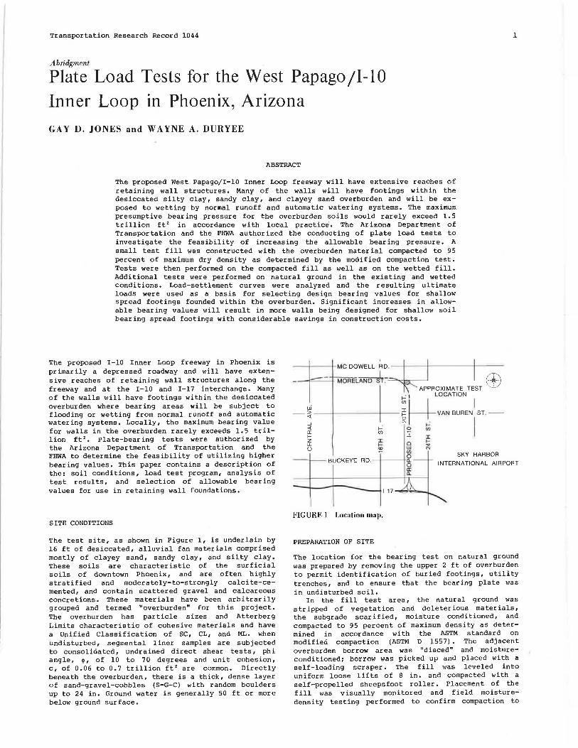
The test site, as shown in Figure 1, is underlain by 16 ft of desiccated, alluvial fan materials comprised mostly of clayey sand, sandy clay, and silty clay. These soils are characteristic of the surficial soils of downtown Phoenix, and are often highly stratified and moderately-to-strongly calcite-ce­mented, and contain scattered gravel and calcareous concretions. These materials have been arbitrarily grouped and termed "overburden" for this project. The overburden has particle sizes and Atterberg Limits characteristic of cohesive materials and have a Unified Classification of SC, CL, and ML. when undisturbed, segmental liner samples are subjected to consolidated, undrained direct shear tests, phi angle, <l>r of 10 to 70 degrees and unit cohesion, c, of 0.06 to 0.7 trillion ft 2 are common. Directly beneath the overburden, there is a thick, dense layer of sand-gravel-cobbles (S-G-C) with random boulders up to 24 in. Ground water is generally 50 ft or more below ground surface.

APPROXIMATE TEST ffi w >' ~COCWO< I

-- ~ ---1-------t)+--- i ~ ~ '" 'Ue>< i"' --z I ~

~ ~ m ~ --1--BUCKEYE RD . ---'---L~

0 a: a.

1-17 ........ " ....... -.J

FIGURE 1 Location map.

PREPARATION OF SITE

SKY HARBOR

INTERNATIONAL AIRPORT

The location for the bearing test on natural ground was prepared by removing the upper 2 ft of overburden to permit identification of buried footings, utility trenches, and to ensure that the bearing plate was in undisturbed soil.

In the fill test area, the natural ground was stripped of vegetation and deleterious materials, the subgrade scarified, moisture conditioned, and compacted to 95 percent of maximum density as deter­mined in accordance with the ASTM standard on modified compaction (ASTM D 1557). The adjacent overburden borrow area was "disced" and moisture­conditioned; borrow was picked UJJ and placed with a self-loading scraper. The fill was leveled into uniform loose lifts of 8 in. and compacted with a self-propelled sheepsfoot roller. Placement of the fill was visually monitored and field moisture­density testing performed to confirm compaction to

2

f­en I

5 N

MORELAND ST.

"FILL" TEST AREA

-----~ / \ I

1

x---x 4 1 SLOPE

1

x 0

0

f s· HIGr FILL

\ Zf~CHOR ~HAFT )

"-._ __ _/

"NATURAL"' TEST AREA

FIGURE 2 Site plan of plate load tests.

lx~xl

L_o J

95 percent of maximum dry density as determined by the Modified Compaction Test. The completed fill was approximately 8 ft high, with a 40 x 40-ft top and side slopes of 4:1. The plate load test site plan is shown in Figure 2.

LOAD-SETTLEMENT MEASUREMENTS

A reaction system capable of applying a 40-t test load was selected, and consisted of a W24 x 104 steel beam. A triangular anchor scheme provided for efficient handling of the beam for adj acent testing (see Figure 3). Anchors consisted of 24-in. straight­sided, drilled shafts.

~ ANCHOR RODS

,&

11 \~m; COCAO'O"'

' -¥ 24" ANCHOR SHAFT

---@-- .~ O"

FIGURE 3 Anchor shaft layout.

Immediately before seating the bearing plate, the U"d" luy i;u1 fa<.:.,:; w""" hdml-L1 lnuu"u, wl Lh fiucil leveling accomplished by a dusting of silica sand. The steel bearing plate was 1-in. thick and 24-in. in diameter, and was reinforced with from one to .three 12- and 18-in. diameter plates. Loads were applied by a manually operated 60-t hydraulic jack fitted with a calibrated pressure gauge. A ball-and­socket joint was positioned between the jack and reaction beam to provide a uniform load application.

Plate settlement was measured by three, 2-in. travel dial gauges positioned 120 degrees around the plate and 1-in. from the edge. Three additional dial gauges were set at 1-ft centers outside the edge of plate to measure movement of the ground surface dur­ing loading. All gauges were fixed to a 2 x 3-in. steel tubing beam supported on both ends at a dis­tance of 11 ft from the center of the bearing plate. The test setup is shown in Figure 4.

For the inundated tests, flooding of the test area was used to wet the soil beneath the plate. A

Transportation Research Record 1044

FIGURE 4 Plate load test setup.

6-in. high soil berm was constructed around the plate in a 6 x 6-ft area and filled with water. Wetting was aided by four, 4-in. diameter borings, 5 ft in depth, drilled radially 4 ft from the center of the plate. The borings were filled with silica sand. Flooding was maintained for 24 hr and ponded water removed just before commencing loading.

PLATE LOADING PROCEDURE

Plate loading was in general accordance with the provisions outlined in ASTM Standard Dll94, Bearing Capacity of Soil For Static Load on Spread Footings. Selected load increments were applied to the plate and maintained for a minimum of 15 min. Loads were added until the 40-t capacity of the load frame was reached or until the total settlement of the plate exceeded 10 percent of the plate diameter, or 2. 4 in. Following the last load increment, the load was released and rebound measurements taken. Intermediate load-unload cycles were necessary in some instances to adjust equipment and provide additional jack extension.

ANALYSIS

The plate settlements recorded for the four tests were used in developing load-settlement plots. Final .!lettlement for each load increment was selected by averaging the final settlement readings for the three dial gauges. The plots of load versus total settlement are shown in Figure 5 for the two tests on compacted overburden fill and in Figure 6 for the two tests on natural ground.

Interpretation of the load-settlement curves involves identification of the failure point, or ultimate load at which the loaded plate causes a bearing capacity failure of the supporting soil. In the case of a general shear failure, the failure point is theoretically clearly definable as a peak or high point in the curve. However, for punching or local shear conditions, there is seldom a sharp break in the curve and the failure point is usually difficult to determine (!.)·

A peak load point was not clearly identifiable on any of the four load-settlement curves. Among the methods reviewed for interpreting plate load test plots, the Semi-Log Plot-Intersecting Tangents method

Jones and Duryee 3

26.000 -- 1 ~1 JACK PSF

TEST NO. 1 - COMPACTED MOISTURE

20,000 ·----

LL Cf)

~

D <(

0 ...J

NO, 2 - INUNDATED

SETTLEMENT IN INCHES

FIGURE 5 Load·settlement curves-compacted overburden fill.

26,000 -

20,000·

LL [ D <(

0 ...J

TEST NO. 3 - NATURAL MOISTURE

10,000 ---

:EST NO. 4 -; INUNDATE~/

I • ~

. ~/I j o..-::::;...::,.---~ - ~ f I i--t

O ·~----....... ---~-t2~--~--~----+------t~-----<6

SETTLEMENT IN INCHES

FIGURE 6 Load.settlement curves-natural ground.

was determined to provide the clearest definition of interpretation and thus selected as the preferred method. In this method, the loads are plotted to a log scale and the settlement to ari thmet ic scale. The ultimate load is de£ined by intersection of two tangents, one to the initial portion of the curve and one to the outer straight-line portion. The semi-log plots and interpretation are shown in Fig­ures 7 and 8. Evaluation of ultimate load values and their relationship to the anticipated behavior of full-size footings is dependent on several factors, including soil type and conditions, plate size, and confinement of the plate, which are directly related to the individual load tests (±_) •

The scattering of soil shear strength test data

and the plate load test procedure resulted in the assumption that the soil be considered to have only cohesive strength. Local shear failure was assumed to occur as the plate was observed to punch into the soil without displacement of the adjacent soil sur­face as would normally be expected in a general shear failure condition (3).

In analyzing the ultimate load test values and solving for soil shear strength, or cohesion, the following basic bearinq capacity equation was con­sidered as best representing the shear failure con­ditions for the test performed (,i):

(1)

~ ii

4

50.000

J I UL Tl MATE LOAD ;

~ ' 2,000 PSF ; 6.0 TSF

I p I

I ~ - TEST NO. 1 - COMPACTED MOISTURE -20.000 A I I

I /I~ 7 --< "-" I I !'--- TEST NO. 2 - INUNDATED -

10.000 u:­(/J 0..

0 <( 0 _J

5.000

v; ,

~

6 ...,

f+-"F--7-J

I I / 1 II

L,j , I

-/ ,

Ir'"

./~ • /

UL Tl MATE LOAD; 8,000 PSF; 4.0 TSF

-

2 4 SETTLEMENT IN INCHES

FIGURE 7 Semi-log plot, intersecting tangents method of interpretation-compacted overburden fill.

5u,OOO

f \ ,~Tl MATE LOAD ; 7 ~000 PSF ; 3.5 T SF

20.000 I /

'

- --

6

I /~TEST NO. 3 - NATURAL MOISTURE

10.000 u:­(/J

~ ~1. v

I /

r

,

/ I __,, .---r--

..A"

~

~

~

LI <( 0 _J

l _/ / "TEST NO. 4 INUNDATED

I _,,. /

I v / , 7 ,I/ , / S.000

r ~;

I I I'- ULTIMATE LOAD; 4,600 PSF; 2.3 TSF

I I I;

\i

0 1,00 0 2 4 SETTLEMENT IN INCHES

FIGURE 8 Semi-log plot, intersecting tangents method of interpretation-natural ground.

-

6

Transportation Research Record 1044

where for the case of a plate loaded at the surface on cohesive soil for local shear conditions

2/3 (5.7) 3.8, (2)

Df o, and

o.

Therefore,

Qult - cNc or 3.8c.

Dy using the coli.,sio11 valu"s u.,L.,1111i11t>ll f1u111 tilt? load tests, the allowable bearing pressures were computed, with the following assumptions:

1. Noninundated conditions apply to all footings embedded 4 ft or more below final constructed grade.

2. Inundated conditions apply to all footings embedded less than 4 ft below the final constructed grade.

3. A factor of safety of 3 should be used in developing bearing pressures in order to limit set­tlement of full-size footings to tolerable amounts, and to provide adequate Factor of Safety against a bearing capacity failure. Evaluation of settlement for expected full-size footings when considering settlement proportional to footing width indicates settlements within reasonable limits.

4. For cohesive soil, since Ny ~ O, the width of footing is not considered to affect bearing capacity.

ml...- --L--.!-- ___ ., ____ ----- .. .L...!,.! __ ..:i .LU'C \..:\JlH:::O.LVU Vd.1.Ut::'O Wt:::L IC' U ""'.L..L.L:6t::U l.Ut::

L - -.! -UCl.b.L\,; 1.n

bearing capacity equation assuming general shear failure for actual spread footings. Allowable bear­ing pressures were calculated for the predetermined conditions. Average footing depths were used because allowable bearing pressures did not vary signifi­cantly for the normal footing depth range expected. Th~ f P-R1Jlting allo~able bearing press1ires are gi':.ren in the following table.

Allowable Bearing Pressure

Condition (trillion ft 2 ! Natural Ground, Non inundated

(Df ~ 4 ft) 2.0 Natural Ground, I nundated

(Df < 4 ft) 1. 3 compacted Fill, Noninundated

(Df ~ 4 ft) 3.0 Compacted Fill, Inundated

(Df < 4 ft) 1.9

These values were recommended as maximum allowable bearing pressures for use in the design of soil­bearing spread footings in overburden.

CONCLUSIONS

Based on the performance of 24-in. diameter plate load tests on compacted overburden fill and natural ground overburden, the following conclusions may be drawn:

1. A peak load point was not clearly identifi­able on any of the four load settlement curves that would easily define an ultimate load. The Semi-Log, Intersecting Tangents Method of Interpretation was selected as the preferred method for determining ultimate load values.

2. A simplified analysis procedure based on the test conditions was used to evaluate the ul timate

Transportation Research Record 1044

load values and develop conservative allowable bear­ing pressures for compacted fill and natural over­burden materials.

3. The consideration for inundation of shallow spread footings was addressed in the program with the e s tablishment of noninundated conditions to apply to all footings embedded 4 ft or more below final constructed grade. Inundated conditions apply to all footings embedded less than 4 ft below final constructed grade.

4. The proposed allowable bearing pressures developed from the load test program were higher than the locally accepted values. Providing these allowable bearing pressures as design criteria to the project design consultants is expected to result in more uniformity in foundation design and con­siderable cost savings to this project.

ACKNOWLEDGMENTS

The authors wish to express their appreciation to Dean Lindsey, 1-10 Principal Engineer, Arizona De­partment of Transportation, and the Federal Highway Administration for authorizing this special load

test program. The participation of Ken er n Technologies, Inc. , in assembly, and operation of the testing equipment acknowledged.

REFERENCES

5

Ricker, West­ins talla ti on, is gratefully

1. H.F. Winterkorn and H-Y. Fang. Foundation Engi­neering Handbook. Van Nostrand Reinhold Company, New York, 1975, pp. 121-147.

2. D.D. Burmister STP No. 322. Prototype Load-Bear­ing Tests for Foundations of Structures and Pavements, ASTM, Philadelphia, Pa., 1962.

3. G.A. Leonards. Foundation Engineering. McGraw­Hill Book Company, New York, 1964, pp. 588-594.

4. J.E. Bowles. Foundation Analysis and Design. McGraw-Hill Book Company, New York, 2nd ed., 1977, pp. 95-101, 113-122.

Publication of this paper sponsored by Committee on Foundations of Bridges and Other Structures .

Prediction of Axial Capacity of Single Piles in Clay

Using Effective Stress Analyses

ANDREW G. HEYDINGER and CARL EALY

ABSTRACT

This paper contains a description of research conducted on piles in clay. A finite element program was used to compute the state of stress in the soil around piles. The formulation accounts for the effects of pile installation and soil consolidation, updating the effective stresses continuously in a step-wise manner. The results of an approximate elastic solution were compared with the finite element solution. The two solutions were used to derive expressions for the effective radial stress after consolidation. A predictive procedure was developed that uses the effective radial stress to calculate the side resistance of piles in clay.

Investigators have attempted to determine the state of stress around piles in clay in order to estimate side frictional capacity <!.-l.!.l. To this end, the state of stress in the soil is updated from the in situ condition to the conditions immediately follow­ing pile installation and soil consolidation, and at pile failure. The purpose of this paper is to de­scribe the results of two computer solutions tor the effects of pile installation, and to propose a design procedure for axially loaded piles in saturated clays for bridge foundations and other structures.

CAMFE is an acronym for Cambridge finite element, a program developed at the University of Cambridge

(12). It uses a o ne-d i mensional finite element formulation to determine the pore pressure and stress changes that occur during pile installation and soil consolidation. For this investigation, an elasto-plastic model was used to represent the soil. The results obtained from CAMFE for the pore pres­sure and stress changes resulting from installation ~re s imilar to those obtained from a cylindrical cavity e xpans ion the o r y (13) for an elastic, per­fectly plastic ma terial. The consolidation phase of the formulation is completed assuming that water flows outward only radially. Thus, as with the cavity expansion procedure, plane stress conditions exist.

ii . .

6

The other solution that was used is referred to as VECONS (5). It uses cylindrical cavity expansion theory to model pile installation and and an ap­proximate elastic solution to model consolidation. For th-= consolidation proces s, it is assumed that the soil modulus varies from the pile surface to a predetermined distance from the pile. Thus, it is an acronym for Variable-E-Consolidation. The solution--a modification of a solution proposed by others (14)-­allows a nis otropic soil s tiffness to be inputfor the radial and circumferential stiffnesses to better physically represent the effects of pile instal­lation.

To develop the predictive procedure, compar ii;um; were made between the two analyses. On completion of the comparisons, a parametric study was conducted using the two programs to predict the state of stress in the soil after consolidation for a number of conditions. The results of the analyses are shown as the radial effective stress after consolidation normalized by the undrained shear strength. The radial effective stress after consolidation is then used to predict side capacity using the correlations between radial stress and side capacity (15-16).

DESCRIPTION OF CAMFE AND VECONS

As already mentioned, CAMFE is a one-dimensional finite element program that uses an elasto-plastic soil model. The elasto- plastic soil model use s a volumetric work-hardening plasticity formulation to represent the soil behavior during yielding. Plastic yielding cccur e when the yie ld crite rion is met. The yield criterion, which is referred to as the modi­fied Cam-clay soil model <ll, specifies an elliptical yield surface when plotting the deviator stress versus the mean normal stress.

Pile installation is modeled assuming that soil is expanded radially from a finite radius to a larger radius. The authors of th1> p r ogr am ha•re shown that the stresses and excess pore pressures after expan­sion are equivalent to those obtained from cylindri­cal cavity expansion, when the initial radius is doubled (£). At the end of installation, there is a zone of soil around the pile that has failed in shear, which then reaches a state referred to as the critical state <..!ll. The resulting stresses and excess pore pressure after installation then become the initial conditions for the consolidation process.

Consolidation occurs when the excess pore pres­sures around the pile dissipate. The assumption that radial consolidation occurs results in conditions in which the radial stress is the maximum principal stress and the vertical and circumferential stresses are the minimum principal stresses. At the end of cuui;ullcJatlun, the ratio between the vertical and circumferential stresses and the radial stress is equivalent to the at-rest lateral earth pressure coefficient for normally consolidated soil. Thus, the soil yielding that occurs during installation causes the soil to behave as a normally consolidated soil. After consolidation, the soil is not at the critical state.

VECONS was written for use in modeling pile in­stallation effects (5). Plane strain cylindrical cavity expansion the~y is used to determine the pore pressure and stresses immediately after instal­lation. For cylindrical cavity theory, it is assumed that the soil behaves as an elastic, perfectly plas­tic material. After shearing occurs, it is assumed that the soil reaches and remains at the critical state for further deformations so that the effective stresses remain constant. There is a zone of soil around the pile at the critical state. Soil outside the critical state zone deforms elastically.

Transportation Research Record 1044

An appr oximate solution pr oposed by others (14) was modif i e d in order to compute the state of stress in the soil after consolidation. It is assumed that the soil modulus varies logarithmically as a down­ward-fac;ing parabola from the pile surface to the outside boundary of the critical state zone. A value of the ratio of the r adial soil modulus Er i at the pile surface t o the r a d ial soil mod ul us (Ero> at the outside boundary equal to 0.1, a nd a dr a ined Poisson's ratio equal to 0.3 were used. To obtain a set of equations that could be used to solve the stress changes during consolidation, the constitu­tive equations were substituted into the equation of ~4uilibrium or total stress. The resulting equations were then solved by dividing the yielded zone into a number of subzones and writing the boundary condi­tions for the boundaries of the subzones.

The major modification to the published solution was the use of an anisotropic formulation for the soil modulus. It was assumed that the soil modulus in the circumferent ial direction, E6 , was grea ter than t he modulus in t h e r a d i a l d irection, Er (Ee/ Er = 2 was u s ed). This e ffect ively caused the s o i l to stiffen in the circumferential direction, which then reduced the radial stress changes. Thus, the radial stresses after consolidation, and the inferred side resistance that could be developed, were reduced to values that agreed with measured capacities (5).

The computed states of stress after soil c onsoli­dation from VECONS were input into AXIPLN, an axisyrn­metric finite element progr am plan (18), which was then used to model pile loading. Good-agreement was obtained between measured and computed values of shear s tress along t he p i le and load i n the p i le for three well-instrumented pile load tests. This veri­fies that VECONS can be used to predict the state of stress in the soil for at least the zone of soil immediately adjacent to the pile.

CO!>l_FAR!SONS BET!-!EEN Cl'-M.FE A1'lD VECONS

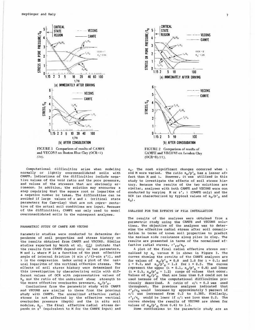
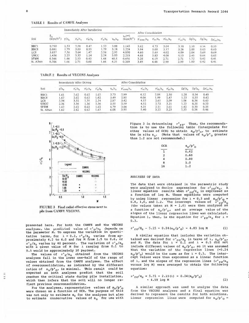
Comparisons between CAMFE and VECONS for five dif­ferent soils t hat have been we ll documented are given. Information on the first two sites was ob­tained from the investigators working at Cambridge who developed CAMFE. This includes Boston Blue Clay with overconsolidation ratios (OCR) of l and 8 (10) and London Clay with an OCR of 8 (11). The other three soils include Beaumont Clay at the University of Houston test site (19) , San Francisco Bay Mud at the Hamilton Air Forcel3ase site (~, and Champlain clay at the St. Alban test site near Quebec, Canada (21,££). The results are shown as plots of stress or pore pressure normalized by the initial undrained shear strength that was obtained from the CAMFE analyses, versus the natural logarithm ot the radial distance from the pile surface. Figure 1 shows the results obtained for Boston Blue Clay with an OCR of l (10), and Figure 2 shows results obtained for London Clay with an OCR of 8 (11).

A summary of the results o~the analyses is given in Tables 1 and 2. Tables l and 2 also give the normalized stress changes that occur immediately after pile installation and after consolidation for the CAMFE and the VECONS analyses. The in situ un­drained shear strength was used in all cases to normalize the stresses. For both solutions, it was necessary to model the stresses at a radial distance greater than at the pile surface, r > r 0 • It was determined that representative results could be obtained by using r values of 1.10 r 0 for VECONS and 1.15 r

0 for the CAMFE analyses. Based on the

comparisons, it was determined that the normalized stresses from both analytical models should be used to represent stresses acting on piles.

Heydinger and Ealy

5 I CRITICAL "' .- STATE ~ 4 REGION = "' "' ~ 3 ..... "" ~ 2 "" = "' "'

- -- VECONS

-- CAMFE

OCR= 1

K0

= 0.55

~ 0 I t S 11 ii

1.15 2 3 5 10 20 40 60 100 r/ro

[a) IMMEDIATELY AFTER DRIVING

:t - -- VECONS

-- CAMFE "' "' ........

"' "' 3 ..... "" ... iir/Su

"' 2

0u5 2 3 5 10 20 40 100

r/ro [b] AFTER CONSOLIDATION

FIGURE I Comparison of results of CAMFE and VECONS on Boston Blue Clay (OCR=l) (10) .

Computational difficulties arise when modeling normally or lightly overconsolidated soils with CAMFE. Indications of the difficulties include nega­tive values of the void ratio and the pore pressure, and values of the stresses that are obviously er­roneous. In addition, the solution may encounter a step requiring that the square root or logarithm of a negative number be taken. The difficulties can be avoided if large values of K and A (critical state parameters for Cam-clay) that are not repre- senta­tive of the actual soil conditions are input. Because of the difficulties, CAMFE was only used to model overconsolidated soils in the subsequent analyses.

PARAMETRIC STUDY OF CAMFE AND VECONS

Parametric studies were conducted to determine de­pende nce of soil properties and stress his t o r y on the results obtained f rom CAMFE and VECONS . S i milar studies reported by Wroth et al. (11) indicate that the results from CAMFE depend only on two parameters, Mand A, where M is a function of the peak effective angle of internal friction [6 sin ~ '/(3-sin ~')],and

A is the compression index using a plot of the nat­ural logarithm of the vertical effective stress . The effects of soil stress histo r y were determined for this investigation by characterizing soils with dif­ferent values of OCR with representative values of K0 and the ratio of the undrained s hear strength to the means effective overburden pressure, su/P'o•

Conclusions from the parametric study with CAMFE and VECONS are similar to those frorr. the previous study with CAMFE. The normalized effective radial stress is not affected by the effective vertical overburden pressure (depth) and the in situ soil modulus, Eu• The final effective radial stress de­pends on ~ · (equivalent to M for the CAMFE input) and

"' "' ;:;:,. "" = "' "' .....

~CRITICAL

5 STATE REGION

4 u;s. - -- VECONS -- CAMFE

:::: 3 ..... "" ~ 2 "" = V)

"' ...... "" t;; 0 "---'---'-'"='"-------'---

"' "' ........ "' "' ...... a: ... V)

1.15 2 5 10 100

6

3

2

0

[a) IMMEDIATELY AFTER DRIVING

1.15 2

- - --:- VECONS -- CAMFE

5 10 100

(b] AFTER CONSOLIDATION

FIGURE 2 Comparison of results of CAMFE and VECONS on London O ay (OCR=8) (1 1).

7

su· The most sign ifican t changes oc curred when 1'

and M we r e var ied. The r a tio su/P 'o has a l esser ef­fec t t ha n M and 1.. However , it was u t ilize d in this study to investigate the effects of soil stress his­tory. Because the results of the two solutions are similar, analyses with both CAMFE and VECONS were con conducted by varying Mor ,., A (CAMFE only) and the OCR (as characterized by typical values of su/P'o and Kol·

ANALYSES FOR THE EFFECTS OF PILE INSTALLATION

The results of the analyses were obtained from a pa r ametric study using t he CAMFE and VECONS s olu­t i ons. The ob j e c tive o f the analyses was to de ter­mine the effective radial s tress a fter soil consoli­dation in terms of known soil properties to predict the maximum side resistance along piles in clay. The results are presented in terms of the normalized ef­fective radial stress, a 'rc/su.

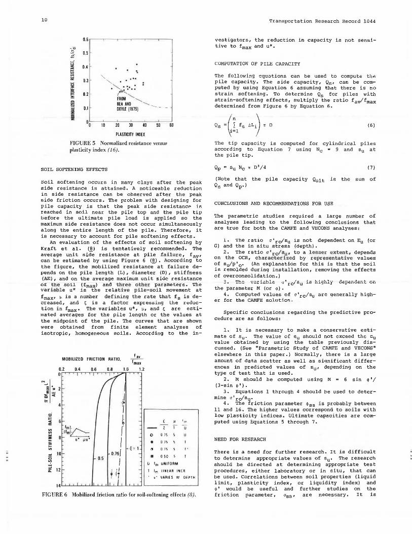
A plot of the final radial effective stress nor­malized by Su versus M is shown in Figure 3. The curves showing the results of the CAMFE analyses are for va l ues of s 4/ p' 0 = 0. 8 and 1 . 0 f o r A = O.l; and a = 0 . 3 , a nd su/ P ' o = 1 . 2 fo r 1' = 0. 5 . The curves represen t th e upper (a = 0. 1 , su/P ' o = 0 . 8) and lower ( 1' = 0 . 5 , Su/ P ' o = 1 . 2 ) r a nge of values t hat occur . Va lues o f su / P 'o t hat a r e less t han 0. 8 could not be used because o f the c omputational difficulties pre­viously de s cribed . A r a tio o f K/ 1' = 0 . 2 was us e d throughou t . The p r e v ious analyse s i ndicated t hat cr' clsu wuuld increa se by app r ox imat ely 5 percent if K/1' was inc rea sed fr om 0. 2 t o 0. 385 . Simi lar ly , a'r/su would be lower if K/1' was less than 0 .2. The curves showing the results of VECONS are s hown for values of Su/P 'o from 0.42 to 1.2.

Some conclusions to the parametric study are as

B Transportation Research Record 1044

TABLE 1 Results of CAMFE Analyses

Immediately After Installation After Consolidation

Su s,.(oo) Soil (kips/ft2

) p/su a;/su a'ofsu U~/SiJ u0 /s0 (kips/ft2 ) P 'cons /su U~c/Su a'oc/Su a'zcfSu 6p'/su 6p'/u0 6a;c/u0

BBC! 0.750 1.53 2.58 0.47 1.53 3.88 1.143 3.62 4.73 3.04 3. iO 2.10 0.54 0.55 BBC8 0. 881 1.79 3.03 0.55 1.79 3.28 1.224 3.84 5.08 3. 17 3.26 2.05 0.63 0.63 LC8 3.657 2.56 3.64 1.4 7 2.56 2.95 4.890 4.60 5.69 4.02 4.09 2.04 0.69 0.69 UHCC 1.436 2.23 3.33 1.14 2.24 3.83 2.218 4.68 5.83 4.08 4.13 2.45 0.64 0.65 SFBM 0.346 1.48 2.53 0.43 1.48 40.5 0.456 3.20 4.19 2.71 2.71 1.72 0.42 0.4 1 St. Alban 0.206 1.66 2.71 0.60 1.66 4.31 0.268 3.49 4.48 2.99 2.99 1.83 0.42 0.41

TABLE 2 Results of VECONS Analyses

Immediately After Driving After Consolidation

Soil Pf Su a;Jsu a'ofsu a'z/Su u0 /su P1

cons/Su a~cfsu a'ocfsu O~c/Su 6p'/su 6p'/u0 6a;c/u0

BBC! 1.61 2.62 0.62 1.62 BBC8 1.62 2.62 0.62 1.62 LC8 2.34 3.32 1.35 2.34 UHCC 2.36 3.36 1.36 2.36 SFBM 1.62 2.62 0.62 1.62 St. Alban 1.62 2.62 0.62 1.62

.A =0 .1 Su/Po =0.8

7 . \~0. 3 Su/ Po =O.a

6 ,\ =0.5 ' "' .,..,~ su; P0 =1.2 ';;[~ "'-.

S · " O '

'~ ---~-~~--_ _,,,,,...~ --. ~nd

CAM FE

------ YECOkS • Su/ Po - CAMFE ~ECOllS

0.42 0

0.60 0

0.80 1.00 • 0

1.20

1.0 1.5 M

FIGURE 3 Final radial effective stress next to pile from CAMFE VECONS.

3.73 2.89 3.49 2.85 2.8 7 3.42 3.55 3.59 4.79 3.04 6.08 3.95

presented here. For both the CAMFE and the VECONS audly:;..,:;, Lilt! lJLt!llluLt!ll vdlu"' ur u 'rf:;u Ut!1Jt!nll:; u11 the parameter M. To express the variation in quanti­tative terms, for ). = 0.3, a'rlsu varies from ap­proximately 4.2 to 6.0 and for M from 1.5 to 0.6, or cr'r/su varies by 40 percent. The variation of cr'r/su with a given value of M for ). ranging from 0.1 to 0.5 would be approximately 20 percent.

The values of a 'r/Su obtained from the VECONS analyses fall in the lower one-half of the range of values obtained from the CAMFE analyses. The effect of overconsolidation, as indicated by the different ratios of su/P'o• is minimal. This result could be expected as both analyses predict that the soil reaches the critical state during pile installation, which then infers that the soil will no longer re­flect previous overconsolidation.

For the analyses, representative values of su/P'o were chosen as a function of OCR. The purpose of this was not only to estimate su for the analyses but also to estimate conservative values of Su for use with

4.12 2.04 2.50 1.28 0.34 0.40 4.08 1.99 2.47 1.23 0.35 0.42 4.57 2.61 3.09 1. 08 0.38 0.43 4.52 2.73 3.2 1 l.23 0.35 0.33 4.3 1 2.21 2.61 1.42 0.30 0.35 5.40 3.22 3.23 2.33 0.38 0.46

Figure 3 in determining a'rc· Thus , the recommenda­tion is to use the following table (inter polate for other values of OCR) to obtain su/P'o• to estimate the in situ su• (Note that values of su/P'o greater than 1.2 are not recommended.)

OCR su/P'o

1 o.42 2 0.60 4 0.80 B 1.0

16 1.2

ANALYSES OF DATA

The data that were obtained in the parametric study were ana lyzed to derive expressions for o 'rcfsu• A linear equa t i on results when a ' r cfsu i s expressed as a f unct i on of log M. These equations were computed by using l i nea r regression for ). = 0 . 3 a nd s u/P' = 0.8, 1,0, and 1 .2. The intercept values of o 'rc:Js u (the values t aken at M = 1.0) were then a na l yzed a s a function of su/P'o• and an average value of the slopes of the linear regression lines was calculated. Equation 1, then, is the equation for a'rcfsu for ). = 0.3.

cr'rc/Su - ~-1~ - 0.24(,;u/l''ol - 4.83 lug M (1)

A similar equation that includes the variation ob­tained was derived for cr'rc/su in terms of :i., su/P'o• and M. The data for :i. = 0.1 and ). = 0.5 did not include different values of su/P'o• so it was assumed that the variation of the regression lines (-0.24 su/P'ol would be the same as for ). = 0,3. The inter­cept values were then expressed as a linear function of )., and the slopes of the regression lines (a'rcfsu versus log M) were averaged to obtain the following equation:

cr'rc/Su 5.71 - 2.23().) - 0.24(su/P' 0 )

- 4.59 log M (2)

A similar appr oach was used to analyze t he data from the VECONS analyses and a final equa tion wa s derived to represent the res ul ts for both solutions . Linear regression l ines were computed for su/ P ' o =

Heydinger and Ealy

0.42, 0.6, and 1.2 . Equation 3 gives the relationship for a' re/ Su .

a'rclsu = 4.91 - 0.3l(su/p' 0 ) - 3.94 log M (3)

The final equation was derived by using a linear re­gression of all the data.

a'rc/ su = 4.80 - 4 . 57 log M (4)

The correlation coefficient computed results for Equation 4 is -0.929 and the standard deviation is 0.67. Equation 1 can be used if the respective values of A and Su/P'o can be estimated. The equations indi­cate the dependence of a 'rclsu on the parameters.

ANALYSES FOR NONDISPLACEMENT PILES

Additional analyses were conducted to investigate the stress changes on piles that do not fully dis­place the soil. Such piles include unplugged, open­ended, pipe piles and ideal H-piles. [In some cases, soil can block off the ends of open-ended pipe piles or the sides (between the flanges) of H-piles, caus­ing them to act as full displacement piles for fur­ther penetrations. It is not within the scope of this paper to predict whether soil would block off a pile and, if so, the depth where the soil plug would form.] For H-piles, it would be necessary to assume a circular cross-section with the same area as the H-pile as an approximation.

Analyses were conducted for partial displacement piles with displacement ratios of 0.05, 0.10, and 0.20. The displacement ratio is defined as the ratio of the cross-sectional area of steel of the piles to the gross cross-sectional area. Both of the computer solutions were programmed so that nondisplacement piles could be analyzed. According to the solutions, the soil reaches the er i tical state i consequently, stress changes during installation are the same as displacement piles except that the pore pressure is not as large. The critical state zone, the zone of soil at the critical state, is not as large for a nondisplacement pile.

To analyze the effects of nondisplacement piles quantitatively, a number of the cases that were used in the previous parametric study were analyzed using different displacement ratios. Based on the results of the analyses, it was concluded that the reductions in a'rc/Su for a displacement pile c a n be ex pressed in terms of the displacement r atio i ndependent of M or su/P'o· The reduc tion in a'rclsu, is expressed in terms of the value ob t a ined for a full displacement pile. The recommendation is to reduce a'rclsu com­puted for full displacement piles by multiplying by factors of 0.80, 0.85, and 0.90, respectively, for displacement ratios equal to 0.05, 0.10, and 0.20, respectively.

PREDICTION OF ULTIMATE SIDE FRICTION

For rapid pile loading, undrained conditions with no soil consolidation are assumed. For undrained load­ing, excess pore pressure can be generated, causing changes in the effective stresses. The excess pore pressures ar e a f raction of the shear s tresses in the s o il tha t -are c a us ed by pile load i ng <1 >. There are also some changes in the soil stresses as a result of applied shear stress. The orientation of the major pr incipal stress rotat es around from the radial direct i on toward the ver t i cal direction. To determine the state of stress at failure, it is necessary to determine both the effective stress

9

changes caused by pile loading and the reorientation of the principal stress directions.

The results of finite element analyses on piles in clay (~) indicate that the total radial stress (excluding the hydrostatic pore pressure) acting on piles remains nearly constant dur i ng pile loading. The total radial stress at pile failure is approxi­mately 2 to 4 percent greater than the total radial stress after consolidation except for soil near the ground surface and near the pile tip. The total radial stress increases by as much as 20 percent within approximately 5 pile radii of the ground surface. The total radial stress decreases near the pile tip. Thus, the effective radial stress after consolidation, equivalent to the total radial stress, can be used to predict the side friction capacity for the major part of the pile shaft.

The authors recommend computing the side friction capacity by using the effective radial stress after consolidation a'rc• and a friction parameter. The friction parameter is the peak total friction angle between the pile and soil, $ss• Equation 5 can then be used to compute the side friction, fs as follows:

fs = a 'rc tan $ss (5)

The determina tion of $ss can be made from undrained direct s hear , direct simple shear , or rod shear tests.

The findings from two rod shear testing programs are used to estimate the friction parameter (15,16). The results that are presented here are in termsof the peak interface friction, fs, and the initial effective confining (radial) pressure, a'ci• Figure 4 (J&) shows a plot offs versus a'ci showing computed ·friction angles, tan $ss = (fs/a' ci>. The range of

~ 60

.:!! 50 ... ~ 40 z c t;; iii !I;!

~ c ::=: i .. c ~ 20 40 60 80 100 120 140 160 180 200

INITIAL EFFECTIVE CONFINING PRESSURE, 11 ci (psij

FIGURE 4 Peak interface resistance versus initial effective confining pressure (1 6).

values of $ss for the undrained t e s ts was from 12 to 16.5. Figure 5 (16) shows the relationship between fs/ a 'ci and the plastic ity i ndex. Ratios of fs/a'ci between 0.2 and 0. 3 , or ~ ss be twee n 11 and 16 are recommended. The major conc lusion from the two in­vestigations is that there is no limit to the side friction that can be obtained. This is in contrast to the concept of limiting side friction used by the American Petroleum Institute (23).

The procedure to compute the ultimate side fric­tion capacity is complete. Any one of Equations 1 through 4 can be used to es tima t e a' r clsu. The ef­fective radial st.rP.ss after consolidation is equiva­lent to a'ci that was obtained in the laboratory rod shear tests. The ultimate side friction is computed at a number of depths using either Figure 4 or 5 to estimate $ss and Equation 5. (Some computation exam­ples are presented later in this paper.)

.. •

10

0.6

• 'f::i b 0.5 '-~

~ "" 0.4 c t; ' ;;; ', ~ O.J

... ~

"--._

l:li: ·"'- . :·.: ~ 0.2 1 · l!E FROM '--........_ = ~

BU AND ......._ 0.1 DOYLE 11975) -__

• "' -"" DO 10 20 JO 40 50

PLASTICITY INDEX

FIGURE 5 Normalized resistance versu8 plasticity index (16).

60

SOIL SOFTENING EFFECTS

Soil softening occurs in many clays after the peak side resistance is attained. A noticeable reduction in side resistance can be observed after the peak side friction occurs. The problem with designing for pile capacity is that the peak side resistancf> is reached in soil near the pile top and the pile tip before the ultimate pile load is applied so the maximum side resistance does not occur simultaneously a long the entire length of the pile. Therefore, it is necessary to account for pile softening effects.

An evaluation of the effects of soil softening by Kraft et al. (§.l is tentatively recommended. The average unit side resistance at pile failure, fav• can be estimated by using Figure 6 (8). According to the figure, the mobilized resistanc;- at failure de­pends on the pile length (L) , diameter (D) , stiffness (AE), and on the average maximum unit side resistance of the soil (fmaxl and three other parameters. The variable u* is the relative [>He-soil movement at fmax• µ is a number defining the rate that f s is de­creased, and ~ is a factor expressing the reduc­tion in fmax• The variables u*, µ, and ~ are esti­mated averages for the pile length or the values at the midpoint of the pile. The curves that are shown were obtained from finite element analyses of isotropic, homogeneous soils. According to the in-

MOBILIZED FRICTION RATIO, I av

lmu 0.2 0.4 0.6 0.8 1.0 1.2 0

N .... .. . .. " E w c c( J ~ 4

'/ Q ;::::

6 ~ c( µ Im cc

"' Im~ r 1 u

"' llm w

8 0 0 75 u z u• µu• I ... ... • 0 75

;:::: t : 1 "' 0.75/ " 0 75 1· .... 10 c; ~ o .5 • 0 50 , "' I ..:. u Im UNIFORM .... a: 12 , •I T Im LINEAR IN CR H•

' I u· VARIES W OIPTH

14

FIGURE 6 Mobilized friction ratio for soil-softening effects (8).

Transportation Research Record 1044

vestigators, the reduction in capacity is not sensi­tive to fmax and u* •

COMPUTATION OF PILE CAPACITY

The following equations can be used to compute the pile capacity. The side capacity, Qs, can be com­puted by using Equation 6 assuming that there is no strain softening. To determine Qs for piles with strain~softening effects, multiply the ratio favl fmax determined from Figure 6 by Equation 6.

Qs ='r fs [ILi) 11 D i=l I

(6)

The tip capacity is computed for cylindrical piles according to Equation 7 using Ne = 9 and su at the pile tip.

(7)

(Note that the pile capacity Qult is the sum of Qs and Qp.J

CONCLUSIONS AND RECOMMENDATIONS FOR USE

The parametric studies required a large number of analyses leading to the following conclusions that are true for both the CAMFE and VECONS analyses:

l. 'l'he ratio o'rcfsu is not dependent on Eu (or G) and the in situ stress (depth).

2. The ratio a 'rcls u, to a lesser extent, depends on the OCR, characterized by r e[>resentative values of su/P'o• (An explanation for this is that the soil is remolded during installation, removing the effects of overconsolidation.)

3. Th~ vai:' iablc; u' rc/5u i.s the parameter M (or <1>) •

4. Computed values of o 're/Su er for the CAMFE solution.

t....:-\...,.. ..:J----..:1--.L --U.L~ll..L.f UCt"CllU.Cll\.. VU

are generally high-

Specific conclusions regarding the predictive pro­cedure are as follows:

1. It is necessary to make a conservative esti­mate of Su· The value of Su should not exceed the Su value obtained by using the table previously dis­cussed. (See "Parametric Study of CAMFE and VECONS" elsewhere in this paper.) Normally, there is a large amount of data scatter as well as significant differ­ences in predicted values of Sur depending on the type of test that is used.

2. M should be computed using M = 6 sin <I>'/ (3-sin <1>') •

3. Equations 1 through 4 should be used to deter­mine a' re/Su.

4. The friction parameter <l>ss is probably between 11 and 16. The higher values correspond to soils with low plasticity indices. Ultimate capacities are com­puted using Equations 5 through 7.

NEED FOR RESEARCH

There is a need for further research. It is difficult to determine appropriate values of Su· The research should be directed at determining appropriate test procedures, either laboratory or in situ, that can be used. Correlations between soil properties (liquid limit, plasticity index, or liquidity index) and <I>' would be useful and further studies on the friction parameter, ass, are necessary. It is

Heydinger and Ealy

probable that other solutions for the effects of pile installation will be developed, and, when this happens, similar studies should be conducted. More full-scale field tests on piles are necessary, how­ever, to verify any predictive procedure. Design charts for different soil and pile conditions could be developed using the predictive procedure.

The recommended predictive procedure was compared to the findings of other investigations and field test data. There are some conditions that the recom­mended procedure has not verified experimentally. The validity of the solutions for permeable piles (con­crete or timber) is questioned. The pile-soil adhe­sion is higher for timber piles. For nondisplacement piles (open-ended pile or H-piles) , the solutions have not been verified. The strain-softening effects need to be investigated further. The solutions may not be valid for tapered (straight-sided or step­tapered) piles. The predictive procedure was devel­oped from analytical solutions and load tests on single piles. It would not apply to piles in groups where the group effects of pile installation and loading would be significant.

Discussion Michael W. O'Neill*

The authors describe a method to reduce average shaft resistance for flexible piles. They speculate that strain softening occurs in clay soils following the development of peak shaft resistance in driven piles. This phenomenon purportedly explains the well-known effect that average unit shaft resistance along a pile at plunging decreases with increasing pile length in relatively uniform soils. Because progressive failure occurs along the shaft, the average unit shaft resistance at plunging failure consists of contributions of peak resistances at some levels (presumably at lower levels) a nd post­peak (teduced) resistances at o·thet (higher) levels. The more flexible the pile, the larger would be the post-peak reduction in unit shaft friction along the upper part of the pile; consequently, the smaller would be the average unit shaft resistance.

This writer would like to offer an alternative explanation of this phenomenon, based on full-scale and model tests that he has conducted on driven piles in clay.

Figure 7 shows a set of f-z curves for a 10. 75-in.-outer diameter x 0.365-in.-wall, steel pipe pile driven to a depth of 43 ft in stiff, saturated, fairly uniform, overconsolidated clay with an OCR between 4 and 8 (~,~·Strain softening is observed to be almost nonexistent in the upper one-half of the pile but to increase markedly with depth. In the notation of the authors' F i gure 6, !; at a dis­placement of ~u*" 0 . 6 in. (3 to 10 times the displacement at yield), is shown i.n parentheses for each level. The test pile was moderately rigid. Had it been perfectly rigid, the conditions producing the largest avei:age side resistance, fmax, are shown by the solid dots. The value of this average fmax is 8.97 psi.

Had the pile been much more flexible (wall thick­ness of 0.25 in. corresponding to a stiffness ratio uf 6, u,;ing the defin.ition in Figure 6), the aver<ige fmax corresponding to a tip deflection of 3 per­cent of the pile diameter (top deflection of 5 per-

*University of Houston, Houston, Texas 77004.

I 1=10 PSI

l

J: l­a.. w 0

11

z (IN.)

00 0.2 0.4 0.6

10

20

30

40

10.5' ce = o.00>

1----~-- 23.5' ce = 0.09>

---o-- 20.5' c e = o .9o>

33.5' ce = 0.85)

37 .5' <e=o.79> 40.5' ce=o.1n

• MAX AVG IMAX: RIGID PILE

o MAX AVG fMAi FLEXIBLE PILE

(STIFFNESS RATI0=6.0)

430 0.2 0.4 0.6

FIGURE 7 Set of f-z curves.

cent of the pile diame-ter), which would tesult in plunging failure of the pile, would be derived from the points represented by the open circles. The value of the resulting average fmax for such a flexible pile is 8. 41 psi, or 6. 2 percent less than the value for the rigid pile. Although the effect of pile-soil flexibility is demonstrable in this soil, it is not as significant in reducing average maximum load transfer as at least one other phenomenon, discussed below.

The results of Figure 7 have been replotted in Figure 8 in the form of E; (at 0.6 in.) versus A, the normalized vertical distance bet1'1een the pile tip and a generic depth i.n the soil. The vat iable E: is approximately constant at 0.90-0.95 for A exceeding 15 diameters. For A less than 15 diam­eters, l; decreases sharply to approximately 0.70 at A = 2 diameters. This behavior suggests that the fai:ther the pile travels past a given depth of s oil during installation, the greater the degree of soil destructuring at the pile-soil interface and the higher the value of i; . If such is the case, the average fmax decreases with increasing pile penetration because the angle of soil-to-pile fr ic­tion ~ss decreases at a given depth as the ·pene­tration increases, assuming the correctness of the

1.0

10 20 30 40

t:.(DIAMETERS)

FIGURE 8 ~versus to for field test.

12

assertion of the authors that lateral effective stress is generally independent of depth in a uni­form soil . (The fric tion angle may only a ppe ar to decrease if lateral movements during driving , not accounted tor by existing effective stress methods, produce permanent strain in the soil.)

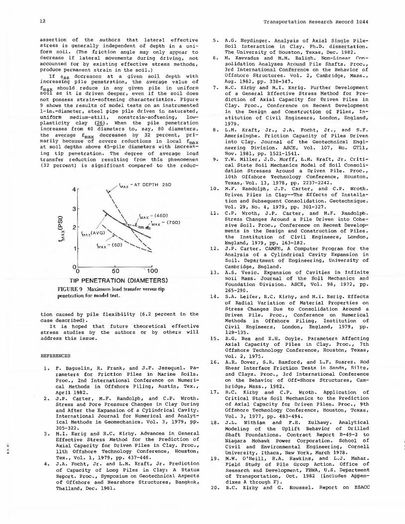
If ~ ss decreases at a g iven soil depth with increasing pile pene tration, the average value of fmq.x should reduce in any given pile in uniform soil as it is driven deeper , even if the soil does not possess strain-softening characteristics. Figure 9 shows the results of model tests on an instrumented 1-in.-diameter, steel pipe pile driven in saturated, uni!orm medium-s till , nonstrain-softening, low­plasticity clay (~. When the pile penetration increases from 40 diameters to, say, 80 diameters, the average fmax decreases by 32 percent, pri­marily because of severe reduct ions in local fmax at soil depth s above 45-pile diameters wi th i ncreas­ing tip penetration. The degree of average load transfer reduction resulting from this phenomenen (32 percent) is significant compared to the reduc-

........ Ci) a. ......

x <(

_::?.

4 IMAX~ AT DEPTH 250

3

2

0o 50 - 100

TIP PENETRATION (DIAMETERS)

FIGURE 9 Maximum load transfer versus tip penetration for model test.

tion caused by pile flexibility (6. 2 percent in the case described).

It is hoped that future theoretical effective stress studies by the authors or by others will address this issue.

REFERENCES

l. F. Baguelin, R. Frank, and J.F. Jezequel. Pa­rameters for Friction Piles in Marine Soils. Proc., 2nd International Conference on Numeri­cal Methods in Offshore Piling, Austin, Tex., April 1982.

2. J.P. Carter, M.F. Randolph, and C.P. Wroth. Stress and Pore Pressure Changes in Clay During and After the Expansion of a Cylindrical Cavity. International Journal for Numerical and Analyt­ical Methods in Geomechanics. Vol. 3, 1979, pp. 305-322.

3. M.I. Esrig and R.C. Kirby. Advances in General Effective Stress Method for the Prediction of Axial Capacity for Driven Piles in Clay. Proc., 11th Offshore Technology Conference, Houston, Tex., Vol. 1, 1979, pp. 437-448.

4. J .A. Focht, Jr. and L.M. Kraft, Jr. Prediction of capacity of Long Piles in Clay: A Status Report. Proc., Symposium on Geotechnical Aspects of Offshore and Near shore Structures, Bangkok, Thailand, Dec. 1981.

Transportation Research Record 1044

5. A.G. Heydinger. Analysis of Axial Single Pile­Soil Interaction in Clay. Ph.D. dissertation. The University of Houston, Texas, Dec. 1982.

6. M. Kavvadas and M.M. Baligh. Non-Linear Con­solidation Analyses Around Pile Shafts. Proc., 3rd International Conference on the Behavior of Offshore Structures, Vol. 2, Cambridge, Mass. , Aug. 1982, pp. 338-347.

7. R.C. Kirby and M. I. Esr ig. Further Development of a General Effective Stress Method for Pre­diction of Axial Capacity for Driven Piles in Clay. Proc., Conference on Recent Development in the Design and Construction of Piles, In­stitution of Civil Engineers, London, England, 1979.

8 . L.M. Kraft, Jr., J.A. Focht, Jr ., and S.F. Amer isinghe. Friction Capacity of Piles Driven into Clay. Journal of the Geotechnical Engi­neering Division. ASCE, Vol. 107, No. GTll, Nov. 1981, pp. 1521-1541.

9. T.w. Miller, J.D. Murff, L.M. Kraft, Jr. Criti­cal State Soil Mechanics Model of Soil Consoli­dation Stresses Around a Driven Pile. Proc., 10th Offshore Technology Conference, Houston, Texas,·Vol. 13, 1978, pp. 2237-2242.

10. M.F. Randolph, J.P. Carter, and C.P. Wroth. Driven Piles in Clay--The Effects of Installa­tion and Subsequent Consolidation. Geotechnique. Vol. 29, No. 4, 1979, pp. 301-327.

11. C.P. Wroth, J.P. Carter, and M.F. Randolph . Stress Changes Around a Pile Driven into Cohe­sive Soil. Proc ., Conference on Recen t Develop­ments in the Design and Construction of Piles, the Institution of Civil Engineers, London, England, 1979, pp, 163-182.

12. J.P. Carter. CAMFE, A Computer Program for the Analysis of a Cylindrical Cavity Expansion in Soil. Department of Engineering, University of Cambridge, England.

13. A.S. Vesic. Expansion of Cavities in Infinite 8oil Mass. Journal of the Soil Mechanics and Foundation Division. ASCE, Vol. 98, 1972, pp. 265-290.

14. S.A. Leifer, R.C. Kirby, and M.I. Esrig. Effects of Radial Variation of Material Properties on Stress Changes Due to Consolidation Around a Driven Pile. Proc., Conference on Numerical Methods in Offshore Piling, Institution of Civil Engineers, London, England, 1979, pp. 129-135.

15. R.G. Bea and E.H. Doyle. Parameters Affecting Axial Capacity of Piles in Clay. Proc., 7th Offshore Technology Conference, Houston, Texas, Vol. 2, 1975.

16. A.R. Dover, S.R. Bamford, and L.F. Suarez. Rod Shear Interface Friction TestR in S~nnR, Silts, and Clays. Proc., 3rd International Conference on the Behavior of Off-Shore Structures, Cam­bridge, Mass., 1982.

17. R.C. Kirby and C.P. Wroth. Application of Critical State Soil Mechanics to the Prediction of Axial Capacity for Driven Piles. Proc., 9th Offshore Technology Conference, Houston, Texas, Vol. 3, 1977, pp. 483-494.

18. J.L. Withiam and F.H. Kulhawy. Analytical Modeling of the Uplift Behavior of Drilled Shaft Foundations. Contract Report B-49-3 to Niagara Mohawk Power Corporation. School of Civil and Environmental Engineering, Cornell University, Ithaca, New York, March 1978.

19. M.W. O'Neill, R.A. Hawkins, and L.J. Mahar. Field Study of Pile Group Action. Office of Research and Development, FHWA, U.S. Department of Transportation, Oct. 1982 (includes Appen­dixes A through F) •

20. R.C. Kirby and G. Roussel. Report on ESACC

Transportation Research Record 1044

Project Field Model Pile Load Test, Hamilton Air Force Base Test Site, Novato, California. Prepared for Amoco Production Company by Wood­ward-Clyde Consultants, Clifton, N.J., 1980.

21. J.M. Konrad. Contribution Au Calcul de Frotte­ment Lateral des Pieux Flottants Fences dans des Argiles Molles et Sensibles. M.S. thesis. The Graduate School of the University of Laval, Quebec, Canada, 1977.

22. M. Roy, R. Blanchet, F. Tavenas, and P. LaRo­chelle. Behavior of a Sensitive Clay During Pile Driving. Canadian Geotechnical Journal. Vol. 18, July 1981, pp. 67-85.

23. American Petroleum Institute. Recommended Practice for Planning, Designing, and Con­structing Offshore Platforms. API RP 2A. 9th ed., Washington, D.C., 1979.

Abri<lg1111111l

13

24. M.W. O'Neill, R.A. Hawkins, and L.J. Mahar. Field Study of Pile Group Action, Appendix D. FHWA RD-Bl-006. FHWA, U.S. Department of Trans­portation, March 1981, pp. Dl4-Dl7.

25. L.J. Mahar and M.W. O'Neill. Geotechnical Characterization of Desiccated Clay. Journal of Geotechnical Engineering. ASCE, Vol. 109, No. 1, Jan. 1983, pp. 56-71.

26. R.P. Aurora, E.H. Peterson, and M.W. O'Neill. Model Study of Load Transfer in Slender Pile. Journal of the Geotechnical Engineering Divi­sion. ASCE, Vol. 106, Aug. 1980, pp. 941-945.

Publication of this paper sponsored by Committee on Foundations of Bridges and Other Structures.

Large Observation Borings 1n Subsurface Investigation Programs GAY D. JONES

ABSTRACT

The West Papago/I-10 Inner Loop Freeway alignment in Phoenix, Arizona is under­lain by up to ±20 ft of surficial silty clay, sandy clay, clayey sand over­burden, and ±200 ft of dense sand-gravel-cobbles (S-G-C) with occasional ±18-in boulders. Conventional, small-diameter borings are used for disturbed and undisturbed sampling in the overburden. Atterberg Limits, mechanical analy­ses, consolidation, collapse-potential, direct shear, and triaxial compression tests are performed on the overburden material. Refusal to helical-auger pene­tration usually occurs at or near the top of the S-G-C deposit. Local practice is to utilize percussion drilling to penetrate the S-G-C deposit. This procedure does not produce representative specimens of the foundation material and labo­ratory testing is not attempted. This paper contains a description of the com­position of the subsurface materials, current drilling-sampling techniques for the S-G-C deposit, and the use of large observation borings as a supplementary means for conducting visual examination of the S-G-C material. This examination a ids in the assessment of the S-G-C material as a foundation material for bridges and retaining walls, as a tunneling medium, and in the slopes of a depressed roadway.

The final link of Interstate 10 (I-10) is under design and construction by the Arizona Department of Transportation. This ±9 mi segment of the West Papago/I-10 Inner-Loop Freeway through downtown Phoenix will involve major multi-level interchanges, a <ll:!pressed r-10 roadway in highly developed areas with multi-level buildings, and historic properties immediately adjacent to the alignment. The depressed roadway will intercept the surface drainage of the Phoenix Basin and separate the watershed into two regions. Storm runoff collected from the northern half of the drainage area must be conveyed through

tunnels to its natural outlet at the Salt River. Subsoils through which the tunnels must be driven, and that will support structure foundations and form the depressed section side slopes, have been exten­sively investigated. The primary exploration method has been conventional, small-diameter drill holes with limited in-hole testing and, where feasible, acquisition of samples for use in laboratory testing.

The variation of particle sizes from clay to boulders, and material desiccation and cementation, prevents acquisition of samples suitable for labora­tory testing. The absence of suitable test informa-

ii ii

14

tion for assessing soil strength and deformation characteristics of the sand-gravel-cobbles (S-G-C) deposit has resulted in greater than normal use of engineering judgment in predicting soil structure interaction and performance of slopes and structure foundations. Large observation borings were drilled to supplement the information obtained through small-diameter borings.

SUBSURFACE CONDITIONS

The project lies within an intermontane basin that is drained by the Salt, Gila, and Colorado Rivers into the Gulf of California. The surficial deposits consist of alluv ia l fan material composed of silty clay, sandy c1ay, and clayey sand with lesser amounts of silty sand and sand. This overburden is often highly stratified, moderately-to-strongly calcite­cemented, and generally possesses scattered gravel and calcareous concretions. Its thickness varies from less than approximately 10-20 ft along much of the east-west freeway alignment and decreases to less than approximately 2 ft in the area of the Salt River. The overburden is underlain by S-G-C deposits.

The rapid washing of eroded material from the nearby mountain ranges into the broad Phoenix Basin resulted in massive S-G-C deposits, which, as indi­cated in well logs, extend to a depth of several hundred feet in many areas of the Salt River Valley. The gravel- and cobble-size particles are subrounded, hard, and durable; and are composed of quartzite, grani tics, volcanics, and other metamorphics. These S-G-C deposits contain numerous cobbles with nominal diameters of up to approximately 12 in. and occa­sional boulders with maximum diameters of up to 18 in. The upper 20-30 ft of the S-G-C deposits are generally weakly or uncemented and are relatively clean. Below 30 ft, the S-G-C deposits contain more silt and traces of clay and are locally weakly cemented.

CONVENTIONAL SUBSURFACE INVESTIGATIONS

The methods usually employed to drill the overburden will permit the taking of disturbed and undisturbed samples that can be used for establishing soil strength and deformation characteristics. The per­cussion drilling procedures required for s-G-C pene­tration produce degraded specimens that are unsatis­factory for any meaningful testing in the laboratory.

The drilling, sampling, and field testing of the overburden and S-G-C materials currently include the procedures discussed in the following paragraphs.

Auger Boring--Overburden

Drilling in overburden is performed with a 6.5-in. outer diameter (O.D.), 3.25-in. inner diameter (I.D.), hollow-stem auger, or a ±4-in. solid-stem, continuous flight auger. The point of refusal to auger penetration is usually coincident with the top of the s-G-C deposits. Grab samples may be taken from auger cuttings and standard penetration tests, or 2.42-in. diameter ring (liner) samples may be taken to provide disturbed and undisturbed samples for testing.

Becker Drill--S-G-C

Drilling with the Becker Hammer Drill is accomplished by advancing a double-walled drive casing with a Link-Belt, 180-diesel, pile hammei:: having a rated

Transportation Research Record 1044

energy of 8,100 ft-lb per blow, or 12,000 ft-lb per bl ow when equipped with a supercharger. Cuttings are r emoved with compressed air by reverse circula tion and collect~a at the surface , " a cyclone, from which grab samples are t.aken.

Ode x System--S-G-C

The Overburden Drilling with Eccentric System, or ODEX, is a1so referred to as a "down-the-hole hammer system." The system consists of a pneumatic rotary­percussion, down-the-hole hanuner operating nt the bottom of the hole, being drilled through a 5-in. diameter steel casing. The eccentric button percus­sion bit underreams the bore hole and allows ad­vancement of the casing. The same compressed air or air-detergent that operates the hanuner also serves to expel the cuttings from the bore hole.

Schranun Rotadrill--S-G-C

The Schramm T605 Ii, truck-mounted drill rig is a top-drive, rotary rig that is capable of up to 85,500 in.-lb of torque with a pull-down capacity of 35,000 lb. Drilling is performed with either 8-in. or 5.625-in.-diameter tricone roller bits. Cuttings are re­moved by compressed air or an air-water mixture. Grab samples are taken f,rom the cuttings. When casing is required to stabilize the bore hole, a Ha.mmerhawk drill-thru casing hanuner is used, permitting simulta­neous rotary-tricone drilling ana driving of casing.

LARGE OBSERVATION BORINGS

Since early 1983, the Arizona Department of Trans­portation has utilized large observation bor ings to supplement small-diameter explorations and testing. This procedure was first used in value engineering studies for the tunnel drainage system when a 36-in.-diameter boring was drilled to a depth of 65 ft to permit in-situ examination of the material. A 36-in. auger was selected for access purposes (Fig­ure l) . Repeated entry and withd.rawal of the auger resulted in actual hole dimensions varying from 42 to 66 in.

The boring was logged and bag samples were taken during drilling. A 60-ft section of 36-in.-diameter, steel safety casing with approximately 8 x 8-in. viewing ports at approximately 5-ft intervals, was positioned in the boring. The sidewalls of the boring were examined , the material visually classified, and color photographs taken (Figure 2). The following conditions were rPpnrted:

1. Side walls stood unsupported at full depth even in sand layers for approximately 24 hr.

2. The size of the hole varied from 42 to 66 in. 3. Cobbles and boulders were primar ily flat,

thin, and rounded in approximately the same way as the exposed materials from the Salt River Channel.

4. The largest boulder observed in the excavated material was 18 x 18 x 6-in.

5. In the sidewall, large boulders greater than 10 in. were observed to be scattered throughout the profile rather than concentrated at particular depths.

6. Cobbles and boulders were observed to be rather flat-lying, (i.e., with the greatest surface exposure along a horizontal plane).

7. Roots were observed to exist as deep as 33 ft. Large trees were growing adjacent to the boring.

8. s-G-C deposits appeared to be cemented for the full depth, from their first appearance at 20 ft

Jones

FIGURE 1 A 36-in . hel.icaJ aug r for large ob rvalion horing .

FIGURE 2 Sand-gravel cobbles (S-G-C) as viewed through 8 x 7. in. hole at 30-ft depth.

down to 65 ft. The amount of cementation increased with depth as noted by an increase in the whitish coating on particles. This was particularly notice­<ible below 48 ft. There may not be a significant cementation effect, however, because materials still crumbled easily with hand pressure at all depths. The cementing material did not react with HCL.

This large observation boring presented an oppor­tunity to study the drilling effort and excavated

15

material, and to examine the in-situ subsurface materials, which was more beneficial in the design process than reviewing the results of many small­diameter percussion borings required to penetrate the S-G-C deposits.

Two 28-ft-deep large observation borings were drilled specifically for access by geotechnical engineers representing the FHWA, the Arizona Depart­ment of Transportation, and the management and design consultants. The objectives were to

1. Compare the in-situ condition of the over­burden with the results of a small-diameter auger hole drilled nearby;

2. Examine the gradational changes at the inter­face of the overburden and S-G-C deposits;

3. Witness the effort required to drill the S-G-C;

4. Make a personal assessment of the S-G-C with respect to adopted end-bearing and side-resistance parameters for drilled shafts; and

5. Take samples of the S-G-C deposits for use in laboratory corrosivity testing.

A final design exploration program was developed for the tunnel alignments and included auger borings to establish the top of the S-G-C deposits along the alignment, and ODEX holes through the tunnel enve­lope and for installation of groundwater observation wells. Four large observation bar ings were planned as part of the tunnel bidding procedure. Subsurface information acquired through conventional, small­diameter explorations was furnished with the bidding plans. The prospective bidders were advised of the drilling of the large observation borings. A prebid conference was set for the afternoon of April 10, 1984. Early April 9, two large observation borings were started simultaneously at the west and east tunnel alignments.

Representatives of the contractors, their con­sultants, equipment manufacturers, suppliers, and construction engineers observed the drilling process with intermittent examination of the side walls during drilling (Figure 3). The borings were planned to penetrate the full depth of the tunnel envelope. Some holes achieved this while others were termi­nated at groundwater level, but, in all cases, the borings penetrated into the tunnel envelope. A 36-in. corrugated metal pipe (CMP), 16-gauge, protective casing having approximately 8 x 10-in. viewing ports cut at approximately 5-ft centers, staggered at 180 degrees, was positioned in the boring with viewing ports along the tunnel alignment.

--

16

On April 9 and 10, 1984, 122 representatives of 52 firms entered the four large observation borings for personal examination of overburden and S-G-C deposits; and a pre-bid conference was hGld on April 10. Logs of these boring and water depths were subsequently included in an addendum to the bidding documents and provided to all bidders. The concept and execution of these large observation borings as a part of the bidding package were well received.

Two rigs have been used to date to drill the large observation borings on the west Papago/I-10 Freeway in Phoenix--A Watson Model 3000 and a Texoma '!'arm;, The Watson Model 3000 io equipped with a JlB­in.' diesel engine, a sliding frame permitting clearance for 7-to-14.5-ft-diameter tools and 46 in. of travel . A telescoping kelly permits drilling to approximately 105 ft. It develops 100 ,000 ft-lb of rotary torque and 24,000 lb of positive crowd. Full­stroke crowd and quick hoist speed results in a reduced cycle time, allowing greater production rates. Two hundred rpm of the drilling tool allows for quick spinoffs and increased production.

The Texoma Tarus Hole digger is equipped with a 426-in.' diesel engine that develops 83, 741 ft-lb of rotary torque and 51,200 lb of positive crowd pressure. A telescoping kelly per mi ts drilling to 100 ft. A spinoff speed of 281 rpm allows for quick spinoff.

CONCLUSIONS

The fellowing conclusions are presented:

1. Geologic conditions in the Salt River Valley at Phoenix require special drilling and sampling techniques in the acquisition of subsurface informa­tion for design and construction. Some of these

Transportation Research Record 1044

techniques involve percussion drilling that does not produce the quality of results desired.

2. Large observation borings were a valuable ~uppl2ment to the conventional subsurface investiga­tion program, particularly in the S-G-C materials. It was possible to observe the in situ composition of the S-G-C materials, and the distribution and concentration of sand, gravel, cobbles, and boulders, which had not been possible with small-diameter percussion borings.

3. The in-situ visual examination of the S-G-C materials aided considerably in the formulation of judgm1o<11Ls relative to the acceptability of end-bear­ing and side-resistance values adopted for deep foundation design, and potential problems associated with construction of temporary earth support systems within the S-G-C materials.

4. The random, heavy concentration of cobbles and boulders within much of the S-G-C deposits is a deterrent to in-situ testing within large observation borings in the S-G-C material.

5. In a different geologic environment, large observation borings may provide opportunity for in-situ testing as well as visual examination of critical subsurface materials.

ACKNOWLEDGMENT

The encouragement of the Arizona Department of Transportation in conducting this program is grate­fully acknowledged. Ken Ricker of Western Technolo­gies r Inc.r was most helpful in the field management of the exploration subcontract.

Publication of this paper sponsored by Committee on Exploration and Classification of Earth Materials.

Transportation Research Record 1044 17

Fundamental Characteristics and Behavior of

Reinforced Concrete Bridge Piers

Subjected to Reversed Cyclic Loading

S. H. RIZKALLA, F. SAADAT, and T. HIGAI

ABSTRACT

Sixteen large-scale reinforced concrete specimens without web reinforcements were tested to study the behavior of typical bridge piers subjected to deflec­tion reversals that were large enough to cause extensive yielding of the longi­tudinal reinforcement. The different parameters considered included shear span­to-depth ratio, percentage of longitudinal reinforcement, frequency of the applied load, and axial compressive stresses. Each specimen was subjected to a multiple of three cycles of deflection reversals, in increments equal to the yield deflection until failure. Based on parametric studies of the experimental results, a nondimensional factor was introduced to describe the fundamental behavior of such members. The proposed characteristic factor was used to eval­uate the ductility, maximum shear stress, energy absorption-dissipation capac­ities, and the equivalent viscous damping coefficient. The three modes of fail­ure observed were classified according to the range of the proposed factor, and also to the maximum intensity of shear stresses. Based on the experimental results, an expression was introduced to predict the equivalent flexural stiff­ness in the post-yielding range.

Bridge piers are commonly lightly reinforced in both longitudinal and transverse directions. Unlike beams and columns, they fall into different categories in terms of shear span-to-depth ratio, as related to the percentage of reinforcement and level of axial compressive stresses. The main objective of this paper is to study the behavior of typical bridge piers when they are subjected to reversed cyclic deflections large enough to cause extensive yielding of the longitudinal reinforcement.

Sixteen large-scale, reinforced concrete specimens without web reinforcements were tested. The speci­mens were representative of typical bridge piers in terms of material properties, section properties, and construction details. The different parameters considered in this program are the shear span-to­depth ratio (a/d), percentage of longitudinal rein­forcement (p), frequency of the applied load, and level of axial compressive stresses (a) •

The experimental program was divided into three major series, as given in Table 1. The objective for subser ies I-A was to examine the effect of shear span-to-depth ratio, a/d, on the mode of failure and ductility. For these specimens, the percentage of longitudinal reinforcement was varied to maintain a constant ratio between the shear strength under monotonic load, Ve, and the shear stress at yield­ing of the longitudinal reinforcement, Vy· In subseries I-B, seven specimens were tested to examine the effect of the percentage of steel, p. The effect of the load frequency was examined in Series II. Finally, two specimens were tested in Series III with axial compressive force to simulate the actual ~umlllions of the prototype.

TEST SPECIMENS

The relationship between a tested specimen and a typical bridge pier is shown in Figure 1. The dimen-

sions and reinforcement details of a typical specimen are also shown in the same figure. The effective depth, d, was varied to allow for the variation of shear span-to-depth ratio, a/d, between 3.29 and 6.05. The percentage of steel, p, was also selected to cover the typical range for such members, as given in Table 1. The end block was designed to simulate the boundary conditions provided by the foundation of typical reinforced concrete bridge piers. All concrete used in fabrication of the specimens was designed for a nominal ultimate strength of 30 MPa and was ready-mixed from a local concrete mix plant. The reinforcement used consisted of hot, deformed bar grade of 300 MPa.

For the two specimens in Series III, the axial compression load was applied using an especially designed load frame equipped with two hydraulic jacks and pin connection to allow for the rotation of the cantilever in the vertical plane, as shown in Figure 2. A bracing system provided by Teflon strips was attached at the end of the cantilever to minimize its lateral rotation.

TESTING APPARATUS AND PROCEDURE

The vertical reversing loads and deflections were applied using an electric-servo, closed-loop, MTS testing system. The specimen was loaded downward (negative load) up to a load equal to the calculated yield load, Py• The corresponding deflection at the location of the load, 6y, was measured. The specimen was unloaded and then loaded upward (posi­tive load) to a deflection equal to the yield de­flection. The specimen was unloaded and the same procedure was repeated for two more cycles of de­flection reversals, as shown in Figure 3. After three cycles, the deflection was increased by incre­ments of 6y until the load-resisting capacity of

.. iii

18

TABLE 1 Variables Considel'ed in the Experimental Program

Specimen bxd Longitudinal p Series No. (mm) Reinforcement (percent) a/d

1-A 1-1 500x350 3-20 M 0.51 .29 1-2 500x230 3-20 M 0.96 .0

1-15 M 1-3 500x190 4-20 M 1.26 6.05

1-B 1-4 500xl90 6-20 M 1.89 6.05 1-5 500xl90 3-20 M 0.95 6.05 1-6 500xl90 5-20 M 1.58 6.05 1-7 500x350 2-20 M 0.40 3.29

1-10 M 1-8 500x350 2-20 M 0.46 3.29

1-15 M 1-9 500x350 5-20 M 0.86 3.29 1-l 0 500x280 3-20 M 0.64 4.11

II 2-1 500x350 3-20 M 0.5 I 3.29 2-2 500x350 3-20 M 0.51 3.29 2-3 500x350 3-20 M 0.51 3.29 2-5 500xl90 4-20 M l.26 o.U)

III 3-1 500x350 3-20 M 0.51 3.29 3-3 500xl90 4-20 M 1.26 6.05

p~ (kN)

83.9 65.8

57.8 83. 70 43.80 70.80 66. 10

74.80

140.70 68.0 83.8 83.8 83.8 58.8

108.70 64.76

c 0 0. U>-

0 s-• .c

v~

(MPa)

0.80 0.96

1.06 1.27 1.02 1.12 0.74

0.77

0.99 0.89 0.77 0.77 0.78 I. I 0 0.84 1.18

U'l·lm~71111.~"V'N~;:I

Transportation Research Record 1044

Frequency Axial Vy cf Lo2ding Ccmpret;t;ic n (MPa) Yc/Yy (Hz) Stress (MPa)

0.48 1.67 0.0004 None 0.57 1.68 0.0004 None

0.61 1.74 0.0004 None 0.88 1.44 0.0004 None 0.46 2.22 0.0004 None 0.75 1.49 0.0004 None 0,38 1.95 0.0004 None

0.43 1.79 0.0004 None

0.80 1.24 0.0004 None 0.49 1.82 0.0004 None 0.48 1.60 0.01 None 0.48 1.60 0.2 None 0.48 1.60 0.05 None 0.62 I. 77 0.1 None 0.62 1.35 0.0004 0.98 0.68 I. 74 0.0004 0.98

Typical Bridge

Foundation

Bottom Reinforcements

FIGURE 1 Relationship between a typical specimen and bridge piers-

the specimen was less than the yield load, indicating failure of the specimen.

For Series II, the preceding procedures were used for the first half-cycle followed by a fully reversed sine wave loading under the deflection control mode. For Series III, the axial load was applied and main­tained constant by using a pressure regulator before the application of the yield load and the measurement of the yield deflection.

The strains of the longitudinal steel were mea­sured using electric resistance strain gauges. The average steel strain was also measured using a linear variable differential transformer (LVDT) , which was mounted on steel studs projecting from the longi­tudinal reinforcement, as shown in Figure 4. By using the same technique, the average diagonal and vertical strains were measured to determine the average shear strain. Loads and deflections at the end of the cantilever part of the specimen were recorded continuously by an X-Y recorder. Crack propagation was observed using a magnifying lens, and sketches were plotted as the cracks progressed.

TEST RESULTS

Material properties and the experimental results for the sixteen specimens are given in Table 2. Because of the nature of the applied reversed loading, the diagonal shear cracks intersected each other to form an x-shaped crack for most of the specimens. The load deflection hysteresis response for a typical specimen, 1-4, is shown in Figure 5.

DUCTILITY

The ductility factor, µ, defined as the ratio between the maximum deflection before failure, 6u, and the deflection at yielding, 6y' is given for all the specimens in Table 2. In this table, specimen 1-3, which failed to sustain a load higher than the yield load (Py) during the first cycle of the fourth deflection increment a·t a deflection of 3. 74 6y, has a ductility factor equal to 3. However, specimen 1-4, which failed during the same cycle (46y/l), attains a

Rizkalla et al.

FIGURE 2 Test set-up with the presence of axial load.

z 0 ~ 68y (.)

43y LL.I ...J u... 23y LL.I 0 0 I- -23y z I I 3 0 -43y Q. I

-63y 0

~ ...J

0 3 6 9 12 15

CYCLE NUMBER

FIGURE 3 Load pattern.

ductility factor of 2 because the load carrying ca­pacity for this specimen dropped below Py at a de­flection of 3oy• In general, the results indicated that ductility decreases with the increase of the percentage of longitudinal steel and the yield strength of the s t eel, pfy· It is also clear that the ductility is i nfluenced by the shear span-to­depth ratio, a/d, and the tensile strength of the concrete, ft, as all the specimens failed in shear Ill·

The relationship between the ductility factor, µ, and the previously mentioned parameters was examined using the experimental data for all the

TABLE 2 Test Results

Specimen f' f f1 oy c (MPa) Series No. (MPa) (MPa) K (mm)

I-A 1-1 37 343 2.34 4.33 3.77 1-2 35 341 2.10 3.19 6.70 1-3 36 343 2.28 3.17 8.56

1-B 1-4 40 341 2.58 2.4 8.40 1-5 42 341 2.40 4.54 6.90 1-6 33 342 2.04 2.28 8.50 1-7 38 342 2.16 5.14 2.66 1-8 38 343 2.52 5.24 2.77 1-9 41 343 2.52 2.82 4.68 l-10 41 J4J 2.64 4.88 1.21

II 2-1 34 343 2.00 3.76 3.74 2-2 34 343 2.00 3.76 3.80 2-3 35 341 2.04 3.86 3.33 2-5 40 350 2.23 3.06 6.54

Ill 3-1 36 342 2.04 3.85 3.55 3-3 41 342 2.52 3.54 8.14

19

FIGURE 4 Instrumentation for average steel strain.

specimens tested in Series I of this program. Based on a multiple linear regression analysis, the fol­lowing relationship was obtained:

(1)

The mean and the standard deviation values were found to be 1.00 and 0.11, respectively. The tensile strength, ft, could be evaluated based on the mea­sured concrete spl i t ting strength, fsp • or the ultimate compressive strength, f~, as f ollows (~):

(2a)

or

(2b)

The powers of the different variables included in the parametric relationship, Equation 1, suggest the possibility of using a nondimensional charac­teristic factor, K, to predict the ductility, where

K = [ (a/d) ftl /Pfy (3)

The relationship between the ductility factor, µ, and the proposed characteristic factor, K, for all the specimens in Series I of this program is shown in Figure 6. Based on a best-fitting curve for the experimental data, the following relationship is proposed:

µ = 1/(0.8 - 0.13 K) (4)

Pmax Yu Failure Yielding (kN) (MPa) Yu/Vy Cycle Location µ NED

-103.76 0.59 1.23 -6oy/I Id 4 37.43 -73.43 0.64 l.12 -Soy/I l.5d 3 22.37 68.29 0.72 1.18 +4oy/I ld 3 20.64 88.64 0.93 1.06 +4oy/I 2d 2 7.57

-52.52 0.55 l.20 -6oy/2 2d 5 69.72 75.34 0.80 1.07 +4oyfl 2d 2 8.28

-79.15 0.45 1.18 -8oy/2 7 114.89 -92.15 0.53 1.23 -9oy/3 8 15 l. I l 145.55 0.83 l.04 +4oy/I ld 2 7.4 -78.83 0.57 1.16 -8~y/J lrl 6 97.39 -99.5 0.59 l.23 -4oy/2 Id 3 18.28

-107.5 0.61 l.27 -Soy/2 ld 4 39.42 -101.5 0.58 1.21 -6oy/I ld 4 39.52

-74.0 0.78 l.26 -6oy/2 2d 5 59.8 +122.12 0.70 I.I 3 +6oy/2 Id 5 46.88 -73.62 0.77 I.I 3 -5oy/2 2d 4 32.48

20

-40

5":CKN 1-4 ', •113 7 (KNl

a, ., ... , .. "" ,,.., !l-6, IH3

-ow

~ 0 __J

Transportation Research Record 1044

... , DEFLECTION (mm)

FIGURE 5 Typical load-deflection hysteresis.

10 0

9.0

B.O

~ Q: 70 0 I-u <(

60 LL.

>-':::: ~ I-

50 u :::> 0 40

3 0

2 0

10

MEAN•I 00

STD. •0.09

C O.V.•9"4

C!I SERIES [

0 SERIES II

2 0 2 3 3.0 4 .0 4.75 5.3

CHARACTERISTIC FACTOR (K)

FIGURE 6 Relationship between ductility and the characteristic factor, K.

6 .0

The preceding relationship is shown also in Figure 6 as a solid line. The mean and the coefficient of variance values were found to be 1.00 and 9 percent, respectively, clearly indicating a high degree of predictive accuracy of the proposed expression. Specimens in Series II are also shown in the same figure.

The proposed relation suggests a minimum value of 2.3 for the characteristic factor, K, which corre­sponds to an integer value for the ductility factor of 2. The proposed expression also provides the max­imum value for K of 5.3, which corresponds to a duc­tility factor of 9 for possible shear failure.

MODES OF FAILURE

The appearance of the crack configuration failed to indicate a clear trend that could be used to classify the mode of failure for such members. The location of yielding of the longitudinal reinforcement was the only common observation that could be used to classify the different mechanisms. By using the

proposed characteristic factor, K, it was possible to classify the modes of failure accordingly, as shown in Figure 6. Based on the range of the K­values, the critical crack pattern and the extent of yielding of the longitudinal reinforcement could be predicted. The proposed classification of mode of failure can be summarized as follows:

Failure is due mainly to a large vertical relative movement at the maximum moment section, caused by the localization of the yielding of the longitudinal reinforcement at this section, as shown in Figure 7 for specimen 1-7. This mode is typical for K-values L..-.L.----- A n __ ...:i r- -. 1,.111;::'-W'C'C'.ll '1:•0 CIUU :JeJe

F1GURE 7 Final crack pattern for Specimen 1-7, 9fJy/3.

This failure mode is characterized by yielding of the longitudinal reinforcement within a distance d from the maximum moment section. The failure is due mainly to widening of the x-shaped crack or buckling of the longitudinal reinforcement within the same distance, as shown in Figures 8 and 9 for specimens 1-1 and 1-5, respectively. This mode is typical for K-values between 4 and 4.8.

--

Rizkalla et al.

FIGURE 8 Final crack pattern for Specimen 1-1, 6/ly/1.

FIGURE 9 Final crack pattern for Specimen 1-5, 75y/1.

The failure is characterized by yielding of the longitudinal reinforcement within a distance 2d from the maximum moment section. Failure is due mainly to the initiation and widening of a second diagonal crack, as shown in Figure 10 for specimen 1-4. This mode is typical for K-values between 2.3 and 4.

EFFECT OF LOAD FREQUENCY

Four specimens were tested in Series II, with dif­ferent frequencies, as given in Table 1. The crack patterns at failure for the different a/d categories were approximately similar to those for the similar specimens tested under static loading conditions. The variations in load frequency with in the limited ranges constituted by the limitation of testing facility in this program seemed to have a negligible effect on the ductility and maximum shear stresses. Test results suggest possible changes in the failure criteria under higher frequencies: however, no gen­eral conclusion can be made at this stage because of the limited number of specimens and limited range of frequency used in this program.

21

FIGURE 10 Final crack pattern for Specimen 1-4, 45y/l.

EFFECT OF AXIAL LOAD

To study the effect of axial load, specimen 3-1 and 3-3, used as representatives of the lower and higher ranges of a/d, were tested in this program. The two specimens were subjected to an axial compressive stress of 0.98 MPa, which is typical for short and intermediate bridge piers <1>· The results indicated that the presence of low-intensity, axial compres­sive stresses appeared to enhance the maximum shear resistance and ductility of such members (4). This observation is contrary to the fact that high in­tensity axial stresses decrease the ductility. It was also observed that axial compressive stresses affected the modes of failure. However, no general conclusion can be made at this stage because of the limited ranges considered in this program.

ENERGY ABSORPTION CAPACITY

In general, the magnitude of the energy absorption capacity, Wa, provides a means to evaluate the response of a structure to the various loading his­tories. By definition, this energy could be deter­mined based on the actual area under the load­deflection hysteresis preceding failure deflection increment. The relationship between the normalized energy absorption capacity with respect to the prod­uct of yield load and deflection, r;, and the proposed characteristic factor, K, for all the spec­imens in Series I could be mathematically expressed as follows:

r; E 1.82 exp(0.86K) (5)

The mean and coefficient of variance values for the preceding relationship are 1.02 and 14 percent, respectively.

The work index Iw, introduced by Gosain et al. <il , can be expressed as

n l (Pi oi)/(Py oy)

i=l (6)

where Pi and oi are the maximum applied load and deflection at the ith cycle, and n represents the number of cycles preceding the failure deflection increment. Based on the exJ?,erimental results, the relationship between Iw and Iw was examined and found

22

to be linear. The obtained mean and coefficient of variance values of 1.04 and 7 percent, respectively, indicate an excellent agreement between the two ind.ic~s: Thi~ wo~ld_ ~usti:y ~he use of the simplified worK inaex , i w, in iieu or iw to represent t he actual absor bed energy, Wa · The r e l ationship between Iw and the proposed nondimensional factor K for all the specimens in Series I is shown in Figure 11. The

140

120

100 3:

80 K x 1w = 0.4 i -0.0 7K w 0 ~ MEAN •1.01

~ 60 STO. •0.09

0:: C. 0. V.•B .9 % 0 3: 40

0

20

0 '--~~~--'~~-'--~--'~~-'-~--L~~..__~_.

1.5 2.0 2 .5 3.0 3.5 4.0 4.5 5.0 5.5

CHARACTERISTIC FACTOR (K)

FIGURE 11 Relationship between work index and the characteristic factor, K.

solid line represents the best-fitting curve to the experimental data, and can be mathematically ex­pressed as

Iw = K/(0.41 - 0.07 K) (7i

The mean and coefficient of variance of 1. 01 and 9 percent, respectively, were obtained.

To minimize the effect of the loading pattern used in this program, an average work index, Iwave' could be used as follows (&_):

I Wave

(8)

The relationship between the ductility factor and the average work index for all the specimens tested in Series I without web reinforcement is shown in Figure 12. The solid line represents the best-fitting curve to the experimental data, which can be mathe­matically expressed as

µ = 1.72 Iwave - 0.72 (9)

The mean and coefficient of variance of 1.00 and 5 percent, respectively, were obtained. The comparison between the preceding equation for piers without web reinforcement and the expression proposed by Arakawa (~)for columns with 0.3-percent, transverse rein­forcement is also shown in Figure 12. The proposed relationship complements Arakawa's findings by in­troducing the lower bound for the family of curves with different percentages of web reinforcement.

ENERGY DISSIPATION CAPACITY

In general, the magnitude of the energy dissipation capacity provides a measure for the inelastic per­formance of a structure under reversed loads. By

"' 5 l­o Lt >­I­_J

~ 0 ::J 0

Transportation Research Record 1044

8 [ UM Sp1clm1n1 L Arakawa,•!. al.

: µ.•tel:! (lw6'- c.e!:! •• 5 Pr•0.11% (Arakawa, •I. al.)

4

3

2

fL •l.72 lwava-0.72

Pi =O

0 '--~~~....._~~~-'--~~~~~~~--&.~~~--' I 2 3 4 5 6

AVERAGE WORK INDEX !Iwave)

FIGURE 12 Relationship between ductility and average work index, Iwave·

definition, this energy could be evaluated based on the areas enclosed by the load-deformation hysteresis loops preceding failure deflection. The relationship between the normalized energy dissipation, NED, with respect to the linearized applied energy of the first cycle, Pyx (6y/2), and the ductility factor, µ, for all the specimens in Series I, is shown in Figure 13.

160 5 ILi ~ 140

z 0

120 ~ a: iii

100 (f)

i3 '-<!> tlU fl: ILi z 60 ILi

0 ILi

40 !:::! _J

<! ::;: 20 fl: 0 z

0 I 2

MEAN •l,01 STO •0.09 c.o.v. •9 .3 •-1.

3 4

"

5

"

0

0

6 7 8

DUCTILITY FACTOR (µ.)

FIGURE 13 Relationship between normalized energy dissipation and ductility.

9

The solid line represents the best-fitting curve for the experimental data, which can be mathematically expressed as

NED= 1.8 (µ)2.19 (10)

The mean and the coefficient of variance are found to be 1.01 and 9 percent, respectively. Thus, for a given ductility, which can be predicted by using Equation 3, the normalized energy dissipation can be determined.

MAXIMUM SHEAR STRESS

Based on the measured data, the maximum shear stress, Vur is normalized with respect to the concrete tensile strength ft, and related to the charac­teristic factor, K, for all the specimens in Series I, (Figure 14) • The solid line represents the best-

Rizkalla et al.

>"!--,,, 0.40 I/)

~ ~ ~ 0.35

~ en :I j 0 .30 x "" ::E 0 ~ 0.25 _J

~ a:: ~ 0 .20

0.2~0

<>SERIES I

e SERIES II MEAN•O 99

STD. •0.02

c 0,11.•2 0%

-- -~ :o:: ~z~ - - -

~~ ~-----------0 .207 ~MO[)[(I) 0 ---~----------- -

FLEXURAL

0.15 '--~-.......... -~ _ _.c__..___ _ _,__~ _ ___.. _ __, 2 .0 30 4,0 5.0 60

CHARACTERISTIC FACTOR K

FIGURE 14 Relationship between normalized shear resistance and the characteristic factor, K.

fitting curve for the experimental data, which can be expressed mathematically as

(11)

The high predictive accuracy of this proposed ex­pression is reflected by the values for the mean and the coefficient of variance of 0.99 and 2.5 percent, respectively. Specimens in Series II are also shown in the same figure. Based on this relationship, it is recommended that for bridge piers without web reinforcement, the intensity of shear stresses cor­responding to the yield load be limited to 45 per­cent of the shear strength of the concrete under monotonic load, Ve• This would ensure reasonable performance under large deflection reversals (µ=6). The modes of failure were also classified according to the intensity of maximum shear stresses. By using the same specified ranges of K-value for each failure mode, the ranges of the intensity of maximum shear stresses are established for the three proposed modes (Figure 14).

The maximum shear stress resistance, vu, of a structural member depends also on the degree of severity of the applied energy represented by the work index, Iw• The relationship between the nor­malized maximum shear stress with respect to the tensile strength of concrete, vu/ft, and the work index based on the experimental results of Series I is shown in Figure 15. The solid line rep­resenting the best-fitting curve to the experimental data can be expressed mathematically as

(12)

The obtained mean and coefficient of variance values are 1.01 and 6 percent, respectively. By using this relationship, it is possible to evaluate the shear stress of a pier without web reinforcement, vu, for any level of desired deformation capacity. For example, assume that a pier is required to pro­vide energy absorption such that it can withstand a deflection of five times the yield deflection with a deflection history as shown in Figure 3, and that the load capacity should always be more than the yield load. The corresponding work index in this case is approximately equal to 45, which would trans-

-..... ::J

>

en (f) w a:: f­en a:: <t w I Cf)

::2 :::i ~ x <t ::2 0 w N _J

<t ::2 a:: 0 z

0.40

0 .35

0 .30

0 .25

0 .20

Vu 0 ,6

/

f;- = (lwl0.23

MEAN • l ,01

STD. •0.06

0

ooo ~-~-.......... -~-~-__,..____..__~

0 20 40 60 80 100 120 140

WORK INDEX (lwl

FIGURE 15 Relationship between normalized shear resistance and work index, lw.

23

late into a maximum shear stress of approximately 25 percent of the tensile strength of the concrete ac­cording to Equation 12. This value could also repre­sent the concrete contribution in resisting shear for pier structural members with web reinforcement.

EQUIVALENT VISCOUS DAMPING COEFFICIENT

The use of the equivalent viscous damping coeffi­cient, ~e , has the advantage of linearizing the equation o't motion. This coefficient may approximate the other forms of damping if the dissipative energy is small. The coefficient,. ~eq • .can be ~xpressed in terms of the energ·y diss ipa tion capac1 ty, w0 , and the linear strain energy stored at maximum dis­placement, Wsr as follows (1):

(13)

The equivalent viscous damping at the ultimate stage, as related to the character is tic factor (Kl for all the specimens tested in Series I, is shown in Figure 16. The relationship for a given range of K between 2. 3 and 5. 3 can be approximated by the following equation, which is also shown as the solid line in the same figure:

(14)

The accumulated equivalent viscous damping coef­ficient at different deflection increments for all the specimens tested in Series I is shown in Figure 17. It is clear that the histories of all these specimens can be represented by a single curve inde­pendent of their fundamental variables, as shown by the solid line. By using linear regression analysis, the relationship can be expressed mathematically as

~eq = 0.22 - (0.15/6/6yl (15)

in which 6 is the deflection limit at which the accumulated equivalent viscous damping coefficient is sought. In the same figure, the dotted line rep­resents the relationship proposed by Gulkan et al. (_!!) for reinforced concrete columns with web rein­forcement under high-frequency loading conditions.

24

er

~ 1-z ~ u LL u. UJ 0 u

0.24

0 0.22 ..

.,. 0.20 .. ~ .. .. I- 0.18 z !!.! .. u ( 1 q•O.IZW° LL 0.16 u. llEAIPl.01 w 0 .. STD. •0.09 u 0.14 C.O.V.•9.1'11.

~ ii: ::E 0.12 ~ U)

::> 0.10 0 :,: > 0.08 I-z w ..J 0.06 ~ 5 0 0.04 w

0.02

1.5 2.0 2.5 3.0 3.5 4.0 4.5 5.0 5.5

CHARACTERISTIC FACTOR (K)

FIGURE 16 Relationship between equivalent viscous damping coefficient and the characteristic factor, K.

] '·q•0.22- ~;~, MEAN •0.99 0 0

STO. •0 . 11 c ov •11%

U,£U 0 0 "

~ 0 .15 ---z a: ::E <I 0 (f) 0.10 ::> 0 u (f)

> 1-z UJ ..J

~ 5 @

( 1 q•(I + 10 (1-11'11"8/"8 l) I 5 o

(GULKAN, ET AL . )

----- DYNAMIC

o 2 3 4 5 s 1 e 9 10

DISPLACEMENT DUCTILITY RATIO (8!8y)

FIGURE 17 Variations of equivalent viscous damping coefficient with displacement ductility ratio, l'J/l'Jy.

It is evident that both curves follow the same trend. The difference in the response according to the pre­ceding curves may be attributed to the effect of web reinforcement and influence of the load frequency.

EQUIVALENT FLEXURAL STIFFNESS

The change of the overall flexural stiffness could be attributed to cracking of concrete, local spall­ing, slippage of the longitudinal reinforcement, and reduction of modulus of elasticity of the steel (~).

Transportation Research Record 1044

For deflection calculation at service load condi­tions, the flexural stiffness, EI, could be predicted by using the effective moment of inertia, Ieff• and the concrete modulus of elasticity, Ee, as proposed by the ACI code (9), The comparison between the computed and measured- values proved to be in good agreement up to 70 percent of the yield load ( 10) 1 However, at higher load levels, the seat ter appears and increases as the load approaches the ultimate load under monotonic loading condition.

Under deflection reversals large enough to cause extensive yielding of the longitudinal reinforcement, extensive cracking of the concrete occurs both at the top and the bottom surtaces ot the beam, leading to a substantial reduction in the stiffness. The stiffness changes continuously with the variation of the applied load. However , the slope of the secant line at any point on the load-deflection curve could be used to represent the equivalent flexural stiff­ness, EI, at that level. The stiffness ratios, <l>r

between the equivalent flexural stiffness, EI, and the effective flexural stiffness, Ecieff• were calculated for all the specimens tested in Series I in this program. Based on the multiple regression analysis of the data, the relationship between the stiffness ratio, <I>• 6/6y, and a/d were established as shown in Figure 18 by the solid line, which can be expressed mathematically in the following form (i_l:

<I>= 0.17 (a/d)0.78 16y/ 6)0.85 (16)

The mean and coefficient of variance of O. 99 and 12. 9 percent, respectively, were obtained, By using the preceding equa~ion, the equivalent flexural stiffness, EI, for a given, reinforced concrete bridge pier at any desired deflection level, 6, in the post-yielding range could be evaluated.

SUMMARY AND CONCLUSIONS

The following observations and conclusions are based on the experimental program discussed in this study:

1. The fundamental behavior of bridge piers can be fully des er ibed using a proposed nond imens ional characteristic factor, K, as follows:

K = [(a/d) ftl/Pfy (17)

2. The proposed factor, K, was used to derive expressions that could be used to evaluate the duc­tility, maximum shear stress, energy dissipation and absorption capacities, and the ultimate, equivalent, viscous damping coefficient of such members.

3. By using the proposed character is tic factor, K, iL was pos:;iule lu cltti;i;lfy Lhe fttllure mechanisms into three different distinct modes of failure. This classification was accomplished parallel to a ra­tional categorization of these failure modes based on the maximum intensity of the applied shear stresses.

4. The load frequency within the limited range of this program is considered to have an insignifi­cant effect on the mode of failure, maximum shear stress, and ductility.

5. The results of the two specimens tested in the presence of the axial compressive load indicated that the low intensity of axial compressive stresses enhance the shear strength and ductility.

6. For the given loading history, a relationship between the ductility factor and the average work index, Iwave' was developed to allow for the predic­tion of the deformation capacity of such members subjected to various degrees of severity of the applied load.

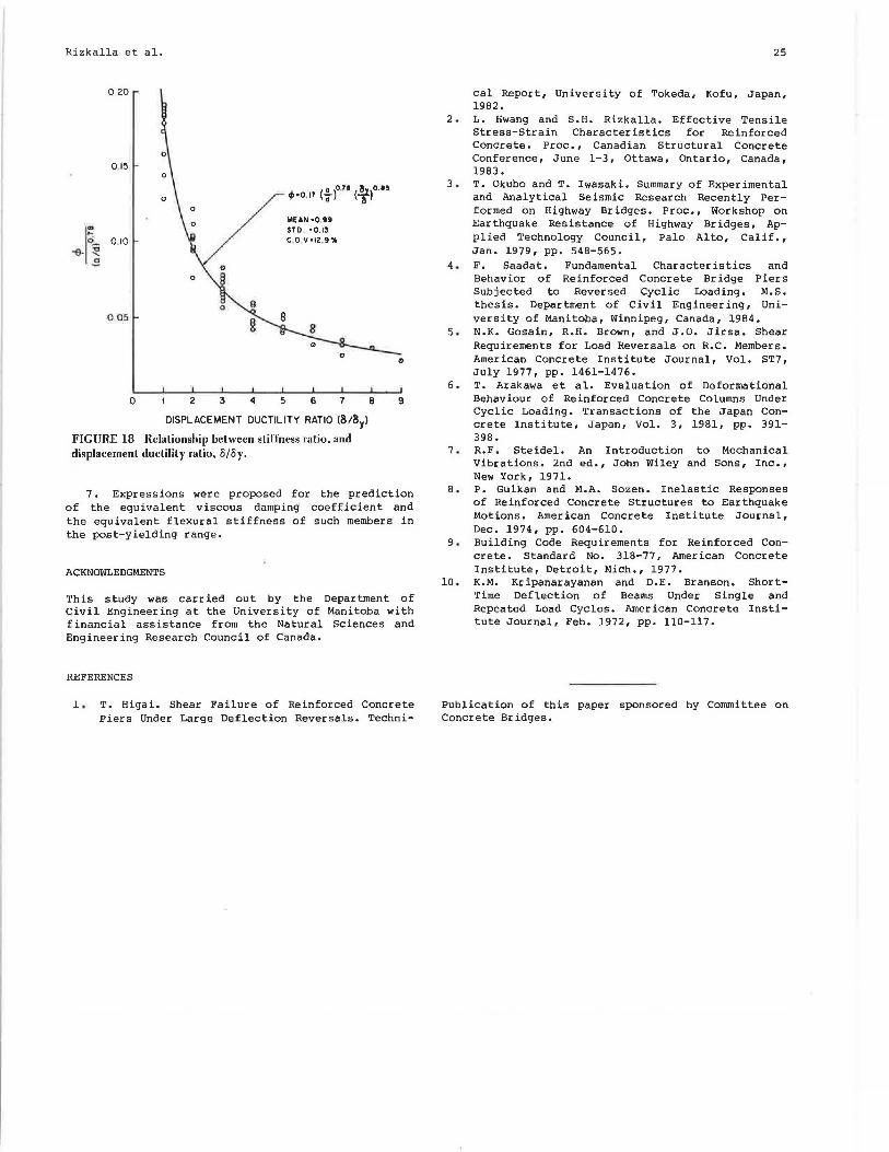
Rizkalla et al.

0 20

0 ,15

I~- 0 .10 -e- ~

s

0 05

0

0

0

• (~)0_11 (.!r_)0.15 4> 0 ,17 d 8

MEAN •0.99 STD •0.13 c 0 v •12 .9%

2 3 4 5 6 7 8

DISPLACEMENT DUCTILITY RATIO (818yl

FIGURE 18 Relationship between stiffness ratio, and displacement ductility ratio, 5/fJy.

0

9

7. Expressions were proposed for the prediction of the equivalent viscous damping coefficient and the equivalent flexural stiffness of such members in the post-yielding range.

ACKNOWLEDGMENTS

This study was carried out by the Department of Civil Engineering at the University of Manitoba with financial assistance from the Natural Sciences and Engineering Research Council of Canada.

REFERENCES

1. T. Higai. Shear Failure of Reinforced Concrete Piers Under Large Deflection Reversals. Techni-

25

cal Report, University of Tokeda, Kofu, Japan, 1982.

2. L. Hwang and S.H. Rizkalla. Effective Tensile Stress-Strain Character is tics for Reinforced Concrete. Proc., Canadian Structural Concrete Conference, June 1-3, Ottawa, Ontario, Canada, 1983.

3. T. Okubo and T. Iwasaki. Summary of Experimental and Analytical Seismic Research Recently Per­formed on Highway Bridges. Proc., Workshop on Earthquake Resistance of Highway Bridges, Ap­plied Technology Council, Palo Alto, Calif., Jan. 1979, pp. 548-565.

4. F. Saadat. Fundamental Characteristics and Behavior of Reinforced Concrete Bridge Piers Subjected to Reversed Cyclic Loading. M.S. thesis. Department of Civil Engineering, Uni­versity of Manitoba, Winnipeg, Canada, 1984.

5. N.K. Gosain, R.H. Brown, and J.O. Jirsa. Shear Requirements for Load Reversals on R.C. Members. American Concrete Institute Journal, Vol. ST7, July 1977, pp. 1461-1476.

6. T. Arakawa et al. Evaluation of Deformational Behaviour of Reinforced Concrete Columns Under Cyclic Loading. Transactions of the Japan Con­crete Institute, Japan, Vol. 3, 1981, pp. 391-398.

7. R.F. Steidel. An Introduction to Mechanical Vibrations. 2nd ed., John Wiley and Sons, Inc., New York, 1971.

8. P. Gulkan and M.A. Sozen. Inelastic Responses of Reinforced Concrete Structures to Earthquake Motions. American Concrete Institute Journal, Dec. 1974, pp. 604-610.

9. Building Code Requirements for Reinforced Con­crete. Standard No. 318-77, American Concrete Institute, Detroit, Mich., 1977.

10. K.M. Kripanarayanan and D.E. Branson. Short­Time Deflection of Beams Under Single and Repeated Load Cycles. American Concrete Insti­tute Journal, Feb. 1972, pp. 110-117.

Publication of this paper sponsored by Committee on Concrete Bridges.

26 Transportation Research Record 1044

Bridges Produced by an Architectural Engineering Team Tl\lll\.T £'1 DTT1'.TVD JV.1.J.l., '-.A· J.\..1..1.1.,.1..'.J.U.

ABSTRACT

In this paper, the aesthetic qualities of bridges are defined, the methods and principles employed to achieve these qualities are described, and seven award­wl1111l11g IJL luyt!o; dLt! !JLt!>;t!ult!u lu tlt!muno;trate the effect of public opinion 011

bridge appearance.

The purpose of this paper is to document {a) the reasons for producing bridges with aesthetic qual­ities and (b) the methods utilized to accomplish this task. The goal of the author's architectural engineering team is to comply with legislative direction for producing bridges built with public funds. These bridges must also satisfy the public's concern for quality while operating within strict fiscal limitations.

Many beautiful bridges were built before 1950, most of them depending on the arch for their beauty. Some were spectacular in their accomplishments but could only be considered beautiful by engineers. Before the age of formal calculations, bridge designers were generally intuitive in their design plans--they were more artist than engineer. The age of formal calculations produced a spectacular and plentiful array of bridges that did not collapse.

The midpoint of our century appears to have been the starting point in California for a formal blend­ing of intuitive bridge design with formal calcula-ticns en a normal, continuous basis. The scientific method has been expanded to include more than the object to be produced. This object, a bridge, is subjected to close scrutiny from every conceivable direction. Decisions concerning its appearance are no longer the values of one man, but the values of the recipient community as a whole. Within the Cali­fornia Bridge Department, the methods and principles used in assessing these values have been passed from one "bridge architect" to the next for approximately the last 60 years.

DISCUSSION

'rh e Team Approach

Before 1956, bridges in California were produced by an informal working relationship between engineers and one engineer-architect. After 1956, federal legislation that defined routes and provided funds for the Interstate Highway System led the California Department of Transportation to select the team approach as the most desirable method for obtaining high production and good quality.

Every bridge designed for California's highway system must receive an aesthetic review by a design team composed of a bridge architect and engineers of appropriate disciplines before it enters the final structural design stage. The area surrounding a bridge site must first be examined to determine the effect the structure might have on natural or man­made landscapes, existing or future cultures, and inhabitants. A harmonious relationship between all elements of the complete problem must exist for the project to be successful.

Consideration is given to any existing bridges in the vicinity that may have special architectural treatment. Finally, the bridge itself is architec­turally designed so that it is aesthetically compat­ible with its route. Special safety measures, new bridge rails, median, rails, approach rails, or pedestrian protection, are also given aesthetic consideration at this time. In order to allow all concerned interests to perceive the finished rela­tionships, artists prepare architectural renderings, photo retouches, and models for display at public hearings. The public is treated as a paying client.

The cooperative effort between engineer and architect begins at the earliest possible time. Open discussion of the site and possible solutions can save time and money. Bridges have been moved to sher ten them or place supporting systems in areas removed from posi­tivfLS orig i11ally plcuu1eU.

The engineer is in charge of producing contract plans. The architect is the engineer's consultant. Advanced planning studies prepared by the engineers are reviewed by bridge architects. These reviews consist of selecting column type, girder edge treat­ment, and surface treatment. A preliminary architec­tural sketch is drawn consisting of section, eleva­tion, and a rough perspective. Cost estimates are prepared and the suitability of structural design to architectural features and cost are determined before work progresses. A separate evaluation for each bridge in a group is not carried out until a type selection meeting is attended by representatives from the Specifications, Structural Design, and Architectural Design departments; and the appro­priate supervisors. After discussion, these general plans become the basis for drawings and models produced as needed to satisfy the public's demand for information. Sometimes, the public demands a particular style of architecture. However, the general policy is to produce the most efficient bridge by incorporating aesthetics into the structural requirements.

Ornamentation

Ornamentation is limited to surface textures and does not interfere with the visually exhibited, overall purpose of providing structure from one point to another. The ornament shown in Figure 1 was generated by a request from the community to acknowledge the path of the Oregon Trail. A bridge architect produced a preliminary drawing for com­munity approval. Figure 2 shows a drawing similar to

... -

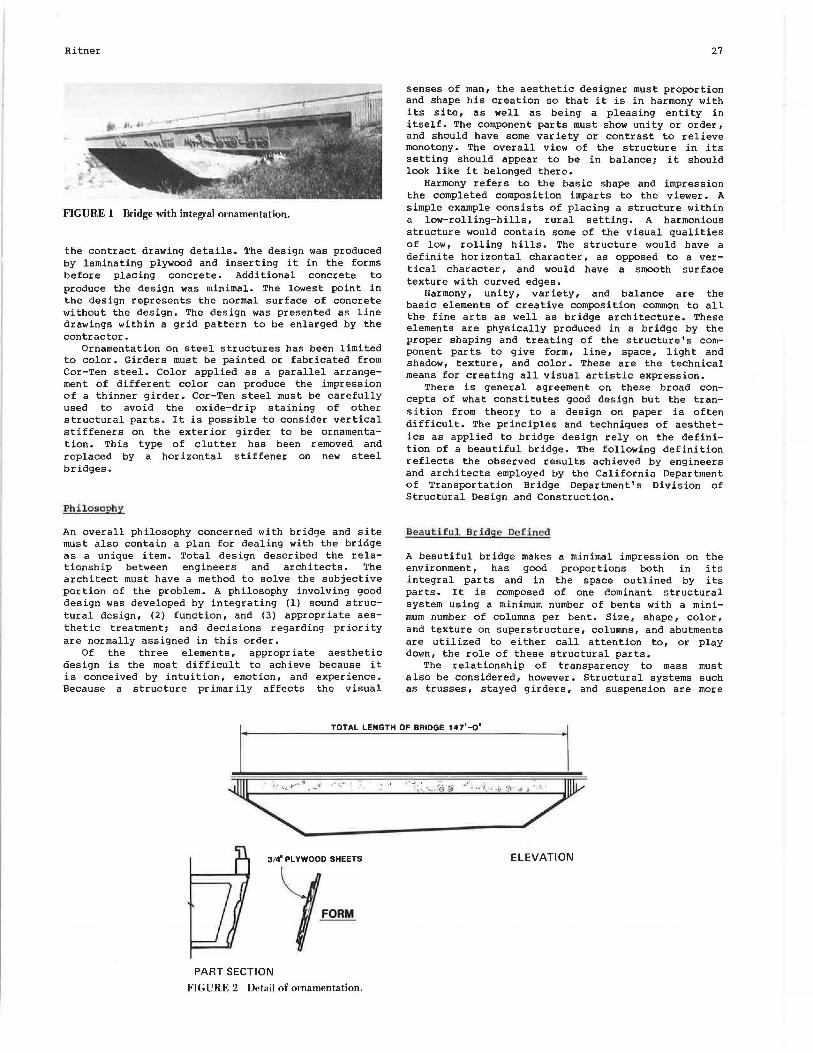
Ritner

FIGURE 1 Bridge with integral ornamentation.

the contract drawing details. The design was produced by laminating plywood and inserting it in the forms before placing concrete. Additional concrete to produce the design was minimal. The lowest point in the design represents the normal surface of concrete without the design. The design was presented as line drawings within a grid pattern to be enlarged by the contractor.

Ornamentation on steel structures has been limited to color. Girders must be painted or fabricated from Cor-Ten steel. Color applied as a parallel arrange­ment of different color can produce the impression of a thinner girder. Cor-Ten steel must be carefully used to avoid the oxide-drip staining of other structural parts. It is possible to consider vertical stiffeners on the exterior girder to be ornamenta­tion. This type of clutter has been removed and replaced by a horizontal stiffener on new steel bridges.

Philosophy

An overall philosophy concerned with bridge and site must also contain a plan for dealing with the bridge as a unique item. Total design described the rela­tionship between engineers and architects. The architect must have a method to solve the subjective portion of the problem. A philosophy involving good design was developed by integrating (1) sound struc­tural design, (2) function, and (3) appropriate aes­thetic treatment; and decisions regarding priority are normally assigned in this order.

Of the three elements, appropriate aesthetic design is the most difficult to achieve because it is conceived by intuition, emotion, and experience. Because a structure primarily affects the visual

27

senses of man, the aesthetic designer must proportion and shape his creation so that it is in harmony with its site, as well as being a pleasing entity in itself. The component parts must show unity or order, and should have some variety or contrast to relieve monotony. The overall view of the structure in its setting should appear to be in balance 1 it should look like it belonged there.

Harmony refers to the basic shape and impression the completed composition imparts to the viewer. A simple example consists of placing a structure within a low-rolling-hills, rural setting. A harmonious structure would contain some of the visual qualities of low, rolling hills. The structure would have a definite horizontal character, as opposed to a ver­tical character, and would have a smooth surface texture with curved edges.

Harmony, unity, variety, and balance are the basic elements of creative composition common to all the fine arts as well as bridge architecture. These elements are physically produced in a bridge by the proper shaping and treating of the structure's com­ponent parts to give form, line, space, light and shadow, texture, and color. These are the technical means for creating all visual artistic expression.

There is general agreement on these broad con­cepts of what constitutes good design but the tran­sition from theory to a design on paper is often difficult. The principles and techniques of aesthet­ics as applied to bridge design rely on the defini­tion of a beautiful bridge. The following definition reflects the observed results achieved by engineers and architects employed by the California Department of Transportation Bridge Department's Division of Structural Design and Construction.

Beautiful Bridge Defined

A beautiful bridge makes a minimal impression on the environment, has good proportions both in its integral parts and in the space outlined by its parts. It is composed of one dominant structural system using a minimum number of bents with a mini­mum number of columns per bent. Size, shape, color, and texture on superstructure, columns, and abutments are utilized to either call attention to, or play down, the role of these structural parts.

The relationship of transparency to mass must also be considered, however. Structural systems such as trusses, stayed girders, and suspension are more

1 · •om ''""'" .,.., .. .,.,. -o' 'I

~~· _-" _.·-_· ____ .. "_:"_- e_§_-· _ .. ,,_ ... _8·_,~

314' PLYWOOD SHEETS ELEVATION

PART SECTION

FIGURE 2 Detail of ornamentation.

28

transparent than box girders or plate girders. The ability to see through a structure can convey an air of mystery or magical quality to the viewer.

Aesthetic Qualities of Span Layouts

The span layout fixed by structural considerations can be changed by extending the limits of structure required. Prestressing a concrete structure illus­trates this principle. A different type of struc­tural system can also be used to retain economy even though the span or spans is lengthened or shortened. The following situations illustrate aesthetic qual­ities fixed by the structural layout:

1. A single span represents the ultimate bridge provided it can be thin enough, and sufficient camber can be applied to present the appearance of a straight line without a sag.

2. Two spans cause a split-composition effect in a natural setting but appear to belong to a freeway environment (Figure 3).

3. A multiple, even number of spans places a column in the center splitting the composition and causing the expected space in the center to be blocked by a column.

4. A multiple number of odd spans avoids the problem--there is no column in the center.

5. A three-span, arched girder with haunches produced by long curves appears especially graceful (Figure 4) •

6. Multiple-span, arched girders appear busy and tend to disturb structure flow.

FIGURE 3 Two equal spans.

FIGURE 4 Three-span arched girder.

:;tandard uesign

Standard designs have been employed to cope with the large number of bridges required. Standard refers to a general design in either concrete or steel re­flecting the philosophy stated without ornamental embellishment. The details are standard, not the bridge. These designs are modified to satisfy various site conditions. Unusual conditions are dealt with by producing custom designs. Crossings over large bodies of water, deep ravines, and pedestrian struc­tures are representative of custom design. Versatil­ity in design along with low maintenance and com­petitive cost has resulted in the majority of bridges being constructed of concrete, with the box girder as the dominant structural type.

Abutment

The apparent bridge length (slenderness) is increased when viewed by using the shortest wing wall length.

Transportation Research Record 1044

From an aesthetic viewpoint, an abutment reflecting the features of the mass connecting it to the bridge should be used. Abutments connecting to earth are usually concrete with a rough texture. The wing walls are made as small as possible, and are set back from the deck to continue part of the shadow of the deck on the wing wall. Abutments connecting to man-made structures can often be hidden within the structure causing the bridge to simply end at the man-made structure. This basic design of producing minimal apparent size in abutments enhances the feeling of lightness in a bridge. Abutments of large apparent size would only be used to stop visual movement along the bridge. (The building of defensive constructions at bridge terminations is not generally practiced.) Abutments with vertical faces appear static and stop visual continuity along the length of the bridge. Bridge length effectively stops at the abutment (Figure 5) •

FIGURE 5 Static lines.

Abutments with sloping faces continue the line of the deck and rail downward into the ground. The apparent length of the bridge can be increased and a feeling of ground integrated with bridge established (Figure 6) •

Columns

Many types of columns nave been used througnout history, but present-day bridges promote movement. The historic use of elaborate columns has been to restrict movement.

FIGURE 6 Dynamic lines.

:;tandard architectural columns have been designed as a series of modular shapes. Cross sections are available in round, octagonal, and hexagonal forms. These forms can be expanded to include a rectangle between the basic form. A round cross section can become a cross section that is semicircular at the edge with flat sides Joining another semicircular edge. This system is used for all the geometrical forms to increase the load bearing ability of a single column. Therefore, a minimum number of columns can be used. The edge column directly adjacent to the viewer provides the impression of column width that the viewer normally perceives. This impression is controlled by light reflecting from the column edge. Octagonal columns appear slimmest as a result of the greater number of surfaces. The viewer sees a large area broken up by several planes. Round columns are affected less and square or rectangular columns are not affected. The architect can take advantage of this light reflection by using the principles to slim down a massive column or increase the apparent

Ritner

size of a column to offset a massive superstructure. Column proportions therefore have a large effect on the aesthetics of bridges.

Columns that appear larger than necessary to support the superstructure are not desirable because attention is directed away from the primary purpose of a bridge, which is to provide free movement. Columns that are obviously needed to support the superstructure should appear to be of sufficient size to perform their function. Columns that appear thinner than the visual requirement impart the feel­ing of possible collapse to the viewer.

The upper part of standard architectural columns is curved, arched, or flared to visually integrate the column with the superstructure. This spreading outward of the standard architectural column is designed to be compatible with the sloped exterior girder of a trapezoidal box girder. Standard, flared architectural columns are not compatible with verti­cal exterior girder shapes. A transition between the column and the superstructure similar to the capital on classic style columns must be introduced. This "capital" usually takes a simplified form involving straight lines tapering in the opposite direction of the flare for a distance less than the girder depth. The capital actually becomes an exposed column cap, or part of an exposed column cap. This treatment is effective only when the extremities of the flare are wider than the superstructure.

Flared columns as described previously are de­signated as one-way-flare columns (Figure 7). They promote flow perpendicular to the bridge, under the bridgei therefore, they are directional.

0 0 0 FIGURE 7 Standard architectural columns with one-way flare.

Standard architectural columns have also been designed with two-way flare (Figure 8). These columns are nondirectional (they do not direct flow in a particular direction) and are particularly appro­priate in situations involving more than one bridge, such as in an interchange. Two-way-flare columns are more effective from a visual judgment because the flare is evident from any viewing position.

The lower portion of a column must connect with earth, man-made material, or water. Standard archi­tectural columns all have vertical lower portions. while although this may not provide the best solution aesthetically, it is the only practical solution for a column that must cope with great changes in height while retaining the same width at the top.

Columns with their lower portions in water rely on the structural conditions for their shape. Columns res ting on spread footings or in drilled holes can appear to disappear into the water, This is a dis­tinct advantage with fluctuating water levels. Col­umns in water supported on pile caps must consider the pile cap as an element in their overall design. Pile bents exposed as columns are used only when low clearance dictates the use of thin superstructure.

FRONT ©

SIDE FIGURE 8 Standard architectural columns with two-way flare.

29

These situations usually occur in areas where restricted passage and aesthetic concerns are minimal.

The standard architectural columns are the result of many nonstandard or custom designed columns. Typical undercrossing, overcrossing, and connector bridges can use similarly sized columns. The current series of standard architectural columns is the second attempt to produce standards to simplify design and lower construction costs by repetition.

There will always be a need for nonstandard columns. Special site conditions, such as Figure 9, require an overcrossing to span a divided highway with a depression in the center for mass transit. Inadequate space for one large column presented the problem of two thin columns resulting in a three-span structure. The structure depth would have visually overpowered the columns. The result was a massive­looking superstructure. Combining all the problems produced a unique solution with columns and super­structure in proportion.

FIGURE 9 Nonstandard architectural column.

Superstructure

Profile View

The profile view describes the structural type such as arch, post, and lintel, or combined variations of these types. Sound structural design (1), function (2), and appropriate aesthetic treatment (3) have been established as the order of priority. The first priority must begin with geology to determine where supports may reasonably be located. The structural type is therefore dependent on possible support in order to determine the span lengths. Technology has made it possible to have single-span lengths of 200 ft in concrete. This base can be expanded by using steel and adapting continuous span procedure to

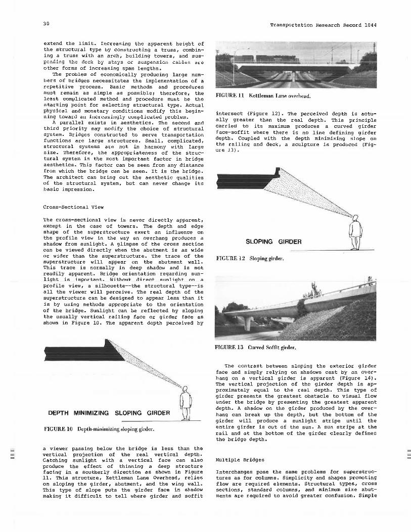
30

extend the limit. Increasing the apparent height of the structural type by constructing a truss, combin­ing a truss with an arch, building towers, and sus-....,...,_.:I~- .... .&-\...-. ..::1.-..,..J. ),....,.,. -~- .... - ~- -··-----!-- --L,-- ----.t"""'" ..... .&.U':j 11..U<;;;; U'l;;".._.n, LJ;t O"-Cl.}'0 VI. OUO}JCllO.LVU \,;QU.1.t:::O Cl.Lt::'

other forms of increasing span lengths. The problem of economically producing large num­

bers of bridges necessitates the implementation of a repetitive process. Basic methods and procedures must remain as simple as possiblei therefore, the least complicated method and procedure must be the starting point for selecting structural type. Actual physical and monetary conditions modify this begin­ning towaru ci11 iw:aect>1i11gly <.:umJ,!lil:aleu !Jrul>l.,m.

A parallel exists in aesthetics. The second and third priority may modify the choice of structural system. Bridges constructed to serve transportation functions are large structures. Small, complicated, structural systems are not in harmony with large size. Therefore, the appropriateness of the struc­tural system is the most important factor in bridge aesthetics. This factor can be seen from any distance from which the bridge can be seen. It is the bridge. The architect can bring out the aesthetic qualities of the structural system, but can never change its basic impression.

Cross-Sectional View

The cross- sectional view is never directly apparent, except in the case of towers. The depth and edge shape of the superstructure exert an influence on .&-1... ..... ..,...,,_ ..... .,::.:, ...... ..: ....... -=- ........... ··-·· -- _____ ,_ ___ ----..::1··--- -'-.L.l'I;;" ,t-'.L V.&. .l....L'I;;; y .1.CW .LU .... u1; WO:J au UV CJ.. uauy !''- VUU\,;CO Cl

shadow from sunlight. A glimpse of the cross section can be viewed directly when the abutment is as wide or wider than the superstructure. The trace of the superstructure will appear on the abutment wall. This trace is normally in deep shadow and is not readily apparent. Bridge orientation regarding sun­light is important. Without direct sunlight on a profile view, a silhouette--the structural type--is all the viewer will perceive. The real depth of the superstructure can be designed to appear less than it is by using methods appropriate to the orientation of the bridge. Sunlight can be reflected by sloping the usually vertical railing face or girder face as shown in Figure 10. The apparent depth perceived by

DEPTH MINIMIZING SLOPING GIRDER

FIGURE 10 Depth-minimizing sloping girder.

a viewer passing below the bridge is less than the vertical projection of the real vertical depth. Catching sunlight with a vertical face can also produce the effect of thinning a deep structure facing in a southerly direction as shown in Figure 11. This structure, Kettleman Lane Overhead, relies on sloping the girder, abutment, and the wing wall. This type of slope puts the girder face in shadow making it difficult to tell where girder and soffit

Transportation Research Record 1044

FIGURE 11 Kettleman Lane overhead.

intersect (Figure 12). The perceived depth is actu­ally greater than the real depth. This principle carried to its maximum produces a curved girder face-soffit where there is no line defining girder depth. Coupled with the depth minimizing slope on the railing and deck, a sculpture is produced (Fig­ure 13).

SLOPING GIRDER

FIGURE 12 Sloping girder_

FIGURE 13 Curved Soffit girder.

The contrast between sloping the exterior girder face and simply relying on shadows cast by an over­hang on a vertical girder is apparent (Figure 14). The vertical projection of the girder depth is ap­proximately equal to the real depth. This type of girder presents the greatest obstacle to visual flow under the bridge by presenting the greatest apparent depth. A shadow on the girder produced by the over­hang can break up the depth, but the bottom of the girder will produce a sunlight stripe until the entire girder is out of the sun. A sun stripe at the rail and at the bottom of the girder clearly defines the bridge depth.

Multiple Bridges

Interchanges pose the same problems for superstruc­tures as for columns. Simplicity and shapes promoting flow are required elements. Structural types, cross sections, standard columns, and minimum size abut­ments are required to avoid greater confusion. Simple

Ritner

FIGURE 14 Typical standard bridge.

ornamentation is required to avoid the monotony in­herent in the ascetic scene described previously.

This ornament can be made an integral part of concrete structures. Depressions and bumps within an area framed with smooth concrete produce dramatic visual contrasts (Figure 15). Color can add to this contrast.

FIGURE 15 Ornament relieves sterility.

APPLIED PHILOSOPHY

Tuolumne Rive r Bridge

This bridge was built in a canyon. The canyon became a reservoir (Figure 16 and Table 1). The span and cleai::ance requirements dictated a multi-span struc­ture. The structure was designed to carry only one­half of the projected traffic initially. Provision for widening was required. This bridge improved an existing entry to Yosemite National Park. The exist­ing two-lane road contained tight radius curves that restricted the choice of structural systems. Steel plate girders were chosen and a wide overhang pro­vided the method for producing shadow to relieve the girder depth. Both the concrete deck and the steel

FIGURE 16 Design drawings for Tuolumne River Bridge.

31

girders are curved in the plan view, allowing the shadow produced by the overhang to be parallel to the top and bottom flanges . A scalloped shadow would have resulted from using a curved deck and straight girders.

The concrete columns were specially shaped to provide resistance to water accelerated by earthquake forces. The transition from superstructure to column conforms to the requirement for the suggestion of a capital when using flared columns with vert i cal girders. The necessity of providing for a method of anchoring future girders to widen the structure produced the flared column. The mass of this column at the top was designed to be open in the dark a rea. Structural conditions did not allow for an opening: therefore, a depression painted the color of the surrounding landscape was substituted to promote the effect of an open area. Girders were painted the same color to minimize the impact of the structure on the surrounding landscape.

Award Received

1972 Arner ican Institute of Steel Construction Prize Bridge--Medium Span High Clearance.

Archie Stevenot Bridge

A deeper, wider canyon in approximately the same geographical area as the Tuolumne River Bridge pro­duced a bridge with an entirely different appearance (Figure 17 and Table 1). This bridge was also con­structed in a canyon that later became a reservoir.

Longer spans were required. Therefore steel box girders or concrete box girders were presented to contractors as options. The steel box girder was opted for and constructed with a provision for widening by increasing the overhang. The necessity of a wide overhang to provide shadow was not as evident when a large clearance condition was in effect. Filling the reservoir, and reducing the clearance increased the need to reduce the apparent height of the girders (Figure 17 and Table 1). The concrete columns were designed as rectangular, cross-section pyramids. This design recognized the forces produced by earthquakes and the increasing water level produced by the reservoir. Column size was proportional to the exposed height. Renderings were used to obtain a document to allow all team members to reach a point of understanding. Photo retouches produced from the design renderings com­municated the team's intent to all outside parties, and models were constructed to clarify design deci­sions.

Awards Received

1978 American Institute of Steel Construction--First Place: 1977 U.S. Department of Transportation--First Place in Outstanding Structure Category, Award for Best Entry: and 1981 Design for Transportation Awards--National Award for Design Excellence.

Adams Avenue Over c r ossing

The site for this hr idge (Figures 18 and 19, and Table 1) was an unexcavated depression within the San Diego city limits. The possibility of building the bridge in a hole allowed the exterior girder to be a warped surface due to the relative ease of constructing formwork.

32

TABLE 1 Physical Data

Y~ar Bridge Completed

Tuolumne River 1971

Archie Stevena! 1976

Adams Avenue 1970 East Fork of the Chowchilla 1972 Napa River 1977

Montana Pedestrian Overerossing 1979 Broadway Pedestrian Overerossing 1979 California Incline Pedestrian

Overcrossing 1979 Castellamare Pedestrian Overcrossing 1979 West Lilac Road Overcrossing 1978

County Road 8 Overcrossing 1968

Transportation Research Record 1044

Total Girder Column Span Length Length Depth u.,,.;....,i-.+

.l.L"'.l6UL

(ft) (ft) (ft) (ft)

132, 195, 260 1,394 15 220 350, 260 197 200,250, 500 2,250 11-26 380 550,500, 250 Varies 110, 218, 110 439 6-15 50 232,300, 188 720 8.5 min 100 1 SO, 175, 230, 250 2,230 7.75-12 100 230, 175, 6@150, 120 Varies 111,110,60 290 4 16 143 143 S min None

164, 141, 42 348 5 Varies 112 504 arch

IOI, IOI

112 4 20 695 7-14 135

(arch above road) 202 6 17

diffusing break-up occurs. If the girder slope varied to cause the soffit width to become a vertical projection of the horizontal soffit width at the point of least girder depth, soffit width would be constant and a warped, sloped, exterior girder sur­face would occur. A light reflecting surface dif­ferent from previous constant slope surfaces would have been created. This surface combined with sloping columns could produce a structure with greater visual continuity than previous sloped exterior structures without paying the pr ice of large, flat, reflective surfaces.

FIGURE 17 Archie Stevenot Bridge over the completed reservoir. Models were constructed to work out the actual

details. Calculating the volume of concrete proved to be difficult, so a scale model was constructed and filled with grout. The grout was measured as it was poured.

FIGURE 18 Adams Avenue Overcrossing-model.

FIGURE 19 Adams Avenue Overcrossing-actual.

Bridges with a curved soffi t profile change the point of intersection between soffit and exterior girder when the exterior girder is not perpendicular to the soffit. If the slope remains constant, the soffitt width varies from maximum width at thinnest girder depth section to minimum width at maximum depth girder section. The constant slope girder produces a flat exterior girder surface. No light-

Award Received

1969 Portland Cement Association Award of Excellence.

East Fork of the Chowchilla River

Located on the western slope of the Sierra Nevada Mountains, this three-span structure (Figure 20 and Table 1) is the southernmost member of the Tuolumne River, Archie Stevenot Bridge group. A reservoir was not involved in this project. The isolated loca­tion provides space to allow the large, flat, re­flective surface of the constant slope box girder to relate to the environment. !I. large oitc deco not require as much surface break-up as a small site to allow a harmonious relationship between structure and site. The deck overhang produces a shadow to accentuate the slim girder depth and create a cap or a top for the superstructure. Columns form a logical extension of the superstructure. Renderings and models were used to develop the design.

Award Received

1972 Fifth Annual National Scenic Highways Competi­tion--First Place in Outstanding Structures Category.

Napa River Bridge

The southern extremity of the Napa Valley provides the site for this multi-span concrete bridge using box girders arched over the longest spans to present

Ritner

F1GURE 20 East Fork of the Chowchilla River.

the thinnest profile (Figure 21 and Table 1). Arched or curved soffit girders add interest and variety to an otherwise repetitive bridge. These forms also help the structure to relate to the adjacent rounded hills. The integral column treatment used at the East Fork of the Chowchilla River would have increased the perceived size of the total structure, due to the relatively larger bridge at Napa River.

FIGURE 21 Napa River Bridge.

Single column bents relate by virtue of their flared, lozenge, cross sections to the curved sof­f its and sloped sides of the exterior girder faces. Textured detail provides relief from the expanse of concrete at the top center of all columns. (Render­ings were the only visual aids used to prepare this design.)

Awards Received

1978 Prestressed Concrete Institute Award, and 1982 U.S. Department of Transportation--Second Place in Major Highway Structure Category.

Pedestrian Overcrossings in Santa Monica

Bridges of different architectural design demonstrate the effect of public influence on bridges designed to solve a common functional problem. These struc­tures provide pedestrian access from Santa Monica to the beach over busy Route 1. Space along Route 1 is at a premium, which dictated stairs instead of ramps.

The California Coastal Commission was concerned about these structures. This concern provided the opportunity to deviate from completely standard

33

design. Pedestrian structures have an additional element to consider in their design: the direct users of these structures are people. Therefore, the scale and detail should make people feel comfortable. The experience of using the facility should be plea­sant.

Photo retouches were used extensively in public meetings held to obtain general approval from the public. This background helped to obtain approval from the Coastal Commission.

Montana Ped_estr_ian Overcrossing

The Montana Pedestrian Overcrossing is an example of a different type of integral column combined with the height-reducing, sloped girder to create an integrated structure that reflects light and adds to the beach atmosphere (Figure 22 and Table 1).

F1GURE 22 Montana Pedestrian Overcrossing.

Broadway Pedestrian Over crossing

Broadway intercepts an old brick stairway part way up the hillside. Brick was used as a design element to carry the stairway theme over Route 1 and tie it to the beach side. This structure is located less than 1 mi south of Montana (Figure 23 and Table 1). Montana has an appearance unlike Broadway yet both structures are compatible and serve as landmarks due to their difference.

FIGURE 23 Broadway Pedestrian Overcrossing rendering.

California Incl ine Pedestrian Overcrossing

A variation on the theme set by Montana. This struc­ture is located within sight of Montana (Figure 24 and Table 1) •

Award Received

1982 U.S. Department of Transportation--Third Place in Intermodal Facilities Category.

34

FIGURE 24 California Incline Pedestrian Overcrossing.

Castel lamare Pedestrian Overcr ossinq

The Castellamare Pedestrian Overcrossing, located approximately 1 mi north of Montana, bears no resem­blance to the Mon t ana or Broadway ove rcross i ngs, even though the designer was the same for all three overcrossings (Figure 25 and Table 1). The Los Angeles County Parks Department had definite design requirements. The structure replaced a 1920- vintage arch tied directly to a building of historical im­portance. The basic design for this structure re­sulted from grade school competitions. The exposed aggregate rocks are from a particular beach in Mexico specified by the Parks Department.

FIGURE 25 Castellamare Pedestrian Overcrossing.

West Li lac Road Overcross ing

West Lilac Overcrossing (Figure 26 and Table 1), which is located north of San Diego was designed without input from committees. It was designed by an architect and an engineer to be built within a cut section. Before the section was cut, however, every

Transportation Research Record 1044

FIGURE 26 West Lilac Road Overcrossing.

aspect of aesthetics had to be visualized because the site did not physically exist during design. A similar s ituation existed at Adams Avenue. Models were used extensively to find and solve the problems of integrating an arch with a sloping box girder. Complete integration of column and superstructure produces a structure more like a gateway than a bridge.

Awards Received

1978 Portland Cement Association Award of Excellence, and 1979 Prestressed Concrete Institute Award.

Typical Standard Bridge

County Road 8 Overcrossing is the type of bridge built to pure engineering considerations (Figure 14 and Table 1). Bridges built according to this formula could probably be successful today in award competi­tions provi ded they were stretched to their struc­tural limits by displaying the last word in technical efficiency. The point is that something must be added to the basic standard formula to raise the struct!.!re out of its absol!.!te ly sta!!dard situation~

That something is a quality that is achieved by incorporating either the public's will or engineering genius. Ideally , it would be a blend of both.

CONCLUSION

Bridges designed to fulfill engineering requirements wi t hou t regard for their appear ance may be withou t aesthetic qualities. Public opinion demands these qualities. Engineering and aesthetic concerns can successfully be combined by a team of special ists working on a large number of bridges with varying requirements. The team must combine structural, functional, and aesthetic values using rational methods. The degree ot success depends on the ability of all concerned parties to accurately perceive the completed p roj ect. Drawings and models provide the tools to create an accurate perception.

ACKNOWLEDGMENT

The author wishes to acknowledge Arthur L. Elliot and Warren S. Ludlow. Their unpublished manual, "Aesthetics in Bridge Design," written in 1970 for bridge design practice, forms the basis for this paper.

Publication of this paper sponsored by Committee on General Structures.

Transportation Research Record 1044 35

An Experimental Evaluation of Autostress Design

CHARLES W. ROEDER and LIV ELTVIK

ABSTRACT

Autostress design has been proposed as an economical and rational method for designing steel bridges. It is an extension of existing AASHTO load factor design, and it utilizes three load level limit states. Limited plastic redis­tribution of load is permitted during overload and maximum load limit states, because of the ductility of steel. However, the deflections are controlled to assure continued serviceability. This concept is somewhat new for bridge de­sign, and extensive research has been performed to substantiate the method. However, it was believed that a full-scale field test was needed to assure that the autostress method performs as expected under practical conditions. This paper describes such a test program. In this paper, the bridge, instrumenta­tion, and test program are described, and the test results are discussed and analyzed. Theoretical predictions are made and compared to the test results, and long-term observations of the bridge behavior are noted. The study shows that the autostress method performs well under service load and overload. Plastic deformations occurred but they were controlled. Therefore, permanent deflection and cracking of the concrete deck were minimal, and the design method should result in satisfactory performance of the bridge for many years.

Autostress design (ASD) has been proposed (1) as an economical and rational method for design{;:;g steel bridges. It is an extension of existing AASHTO (2) load factor design (LFD) and it utilizes three load level limit states. Under service load, the ASD method has identical design provisions to the LFD method including factors such as fatigue and deflec­tion control. However, steel bridges are ductile and may have considerable reserve strength, because of plastic redistribution of loads, and so ASD permits limited yielding during overloads that may occur a few times in the life of the structure. The deflec­t ions caused by yielding, however, are controlled to assure continued serviceability. The maximum load occurs only once or twice in the life of a bridge, and so the ASD method permits plastic analysis meth­ods for this load condition.

The concept of deliberate yielding is widely understood in some types of structural design, but is new for bridge design. Therefore, extensive re­search (.2_-~l has been performed to substantiate the method. Testing (~,!!_) of full-scale components has been performed to verify the load capacity and rota­tional ductility of bridge girders. A scale model bridge has been tested ( 4, 7) to verify the general concept, and linear and n~nlinear analyses have been performed. Thus, the ASD method has been well docu­mented, but a full-scale field test was needed to assure that the ASD method performs as predicted under practical field conditions.

The Whitechuck River Bridge was this test struc­ture (i,!.Q.). The bridge was designed by the ASD method and was constructed in 1982. A nondestructive load test, which simulated overload and induced yielding, was performed immediately after construc­tion. Strains, deflections, temperatures, and con­crete deck cracking were measured and observed during the load test, and a series of long-term observa­tions were taken for the 2-year period after the load test.

The results of this test program are presented in this paper. The bridge is described and the instru­mentation used during the study is noted. The load

test is discussed and the test results are analyzed. Theoretical predictions are made and compared to the test results. Finally, a series of long-term obser­vations are described and compared to the earlier results. This study shows that a bridge designed by using the ASD method may perform well under service load and overload. Plastic deformations occurred but they were controlled. Therefore, permanent deflec­tion and cracking of concrete bridge decking were minimal and so deterioration of the bridge and bridge deck should not be excessive for this method.

THE TEST BRIDGE

The Whitechuck River is located in the Glacier Peak area of Mount Baker and Snoqualmie National Forest near Darrington, Washington. The river is crossed by an unpaved road that is heavily used by logging trucks and recreational traffic. There are minimal constraints on the speed and weight of the logging vehicles. On occasion, the road is used by heavy timber yarding equipment that may overload the structure. A timber truss bridge crossed this river before 1982, but the U.S. Forest Service determined that it was not up to the required standards. As a result, the new bridge was designed by the ASD method through the joint efforts of the U.S. Steel Research Laboratory and the Denver Office of the U.S. Department of Transportation's Office of the western Bridge Design. The resulting structure is a single-lane, 3-span bridge with two continuous, composite girders and an orthogonal crossing as shown in Figure 1. The wide flanges are made of ASTM A588 (AASHTO M222) steel and are relatively shallow because of the economy achieved with the ASD Method.

The new bridge was designed for AASHTO HS-20 service loads. The overload limit state used a 1.0 load factor applied to the axle loads shown in Fig­ure 2 plus impact, and the maximum load limit state used a load factor of 1. 3 applied to the overload. ASD permits controlled yielding during overload and plastic limit analysis behavior during maximum load.

36

W30Xll6 t--63' ___,

W30X191

~ '»-~U.~-,,,--__,LJ~;;;p L 50' sr;· 50' _J

14'-0"

• •• -• • _ 1 •• -. • • • • • • • • ~ • • /T] __l • ., -' UI ol'· •, • •, # - • • • .. .. I • • t ' ' . ' . . . .. · -· .. . ... . . . 1

,b.. 1 ''" f1-0"

16'-4"

54.5k 54.5k 51.5k 51.5k

I I l ! 00 00

4'-10" _j l..-- 24'-10" _j l-- 4'-10"

W ASHINcn'ON 217D YARDER AND 110 SPAR

10k 27k 27k 72.5k 72.5k

I I I I I 0 0 0 00 ~ 17' --I 4' ~~--- 24' __ _J 5' l

SKAGIT BU-101 YARDER AND T-110 TOWER

45k 45k 60k 60k

l i l i 00 00 --..! 5' I-- 13' ~ 5' 1----

SKAGIT BU-99 YARDER AND T-110 TOWER

FIGURE 2 Design vehicle axle loads for overload limit state.

This yielding causes residual stress and strain and permanent deflections. The designers estimated a permanent deflection of 0.69 in. for the design over load, and the bridge girders were cambered for this deflection.

INSTRUMENTATION

Because a load test was performed to simulate over­load and induce limited yielding before the bridge was opened to normal traffic, all instrumentation was installed during the construction process. Stainless steel bolts were machined, painted, and bolted to the web of the steel beam to provide ac­curate, visible targets as shown in Figure 3. Twenty targets were attached to each beam at 9-10 ft inter­vals, and deflections of the targets were measured to approximately 0.01 in. accuracy with theodolites placed at one of four different stations. The theod­olites typically had a sight distance of less than

Transportation Research Record 1044

FIGURE 3 Typical theodolite target used for deflection measurements.

200 ft, so a 0.01 in.-deflection approximately coin­cided with 1-sec of angle. The theodolite supports were steel pipes filled with concrete and anchored into a concrete base.

One hundred and twenty strain gauges were at­tached to the bridge to measure strain level, locate neutral dAL~, determine initiation of yielding, estimate the effective width of the composite slab, and evaluate bending moments. Ninety-six of the gauges were attached to the steel, wide flanges in groups of six at eight locations of each girder as shown in Figure 4. This arrangement permitted re­dundancy of measurement and provided an estimate of

1 3

2

4 5 6 FIGURE 4 Typical strain gage configuration on the steel beams.

the distribution of strain over the beam depth and flange width. Two of the six groups were in the zone of yielding and were installed to estimate the initiation of yielding and locate the neutral axis. The other six locations were in areas that remained elastic, and they were also used to estimate bending moments. Four strain gauges were attached to longi­tudinal reinforcing bars over the bridge piers and steel girders. They showed the tensile strains in reinforcement and these strains were correlated to tensile cracking in regions of negative bending of the bridge deck. Twenty additional gauges were em­bedded in the bridge deck to measure concrete strains and evaluate the effective width. The strains were measured with a Hewlett Packard HP85 computer and HP 3054A data acquisition system.

Roeder and Eltvik

LOAD TEST

Four thermocouples were used to measure the tempera­ture of the steel girders and extensive material property tests were performed. Test cylinders were taken from each concrete mixer load for the deck, cured at the bridge site, and tested within 2 days of the load test. The average strength and elastic modules of the in-situ concrete were much larger than design values with results of 6.5 ksi and 4,600 ksi, respectively. Properties of the steel wide flanges and reinforcing bar were also measured and are given in Tables 1 and 2. Wheel loads of the test vehicles were measured with portable scales that were calibrated before the test. Finally, the as-built geometry was measured before testing and tension cracks in the concrete deck were monitored before, during, and after the test.

TABLE 1 Properties of Steel Reinforcing Bar

Properties

Yield stress (ksi) Modulus of Elasticity Based on Nominal Area (ksi)

TABLE 2 Properties of Steel Shape

Bar Size

No. 5

84 35,000

Heat Number

Properties

Yield Stress (mill report) (ksi) Tensile Strength (mill report) (ksi) Structural Shape

Static Yield Stress (ksi) Elastic Modulus (ksi)

X49411

56.4 to 62.9 73.8 to 78.3 W30x 116 W30 x 191 50.1 29,000

No. 6

73 36,000

K49721

57.3 75.7 W30 x 191

50.5 29,000

The temperature during the test, which was per­formed in November 1982, was reasonably constant (approximately 30°F) during the test, and so thermal strain had little effect on the results. Two load vehicles were used with wheel loads and geometry shown in Figure 5. The original intent had been to use a single vehicle with the axle loads and spacing of the Skagit BU-99 unit shown in Figure 2, but at the time, no such vehicle was available. Discussions with representatives of logging firms in the area suggest that the axle loads of Figure 2 do not rep­resent a real vehicle, since yarding equipment is usually custom built to customer specifications around a general model. Thus, the two vehicles of Figure 5 were a compromise selection. Both vehicles exceeded the normal HS-20 service load condition, and the combination of the two vehicles simulated the overload limit state.

Eighteen major load points, LPl to LP18, and eleven minor load points (LPlA, LP2A, etc.) were used in the load test. LPl through LP3 simulated service load conditions and no yielding was ex­pected, since a single vehicle was used. Although a single vehicle was used in LP4 and LPS, limited yielding was expected because the loads were applied at critical locations (near the curb and with the heavier, longer vehicle straddling the piers). LPG, 7, 8, and 9 all used both vehicles back-to-back and near the curb as shown in the photo of Figure 6. Significant yielding was expected during LP6 and LP?, but little or no yielding was expected during

6.3K

6.6K

5.5K

7.0K

WHEEL LOADS

4.5K 4.4K 5.9K 6.8K

8.5K 8.7K 7.0K 6.7K

6.4K 7.0K 8.4K 9.4K

6 .7K 6.7K 3.7K 3.5K

Vehlcle Logging Truck - Total Weight 116.8 KIPS

8.2K 8.0K 11.4K 12.2K 11.9K 11.9K 13.0K 15.7K

12.9K 11.2K 10.8K 3.9K 8.7K 8.8K 12.2K 17.4K

Vehlcle 2 L- Boy - Total Weight 191.1 KIPS

LOAD PROGRAM SUMMARY

VEHICLE GEOMETRY

B B S' 7"-- - --- --- - - - -- - --- 5' 11"

6"1_ = E3 B B a-112" r ' ~ 11' 4" --14' 8"~ 21' 11" ----14• 4'1-

Vehlcle 1 Logging Truck

,-o B B B 81 6' 9" ------- - - --- - - - - -------- 1' 5"

37

rl = a a a a:b2 .. ' 1

l---1s• 8" ---14'9" 29• 8" l- 4• 10"

Vehlcla 2 Low Boy

FIGURE 5 Wheel weights and axJe geometry for two test vehicles.

FIGURE 6 Photograph of two test vehicles applied simultaneously back-to-hack during LP6.

LP8 and LP9, because of the Automoment (!_,11,12) formed during earlier yielding (i.e., the structure experiences shakedown).

The trucks were moved into position for each of the load points, and strains and deflections were measured after a 15-min delay. The delay permitted completion of all yielding before measurements were made. The concrete deck over the bridge pier was

38

closely examined for tension cracks at each load point. Concrete cracking was smaller and less wide­spread than expected. A single tension crack formed over approximately the center of each pier during tne test (see Figure 7). The cracks started initia­tion during LP2 and were formed or were visible on the deck surface through LP9. The cracks were not visible on the deck surface after the loads were removed.

F1GURE 7 Photograph of deck crack marked and observed during LP6.

TEST P.ESULTS

The results of these tests clearly indicate that yielding occurred during the test program. Figure B is a plot of the measured deflections of the bridge girders with no load applied at various times during the test, It can be seen that permanent deflections started to develop early in the test and generally continued to increase through LP7A, but remained essentially constant after LP7A. This suggests that yielding started at LPl and continued through LP7, when shakedown occurred. The maximum permanent de-

West End

Transportation Research Record 1044

flections were 0.16 and 0.11 in. for the north and south girders, respectively. This permanent deflec­tion is considerably smaller than the 0. 6 in. pre­dicted by nonlinear analysis for the test vehicles.

The measured strains also indicated that yielding started early in the test but stopped after LP7. Figure 9 shows the strain in the reinforcing bar in the bridge deck over the steel girders and interior piers with no loads on the bridge. Tensile residual strain develops at these locations when plastic deformation occurs, and Automoments form. These residual strains first developed at the west pier, because LPl and LP2 used loads on the west and cen­ter spans only. After LP7, the residual strains did not change and the structure remained elastic.

The strain gauges on the steel girders were used to locate the neutral axis and measure the curva­ture. Figure 10 shows the measured permanent curva­ture for LP2A, LP4A, and LPBA, Curvature generally increases during the early load points and remains essentially constant after LPBJ\, Curvature at the interior piers is caused by yielding of the steel. The smaller curvatures noted in the spans is elastic curvature caused by positive residual bending moments [i.e., the Automoments (1,12)). These curvatures are small and of opposite ;ign to that noted at the piers. The experimental data of Figure 10 are con­nected with straight lines for simplicity, but the curvature distribution between measured points would be quite different for the actual structure.

The previous data indicate that yielding occurred due to overload of the structure. However, the yielding started sooner than was expected and the permanent deflection and concrete cracking were S:!!l?.l!er th:n ':!=.: :nticip:.ted ~ Figure 11 help!:! to illustrate why these unexpected results were noted. This figure shows the reported camber of the steel girders in the fabrication shop, the camber with computed, elastic, dead load deflections removed, and the absolute deflection of the bridge girders at the start of the test. (Note that the deflections shown in Figure 8 and all later figures are relative to this absolute value,) The figure shows that the actual dead load deflection was larger than expected, The girders were cambered by the flame-cambering process, and this process, when combined with hot-

\j 0 Nuth Girder u --0.25" r

0 .. . .. . 4

"' 0.25" z 0

!3 l"l ...:I r« ~--0.250

• . 0 ..

0.25"

' . . .

South Girder

t

A

i f

6

" IP2A . IP4A

• IPlA

• IP8A

l

FIGURE 8 Measured deflections of bridge girders with no loads on the bridge.

..

Roeder and Eltvik

300

I 200 ~ --~ Overnight Temperature

Effects

100 GAGE97 - NE GAGE98 -NW

~ GAGE99-SE

@ GAGE 100 -SW

0 0 2A 3A 4A 5A 6A 7A SA 9A 18A

WAD POINI'S

FIGURE 9 Measured strains in the reinforcing bar in the bridge deck over the steel girders and interior pier with no load on the bridge.

rolling, introduces residual stresses approaching the yield stress (13). The residual stresses caused the steel to yield'"° during placement of the dead load, and permanent deflection had occurred before any live load was applied. These plastic dead load deflections were larger at the east end because the deck concrete was placed from east to west. During the load test, yielding continued through LPl to LP7, but the permanent deflections were much smaller than expected during these later loads, because much of the permanent deflection had already occurred. Fabrication residual stresses affect the order and time of yielding but they have no impact on the ultimate strength of the bridge girders (12,_!l).

COMPARISON OF THEORETICAL PREDICTIONS WITH TEST RESULTS

39

A series of linear, elastic, theoretical predictions were performed (2_,.!Q_) using the average measured material properties and bridge geometry, and the results were compared with the experimental observa­tions. Figures 12 and 13 are typical comparisons for the deflections and bending moments, respectively. These comparisons showed that the concrete curb and steel guardrail significantly contributed to the bridge stiffness, and therefore had to be considered in the elastic analysis and prediction of bending moments. Further, the uncracked stiffness of the concrete deck was used even in the region of nega­tive bending. The uncracked stiffness provided good comparison between theoretical predictions and ex­perimental observations and agreed well with the observation that little deck cracking occurred dur­ing the load test. The actual in situ concrete had an average strength that was 85 percent larger than the design value. This stiff, strong concrete prob­ably contributed to the minimal cracking that was observed. This stiff material also necessitated the use of uncracked concrete stiffness and contributed to the small permanent deflections, since these permanent deflections are elastic deflections due to positive residual moments <.!l, such as Automoments.

The distribution of load between girders was also studied. One simple method, which is commonly used in design, distributes the loads to the individual girders by simple transverse equilibrium. This meth­od implicitly assumes that the torsional stiffness of the bridge is warping stiffness, and it resulted in much larger moment and deflection predictions for the heavily loaded girder when the bridge was ec­centrically loaded as shown in Figures 12 and 13. A more refined analysis including Saint Venant and warping torsion stiffness (14 ,15) was then used and much better comparison with experimental data re­sulted as shown in Figures 12 and 13. The exper i-

\J~~u~-~u---D Corrected Curvature North Giroer

1.0

... 0

~

>< ~

~ 1.0

A IP2A

~ IP4A

• IF8A

1.0

0

1.0 Nlte That lPBAAnl U'!lAAre &wrtinlly Ideitical

FIGURE 10 Measured curvature of the bridge girders with no load on the bridge.

40 Transportation Research Record 1044

West End F.ast End

~~1~~~1~1 ~~~~~1~,~~~r1 LJ LJ v

3.()"

2.0"

~ LO"

Reported Shop Camber

Reported Camber Less Dead

Load Deflection

~ o __;:---o --------u • • 0

0 • •

o Measured Camber North Girder -1.0"

• Measured Camber South Girder

FIGURE 11 Reported camber for the bridge girders at the fabricator shop and measured camber prior to testing.

LOAD POiNT LPZ

WEffi' END EAfIT END

u 0

0.25 EQU!LlBRIUM DJSI'RIBUl'ION sourn

~ 0 Q

~ 00. 0.25 ~ § &XPERIMENfAI, NORTH r;il 0.50 ~

'IDRSIONAL ANALYSIS SOUI'H

f:1 'IDRSIONAL ANALYSIS NORTH

0.75 EQUlLIBRlUM DISI'RlBUilON NORTH

FIGURE 12 Measured and computed deflectiom for loarl point LP2 ,

mental data shown in Figures 12 and 13 include the permanent deflections and Automoments caused by yielding, while the theoretical predictions do not. Therefore, the experimental data should overestimate the theoretical deflection and underestimate the positive and bending moment by approximately 8 per­cent. This comparison indicates that the Saint Venant torsion stiffness caused by the thick concrete deck dominated the solution, and the more refined analy­sis clearly provided more reliable results. Saint Venant torsion helped to distribute the load between the girders and reduced the maximum strains and deflections in the beams.

LONG-TERM OBSERVATIONS

A series of approximately

long-term observations were 6-month intervals for the

made at 2 years

following the load test. These were to verify shake­down and assure that no deterioration in the struc­tural performance had occurred. Deflections were measured in the early morning while the bridge was in thermal equilibrium (i.e., the temperature was essentially constant throughout the bridge). This negated thermal deflections, and the resulting changes in bridge deflections over the 2-year period can be seen in Figure 14. The changes were con­sistently less than 0. 02 in., which represents the statistical reliability of the measuring technique (~). Few outlying data points can be seen but those that can be seen have long sighting distances and potentially larger errors.

Cracking of the concrete bridge deck was also carefully monitored. At the end of the load test, a single tension crack existed in the bridge deck over the interior piers. The crack was closed and not visible on the deck surface unless live loads were

Roeder and Eltvik 41

LOAD POINT LP2 WES!' END EASl' END

0 Li

-500 ~ DISTRCBlJllON NORI'H ")

' -250 ~

TORSIONAL ANALYSIS NORI'H I r: . '-.. /

I :'0-. .. . . , A · ;::;;; 250 \· '·--·--- · .

~ ~Al. SOUI'H ~ ., TOOSIONAL ANALYSIS soum

~ 500

i:Q EXl'ER!lllENl'AL NORI'H

'. -.. ~ .......... +I

750

FIGURE 13 Bending moments estimated from experimental data and computed by analysis for load point LP2.

WEST END EAST END

~!--------~---------------~~~~~~~~~--'' I 11 NORrH GIRDER 11 I

( 0.50"

! JULY1983 5 O.O"l--....,"""=:==.~="==--_..."'--'--_:._....:....::::=.:....._,=::!"'--"'-'-'--'-'-'~--==="""'~,__--. ...._ OOl'OBER 1984

i::I

! ~ ~-0.50" FIGURE 14 Measured change in permanent deflection observed during the two years following the load test.

applied, but it could be seen on the underside of the deck, which was smooth. The size of these cracks did not grow during the long-term observation period, and they may have become smaller. However, the number of cracks increased slightly during this period. In October 1984, two small cracks could be seen over the west pier and three over the east pier. They are approximately 12 in. apart, and visible on the smooth underside of the deck only. In view of these obser­vations, it is believed that no additional yielding of the bridge girders occurred during the 2 years following the load test, and the bridge deck shows no tendency toward deterioration.

SUMMARY AND CONCLUSIONS

The ASD method is a new design method that permits limited, controlled yielding during the overload and

maximum load limit states. The Whitechuck River Bridge was designed by this method, constructed, load tested, and observed. The bridge performed well during this period as only controlled yielding of the steel occurred during overload_ and the permanent deflection and tension cracking of the concrete deck were less severe than expected. After the yielding occurred, the structure remained elastic for all future loadings. Long-term measurements substantiate these load test observations. The deck surface was nearly straight at the end of the test, and the bridge should have a normal service life before it.

The following conclusions are made:

1. The thick concrete slab helped to distribute the loads between the bridge girders. This reduced the maximum strains and deflections in the bridge girders well below simple design predictions. Tor­sional analysis methods that include warping and

42

Saint Venant torsion provide a reasonable estimate of this reduction.

2. The permanent deflections and tension crack-.:_,. - ~ ... , .. _ ------ a. - ..:i --·· -- .... -- ..__ "" ""' --.:.-- ____ ,,.. ... _,.. -··:::i ........ -··- --··-.. - ....... ----- -t"r--- ... --- --- ....... J ... - .... _ ....... .... ..... _

with the ASD method since they represent possible sources of serviceability and deterioration problems within the bridge. This test program appears to suggest that these concerns may be overstated. The ASD method has the unique advantage that limited yielding is anticipated. This yielding is accounted for with additional camber. Virtually all cambering methods cause large residual stresses, and these residual stresses induce early yielding when live or dead loads are applied. However, they do not affect the ultimate strength of the structure. Therefore, much of the permanent deflection may be completed before the concrete is hardened and live loads are applied. This is consistent with the Whitechuck Bridge observations and other earlier (]d) research .re.sui t :r

ACKNOWLEDGMENTS

The authors wish to acknowledge the financial sup­port of the American Iron and Steel Institute, AISI Project 188, and the FHWA (DTFH61-81-C-00114).

A number of people were most helpful in the per­formance of this research. The authors would like to thanK n.c. Kuentz at hISI, J. Nishanian of FHWn, and the AISI Task Committee for help in formulating the research plan and for their guidance during the study. In particular the authors would also like to thank R. Fountain, M. Grubb, G. Hasijer, A.H. Mat­tock, and the many students at the University of Washington for their help and advice.

REFERENCES

1. G. Hasijer, P.S. Carskadden, and M.A. Grubb. Autostress Design of Steel Bridges. ASCE, Jour­nal of Structural Division, Vol. 109, No. STl, Jan. 1983.

2. Standard Specifications for Highway Bridges. 12th ed., AASHTO, Washington, D.C., 1977.

3. P.S. Carskadden. Autostress Design of Highway Bridges Phase I: Design Procedure and Example Design. Technical Report 97-H-045 (019-1). U.S. Steel Corporation, March 1976.

4. P.S. Carskadden. Autostress Design of Highway Bridges Phase 2A: Test Planning. Technical Report 97-H-045 (019-2). U.S. Steel Corpora­tion, Jan. 1977.

s.

Transportation Research Record 1044

P.S. Carskadden and Design of Highway Studies. Technical

R.E. Bridges Report

Leffler. Autostress Phase 2B: Design 97-H-045 (019-3) .

~.~ . ~~~~~ ~~~~~~~~!~~ . 2!..!-~~ l~77

6. M.A. Grubb and P.S. Carskadden. Autostress Design of Highway Bridges Phase 3: Initial Moment Rotation Tests. Technical Report 97-H-045 (019-4). u.s. Steel Corporation, April 1979.

7. P.S. Carskadden. Autostress Design of Highway Bridges Phase 3: Inter ior--Suppor t--Model Test. Technical Report 97-H-045 (019-5). U.S. Steel Corporation, Feb. 1980.

8. M.A. Grubb and P.S. Carskadden. Autostress Design of Highway Bridges Phase 3: Moment-Rota­tion Requirements. Technical Report 97-H-045 (018-1). U.S. Steel Corporation, July 1981.

9. c.w. Roeder and L. Eltvik. Autostress Design Criteria: Load Test of the Whitechuck River Bridge. Final Report. FHWA, U.S. Department of ~ransportation, Dec. 1984 .

10. L. Eltvik. A Field Tei;t of Lhe Whilechuck River Bridge: Investigation of Autostress Design. M.S. thesis. Department of Civil Engineering, University of Washington, Seattle, 1983.

11. G. Hasijer and P.S. Carskadden. Autostress Design of Continuous Steel Bridge Members. Proc., 1980 Canadian Structural Engineering Conference, Toronto, Ontario, Canada.

12. B.G. Neal. The Plastic Methods of Structural Analysis. 3rd ed., Halstead Press, John Wiley and Sons, Inc., New York, 1977.

13. J .w. Baldwin and D.C. Guell. Permanent Deflec­tions and Loss of Camber in Steel Bridge Beams. Final Report. NCHRP Projects 12-1 and 12-6, TRB, National Research Council, Washington, D.C., Nov. 1971.

14. R.J. Reilly. Stiffness Analysis of Grids In­cluding Working. ASCE, Journal of Structural Division, Vol. 98, No. ST7, July 1972.

15. A. Fricher and F. Sawka. (Discussion to Refer­ence 14.) ASCE, Journal of Structural Division, Vol. 99, No. ST7, July 1983.

The findings expressed in this paper are based on the opinions of the authors and do not necessarily reflect the opinions of the funding agencies.

Publication of this paper sponsored by Cammi ttee on Dynamics and Field Testing of Bridges.

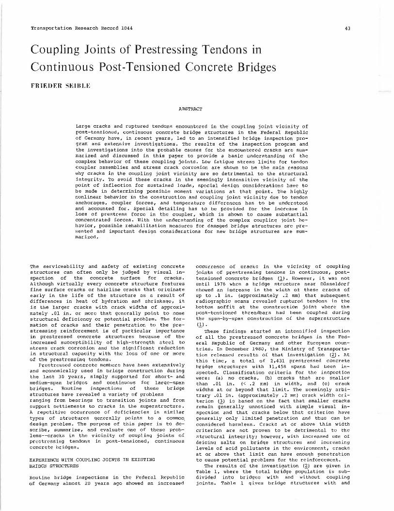
Transportation Research Record 1044 43

Coupling Joints of Prestressing Tendons 1n

Continuous Post-Tensioned Concrete Bridges

FRIEDER SEIBLE

ABSTRACT

Large cracks and ruptured tendons encountered in the coupling joint vicinity of post-tensioned, continuous concrete bridge structures in the Federal Republic of Germany have, in recent years, led to an intensified bridge inspection pro­gram and extensive investigations. The results of the inspection program and the investigations into the probable causes for the encountered cracks are sum­marized and discussed in this paper to provide a basic understanding of the complex behavior of these coupling joints. Low fatigue stress limits for tendon coupler assemblies and stress crack corrosion are shown to be the main reasons why cracks in the coupling joint vicinity are so detrimental to the structural integrity. To avoid these cracks in the seemingly insensitive vicinity of the point of inflection for sustained loads, special design considerations have to be made in determining possible moment variations at that point. The highly nonlinear behavior in the construction and coupling joint vicinity due to tendon anchorages, coupler forces, and temperature differences has to be understood and accounted for. Special detailing has to be provided for the increase in loss of pres tress force in the coupler, which is shown to cause substantial concentrated forces. With the understanding of the complex coupling joint be­havior, possible rehabilitation measures for damaged bridge structures are pre­sented and important design considerations for new bridge structures are sum­marized.

The serviceability and safety of existing concrete structures can often only be judged by visual in­spection of the concrete surface for cracks. Although virtually every concrete structure features fine surface cracks or hairline cracks that originate early in the life of the structure as a result of differences in heat of hydration and shrinkage, it is the larger cracks with crack widths of approxi­mately .01 in. or more that generally point to some structural deficiency or potential problem. The for­mation of cracks and their penetration to the pre­stressing reinforcement is of particular importance in prestressed concrete structures because of the increased susceptibility of high-strength steel to stress crack corrosion and the significant reduction in structural capacity with the loss of one or more of the prestressing tendons.

Prestressed concrete members have been extensively and economically used in bridge construction during the last 30 years, simply supported for short- and medium-span bridges and continuous for large-span bridges. Routine inspections of these bridge structures have revealed a variety of problems ranging from bearings to transition joints and from support settlements to cracks in the superstructure. A repetitive occurrence of deficiencies in similar types of structures generally points to a common. design problem. The purpose of this paper is to de­scribe, summarize, and evaluate one of these prob­lems--cracks in the vicinity of coupling joints of prestressing tendons in post-tensioned, continuous concrete bridges.

EXPERIENCE WITH COUPLING JOINTS IN EXISTING BRIDGE STRUCTURES

Routine bridge inspections in the Federal Republic of Germany almost 20 years ago showed an increased

occurrence of cracks in the vicinity of coupling joints of pres tressing tendons in continuous, post­tensioned concrete bridges (1). However, it was not until 1976 when a bridge st"iucture near Dilsseldor f showed an increase in the width of these cracks of up to .1 in. (approximately .2 mm) that subsequent radiographic scans revealed ruptured tendons in the bottom soffit at the construction joint where the post-tensioned threadbars had been coupled during the span-by-span construction of the superstructure

<1J. These findings started an intensified inspection

of all the prestressed concrete bridges in the Fed­eral Republic of Germany and other European coun­tries. In December 1980, the Ministry of Transporta­tion released results of that investigation (~). At this time, a total of 2,431 prestressed concrete bridge structures with 11,458 spans had been in­spected. Classification criteria for the inspection were: (a) no cracks, (b) cracks that are smaller than .01 in. (< .2 mm) in width, and (c) crack widths at or beyond that limit. The seemingly arbi­trary .01 in. (approximately .2 mm) crack width cri­terion (3) is based on the fact that smaller cracks remain generally unnoticed with simple visual in­spection and that cracks below that criterion have generally only limited penetration and thus can be considered harmless. Cracks at or above this width criterion are not proven to be detrimental to the structural integrity; however, with increased use of deicing salts on bridge structures and increasing levels of acid pollutants in the environment, cracks at or above that limit can have enough penetration to cause potential problems for the reinforcement.

The results of the investigation (~) are given in Table 1, where the total bridge population is sub­divided into bridges with and without coupling joints. Table 1 gives bridge structures with and

44

TABLE 1 Results of Bridge Inspection, Status 12-31-80 Ministry of Transportation, Federal Republic of Germany (2)

~u::=.~! Uli!!! Prestressed Concrete Coupling Coupling Bridge Structures Joints Joints Total

No cracks 1,477 (88%) 196 (12%) 1,673 (100%) (80%) (34%) (69%)

Cracks< 0.2 mm 187 (54%) 160 (46%) 347 (100%) (10%) (27%) (14%)

Cracks;;. 0.2 mm 184 (45%) 227 (55%) 411(100%) (10%) (39%) (17%)

Total 1,848 583 2,431 (100%) (100%) (I 00%)

without cracks not only by number, but also in parentheses, the individual percentage distributions with respect to corresponding top or left-column .r.,ference values. It can be seen that the bridges with coupling joints show not only a tendency toward having more cracks than bridges without coupling joints, but also a tendency toward wider cracks. While the statistics in Table 1 are for all cracks encountered in a bridge structure, it also is in­teresting to note that 104 br idges--almost one-half of the 227 bridges (cracks > • 2 mm) with coupling joi nts--showed these cracks in the direct vicinity of the coupling joints. It shou l d be noted thar. r.he survey (2) includes only bridge structures with coupling -joints built before 1977, at which time substantial changes in the code provisions for cou-

COMPLETED SECTION NEXT SECTION

~~~~--------~---------~ I ~ --------- - - ----1

--..._,1,.----r-- TEN DON COUPLERS I

I

TENDONS

- 0 2L

FIGURE 1 Coupling joint.

Transportation Research Record 1044

pling joint design were introduced into the West German Standards for prestressed concrete.

CRACK DEVELOPMENT I N COUPLING JOINT VICINITY

The coupling of prestressing tendons as shown sche­matically in Figure 1 is primarily used for medium­span, continuous, post-tensioned bridge structures with a large number of repetitive spans. Two con­struction methods that proved to be economical in these cases were the span-by-span construction with traveling self-supporting falsework ana the incre­mental launching method (see Figure 2). Bridge cross-sections most frequently used for these methods are shown in Figure 3. While expensive scaffolding is no longer needed, both methods rely on the early post-tensioning of each new section to the already­built bridge structure. This is accomplished by cou­pling the prestressing tendons in the construction joints (:;.,., Figur" 4). In the span-by-span construc­tion method, the construction and coupling joints are generally located at the theoretical point of inflection for sustained loads (combined dead load and prestressing) and it is at these locations that severe cracking parallel to the construction joints was encountered in the bottom soffi t and lower web portions of the bridge structure.

Substantial investigations of these phenomena (l_-2l have led to the following possible causes pointing to inadequate design for:

• variations of sustained loads, ' Secondary moments and nonlinear stress dis­

tributions resulting from temperature differences, Time-dependent moment redistributions,

• Support settlements, • Nonlinear (local) stress state in coupling

joint, • Increased loss of prestress in coupling joint, • Inaccuracies in prestressing force due to

friction, and • Heat of hydration and creep and shrinkage

differences in adjacent members with different di­mensions.

Although most of the preceding points are common problems in bridge design, their implication in the particular case of a coupling joint at the point of inflection of a bridge structure is of importance.

Coupling Joint

SPAN BY SPAN ERECTION WITH TRAVELLING SELFSUPPORTING FALSEWORK

INCREMENTAL LAUNCHING METHOD

(onctntrlc Prestressing

FIGURE 2 Construction methods with coupling joints.

Launching Nose

--

Seible 45

BOX GIRDER T - BEAH

\\ 7/LJ \oor ~

r FIGURE 3 Typical cross sections for sectional construction methods.

TREADBAR ( OUPLER

Coupler

I" 220

j~b FIXED TENDON

l~b 700

Coupler

l.J= J';

ZQQ

COUPLER

M2~

2J)

700

~~

Section b-b 1

{i

MOVABLE TENDON COUPLER

FIGURE 4 Prestressing couplers (dimensions in millimeters).

Variations in Point of Inflection and Design Moments

Construction joints are placed at the point of in­flection for sustained loads to minimize the amount of reinforcement required at that section. Generally, only minimum reinforcement or a minimum amount of pres tress will be provided in the design. However, the location of the point of inflection can change because of variations in the sustained loads (e.g., variations in dead load and pres tressing forces), thus introducing moments at the design point of in­flection (~). If these moments are superimposed with possible variations in the determination of secondary temperature effects, support settlements, and over­estimated moment redistributions in the structure due to the span-by-span erection process and creep and shrinkage, the design moment at this location can change significantly, not only in magnitude but also in sign. Small moment changes in areas of large design moments are generally sufficiently provided

for by the applied load and safety factors, whereas areas of small design moments do not have this built-in safety feature and have to be much more carefully evaluated for these moment variations (see Figure 5). Although this is the case in all con·­t inuous bridge structures in the vicinity of the point of inflection for sustained loads, problems may arise if this area is weakened by a construction joint and, in addition, by tendon anchorages and couplers.

Nonlinear Stress Distribution

The temperature distribution over the depth of a bridge structure is generally parabolic with extreme values at the top and bottom fibers (6). Most analy­ses account for the linear portion of the resulting stress distribution by assuming a certain tempera­ture difference, [IT, over the structural depth and

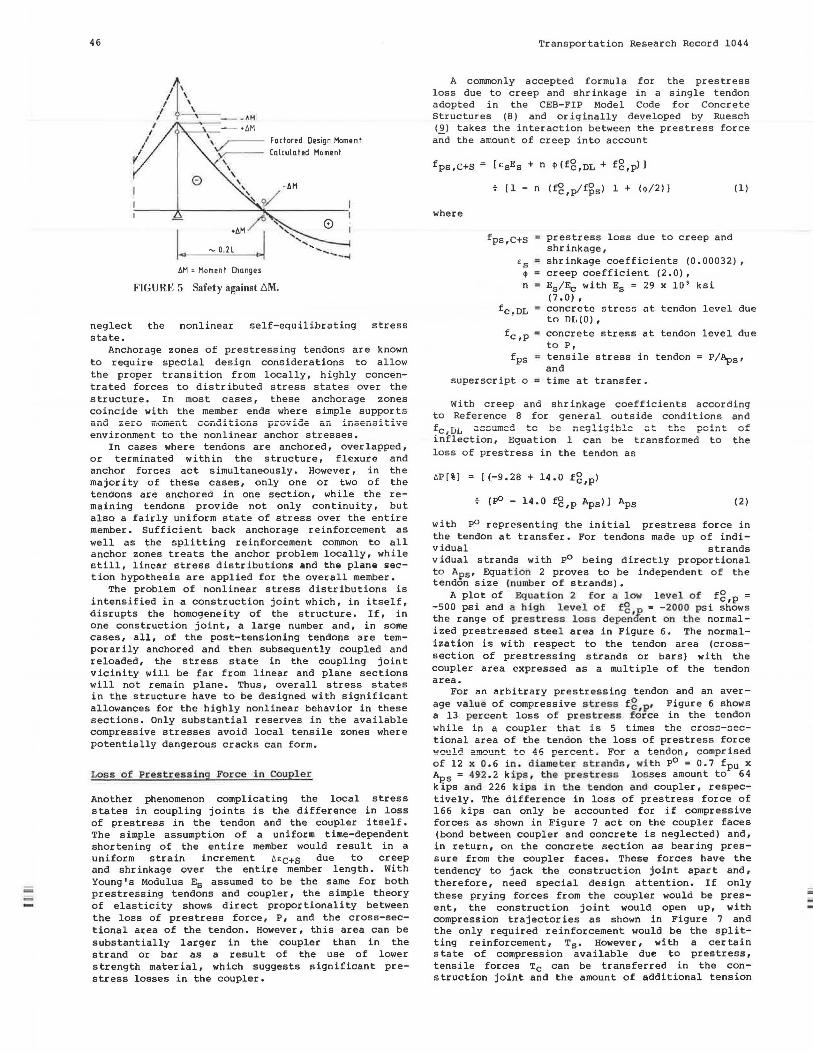
46

, I

/ I r

/1\ I ' I -'~-- - AH

Q..,.---";-_- •6M

0

\~ Factored Design Moment

(alculatod Moment \

\ \

- 0.2L

\

' ' :,..

llM = Homen I Olanges

FIGURE 5 Safety against L'IM.

neglect the nonlinear self-equilibrating stress state.

Anchorage zones of prestressing tendons are known to require special design considerations to allow the proper transition from locally, highly concen­trated forces to distributed stress states over the structure. In most cases, these anchorage zones coincide with the member ends where simple supports ana zero moment conditions provide an insensiti;te environment to the nonlinear anchor stresses.

In cases where tendons are anchored, over lapped, or terminated within the structure, flexure and anchor forces act simultaneously. However, in the majority of these cases, only one or two of the tendons are anchored in one section, while the re­maining tendons provide not only continuity, but also a fairly uniform state of stress over the entire member. Sufficient back anchorage reinforcement as well as the splitting reinforcement common to all anchor zones treats the anchor problem locally, while still, linear stress distributions and the plan& ~ec­tion hypothesis are applied for the overall member.

The problem of nonlinear stress distributions is intensified in a construction joint which, in itself, disrupts the homogeneity of the structure. If, in one construction joint, a large number and, in some cases, all, of the post-tensioning tendons are tem­porarily anchored and then subsequently coupled and reloaded, the stress state in the coupling joint vicinity will be far from linear and plane sections will not remain plane. Thus, overall stress states in the structure have to be designed with significant allowances for the highly nonlinear behavior in these sections. Only substantial reserves in the available compressive stresses avoid local tensile zones where potentially dangerous cracks can form.

Loss of Prestressing Force in Coupler

Another phenomenon complicating the local stress states in coupling joints is the difference in loss of pres tress in the tendon and the coupler itself. The simple assumption of a uniform time-dependent shortening of the entire member would result in a uniform strain increment 6<c+s due to creep and shrinkage over the entire member length. With Young's Modulus Es assumed to be the same for both prestressing tendons and coupler, the simple theory of elasticity shows direct proportionality between the loss of pres tress force, P, and the cross-sec­tional area of the tendon. However, this area can be substantially larger in the coupler than in the strand or bar as a result of the use of lower strength material, which suggests significant pre­stress losses in the coupler.

Transportation Research Record 1044

A commonly accepted formula for the prestress loss due to creep and shrinkage in a single tendon adopted in the CEB-FIP Model Code for Concrete Structures (8) and originally developed by Ruesch (~) takes the interaction between the prestress force and the amount of creep into account

fps,C+S

where

+ [l - n (£<6,plfgs> 1 + (~/2))

fps,C+S = prestress loss due to creep and shrinkage,

(1)

£ s = shrinkage coefficients (0. 00032) , ~ = creep coefficient (2.0), n = Es/Ee with Es = 29 x 10 3 ksi

(7 .0) , fc,DL s concrete stress at tendon level due

to Dl,(0) 1

fc,p = concrete stress at tendon level due to P, tensile stress in tendon = P/Aps• and

superscript o time at transfer.

With creep and shrinkage coefficients according to Reference 8 for general outside conditions and fc,DL ~s~umea to be negligibla ~t the point cf inflection, Equation 1 can be transformed to the loss of prestress in the tendon as

6P[%) [(-9.28 + 14.0 f2,p>

(pO - 14.0 f8,p Apsll Aps (2)

with P0 representing the initial prestress force in the tendon at transfer. For tendons made up of indi­vidual strands vidual strands with P0 being directly proportional to Aps• Equation 2 proves to be independent of the tendon size (number of strands).

A plot of Equation 2 for a low level of f2,p = -500 psi and a high level of fg = -2000 psi shows the range of pres tress loss depen~nt on the normal­ized prestressed steel area in Figure 6. The normal­ization is with respect to the tendon area (cross­section of prestressing strands or bars) with the coupler area expressed as a multiple of the tendon area.

For an arbitrary prestressing tendon and an aver­age value of compressive stress fg P' Figure 6 shows a 13 percent loss of prestress force in the tendon while in a coupler that is 5 times the crosc-cec-tional area of the tendon the loss of prestress force would amount to 46 p~rcent= For a tendon: ~omprised

of 12 x 0.6 in. diameter strands, with P0 = 0.7 fpu x ~s = 492.2 kips, the prestress losses amount to 64 kips and 226 kips in the tendon and coupler, respec­tively. The difference in loss of prestress force of 166 kips can only be accounted for if compressive forces as shown in Figure 7 act on the coupler faces (bond between coupler and concrete is neglected) and, in return, on the concrete section as bearing pres­sure from the coupler faces. These forces have the tendency to jack the construction joint apart and, therefore, need special design attention. If only these prying forces from the coupler would be pres­ent, the construction joint would open up, with compression trajectories as shown in Figure 7 and the only required reinforcement would be the split­ting reinforcement, Ts· However, with a certain state of compression available due to prestress, tensile forces Tc can be transferred in the con­struction joint and the amount of additional tension

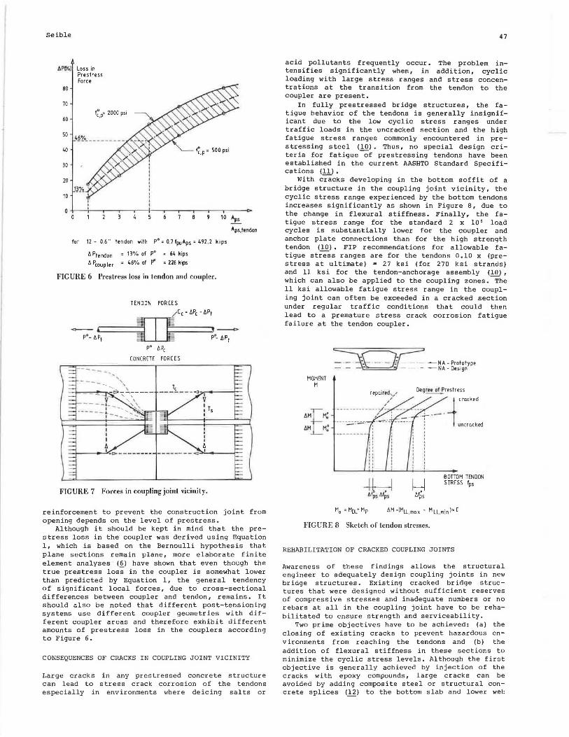
Seible

LI Pl%1 Loss in Pres1ress Force

BO

70

60 f~.P= 2000 psi

50

30

20

10

10 Aps

Aps,tendon

for 12 - O 6" tendon with P' = 0.7 fpuAps = 492 .2 kips

/::. Ptendon = 13% of P' = 6~ kips

/::. Pcoup ler = 46% of p" • 226 kips

FIGURE 6 Prestress loss in tendon and coupler.

TENDON FORCES

~/::.~rt-----=j=t I f .. ,,_,,,~_-;;,-P0 - t:.P,

CONCRETE FORCES

I v : Ts I

I I

I A I

FIGURE 7 Forces in coupling joint vicinity.

reinforcement to prevent the construction joint from opening depends on the level of prestress.

Although it should be kept in mind that the pre­s tress loss in the coupler was derived using Equation 1, which is based on the Bernoulli hypothesis that plane sections remain plane, more elaborate finite element analyses (~) have shown that even though the true prestress loss in the coupler is somewhat lower than predicted by Equation 1, the general tendency of significant local forces, due to cross-sectional differences between coupler and tendon, remains. It should also be noted that different post-tensioning systems use different coupler geometries with dif­ferent coupler areas and therefore exhibit different amounts of prestress loss in the couplers according to Figure 6.

CONSEQUENCES OF CRACKS IN COUPLING JOINT VICINITY

Large cracks in any prestressed concrete structure can lead to stress crack corrosion of the tendons especially in environments where deicing salts or

47

acid pollutants frequently occur. The problem in­tensifies significantly when, in addition, cyclic loading with large stress ranges and stress concen­trations at the transition from the tendon to the coupler are present.

In fully pres tressed bridge structures, the fa­tigue behavior of the tendons is generally insignif­icant due to the low cyclic stress ranges under traffic loads in the uncracked section and the high fatigue stress ranges commonly encountered in pre­stressing steel (10). Thus, no special design cri­teria for fatigue -Of prestressing tendons have been established in the current AASHTO Standard Specifi­cations (11).

With c~cks developing in the bottom soffit of a bridge structure in the coupling joint vicinity, the cyclic stress range experienced by the bottom tendons increases significantly as shown in Figure 8, due to the change in flexural stiffness. Finally, the fa­tigue stress range for the standard 2 x 10 6 load cycles is substantially lower for the coupler and anchor plate connections than for the high strength tendon (10). FIP recommendations for allowable fa­tigue stress ranges are for the tendons 0.10 x (pre­stress at ultimate) = 27 ksi (for 270 ksi strands) and 11 ksi for the tendon-anchorage assembly (10) , which can also be applied to the coupling zones. The 11 ksi allowable fatigue stress range in the coupl­ing joint can often be exceeded in a cracked section under regular traffic conditions that could then lead to a premature stress crack corrosion fatigue failure at the tendon coupler.

MOMENT M

~~-NA-Prototype - - _i~ - - - -NA-Design

' , I

1: ,, :: :: " ..

Deg ree of Prestress

. ...;..- . - · -t crocked

! uncrocked

BOTTOM TENDON STRESS fps

FIGURE 8 Sketch of tendon stresses.

REHABILITATION OF CRACKED COUPLING JOINTS

Awareness of these findings allows the structural engineer to adequately design coupling joints in new bridge structures. Existing cracked bridge struc­tures that were designed without sufficient reserves of compressive stresses and inadequate numbers or no rebars at all in the coupling joint have to be reha­bilitated to ensure strength and serviceability.

Two prime objectives have to be achieved: (a) the closing of existing cracks to prevent hazardous en­vironments from reaching the tendons and (b) the addition of flexural stiffness in these sections to minimize the cyclic stress levels. Although the first objective is generally achieved by injection of the cracks with epoxy compounds, large cracks can be avoided by adding composite steel or structural con­crete splices (~) to the bottom slab and lower web

--

48

-0.2 L Coupling Joint

/pres tressing

composito structural concreto additions

Transportation Research Record 1044

LONGITUDINAL SECTION TROUGH BRIDGE SUPERSTRUCTURE

COUPLING JOINT SECTIONS

FIGURE 9 Possible repair measures.

areas (see Figure 9). The added stiffness (see dotted line in Figure 8), reduces the cyclic stress range in the tendons and thus increases the service life of the structure (12) • Both objectives can be achieved simultaneously by adding more post-tensioning to be structured (see Figure 9) , which closes the cracks and prevents them from reopening. This is equivalent to a highe r deg r ee o f pre8treBs in Figure 8~ However, special attention has to be given to the anchor points of the additional prestressing tendons.

CONCLUSIONS AND DESIGN CONSIDERATIONS

The cracks found in the vicinity of coupling joints of prestressing tendons in a large number of post­tensioned continuous concrete bridges (1,2) have exposed deficiencies of these coupling joii;'°t;. These deficiencies, however, can be minimized or eliminated by a proper understanding of the complex behavior of a coupling joint and by appropriate design measures.

The low-fatigue stress levels of tendon-coupler assemblies combined with their sensitivity to stress crack corrosion require that acid environments are prevented from reaching the tendons and that the structural integrity is preserved by minimizing the stiffness deterioration and, with it, the cyclic stress levels in the coupling elements. The design objective is therefore to eliminate cracks in the coupling joint vicinity completely, or at least, to prevent possible cracks from opening and penetrating.

The increased loss of prestress in the coupl<>rs and, with it, the highly nonlinear stress distribu­tion in the coupling joint vicinity have to be ac­counted for in the design.

The following specific design considerations should be made:

1. A

tendons balance

in each between coupled and construct i on joint

uncoupled should be

provided. 2. The tendons to be coupled should be distrib­

uted as much as possible over the cross-section of the bridge structure to minimize the local non­linearities.

3. A sufficient level of prestress should be provided to cover inaccuracies of the bending moments.

4. Sufficient and closely forcement should be provided cracks from opening.

in the determination

spaced minimum rein­to prevent possible

5. Additional local forces due to the increased

loss of prestress force in the coupler should be considered and accounted for.

6. The cyclic stress levels in the tendon coupler assemblies should be checked under traffic loads in the cracked and uncracked stages.

With these design considerations in mind, new br id~e cons tr uct. i on 1oetb0Us traveling, self-supporting launching, which both rely stressing tendons, can be implemented.

REFERENCES

- - _,_ - - ....,--- L.-- ---- __ .: .&..k bU{.;11 db b.Pd.U-uy-~l-'d.11 W.LL.U

falsework or incremental on the coupling of pre­saf ely and economically

1. Der Bundesminister fuer Verkehr, Abteilung Strassenbau. Schaeden an Bruecken und anderen Ingenieurbauwerken. verkehrsblattverlag Borg­mann GmbH u. Co. KG, Dortmund, Wcot Germany, 1982, 462 pp.

2. Risse in Spannbetonbruecken, insbesondere in Koppelfugenbereichen, Ergebnisse der Risser­fassung. B 3.2- 3590. Stand von 31.12.80, Bun­desanstalt fuer Strassenwesen, West Germany, June 1981.

3. F. Leonhardt. Risseschaeden an Betonbruecken-­Ursachen und Abhilfe. Beton u. Stahlbetonbau, Heft, Feb. 1979, pp. 36-44.

4. F. Leonhardt. Vorlesungen ueber Massivbau, Fuenfter Teil, Spannbeton. Springer Verlag, New York, 1980, 296 pp.

5. F. Leonhardt. Vorlesungen ueber Massivbau, Sechster Teil, Grundlagen des Massivbruecken­baues. Springer Verlag, New York, 1980, 296 pp.

6. G. Koenig and T. Zichner. Beruecksichtigung der Temperaturdifferenz 6T, der Steuung des Eigen­gewichts und der erhoehten Spannkraffverluste an Spanngliedkopplungen bei der Bemessung Mas­siver Bruecken. Proc., 8th International FIP Conference, London, England, 1978.

7. G. Ivanyi and K. Kardina. Schaeden an Spannbe­tonbruecken im Bereich von Koppelfugen. Proc., 8th International FIP Conference, London, Eng­land, 1978.

8. CEB-FIP, Model Code for Concrete Structures International Recommendations. 3rd ed., Federa­tion Internationale d~ la Precontrainte, T. Telford, London, England, 1978, 347 pp.

9. H. Ruesch, D. Jungwirth, and H. Hilsdorf. Creep and Shrinkage, Their Effect on the Behavior of Concrete Structures. Springer Verlag, New York, 1983, 284 pp.

10. A. Naaman. Prestressed Concrete Analysis and

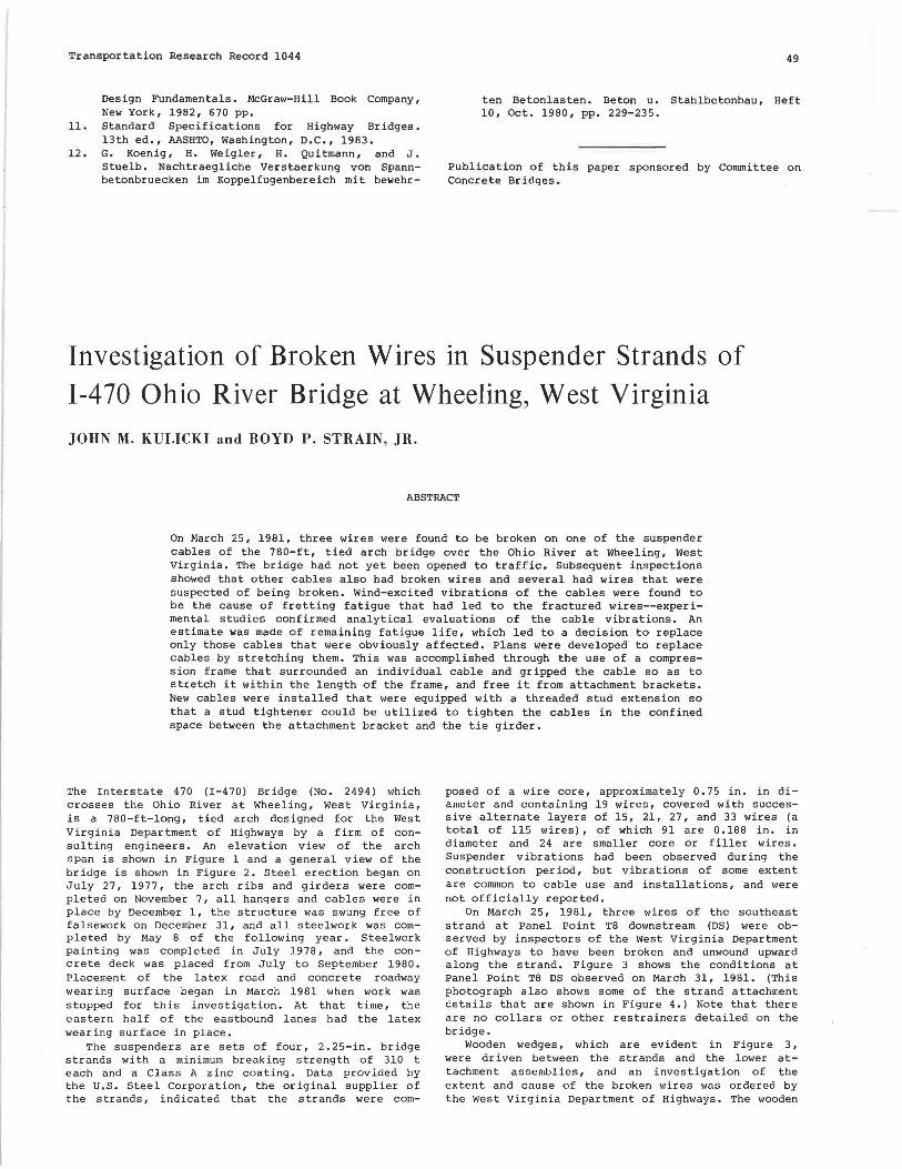
Transportation Research Record 1044

Design Fundamentals. McGraw-Hill Book Company, New York, 19B2, 670 pp.

11. Standard Specifications for Highway Bridges. 13th ed., AASHTO, Washington, D.C., 19B3.

12. G. Koenig, H. Weigler, H. Quitmann, and J. Stuelb. Nachtraegliche Verstaerkung von Spann­betonbruecken im Koppelfugenbereich mi t bewehr-

49

ten Betonlasten. Be ton u. Stahlbetonbau, Heft 10, Oct. 19BO, pp. 229-235.

Publication of this paper sponsored by Committee on Concrete Bridges.

Investigation of Broken Wires 1n Suspender Strands of 1-4 70 0 hio River Bridge at Wheeling, West Virginia JOHN M. KULICKI and BOYD P. STRAIN, JR.

ABSTRACT

On March 25, 19Bl, three wires were found to be broken on one of the suspender cables of the 7BO-ft, tied arch bridge over the Ohio River at Wheeling, West Virginia. The bridge had not yet been opened to traffic. Subsequent inspections showed that other cables also had broken wires and several had wires that were suspected of being broken. Wind-excited vibrations of the cables were found to be the cause of fretting fatigue that had led to the fractured wires--exper i­mental studies confirmed analytical evaluations of the cable vibrations. An estimate was made of remaining fatigue life, which led to a decision to replace only those cables that were obviously affected. Plans were developed to replace cables by stretching them. This was accomplished through the use of a compres­sion frame that surrounded an individual cable and gripped the cable so as to stretch it within the length of the frame, and free it from attachment brackets. New cables were installed that were equipped with a threaded stud extension so that a stud tightener could be utilized to tighten the cables in the confined space between the attachment bracket and the tie girder.

The Interstate 470 (I-470) Bridge (No. 2494) which crosses the Ohio River at Wheeling, west Virginia, is a 7BO-ft-long, tied arch designed for the West Virginia Department of Highways by a firm of con­sulting engineers. An elevation view of the arch span is shown in Figure 1 and a general view of the bridge is shown in Figure 2. Steel e rection began on July 27, 1977, the arch ribs and girders were com­pleted on November 7, all hangers and cables were in place by December 1, the structure was swung free of falsework on December 31, and all steelwork was com­pleted by May B of the following year. Steelwork painting was completed in July 1978, and the con­crete deck was placed from July to September 19BO. Placement of the latex road and concrete roadway wearing surface began in March 19Bl when work was stopped for this investigation. At that time, the eastern half of the eastbound lanes had the latex wearing surface in place.

The suspenders are sets of four, 2.25-in. bridge strands with a minimum breaking strength of 310 t each and a Class A zinc coating. Data provided by the u.s. Steel Corporation, the original supplier of the strands, indicated that the strands were com-

posed of a wire core, approximately 0.75 in. in di­ameter and containing 19 wires, covered with succes­sive alternate layers of 15, 21, 27, and 33 wires (a total of 115 wires), of which 91 are O.lBB in. in diameter and 24 are smaller core or filler wires. Suspender vibrations had been observed during the construction period, but vibrations of some extent are common to cable use and installations, and were not officially reported.

On March 25, 19Bl, three wires of the southeast strand at Panel Point TB downstream (DS) were ob­served by inspectors of the West Virginia Department of Highways to have been broken and unwound upward along the strand. Figure 3 shows the conditions at Panel Point TB OS observed on March 31, 19Bl. (This photograph also shows some of the strand attachment details that are shown in Figure 4,) Note that there are no collars or other restrainers detailed on the bridge.

Wooden wedges, which are evident in Figure 3, were driven between the strands and the lower at­tachment assemblies, and an investigation of the extent and cause of the broken wires was ordered by the West Virginia Department of Highways. The wooden

--

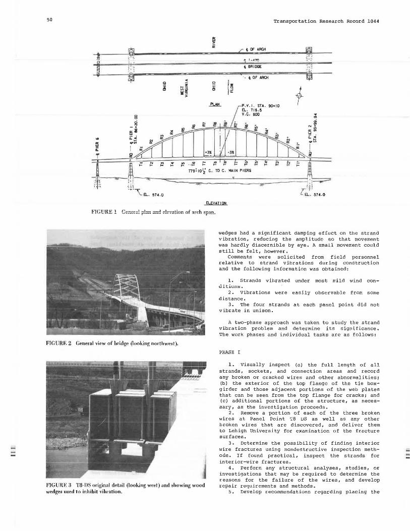
50

~ ~1 ~1 ill

... el i: .,

I

~ :1 · ~.~

~

Transportation Research Record 1044

~I.A~

~ BRIDGE

·- ~ OF MICH

90•10

f

~ .. ~ := t= ~ 779!1012' C. TO C. M41N PIERS

574.0

EUVATl!JI

FIGURE l Gener:!! pl:.n :ind ele~12ticn cf ~uch span.

FIGURE 2 General view of bridge (looking northwest).

FIGURE 3 T8-DS original detail (looking west) and showing wood wedges used to inhibit vibration.

wedges had a significant damping effect on the strand vibration, reducing the amplitude so that movement was hardly discernible by eye. A small movement could still be felt, however.

Comments were solicited from field personnel relative to strand vibrations during construction and the following information was obtained:

1. Strands vibrated under most mild wind con­d i tlum;.

2. Vibrations were easily observable from some distance.

3. The four strands at each panel point did not vibrate in unison.

A two-phase approach was taken to study the strand vibration problem and determine its significance. The work phases and individual tasks are as follows:

PHASE I

l. visually inspect {a) the full length of all strands, sockets, and connection areas and record any broken or cracked wires and other abnormalities; {b) the exterior of the top flange of the tie box­g irder and those adjacent portions of the web plates that can be seen from the top flange for cracks; and {c) additional portions of the structure, as neces­sary, as the investigation proceeds.

2. Remove a portion of each of the three broken wires at Panel Point TB DS as well as any other broken wires that are discovered, and deliver them to Lehigh University for examination of the fracture surfaces.

3. Determine the possibility of finding interior wire fractures using nondestructive inspection meth­ods. If found practical, inspect the strands for interior-wire fractures.

4. Perform any structural analyses, studies, or investigations that may be required to determine the reasons for the failure of the wires, and develop repair requirements and methods.

5. Develop recommendations regarding placing the

--

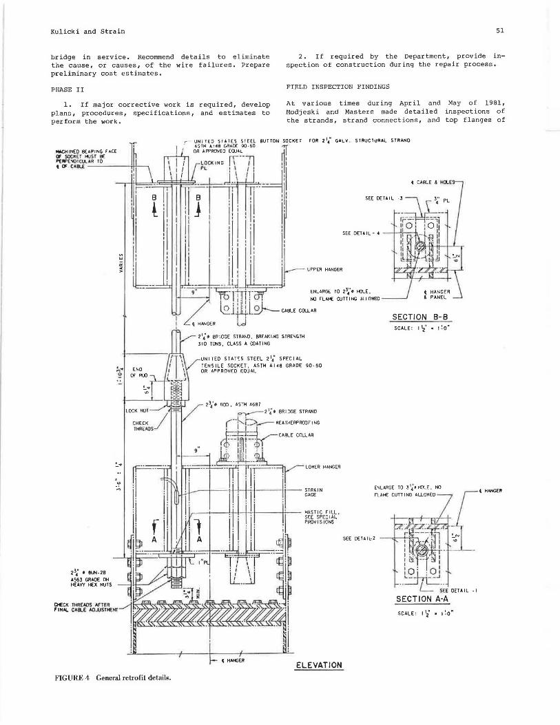
Kulicki and Strain 51

bridge in service. Recommend details to eliminate the cause, or causes, of the wire failures. Prepare preliminary cost estimates.

2. If required by the Department, provide in­spection of construction during the repair process.

PHASE II FIELD INSPECTION FINDINGS

1. If major corrective work is required, develop plans, procedures, specifications, and estimates to perform the work.

At various times during April and May of 1981, Modjeski and Masters made detailed inspections of the strands, strand connections, and top flanges of

23; t Bl.N-28 A563 GRAOE CJi HEAVY HEX NUTS

:,,. 0

"' "'

CHECK THRE AOS ~ TEii "HAL C~ll.E AO..USTl€HI

FIGURE 4 General retrofit details.

BUTTON SOCKET FOR Z 1c GALV . STRUCTURAL STRANO

~ '·--~1i l I I ii

i 1· j I ! : i ~ ' ' ti '

-_] I 1 i __ J- ~·~ "~~· ....._ __ __, "151~ ~L::~T~~~~::G:~~~O

lC?.J~ ~ l l.~ CA£U CCllAR

- t HANGER D 2 1~'• BRIOGE STRANO, BREAKING STRENGTH 310 TONS, CLASS A COATING

UNITEO STAT~S STEEL 2 14" SPECIAL TENS ILE SOCKET, ASTH Al 48 GRACE 90 · 60 OR APPROVED EQUAL

ELEVATION

SECTION B-B SCALE: I '2' • 1 '.o"

ENLARGE TO 3 1;·, HOLE, t..o Fl..A>E cun I NG ALLO•EO

SEE OETAl~2

t HANGE~

·I

--

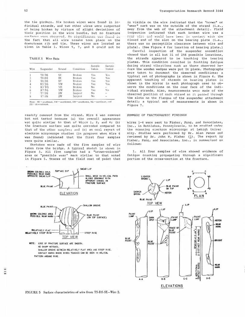
52

the tie girders. Six broken wires were found in in­dividual strands, and two other wires were suspecte d of being broken by virture of slight deviations of their position in the wire bundle, but no fracture

the fact that all wire breaks took place on the downstream rib and tie. These wires are located as given in 'l.'able 1. Wires 5, 7, and B could not be

TARLE l Wire Data

Sample Sample Wire Suspender Strand Condition Taken Tested

I T8 DS SE Broken Yes Yes 2 T8 DS SE Broken Yes Yes 3 T8 DS SE Broken Yes Yes 4 RS'DS NW Broken Yes Yes s RS'DS NE Broken No 6 R7 DS NW Broken Yes No 7 T7 DS SW Suspect No M T7 us SW Suspect No

Note: SE= southeast, NW= northwest, SW= southwest, NE= northe~st, and OS = downstream.

readily removed from the strand. Wire 6 was removed but not tested because (a) the overall appearance war; quite similar to that of Wir:es 1, 2, autl 4; (b) the fracture surface was quite corroded compared to that of the othe r samplt!~ : a nd (c) a n orai report o f electron microscope studies (in progress when Wire 6 was found) indicated that the first four sample s were quite similar.

Sketches were made of the five samples of wire taken from the bridge. A typical sketch is shown iu Figure 5. All five samples had a "brown-colored" area or "possible wear" mark similar to that noted in Figure 5. Traces of the field coat of paint that

llUtf COl.Ollf;U AH~A POSS IBLE llOll HARK (PPOSITE SHEM LIP

BLUE PAINT

ELEVATION

SIEN! LIP

SMALL BEED IN HEl.ICAL PATH ALIGNS SOMErtiAT WITH APPARENT CHAI-GE IN FRACl\JlE SlJlF ACE

BLUE PAINT (<JI TOP SlJlFACE)

ND1£: EOGE Of FRACllJRE SURFACE ARE Sl«JOTH.

NO SHARP NOlCHES. SHALLOW GROOVE BETWEEN Aa.ATIVELY Fl.AT AREA »ll STEEP RISE . CONTACT MARKS l'f1ERE lllRES TOUCHED CAN BE SEEN IN HELICAL

PATIE.RN AIUNJ nu~.

FIGURE 5 Surface characteristics of wire from TS-DS-SE-Wire 2.

Transportation Research Record 1044

is visible on the wire indicated that the "brown" or "wear" mark was on the outside of the strand (i.e., away from the web of the attachment detail) • Field inspection indicated that each broken wire was a ---- _ _ :. -- -·- .:::J _ _ ___ ., ... ' •

•• ~ .............. ~ .,.,...,u...1..Y uavit: uc:c11

closed end of the slot on the bearing plate (i.e., there was no perceptible clearance between wire and plate). (See Figure 4 for location of bearing plate.)

Careful inspection of the suspender assemblies showed that in all but 31 of 256 possible locations, the strands appear e d to be touching the bearing plates. This condition resulted in fretting fatigue during s trand vibrations such as those observed be­fore the wooden wedges were put in place. Photographs were taken to document the observed conditions; a typical set of photographs is shown in Figure 6. The apparent touching of strands on bearing plates is shown in the mirror in each photograph used to ob­serve the conditions on the rear face of the indi­vidual strands. Also, measurements were made of the observed position cf each strand as it pa s sed thr ough the slots on the flanges of the suspender attachment detail; a typical set of measurements is shown in Figure 7.

SUMMARY OF FRACTOGRAPHIC FINDINGS

wires 1-4 were sent to Fisher, Fang, and Associates, Inc., in Bethlehem, Pennsylvania, t o he "t11ilif'>n •Jni:1t"r t h e scanning electron microscope at Lehigh Uni·ver­sity. Studies were performed by Dr. Alan Pense and reviewed by or. John W. Fisher (1) • The report by Fisher, Fang, and Associates, Inc.~ is summarized as follows:

1. All four samples of wire showed evidence of fatigue cracking propagating through a significant portion of the cross-section at the fracture.

BLUE PAINT

LIGHTER

!!/:.LIP

• BLUE PAINT ; ' <JI TIP

OllRl<E.R ' BROnN . t.OTOI

BLUE PAINT

TOP VIEW

IP

A-A B·B

c c

JOI ~LIP

c-c

h. A A A PLAN

PAINT LIM'

D-D

ELEVATIONS

II'

llUOHf

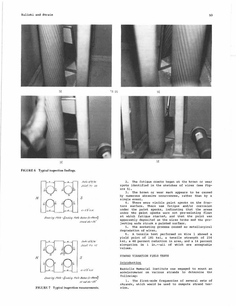
Kulicki and Strain

SE

SE

FIGURE 6 Typical inspection findings.

N

N

o.,k:s/'1/81 Joi,,/.· Tl VS

s

Bean/1.9 !'hi<' -/!.oclr1;,g l'/q/.,. 8dow (cr.¢,h,,,,~ Slrorx/ aO.: Zfi. ..

o.,k:s/'l/81 Joi,,/; TL US

s

Beari'7,9 !'hi<' -/!.oclr1;,g ,P/..,f.. Pdon' {cr,..lv•~8 .J'I• ,,Nf t>d . ..M Z1

'"'

FIGURE 7 Typical inspection measurements.

T8 OS

53

SE

SE

2. The fatigue cracks began at the brown or wear spots identified in the sketches of wires (see Fig­ure 5).

3. The brown or wear mark appears to be caused by numerous abrasive occurrences, rather than by a single event.

4. There were visible paint specks on the frac­ture surface. There was fatigue and/or corrosion under the paint s peck s , indicating that the areas under the pain t specks were not pre- ex isting flaws at which fatigue started, and that the paint was apparently deposited as the wires broke and the pro­jecting ends struck a pain ted s ur f ace.

5. The socketing process caused no metallurgical degradation of wires.

6. A tensile test performed on Wire 1 showed a yield point of 185 ksi, a tensile strength of 234 ksi, a 48 percent reduction in area, and a 14 percent elongation in 1 in.--all of which are acceptable values.

STRAND VIBRATION FIELD TESTS

Introduction

Battelle Memorial Institute was engaged to mount an accelerometer on various strands to determine the following:

1. The first-mode frequencies of several sets of strands, which would be used to compute strand ten­s ion.

-...

54

2. Frequencies of vibration for comparison with computed modes under various wind speeds.

3. Wind-induced vibration characteristics. 4. The amount of damping provided by the as-de­

s lgned system and the system modified by the addi­tion of wooden wedges. (The wedge-modified damping values were thought to be of value because the damp­ing caused by the wedges appeared to be enough to still the v ibration.)

A summary of the report Ill is presented in the following sections.

Experimental Procedure

The sixteen strands selected as representative are the four sets of four each at RB, RB', RS', and R3'. All strands examined were on the downstream side of the bridge. The RB and RB' sets of suspenders are nomi nally identical undP.r foll dead load, and only slightly different with the partial application of the latex-modified concrete wearing surface pre­viously noted. From the nominal tension, lengths, and mass, the theoretical natural frequencies for lateral vibrations in the strands can be computed as shown in the sec t.ion entitled "Analysis of Cable Vibrations." The ca oulated natural frequencies ar e given in Table 2.

TABLE 2 Calculated First-Mode Natural Frequencies of Representative Strands

Strand Natural Length" Tension Frequency

Suspender (ft) (kips per strand) (Hz)

3' 64.77 118 4. 80 5' 97.23 115 3.11 8 119.18 113 2.4B

3From the fabricator'.s .shop dr.iwlng~. Lt:twt:t:u l.Jearh1K races of SO¢kels.

Determination of Na tural Frequencies

An accelerometer was clamped to the midpoint of the strand such that its measurement axis was horizontal. The midpoint was chosen to maximize the acceleration attributable to the first or fundamental mode of vibration. The strand was manually pushed and pulled in a periodic way that approximately corresponded with the observed natural frequency. After building up the amplitude of the .strand, it was released and allowed to vibrate freely for approximately 2 min. Generally, the strand vibrated in the first mode with little contamination from the higher modes. In some cases, the third mode contributed sufficiently to be evident in the recordings: however, even in these cases, the first mode was clearly discernible. The peak-to-peak amplitude of Strand RB' SW result­ing from manual excitation was calculated as 1.7 in. On-site measurements indicated an estimated amplitude of 1.5 in.

Results

Table 3 gives the measured fundamental frequencies of vibration of the 16 strands. Strand tensions shown in the table were calculated by using the relation­ships shown in the section entitled "Fundamentals of Vortex Shedding Excitation." These values are for individual strands. Because they were evaluated ex­perimentally, the total load for the four strands

Transportation Research Record 1044

'I' BLE3 Measured atural Frequencies and Damping of Rcpresentativ lrancls

n ................ ; ...... r" ......... nf-n_.,..a - --r--.o - -··-·- · · ·

Natural Dead Load Length Frequency Tension With Without

Strand (ft) (Hz) (kips) Wedges Wedges

RB NE 119.18 2.33 97 .0005 (0) NW 119.IB 2.25 91 .0005 (0) SE 11 9 .l B 2.25 91 .0011 (O) SW 119.l B 2.2B 93 .0013 (0)

RB' NE 119. IR 2.22 88 (O) .0005 NW 119.1 8 2.4 1 104 .0005 .0003 SE 119.18 2.26 93 .0005 (0 ) SW 119.1 8 2.03 74 .0004 (0)

RS' NE 97.23 3.25 126 .0006 .0003 NW 97.23 3.47 144 .0006 .0002 SE 97.23 3.40 138 .0009 .0003 SW 97.23 3.33 132 .0006 .0001

R3 ' NE 64.77 4.26 93 .0005 .0004 NW 64.77 5.05 133 .0005 .0004 SE 64.77 5.lB 140 .0005 .0003 SW 64.77 4.93 126 .0005 .0006

aParentheses indicate that damping value was too small to estimate reHably.

forming one suspender does not agree exactly with the thecreticYl loads.

The attempts to determine the damping of the strands without the wedges were thwarted by two fac­tors: the damping is low and, in some cases, random excitation caused by wind was sufficiently large to cause an increase in amplitude during the time in­terval recorded. Even the attempts to determine the damping with wedges were not completely satisfactory for the same reasons. Nevertheless, an estimated damping factor, which follows, is given in Table 3 for each of the 16 strands, with and without wedges :

~ ; Loge (R)/2~N (1)

where R is the ratio of displacements at cycle number Nl and N2, and N is N2 - Nl (absolute value).

ANALYSIS OF CABLE VIBRATIONS

Discussions throughout this section will be in the context of air mnving around an obstruction that is basically circular in cross-section.

The design dead loads calculated by the original designer were reviewed, found to be correct, and then revised to reflect thP. cnna i tion of the bridge when work stopped. The resulting strand tensions, in kips, are given in Table 4. (Note that the average values of the symmetric panel points were used in the analysis presented herein.)

Fundamentals of Vortex Sheddi ng Exci t a t ion

When air passes by a circular shape, the air flow divides to pass around the obstruction. The activity generated in the wake of the obstruction can be related to the Reynolds Number

where

v d p

µ

velocity (ft/sec), characteristic dimension (ft) , mass density (lb-sec'/ft"), and dynamic viscosity (lb-sec/ft').

(2)

Kulicki and Strain

TABLE 4 Strand Tensions

Suspender No.

l 2 3 4 5 6 7 8

Tension per Strand (kips)

118 102 117 93

115 114 96

113

Suspender No,

8' 7' 6' 5' 4' 3' 2' l'

Tension per Strand (kips)

113 96

114 115 93

I 18 102 119

Chi has categorized wake responses ranging from Reynolds Numbers 1 to 3.5 x 10' (},_!). The most practical cases (temperatures greater than 0°F and wind speeds less than 50 mph) are in the subcritical flow range. In this regime, the wake consists of regularly spaced alternating vortices similar to the "Von Karman vortex street" that occurs at lower Reynolds Numbers, except that the fluid action in the vortices may be turbulent, and the frequency of vortex shedding is given by

where

v wind velocity (ft/sec), d diameter (ft),

St Strouhal number (unitless), and fs frequency of vortex shedding (Hz).

(3)

For a circular cylinder, the Strouhal number is relatively constant at approximately 0 . 20 for the Reynolds Numbers under consideration, although ex­perimental i::esults have ranged from about 0.185 to 0.22 (5,6).

The- potential for large amplitude vibrations exists when a forcing function drives a structural component at a frequency close to one of its natural frequencies (i.e., resonance) and when there is very little damping. Strands, such as the one on the I-470 Bridge, have little natural damping as evidenced by the low value of damping obtained in the field studies. Thus, the basic principle underlying an investigation of vortex-shedding-induced vibrations is to equate the vortex shedding frequency equation to an equation for natural frequencies and solve for er i tical wind speeds. Theoretica.lly, this yields a discrete wind speed for each natural frequency.

In actuality, a phenomenon called "lock-in" occurs in which the vortex shedding and structural vibration interact with each other. The result is that the structure vibrates in a given mode for a range of wind speeds generally regarded as being from the critical wind speed for that mode to approximately 140 percent of the critical wind speed (l.J. During this interval of wind speeds, the frequency of vortex shedding is controlled by the structural frequency, rather than the wind speed.

The simplest representation of a vibrating cable is obtained by neglecting the bending s tiffness and treating the cable a s a string. The frequencies of vibration are given by the following equation:

fn = (n/2L) [ (T/m)l/21

where

n =mode number, f frequency (Hz), L length (ft),

(4)

T

m load (kips) , and mass per unit length (kips-sec'/ft').

55

If the bending rigidity is included, the following differential equation results:

[EI(a"y/ax")l - [T(a'y/ax 2 )] + [m(a'y/at')J = o (5)

This equation has been solved by Modjeski and Masters (8) and others, including Chi (3,4). For the appli­c;ble case of fixed ends, there- is no simple solu­tion; rather, a trial and error process results. By generally using the nomenclature in reports by Chi (_l,_!), the following equations result:

z z Coshfln Cos an + [ (an-flnl /2an fln l

z "n

z fln

Q

p

Sinhen Sin"n = 1.0

(p/2) f-1 + {l + [ (4Q/p'J ]}l/2 I

(P/2) 11 + {l + [ (4Q/p')] }l/21

TL'/EI

where

wn frequency (rads/sec), I moment of inertia (in.'/ft'), and E Young's modulus (ksi).

(6)

(7)

(8)

(9)

(10)

The solution, given M, E, I, T, and L, is to as­sume trial values of n until Equation 6 is satisfied. The only practical way to solve Equation 5 is by trial-and-error calculations or by using graphs de­veloped by Chi. A computer program was written for this investigation.

Equation 6 requires a value for the moment of inertia of the cable. For the I-470 Bridge, this value could reasonably be expected to lie between a solid cylinder 2.25 in. in diameter (I = 1.258 in. "l and the sum of the moments of inertia of the 91 large wires (I = 0.0056 in. 'J, depending on the inter­wire shear which, in turn, depends on the wire-to­wire transverse pressure. The transverse pressure varies with the amount of tension and the extent of "birdcaging" caused by the vibration. Not surpris­ingly, tests on stranded transmission wire by Scanlan and Swart (9) indicated that the flexural stiffness of the stra~ded wire varied along the length of the wire, being higher near regions of lateral confine­ment, and that the effective rigidity varied from 0.1 to 0.5 of that of a solid shape.

Frequencies were computed using 10, 30, 50, and 100 percent of the moment of inertia of a solid shape. The effect of bending stiffness increased with higher modes, and was more significant for the shorter strands.

The experimental results were used to provide some insight into the amount of bending rigidity present. I f there were no bend i ng rigidity, the fre­quenci es would f orm an arithme·tical progression (i. e ., 1, 2 , 3 , 4 ••• ) as s hown by Equation 4. A plot of mode number versus frequency would be a straight line . Equation 6 becomes increasingly non­linear for a given strand as the bending rigidity increases . Figure B s hows the degree o f nonlinearity [i.e., fn/ln x f1ll associated with each of the assumed percentages o f solid rigidity. Also plotted are var ious ratios of peak frequency to multiples of measured frequencies. These data are neither numerous enough nor of high enough modes (large nonlinearity regions) to make strong quantitative conclusions, but they indicate a trend toward effective rigidities

;;;

56 Transportation Research Record 1044

1.20-.----...--- t--------'----'-------- --

I 9' SOLID MOMENT OF l_NERT I A~q'.!V'

I , 7 ~ ... ~ I I Iii I.I 0 -+--s_o_s_P+EC_N_D_E_R_,Tr-3_-_R_3_+----+----+-,,,.c--------~~

"' ~ 0 >- 1.0 6 + ----t--- -+1---;-=-"""--l----l:::>-""""'--r---:::-....C::::......-c.> z ~ 2 I OO-t----.---+11---~--....... ---1----~----~0~9'"-­a:: ~

>-a:i

Q

~ I 1 0-t----t---t-----+----+---'t----+----'---~ s: Ci SUSPENDER ~ 1os---- ----,r---+----+----1--::;;....-::T--- - ""'Z1''!'1>-± z L&J

~ 1 00-~-==========~~~~~~~=====lR:==:=:~=::==:::!:~~~ ~

I

I

I • ! I

T8 -R8~: L ~ I I SO"

I , 3 "

100-~-========::::::;;;;;;;;;;;;;;~~==:;t:::==:~t::::::::::::::=:=.=~-~o~"~ . .

SUSPENDER 1.0 6

2 3 4 s 6 7 8 8

MODE NUMBER FIGURE 8 Effect of strand bending stiffness on frequency.

such as those encountered by Scanlan and Swart (i.e., varying from 10 to 50 percent effective stiffness along the length of the cable), which means an aver­age value of less than 50 percent. An average value of 30 percent effective stiffness was used in devel­oping the critical wind speeds given in Table 5. Given that the Strouhal Number could vary by 10 per­cent, a more involved evaluation of effective strand

bending stiffness would have no practical signifi­cance for this study.

Correlation of Measured and Compu ted Wind Speeds

The wind during the test periods had noticeable gusting and excited several modes of strand vibra-

TABLE 5 Critical Wind Speeds

Winds Speed (mph) by Strand Identification Mode No Tl-R! TI-R2 T3-R3 T4-R4 T4,. R5 T6-R6 T7-R7 "T"O no

.io-n.o

I 13 4 3 2 2 2 2 2 2 28 9 6 4 4 4 3 3 3 44 14 9 6 6 5 5 5 4 62 18 12 9 8 7 6 6 5 84 23 16 11 10 9 8 8 6 108 29 19 13 12 II 9 10 7 136 34 22 15 14 13 II II 8 167 40 26 18 16 14 13 13 9 201 46 29 20 18 16 14 15

10 239 53 33 23 21 18 16 16 II 281 60 37 25 23 20 17 18 12 326 67 41 28 25 22 19 20 13 375 75 45 30 27 24 21 22 14 428 84 49 33 30 26 23 23 15 484 92 53 36 32 28 25 25 16 544 102 58 39 34 30 26 27 17 608 Ill 63 42 37 33 28 29 18 675 122 68 45 40 35 30 31 19 746 133 73 48 42 37 32 33 20 821 144 78 52 45 39 34 35

Note: In this table, strand I = 0.3774 and E = 24,000.

;;;; --

Kulicki and Strain

tion. The recording anemometer set up on the bridge measured only average data for 1-min intervals and did not function reliably. Readings from the anemom­eter on Wheeling Island, which is several miles away, were obtained but did not seem to correlate to winds observed at the bridge site. The result is that the only available, reliable measurements of wind speed were those made with a hand-held anemometer (pressure plate type). Nevertheless, the following correlations between calculated and measured wind speeds were possible:

1. The 3rd, 4th, and 5th modes of Strand B DS-NE were reasonably represented in field data, with the 3rd and 4th modes dominant when the wind speed was about 5 mph. Table 5 gives the computed wind speeds at 5, 6, and B mph, respectively, for the 3rd, 4th, and 5th modes.

2. The 7th mode was dominant in the field data with some 6th and Bth mode participation for Strand B DS-NE when the wind speed was 12-15 mph. The com­puted wind speeds are 10, 11, and 13 mph, respec­tively, for the 6th, 7th, and Bth modes.

3. Strand 5' DS-SE was observed in winds ranging from 10-15 mph. Modal representation in the field data included the 4th through 7th modes. The corre­sponding computed wind speeds are B, 10, 12, and 14 mph, respectively.

4. Strand 3' DS-NE was also observed in 10-15 mph winds. Field data indicate that the 3rd to 5th modes were active. Corresponding computed wind speeds were 9, 12, and 16 mph, respectively.

In considering the uncertainties in the Strouhal Number, the effective strand rigidity, and the mea­sured wind speed, as well as the fact that individual strands in a set of four at a panel point had slightly different frequencies (largely because of unequal tensions), the computed and measured critical wind speeds are in good agreement.

Strand Vibration Arnpli tude.s and Tensions

Analytic procedures described by Chi (_!) were also used to estimate vibration amplitudes and strand tensions. This procedure, as modified by the authors, consists of the following equations:

~n(X) = !An Sinan(X/L)] + IBn Cosan(X/L)] + [Cn SinhBn(X/L)] + [DnCoshBn(X/L)] (11)

where

Bn (anSinhBn - BnSinanl + [Bn(Cosan - CoshBnll

Y (x,t) = IYn (x,t) = l:~n (x) (G1nsinwst n n + G2ncoswstl

(12)

(13)

(14)

(15)

(16)

In Equation 16, ws is the frequency of vortex shedding. A reasonable simplification for wind-in­duced, essentially resonant, vibration is to assume that the vibration consists of one mode shape and that wn = Ws• Since ~ is a shape function and, there­fore, has a maximum value of 1.0, G2~ is O when wn = ws<!l, and Sinwst has a maximum value of 1.0, so that:

57

(17)

For the case of wn to

ws, the equation for Gin reduces

L

Mn = J m~n (x) 2 dx 0

L

(1/2) PadV~rCL J ~n (x)dx 0

where

~ damping factor, Pa mass density of air, and CL lift coefficient taken as 1.20.

(18)

(19)

(20)

Equations 19 and 20 were evaluated by using numerical methods.

Maximum amplitudes computed by using Equations 11-20 are shown in Table 6 for a damping factor of 0. 0003, which is representative of the values ob­tained during the field tests. The single amplitudes shown in Table 6 are approximately one-half of the double amplitudes observed in the field, which were approximately O. 75 in. Although this result is en­couraging, Equation 18 shows that the maximum com­puted amplitude is a linear function of the damping factor, a factor found with limited accuracy during the field tests, and seldom known with reliability during design. Similarly, the lift coefficient has been assumed to be a constant and it, too, varies with frequency.

Tension may be computed by differentiating Equa­tion 16 twice to compute curvature. The magnitude of the curvature is also a linear function of damping and is dependent on the value chosen for effective bending stiffness of the strand. The local bending stiffness near points of lateral restraint (i.e., the sockets) results in local stresses that are higher than those that would be obtained by using the average bending stiffness. The stresses reported herein are based on curvatures computed using an average stiffness of 30 percent of a solid and then multiplied by the ratio of an assumed locally higher bending stiffness to the average bending stiffness. For comparison, Table 7 shows stresses based on 3 0 percent average stiffness, and local stiffness of 30, 60, and 100 percent of a solid. The 60 percent stiffness was chosen as the most realistic on the basis of experimental work by Scanlan and Swart that indicated effective stiffness of up to 50 percent of a solid and the assumption that the socket is more effective in providing lateral restraint than trans­mission wire fittings.

In considering the magnitude of computed stresses, and therefore stress ranges, it is important to bear in mind that the computed results depend on the chosen values of damping, local stiffness, and aver­age stiffness. Values have been used that were be­lieved to be representative and documentable to the extent possible, but they are still only assumptions.

Analysis of Fatigue

There are three stages of fatigue life: initiation, propagation, and instabil ity . Basically, only the first two stages are important in this investigation.

Much of the available information on fatigue of wire and fabricated strands deals with wire, rather than strand. There is a limited body of information on wire fatigue and this has been reviewed by Chi <!> • Much of the same information had been obtained

;;;

58

for th i s investigation before Chi's report was available, and, fortuitously, has been analyzed and critiqued by Chi. Co11U11ents in this section of this rP!lnrt. ;:arp. h;:a~p.n l;:ar~i:iol~ nn ,.,h; 'C! =iin:::al!1ci i_~ ':'~ ":.~ '='

available data. When clean, smooth wire is tested in fatigue, it

is generally found to have a reasonably high fatigue

Transportation Research Record 1044

life. It is also found that the majority of the fa­tigue life is represented by the crack initiation phase, with relatively little life in the crack prop-

tiated, they propagate quickly). In the case of a helically wound strand, fatigue cracks usually start at mechanical notches caused by point contact between

TABLE 6 Strand Vibration Amplitudes from Analytic Solution

Strand Identification

Specifications Tl-RI T2-R2 T3-R3 T4-R4 TS-RS T6-R6 T7-R7 T8-R8

Tension (kips) 474 409 470 372 4S9 4SS 383 442 Length (ft) 16.1 42.0 64.2 82.1 97.2 108.I 144.8 I 19. 2 Mode no. (in.)

I .4S .46 .46 .46 .46 .46 .46 .46 2 .44 .4S .46 .46 .46 .46 .46 .46 3 .42 .4S .4S .4S .46 .46 .46 .46 4 .40 .44 .4S .4S .4S .4S .4S .46 s .39 .44 .4S .4S .45 .45 .45 .45 6 .37 .43 .44 .45 .45 .45 .45 .45 7 .37 .42 .44 .45 .45 .45 .45 .4S 8 .36 .41 .44 .44 .4S .4S .4S .4S 9 .3S .41 .43 .44 .44 .4S .4S .4S

10 .3S .40 .43 .43 .44 .44 .44 .4S 11 .34 .39 .42 .43 .44 .44 .44 .44 12 .34 .3 9 .42 .43 .44 .44 .44 .44 13 .34 .38 .41 .42 .43 .44 .44 .44 14 .34 .38 .41 .42 .41 .44 44 .44 " .33 .37 .41 Ai -43 .43 .43 .44 ., 16 .33 .37 .40 .41 .43 .43 .43 .43 17 .33 .37 .40 .41 .42 .43 .43 .43 18 .33 .36 .39 .40 .42 .42 .42 .43 19 .33 .36 .39 .40 .42 .42 .42 .43 20 .33 .36 .39 .39 .41 .42 .42 .42

No te: In this table, the assumed strand I value is 0.3774, the damping va lue is .0003, and the moment of inertia used to calculate local bending stress is 0.7548.

TABLE 7 Strand Bending Stresses at Socket (ksi)

Strand Identification Mode No. Tl -RI T2-R2 T3-R3 T4-R4 TS-RS T6-R6 T7-R7 T8-R8

Assuming I = 30 Percent of That of Solid Bar

I 29 9 6 4 4 4 3 3 2 62 19 13 9 8 7 6 7 3 >100 29 20 14 13 II 10 10 4 >100 40 27 18 17 IS 13 14 s >100 S2 34 23 21 19 16 17 6 > 100 64 41 28 26 23 20 ?.1 7 > 100 78 49 33 30 27 23 24 8 >100 93 S7 39 3S 31 27 28 9 >100 > 100 6S 44 40 3S 30 31

10 >100 > 100 74 so 44 39 34 3S

Assuming I = 60 Percent of That of Solid Bar

58 rn '0 9 7 6 7 ., >J

2 >100 38 26 18 17 IS 13 13 3 >100 S8 39 27 25 23 19 20 4 > 100 80 S3 37 34 30 26 27 s > 100 > 100 67 46 43 38 33 34 6 >100 > 100 82 S6 SI 46 40 41 7 >100 > 100 97 67 61 S4 47 48 8 >100 > 100 > 100 77 70 62 S4 SS 9 >100 > 100 > 100 88 79 70 61 62

10 > 100 > 100 > 100 > 100 89 79 68 70

Assuming I = I 00 Percent of That of Solid Bar

I 97 31 22 IS 14 12 II II 2 > 100 64 43 30 28 2S 22 23 3 > 100 97 66 4S 42 38 32 34 4 >100 > 100 88 61 S6 so 43 4S s >100 > 100 > 100 77 71 63 SS S7 6 >100 > 100 > 100 93 86 76 66 69 7 > 100 > 100 > 100 > 100 > 100 90 78 81 8 > 100 > 100 > 100 > 100 > 100 > 100 89 93 9 >100 > 100 > 100 > 100 > 100 > 100 > 100 >100

10 >100 > 100 > 100 > 100 > 100 > 100 >100 >100

;;;; --

Kulicki and Strain

individual wires. This reduces the crack initiation phase of fatigue life .

The re is even less knowledge o f the fatigue life of strand than of wire. While the mechanism of fret­ting is a factor in strand fatigue, there is ap­parently no accepted analytical model for predicting cycles-to-failure under a given stress range. How­ever, some of the experimental work reviewed by Chi indicates the order of magnitude of strand fatigue life. For example,

1. Reemsnyder (10) tested a 37-wire strand of 250 ksi tensile strength under axial fatigue loading. At a stress range of 50 ksi, the first wire break occurred at 200,000 cycles. At the 75 ksi range, the first wire break occurred at 150,000 cycles.

2. Fisher and Viest (11) tested 0 .192-in. wire with a strength of 257.5 ksi and a 0.375-in., 7-wire strand with a strength of 274 ksi. At a stress range of 38.4 ksi (maximum stress of approximately 200 ksi), some wires were unbroken at 2.5 million cycles, whereas at a stress range of 75. 7 ksi, the fatigue life was as low as 38,000 cycles. Some wires tested at 33.5 ksi survived 7.5 million cycles. At 97.8 ksi, the fatigue life was reduced to 104,000 cycles.

Other test data could be cited that would demon­strate similar finding s , but no results would deal with precisely the same wire and fretting conditions as exhibited on the I-470 Bridge.

Computed bending stresses for the first 10 modes of vibration are summarized in Table 7. Stress ranges are, of course, twice the computed stresses. Neglect­ing the 100 percent local stiffness values (these are shown as upper-bound stress ranges for comparison only), the seventh mode vibration of Hanger 8, the fifth and sixth modes of Hanger 5, and the fifth mode of Hanger 3, all of which were observed during the field monitoring of vibrations, correspond to stress ranges on the order of 48 to 96 ksi, 51 to 103 ksi, and 67 to 134 ksi, respectively. If 500,000 cycles is considered to be the approximate fatigue life, Strands 8, 5, and 3 would reach 500,000 cycles in only 7.9, 7.4, and 5.7 hr of vibration, respec­tively.

Obviously, the wind-induced strand vibration ex­perienced on this bridge was a random loading. Modes of vibration higher than the seventh mode could have been experienced, and most certainly were experi­enced, under higher wind speeds than those observed during the field testing. Similarly, while the ob­served and computed amplitudes were in good agree­ment, under more uniform winds of longer duration, it is possible that higher amplitudes (and therefore stress r anges ) coul d have been developed.

Some i nd i cation of the r emain i ng liveload fatigue life, for those strands that have an undetectable crack as a result of fretting against the bearing plates, can be obtained by considering the number of cycles to propagate an assumed initial crack to crit­ical crack size. Again, only limited information is available, and that is based on assumptions that did not fit the existing situation. In utilizing Equa­tions 21-23, and the table of factors relating the crack depth, a, to the stress intensity factor, f(a), from Chi, it is possible by numerical integration to compute the theoretical number of cycles to propa­gate an initial crack of size a0 , to critical crack size, acr• for a given stress range, maximum stress, and fracture toughness as follows:

ac N = f da/(0.66 x 10-•) i1K2.25 (21)

a o

where

N number of cycles, ac critical crack size, a0 initial crack size, llK lla K1r and Ila stress range.

where B is the half area.

Ac = (11R2 /2) - (R-a) [ (2aR-a') 1/21

- R2 tan- 1 [(R-a)/(2aR-a')l/21

59

(22)

(23)

The relationship between Ac/B and f(Ac/B) is as follows:

0.1 0.2 0.3 0.4 0.5 0.6 0.7 0.8 0.9 1.0 1.1 5 1.20 1.29 1.37 1.51 1.68 1.89 2.14 2.46 2. 86

This has been done for the 0.188-in. diameter gal­vanized wire used in the hangers on the I-470 Bridge for ass umed f"racture t ou.ghnes s values of

1 69 ksi

(in.)1/2 , 80 ksi (in.) 112 , a nd 100 ks i (in.) I (the values assumed by Chi in his a nalysis o f 0 . 25-in. di­ameter wire). The computed critical crack size for the higher two val.ues of assumed fracture toughness exceeded the rad ius of the wi r e under consideration. As a practical matter, the additional number of cycles required to propagate assumed cracks from a critical crack size of 0.0837 in. (corres~onding t o a fracture toughness of 60 ksi (in.) l/ to one­half the thickness] is quite small. The following values correspond to half-thickness cracks and can be considered representative estimates of remaining fatigue life for the initial crack sizes assumed.

a 0 (in.)

0.001 0.010 0.030 0.050

Cycles (million N)

3.828 1.192

.390

.139 ) Maximum stress = 50.4 ksi

Stress range= 6.71 ksi

Traffic data given on the contract plans for the I-470 Bridge indicate average daily traffic counts of 21,800 and 31, 700, respectively, for 1975 and 1995 and an estimated 7 percent truck volume. This corresponds to average daily tr uc k traffic counts (ADTTs) of 1,526 and 2,219, r espec t ively, for 1975 and 1995. For the discussion that follows, an ave r age AD'l'T of 1,870 trucks will be used.

The maximum computed stress range is 6. 71 ksi. This stress range results from 6 lanes of AASHTO lane loading, including the 75 percent, multi-lane reduction factor. Practically speaking, the lane loading is sel dom realized i n t he f ie.ld . Similarly, it is more app r opriate to base f a tigue considera­tions on the act ual lane positions , rather t han de­sign positions, when trying to arrive at a more ac­curate estimate of fatigue life. In the case of the I-470 Bridge , if all four traffic lanes were loaded with t ruc ks spaced at approximately 80 ft, each weighing 82 percent of the AASHTO design truck load, this would be approximately the same total weight as the six lanes of lane load at 75 percent used as the design loading. This would require 40 heavily loaded trucks to be on the br idge at one time. Obviously, the probability of t h is happen ing r epeatedly during the life of the br idge is nil. Neve rtheless, and only for the purpose of illustrat i on , if the full truck traffic consisted of r epeti t i ons of this 40-truck loading, the annual ADTT would correspond to

60

only 17,103 cycles per year. This corresponds to fatigue lives of 224, 70, 23, and 8 years for wires having assumed initial cracks of 0.001, 0.010, 0.030, and 0.050 in., respectivelv. at the time the bridae was put into service.

A consideration of truck loading results in even better fatigue life estimates. Based on FHWA loadom­eter studies, the current AASHTO fatigue specifica­tion relates the variable-amplitude loading from random truck loading to constant cycles of HS 20 design load vehicles. Basically, this results in a multiplier of 0.35 to relate ADTT to cycles of HS 20 truck loading (.!£). In the case of wire using a crack growth exponent of 2.25, the corresponding variable amplitude factor is 0. 45. Thus, the annual ADTT of 1,870 corresponds to 843 HS 20 vehicles per day. As an illustration, if four lanes of AASHTO truck load­ing at 100 percent are used and if each vehicle oc­cupies the center of its respective traffic lane, the maximum tensile stress induced in a strand is 1. 5 ksi. The corresponding cycles to er i tical crack size for assumed initial cracks are shown in the following table. The estimated strand fatigue lives for the initial crack sizes discussed previously are then 1,450, 450, 150, and 50 years, respectively. If the two most significant of the four traffic lanes are used, resulting in twice as many cycles, virtu­ally the same fatigue life results, as follows:

a 0 (in.)

0.001 0.010 0.030 o.oso

Cycles (million N)

111.410 34.696 11.346

4.035

Maximum stress = 50.4 ksi Stress range = 1.50 ksi

The discussion of remaining life has been based on several assumed configurations of the ADTT. An infinite number of ether choices are possible. Ob­viously, many assumptions are required and the basic computational procedure is only an approximation. Nevertheless, it seems reasonable to expect that latent cracks of up to 0.03 in. will have relatively little impact on fatigue life of wires under liveload stress cycles. A latent fatigue crack of approxi­mately 0.05 in. could be expected to have a signifi­cant effect on fatigue life only under highly improb­able loadings.

CORRECTIVE ACTIONS

Recommendation

Based on the considerations outlined heretofore, recommendations were made (and eventually approved) as follows:

. Eliminate the strand vibrations through the installation of collars and strand cross ties. . Replace only those strands with known or suspected broken wires. . Protect lower ends of strands by means of weather-resistant enclosures.

These recommendations assume that (a) the elimi­nation of strand vibration will eliminate the fret­ting potential on those original strands that are retained and that are apparently in contact with locking plates or bearing plates, and (b) some strands will crack and will have to be replaced from time to time. This latter assumption was evaluated and was found to be the cost-justified procedure.

Transportation Research Record 1044

Contract Details for Eliminating Cable Vibrations

The cable collar detail was proposed by the original rlP~innPr ~n~ w~Q ~~Q~~ ~~ t~~ ~!!~=!~!= t~~t !~ t~=

uncontrolled installation of wooden wedges had ef­fectively reduced the cable vibration, then permanent restraints should perform as well or better.

The cable collar is shown in Figure 4, and struc­tural details thereof are shown in Figure 9. The function of the cable collar is to increase damping, and to move the fixed point away from the socket, thereby reducing bending stresses if vibrations were to continue despite the increased damping.

Details of Strand Replacement

To procedure for strand replacement involved sur­rounding the individual strand to be removed with a compression frame and jacking the strand to stretch it within the length of the frame. The strand to be removed could then be stretched sufficiently to free it from the attachment details. In the process, the load in that strand was transferred primarily to the other three strands in the suspender being worked on, and secondarily to other par ts of the bridge. Changes in elevation along the tie member caused by bridge movement during strand replaceme t were barely measurable with a transit. Details of the cable re-mo\ral equipment .:ire shewn in Figure 10. Note that cable grips were used to anchor the jacking force to the strand. Examination of the removed strand indi­cated little or no damage to individual wires re­sulting from the use of the cable grips. In terms of field efforts, installing the frame on each strand was the time-consuming phase of the strand replace­ment. This took between one and two days per instal­lation. Jacking, relieving, and removing the strand took only a matter of minutes.

Some of the strands that were removed underwent laboratory study at Lehigh University to determine remaining fatigue resistance and to evaluate the condition of interior wires by dissection of a length of strand adjacent to a socket. Therefore, the length over which a strand was stretched was chosen to keep the strand tension below - the prestretching load and within the range of linear behavior. In this manner, the strand specimen delivered to the laboratory had essentially minimized properties.

The new strands were identical to the old strands. The new Lop svcket was also i~entical to the old top socket: the bottom socket was changed to a stud ex­tension detail as shown in Figure 4. During the de­sign phase, consideration was given to using the removal frame to stretch the n~w ::;trands sufficiently for installation. This idea was rejected because, at that time, the extent of damag2 cauaed by the strand grips was not known. Once this idea was rejected, the limited working space between the suspender at­tachment detail and the tie girder narrowed the choice of reinstallation procedures to the use of a stud tightener. (As noted earlier, damage was found to be virtually nil during the field operations.) The stud detail also provides an effective way to tension the strand to its proper share of the sus­pender load because it eliminates the question of tolerance on strand length.

SUBSEQUENT DEVELOPMENTS

During the winter and early spring of 1983, the retrofit procedures described herein were undertaken. When Strand 7 DS-NW was removed, four broken wires were discovered, whereas the original inspection had indicated two suspect wires. The newly discovered broken wires were fractured approximately 0 .5 in.

Kulicki and Strain

I 0 , Of' PVC PIP£

9Aff 38' 1)~1 ,. LONG or

90" SPACING (GRIND

TO RADIUS Of' PIPE) J" e

:J_ ,12·

5TIFF PL

1• •

8~

-PL 34 x7 14 xl~2"

- C. F , •"•EXTRA STRCNG 0! PIPE (I" SECTION ::: _f RE1'IOVEO FRO< EACH SI~ J

- so DURCOIETER NEOFRE~ 8Cl<DED TO INSIDE Of' PIPE .

151'6 THICK FOR 21~'o STRANO (TYi')

I 11•5 TH I CK FDR 2J~'f ROD ( m'. )

61

~ HANGER & PANEL I 8~

PLAN - DETAIL OF

COLLAR ASSEMBLY SCALE : J" • I '.o"

VIEW B-B SCllLE: 3" • I '.o"

FIGURE 9 Details of cable collar.

from the socket and had therefore been held firmly in place by the bearing and locking plates of the connection detail.

The contract to replace the strands was extended to include removal and reinstallation of ten randomly selected strands. Observation of the satisfactory condition of the grip area of the originally removed strand made this procedure acceptable. In addi­tion, another detailed visual inspection was under­taken of the tie girder and of the strands and aug­mented by a sounding test (hammer blow) on both ends of every exterior wire in every strand. Eight addi­tional broken wires were discovered during the re­moval of 15 strands (5 original and 10 random). Four additional suspected broken wires were discovered by the soundings. Another inspection in February and March 1984 resulted in three more suspected broken wires, all at the rib end of the affected strands that had not been inspected in 1983. Plans were under way, as of December 1984, to replace the seven af­fected strands.

SUMMARY AND CONCLUSIONS

In this paper, a presentation has been made of a case study dealing with the investigation of the

4"o EXTRA STRCNG "P'(

J" 4 Pl

SECTION D-0

cause of broken wires in suspender strands of the I-4 70 Ohio River Bridge at Wheeling, west Virginia. Analytical investigation, field measurement of suspender strand vibrations, and fractographic studies of fracture surfaces led to the conclusion that vortex shedding-induced vibrations of the strands resulted in fretting fatigue where the strands were in contact with bearing plates on the weldments used to attach the suspenders to the arch tie and rib. Analytic predictions of frequencies, critical wind speeds, and amplitudes of motion were verified by field measurements.

Estimates of remaining life for partially damaged wires in the suspender strands were described for various assumed traffic configurations. Based on economic analysis of various schedules of maintenance developed from the future life estimates, decisions were made to replace selected strands that had al­ready exhibited either known or suspected broken wires, and to maintain and service those strands that had neither confirmed nor suspected broken wires.

A technique was described by which the suspender strands were replaced. This technique is suitable on other bridges utilizing rope or bridge strand suspenders or hangers. Details of vibration dampers installed on the strands were also presented.

--

62

m : :!

Sl'ACER ~· TH I CK • J"• (TYP .) _....~

200 TCl'4 CENTER tO..E JAO< WITH 12" STROKE

MILL MC-4'13 . 8

:----,-----: n m : !1 N'h

w u

...J ... "'

u

1U ll(AR~~~--l-~l__;..;--1-~..+.:U-•'...1---l-...Lh

8

i

CAll.E GR IP

I

-U ~ ,312 x\ ! (TYP , ) I

I .:...N ..

_r -1:6 " CLEAR (BEFalE TENSIONING)

f~

l

Transportation Research Hecord 1044

n E..i 111

/1 I I I I I ~CABLE: GRIP

I D

j

~ ..... r-.._..i.---1-1~~....J""""....._. I

I~----il A

i i'1 )'• H, S. IJJLTS

FRAME SY~. A8'.JUT ~ STRAND

FIGURE 10 Details of cable removal equipment.

REFERENCES

l. J.W. Fisher. Observations and Findings from Examinations of Broken Wire Samples from the I-470 Bridge. Fisher, Fang, and Associates, Inc., Bethlehem, Pa., May 1981.

2. J.D. Allen and M.D. Kurre. Measurement of Nat-

KEY ELEVATION SCALE : 1" 0 10'.o"

ural Frequencies and Response to Wind-Induced Forces on Bridge Strands. Battelle Memorial Institute, Columbus, Ohio, May 1981.

3. M. Chi. Response of Bridge Structural Members Under Wind-Induced Vibrations. Report FHWA-RD-78-25. FHWA, U.S. Department of Transportation, June 1976.

Transportation Research Record 1044

4. M. Chi and S. Basu. Analytical Study for Fa­tigue of Highway Bridge Cables. Report FHWA/RD-81/090. FHWA, U.S. Department of Transporta­tion, July 1981.

5. K. Harada et al. Aeolian Vibration of Conductor and Its Suppression Method. The Hokkaido Elec­tric Power Company, Inc., April 1968.

6. R.A. Komenda. Wind Excitation of Stranded Cable. Preformed Line Products Company, Cleveland, Ohio, 1974.

7. H.C.s. Thom et al. Wind Forces on structures. Paper 3269. Transactions, ASCE, Vol. 126, Part II, 1961.

8. J.M. Kulicki. Aerodynamically Induced Vibra­tions of H-Shapes for the Second Newburgh-Bea­con Bridge (Deck Truss Spans). Modjeski and Masters, Harrisburg, Pa., April 1976.

9 . R.H. Scanlan and R.L. Swart. Bending Stiffness and Strain in Stranded Cables. Conference Paper 68 CP 43-PWR. IEEE Winter Power Meeting, New York, 1968.

63

10. H.S. Reemsnyder. The Mechanical Behavior and Fatigue Resistance of Steel Wire, Strand, and Rope. Report of the Ad Hoc Committee on Mechan­ical Rope and Cable, National Materials Ad­visory Board, National Research Council, Wash­ington, D.C., 1972.

11. J.W. Fisher and I.M. Viest. Fatigue Tests of Bridge Materials of The AASHO Road Test. Special Report 66, HRB, National Research Council, Wash­ington, D.C., 1961.

12. J.W. Fisher. Bridge Fatigue Guide Design and Details. American Institute of Steel Construc­tion, New York, 1977.

Publication of this paper sponsored by Committee on Steel Bridges.

Finite Element Analysis of Cracked Diaphragm

Welds on the Ohio River Bridge at

Wheeling, West Virginia

JOHN M. KULICK!, STEVEN W. MARQUISS, and RALPH J. DeSTEFANO

ABSTRACT

This paper contains a discussion on the finite element analysis of cracks in welds connecting floorbeam back-up diaphragms and web plates of box tie girders in a tied-arch bridge. Comparisons of the finite element analysis and the field instrumentation results are made at selected locations, and for one typical position of a test truck. Drawing on the conclusions of the finite element analysis, contract plans were developed to retrofit the tie girder. Two pre­viously unconnected edges of the diaphragms were connected to the top and bottom flanges of the tie girder. Also, the floor beam bottom flange was connected directly to the tie girder bottom flange.

Two terms are used in this paper that require defi­nition:

• Web gap: The space left between partial­depth, tie girder diaphragms and a tie girder flange.

• Floorbeam gap: An area of incomplete or non­existent contact between a floorbeam end plate and a tie girder web.

In March 1983, a West Virginia Department of Highways inspector made a routine inspection of the unopened, tied-arch Bridge Number 2494, which enables Interstate 4 70 to cross the Ohio River at Wheeling, West Virginia. A recurring pattern of weld cracking

was observed during the inspection of the interior of one of the 780-ft Langer Girder arch ties. The detail involved was a fillet-welded connection of the floor beam diaphragm and the exterior tie girder web. The interior web connection to the diaphragm was an end plate detail bolted through the tie girder web and a floorbeam end plate. Sealing diaphragms, approximately 5 ft 2 in. on each side of each floor­beam diaphragm, extended to the top and bottom tie girder flanges (no web gaps) and similar cracking was not found in these diaphragms. A Plan and Eleva­tion view of the bridge, taken from the original designer's drawings, is shown in Figure 1 and the typical cracked diaphragm weld is shown in Figure 2.

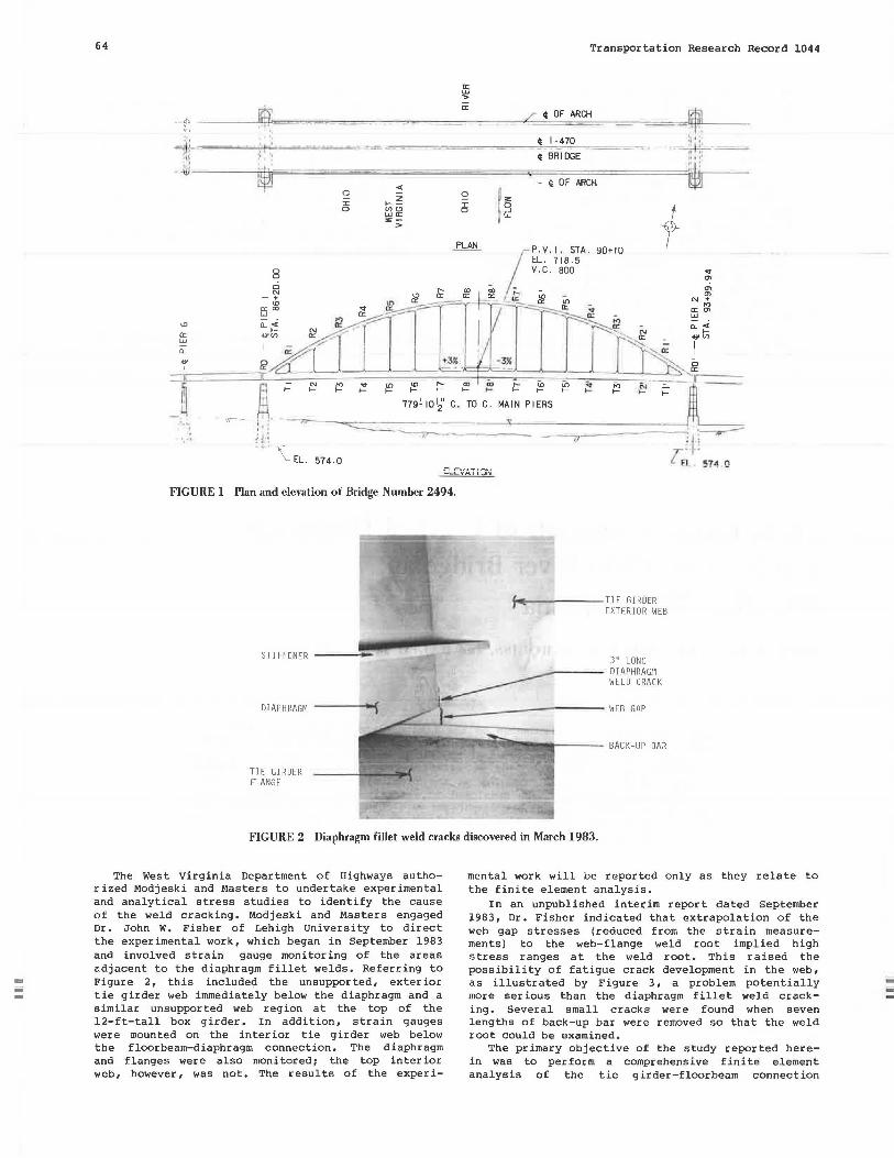
64

·· ~ lr'o

8

a: w > a:

Transportation Research Record 1044

/ ~OF ARCH =='

90+10 f

ELCVATIGN

FIGURE 1 Plan and elevation of Bridge Number 2494.

'l'~-------TI E GIRDER EXTERIOR WEB

3" LONG

--------- DIAPHRAGM ~ WELD CRACK

) WEB GAP DIAPHRAGM

TIE GIRDER FLANGE

FIGURE 2 Diaphragm fillet weld cracks discovered in March 1983.

The West Virginia Department of Highways autho­rized Modjeski and Masters to undertake experimental and analytical stress studies to identify the cause of the weld cracking. Modjeski and Masters engaged Dr. John W. Fisher of Lehigh University to direct the experimental work, which began in September 1983 and involved strain gauge monitoring of the areas adjacent to the diaphragm fillet welds. Referring to Figure 2, this included the unsupported, exterior tie girder web immediately below the diaphragm and a similar unsupported web region at the top of the 12-ft-tall box girder. In addition, strain gauges were mounted on the interior tie girder web below the floorbeam-diaphragm connection. The diaphragm and flanges were also monitored; the top interior web, however, was not. The results of the experi-

mental work will be reported only as they relate to the finite element analysis.

In an unpublished interim report dated September 1983, Dr. Fisher indicated that extrapolation of the web gap stresses (reduced from the strain measure­ments) to the web-flange weld root implied high stress ranges at the weld root. This raised the possibility of fatigue crack development in the web, as illustrated by Figure 3, a problem potentially more serious than the diaphragm fillet weld crack­ing. Several small cracks were found when seven lengths of back-up bar were removed so that the weld root could be examined.

The primary objective of the study reported here­in was to perform a comprehensive finite element analysis of the tie girder-floorbeam connection

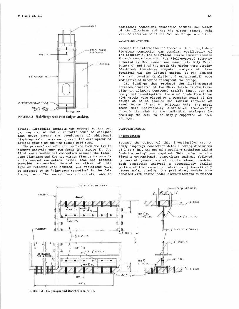
Kulicki et al.

---- ABLE

WEB GAP ____ __, • ' _,,,,,--- PANEL PO I NT _/ DIAPHRAGM

FLDDRBEAM

TIE GIRDER WEB

0 ' .

DIAPHRAGM WELD CRACK

WEB/FLANGE WELD ROOT

WEB GAP

FIGURE 3 Web/flange weld root fatigue cracking.

detail. Particular emphasis was devoted to the web gap regions, so that a retrofit could be designed that would arrest the development of additional diaphragm weld cracks and prevent the development of fatigue cracks at the web-flange weld root.

The proposed retrofit that evolved from the finite element analysis took two forms (see Figure 4) • The first was a mechanical connection between the floor­beam diaphragm and the tie girder flanges to provide a four-sided connection rather than the present two-sided connection. Several variations of this type of retrofit were studied. All variations will be referred to as "diaphragm retrofits" in the fol­lowing text. The second form of retrofit was an

3'5" 0 TOD . TIE GIRDER

~c

--1- - --1--

FIGURE 4 Diaphragm and floorheam retrofits .

65

additional mechanical connection between the bottom of the floor beam and the tie girder flange. This will be referred to as the "bottom flange retrofit."

LOCATIONS STUDIED

Because the interaction of forces at the tie girder­floorbeam connection was complex, verification of the accuracy of the analytical finite element results through comparison with the field-measured response reported by Dr. Fisher was essential. Only Panel Points 4' and 8 of the north tie girder were strain­monitored; therefore, computer analysis of these locations was the logical choice. It was assumed that all results (analytic and experimental) were indicative of behavior throughout the bridge.

The loadings that produced the field-measured stresses consisted of two 80-k, 5-axle trucks trav­eling in adjacent westbound traffic lanes. For the analytical investigation, the wheel loads from these 80-k trucks were placed on a computer model of the bridge so as to produce the maximum response at Panel Points 4' and 8. Following this, the wheel loads were individually distributed transversely through the slab to the individual stringers by assuming the deck to be simply supported at each stringer.

COMPUTER MODELS

Introduction

Because the object of this investigation was to study diaphragm connection details having dimensions of 1 to 5 in., the use of a modeling technique called "substructuring" was required. This technique uti­lized a conventional, space-frame analysis followed by several generations of finite element models. Each generation analyzed a successively smaller portion of the connection detail using successively closer nodal spacing. The preliminary models con­structed with coarse nodal discretizations furnished

-.,

"' N

NEW 1" PL ~ 3~3,i

1

LONG NEW 12· ST I FF PL

12' OIAPH PL (VERTICAL)

--

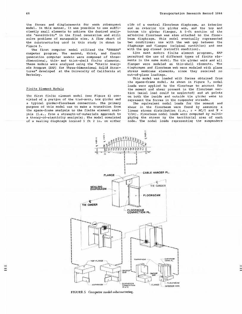
66

the forces and displacements for each subsequent model. In this manner, it was possible to use suffi­ciently small elements to achieve the desired analy­sis "sensitivitv" in the final aeneration and still solve problems of manageable size. A flow chart of the substructur ing used in this study is shown in Figure 5.

The first computer model utilized the "STRESS" computer program. The second, third, and fourth generation computer models were composed of three­dimensional, thin- and thick-shell finite elements. These models were analyzed using the "Static Analy­sis Program (SAP) for Three-Dimensional Solid Struc­tures" developed at the University of California at Berkeley.

Finite Element Models

The first finite element model (sec Figure 6) con­sisted of a portion of the tied-arch, box girder and a typical g irder-floorbeam connection. The primary purpose of this model was to make a transition from the space-frame analysis to the finite element anal­ysis (i.e., from a strength-of-materials approach to a theory-of-elasticity analysis). The model consisted of a seallng diaphragm localed 5 fl 2 in. on either

SEALING DIAPHRAGM -

-----·-__..-er ( TIE GIRDER

! !

\_ DIAPHRAGM _J

Transportation Research Record 1044

side of a central floor beam diaphragm, an interior and an exterior tie girder web, and the top and bottom tie girder flanges. A 5-ft section of the adioinina floorbeam was also attached to the floor­beam diaphragm. This model eventually represented two conditions: one with the web gap between the diaphragm and flanges (original condition) and one with the gap closed (retrofit condition).

Like most modern finite element programs, SAP permitted the use of different types of finite ele­ments in the same model. The tie girder webs and all flanges were modeled as thin-shell elements. The diaphragms and floorbeam web were modeled with plane stress membrane elements, since they received no out-of-plane loadings.

This model was loaded with forces obtained from the space-frame model. As shown in Figure 7, nodal loads were applied to the floorbeam to account for the moment and shear present in the floorbeam sec­tion (axial load could be neglected) and at points on both the inside and outside tie girder webs to represent the forces in the suspender strands.

The equivalent nodal loads for the moment and shear in the floorbeam were found by assuming a linear stress distribution (i.e., a = MC/I and T = V/bt). Floorbeam nodal loads were computed by multi­plying the stress by the territorial area of each node. The nodal loads representing the suspenders

' 1 1

1 1 ,----! I CABLE HANGER PL.

FLOOR BEAM

- FLOORBEAM CONNECTION PL.

I

i _J

FIGURE 5 Computer model suhstructuring.

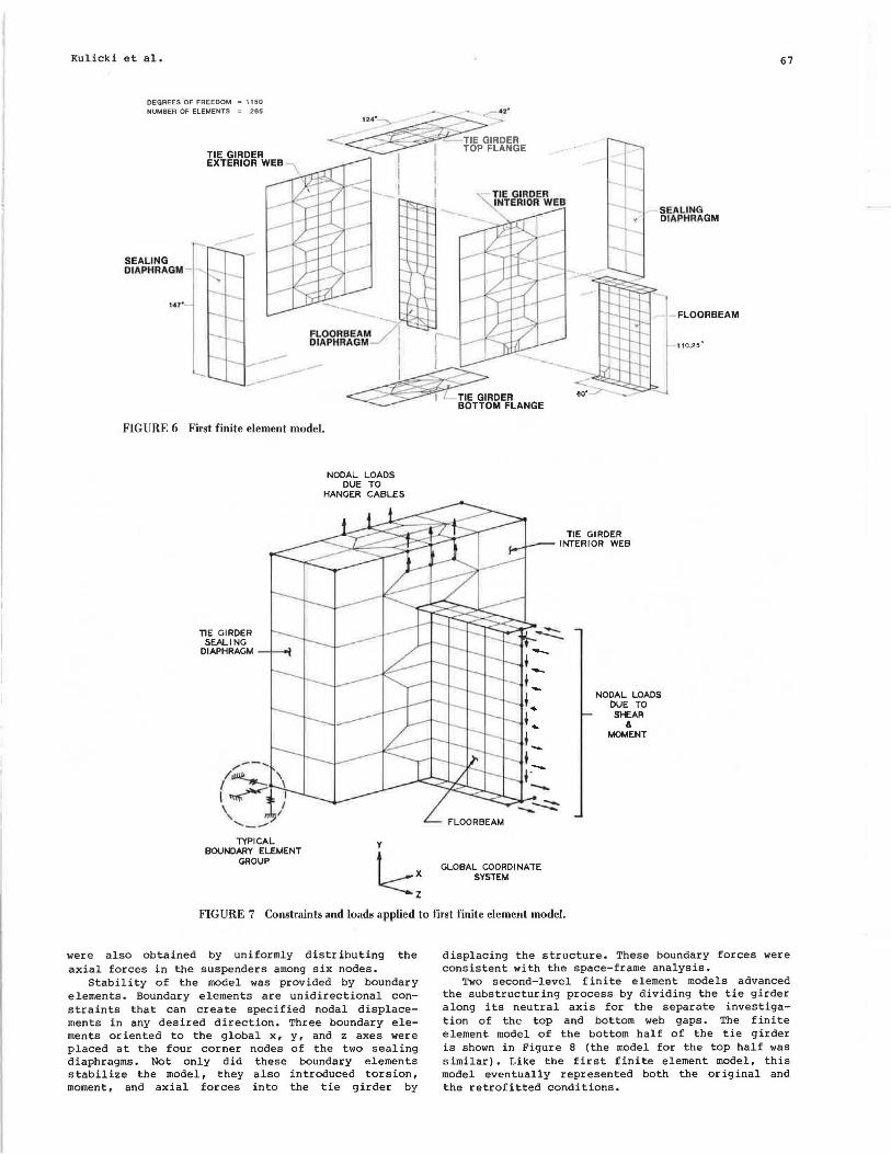
Kulicki et al.

DEGREES OF FREEDOM = 1150 NUMBER OF ELEMENTS = 265

SEALING DIAPHRAGM -

TIE GIRDER EXTERIOR WEB \

SEALING DIAPHRAGM

FLOOR BEAM

67

-.. FLOORBEAM /j I DIAPHRAGM'...../ ii I 110. 25"

-.. :::-~ ~I .

I L TIE GIRDER BOTTOM FLANGE

-FIGURE 6 First finite element model.

TIE GIRDER SEALING

DIAPHRAGM

TYPICAL BOUNDARY ELEMENT

GROUP

NODAL LOADS DUE TO

HANGER CABLES

y

l:: GLOBAL COORDINATE SYSTEM

TIE GIRDER INTERIOR WEB

NODAL LOADS DUE TO SHEAR

& "40MENT

FIGURE 7 Constraints and loads applied to first finite element model.

were also obtained by uniformly distributing the axial forces in the suspenders among six nodes.

Stability of the model was provided by boundary elements. Boundary elements are unidirectional con­straints that can create specified nodal displace­ments in any desired direction. Three boundary ele­ments oriented to the global x, y, and z axes were placed at the four corner nodes of the two sealing diaphragms. Not only did these boundary elements stabilize the model, they also introduced torsion, moment, and axial forces into the tie girder by

displacing the structure. These boundary forces were consistent with the space-frame analysis.

Two second-level finite element models advanced the substructuring process by dividing the tie girder along its neutral axis for the separate investiga­tion of the top and bottom web gaps. The finite element model of the bottom half of the tie girder is shown in Figure 8 (the model for the top half was similar). Like the first finite element model, this model eventually represented both the original and the retrofitted conditions.

68

TIE GIRDER NEB ~ ~ EXTERIO: ~r-I

TIE GIRDER BOTTOM FLANGE

FIGURE 8 Second-level finite element model.

These second-level models confined the analysis to a region bounded by a line 2 ft on either side of the floorbeam diaphragm and by the tie- g i rder neutral axis. A 2-ft length of the floor beam was a gain at­tached to the floorbeam diaphragm. Boundary elements were located at the corners of the box girder, along the neutral axis, and on the attached floorbeam.

With the increased elemental thickness-to-length ratios caused by the finer nodal discre t ization , the use o f "bric k elemen t s " was preferable for all the flanges and the tie girder - floorbeam connection plates. (A brick element is a solid, three-dimen­sional element that effectively models the assemblage of plates utilized within the connection details.) The other model components remained as previously described.

The final substructuring o f the tie girder-floor­beam connection was a set of four, third-level finite e l ement mode l s , one of which is shown i n Figure 9 . This model shows the finite element mesh for the bottom interior corner of the tie girder (the models

...

TIE GIRDER BOTTOM FLANGE-

FIGURE 9 Third-level finite element model.

DIAPHRAGM -­CONN. PL.

Transportation Research Record 1044

DEGREES OF FREEDOM 1700 NUMBER OF ELEMENTS 460

- FLOORBEAM WEB

FLOORBEAM FLANGE

for the remaining tie girder corners were similar). Each of the four, third-level models focused on one of the tie girder' s cor ner web gap regions , so that stre ss g r ad i e n ts along the interior surface of each web gap could be determined. By comparing the stress gradients obtained from these models with varying structural parameters (e.g., with and without retro­fits), the effectiveness of various retrofit details could be evaluated.

The t h ird-level models consisted almost entirely of o;uliu, Lhree-dimensional elements so that the most accurate representation of the web gap regions could be obtained. Stresses were induced in the models by imposing boundary element displacements obtained from the previous substructure models; there were no surface loads applied to the models. These boundary e l ements were l oca ted a t t he tie ­g irder flange below the web gap and along the £loor­beam dia phr a gm a bove t he web gap.

The only variations in modeling that were studied at this level of substructuring, without starting at

DEGREES OF FREEDOM 4IO NUMBER OF ELEMENTS 1215

,-FLOORBEAM r CONNECTION PLATE

Kulicki et al.

an earlier level, were the inclusion of the back-up bars and fillet welds between the tie-girder flange and web. All other parameters investigated (i.e., variations of the diaphragm retrofit and the bottom flange retrofit) were carried through all stages of substructur ing to obtain the most accurate results possible with the procedure described previously.

ANALYTIC RESULTS

The results of the computer analysis will be pre­sented in this section. First, the top and bottom web gap regions (i.e., four corners), at Panel Point B will be discussed without the retrofit installed, and then with the retrofit installed. This will be followed by a similar discussion of the bottom web gaps at Panel Point 4'. The top web gap region was not reanalyzed at Panel Point 4' because the experi­mentally measured stress gradients there were not significantly different from those obtained at Panel Point B.

Obviously, fatigue of welded details is caused by a fluctuating stress (i.e., stress range). In eval­uating both the accuracy of finite element models and the effectiveness of retrofits, no effort was made to reproduce both the positive and negative phases of the experimentally observed stress ranges. Rather, it was assumed that good agreement between measured and analytic results, and the analytically determined effectiveness of a retrofit obtained for one live load position, would also apply to other live load positions (i.e., superposition).

Panel Point B Results Without Retrofit

The deformations of the tie girder top and bottom web gap regions at Panel Point B without the dia­phragm retrofit are shown in Figures 10 and 11. A differential displacement between the floorbeam

69

diaphragm and the tie girder flange equal to 0.00517 in. occurred within the top web gap region. The bot­tom web gap displacements were much smaller. Never­theless, in gap details, displacements of even this small order of magnitude characteristically cause high stresses. Conclusions as to the mechanism caus­ing the web gap stresses were drawn by analyzing these deformations.

In both the top exterior and top interior web gaps, it was evident that the out-of-plane transla­tion of the diaphragm relative to the tie girder flange induced most of the web gap stresses. Although some rotation occurred in both the flange and dia­phragm, the rotation had the effect of reducing the stresses in the web, rather than increasing them. Comparison of the stress gradients obtained from the finite element analysis with those measured experi­mentally are shown in Figures 12 and 13.

In Figure 12, experimentally measured stresses in the top exterior web gap varied from -2 ksi (com­pression) at the back-up bar to +4 ksi (tension) at the top of the diaphragm. The analytical stresses (without retrofit) varied between -4 ksi and +4 ksi.

The top interior web gap was not strain-gauged; how­ever, analytical stresses obtained at this location (see Figure 13) varied between +3 ksi at the back-up bar and -2 ksi at the top of the diaphragm. This reversal in sign of the web stresses through the gap length was expected in light of the displacements shown by Figure 10.

Similarly, the bottom exterior web gap experi­mentally measured stresses at Panel Point B varied between -2 ksi at the bottom of the diaphragm and +3 ksi at the web-flange weld root as shown in Figure 14. This response was also observed in the finite element model that yielded a stress variation from -.5 ksi to +4 ksi in the same region.

The bottom interior web gap--the fourth and final location studied at Panel Point B--showed a struc­tural response different from the previous three web

FIGURE 10 Top web gap deformation without retrofit at Panel Point 8.

j=1"1"_°_:~~8~---~~~~A~~ n o.00100'

0.00058" I r-----------7L-_-_-_-_-_-_-_1~ Jo.00287'

I OUTSIDE I I

WEB I I I

-----------------------! I

INSIDE WEB a

DIAPHRAGM CONN. rt

0 .001 29 '

FIGURE 11 Bottom web gap deformation without retrofit at Panel Point 8.

70

24

"' ... z

"' 2 23 "' ..J

"' "' ... 22 ~ ... 21

BACKUP BAR

I I I I

I I

' ' I

!! /

:;/ _L •

71 1/'' I:

~ • ' -3 -2 -1 0

STRESS (k>I)

v I

24

VI I-z :IE

23 ~ UJ

UJ I-

~ 22 IL

21

Transportation Research Record 1044

f I BACKUP BAR

WrfL ANGE WELP ROOT

11:7~ ----·· -- -·-·· ··--·-t 1'

t I'

t I'

+ I'

l

i-----.----.-..~ r~:·· ........ ·--\

'

-4

\

-3 -2 -1 0

STRESS (bl)

2 3

0.84' + lA2

~-\u 0.84'

_l lA4

MEASURED STRESSES BY FHWA a LEHIGH UNIVERSITV

'SAP' STRESSES: DIAPHRAGM W/O RETROFIT : I" X 2'·0" RETROFIT

: 1112" X 2'·0" RETROFIT : I" X 3'·1" RETROFIT

STRAIN GAGES

FIGURE 12 Stress gradients in top exterior web gap at Panel Point 8.

WEB·FLANOE WELD ROOT

I I'' I BOTTOM Of BACK-UP BAR

/ 1·

+ I'

+ I'

+ I'

l TnP r& nlA"""'"_...

gaps described. Here, the measured stresses (see Figure 15) indicated that there was no change in the direction of applied moment along the entire web gap surface. All previous web gaps showed change in sign of static stresses within the gap. The initial analytical results at this web gap indicated that this type of behavior (change in sign of stresses) could be expected here also. Clearly, some improve­ment in the modeling of the bottom interior web gap was needed.

STRESS (k11)

2 J

72 3 .. • 'SAP' STRESSES: DIAPHRAGM W/O RETROFIT

I" X 2'·0· RETROFIT "' ~ 64

o.1e" I " \ 2

I' X J'· I' RETROFIT "' I 'l_ AIO

56 ' -~ o.1e· NOTE : FHWA DID NOT STRAIN GAGE THIS WEB GAP.

§ w \

FIGURE 13 Stress gradients in top interior web gap at Panel PD-int 8.

114 !II I-z UJ 110 :IE ~ 106 ILi

UJ I- 102 z ii:

98

94

STRESS (k1I)

"34"-

I ' 2

I • 2

I " 2

I" 2

1" 2

MEASURED STRESSES BY FHWA a LEHIGH UNIVERSITY. 'SAP' STRESSES : DIAPHRAGM W/O RETROFIT.

: I' X 2'·0' RETROFIT.

FIGURE 14 Stress gradients in bottom exterior web gap at Panel Point 8.

w 48 ,.

~ 2

G'.

36 , ..

\ \ t All \ rop Of BACKUP BAR

i I\ . I \\ ., I ., ' / \\

MEASURED STRESSES BY FHWA 8 LEHIGH UNIVERSITY.

'SAP' STRESSES: DIAPHRAGM W/O RETROFIT I' X 2'·0" RETROFIT FLOORBEAM MOVED UP 3/4"

FLOORBEAM MOVED DOWN !114"

FLOORBEAM MOVED DOWN 1-112"

FIGURE 15 Stress gradient in bottom interior web gap at Panel Point 8.

In an attempt to reproduce the measured values on the entire web gap surface, the floorbeam was ana­lytically repositioned vertically so as to introduce an eccentric loading into the flange and cause the rotation of the flange necessary to produce the experimentally measured stress variation. However, when the stresses did not match the measured values even with the floor beam flange lowered 1. 5 in., it

.... --

Kulicki et al.

became obvious that some other phenomenon was pre­cipitating the experimental results, because no misalignment of the indicated magnitude was observed in the field. It is important to note here that all connection details discussed previously were modeled as designed (i.e., the floorbeam flange was assumed to bear perfectly against the tie girder flange) •

It was evident that still another modification to the original model was needed to resolve the bottom interior stresses. It was therefore decided that concentration should be on the bottom interior web stresses at Panel Point 4', since those experi­mentally measured stresses were much higher than those at Panel Point 8. The results obtained at Panel Point 4' will be discussed later, and an explanation for the difference in behavior between the bottom exterior and interior corner will be presented.

Panel Point 8 Results with Diaphragm Retrofit

Figures 16 and 17 show, respectively, the deforma­tions of the top and bottom web gap regions with the most effective diaphragm retrofit installed. This retrofit is a T-section fabricated from 1-in. plates bolted to the tie girder diaphragm and flange, thus effectively filling the gap between these structural elements

Figures 12 and 13 show the reduction in stresses for the top exterior and interior web gaps caused by varying the length and thickness of the retrofit. As expected, the retrofit that provided the maximum shear stiffness between the translating diaphragm and the rigid tie girder flange reduced the stresses most significantly (i.e., the 3 ft 1 in. retrofit). The analytical stresses at the top exterior web gap were reduced to -.5 ksi at the back-up bar and +l ksi at the top of the diaphragm. A similar reduction

71

of stresses was observed at the top interior web gap with the 3 ft 1 in. retrofit. The 2-ft retrofit was found to be adequate for the bottom exterior and interior web gaps at Panel Point 8 and was not re­analyzed with the 3 ft 1 in. retrofit as an expedi­ence. In the top web gaps, it became evident that the ability of diaphragm retrofit to almost com­pletely eliminate the rotation and translation between the tie girder flange and the floorbeam diaphragm was the primary reason why it was effec­tive in reducing the web gap stresses.

Panel Point 4' Results Without Retrofit

As stated previously, the previous results at Panel Point 8 led to the hypothesis that (a) the connec­tion detail was not acting as designed, and (b) vertical misalignment of the floorbeams was an im­probable cause, since analytical stresses of the indicated magnitude did not result from this mis­alignment.

It was clear, then, that some other mechanism had to be responsible for:: such high stresses. It was deduced that the only way to simultaneously obtain the measured stress gradients in both the exterior and interior:: web gaps was for the force from the floor:: beam to be transmitted directly into the dia­phragm. This would cause a net reduction of length of the bottom of the diaphragm combined with a local rotation at the inter:: ior bottom corner:: of the dia­phragm, as shown in Figure 18. As a result of this reasoning, it became apparent that the floor::beam must not be bearing against the tie girder flange at the two panel points that were instrumented (and probably elsewhere). This lack of bearing between the floorbeam and the tie girder:: was called "the floor::beam gap" as shown in Figure 19.

The floorbeam gap was first assumed to extend to

ORIGINAL o.ooo

67,, CONFIGURATION I --rro.ooo61 ,

0.00119•.qr-----------------L------~ LJO.OOl 6 6"

II I I I I

I I I I I I I I L -- ---- ------------------_J

0 .00 120·-LJ:..:: ~----.--------------1-l 0 . 00 156'"-l----I- DEFORMED

CONFIGURATION

FIGURE 16 Top web gap deformation with retrofit at Panel Point 8.

0 .0007 3"

0 .00 0 75"

ORIGINAL 'I t· 0 .00101 · CONFIGURATION --, I - ------------------'------

! I I I I I I-I r---..:-

1-I

DEFORMED CONFIGURATION

I I I I

r------1 I

FIGURE 17 Bottom web gap deformation with retrofit at Panel Point 8.

0 .00178"

0.00168'

0 .00280"

0.00089"

72

=.n <1J

"' a a a a

OUTSIDE WEB

WEB GAP

I I

~DIAPHRAGM

Transportation Research Record 1044

0.00249"

I INSIDE I WiB

__ [____________________ -~ DIAPHRAGM

:s::::r_=-=-=-=-=-==-=-=-=-=-=-=-==-=-=-=-~_j ___ j CONN . it_

tJ==--==-=--===-=-==-:-~---~=-==~~l 0.000327 ' FLANGE 0004-30"

FIG URE 18 Bottom web gap deformation without retrofit at Panel Point 4'.

the bottom of the diaphragm. This gap length produced a stress gradient (see Figure 20) on the inside web surface ranging from -14 ksi at the web-flange weld root to +12 ksi at the bottom of the diaphragm. Reducing the floorbeam gap length to the web gap midpoint (by increasing the connection plate length) concentrated the web translation and rotation at the web-flange weld root and increased the stresses accoLdingly f as shown in Figure 21. This second set of stresses contained weld root tensile stresses

significantly greater than those previously modeled or measured.

In summary, the best match between measured and calculated stresses resulted when the inferred floorbeam gap was assumed to extend from the bottom flange of the floorbeam to the bottom edge of the tie girder diaphragm. This gap could not be physi­cally confirmed, and is more academic than con­sequential after the retrofit is installed. Figure 22 shows the bottom exterior web gap stresses at

DIAPHRAGM CONNECTION PLATE

TIE GIRDER

TIE GIRDER INTERIOR WEB

0

FLOOR BEAM

BOTTOM INTERIOR WEB GAP SEE DETAILS BELOW FOR INFORMATION ON FLOORBEAM GAP.

DIAPHRAGM - FLOORBEAM CONNECTION PL

FLOORBEAM FLANGE

.___ _ ____ _,._ TIE GIRDER FLANGE

DESIGN CONDITION

FLOOR BEAM GAP

FINITE ELEMENT MODEL

CASE I : FLOORBEAM GAP EXTENDED TO BOTTOM OF DIAPHRAGM.

FIGURE 19 Floorbeam gap configurations.

"- FLOORBEAM GAP

PROBABLE FIELD CONDITION

FLOOR BEAM GAP

FINITE ELEMENT MODEL

CASE II: FLOORBEAM GAP EXTENDED TO WEB GAP MIDPOINT.

Kulicki et al.

I/) ... '1!

"' ~ -' "' "' I-

~ u.

43 34

I• i

I" 2

I • 2

27 I • 2

STRESS (hi)

- 12 10 a s 4 2 . - - - - 0 2 4 6 8 BOP "" OF-ll.IAelffiAllM_ / ..... -- o ... o·-v --- - II. B9

/ - 0.40"-.. -,,,/ :.- - l BIO

-~ 0 .4011

--- -:' - 11. Bii v_...... ......- ,• _.,-:; .-

I-' TQP QE 1111!<!11.!I! aaB /v --,

/ / ,

. , ~a-Fl . A,"1~C" UJC"I n Dl"V"OT

MEASURED STRESSES BY FHWA 8 LEHIGH UNIVERSITY. 'SAP' STRESSES : DIAPHRAGM W/O RETROFIT

: 111

X 3'-1 11 RETROFIT

FIGURE 20 Stress gradients in bottom interior web gap at Panel Point 4' -floorbeam gap extended to bottom of diaphragm.

43 3. 4

39 1 • 2

35 1 • 2

31 ,. 2

27 1 • 2

STRESS (kill

-12 10 a - - - 6 4 2 0 - - 2 4 s a

[,......- __......-,. I

,/ I ,

,/ , ,.

/ ! ,. . / , ..... v / ' / ...... ::.:: -- ·---,_r: -- - --- I -- -- I L .. -- ... ---

MEASURED STRESSES BY FHWA 8 LEHIGH UNIVERSITY.

'SAP' STRESSES: DIAPHRP.GM W/O RETROFIT

: I" X 3'-1' RETROFIT

I 0 OOTTOM OF DIP.PHRAGM 0..40 .. _

I - II. 89 0.40"-

- l 810

I 0.40"-. I - '!. 811

TOP OF BACKU~ aeB

WEB.C1 .IUoJf!J:' l.l.IC'I n DIV\'r

I' X 3'-1" RETROFIT a 314' X 18' STRAP PLATE.

FIGURE 21 Stress gradients in bottom interior web gap at Panel Point 4'-floorbeam gap extended to web gap midpoint.

STRESS (k11)

-a s 4 2 o 2 - - - 4 6 a I 0 12 14 ...,. TOMOF""

~ 1: 0 ,4~"' ..__ ~! - '!. 8~ --- \ ~ 0, 27"

-\ '-""" C>d l B6

!--- '" - '!. B7

0.26'•

\ """"

- c. 88

I\ r':- ' ~ IQf QE aa~ts!JE aaa

~ ' " '·...__

1 "' -r-, \ ' -~ .....

.i \ " Ulta ~ -=-- 11.ur_r t.AICI I'\ Dl'\l'\T

~ 11 4 ~· 4

;;!'.

~ 110 ,. 2

-' "' 106

I •

"' 2 I-z 102 I • " • (;: 98 I"

4

94 I• 2

MEASURED STRESSES BY FHWA 8 LEHIGH UNIVERSITY. 'SAP' STRESSES: DIAPHRP.GM W/O RETROFIT

: I" X 3'-1" RETROFIT

: 3/4" X 18' STRAP PLATE a I' X 3'-1' RETROFIT

FIGURE 22 Stress gradients in bottom exterior web gap at Panel Point 4'.

73

Panel Point 4' with the floorbeam gap assumed to extend to the bottom of the diaphragm. Good agree­ment with the measured stresses is evident. Var ia­tions in the floorbeam gap length did not affect the bottom exterior web gap displacements and, inferen­tially, would not be expected to affect the resulting stresses.

phragm retrofit installed. For the case in which the floorbeam gap extended up to the bottom of the dia­phragm (Figure 20), a stress reduction to one-half of the original values at the bottom interior web­flange weld root was observed. The most critical case (the floorbeam gap extended to the web gap midpoint, which is shown in Figure 21) has a stress range between 15 and 20 ksi. Thus, the 3 ft 1 in. retrofit did not adequately reduce the stress range at the bottom interior web gap at Panel Point 4'. The floorbeam gap apparently caused transfer of all the load through the flooi::beam diaphragm. A positive means of forcing the load directly into the tie

Panel Point 4 ' Resul"ts with Diaphragm Retrofit

Figures 20 and 21 show the interior web stress gra­dients for the two floorbeam gap lengths with a dia-

74 Transportation Research Record 1044

.. ORIGINAL ·t- ~c~-~o~~ - ___ :?~~~~A~1~_7 _______ Tfio.00110· 0.00078 . i 0.00265"

I J I I l I

o onn7A" be-----,. __ --------------------------0·00012" DEFORMED

CONFIGURATION 0.00020'

FIGURE 23 Bottom web gap deformation with retrofit and tie plate at Panel Point 4 '.

flange without passing through the diaphragm was required.

The bottom exterior web gap stresses (see Figure 22) were reduced to approximately one-fifth of their original value by the displacement-reducing action of the diaphragm retrofit. Even though this was a significant decrease, the stress range was still relatively high (i.e., approximately 7 ksi).

Results with Diaphragm Retrofit and Tie Strap Plate

It was found that the installation of a structural plate (tie s t rap ) bol t ed t o the tie g irder and floorbeam bottom flanges would adequately reduce the stresses and web deformations, as shown in Figures 21-23. It is important to note that the combined floorbeam and diaphragm retrofits reduced the stress range to approximately l ksi on the bottom interior web gap (see Figure 21), which previously had ex­hibited a stress range of 15 to 20 ksi; thus, the bottom exterior web gap bending stresses (see Figure 22) were essentially eliminated. The combined effect on top gap stresses was not significantly different from the effect of the diaphragm retrofit alone.

Back-Up Bar and Fillet Weld Effects

The presence of a back-up bar in the corners of the tie girder raised some questions about the accuracy of the modeling. Several analyses were made to study i: 11 t:ffcct t o ~z:lu: c t~s t -th~ ~·,~rst conditio W(IA

investigated and corrected by the retrofit proce­dures .

The inclusion of a back-up bar continuously fillet-welded to the north tie girder flange and web significantly reduced the calculated bending stresses induced in the web. Th i s occurred because of the increased section properties available at the rigidly fixed web-flange connection. The structural contri­bution was negligible for the back-up bar connected to the web only by the web-flange groove weld (south tie) . This second condition was modeled by complete removal of the back-up bar from the models.

Even though the back-up bar was found to be s uc­cessf ul in reducing the web stresses, it was not the solution to the web bending problem; it simply transferred the bending stresses to the back-up bar and fillet welds .

CONCLUSIONS

The tollowing conclusions are made:

1. Web gap movements on the order of thousandths­of-an-inch caused the high stresses capable of pro­ducing fatigue cracking.

2. The measured web gap stresses could only be reproduced within tho bottom \·:eb gaps by placing a floorbeam gap between the floorbeam and the tie girder flange.

3. The closest reproduction of measured stresses occurred with the floorbeam gap extended to the bottom of the tie girder diaphr agm.

4 . The inclusion of the diaphragm retrofit in the finite element analysis models reduced the web­flange weld root stresses at locations other than the bottom interior corner by one-half to one-fifth of their original values.

s. A tie plate (i.e., floorbeam retrofit) was required to transmit the floorbeam flange force directly into the tie girder flange. With the com­bined floorbeam and diaphragm retrofits, the bottom interior web gap stresses were reduced to ± 1 ksi when two adjacent directional lanes of HS20 trucks were positioned over the floorbeam. The bottom ex­terior web gap stresses were essentially eliminated.

6. The retrofit details shown in Figure 4 (taken from contract drawings) implemented all stress-range reducing techniques developed in the study. The particular details are for a tie girder section without a field splice. Similar, but somewhat more complex, detailing was required at tie-girder field splices.

7. The diaphragm stress field was redirected from the diaphragm-web fillet weld to the diaphragm retrofit (not a fatigue-critical connection) and the bottom flange retrofit.

B. The computed web bending stresses at the web-flange weld root doubled when the back-up bars were removed from the models. The back-up bars in the south tie were not continuously fillet-welded to the flange or web and, as such, provided little additional support (essentially removed) to the web. This is of no consequence once the retrofits are provided.

Publication of this paper sponsored by Committee on Steel Bridges.

... -