Effective and Robust Coordination of Traffic Signals on Arterial ...

FHWA/IN/JTRP-2006/26

Final Report

EFFECTIVE AND ROBUST COORDINATION OF TRAFFIC SIGNALS ON ARTERIAL STREETS

VOLUME 2 GUIDELINES OF DESIGN

Wei Li Andrew P. Tarko

January 2007

- I -

Final Report

FHWA/IN/JTRP-2006/26

EFFECTIVE AND ROBUST COORDINATION OF TRAFFIC SIGNALS ON ARTERIAL STREETS

Volume 2

Guidelines of Design

By

Wei Li Graduate Research Assistant

and

Andrew P. Tarko

Associate Professor

School of Civil Engineering Purdue University

Joint Transportation Research Program

Project No. C-36-17WWW File No. 8-4-75

SPR-2947

Conducted in Cooperation with the Indiana Department of Transportation and the

U.S. Department of Transportation Federal Highway Administration

The contents of this report reflect the views of the authors, who are responsible for the facts and the accuracy of the data presented herein. The contents do not necessarily reflect the official views or policies of the Indiana Department of Transportation or the Federal Highway Administration at the time of publication. The report does not constitute a standard, specification, or regulation.

Purdue University West Lafayette, Indiana

January 2007

- II -

TABLE OF CONTENTS

1 INTRODUCTION ...................................................................................................... 1 2 OVERVIEW OF ARTERIAL SIGNAL DESIGN ...................................................... 2

2.1 Conditions of Good Coordination .......................................................................... 2 2.2 Design Procedures ..................................................................................................... 3

3 OVERVIEW OF SYNCHRO AND SIMTRAFFIC .................................................... 4 3.1 A Tour of Synchro and SimTraffic Design .......................................................... 4 3.2 Tools for Evaluating Signal Solutions ................................................................ 19

3.2.1 Synchro Control Indicators ................................................................................... 19 3.2.2 Time-Space Diagram ............................................................................................. 20 3.2.3 Quick Report ......................................................................................................... 21 3.2.4 Signal Plan Output ................................................................................................ 24 3.2.5 SimTraffic Static Graphics Tool ............................................................................ 24 3.2.6 SimTraffic Animation ............................................................................................ 26

3.3 Advanced Issues of the Simulation .................................................................... 27 3.3.1 Random Number Seed of Simulation .................................................................... 28 3.3.2 Multiple Simulation Runs ..................................................................................... 29 3.3.3 Simulation of Multiple Intervals ........................................................................... 33

4 LOCAL VALUES OF TRAFFIC PARAMETERS .................................................... 35 4.1 Saturation Flow Rate in Synchro ........................................................................ 35 4.2 Saturation Flow Rate in SimTraffic .................................................................... 37 4.3 Speed Model in SimTraffic ..................................................................................... 38

5 IDENTIFYING SOLUTION DEFICIENCY WITH SYNCHRO ........................... 44 5.1 Insufficient Capacity Reserve ............................................................................... 44 5.2 Lane blockage by adjacent traffic queues ......................................................... 48 5.3 Fixed-time Operation of an Actuated Phase .................................................... 49 5.4 Early-return-to-green .............................................................................................. 51 5.5 Back-to-back Stops.................................................................................................. 53 5.6 Strong Turning Volumes ........................................................................................ 54

6 IDENTIFYING SOLUTION DEFICIENCY WITH SIMTRAFFIC ....................... 57 6.1 Insufficient Capacity Reserve ............................................................................... 57 6.2 Lane blockage by adjacent traffic queues ......................................................... 59 6.3 Early-Return-to-Green ............................................................................................ 60 6.4 Back-to-back Stops.................................................................................................. 61

7 REMEDIES OF SOLUTION DEFICIENCIES ....................................................... 63 7.1 Insufficient Capacity Reserve ............................................................................... 63 7.2 Queue blockage of adjacent traffic...................................................................... 64 7.3 Fixed-time Operation of Actuated Phases ........................................................ 65 7.4 Early-Return-to-Green ............................................................................................ 66 7.5 Strong Turning Volumes ........................................................................................ 67 7.6 Under-estimated Speed in Simulation ............................................................... 67

- III -

8 ADDITIONAL ISSUES............................................................................................. 68 8.1 Unbalanced Lane Utilization ................................................................................. 68 8.2 Special optimizer options ....................................................................................... 68 8.3 Inconsistent MOE output ...................................................................................... 69 8.4 Data Temporal Adjustment ................................................................................... 69 8.5 Field Tuning ............................................................................................................... 70

REFERENCE ................................................................................................................... 71

- IV -

LIST OF FIGURES Figure 3-1 Create and save a new model in Synchro ......................................................................... 4 Figure 3-2 Lay out links and intersections in the model .................................................................... 5 Figure 3-3 Edit intersection properties ............................................................................................... 6 Figure 3-4 Edit link settings ............................................................................................................... 7 Figure 3-5 Switch between design windows ...................................................................................... 7 Figure 3-6 Lane window settings ....................................................................................................... 8 Figure 3-7 Volume window settings .................................................................................................. 9 Figure 3-8 Timing window settings ................................................................................................. 10 Figure 3-9 Phasing window settings ................................................................................................ 11 Figure 3-10 Optimize intersection timings .................................................................................... 12 Figure 3-11 Optimize network signal cycle length ....................................................................... 12 Figure 3-12 Select desirable solution ............................................................................................ 13 Figure 3-13 Optimize network offsets ........................................................................................... 13 Figure 3-14 Review quick reports in phasing window .................................................................. 14 Figure 3-15 A sample quick report of “starts” of phases ............................................................... 15 Figure 3-16 Traffic animation in SimTraffic ................................................................................. 16 Figure 3-17 Select the parameters included in the performance report of SimTraffic .................. 17 Figure 3-18 A sample report of SimTraffic ................................................................................... 18 Figure 3-19 V/C for all lane groups displayed in the map window ............................................... 19 Figure 3-20 Time-Space Diagram button ...................................................................................... 20 Figure 3-21 A sample Time-space Diagram .................................................................................. 20 Figure 3-22 Location of the quick report buttons .......................................................................... 22 Figure 3-23 A sample quick report of the starting times of all phases .......................................... 23 Figure 3-24 Signal plan parameters in timing window ................................................................. 24 Figure 3-25 Static graph of delay/vehicle ...................................................................................... 25 Figure 3-26 Static graph of speeds ................................................................................................ 26 Figure 3-27 Monitor intersection and vehicle status during simulation ........................................ 27 Figure 3-28 Playback control of animation ................................................................................... 27 Figure 3-29 Random Number Seed Configuration ........................................................................ 29 Figure 3-30 Multiple Runs Configuration ..................................................................................... 29 Figure 3-31 Multiple Runs Report ................................................................................................ 30 Figure 3-32 Select multiple simulation result files ........................................................................ 31 Figure 3-33 Reports of multiple runs ............................................................................................ 32 Figure 3-34 Simulation of multiple intervals ................................................................................ 33 Figure 4-1 Adjust saturation flow rate and lost times in Synchro .................................................... 35 Figure 4-2 Adjust the saturation flow rate for the entire network .................................................... 36 Figure 4-3 Adjust headway factors of external links ....................................................................... 37 Figure 4-4 Adjust headway factors for internal movements ............................................................ 37 Figure 4-5 Simulated saturation flow rate against Headway Factor ................................................ 38

- V -

Figure 4-6 Adjust speed factors in SimTraffic ................................................................................. 40 Figure 4-7 Vehicle Parameters Window ........................................................................................... 41 Figure 4-8 Vehicles types parameters .............................................................................................. 42 Figure 4-9 Acceleration curves of different max speeds .................................................................. 43 Figure 5-1 V/C indicator in Synchro ................................................................................................ 45 Figure 5-2 Queue length indicator in Synchro ................................................................................. 46 Figure 5-3 TSD when capacity is insufficient .................................................................................. 47 Figure 5-4 TSD when capacity is enough ........................................................................................ 47 Figure 5-5 Request queue related report .......................................................................................... 48 Figure 5-6 Sample queue report ....................................................................................................... 49 Figure 5-7 Sample quick report of actual green times ..................................................................... 50 Figure 5-8 Sample phasing parameters ............................................................................................ 50 Figure 5-9 Ring structure with “lag phase hold” problem ............................................................... 51 Figure 5-10 Detect early-return-to-green problem with quick report of green starting time ......... 52 Figure 5-11 Diagnose Early-return-to-green problem with TSD .................................................. 53 Figure 5-12 Detect back-to-back stop with TSD ........................................................................... 54 Figure 5-13 Request report of queue interactions ......................................................................... 55 Figure 5-14 Queue interaction information in the report ............................................................... 56 Figure 6-1 Static Graphics of delay/vehicle under 50th percentile traffic ....................................... 58 Figure 6-2 Static Graphics of Delay under 75th percentile traffic .................................................... 58 Figure 6-3 Static graph indicating queue blockage problem ............................................................ 59 Figure 6-4 Static graph of queue length ........................................................................................... 60 Figure 6-5 Vehicles in queue at the beginning of green at the upstream intersection ...................... 61 Figure 6-6 Positions of the tagged vehicle at the end of yellow at the downstream intersection ..... 62 Figure 7-1 Growth factor adjustment in volume window ................................................................ 64 Figure 7-2 Lead-lag configurations .................................................................................................. 65 Figure 8-1 Lane utilization factor settings ....................................................................................... 68

- 1 -

1 Introduction

These guidelines focus on the use of the software package Synchro/SimTraffic in designing traffic signal plans for arterial streets. This package in general effectively reduces the efforts of traffic systems engineers and improves the quality of the designed coordination. However, it is noted that sometimes advanced knowledge and techniques beyond the routine use of the software are needed to obtain satisfactory signal solutions. Two cases are frequently encountered and reported by INDOT signal systems engineers: (1) the initial solution is not fully in line with the INDOT criteria for a good coordination plan; and (2) additional field-tuning is needed since the actual operational performance of the signalized arterial system deviates substantially from the performance predicted with the software. The objectives of these guidelines are to serve as a reference to experienced users and to assist less experienced engineers in using Synchro and SimTraffic. The guidelines are not meant to be an exact manual of arterial signal coordination design. Each traffic systems engineer encounters different issues in each system and may use different approaches to resolve them. The guidelines are intended to assist traffic system engineers in finding acceptable signal solutions within a shorter period of time. Chapter 2 defines INDOT’s conditions for good signal coordination and then introduces the general procedures for arterial signal design. Chapter 3 briefly introduces the procedural context in which the software package is used. It presents the general procedure for arterial signal design by demonstrating a simple step by step example. Then, the major tools to identify potential improvements of the obtained solution are introduced. Chapter 3 concludes with a brief discussion of selected issues of simulation. Chapter 4 discusses the calibration of the traffic parameters used by the software. Chapters 5 and 6 explain Synchro- and SimTraffic-based identification of possible improvements of obtained signal coordination plans. Chapter 7 proposes specific improvement methods, and Chapter 8 concludes the guidelines with a discussion of additional miscellaneous arterial signal design topics. These guidelines are not substitutes for the on-line help manual of the software package but are rather a complementary document to guide the design of arterial signal systems. References to the on-line manual are given for some topics for the convenience of usage. The assumed version of the software is 6.0.

- 2 -

2 Overview of Arterial Signal Design

2.1 Conditions of Good Coordination

Typically, signal optimization software minimizes the total delays and the number of stops at intersections along the subject arterial street (Husch and Albeck. Copyright 1993-2004) (McTransCenter 1990-2006). INDOT engineers follow a mainly perception-based approach to coordination design that exceeds the routine optimization objective of Synchro and other commercial optimization packages. An arterial signal plan is acceptable when the following conditions of good coordination are satisfied:

1. Traffic progression along the arterial is reasonably smooth. Most of the drivers moving along the arterial street do not stop at two consecutive intersections. Drivers do not stop more than once at the same intersection (no congestion).

2. No perceptible queuing interaction persists during the design period. There is no queue spillback affecting queue discharge at the upstream intersection. Through lanes on the arterial street are not blocked by adjacent queues of turning vehicles.

3. If the studied street is modernized, the average arterial travel time is shorter or at least comparable to the travel time before modernization.

A current signal timing plan is warranted for updating if a new solution can be found that eliminates some of the problems of the existing solution and it meets the three conditions of good coordination. For new installations, only the first two conditions apply. The design process usually progresses through a sequence of iterations. The above conditions are used repeatedly during the design process to evaluate the intermediate signal solutions and to decide if the design is complete or should be continued. Under adverse traffic and/or geometry conditions, good coordination as determined by the three criteria may be difficult or impossible to reach. In such a case, modernization is warranted and successful if it alleviates the current operational deficiencies.

- 3 -

2.2 Design Procedures

Signal coordination plans are updated and designed in the following steps.

1 A travel time study is conducted under existing signal timing conditions.

2 Data inputs for Synchro are assembled, including the geometry and volume. Typically, traffic volumes are measured for 12 hours or extracted from recent measurements.

3 The traffic volumes and existing, or designed, arterial geometry are coded into Synchro. The performance of the existing systems is recorded for later comparison.

4 A tentative signal coordination plan is obtained with the optimizer of Synchro.

5 The signal plan performance is evaluated in both Synchro and SimTraffic. If potential improvements are identified, return to step 4 and tune up the plan.

6 The fine-tuned signal settings are implemented on the arterial.

7 Observations of the signal conditions and adjustments to the settings are made to eliminate conspicuous traffic problems, such as queue spillbacks or poor offsets.

8 A travel time study under the new signal coordination plan is conducted to verify and document the improvements.

These guidelines focus on steps 3, 4, and 5 of the above procedures; however some important aspects of other steps are also discussed.

- 4 -

3 Overview of Synchro and SimTraffic

3.1 A Tour of Synchro and SimTraffic Design

In this section, an illustrative minimal arterial system is setup in Synchro 6 and its performance is reviewed in SimTraffic. It is assumed that the input data are readily available. The backbone features and the basic usages will be illustrated by the end of the brief tour.

1. As in a typical Microsoft Windows application, build a new Synchro model by choosing the menu command “File/New” and save the file in the proper location with the menu command “File/Save As...” as shown in the following screen capture.

Figure 3-1 Create and save a new model in Synchro

2. To add a street in the map, first click the “Add Link” button in the function

panel (on the left) or shortcut key “a,” and then click two points in the map to place a street between them. An intersection will be automatically created where

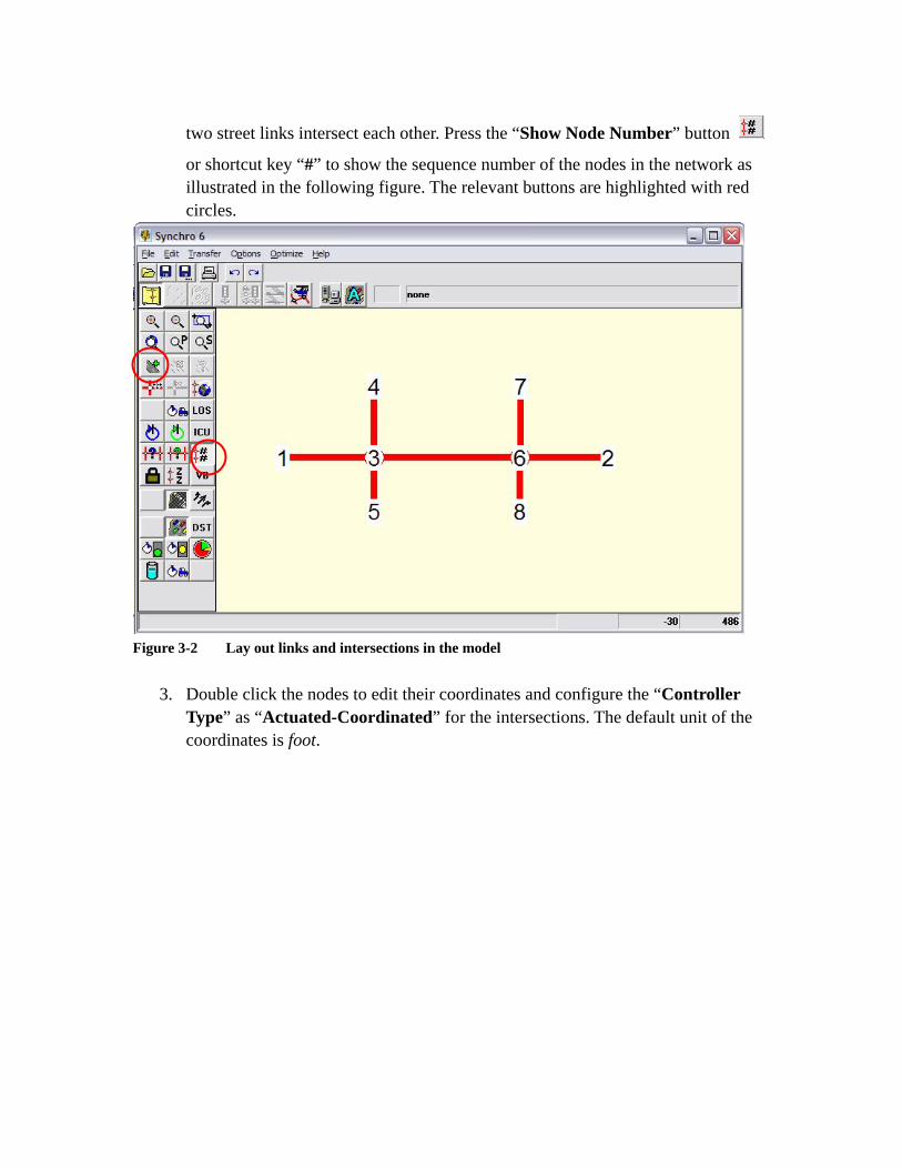
- 5 -

two street links intersect each other. Press the “Show Node Number” button

or shortcut key “#” to show the sequence number of the nodes in the network as illustrated in the following figure. The relevant buttons are highlighted with red circles.

Figure 3-2 Lay out links and intersections in the model

3. Double click the nodes to edit their coordinates and configure the “Controller Type” as “Actuated-Coordinated” for the intersections. The default unit of the coordinates is foot.

- 6 -

Figure 3-3 Edit intersection properties

4. Double click the links. Input the street names and link speed in the pop-up window.

- 7 -

Figure 3-4 Edit link settings

5. Select any intersection by clicking the middle of the node. Click the “Lane

Window” button below the menu (or press F3) to switch to the lane window and enter the geometry data. To switch back to the map window, press

F2 or click the “Map Button” to the left of the “Lane Window” button.

Figure 3-5 Switch between design windows

- 8 -

Figure 3-6 Lane window settings

6. Select the intersections and click the “Volume Window” button (or press F4 ) to switch to the volume window. Input the volume data for each lane group.

- 9 -

Figure 3-7 Volume window settings

7. Select any intersection and input the signal timing settings in the timing tab by

clicking the “Timing Window” button (or press F5). Click the “Options” button on the left and “Set to the East-West Template Phase” to use the template in which the eastbound and westbound movements are coordinated. The turning types are also configured in this window. In addition, the ring structure of the signal is shown at the bottom of this window.

- 10 -

Figure 3-8 Timing window settings

8. Switch to the “Phasing Window” by using the button or shortcut F6 . Numerous important signal timing parameters can be set in this window, such as the minimum and maximum splits, yellow and all-red intervals, and recall modes.

- 11 -

Figure 3-9 Phasing window settings

9. Click the menu command “Optimize/Intersection Cycle Length” and

“Optimize/Intersection Splits” for each intersection.

- 12 -

Figure 3-10 Optimize intersection timings

10. Use the menu command “Optimize/Network Cycle Lengths” to optimize the Network Cycle Length. Configure the Network Cycle Length Optimization settings and click the “Manual” button to instruct Synchro to iterate through the possible cycle length and output the associated performance.

Figure 3-11 Optimize network signal cycle length

- 13 -

11. After the optimization finishes and the results are displayed in the pop-up window, review the summary of estimated performance and select the desired cycle length.

Figure 3-12 Select desirable solution

12. Use the “Optimize /Network Offsets” command to optimize the Network Offsets and configure the window as in Figure 3-13.

Figure 3-13 Optimize network offsets

- 14 -

13. Switch to the “Timing Window” to view the solution parameters and the expected split of each phase. In the “Phasing Window” there is a group of “Quick reports” buttons on the left side with which we can request quick reports of the calculated operations of the plan.

Figure 3-14 Review quick reports in phasing window

- 15 -

Figure 3-15 A sample quick report of “starts” of phases

14. Click the “SimTraffic Animation” button or use shortcut “CTRL+G” to start SimTraffic. SimTraffic will automatically replay the animation after the simulation is recorded.

- 16 -

Figure 3-16 Traffic animation in SimTraffic

15. For a detailed performance report, click the “Create Report” button or “CTRL+R”. Choose the concerned measures of effectiveness and click “Preview.” A report of the arterial can also be requested by checking the “Arterial Report” box.

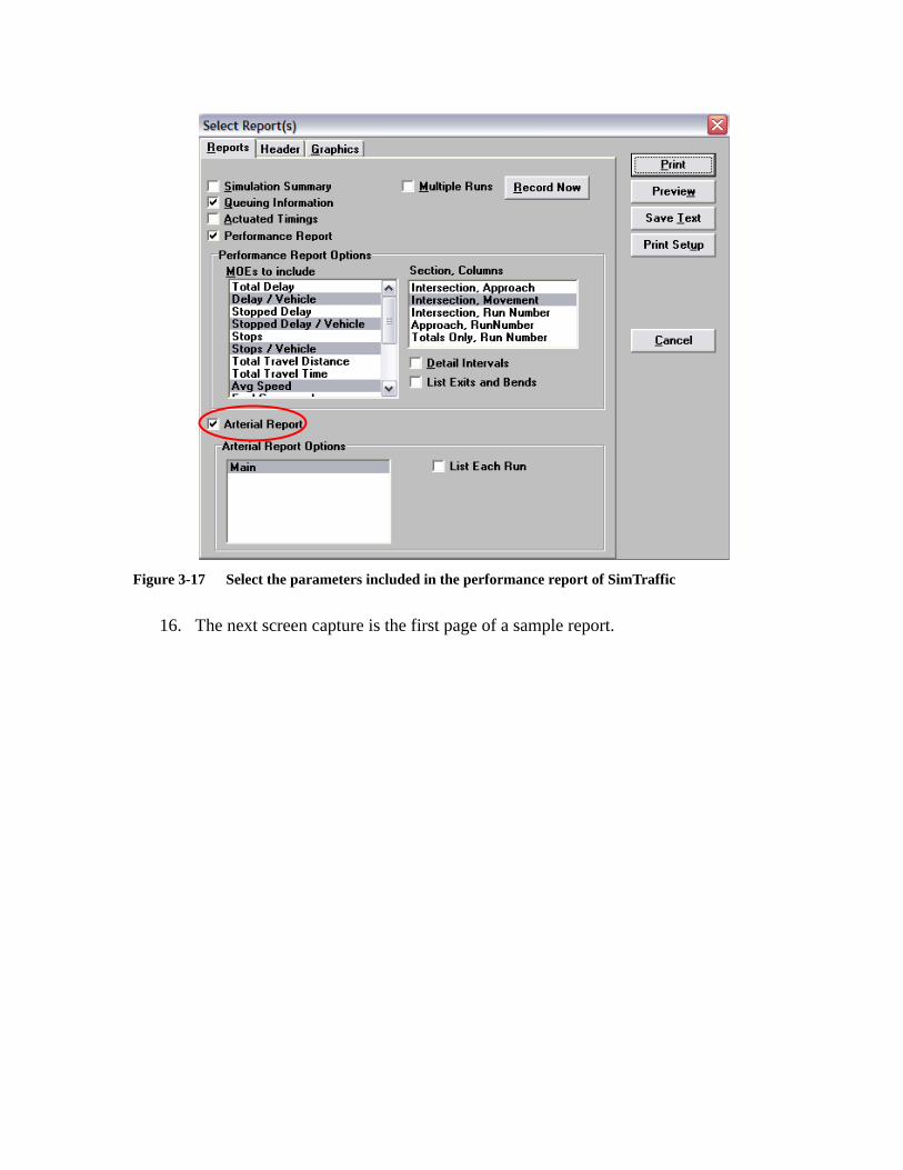
- 17 -

Figure 3-17 Select the parameters included in the performance report of SimTraffic

16. The next screen capture is the first page of a sample report.

- 18 -

Figure 3-18 A sample report of SimTraffic

- 19 -

3.2 Tools for Evaluating Signal Solutions

Synchro and SimTraffic provide several tools to examine the input and output values. In this section, the tools that are useful for identifying potential improvements of the obtained solution are briefly introduced. Familiarity with these tools is needed in Chapters 5 and 6, where problem identification techniques are discussed at length.

3.2.1 Synchro Control Indicators

Synchro reports performance measures such as V/C (volume-to-capacity ratio), LOS (level-of-service), delay, and travel time. Most of them can be displayed in the map window by toggling on corresponding function buttons located on the left panel. The following figure shows the V/C for each lane group and the intersection delays. This tool presents the important measures intuitively and quickly. Thus, it is often used as the first tool of problem identification.

Figure 3-19 V/C for all lane groups displayed in the map window In addition, Synchro provides special control indicators such as ICU, natural cycle length,

- 20 -

and the harmony of the factors. The definitions of these measures can be found in the on-line help manual of Synchro (Husch and Albeck. Copyright 1993-2004). INDOT traffic systems engineers usually consider these measures as supplementary and do not use them extensively.

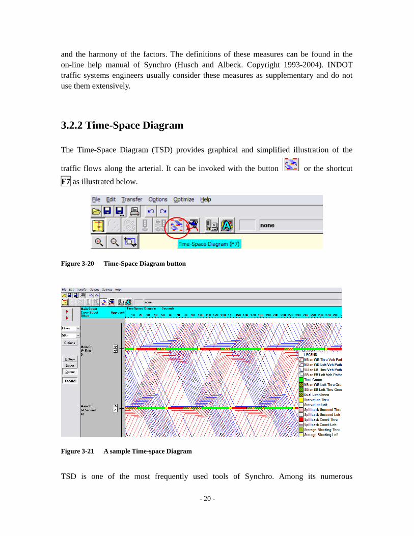
3.2.2 Time-Space Diagram

The Time-Space Diagram (TSD) provides graphical and simplified illustration of the

traffic flows along the arterial. It can be invoked with the button or the shortcut F7 as illustrated below.

Figure 3-20 Time-Space Diagram button

Figure 3-21 A sample Time-space Diagram

TSD is one of the most frequently used tools of Synchro. Among its numerous

- 21 -

capabilities, there is a unique function that displays the flow diagram under several traffic volume levels: 10th, 30th, 50th, 70th, and 90th percentiles. It is a major tool for identifying poor offsets and the so-called “early-return-to-green” problems in the design stage. In the solution implementation stage, the TSD is sometimes used in test runs along the arterial to assure the offsets are properly implemented in the signal controllers.

It should be noted that the early-return-to-green effect is strongest when different intersections experience different volume levels, which frequently happens in the real world. Synchro assumes that the selected level of volume occurs simultaneously at all the intersections. This simplification may mask the early-return-to-green issue and may result in an overly optimistic estimation of the arterial street performance. Please refer to Sections 5.4, 6.3, and 7.4 for further discussion of the early-return-to-green issue.

The readily comprehendible graphics and the ease of tuning the offsets in the TSD encourage offsets adjustments. It should be recognized, however, that adjusting the offsets in the TSD may lead to inferior solutions. The TSD shows deterministic traffic trajectories under typical situations. Although it is often attainable to “outdo” the optimizer by manual adjustment, the overall performance improvement, if any, is generally not guaranteed under varying traffic conditions. Therefore, if the signal offsets are unacceptable from the perception-based point of view and manual adjustment is inevitable, recording the performance measures before and after the tuning is recommended.

3.2.3 Quick Report

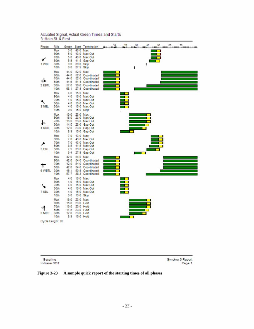
In the phase window, there is a set of “Quick Reports” buttons. Brief graphical reports of the operations of actuated signals can be requested through this tool, including the green times, starting times, and details of the phases. Although all such information is included in Synchro reports, the Quick Reports are handy and their graphical format enables discerning problems easily. A sample quick report of the starting times of the phases is shown in Figure 3-23.

- 22 -

Figure 3-22 Location of the quick report buttons

- 23 -

Figure 3-23 A sample quick report of the starting times of all phases

- 24 -

3.2.4 Signal Plan Output

The key parameters of a signal plan (i.e., ring structure, cycle length, offset, and splits) are presented in the timing window as shown below. Sometimes, a problem can be identified in this window with certain calculations.

Figure 3-24 Signal plan parameters in timing window

3.2.5 SimTraffic Static Graphics Tool

The static graphics tool is a set of convenient tools of SimTraffic to check various aspects of system performance. It can be invoked by choosing the menu command “Graphics/Show Static Graphics.” Various performance measures, such as delay, speed, and stops, can be clearly displayed on top of the intersection layout. The following examples of Figure 3-25 and Figure 3-26 are the delay/vehicle static graph and the speed static graph. In Figure 3-25, the simulated levels of delay/vehicle are displayed for

- 25 -

intersection 6. Different levels are differentiated by different grayscales (on the computer screen, by different colors). It is obvious that the northbound left-turn traffic and the southbound through traffic experience the longest delays. In the second example (Figure 3-26), the average running speeds of all vehicles on the road segments are displayed.

Figure 3-25 Static graph of delay/vehicle

- 26 -

Figure 3-26 Static graph of speeds

3.2.6 SimTraffic Animation

SimTraffic animation is probably the most intuitive way of presenting the simulation results. It replicates the dynamic operations of the analyzed arterial road. Without this tool, some solution deficiencies would be difficult, if not impossible, to identify. INDOT engineers use animation to inspect various issues of coordination, including platoon progression, offset adjustments, left-turn problems, capacity problems, lane blockage by queues, and back-to-back stops. The capabilities to monitor the signal status at the intersection and the operational status of individual vehicles are worth mentioning. By clicking in the middle of an intersection, the signal status window is invoked. Similarly, the vehicle status window will be brought up by clicking a vehicle. The explanation of the status windows can be found in the on-line help file of SimTraffic under the topic “SimTraffic Operations/Signal Status” and the topic “SimTraffic Operations/Vehicle Status.” In the example below, the status of the intersection and the status of two vehicles are shown in the floating windows on the right.

- 27 -

Figure 3-27 Monitor intersection and vehicle status during simulation Another useful feature of SimTraffic is the playback control. The user can play the animation at 0.5, 1, 2, 4, or 8 times the actual speed forward and backward. A frame-by-frame play option is also available. Although playback control itself is not a direct tool for problem identification, many techniques become easier due to this feature. It is highly recommended that the user become acquainted with this feature. The details of this feature are explained in the on-line help of SimTraffic under the topic “SimTraffic Operations/SimTraffic Operations/Recording and Playback.”

Figure 3-28 Playback control of animation

3.3 Advanced Issues of the Simulation

As a micro-simulation tool, SimTraffic reasonably replicates the operations of traffic signal systems. Not surprisingly, the inherent issues of simulation tools can also be found in SimTraffic. One of the unavoidable characteristics is the quasi-stochastic nature of the

- 28 -

simulation results. Unlike the analytical model (Synchro), SimTraffic will produce different results given the same signal plan and demand level – a situation found in the real world. This fluctuation of the results makes comparing alternative solutions more difficult. For example, if the total delay is 1,200 minutes under signal plan 1, and 1,250 minutes under signal plan 2, there is no guarantee that signal plan 1 is better than signal plan 2. It is possible that an opposite result will be obtained in the second run. The seeming superiority of a plan may be attributed to pure randomness rather than systematic advantage. The following sections are intended to assist with correct conclusions based on the simulation results.

3.3.1 Random Number Seed of Simulation

To emulate the random fluctuations of traffic, the simulation software employs a sequence of “pseudo random numbers” that mimics a random variable. These pseudo random numbers are then used to introduce “randomness” to traffic. Generation of these pseudo numbers is initiated with a random number seed. Two sequences of pseudo random numbers are identical if the corresponding pseudo random seeds are identical. Thus, identical user input values and random number seeds in multiple simulation executions generate identical simulation results. The random number seed can be entered through “Options/ Intervals and Volumes” as shown in Figure 3-29.

- 29 -

Figure 3-29 Random Number Seed Configuration

Performance of different signal control scenarios is easier to compare when the same random seed number is used. By default, the random number seed is set as “1.” The engineer can readily change this to other numbers to generate a new sequence of traffic fluctuations.

Random number seed zero (0) is a special case. SimTraffic will use different random number seeds in different simulation executions when the seed is set to 0. This feature is useful when the engineer wants to examine the performance of a scenario under different fluctuation patterns and does not want to change the seed manually in each simulation execution.

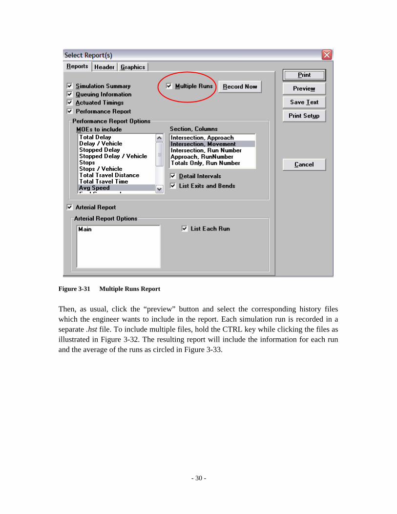
3.3.2 Multiple Simulation Runs

One run of SimTraffic represents only one traffic realization out of numerous possibilities and therefore does not realistically reflect the average performance. It is advised to perform at least five simulation runs and average the MOEs obtained in these runs.

Multiple runs can be set in the menu command “Animate/Record Multiple Runs”. The number of runs and the random seed number for the first simulation run can be set in the pop-up window as in Figure 3-30. This seed will initiate a sequence of pseudo random numbers long enough for all the simulation runs. It is equivalent to using different seeds in different simulation runs. SimTraffic will start recording when “OK” is clicked.

Figure 3-30 Multiple Runs Configuration To include the results of multiple runs in the report, the “multiple runs” option (circled in Figure 3-31) must be checked in the report setting window pops up when “create report” button is clicked.

- 30 -

Figure 3-31 Multiple Runs Report Then, as usual, click the “preview” button and select the corresponding history files which the engineer wants to include in the report. Each simulation run is recorded in a separate .hst file. To include multiple files, hold the CTRL key while clicking the files as illustrated in Figure 3-32. The resulting report will include the information for each run and the average of the runs as circled in Figure 3-33.

- 31 -

Figure 3-32 Select multiple simulation result files

- 32 -

Figure 3-33 Reports of multiple runs Each of the multiple simulation runs begins with an empty road. SimTraffic loads the road with vehicles before the simulation results are recorded. If the traffic demand exceeds the capacity, then the queue of vehicles grows during the simulated period. The initial queue in each simulation run does not reflect what happened in the previous simulation run. The average performance over five simulation runs, for example, reflects the traffic situation observed over five similar days (e.g., five weekdays) and during the same time of day. On the other hand, simulating a signalized street for a five times longer period with the intention to substitute the five simulation runs with a single run produces longer queues than in the real-world. It may lead to grossly overestimated delays and numbers of stops.

- 33 -

3.3.3 Simulation of Multiple Intervals

SimTraffic also has the capability to simulate multiple time intervals with varying traffic volumes in a single simulation run. The settings can be accessed through the menu command “Options/Intervals and Volumes.” The volume adjustment methods are discussed under the topic “Advanced Parameters/Intervals and Volume Adjustments.” One of the methods is to record four 15-minute intervals and apply “PHF Adjust” to one interval and “Anti PHF Adjust” to the other three intervals (AlbeckGerkenInc 2006) The settings are illustrated below.

Figure 3-34 Simulation of multiple intervals For example, if the hourly volume is 1,000 vph and the PHF factor is 0.9. Then the vehicle count in the peak 15 minutes is

1 1000 2784 0.9

veh× ≈

- 34 -

The vehicle counts in the other three intervals where the “Anti PHF Adjust” is applied, the volume is

1 (1000 278) 2413

veh× − ≈ .

In contrast, if no adjustment is applied, then each interval has the vehicle count of

1 1000 2504

veh× = .

The volume can also be adjusted by using the “Percentile Adjust” settings or the “Growth Factor Adjust.” The “Percentile Adjust” entry is used to adjust traffic based on its statistical properties. For example, if the engineer wants to examine the performance of the system under a 95th percentile traffic volume level (95% of the time traffic demand will be lower or equal), then the engineer can do so by selecting “Yes” in the “Percentile Adjust” entry of the corresponding interval and input 95 in the cell below. In Figure 3-34, the last interval is adjusted to 50th percentile traffic, which is the median traffic level. The “Growth Factor Adjust” uses the growth factor input in Synchro’s volume window and simply times the traffic by this factor.

- 35 -

4 Local Values of Traffic Parameters

As a powerful micro-simulation tool, SimTraffic is capable of providing realistic replication of arterial operations. However, the accuracy of the simulation depends heavily on the proper selection of the key traffic parameters, especially speed and saturation flow rates. Speed strongly affects the time when vehicles arrive at downstream intersections, and an incorrect speed thus may necessitate adjusting some of the signal offsets after they are implemented in the field. The saturation flow rate strongly affects the queue discharge time. Too large saturation flow rates used in the design stage may hide the capacity shortage, which is revealed after the signals are implemented. This deficiency typically calls for adjusting the signal splits. For all the above reasons, calibration of speeds and saturated time headways (inverse of saturation flow rate) are strongly recommended. In the help manual of SimTraffic, the calibration is discussed under the topic “Advanced Parameters/Calibrate Speeds and Headways.”

4.1 Saturation Flow Rate in Synchro

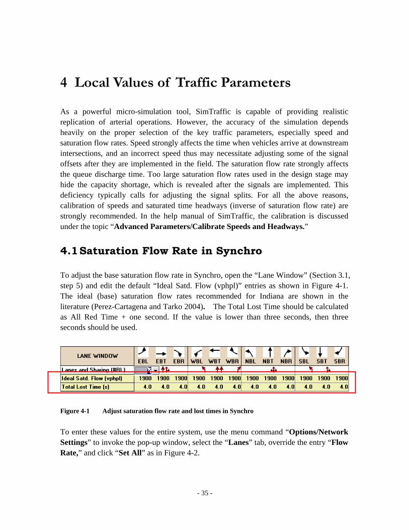
To adjust the base saturation flow rate in Synchro, open the “Lane Window” (Section 3.1, step 5) and edit the default “Ideal Satd. Flow (vphpl)” entries as shown in Figure 4-1. The ideal (base) saturation flow rates recommended for Indiana are shown in the literature (Perez-Cartagena and Tarko 2004). The Total Lost Time should be calculated as All Red Time + one second. If the value is lower than three seconds, then three seconds should be used.

Figure 4-1 Adjust saturation flow rate and lost times in Synchro To enter these values for the entire system, use the menu command “Options/Network Settings” to invoke the pop-up window, select the “Lanes” tab, override the entry “Flow Rate,” and click “Set All” as in Figure 4-2.

- 36 -

Table 4-1 Recommended base saturation flow rates for Indiana (Perez-Cartagena and Tarko

2004)

Figure 4-2 Adjust the saturation flow rate for the entire network

However, it should be clarified that the Ideal Saturation Flow Rate setting in the Lane Window of Synchro only affects the calculations in Synchro and has no impact on the flow simulation in SimTraffic.

- 37 -

4.2 Saturation Flow Rate in SimTraffic

According to the help manual of SimTraffic, there is no method of controlling the saturation flow rate precisely. The only means is to change the so-called “headway factors” for all links in Synchro. For example, in the system below, to increase the saturation flow rate simulated in SimTraffic, the headway factors of the external link “1-3”, “3-4”, “3-5”, “6-7”, “6-8”, and “6-2” first must be replaced by a value smaller than 1.

Figure 4-3 Adjust headway factors of external links Second, the headway factors of the internal movements must be overridden accordingly in the lane window of the intersections, as illustrated below.

Figure 4-4 Adjust headway factors for internal movements The simulated saturation rate also depends on the link speed. The following Figure 4-5 summarizes the experimental results of the effects of headway factor adjustment on the simulated saturated flow rate with different link speeds. This figure can be used as a guide to help approximate the desired saturation flow rates in SimTraffic. The recommended saturation flow rates for Indiana can be found in (Perez-Cartagena and

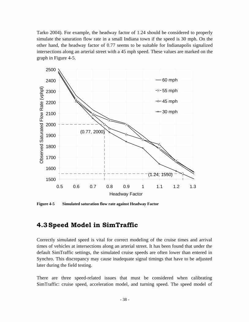
- 38 -

Tarko 2004). For example, the headway factor of 1.24 should be considered to properly simulate the saturation flow rate in a small Indiana town if the speed is 30 mph. On the other hand, the headway factor of 0.77 seems to be suitable for Indianapolis signalized intersections along an arterial street with a 45 mph speed. These values are marked on the graph in Figure 4-5.

(0.77, 2000)

(1.24, 1550)1500

1600

1700

1800

1900

2000

2100

2200

2300

2400

2500

0.5 0.6 0.7 0.8 0.9 1 1.1 1.2 1.3Headway Factor

Obs

erve

d Sa

tura

ted

Flow

Rat

e (v

phpl

)

60 mph

55 mph

45 mph

30 mph

Figure 4-5 Simulated saturation flow rate against Headway Factor

4.3 Speed Model in SimTraffic

Correctly simulated speed is vital for correct modeling of the cruise times and arrival times of vehicles at intersections along an arterial street. It has been found that under the default SimTraffic settings, the simulated cruise speeds are often lower than entered in Synchro. This discrepancy may cause inadequate signal timings that have to be adjusted later during the field testing. There are three speed-related issues that must be considered when calibrating SimTraffic: cruise speed, acceleration model, and turning speed. The speed model of

- 39 -

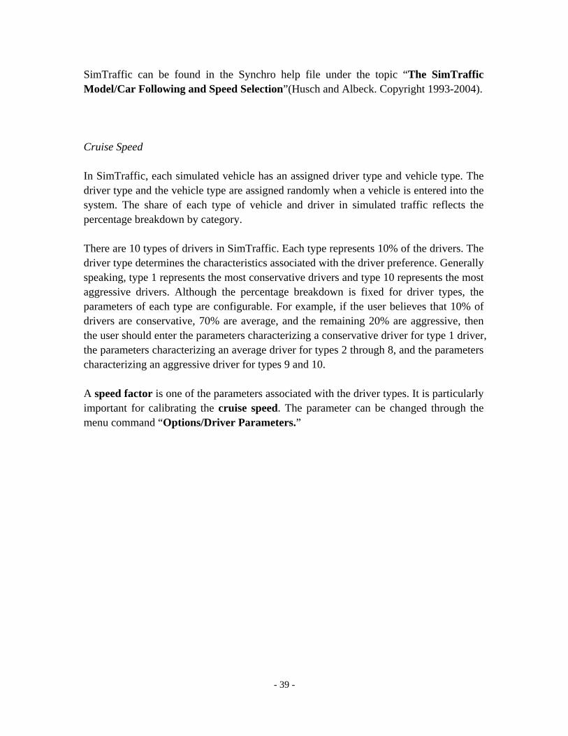
SimTraffic can be found in the Synchro help file under the topic “The SimTraffic Model/Car Following and Speed Selection”(Husch and Albeck. Copyright 1993-2004). Cruise Speed In SimTraffic, each simulated vehicle has an assigned driver type and vehicle type. The driver type and the vehicle type are assigned randomly when a vehicle is entered into the system. The share of each type of vehicle and driver in simulated traffic reflects the percentage breakdown by category. There are 10 types of drivers in SimTraffic. Each type represents 10% of the drivers. The driver type determines the characteristics associated with the driver preference. Generally speaking, type 1 represents the most conservative drivers and type 10 represents the most aggressive drivers. Although the percentage breakdown is fixed for driver types, the parameters of each type are configurable. For example, if the user believes that 10% of drivers are conservative, 70% are average, and the remaining 20% are aggressive, then the user should enter the parameters characterizing a conservative driver for type 1 driver, the parameters characterizing an average driver for types 2 through 8, and the parameters characterizing an aggressive driver for types 9 and 10. A speed factor is one of the parameters associated with the driver types. It is particularly important for calibrating the cruise speed. The parameter can be changed through the menu command “Options/Driver Parameters.”

- 40 -

Figure 4-6 Adjust speed factors in SimTraffic

The cruise speed, as described in the manual, is defined as the preferred speed of drivers when no impediment exists. It has to be noted that the definition provided by the Synchro manual applies to the speed frequently called “free-flow speed.” We will follow the terminology of Synchro to avoid confusion among users already familiar with the Synchro terminology. The cruise speed is calculated as:

Cruise Speed Speed Factor Link Speed= ×

If the traffic systems engineer believes that there are discrepancies between the actual and simulated average speeds between intersections, then the speed factors should be adjusted to better approximate reality. For example, if the link speed (design speed or speed limit) entered in Synchro is 30 mph and seems to be too low, then changing the speed factor in SimTraffic to higher than 1, say 1.2, will modify the cruise speed as follows:

1.2 30 36 mphCruise Speed = × = .

- 41 -

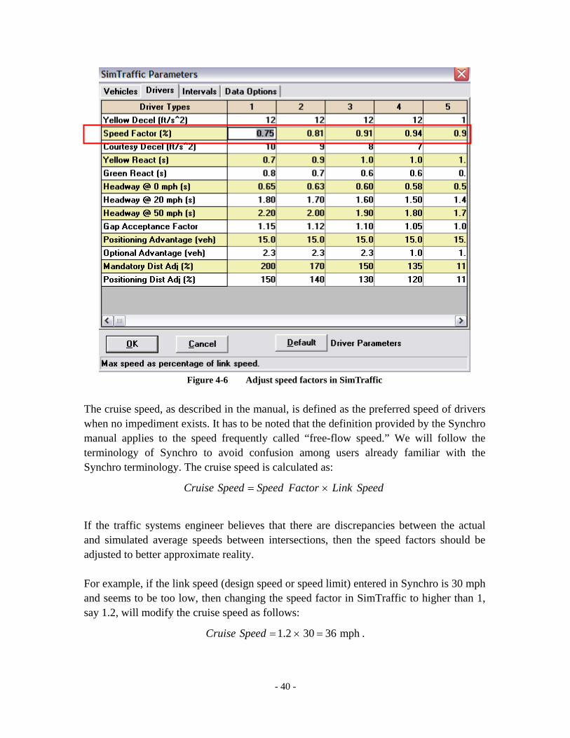
Acceleration Model The parameters characterizing the vehicle types are also configurable to reduce the number of types and to override the standard 10% shares. The parameters can be accessed through the menu command “Options/Vehicle Parameters.” The important parameters of each vehicle type can also be changed in the window (Figure 4-7).

Figure 4-7 Vehicle Parameters Window There are two important vehicle characteristics affecting the vehicle speed: maximum speed and acceleration model. The maximum speed is the speed reachable by the vehicle. On the other hand, a driver accelerates only to the cruise speed. Second, the acceleration model determines the vehicle’s speed profile with time if continued acceleration is possible. According to the help manual, a vehicle increases speed at a declining acceleration rate. This rate reaches zero at the maximum speed. An analytical formula is obtained based on the description of the help manual. If a vehicle begins to accelerate from stop when no obstruction is ahead, then the speed at time t is

- 42 -

maxmax

max

( ) [1 exp( )]av t v tv

= - - × .

where maxa is the maximum acceleration rate at the beginning of acceleration and maxv

is the maximum speed. These two parameters can be accessed through the menu command “Options/Vehicle Parameters.” It follows that the time needed to accelerate to v from 0 is:

max

max max

ln(1 )v vta v

= - -

As illustrated in the following figure, the default maximum speed for the Car1 type is 75 mph and the default maximum acceleration rate is 10 ft/s2. Please notice that their units are not compatible. Proper conversions must be performed before using this formula.

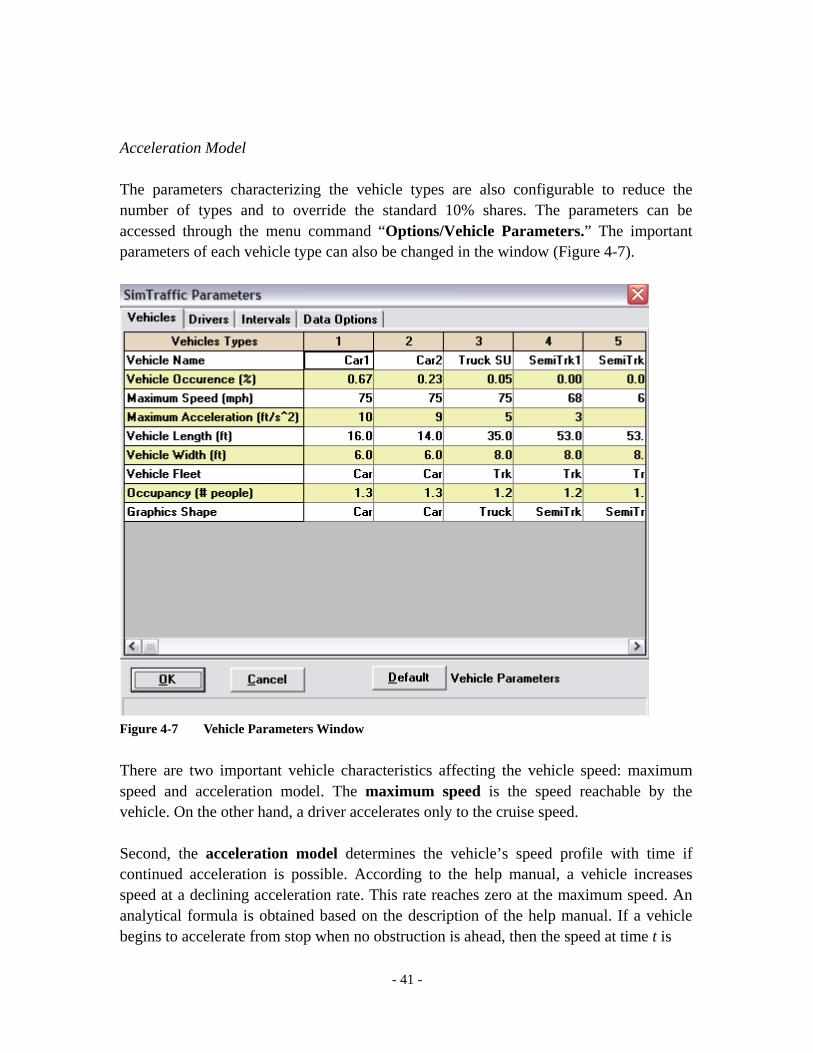
Figure 4-8 Vehicles types parameters The effect of changing the maximum acceleration rate is illustrated in Figure 4-9. This figure can be used as guidance for selecting the maximum acceleration rate. For example, if a typical passenger car needs 17 seconds to accelerate to the speed of 40 mph from a stop, then the maximum acceleration rate should be set as 5 ft/s2. The acceleration time and speed are only for illustration purposes and may not reflect the actual situation.

- 43 -

(17, 40)

(30, 8)

0

10

20

30

40

50

60

70

80

0 10 20 30 40 50 60 70Time (sec)

Spe

ed (m

ph)

amax = 15 ft/s2

amax = 5 ft/s2

amax = 3 ft/s2

amax = 7 ft/s2

amax = 10 ft/s2

Figure 4-9 Acceleration curves of different max speeds The traffic engineer can also select the proper acceleration rate by backward calculation. For example, if it is determined that the typical time needed to accelerate from 0 to 30

mph is eight seconds, then plug 30 , 8 secv mph t= = into the following formula:

max 2max

max

5280 5280 75 30ln(1 ) ln(1 ) 7 ft / s3600 3600 8 75

v vat v

= - × - = - × × - = .

It is determined that the maximum acceleration rate should be set as 7 ft/s2. Once more, the unit compatibility should be scrutinized. In traffic simulation with SimTraffic, a default turning speed of 15 mph is assumed for left-turning vehicles and nine mph for right-turning vehicles. According to the Synchro help manual “Advanced Parameters/Calibrate Speeds and Headways,” the saturation flow rate is highly sensitive to speed when speed is low. Increasing the right turn speed from nine mph to 10 mph increases the saturation flow rate from 1,542 to 1,617 vph. The use of adequate turning speeds is important for correct capacity modeling of turning traffic streams in SimTraffic.

- 44 -

5 Identifying Solution Deficiency with

Synchro

Applying the basic design procedure, a traffic systems engineer can obtain an initial signal plan in a relatively short time. This initial plan, however, should be evaluated from the point of view of good coordination conditions and modified if needed. As mentioned earlier, the optimization algorithms and objectives are oriented towards the global assessment of mobility in the optimized system. They do not address some of the operational aspects important to the drivers and to their perception of the coordination quality. As introduced in Section 3.2, Synchro provides many evaluation tools including Traffic Control Indicators, Quick Report, and Time-Space Diagram. To identify the problem, it is often needed to cross-reference the results of these tools. In the following parts of this chapter, identification techniques of possible coordination issues with Synchro are discussed.

5.1 Insufficient Capacity Reserve

Synchro sometimes generates a solution with insufficient capacity reserves for some signal phases that serve arterial flows. Although the system works reasonably fine under the 50th percentile volume, its performance drops dramatically under elevated volume levels. Another possible consequence is the loss of flexibility of the actuated control. When the capacity reserve is insufficient, each phase is forced to extend until its force-off points under elevated volume levels. The actuated signal becomes de facto pre-timed. There are several ways to identify this problem. First, quickly estimate the capacity reserves with the V/C ratio indicators. The V/C ratio of each movement can be requested to display in the Synchro “Map Window” as shown in Figure 5-1.

- 45 -

Figure 5-1 V/C indicator in Synchro It is not difficult to determine if the capacity reserves are sufficient for the system. The V/C ratios for the coordinated eastbound and westbound through phases at the left intersection are higher than 0.9. These high ratios, calculated under the assumption of deterministic 50th percentile volumes, indicate frequent cycles when higher than average traffic overflows the intersection approaches. This will cause multiple stops of the same arterial vehicles at the same intersection. The second method is to check the back-of-queue of the movements under different levels of traffic demand. In the “Timing Window” some performance indices of the signal plan can be reviewed, such as the delays, stops, and queues. Among them, capacity sufficiency is reflected by the “Queue Length” indicators. The values shown in the window are the maximum back-of-queue in a cycle with the corresponding traffic volumes. These results, however, can be misleading when the flow capacity can satisfy the demand. Theoretically speaking, the queue will grow infinitely if the demand remains when capacity is insufficient. Synchro gives warning footnotes beside the back-of-queue outputs. There are three footnotes: “~”, “#”, and “m”. The “~” and “#” footnotes indicate that the traffic volume is above flow capacity under the 50th or 95th percentile volumes, respectively. The “m” footnote indicates that the 95th percentile volume is metered by the upstream signal (Husch and Albeck. Copyright 1993-2004). Although these warning footnotes are intended to warn the underestimation of queue length, the traffic engineer may consider them as signals of potential capacity shortage.

- 46 -

Figure 5-2 Queue length indicator in Synchro The third tool is the Time-Space Diagram (TSD). In the TSD window, enable the “Super” option to relax the assumption that the queue is cleared at the beginning of the phases. Choose the “Flows” diagram and try the scenarios at different percentiles of traffic levels. It is found that the queue of the westbound movement at the “Main at First” intersection keeps growing even at the 50th percentile traffic level. This clearly violates the first criterion of INDOT’s coordination. In contrast, in the second scenario where the capacity reserves are sufficient, the queue can be cleared even at the 90th percentile traffic level.

- 47 -

Figure 5-3 TSD when capacity is insufficient

Figure 5-4 TSD when capacity is enough

- 48 -

In practice, it is advised to first identify the problematic movements by checking the V/C ratios. Then, use the “Queue Length” and “Time Space Diagram” to further examine the vehicle queues under varied traffic volume levels. It should be noted that these results might not reflect reality very closely due to simplifications in traffic representation in Synchro. In the next chapter, methods to diagnosis the insufficient capacity problem with SimTraffic will be introduced.

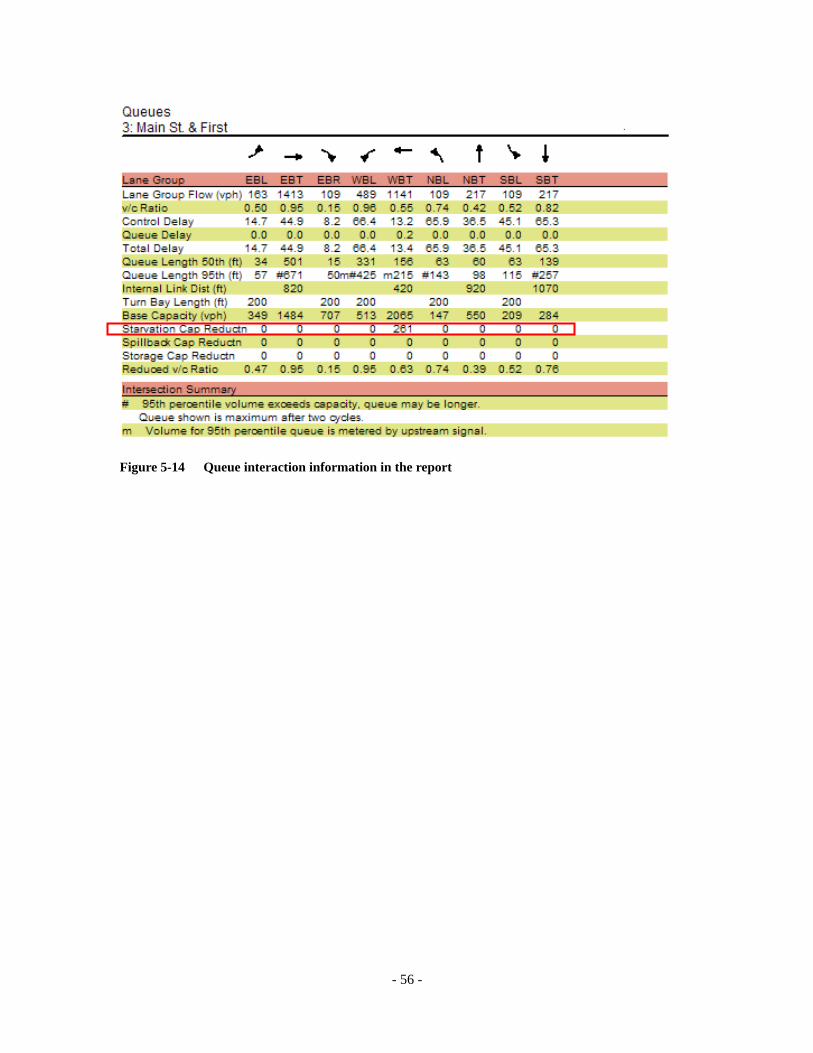
5.2 Lane blockage by adjacent traffic queues

According to INDOT’s criteria for good coordination, queue blockage of adjacent traffic is one of the serious problems that traffic systems engineers try to avoid. For example, if the left turn traffic does not get enough green time, the queue will build up in the turning bay and block the through traffic if the back-of-queue exceed the length of the storage.

In Synchro, this problem can be diagnosed by examining the queue report of each intersection. First, select the menu command “File/Create Report”; second, select the “Int: Queues” report as below; and third, click “Preview” to read the report.

Figure 5-5 Request queue related report To diagnose the queue blockage problem, the “Queue Length” and the “Turning Bay Length” should be compared. In the sample report below, all the turning bay lengths are 200 feet. However, the 50th percentile queue lengths of the “EBT” and “WBT” phases exceed this number, which indicates the eastbound and westbound through queue will

- 49 -

block the turning traffic in the corresponding approach. SimTraffic tends to provide a more reliable diagnosis of this problem thanks to its better traffic representation.

Figure 5-6 Sample queue report

5.3 Fixed-time Operation of an Actuated Phase

INDOT traffic systems engineers report problems with the Synchro-generated optimal signal splits. In the solution given by Synchro, sometimes certain phases (e.g., the left turn phase or the side street through phase) do not have much room for adjusting to current traffic volumes and they operate as pre-timed or near pre-timed.

A convenient diagnostic tool is the “Green Times” quick report under the “Phasing Window.” Part of a sample report is shown in the following figure. It is found that in this solution the length of phase 1 is fixed under all traffic levels, and the length of phases 3 and 7 are fixed except for the lowest 10th percentile traffic volume.

- 50 -

Figure 5-7 Sample quick report of actual green times Second, to further verify this observation, the phase timings and the force-off points of the solution should be examined. In the “Phasing Window,” it is found that for phases 1, 3, and 7,

Maximum Split Minimum Initials + Yellow + All-Red=

By definition (Husch and Albeck. Copyright 1993-2004), however, it is required that

Maximum Split Minimum Split Minimum Initials + Yellow + All-Red≥ ≥ .

It follows naturally that the actual length of the phase, bounded by the “maximum split” and the “minimum split,” can only equal a fixed value unless skipped.

Figure 5-8 Sample phasing parameters The signal plan output reveals a special case of this issue where some actuated phases become fixed. As in the following ring structure, when both coordinated phases 6 and 2 are set to “C-Max,” then the actual duration of the lagging left-turn phase 5 becomes fixed since it is bounded by two force-off points of the two coordinated phases. This is referred to as the “lag phase hold” and is discussed in the topic “Timing/Signing Window /Lead-Lag Phase” of the help manual of Synchro.

- 51 -

Figure 5-9 Ring structure with “lag phase hold” problem

5.4 Early-return-to-green

Early-return-to-green is caused by asynchronous fluctuations of the beginning of green of the coordination phases at adjacent intersections. If a coordinated phase returns to green early at the upstream intersection due to low traffic in the non-coordinated phases, then the arterial vehicles released at the beginning of green may arrive at the downstream intersection before the green signal starts there. For example, let us consider the fluctuation of the beginning of green in the coordinated eastbound traffic phase at the Main at First intersection shown in the “Quick Report” tool in the “Phasing Window” (Figure 5-10). The starting time of the eastbound phase at each traffic level can be easily checked with this tool. The coordinated phase starts earlier under the 30th volume percentile and much earlier under the 10th volume percentile. The latter case is caused by skipping the westbound left-turn phase. This situation causes the early-return-to-green problem shown in the time-space diagram in Figure 5-11.

- 52 -

Figure 5-10 Detect early-return-to-green problem with quick report of green starting time The Time Space Diagram (TSD) is a major tool to identify poor offsets and early-return-to-green problems under different volume levels. In the following TSD, the first several vehicles released during the lead period at the Main-First intersection hit the red and stop at the Main at Second intersection as seen in the diagram. In the higher volume scenarios, the westbound left-turn phase is not skipped and the arterial traffic released from the Main-First intersection later arrives at the beginning of a green signal at the Main-Second intersection. The early-return-to-green problem is particularly evident when low volumes at the upstream intersection simultaneously occur with high volumes at the downstream intersection.

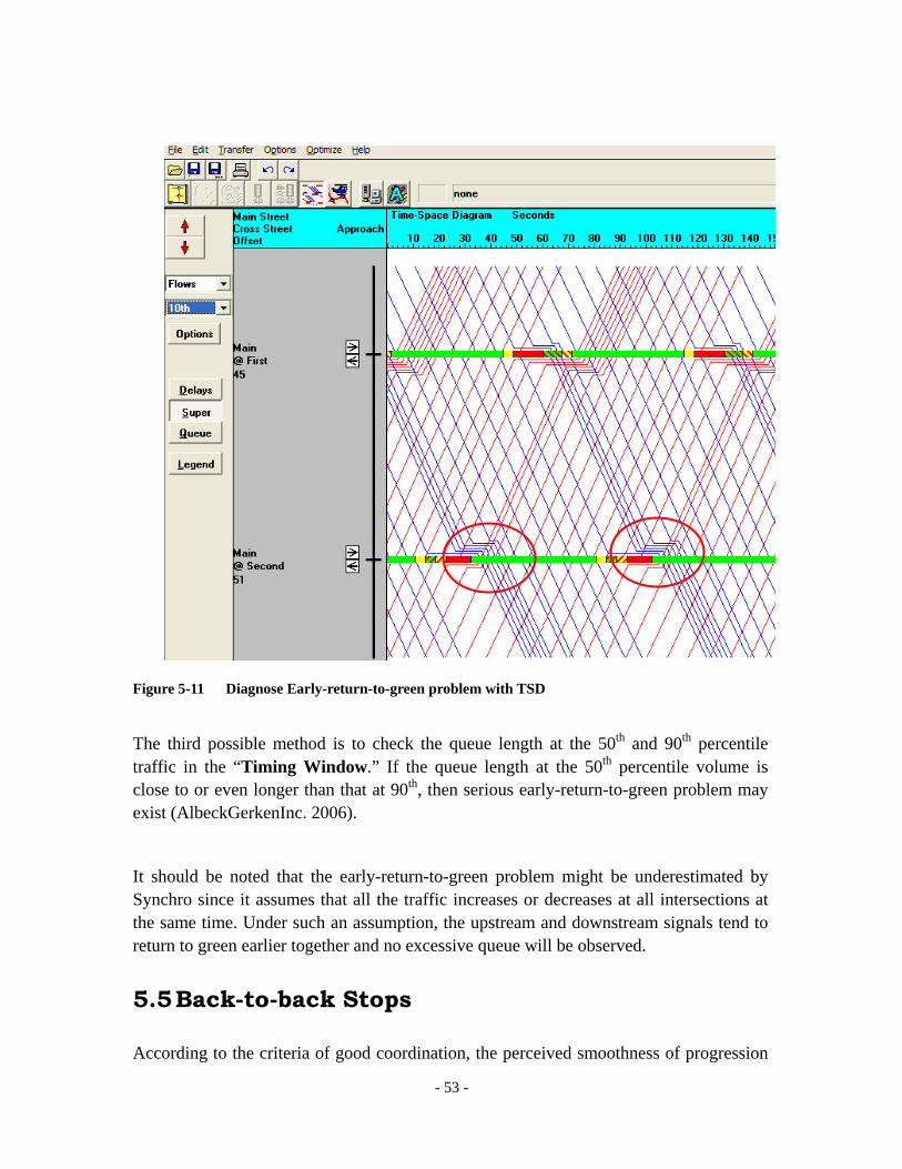
- 53 -

Figure 5-11 Diagnose Early-return-to-green problem with TSD

The third possible method is to check the queue length at the 50th and 90th percentile traffic in the “Timing Window.” If the queue length at the 50th percentile volume is close to or even longer than that at 90th, then serious early-return-to-green problem may exist (AlbeckGerkenInc. 2006).

It should be noted that the early-return-to-green problem might be underestimated by Synchro since it assumes that all the traffic increases or decreases at all intersections at the same time. Under such an assumption, the upstream and downstream signals tend to return to green earlier together and no excessive queue will be observed.

5.5 Back-to-back Stops

According to the criteria of good coordination, the perceived smoothness of progression

- 54 -

along the arterial is considered a vital measure of performance. Back-to-back stops at adjacent intersections considerably lower the comfort level of drivers and thus back-to-back stops should be avoided in arterial signal design.

The TSD is the major tool to identify this problem in Synchro. In the following TSD, the eastbound traffic represented by the trajectories from left-top to right-bottom encounters this problem. As highlighted by the circles, part of the eastbound traffic released from the upstream intersections always has to stop again at the next downstream intersection. A trajectory of one of the vehicles experiencing the problem is also highlighted. In contrast, the westbound traffic, represented by the trajectories from the left-bottom to the right-top, is free of this problem. The traffic released from the queue at upstream intersections always hit the downstream green.

Figure 5-12 Detect back-to-back stop with TSD

5.6 Strong Turning Volumes

When two intersections are closely spaced and the turning traffic is strong, it is difficult

- 55 -

to obtain effective coordination plans with the standard procedures. Symptoms of this problem often include the queue spillback, demand or queue starvation (an empty lane group during green time at the downstream intersection while a red signal at the upstream intersection does not allow more traffic), and storage blocking. These issues are discussed in detail in the help manual of Synchro under the topic “Optimizations and Calculations/ Calculations/ Queue Interactions.” Synchro 6 has added several methods to detect these problems. The TSD can show the time where queue interactions happen; the “Coding Error Check” command under the menu item “Options” includes the queue interaction errors lookup; and the queue report also include entries of these problems. To request the queue report, select the report options as follows and click “Preview.”

Figure 5-13 Request report of queue interactions A sample queue report is shown in Figure 5-14. It is found that the queue starvation problem exists for the WBT traffic in this intersection.

- 56 -

Figure 5-14 Queue interaction information in the report

- 57 -

6 Identifying Solution Deficiency with

SimTraffic


The capacity reserve at an elevated traffic level can be checked in SimTraffic with the static graphics tool together with the percentile volume adjustment technique described in Section 3.3.3. To identify problematic movements, adjust the volume to a higher percentile and inspect the static graphics of the queues and delays. A dramatic deterioration of performance indicates insufficient capacity reserve. For example, Figure 6-2 shows that under the 50th percentile volume none of the through movements along Main Street experience a delay longer than 15 seconds. In contrast, Figure 6-3 indicates a number of through movements that experience considerable delay, even exceeding 60 seconds, when the traffic volume reaches the 75th percentile. It should be noted that this method may overestimate the capacity shortage since it is rare that all the volumes surge simultaneously.

An alternative method is to perform multiple runs of simulation as introduced in Section 3.3. The user watches the animation to identify movements that experience long queues over extended periods. This method, although more time consuming than the first one, yields better results because traffic volumes vary in a more realistic way.

- 58 -

Figure 6-1 Static Graphics of delay/vehicle under 50th percentile traffic

Figure 6-2 Static Graphics of Delay under 75th percentile traffic

- 59 -

6.2 Lane blockage by adjacent traffic queues

In SimTraffic, the queue blockage problem can be readily identified using the static graphics tool. Request the static graph “% of Time Blocked,” and SimTraffic will show the blockage problem at the hot-spots. In the example below, the static graph shows that there are queue blockage problems with the eastbound through traffic and the westbound left-turn traffic. In the simulation, between %1~%5 of the two-minute periods experience maximum queues that are longer than the length of the turning bays.

Figure 6-3 Static graph indicating queue blockage problem The “Queue” static graph can be used to verify this observation. It shows the maximum, average, and the 95th percentile back-of-queue for each lane. It should be noted that the “max observed” back-of-queue and the “average” back-of-queue are determined from the simulated results while the “95th percentile” queue is estimated based on the mean and standard deviation. It may cause inconsistencies in the results; namely, the estimated “95th percentile” queue may be longer than the “maximum observed” queue. In the graph

- 60 -

below, it can be seen that all the average back-of-queues are much shorter than the length of the turning bays and the maximum observed back-of-queue of the EBT and WB LT almost reach the end of the corresponding turning bay. This is consistent with the results obtained by the previous “% of Time Blocked” graph.

Figure 6-4 Static graph of queue length

6.3 Early-Return-to-Green

It is relatively easy to detect the early-return-to-green problem with the initial hint from Synchro. In SimTraffic, the engineer invokes the status window of the “suspicious” intersections identified in Synchro and watches the animation. The problem is confirmed if under a lower traffic percentile, a platoon of vehicles often arrives at an intersection before the beginning of green. Multiple simulation intervals with varying levels of traffic can be watched with the “Options/Intervals and Volumes” feature described in Chapter 3.

- 61 -

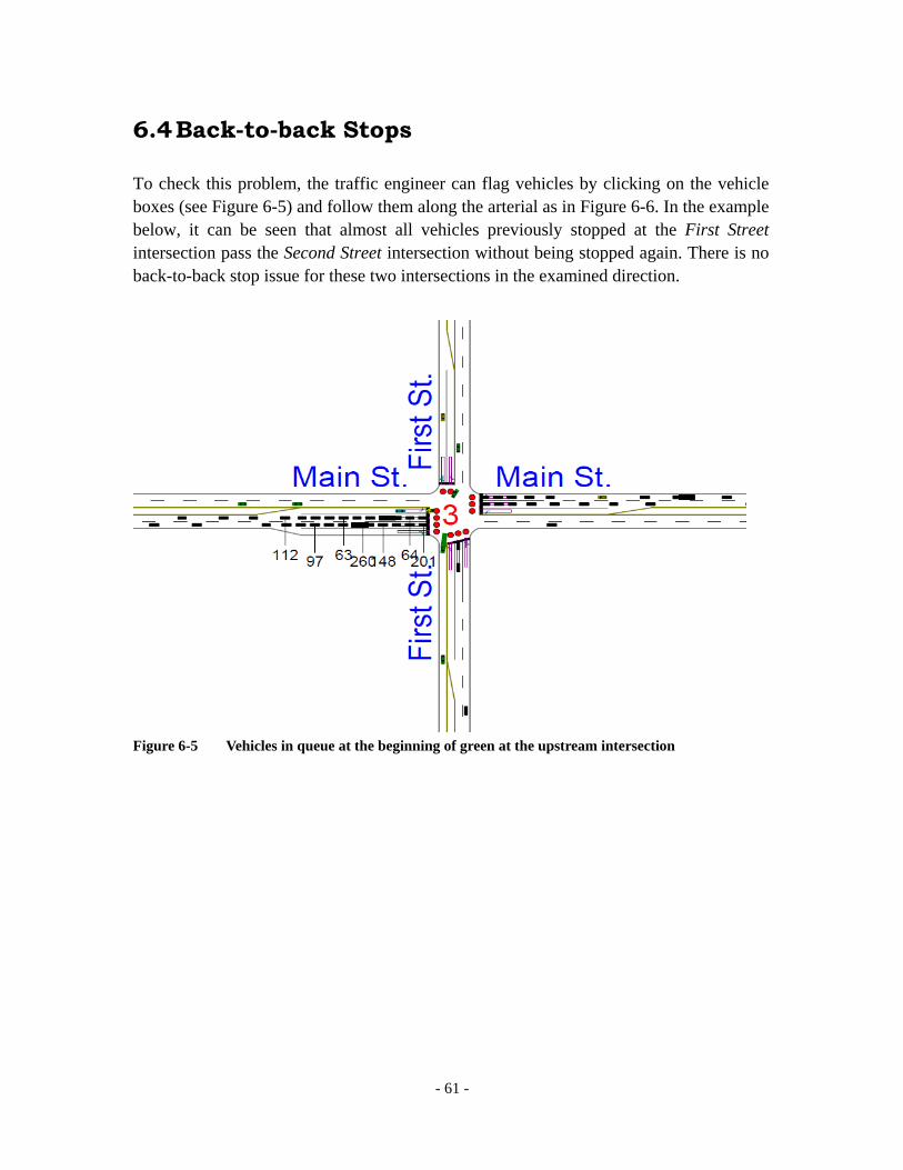
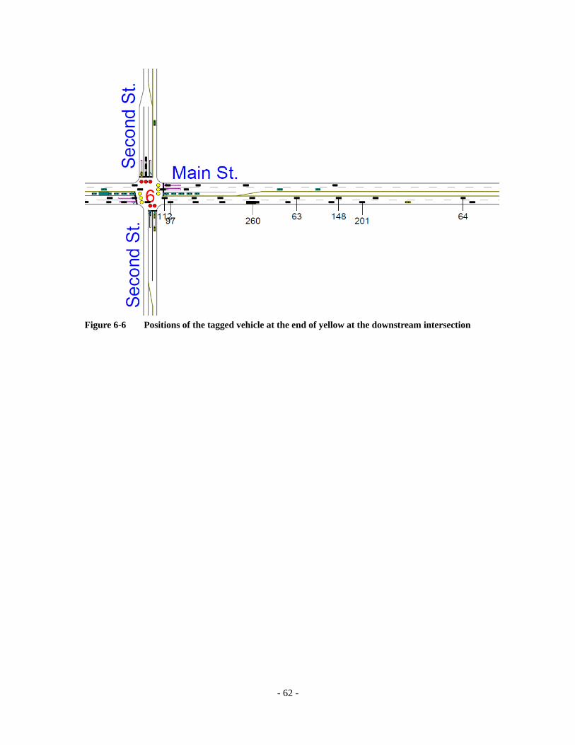
6.4 Back-to-back Stops

To check this problem, the traffic engineer can flag vehicles by clicking on the vehicle boxes (see Figure 6-5) and follow them along the arterial as in Figure 6-6. In the example below, it can be seen that almost all vehicles previously stopped at the First Street intersection pass the Second Street intersection without being stopped again. There is no back-to-back stop issue for these two intersections in the examined direction.

Figure 6-5 Vehicles in queue at the beginning of green at the upstream intersection

- 62 -

Figure 6-6 Positions of the tagged vehicle at the end of yellow at the downstream intersection

- 63 -

7 Remedies of Solution Deficiencies


According to INDOT traffic systems engineers, Synchro’s signal optimizer applied to arterial streets sometimes generates short cycle lengths that may lead to low capacity reserve at intersections and/or to fixed-time operation of signal phases. Insufficient capacity reserve on the limited number of side street approaches with low traffic volumes might be acceptable if it allows obtaining considerable improvement in coordination since the performance of the arterial signal system is mainly measured with the comfort level of the arterial drivers.

Insufficient capacity identified for at least one arterial traffic movement and/or for several side street movements requires attention. First, check the natural cycle length of all the intersections. The selected cycle length should be no less than the natural cycle length of any intersection in the system. Second, re-optimize the network cycle length and select the “Manual” option as described in step 10 of Section 3.1. Choosing a solution with a longer cycle length and near-optimal performance measures (as defined in Synchro) may lead to a better coordination plan. In addition, if it is found that the performance of the solution deteriorates considerably when the volume is slightly increased, then the volume should be increased with the growth factor and then let Synchro find the optimal solution for the increased volume. For example, if the growth factor is set as 1.1 for the EBT movement in the following window, then the corresponding volume will increase by 10%.

- 64 -

Figure 7-1 Growth factor adjustment in volume window

Another common practice is to modify the range of allowed cycle lengths to exclude unrealistic results. Manually selecting a longer cycle length can improve the capacity reserve and brings robustness to the signal plan. A typical minimum cycle used in Indiana is 70 seconds. More specifically, to determine the minimum cycle length of an arterial system, an engineer can determine the minimum cycle length which satisfies the minimum phase requirements and provides sufficient room for adjusting green signals to varying traffic. This cycle length is used as the lower bound when searching for the optimal cycle length in Synchro. It is reported that Synchro often points out this manually-determined lower bound of the cycle length as the optimal value. In this case, the traffic engineer is in fact selecting the cycle length according to his/her understanding of coordination optimality.

7.2 Queue blockage of adjacent traffic

If this issue is identified for some turning movements, check if the capacity is sufficient. If the capacity is insufficient, then protect the turning movement and/or increase the phase length. Improving progression of the movements with excessive queues blocking other movements may also help. If modifying the signal timing does not rectify the problem, then consider increasing the length of the turning bay or adding another lane to the turning bay. If blocking lanes is a serious safety and operational issue, then prohibiting the trouble movements may be the last-resort solution.

- 65 -

7.3 Fixed-time Operation of Actuated Phases

If this problem is identified, first check the ring structure. If the actuated phase operating as a fixed-time one is bounded by two force-off points of the coordinated phases, then configure the left-turn phase to be fixed leading as illustrated below in Figure 7-2. In doing so, the “lag phase hold” problem described in Section 5.3 is prevented. Furthermore, a leading left turn is preferred by INDOT since it avoids the safety problem of the “left turn yellow trap.” However, the great potential of delay reduction by using lead-lag optimization is lost.

Figure 7-2 Lead-lag configurations Second, this problem may be caused by capacity shortage. The suggestions in the previous Sections 7.1 and 7.2 may be helpful to resolve this issue. A longer cycle generally brings more capacity and allows more flexibility of the phase adjustments. However, the associated delay tends to increase with an unnecessarily long cycle length.

Third, set the recall mode of the phase to be “None.” This will prompt the corresponding phase to be skipped when there is no vehicle present and brings extra flexibility. This method, however, may induce or elevate the problem of early-return-to-green.

Finally, it is also observed that when an intersection is significantly below capacity, the non-coordinated phases often receive an unnecessarily long green. Tightening up the non-coordinated phases with excessive capacity by enforcing shorter splits or avoiding min-recall, may help bring more flexibility to the coordinated phases.

- 66 -

7.4 Early-Return-to-Green

Early-return-to-green is caused by asynchronous fluctuations of the beginning of green of the coordination phases of adjacent signals. If the coordinated phase of an upstream intersection returns to green early while the downstream phase does not, then arterial traffic that passes at the beginning of green at the upstream will hit the red at the downstream intersection. The reasons for the lack of synchronicity in coordinated green signal fluctuation are twofold. First, the signal settings for different phases may provide different levels of flexibility for adjusting signals to varying traffic volumes. Non-coordinated traffic volumes during non-peak periods “consume” a much smaller portion of a cycle than during the peak time, which causes the beginning of the coordinate phases to start much earlier than in the optimal solution for the peak traffic. If signal settings at the downstream intersection do not allow for considerable adjustments, then the arterial traffic is released early at the upstream intersection and arrives at the next intersection before the green signal begins there. Second, traffic demand utilizing non-coordinated phases fluctuates from cycle to cycle and at different intersections independently. If an uncoordinated phase is skipped at the upstream intersection due to low traffic while no phase is skipped at the downstream intersection, then the upstream coordinated phase starts much earlier than it typically does while the downstream coordinated phase does not.

There is no ultimate solution of this issue under the logic of the currently implemented arterial signal control. There are two ways to mitigate the problem: (1) Design an offset such that the traffic released at the beginning of the upstream green

signal arrives well into the downstream green. This solution provides a sufficient buffer in case the upstream signal starts earlier than in the average situation.

(2) Reduce the variability of the coordinated green. Sometimes if this problem is severe, the engineers will try to hold the traffic longer at the upstream intersections, probably by recalling all the non-coordinated phases regardless of the demand. Another possible countermeasure is tightening up the uncoordinated phases by applying longer minimum green times or reducing their capacity reserves through applying shorter maximum greens and earlier force-off points. Although the overall performance of the arterial street may worsen, the number of stops of arterial vehicles will be reduced, leading to the increased perception of the signal coordination. This is in line with the second condition of INDOT good coordination in Section 2.1.

- 67 -

Great caution should be exerted to the manual adjusting of signals when using the TSD, which is a deterministic and simplified representation of random traffic. As discussed in Section 3.2.2, manual adjustment may make the arterial street perform worse under fluctuating volumes.

7.5 Strong Turning Volumes

This problem is often associated with closely spaced intersections or diamond interchanges. Special treatments are strongly required for these scenarios. In the help file of Synchro, the design recommendations are provided under the topic “Signal Timing Background/ Interchanges and Closely Spaced Intersections,” “Signal Timing Background/ Diamond Interchange Timing Plans,” and “Examples/ Coding Interchanges and Closely Spaced Intersections.”

If these intersections are part of a larger traffic signal system, it is good practice to first design coordination plans for these intersections and locks the timings. Then incorporate them into the large system and perform optimization around them. The other solution is to partition the network so that these intersections are isolated from other intersections.

If possible, the traffic engineer should consider the usage of other software specialized in diamond interchange timing designs, for example, PASSER software.

7.6 Under-estimated Speed in Simulation

Traffic engineers using Synchro and SimTraffic often adjust the Synchro-generated signal coordination plans by watching the animation or examining the MOE produced in SimTraffic. Vehicles simulated in SimTraffic sometimes are found to run at lower speeds than expected. Unrealistically low speeds may cause a serious inconsistency between the real traffic situation and the simulation. If the simulated speeds of vehicles are too low, the traffic engineers should adjust the coordination to lower running speeds. The offsets of the signals may be too large, causing frequent vehicle stops or deceleration. Consequently, the signal coordination plan implemented in the field may require a considerable tuning effort, which is the most undesirable situation. The method to calibrate the simulated speed model is discussed in Section 4.3 .

- 68 -

8 Additional Issues

Several additional issues were reported by INDOT engineers in the Synchro user survey conducted in the summer of 2005. Although important, these issues do not fit the scope of previous chapters and they are presented below.

8.1 Unbalanced Lane Utilization

It is noticed that in some traffic systems, the utilization rates of adjacent lanes can be vastly different. Synchro calculates the adjustment factors automatically. If the adjustment is found to be inaccurate, the traffic engineer may override the “Lane utilization factor” in the Lane window of the relevant intersection as illustrated in Figure 8-1 .

Figure 8-1 Lane utilization factor settings

8.2 Special optimizer options

Most options of Synchro are intuitive. The typical parameters of the Synchro optimizer are set as: five seconds of cycle increment, extensive optimization intensity, and 70 seconds of minimum cycle. Some special settings like the “half cycle length” and the “uncoordinated” signals are not usually applied in optimization. In practice, it is rare to allow an uncoordinated signal in a coordinated arterial system in Indiana. “Half cycle length” is seldom used except for a two-phase signal among several eight-phase signals or for an exit ramp. When it becomes necessary, the system engineer usually runs several scenarios to check the impacts of the alternatives. For example, the engineer will run the following scenarios: (1) never allow uncoordinated and never allow half cycle length; (2) allow sometimes uncoordinated and never allow half cycle length; and (3) never allow uncoordinated and allow half cycle length. By doing so, the engineer knows whether these two special settings will help to improve the solution.

- 69 -

8.3 Inconsistent MOE output

Traffic engineers can often improve some of the MOEs by tuning up the solution given by the optimizer. This may be caused by the discrepancy between Synchro’s criteria of “optimality” and that of the engineer. Synchro optimizer tries to minimize the performance index, which is proportional to 10*(number of stops) + (seconds of delay). On the other hand, a traffic engineer’s objectives are far more diversified. For example, the relative importance of the number of stops and the duration of delay is hardly 10 for real systems.

One method to alleviate such problems is to use the “manual” option instead of “automatic” when requesting Synchro to search for the solution and then select the optimal solution manually based on the MOE outputs of the alternatives as described in step 10 of Section 3.1.

8.4 Data Temporal Adjustment

Due to the high costs of data collection, the volume data of different intersections are generally collected across days, months, seasons, or even years. Serious data inconsistency may result in unrealistic signal plans and thus greatly increase the tuning efforts required after implementation. It is recommended that the data be adjusted to represent the volume of approximately the same time.

- 70 -

8.5 Field Tuning

After the coordination plan is implemented, additional operational problems may still occur. Extra efforts of field-tuning are crucial. The problems to observe in the field include: (1) poor platoon progression, (2) left turn and side street blockage, (3) possible early return to green, (4) excessively low travel speed, (5) long queues, and (6) back to back stops.

Typically, adjustments are made to the original plan. Offsets are most often adjusted and splits are sometimes changed. The typical field tuning includes the following steps: (1) implement the plan, (2) identify problematic areas by test runs, (3) watch the traffic and revise settings, (4) make sure other intersections are not negatively affected, and (5) test drive again after a week or two. PCTravel is used to record travel times. As introduced in Chapter 4, proper calibration of the traffic parameters will reduce the effort of field-tuning.

- 71 -

Reference

AlbeckGerkenInc (2006). Proper application of the peak hour factor in SimTraffic

<http://www.albeckgerken.com/03_news/Using the Peak Hour factor in SimTraffic.pdf>.

AlbeckGerkenInc. (2006). Why the 50th Percentile Queue may be larger than the 95th Percentile Queue? <http://www.albeckgerken.com/03_news/50th q greater than 20th q.pdf>.

Husch, D. and J. Albeck. (Copyright 1993-2004). Synchro 6 User Guide. Trafficware Ltd. 1009B Solano Avenue Albany, CA 94706.

McTransCenter (1990-2006). Transyt7F Hardcopy Users Guide, University of Florida.

Perez-Cartagena, R. I. and A. P. Tarko (2004). Predicting Traffic Conditions at Indiana Signalized Intersections. West Lafayette, Purdue University.

Effective and Robust Coordination of Traffic Signals on Arterial ...

Documents

Transcript of Effective and Robust Coordination of Traffic Signals on Arterial ...