arX

iv:1

004.

1112

v2 [

stat

.ME

] 1

3 A

pr 2

011

Constructing Summary Statistics for Approximate

Bayesian Computation: Semi-automatic ABC

Paul Fearnhead and Dennis Prangle

Department of Mathematics and Statistics, Lancaster University, UK

Abstract

Many modern statistical applications involve inference for complex stochastic models,

where it is easy to simulate from the models, but impossible to calculate likelihoods.

Approximate Bayesian computation (ABC) is a method of inference for such models.

It replaces calculation of the likelihood by a step which involves simulating artificial

data for different parameter values, and comparing summary statistics of the simu-

lated data to summary statistics of the observed data. Here we show how to construct

appropriate summary statistics for ABC in a semi-automatic manner. We aim for

summary statistics which will enable inference about certain parameters of interest to

be as accurate as possible. Theoretical results show that optimal summary statistics

are the posterior means of the parameters. While these cannot be calculated analyti-

cally, we use an extra stage of simulation to estimate how the posterior means vary as

a function of the data; and then use these estimates of our summary statistics within

ABC. Empirical results show that our approach is a robust method for choosing sum-

mary statistics, that can result in substantially more accurate ABC analyses than the

ad-hoc choices of summary statistics proposed in the literature. We also demonstrate

advantages over two alternative methods of simulation-based inference.

Keywords: Indirect Inference, Likelihood-free inference, Markov chain Monte Carlo,

Simulation, Stochastic Kinetic Networks

1

1 Introduction

1.1 Background

Many modern statistical applications involve inference for stochastic models given

partial observations. Often it is easy to simulate from the models but calculating

the likelihood of the data, even using computationally-intensive methods, is

impracticable. In these cases a natural approach to inference is to use simulations

from the model for different parameter values, and to compare the simulated data

sets with the observed data. Loosely, the idea is to estimate the likelihood of a given

parameter value from the proportion of data sets, simulated using that parameter

value, that are ‘similar to’ the observed data. This idea dates back at least as far as

Diggle and Gratton (1984).

Note that if we replace ‘similar to’ with ‘the same as’ (see e.g. Tavare et al., 1997),

then this approach would give an unbiased estimate of the likelihood; and

asymptotically as we increase the amount of simulation we get a consistent estimate.

However in most applications the probability of an exact match of the simulated

data with the observed data is negligible, or zero, so we cannot consider such exact

matches. The focus of this paper is how to define ‘similar to’ for these cases.

In this paper we focus on a particular approach: approximate Bayesian computation

(ABC). This approach combines an estimate of the likelihood with a prior to

produce an approximate posterior, which we will refer to as the ABC posterior. The

use of ABC initially became popular within population genetics, where simulation

from a range of population genetic models is possible using the coalescent

(Kingman, 1982), but where calculating likelihoods is impracticable for realistic

sized data sets. The first use of ABC was by Pritchard et al. (1999) who looked at

inference about human demographic history. Further applications include inference

for recombination rates (Padhukasahasram et al., 2006), evolution of pathogens

(Wilson et al., 2009) and evolution of protein networks (Ratmann et al., 2009). Its

increasing importance can be seen by current range of application of ABC, which

has recently been applied within epidemiology (McKinley et al., 2009; Tanaka et al.,

2006), inference for extremes (Bortot et al., 2007), dynamical systems (Toni et al.,

2009) and Gibbs random fields (Grelaud et al., 2009) amongst many others. Part of

the appeal of ABC is its flexibility, it can easily be applied to any model for which

forward simulation is possible. For example Wegmann et al. (2009) state that ABC

2

‘should allow evolutionary geneticists to reasonably estimate the parameters they

are really interested in, rather than require them to shift their interest to problems

for which full-likelihood solutions are available’. Recently there has been software

developed to help implement ABC within population genetics (Cornuet et al., 2008;

Lopes et al., 2009), and systems biology (Liepe et al., 2010)

1.2 ABC Algorithms and Approximations

Consider analysing n-dimensional data yobs. We have a model for the data, which

depends on an unknown p-dimensional parameter, θ. Denote the probability density

of the data given a specific parameter value by π(y|θ), and denote our prior by π(θ).

We assume it is simple to simulate Y from π(y|θ) for any θ, but that we do not

have an analytic form for π(y|θ).

We define the ABC posterior in terms of (i) a function S(·) which maps the

n-dimensional data onto a d-dimensional summary statistic; (ii) a density kernel

K(x) for a d-dimensional vector x, which integrates to 1; and (iii) a bandwidth

h > 0. Let sobs = S(yobs). If we now define an approximation to the likelihood as

p(θ|sobs) =∫

π(y|θ)K({S(y)− sobs}/h)dy,

then the ABC posterior can be defined as

πABC(θ|sobs) ∝ π(θ)p(θ|sobs). (1)

The idea of ABC is that the ABC posterior will approximate, in some way, the true

posterior for θ and can be used for inference about θ. The form of approximation

will depend on the choice of S(·), K(·) and h. For example, if S(·) is the identity

function then we can view p(θ|sobs) as a kernel density approximation to the

likelihood. If also h → 0, then the ABC posterior will converge to the true posterior.

For other choices of S(·), the kernel is measuring the closeness of y to yobs just via

the closeness of S(y) to sobs. The reason for considering ABC is that we can

construct Monte Carlo algorithms which approximate the ABC posterior and only

require the ability to be able to simulate from π(y|θ).

For simplicity of the future exposition, we will assume that maxK(x) = 1. This

assumption imposes no restriction, as if K0(x) is a density kernel, then so is

K(x) = h−d0 K0(x/h0) for any h0 > 0. Thus we can choose h0 so that maxK(x) = 1.

3

Note that a bandwidth λ for kernel K0(x) is equivalent to a bandwidth h = λh0 for

K(x), so the value of h0 just redefines the units of the bandwidth h.

One algorithm for approximating the ABC posterior (1), based upon importance

sampling, is given by Algorithm 1. (For alternative importance sampling

approaches, based on sequential Monte Carlo, see Beaumont et al., 2009;

Sisson et al., 2007, 2009). A standard importance sampler for approximating the

ABC posterior would repeatedly simulate a paramater value, θ′, from a proposal

g(θ) and then assign it an importance sampling weight

π(θ′)

g(θ′)

∫

π(y|θ′)K({S(y)− sobs}/h)dy (2)

This is not possible here, as π(y|θ) is intractable, so Algorithm 1 introduces an

extra Monte Carlo step. This step first simulates ysim from π(y|θ′) and then

accepts this value with probability K({S(ysim)− sobs}/h). Accepted values are

assigned weights π(θ′)/g(θ′). The key thing is that the expected value of such

weights is just (2), which is all that is required for this to be a valid importance

sampling algorithm targeting (1).

The output of Algorithm 1 is a weighted sample of θ values, which approximates the

ABC posterior of θ. Many of the weights will be 0, and in practice we would remove

the corresponding θ values from the sample. A specific case of Algorithm 1 occurs

when g(θ) = π(θ), and then we have a rejection sampling algorithm. The most

common implementation of ABC has a deterministic accept-reject decision in step

3, and this corresponds to K(·) being the density of a uniform random variable –

the support of the uniform random variable defining the values of s− sobs which

are accepted.

An alternative Monte Carlo procedure for implementing ABC is based on MCMC

(Marjoram et al., 2003; Bortot et al., 2007), and given in Algorithm 2. Both this

and Algorithm 1 target the same ABC posterior (for a proof of the validity of this

algorithm see Sisson et al., 2010).

Good implementation of ABC requires a trade-off between the approximation error

between the ABC posterior and the true posterior, and the Monte Carlo

approximation error of the ABC posterior. The last of these will also be affected by

the algorithm used to implement ABC, and the specific implementation of that

algorithm. We will consider both of these approximations in turn.

To understand the former approximation, consider the following alternative

4

Importance Sampling ABC

Input: A set of data yobs, and a function S(·).A density kernel K(·), with maxK(x) = 1 and a bandwidth h > 0.

A proposal density g(θ); with g(θ) > 0 if π(θ) > 0.

An integer N > 0.

Initialise: Define sobs = S(yobs).

Iterate: For i = 1, . . . , N

1. Simulate θi from g(θ).

2. Simulate ysim from π(y|θi), and calculate s = S(ysim).

3. With probability K((s− sobs)/h set wi = π(θi)/g(θi), otherwise set wi = 0.

Output: A set of parameter values {θi}Ni=1 and corresponding weights {wi}Ni=1.

Algorithm 1: Importance (and rejection) sampling implementation of ABC.

expression of the ABC posterior as a continuous mixture of posteriors. Consider the

random variable S = S(Y), which is just the summary statistic of the data. Denote

the posterior for θ given S = s by π(θ|s), and the marginal density for S by

π(s) :=∫

π(s|θ)π(θ)dθ. Then,

πABC(θ|sobs) =∫

β(s)π(θ|s)ds, where β(s) =π(s)K({s− sobs}/h)

∫

π(s)K({s− sobs}/h)ds. (3)

The mixing weight for a given value of S is just the conditional density for such a

value of S given acceptance in step 3 of Algorithm 1. If h is small then

πABC(θ|sobs) ≈ π(θ|sobs). Thus we can split the approximation of the posterior by

ABC into the approximation of π(θ|yobs) by π(θ|sobs), and the further

approximation of π(θ|sobs) by πABC(θ|sobs). The former is controlled by the choice

of S(·), the latter by K(·) and h.

Now consider the Monte Carlo approximation within importance sampling ABC.

Consider a scalar function h(θ), and define the ABC posterior mean of h(θ) as

EABC(h(θ)|sobs) =∫

h(θ)πABC(θ|sobs)dθ.

5

MCMC ABC

Input: A set of data yobs, and a function S(·).A density kernel K(·), with maxK(x) = 1 and a bandwidth h > 0.

A transition kernel g(·|·).An integer N > 0.

Initialise: Define sobs = S(yobs), and choose or simulate θ0 and s0.

Iterate: For i = 1, . . . , N

1. Simulate θ from g(θ|θi−1).

2. Simulate ysim from π(y|θ), and calculate s = S(ysim).

3. With probability

min

{

1,K((s − sobs)/h)

K((si−1 − sobs)/h)

π(θ)g(θi−1|θ)π(θi−1)g(θ|θi−1)

}

accept θ and set θi = θ and si = s; otherwise set θi = θi−1 and si = si−1.

Output: A set of parameter values {θi}Ni=1.

Algorithm 2: MCMC sampling implementation of ABC.

Assuming this exists then, by the law of large numbers, as N → ∞∑N

i=1wih(θi)∑N

i=1wi

→ EABC(h(θ)|sobs), (4)

where convergence is in probability. For rejection sampling, for large N the variance

of this estimator is justVarABC(h(θ)|sobs)

Nacc, (5)

where the numerator is the ABC posterior variance of h(θ), and the denominator is

Nacc = N∫

p(θ|sobs)π(θ)dθ, the expected number of acceptances.

Similar calculations for both importance sampling in general and for the MCMC

version of ABC are given in Appendix A. In all cases the Monte Carlo error depends

on∫

p(θ|sobs)π(θ)dθ, the average acceptance probability of the rejection sampling

algorithm. The following Lemma characterises this acceptance probability for small

h in this case of continuous summary statistics (similar results can be shown for

discrete summary statistics).

6

Lemma 1 Assume that either (i) the marginal distribution for the summary

statistics, π(s) is continuous at s = sobs and that the kernel K(·) has finite support;

or (ii) π(s) is continuously differentiable, |∂π(s)/∂si| is bounded above for all i, and∫

|xi|K(x)dx is bounded for all i. Then, in the limit as h → 0∫

p(θ|sobs)π(θ)dθ = π(sobs)hd + o

(

hd)

, (6)

where d is the dimension of sobs.

Proof: See Appendix B.

This result gives insight into how S(·) and h affect the Monte Carlo error. To

minimise Monte Carlo error, we need hd to not be too small. Thus ideally we want

S(·) to be a low-dimensional summary of the data that is sufficiently informative

about θ so that π(θ|sobs) is close, in some sense, to π(θ|yobs). The choice of h

affects the accuracy of πABC in approximating π(θ|sobs), but also the average

acceptance probability (6), and hence the Monte Carlo error.

1.3 Approach and Outline

Previous justification for ABC has, at least informally, been based around πABC

approximating π(θ|yobs) globally. This is possible if yobs is low-dimensional, and

S(·) is the identity function, or if we have low-dimensional sufficient statistics for

the data. In these cases we can control the error in the ABC approximation by

choosing h sufficiently small. In general applications this is not the case. Arguments

have been made about trying to choose approximate sufficient statistics (see e.g.

Joyce and Marjoram, 2008). However the definition of such statistics is not clear,

and more importantly it is difficult or impossible to construct a general method for

finding such statistics.

We take a different approach, and weaken the requirement for πABC to be a good

approximation to π(θ|yobs). We argue for πABC to be a good approximation solely

in terms of the accuracy of certain estimates of the parameters. We also would like

to know how to interpret the ABC posterior and probability statements derived

from it. To do this we consider a property we call calibration, which we define

formally below. If πABC is calibrated, then this means that probability statements

derived from it are appropriate, and in particular that we can use πABC to quantify

uncertainty in estimates. We argue that using such criteria we can construct ABC

7

posteriors which have both good inferential properties, and which can be estimated

well using Monte Carlo methods such as in Algorithm 1.

In Section 2 we define formally what we mean be calibration and accuracy.

Standard ABC is not calibrated, but a simple modification, which we call noisy

ABC, is. We further show that if the bandwidth, h, is small then standard ABC is

approximately calibrated. Theoretical results are used to produce recommendations

about when standard ABC and when noisy ABC should be used. Then, for a

certain definition of accuracy we show that the optimal choice of summary statistics

S(Y) are the true posterior means of the parameters. Whilst these are unknown,

simulation can be used to estimate the summary statistics. Our approach to doing

this is described in Section 3, together with results that show the advantage of ABC

over directly using the summary statistics to estimate parameters. Section 4 gives

examples comparing our implementation of ABC with previous methods. The paper

ends with a discussion.

2 Calibration and Accuracy of ABC

Firstly we define what we mean by calibration, and introduce a version of ABC that

is calibrated. We show how the idea of calibration can be particularly important

when analysing multiple data sets. We then discuss our definition of accuracy of the

ABC posterior, and how this can be used to guide the choice of summary statistic

we use.

2.1 Calibration and Noisy ABC

Consider a subset of the parameter space A. For given data yobs, the ABC

posterior will assign a probability to the event θ ∈ A

PrABC

(θ ∈ A|sobs) =∫

A

πABC(θ|sobs)dθ.

For a given probability, q, consider the event Eq(A) that PrABC(θ ∈ A|sobs) = q.

Then the ABC posterior is calibrated if

Pr(θ ∈ A|Eq(A)) = q. (7)

8

The probability is then defined in terms of the density on parameters and data

given by our prior and likelihood model, π(θ)π(y|θ), but ignoring any Monte Carlo

randomness. Statement (7) states that under repeated sampling from the prior,

data, and summary statistics, events assigned probability q by the ABC posterior

will occur with probability q. A consequence of calibration is that the ABC

posterior will appropriately represent uncertainty in the parameters: for example we

can construct appropriate credible intervals. That is calibration means we can use

the ABC posterior as we would any standard posterior distribution.

Standard ABC posteriors (3) are not calibrated in general. Instead we introduce the

idea of noisy ABC which is calibrated. Noisy ABC involves defining summary

statistics which are random. A noisy ABC importance sampling algorithm is

obtained by changing the initialisation within Algorithm 1 or Algorithm 2; details

are given in Algorithm 3. The resulting ABC posterior for a given yobs is random,

and the definition of the probability in (7) needs to account for this extra

randomness.

Noisy ABC

Replace the initialisation step in Algorithm 1 and 2 with:

Initialise: Simulate x from K(x). Define sobs = S(yobs) + hx.

Algorithm 3: Change of Algorithm 1 or 2 for noisy ABC.

Theorem 1 Algorithm 3 produces an ABC posterior that is calibrated.

Proof: The ABC posterior derived by Algorithm 3 is πABC(θ|sobs) where sobs is

related to the data by yobs by

sobs = S(yobs) + hx, (8)

and x is the realisation of a random variable with density K(x). However the

definition of πABC(θ|sobs) is just that of the true posterior for θ given data sobsgenerated by (8). It immediately follows that this density is calibrated. �

A related idea is used by Wilkinson (2008) who shows that the ABC posterior is

equivalent to the true posterior under an assumption of appropriate model error. In

the limit as h → 0 noisy ABC is equivalent to standard ABC, we discuss the links

between the two in more detail in Section 2.4.

9

2.2 Inference from Multiple Data Sources

Consider combining data from m independent sources, y(1)

obs, . . . ,y

(m)

obs. It is possible

to use individual ABC analyses for each data set, and then combine these

inferences. One sequential approach is to use the ABC posterior after analysing the

ith data set as a prior for analysing the (i+ 1)st data set. Algorithms for such an

approach are a special case of those discussed in Wilkinson (2011).

One consequence of calibration is that such inferences will be well behaved in the

limit as m gets large. To see this define the ABC approximation to the ith data set

as p(θ|s(i)obs

), and note that the above approach is targeting the follow ABC posterior

πABC(θ|s(1)obs, . . . , s(m)

obs) ∝ π(θ)

m∏

i=1

p(θ|s(i)obs

).

If we use noisy ABC, where s(i)

obsis random centered on S(y

(i)

obs), then by same

argument as for Thereom 1 this ABC posterior will be calibrated. Furthermore, we

have the following result

Theorem 2 Let θ0 be the true parameter value. Consider noisy ABC, where

sobs = S(yobs) + hx, where x is drawn from K(·), then the expected noisy-ABC

log-likelihood,

E{

log[p(θ|Sobs)]}

=

∫ ∫

log[p(θ|S(y) + hx)]π(y|θ0)K(x)dydx,

has its maximum at θ = θ0.

Proof: Make the change of variable sobs = S(y) + hx, then

E{

log[p(θ|Sobs)]}

=1

h

∫ ∫

log[p(θ|sobs)]π(y|θ0)K([sobs − S(y)]/h)dydsobs.

Now by definition p(θ|sobs) =∫

π(y|θ)K([sobs − S(y)]/h)dy, thus we get

E{

log[p(θ|Sobs)]}

=1

h

∫ ∫

log[p(θ|sobs]p(θ|sobs)dsobs.

and by Jensen’s inequality this has its maximum at θ = θ0. �

The importance of this result, is that under the standard regularity conditions

(Bernardo and Smith, 1994), the ABC posterior will converge onto a point mass on

10

the true parameter value as m → ∞. By comparison, if we use standard ABC, then

we have no such guarantee. As a simple example assume Y (i) are independent

identically distributed from a Normal distribution with mean 0 and variance σ2, and

our kernel is chosen to be Normal with variance τ < σ2. If we use standard ABC,

the ABC posterior given y(1), . . . , y(m) will converge to a point mass on σ2 − τ as

m → ∞.

We look empirically at this issue in Section 4.3.

2.3 Accuracy and Choice of Summary Statistics

Calibration itself is not sufficient to define a sensible ABC posterior. For example

the prior distribution is always calibrated, but will not give accurate estimates of

parameters. Thus we also want to maximise accuracy of estimates based on the

ABC posterior. We will define accuracy in terms of a loss function for estimating

the parameters. A natural choice of loss function is quadratic loss. Let θ0 be the

true parameter values, and θ an estimate. Then we will consider the class of loss

functions, defined in terms of a p× p positive-definite matrix A,

L(θ0, θ;A) = (θ0 − θ)TA(θ0 − θ). (9)

We now consider implementing ABC to minimise this quadratic error loss of

estimating the parameters. We consider the limit of h → 0. This will give results

that define the optimal choice of summary statistics, S(·).

For any choice of weight matrix A that is of full-rank, the following theorem shows

that the optimal choice of summary statistics is S(yobs) = E(θ|yobs), the true

posterior mean.

Theorem 3 Consider a p× p positive-definite matrix A of full rank. Given

observation yobs, let Σ be the true posterior variance for θ. Then

(i) The minimal possible quadratic error loss, E(L(θ, θ;A)|yobs) occurs when

θ = E(θ|yobs) and is trace(AΣ).

(ii) If S(yobs) = E(θ|yobs) then in the limit as h → 0 the minimum loss, based on

inference using the ABC posterior, is achieved by θ = EABC(θ|sobs). The

resulting expected loss is trace(AΣ).

11

Proof: Part (i) is a standard result of Bayesian statistics (Bernardo and Smith,

1994). For (ii) we just need to show that in the limit as h → 0,

EABC(θ|sobs) = E(θ|yobs). By definition in the limit h → 0 sobs = S(yobs) with

probability 1, and πABC(θ|sobs) = π(θ|sobs). Furthermore

EABC(θ|sobs) =

∫

θπ(θ|sobs)dθ,

=

∫ ∫

θπ(θ|y)π(y|sobs)dydθ,

where π(y|sobs) is the conditional distribution of the data y given the summary

statistic sobs. Finally by definition, all y that are consistent with sobs satisfy∫

θπ(θ|y)dθ = E(θ|yobs), and hence the result follows. �

Use of square error loss leads to ABC approximations that attempt to have the

same posterior mean as the true posterior. Using alternative loss functions would

mean matching other features of the posterior: for example absolute error loss

would result in matching the posterior medians. It is possible to choose other

summary statistics that also achieve the minimum expected loss. However any such

statistic with dimension d > p will cause larger Monte Carlo error (see Lemma 1

and the discussion below).

2.4 Comparison of standard ABC and noisy ABC

Standard and noisy ABC are equivalent in the limit as h → 0, with the ABC

posteriors converging to E(θ|S(yobs)). We can further quantify the accuracy of

estimates based on standard or noisy ABC for h ≈ 0. For noisy ABC we have the

following result

Theorem 4 Assume condition (i) of Lemma 1, that π(E(θ|yobs)) > 0, and the

kernel K(·) corresponds to a random variable with mean zero. If

S(yobs) = E(θ|yobs) then for small h the expected quadratic loss associated with

θ = EABC(θ|sobs) is

E(L(θ, θ;A)|yobs) = trace(AΣ) + h2

∫

xTAxK(x)dx+ o(h2).

Proof: The idea is that EABC(θ|sobs) = sobs + o(h); and the squared error loss

based on θ = sobs is just trace(AΣ) + h2∫

xTAxK(x)dx. See Appendix C.

12

A similar result exists for standard ABC (Prangle, 2010), which shows that in this

case

E(L(θ, θ;A)|yobs) = trace(AΣ) +O(h4).

Extensions of these results can be used to give guidance on the choice of kernel. For

noisy ABC they suggest a uniform kernel on the ellipse xTAx < c, for some c, for

standard ABC they also suggest a uniform kernel on an ellipse, but the form of the

ellipse is difficult to calculate in practice. We do not give these results in more

detail, as in practice we have found the choice of kernel has relatively little effect on

the accuracy of either ABC algorithm.

These two results also give an insight into the overall accuracy of a Monte Carlo

ABC algorithm. For simplicity consider a rejection sampling algorithm. The Monte

Carlo variance is inversely proportional to the acceptance probability. Thus using

Lemma 1 we have that the Monte Carlo variance is O(N−1h−d), where N is the

number of proposals. The expected quadratic loss based on estimates from the ABC

importance sampler will been increased by this amount. Thus for noisy ABC we

want to choose h to minimise

trace(AΣ) + h2

∫

xTAxK(x)dx+C0

Nhd,

for some constant C0. This gives that we want h = O(N−1/(2+d)), and the overall

expected loss above trace(AΣ) would then decay as N−2/(2+d). For standard ABC a

similar argument give h = O(N−1/(4+d)), and the overall expected loss would then

decay as N−4/(4+d).

Thus we can see that the choice between using standard ABC and noisy ABC is one

of a trade-off between accuracy and calibration. Noisy ABC is calibrated, but for

small h will give less accurate estimates. As such for the analysis of a single data set

where the number of summary statistics is not too large, and hence h is small, we

would recommend the use of standard ABC. If we wish to combine inferences from

ABC analyses of multiple data sets, then in light of the discussion in Section 2.2, we

would recommend noisy ABC. For all the examples in Section 4 we found that this

approach worked well in practice.

Note that possibly the best approach is to use noisy ABC, but to use

Rao-Blackwellisation ideas to average out the noise that is added to the summary

statistics. Such an approach would have the guarantee that the resulting expected

quadratic loss for estimating any function of the parameters would be smaller than

13

that from noisy ABC. However implementing such a Rao-Blackwellisation scheme

efficiently appears non-trivial, with the only simple approach being to run noisy

ABC independently on the same data set, and then to average the estimates across

each of these runs.

3 Semi-automatic ABC

The above theory suggests that we wish to choose summary statistics that are equal

to posterior means. Whilst we cannot use this result directly, as we cannot calculate

the posterior means, we can use simulation to estimate appropriate summary

statistics.

Our approach is to:

(i) use a pilot run of ABC to determine a region of non-negligible posterior mass;

(ii) simulate sets of parameter values and data;

(iii) use the simulated sets of parameter values and data to estimate the summary

statistics; and

(iv) run ABC with this choice of summary statistics.

Step (i) of this algorithm is optional. Its aim is to help define an appropriate

training region of parameter space from which we should simulate parameter values.

In applications where our prior distributions are relatively informative, this step

should be avoided as we can simulate parameter values from the prior in step (ii).

However it is important if we have uninformative priors, particularly if they are

improper.

If we implement (i), we assume we have arbitrarily chosen some summary statistics

to use within ABC. In our implementation below we choose our training region as a

hypercube, with the range for each parameter being the range of that parameter

observed within our pilot run. Then in (ii) we simulate parameter values from the

prior truncated to this training region, and for each choice of parameter value we

simulate an artificial data set. We repeat this M times, so that we have M sets of

parameter values, each with a corresponding simulated data set.

14

There are various approaches that we can take for (iii). In practice we found that

using linear regression, with appropriate functions of the data as predictors, is both

simple and worked well. We also considered using LASSO (Hastie et al., 2001), and

canonical correlation analysis (Mardia et al., 1979) but in general neither of these

performed better than linear regression (though the LASSO maybe appropriate if

we wish to use a large number of explanatory variables within the linear model).

Our linear regression approach involved considering each parameter in term. First

we introduce a vector-valued function f(·), so that f(y) is a vector of, possibly

non-linear, transformations of the data. The simplest choice is f(y) = y, but in

practice including other or different transformation as well may be beneficial. For

example, in one application below we found f(y) = (y,y2,y3,y4), that is a vector of

length 4n that consists of the data plus all second to fourth powers of individual

data points, produced a better set of summary statistics.

For the ith summary statistic the simulated values of the ith parameter,

θ(1)i , . . . , θ

(M)i , are used as the responses; and the transformations of the simulated

data, f(y(1)), . . . , f(y(M)), are used as the explanatory variables. We then fit the

model

θi = E(θi|y) + ǫi = β(i)0 + β(i)f(y) + ǫi,

where ǫi is some mean-zero noise, using least squares. The fitted function

β(i)0 + β(i)f(y) is then an estimate of E(θi|y). The constant terms can be neglected

in practice as ABC only uses the difference in summary statistics. Thus the ith

summary statistic for ABC is just β(i)f(y).

Note that our approach of using a training region means that our model for the

posterior means are based only on parameter values simulated within this region.

We therefore suggest adapting the ABC run in step (iv) so that the prior is

truncated to lie within this training region (a similar idea is used in

Blum and Francois, 2010). This can be viewed as using, weakly, the information we

have from the pilot ABC run within the final ABC run, and has links with

composite likelihood methods (Lindsay, 1988). More importantly it makes the

overall algorithm robust to problems where E(β(i)f(Y)|θi) is similar for two

dissimilar values of θi, one inside the training region and one outside.

In practice below we use roughly a quarter of our total CPU time on (i) and (ii) and

half on (iv), with step (iii) having negligible CPU cost. Note that we call this

semi-automatic ABC as the choice of summary statistics is now based on

15

simulation, but that there are still choices by the user in terms of fitting the linear

model in step (iii). This input is in terms of the choice of f(y) to use. Note that

(iii) is now a familiar statistical problem, and that standard model checks can be

used to decide whether that choice of f(y) is appropriate, and if not, how it could

be improved. Also note that repeating step (iii) with a different choice of f(y) can

be done without any further simulation of data, and thus is quick in terms of the

CPU cost. Furthermore standard model comparison procedures (e.g. using BIC)

can be used to choose between summary statistics obtained from linear-regressions

using different explanatory variables.

A natural question is whether this approach is better than the current approach to

ABC, where summary statistics are chosen arbitrarily. In our implementation we

still need to choose summary statistics for step (i), and we also need to choose the

set of explanatory variables for the linear model. However we believe our approach

is more robust to these choices than standard ABC. Firstly the choice of summary

statistics in step (i) is purely to make step (ii) more efficient, and as such the final

results depend little on this choice. Secondly, when we choose the explanatory

variables we are able to choose many such variables (of the order of 100s). As such

we are much more likely to include amongst these some variables which are

informative about the parameters of interest than standard ABC where generally a

few summary statistics are used. If many summary statistics are used in ABC, then

this will require a large value of h, and will often be inefficient due to the

accept/reject decision being based not only on the informative summary statistics,

but also those which are less informative. These issues are demonstrated empirically

in the examples we consider.

Our approach has similarities to that of Beaumont et al. (2002) (see also

Blum and Francois, 2010), where the authors use linear regression to correct the

output from ABC. The key difference is that our approach uses linear regression to

construct the summary statistics, whereas Beaumont et al. (2002) uses linear

regression to reduce the error between πABC(θ|sobs) and π(θ|sobs). In particular the

method of Beaumont et al. (2002) assumes that appropriate low-dimensional

summary statistics have already been chosen. We look at differences between our

approach and that of Beaumont et al. (2002) empirically in the examples.

16

3.1 Why use ABC?

Our approach involves using simulation to find estimates of the posterior mean of

each parameter. A natural question is why not use these estimates directly? We

think using ABC has two important advantages over just using these estimates

directly. The first is that ABC gives you a posterior distribution, and thus you can

quantify uncertainty in the parameters as well as getting point estimates.

Moreover we have the following result.

Theorem 5 Let θ = E(θ|S(yobs)). Then for any function g,

E(

L(θ, θ;A)|S(yobs))

≤ E(

L(θ, g(S(yobs));A)|S(yobs))

.

Furthermore, asymptotically as h → 0 the ABC posterior mean estimate of θ is

optimal amongst estimates based on S(yobs).

Proof: The proof of the first part is the standard argument that the mean is the

optimal estimator under quadratic loss Bernardo and Smith (1994). The second

part follows because as h → 0 the ABC posterior mean tends to θ. �

Note that this result states that, in the limit as h → 0, ABC gives estimates that

are at least as or more accurate than any other estimators based on the same

summary statistics.

Comparison with Indirect Inference

Indirect inference (Gourieroux and Ronchetti, 1993) is a method similar to ABC in

that it uses simulation from a model to produce estimates of the model’s

parameters. The general procedure involves first analysing the data under an

approximating model, and estimating the parameters, called auxilary parameters,

for this model. Then data is simulated for a range of parameter values, and for each

simulated data set we get an estimate of the auxilary parameters. Finally we

estimate the true parameters based on which parameter values produced estimates

of the auxilary parameters closest to those estimated from the true data. (In

practice we simulate multiple data sets for each parameter value, and get an

estimate of the auxilary parameters based on these multiple data sets.) The link to

ABC is that the auxilary parameters in indirect inference are equivalent to the

summary statistics in ABC. Both methods then use (different) simulation

17

approaches to produce estimates of the true parameters from the values of the

auxilary paramaters (or summary statistics) for the real data.

For many approximating models, the auxilary parameters depend on a small set of

summary statistics of the data; these are called auxilary statistics in

Heggland and Frigessi (2004). In these cases indirect inference is performing

inference based on these auxilary statistics. The above result shows that in the limit

as h → 0, ABC will be more accurate than an indirect inference method whose

auxilary statistics are the same as the summary statistic used for ABC. We

investigate this empirically in Section 4.

4 Examples

The performance of semi-automatic ABC was investigated in a range of examples:

independent draws from a complex distribution (Section 4.2), a stochastic kinetic

network for biochemical reactions (Section 4.3), a partially observed M/G/1 queue

(Section 4.5), an ecological population size model (Section 4.4), and a Tuberculosis

transmission model (Section 4.6). Section 4.1 describes implementation details that

are common to all examples. Section 4.3 concerns a dataset for which ABC and

related methods have not previously been used, and highlights the use of noisy ABC

in the sequential approach of Section 2.2. The other examples have previous

analyses in the literature, and we show that semi-automatic ABC compares

favourably against existing methods including indirect inference, the synthetic

likelihood method of Wood (2010) and ABC with ad-hoc summary statistics, with

or without the regression correction method of Beaumont et al. (2002). We also

show that direct use of the linear predictors created during semi-automatic ABC

can be inaccurate (e.g Section 4.6). Outside Section 4.3 noisy ABC runs are not

shown; they are similar to non-noisy semi-automatic ABC but slightly less accurate.

The practical details of implementing our method are also explored, in particular

how the choice of explanatory variables f(y) is made.

4.1 Implementation details

Apart from the sequential implementation of ABC in 4.3, all ABC analyses were

performed using Algorithm 2 with a Normal transition kernel. The density kernel

18

was uniform on an ellipsoid xTAx < c. This is a common choice in the literature

and close to optimal for runs using semi-automatic ABC summary statistics as

discussed in Section 2.4. For summary statistics not generated by our method we

generally we used A = I. In Section 4.4 a different choice was necessary and is

discussed there. For ABC using summary statistics from our method, recall from

Section 2.3 that A defines the relative weighting of the parameters in our loss

function. In Sections 4.2 and 4.6 the parameters are on similar scales so we used

A = I. Elsewhere, marginal parameter variances were calculated for the output of

each pilot run and the means of these (s21, s22, . . .) taken. A diagonal A matrix was

formed with ith diagonal entry s−2i .

Other tuning details required by Algorithm 2 are the choice of h, the variance

matrix of the transition kernel and the starting values of the chain. Where possible,

these were chosen by manual experimentation or based on previous analyses

(e.g. from pilot runs). Otherwise they were based on a very short ABC rejection

sampling analysis. Except where noted otherwise, h was tuned to give an

acceptance rate of roughly 1% as this gave reasonable results in the applications

considered. (An alternative would be to use computational methods that try and

choose h for each run, see Bortot et al., 2007; Ratmann et al., 2007).

In the following examples our method is compared against an ABC analysis with

summary statistic based on the existing literature, referred to as the “comparison”

analysis. To allow a fair comparison, this uses the same number of simulations as

the entire semi-automatic method and a lower acceptance rate, roughly 0.5%.

For simulation studies on multiple datasets, the accuracies of the various analyses

were compared as follows. The point estimate for each dataset was calculated, and

the quadratic loss (9) of each parameter estimate relative the true parameter value

was calculated. We present the mean quadratic losses of the individual parameters.

In tables of results we highlight the smaller quadratic losses (all with 10% of the

smallest values) by italicising.

4.2 Inference for g and k Distribution

The g and k distribution is a flexibly shaped distribution used to model

non-standard data through a small number of parameters (Haynes, 1998). It is

defined by its inverse distribution function (10), below, but has no closed form

19

density. Likelihoods can be evaluated numerically but this is costly

(Rayner and MacGillivray, 2002; Drovandi and Pettit, 2009). ABC methods are

attractive because simulation is straightforward by the inversion method. Here we

use the fact we can calculate the maximum likelihood estimate numerically to also

compare ABC with a full-likelihood analysis.

The distribution is defined by:

F−1(x;A,B, c, g, k) = A +B

(

1 + c1− exp(−gz(x)

1 + exp(−gz(x)

)

(1 + z(x)2)kz(x) (10)

where z(x) is the xth standard Normal quantile, A and B are location and scale

parameters and g and k are related to skewness and kurtosis. The final parameter c

is typically fixed as 0.8, and this is assumed throughout, leaving unknown

parameters θ = (A,B, g, k). The only parameter restrictions are B > 0 and

k > −1/2 (Rayner and MacGillivray, 2002).

Allingham et al. (2009) used ABC to analyse a simulated dataset of n = 104

independent draws from the g-and-k distribution with parameters θ0 = (3, 1, 2, 0.5).

A uniform prior on [0, 10]4 was used and the summary statistics were the full set of

order statistics. We studied multiple datasets of a similar form as detailed below.

Our aim is firstly to show how we can implement semi-automatic ABC in a

situation where there are large numbers of possible explanatory variables (just using

the order statistics gives 104 explanatory variables), and to see how the accuracy of

semi-automatic ABC compares with the use of arbitrarily chosen summary statistics

in Allingham et al. (2009). We also aim to look at comparing semi-automatic ABC

with the linear regression correction of Beaumont et al. (2002), and with indirect

inference.

Comparison of ABC methods

The natural choice of explanatory variables for this problem are based upon the

order statistics, and also powers of the order statistics. Considering up to the fourth

power seems appropriate as informally the four parameters are linked to location,

scale, skewness and kurtosis. However fitting the linear model with the resulting

4× 104 exaplanatory variables is impracticable. As a result we considered using a

subset of m evenly spaced order statistics, together with up to l powers of this

subset. To choose appropriate values for m and l we fitted linear models with m

ranging over a grid of values between 60 and 140, and l ranging between 1 and 4,

and used BIC (averaged across the models for the four parameter values) to choose

20

an appropriate value for m and l. We then used the summary statistics obtained

from the linear model with this value of m and l in the final run of ABC. For

simplicity we did this for the first data set, and kept the same value of m and l for

analysing all subsequent data sets.

Note that using subsets of order statistics has computational advantages, as these

can be generated efficiently by simulating corresponding standard uniform order

statistics using the exponential spacings method of Ripley (1987) (page 98) and

performing inversion by substituting these in (10). The cost is linear in the number

of order statistics required. Our pilot ABC run used the summary statistics from

Allingham et al. (2009). Fitting the different linear models added little to the

overall computational cost, which is dominated by the simulation of the data sets at

the different stages of the procedure.

Our semi-automatic ABC procedure chose m = 100 order statistics and l = 4. The

accuracy of the resulting parameter estimates, measured by square error loss across

implementation of semi-automatic ABC on 50 data sets is shown in Table 1. For

comparison we show results of the Allingham et al. (2009) ABC method,

implemented to have the same overall computational cost. We also show the

accuracy of estimates obtained by post-processing the Allingham et al. (2009)

results using the Beaumont et al. (2002) regression correction. We could only use

this regression correction on 48 of the 50 data sets, as for the remaining 2, there

were too few acceptances in the ABC run for the regression correction to be stable

(on those two data sets the resulting loss after performing the regression correction

was orders of magnitude greater than the original ABC estimates).

Despite the Allingham et al. (2009) analysis performing poorly, and hence

producing a poor pilot region for semi-automatic ABC; semi-automatic ABC

appears to perform well. It has losses that are between a factor of 2 and 100 smaller

than the method of Allingham et al. (2009) with or without the regression

correction. Using the regression correction does improve accuracy of the estimates

for three of the four parameters, but to a lesser extent than semi-automatic ABC.

For comparison, using the predictors from the linear-regression to directly estimate

the parameters had similar accuracy for all parameters except g, where the

linear-predictor’s average error was greater by about a third.

To investigate the effect of the pilot run on semi-automatic ABC, and the choice of

summary statistics on the regression correction, we repeated this analysis by

21

implementing ABC with 100 order statistics. This greatly improved the

performance of ABC, showing the importance of the choice of summary statistics.

The improved pilot run also improves semi-automatic ABC but to a much lesser

extent. In this case semi-automatic ABC has similar accuracy to the comparison

ABC run with the regression correction. For a further comparison we also

calculated the MLEs for each data set numerically. The two best ABC runs have

mean quadratic loss that is almost identical to that of the MLEs.

A B g k

Allingham et al 0.0059 0.0013 3.85 0.00063

Allingham + reg 0.00040 0.0017 0.28 0.00051

Semi-Automatic ABC 0.00016 0.00056 0.044 0.00023

Comparison 0.00025 0.00063 0.0061 0.00041

Comparison + reg 0.00016 0.00055 0.0014 0.00015

Semi-Automatic ABC 0.00015 0.00053 0.0014 0.00015

MLE 0.00016 0.00055 0.0013 0.00014

Table 1: Mean quadratic losses of various ABC analyses of 50 g-and-k datasets with parameters

(3, 1, 2, 0.5). The first three rows are based on using the Allingham et al. summary statistics in

ABC, and in the ABC pilot run for semi-automatic ABC. The next three rows use just 100 evenly

spaced order statistics. Results based on using the Beaumont et al. (2002) regression correction are

denoted reg. For Allingham + reg, we give the mean loss for just 48 of the 50 data sets. For the

remaining 2 data sets the number of ABC acceptances was low ≈ 200, and the regression correction

was unstable. For comparison we give the mean quadratic loss of the true MLEs.

Comparison with Indirect Inference

Theorem 5 shows that asymptotically ABC is at least as accurate as other

estimators based on the same summary statistics. We tested this with a comparison

against indirect inference (see Section 3.1). The semi-automatic ABC analysis was

repeated, and to give a direct comparison, its summary statistics were used as the

indirect inference auxiliary statistics.

Initial analysis showed that which method is more accurate depends on the true

value of θ and in particular the parameter g; this is illustrated by Figure 1.

Therefore we studied datasets produced from variables g values; we drew 50 g values

from its prior and for each simulated datasets of n g-and-k draws conditional on

θ = (3, 1, g, 0.5) for n = 102, 103 and 104.

22

Each semi-automatic ABC analysis used a total of 3.1× 106 simulated data sets.

Indirect inference was roughly tuned so that the total number of simulations

equalled this. (Similar results can be obtained from indirect inference using many

fewer simulations, and indirect inference is thus a computationally quicker

algorithm). Mean losses are given in Table 2, showing that while the methods

perform similarly for n = 104, ABC is more accurate for smaller n.

More detail is given in Figure 1 which plots the true against estimated g values. Of

particular interest is the n = 100 case where the g parameter is very hard to identify

for g > 3. It is over this range that ABC out-performs indirect inference most

clearly, with estimates from indirect inference being substantially more variable

than those for ABC.

A B g k

Pilot 0.0003 0.0008 1.7 0.0004

n = 104 Indirect inference 0.0003 0.0022 0.082 0.0063

Semi-automatic ABC 0.0001 0.0005 0.059 0.0002

Pilot 0.0031 0.014 4.6 0.0073

n = 103 Indirect inference 0.0066 0.014 0.83 0.0053

Semi-automatic ABC 0.0012 0.0094 0.51 0.0042

Pilot 0.0089 0.039 4.8 0.057

n = 102 Indirect inference 0.018 0.059 5.5 0.067

Semi-automatic ABC 0.0075 0.046 3.5 0.040

Table 2: Mean quadratic losses of semi-automatic ABC and indirect inference analyses of 50

g-and-k datasets with variable g parameters.

4.3 Inference for Stochastic Kinetic Networks

Stochastic kinetic networks are used to model biochemical networks. The state of

the network is determined by the number of each of a discrete set of molecules, and

evolves stochastically through reactions between these molecules. See Wilkinson

(2009) and references therein for further background.

Inference for these models is challenging, as the transition density of the model is

intractable. However simulation from the models is possible, for example using the

23

0 2 4 6 8 10

02

46

810

n=1E4

True g

g es

timat

e

0 2 4 6 8 10

02

46

810

n=1E3

True g

g es

timat

e

0 2 4 6 8 10

02

46

810

n=1E2

True g

g es

timat

e

Figure 1: Estimated g values from indirect inference (blue) and semi-automatic ABC pilot (black)

and final (red) analyses, plotted against true g values for 50 g-and-k datasets of sample size n.

Gillespie Algorithm (Gillespie, 1977). As such they are natural applications for

ABC methods. Here we focus on a simple example of a stochastic kinetic network,

the Lotka-Volterra model of Boys et al. (2008). While simple, Boys et al. (2008)

show the difficulty of full-likelihood inference.

This model has a state which consists of two molecules. Denote the state at time t

by Yt = (Y(1)t , Y

(2)t ). There are three types of reaction: the birth of a molecule of

type 1, the death of a molecule of type 2, and a reaction between the two molecules

which removes a type 1 molecule and adds a type 2 molecule. (The network is called

the Lotka-Volterra model, due to its link with predator-prey models, type 1

molecules being prey and type 2 being predators.)

The dynamics for the model are Markov, and can be specified in terms of transition

24

over a small time-interval δt. For positive parameters θ1, θ2 and θ3, we have

Pr(Yt+δt = (z1, z2)|Yt = (y1, y2))

=

1− (θ1y1 + θ2y1y2 + θ3y2)δt+ o(δt) if z1 = y1 and z2 = y2,

θ1y1δt+ o(δt) if z1 = y1 + 1 and z2 = y2,

θ2y1y2δt+ o(δt) if z1 = y1 − 1 and z2 = y2 + 1,

θ3y3δt+ o(δt) if z1 = y1 and z2 = y2 − 1,

o(δt) otherwise.

We will focus on the case of the network being fully observed at discrete

time-points, and also on just observing the type 2 molecules initially, together with

the type 1 molecules at all observation points. All simulations use the parameters

from Boys et al. (2008), with θ1 = 0.5, θ2 = 0.0025, and θ3 = 0.3, and evenly

sampled data collected at time-intervals of length τ . We will perform analysis

conditional on the known initial state of the system.

Sequential ABC Analysis

Wilkinson (2011) consider simulation-based approaches for analysing stochastic

kinetic networks which are based upon sequential Monte Carlo methods (see

Doucet et al., 2000, for an introduction). In some applications, to get these methods

to work for reasonable computational cost, Wilkinson (2011) suggests using ABC. A

version of such an algorithm (though based on importance sampling rather than

MCMC for the sequential update) for the Lotka-Volterra model is given in

Algorithm 4. Note there are many approaches to improve the computational

efficiency of this algorithm see for example Doucet et al. (2000) and Doucet et al.

(2001) for details.

The discussion following Theorem 2 shows that an algorithm like Algorithm 4 may

give inconsistent parameter estimates, even when ignoring the Monte Carlo error. A

simple remedy to this is to implement noisy ABC within this algorithm. This can

be done by adding noise to the observed values. The noisy sequential ABC

algorithm is given in Algorithm 5.

To evaluate the relative merits of the two sequential ABC algorithms, we analysed

100 simulated data sets for the Lotka-Volterra model. For stability of the sequential

Monte Carlo algorithm we chose K(·) to be the density function of a bivariate

normal random variable, as a uniform kernel can lead to iterations where all weights

are 0. We analysed two data scenarios, with τ = 0.1, one with full observations, and

25

Sequential ABC for Lotka-Volterra Model

Input: A set of times, t0, . . . , tn, and data values, yt0 , . . . ,ytn .

A number of particles, N , a kernel, K(·), and a bandwidth, h.

Initialise: For i = 1, . . . , N sample θ(i) = (θ(i)1 , θ

(i)2 , θ

(i)3 ) from the prior distribution for the parameters.

Iterate: For j = 1, 2, . . . , n

1. For i = 1, . . . , N , sample a value for the state at time tj , y(i)tj, given its value at time tj−1,

ytj−1, and θ(i) using the Gillespie algorithm.

2. For i = 1, . . . , N , calculate weights

w(i) = K(

[y(i)tj

− ytj ]/h)

3. Sample N times from a Kernel density approximation to weighted sample of θ values,

{θ(i), wi}Ni=1 (see e.g. Liu and West, 2001). Denote this sample θ(1), . . . , θ(N).

Output: A sample of θ values.

Algorithm 4: A sequential ABC sampler for the Lotka-Volterra model.

one where only the number of type 1 molecules is observed. The sequential ABC

algorithms were implemented with N = 5, 000 and h =√τ . The latter was chosen

to be a small value for which the sequential algorithms still performed adequately in

terms of Monte Carlo performance (as measured by variability of the weights after

each iteration).

Results are shown in Figure 2. These show both the absolute bias and the root

mean quadratic loss for estimating each parameter for both ABC algorithms as the

number of observations analysed varies between 1 and 200. For the full observation

case, we can see evidence of bias in all three parameters for the standard sequential

ABC algorithm. Noisy ABC shows evidence of being asymptotically unbiased as the

number of observations increases. Overall, noisy ABC appears more accurate, except

perhaps if only a handful of observations are made. When just type 1 molecules are

observed, the picture is slightly more complex. We observed evidence of bias for the

standard ABC algorithm for θ1, and for this parameter noisy ABC is more accurate.

For the other parameters, there appears little difference between the accuracy and

bias of the two ABC algorithms. The difference between the parameters is likely to

26

Noisy Sequential ABC

Replace step 2 in Algorithm 4 with:

2. Simulate xj from K(x). For i = 1, . . . , N , calculate weights

w(i) = K(

[y(i)tj

− ytj − hxj ]/h)

Algorithm 5: Change of Algorithm 4 for noisy sequential ABC.

be because θ1 only affects the dynamics of the observed molecule.

4.4 Inference for Ricker model

The Ricker map is an example of an ecological model with complex dynamics. It

updates a population size Nt over a time step by

Nt+1 = rNte−Nt+et

where the et are independent N(0, σ2e) noise terms. Wood (2010) studies a model in

which Poisson observations yt are made with means φNt. The parameters of interest

are θ = (log r, σe, φ). The initial state is N0 = 1 and the observations are

y51, y52, . . . , y100. This is a complex inference scenario in which there is no obvious

natural choice of summary statistics. Furthermore Wood (2010) argues that

estimating parameters by maximum likelihood is difficult for this model due to the

chaotic nature of the system.

Wood (2010) analyses this model using a Metropolis-Hastings algorithm to explore

a “synthetic likelihood”, Ls(θ). A summary statistic function must be specified as in

ABC, and Ls(θ) is then the density of sobs under a N(µθ,Σθ) model where µθ and

Σθ are an approximation of the mean and variance of sobs for the given parameter

value obtained through simulation (see Wood, 2010, for more details).

We simulated 50 datasets with log r = 3.8, φ = 10 and log σe values drawn from a

uniform distribution on [log 0.1, 0] (Initial analysis showed that the true log σe value

affected the performance of the different methods). These were analysed under our

approach and that of Wood (2010) (using the code in that paper’s supplementary

27

0 50 100 200

0.00

0.15

0.30

theta_1

Observations

0 50 100 200

0.00

000.

0008

theta_2

Observations

0 50 100 200

0.00

0.10

theta_3

Observations

0 50 100 200

0.00

0.10

0.20

Observations

0 50 100 200

0.00

000.

0008

Observations

0 50 100 200

0.00

0.10

Observations

Figure 2: Plots of root square error loss (full-lines) and absolute bias (dashed lines) for the standard

sequential ABC algorithm (black), and the noisy ABC version (red) as a function of the number of

observations. Top row is observing the number of both molecules; bottom row is for only observing

the number of type 1 molecules. Both have τ = 0.1.

material). The distribution just mentioned was used as prior for log σe, and

improper uniforms priors were placed on log r ≥ 0 and φ. All parameters were

assumed independent under the prior. As each parameter had a non-negativity

constraint, the MCMC algorithms used log transforms of θ as the state. Each

semi-automatic ABC analysis used 106 simulated datasets.

The summary statistics used by Wood (2010) were the autocovariances to lag 5, the

coefficients of a cubic regression of the ordered differences ∆t = yt − yt−1 on those of

the observed data, least squares estimates for the model y0.3t+1 = β1y0.3t + β2y

0.6t + ǫt,

the mean observation, y, and∑100

t=51 I(yt = 0) (the number of zero observations). We

denote this set E0 and use it in the semi-automatic ABC pilot runs. The pilot runs

used acceptance kernel A = Σ−1 where Σ is the sample variance matrix of 500

simulated summary statistics vectors for a representative fixed parameter value.

28

In the regression stage of semi-automatic ABC, training datasets mostly comprised

of zeros were fitted poorly. Since the observed datasets had at most 31 zeros, any

datasets with 45 or more zeros was discarded from our training data, and

automatically rejected in the subsequent ABC runs. Summary statistics were

constructed for two nested sets of explanatory variables. The smaller set, E1,

included E0 and additionally∑100

t=51 I(yt = j) for 1 ≤ j ≤ 4, log y, log of the sample

variance, log∑100

i=51 yji for 2 ≤ j ≤ 6 and autocorrelations up to lag 5. The larger set,

E2, also added (yt)51≤t≤100 (time ordered observations), (y(t))1≤t≤50 (magnitude

ordered observations), (y2t )51≤t≤100, (y2(t))1≤t≤50, (log(1 + yt))51≤t≤100,

(log(1 + y(t)))1≤t≤50, (∆2t )52≤t≤100 and (∆2

(t))1≤t≤49.

Using E2 instead of E1 reduced BIC in each linear regression by the order of

thousands for all but one dataset, suggesting that E2 gives better predictors. Thus

we used the summary statistics based on E2 within the ABC analysis. The results

for these ABC analyses show an improvement over the synthetic likelihood for

estimating log r and φ, and identical performance for estimating σe. The

semi-automatic ABC analysis also does better than the comparison ABC one (based

on summary statistics E0). Note that for this application the linear regression

adjustment of Beaumont et al. (2002) actually produces worse results then using the

raw output of the comparison ABC analyses.

Finally we looked at 95% credible intervals that were constructed from the

semi-automatic ABC and synthetic likelihood method. The coverage frequencies of

these intervals were 0.86, 0.70, 0.96 for synthetic likelihood and 0.98, 0.92, 1 for our

method. Whilst the synthetic likelihood intervals appear to have coverage

frequencies that are too low for two of the parameters, those from ABC are

consistent with 0.95 coverage given a sample size of 50 datasets.

log r σe φ

Synthetic likelihood 0.050 0.032 0.66

Comparison 0.039 0.038 0.54

Comparison + regression 0.046 0.041 0.78

Semi-automatic ABC 0.039 0.032 0.36

Table 3: Mean quadratic losses for various analyses of 50 simulated Ricker datasets.

29

4.5 Inference for M/G/1 Queue

Queuing models are an example of stochastic models which are easy to simulate

from, but often have intractable likelihoods. It has been suggested to analyse such

models using simulation-based procedures, and we will look at a specific M/G/1

queue that has been analysed by both ABC (Blum and Francois, 2010) and indirect

inference (Heggland and Frigessi, 2004) before. In this model, the service times

uniformly distributed in the interval [θ1, θ2] and inter-arrival times exponentially

distributed with rate θ3. The queue is initially empty and only the inter-departure

times y1, y2, . . . , y50 are observed.

We analysed 50 simulated datasets from this model. The true parameters were

drawn from the prior under which (θ1, θ2 − θ1, θ3) are uniformly distributed on

[0, 10]2 × [0, 1/3]. This choice gives arrival and service times of similar magnitudes,

avoiding the less interesting situation where all yi values are independent draws

from a single distribution.

The analysis of Blum and Francois (2010) used as summary statistics evenly spaced

quantiles of the interdeparture times, including the minimum and maximum. Our

semi-automatic ABC pilot analyses replicate this choice, using 20 quantiles. The

explanatory variables f(y) we used to construct summary statistics were the

ordered interdeparture times. Adding powers of these values to f(y) produced only

minor improvements so the results are not reported. The analysis of each dataset

used 107 simulated datasets, split in the usual way.

We also applied the indirect inference approach of Heggland and Frigessi (2004).

This used auxiliary statistics (y,min yi, θML2 ) where θML

2 is the maximum likelihood

estimate of θ2 under an auxiliary model which has a closed form likelihood;

independent observations from the steady state of the queue. Numerical calculation

of θML2 is expensive so indirect inference used many fewer simulated datasets than

ABC but had similar runtimes.

Table 4 shows the results. Semi-automatic ABC outperforms a comparison analysis

using 20 quantiles as the summary statistics, but once a regression correction is

applied to the latter the results become very similar. Note that here the

semi-automatic linear predictors are less accurate when used directly rather than in

ABC. Indirect inference is more accurate at estimating θ2, presumably due to the

accuracy of θML2 as an estimate of θ2. However it is still substantially less accurate

30

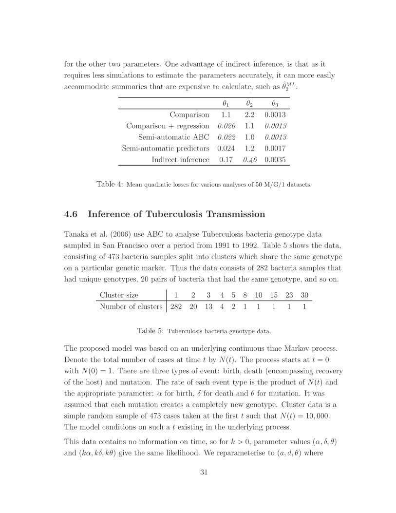
for the other two parameters. One advantage of indirect inference, is that as it

requires less simulations to estimate the parameters accurately, it can more easily

accommodate summaries that are expensive to calculate, such as θML2 .

θ1 θ2 θ3

Comparison 1.1 2.2 0.0013

Comparison + regression 0.020 1.1 0.0013

Semi-automatic ABC 0.022 1.0 0.0013

Semi-automatic predictors 0.024 1.2 0.0017

Indirect inference 0.17 0.46 0.0035

Table 4: Mean quadratic losses for various analyses of 50 M/G/1 datasets.

4.6 Inference of Tuberculosis Transmission

Tanaka et al. (2006) use ABC to analyse Tuberculosis bacteria genotype data

sampled in San Francisco over a period from 1991 to 1992. Table 5 shows the data,

consisting of 473 bacteria samples split into clusters which share the same genotype

on a particular genetic marker. Thus the data consists of 282 bacteria samples that

had unique genotypes, 20 pairs of bacteria that had the same genotype, and so on.

Cluster size 1 2 3 4 5 8 10 15 23 30

Number of clusters 282 20 13 4 2 1 1 1 1 1

Table 5: Tuberculosis bacteria genotype data.

The proposed model was based on an underlying continuous time Markov process.

Denote the total number of cases at time t by N(t). The process starts at t = 0

with N(0) = 1. There are three types of event: birth, death (encompassing recovery

of the host) and mutation. The rate of each event type is the product of N(t) and

the appropriate parameter: α for birth, δ for death and θ for mutation. It was

assumed that each mutation creates a completely new genotype. Cluster data is a

simple random sample of 473 cases taken at the first t such that N(t) = 10, 000.

The model conditions on such a t existing in the underlying process.

This data contains no information on time, so for k > 0, parameter values (α, δ, θ)

and (kα, kδ, kθ) give the same likelihood. We reparameterise to (a, d, θ) where

31

a = α/(α+ δ+ θ) and d = δ/(α+ δ+ θ). The likelihood under this parameterisation

depends only on a and d. To reflect prior ignorance of (a, d) we use the prior density

π(a, d, θ) ∝ π(θ)I(0 ≤ d ≤ a)I(a+ d < 1), where π(θ) is the marginal prior for θ used

in Tanaka et al. (2006). The prior restriction d ≤ a avoids the need for simulations

in which N(t) = 10, 000 is highly unlikely to occur. The other prior restrictions

follow from positivity constraints on the original parameters. Under this prior and

parameterisation, the marginal posterior of θ is equal to its prior and the problem

reduces to inference on a and d.

Tanaka et al. (2006) used two summary statistics for their ABC analysis: g/473 and

H = 1−∑

i(ni/473)2, where g is the number of distinct clusters in the sample, and

ni is the number of observed samples in the ith genotype cluster. We retain this

choice for our semi-automatic ABC pilot and the comparison ABC analysis reported

below.

As parameters in the pilot output are highly correlated (see Figure 3), we fitted a

line to the output by linear regression and made a reparameterisation

(u v)T = M(a d)T where M is a rotation matrix chosen so that on the fitted line u

is constant. The semi-automatic ABC analysis was continued using (u, v) as the

parameters of interest. The explanatory variables f(y) comprised: the number of

clusters of size i for 1 ≤ i ≤ 5, the number of clusters of size above 5, average cluster

size, H , the size of the three largest clusters, and the squares of all these quantities.

The semi-automatic ABC analysis used 4× 106 simulated datasets in total.

Figure 3 shows the ABC posteriors, indicating that our methodology places less

weight on the high d tail of the ABC posterior, reducing the marginal variances

from (0.0029, 0.0088) (comparison) to (0.0017, 0.0048) (semi-automatic ABC).

We further investigated this model through a simulation study. We constructed 50

data sets by simulating parameters from the ABC posterior, and simulating data

from the model for each of these pairs. We then compared ABC with the summary

statistics of Tanaka et al. (2006) to semi-automatic ABC. Averaged across these

data sets, semi-automatic ABC reduced square error loss by around 20%-25% for

the two parameters. Here we also found that regression correction of

Beaumont et al. (2002) did not change the accuracy of the Tanaka et al. (2006)

method. Using the linear predictors obtained within semi-automatic ABC to

estimate parameters (rather than as summary statistics) gave substantially worse

estimates, with mean square error for a increasing by a factor of over 3.

32

0.4 0.5 0.6 0.7 0.8 0.9 1.0

0.0

0.1

0.2

0.3

0.4

0.5

Comparison

a

d

X

0.4 0.5 0.6 0.7 0.8 0.9 1.0

0.0

0.1

0.2

0.3

0.4

0.5

Semi−automatic ABC

a

d

X

Figure 3: ABC output for the Tuberculosis application. Every 1000th state is plotted. The blue

crosses show the ABC means.

5 Discussion

We have argued that ABC can be justified by aiming for calibration of the ABC

posterior, together with accuracy of estimates of the parameters. We have

introduced a new variant of ABC, called noisy ABC, which is calibrated. Standard

ABC can be justified as an approximation to noisy ABC, but one which can be

more accurate. Theoretical results suggest that when analysing a single data set,

using a relatively small number of summary statistics, that standard ABC should be

preferred.

However we show that when attempting to combine ABC analyses of multiple data

sets, noisy ABC is to be preferred. Empirical evidence for this comes from our

analysis of a stochastic kinetic network, where using standard ABC within a

sequential ABC algorithm, leads to biased parameter estimates. This result could

be important for ABC analyses of population genetic data, if inferences are

combined across multiple genomic regions. We believe the ideal approach would be

to implement a Rao-Blackwellised version of noisy ABC, where we attempt to

average out the noise that is added to the summary statistics. If implemented, this

33

would lead to a method which is more accurate than noisy ABC for estimating any

function of the parameters. However, at present we are unsure how to implement

such a Rao-Blackwellisation scheme in a computationally efficient manner.

The main focus of this paper was a semi-automatic approach to implementing ABC.

The main idea is to use simulation to construct appropriate summary statistics,

with these summary statistics being estimates of the posterior mean of the

parameters. This approach is based on theoretical results which show that choosing

summary statistics as the posterior means produces ABC estimators that are

optimal in terms of minimising quadratic loss. We have evaluated our method on a

number of different models, comparing both to ABC as it has been implemented in

the literature, to indirect inference, and the synthetic likelihood approach of Wood

(2010).

The most interesting comparison was with between semi-automatic ABC and ABC

using the regression correction of Beaumont et al. (2002). In a number of examples,

these two approaches gave similarly accurate estimates. However, the

semi-automatic ABC seemed to be more robust, with the regression correction

actually producing less accurate estimates for the Ricker model, and not improving

the accuracy for the Tuberculosis model.

There are alternatives to using linear regression to construct the summary statistics.

One approach motivated by our theory, is to use approximate estimates for each

parameter. Such an approach has been used in Wilson et al. (2009), where estimates

of recombination rate under the incorrect demographic model were used as summary

statistics in ABC. It is also the idea behind the approach of Drovandi et al. (2011),

where the authors summarise the data through parameter estimates under an

approximating model. A further alternative is to use sliced-inverse regression (Li,

1991) rather than linear regression to produce the summary statistics. The

advantage of sliced-inverse regression is that it is able, where appropriate, to

generate multiple linear combinations of the explanatory variables, such that the

posterior mean is approximately a function of these linear combinations. Each linear

combination could then be used as a summary statistic within ABC.

Finally we note that there has been much recent research into the computational

algorithms underpinning ABC. As well as the rejection sampling, importance

sampling and MCMC algorithms we have mentioned, there has been work on using

sequential Monte Carlo methods (Beaumont et al., 2009; Sisson et al., 2007;

34

Peters et al., 2010), and adaptive methods (Bortot et al., 2007; Del Moral et al.,

2009) amongst others. The ideas in this paper are focussing a separate issue within

ABC, and we think the semi-automatic approach for implementing ABC that we

describe can be utilised within whatever computational method is preferred.

Acknowledgements: We thank Chris Sherlock for many helpful discussions, and

the reviewers for their detailed comments.

Appendix

Appendix A: Variance of IS-ABC and MCMC-ABC

Calculating the variance of estimates of posterior means using importance sampling

are complicated by the dependence between the importance sampling weights and

values of h(θ) (see Liu, 1996). A common approach to quantifying the accuracy of

importance sampling is to use an effective sample size. If the weights are normalised

to have mean 1, then the effective sample size, Neff is N divided by the mean of the

square of the weights. Liu (1996) argue that for most functions h(θ), the variance of

the estimator in (4) will be approximately (5) but with Nacc replaced by Neff.

For a given proposal distribution g(θ), the effective sample size is

Neff = N

∫

p(θ|sobs)π(θ)dθEABC (π(θ)/g(θ))

. (11)

It can be shown that the optimal proposal distribution, in terms of maximising the

Neff/N is

gopt(θ|yobs) ∝ π(θ)p(θ|sobs)1/2.

In which case

N∗

eff = Nacc

(

1 +Varπ(p(θ|sobs))Eπ(p(θ|sobs)1/2)2

)

,

where the variance and expectation on the right-hand side are with respect to π(θ).

It is immediate that N∗

eff ≥ Nacc, with equality only if p(θ|sobs) does not depend on

θ. The potential gains of importance sampling occur when p(θ|sobs) varies greatly.

Analysis of the Monte Carlo error within the MCMC ABC algorithm is harder.

However, consider fixing a proposal kernel g(·|·), which will fix the type of

transitions attempted. The Monte Carlo error then will be primarily governed by

35

the average acceptance probability. For simplicity assume that K(·) is uniformkernel, and that either g(·|·) is chosen to have the prior π(θ) as its stationary

distribution, or that the term π(θ)g(θi−1|θ)/{π(θi−1g(θ|θi−1)} ≈ 1 and can be

ignored. The average acceptance probability at stationarity is∫ ∫

πABC(θ|sobs)g(θ′|θ)p(θ′|sobs)dθdθ

′ =

(∫

π(θ)p(θ|sobs)dθ)

×∫ ∫

πABC(θ|sobs)g(θ′|θ)πABC(θ

′|sobs)π(θ′)

dθdθ′.

The integral comes from averaging over the current and proposed values for the

MCMC algorithm, with the average acceptance probability for a given proposed

value θ′ being p(θ′|sobs). The right-hand side comes from using (1). The first term

on the right-hand side is the average acceptance probability of the rejection

algorithm. The second term is 1 if we use an independence sampler g(θ′|θ), and will

be >> 1 if the ABC posterior is peaked relative to the prior, and if the transition

kernel proposes localised moves.

Appendix B: Proof of Lemma 1

Write∫

p(θ|sobs)π(θ)dθ =

∫ ∫

K(s− sobs)/h)π(s|θ)π(θ)dθds

=

∫

hdK(x)π(sobs + hx)dx.

The first equality comes from the definition of p(θ|sobs), the second by integrating

out θ and making a change of variable x = (s− sobs)/h. So

∣

∣

∣

∣

h−d

∫

p(θ|sobs)π(θ)dθ − π(sobs)

∣

∣

∣

∣

≤∫

K(x)|π(sobs + hx)− π(sobs)|dx

This bound is shown to be o(1) under either condition.

Consider first condition (i). Define c to be the maximum value of |x| such that

K(|x|) > 0. For any ǫ > 0, by continuity of π(s) at sobs we have that there exists a

δ > 0 such that |x| < δ implies |π(sobs + x)− π(sobs)| < ǫ. Define hǫ = δ/c. Then

for h < hǫ we have∫

K(x)|π(sobs + hx)− π(sobs)|dx ≤ ǫ.

36

This inequality follows as h|x| < δ for all x where K(x) > 0.

Now consider condition (ii). By differentiable continuity, Taylor’s theorem gives

π(sobs + hx) = π(sobs) +∑

i

hxiri(x).

The remainder factor ri(x) is |∂π(z)/∂si| for some z(x), so by assumption,

|ri(x)| ≤ R, a finite bound. Thus

∫

K(x)|π(sobs + hx)− π(sobs)|dx ≤ hR∑

i

∫

|xi|K(x)dx.

Appendix C: Proof of Theorem 4

Rearrangement of the loss function gives

E(L(θ, θ;A)|yobs)− trace(AΣ) = E((θ − θ)TA(θ − θ)|yobs),

where θ = E(θ|yobs), the mean under the true posterior, which equals S(yobs) for

the summary statistics under discussion. Define δ(sobs) = θ(sobs)− sobs and make

the change of variables x = (θ − sobs)/h. Now

E(L(θ, θ;A)|yobs)− trace(AΣ)− h2

∫

xTAxK(x)dx

= −2h

∫

xTAδ(θ + hx)K(x)dx+

∫

δ(θ + hx)TAδ(θ + hx)K(x)dx.

It is required that the modulus of the right hand side is o(h2). Let R be the support

of K. Since this is finite, it suffices to show that

maxx∈R

δ(θ + hx) = o(h).

To find an expression for δ, observe that (1) holds for noisy ABC. Taking its

expectation and making the change of variable s = S(y) gives

θ(t) =

∫

θπ(θ)π(s|θ)K({s− t}/h)dθds∫

π(s)K({s− t}/h)ds .

Note∫

θπ(θ)π(s|θ)dθ = π(s)E(θ|s) = sπ(s),

37

where the second equality is due to our choice of S. Thus

δ(t) =

∫

(s− t)π(s)K({s− t}/h)ds∫

π(s)K({s− t}/h)ds .

Make the change of variables y = (s− t)/h and consider the case t = θ + hx, then

δ(θ + hx) =h∫

yπ(θ + h[x + y])K(y)dy∫

π(θ + h[x + y])K(y)dy.

By the argument in Appendix B, continuity of π(s) at s = θ gives denominator

π(θ) + o(1). Consider the ith component of the integral in the numerator

∣

∣

∣

∣

∫

yiπ(θ + h[x+ y])K(y)dy −∫

yiπ(θ)K(y)dy

∣

∣

∣

∣

≤ maxy∈R

|yi|∣

∣

∣

∣

∫

(π(θ + h[x + y])− π(θ))K(y)dy

∣

∣

∣

∣

This integral is o(h) by the continuity argument just mentioned. Noting that∫

yiK(y)dy = 0 by assumption, we have

∫

yπ(θ + h[x + y])K(y)dy = o(1).

Combining these results gives the required bound for δ.

References

Allingham, D., King, R. A. R., and Mengersen, K. L. (2009). Bayesian estimation of

quantile distributions. Statistics and Computing, 19(2).

Beaumont, M. A., Cornuet, J.-M., Marin, J.-M., and Robert, C. P. (2009). Adaptive

approximate Bayesian computation. Biometrika, 96:983–990.

Beaumont, M. A., Zhang, W., and Balding, D. J. (2002). Approximate Bayesian

computation in population genetics. Genetics, 162:2025–2035.

Bernardo, J. M. and Smith, A. F. M. (1994). Bayesian Theory. Wiley, Chichester.

Blum, M. G. B. and Francois, O. (2010). Non-linear regression models for

Approximate Bayesian Computation. Statistics and Computing, 20:63–73.

38

Bortot, P., Coles, S., and Sisson, S. (2007). Inference for stereological extremes.

Journal of the American Statistical Association, 102:84–92.

Boys, R. J., Wilkinson, D. J., and Kirkwood, T. B. L. (2008). Bayesian inference for

a discretely observed stochastic kinetic model. Statistics and Computing,

18:125–135.

Cornuet, J.-M., Santos, F., Beaumont, M. A., Robert, C. P., Marin, J.-M., Balding,

D. J., Guillemaud, T., and Estoup, A. (2008). Inferring population history with

DIY ABC: a user-friendly approach to approximate Bayesian computation.

Bioinformatics, 24(23):2713–2719.

Del Moral, P., Doucet, A., and Jasra, A. (2009). An adaptive sequential Monte

Carlo method for approximate Bayesian computation. Submitted.

Diggle, P. J. and Gratton, R. J. (1984). Monte carlo methods of inference for

implicit statistical models. Journal of the Royal Statistical Society. Series B

(Methodological), 46(2):pp. 193–227.

Doucet, A., de Freitas, J. F. G., and Gordon, N. J., editors (2001). Sequential

Monte Carlo Methods in Practice. Springer-Verlag, New York.

Doucet, A., Godsill, S. J., and Andrieu, C. (2000). On sequential Monte Carlo

sampling methods for Bayesian filtering. Statistics and Computing, 10:197–208.

Drovandi, C. C. and Pettit, A. P. (2009). Likelihood-free Bayesian estimation of

quantile distributions. Technical report, Queensland University of Technology.

Drovandi, C. C., Pettitt, A. N., and Faddy, M. J. (2011). Approximate bayesian

computation using indirect inference. Journal of the Royal Statistical Society,

Series C (Applied Statistics).

Gillespie, D. T. (1977). Exact stochastic simulation of coupled chemical reactions.

The Journal of Physical Chemistry, 81:2340–2361.

Gourieroux, C. and Ronchetti, E. (1993). Indirect inference. Journal of Applied

Econometrics, 8:s85–s118.

Grelaud, A., Robert, C., Marin, J. M., Rodolphe, F., and Taly, J. F. (2009). ABC

likelihood-free methods for model choice in Gibbs random fields. Bayesian

Analysis, 4(2):317–336.

39

Hastie, T., Tibshirani, R., and Friedman, J. (2001). The Elements of Statistical

Learning: Data Mining, Inference, and Prediction. Springer.

Haynes, M. (1998). Flexible distributions and statistical models in ranking and

selection procedures, with applications. PhD thesis, Queensland University of

Technology.

Heggland, K. and Frigessi, A. (2004). Estimating functions in indirect inference.

Journal of the Royal Statistical Society, series B, 66:447–462.

Joyce, P. and Marjoram, P. (2008). Approximately sufficient statistics and Bayesian

computation. Statistical Applications in Genetics and Molecular Biology, 7.

article 26.

Kingman, J. F. C. (1982). The coalescent. Stochastic Processes and their

Applications, 13:235–248.

Li, K.-C. (1991). Sliced Inverse Regression for Dimension Reduction. Journal of the

American Statistical Association, 86(414):316–327.

Liepe, J., Barnes, C., Cule, E., Erguler, K., Kirk, P., Toni, T., and Stumpf, M. P.

(2010). ABC-SysBioapproximate Bayesian computation in Python with GPU

support. Bioinformatics, 26(14):1797–1799.

Lindsay, B. G. (1988). Composite likelihood methods. Contemporary Mathematics,

80:221–239.

Liu, J. and West, M. (2001). Combined parameter and state estimation in

simulation based filtering. In Doucet, A., de Freitas, J. F. G., and Gordon, N. J.,

editors, Sequential Monte Carlo in Practice, pages 197–223, New York.

Springer-Verlag.

Liu, J. S. (1996). Metropolised independent sampling with comparisons to rejection

sampling and importance sampling. Statistics and Computing, 6:113–119.

Lopes, J. S., Balding, D., and Beaumont, M. A. (2009). PopABC: a program to

infer historical demographic parameters. Bioinformatics, 25(20):2747–2749.

Mardia, K. V., Kent, J. T., and Bibby, J. M. (1979). Multivariate Analysis.

Academic Press.

40

Marjoram, P., Molitor, J., Plagnol, V., and Tavare, S. (2003). Markov chain Monte

Carlo without likelihoods. PNAS, 100:15324–15328.

McKinley, T., Cook, A. R., and Deardon, R. (2009). Inference in Epidemic Models

without Likelihoods. The International Journal of Biostatistics, 5(1):24.

Padhukasahasram, B., Wall, J. D., Marjoram, P., and Nordborg, M. (2006).

Estimating Recombination Rates From Single-Nucleotide Polymorphisms Using

Summary Statistics. Genetics, 174(3):1517–1528.

Peters, G. W., Fan, Y., and Sisson, S. A. (2010). On sequential Monte Carlo, partial

rejection control and approximate Bayesian computation. Submitted.

Prangle, D. (2010). ABC paper: Additional results. Technical report, Lancaster

University.

Pritchard, J. K., Seielstad, M. T., Perez-Lezaun, A., and Feldman, M. W. (1999).

Population growth of human Y chromosomes: a study of Y chromosome

microsatellites. Molecular Biology and Evolution, 16:1791–1798.

Ratmann, O., Andrieu, C., Wiuf, C., and Richardson, S. (2009). Model criticism

based on likelihood-free inference, with an application to protein network

evolution. Proceedings of the National Academy of Sciences, 106(26):10576.

Ratmann, O., Jrgensen, O., Hinkley, T., Stumpf, M., Richardson, S., and Wiuf, C.

(2007). Using likelihood-free inference to compare evolutionary dynamics of the

protein networks of h. pylori and p. falciparum. PLoS Comput Biol, 3(11):e230.

Rayner, G. D. and MacGillivray, H. L. (2002). Numerical maximum likelihood

estimation for the g-and-k and generalized g-and-h distributions. Statistics and

Computing, 12(1):57–75.

Ripley, B. (1987). Stochastic Simulation. Wiley.

Sisson, S. A., Fan, Y., and Tanaka, M. M. (2007). Sequential Monte Carlo without

likelihoods. Proceedings of the National Academy of Sciences, 104(6):1760–1765.

Sisson, S. A., Fan, Y., and Tanaka, M. M. (2009). Correction for Sisson et al.,

Sequential Monte Carlo without likelihoods. Proceedings of the National Academy

of Sciences, 106(39):16889.

41

Sisson, S. A., Peters, G. W., Briers, M., and Fan, Y. (2010). A note on target

distribution ambiguity of likelihood-free samplers. ArXiv e-prints.

Tanaka, M. M., Francis, A. R., Luciani, F., and Sisson, S. A. (2006). Using

Approximate Bayesian Computation to Estimate Tuberculosis Transmission

Parameters from Genotype Data. Genetics, 173:1511–1520.

Tavare, S., Balding, D. J., Griffiths, R. C., and Donnelly, P. (1997). Inferring

coalescent times from DNA sequence data. Genetics, 145:505–518.

Toni, T., Welch, D., Strelkowa, N., Ipsen, A., and Stumpf, M. (2009). Approximate

Bayesian computation scheme for parameter inference and model selection in

dynamical systems. Journal of The Royal Society Interface, 6(31):187–202.

Wegmann, D., Leuenberger, C., and Excoffier, L. (2009). Efficient Approximate

Bayesian Computation Coupled With Markov Chain Monte Carlo Without

Likelihood. Genetics, 182:1207–1218.

Wilkinson, D. J. (2009). Stochastic modelling for quantitative description of

heterogeneous biological systems. Nature Review Genetics, 10:122–133.

Wilkinson, D. J. (2011). Parameter inference for stochastic kinetic models of

bacterial gene regulation: a Bayesian approach to systems biology. In Bernardo,

J. M., Bayarri, M. J., Berger, J. O., Dawid, A. P., Heckerman, D., Smith, A.

F. M., and West, M., editors, Bayesian Statistics, volume 9, pages 679–690.

Oxford University Press.

Wilkinson, R. D. (2008). Approximate Bayesian computation (ABC) gives exact

results under the assumption of model error. Technical Report

arXiv:0811.3355v1, Arxiv.

Wilson, D. J., Gabriel, E., Leatherbarrow, A. J. H., Cheesebrough, J., Gee, S.,

Bolton, E., Fox, A., Hart, C. A., Diggle, P. J., and Fearnhead, P. (2009). Rapid

evolution and the importance of recombination to the gastro-enteric pathogen

campylobacter jejuni. Molecular Biology and Evolution, 26:385–397.

Wood, S. (2010). Statistical inference for noisy nonlinear ecological dynamic

systems. Nature, 466(7310):1102–1104.

42

−4 −3 −2 −1

−10

−6

−4

−2

0

Log h

Log

acce

ptan

ce r

ate

+

+

++

++ + + + + + ++++++++++++++++++++++++++++

+

Theoretical quantile

A p

−va

lue

0 0.25 0.5 0.75 1

00.

250.

50.

751

Theoretical quantile

B p

−va

lue

0 0.25 0.5 0.75 1

00.

250.

50.

751

Theoretical quantile

g p

−va

lue

0 0.25 0.5 0.75 1

00.

250.

50.

751

Theoretical quantile

k p

−va

lue

0 0.25 0.5 0.75 1

00.

250.

50.

751

Theoretical quantile

A p

−va

lue

0 0.25 0.5 0.75 1

00.

250.

50.

751

Theoretical quantile

B p

−va

lue

0 0.25 0.5 0.75 1

00.

250.

50.

751

Theoretical quantile

g p

−va

lue

0 0.25 0.5 0.75 1

00.

250.

50.

751

Theoretical quantile

k p

−va

lue

0 0.25 0.5 0.75 1

00.

250.

50.

751