A Novel Approach for Choosing Summary Statistics in Approximate Bayesian Computation

A novel approach for choosing summary statistics in

approximate Bayesian computation2

Simon Aeschbacher∗,§,1, Mark A. Beaumont∗∗, Andreas Futschik§§

August 24, 20124

∗Institute of Evolutionary Biology, University of Edinburgh, Edinburgh EH9 3JT, United

Kingdom, §IST Austria (Institute of Science and Technology Austria), 3400 Klosterneuburg,6

Austria, ∗∗Department of Mathematics and School of Biological Sciences, University of Bristol,

Bristol BS8 1TW, United Kingdom, and §§Institute of Statistics and Decision Support Systems,8

University of Vienna, 1010 Vienna, Austria

1

Running title: Choice of statistics in ABC via boosting10

Key words : choice of summary statistics, approximate Bayesian computation (ABC), Alpine12

ibex, mutation rate, mating skew

14

1Corresponding author : Simon Aeschbacher, Faculty of Mathematics, University of Vienna,

Nordbergstrasse 15, A-1090 Vienna, Austria.16

Phone: +43 (0)1 4277 50773

Fax: +43 (0)1 4277 950618

E-mail: [email protected]

20

This manuscript is intended for publication as an Investigation in Genetics.

22

2 S. Aeschbacher, M. A. Beaumont, and A. Futschik

mailto:[email protected]

Abstract

The choice of summary statistics is a crucial step in approximate Bayesian com-24

putation (ABC). Since statistics are often not sufficient, this choice involves a trade-off

between loss of information and reduction of dimensionality. The latter may increase the26

efficiency of ABC. Here, we propose an approach for choosing summary statistics based

on boosting, a technique from the machine learning literature. We consider different28

types of boosting and compare them to partial least squares regression as an alternative.

To mitigate the lack of sufficiency, we also propose an approach for choosing summary30

statistics locally, in the putative neighborhood of the true parameter value. We study

a demographic model motivated by the re-introduction of Alpine ibex (Capra ibex ) into32

the Swiss Alps. The parameters of interest are the mean and standard deviation across

microsatellites of the scaled ancestral mutation rate (θanc = 4Neu), and the proportion of34

males obtaining access to matings per breeding season (ω). By simulation, we assess the

properties of the posterior distribution obtained with the various methods. According to36

our criteria, ABC with summary statistics chosen locally via boosting with the L2-loss

performs best. Applying that method to the ibex data, we estimate θanc ≈ 1.288, and38

find that most of the variation across loci of the ancestral mutation rate u is between

7.7 ·10−4 and 3.5 ·10−3 per locus per generation. The proportion of males with access to40

matings is estimated as ω ≈ 0.21, which is in good agreement with recent independent

estimates.42

Choice of statistics in ABC via boosting 3

1 Introduction

Understanding the mechanisms leading to observed patterns of genetic diversity has been44

a central objective since the beginnings of population genetics (Fisher 1922, Haldane 1932,

Wright 1951, Charlesworth and Charlesworth 2010). Three recent trends keep advancing this46

undertaking: i) molecular data are becoming available at an ever higher pace (Rosenberg

et al. 2002, Frazer et al. 2007), ii) new theory continues to be developed, and iii) increased48

computational power allows solution of problems that were intractable just a few years ago.

In parallel, the focus has shifted to inference under complex models (e.g. Fagundes et al.50

2007, Blum and Jakobsson 2011), and to the joint estimation of parameters (e.g. Williamson

et al. 2005). Usually, these models are stochastic. The increasing complexity of models is52

justified by the underlying processes like inheritance, mutation, modes of reproduction and

spatial subdivision. On the other hand, complex models are often not amenable to inference54

based on exact analytical results. Instead, approximate methods such as Markov chain Monte

Carlo (MCMC, Gelman et al. 2004) or approximate Bayesian computation (ABC, Marjoram56

and Tavare 2006) are used. These approximate methods address different issues in inference

and the choice therefore depends on the specific problem. A significant part of research in58

the field is currently devoted to the refinement and development of such methods. ABC is

a Monte Carlo method of inference that emerged from the confrontation with models for60

which the evaluation of the likelihood is computationally prohibitive or impossible (Fu and Li

1997, Tavare et al. 1997, Weiss and von Haeseler 1998, Pritchard et al. 1999, Beaumont et al.62

2002). ABC may be viewed as a class of rejection algorithms (Marjoram et al. 2003, Marjoram

and Tavare 2006), where the full data are projected to a lower-dimensional set of summary64

statistics. Here, we propose an approach for choosing summary statistics based on boosting

(see below), and we apply it to the estimation of the mean and variance across microsatellites66

of the scaled ancestral mutation rate and of the mating skew in Alpine ibex (Capra ibex ). We


further show that focussing the choice of statistics on the putative neighborhood of the true68

parameter value improves estimation in this context.

The principle of ABC is to first simulate data under the model of interest and then accept70

simulations that produced data close to the observation. Parameter values belonging to ac-

cepted simulations yield an approximation to the posterior distribution, without the need to72

explicitly calculate the likelihood. The full data are usually compressed to summary statistics

in order to reduce the number of dimensions. Formally, the posterior distribution of interest74

is given by

π(φ | D) =π(D | φ) π(φ)

π(D)=

π(D | φ) π(φ)∫Φπ(D | φ) π(φ) dφ

, (1)

where φ is a vector of parameters living in space Φ, D denotes the observed data, π(φ) the76

prior distribution, and π(D | φ) the likelihood. With ABC, (1) is approximated by

πε(φ | s) ∝ π(ρ(s′, s) ≤ δε | φ

)π(φ), (2)

where s and s′ are abbreviations for realisations of S(D) and S(D′), respectively, and S is78

a function generating a q-dimensional vector of summary statistics calculated from the full

data. The prime denotes simulated points, in contrast to quantities related to the observed80

data. Further, ρ(·) is a distance metric and δε the rejection tolerance in that metric space,

such that on average a proportion ε of all simulated points is accepted. ABC, its position in82

the ensemble of model-based inference methods, and its application in evolutionary genetics

are reviewed in Marjoram et al. (2003), Beaumont and Rannala (2004), Marjoram and Tavare84

(2006), Beaumont (2010), Bertorelle et al. (2010) and Csillery et al. (2010). Although the

origin of ABC is generally assigned to Fu and Li (1997), Tavare et al. (1997) and Pritchard86

et al. (1999), some aspects, such as the summary description of the full data, inference for

implicit stochastic models and algorithms directly sampling from the posterior distribution88

trace further back (e.g. Diggle 1979, Diggle and Gratton 1984, Rubin 1984).


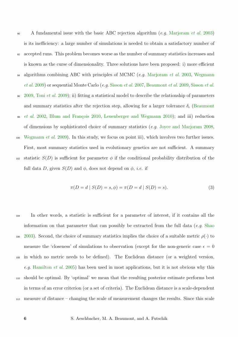
A fundamental issue with the basic ABC rejection algorithm (e.g. Marjoram et al. 2003)90

is its inefficiency: a large number of simulations is needed to obtain a satisfactory number of

accepted runs. This problem becomes worse as the number of summary statistics increases and92

is known as the curse of dimensionality. Three solutions have been proposed: i) more efficient

algorithms combining ABC with principles of MCMC (e.g. Marjoram et al. 2003, Wegmann94

et al. 2009) or sequential Monte Carlo (e.g. Sisson et al. 2007, Beaumont et al. 2009, Sisson et al.

2009, Toni et al. 2009); ii) fitting a statistical model to describe the relationship of parameters96

and summary statistics after the rejection step, allowing for a larger tolerance δε (Beaumont

et al. 2002, Blum and Francois 2010, Leuenberger and Wegmann 2010); and iii) reduction98

of dimensions by sophisticated choice of summary statistics (e.g. Joyce and Marjoram 2008,

Wegmann et al. 2009). In this study, we focus on point iii), which involves two further issues.100

First, most summary statistics used in evolutionary genetics are not sufficient. A summary

statistic S(D) is sufficient for parameter φ if the conditional probability distribution of the102

full data D, given S(D) and φ, does not depend on φ, i.e. if

π(D = d | S(D) = s, φ) = π(D = d | S(D) = s). (3)

In other words, a statistic is sufficient for a parameter of interest, if it contains all the104

information on that parameter that can possibly be extracted from the full data (e.g. Shao

2003). Second, the choice of summary statistics implies the choice of a suitable metric ρ(·) to106

measure the ‘closeness’ of simulations to observation (except for the non-generic case ε = 0

in which no metric needs to be defined). The Euclidean distance (or a weighted version,108

e.g. Hamilton et al. 2005) has been used in most applications, but it is not obvious why this

should be optimal. By ‘optimal’ we mean that the resulting posterior estimate performs best110

in terms of an error criterion (or a set of criteria). The Euclidean distance is a scale-dependent

measure of distance – changing the scale of measurement changes the results. Since this scale112


is determined by the summary statistics, the choice of summary statistics has implications for

the choice of the metric. For these reasons, the choice of summary statistics should aim at114

reducing the dimensions, but also at extracting (combinations of) statistics that contain the

essential information about the parameters of interest. This task is reminiscent of the classical116

problem of variable selection in statistics and machine learning (Hastie et al. 2011), and it is

of principal interest here.118

The choice of summary statistics in ABC has become a focus of research only recently.

Joyce and Marjoram (2008) proposed a sequential scheme based on the principle of approx-120

imate sufficiency. Statistics are included if their effect on the posterior distribution is larger

than some threshold. Their approach seems demanding to implement, and it is not obvious how122

to define an optimal threshold. Wegmann et al. (2009) suggested partial least squares (PLS)

regression as an alternative. In this context, PLS regression seeks linear combinations of the124

original summary statistics that are maximally decorrelated and, at the same time, have high

correlation with the parameters (Hastie et al. 2011). A reduction in dimensions is achieved by126

choosing only the first r PLS components, where r is determined via cross-validation. PLS is

one out of several approaches for variable selection, but it is an open question how it compares128

to alternative methods in any specific ABC setting. Moreover, the optimal choice of summary

statistics may depend on the location of the true (but unknown) parameter values. By defini-130

tion, this is to be expected whenever the summary statistics are not sufficient, because then

the information extracted from the full data by the summary statistics depends on the param-132

eter value (see equation (3)). It is therefore not obvious why methods that assess the relation

between statistics and parameters on a global scale should be optimal. Instead, focussing on134

the correlation only in the (supposed) neighborhood of the true parameter values might be

preferable. The issue is that this neighborhood is not known in advance – if we could choose136

an arbitrarily small neighborhood around the truth, our inference problem would be solved

and we would not need ABC or any other approximate method. However, the neighborhood138


may be established approximately, as we will argue later. The idea of focussing the choice of

summary statistics on some local optimization has recently also been followed by Nunes and140

Balding (2010) and Fearnhead and Prangle (2012). Nunes and Balding (2010) proposed using

a minimum-entropy algorithm to identify the neighborhood of the true value, and then chose142

the set of summary statistics that minimized the mean squared error across a test data set.

Fearnhead and Prangle (2012), on the other hand, first proved that, for a given loss function,144

an optimal summary statistic may be defined. For example, when the quadratic loss is used

to quantify the cost of an error, the optimal summary statistic is the posterior mean. Since146

the latter is not available a priori, the authors devised a heuristic to estimate it and were

able to show good performance of their approach. The choice of the optimization criterion148

may include a more local or a global focus on the parameter range. Different criteria will

lead to different optimal summary statistics. The approaches by Nunes and Balding (2010)150

and Fearnhead and Prangle (2012), and the one we will take here, have in common that they

employ a two-step procedure, first defining ‘locality’, and then using standard methods from152

statistics or machine learning to select summary statistics in this restricted range. They differ

in the details of these two steps (see Discussion).154

Here, we propose a novel approach for choosing summary statistics in ABC. It is based

on boosting, a method developed in machine learning to establish the relationship between156

predictors and response variables in complex models (Freund 1995, Freund and Schapire 1996;

1999, Schapire 1990). Given some training data, the idea of boosting is to iteratively train a158

function that describes this relationship. At each iteration, the training data are reweighted

according to the current prediction error (loss), and the function is updated according to160

an optimization rule. It has been argued that boosting is relatively robust to overfitting

(Friedman et al. 2000), which would be an advantage with regard to high-dimensional problems162

as encountered in ABC. Different flavors of boosting exist, depending on assumptions about

the error distribution, the loss function and the learning procedure. In a simulation study,164


we compare the performance of ABC with three types of boosting to ABC with summary

statistics choosen via PLS, and to ABC with all candidate statistics. We further suggest166

an approach for choosing summary statistics locally, and compare the local variants of the

various methods to their global versions. Throughout, we study a model that is motivated168

by the re-introduction of Alpine ibex into the Swiss Alps. The parameters of interest are the

mean and standard deviation across microsatellites of the scaled ancestral mutation rate, and170

the proportion of males that obtain access to matings per breeding season. This model is used

first in the simulation study for inference on synthetic data and assessment of performance.172

Later, we apply the best method to infer posterior distributions given genetic data from Alpine

ibex. It is not our goal to compare all the approaches recently proposed for choosing summary174

statistics in ABC. This would reach beyond the scope of the paper, but provides a perspective

for future research. Recently, Blum et al. (2012) carried out a comparative study of the176

various approaches and found that, for an example similar to our context, PLS performed

slightly better than approximate sufficiency (Joyce and Marjoram 2008), but worse than a178

number of alternative approaches including the posterior loss method (Fearnhead and Prangle

2012) and the two-stage minimum entropy procedure (Nunes and Balding 2010). Nevertheless,180

PLS has been widely used in recent applications and we have therefore focussed on comparing

our approach to PLS.182

We start by describing the ibex model and its parameters. We then present an ABC

algorithm that includes a step for choosing summary statistics. Later, we describe the boosting184

approach for choosing the statistics and we suggest how to focus this choice on the putative

neighborhood of the true parameter value. Comparing different versions of boosting among186

each other and with PLS, we conclude that boosting with the L2-loss restricted to the vicinity

of the true parameter performs best, given our criteria. However, the difference to the next188

best methods (local boosting with the L1-loss, and local PLS) is small.


2 Model and parameters190

We study a neutral model of a spatially structured population with genetic drift, mutation

and migration. The demography includes admixture, subdivision and changes in population192

size. This model is motivated by the recent history of Alpine ibex and their re-introduction

into the Swiss Alps (Figures 1 and 2). By the beginning of the 18th century, Alpine ibex had194

been extinct except for about 100 individuals in the Gran Paradiso area in Northern Italy

(Figure 1). At the beginning of the 20th century, a schedule was set up to re-establish former196

demes in Switzerland (Couturier 1962, Stuwe and Nievergelt 1991, Scribner and Stuwe 1994,

Maudet et al. 2002). The re-introduction has been documented in great detail by game keepers198

and authorities. We could reconstruct for 35 demes their census sizes between 1906 and 2006

(Supporting File 1 census sizes) and the number of females and males transferred between200

them, as well as the times of these founder/admixture events (Supporting File 2 transfers).

Inference on mutation and migration can therefore be done conditional on this information.202

The signal for this inference comes from the distribution of allele frequencies across loci and

across demes.204

We constructed a forwards in time model starting with an ancestral gene pool danc of

unknown effective size, Ne, representing the Gran Paradiso ibex deme. At times t1 and t2, two206

demes, d1 and d2, are derived from the ancestral gene pool. They represent the breeding stocks

that were established in two zoological gardens in Switzerland in 1906 and 1911 (Figure 1;208

Stuwe and Nievergelt 1991). Further demes are then derived from these. We let ti be the time

at which deme di is established. Once a derived deme has been established, it may contribute210

to the foundation of additional demes. The sizes of derived demes follow the observed census

size trajectories (Supporting File 1 census sizes). We interpolated missing values linearly, if the212

gap was only one year, or exponentially, if values for two or more successive years were missing.

Derived demes may exchange migrants if they are connected. This depends on information214


obtained from game keepers and on geography (Figure 1). Given a pair of connected demes

di and dj, we define the forward migration rates, mi,j and mj,i. More precisely, mi,j is the216

proportion of potential emigrants (see Supporting Information (SI)) in deme di that migrate

to deme dj per year. We assume that mi,j is constant over time and the same for females and218

males. Migration is included in the model, although we do not estimate migration rates in this

paper, but in a related paper (Aeschbacher et al. 2012). Here, we restrict our attention to the220

ancestral mutation rate and the proportion of males getting access to matings, marginal to the

migration rates (see below). Estimating migration rates comes with additional complications222

that go beyond the focus of the current paper. A schematic representation of the model is

given in Figure 2. When modeling migration, reproduction and founder events, we take into224

account the age structure of the population (see SI for details).

Population history is split into two phases. The first started at some unknown point in226

the past and ended at t1 = 1906, when the first ibex were brought from Gran Paradiso (danc)

to d1. For this ancestral phase, we assume constant, but unknown effective size Ne, and228

mutation following the single stepwise model (Ohta and Kimura 1973) at a rate u per locus

and generation. Accordingly, we define the scaled mutation rate in the ancestral deme as230

θanc = 4Neu. Mutation rates may vary among microsatellites for several reasons (Estoup and

Cornuet 1999). To account for this, we use a hierarchical model, assuming that θanc is normally232

distributed across loci on the log10-scale with mean µθanc and standard deviation σθanc . In our

case, µθanc and σθanc are the hyperparameters (Gelman et al. 2004) of interest. We assume234

that Ne is the same for all loci, so that variance in θanc can be attributed to u exclusively.

In principle, variation in diversity across loci could also be due to selection at linked genes236

(Maynard Smith and Haigh 1974, Charlesworth et al. 1993, Barton 2000), rather than variable

mutation rates. Most likely, we cannot distinguish these alternatives with our data. The238

second, recent phase started at time t1 and went up to the time of genetic sampling, tg = 2006.

During this phase, the number of males and females transferred at founder/admixture events240


and census population sizes are known and accounted for. Mutation is neglected, since, in the

case of ibex, this phase spans only about eleven generations at most (Stuwe and Grodinsky242

1987). At the transition from the ancestral to the recent phase, genotypes of the founder

individuals introduced to demes d1 and d2 are sampled at random from the ancestral deme,244

danc. At the end of the recent phase (tg), genetic samples are taken according to the sampling

scheme under which the real data were obtained. Out of the total 35 demes, 31 were sampled246

(Table S1).

In Alpine ibex, male reproductive success is highly skewed towards dominant males. Dom-248

inance is correlated with male age (Willisch et al. 2012), and ranks are established during

summer. Only a small proportion of males obtain access to matings during the rut in win-250

ter (Aeschbacher 1978, Stuwe and Grodinsky 1987, Scribner and Stuwe 1994, Willisch and

Neuhaus 2009, Willisch et al. 2012). To take this into account, we introduce the proportion252

of males obtaining access to matings, ω, as a parameter. It is defined relative to the number

of potentially reproducing males (and therefore conditional on male age; see SI), and has an254

impact on the strength of genetic drift. For simplicity, we assume that ω is the same in all

demes and independent of deme size and time.256

In principle, we would like to infer the joint posterior distribution π(m, α | D), where

α = (µθanc , σθanc , ω) and m = {mi,j : i 6= j, i ∈ Jm, j ∈ Jm}, with Jm denoting the set of258

all demes connected via migration to at least one other deme (Figure 1). This is a complex

problem because there are many parameters and even more candidate summary statistics; the260

curse of dimensionality is severe. Targeting the joint posterior with ABC naıvely would give a

result, but it would be hard to assess its validity. It is more promising to address intermediate262

steps and assess them one by one. A first step is to focus on a subset of parameters and

marginalize over the others. By marginalizing we mean that the joint posterior distribution264

is integrated with respect to the parameters that are not of interest. In our case, we may

focus on α and integrate over the migration rates m where they have prior support (Table266


1). In practice, marginal posteriors can be targeted directly with ABC – without the need to

compute the joint likelihood explicitly and integrate over it (see below). A second step is to268

clarify what summary statistics should be chosen for the subset of focal parameters (α). A

third one is to deal with the curse of dimensionality related to estimating m. In this paper,270

we deal with steps one and two: We aim at estimating α marginally to m, and we seek a

good method for choosing summary statistics with respect to α. The third step – estimating272

m and dealing with its high dimensionality – is treated in Aeschbacher et al. (2012). Notice

that this division of the problem implies the assumption that priors of the migration rates and274

male mating success are independent. We make this assumption partly for convenience, and

partly because we are not aware of any study that has shown a relation between the two in276

Alpine ibex. The division into two steps also requires that the set of all summary statistics

(S) can be split into two subsets, such that the first (Sα) contains most of the information278

on α, whereas the second (Sm) contains most of the information on m. Moreover, Sα should

not be affected much by m. As shown in the Appendix, the results are not much affected280

in such a situation while the computational burden decreases significantly. The arguments in

the Appendix rely on the notions of approximate sufficiency and approximate ancillarity.282


31

1

2

3

4

5

6

7

8

9

10

11

12

13

14

15

16

17

18 19

21

22

23

24

25

26

27

2829

30

31

32

33

35

34

20

Ancestral deme

Derived deme

Zoological garden

Putative connection

0 20 40km

N

@ 2004 swisstopo

Figure 1 Location of Alpine ibex demes in the Swiss Alps. The dark shaded parts represent areas inhabited

by ibex. The ancestral deme is located in the Gran Paradiso area in Northern Italy, close to the Swiss border.

The two demes in the zoological gardens 33 and 34 were first established from the ancestral one. Further

demes, including the two in zoological gardens 32 and 35, were derived from demes 33 and 34. Putative

connections indicate the pairs of demes for which migration is considered possible. For a detailed record of

the demography and the genealogy of demes see Figure S1 and Supporting File transfers. For deme names

see Table S1. Map obtained via the Swiss Federal Office for the Environment (FOEN) and modified with

permission.


t1

tg

recent phaseno mutation

ancestral phasewith mutation

ω

ω

ωωωd4 d5 d3 d7d1 d2

danc

θanc

m4,5

m5,4

m3,7

m7,3ωd6

ω ω

t4

t2t3

t5

t6t7

~~

~~

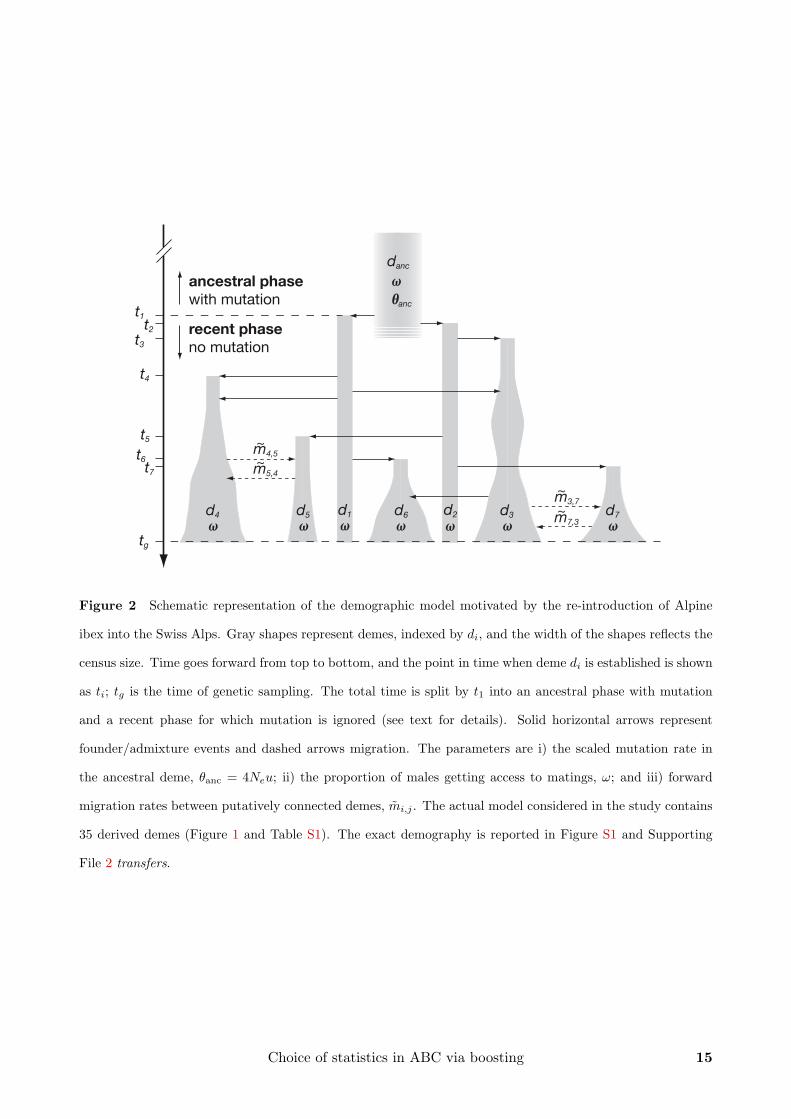
Figure 2 Schematic representation of the demographic model motivated by the re-introduction of Alpine

ibex into the Swiss Alps. Gray shapes represent demes, indexed by di, and the width of the shapes reflects the

census size. Time goes forward from top to bottom, and the point in time when deme di is established is shown

as ti; tg is the time of genetic sampling. The total time is split by t1 into an ancestral phase with mutation

and a recent phase for which mutation is ignored (see text for details). Solid horizontal arrows represent

founder/admixture events and dashed arrows migration. The parameters are i) the scaled mutation rate in

the ancestral deme, θanc = 4Neu; ii) the proportion of males getting access to matings, ω; and iii) forward

migration rates between putatively connected demes, mi,j . The actual model considered in the study contains

35 derived demes (Figure 1 and Table S1). The exact demography is reported in Figure S1 and Supporting

File 2 transfers.


3 Methods

The joint posterior distribution of our model may be factorized as284

π(m, α | D) = π(m | α, D) π(α | D). (4)

As mentioned, here we only target the marginal posterior of α, which is formally obtained as

π(α | D) =

∫Mπ(m, α | D) dm, (5)

whereM is the domain of possible values for m. By the nature of our problem, π(m, α | D)286

is not available. However, with ABC we may target (5) directly by sampling from πε(α | sα =

Sα(D)), where we assume that Sα is a subset of summary statistics approximately sufficient288

for estimating α (Appendix). Notice that Sα may not be sufficient to estimate the joint

posterior (4), however (Raiffa and Schlaifer 1968). The following standard ABC algorithm290

provides an approximation to π(α | sα) (e.g. Marjoram et al. 2003):

Algorithm A:292

A.1 Calculate summary statistics sα = Sα(D) from observed data.

A.2 For t = 1 to t = N :294

i Sample (α′t, m′t) from π(α, m) = π(α) π(m).

ii Simulate data D′t (at all loci and for all demes) from π(D | α′t, m′t).296

iii Calculate s′α,t = Sα(D′t) from simulated data.

A.3 Scale sα and s′α,t (t = 1, . . . , N) appropriately.298

A.4 For each t, accept α′t if ρ(s′α,t, sα) ≤ δε, using scaled summary statistics from A.3.

A.5 Estimate the posterior density πε(α | sα) from the εN accepted points 〈s′α,t, α′t〉.300


Step A.2 may be easily parallelized on a cluster computer. In doing so, one needs to store

〈s′α,t, α′t〉. Step A.5 may include post-rejection adjustment via regression (Beaumont et al.302

2002, Blum and Francois 2010, Leuenberger and Wegmann 2010) and scaling of parameters.

In general, the set of well-chosen, informative summary statistics Sα is not known in advance.304

Instead, a set of candidate statistics S (chosen based on intuition or analogy to simpler models)

may be available. Therefore, we propose algorithm B – a modified version of algorithm A –306

that includes an additional step for the empirical choice of summary statistics Sα informative

on α given a set of candidate statistics, S (for similar approaches, see Hamilton et al. 2005,308

Wegmann et al. 2009):

Algorithm B:310

B.1 Calculate candidate summary statistics s = S(D) from observed data.

B.2 For t = 1 to t = N :312

i Sample (α′t, m′t) from π(α, m) = π(α) π(m).

ii Simulate data D′t (at all loci and for all demes) from π(D | α′t, m′t).314

iii Calculate candidate summary statistics s′t = S(D′t) from simulated data.

B.3 Sample without replacement n ≤ N simulated pairs 〈s′t, α′t〉, denote them by 〈s′t∗ , α′t∗〉316

and use them as a training data set to choose informative statistics Sα.

B.4 According to B.3, obtain sα from s; for t = 1 to t = N , obtain s′α,t from s′t.318

B.5 Scale sα and s′α,t (t = 1, . . . , N) appropriately.

B.6 For each t, accept α′t if ρ(s′α,t, sα) ≤ δε, using scaled summary statistics from B.5.320

B.7 Estimate the posterior density πε(α | sα) from the εN accepted points 〈s′α,t, α′t〉.

Notice that Sα in steps B.3 and B.4 may either be a subset of S or some function (e.g. a linear322

combination) of S (details of implementation given below). In the following, we describe a

novel approach based on boosting and recently proposed by Lin et al. (2011) for the choice of324


Sα in B.3.

326

3.1 Choice of summary statistics via boosting

Boosting is a collective term for meta-algorithms originally developed for supervised learning328

in classification problems (Schapire 1990, Freund 1995). Later, versions for regression (Fried-

man et al. 2000) and other contexts have been developed (Buhlmann and Hothorn 2007and330

references therein). Assume a set of n observations indexed by i and associated with a one-

dimensional response Yi. For (binary) classification, Yi ∈ {0, 1}, but in a regression context, Yi332

may be continuous in R. Further, each observation is associated with a vector of q predictors

Xi = (X(1)i , . . . , X

(q)i ). Given a training data set {〈X1, Y1〉, . . . , 〈Xn, Yn〉}, the task of a boost-334

ing algorithm is to learn a function F (X) that predicts Y . Boosting was invented to deal with

cases where the relationship between predictors and response is potentially complex, for ex-336

ample non-linear (Schapire 1990, Freund 1995, Freund and Schapire 1996; 1999). Establishing

the relationship between predictors and response, and weighting predictors according to their338

importance, directly relates to the problem of choosing summary statistics in ABC: Given

candidate statistics S, we want to find a subset or combination of statistics Sα(k) informative340

for the kth parameter α(k) in α, for every k. Taking the set of simulated pairs 〈s′t, f(α′t)〉

(t = 1 . . . N) from step B.3 of algorithm B as a training data set, this may be achieved by342

boosting. For this purpose, we interpret the summary statistics S as predictors X and the

parameters α(k) as the response Y . Notice that we use f(α′t) to be generic in the sense that344

the response might actually be a function – such as a discretisation step (see below) – of α′t.

The principle of boosting is to iteratively apply a weak learner to the training data, and346

then combine the ensemble of weak learners to construct a strong learner. While the weak

learner predicts only slightly better than random guessing, the strong learner will usually348


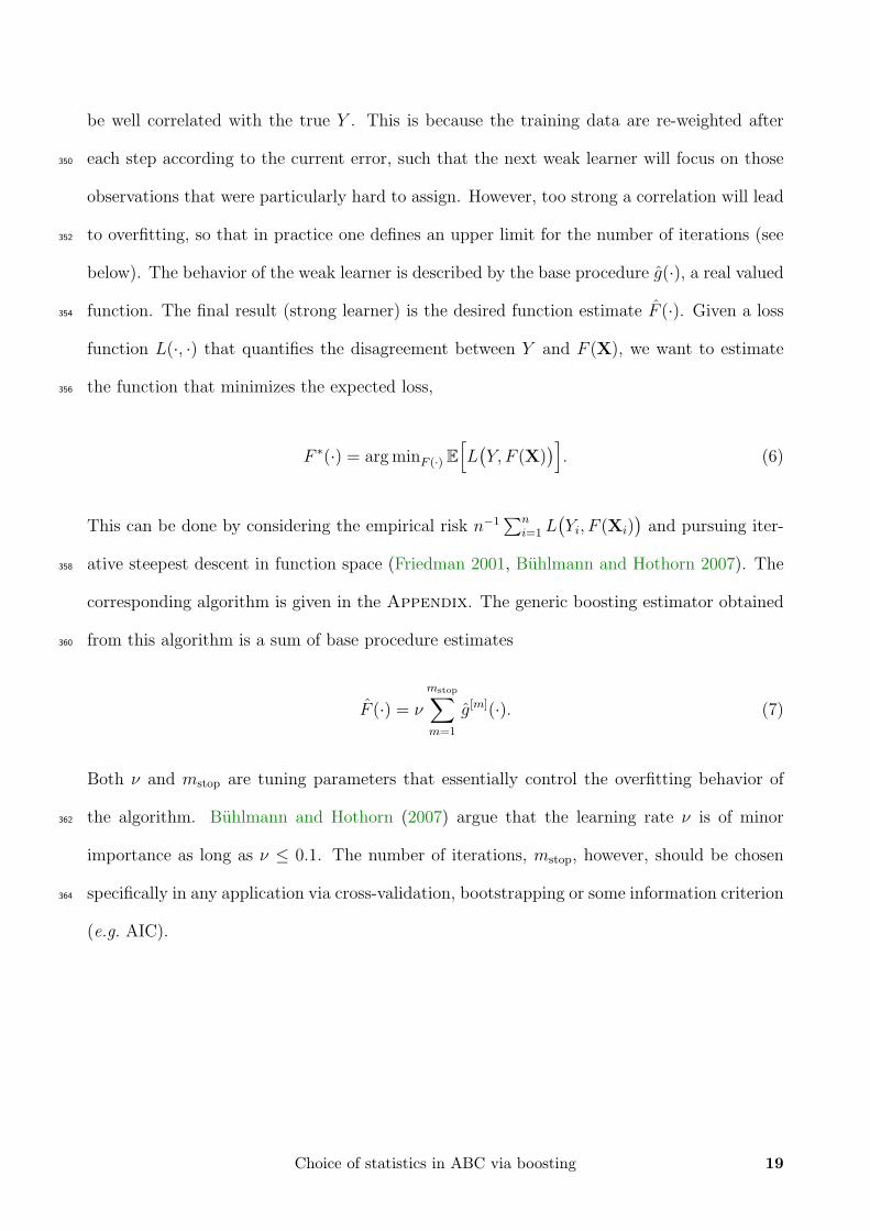
be well correlated with the true Y . This is because the training data are re-weighted after

each step according to the current error, such that the next weak learner will focus on those350

observations that were particularly hard to assign. However, too strong a correlation will lead

to overfitting, so that in practice one defines an upper limit for the number of iterations (see352

below). The behavior of the weak learner is described by the base procedure g(·), a real valued

function. The final result (strong learner) is the desired function estimate F (·). Given a loss354

function L(·, ·) that quantifies the disagreement between Y and F (X), we want to estimate

the function that minimizes the expected loss,356

F ∗(·) = arg minF (·) E[L(Y, F (X)

)]. (6)

This can be done by considering the empirical risk n−1∑n

i=1 L(Yi, F (Xi)

)and pursuing iter-

ative steepest descent in function space (Friedman 2001, Buhlmann and Hothorn 2007). The358

corresponding algorithm is given in the Appendix. The generic boosting estimator obtained

from this algorithm is a sum of base procedure estimates360

F (·) = ν

mstop∑m=1

g[m](·). (7)

Both ν and mstop are tuning parameters that essentially control the overfitting behavior of

the algorithm. Buhlmann and Hothorn (2007) argue that the learning rate ν is of minor362

importance as long as ν ≤ 0.1. The number of iterations, mstop, however, should be chosen

specifically in any application via cross-validation, bootstrapping or some information criterion364

(e.g. AIC).


3.1.1 Base procedure366

Different versions of boosting are obtained depending on the base procedure g(·) and the loss

function L(·, ·). Here, we let g(·) be a simple component-wise linear regression (Buhlmann368

and Hothorn 2007; see Appendix). With this choice, the boosting algorithm selects in every

iteration only one predictor, namely the one that is most effective in reducing the current370

loss. For instance, with the L2-loss (defined below), after each step, F (·) is updated linearly

according to372

F [m](x) = F [m−1](x) + νλ(ζm)x(ζm), (8)

where ζm denotes the index of the predictor variable selected in iteration m. Accordingly, in

iteration m only the ζth component of the coefficient estimate λ[m] is updated. As m goes374

to infinity, F (·) converges to a least squares solution. In practice, we stop at mstop, and we

denote the final vector of estimated coefficients as λ = λ[mstop]. Recall that in our context, the376

predictor variables X correspond to the candidate summary statistics S. For each of the k

parameters in α, we estimate one function F [mstop] and use it to obtain new parameter specific378

statistics Sα(k) .

3.1.2 Loss functions380

We employed boosting with three loss functions. The first two, L1-loss and L2-loss, are

appropriate for a regression context with a continuous response Y ∈ R. In this case, the382

parameters α′t are directly interpreted as yi (i.e. f(α′t) = α′t). The L1-loss is given by

LL1(y, F ) = |y − F | , (9)


and results in L1Boosting. The L2-loss is given by384

LL2(y, F ) =1

2|y − F |2 , (10)

and results in L2Boosting. The scaling factor 1/2 in (10) ensures that the negative gradient

vector U in the FGD algorithm (Appendix and SI) equals the residuals (Buhlmann and386

Hothorn 2007). L1- and L2Boosting result in a fit of a linear regression, similarly to ordinary

regression using the least absolute deviation (L1-norm) or the least squares criterion (L2-388

norm), respectively. The difference, and a potential advantage of boosting, is that residuals

are fitted multiple times depending on the importance of the components of X. Moreover,390

boosting is considered less prone to overfitting than ordinary L1- or L2-fitting (Buhlmann and

Hothorn 2007). In general, the L1-loss is more robust to outliers, but it may produce multiple,392

potentially unstable solutions. Using L1- and L2Boosting to choose summary statistics means

assuming a linear relationship between summary statistics and parameters. This is a strong394

assumption, and most likely not globally true. However, the advantage is that the resulting

linear combination has only one dimension, such that the curse of dimensionality in ABC396

may be strongly reduced. Again, the approach using the L1- or L2-loss results in one linear

combination F [mstop] per parameter α(k), such that Sα(k) has only one component. These linear398

combinations may end up being correlated across parameters, especially if parameters are not

identifiable, e.g. because they are confounded with each other.400

To motivate the third loss function, we propose considering the choice of summary statistics

as a classification problem. Imagine two classes of parameter values – say, high values in one402

class, and low values in the other. We may ask what summary statistics are important

to assign simulations to one of these two classes. With Y ∈ {0, 1} as the class label and404


p(x) := Pr[Y = 1 | X = x], a natural choice is the negative binomial log-likelihood loss

Llog-lik(y, p) = −[y log(p) + (1− y) log(1− p)

], (11)

omitting the argument of p for ease of notation. If we parametrize p = eF/(1 + eF ) so that we406

obtain F = log [p/(1− p)] corresponding to the logit-transformation, the loss in (11) becomes

Llog-lik(y, F ) = log[1 + e−(2y−1)F

]. (12)

The corresponding boosting algorithm is called LogitBoost (or Binomial Boosting; Buhlmann408

and Hothorn 2007). An advantage is that it does not assume a linear relationship between

summary statistics and parameters, as is the case for L1- and L2Boosting. Instead, LogitBoost410

fits a logistic regression model, which might be more appropriate. On the other hand, it re-

quires choosing a discretization procedure f(·) to map αt ∈ R to y ∈ {0, 1} (see below). Since412

such a choice is arbitrary, it would be problematic to use the resulting fit (a linear combina-

tion on the logit-scale) directly as Sα(k) . In practice, we instead assigned a candidate statistic414

S(j) (j = 1, . . . , q) to Sα(k) if the corresponding boosted coefficient λ(j) (cf. equation (8)) was

different from zero, and omitted it otherwise. Therefore, compared to L1- and L2Boosting,416

the reduction in dimensionality was on average lower, but the strong assumption of a linear

relationship between α(k) and Sα(k) was avoided. Notice that, in principle, non-linear relation-418

ships may be fitted with the L1- and L2-loss, too (Friedman et al. 2000). In the SI we provide

explicit expressions for the population minimizers (6) and some more insight on the boosting420

algorithms under the three loss functions used here.


3.1.3 Partial Least Squares regression422

Recently, Wegmann et al. (2009) proposed to choose summary statistics in ABC via Partial

Least Squares (PLS) regression (e.g. Hastie et al. 2011 and references therein). PLS is related424

to Principal Component regression. But in addition to maximizing the variance of the pre-

dictors X, at the same time, it maximizes the correlation of X with the response Y . Applied426

to the choice of summary statistics, it therefore not only decorrelates the summary statistics,

but also chooses them according to their relation to α. Hastie et al. (2011) argue that the428

first aspect dominates over the latter, however. The number r of PLS components to keep is

usually determined based on some cross-validation procedure (see below). In the context of430

ABC, the r components are multiplied by the corresponding statistics S(j) (j ≤ r) to obtain

Sα(k) (Wegmann et al. 2009)432

3.2 Global versus local choice

We have so far suggested that Sα is close to sufficient for estimating α. This will hardly be434

the case in practice. By definition, the optimal choice of Sα then depends on the unknown

true parameter value(s). Ideally, we would therefore like to focus the choice of Sα on the436

neighborhood of the truth. The latter is not known in practice. As a workaround, we propose

to use the n simulated pairs 〈s′t∗ , α′t∗〉 from step B.3 in algorithm B and the observed summary438

statistics s to approximately establish this neighborhood as follows:

Local choice of summary statistics in B.3:440

1. Consider the n pairs 〈s′t∗ , α′t∗〉 (t∗ = 1, . . . , n) from step B.3 in algorithm B.

2. Mean center each component s′(j) (j = 1, . . . , q) and scale it to have unit variance.442

3. Rotate s′ using Principal Component Analysis (PCA).

4. Apply the scaling from steps 2 and 3 to the observed summary statistics s.444


5. Mean center the PCA-scaled summary statistics obtained in step 3, and scale them to

have unit variance. Do the same for the PCA-scaled observed statistics obtained in step446

4. Denote the results by s′ and s, respectively.

6. For each t∗ ∈ n, compute the Euclidean distance δt∗ = ‖s′t∗ − st∗‖.448

7. Keep the n′ pairs 〈s′t∗∗ , α′t∗∗〉 (t∗∗ = 1, . . . , n′) for which δt∗ ≤ z, where z is some threshold.

8. Use the n′ points accepted in step 7 as a training set to choose statistics Sα with the450

desired method.

9. Continue with step B.4 in algorithm B.452

In step 2 above, the original summary statistics are brought to the same scale. Otherwise,

summary statistics with a high variance would on average contribute relatively more to the454

Euclidean distance than summary statistics with a low variance. However, whether a simulated

data point is far or close to the target (s) in multidimensional space may not only depend on456

the distance along the dimension of each statistic, but also on the correlation among statistics.

This can be accounted for by decorrelating the statistics, as is done by PCA in step 3. In458

combination with the Euclidean distance in step 6, the procedure above essentially uses the

Mahalanobis distance as metric (Mahalanobis 1936). Although we cannot prove the optimality460

of this approach, it seems to work well in our simulations. Notice that in steps 8 and 9, the

summary statistics are used on their original scale again. This is because we want our method462

for choosing parameter-specific combinations of statistics to use the information comprised in

the difference in scale among the original statistics – even in the vicinity of s. The PCA-scaling464

in step 5 is only used temporarily to determine δt∗ in step 6. Figure S2 visualizes the different

scales and the effect of determining an approximate neighborhood around s.466

The scheme just described may be combined with any of the methods for choosing sum-

mary statistics described above. In our case, we considered ABC with global and local versions468

of PLS (called pls.glob and pls.loc in the following), LogitBoost (lgb.glob, lgb.loc),


L1Boosting (l1b.glob, l1b.loc), and L2Boosting (l2b.glob, l2b.loc). Moreover, we per-470

formed ABC with all candidate statistics S (all) as a reference.

3.2.1 Candidate summary statistics472

Our set S of candidate summary statistics consisted of the mean and standard devation across

loci of the following statistics: the average within-deme variance of allele length, the average474

within-deme gene diversity (H1), the average between-deme gene diversity (H2), the total FIS,

the total FST, the total within-deme mean squared difference (MSD) in allele length (S1), the476

total between-deme MSD in allele length (S2), the total RST, and the number of allele types

in the total population. This amounts to a total of 18 summary statistics. We computed H1,478

H2, FIS and FST according to Nei and Chesser (1983), and S1, S2 and RST according to Slatkin

(1995). Notice that all summary statistics are symmetrical with respect to the order of the480

loci, which is consistent with our hierarchical parametrization of the ancestral mutation rate.

3.2.2 Implementation482

Throughout, we used the prior distributions given in Table 1. In algorithm B, we performed

N = 106 simulations and in B.2i we assumed that π(α, m) = π(α) π(m). In B.3, we used484

n = 104 simulations for the choice of summary statistics (both in the global and local versions).

Moreover, we first chose sets of summary statistics for each parameter separately, and then486

took the union of the sets, i.e. Sα =⋃k Sα(k) , where each Sα(k) is chosen according to one

of the methods proposed. This also applies to step 8 in the procedure for the local choice of488

summary statistics (see above). For the local choice, we kept the n′ = 1000 pairs closest to

the observation s, and we used the pcrcomp function in R version 2.11 (R Development Core490

Team 2011) for PCA. Notice that the set of the n′ simulations closest to s – and, hence, z in

step 7 of the procedure for the local choice – were the same for all local methods compared.492


In B.5, we mean-centered the summary statistics and scaled them to have unit variance. In

B.6, we chose the Euclidean distance as metric ρ(·). In B.7 we did post-rejection adjustment494

with a weighted local-linear regression with weights from an Epanechnikov kernel (Beaumont

et al. 2002), without additional scaling of parameters. For steps B.6 and B.7 we used the abc496

package (Csillery et al. 2011) for R. We estimated the parameters and performed the linear

regression on the same scale as the respective priors were defined.

Table 1 Parameters and prior distributions

Param. Description Prior distribution

θanc, l Scaled ancestral mutation rate at locus l, 4Neu log10(θanc, l) ∼ N(µθanc , σ

2θanc

)aµθanc Mean across loci of θanc, l (on log10-scale) µθanc ∼ N (0.5, 1)σθanc Standard deviation across loci of θanc, l (on log10-scale) σθanc ∼ log10 -uniform in

[0.01, 1]

ω Proportion of mature males with access to matings ω ∼ log10 -uniform in [0.01, 1]

m bi,j Forward migration rate per year from deme i to deme j mi,j ∼ log10 -uniform in[

10−3.5, 10−0.5]

aN(µ, σ2

), normal distribution with mean µ and variance σ2.

bAlthough migration rates are not estimated here, they are drawn from the prior in all simulations(see main text).

498

For the PLS method, we used the pls package (Mevik and Wehrens 2007) for R and followed

Wegmann et al. (2009; 2010). Specifically, we performed a Box-Cox transformation of the500

summary statistics prior to the PLS regression, and we chose the number of components to keep

based on a plot of the root mean squared prediction error. We kept r = 10 components, both502

for pls.glob and pls.loc (Figure S3). For all methods based on boosting, we mean-centered

the summary statistics before boosting and used the glmboost function of the mboost package504

(Buhlmann and Hothorn 2007, Hothorn et al. 2011) for R. For the LogitBoost methods, we

chose for each k the first and third quartile of the sample of α(k) drawn in step B.3 of algorithm506

B.3 as the centers of the two classes of parameter values. For lgb.glob, we then assigned

the 500 α(k)-values closest to the first quartile to the first class (y = 0) and the 500 values508


closest to the third quartile to the second class (y = 1). For lgb.loc, we analogously assigned

the 100 α(k)-values closest to the two quartiles to the two classes. For both lgb.glob and510

lgb.loc, we chose the optimal mstop based on the Akaike information criterion (AIC, Akaike

1974, Buhlmann and Hothorn 2007), but set an upper limit for mstop of 500 iterations. For512

l1b.glob and l1b.loc, we chose mstop via 10-fold cross-validation with the cvrisk function

of the mboost package, setting an upper limit of 100. Last, for l2b.glob and l2b.loc, we514

chose mstop based on the AIC, with an upper limit of 100. Figures S4 to S6 further illustrate

the boosting procedure.516

3.3 Simulation study and application to data

To assess the performance of the different methods for choosing summary statistics and to518

study the influence of the rejection tolerance ε, we carried out a simulation study. For each

ε ∈ {0.001, 0.01, 0.1}, we simulated 500 test data sets with parameter values sampled from520

the prior distributions and then inferred the posterior distribution for each set. In the case of

local choice of summary statistics, the procedure of defining informative summary statistics522

based on the candidate statistics was run for each test data set separately. For the global

choice, it was run only once per method, because there is no dependence on the supposed524

true value. Similar to Wegmann et al. (2009), we used as a measure of accuracy of the

marginal posterior distributions the root mean integrated squared error (RMISE), defined as526

RMISEk =√∫

Φ(k)(φ(k) − µk)2 π(φ(k) | s) dφ(k), where µk is the true value of the kth com-

ponent of the parameter vector φ and π(φ(k) | s) is the corresponding estimated marginal528

posterior density. Recall that φ = α = (µθanc , σθanc , ω) in our case. From this, we obtained

the relative absolute RMISE (RARMISE) as RARMISEk = RMISEk/|µk|. We also computed530

the absolute error (AEk) between three marginal posterior point estimates (mode, mean and

median) and µk. Dividing by |µk|, we obtained the relative absolute error (RAEk). To directly532


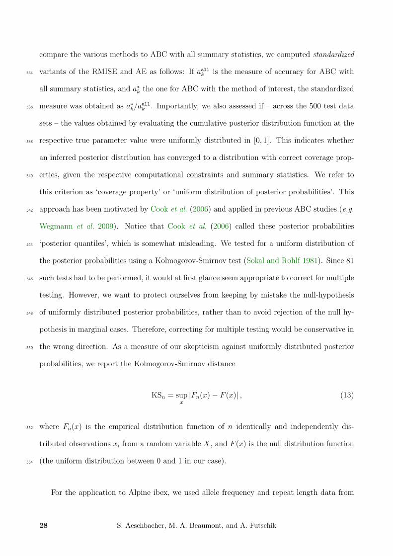
compare the various methods to ABC with all summary statistics, we computed standardized

variants of the RMISE and AE as follows: If aallk is the measure of accuracy for ABC with534

all summary statistics, and a∗k the one for ABC with the method of interest, the standardized

measure was obtained as a∗k/aallk . Importantly, we also assessed if – across the 500 test data536

sets – the values obtained by evaluating the cumulative posterior distribution function at the

respective true parameter value were uniformly distributed in [0, 1]. This indicates whether538

an inferred posterior distribution has converged to a distribution with correct coverage prop-

erties, given the respective computational constraints and summary statistics. We refer to540

this criterion as ‘coverage property’ or ‘uniform distribution of posterior probabilities’. This

approach has been motivated by Cook et al. (2006) and applied in previous ABC studies (e.g.542

Wegmann et al. 2009). Notice that Cook et al. (2006) called these posterior probabilities

‘posterior quantiles’, which is somewhat misleading. We tested for a uniform distribution of544

the posterior probabilities using a Kolmogorov-Smirnov test (Sokal and Rohlf 1981). Since 81

such tests had to be performed, it would at first glance seem appropriate to correct for multiple546

testing. However, we want to protect ourselves from keeping by mistake the null-hypothesis

of uniformly distributed posterior probabilities, rather than to avoid rejection of the null hy-548

pothesis in marginal cases. Therefore, correcting for multiple testing would be conservative in

the wrong direction. As a measure of our skepticism against uniformly distributed posterior550

probabilities, we report the Kolmogorov-Smirnov distance

KSn = supx|Fn(x)− F (x)| , (13)

where Fn(x) is the empirical distribution function of n identically and independently dis-552

tributed observations xi from a random variable X, and F (x) is the null distribution function

(the uniform distribution between 0 and 1 in our case).554

For the application to Alpine ibex, we used allele frequency and repeat length data from


37 putatively neutral microsatellites as described in Biebach and Keller (2009; Figure 1 and556

Table S1). The data were provided to us by the authors. ABC simulations and inference

were identical to those in the simulation study, with the same number of markers (see also558

SI). The program called SPoCS that we wrote and used for simulation of the ibex scenario,

and a collection of R and shell scripts used for inference are available on the website http:560

//pub.ist.ac.at/~saeschbacher/phd_e-sources/.


http://pub.ist.ac.at/~saeschbacher/phd_e-sources/



4 Results562

4.1 Comparison of methods for choice of summary statistics

We have suggested boosting with component-wise linear regression as a base procedure for564

choosing summary statistics in ABC. Three loss functions were considered: the L1-, and L2-

loss, and the negative binomial log-likelihood. We have compared the performance of ABC566

with summary statistics chosen via different types of boosting to ABC with statistics choosen

via partial least squares (PLS, Wegmann et al. 2009), and to ABC with all candidate summary568

statistics (Table 2). The relative absolute error (RAE) behaved similarly for the three point

estimates (mode, mean, median), but the mode was less reliable in cases were the posterior570

distributions did not have a unique mode (Figure S7). We decided to focus on the median.

For assessment of the methods, we sought a low RARMISE and a low RAE of the median572

(RAEmedian in the following), and we required that the distribution of posterior probabilities

of the true value did not deviate from uniformity for any parameter.574

ABC with all summary statistics (all) and ABC with LogitBoost (lgb.glob) performed

well in terms of RARMISE and RAEmedian, especially when estimating µθanc and ω (Figure 3A576

and 3B). However, the posteriors of µθanc inferred with all and lgb.glob tended to be biased

(Kolmogorov-Smirnov distance and coverage p-value in Table 2).578


μθanc

log10(ε)

Rel

ative

abs

olut

e R

MIS

E

log10(σθanc)

log10(ε)

log10(ω)

log10(ε)

μθanc

log10(ε)

Rel

ative

abs

olut

e er

ror o

f med

ian

log10(σθanc)

log10(ε)

log10(ω)

log10(ε)

μθanc

log10(ε)

Rel

ative

abs

olut

e R

MIS

E

log10(σθanc)

log10(ε)

log10(ω)

log10(ε)

μθanc

log10(ε)

Rel

ative

abs

olut

e er

ror o

f med

ian

log10(σθanc)

log10(ε)

log10(ω)

log10(ε)

A B

C D

−3.0 −2.0 −1.0

0.060

0.065

0.070

0.075

0.080

0.085

0.090

−3.0 −2.0 −1.0

0.24

0.26

0.28

0.30

0.32

−3.0 −2.0 −1.0

0.21

0.22

0.23

0.24

0.25

allpls.globlgb.globl1b.globl2b.glob

−3.0 −2.0 −1.0

0.14

0.15

0.16

0.17

0.18

0.19

−3.0 −2.0 −1.0

0.44

0.46

0.48

0.50

0.52

−3.0 −2.0 −1.0

0.42

0.44

0.46

0.48

0.50

−3.0 −2.0 −1.0

0.14

0.16

0.18

0.20

0.22

−3.0 −2.0 −1.0

0.44

0.46

0.48

0.50

−3.0 −2.0 −1.0

0.42

0.44

0.46

0.48

0.50

−3.0 −2.0 −1.0

0.06

0.07

0.08

0.09

0.10

0.11

−3.0 −2.0 −1.0

0.25

0.26

0.27

0.28

0.29

0.30

−3.0 −2.0 −1.0

0.21

0.22

0.23

0.24

0.25

allpls.loclgb.locl1b.locl2b.loc

Figure 3 Accuracy of different methods for choosing summary statistics as a function of the acceptance rate

(ε). (A) and (B) show results for different methods when applied to the whole parameter range (global choice).

In (C) and (D), the methods were applied only in the neighborhood of the (supposed) true value (local choice).

The performance resulting from using all candidate summary statistics is shown for comparison in both rows.

(A) and (C) show the root mean integrated squared error (RMISE), relative to the absolute true value. (B)

and (D) give the absolute error of the posterior median, relative to the absolute true value. Plotted are the

medians across n = 500 independent test estimations with true values drawn from the prior (error bars denote

the median±MAD/√n, where MAD is the median absolute deviation).


Table 2 Accuracy of different methods for choosing summary statistics on a globalscale

Method ε Parameter RARMISEa RAEb mode RAE mean RAE median KS500c Cov. pd

all 0.001 µθanc 0.143 (0.147) 0.062 (0.074) 0.065 (0.075) 0.062 (0.075) 0.072 0.011∗

σθanc 0.452 (0.231) 0.269 (0.213) 0.269 (0.222) 0.265 (0.218) 0.034 0.610ω 0.446 (0.272) 0.221 (0.225) 0.215 (0.218) 0.219 (0.22) 0.027 0.859

0.01 µθanc 0.141 (0.145) 0.061 (0.072) 0.064 (0.074) 0.065 (0.075) 0.082 0.003∗

σθanc 0.466 (0.257) 0.299 (0.21) 0.286 (0.225) 0.282 (0.226) 0.019 0.992ω 0.432 (0.259) 0.233 (0.232) 0.226 (0.23) 0.232 (0.232) 0.026 0.880

0.1 µθanc 0.140 (0.134) 0.065 (0.075) 0.067 (0.078) 0.067 (0.075) 0.081 0.003∗

σθanc 0.463 (0.272) 0.324 (0.238) 0.306 (0.248) 0.296 (0.243) 0.032 0.677ω 0.431 (0.263) 0.234 (0.229) 0.228 (0.22) 0.226 (0.223) 0.038 0.482

pls.glob 0.001 µθanc 0.171 (0.16) 0.077 (0.087) 0.083 (0.089) 0.081 (0.088) 0.038 0.466σθanc 0.488 (0.276) 0.291 (0.223) 0.289 (0.252) 0.276 (0.228) 0.024 0.936ω 0.451 (0.275) 0.238 (0.221) 0.234 (0.224) 0.237 (0.227) 0.022 0.969

0.01 µθanc 0.166 (0.152) 0.080 (0.09) 0.079 (0.09) 0.079 (0.089) 0.035 0.562σθanc 0.480 (0.291) 0.307 (0.223) 0.295 (0.268) 0.293 (0.242) 0.038 0.473ω 0.441 (0.262) 0.241 (0.234) 0.230 (0.225) 0.229 (0.226) 0.035 0.562

0.1 µθanc 0.171 (0.146) 0.083 (0.091) 0.086 (0.097) 0.087 (0.094) 0.037 0.497σθanc 0.469 (0.283) 0.319 (0.237) 0.307 (0.286) 0.310 (0.276) 0.056 0.089ω 0.433 (0.265) 0.240 (0.226) 0.234 (0.224) 0.234 (0.23) 0.049 0.178

lgb.glob 0.001 µθanc 0.149 (0.152) 0.064 (0.074) 0.065 (0.076) 0.064 (0.074) 0.082 0.002∗

σθanc 0.435 (0.204) 0.270 (0.231) 0.261 (0.214) 0.247 (0.205) 0.038 0.466ω 0.456 (0.275) 0.235 (0.23) 0.230 (0.237) 0.232 (0.224) 0.025 0.913

0.01 µθanc 0.145 (0.15) 0.066 (0.076) 0.066 (0.078) 0.066 (0.076) 0.103 <0.001∗

σθanc 0.450 (0.223) 0.281 (0.215) 0.269 (0.217) 0.258 (0.209) 0.046 0.238ω 0.436 (0.27) 0.235 (0.234) 0.222 (0.223) 0.225 (0.228) 0.025 0.916

0.1 µθanc 0.147 (0.142) 0.068 (0.079) 0.067 (0.078) 0.069 (0.079) 0.135 <0.001∗

σθanc 0.471 (0.284) 0.288 (0.209) 0.301 (0.249) 0.271 (0.233) 0.054 0.103ω 0.427 (0.259) 0.232 (0.222) 0.225 (0.216) 0.228 (0.22) 0.042 0.329

l1b.glob 0.001 µθanc 0.188 (0.178) 0.075 (0.087) 0.074 (0.087) 0.076 (0.088) 0.035 0.573σθanc 0.445 (0.202) 0.271 (0.236) 0.261 (0.232) 0.256 (0.216) 0.023 0.954ω 0.487 (0.297) 0.251 (0.259) 0.226 (0.227) 0.232 (0.226) 0.031 0.723

0.01 µθanc 0.178 (0.17) 0.075 (0.087) 0.075 (0.088) 0.075 (0.085) 0.031 0.711σθanc 0.463 (0.217) 0.288 (0.24) 0.271 (0.238) 0.259 (0.221) 0.029 0.805ω 0.468 (0.288) 0.255 (0.262) 0.228 (0.222) 0.235 (0.233) 0.034 0.595

0.1 µθanc 0.177 (0.173) 0.078 (0.092) 0.078 (0.094) 0.079 (0.094) 0.043 0.311σθanc 0.508 (0.299) 0.307 (0.21) 0.304 (0.269) 0.290 (0.248) 0.051 0.144ω 0.449 (0.272) 0.238 (0.241) 0.237 (0.222) 0.239 (0.227) 0.031 0.716

l2b.glob 0.001 µθanc 0.183 (0.173) 0.075 (0.087) 0.074 (0.085) 0.074 (0.086) 0.029 0.794σθanc 0.441 (0.202) 0.273 (0.229) 0.257 (0.228) 0.254 (0.212) 0.028 0.828ω 0.487 (0.296) 0.251 (0.257) 0.231 (0.226) 0.234 (0.229) 0.033 0.648

0.01 µθanc 0.180 (0.173) 0.077 (0.087) 0.077 (0.088) 0.076 (0.087) 0.030 0.766σθanc 0.459 (0.213) 0.278 (0.242) 0.262 (0.235) 0.259 (0.214) 0.028 0.815ω 0.470 (0.288) 0.253 (0.26) 0.231 (0.221) 0.237 (0.229) 0.037 0.497

0.1 µθanc 0.176 (0.171) 0.080 (0.092) 0.080 (0.096) 0.080 (0.093) 0.041 0.365σθanc 0.503 (0.281) 0.300 (0.213) 0.297 (0.249) 0.283 (0.253) 0.052 0.139ω 0.445 (0.267) 0.240 (0.24) 0.239 (0.227) 0.236 (0.225) 0.030 0.755

RARMISE and RAE (see below) are given as the median across 500 independent estimations with true valuesdrawn from the prior (median absolute deviation in parentheses). σθanc and ω were estimated on the log10

scale.aRelative absolute root mean integrated squared error (see text) with respect to the true value.bRelative absolute error with respect to the true value.cKolmogorov-Smirnov distance between empirical distribution of posterior probabilities of the true parameterand U(0, 1).

dP-value from a Kolmogorov-Smirnov test (∗p < 0.05 without correction for multiple testing; cf. Figure S8).


Figure S8 implies that all yielded too narrow a posterior on average (U-shaped distribution

of posterior probabilities of the true value), while lgb.glob tended to underestimate µθanc (left-580

skewed distribution of posterior probabilities). This made us disfavor the methods all and

lgb.glob. Throughout, ABC with L1- and L2Boosting on the global scale (l1b.glob and582

l2b.glob) performed very similarly in terms of RARMISE and RAEmedian (Figure 3A and

3B). Because the L2-loss is in general more sensitive to outliers, similarity in performance of584

l1b.glob and l2b.glob suggests that there were no problems with outliers, i.e. no simulations

producing extreme combinations of parameters and summary statistics. The accuracy of586

the pls.glob method was intermediate, except for the RAEmedian of µθanc and σθanc , where

pls.glob performed worst (Figure 3B). For all methods, the RARMISE and the RAEmedian588

were considerably lower for µθanc than for σθanc and ω. This implies that the latter two are

more difficult to estimate with the data and model given here (see Figure S7). For an idea590

of how the data drive the parameter estimates, it is instructive to consider the correlation of

individual summary statistics with the parameters (see Figures S11 to S13).592

The accuracy of estimation is expected to depend on the acceptance rate ε in a way

determined by a trade-off between bias and variance (e.g. Beaumont et al. 2002). While the594

RAE only measures the error of the point estimator, the RARMISE is a joint measure of

bias and variance across the whole posterior distribution. The variance may be assigned to596

different sources. A first component – call it simulation variance – is a consequence of the finite

number N of simulations. The lower ε, the fewer points are accepted in the rejection step (B.6598

of algorithm B, see above). Posterior densities estimated from fewer points will be less stable

than those inferred from more points, i.e. show higher variance around the true posterior.600

A second variance component – the sampling variance – is due to the loss of information

caused by using summary statistics that are not sufficient. To illustrate the trade-off between602

simulation and sampling variance, assume ε fixed. If a large number of summary statistics

is chosen, these may extract most of the information and thus limit the sampling variance.604


However, more summary statistics means more dimensions, and therefore a lower chance of

accepting the same number of simulations than with fewer summary statistics, hence a higher606

simulation variance. In addition, accepting with δε > 0 – which is characteristic of ABC

– will introduce a systematic bias if the multi-dimensional density is not symmetric on the608

chosen metric with respect to the observation s. On the other hand, increasing δε reduces the

simulation variance. Hence, there are in fact multiple trade-offs. It is not obvious in advance610

which one will dominate, and it is hard to make a prediction. This is reflected in our results:

We found no uniform pattern for the dependence on ε of the RARMISE and the RAEmedian.612

For instance, with l2b.glob the RARMISE increased as a function of ε for σθanc , but decreased

for ω (Figure 3A). Moreover, and typically for a trade-off, the relationship between accuracy614

and ε need not be monotonic (Figure 3; cf. Beaumont et al. 2002).

Attempting to mitigate the lack of sufficiency, we have proposed to choose summary statis-616

tics locally – in the putative neighborhood of the true parameter values – rather than globally

over the whole prior range. As expected, the local choice led to different combinations of618

statistics, and it had an effect on the scaling of the statistics for pls.loc, l1b.loc and l2b.loc

(Figure S14). However, the local versions of the different methods performed similarly to their620

global counterparts in terms of RARMISE and RAEmedian (Table 3 and Figure 3). The only

exception to this is PLS when estimating µθanc , where the local version (pls.loc) resulted622

in an estimation error that increased more strongly with ε compared to the global version

(pls.glob). More importantly, however, the coverage properties of the posteriors for µθanc624

deteriorated for pls.loc, l1b.loc and l2b.loc (Table 3), compared to their global versions

(Table 2). The effect was weakest for l2b.loc, and in general increased as a function of ε.626

Method pls.loc tended to overestimate µθanc , while lgb.loc, l1b.loc and l2b.loc tended to

underestimate it (Figure S9).628

For direct comparison of methods, before averaging across test sets, we standardized the

measures of accuracy relative to those obtained with all summary statistics (Figure 4). The630


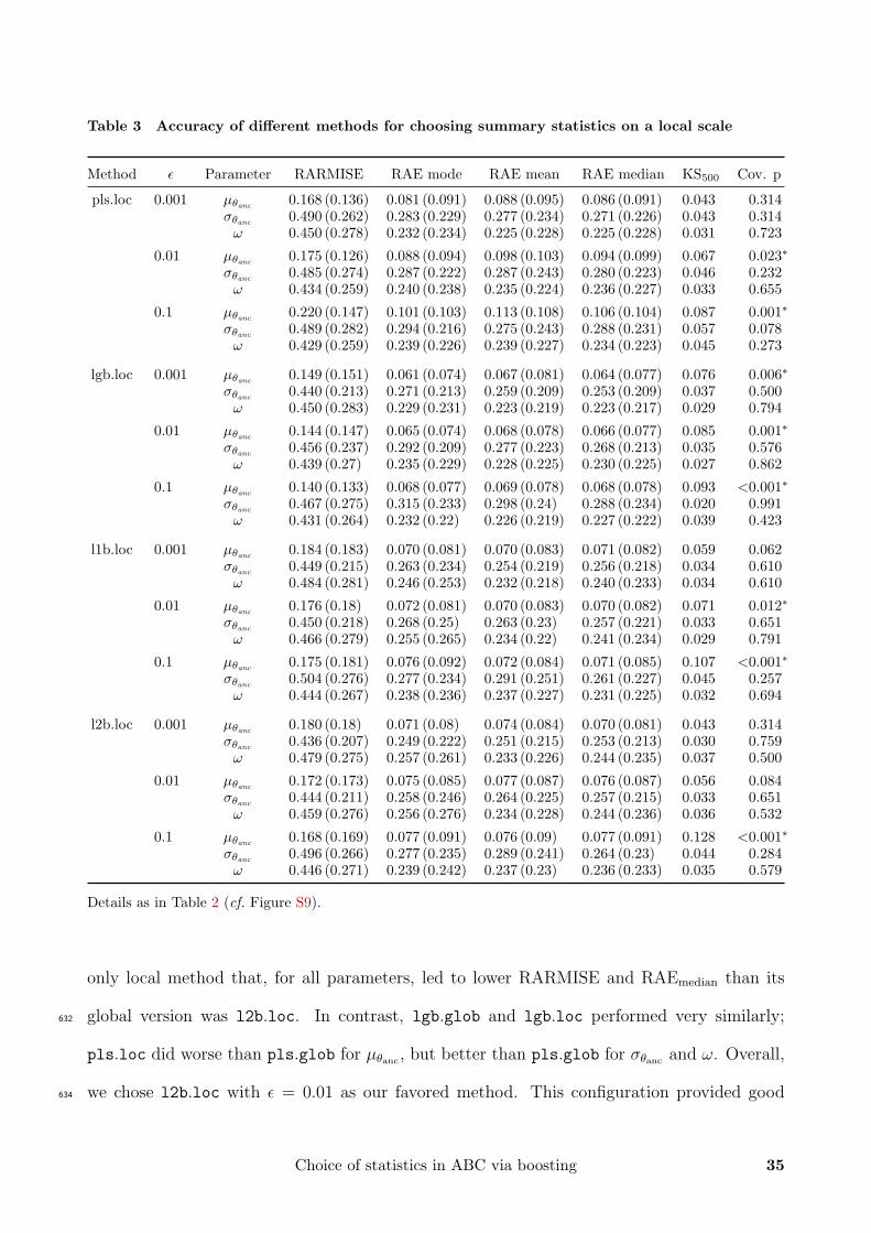
Table 3 Accuracy of different methods for choosing summary statistics on a local scale

Method ε Parameter RARMISE RAE mode RAE mean RAE median KS500 Cov. p

pls.loc 0.001 µθanc 0.168 (0.136) 0.081 (0.091) 0.088 (0.095) 0.086 (0.091) 0.043 0.314σθanc

0.490 (0.262) 0.283 (0.229) 0.277 (0.234) 0.271 (0.226) 0.043 0.314ω 0.450 (0.278) 0.232 (0.234) 0.225 (0.228) 0.225 (0.228) 0.031 0.723

0.01 µθanc0.175 (0.126) 0.088 (0.094) 0.098 (0.103) 0.094 (0.099) 0.067 0.023∗

σθanc 0.485 (0.274) 0.287 (0.222) 0.287 (0.243) 0.280 (0.223) 0.046 0.232ω 0.434 (0.259) 0.240 (0.238) 0.235 (0.224) 0.236 (0.227) 0.033 0.655

0.1 µθanc 0.220 (0.147) 0.101 (0.103) 0.113 (0.108) 0.106 (0.104) 0.087 0.001∗σθanc

0.489 (0.282) 0.294 (0.216) 0.275 (0.243) 0.288 (0.231) 0.057 0.078ω 0.429 (0.259) 0.239 (0.226) 0.239 (0.227) 0.234 (0.223) 0.045 0.273

lgb.loc 0.001 µθanc 0.149 (0.151) 0.061 (0.074) 0.067 (0.081) 0.064 (0.077) 0.076 0.006∗σθanc

0.440 (0.213) 0.271 (0.213) 0.259 (0.209) 0.253 (0.209) 0.037 0.500ω 0.450 (0.283) 0.229 (0.231) 0.223 (0.219) 0.223 (0.217) 0.029 0.794

0.01 µθanc0.144 (0.147) 0.065 (0.074) 0.068 (0.078) 0.066 (0.077) 0.085 0.001∗

σθanc 0.456 (0.237) 0.292 (0.209) 0.277 (0.223) 0.268 (0.213) 0.035 0.576ω 0.439 (0.27) 0.235 (0.229) 0.228 (0.225) 0.230 (0.225) 0.027 0.862

0.1 µθanc 0.140 (0.133) 0.068 (0.077) 0.069 (0.078) 0.068 (0.078) 0.093 <0.001∗σθanc

0.467 (0.275) 0.315 (0.233) 0.298 (0.24) 0.288 (0.234) 0.020 0.991ω 0.431 (0.264) 0.232 (0.22) 0.226 (0.219) 0.227 (0.222) 0.039 0.423

l1b.loc 0.001 µθanc 0.184 (0.183) 0.070 (0.081) 0.070 (0.083) 0.071 (0.082) 0.059 0.062σθanc

0.449 (0.215) 0.263 (0.234) 0.254 (0.219) 0.256 (0.218) 0.034 0.610ω 0.484 (0.281) 0.246 (0.253) 0.232 (0.218) 0.240 (0.233) 0.034 0.610

0.01 µθanc0.176 (0.18) 0.072 (0.081) 0.070 (0.083) 0.070 (0.082) 0.071 0.012∗

σθanc 0.450 (0.218) 0.268 (0.25) 0.263 (0.23) 0.257 (0.221) 0.033 0.651ω 0.466 (0.279) 0.255 (0.265) 0.234 (0.22) 0.241 (0.234) 0.029 0.791

0.1 µθanc0.175 (0.181) 0.076 (0.092) 0.072 (0.084) 0.071 (0.085) 0.107 <0.001∗

σθanc0.504 (0.276) 0.277 (0.234) 0.291 (0.251) 0.261 (0.227) 0.045 0.257

ω 0.444 (0.267) 0.238 (0.236) 0.237 (0.227) 0.231 (0.225) 0.032 0.694

l2b.loc 0.001 µθanc0.180 (0.18) 0.071 (0.08) 0.074 (0.084) 0.070 (0.081) 0.043 0.314

σθanc0.436 (0.207) 0.249 (0.222) 0.251 (0.215) 0.253 (0.213) 0.030 0.759

ω 0.479 (0.275) 0.257 (0.261) 0.233 (0.226) 0.244 (0.235) 0.037 0.500

0.01 µθanc0.172 (0.173) 0.075 (0.085) 0.077 (0.087) 0.076 (0.087) 0.056 0.084

σθanc 0.444 (0.211) 0.258 (0.246) 0.264 (0.225) 0.257 (0.215) 0.033 0.651ω 0.459 (0.276) 0.256 (0.276) 0.234 (0.228) 0.244 (0.236) 0.036 0.532

0.1 µθanc0.168 (0.169) 0.077 (0.091) 0.076 (0.09) 0.077 (0.091) 0.128 <0.001∗

σθanc0.496 (0.266) 0.277 (0.235) 0.289 (0.241) 0.264 (0.23) 0.044 0.284

ω 0.446 (0.271) 0.239 (0.242) 0.237 (0.23) 0.236 (0.233) 0.035 0.579

Details as in Table 2 (cf. Figure S9).

only local method that, for all parameters, led to lower RARMISE and RAEmedian than its

global version was l2b.loc. In contrast, lgb.glob and lgb.loc performed very similarly;632

pls.loc did worse than pls.glob for µθanc , but better than pls.glob for σθanc and ω. Overall,

we chose l2b.loc with ε = 0.01 as our favored method. This configuration provided good634


coverage for all parameters (Table 3). At the same time, it had lower RARMISE and RAEmedian

than pls.glob, the method that would also have had good coverage properties for µθanc . We636

disfavored all, lgb.glob and lgb.loc due to their relatively weak coverage properties. Notice

that all methods compared in Figure 4 performed worse in terms of RARMISE and RAEmedian638

than all when estimating µθanc . This might be due to the loss of information caused by leaving

out some summary statistics. Apparently, this loss is not fully compensated in our setting by640

the potential gain from reducing the dimensions. In models with many more dimensions, this

may be different.642

In summary, although performance in terms of RMISE and absolute error was not uni-

vocally in favor of l2b.loc, we preferred this method based on its good coverage properties644

(Tables 2 and 3). Moreover, for log10(σθanc) and log10(ω), the differences between methods

measured by RMISE and absolute error were small compared to the error bars (±MAD/√n),646

implying that too much weight should not be given to the respective rankings in Figures 3

and 4.648

It is worth recalling some of the characteristics of the methods compared here. The pls

method is the only one that involves de-correlation of the statistics. Apparently, this did650

not lead to a net improvement compared to the other methods. Although one explanation

might be that the statistics were only weakly correlated, Figure S10 shows evidence of strong652

correlation among some statistics. Thus, it would appear that correlation among statistics

does not substantially reduce efficiency (but this finding cannot be readily extrapolated to654

other settings, as we have only used a moderate number of summary statistics here). The

reduction of dimensions is strongest with the l1b and l2b methods, since they result in one656

linear predictor per parameter. On the other hand, these methods assume a linear relationship

between parameters and statistics. Since the latter was clearly not the case (e.g. Figure S11),658

it seems that the reduction of dimensions compensated for that assumption. This effect might

be more pronounced in problems with many more statistics.660


μθanc

log10(ε)

Stan

dard

ized

1 abs

olut

e R

MIS

E

log10(σθanc)

log10(ε)

log10(ω)

log10(ε)

A B μθanc

log10(ε)

Stan

dard

ized

1 abs

olut

e er

ror o

f med

ian

log10(σθanc)

log10(ε)

log10(ω)

log10(ε)−3.0 −2.0 −1.0

1.0

1.1

1.2

1.3

1.4

1.5

1.6

−3.0 −2.0 −1.0

0.98

1.00

1.02

1.04

1.06

−3.0 −2.0 −1.0

0.99

1.00

1.01

1.02

1.03

−3.0 −2.0 −1.0

1.00

1.05

1.10

1.15

1.20

1.25

1.30

1.35

−3.0 −2.0 −1.0

0.90

0.95

1.00

1.05

−3.0 −2.0 −1.0

0.98

1.00

1.02

1.04

1.06

1.08

pls.globlgb.globl1b.globl2b.globpls.loclgb.locl1b.locl2b.loc

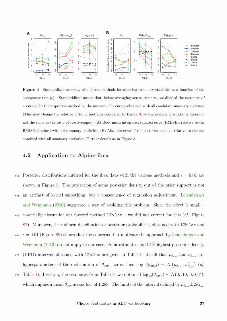
Figure 4 Standardized accuracy of different methods for choosing summary statistics as a function of the

acceptance rate (ε). 1Standaridized means that, before averaging across test sets, we divided the measures of

accuracy for the respective method by the measure of accuracy obtained with all candidate summary statistics

(This may change the relative order of methods compared to Figure 3, as the average of a ratio is generally

not the same as the ratio of two averages). (A) Root mean integrated squared error (RMISE), relative to the

RMISE obtained with all summary statistics. (B) Absolute error of the posterior median, relative to the one

obtained with all summary statistics. Further details as in Figure 3.

4.2 Application to Alpine ibex

Posterior distributions inferred for the ibex data with the various methods and ε = 0.01 are662

shown in Figure 5. The projection of some posterior density out of the prior support is not

an artifact of kernel smoothing, but a consequence of regression adjustment. Leuenberger664

and Wegmann (2010) suggested a way of avoiding this problem. Since the effect is small –

essentially absent for our favored method l2b.loc – we did not correct for this (cf. Figure666

S7). Moreover, the uniform distribution of posterior probabilities obtained with l2b.loc and

ε = 0.01 (Figure S9) shows that the concerns that motivate the approach by Leuenberger and668

Wegmann (2010) do not apply in our case. Point estimates and 95% highest posterior density

(HPD) intervals obtained with l2b.loc are given in Table 4. Recall that µθanc and σθanc are670

hyperparameters of the distribution of θanc,l across loci: log10(θanc,l) ∼ N(µθanc , σ

2θanc

)(cf.

Table 1). Inserting the estimates from Table 4, we obtained log10(θanc,l) ∼ N(0.110, 0.1632),672

which implies a mean θanc across loci of 1.288. The limits of the interval defined by µθanc±2σθanc


translate into (0.607, 2.735) on the scale of θanc. Remember that θanc = 4Neu; it measures674

the total genetic diversity present in the ancestral deme at time t1 = 1906 (Figure 2), i.e. at

the start of the re-introduction phase. Although we were able to estimate θanc with relatively676

high precision, that does not immediately tell us about Ne or u without knowing one of the

two. However, given some rough, independent estimates of Ne and u, we may assess if our678

estimate θanc ≈ 1.288 is plausible. On the one hand, historical records of the census size of

the ancestral Gran Paradiso deme are available. In combination with an estimate of the ratio680

of effective to census size, we may therefore obtain a rough estimate of Ne. Specifically, the

census size of the Gran Paradiso deme (Figure 1) was estimated as less than 100 for the early682

19th century (Scribner and Stuwe 1994, Stuwe and Nievergelt 1991), as 3000 for the early 20th

century (Stuwe and Scribner 1989), and as 4000 for the year 1913 (Maudet et al. 2002). In684

addition, Scribner and Stuwe (1994) estimated for eight ibex demes in the Swiss Alps the

effective population size from census estimates of the numbers of adult males and females.686

Their estimates of Ne were about one third of the respective total census estimates. Together,

these figures suggest that a realistic range for the ancestral effective size Ne might be between688

30 and 1300. On the other hand, estimates of the mutation rate u for microsatellites range

from 10−4 to 10−2 per locus and generation (Di Rienzo et al. 1998, Estoup and Angers 1998).690

Combining these two ranges results in θanc ranging from 1.2 · 10−2 ≈ 10−2 to 5.2 · 10 ≈ 102,

suggesting that our estimate θanc ≈ 1.288 is plausible. Perhaps more interestingly, we may692

ask about the range across loci of u that is compatible with the range of θanc corresponding

to µθanc ± 2σθanc , (0.607, 2.735). The underlying assumption is that Ne is roughly the same694

for all loci, so that variation in θanc is exclusively due to variation of u across loci. Taking the

geometric mean of the extremes from above, Ne = (30 · 1300)1/2 ≈ 197, as a typical value, the696

corresponding interval for u across loci is (7.7 · 10−4, 3.5 · 10−3). In other words, most of the

variation in u across loci spans less than one order of magnitude.698

The estimates for log10(ω) from Table 4 imply a proportion of males obtaining access


−0.4 −0.2 0.0 0.2 0.4

01

23

45

67

μθanc

Den

sity

−2.0 −1.5 −1.0 −0.5 0.0

0.0

0.5

1.0

1.5

ε = 0.01

log10(σθanc)−2.0 −1.5 −1.0 −0.5 0.0

0.0

0.5

1.0

1.5

log10(ω)

allpls.globlgb.globl1b.globl2b.globpls.loclgb.locl1b.locl2b.loc

Figure 5 Marginal posterior distributions inferred from the Alpine ibex data. Posteriors obtained with

tolerance ε = 0.01 and various methods for choosing summary statistics are compared. The dotdashed red line

corresponds to the method that performed best in the simulation study (l2b.loc; Tables 2 and 3, and Figures

3 and 4). Thin blue lines give the prior distribution (cf. Table 1). For pairwise joint posterior distributions,

see Figure 6. Point estimates and 95% HPD intervals are given in Table 4.

to matings of ω ≈ 0.208, or about 21%. The 95% HPD interval for ω is (0.047, 0.934).700

An observational study in a free-ranging ibex deme suggested that roughly 10% of males

reproduced (Aeschbacher 1978). More recently, Willisch et al. (2012) conducted a behavioral702

and genetic study and reported paternity scores for males of different age classes. The weighted

mean across age classes from this study is about 14% successful males. Given the many factors704

that influence such estimates, our result of 21% seems in good agreement with these values,

and our 95% HPD interval includes them. Two points are worth noting. First, our 95% HPD706

interval for ω seems large, which reflects the uncertainty involved in this parameter. Second,

when estimating ω, we are essentially estimating the ratio of recent effective population size708

Table 4 Posterior estimates for Alpine ibex data from ABC with summary statistics chosen

locally via L2Boosting and acceptance rate ε = 0.01

Parameter Mode Mean Median 95% HPDa interval

µθanc 0.1089 0.1081 0.1101 (−0.0391, 0.2545)log10(σθanc) −0.6453 −0.8928 −0.7867 (−1.7615, −0.2613)log10(ω) −0.6159 −0.6933 −0.6824 (−1.33, −0.0294)

aHighest posterior density.


to census population size, N(i)e /N , where N

(i)e is the effective size of a derived deme di. This

ratio may be smaller than one for many reasons – not just male mating access. Thus, we have710

strictly speaking estimated the strength of genetic drift due to deviations in reproduction

from that in an idealized population. Nevertheless, the good agreement with the independent712

estimates of male mating access is striking.

In Figure 6, we report pairwise joint posterior distributions for l2b.loc and ε = 0.01. The714

pairwise joint modes are close to the marginal point estimates in Table 4. Moreover, Figure 6

suggests no strong correlation among parameters.

−0.4 −0.2 0.0 0.2

−2.0

−1.5

−1.0

−0.5

0.0

μθanc

log 1

0(σθ a

nc)

0.5

1

1.5 2

2.5

3

3.5

4.5

5

0.11

−0.66

−0.4 −0.2 0.0 0.2

−1.5

−1.0

−0.5

0.0

l2b.loc, ε = 0.01

μθanc

log 1

0(ω)

0.5

1

1.5

2

2.5

3

3.5

4

4.5

5

0.12

−0.68

−2.0 −1.5 −1.0 −0.5 0.0

−1.5

−1.0

−0.5

0.0

log10(σθanc)

log 1

0(ω)

0.1

0.2

0.3

0.4

0.5

0.6

0.7 0.8

0.9 1

1.1

1.2

−0.66

−0.66

Figure 6 Pairwise joint posterior distributions given data observed in Alpine ibex, obtained with tolerance

ε = 0.01 and summary statistics choosen locally via L2Boosting (l2b.loc). Red triangles denote parameter

values corresponding to the pairwise joint modes. Each time, the third parameter has been marginalized over.

716


5 Discussion

We have suggested three variants of boosting for the choice of summary statistics in ABC718

and compared them to each other, to partial least squares (PLS) regression and to ABC

with all candidate summary statistics. Moreover, we proposed to choose summary statistics720

locally, in the putative neighborhood of the observed data. Overall, the mean of the ancestral

mutation rate µθanc was more precisely estimated than its standard deviation σθanc and the722

male mating access rate ω. In our context, ABC with summary statistics chosen locally via

boosting with component-wise linear regression as base procedure and the L2-loss performed724

best in terms of accuracy (measured by RARMISE and RAEmedian) and uniformity of posterior

probabilities together. However, the difference between the methods was moderate and the726

ranking depended to some degree on our choice of criteria to assess performance. If the main

interest had been in a small error of point estimates (low RAEmedian), but less in good overall728

posterior properties (low RARMISE and uniform posterior probabilities of the true value)

at the same time, boosting with the negative binomial log-likelihood loss and, somewhat730

surprisingly, ABC with all candidate statistics, would have been preferable to boosting with

the L1- and L2-loss. Under this criterion (low RAEmedian), the performance of the PLS method732

was intermediate when estimating ω, but inferior to that of any boosting approach when

estimating µθanc and σθanc . In general, choosing summary statistics locally slightly improved734

the accuracy compared to the global choice, but it led to worse posterior coverage for µθanc .

The local version of L2Boosting with acceptance rate ε = 0.01 coped best with this trade-off.736

Applying that method to Alpine ibex data, we estimated the mean across loci of the

scaled ancestral mutation rate as θanc ≈ 1.288. The estimates for σθanc implied that most738

of the variation across loci of the mutation rate u was between 7.7 · 10−4 and 3.5 · 10−3.

The proportion of males obtaining access to matings per breeding season was estimated to740

ω ≈ 0.21, which is in good agreement with recent independent estimates. This result suggests


that the strong dominance hierarchy in Alpine ibex is reflected in overall genetic diversity, and742

should therefore be considered an important factor determining the strength of genetic drift.

It should be noted that the results we reported here about the choice of summary statistics744

are specific to the model, the data and, in particular, to the choice of criteria used to assess

performance. Another method may perform better under a different setting, and this is746

most likely a general feature of inference with ABC (cf. Blum et al. 2012). For the various

points where some choice must be made – summary statistics, metric, algorithm, post-rejection748

adjustment – by nature, no single strategy is best in every case. Rather, the focus should be

on choosing the best strategy for a specific problem. In practice, this implies comparing750

alternatives and assessing performance in a simulation study. Along these lines, there is still

scope for new ideas concerning the various choices in ABC (see Beaumont et al. 2010). In752

particular, the choice of the metric makes ABC a scale-dependent method. This applies both

to the ABC algorithm in general, as well as to our suggestion of choosing summary statistics in754

the putative neighborhood of the truth. One could, for instance, use the Mahalanobis instead

of the Euclidean distance, but even this is based on an assumption that is not necessarily756

appropriate (multivariate normal distribution of variables). In a specific application, one

metric may do better than another, but it may not be obvious why. Overall, this poses an758

open problem and motivates future research (Wilkinson 2008).

As more data become available and more complex models are justifiable, it will be necessary760

that methods of inference keep pace. In principle, ABC is scalable and able to face this

challenge. The problems arise in practice, and the combination of approaches devised to762

tackle them is itself becoming intricate. Researchers may be interested in a single program

that implements these approaches and allows for inference with limited effort needed for tuning,764

simulation and cross-validation. However, such software runs the risk of being treated as a

black box. This problem is not unique to ABC, but equally applies to other sophisticated766

approaches of inference, such as coalescent-based genealogy samplers (Kuhner 2009). In the


context of ABC, rather than having a single piece of software, we find it more promising to768

combine separate pieces of software that each implement a specific step. The appropriate

combination must be chosen specifically for any application. It will always be necessary to770

evaluate the performance of any ABC method through simulation-based studies. Such a

modular approach has recently been fostered by the developers of ABCtoolbox (Wegmann772

et al. 2010) or the abc package for R (Csillery et al. 2011). Here, we contribute to this by

providing a flexible simulation program that readily integrates into any ABC procedure.774

Recently, two interesting alternative approaches have been proposed for choosing summary

statistics with a focus on the putative location of the true parameter value, rather than the776

whole prior range. Nunes and Balding (2010) suggest a two-step procedure. Starting with a

set of candidate summary statistics, at a first stage, standard ABC is carried out for (possibly)778

all subsets of these statistics, and the subset resulting in the posterior distribution with the

minimum entropy is chosen. This subset of statistics is used to determine the n′ simulations780

with the smallest Euclidean distance to the observation. At the second stage, the n′ data

sets close to the putative truth are used as a training set to choose, again, among (possibly)782

all subsets of the original candidate statistics. Here, Nunes and Balding (2010) propose as

optimization criterion the average square root of the sum of squared errors, averaged over the784

training data sets.

Fearnhead and Prangle (2012) follow the idea of optimizing the choice of summary statistics786

with respect to the accuracy of certain estimates of the parameters (e.g. a point estimate),

rather than the full posterior distribution. For instance, if the goal is to minimize the quadratic788

loss between the point estimate and the true value, the authors prove that the posterior mean

is the optimal summary statistic. Since the posterior mean is not available in advance, they790

propose to first conduct a pilot ABC study to determine the region of high posterior mass.

For this region, they then draw parameters and simulate data to obtain training data sets.792

These are used in a third step to fit a linear regression with the parameters as responses and a


vector-valued function of the original summary statistics as explanatory variables (allowing for794

non-linear transformations of the original statistics). The linear fits are used as new summary

statistics for the corresponding parameter. A final ABC run is then performed, with a prior796

restricted to the range established in the first step, and summary statistics chosen in the

third step. Fearnhead and Prangle (2012) refer to this as semi-automatic and independent798

of the choice of statistics. However, as the authors note, it does depend on the initial choice

of candidate statistics and on the choice of the vector-valued function. Moreover, if the800

(transposed) candidate statistics are uncorrelated, we suspect that their method would be

equivalent to using the first component in a univariate PLS regression.802

The approaches by Nunes and Balding (2010) and Fearnhead and Prangle (2012), and our

local boosting procedures all consist of several steps, at least one being devoted to establishing804

the vicinity of the putative truth. While the method by Nunes and Balding (2010) and Logit-

Boost aim at choosing the ‘best subset’ from a set of candidate statistics (without transforming806

them), the method by Fearnhead and Prangle (2012), PLS, L1-, and L2Boosting ‘construct’

new summary statistics as functions of the original ones. The former has the advantage that808

the summary statistics conserve their interpretation, while the latter has the potential of bet-

ter extracting and combining information contained partly in the various candidate statistics.810

The method by Nunes and Balding (2010) suffers from the fact that all subsets of candidate

statistics must be explored, which is prohibitive in the case of large numbers of statistics. Here,812

boosting offers a potential advantage, because the functional gradient descent is a ‘greedy’ al-

gorithm (see Appendix). It does not explore all possible combinations of statistics, but in814

any iteration selects only one candidate statistic that improves an optimization criterion, given

the current stage of the algorithm.816

A direct comparison of all the recently proposed methods for the choice of statistics in ABC

(e.g. Joyce and Marjoram 2008, Wegmann et al. 2009, Nunes and Balding 2010, Fearnhead818

and Prangle 2012, Jung and Marjoram 2011) seems due. Nunes and Balding (2010) and


Blum et al. (2012) compare a subset of these methods for a simple toy model with mutation820

and recombination in a panmictic population (cf. Joyce and Marjoram 2008). Blum et al.

(2012) also include two examples from epidemiological modeling and material science. Their822

main conclusion is that the best method depends on the model. Crucial aspects seem to be

the number of parameters, the number of candidate summary statistics, and the degree of824

collinearity of the statistics. Importantly, the PLS method (Wegmann et al. 2009) – although

widely used in recent ABC applications – has been shown not to be very efficient and our826

results are consistent with this. However, a comparison for a range of relevant population

genetic models, including some with larger numbers of parameters, is currently missing.828

The boosting approach proposed here should also be suitable for constructing summary

statistics to perform model comparison with ABC (e.g. Fagundes et al. 2007, Blum and Jakob-830

sson 2011). Despite recent criticism (Robert et al. 2011, but see Didelot et al. 2011), ABC-type

model comparison remains an interesting option. By treating the model index as the single832

response, the algorithm proposed here might be used in this context.


Literature Cited834

Aeschbacher, A., 1978 Das Brunftverhalten des Alpensteinbocks . Eugen Rentsch Verlag,

Erlenbach-Zurich.836

Aeschbacher, S., A. Futschik, and M. A. Beaumont, 2012 Approximate Bayesian computation

for modular inference problems with many parameters: the example of migration rates. In838

revision.

Akaike, H., 1974 A new look at the statistical model identification. IEEE Trans. Autom.840

Control 19: 716–723.

Barton, N. H., 2000 Genetic hitchhiking. Phil. Trans. R. Soc. B. 355: 1553–1562.842

Beaumont, M. A., 2010 Approximate Bayesian computation in evolution and ecology. Annu.

Rev. Ecol. Evol. Syst. 41: 379–406.844

Beaumont, M. A., J.-M. Cornuet, J.-M. Marin, and C. P. Robert, 2009 Adaptive approximate

Bayesian computation. Biometrika 96: 983–990.846

Beaumont, M. A., R. Nielsen, C. P. Robert, J. Hey, O. Gaggiotti, L. Knowles, A. Estoup,

M. Panchal, J. Corander, M. Hickerson, S. A. Sisson, N. Fagundes, L. Chikhi, P. Beerli,848

R. Vitalis, J.-M. Cornuet, J. Huelsenbeck, M. Foll, Z. H. Yang, F. Rousset, D. Balding,

and L. Excoffier, 2010 In defence of model-based inference in phylogeography – Reply. Mol.850

Ecol. 19: 436–446.

Beaumont, M. A. and B. Rannala, 2004 The Bayesian revolution in genetics. Nat. Rev. Genet.852

5: 251–261.

Beaumont, M. A., W. Zhang, and D. J. Balding, 2002 Approximate Bayesian computation in854

population genetics. Genetics 162: 2025–2035.


Bertorelle, G., A. Benazzo, and S. Mona, 2010 ABC as a flexible framework to estimate856

demography over space and time: some cons, many pros. Mol. Ecol. 19: 2609–2625.

Biebach, I. and L. F. Keller, 2009 A strong genetic footprint of the re-introduction history of858

Alpine ibex (Capra ibex ibex ). Mol. Ecol. 18: 5046–5058.

Blum, M. and O. Francois, 2010 Non-linear regression models for approximate Bayesian com-860

putation. Stat. Comput. 20: 63–73.

Blum, M. G. B. and M. Jakobsson, 2011 Deep divergences of human gene trees and models of862

human origins. Mol. Biol. Evol. 28: 889–898.

Blum, M. G. B., M. A. Nunes, D. Prangle, and S. A. Sisson, 2012 A comparative review of864

dimension reduction methods in approximate Bayesian comptutation. In Review .

Buhlmann, P. and T. Hothorn, 2007 Boosting algorithms: Regularization, prediction and866

model fitting. Stat. Sci. 22: 477–505.

Charlesworth, B. and D. Charlesworth, 2010 Elements of Evolutionary Genetics . Roberts &868

Company Publishers, Greenwood Village, Colorado.

Charlesworth, B., M. T. Morgan, and D. Charlesworth, 1993 The effect of deleterious muta-870

tions on neutral molecular variation. Genetics 134: 1289–1303.

Cook, S. R., A. Gelman, and D. B. Rubin, 2006 Validation of software for Bayesian models872

using posterior quantiles. J. Comput. Graph. Stat. 15: 675–692.

Couturier, M. A. J., 1962 Le bouquetin des Alpes – Capra aegagrus ibex ibex L.. Chez l’auteur,874

54, Rue Thiers, Allier, Grenoble.

Csillery, K., M. Blum, and O. Francois, 2011 Tools for Approximate Bayesian Computation876

(ABC). The Comprehensive R Archive Network.


Csillery, K., M. G. B. Blum, O. E. Gaggiotti, and O. Francois, 2010 Approximate Bayesian878

computation (ABC) in practice. Trends Ecol. Evolut. 25: 410–418.

Di Rienzo, A., P. Donnelly, C. Toomajian, B. Sisk, A. Hill, M. L. Petzl-Erler, G. K. Haines,880

and D. H. Barch, 1998 Heterogeneity of microsatellite mutations within and between loci,

and implications for human demographic histories. Genetics 148: 1269–1284.882

Didelot, X., R. G. Everitt, A. M. Johansen, and D. J. Lawson, 2011 Likelihood-free estimation

of model evidence. Bayes. Anal. 6: 49–76.884

Diggle, P. J., 1979 On parameter estimation and goodness-of-fit testing for spatial point pat-

terns. Biometrics 35: 87–101.886

Diggle, P. J. and R. J. Gratton, 1984 Monte carlo methods of inference for implicit statistical

models. J. R. Stat. Soc. B 46: 193–227.888

Estoup, A. and B. Angers, 1998 Microsatellites and minisatellites for molecular ecology: The-

oretical and empirical considerations. In Advances in Molecular Ecology , edited by G. R.890

Carvalho, volume 306, pp. 55–86, IOS Press, Amsterdam, Netherlands.

Estoup, A. and J.-M. Cornuet, 1999 Microsatellite evolution: inference from population data.892

In Microsatellites – Evolution and Application, edited by D. B. Goldstein and C. Schloet-

terer, pp. 49–65, Oxford University Press Inc.894

Fagundes, N. J. R., N. Ray, M. Beaumont, S. Neuenschwander, F. M. Salzano, S. L. Bonatto,

and L. Excoffier, 2007 Statistical evaluation of alternative models of human evolution. Proc.896

Natl. Acad. Sci. U.S.A. 104: 17614–17619.

Fearnhead, P. and D. Prangle, 2012 Constructing summary statistics for approximate Bayesian898

computation: semi-automatic approximate Bayesian computation. J. R. Stat. Soc. B 74:

419–474.900


Fisher, R. A., 1922 On the mathematical foundations of theoretical statistics. Phil. Trans. R.

Soc. A 222: 309–368.902

Frazer, K. A., D. G. Ballinger, D. R. Cox, D. A. Hinds, and L. L. e. Stuve, 2007 A second

generation human haplotype map of over 3.1 million SNPs. Nature 449: 851–861.904

Freund, Y., 1995 Boosting a weak learning algorithm by majority. Informa. Comput. 121:

256–285.906

Freund, Y. and R. E. Schapire, 1996 Experiments with a new boosting algorithm. In Machine

Learning: Proceedings of the Thirteenth International Conference (ICML ’96), edited by908

L. Saitta, pp. 148–156, San Francisco, California, Morgan Kaufmann Publishers Inc.

Freund, Y. and R. E. Schapire, 1999 A short introduction to boosting. J. Jpn. Soc. Artif.910

Intell. 14: 771–780.

Friedman, J., T. Hastie, and R. Tibshirani, 2000 Special Invited Paper. Additive Logistic912

Regression: A Statistical View of Boosting. Ann. Stat. 28: 337–374.

Friedman, J. H., 2001 Greedy function approximation: A gradient boosting machine. Ann.914

Stat. 29: 1189–1232.

Fu, Y. X. and W. H. Li, 1997 Estimating the age of the common ancestor of a sample of DNA916

sequences. Mol. Biol. Evol. 14: 195–199.

Gelman, A., J. B. Carlin, H. S. Stern, and D. B. Rubin, 2004 Bayesian Data Analysis . Chap-918

man & Hall/CRC, Boca Raton, Florida, second edition.

Ghosh, M., N. Reid, and D. A. S. Fraser, 2010 Ancillary statistics: a review. Stat. Sinica 20:920

1309–1332.

Haldane, J. B. S., 1932 The Causes of Evolution. Princeton University Press, second edition.922


Hamilton, G., M. Currat, N. Ray, G. Heckel, M. Beaumont, and L. Excoffier, 2005 Bayesian

estimation of recent migration rates after a spatial expansion. Genetics 170: 409–417.924

Hastie, T., R. Tibshirani, and J. Friedman, 2011 The Elements of Statistical Learning – Data

Mining, Inference, and Prediction. Springer Verlag, second edition.926

Hothorn, T., P. Buhlmann, T. Kneib, S. M., and H. B., 2011 mboost: Model-based boosting,

R package version 2.0-11.928

Joyce, P. and P. Marjoram, 2008 Approximately sufficient statistics and Bayesian computation.

Stat. Appl. Genet. Mol. Biol. 7.930

Jung, H. and P. Marjoram, 2011 Choice of Summary Statistic Weights in Approximate

Bayesian Computation. Stat. Appl. Genet. Mol. Biol. 10.932

Kuhner, M. K., 2009 Coalescent genealogy samplers: windows into population history. Trends

Ecol. Evolut. 24: 86–93.934

Le Cam, L., 1964 Sufficiency and approximate sufficiency. Ann. Math. Stat. 35: 1419–1455.

Leuenberger, C. and D. Wegmann, 2010 Bayesian computation and model selection without936

likelihoods. Genetics 184: 243–252.

Lin, K., H. Li, C. Schlotterer, and A. Futschik, 2011 Distinguishing positive selection from938

neutral evolution: Boosting the performance of summary statistics. Genetics 187: 229–244.

Mahalanobis, P. C., 1936 On the generalized distance in statistics. Proc. Natl. Inst. Sci. India940

2: 49–55.

Marjoram, P., J. Molitor, V. Plagnol, and S. Tavare, 2003 Markov chain Monte Carlo without942

likelihoods. Proc. Natl. Acad. Sci. U.S.A. 100: 15324–15328.

Marjoram, P. and S. Tavare, 2006 Modern computational approaches for analysing molecular944

genetic variation data. Nat. Rev. Genet. 7: 759–770.


Maudet, C., C. Miller, B. Bassano, C. Breitenmoser-Wursten, D. Gauthier, G. Obexer-Ruff,946

J. Michallet, P. Taberlet, and G. Luikart, 2002 Microsatellite DNA and recent statisti-

cal methods in wildlife conservation management: applications in Alpine ibex [Capra ibex948

(ibex)]. Mol. Ecol. 11: 421–436.

Maynard Smith, J. and J. Haigh, 1974 Hitch-hiking effect of a favorable gene. Genet. Res. 23:950

23–35.

Mevik, B.-H. and R. Wehrens, 2007 The pls package: Principal component and partial least952

squares regression in R. J. Stat. Software 18: 1–24.

Nei, M. and R. K. Chesser, 1983 Estimation of fixation indexes and gene diversities. Ann.954

Hum. Genet. 47: 253–259.

Nunes, M. A. and D. J. Balding, 2010 On optimal selection of summary statistics for approx-956

imate Bayesian computation. Stat. Appl. Genet. Mol. Biol. 9.

Ohta, T. and M. Kimura, 1973 Model of mutation appropriate to estimate number of elec-958

trophoretically detectable alleles in a finite population. Genet. Res. 22: 201–204.

Pritchard, J., M. Seielstad, A. Perez-Lezaun, and M. Feldman, 1999 Population growth of960

human Y chromosomes: a study of Y chromosome microsatellites. Mol. Biol. Evol. 16:

1791–1798.962

R Development Core Team, 2011 R: A Language and Environment for Statistical Computing .

R Foundation for Statistical Computing, Vienna, Austria.964

Raiffa, H. and R. Schlaifer, 1968 Applied Statistical Decision Theory . John Wiley and Sons,

Ltd.966


Robert, C. P., J.-M. Cornuet, J.-M. Marin, and N. S. Pillai, 2011 Lack of confidence in

approximate bayesian computation model choice. Proc. Natl. Acad. Sci. U.S.A. 108: 15112–968

15117.

Rosenberg, N. A., J. K. Pritchard, J. L. Weber, H. M. Cann, K. K. Kidd, L. A. Zhivotovsky,970

and M. W. Feldman, 2002 Genetic structure of human populations. Science 298: 2381–2385.

Rubin, D. B., 1984 Bayesianly justifiable and relevant frequency calculations for the applied972

statistician. Ann. Stat. 12: 1151–1172.

Schapire, R. E., 1990 The strength of weak learnability. Mach. Learn. 5: 197–227.974

Scribner, K. T. and M. Stuwe, 1994 Genetic relationships among Alpine ibex Capra ibex

populations reestablished from a common ancestral source. Biol. Conserv. 69: 137–143.976

Shao, J., 2003 Mathematical Statistics . Springer, New York, second edition.

Sisson, S. A., Y. Fan, and M. M. Tanaka, 2007 Sequential Monte Carlo without likelihoods.978

Proc. Natl. Acad. Sci. U.S.A. 104: 1760–1765.

Sisson, S. A., Y. Fan, and M. M. Tanaka, 2009 Correction for Sisson et al., Sequential Monte980

Carlo without likelihoods. Proc. Natl. Acad. Sci. U.S.A. 106: 16889–16889.

Slatkin, M., 1995 A measure of population subdivision based on microsatellite allele frequen-982

cies. Genetics 139: 457–462.

Sokal, R. R. and J. F. Rohlf, 1981 Biometry – The Principles and Practice of Statistics in984

Biological Research. W. H. Freeman and Company, New York, second edition.

Stuwe, M. and C. Grodinsky, 1987 Reproductive biology of captive Alpine ibex (Capra i.986

ibex ). Zoo Biol. 6: 331–339.


Stuwe, M. and B. Nievergelt, 1991 Recovery of Alpine ibex from near extinction – the result988

of effective protection, captive breeding, and reintroduction. Appl. Anim. Behav. Sci. 29:

379–387.990

Stuwe, M. and K. T. Scribner, 1989 Low genetic variablility in reintroduced Alpine ibex (Capra

ibex ibex ) populations. J. Mammal. 70: 370–373.992

Tavare, S., D. J. Balding, R. C. Griffiths, and P. Donnelly, 1997 Inferring coalescence times

from DNA sequence data. Genetics 145: 505–518.994

Toni, T., D. Welch, N. Strelkowa, A. Ipsen, and M. P. H. Stumpf, 2009 Approximate Bayesian

computation scheme for parameter inference and model selection in dynamical systems. J.996

R. Soc. Interface 6: 187–202.

Wegmann, D., C. Leuenberger, and L. Excoffier, 2009 Efficient approximate Bayesian compu-998

tation coupled with Markov chain Monte Carlo without likelihood. Genetics 182: 1207–1218.

Wegmann, D., C. Leuenberger, S. Neuenschwander, and L. Excoffier, 2010 ABCtoolbox: a1000

versatile toolkit for approximate Bayesian computations. BMC Bioinformatics 11.

Weiss, G. and A. von Haeseler, 1998 Inference of population history using a likelihood ap-1002

proach. Genetics 149: 1539–1546.

Wilkinson, R. D., 2008 Approximate Bayesian computation (ABC) gives exact results under1004

the assumption of model error. arXiv:0811.3355v1.

Williamson, S. H., R. Hernandez, A. Fledel-Alon, L. Zhu, R. Nielsen, and C. D. Bustamante,1006

2005 Simultaneous inference of selection and population growth from patterns of variation

in the human genome. Proc. Natl. Acad. Sci. U.S.A. 102: 7882–7887.1008

Willisch, C., I. Biebach, U. Koller, T. Bucher, N. Marreros, M.-P. Ryser-Degiorgis, L. Keller,

and P. Neuhaus, 2012 Male reproductive pattern in a polygynous ungulate with a slow1010


life-history: the role of age, social status and alternative mating tactics. Evol. Ecol. 26:

187–206.1012

Willisch, C. S. and P. Neuhaus, 2009 Alternative mating tactics and their impact on survival

in adult male Alpine ibex (Capra ibex ibex ). J. Mammal. 90: 1421–1430.1014

Wright, S., 1951 The genetical structure of populations. Ann. Eugenics 15: 323–354.

Acknowledgements1016

We thank Nick Barton, Christoph Lampert, and three anonymous reviewers for helpful com-

ments on earlier versions of the manuscript. We are grateful to Iris Biebach and Lukas Keller1018

for providing genetic data and for help in reconstructing the demographic data. We thank

Markus Brulisauer, Erwin Eggenberger, Flurin Filli, Bernhard Nievergelt, Marc Rosset Urs1020

Zimmermann, Martin Zuber, the staff from Tierpark Langenberg, Tierpark Dahlholzli (Bern),

Wildpark Peter and Paul (St. Gallen), Wildtier Schweiz, and the Swiss Federal Office for1022

the Environment for providing information on population history and re-introduction, and

Barbara Oberholzer for double-checking the re-introduction history. We thank Walter Abder-1024

halden, Iris Biebach, Michael Blum, Kati Csillery, Lukas Keller, and Christian Willisch for

discussion. This work has made use of the computational resources provided by IST Austria1026

and the Edinburgh Compute and Data Facility (ECDF; http://www.ecdf.ed.ac.uk). The

ECDF is partially supported by the eDIKT initiative (http://www.edikt.org.uk). S.A. ac-1028

knowledges financial support by IST Austria, the Janggen-Pohn Foundation, St. Gallen, the

Roche Research Foundation, Basel, and by the University of Edinburgh in form of a Torrance1030

Studentship.


http://www.ecdf.ed.ac.uk

http://www.edikt.org.uk

6 Appendix1032

6.1 Modular inference for high dimensional problems using ABC

Here, we explore how ABC can be applied to complex situations, where a modular structure of1034

the inferential problem can be exploited. For this purpose, we will assume that the parameter

vector φ relevant to the problem can be split into two subvectors α and m, and that we have1036

two corresponding vectors of summary statistics Sα and Sm, such that Sα contains most of

the information on α, whereas Sm contains most of the information on m. It turns out that1038

the modular structure can be exploited in such a situation, to split a high dimensional problem

into sub-problems involving only lower dimensional summary statistics.1040

To make this precise, we adapt the concepts of approximate sufficiency (e.g. Le Cam 1964)

and approximate ancillarity (Ghosh et al. 2010 and references therein). In the context of ABC,1042

Joyce and Marjoram (2008) proposed an approach for choosing summary statistics based on

approximate sufficiency.1044

In particular, we call Sα to be ε-sufficient for α with respect to Sm, if

supα

lnπ(Sm | Sα, m, α)− infα

lnπ(Sm | Sα, m, α) ≤ ε (14)

for all m. We further define Sα to be δ-ancillary with respect to m, if1046

supm

ln π(Sα | m, α)− infm

lnπ(Sα | m, α) < δ (15)

for all α. Analogously, we define ε-sufficiency and δ-ancillarity for Sm (notice that ε and δ do

not have the same meaning here as in the main text).1048

We first assume that Sα is ε-sufficient for α relative to Sm, and δ-ancillary with respect


to m. Then,1050

π(α | S) =

∫π(m, α | S) dm

=

∫π(Sα, Sm | m, α) π(α) π(m) dm∫ ∫π(Sα, Sm | m, α) π(α) π(m) dm dα

=

∫π(Sα | m, α)π(α)π(Sm | Sα, m, α) π(m) dm∫ ∫π(Sα | m, α) π(α) π(Sm | Sα, m, α)π(m) dm dα

≤π(Sα | α) π(α) eδ

∫supα π(Sm | Sα, m, α) π(m) dm

e−δ∫π(Sα | α) π(α) dα

∫infα π(Sm | Sα, m, α) π(m) dm

≤ π(α | Sα) e2δ+ε.

(16)

A lower bound can be obtained in an analogous way, and we get

π(α | Sα) e−2δ−ε ≤ π(α | S) ≤ π(α | Sα) e2δ+ε. (17)

If δ and ε are both small, a good approximation to the ABC-posterior π(α | S) can therefore1052

be obtained by using only Sα.

Next, we will look at the ABC-posterior for m given α, π(m | α, Sm), and start with1054

formulas (4)

π(m, α | S) = π(m | α, S) π(α | S) (18)

and (5)1056

π(α | S) =

∫π(m, α | S) dm (19)

from the main paper, replacing the full data D by the summary statistics S.

From (19) it follows that a sample from the marginal posterior of α can be obtained by1058

taking the α components of a sample from the joint posterior of m and α.

As shown above, π(α | S) can be replaced without much loss by π(α | Sα), if Sm is not1060

informative for α and Sα is not informative for m. We will show that π(m | α, S) = π(m |


α, Sα, Sm) ≈ π(m | α, Sm), given that Sm is ε-sufficient for m.1062

π(m | α, Sα, Sm) = π(Sα | α, m, Sm)π(α, m, Sm)

π(α, Sα,Sm)

≤ eε π(Sα | α, Sm)π(α, m, Sm)

π(α, Sα, Sm)

= eε π(Sα | α, Sm)π(α, m, Sm)

π(Sα | α, Sm) π(α, Sm)

= eεπ(α, m, Sm)

π(α, Sm)

= eε π(m | α, Sm).

(20)

Together with an analogously obtained lower bound, we have that

e−ε π(m | α, Sm) ≤ π(m | α, Sα, Sm) ≤ eε π(m | α, Sm) (21)

and again Sα can be omitted without much loss, if Sα does not provide much further infor-1064

mation about m given Sm.

To summarize, breaking up ABC into lower dimensional modules with separate summary1066

statistics can be shown to lead to good approximations, if Sα and Sm are ε-sufficient with

respect to each other for their respective parameters. Also, Sα should be δ-ancillary for m.1068

6.2 Functional gradient descent boosting algorithm

The general functional gradient descent (FGD) algorithm for boosting, as given by Friedman1070

(2001) and modified by Buhlmann and Hothorn (2007), is:

FGD algorithm:1072

1. Initialize F [0](·) ≡ arg minc n−1∑n

i=1 L(Yi, c),

set m = 0.1074


2. Increase m by 1. Compute the negative gradient and evaluate at F [m−1](Xi):

Ui = − ∂

∂FL(Yi, F )|F=F [m−1](Xi)

.

3. Fit the negative gradient vector (U1, . . . , Un) to (X1, . . . , Xn) by the base procedure:1076

(Xi, Ui)ni=1 −→ g[m].

4. Update F [m](·) = F [m−1](·) + νg[m](·), where ν is a step-length factor.

5. Iterate steps 2 to 4 until m = mstop.1078

Here, ν and mstop are tuning parameters discussed in the main text. The result of this

algorithm is a linear combination F (·) of base procedure estimates, as shown in equation (7)1080

of the main text. In any specific version of boosting, the form of the initial function F [0](·)

in step 1, and the negative gradient Ui in step 2 may be expressed explicitly according to the1082

loss function L(·, ·) (see SI).

6.3 Base procedure: component-wise linear regression1084

We write the jth component of a vector v as v(j). The following base procedure performs

simple component-wise linear regression:1086

g(X) = λ(ζ)X(ζ),

λ(j) =n∑i=1

X(j)Ui

/ n∑i=1

(X

(j)i

)2

,

ζ = arg min1≤j≤p

n∑i=1

(Ui − λ(j)X

(j)i

)2

,

(22)

where g(·), X and Ui are as in the FGD algorithm above. This base procedure selects the best

variable in a simple linear model in the sense of ordinary least squares fitting (Buhlmann and1088


Hothorn 2007). To see this, note that λ(j) in (22) is the ordinary least squares solution of a

linear regression Ui = X(j)i λ(j), in matrix form λ(j) =

(X

(j)>i X

(j)i

)−1X

(j)>i Ui. The choice of the1090

loss functions enters indirectly via Ui (see SI).


A Novel Approach for Choosing Summary Statistics in Approximate Bayesian Computation

Documents

Transcript of A Novel Approach for Choosing Summary Statistics in Approximate Bayesian Computation