Choosing Brands: Fresh Produce versus Other Products

CHOOSING BRANDS: FRESH PRODUCE VERSUS

OTHER PRODUCTS

YANHONG H. JIN, DAVID ZILBERMAN, AND AMIR HEIMAN

Assuming that brands contribute to quality risk reduction, prestige, and design, we derive and testhypothesis on the willingness to pay (WTP) for brands across different product categories (electronics,clothing, packaged food, and fresh produce). Using the random effect tobit model on the stated pointvalue of WTP and the ordered probit model on the stated range of WTP, we find that WTP for brandsof fresh produce is least among the four product categories controlling for relevant demographicvariations. Simulations show that fresh produce has a higher optimal price premium for brands butwith a much smaller market share.

Key words: brands, fresh produce, hedonic pricing, maximum entropy, ordered probit, tobit, willing-ness to pay.

Brands tend to generate significant premiums,and thus their uses have been considered inenhancing the value added of farming (Hayesand Lence 2002). Yet, brands are less com-monly used in fresh agricultural produce thanother products (Kaufman et al. 2000). With thegreater emphasis on product differentiation,research on agricultural marketing strategiesrequires understanding the reasons for the rel-ative paltry use of brands in the farm sector. Inaddition, it is important to assess the relativegains from introducing brands of fresh agricul-tural products and to identify features of theirlikely buyers. This article develops a method-ological and empirical strategy to answer thesequestions and applies it to data collected inCollege Station and Bryan, Texas, in fall 2006.

We will investigate the following questionsto explain the lack of brands of fresh produce:(a) Do the same causes of preferring brandsover generics apply to fresh produce? (b) Doconsumers have significantly lower willingnessto pay (WTP) for brands of fresh produce thanother product categories? (c) To what extentare brands’ premiums and market shares ofproduce different from other products? (d) To

Yanhong H. Jin is assistant professor in the Department of Agri-cultural Economics at Texas A&M University. David Zilbermanis professor in the Department of Agricultural and Resource Eco-nomics at University of California, Berkeley, and a member of theGiannini Foundation of Agricultural Economics. Amir Heiman issenior lecturer in the Department of Agricultural Economics andManagement at Hebrew University, Israel.

The authors thank Ellen Yi-Qian Hsu for conducting the surveyand Ximing Wu for review of an earlier draft. The authors aregrateful to the editor and three anonymous referees for helpfulcomments that significantly improved the article. Of course, anyremaining errors are the authors’.

what extent are consumers consistent in theirbrand preference across product categories?

The rest of this article is organized as follows.We present a simple framework to explain dif-ferent components that contribute to the brandpremium. We then provide data informationand discuss the empirical results. Our estima-tion results show that (a) consumers have alower WTP for brands of fresh produce thanin other categories including electronics, cloth-ing, and packaged food; and (b) certain socio-demographic factors play an important rolein WTP for brands, including income, educa-tion, age, race, gender, and household size.The simulation results suggest that brands offresh produce have a higher optimal price pre-mium but a much smaller market share thanthose of other products. The simulation re-sults also show that individuals are consistentin their WTP for brands across product cate-gories, and thus there is a potential gain fromselling brands of fresh fruits and vegetables inoutlets selling brands of other products.

The Simple Brand Value Equation and theBasic Hypothesis

Adopting Rosen’s hedonic pricing methodol-ogy (Rosen 1974), we introduce a simple for-mulation to compare the relative gain of brandproducts over generic across different productcategories. The term, “the value of the prod-uct to a consumer,” is used here to denotethe consumer’s WTP for the product, i.e., theprice that will make the consumer indifferent

Amer. J. Agr. Econ. 90(2) (May 2008): 463–475Copyright 2007 American Agricultural Economics Association

DOI: 10.1111/j.1467-8276.2007.01062.x

464 May 2008 Amer. J. Agr. Econ.

to purchasing or not purchasing the product.The value of the product to a consumer is afunction of the features of the product and thecharacteristics of the buyer. The literature sug-gests that branded products are more valuablebecause consumers associate them with betterperformance in three key areas:

• Quality/reliability. Erdem, Zhao, and Valen-zuela (2004) find that both the perceived av-erage and variability levels of quality explainthe premium received by national brandsover store brands for different productsacross countries.

• Design. Brands may have more attractiveappearance and better performance relatedto design than generic products. Vranesevicand Stancec (2003) suggest that appearanceis viewed as a distinct characteristic of a foodbrand.

• Prestige. Aaker and Joachimsthaler (2002)find that brands provide “self-expressivebenefits,” as the association with brands con-tributes to the buyer’s self-image.

Let �V be the value difference to consumersbetween a brand product and a generic prod-uct, i.e., the perceived extra value of the brandproduct relative to the generic product’s orig-inal value, V. We assume that this differencecan be simply decomposed into three hedoniccomponents relating to quality/reliability, de-sign, and prestige:

�V = �D + �P + �Q.(1)

�D is the extra value attributed to improveddesign of the brand product, i.e., a better de-sign contributes to more attractive appearanceand/or better functionality of the product. �Pis the added value reflecting the prestige addedby a brand. The value of the extra quality addedby the product is denoted by �Q. We narrowlyinterpret quality to mean improved reliability,reflecting risk reduction due to a lower prob-ability of product failure and a lower loss incase of failure. The quality gain can be furtherdecomposed to

�Q = qG LG − qB L B = �q L B + �LqG(2)

where qG and qB are the product failure prob-abilities, and LG and LB are the losses afterproduct failure for the generic and the brandvarieties, respectively. It is plausible to assumethat brands reduce the probability of loss, andthis reduction is�q = qG − qB > 0. Brands are

likely to cause less loss in case of product fail-ure since they tend to have a better prod-uct support, for example, better warranties ormoney-back guarantee programs, thus we as-sume �L = LG − L B > 0. Therefore, brandsprovide better quality in the sense of a reli-able product, so �Q > 0. Similarly, we assumebrands provide extra value in terms of prestigeand design. However, the relative gains frombrands vary across product categories. We relyon prior studies to hypothesize on the relativevalue gains from brands for the four productcategories we consider, in terms of value inquality, design, and prestige effects.

The relative contributions of the brand’squality effect. Two factors determine the qual-ity gain from buying brands of products, ex anteconsumer learning and durability. Ex ante con-sumer learning, where consumers use demon-strations and in-store tests to reduce productquality uncertainty, is a partial substitute tobrands in providing information about prod-uct quality. Brands have significant value inproviding information about quality of expe-rience goods when ex ante learning is limited,as is the case with electronics and packagedfoods, in contrast to fresh produce and cloth-ing. The second factor is durability. Caves andGreene (1996) state that the value of brands asa quality signal is larger for durables becausebuyers cannot frequently adjust purchasing be-havior. Electronics and clothing are durableexperience products, while food products arefrequently purchased items; hence, the brandeffect for electronics and clothing is greaterthan for food. Therefore, brands provide extravalue as quality signals for electronics both be-cause they are durable goods and because oflimited ex ante consumer learning. For cloth-ing, brands convey quality information mostlybecause of durability, but provide limited exante consumer learning because clothing istried on pre-purchase. In the case of pack-aged food products, the quality value of brandsstems from the lack of effective ex ante meansto assess quality, but is limited by the non-durable nature of the product. Both lack ofdurability and high availability of ex ante learn-ing reduce the value of brands in fresh produce.Based on this analysis, we conjecture

(�Q

V

)electronics

>

(�Q

V

)clothing

>

(�Q

V

)packaged food

>

(�Q

V

)fresh produce

.

(3)

Jin, Zilberman, and Heiman Choosing Brands 465

The relative contributions of the brand’s de-sign effect. Design and appearance are majorattributes of brand fashion products (Moore,Fernie, and Burt 2000). The additional valuegain in brand electronics is stronger whenproducts are differentiated in their externaldesign (Holbrook 1992). Fresh fruits and veg-etables can be “designed” by plant breedingand cultural practices, and design features likesize and color strongly affect produce prices(Parker and Zilberman 1993), but we could notfind evidence that consumers associate betterdesign with produce brands. The above sug-gests

(�D

V

)clothing

>

(�D

V

)electronics

>

{(�D

V

)packaged food

,

(�D

V

)fresh produce

}.

(4)

The relative contributions of the brand’s pres-tige effect. Auty and Elliott (1999) find thatbrand fashion products affect the self-imageof buyers, and Holbrook (1992) argues that im-age effects contribute to the value of brands inelectronics to the extent that consumption isseen by others. Thus, clothing will likely pro-vide the most prestige, as it has the most ex-posure to other people, followed by electronicgadgets. Brand products of food items are theleast valuable source of prestige. We are awarethat consumers may convey certain images bybuying organic food, fair-trade food, etc., butthe prestige impact is certainly much lowerthan for clothing or electronics. This discussionsuggests an inequality similar to equation (4),namely,

(�P

V

)clothing

>

(�P

V

)electronics

>

{(�P

V

)packaged food

,

(�P

V

)fresh produce

}.

(5)

The results of inequalities relating to three di-mensions of brand value to consumers allow

some comparison of the relative contributionsof brands to the product values. They suggestthat brands make relatively the least contribu-tion for fresh produce, and for packaged foodsthe contribution of brands to value is likelyto be smaller than in electronics and clothing,i.e.,

{(�V

V

)electronics

,

(�V

V

)clothing

}

>

(�V

V

)packaged food

>

(�V

V

)fresh produce

.

(6)

The inequalities in (6) provide basic hypothe-ses for our empirical analysis, but these hy-potheses are not complete. If the quality ef-fects dominate the prestige and design effectsfor all product categories, then the extra valueof brands in electronics is the highest, and viceversa. However, the shares of the effects ofthese three dimensions in the overall brandvalues may significantly vary among the fourproduct categories, which limits our abilityto have complete hypotheses about the rank-ing of the perceived brand value among theproducts. Furthermore, fresh produce faces agreater uncertainty in the production processthat makes it harder to maintain a standardof quality and design. A possible inconsistentquality of a brand will reduce the likelihoodof repeated purchases, generate adverse im-ages (word of mouth), and undermine the in-vestment in brands (Heiman and Goldschmidt2004). This process uncertainty will unavoid-ably challenge brands of fresh produce. Nev-ertheless, our analysis suggests that, relativeto the base generic value, consumers have thelowest WTP for brands of fresh produce, fol-lowed by brands of packaged foods, and theyhave the highest WTP for brands of clothingand electronics.

Our analysis compares the WTP for brandsacross broad product categories, but each ofthese categories includes different products,and there is variation in WTP within a cat-egory. For example, refrigerators and toasterovens are both electronics, but it is likely thatbrand premiums for refrigerators are higherbecause they generally last longer and repre-sent a larger investment. Similarly, there arelikely to be different brand premiums for dif-ferent types of food products and differentfood categories (organic versus nonorganic).Because organic foods are credence goods,


where quality depends on unobserved farmerbehavior, and hence greater uncertainty, hav-ing brands may be more valuable. Some valueof brands may be reduced with the introduc-tion of organic certification programs, but inthis case, the brand of the certifying agencyacts as a brand in and of itself. Another is-sue for food items is geographic identification.In many cases, products differ by regions, andas a result there is growing usage of regionaldesignated products (Champagne, Burgundy,and Napa Valley wines; Washington apples;etc.). However, within each region, there maystill exist WTP for a brand (Sunkist versus amore generic Florida orange brand). In somecases, regional indicators may substitute for abrand. In our analysis, we elicit only consumerresponses for brands in packaged food andfresh produce as broad food categories alongwith clothing and electronics. Future researchshould investigate WTP for brands within sub-categories such as organics and the extent towhich regional identification substitutes forbrands.

Individuals with different socioeconomicbackgrounds may have different attitudestoward brands. Retailers and brand man-agers may utilize sociodemographic informa-tion to create market segmentation (Guptaand Chintagunta 1994), choose retail locations(Ghosh and McLafferty 1987), forecast brandchoices (Allenby and Rossi 1991; Chiang 1991;Kalyanam and Putler 1997; and Ainslie andRossi 1998), etc.

Individuals’ WTP for brands is likely to berelated to informational gain that brands pro-vide. As a source of information, brands willbe substitutes to time and skills in the prod-uct quality assessment. They will provide extrainformational value to (a) those lacking ed-ucation, skills, experience, or product knowl-edge to detect quality and (b) those whosetime is constrained or too valuable to inten-sively engage in pre-purchase product qual-ity assessments. Zeithaml (1988) shows thatwomen whose time constraint is more bindingrelied on brands when purchasing orange juice.Individuals with higher income have higheropportunity cost of search time, which leadsthem to have higher WTP for brands. Indi-viduals who have sufficient status may notgain as much prestige from a brand as indi-viduals without that status. Brands may bemore valuable as status symbols to less edu-cated individuals, as Fussell (1983) suggests forclothing.

Data

We conducted a survey on consumers’ percep-tion toward brands at one HEB store, two Al-bertson stores, one Wal-Mart Supercenter, andone local grocery store in College Station andBryan, Texas, in fall 2006. We did not have per-mission to conduct a survey in other stores,including one Albertson store, three Krogerstores, and one HEB store in the study area. Atotal of 302 usable observations were collectedamong 305 in-person surveys conducted. Asshown in table 1, the usable sample well repre-sents the population of the study area based onthe demographic information, including gen-der, age, race, household size, education, andincome. Of the usable sample, 55% are femalescompared with 48% of the population in Col-lege Station and 53% in Bryan. The averagehousehold size in the usable sample is 2.43versus 2.25 for College Station and 2.49 forBryan. The race distribution of the usable sam-ple is similar to the population. Obviously, thesample is affected by who collected the dataand where the collection was done. Becausethe data were collected by a Chinese-Canadianstudent in a college town, the percentage ofAsian respondents is higher than otherwise.Similarly, the percentage with college educa-tion is higher than the U.S. Census Bureau datafor the overall population because the CensusBureau does not account for students.

Respondents were asked to report theirbrand preference of four products (electron-ics, clothing, packaged food, and fresh fruitsand vegetables), including the brand prefer-ence ranking from zero (do not buy brands atall) to 10 (always buy brands), and the choiceof the WTP range as well as the best point es-timate of WTP.

Individuals with a brand preference rankingof 8, 9, or 10 are considered to have a strongbrand preference, and a WTP greater than zerois called positive WTP. Table 2 shows that (a)more than half exhibit strong brand preferencefor electronics but much fewer for food (lessthan 30%); (b) almost all respondents are will-ing to pay more for brands in the electronicsproduct category (97%) but fewer for freshproduce (78%); (c) among people with strongbrand preference in the associated product cat-egory, the average WTP of fresh produce andclothing is higher than that for electronics andpackaged food; and (d) among people who arewilling to pay more for brands, the average ad-ditional WTP for durable goods (electronics


Table 1. Sample Representativeness

Census Data

Demographic Variables College Station Bryan Survey Data

Gender: Female (%) 47.80 53.00 55.30Age distribution

18 years and over (%) 82.00 72.40 92.0565 years and over (%) 4.60 7.20 6.62

RaceWhite (%) 71.50 53.94 64.24Black or African American (%) 7.41 12.62 5.63Asian (%) 7.59 2.08 22.85Hispanic (%) 11.27 24.59 5.30Others (%) 2.23 6.77 1.99

Household size 2.25 2.49 2.43Education among population 25 years and over

High school graduate or higher (%) 93.70 72.50 100.00Bachelor’s degree or higher (%) 57.70 32.20 85.38

IncomeMedian household income ($) 24,218 30,012 53,344Income per capita ($) 18,770 16,567 21,978

Note: Census data are from the 2005 American Community Survey Data of the U.S. Census Bureau.

Table 2. Summary Statistics of Brand Preference and WTP for Brands

Packaged FreshElectronics Clothing Food Produce

Attitude toward the brand of the particular product% of respondents with strong brand preference 65.12 30.46 22.85 27.81% of respondents with positive WTP 96.69 85.10 87.09 78.48Average WTP among all respondents 31.34 28.49 22.63 21.64Average WTP among those with strong brand

preference34.51 45.58 30.79 41.44

Average WTP among those with positive WTP 32.41 33.48 25.98 27.57Attitude toward brand of all the four products

% of respondents with strong brandpreference toward all the products

6.95

% of respondents with positive WTP to brandsof all the products

69.87

Average WTP among those with strong brandpreference to all the products

36.09 53.57 21.72 22.89

Average WTP among those with positive WTPtoward brands of all the products

33.94 32.26 27.90 28.24

and clothing) is about 32%, while the averagefor food products is 26%. Furthermore, table 2also shows some patterns of brand preferenceand WTP for brands in four product categories.For example, about 70% of respondents havea positive WTP for brand products and 7% ofrespondents state a strong brand preferencetoward all of the four categories. The WTP forbrands of fresh produce is almost as high asin electronics and clothing among those whohave a positive WTP for brands in all four ofthese product categories.

We asked respondents to choose the closestrange of WTP for brands among six intervals

(0–20%, 20–40%, 40–60%, 60–80%, 80–100%,and at least 100%). Based on their choices ofWTP ranges, we estimate the empirical proba-bility density function of the underlying WTPfor brand products relative to generic onesusing the maximum entropy density method.Adopting the methodology of Wu and Perloff(2007), we use a flexible functional form thatnests many commonly used distributions,

f(W ∗

ik

) = exp

(−

M∑m=0

�m(W ∗

ik

)m

)(7)


Figure 1. Estimated density and histogram based on the stated WTP ranges for brand productsof each product category

where W ∗ik is the underlying WTP of consumer

i for brands of product category k that is unob-servable to researchers, �m’s are parameters tobe estimated, and m = 0, 1, . . . , M are polyno-mial orders. As figure 1 shows, the estimateddensity function based on the interval frequen-cies matches well with the histogram based onthe perceived WTP ranges for each productcategory. Furthermore, the Pearson’s � 2 testfor each product category also suggests a goodfit. Based on the estimated density of WTP, weare able to conduct statistical tests on the meandifference of WTP between products (see ta-ble 3). The results indicate the highest WTPfor brands of electronics, a substantial WTP forbrands of clothing, followed by packaged food,and the lowest in fresh produce. However, themean difference of WTP for food brands is notstatistically significant.

We have not found empirical evidence ofWTP for brands in the literature. To assess

our results, we compare prices at one of thestores we surveyed, a Wal-Mart Supercenter,in Bryan, Texas. A typical example for elec-tronics is the digital camera where the priceof a Cannon Powershot with 6MP is over 50%more than similar products of other brands. Wepicked jeans as a typical case for clothing—theprice of men’s Levi-Strauss signature regular-fit is about 30% more than other brands. Re-garding food items, Del Monte’s fruit cansare 10% more than Dole’s and 25% morethan Great Value’s, Wal-Mart’s private label.Minute Maid’s 1-gallon orange juice (pulpfree) is 25% more than Tropicana’s and 42%more than Great Value’s. These antecedentevidences suggest that the stated WTP inthe survey are comparable with actual brandpremiums.

Of course, there are some confoundingfactors including demographic characteristicsattributed to the differences of WTP for


Table 3. WTP for Brand Products Based on the Stated Point WTP or the Estimated WTPBased on the Stated WTP Ranges

Electronics Clothing Packaged Food Fresh Produce

Mean of the stated point WTP 31.34 28.49 22.62 21.64[24.27] [38.29] [23.77] [25.76]

Mean of the estimated WTP 34.97 31.09 25.53 24.78[22.55] [27.03] [25.49] [27.08]

Test for the difference of the average WTP between two product categoriesOn the stated point WTP On the estimated WTP

mean(WTPe) > mean(WTPc) 2.85∗ 3.87∗∗

(1.35) (1.91)mean(WTPe) > mean(WTPp) 8.71∗∗∗ 9.43∗∗∗

(6.39) (4.82)mean(WTPe) > mean(WTPf) 9.70∗∗∗ 10.19∗∗∗

(6.17) (5.02)mean(WTPc) > mean(WTPp) 5.86∗∗∗ 5.56∗∗∗

(2.70) (2.60)mean(WTPc) > mean(WTPf) 6.85∗∗∗ 6.31∗∗∗

(3.15) (2.87)mean(WTPp) > mean(WTPf) 0.98 0.75

(0.91) (0.35)

Note: Figures in brackets are standard deviations of the average WTP for brands, and figures in parentheses are t-statistics of the test for the difference of theaverage WTP for brands between two product categories. The single, double, and triple asterisks (∗,∗∗,∗∗∗) represent 1%, 5%, and 10% significance levels,respectively.

brands across product categories. To investi-gate whether the WTP for brands is still sensi-tive to product categories, we conduct econo-metric estimation to control for the relevantsociodemographic variations.

Econometric Estimation and Discussion

The underlying WTP for brands of productcategory k that is denoted by W ∗

ik for con-sumer i is not completely observable to re-searchers. Instead, we conduct survey and col-lect the perceived nonnegative value and therange of WTP for brands of each product cat-egory. Let IWik and Wik denote the perceivedrange of WTP and the perceived point WTPfor brands of product category k for consumeri. To fully utilize the survey data, we investigateboth IWik and Wik..

Furthermore, we assume that the latentWTP is linear for all relevant explanatory vari-ables,

W ∗ik = �′ X + �i + εik(8)

where X = [IPk, Zi, IPREFk] is a covari-ate matrix, B’s are associated coefficients, and�i and εik are components of error terms.IPk for k = 1, 2, 3, 4 are the product cate-

gory dummies that capture the effects of prod-uct attributes. People prefer brands for differ-ent reasons due to the nature of product at-tributes and consumers’ idiosyncratic charac-teristics. The product category dummies willallow for testing and quantifying the results ofinequality (6), in particular, to quantify howmuch lower the WTP is for fresh producethan other products. Zi consists of the relevantsocio-demographic characteristics of an indi-vidual consumer i. We introduce household in-come per member in thousand dollars (inc)and its quadratic term (inc2), age (age) andits quadratic term (age2), education indicators(edu1 and edu2), where edu1 equals one forrespondents with bachelor’s degree or higherand zero otherwise and edu2 reflects whethera respondent is currently enrolled in college,gender dummy (gender), race dummies, andhousehold size (hsize). IPREFik = 1 indicatesthat consumer i has a strong brand prefer-ence for product k, and zero otherwise. Ta-ble 2 shows that brand-preferring respondentsare willing to pay more than their counterpartsfor brands of any product category. Hence,we expect a positive sign of IPREFik. �i andεik depict individual heterogeneity among con-sumers and idiosyncratic disturbances, respec-tively.


Econometric Estimation Based on Wik

Suppose researchers observe a nonnegativevalue of the perceived WTP,

Wik ={

W ∗ik if W ∗

ik > 00 otherwise

(9)

where W ∗ik is given in equation (8). We

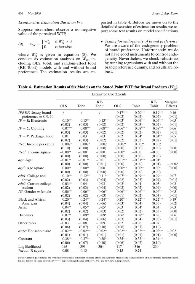
conduct six estimation analyses on Wik, in-cluding OLS, tobit, and random-effect tobit(RE-Tobit) models with and without brandpreference. The estimation results are re-

Table 4. Estimation Results of Six Models on the Stated Point WTP for Brand Products (W∗ik)

Estimated Coefficients

RE- RE- MarginalOLS Tobit Tobit OLS Tobit Tobit Effects

IPREF: Strong brand / / / 0.17∗∗∗ 0.20∗∗∗ 0.19∗∗∗ 0.16preference = 8, 9, 10 (0.02) (0.02) (0.02) [0.01]

IP = E: Electronic 0.10∗∗∗ 0.13∗∗∗ 0.13∗∗∗ 0.03∗ 0.06∗∗∗ 0.06∗∗∗ 0.05(0.02) (0.03) (0.02) (0.02) (0.03) (0.02) [0.01]

IP = C: Clothing 0.07∗∗∗ 0.08∗∗∗ 0.08∗∗∗ 0.06∗∗∗ 0.08∗∗∗ 0.08∗∗∗ 0.06(0.03) (0.03) (0.02) (0.02) (0.02) (0.02) [0.01]

IP = P: Packaged food 0.01 0.03 0.03 0.02 0.04∗ 0.04∗∗ 0.05(0.02) (0.03) (0.02) (0.02) (0.02) (0.02) [0.01]

INC: Income per capita 0.002∗ 0.002∗ 0.002 0.002∗ 0.002∗ 0.002(0.10) (0.00) (0.00) (0.00) (0.00) (0.00) 0.001

INC2: Income square −0.00∗∗ −0.00 −0.00 −0.00∗∗ −0.00 −0.00 [0.00](0.00) (0.00) (0.00) (0.00) (0.00) (0.00)

age: Age −0.01∗∗ −0.01∗∗ −0.01 −0.01∗∗∗ −0.01∗∗∗ −0.01∗

(0.00) (0.00) (0.01) (0.00) (0.00) (0.01) −0.002age2: Age square 0.00∗∗ 0.00∗∗ 0.00 0.00∗∗∗ 0.00∗∗ 0.00∗ [0.00]

(0.00) (0.00) (0.00) (0.00) (0.00) (0.00)edu1: College and −0.10∗∗∗ −0.12∗∗∗ −0.11∗∗∗ −0.07∗∗∗ −0.09∗∗∗ −0.09∗∗ −0.07

above (0.02) (0.03) (0.04) (0.02) (0.03) (0.04) [0.01]edu2: Current college 0.03∗∗∗ 0.04 0.03 0.03∗ 0.04 0.03 0.03

student (0.02) (0.03) (0.04) (0.02) (0.02) (0.04) [0.00]IG: Gender = female 0.06∗∗∗ 0.06∗∗∗ 0.06∗∗ 0.06∗∗∗ 0.06∗∗∗ 0.06∗∗ 0.05

(0.02) (0.02) (0.03) (0.01) (0.02) (0.03) [0.01]Black and African 0.20∗∗∗ 0.24∗∗∗ 0.24∗∗∗ 0.20∗∗∗ 0.22∗∗∗ 0.22∗∗∗ 0.19

American (0.04) (0.04) (0.06) (0.03) (0.04) (0.06) [0.02]Asian 0.04∗∗ 0.05∗∗ 0.05∗ 0.03 0.04∗ 0.04 0.03

(0.02) (0.02) (0.03) (0.02) (0.02) (0.03) [0.00]Hispanics 0.07∗∗ 0.09∗∗ 0.09∗ 0.06∗ 0.08∗∗ 0.08 0.06

(0.03) (0.04) (0.06) (0.03) (0.04) (0.06) [0.01]Other races −0.03 −0.08 −0.09 −0.02 −0.06 −0.07

(0.06) (0.07) (0.10) (0.06) (0.07) (0.10)hsize: Household size −0.02∗∗∗ −0.02∗∗∗ −0.02∗∗ −0.02∗∗∗ −0.02∗∗∗ −0.02∗∗∗ −0.02

(0.01) (0.01) (0.01) (0.01) (0.01) (0.01) [0.00]Constant 0.38∗∗∗ 0.37∗∗∗ 0.38∗∗∗ 0.35∗∗∗ 0.33∗∗∗ 0.34∗∗∗

(0.06) (0.07) (0.10) (0.06) (0.07) (0.10)Log likelihood −163 −396 −304 −117 −346 −250Pseudo R-square 0.08 0.13 0.15 0.24

Note: Figures in parentheses are White heteroskedastic consistent standard errors and figures in brackets are standard errors of the estimated marginal effects.Single, double, or triple asterisks (∗,∗∗,∗∗∗) represent significance at the 1%, 5%, and 10% levels, respectively.

ported in table 4. Before we move on to thedetailed discussion of estimation results, we re-port some test results on model specifications.

• Testing for endogeneity of brand preference:We are aware of the endogeneity problemof brand preference. Unfortunately, we donot have good instruments to control endo-geneity. Nevertheless, we check robustnessby running regressions with and without thebrand preference dummy, and results are ro-bust.


• Testing for heteroskedasticity, including theBreusch-Page test and the unrestricted Whitetest in the OLS regressions: Our resultsreject the null hypothesis of homoskedas-ticity at the 1% significance level for theOLS models with or without brand prefer-ence. Hence, we report heteroskedasticity-consistent standard errors for the OLSmodels.

• Testing for the presence of individual hetero-geneity: If the model does not actually con-tain the individual heterogeneity, the panelestimator is not significantly different fromthe pooled estimator. The absence of an in-dividual heterogeneity effect is statisticallyequivalent to H0 : �2

� = 0 (Wooldridge 2002,p. 264). A likelihood ratio test for H0 : �2

� =0 rejects the null hypotheses at the 1% sig-nificance level (� 2(1) = 192 and � 2(1) = 185with or without brand preference, both hav-ing a zero p-value). Hence, the RE-Tobit es-timation is more appropriate than the tobitestimation on the pooled data.

Table 4 shows that the results of the six mod-els on Wik are qualitatively similar and robust.Based on the tests discussed above, we reportthe marginal effects and discuss the estima-tion results based on the RE-Tobit model withbrand preference.

We found that consumers are willing to pay5–6% more for brands of electronics, cloth-ing, and packaged food than in fresh produceafter controlling for brand preferences, and9–10% without controlling for brand prefer-ence. The results confirm that consumers arewilling to pay substantially less for brands infresh produce than other product categoriesafter controlling for sociodemographic varia-tions. The empirical results also support ourexpectations regarding the impacts of socio-demographic factors on WTP for brands. Inparticular:

• The income per household member in-creases the WTP for brand products, whilethe marginal increase declines as incomegoes up in the OLS estimations. However,the marginal effect of income is minimal.

• An increase in age decreases the WTP forbrands while the marginal effect of age in-creases as age goes up. The results suggestthat both younger and elder respondents aremore likely willing to pay for brands than therest of the population.

• Females are willing to pay approximately5% more for brand products than males.

• Less educated people have a 7% higherstated WTP for brands than more educatedindividuals.

• White respondents have significantlysmaller WTP for brands compared withother ethnic groups. Among all ethnicgroups, African Americans have the higheststated WTP for brands—19% more thanwhite respondents.

• The intensity of preference for brand prod-ucts affects the level of WTP. Consumerswith stronger brand preference are willingto pay approximately 16% more for brandproducts than their counterparts.

Econometric Estimation Based on IWik

Rather than using the double-bounded contin-gent valuation method approach (Hanemann,Loomis, and Kanninen 1991) to directly esti-mate WTP, we use the ordered probit (OPRO-BIT) model to investigate the impacts of prod-uct category and demographic variations onthe WTP for brands. The OPROBIT model isbuilt around a latent regression as in the tobitmodel except the OPROBIT has an orderedcategorical dependent variable. The OPRO-BIT model assumes that the underlying WTPdenoted by W∗

ik in equation (8) is unobserv-able, and respondents’ choices of the WTPranges denoted by IWik are observable to re-searchers. In this case, the ordered categoricalchoice of the WTP ranges between six inter-vals, 0–20%, 20–40%, 40–60%, 60–80%, 80–100%, and at least 100%,

IWik =

1 if 0 ≤ W ∗ik < C1,

j if C j−1 ≤ W ∗ik < C j

for j = 2, 3, 4, 5,

6 if C5 ≤ W ∗ik,

(10)

where the C’s are unknown parameters to beestimated together with �’s in equation (8).The probability of having IWik = j is the proba-bility that W∗

ik lies between a pair of cut points,Cj−1 and Cj. Let �(·) denote the standard nor-mal cumulative distribution function. We havethe following probabilities,


P(IWik = j)

=

P(0 ≤ W ∗

ik < C1)

= �(C1 − �′ X)−�(−�′ X) for j = 1,

P(C j−1 ≤ W ∗

ik < C j)

= �(C j − �′ X

)−�

(C j−1 − �′ X

)for j = 2, 3, 4, 5,

P(C6 ≤ W ∗

ik

)= 1 − �

(C5 − �′ X

)for j = 6.

(11)

The results presented in table 5 suggest thatresults are robust with or without incorporat-ing brand preference. Hence, we only reportthe marginal effects and discuss the resultsbased on the OPROBIT model with brandpreference. The comparison of the observedand predicted frequencies for each WTP rangein the bottom part of table 5 suggests that over-all the OPROBIT models fit data well. Forexample, 45.70% of respondents indicate thattheir WTP is less than 20%, and the OPRO-BIT model predicts 45.01% of such respon-dents. Similar to the tobit panel estimation onthe perceived WTP, the OPROBIT model sug-gests the following results: (a) respondents’WTP for brands in fresh produce is signifi-cantly less than in electronics, clothing, andpackaged food; (b) age has a negative effect atan increasing rate on the WTP range; (c) moreeducated consumers have a lower WTP rangethan less educated; (d) female respondentslikely have a higher WTP level than males; and(e) white respondents are likely less willing topay more for brands than other ethnic groupsincluding African-American, Asian, and His-panic respondents.

Marketing Implications with SimulatedBrand Premiums

Our results so far show that consumers havea lower WTP for brands of fresh producecompared with electronics, clothing, and pack-aged food regardless of whether the socio-demographic variations are controlled for. Thelower WTP for brands of fresh produce can bea driver for either a low brand price premiumor a small market share, or both. In order toidentify the likely consequence, we simulatethe price premium and the corresponding mar-ket share in this section.

We assume consumers are heterogeneous bytheir WTP for brands. As we discussed in thedata section, we estimate the empirical den-sity function of the underlying WTP based onthe perceived WTP ranges using the maximumentropy method. Assuming that the estimateddensity function of WTP for brands of productcategory k is f (W ∗

ik),∫ Wk

W¯ k

f (s) ds = 1, whereWk and W

¯ k are the upper and lower boundof W ∗

ik . We assume a monopolistic competi-tive market in a sense that brands are substi-tutes for generic products to some extent. Afirm produces a brand product with an extramarginal cost c and charges an extra percent-age pk relative to the generic product. An in-dividual consumer will buy the brand if andonly if pk ≤ W ∗

ik . Hence, the market share ofthis brand is

Dk =∫ Wk

pk

f (s) ds.(12)

This monopolistic firm will choose the optimalpremium to maximize profits,

maxpk

(pk − c)N Dk(13)

where N is the total number of consumers.The optimal premium is achieved when themarginal revenue equals the marginal cost c:

pk −∫ Wk

pkf (s) ds

f (pk)= c.(14)

Equation (14) shows that a one-unit increasein pk will increase the revenue by pk, but at

the marginal loss,∫ Wk

pkf (s) ds

f (pk ), resulting from a

decrease in the demand. Solving equation (14)yields the optimal price premium p∗

k . Substi-tuting p∗

k into equation (12) yields the corre-sponding market share thereafter.

The simulation results show that the opti-mal price premiums for brands in fresh pro-duce actually are higher than brands of elec-tronics, clothing, and packaged food; however,the market shares of fresh produce brands aremuch smaller. For example, when the extracost of brand products is 10%, the price pre-mium for electronics, clothing, processed food,and fresh fruits and vegetables are 29%, 37%,39%, and 44%, respectively; and 39%, 48%,49%, and 59% when the extra marginal costis 20%. However, the optimal market sharesfor brands of fresh produce are much smaller


Table 5. Estimation Results and Marginal Effects of the Ordered Probit Models on the StatedWTP Ranges (IWik)

Estimated Marginal Effects On The OPROBIT ModelCoefficients with Brand Preference

Independent P P P P P PVariables: OPROBIT OPROBIT (IW = 1) (IW = 2) (IW = 3) (IW = 4) (IW = 5) (IW = 6)

IPREF: Brand 0.70∗∗∗ −0.27 0.05 0.08 0.06 0.04 0.04preference > 7 / (0.08) [0.03] [0.01] [0.01] [0.01] [0.01] [0.01]

IP=E: Electronic 0.58∗∗∗ 0.34∗∗∗ −0.14 0.03 0.04 0.03 0.02 0.02(0.07) (0.08) [0.03] [0.01] [0.01] [0.01] [0.01] [0.01]

IP=C: Clothing 0.33∗∗∗ 0.33∗∗∗ −0.14 0.03 0.04 0.03 0.02 0.02(0.08) (0.08) [0.02] [0.01] [0.01] [0.01] [0.01] [0.01]

IP=P: Packaged 0.07∗ 0.13∗∗ −0.05 0.01 0.01 0.01 0.01 0.01food (0.06) (0.06) [0.03] [0.01] [0.01] [0.00] [0.00] [0.00]

INC: Income per 0.01 0.01 −0.0016 0.0004 0.0004 0.0003 0.0002 0.0003capita (0.01) (0.01)

INC2: Income −0.00 −0.00 [0.00] [0.00] [0.00] [0.00] [0.00] [0.00]square (0.00) (0.00)

age: Age −0.04∗ −0.04∗∗ 0.0036 0.0007 −0.0010 −0.0007 −0.0005 −0.007(0.04) (0.02)

age2: Age square 0.00∗ 0.00∗ [0.01] [0.00] [0.00] [0.00] [0.00] [0.00](0.00) (0.00)

edu1: College andabove

−0.38∗∗ −0.30∗ 0.12 −0.02 −0.04 −0.02 −0.02 −0.02

(0.17) (0.17) [0.06] [0.01] [0.02] [0.02] [0.01 [0.01]edu2: Current 0.13 0.14 −0.06 0.01 0.02 0.01 0.01 0.01

college student (0.14) (0.14) [0.05] [0.01] [0.02] [0.01] [0.01] [0.01]IG:Gender= 0.25∗∗ 0.26∗∗ −0.10 0.03 0.03 0.02 0.01 0.01

female (0.11) (0.11) [0.04] [0.01] [0.01] [0.01] [0.01] [0.00]Black & African

American0.96∗∗∗ 0.93∗∗∗ −0.31 −0.02 0.09 0.08 0.07 0.09

(0.21) (0.22) [0.06] [0.03] [0.02] [0.02] [0.02] [0.04]Asian 0.19∗ 0.15 −0.06 0.01 0.02 0.01 0.01 0.01

(0.13) (0.13) [0.05] [0.01] [0.02] [0.01] [0.01] [0.01]Hispanics 0.47∗∗ 0.44∗∗ −0.17 0.02 0.05 0.04 0.03 0.03

(0.20) (0.22) [0.08] [0.01] [0.02] [0.02] [0.02] [0.02]Other races −0.29 −0.24 0.10 −0.03 −0.03 −0.02 −0.01 −0.01

(0.61) (0.40) [0.16] [0.06] [0.05] [0.02] [0.01] [0.01]Hsize: Household −0.10 −0.06 0.02 −0.01 −0.01 −0.00 −0.00 −0.00

size (0.40) (0.04) [0.02] [0.00] [0.00] [0.00] [0.00] [0.00]

Cut EstimatedPoints Cut Points Probability Observed Predicted

C1 −0.65 −0.52 prob(IWik = 1) = prob(0 ≤ W ∗ik < C1) 45.70% 45.01%

(0.43) (0.44)C2 0.24 0.41 prob(IWik = 2) = prob(C1 ≤ W ∗

ik < C2) 30.38% 33.95%(0.42) (0.44)

C3 0.74 0.93 prob(IWik = 3) = prob(C2 ≤ W ∗ik < C3) 11.92% 11.80%

(0.42) (0.43)C4 1.11 1.32 prob(IWik = 4) = prob(C3 ≤ W ∗

ik < C4) 5.79% 5.02%(0.42) (0.43)

C5 1.50 1.74 prob(IWik = 5) = prob(C4 ≤ W ∗ik < C5) 3.39% 2.62%

(0.41) (0.42)prob(IWik = 6) = prob(C5 ≤ W ∗

ik) 2.81% 1.60%No. of OBS 1208 1207Pseudo R2 0.05 0.07

Note: Figures in parentheses are standard errors of the estimated coefficients adjusted for 302 clusters (there are 302 respondents in total). Single, double, ortriple asterisks (∗,∗∗,∗∗∗) represent significance at the 1%, 5%, and 10% levels, respectively. Figures in brackets are standard errors of the estimated marginaleffects.


than in other product categories. For exam-ple, when the extra marginal cost is 10%, only18% of the population will buy brand prod-ucts of fresh produce in contrast to 23% forpackaged food, 30% for clothing, and 50% forelectronics. When the extra cost is 20%, 12%of the population will buy brand products offresh produce, 16% for packaged food, 20%for clothing, and 30% for electronics. The smallmarket share can partly explain fewer brandsof fresh fruits and vegetables.

Once the optimal price premiums are estab-lished, we can identify whether an individualconsumer will buy brands of a certain productand assess whether people are consistent withbrand preferences across product categories.This assessment will provide insight to storeorganization and prediction of percentage ofthe population who will shop in each of thesestores. Assuming that the extra marginal costof brands is 10% relative to the generic one,almost half of the respondents will always buygeneric products and another 9.27% will onlybuy brand products. In total, at least 58.94%of the potential consumers are consistent interms of their brand preferences for electron-ics, clothing, packaged food, and fresh produce.We can at least identify three types of stores:(a) discount stores that sell generic productstargeting half of the potential consumers, (b)elite stores that sell only brand items and at-tract 9.27% of the potential consumers, and (c)supermarkets that sell everything. Our analysissuggests that elite stores with brand productsare attractive to the consumer segment shar-ing consistent high brand preferences as wellas WTP across product categories. Harry andDavid is one example of a company that takesadvantage of the upper end of the distribution(http://www.harryanddavid.com/).

Overall, the simulation results suggest twothings: (a) if we market brands of fruits andvegetables, we have to target a small marketsegment and charge a high price; and (b) sincewe find that people who are willing to pay forbrands of fruits and vegetables are also will-ing to pay for brands in other categories, ourresults suggest targeting outlets that focus onbrands of products in all categories, for exam-ple, high-end malls, like sky malls, or brand-focused retailers, like Macy’s, Nordstrom, orNeiman Marcus.

Conclusions

The basic premise of this article is that brandvalue comes from its contribution to reduction

in quality risk, the prestige it confers, and fromsuperior design. The features for brand prod-ucts are likely to vary in value among productsand be appreciated differently by individualswith different sociodemographic characteris-tics. Based on this premise, we hypothesize thatthe relative value of brands in fresh produce ismuch smaller than in electronics, clothing, andpackaged food. We also investigate the rolesof sociodemographic factors on the WTP forbrands.

Empirical results based on the data fromCollege Station and Bryan, Texas, on WTP forbrands of four product categories support ourhypotheses. Tests on the mean difference ofWTP across product categories based on thestated WTP or the estimated WTP distribu-tion using the maximum entropy method sug-gest that WTP for brands in fresh produce ismuch smaller than in electronics, clothing, andpackaged food. Using the random effect tobitmodel on the stated point WTP and the or-dered probit model on stated range of WTP, wealso find similar results that WTP for brandsof fresh produce is least among four prod-uct categories controlling for relevant demo-graphic variations. The empirical study alsoshows (a) the nonlinear effects of income andage (income increases WTP at a diminishingrate and age decreases WTP at an increas-ing rate); (b) females, less educated people, orsmaller households are willing to pay more forbrands; and (c) white respondents are less will-ing to pay for brands than other ethnic groupsincluding African Americans, Asians, and His-panics.

Based on the distribution of WTP for eachproduct, we determined the optimal brand pre-mium and the corresponding market share.The simulations suggest a potential for a smallmarket of brands of fresh produce with a highmargin relative to the generic products. Sinceconsumers with strong brand preferences inother product categories tend to have a higherWTP for brands of produce, one strategy isto introduce brands in outlets that emphasizebrands across the board. Another is to tar-get market segments with consumers who aremore likely to buy brands regardless of productcategories, like high-income individuals, youngpeople, and female shoppers.

The empirical results of this article are basedon the stated preferences and not actual be-havior. In spite of the obvious limitation ofthe data, it allowed us to compare preferencesto brands in several product categories andrelate WTP with sociodemographic variables.


However, further empirical work with actualpurchasing behavior is needed to further studythe role and potential of brands of fresh pro-duce.

Second, while we found WTP for brands offood products in general, it is useful to assessWTP for subgroups (e.g., organic versus nonor-ganic products), as well as different types offoods (vegetables versus fruits). Further re-search should assess the value of brands of or-ganic food as well as the role of geographicindictor labeling as substitutes and/or comple-ments to brands.

[Received May 2006;accepted July 2007.]

References

Aaker, D., and E. Joachimsthaler. 2002. BrandLeadership: The Next Level of the Brand Rev-olution. London, U.K.: Simon and Shuster.

Ainslie, A., and P.E. Rossi. 1998. “Similarities inChoice Behavior across Product Categories.”Marketing Science 17(2):91–106.

Allenby, G.M., and P.E. Rossi. 1991. “Quality Per-ceptions and Asymmetric Switching BetweenBrands.” Marketing Science 10(3):185–204.

Auty, S., and R. Elliott. 1999. “Fashion Involvement,Self-Monitoring and the Meaning of Brands.”Journal of Product and Brand Management7(2):109–123.

Caves, R. E., and D. P. Greene. 1996. “Brands’Quality Levels, Prices, and Advertising Out-lays: Empirical Evidence on Signals and Infor-mation Costs.” International Journal of Indus-trial Organization 14(1):29–52.

Chiang, J. 1991. “A Simultaneous Approachto the Whether, What and How Much toBuy Questions.” Marketing Science 10(4):297–315.

Erdem, T., Y. Zhao, and A. Valenzuela. 2004. “Per-formance of Store Brands: A Cross-CountryAnalysis of Consumer Store-Brand Prefer-ences, Perceptions, and Risk.” Journal of Mar-keting Research 41(1):86–100.

Fussell, P. 1983. Class: A Guide through the Ameri-can Status System. New York: Touchstone.

Ghosh, A., and S.L. McLafferty. 1987. LocationStrategies for Retail and Service Firms. Lexing-ton, KY: D. C. Heath.

Gupta, S., and P.K. Chintagunta. 1994. “On UsingDemographic Variables to Determine SegmentMembership in Logit Mixture Models.” Journalof Marketing Research 31(1):128–136.

Hanemann, W.M., J. Loomis, and B. Kanni-nen. 1991. “Statistical Efficiency of Double-Bounded Dichotomous Choice ContingentValuation.” American Journal of AgriculturalEconomics 73(4):1255–1263.

Hayes, D., and S.H. Lence. 2002. “A New Brand ofAgriculture? Farmer-Owned Brands RewardInnovation.” AgDM newsletter article. Avail-able at http://www.extension.iastate.edu/agdm/articles/hayes/HayDec02.htm (Last accessed inJuly 2007).

Heiman, A., and E. Goldschmidt. 2004. “Testing thePotential Benefits of Brands in HorticulturalProducts: The Case of Oranges.” HorTechnol-ogy 14(1):28–32.

Holbrook, B.M. 1992. “Product Quality, Attributes,and Brand Name as Determinants of Price:The Case of Consumer Electronics.” Market-ing Letters 3(1):71–83.

Kalyanam, K., and D.S. Putler. 1997. “IncorporatingDemographic Variables in Brand Choice Mod-els: An Indivisible Alternative Framework.”Marketing Science 16(2):166–181.

Kaufman, P., C.R. Handy, E.W. McLaughlin, K.Park, and G.M. Green. 2000. “Understandingthe Dynamics of Produce Markets: Consump-tion and Consolidation Grow.” USDA/ERSAIB-758.

Moore, C.M., J. Fernie, and S. Burt. 2000. “Brandwithout Boundaries—The Internationalizationof the Designer Retailer’s Brand.” EuropeanJournal of Marketing 34(8):919–937.

Parker, D.D., and D. Zilberman. 1993. “Hedonic Es-timation of Quality Factors Affecting the Farm-Retail Margin.” American Journal of Agricul-tural Economics 75(2):458–466.

Rosen, S. 1974. “Hedonic Prices and Implicit Mar-kets: Product Differentiation in Pure Com-petition.” The Journal of Political Economy82(1):34–55.

Vranesevic, T., and R. Stancec. 2003. “The Effectof the Brand on Perceived Quality of FoodProducts.” British Food Journal 105(11):811–825.

Wooldridge, J. 2002. Econometric Analysis of CrossSection and Panel Data. Cambridge, MA: TheMIT Press.

Wu, X.M., and J. Perloff. 2007. “GMM Estimationof Maximum Entropy Density with IntervalData.” Journal of Econometrics 138(2): 532–546.

Zeithaml, A.V. 1988. “Consumer Perceptions ofPrice, Quality, and Value: A Means-End Modeland Synthesis of Evidence.” Journal of Market-ing 52(3):2–22.

Choosing Brands: Fresh Produce versus Other Products

Documents

Transcript of Choosing Brands: Fresh Produce versus Other Products