ZlsZ-fL

REPORT 76-46

Dupe

Research Libra!*,Iowa Institute

of

Hydraulic Research

Topological properties of sometrellis pattern channel networks

j.C.TATINCLAUX

CRREL

3Z

Cover: The ridge and valley section ofcentral Pennsylvania from 50,000 feet. Trellispattern streamnetworks are classically developed here.

(Photograph by National Aeronautics andSpace Administration.)

CRREL Report 76-46

Topological properties of sometrellis pattern channel networks

Steven J. Mock

December 1976

I'rep.iivd tor

DIRECTORATE OF FACILITIES ENGINEERING

OFFICE, CHIEF OF ENGINEERS

Bv

CORPS OF ENGINEERS, U.S. ARMY

COLD REGIONS RESEARCH AND ENGINEERING LABORATORYHANOVER, NEW HAMPSHIRE

Approvedlor puhlu rc/ea.se; distribution unlimited.

UnclassifiedSECURITY CLASSIFICATION OF THIS PAGE (When Data Entered)

REPORT DOCUMENTATION PAGE1. REPORT NUMBER

CRREL Report 76-46

2. GOVT ACCESSION NO.

4. TITLE (and Subtitle)

TOPOLOGICAL PROPERTIES OF SOME TRELLIS

PATTERN CHANNEL NETWORKS

7. AUTHORfsJ

Steven J. Mock

9. PERFORMING ORGANIZATION NAME AND ADDRESS

U.S. Army Cold Regions Research and Engineering LaboratoryHanover, New Hampshire 03755

11. CONTROLLING OFFICE NAME AND ADDRESS

Directorate of Facilities Engineering

Office, Chief of EngineersWashington. D.C. 20314

14. MONITORING AGENCY NAME & AODRESS(if different from Controlling Office)

16. DISTRIBUTION STATEMENT (of this Report)

Approved for public release;distribution unlimited.

READ INSTRUCTIONS

• BEFORE COMPLETING FORM

3. RECIPIENT'S CATALOG NUMBER

5. TYPE OF REPORT & PERIOD COVERED

6. PERFORMING ORG. REPORT NUMBER

8. CONTRACT OR GRANT NUMBER(s)

10. PROGRAM ELEMENT, PROJECT, TASKAREA & WORK UNIT NUMBERS

DA Project 4A161102AT24

Task Area A2, Work Unit 001

12. REPORT DATE

December 1976

13. NUMBER OF PAGES

59

15. SECURITY CLASS, (of this report)

Unclassified

15a. DECLASSIFI CATION/DOWN GRADINGSCHEDULE

17. DISTRIBUTION STATEMENT (of the abstract entered In Block 20, If different from Report)

18. SUPPLEMENTARY NOTES

19. KEY WORDS (Continue on reverse side if necessary and identify by block number)

Geology

Geomorphology

Streams

TopologyWatersheds

2Qk ABSTRACT (Contimie an r*v*r*m sfcto ft rmcv&aary and. Identity by block number)

The topological properties of 10 stream networks having moderate to well developed trellis drainage patterns havebeen compared with thoseexpected in a topologically random population. Magnitude 4 subnetworks showasystematic departure from expectation which can be related to geological controls. Alink type classification systemwas developed and a series of equations describing the probability of occurrence of link types in topologically randompopulations derived. Analysis of the link structure in the channel networks showed small but persistent deviationsfrom expectation in the well developed trellis pattern streams. The general conclusion is that the topologically randommodel is a very useful standard with which to compare real channel networks.

DD , ;ST„ M73 EDfTtON OF t MOV 65 IS OBSOLETE Unclassified

SECURITY CLASSIFICATION OF THIS PAGE (When Data Entered)

PREFACE

This report was prepared by Dr. Steven J. Mock, Research Geologist, Snow and IceBranch, Research Division, U.S. Army Cold Regions Research and Engineering Laboratory. It was submitted to the Department of Geology, Northwestern University, inpartial fulfillment of the requirements for the degree of Doctor of Philosophy in the fieldof geology. The work was funded under DA Project 4A161102AT24, Research in Snow,Ice andFrozen Ground, Task AreaA2, Cold Regions Environmental Interactions, WorkUnit 001, Quantification of Cold Regions Terrain and Climatic Parameters.

The author would like to express sincere appreciation to Dr. W.F. Weeks, Dr. C.C.Langway, Jr., and Dr. K.F. Sterrett, who provided continual encouragementprior to andthroughout the project. Professor W.C. Krumbein of Northwestern University introducedthe author to the subjectof channel network topology and encouraged him to explore itfurther. The author would also like to acknowledge the assistance of the CRRELdrafting section under H. Larsen, and in particular M. Pacillo who undertook the task ofpreparing the final channel network maps. Technical reviewof the report was performedby Dr. Weeks and S.F. Ackley of CRREL.

CONTENTS

Page

Abstract

Preface '.-

Summary r. V1

Background and objectives '••• N 1Introduction • 1

Objective of study 1Quantitative geomorphology and the infinite topologically random model.... 3Stream ordering 3Stream magnitude 4Basic properties of networks ••• 4

Channel networks and geology 5Introduction 5The dendritic pattern 6The trellis pattern •• 6Study areas 7

~ Geology and physiography .....' .\ — 7Channel network mapping ". 17

Topological properties of the networks 17Introduction 17Magnjtude-4 networks 18Magnitude-5 networks 20Magnitude-6 to magnitude-10 networks 23Summary • 23

Link probabilities • 26Introduction 26Link frequencies 26Link types 28Probability of occurrence 31Joint probability for link magnitude and type 39

Link lengths 42Introduction • 42Link lengths • 42Previous work ? • r 42Observed link-length frequency distribution 42Statistical analysis of interior links : 42Summary 46

Summary and conclusions 48Introduction 48Sub-networks 48Links 49

Literature cited • 50Appendix A. Statistical data for the contiguous-seven and Triassic channel net

works 53

ILLUSTRATIONS

Figure page1. Topologically identical and distinct channel networks 2

2. All topologically distinct arrangements for magnitude-3, magnitude-4 andmagnitude-5 networks 2

3. A channel network illustrating the Strahler ordering system 34. The same channel networks as shown in Figure 3, illustrating the magni

tude system 4

5. Location map for central Pennsylvania streams 76. Generalized geologic map of Willow Run, Barton Hollow, Lick Run,

Rhines Hollow and Horse Valley Run 87. Channel-network maps of central Pennsylvania streams 9

8. Geologic section along line A-A' of Figure 6 129. Geologic map of eastern Pennsylvania and western New Jersey with stream

basins shown 13

10. Channel network maps of eastern Pennsylvania and western New Jerseystreams 14

11. Hanging rootogram showing expected frequencies and deviations fromexpected frequencies as a function of magnitudes for the contiguous-seven networks 27

12. Definition of link types by the magnitude relationships of linkof magnitude fi and its adjacent upstream and downstream neighbors 30

13. Idealized network showing link magnitudesand types 3014. The randomly drawn link n3,and the four links to which it is attached .. 3215. Probability matrix for an infinite topologically random network 3616. Observed interior-link-length frequency distributions 4317. Mean length of each of the seven link types for the Triassic and contiguous-

seven samples plotted against each other .- 47

TABLES

Table

I. Summary data for stream networks 18

11. Statistics of the 123 magnitude-4 networks from the contiguous-sevenstreams 19

III. Statistics of the 48 magnitude-4 networks from the Triassic streams 19IV. Statistical analysis of magnitude-4 networks from the contiguous-seven

streams 19

V. Statistical analysis of magnitude-4 networks from the Triassic streams.... 19

VI. Direction of flow with respect to regional strike of contiguous-sevenimagnitude-4 networks 21

VII. Direction of flow with respect to dip of contiguous-seven magnitude-4networks 21

VIII. Topological classes for magnitude-5 networks 21IX. Statistics of magnitude-5 networks from the contiguous-seven streams ... 22X. Statistics of magnitude-5 networks from the Triassic streams 22

XI. Statistical analysis of magnitude-5 networks from Triassic streams ......... 22XII. Statistical analysis of magnitude-5 networks from the contiguous-seven

streams 23

IV

Table Page

XIII. Statistics of magnitude-6 networks from the contiguous-seven streams .... 24XIV. Statistics of magnitude-6 networks from Triassic streams 24XV. Stream-number statistics for the contiguous-seven streams 24

XVI. Stream-number statistics for Triassic streams 25

XVII. Statistical analysis for contiguous-seven streams 25XVIII. Statistical analysis for Triassic streams 25

XIX. Statistics and analysis of link-magnitude frequencies, contiguous-seven

and Triassic streams 27

XX. Statistics and statistical analysis of trans- and cis-links for contiguous-

seven streams 29XXI. Statistics and statistical analysis of trans- and cis-links for Triassicstreams 29

XXII. Probability of occurrence of link types for networks of various magnitudes 37XXIII. Link-type statistics for the contiguous-seven streams 38XXIV. Link-type statistics for Triassic streams 38XXV. Statistical analysis of link types for contiguous-seven streams 38

XXVI. Statistical analysis of link types for Triassic streams 38XXVII. Joint probabilities of interior-link types and magnitude for an infinite

topologically random channel network 39XXVIII. Observed and expected frequencies of interior links as a function of link

type and link magnitude - Contiguous-seven sample 40XXIX. Observed and expected frequencies of interior links as a function of link

type and link magnitude - Triassic sample... 41XXX. Contingency table showing length frequencies versus link type for the

contiguous-seven sample 44XXXI. Contingency table showing length frequencies versus link type for the

Triassic sample 45XXXII. Results of two-way contingency tests of link type pairs and length fre

quencies for the contiguous-seven sample 45XXXIII. Resultsof two-way contingency test of link type pairs and length fre

quencies for the Triassic sample 46XXXIV. Link pairs having different length-distribution based on contingency tests 47XXXV. Link types of contiguous-seven and Triassic samples arranged in descending

order of mean length 47

CONVERSION FACTORS: U.S. CUSTOMARY TO METRIC (SI)UNITS OF MEASUREMENT

Multiply By_ To obtain

foot 0.3048 meter

mile 1.6093 kilometer

SUMMARY

The topological properties often stream networks have been analyzed and comparedwith those predicted by the topologically random model. The topologically random modelstates that, in the absence of geological controls, all topologically distinct channel networkshaving the same number of sources areequally likely, and, in an infinite topologicallyrandom network, all topologically distinct sub-networks occur with equal frequency. Theten stream networks have moderately- to well-developed trellis drainage patterns whichhave formed in response to differential erosion actingon sequences of folded and tiltedsedimentary rocks. Testing procedures included examining the frequency of occurrence oftopologically distinct channel networks, ambilateral classes and sets of Strahler stream numbers for sub-networks up to magnitude 10. Deviations from predictions of the topologicallyrandom model occur in the magnitude-4 networks and are attributed to preferential development of minor tributaries flowing in the down-dip direction of the local rocks. The onlyother deviation from predicted frequencies occurs in the magnitude-10 stream number setsand is not obviously explicable as a response to geologiccontrols.

To examine the stream networks in greater detail, a system was devised for classifyingindividual links by type. Six link types were defined: two exterior types, the T-link andTS-link; and four interior types, the CT-link, B-link, TB-link and T-link. Link types weredefined by the magnitude relationships with adjoining linksat a link's upstream and downstream terminating forks. Analysis of the link structure showsa greater than expectednumber of low magnitude T- and TB-links occurring in the sample having a well developedtrellis pattern.

The observed departures from the expectations of a topologically random model arerelated to geological factors, but the deviations are subtle and not observed in the streamshaving less well developed trellis patterns.

The use of magnitude as a measure of channel network size has great potential, enablingdirect comparison of various streams from remotely sensed dataor maps. Furthermore, inthe absence of gage data,.the relative flood potential at any pointalong a stream can beassessed simply from the growth rate of the magnitude of the main channel up to that point.The fact that trellis patterns deviate only marginally from topological randomness impliesthat flood hazards within such systems are more or less similar to those within the more

common dendritic systems. This information enables assessment of river barrier crossingand denial to be estimated without recourse to long-term flood records which generally arenot available at specific sites.

Thegeneral conclusion is that the topologically random model'serves asa very usefulstandard with which to compare real channel networks. Furthermore, the presence ofstrong geological controls, which affect the channel network patterns, has only minor effects on the topological properties.

TOPOLOGICAL PROPERTIES OF SOME TRELLIS

PATTERN CHANNEL NETWORKS

by

Steven J. Mock

BACKGROUND AND OBJECTIVES

Introduction

The study of streams and stream networks from a geomorphological rather than a hydrologicalviewpoint has encompassed "three clear and distinct eras, each of which can be associated with oneor two dominating individuals. The first erawas largely given to descriptive work, theelucidationof a stream's age and place in theerosion cycle by observation and inductive reasoning. Theculmination of this era was reached in the many works of W.M. Davis and D. Johnson.

The second era was inaugurated by Robert Horton's work (1932, 1945) and culminated in thestudiesof Strahler and his students. Horton's major contribution was in devising a methodical system of describing networks numerically, thus allowing statistical analysis and comparative studiesofstream systems. Under Strahler's impetus, stream basin parameters were devised and quantified,and the interrelationships among parameters were sought by statistical techniques. Extensive studiesof drainage basins have led to the exposition of several "laws" relating various stream and basinparameters. Many of his techniques, including the stream ordering system, are in standard use today.

The third period began with R.L. Shreve's publications of 1966 and 1967 in which he examinedthe network structure of stream systems from a topological point of view. Once a single basicassumption was made, several of the empirical laws then became derivable as maximum-likelihoodevents. The concepts of magnitude and links were introduced, and these focused attention on whatnow seems to be a fundamental element in stream networks. A fusion of elements from the Horton-Strahler "school" with the newer topological view is now in progress, promising and delivering basicinsights into the makeup of streams.

Objective of study

The infinite, topologically random model asstated by Shreve (1966, p. 27) is "...in the absenceofgeologic controls a natural population ofchannel networks will be topologically random," andlater (Shreve 1967, p. 178) "...in the overall network which will be termed an infinite topologicallyrandom channel network, all topologically distinct sub-networks with the same numberof sourcesoccur with equal frequency."

Topological identity means that the planimetric projections of twochannel networks with thesame number of sources can be rotated and deformed within the projection plane so as to becomecongruent. Figure 1 illustrates topological identity and distinction. Only two properties are

^c

Figure I. Topologically identical(A andB) and distinct (C)channelnetworks.

V V

V "v" v v v>/b _: - - " T

\

v v V V V V V \/

y Y ^o{-<

Figure 2. All topologically distinct arrangements formagnitude-3 (A), magnitude-4 (B) andmagnitude-5

(C)networks.

necessary to define topological identity - the number of sources, and the arrangement by whichthey are linked together to form a network. Most of the common geomorphic descriptors andparameters are independent of topology.

Figure 2 shows the topologically distinct arrangements possible for three different size networks.While it is obvious from Figure 2 that the number of topologically distinct arrangements increasesrapidly with increasing network size, a specific expression for thatnumber will be postponed untila later section.

Since Shreve introduced the topologically random model, a sizable body of work has accumulatedin which natural channel networks have been examined within the predictive framework of themodel. For the most part, Smart (1969) being an exception, such studies have examined natural networks which have evidence of minimal geologic control in the channel network development. Channelnetworks developed on horizontal orgently dipping rocks with homogeneous lithologies and displaying the classical pattern have formed the dominant subject material.

In this study, the topologic properties of 10channel networks, all showing clear evidence ofgeologic control, are compared with those predicted by topologically random models. If it can bedemonstrated that a correlation exists between geological structure and topological properties thena new method of examining the interaction of geology and streams is available which may provideinsights into the evolution and subsequent readjustments within the system. Conversely, ifno suchcorrelation can be shown, then there is legitimate reason for broadening the scope of the topologi- .cally random model by deleting "...in the absence ofgeologic controls..." from Shreve's originalstatement.

In order to carry out the comparison cited above, several new methods of describing channelnetworks and theircomponent partsare developed. Each of these is shown as being predictable,in a probabilistic sense, from the topologically random model. In particular, a small set of definable sub-units or links are defined with which an entire channel network can be described. While

these link types are defined on the basis of numerical relationships with other links at junctions,evidence indicates that each of the link types hasdistinct length-frequency distributions.

Figure 3. A channelnetwork illustrating theStrahler ordering system.

Quantitative geomorphology and the infinitetopologically random model

Horton (1945) can fairly be said to have suppliedthe foundations for what has since become known

as quantitative geomorphology. While Horton'swork considered the morphological development ofthe entire drainage basin, three important aspects ofthe study deal only with channel networks:

1. Development of a numerical method (streamorder) for describing a channel network.

2. The law of stream numbers.

3. The law of stream lengths.

Subsequently, the ordering system was modifiedslightly by Strahler (1952). The Strahler system isused here.

Stream ordering

The ultimate tributaries in a channel network

are designated as order 1. Wherever two streams of

the same order, 12, join, the resulting stream isof order£2+1. Wherever twostreams of unequal orderjoin, the succeeding streams are of the higher order. Figure 3 illustrates the ordering system.

Acomplete stream consists of the entire reach of channels from the formation of order H to thepoint where it terminates in a higher order. Thus in Figure 3 there are eight 1st order streams, three2nd order streams, and one 3rd order stream. If we let Nn and Nn+{ be the number of streams oforder £2 and ^2+1 respectively, then Rh, the bifurcation ratio, isdefined as

Nn

N0

n+i

The empirical fact that Rb tends towards aconstant through a range of H's led Horton (1945) toformulate the law of stream numbers, namely:

Na =*£-" (2)

where k is the order of the master stream (or drainage basin).

One would intuitively expect that on the average the mean length of streams would increase withorder. Based on observed data, Horton stated the law of stream lengths:

n-i

Ln -Z-i'^l (3)

where Ln is the mean length of £"2 order streams and

RL=Tn

•n-i

While both eq 2 and 3 have been found to be valid in many studies, it should be rememberedthat they are empirical laws based on observation.

Figure 4. The same channel network as shown

in Figure3, illustrating the magnitude system.

N{M)2AM

2M-\

M

Stream magnitude

Shreve (1967) introduced the concept ofstream magnitude. However, before magnitude

can be defined, it is necessary to define certain

other items. Shreve (1966, p. 20) defined termsin the following manner: "The points farthest

upstream in a channel network are termed

sources. The point of confluence of two chan

nels is a fork. The term link will refer to a sec

tion of channel reaching without interveningforks from either a fork or a source at its up-

stream end to either a fork or the outlet at its

downstream end." Links may be subdivided

into exterior links, which head at a source, andinterior links, which head at a fork (Shreve 1967).The magnitude of a link "is equal to the totalnumber of sources ultimately tributary to it"

(Shreve 1967, p. 179) where all sources areassigned a magnitude of 1. Magnitude is an additive property; two links joining at a fork producea third link whose magnitude is the sum of the magnitudes of the first two. The magnitude ofastream network is defined as being equal to the magnitude of the outlet link, which is defined bythe investigator.

Figure 4 shows the same drainage basin as in Figure 3 but now with each link assigned a magnitude according to the above stated rules. Two items worth noting here are 1) 1st order streams andmagnitude-1 links are equivalent, and 2) the focus shifts from streams to links as basic entities inthe system.

Basic properties of networks

Let Msignify the magnitude of a network, and n the magnitude of individual links. A networkof magnitude Mcontains Mexterior links (ji = 1) and A7-1 interior (ju > 1) links. The total numberof links is 2/W-1 for a network of magnitude M.

Let N(M) be the number of topologically distinct arrangements possible for a network of magnitude M. N{M) is given by

(4)

(Shreve 1966, p. 29). The number of topologically distinct networks of order 12 having a magnitudeof M (Shreve 1966, p. 29) isgiven by

M-l ft-1

N{M;Sl) ='£ [/V(/;n-1)x/V(/W-/;f2-1)+2/V(/;n)x^ N{M-i;u)]i=i

A/(1;1) =1

/V(1;ft)=0$2 = 2,3,...,-N{M;1) = 0M>2.

CJ=1

(5)

In a topologically random population of networks of magnitudeM, in which all topologicallydistinct arrangements occur with equal frequency, the probability of occurrence of any particular

order is given by

P(M;n)-m^l. (6)

The number of topologically distinct networks of order 12 having^, n2, ...,nn_x, 1 streams oforder 1, 2, ..., 12 is given by

, ^(^,,,,...,^,1)^.2^-^!)/ ^ \ (7)

and the probability of occurrence of any set of stream numbers in a topologically random popula-tion of magnitude M(M =n{) is

„/ .._Ninvn2,...,naA) mP{pltn2,...,nn,}) —JJJJvf) • (8)

An infinite topologically random network is a network of infinite size in which all topologicallydistinct subnetworks of the same magnitude occur with equal frequency. The probability of draw

inga link of magnitude id at random from a topologically random population of networks of magnitude M is given by

UW.M) (2M-i)N{M) K'

and as Mgoes to °°, it becomes an infinite topologically random network and the probability ofdrawing a link of magnitude id at random becomes

*>-^r(r) (10)(Shreve 1967, p. 181). Equations 9 and 10 will be used extensively in a later chapter when linktypes are studied. Details of the derivation of eq 4-10 may be found in the series of papers 6yShreve (1966, 1967, 1969).

CHANNEL NETWORKS AND GEOLOGY

Introduction

A channel network is a complex and dynamic response to climatic and geological factors. If oneaccepts an equilibrium point of view, both the network and the individual channels adjust to minimize the amount of work necessary to transport the products of erosion. Because of constant

changes in the system, a quasi-equilibrium condition prevails. Becauseactual drainage patterns andhillslopes are quite well adjusted in form and pattern for handling erosional products under many

different environments, the implication is that readjustment to radically changed conditions isrelatively rapid (Leopold et al. 1964). Geologists and geomorphologists have implicitly assumedthat certain patterns manifested by channel networks reflect a degree of equilibrium between the

network and the underlying geology, and have long made use of this as an aid in interpretinggeology.

The geometric patterns displayed in plan view (either on maps or aerial or space photos) havebeen classified by various authorities into anywhere from seven (Zernitz 1932) to eleven (Feldmanet al. 1968) major types. In terms of the equilibrium concepts discussed above, several of themajor drainage-pattern, types (dendritic, trellis, rectangular, annular) can be considered products ofan equilibrium adjustmentof the streams to the geology. Other types, however, such as a derangedpattern, are not in equilibrium and are the result of recent (in geologic time) catastrophic events.

Fundamental to the relationship between drainage patterns and geology is the concept ofdifferential erosion, which assumes that channels will tend to develop preferentially along lines ofleast resistance. The principal geological elementgiving rise to differential resistance to weatheringand erosion is lithology. While structural features per se, such as joint systems or fault traces, arealso zones of weakness which can and do control stream patterns, the primary influence of geologicstructures is in making a variety of lithologies, having differing resistances to erosion, available toerosion. The drainage patterns which develop though are far more diagnostic of the underlyingstructural features than they are of particular lithologies.

The dendritic pattern

Zernitz (1932) stated that the "dendritic drainage pattern is characterized by irregular branchingin all directions with the tributaries joining at all angles." In fact, such a pattern is more in accord

with what is generally considered an insequent pattern, which is normally taken to mean a pattern-less system (Lattman 1968). The dendritic pattern is usually taken to mean a pattern which hasthe familiar tree-like appearance with random branchingand non-random junction angles.

The dendritic pattern characteristically occurs where there is homogeneity in bedrock resistanceto erosion. While such a pattern can develop over complexly deformed crystalline rocks, wheresedimentary rocks form the bedrock, the dendritic pattern is usually indicative of, at most, gentletilting such that a widespread lateral homogeneity in lithology exists. Thus, although a gentle tilton a regional scale may impart a generalized preferred direction of flow, lateral homogeneity in resistance to erosion should allow random branching.

The trellis pattern

The trellis pattern is characterized by one dominantstream direction with a near-orthogonaldirection along which major streams are connected and minor tributaries formed. The majorgeological requirement for the development of trellis patterns is parallel or sub-parallel zoneshaving differential resistance to erosion. While purely structural features such as jointing (Thorn-bury 1954, p. 121) can lead to the development of a trellis pattern, parallel belts of moderatelyto steeply dipping sedimentary rocks of diverse lithology far more commonly give rise toytrellispatterns. The overall linearappearance of trellis drainage patterns isa result of preferential streamdevelopment along the more easily eroded rock units and generally reflects the direction of theregional strike.

While the classification of stream patterns is largely a subjective matter, and the gradations whichoccur between types are subject to varied interpretation, there is no question that the dendriticpattern is indicative of minor geologic control and the trellis pattern isa response to major, andusually easily recognized, geological factors.

Wi How Run

West

\ ---^Barton Hollow /

Lick Run/ /^^/^ ^/^*^r.s'-</Shines T /

George Creek/ ^s~^j Hollow</// / / ///'Horse Valley Run

/ IN"' <Tuscarora

xt

Pennsylvania

•

Location Map

Figure 5. Location map for central Pennsylvania streams. Streamsareshown in correct relative positions.

Study areas

Twelve drainage basins were selected for detailed study, nine in central Pennsylvania and threein eastern Pennsylvania and western New Jersey. The basic criterion for selection was that a channelnetwork exhibit a pattern which was clearlya response to geological controls. This in turn dictatedthat the local geology be known in sufficient detail for identification of at least the major geologicalcontrols. Figure 5 shows the location of the central Pennsylvania streams. Figure 9 shows theeastern Pennsylvania and western New Jersey streams.

Geology and physiography

Central Pennsylvania streams. The ninecentral Pennsylvania streams lie entirely within theFolded Appalachians Physiographic Province (USGS 1970). The area ischaracterized by a series ofalternating and parallel ridges and valleys. Within the study area major ridge crests have an averageheight of 1900feet above msl (mean sea level) while the elevation of major valleys is about600feetabove msl. Secondary ridges and valleys, all paralleling the major relief features, have intermediateelevations. The most distinctive feature of this typical ridge and valley topography is "grain" imparted by the parallelism of the physiographic elements.

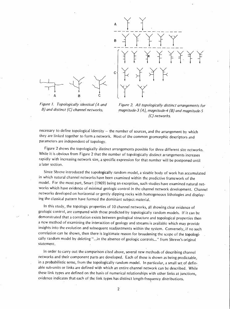
Figure 6 is a generalized geologic map of the area in which five of the central Pennsylvaniastreamsare located. The geology shown in Figure 6 is typical of that found throughout this partof Pennsylvania: a Paleozoic sequence of sedimentary rocks with diverse lithologies which has beenfolded into a series of parallel anticlines and synclines, imparting a regional,NE-SW strike to the

rocks.

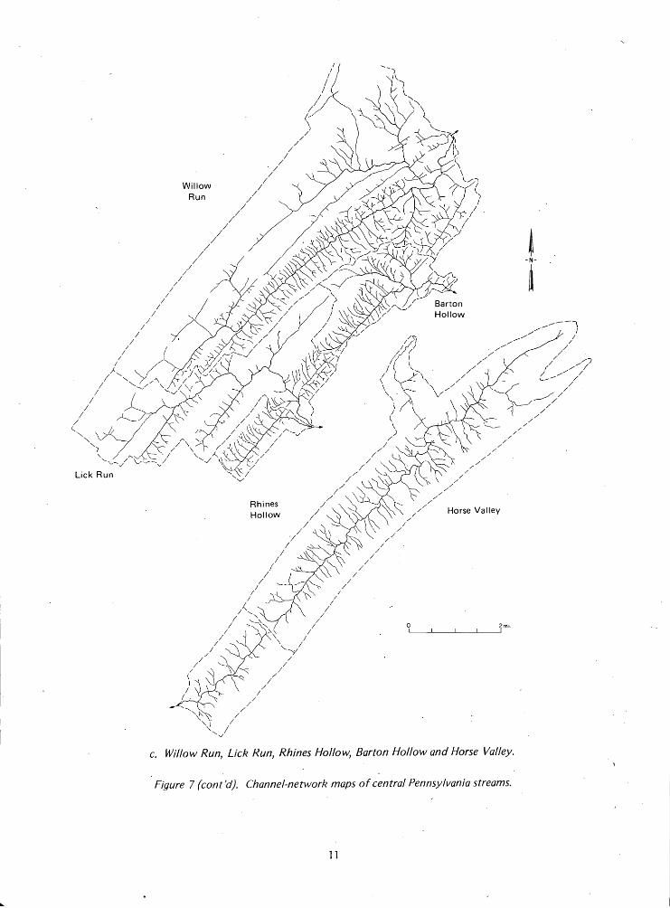
Complete channel networks of the nine central Pennsylvania streams are shown in Figure 7.The drainage patterns are of the classical trellis type. Reference to Figures 6 and 7c, the geologicand channel network maps of the same area, will be useful in understanding the way in whichgeology has controlled the developmentof the drainage patterns. The elongated master streamsarealigned parallel to the regional strike of rocks while the majority of the lesser tributaries are orientedperpendicular to the master streams and flaw up-or down-section, depending upon the local bedrock attitude. The master streams have preferentially developed along zones of weakness which

V /

Devonian System

Dm Marine beds: Shales, graywackes and sandstones.

Dho Mahantango —Marcellus —Onandaga Formations, undivided. Shales with interbedded sandstones atbottom, black fissile, carbonaceous shale in middle, and thin bedded shale and medium bedded limestone at top.

Doh Helderberg —Oriskany Formations, undivided. Fine to coarse grained sandstone, cherty limestone withsome interbedded shales and sandstone at top. Thin bedded shales, cherty limestones to thick beddedcrystalline limestone at bottom.

Silurian System

Skm Keyser —Tonoloway —Wills Creek —Bloomsburg —McKenzie Formations, undivided. Limestonesgrading downward to argillaceous limestones to interbedded shales and limestones.

Sc Clinton Group. Shales, interbedded downward with quartzitic sandstone to thin to medium, bedded shalewith intertonguing "iron sandstone."

St Tuscarora Formation. Medium to thick bedded, fine grained, quartzitic sandstone.

Ordovician System

Ojb Juniata —Bald Eagle Formations, undivided. Fine grained to conglomeratic quartzitic sandstones.Or Reedsville Formation. Shale with thin silty to sandy interbeds.

Figure 6. Generalized geologic mapof Willow Run, Barton Hollow, Lick Run, Rhines HollowandHorse Valley Run. Source: GeologicMap of Pennsylvania (Pennsylvania Geological Survey I960)

and unpublished base maps.

a. George Creek and Bixler Run.

Figure 7. Channel-network maps of central Pennsylvania streams.

b. Tuscarora.

10

Willow

Run

Horse Valley

i i i i i

c. Willow Run, Lick Run, Rhines Hollow, Barton Hollow andHorse Valley.

Figure 7 (cont'd). Channel-network maps of central Pennsylvania streams.

11

3 ^ 6Geological Section A-A'

Tuscarora

ConococheagueMtn

9miles

Figure 8. Geologic section along line A-A' of Figure 6. (See Fig. 6 for legend.)

are either more easily eroded rocks or formational contacts. The narrow outcrop pattern of therock units has caused the development of a series of parallel elongated channels rather than a treelike channel system.

The present result ofdifferential erosion in this area is a landscape characterized by parallelridges and valleys. The geologic cross section shown in Figure 8 illustrates the relationship betweentopography, lithology and structure. The most resistant rock unit, the Tuscarora Formation, aquartzitic sandstone, underlies the three major ridges, while streams are incised into less resistantsiltstones, shales and argillaceous limestones.

Eastern Pennsylvania - New Jersey streams. The three drainage basins in this group lie in theTriassic Lowland physiographic province (USGS 1970).

The region and each ofthe three drainage basins have low to moderate relief with gently rollinghills and occasional steep ridges with local relief on the order of 300to 400 feet.

The geology of the area is shown in Figure 9and the channel networks in Figure 10. Geologically,the area is much simpler than that ofcentral Pennsylvania, in that for the most part it can be considered a simple homocline locally interrupted by broad anticlines and synclines. The regionalstrike is NE-SW with an average regional dip of 15° to 20° to the northwest.

The underlying bedrock in each stream basin is composed of members of the Triassic NewarkGroup. Three interfingering lithofacies (the Stockton, Lockatong and Brunswick) compose thesedimentary section (Willard et al. 1959). While the lithofacies exhibit a variety oflithologies, eachhas a dominant one, arkose in the Stockton, argillite in the Lockatong, and shale in the Brunswick.In addition, diabase dikes and sills have been intruded.

The stream patterns in these basins range from moderately well developed trellis to dendritic.The trellis pattern is best developed where the Lockatong and Brunswick lithofacies interfinger,such as in the eastern part of the Tohickon drainage. Streams have preferentially developed in thedirection of the regional strike on the less resistant shales of the Brunswick lithofacies. Wherelithology becomes more homogeneous, such as the eastern part of the Stony Brook drainage oronthediabase of the Tohickon, a more typical dendritic pattern forms. Despite the less-pronounceddevelopment of trellis patterns, the effectsof varying resistance to erosion between and within thelithofacies of the Newark Group and the homoclinal structure have enabled differential erosion todevelop stream patterns characterized bya moderate degree of parallelism to the regional strike.

.12

Figure 9. Geologic map of eastern Pennsylvania and western New Jersey with stream basins shown. (Adapted from Willard et al. 1959.)

a. Stony Brook.

Figure 10. Channel network maps of eastern Pennsylvania and western New Jersey streams.

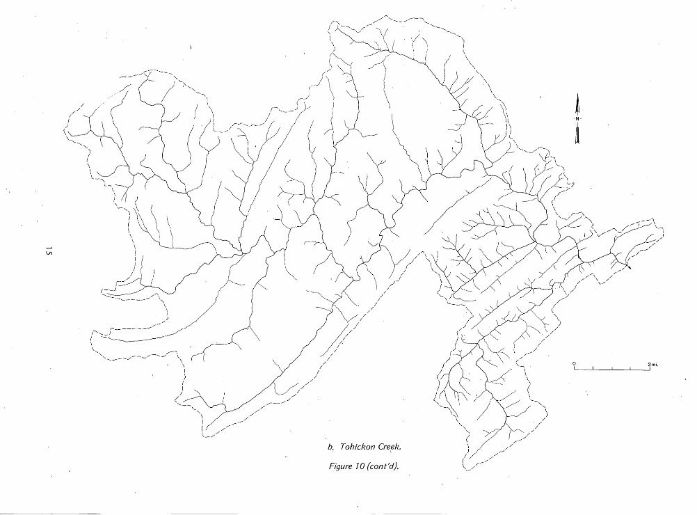
b. Tohickon Creek.

Figure 10 (cont'd).

c. Neshanic River.i

Figure 10(cont'd). Channel network maps of eastern Pennsylvania and western New Jersey streams.

16

Channel network mapping

The channel network of each of the streams was traced in its entirety from 1:24,000 scaletopographic maps. Channels not shown as blue lines on the maps were defined by continuousV-shaped contour lines. As a consequence of using contour shape to define channels, an elementofoperator judgment becomes part of the data. For the most part, this manifests itself in decidingwhere to terminate a channel as V-shaped contours grade slowly towards U-shaped ones. Thisproblem does not affect topology so much as the study oflink lengths, or the measurement ofdrainage density.

Each linkof a channel network was assigned an identification number and the following datawere tabulated:

1. Identification number

2. Magnitude

3. Length

4. Type

This information formed the basic data set for much of the subsequent work.

TOPOLOGICAL PROPERTIES OF THE NETWORKS

Introduction

Equation 5gives the number oftopologically distinct channel networks (TDCN) possible for anetwork ofgiven magnitude. The simplest possible statistical analysis is to test the null hypothesisthatTDCN of the same magnitude occur with equal frequency. As a practical matter, this isfeasible only with low-magnitude networks because ofthe rapid increase ofN(M) with increasing Mand the concomitant difficulty in obtaining a sufficiently large sample. Consequently, it becomesnecessary to group TDCN into classes having some common property or, alternatively, to develop"other means of classification which can be predicted by the model.

Smart (1968) and Werner and Smart (1973) have reviewed existing methods oftopologicclassification and have proposed new classification schemes. The general strategy used herein will beto proceed from examining low-magnitude networks to greater-magnitude networks, using ateachscale a classification system commensurate with the samplesize.

Three methods of classification will be used in addition to TDCN, namely the ambilateral classification introduced by Smart (1969), the right-left classes used by Krumbein and Shreve (1970), andstream number sets.

The following convention will.be used in this chapter. Each topologically distinct channel network discussed will be initially illustrated by a schematic channel network map. Associated with aparticular TDCN will be a roman numeral, designating the ambilateral class to which it belongs, andone or two letters designating its right-left class. See Table 11 asan illustration of usage.

The essence of Smart's ambilateral classification is that all TDCN which can be made equivalentby simple right-left reversals at one or more junctions belong to the same ambilateral class. Smartargued that the individual TDCN's within an ambilateral class would be expected to have similarhydrological properties. Furthermore he noted that all TDCN's within an ambilateral class wouldhave the same set of link magnitudes and the same set of stream numbers.

The right-left classification used by Krumbein and Shreve assigns a TDCN to a right or left classbased on which side of the main channel (when viewed upstream) has the greatest number of

17

magnitude-1 streams ultimately tributary to it.. In the modified form used herein, TDCN havingequal contributions from both sides are classified as rl or Ir as shown in Tables II and III.

Stream-number sets are shown in the form {nl,n2, ...,nn_v 1) where n1 is the number of Strahlerfirst-order streams, n2 the number ofsecond order streams, etc. Within a topologically randompopulation of given magnitude, the probability of occurrence of each possible stream number setcanbe calculated from eq 8.

Table I contains basic information for the 12 streams studied here. The first seven streams inTable I are referred to throughout as the contiguous-seven and the last three as the Triassic. For themost part, statistical analysis isconfined to these two groups. Complete data for each channel network are given in the Appendix.

Table I. Summary data for stream networks.

Area Drainage densityStream Magnitude. (miles2) (mile~1)

Contiguous seven

Rhines Hollow 51 1.56 7.74

Barton Hollow 102 3.70 7.47

Lick Run 117 9.19 3.83Willow Run 380 22.84 4.63

George Creek 246 9.49 6.51

Tuscarora Creek E. 385 15.25 5.67-

Tuscarora Creek W. 281 13.77 5.32

Horse Valley Run 175 15.24 3.91Bixler Run 274 15.00 5.06

Triassic

Neshanic River 259 25.7 4.11

Stony Brook 274 44.5 3.29

Tohickon Creek 311 97.4 2.27

Magnitude-4 networks

There are five topologically distinct arrangements possible for magnitude-4 networks. Thesearrangements are shown in the first column of Tables 11 and 111. Thestatistics of magnitude-4 networks for the contiguous-seven and Triassic streams are shown in Tables II and III. In these and

later statistical tables, the column headed Expected is the expected number of networks whichwould occur in that particular class for random selection of a sample of size n from a topologicallyrandom population of magnitude-/^ networks.

Statistical analysis of the data is given in Tables IV and V. Throughout the statistical analysis,unless stated otherwise, the null hypothesis tested is: the observed sample data have frequenciesof occurrence which could be expected from random selection of an equivalent-size sample froma topologically random population of networks of the particular magnitude under consideration.For samples having three or more classesa chi-square goodness of fit test will be used to decide onacceptance or rejection of the null hypothesis. The generalized likelihood ratio is

Table II. Statistics of the 123 magnitude-4 networks

from the contiguous-seven streams.

TDCN Class Observed Expected Class Observed Expected

' >

Ir 36 24.6 Ir

and

I

59 49 2

T II 23 24.6

T Irl 20 24.6 Irl

and

Mr

37 49 2

•

Mr 17 24.6

T II 27 24.6 II 27 24.6

Table III. Statistics of the 48 magnitude-4 networks from the Triassic streams.

TDCN Class Observed Expected Class Observed Expected

10 9.6

9.6

9.6

i 15 9.6

X 9.6

Ir

and

Irl

and

Mr

19

20

19.2

19.2

9.6

Table IV. Statistical analysis of magnitude-4 networks fromthe contiguous-seven streams.

Sample -21n\ Degrees of freedom X2.0s,df Decision

TDCN

Irll, Irl IIr, II

Sample

Ir, Hand Irl, Mr

8.50

5.37

Observed

59

4

2

Sample size

96

9.49

5.99

Accept

Accept

Crit val Decision

56 Reject

Table V. Statistical analysis of magnitude-4 networks from the Triassic streams.

Sample -2/nX Degrees of freedom X2.0s,df Decision

TDCN 5.36

Irll, Irl IIr, II 0.07

19

9.49

5.99

Accept

Accept

fc+1 /p

where n is the total sample size, ni is the number of samples in they'th class of the &+1 classes, andPi is the given or known probability of the/th class (Mood et al. 1974, p. 444). For large values ofn, -2ln\ hasapproximately the chi-square distribution with k degrees of freedom, and the decisionto reject the null hypothesis is made if -2/n\ > x2, k for the a level of confidence.

In those cases where just two samples are beingcompared, the binomial distribution is used fortesting the null hypothesis. For samplesizes up to 150, tables of the cumulative binomial probabilities were consulted (Army Materiel Command 1972) while for larger sample sizes the normal approximation for the binomial distribution was used (Mood et al. 1974, p. 120-121). For all tests, thedecision to accept or reject the null hypothesis was made at the 0.05 level of confidence.

The statistical analysis in Tables IVand V indicates that, with one exception, the null hypothesiscan be accepted at the 0.05 significance level. That exception occurs in the comparison of Class Irand II networks with Class Irl and 11 r networks in the contiguous-seven sample. In a topologicallyrandom population the two groups occur with equal frequency but the excess of the r and I groupover the rl and Ir group is sufficiently large to reject the null hypothesis.

The question raised by the excess of the grouped Class Ir and II channel networks is whetherthis excess occurs randomly throughout the sample or in some systematic way which can be relatedto geological or geographical factors. In order to answer this question, the magnitude-4 TDCN'sfrom the contiguous-seven streams were classified as a function of two attributes: 1) direction offlow with respect to local strike, i.e. along-strike or across-strike, and 2) direction of flow withrespect to dip, i.e. up- or down-section. The original statement of the topologically random modelcontains no reference to directional properties of topology. However, "in the absence of geologiccontrols" implies that the topological properties should be isotropic with respect to geological factors.This in turn means that any subset chosen as a function of a geological characteristic should also betopologically random.

In Tables VI and VII samples from various possible subsets are statistically tested. The nullhypothesis in each of these tests is that the sample could have been drawn from a topologicallyrandom subset. The results shown in the tables indicate that the null hypothesis can be rejectedfor the population of networks flowing along-strike. These, of course, are the streams whosetributaries are flowing either up-dip or down-dip to reach the main channel. Of the Class I networkswhose tributaries can unambiguously be defined as flowing up- or down-section, approximately 67%have their tributaries flowing down-section, suggesting that this may be the controlling geologicfactor.

A similar analysis of the Triassic magnitude-4 networks cannot be made. Orientations of themagnitude-4 networks are less systematic with respect to the bedrockattitude. This, in conjunctionwith the initially smaller sample, provides a sample size which is too small for meaningful statisticaltesting.

Magnitude-5 networks

The 14 possible topologically distinct arrangements of a magnitude-5 channel network are shownin Table VIII with right-left and ambilateral classes indicated. Tables IX and X show the statistical

analysis. Note that although the observed and expected frequencies of TDCN's are shown in

Tables IX and X, no goodness-of-fit tests are given in Tables XI and XII. This illustrates the majordifficulties in comparing real channel networks with the topologically random model at the level

20

Table VI. Direction of flow with respect to regional strike

of contiguous-seven magnitude-4 networks.

Direction of flowAlong- Across- Inter- Along- Across- Inter-

Class strike strike mediate strike strike mediate

Ir

II

15

8

19

14

3

123 33 4

Irl

Mr i}-12"

14

2

27 26 4

II 9 15 2 9 15 2

-2/nX 11.38 1.75 6.43 0.84

Decision Reject Accept Reject Accept

* Combined for goodness-of-fit test.

lar

lar

Table VII. Direction of flow with respect to dip of

contiguous-seven magnitude-4 networks.

Direction of flow

Class Down-section Up-section Down-section Up-section

Ir

II

7

9

12

516 17

Irl

llr

3

7

9

710 16

II 6 8 6 8

-2lnX 3.33 . 3.26 1.43 0.036

Decision Accept Accept Accept Accept

Table Vlll. Topological classes for magnitude-5 networks.

Ibr

t

Ibr

Icr

f

Hal

Idr

f

Ibl

lal Ibl Id Idl

Ambilateral

class

-< -<

nir mi

>~ >-

21

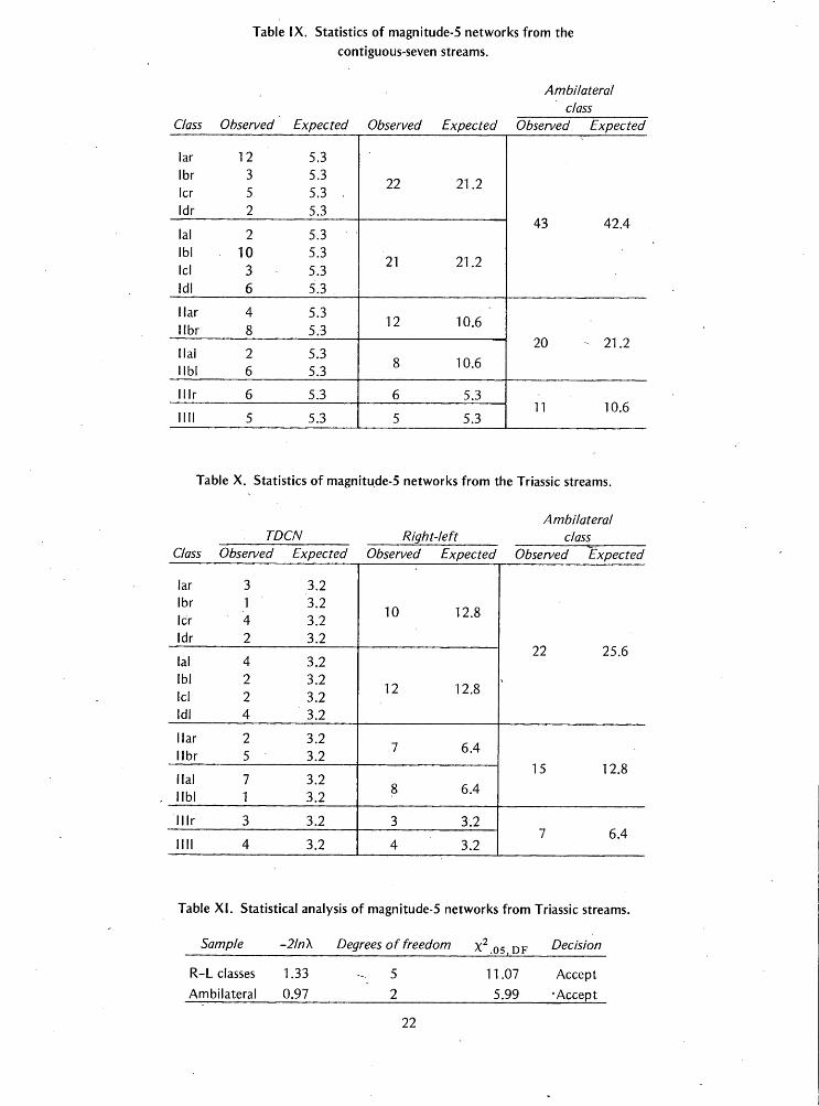
Table IX. Statistics of magnitude-5 networks from the

contiguous-seven streams.

Ambilateral

class

Class Observed Expected Observed Expected Observed Expected

lar 12 5.3

Ibr

Icr

3

5

5.3

5.3 .22 21.2

Idr 2 5.343

lal 2 5.342.4

Ibl

Id

10

3

5.3

5.321 21.2

Idl 6 5.3

Mar

llbr

4

8

5.3

5.312 10.6

20Hal

llbl

2

6

5.3

5.38 10.6

- 21.2

11Ir 6 5.3 6 5.311

llll 5 5.3 5 5.310.6

Table X. Statistics of magnitude-5 networks from the Triassic streams.

TDCN Right-leftAmbilateral

class

Class Observed Expected Observed Expected Observed Expected

lar 3 3.2

Ibr

Icr

1

4

3.2

3.210 12.8

Idr 2 3.222

lal 4 3.225.6

Ibl

Id

2

2

3.2

3.212 12.8

*

Idl 4 3.2

liar

llbr

2

5

3.2

3.27 6.4

15Hal

llbl

7

1

3.2

3.28 6.4

12.8

lllr 3 3.2 3 3.27

llll 4 3.2 4 3.26.4

Table XI. Statistical analysis of magnitude-5 networks from Triassic streams.

Sample -2/nX Degrees of freedom X2 os df Decision

R-L classes

Ambilateral

1.33

0.97

22

11.07

5.99

Accept

'Accept

Table XII. Statistical analysis of magnitude-5 networks

from the contiguous-seven streams.

Sample -21nX Degrees of freedom X2.os,df Decision

R-L classes

Ambilateral

1.76

0.12

11.07

5.99

Accept

Accept

of TDCN, namely that the number of possible TDCN rises with such rapidity as magnitude increases,that the problem of maintaining a sample size ofat least five per class, considered good statisticalpractice (Miller and Kahn 1962), becomes impractical.

The null hypothesis that these samples could have been drawn from a topologically randompopulation of magnitude-5 networkscan be accepted for both samples whether classified by theright-left or the ambilateral system. It is worth noting that the wide disparity between observedand expected TDCN in some classes is completely hidden in the right-leftand ambilateral classification.

Magnitude-6 to magnitude-10 networks

The statistics and statistical analyses of magnitude-6 through magnitude-10 streams are shownin Tables XIII-XVIII. For magnitude-6 networks TDCN were grouped according to ambilateralclass, while for greater magnitude networks they were combined into stream number sets. Notealso that even at the level of stream number sets, it was necessary to combine groups in order to have

a satisfactory sample size.

The statistical analysis indicates that, with one exception, there is no reason to reject the hypothesis that these samples were drawn from topologically random populations of the indicated magnitude.That sample for which the null hypothesis can be rejected occurs in the Triassic samples where thestream number set (10, 2, 1) occurs with greater frequency than would be expected in a topologically random population of magnitude-10 networks.

Summary

All channel networks ranging from magnitude 4 to magnitude 10 within the contiguous-sevenand Triassic samples have been classified and grouped by TDCN's, right-left classes, ambilateralclasses, or stream number sets as appropriate for the available samplesize. For each magnitude thenull hypothesis that the observed sample could have been drawn from a topologically randompopulation of that magnitude was tested using either a chi-square goodness-of-fit test or a binomialtest. The null hypothesiscould be rejected at the 0.05 confidence level for two of the samples, thatof class I magnitude-4 TDCN's from the contiguous-seven sample and that of magnitude-10 streamnumber sets from the Triassic sample. '

The magnitude-4 networks, for which the null hypothesis could be rejected, were subjected tofurther study, examining TDCN as function of their flow direction with respect to the attitude of thelocal bedrock. In so doing it is argued that the topologically random model, in particular the keyphrase "in the absence of geologic controls," implies directional isotropy of topology with respectto any geological parameter. Examination of the magnitude-4 streams shows that of those streamswhich flow in the direction of the local strike, those having tributaries entering from the same sideoccur with much greater frequency than can be expected in a topologically random population.

23

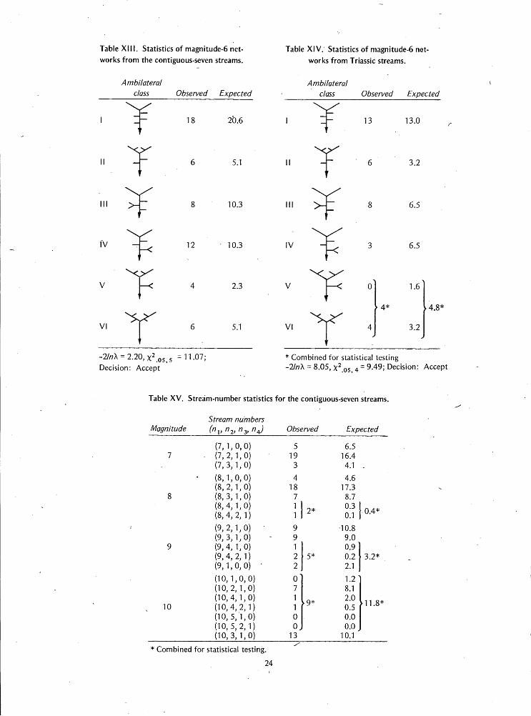
Table XIII. Statistics of magnitude-6 net

works from the contiguous-seven streams.

Table XIV. Statistics of magnitude-6 net

works from Triassic streams.

III

fv

VI

Ambilateral

class Observed Expected

18 20.6

XX

5.1

10.3

12 10.3

2.3

^v^5.1

III

IV

VI

Ambilateral

class Observed Expected

13 13.0

3.2

>- 6.5

-<6.5

1.6

^r-> 4*

3.2

U.8*

-2/nX =2.20, x2.os,5 =11-07;Decision: Accept

* Combined for statistical testing-2Jn\ =8.05, x2.05,4 =9-49J Decision: Accept

Table XV. Stream-number statistics for the contiguous-seven streams.

MagnitudeStream numbers

(nv n2, ny nj Observed Expected

(7,1,0,0) 5 6.5

1 - (7,2,1,0) 19 16.4

(7,3,1,0) 3 4.1 .

• (8,1,0,0) 4 4.6

(8,2,1,0) 18 17.3

8 (8,3,1,6) 7 8.7

(8,4,1,0)(8,4,2,1)

1

12* 03 I04*o.i ru/f

(9,2,1,0) 9 •10.8

(9,3,1,0) 9 9.0

9 (9,4,1,0) 1 0.9

(9,4,2,1) 2 •5* 0.2 3.2*

(9,1,0,0) ' 2 2.1

(10,1,0,0) 0" 1.2'(10,2,1,0) 7 8.1

(10,4,1,0) 1 2.0

10 (10,4,2,1) 1.9*

0.5• 11.8*

(10,5,1,0) 0 0.0

(10,5,2,1) oj 0.0

(10,3,1,0) 13 10.1

* Combined for statistical testing.

24

Table XVI. Stream-number statistics for Triassic streams.

Stream numbers

Magnitude (nv n2,n3, nj Observed Expected

(7,1,0,0) . 5 7.0

1 (7,2,1,0) 22 17.6

(7,3,1,0) 2 4.4

(8,2,1,0) 16 13.4

(8,1,0,0) 2 3.6

8 (8,3,1,0)(8,4,1,0)

5

07*

6.7

0.2•10.6*

(8, 4, 2,1) 0 0.1 ](9,2,1,0) 9 7.5

(9,1,0,0) x 1 , 1.4

9 (9,3,1,0)(9,4,1,0)

^-51

•7*6.3

0.6•8.5*

(9,4,2,1) . 0 0.2

(10,2,1,0) 10 5.9

(10,1,0,0) 0 0.8](10,3,1,0) 4 7.4

10 ' (10,4,1,0)(10,4,2,1)

2

0• 6*

1.5

0.4• 10.1*

(10,5,1,0) 0 0.0

(10,5,2,1) o, 0.0 J* Combined for statistical testing.

Table XVII. Statistical analysis for contiguous-seven streams.

Sample -21nX Degrees of freedom X2.0s,df Decision

Mag 7Mag 8Mag 9

1.11

4.28

1.14

Observed

2

3

2

Sample size

5.99

7.82

5.99

Crit val

Accept

Accept

Accept

Decision

Mag 10 13 22 15 Accept

Table XVIII. Statistical analysis for Triassic streams.

Sample -2/nX Degrees of freedom x2.0s df Decision

Mag 7

Mag 8Mag 9Mag 10

3.32

Observed

16

9

10

Sample size

24

16

16

25

5.99

Crit val

17

12

10

Accept

Decision

Accept

Accept

Reject

Furtherexamination indicates that the tributaries entering on the same side and flowing down-sectionare preferentially developed, in a ratio of about 2:1 over those flowing up-section. Thus itisconcluded that an identifiable geological factor is influencing the topological arrangements inthese small networks.

It is perhaps more remarkable that these drainage systems, which show stronggeological controlof their channel patterns, have no apparent systematic or identifiable bias in their topologicalproperties above the level of the magnitude-4 networks cited above.

LINK PROBABILITIES

Introduction

The analysis has sofar considered networks from, magnitude 4 to magnitude 10 with varyingdegrees of topological resolution. To continue the statistical analysis to larger network sizes in asimilar manner becomes increasingly difficult. For instance, the entiresample contains 25 magni-tude-20 channel networks, while thereexist 30 sets of possible stream numbers for that magnitude.Thus, it is necessary to devise a system which allows examination of topological properties of higher-magnitude systems.

In the preceding analysis, the TDCN has been considered the basic element and, as the networkmagnitude increased, TDCN's were grouped, by right-left classes, ambilateral classes and finally intostream-number sets. The strategy to be applied now is to examine a more fundamental element thanthe individual TDCN, namely the individual links. Acoherent and consistent method of classifyinglinks is developed. Then, a setof equations describing their frequency of occurrence for topologically random populations isderived, followed by examination of the sample networks in the contextof these predictions.

The overall link-type classification and derivations which follow are largely abstracted from thepublished paper A Classification of Channel Links in Stream Networks (Mock 1971).

Link frequencies

. In a topologically random population of channel networks of any given magnitude M, theprobability of drawing a link at random of magnitude p. was given by eq 9, while the probability ofdrawing at random a link of magnitude p from an infinite topologically random network was givenby eq 10. It is possible to examine the frequency distribution of link magnitudes to test thehypothesis that the samples were drawn from an infinite topologically random population.

To properly test the hypothesis that a set of links could have been drawn from an infinite

topologically random population requires that the links be randomly selected. The links whichform the samples to be analyzed are the set of all links contained ina series of complete networksand do not represent random selection;. The fact that they are complete networks puts certainlimits on link magnitudes which would not be applicable had they been randomly selected. Toillustrate this point consider the following differences between a random selection of 3117 linksfrom an infinite topologically random population and the 3117 links that compose the contiguous-seven sample. The numberof magnitude-1 links is rigorously set in the contiguous-seven samplewhile ina randomly selected sample it isnot. There is no upper limit on the magnitude of a link ina randomly chosen sample while in the contiguous-seven sample it is 385and isequal to the magnitude of the largestnetwork in any sampleconsistingof integrated networks. The point is thatselection of complete networks puts constraints on the possible outcomes and requires a certainrestraint in interpretation of results. Table XIX shows the statistical data for the contiguous-sevenand the Triassic samples.

26

Table XIX. Statistics and analysis of link-magnitude

frequencies, contiguous-seven and Triassic streams.

Contiguous-seven Triassic

Link magnitude Observed Expected Link magnitude Observed Expected

2 420 389.6 2 214 210.3

3 214 193.3 3 104 105.8

4 123 121.8 4 47 . 65.7

5 74 85.2 5 44 46.0

6 54 63.9 6 34 34.5

7 34 50.2 7 29 27.1

8 31 40.8 8 24 22.0

9 23 34.0 9 15 18.4

10 22 28.9 10 16 15.6

> 10 558 548.0 > 10

-2/nX = 7.69, X2

314

05,9=16.92

295.7

-2/nX = 21.58,X2 OS9=16.92

5% Decision: Reject 5% Decision: Accept

Magnitude

2,3,4,5,6,7,8,9, I0,>I0,

//////A

•vzzzzzz^zzzz&zZ

•8-

'Freq

-I2-

-I6-

-20-

•24-

Figure 11. Hanging rootogram showing expectedfrequenciesand deviations from expected frequencies as a function of

magnitudes for the contiguous-seven networks.

27

The null hypothesis that the observed link frequencies could have been drawn from an infinitetopologically random population can be rejected at the 0.05 confidence level for the contiguous-seven sample. In Figure 11, the contiguous-seven observed link frequencies and their deviationsfrom predicted values are plotted by means of a hanging rootogram (Jamesand Krumbein 1969).Figure 11 shows graphically the excess of observed magnitude-2 and -3 links and the dearth of observed links in the magnitude-5 -10 range, in comparison with the expected frequencies.

The observed deviations can be related to geological factors in the area of the contiguous-sevenstreams. The master channels, occupying strike valleys, are separated from each other by lesseasily eroded rock units. Networks tributary to the master channels are constrained by the intervening, more resistant rocks, to a size rangegoverned in part by the spacing of the resistant rocks.Thus, depending upon local lithologies and structures, a certain range of link magnitudes will bedepleted in frequency with respect to an infinite topologically random population.

Within the contiguous-seven streams the factors cited above appear to inhibit development ofchannel networks in the magnitude-5 to magnitude-10 range. The Triassic streams, on the otherhand, do not show any similar trends.

Link types

Interior and exterior links have been defined in Chapter I. Within the set of interior links, Jamesand Krumbein (1969) defined two further types: cis-links and trans-links. A cis-link was definedas an interior link bounded at its upper and lower forks by tributaries entering from the same side.A trans-link was defined as an interior link bounded at its forks by tributaries entering from oppositesides. A tributary, in the sense used here, is the link of lesser magnitude of the two links upstreamfrom a junction. In the context of their study, James and Krumbein limited cis- and trans-links tothose having a magnitude greater than 10. That restriction will be relaxed here, with no magnitudelimits placed upon these link types.

In a topologically random population, cis- and trans-links occur with equal frequency. However,in the James and Krumbein study cited above, in a sample of 485 links, over 60% were trans-links,an occurrence with a probability of less than 0.00001 if the probability of occurrence of cis- andtrans-links were equal.

A later study (Krumbein and Shreve 1970) in the same area (Inez quadrangle, Kentucky) butdealing with magnitude-5 networks, found trans-links occurring with greater frequency than cis-links, but not in sufficient quantity to justify rejecting the hypothesis that they have an equalprobability of occurrence.

James and Krumbein (1969) proposed a model to explain observed cis- and trans-link lengthfrequencies. At its headward end, a channel network grows by random bifurcations, but withinthe network channel adjustments take place, with coalescence of tributaries enteringclose to eachother on the same side and thus extinction of some cis-links. While the model has been criticized

(Abrahams 1972) it does satisfactorily explain the excess of trans-links in their study area.

The observed numbers of trans-and cis-links for the contiguous-seven and Triassic streams areshown in Tables XX and XXI asa function of magnitude. In an infinite topologically randompopulation, the probability of occurrence of trans- and cis-links is the same, independent of theirmagnitude. The null hypothesis tested in Tables XX and XXI is that the cis- and trans-links could

have been drawn from a population in which they occur with equal frequency. There is no reasonto reject this hypothesis for either the contiguous-seven or Triassic samples when the total samplesare considered. However when the link frequencies are examined as a function of magnitude, thenull hypothesis can be rejected for three subsets, two in the contiguous-seven sample and one in theTriassic sample.

28

Table XX. Statistics and statistical analysis of trans-

and cis-links for contiguous-seven streams.

Link Number of % Number of Critical 5%magnitude trans trans cis value decision

1-10 145 42.8 194 188 Reject

11-20 81 54.0 69 86 Accept

21-30 47 58.8 33 ~ 48 Accept

31-40 19 63.3 11 2.0 . Accept

> 40 164 63.6 94 145 Reject

Total 456 53.2 401 458 Accept

Table XXI. Statistics and statistical analysis of trans-

and cis-links for Triassic streams.

Link Number of % Number of Critical 5%

magnitude trans trans cis value decision

1-10 98 413 109 118 Accept

11-20 21 36.2 37 36 Reject

" 21-30 21 47.7 23 28 Accept

31-40 12 57.1 9 15 Accept

>40 88 54.0 75 94 Accept

Total 240 48.7 253 269 Accept

The earlier analysis of magnitude-4 TDCN from the contiguous-seven sample indicated a preferential development of what have now beendesignated cis-links. From Table XX it isclear that up tomagnitude 10 there isa preferential development of the cis type. The same holds true for the Triassicsample although the frequency of occurrenceof cis-links is not sufficiently different from that oftrans-links for rejection of the null hypothesis. At the opposite end of the scale, i.e. for links withmagnitudes greater than 40, exactly the opposite situation occurs. Both samples have more trans-links than cis-links, but the null hypothesiscan be rejected only for the contiguous-seven sample.

The data shown in Tables XXand XXI and the analysis of magnitude-4 networks suggests thefollowing hypothesis: in regions where trellis drainage patterns are developed bedrock attitude willpreferentially favor certain flow directions. In low magnitude networks this will lead to moretributaries entering from thesame side, hence more cis- than trans-links. At higher magnitudes,implying greater age, interaction of tributaries entering from the same side will eliminate some cis-links with an eventual predominance of trans-links.

Admittedly, theevidence which has suggested this hypothesis is hardly overwhelming and hascertain ambiguities. For instance, the large percentage of low magnitude cis-links in thecontiguous-seven sample as compared to the Triassic sample is consistent with its greater lithological diversityand bedrock dips, but thegreater frequency of occurrence of trans-links at higher magnitudes is not.It is an area worth more study.

Exterior links. Two types ofexterior links will be defined: 1) The S (source) link is a magnitude-1 link that joins another magnitude-1 link at its downstream fork. 2) The TS (tributary source) linkis a magnitude-1 link that joins a link of magnitude greater than 1 at itsdownstream fork.

29

TB

\v Magnitude ofX. upstream

Nv link= #|U TV2P

Magnitude \^

or" downstreams,

link \.<?&;**; K(id;M)

< 2p. B-link CT-link

S(p;M) p(jub;M) P(juCT;M)

>2ju TB-link T-link

T(m;M) P(Hb>m) P(MT;M)

Figure 12. Definition of link types by the magnituderelationshipsof link ofmagnitude p. and its adjacentup

stream and downstream neighbors.

TB

CT

CT TS

T.I B

CT

TS

Figure 13. Idealized network

showing link magnitudes and

types.

Interior links. Figure 12 shows the upstream and downstream

criteria for defining interior links. 1) The B (bifurcating) link isa link of magnitude p that is formed at its upstream fork by theconfluence of two links, each of magnitude p/2, and that flowsat its downstream fork into a link of magnitude less than 2p.2) A TB (tributary bifurcating) link is a linkof magnitude p thatis formed at its upstream fork by the confluence of two links,each of magnitude jit/2, and that flows at its downstream fork

into a link of magnitude greater than or equal to 2p. 3) The T(tributary) link isa linkof magnitude p that is formed at its upstream fork by the confluence of two links of unequal magnitude and that flows at its downstream fork into a link of magnitude greater than or equal to 2p. 4) The CT-(cis-trans) link isa link of magnitude p that is formed at its upstream fork by theconfluence of two links of unequal magnitude and that flows atits downstream fork into a link of magnitude less than 2p.Figure 13 showsan idealized network illustratingthe link types.

The last downstream link in any system under study, i.e. thehighest magnitude link, is defined as either a T- or TB-link

depending on the magnitude relationships at its upstream fork.

Note that the CT category of links includes the cis- and trans-links defined by James and Krumbein (1969). Cis- and trans-

links are not considered individually since they are dependent on topologic relationships as well asmagnitude relationships at successive forks, while the criteriaused here are based entirelyon arithmetic relationships of the link magnitudes.

Since link types have been defined in termsof magnitude relationships, eq 9 and 10 provide thebases for calculation of the probability of occurrence of each link type in finite and infinite topologically random networks.

30

Probability of occurrence

Exterior links. Exterior links are by.definition links of magnitude 1. The probability of drawing

an exterior link at random from a topologically random population of networks of magnitude M is

given by eq 9, with p = 1. Designating this as P{ext; M) it is

P{ext;M) = co{-\;M)=M/{2MA). (12)

The probability of drawing an exterior link at random from an infinite topologically random popula

tion is

/>(ext)=^J/(^1) =0.5.

Draw a link at random from a topologically random population of networks of magnitude M.If the link is of magnitude 1, what is the probability that it connects with another magnitude-1 link?The original draw leaves a topologically random population of magnitude MA . The original linkhas an equal probability of connecting with any one of the 2/W-3 remaining links. The probabilitythat it connects with another magnitude-1 link is equal to the proportion in which the magnitude-1links occur or {MA )/(2M-3). Thus, the probability of occurrence of an S-link is

P(S-M)= M x «MA (13)1 ' ; 2MA 2M-3 V '

and the probability of occurrence of 5-links in an infinite topologically random population is

P(S)= lim M(M~]) =0 25 (14)^1 M-**> (2MA)(2M-3) u""' - l ;

To determine the probability of drawing a 73-1 ink, a similar type of argument is used.

A link is drawn at random. If it is a magnitude-1 link, determine the probability that it connectswith an interior link in the {MA )-magnitude network which remains. The probability of drawing atrandom an interior linkfrom a topologically random population of magnitude-M networks is (usingeq12):

P{\nt; M) = 1-P{ext; M) = {MA )/{2MA). (15)

The probability of occurrence of 7"S-links is given by

P{TS;M)=^-rxP{\nt;MA)

PITS- M) =-M— x J$=L (16)K ' ' 2MA 2M-3 ' V '

for topologically random populations of magnitude M and by

PlTS)= lim M x M~2 -0 25 (17)r{,b) M^°o 2MA X2M-3 U^' l '

for an infinite topologically random network.

31

M3

Figure 14. The randomly

drawn link p3, andthefour links to which it is

attached. The arrow designates the flow direction.

Interior links. The essence of the rather heuristic arguments

to be presented is that a series of successive random selections of

links from topologically random populations of appropriately sized

networks will serve to define interior link types. Consider a topo

logically random population of networks of magnitude M. From

this population a link of magnitude ju, designated as p3, is randomlydrawn. Along with the link ju3, the four links joined to p3 at itsupper and lower junctions are shown in Figure 14.

From the definition of link magnitudes it is known only that

pl+p2=p3

p3+p4=p5 .

In terms of the defining criteria shown in Figure 12 the possibletypes of p3 are:

jU3 = B-link if jUj orp2 - p3\2 and ju5 < 2pp3 - TB-link if jux or p2 =p3/2 and p5 > 2pp3 = CT-link if pl or p2\p3/2 and p5 < 2pp3 = T-link if ^j or p2 ^ p2/2 and ps> 2p .

In the following discussion reference to a network of any stated magnitude will refer to a topologically random population of such networks, and random selection of a link will mean random selection

from a topologically random population of the specified magnitude.

Consider now the linkM3. It is the ultimate linkof a sub-network of magnitude p3, imbedded inthe overall network of magnitude M. Since the link was randomly selected from a topologicallyrandom population the possible topological arrangements of its network form a topologically random

population of magnitude p3. Since/i, +p2 =p3 only the magnitude of one of the two upstream linksis independent and need be considered. Taking jUj, it can have any magnitude from 1 to (ju3-1) andthe sub-network which it defines is a topologically random population of networks of magnitude{p3-1). Thus the probability thatpl=p3/2, denoted asq{p3;M) is, using eq 11,

q(p3;M)=u{p3/2;p3-]).

In the general case then, the probability that a randomly selected link from a topologically randompopulation of networks of magnitude M will bifurcate at its upper junction is

q{p;M) = to{p/2;p-l)

and the probability of occurrence is

Q{p;M) = oj{p;M)co{p/2;p-l). (18)

Since there is only one other possibility, the probability that the link p does not bifurcate at itsupper junction is

*(ju;Af) = 1-coGu/2;/i-1)

and

32

K{p;M) =aj{p;M)[\-Gj{p/2;p-l)] . (19)

Note that q{p;M) and k{p;M) are independent of M. Such is not the case for the downstream

possibilities relating /Li3, ^4 and

The two possibilities at the downstream junction of linkju3, shown in Figure 14, are

p5<2p3=>p^<p3,

and

p5 > 2p3 - p4 > M3 •

It is convenient to work with p4 rather than ju5, so that the probabilities of interest are, havingrandomly selected p3, the probability that it joins a link ju4 < p3 or that it joins a link p4 > p3 .Remembering that these are topologically random populations, the effect of selecting p3 is to remove all links tributary to it from the population of magnitude-ZW networks. That is, the remainingpopulation is now a topologically random population of diminished magnitude {M -p3). Since p3can join any link in the diminished network, the problem is reduced to the problem of randomlyselecting a link of magnitude ju4 from the networks of {M-p3) magnitude. Thus, the probabilitythat ju4 < p3 is

M3-1

and for the general case, designating the second link as 7, the equation is

M-l

s{p;M)=Y] co{y;M-p)7=1

and summing over all possibilities the probability of occurrence is

5(M3;^) =_P u{p4;M-p3)

M M-l

s(ju;M)=]TV oj{p;M)co{r,M-p). (20)M=l 7=1

The probability that 7 > p is then given by

M-i

5M-l

f(m;Af) =i-V o>{r,M-n)

and

ZM r M-l -1

Up; m) =2^ w(m; m) [i -_T "(t; ^-m)J . (21M=l 7=1

33

Equations 18-21 define the probability of occurrence of the defining criteria for topologicallyrandom populations of magnitude-/^ networks.

The probability of drawinga link of specified p which satisfiesa set of upstream and downstreamrelationships is simply the intersection of the three probability spaces co{p; M), q{p; M) or k{p; M),and s{p; M) or t{p; M). Designating this as P{ptyp&; M) as shown in Figure 12 the probabilities are:

P{pB;M)=cj{p;M)q{p;M)s{p;M)P{pTB;M) = cJo{p;M)q{p;M)t{p;M)P{pCT;M) = u{p; M) k{p; M) s{p; M)P{pT;M) = oj{p;M)k{pt;M)t{p;M).

Finally, to define the probability of occurrence of a particular typeof link in a topologicallyrandom population of magnitude-/^ networks it is necessary to sum over all possibilities. Designating this as P{type; M) the equations are:

and

M M a-\

P{B;M)=22 P^B> M) =_>_] 22 o>{p;M)co{p/2;pA)u{r,M-p)M=l 7=1M=l

M M r- M-l "I

P{TB;M)=J2p{pB;M) =J2a:{p;M)u{p/2;pA) 1-V w(r;Af-/i) LM=l M=l - . L y^f J

M M M-l

P{CT;M)^P{pCJ;M)=^2^2 ^;M) [Uco{p/2;pA)} aj{y;M-p)M=l M=l 7=1

M

P{T;M)-^2p{pT;M)M=l

M

u{p;M)[-\-o>{p/2;p-f M-l

;H)]IiTMt;M=l

M-p) •-co(1;Af).

(22)

(23)

(24)

(25)

The quantity co(1;M) in eq 25 removes the exterior links which are included in the summation.

It is of interest to determine the limiting values, ifany, of the probabilities expressed in eq 22-25asMbecomes infinite, i.e. for an infinite topologically random network. The approach is to calculateanalytically the marginal probabilities shown in Figure 12 for the infinite case and then to evaluatenumerically the joint probabilitiesP{B; M) and P{TB; M), which are sufficient to define the remaining joint probabilities. It can be shown that

M

M=l

M

co{p;M)cj{p/2;pA) =l- ^ u{p/2; M) co[p/2; M-{p/2)] =m=i

M

^ w(m; M)co{p; M-p).M=l

34

Thus, the marginal probability Q{p; M) of Figure 12 can be rewritten as

M

Q{p;M)=Y22^)M)o,{p;M-p). (26)M=l

Shreve (1967, p. 181) has shown that

lim u{p;M)=2^(^)--H»),

so that eq 26 can be rewritten as

oo

lim Q{p;M) =]-^2 u{p)v{p). (27)M^-°° m=i

This summation can be calculated exactly by using the functional relationships satisfied by the

gamma function (M. Dacey, personal communication, 1970), which gives

lim Q{p;M) =1 [(4/tt) -1] =0.13622.... (28)M^-oo

Thus,

lim K{n;M) =1 -0.13662-0.5 = 0.36338... . (29)M-+°°

The remaining marginal probabilities for the infinite topologically random case become

°° M-l

lim S{p;M)^^2^2 v{p)v{y) (30)M^°° M=l 7=1

and

lim 7-(ju;/W)=^_>_ v{p)v{y). (31)A/-»°° M=l 7=M

Consider now an infinite topologically random network from which two consecutive randomdrawings are made designating the magnitude of the first link ju and the second link 7. Designatethe joint probabilities of v{p) v{y) as v{p, 7); then a matrix of probabilities, as shown in Figure 15,is symmetric. Because of symmetry,

]C_C »b>y) =J2 _C »b.y) • (32)M=2 7=1' M=l 7=M+1

35

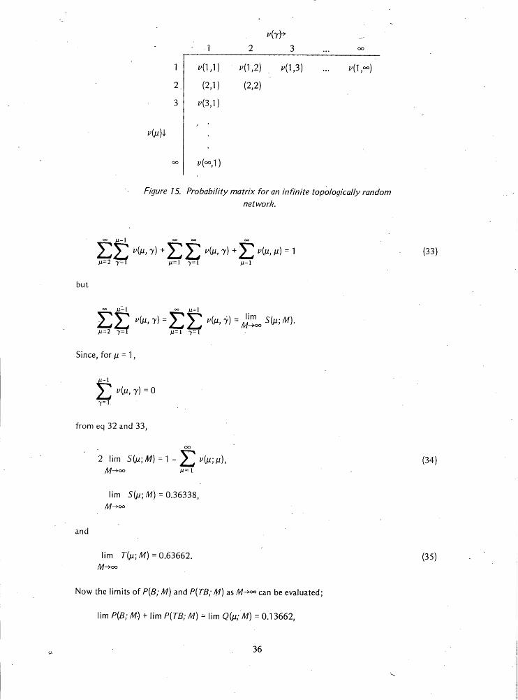
v{p)\

1

*(1,1

(2,1

v{3,\

v{°°,\)

2 3_

"(1,2) . "(1,3)

(2,2)

v{\,c

Figure 15. Probability matrix for an infinite topologically randomnetwork.

but

z222u^'y^+^2 £v^'7^+£v^' ^li=2 7=T M=l 7=1

> > v{ii, 7)=2]^ v{p, 7) =M-l

zM= 1 7= 1U=2y=i

Since, for p - 1,

J2 v^> t) =o7=1

from eq 32 and 33,

oo

2 lim S(m;/W) =1-2^(m;m),/W-*» M=l

lim S{p;M) = 0.36338,

and

lim T{p; M) = 0.63662.

M-l

lim

Af-*»S{p;M).

Now the limits of P{B; M) and /'(TiB; Af) as M-+°° can be evaluated;

lim P{B; M) + lim P{TB; Af) = lim C?(m; M) = 0.13662,

36

(33)

(34)

(35)

which is

°° M-l . °° °°

• 227 ^)WW2;M-1)"W=2^]P v{p)u{pl2;pA)v{y) =0.13662. (36)M=l 7=1 M=l 7=M

Equation 36 can be rapidly evaluated to five significant figures by means of a computer, so that

lim P{B; M) = 0.07086, (37)

lim P{TB;M) =0.06576, (38)M-*°°

and using the remaining marginal probabilities of Figure 12

lim P{CT; M) = 0.29252 (39)

and

lim P{T;M)= 0.07086. (40)

Table XXII shows the probability of occurrence of each link type for topologically random popula

tions of various magnitudes.

In Table XXII note that the probability of occurrence of T- and B-links is the same. It isimplicit in the definingcriteria that, on moving upstream from a T-link, a main channel sequencemust terminate at a B-link. This holds true for any channel sequence within a network, thus giving

a one for one correspondence of T-linksand B-links. Thus, although six types of links have beendefined, two exterior and four interior, there are only three independent link categories.

Table XXI I. Probability of occurrence of link types for networks of various magnitudes.

M P(S;M) P(TS;M) P(CT; M) P(T; M) P(B; M) P(TB; M)

2 0.667- 0.333

3 0.400 0.200 0.200 0.200

4 . 0.343 0.229 0.114 0.114 0.114 0.086

5 0.317 0.238 0.159 0.111 0.111 0.063

6 0.303 0.242 0.182 0.100 0.100 0.074

7 0.294 0.245 0.200 0.098 0.098 0.065

8 0.287 0.246 0.213 0.091 0.091 0.071

9 0.282 0.247 0.224 0.090 0.090 0.067

10 0.279 0.248 0.231 0.087 0.087 0.069

20 0.263 0.249 0.264 0.078 0.078 0.067

50 0.255 0.250 0.281 0.074 0.074 0.066

100 0.253 0.250 0.287 0.072 0.072 0.066

200 0.251 0.250 0.290 0.072 0.072 0.066

400 0.251 0.250 0.291 0.071 0.071 0:066

oo 0.250 0.250 0.293 0.071 0.071 - 0.066

37

Tables XXIII-XXVI give the statistics and statistical analyses for link types of the contiguous-seven and Triassic streams. There is no reason to reject the hypothesis that the Triassic samplewas drawn from an infinite topologically random population. However the hypothesis can berejected for the case of the contiguous-seven networks. As shown in Table XXV, we can also reject the hypothesis that the interior and exterior types occur with the frequencies expected in atopologically random population.

Table XXIII. Link-type statistics

for the contiguous-seven streams.Table XXIV. Link-type statistics

for Triassic streams.

Link type Observed Expected Link type Observed Expected

CT 856 913.3 CT . 493 493.7

T 238 221.3 T 119 119.6

B 238 221.3 B 119 119.6

TB 223 205.7 - TB 110 111.2

S 844 779.3 S 432 421.3

TS 718 779.3 TS 412 421.3

Table XXV. Statistical analysis of link types for contiguous-seven streams.

5%Sample Degrees of freedom -2lnX Crit val decision

All link types 3 18.13 Reject

Interior link types 2 7.61 Reject

S- vs TS-links 820 Reject

Table XXVI. Statistical analysis of link types for Triassic streams.

5%Sample Degrees of freedom -2/nX Crit val decision

All link types 3 0.58 Accept

Interior link types 2 0.006 Accept

S- vs TS-links 451 Accept

The deviations observed from predicted link type in the contiguous-seven sample areconsistentwith the link-magnitude deviations shown in Table XIX and Figure 9. A large part of the deviationof CT-links is a result of the less-than-expected number of magnitude-5 through magnitude-10 links,and at least part of the excess in TB- and T-links corresponds to the greater-than-expected numberof magnitude-2 links.-

38

Joint probability for link magnitude and type

It is now possible to construct the joint-probability distribution for link type and link magnitude

for an infinite topologically random population using eq 22-25. The resulting probabilities are

shown in Table XXVII.

Table XXVII. Joint probabilities of interior-link types and magnitude

for an infinite topologically random channel network.

Trans Cis T B TB "M

2 0 0 0 .06250 .0625 .12500

3 .01953 .01953 .02344 .06250

4 .01074 .01074 .00977 .00537 .00244 .03906

5 .00993 .00993 .00748 , .02734

6 .00699 .00699 .00457 .00147 .00048 .02051

7 .00624 .00624 .00363 .01611

8 .00487 .00487 .00258 .00060 .00016 .01309

9 .00438 .00438 .00214 .01091

10 .00362 .00362 .00165 .00030 .00007 .00927

> 10 .07996 .07996 .01560 .00062 .00001 .17621

P(type) .14626 .14626 .07086 .07086 .06566 .50000

Tables XXVIII and XXIX show the observed and predicted numbers of links as a function of

link type and link magnitude. The predicted values are those expected for random selection of

samples of equivalent sizes from an infinite topologically random population. As was discussed

previously, the samples do not consist of randomly selected links, thus a certain bias will occur.

This implies that rejection of the null hypothesis that the observed frequencies could have been

drawn from an infinite topologically random population will have some ambiguity. For con

venience the statistic U = (Observed-Expected)2/Expected has been calculated. This statistic

follows the chi-square distribution so that if U> xi df tne nu" hypothesis can be rejected at thea confidence level.

The results of the statistical analyses are included in Tables XXVIII and XXIX. There is noreason to reject the null hypothesis in the case of the Triassic sample. For the contiguous-seven

sample the null hypothesis can be rejected for each of the following:

a. The total sample.

b. The total sample with cis- and trans-links combined.

c. The subset consisting of all links up to and including magnitude 10.

d. The subset defined in c. but with cis- and trans-links combined.

The results are consistent with many of the earlier results, and enable specific identification of

where deviations from expectation occur. For example, in Table XIX magnitude-3.links were ob

served to occur with greater frequency than predicted. Table XXVIII shows that the major part ofthe deviation is accounted for by the large number of T-links. In fact T-links occur with greater

than expected frequency up to and including magnitude 5, as do also TB-links. This means that

there are more small, but complete, networks in the sample than would be expected in a topologically random population. . - -

39

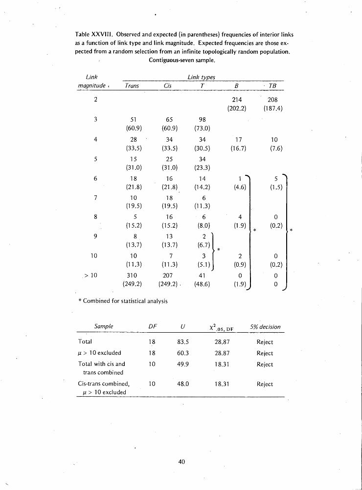
Table XXVIII. Observed and expected (in parentheses) frequencies of interior linksas a function of link type and link magnitude. Expected frequencies are those ex

pected from a random selection from an infinite topologically random population.

Contiguous-seven sample.

Link

magnitude

9

10

> 10

* Combined for statistical analysis

Sample

Link types

Trans Cis T B TB

214 208

(202.2) (187.4)

51

(60.9)65

(60.9)98

(73.0)

28

(33.5)

34

(33.5)

34

(30.5)17

(16.7)10

(7.6)

15

(31.0)25

(31.0)34

(23.3)

18

(21.8)16

(21.8)

14

(14.2)1 ^|

(4.6)

5

(1.5)

10

(19.5)18

(19.5)6

(11.3)

5

(15.2)16

(15.2)6

(8.0)4

(1.9)

0

* (0-2)*

8

(13.7)13

(13.7)2 ^

(6.7)• *

10

(11.3)7

(11.3)3

(5.1)

2

(0.9)0

(0.2)

310

(249.2)207

(249.2) .41

(48.6)0

(1.9)

0

0J

DF U 5% decision.05, DF

Total 18 83.5 28.87 Reject

ju > 10 excluded 18 60.3 28.87 Reject

Total with cis and 10 49.9 18.31 Reject

trans combined

Cis-trans combined, 10 48.0 18.31 Reject

p > 10 excluded

40

Table XXIX. Observed and expected (in parentheses) frequencies of interior linksas a function of link type and link magnitude. Expected frequencies are those expected from random selection from an infinite topologically random population.

Triassic sample.

Link

magnitude Trans

3 25

(32.9)

4 11

(18.1)

5 16

(16.7)

6 12

(11.8)

7 14

(10.5)

8 10

(8.2)

9 4

(7.4)

10 6

(6.1)

> 10 142

(134.7)

Link types

Cis T B TB

105 108

(109.3) (101.3)

28 52

(32.9)' (39.5)

17 10 8 1

(18.1) (16.5) (9.0) (4.1)

18 10

(16.7) (12.6)

13 5 4 "1 0

(11.8) (7.7) (2.5) (0.8)

9 6

(10.5) (6.1)

8 5 ' 0 1

(8.2) (4.3) (1.0)

8

* (7-4)3

(3.6)• *

>

8 1 1 0

(6.1) (2.8), (0.5) (0.1)

144 -27 1 0

(134.7) (26.3) (1.0) 0

J

>

J

- * Combined for statistical analysis

Sample DF U X .05, DF 5% decision

Total 11 18.66 19.68 Accept

Abrahams (1972) has cited the significance of "maximum extension" in the study of thefrequency distribution of interior-link lengths. Paraphrasing dock (1931), as quoted by Abrahams(1972, p. 731), maximum extension is the time when a drainage system is fully developed. In atrellis pattern drainage network the master channels extend headward, usually along-strike; when abifurcation occurs, that link which isgrowing across-strike has a much more limited potential forgrowth than its sister link. This arises from the fact that another master channel exists, at somedistance depending upon local geology, developing parallel to the first channel. Thus, cross-strikechannels are constrained to reach their maximum development within an area bounded by themaster streams. The net result one would expect is what has been observed in the contiguous-seven sample, an excess of low-magnitude tributaries over what should beexpected in a randomlybifurcating system.

41

LINK LENGTHS

Introduction

In previous chapters a systematic study of a sample of real channel networks has been made,comparing observed properties with those predictable from a topologically random model. Aclassification of channel-link types was devised to enable the study to proceed at a level differentfrom that of past work. The question arises: Do the link types defined on pages 28-30 differ fromeach other in any way other than in the numerical relationships of links at their upper and lowerforks? Are there physical or geometric differences between link types, or are they only definablein the context of a particular numeration scheme?

The above question is the subjectof this section. In examining this question, the idea oftopological randomness or nonrandomness can be left aside as not germane, at least at the level ofsimply determining if a physical difference exists between link types. Furthermore, the fact thatthe sample under study here has been drawn from a particular type of stream pattern largely controlled by geology will be disregarded in the analysis, although it may be a caveat in the conclusions.

Link lengths

The particular property of links to be examined here is their length. Two reasons exist for this,one that it is the simplest property, other than magnitude, to measure from a mapof a channel network and two, there is a limited amount of pre-existing work on link lengths.

Previous work

Strahler (1954) and Schumm (1956) showed that length-frequency distributions of 1st-orderstreams, i.e. exterior links, could be well represented by a log normal distribution. Smart (1968,p.1005) made the following assumption: lengths of interior links in a given network are independent random variables drawn from the same population. Later in the same paper, he introduced anegative exponential densityas a specific model for the interior-link-length-frequency distribution.Shreve (1969) proposed a gamma density with a shapefactor of 2 as a model for interior-linklengths. These models have had varying degrees of success in describing observed interior-link-length distributions. The most detailed study was conducted by James and Krumbein (1969) inwhich they developed models for the distribution of trans-links and cis-links.

ObservedJink-length frequency distribution

Observed interior-link-length frequency distributions for the contiguous-seven and Triassic networks are shown in Figure 16. The basic assumption at the start will be that cited above, namelythat the lengths of interior links in a given network are independent random variables drawn fromthe same population. The following hypothesis will be tested: The link-length-frequency distributions for each interior-link type were drawn from the same population as the total interior-link-length-frequency distribution. Note that no specific population models are implied here.

Statistical analysis of interior links

The null hypothesis to be tested is: link-length frequencies are independent of link type.Tables XXX and XXXI show the observed and expected link-length frequencies calculated underthe assumption that they were all drawn from the same population. These tablesare contingencytables for a two-way classification. The null hypothesis can be rejected at the 0.05 confidencelevel for both samples.

42

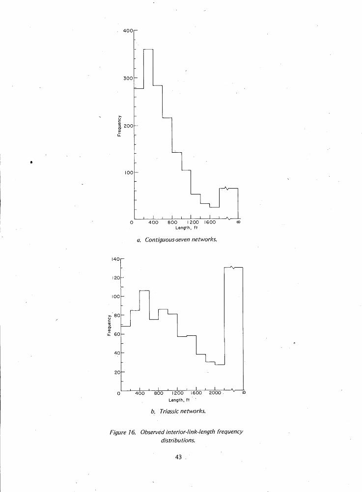
400

300-

3 200

100

I40i-

120

100

80

60

40

20

0 400 800 1200 1600

Length, ft

a. Contiguous-seven networks.

I • I L. J I l_0 400 800 1200 1600 2000

Length, ft

b. Triassic networks.

Figure 16. Observed interior-link-length frequencydistributions.

43

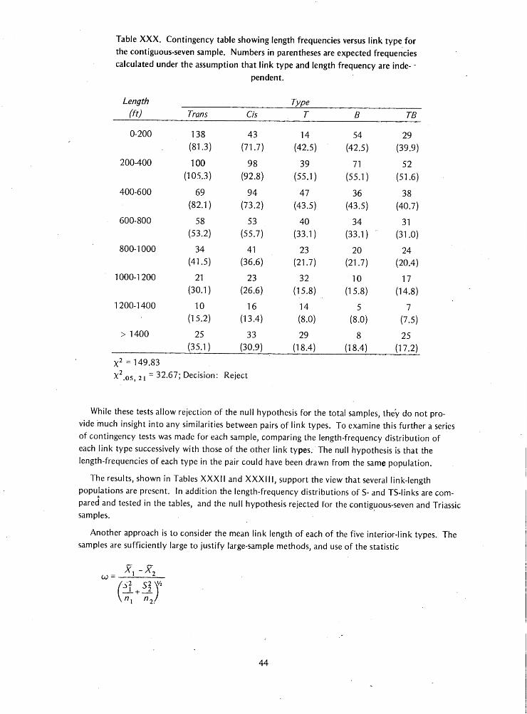
Table XXX. Contingency table showing length frequencies versus link type forthe contiguous-seven sample. Numbers in parentheses are expectedfrequenciescalculated under the assumption that link type and length frequency are inde

pendent.

Length Type

(ft) Trans Cis T B TB

0-200 138 43 14 54 29

(81.3) (71.7) (42.5) (42.5) (39.9)

200-400 100 98 39 71 52

(105.3) (92.8) (55.1) (55.1) (51.6)

400-600 69 94 47 36 38

(82.1) (73.2) (43.5) (43.5) (40.7)

600-800 58 53 40 34 31

(53.2) (55.7) (33.1) (33.1) (31.0)

800-1000 34 41 23 20 24

(41.5) (36.6) (21.7) (21.7) (20.4)

1000-1200 21 23 32 10 17

(30.1) (26.6) (15.8) (15.8) (14.8)

1200-1400 10 16 14 5 7

(15.2) (13.4) (8.0) (8.0) (7.5)

> 1400 25 33 29 8 25

(35.1) (30.9) (18.4) (18.4) (17.2)

X2 =149.83

X2.05, 21 =32.67; Decision: Reject

While these tests allow rejection of the null hypothesis for the total samples, the'y do not provide much insight into any similarities between pairs of link types. To examine this further a seriesof contingency tests was made for each sample, comparing the length-frequency distribution ofeach link type successively with those of the other link types. The null hypothesis is that thelength-frequencies of each type in the pair could have been drawn from the same population.

The results, shown in Tables XXXII and XXXIII, support the view that several link-lengthpopulations are present. In addition the length-frequency distributions of S-and TS-links are compared and tested in the tables, and the null hypothesis rejected for the contiguous-seven and Triassicsamples.

Another approach is to consider the mean link length of each of the five interior-link types. Thesamples are sufficiently large to justify large-sample methods, and use of the statistic

CO =X\ ~X2

_i+__Y2ni n:

44

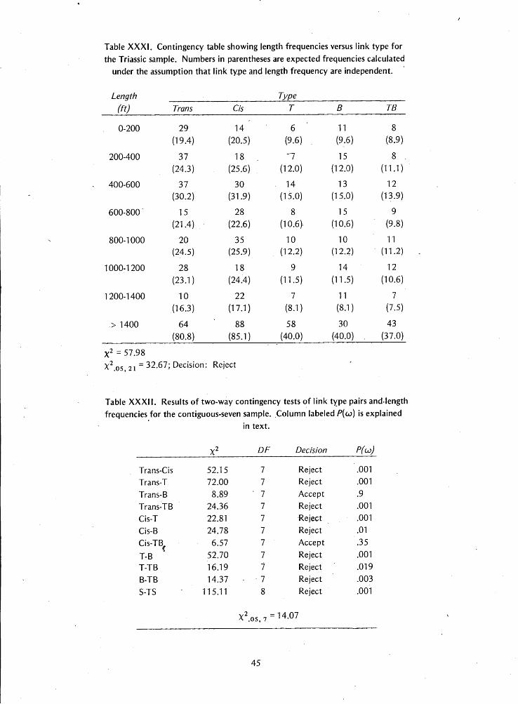
Table XXXI. Contingency table showing length frequencies versus link type for

the Triassic sample. Numbers in parentheses are expected frequencies calculated

under the assumption that link type and length frequency are independent.

Length

(ft) Trans Cis

Type

TB

0-200 29

(19.4)14

(20.5)6

(9.6)

11

(9.6)

8

(8.9)

200-400 37

(24.3)18

(25.6)1

(12.0)15

(12.0)8 .

(11.1)

400-600 37

(30.2)30

(31.9)14

(15.0)13

(15.0)12

(13.9)

600-800 15

(21.4) -

28

(22.6)

8

(10.6).15

(10.6)9

(9.8)

800-1000 20

(24.5)35

(25.9)

10

(12.2)10

(12.2)

11

(11.2)

1000-1200 28

(23.1)18

(24.4)9

(11.5)

14

(11.5)

12

(10.6)

1200-1400 10

(16.3)22

(17.1)7

(8.1)

11

(8.1)

7

(7.5)

> 1400 64

(80.8)88

(85.1)58

(40.0)30

(40.0) .43

(37.0)

X2 = 57.98X2 05 2i = 32.67; Decision: Reject

Table XXXII. Results of two-way contingency tests of link type pairs andlengthfrequencies for the contiguous-seven sample. Column labeled P{co) isexplained

in text.

DF Decision PW

Trans-Cis 52.15 7 Reject .001

Trans-T 72.00 7 Reject .001

Trans-B 8.89 • 7 Accept .9

Trans-TB 24.36 7 Reject .001

Cis-T 22.81 7 Reject .001

Cis-B 24.78 7 Reject .01

Cis-TB^T-B

6.57 7 Accept .35

52.70 7 Reject .001

T-TB 16.19 7 Reject .019

B-TB 14.37 7 Reject .003

S-TS 115.11 8

X .05, 7 "

Reject

= 14.07

.001

45

Table XXXIII. Results of two-way contingency test of link type pairs and lengthfrequencies for the Triassic sample. Column labeled P{u>) is explained in text.

DF Decision P(co)

Trans-Cis 30.79 8 Reject .007

Trans-T 24.28 *8 Reject .001

Trans-B 9.86 8 Accept .9

Trans-TB 16.53 8 Reject .01

Cis-T 8.73 8 - Accept .17

Cis-B 11.09 8 Accept .008

Cis-TB 7.84 8 Accept .29

T-B 17.44 8 Reject .001

T-TB 5.27 8 Accept .96

B-TB 8.87 8 Accept .009

S-TS 50.16

X .05,

8

8 = 15.51

Reject .002

where X{ is the mean link length, Sf is the sample variance, and ni is the sample size. For largesample sizes, co asymptotically approacheszero mean and unit standard deviation (Rao 1952,p. 217). co is then a measure, in Gaussian standard deviation units, of the difference between themeans; thus, the probability that the two sample means were drawn from populations having thesame mean can be taken from normal probability tables. The u> statistic was calculated for each

link pair and, if 0.05 probability is used as a decision criterion, similar results to those obtained withthe contingency tests will be obtained with the following exceptions: the cis-B and B-TB link pairsfrom the Triassic sample can be rejected. The columns labeled P{oj) in Tables XXXII and XXXIIIare the probabilities that the sample means were drawn from populations having the same meanlink length."

The results of these tests imply that there exists a relationship between link type and lengthfrequency distributions, i.e. there are different populations for certain of the link types. This issummarized in Table XXXIV where the link pairs which appear to be drawn from different populations are tabulated.

As a final but qualitative demonstration of the relationship between link type and link length,consider the data shown in Table XXXV, where link types for the two samples are listed in descending order of mean link length. If link types and length are related, then a similar sequence of typesas a function of length should occur. As can be seen in Table XXXV, there is a similarity in thesequences. This is illustrated graphically in Figure 17 where the mean lengths of link types from thecontiguous-seven networks are plotted versus the corresponding mean link length from the Triassicnetworks. The solid line is a least-squares regression line having a correlation coefficient of 0.898,significant at the 0.01 level. No predictive capability is implied by Figure 17; rather it indicates thatthe link type and link length properties behave similarly in two widely separated samples.

Summary

The link types developed in the section Link Probabilities (p. 26) have been examined in thecontext of their length-frequency distributions. Statistical tests strongly imply that the lengthsof interior links are not independent random variables drawn from the same population or

46

Table XXXIV. Link pairs having different length-distribution

based on contingency tests.

Contiguous-seven

Trans-Cis

Trans-T

Trans-TB

Cis-T

Cis-B

T-B

T-TB

B-TB

S-TS

Triassic

Trans-Cis

Trans-T

Trans-TB

T-B

S-TS

Table XXXV. Link types of contiguous-seven and Triassic samples

arranged in descending order of mean length.

TriassicContiguous-seven

Link type Mean length (feet) Link type Mean length (feet)

T 880 TS 1752

TS 827 T 1663

TB 725 TB 1650

Cis 682 S 1454

S 601 Cis 1435

B 553 Trans 1132

Trans 544 B 1118

2400 I 1 1

1 • ;i

//

- / ~

/

-

• /

-

-

/

-

-

1

/

i i • i i •

2000-

- I600-

- Eo o

? . I200-

8000 400 800 1200 1600Mean Length of Link Types from Contiguous-

seven Sample, ft

Figure 17. Mean length ofeach of the seven link typesfor the Triassic and contiguous-seven samples plotted

against each other.

47

populations. When considered by type, the evidence for a characteristic link length property is

stronger in the contiguous-seven sample than in the Triassic streams. This may be of some signifi

cance (the Triassic sample being less geologically controlled than the contiguous-seven streams) inlight of Werner and Smart's (1973) comment that, in an unpublished study of dendritic networks,they found all interior links had essentially the same link-length distribution with the exception of

T-links.

The high correlation between link type and mean length for the two samples suggests that a

systematic relationship exists between these variables. It is apparent though that this area of

inquiry needs more study, particularly with a more homogeneous set of channel networks'.

SUMMARY AND CONCLUSIONS

Introduction

The infinite topologically random model serves as a norm with which the topological properties

of real networks can be compared. The model postulates that, in the absence of geologic controls,

channel networks will be topologically random. This study examines in detail a sample of channel

networks in which the presence of geologic controls is clearly evident from their network patterns.

While the stream patterns are striking, their departure from the expectations of topological randomness are much less discernible.

The samples used in this study can be considered as two parts of a continuum which ranges from

the classic trellis patterns with a dominance of geologic control to the classic dendritic pattern

developed with minimal geologic control. The contiguous-seven sample is representative of the treljis

end member of this system, while the Triassic sample lies somewhere in the mid range. In this

summary, it is shown that the topological characteristics of the channel networks follow a similar

continuum, albeit one which is not nearly so broad or as readily visualized.

Basically, two different methods have been used to analyze the topological properties of the sam

ple networks. The first method was to examine sub-networks within the larger samples, grouping

the sub-networks into classes such that their frequency of occurrence could be compared with

expected frequencies in topologically random populations. The second method examined individual

links, looking at their frequency of occurrence as a function of magnitude, then as a function of type,and finally as a function of type and magnitude.

Sub-networks

All sub-networks ranging in size from magnitude 4 to magnitude 10 within the two samples were

examined. At the magnitude-4 level, the networks were grouped into individual TDCN and right-left classes. At higher magnitudes, right-left classes, ambilateral classes, and stream numbers formed

the bases for grouping. In all cases, the observed frequencies of occurrence were compared with

those expected in a topologically random population. Interpretation of the results from the Triassic

streams is quite simple; the hypothesis that these samples were drawn from a topologically random

population can be accepted at the 0.05 level except in the one case in which an excessive number of

magnitude-10 streams have the stream numbers (10, 2, 1). Considering the number of tests, thisconstitutes only a small deviation, and the general conclusion that these samples were drawn from

a topologically random population is justified.

Apparent geologic controls are discernible in the topological characteristics of the contiguous-

seven sample. However, they are subtle and appear to affect only the smallest streams, i.e. the

magnitude-4 networks, where there is a preferential development of tributaries entering from the

- 48

same side. This excess is most pronounced in those networks whose direction of flow is parallel

to the regional strike, indicating a preferential development of tributaries, related to the dip direc

tion. Surprisingly enough, a similar tendency is not apparent in the magnitude-5 networks, although

the smaller sample size limits the detail of study. This leads to caution in ascribing geologic controls

as a causal mechanism. From magnitude 5 to magnitude 10, all tests indicate no reason to reject the

hypothesis that the samples could have been drawn from topologically random populations. Thus,

the general conclusion is that, with the exception of magnitude-4 networks, the topologically ran

dom model provides the best explanation for the observations.

Links

Analysis of the link structure of networks provides quite a different means of viewing topologicalcharacteristics. In this study, analysis of link frequencies as a function of type and magnitude hasrevealed departures from the expectations of topological randomness that can be related to geologi

cal controls.

The contiguous-seven channel networks have a classical trellis drainage pattern. Major channelsare approximately parallel to each other and flow along the strike direction. This particular geometry puts a constraint on tributary development, both in the formative stage of the networks and inlater adjustments. The parallelism of the main channels and more resistant intervening rocks limits

the size to which tributary channel networks can expand. Thus one can expect to find an excess oflinks in some particular magnitude range depending upon the spacing of master channels, and adeficiency through some higher magnitude range, when compared with the expected frequencies ofa topologically random network.

Interior and exterior links form the basic subdivision of links by type. However, in the section

Link Probabilities (p. 26) both interior and exterior types were further subdivided. The interior-linktypes can be thought of in terms of their relationship to channel sequences. A channel sequence isterminated downstream with a T-link when it meets an equal- or higher-magnitude sequence, and

upstream with a B-link; a link bifurcates into two links of equal magnitude. All the interveninglinks constitute CT-links. A TB-link is a channel sequence of one link. Thus, for each T-link, thereexists exactly one B-link and zero or more CT-links. For finite or infinite topologically random networks, the expected numbers of each type can be specified. If'geological controls actively limitrandom growth, i.e. force development of small networks, then an excess of T- and B-links, and adeficiency of CT-links, can be expected.

The frequency distribution of link magnitudes observed in the contiguous-seven and Triassicstreams were compared with the expected frequencies assuming both samples were drawn from an

infinite topologically random population. Usinga chi-square goodness-of-fit test, there was no reason to reject the hypothesis at the 0.05 level for the Triassic sample. The hypothesis was rejectedfor the contiguous-seven sample where an excess of magnitude-2 and -3 links, and a dearth ofmagnitude-5 through -9 links, largely caused the rejection.

The frequency distribution of link types in both samples was compared and tested in the samemanner as above with similar results; the Triassic sample could have been drawn from a topologicallyrandom population; and 4he contiguous-seven improbably so. Further testing of the contiguous-seven sample showed that neither the interior-link types nor the exterior-link types, when considered separately, occurred with the frequencies expected if drawn from a topologically random population. Greater than expected frequencies occur in the T, Band TB categories (those links whichterminate channel sequences), and a deficiency of CT-links, implying an organization made up ofgreater than expected short channel sequences.

49

By combining the frequencies of link type and link magnitude for comparison with expected

frequencies, a fairly powerful tool is available for detection of the network structure. As in previousstatistical tests, the contiguous-seven networks can be rejected as having been drawn from a

topologically random population. Table XXIX reveals in detail where the major departures occur:

1. An excess of magnitude-3 to -5 T-links, i.e. short channel sequences.

2. A deficiency of CT-links (trans and cis) through magnitude 8.

At magnitudes greater than 10, large departures from expected frequencies also occur but, be

cause of the nature of the sample, i.e. complete networks rather than a random sample, less signifi

cance can be attributed to those departures. The significance of item 1 above is that geological factors are acting as a partial constraint on network growth, limiting the potential expansion of networks

tributary to the master streams, thus resulting in a much larger number of relatively small completenetworks than would occur in a topologically random network.

In contrast to the contiguous-seven, the Triassic streams appear to represent a topologically random population.

The classification of link types was based solely on the numerical relationships of each link withits adjoining links at the upstream and downstream junctions. The mean lengths of each link typeand their length-frequency distributions were analyzed to determine whether type differences werealso reflected in length differences. The results were somewhat ambiguous in that separate lengthpopulations did not appear to be present for each link type, while, at the same time, the hypothesisthat the individual samples were drawn from a common link-length population could be rejected.The similarity in the trend of mean link length as a function of type, shown by both the Triassicand contiguous-seven samples (Fig. 17), suggests a correlation between link type and link length.

To summarize, the infinite topologically random model of channel networks servesas a comparative base for interpreting topological properties of real channel networks. Asa predictor, it is remarkably accurate, to the extent that even a network with strong geologic controls, such as thecontiguous-seven sample, shows only subtle departures from topological randomness.

LITERATURE CITED

Abrahams, A.D. (1972) The significance of maximum extension of drainage networks for the frequency distribution of interior link lengths. Journal ofGeology, vol. 80, p. 730-736.

Army Materiel Command (1972) Engineering Design Handbook. Tables of theCumulative Binomial Probabilities; AMCP 706-109, 626 p.

Feldman, S., S.A. Harris and R.W. Fairbridge (1968) Drainage patterns.In Encyclopedia ofgeomorphology (R.W. Fairbridge, Ed.). New York:Reinhold Book Corporation, p. 284-291.

Glock, W.S. (1931) The development of drainage systems: a synopticview.Geog. Rev., vol. 21, p. 475-482. #

Horton, R.E. (1932) Drainage basin characteristics. American Geophysical UnionTransactions, p. 446-460.

Horton, R.E. (1945) Erosional development of streams and their drainage basins;hydrophysical approach to quantitative morphology. Bull. Geol. Soc. Amer.,vol. 56y p. 275-370.

50

James, W.R. and W.C. Krumbein (1969) Frequency distribution of stream linklengths. Journal of Geology, vol. 77, p. 544-565.

Krumbein, W.R. and R.L. Shreve (1970) Some statistical properties of dendriticchannel networks. Technical Report no. 13; Office of Naval ResearchGeography Br., Contract Nonr-1228(36), ONR Task No. 389-150 andSpecial Proj. Rpt. NSF Grant GA-1137, Dept. of Geol., U. of Calif., L.A.,117 p.

Lattman, L. (1968) Structural control in geomorphology. In Encyclopediaofgeomorphology (R.W. Fairbridge, Ed.). New York: ReinholdBook Corporation, p. 1074-1079.

Leopold, L.B., M.G. Wolman and J.P. Miller (1964) Fluvial processes ingeomorphology. W.H. Freeman and Co., San Francisco, 522 p.

Mock, S.J. (1971) A classification of channel links in stream networks. WaterResources Research, vol. 7, p. 1558-1566.

Mood, A.M., F.A. Graybill and D.C. Boes (1974) Introduction to the theory ofstatistics. 3rd ed. New York: McGraw-Hill Book Co., 564 p.

Miller, R.L. and J.S. Kahn (1962) Statistical analysis in the geological sciences.New York: John Wiley & Sons, Inc., 483 p.

Rao, C.R. (1952) Advancedstatisticalmethods of biometricresearch. NewYork: John Wiley & Sons, Inc., 390 p.

Schumm, S.A. (1956) Evolution of drainage systems and slopes in badlands atPerth Amboy, N.J. Bull. Geol. Soc. Amer., vol. 67, p. 597-646.

Shreve, R.L. (1966) Statistical law of stream numbers. Journalof Geology, vol.74, p. 17-37.

Shreve, R.L. (1967) Infinite topologically random channel networks. Journalof Geology, vol. 75, p. 178-186.

Shreve, R.L. (1969) Stream lengths and basin areas in topologically randomchannel networks. Journal of Geology, vol. 77, p. 397-414.

Smart, J.S. (1968) Statistical properties of stream lengths. Water ResourcesResearch, vol. 4, p. 1001 -1014.

Smart, J.S. (1969) Topological properties of channel networks. Bull. Geol. Soc.Amer., vol.80, p. 1757-1774.

Strahler, A.N. (1952) Hypsometric (area-altitude) analysis of erosional topography.Bull. Geol. Soc. Amer., vol. 63, p. 1117-1142.

Strahler, A.N. (1954) Statistical analysis in geomorphic research. JournalofGeology, vol. 62, p. 1-25.

Thombury, W.D. (1954) Principles ofgeomorphology. New York: John Wiley &Sons, Inc., 618 p.

U.S. Geological Survey (1970) The national atlas of the United States of America.U.S. Dept. of Interior, Geological Survey, Wash., D.C, 417 p.

Werner, C. and J.S. Smart (1973) Some new methods of topologic classification ofchannel networks. Geogr. Anal., vol. 55A, p. 271-295.

Willard, B., J. Freedman, H.B. Roberts, D.B. McLaughlin, L.C. Peltier, H.R. Gaultand J.H. Both, Jr. (1959) Geology and mineral resources of Bucks Co.,Pennsylvania, Pa. Geol. Survey, Fourth Series, Bulletin C9, 243 p.

Zernitz, E.R. (1932) Drainage patterns and their significance. Journal of Geology,vol.40, p. 498-521.

51

APPENDIX A. STATISTICAL DATA FOR THE CONTIGUOUS-SEVEN

AND TRIASSIC CHANNEL NETWORKS

Stream Magnitude

Lick Run 117

Barton Hollow 102

Willow Run 380

George Creek 246

Tuscarora East 385

Tuscarora West 281

Link type Number Mean length (feet)

Trans 34 734

Cis 31 785

T 15 - 867

B 15 456

TB 21 958

S 66 743

TS 51 930

Trans 33 435

Cis 23 525

T 12 741

B 12 787

TB 20 748

S 56 744

TS 46 970

Trans 117 561

Cis 81 779

T 63 1055

B 63 722

TB 55 724

S 218 588

TS 162 -925

Trans 76 530

Cis 60 633

T 38 742

B .38 603

TB 33 735

S 126 610

TS 120 800

Trans 93 555

Cis 114 635

T 68 831

B 68 409

TB 41 545

S 200 . 482

TS 185 700

Trans 87 516

Cis 82 706

T 32 836

B 32 435

TB 47 787

S 150 653

TS 131 827

53

Stream

Rhines Hollow

Contiguous seven

Stony Brook

Neshanic River

Tohickon Creek

Triassic

Magnitude

51

274

259

311

Link type Number

Trans 15

Cis 9

T 10

B 10

TB 6

S 28

TS 23

Trans 455

Cis 401

T 238

B 238

TB 223

S 844

TS 718

Trans 73

Cis 78

T 46

B 46

TB * 30

S 142

TS 132

Trans 78

Cis 65

T 38

B 38

TB 39

S 142

TS 117

Trans 89

Cis 110

T 35

B 35

TB 41

S 148

TS 163

Trans 240

Cis 253

T 119

B 119

TB 110

S 432

TS 412

54

"frU.S. GOVERNMENT PRINTING OFFICE: 1976-A-0703/95

Mean length (feet)

363

569

968

508

540

613

786

544

682

880

553

725

601

827

1095

1167

1875

1113

1356

1465

1634

997

946

1025

885

905

991

1446

1281

1914

2077

1376

2574

1885

2068

1132

1435

1663

1118

1650

1454

1752