Pattern Recognition

IntroductionGeneralization

Overview of the main methodsResources

Pattern Recognition

Bertrand Thirion and John Ashburner

Bertrand Thirion and John Ashburner Pattern Recognition



DefinitionsClassification and RegressionCurse of Dimensionality





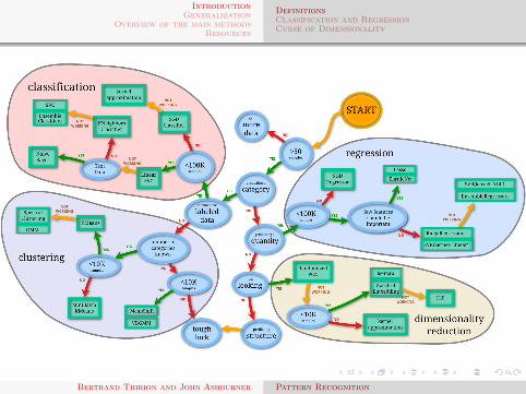
Some key concepts

supervised learning: The data comes with additional attributesthat we want to predict =⇒ classification and regression.

unsupervised learning: No target values.

Discover groups of similar examples within the data(clustering).

Determine the distribution of data within the input space(density estimation).

Project the data down to two or three dimensions forvisualization.





General supervised learning setting

We have a training dataset of n observations, each consisting of aninput xi and a target yi .Each input, xi , consists of a vector of p features.

D = {(xi , yi )|i = 1, .., n}

The aim is to predict the target for a new input x∗.





Classification

Targets (y) are categoricallabels.Train with D and useresult to make best guessof y∗ given x∗.

Classification

Feature 1

Featu

re 2

0 2 4

−7

−6

−5

−4

−3

−2

−1





Probabilistic classification

Targets (y) are categoricallabels.Train with D and computeP(y∗ = k |x∗,D).

Probabilistic classification

Feature 1

Featu

re 2

0 2 4

−7

−6

−5

−4

−3

−2

−1





Regression

Targets (y) are continuousreal variables.Train with D and computep(y∗|x∗,D).

0

10

20

30

40

50

60

70

31

14

23

31

63

55

14

58

35

27

Feature 1

Fea

ture

2





Many other settings

Multi-class classification when there are more than twopossible categories.

Ordinal regression for classification when there is someordering of the categories.Chu, Wei, and Zoubin Ghahramani. “Gaussian processes for ordinal regression.” In Journal of MachineLearning Research, pp. 1019-1041. 2005.

Multi-task learning when there are multiple targets topredict, which may be related.

etc





Multi-Class classification

Multinomial Logistic regression Theoretically optimal.Expensive optimization.

One-versus-all classification [SVMs] Among severalhyperplane, choose the one with maximal margin.=⇒ recommended

One-versus-one classification Vote across each pair of class.Expensive, not optimal.





Curse of dimensionality

Large p, small n.





Nearest-neighbour classification

−3 −2 −1 0 1 2−2

−1

0

1

2

Feature 1

Featu

re 2

Not nicesmoothseparations.

Lots of sharpcorners.

May beimproved withK-nearestneighbours.





Behaviour changes in high-dimensions





Behaviour changes in high-dimensions

0 2 4 6 8 10 12 14 16 18 200

0.1

0.2

0.3

0.4

0.5

0.6

0.7

0.8

0.9

1

Circle area = π r2

Sphere volume = 4/3 π r3

Number of dimensions

Vo

lum

e o

f h

yp

er−

sp

he

re (

r=1

/2)




Assessing generalizabilityAccuracy Measures

Occam’s razor

“Everything should be kept as simple as possible, but nosimpler.”

— Einstein (allegedly)

Complex models (with many estimated parameters) usuallyexplain training data better than simpler models.

Simpler models often generalise better to new data than norecomplex models.

Need to find the model with the optimal bias/variance tradeoff.





Model selection

Some approximations/alternatives to the Bayesian approach:

Laplace approximations: find the MAP/ML solution and usea Gaussian approximation to the parameter uncertainty.

Minimum Message Length (MML): an informationtheoretic approach.

Minimum Description Length (MDL): an informationtheoretic approach based on how well the model compressesthe data.

Akaike Information Criterion (AIC): −2 log p(D|θ) + 2k ,where k is the number of estimated parameters.

Bayesian Information Criterion (BIC):−2 log p(D|θ) + k log q, where q is the number ofobservations.





Model selection by nested cross-validation

Inner cross-validation loop used to evaluate model’s performanceon a pre-defined grid of parameters and retain the best one.

Safe, but costly.

Supported by some libraries (e.g. scikit-learn).

Some estimators have path model, hence allow fasterevaluation (e.g. LASSO).

Randomized techniques also exist, sometimes more efficient.

Caveat: Inner cross-validation loop 6= outer cross-validationloop for parameter evaluation.





Accuracy measures for regression

Root-mean squared error for point predictions.

Correlation coefficient for point predictions.

Log predictive probability can be used for probabilisticpredictions.

Expected loss/risk for point predictions for decision making.





Accuracy measures for binary classification

Wikipedia contributors,“Sensitivity and specificity,”Wikipedia, The FreeEncyclopedia, http://en.wikipedia.org/w/index.

php?title=Sensitivity_and_

specificity&oldid=655245669

(accessed April 9, 2015).


http://en.wikipedia.org/w/index.php?title=Sensitivity_and_specificity&oldid=655245669







Accuracy measures from ROC curve

The Receiver operatingcharacteristic (ROC) curve is aplot of true-positive rate(sensitivity) versus false-positiverate (1-specificity) over the fullrange of possible thresholds.

The area under the curve(AUC) is the integral under theROC curve.

0 0.2 0.4 0.6 0.8 1

0.2

0.4

0.6

0.8

1

ROC Curve (AUC=0.9769)

1−Specificity

Se

nsitiv

ity





Log predictive probability

Some data are more easily classified than others.Probabilistic classifiers provide a level of confidence for eachprediction.

p(y∗|x∗, y,X, θ)

Quality of predictions can be assessed using the test logpredictive probability:

1m

m∑i=1

log2 p(y∗i = ti |x∗i , y,X, θ)

After subtracting the baseline measure, this shows the average bitsof information given by the model.

Rasmussen & Williams. “Gaussian Processes for Machine Learning”, MIT Press (2006).http://www.gaussianprocess.org/gpml/


http://www.gaussianprocess.org/gpml/



Simple Generative Models: Naive Bayes, Linear Discriminant AnalysisSimple Discriminative Models: Gaussian Processes, Support-Vector MachinesModel Averaging

Overview of classification tools

Only one rule: No tool wins in all situations.





Generative models for classification

P(y =k |x) =P(y =k)p(x|y =k)∑j P(y = j)p(x|y = j)

Ground truth

Feature 1

Fe

atu

re 2

0 2 4

−7

−6

−5

−4

−3

−2

−1





Linear discriminant analysis


Assumes:

P(x|y =k) = N (x|µk ,Σ)

p(x,y=0) = p(x|y=0) p(y=0)

Feature 1

Featu

re 2

0 2 4

−7

−6

−5

−4

−3

−2

−1

p(x,y=1) = p(x|y=1) p(y=1)

Feature 1

Featu

re 2

0 2 4

−7

−6

−5

−4

−3

−2

−1

p(x) = p(x,y=0) + p(x,y=1)

Feature 1

Featu

re 2

0 2 4

−7

−6

−5

−4

−3

−2

−1

p(y=0|x) = p(x,y=0)/p(x)

Feature 1

Featu

re 2

0 2 4

−7

−6

−5

−4

−3

−2

−1

Model has 2p + p(p − 1) parameters to estimate (two means and asingle covariance).Number of observations is pn (size of inputs).





Quadratic discriminant analysis


Assumes different covariances:

P(x|y =k) = N (x|µk ,Σk)

p(x,y=0) = p(x|y=0) p(y=0)

Feature 1

Featu

re 2

0 2 4

−7

−6

−5

−4

−3

−2

−1

p(x,y=1) = p(x|y=1) p(y=1)

Feature 1

Featu

re 2

0 2 4

−7

−6

−5

−4

−3

−2

−1

p(x) = p(x,y=0) + p(x,y=1)

Feature 1

Featu

re 2

0 2 4

−7

−6

−5

−4

−3

−2

−1

p(y=0|x) = p(x,y=0)/p(x)

Feature 1

Featu

re 2

0 2 4

−7

−6

−5

−4

−3

−2

−1

Model has 2p + 2p(p − 1) parameters to estimate (two means andtwo covariances).Number of observations is pn.





Naive Bayes


Assumes that features areindependent:

p(x|y =k) =∏i

p(xi |y =k)

p(x,y=0) = p(x|y=0) p(y=0)

Feature 1

Featu

re 2

0 2 4

−7

−6

−5

−4

−3

−2

−1

p(x,y=1) = p(x|y=1) p(y=1)

Feature 1

Featu

re 2

0 2 4

−7

−6

−5

−4

−3

−2

−1

p(x) = p(x,y=0) + p(x,y=1)

Feature 1

Featu

re 2

0 2 4

−7

−6

−5

−4

−3

−2

−1

p(y=0|x) = p(x,y=0)/p(x)

Feature 1

Featu

re 2

0 2 4

−7

−6

−5

−4

−3

−2

−1

Model has variable number of parameters to estimate, but theabove example has 3p.Number of observations is pn.





Linear regression: maximum likelihood

A simple way to do regression is by:

f (x∗) = wTx∗

Assuming Gaussian noise on y, the ML estimate of w is by:

w = (XTX)−1XTy

where

X =(x1 x2 . . . xn

)T, and y =

(y1 y2 . . . yn

)TModel has p parameters to estimate.Number of observations is n (number of targets).Usually needs dimensionality reduction, with (eg) SVD.





Linear regression: maximum posterior

We may have prior knowledge about various distributions:

p(y∗|x∗,w) =N (wTx∗, σ2)

p(w) =N (0,Σ0)

Therefore,

p(w|y,X) =N (σ−2B−1XTy,B−1), where B = σ−2XTX + Σ−10

Maximum a posteriori (MAP) estimate of w is by:

w = σ−2B−1XTy, where B = σ−2XTX + Σ−10





Linear regression: Bayesian

We may have prior knowledge about various distributions:

p(y∗|x∗,w) =N (wTx∗, σ2)

p(w) =N (0,Σ0)

Therefore,

p(w|y,X) =N (σ−2B−1XTy,B−1), where B = σ−2XTX + Σ−10

Predictions are made by integrating out the uncertainty of theweights, rather than estimating them:

p(y∗|x∗, y,X) =

∫wp(y∗|x∗,w)p(w|y,X)dw

=N (σ−2xT∗ B−1XTy, xT∗ B−1x∗)

Estimated parameters may be σ2, and parameters encoding Σ0.Bertrand Thirion and John Ashburner Pattern Recognition




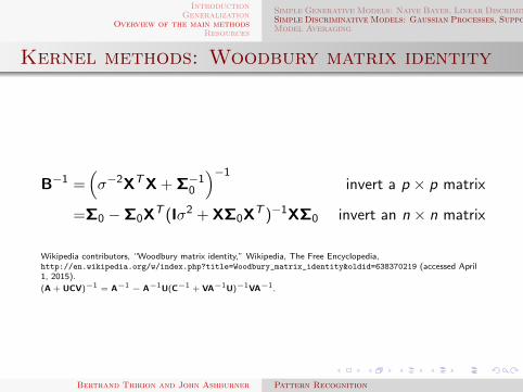
Kernel methods: Woodbury matrix identity

B−1 =(σ−2XTX + Σ−1

0

)−1invert a p × p matrix

=Σ0 −Σ0XT (Iσ2 + XΣ0XT )−1XΣ0 invert an n × n matrix

Wikipedia contributors, “Woodbury matrix identity,” Wikipedia, The Free Encyclopedia,http://en.wikipedia.org/w/index.php?title=Woodbury_matrix_identity&oldid=638370219 (accessed April1, 2015).

(A + UCV)−1 = A−1 − A−1U(C−1 + VA−1U)−1VA−1.


http://en.wikipedia.org/w/index.php?title=Woodbury_matrix_identity&oldid=638370219




Kernel methods: Gaussian process regression

The predicted distribution is:

p(y∗|x∗, y,X) =N (kTC−1y, c − kTC−1k)

where:

C =XΣ0XT + Iσ2

k =XΣ0x∗

c =xT∗ Σ0x∗ + σ2





Kernel methods: nonlinear methods

Sometimes, we want alternatives to C = XΣ0XT + Iσ2.Nonlinearity is achieved by replacing the matrix K = XΣ0XT withsome function of the data that gives a positive definite matrixencoding similarities.eg

k(xi , xj) = θ1 + θ2xi · xj + θ3 exp

(−||xi − xj||2

2θ24

)Hyper-parameters θ1 to θ4 can be optimised in a number of ways.





Kernel methods: nonlinear methods

Non-linear methods areuseful in low-dimension toadapt the shape ofdecision boundaries.

For large p, small n problems, nonlinear methods do not seem tohelp much.Nonlinearity also reduces interpretability.





Probabilistic discriminative models

Regression

Continuous targets:

y ∈ R

Usually assume a Gaussiandistribution:

p(y |x,w) =

N (f (x,w), σ2)

where σ2 is a variance.

Binary Classification

Categorical targets:

y ∈ {0, 1}

Usually assume a binomialdistribution:

p(y |x,w) =

σ(f (x,w))y (1− σ(f (x,w)))1−y

where σ is a squashing function.






For binary classification:

p(y∗ = 1|x∗,w) = σ(f (x∗,w))

where σ is some squashingfunction, eg:

Logistic sigmoid function(inverse of Logit).

Normal CDF (inverse ofProbit).

−5 0 50

0.5

1

f*

σ(f

*)

Logistic function

−2 0 20

0.5

1

f*

σ(f

*)

Inverse Probit function (Normal CDF)






Integrating over the uncertaintyof the separating hyperplaneallows probabilistic predictionsfurther from the training data.This is not usually done formethods such as therelevance-vector machine (RVM).

Rasmussen, Carl Edward, and JoaquinQuinonero-Candela. “Healing the relevance vectormachine through augmentation.” In Proceedings of the22nd international conference on Machine learning, pp.689-696. ACM, 2005.

Simple Logistic Regression

Feature 1

Featu

re 2

0 2 4

−7

−6

−5

−4

−3

−2

−1

0 2 4

−7

−6

−5

−4

−3

−2

−1

Hyperplane Uncertainty

Feature 1

Featu

re 2

Bayesian Logistic Regression

Feature 1

Featu

re 2

0 2 4

−7

−6

−5

−4

−3

−2

−1

Bayesian Logistic Regression

Feature 1

Featu

re 2

0 2 4

−7

−6

−5

−4

−3

−2

−1






Making probabilistic predictions involves:

1 Computing the distribution of a latent variable correspondingto the test data (cf regression):

p(f∗|x∗, y,X) =

∫fp(f∗|x∗, f)p(f|y,X)df

2 Using this distribution to give a probabilistic prediction:

P(y∗ = 1|x∗, y,X) =

∫f∗

σ(f∗)p(f∗|x∗, y,X)df∗

Unfortunately, these integrals are analytically intractable, soapproximations are needed.






Approximate methods for probabilistic classification include:

The Laplace Approximation (LA). Fastest, but lessaccurate.

Expectation Propagation (EP). More accurate than theLaplace approximation, but slightly slower.

MCMC methods. The “gold standard”, but very slow todraw lots of random samples.

Nickisch, Hannes, and Carl Edward Rasmussen. “Approximations for Binary Gaussian Process Classification.”Journal of Machine Learning Research 9 (2008): 2035-2078.





Discriminative models for classification

t = σ(f (x∗))

where σ is some squashingfunction, eg:

Logistic function (inverse ofLogit).

Normal CDF (inverse ofProbit).

Hinge loss (support vectormachines)

−5 0 50

0.5

1

f*

σ(f

*)

Logistic function

−2 0 20

0.5

1

f*

σ(f

*)

Inverse Probit function (Normal CDF)





Discriminative models for classification:convexity

In practice, the hinge and logistic losses yield a convex estimationproblem and are preferred.

minw

n∑i=1

L(yi ,Xi,w) + λR(w)

(M-estimators framework)

L is the loss function (hinge, logistic, quadratic...)

R is the regularizer (typically a norm on w)

λ > 0 balances the two terms

L and R convex → unique minimizer (SVMs, `2-logistic,`1-logistic).





Support vector classification

SVMs are reasonably fast,accurate and easy to tune(C = 103 is a good default, nodramatic failure).Multi-class: One-versus-one,One-versus all.





Ensemble learning

Combining predictions from weak learners.

Bootstrap aggregating (bagging)Train several weak classifiers, with different models orrandomly drawn subsets of the data.Average their predictions with equal weight.

BoostingA family of approaches, where models are weighted accordingto their accuracy.AdaBoost is popular, but has problems with target noise.

Bayesian model averagingReally a model selection method.Relatively ineffective for combining models.

Bayesian model combinationShows promise.

Monteith, et al. “Turning Bayesian model averaging into Bayesian model combination.” Neural Networks (IJCNN),The 2011 International Joint Conference on. IEEE, 2011.





Boosting

Reduce sequentially the bias of the combined estimator.Examples: AdaBoost, Gradient Tree Boosting, ...





Bagging

Build several estimators independently and average theirpredictions. Reduce the variance.Examples: Bagging methods, Forests of randomized trees, ...




Free Books

The Elements of Statistical Learning: Data Mining,Inference, and Prediction Trevor Hastie, Robert Tibshirani,Jerome Fried(2009)http://statweb.stanford.edu/~tibs/ElemStatLearn/

An Introduction to Statistical Learning with Applicationsin R Gareth James, Daniela Witten, Trevor Hastie and RobertTibshirani (2013)http://www-bcf.usc.edu/%7Egareth/ISL/

Introduction to Machine Learning Amnon Shashua (2008)http://arxiv.org/pdf/0904.3664.pdf


http://statweb.stanford.edu/~tibs/ElemStatLearn/

http://www-bcf.usc.edu/%7Egareth/ISL/

http://arxiv.org/pdf/0904.3664.pdf



Free Books

Bayesian Reasoning and Machine Learning David Barber(2014)http://www.cs.ucl.ac.uk/staff/d.barber/brml/

Gaussian Processes for Machine Learning Carl EdwardRasmussen and Christopher K. I. Williams (2006)http://www.gaussianprocess.org/gpml/chapters/

Information Theory, Inference, and Learning AlgorithmsDavid J.C. MacKay (2003) http:

//www.inference.phy.cam.ac.uk/itila/book.html


http://www.cs.ucl.ac.uk/staff/d.barber/brml/

http://www.gaussianprocess.org/gpml/chapters/

http://www.inference.phy.cam.ac.uk/itila/book.html

http://www.inference.phy.cam.ac.uk/itila/book.html



Web sites

Kernel Machines http://www.kernel-machines.org/

The Gaussian Processes Web Site includes links tosoftware. http://www.gaussianprocess.org/

SVM - Support Vector Machines includes links to software.http://www.support-vector-machines.org/

Pascal Video Lectureshttp://videolectures.net/pascal


http://www.kernel-machines.org/

http://www.gaussianprocess.org/

http://www.support-vector-machines.org/

http://videolectures.net/pascal



MATLAB tools

Spider Object orientated environment for machine learning inMATLAB.

GPML Gaussian processes for supervised learning.

Pronto MATLAB ML tbx for neuroimaging. GUI. Implementsmany ML concepts. Continuity with SPM.




Python tools

Scikit-learn Generic ML in Python. Complete, high-quality,well-documented, reference implementations.

Nilearn Python interface to Scikit-learn for Neuroimaging.Easy-to-use/install. Good viz.

Pymvpa Python tool for ML. Advanced stuff (Pipelines,Hyperalignment).


Pattern Recognition

Documents

Transcript of Pattern Recognition