Pattern Recognition in Flow CytometryLynne Boddy,1* Malcolm F. Wilkins,1 and Colin W. Morris2

1Cardiff School of Biosciences, Cardiff University, Cardiff, United Kingdom2School of Computing, University of Glamorgan, Trefforest, Pontypridd, United Kingdom

Received 24 October 2000; Revision Received 8 March 2001; Accepted 2 April 2001

Background: Analytical flow cytometry (AFC), by quan-tifying sometimes more than 10 optical parameters oncells at rates of approximately 103 cells/s, rapidly gener-ates vast quantities of multidimensional data, which pro-vides a considerable challenge for data analysis. We re-view the application of multivariate data analysis andpattern recognition techniques to flow cytometry.Methods: Approaches were divided into two broad typesdepending on whether the aim was identification or clus-tering. Multivariate statistical approaches, supervised arti-ficial neural networks (ANNs), problems of overlappingcharacter distributions, unbounded data sets, missing pa-rameters, scaling up, and estimating proportions of differ-ent types of cells comprised the first category. Classic

clustering methods, fuzzy clustering, and unsupervisedANNs comprised the second category.We demonstratethe state of the art by using AFC data on marine phyto-plankton populations.Results and Conclusions: Information held within thelarge quantities of data generated by AFC was tractableusing ANNs, but for field studies the problem of obtainingsuitable training data needs to be resolved, and copingwith an almost infinite number of cell categories needsfurther research. Cytometry 44:195–209, 2001.© 2001 Wiley-Liss, Inc.

Key terms: phytoplankton; multivariate statistics; artifi-cial neural networks; clustering

Analytical flow cytometry (AFC) rapidly generates verylarge quantities of multivariate data comprising a numberof measurements of the optical and fluorescence proper-ties of particles in suspension. Flow cytometry is used inthe medical field for detection of cancerous cells in bodytissue and fluid samples and in clinical microbiology, e.g.,for testing antibiotic efficiency (1,2). Those applicationsare typically characterized by a relatively small andbounded number of particle types (categories) that alsocan be made highly distinctive with regard to their flowcytometric signatures through the use of fluorescentlylabeled markers. However, AFC also is used for determin-ing the microbial composition of samples from industrialprocesses (e.g., 3–5) or the natural environment, e.g., inthe identification of phytoplankton populations and mon-itoring of population dynamics (e.g., 6–9). Such applica-tions are generally more challenging for data analysis:there may be a very large (in some cases open-ended)number of potential categories from which the particlescan be drawn, the degree of potential variability of flowcytometric signatures within categories might be large,and the distributions of different categories might overlapconsiderably.

Manual analysis of AFC data is still frequently performedand typically consists of examining the data distributionwith histograms and two- or three-dimensional scatterplots to locate the clusters. The multivariate nature of thedata makes visualization difficult. Graphical techniques

have been developed which allow visualization of multi-variate data in more than three dimensions (10); however,the use of dimensionality reduction techniques such asprincipal component analysis (11) might be necessary fordetecting combinations of clusters that cannot be resolvedwith any pair of original AFC parameters alone. Interpre-tation of the clusters in terms of the particles presentrelies on the knowledge of the investigator. Automatedanalysis of AFC data is now possible, especially with thecurrent rapidly increasing availability of computingpower. In this article we review the use of computationalpattern recognition techniques in the analysis of AFC data,with specific emphasis on determining phytoplanktoncommunity composition from marine samples.

FEATURE EXTRACTIONThe first step in data analysis is to extract important

features. In general pattern recognition terms, a feature isa quantifiable attribute of the individual under study thatprovides useful information allowing it to be discrimi-nated from other fundamentally dissimilar individuals(12). Features can be binary (presence or absence of a

Grant sponsor: AIMS, Commission of the European Community; Grantnumber: CEC MAS3-CT97-0080.

*Correspondence to: Lynne Boddy, Cardiff School of Biosciences, P.O.Box 915, Park Place, Cardiff CF10 3TL, UK.

E-mail: boddyl@cf.ac.uk

© 2001 Wiley-Liss, Inc. Cytometry 44:195–209 (2001)

characteristic) or continuous. A pattern is a combinationof features that together characterize the individual understudy. For cytometric data, the features are typically themeasured optical and fluorescence parameters of individ-ual particles or cells, measured in flow or via static imagecytometry (13). Derived features also can be used; forexample, a measure of cellular chlorophyll content perunit size can be derived from raw AFC chlorophyll fluo-rescence data. The shape of the fluorescence and lightscatter signal pulses during the passage of a particle con-tains additional discriminatory information (14), and arecently developed flow cytometer captures full pulseshapes for two fluorescence and two light scatter param-eters (15,16). That pulse shape information can be used toderive additional discriminatory features (14,17). The anal-ysis can also be carried out at the level of entire popula-tions rather than individual particles, e.g., in generatingbreast cancer prognosis indices (18) in which the featuresare binned DNA histogram values.

For a feature to be useful for pattern recognition, itmust be possible to measure it reliably and repeatably.The use of raw AFC parameters as feature values requirescaution because, even among a population of individualsfrom the same category, AFC signatures can show a widerange of variation due to natural biological variability.Further variability can be introduced during the samplestorage and preparation protocols before analysis, as inthe use of stains and fluorescent marker probes. If theapplication requires the use of multiple samples, thoseprotocols should be standardized as far as possible tominimize that source of extraneous variation. Any variabil-ity must be taken into account by the pattern recognitionprocedure. Additional variability due to instrumental driftoften can be compensated for by using derived featuresrelative to a standard sample of fluorescent calibrationbeads, although other methods have been tried with suc-cess (19).

IDENTIFICATION VERSUS CLUSTERINGAFC data analysis can be divided into two types: iden-

tification and clustering (classification). Identification con-sists of attempting to assign category labels to each de-tected particle in the sample based on the characteristicsof the corresponding AFC data pattern. It is assumed thatthe number of potential categories and the AFC charac-teristics of each are known in advance so that the mostlikely category can be determined for a given data pattern;optionally, an “unknown” category can be included, intowhich are placed all those data patterns not correspond-ing to one of the known categories. A variety of ap-proaches have been adopted, including classification andregression trees (CARTs), multivariate statistics, and arti-ficial neural networks (ANNs). All abbreviations used inthis article are presented in Table 1.

In contrast, clustering does not apply a preconceivedclassification scheme to the data but seeks to discover theclusters that are naturally present; thus, the data points arelabeled not with a category name but with an indexnumber denoting the cluster to which they belong. Inter-

pretation of these clusters then requires a higher levelprocedure, either manual or the use of some kind ofartificial intelligence procedure, such as an expert systemused for forming a medical diagnosis or prognosis (20).Clustering is rarely entirely automatic, usually requiringdecisions of a human expert.

IDENTIFICATIONClassification and Regression Trees (CART)

Given a labeled set of training data, the CART method(21) repeatedly subdivides the data space using a succes-sion of binary splits to separate known populations in thedata. An iterative algorithm attempts at each stage to findthe optimum split plane to increase the homogeneity ofthe two generated subpopulations until the subpopula-tions are sufficiently homogeneous for no further splits totake place. The algorithm thus constructs a tree of splitplanes; with this tree, an unknown data pattern can beclassified into one of the known subpopulations. Thealgorithm has been applied to a five-dimensional three-color bone marrow immunophenotype data set (22), inassessment of antibiotic efficiency (23), and to character-ize leiomyomatous tumors (from digital cell image analysisnot flow cytometry data) (24) and found to perform well.The primary disadvantage of the method is that all datapatterns are identified into one of the categories in thetraining data set, even if they belong to a category notpresent in the training data; although this deficiency canbe overcome for low dimensionality data by populatingthe data space with artificially generated data points (22),this approach would be impractical for high dimensionaldata.

Free and commercial software packages are available(http://www.cse.unsw.edu.au/;quinlan) (25).

Multivariate Statistics

Where the category data distributions are described, atleast approximately, by an underlying theoretical model, amultivariate parametric statistical approach can beadopted (26–29). This contrasts fundamentally with non-parametric techniques (which can be statistical or neural;see following section) that make no prior assumptions asto the nature of the category data distributions.

Table 1Commonly Used Abbreviations

Abbreviation Meaning

ANN Artificial neural networkARBF Asymmetric radial basis functionART Adaptive resonance theoryHLN Hidden layer nodeMLP Multilayer perceptronPR Pattern recognitionQDA Quadratic discriminant analysisRBF Radial basis functionSOM Self-organising mapSVM Support vector machine

196 BODDY ET AL.

With parametric approaches, the parameters of the as-sumed distribution for each category are estimated from asuitable representative set of data. An unknown data pat-tern then can be assigned to a category by calculatingwhich of the theoretical category data distributions hasthe highest likelihood of generating the data pattern. Mak-ing the assumption that the category distributions arenormal (multivariate Gaussian) in form results in the qua-dratic discriminant analysis (QDA) classifier, so called be-cause the decision boundaries between categories arehyperdimensional quadratic surfaces. QDA classifiers havebeen applied to AFC on phytoplankton (27,29). QDAclassifiers generate probabilistic estimates of the likeli-hood of the unknown data pattern belonging to any of theknown categories, allowing a minimum-cost identificationstrategy to be adopted in applications where certain typesof misidentification are more costly than others (12). Thedisadvantage of the method is the prior assumption of theform of the data distribution. Flow cytometer categorydistributions are frequently significantly non–normal,even multimodal, thereby distorting the decision bound-aries between categories and leading to poor likelihoodestimation and poor performance.

The k-nearest neighbors (KNN) approach is nonpara-metric, making no strong a priori assumptions about theform of the data distribution (12). It takes a poll of thenearest training patterns to the pattern presented for iden-tification and assigns the pattern to the most representa-tive class among them. Effectively, this estimates the rel-ative densities of patterns in each category in theimmediate vicinity of the presented pattern and selectsthe most densely represented category. The KNN ap-proach requires no training and can represent arbitrarilycomplex data distributions. It has been used with flowcytometry data on phytoplankton (30), but it is slow inoperation and requires storage of a large representativedata set, which can be impractical.

Supervised Artificial Neural Networks

ANNs, first developed to mimic the storage and analyt-ical operations of the brain, are non–parametric and arenot rule based but “train” or learn from examples pre-sented to them (12,31–37). Essentially, there are twotypes of training: (a) supervised, which is appropriate foridentification; and (b) unsupervised, which can be usedfor clustering (see later). With the former, data patterns(flow cytometric signatures) of known identity are pre-sented to the ANN as exemplars. Once an ANN has beentrained, any data pattern can be presented to it and theoutput analyzed to find the most likely identity of thepattern.

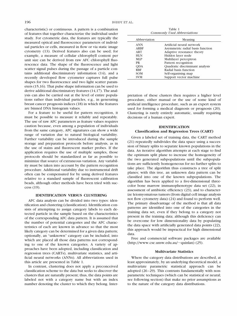
The basic building blocks of ANNs are nodes, which arein some ways analogous to the neurons of brains. Thesenodes have inputs from the outside world or the outputsof other nodes, which are commonly weighted. They areinterconnected (either fully or partially) in defined, regu-lar layers (e.g., Fig. 1). It is the organization of a largenumber of nodes and the large number of interconnectingweights that give ANNs their processing power. ANNs for

identification commonly consist of three interconnectedlayers: an input layer, a hidden layer, and an output layer.When training and using trained networks to make iden-tifications, the data pattern of characters for each cell(flow cytometric signature) is applied to the nodes of theinput layer (one node per flow cytometric parameter),which serve merely to distribute the data. Data are thenpassed to the next layer nodes (hidden layer nodes, HLNs)and subsequently to the output layer nodes, which indi-cate cell identity (one node per possible cell identity).Networks differ in the detailed functioning of the HLNsand output layer nodes and the method by which theycollectively “learn” to represent the training data (a rep-resentative selection of data patterns labeled with cellidentity). How well a network trains depends on a varietyof factors, e.g., the number of HLNs, some of which differdepending on the type of network. Optimizing a networkcan be achieved only by experimentally altering thesefactors in turn, although this can be automated to someextent. How well a network has been trained can bedetermined by comparing predicted identity of cells withtheir known identity. When an optimized network hasbeen obtained, its ability to generalize must be tested bypresenting it with an “unseen” independent set of dataand comparing predicted cell identity with known iden-tity. It is important that there is high identification success(i.e., proportion of each cell type correctly identified) andhigh confidence of correct identification, an estimate ofwhich can be obtained by expressing the identificationsuccess of each cell type as a percentage of the typesidentified as that type. High identification success alone isnot sufficient because a large number of cells being incor-rectly identified as a certain cell type can result in totallymisleading information on the proportion of that cell typein the population. To examine identification success andconfidence of correct identification, a misidentificationmatrix can be drawn up (Table 2). Successful identifica-tion of a particular cell type is indicated along the leadingdiagonal, and misidentification as other cell types is indi-cated in the rest of the body of the table.

FIG. 1. Schematic of a radial basis function/asymmetric radial basisfunction network.

197PATTERN RECOGNITION IN FLOW CYTOMETRY

ANNs have been used successfully to analyze flow cy-tometric data on fungal spores (38); bacteria (39); phyto-plankton (30,40–49); and DNA histograms of breast can-cer cells (18), lung cancer aspirates (50), and leukemiaimmunophenotype using fluorescent anti bodies (51).However, apart from the studies by Boddy et al. (40,41)and Morris et al. (52), only a few cell categories have beendiscriminated from one another. Scaling up is not a trivialtask, and the major issues involved are examined below.The mechanics of implementing ANNs for biological iden-tification is explained in more detail in (31).

MULTILAYER PERCEPTRON (MLP)The MLP (or back propagation network) is probably still

the most commonly used in biological identification.Training is by repeated presentation of patterns to thenetwork, with small iterative weight changes to nodeinputs (12,31–37). When the first training pattern is pre-sented to the network, it propagates through the networkand produces an output. Because weights are initiallyrandomized, the output obtained will not usually be thatrequired. The weights of the output layer nodes are al-tered slightly, so that the error is reduced by a smallamount. These error values are propagated back throughthe network, and the weights on the inputs to the HLNsare then also adjusted accordingly by a small amount. Thatprocess is repeated for all of the training patterns manytimes (often many thousands) until the network is consid-ered to have learned the patterns.

Each HLN represents a hyperplanar decision boundary,the position and orientation of which are determined bythe input weight values. The output from the HLNs indi-cates on which side of its hyperplane the input patternfalls. The output layer nodes interpolate smoothly to pro-duce arbitrarily convex decision boundaries between celltypes (Fig. 2a).

MLPs are relatively simple to train, lots of free softwareare available, and most of the early applications of ANNs

to identification of cells from flow cytometric signatureshave adopted this approach (39,41,47,50,51). However, itoften takes a lot of experimentation to optimize MLPs, andtraining is relatively slow and not always successful.

RADIAL BASIS FUNCTION (RBF)RBF ANNs (Fig. 1) are at least as successful as MLPs in

analysis of biological data (30,53,54) and they train rap-idly, taking in the order of minutes rather than the hoursor even days required to train MLPs. Moreover, they candetect “novel” patterns, for which the identity is notknown to the network (46,55). As with most MLPs, RBFANNs comprise three layers of nodes. The difference liesin the nodes of the hidden layer, which use kernels (basisfunctions) to represent the data (Fig. 2b). A Gaussian-shaped kernel of the following form is commonly chosen:

Output 5 exp~2x2/2s2!

where s controls the spread of the function, and x is theEuclidean distance between the kernel center and vectorof interest. Each HLN has a defined response to input datathat changes depending on the distance of the data pointfrom the kernel center. If the Euclidean distance measureis used, the kernels are hyperspherical (radially symmet-ric); but if the Mahalanobis distance metric is used, thekernels are asymmetrical, becoming elongated into hy-perellipsoids that adopt the orientation that best fits thedata distribution (Fig. 2c) (34). The kernels are initiallyplaced by using one of a variety of paradigms: the initiallocation of the kernel centers can be randomly chosen orplaced by some clustering algorithm, e.g., learning vectorquantization (56). The optimum number of HLNs can bedetermined automatically by starting with a large numberof candidate HLNs and selecting from that an optimalsubset, e.g., using an orthogonal least squares algorithm(57).

Table 2Misidentification Matrix Using an RBF Network (36 HLNs) to Discriminate 10 Phytoplankton Species

in Pure Culture From FACS Data*

Species

Identified as nPatterns1 2 3 4 5 6 7 8 9 10 Unknown

1. Cryptomonas maculata 0.93 0.00 0.00 0.00 0.00 0.00 0.00 0.00 0.00 0.00 0.07 10002. Emiliania huxleyi B11 0.00 0.91 0.00 0.01 0.00 0.00 0.00 0.00 0.00 0.00 0.08 10003. Gymnodinium simplex 0.00 0.00 0.65 0.00 0.00 0.01 0.01 0.00 0.00 0.17 0.16 10004. Nephroselmis pyriformis 0.00 0.03 0.00 0.72 0.01 0.03 0.00 0.02 0.01 0.00 0.18 10005. Phaeocystis pouchetti 0.00 0.00 0.00 0.01 0.77 0.02 0.00 0.00 0.04 0.00 0.16 10006. Phaeodactylum tricornutum 0.00 0.00 0.00 0.04 0.01 0.56 0.00 0.10 0.08 0.00 0.21 10007. Prorocentrum balticum 0.00 0.00 0.01 0.00 0.00 0.00 0.92 0.00 0.00 0.00 0.07 10008. Prymnesium parvum 0.00 0.00 0.00 0.02 0.01 0.08 0.00 0.74 0.01 0.00 0.14 10009. Pyramimonas obovata 0.00 0.00 0.00 0.01 0.14 0.03 0.00 0.02 0.59 0.00 0.21 1000

10. Tetraselmis verrucosa 0.00 0.00 0.19 0.00 0.00 0.00 0.01 0.00 0.00 0.60 0.21 1000

Proportion overall correctlyidentified 0.93 0.91 0.65 0.72 0.77 0.56 0.92 0.74 0.59 0.60

Confidence of identification 1.00 0.97 0.77 0.88 0.82 0.77 0.98 0.83 0.82 0.77

*Overall proportion of data correctly identified was 0.74; the proportion of unrejected patterns correctly identified was 0.87; theproportion rejected was 0.15. HLN, hidden layer node; RBF, radial basis function.

198 BODDY ET AL.

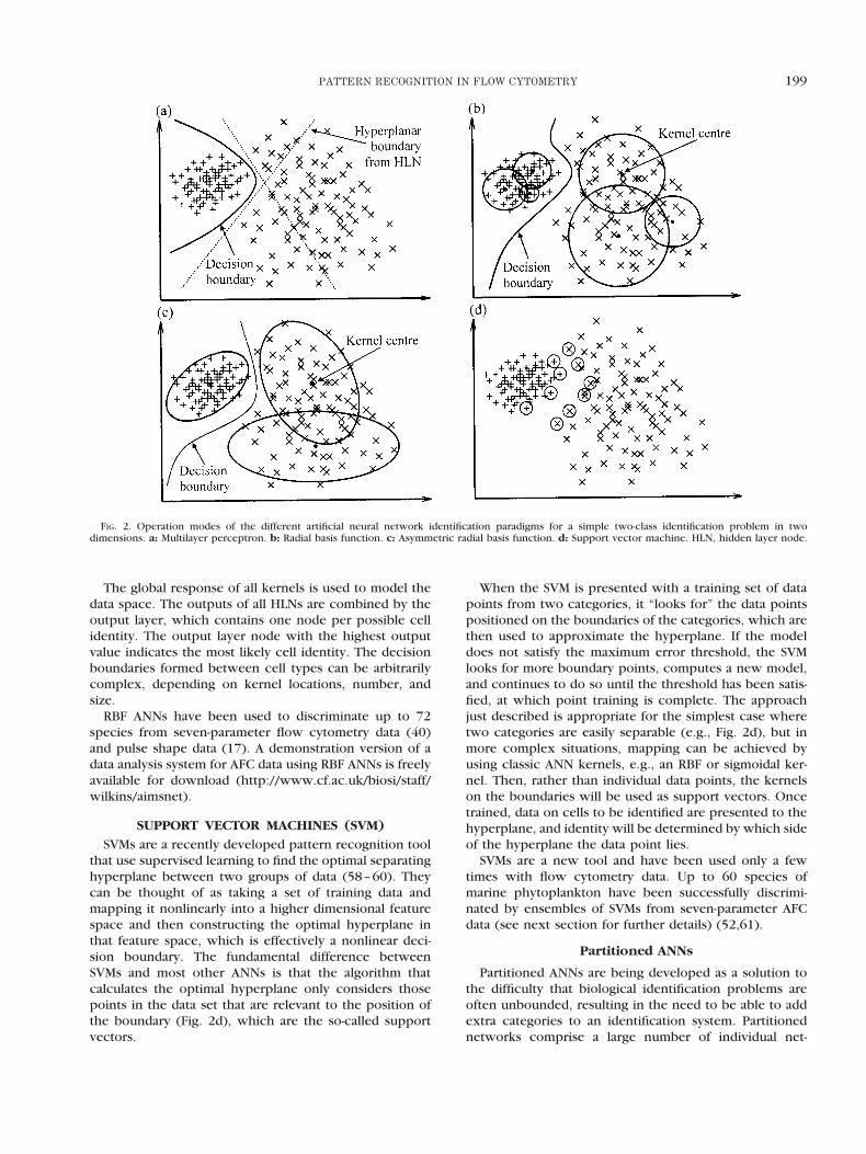
The global response of all kernels is used to model thedata space. The outputs of all HLNs are combined by theoutput layer, which contains one node per possible cellidentity. The output layer node with the highest outputvalue indicates the most likely cell identity. The decisionboundaries formed between cell types can be arbitrarilycomplex, depending on kernel locations, number, andsize.

RBF ANNs have been used to discriminate up to 72species from seven-parameter flow cytometry data (40)and pulse shape data (17). A demonstration version of adata analysis system for AFC data using RBF ANNs is freelyavailable for download (http://www.cf.ac.uk/biosi/staff/wilkins/aimsnet).

SUPPORT VECTOR MACHINES (SVM)SVMs are a recently developed pattern recognition tool

that use supervised learning to find the optimal separatinghyperplane between two groups of data (58–60). Theycan be thought of as taking a set of training data andmapping it nonlinearly into a higher dimensional featurespace and then constructing the optimal hyperplane inthat feature space, which is effectively a nonlinear deci-sion boundary. The fundamental difference betweenSVMs and most other ANNs is that the algorithm thatcalculates the optimal hyperplane only considers thosepoints in the data set that are relevant to the position ofthe boundary (Fig. 2d), which are the so-called supportvectors.

When the SVM is presented with a training set of datapoints from two categories, it “looks for” the data pointspositioned on the boundaries of the categories, which arethen used to approximate the hyperplane. If the modeldoes not satisfy the maximum error threshold, the SVMlooks for more boundary points, computes a new model,and continues to do so until the threshold has been satis-fied, at which point training is complete. The approachjust described is appropriate for the simplest case wheretwo categories are easily separable (e.g., Fig. 2d), but inmore complex situations, mapping can be achieved byusing classic ANN kernels, e.g., an RBF or sigmoidal ker-nel. Then, rather than individual data points, the kernelson the boundaries will be used as support vectors. Oncetrained, data on cells to be identified are presented to thehyperplane, and identity will be determined by which sideof the hyperplane the data point lies.

SVMs are a new tool and have been used only a fewtimes with flow cytometry data. Up to 60 species ofmarine phytoplankton have been successfully discrimi-nated by ensembles of SVMs from seven-parameter AFCdata (see next section for further details) (52,61).

Partitioned ANNs

Partitioned ANNs are being developed as a solution tothe difficulty that biological identification problems areoften unbounded, resulting in the need to be able to addextra categories to an identification system. Partitionednetworks comprise a large number of individual net-

FIG. 2. Operation modes of the different artificial neural network identification paradigms for a simple two-class identification problem in twodimensions. a: Multilayer perceptron. b: Radial basis function. c: Asymmetric radial basis function. d: Support vector machine. HLN, hidden layer node.

199PATTERN RECOGNITION IN FLOW CYTOMETRY

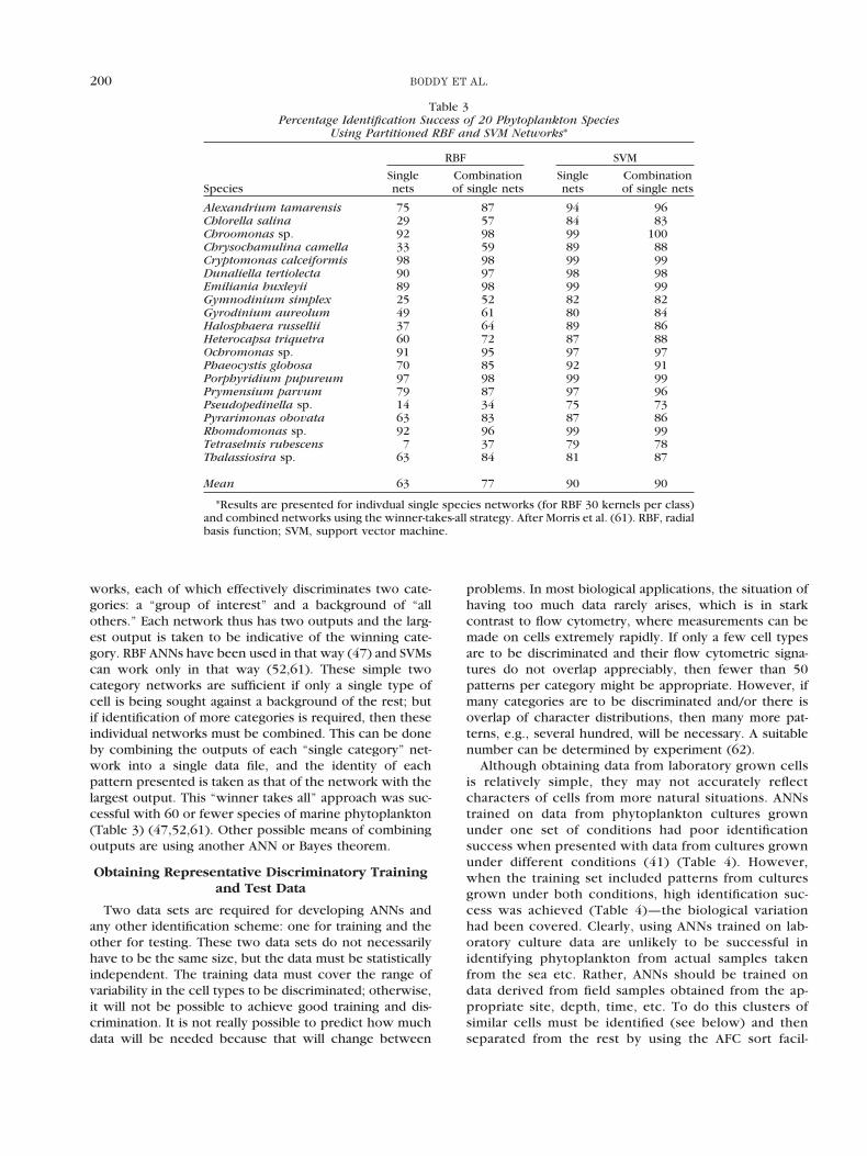
works, each of which effectively discriminates two cate-gories: a “group of interest” and a background of “allothers.” Each network thus has two outputs and the larg-est output is taken to be indicative of the winning cate-gory. RBF ANNs have been used in that way (47) and SVMscan work only in that way (52,61). These simple twocategory networks are sufficient if only a single type ofcell is being sought against a background of the rest; butif identification of more categories is required, then theseindividual networks must be combined. This can be doneby combining the outputs of each “single category” net-work into a single data file, and the identity of eachpattern presented is taken as that of the network with thelargest output. This “winner takes all” approach was suc-cessful with 60 or fewer species of marine phytoplankton(Table 3) (47,52,61). Other possible means of combiningoutputs are using another ANN or Bayes theorem.

Obtaining Representative Discriminatory Trainingand Test Data

Two data sets are required for developing ANNs andany other identification scheme: one for training and theother for testing. These two data sets do not necessarilyhave to be the same size, but the data must be statisticallyindependent. The training data must cover the range ofvariability in the cell types to be discriminated; otherwise,it will not be possible to achieve good training and dis-crimination. It is not really possible to predict how muchdata will be needed because that will change between

problems. In most biological applications, the situation ofhaving too much data rarely arises, which is in starkcontrast to flow cytometry, where measurements can bemade on cells extremely rapidly. If only a few cell typesare to be discriminated and their flow cytometric signa-tures do not overlap appreciably, then fewer than 50patterns per category might be appropriate. However, ifmany categories are to be discriminated and/or there isoverlap of character distributions, then many more pat-terns, e.g., several hundred, will be necessary. A suitablenumber can be determined by experiment (62).

Although obtaining data from laboratory grown cellsis relatively simple, they may not accurately reflectcharacters of cells from more natural situations. ANNstrained on data from phytoplankton cultures grownunder one set of conditions had poor identificationsuccess when presented with data from cultures grownunder different conditions (41) (Table 4). However,when the training set included patterns from culturesgrown under both conditions, high identification suc-cess was achieved (Table 4)—the biological variationhad been covered. Clearly, using ANNs trained on lab-oratory culture data are unlikely to be successful inidentifying phytoplankton from actual samples takenfrom the sea etc. Rather, ANNs should be trained ondata derived from field samples obtained from the ap-propriate site, depth, time, etc. To do this clusters ofsimilar cells must be identified (see below) and thenseparated from the rest by using the AFC sort facil-

Table 3Percentage Identification Success of 20 Phytoplankton Species

Using Partitioned RBF and SVM Networks*

Species

RBF SVM

Singlenets

Combinationof single nets

Singlenets

Combinationof single nets

Alexandrium tamarensis 75 87 94 96Chlorella salina 29 57 84 83Chroomonas sp. 92 98 99 100Chrysochamulina camella 33 59 89 88Cryptomonas calceiformis 98 98 99 99Dunaliella tertiolecta 90 97 98 98Emiliania huxleyii 89 98 99 99Gymnodinium simplex 25 52 82 82Gyrodinium aureolum 49 61 80 84Halosphaera russellii 37 64 89 86Heterocapsa triquetra 60 72 87 88Ochromonas sp. 91 95 97 97Phaeocystis globosa 70 85 92 91Porphyridium pupureum 97 98 99 99Prymensium parvum 79 87 97 96Pseudopedinella sp. 14 34 75 73Pyrarimonas obovata 63 83 87 86Rhomdomonas sp. 92 96 99 99Tetraselmis rubescens 7 37 79 78Thalassiosira sp. 63 84 81 87

Mean 63 77 90 90

*Results are presented for indivdual single species networks (for RBF 30 kernels per class)and combined networks using the winner-takes-all strategy. After Morris et al. (61). RBF, radialbasis function; SVM, support vector machine.

200 BODDY ET AL.

ity, followed by traditional microscopic identifica-tion. When the identity of a selected cluster has beendetermined, the flow cytometric signatures of the ap-

propriate cells can be used in the training and test datasets.

Even when data cover the spectrum of biological vari-ability of a particular cell type or species, identificationsuccess of some may not be as good as for others. Anetwork that has been optimized usually reflects overlapof AFC character distributions (e.g., Fig. 3) rather than anyinherent flaw in the ANN approach. Better discriminationcan usually then only be achieved by obtaining moreand/or different characters. Where there is large overlapof character distributions between two cell types, it maynot be possible to obtain discriminatory AFC signatures. Inwhich case, the best option may be to consider the twocategories as one, the network output indicating thatseveral possible identities exist.

Sometimes unequal numbers of training patterns areavailable for each category to be distinguished; and if animbalance in number of training patterns per category isused, training success can be affected (63). In a study withmarine phytoplankton cultured in the laboratory, whentraining ANNs to discriminate 40 or 60 species, an imbal-ance in the number of training patterns per species alwaysaffected training success—the greater the imbalance, thegreater the effect (62). However, because the networkoutputs approximate a posteriori probabilities (64), it hasbeen suggested that the outputs of the networks can beadjusted to take account of differences between propor-tions of patterns for each category in training and test datasets. That can be done by dividing network outputs by the“class probability” (i.e., the probability that a particularpattern in the training data comes from a particular cellcategory) and multiplying by the “correct class probabil-ity” (i.e., the probability that an event comes from aparticular cell category). Adjusting the networks in thatway in the phytoplankton study to compensate for imbal-anced training data sets did dramatically improve identifi-cation success for test data (62): there was a large im-provement in identification success of each species for theunder represented species at the expense of a slight de-crease in identification success of the well-representedspecies.

Richard and Lippmann (64) suggested that data on cor-rect class probabilities are often readily available. How-ever, in practice with biological applications, when apply-ing ANNs to field data or samples from laboratory mixedculture experiments, the correct probability that a patternbelongs to a particular species would usually be unknownand equal probabilities must be assumed. This assumptionwill, unfortunately, usually be incorrect. Indeed, often thewhole point of using a trained ANN to identify individualpatterns is to determine the proportions of each categoryin a sample! The value of obtaining “corrected” classifiersfor networks trained with imbalanced data sets in the wayjust described is, therefore, unclear in most biologicalidentification problems. However, there may be situationswhen this type of adjustment to a network is be beneficial,e.g., when it is important to take into account the cost ofmisidentification. For example, when trying to detecttoxic algal species, making a few false-positive identifica-

Table 4Effect of Variation Due to Culture Conditions on Network

Identification Performance*

Species name

1a 2a

Ab A1Bb

Ac Bc Ac Bc

Amphidinium carterae 80 4 73 87Amphora coffaeformis 91 77 92 81Aureodinium pigmentosum 87 0 87 24Chaetoceros calcitrans 90 3 89 85Chlorella salina 57 18 47 52Chroomonas salina 96 14 94 95Chrysochromulina camella 84 0 87 70Chrysochromulina chiton 63 0 67 14Chrysochromulina cymbium 41 0 15 88Chrysochromulina polylepis 63 0 70 29Cryptomonas appendiculata 99 0 98 97Cryptomonas calceiformis 94 9 95 94Cryptomonas reticulata 97 0 97 94Cryptomonas rostrella 99 1 99 87Dunaliella minuta 79 7 80 83Dunaliella primolecta 92 0 90 88Emiliania hyxleyi 79 2 81 63Gymnodinium micrum 65 0 69 60Gymnodinium simplex 66 1 61 75Gymnodinium vitiligo 83 0 82 39Hemiselmis brunnescens 95 32 90 69Hemiselmis virescens 96 62 98 94Micromonas pusilla 99 100 98 100Nephroselmis pyriformis 72 42 51 82Nephroselmis rotunda 54 8 47 81Ochromonas sp. 79 61 75 73Ochrosphaera neopolitana 57 22 55 68Pavolva lutheri 78 0 73 95Phaeocystis pouchetti 65 27 55 67Plagioselmis punctata 92 54 88 81Pleurochrysis carterae 96 12 94 96Prorocentrum micans 83 0 80 80Prorocentrum minimum 76 0 74 89Proocentrum nanum 71 2 60 39Prymnesium parvum 82 10 70 65Pyramimonas grossii 71 25 67 63Pyramimonas obovata 67 8 46 37Rhodmonas sp. 93 6 96 94Stichococcus bacillaris 80 56 71 47Tetraselmis striata 75 0 74 14Tetraselmis suecica 87 5 90 51Tetraselmis tetrathele 95 1 94 77Tetraselmis verrucosa 72 2 70 35

Overall percentage correctlyidentified 80 16 77 70

*Percentage correct identification of two asymmetric radialbasis function networks trained on data from two data sets (A andB) phytoplankton species maintained at 15°C under differentilluminations (A) 50 and (B) 130 mmol quanta m22 z s21 on a12:12 h light:dark cycle. Network 1 (131 hidden layer nodes) wastrained on data set A alone and network 2 (146 hidden layernodes) on data from both data sets. Each network was tested onindependent test sets for both data sets: only network 2 per-formed well on both. After Boddy et al. (41).

aNetwork.bData set used for training.cData set used for testing.

201PATTERN RECOGNITION IN FLOW CYTOMETRY

tions may be tolerable, but false negatives may not be.Network outputs could then be scaled accordingly.

Unbounded Data: Coping With Unknowns

In many biological and biomedical applications, theproblem domain is unbounded, i.e., the number of possi-ble categories is unknown. ANNs always try and fit apresented pattern to a category upon which it has beentrained. However, it is often essential to be able to rejectas “unknown” cells from categories upon which a net-work has not been trained rather than to identify themincorrectly. Attempting to do that with MLPs is not verysatisfactory because identification is based on which sideof a decision boundary the data pattern lies (see above).Thus, an unknown that might lie a long way from a knowncategory will be identified simply in terms of its locationwith respect to the decision boundary. In contrast, withRBF ANNs, “unknown” cells can be noted because theirdata patterns will lie a long way from any of the kernels(represented by HLNs). A “threshold distance,” therefore,can be defined, and cell patterns lying outside this thresh-old can be rejected as unknown or unidentifiable. Thereare several possible criteria for rejection of novel datapatterns that can be used for RBF ANNs (46,54): (a) rejec-tion if the sum of all basis functions is less than a thresholdvalue; (b) rejection if the closest basis function to theinput vector is less than a threshold value; and (c) rejec-tion if there is not at least a specified distance between thehighest and the next highest output node. The latter cansometimes work with MLPs. The three approaches oftenwork equally well (Fig. 4). Inevitably, patterns of “known”cell categories sometimes can be rejected as “unknown.”Rejection of “novel” data patterns must be decided uponby balancing between what is acceptable for nonrejectionof “unknowns” and what is acceptable for incorrect rejec-tion of “known” as “unknown.” Subsequently, “un-knowns” could be identified microscopically and added tothe identification system. In a study with 20 “known” and14 “unknown” phytoplankton species, using the criterionto reject as “unknown” if the HLN with the largest output

was less than 0.4 successfully rejected more than 95% ofnovel cells and incorrectly rejected only 6% of the speciesupon which the network had been trained (46). Un-knowns also were successfully rejected if the value of thelargest output node was less than 0.3. There was a differ-ence in ease with which different species were noted as“unknown.”

Coping With Missing Parameters

If the value of one of the parameters making up the flowcytometric signature is lost, e.g., as a result of problemswith data logging, detector failure, or failure of a laser ina two-laser machine, it is possible to take account of themissing value when presenting the pattern to a trainedANN for prediction. Using a zero value is entirely inappro-priate because it might be a valid data point and does notrepresent a missing value. Naively, the missing value(s)could be estimated as the mean, etc., of the values that areavailable, but that is often unsatisfactory (65). One possi-bility is to impute the missing value statistically or use aneural network, and this approach has been used success-fully (66–68).

Another approach is to obtain a maximum likelihoodestimate of the most probable value, given the values ofthe known parameters (65). That can be achieved rela-tively rapidly and simply with RBF ANNs by determiningthe missing parameter values that maximize the output ofthe HLN with the highest output. The output of the HLNis inversely related to the distance between the inputpattern and the kernel center, where the kernels areGaussian. This is equivalent to minimizing the distancebetween the input pattern and the closest kernel centerover the space of all possible values for the missing pa-rameter. This is achieved by computing, for each kernel,the distance between the center of that kernel and theclosest pattern lying in the space of possible input pat-terns. The pattern for which that distance is minimized isthen selected. This approach works well overall, althoughin experiments with phytoplankton some species wereidentified with considerably reduced success, notably

FIG. 3. Scatter plots showing distribution of two species listed in Table 2; Gymnodinium simplex (crosses) and Tetraselmis verrucosa (circles) in theplane of forward scatter and red fluorescence (a) and the first two principal components (b). The neural network successfully identifies more than 60%of individuals within each species, despite the extensive overlap when viewed from two-dimensional scatter plots.

202 BODDY ET AL.

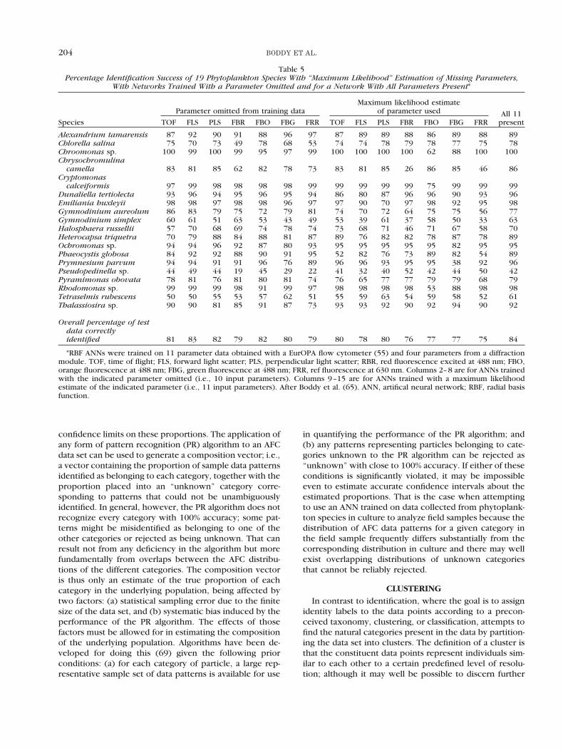
Chrysochromulina camella and Psudopedinella sp., withestimation of red fluorescence excited at 488nm (Table 5).One drawback with this approach is that the time taken toidentify a pattern is more than five times longer (65),which can be significant if a system is operating in nearreal time.

The way to achieve highest overall successful identifi-cation when input parameters are missing, and with noreduction in speed, is to use a network trained with themissing parameter omitted (Table 5). For routine opera-tion, a library of pretrained networks, each appropriate tothe absence of a particular parameter, would be neces-sary. However, if more than one parameter is missing,

maximum likelihood estimation seems to be as successfulas training networks with the parameters missing (65).

It is sensible to analyze the effects of omitting parame-ters from the training and test data set or of replacingmissing values with estimates in the test set to determinevalue of each character for identification and assess therobustness of the network when characters are missing.

Estimating Proportions

It is frequently desired to estimate the composition ofthe sample (and thus the underlying population fromwhich the sample was drawn) in terms of the proportionof particles present from each category, together with

FIG. 4. Effect of using different constraints to reject novel data by using a radial basis function network (39 hidden layer nodes; HLNs) trained onsix-parameter FACS data for 10 phytoplankton species in pure culture (Table 2). Data patterns are of two types: “known,” drawn equally from the specieson which the artificial neural network was trained (Table 2), and “novel,” drawn equally from six more phytoplankton species (Amphidinium carterae,Aureodinium pigmentosum, Crysochromulina polylepis, Dunaliella tertiolecta, Hemiselmis virescens, and Rhodomonas). Three different constraintsare shown: (a) threshold on the maximum HLN output value, (b) threshold on the highest output node value, and (c) threshold on the difference betweenthe highest and second highest output node values. For each constraint, four measures of performance are shown: proportion of known patterns correctlyidentified (squares), proportion of unrejected known patterns correctly identified (circles), proportion of known patterns rejected (triangles), andproportion of novel patterns rejected (plus signs). d: Receiver operating characteristic curves for the three constraints in a–c are represented by opencircles (a), triangles (b), and solid circles (c). The three constraints performed similarly, although the threshold on the maximum output layer node valuewas superior to the others.

203PATTERN RECOGNITION IN FLOW CYTOMETRY

confidence limits on these proportions. The application ofany form of pattern recognition (PR) algorithm to an AFCdata set can be used to generate a composition vector; i.e.,a vector containing the proportion of sample data patternsidentified as belonging to each category, together with theproportion placed into an “unknown” category corre-sponding to patterns that could not be unambiguouslyidentified. In general, however, the PR algorithm does notrecognize every category with 100% accuracy; some pat-terns might be misidentified as belonging to one of theother categories or rejected as being unknown. That canresult not from any deficiency in the algorithm but morefundamentally from overlaps between the AFC distribu-tions of the different categories. The composition vectoris thus only an estimate of the true proportion of eachcategory in the underlying population, being affected bytwo factors: (a) statistical sampling error due to the finitesize of the data set, and (b) systematic bias induced by theperformance of the PR algorithm. The effects of thosefactors must be allowed for in estimating the compositionof the underlying population. Algorithms have been de-veloped for doing this (69) given the following priorconditions: (a) for each category of particle, a large rep-resentative sample set of data patterns is available for use

in quantifying the performance of the PR algorithm; and(b) any patterns representing particles belonging to cate-gories unknown to the PR algorithm can be rejected as“unknown” with close to 100% accuracy. If either of theseconditions is significantly violated, it may be impossibleeven to estimate accurate confidence intervals about theestimated proportions. That is the case when attemptingto use an ANN trained on data collected from phytoplank-ton species in culture to analyze field samples because thedistribution of AFC data patterns for a given category inthe field sample frequently differs substantially from thecorresponding distribution in culture and there may wellexist overlapping distributions of unknown categoriesthat cannot be reliably rejected.

CLUSTERINGIn contrast to identification, where the goal is to assign

identity labels to the data points according to a precon-ceived taxonomy, clustering, or classification, attempts tofind the natural categories present in the data by partition-ing the data set into clusters. The definition of a cluster isthat the constituent data points represent individuals sim-ilar to each other to a certain predefined level of resolu-tion; although it may well be possible to discern further

Table 5Percentage Identification Success of 19 Phytoplankton Species With “Maximum Likelihood” Estimation of Missing Parameters,

With Networks Trained With a Parameter Omitted and for a Network With All Parameters Present*

Species

Parameter omitted from training dataMaximum likelihood estimate

of parameter used All 11presentTOF FLS PLS FBR FBO FBG FRR TOF FLS PLS FBR FBO FBG FRR

Alexandrium tamarensis 87 92 90 91 88 96 97 87 89 89 88 86 89 88 89Chlorella salina 75 70 73 49 78 68 53 74 74 78 79 78 77 75 78Chroomonas sp. 100 99 100 99 95 97 99 100 100 100 100 62 88 100 100Chrysochromulina

camella 83 81 85 62 82 78 73 83 81 85 26 86 85 46 86Cryptomonas

calceiformis 97 99 98 98 98 98 99 99 99 99 99 75 99 99 99Dunaliella tertiolecta 93 96 94 95 96 95 94 86 80 87 96 96 90 93 96Emiliania huxleyii 98 98 97 98 98 96 97 97 90 70 97 98 92 95 98Gymnodinium aureolum 86 83 79 75 72 79 81 74 70 72 64 75 75 56 77Gymnodinium simplex 60 61 51 63 53 43 49 53 39 61 37 58 50 33 63Halosphaera russellii 57 70 68 69 74 78 74 73 68 71 46 71 67 58 70Heterocapsa triquetra 70 79 88 84 88 81 87 89 76 82 82 78 87 78 89Ochromonas sp. 94 94 96 92 87 80 93 95 95 95 95 95 82 95 95Phaeocystis globosa 84 92 92 88 90 91 95 52 82 76 73 89 82 54 89Prymnesium parvum 94 94 91 91 96 76 89 96 96 93 95 95 38 92 96Pseudopedinella sp. 44 49 44 19 45 29 22 41 32 40 52 42 44 50 42Pyramimonas obovata 78 81 76 81 80 81 74 76 65 77 77 79 79 68 79Rhodomonas sp. 99 99 99 98 91 99 97 98 98 98 98 53 88 98 98Tetraselmis rubescens 50 50 55 53 57 62 51 55 59 63 54 59 58 52 61Thalassiosira sp. 90 90 81 85 91 87 73 93 93 92 90 92 94 90 92

Overall percentage of testdata correctlyidentified 81 83 82 79 82 80 79 80 78 80 76 77 77 75 84

*RBF ANNs were trained on 11 parameter data obtained with a EurOPA flow cytometer (55) and four parameters from a diffractionmodule. TOF, time of flight; FLS, forward light scatter; PLS, perpendicular light scatter; RBR, red fluorescence excited at 488 nm; FBO,orange fluorescence at 488 nm; FBG, green fluorescence at 488 nm; FRR, ref fluorescence at 630 nm. Columns 2–8 are for ANNs trainedwith the indicated parameter omitted (i.e., 10 input parameters). Columns 9–15 are for ANNs trained with a maximum likelihoodestimate of the indicated parameter (i.e., 11 input parameters). After Boddy et al. (65). ANN, artifical neural network; RBF, radial basisfunction.

204 BODDY ET AL.

levels of structure in the data at finer scales, whether ornot this is appropriate depends on the nature of the data.Although the presence of clusters is easy to detect visuallyin two- or even three-dimensional data sets from scatterplots, higher dimensional data sets require more sophisti-cated techniques. One option is to first reduce the higherdimensional data to two or three dimensions, e.g.,through principal component analysis (11); however, theresulting projection of the data may well discard impor-tant discriminatory information. It is generally preferableto use a clustering algorithm capable of exploiting the fullmultivariate nature of the data.

Flow cytometric data have a number of characteristicsthat make it challenging for clustering algorithms. Datasets are typically large (n . 104 patterns), which posespractical problems for algorithms requiring the calcula-tion of pairwise distances (distances between every pair ofpatterns) such as the hierarchical agglomerative pair-group methods (70). Typical flow cytometer clusters canbe approximately spherical, highly elongated, or evencurved: algorithms that do not allow for clusters of differ-ent shapes are certain to perform poorly. A data set cancontain clusters of very different cardinalities (in terms ofthe number of data patterns in each) and densities (someclusters may be relatively large and sparse, whereas othersare highly compact and dense). Furthermore, clustersmight be degenerate (possessing zero extent in one ormore dimensions); the hypervolume of such clusters iszero, thus rendering their densities infinite.

Non–neural Methods

Statistical cluster analysis determines possible clustersor classes within a data set by using hierarchical or parti-tional algorithms. Hierarchical algorithms iteratively formclusters by merging data (i.e., agglomerative methods) ordividing the data at various levels (i.e., divisive). Partitionalmethods differ from hierarchical methods by allowingdata points to be reassigned to different clusters if itbecomes apparent that the initial decision was incorrect.

The hierarchical (linkage) agglomerative algorithms,also known as pair-group methods, are popular clusteringprocedures (70,71). Each data point is initially assigned toa separate cluster. The algorithms proceed by repeatedlymerging the two “closest” clusters at each stage, accord-ing to some specific measure of intercluster distance, untilall data points have been merged into a single cluster.Large clusters are thereby composed of a combination ofsmaller subclusters, and this hierarchy of clusters extendsto all length scales. The order in which clusters aremerged provides a lot of information about the data set,and by selecting only those clusters that remain stable forlonger than a preset number of iterations of the algorithm,the “correct” number of clusters can be determined. How-ever, all algorithms of this type have the fundamentaldrawback of requiring the calculation of pairwise dis-tances between clusters. For n clusters, that is of the orderof n2 distances; this tends to be prohibitive for the largedata sets typical in flow cytometry.

Density clustering, a nonparametric, noniterativemethod, gets around some of those problems (72). Essen-tially, the local event density (based on histogram counts)is examined to determine modes, and then regions ofmonotonically decreasing density around each of theseare grouped into a cluster. Adjacent clusters subsequentlymight be merged. The method copes with clusters of anyshape, and the exact number need not be specified inadvance. However, a user-specified threshold is used,which effectively determines the degree of clustering.

With partitional methods, which are iterative in nature,an initial number of clusters is specified by the user basedon prior knowledge of the data. The algorithm repeatedlytransfers data points between the clusters in an attempt toimprove some predefined measure of clustering goodnessand ceases when no further improvement can be ob-tained. The clustering solution arrived at depends on theparticular objective function (measure of “goodness”)used. Minimizing the sum of the squared Euclidean dis-tances between each data point and the nearest clustercenter leads to the well-known k-means algorithm (73).That algorithm can perform well when clusters are rea-sonably well separated and spherical in shape (74); how-ever, clusters in flow cytometry are frequently highlyelongated.

Those two approaches can be combined in a compositealgorithm that uses an iterative k-means approach to re-duce the large number of data points to a manageablenumber of small subclusters and then employs a hierar-chical approach to merge the subclusters (75). This algo-rithm was found to generate good cluster partitions thatcompared well with those obtained by manual clusteranalysis.

A development of the k-means algorithm (76) attemptsto address the problem of elongated clusters by using amore general measure of distance that incorporates infor-mation about the shape of each cluster by means of ascatter matrix estimated from the data points in the vicin-ity of the cluster center. That algorithm, as all iterativealgorithms, can become trapped by local minima (poorclustering solutions), requiring user intervention to recog-nize and reject inadequate results (76). By allowing datapoints to be associated to some degree with all clusters,not just the closest, the algorithm can be made morerobust to the problem of local minima. Several extensionsof this “fuzzy” version of the k-means algorithm, incorpo-rating cluster shape information via scatter matrices (77),have recently been tried on a flow cytometric data setwith some success (78). However, the value of k, thenumber of clusters, must be specified beforehand, and itwould be preferable if the “natural” number of clusterscould be determined automatically from the data. Thatcould be achieved in several ways, e.g., by overspecifyingthe number of clusters and removing those that accordingto some criterion become redundant during the course ofthe algorithm (79) or examining the stability of clustersover a wide range of values of a length-scale parameter(80–82).

205PATTERN RECOGNITION IN FLOW CYTOMETRY

Neural Methods: Kohonen Self-Organizing Map

Probably the best known of the neural clustering meth-ods is the Kohonen self-organizing map (SOM) (56). Themap consists of a grid or lattice of network nodes, com-monly two-dimensional, although other dimensionalitiescan be used. Each node in the lattice represents a proto-type, a point within the data space that serves to representdata patterns occurring within its vicinity. The nodescompete to represent the data presented to the network,with the winning node being that for which the prototypeis closest to the input data pattern. Initially these proto-types are randomly selected, being initialized, e.g., torandomly selected patterns from the data set. During the

course of the algorithm, patterns are randomly selectedfrom the data set and presented to the network, and theprototypes of the winning node and those surrounding itin the lattice are updated by moving them slightly closerto the presented pattern. The size of the neighborhoodupdate region is decreased as the algorithm proceeds: atthe start large areas of the lattice are being simultaneouslyupdated; by the end only the winning node itself and itsimmediate neighbors are updated. The effect of this isthat, over the course of many pattern presentations, themap comes to form a low-dimensional representation ofthe data set with a topology-preserving property. Patternsrepresented by the prototypes of nodes that are close toeach other in the lattice typically are similar to each other.

The ability of Kohonen SOMs to reduce dimensionalityand map closely related patterns (in terms of the charac-ters used) close together makes them useful for investi-gating relatedness or otherwise of genomes, cells, species,etc. They have been applied to classifying phytoplanktonfrom flow cytometry data (43,45,83,84) (Fig. 5). The rela-tions between known groupings can be examined byoverlying class identity onto the mapping produced, asshown in Figure 5 with a mapping of 40 marine phyto-plankton species onto a 16 3 16 grid. Where the characterdistributions of classes overlap, nodes respond to patternsfrom two or more classes, and the maps are produced byassigning each node to the taxon with the highest fre-quency of classification at that node. Where there is over-lap of character distributions, the extent of overlap can bevisualized by plotting the percentage of each class at eachnode. In the marine phytoplankton example, closeness ofspecies in the SOM (Fig. 5) does not always relate tocloseness in traditional taxonomic classifications, e.g., thediatoms do not lie close together (Fig. 5b), because thecharacters used are not the morphologic characteristicsupon which the traditional taxonomy is based, but rather

4™™™™™™™™™™™™™™™™™™™™™™™™™™™™™™™™™™™™™™™™™™™™™™™™™™™™™™™™™™™™™FIG. 5. a: Kohonen self-organizing map (SOM; 16 3 16) of 40 species of

marine phytoplankton grown in axenic culture and analyzed with theoptical plankton analyzer flow cytometer (OPA). The network was trainedon 300 patterns/species for more than 200,000 cycles, with six inputparameters: time of flight (i.e., cell size), forward light scatter, perpen-dicular light scatter, red fluorescence under blue light, green fluorescenceunder blue light, and red fluorescence under red light. b: The same SOMshowing to which orders the species belong. The flagellate group com-prises Rhodophyceae, Volvocida, Chrysomonadida, and Prasinomona-dida. Dinoflagellates: S.t., Scrippsiella trochoidea; P.m., Prorocentrummicans; H.t., Heterocapsa triqueta; A.t., Alexandrium tamarensis; G.a.,Gyrodinium aureolum; O.m., Oxyrrhis marina; G.s., Gymnodiniumsimplex; G.m., Gymnodinium micrum; G.v., Gymnodinium veneficum.Prymnesiomonads: Ch.ca., Chrysochromulina camella; Ch.ch., Chryso-chromulina chiton; Ch.cy., Chrysochromulina cymbium; P.c., Pleuro-chrysis carterae; O.n., Ochrosphaera neopolitana; P.l., Pavlova lutheri;P.po., Phaeocystis pouchetii; P.pa., Prymnesium parvum. Flagellates:Po.pu., Porphyridium pupureum; D.t., Dunaliella tertiolecta; Chl.sa.,Chlorella salina; S.b., Stichococcus bacillaris; O.sp., Ochromonas sp.;P.sp., Pseudopedinella sp.; P.o., Pyramimonas obovata; H.r., Halospha-era russellii; N.r., Nephroselmis rotunda; P.g., Pyramimonas grossii;T.v., Tetraselmis verrucosa. Cryptomonads: H.b., Hemiselmis brunne-scens; Pl.pu., Plagioselmis punctata; Cr.ca., Cryptomonas calceiformis;Cr.ma., Cryptomonas maculata; Cr.ro., Cryptomonas rostrella; Chr.sa.,Chroomonas salina. Diatoms: Ch.d., Chaetoceros didymus; T.r., Thalas-siosira rotula; T.w., Thalassiosira weissflogii; T.p., Thalassiosira pseud-onana; A.c., Amphora coffaeformis. After Morris and Boddy (83).

206 BODDY ET AL.

relate to photosynthetic pigments, size and influences ofshape, surface properties, etc.

A major problem with using SOMs as a clustering toolwithout knowledge of class identity, as with other clusteringschemes, is how to decide on the limits of a cluster. Thisproblem does not appear to have received much attention.Although SOMs map data to the nodes in the grid and eachnode in the grid can be considered to be a cluster, it is likelythat in reality clusters will naturally be made up of the datamapped to several nodes. There are a number of possibleways by which the Kohonen nodes could be clustered toform higher level groupings. An obvious approach would beto allocate the SOM only the same number of nodes as thenumber of clusters required. That has the same two majordrawbacks as with statistical clustering: it assumes that (a)we have a priori knowledge regarding the number of clustersthat we want and (b) we may not get the “correct” clustersforming at the level of separation that we want. We currentlyare investigating a number of approaches that could be usedsingly or in combination, as follows.

The first method, agglomerative clustering, in whichthe Euclidean distances between every pair of nodes inthe map are calculated, each node is assumed to be acluster at the outset of the algorithm. The two closestnodes are then merged to form a cluster, followed by thenext two, etc. If closest nodes are already part of clusters,then the clusters are merged. That process is continueduntil some predetermined number of clusters is reachedor until the closest nodes are farther apart than someuser-defined threshold.

The second method looks for candidate cluster centersby considering the number of data points that has beenmapped to that node, and the nodes with the highestdensity of data points are considered to be possible clustercenters. Other nodes in the map are then assigned tothose clusters dependent on their Euclidean distancesfrom the center of the cluster. There is a tendency for thismethod to produce many cluster centers in areas of highdata density and few in areas of low density; the centers inhigh density areas often need to be merged, whereasthose in lower density areas might be missed completely.

The third technique uses a mapping grid that is muchlarger than needed. The data then map to certain areas,leaving other areas with no data mapped onto them. It willautomatically produce “fences” of low usage nodesaround high density areas.

The fourth method uses a hierarchical technique thatinitially performs a very coarse clustering of the data on amap with few nodes. Data mapped to each node of thecoarse map then are used to create a new map that breaksthe coarse clustering into a finer set of clusters.

In the fifth method, purely visual clustering can beachieved by plotting the SOM with the Euclidean dis-tances between neighboring nodes plotted as lines whosewidths correspond to the distances.

Neural Methods: Adaptive Clustering

Adaptive resonance theory (ART) is another unsuper-vised ANN approach that can be used for clustering (85).

There are two main types of ART network: ART-1, whichprocesses only binary inputs, and ART-2, a later versionthat accepts binary and continuous inputs; numerousother variants have been developed. ART has a complexunderlying theoretical basis. Effectively, the first patternpresented to the network is allocated to the first cluster.Subsequently, each pattern presented to the network iscompared with each cluster that has been detected; if nomatch is found, a new cluster is formed by adding a newcluster node. How similar patterns must be to constitute amatch can be changed by altering a threshold value(termed vigilance). The size of the threshold value effec-tively determines the number of clusters. These ANNsclearly learn incrementally, which is a useful feature lack-ing from most supervised learning networks.

Although ART does not appear to have been used foranalysis of flow cytometry data, a similar approach has:real-time adaptive clustering (RTAC) (33,86). Like ART,RTAC does not make assumptions about the number ofclusters, and it is adaptive to dynamically changing con-ditions. The fundamental difference between the two is inthe choice of the similarity function and the method oftraining. Also, RTAC is simpler to implement. When com-parisons were made with the same level of vigilence,RTAC resulted in more clusters than ART (33).

CONCLUSIONSInformation held within the large quantities of data

generated by flow cytometry is now tractable with the useof ANNs. Analysis is so rapid that identification of particlescan be made in real or near-real time. Two main problemsthat still need to be resolved are obtaining appropriatetraining data for identification of cells from field samplesand coping with the almost infinite number of cell typesfound in field samples. Using the sort facility and beingable to drive it from ANN or non–neural clustering soft-ware is crucial to the former problem; essential steps areidentification of clusters of similar cells, separation ofthose clusters from the rest, identification, and use oflabeled patterns of characters for training ANNs for iden-tification. Detecting clusters is obviously a very importantstep in obtaining training data from the field and in anal-ysis of flow cytometric data sets in general. Ways ofdetermining clusters without prior specification of num-ber of clusters, whether for neural or non–neural ap-proaches, requires urgent attention. With regard to cop-ing with additional cell types, rejection of “unknowns”works well, and the use of partitioned networks (RBF orSVM) for easy addition of new categories to identificationschemes looks very promising.

LITERATURE CITED1. Alvarez-Barrientos A, Arroyo J, Canton R, Nombela C, Sanchez-Perez

M. Applications of flow cytometry to clinical microbiology. ClinMicrobiol Rev 2000;13:167–195.

2. Ahmad S, Tresp V. Classification with missing and uncertain inputs.In: Proceedings of the IEEE International Conference on Neural Net-works. IEEE Press: San Fransisco, CA. 1993. p 1949–1954.

3. Jespersen L, Lassen S, Jakobsen M. Flow cytometric detection of wildyeast in lager breweries. Int J Food Microbiol 1993;17:321–328.

4. Laplacebuilhe C, Hahne K, Hunger W, Tirilly Y, Drocourt JL. Appli-

207PATTERN RECOGNITION IN FLOW CYTOMETRY

cation of flow-cytometry to rapid microbial analysis in food anddrinks industries. Biol Cell 1993;78:123–128.

5. Urano N, Nomura M, Sahara H, Koshino S. The use of flow cytometryand small-scale brewing in protoplast fusion–exclusion of undesiredphenotypes in yeasts. Enzyme Microbi Technol 1994;16:839–843.

6. Burkill PH, Mantoura RFC. The rapid analysis of single marine cells byflow cytometry. Phil Trans R Soc 1990;A333:99–112.

7. Burkill PH. Analytical flow cytometry and its application to marinemicrobial ecology. In: Sleigh MA, editor. Microbes in the sea. Chich-ester: Ellis Horwood; 1987. p 139–166.

8. Collier JL. Flow cytometry and the single cell in phycology. J Phycol2000;36:628–644.

9. Hofstraat JW, Vanzeijl WJM, Devreeze MEJ, Peeters JCH, Peperzak L,Colijn F, Rademaker TWM. Phytoplankton monitoring by flow-cytom-etry. J Plankton Res 1994;16:1197–1224.

10. Mann RC. On multiparameter data analysis in flow cytometry. Cytom-etry 1987;8:184–189.

11. Joliffe IT. Principal components analysis. Springer series in statistics.New York: Springer-Verlag; 1986.

12. Schalkoff RJ. Pattern recognition: statistical, structural and neuralapproaches. Chichester: Wiley International; 1992.

13. Blackburn N, Hagstrom A, Wikner J, Cuadros-Hansson R, BjornsenPK. Rapid determination of bacterial abundance, biovolume, mor-phology, and growth by neural network-based image analysis. ApplEnviron Microbiol 1998;64:3246–3255.

14. Godavarti M, Rodriguez JJ, Yopp TA, Lambert GM, Galbraith DW.Automated particle classification based on digital acquisition andanalysis of flow cytometric pulse waveforms. Cytometry 1996;24:330–339.

15. Dubelaar GBJ, Gerritzen PL, Beeker AER, Jonker RR, Tangen K.Design and first results of CytoBuoy: a wireless flow cytometer for insitu analysis of marine and fresh waters. Cytometry 1999;37:247–254.

16. Dubelaar GBJ, Gerritzen PL. CytoBuoy: a step forward towards usingflow cytometry in operational oceanography. Sci Mar 2000;64:255–265.

17. Wilkins MF, Boddy L, Dubelaar GBJ. Identification of marine microal-gae by neural network analysis of simple descriptors of flow cyto-metric pulse shapes. Ecol Model 2001. Forthcoming.

18. Ravdin PM, Clark GM, Hough JJ, Owens MA, McGuire WL. Neuralnetwork analysis of DNA flow cytometry histograms. Cytometry1993;14:74–80.

19. Smits JRM, Melssen WJ, Derksen MWJ, Kateman G. Drift correctionfor pattern-classification with neural networks. Anal Chim Acta 1993;284:91–105.

20. Thews O, Thews A, Huber C, Vaupel P. Computer-assisted interpre-tation of flow cytometry data in hematology. Cytometry 1996;23:140–149.

21. Breiman L, Friedman JH, Olshen RA, Stone CJ. Classification andregression trees. Monterey (CA): Wadsworth & Brooks; 1984.

22. Beckman RJ, Salzman GC, Stewart CC. Classification and regressiontrees for bone marrow immunophenotyping. Cytometry 1995;20:210–217.

23. Dybowski R, Gant VA, Riley PA, Phillips I. Rapid compound patternclassification by recursive poartitioning of feature space. An applica-tion in flow cytometry. Pattern Recog Lett 1995;16:703–709.

24. Decaestecker C, Remmelink M, Salmon I, Camby I, Goldschmidt D,Petein M, VanHam P, Pasteels JL, Kiss R. Methodological aspects ofusing decision trees to characterise leiomyomatous tumours. Cytom-etry 1996;24:83–92.

25. Quinlan JR. C4.5 programs for machine learning. San Mateo (CA):Morgan Kaufmann; 1993.

26. Baldetorp B, Dalberg M, Holst U, Lindgren G. Statistical evaluation ofcell kinetic data from DNA flow cytometry (FCM) by the EM algo-rithm. Cytometry 1989;10:695–705.

27. Carr MR, Tarran GA, Burkill PH. Discrimination of marine phytoplank-ton species through the statistical analysis of their flow cytometricsignatures. J Plankton Res 1996;18:1225–1238.

28. Molnar B, Szentirmay Z, Bodo M, Sugar J, Feher J. Application ofmultivariate, fuzzy set and neural network analysis in quantitaltivecytological examinations. Anal Cell Pathol 1993;5:161–175.

29. Valet G, Valet M, Tschope D, Gabriel H, Rothe G, Kellermann W,Kahle H. Standardized, self learning flow cytometric list mode dataclassification with the CLASSIF1 program system. Ann NY Acad Sci1992;677:233–251.

30. Wilkins MF, Boddy L, Morris CW, Jonker R. A comparison of someneural and non-neural methods for identification of phytoplanktonfrom flow cytometry data. CABIOS 1996;12:9–18.

31. Boddy L, Morris CW. Artificial neural networks for pattern recogni-tion. In: Fielding AH, editor. Machine learning methods for ecologicalapplications. Boston: Kluwer; 1999. p 37–87.

32. Caudill M, Butler C. Naturally intelligent systems. Cambridge: Massa-chusetts Institute of Technology Press; 1992.

33. Fu L. Neural networks in computer intelligence. New York: McGraw-Hill; 1994.

34. Haykin S. Neural networks: a comprehensive foundation. New York:Maxwell MacMillan International; 1994.

35. Hush DR, Horne BB. Progress in supervised neural networks—what’snew since Lippmann? IEEE Sig Proc Mag 1993;10:8–39.

36. Lippmann RP. An introduction to computing with neural nets. IEEEAcoust Speech Signal Process Mag 1987;4:4–22.

37. Maren AJ, Harston C, Pap R. Handbook of neural computing applica-tions. New York: Academic Press; 1990.

38. Morris C W, Boddy L, Allman R. Identification of basidiomycetespores by neural network analysis of flow cytometry data. Mycol Res1992;96:697–701.

39. Davey HM, Jones A, Shaw AD, Kell DB. Variable selection and multi-variate methods for the identification of microorganisms by flowcytometry. Cytometry 1999;35:162–168.

40. Balfoort HW, Snoek J, Smits JRM, Breedveld LW, Hofstraat JW, Rin-gelberg J. Automatic identification of algae: neural network analysisof flow cytometric data. J Plankton Res 1992;14:575–589.

41. Boddy L, Morris CW, Wilkins MF, Al-Haddad L, Tarran GA, Jonker RR,Burkill PH. Identification of 72 phytoplankton species by radial basisfunction neural network analysis of flow cytometric. Mar Ecol ProgSer 2000;195:47–59.

42. Boddy L, Morris CW, Wilkins MF, Tarran GA, Burkill PH. Neuralnetwork analysis of flow cytometric data for 40 marine phytoplank-ton species. Cytometry 1994;15:283–293.

43. Frankel DS, Frankel SL, Binder BJ, Vogt RF. Application of neuralnetworks to flow cytometry data analysis and real-time cell classifica-tion. Cytometry 1996;23:290–302.

44. Frankel DS, Olson RJ, Frankel SL, Chisholm SW. Use of a neural netcomputer system for analysis of flow cytometric data of phytoplank-ton populations. Cytometry 1989;10:540–550.

45. Morris CW, Boddy L, Wilkins MF. Approaches to applying neuralnetworks to the identification of phytoplankton taxa from flow cy-tometry data. In: Dagli CH, Fernandez BR, Ghosh J, Kumara RTS,editors. Intelligent engineering systems through artificial neural net-works. Volume 4. New York: ASME Press; 1994. p 619–627.

46. Morris CW, Boddy L. Classification as unknown by RBF networks:discriminating phytoplankton taxa from flow cytometry data. In:Dagli CH, Akay M, Chen CLP, Fernandez BR, Ghosh J, editors. Intel-ligent engineering systems through artificial neural networks. Volume6. New York: ASME Press; 1996. p 629–634.

47. Morris CW, Boddy L. Partitioned RBF networks for identification ofbiological taxa: discrimination of phytoplankton from flow cytometrydata. In: Dagli CH, Akay M, Buczak CLP, Ersoy AL, Fernandez, BR,editors. Intelligent engineering systems through artificial neural net-works. Volume 8. New York: ASME Press; 1998. p 637–642.

48. Smits JRM, Breedveld LW, Derksen MWJ, Kateman G. Pattern classi-fication with artificial neural networks: classification of algae, basedupon flow cytometer data. Anal Chim Acta 1992;258:11–25.

49. Smits JRM, Breedveld LW, Derksen MWJ, Kateman G, Balfoort HW,Snoek J, Hofstraat JW. Pattern classification with artificial neuralnetworks: classification of algae, based upon flow cytometer data.Anal Chim Acta 1992;258;11–25.

50. Bellotti M, Elsner B, De Lima AP, Esteva H, Marchevsky AM. Neuralnetworks as a prognostic tool for patients with non–small cell carci-noma of the lung. Mod Pathol 1997;10:1221–1227.

51. Kothari R, Cualing H, Balachander T. Neural network analysis of flowcytometry immunophenotype data. IEEE Trans Biomed Engin 1996;43:803–810.

52. Morris CW, Autret A, Boddy L. Support vector machines for identify-ing organisms—a comparison with strongly partitioned radial basisfunction networks. Ecol Model 2001. in press.

53. Morgan A, Boddy L, Morris CW, Mordue JEM. Identification of speciesin the genus Pestalotiopsis from spore morphometric data: a com-parison of some neural and non-neural methods. Mycol Res 1998;102:975–984.

54. Wilkins MF, Morris CW, Boddy L. A comparison of radial basis func-tion and backpropagation neural networks for identification of ma-rine phytoplankton from multivariate flow cytometry data. CABIOS1994;10:285–294.

55. Wilkins MF, Boddy L, Morris CW, Jonker R. Identification of phyto-plankton from EurOPA flow cytometry data using radial basis func-tion neural networks. Appl Environ Microbiol 1999;65:4404–4410.

56. Kohonen T. The self-organising map. Proc IEEE 1990;78:1464–1480.57. Chen S, Cowan CFN, Grant PM. Orthogonal least-squares learning

algorithm for radial basis function networks. IEEE Trans Neural Netw1991;2:302–309.

208 BODDY ET AL.

58. Burges CJC. A tutorial on support vector machines for pattern recog-nition. Boston: Kluwer and London: Academic Press; 1998.

59. Joachims T. Making large-scale learning practical. In: Scholkopf B,Burges C, Smola A, editors. Advances in kernel methods—supportvector learning. Cambridge: Massachusetts Institute of TechnologyPress; 1999.

60. Vapnik VN. The nature of statistical learning theory. New York:Springer-Verlag; 1995.

61. Morris CW, Autret A, Boddy L. A comparison of strongly partitionedRBF networks and support vector machines for identification ofbiological taxa. In: Dagli CH, Buczak CLP, Ghosh J, Ersoy OAL,Embrechts MJ, Kercel S, editors. Intelligent engineering systemsthrough artificial neural networks. Volume 10. New York: ASMEPress; 2000. p 783–788.

62. Al-Haddad L, Morris CW, Boddy L. Training radial basis functionneural networks: effects of training set size and imbalanced trainingsets. J Microbiol Methods 2000;43:33–44.

63. Barnard E, Botha EC. Back-propagation uses prior information effi-ciently. IEEE Trans Neural Netw 1993;4:794–802.

64. Richard MD, Lippmann RP. Neural network classifiers estimate Bayes-ian a posteriori probabilities. Neural Comput 1991;3:461–483.

65. Boddy L, Wilkins MF, Morris CW. Effects of missing data on neuralnetwork identification of biological taxa: RBF network discriminationof phytoplankton from flow cytometry data. In: Dagli CH, Akay M,Buczak CLP, Ersoy AL, Fernandez BR, editors. Intelligent engineeringsystems through artificial neural networks. Volume 8. New York:ASME Press; 1998. p 655–666.

66. Ahmad S, Tresp V. Classification with missing and uncertain inputs.In: Proceedings of the IEEE International Conference on Neural Net-works, San Fransisco, CA. 1993. p 1949–1954.

67. Gupta A, Lam MS. Estimating missing values using neural networks. JOperat Res Soc 1996;47:229–238.

68. Sharpe PK, Solly RJ. Dealing with missing values in neural-networkbased diagnostic systems. Neural Comput Appl 1995;3:73–77.

69. Wilkins MF, Boddy L, Morris CW. Proportion estimation with confi-dence limits. J Microbiol Methods 2000;43(1):55–64.

70. Sneath PHA, Sokal RR. Numerical taxonomy. San Francisco: WHFreeman & Co.; 1973.

71. Dunn G, Everitt BS. An introduction to mathematical taxonomy.Cambridge: Cambridge University Press; 1982.

72. Conrad MP. A rapid nonparametric clustering scheme for flow cy-tometry data. Pattern Recog Lett 1987;20:229–235.

73. Hartigan J. Clustering algorithms. New York: Wiley; 1975.74. Murphy RF. Automated identification of subpopulations in flow cy-

tometric list mode data using cluster analysis. Cytometry 1985;6:302–309.

75. Bakker Schut TC, De Grooth BG, Greve J. Cluster analysis of flowcytometric list mode data on a personal computer. Cytometry 1993;14:649–659.

76. Demers S, Kim J, Legendre P, Legendre L. Analysing multivariate flowcytometric data in aquatic sciences. Cytometry 1992;13:291–298.

77. Rousseeuw PJ, Kaufman L, Trauwaert E. Fuzzy clustering using scat-ter matrices. Comput Stat Data Anal 1996;23:135–151.

78. Wilkins MF, Hardy S, Boddy L, Morris CW. Comparison of five clus-tering algorithms to classify phytoplankton from flow cytometry data.Cytometry 2001;44:210–217.

79. Frigui H, Krishnapuram R. A robust algorithm for automatic extrac-tion of an unknown number of clusters from noisy data. PatternRecog Lett 1996;17:1223–1232.

80. Chakravarthy SV, Ghosh J. Scale-based clustering using the radialbasis function network. IEEE Trans Neural Netw 1996;7:1250–1261.

81. Frattale Mascioli FM, Rizzi A, Panella M, Martinelli G. Scale-basedapproach to hierarchical fuzzy clustering. Sig Proc 2000;80:1001–1016.

82. Kothari R, Pitts D. On finding the number of clusters. Pattern RecogLett 1999;20:405–416.

83. Morris CW, Boddy L. Artificial neural networks in identification andsystematics of eukaryotic microorganisms. Binary 1995;7:70–76.

84. Wilkins MF, Boddy L, Morris CW. Kohonen maps and learning vectorquantization neural networks for analysis of multivariate biologicaldata. Binary 1994;6:64–72.

85. Carpenter GA, Grossberg S. The ART of adaptive pattern recognitionby a self-organizing neural network. Computer 1988;77–88.

86. Fu L, Yang M, Braylan R, Benson N. Real-time adaptive clustering offlow cytometric data. Pattern Recog Lett 1993;26:365–373.

209PATTERN RECOGNITION IN FLOW CYTOMETRY