energies

Article

Partial Discharge Pattern Recognition ofGas-Insulated Switchgear via a Light-ScaleConvolutional Neural Network

Yanxin Wang 1, Jing Yan 1,* , Zhou Yang 2, Tingliang Liu 1, Yiming Zhao 1 and Junyi Li 1

1 State Key Laboratory of Electrical Insulation and Power Equipment, Xi’an Jiaotong University, Xi’an 710049,China; yxwang199501@163.com (Y.W.); liu1741770229@163.com (T.L.); yiming_zhao96@163.com (Y.Z.);hc513353489@stu.xjtu.edu.cn (J.L.)

2 School of Computer Science, Xi’an Jiaotong University, Xi’an 710049, China; nextimesyo@foxmail.com* Correspondence: yanjing@mail.xjtu.edu.cn

Received: 9 November 2019; Accepted: 5 December 2019; Published: 9 December 2019�����������������

Abstract: Partial discharge (PD) is one of the major form expressions of gas-insulated switchgear(GIS) insulation defects. Because PD will accelerate equipment aging, online monitoring and faultdiagnosis plays a significant role in ensuring safe and reliable operation of the power system. Owingto feature engineering or vanishing gradients, however, existing pattern recognition methods for GISPD are complex and inefficient. To improve recognition accuracy, a novel GIS PD pattern recognitionmethod based on a light-scale convolutional neural network (LCNN) without artificial featureengineering is proposed. Firstly, GIS PD data are obtained through experiments and finite-differencetime-domain simulations. Secondly, data enhancement is reinforced by a conditional variationauto-encoder. Thirdly, the LCNN structure is applied for GIS PD pattern recognition while thedeconvolution neural network is used for model visualization. The recognition accuracy of the LCNNwas 98.13%. Compared with traditional machine learning and other deep convolutional neuralnetworks, the proposed method can effectively improve recognition accuracy and shorten calculationtime, thus making it much more suitable for the ubiquitous-power Internet of Things and big data.

Keywords: partial discharge; pattern recognition; light-scale convolutional neural network;the ubiquitous power Internet of Things

1. Introduction

Gas-insulated switchgear (GIS) is widely used in power systems because of its small footprint,high reliability, low environmental impact, and maintenance-free features. Potential risks exist,however, in design, manufacturing, transportation, installation, and operation and maintenance,which may further give rise to latent GIS failures [1–3]. Because the GIS is one of the main control andprotection components of the power system, once it fails, it will significantly shock the power grid,not only causing large-scale power outages and negatively affecting power supply reliability but alsoresulting in massive economic losses. Therefore, effective detection of GIS latent defects and takingnecessary measures before failures are of great importance in ensuring safe and reliable operation ofthe power grid while reducing maintenance time and cost.

The advancement of the construction of the ubiquitous-power Internet of Things (IoT) providesnew opportunities for GIS fault diagnosis and challenges [4,5]. Exploring not only real-time rapidprocessing of GIS fault signals but also the ability to accurately identify fault diagnosis methods forGIS faults has become an urgent problem to be solved. According to the statistics, insulation faults arethe main cause of accidents in GIS [6], and most insulation faults are manifested in the form of partialdischarges (PDs), which will further accelerate equipment aging. Currently, the detection of insulation

Energies 2019, 12, 4674; doi:10.3390/en12244674 www.mdpi.com/journal/energies

Energies 2019, 12, 4674 2 of 19

faults is mainly done by means of measuring sound, light-scale, heat, and electromagnetic waves andthe decomposition of chemical products induced by PD [7]. Detection methods include pulse current,ultra-high-frequency (UHF), ultrasonic, optical detection, and gas decomposition product detectionmethods [8–12]. Among these methods, the UHF method is widely adopted because of its stronganti-interference ability and high detection sensitivity [13]. As a result of visible feature differences ofdifferent PD sources, these characteristics can be used for PD pattern recognition and classification.

Given the randomness of PD, traditional machine learning methods are widely applied toPD pattern recognition and classification. The current main classification methods are supportvector machine, decision tree, random forest, neural network, and improved algorithms of theaforementioned methods [14–18]. Compared with the classification methods, feature extraction plays amore important role in pattern recognition, as the quality of the feature directly affects the performanceof the classification algorithm. Numerous feature extraction methods involving time-resolved partialdischarge (TRPD) and phase-resolved partial discharge (PRPD) have emerged, mainly including Fouriertransforms, wavelet transforms, Hilbert transforms, empirical mode decomposition, S-parametertransformation, fractal parameters, and polar coordinate transformation [19–25]. The identificationmethod based on PRPD mode has strong anti-interference ability; however, the synchronous phase ofthe high voltage side is not necessarily obtained in the field measurement, and this analysis method isdifficult to implement when there is external electromagnetic interference. Since TRPD mode needs toanalyze the relationship between different insulation defects and discharge pulse waveform, it is adirect analysis method closer to the discharge mechanism. Its data acquisition system is simple andcan distinguish noise signals, which can be extended to PD detection of direct current (DC) equipment.Therefore, the recognition method based on the TRPD pattern has high research value [26–28].

Traditional machine learning methods exhibit excellent performance in PD pattern recognitionclassification. Their feature extraction methods, however, excessively rely on expert experience whilemassive manual interventions will lead to artificial error. At the same time, the features extracted bydifferent algorithms can neither be shared nor are transferable, so it is difficult to guarantee that they arestill the best in other algorithms [29]. To effectively solve this problem, deep learning methods that relyon automatic feature extraction are introduced into GIS PD pattern recognition. At present, these deeplearning models include LeNet5, AlexNet, one-dimensional convolution, and long short-term memory(LSTM) models [30–34].

In the aforementioned methods, however, the input requirement of LeNet5 is 28× 28, and shrinkingthe original image to such a small size may result in incomplete information utilization as well as lowrecognition accuracy of the TRPD pattern. Deepening of the network causes a vanishing gradient,which prevents AlexNet from being trained and significantly prolongs the model training time.This problem may become exacerbated with deepening of the network. Therefore, deep convolutionalneural networks (CNNs) may not work in TRPD-based GIS PD pattern recognition. To solve the problemof insufficient utilization of feature information in traditional methods as well as the low recognitionaccuracy resulting from the vanishing gradient, a new method using a light-scale convolutional neuralnetwork (LCNN) is proposed in this paper. The proposed method can, to a large extent, optimize thetime performance of the model for better application to IoT conditions. It can improve the recognitionaccuracy of the model in characterizing TRPD-based GIS PD features while greatly shortening themodel training and testing time. Therefore, it can rapidly process failures in real time. The maincontributions of this paper are as follows:

(1) An LCNN model is proposed for GIS PD pattern recognition. By combining experimental dataand simulation data, it maximizes the stochastic simulation of PD and reduces the model’s dependenceon expert experience via automatic feature extraction and full utilization of feature information. Hence,it effectively increases the accuracy of pattern recognition.

(2) The conditional variation auto-encoder is used for data enhancement. Considering thestandardization of TRPD waveform images, it is difficult to meet the requirements by data enhancementmethods, such as image rotation and transformation. This paper uses a conditional variation

Energies 2019, 12, 4674 3 of 19

auto-encoder to generate new data for data enhancement. Meanwhile, through dropout, normalization,and other methods, it effectively reduces the model training and testing time, making it more applicableto the ubiquitous-power IoT context.

(3) The model is visualized by a deconvolution neural network and TensorBoard, and the“black-box” problem of CNNs is solved.

2. Proposed Method

2.1. Data Enhancement with Conditional Variation Auto-Encoder

Based on the raw sample, data enhancement is aimed at learning the sample features andreconstructing the samples in the same feature distributions through constructing a deep network.It can greatly increase the number of samples [35–38], thus improving classification performance.The technique, which originates from game theory, entails making the generator and discriminatorin the network gradually achieve dynamic equilibrium (Nash equilibrium), so that the model canbetter learn the approximate feature distribution from the input samples. Since the acquired PDsignals are stored in a unified standard manner, the image scaling can only introduce noise interferenceand cannot achieve data enhancement. Considering the standardization of TRPD waveform images,data enhancement methods through image rotation and transformation can result in enhanced databecoming difficult to classify as special samples. In PD pattern recognition, because of the relativelysmall number of total data sets, in this paper, a conditional variation auto encoder (CVAE) is adoptedas the data enhancement model to increase the number of training data and improve the generalizationability of the model.

The basic idea of the CVAE algorithm is that each entry point, x ∈ µi, is replaced by a respectivehidden variable, z. Therefore, the final output, x̃, can be generated by a certain probability distribution,Pθ(x|z) , which is assumed to be Gaussian. The decoder function, fθ(z), can generate the finalparameters of the generated distribution and itself is constrained by a set of uniform parameters,θ. At the same time, the encoder function, gθ(x), can generate a parameter for each probabilitydistribution, qφ(z|x) , which is also restrained by the parameter, θ. In training and testing, a label factoris added to the network learning image distribution. The condition of the label factor is set as y, and,in this sense, the specified image can be generated according to the label value.

The variational derivation indicates that an approximate distribution, p(z), is needed in place ofthe distribution, qφ(z|x) . The similarity of the two distributions is usually measured by a functioncalled Kullback–Leibler (KL) divergence. Thereby, the objective function of the confidence lower boundfor a single entry point is as follows:

L(x, y;φ,θ) = −DKL(qφ(zx, y) ‖ pθ(z|y)) + Eqφ(z|x,y)[log pθ(x|z, y)]. (1)

In Equation (1), the first divergence function, DKL(), can be regarded as a regularized item, whilethe second expression, Eq(), can be viewed as the desired auto-coded reconstruction error. It maygreatly simplify the calculation by approximating Eq with the mean of the samples, S, from qφ(z|x) :

L(x, y;φ,θ) = −DKL(qφ(z|x, y) ‖ pθ(z|y)

)+

∫qφ(z|x, y) log pθ(x|z, y) ≈ L̃(x, y;φ,θ) =

−DKL(qφ(z|x, y) ‖ pθ(z|y)

)+ 1

S∑S

s=1 log pθ(x|z(S), y

),

(2)

where z(S) is one of the S samples. Because p(z) is a Gaussian distribution, re-parameter quantizationcan be used to simplify the operation. For the sample, z(S), a small variable, ε, can be obtained fromthe distribution, N(0, 1), instead of the normal distribution, N(µ, δ). It can be calculated through theexpectation, µ, and standard deviation, δ:

z(S) = δε+ µ, (3)

Energies 2019, 12, 4674 4 of 19

L̃(x, y;φ,θ) = −DKL(qφ(z|x, y) ‖ pθ(z|y)

)+

1S

S∑s=1

log pθ(x|ε(S)δ, y

)(4)

Up to now, all parameters can be optimized by adopting the stochastic gradient descent method.In this paper, the conditional variation auto-encoder is used to randomly select 20% of the data from thetraining set to generate new samples for model training. The variation auto-encoder can improve thegeneralization ability of the model and the recognition and classification performance of PD patterns.

2.2. Convolutional Neural Network

Developed in recent years, CNN has been widely considered as one of efficient pattern recognitionmethods. Generally, the basic structure of CNN consists of two layers, feature extraction layer andfeature mapping layer [39]. In feature extraction layer, each neuron input is connected to the localreceptive field of the previous one. Once the local features are extracted, their positional relationshipwith other features is also determined. In feature mapping layer, each computing layer of the networkis composed of multiple feature maps. Each feature map is a plane where the weights of all neuronsare equal. The feature mapping structure adopts the ReLU function, a small influence function, as theactivation function of the convolution network, to ensure the shifting invariance of the feature map.In addition, since the neurons on one map plane share weights, the number of network free parametersis reduced. Each convolutional layer in the CNN is closely followed by a computational layer for localaveraging and quadratic extraction. This unique structure of two-phase feature extraction effectivelyreduces feature dimensions.

The CNN is mostly composed of multiple convolution layers and pooling layers, which canbe subdivided as feature extraction layers, fully-connected layers, and Softmax layers; the featuremap first convolutedly calculates with multiple convolution kernels and then is connected to thenext layer with bias calculation, activation function, and pooling operation. In the convolution layer,each convolution kernel is convolved with the feature maps of the previous one, and then an outputfeature map can be obtained through an activation function, which can be expressed as:

Hi = σ(Hi−1 ×Wi + b), (5)

where Hi refers to the feature map of the ith layer of the CNN, σ is the activation function, ∗ is theconvolution operator, Wi is the weight matrix of the ith convolution kernel, and bi is the offset vector ofthe ith layer. Currently, the main activation functions are tanh, sigmoid, and ReLU.

For the pooling layer, the calculation process can be expressed as:

Hi = pooling(Hi−1). (6)

Pooling represents the pooling operation, which involves averaging, maximization,and random pooling.

In the fully connected layer, the feature maps of the previous layer are processed with theweighted sum method. The output feature map can be attained by the activation function, which canbe expressed as:

Hi = σ(Hi−1Wi + bi). (7)

The training goal of the CNN is to minimize the loss function. When used for classificationproblems, the loss function uses cross entropy:

J(θ) = −1m

∑mi=1yi log

(hθ(xi)

)+ (1− yi) log

(1− hθ(xi)

), (8)

where xi is the ith input, yi is the true value of the ith entry input, m is the number of training samples,and hθ(xi) is the predicted value of the ith entry input.

Energies 2019, 12, 4674 5 of 19

When used for regression problems, the loss function uses the mean square error function:

J(θ) =

∑mi=1((yi

− hθ(xi))2

m. (9)

In the training process, the gradient descent method is used for model optimization while theback-propagated residual layer by layer updates the parameters (W and b) of each layer in theCNN. Some variations of the gradient descent method include Momentum, Ada Grad, RMS Prop,the stochastic gradient descent algorithm, and the Adam algorithm [40].

2.3. Convolutional Neural Network

Deconvolution, proposed by Zeilor et al. [41], is the process of reconstructing the unknown inputby measuring the output and the input. In neural networks, the deconvolution process does notinvolve learning and is merely used to visualize a trained convolutional network model. The visualfilter characteristics obtained by the deconvolution network are similar to the Tokens proposed byMarr in Vision.

Assume that the ith layer input image is yi, which is composed of K0 channels, yi1, yi

2, . . . , yiK0

,and c is the channel of the image. The deconvolution operation is expressed as a linear sum of theconvolution of K1 feature maps, Zi

k, and filter, fK,c:∑K1k=1Zi

k ⊕ fk,c = yic. (10)

As for yi:

yi =

K0∑c=1

yic =

K0∑c=1

K1∑k=1

Zik ⊕ fk,c. (11)

If yic is an image with Nr ×Nc pixels and the filter size is H ×H, then the size of the derived feature

map, Zik, is (Nr + H− 1) × (Nc + H− 1). The loss function can be expressed as:

C1(yi) =λ2∑K0

c=1|

∣∣∣∣∑K1K=1Zi

k ⊕ fk,c − yic

∣∣∣∣|22 +∑K1k=1

∣∣∣zik

∣∣∣p, (12)

where the first term is the mean square error of the reconstructed image and the input image, and thesecond is the regularization term in the form of the p norm.

In contrast to the CNN, the structure of the deconvolution neural network is mainly composed ofa reverse pooling layer and a deconvolution layer. For a complex deep convolutional neural network,through the transformation of several convolution kernels in each layer, it is impossible to know theinformation automatically extracted by each convolution kernel. Through deconvolution reduction,however, the information can be clearly visualized. The feature maps obtained by each layer areinputted, and then deconvolution is conducted to obtain deconvolution results, which can be used toverify the feature maps extracted by each layer.

3. GIS PD Pattern Recognition Using Light-Scale Convolutional Neural Network

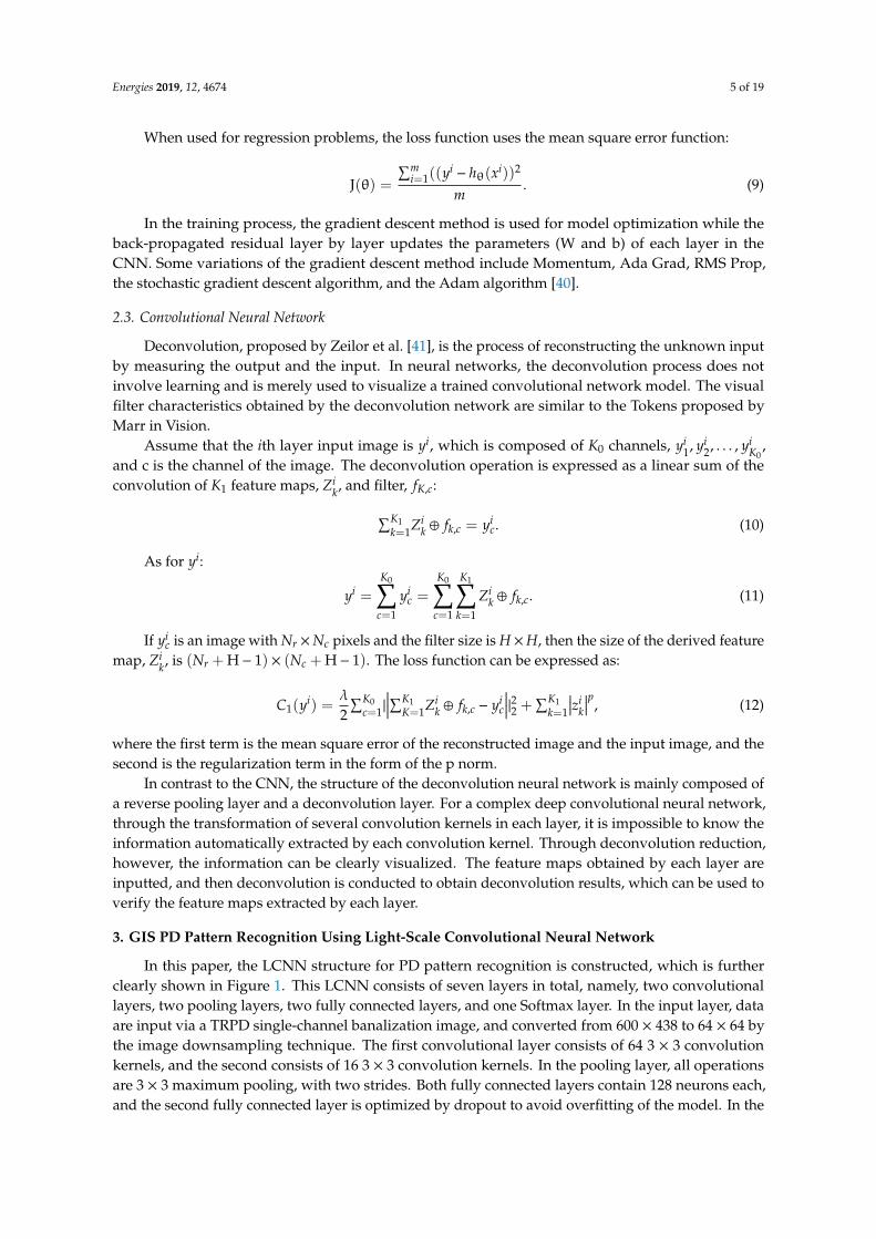
In this paper, the LCNN structure for PD pattern recognition is constructed, which is furtherclearly shown in Figure 1. This LCNN consists of seven layers in total, namely, two convolutionallayers, two pooling layers, two fully connected layers, and one Softmax layer. In the input layer, dataare input via a TRPD single-channel banalization image, and converted from 600 × 438 to 64 × 64 bythe image downsampling technique. The first convolutional layer consists of 64 3 × 3 convolutionkernels, and the second consists of 16 3 × 3 convolution kernels. In the pooling layer, all operationsare 3 × 3 maximum pooling, with two strides. Both fully connected layers contain 128 neurons each,and the second fully connected layer is optimized by dropout to avoid overfitting of the model. In the

Energies 2019, 12, 4674 6 of 19

output layer, Softmax is used as a classifier, and one-hot encoding is used to identify four PDs patternmaps. All activation functions in the model are ReLU functions.

Energies 2019, 12, x FOR PEER REVIEW 5 of 19

Deconvolution, proposed by Zeilor et al. [41], is the process of reconstructing the unknown input by measuring the output and the input. In neural networks, the deconvolution process does not involve learning and is merely used to visualize a trained convolutional network model. The visual filter characteristics obtained by the deconvolution network are similar to the Tokens proposed by Marr in Vision.

Assume that the 𝑖th layer input image is 𝑦 , which is composed of 𝐾 channels, 𝑦 , 𝑦 , … , 𝑦 , and c is the channel of the image. The deconvolution operation is expressed as a linear sum of the convolution of 𝐾 feature maps, 𝑍 , and filter, 𝑓 , : ∑ 𝑍 ⊕ 𝑓 , = 𝑦 . (10)

As for 𝑦 :

𝑦 = 𝑦 = 𝑍 ⨁𝑓 , . (11)

If 𝑦 is an image with 𝑁 × 𝑁 pixels and the filter size is 𝐻 × 𝐻, then the size of the derived feature map, 𝑍 , is (𝑁 + H − 1) × (𝑁 + H − 1). The loss function can be expressed as: 𝐶 (𝑦 ) = ∑ | ∑ 𝑍 ⨁𝑓 , − 𝑦 | + ∑ |𝑧 | , (12)

where the first term is the mean square error of the reconstructed image and the input image, and the second is the regularization term in the form of the p norm.

In contrast to the CNN, the structure of the deconvolution neural network is mainly composed of a reverse pooling layer and a deconvolution layer. For a complex deep convolutional neural network, through the transformation of several convolution kernels in each layer, it is impossible to know the information automatically extracted by each convolution kernel. Through deconvolution reduction, however, the information can be clearly visualized. The feature maps obtained by each layer are inputted, and then deconvolution is conducted to obtain deconvolution results, which can be used to verify the feature maps extracted by each layer.

3. GIS PD Pattern Recognition Using Light-Scale Convolutional Neural Network

In this paper, the LCNN structure for PD pattern recognition is constructed, which is further clearly shown in Figure 1. This LCNN consists of seven layers in total, namely, two convolutional layers, two pooling layers, two fully connected layers, and one Softmax layer. In the input layer, data are input via a TRPD single-channel banalization image, and converted from 600 × 438 to 64 × 64 by the image downsampling technique. The first convolutional layer consists of 64 3 × 3 convolution kernels, and the second consists of 16 3 × 3 convolution kernels. In the pooling layer, all operations are 3 × 3 maximum pooling, with two strides. Both fully connected layers contain 128 neurons each,

Figure 1. The structure of LCNN.

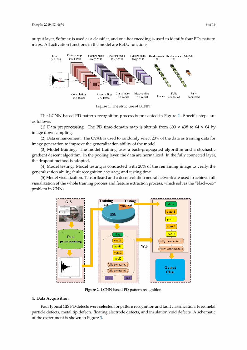
The LCNN-based PD pattern recognition process is presented in Figure 2. Specific steps are as follows:

Figure 1. The structure of LCNN.

The LCNN-based PD pattern recognition process is presented in Figure 2. Specific steps areas follows:

(1) Data preprocessing. The PD time-domain map is shrunk from 600 × 438 to 64 × 64 byimage downsampling.

(2) Data enhancement. The CVAE is used to randomly select 20% of the data as training data forimage generation to improve the generalization ability of the model.

(3) Model training. The model training uses a back-propagated algorithm and a stochasticgradient descent algorithm. In the pooling layer, the data are normalized. In the fully connected layer,the dropout method is adopted.

(4) Model testing. Model testing is conducted with 20% of the remaining image to verify thegeneralization ability, fault recognition accuracy, and testing time.

(5) Model visualization. TensorBoard and a deconvolution neural network are used to achieve fullvisualization of the whole training process and feature extraction process, which solves the “black-box”problem in CNNs.

Energies 2019, 12, x FOR PEER REVIEW 6 of 19

(1) Data preprocessing. The PD time-domain map is shrunk from 600 × 438 to 64 × 64 by image downsampling.

(2) Data enhancement. The CVAE is used to randomly select 20% of the data as training data for image generation to improve the generalization ability of the model.

(3) Model training. The model training uses a back-propagated algorithm and a stochastic gradient descent algorithm. In the pooling layer, the data are normalized. In the fully connected layer, the dropout method is adopted.

(4) Model testing. Model testing is conducted with 20% of the remaining image to verify the generalization ability, fault recognition accuracy, and testing time.

Figure 2. LCNN-based PD pattern recognition.

4. Data Acquisition

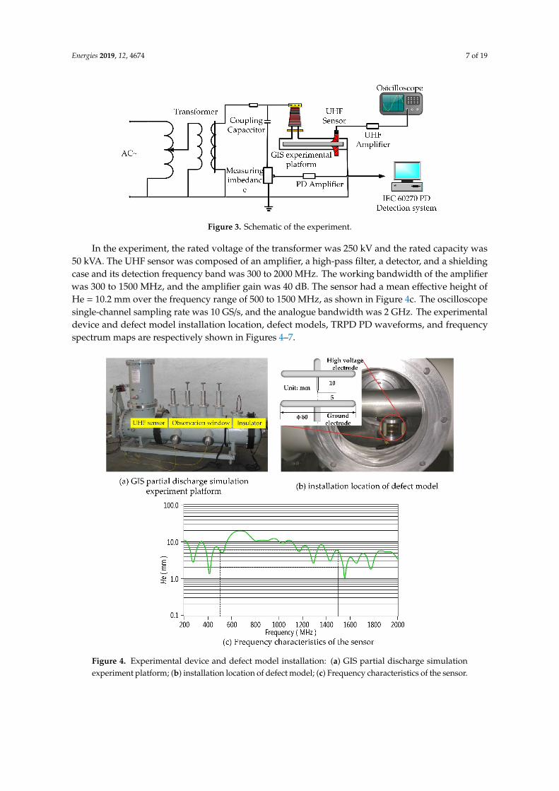
Four typical GIS PD defects were selected for pattern recognition and fault classification: Free metal particle defects, metal tip defects, floating electrode defects, and insulation void defects. A schematic of the experiment is shown in Figure 3.

Figure 3. Schematic of the experiment.

In the experiment, the rated voltage of the transformer was 250 kV and the rated capacity was 50 kVA. The UHF sensor was composed of an amplifier, a high-pass filter, a detector, and a shielding case and its detection frequency band was 300 to 2000 MHz. The working bandwidth of the amplifier was 300 to 1500 MHz, and the amplifier gain was 40 dB. The sensor had a mean effective height of He = 10.2 mm over the frequency range of 500 to 1500 MHz, as shown in Figure 4c. The oscilloscope

Figure 2. LCNN-based PD pattern recognition.

4. Data Acquisition

Four typical GIS PD defects were selected for pattern recognition and fault classification: Free metalparticle defects, metal tip defects, floating electrode defects, and insulation void defects. A schematicof the experiment is shown in Figure 3.

Energies 2019, 12, 4674 7 of 19

Energies 2019, 12, x FOR PEER REVIEW 6 of 19

(1) Data preprocessing. The PD time-domain map is shrunk from 600 × 438 to 64 × 64 by image downsampling.

(2) Data enhancement. The CVAE is used to randomly select 20% of the data as training data for image generation to improve the generalization ability of the model.

(3) Model training. The model training uses a back-propagated algorithm and a stochastic gradient descent algorithm. In the pooling layer, the data are normalized. In the fully connected layer, the dropout method is adopted.

(4) Model testing. Model testing is conducted with 20% of the remaining image to verify the generalization ability, fault recognition accuracy, and testing time.

Figure 2. LCNN-based PD pattern recognition.

4. Data Acquisition

Four typical GIS PD defects were selected for pattern recognition and fault classification: Free metal particle defects, metal tip defects, floating electrode defects, and insulation void defects. A schematic of the experiment is shown in Figure 3.

Figure 3. Schematic of the experiment.

In the experiment, the rated voltage of the transformer was 250 kV and the rated capacity was 50 kVA. The UHF sensor was composed of an amplifier, a high-pass filter, a detector, and a shielding case and its detection frequency band was 300 to 2000 MHz. The working bandwidth of the amplifier was 300 to 1500 MHz, and the amplifier gain was 40 dB. The sensor had a mean effective height of He = 10.2 mm over the frequency range of 500 to 1500 MHz, as shown in Figure 4c. The oscilloscope

Figure 3. Schematic of the experiment.

In the experiment, the rated voltage of the transformer was 250 kV and the rated capacity was50 kVA. The UHF sensor was composed of an amplifier, a high-pass filter, a detector, and a shieldingcase and its detection frequency band was 300 to 2000 MHz. The working bandwidth of the amplifierwas 300 to 1500 MHz, and the amplifier gain was 40 dB. The sensor had a mean effective height ofHe = 10.2 mm over the frequency range of 500 to 1500 MHz, as shown in Figure 4c. The oscilloscopesingle-channel sampling rate was 10 GS/s, and the analogue bandwidth was 2 GHz. The experimentaldevice and defect model installation location, defect models, TRPD PD waveforms, and frequencyspectrum maps are respectively shown in Figures 4–7.

Energies 2019, 12, x FOR PEER REVIEW 7 of 19

single-channel sampling rate was 10 GS/s, and the analogue bandwidth was 2 GHz. The experimental d

Figure 4. Experimental device and defect model installation: (a) GIS partial discharge simulation experiment platform; (b) installation location of defect model; (c) Frequency characteristics of the sensor.

Figure 4. Experimental device and defect model installation: (a) GIS partial discharge simulationexperiment platform; (b) installation location of defect model; (c) Frequency characteristics of the sensor.

Energies 2019, 12, 4674 8 of 19

Energies 2019, 12, x FOR PEER REVIEW 8 of 19

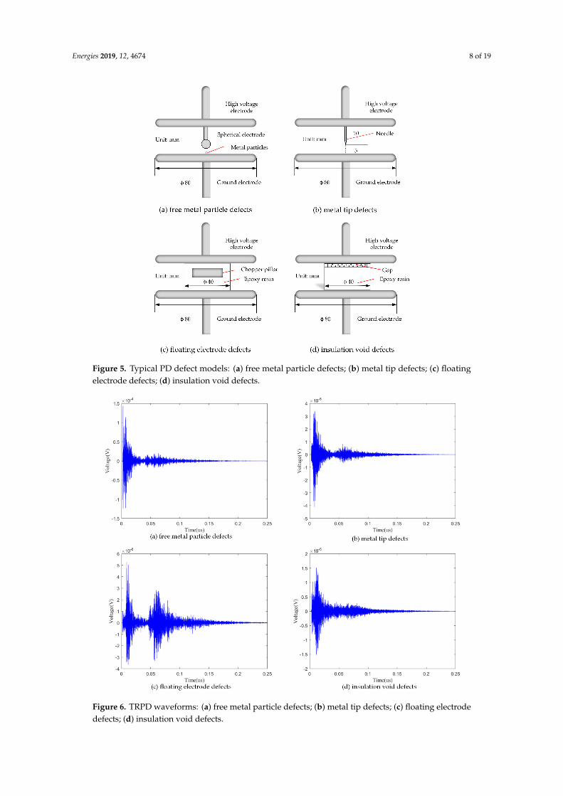
Figure 5. Typical PD defect models: (a) free metal particle defects; (b) metal tip defects; (c) floating electrode defects; (d) insulation void defects.

Figure 5. Typical PD defect models: (a) free metal particle defects; (b) metal tip defects; (c) floatingelectrode defects; (d) insulation void defects.

Energies 2019, 12, x FOR PEER REVIEW 8 of 19

Figure 5. Typical PD defect models: (a) free metal particle defects; (b) metal tip defects; (c) floating electrode defects; (d) insulation void defects.

Figure 6. TRPD waveforms: (a) free metal particle defects; (b) metal tip defects; (c) floating electrodedefects; (d) insulation void defects.

Energies 2019, 12, 4674 9 of 19

1

(a) free metal particle defects (b) metal tip defects

(c) floating electrode defects (d) insulation void defects

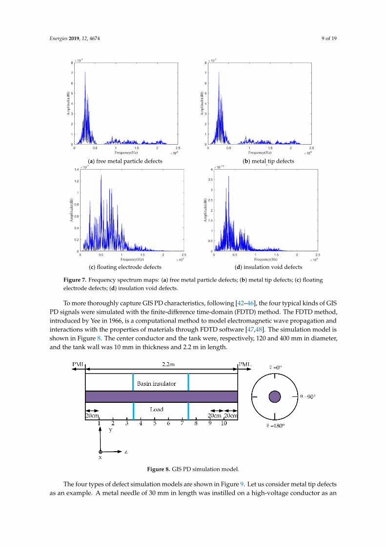
Figure 7. Frequency spectrum maps: (a) free metal particle defects; (b) metal tip defects; (c) floatingelectrode defects; (d) insulation void defects.

To more thoroughly capture GIS PD characteristics, following [42–46], the four typical kinds of GISPD signals were simulated with the finite-difference time-domain (FDTD) method. The FDTD method,introduced by Yee in 1966, is a computational method to model electromagnetic wave propagation andinteractions with the properties of materials through FDTD software [47,48]. The simulation model isshown in Figure 8. The center conductor and the tank were, respectively, 120 and 400 mm in diameter,and the tank wall was 10 mm in thickness and 2.2 m in length.

Energies 2019, 12, x FOR PEER REVIEW 9 of 19

Figure 6. TRPD waveforms: (a) free metal particle defects; (b) metal tip defects; (c) floating electrode defects; (d) insulation void defects.

To more thoroughly capture GIS PD characteristics, following [42–46], the four typical kinds of GIS PD signals were simulated with the finite-difference time-domain (FDTD) method. The FDTD method, introduced by Yee in 1966, is a computational method to model electromagnetic wave propagation and interactions with the properties of materials through FDTD software [47,48]. The simulation model is shown in Figure 8. The center conductor and the tank were, respectively, 120 and 400 mm in diameter, and the tank wall was 10 mm in thickness and 2.2 m in length.

Figure 7. Frequency spectrum maps: (a) free metal particle defects; (b) metal tip defects; (c) floating electrode defects; (d) insulation void defects.

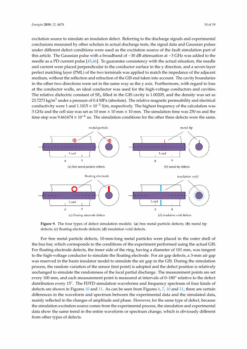
Figure 8. GIS PD simulation model. Figure 8. GIS PD simulation model.

The four types of defect simulation models are shown in Figure 9. Let us consider metal tip defectsas an example. A metal needle of 30 mm in length was instilled on a high-voltage conductor as an

Energies 2019, 12, 4674 10 of 19

excitation source to simulate an insulation defect. Referring to the discharge signals and experimentalconclusions measured by other scholars in actual discharge tests, the signal data and Gaussian pulsesunder different defect conditions were used as the excitation source of the fault simulation part ofthis article. The Gaussian pulse with a broadband of −30 dB attenuation at −3 GHz was added to theneedle as a PD current pulse [45,46]. To guarantee consistency with the actual situation, the needleand current were placed perpendicular to the conductor surface in the y direction, and a seven-layerperfect matching layer (PML) of the two terminals was applied to match the impedance of the adjacentmedium, without the reflection and refraction of the GIS end taken into account. The cavity boundariesin the other two directions were set in the same way as the y axis. Furthermore, with regard to lossat the conductor walls, an ideal conductor was used for the high-voltage conductors and cavities.The relative dielectric constant of SF6 filled in the GIS cavity is 1.00205, and the density was set as23.7273 kg/m3 under a pressure of 0.4 MPa (absolute). The relative magnetic permeability and electricalconductivity were 1 and 1.1015 × 10−5 S/m, respectively. The highest frequency of the calculation was3 GHz and the cell size was set as 10 mm × 10 mm × 10 mm. The simulation time was 250 ns and thetime step was 9.661674 × 10−6 us. The simulation conditions for the other three defects were the same.

Energies 2019, 12, x FOR PEER REVIEW 10 of 19

The four types of defect simulation models are shown in Figure 9. Let us consider metal tip defects as an example. A metal needle of 30 mm in length was instilled on a high-voltage conductor as an excitation source to simulate an insulation defect. Referring to the discharge signals and experimental conclusions measured by other scholars in actual discharge tests, the signal data and Gaussian pulses under different defect conditions were used as the excitation source of the fault simulation part of this article. The Gaussian pulse with a broadband of −30 dB attenuation at −3 GHz was added to the needle as a PD current pulse [45,46]. To guarantee consistency with the actual situation, the needle and current were placed perpendicular to the conductor surface in the y direction, and a seven-layer perfect matching layer (PML) of the two terminals was applied to match the impedance of the adjacent medium, without the reflection and refraction of the GIS end taken into account. The cavity boundaries in the other two directions were set in the same way as the y axis. Furthermore, with regard to loss at the conductor walls, an ideal conductor was used for the high-voltage conductors and cavities. The relative dielectric constant of SF6 filled in the GIS cavity is 1.00205, and the density was set as 23.7273 kg/m3 under a pressure of 0.4 MPa (absolute). The relative magnetic permeability and electrical conductivity were 1 and 1.1015 × 10−5 S/m, respectively. The highest frequency of the calculation was 3 GHz and the cell size was set as 10 mm × 10 mm × 10 mm. The simulation time was 250 ns and the time step was 9.661674 × 10−6 us. The simulation conditions for the other three defects were the same.

Figure 9. The four types of defect simulation models: (a) free metal particle defects; (b) metal tip defects; (c) floating electrode defects; (d) insulation void defects.

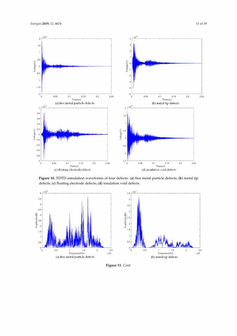
For free metal particle defects, 10-mm-long metal particles were placed in the outer shell of the bus bar, which corresponds to the conditions of the experiment performed using the actual GIS. For floating electrode defects, the inner side of the ring, having a diameter of 101 mm, was tangent to the high-voltage conductor to simulate the floating electrode. For air gap defects, a 3-mm air gap was reserved in the basin insulator model to simulate the air gap in the GIS. During the simulation process, the random variation of the sensor (test point) is adopted and the defect position is relatively unchanged to simulate the randomness of the local partial discharge. The measurement points are set every 100 mm, and each measurement point is measured at intervals of 0–180° relative to the defect distribution every 15°. The FDTD simulation waveforms and frequency spectrum of four kinds of defects are shown in Figures 10 and 11. As can be seen from Figures 6, 7, 10 and 11, there are certain differences in the waveform and spectrum between the experimental data and the simulated data, mainly reflected in the changes of amplitude and phase. However, for the same type of defect, because the simulation excitation source comes from the experimental process, the simulation and

Figure 9. The four types of defect simulation models: (a) free metal particle defects; (b) metal tipdefects; (c) floating electrode defects; (d) insulation void defects.

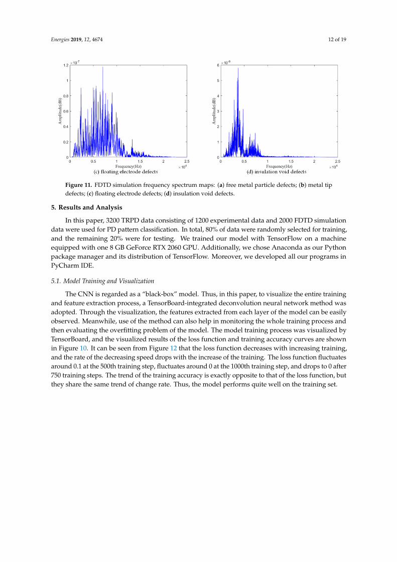
For free metal particle defects, 10-mm-long metal particles were placed in the outer shell ofthe bus bar, which corresponds to the conditions of the experiment performed using the actual GIS.For floating electrode defects, the inner side of the ring, having a diameter of 101 mm, was tangentto the high-voltage conductor to simulate the floating electrode. For air gap defects, a 3-mm air gapwas reserved in the basin insulator model to simulate the air gap in the GIS. During the simulationprocess, the random variation of the sensor (test point) is adopted and the defect position is relativelyunchanged to simulate the randomness of the local partial discharge. The measurement points are setevery 100 mm, and each measurement point is measured at intervals of 0–180◦ relative to the defectdistribution every 15◦. The FDTD simulation waveforms and frequency spectrum of four kinds ofdefects are shown in Figures 10 and 11. As can be seen from Figures 6, 7, 10 and 11, there are certaindifferences in the waveform and spectrum between the experimental data and the simulated data,mainly reflected in the changes of amplitude and phase. However, for the same type of defect, becausethe simulation excitation source comes from the experimental process, the simulation and experimentaldata show the same trend in the entire waveform or spectrum change, which is obviously differentfrom other types of defects.

Energies 2019, 12, 4674 11 of 19

Energies 2019, 12, x FOR PEER REVIEW 11 of 19

experimental data show the same trend in the entire waveform or spectrum change, which is obviously different from other types of defects.

Figure 10. FDTD simulation waveforms of four defects: (a) free metal particle defects; (b) metal tip defects; (c) floating electrode defects; (d) insulation void defects.

Figure 10. FDTD simulation waveforms of four defects: (a) free metal particle defects; (b) metal tipdefects; (c) floating electrode defects; (d) insulation void defects.

Energies 2019, 12, x FOR PEER REVIEW 11 of 19

experimental data show the same trend in the entire waveform or spectrum change, which is obviously different from other types of defects.

Figure 10. FDTD simulation waveforms of four defects: (a) free metal particle defects; (b) metal tip defects; (c) floating electrode defects; (d) insulation void defects.

Figure 11. Cont.

Energies 2019, 12, 4674 12 of 19

Energies 2019, 12, x FOR PEER REVIEW 12 of 19

Figure 11. FDTD simulation frequency spectrum maps: (a) free metal particle defects; (b) metal tip defects; (c) floating electrode defects; (d) insulation void defects.

5. Results and Analysis

In this paper, 3200 TRPD data consisting of 1200 experimental data and 2000 FDTD simulation data were used for PD pattern classification. In total, 80% of data were randomly selected for training, and the remaining 20% were for testing. We trained our model with TensorFlow on a machine equipped with one 8 GB GeForce RTX 2060 GPU. Additionally, we chose Anaconda as our Python package manager and its distribution of TensorFlow. Moreover, we developed all our programs in PyCharm IDE.

5.1. Model Training and Visualization

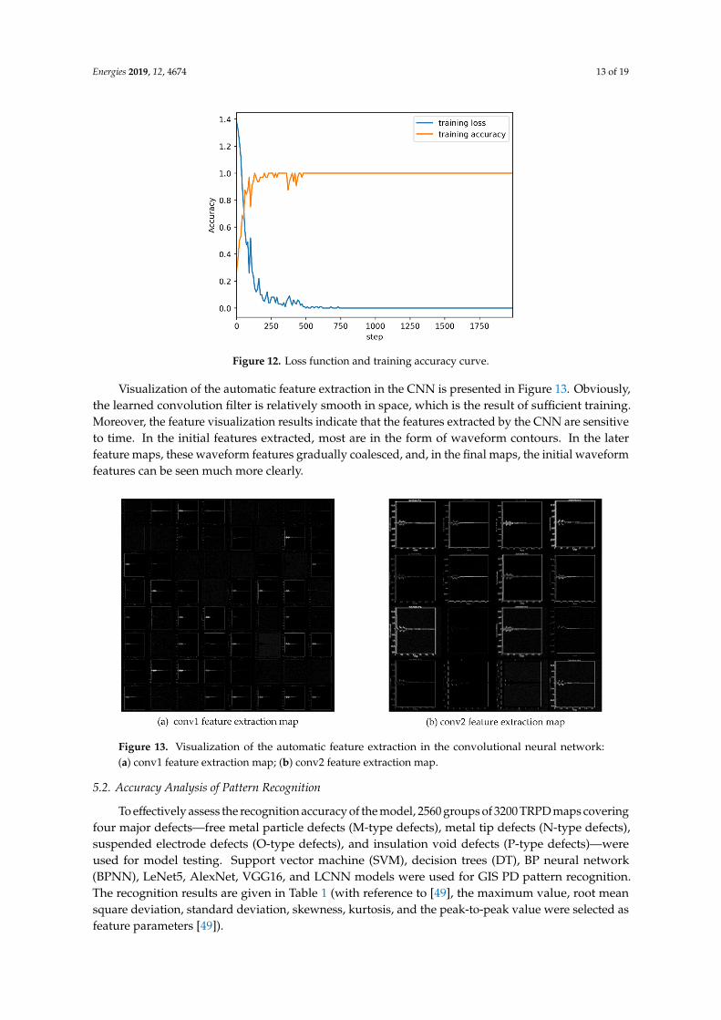
The CNN is regarded as a “black-box” model. Thus, in this paper, to visualize the entire training and feature extraction process, a TensorBoard-integrated deconvolution neural network method was adopted. Through the visualization, the features extracted from each layer of the model can be easily observed. Meanwhile, use of the method can also help in monitoring the whole training process and then evaluating the overfitting problem of the model. The model training process was visualized by TensorBoard, and the visualized results of the loss function and training accuracy curves are shown in Figure 10. It can be seen from Figure 12 that the loss function decreases with increasing training, and the rate of the decreasing speed drops with the increase of the training. The loss function fluctuates around 0.1 at the 500th training step, fluctuates around 0 at the 1000th training step, and drops to 0 after 750 training steps. The trend of the training accuracy is exactly opposite to that of the loss function, but they share the same trend of change rate. Thus, the model performs quite well on the training set.

Figure 11. FDTD simulation frequency spectrum maps: (a) free metal particle defects; (b) metal tipdefects; (c) floating electrode defects; (d) insulation void defects.

5. Results and Analysis

In this paper, 3200 TRPD data consisting of 1200 experimental data and 2000 FDTD simulationdata were used for PD pattern classification. In total, 80% of data were randomly selected for training,and the remaining 20% were for testing. We trained our model with TensorFlow on a machineequipped with one 8 GB GeForce RTX 2060 GPU. Additionally, we chose Anaconda as our Pythonpackage manager and its distribution of TensorFlow. Moreover, we developed all our programs inPyCharm IDE.

5.1. Model Training and Visualization

The CNN is regarded as a “black-box” model. Thus, in this paper, to visualize the entire trainingand feature extraction process, a TensorBoard-integrated deconvolution neural network method wasadopted. Through the visualization, the features extracted from each layer of the model can be easilyobserved. Meanwhile, use of the method can also help in monitoring the whole training process andthen evaluating the overfitting problem of the model. The model training process was visualized byTensorBoard, and the visualized results of the loss function and training accuracy curves are shownin Figure 10. It can be seen from Figure 12 that the loss function decreases with increasing training,and the rate of the decreasing speed drops with the increase of the training. The loss function fluctuatesaround 0.1 at the 500th training step, fluctuates around 0 at the 1000th training step, and drops to 0 after750 training steps. The trend of the training accuracy is exactly opposite to that of the loss function, butthey share the same trend of change rate. Thus, the model performs quite well on the training set.

Energies 2019, 12, 4674 13 of 19Energies 2019, 12, x FOR PEER REVIEW 13 of 19

Figure 12. Loss function and training accuracy curve.

Visualization of the automatic feature extraction in the CNN is presented in Figure 13. Obviously, the learned convolution filter is relatively smooth in space, which is the result of sufficient training. Moreover, the feature visualization results indicate that the features extracted by the CNN are sensitive to time. In the initial features extracted, most are in the form of waveform contours. In the later feature maps, these waveform features gradually coalesced, and, in the final maps, the initial waveform features can be seen much more clearly.

Figure 13. Visualization of the automatic feature extraction in the convolutional neural network: (a) conv1 feature extraction map; (b) conv2 feature extraction map.

5.2. Accuracy Analysis of Pattern Recognition

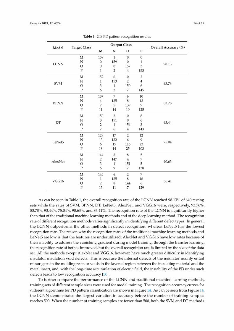
To effectively assess the recognition accuracy of the model, 2560 groups of 3200 TRPD maps covering four major defects—free metal particle defects (M-type defects), metal tip defects (N-type defects), suspended electrode defects (O-type defects), and insulation void defects (P-type defects)—were used for model testing. Support vector machine (SVM), decision trees (DT), BP neural network (BPNN), LeNet5, AlexNet, VGG16, and LCNN models were used for GIS PD pattern recognition. The recognition results are given in Table 1 (with reference to [49], the maximum value, root mean square deviation, standard deviation, skewness, kurtosis, and the peak-to-peak value were selected as feature parameters [49]).

Figure 12. Loss function and training accuracy curve.

Visualization of the automatic feature extraction in the CNN is presented in Figure 13. Obviously,the learned convolution filter is relatively smooth in space, which is the result of sufficient training.Moreover, the feature visualization results indicate that the features extracted by the CNN are sensitiveto time. In the initial features extracted, most are in the form of waveform contours. In the laterfeature maps, these waveform features gradually coalesced, and, in the final maps, the initial waveformfeatures can be seen much more clearly.

Energies 2019, 12, x FOR PEER REVIEW 13 of 19

Figure 12. Loss function and training accuracy curve.

Visualization of the automatic feature extraction in the CNN is presented in Figure 13. Obviously, the learned convolution filter is relatively smooth in space, which is the result of sufficient training. Moreover, the feature visualization results indicate that the features extracted by the CNN are sensitive to time. In the initial features extracted, most are in the form of waveform contours. In the later feature maps, these waveform features gradually coalesced, and, in the final maps, the initial waveform features can be seen much more clearly.

Figure 13. Visualization of the automatic feature extraction in the convolutional neural network: (a) conv1 feature extraction map; (b) conv2 feature extraction map.

5.2. Accuracy Analysis of Pattern Recognition

To effectively assess the recognition accuracy of the model, 2560 groups of 3200 TRPD maps covering four major defects—free metal particle defects (M-type defects), metal tip defects (N-type defects), suspended electrode defects (O-type defects), and insulation void defects (P-type defects)—were used for model testing. Support vector machine (SVM), decision trees (DT), BP neural network (BPNN), LeNet5, AlexNet, VGG16, and LCNN models were used for GIS PD pattern recognition. The recognition results are given in Table 1 (with reference to [49], the maximum value, root mean square deviation, standard deviation, skewness, kurtosis, and the peak-to-peak value were selected as feature parameters [49]).

Figure 13. Visualization of the automatic feature extraction in the convolutional neural network:(a) conv1 feature extraction map; (b) conv2 feature extraction map.

5.2. Accuracy Analysis of Pattern Recognition

To effectively assess the recognition accuracy of the model, 2560 groups of 3200 TRPD maps coveringfour major defects—free metal particle defects (M-type defects), metal tip defects (N-type defects),suspended electrode defects (O-type defects), and insulation void defects (P-type defects)—wereused for model testing. Support vector machine (SVM), decision trees (DT), BP neural network(BPNN), LeNet5, AlexNet, VGG16, and LCNN models were used for GIS PD pattern recognition.The recognition results are given in Table 1 (with reference to [49], the maximum value, root meansquare deviation, standard deviation, skewness, kurtosis, and the peak-to-peak value were selected asfeature parameters [49]).

Energies 2019, 12, 4674 14 of 19

Table 1. GIS PD pattern recognition results.

Model Target ClassOutput Class

Overall Accuracy (%)M N O P

LCNN

M 159 1 0 0

98.13N 0 159 0 1O 0 0 157 3P 1 2 4 153

SVM

M 152 6 0 2

93.76N 1 153 2 4O 3 1 150 6P 6 2 7 145

BPNN

M 137 7 6 10

83.78N 4 135 8 13O 7 5 139 9P 11 14 10 125

DT

M 150 2 0 8

93.44N 3 151 0 6O 2 1 154 3P 7 6 4 143

LeNet5

M 129 17 2 12

75.04N 13 132 6 9O 6 15 116 23P 18 14 25 103

AlexNet

M 144 3 8 5

90.63N 2 147 4 7O 3 1 151 5P 6 9 7 138

VGG16

M 145 6 2 7

86.41N 1 135 8 16O 2 8 144 6P 13 11 7 129

As can be seen in Table 1, the overall recognition rate of the LCNN reached 98.13% of 640 testingsets while the rates of SVM, BPNN, DT, LeNet5, AlexNet, and VGG16 were, respectively, 93.76%,83.78%, 93.44%, 75.04%, 90.63%, and 86.41%. The recognition rate of the LCNN is significantly higherthan that of the traditional machine learning methods and of the deep learning method. The recognitionrate of different recognition methods varies significantly in identifying different defect types. In general,the LCNN outperforms the other methods in defect recognition, whereas LeNet5 has the lowestrecognition rate. The reason why the recognition rates of the traditional machine learning methods andLeNet5 are low is that the features are underutilized; AlexNet and VGG16 have low rates because oftheir inability to address the vanishing gradient during model training, through the transfer learning,the recognition rate of both is improved, but the overall recognition rate is limited by the size of the dataset. All the methods except AlexNet and VGG16, however, have much greater difficulty in identifyinginsulator insulation void defects. This is because the internal defects of the insulator mainly entailminor gaps in the molding resin or voids in the layered region between the insulating material and themetal insert, and, with the long-time accumulation of electric field, the instability of the PD under suchdefects leads to low recognition accuracy [50].

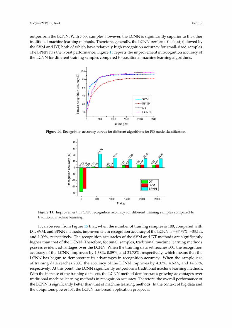
To further compare the performance of the LCNN and traditional machine learning methods,training sets of different sample sizes were used for model training. The recognition accuracy curves fordifferent algorithms for PD pattern classification are shown in Figure 14. As can be seen from Figure 14,the LCNN demonstrates the largest variation in accuracy before the number of training samplesreaches 500. When the number of training samples are fewer than 500, both the SVM and DT methods

Energies 2019, 12, 4674 15 of 19

outperform the LCNN. With >500 samples, however, the LCNN is significantly superior to the othertraditional machine learning methods. Therefore, generally, the LCNN performs the best, followed bythe SVM and DT, both of which have relatively high recognition accuracy for small-sized samples.The BPNN has the worst performance. Figure 15 reports the improvement in recognition accuracy ofthe LCNN for different training samples compared to traditional machine learning algorithms.

Energies 2019, 12, x FOR PEER REVIEW 15 of 19

samples reaches 500. When the number of training samples are fewer than 500, both the SVM and DT methods outperform the LCNN. With >500 samples, however, the LCNN is significantly superior to the other traditional machine learning methods. Therefore, generally, the LCNN performs the best, followed by the SVM and DT, both of which have relatively high recognition accuracy for small-sized samples. The BPNN has the worst performance. Figure 15 reports the improvement in recognition accuracy of the LCNN for different training samples compared to traditional machine learning algorithms.

Figure 14. Recognition accuracy curves for different algorithms for PD mode classification.

Figure 15. Improvement in CNN recognition accuracy for different training samples compared to traditional machine learning.

It can be seen from Figure 15 that, when the number of training samples is 100, compared with DT, SVM, and BPNN methods, improvement in recognition accuracy of the LCNN is −37.79%, −33.1%, and 1.09%, respectively. The recognition accuracies of the SVM and DT methods are significantly higher than that of the LCNN. Therefore, for small samples, traditional machine learning methods possess evident advantages over the LCNN. When the training data set reaches 500, the recognition accuracy of the LCNN, improves by 1.38%, 0.89%, and 21.78%, respectively, which means that the LCNN has begun to demonstrate its advantages in recognition accuracy. When the sample size of training data reaches 2500, the accuracy of the LCNN improves by 4.37%, 4.69%, and 14.35%, respectively. At this point, the LCNN significantly outperforms traditional machine learning methods. With the increase of the training data sets, the LCNN method demonstrates growing advantages over traditional machine learning methods in recognition accuracy. Therefore, the overall performance of the LCNN is significantly better than that of machine learning methods. In the context of big data and the ubiquitous-power IoT, the LCNN has broad application prospects.

Figure 14. Recognition accuracy curves for different algorithms for PD mode classification.

Energies 2019, 12, x FOR PEER REVIEW 15 of 19

samples reaches 500. When the number of training samples are fewer than 500, both the SVM and DT methods outperform the LCNN. With >500 samples, however, the LCNN is significantly superior to the other traditional machine learning methods. Therefore, generally, the LCNN performs the best, followed by the SVM and DT, both of which have relatively high recognition accuracy for small-sized samples. The BPNN has the worst performance. Figure 15 reports the improvement in recognition accuracy of the LCNN for different training samples compared to traditional machine learning algorithms.

Figure 14. Recognition accuracy curves for different algorithms for PD mode classification.

Figure 15. Improvement in CNN recognition accuracy for different training samples compared to traditional machine learning.

It can be seen from Figure 15 that, when the number of training samples is 100, compared with DT, SVM, and BPNN methods, improvement in recognition accuracy of the LCNN is −37.79%, −33.1%, and 1.09%, respectively. The recognition accuracies of the SVM and DT methods are significantly higher than that of the LCNN. Therefore, for small samples, traditional machine learning methods possess evident advantages over the LCNN. When the training data set reaches 500, the recognition accuracy of the LCNN, improves by 1.38%, 0.89%, and 21.78%, respectively, which means that the LCNN has begun to demonstrate its advantages in recognition accuracy. When the sample size of training data reaches 2500, the accuracy of the LCNN improves by 4.37%, 4.69%, and 14.35%, respectively. At this point, the LCNN significantly outperforms traditional machine learning methods. With the increase of the training data sets, the LCNN method demonstrates growing advantages over traditional machine learning methods in recognition accuracy. Therefore, the overall performance of the LCNN is significantly better than that of machine learning methods. In the context of big data and the ubiquitous-power IoT, the LCNN has broad application prospects.

Figure 15. Improvement in CNN recognition accuracy for different training samples compared totraditional machine learning.

It can be seen from Figure 15 that, when the number of training samples is 100, compared withDT, SVM, and BPNN methods, improvement in recognition accuracy of the LCNN is −37.79%, −33.1%,and 1.09%, respectively. The recognition accuracies of the SVM and DT methods are significantlyhigher than that of the LCNN. Therefore, for small samples, traditional machine learning methodspossess evident advantages over the LCNN. When the training data set reaches 500, the recognitionaccuracy of the LCNN, improves by 1.38%, 0.89%, and 21.78%, respectively, which means that theLCNN has begun to demonstrate its advantages in recognition accuracy. When the sample sizeof training data reaches 2500, the accuracy of the LCNN improves by 4.37%, 4.69%, and 14.35%,respectively. At this point, the LCNN significantly outperforms traditional machine learning methods.With the increase of the training data sets, the LCNN method demonstrates growing advantages overtraditional machine learning methods in recognition accuracy. Therefore, the overall performance ofthe LCNN is significantly better than that of machine learning methods. In the context of big data andthe ubiquitous-power IoT, the LCNN has broad application prospects.

Energies 2019, 12, 4674 16 of 19

5.3. Model Time Analysis

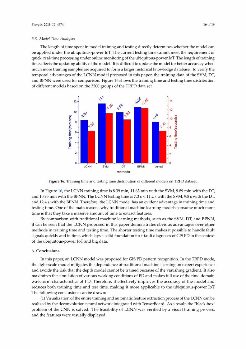
The length of time spent in model training and testing directly determines whether the model canbe applied under the ubiquitous-power IoT. The current testing time cannot meet the requirement ofquick, real-time processing under online monitoring of the ubiquitous-power IoT. The length of trainingtime affects the updating ability of the model. It is difficult to update the model for better accuracy whenmuch more training samples are acquired to form a larger historical knowledge database. To verify thetemporal advantages of the LCNN model proposed in this paper, the training data of the SVM, DT,and BPNN were used for comparison. Figure 16 shows the training time and testing time distributionof different models based on the 3200 groups of the TRPD data set.

Energies 2019, 12, x FOR PEER REVIEW 16 of 19

5.3. Model Time Analysis

The length of time spent in model training and testing directly determines whether the model can be applied under the ubiquitous-power IoT. The current testing time cannot meet the requirement of quick, real-time processing under online monitoring of the ubiquitous-power IoT. The length of training time affects the updating ability of the model. It is difficult to update the model for better accuracy when much more training samples are acquired to form a larger historical knowledge database. To verify the temporal advantages of the LCNN model proposed in this paper, the training data of the SVM, DT, and BPNN were used for comparison. Figure 16 shows the training time and testing time distribution of different models based on the 3200 groups of the TRPD data set.

Figure 16. Training time and testing time distribution of different models on TRPD dataset.

In Figure 16, the LCNN training time is 8.39 min, 11.63 min with the SVM, 9.89 min with the DT, and 10.95 min with the BPNN. The LCNN testing time is 7.3 s < 11.2 s with the SVM, 9.8 s with the DT, and 12.4 s with the BPNN. Therefore, the LCNN model has an evident advantage in training time and testing time. One of the main reasons why traditional machine learning models consume much more time is that they take a massive amount of time to extract features.

By comparison with traditional machine learning methods, such as the SVM, DT, and BPNN, it can be seen that the LCNN proposed in this paper demonstrates obvious advantages over other methods in training time and testing time. The shorter testing time makes it possible to handle fault signals quickly and in time, which lays a solid foundation for t-fault diagnoses of GIS PD in the context of the ubiquitous-power IoT and big data.

6. Conclusions

In this paper, an LCNN model was proposed for GIS PD pattern recognition. In the TRPD mode, the light-scale model mitigates the dependence of traditional machine learning on expert experience and avoids the risk that the depth model cannot be trained because of the vanishing gradient. It also maximizes the simulation of various working conditions of PD and makes full use of the time-domain waveform characteristics of PD. Therefore, it effectively improves the accuracy of the model and reduces both training time and test time, making it more applicable to the ubiquitous-power IoT. The following conclusions can be drawn:

(1) Visualization of the entire training and automatic feature extraction process of the LCNN can be realized by the deconvolution neural network integrated with TensorBoard. As a result, the “black-box” problem of the CNN is solved. The feasibility of LCNN was verified by a visual training process, and the features were visually displayed.

Figure 16. Training time and testing time distribution of different models on TRPD dataset.

In Figure 16, the LCNN training time is 8.39 min, 11.63 min with the SVM, 9.89 min with the DT,and 10.95 min with the BPNN. The LCNN testing time is 7.3 s < 11.2 s with the SVM, 9.8 s with the DT,and 12.4 s with the BPNN. Therefore, the LCNN model has an evident advantage in training time andtesting time. One of the main reasons why traditional machine learning models consume much moretime is that they take a massive amount of time to extract features.

By comparison with traditional machine learning methods, such as the SVM, DT, and BPNN,it can be seen that the LCNN proposed in this paper demonstrates obvious advantages over othermethods in training time and testing time. The shorter testing time makes it possible to handle faultsignals quickly and in time, which lays a solid foundation for t-fault diagnoses of GIS PD in the contextof the ubiquitous-power IoT and big data.

6. Conclusions

In this paper, an LCNN model was proposed for GIS PD pattern recognition. In the TRPD mode,the light-scale model mitigates the dependence of traditional machine learning on expert experienceand avoids the risk that the depth model cannot be trained because of the vanishing gradient. It alsomaximizes the simulation of various working conditions of PD and makes full use of the time-domainwaveform characteristics of PD. Therefore, it effectively improves the accuracy of the model andreduces both training time and test time, making it more applicable to the ubiquitous-power IoT.The following conclusions can be drawn:

(1) Visualization of the entire training and automatic feature extraction process of the LCNN can berealized by the deconvolution neural network integrated with TensorBoard. As a result, the “black-box”problem of the CNN is solved. The feasibility of LCNN was verified by a visual training process,and the features were visually displayed.

Energies 2019, 12, 4674 17 of 19

(2) LCNN has superior feature capture capability for GIS PD signals and effectively implementsGIS PD pattern recognition. Based on TRPD, the overall recognition rate of the LCNN reached 98.13%,while rates of the SVM, BPNN, DT, LeNet5, AlexNet, and VGG16 were 93.76%, 83.78%, 93.44%,75.04%, 90.63%, and 86.41%, respectively. With the increase of the number of samples, the LCNNdemonstrates more advantages, which make it much more suitable for application to big data and theubiquitous-power IoT.

(3) Banalization and image downsampling considerably alleviated the burden of time consumptionfor model training. By comparison with traditional machine learning methods, the TRPD-based LCNNdemonstrates significant advantages over other methods in training time and testing time. It can notonly accomplish quick, real-time online monitoring of fault signals but also rapidly update the modelafter resetting the fault knowledge base.

Author Contributions: Y.W. and J.Y. conceived and designed the experiments; J.L. provided the experimentaldata; Y.W. wrote the paper; Z.Y. modified the code of the paper; T.L. revised the contents and reviewed themanuscript; Y.Z. provided the simulation data.

Funding: This research received no external funding.

Acknowledgments: Special thanks to NVIDIA graphic processing unit and XFDTD software for technical support.Thanks to Anhui Electric Power Research Institute for data support.

Conflicts of Interest: The authors declare no conflict of interest.

References

1. Khan, Q.; Refaat, S.S.; Abu-Rub, H.; Toliyat, H.A. Partial discharge detection and diagnosis in gas insulatedswitchgear: State of the art. IEEE Electr. Insul. Mag. 2019, 35, 16–33. [CrossRef]

2. Gao, W.; Ding, D.; Liu, W. Research on the typical partial discharge using the UHF detection method for GIS.IEEE Trans. Power Deliv. 2011, 26, 2621–2629. [CrossRef]

3. Stone, G.C. Partial discharge diagnostics and electrical equipment insulation condition assessment. IEEE Trans.Dielectr. Electr. Insul. 2005, 12, 891–904. [CrossRef]

4. Niu, X.; Shao, S.; Xin, C.; Zhou, J.; Guo, S.; Chen, X.; Qi, F. Workload Allocation Mechanism for MinimumService Delay in Edge Computing-Based Power Internet of Things. IEEE Access 2019, 7, 83771–83784.[CrossRef]

5. Hu, W.; Yao, W.; Hu, Y.; Li, H. Selection of Cluster Heads for Wireless Sensor Network in Ubiquitous PowerInternet of Things. Int. J. Comput. Commun. Control 2019, 14, 344–358. [CrossRef]

6. Yao, R.; Hui, M.; Li, J.; Bai, L.; Wu, Q. A New Discharge Pattern for the Characterization and Identification ofInsulation Defects in GIS. Energies 2018, 11, 971. [CrossRef]

7. Han, X.; Li, J.; Zhang, L.; Pang, P.; Shen, S. A Novel PD Detection Technique for Use in GIS Based on aCombination of UHF and Optical Sensors. IEEE Trans. Instrum. Meas. 2019, 68, 2890–2897. [CrossRef]

8. Okubo, H.; Hayakawa, N. A novel technique for partial discharge and breakdown investigation based oncurrent pulse waveform analysis. IEEE Trans. Dielectr. Electr. Insul. 2005, 12, 736–744. [CrossRef]

9. Li, T.; Rong, M.; Zheng, C.; Wang, X. Development simulation and experiment study on UHF partialdischarge sensor in GIS. IEEE Trans. Dielectr. Electr. Insul. 2012, 19, 1421–1430. [CrossRef]

10. Si, W.; Li, J.; Li, D.; Yang, J.; Li, Y. Investigation of a comprehensive identification method used in acousticdetection system for GIS. IEEE Trans. Dielectr. Electr. Insul. 2010, 17, 721–732. [CrossRef]

11. Li, J.; Han, X.; Liu, Z.; Yao, X. A novel GIS partial discharge detection sensor with integrated optical andUHF methods. IEEE Trans. Power Deliv. 2016, 33, 2047–2049. [CrossRef]

12. Tang, J.; Liu, F.; Zhang, X.; Meng, Q.; Zhou, J. Partial discharge recognition through an analysis of SF6decomposition products part 1: Decomposition characteristics of SF 6 under four different partial discharges.IEEE Trans. Dielectr. Electr. Insul. 2012, 19, 29–36. [CrossRef]

13. Gao, W.; Ding, D.; Liu, W.; Huang, X. Investigation of the Evaluation of the PD Severity and Verification ofthe Sensitivity of Partial-Discharge Detection Using the UHF Method in GIS. IEEE Trans. Power Deliv. 2013,29, 38–47.

Energies 2019, 12, 4674 18 of 19

14. Umamaheswari, R.; Sarathi, R. Identification of partial discharges in gas-insulated switchgear byultra-high-frequency technique and classification by adopting multi-class support vector machines.Electr. Power Compon. Syst. 2011, 39, 1577–1595. [CrossRef]

15. Hirose, H.; Hikita, M.; Ohtsuka, S.; Tsuru, S.-I.; Ichimaru, J. Diagnosis of electric power apparatus using thedecision tree method. IEEE Trans. Dielectr. Electr. Insul. 2008, 15, 1252–1260. [CrossRef]

16. Deng, R.; Zhu, Y.; Liu, X.; Zhai, Y. Multi-source Partial Discharge Identification of Power Equipment Basedon Random Forest. In The IOP Conference Series: Earth and Environmental Science; IOP Publishing: Qingdao,China, 2019; Volume 17, p. 062039.

17. Su, M.-S.; Chia, C.-C.; Chen, C.-Y.; Chen, J.-F. Classification of partial discharge events in GILBS usingprobabilistic neural networks and the fuzzy c-means clustering approach. Int. J. Electr. Power Energy Syst.2014, 61, 173–179. [CrossRef]

18. Tang, J.; Wang, D.; Fan, L.; Zhuo, R.; Zhang, X. Feature parameters extraction of GIS partial discharge signalwith multifractal detrended fluctuation analysis. IEEE Trans. Dielectr. Electr. Insul. 2015, 22, 3037–3045.[CrossRef]

19. Li, X.; Wang, X.; Xie, D.; Wang, X.; Yang, A.; Rong, M. Time–frequency analysis of PD-induced UHF signal inGIS and feature extraction using invariant moments. IET Sci. Meas. Technol. 2017, 12, 169–175. [CrossRef]

20. Kawada, M.; Tungkanawanich, A.; Kawasaki, Z.-I.; Matsu-Ura, K. Detection of wide-band EM signalsemitted from partial discharge occurring in GIS using wavelet transform. IEEE Trans. Power Deliv. 2000, 15,467–471. [CrossRef]

21. Gu, F.-C.; Chang, H.-C.; Kuo, C.-C. Gas-insulated switchgear PD signal analysis based on Hilbert-Huangtransform with fractal parameters enhancement. IEEE Trans. Dielectr. Electr. Insul. 2013, 20, 1049–1055.

22. Shang, H.; Lo, K.; Li, F. Partial discharge feature extraction based on ensemble empirical mode decompositionand sample entropy. Entropy 2017, 19, 439. [CrossRef]

23. Dai, D.; Wang, X.; Long, J.; Tian, M.; Zhu, G.; Zhang, J. Feature extraction of GIS partial discharge signal basedon S-transform and singular value decomposition. IET Sci. Meas. Technol. 2016, 11, 186–193. [CrossRef]

24. Candela, R.; Mirelli, G.; Schifani, R. PD recognition by means of statistical and fractal parameters and aneural network. IEEE Trans. Dielectr. Electr. Insul. 2000, 7, 87–94. [CrossRef]

25. Xue, J.; Zhang, X.-L.; Qi, W.-D.; Huang, G.-Q.; Niu, B.; Wang, J. Research on a method for GIS partialdischarge pattern recognition based on polar coordinate map. In Proceedings of the 2016 IEEE InternationalConference on High Voltage Engineering and Application (ICHVE), Chengdu, China, 19–22 September 2016;pp. 1–4.

26. Li, L.; Tang, J.; Liu, Y. Partial discharge recognition in gas insulated switchgear based on multi-informationfusion. IEEE Trans. Dielectr. Electr. Insul. 2015, 22, 1080–1087. [CrossRef]

27. Piccin, R.; Mor, A.R.; Morshuis, P.; Girodet, A.; Smit, J. Partial discharge analysis of gas-insulated systems athigh voltage AC and DC. IEEE Trans. Dielectr. Electr. Insul. 2015, 22, 218–228. [CrossRef]

28. Hao, L.; Lewin, P.L. Partial discharge source discrimination using a support vector machine. IEEE Trans.Dielectr. Electr. Insul. 2010, 17, 189–197. [CrossRef]

29. Blufpand, S.; Mor, A.R.; Morshuis, P.; Montanari, G.C. Partial discharge recognition of insulation defects inHVDC GIS and a calibration approach. In Proceedings of the 2015 IEEE Electrical Insulation Conference(EIC), Seattle, WA, USA, 7–10 June 2015; pp. 564–567.

30. Li, G.; Wang, X.; Li, X.; Yang, A.; Rong, M. Partial discharge recognition with a multi-resolution convolutionalneural network. Sensors 2018, 18, 3512. [CrossRef]

31. Song, H.; Dai, J.; Sheng, G.; Jiang, X. GIS partial discharge pattern recognition via deep convolutional neuralnetwork under complex data source. IEEE Trans. Dielectr. Electr. Insul. 2018, 25, 678–685. [CrossRef]

32. Li, G.; Rong, M.; Wang, X.; Li, X.; Li, Y. Partial discharge patterns recognition with deep ConvolutionalNeural Network. In Proceedings of the Condition Monitoring and Diagnosis, Xi’an, China, 25–28 September2016; pp. 324–327.

33. Wan, X.; Song, H.; Luo, L.; Li, Z.; Sheng, G.; Jiang, X. Pattern Recognition of Partial Discharge Image Basedon One-dimensional Convolutional Neural Network. In Proceedings of the 2018 Condition Monitoring andDiagnosis (CMD), Perth, WA, Australia, 23–26 September 2018; pp. 1–4.

34. Nguyen, M.-T.; Nguyen, V.-H.; Yun, S.-J.; Kim, Y.-H. Recurrent neural network for partial discharge diagnosisin gas-insulated switchgear. Energies 2018, 11, 1202. [CrossRef]

Energies 2019, 12, 4674 19 of 19

35. Fawzi, A.; Samulowitz, H.; Turaga, D.; Frossard, P. Adaptive data augmentation for image classification.In Proceedings of the 2016 IEEE International Conference on Image Processing (ICIP), Phoenix, AZ, USA,25–28 September 2016; pp. 3688–3692.

36. Židek, K.; Hošovský, A. Image thresholding and contour detection with dynamic background selection forinspection tasks in machine vision. Int. J. Circ. 2014, 8, 545–554.

37. Strub, F.; Gaudel, R.; Mary, J. Hybrid Recommender System based on Autoencoders. In Proceedings of the1st Workshop on Deep Learning for Recommender Systems, Boston, MA, USA, 15 September 2016; pp. 11–16.

38. Wang, H.; Wang, N.; Yeung, D.-Y. Collaborative deep learning for recommender systems. In Proceedingsof the 21th ACM SIGKDD International Conference on Knowledge Discovery and Data Mining, Sydney,Australia, 10–13 August 2015; pp. 1235–1244.

39. Hershey, S.; Chaudhuri, S.; Ellis, D.P.W.; Gemmeke, J.F.; Jansen, A.; Moore, R.C.; Plakal, M.; Platt, D.;Saurous, R.A.; Seybold, B.; et al. CNN architectures for large-scale audio classification. In Proceedings of the2017 IEEE International Conference on Acoustics, Speech and Signal Processing (ICASSP), New Orleans, LA,USA, 5–9 March 2017; pp. 131–135.

40. Ruder, S. An Overview of Gradient Descent Optimization Algorithms. arXiv 2016, arXiv:1609.04747.41. Zeiler, M.D.; Fergus, R. Visualizing and understanding convolutional networks. In Proceedings of the

European Conference on Computer Vision, Zurich, Switzerland, 6–12 September 2014; pp. 818–833.42. Li, X.; Wang, X.; Yang, A.; Xie, D.; Ding, D.; Rong, M. Propogation characteristics of PD-induced UHF signal

in 126 kV GIS with three-phase construction based on time–frequency analysis. IET Sci. Meas. Technol. 2016,10, 805–812. [CrossRef]

43. Hoshino, T.; Maruyama, S.; Sakakibara, T. Simulation of propagating electromagnetic wave due to partialdischarge in GIS using FDTD. IEEE Trans. Power Deliv. 2008, 24, 153–159. [CrossRef]

44. Nishigouchi, K.; Kozako, M.; Hikita, M.; Hoshino, T.; Maruyama, S.; Nakajima, T. Waveform estimationof particle discharge currents in straight 154 kV GIS using electromagnetic wave propagation simulation.IEEE Trans. Dielectr. Electr. Insul. 2013, 20, 2239–2245. [CrossRef]

45. Yan, T.; Zhan, H.; Zheng, S.; Liu, B.; Wang, J.; Li, C.; Deng, L. Study on the propagation characteristics ofpartial discharge electromagnetic waves in 252 kV GIS. In Proceedings of the Condition Monitoring andDiagnosis, Bali, Indonesia, 23–27 September 2012; pp. 685–689.

46. Hikita, M.; Ohtsuka, S.; Okabe, S.; Wada, J.; Hoshino, T.; Maruyama, S. Influence of disconnecting part onpropagation properties of PD-induced electromagnetic wave in model GIS. IEEE Trans. Dielectr. Electr. Insul.2010, 17, 1731–1737. [CrossRef]

47. Taflove, A. Advances in Computational Electrodynamics: The Finite-Difference Time-Domain Method; Artech House:Norwood, MA, USA, 1998; pp. 11–17.

48. Loubani, A.; Harid, N.; Griffiths, H.; Barkat, B. Simulation of Partial Discharge Induced EM Waves UsingFDTD Method—A Parametric Study. Energies 2019, 12, 3364. [CrossRef]

49. Zeng, F.; Dong, Y.; Ju, T. Feature extraction and severity assessment of partial discharge under protrusiondefect based on fuzzy comprehensive evaluation. IET Gener. Transm. Dis. 2015, 9, 2493–2500. [CrossRef]

50. Ueta, G.; Wada, J.; Okabe, S.; Miyashita, M.; Nishida, C.; Kamei, M. Insulation characteristics of epoxyinsulator with internal void-shaped micro-defects. IEEE Trans. Dielectr. Electr. Insul. 2013, 20, 535–543.[CrossRef]

© 2019 by the authors. Licensee MDPI, Basel, Switzerland. This article is an open accessarticle distributed under the terms and conditions of the Creative Commons Attribution(CC BY) license (http://creativecommons.org/licenses/by/4.0/).