Sequence Impedances of Land Single-Core Insulated Cables

energies

Article

Sequence Impedances of Land Single-Core InsulatedCables: Direct Formulae and Multiconductor CellAnalyses Compared with Measurements

Roberto Benato 1 , Sebastian Dambone Sessa 1,* , Michele Poli 2 and Francesco Sanniti 1

1 Department of Industrial Engineering, University of Padova, 35131 Padova, Italy;[email protected] (R.B.); [email protected] (F.S.)

2 Terna, 00156 Rome, Italy; [email protected]* Correspondence: [email protected]

Received: 1 January 2020; Accepted: 25 February 2020; Published: 1 March 2020

Abstract: The paper deals with the sequence impedances (positive/negative and zero sequences)of high- and extra-high-voltage land single-core insulated cables. In particular, it presents thecomparisons between sequence impedance measurements and computations. The computations ofthe sequence impedances are carried out by means of the most important international normativeand council references (IEC/Cigré) and of multiconductor cell analysis which is a consolidated andpowerful tool developed by University of Padova in order to analyse power frequency regimes ofmulticonductor asymmetric power systems. The comparisons are presented with reference to fourhigh- and extra-high voltage insulated cables, even if the available ones are much higher: however,the conclusions derived from these four reference cases are general and can be useful for transmissionsystem operators and for power electric system engineers involved in insulated cables. The paperdemonstrates, for the first time in technical literature, that direct formulae cannot correctly evaluatethe sequence impedances of installed single-core land cable systems. Extensive on-field measurementcampaigns have served to this purpose.

Keywords: insulated cables; sequence impedances; multiconductor cell analysis (MCA); extra-highvoltage; asymmetric systems

1. Introduction

In 2012, the first author presented a conference paper with a comparison between analyticalformulae of insulated cable sequence impedances and the results of two measurement campaigns [1].At that time, high-voltage (HV) cables in Italy were short in length, and the experience with suchsystems was limited. That paper [1] dealt with two HV insulated cables of medium length (6–8 km).After 8 years, the cable lengths installed in the Italian high and extra-high voltage (EHV) grid havestrongly increased: therefore, the amount of experience has also increased thanks to more measurementcampaigns. The measurement campaigns have the aim of obtaining on-field sequence impedancevalues. Once the measurements are available, a comparison with formulae is always performed.Italian Academia, together with Terna, which is the Italian transmission system operator (TSO) andowner, have decided to give electrical engineers a wide account on these comparisons, i.e., sequenceimpedance measurements compared with analytical and procedural computations. Since it is notpossible to present the comparisons for all installed HV and EHV cables, a selection of the moremeaningful cases is made in this paper, aiming at covering all the Italian high and extra-high voltagelevels (132–380 kV). The importance of the exact knowledge of the sequence impedances of an electricline is paramount both for planning and operating activities: it is worth noting that power flow and

Energies 2020, 13, 1084; doi:10.3390/en13051084 www.mdpi.com/journal/energies

http://www.mdpi.com/journal/energies

http://www.mdpi.com

https://orcid.org/0000-0003-2235-7927

https://orcid.org/0000-0002-1921-9892

https://orcid.org/0000-0002-1562-2991

http://dx.doi.org/10.3390/en13051084

http://www.mdpi.com/journal/energies

https://www.mdpi.com/1996-1073/13/5/1084?type=check_update&version=3

Energies 2020, 13, 1084 2 of 16

short circuit studies are always based on them. Furthermore, the correct behaviour of distance relays isstrictly dependent upon their correct settings, which are based on the sequence impedances. Also, theassessment of a new insulated cable insertion into the grid needs to know the sequence impedances.Theoretically, the use of zero, positive–negative sequence impedances is only exact if the system issymmetric, since the application of voltage phasors of a sequence causes the circulation only of thesame sequence current phasors so that it is possible to compute the ratios between voltage and currentphasors (i.e., the impedances). For cable lines, this assumption is only true if the insulated cables arecross-bonded with phase transpositions or if they are cross-bonded in trefoil arrangement [1]. In allother cases, the use of the sequence impedances would be theoretically wrong. However, the error issmall for engineering purposes. Even if an insulated cable is cross-bonded with phase transpositions(or in trefoil laying) there could be many causes of asymmetry:

• Different lengths in the minor sections provoke not zeroed induced currents in the screens;• Joint chambers and terminals which force a flat arrangement with a consequent asymmetry;• The crossings of interfering services or natural obstacles, if any, usually overcome by directional

drillings which may introduce a great cable spacing;• That the as-built installation is always different from the project.

The presence of these causes has a lower impact for long cables but they would, theoretically,always result in an asymmetric system.

The two most important references for the computation of insulated cable sequence impedances arethe IEC 60909-2 [2] and the Cigré Technical Brochure #531 “Cable Systems Electrical Characteristics” [3].Other interesting calculation approaches are proposed in [4,5]. Moreover, multiconductor cell analysis(MCA) was presented in the technical literature 10 years ago [6]. It has been applied successfully tothe analysis of a great number of asymmetrical/multiconductor systems from overhead lines withone or more ground wires to single-core ac and dc cables with screens and armour, gas insulatedlines, and distribution line carriers. Papers [7–13] give some suggestions to deepen such applications,and [14] deals with the validation of the MCA method by exploiting the comparison with experimentalmeasurements. MCA is based on the subdivision of the system into n elementary cells: the modeltype for the computation of elementary cell impedances can be chosen between Carson theory [15,16],Carson-Clem simplified formulae [17] or Schelkunoff/Wedepohl [18,19] formulae: at power frequency,all the formulations give the same results. With regard to other literature contributions similar to thispaper, the authors want to remember the following contributions: [20] is devoted to the measurements ofsequence impedances of a 150 kV three-core submarine cable; [21] deals with only one cable systems at345 kV; [22] is a very interesting measurement campaign on a 400 kV cross-bonded cable devoted moreto transient behaviour than to power frequency sequence impedances. There are some books [23–25]on cable sequence impedances but none of them expounds comparisons with measurements.

The focus of the paper is to compare the sequence impedance values obtained by applyingthe IEC/Cigrè and MCA approaches with the experimental measurements performed on real cableinstallations. The aim of this work is to highlight the accuracy of each estimation method in differentinstallation conditions. In particular, since the IEC/Cigrè formulations do not allow considering thepresence of the cable metallic screens in the case of cross-bonding arrangement, the effect of thissimplifying hypothesis in the sequence impedance estimation is investigated.

Furthermore, because of the wide carried out measurement campaign performed for differentinstallation scenarios, this paper aims at giving an idea of how the installation area significantly affectsthe zero sequence impedance of cable lines.

2. Normative and Council Direct Formulae for Computing Cable Sequence Impedances

The proposed direct formulae for the computation of sequence impedances (Z1–Z2 and Z0) heldin [2] and [3] seem different but it could be demonstrated, by means of simple mathematical passages,that they are exactly the same. IEC 60909-2 [2] gives (1) and (2), i.e., the p.u.l. sequence impedances

Energies 2020, 13, 1084 3 of 16

of three single-core cables (in trefoil or flat arrangement but with phase transpositions) withoutmetallic screens:

z1 = z1Cross−bond. = Rc + jωµ0

2π

[14+ ln

(Dm

rc

)][Ωm

](1)

z0 = Rc + 3ωµ0

8+ jω

µ0

2π

14+ 3 ln

δ

3√

rcD2m

[Ωm

](2)

where Rc is the conductor ac p.u.l. resistance (including the skin and proximity effects) [Ω/m]; µ0

is the soil magnetic permeability = 4 · π · 10−7 [H/m]; Dm is the geometrical mean distance (GMD)

between phases [m], and rc is the phase conductor radius [m]; δ = 1.851/√ωµ0ρt

is the equivalentearth penetration depth (Equation (36) of [26]) in m (which coincides with Carson distance DCarson ofconductor from the earth return currents usually written as 658 ·

√ρt/ f [m]), with ρt soil resistivity in

[Ω·m] andω = 2 π f angular frequency in [rad/s] (f = power frequency in [Hz]).Equation (1) can be used only for three single-core cables where there are no induced currents in

the screens: this is the case of positive sequence supply with perfectly cross-bonded screens. As it willbe shown in Sections 7 and 8 and has already been highlighted in the Introduction, in real installations,this is never verified (perfect cross-bonding does not exist) so that non-null induced currents flow inthe metallic screens. In case of solid-bonded screens, (1) and (2) serve as a basis for (3) and (4):

z1Solid−bonding= z1 +

[ωµ02π ln

(Dmrsm

)]2

Rs + jω µ02π ln

(Dmrsm

) [Ωm

](3)

z0Cross−bond.= z0Solid−bond.

= z0 −

[3ωµ0

8 + j3ωµ02π ln

(DCarson3√rsmD2

m

)]2

Rs + 3ωµ08 + j3ωµ0

2π ln(

DCarson3√rsmD2

m

) [Ωm

](4)

where z1 must be computed as in (1); z0 must be computed as (2); rsm is the mean screen radius [m] =(rsi+rse)

2 , with rsi and rse inner and outer screen radii [m]; Rs is the ac screen p.u.l. resistance [Ω/m] (forthe usual thicknesses of the screens the current can be considered as uniformly distributed so that dcand ac resistances are equal).

With regard to the zero sequence, it is worth remembering that (4) is valid for both solid-bondingand cross-bonding: the cross-bonding screen arrangement has the same effect of the solid-bondingone since the zero sequence currents are in phase such that the screen transpositions do not cancel theinduced voltages along a major section.

3. MCA for Evaluating Sequence Impedances of Cable Systems

The MCA is based on the principle that the multiconductor system which constitutes a powertransmission line can be represented as a cascade of m elementary cells of length ∆`. Each cell ismodelled by a lumped PI-circuit where the voltage column vectors uS, uR, and the current columnvectors iS, iSL, iST, and iR have a number of elements equal to n, with n the number of the conductiveelements of the system. Figure 1 shows the cell cascade where S and R stand for sending and receivingends respectively. Being that ∆` is sufficiently small, it is possible to lump the uniformly distributedshunt admittances at both ends of the cell (transverse blocks TS and TR) and to consider separately thelongitudinal elements in the block L (where iRL ≡ iSL) [6–14]. By applying this modelling approach, itis possible to compute the currents and voltages along the cable length for each conductive element ofthe multiconductor system, i.e., phase conductors, screens, and armour (if present).

Energies 2020, 13, 1084 4 of 16

Energies 2020, 13, 1084 4 of 16

vectors iS, iSL, iST, and iR have a number of elements equal to n, with n the number of the conductive elements of the system. Figure 1 shows the cell cascade where S and R stand for sending and receiving ends respectively. Being that Δℓ is sufficiently small, it is possible to lump the uniformly distributed shunt admittances at both ends of the cell (transverse blocks TS and TR) and to consider separately the longitudinal elements in the block L (where iRL ≡ iSL) [6–14]. By applying this modelling approach, it is possible to compute the currents and voltages along the cable length for each conductive element of the multiconductor system, i.e., phase conductors, screens, and armour (if present).

Figure 1. Elementary cell cascade for single-circuit cable line modelling.

With regard to the computations of sequence impedances by means of MCA, it is possible to apply three voltage generators, u1, u2, u3, of the involved sequence and, once the power frequency regime is solved by knowing the currents i1, i2, i3 circulating into the phase conductors, to compute the following positive sequence impedances:

α

α

= =

= =

= =

11_ 11

1

221_ 22

2

31_ 33

3

1

.

MCA ph

MCA ph

MCA ph

uz with uiuz with uiuz with ui

(5a)

(5b)

(5c)

If the considered power system is asymmetrical, the three impedances in (5) have different values so that, even with a “theoretical stretch”, it is possible to compute a unique sequence impedance meant as an average value, i.e.,

( )+ +=

1 _ 1 _ 1 _1 2 31 _ 3

MCA MCA MCAph ph phMCA

z z zz . (6)

Analogously with regard to the zero sequence, this yields

= =

= =

= =

00 _ 01

1

00 _ 02

2

00 _ 03

3

1;

1;

1

MCA ph

MCA ph

MCA ph

uz with uiuz with uiuz with ui

(7a)

(7b)

(7c)

whose average value is given by

( )+ +=

0 _ 0 _ 0 _1 2 30 _ 3

MCA MCA MCAph ph phMCA

z z zz . (8)

4. Description of the Four Reference Cable Systems

The first insulated cable line is the so-called “SE Calenzano-SE Rifredi RT” with a total length of 8.325 km and phase-to-phase nominal voltage of 132 kV. Table 1 reports both the laying and single-core cable characteristics. The line is located in a highly urbanised area near Firenze and the soil

Δ

Δ Δ

Figure 1. Elementary cell cascade for single-circuit cable line modelling.

With regard to the computations of sequence impedances by means of MCA, it is possible to applythree voltage generators, u1, u2, u3, of the involved sequence and, once the power frequency regime issolved by knowing the currents i1, i2, i3 circulating into the phase conductors, to compute the followingpositive sequence impedances:

z1_MCA

∣∣∣ph1

=u1i1

with u1 = 1 (5a)

z1_MCA

∣∣∣ph2

=u2i2

with u2 = α2 (5b)

z1_MCA

∣∣∣ph3

=u3i3

with u3 = α . (5c)

If the considered power system is asymmetrical, the three impedances in (5) have different valuesso that, even with a “theoretical stretch”, it is possible to compute a unique sequence impedance meantas an average value, i.e.,

z1_MCA =

(z1_MCA

∣∣∣ph1

+ z1_MCA

∣∣∣ph2

+ z1_MCA

∣∣∣ph 3

)3

. (6)

Analogously with regard to the zero sequence, this yields

z0_MCA

∣∣∣ph 1

=u0i1

with u0 = 1; (7a)

z0_MCA

∣∣∣ph2

=u0i2

with u0 = 1; (7b)

z0_MCA

∣∣∣ph 3

=u0i3

with u0 = 1 (7c)

whose average value is given by

z0_MCA =

(z0_MCA

∣∣∣ph1

+ z0_MCA

∣∣∣ph2

+ z0_MCA

∣∣∣ph3

)3

. (8)

4. Description of the Four Reference Cable Systems

The first insulated cable line is the so-called “SE Calenzano-SE Rifredi RT” with a total length of8.325 km and phase-to-phase nominal voltage of 132 kV. Table 1 reports both the laying and single-corecable characteristics. The line is located in a highly urbanised area near Firenze and the soil resistivityis equal to 100 Ωm. The second insulated cable line is the so-called “CP San Giuseppe-CP Portoferraio”with a total length of 5.87 km and phase-to-phase nominal voltage of 132 kV. Table 2 reports boththe laying and single-core cable characteristics. The line is located in the Elba Island in a rural andnatural area with a soil resistivity of 700 Ωm. The third insulated cable line is the so-called “SECamin-CP Bassanello” with a total length of 10.851 km and phase-to-phase nominal voltage of 132kV. Table 3 reports both the laying and single-core cable characteristics. The line is located in VenetoRegion in rural/urban areas with soil resistivity of 100 Ωm. The fourth insulated cable line is theso-called “SE Ferrara Nord-C.le SEF” with a total length of 2.05 km and phase-to-phase nominal

Energies 2020, 13, 1084 5 of 16

voltage of 380 kV. Table 4 reports both the laying and single-core cable characteristics. The line islocated in the industrialised area of Ferrara with soil resistivity of 100 Ωm. Table 5 reports the dc andac conductor p.u.l. resistances and other electrical parameters useful in the computations of the fourland cable systems.

Table 1. Three single-core insulated cables of 132 kV in SE Calenzano-SE Rifredi RT.

Line Geometrical Characteristics

Total length km 8.325Trefoil laying length km 6.495

Flat laying (spacing =1 m) length km 1.785Trefoil in ducts length (duct spacing = 0.150 m) km 0.045

Conductor cross section and material mm2 1000 Al

Screen Arrangement cross-bonding

Conductor diam. (dc) mm 38.4Conductor semic. screen diameter (d0) mm 42.3

Insulating material diameter (d1) mm 83.1Insulating semic. screen diam. mm 85.3

Metallic screen diameter mm 87.5Screen cross-section mm2 85

External jacket diameter mm 96

Table 2. Three single-core insulated cables of 132 kV in CP San Giuseppe-CP Portoferraio.



Open trefoil length (spacing = 0.225 m) km 0.886Flat laying (spacing = 0.35 m) length km 0.239Conductor cross section and material mm2 1600 Al


Conductor diameter (dc) mm 47.5Conductor semic. screen diameter (d0) mm 52.9

Insulating material diameter (d1) mm 86.9Insulating semic. screen diam. mm 90.7

Equivalent metallic screen diameter mm 91.93Copper screen cross-section mm2 140

Aluminium screen cross-section mm2 60External jacket diameter mm 106

Table 3. Three single-core insulated cables of 132 kV in SE Camin-CP Bassanello.



Flat laying (spacing = 0.25 m) length km 0.204Trefoil in ducts length (duct spacing = 0.180 m) km 0.267

FlowMole (guide drill system) length (spacing = 0.5 m) km 0.549Conductor cross section and material mm2 1600 Al

Energies 2020, 13, 1084 6 of 16

Table 3. Cont.



Insulating material diameter (d1) mm 89.1Insulating semic. screen diam. mm 93.1Copper screen inner diameter mm 93.9Copper screen cross-section mm2 70

Copper screen thickness mm 1.35Aluminium foil inner diameter mm 97.4Aluminium foil cross-section mm2 61.3

Aluminium foil thickness mm 0.2External jacket diameter mm 105.8

Table 4. Three single-core insulated cables of 380 kV in SE Ferrara Nord-C.le SEF.



Open trefoil laying length (spacing = 0.20 m) km 0.045Flat laying (spacing = 0.60 m) length km 0.310Conductor cross section and material mm2 1600 Cu



Insulating material diameter (d1) mm 107.8Insulating semic. screen diameter mm 110.8

Equivalent metallic screen diameter mm 115.3Copper screen cross-section mm2 122Lead screen outer diameter mm 121.8Lead screen cross-section mm2 748External jacket diameter mm 132

Table 5. Electrical characteristics of the four reference cables.

Electrical Quantity #11000 Al

#21600 Al

#31600 Al

#42500 Cu

DC p.u.l. conductor resistance at 20 C in Ω/km 0.0291 0.0186 0.0186 0.0113AC p.u.l. conductor resistance at 20 C in Ω/km 0.0323 0.0227 0.0224 0.0162

Screen or equiv. screen p.u.l. resistance at 20 C in Ω/km 0.216 0.0977 0.162 0.0946Relative permittivity of insul. 2.7 2.5 2.3 2.3

5. Measurement Campaigns

As soon as a new underground installation is realised, TERNA can decide to perform ameasurement campaign before cable operation into the grid. The accuracy class of the used measurementtransformers is 0.2 and their characteristics are consistent with [27,28]. These campaigns aim at verifyingthe shunt parameters (chiefly, the phase-to-screen capacitance) and the sequence impedance. The usedmethod is four-wire voltamperometric [29]. In Figure 2, the usual arrangement for the shunt parametermeasurements is shown. The phase conductors are open at the receiving end and are energised withthe phase-to-ground nominal voltages. The current and voltage magnitudes (by means of currenttransformers (CTs) and capacitor voltage transformers (CVTs), respectively) and the active powerabsorbed by the cable together with angles (by means of Ws) allow for the measurement of real andimaginary parts of the shunt admittance. Figure 3 gives the scheme for measuring the positive sequenceimpedance: the three phases are short-circuited and earthed at the receiving end. In order to perform

Energies 2020, 13, 1084 7 of 16

the sequence impedance measurements, three dry-type single-phase delta-wye transformers withrated power of 4 kVA are used. Their transformation ratios are 380/25–100 V/V, 50 Hz; the maximumcurrents for each voltage tap are 25–40, 50–80, 75–120, and 100–160 A. The star point (neutral point)is unearthed in order to avoid zero sequence current circulation. The measurements of voltage andcurrent magnitudes and of the angles allow for the computation of positive sequence impedances of thethree phases and then their average value. It is worth noting that the scheme also foresees the presenceof current probes installed on the metallic screens in order to measure the induced current magnitudes.Energies 2020, 13, x FOR PEER REVIEW 7 of 16

Figure 2. Equipment for measuring the shunt parameters. CT and A—current transformer; CVT and

V—capacitor voltage transformer; W—wattmeter.

As soon as a new underground installation is realised, TERNA can decide to perform a

measurement campaign before cable operation into the grid. The accuracy class of the used

measurement transformers is 0.2 and their characteristics are consistent with [27,28]. These

campaigns aim at verifying the shunt parameters (chiefly, the phase-to-screen capacitance) and the

sequence impedance. The used method is four-wire voltamperometric [29]. In Figure 2, the usual

arrangement for the shunt parameter measurements is shown. The phase conductors are open at the

receiving end and are energised with the phase-to-ground nominal voltages. The current and voltage

magnitudes (by means of current transformers (CTs) and capacitor voltage transformers (CVTs),

respectively) and the active power absorbed by the cable together with angles (by means of Ws) allow

for the measurement of real and imaginary parts of the shunt admittance. Figure 3 gives the scheme

for measuring the positive sequence impedance: the three phases are short-circuited and earthed at

the receiving end. In order to perform the sequence impedance measurements, three dry-type single-

phase delta-wye transformers with rated power of 4 kVA are used. Their transformation ratios are

380/25–100 V/V, 50 Hz; the maximum currents for each voltage tap are 25–40, 50–80, 75–120, and 100–

160 A. The star point (neutral point) is unearthed in order to avoid zero sequence current circulation.

The measurements of voltage and current magnitudes and of the angles allow for the computation

of positive sequence impedances of the three phases and then their average value. It is worth noting

that the scheme also foresees the presence of current probes installed on the metallic screens in order

to measure the induced current magnitudes.

Figure 2. Equipment for measuring the shunt parameters. CT and A—current transformer; CVT andV—capacitor voltage transformer; W—wattmeter.Energies 2020, 13, 1084 8 of 16

Figure 3. Equipment for measuring the positive sequence impedance. CT (not used for the sequence impedance measurements) and A stand for current transformer; CVT (not used for the sequence impedance measurements) and V stand for capacitor voltage transformer; ϕ stands for phasemeter.

Figure 4 shows the scheme for measuring the zero sequence impedance. The behaviour of the current ground return path in this specific installation condition is investigated in detail in [7]. In order to supply the cable system with three equal voltages, only one transformer is used. Of course, the star point is earthed, and also in this case, the presence of current probes in the metallic screens allows the measurement of currents flowing in the screens.

The measured values of the p.u.l. capacitances are reported in Table 6, whereas Table 7 reports the measured positive and zero sequence impedances. Only for the case #1, Table 8 reports the measured imposed voltage magnitudes, the current magnitudes and angles in the phases and the induced current magnitudes in the metallic screens. This will serve as a comparison with the MCA results (see Section VII).

Table 6. Measured p.u.l. capacitances of the four cases in μF/km.

Case #1 Case #2 Case #3 Case #4 Shunt capacitance c 0.22 0.2755 0.2320 0.1889

Table 7. Measured positive and zero sequence impedances in Ω.

Sequence Impedances

Z1 = R1 + jX1 Z0 = R0 + jX0

Case #1 0.3074 + j1.2548 1.9549 + j1.0452 Case #2 0.1588 + j0.7623 0.6832 + j0.3699 Case #3 0.2685 + j1.3882 2.0252 + j1.0054 Case #4 0.0479 + j0.2864 0.2435 + j0.1913

Table 8. Measured imposed voltage magnitudes, current magnitudes and angles in the phases and the induced current magnitudes in the metallic screens for case #1.

Phase Number 1 2 3 Phase voltage magnitudes V 52.27 52.03 52.05 Phase current magnitudes A 40.51 39.91 40.61 Phase current angles ° 76.5 76.1 76.1

Figure 3. Equipment for measuring the positive sequence impedance. CT (not used for the sequenceimpedance measurements) and A stand for current transformer; CVT (not used for the sequenceimpedance measurements) and V stand for capacitor voltage transformer; ϕ stands for phasemeter.

Figure 4 shows the scheme for measuring the zero sequence impedance. The behaviour of thecurrent ground return path in this specific installation condition is investigated in detail in [7]. In orderto supply the cable system with three equal voltages, only one transformer is used. Of course, the star

Energies 2020, 13, 1084 8 of 16

point is earthed, and also in this case, the presence of current probes in the metallic screens allows themeasurement of currents flowing in the screens.

The measured values of the p.u.l. capacitances are reported in Table 6, whereas Table 7 reports themeasured positive and zero sequence impedances. Only for the case #1, Table 8 reports the measuredimposed voltage magnitudes, the current magnitudes and angles in the phases and the inducedcurrent magnitudes in the metallic screens. This will serve as a comparison with the MCA results (seeSection 7).

Table 6. Measured p.u.l. capacitances of the four cases in µF/km.

Case #1 Case #2 Case #3 Case #4

Shunt capacitance c 0.22 0.2755 0.2320 0.1889

Table 7. Measured positive and zero sequence impedances in Ω.

Sequence Impedances Z1 = R1 + jX1 Z0 = R0 + jX0

Case #1 0.3074 + j1.2548 1.9549 + j1.0452

Case #2 0.1588 + j0.7623 0.6832 + j0.3699

Case #3 0.2685 + j1.3882 2.0252 + j1.0054

Case #4 0.0479 + j0.2864 0.2435 + j0.1913

Table 8. Measured imposed voltage magnitudes, current magnitudes and angles in the phases and theinduced current magnitudes in the metallic screens for case #1.

Phase Number 1 2 3

Phase voltage magnitudes V 52.27 52.03 52.05

Phase current magnitudes A 40.51 39.91 40.61

Phase current angles 76.5 76.1 76.1

Screen current magnitudes A 1.30 1.70 1.40

Energies 2020, 13, 1084 9 of 16

Screen current magnitudes A 1.30 1.70 1.40

Figure 4. Equipment for measuring the zero sequence impedance. CT and A—current transformer; CVT and V—capacitor voltage transformer; ϕ—phasemeter.

6. IEC/Cigré Computations

With regard to the computation of p.u.l. phase-to-screen capacitance, the IEC formula gives:

1

0

18 ln

r Fckmd

d

ε μ = ⋅

(9)

where εr = relative permittivity of the insulating material; d1 = outer diameter of insulating medium excluding semiconductive screen or layer; d0 = conductor diameter including semiconductive screen or layer, if any.

The presence of semiconductive layers (around the phase conductors and the insulations) is taken into account by considering them as part of the conductors in the diameters d1 and d0. Table 9 reports the computed values of shunt p.u.l. capacitances for the four cases.

Table 9. Capacitances in p.u.l. of the four cases in μF/km with IEC.

Case #1 Case #2 Case #3 Case #4 Shunt capacitance c 0.2225 0.2802 0.2301 0.1842

For each case #1–#4, by means of (1) and (4), the positive and zero sequence impedances are computed. The results are reported in Table 10. With regard to the case #4, the presence of a Milliken-type conductor makes the positive sequence resistance computation difficult (i.e., the Rac/Rdc ratio) since it is not known the exact realization of Milliken conductor: therefore, the computation of skin and proximity effects are obtained with a range in the parameters ks and kp (responsible for ac resistance increase due to skin and proximity effects [26]) given by

= − = −

0.7 10.37 1

s

p

kk

. (10)

It is worth remembering that the IEC/Cigré formulae for cross-bonded cables implies the complete absence of induced currents in the metallic screens. This hypothesis is never verified in the real installations due to resulting asymmetry as outlined in the Introduction.

Figure 4. Equipment for measuring the zero sequence impedance. CT and A—current transformer;CVT and V—capacitor voltage transformer; ϕ—phasemeter.

Energies 2020, 13, 1084 9 of 16

6. IEC/Cigré Computations

With regard to the computation of p.u.l. phase-to-screen capacitance, the IEC formula gives:

c =εr

18 · ln( d1

d0

) [µFkm

](9)

where εr = relative permittivity of the insulating material; d1 = outer diameter of insulating mediumexcluding semiconductive screen or layer; d0 = conductor diameter including semiconductive screenor layer, if any.

The presence of semiconductive layers (around the phase conductors and the insulations) is takeninto account by considering them as part of the conductors in the diameters d1 and d0. Table 9 reportsthe computed values of shunt p.u.l. capacitances for the four cases.

Table 9. Capacitances in p.u.l. of the four cases in µF/km with IEC.


Shunt capacitance c 0.2225 0.2802 0.2301 0.1842

For each case #1–#4, by means of (1) and (4), the positive and zero sequence impedances arecomputed. The results are reported in Table 10. With regard to the case #4, the presence of aMilliken-type conductor makes the positive sequence resistance computation difficult (i.e., the Rac/Rdcratio) since it is not known the exact realization of Milliken conductor: therefore, the computation ofskin and proximity effects are obtained with a range in the parameters ks and kp (responsible for acresistance increase due to skin and proximity effects [26]) given by

ks = 0.7− 1kp = 0.37− 1

. (10)

It is worth remembering that the IEC/Cigré formulae for cross-bonded cables implies the completeabsence of induced currents in the metallic screens. This hypothesis is never verified in the realinstallations due to resulting asymmetry as outlined in the Introduction.

Table 10. Positive and zero sequence impedances in Ω with IEC.

Sequence Impedances Z1 = R1 + jX1 Z0= R0 + jX0

Case #1 0.2821 + j1.2626 2.0243 + j0.7733

Case #2 0.1405 + j0.7070 0.7101 + j0.3634

Case #3 0.2627 + j1.2509 1.9925 + j0.7874

Case #4 (0.0311 – 0.035) + j0.2832 (0.2235 – 0.2274) + j0.1523

In particular, the possibility of minor sections of different lengths is considered in another IECstandard (i.e., IEC 60287-1-1 clause 2.3.6.2 [30]) not for the computation of the sequence impedances butonly for the circulating current losses with the aim of ampacity evaluation. As will be demonstrated bythe measurements and by the MCA, this implies an underestimation of the positive sequence resistanceand an overestimation of the positive sequence reactance.

7. Some Notes on MCA Results

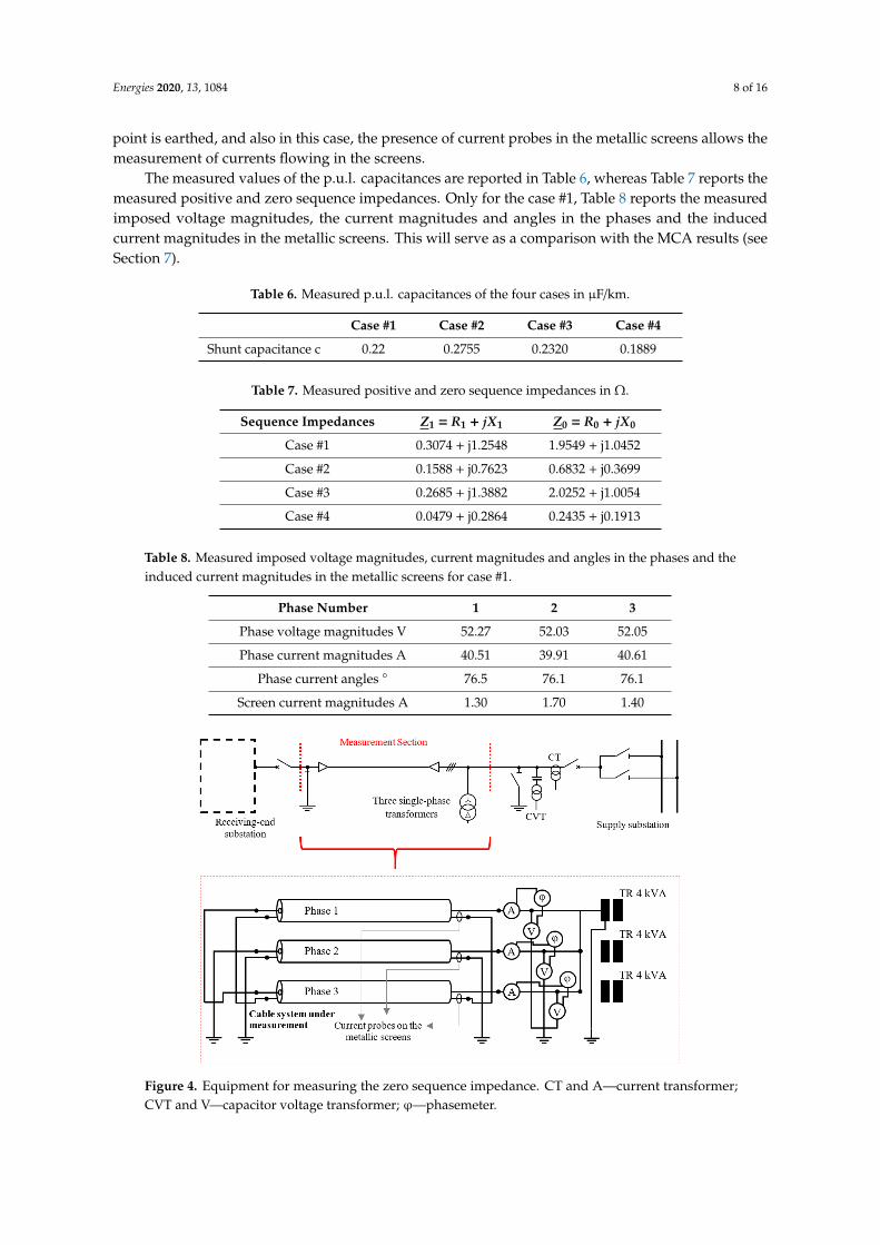
Figure 5 shows the subdivision of the cable system into elementary cells necessary for MCAapplication. This Figure is also very useful to have an immediate view of the different layings (trefoil,open trefoil, flat, etc.) along the route. The very short cell length (5 m in both case #1 and #4, and in the

Energies 2020, 13, 1084 10 of 16

other two cases, ranging from 3.62 to 10 m) implies knowledge of the electric quantities with a greatdetail along the entire route. For the sake of brevity, it is impossible to show all the electric quantitiesfor all the four cases.

Energies 2020, 13, 1084 10 of 16

Table 10. Positive and zero sequence impedances in Ω with IEC.

Sequence Impedances

Z1 = R1 + jX1 Z0= R0 + jX0

Case #1 0.2821 + j1.2626 2.0243 + j0.7733 Case #2 0.1405 + j0.7070 0.7101 + j0.3634 Case #3 0.2627 + j1.2509 1.9925 + j0.7874 Case #4 (0.0311 – 0.035) + j0.2832 (0.2235 – 0.2274) + j0.1523

In particular, the possibility of minor sections of different lengths is considered in another IEC standard (i.e., IEC 60287-1-1 clause 2.3.6.2 [30]) not for the computation of the sequence impedances but only for the circulating current losses with the aim of ampacity evaluation. As will be demonstrated by the measurements and by the MCA, this implies an underestimation of the positive sequence resistance and an overestimation of the positive sequence reactance.

7. Some Notes on MCA Results

Figure 5 shows the subdivision of the cable system into elementary cells necessary for MCA application. This Figure is also very useful to have an immediate view of the different layings (trefoil, open trefoil, flat, etc.) along the route. The very short cell length (5 m in both case #1 and #4, and in the other two cases, ranging from 3.62 to 10 m) implies knowledge of the electric quantities with a great detail along the entire route. For the sake of brevity, it is impossible to show all the electric quantities for all the four cases.

Figure 5. Subdivision of case #1 in elementary cells, minor and major sections. OT—open trefoil with spacing = 0.15 m; F—flat laying with spacing = 1 m; T—close trefoil.

Since the errors in the evaluation of positive sequence impedances by means of IEC/Cigré depend upon the existence of induced screen currents even if the screens are cross-bonded, Figure 6 shows the inducing currents in the phases, and Figure 7 the induced currents in the metallic screens. The current magnitudes in Figure 6 are obtained by imposing the same voltage generators of the corresponding measurement campaign (see Table 8 first row) such as to compare the phase and the induced screen currents. It is impressive how the measured current magnitudes induced in the screens (see Table 8 last row) at the sending end present a slight difference compared to the values at the beginning (i.e., x = 0 km) of the x-axes of Figure 7. The screen current magnitudes vary along the route of the cable due to the different lengths in the cross-bonding minor sections which determine the non-zero induced currents in the screens, which reach almost 9 A (or about 40 A in the phases).

Minor section=555 m

Major section=555 m × 3=1665 m

Multiconductor cell length=5 m

Major section =1665 km

Line length=8325 m

T F TOTF

F T F T F T

OT 50 m

F 55 m

T 1650 m

F 705 m

T 900 m

F 475 m

T 1180 m

F 275 m

T 1380 m

F 275 m

T 1380 m

Figure 5. Subdivision of case #1 in elementary cells, minor and major sections. OT—open trefoil withspacing = 0.15 m; F—flat laying with spacing = 1 m; T—close trefoil.

Since the errors in the evaluation of positive sequence impedances by means of IEC/Cigré dependupon the existence of induced screen currents even if the screens are cross-bonded, Figure 6 shows theinducing currents in the phases, and Figure 7 the induced currents in the metallic screens. The currentmagnitudes in Figure 6 are obtained by imposing the same voltage generators of the correspondingmeasurement campaign (see Table 8 first row) such as to compare the phase and the induced screencurrents. It is impressive how the measured current magnitudes induced in the screens (see Table 8last row) at the sending end present a slight difference compared to the values at the beginning (i.e., x= 0 km) of the x-axes of Figure 7. The screen current magnitudes vary along the route of the cable dueto the different lengths in the cross-bonding minor sections which determine the non-zero inducedcurrents in the screens, which reach almost 9 A (or about 40 A in the phases). This demonstrates theinfluence of circulating currents in the screens on the positive sequence parameters.

Energies 2020, 13, 1084 11 of 16

This demonstrates the influence of circulating currents in the screens on the positive sequence parameters.

Figure 6. Current magnitudes in the three phases for case #1 (current magnitudes).

Figure 7. Induced current magnitudes in the three screens for case #1.

Figures 8–10 give the subdivision into elementary cells performed for cases #2–#4.

Figure 8. Subdivision of case #2 in elementary cells, minor and major sections. OT—open trefoil with spacing = 0.225 m; F—flat laying with spacing = 0.35 m; T—close trefoil.

Minor section=490 m


Multiconductor cell length =10 m

Major section=1470 m

Line length=5880 m

OT F OTT T

T 220 m OT 410 m F 240 m OT 470 m T 4540 m

Cable length km

Curre

nt m

agni

tude

s A

Cable length km

Curre

nt m

agni

tude

s A


Energies 2020, 13, 1084 11 of 16

Energies 2020, 13, 1084 11 of 16






Minor section=490 m




Line length=5880 m

OT F OTT T

T 220 m OT 410 m F 240 m OT 470 m T 4540 m

Cable length km

Curre

nt m

agni

tude

s A

Cable length km

Curre

nt m

agni

tude

s A



Energies 2020, 13, 1084 11 of 16






Minor section=490 m




Line length=5880 m

OT F OTT T

T 220 m OT 410 m F 240 m OT 470 m T 4540 m

Cable length km

Curre

nt m

agni

tude

s A

Cable length km

Curre

nt m

agni

tude

s A

Figure 8. Subdivision of case #2 in elementary cells, minor and major sections. OT—open trefoil withspacing = 0.225 m; F—flat laying with spacing = 0.35 m; T—close trefoil.Energies 2020, 13, 1084 12 of 16

Figure 9. Subdivision of case #3 in elementary cells, minor and major sections. OT—open trefoil with spacing = 0.18 m; F1—flat laying with spacing = 0.25 m; F2—flat laying with spacing = 0.5 m; T—close trefoil.

Table 11 reports the computations of p.u.l. shunt capacitance taking into account the semiconductive layers, but the results are practically identical to those obtained with IEC formula in (9).

It is worth noting that also commercial software as EMTP-RV or DigSilent Power Factory can reach the same precision of MCA.

The advantage of MCA is that it is a free self-made matrix algorithm whose inner characteristics are not hidden but available in the technical literature.

Figure 10. Subdivision of case #4 in elementary cells, minor and major sections. OT—open trefoil with spacing = 0.2 m; F—flat laying with spacing = 0.6 m; T—close trefoil; JC—joint chamber.

Table 11. The p.u.l. capacitances of the four cases in μF/km with multiconductor cell analysis (MCA).

Case #1 Case #2 Case #3 Case #4 Shunt p.u.l. capacitance c 0.2225 0.2802 0.2301 0.1842

For each case #1–#4, by means of (6) and (8), the positive and zero sequence are computed. The results are reported in Table 12.

Figure 9. Subdivision of case #3 in elementary cells, minor and major sections. OT—open trefoilwith spacing = 0.18 m; F1—flat laying with spacing = 0.25 m; F2—flat laying with spacing = 0.5 m;T—close trefoil.

Energies 2020, 13, 1084 12 of 16

Table 11 reports the computations of p.u.l. shunt capacitance taking into account thesemiconductive layers, but the results are practically identical to those obtained with IEC formulain (9).

It is worth noting that also commercial software as EMTP-RV or DigSilent Power Factory canreach the same precision of MCA.

The advantage of MCA is that it is a free self-made matrix algorithm whose inner characteristicsare not hidden but available in the technical literature.

Energies 2020, 13, 1084 12 of 16

Figure 9. Subdivision of case #3 in elementary cells, minor and major sections. OT—open trefoil with spacing = 0.18 m; F1—flat laying with spacing = 0.25 m; F2—flat laying with spacing = 0.5 m; T—close trefoil.

Table 11 reports the computations of p.u.l. shunt capacitance taking into account the semiconductive layers, but the results are practically identical to those obtained with IEC formula in (9).

It is worth noting that also commercial software as EMTP-RV or DigSilent Power Factory can reach the same precision of MCA.

The advantage of MCA is that it is a free self-made matrix algorithm whose inner characteristics are not hidden but available in the technical literature.

Figure 10. Subdivision of case #4 in elementary cells, minor and major sections. OT—open trefoil with spacing = 0.2 m; F—flat laying with spacing = 0.6 m; T—close trefoil; JC—joint chamber.

Table 11. The p.u.l. capacitances of the four cases in μF/km with multiconductor cell analysis (MCA).

Case #1 Case #2 Case #3 Case #4 Shunt p.u.l. capacitance c 0.2225 0.2802 0.2301 0.1842

For each case #1–#4, by means of (6) and (8), the positive and zero sequence are computed. The results are reported in Table 12.

Figure 10. Subdivision of case #4 in elementary cells, minor and major sections. OT—open trefoil withspacing = 0.2 m; F—flat laying with spacing = 0.6 m; T—close trefoil; JC—joint chamber.

Table 11. The p.u.l. capacitances of the four cases in µF/km with multiconductor cell analysis (MCA).


Shunt p.u.l.capacitance c 0.2225 0.2802 0.2301 0.1842

For each case #1–#4, by means of (6) and (8), the positive and zero sequence are computed. Theresults are reported in Table 12.

Table 12. The p.u.l. posit. and zero sequence impedances in Ω with MCA.

Sequence Impedances Z1 = R1 + jX1 Z0 = R0 + jX0

Case #1 0.3064 + j1.2446 2.1911 + j0.819

Case #2 0.1558 + j0.7027 0.7256 + j0.3587

Case #3 0.2767 + j1.3694 1.9991 + j0.7672

Case #4 (0.0432 – 0.0451) + j0.277 (0.2807 – 0.2827) + j0.1518

It is worth noting that the results of commercial power systems software as EMTP-RV would givethe same results of MCA. For power frequency analysis, the authors prefer to use MCA since it is anopen-source algorithm and allows knowing all the hypotheses and assumptions which are the basis ofcomputations. By contrast, the commercial software are black boxes.

8. Final Comparisons of MCA and IEC/Cigrè with Measurements

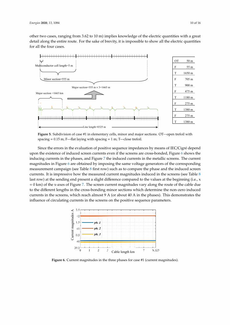
In order to have a general overview of the differences between the two computation methods andthe measurements, Table 13 reports the percentage errors of MCA and of IEC/Cigré with respect to

Energies 2020, 13, 1084 13 of 16

the measurement values. For example, the error of MCA with respect to the measurements (acronymMEA) are expressed by

∆ec =cMEA − cMCA

cMEA· 100; (11)

∆eR1 =R1_MEA −R1_MCA

R1_MEA· 100; ∆eX1 =

X1_MEA −X1_MCA

X1_MEA· 100; (12)

∆eR0 =R0_MEA −R0_MCA

R0_MEA· 100; ∆eX0 =

X0_MEA −X0_MCA

X0_MEA· 100. (13)

The cell colours help to immediately visualise the error ranges with the following choices:

• RED for errors greater than 15 %;• YELLOW for errors ranging between 7.5% and 15%;• GREEN for errors smaller than 7.5%.

The first important outcome of this research is that the precision in the computation of shuntcapacitance of land single-core cables is very high both with IEC formula and with MCA whichalso considers semiconductive layers: the measures confirm that, at power frequency, the effects ofsemiconductive layers can surely be neglected.

Table 13. Final comparisons of the measurements with MCA and IEC/Cigré computations.

COMPARISON BETWEEN THE DIFFERENT METHODS APPLIED TO THE ANALYSED CASE STUDIES

Case #1SE Calenzano-SE

Rifredi RT

Case #2CP S. Giuseppe-CP

Portoferraio

Case #3SE Camin-CP

Bassanello

Case #4CP Ferrara Nord-C.le SEF

IECCigré MCA Mea. IEC

Cigré MCA Mea. IECCigré MCA Mea. IEC

Cigré MCA Mea.

c µF/km 0.2224 0.2224 0.2200 0.2802 0.2802 0.2755 0.2301 0.2301 0.2320 0.1842 0.1842 0.1889∆e % −1.09 −1.09 −1.71 −1.71 0.82 0.82 2.49 2.49R1 Ω 0.2821 0.3064 0.3074 0.1405 0.1558 0.1588 0.2627 0.2767 0.2865 0.0311 ÷ 0.0350 0.0432 ÷ 0.0451 0.0479∆e % 8.23 0.33 11.52 1.89 8.31 3.42 35 ÷ 26.9 9.3 ÷ 5.9X1 Ω 1.2626 1.2446 1.2548 0.7069 0.7063 0.7623 1.2509 1.3694 1.3882 0.2832 0.2769 0.2864∆e % −0.62 0.81 7.27 7.35 9.89 1.35 1.12 3.32R0 Ω 2.0243 2.0239 1.9549 0.7101 0.7256 0.6832 1.9925 1.9991 2.0252 0.2235 ÷ 0.2274 0.2406 ÷ 0.2434 0.2435

∆e % −3.55 −3.53 −3.94 −6.21 1.61 1.29 8.2 ÷ 6.6 −1.19 ÷ −0.04X0 Ω 0.7733 0.7711 1.0452 0.3634 0.3587 0.3699 0.7847 0.7672 1.0054 0.1523 0.1470 0.1913∆e % 26.01 26.22 1.76 3.03 21.95 23.69 20.39 23.16

The second result is the strong underestimation (up to 35%) of IEC/Cigré positive sequenceresistances due to the already highlighted wrong hypothesis of null screen circulating currents.

The third note deals with the great errors in the zero sequence reactance (always about 20% bothfor MCA and IEC/Cigré) in all the cases (#1, #3, and #4) of cable located in industrialised and urbanisedareas. This is due to the fact that the repartition of the currents between screens and earth is influencedby the presence of underground metallic pipes which are not known.

The demonstration of this fact is that for case #2, located in a natural area, the errors are whollynegligible (about 3%). In any case, since the calculated value is lower than that measured, this is on thesafe side for the calculation of the short circuit currents but may lead to an error in the setting of thedistance relays and consequent untimely tripping.

9. Conclusions

The formula IEC/Cigré for the computation of the phase-to-screen capacitance (equal for bothpositive and zero sequences) gives extremely precise values in full agreement with measurements whenthe relative permittivity and the semiconductive screen thicknesses are known. The maximum error issmaller than 2.5%. The same error is given by MCA even if it considers the relative permittivities ofsemiconductive layers. All the direct formulae of the positive sequence impedance hypothesise that

Energies 2020, 13, 1084 14 of 16

the screen arrangements completely zero the induced currents in the screens. This would be true inreal installations only if:

(1) The minor section lengths are exactly equal (practically impossible);(2) There is perfect laying symmetry along the route (trefoil laying or any laying performed with

phase transpositions: both very difficult to obtain).

In engineering practice (very often, the “as-built” differs from the project specifications) one orboth the conditions cannot be satisfied. This gives errors between 8% and 35% for the real part ofpositive sequence impedance and up to 8% in the imaginary part.

In these cases, the hypotheses for Carson theory applications fail so that the ground return currentuses different metallic paths and, therefore, nor analytical formulae neither matrix procedures can giveexact impedance values.

MCA, together with commercial software as DigSilent PowerFactory or EMTP-RV, is the onlycomputation approach able to obtain zero and positive sequence impedances in tune with themeasurements when the exact laying conditions, homogeneous stretch per homogeneous stretch, areknown. This is demonstrated by the fact that an error greater than 20% is given only in presence ofunknown metallic return path for the currents.

Hence, the paper demonstrates, for the first time in the technical literature, that direct formulaecannot correctly evaluate the sequence impedances of installed single-core land cable systems. Extensiveon-field measurement campaigns have served to this purpose.

Only by considering all the conductors (active and passive ones) in their real arrangement, itis possible to have reliable and correct sequence impedance values. The authors have extensivelyused their open-source algorithm, i.e., MCA, in order to demonstrate that the differences withon-field measurements are always negligible. The only difference between measurements and MCAresults persists in the zero sequence reactance but only when cable systems are installed in urbanor industrialised areas. This is not due to MCA limitations but only to the presence of differentunderground subservices (e.g., gas metallic pipes, etc.) in urbanised or industrialised areas, which alterthe current return path. The final scientific demonstration of this important conclusion comes from themeasurements of zero sequence in the cable system installed in Elba Island Island (CP S. Giuseppe-CPPortoferraio, i.e., case #3) where there is no congestion of underground subservices which lead to errorsin determination the current return path. Hence, MCA can correctly evaluate also the zero sequencereactance with a difference of about 3% compared to measurements.

In conclusion, in this paper, we aim to help the entire insulated cable community to become awareof and pay attention to the issues in computation of sequence impedances with simplified analyticdirect formulae: they can give high errors, which jeopardise the evaluations and the settings involvingsequence impedance values.

Author Contributions: Conceptualization, R.B., S.D.S., M.P.; Investigation R.B., S.D.S., F.S.; Formal Analysis,R.B., S.D.S., F.S.; Writing Original Draft Preparation, Review & Editing R.B., S.D.S.; Supervision, R.B.; ProjectAdministration, R.B., M.P.; Funding Acquisition, M.P. All authors have read and agreed to the published versionof the manuscript.

Funding: This research was funded by [Ensiel/Terna], grant number [ST16].

Conflicts of Interest: The authors declare no conflict of interest.

References

1. Benato, R.; Caciolli, L. Sequence impedances of insulated cables: Measurements versus computations.PES T&D 2012, 2012, 1–7. [CrossRef]

2. IEC 60909-2: Short-Circuit Currents in Three-Phase a.c. Systems—Part 2: Data of Electrical Equipment forShort-Circuit Current Calculations, 2nd ed.; IEC: Geneva, Switzerland, 2008.

http://dx.doi.org/10.1109/TDC.2012.6281574

Energies 2020, 13, 1084 15 of 16

3. Royer, C.; Dorison, E.; Anderson, N.; Benato, R.; Brijs, B.; Chang, K.W.; Falconer, A.; Fernandez, S.;Gudmunsdottir, U.S.; Li, J.; et al. Cable Systems Electrical Characteristics. Technical Report for CIGRETechnical Brochure N531. 2013. Available online: https://e-cigre.org/publication/531-cable-systems-electrical-characteristics (accessed on 28 February 2020).

4. Ametani, A.; Ohno, T. Derivation of Theoretical Formulas of Sequence Currents on Underground CableSystems. IEEJ Trans. Power Energy 2011, 131, 277–282. [CrossRef]

5. Ramya, G.M.; Radhika, P. Computation of Sequence Impedances for 220kv Underground Cable with DifferentShort Circuit Capacities. Int. J. Mod. Trends Sci. Technol. 2017, 3. Available online: http://www.ijmtst.com(accessed on 28 February 2020).

6. Benato, R. Multiconductor analysis of underground power transmission systems: EHV AC cables. Electr. PowerSyst. Res. 2009, 79, 27–38. [CrossRef]

7. Benato, R.; Paolucci, A. Multiconductor cell analysis of skin effect in Milliken type cables. Electr. PowerSyst. Res. 2012, 90, 99–106. [CrossRef]

8. Benato, R.; Napolitano, D. Overall Cost Comparison between Cable and Overhead Lines Including the Costsfor Repair After Random Failures. IEEE Trans. Power Deliv. 2012, 27, 1213–1222. [CrossRef]

9. Benato, S.R.; Dambone Sessa, F.; Guglielmi, E.; Partal, E.; Tleis, N. Ground Return Current Behaviour in HighVoltage Alternating Current Insulated Cables. Energies 2014, 7, 8116–8131. [CrossRef]

10. Benato, R.; Sessa, S.D.; De Zan, R.; Guarniere, M.; Lavecchia, G.; Labini, P.S. Different Bonding Types ofScilla-Villafranca (Sicily-Calabria) 43 km Double-Circuit AC 380 kV Submarine-Land Cable. IEEE Trans.Ind. Appl. 2015, 51, 5050–5057. [CrossRef]

11. Benato, R.; Colla, L.; Sessa, S.D.; Marelli, M. Review of high current rating insulated cable solutions.Electr. Power Syst. Res. 2016, 133, 36–41. [CrossRef]

12. Benato, R.; Sessa, S.D.; Guglielmi, F.; Partal, E.; Tleis, N. Zero sequence behaviour of a double-circuit overheadline. Electr. Power Syst. Res. 2014, 116, 419–426. [CrossRef]

13. Benato, R.; Sessa, S.D.; Guizzo, L.; Rebolini, M. The synergy of the future: high voltage insulated powercables and railway-highway infrastructures. IET Gener. Transm. Distrib. 2017, 11, 2712–2720. [CrossRef]

14. Benato, R.; Sessa, S.D. A New Multiconductor Cell Three-Dimension Matrix-Based Analysis Applied to aThree-Core Armoured Cable. IEEE Trans. Power Deliv. 2018, 33, 1636–1646. [CrossRef]

15. Carson, J.R. Wave Propagation in Overhead Wires with Ground Return. Bell Syst. Tech. J. 1926, 5, 539–554.[CrossRef]

16. Pollaczek, F. Über das Feld einer unendlich langen wechsel stromdurchflossenen Einfachleitung. ElectrisheNachrichten Technik 1926, 3, 339–360.

17. CCITT. Directives Concerning the Protection of Telecommunication Lines against Harmful Effects from Electric Powerand Electrified Railway Lines; CCITT: Geneva, Switzerland, 1989.

18. Schelkunhoff, S.A. The electromagnetic theory of coaxial transmission lines and cylindrical shields. Bell Syst.Tech. J. 1934, 13, 532–579. [CrossRef]

19. Wedepohl, L.M.; Wilcox, D.J. Transient analysis of underground power transmission systems. Proc. IEEE1973, 120, 253–260.

20. Benato, R.; Sessa, S.D.; Forzan, M. Experimental Validation of 3-Dimension Multiconductor Cell Analysisby a 30 km Long Submarine Three-Core Armoured Cable. IEEE Trans. Power Deliv. 2018, 33, 2910–2919.[CrossRef]

21. Choi, J.K.; Kwak, J.S.; Lee, W.K.; Jung, C.K.; Kim, J.W.; Oh, S.I. Analysis of Sequence impedance of 345 kVCable systems with Special bondings using ATP. In Proceedings of the 2009 Transmission & DistributionConference & Exposition: Asia and Pacific, Seoul, South Korea, 26–30 October 2009.

22. Gudmundsdottir, U.S.; Gustavsen, B.; Bak, C.L.; Wiechowski, W. Field Test and Simulation of a 400-kVCross-Bonded Cable System. IEEE Trans. Power Deliv. 2011, 26, 1403–1410. [CrossRef]

23. Das, J.C. Understanding Symmetrical Components for Power System Modelling; IEEE Press Wiley: Hoboken, NJ,USA, 2017.

24. Tleis, N. Power Systems Modelling and Fault Analysis: Theory and Practice, 2nd ed.; Newnes: London, UK, 2019.25. Blackburn, J.L. Symmetrical Components for Power Systems Engineering; CRC Press: Boca Raton, FL, USA, 1993.26. IEC 60909-3: Short-Circuit Currents in Three-Phase a.c. Systems—Part 3: Currents during Two Separate

Simultaneous Line-to-Earth Short-Circuits and Partial Short-Circuit Currents Flowing through Earth; IEC: Geneva,Switzerland, 2010.

https://e-cigre.org/publication/531-cable-systems-electrical-characteristics

https://e-cigre.org/publication/531-cable-systems-electrical-characteristics

http://dx.doi.org/10.1541/ieejpes.131.277

http://www.ijmtst.com

http://dx.doi.org/10.1016/j.epsr.2008.05.016


http://dx.doi.org/10.1109/TPWRD.2012.2191803

http://dx.doi.org/10.3390/en7128116

http://dx.doi.org/10.1109/TIA.2015.2448676



http://dx.doi.org/10.1049/iet-gtd.2016.2082


http://dx.doi.org/10.1002/j.1538-7305.1926.tb00122.x

http://dx.doi.org/10.1002/j.1538-7305.1934.tb00679.x



Energies 2020, 13, 1084 16 of 16

27. IEC EN 60044-1, Instrument Transformers—Part 1: Current Transformers; IEC: Geneva, Switzerland, 1999.28. IEC EN 60044-5, Instrument Transformers—Part 5: Capacitor Voltage Transformers; IEC: Geneva,

Switzerland, 2004.29. Callegaro, L. Electrical Impedance Principles, Measurement, and Applications; Taylor & Francis Group: Milton Park,

UK, 2013.30. IEC 60287: Electric Cables—Calculation of the Current Rating, (in 8 parts: 1.1, 1.2, 1.3, 2.1, 2.2, 3.1, 3.2, 3.3); IEC:

Geneva, Switzerland, 2015.

© 2020 by the authors. Licensee MDPI, Basel, Switzerland. This article is an open accessarticle distributed under the terms and conditions of the Creative Commons Attribution(CC BY) license (http://creativecommons.org/licenses/by/4.0/).

http://creativecommons.org/

http://creativecommons.org/licenses/by/4.0/.

Sequence Impedances of Land Single-Core Insulated Cables

Documents

Transcript of Sequence Impedances of Land Single-Core Insulated Cables