Pattern Recognition and Classification

Geoff Dougherty

Pattern Recognitionand Classification

An Introduction

Geoff DoughertyApplied Physics and Medical ImagingCalifornia State University, Channel IslandsCamarillo, CA, USA

Please note that additional material for this book can be downloaded fromhttp://extras.springer.com

ISBN 978-1-4614-5322-2 ISBN 978-1-4614-5323-9 (eBook)DOI 10.1007/978-1-4614-5323-9Springer New York Heidelberg Dordrecht London

Library of Congress Control Number: 2012949108

# Springer Science+Business Media New York 2013This work is subject to copyright. All rights are reserved by the Publisher, whether the whole or partof the material is concerned, specifically the rights of translation, reprinting, reuse of illustrations,recitation, broadcasting, reproduction on microfilms or in any other physical way, and transmission orinformation storage and retrieval, electronic adaptation, computer software, or by similar or dissimilarmethodology now known or hereafter developed. Exempted from this legal reservation are brief excerptsin connection with reviews or scholarly analysis or material supplied specifically for the purpose of beingentered and executed on a computer system, for exclusive use by the purchaser of the work. Duplicationof this publication or parts thereof is permitted only under the provisions of the Copyright Law of thePublisher’s location, in its current version, and permission for use must always be obtained fromSpringer. Permissions for use may be obtained through RightsLink at the Copyright Clearance Center.Violations are liable to prosecution under the respective Copyright Law.The use of general descriptive names, registered names, trademarks, service marks, etc. in thispublication does not imply, even in the absence of a specific statement, that such names are exemptfrom the relevant protective laws and regulations and therefore free for general use.While the advice and information in this book are believed to be true and accurate at the date ofpublication, neither the authors nor the editors nor the publisher can accept any legal responsibility forany errors or omissions that may be made. The publisher makes no warranty, express or implied, withrespect to the material contained herein.

Printed on acid-free paper

Springer is part of Springer Science+Business Media (www.springer.com)

Preface

The use of pattern recognition and classification is fundamental to many of the

automated electronic systems in use today. Its applications range from military

defense to medical diagnosis, from biometrics to machine learning, from bioinfor-

matics to home entertainment, and more. However, despite the existence of a

number of notable books in the field, the subject remains very challenging, espe-

cially for the beginner.

We have found that the current textbooks are not completely satisfactory for our

students, who are primarily computer science students but also include students

from mathematics and physics backgrounds and those from industry. Their mathe-

matical and computer backgrounds are considerably varied, but they all want to

understand and absorb the core concepts with a minimal time investment to the

point where they can use and adapt them to problems in their own fields. Texts with

extensive mathematical or statistical prerequisites were daunting and unappealing

to them. Our students complained of “not seeing the wood for the trees,” which is

rather ironic for textbooks in pattern recognition. It is crucial for newcomers to the

field to be introduced to the key concepts at a basic level in an ordered, logical

fashion, so that they appreciate the “big picture”; they can then handle progres-

sively more detail, building on prior knowledge, without being overwhelmed. Too

often our students have dipped into various textbooks to sample different

approaches but have ended up confused by the different terminologies in use.

We have noticed that the majority of our students are very comfortable with and

respond well to visual learning, building on their often limited entry knowledge, but

focusing on key concepts illustrated by practical examples and exercises. We

believe that a more visual presentation and the inclusion of worked examples

promote a greater understanding and insight and appeal to a wider audience.

This book began as notes and lecture slides for a senior undergraduate course

and a graduate course in Pattern Recognition at California State University Channel

Islands (CSUCI). Over time it grew and approached its current form, which has

been class tested over several years at CSUCI. It is suitable for a wide range of

students at the advanced undergraduate or graduate level. It assumes only a modest

v

background in statistics and mathematics, with the necessary additional material

integrated into the text so that the book is essentially self-contained.

The book is suitable both for individual study and for classroom use for students

in physics, computer science, computer engineering, electronic engineering, bio-

medical engineering, and applied mathematics taking senior undergraduate and

graduate courses in pattern recognition and machine learning. It presents a compre-

hensive introduction to the core concepts that must be understood in order to make

independent contributions to the field. It is designed to be accessible to newcomers

from varied backgrounds, but it will also be useful to researchers and professionals

in image and signal processing and analysis, and in computer vision. The goal is to

present the fundamental concepts of supervised and unsupervised classification in

an informal, rather than axiomatic, treatment so that the reader can quickly acquire

the necessary background for applying the concepts to real problems. A final

chapter indicates some useful and accessible projects which may be undertaken.

We use ImageJ (http://rsbweb.nih.gov/ij/) and the related distribution, Fiji (http://

fiji.sc/wiki/index.php/Fiji) in the early stages of image exploration and analysis,

because of its intuitive interface and ease of use. We then tend to move on to

MATLAB for its extensive capabilities in manipulating matrices and its image

processing and statistics toolboxes. We recommend using an attractive GUI called

DipImage (from http://www.diplib.org/download) to avoid much of the command

line typing when manipulating images. There are also classification toolboxes

available for MATLAB, such as Classification Toolbox (http://www.wiley.com/

WileyCDA/Section/id-105036.html) which requires a password obtainable from

the associated computer manual) and PRTools (http://www.prtools.org/download.

html). We use the Classification Toolbox in Chap. 8 and recommend it highly for its

intuitive GUI. Some of our students have explored Weka, a collection of machine

learning algorithms for solving data mining problems implemented in Java and open

sourced (http://www.cs.waikato.ac.nz/ml/weka/index_downloading.html).

There are a number of additional resources, which can be downloaded from the

companion Web site for this book at http://extras.springer.com/, including several

useful Excel files and data files. Lecturers who adopt the book can also obtain

access to the end-of-chapter exercises.

In spite of our best efforts at proofreading, it is still possible that some typos may

have survived. Please notify me if you find any.

I have very much enjoyed writing this book; I hope you enjoy reading it!

Camarillo, CA Geoff Dougherty

vi Preface

http://rsbweb.nih.gov/ij/

http://fiji.sc/wiki/index.php/Fiji

http://fiji.sc/wiki/index.php/Fiji

http://www.diplib.org/download

http://www.wiley.com/WileyCDA/Section/id-105036.html

http://www.wiley.com/WileyCDA/Section/id-105036.html

http://www.prtools.org/download.html

http://www.prtools.org/download.html

http://dx.doi.org/10.1007/978-1-4614-5323-9_8

http://www.cs.waikato.ac.nz/ml/weka/index_downloading.html

http://extras.springer.com/

Acknowledgments

I would like to thank my colleague Matthew Wiers for many useful conversations

and for helping with several of the Excel files bundled with the book. And thanks to

all my previous students for their feedback on the courses which eventually led

to this book; especially to Brandon Ausmus, Elisabeth Perkins, Michelle Moeller,

Charles Walden, Shawn Richardson, and Ray Alfano.

I am grateful to Chris Coughlin at Springer for his support and encouragement

throughout the process of writing the book and to various anonymous reviewers

who have critiqued the manuscript and trialed it with their classes. Special thanks

go to my wife Hajijah and family (Daniel, Adeline, and Nadia) for their patience

and support, and to my parents, Maud and Harry (who passed away in 2009),

without whom this would never have happened.

vii

Contents

1 Introduction . . . . . . . . . . . . . . . . . . . . . . . . . . . . . . . . . . . . . . . . . . 1

1.1 Overview . . . . . . . . . . . . . . . . . . . . . . . . . . . . . . . . . . . . . . . . . 1

1.2 Classification . . . . . . . . . . . . . . . . . . . . . . . . . . . . . . . . . . . . . . 3

1.3 Organization of the Book . . . . . . . . . . . . . . . . . . . . . . . . . . . . . 6

1.4 Exercises . . . . . . . . . . . . . . . . . . . . . . . . . . . . . . . . . . . . . . . . . 6

References . . . . . . . . . . . . . . . . . . . . . . . . . . . . . . . . . . . . . . . . . . . . 7

2 Classification . . . . . . . . . . . . . . . . . . . . . . . . . . . . . . . . . . . . . . . . . . 9

2.1 The Classification Process . . . . . . . . . . . . . . . . . . . . . . . . . . . . . 9

2.2 Features . . . . . . . . . . . . . . . . . . . . . . . . . . . . . . . . . . . . . . . . . . 11

2.3 Training and Learning . . . . . . . . . . . . . . . . . . . . . . . . . . . . . . . 16

2.4 Supervised Learning and Algorithm Selection . . . . . . . . . . . . . . 17

2.5 Approaches to Classification . . . . . . . . . . . . . . . . . . . . . . . . . . . 18

2.6 Examples . . . . . . . . . . . . . . . . . . . . . . . . . . . . . . . . . . . . . . . . . 21

2.6.1 Classification by Shape . . . . . . . . . . . . . . . . . . . . . . . . . 21

2.6.2 Classification by Size . . . . . . . . . . . . . . . . . . . . . . . . . . . 22

2.6.3 More Examples . . . . . . . . . . . . . . . . . . . . . . . . . . . . . . . 23

2.6.4 Classification of Letters . . . . . . . . . . . . . . . . . . . . . . . . . 25

2.7 Exercises . . . . . . . . . . . . . . . . . . . . . . . . . . . . . . . . . . . . . . . . . 25

References . . . . . . . . . . . . . . . . . . . . . . . . . . . . . . . . . . . . . . . . . . . . 26

3 Nonmetric Methods . . . . . . . . . . . . . . . . . . . . . . . . . . . . . . . . . . . . 27

3.1 Introduction . . . . . . . . . . . . . . . . . . . . . . . . . . . . . . . . . . . . . . . 27

3.2 Decision Tree Classifier . . . . . . . . . . . . . . . . . . . . . . . . . . . . . . 27

3.2.1 Information, Entropy, and Impurity . . . . . . . . . . . . . . . . 29

3.2.2 Information Gain . . . . . . . . . . . . . . . . . . . . . . . . . . . . . . 31

3.2.3 Decision Tree Issues . . . . . . . . . . . . . . . . . . . . . . . . . . . 35

3.2.4 Strengths and Weaknesses . . . . . . . . . . . . . . . . . . . . . . . 38

3.3 Rule-Based Classifier . . . . . . . . . . . . . . . . . . . . . . . . . . . . . . . . 39

3.4 Other Methods . . . . . . . . . . . . . . . . . . . . . . . . . . . . . . . . . . . . . 39

3.5 Exercises . . . . . . . . . . . . . . . . . . . . . . . . . . . . . . . . . . . . . . . . . 40

References . . . . . . . . . . . . . . . . . . . . . . . . . . . . . . . . . . . . . . . . . . . . 41

ix

4 Statistical Pattern Recognition . . . . . . . . . . . . . . . . . . . . . . . . . . . . 43

4.1 Measured Data and Measurement Errors . . . . . . . . . . . . . . . . . . 43

4.2 Probability Theory . . . . . . . . . . . . . . . . . . . . . . . . . . . . . . . . . . 43

4.2.1 Simple Probability Theory . . . . . . . . . . . . . . . . . . . . . . . 43

4.2.2 Conditional Probability and Bayes’ Rule . . . . . . . . . . . . . 46

4.2.3 Naıve Bayes Classifier . . . . . . . . . . . . . . . . . . . . . . . . . . 53

4.3 Continuous Random Variables . . . . . . . . . . . . . . . . . . . . . . . . . 54

4.3.1 The Multivariate Gaussian . . . . . . . . . . . . . . . . . . . . . . . 57

4.3.2 The Covariance Matrix . . . . . . . . . . . . . . . . . . . . . . . . . 59

4.3.3 The Mahalanobis Distance . . . . . . . . . . . . . . . . . . . . . . . 69

4.4 Exercises . . . . . . . . . . . . . . . . . . . . . . . . . . . . . . . . . . . . . . . . . 72

References . . . . . . . . . . . . . . . . . . . . . . . . . . . . . . . . . . . . . . . . . . . . 74

5 Supervised Learning . . . . . . . . . . . . . . . . . . . . . . . . . . . . . . . . . . . . 75

5.1 Parametric and Non-parametric Learning . . . . . . . . . . . . . . . . . . 75

5.2 Parametric Learning . . . . . . . . . . . . . . . . . . . . . . . . . . . . . . . . . 75

5.2.1 Bayesian Decision Theory . . . . . . . . . . . . . . . . . . . . . . . 75

5.2.2 Discriminant Functions and Decision Boundaries . . . . . . 87

5.2.3 MAP (Maximum A Posteriori) Estimator . . . . . . . . . . . . 94

5.3 Exercises . . . . . . . . . . . . . . . . . . . . . . . . . . . . . . . . . . . . . . . . . 96

References . . . . . . . . . . . . . . . . . . . . . . . . . . . . . . . . . . . . . . . . . . . . 98

6 Nonparametric Learning . . . . . . . . . . . . . . . . . . . . . . . . . . . . . . . . 99

6.1 Histogram Estimator and Parzen Windows . . . . . . . . . . . . . . . . . 99

6.2 k-Nearest Neighbor (k-NN) Classification . . . . . . . . . . . . . . . . . 100

6.3 Artificial Neural Networks . . . . . . . . . . . . . . . . . . . . . . . . . . . . 104

6.4 Kernel Machines . . . . . . . . . . . . . . . . . . . . . . . . . . . . . . . . . . . 117

6.5 Exercises . . . . . . . . . . . . . . . . . . . . . . . . . . . . . . . . . . . . . . . . . 120

References . . . . . . . . . . . . . . . . . . . . . . . . . . . . . . . . . . . . . . . . . . . . 121

7 Feature Extraction and Selection . . . . . . . . . . . . . . . . . . . . . . . . . . 123

7.1 Reducing Dimensionality . . . . . . . . . . . . . . . . . . . . . . . . . . . . . 123

7.1.1 Preprocessing . . . . . . . . . . . . . . . . . . . . . . . . . . . . . . . . 124

7.2 Feature Selection . . . . . . . . . . . . . . . . . . . . . . . . . . . . . . . . . . . 124

7.2.1 Inter/Intraclass Distance . . . . . . . . . . . . . . . . . . . . . . . . . 124

7.2.2 Subset Selection . . . . . . . . . . . . . . . . . . . . . . . . . . . . . . 126

7.3 Feature Extraction . . . . . . . . . . . . . . . . . . . . . . . . . . . . . . . . . . 127

7.3.1 Principal Component Analysis . . . . . . . . . . . . . . . . . . . . 127

7.3.2 Linear Discriminant Analysis . . . . . . . . . . . . . . . . . . . . . 135

7.4 Exercises . . . . . . . . . . . . . . . . . . . . . . . . . . . . . . . . . . . . . . . . . 140

References . . . . . . . . . . . . . . . . . . . . . . . . . . . . . . . . . . . . . . . . . . . . 141

x Contents

8 Unsupervised Learning . . . . . . . . . . . . . . . . . . . . . . . . . . . . . . . . . . 143

8.1 Clustering . . . . . . . . . . . . . . . . . . . . . . . . . . . . . . . . . . . . . . . 143

8.2 k-Means Clustering . . . . . . . . . . . . . . . . . . . . . . . . . . . . . . . . . 145

8.2.1 Fuzzy c-Means Clustering . . . . . . . . . . . . . . . . . . . . . 148

8.3 (Agglomerative) Hierarchical Clustering . . . . . . . . . . . . . . . . . 150

8.4 Exercises . . . . . . . . . . . . . . . . . . . . . . . . . . . . . . . . . . . . . . . . 154

References . . . . . . . . . . . . . . . . . . . . . . . . . . . . . . . . . . . . . . . . . . . . 155

9 Estimating and Comparing Classifiers . . . . . . . . . . . . . . . . . . . . . . 157

9.1 Comparing Classifiers and the No Free Lunch Theorem . . . . . . 157

9.1.1 Bias and Variance . . . . . . . . . . . . . . . . . . . . . . . . . . . 159

9.2 Cross-Validation and Resampling Methods . . . . . . . . . . . . . . . 160

9.2.1 The Holdout Method . . . . . . . . . . . . . . . . . . . . . . . . . 161

9.2.2 k-Fold Cross-Validation . . . . . . . . . . . . . . . . . . . . . . . 162

9.2.3 Bootstrap . . . . . . . . . . . . . . . . . . . . . . . . . . . . . . . . . . 163

9.3 Measuring Classifier Performance . . . . . . . . . . . . . . . . . . . . . . 164

9.4 Comparing Classifiers . . . . . . . . . . . . . . . . . . . . . . . . . . . . . . . 169

9.4.1 ROC Curves . . . . . . . . . . . . . . . . . . . . . . . . . . . . . . . 169

9.4.2 McNemar’s Test . . . . . . . . . . . . . . . . . . . . . . . . . . . . 169

9.4.3 Other Statistical Tests . . . . . . . . . . . . . . . . . . . . . . . . 169

9.4.4 The Classification Toolbox . . . . . . . . . . . . . . . . . . . . . 171

9.5 Combining Classifiers . . . . . . . . . . . . . . . . . . . . . . . . . . . . . . . 174

References . . . . . . . . . . . . . . . . . . . . . . . . . . . . . . . . . . . . . . . . . . . . 176

10 Projects . . . . . . . . . . . . . . . . . . . . . . . . . . . . . . . . . . . . . . . . . . . . . . 177

10.1 Retinal Tortuosity as an Indicator of Disease . . . . . . . . . . . . . . 177

10.2 Segmentation by Texture . . . . . . . . . . . . . . . . . . . . . . . . . . . . 181

10.3 Biometric Systems . . . . . . . . . . . . . . . . . . . . . . . . . . . . . . . . . 183

10.3.1 Fingerprint Recognition . . . . . . . . . . . . . . . . . . . . . . . 184

10.3.2 Face Recognition . . . . . . . . . . . . . . . . . . . . . . . . . . . . 187

References . . . . . . . . . . . . . . . . . . . . . . . . . . . . . . . . . . . . . . . . . . . . 187

Index . . . . . . . . . . . . . . . . . . . . . . . . . . . . . . . . . . . . . . . . . . . . . . . . . . . 189

Contents xi

Chapter 1

Introduction

1.1 Overview

Humans are good at recognizing objects (or patterns, to use the generic term). We

are so good that we take this ability for granted, and find it difficult to analyze the

steps in the process. It is generally easy to distinguish the sound of a human voice,

from that of a violin; a handwritten numeral “3,” from an “8”; and the aroma of a

rose, from that of an onion. Every day, we recognize faces around us, but we do it

unconsciously and because we cannot explain our expertise, we find it difficult to

write a computer program to do the same. Each person’s face is a pattern

composed of a particular combination of structures (eyes, nose, mouth, . . .)located in certain positions on the face. By analyzing sample images of faces, a

program should be able to capture the pattern specific to a face and identify (or

recognize) it as a face (as a member of a category or class we already know); this

would be pattern recognition. There may be several categories (or classes) and we

have to sort (or classify) a particular face into a certain category (or class); hencethe term classification. Note that in pattern recognition, the term pattern is

interpreted widely and does not necessarily imply a repetition; it is used to include

all objects that we might want to classify, e.g., apples (or oranges), speech

waveforms, and fingerprints.

A class is a collection of objects that are similar, but not necessarily identical,

and which is distinguishable from other classes. Figure 1.1 illustrates the difference

between classification where the classes are known beforehand and classification

where classes are created after inspecting the objects.

Interest in pattern recognition and classification has grown due to emerging

applications, which are not only challenging but also computationally demanding.

These applications include:

• Data mining (sifting through a large volume of data to extract a small amount of

relevant and useful information, e.g., fraud detection, financial forecasting, and

credit scoring)

G. Dougherty, Pattern Recognition and Classification: An Introduction,DOI 10.1007/978-1-4614-5323-9_1, # Springer Science+Business Media New York 2013

1

• Biometrics (personal identification based on physical attributes of the face, iris,

fingerprints, etc.)

• Machine vision (e.g., automated visual inspection in an assembly line)

• Character recognition [e.g., automatic mail sorting by zip code, automated check

scanners at ATMs (automated teller machines)]

• Document recognition (e.g., recognize whether an e-mail is spam or not, based

on the message header and content)

• Computer-aided diagnosis [e.g., helping doctors make diagnostic decisions

based on interpreting medical data such as mammographic images, ultrasound

images, electrocardiograms (ECGs), and electroencephalograms (EEGs)]

• Medical imaging [e.g., classifying cells as malignant or benign based on the

results of magnetic resonance imaging (MRI) scans, or classify different emo-

tional and cognitive states from the images of brain activity in functional MRI]

• Speech recognition (e.g., helping handicapped patients to control machines)

• Bioinformatics (e.g., DNA sequence analysis to detect genes related to particular

diseases)

• Remote sensing (e.g., land use and crop yield)

• Astronomy (classifying galaxies based on their shapes; or automated searches

such as the Search for Extra-Terrestrial Intelligence (SETI) which analyzes

radio telescope data in an attempt to locate signals that might be artificial in

origin)

The methods used have been developed in various fields, often independently.

In statistics, going from particular observations to general descriptions is called

inference, learning [i.e., using example (training) data] is called estimation, and

classification is known as discriminant analysis (McLachlan 1992). In engineer-

ing, classification is called pattern recognition and the approach is nonparametric

and much more empirical (Duda et al. 2001). Other approaches have their origins

in machine learning (Alpaydin 2010), artificial intelligence (Russell and Norvig

2002), artificial neural networks (Bishop 2006), and data mining (Han and Kamber

2006). We will incorporate techniques from these different emphases to give a more

unified treatment (Fig. 1.2).

Fig. 1.1 Classification when the classes are (a) known and (b) unknown beforehand

2 1 Introduction

1.2 Classification

Classification is often the final step in a general process (Fig. 1.3). It involves

sorting objects into separate classes. In the case of an image, the acquired image is

segmented to isolate different objects from each other and from the background,

and the different objects are labeled. A typical pattern recognition system contains a

sensor, a preprocessing mechanism (prior to segmentation), a feature extraction

mechanism, a set of examples (training data) already classified (post-processing),

and a classification algorithm. The feature extraction step reduces the data by

measuring certain characteristic properties or features (such as size, shape, and

texture) of the labeled objects. These features (or, more precisely, the values of

these features) are then passed to a classifier that evaluates the evidence presentedand makes a decision regarding the class each object should be assigned, depending

on whether the values of its features fall inside or outside the tolerance of that class.

This process is used, for example, in classifying lesions as benign or malignant.

The quality of the acquired image depends on the resolution, sensitivity, bandwidth

and signal-to-noise ratio of the imaging system. Pre-processing steps such as image

enhancement (e.g., brightness adjustment, contrast enhancement, image averaging,

frequency domain filtering, edge enhancement) and image restoration (e.g., photo-

metric correction, inverse filtering,Wiener filtering) may be required prior to segmen-

tation, which is often a challenging process. Typically enhancement will precede

restoration. Often these are performed sequentially, but more sophisticated tasks will

require feedback i.e., advanced processing steps will pass parameters back to preced-

ing steps so that the processing includes a number of iterative loops.

Fig. 1.2 Pattern recognition and related fields

1.2 Classification 3

The quality of the features is related to their ability to discriminate examples

from different classes. Examples from the same class should have similar feature

values, while examples from different classes should have different feature values,

i.e., good features should have small intra-class variations and large inter-class

variations (Fig. 1.4). The measured features can be transformed or mapped into an

alternative feature space, to produce better features, before being sent to the

classifier.

We have assumed that the features are continuous (i.e., quantitative), but they

could be categorical or non-metric (i.e., qualitative) instead, which is often the case

in data mining. Categorical features can either be nominal (i.e., unordered, e.g., zip

codes, employee ID, gender) or ordinal [i.e., ordered, e.g., street numbers, grades,

degree of satisfaction (very bad, bad, OK, good, very good)]. There is some ability

to move data from one type to another, e.g., continuous data could be discretized

into ordinal data, and ordinal data could be assigned integer numbers (although they

would lack many of the properties of real numbers, and should be treated more like

symbols). The preferred features are always the most informative (and, therefore in

this context, the most discriminating). Given a choice, scientific applications will

generally prefer continuous data since more operations can be performed on them

(e.g., mean and standard deviation). With categorical data, there may be doubts

as to whether all relevant categories have been accounted for, or they may evolve

with time.

Humans are adept at recognizing objects within an image, using size, shape,

color, and other visual clues. They can do this despite the fact that the objects may

appear from different viewpoints and under different lighting conditions, have

Fig. 1.3 A general classification system

Fig. 1.4 A good feature, x, measured for two different classes (blue and red) should have small

intra-class variations and large inter-class variations

4 1 Introduction

different sizes, or be rotated. We can even recognize them when they are partially

obstructed from view (Fig. 1.5). These tasks are challenging for machine vision

systems in general.

The goal of the classifier is to classify new data (test data) to one of the classes,

characterized by a decision region. The borders between decision regions are called

decision boundaries (Fig. 1.6).

Classification techniques can be divided into two broad areas: statistical orstructural (or syntactic) techniques, with a third area that borrows from both,

sometimes called cognitive methods, which include neural networks and geneticalgorithms. The first area deals with objects or patterns that have an underlying andquantifiable statistical basis for their generation and are described by quantitative

features such as length, area, and texture. The second area deals with objects best

described by qualitative features describing structural or syntactic relationships

inherent in the object. Statistical classification methods are more popular than

Fig. 1.5 Face recognition needs to be able to handle different expressions, lighting, and

occlusions

Fig. 1.6 Classes mapped as decision regions, with decision boundaries

1.2 Classification 5

structural methods; cognitive methods have gained popularity over the last decade

or so. The models are not necessarily independent and hybrid systems involving

multiple classifiers are increasingly common (Fu 1983).

1.3 Organization of the Book

In Chap. 2, we will look at the classification process in detail and the different

approaches to it, and will look at a few examples of classification tasks. In Chap. 3,

we will look at non-metric methods such as decision trees; and in Chap. 4, we will

consider probability theory, leading to Bayes’ Rule and the roots of statistical

pattern recognition. Chapter 5 considers supervised learning—and examples of

both parametric and non-parametric learning. We will look at different ways to

evaluate the performance of classifiers in Chap. 5. Chapter 6 considers the curse of

dimensionality and how to keep the number of features to a useful minimum.

Chapter 7 considers unsupervised learning techniques, and Chap. 8 looks at ways

to evaluate the performance of the various classifiers. Chapter 9 will consider

stochastic methods, and Chap. 10 will discuss some interesting classification

problems.

By judiciously avoiding some of the details, the material can be covered in a

single semester. Alternatively, fully featured (!!) and with a healthy dose of

exercises/applications and some project work, it would form the basis for two

semesters of work. The independent reader, on the other hand, can follow the

material at his or her own pace and should find sufficient amusement for a few

months! Enjoy, and happy studying!

1.4 Exercises

1. List a number of applications of classification, additional to those mentioned in

the text.

2. Consider the data of four adults, indicating their weight (actually, their mass)

and their health status. Devise a simple classifier that can properly classify all

four patterns.

Weight (kg) Class label

50 Unhealthy

60 Healthy

70 Healthy

80 Unhealthy

How is a fifth adult of weight 76 kg classified using this classifier?

6 1 Introduction

http://dx.doi.org/10.1007/978-1-4614-5323-9_2

http://dx.doi.org/10.1007/978-1-4614-5323-9_3

http://dx.doi.org/10.1007/978-1-4614-5323-9_4

http://dx.doi.org/10.1007/978-1-4614-5323-9_5

http://dx.doi.org/10.1007/978-1-4614-5323-9_5

http://dx.doi.org/10.1007/978-1-4614-5323-9_6

http://dx.doi.org/10.1007/978-1-4614-5323-9_7

http://dx.doi.org/10.1007/978-1-4614-5323-9_8

http://dx.doi.org/10.1007/978-1-4614-5323-9_9

http://dx.doi.org/10.1007/978-1-4614-5323-9_10

3. Consider the following items bought in a supermarket and some of their

characteristics:

Item

no.

Cost

($)

Volume

(cm3) Color Class label

1 20 6 Blue Inexpensive



4 100 20 Red Expensive



Which of the three features (cost, volume and color) is the best classifier?

4. Consider the problem of classifying objects into circles and ellipses. How would

you classify such objects?

References

Alpaydin, E.: Introduction to Machine learning, 2nd edn. MIT Press, Cambridge (2010)

Bishop, C.M.: Neural Networks for Pattern Recognition. Oxford University Press, Oxford (2006)

Duda, R.O., Hart, P.E., Stork, D.G.: Pattern Classification, 2nd edn. Wiley, New York (2001)

Fu, K.S.: A step towards unification of syntactic and statistical pattern recognition. IEEE Trans.

Pattern Anal. Mach. Intell. 5, 200–205 (1983)

Han, J., Kamber, M.: Data Mining: Concepts and Techniques, 2nd edn. Morgan Kaufmann, San

Francisco (2006)

McLachlan, G.J.: Discriminant Analysis and Statistical Pattern Recognition. Wiley, New York

(1992)

Russell, S., Norvig, P.: Artificial Intelligence: A Modern Approach, 2nd edn. Prentice Hall, New

York (2002)

References 7

Chapter 2

Classification

2.1 The Classification Process

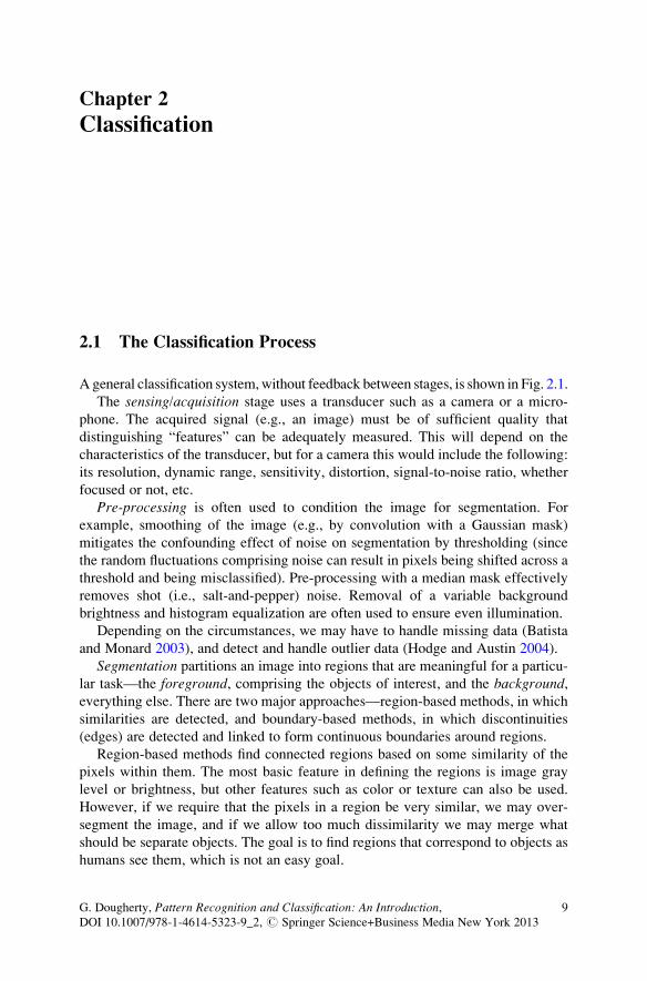
Ageneral classification system,without feedback between stages, is shown in Fig. 2.1.

The sensing/acquisition stage uses a transducer such as a camera or a micro-

phone. The acquired signal (e.g., an image) must be of sufficient quality that

distinguishing “features” can be adequately measured. This will depend on the

characteristics of the transducer, but for a camera this would include the following:

its resolution, dynamic range, sensitivity, distortion, signal-to-noise ratio, whether

focused or not, etc.

Pre-processing is often used to condition the image for segmentation. For

example, smoothing of the image (e.g., by convolution with a Gaussian mask)

mitigates the confounding effect of noise on segmentation by thresholding (since

the random fluctuations comprising noise can result in pixels being shifted across a

threshold and being misclassified). Pre-processing with a median mask effectively

removes shot (i.e., salt-and-pepper) noise. Removal of a variable background

brightness and histogram equalization are often used to ensure even illumination.

Depending on the circumstances, we may have to handle missing data (Batista

and Monard 2003), and detect and handle outlier data (Hodge and Austin 2004).

Segmentation partitions an image into regions that are meaningful for a particu-

lar task—the foreground, comprising the objects of interest, and the background,everything else. There are two major approaches—region-based methods, in which

similarities are detected, and boundary-based methods, in which discontinuities

(edges) are detected and linked to form continuous boundaries around regions.

Region-based methods find connected regions based on some similarity of the

pixels within them. The most basic feature in defining the regions is image gray

level or brightness, but other features such as color or texture can also be used.

However, if we require that the pixels in a region be very similar, we may over-

segment the image, and if we allow too much dissimilarity we may merge what

should be separate objects. The goal is to find regions that correspond to objects as

humans see them, which is not an easy goal.


9

Region-based methods include thresholding [either using a global or a locally

adaptive threshold; optimal thresholding (e.g., Otsu, isodata, or maximum entropy

thresholding)]. If this results in overlapping objects, thresholding of the distance

transform of the image or using the watershed algorithm can help to separate them.

Other region-based methods include region growing (a bottom-up approach using

“seed” pixels) and split-and-merge (a top-down quadtree-based approach).

Boundary-based methods tend to use either an edge detector (e.g., the Canny

detector) and edge linking to link any breaks in the edges, or boundary tracking to

form continuous boundaries. Alternatively, an active contour (or snake) can be

used; this is a controlled continuity contour which elastically snaps around and

encloses a target object by locking on to its edges.

Segmentation provides a simplified, binary image that separates objects of interest

(foreground) from the background, while retaining their shape and size for later

measurement. The foreground pixels are set to “1” (white), and the background pixels

set to “0” (black). It is often desirable to label the objects in the image with discrete

numbers. Connected components labeling scans the segmented, binary image and

groups its pixels into components based on pixel connectivity, i.e., all pixels in a

connected component share similar pixel values and are in some way connected with

each other. Once all groups have been determined, each pixel is labeled with a number

(1, 2, 3, . . .), according to the component to which it was assigned, and these numbers

can be looked up as gray levels or colors for display (Fig. 2.2).

One obvious result of labeling is that the objects in an image can be readily

counted. More generally, the labeled binary objects can be used tomask the originalimage to isolate each (grayscale) object but retain its original pixel values so that its

properties or features can be measured separately. Masking can be performed in

several different ways. The binary mask can be used in an overlay, or alpha channel,

in the display hardware to prevent pixels from being displayed. It is also possible to

use the mask to modify the stored image. This can be achieved either by multiplying

the grayscale image by the binary mask or by bit-wise ANDing the original image

with the binary mask. Isolating features, which can then be measured indepen-

dently, are the basis of region-of-interest (RoI) processing.Post-processing of the segmented image can be used to prepare it for feature

extraction. For example, partial objects can be removed from around the periphery

of the image (e.g., Fig. 2.2e), disconnected objects can be merged, objects smaller

or larger than certain limits can be removed, or holes in the objects or background

can be filled by morphological opening or closing.

Fig. 2.1 A general classification process

10 2 Classification

2.2 Features

The next stage is feature extraction. Features are characteristic properties of the

objects whose value should be similar for objects in a particular class, and different

from the values for objects in another class (or from the background). Features may

be continuous (i.e., with numerical values) or categorical (i.e., with labeled values).

Examples of continuous variables would be length, area, and texture. Categorical

features are either ordinal [where the order of the labeling is meaningful (e.g., class

standing, military rank, level of satisfaction)] or nominal [where the ordering is not

Fig. 2.2 (a) Original image, (b) variable background [from blurring (a)], (c) improved image

[¼(a) � (b)], (d) segmented image [Otsu thresholding of (c)], (e) partial objects removed from

(d), (f) labeled components image, (g) color-coded labeled components image

2.2 Features 11

meaningful (e.g., name, zip code, department)]. The choice of appropriate features

depends on the particular image and the application at hand. However, they should be:

• Robust (i.e., they should normally be invariant to translation, orientation (rota-

tion), scale, and illumination and well-designed features will be at least partially

invariant to the presence of noise and artifacts; this may require some pre-

processing of the image)

• Discriminating (i.e., the range of values for objects in different classes should bedifferent and preferably be well separated and non-overlapping)

• Reliable (i.e., all objects of the same class should have similar values)

• Independent (i.e., uncorrelated; as a counter-example, length and area are

correlated and it would be wasteful to consider both as separate features)

Features are higher level representations of structure and shape. Structural

features include:

• Measurements obtainable from the gray-level histogram of an object (using

region-of-interest processing), such as its mean pixel value (grayness or color)

and its standard deviation, its contrast, and its entropy

• The texture of an object, using either statistical moments of the gray-level

histogram of the object or its fractal dimension

Shape features include:

• The size or area, A, of an object, obtained directly from the number of pixels

comprising each object, and its perimeter, P (obtained from its chain code)

• Its circularity (a ratio of perimeter2 to area, or area to perimeter2 (or a scaled

version, such as 4pA/P2))

• Its aspect ratio (i.e., the ratio of the feret diameters, given by placing a bounding

box around the object)

• Its skeleton or medial axis transform, or points within it such as branch points

and end points, which can be obtained by counting the number of neighboring

pixels on the skeleton (viz., 3 and 1, respectively) (e.g., Fig. 2.3)

Fig. 2.3 (a) Image and (b) its skeleton (red), with its branch points (white) and end points (green)circled

12 2 Classification

• The Euler number: the number of connected components (i.e., objects) minus the

number of holes in the image

• Statisticalmoments of the boundary (1D) or area (2D): the (m, n)thmoment of a 2D

discrete function, f(x, y), such as a digital image withM � N pixels is defined as

mmn ¼XM

x¼1

XN

y¼1

xmynf ðx; yÞ (2.1)

where m00 is the sum of the pixels of an image: for a binary image, it is equal to its

area. The centroid, or center of gravity, of the image, (mx, my), is given by (m10/m00,

m01/m00). The central moments (viz., taken about the mean) are given by

mmn ¼XM

x¼1

XN

y¼1

ðx� mxÞmðy� myÞnf ðx; yÞ (2.2)

where m20 and m02 are the variances of x and y, respectively, and m02 is the

covariance between x and y. The covariance matrix, C or cov(x, y), is

C ¼ m20 m11m11 m02

� �(2.3)

from which shape features can be computed.

The reader should consider what features would separate out the nuts (some

face-on and some edge-on) and the bolts in Fig. 2.4.

A feature vector, x, is a vector containing the measured features, x1, x2, . . ., xn

Fig. 2.4 Image containing

nuts and bolts

2.2 Features 13

x ¼ x1x2__xn

(2.4)

for a particular object. The feature vectors can be plotted as points in feature space(Fig. 2.5). For n features, the feature space is n-dimensional with each feature

constituting a dimension.Objects from the sameclass should cluster together in feature

space (reliability), and be well separated from different classes (discriminating). In

classification, our goal is to assign each feature vector to one of the set of classes {oi}.

If the different features have different scales, it would be prudent to normalize

each by its standard deviation (Fig. 2.6).

Class 1

Feature 3

-2 -20

24

02

4-2

-1

0

1

2

3

4

5

Feature 1Feature 2

Class 2

Fig. 2.5 Three-dimensional feature space containing two classes of features, class 1 (in gray) andclass 2 (in black)

x2

-6

-6 -2.5-2

-1

00.5

-1.5

2

1

2.5

-0.5

1.5

-4

-2

0

2

4

6

-4 -2 0 2 4 6 8 -2 -1 0 1 2 3

x1

x1

var(x1)=

=var(x2)

x2

x’2

x’2x’1

x’1

Fig. 2.6 Scaling of features

14 2 Classification

The classification stage assigns objects to certain categories (or classes) based onthe feature information. How many features should we measure? And which are the

best? The problem is that the more we measure the higher is the dimension of

feature space, and the more complicated the classification will become (not to

mention the added requirements for computation time and storage). This is referred

to as the “curse of dimensionality.” In our search for a simple, yet efficient,

classifier we are frequently drawn to using the minimum number of “good” features

that will be sufficient to do the classification adequately (for which we need a

measure of the performance of the classifier) for a particular problem. This follows

the heuristic principle known traditionally as Occam’s razor (viz., the simplest

solution is the best) or referred to as KISS (Keep It Simple, Stupid) in more

contemporary language; while it may not be true in all situations, we will adopt a

natural bias towards simplicity.

The prudent approach is to err on the side of measuring more features per object

than that might be necessary, and then reduce the number of features by either (1)

feature selection—choosing the most informative subset of features, and removing

as many irrelevant and redundant features as possible (Yu and Liu 2004) or (2)

feature extraction—combining the existing feature set into a smaller set of new,

more informative features (Markovitch and Rosenstein 2002). The most well-

known feature extraction method is Principal Component Analysis (PCA), whichwe will consider fully in Chap. 6.

One paradigm for classification is the learning from examples approach. If a

sample of labeled objects (called the training set) is randomly selected, and their

feature vectors plotted in feature space, then it may be possible to build a classifier

which separates the two (or more) classes adequately using a decision boundary or

decision surface. A linear classifier results in a decision surface which is a hyper-

plane (Fig. 2.7). Again, the decision boundary should be as simple as possible,

consistent with doing an adequate job of classifying. The use of a labeled training

set, in which it is known to which class the sample objects belong, constitutes

supervised learning.

Fig. 2.7 Linear classification, using labeled training sets and two features, results in a linear

decision boundary

2.2 Features 15

http://dx.doi.org/10.1007/978-1-4614-5323-9_6

2.3 Training and Learning

A typical classification problem comprises the following task: given example (or

instance) objects typical of a number of classes (the training set), and classify otherobjects (the test set) into one of these classes. Features need to be identified such

that the in-class variations are less than the between-class variations.

If the classes to which the objects belong are known, the process is called

supervised learning, and if they are unknown, in which case the most appropriate

classes must be found, it is called unsupervised learning. With unsupervised

learning, the hope is to discover the unknown, but useful, classes of items (Jain

et al. 2000).

The process of using data to determine the best set of features for a classifier is

known as training the classifier. The most effective methods for training classifiers

involve learning from examples. A performance metric for a set of features, based

on the classification errors it produces, should be calculated in order to evaluate the

usefulness of the features.

Learning (aka machine learning or artificial intelligence) refers to some form of

adaptation of the classification algorithm to achieve a better response, i.e., to reduce

the classification error on a set of training data. This would involve feedback to

earlier steps in the process in an iterative manner until some desired level of

accuracy is achieved. Ideally this would result in a monotonically increasing

performance (Fig. 2.8), although this is often difficult to achieve.

In reinforcement learning (Barto and Sutton 1997), the output of the system is a

sequence of actions to best reach the goal. The machine learning program must

discover the best sequence of actions to take to yield the best reward. A robot

Fig. 2.8 Idealized learning curve

16 2 Classification

navigating in an environment in search of a particular location is an example of

reinforcement learning. After a number of trials, it should learn the correct

sequence of moves to reach the location as quickly as possible without hitting

any of the obstacles. A task may require multiple agents to interact to accomplish a

common goal, such as with a team of robots playing soccer.

2.4 Supervised Learning and Algorithm Selection

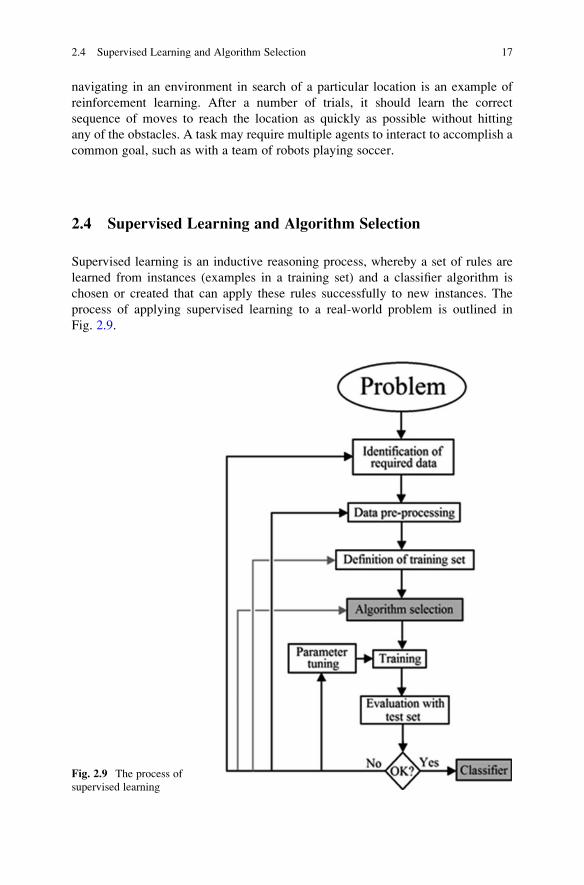
Supervised learning is an inductive reasoning process, whereby a set of rules are

learned from instances (examples in a training set) and a classifier algorithm is

chosen or created that can apply these rules successfully to new instances. The

process of applying supervised learning to a real-world problem is outlined in

Fig. 2.9.

Fig. 2.9 The process of

supervised learning

2.4 Supervised Learning and Algorithm Selection 17

The choice of which specific learning algorithm to use is a critical step. We

should choose an algorithm, apply it to a training set, and then evaluate it before

adopting it for general use. The evaluation is most often based on prediction

accuracy, i.e., the percentage of correct prediction divided by the total number of

predictions. There are at least three techniques which are used to calculate the

accuracy of a classifier

1. Split the training set by using two-thirds for training and the other third for

estimating performance.

2. Divide the training set into mutually exclusive and equal-sized subsets and for

each subset, train the classifier on the union of all the other subsets. The average

of the error rate of each subset is then an estimate of the error rate of the

classifier. This is known as cross-validation.3. Leave-one-out validation is a special case of cross-validation, with all test

subsets consisting of a single instance. This type of validation is, of course,

more expensive computationally, but useful when the most accurate estimate of

a classifier’s error rate is required.

We will consider ways to estimate the performance and accuracy of classifiers in

Chap. 8.

2.5 Approaches to Classification

There are a variety of approaches to classification:

1. Statistical approaches (Chaps. 4 and 5) are characterized by their reliance on an

explicit underlying probability model. The features are extracted from the

input data (object) and are used to assign each object (described by a feature

vector) to one of the labeled classes. The decision boundaries are determined

by the probability distributions of the objects belonging to each class, which

must either be specified or learned. A priori probabilities (i.e., probabilities

before measurement—described by probability density functions) are

converted into a posteriori (or class-/measurement-conditioned probabilities)

probabilities (i.e., probabilities after measurement). Bayesian networks (e.g.,

Jensen 1996) are the most well-known representative of statistical learning

algorithms.

In a discriminant analysis-based approach, a parametric form of the decision

boundary (e.g., linear or quadratic) is specified, and then the best decision

boundary of this form is found based on the classification of training objects.

Such boundaries can be constructed using, for example, a mean squared error

criterion.

In maximum entropy techniques, the overriding principle is that when

nothing is known, the distribution should be as uniform as possible, i.e., have

maximal entropy. Labeled training data are used to derive a set of constraints for

18 2 Classification

http://dx.doi.org/10.1007/978-1-4614-5323-9_8

http://dx.doi.org/10.1007/978-1-4614-5323-9_4

http://dx.doi.org/10.1007/978-1-4614-5323-9_5

the model that characterizes the class-specific expectations for the distribution

(Csiszar 1996).

Instance-based learning algorithms are lazy-learning algorithms (Mitchell

1997), so-called because they delay the induction or generalization process

until classification is performed. Lazy-learning algorithms (Aha 1998; De

Mantaras and Armengol 1998) require less computation time during the training

phase than eager-learning algorithms (such as Bayesian networks, decision trees,

or neural networks) but more computation time during the classification process.

One of the most straightforward instance-based learning algorithms is the

nearest neighbor algorithm.

The relationship between a number of statistical pattern recognition methods

is shown in Fig. 2.10. Moving from top to bottom and left to right, less

information is available and as a result, the difficulty of classification increases.

2. Nonmetric approaches (Chap. 3): decision trees, syntactic (or grammatical)

methods, and rule-based classifiers.

It is natural and intuitive to classify a pattern by asking a series of questions,

in which the next question depends on the answer to the previous question. This

approach is particularly useful for nonmetric (or categorical) data, because the

questions can be posed to elicit “yes/no” or “true/false” answers, although it can

also be used with quantitative data. The sequence of questions can be displayed

as a decision tree in the form of a tree structure (Fig. 2.11), which has decisionnodes that ask a question and have branches for each possible answer (outcome).

These are connected until we reach the terminal or leaf node which indicates theclassification.

In the case of complex patterns, a pattern can be viewed as a hierarchical

composite of simple sub-patterns which themselves are built from yet simpler

Class-ConditionalDensities

SupervisedLearning

UnsupervisedLearning

Bayes DecisionTheory

Known

Parametric ParametricNonparametric Nonparametric

“Optimal”Rules

Density-Based Approaches Geometric Approach

Plug-inRules

DecisionBoundaryConstruction(e.g., k-NN)

DensityEstimation

ArtificialNeuralNetworks

MixtureResolving

ClusterAnalysis

Unknown

Fig. 2.10 Various approaches in statistical pattern recognition

2.5 Approaches to Classification 19

http://dx.doi.org/10.1007/978-1-4614-5323-9_3

sub-patterns (Fu 1982). The simplest sub-patterns are called primitives, and the

complex pattern is represented in terms of relationships between these primitives

in a way similar to the syntax of a language. The primitives are viewed as a

language, and the patterns are sentences generated according to a certain gram-

mar (i.e., set of rules) that is inferred from the available training samples. This

approach is appealing in situations where patterns have a definite structure which

can be coded by a set of rules (e.g., ECG waveforms, texture in images).

However, difficulties in segmentation of noisy images to detect the primitives

and the inference of the grammar from training data often impede their imple-

mentation. The syntactic approach may yield a combinatorial explosion of

possibilities to be investigated, requiring large training sets and huge computa-

tional efforts (Perlovsky 1998).

3. Cognitive approaches, which include neural networks and support vector

machines (SVMs).

Neural networks are based on the organization of the human brain, where

nerve cells (neurons) are linked together by strands of fiber (axons). Neural

networks are massively parallel computing systems consisting of a huge number

of simple processors with many interconnections. They are able to learn com-

plex non-linear input–output relationships and use sequential training

procedures. However, in spite of the seemingly different underlying principles,

most of the neural network models are implicitly similar to statistical pattern

recognition methods (Anderson et al. 1990; Ripley 1993). It has been pointed out

(Anderson et al. 1990) that “neural networks are statistics for amateurs . . .Most

NNs conceal the statistics from the user”.

Support Vector Machines, SVMs (Cristianini and Shawe-Taylor 2000), rep-

resent the training examples as points in p-dimensional space, mapped so that the

examples of the data classes are separated by a (p � 1)-dimensional hyperplane,

which is chosen to maximize the “margins” on either side of the hyperplane

(Fig. 2.12).

Travel Cost/Km?

Gender?

Car Ownership?

Train

Car

ExpensiveStandard

Cheap

Male Female

10

Bus

Bus Train

Fig. 2.11 A decision tree (the decision nodes are colored blue, and the leaf nodes orange)

20 2 Classification

2.6 Examples

2.6.1 Classification by Shape

Figure 2.13a is an image containing both bolts and nuts, some of which lie on their

sides. We should be able to distinguish (and therefore classify) the objects on the

basis of their shape. The bolts are long, with an end piece, and the nuts either have a

hole in them (the “face-on” nuts) or are short and linear (the “end-on” nuts). In this

case, pre-processing was not required and automatic segmentation (using Otsu

thresholding) produces a simplified, binary image (Fig. 2.13b).

The skeleton of this image shows the essential shape differences between the

bolts and the two types of nut (Fig. 2.13c). A skeleton comprises pixels which

can be distinguished on the basis of their connectivity to other pixels on the

skeleton: end pixels (which have only one neighboring pixel on the skeleton), link

pixels (which have two neighbors), and branch pixels (which have three

neighbors). Because of their characteristic shape, only the skeletons of the

bolts will have branch pixels. If they are used as a seed image, and conditionallydilated under the condition that the seed image is constrained to remain within

the bounds of a mask image (the original binary image, Fig. 2.13b), then an image

of the bolts alone results (Fig. 2.13d). The nuts can now be obtained (Fig. 2.13e)

by logically combining this figure with the original binary figure (using

(Fig. 2.13b AND (NOT Fig. 2.13d)). The nuts and bolts can then be joined in a

color-coded image (Fig. 2.13f), which presents the nuts and bolts in different

pseudocolors.

Fig. 2.12 A linear SVM in

2D feature space. H1

separates the two classes with

a small margin, but H2

separates them with the

maximum margin (H3

doesn’t separate the two

classes at all)

2.6 Examples 21

2.6.2 Classification by Size

An alternative approach to separating the nuts and bolts involves measuring

different feature properties, such as the area, perimeter, or length. If we measure

the area of the labeled objects in the segmented image (Fig. 2.14a) by counting the

pixels belonging to each label and plot these values in one dimension (Fig. 2.14b),

then we can see that the nuts and bolts are well discriminated on the basis of area

with the bolts having larger areas. There are three clusters, comprising the bolts

with the highest areas, followed by the face-on nuts with intermediate areas, and the

edge-on nuts with the lowest areas. If the objects are then re-labeled with their area

values (Fig. 2.14c), that image (or the “area” feature) can be thresholded to show

just the bolts (Fig. 2.14d): in this particular case, a threshold of 800 (viz., an area of

800 pixels) would work well, although auto-thresholding, using either the isodata(Dubes and Jain 1976) or Otsu (Otsu 1979) algorithm, for example, is preferable

since that will preserve generality. The nuts can then be found by logically

combining this image with the segmented nuts-and-bolts image as before. Only

one feature (area) is used to discriminate the two classes, that is, the feature space

(Fig. 2.14b) is one-dimensional.

Fig. 2.13 (a) Original image, (b) after Otsu thresholding, (c) after subsequent skeletonization,

(d) after conditionally dilating the branch pixels from (c), (e) after logically combining (b) and (d),

(f) color coding the nuts and bolts

22 2 Classification

The two alternative measures, shape and size, could be tested for robustness on

other images of nuts and bolts to see which performs better.

2.6.3 More Examples

Figure 2.15a is an image containing a number of electronic components, of different

shapes and sizes (the transistors are three-legged, the thyristors are three-legged

with a hole in them, the electrolytic capacitors have a round body with two legs, and

the ceramic capacitors are larger than the resistors). A combination of the shape and

size methods can be used to separate the objects into their different classes

(Fig. 2.15b).

Similar techniques havebeen used to classify the fruit in Fig. 2.16 into three different

classes. Think about the features that would be most discriminating in this case.

a

c

b

d

2000

0.10.20.30.40.50.60.70.80.9

1

400 600 800 1000 1200 1400

Fig. 2.14 (a) Segmented, labeled image (using Fig. 2.13a), (b) one-dimensional feature space

showing the areas of the features, (c) the features “painted” with grayscales representing their

measured areas, and (d) after thresholding image (c) at a value of 800

2.6 Examples 23

Circularity can distinguish the bananas from the other two fruit: size (or, perhaps

texture, but not color in this grayscale image) could be used to distinguish the apples

from the grapefruit. The single-pixel outlines of the fruit can be obtained from

subtracting the segmented image from a dilated version of itself, and colored outlines

have then been overlaid on the original image.

Fig. 2.15 (a) Electronic components (b) classified according to type, using shape and size

Fig. 2.16 Objects have been classified into three classes of fruit, and outlines superimposed on the

original image

24 2 Classification

2.6.4 Classification of Letters

In Fig. 2.17a the letters A through E appear in different fonts, orientations and sizes,

but are distinguished by shape factors (Euler number, aspect ratio, and circularity)

which are invariant to size, position, and orientation. These can be used to classify

the letters and color code them (Fig. 2.17b). This is an example of a decision tree

(Fig. 2.17c), with three levels. It is important to design the system so that the most

easily measured features are used first, to minimize the time for the overall

identification (see Chap. 3). The decision values of the features for each letter

were determined experimentally, by measuring several examples of each letter.

One of the disadvantages to such systems is that the addition of another class

(e.g., the letter F) does not simply add another step to the process, but may

completely reshuffle the order in which the rules are applied, or even replace

some of the rules with others.

2.7 Exercises

1. Discuss the invariance of shape features to translation, rotation, scaling, noise,

and illumination. Illustrate your answer with specific examples of features.

2. Explain the following terms (1) a pattern, (2) a class, (3) a classifier, (4) feature

space, (5) a decision rule, and (6) a decision boundary.

3. What is a training set? How is it chosen? What influences its desired size?

4. There are two cookie jars: jar 1 contains two chocolate chip cookies and three plain

cookies, and jar 2 contains one chocolate chip cookie and one plain cookie. Blind-

folded Fred chooses a jar at randomand then a cookie at random from that jar.What

is the probability of him getting a chocolate chip cookie? (Hint: use a decision tree).

Fig. 2.17 (a) Letters A through E (b) shape factors used to classify them and (c) the resulting

color-coded image

2.7 Exercises 25

http://dx.doi.org/10.1007/978-1-4614-5323-9_3

References

Aha, D.: Feature weighting for lazy learning algorithms. In: Liu, H., Motoda, H. (eds.) Feature

Extraction, Construction and Selection: A Data Mining Perspective, pp. 13–32. Kluwer,

Norwell, MA (1998)

Anderson, J., Pellionisz, A., Rosenfeld, E.: Neurocomputing 2: Directions for Research. MIT,

Cambridge, MA (1990)

Barto, A.G., Sutton, R.S.: Reinforcement learning in artificial intelligence. In: Donahue, J.W.,

Packard Dorsal, V. (eds.) Neural Network Models of Cognition, pp. 358–386. Elsevier,

Amsterdam (1997)

Batista, G., Monard, M.: An analysis of four missing data treatment methods for supervised

learning. Appl. Artif. Intell. 17, 519–533 (2003)

Cristianini, N., Shawe-Taylor, J.: An Introduction to Support Vector Machines. Cambridge

University Press, Cambridge (2000)

Csiszar, I.: Maxent, mathematics, and information theory. In: Hanson, K.M., Silver, R.N. (eds.)

Maximum Entropy and Bayesian Methods, pp. 35–50. Kluwer, Norwell, MA (1996)

De Mantaras, R.L., Armengol, E.: Machine learning from examples: inductive and lazy methods.

Data Knowl. Eng. 25, 99–123 (1998)

Dubes, R.C., Jain, A.K.: Clustering techniques: the user’s dilemma. Pattern Recognit. 8, 247–290

(1976)

Fu, K.S.: Syntactic Pattern Recognition and Applications. Prentice-Hall, Englewood Cliffs (1982)

Hodge, V.J., Austin, J.: A survey of outlier detection methodologies. Artif. Intell. Rev. 22, 85–126

(2004)

Jain, A.K., Duin, R.P.W., Mao, J.: Statistical pattern recognition: a review. IEEE Trans. Pattern

Anal. Mach. Intell. 33, 1475–1485 (2000)

Jensen, F.V.: An Introduction to Bayesian Networks. UCL Press, London (1996)

Markovitch, S., Rosenstein, D.: Feature generation using general constructor functions. Mach.

Learn. 49, 59–98 (2002)

Mitchell, T.: Machine Learning. McGraw Hill, New York (1997)

Otsu, N.: A threshold selection method from gray-level histograms. IEEE Trans. Syst. Man

Cybern. SMC-9, 62–66 (1979)

Perlovsky, L.I.: Conundrum of combinatorial complexity. IEEE Trans. Pattern Anal. Mach. Intell.

20, 666–670 (1998)

Ripley, B.: Statistical aspects of neural networks. In: Bornndorff-Nielsen, U., Jensen, J., Kendal,

W. (eds.) Networks and Chaos - Statistical and Probabilistic Aspects, pp. 40–123. Chapman

and Hall, London (1993)

Yu, L., Liu, H.: Efficient feature selection via analysis of relevance and redundancy. J. Mach.

Learn. Res. 5, 1205–1224 (2004)

26 2 Classification

Chapter 3

Nonmetric Methods

3.1 Introduction

With nonmetric (i.e., categorical) data, we have lists of attributes as features rather

than real numbers. For example, a fruit may be described as {(color¼) red,

(texture¼), shiny, (taste¼) sweet, (size¼) large} or a segment of DNA as a

sequence of base pairs, such as “GACTTAGATTCCA.” These are discrete data,

and they are conveniently addressed by decision trees, rule-based classifiers, and

syntactic (grammar-based) methods.

3.2 Decision Tree Classifier

A decision tree is a simple classifier in the form of a hierarchical tree structure,

which performs supervised classification using a divide-and-conquer strategy. It

comprises a directed branching structure with a series of questions (Fig. 3.1), like

the Twenty Questions game. The questions are placed at decision nodes; each tests

the value of a particular attribute (feature) of the pattern (object) and provides a

binary or multi-way split. The starting node is known as the root node, which is

considered the parent of every other node. The branches correspond to the possible

answers. Successive decision nodes are visited until a terminal or leaf node is

reached, where the class (category) is read (assigned). (The decision tree is an

upside-down tree, with the root at the top and the leaves at the bottom!). Classifica-

tion is performed by routing from the root node until arriving at a leaf node. The tree

structure is not fixed a priori but the tree grows and branches during learning

depending on the complexity of the problem.

Figure 3.2 is an example of a three-level decision tree, used to decide what to do

on a Saturday morning. Suppose, for example, that our parents haven’t turned up

and the sun is shining; the decision tree tells us to go off and play tennis. Note that

the decision tree covers all eventualities: there are no values that the weather, our


27

parents turning up or not, and our financial situation can take which aren’t catered

for in the decision tree.

Decision trees are more general than representations of decision-making pro-

cesses. By rephrasing the questions, they can be applied to classification problems.

An advantage of the decision tree classifier is that it can be used with nonmetric/

categorical data, including nominal data with no natural ordering (although it can

also be adapted to use quantitative data). Another benefit is its clear interpretability,

providing a natural way to incorporate prior knowledge (and it is straightforward to

convert the tests into logical expressions). Decision trees, once constructed, are

very fast since they require very little computation.

Fig. 3.1 A (two-level)

decision tree for determining

whether to play tennis. We

have used elliptical shapes forthe decision nodes (including

the root node) and

rectangular shapes for theleaf nodes

Fig. 3.2 A three-level

decision tree for determining

what to do on a Saturday

morning

28 3 Nonmetric Methods

The decision tree is easy to use; the more interesting question is how to construct

the tree from training data (records), after having chosen a set of discriminating

features. In principle, there are exponentially many decision trees that can be

constructed from a given set of features. While some of the trees will be more

accurate than others, finding the optimal tree is not computationally feasible.

Nevertheless, a number of efficient algorithms have been developed to create or

“grow” a reasonably accurate, albeit suboptimal, decision tree in a reasonable

amount of time. These algorithms usually employ a greedy strategy that grows

the tree using the most informative attribute (feature) at each step and does not

allow backtracking. The most informative attribute will be the one which splits the

set arriving at the node into the most homogeneous subsets.

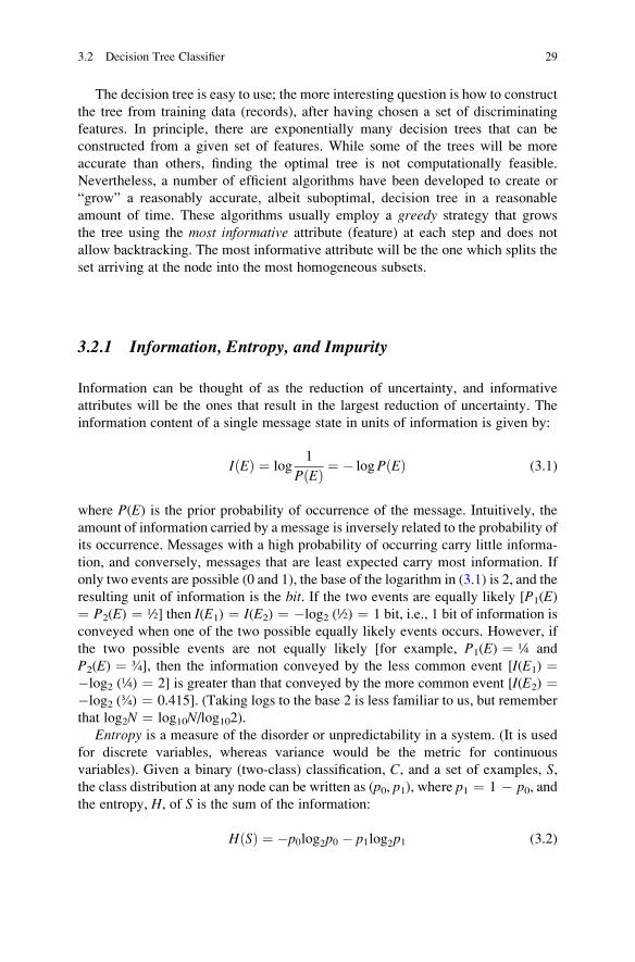
3.2.1 Information, Entropy, and Impurity

Information can be thought of as the reduction of uncertainty, and informative

attributes will be the ones that result in the largest reduction of uncertainty. The

information content of a single message state in units of information is given by:

IðEÞ ¼ log1

PðEÞ ¼ � logPðEÞ (3.1)

where P(E) is the prior probability of occurrence of the message. Intuitively, the

amount of information carried by a message is inversely related to the probability of

its occurrence. Messages with a high probability of occurring carry little informa-

tion, and conversely, messages that are least expected carry most information. If

only two events are possible (0 and 1), the base of the logarithm in (3.1) is 2, and the

resulting unit of information is the bit. If the two events are equally likely [P1(E)¼ P2(E) ¼ ½] then I(E1) ¼ I(E2) ¼ �log2 (½) ¼ 1 bit, i.e., 1 bit of information is

conveyed when one of the two possible equally likely events occurs. However, if

the two possible events are not equally likely [for example, P1(E) ¼ ¼ and

P2(E) ¼ ¾], then the information conveyed by the less common event [I(E1) ¼�log2 (¼) ¼ 2] is greater than that conveyed by the more common event [I(E2) ¼�log2 (¾) ¼ 0.415]. (Taking logs to the base 2 is less familiar to us, but remember

that log2N ¼ log10N/log102).Entropy is a measure of the disorder or unpredictability in a system. (It is used

for discrete variables, whereas variance would be the metric for continuous

variables). Given a binary (two-class) classification, C, and a set of examples, S,the class distribution at any node can be written as (p0, p1), where p1 ¼ 1 � p0, andthe entropy, H, of S is the sum of the information:

HðSÞ ¼ �p0log2p0 � p1log2p1 (3.2)

3.2 Decision Tree Classifier 29

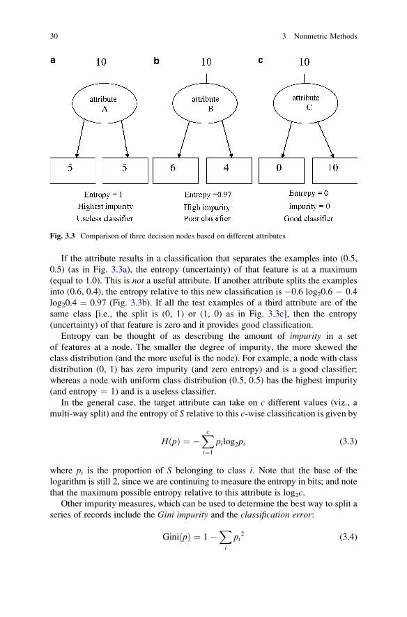
If the attribute results in a classification that separates the examples into (0.5,

0.5) (as in Fig. 3.3a), the entropy (uncertainty) of that feature is at a maximum

(equal to 1.0). This is not a useful attribute. If another attribute splits the examples

into (0.6, 0.4), the entropy relative to this new classification is �0.6 log20.6 � 0.4

log20.4 ¼ 0.97 (Fig. 3.3b). If all the test examples of a third attribute are of the

same class [i.e., the split is (0, 1) or (1, 0) as in Fig. 3.3c], then the entropy

(uncertainty) of that feature is zero and it provides good classification.

Entropy can be thought of as describing the amount of impurity in a set

of features at a node. The smaller the degree of impurity, the more skewed the

class distribution (and the more useful is the node). For example, a node with class

distribution (0, 1) has zero impurity (and zero entropy) and is a good classifier;

whereas a node with uniform class distribution (0.5, 0.5) has the highest impurity

(and entropy ¼ 1) and is a useless classifier.

In the general case, the target attribute can take on c different values (viz., a

multi-way split) and the entropy of S relative to this c-wise classification is given by

HðpÞ ¼ �Xc

i¼1

pilog2pi (3.3)

where pi is the proportion of S belonging to class i. Note that the base of the

logarithm is still 2, since we are continuing to measure the entropy in bits; and note

that the maximum possible entropy relative to this attribute is log2c.Other impurity measures, which can be used to determine the best way to split a

series of records include the Gini impurity and the classification error:

GiniðpÞ ¼ 1�X

i

pi2 (3.4)

Fig. 3.3 Comparison of three decision nodes based on different attributes


classification errorðpÞ ¼ 1�maxðpiÞ (3.5)

(the Gini impurity is actually the expected error rate if the class label is selected

randomly from the class distribution present).

The values of these impurity measures for binary classification are shown in

Fig. 3.4. All three measures attain a maximum value for a uniform distribution

(p ¼ 0.5), and a minimum when all the examples belong to the same class (p ¼ 0

or 1). A disadvantage of the classification error is that it has a discontinuous

derivative, which may be a problem when searching for an optimal decision over a

continuous parameter space.

3.2.2 Information Gain

We now return to the problem of trying to determine the best attribute to choose for

each decision node of the tree. The decision mode will receive a mixed bag of

instances, and the best attribute will be the one that best separates them into

homogeneous subsets (Fig. 3.5). The measure we will use is the gain, which is

the expected reduction in impurity caused by partitioning the examples according to

this attribute. More precisely, the gain, Gain(S, A), of an attribute A, relative to a

collection of samples S, is defined as:

Fig. 3.4 Impurity measures for binary classification


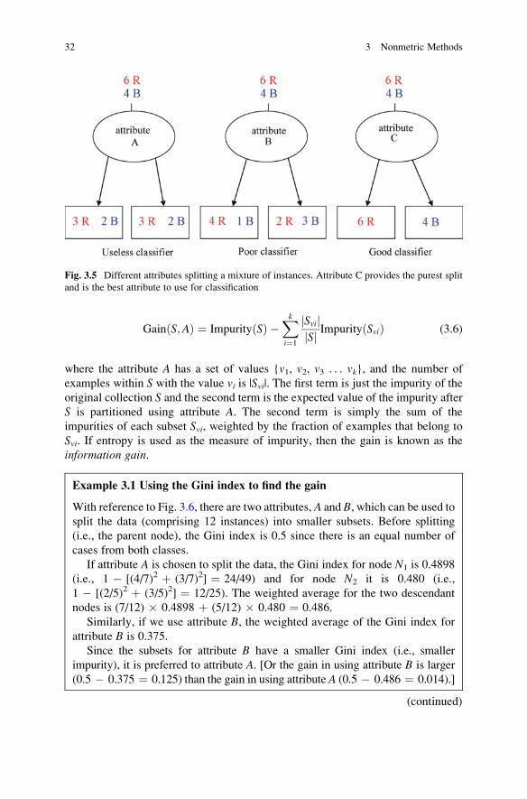
GainðS;AÞ ¼ ImpurityðSÞ �Xk

i¼1

Svij jSj j ImpurityðSviÞ (3.6)

where the attribute A has a set of values {v1, v2, v3 . . . vk}, and the number of

examples within S with the value vi is |Svi|. The first term is just the impurity of the

original collection S and the second term is the expected value of the impurity after

S is partitioned using attribute A. The second term is simply the sum of the

impurities of each subset Svi, weighted by the fraction of examples that belong to

Svi. If entropy is used as the measure of impurity, then the gain is known as the

information gain.

Example 3.1 Using the Gini index to find the gain

With reference to Fig. 3.6, there are two attributes, A and B, which can be used tosplit the data (comprising 12 instances) into smaller subsets. Before splitting

(i.e., the parent node), the Gini index is 0.5 since there is an equal number of

cases from both classes.

If attribute A is chosen to split the data, the Gini index for node N1 is 0.4898

(i.e., 1 � [(4/7)2 þ (3/7)2] ¼ 24/49) and for node N2 it is 0.480 (i.e.,

1 � [(2/5)2 þ (3/5)2] ¼ 12/25). The weighted average for the two descendant

nodes is (7/12) � 0.4898 þ (5/12) � 0.480 ¼ 0.486.

Similarly, if we use attribute B, the weighted average of the Gini index for

attribute B is 0.375.

Since the subsets for attribute B have a smaller Gini index (i.e., smaller

impurity), it is preferred to attribute A. [Or the gain in using attribute B is larger

(0.5 � 0.375 ¼ 0.125) than the gain in using attribute A (0.5 � 0.486 ¼ 0.014).]

(continued)

Fig. 3.5 Different attributes splitting a mixture of instances. Attribute C provides the purest split

and is the best attribute to use for classification


(continued)

Fig. 3.6 Splitting binary attributes

This basic algorithm, the ID3 algorithm (Quinlan 1986), employs a top-down,

greedy search through the space of possible decision trees. (The name ID3 was

given because it was the third in a series of “interactive dichotomizer” procedures.)

Example 3.2 Using the ID3 algorithm to build a decision tree.

Suppose we want to train a decision tree using the examples (instances) in

Table 3.1.

Table 3.1 Examples of decisions made over the past ten weekends

Examples Weather Parents visiting? Money Decision (category)

1 Sunny Yes Rich Cinema

2 Sunny No Rich Tennis

3 Windy Yes Rich Cinema

4 Rainy Yes Poor Cinema

5 Rainy No Rich Stay in

6 Rainy Yes Poor Cinema

7 Windy No Poor Cinema

8 Windy No Rich Shopping

9 Windy Yes Rich Cinema

10 Sunny No Rich Tennis

(continued)


(continued)

The first thing is to find the attribute for the root node. To do this, we need to

calculate the entropy, H(S), before any splitting. Using (3.3), this comes to

S ¼ 1.571 [viz., �0.6 log20.6 � 0.2 log20.2 � 2 � (0.1 log20.1)].

Then we need to determine the values of Gain(S, parents), Gain(S, weather),and Gain(S, money), using (3.6):

GainðS; parentsÞ ¼ 1:571� ð Syes�� =10Þ � EntropyðSyesÞ � ð Snoj j=10Þ

� EntropyðSnoÞ ¼ 1:571� ð0:5Þ � 0� ð0:5Þ � ð1:922Þ ¼ 0:61

If “parents coming?” is the node, then five instances will go down the “Yes”

branch (and then will all be class “cinema,” with an entropy of zero: this would

be a terminal node) and five will go down the “No” branch [and they will

comprise two “tennis,” one “stay-in,” one “cinema,” and one “shopping”: the

entropy of this node is �0.4 log20.4 � 3�(0.2 log20.2), which is 1.922].

GainðS;weatherÞ ¼ 1:571� ð Ssunj j=10Þ � EntropyðSsunÞ � ð Swindj j=10Þ� EntropyðSwindÞ � ð Srainj j=10Þ � EntropyðSrainÞ

¼ 1:571� ð0:3Þ � ð0:918Þ � ð0:4Þ � ð0:8113Þ � ð0:3Þ� ð0:918Þ ¼ 0:70

GainðS;moneyÞ ¼ 1:571� ð Srichj j=10Þ � EntropyðSrichÞ� ð Spoor

�� =10Þ � EntropyðSpoorÞ¼ 1:571� ð0:7Þ � ð1:842Þ � ð0:3Þ � 0 ¼ 0:2816

This means that the weather attribute, with its three branches, should be the

first (root) node (Fig. 3.7a).

Now we look at the branches. For the sunny branch, Ssunny ¼ {1, 2, 10}.

Since the classes (cinema, tennis, and tennis respectively) are not the same, we

will need another decision node here (Fig. 3.7b). The same situation occurs for

the other two branches (where Swindy ¼ {3, 7, 8, 9}, and Srainy ¼ {4, 5, 6}).

Returning to the sunny branch, we are only interested in the three examples

{1, 2, 10} and we set S to be Ssunny, from which H(S) turns out to be 0.918 (viz.,�0.1 log20.1 � 0.2 log20.2), since two examples end up together (as “tennis”)

and one ends up on its own (as “cinema”). We now need to calculate Gain

(Ssunny, parents) and Gain(Ssunny, money):

GainðSsunny; parentsÞ ¼ 0:918� ð Syes�� =jSjÞ � EntropyðSyesÞ � ð Snoj j=jSjÞ

� EntropyðSnoÞ¼ 0:918� ð1=3Þ � 0� ð2=3Þ � 0 ¼ 0:918

(continued)


(continued)

Gain ðSsunny;moneyÞ ¼ 0:918� ð Srichj j=jSjÞ � EntropyðSrichÞ� ð Spoor

�� =jSjÞ � EntropyðSpoorÞ¼ 0:918� ð3=3Þ � 0:918� ð0=3Þ � 0 ¼ 0

Note that Entropy(Syes) and Entropy(Sno) are both zero, because both Syes andSno contain examples which are all in the same category (cinema and tennis,

respectively). Hence, the parents attribute should be chosen next. It has two

branches for “Yes” and “No”: the “Yes” branch contains a single example {1},

and the “No” branch contains two examples, {2, 10} which are in the same class.

Hence both these branches end at leaf nodes (Fig. 3.7c).

The rest of the tree is left as an exercise for the reader!

Fig. 3.7 Stages in building a decision tree

3.2.3 Decision Tree Issues

There are a number of issues arising with decision trees

• Decision trees partition feature space into disjoint regions,with decision boundaries

that are rectilinear and parallel to the feature axes (Fig. 3.8).

Oblique decision trees can be used to overcome this limitation by using test

conditions such as w11x1 þ w12x2 þ w10 > 0, where x1 and x2 are the features,

w11 and w12 are weights, and w10 is a bias or threshold value (Fig. 3.9).

The decision tree is now a linear, multivariate tree. If these test conditions occurnear the top of the tree, and the training set is large, then training can be slow.

• When should we stop splitting during training? If we continue splitting too far,

the data will be overfit. In the extreme, each terminal (or leaf) node will

correspond to a single training point and the full tree is merely a look-up table,

which cannot be expected to generalize well to (noisy) test data. Conversely, if

splitting is stopped too early, then the error on the training data is not sufficiently

low and performance with test data will suffer.


The training and test error rates are large when the tree is very small. This

situation is known as underfitting: the model has yet to learn the true structure of the

data. As the number of nodes in the tree increases, it will have fewer training and

test errors (Fig. 3.10). However, once the tree becomes large, its test error rate

begins to increase even though its training error rate continues to fall. This is known

as overfitting, where the tree contains some nodes that accidentally fit noisy points

in the training data but do not generalize to the test data.

One way to decide when to stop splitting is by using validation or cross-validation. In validation, the tree is trained using a subset of the data (e.g., 90%)

with the remaining (10%) kept as a validation set. We continue splitting until the

error in the validation set is minimized. (In cross-validation several independently

chosen subsets are used.)

Fig. 3.8 (a) A decision tree and (b) the resulting decision boundaries in feature space

Fig. 3.9 (a) An oblique decision tree and (b) the resulting decision boundary in feature space


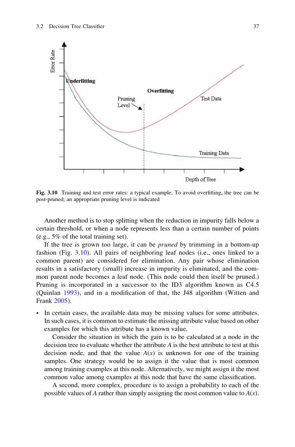
Another method is to stop splitting when the reduction in impurity falls below a

certain threshold, or when a node represents less than a certain number of points

(e.g., 5% of the total training set).

If the tree is grown too large, it can be pruned by trimming in a bottom-up

fashion (Fig. 3.10). All pairs of neighboring leaf nodes (i.e., ones linked to a

common parent) are considered for elimination. Any pair whose elimination

results in a satisfactory (small) increase in impurity is eliminated, and the com-

mon parent node becomes a leaf node. (This node could then itself be pruned.)

Pruning is incorporated in a successor to the ID3 algorithm known as C4.5

(Quinlan 1993), and in a modification of that, the J48 algorithm (Witten and

Frank 2005).

• In certain cases, the available data may be missing values for some attributes.

In such cases, it is common to estimate the missing attribute value based on other

examples for which this attribute has a known value.

Consider the situation in which the gain is to be calculated at a node in the

decision tree to evaluate whether the attribute A is the best attribute to test at this

decision node, and that the value A(x) is unknown for one of the training

samples. One strategy would be to assign it the value that is most common

among training examples at this node. Alternatively, we might assign it the most

common value among examples at this node that have the same classification.

A second, more complex, procedure is to assign a probability to each of the

possible values of A rather than simply assigning the most common value to A(x).

Fig. 3.10 Training and test error rates: a typical example. To avoid overfitting, the tree can be

post-pruned; an appropriate pruning level is indicated


These probabilities can be estimated again based on the observed frequencies of

the various values for A among the examples at the particular node. For

example, given a Boolean attribute A, if the node contains six known examples

with A ¼ 1 and four with A ¼ 0, then we would say the probability that A(x) ¼ 1 is 0.6, and the probability that A(x) ¼ 0 is 0.4. A fractional 0.6 of

instance x is now distributed down the branch for A ¼ 1 and a fractional 0.4 of xdown the other tree branch. These fractional examples are used for the purpose

of computing the gain and can be further subdivided at subsequent branches of

the tree if a second missing attribute value must be tested. This same fractioning

of examples can also be applied after learning to classify new instances whose

attribute values are unknown. In this case, the classification of the new instance

is simply the most probable classification, computed by summing the weights of

the instance fragments classified in different ways at the leaf nodes of the tree.

This method for handling missing attribute values is incorporated in the C4.5

(Quinlan 1993) and J48 (Witten and Frank 2005) algorithms.

• When comparing binary splits with multi-way splits, the multi-way split is

inherently favored. To avoid this, the gains should be normalized by dividing

by �S pi log2 pi (summed over the number of splits, k): if each attribute has the

same number of cases, then pi ¼ 1/k and the normalizing factor is log2 k. With

multi-way splits, it is important to ensure that there are sufficient numbers of

cases associated with each choice in order to make reliable predictions.

• With binary splits of continuous data, we have to decide the best value of the

threshold at which the split is to occur, i.e., the threshold value that produces

the greatest information gain. This could be achieved by histogramming the

data (in which case a bin width has to be chosen), computing the Gini index

for all the possible splits, and choosing the split that produces the smallest

Gini index.

3.2.4 Strengths and Weaknesses

Decision trees are easy to understand, do not require much computation when

performing classification, and provide a clear indication of which attributes (fields)

are most important. They are most useful for categorical data but can be adapted to

handle continuous data.

On the other hand, they are prone to errors when there are many classes and a

relatively small number of training examples. They can be computationally expen-

sive to train, and pruning is also computationally expensive. They tend to give

rectangular decision regions, unless more computationally expensive strategies

are used.


3.3 Rule-Based Classifier

In problems where classes can be characterized by general relationships, rather than

just by examples (instances), it becomes attractive to build classifiers based on

rules. Humans generally like explanations for most decisions, and sometimes there

are legal and ethical requirements for this (e.g., rejection of a credit card applica-

tion, medical diagnosis).

It is possible to extract rules from a decision tree. Each path from root to a leaf

can be written down as a series of IF. . .THEN rules. For example, the left-most path

in Fig. 3.1 would lead to the rule IF (outlook ¼ sunny) AND (humidity ¼ high)

THEN do not play tennis. When more than one leaf is labeled with the same class,

then the paths can be combined with a logical OR. It may be possible to prune the

resulting rules, although they may not be able to be written back as a tree after that.

Another way is to learn the rules directly from the data. Such rule induction is

similar to decision tree induction except that rule induction does a depth-first search

and generates one rule (path) at a time, whereas tree induction goes breadth-first and

generates all paths simultaneously.

Rules are learned one at a time. Each rule is a combination of conditions, which

are added one at a time to minimize some criterion (such as entropy). Once a rule is

grown and pruned, it is added to the rule base and all the training examples covered

by that rule are removed from the training set: and the process continues until enough

rules are generated. There is an outer loop of adding one rule at a time to the rule base

and an inner loop of adding one condition at a time to the current rule. Both steps are

greedy, and do not guarantee optimality; and both loops incorporate pruning for

better generalization. An example of a rule-induction algorithm is Ripper (Cohen1995), which is based on an earlier algorithm Irep (Furnkranz andWidmer 1994). It

is well suited for handling datasets with imbalanced class distributions.

Rule-based classifiers give comparable performance to the decision tree classifier.

They create rectilinear partitions similar to those created by (non-oblique) decision

trees. Nevertheless, if the rule-based classifier allows multiple rules to be triggered for

a given example, then a more complex decision boundary can be constructed.

3.4 Other Methods

Ordered sequences or strings of discrete items, as in a sequence of letters in an English

word or aDNAsequence, such as “AGCTTGGCATC” (whereA,G,C, andT stand for

the nucleic acids adenine, guanine, cytosine, and thymine, respectively), are nominal

elements. The strings can be of different lengths and there is no obvious distance

metric. String matching involves finding whether a sub-string appears in a string for aparticular shift of characters. An edit distance, based on the nearest neighbor distance(Chap. 5), can be invoked to measure the similarity or difference between two strings.

Such an edit distance describes how many fundamental operations (substitution,

insertion, or deletion of a character) are required to transform one string into another.

3.4 Other Methods 39

http://dx.doi.org/10.1007/978-1-4614-5323-9_5

For example, the string x ¼ “excused” can be transformed into the string y ¼ “

exhausted” using one substitution and two insertions (Fig. 3.11). If these operations

are equally costly, then the edit distance is 3.

The sequence of characters may be generated according to particular structural

rules, viz., grammar. An example would be valid telephone numbers, with interna-

tional, national, and local codes. Often this structure is hierarchical, with “noun”

and “verb” phrases. Grammatical methods can be used to provide constraints and

improve accuracy. For example, an optical character recognition (OCR) system that

recognizes and interprets mathematical equations based on a scanned pixel image

can have particular “slots” which can be filled by only a limited set of symbols.

The string generated by a set of rules is referred to as a sentence; and the rules arespecified by a grammar. In pattern recognition, we are given a sentence and a

grammar and seek to determine whether the sentence was generated by the gram-

mar. The general process is known as parsing. Many parsing methods depend on

the model underlying the grammar. One popular such model is finite-statemachines.

3.5 Exercises

1. Suppose that the probability of five events are P(1) ¼ 0.5, and P(2) ¼ P(3) ¼P (4)¼ P(5) ¼ 0.125. Calculate the entropy. Explain in words what this means.

2. Three binary nodes, N1, N2, and N3, split examples into (0, 6), (1,5), and (3,3),

respectively. For each node, calculate its entropy, Gini impurity, and classifica-

tion error.

3. Build a decision tree that computes the logical AND function.

4. Imagine that there are four things that you like to do in the evening: going to a

pub, watching TV, going to a party, or studying (!). The choice is sometimes

made for you—if you have an assignment due the next day, you need to study, if

you’re feeling lazy then the pub isn’t for you, and if there isn’t a party then you

can’t go to it. You are looking for a decision tree which will help you decide what

to do each evening. Here is a list of everything you’ve done in the past 10 days.

Fig. 3.11 The edit distance calculation for strings x and y can be illustrated in a table. (A grayarrow indicates no change. A black diagonal arrow indicates substitution, and a black horizontalarrow an insertion)


Deadline? Is there a party? Lazy? Activity

Urgent Yes Yes Party

Urgent No Yes Study

Near Yes Yes Party

None Yes No Party

None No Yes Pub

None Yes No Party

Near No No Study

Near No Yes TV

Near Yes Yes Party

Urgent No No Study

(The first thing to do is to work out which feature to use as the starting (root)

node. For this you need to compute the entropy, and then find out which feature

has the maximal information gain).

5. Write out the steps in the ID3 algorithm in pseudo code.

6. Consider the training data from the alphabet A ¼ {a, b, c}:

o1 o2 o3aabbc Bccba caaaa

ababcc Bbbca cbcaab

babbcc cbbaaaa baaca

Use the edit distance to classify each of the following strings [if there are

ambiguities in the classification, state which two (or all three) categories are

candidates]: “abacc,” “abca,” “ccbba,” “bbaaac”

References

Cohen, W.: Fast effective rule induction. In: Prieditis, A., Russell, S.J. (eds.) Twelfth International

Conference on Machine Learning, pp. 115–123. Morgan Kaufmann, San Mateo, CA (1995)

Furnkranz, J., Widmer, G.: Incremental reduced error pruning. In: Cohen, W., Hirsch, H. (eds.)

Eleventh International Conference on Machine Learning, pp. 70–77. Morgan Kaufmann, San

Mateo, CA (1994)

Quinlan, J.R.: Induction of decision trees. Mach. Learn. 1, 81–106 (1986)

Quinlan, J.R.: C4.5: Programs for Machine Learning. Morgan Kaufmann, San Mateo, CA (1993)

Witten, I.H., Frank, E.: Data Mining: Practical Machine Learning Tools and Techniques. Morgan

Kaufmann, San Mateo, CA (2005)

References 41

Chapter 4

Statistical Pattern Recognition

4.1 Measured Data and Measurement Errors

It is unrealistic to expect that data will be perfect. There may be problems related to

human error (e.g., transcription errors), limitations of the measuring sensors (e.g.,

limited resolution), or flaws in the data collection process (e.g., missing values).

Measured data comes with a margin of error or uncertainty. The term measure-ment error refers to any problem resulting from the measurement process. In

statistics and experimental sciences, this error is measured by precision (repeatabil-ity or random error—the closeness of repeated measurements of the same feature to

one another) and accuracy (systematic error—a fixed bias in all the measurements),

as shown in Fig. 4.1. Data may be subject to various amounts of one or both of these

types of errors, as illustrated by darts around a bull’s eye (Fig. 4.2).

Probability theory helps us to model random error and is therefore a solid basis

for classifier design [Systematic error requires that the actual (true) values are

known by some external means].

4.2 Probability Theory

4.2.1 Simple Probability Theory

If A, B, C, . . . are events, the probability of these events can be denoted by a real

number between 0 and 1, viz., P(A), P(B), P(C), . . . (The probability is linked to therelative frequency of that event happening, i.e., an experiment is observed a large

number of times (N), and if event A occurs M times then P(A) ¼ M/N).A Venn diagram can be used to illustrate these events, where the whole area

represents the sample space, S (the set of all possible outcomes). If A and B are


43

mutually exclusive (i.e., they cannot occur simultaneously) they are shown as

in Fig. 4.3a. The probability that either A or B occur is denoted by P(A or B)(or P(A[B)), which is given by

PðA or BÞ ¼ PðAÞ þ PðBÞ (4.1)

Fig. 4.1 Diagram illustrating precision and accuracy

Fig. 4.2 Showing data with large (and small) errors in precision and accuracy

44 4 Statistical Pattern Recognition

If events A and B can occur simultaneously, then a more general relationship holds

PðA or BÞ ¼ PðAÞ þ PðBÞ � PðA and BÞ (4.2)

where P(A and B) (or P(A\B)) is the overlapping area (Fig. 4.3b). This is sometimes

called the General Addition Rule.

Also note that the sum of the probabilities of all possible events is 1 (i.e., certainty).

If an event A is certain, then P(A) ¼ 1; if it is impossible, P(A) ¼ 0.

The complement of an event is everything that is not part of A, and its probability

(P(not A)) or Pð �AÞ is given by

Pð �AÞ ¼ 1� PðAÞ (4.3)

Example 4.1

If two independent dice are thrown, the sample space (i.e., all possible

outcomes) is shown in Fig. 4.4. The probability of event A (the first dice showing

a “1”) is P(A) ¼ 6/36 ¼ 1/6. And the probability of event B (the second dice

showing a “1”) is P(B) ¼ 6/36 ¼ 1/6.

The probability of either dice showing a “1” (i.e., P(A or B)) is

PðA or BÞ ¼ PðAÞ þ PðBÞ � PðA and BÞ ¼ 6=36þ 6=36� 1=36 ¼ 11=36

using (4.2) or by inspection of the sample space.

Fig. 4.4 The sample space for rolling two dice, with events A (the first dice showing a “6”)

and B (the second dice showing a “6”) marked

Fig. 4.3 Venn diagrams if events A and B are (a) mutually exclusive (nonoverlapping) and (b) not

mutually exclusive (overlapping)

4.2 Probability Theory 45

Events, A and B, are independent if

PðA and BÞ ¼ PðAÞ � PðBÞ (4.4)

This would be true, for example, in the throwing of two dice; the score on the

second is independent of the throw on the first.

A contingency table (Table 4.1) is used to display the (multivariate) frequency

distribution of two or more variables, most commonly categorical variables, i.e.,

variables which are classifying labels, such as sex, race, birthplace, etc. The

numbers in the right-hand column and the bottom row are called marginal totals

and the figure in the bottom right-hand corner is the grand total.

Provided the entries in the table represent a random sample from the population,

probabilities of various events can be read from it or calculated, e.g., the probability

of selecting a male, P(M), is 120/200, i.e., 0.6; and the probability of selecting a

person under 30 years old, P(U), is 100/200, i.e., 0.5. The probability of selecting

a person who is female and under 30 years old, P(F and U), is 40/200, i.e., 0.2.This is often called the joint probability. (Note that the events F and U are

independent of each other, so that the joint probability is equal to the product of

the individual probabilities, 0.4 � 0.5.) The probability of selecting a person who is

male or under 30 years old, P(M or U), is 160/200, i.e., 0.8.

4.2.2 Conditional Probability and Bayes’ Rule

Conditional probability is the probability of some event A, given the occurrence of

some other event B. Conditional probability is written P(A|B), and is read “the

probability of A, given that B is true”. Conditional probability can be explained

using the Venn diagram shown in Fig. 4.3b. The probability that B is true is P(B),and the area within B where A is true is P(A and B), so that the conditional

probability of A given that B is true is

PðAjBÞ ¼ PðA and BÞ=PðBÞ (4.5a)

Note that the conditional probability of event B, given that A is true, is

Table 4.1 A contingency

tableAge (years)

Sex <30 30–45 >45 Total

Male (M) 60 20 40 120

Female (F) 40 30 10 80

Total 100 50 50 200


PðBjAÞ ¼ PðA and BÞ=PðAÞ (4.5b)

(If the events A and B are statistically independent, (4.4) would reduce to

PðAjBÞ ¼ PðAÞ (4.6a)

and

PðBjAÞ ¼ PðBÞ (4.6b)

which can be used as an alternative to (4.4) as a test for independence).

The general conditional probability definitions, (4.5a) and (4.5b), can be cross-

multiplied to give the so-called multiplicative rule

PðA and BÞ ¼ PðAjBÞ � PðBÞ¼ PðBjAÞ � PðAÞ (4.7)

Manipulating this further, by equating the equivalent two terms on the right, and

re-arranging gives Bayes’ Rule:

PðAjBÞ ¼ PðBjAÞ � PðAÞPðBÞ (4.8)

where P(AjB) is known as the posterior probability. Bayes’ rule is one of the most

useful relations in probability and statistical theory. It can be paraphrased as:

PosteriorðprobabilityÞ ¼ likelihood� priorðprobabilityÞevidence

(4.9)

If {A1, A2, A3, . . . An} are a set of mutually exclusive outcomes that together

form the sample space, S, P(B) is constant for each of them so that it can be regarded

as a normalizing constant which ensures that the probabilities sum to unity. In this

general case

PðAjBÞ ¼ PðBjAÞ � PðAÞSPðBjAiÞ � PðAiÞ (4.10)

In the case of a binary partition, where S is comprised of fA; �Ag

PðAjBÞ ¼ PðBjAÞ � PðAÞPðBjAÞ � PðAÞ þ PðBj �AÞ � Pð �AÞ (4.11)


Example 4.2 Let’s Make a Deal

In a game show (Monty Hall’s Let’s Make a Deal) there are three closed doors.

Behind one of these doors is a car, and behind the other two are goats. The

contestant picks a door, and Monty opens one of the remaining doors to reveal a

goat. The contestant is then given the option to switch doors. Is it to their

advantage to do so? Think about it for a while. (This problem has attracted

a lot of coverage, and it has been said that no other statistical problem comes so

close to fooling all of the people all of the time!)

One way to explain this is as follows. Suppose the doors are labeled 1, 2 and

3. Let’s say the contestant picks door 1: the probability that the car is behind

door 1 is 1/3. The probability that it is either behind doors 2 or 3 is the remaining

2/3. Now, Monty Hall knows which door the car is behind, and always opens

a door to reveal a goat. Once the goat is revealed (behind door 2 or 3), then

the probability that the car is there drops to zero, and the probability that the car

is behind the other door is the full 2/3. So it is better to switch to the other

(unopened) door than to remain with door 1. The chance of winning rises from

1/3 to 2/3! Note that Monty Hall does not open his door randomly (which would

not affect the outcome of sticking or switching): he knows where the car is. The

additional information that he gives the contestant changes the (prior) probabil-

ity (1/3) into a (posterior) probability, which is 2/3 if the contestant decides to

switch.

In a statistical formulation, let C ¼ the door number hiding the car and

H ¼ the number of the door opened by the host. As the initial choice of the

player is independent of the placing of the car, the solution may be given on the

condition of the player having initially chosen door 1. Then:

P(C ¼ 1) ¼ P(C ¼ 2) ¼ P(C ¼ 3) ¼ 1/3 (the car is placed randomly)

The strategy of the host is reflected by:

P(H ¼ 1|C ¼ 1) ¼ 0 (the host never opens the chosen door)

P(H ¼ 2|C ¼ 1) ¼ P(H ¼ 3|C ¼ 1) ¼ 1/2 (the host acts randomly if

needed)

P(H ¼ 2|C ¼ 3) ¼ 1 (the host has no other option)

P(H ¼ 3|C ¼ 2) ¼ 1 (the host has no other option)

The player now may calculate the probability of finding the car behind door

No. 2, after the host has opened door No. 3, using Bayes’ rule:

PðC ¼ 2jH ¼ 3Þ ¼ PðH ¼ 3jC ¼ 2ÞPðC ¼ 2ÞPðH ¼ 3jC ¼ 2ÞPðC ¼ 2Þ þ PðH ¼ 3jC ¼ 1ÞPðC ¼ 1Þ

¼ 1 � 13

1 � 13þ 1

2� 13

¼ 2

3

Diagnostic testing of a person for a disease typically delivers a score, e.g., a red

blood cell count, which is compared with the range of scores that random samples


from normal and abnormal (diseased) populations obtain on the test. The situation

is shown in Fig. 4.5, where the ranges of scores for the normal and abnormal

population samples are shown as Gaussian distributions. We would like to have a

decision threshold, below which a person tested would be diagnosed disease-free

and above which the person would be diagnosed as having the disease. The

complication is that the two ranges of scores overlap and the degree of overlap

will affect the goodness of our diagnosis of the tested patient, viz., the more the

overlap, the less likely that our diagnosis will be definitive.

The decision threshold should be in the region of overlap, i.e., between min

2 and max 1. It distinguishes between those who will receive a negative diagnosis

(test negative) from those who will receive a positive diagnosis (test positive). The

distribution of the scores from the normal population (1) is split into two regions,

“d” (below the threshold) and “c” (above the threshold), and the distribution of

the scores from the abnormal or diseased population (2) is split into “b” (below the

threshold) and “a” (above the threshold).The sample space thus can be arranged in a contingency table (Table 4.2), to

show the relationship between the two events—event A (actually having the

disease) and event B (having a positive result that indicates having the disease).

Fig. 4.5 Diagnostic test score distributions for normal (1) and abnormal (2) population samples

Table 4.2 Contingency table for the diagnostic test illustrated

in Fig. 4.5 (Actual rows by predicted columns)

B �B

A a (TP) b (FN)�A c (FP) d (TN)


Events A and B are not identical since the test will not be ideal. Thus a person may

or may not have the disease and the test may or may not indicate that he/she has the

disease. There are four mutually exclusive events. A person from region “a” testspositive and actually has the disease and is known as a true positive (TP). A person

from region “b” tests negative although he/she actually has the disease and is

known as a false negative (FN). A person from region “c” tests positive but does

not have the disease and is known as a false positive (FP). And a person from region

“d” tests negative and does not have the disease, and is known as a true negative

(TN). A good test would have a large TP and TN, and a small FP and FN, i.e., little

overlap of the two distributions.

This table can be written in terms of probabilities (Table 4.3), where the

marginals are shown around the periphery.

The corresponding Venn diagram is shown in Fig. 4.6, in which the areas are not

drawn to scale.

The traditional measures of the diagnostic value of a test are its sensitivity [the

(conditional) probability of the test identifying those with the disease given that

they have the disease] and its specificity [the (conditional) probability of the test

identifying those free of the disease given that they do not have the disease]. With

reference to Figs. 4.5 and 4.6

sensitivity;PðBjAÞ ¼ TP=ðTPþ FNÞ ¼ a=ðaþ bÞ (4.12)

specificity;Pð �Bj �AÞ ¼ TN=ðTNþ FPÞ ¼ d=ðd þ cÞ (4.13)

where a, b, c, and d are the areas of the labeled regions in Fig. 4.4. However,

sensitivity and specificity do not answer the more clinically relevant questions.

Table 4.3 Contingency table

with marginal probabilities

(Actual rows by predicted

columns)

Actual Predicted

B �B Sum

A P(A and B) PðA and �BÞ P(A)�A Pð �A andBÞ Pð �A and �BÞ Pð �AÞ

P(B) Pð �BÞ 1

Fig. 4.6 Venn diagram

for diagnostic testing


If the test is positive, how likely is it that an individual has the disease? Or, if the

test is negative, how likely is it that an individual does not have the disease?

The answers to these questions require the posterior probabilities from Bayes’

rule [(4.8)].

For example, the posterior probability of having the disease (after having tested

positive), the conditional probability P(A|B), is obtained from the probability of

testing positive, given that you have the disease, i.e., the sensitivity, P(B|A); theoccurrence of the disease in the population, i.e., the prior probability, P(A); and theprobability of testing positive, i.e., the evidence, P(B). This is also known as the

predictive value of a positive test; from Figs. 4.5 and 4.6 it is equal to TP/((TP +

FP) ¼ a/(a + c)). (The predictive value of a negative test, Pð �Aj �BÞ, is equal to TN/

(TN + FN) ¼ d/(d + b)).

Example 4.3 Breast Screening

About 1% of women who participate in routine breast screening have breast

cancer.

About 80% of those with breast cancer get a positive test result and 9.6%

without breast cancer also get a positive result. A woman gets a positive test

result. What is the probability that she has breast cancer?

The women who have a positive mammography results and actually have

breast cancer amount to 80% of 1%, or 0.8%, of all the women who were tested.

The women who do not have breast cancer, but still show a (false) positive

mammography results, amount to 9.6% of 99%, or 9.504%, of all the women

who were tested. Therefore, total positive mammography results amount to

0.8% + 9.504%, or 10.304%, of all the women who were tested. Of this per-

centage, the women who actually have cancer (0.8%) are in the distinctminority.The probability of a woman who has a positive test result actually having cancer,

P(A|B), is 0.8/10.304 ¼ 0.0776 or 7.76%.

We can see this by using a Venn diagram and taking a population of 100,000

(Fig. 4.7). About 1% of these have breast cancer, i.e., A ¼ 1,000. Now 80% of

(continued)

Fig. 4.7 Venn diagram

for mammographic testing

example


(continued)

these test positive (TP ¼ 800, and the remaining 200 are FN). Now 9.6% of

those without breast cancer (FP + TN ¼ 99,000) get a positive result (FP):

therefore FP is 9,504. The probability of a woman who has a positive test result

actually having cancer is TP/(TP + FP) ¼ 7.76%.

This is not as bad as youmay have thought given the large values of sensitivity

(80%) and specificity of the test (100 � 9.6% ¼ 90.4%). Since the probability of

having the disease after having tested positive is low, 7.76% in this example, this

is sometimes known as the False Positive Paradox. The reason for this low

probability is because the disease is comparatively rare (1%). Although the

probability of having the disease is small despite having tested positive, the test

has been useful. By testing positive, the probability of having the disease has

increased from the prior probability of 1% to the posterior probability of 7.76%.

And the posterior probability, P(A|B) (or positive predictive value) is seen to be amore useful parameter than the sensitivity of the test, P(B|A).

Alternatively, we could approach the problem like this:

A ¼ have breast cancer

B ¼ test positive

P(A) ¼ 0.01

Sensitivity PðBjAÞ ¼ 0:8PðBj �AÞ ¼ 0:096Therefore,

SpecificityPð �Bj �AÞ ¼ 1� 0:096 ¼ 0:904 andPð �AÞ ¼ 1� 0:01 ¼ 0:99Using P(A and B) ¼ P(A|B)·P(B);P(B and A) ¼ P(B|A)�P(A) ¼ 0.8 � 0.01 ¼ 0.008

PðB and �AÞ ¼ PðBj �AÞ � Pð �AÞ ¼ 0:096� 0:99 ¼ 0:09504Filling in these values into the contingency table (Table 4.3) gives:

Actual Predicted

B �B

A 0.00800 0.00200 0.01000�A 0.09504 0.89496 0.99000

0.10304 0.89696 1.00000

The posterior probability of having breast cancer ¼ PðAjBÞ ¼ PðA andBÞ=PðBÞ¼ 0:008=0:10304

¼ 0:07764

¼ 7:76%

The Excel file, CondProb.xls (which can be downloaded from http://extras.

springer.com) finds the posterior (or predictive) probability of a positive test, P(A|B), and the posterior (or predictive) probability of a negative test (NPV), Pð �Aj �BÞ,given the sensitivity and specificity of the test and the prior probability of the


http://extras.springer.com


disease (Formulation I) or the contingency table (Formulation II). Try

solving Example 4.3 using this file, paying special attention to the formulae in

the cells.

4.2.3 Naıve Bayes Classifier

A naıve Bayes classifier is a simple probabilistic classifier based on applying

Bayes’ rule, but assuming that the features (f1, f2, f3, . . ., fn) are independent.Bayes’ rule [(4.8)] for a classifier can be written as:

PðCjf1; f2; f3; . . . ; fnÞ ¼ PðCÞPðf1; f2; f3; . . . ; fnjCÞPðf1; f2; f3; . . . ; fnÞ (4.14)

where the class, C, is dependent on several features (f1, f2, f3, . . ., fn).The denomi-

nator is a constant designed to normalize the probabilities so that they add to 1: it

does not depend on C, and can effectively be ignored in the classification.

If the features are all independent (viz., the assumption for the naıve Bayes

classifier), then the term P(f1, f2, f3, . . ., fn|C) can be re-written as a product of the

component probabilities [as in (4.4)], and the posterior probability becomes

PðCjf1; f2; f3; . . . ; fnÞ / PðCÞPðf1jCÞPðf2jCÞPðf3jCÞ . . .PðfnjCÞ

/ PðCÞYn

i¼1

PðfijCÞ (4.15)

Using this formulation, the naıve Bayes classifier assigns a test sample to the

class with the maximum a posterior (MAP) probability.

Despite the fact that the far-reaching independence assumptions are often inac-

curate, the naıve Bayes classifier works well in many real-world situations.

The decoupling of the class conditional feature distributions means that each

distribution can be independently estimated as a one-dimensional distribution.

This in turn helps to alleviate problems stemming from the curse of dimensionality.

[In the language of the next section, we need only determine the variances of the

features in each class and not the covariances (because the features are considered

to be independent.)] Like all probabilistic classifiers under the MAP decision rule,

it arrives at the correct classification as long as the correct class is more probable

than any other class; hence, class probabilities do not have to be estimated very

well. In other words, the overall classifier is robust enough to ignore serious

deficiencies in its underlying naıve probability model.

Bayesian spam filtering of e-mails uses a (naıve) Bayes classifier to identify

spam. Bayesian spam filtering can tailor itself to the e-mail needs of individual

users and gives low false-positive spam detection rates that are generally acceptable

to users. Particular words have particular probabilities of occurring in spam e-mail


and in legitimate e-mail (e.g., the word “Viagra”). The classifier does not know

these probabilities in advance, and must first be trained so it can build them up. To

train the classifier, the user must manually indicate whether a new e-mail is spam or

not. For all words in each training e-mail, the classifier will adjust the probabilities

that each word will appear in spam or legitimate e-mail in its database. After

training, the word probabilities are used to compute the probability that an e-mail

with a particular set of words in it belongs to either category. Using Bayes’ rule

PðSjWÞ ¼ PðWjSÞ � PðSÞPðWjSÞ � PðSÞ þ PðWj�SÞ � Pð�SÞ (4.16)

where P(S|W) is the probability that a message is spam, given that a particular word

is in it, and the other terms have their usual meaning. Recent statistics show that the

probability of any message being spam is�80%, but most Bayesian spam detection

considers spam and no spam to have equal probabilities of 50%. Such a classifier

is said to be unbiased. Each word in the message contributes to the e-mail’s

spam probability, so that the (posterior) probability is computed over all words in

the e-mail. The classifier makes the naıve assumption that the words present in the

message are independent [see (4.4)]: so that

P ¼ P1P2 . . .PN

P1P2 . . .PN þ ð1� P1Þð1� P2Þ . . . ð1� PNÞ (4.17)

Under this assumption it is a naıve Bayes classifier. If the total spam probability

exceeds a certain threshold (say 95%), the classifier marks the e-mail as spam.

4.3 Continuous Random Variables

Since a measurement has some uncertainty, it can be likened to an experiment (like

rolling a dice) whose outcome is not known in advance. The variable that associates

a number with the outcome of a random experiment is referred to as a randomvariable. Owing to its random nature, we may assign probabilities to the possible

values (events) of the variable. If a random value can assume any value, not just

certain discrete values, it is called a continuous random variable, X.If X is a continuous random variable, then the probability density function (PDF)

of X is a function f(x) such the probability of X taking on a value between x ¼ x1and x ¼ x2 is

Pðx1 �X� x2Þ ¼ðb

a

f ðxÞdx (4.18)


i.e., the area under the PDF from x1 to x2 (Fig. 4.8). The total area under the curveequals unity (i.e., certainty).

The cumulative distribution function (CDF) is a function F(x), of a random

variable X, that is defined for a number x by

FðxÞ ¼ PðX� xÞ ¼ðx

0

f ðuÞdu (4.19)

i.e., for a number x, F(x) is the probability that the observed value will be at most x.The mathematical relationship between the PDF and the CDF is given by

FðxÞ ¼ðx

0

f ðsÞds (4.20)

where s is a dummy variable.

Conversely:

f ðxÞ ¼ � dðFðxÞÞdx

(4.21)

i.e., the CDF is the integral of the PDF and, conversely, the PDF is the differential

of the CDF (Fig. 4.9).

Fig. 4.8 The probability

function, f(x)

4.3 Continuous Random Variables 55

An example of a PDF is the well-known normal (or Gaussian) distribution

(Fig. 4.9), for which the PDF is given by:

f ðxÞ ¼ 1ffiffiffiffiffiffiffiffiffiffi2ps2

p e�ðx�mÞ2

2s2 (4.22)

where m is the mean, or expected, value of X, denoted as E[X]. [The normal

distribution is often referred to as N(m, s2)]. For a random variable it is the weighted

average of all possible values that this random variable can take. The weights used in

computing this average correspond to the probabilities (pi) in the case of a discrete

random variable, or the probability densities (pdf’s) in the case of a continuous

random variable, i.e.,

mð¼ E½X�Þ ¼XN

i¼1

xipi (4.23a)

or

mð¼ E½X�Þ ¼ð1

�1xf ðxÞdx (4.23b)

Fig. 4.9 Graphical

representations of the PDF

(top) and CDF (bottom)


and s2 (or Var[X]) is the variance of X, a measure of the spread of the distribution,

given by

s2ð¼ E½ðX � mÞ2�Þ ¼XN

i¼1

ðxi � mÞ2pi (4.24a)

or

s2ð¼ E½ðX � mÞ2�Þ ¼ð1

�1ðxi � mÞ2f ðxÞdx (4.24b)

for discrete and continuous random variables, respectively.

The standard deviation, s (or SD[X]), is the square root of the variance. For a

normal (Gaussian) distribution, about 68% of the data values are within one standard

deviation of the mean, and about 95% are within two standard deviations (Fig. 4.10).

The normal/Gaussian distribution is very convenient, since the parameters m and

s are sufficient to uniquely characterize it. The normal distribution is the

most widespread probability distribution used to describe measurements. It arises

as the outcome of the Central Limit Theorem, which states that under mild

conditions the sum of a large number of random variables will distribute approxi-

mately normally (e.g., the distribution of the sum (or average) of the rolled numbers

from a large number of identical dice will be well approximated by a normal

distribution). It can be shown that the Gaussian distribution has the maximum

entropy (randomness) of all distributions having a given mean and variance.

4.3.1 The Multivariate Gaussian

The multivariate normal/Gaussian is a generalization of the one-dimensional

(univariate) normal/Gaussian distribution to a higher number of dimensions, n.

Fig. 4.10 The normal (or Gaussian) distribution function


(A random variable is multivariate normally distributed if every linear combination

of its components has a univariate normal distribution.) The multivariate

normal distribution is often used to describe, at least approximately, any set of

(possibly) correlated real-valued random variables each of which clusters around a

mean value.

Compared to (4.22), X, m are now vectors of dimension n, and the variance (s2)has been replaced by the covariance matrix, S. Note the use of S as the symbol for

the covariance matrix; not to be confused with its use as a summation symbol!

(T indicates the transpose, viz., columns changed to rows). Figure 4.11 shows the

multivariate distribution for a 2D variable.

The formula for the multivariate Gaussian is a generalization of the formula for

the one-dimensional Gaussian [(4.22)—note the similarity in form, and how the

covariance matrix, S, takes the place of the variance, s2]:

f ðXÞ ¼ 1

ðð2pÞn=2jSj1=2Þexpð� 1

2ðX� mÞTS�1ðX� mÞÞ (4.25)

where T indicates the transpose operator. [We may also use the alternative notation

of it as N(x; m, S)].

Example 4.4 Factorization of a 2D Gaussian

For a 2D normal/Gaussian distribution, where the variables (features) are uncorre-

lated (which means that the covariance terms are zero), show that the distribution

can be factorized into two 1D Gaussians.

X ¼ x1x2

� �m ¼ m1

m2

� �S ¼ s21 0

0 s22

� �

(continued)

0.15

0.1

0.05

0-3

-2-1

10

23 3

21

0-1

-2-3

Fig. 4.11 A bivariate

normal/Gaussian distribution


(continued)

pðx : m;SÞ ¼ 1

2ps21 0

0 s22

��

��

12

exp � 1

2

x1 � m1x2 � m2

� �T s21 0

0 s22

" #�1x1 � m1x2 � m2

� �0

@

1

A

¼ 1

2pðs21 � s22 � 0� 0Þ12exp � 1

2

x1 � m1x2 � m2

� �T 1s21

0

0 1s22

24

35 x1 � m1

x2 � m2

� �0@

1A

¼ 1

2ps21s22

exp � 1

2

x1 � m1x2 � m2

� �T 1s21

ðx1 � m1Þ1s22

ðx2 � m2Þ

24

35

0@

1A

¼ 1

2ps21s22

exp � 1

2s21ðx1 � m1Þ2 �

1

2s22ðx2 � m2Þ2

� �

¼ 1ffiffiffiffiffiffi2p

ps1

exp � 1

2s21ðx1 � m1Þ2

� �� 1ffiffiffiffiffiffi

2pp

s2exp � 1

2s22ðx2 � m2Þ2

� �

This shows that for uncorrelated variables, the 2D Gaussian can be factorized

into two 1D Gaussians. (This holds true for higher numbers of variables too!)

4.3.2 The Covariance Matrix

The variance is a measure of the amount that a distribution varies about its mean.

The covariance, on the other hand, is a measure of the similarity between two

random variables (say, X1 and X2), i.e., how they vary with respect to each other. If

there is no similarity, they are independent. The similarity could be so strong that

knowing one determines the other without any uncertainty. Or the similarity could

be somewhere in between, where knowing one of the variables reduces the uncer-

tainty about the value the other will take. For a pair of random variables, X1 and X2,

their covariance is defined as

s212 ¼ CovðX1;X2Þ ¼ E½ðX1 � m1Þ � ðX2 � m2Þ� (4.26)

where m1, m2 are the respective means (or expected values, E[X1], E[X2]).

In the case of X1 ¼ X2 the covariance reduces to the variance

s21 ¼ CovðX1;X1Þ ¼ E½ðX1 � m1Þ � ðX1 � m2Þ� (4.27)

When working with multiple variables, the covariance matrix provides a suc-

cinct way to summarize the covariances of all pairs of variables. In particular, the

covariance matrix, S, is the n � n matrix whose (i, j)th entry is Cov(Xi, Xj);

by definition, it is square and symmetric.


For the case of three random variables (i.e., features), the covariance matrix is

S ¼CovðX1;X1Þ CovðX1;X2Þ CovðX1;X3ÞCovðX2;X1Þ CovðX2;X2Þ CovðX2;X3ÞCovðX3;X1Þ CovðX3;X2Þ CovðX3;X3Þ

2

64

3

75 (4.28)

where the terms on the leading diagonal are the variances, s21, s22, and s23, and the

off-diagonal terms are the covariances between pairs of variables (features),s2ij, i.e.,

S ¼s21 s21;2 s21;3s22;1 s22 s22;3s23;1 s23;2 s23

264

375 (4.29)

Example 4.5

Five measurements (observations) each are taken of three features, X1, X2, and

X3, so that the feature vector is

X1 X2 X3

X 4.0 2.0 0.6

4.2 2.1 0.59

3.9 2.0 0.58

4.3 2.1 0.62

4.1 2.2 0.63

The mean values are given by m ¼ |4.10 2.08 0.604|

And the covariance matrix by

S ¼0:025 0:0075 0:001750:0075 0:0070 0:001350:00175 0:00135 0:0043

24

35

where 0.025 is the variance of X1, 0.0075 is the covariance between X1 and X2,

0.00175 is the covariance between X1 and X3, etc.

(The calculation of the individual terms in the covariance matrix introduces

a subtle point. The variance is calculated from (4.24a). It is the mean of the

squares of the deviations. However we do not know the mean of the population,

so that we will have to use the sample values to calculate �x , and then reuse

the sample values to calculate the variance. This gives the result a bias, which

can be removed by using “n � 1” rather than “n” in the division to get the mean

of the squares of the deviations (“n � 1” is known in statistics as the number of

(continued)


(continued)

degrees of freedom). In practice, it is not going to make much difference if we

divide by n or n � 1, as long as n is reasonably large (i.e., we have a reasonableamount of data, say n > 10). However, in this example, n is only 5 and it will

make a difference: you need to divide by 4 (i.e., n � 1) to get the values of

variance (and covariance) shown above).

The covariance matrix can be factorized as

S ¼ GRG ¼

s1 0 . . . 0

0 s2 . . . 0

. . . . . . . . .

0 . . . . . . sn

26664

37775

1 r12 . . . r1nr21 1 . . . r2n. . . . . . . . . . . .

rn1 . . . . . . 1

26664

37775

s1 0 . . . 0

0 s2 . . . 0

. . . . . . . . . . . . . . .

0 . . . . . . sn

26664

37775

(4.30)

This is convenient since the diagonal matrix G contains the scales of the features,

andR retains the essential information of the relationship between the features. R is

called the correlation matrix. The individual terms of the correlation matrix are the

(Pearson) correlation coefficients between pairs of variables/features and are equal

to the corresponding covariances scaled by the standard deviations, i.e.,

rij ¼ CovðXi;XjÞ=si � sjðor sij=si � sjÞ (4.31)

Thus the correlation between two random variables is simply the covariance

of the corresponding standardized random variables (Z ¼ (X � E[X])/SD[X] or

(X � m)/s).Both the covariance and the correlation (coefficient) describe the degree of

similarity between two random variables (and assume a linear link). The correlation

coefficient is dimensionless due to the scaling and assumes a value between�1 and

+1 (Fig. 4.12). The more dispersed the data points, the lower the value of the

correlation coefficient. (Note that although best-fitted straight lines have been

included in the figure, the correlation does not depend on their gradient.)

X1

X2

σ1σ2 σ1σ2Σ = Σ = Σ =ρ1,2 ρ1,2 ρ1,2−1 = −0.5 = 0 ρ1,2 = +0.5 ρ1,2 = +1

0− −0.5 Σ = Σ =+0.5σ1σ2 +σ1σ2=

Fig. 4.12 The values of covariance and correlation coefficient for various data sets


In passing we should note that the square of the correlation coefficient, r2, knownas r-squared or the coefficient of determination, gives the proportion of the variance(fluctuation) of one variable that is predictable from the other variable. For example,

if the correlation between height and weight measurements is r ¼ 0.70, then the

coefficient of determination is 0.49. Thus, 49% of the weight is directly accounted

for by the height and vice versa.

We have made a distinction between r, the correlation coefficient measured from

a limited sample of Xi, Yi pairs, and r, the correlation that exists in the larger

population, between X and Y, in general. It is possible, by chance, to obtain rather

impressive-looking values of r within a sample, even when the correlation between

X and Y, in general, is zero. This is especially true when the size of the sample is

small. We need to address the question of the statistical significance of a given

value or r (for a particular sample size, N), viz., what confidence can we have that

a particular observed correlation value is not just a result of chance/coincidence in

the sampling. Statistical significance is conventionally set at the 5% level. That is,

an observed result is regarded as statistically significant—as something more than

a mere fluke—only if it had a 5% or smaller likelihood of occurring by mere

chance. Otherwise, it is regarded as statistically nonsignificant. Figure 4.13 plots

the values of r that are required for statistical significance (at the 5% level)

for various sample sizes. (In a directional hypothesis the relationship is expected

Fig. 4.13 Values of r required for statistical significance at the 5 % level, for samples of size

N ¼ 5 through N ¼ 100


to show either a positive or negative correlation; in a nondirectional hypothesis

either type of correlation is acceptable.)

Returning to the 2D Gaussian, we should appreciate that if S is diagonal

the variables are uncorrelated. If S is a multiple of the identity matrix, then the

isocontours of the Gaussian [slices through the Gaussian at varying heights/

probabilities, centered on the mean values (m1, m2)] are circular. Changing the

values on the diagonal of the covariance matrix simultaneously gives a narrower

or broader Gaussian (Fig. 4.14).

If the values along the diagonal of the covariance matrix are not equal, then the

isocontours of the Gaussian are elliptical, elongated along the feature axis with

the larger variance (Fig. 4.15).

If there are off-diagonal elements in the covariance matrix, then the features are

correlated (i.e., not independent). Increasingly large off-diagonal elements within Sreflect increasing correlation between the variables (features) (Fig. 4.16). The

isocontours of the Gaussian are elliptical, but are not aligned with the feature axes.

(In Principal Component Analysis, the covariance matrix is diagonalized to remove

the off-diagonal, correlated elements.)

0.25

0.2

0.15

0.1

0.05

0.25

a b

c

0.2

0.15

0.1

0.05

3

0.25

0.2

0.15

0.1

0.05

32

10

-1-2

-3

21

00.1

0.20.3

32

10

0.10.2

0.3

0.30.2

0.10

12

3

0.30.2

0.10

12

3

-3-2

-10

12

3

Fig. 4.14 2D Gaussians with (a) S ¼ I (the identity matrix,1 0

0 1

��

��), (b) S ¼ 0.6 I, and (c)

S ¼ 2 I


Consider the case of a zero mean random vector with a diagonal covariance

matrix. The isocontours are obtained by computing the curves of constant values for

the exponent, that is,

xTS�1x ¼ ½x1; x2� 1=s21 0

0 1=s22

��

��x1x2

��

�� ¼ C (4.32)

orx21s21

þ x22s22

¼ C (4.33)

Fig. 4.15 2D Gaussians with (a) S ¼ 1 0

0 1

��

��, (b)0:6 0

0 1

��

��, (c)2 0

0 1

��

��


for some constant. This is the equation of an ellipse whose axes are determined by

the variances of the respective features.

If there are nonzero off-diagonal elements in the covariance matrix (e.g.,

Figs. 4.16b, c, and 4.17) the ellipses are rotated relative to the feature axes, and the

angle of rotation depends on the eigenvectors/eigenvalues of the covariance matrix.

0.25

a b

c

0.2

0.15

0.1

0.05

0.25

0.2

0.15

0.1

0.05

0.25

0.2

0.15

0.1

0.05

3

2

1

0

0.1

0.2

0.3

3

2

1

0

0.1

0.2

0.3

3

2

1

0

0.1

0.2

0.3 0.30.2

0.10

12

3

0.30.2

0.10

12

3

0.30.2

0.10

12

3

Fig. 4.16 2D Gaussians with (a) S ¼ 1 0

0 1

��

��, (b) S ¼ 1 0:50:5 1

��

��, (c) S ¼ 1 0:80:8 1

��

��

3

a b c

2

1

0

0.1

0.2

0.3

3

2

1

0

0.1

0.2

0.3

3

2

1

0

0.1

0.2

0.30.3 0.2 0.1 0 1 2 3 0.3 0.2 0.1 0 1 2 3 0.3 0.2 0.1 0 1 2 3

Fig. 4.17 Isocontours for 2D Gaussians with (a)S ¼ 1 �0:5�0:5 1

��

��, (b)S ¼ 1 �0:8�0:8 1

��

��, (c)

S ¼ 3 0:80:8 1

��

��


The covariance matrix describes the shape and orientation of sample points

using their variances and covariances. If the distribution of samples is known to

be multinormal (i.e., multivariate Gaussian), then the covariance matrix completely

specifies the distribution (except for the position of its mean) and its isocontours are

ellipses centered on the centroid of the distribution. Figure 4.18 shows an

isocontour of a bivariate Gaussian distribution of samples corresponding to a

value of one standard deviation from the mean (in any direction). The long axis

of the ellipse (x0) is the direction such that the projection of the sample data on x0 hasthe largest possible variance. In intuitive terms, the sample stretches out more in

this direction than in any other direction. (In Principal Components Analysis

(PCA), x0 is known as the First Principal Component of the sample.) The small

axis of the ellipse y’ (the Second Principal Component of the sample) is defined as

being orthogonal to x’. It is the direction such that the projected sample has the

smallest possible variance.

Diagonalization of the covariance matrix rotates the isocontours into line

with axes corresponding to new features (x0, y0), which are linear combinations

of the original features (Fig. 4.19). The diagonal elements are the variances of

the projections of the sample points on the x0 and y0 axes. The first value is the

largest possible variance of the projection of the sample points on any axis

(Notice that it is larger than either variance in the original covariance matrix).

In the language of PCA, this value is the first eigenvalue of the (original)

covariance matrix. The half-length of the long axis of the ellipse is the square

Fig. 4.18 Bivariate Gaussian

comprising a univariate

Gaussian (green) whosevariance is 1.6 times the

variance of the other (blue)univariate Gaussian.

The correlation coefficient

between the two variables

is 0.3


root of the first eigenvalue. The second value (second eigenvalue) is the

smallest possible variance of the projection of a sample on any axis, and its

square root gives the half-length of the short axis of the ellipse. The sum of the

two variances in the (original) covariance matrix is equal to the sum of the

variances in the diagonalized covariance matrix, viz., the trace of a square

matrix is invariant under a change of unitary orthogonal frame. Both off-

diagonal elements are zero, of course, indicating that the new variables x’ andy’ have zero covariance and are therefore uncorrelated, i.e., the projections of xon the eigenvectors of the covariance matrix are uncorrelated random variables.

Diagonalization has rotated and shifted the elliptical isocontours, so that they are

now centered on the centroid of the data points.

The variance of a probability distribution is analogous to the moment of inertia

in classical mechanics of a corresponding mass distribution along a line, with

respect to rotation about its center of mass.

Fig. 4.19 Showing the covariance matrix and a corresponding isocontour of a bivariate Gaussian

distribution, before (top) and after (bottom) diagonalization. [The blue ellipses represent one

standard deviation from the mean. The orange segments (the half-lengths of the rotated ellipse)

are the square root of the eigenvalues of the covariance matrix]


Example 4.6 Eigenvalues and eigenvectors

Find the eigenvalues and corresponding eigenvectors of the matrix, A ¼ 5 3

3 5

��

��(Note that this is a real, symmetric matrix, i.e., A ¼ AT, typical of the

covariance matrix).

In the equation Ax ¼ lx, x is an eigenvector of A and l its corresponding

eigenvalue. We can re-write this as Ax ¼ lIx, where I is the identity matrix, or

as (lI � A)x ¼ 0

For l to be an eigenvalue, there must be a nonzero solution of this equation:

and this occurs when det(lI � A) ¼ 0 (called the characteristic equation of A).

detðlI � AÞ ¼ l� 5 �3

�3 l� 5

��

�� ¼ 0

l2 � 10lþ 16 ¼ 0

ðl� 2Þðl� 8Þ ¼ 0

So the eigenvalues of A are l1 ¼ 2 and l2 ¼ 8.

Substituting l1 ¼ �2 into Ax ¼ lx

5 3

3 5

��

��x1x2

��

�� ¼2 0

0

��

��

which gives 3x1 + 3x2 ¼ 0

from which we deduce that the corresponding eigenvector, e1 ¼ 1

�1

��

��In a similar manner, for the eigenvalue l2 ¼ 8, we get�3x1 + 3x2 ¼ 0; from

which e2 ¼ 1

1

��

��The eigenvectors are orthogonal (which only happens for a real, symmetric

matrix) and, in this case, are rotated p/4 rad from the original axes. In the

coordinate system of these new (principal) directions the isocontours will be

ellipses and the ellipse corresponding to one standard deviation will be

u2

82þ v2

22¼ 1

It is sometimes convenient to transform an arbitrary multivariate distribution

(i.e., with ellipsoidal isocontours) into a distribution with spherical isocontours.

Such a transform is known as a whitening transform. This achieves the same result

as standardizing or normalizing the data (to zero mean and unit variance) during

pre-processing.


4.3.3 The Mahalanobis Distance

The Mahalanobis distance is a generalization of Euclidean distance. It is an

appropriate measure when variables have different scales and are correlated, but

still are approximately Gaussian distributed. The Mahalanobis distance between

two objects, D, in feature space is given by

Dmðx; yÞ ¼ sqrtððx� yÞS�1ðx� yÞTÞ (4.34)

where S�1 is the inverse of the covariance matrix of the data. It is common to work

with the square of the Mahalanobis distance, and this is what appears within the

exponential in the multivariate Gaussian [(4.23)]. Thus, the isocontours of the

multivariate Gaussian are ellipsoids of constant Mahalanobis distance.

Consider the problem of estimating the probability that a test data point in

N-dimensional feature space belongs to a (labeled) class. The first step would be

to find the average or center of mass of the sample points, m. Intuitively, the closerthe point in question is to this center of mass, the more likely it is to belong to the

class. However, we also need to know if the class is spread out over a large range or

a small range, so that we can decide whether a given distance from the center is

significant or not. The simplistic approach would be to estimate the width of the

class distribution (viz., the standard deviation of the distances of the sample points

from the center of mass). If the distance between the test point and the center of

mass is less than one standard deviation, then we might conclude that it is highly

probable that the test point belongs to the class. The further away it is, the more

likely that the test point should not be classified as belonging to the class.

This intuitive approach can be made scale-independent by using normalized

distances, i.e., (x � m)/s. However, this assumes that the sample points are

distributed about the center of mass in a spherical manner. This is not the case for

a multivariate Gaussian distribution: the isocontours are elliptical (in 2D) or

ellipsoidal (in 3D) and the probability of the test point belonging to the class

will depend not only on the distance from the center of mass, but also on the

direction. In those directions where the ellipsoid has a short axis, the test point must

be closer, while in those where the axis is long the test point can be further away

from the center. The isocontours can be estimated by building the covariance matrix

of the samples. The Mahalanobis distance is then the distance of the test point from

the center of mass, normalized (i.e., divided) by the width of the ellipsoid in the

direction of the test point. Figure 4.20 shows two points in feature space which are

at the same Mahalanobis distance from the center of a distribution. The square of

their Mahalanobis distance is given by

D2m ¼ ðx� mÞ S�1ðx� mÞT (4.35)


If the covariance matrix is diagonal, the Mahalanobis distance reduces to the

normalized Euclidean distance; and if the covariance matrix is the identity matrix,

the Mahalanobis distance reduces to the (standard) Euclidean distance.

The Mahalanobis distance is widely used in supervised classification techniques

(e.g., Fisher’s Linear Discriminant Analysis (LDA), see Sect. 7.3.2) and in cluster

analysis (see Chap. 7). A test point is classified as belonging to that class for which

the Mahalanobis distance is minimal.

Example 4.7

In a two-class, two-feature classification task, the feature vectors are described

by two normal distributions sharing the same covariance, S ¼ 1:1 0:30:3 1:9

��

��and the mean vectors are m1 ¼ [0, 0]T, m2 ¼ [3, 3]T, respectively.

1. Classify the vector [1.0, 2.2]T.

Compute the Mahalanobis distances from the two means

D2mðm1; xÞ ¼ ðx� m1ÞTS�1ðx� m1Þ ¼ ½1:0; 2:2� 0:95 �0:15

�0:15 0:55

��

��1:02:2

��

��

¼ 2:952

D2mðm2; xÞ ¼ ðx� m2ÞTS�1ðx� m2Þ ¼ ½�2:0;�0:8� 0:95 �0:15

�0:15 0:55

��

��2:0�0:8

��

��

¼ 3:672

The vector is assigned to class 1, since it is closer to m1. (Note that it is closer

to m2 if Euclidean distances are taken.)

2. Compute the principal axes of the ellipse centered at [0, 0]T that corresponds

to a constant Mahalanobis distance Dm ¼ √2.952 from the center.

Calculating the eigenvalues of S

det1:1� l 0:30:3 1:9� l

��

�� ¼ l2 � 3lþ 2 ¼ 0

(continued)

Fig. 4.20 Two points, A and

B, at the same Mahalanobis

distance from the centroid, m


http://dx.doi.org/10.1007/978-1-4614-5323-9_7#Sec00078_7

http://dx.doi.org/10.1007/978-1-4614-5323-9_7

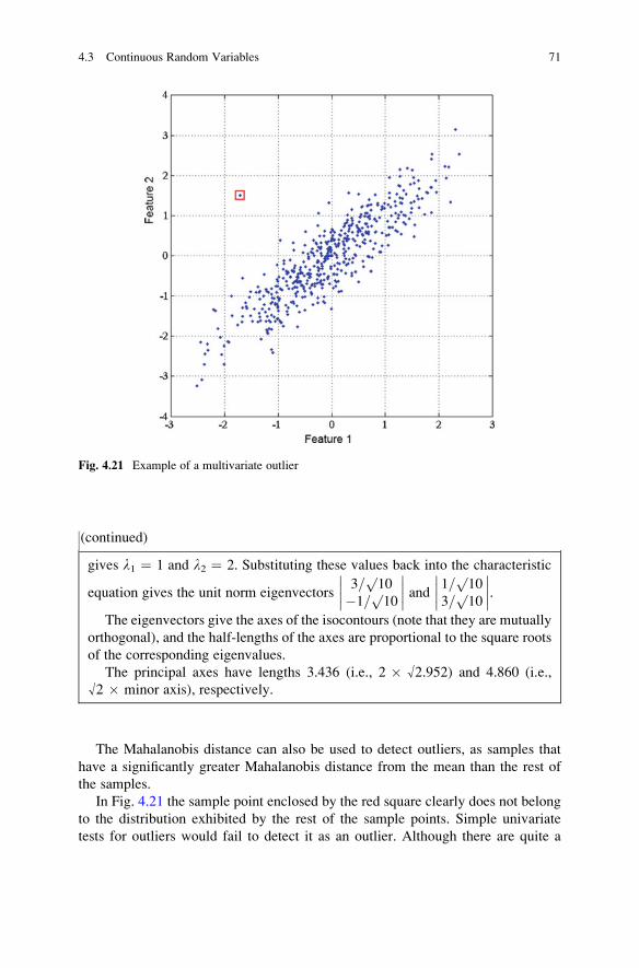
(continued)

gives l1 ¼ 1 and l2 ¼ 2. Substituting these values back into the characteristic

equation gives the unit norm eigenvectors3=

p10

�1=p10

��

�� and1=

p10

3=p10

��

��.

The eigenvectors give the axes of the isocontours (note that they are mutually

orthogonal), and the half-lengths of the axes are proportional to the square roots

of the corresponding eigenvalues.

The principal axes have lengths 3.436 (i.e., 2 � √2.952) and 4.860 (i.e.,

√2 � minor axis), respectively.

The Mahalanobis distance can also be used to detect outliers, as samples that

have a significantly greater Mahalanobis distance from the mean than the rest of

the samples.

In Fig. 4.21 the sample point enclosed by the red square clearly does not belong

to the distribution exhibited by the rest of the sample points. Simple univariate

tests for outliers would fail to detect it as an outlier. Although there are quite a

Fig. 4.21 Example of a multivariate outlier


few sample points with more extreme values of both feature 1 and feature 2, the

Mahalanobis distance of this sample point would be larger than for any other point.

The Mahalanobis distance could be used to measure the separation between two

classes (i.e., their dissimilarity), by measuring the distance between their respective

centers. Each class may have different numbers of samples. For two classes with

identical covariance matrices, the Mahalanobis distance is Dm(1, 2) ¼ (m1 � m2)T

S�1 (m1 � m2). A Mahalanobis distance greater than 3 (i.e., the two centers differ

by more than three standard deviations) would indicate that the overlap between the

two classes is small.

4.4 Exercises

1. Three coins are tossed simultaneously. What is the probability of them showing

two heads?

2. (a) What is the probability of getting at least one “6” if three dice are rolled? (b)

What is the probability of getting at least one “6” in four rolls of a single die?

(c) What is the probability of getting at least one double-6 in 24 throws of a pair

of dice?

3. Consider a family with two children. Given that one of the children is a boy,

what is the probability that both children are boys?

4. There are two cookie jars. Jar 1 contains two chocolate chip cookies and a plain

cookie, and jar 2 contains one chocolate chip cookie and one plain cookie.

If Fred is blind-folded and chooses a jar at random, and then a cookie at random

from that jar, what is the probability that he will choose a chocolate chip

cookie? What is the probability that it came from jar 1?

5. Suppose that a rare disease affects 1 out of every 1,000 people in a population,

i.e., the prior probability is 1/1,000. And suppose that there is a good, but not

perfect, test for the disease. For a person who has the disease, the test comes

back positive 99% of the time (sensitivity ¼ 0.99) and if for a person who does

not have the disease the test is negative 98% of the time (specificity ¼ 0.98).

You have just tested positive; what are your chances of having the disease?

(Try by calculation, and then check using CondProb.xls).

6. Consider the situation discussed in Example 4.3 in the text. The woman in

question tested positive and her posterior probability of having breast cancer

was calculated to be 7.76%. If she decides to go for another test and she tests

positive a second time, what is the probability of her having breast cancer?

(And what if a third, fourth, fifth test was positive, what would the

corresponding probabilities be? Of course, this is an unlikely scenario since

each test exposes her to X-rays and a consequent risk of actually causing

cancer.) (Try by calculation, and then check using CondProb.xls.)


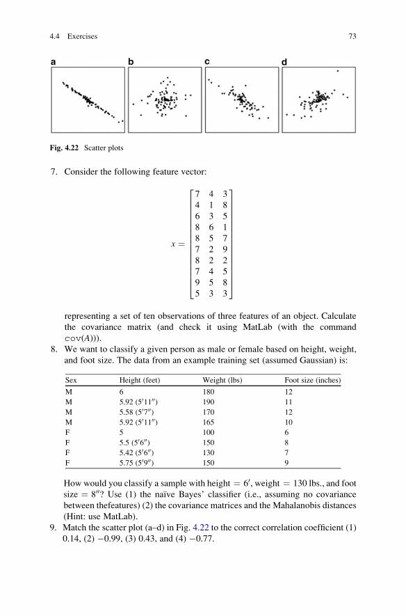
7. Consider the following feature vector:

x ¼

7 4 3

4 1 8

6 3 5

8 6 1

8 5 7

7 2 9

8 2 2

7 4 5

9 5 8

5 3 3

2

666666666666664

3

777777777777775

representing a set of ten observations of three features of an object. Calculate

the covariance matrix (and check it using MatLab (with the command

cov(A))).8. We want to classify a given person as male or female based on height, weight,

and foot size. The data from an example training set (assumed Gaussian) is:

Sex Height (feet) Weight (lbs) Foot size (inches)

M 6 180 12

M 5.92 (501100) 190 11

M 5.58 (50700) 170 12

M 5.92 (501100) 165 10

F 5 100 6

F 5.5 (50600) 150 8

F 5.42 (50600) 130 7

F 5.75 (50900) 150 9

How would you classify a sample with height ¼ 60, weight ¼ 130 lbs., and foot

size ¼ 800? Use (1) the naıve Bayes’ classifier (i.e., assuming no covariance

between thefeatures) (2) the covariance matrices and the Mahalanobis distances

(Hint: use MatLab).

9. Match the scatter plot (a–d) in Fig. 4.22 to the correct correlation coefficient (1)

0.14, (2) �0.99, (3) 0.43, and (4) �0.77.

Fig. 4.22 Scatter plots

4.4 Exercises 73

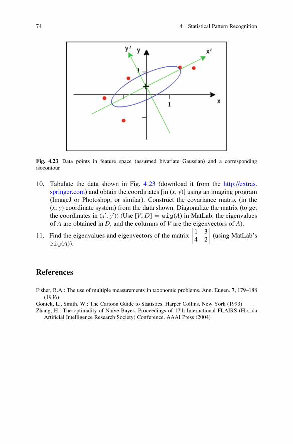
10. Tabulate the data shown in Fig. 4.23 (download it from the http://extras.

springer.com) and obtain the coordinates [in (x, y)] using an imaging program

(ImageJ or Photoshop, or similar). Construct the covariance matrix (in the

(x, y) coordinate system) from the data shown. Diagonalize the matrix (to get

the coordinates in (x0, y0)) (Use [V, D] ¼ eig(A) in MatLab: the eigenvalues

of A are obtained in D, and the columns of V are the eigenvectors of A).

11. Find the eigenvalues and eigenvectors of the matrix1 3

4 2

��

�� (using MatLab’s

eig(A)).

References

Fisher, R.A.: The use of multiple measurements in taxonomic problems. Ann. Eugen. 7, 179–188

(1936)

Gonick, L., Smith, W.: The Cartoon Guide to Statistics. Harper Collins, New York (1993)

Zhang, H.: The optimality of Naıve Bayes. Proceedings of 17th International FLAIRS (Florida

Artificial Intelligence Research Society) Conference. AAAI Press (2004)

Fig. 4.23 Data points in feature space (assumed bivariate Gaussian) and a corresponding

isocontour




Chapter 5

Supervised Learning

5.1 Parametric and Non-parametric Learning

Parametricmethods of statistical classification require probability distributions and

estimate parameters derived from them such as the mean and standard deviation to

provide a compact representation of the classes. Examples include Bayes’ decisionrule, based explicitly on probability distributions, and discriminant analysis, aparametric method based on functions which separate the classes. Parametric

methods tend to be slow at training, but once trained they are fast at classifying

test data. If the probability distributions are not known, then we must use non-parametric methods. In this case, we either estimate the density functions (e.g., the

Parzen window approach) or bypass the probabilities and directly construct decision

boundaries based on the training data (e.g., the k-nearest neighbor rule). (In fact, themultilayer perceptron can also be viewed as a supervised non-parametric method

which constructs a decision boundary).

5.2 Parametric Learning

5.2.1 Bayesian Decision Theory

5.2.1.1 Single Feature (1D)

In statistical pattern recognition approaches, we develop classifiers which use all

the available information, such as measurements and an a priori (or simply prior)

probability. Combining this information leads to a measurement-conditioned or a

posteriori (or posterior) probability. We can formulate a decision rule based on the

posterior probabilities.


75

Let us consider that there are just two classes [class 1 (o1) and class 2 (o2)] and

that the (prior) probabilities are known [for example, P(o1) ¼ 0.7 and P(o2) ¼ 0.3

(which sum to unity)]. Faced with a new sample and no additional information,

the decision rule would be to classify this sample as belonging to o1, since

P(o1) > P(o2). The probability of classification error, in general, is

PðerrorÞ ¼ Pðchoose o2jo1Þ � Pðo1Þ þ Pðchoose o1jo2Þ � Pðo2Þ (5.1)

In this case, since we always choose o1, P(error) ¼ P(choose o1jo2).

P(o2) ¼ 1.0 � 0.3 ¼ 0.3.

Now consider that we have a single feature, x (e.g., a length or brightness). We

have a training set, which includes representative examples from both classes;

so that we can measure the feature for both classes and construct probability

distributions for each (Fig. 5.1). These are formally known as the probability density

functions or class-conditional probabilities, p(x|o1) and p(x|o2), i.e., the

probabilities of measuring the value x, given that the feature is in class 1 or class

2, respectively. If we have a large number of examples in each class, then the

probability density functions will be Gaussian in shape (the Central Limit Theorem).

The classification problem is: given a new object with a particular value of

this feature, to which class does this object belong? If the two probability density

functions overlap, then this cannot be answered definitively, only statistically.

If the probability density functions and the prior probabilities are known, then the

posterior probability, P(oijx) (i.e., the probability that given a feature value of x, thefeature belongs to class oi) can be calculated using Bayes’ rule (from Chap. 4)

PðAjBÞ ¼ PðBjAÞ � PðAÞPðBÞ

which will help in the decision. We would evaluate the posterior probability of

each class and choose the class with the largest posterior probability [i.e., this

Class 1

Pro

babi

lity

dens

ity

σ1

σ2

μ1 μ2

Class 2

x

Fig. 5.1 Probability density functions for two classes, 1 and 2; often they will be Gaussian in shape

76 5 Supervised Learning

http://dx.doi.org/10.1007/978-1-4614-5323-9_4

is a maximum a posteriori (MAP) classifier]. Using Bayes’ rule, the posterior

probability for each class (i ¼ 1, 2) of measuring a particular feature, x, is

PðoijxÞ ¼ pðxjoiÞ � PðoiÞpðxÞ (5.2)

and our decision rule becomes

Ifpðxjo1Þ � Pðo1Þ

pðxÞ >pðxjo2Þ � Pðo2Þ

pðxÞ choose o1

else choose o2

(where we are using upper-case P for probability and lower-case p for probability

density). The term p(x) can be considered a scale factor that states how frequently we

will actually measure an object with value x: it guarantees that the posterior

probabilities sum to unity, but is unimportant in making a decision.

Dividing through by p(x) and re-arranging, the decision rule can be written in a

different (but equivalent) form

pðxjo1Þpðxjo2Þ>

Pðo2ÞPðo1Þ choose o1

else choose o2

The quantity on the left-hand side of this equation (the ratio of the class-

conditional density functions) is called the likelihood ratio, and the decision rule

is called the likelihood ratio test.

Example 5.1

Let us suppose that a single measurement has Gaussian class-conditional

densities of equal variance (s2 ¼ 1) but different means (m1 ¼ 4 and m2 ¼ 10)

and that the prior probabilities are equally likely [P(o1) ¼ P(o2) ¼ 0.5]. The

corresponding class-conditional probability density functions and posterior

probabilities are shown in Fig. 5.2.

Using (1D) Gaussians [(4.22)] as the class-conditional probability functions,

and the given values for the means, the variances and the prior probabilities, the

likelihood ratio test [(5.4)] becomes

expð� 12ðx� 4Þ2Þ

expð� 12ðx� 10Þ2Þ>

0:5

0:5>1 choose o1

else choose o2

(continued)

5.2 Parametric Learning 77

(continued)

00

0.05

0.1

0.15

0.2

0.25

0

0.05

0.1

0.15

0.2

0.25

0.3

0.35

0.4

0.45

2 4 6 8 10 12

X

Po

ster

ior

pro

bab

iliti

es

Cla

ss-c

on

dit

ion

al p

rob

abili

ty d

ensi

ty

14 160 2 4 6 8 10 12

X

14 16

a b

Fig. 5.2 For Gaussians with means of m1 ¼ 4 and m2 ¼ 10 and equal variances ðs21 ¼ s22 ¼ 1Þ(a) the class-conditional probabilities and (b) the posterior probabilities of measuring a feature,

x

Cross-multiplying, taking the natural logs and simplifying gives

ðx� 4Þ2 � ðx� 10Þ2<0

or

x<7 choose o1

else choose o2

As intuitively expected for this case, the decision threshold is mid-way between

the two means. The decision threshold is the value at which the two posterior

probabilities are equal, given by the intersection of the posterior probabilities in

Fig. 5.2b. (In the case of equal prior probabilities, this corresponds to the intersec-

tion of class-conditional probability densities). Note that the area under each

class-conditional probability function equals unity, whereas it is the sum of the

areas under the posterior probabilities which sums to unity.

Example 5.2

If the prior probabilities are equal [P(o1) ¼ P(o2) ¼ 0.5], the means remain the

same as before (m1 ¼ 4 and m2 ¼ 10), but the class-conditional densities have

different variances, s21 ¼ 4 and s22 ¼ 1 (Fig. 5.3), the decision rule becomes

12� expð�1=ð2� 4Þðx� 4Þ2Þ

expð� 12ðx� 10Þ2Þ >1 choose o1else choose o2

(continued)


(continued)

XX

0

0.05

0.1

0.15

0.2

0.25

0

0.05

0.1

0.15

0.2

0.25

0.3

0.35

0.4

0.45

Po

ster

ior

pro

bab

iliti

es

Cla

ss-c

on

dit

ion

al p

rob

abili

ty d

ensi

ty

0-2-4-6 2 4 6 8 10 12 14 16 0-2-4-6 2 4 6 8 10 12 14 16

a b

Fig. 5.3 For Gaussians with means of m1 ¼ 4 (in red) and m2 ¼ 10 (in blue), and variances of

s21 ¼ 4 and s22 ¼ 1 (a) the class-conditional probabilities and (b) the posterior probabilities

of measuring a feature, x

Cross-multiplying, taking the natural logs and simplifying gives

8 ln1

2� ðx� 4Þ2>� 4ðx� 10Þ2 choose o1

3x2 � 72xþ ð384þ 8 ln1

2Þ>0

Solving this quadratic gives two different roots, and therefore two different

decision thresholds, at

x ¼ ð72� 25:3Þ=6¼ 7:78 and 16:22

The class-conditional probability densities and posterior probabilities are

shown in Fig. 5.3. (Since the prior probabilities, P(oi), are equal, the class-

conditional and posterior probability functions are just scaled version of each

other). The lower decision threshold (corresponding to the smaller root,

x ¼ 7.78) is easily seen, but the upper decision threshold (corresponding to

the larger root, x ¼ 16.22) is not so obvious in Fig. 5.3b. However, if we note

that the posterior probability for class o1 does not decay as fast as that for class

o2 at higher values of x, we can understand that a second intersection will occur(and this is at x ¼ 16.22). With reference to Fig. 5.3b, we can see that the

decision rule is

(continued)


(continued)

x<7:78 or x>16:22 choose o1

7:78<x<16:22 choose o2

(Note that it is much easier to get the “greater than” and “less than” signs

correct if there is a diagram with which to visualize the situation).

Example 5.3

If the prior probabilities are not equal [say P(o1) ¼ 2/3 and P(o2) ¼ 1/3], but

the variances are equal ðs21 ¼ s22 ¼ 1Þ the likelihood test becomes

expð� 12ðx� 4Þ2Þ � 2=3

expð� 12ðx� 10Þ2Þ � 1=3>1 choose o1

else choose o2

Solving this gives a single decision boundary at x ¼ 7.12 (Fig. 5.4), because

the roots of the resulting quadratic are equal. The decision threshold(s) is/are

given by the intersection(s) of the posterior probabilities. (Note that in the case

of unequal priors, this does not correspond to the intersection of the class-

conditional probabilities). In the case of several features, the decisionboundaries will be lines or planes.

00

0.05

0.1

0.15

0.2

0.25

0.3

0

0.05

0.1

0.15

0.2

0.25

0.3

0.35

0.4

0.45

2 4 6 8 10 12

X

Po

ster

ior

pro

bab

iliti

es

Cla

ss-c

on

dit

ion

al p

rob

abili

ty d

ensi

ty

14 160 2 4 6 8 10 12

X

14 16

a b

Fig. 5.4 For Gaussians with means of m1 ¼ 4 and m2 ¼ 10, equal variances ðs21 ¼ s22 ¼ 1Þand prior probabilities P(o1) ¼ 2/3 and P(o2) ¼ 1/3 (a) the class-conditional probabilities

and (b) the posterior probabilities of measuring a feature, x

In the case of two Gaussian distributions with equal priors (Fig. 5.5a), the

decision threshold (D1) will be at the intersection of the probability distribution

functions, and there will be misclassification errors (shown by the striped areas in

the figure): both false positives (or type I errors) and false negatives (or type II


errors). Moving the decision threshold changes the classification. For example,

moving the decision threshold higher (to D2 in Fig. 5.5b) reduces the number of

false positives but unfortunately it also increases the number of false negatives.

(Moving the decision threshold lower will increase the number of false positives

and reduce the number of false negatives). From Fig. 5.5b, we see that the false

negatives will be reduced somewhat, but the false positives will be increased by an

even larger amount; so that the total number of errors in classification (FP + FN)

will actually increase (by the area shown in light brown in Fig. 5.5b). (This is also

the case if the decision threshold is lowered from D1). Thus taking the decision

threshold at the intersection of the distributions minimizes the total errors (FPF +

FNF). This general geometric argument also holds if the Gaussians have different

variances or if they are scaled by different priors. Indeed, the posterior probabilities

do not even have to be Gaussian; they just need to be monotonic in the region

around their intersection point(s). Thus Bayes’ rule, whereby we choose the class

according to the maximum (posterior) probability, corresponds to minimizing the

(total) probability of error (the error rate) and therefore our decision rule is an

optimal decision rule.

Let us consider the problem of classifying two types of fish: sea bass (class o1)

and salmon (class o2) as they travel down a conveyor belt in a canning factory.

Let us say that the lightness of the fish are measured for samples of the two types

of fish, and the resulting class-conditional probability density functions, p(x|o1) and

p(x|o2), are shown in Fig. 5.6.

The season and the locale (and many other variables) determine directly the

probability of the two different types of fish being caught, but suppose that for this

particular catch, twice as many sea bass as salmon were caught, so that P(o1) ¼ 2/3

and P(o2) ¼ 1/3. We can determine the posterior probabilities using (5.2),

by scaling the class-conditional probabilities by the priors, and dividing by the

evidence term to ensure that the probabilities sum to 1 (Fig. 5.7). Check on this

figure that any feature measurement for a test sample (e.g., lightness ¼ 13) results

in posterior probabilities that sum to 1 (in the case of lightness ¼ 13, the posterior

probabilities are 0.79 and 0.21 for class 1 and 2, respectively): note that the two

curves are mirror images of each other about the (horizontal) P(oi|x) ¼ 0.5 line.

D1

diseased (2)

FP

healthy (1)

FN

D2

a b

Fig. 5.5 Intersecting distributions with a decision threshold (a) at the intersection point and

(b) higher than the intersection point


The lightness of each new fish coming along the conveyor belt is measured, and we

will classify it as sea bass or salmon according to the posterior probabilities. Specifi-

cally, wewill choose the class with the larger posterior probability of having that value

of lightness. From Fig. 5.7, we will classify the fish as sea bass (o1) if its lightness, x,is 9.9 < x < 11.2 or x > 11.8, otherwise we will classify it as salmon (o2).

P(wi|x)

w2

w1

9 10 11 12 13 14 15x

0.2

0.4

0.6

1

0.8

Fig. 5.7 Posterior probabilities corresponding to the class-conditional probabilities of Fig. 5.4,

with P(o1) ¼ 2/3 and P(o2) ¼ 1/3. Note that the posterior probabilities sum to unity, at every

value of x

9 10

0.2

0.3

w2

p(x |wi)

w1

0.4

11 12 13 14 15x

0.1

Fig. 5.6 Class-conditional probability functions of measuring the lightness, x, of fish that are in

classes o1 (sea bass) and o2 (salmon). (Note that the area under each density function is unity)

(after Duda et al. 2001)


We have assumed that the two types of classification errors (misclassifying

sea bass as salmon, and misclassifying salmon as sea bass) are of equal importance.

However, this may not always be true. For example, our customers may not

mind some of the more expensive salmon turning up in their cans of sea bass,

but they may have more objections to misclassified sea bass turning up in their salmon

cans. [Or, in our medical example, it may be less serious to misdiagnose a benign

tumor as a malignant cancer (a false positive), than to misdiagnose a malignant

cancer as a benign one (a false negative): the false positive will result

in unnecessary treatment, but the false negative may result in no treatment being

given resulting in the death of the patient.] For these cases, we can introduce

a penalty term, lij, known as the loss, associated with a wrong decision (viz., a

misclassification). lij, is the loss associated with deciding oi when the correct state

is oj. (The expected loss by deciding oi when the correct state is oj, is called a risk,R, in this case the conditional risk). The complete loss matrix for a two-class

problem would be

l ¼ l11 l12l21 l22

��

�� (5.5)

where the diagonal terms are usually set to zero (i.e., no cost for making the correct

decision). In the case where o1 represents the healthy distribution and o2 the

diseased distribution, then l12 (the loss associated with a false negative) > l21(the loss associated with a false positive). If action a1 corresponds to deciding

that the true state of nature is o1, and action a2 corresponds to deciding that the truestate of nature iso2, then lij is shorthand for l(ai|oj). The conditional risks involved

in choosing either way are

Rða1jxÞ ¼ l11Pðo1jxÞ þ l12Pðo2jxÞ (5.6a)

Rða2jxÞ ¼ l21Pðo1jxÞ þ l22Pðo2jxÞ (5.6b)

Generalizing (5.4), to include the loss terms, the decision rule (in terms of the

likelihood ratio) can be written

pðxjo1Þpðxjo2Þ>

ðl12 � l22Þ � Pðo2Þðl21 � l11Þ � Pðo1Þ choose o1

else choose o2

The effect of introducing loss terms such that l12 > l21 is to shift the decision

threshold in Fig. 5.5a to the left, reducing the number of false negatives. [In the

case where the diagonal terms are zero and the errors are equally costly (l12 ¼ l21),then l is the so-called symmetrical or zero-one loss function, and (5.7) reduces

to (5.4)].


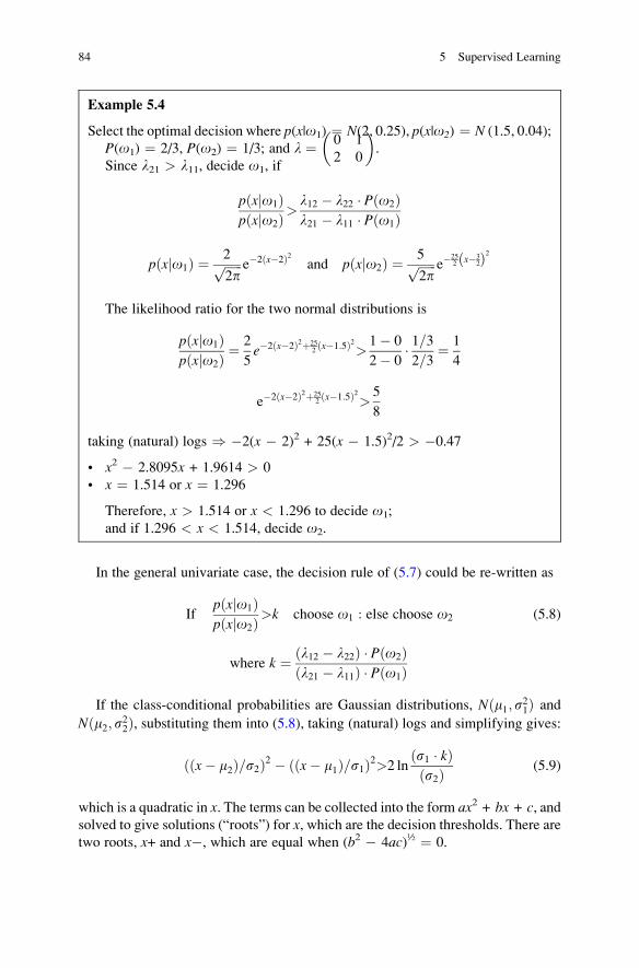
Example 5.4

Select the optimal decision where p(x|o1) ¼ N(2, 0.25), p(x|o2) ¼ N (1.5, 0.04);

P(o1) ¼ 2/3, P(o2) ¼ 1/3; and l ¼ 0 1

2 0

� �.

Since l21 > l11, decide o1, if

pðxjo1Þpðxjo2Þ>

l12 � l22 � Pðo2Þl21 � l11 � Pðo1Þ

pðxjo1Þ ¼ 2ffiffiffiffiffiffi2p

p e�2ðx�2Þ2 and pðxjo2Þ ¼ 5ffiffiffiffiffiffi2p

p e�252

x�32ð Þ2

The likelihood ratio for the two normal distributions is

pðxjo1Þpðxjo2Þ ¼

2

5e�2ðx�2Þ2þ25

2ðx�1:5Þ2>

1� 0

2� 0� 1=32=3

¼ 1

4

e�2ðx�2Þ2þ252ðx�1:5Þ2>

5

8

taking (natural) logs ) �2(x � 2)2 + 25(x � 1.5)2/2 > �0.47

• x2 � 2.8095x + 1.9614 > 0

• x ¼ 1.514 or x ¼ 1.296

Therefore, x > 1.514 or x < 1.296 to decide o1;

and if 1.296 < x < 1.514, decide o2.

In the general univariate case, the decision rule of (5.7) could be re-written as

Ifpðxjo1Þpðxjo2Þ>k choose o1 : else choose o2 (5.8)

where k ¼ ðl12 � l22Þ � Pðo2Þðl21 � l11Þ � Pðo1Þ

If the class-conditional probabilities are Gaussian distributions, Nðm1;s21Þ and

Nðm2; s22Þ, substituting them into (5.8), taking (natural) logs and simplifying gives:

ððx� m2Þ=s2Þ2 � ððx� m1Þ=s1Þ2>2 lnðs1 � kÞðs2Þ (5.9)

which is a quadratic in x. The terms can be collected into the form ax2 + bx + c, andsolved to give solutions (“roots”) for x, which are the decision thresholds. There aretwo roots, x+ and x�, which are equal when (b2 � 4ac)½ ¼ 0.


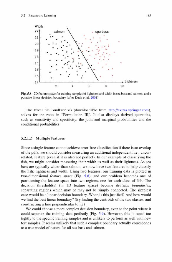
The Excel file,CondProb.xls (downloadable from http://extras.springer.com),

solves for the roots in “Formulation III”. It also displays derived quantities,

such as sensitivity and specificity, the joint and marginal probabilities and the

conditional probabilities.

5.2.1.2 Multiple features

Since a single feature cannot achieve error-free classification if there is an overlap

of the pdfs, we should consider measuring an additional independent, i.e., uncor-

related, feature (even if it is also not perfect). In our example of classifying the

fish, we might consider measuring their width as well as their lightness. As sea

bass are typically wider than salmon, we now have two features to help classify

the fish: lightness and width. Using two features, our training data is plotted in

two-dimensional feature space (Fig. 5.8), and our problem becomes one of

partitioning the feature space into two regions, one for each class of fish. The

decision threshold(s) (in 1D feature space) become decision boundaries,separating regions which may or may not be simply connected. The simplest

case would be a linear decision boundary. When is this justified? And how would

we find the best linear boundary? (By finding the centroids of the two classes, and

constructing a line perpendicular to it?)

We could choose a more complex decision boundary, even to the point where it

could separate the training data perfectly (Fig. 5.9). However, this is tuned too

tightly to the specific training samples and is unlikely to perform as well with new

test samples. It seems unlikely that such a complex boundary actually corresponds

to a true model of nature for all sea bass and salmon.

Fig. 5.8 2D feature space for training samples of lightness and width in sea bass and salmon, and a

putative linear decision boundary (after Duda et al. 2001)



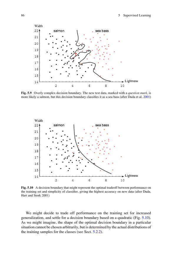
We might decide to trade off performance on the training set for increased

generalization, and settle for a decision boundary based on a quadratic (Fig. 5.10).

As we might imagine, the shape of the optimal decision boundary in a particular

situation cannot be chosen arbitrarily, but is determined by the actual distributions of

the training samples for the classes (see Sect. 5.2.2).

Fig. 5.9 Overly complex decision boundary. The new test data, marked with a question mark, ismore likely a salmon, but this decision boundary classifies it as a sea bass (after Duda et al. 2001)

Fig. 5.10 A decision boundary that might represent the optimal tradeoff between performance on

the training set and simplicity of classifier, giving the highest accuracy on new data (after Duda,

Hart and Stork 2001)


5.2.2 Discriminant Functions and Decision Boundaries

There are many different ways to represent pattern classifiers. One of the most

useful is to obtain decision boundaries by considering a set of discriminantfunctions, gi(x) for each class, i ¼ 1, 2, 3 . . ., M, where x is the feature vector:

classification is based on finding the largest discriminant function. For the Bayes’

classifier (minimum-error-rate classification), the discriminant functions are the

posterior probabilities, P(oi|x). Using Bayes’ rule gives

giðxÞ ¼ PðoijxÞ ¼ pðxjoiÞ � PðoiÞpðxÞ (5.10)

The discriminant function is not unique. It can be multiplied by a constant or

shifted by adding a constant, without affecting the classification. Indeed, any

monotonically increasing function of gi(x) is also a valid discriminant function.

For Bayes’ classification, it is convenient to use the natural log of the numerator

of (5.8), viz.,

giðxÞ ¼ ln pðxjoiÞ þ lnPðoiÞ (5.11)

Using these discriminant functions, the decision rules will divide the feature

space into decision regions, separated by decision boundaries or surfaces.

The multivariate Gaussian is the most frequently used (class-conditional) prob-

ability density function because of its tractability and its relationship to the Central

Limit Theorem. The n-dimensional Gaussian is given by

fXðxÞðor Nðm;SÞ ¼ 1

ðð2pÞn=2jSj1=2Þexpð� 1

2ðx� mÞTS�1ðx� mÞÞ (5.12)

where m is the mean value of x, and S is the (n � n) covariance matrix.

In this case, the discriminant functions are

giðxÞ ¼ � 1

2ðx� miÞTS�1

i ðx� miÞ � n=2 � ln 2p� 1

2ln jSij þ lnPðoiÞ (5.13)

Let us examine several special cases:

Case 1: Independent features, each with the same variance (s2).

Let us consider the case where all features are represented by circular contours.

Circular (or spherical, in 3D) isocontours result from a covariance matrix which is

diagonal and equal to s2I. It follows that |Si| ¼ s2n andS�1i ¼ ð1=s2ÞI. The second

and third terms in (5.11) are class-independent constant biases and can be

eliminated, giving

giðxÞ ¼ � 1

2ðx� miÞTS�1

i ðx� miÞ þ lnPðoiÞ (5.14)


In this case, this simplifies to

giðxÞ ¼ � x� mik k22s2

þ lnPðoiÞ (5.15)

Where ||●|| denotes the Euclidean norm, i.e.,

x� mik k2 ¼ ðx� miÞTðx� miÞ (5.16)

Expansion of the squared term in (5.15) gives

giðxÞ ¼ � 1

2s2½xTx� 2mTi xþ mTi mi� þ lnPðoiÞ (5.17)

The term xTx is constant for all i, and can be ignored. Thus

giðxÞ ¼ wTi xþ wi0 (5.18)

where

wi ¼ 1

s2mi (5.19)

and

wi0 ¼ � 1

2s2mTi mi þ lnPðoiÞ (5.20)

(wi0 is known as the threshold or bias for the ith class).

Equation (5.18) defines a linear discriminant function; the associated Bayesian

classifier is linear in nature, and the approach to classification is known as lineardiscriminant analysis (LDA).

The decision surfaces are defined by the linear equations gi(x) ¼ gj(x) for thetwo classes with the highest posterior probabilities. For this case

wTðx� x0Þ ¼ 0 (5.21)

where

w ¼ mi � mj (5.22)

and

x0 ¼ 1

2ðmi þ mjÞ �

s2

mi � mj�� 2 � lnPðoiÞ � ðmi � mjÞ (5.23)


This defines a hyperplane through the point x0, orthogonal to w. Since w ¼ mi

� mj, the hyperplane is orthogonal to the line that links their means. (A classifier

that uses linear discriminant functions is called a linear machine).If P(oi) ¼ P(oj), then x0 is midway between the means, and the decision

hyperplane is the perpendicular bisector of the line between the means (i.e.,

centroids), as in Fig. 5.11. [If P(oi) 6¼ P(oj) then x0 shifts away from the mean

with the higher (prior) probability. However, if the variance s2 is small relative to

the squared distance ||mi � mj||2, then the position boundary if fairly insensitive to

the values of the prior probabilities.]

If the prior probabilities, P(oi), are the same for all classes, the P(oi) in (5.23)

disappears and the optimum decision rule becomes: measure the Euclidean distance

of a feature vector to the centroids of each class, ||x � mi||, and assign x to the class

corresponding to the shortest distance. The classifier is therefore a minimum-distance classifier.

Note that the condition that the posterior probabilities are equal on the decision

boundary means that the log of the ratio of posterior probabilities must be zero. If

the data in each class is Gaussian with equal variance, then the boundary between

any two classes is a straight line. For three classes, there will be three lines

(Fig. 5.12).

Fig. 5.11 Two bivariate normal distributions, whose priors are equal. Therefore, the decision

boundary is exactly at the midpoint between the two means. The decision boundary is the

perpendicular bisector of the line between the centroids


Case 2: When the covariance matrices for all the classes are equal, but

otherwise arbitrary (so that the isocontours are ellipses (in 2D) of similar size

and orientation).

Geometrically, this corresponds to having samples in (hyper)ellipsoidal clusters

of equal size and shape: the elliptical contours are parallel to each other. Since both

(n/2) and jSij in (5.13) are independent of i, they can be ignored as superfluous

additive constants. (It is left as an exercise to work through the math and find the

decision boundary).

Again, the decision boundary is a linear surface (or line for 2D feature space),

although it is not orthogonal to the line joining the means. If the priors are equal

it intersects mid-way between the means (Fig. 5.13). (If the priors are not equal,

then the decision boundary shifts away from the mean with the higher (prior)

probability).

Case 3: General case, with different covariance matrices for each class.

In the general case, only the constant term, (n/2) ln2p, drops out of (5.13) and the

resulting discriminant functions are inherently quadratic, giving rise to decision

curves which are hyperquadrics for the two-class case. For two features, they will

be ellipses, circles, parabolas, hyperbolas, lines or pairs of lines. In such cases, the

Bayesian classifier is a quadratic classifier, and the approach is known as quadraticdiscriminant analysis (QDA).

When one class has circular contours, a parabolic decision boundary is the result

(Fig. 5.14).

Fig. 5.12 Showing the decision lines between three classes of equal variance. A new data point is

assigned to the class that gives the largest numerator in the posterior probability ratio


Fig. 5.14 Parabolic decision boundary when one distribution has circular isocontours

Fig. 5.13 Two classes with equal covariance matrices, showing the line between the centroids and

the linear discriminant function which intersect it mid-way (but not at right-angles)


In the case of (equiprobable) distributions with elliptical contours, oriented

orthogonally to each other, the decision boundary will be hyperbolic (Fig. 5.15).

It is left to the reader to determine the conditions under which the decision

boundaries will be ellipses, and when they degenerate into lines (Fig. 5.16).

To clarify these ideas, let us consider two examples. In both cases the priors are

equal. In the first example, the means are m1 ¼ [0, 0] and m2 ¼ [4, 0], and the

covariance matrices are

S1 ¼ 0:3 0:00:0 0:35

��

�� S2 ¼ 1:2 0:00:0 1:85

��

��

There are no covariance terms, but the variances are different in each covariance

matrix and the covariance matrices are not equal. The resulting isocontours are

ellipses (of different sizes) oriented parallel to the feature axes. Figure 5.17 shows

the two pdfs, where the red color (class o1) indicates the points where the posterior

probability is greater for class o1. The decision curve is an ellipse.

For the second example, m1 ¼ [0, 0] and m2 ¼ [3.2, 0] and

S1 ¼ 0:1 0:00:0 0:75

��

�� S2 ¼ 0:75 0:00:0 0:1

��

��

Again, these are ellipses, with axes parallel to the feature axes but inspection of

the variances shows that their isocontours are orthogonal to each other. This results

in a hyperbolic decision boundary (Fig. 5.18).

Fig. 5.15 Hyperbolic decision boundaries from two (equiprobable) sets of orthogonal elliptical

isocontours


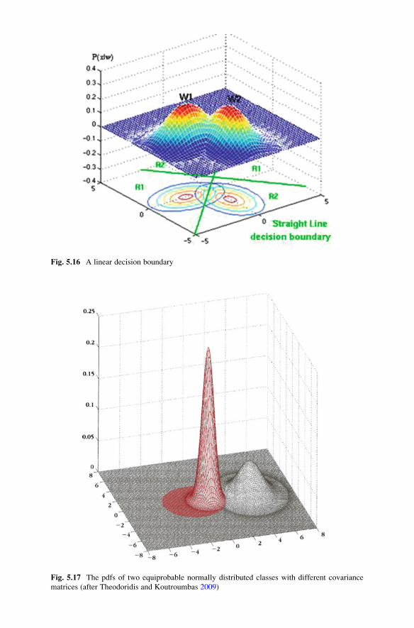
Fig. 5.16 A linear decision boundary

Fig. 5.17 The pdfs of two equiprobable normally distributed classes with different covariance

matrices (after Theodoridis and Koutroumbas 2009)

Figure 5.19 shows the decision curves for an example with three classes (and two

features, viz., 2D feature space).

We should also note that even in 1D feature space, the case of two unequal

variances can result in a parabolic decision curve, which results in two decision

thresholds, and a disconnected decision region (Fig. 5.20). We have seen this earlier

in the chapter (Example 5.2).

5.2.3 MAP (Maximum A Posteriori) Estimator

With the MAP variant of the classifier, the new object is assigned to the class

with the largest posterior probability. For multivariate data (viz., several features),

the multivariate Gaussian is used. Figure 5.21 illustrates the case where there are

two features (y1 and y2) and three classes (A, B, and C), each with its own mean (mA,mB, and mC). The covariance matrix is

Fig. 5.18 The pdfs of two equiprobable normally distributed classes with different covariance

matrices (after Theodoridis and Koutroumbas 2009)


green

blue

-8

-4

-2

0

2

4

6

-6 -4 -2 0

red

Fig. 5.19 The decision curves between any two of the three classes (red, green, and blue) arequadrics

Fig. 5.20 The decision curve in 1D feature space for normal distributions with unequal variance

S ¼ s11 s12s12 s22

� �

Then the posterior probabilities are calculated using

Pð~mjj~yÞ ¼Pð~mj \ ~yÞPð~yÞ

¼ Pð~mjÞPð~yj~mjÞPð~mA \ ~yÞ þ Pð~mB \ ~yÞ þ Pð~mC \ ~yÞ

¼ Pð~mjÞPð~yj~mjÞPð~mAÞPð~yj~mAÞ þ Pð~mBÞPð~yj~mBÞ þ Pð~mCÞPð~yj~mCÞ

¼Pð~mjÞ e

�12ð~y�~mjÞ0S�1

jð~y�~mjÞ

Sjj j12

" #

Pð~mAÞ e�12ðSqDistAÞ

SAj j12

� �þ Pð~mBÞ e�1

2ðSqDistBÞ

SBj j12

� �þ Pð~mCÞ e�1

2ðSqDistCÞ

SCj j12

� � (5.24)

and an object is classified into one of the classes (A, B, or C) based on its highest

posterior probability.

5.3 Exercises

1. Suppose that the class-conditional probability functions for o1 and o2 are

Gaussians with (mi, si) of (4, 2) and (10, 1), and that they have equal prior

probabilities (P1 ¼ P2 ¼ ½). What is the optimal decision threshold?


2. What are the decision thresholds for two class-conditional probabilities which

are Gaussian in shape, with means m1 ¼ 4 and m2 ¼ 10, variances s21 ¼ 4 and

s22 ¼ 1, and prior probabilities P(o1) ¼ 2/3 and P(o2) ¼ 1/3?


Fig. 5.21 Three-class

problem


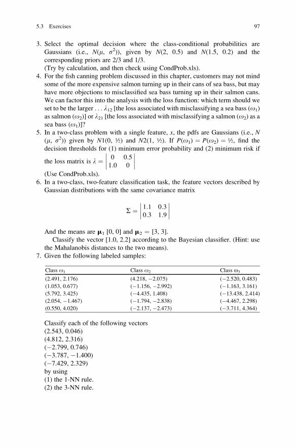
3. Select the optimal decision where the class-conditional probabilities are

Gaussians (i.e., N(m, s2)), given by N(2, 0.5) and N(1.5, 0.2) and the

corresponding priors are 2/3 and 1/3.


4. For the fish canning problem discussed in this chapter, customers may not mind

some of the more expensive salmon turning up in their cans of sea bass, but may

have more objections to misclassified sea bass turning up in their salmon cans.

We can factor this into the analysis with the loss function: which term should we

set to be the larger . . . l12 [the loss associated with misclassifying a sea bass (o1)

as salmon (o2)] or l21 [the loss associated with misclassifying a salmon (o2) as a

sea bass (o1)]?

5. In a two-class problem with a single feature, x, the pdfs are Gaussians (i.e., N(m, s2)) given by N1(0, ½) and N2(1, ½). If P(o1) ¼ P(o2) ¼ ½, find the

decision thresholds for (1) minimum error probability and (2) minimum risk if

the loss matrix is l ¼ 0 0:51:0 0

��

��(Use CondProb.xls).

6. In a two-class, two-feature classification task, the feature vectors described by

Gaussian distributions with the same covariance matrix

S ¼ 1:1 0:30:3 1:9

��

��

And the means are m1 [0, 0] and m2 ¼ [3, 3].

Classify the vector [1.0, 2.2] according to the Bayesian classifier. (Hint: use

the Mahalanobis distances to the two means).

7. Given the following labeled samples:

Class o1 Class o2 Class o3

(2.491, 2.176) (4.218, �2.075) (�2.520, 0.483)

(1.053, 0.677) (�1.156, �2.992) (�1.163, 3.161)

(5.792, 3.425) (�4.435, 1.408) (�13.438, 2.414)

(2.054, �1.467) (�1.794, �2.838) (�4.467, 2.298)

(0.550, 4.020) (�2.137, �2.473) (�3.711, 4.364)

Classify each of the following vectors

(2.543, 0.046)

(4.812, 2.316)

(�2.799, 0.746)

(�3.787, �1.400)

(�7.429, 2.329)

by using

(1) the 1-NN rule.

(2) the 3-NN rule.

5.3 Exercises 97

References

Duda, R.O., Hart, P.E., Stork, D.G.: Pattern Classification. Wiley, New York, NY (2001)

Theodoridis, S., Koutroumbas, K.: Pattern Recognition, 4th edn. Academic, Amsterdam (2009)


Chapter 6

Nonparametric Learning

6.1 Histogram Estimator and Parzen Windows

For the one-dimensional case, if we have N independent samples (x1, x2, x3, . . . xN)of a random variable x (our chosen feature). The density function (pdf) can be

approximated by a histogram formed from the samples with bins that are Dx (¼2h)wide (Fig. 6.1). If there are a large number of samples and k is the number of

samples in a bin, of mid-point xi, then the probability that a sample is in that bin

(xi � h) can be estimated by the relative frequency, k/N, and the density at xi, p(xi),estimated by k/(2hN). In constructing the histogram, we have to choose both an

origin and a bin width. The estimate of the pdf is affected by the choice of origin,

but mostly by the bin width: with small bins the estimate is spiky, and with large

bins it is smoother.

To get a smoother estimate, without smoothing out the details, we use a smooth

weighting function, called a kernel function or Parzen window. The most popular is

the Gaussian kernel (Fig. 6.2). The estimate of the pdf is then the sum of the kernels

placed at each data point.

The width of the kernel (just as the histogram bin width) has to be chosen with

care. A large width will over-smooth the density and mask the structure in the data,

while a small width will yield a density estimate that is spiky and very hard to

interpret (Fig. 6.3). The density estimate will inherit all the continuity and differen-

tiability properties of the kernel, so that for a Gaussian kernel, it will be smooth and

have all the derivatives.

Wewould like to find a value of the smoothing parameter, the kernel width, which

minimizes the error between the estimated density and the true density. A natural

measure is the mean square error at the estimation point x. This expression is an

example of the bias–variance tradeoff; the bias can be reduced at the expense of the

variance, and vice versa. (The bias of an estimate is the systematic error incurred in

the estimation; the variance of an estimate is the random error incurred in the

estimation). The bias–variance dilemma applied to window width selection simply

means that a large window width will reduce the differences among the estimates of


99

density function for different data sets (the variance). A small window width will

reduce the bias of density function, at the expense of a larger variance in the

estimates of density function (Fig. 6.4).

6.2 k-Nearest Neighbor (k-NN) Classification

Since the kernel in the Parzen density estimate is fixed in size, it may be difficult to

obtain a satisfactory estimate of the density everywhere when the samples are not

evenly distributed. One way is to fix the number of samples, k, and let the width

change so that each region contains exactly k samples. This is the k-nearestneighbor classification approach. The classifier exemplifies the following saying

2h

p(x)

x

Fig. 6.1 Estimation of the probability distribution function by a histogram

Kernel: K(xi)

x1

x1

K(xi)

xx2 x3 x4 x5

x2 x3 x4 x5 x

f(x) =1

n

i = 1n

Σˆ

f(x) =ˆ

Fig. 6.2 Using a Gaussian kernel to weight each sample in the training set

100 6 Nonparametric Learning

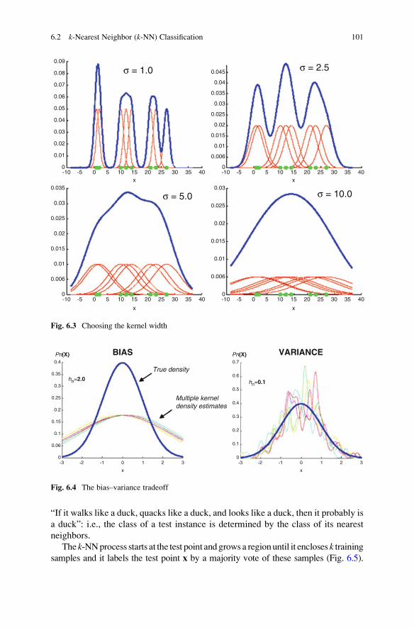
“If it walks like a duck, quacks like a duck, and looks like a duck, then it probably is

a duck”: i.e., the class of a test instance is determined by the class of its nearest

neighbors.

The k-NNprocess starts at the test point andgrows a regionuntil it encloses k trainingsamples and it labels the test point x by a majority vote of these samples (Fig. 6.5).

σ = 1.00.09

0.08

0.07

0.06

0.05

0.04

0.03

0.02

0.01

0

0.045

0.04

0.035

0.03

0.025

0.02

0.015

0.01

0.006

0

0.035

0.03

0.025

0.02

0.015

0.01

0.006

0

0.03

0.025

0.02

0.015

0.01

0.006

0

-10 -5 0 5 10 15x

20 25 30 35 40 -10 -5 0 5 10 15x

20 25 30 35 40

-10 -5 0 5 10 15

x

20 25 30 35 40 -10 -5 0 5 10 15

x

20 25 30 35 40

σ = 2.5

σ = 5.0 σ = 10.0

Fig. 6.3 Choosing the kernel width

BIAS

True density

Multiple kerneldensity estimates

Pn(X) Pn(X)

hn=2.0

0.4

0.35

0.3

0.25

0.2

0.15

0.1

0.06

0-3 -2 -1 0

x

1 2 3 -3 -2 -1 0

x

1 2 3

0.7

0.6

0.5

0.4

0.3

0.2

0.1

0

hn=0.1

VARIANCE

Fig. 6.4 The bias–variance tradeoff

6.2 k-Nearest Neighbor (k-NN) Classification 101

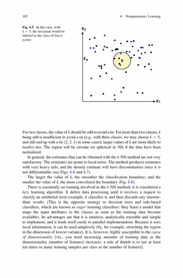
For two classes, the value of k should be odd to avoid a tie. For more than two classes, kbeing odd is insufficient to avoid a tie [e.g., with three classes, we may choose k ¼ 5,

and still end up with a tie (2, 2, 1) in some cases]: larger values of k are more likely to

resolve ties. The region will be circular (or spherical in 3D) if the data have been

normalized.

In general, the estimates that can be obtained with the k-NN method are not very

satisfactory. The estimates are prone to local noise. The method produces estimates

with very heavy tails, and the density estimate will have discontinuities since it is

not differentiable (see Figs. 6.6 and 6.7).

The larger the value of k, the smoother the classification boundary; and the

smaller the value of k, the more convoluted the boundary (Fig. 6.8).

There is essentially no training involved in the k-NN method; it is considered a

lazy learning algorithm. It defers data processing until it receives a request to

classify an unlabeled (test) example, it classifies it, and then discards any interme-

diate results. (This is the opposite strategy to decision trees and rule-based

classifiers, which are known as eager learning classifiers: they learn a model that

maps the input attributes to the classes as soon as the training data become

available). Its advantages are that it is intuitive, analytically tractable and simple

to implement, and it lends itself easily to parallel implementation. Because it uses

local information, it can be used adaptively (by, for example, stretching the region

in the dimension of lowest variance). It is, however, highly susceptible to the curseof dimensionality [viz., you need increasing amounts of training data as the

dimensionality (number of features) increases: a rule of thumb is to use at least

ten times as many training samples per class as the number of features].

Fig. 6.5 In this case, with

k ¼ 5, the test point would be

labeled in the class of blackpoints


When distinguishing normal and abnormal classes in, for example, tumor

detection, it is more useful to modify the criterion to assign a new vector to a

particular class if at least l of the k nearest neighbors is in that particular class. Thisis useful when (1) the penalty for misclassifying one class (e.g., abnormal as

normal—false negatives) is much greater than the penalty for misclassifying

the other class (e.g., normal as abnormal—false positives) and (2) when there is

an unbalanced training set, with many more samples in one class than the other.

P(x)

0.15

0.1

0.05

0

0

0.02

0.04

0.06

0.08

0.1

0-2-4

-20

24

6

24

6

0-2-4

-20

24

6

24

6

P(x)

a

b

Fig. 6.6 An illustration of the performance of the k-NN method. (a) The true density, which is a

mixture of two bivariate Gaussians and (b) the density estimate for k ¼ 10 and N ¼ 200 examples

6.2 k-Nearest Neighbor (k-NN) Classification 103

6.3 Artificial Neural Networks

Artificial neural network (ANN) models take their motivation from the

human nervous system. Signals from sensors in the body convey information for

sight, hearing, taste, smell, touch, balance, temperature, pain, etc. The nerve cells

x1

-2 0 2 4 6x1

-2 0 2 4 6

6

4

2

0

-2

-4

6

4

x 2

2

0

-2

-4

a b

Fig. 6.7 Isocontours of Fig. 6.6. (a) The true density and (b) the k-NN estimate

Fig. 6.8 k-NN classifiers (a) k ¼ 15, (b) k ¼ 1 (the broken curve is the Bayes decision boundary)


(or neurons) are autonomous cells specialized in transmitting, processing and

storing this information, which is essential for us to respond properly to external

and internal stimuli. The neuron transmits spikes of electrical activity along a long,

thin strand known as an axon, which splits into thousands of branches or terminals,

where they can fire across a gap (synapse) to the dendrites of other neurons

depending on the size of the signal (Fig. 6.9a). The brain is composed of a very

large number (~2 � 1010) of neurons acting in parallel. It is believed that in the

brain both the processing (by the neurons) and the memory (in the synapses) are

distributed together over the network. Information is processed and stored

according to the threshold levels for firing, and the weights assigned by each neuron

to each of its inputs.

A mathematical model of the neuron [called the perceptron (Fig. 6.9b)] has been

used to try and mimic our understanding of the functioning of the brain, in

particular its parallel processing characteristics, in order to emulate some of its

pattern recognition capabilities. An artificial neural network is a parallel system,

which is capable of resolving paradigms that linear computing cannot resolve. Like

its biological predecessor, an ANN is an adaptive system, i.e., parameters can be

changed during operation (training) to suit the problem. They can be used in a wide

variety of classification tasks, e.g., character recognition, speech recognition, fraud

detection, medical diagnosis. The wide applicability of neural networks once led

aviation scientist John Denker (AT&T Bell laboratories) to remark that “neural

networks are the second best way of doing just about anything.”

The artificial neuron is a threshold logic unit that accepts multiple inputs, which

are weighted and summed; if the sum exceeds a certain threshold, the perceptron

fires and an output value (a probability) is transmitted to the next unit.

The artificial neuron or perceptron (McCulloch and Pitts 1943) has n inputs x1,x2, . . . xn that model the signals coming from dendrites (Fig. 6.10). Each input is

connected by a weighted link to an output. The inputs are labeled with the

corresponding, generally real, weights w1, w2, . . . wn. According to the neurophysi-

ological motivation, some of these synaptic weights may be negative to express

their inhibitory character. w0 is the bias, an intercept value to make the model

more general that comes from an extra bias unit x0, which is always +1. If the sum

Fig. 6.9 Structure of (a) a neuron, (b) an artificial neuron

6.3 Artificial Neural Networks 105

of the weighted inputs is greater than a threshold value, y, then the neuron fires,

producing an output of +1: otherwise it does not fire, and the output is 0. (Note that

the threshold, y, can be set to zero without loss of generality; in this case the actual

threshold is modeled by the bias term w0x0).Consider the implementation of the logical AND function. The inputs are binary

and the output is 1 if the function is true (i.e., if input x1 and input x2 are both 1’s)

and 0 otherwise (Fig. 6.11a). Therefore, it can be seen as a two-class classification

problem. A possible discriminant function for the AND function is

g ¼ x1 þ x2 � 1:5 (6.1)

It takes the value zero on the decision boundary line, and positive and negative

values to the right and left of the line respectively (Fig. 6.11b).

This could be implemented by a single neuron whose output is

y ¼ stepð1x1 þ 1x2 þ ð�1:5Þx0Þ (6.2)

The inputs (including the bias) are summed and passed to the threshold function

(which has a threshold of 0, in this case). For ([0,0]) it receives an input of�1.5, for

([0,1]) it receives �0.5, and for ([1,0]) it receives �0.5, all below the threshold,

producing outputs of “0” in each case: for ([1,1]) it receives 0.5, above the

threshold, producing an output of “1.”

Inputsignals

xpwp

w2

w1

w0

x2

x1

x0 = I

SynapticWeights

Thresholdθ

SummingJunction

Output

yΣ

Fig. 6.10 The McCullough and Pitts (MCP) neuron


Similarly, the discriminant function

g ¼ x1 þ x2 � 0:5 (6.3)

would implement the logical OR function.

The perceptron models a linear discriminant function, which partitions feature

space using a decision boundary that is a straight line in two dimensions, a plane in

three dimensions or a hyperplane in higher dimensions. The bias term (w0) alters the

position, but not the orientation, of the decision boundary; and the weights (w1, w2,

. . . wn) determine the gradient.

The outputs of the logical XOR (exclusive OR) function are shown in Fig. 6.12a;

it produces an output of “1” if either input, but not both, is a “1.” Feature space

(Fig. 6.12b) shows that there is no single line that separates the two classes (“0” and

“1,” i.e., “true” and “false”). The XOR function is said to be not linearly separable.The situation is more complicated than with the AND or OR logical functions, and

generally we would use a multilayer neural network to model the XOR function

(see later in this section). Indeed, when it was first realized that the perceptron could

only learn (i.e., model) linearly separable functions (Minsky and Papert 1969),

Fig. 6.11 (a) Truth table for the logical AND function, (b) the required discriminant function in

feature space [where the filled circle indicates an output of 1 (“true”), and hollow circles indicateoutputs of 0 (“false”)], and (c) the perceptron which implements it


research into neural networks declined. However, it was revived in the 1980s when

it was shown that multilayer networks could learn nonlinearly separable functions

(Parker 1985; Le Cun 1986).

For a single perceptron with two binary inputs and one binary output, there are

four possible input patterns each of which can produce a “0” or a “1.” Of the 16

possible logic functions, only 14 (those that are linearly separable) can be realized.

The two that cannot be learned are the exclusive OR (XOR) and the exclusive NOR

functions.

However, there is a trick to implementing the XOR function using a linear

function. It involves using a third (dummy) input, which transforms the problem

into three dimensions (Fig. 6.13). The dummy input does not change the data when

looked at in the (x1, x2) plane (which is the floor of the cube in Fig. 6.13), but moves

the point [(1,1)] along a third dimension (x3). This allows a plane to separate the twoclasses.

x1 x2 x3 Output

0 0 0 0

0 1 0 1

1 0 0 1

1 1 1 0

The third input, x3, is obtained from the first two inputs (by ANDing them);

so that we have effectively introduced another layer into the network. (We will

return to multilayer networks shortly).

Fig. 6.12 (a) Truth table for

the XOR function and (b) therequired outputs in feature

space


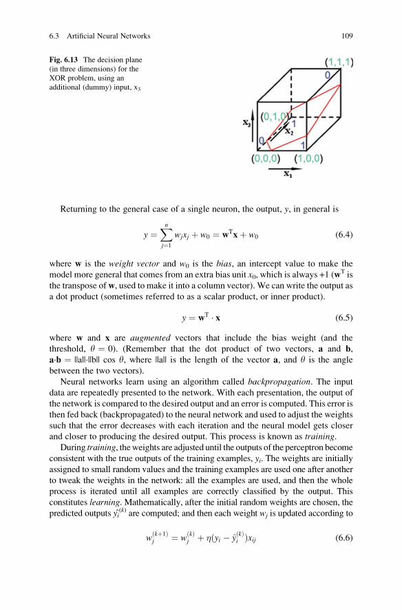
Returning to the general case of a single neuron, the output, y, in general is

y ¼Xn

j¼1

wjxj þ w0 ¼ wTxþ w0 (6.4)

where w is the weight vector and w0 is the bias, an intercept value to make the

model more general that comes from an extra bias unit x0, which is always +1 (wT is

the transpose ofw, used to make it into a column vector). We can write the output as

a dot product (sometimes referred to as a scalar product, or inner product).

y ¼ wT � x (6.5)

where w and x are augmented vectors that include the bias weight (and the

threshold, y ¼ 0). (Remember that the dot product of two vectors, a and b,a·b ¼ ||a||·||b|| cos y, where ||a|| is the length of the vector a, and y is the angle

between the two vectors).

Neural networks learn using an algorithm called backpropagation. The input

data are repeatedly presented to the network. With each presentation, the output of

the network is compared to the desired output and an error is computed. This error is

then fed back (backpropagated) to the neural network and used to adjust the weights

such that the error decreases with each iteration and the neural model gets closer

and closer to producing the desired output. This process is known as training.During training, theweights are adjusted until the outputs of the perceptron become

consistent with the true outputs of the training examples, yi. The weights are initiallyassigned to small random values and the training examples are used one after another

to tweak the weights in the network: all the examples are used, and then the whole

process is iterated until all examples are correctly classified by the output. This

constitutes learning. Mathematically, after the initial random weights are chosen, the

predicted outputs yi(k) are computed; and then each weight wj is updated according to

wðkþ1Þj ¼ w

ðkÞj þ �ðyi � y

ðkÞi Þxij (6.6)

Fig. 6.13 The decision plane

(in three dimensions) for the

XOR problem, using an

additional (dummy) input, x3


where w(k) is the weight associated with the ith input link after the kth iteration, � isknown as the learning rate, and wij is the value of the jth attribute of the training

parameter xi. In the weight update formula, links that contribute most to the error

term are the ones that require the largest adjustment. However, the weights should

not be changed too drastically because the error term is computed only for the

current training example: otherwise, the adjustments made in earlier iterations will

be undone. The learning rate (between 0 and 1, but typically set to 0.1 < � < 0.4)

is used to control the amount of adjustments made in each iteration. If � ~ 0, then

the new weight is mostly influenced by the old weight; if � ~ 1, then the new weight

is sensitive to the adjustment in the current iteration. Learning continues until either

the iteration error, yi � yðkÞi , is less than a user-specified threshold or a

predetermined number of iterations has been completed.

The weight learning problem can be seen as finding the global minimum error,

calculated as the proportion of misclassified training examples, over a space

where all the input values can vary. Therefore, it is possible to move too far in a

direction and improve one particular weight to the detriment of the overall sum.

While the sum may work for the training example being looked at, it may no

longer be a good value for classifying all the examples correctly. For this reason, �restricts the amount of movement possible. If a large movement is actually

required for a weight, then this will happen over a series of iterations through

the example set. If � is too small, the weights change very little at each step, and

the algorithm takes a long time to converge (Fig. 6.14a). Conversely, if � is too

large we may bounce around the error surface with the algorithm diverging

(Fig. 6.14b): this usually ends up with an overflow error in the computer’s

floating-point arithmetic.

Sometimes, � is set to decay as the number of such iterations through the whole

set of training examples increases, so that it can move more slowly toward the

global minimum in order not to overshoot in one direction. (This is the kind of

gradient descent used in the learning algorithm for multilayered networks).

Small Learning Rate

Slow Convergence

Large Learning Rate

Divergence!

a b

Fig. 6.14 (a) A small value of � results in slow convergence, while (b) a large value of � can resultin divergence!


Example 6.1 Learning

For a neuron with two inputs, we can easily decide what weights to use to give us

the correct output, but with more complex functions (more inputs or more

layers) it will not be so easy to decide. We would like our perceptron to

“learn” so that it can come up with its own weights. Let us consider the AND

function again (Fig. 6.11). We want to be able to assign random weights, and to

train the perceptron to give the correct output (which we will present as the

training value required) by adjusting these weights as it is presented with the

entire training set (this presentation being known as an epoch) a number of

times. This adjusting of the weights will proceed according to (6.6).

Look at the spreadsheet, perceptron.xls (downloadable from http://

extras.springer.com), which allows us to learn simple functions such as AND.

If we start with weights of w0 ¼ w1 ¼ w2 ¼ 0.5, and present the network

with the first training pair ([0,0]), from the first epoch, the network produces an

output of 1, when it should produce a 0: the error is �1 and so the weights will

change. Using (6.6) and a learning rate, � ¼ 0.1,

w0 ¼ 0.5 + (0.1 � 1 � �1) ¼ 0.4

w1 ¼ 0.5 + (0.1 � 0 � �1) ¼ 0.5

w2 ¼ 0.5 + (0.1 � 0 � �1) ¼ 0.5

These values become the new weights. The next training pair ([0,1]) also

produces a 1, when it should produce a 0, and so again the weights need to be re-

computed. The following training pair ([1,0]) also produces an output of 1, when

the required output is 0, and the weights have to be adjusted again. Finally, we

apply the input ([1,1]) to the network. This produces an output of 1, which is the

required output: no error has occurred here, so the weights remain the same.

As this presentation of the epoch produced three errors, we need to continue the

training and present the network with another epoch. Training continues until an

epoch is presented that does not produce an error (i.e., until the outputs

have converged on the required outputs); at this stage, after the fourth epoch,

the weights have become �0.3, 0.2, and 0.2 respectively. These are different

values for the weights to those in Fig. 6.11c, but the weights are in the same ratio

so that the resulting decision boundary turns out to be the same. (But note that

the decision boundary could be moved around a little and still implement the

AND function: it just needs to be able to distinguish the two classes).

We could keep track of the decision boundary after each epoch, and plot

them, confirming that only after the fourth epoch is the decision boundary able

to discriminate the two classes of output.

What is the effect of changing the starting weights?

What happens if the learning rate, �, is changed?What happens if you try to get the perceptron to learn the OR, NAND, and

XOR functions?




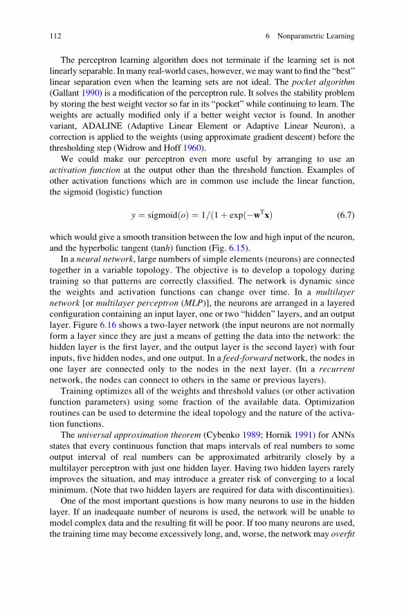
The perceptron learning algorithm does not terminate if the learning set is not

linearly separable. In many real-world cases, however, wemay want to find the “best”

linear separation even when the learning sets are not ideal. The pocket algorithm(Gallant 1990) is a modification of the perceptron rule. It solves the stability problem

by storing the best weight vector so far in its “pocket” while continuing to learn. The

weights are actually modified only if a better weight vector is found. In another

variant, ADALINE (Adaptive Linear Element or Adaptive Linear Neuron), a

correction is applied to the weights (using approximate gradient descent) before the

thresholding step (Widrow and Hoff 1960).

We could make our perceptron even more useful by arranging to use an

activation function at the output other than the threshold function. Examples of

other activation functions which are in common use include the linear function,

the sigmoid (logistic) function

y ¼ sigmoidðoÞ ¼ 1=ð1þ expð�wTxÞ (6.7)

which would give a smooth transition between the low and high input of the neuron,

and the hyperbolic tangent (tanh) function (Fig. 6.15).

In a neural network, large numbers of simple elements (neurons) are connected

together in a variable topology. The objective is to develop a topology during

training so that patterns are correctly classified. The network is dynamic since

the weights and activation functions can change over time. In a multilayernetwork [or multilayer perceptron (MLP)], the neurons are arranged in a layered

configuration containing an input layer, one or two “hidden” layers, and an output

layer. Figure 6.16 shows a two-layer network (the input neurons are not normally

form a layer since they are just a means of getting the data into the network: the

hidden layer is the first layer, and the output layer is the second layer) with four

inputs, five hidden nodes, and one output. In a feed-forward network, the nodes inone layer are connected only to the nodes in the next layer. (In a recurrentnetwork, the nodes can connect to others in the same or previous layers).

Training optimizes all of the weights and threshold values (or other activation

function parameters) using some fraction of the available data. Optimization

routines can be used to determine the ideal topology and the nature of the activa-

tion functions.

The universal approximation theorem (Cybenko 1989; Hornik 1991) for ANNs

states that every continuous function that maps intervals of real numbers to some

output interval of real numbers can be approximated arbitrarily closely by a

multilayer perceptron with just one hidden layer. Having two hidden layers rarely

improves the situation, and may introduce a greater risk of converging to a local

minimum. (Note that two hidden layers are required for data with discontinuities).

One of the most important questions is how many neurons to use in the hidden

layer. If an inadequate number of neurons is used, the network will be unable to

model complex data and the resulting fit will be poor. If too many neurons are used,

the training time may become excessively long, and, worse, the network may overfit


the data. When overfitting occurs, the network will begin to model random noise

in the data. The result is that the model fits the training data extremely well, but

it generalizes poorly to new, test data. Validation must be used to check for this.

Fig. 6.16 A simple two-layer

(feed-forward) ANN

-1-1

-0.5

0

0.5

1a b

c

-0.5 0 0.5 1

-1-1

-0.5

0

0.5

1

-0.5 0 0.5 1

-4

0.0

0.2

0.4

0.6

0.8

1.0

-2 0 2 4

Fig. 6.15 Activation functions (a) linear, (b) sigmoid, where changing the weight, w, alters thesteepness of the function (c) tanh


Example 6.2 Implementation of the logical XOR function

x1 x2 y

0 0 0

0 1 1

1 0 1

1 1 0

Let us return to the XOR function, which we saw could not be solved using a

decision boundary that is a single line (Fig. 6.12). However, two discriminant

lines could be used to separate “true” from “false” (Fig. 6.17a); the discriminant

functions could be

y1 ¼ x2 � x1 � 0:5

y2 ¼ x2 � x1 þ 0:5

which would require a two-layer network (Fig. 6.17b), with w11 ¼ w12 ¼ �1;

w21 ¼ w22 ¼ 1; b1 ¼ �0.5; and b2 ¼ 0.5. We could also make w1 ¼ �1,

w2 ¼ 1 and b0 ¼ 0. (What are the three required thresholds?)

Alternatively, we could have w11 ¼ w12 ¼ w21 ¼ w22 ¼ 1: w1 ¼ 1,

w2 ¼ �1: b0 ¼ b1 ¼ b2 ¼ �0.5. For an input of (1,0), the input to the top

neuron in the hidden layer is 0.5, which is above the threshold (0), so that this

neuron fires giving an output of 1. The input to the bottom neuron in the hidden

layer is 0, so it does not fire and the output is 0. The signal reaching the output

neuron is then 0.5, so this neuron fires to give an output of 1. You should check

the outputs for all the other possible inputs. You should be able to see that the

neuron in the output layer fires (giving 1), when the inputs x1 and x2 are differentto each other, but does not fire when they are the same: this is exactly the XOR

function.

To learn the weights of an artificial neural network model, we need an efficient

algorithm that converges to the correct solution when a sufficient number of

training samples are provided. The goal is to determine a set of weights w that

minimizes the total sum of squared errors:

y1 ¼ x2 � x1 � 0:5

y2 ¼ x2 � x1 þ 0:5

Note that the sum of the squared errors depends on w because the predicted class

y is a function of the weights assigned to the hidden and output nodes. If we replacey by wTx then the error function is a quadratic surface.


Optimization methods such as steepest (or gradient) descent and conjugategradient are highly susceptible to finding local minima if they begin the search in

a valley near a local minimum. They have no ability to see the big picture and find

the global minimum. Several methods have been tried to avoid local minima.

The simplest is just to try a number of random starting points and use the one

with the best value. A more sophisticated technique called simulated annealingimproves on this by trying widely separated random values and then gradually

reducing (“cooling”) the random jumps in the hope that the location is getting closer

to the global minimum.

The computation of the weights for the hidden nodes is not trivial because it is

difficult to assess their error term without knowing what their output values should

be. Backpropagation (more specifically, the backpropagation of errors) has been

developed to address this issue for multilayered networks. With backpropagation,

the input data are repeatedly presented to the neural network. With each presenta-

tion, the output of the neural network is compared to the desired output and an error

is computed (Fig. 6.18). This error is then fed back (backpropagated) to the neural

network and used to adjust the weights such that the error decreases with each

iteration and the neural model gets closer and closer to producing the desired

output. This sequence of events is repeated until an acceptable error has been

reached or until the network no longer appears to be learning. This process is

known as training.Training an ANN is a time-consuming process, especially when the number of

hidden nodes is large. The training set (i.e., the patterns whose class labels are

known) are presented to the network, and the weights are adjusted tomake the output

similar to the target values. In stochastic training patterns are chosen randomly from

the training set, and the network weights are updated for each pattern presentation.

Fig. 6.17 (a) The required discriminant functions in feature space [where the dark circle indicatesthe “true” output (“1”), and white circles indicates the “false” outputs (“0”)], and (b) the

corresponding neural network to implement it


In stochastic training, a weight updatemay reduce the error on the single pattern being

presented, yet increase the error on the full training set. However, given a large number

of such individual updates the total error decreases. In batch training, all patterns arepresented to the network before learning takes place. In virtually every case, we must

make several passes through the training data. In the batch training protocol, all the

training patterns are presented first and their corresponding weight updates summed;

only then are the actual weights in the network updated. This process is iterated until

some stopping criterion is met. In on-line training, each pattern is presented once andonly once; there is no use of memory for storing the patterns.

Before training has begun, the error on the training set is typically high; through

learning, the error becomes lower, as shown in a learning curve (Fig. 6.19). The

average error (per pattern) on an independent test set is always higher than on the

training set, and while it generally decreases, it can increase or oscillate. A valida-tion set (comprising new representative test patterns) is used to decide when to stop

training: we stop training at the minimum of the average error on this set. The curve

for the validation set in Fig. 6.19 indicates that training should stop at about the fifth

epoch. (We will consider validation, or more generally cross-validation, in some

detail in Chap. 8). The test set is used to measure the performance of the network.

Table 6.1 summarizes the advantages and disadvantage of a neural network.

In separable problems, perceptrons can find different solutions. It would be

interesting to find the hyperplane that assures the maximal safety tolerance training,

i.e., the largest separating margin between the classes (Fig. 6.20). The margins of

that hyperplane touch a limited number of special points (called the supportvectors), which define the hyperplane. Only the support vectors are required to

obtain this hyperplane, the other training samples can be ignored.

This so-called optimal perceptron (i.e., having optimal stability) can be deter-

mined by means of iterative training and optimization schemes [such as the

Min-Over algorithm (Krauth and Mezard 1987) or the AdaTron (Anlauf and

Biehl 1989)]. The perceptron of optimal stability is, together with the kerneltrick, one of the conceptual foundations of the support vector machine.

1 1 0 0 1 1 0 0 1 1 0 0 1 1 0 0

0 1 1 0 0 1 1 0

NeuralNetwork

AdjustWeights

Output Error

Desired+

0 1 1 0 0 1 1 0

1 0 1 0 1 0 1 0

Repeated presentation of XOR data

1 0 1 0 1 0 1 0 -∑

Fig. 6.18 Multilayer neural network learning to model the XOR function


http://dx.doi.org/10.1007/978-1-4614-5323-9_8

6.4 Kernel Machines

The support vector machine, SVM (Cortes and Vapnick 1995), later generalized

under the name kernel machine, became popular when it was applied to a hand-

writing recognition task, given pixel maps as input, and produced very accurate

results. For linearly separable problems, it finds the optimal separating hyperplane

Fig. 6.19 A typical learning curve. The average error per pattern is plotted as a function of the

number of epochs

Table 6.1 The advantages and disadvantages of neural networks

Advantages Disadvantages

It can perform tasks which a linear classifier

cannot

It needs training to operate

It uses a different architecture from most

microprocessors (needs emulation

mode)

If a neuron fails, the network can continue

because of its parallel nature

Large networks require high processing

time

It learns and does not need to be reprogrammed

It can be implemented easily for any

application

Fig. 6.20 (a) A perceptron can find different solutions to a linearly separable problem. (b) Thissolution assures the maximal safety tolerance

6.4 Kernel Machines 117

by maximizing the margin, the perpendicular distance across the hyperplane to

the closest instances (the support vectors) on either side of it. For nonlinearly

separable problems, we can settle on the hyperplane that incurs the least error; or

we can map the data by doing a nonlinear transformation using suitable chosen

basis functions into a higher-dimensional space, where the problem may become

linear. For example, we saw in Sect. 6.3 that the XOR problem is a nonlinearly

separable problem. However, it is possible to solve it by transforming the inputs

into a higher-dimensional space, where it is linearly separable (Fig. 6.13). This is

the basic idea behind the kernel trick (and the origin of the name kernel machine).Maximizing margins around the separating hyperplane seems a good idea both

intuitively and according to PAC (Probably Approximately Correct) theory. Given

that the equation of a separating hyperplane is

wTxþ b ¼ 0 (6.9)

where w and b are parameters of the model, the distance from an example, xi, to thehyperplane is given by

r ¼ ðwTxþ bÞ= wk k (6.10)

The examples closest to the hyperplane are called the support vectors, and the

(classification) margin of the separator is the distance between support vectors fromthe different classes (Fig. 6.21). The problem is one of quadratic optimization

subject to linear constraints. These are a well-known class of mathematical pro-

gramming problems, albeit beyond the scope of this text.

SVMs are basically two-class classifiers. If the training set is not linearly

separable, it may still be possible to find a solution by introducing slack variables

Fig. 6.21 Support vectors

and classification margin


to allow misclassification of difficult or noisy examples, resulting in a so-called softmargin. If this does not work, the original feature space needs to be mapped to a

higher-dimensional feature space where the training set is separable (Fig. 6.22).

This involves the so-called kernel trick, and relies on computing the inner product

between vectors, xTi xj . Typical kernel functions are linear, polynomials, and

Gaussians (radial basis functions).

Example 6.3 Using a polynomial kernel

Suppose we have five 1D data points, x1 ¼ 1, x2 ¼ 2, x3 ¼ 4, x4 ¼ 5 and

x5 ¼ 6, with 1, 2 and 6 as class 1 and 4, 5 as class 2 (Fig. 6.23a). This is clearly

a nonlinear problem.

Introducing a second dimension, y, with y1 ¼ 1, y2 ¼ 1, y3 ¼ �1, y4 ¼ �1,

y5 ¼ 1, and using a polynomial kernel of degree 2, K(x, y) ¼ (xy + 1)2 gives a

discriminant function, f(y) ¼ 0.6667x2 � 5.333x + 9 which successfully

separates the two classes (Fig. 6.23b).

Fig. 6.23 (a) Original 1D data (b) transformed to 2D

Fig. 6.22 Transform nonlinear SVM into a higher-dimensional feature space

6.4 Kernel Machines 119

6.5 Exercises

1. Show how a perceptron can be used to implement the logical OR function.

Sketch the discriminant function.

2. Consider a neuron with two inputs, one output and a threshold activation

function. If the two weights are w1 ¼ w2 ¼ 1, and the bias is �1.5, what is the

output for an input of ([0,0])? What about inputs ([0,1]), ([1.0]) and ([1,1]). Draw

the discriminant function, and write down its equation. What logic function does

it represent?

3. An approach to solving the XOR function is to map the problem to three

dimensions, by including a third input, x3, which moves the point at x1 ¼ 1,

x2 ¼ 1 along a third dimension but does not change the result when it is looked

at using a projection into the x1, x2 plane. This allows a linear plane (the 2D

analog of a straight line) to separate the points. (a) Construct a truth table for

XOR with three inputs, (b) plot a decision plane in a 3D diagram and (c) show

how this could be implemented with a neural network.

4. The following Fig. 6.24 shows a multilayer neural network involving a single

hidden neuron and jumping connections from the inputs to the output directly. (a)

Construct a truth table for all variables x1, x2, x3, and x4. Show that the network

solves the XOR problem. (b) Plot the decision boundary of x3 in the x1–x2 plane;(c) Plot the decision boundary of x4 in the x1–x2 plane and explain how you derive

it. (Note that your decision boundary should not be limited to the unit square only).

Note that the number on top of each neuron is the threshold and it is subtracted

from the net input. For instance, the equation for x3 is x3 ¼ step(x1 + x2�1.5).

5. Example 6.2 in the text considers a two-layer network (Fig. 6.17b) to implement

the XOR function, with w11 ¼ w12 ¼ �1; w21 ¼ w22 ¼ 1; b1 ¼ �0.5; and

b2 ¼ 0.5. We could also make w1 ¼ �1, w2 ¼ 1 and b0 ¼ 0. Follow the signals

through the network, and find the required values of the three thresholds.

(See spreadsheet, Q6.5.xls, downloadable from http://extras.springer.com).

Fig. 6.24 XOR implementation



References

Anlauf, J.K., Biehl, M.: The AdaTron: an adaptive perceptron algorithm. Europhys. Lett. 10,687–692 (1989)

Cortes, C., Vapnick, V.N.: Support-vector networks. Mach. Learn. 20, 273–297 (1995)

Cybenko, G.: Approximations by superpositions of sigmoidal functions. Math Control Signal Syst

2, 303–314 (1989)

Gallant, S.I.: Perceptron-based learning algorithms. IEEE Trans. Neural Netw. 1, 179–191 (1990)Hornik, K.: Approximation capabilities of multilayer feedforward networks. Neural Netw. 4,

251–257 (1991)

Krauth, W., Mezard, M.: Learning algorithms with optimal stability in neural networks. J. Phys.

A 20, 745–752 (1987)

Le Cun, Y.: Learning processes in an asymmetric threshold network. In: Bienenstock, E.,

Fogelman-Smith, F., Weisbuch, G. (eds.) Disordered Systems and Biological Organization,

NATO ASI Series, F20. Springer-Verlag, Berlin (1986)

McCulloch, W., Pitts, W.: A logical calculus of the ideas immanent in nervous activity. Bull.

Math. Biophys. 7, 115–133 (1943)

Minsky, M.L., Papert, S.A.: Perceptrons. MIT Press, MA (1969)

Parker, D.: Learning Logic. Technical Report TR-87. MIT Center for Computational Research in

Economics and Management Science, Cambridge, MA (1985)

Widrow, B., Hoff, M.E.: Adaptive switching circuits. In 1960 IRE WESCON Convention Record,

part 4, pp. 96–104. IRE, New York (1960)

References 121

Chapter 7

Feature Extraction and Selection

7.1 Reducing Dimensionality

In most classification applications, the complexity depends on the number of features,

d (which result in a d-dimensional feature space) and the number of (training) data

samples,N. As the dimensionality (number of features) increases, increasing amounts

of training data are required (this is called the curse of dimensionality). In order to

reduce the computational complexity, the number of features should be reduced to a

sufficient minimum.Whenwe decide that a feature is unnecessary, we save the cost of

extracting it. When data can be explained in terms of fewer features, the data can be

analyzed visually more easily and we get a better idea about the underlying process.

Humans have an extraordinary capacity to discern patterns and clusters in one, two or

three dimensions, but these abilities degrade drastically for four or higher dimensions.

If we keep features that have little discriminative power (because of a high correlation

with another feature), the classifier will be more complex and is likely to perform

poorly. Simple models will consequently require smaller datasets.

For a finite sample size, N, increasing the number of features (from 1) will

initially improve the performance of a classifier, but after a critical value, further

increase in the number of features (d) will reduce the performance resulting in

overfitting the data (Fig. 7.1). This is known as the peaking phenomenon. In most

cases, the additional information that is lost by discarding some features is (more

than) compensated by a more accurate mapping in the lower-dimensional space.

There are two main methods for reducing dimensionality; feature selection and

feature extraction. In feature selection, we want to select the k features (out of d)that provide the most information, discarding the other (d � k) features. Methods to

implement feature selection include using the inter/intraclass distance and subsetselection. In feature extraction, we find a new set of k (<d) features which are

combinations of the original d features. These methods may be supervised or

unsupervised. The most widely used feature extraction methods are PrincipalComponents Analysis (PCA) and Linear Discriminant Analysis (LDA), which are

both linear projection methods, unsupervised and supervised respectively.


123

7.1.1 Preprocessing

Prior to using the data we should remove outliers, scale the features to comparable

dynamic ranges (viz., normalization), and treat incomplete data.

Outliers are data that lie far from the mean of the corresponding random

variable. They can produce large errors during training, especially when they are

a result of noise. For a normal distribution, we could remove data points which are

more than three standard deviations from the mean (since they have less than a 1%

chance of belonging to the distribution).

The features can be normalized to have zero mean and unit variance using the

transform

x0¼ ðx� �xÞs

(7.1)

where �x and s are the mean and standard deviation of the original feature values.

If the original data are not evenly distributed around the mean, then a further

transform (so-called softmax scaling) can be used:

x0 ¼ 1

1þ expð�x0Þ (7.2)

One way of dealing with incomplete data is to generate missing values randomly

from the distribution characterized by the known values.

7.2 Feature Selection

7.2.1 Inter/Intraclass Distance

Good features are discriminative. Intuitively, there should be a large intraclass

distance and a small interclass distance. Figure 7.2 shows the case for a single

feature, two equiprobable class situation.

Fig. 7.1 The performance of

a classifier in terms of the

dimensionality of the feature

space

124 7 Feature Extraction and Selection

Figure 7.3 shows a more complicated case, a training set with two features and

four classes. The scatter diagram shows the four classes, each of which has its own

(within-scatter) matrix, Sw, describing the scattering within each class and resultingin characteristic elliptical isocontours around the class means, and one isocontour is

Fig. 7.3 Two-feature, four-class data: (a) scatter diagram, (b) after normalization, (c) after

decorrelation, and (d) after whitening. (After Van der Heijden et al. 2004)

Fig. 7.2 Single feature, x, distinguishing two equiprobable classes

7.2 Feature Selection 125

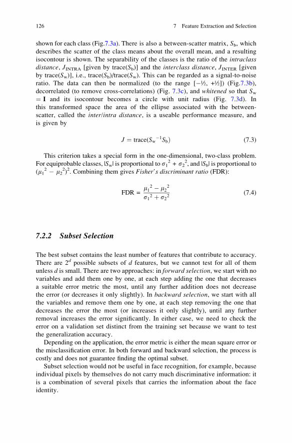
shown for each class (Fig.7.3a). There is also a between-scatter matrix, Sb, whichdescribes the scatter of the class means about the overall mean, and a resulting

isocontour is shown. The separability of the classes is the ratio of the intraclassdistance, JINTRA [given by trace(Sb)] and the interclass distance, JINTER [given

by trace(Sw)], i.e., trace(Sb)/trace(Sw). This can be regarded as a signal-to-noise

ratio. The data can then be normalized (to the range [�½, +½]) (Fig.7.3b),

decorrelated (to remove cross-correlations) (Fig. 7.3c), and whitened so that Sw¼ I and its isocontour becomes a circle with unit radius (Fig. 7.3d). In

this transformed space the area of the ellipse associated with the between-

scatter, called the inter/intra distance, is a useable performance measure, and

is given by

J ¼ trace(Sw�1SbÞ (7.3)

This criterion takes a special form in the one-dimensional, two-class problem.

For equiprobable classes, |Sw| is proportional to s12 + s2

2, and |Sb| is proportional to(m1

2 � m22)2. Combining them gives Fisher’s discriminant ratio (FDR):

FDR =m1

2 � m22

s12 þ s22(7.4)

7.2.2 Subset Selection

The best subset contains the least number of features that contribute to accuracy.

There are 2d possible subsets of d features, but we cannot test for all of them

unless d is small. There are two approaches: in forward selection, we start with novariables and add them one by one, at each step adding the one that decreases

a suitable error metric the most, until any further addition does not decrease

the error (or decreases it only slightly). In backward selection, we start with all

the variables and remove them one by one, at each step removing the one that

decreases the error the most (or increases it only slightly), until any further

removal increases the error significantly. In either case, we need to check the

error on a validation set distinct from the training set because we want to test

the generalization accuracy.

Depending on the application, the error metric is either the mean square error or

the misclassification error. In both forward and backward selection, the process is

costly and does not guarantee finding the optimal subset.

Subset selection would not be useful in face recognition, for example, because

individual pixels by themselves do not carry much discriminative information: it

is a combination of several pixels that carries the information about the face

identity.


7.3 Feature Extraction

In projection methods, we want to find a mapping from the original d-dimensional

space to a new k (<d)-dimensional space, with minimum loss of information.

An optimal mapping would be one that results in no increase in the minimum

probability of error, i.e., a Bayes decision rule applied to the initial (d-dimensional)

space and to the reduced (k-dimensional) space yields the same classification error.

In general, optimal mapping will require a nonlinear function, but we will restrict

ourselves to linear mapping. Within the realm of linear feature extraction, two

techniques are in common use: Principal Component Analysis (PCA) and Linear

Discriminant Analysis (LDA).

7.3.1 Principal Component Analysis

The goal of Principal Component Analysis [also known as the Karhunen–Loeve(KL) transform] is to represent the data accurately in a lower-dimensional space.

As much of the randomness (variance) in the higher-dimensional space as possible

should be preserved. This is achieved by a transformation that centers the data and

rotates the axes to line up with the direction of highest variance (Fig. 7.4).

Each principal component (PC1, PC2, . . .) is a linear combination of the original

variables, and there are as many principal components as original variables. The

first principal component has as high a variance as possible (i.e., it accounts for as

much of the variability in the data as possible), and each succeeding component

in turn has the highest variance possible under the constraint that it is orthogonal

to (i.e., uncorrelated with) the preceding components. Usually, the variance of the

original data can be explained by the first few principal components and the rest can

be ignored. In this case, using the principal components reduces the dimensionality

of the data, making it more amenable to visual inspection, clustering, and pattern

Fig. 7.4 Principal components analysis centers the data and then rotates the axes to line up with

the directions of highest variance. If the variance on PCA2 is small, it can be ignored and the

dimensionality reduces from two to one

7.3 Feature Extraction 127

recognition efforts. In Fig. 7.5, most of the variance occurs in the x01 direction, and x02

can be ignored.

PCA can reveal the internal structure of the data in a way that best explains its

variance, but it treats the total data and does not take into account class labels (i.e., it

is unsupervised). There is no guarantee that the directions of maximum variance

will make good features for discrimination.

The principal components are obtained by diagonalizing the covariance matrix

of the original data (Fig. 7.6). Their directions and magnitudes are given by the

eigenvectors and eigenvalues, respectively, of the original covariance matrix.

Sx ¼ lxðS� lIÞx ¼ 0

where the l’s are the eigenvalues of S, and the x’s are the corresponding

eigenvectors.

If we order the eigenvalues in descending order, then the first eigenvector will be

the directional cosines of the first principal component axis and the first eigenvalue

will be the variance along this axis, and so on. Note that the total invariance is

conserved, i.e., the sum of the variances of the principal components is equal to the

sum of the variances [trace (S)] of the original variables. Thus the contribution of

any eigenvalue, li, to the total variance is li/trace (S).It is important to realize that principal components analysis only helps if the

original variables are correlated. If they are highly correlated, there will be a small

number of eigenvectors with large eigenvalues; a large reduction in dimensionality

can be obtained by keeping only the k largest principal components.

(Note that if the data are extremely noisy, PCA may end up suggesting that the

noisiest variables are the most significant: measuring the entropy of the variables

would be a way to identify whether some variables are too noisy to be included in

the analysis).

Fig. 7.5 PCA in 2D: rotation

of axes to line up

with direction of largest

variance (x01).


In 3D, there will be three principal components (Fig. 7.7), ranked from the most

significant to the least.

A classic multivariate dataset is Fisher’s iris data [Fisher 1936], comprising 50

samples from each of three species (setosa, virginica, and versicolor) of iris flowers(Fig. 7.8). Four features (the length and width of the sepal and the petal) were

measured from each sample.

A scatter plot matrix of the features (in pairs) is useful to see whether any of thefeatures are correlated, i.e., whether they are connected to some degree within

the dataset (Fig. 7.9).

Fig. 7.6 The covariance matrix and a corresponding isocontour of a bivariate Gaussian distribu-

tion, before (top) and after (bottom) diagonalization

Fig. 7.7 (a) A dataset in 3D, (b) the principal component directions, (c) the two largest principal

components


The correlation coefficients from the scatter plot matrix form a correlation

matrix (Table 7.1).

The petal length is highly correlated with the petal width, somewhat less

correlated with the sepal length and the sepal width. Because of the high

Fig. 7.8 Iris flowers (a) Iris setosa, (b) Iris versicolor, and (c) Iris virginica

Fig. 7.9 Scatter plot matrix of Fisher’s iris data. (The features from Iris setosa are plotted in red,those from Iris versicolor are plotted in green, and those from Iris virginica are plotted in blue; theelliptical contours enclose 95% of the features in each plot.)


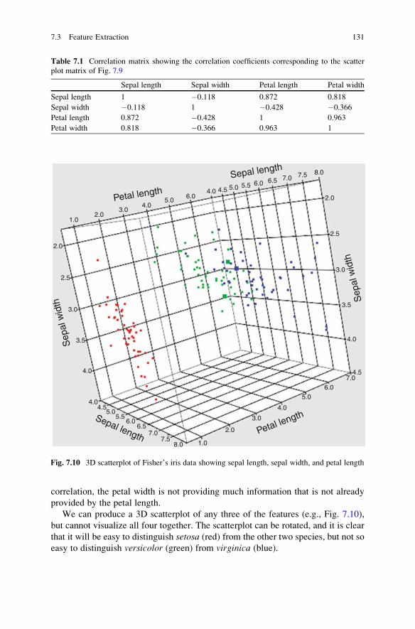
correlation, the petal width is not providing much information that is not already

provided by the petal length.

We can produce a 3D scatterplot of any three of the features (e.g., Fig. 7.10),

but cannot visualize all four together. The scatterplot can be rotated, and it is clear

that it will be easy to distinguish setosa (red) from the other two species, but not so

easy to distinguish versicolor (green) from virginica (blue).

Table 7.1 Correlation matrix showing the correlation coefficients corresponding to the scatter

plot matrix of Fig. 7.9

Sepal length Sepal width Petal length Petal width

Sepal length 1 �0.118 0.872 0.818

Sepal width �0.118 1 �0.428 �0.366

Petal length 0.872 �0.428 1 0.963

Petal width 0.818 �0.366 0.963 1

1.02.0

3.04.0

Petal length

Petal lengthSepal length

Sep

al w

idth S

epal

wid

th

Sepal length

5.06.0

4.0 4.5 5.0 5.5 6.0 6.5 7.0 7.5 8.0

2.0

2.5

3.0

3.5

4.0

4.57.0

6.05.0

4.0

3.0

2.0

1.08.07.5

7.06.5

6.05.5

5.04.5

4.0

4.0

3.5

3.0

2.5

2.0

Fig. 7.10 3D scatterplot of Fisher’s iris data showing sepal length, sepal width, and petal length


PCA reveals the directions of greatest variance. For the iris data, the three largest

principal components are shown in Fig. 7.11. The overlaid biplot shows the

directions of the original four variables. It can be seen that two of them are highly

correlated (i.e., in very similar directions).

The percentage of the total variance accounted for by each of the principal

components is proportional to the value of the individual eigenvalues (Fig. 7.12a).

The eigenvalues (or percentage contributions) plotted against the number of princi-

pal components is known as a scree plot and is useful for determining how many

principal components need to be kept to capture most of the variability of the data.

The first two principal components account for 95.8% of the variation, so that

keeping only them will preserve most of the variability of the data and reduce the

dimensionality from four to two. This is shown in the so-called scree plot ofFig. 7.12b. (Scree is a term for the rubble that accumulates at the bottom of steep

cliffs, which this plot resembles).

Fig. 7.11 3D scatterplot of the three largest principal components. The overlaid biplot shows the

directions of the original four variables. It can be seen that two of them are highly correlated (i.e.,

in very similar directions)


The principal components are linear combinations of the original variables; for

these data, the first two principal components, P1 and P2, are given by

P1 ¼ (0.3683 � Sepal length) + (�0.3617 � Sepal width) + (0.1925 � Petal

length) + (0.4338 � Petal width) + (�2.2899)

P2 ¼ (0.4767 � Sepal length) + (2.2156 � Sepal width) + (0.0145 � Petal

length) + (0.0919 � Petal width) + (�9.7245)

(Note the constant term which comes from moving the original axis to the

centroid if the dataset).

Figure 7.13 shows a scatterplot of the iris data based on the first two principal

components. PCA is sensitive to outliers (which should be discarded on the basis

of their Mahalanobis distances to the centroids) and noise (see earlier comments

on entropy).

We must remember that PCA is a one-class procedure (even though we have

colored our iris data according to class) and therefore cannot help in separating

classes. [The Karhunen–Loeve expansion allows the use of class information;

instead of using the covariance matrix of the whole sample, it estimates separate

class covariance matrices, take their average (weighted by the priors), and use its

eigenvectors.]

PCA is limited to finding linear combinations of the original features, which is

sufficient inmany applications but may result in the loss of toomuch information. To

retain such information, a nonlinear mapping method [such as multi-dimensionalscaling (MDS) (Kruskal and Wish 1977)] is needed.

Numbera

b

Eigenvalue 20 40 60 80Percent Cum Percent72.96295.813

100.00099.482

12

43

2.91850.9140

0.02070.1468

72.96222.851

0.518

Number of Components

1.0

-0.5

0.5

1.5

Eig

enva

lue 2.5

3.5

2.0 3.0 4.0

3.669

Fig. 7.12 (a) The eigenvalues and contributions of the principal components to the total variance,

(b) the scree plot


P1

-2-3

-2

-1

0

1

2

3

-1.5 -1 -0.5 0 0.5 1 1.5 2 2.5

P2

Fig. 7.13 Scatterplot of the first two principal components of the iris data

Fig. 7.14 Dataset, x, and the eigenvectors (principal component axes)—not drawn to scale


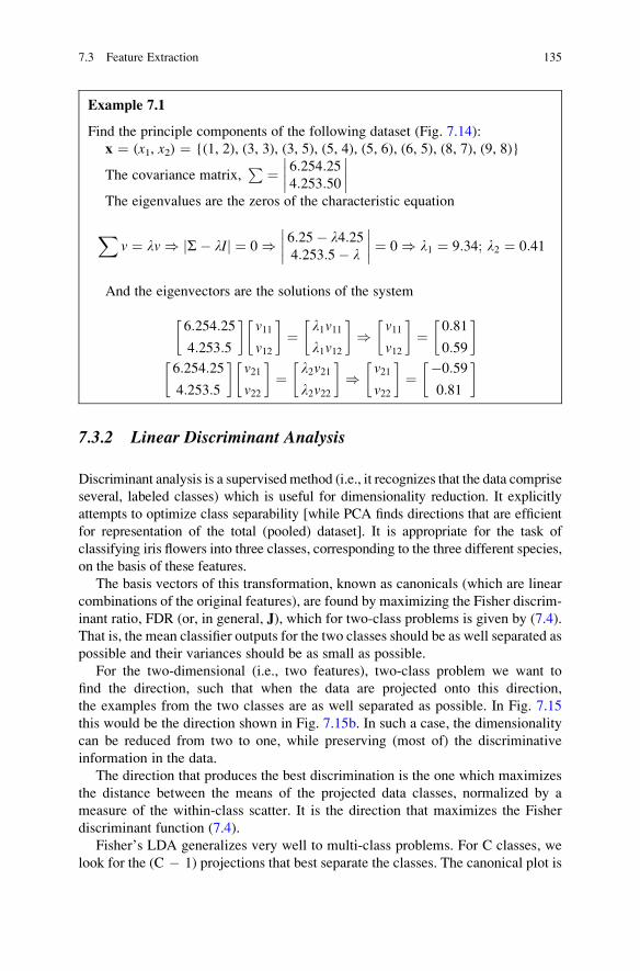
Example 7.1

Find the principle components of the following dataset (Fig. 7.14):

x ¼ (x1, x2) ¼ {(1, 2), (3, 3), (3, 5), (5, 4), (5, 6), (6, 5), (8, 7), (9, 8)}

The covariance matrix,P ¼ 6:254:25

4:253:50

��

��The eigenvalues are the zeros of the characteristic equation

Xv ¼ lv ) S� lIj j ¼ 0 ) 6:25� l4:25

4:253:5� l

��

�� ¼ 0 ) l1 ¼ 9:34; l2 ¼ 0:41

And the eigenvectors are the solutions of the system

6:254:25

4:253:5

� �v11

v12

� �¼ l1v11

l1v12

� �) v11

v12

� �¼ 0:81

0:59

� �

6:254:25

4:253:5

� �v21

v22

� �¼ l2v21

l2v22

� �) v21

v22

� �¼ �0:59

0:81

� �

7.3.2 Linear Discriminant Analysis

Discriminant analysis is a supervisedmethod (i.e., it recognizes that the data comprise

several, labeled classes) which is useful for dimensionality reduction. It explicitly

attempts to optimize class separability [while PCA finds directions that are efficient

for representation of the total (pooled) dataset]. It is appropriate for the task of

classifying iris flowers into three classes, corresponding to the three different species,

on the basis of these features.

The basis vectors of this transformation, known as canonicals (which are linear

combinations of the original features), are found by maximizing the Fisher discrim-

inant ratio, FDR (or, in general, J), which for two-class problems is given by (7.4).

That is, the mean classifier outputs for the two classes should be as well separated as

possible and their variances should be as small as possible.

For the two-dimensional (i.e., two features), two-class problem we want to

find the direction, such that when the data are projected onto this direction,

the examples from the two classes are as well separated as possible. In Fig. 7.15

this would be the direction shown in Fig. 7.15b. In such a case, the dimensionality

can be reduced from two to one, while preserving (most of) the discriminative

information in the data.

The direction that produces the best discrimination is the one which maximizes

the distance between the means of the projected data classes, normalized by a

measure of the within-class scatter. It is the direction that maximizes the Fisher

discriminant function (7.4).

Fisher’s LDA generalizes very well to multi-class problems. For C classes, we

look for the (C � 1) projections that best separate the classes. The canonical plot is


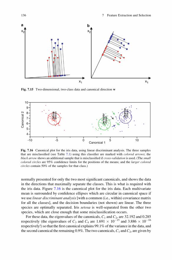
normally presented for only the two most significant canonicals, and shows the data

in the directions that maximally separate the classes. This is what is required with

the iris data. Figure 7.16 is the canonical plot for the iris data. Each multivariate

mean is surrounded by confidence ellipses which are circular in canonical space if

we use linear discriminant analysis [with a common (i.e., within) covariance matrix

for all the classes], and the decision boundaries (not shown) are linear. The three

species are optimally separated. Iris setosa is well-separated from the other two

species, which are close enough that some misclassification occurs.

For these data, the eigenvalues of the canonicals, C1 and C2, are 32.192 and 0.285

respectively (the eigenvalues of C3 and C4 are 1.691 � 10�15 and 3.886 � 10�16

respectively!) so that the first canonical explains 99.1% of the variance in the data, and

the second canonical the remaining 0.9%. The two canonicals,C1 andC2, are given by

-10

10

9

8

7

6

5

4

-5 0Canonical 1

Can

onic

al 2

5 10

Fig. 7.16 Canonical plot for the iris data, using linear discriminant analysis. The three samples

that are misclassified (see Table 7.1) using this classifier are marked with colored arrows; theblack arrow shows an additional sample that is misclassified if cross-validation is used. (The smallcolored circles are 95% confidence limits for the positions of the means; and the larger coloredcircles contain 50% of the samples for that class.)

Fig. 7.15 Two-dimensional, two-class data and canonical direction w


C1 ¼ (�0.8294 � Sepal length) + (�1.5345 � Sepal width) + (2.2012 �Petal length)

(2.8105 � Petal width)

C2 ¼ (0.0241 � Sepal length) + (2.1645 � Sepal width) + (�0.9319 � Petal

length)

(2.8392 � Petal width)

Samples are assigned to the class whose multivariate mean is closest. (Since

different features have different scales, and likely have different dimensions, the

appropriate distances to calculate are the Mahalanobis distances rather than

Euclidean distances). For these data, the three samples marked in Fig. 7.16 are

misclassified, i.e., assigned to the wrong classes. Two features from versicolorare misclassified as virginica, because they are closer to its mean; and one feature

from virginica is misclassified as versicolor, because it is closer to that mean. The

final classifications can be tallied in a confusion matrix (Table 7.2), which is a

contingency table in which the actual (in the rows) and the predicted (in the

columns) classes of the data (or vice versa in some implementations) are presented.

Entries on the diagonal of the matrix are the correct classifications; and entries off

the diagonal are the misclassifications. The confusionmatrix shows the performanceof the classifier. In this case, three features were misclassified and appear as off-

diagonal entries, representing a total misclassification rate of 2% (i.e., 3 out of 150).

Cross-validation shows the prediction for a given observation if it is left out of

the estimation sample [a re-sampling technique known as jack-knifing (or leave-one-out)]. In this case an additional sample is misclassified if cross-validation is

used (Fig. 7.16). The confusion matrix if cross-validation is used is displayed below

(Table 7.3).

If a separate covariance matrix is used for each class, which is preferable, the

analysis is quadratic discriminant analysis; the isocontours (Fig. 7.17) are ellipses

Table 7.2 Confusion matrix showing the results of linear discriminant analysis used to distin-

guish three species of iris flower

Predicted

Actual setosa versicolor virginica

Class 1 (setosa) 50 0 0

Class 2 (versicolor) 0 48 1

Class 3 (virginica) 0 2 49

Table 7.3 Confusion matrix showing the results of linear discriminant analysis if cross-validation

is used with the iris data

Predicted






and the decision boundaries (not shown) are quadrics. For this particular dataset, the

same three samples are misclassified but this will not generally be the case.

Quadratic discriminant analysis suffers in small datasets because it does not have

enough data to make nicely invertible and stable covariance matrices.

Of course Fisher’s discriminant analysis (whether linear or quadratic) works in

higher dimensions and with multiple classes, always seeking to project the data

onto a lesser-dimensional space and maximize the separability of the classes. It is a

parametric method since it assumes unimodal Gaussian likelihoods, and will not

work properly if the distributions are significantly non-Gaussian. It does depend on

the prior probabilities; these can either be taken as proportional to the occurrence

of the classes in the sample set, or, preferably, if these are known, to the occurrences

in the whole population. Linear Discriminant Analysis will fail when the discrimina-

tory information is not in the mean, but rather in the variance of the data (Fig. 7.18).

-10

10

9

8

7

6

5

4

-5 0Canonical 1

Can

onic

al 2

5 10

Fig. 7.17 Canonical plot for the iris data, using quadratic discriminant analysis. The three samples

that are misclassified (see Table 7.4) using this classifier are marked with colored arrows. (Thesmall colored circles are 95% confidence limits for the positions of the means; and the largercolored circles contain 50% of the samples for that class.)

Fig. 7.18 LDA is not successful if the discriminatory information is in the variance


Example 7.2

For the small sample of business executives given below, is it possible to

discriminate them into classes according to their education (viz., Associate,

Bachelors or Masters degree) based on their current salary, age, and number

of times that they have been promoted?

Number Education Gender Annual salary (,000’s) Age (years) Number of promotions

1 Masters M 94 63 5

2 Associate F 54 38 2

3 Bachelors M 89 54 4


5 Bachelors F 71 47 3



8 Masters M 85 58 4


10 Masters M 103 60 5

11 Masters F 75 48 4

12 Associate M 73 53 3

The resulting canonical plot, using linear discriminant analysis (with separate

covariances), is shown in Fig. 7.19. The canonical have eigenvalues of 4.241

and 0.1149, so that canonical1 accounts for 97.36% of the discriminative

information. The formula for canonical1 is �0.1935 � Salary + 0.0433 �Age + 4.4920 � Promotions: it is not immediately clear which of the variables

is the most important because they have not been standardized.

6.0

5.0

4.5

4.0

3.5

0 1 2 3 4

Canonical1

Can

onic

al2

Bac

helo

rs

Mas

ters

Ass

ocia

tes

5 6 7 8

5.5

Fig. 7.19 Canonical plot showing contours around the three classes. The misclassified sample

is shown as a blue square

(continued)


(continued)

The confusion matrix is given in Table 7.4. Only one of the executives

(number 8) is misclassified; he actually has a Masters degree but is predicted

as having a Bachelors degree.

Table 7.4 Confusion matrix showing the results of linear discriminant analysis used to

distinguish three classes on the basis of their education (actual rows by predicted columns)

Associate Bachelors Master

Associate 4 0 0

Bachelors 0 4 0

Masters 0 1 3

Example 7.3

The Excel file, LDA with Priors and losses.xls, downloadable from

http://extras.springer.com contains the embedded equations to calculate the

state-conditional density functions and the posterior probabilities, from which

a prediction can be made on the basis of maximum a posteriori (MAP) proba-

bility. It also incorporates the prior probabilities, and allows easy entry of loss

function terms, lij, and inspection of the effect on the decision.

Using the same dataset of business executives as in Example 7.2, viz., can we

predict their education based on their current salary, age, and number of times

that they have been promoted. With equal losses, the predictions are correct

except for executive number 8, who is predicted to have a Bachelors education,

rather than a Masters.

The diagonal terms of the loss function matrix are zero (reflecting no penalty

for a correct prediction), and non-zero off-diagonal terms (often taken as 1s).

If we double the loss associated with predicting an actual Masters as a Bachelors

(Table 7.5), we can follow through the calculations on the spreadsheet and find

100% accuracy in prediction.

Table 7.5 Loss function

terms (actual rows by

predicted columns)

Losses

Associate Bachelors Master

Associate 0 1 1

Bachelors 1 0 1

Masters 1 2 0

7.4 Exercises

(These are most conveniently done with access to either MatLab or JMP (SAS,

Inc.). Indeed Q.7.2 and 7.3 use datasets in the .JMP format (which can be

downloaded from http://extras.springer.com).




1. Principal Components Analysis (PCA) and Linear Discriminant Analysis (LDA)

have different purposes. The former operates on the total (unlabeled) dataset to

find the directions that contain the maximum variance; the latter operates on

labeled data to find the directions which are best at distinguishing the labeled

classes. In general, the results (principal components and canonicals, respec-

tively) will be quite different. However, for special examples of data the

principal components and canonicals could be in the same directions. (1) Draw

an example of two-class, two-dimensional data such that PCA and LDA find the

same directions. (2) Draw an example of two-class, two-dimensional data such

that PCA and LDA find totally different directions.

2. The data in socioeconomic.jmp consists of five socioeconomic variables/

features for 12 census tracts in the LA Metropolitan area.

(a) Use the Multivariate platform to produce a scatterplot matrix of all five

features.

(b) Conduct a principal component analysis (on the correlations) of all five

features. Considering the eigenvectors, which are the most useful features?

Considering the eigenvalues, how many principal components would you

use in subsequent analysis?

3. The measurements in adolescent.jmp are of 58 high-school students.

Using LDA (quadratic) explore how well the variables height, and length of

arm, leg and hand are at distinguishing the ethnicity of the students. Use the

occurrence of the classes in the sampled set as the prior probabilities. What

happens if a fifth variable, the length of the foot, is included? What if weight and

the size of the wrist and neck are included? How independent are the measured

features? What additional factor is limiting the usefulness of the results?

References

Fisher, R.A.: The use of multiple measurements in taxonomic problems. Ann. Eugen. 7, 179–188

(1936)

Kruskal, J.B., Wish, M.: Multidimensional Scaling. Sage, Beverly Hills, CA (1977)

Van der Heijden, F., Duin, R.P.W., de Ridder, D., Tax, D.M.J.: Classification, Parameter Estima-

tion and State Estimation. Wiley, Chichester (2004)

References 141

Chapter 8

Unsupervised Learning

8.1 Clustering

With unsupervised learning, the class labels are unknown, and the data are plotted

to see whether it clusters naturally. Cluster analysis divides the data into clusters

(classes) that are hopefully meaningful and/or useful: the clusters may or may not

correspond with the human perception of similarity.

Cluster analysis has been used in a wide variety of fields, e.g.,

• In biology, to find groups of genes that have similar functions

• In climatology, to find clusters of atmospheric pressure that have an impact on

climate

• In medicine, to identify different variants of a disease

• In business, to cluster customers for marketing activities

• In information retrieval, to group search results into clusters and subclusters in a

hierarchical structure

• In imaging, to segment an image (into several different regions): or to compress

image and video data by replacing objects by the prototype of each cluster

(known as vector quantization).

Clusters should comprise objects that are similar to each other and different from

those in other clusters. This will require adoption of a (dis)similarity measure, which

is often taken as a proximity measure (e.g., a power norm, such as the L1 norm (the

Manhattan or city-block distance), given by jx1 � y1j þ jx2 � y2j ; the L2 norm

(the Euclidean distance), given by

ffiffiffiffiffiffiffiffiffiffiffiffiffiffiffiffiffiffiffiffiffiffiffiffiffiffiffiffiffiffiffiffiffiffiffiffiffiffiffiffiffiffiffiffiffiffiðx1 � y1Þ2 þ ðx2 � y2Þ2

q; or the L1 norm (the

Chebyshev or chess-board distance), given by maxfx1 � y1; x2 � y2g). Once a (dis)similarity measure has been chosen, we need to define a criterion to be optimized.

The most widely used criterion function for clustering is the sum of the squared error

(SSE). We calculate the error of each data point (i.e., its distance to the closest

centroid), and then compute the total sum of the squared errors. Clustering methods

which use this criterion are known as minimum variance methods. Other criterion


143

functions exist, based on the scatter matrices used in linear discriminant analysis

(LDA).

Clusters can be either partitional (or flat), in which the data are divided into

nonoverlapping subsets (clusters) such that each data point is in exactly one subset

(Fig. 8.1a), or they may be hierarchical, in which the clusters are nested (Fig. 8.1b).Nested clusters are often represented by a hierarchical tree or dendrogram

(Fig. 8.1c).

The notion of a cluster is not well defined; they are often in the eye of the

beholder. For example, in Fig. 8.2 it is unclear whether there are two, four, or six

partitional clusters. It may even be that there are two partitional clusters, with

nested (hierarchical) subclusters. Because clusters are not well defined, we can

anticipate that it may be difficult to determine the extent to which clustering should

continue in a clustering algorithm.

In non-exclusive clusters, data points may belong to multiple clusters. In addi-

tion, in fuzzy clustering, a data point belongs to every cluster with some weight

(or probability) between 0 and 1.

Fig. 8.1 (a) Partitional clustering (b) hierarchical clustering, represented as (c) a dendrogram

Fig. 8.2 Different ways of clustering the same set of points

144 8 Unsupervised Learning

We will consider one example of each clustering technique: k-means clustering,

and its variants, as an example of partitional clustering, and agglomerative hierar-

chical clustering as an example of hierarchical clustering.

8.2 k-Means Clustering

k-Means clustering (MacQueen 1967) is one of the oldest and most widely used

clustering algorithms. It is a partitional clustering approach. Each cluster is

represented by one prototype object, and a new data sample is assigned to the

nearest prototype and therefore to that cluster. The training consists of a very simple

iterative scheme to adjust the placing of the prototypes:

(i) Randomly choose k objects from the training set, which become the prototypes

(ii) Assign all the other objects to the nearest prototype to form clusters; “near-

ness” is measured by Euclidean distance (or some other norm)

(iii) Update the new prototype of each cluster as the centroid of all the objects

assigned to that cluster

(iv) Return to step (ii) until convergence (i.e., when no data point changes clusters,

or equivalently, until the centroids remain the same. Because most of the

convergence occurs in the early iterations, this condition is often replaced by

a weaker condition, e.g., repeat until only 1% of the points change clusters).

Figure 8.3 shows the result of several iterations on a particular dataset.

The “assignment” step is also referred to as the expectation step, and the “updatestep” as the maximization step, making this algorithm a variant of the generalized

expectation–maximization (EM) algorithm.

As it is a heuristic algorithm, there is no guarantee that k-means clustering will

converge to the global optimum. The result is sensitive to the initial choice of

objects as cluster centers, especially for small data sets. Larger data sets comprising

approximately 200–100,000 observations are best. Since the algorithm is usually

very fast, it is common to run it multiple times with different starting conditions to

minimize this effect.

The algorithm can be viewed as a greedy algorithm for partitioning n samples

into k clusters so as to minimize an objective function, which can be taken as the

sum of the squared distances to the cluster centers, the sum of the squared error

(SSE). We calculate the error of each data point (i.e., its distance to the closest

centroid), and then compute the total sum of the squared errors.

SSE ¼XK

i¼1

X

x2Ci

distðci; xÞ2 (8.1)

where ci is the center of the ith cluster, and dist is the Euclidean distance [in which

case it is better to work with standardized features, and the clusters become circular

8.2 k-Means Clustering 145

(or spherical) in shape]. For two different runs of k-means, with the same value of kbut different starting prototypes, we will choose the one with the smallest value of

SSE. The complexity of the algorithm is O(n � k � I � d), where n is the number

of data points, k the number of clusters, I the number of iterations, and d is the

number of features.

Pre-processing and post-processing steps can be used to improve the final result.

Pre-processing steps include standardizing (or normalizing) the data, and

eliminating or reducing the effect of outliers. Outliers can pull the centroid away

from its true position; to prevent this, the median can be used instead of the average

in finding the new prototype during each iteration. Post-processing can include

splitting “loose” clusters, i.e., clusters with relatively high SSEs, and merging

“close” clusters, i.e., those with relatively low SSEs.

A variant of the k-means algorithm, called the bisecting k-means algorithm, canbe used to minimize the dependence on the initial set of prototypes. The basic idea

is to split the points into two clusters, then split each of these into two, and so on.

There are a number of different ways to do this. You could compute the centroid of

all the data points, select a point at random (cL), and construct a point (cR) which is

symmetrically placed with regard to the centroid. Cluster the data around these two

points, and then repeat the process within these two clusters. If you want k clusters,where k is a power of 2, say 2m, you iteratem times. If you want k clusters with k nota power of 2 (say, 24), you take the closest inferior power of 2 (i.e., 16), take these

16 clusters, and then randomly choose 8 of them to subcluster.

Fig. 8.3 Results of k-means clustering in various iterations (The prototypes in each iteration are

marked with a “plus.”)


k-Means and its variants have a number of limitations for certain types of

clusters. In particular, there are difficulties in detecting “natural” clusters when

they have widely different sizes or densities, or when they have non-spherical

shapes (Fig. 8.4). In Fig. 8.4a, the largest cluster is broken and pieces of it are

assigned to the smaller clusters. In Fig. 8.4b, the two smaller clusters are much

denser than the larger cluster and this confounds the algorithm. Finally, in Fig. 8.4c,

3a

b

c

2

1

0

-1

-2

-3

3

2

1

0

-1

-2

-3

3

2

1

0

-1

-2

-3

3

2

1

0

-1

-2

-3

-4 -3 -2 -1 0x

x

x

x

x

x

yy y

yy

y

1 2 3 4

-2 -1 0

15

10

5

0

-5

15

10

5

0

-5

1 2 3 4 5 6

-15 -10 -5 0 5 10 15 -15 -10 -5 0 5 10 15

-2 -1 0 1 2 3 4 5 6

-4 -3 -2 -1 0 1 2 3 4

Fig. 8.4 Natural clusters and the results of k-means clustering when (a) the sizes are very

different, (b) the densities are very different, and (c) the shapes are non-spherical


k-means mixes the natural clusters because they are non-spherical in shape. These

difficulties can be overcome to an extent if the user is willing to accept a larger

number of clusters (say, six instead of two or three), and merge some of them later.

Unfortunately, there is no general theoretical solution to find the optimal number

of clusters for any given dataset. A simple approach is to compare the results of

multiple runs with different k classes and choose the best one, but we need to be

careful because increasing k not only results in smaller error function values by

definition but also an increasing risk of overfitting.The result of k-means clustering can also be seen as the Voronoi cells (i.e.,

polygonal spheres of influence) of the cluster means (Fig. 8.5). Since data are split

halfway between cluster means, this can lead to suboptimal splits. The Gaussian

models used by the expectation–maximization (EM) algorithm (which can be seen

as a generalization of k-means) are more flexible here by having both variances and

covariances. The EM algorithm is thus able to accommodate clusters of variable

sizes much better than k-means, as well as correlated clusters.

It has been shown (Zha et al. 2001; Ding and He 2004) that the “relaxed”

solution of k-means clustering, specified by the cluster indicators, is given by the

PCA principal components.

8.2.1 Fuzzy c-Means Clustering

k-Means clustering is an example of partitional clustering where the data are

divided between nonoverlapping clusters, each represented by a prototype which

is the centroid of the objects in a cluster. In such clustering, each data object belongs

Fig. 8.5 The result of k-means clustering on handwritten digits data (The centroids of the clusters

are marked with a white cross, and the Voronoi cells for each cluster are colorized)


to just one cluster, whereas in fuzzy clustering, each object can belong to more than

one cluster, and associated with each object is a set of membership weights, wij,

representing the strength of the association between that xi and a particular cluster

Cj. Membership weights vary between 0 and 1, and all the weights for a particular

object, xi, add up to 1. Fuzzy clustering is a process of assigning these membership

weights.

One of the most widely used fuzzy clustering algorithms is the fuzzy c-meansalgorithm (Bezdek 1981), which is a direct generalization of the k-means clustering

algorithm. With fuzzy c-means, the centroid of a cluster, cj, is the weighted of all

the points, weighted by their membership weight or degree of belonging to that

particular cluster: The membership weight is inversely related to the distance of the

object to the cluster center as calculated on the previous pass.

The training consists of a very simple iterative scheme to adjust the placing of

the prototypes:

(i) Choose a number of clusters, k, and randomly assign weights, wij, to each of the

m objects for being in the clusters

(ii) Compute the centroid for each cluster, cj, as the weighted mean of each object

cj ¼Pm

i¼1

wpijxi

Pm

i¼1

wpij

(8.2)

(iii) For each object, update its membership weights of being in the clusters by

minimizing the (modified) SSE:

SSEðC1;C2; . . . ;CkÞ ¼Xk

j¼1

Xm

i¼1

wpijdistðxi; cjÞ2 (8.3)

subject to the constraint that the weights sum to 1, where p is an exponent, thefuzzifier, that has a value between 1 and 1, and determines the influence of

the weights and, therefore, the level of cluster fuzziness. A large value results in

smaller values of the membership weights and, hence, fuzzier clusters. Com-

monly p is set to 2. If p is close to 1, then the membership weights,wij, converge

to 0 or 1, and the algorithm behaves like k-means clustering.

(iv) Finally, return to step (ii) until convergence (i.e., when the change of the

weights is no more than a given sensitivity threshold).

The algorithmminimizes intra-cluster variance and is less susceptible to outliers,

but still suffers from the problem that the minimum is likely to be a local minimum

rather than the global minimum and the results depend on the initial choice of

weights.


8.3 (Agglomerative) Hierarchical Clustering

Hierarchical clustering produces a set of nested clusters organized as a hierarchicaltree, which can be visualized as a dendrogram that records the sequences of merges

or splits (Fig. 8.6).

In (agglomerative, as opposed to divisive) hierarchical clustering, each instancestarts off as its own cluster, and is subsequently joined to the “nearest” instance to

form a new cluster. It is a bottom-up technique. At each step of the clustering, larger

clusters are obtained. The algorithm is to:

(i) Find the two features that are “closest” in multivariate space

(ii) Replace them with a single feature at their mean

(iii) Repeat with the next two closest features, and continue until all the features are

subsumed into one cluster

The key operation is the computation of the proximity in step (i). There are

several definitions of cluster proximity that could be used. We could use the

Euclidean distance between instances, if we make sure that all the features

have the same scale, i.e., use standardized features. At each iteration, we choose

the two closest groups to merge. In single-link clustering, this distance is defined

as the smallest distance between all possible pairs of elements of the two groups,

dmin (Fig. 8.7). The single-link method corresponds to constructing the minimalspanning tree (MST). In complete-link clustering, the distance between the groups

is taken as the largest distance between all possible pairs, dmax. (Another option

would be to use the distance between the centroids of the two groups). Complete-

linkage clustering avoids the drawback of chaining that occurs with the single-

linkage method, where clusters may be forced together due to single instances being

close to each other even though many of the instances may be very distant to each

other. Complete-linkage clustering tends to find compact clusters of approximately

equal diameters. The resulting hierarchical tree is known as a dendrogram.

0.2

a b

0.15

0.1

0.05

01 3 2 5 4 6

3

11

32

4

5

2

5

4

6

Fig. 8.6 (a) Dendrogram and (b) nested clusters


In Ward’s method (1963), the proximity between the two clusters is defined as

the increase in the SSE (the sum of the squared distances to the cluster centers) that

results from merging two clusters, i.e., it uses the same objective function as

k-means clustering. When clusters are merged, we can either keep track of the

number of data points in each cluster, or we can just treat all the merged clusters as

equals. The first approach will result in a weighted averaging, the second to

unweighted averaging when we come to compute the SSE increase in the next

merging. In general, the unweighted approach is used.

The result of applying (agglomerative) hierarchical clustering to the Fisher iris

data is the dendrogram shown in Fig. 8.8. Branches that merge on the left were

joined earlier in the iterative algorithm. An advantage of the method is that you do

not need to assume a particular number of clusters at the outset: any desired number

can be obtained by cutting the dendrogram with a vertical line. Although there is no

standard criterion for the optimal number of clusters, the scree plot (at the bottom of

the figure) offers some guidance. It gets its name from the rubble that accumulates

at the bottom of steep cliffs. The place where the scree plot changes from a sharp

downward slope to a more level slope, not always obvious, is an indication of the

optimal number of clusters.

With agglomerative hierarchical clustering, merging decisions are final: once a

decision is made to merge two clusters, it cannot be undone at a later time. This

approach prevents a local optimization criterion from becoming a global optimiza-

tion criterion, and can prove troublesome with noisy, high-dimensional data such as

document data. The algorithm is typically used when the underlying application

requires a hierarchy, e.g., creation of a taxonomy. However, it is expensive in terms

of computational and storage requirements.

Figure 8.9 shows how the classification changes as the number of clusters is

changed. Three clusters (Fig. 8.9c) are satisfyingly simple classification, and

correspond to the leveling off of the scree plot. [It is also desirable to have three

classes, corresponding closely (one hopes!) to the three species of iris].

Fig. 8.7 (a) A 2D dataset and (b) the resulting dendrogram from single-link clustering (The

dendrogram can be intersected at any value, h, to give the desired number of clusters)

8.3 (Agglomerative) Hierarchical Clustering 151

Fig. 8.8 Dendrogram and scree plot obtained by hierarchical clustering of the canonical data from

the Fisher iris database, using Ward’s method. The number of classes can be chosen by drawing a

vertical line down the dendrogram at a particular position. The scree plot helps determine this

position (Note: this dendrogram is oriented differently than the one in Fig. 8.7)


There are a number of data points in the bottom right side of the plot which

originate from Iris virginica and are mistakenly classified as Iris versicolor, andseveral other points which originate from Iris versicolor and are mistakenly classi-

fied as Iris virginica. These points are enclosed within the black lines overlaid on

Fig. 8.9c. The resulting confusion matrix is given in Table 8.1. The misclassi-

fication rate of 14.7% [i.e., (4 + 18)/150] is significantly worse than the 2%

achieved using discriminant analysis on the same data set.

9a b

c

8

7

6

5

4

9

8

7

6

5

4

9

8

7

6

5

4

-10 -5 0Canon[1]

Can

on[2

]

Can

on[2

]

Canon[1]

Can

on[2

]

Canon[1]5 10 -10 -5 0 5 10

-10 -5 0 5 10

Fig. 8.9 Scatter plots of Fisher’s canonicals with data colorized according to the number of

clusters chosen in the dendrogram obtained by hierarchical clustering: (a) six clusters, (b) four

clusters, and (c) three clusters. The data points within the black lines are misclassified

Table 8.1 Confusion matrix showing the results of hierarchical clustering used to distinguish

three species of iris flower

Predicted





8.3 (Agglomerative) Hierarchical Clustering 153

Example 8.1

Perform agglomerative hierarchical clustering on the following dataset using

nearest-neighbor (or single-linkage) clustering: {1, 3, 4, 9, 10, 13, 21, 23, 28,

29}.

Note that in the case of ties, you should merge the pair of clusters with the

largest mean first (Fig. 8.10).

Fig. 8.10 Clustering, with the order in which the merging operations occur marked

Note that if the clustering is allowed to run until only one cluster remains, the

result is the minimum spanning tree (MST).

8.4 Exercises

1. The data set Birth Death.jmp contains mortality (i.e., birth and death) rates

for several countries. Use cluster analysis to determine which countries share

similar mortality characteristics. What do you notice that is similar among the

countries that cluster together?

2. Consider the data in teeth.jmp, which contains data on the numbers of teeth

of different types in a variety of mammals. Do hierarchical clustering to obtain

the relevant dendrogram vary the number of clusters? With reference to the scree

plot, and your own opinion of which animals should be clustered together, how

many clusters do you think is optimal?

3. Consider the problem of clustering nine major cities in the United States. The

distance between them (in miles) is given below:

BOS NYC DC MIA CHI SEA SF LA DEN

BOS 0 206 429 1,504 963 2,976 3,095 2,979 1,949

NYC 206 0 233 1,308 802 2,815 2,934 2,786 1,771

DC 429 233 0 1,075 671 2,684 2,799 2,631 1,616

MIA 1,504 1,308 1,075 0 1,329 3,273 3,053 2,687 2,037

CHI 963 802 671 1,329 0 2,013 2,142 2,054 996

(continued)


(i) Use single-linkage and (ii) complete-linkage.

References

Bezdek, J.C.: Pattern Recognition with Fuzzy Objective Function Algorithms. Plenum, New York

(1981)

Ding, C., He, X.: K-means clustering via principal component analysis. In: Proceedings of the

International Conference on Machine Learning, pp. 225–232 (2004)

MacQueen, J.B.: Some methods for classification and analysis of multivariate observations. In:

Proceedings of the 5th Berkeley Symposium on Mathematical Statistics and Probability,

pp. 281–297. University of California Press, Berkeley (1967)

Ward, J.H.: Hierarchical grouping to optimize an objective function. J. Am. Statist. Assoc. 48,

236–244 (1963)

Zha, H., Ding, C., Gu, M., He, X., Simon, H.D.: Spectral relaxation for k-means clustering. Neural

Information Processing Systems, vol. 14, pp. 1057–1064. Vancouver, Canada (2001)

BOS NYC DC MIA CHI SEA SF LA DEN

SEA 2,976 2,815 2,684 3,273 2,013 0 808 1,131 1,307

SF 3,095 2,934 2,799 3,053 2,142 808 0 379 1,235

LA 2,979 2,786 2,631 2,687 2,054 1,131 379 0 1,059

DEN 1,949 1,771 1,616 2,037 996 1,307 1,235 1,059 0

(continued)

References 155

Chapter 9

Estimating and Comparing Classifiers

9.1 Comparing Classifiers and the No Free Lunch Theorem

We can attempt to estimate the performance of a classifier, and use this metric to

compare classifiers and choose between them, i.e., find a classifier of the right

complexity that does not over-fit the data. However, we should bear in mind the

so-called No Free Lunch Theorem, which says that there is no one ideal solution tothe classification problem. That is, no one algorithm is guaranteed to perform best

on every problem that is presented to it. It is the type of problem, the prior

distribution and other information (such as the amount of training and the cost

functions) that determine which classifier should provide the best performance.

If one algorithm seems to outperform another in a particular situation, it is because

it fits that particular task better, not because it is generally superior.

The error rate on the training set, by definition, is always smaller than the error

rate on a test set containing data unseen during training. Similarly, training errors

cannot be used to compare two algorithms since, over the training set, the more

complex algorithm having more parameters will almost always give fewer errors

than the simple one. This is why we need a validation set, and, even with a

validation set, just one run may not be enough. There may be exceptional data,

like noise and outliers, within the training and validation sets, and there may be

random factors, such as starting weights, which may cause the algorithm to

converge on a local minimum during training and validation. When we compare

algorithms on a particular application, the comparison is only true for that applica-

tion and that dataset.

If we want to select the classification model and estimate the errors simulta-

neously, the data should be divided into three disjoint sets. Given a particular

dataset, we should leave a fraction of it aside as the test set (typically, one-third)

and use the rest for training and validation. The remainder (typically, two-thirds)

should be used for cross-validation to generate multiple training/validation set

pairs, as explained shortly. The training set is used for learning, i.e., to optimize

the parameters of the classifier, given a particular learning algorithm and model.


157

The validation set is used to optimize the hyperparameters of the algorithm or

model; and finally the test set is used, once both have been optimized. (For example,

with neural networks, the training set is used to optimize the weights, and the

validation set is used to decide on the number of hidden units, the length of training,

and the training rate) Why separate the test and validation sets? Since the validation

set is used to select the final model, it should not be used for estimating the true

error rate as it will be biased. After assessing the final model on the test set, you

should not tune the model any further.

The procedure, using a three-way data split (Fig. 9.1), is then

(i) Divide the available data into training, validation, and test data

(ii) Select the architecture and training parameters

(iii) Train the model using the training set

(iv) Evaluate the model using the validation set

(v) Repeat steps (ii)–(iv) using different architectures and training parameters

(vi) Select the best model and train it using data from the training and validation

sets

(vii) Assess the model using the test set

(Note that Fig. 9.1 and the procedure describing it assume a holdout method. If

cross-validation or bootstrap is used, steps (iii) and (iv) have to be repeated for each

of the k folds)

Fig. 9.1 Model selection and error estimation using three-way data split

158 9 Estimating and Comparing Classifiers

The No Free Lunch Theorem throws into question our preference for avoiding

over-fitting and choosing the simplest classifiers with fewer features and

parameters. In the former case, there are indeed problems for which avoiding

overfitting actually leads to worse performance. It is not overfitting per se that

causes poor performance; it is rather the mis-match of the algorithm to the specific

algorithm. Despite the qualifications here, we will keep an eye out for signs of

overfitting. As for simple classifiers (in line with Occam’s razor), our bias towards

simple solutions may have an evolutionary basis, i.e., there is strong selection

pressure for simple schemes which require fewer neurons and less computational

time. The Scientific Method itself imposes a bias towards simplicity, where we

accept solutions that are “good enough” to explain the data at hand. At the very

least, it would be wise to adopt a balanced and flexible position between these

competing philosophies.

In general we will compare algorithms by their error rates, but there are other

criteria such as the training/testing time and space complexity, the complexity of

the programming, and the ease of interpretability (viz., whether the results can be

checked and validated by experts). The relative importance of these factors depends

on the application.

9.1.1 Bias and Variance

The variance–bias tradeoff is most simply explained in terms of estimating a single

parameter x with an estimator, �x. Then the mean-square error (MSE) of estimation

for x provides an estimate of the accuracy of the estimator and is defined by

MSEðxÞ ¼ Efð�x� xÞ2g

where E denotes mathematical expectation.

The bias is defined by BðxÞ ¼ Efð�x� xÞg and the variance is VðxÞ ¼Efð�x� Eð�xÞÞ2g; hence

MSE(xÞ ¼ B2ðxÞ þ VðxÞ

Thus there are two components to the error of estimation—one due to bias and

the other due to variance.

We have previously encountered the tradeoff between bias and variance [Geman

et al. 1992] (Sect. 6.1). In general terms, imagine that we have available several

different, but equally good, training datasets. A learning algorithm is biased for a

particular input x if, when trained on each of these datasets, it is systematically

incorrect when predicting the correct output for x. A learning algorithm has high

variance for a particular input x if it predicts different output values when trained on

different training sets. The prediction error of a learned classifier is related to the

9.1 Comparing Classifiers and the No Free Lunch Theorem 159

http://dx.doi.org/

sum of the bias and the variance of the learning algorithm [James 2003]. Generally,

there is a tradeoff between bias and variance (Fig. 9.2). A learning algorithm with

low bias must be “flexible” so that it can fit the data well. But if the learning

algorithm is too flexible, it will fit each training dataset differently, and hence have

high variance. This paradigm is very general and includes all statistical modeling

problems involving smoothing or parameter estimation. A key aspect of many

supervised learning methods is that they are able to adjust this tradeoff between

bias and variance (either automatically or by providing a bias/variance parameter

that the user can adjust).

Models with too few parameters are inaccurate because of a large bias (not

enough flexibility), while models with too many parameters are inaccurate because

of a large variance (too much sensitivity to the sample). Identifying the best model

requires trying to identify the best model complexity (viz., number of parameters).

9.2 Cross-Validation and Resampling Methods

Once we have chosen a classifier, how do we estimate its true error rate [i.e., the

error (or misclassification) rate when tested on the entire population]? In real

applications only a finite set of examples (or instances) is available, and that

number is usually smaller than we would hope for! We may be tempted to use

the entire data as the training set. However, that would result in a model that overfits

the training data, and is unable to generalize to new data. The problem of overfitting

is exacerbated with classifiers which have a large number of parameters. Moreover,

the error rate estimate will be overly optimistic. Indeed, it is not uncommon to have

100% correct classification on training data. So we need to consider techniques

which will allow us to make the best use of our (limited) data for training, model

selection, and performance estimation.

Number of ParametersManyFew

Var

ianc

e

Bia

s2

Fig. 9.2 Showing the

bias–variance tradeoff


Cross-validation is a general method for evaluating a classifier, in which some of

the data is removed before training. This “new” data is then used to test the

performance of the learned model.

9.2.1 The Holdout Method

This is the simplest kind of cross-validation. The dataset is separated into two sets,

called the training set and the test set (Fig. 9.3). The classifier learns (i.e., induces a

model) on the training data, and its performance is measured on the test data. The

proportion of the data used in the training set is typically either one-half or two-thirds.

The holdout method has certain well-known limitations. Not all the data is used

for training; the smaller the training set, the larger the variance of the model. On the

other hand, if the training set is too large, then the estimated accuracy (bias)

computed from the smaller test set is poor. This is the essence of the bias–variance

tradeoff. Furthermore, the training and test sets are not independent of each other; a

class that is under-represented in one subset will be over-represented in the other.

In random subsampling the holdout method is repeated several times (Fig. 9.4),

by randomly selecting a fixed number of examples. For each of these k data splits(or experiments) we retrain the classifier from scratch with the training examples,

and estimate the error rate using the test examples. The estimate of the true error

rate is obtained from the average of these separate estimates, which is significantly

better than the holdout estimate. However, random subsampling still retains some

of the problems associated with the holdout method.

Fig. 9.3 The holdout method

Fig. 9.4 Random subsampling

9.2 Cross-Validation and Resampling Methods 161

9.2.2 k-Fold Cross-Validation

In this approach, the dataset is divided into k equal-sized subsets (Fig. 9.5). One of

the subsets is chosen for testing and the rest of them are used for training. This

procedure is repeated k times, so that each subset is used for testing exactly once.

The total error is obtained by averaging the errors for all the runs. The method is

similar to random subsampling, except that all the examples in the dataset are

eventually used for both training and testing.

A special case of the k-fold cross-validation method sets, k ¼ N, the size of thedataset (Fig. 9.6). In this so-called leave-one-out approach, each test set contains

only one sample. This uses as much data as possible for training. This is typically

used in applications such as medical diagnosis, where labeled data is hard to find.

The method can be computationally expensive, and the variance of the estimated

performance metric tends to be high. Jack-knifing repeats the leave-one-out method

N times, and takes the average of the estimates.

So how many folds should we use? With a large number of folds, the bias of the

true error rate estimate will be small (i.e., it will be very accurate), but the variance of

Fig. 9.5 k-Fold cross-validation, with k ¼ 4

Fig. 9.6 Leave-one-out cross-validation


the estimate will be large, as will the computation time. With a small number of

folds, the variance and the computation time will be small, but the bias will be large.

In practice, the choice of the number of folds depends on the size of the dataset.

For large datasets, even threefold cross-validation will be quite accurate. For very

sparse datasets, wemay have to use the leave-one-out approach in order to train on as

many examples as possible. For many cases, a value of k ¼ 10 is a common choice.

9.2.3 Bootstrap

An alternative to the cross-validation techniques just described is the bootstrapmethod, in which the dataset is sampled with replacement (or resubstitution), i.e., a

record already chosen for training is put back into the original pool and can be

chosen again so that there can be duplicate objects in the training set (Fig. 9.7). This

is considered the best way to do resampling for very small datasets. The remaining

samples not selected for training are used for testing. The process is repeated for a

specified number of folds, k. As before, the true error is estimated as the average

error rate.

In the bootstrap, we sample N instances from a dataset of size N with replace-

ment. The original dataset is used as the validation set. The probability that we pick

an instance is 1/N; and the probability that it is not picked is 1 � 1/N. (Note that

sampling with replacement preserves the a priori probabilities of the classes

throughout the random selection process) The probability that we do not pick it

after N draws is

ð1� 1=NÞN � e�1 ¼ 0:368

This means that the training data contains ~63.2% of the instances (but not the

other 36.8%).

Complete dataset X1

X1

X1

X1 X1

X1

X2

X2

X2

X3

X3

X3

X3

X4

X4 X4 X4 X4

X4

X5

X5

X5 X5

X5 X5

Experiment 1

Experiment 2

Experiment 3

Experiment K

Training sets Test sets

X2

X2 X3

X3

X4

X4

X4

X5

Fig. 9.7 The bootstrap method

9.2 Cross-Validation and Resampling Methods 163

Compared to basic cross-validation, the bootstrap method increases the variance

that can occur in each fold. This is a desirable property since it is a more realistic

simulation of the real-life experiment from which our dataset was obtained.

9.3 Measuring Classifier Performance

There are a number of metrics for quantifying the performance of a classifier,

especially for two-class problems. For the case of two overlapping probability

density functions describing the distribution of a feature in two classes and equal

prior probabilities, the posterior probabilities are just scaled versions of the proba-

bility density functions: and we can consider the pdf’s (Fig. 9.8a). Misclassification

errors are inevitable when a threshold (or decision point) is taken to discriminate

the classes. We decide class o1 (the “negatives”) for values to the left of the

threshold, and class o2 (the “positives”) for values to the right. For a positive

example, if the prediction is also positive, this is a true positive (TP); if the predictionis negative, this is a false negative (FN). For a negative example, if the prediction is

also negative, this is a true negative (TN); if the prediction is positive, this is a falsepositive (FP). The error probability of the false positive, known as a type I error, is

denoted by a (in which case the probability of the true positive is 1 � a). The errorprobability of a false negative, known as a type II error, is denoted by b (and the

probability of a true negative is 1 � b).A confusion matrix is a table that illustrates how well a classifier predicts

(usually organized as actual rows versus predicted columns). Table 9.1 shows the

corresponding confusion matrix for the two-class problem illustrated in Fig. 9.8.

Both types of classification errors, type I and type II, are problematic. In medical

diagnosis, a false positive causes unnecessary worry and unnecessary treatment,

while a false negative gives the patient the dangerous illusion of good health and no

treatment when treatment would be helpful. (In this situation we could adopt a

larger loss factor for the false negatives).

1

TPF

TPF

TNF

FPF

FNF0.225

0.2250.774

0.774

0β α

1FPF

A.U.C ~ 0.859

ROC curve

a b

Fig. 9.8 (a) Overlapping pdf’s of the same feature in two classes and (b) the resulting receiver

operating characteristic (ROC) curve


Different performance measures can be introduced in terms of these parameters

(Table 9.2).

By moving the threshold point in Fig. 9.8a, we can obtain different values of aand b [and, therefore of (a + b)]. We can move it from the minimum of class o1 to

the maximum of class o2, but realistically the range is from the minimum of

o2 to the maximum of o1. When the threshold is at the intersection of the two

curves, the total error (a + b) is a minimum: choosing the threshold (i.e., decision

point) at the intersection minimizes the (total) probability of error and is the optimal

decision rule. On either side of the intersection, we can reduce a by increasing the

threshold or we can reduce b by reducing the threshold, but the total error will be

larger than at the intersection point.

The receiver operating characteristic (ROC) curve is a plot of the true positive

fraction, TPF (or sensitivity), against the false positive fraction, FPF [or (1 �specificity)]. As the test threshold is swept from left to right, the corresponding

point on the ROC curve moves from right to left (Fig. 9.8b). At a very low threshold

there are almost no false negatives, and also very few true negatives; so that both

TPF and FPF will be close to 1. As we increase the threshold, the number of true

positives and false positives decreases. When we reach the intersection point, we

will be at the point on the ROC plot which is closest to the left hand, top corner

(where TPF ¼ 1 and FPF ¼ 0), which is the optimal condition. As the threshold is

increased past this point, both TPF and FPF fall.

If the two distributions overlap a lot, the ROC line drops close to the diagonal

and the area below it (the AUC, area under curve, or Az) drops towards 0.5

(Fig. 9.9): a value of exactly 0.5 indicates that there is complete overlap, and a

classifier using this feature will be no better than random choice at discriminating

the classes. If the two distributions are well separated, the ROC line rises and

Table 9.1 Confusion

matrix for two classesPredicted

Actual Positive Negative Total

Positive TP FN p

Negative FP TN n

Total p0 n0 N

Table 9.2 Performance

measures used in two-class

problems

Name Formula

(total) error (FP + FN)/N (¼a + b)Accuracy (TP + TN)/N [¼1 � (total) error]

FPF, false positive fraction

(or FP rate)

FP/n (or a)

TPF, true positive fraction

(or TP rate)

TP/p [or (1 � a)]

Precision TP/p0

Recall TP/p (¼TP fraction)

Sensitivity TP/p (¼TPF)

Specificity TN/n (¼TNF ¼ 1 � FPF)

9.3 Measuring Classifier Performance 165

the AUC approaches 1 (Fig. 9.10). Thus, the AUC is a measure of the class

discrimination ability of the specific feature used by a (single-feature) classifier.

It is a measure of the probability that in randomly paired normal and abnormal

images, the images will be correctly identified (Hanley and McNeil 1982). It does

not require a quantitative scale of abnormality [in radiology, a five-category

ranking (from definitely normal to definitely abnormal) is commonly used], nor

does it require that the underlying distributions be Gaussian. Indeed, the AUC

parameter (found by the trapezoidal rule) corresponds to the well-known Wilcoxon

statistic.

In statistical test theory, the notion of statistical error is an integral part of

hypothesis testing. The test requires an unambiguous statement of a null hypothesis,

H0, viz., that there is no statistically significant difference between two populations.For example, in a medical application, the null hypothesis is that a particular

treatment has no effect. The extent to which the test supports the alternative

hypothesis (i.e., that there is a statistically significant difference between the two

populations) is called its significance level; and the higher the significance level, theless likely it is that there is no (statistically significant) difference between the two

populations.

1

0 1FPF

TPF

ROC curve

A.U.C ~ 0.577

TPF

TNFFNF

FPF

0.553

0.446

0.446

0.553

Fig. 9.9 Distributions with a lot of overlap result in a ROC plot, with an AUC close to 0.5

1

TPF

TPF

TNFFNF

FPF

0.8820.117

0.1170.882

FPF

ROC curve

A.U.C ~ 0.955

0 1

Fig. 9.10 Distributions that are well-separated result in a ROC plot, with an AUC close to 1


In medical diagnosis (with the null hypothesis of health), a false positive causes

unnecessary worry and unnecessary treatment, while a false negative gives the

patient the dangerous illusion of good health and no treatment when treatment

would be helpful. (In this situation we could adopt a larger loss factor for the false

negatives) A false positive in manufacturing quality control (with a null hypothesis

of a product being well-made) discards a product, which is actually well-made,

while a false negative passes a faulty product as well-made. A false positive (with

null hypothesis of no effect) in scientific research suggests an effect, which is not

actually there, while a false negative fails to detect an effect that is there.

A type I error is the wrong decision that is made when a test rejects a true null

hypothesis (H0). (It is usually identified as a false positive) The proportion of type I

error (FPF) is denoted by a, and usually equals the significance level of a test. [If thenull hypothesis is composite, a is the maximum (supremum) of the possible

probabilities of a type I error.] Choosing the level of significance is a somewhat

arbitrary task, but traditionally we allow a one in 20 chance that we have made a

type I error; in other words, we set our criterion for a significant difference between

two populations at the 5% level. A type II error is the wrong decision that is made

when a test fails to reject a false null hypothesis, i.e., we accept our null hypothesis

when, in fact, the two populations do differ, and the hypothesis should have been

rejected (viz. a false negative). The probability associated with a type II error is

denoted by b. Clearly, the smaller our sample size, the more likely is a type II error.

It is common to be more tolerant with b—to accept, say, a one in ten chance that we

have missed a significant difference between the two populations. Often,

statisticians refer to the power of a test. The power is simply (1 � b), so if b is

10%, then the power is 90%. (The power of a test is also known as its sensitivity)

The relationship between truth/falseness of the null hypothesis and the outcomes of

a test are shown in Table 9.3. (Note that what we actually call type I or type II error

depends directly on the null hypothesis; negation of the null hypothesis causes type

I and type II errors to switch roles)

Having obtained a parameter (AUC or Az) which describes the performance of

the test or classifier, it would be useful to estimate its standard error (SE). This

estimate depends to some extent on the shapes of the underlying distributions, but is

conservative so that even if the distributions are not normal, the estimates of the SE

will tend to be a little too large, rather than too small. The standard error of Az, SE,

has been shown to be (Hanley and McNeil 1982)

SE ¼ sqrt(f ðAzð1� AzÞ þ ðnA � 1ÞðQ1 � Az2Þ

þ ðnN � 1ÞðQ2 � Az2Þg =fnAnNgÞ

(9.1)

Table 9.3 Relation between truth/falseness of the null hypothesis and outcomes of a test

Decision

Actual Fail to reject null hypothesis Reject null hypothesis

Null hypothesis (H0) is true Correct outcome Type I error

Null hypothesis (H0) is false Type II error Correct outcome

9.3 Measuring Classifier Performance 167

where nA and nN are the number of abnormal and normals (or class 1 and class 2),

respectively, and

Q1 ¼ Az=ð2� AzÞ (9.2)

Q2 ¼ 2Az2=ð1þ AzÞ (9.3)

Now that we can calculate the standard error for a particular sample size, given a

certain Az, we can plan sample size for a study! Simply vary sample size until you

achieve an appropriately small standard error. Note that, to do this, you do need an

idea of the area under the ROC curve that is anticipated. Figure 9.11 plots standard

error against nA (assumed equal to nN) for various values of Az. As usual, standard

errors vary with the square root of the number of samples, and (as you might expect)

the numbers required will be smaller with larger values of Az.

The probability that an observed positive result is a false positive may be

calculated using Bayes rule. The key concept of Bayes rule is that the error rates

(false positives and false negatives) are not a function of the accuracy of the test

alone, but also the actual rate or frequency of occurrence within the test population;

and, often, the more powerful issue is the actual rates of the condition within the

sample being tested (or the rate in the whole population, i.e., the prior probability of

the condition).

Fig. 9.11 Standard error

(SE) for various values of AZ

in relation to sample size

(nA ¼ number of

abnormals ¼ nN) (afterHanley and McNeil 1982)


9.4 Comparing Classifiers

9.4.1 ROC Curves

ROC curves allow us to compare the performance of two different classifiers.

Table 9.4 gives the numbers of normal and abnormal subjects required to provide

a probability of 80, 90 or 95% of detecting differences between various ROC areas

under the curve. For example, if we have one Az of 0.775 and a second (A0z) of 0.900,

and we want a power of 90%, then we need 104 cases in each group (normals and

abnormals). Note that generally, the greater the areas under both curves, the smaller

the required difference between the areas in order to achieve significance. The

tables are however not applicable where two tests are applied to the same set of

cases. That requires more complex statistical tests (see Hanley and McNeil 1983).

Note that noise in the data will in general degrade test performance.

9.4.2 McNemar’s Test

Given a training set and a validation set, we train two classifiers on the training set

and test them on the validation set and compute their errors in the form of a

contingency table such as Table 9.5.

Under the null hypothesis that the two classifiers have the same error rate, we

expect e01 ¼ e10 and these to be equal to (e01 + e10)/2. We have the chi-squared

statistic with one degree of freedom

e01 ��e10j j � 1ð Þ2e01 þ e10

� w2 (9.4)

and McNemar’s test rejects the hypothesis that the classifiers have the same error

rate at significance level a if this value is greater than w2a,1. For a ¼ 0.05,

w0.05,12 ¼ 3.84.

9.4.3 Other Statistical Tests

There is a plethora of statistical tests that can be used to compare classifiers, but we

will only mention some of them in passing. In the case of multiple classifiers,

analysis of variance (ANOVA) can be used (e.g., Alpaydin 2010). This is based on

binomial distributions being approximately normal. If we wish to compare two or

more classifiers on several datasets, rather than just one, this is no longer applicable

and we need to resort to non-parametric tests, such as theWilcoxon signed rank test

9.4 Comparing Classifiers 169

Table 9.4 Number of normal and abnormals (or class I and class II) required to provide a

probability of 80, 90 or 95% of detecting various differences between the AUCs, Az and A0z

(using a one-sided test of significance with p ¼ 0.05) (Top number ¼ 80% probability; middle

number ¼ 90% probability; bottom number ¼ 95% probability)

A0z

Az 0.7500.775 0.8000.8250.8500.8750.9000.9250.9500.975

0.700 652 286 158 100 68 49 37 28 22 18

897 392 216 135 92 66 49 38 29 23

1,131 493 271 169 115 82 61 46 36 29

0.725 610 267 148 93 63 45 34 26 20

839 366 201 126 85 61 45 34 27

1,057 459 252 157 106 75 55 42 33

0.750 565 246 136 85 58 41 31 23

776 337 185 115 77 55 41 31

976 423 231 143 96 68 50 38

0.775 516 224 123 77 52 37 27

707 306 167 104 69 49 36

889 383 209 129 86 60 44

0.800 463 201 110 68 46 33

634 273 149 92 61 43

797 342 185 113 75 53

0.825 408 176 96 59 40

557 239 129 79 52

699 298 160 97 64

0.850 350 150 81 50

477 203 108 66

597 252 134 81

0.875 290 123 66

393 165 87

491 205107

0.900 960 228 96

1,314 308127

1,648 383156

0.925 710165

966220

1,209272

0.950 457

615

765

Table 9.5 Contingency table for McNemar’s test

e00: number of examples misclassified

by both


by 1 but not by 2


by 2 but not by 1

e11: number of examples correctly classified

by both


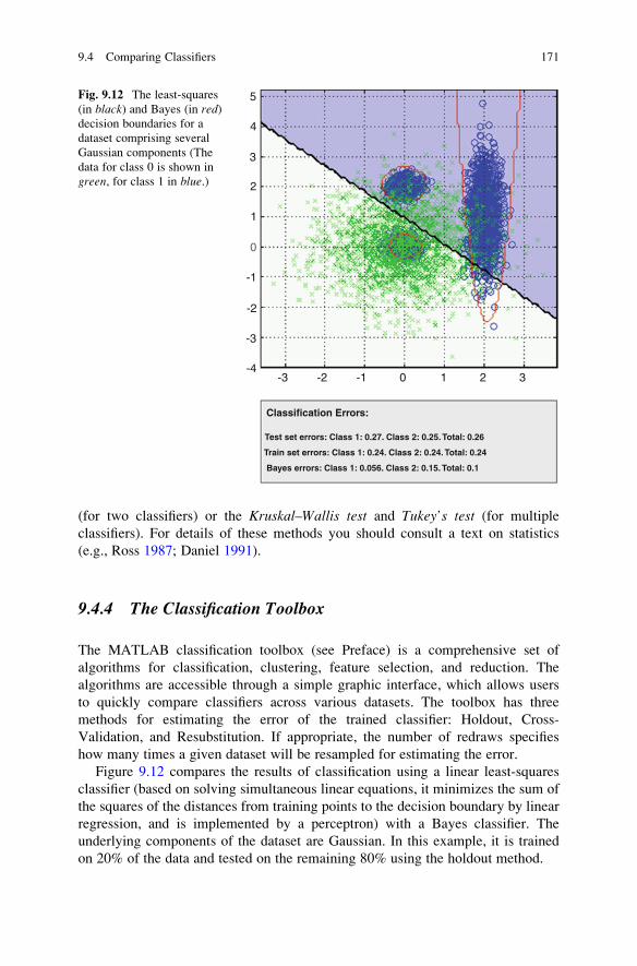
(for two classifiers) or the Kruskal–Wallis test and Tukey’s test (for multiple

classifiers). For details of these methods you should consult a text on statistics

(e.g., Ross 1987; Daniel 1991).

9.4.4 The Classification Toolbox

The MATLAB classification toolbox (see Preface) is a comprehensive set of

algorithms for classification, clustering, feature selection, and reduction. The

algorithms are accessible through a simple graphic interface, which allows users

to quickly compare classifiers across various datasets. The toolbox has three

methods for estimating the error of the trained classifier: Holdout, Cross-

Validation, and Resubstitution. If appropriate, the number of redraws specifies

how many times a given dataset will be resampled for estimating the error.

Figure 9.12 compares the results of classification using a linear least-squares

classifier (based on solving simultaneous linear equations, it minimizes the sum of

the squares of the distances from training points to the decision boundary by linear

regression, and is implemented by a perceptron) with a Bayes classifier. The

underlying components of the dataset are Gaussian. In this example, it is trained

on 20% of the data and tested on the remaining 80% using the holdout method.

5

4

3

2

1

0

-1

-2

-3

-3

Classification Errors:

Test set errors: Class 1: 0.27. Class 2: 0.25. Total: 0.26

Train set errors: Class 1: 0.24. Class 2: 0.24. Total: 0.24

Bayes errors: Class 1: 0.056. Class 2: 0.15. Total: 0.1

-2 -1 0 1 2 3-4

Fig. 9.12 The least-squares

(in black) and Bayes (in red)decision boundaries for a

dataset comprising several

Gaussian components (The

data for class 0 is shown in

green, for class 1 in blue.)

9.4 Comparing Classifiers 171

Clearly the least-squares classifier, which is constrained to producing a linear

decision boundary, performs less well on this dataset. Both types of classification

errors are shown both for the training set and the test set; they are around 25%.

On the other hand, the Bayes’ classifier uses non-linear decision boundary, and

produces an average misclassification error of 105 with this dataset. The toolbox

allows you to conveniently re-run the data, changing parameters such as the

sampling method, the number of re-draws and the percentage of data points used

for training. The data can also be preprocessed, e.g., using the whitening transformto translate and scale the axes so that each feature has zero mean and unit variance.

Figure 9.13 shows the results of using the k-NN classifier, for two different

values of k. The decision boundary will change slightly from run to run as the

classifier tries to learn the best way to classify the data, but a trend is clearly visible.

Small values of k result in a very tortuous boundary, whereas larger values of kresult in a smoother boundary. Using a small value of k results in few errors in the

training set, but this will likely not be the case for the test set. Large values of k willnot classify the training set particularly well, but the performance on the test set is

likely to be similar.

The toolbox allows you to compare several classifiers on a particular dataset,

using a chosen resampling method (Fig. 9.14).

There is a convenient method for manually entering distributions (specifying the

number and relative weights of distributions within a class, their means, and

covariances) and generating a sample dataset (of whatever size desired). Figure 9.15

shows an XOR distribution, and the decision boundaries obtained with a 5-NN

classifier and a Bayes’ classifier.

5

4

3

2

1

0

-1

-2

-3

-3 -2


a b


Test set errors: Class 1: 0.14. Class 2: 0.17. Total: 0.16 Test set errors: Class 1: 0.05. Class 2: 0.2. Total: 0.13





-1 0 1 2 3 -3 -2 -1 0 1 2 3-4

5

4

3

2

1

0

-1

-2

-3

-4

Fig. 9.13 The k-NN (in black) and Bayes (in red) decision boundaries for the same dataset used in

Fig. 9.12 (20% training set). (a) k ¼ 1 (b) 25


Fig. 9.14 Comparison of several classifiers on the dataset introduced in Fig. 9.12 (Cross-

validation was used; and k ¼ 3 was used in the k-NN classifier.)

4

2

0

-2

-4

-4


-2

Test set errors: Class 1: 0.052. Class 2: 0.082. Total: 0.068



0 2 4 6-6

Fig. 9.15 The decision boundaries obtained for an XOR distribution, using 5-NN and Bayes’

classifiers

Any dataset can be imported (for example, from Excel or JMP) and used within

the classification toolbox. The data must be read into MATLAB as a D-by-Nmatrix, patterns, where d is the number of dimensions of the data and N the

number of examples. (If D > 2, a feature selection GUI will open and request

the user preprocess the data to yield two-dimensional data to be compatible with the

display) In addition, a 1-by-N vector, targets, is required to hold the category

labels, 0 or 1. If the distribution is a mixture of Gaussians, and their parameters are

known, these parameters can be stored in a structure, named distribution_-parameters, for computation of the Bayes error. (The fields of this structure are

the means of the Gaussians in each class, the covariance matrices of the Gaussians,

the relative weights of each of the Gaussians, and the prior probability of class 0)

9.5 Combining Classifiers

In any application,we canuse a particular classifier, and try to optimize its performance.

The No Free Lunch Theorem states that there is no single classifier that in any domain

always induces the most accurate learner. The usual approach is to try several different

classifiers and choose the one that performs the best on a separate validation set.

Each classifier comes with its own set of assumptions, which will lead to errors if

the assumptions do not hold for the data. Learning itself is an ill-posed problem, and

with finite data each classifier converges to a different solution. We can fine-tune

the classifier to get the best possible accuracy on a validation set, but this is a

complex task and there may be some data points which it may never handle well,

and could be better handled by a completely different classifier. There is a saying

that two heads are better than one, although extrapolation of the concept ends up

with decision by committee, which is famously useless for human activities.

Nevertheless, with appropriate safeguards, we might consider the idea of using

several different classifiers, known as base classifiers, on a dataset—each learning

in different ways—and combining their outputs in some way. This is known as

combining classifiers or ensemble learning.

Example 9.1

Consider an ensemble of 25 binary classifiers, each of which has an error rate, e,of 0.35. If they are independent and a majority vote is taken on their predictions,

what will be the error rate of the ensemble classifier?

Of course, if the classifiers are identical, each will misclassify the same

examples and the error rate of the ensemble will remain at 0.35. However, if

they are independent (i.e., their errors are uncorrelated), then the ensemble

makes a wrong prediction only if more than half of the base classifiers predict

incorrectly. In this case, the error rate of the ensemble classifier will be

e ¼X25

i¼13

25

i

� �eið1� eÞ25�i ¼ 0:06 (9.5)

which is considerably lower than the error rate of the base classifiers.


We want to choose a set of diverse classifiers: they should differ in their

decisions but complement each other. And, in order to obtain an overall gain in

performance, they should each be reasonably accurate, at least in their domain of

expertise. [If we have lots of data, we might consider partitioning it and giving

different sets of (overlapping or nonoverlapping?) data to different classifiers].

Ensemble methods work better with unstable classifiers, i.e., base classifiers that

are sensitive to minor perturbations in the training set. Examples of unstable

classifiers include decision trees, rule-based classifiers, and artificial neural

networks. By combining or aggregating over a number of different base classifiers,

we are likely to reduce variance and therefore error.

The simplest and most intuitive way to combine multiple classifiers is by voting(Fig. 9.16), which corresponds to taking a linear combination of the classifier

outputs. In the simplest case, all the classifiers are given equal weight, but their

outputs could be weighted by, say, the success rate of each base classifier acting

alone or by respective posterior probabilities. There are other possibilities. Com-

bining them via a median rule is more robust to outliers; a minimum or maximum

rule is pessimistic or optimistic, respectively. Combining them as a product would

give each classifier veto power.

Bagging, or bootstrap aggregating, is a voting method whereby classifiers are

made different by training them over slightly different training sets, generated by

the bootstrap method (resampling with replacement). Bagging is a variance reduc-ing algorithm, although some might suspect it is just a case of throwing computer

resources at a problem!

Whereas in bagging, generating complementary base classifiers is left to chance

and to the instability of the classifier itself, in boosting we actively try to generate

complementary classifiers by training the next classifier on the mistakes of the

previous classifiers. The original boosting algorithm (Schapire 1990) combined

Fig. 9.16 An ensemble classifier, combining the outputs of N base classifiers

9.5 Combining Classifiers 175

three weak learners (each performing only just better than chance) to generate a

strong learner (with a very small error probability). Given a large training set, it is

randomly divided into three. A classifier was trained on the first third, and then

tested on the second third. All of the data that was misclassified during that testing

was used to form a new dataset, along with an equally sized random selection of the

data that was correctly classified. A second classifier was trained on this new

dataset, and then both of the classifiers were tested on the final third of the dataset.

If they both produced the same output, then that datapoint was ignored, otherwise

the datapoint was added to form yet another dataset, which formed the training set

for the third classifier. The system reduced the final error rate, but was rather data

hungry. Drucker et al. (1994) used a set of 118,000 instances in boosting multilayer

perceptrons for optical handwritten digit recognition.

A variant, AdaBoost (adaptive boosting), gives weights to each datapoint

according to how difficult previous classifiers have found to get it correct (Freund

and Schapire 1996). These weights are given to the classifier as part of the input

when it is trained. (They are initially all set to the same value, 1/N, where N is the

number of datapoints in the training set) AdaBoost can combine an arbitrary

number of base classifiers, not just three. It uses classifiers that are simple and not

particularly accurate, where the next classifier can focus on the incorrect choices.

For example, with decision trees, it uses decision stumps (trees that are only grown

to one or two levels). Clearly these are biased, but the decrease in variance is larger

and the overall error decreases. A classifier such as linear discriminant analysis has

low variance, and no gain can be achieved with it using AdaBoost.

References

Alpaydin, E.: Introduction to Machine Learning, 2nd edn. MIT, Cambridge, MA (2010).

Chapter 19

Daniel, W.W.: Biostatistics: A Foundation for Analysis in the Health Sciences, 5th edn. Wiley,

New York (1991)

Drucker, H., Cortes, C., Jackel, L.D., Le Cun, Y., Vapnik, V.: Boosting and other ensemble

methods. Neural Comput. 6, 1289–1301 (1994)

Freund, Y., Schapire, R.E.: Experiments with a new boosting algorithm. In: Saitta, L. (ed)

Thirteenth International Conference on Machine Learning, pp. 148–156. Morgan Kaufmann,

San Mateo, CA (1996)

Geman, S., Bienenstock, E., Doursat, R.: Neural networks and the bias/variance dilemma. Neural

Comput. 4, 1–58 (1992)

Hanley, J.A., McNeil, B.J.: The meaning and use of the area under a receiver operating character-

istic (ROC) curve. Radiology 143, 29–36 (1982)

Hanley, J.A., McNeil, B.J.: A method of comparing the areas under receiver operating character-

istic curves derived from the same cases. Radiology 148, 839–843 (1983)

James, G.: Variance and bias for general loss functions. Mach. Learn. 51, 115–135 (2003)

Ross, S.M.: Introduction to Probability and Statistics for Engineers and Scientists. Wiley, New

York (1987)

Schapire, R.E.: The strength of weak learnability. Mach. Learn. 5, 197–227 (1990)


Chapter 10

Projects

10.1 Retinal Tortuosity as an Indicator of Disease

Retinal blood vessels can be viewed directly and noninvasively, offering a unique

and accessible window to study the health of the human vasculature in vivo. Their

appearance, as seen in retinal fundus images, is an important diagnostic indicator

for much systemic pathology, including diabetes mellitus, hypertension and athero-

sclerosis (Fig. 10.1). Specifically, the blood vessels become dilated and tortuous in

a number of disease conditions including high blood flow, angiogenesis, and blood

vessel congestion. Tortuosity (i.e., integrated curvature) is a feature that may well

be used to classify different retinal pathologies.

There are many different ways to define tortuosity, but useful metrics should be

additive and scale invariant and largely independent of image noise and the

resolution of the imaging system. One of these metrics, the mean tortuosity (M),

is equivalent to the accumulating angle change along the length of a vessel

considered to comprise straight-line segments between closely digitized points

along its mid-line. There is an issue regarding the closeness of these digitized

points. With small sampling intervals there are large digitization errors, which

results in an artificially elevated tortuosity. Conversely, large sampling intervals

miss high-frequency changes and underestimate the tortuosity of highly tortuous

vessels. A compromise distance has to be struck to minimize digitization errors and

accurately trace the vessels. An alternative metric is the normalized root-mean-

square curvature (K) of the blood vessel (Johnson and Dougherty 2007). This

incorporates approximate polynomial spline-fitting to “data balls” centered along

the mid-line axis of the vessel, and avoids the arbitrary filtering of mid-line data

needed with other methods to minimize digitization errors. Since tortuosity is

additive, it is clear that it is the tortuosity per unit length, rather than tortuosity

itself, that is the actual metric of interest.

Retinal images can be obtained from university departments of ophthalmology

or from publicly available databases. The STARE (http://www.ces.clemson.edu/

ahoover/stare) and DRIVE (http://www.isi.uu.nl/Research/Databases/DRIVE/)


177

http://www.ces.clemson.edu/ahoover/stare

http://www.ces.clemson.edu/ahoover/stare

http://www.isi.uu.nl/Research/Databases/DRIVE/

databases of retinal images have been widely used to compare various vessel

segmentation algorithms. The Messidor project database (Niemeijer et al. 2004)

is the largest database of retinal images currently available on the internet. It was

established to facilitate studies on computer-assisted diagnoses of diabetic retinop-

athy; each of the 1,200 images includes diagnoses by expert ophthalmologists

(Fig. 10.2).

Fig. 10.1 Binarized retinal images: diagnosed as showing (a) vasculitis, (b) normal, and

(c) retinitis pigmentosa. A typical vessel in each is shown in gray

Fig. 10.2 Example images from the Messidor database showing various severities of diabetic

retinopathy (a) grade 0, (b) grade 1, (c) grade 2, and (d) grade 3

178 10 Projects

A common approach has been to segment retinal images, and skeletonize

the resulting blood vessels to extract their centerlines prior to measuring the

tortuosity. However, segmentation is a challenging process fraught with difficulties.

It generally requires preprocessing to minimize noise and other artifacts, adaptive

thresholding, and postprocessing for subsequent linking of broken vessels.

Skeletonization is very sensitive to noise, and generally requires various filling

and pruning strategies to rectify spurious gaps, branches, and crossings. An alter-

native approach, which circumvents the problems inherent in segmentation and

skeletonization, is to obtain the centerlines directly from the gray-scale images by

applying a Hessian (Fan et al. 2009) or Jacobian (Yuan et al. 2009)-based analysis

of critical points, using matched or steerable filters (Sofka and Stewart 2006) or by

nonmaximum suppression (Sun and Vallotton 2009). The Hessian is a generaliza-

tion of the Laplacian operator; it is a square matrix comprising second-order partial

derivatives of the image, and can therefore be used to locate the center of a ridge-

like structure. Specifically, the local principal ridge directions at any point in an

image are given by the eigenvectors of the second-derivative matrix computed from

the intensity values around that point.

NeuronJ is a semi-automated tracing method which uses the Hessian to identify

and trace vessels with minimal user intervention directly from a grayscale image

(or the green plane of an RGB color image). It has been used successfully to trace the

arterioles from retinal images (Fig. 10.3), producing digitized coordinates of

the vessel centerlines that can be conveniently exported to an Excel file for the

computation of mean tortuosity (Iorga and Dougherty 2011).

Fig. 10.3 Tracing of blood vessels using NeuronJ. Themagnified area shows the choice of tracing(viz. the larger branch) at bifurcations

10.1 Retinal Tortuosity as an Indicator of Disease 179

In a preliminary study (Dougherty et al. 2010), using 120 images of normal

retinal vessels and 70 images each of three retinopathies (diabetic retinopathy,

retinitis pigmentosa, and retinal vasculitis), discriminant analysis was used to

produce a canonical plot (Fig. 10.4) showing the linear combinations of the

tortuosity features (M and K) in the two dimensions that best separate the groups.

The conditions are fairly well separated, although the vessels showing diabetic

retinopathy are often misclassified.

Classification depends on the prevalences of the conditions in the general

population (the pretest probabilities). Taking these into account results in a contin-

gency table (Table 10.1), in which the diagonal elements show correct diagnoses

and the off-diagonal elements show mis-diagnoses. A total of 150 of the 330

Fig. 10.4 Canonical plot. Data from the ground truth conditions are indicated by separate symbols

(black small square, vasculitis; asterisk, normal; multiplication sign, diabetes; plus, retinitis), eachindicating the mean of 10 measurements. The directions of the features,M and K, are shown in thecanonical space by the labeled rays. The size of each circle corresponds to a 95% confidence limit

for the mean (marked with plus) of that group. The small arrows indicate misclassified data points

Table 10.1 Contingency table using both M and K together, with the prevalences of the diseased

conditions in the general population and in the samples (in parentheses)

Diagnosis

Diabetic

retinopathy Normal

Retinitis

pigmentosa Vasculitis

Actual condition Diabetic

retinopathy

20 (30) 50 (20) 0 (20) 0 (0)

Normal 0 (10) 120 (100) 0 (0) 0 (10)

Retinitis

pigmentosa

20 (0) 10 (0) 40 (70) 0 (0)

Vasculitis 0 (0) 70 (10) 0 (0) 0 (60)

180 10 Projects

images (45%) are misclassified. However, if we consider the images as a referred

population with probabilities proportional to their occurrence, then the total number

of misclassified images drops to 70 (i.e., 21%). Clearly tortuosity is a valuable

feature in distinguishing these conditions. However, these high misclassification

rates preclude the use of tortuosity for classifying all of these conditions simulta-neously, even in a referred population. Other features need to be identified and

measured to increase the accuracy of classification. A count of microaneurysms has

been shown to be useful in identifying diabetic retinopathy (Iorga and Dougherty

2011). Further work needs to be done to identify other informative features, based

on vessel morphology; and larger datasets should be explored.

An as yet unexplored application of retinal vasculature is biometric identification.

10.2 Segmentation by Texture

Texture is an intuitively obvious phenomenon, but it is very difficult to define

precisely. It represents a variety in fine detail, and is distinct from pattern which

measures regularity. Roughness or smoothness is an important component of

texture, and is related to the decay of the Fourier transform (Dougherty and

Henebry 2001). The radial Fourier power spectrum of rough (2D) images tend to

decay as 1/o2, showing a gradient of �2 on a log–log plot; while smooth (2D)

images decay as 1/o4 with a gradient of �4. By invoking fractional Brownian

motion, we can use fractals as a model for texture. It can be shown that the fractal

dimension, D, of an image (with Euclidean dimension ¼ 2) is given by

D ¼ 4� b (10.1)

where b is the magnitude of the slope of the radial power spectrum. This constrains

D, averaged over all directions, to be between 2 (smooth) and 3 (rough) and up to 4

(for white noise).

So, while there is a multiplicity of possible definitions of texture (including

statistical moments, edgeness, entropy, and terms related to the correlation and

co-occurrence matrices), the use of fractal dimension as a compact descriptor and

its estimation using the Fourier power spectrum has been widely used. Exact

fractals have attractive properties, such as invariance to scale and projection.

However, for real structures, fractality is present only in a statistical sense and

only over a limited range of scales; hence the notion of a fractal signature.

There are a number of texture databases which can be used as a training set to

investigate classification. Brodatz textures are a well-known benchmark for

evaluating texture recognition algorithms, and digitized images of them,

512 � 512 and histogram-equalized, can be conveniently downloaded (http://sipi.

usc.edu/database/database.php?volume¼textures). A two-dimensional Fourier

power spectrum (of intensity against spatial frequencies, u and v) can be convenientlyobtained from most image analysis programs (e.g., ImageJ, MatLab). The spectrum

can be radially averaged (Fig. 10.5a) for an image (Fig. 10.5b) to provide the radial

10.2 Segmentation by Texture 181

http://sipi.usc.edu/database/database.php?volume=textures



power spectrum (Fig. 10.5c) which can then be fitted to a straight line to give an

average fractal dimension for the image.

Different images of the same texture produce slightly different radial power

spectra, but an average can be taken as the fractal signature. It should then be

possible to classify an unknown texture by comparing its signature with the average

signatures of a number of standard signatures, rather than attempting to extract a

single fractal dimension from each plot. One way of doing this would be to plot the

test signature against the standard signatures (over the whole range of spatial

frequencies), and use the goodness-of-fit as a parameter to choose the best classifi-

cation. Figure 10.6 shows this for a test image and four images of walls: the resulting

a b c

30

28

26

24

Log

Mag

nitu

de

22

20

18

160 1 2 3 4 5 6

Log Frequency

v

u

Fig. 10.5 (a) Radial averaging the spectrum involves averaging the spectrum over annuli

corresponding to different frequencies, (b) an image of fur, and (c) its radial power spectrum

plot (log–log)

Fig. 10.6 (a) Four examples of wall images, (b) a test wall image, and (c) a log–log plot of the

radial power magnitudes for image (b) against the average for the four images in (a)

182 10 Projects

goodness-of-fit for the test image is 0.9063, indicating that it is probably an image

of a wall too with the characteristic texture of a wall.

The radial power spectrum averages out any angular anisotropy of the Fourier

power spectrum. It is possible to retain the angular information, and display a polar

plot of the fractal dimension as a function of angle (Fig. 10.7). (A MatLab m-file.

fracdim.m, to do this is available for downloading from the book Web site.) With

some thought a compact feature (e.g., the circularity of the polar plot) to capture the

angular anisotropy could be proposed, and added to the goodness-of-fit feature to

improve classification.

In order to apply these methods to segmenting images, it would be important to

determine the smallest region of interest (RoI) within an image that captures the

essential features of the radial power spectrum. Overlapping windows of this size

could then be used to compute local fractal dimensions throughout the image, and

their values used to draw boundaries based on texture.

10.3 Biometric Systems

Biometric systems are used to recognize and/or identify a person using some

specific physiological or behavioral characteristics. Depending on the application

context, they can either be used for verification (a one-to-one comparison to

authenticate a person by comparing the captured characteristic feature with his/

her own template) or matching (a one-to-many comparison to establish the identity

of an individual by searching a database for the best match).

90 4

3

2

1

60

30

0

330

300

270

240

210

180

150

120

Fig. 10.7 Polar plot of the

fractal dimension of the

wall image of Fig. 10.6b

10.3 Biometric Systems 183

A number of biometric technologies have been developed and are in use in a

variety of applications. Among these, fingerprints, face, iris, speech, gait, and hand

and finger geometry are the most commonly used. Recently hand and finger vein

scans (Fig. 10.8), using infrared sensors, have been employed to authenticate ATM

(automated teller machine) customers. Table 10.2 compares some of the tech-

nologies in terms of cost, accuracy, and security.

10.3.1 Fingerprint Recognition

Fingerprints are the oldest and most widely used form of biometric identification.

However, fingerprints are rarely of perfect quality as they are often corrupted due to

variations in skin and impression conditions. Consequently, fingerprint recognition

Fig. 10.8 An infrared

scan of a hand

Table 10.2 A comparison

of biometric systemsFingerprint Face Iris Voice Vein

Easy to use • • • •

Cheap • • • •

Accurate • • •

Secure • •

184 10 Projects

remains a challenging problem and image enhancement techniques used for reliable

extraction of features from fingerprint images are a critical step in fingerprint

matching. FVC-onGoing (https://biolab.csr.unibo.it/FVCOnGoing) provides exten-

sive fingerprint databases as benchmarks to unambiguously compare the perfor-

mance of different algorithms.

A fingerprint is the pattern of ridges and valleys on each finger tip (Fig. 10.9a).

Minutiae points are the local ridge characteristics that occur either at a ridge ending

(the point where the ridge ends abruptly) or a ridge bifurcation (the point where the

ridge splits into two or more branches). The distinctiveness of a fingerprint is based

on the unique spatial relationships between the two types of minutiae. Unfortu-

nately, degraded fingerprint images can result in a significant number of spurious

minutiae being created and genuine minutiae being ignored. A critical step in

studying the statistics of fingerprint minutiae is to reliably extract minutiae from

fingerprint images. Image enhancement techniques need to be employed prior to

minutiae extraction to obtain a more reliable estimate of minutiae locations.

Typical preprocessing involves subtraction of any nonuniform background and

contrast enhancement, possibly by histogram equalization, and produces a

normalized fingerprint (Fig. 10.9b). This is followed by extraction of the minutiae:

segmentation (Fig. 10.9c, e.g., by adaptive thresholding), skeletonization

(Fig. 10.9d, to show ridges one pixel wide), and then selection of end point minutiae

Fig. 10.9 (a) Original fingerprint image, (b) normalized image, (c) segmented (binarized) image,

(d) skeletonized image, (e) end points (before deletion of spurious points), (f) branch points

(before deletion of spurious points)

10.3 Biometric Systems 185

https://biolab.csr.unibo.it/FVCOnGoing

[with only one neighbor (Fig. 10.9e)] and bifurcation minutiae [with three

neighbors (Fig. 10.9f)]. False minutiae at the edges of the fingerprint are deleted

using a mask created during segmentation. Many spurious end point minutiae

resulting from ridge breaks due to degraded images can also be deleted by checking

the distance between these minutiae. This results in two sets of minutiae, one

comprising the end points and the other the bifurcations or branch points, with

each minutia characterized by its coordinates (x, y). (The minutia angle, y, the anglethat the ridge makes at each position could also be considered.) The problem is then

one of point pattern matching, which can be approached in a number of ways

including relaxation methods, algebraic and operational research solutions, tree-

pruning approaches, energy-minimization methods and the Hough transform

(Maltoni et al. 2003).

An alternative approach is to form two sets of triangles from the two sets of

minutiae, and then to compare the angles of the triangles in the test image

(Fig. 10.10) with the angles of the triangles in the standard image(s). This

eliminates the need for scaling and aligning the images, which saves a considerable

computational cost. It does increase the size of the feature database. For N minutia

[each characterized by (x, y)], we now haveN3

� �triangles, each characterized by

three angles; triangles with very small sides should be eliminated. This may still

correspond to a computational saving, depending on the search algorithm employed

for comparing the data. The comparison of the angles can be organized to deliver a

score indicating the goodness of a match between images.

Fig. 10.10 Trianglesformed from branch points

(after elimination of spurious

points)

186 10 Projects

10.3.2 Face Recognition

The face is the primary focus in everyday social interactions and plays a significant

role in conveying identity and emotion. Our brain’s ability to recognize faces is

incredible; we are able to recognize and identify thousands of faces seen throughout

our lifetime. Automated face recognition systems try to emulate the neurological

thought processes of the human visual system, but developing such a system is a

daunting task because our faces are extremely complex, multidimensional visual

stimuli. It is very challenging to develop face recognition techniques that can

tolerate the effects of aging, facial expressions, and variations in lighting and

pose. However, once developed, they have numerous applications, for example in

security systems, criminal identification, and human–computer interaction.

There are a number of models that have been used; some models measure the

characteristics of informative landmarks from images of the face, using for example

elastic bunch graphs (Campadelli and Lanzarotti 2005) or Gabor wavelets (Gokberk

et al. 2005), while others, such as the Eigenfaces and Fisherfaces approaches,

consider the salient features as combinations of a basis set of standardized faces

derived from the statistical analysis of many pictures of faces. There are many

databases available (http://www.face-rec.org/databases/) to benchmark algorithms.

The Eigenfaces model is based on linearly projecting a high-dimensional image

space to a low-dimensional feature space (face space), using Principle Component

Analysis (PCA). The principle components are calculated from the covariance

matrix of the probability distribution of the high-dimensional vector space of

possible faces of common resolution, with the eyes and mouth approximately

aligned across all the images, from an initial training set. These principle

components, also known as eigenfaces, are the eigenvectors of the covariancematrix

and they represent the basis features of all the faces. The principle components

represent the projection directions that maximize the total spread or scatter of all the

features in the images, regardless of class (identity). This differs from the

Fisherfaces method which uses discriminant analysis to project the initial high-

dimensional image space into the (canonical) directions that best separate the

classes, by maximizing the ratio of between-class scatter to that of within-class

scatter. Since face recognition is essentially a classification task, Fisherfaces is

preferredmethod although the Eigenfaces method has been widely used (Belhumeur

et al. 1997).

References

Belhumeur, P.N., Hespanha, J.P., Kriegman, D.J.: Eigenfaces vs. Fisherfaces: recognition using

class specific linear projection. IEEE Trans. Pattern Anal. Mach. Intell. 19, 711–720 (1997)

Campadelli, P., Lanzarotti, R.: A face recognition system based on local feature characterization.

In: Tistarelli, M., Bigun, J., Grosso, E. (eds.) Advanced Studies in Biometrics. Springer, Berlin

(2005)

References 187

http://www.face-rec.org/databases/

Dougherty, G., Henebry, G.M.: Fractal signature and lacunarity in the measurement of the texture

of trabecular bone in CT images. Med. Biol. Eng. Comput. 23, 369–380 (2001)

Dougherty, G., Johnson, M.J., Wiers, M.D.: Measurement of retinal vascular tortuosity and its

application to retinal pathologies. Med. Biol. Eng. Comput. 48, 87–95 (2010)

Fan, J., Zhou, X., Dy, J.G., et al.: An automated pipeline for dendrite spine detection and tracking

of 3D optical microscopy neuron images of in vivo mouse models. Neuroinformatics 7,

113–130 (2009)

Gokberk, B., Irfanoglu, M.O., Akarun, L., Alpaydin, E.: Selection of location, frequency, and

orientation parameters of 2D Gabor wavelets for face recognition. In: Tistarelli, M., Bigun, J.,

Grosso, E. (eds.) Advanced Studies in Biometrics. Springer, Berlin (2005)

Iorga, M., Dougherty, G.: Tortuosity as an indicator of the severity of diabetic retinopathy. In:

Dougherty, G. (ed.) Medical Image Processing: Techniques and Applications. Springer, Berlin

(2011)

Johnson, M.J., Dougherty, G.: Robust measures of three-dimensional vascular tortuosity based on

the minimum curvature of approximating polynomial spline fits to the vessel mid-line. Med.

Eng. Phys. 29, 677–690 (2007)

Maltoni, D., Maio, D., Jain, A.K., Prabhakar, S.: Handbook of Fingerprint Recognition, p. 145.

Springer, New York (2003)

Niemeijer, M., Staal, J.S., van Ginneken, B., et al.: Comparative study of retinal vessel segmenta-

tion on a new publicly available database. Proceedings of the SPIE 5370-5379 (2004)

Sofka, M., Stewart, C.V.: Retinal vessel centerline extraction using multiscale matched filters,

confidence and edge measures. IEEE Trans. Med. Imaging 25, 1531–1546 (2006)

Sun, C., Vallotton, P.: Fast linear feature detection using multiple directional non-maximum

suppression. J. Microsc. 234, 147–157 (2009)

Yuan, X., Trachtenberg, J.T., Potter, S.M., et al.: MDL constrained 3-D grayscale skeletonization

algorithm for automated extraction of dendrites and spines from fluorescence confocal images.

Neuroinformatics 7, 213–232 (2009)

188 10 Projects

Index

AAdaBoost, 176

ADALINE. See Adaptive Linear Element/

Adaptive Linear Neuron

(ADALINE)

Adaptive Linear Element/Adaptive Linear

Neuron (ADALINE), 112

Agglomerative hierarchical clustering. SeeHierarchical clustering

Angular anisotropy, 183

ANN. See Artificial neural network (ANN)

Artificial neural network (ANN)

activation function, 112, 113

ADALINE, 112

advantages and disadvantages, 116, 117

backpropagation, 109, 115

bias, 99–100, 105–106, 109

feed-forward, 112, 113

global minimum, 110

learning rate, 109–111

linear discriminant function, 107

logical AND function, 106, 107

logical OR function, 107

logical XOR function, 107–109, 114

multi-layer network, 107, 112, 116

neurons, 104–105

overfitting, 112–113

perceptron (see Perceptron, ANN)recurrent network, 112

signals, 104

simulated annealing, 115

steepest/gradient descent, 110, 115

structure, neurons, 105

training, 109, 115–116

universal approximation theorem, 112

weight vector, 109, 112

Astronomy, 2

BBayes’ classifier, 171–173

Bayesian decision theory

multiple features

complex decision boundary,

85, 86

trade off performance, 86

two-dimensional feature space, 85

single dimensional (1D) feature

class-conditional probabilities (seeClass-conditional probabilities)

classification error, 81–83

CondProb.xls, 85

likelihood ratio, 77, 83, 84

optimal decision rule, 81

posterior probability, 76–77

recognition approaches, 75

symmetrical/zero-one loss

function, 83

Bayes’ rule

conditional probability and, 46–53

Let’s Make a Deal, 48

naıve Bayes classifier, 53–54

posterior probability, 47

Bias-variance tradeoff, 99–101

Bioinformatics, 2

Biometrics, 2

Biometric systems

cost, accuracy, and security, 184

face recognition, 187

fingerprint recognition, 184–186

infrared scan, hand, 184

physiological/behavioral

characteristics, 183

Bootstrap, 163–164

Breast Screening, 51–52

Brodatz textures, 181

G. Dougherty, Pattern Recognition and Classification: An Introduction,DOI 10.1007/978-1-4614-5323-9, # Springer Science+Business Media New York 2013

189

CCanonical plot

confusion matrix, 140

contours, classes, 139

description, 135

eigenvalues, 136–137

iris data, 136

CDF. See Cumulative distribution

function (CDF)

Central Limit Theorem, 57, 76, 87

Chaining, 150

Character recognition, 2

Chebyshev distance, 143

Class-conditional probabilities

classification error, 81–83

decision threshold, 81

densities, 79

description, 76

different variances, 78–80

equal variance, 77–78

likelihood test, 80

Classification

acquired image, 3

algorithm selection and supervised

learning, 17–18

decision boundaries, 5

electronic components, shapes

and sizes, 23, 24

face recognition, 5

features (see Features)labeling, 10, 11

letters, 25

nonmetric approaches, 19–20

post-processing, 10

pre-processing, 3, 9

process, 3, 4

rule-based classifier, 39

segmentation, 9–10

sensing/acquisition stage, 9

shape, 21–22

single-pixel outlines, fruit, 24

size, 22–23

stages, 9, 10

statistical approaches, 18–19

statistical/structural techniques, 5–6

string matching, 40

SVM, 20–21

training and learning, 16–17

Classification error, 30–31

Classifiers

AdaBoost, 176

AUC approaches, 165, 166

bagging/bootstrap aggregating, 175

Bayes rule, 168

bias and variance, 159–160

classification toolbox, 171–174

confusion matrix, 164, 165

cross-validation and resampling

methods, 160–164

decision stumps, 176

diverse, 175

ensemble output, 175

error rate, 157, 174

learning, 174

McNemar’s test, 169, 170

medical diagnosis, 167

null hypothesis and outcomes, test, 167

overlapping probability density

functions, 164

performance measures, 165

ROC, 165, 166, 169, 170

scientific method, 159

SE, 167–168

significance level, 166

statistical tests, 169, 171

three-way data split, 158

training set, 157

validation set, 158

Cluster analysis, 143

Clusters

analysis, 143

hierarchical, 150–154

k-means clustering (see k-Means

clustering)

non-exclusive, 144

partitional, 144, 145

Coefficient of determination, 62

Computer-aided diagnosis, 2

Conditionally dilation, 21, 22

Conditional probability

description, 46

multiplicative rule, 47

sensitivity and specificity, 50

Venn diagram, 45, 46

CondProb.xls, 52–53, 85

Confusion matrix, 137, 140, 153

Contingency table

description, 46

diagnostic test, 49

marginal probabilities, 50, 52

Correlation coefficients, 130, 131

Correlation matrix, 61

Covariance matrices

bivariate Gaussian distribution, 66

coefficient of determination, 62

correlation matrix, 61

190 Index

decision boundary

hyperbolic, 92

linear, 92, 93

parabolic, 90, 91

definition, 59–60

2D Gaussian and isocontours,

63–65

diagonalization, 66–67

eigenvalues and eigenvectors, 135

equal, 90, 91

equiprobable normally distributed

classes, 92–94

factorization, 61

feature vector, 60

LDA, 136

nonzero off-diagonal elements, 65–66

PCA, 66, 128, 129

QDA, 90, 137–138

statistical significance, 62–63

symmetric matrix, 68

whitening transform, 68

Cross-validation

bootstrap, 163–164

holdout method, 161

k-fold cross-validation, 162–163

leave-one-out validation, 18

overfitting, 160

Cumulative distribution function (CDF)

definition, 55

and PDF, 55–56

Curse of dimensionality, 102, 123

DData mining, 1

Decision boundary

bivariate normal distributions, 89

complex, 85, 86

decision thresholds, 85

and discriminant functions, 87

hyperbolic, 92, 94

linear, 90, 91

parabolic, 90, 91

quadratic, 86

Decision nodes, 27, 28, 35

Decision regions, 87, 94, 95

Decision rule

class-conditional probabilities, 78, 79

decision regions, 87

likelihood ratio, 77, 83

minimum-distance classifier, 89

optimal decision rule, 81

probability, classification error, 76

Decision threshold

decision boundaries, 85

intersecting distributions, 81

intersection, probability distribution, 80–81

posterior probabilities, 78

Decision tree

advantages and disadvantages, 38–39

benefit, 28

binary splits, 38

branching structure, 27, 28

computes, logical AND function, 40

cross-validation, 37

entropy, information and impurity, 29–31

feature axes, 35, 36

gain (see Gain)greedy strategy, 29

ID3 algorithm, 37

oblique, 36

overfit, 36, 37

structure, 19, 20

three-level, 27, 28

training and test error rat, 36–37

underfitting, 36–37

Dendrogram

description, 150

hierarchical clustering, Fisher iris

data, 151, 152

nested clusters, 144

scatter plots, Fisher’s canonicals, 151, 153

Diagonalization, 66–67

Dimensionality

curse of dimensionality, 123

methods

feature extraction (see Featureextraction)

feature selection (see Feature selection)peaking phenomenon, 123, 124

preprocessing, 124

Discriminant functions

classes, decision curves, 94, 95

covariance matrices (see Covariancematrices)

decision boundary, 89

decision regions, 87

description, 87

equal variance, decision lines, 89, 90

LDA, 87–88

linear machine, 87–88

minimum-distance classifier, 89

Dissimilarity, 72

Diverse classifiers, 175

Document recognition, 2

Drucker, H., 176

Index 191

EEM algorithm. See Expectation-

maximization (EM) algorithm

Entropy, 29–30

Errors

accuracy, 43, 44

precision, 43, 44

Expectation-maximization (EM)

algorithm, 145, 148

FFace recognition, 5, 187

False Positive Paradox, 52

FDR. See Fisher’s discriminant ratio (FDR)

Feature extraction

LDA (see Linear discriminant

analysis (LDA))

optimal mapping, 127

PCA (see Principal Component

Analysis (PCA))

Features

categorical/non-metric, 4

classification, 15

continuous, 4

discriminating, 12

extraction, 11

independent, 12

linear decision boundary, 15

prudent approach, 15

reliable, 12

robust, 12

scaling, 14

shape, 12–13

structural, 12

vector, 13–14

Feature selection

inter/intraclass distance (seeInter/interclass distance)

subset selection, 126

Fingerprint recognition

biometric identification, 184

FVC-onGoing, 185

minutiae points, 185

point pattern matching, 186

triangles, 186

Fisher, R.A., 70, 126, 129–131, 135, 138

Fisher’s discriminant ratio (FDR),

126, 135

Fisher’s iris data

correlation matrix, 130, 131

3D scatterplot, 131

eigenvalues, 132, 133

eigenvectors, 134, 135

iris flowers, 129, 130

MDS, 133

overlaid biplot, 132

principal components, 133, 134

scatter plot matrix, 129, 130

Fuzzy c-means clustering, 148–149

GGain

attributes, 31–32

decisions made, 33, 34

Gini index, 32

ID3 algorithm, 34–36

splitting binary attributes, 33

stages, weather attribute, 34, 35

Gaussian distribution

bivariate, 66, 67

diagnostic testing, 48–49

Mahalanobis distance, 69

multivariate Gaussian

(see Multivariate Gaussian)

PDF, 56

standard deviation, 57

Gini impurity, 30–31

Goodness-of-fit, 182–183

HHessian, 179

Hierarchical clustering

algorithm, 150

complete-link clustering, 150

dendrogram and nested clusters, 150

operation, 150

single-link clustering, 150, 151

Ward’s method (see Ward’s method)

Holdout method, 161

IID3 algorithm, 33, 34, 37, 41

Impurity

classification error, 31

Gini, 30–31

Information, 29

Inter/interclass distance

between-scatter matrix, 126

FDR, 126

single feature, two equiprobable

classes, 124, 125

within-scatter matrix, 125

192 Index

Isocontours

diagonalization, 66–67

ellipsoidal, 68

Gaussian, 63–66

Mahalanobis distance, 69

JJack-knifing, 137

KKarhunen-Loeve (KL) transform. See

Principal Component

Analysis (PCA)

Kernel

Gaussian kernel, 99, 100

machine, SVM, 117–119

Parzen window, 99

polynomial kernel, 119, 120

trick, 116

width, 99

k-fold cross-validation, 162–163

k-Means clustering

bisecting k-means algorithm, 146

description, 145

EM algorithm, 145, 148

fuzzy c-means clustering, 148–149

heuristic algorithm, 145

iterations, 145, 146

“natural” clusters, 147–148

overfitting, 148

pre-and post-processing steps, 146

SSE, 145–146

k-Nearest neighbor (k-NN) classificationapproach, 100–101

Bayes decision boundary, 102, 104

isocontours, 102, 104

lazy learning algorithm, 102

normal and abnormal classes, 103

Parzen density, 100

performance, 102, 103

process, 101–102

k-NN classifier, 172

Koutroumbas, K., 93, 94

Kruskal–Wallis test, 169, 171

LLazy-learning, 19

LDA. See Linear discriminant

analysis (LDA)

Leaf node, 27, 28, 36, 37

Learning

classification error, 16

eager learning, 102

Lazy-learning, 19

reinforcement learning, 16–17

supervised learning, 16–18

training set, 16

unsupervised learning, 16

Least-squares classifier, 171, 172

Leave-one-out approach, 162, 163

Let’s Make a Deal, 48

Likelihood ratio, 77, 83, 84

Linear discriminant analysis (LDA)

canonicals (see Canonical plot)confusion matrix, 137

description, 135

jack-knifing, 137

loss function terms, 140

Mahalanobis distances, 137

QDA, 137–138

two-dimensional and class data, 135, 136

variance, 138

Linear machine, 89

Loss matrix, 83

MMahalanobis distance

definition, 69

dissimilarity, 72

feature vectors, 70–71

LDA, 70

multivariate outlier, 71–72

normalized, 69–70

probability, 69

Manhattan distance, 143

MATLAB classification toolbox, 171

Maximum a posteriori (MAP) estimator

classifier, 76–77

covariance matrix, 94, 96

multivariate Gaussian, 94

posterior probabilities, 96

McCulloch, W., 106

McNemar’s Test, 169, 170

MDS. See Multi-dimensional scaling (MDS)

Mean-square error (MSE), 159

Measurement error

accuracy, 43, 44

description, 43

precision, 43, 44

Medical imaging, 2

Minimal spanning tree (MST), 150, 154

Minimum-distance classifier, 89

Index 193

Minimum variance methods, 143–144

MSE. See Mean-square error (MSE)

MST. See Minimal spanning tree (MST)

Multi-dimensional scaling (MDS), 133

Multivariate Gaussian

covariance matrix, 58

description, 57–58

factorization, 2D Gaussian, 58–59

formula, 58

NNaıve Bayes classifier

definition, 53

formula, 53

one-dimensional distribution, 53

spam filtering, 53–54

NeuronJ, 179

No Free Lunch Theorem, 157–160, 174

Nonmetric approaches, 19–20

Non-metric methods

decision tree (see Decision tree)

description, 27

DNA sequence, 39

OCR, 40

rule-based classifier, 39

string matching, 40

Nonparametric learning

ANN, 104–117

histogram estimator and parzen windows,

99–100

Kernel Machines, 117–119

k-NN classification (see k-Nearest neighbor(k-NN) classification)

OObjective function, 145, 151

Oblique decision trees, 36

Occam’s razor, 15

OCR. See Optical character recognition (OCR)

Optical character recognition (OCR), 40

Optimal decision rule, 81

Outliers, 124, 133

Overfitting, 36, 37, 113, 123

PParametric learning

Bayesian decision theory (see Bayesiandecision theory)

discriminant functions and decision

boundaries, 87–94

MAP estimator (see Maximum a

posteriori (MAP) estimator)

Parzen window, 99–100

Pattern recognition, 1–3

PCA. See Principal component

analysis (PCA)

PDF. See Probability density

function (PDF)

Peaking phenomenon, 123

Perceptron, ANN

activation function, 112

description, 105

input patterns, 108

learning, 111, 112

linear discriminant function, 107

MCP neuron, 105, 106

multilayer perceptron (MLP), 112

neurophysiological motivation, 105–106

optimal perceptron, 116, 117

training, 109

Pitts, W., 106

Post-processing, 10

Predictive value, 51, 52

Pre-processing, 9, 21

Prevalences, 180

Primitives, 20

Principal component analysis (PCA)

covariance matrix, 128, 129

3D, 129

description, 127

dimensionality, 127–128

eigenvectors and eigenvalues, 128

Fisher’s iris data (see Fisher’s iris data)variance, 128

Probability density function (PDF)

CDF, 55–56

certainty, 55


Gaussian distribution, 56

Probability theory

Bayes’ rule (see Bayes’ rule)conditional probability (see Conditional

probability)

contingency table, 46

General Addition Rule, 45

independent, 45–46

joint probability, 46

multiplicative rule, 47

mutually exclusive, 44, 45

naıve Bayes classifier, 53–54

possible events, 43

sample space, 43, 45

Prudent approach, 15

194 Index

QQDA. See Quadratic discriminant analysis

(QDA)

Quadratic discriminant analysis (QDA), 90,

137–138

RRadial Fourier power spectrum, 181

Random variables


description, 54

Mahalanobis distance (see Mahalanobis

distance)

multivariate normal/Gaussian, 57–59

PDF and CDF, 54–56


weights, 56–57

Receiver operating characteristic (ROC)

curves, 164–166, 169, 170

Reinforcement learning, 16–17

Remote sensing, 2

Resampling methods, 160–164

Retinal tortuosity

binarized images, 177, 178

canonical plot, 180

diagonal elements, 180

mean tortuosity, 177

Messidor database, 178

microaneurysms, 181

NeuronJ, 179

normalized root-mean-square curvature, 177

polynomial spline-fitting, 177

skeletonization, 179

STARE and DRIVE databases, 177–178

tracing, blood vessels, 179

Ripper, 39

Root node, 27, 28, 35, 41

Rule-based classifier, 28, 39

SScatter plot matrix, 129–130

Scree plot, 132, 133, 151, 152

SE. See Standard error (SE)

Segmentation

boundary-based methods, 10

region-based methods, 9–10

Sensitivity


probability, negative test (NPV), 52–53

values, breast screening, 52

Slack variables, 118–119

Spam filter, 53–54

Specificity


probability, negative test (NPV), 52–53

values, breast screening, 52

Speech recognition, 2

SSE. See Sum of the squared error (SSE)

Standard error (SE), 167–168

Statistical approaches, 18–19

Statistical moments, 12, 13

Statistical pattern recognition

continuous random variables

(see Random variables)

measurement error, 43, 44

probability theory

(see Probability theory)

String matching, 40

Subset selection, 126

Sum of the squared error (SSE)

description, 145

fuzzy clustering, 149

minimum variance methods, 143–144

Ward’s method, 151

Supervised learning

Bayes’ decision rule, 75

discriminant analysis, 75

non-parametric methods, 75

parametric (see Parametric learning)

process, 17

techniques, accuracy of classifier, 18

Support vector machines (SVMs)

and classification margin, 118

classifiers, 118–119


kernel trick, 118, 119

polynomial kernel, 119, 120

transform nonlinear, 119

SVMs. See Support vectormachines (SVMs)

TTexture

Fourier power spectrum, 181

fractal dimension, 183

radial averaging, spectrum, 181–182

RoI, 183

roughness/smoothness, 181

wall images, 182–183

Theodoridis, S., 93, 94

Training, 16–17

Tukey’s test, 169, 171

Index 195

UUnderfitting, 36–37

Unsupervised learning

clustering, 143–145

fuzzy c-means clustering, 148–149

hierarchical clustering, 150–154

k-means clustering, 145–149

VValidation set, 116, 117

Variance


naıve Bayes classifier, 53


Venn diagram

conditional probability, 45, 46

diagnostic testing, 50

mammographic testing, 51–52

mutually exclusive, 44, 45

sample space, 43, 45

Voronoi cells, 148

WWard, J.H., 151, 152

Ward’s method

advantages, 151

definition, 151

Fisher iris data

clustering, 154

confusion matrix, 153

dendrogram, 151, 152

scatter plots, 151, 153

scree plot, 151, 152

Wilcoxon signed rank test, 169, 171

Within-scatter matrix, 125

196 Index

Pattern Recognition and Classification

Documents

Transcript of Pattern Recognition and Classification