UNITED INSTITUTE OF INFORMATICS PROBLEMS NATIONAL ACADEMY OF SCIENCES OF BELARUS

Pattern Recognition and Information Processing

PRIP’2007

PROCEEDINGS OF THE NINTH INTERNATIONAL CONFERENCE 22–24 May 2007, Minsk, Belarus

Volume II

Minsk 2007

УДК 004.9 Pattern Recognition and Information Processing (PRIP’2007): Proceedings of

the Ninth International Conference (22–24 May 2007, Minsk, Republic of Belarus). In two volumes. Vol. I. – Minsk: United Institute of Informatics Problems of National Academy of Sciences of Belarus, 2007. – 300 p.

The book contains papers accepted for publication and presentation at the Ninth International

Conference on Pattern Recognition and Information Processing (PRIP’2007) that will held at May 22–24 2007 in Minsk, Belarus. The proceedings are prepared for publication by PRIP’2007 Program Committee and Belarusian Association for Image Analysis and Recognition.

The proceedings will be useful for students and researchers working in field of information processing, image analysis and recognition.

Papers are reviewed and approved by the conference Program Committee. Papers are printed as submitted by authors.

Представлены материалы Девятой Международной конференции «Распознавание образов и

обработка информации» (22–24 мая 2007 г., Минск, Беларусь). Подготовлены к выпуску программным комитетом конференции совместно с Белорусской ассоциацией по анализу и распознаванию изображений (БААРИ).

Материалы будут полезны специалистам, работающим в области обработки информации, анализа и распознавания цифровых изображений.

Одобрены программным комитетом конференции и печатаются в виде, представленном авторами.

Editors: Alexander Tuzikov,

Vassili Kovalev, Sergey Ablameyko

ISBN 978-985-6744-29-0 (Vol. I) ISBN 978-985-6744-28-3

© United Institute of Informatics Problems of National Academy of Sciences of Belarus, 2007

Contributors to PRIP’2007

Conference is organized by:

• United Institute of Informatics Problems of National Academy of Sciences of Belarus

In cooperation with:

• National Academy of Science of Belarus • Belarusian Association for Image Analysis and Recognition • Belarusian State University • Belarusian State University of Informatics and Radioelectronics

Supported by:

• National Academy of Science of Belarus • Belarusian Republican Foundation for Fundamental Research • International Association for Pattern Recognition (IAPR)

Committees PRIP’2007

Chairman Prof. A.V. Tuzikov

Vice-Chairman Prof. S.V. Ablameyko

International Program Committee: Dr. V. Kovalev (United Kingdom) – Chairman Prof. G. Borgefors (Sweeden) Prof. R. Kasturi (USA) Prof. B. C. Lovell (Australia) Dr. I. B. Gurevich (Russia) Dr. A. Marcelli (Italy) Prof. M. Petrou (United Kingdom) Prof. R. Sadykhov (Belarus) Dr. G. Sanniti di Baja (Italy) Prof. M. Viergever (Netherlands) Prof. V. P. Shmerko (USA) Dr. T. Lehmann (Germany) Dr. V.Krasnoproshin Prof. A. Asano (Japan) Dr. S. Uchida (Japan)

Local Organizing Committee:

A. Belotserkovsky – Chairman A. Volkovich – Vice-Chairman E. Snezhko A. Dmitruk A. Bogush V. Arkhipov A. Shafranskaya T. Kyris P. Lukashevich

Welcome Words from the PRIP’2007 Chairman

On behalf of the Conference Organizing Committee it is my great pleasure to welcome you at the Ninth International Conference on Pattern Recognition and Information Processing. The conference is the main biennial event of the Belarusian Association on Image Analysis and Recognition. The previous conferences PRIP’2005 and PRIP’2003 were held respectively at the Belarusian State University of Informatics and Radioelectronics and the Belarusian State University. PRIP’2007 is held at the United Institute of Informatics Problems of the National Academy of Sciences of Belarus. It is endorsed by the International Association for Pattern Recognition.

All submitted papers were reviewed by two reviewers and 108 papers were selected for presentation at the conference and inclusion into the conference proceedings.

The conference would not take place without the help of many people. Therefore I would like to express my sincere gratitude to all members of the Program Committee and reviewers for their help in reading and selecting papers, to the members of the Local Organizing Committee for the hard work on arranging the conference, communication with the conference participants, preparation of the proceedings.

We gratefully acknowledge the National Academy of Sciences of Belarus and the Belarusian Republican Foundation for Fundamental Research for their financial support of the conference.

I am very glad to welcome you to Minsk and hope for the conference success that it will be interesting and useful for the participants.

Alexander Tuzikov Minsk, Belarus, May 2007

6

RECONSTRUCTION OF HISTORIC IMAGES TAKEN IN 1900’S BY THE TECHNIQUE OF TRIPLE COLOR PHOTOGRAPHY: PROBLEMS AND

SUGGESTED SOLUTIONS

V. Minachin1, D. Murashov1, Yu. Davidov2, D. Dimentman3 1Dorodnicyn Computing Centre of the Russian Academy of Sciences,

Moscow, Russia; 2“Restavrator-M” Ltd., Moscow, Russia;

3State Historical Museum, Moscow, Russia

The problems related to the restoration of digital images reconstructed in color from triple black and white negatives taken in 1900’s by the technique of triple color photography are considered and solutions are proposed. Classification of defects in images acquired by scanning triple glass negatives is developed. Automatic algorithms for detecting, identifying, and correcting defects in registered color images are proposed and discussed.

Introduction In this paper we consider problems related to the restoration of digital images

reconstructed in color from triple black and white negatives taken by S.M. Prokudin-Gorsky. In 1905-1916 S.M. Prokudin-Gorsky (1863-1944), an early 20th century Russian photographer and researcher, has created "The Collection of the Splendours of Russia in Natural Colours" - the unique set of colour photographs of the Russian Empire on the eve of the October Revolution of 1917. The particular implementation of the technique of triple colour photography used by Prokudin-Gorsky has been developed by A. Miethe at the beginning of the 20th century. The camera registered on a single glass plate three separate black and white frames taken through the blue, green and red filters. The collection includes 1902 glass negatives of size 9 by 24 cm. The glass negatives are preserved at the Library of Congress, USA. In 2000 all triple-frame glass negatives were scanned in 16-bit grayscale with a resolution in excess of 1000 dpi. All of the images are available online [1].

This is the first example of a collection of historic triple color photographs which was made available for reconstruction in color. The complete collection (1902 images) was for the first time reconstcructed in color in high resolution by V. Minachin and his team in 2003 [2]. Levenberg-Marquardt numerical algorithm [5] was used for finding the optimal perspective transformation of the “blue” and “red” frames with respect to the “green” in such a way as to minimize the total matching error on the sub-pixel level. Before that no one, including the photographer, has ever seen the complete set of images in color – the hard copy archival items present triple black and white images. Only a smaller part of the collection has been displayed in the years of its creation – mostly by triple projection or printing, none of which had been able to exhibit the quality of color detail retained in the triple glass plate. This irony of triple color photography (i.e. that the authors had never seen their complete collections in color) probably contributed to its eventual replacement by other techniques (e.g. autochromes) which produced color images directly (instead of a set of three black and white frames).

Prokudin-Gorsky collection was the first triple color archive which has been fully reconstructed in color [3, 4]. Others will probably follow. In our days it is both necessary and possible that in order to be usable a triple color collection should include a set of digital color reconstructions as its essential part. Its purpose goes beyond the customary digital backup of the hard copy items. Indeed, the color reconstructions is what the end users of the collection will most often go to. We believe it important that in order to qualify for the position of the primary usable set such reconstructions should observe a number of conditions.

6

1. The color reconstructions should be produced from the scans of the highest possible quality. The resolution of the scans must be selected in such a way that every image detail visible on the triple black and white carrier is visible on the scan.

2. The “first line” color registrations should be made with the pixel accuracy over static objects.

3. No retouching or cropping of the color images are desirable at this stage. Therefore, the “minimal” triple color archive should consist of (a) triple hard copy

originals and any accompanying historic material; (b) a set of “first line” color reconstructions satisfying conditions (1)-(3).

The experience of reconstructing Prokudin-Gorsky collection has shown that the color reconstructions created [2] according to these principles not only preserve the complete archival information but also in most cases provide color images which are quite usable and in fact attractive for the exhibition purposes.

However these images are scanned from the material which is over 100 years old and the original glass plates usually contain defects of different kind. We strongly advocate the “non-retouching” policy for the “first line” archival set of registered color images. If this principle is observed this set of digital reconstructions will contain defects which, in most cases, are inherited from one of the three frames of triple black and white negatives.

The question which we start to investigate in this paper is whether the properties of triple color material does in principle allow for the production of the “second line” set of partially corrected digital reconstructions which will have some of these defects removed on the basis of information contained in two other frames of the image.

More precisely we address the following research tasks. (1) Describe the class of defects which can be automatically identified in the registered color image and develop reliability criteria for the detection process. (2) Analyze and describe the subclass of such defects which can be reliably corrected without adding arbitrary changes to the image that cannot be justified by information containing in the original triple black and white material.

This article contains partial results related to both issues.

1. Defects of Historic Glass Negatives: Features, Classification, Description For the purpose of obtaining feature sets and developing techniques for successful

detection and compensation of defects, their etiology, localization, and appearance in images should be taken into consideration [10, 11]. We start by providing description and preliminary classification of defects appearing in the Prokudin-Gorsly negatives. Archival practice usually classifies negative defects according to the following features.

I. Localization. Defects may be located on the base, on the emulsion, mixed (i.e. the defect affects both the base and the emulsion).

II. Cause. Mechanical damage (caused from either outside or inside), exogenous pollution (fingerprints, dust, mud, dye, paper or glue fragments etc.); endogenous physical and/or chemical processes, biological damage (fungus, etc.); optical artifacts registered by the emulsion (parasitic exposure, specks of lens internal surfaces, plate-holders in cassettes, mixed).

III. Appearance. Negative defects may differ by: (1) form (e.g. scratches or cracks differ from spots); (2) structure; (3) size (in relation to the frame area); (4) gray scale intensity level (or by optical density); (5) intensity profile; (6) transparency: (a) non-transparent, (b) transparent, (c) mixed (with variable and/or peripheral transparency); (7) predictability of damaged region (using information from the neighborhood): (a) smooth gradients, predictable content, (b) many small details, complicated gradients; (c) different degree of duplication of

6

the same fragment in other color components. For the purpose of localizing defects, the most important features are form, size, structure, and intensity profile.

Since our research was conducted on the scanned digital images and we did not examine the glass negatives themselves, our understanding of the causes, nature, and initiation mechanisms of the specific defects is based on prior experience and specific characteristics visible on the scans. Some of the possible factors leading to defect formation are listed below.

1. Degradation of emulsion – the processes of different etiology, initiation mechanisms, chemical and physical nature. Degradation leads to partial or complete destruction of emulsion (silver bromide gelatine emulsion, in this particular case) and formation of salt efflorescence (sodium thiosulfate, aluminium sulphate, and so on). Defect region may be of arbitrary form and size. The typical appearance is the “foam around the bubble”. Degradation is usually combined with exfoliation of different types (“radial”, “butterfly wing”, “spiral with waves”, “fern leaf”, “frosty patterns”, and other branchy patterns) and emulsion loss. At the initial stage of degrading the germ is usually about 0.5-3 mm in diameter and have rounded form, “M”- or bell-shaped intensity profile, and may have bright or dark halo. Salt efflorescence is a component of emulsion degradation with emergence of decay products in the form of powdered coating of different color and consistency on the emulsion surface.

2. Reticulation – a network of cracks or wrinkles in a photographic emulsion. As the emulsion gets older its fragments start flaking or peeling away from the base forming, e.g., “fern leaf” or “frost on a windowpane” patterns. Reticulation may be caused by different factors, e.g. too great a difference in the temperature of baths or between final wash water and the air in which the negative is dried.

3. Flaking emulsion – detachment of the emulsion from its base as a result of weakening of emulsion adhesion properties due to its ageing. The size of such defects may be from 0.5 mm to the whole frame. Some negatives in the Prokudin-Gorsky collection had flaking emulsion probably caused by the exposure to water during storage in the cellar of the apartment house in Paris before 1948 [8].

4. Scratches fall into three main categories. Emulsion scratches (usually look like bright lines on the negative); base scratches (usually dark lines on the negative); and deep emulsion scratches which also damage the base (usually bright lines with dark elements inside). Width of the scratches is mostly about 0,1 – 0,2 mm.

5. Abrasion marks consist of many hair-like fine lines arranged in cellular, concentric, or chaotic structures of different size.

6. Physical defects of “wet process”: air bubbles, emulsion shifts along the base with typical “waved smearing” of defect edges caused by the finger or tweezers contact. This group also includes traces of air bubbles or insufficient agitation of the negative during the development.

7. Pollution of different nature (greasy spots, dust, fingerprints, glue, dye, and other foreign elements sticking to the emulsion or to the base.

8. Biological damages – are often appearing as mould spots on emulsion. 9. Optical effects: caused by improper focusing or insufficient depth of field, blur

caused by moving objects contour shifts, reflexes caused by glittering objects, parasitic flashes, lens glare, shadows from camera components.

10. Fogs – films on emulsion surface changing its optical properties. The following types of fog are typical for glass negatives: colloid silver film, dichroic fog, edge fog.

11. Mechanical damage of emulsion and base (cracks and fragmentation). In the following section the technique for defect detection is considered.

6

2. Defects Detection Taking into account the specificity of the triple colour photography technique, the

following necessary condition for concidering an object in the image as a defect can be formulated: if an object in the colour image is a defect, it can be found only in one component of the tripplet. To reduce the error probability, the following rule is formulated. Once defect regions in different color components may be located at the same spatial position and may overlap in the registered colour image, suspicious region should be considered as a defect only if it is located in the same place in no more than two images of the triplet. In other cases it will be considered as a detail of a scene.

The technique for detecting local defects is based on a set of principles formulated taking into account: first, the specificity of triple colour photography technique, and secondly, the specificity of visual appearance of different defect types given in Section 2. The main principles of the detection technique are as follows. Detection of suspicious regions is performed separately in each component (R, G, B) of the registered color image. The exception is the group of defects (or artifacts) appeared as monochrome fragments. In this case the intensity values in all of the components are analyzed simultaneously. A set of techniques is used for detecting local defects. For detecting defects of a particular group a special technique can be applied. Application of a particular technique results in a binary mask image. Decision on labeling a suspicious region as a defect depends on the result of analysis of three binary masks corresponding to three components. Finally, a set of mask triplets is obtained.

For detecting regions with emulsion losses characterized by a very high intensity level or non-transparent regions caused by pollution and characterized by a very low intensity level, thresholding is applied. For detecting deteriorations appeared as dark or bright spots with rather smooth boundaries, a technique based on combined morphological opening and closure operations, is implemented [6]. Structural elements of two types of size 5x5 (one of them is flat with zero elements, and another one is non-flat) are used in morphological operations. For manual segmenting defect regions that cannot be found automatically, a snake-based segmentation technique is applied [9].

3. Correction Correction of defects is performed using binary masks obtained at the detection step.

Two different classes of techniques should be used. Techniques of the first class should be applied in case when restoration of lost fragments in one of triplet images is possible using information from correspondent regions in other images of a triplet. Methods of the second class [12] are necessary in case when the image fragments are lost in all of three images composing a triplet.

The following algorithm is developed for the first case. 1) In the binary mask obtained for one of color component images the first object corresponding to defect region is found. 2) Mean intensity value in the neighborhood of defect region in color component image is calculated. 3) Using the binary mask, the corresponding fragments in other color components are found. Intensity values of reconstructed pixels in the damaged fragment are calculated taking into account mean intensity value in the neighboring region. 4) The object corresponding to the restored region is removed from the binary mask. 5) The steps 1-4 are repeated till all of the detected defect regions are restored. 6) The next binary mask is taken and steps 1-5 are repeated.

6

Unlike techniques for restoring movies using adjacent frames [6], in this case there is no need to find transformation between two frames for fragments registration because defect detection is performed in already registered images. The result of applying described algorithm is shown in Fig. 1.

Conclusion The problems related to the reconstruction of historic images taken in 1900’s by the

technique of triple color photography are considered and solutions are proposed. The classification of defects in images acquired by scanning triple glass negatives is developed. The techniques for automatic defect detection and compensation are proposed and discussed. The future research will be aimed at the development of more precise techniques for defect detection and compensation.

a)

b)

c)

Fig. 1. Image restoration: a) initial image; b) binary mask of a defect region; c) restored image

Acknowledgements The work is partially supported by the Russian Foundation for Basic Research, Grant

N 06-07-89282.

References

1. http://lcweb2. loc.gov/pp/prokquery.html. 2. Minachin V. The Splendors of Russia Collection in the Library of Congress. In: The

Splenfors of Russia in Natural Colors. The Complete Prokudin-Gorsky. 1905-1916. Moscow, 2003.

3. http://prokudin-gorsky.ru. 4. http://lcweb2.loc.gov/pp/prokhtml. 5. Nielsen H.B. Damping Parameter in Marquardt’s Method. Technical Report IMM-

REP-1999-05, Technical University of Denmark, 1999. 6. Joyeux L., Boukir S., Besserer B., Buisson O. Reconstruction of Degraded Images.

Application to Film Restoration. Image and Vision Computing, 19, 2001, pp. 503-516. 7. Allshouse R.H., ed. and intro. Photographs for the Tsar. The Pioneering Color

Photography of S. M. Prokudin-Gorskii, Commissioned by Tsar Nicholas II, NY: Dial Press, 1980.

8. http://www.loc.gov/loc/lcib/0105/conservation_corner.html. 9. Murashov D.M. Snake-based Segmentation Technique Using Wave and Heat

Equations. Proceedings of the ICO Topical Meeting on Optoinformatics/Information Photonics 2006. – SPb.: "Corvus", 2006, pp. 185-187.

10. Hendricks K.B., Thurgood B., Iraci J., Lesser B., Hill G. Fundamentals of

6

photograph conservation: A Stady Guide. Toronto: Lugus Publications, 1991, 560 p. 11. Conservation of Photographs. Eastman Kodak Company. Rochester, NY, Eastman

Kodak Co., 1985, (Kodak Pub. F-40), 156 p. 12. Bertalmio M., Caselles V., Haro G., Sapiro G. PDE-Based Image and Surface

Inpainting. In Handbook of Mathematical Models in Computer Vision. N. Paragios, Y. Chen, O. Faugeras (Eds.), 2005, pp. 33-61.

A MACHINE VISION MEASUREMENT OF STILL BILLET CAMBER DURING MOLDING PROCESS

N. Mohammadiha, B. Vosoughi Vahdat, E. Fatemizadeh

Biomedical Signal and Image Processing Laboratory (BiSIPL), School of Electrical Engineering, Sharif University of Technology, Tehran, Iran,

n_mohammadiha@yahoo.com, Vahdat@sharif.edu, fatemizadeh@sharif.edu

Camber is one of the most significant defects in the molding process. It leads to instability in the next stages in the rolling process, which can cause operational difficulties and adversely affect product quality. In this paper we describe the design and implementation of a computer vision system for measurement of camber during molding process. The system has been equipped with a Giga-Ethernet camera and an industrial computer (IPC). The billet is moved in front of the inspection system with an external moving mechanism. A new algorithm based on the digital image processing techniques is proposed to measure the still billet camber from the succeeding single view images.

Introduction Longitudinal curvature in the plan view of a billet or strip is known as camber. It leads

to instability in the next stages in the rolling process, which can cause operational difficulties and adversely affect product quality. Billets having more than a tolerable camber can not be used in the next stages. Since off-line camber measurement by staff is exhausting and boring, automated measurement of camber in the molding process would therefore bring benefits to both the hot mill and downstream operations.

Off-line measurement of billet camber is possible using the most basic of measurement equipment. Edge camber is defined as the distance between a concave edge and a straight line applied to it (Fig. 1). Billets can be measured in this way by using two magnets joined with a piece of string and measuring the distance between the string and the billet.

Fig. 1. Edge camber definition

Recently machine vision systems have been being used comprehensively in the

inspection applications. A new system was designed using 3 cameras and the mill moves in front of them [1]. The calibrated drive side edge in the successive images are joined together to construct an edge profile of the mill. In this approach it is supposed that the camber is continuous and also has a continuous derivative. It means if the mill rotates slowly it will consider as camber. The obtained resolution is in the order of mm5± . In the other system the image of the mill is captured by a camera [2]. After projective transformation digital image processing techniques are used to extract a curve as the center line of the mill and the camber is calculated from this curve. Slabs with curvatures of up to 3 125.0 10 m− −× were successfully measured. Other systems are based on several discrete position sensors placed along the way of the moving mill and laser scanning systems that try to get the edge profile and measure camber [3-5].

In this paper we present a machine vision system to measure the camber of steel billets during the molding process. The main problem of the measuring camber is joining the consecutive images. Because a billet without camber may rotate or moves laterally, before joining these effects should be eliminated. A new algorithm is proposed to join the successive

images. In the described approach we don’t consider any limiting assumption about the camber. At last we compare the obtained results from the automatic approach and the off-line measured cambers. The system has proved to be robust against any rotation and lateral fluctuation of billet. The rest of the paper is organized as follows: section 1 provides an overview of the system and then we present the image processing techniques in section 2. In section 3 we present the measuring principle. At last the conclusion is presented.

1. System Overview

The measuring system is based on the machine vision technology. This system

consists of a Giga-Ethernet camera looking downwards at the product line. The optical axis of the camera makes an angle about 20° with the path of the billet. The FOV (field of view) is almost 230 30 cm× (Fig. 2). Main elements of system are: Camera, IPC, and Lens, besides these components Camera Housing and Ethernet Cat-5 Cable are also parts of the system. The hardware specifications can be seen in Table 1. The software is implemented with Matlab.

Fig. 2. Simplified structure of the hardware setup: camera is looking down wards the line

by degree about 20° to 30X30 cm FOV

Table 1

Hardware specifications

Camera Pulnix,TMC-6740GE, 649x480,1/3″progressive scan, Giga Ethernet

IPC Advantech AIMB-742, Intel Pentium4(3GHZ),1GB RAM

Lens 10-300mm,F5.6/560,CMount, 1/3″

2. Image Processing In this section we present a review of image processing techniques that we use to

extract an edge profile of the billet and in the next section we use that to construct an edge profile of the billet and measure camber. We use the color of billet to obtain a good feature to segment the image into background and foreground. We use equation 1 to construct a new image that contrast is increased in it such that foreground pixels have normalized values near to one and on the contrary the background pixels have normalized values near to zero:

. ;

.

image image

imagebackground image

imagebackground image

new image red green

red

green

⎧ = −⎪⎪⎪⎨

=⎪⎪⎪⎩

∑

∑

α

α (1)

Thresholding and some morphological operations are done to improve the

segmentation and after that the result is labeled and the biggest region is considered as the billet. Since the billet has a cubic frame, we estimate the created mask with a convex polygon. Then the sides of this mask are represented by a changed chain code. We suppose Fig. 3 as a model for billet. There is a clear difference between the degrees of border lines of billet and we use this to approximate the edge lines from the resulted chain code. After estimating the border lines, the canny edge detector is applied to the main image around the estimated border lines. To estimate the motion of billet in each image we use the normalized cross correlation [6].The line 1-6 (according to the model) is saved in a new black and white mask and then it is dilated with a disk structural element. Then the result is multiplied by the output of canny edge detector. After labeling this new image the biggest region is kept as an edge profile of the billet. Fig. 4 shows the result of image processing techniques.

3. Camber Measurement Perspective in the obtained edge profile is corrected by means of a calibration procedure.

The well-known pinhole camera model is used. Points on a world plane are mapped to the points on the image plane by a plane to plane homography [7, 8]. We use a common calibration pattern to calculate the homography matrix at different heights. It consists of a specific pattern of calibrated rectangular windows on a panel. The coordinates of corners on this panel are found by edge detection and edge linking techniques and then they are used to determine the homography matrix. Fig. 5 shows this calibration pattern. The edge points obtained in the previous section are translated to common world reference using the homography matrix and also the calculated billet motion between two frames, is converted to common world reference. The co-ordinates of these points are extracted and used to derive a least square quadratic fit. This is illustrated in Fig. 6.

Fig. 3. Model for billet

Fig. 5. Picture of the calibration pattern

Fig. 4. Result of image processing techniques: (a)Main image, (b) segmentation and background

removing, (c) edge detection, (d) edge profile of billet

The billets having maximum 25cm width are moved in a channel with 30cm width so they can move laterally and rotate in the channel. We should eliminate these effects before joining the consecutive images together. In the proposed algorithm we find the edge camber.

Let represent the locus of the billet edge in the captured frame at time t as ( , )E y t , this ( , )E y t includes a rotational fluctuation component ( ( ).r t y ) and a lateral fluctuation

component ( ( )l t ) as expressed in (2):

( , ) ( ) ( ). ( )E y t e y r t y l t= + + , (2)

where ( , )E y t : Locus of the billet edge, ( )e y : Billet edge profile, ( )r t : Rotational factor, ( )l t : Side-walk (lateral fluctuation), and y : Billet longitudinal position, t : time.

To get the Billet edge profile we can estimate the fluctuation components and then subtract them from ( , )E y t (3):

( ) ( , ) ( ). ( )e y E y t r t y l t′ ′= − − . (3)

As we say, the successive images share about 20cm of the billet and just about 10cm of a billet is new presented in the captured image. We use the calculated world reference motion to separate the image into new and common parts. Then we use the common parts of the billet in the two following images to find the existent noise components (Fig. 7).

Since the billet is cold enough, we can consider it as a rigid object. So the rotational factor ( ( )r t ) and the lateral fluctuation ( ( )l t ) will be the same for the whole billet edge profile in a frame. As a result of this we estimate “new part” and “common part” of the billet edge profile in a frame with straight lines. These lines can be obtained by connecting the two ends of each part together (bold continuous lines in Fig. 7). Now we can determine ( ) , ( )r t l t′ ′ as expressed in (4).

2 1( ) 0 , ( ) tan( )l t X X r t θ θ′ ′ ′= − = − . (4)

To validity this approach we used FFT to find the rotational factor [9]. The result of

comparison shows that our approach gives a reliable rotation factor with its near to zero processing time. After finding the Rotational factor and Side-walk, we can remove the noise

Fig. 6. Fitting a least square quadratic to edge profile of billet

θ1 θ1 θ2

New Frame:

with lateral and lack of rotational

fluctuation components

(E(y,t))

New Part

Common Part

Billet Profile(E(y))

New Frame:

with rotational and lateral fluctuation

components(E(y,t))

X0 X’2X’1

X

Y

Fig. 7. Estimating the common parts of billet

in consecutive images by straight lines

components by using (2). After that, the new edge profile ( ( )e y ) is joined to the existent edge profile from the previous images ( ( )E y ).When the whole of the billet moved in font of the camera a high resolution image would be formed that shows the profile of the edge line, line 1-6, of the billet. Now camber is quantified as the maximum deviation of the edge from the straight line that links its ends. Fig. 8 shows the obtained profile for two different models. Left one (a) has 1.03m length and camber about 10mm and the right one (b) has 1.3m length and camber about 5mm. The figure of two profiles shows that the construction process has been done successfully.

To investigate the repeatability and accuracy of the measurement technique, some models with curvatures from 0 to 30mm/m were each measured 10 times. Models are rotated continuously from 0 to -10 degrees and then from -10 to 0 degrees to scrutinize the effect of rotation in the measurements. The results from the two sets of measurements, for two models shown in Fig. 2, are exposed in Table 2. To obtain nominal curvature, each model was measured 5 times manually using the same approach that we mentioned in the introduction and the average of the measurements was considered as the nominal curvature. Automatic results are obtained using the proposed algorithm. Average accuracy per meter for each model was calculated using equation (5):

10

,

1

_1_ , j=1,2, 15, 10

j j ij

i j

nom curavature curvatureA accuracy

L=

−= ∑ K (5)

_nom curavature j is the nominal curvature for the model j . ,j icurvature is the measured

curvature using the proposed algorithm for the billet j in the ith iteration. The root mean square of the 15 values was accepted as the average accuracy of the technique. Comparison the result shows that the proposed algorithm is robust against the rotation and the obtained accuracy is about 0.9mm/m. It is in the order of accuracies that have been obtained by using multi camera systems.

Fig. 8. Images of the reconstructed models. Resolution is 6000×1000 pixel

Table 2 Results of camber measurements

Model Nominal curvature (mm/m)

Automatic measurement

(mm/m)

Average accuracy (mm/m)

1 L1=1.03m) 9.7 10.6 0.874

2 (L2=1.3m) 3.85 4.59 0.57

Total -------- -------- 0.9

Conclusion The optical system developed for the quantifying billet camber makes use of

mathematical algorithms based on image processing techniques. We used one camera to capture images from the moving billet and then we used the common parts of the billet in the consecutive images to eliminate rotation and lateral fluctuation components. Then we joined the edge lines together and constructed edge profile of the billet. The obtained accuracy is about 0.9mm/m that is in the order of accuracies that have been obtained by using multi camera systems. The algorithm is robust enough against different rotations. The proposed system requires almost no calibration as far as the cameras position isn’t changed. The system works almost real time. The proposed algorithm has been implemented in the same system that we used to measure geometrical parameters, so the cost of the required hardware and maintenance for the billet dimensional inspection system will decrease noticeable with some what improvement in the accuracy.

References

1. Fraga C., Gonzalez R.C., Cancelas J.A., Enguita J.M., Rodriguez Loredo L.A. Camber Measurement System in a Hot Rolling Mill, IEEE-IAS, 0-7803-8486-5, 2004.

2. Montague R.J., Watton J., Brown K.J. A machine vision measurement of slab camber in hot strip rolling, ELSEVIER Journal of Materials Processing Technology 168, 2005, pp. 172–180.

3. Harris Instrument Corporation. Continuous online camber measurement system, Available: http://www.harrisinstrument.com/.

4. Shape Technology Camber measurement, Available: http://www.shape-tech.com/pdfs/

5. Sugiyama M., Hamaguchi M. A camber-profile gauge using a laser scanning and light-guide detection edge sensor, Iron and Steel Plant Electrical Equipment Edition, vol. 92, December 2000, pp. 34–37.

6. Inside P. Digital Image Processing, Third Edition, Wiley-Interscience, 2001. 7. Hartley R., Zisserman A. Multiple View Geometry in computer vision, Cambridge

University Press, 2000. 8. Zhang Z. A Flexible New Technique for Camera Calibration, IEEE transactions

on pattern analysis and machine intelligence, vol. 22, no 11, November 2000. 9. Srinivasa Reddy B., Chatterji B.N. An FFT-Based Technique for Translation,

Rotation, and Scale-Invariant Image Registration, IEEE transactions on image processing, vol. 5, no 8, August 1996.

MULTISPECTRAL IMAGE ENHANCEMENT BY NON-LINEAR ADAPTIVE TECHNIQUES

Y. Monich, V. Starovoitov

United Institute of Informatics Problems, National Academy of Sciences of Belarus, Minsk, Belarus

In this paper we study Retinex and adaptive gamma correction techniques in comparison with methods that are widely used for image enhancement such as constant gamma correction, histogram equalization and histogram stretching. We find that Retinex and adaptive gamma correction make clear some image details better than compared methods with global parameters. Examples of enhanced remote sensing images are presented to demonstrate the performance of adaptive image enhancement methods.

Introduction

Many remote sensing images suffer from poor contrast, especially in the areas shaded by clouds. Therefore, it is desirable to enhance such images before further processing and analysis.

Majority of image enhancement methods are based on enhancement of an image contrast using global or local methods [1]. Global methods of contrast improvement can set values in the image close to limiting values of tones, erasing small details. Frequently, local methods do not give good result. Therefore it is necessary to use locally adaptive methods (Fig.1). Apply of these methods allow to reveal details in bright and dark areas of an image. Methods based on Retinex theory and adaptive gamma correction can be used for such purposes.

1. Image enhancement methods

1.1. Retinex technology Retinex technology was first applied in 1950-s by Edwin Land [4]. In the method, he

attempted to use the principle of human vision where process of recognition by human being is the result of forming an image in human brain. This process of forming the image is the result of work of the eye and the brain, where visual information goes through an additional processing such as level of a signal and correction of the strength of light. The method based on this approach consists of the analysis of the processes in the cortex and the following correction of locally nonuniform illumination of a scene. Retinex-type algorithms provide dynamic range compression, color constancy, and color rendition [2, 3, 5].

The primary goal is to decompose a given image S into two different images, the reflectance image R, and the illumination image L, such that, at each point (x, y) in the image domain, S(x, y) = R(x, y) · L(x, y). Recovering illumination from a given image is known to be a mathematically ill-posed problem, and known algorithms proposed for its solution vary in their way of overcoming this limitation.

The Retinex is a member of the class of center/surround functions where the center is defined as each pixel value and the surround is defined as a Gaussian function. Expressed mathematically, the single-scale Retinex (SSR) is defined by

[ ] βα −∗−= )),(),(log),((log),( yxIyxFyxIyxR iii , (1)

where ),( yxI i is input image distribution in the i-th spectral band, ),( yxRi is the Retinex output image, log is the natural logarithm function, α, β are scaling factors and offset parameters respectively, that transform and control the output of the log function. Symbol * represents convolution, ),( yxF is a Gaussian filter defined by:

[ ]222 /)(exp),( σyxkyxF +−= , (2)

whereσ is the Gaussian shaped surrounding space constant and k is selected such that:

∫∫ =1),( dxdyyxF . (3)

Retinex may be defined at several scales of image representation. The equation that describes the multi-scale Retinex (MSR) is:

[ ]∑=

∗−=K

kikkikkMSR yxIyxFyxIWyxR

i1

)),(),(log),((log),( , i =1,…, N, (4)

where N is the number of spectral bands (N = 1 – gray scale image; N = 3 – color image), Wk is the weight of each SSR, K is the number of scales of image representations, ),( yxIik is i-th spectral band at k-th scale.

1.2. Gamma correction Another well known method used for providing dynamic range compression is

application of non-linear transforms such as the gamma nonlinearity. Gamma correction is, in the simplest cases, defined by the following power-law expression:

γ

⎟⎠⎞

⎜⎝⎛⋅=

255255 in

outVV , (5)

where outV is the output image, inV is the input image. The case γ < 1 is often called gamma compression and γ>1 is called gamma expansion.

1.3. Adaptive gamma correction

Adaptive gamma correction – a local color correction that is based on individual gamma value for every pixel [6]. The operation is very fast and does not require any manual adjustment, such as those involved in dodging and burning. The algorithm is equivalent to deriving a specific tone reproduction curve for each pixel in the image.

The first part of the algorithm consists of derivation of an image mask. The mask can be computed by blurring of inverted original gray-scale image using a large radius filter.

The second part is a gamma correction of the input image, where gamma is a function of the mask. A variant of adaptive gamma correction is presented by equation (6). Mask values greater then 128 give gamma less than 1 (the output value will bigger than input), while mask values less than 128 give gamma greater than 1. This operation essentially consists of performing a pixel-dependent gamma correction:

⎟⎟⎟⎟

⎠

⎞

⎜⎜⎜⎜

⎝

⎛⎟⎠⎞

⎜⎝⎛ −

⎟⎠⎞

⎜⎝⎛⋅=

128128

2

255255

Mask

InputOutput (6)

a) b) c)

d) e)

f) g) h)

Fig. 1. Comparison of the image enhancement methods typically used for dynamic range modification: a) a fragment (200x200 pixels) of a red component of Ikonos multispectral image; b) histogram stretching;

c) histogram equalization; d) one variant of Retinex; e) another Retinex variant; f) gamma-correction with γ = 0.5; g) gamma-correction with γ = 0.3; h) adaptive gamma correction

1.4. Fusion of enhanced multispectral images We tested fusion of different multispectral images with enhancement of original images by different methods. Results of enlarged RGB image followed by Retinex are presented in Fig. 2.

a)

b)

c)

Fig. 2. Combination of Fusion HIS and image enhancement: a) a fragment of RGB image from Ikonos (200x120 pixels); b) enlarged fragment (800x480 pixels) by IHS fusion; c) the same by IHS fusion enhanced by Retinex

2. Discussion of results We have studied image enhancement methods typically used for dynamic range

modification on various types of multispectral satellite images. We conducted our experiments on images obtained from Landsat, Ikonos, and QuickBird satellites. We show several examples of satellite images and demonstrate the enhanced results. In Fig. 1 we present a fragment of the original image comparing with enhanced output of histogram stretching, histogram equalization, Retinex, gamma-correction and adaptive gamma correction. Classical histogram stretching and histogram equalization do not use any input parameters. The wider range has the image histogram, the smaller effect produces the histogram stretching. Fig. 1, c shows that histogram equalization emphasizes a texture in dark areas of the image, but it light-struck areas with big gray values. In Fig. 1, d, e, h we can see that Retinex and adaptive gamma correction reveals details in bright and dark areas of the image. Histograms below the images show changes in brightness distribution.

These experiments demonstrate advantages of locally adaptive image enhancement methods such as Retinex and adaptive gamma correction in comparison with methods utilized fixed parameters.

Next experiments were done to demonstrate benefits of locally adaptive methods for enhancement of fusion results. We have increased the original image using IHS fusion method. From Fig. 2 we can see that combination of Retinex and IHS fusion better disclose details in dark areas then fusion alone.

Conclusion

In this paper we presented several methods for multispectral image enhancement. Most of the correction algorithms (histogram stretching, histogram equalization, gamma-correction) increase the overall lightness of the image in every case. On the contrary, adaptive gamma and Retinex are able to modify image lightness taking into account original values of single pixels and their neighbors, respectively.

Combination of Retinex and image fusion produce advanced enhancement of multispectral images.

References

1. Gonzalez R.C., Woods R.E. Digital Image Processing. Addison-Wesley Publishing Company, 2002.

2. Funt B., Ciurea F., McCann J. Retinex in Matlab. Journal of Electronic Imaging 13(1), January 2000, pp. 48-57.

3. Kimmel R., Elad M., Shaked D., Keshet R., Sobel I. A Variational Framework for Retinex. Hewlett Packard Technical Report HPL-1999-151, June 1999.

4. Land E.H., McCann J.J. Lightness and the Retinex Theory. J. Optical Soc. of America A, vol. 61, 1971, pp. 1-11.

5. Elad M., Kimmel R., Shaked D., Keshet R. Reduce complexity Retinex algorithm via the variational approach. J. Vis. Commun. Image R., vol. 14, 2003, pp. 369-388.

6. Moroney N. Local Color Correction Using Non-Linear Masking, IS&T/SID Eighth Color Imaging Conference, 2000.

KERNEL-BASED ORDINAL REGRESSION*

V. Mottl1, A. Tatarchuk1, A. Kurakin2 1 Computing Center of Russian Academy of Science, Moscow, Russia;

2 Moscow Institute of Physics and Technology, Moscow, Russia

The problem of large margin ordinal learning is considered under the assumption that the kernel-based approach is applied. Two main large margin strategies of ranking learning are investigated, namely, fixed-margin and sum-of-margins. The conditions are found under which two existing fixed-margin approaches are equivalent. A new approach to ranking learn-ing is proposed as a generalization of the existing sum-of-margins approach.

Introduction

The supervised learning problem or, what is the same, the problem of finding empiri-cal regularities in a set of objects is still one of the glowing problems of the modern informat-ics. Usually, it is required to estimate an unknown function ( ) :y Yω Ω → that maps a set of real-world objects ω∈ Ω into a set of values of their hidden characteristic. The only informa-tion on the sought-for function is an accessible subset of objects (training set) within which the values of the goal characteristic are known ( )j jy y Y= ω ∈ , *

1, ..., NΩ = ω ω ⊂ Ω [1, 2].

It is typical for practice that the finite set of values of the goal characteristics 0,...,Y m= possesses the properties of the ordinal scale. The learning problem of such kind is called the problem of ordinal regression estimation and bridges regression and classification.

Typically the objects are associated with a set of numeric features. This fact allows for treating the objects as elements of the linear space nR . But there are a lot of practical prob-lems in which it is hard to specify a set of reasonable object features. Such problems frequent-ly arise in public surveys where each element of the population under study (respondent) is represented by several variables expressed in non-trivial scales. But, at the same time, it is relatively easy to evaluate the degree of dissimilarity of any pair of respondents from the specific viewpoint of each item in the questionnaire, i.e. to introduce a series of question-specific metrics in the set of respondents. If these metrics satisfy some conditions [3], each of them produces a kernel [1] and, as a result, embeds the whole population into a question-specific hypothetical linear space without the intervening notion of features [4]. This circums-tance makes it possible to exploit, in the featureless situation, practically all known methods which had been worked up for linear spaces.

In the modern informatics, the most adopted training principle is that of the optimal discriminant hyperplane [1] based on maximization of the margin between two classes of the training-set objects in the respective Euclidean linear space. The known generalizations of this principle onto the problem of ordinal regression estimation [5, 6, 7] exploit the interpretation of this problem as that of pattern recognition with several ordered classes.

In this paper we investigate the existing approaches of ordinal regression and propose a new one that is a generalization of the sum-of-margins strategy of ranking learning.

* This work is supported by the Russian Foundation for Basic Research, Grants 05-01-00679,

06-01-08042, 06-07-89249, and INTAS Grant 04-77-7347.

1. Embedding a set of objects of arbitrary kind into a linear space

Usually a set of objects represented by numeric features is considered as a vector space with well-known linear vector operations. In featureless the methods developed for linear spaces cannot be directly applied.

There exist many practical problems of data analysis in which it is relatively easy to evaluate the degree of dissimilarity of any pair of objects. The natural mathematical model of the general set of objects in this case is a metric space, in which the compactness hypothesis can be expressed directly in terms of the given metric ( , )′ ′′ρ ω ω ∈ R . As a result the metric embeds all objects into the appropriate hypothetical linear space Ω% with inner product in the form of the kernel produced by the metric [2, 3].

A kernel ( , )K ′ ′′ω ω on a set of objects of arbitrary kind ω∈ Ω can be defined as a real-valued function Ω × Ω → R possessing two principal properties – symmetry

( , )K ′ ′′ω ω = ( , )K ′′ ′ω ω and positive semi-definiteness of the matrix ( , ); , 1,...,i jK i j m⎡ ⎤ω ω =⎣ ⎦

for any finite collection of entities 1 ,..., mω ω ⊂ Ω . Any kernel function ( , )K ′ ′′ω ω allows for

mentally embedding the set Ω into a real linear space Ω ⊆ Ω% with the null element φ∈Ω and linear operations defined in a special way [3]. The role of inner product is played by the kernel function itself.

2. Linear decision rule in a linear space as a model of ordinal dependence

As a generalization of the most adopted training principle of the optimal discriminant hyperplane [1] A. Shashua and A. Levin [5] proposed to exploit the idea of separating the vector feature space nR into ordered subspaces by a set of oriented parallel hyperplanes modeling ranks as intervals on the real line [8]. Each hyperplane as a linear function in a vector space is defined by a directional vector common for all hyperplanes and a threshold.

In featureless situation all feasible objects ω∈ Ω under consideration cannot be per-ceived in any other way than through the kernel function ( , ), ,K ′ ′′ ′ ′′ω ω ω ω ∈Ω which as a means of measuring dissimilarity of any two objects in terms of the respective Euclidian metric naturally leads to the notion of linear function ( ) :y ω Ω → R in a set of objects of arbitrary kind [3, 9].

In this case the class of linear functions in the extended linear space Ω ⊃ Ω% is defined by a direction element ϑ∈Ω% and a threshold b ∈ R :

( | , ) ( , )y b K bω ϑ = ϑ ω + , ω∈ Ω . (1)

Like feature case if the real value of the linear function (1) is immediately treated as the goal characteristic of an object we come to a regression dependence. If the sign of the linear function is understood as the goal characteristic, the parameters determine a classification of the set of objects into two classes.

Thus to define some ranking rule a directional element ϑ∈Ω% and a set of numeric thre-sholds (1) ( )... mh h≤ ≤ should be chosen:

(1)

(1) (2)

( )

( , ) ( ) 0,( , ) ( ) 1,

( , ) ( ) .m

K h yh K h y

h K y m

⎧ ϑ ω < → ω =⎪ ≤ ϑ ω < → ω =⎪⎨⎪⎪ ≤ ϑ ω → ω =⎩

L L (2)

It is not meant the directional element of an arbitrary linear function exist in reality. The really existing objects Ω are considered as a subset of elements in Ω ⊃ Ω% . Therefore such a way of specifying a linear function is constructive only if the directional element is an element of the training set 1 ,..., N

∗ϑ∈ Ω = ω ω ⊂ Ω ⊂ Ω% or at least of a set of really existing

objects ϑ∈ Ω ⊂ Ω% . At the same time, according to the featureless approach [9] embedding a set of real world object Ω into a linear space Ω% allows us to operate with hypothetical ele-ments as a linear combination

1

mi ii

a=

ϑ = ω∑ of objects existing in a reality and available in

training, in the sense of linear operation produced in Ω% by the kernel ( , )K ′ ′′ω ω .

3. Fixed-margin strategy of ranking learning

Fixed-margin strategy of ranking learning [5] represents the straight generalization of binary optimal discriminant hyperplane principle [1]. The proposed approach is to find the direction vector and a set of thresholds such that the norm of the direction vector is minimized under constraints of the training set. The parameters of the ranking rule (2) should be chosen so that the training objects of each pair of neighboring classes would be classified corrective by respective hyperplane. The maximized margin in this case is one defined by objects of closest pair of classes.

The primal optimization problem of the proposed approach was formulated as follows:

( )( 1) ( )

( 1) ( )1 1 1

( 1) ( ) ( 1) ( 1) ( 1)

( ) ( ) ( ) ( ) ( )

( , ) min,

( , ) 1 , 0, 1,..., ,( , ) 1 , 0, 1,..., , 1,..., ,

i im N Ni ij ji j j

i i i i ij j ji i i i i

k k k

K C

K h j NK h k N i m

−−

= = =

− − − −

⎧ ′ ′′ϑ ϑ + δ + δ →⎪⎪⎨ ′ ′ϑ ω − ≤ − + δ δ ≥ =⎪

′′ ′′ϑ ω − ≥ + − δ δ ≥ = =⎪⎩

∑ ∑ ∑ (3)

where 0C > - predefined positive constant specifying the rigidity of the procedure; 1,...,i m= - threshold numbers; ( 1)1,..., ij N −= and ( )1,..., ik N= denotes the objects indexes within ranks,

( )0

m ii

N N=

=∑ - the total number of objects in the training set; ( 1)ij

−′δ and ( )ik′′δ are positive for

objects placed outside the boundaries of the respective rank. However the formulated optimization tasks have a problem. It is easy to see that the

ordinal inequalities on the thresholds (1) ( )... mh h≤ ≤ are not included into criterion nether in implicit nor in explicit forms. So there are situations under which this optimization formula-tion results in disordered values of optimal thresholds.

Two corrections of this fixed-margin approach were proposed [6] and both of them lead to the thresholds which properly ordered at the optimal solution. The first idea is to in-clude the explicit inequalities on the thresholds (1) ( )... mh h≤ ≤ to the formulation of the opti-mization problem (3). The second one is to generalize the primal optimization formulation (3) so that the ranking inequalities on the thresholds are satisfied automatically. It was proposed to choose the parameters of the ranking rule (2) so that all training objects would be classified correctly by each hyperplane according to respective rank:

( )

1 1( ) ( ) ( ) ( )

( , ) min,( , ) 1 , 0, 1,..., , 1,..., ,

m N iji j

i i i ij j j j

K Cg K h i m j N

= =⎧ ϑ ϑ + δ →⎪⎨

⎡ ⎤ϑ ω − ≥ − δ δ ≥ = =⎪ ⎣ ⎦⎩

∑ ∑ (4)

where 0C > - predefined positive constant specifying the rigidity of the procedure; 1,...,i m= - threshold numbers; 1,...,j N= denotes the objects indexes within the training set; ( )i

jδ are positive for objects placed outside the boundary of the respective rank; ( )i

jg represents separa-tion of the training set into two classes according to the threshold ( )ih and takes the value 1 if

jy i≥ and -1 otherwise.

It was proved in [6] that the values of thresholds (1) ( )... mh h≤ ≤ at the optimal solu-tion of the optimization problem (4) are properly ordered.

The generalization (4) of the fixed-margin approach (3) seems very natural and it is easy to see that in the ideal separable case these both approaches give equal optimal solutions. So it can be shown that the following theorem holds:

Theorem. The optimal solution (1) ( )ˆ ˆˆ , , ..., mh hϑ of the optimization problem (3) is op-timal for the optimization problem (4) if the optimal values of the nonzero errors of objects satisfy the conditions:

( ) ( 1) ( )ˆ ˆˆ i i ij h h+′δ ≤ − and ( ) ( ) ( 1)ˆ ˆˆ i i i

j h h −′′δ ≤ − .

4. Sum-of-margins strategy of ranking learning

As an alternative to fixed-margin strategy of ranking learning there exists sum-of-margins strategy [5] which base on maximizing the sum of all margins between neighboring classes under constraints of the training set. In contrast to the fixed-margin strategy the prin-ciple of scaling the norm of directional element and the size of margin cannot be applied here. In the proposed approach [5] each class (except the first and last classes) is “sandwiched” by two parallel hyperplanes defined by the common directional element ϑ and a pair of thre-sholds ( ) ( 1),i ia b + . In this case by fixing the directional element ϑ to be an element of unit

norm ( , ) 1K ϑ ϑ = the sum of margins to be maximized is ( ) ( )1( )m i i

ib a

=−∑ .

The primal optimization problem takes the form:

( )( 1) ( )( ) ( ) ( 1) ( )

1 1 1 1( ) ( ) ( ) ( 1)

( 1) ( ) ( 1) ( 1) ( 1)

( ) ( ) ( ) ( )

( ) min,

( , ) 1, , , 1,..., 1,( , ) , 0, 1,..., ,( , ) , 0, 1,...,

i im m N Ni i i ij ji i j j

l l l l

i i i i ij j ji i i i

k k k

a b C

K a b b a l mK a j NK b k

−−

= = = =

+

− − − −

′ ′′− + δ + δ →

ϑ ϑ ≤ ≤ ≤ = −

′ ′ϑ ω ≤ + δ δ ≥ =′′ ′′ϑ ω ≥ − δ δ ≥ =

∑ ∑ ∑ ∑

( ) , 1,..., .iN i m

⎧⎪⎪⎨⎪⎪ =⎩

(5)

where ( 1)1,..., ij N −= and ( )1,..., ik N= denotes the objects indexes within ranks, ( 1)ij

−′δ and ( )i

k′′δ are positive for objects placed outside the boundaries of the respective rank, ( )ia and ( 1)ib + are thresholds defining two parallel hyperplanes which “sandwich” objects of the re-

spective single class. The margins in this notation are defined by objects of the respective pairs of neighbor-

ing classes. The ordering constraints on the thresholds are included into formulation of the optimization problem (5) in explicit form.

In this paper we introduce new sum-of-margins approach which holds the natural in-equalities on the thresholds (1) ( )... mh h≤ ≤ automatically. We propose to choose the parame-ters of ranking rule (2) so that the sum of margins would be maximized and all training ob-jects would be classified correctly by each hyperplane according to respective rank.

The primal optimization problem takes the form:

( ) ( )

1 1 1( ) ( ) ( ) ( ) ( ) ( )

min, ( , ) 1,( , ) , 0, 0, 1,..., , 1,..., ,

m m Ni ijj i j

i i i i i ij j j j

C Kg K h i m j N

= = =⎧− ξ + δ → ϑ ϑ ≤⎪⎨

⎡ ⎤ϑ ω − ≥ ξ − δ δ ≥ ξ ≥ = =⎪ ⎣ ⎦⎩

∑ ∑ ∑ (6)

where ( ) 0iξ ≥ are the values of margins to be maximized. Due to lack of space we directly present the dual optimization task as follows:

( ) ( ) ( ) ( ) ( )

1 1 1 1( ) ( ) ( ) ( )

1 1

( , 1,..., , 1,..., ) ( , ) max,

0, 1, 0 , 1,..., , 1,..., .

N m N mi i q i qj j p j p j pj i p q

N Ni i i ij j j jj j

W j N i m g g K

g C j N i m= = = =

= =

⎧ λ = = = − ω ω λ λ →⎪⎨

λ = λ ≥ ≤ λ ≤ = =⎪⎩

∑ ∑ ∑ ∑∑ ∑

(7)

The obtained formulation is the standard quadratic linear constrained optimization problem. The size of the optimization problem (7) is the number of training objects.

Conclusions

The problem of large margin ordinal learning is considered under the assumption that the kernel-based approach is applied. The kernel-based view of the problem bases on embed-ding all objects under consideration into a hypothetical kernel-specific linear space with inner product. This circumstance makes it possible to exploit, for the featureless case, models and algorithms which had been worked up for linear space. A set of oriented parallel hyperplanes separating the feature space into ordered subspaces was generalized as a model of ordinal dependence in a set of objects of arbitrary kind.

Two existing approaches of fixed-margin strategy were investigated and it was shown the conditions under which both approaches are equivalent.

A new approach to ranking learning is proposed as a generalization of the existing sum-of-margins approach. The approach automatically holds the natural inequalities on the thresholds. The size of the optimization problem is linear in the number of training objects.

References

1. Vapnik V. Statistical Learning Theory, John-Wiley & Sons, Inc. 1998. 2. Aizerman M.A., Braverman E.M., Rozonoer L.I. Theoretical foundations of the po-

tential function method in pattern recognition learning. Automation and Remote Control, vol. 25, 1964, pp. 821-837.

3. Mottl V. Metric spaces admitting linear operations and inner product. Doklady Ma-thematics 67(1), 2003, pp. 140–143.

4. Galitsky E.B., Mottl V.V., Tatarchuk A.I. Pattern recognition in data analysis of public surveys. Proceedings of the 12th Russian Conference on Mathematical Methods for Pattern Recognition, 2005, p. 282 (in Russian).

5. Shashua A., Levin A. Ranking with large margin principle: two approaches. Ad-vances in Neural Information Processing Systems,15, 2003, pp. 937-944.

6. Wei Chu, S. Sathiya Keerthi New approaches to support vector ordinal regression. Proceedings of the 22nd International Conference on Machine Learning, Bonn, Germany, 2005.

7. Waegeman W., Boullart L. An ensemble of weighted support vector machines for ordinal

regression. Transactions on Engineering, Computing and Technology, vol. 12, 2006. 8. Crammer K., Singer Y. Pranking with ranking. In Proceedings of the conference on

Neural Information Processing Systems (NIPS), 2001. 9. Mottl V., Seredin O., Dvoenko S., Kulikowski C., Muchnik I. Featureless pattern

recognition in an imaginary Hilbert space. Proceedings of the 16th International Conference on Pattern Recognition, Quebec City, Canada, August 11-15, 2002.

COMBINING GLOBAL AND LOCAL INFORMATION FOR SEGMENTING SPECIMEN IMAGES

D. Murashov

Computing Centre of the Russian Academy of Sciences, Moscow, Russia

The technique for automated segmenting of cell nuclei in cytological and histological specimen images based on combining global and local image features is proposed. The solution of segmentation problem is obtained by implementing active contour model and thresholding procedure with automatically estimated threshold value from image histogram in CIE Lab color space.

Introduction One of steps of automated information technology for diagnostics of hematological

diseases is the automated segmentation of nuclei in the cytological and histological specimen images for subsequent calculation of diagnostic features. Diagnostic techniques deal with cytological lymphatic node footprint and histological cut-off color images (24 bpp) taken by a camera mounted on Leica DMRB microscope using PlanApo 100/1.3 objective. Cytological lymphoid tissues are stained by the Romanovski-Giemsa technique (Fig. 1, a), histological tissues are stained with hematoxylin-eosin (Fig. 1, b). Objects of interest are cell nuclei. Specimen images are characterized by inhomogeneous color and intensity features of objects in image, weak differences of characteristics of adjacent regions, concavities and gaps in object boundaries. Due to the properties of specimen images the segmentation task cannot be solved easily and any simple technique fails to solve the segmentation task qualitatively. Today, in order to overcome arising difficulties and obtain the suitable segmentation quality, researchers are developing combined techniques.

a)

b)

Fig. 1. Specimen images: a) lymphatic node footprint; b) lymphatic node cut-off In this work a technique combining global and local image features is proposed. The

global features, such as histogram of image components a and b in CIE Lab color space enable automation and provide the coarse solution of segmentation task as initial approximation for the precise solution. The local image information about gradient values provides precise nuclei segmenting. The global features are used by thresholding procedure with automatically estimated threshold value. Obtained binary image gives data for initializing active contour model applied for final segmentation based on the local gradient information.

1. Conventional Techniques One of the popular segmentation techniques in cytology is thresholding with

automatically estimated threshold value [2]. The technique is computationally simple but it is

effective only in case when objects and background differ in color or gray level. In more complicated cases the segmentation consists in extraction of features per pixel and their classification into different classes of sub-regions [3, 4]. In [1], a method for segmentation of cell nuclei in tissue images by combining seeded watersheds with gradient and shape information was presented. But in many cases the segmentation should be controlled and the result should be corrected interactively by another tool. For segmentation of cell nuclei in histological and cytological images, active contour models (parametric and geometric), or snakes, were proposed in [6, 8]. Snakes provide the smooth contour without gaps at the object boundary. In [10] authors proposed a combined snake-based approach to segmentation of tissue images using color gradients in Luv space. For snake initializing, a classifier trained using sample images selected by experts is applied.

Thus, one may conclude that firstly, only combined techniques can provide the suitable result; secondly, snakes are efficient for segmenting cell nuclei images and can be used in automated tools; thirdly, snakes also provide an instrument for manual segmentation in difficult cases. In the next sections the problems concerned with the development of automated combined snake-based technique are considered.

2. Active Contour Model For developing a segmentation technique it is necessary to have a model of the object

boundary. Boundary detection can be accomplished by means of edge detection. Local edges are defined as discontinuities in image luminance from one level to another. In this work the following definition of ridges is used [5]. Let function ( ) : nh x R R→ is of the class C2.

Definition [5]. Define ( )W H h= − , where H(h) is the Hessian matrix, and let iλ and iv , 1 i n≤ ≤ be its eigenvalues and eigenvectors. Assume that 1 ... nλ λ≥ ≥ and 1 d n≤ ≤ . A point x is a ridge point of type n-d if ( ) 0d xλ > and x is a generalized maximum point of type n-d for h with respect to 1[ ,..., ]dV v v= .

The function ( )h x has a generalized maximum of type n-d at x if ( ) 0TV h x∇ = and ( ( ))TV H h x V is negative definite [5].

Let the gray image be described by the function u(x)∈C3, u(x):R2→R+, x=(x,y)T. The coordinate frame Oxyz is introduced; the plane Oxy is coincident with the image plain, and z=u(x,y). Let us consider the function h(x):R2→R+,

2 2( ) ( ) x yh u u u= ∇ = +x x , (1)

where xux

u ∂=∂

, yuy

u ∂=∂

. In this case the ridge of the surface h(x,y) will be a connected set of

generalized maximum points of type 1 on the surface h(x,y), vector v will be aligned with the surface principal direction orthogonal to the ridge direction at this point. For 2D images the following property follows from the ridge definition (from the condition of 1-maximum).

We consider an active contour as a set of n dynamic pointwise objects:

0( ) ( ( )), (0)x t f x t x x= =& , (2)

where x=(x,y)T is the vector of spatial coordinates, t is time. Function f(x(t))∈C2 in the neighborhood of the edge points xe should force the system (2) to move towards xe and should provide stability with respect to xe. It is shown that the following statement is valid.

Statement. If the function in the right-hand part of the system (2) is constructed as ( , )T

x yf h h= , the system (2) will be stable in the neighborhood of intensity edge in the sense of

the first Lyapunov method [7]: [ ]( ) 0, Re ( ) 0x ee x xf x f xλ == < , where ( )x ex xf x = is a matrix of the linear approximation of the system (2) at x=xe. It is necessary to notice, if we consider a set of points modeling a continuous curve it is reasonable to say about stability only in the direction normal to the boundary. To eliminate discontinuities and redundant contour points during evolution, resampling procedure is applied.

Within the developed technique, thresholding and subsequent Gaussian blurring are applied to the function h(x,y) in order to strengthen and to level off image edge map. The standard deviation σ determines the capture range of the model (2). At large σ, the boundaries of the objects in the analyzed image disappear and the adjacent objects merge. The presented model accurately segments the objects of simple shapes with smooth boundaries. But it fails to segment the images with boundary concavities. In [9] the GVF model using the vector field to force snake to move has been proposed. The vector field is computed from the image as the steady-state solution of a pair of linear partial differential equations. The GVF model provides the ability to move the snake into boundary concavities but it is computationally expensive. In this paper, in order to expand the capture range of the model (2), the model of wave propagation is used. The main idea is to spread the large values of the function in the right-hand part of (2). Unlike the GVF model, there is no need to obtain the steady-state solution of parabolic PDE. For this model, the Cauchy problem for the hyperbolic partial differential equation is solved with the initial conditions w= ( , )G h x yσ , wt=0:

2 2 2 2 2

0( , , ) ( , , ), ( ) ( , ), / / ,ttw x y t a w x y t w t G h x y x yσ= ∆ = ∆ = ∂ ∂ +∂ ∂ (3)

where Gσ is the Gaussian kernel with standard deviation σ. Equation (3) describes the wave propagation process generated by the smoothed edge map. When solving equation (3) at each instant time t at a point (x,y) the values of ,x yw w are calculated, and maximal absolute values at the wave front are stored. The sign of the stored value is the same as the sign of the first nonzero value of ,x yw w calculated at this point. Thus, the maximal gradient values of the function ( , )G h x yσ propagate inside and outside the object boundary in natural way. The size of this region is defined by the value of at. In result, the vector field that forms the right hand part of model (2) is obtained. In Fig. 4 , a-e an example of segmenting of artificial object with non-convex boundary is shown: a) initial contour approximation; b) smoothed edge map; c) and d) ,x yw w ; e) resulting contour, bright regions correspond to positive values, dark ones – to non-positive values.

a) b) c) d) e)

Fig. 2. Segmenting of artificial object: a) initial contour approximation; b) blurred edge map; c), d) ,x yw w ; e) resulting contour

3. Automated Snake Initialization In cytological or histological specimen image segmentation tasks a lot of objects

appeared in the image (Fig. 1, a, b) should be segmented. The manual snake initialization making segmentation task crucially time consuming. In [10] a classifier trained by examples provided by experts is applied for obtaining rough approximation of objects used for initializing GVF snake. Taking into account instability of staining properties and conditions of specimen image acquisition the experts should train the classifier rather regularly. In this work a simple automated initialization procedure based on the specimen staining properties is proposed. The procedure is based on the properties of specimens stained by the Romanovsky-Giemza technique and histological specimens stained with hematoxylin-eosin. Cytological specimen images of the a component in the CIE Lab color space (Fig. 3, a) have bimodal intensity histogram (Fig. 3, c). Component b of histological images (Fig. 3, b) also has two peaks and distinguishable cavity (Fig. 3, d). Using thresholding operation with automatically estimated threshold value binary masks of the specimen images are obtained (Fig. 3, e, f).

a)

b)

c)

d)

e)

f)

Fig. 3. Thresholding using CIE Lab component histograms for initializing snakes (a); components a and b of the specimen images in the CIE Lab color space (b); c), d) histograms of images a), b);

e), f) binary masks of images a) and b)

Further, the following operations should be applied to each of the objects taken one-by-one in the binary mask image to obtain the corresponding initial approximation of the contour. 1). Morphological fillhole operation. 2). Filtering by object area value. Too small objects are excluded. If the object area is large, an iterative procedure is applied to image fragment in order to find the threshold value at which the binary object splits into parts. After

that, filtering is applied to each part of the initial object. 3). Finally, morphological dilation and exclusive “OR” operations are applied to obtain contour initial approximation. It is necessary to note, that at step 2 one may use distance transform operation to separate two touching objects instead of described iterative procedure. The iterative procedure is effective because of smoothness of intensity histogram. The results of segmenting cytological image are shown in Fig. 3, a) – initial approximation; b) – nucleus blurred edge map; c), d) – ,x yw w values; e) – resulting contour.

a) b) c) d) e)

Fig. 3. Nucleus segmentation process: a) initial approximation; b) nucleus blurred edge map; c), d) ,x yw w values; (e) resulting contour

Conclusion The technique for automated segmenting of cell nuclei in cytological and histological

specimen images based on combining global and local image features is proposed. The solution of segmentation problem is obtained by implementing active contour model using local image data and thresholding procedure with automatically estimated threshold value from global data - image histogram in CIE Lab color space. The main features of the technique are: implementation of the wave propagation model and automated snake initiation. The technique is implemented in software tool and successfully applied for segmenting cytological and histological specimen images.

This work is partially supported by the Russian Foundation for Basic Research, Grants NN 06-01-81009, 06-07-89203.

References

1. Bengtsson E., Wahlby C., Lindblad J. Robust Sell Image Segmentation Methods. Pattern Recognition and Image Analysis. Advances in Mathematical Theory and Applications, vol. 14, no 2, 2004, pp. 157-167.

2. Borst H., Abmayr W., Gais P. A thresholding method for automatic cell image segmentation, J. Histochem. Cytochem., 27(1), 1979, pp 180-187.

3. Colantonio S., Gurevich I.B. Salvetti O. Automatic Fuzzy-Neural Based Segmentation of Microscopic Cell Images, In Workshop Proceedings: Petra Perner (Ed.), Workshop on Mass-Data Analysis of Images and Signals, MDA 2006 IBaI CD-Report, 2006, pp. 34-45.

4. Comaniciu D., Meer P. Cell Image Segmentation for Diagnostic Pathology, Advanced Algorithmic Approaches to Medical Image Segmentation: State-Of-The-Art Applications in Cardiology, Neurology, Mammography and Pathology . J. Suri, S. Singh, K. Setarehdan (Eds.), Springer, 2001, pp. 541-558.

5. Eberly D., Gardner R., Morse B., Pizer S., Scharlach C. Ridges for image analysis, Journal of Mathematical Imaging and Vision, 4, 4, December, 1994, p. 353-373.

6. Klemencic A., Kovacic S., Pernus F. Automated segmentation of muscul fiber images using active contour models, Cytometry 32, 1998, pp. 317-326.

7. Lee E.B., Markus L. Foundations of optimal control theory, J. Willey & Sons, Inc., New York, London, Sydney, 1971.

8. Leymarie F. Tracking and Describing Deformable Objects Using Active Contour Models. Techn. Report CIM-90-9, McGill Research Center for Intelligent Machines, 1990.

9. Xu C., Prince J.L. Snakes, Shapes, and Gradient Vector Flow. IEEE Transactions On Image Processing, 7 (3), 1998, pp. 359-369.

10. Yang L., Meer P., Foran D. Unsupervised segmentation based on robust estimation and color active contour models, IEEE Trans. on Information Technology in Biomedicine, 9, 2005, pp. 475-486.

REAL-TIME DETECTION OF DEVELOPING CRACKS IN JET ENGINE ROTORS VIA RECOGNITION OF VIBRATION SIGNAL CHANGES

K.N. Nechval1, N.A. Nechval2, I. Bausova2, G. Berzins2, M. Purgailis2, V. Strelchonok3

1 Transport and Telecommunication Institute, Riga, Latvia; 2 University of Latvia, Riga, Latvia;

3 Baltic International Academy, Riga, Latvia

This paper introduces a new technique for early identification of fatigue cracks, namely the constant false alarm rate (CFAR) test. This test works on the null hypotheses that a target vibration signal is statistically similar to a reference vibration signal. In effect, this is a time-domain signal processing technique that compares two signals, and returns the likelihood whether the two signals are similar or not. The system monitors the vibration signal of the rotor as it cycles, and compares that vibration signal with, say, the original vibration signal. The difference vector reflects the change in vibration over time. As a crack develops, the vector changes in a characteristic way. Thus, it is possible, during CFAR test, to determine whether the two signals are similar or not. Therefore, by comparing a given vibration signal to a number of reference vibration signals (for several crack scenarios) it is possible to state which is the most likely condition of the rotor under analysis. The CFAR test not only successfully identifies the presence of the fatigue cracks but also gives an indication related to the advancement of the crack. This test, despite its simplicity, is an extremely powerful method that effectively classifies different vibration signals, allowing for its safe use as another condition monitoring technique.

Introduction The machines and structural components require continuous monitoring for the

detection of cracks and crack growth for ensuring an uninterrupted service. Non-destructive testing methods like ultrasonic testing, X-ray, etc., are generally useful for the purpose. These methods are costly and time consuming for long components, e.g., railway tracks, long pipelines, etc. Vibration-based methods can offer advantages in such cases [1]. This is because measurement of vibration parameters like natural frequencies is easy. Further, this type of data can be easily collected from a single point of the component. This factor lends some advantages for components, which are not fully accessible. This also helps to do away with the collection of experimental data from a number of data points on a component, which is involved in a prediction based on, for example, mode shapes.

Nondestructive evaluation (NDE) of structures using vibration for early detection of cracks has gained popularity over the years and, in the last decade in particular, substantial progress has been made in that direction. Almost all crack diagnosis algorithms based on dynamic behaviour call for a reference signature. The latter is measured on an identical uncracked structure or on the same structure at an earlier stage.

Dynamics of cracked rotors has been a subject of great interest for the last three decades and detection and monitoring have gained increasing importance, recently. Failures of any high speed rotating components (jet engine rotors, centrifuges, high speed fans, etc.) can be very dangerous to surrounding equipment and personnel (Fig. 1), and must always be avoided. Jet engine disks operate under high centrifugal and thermal stresses. These stresses cause microscopic damage as a result of each flight cycle as the engine starts from the cold state, accelerates to maximum speed for take-off, remains at speed for cruise, then spools down after landing and taxi. The cumulative effect of this damage over time creates a crack at a location where high stress and a minor defect combine to create a failure initiation point. As each flight operation occurs, the crack is enlarged by an incremental distance. If allowed to

continue to a critical dimension, the crack would eventually cause the burst of the disk and lead to catastrophic failure (burst) of the engine. Engine burst in flight is rarely survivable.

Fig. 1. Jet engine fan section failure

1. Problem Statement Suppose that we desire to compare a target vibration signal and a kth reference

vibration signal, which have p response variables. Let xij(k) and yij be the ith observation of the jth response variable of the kth reference signal and the target signal, respectively. It is assumed that all observation vectors, xi(k)=(xi1(k), ..., xip(k))′, yi=(yi1, ..., yip)′, i=1(1)n, are independent of each other, where n is a number of paired observations. Let zi(k) = xi(k)−yi, i=1(1)n, be paired comparisons leading to a series of vector differences. Thus, in order to compare the above signals, and return the likelihood whether the two signals are similar or not, it can be obtained and used a sample of n independent observation vectors Z(k)=(z1(k), ..., zn(k)). Each sample Z(k), k∈1, …, m, is declared to be realization of a specific stochastic process with unknown parameters. It is assumed here that zi(k), i=1(1)n, are independent p-multivariate normal random variables (n≥p+2) with common mean a(k) and covariance matrix (positive definite) Q(k). A goodness-of-fit testing for the multivariate normality is based on the following theorem.

Theorem 1 (Characterization of the multivariate normality). Let zi(k), i=1(1)n, be n independent p-multivariate random variables (n≥p+2) with common mean a(k) and covariance matrix (positive definite) Q(k). Let wr(k), r = p+2, …, n, be defined by

( ) ( ))()()()()(1)1()( 11

11 kkkkkr

rpprkw rrrrrr −

−−− −′−

−+−= zzSzz ,1

)()()1(

1⎟⎟⎠

⎞⎜⎜⎝

⎛−

+−=

− kk

ppr

r

r

SS

r= p+2, …, n, (1) where

,)1/()()(1

11 ∑

−

=− −=

r

iir rkk zz (2)

,))()())(()()(1

1111 ∑

−

=−−− ′−−=

r

iririr kkkkk zzz(zS (3)

then the zi(k) (i=1, …, n) are Np(a(k),Q(k)) if and only if wp+2(k), …, wn(k) are independently distributed according to the central F-distribution with p and 1, 2, . . . , n−(p+1) degrees of freedom, respectively.

Proof. The proof is similar to that of [2] and so it is omitted here. Goodness-of-fit testing for the multivariate normality. The results of Theorem 1

can be used to obtain test for the hypothesis of the form H0: zi(k) follows Np(a(k),Q(k)) versus Ha: zi(k) does not follow Np(a(k),Q(k)), ∀i = 1(1)n. The general strategy is to apply the probability integral transforms of wk, ∀k = p+2(1)n, to obtain a set of i.i.d. U(0,1) random variables under H0 [2]. Under Ha this set of random variables will, in general, not be i.i.d. U(0,1). Any statistic, which measures a distance from uniformity in the transformed sample (say, a Kolmogorov-Smirnov statistic), can be used as a test statistic.

Testing for similarity of the two signals. In this paper, for testing that the two signals (target signal and reference signal) are similar, we propose a statistical approach that is based on the generalized maximum likelihood ratio. We have the following hypotheses:

H0(k): Similarity is valid for the acceptable range of accuracy under a given experimental frame;

H1(k): Similarity is invalid for the acceptable range of accuracy under a given experimental frame. Thus, for fixed n, the problem is to construct a test, which consists of testing the null hypothesis

H0(k): zi(k) ∼ Np(0,Q(k)), ∀i = 1(1)n, (4)

where Q(k) is a positive definite covariance matrix, versus the alternative

H1(k): zi(k) ∼ Np(a(k),Q(k)), ∀i = 1(1)n, (5)

where a(k)=(a1(k), ..., ap(k))′ ≠ (0, ..., 0)′ is a mean vector. The parameters Q(k) and a(k) are unknown.

2. GMLR Statistic In order to distinguish the two hypotheses (H0(k) and H1(k)), a generalized maximum

likelihood ratio (GMLR) statistic is used. The GMLR principle is best described by a likelihood ratio defined on a sample space Z with a parameter set Θ, where the probability density function of the sample data is maximized over all unknown parameters, separately for each of the two hypotheses. The maximizing parameter values are, by definition, the maximum likelihood estimators of these parameters; hence the maximized probability functions are obtained by replacing the unknown parameters by their maximum likelihood estimators. Under H0(k), the ratio of these maxima is a Q(k)-free statistic. This is shown in the following. Let the complete parameter space for θ(k)=(a(k),Q(k)) be Θ=(a(k),Q(k)): a(k)∈Rp, Q(k)∈Qp , where Qp is a set of positive definite covariance matrices, and let the restricted parameter space for θ, specified by the H0(k) hypothesis, be Θ0=(a(k),Q(k)): a(k)=0, Q(k)∈Qp. Then one possible statistic for testing H0(k): θ(k)∈Θ0 versus H1(k): θ(k)∈Θ1, where Θ1=Θ−Θ0, is given by the generalized maximum likelihood ratio

).;);=∈∈

)()(( max)()(( maxLR )(00)()(11)(kkLkkL kHkkHk

θθΘθΘθ

ZZ (6)

Under H0(k), the joint likelihood for Z(k) is given by

.1

1/2/2)(0

2/)()]()(exp)()(2=))();(( ⎟⎟⎠

⎞⎜⎜⎝

⎛′− ∑

=

−−−n

iii

nnpkH kkkkkkL z[QzQZ πθ (7)

Under H1(k), the joint likelihood for Z(k) is given by

.1

1/2/2)(1

))/2()(()]([))()((exp)()(2=))();(( ⎟⎟⎠

⎞⎜⎜⎝

⎛−′−∑

=

−−− −n

iii

nnpkH kkkkkkkkL azQazQZ πθ (8)

It can be shown that /2

/2( )( )

max ( ( ) ( ) (2 ) ( ) exp( / 2), 0, 1,n

npH kjk j

L k k k np jjπ−

−

∈; ) = − =Z Q

)

θ Θθ (9)

where 0 ( )kQ)

=Z(k)Z′(k)/n, 1( )kQ)

=(Z(k) −a) (k)u′)(Z(k) −a) (k)u′)′/n, and a) (k)=Z(k)u/u′u are the well-known maximum likelihood estimators of the unknown parameters Q(k) and a(k) under the hypotheses H0(k) and H1(k), respectively, u=(1, ..., 1)′ is the n-dimensional column vector of units. A substitution of (9) into (6) yields

/ 2 / 2

0 1LR ( ) ( ) .n n

k k−

= Q Q) )

(10)

Taking the (n/2)th root, this likelihood ratio is evidently equivalent to

1

0 1 .LR ( ) ( ) ( ) ( ) / ( ) ( ) ( ( ) )( ( ) ) /k k k k k k k k−

• ′ ′ ′ ′= = −Q Q Z Z Z Z Z u Z u u u) )

(11)

Now the likelihood ratio in (11) can be considerably simplified by factoring out the determinant of the p × p matrix Z(k)Z′(k) in the denominator to obtain this ratio in the form

( )./))((])()([))((11LR 1 nkkkk uZZZuZ −• ′′−= (12)

This equation follows from a well-known determinant identity. Clearly (12) is equivalent finally to the statistic

),()]()[()1(LR )( 1 kkknp

pnp

pnkVn aTa )) −• ′⎟⎟

⎠

⎞⎜⎜⎝

⎛ −=−⎟⎟

⎠

⎞⎜⎜⎝

⎛ −= (13)

where )()( 1 knk QT)

= . It is known that ))(,)(( kk Ta) is a complete sufficient statistic for the parameter θ(k)=(a(k),Q(k)). Thus, the problem has been reduced to consideration of the sufficient statistic ))(,)(( kk Ta) . It can be shown that under H0, Vn is a Q(k)-free statistic which has the property that its distribution does not depend on the actual covariance matrix Q(k). This is given by the following theorem.

Theorem 2 (PDF of the statistic Vn(k)). Under H1(k), the statistic Vn(k) is subject to a noncentral F-distribution with p and n−p degrees of freedom, the probability density function of which is

)(

2,2),);((1

221

)(1

−−

⎥⎦

⎤⎢⎣

⎡−⎥⎦

⎤⎢⎣⎡

⎟⎠⎞

⎜⎝⎛ −Β=

p

n

p

nkH kvpn

ppnpqnkvf

,)(12)(;2;2e)(1

1

112/2

⎟⎟⎠

⎞⎜⎜⎝

⎛⎥⎦⎤

⎢⎣⎡ −+

−+×

−−

−

⎥⎥⎥⎥

⎦

⎤

⎢⎢⎢⎢

⎣

⎡

kpvpnknqpnFkvpn

pn

nqn

n 0<vn(k)<∞, (14)

where 1F1(b;c;x) is the confluent hypergeometric function, q(k)=a′(k)[Q(k)]−1a(k) is a noncentrality parameter. Under H0(k), when q(k) = 0, (14) reduces to a standard F-distribution with p and n−p degrees of freedom,

,21

221

)(0)(1 )(

2,2));((n

n

p

n

p

nkH kvpn

pkvpn

ppnpnkvf−

−−

⎥⎦

⎤⎢⎣

⎡−

+⎥⎦

⎤⎢⎣

⎡−⎥⎦

⎤⎢⎣⎡

⎟⎠⎞

⎜⎝⎛ −Β= 0<vn(k)<∞. (15)

Proof. The proof follows by applying Theorem 1 [3] and being straightforward is

omitted here.

3. CFAR Test

The CFAR test of H0(k) versus H1(k), based on Vn(k), is given by

⎩⎨⎧<≥

),( then ),( )( then ),(

)(0

1

kHkhkHkh

kVn (16)

where h(k)>0 is a threshold of the test which is uniquely determined for a prescribed level of significance α(k). It follows from (15) that this test achieves a fixed probability of a false alarm.

If Vn(k)>h(k) then the kth reference vibration signal is eliminated from further consideration.

If (m −1) reference vibration signals are so eliminated, then the remaining reference vibration signal (say, kth) is the one with which the target vibration signal may be identified.

If all reference vibration signals are eliminated from further consideration, we decide that the target vibration signal cannot be identified with one of the m specified reference vibration signals.

If the set of reference vibration signals not yet eliminated has more than one element, then we declare that the target vibration signal may be identified with the k*th reference vibration signal, where

)),()(( max arg* kVkhk nDk−=

∈ (17)

where D is the set of simulation models not yet eliminated by the above test.

Conclusion The main idea of this paper is to find a test statistic whose distribution, under the null

hypothesis, does not depend on unknown (nuisance) parameters. This allows one to eliminate the unknown parameters from the problem.

References

1. Dimarogonas A.D. Vibration of cracked structures: a state of the art review. Engineering and Fracture Mechanics, vol. 55, 1996, pp. 831-857.

2. Nechval N.A., Nechval K.N. Characterization theorems for selecting the type of underlying distribution. Abstracts of Communications of the 7th Vilnius Conference on Probability Theory and Mathematical Statistics & the 22nd European Meeting of Statisticians, Vilnius, Lithuania: TEV, 1998, pp. 352-353.

3. Nechval N.A. Radar CFAR thresholding in clutter under detection of airborne birds. Proceedings of the 21st Meeting of Bird Strike Committee Europe, Jerusalem, Israel: BSCE, 1992, pp. 127-140.

RECOGNITION OF CHANGES IN A MODEL STRUCTURE OF NOISY AUTOREGRESSIVE PROCESS

N.A. Nechval1, K.N. Nechval2, I. Bausova1, G. Berzins1, M. Purgailis1, D. Skiltere1

1 University of Latvia, Riga, Latvia; 2 Transport and Telecommunication Institute, Riga, Latvia

In this paper, we model the noise as an autoregressive (AR) process with unknown parameters. A special case of a general class of problems concerned with recognition of changes of model structure of stochastic processes is considered. It is assumed that a stochastic process can be written in the form of an autoregressive model, which has numerous applications, ranging from industrial quality control to edge recognition in images and the diagnosis of faults in computer communication networks. The approach, which is taken here, is to apply the theory of generalized likelihood ratio testing for composite hypothesis testing. A procedure is used for calculating the exact likelihood function for the autoregressive (AR) process. The decision rule is based on the generalized likelihood ratio statistics.

Introduction The autoregressive (AR) model has proved to be quite useful in communications and

signal processing. For example, in spectral analysis, it provides spectral estimates with high resolution even for rather short record length. In many procedures of adaptive segmentation of nonstationary signal into “homogeneous” parts (where the times of change in the signal spectrum might indicate significant events which are to be monitored (as e.g. with seismic signals)), the signal is modeled by a Gaussian distributed AR process. In several picture processing, an elastic registration of distorted pictures is based on the AR model.

In this paper, the problem of recognizing possible changes in structure of a given autoregressive model is considered. This problem is a special case of a general class of problems concerned with recognition of changes of model structure of stochastic processes.

The approach, which is taken here, is to apply the theory of generalized likelihood ratio testing for composite hypothesis testing. A procedure is used for calculating the exact likelihood function for the AR process. The decision rule is based on the generalized likelihood ratio statistic. The test obtained is invariant to intensity changes in the noise background and achieves a fixed probability of a false alarm. Thus, operating in accordance to the local noise situation, the test is adaptive. In addition, it can be shown that the test is uniformly most powerful invariant.

1. Problem Statement In this section, the problem of change recognition in an AR model is formulated as a

test of the following hypotheses:

∑ += −

p

j=njnjn wxaxH

10 : (unchanged model)

against

∑ −

p

j=jnjn xa = xH

11 : n

p+q

j=p+jnj w xs ∑ ++ −

1 (changed model), (1)

where it is assumed that, under H0, xn, n = ... , −1, 0, 1, ... , is an AR zero-mean Gaussian process of known order p; a=(a1, a2, ..., ap)′ is a p × 1 column vector of the AR process

parameters, the wn′s are Gaussian independent identically distributed random variables, with mean zero and variance σ2, s=(sp+1, sp+2, ..., sp+q)′ is a column vector of order q. Let us call ri=Exix1 for i≥1, the covariance of the process, and

⎟⎟⎟⎟⎟⎟

⎠

⎞

⎜⎜⎜⎜⎜⎜

⎝

⎛

−

−

11

132

21

=

r. . .rr. . .. . .. . .. . .r. . .rrr. . .rr

pp

p

p

Γ (2)

the p × p positive definite Toeplitz covariance matrix of the process, and xn=(xn-1, ..., xn-p)′ the p × 1 column vector of the previous p data points at instant n. Then the joint density of xp+1=(xp, ..., x1)′ is given by

)(2

1 = );( 2/1/21+Γ

θpppf

πx ,2exp 1

11 )/xΓx( pp+ +

−′− (3)

where θ=(a′,σ2)′. The matrix Γ and the vector θ are related through the Yule-Walker equations [1]. The calculation of the joint distribution of the set of measurements (x1, ..., xN) given θ, a vector which contains the unknown parameters a1, ..., ap, σ2, gives (for N>p)

); ( 1 θNx, ...,xf 1 1 1 1= ( ; , , ..., ) ( , ..., ; ) =N N Nf x x x f x x− −θ θ

1 1 1= ( ; , , ... , ) ( , ..., ; ) =N N p N Nf x x x f x x− − −θ θ

1 1 1 2 ( ; , , ..., ) ( ; , , ..., )N N p N N N p Nf x x x f x x x− − − − − −= θ θ 1 1 1. . . ( ; , , ..., ) ( , ..., ; ) =p+ p p pf x x x f x xθ θ

),; ..., ,() ..., , ,; ..., ,( = 111c θθ pppNp+ xxfxxxxf (4)

where

2

1 = ) ..., , ,; ..., ,( )/2(211

cpNpNp+

πxxxxf −

⎟⎟⎠

⎞⎜⎜⎝

⎛ σθ [ ] .)2/(exp

1

22

⎟⎟⎟

⎠

⎞

⎜⎜⎜

⎝

⎛∑

+=

′−−N

pnnnx σxa (5)

In the above, fp(⋅) is the marginal density of the first p observations, while fc(⋅) is the conditional density of the remaining observations given the first p observations.

The above problem can be recast as a test of the following hypotheses:

( )10 , = : +θθ pH ′′′ 0 against

( ) , , , = : 11 0≠′′′ qpqH θθθθ + (6)

where θ′p+1=(a′, σ2), θq = s. In either case the dimensions of θp+1 and θq are p+1 and q, respectively. It is well known that there is no uniformly most powerful (UMP) test for (6). Yet the generalized maximum likelihood ratio (GMLR) test is widely preferred because of its nice asymptotic (large sample size) properties such as consistency, unbiasedness, and constant false alarm rate (CFAR). It is also called the uniformly most powerful invariant (UMPI) test

since it exhibits the UMP property among the class of tests, which are invariant to a natural set of transformations [2].

2. GMLR Test The GMLR test for testing (6) is to decide H1 if

•• hL

Ll

p+

p+qG >

),(),(

= 1

1

θθθ)

))

0 (7)

for some threshold h•, where L is the likelihood function,

),,; ..., ,( = ),( 111 p+qNp+q xxfL θθθθ (8)

1p+θ)

is the MLE of θp+1 assuming H0 is true while qθ)

and 1p+θ)

are joint MLE′s of θq and θp+1

assuming H1 is true. 1p+θ)

is found by maximizing L(0,θp+1) over θp+1. Similarly, qθ)

, 1p+θ)

are obtained by maximizing L(θq, θp+1) over θq and θp+1.

The likelihood ratio for the problem (1) has the form

) , ; ..., ,(),; ..., ,(

=11

11

p+N

p+qNG xxf

xxf l

θθθ)

))

0•

c1 1 1 1

c1 1 1

( , ..., ; , , , ..., , ..., ) =

( , ..., ; , , , ..., )p+ N q p+ q p

p+ N p+ p

f x x x x xf x x x x

− + ×0

) )

)θ θ

θ

.) , ; ..., ,(

),; ..., , ..., ,(

11

111

p+pp

p+qpqp

xxfxxxfθ

θθ)

))

0+−× (9)

The second factor is dropped for ease of computation. A heuristic justification for ignoring the second term is that its contribution to •

Gl will be negligible when N is large and the two hypotheses are close to each other. With this simplification, the test is equivalent to deciding H1 if

oGl ) ..., , , , ; ..., ,(

) ..., , ..., ,,,; ..., ,( =

11+1c

1111

ppNp+

pqp+qNp+c

xxxxfxxxxxf

θ

θθ)

))

0+− > h°, (10)

where

) ..., , ..., ,,,; ..., ,( 1111c

pqp+qNp+ xxxxxf +−θθ))

,)2/(][exp 2

1 max 1

22)/2(2 , , 2 ⎟⎟

⎟⎟

⎠

⎞

⎜⎜⎜⎜

⎝

⎛

+=−− ∑ ′−′−−=

⎟⎟⎠

⎞⎜⎜⎝

⎛

N

pnpnnnpN x σ

πσσxsxa

as (11)

) ..., , , , ; ..., ,( 111c

pp+Np+ xxxxf θ)

0 ,)2/(]exp 2

1max 1

22)/2(2 ,

[2 ⎟⎟

⎟⎟

⎠

⎞

⎜⎜⎜⎜

⎝

⎛

+=− ∑ ′−−=

⎟⎟⎠

⎞⎜⎜⎝

⎛

N

pnnnpN x σ

πσσxa

a (12)

xn−p=(xn−p−1, ..., xn−p−q). It can be shown that oGl is equivalent finally to the statistic

,2 10

1q

VV V

qpNV= HH

H

−−− (13)

where

( )0

2

1

= min ;N

H n nn= p+

V x ′−∑aa x (14)

( )∑ −′−′−N

n=p+pnnnH xV

1

2

, min =

1xsxa

sa. (15)

Here the following theorem clearly holds.

Theorem 1. Under H1, the statistic V is subject to a noncentral F-distribution with k1=q and k2=N−2p−q degrees of freedom, the probability density function of which is

!/2)(e ),,;(

0

2211 j

jλλkkvfj

λH ∑

∞

=

/−=

⎟⎟⎠

⎞⎜⎜⎝

⎛ ++ +

2 ,22B

]2[21

2/2

)/22(1

21

kjkkjk kjk

,])2([ )/22(

12

2)/22(

21

1

kjk

jk

vjkkv

++

−+

++ (16)

0 < v < ∞,

with a noncentrality parameter λ≥0 given by

( ) ,/ )( = 21

1111 σλ sXXXXXXXXs ′′′−′′ − (17)

where X1 is an (N−p) × q matrix and X is an (N−p) × p matrix, respectively,

⎟⎟⎟⎟⎟⎟

⎠

⎞

⎜⎜⎜⎜⎜⎜

⎝

⎛

−−−−−−

−

−−

qpNpNpN

q+

q+

x. . .xx. . .. . .. . .. . .

x. . .xxx. . .xx

21

201

110

1 = X ,

⎟⎟⎟⎟⎟⎟

⎠

⎞

⎜⎜⎜⎜⎜⎜

⎝

⎛

− N-pN-N

pp+

p-p

x. . .xx. . .. . .. . .. . .x. . .xxx. . .xx

21

21

11

= X . (18)

Under H0, when λ=0, (16) reduces to a standard F-distribution with k1 and k2 degrees of freedom,

⎟⎠⎞

⎜⎝⎛

=21

22

21

21

21 ,2

1B ),;(

21

0 kk

kkkkvf/k/k

H ,][ 2)(

12

2)2(

21

1

/kk

/k

vkkv

+

−

+∞<<0 v . (19)

Proof. The proof follows by applying the known results of linear regression analysis

[3-4] and being straightforward it is omitted here.

The GMLR test of H0 versus H1 is given by

⎩⎨⎧≤>

0

1

then , then ,

HhHh

V , (20)

where the threshold h is equal to αkkF

21 , , the upper 100α% point of the central 21 ,kkF

distribution with k1 and k2 degrees of freedom. The probability of deciding H1 when H0 is true (also called the probability of false

alarm) is given by

∫∞

=h

H dvkkvfHV > hhP ),;( ; Pr = )( 210FA 0.

][21 ,2

1B2/)(

12

22

21

22

21

21

121

∫∞

+

−

+=

⎟⎠⎞

⎜⎝⎛

hkk

)/(k/k/kdv

vkkv

kk

kk (21)

Note that PFA(h) is a function only of the integers N, p, and q and threshold h. Hence for these parameters held fixed the recognition test in (20) has a constant false alarm rate.

The probability of correctly deciding H1 (called the power of the test) is

∫∞

=h

H dvkkvfHhVhP ),,;( ; > Pr = )( 211D 1λ !

/2)(e0

2j

jλj

λ∑∞

=

/−=1 2( 2 )/2 2

1 2

1 2

[ 2 ]2B , 2 2

k j k /k j kk j k

++×

+⎛ ⎞⎜ ⎟⎝ ⎠

.])2([

)/22(12

)/222(

21

1

∫∞

++

−+

++×

hkjk

jkdv

vjkkv (22)

Conclusion The authors hope that this work will stimulate further investigation using the approach

on specific applications to see whether obtained results with it are feasible for realistic applications and may be extended to provide existence results for similar problems.

Acknowledgments This research was supported in part by Grant No. 01.0031 and Grant No. 02.0918 from

the Latvian Council of Sciences and the National Institute of Mathematics and Informatics of Latvia.

References

1. Box G., Jenkins G. Time Series Analysis − Forecasting and Control. San Francisco, CA., Holden-Day, 1970.

2. Lehmann E.L. Testing Statistical Hypotheses. New York, Wiley, 1959. 3. Nechval N.A. Modern Statistical Methods of Operations Research. Riga, RCAEI,

1982. 4. Nechval N.A. Theory and Methods of Adaptive Control of Stochastic Processes.

Riga, RCAEI, 1984.

CALCULATION OF OBJECT CHARACTERISTICS OF ENDOSCOPIC IMAGES BY THE EXAMPLE OF APPENDIX

A. Nedzved, A. Belotserkovsky

United Institute of Informatics Problems, National Academy of Sciences of Belarus, Minsk, Belarus

Here we propose a method to automate defining characteristics, which are useful for medicine and for endoscopic diagnostics in particular. A number of morphological and colori-metrical features of appendix is formalized in this paper. It allows to describe an object of in-terest qualitatively and quantitatively, and monitor its pathological changes in real time mode.

Introduction Last years show that endovideosurgery reasonably takes its place in abdominal surgery

[1]. However modern state of the art in the field of laparoscopy is not exclude misdiagnosis, which can give poor consequences [2]. Above all it concerns with verification of thin tissue structures, which are subjected to dissection (vessels, ducts and organ walls in close contact), and with object interpretation due to poor resolution and image distortion of video facilities [3].

It is very important not only to reproduce accurately an operational process but to au-tomate its analysis by endoscopic images. It is possible to monitor a surgery operation in real-time mode but again the weak place is analysis of results. It is clear that the more numerical and statistical analysis to be, the better and optimal diagnostics will be performed.

The most difficult and responsible applications of computer engineering is medical diagnostics and intraoperative tasks, which is also related to the fact that a big amount of different data is used here. Next steps are important to extract information from endoscopic images: preprocessing, segmentation, feature analysis, representation of results. Section 2 is about of new segmentation algorithm which allows to obtain extracted endoscopic objects such as appendix.

For the purpose of accurate diagnostics of acute appendicitis at laparoscopic opera-tions we have formalize a number of organ characteristic such as morphological (shape, size, volume) and colorimetrical (color, texture) features, which describe an object of interest qualitatively and quantitatively. Results of operational treatment of 84 patients make a fool-proof ground for our research. In sections 2 and 3 we discuss about results of it.

1. Segmentation of endoscopic images Image segmentation is for extraction of regions which have same properties [3]. It is

performed after preprocessing step. It is known that it is quite complicated task and depends on application. Here we propose a segmentation algorithm for processing of endoscopic im-ages. We omit here description of first steps of image preprocessing, which is presented on general block-scheme on Fig. 4, and will give segmentation by it self.

Image of appendix takes colors from a red-color range mainly. So, it is better to use opponent green component to enhance contrast of image. Main characteristics of appendix are its borders. That why we have chosen an edge extraction technique to segment such an images (Fig. 1).

a) b)

Fig. 1. Edge extraction on image of appendix: a) initial image; b) result of extraction However, it is only the first step of segmentation because extracted borders be-

long not only to object of interest, and it have a width (more than 1 pixel). Morphologi-cal thinning with deleting of tails is to be the next step of the algorithm (Fig. 2, a). All small open-ended contours are deleted then to remove geometrical noise, and dilatation is used to compensate errors on borders (Fig. 2, b). To reconstruct a width of object a thinning operation is performed followed with image inversion and deletion of objects which are close to edge. Resulting image consists of binary objects including appendix (Fig. 2, c). Appendix is characterized by elongation factor. So, less elongated objects are finally to be deleted (Fig. 2, d).

a) b)

c) d)

Fig. 2. Steps of appendix extraction on binary image: a) borders thinning; b) noise removing; c) extraction of closed regions; d) resulting image of the object

Proposed algorithm of segmentation of appendix is an illustration of particular

task and may be used taking into account features of illumination of endoscopic equip-ment.

Fig. 3. Algorithm of extraction of appendix on color image

2. Analysis of characteristics at acute appendicitis Following signs are usually chosen for diagnostics of acute appendicitis by endoscopic

images: 1. Appendix is tense (rigid); 2. Vessels of serose of appendix are expanded; 3. Color of appendix is pink with glare effect; 4. Color of appendix is pink; 5. Appendix is covered with green coat fully or partly; 6. Liquid beside appendix is green; 7. Liquid beside appendix is red; 8. Bowels loops around appendix are hydropic and pale-pink; 9. Peritoneum of abdominal wall in right iliac region is ruby; 10. Omentum beside appendix is ruby; 11. Omentum beside appendix covered with green coats. Next features are used to determine absence of inflammation: a. Appendix is elastic (non-rigid); b. Appendix is cyan; c. Appendix vessels are not enlarged along all surface; d. Bowels loops around appendix are non-hydropic and pale-pink; e. Peritoneum of abdominal wall in right iliac region is pale-pink; f. Omentum beside appendix is yellow. Since presented above features are reliable and are used in endoscopic diagnostics, we

Initial image

Background correction

Median filtration

Extraction of blue component

Edge detection and binarization

Thinning and tail removing

Background component

Small open-ended contours removing

Inversion

Removing objects closed to edge

Less elongated objects removing

Binary image of appendix

have formalized it by belongings to organs depending on different segmentation approaches (Table 1).

Table 1

color shape texture appendix 3,4,5,b 1,a, appendix neighborhoods

5,6,7,9,10,11,e,f 8,d d

vessels 2,c 2,c There are 5 global formalized features, which can be defined by topological, colorime-

tric and textural characteristics. In the framework of experimental study 36 patients with acute appendicitis were ob-

served and 32 patients without inflammation. Research was made through sequence of 159 digital laparoscopic images of acute appendicitis and 68 images of specimens with suspicion of acute appendicitis. Distribution of features which are specified for acute appendicitis, and features, which are not typical for inflammatory process, are presented in the table.

“Appendix is tense (rigid)” – feature, which is complicated for formalization. It is de-fined by physical method with the help of special endoscopic tools by dynamic changes of shape. Elastic appendix is bending, thus extracted region can be narrowed. Since that it is necessary to analyze ratio of areas before and after intrusion of surgical tool:

%100area1area2elasticity ⋅= , (1)

where area1 – is area of extracted region of appendix before intrusion, and area2 – is area of extracted region after intrusion.

Experimental study shows that elasticity usually is not more that 74%. Features 3,4,5,b characterize color of appendix. Usually inflammation entails red or

green color with glare effect and cyan in opposite case. It is very convenient to use a correla-tion of red, green and blue components as it shown below:

)(*2

GRBC

+= , (2)

where R, G, B – mean values of red, green and blue components correspondingly.

We have achieved results which shows that C equal to 0,76 at acute appendicitis, while glare effect entails parameter in range from 0,98 to 1,1.

Features 5,6,7,9,10,11,e,f are also can be characterized by this parameter. In case of acute appendicitis it varies from 0,4 to 0,75, and from 0,6 to 0,92 for the rest. However, if there is no inflammation, dispersion of each color component is less than 18.

Features 8 and d are extremely difficult to formalize. It is need to perform a segmenta-tion by edge extraction to automate this. Extracted regions should be analyzed with mean values and dispersion to find color similarity. There is no acute appendicitis in case of pres-ence of several homogeneous regions. Since this feature is not very effective and it takes addition time for calculation, we recommend to use it with powerful hardware support only.

One of the most interesting and informative objects of endoscopic research is vessel (features 2, с). Vessels contain much of topological information, which may say about different

topological processes. Nevertheless we do not show here all potentials of vessels analysis and are bounded with simplest characteristics.

To study vessels net it should be extracted on images. For this purpose we extract re-gion which belong to appendix. Well known classical thresholding segmentation does not allow extract vessels net. It is so because of nonuniform distribution of brightness intensity though organ’s body. Vessels have a small width and can be removed with low frequency filtration. (Fig. 4, b). Difference of result of filtration and initial image allows to enhance contrast of vessels (Fig. 4, c). After that procedure its binary pattern can be obtained by thre-sholding segmentation (Fig. 4, d).

a) b) c) d)

Fig. 4. Extraction of vessels net: а) initial image; b) result of low frequency raster filtration; c) enhanced difference between filtration and initial image; d) result of thresholding segmentation of image

(binary pattern of vessels) Main feature of acute appendicitis is a width of vessels. However, it is impossible to

find real dimensions on endoscopic image. Therefore, we use relative values to find a width. The most convenient way is to find a ratio of vessels and organ areas:

AreaAreaVR = , (3)

where AreaV – area of vessels , Area – area of organ.

The value of parameter is very high in case of acute appendicitis and varies in the rage of [0; 0,167] in other case.

A summary table of features for image analysis of appendix is presented in Table 2.

Table 2

Feature Acute appendicitis No inflammation elasticity > 74% ≤ 74% color correlation (C) for organ

< 0,76 or 0,98-1,1 0,76-0,97

color correlation (C) for organ neighborhood

0,4 - 0,75 0,6 - 0,92

maximal dispersion for color components

≥ 18 < 18

relative vessels area > 0,167 0-0,167

Conclusion It is known that applying of computer methods allows to automate defining characte-

ristics, which are useful for medicine and for endoscopic diagnostics in particular. Proposed approach to such automation is very important since it allows to monitor pathological changes in real time mode.

Here we have shown a principal scheme of processing of endoscopic images of acute appendicitis. Main stages of such processing were examined. We have proposed 11 features and have defined 9 of them to use for diagnostics. The most important one is to study topolog-ical changes, although significant variability of organ’s characteristics does not guarantee accuracy of diagnosis.

Acknowledgements This work is partially supported by INTAS project No 04-77-7067 and with the help

of A. Gurevich and N. Gurevich from Mogilev Municipal Emergency Hospital.

References

1. Alexandrov V.B., Alexandrov K.R. Laparoscopic Technology in Surgery of Large Intestine. Endoscopic Surgery, vol.4, no 3, 1998, pp. 4-6.

2. Kriger A.G., Shurkalin B.K., Shogenov A.A., Rzhebaev K.E. Laparoscopy in Di-agnostics of Acute Appendicitis. Surgery, no 8, 2000, pp. 14-19.

3. Ablameyko S.V., Nedzved A.M. Processing of Optical Images of Cell Structures in Medicine. UIIP, NAS of Belarus, Minsk, 2005.

SEAT INFLUENCE AREA EXTRACTION FROM MAGNETOPTICS IMAGES

A. Nedzved1,2, V. Bucha1, W. Dobrogowski2, A. Maziewski2 1 United Institute of Informatics Problems, National Academy of Sciences of Belarus,

Minsk, Belarus; 2 Institute of Experimental Physics, University of Bialystok, Białystok, Poland

In this paper we describe an image-processing pipeline for seat influence area extraction from magnetoptics images. The extracted areas are used for analysis of magnetic structures. Due to proposed approach a number of features can be obtained such as seed coordinates, seat influence area, magnetization front, velocity of magnetic field propagation, etc. These features provide physicists with vital additional information about magnetic materials and help to describe the complex nature of magnetization.

Introduction Many physical experimental setups rely on digital image processing. The introduction

of new generation of digital magnetoptics and scanning probe microscopy (SPM) enables new experiments. However the acquired images are often processed in manual time-consuming mode. And it is clear that complete system for processing and interpretation of magnetoptics images can not be constructed. Nevertheless the system which should extremely reduce the amount of routine work is in a high need.

The macroscopic properties of a magnetic material are determined by its magnetic microstructure. Therefore domain observation is essential for the development of magnetic materials and understanding of magnetization processes. We use magnetooptical microscopy for domain observation [1].

At the most basic level magneto-optic imaging is simply based on the rotation of the polarization plane of linearly polarized light upon reflection from a magnetic surface. The domain contrast in the image is directly sensitive to the magnitude and direction of magnetization. Arbitrary magnetic fields can be applied during observation so domain nucleation and magnetization processes can be observed easily. Possibly the utmost advantage over other domain observation methods is the speed and time-resolution in which images can be acquired.

An image-processing pipeline that assures correct determination of the magnetic field distribution of magneto-optical images is presented [1, 2]. The method remedies image faults resulting from sources that are proportional to the incident light intensity, such as different types of defects in the indicator film and light unevenness, as well as additive signals from detector bias, external light sources, etc. When properly corrected a better measurement of the local magnetic field can be made, even in the case of heavily damaged films.

The physical experiment allows to grab image for every value of magnetic field. This result to grabbing of images sequence. For these images seats of magnetization grow in depending on evolution magnetic fields.

The seats of magnetization, their influence and contribution in overall picture of magnetization are important and challenging problem in applied physics. Hence the approach which allows to estimate the seat influence area is proposed which consist of the following stages: noise reduction for image enhancement, image segmentation for magnetization seats extraction, accumulation image construction to take into account image changes and watershed operation for seat influence area extraction.

1. The proposed approach Image capturing by digital magnetoptics microscopy is a complex process which result

to image distortion and noise appearance (Fig. 1). Thus the first step of our approach is noise reduction. There are several techniques for noise reduction and elimination [3]. For solving this task, it is possible use any methods of noise reduction. We recommend median filtration as more simplest and popular method.

Fig. 1. Magnetoptic image

The segmentation step is required to extract the objects of interest. In our case the

areas of magnetization are under investigation and should be correctly classified. We used the tresholding technique [4] for segmentation step (Fig. 2). On segmented image there are small particles which are treated as a noise to be filtered. The resulting binary image is constructed by seats regions. But often these regions are connected. Therefore, it is necessary to separate its.

Fig. 2. The sequence of binary images after segmentation

In addition the investigated scene is not static but dynamic and magnetization areas are

changed in time. There are two types of magnetization areas: seats and front of magnetization. The seats correspond to stand alone white particles in images and the front is the largest white area in images.

Depend on experimental condition the new seats can arise and the old one can be absorbed by the magnetization front. The changes of images are taken into consideration in accumulation multiphase image which is product of segmented binary images (Fig. 3).

Fig. 3. Multiphase image after accumulation of binary

images

Fig. 4. Seats influence area extraction

The watershed operation is a popular image segmentation algorithm which simulates a flooding process [5, 6, 7]. Multiphase accumulative image is identified with a topological surface, in which the attitude of every point is equal to the phase level of the corresponding pixel. Once the relief is completely covered by water, the set of obstacles depicts the watershed image. In our case watershed image allows to evaluate the degree of seats influence in magnetization front formation (Fig. 4).

In result the proposed pipeline for extraction of seats regions are represented by two phase (Fig. 5): processing every image from sequence and processing accumulated image from sequence.

Fig. 5. Pipeline for seat influence area extraction

Conclusion The described image processing pipeline allows to extract seats area influence from

Gray image after magnetooptical contrast

operation

Median filtration

Thresholding

Image Accumulation

Gray image of objects

Removing small particle

Watershed

Masking

Image of seats area influence

Processing of images sequence

magetoptic images. The result of this processing is multiphase image. which includes information about seats evolution against changing of magnetic field. The proposed approach allow physicists to focus on result interpretation rather than image processing. That is why it is more convenient for analysis of magnetic properties of samples and serving results of analysis.

Acknowledgement This work was supported by the Polish State Committee for Scientific Research (Grant

No. 4 T08A 025 23) and EU project “Transfer of Knowledge” NANOMAG-LAB (No. MTKD-CT-2004-003177)

References

1. Hubert R., Schäfer R. Magnetic Domains, Springer, Berlin 1998. 2. Egelkamp St., Reimer L. Imaging of magnetic domains by the Kerr effect using a

scanning optical microscope. Measurement Science and Technology, vol.1, 1990, pp.79-83. 3. Gonzalez R.C., Woods R.E. Digital Image Processing. Prentice Hall, 2002. 4. Sahoo P.K., Soltani S., Wong A.K.C., Chen Y.C. A survey of thresholding

techniques. Computer Vision, Graphics, and Image processing, n. 41, 1988, pp. 233-260. 5. Chen C.H., Pau L.F., Wang P.S.P. Segmentation tools in Mathematical

Morphology. Handbook of Pattern Recognition and Computer Vision, World Scientific, Chap. 2.6, 1993.

6. Bieniek A., Moga A. A connected component approach to the watershed segmentation, Mathematical morphology and applications to image and signal processing, Edited by H.J.A.M. Heijmans and J.B.T.M. Roerdink. – London: Kluwer Academic publishers, 1998, pp. 215-222.

7. Boomgaard R. Mathematical Morphology: Extension Towards Computer Vision, Academisch proefscrift, Faculteit der Wiskunde en Informatica de Universiteit van Amsterdam, 1992, p. 155.

FEATURES OF MAGNETIC STRUCTURE ANALYSIS IN SOFTWARE “ZUBR”

A. Nedzved1,2, W. Dobrogowski1, S. Ablameyko2, M. Tekielak1, A. Maziewski1 1 Institute of Experimental Physics, University of Bialystok, Białystok, Poland;

2 United Institute of Informatics Problems, National Academy of Sciences of Belarus, Minsk, Belarus

In this paper describe software package ZUBR. This software was developed for analysis of magnetic structures. The structure of this software is described. This structure provide for task magnetic image preprocessing, measurements investigation and analysis of tree type of magnetic structure.

Introduction In order to gain insight into the properties of magnetic materials and performance of

devices it is important to be able to study the magnetic domain structure of the material or device under investigation. Magnetic domains are regions of unidirectional magnetization which are governed by one of the fundamental laws of nature – minimization of energy in the system. The knowledge of domain structures is of great importance of the fundamental phys-ics of magnetism, as well as technical application.

In the last years we have been a growing interest in ultrathin magnetic films properties relating the magnetic domain structure and magnetization reversal process [1, 2]. The magnet-ic microstructure is strongly correlated with the film morphology in the atomic scale, which in turn is determined by the growth conditions. Interesting magnetization distributions can be expected after some magnetic material modifications e.g. by patterning, special buffer, and overlayer structure.

A number of different techniques to study the domain structure of magnetic materials exist today. One such technique is the magneto-optical imaging technique which has signifi-cant advantages of being relatively inexpensive, non-invasive and applicable to a broad range of magnetic samples. The observation of the domain structure was performed using the longi-tudinal magnetoopical Kerr effect in a wide-field optical polarizing microscope equipped with CCD camera and image processing technique. The video signal was electronically processed, subsequently digitized and then improved by standard image processing techniques (including subtracting of reference image). Spatial distribution of the remnant state in the sample was studied on the basis of I(i,j) matrix images. A computer controlled set-up enabled changes of: (i) sample image I(i,j) registration time, (ii) pulse amplitude H⊥ and its duration ∆ (∆=1 s was in experiments described below) of the magnetic field perpendicular to the sample plane.

The following procedure was used for domain structure study during magnetization reversal: (i) the reference image I-(i,j) was registered after sample saturation in H⊥<0 (“black” direction), then (ii) remnant domain structure image IDS(i,j) was recorded in zero magnetic field after application of a pulse of the H⊥>0 (“white” field direction, ∆ duration time). Each resulting images was calculated using the formula: PDS(i,j)=IDS(i,j)-I-(i,j).

There are many software packages of image processing that are used for analysis magnetic structures [3-5]. But these software packages include function of image preprocess-ing for improving magnetic image and common image processing procedure. We are develop-ing new software package that include function of analysis of separate magnetic structures and calculation complex characteristics for description of its evolution.

1. Magnetic structures There are many different types of magnetic structures [6]. We observe four basic con-

figurations of magnetic structures in ultrathin magnetic films in the frame of two types of magnetization reversal.

(A) Magnetization reversal proces is characterized by many nucleation centers in ob-servation area.

1. Blobs (Fig. 1, a): they are solid objects, without internal structure; blobs growing is isotropic.

(B) Magnetization reversal proces is characterized by limited number of nucleation centers in observation area.

2. Front (Fig. 1, b): this is a big object that is characterized by flat growing in one di-rection.

3. Needles (Fig. 1, c): they are very elongated in one direction objects. Usually they have sharp terminations.

4. Dendrites (Fig 1, d): they are very complex objects. Dendrites represent connected structure of branch.

Other objects usually constructed by these four types of structures.

a) b)

c) d)

Fig 1. Four types of magnetic structures: a) blobs; b) fronts; c) needles; d) dendrites

This magnetic structures classification lay on base additional features of software package “Zubr”.

2. Organization of software package The software package “Zubr” is developing by toolsets LabView. This software pack-

age allow to processing 10 images. Every image describe by index, palette, zoom and are presented in separate special window (Fig. 2).

Fig. 2. Shell of software package Zubr

Workspace of software package is divided into menu and working panel. Menu allows

selecting operation for image processing or analysis. Working panel can include graphics and tables with results of analysis and fields of image description.

Functions of this software are divided into tree functional group (Fig. 3): − common image processing, − static analysis of magnetic structure, − dynamical analysis of sequence of magnetic images. The group of common image processing includes function of input or output organiza-

tion, image improving, background correction, segmentation, transformation and traditional interactive tools for image editing and measurement.

Fig. 3. Common structure of software package Zubr

The group of static analysis of magnetic structure include as traditional function: mea-surement connected objects and few regions and fractal properties, as additional functions of analysis of blobs, front, needles, dendrites. Additional functions include phases of object extraction and calculation of specialized characteristics and features.

The group of dynamical analysis of magnetic images also includes traditional tools of processing sequences of images and additional tools of structures changing. Additional tools are evolution of static function of analysis. But tools of dynamical analysis are organized as separate virtual instruments. They can be started from basic package and from program shell LabView. The every function of dynamical analysis has unique dialog for process manage-ment (Fig. 4).

Fig. 4. The special dialog of dynamical analysis of dendrites structure evolution

The sequences of the images is usually investigate for the analysis of the evolution of

the domain structure during the magnetization reversal process. In this connection, the image processing managing in Zubr has complex structure (Fig. 5).

Fig. 5. The structure of images sequence processing in Zubr

This structure includes two parts for one image processing and sequence processing. For one image processing usually image is extracted from sequence or is creating by images merging. In phase of one image processing, the user can develop script by using image processing functions through menu. The user can repeat processing by script for every image from sequences. In this case calculated characteristics for objects like as array of results of one image processing.

Conclusion The software package “Zubr” has unique function for magnetic structures image inves-

tigation. The analysis divided to four basic groups: blobs, fronts, needles, dendrites. This groups are basis for analysis many other more complex structures. The software package “Zubr” allows to study static structures and it evolution. The fact of developing this package in LabView allows to use this along with instruments of managing of physical experiments. It is necessary to use LabView for investigation of dependence of magnetic structures and dif-ferent physical characteristics.

Acknowledgement This work was supported by the Polish State Committee for Scientific Research (Grant

No. 4 T08A 025 23) and EU project “Transfer of Knowledge” NANOMAG-LAB (No. MTKD-CT-2004-003177).

References

1. Kisielewski M., Maziewski A., Tekielak M., Wawro A., Baczewski L.T. New possibilities for tuning ultrathin cobalt film magnetic properties by a noble metals overlayer, Physical Review Letters, vol. 89, n. 8, 2002, pp.87203-1 – 87203-4.

2. Kisielewski M., Maziewski A., Kurant Z., Tekielak M., Wawro A., Baczews-ki L.T. Magnetic ordering in ultrathin cobalt film covered by a noble metals overlayer. J. Appl. Phys., vol. 93, n.10, 2003, pp.7628-7630.

3. Paturi P, Hvolbaek Larsen B., Jacobsen B., Andersen N. Image correction in mag-neto-optical microscopy. Review of scientific instruments, vol. 74, n. 6, 2003, pp.2999-3001.

4. Szmaja W. Digital image processing system for magnetic domain observation in SEM. Journal of Magnetism and Magnetic Materials, vol. 189, issue 3, n.16, 1998, pp. 353-365.

5. Egelkamp St., Reimer L. Imaging of magnetic domains by the Kerr effect using a scanning optical microscope. Measurement Science and Technology, vol.1 1990, pp. 79-83.

6. Hubert R., Schäfer R. Magnetic Domains, Springer, Berlin, 1998.

PARALLEL PROCESSING OF INTEGRATED CIRCUITS LAYOUTS IMAGES

A. Otwagin, A. Doudkin United Institute of Informatics Problems, National Academy of Sciences of Belarus,

Minsk, Belarus, forlelik@yahoo.com, doudkin@newman.bas-net.by

The integrated framework for parallel processing of images of integrated circuits layouts that based on a graph-oriented parallel algorithm representation is described. A parallel program is developed from single computational units (grains) in specialized visual editor. This visual schema is translated into XML form that is interpreted by multiagent runtime system, based on a MPI library. The runtime system realizes a dynamic optimization of parallel computations with the algorithm of virtual associative network. The proposed tools are well suited for rapid development, analysis and execution of parallel algorithms with adaptation to specific cluster architecture.

Introduction The modern semiconductor manufacturing needs to control all of the critical process

modules that drive integrated circuits manufacturing success. An optical inspection is the important part of such control solutions. It implies the presence of some operative analysis system [1] providing image registration, visual information processing and analysis.

The effective processing of large amounts of inspection data can be achieved only with use of modern software design technologies. The one of the leading modern technologies is a parallel processing. The great obstacle for the broad use of this technique is a necessity of solution of additional optimization tasks of developed applications for higher performance. Providing and using of high-level abstractions can greatly increase a quality and speed of application development. Developers have a feasibility of a rapid transfer of existing applications and algorithms to parallel platforms.

There exists a necessity of a development of integrated tool suite for easy development, analysis and optimization of parallel applications. This tool must hide specific mechanisms of parallelism realization that a programmer can attend to information processing algorithm. The tool also must provide a visual program presentation and features for reengineering and adjusting the program structure to specific cluster architecture.

The basis of parallel application development is a certain computational model. The broadly used one is a task-parallel model that is perfect suited for realization of many parallel applications. This model is very good expressed in graph-oriented visual representations. The extension of graph model by specification of its elements can be used for development of complicated applications.

In many cases the development of newly created parallel applications is made on the basis of existing sequential algorithms. A transfer and an adaptation of existing code for parallel virtual machines require many expenses. The realization of algorithm parts in form of independent components allows using component development paradigm, when the program is constructed from large blocks of codes. The development and testing time of program can be reduced significantly in this case.

The process of parallel program execution itself needs an application of sophisticated methods for load balancing, planning and optimization. In many cases the nodes of parallel system can have temporal or spatial heterogeneity. Such system must be equipped by means and tools of runtime control and dynamic reconfiguration to achieve a high performance rates.

We propose an integrated tool suite for development, analysis and support of parallel processing. It has a visual editor, translator, optimization tool and a runtime system, based on MPI [2] library. The use of MPI makes our tool suitable for wide range of parallel computers. In the proposed system we realize the following remarkable features:

1. Visual representation of algorithm based on a graph-oriented form and task-parallel computation model. We introduce a concept of a computational grain that means a single unit of processing. The grain can be developed in different languages and must perform a dedicated interface for integration into parallel application.

2. Application mobility that is realized through a grain libraries that are attached to runtime system. The tools of our framework are also developed in platform-independent manner by use of open standards and tools (C++, Java and MPI).

3. Static and dynamic optimization of parallel algorithms with use of virtual associative network algorithm. This algorithm is a variant of hybrid genetic algorithm and ensures a fast search of optimal solutions. We use two modifications of algorithm for static and dynamic optimization respectively.

4. Dynamic mapping of grains on the processors of a computer cluster with use of information that is collected in runtime. This information can be used for scheduling of parallel processing application.

The tools for parallel processing support are based on modern architectures, in particular, on an agent-oriented approach. This one allows realizing a complex behavior for optimization of parallel computing under circumstances of instable resource and computation load.

This paper is organized as follows. In section 1 the graph-oriented model of program construction is considered and the concept of computational grains is introduced. Section 2 describes the main parts of a framework and its cooperation in program development process. Section 3 is dedicated to design and implementation of runtime system for parallel applications support. Section 4 describes experimental results of practical use of proposed tools for parallel processing optimization.

1. A parallel application model and a computational grain concept The basic principles of creation a graph-oriented parallel program representation are

defined in [3]. The scenarios for data processing are represented in the form of Directed Acyclic Graph (DAG). DAG is represented as a tuple ),,,( CWEVG = , where:

• V is a set of graph vertices NiVvi ≤≤∈ 1, . Each vertex is associated with data processing operation. A set of graph vertices represents decomposition of parallel dataflow processing program on the separated operations;

• E is a set of graph edges jiNjNiEvve jiji ≠==∈= ,,1,,1,),( , . An edge represents a precedence relation between operations in scenario and determines a data transfer between these nodes;

• W is an operation cost matrix; • С is an edge cost set, where Cc ji ∈, determines the communication volume

between two data processing operations, which is transferred by edge Ee ji ∈, . We consider those operations, which are related and connected by the edge, use an identical data format for a predecessor output and a successor input. For all scenarios, particular edge has an equal cost.

The development of dataflow processing application includes the following three stages:

• building of a scenario DAG that describes logical structure of application; • assignment of operations to graph vertices and editing of operations parameters for

each data type; • mapping of scenario DAG to cluster architecture. Each computational operation in scenario is realized as a separate unit called a grain.

The grain uses specific interface for integration into framework and data exchange. A design of the grain makes possible a rapid adaptation of existing processing algorithms into parallel application. These algorithms are transformed to objects that are capable to form its own calling context on the base of received parameters. Each operation interprets its parameter string by convenient way and converts parameters to variable name or to constant value. The order and rules of parameter transform are determined by operation specification.

All operations work with a specific data storage facility that is incorporated into framework architecture. The storage realizes a shared memory abstraction for source data and results of processing. A variant of shared memory is realized on a shared file system that is common for many cluster architectures. A storage interface provides operations for writing and reading of data. There exists also an intermediate storage mechanism in local memory of each processor, where the results of this processor operation are stored. This one allows reducing time expenses for variable reading in case of repeated access.

The parameters of operation are read from storage. Each parameter is identified by an object name, represented as a string. Each parameter value is placed into corresponding internal grain variable, thus all parameters form a calling context. Further the operation is executed and results of processing are placed in storage. At this moment these values are accessible for other grains in parallel application.

The grains are collected in specific libraries that are dynamically linked into parallel application. The grain is loaded from library in due time and identified by operation name. The realization of specific grain libraries for different classes of processing algorithms easy expands the application area of proposed framework.

2. The framework architecture

The framework architecture and its main components are shown on Fig. 1.

Fig. 1. The framework architecture

The user interface is a collection of tools for visual development and analysis of parallel application. It contains a specific visual editor that uses a graph-oriented model of algorithm representation. Using the editor it can draw a logical algorithm graph, map operations to graph vertices, and define parameters for operation execution to process different data objects. For analysis of deterministic data flows the editor makes possible to define a dataflow pattern as a queue of objects with corresponding types. It can also create a cluster topology and define performance characteristics of each node of cluster.

The optimization and mapping tools contains a simulation model and optimization algorithm. The simulation model is used for evaluation of schedules, produced by optimization algorithm and for visual representation of best schedule. User can compare two different schedules in graphical form as a Gantt chart and change schedule manually to achieve best results.

There exist many algorithms of DAG scheduling that use various optimization techniques and heuristics. The techniques include priority based list scheduling [4-6]. Another famous technique is clusterization [7, 8]. The perspective search techniques use evolutionary optimization. These techniques are based on such algorithms, as a tabu search [9], simulated annealing, and genetic algorithms [10]. A genetic algorithm (GA) technique is the most powerful, and many of algorithms are proposed in this field. However, the classical genetic algorithm is a blind search technique. To speedup genetic algorithms we proposed an algorithm of virtual associative network [11-13], which belongs to a class of hybrid algorithms.

The solutions, created by the virtual network algorithm, are stored in XML form together with the parallel algorithm representation. This file is interpreted by runtime system that is constructed as a multiagent application. The runtime system is build on top of MPI library. The architecture of runtime system isolates parallel application logic from basic tools for parallel process creation and control. This approach makes the parallel applications more platform-independent and flexible.

3. Design and implementation of runtime system The runtime system for dataflow processing is designed as distributed multi-agent system

[14]. The system consists of two types of program agents: a coordinator and an executor. All agents are realized as MPI processes and use MPI facilities for execution control and data exchange. The principles of system functioning allow to use it for processing both deterministic and stochastic image flows. The architecture of runtime system is presented in Fig. 2.

Fig. 2. Runtime system architecture

The system uses a “master-slave” approach. Coordinator is a main process that controls the logic structure of a parallel algorithm. It contains a descriptor queue for all processing objects. Each descriptor determines a type of the object and a current grain that must be executed for this one. The descriptor queue contains descriptors for all operations ready for execution. The main task of coordinator consists in transferring ready descriptors to free executors accordingly to operation to processor mapping. The coordinator also checks a moment of the operation finish and places new ready descriptors to the queue.

An executor agent is an abstraction of a real physical processor. The main task of this one consists in execution of computational grains that are received from coordinator. The executor works with the grains library and loads required grains for execution on dedicated processor. After completion of the grain, the descriptor is returned to the coordinator. The executor works while stop instruction is not received from the coordinator. The interaction between agents is performed through shared memory storage interface. All synchronization tasks are performed by coordinator thus ensures deterministic parallel computations.

In case of processing a stochastic dataflow the fixed operation to processor mapping can be ineffective. The runtime agents check system state and characteristics continuously. These characteristics are collected in the coordinator and used for runtime optimization. The optimization is based on the measuring of data processing speed. When the dataflow changes its pattern significantly, the system must adapt to this situation. The adaptation procedure performs reconfiguration of the operation mapping for all processors. When this reconfiguration is done, the coordinator applies new scheme to transfer the descriptors. The system tries to adapt to changed conditions in order to achieve a high processing speed.

4. Experimental results The proposed tools for parallel processing of data flows are used for development of

applications to process integrated circuits layers images. The library of grains contains in this case a set of preprocessing operations, and operations for contour detection and uniforms area selection. The data types for these operations (images, filters and so on) are placed in library too.

For evaluating of proposed algorithms and a framework two series of experiments have been made. First, we studied the deterministic flows, which had a fixed number of objects with known types. The second group of experiments was run with stochastic image flows, where the input data were generated randomly.

The results of a first group experiments shows that the algorithm of virtual networks for static scheduling finds better solutions and the performance of the algorithm is increased, when the complexity of schedule is increased too. The algorithm based on virtual networks finds solutions faster, than classical GA and requires fewer computations.

The second group experiments with stochastic image flows shows that the dynamic optimization of operation mapping in dataflow processing can significantly improve the processing rate. The modified virtual associative network algorithm brings very small overhead to parallel application execution.

Conclusion The development of parallel applications with specific integrated component

frameworks makes possible to significantly increase the speed and quality of all project procedures. The use of visual editing, automatic analysis and optimization can attract new users to this area of computing.

The architecture of framework based on a multi-agent paradigm can be easy adapted to many other industrial applications that require a parallel processing. The flexible application construction and runtime adaptation allows obtaining a high performance of application. The proposed tools are easy expandable with the new grain libraries, storage mechanisms and optimization algorithms.

References

1. Voganti M., Ercal F., Dagli C., Tsunekawa S. Automatic PCI Inspection Algorithms: A Survey, Computer Vision and Image Understanding, 63, 1996, pp. 287-313, http://citeseer.ist.psu.edu/moganti96automatic.html.

2. Gropp W., Lusk E., Skjellum A. Using MPI: Portable Parallel Programming with the Message Passing Interface. MIT Press, 1995.

3. A Framework for Parallel Processing of Image Dataflow in Industrial Applications / A. Otwagin, A. Doudkin // Proceedings of the fourth International Conference on Neural Networks and Artificial Intelligence (ICNNAI’2006), May 31 – June 2, Brest, Belarus / Brest: BSTU, 2006, pp. 162-167.

4. Beaumont O., Legrand A., Robert Y. Static scheduling strategies for heterogeneous systems // Computing and Informatics, vol. 21, 2002, pp. 413-430.

5. Kwok Y.-K., Ahmad I. Static Scheduling Algorithms for Allocating Directed Task Graphs to Multiprocessors // ACM Computing Surveys, vol. 31, no 4, 1999, pp. 406-471.

6. Hagras T., Janecek J. A Fast Compile-Time Task Scheduling Heuristic for Homogeneous Computing Environments // International Journal of Computers and Their Applications, vol. 12, no 2, 2005, pp. 76-82.

7. Gerasoulis, T. Yang. A comparison of clustering heuristics for scheduling directed acyclic graphs onto multiprocessors // Journal of Parallel and Distributed Computing, no 4 (16), 1992, pp. 276-291.

8. Palis M.A., Liou J.-C., Wei D.S.L. Task Clustering and Scheduling for Distributed Memory Parallel Architectures // Trans. Parallel and Dist. Systems, vol. 7, no 1, Jan. 1996, pp. 46-55.

9. Porto S., Ribeiro A.C. A Tabu Search Approach to Task Scheduling on Heterogeneous Processors under Precedence Constraints // International Journal of High-Speed Computing, no 2 (7), 1995, pp. 45-71.

10. Michalewicz Z. Genetic Algorithms + Data Structures = Evolution Programs. Second, Extended Edition. Springer-Verlag, 1994.

11. Yufik Y.M., Sheridan T.B. Virtual Networks: New framework for operator modeling and interface optimization in complex supervisory control systems // A Rev. Control, vol. 20, 1997, pp. 179-195.

12. Sadykhov R.Kh., Otwagin A.V. Solution search algorithm of solution search for systems of parallel processing based on a virtual neural network model // Automatic Control and Computer Science, vol. 35 (1), Allerton Press Inc., New York, 2001, pp. 25-33.

13. Sadykhov R.Kh., Otwagin A.V. Algorithm for optimization of parallel computation on the basis of genetic algorithms and model of a virtual network // Proceedings of the International Workshop on Discrete-Event System Design DESDes’01, Przytok, Poland, June 27-29, 2001, pp. 121-126.

14. Poslad S., Buckle P., Hadingham R. Open Source, Standards and Scaleable Agencies // International Workshop on Infrastructure for Agents, Multi-Agent Systems, and Scalable Multi-Agent Systems, Manchester, UK, June 3-7, 2000, pp. 296-303.

THE DEVELOPMENT OF SCALING EFFECTS IN FRACTAL THEORY AND ITERATIVE PROCEDURES FOR

PROCESSING OF THE DISTORTED IMAGES

А.А. Pakhomov, А.А. Potapov Institute of Radio Engineering and Electronics Russian Academy of Sciences,

Moscow, Russia

The principles of designing the functional algorithms had been elaborated and the principles of hardware design for the fractal non-parametric detector of radar signals (FNDRS) had been investigated. The FNDRS model structure had been determined basing on firstly proposed in IRE RAS conception on topology sampling and fractal signature. The FNDRS model had been tested experimentally using both frequency and time scaling to detect the sinusoidal and pulse signals covered by additive noise and disturbance with one-dimensional sampling. The probabilities for correct detection had been calculated and the comparison between the classical accumulation mode and the elaborated fractal filtration method had been carried out. The iterative concept is the actual for the reconstructing distorted images by the Earths atmosphere.

Introduction

The fractal radio systems conception suggested and successively developing in IRE RAS [1 – 8] allow us look in a new fashion on the traditional methods of the radio systems design. In such “fractal” approach it is naturally to focus an attention on the description and processing of the radio physical fields (signals) exceptionally in the fractal measure space, using the scaling hypothesis and “heavy tails” distributions or stable distributions. All results set forth below have priority in Russia and serve as a starting material for the further development and foundation the practical application for fractal methods in radio electronics and radio physics, as well as for the developing the fundamentally new fractal devices and fractal radio systems.

The development of the first etalon dictionary of fractal properties for target classes [2, 6] and the constant improvement of algorithmic supply are the main stages when developing and modeling the fractal non-parametric detector of radar signals (FNDRS) in the specially designed processor form [7]. Basing on the obtained results we may talk about the designing not only fractal blocks (devices) but also the total fractal radio system itself directly. Such fractal radio systems are involving structurally (starting from an input) fractal antennae and the digital fractal detectors. They are established on the fractal methods of information processing and in long-range outlook they can use fractal methods for radio signals modulation and demodulation. The recursive process application allows in principle to create the self-similar hierarchical structure down to separate conducting stripes in a chip. 1. The system-defined principles for FNDRS

Let us consider the technical principles and organization of the hypothetical model of FNDRS. In general FNDRS consists of the digital receiver module (HF part), ADC and control PC. The large assortment of analog-to-digital sub-modules, differing by a word width, processing speed, number of channels and functional ability together with the basic modules resources concerning the digital signal processing and the high-speed lead-in the digitized data into PC gives the possibility of creation on their basis the wide gamma of digital

processing and data storage systems suitable for the different applications of the fractal treatment under consideration.

The block diagram of the first FNDRS model presented on Fig. 1 has been elaborated basing on our investigations. The following labeling is accepted for this diagram (Fig. 1): HFA – high frequency amplifier, X – mixer, G – heterodyne, F – band filter, IFA – intermediate frequency amplifier, DDK – quadric detector (spectrum transfer to zero frequency), Re, Im – real and imaginary quadratures, ADC – analog-to-digital converter, CPU – central processor, Interface – input/output device (monitor, keyboard, mouse, printer, internet adapter), HDD – hard disc, ОS – operational system, Algor – software.

The following programs are stored in the hard disc of FNDRS: a) the instantaneous values calculation of the fractal dimension, b) the total signature of data array under processing calculation, c) the real time calculation of the processed data realization in different time scales, decimation, interpolation (“interleaving”), d) the data sorting according to its fractal measure values, e) the usable signal restoration from the input mixture using the multi-scaled fractal treatment. In accordance with the practical applications the FNDRS software can be extend drastically with the additional programs.

Fig. 1. Generalized block-diagram of FNDRS model

2. Iterative image processing consept

One of the important problems of optical astronomy is the improvement of quality of images of celestial objects when observed by large ground-based telescopes. The turbulent Earth atmosphere is known to limit the resolution of the observed by the value 0/ rλ , where

mµλ 55.0= is in visual range and 2010 −=r cm is Fried parameter. On average, the resolution of recorded images is 1", while the diffractional - limited resolution of the telescope - D/λ is better by about an order of magnitude. Here D is the aperture diameter and λ is wavelength. At present, three main methods to deal with turbulence problem are known: the Labeyrie method, the Knox-Thompson method and a generalization of closure phases method, the method of triple correlation. Experiments with the only one image processing technique that is useful for fast-rotating bright objects have been undertaken for the first time by. However this problem is rather complicated and the method of "blind-

deconvolution" is poorly convergent due to the non-convex character of set with given spectra product. Given two or more registered images, as shown by Pakhomov and Lozin [8-11] or by using Hartmann sensor, it should be possible to obtain stable restoration mechanisms, but the control of such a telescope is rather complicated technical problem. At the same time for images of weak astronomical objects observed with photon counting techniques the triple correlation method allows significant improvement of resolution.

The idea of present method consist in registration some images of the object during atmospheric "freezing" time st 02.001.0 −=∆ . In this case atmospheric phase distortions are constant in the observing time and the object orientation is changing. For registration those images is necessary high-velocity camera or high-velocity photorecoder with registration time about 0.001-0.0001s. The supplement condition for deciding this task is the presence a number of very rapid objects with full rotation period about 0.1s.

The are the following general requirements for the recorded images: the recording time must be very small in comparison with atmospheric "freezing" timescale, st 001.0≈∆ , the spectral interval must be rather narrow ( Dr /0λλ =∆ ), the angular dimensions of object must be small (about 5-10", space invariance condition).

A mathematical simulation of algorithm has been carried out by the authors on images 128x128-pixel square with A/T-486 one of those was rotated on angle 900. Gaussian noises was takes as initial estimates for both images and in another case the distorted images ware take as initial estimates. Sizes of image mask are true or obtained by threshold filtering of distorted images. Two distorted images obtained by digital simulator, D/r ratio and two masks comprised the input information. One full cycle of iterative projection algorithm involves 4 Fourier transforms. Other operations being taking in account, the duration of the iteration becomes 6 fast Fourier transforms. The experiment was performed for D/r = 4, 6, 8, 20 with true mask size. A significant quality improvement was observed after 10 iterations; after 100-200 iterations an image identical to the initial one had been restored. For very complicated objects 300 iterations are needed. In the combined processing of 5 and 10 distorted images with D/r=10 total restoration was obtained after 3-5 iterations. 3. Investigation of the influence of noise

The experimental verification of algorithm stability in noise was carried out by the addition of random Gaussian noise with zero average value and with unit dispersion to two images distorted by the atmosphere, where the noise level was varied by a constant value. For the signal-to-noise ratio we used the quantity q.

Simulation was performed for signal-to-noise ratio of 10, 5, 3. Without exception the restored image was free of atmospheric distortions, but it was distorted by the noise with practically constant level. The presence of noise had little effect on the convergence of the algorithm, but for images with fine, high frequency structure, the noise caused significant distorts of the smallest details. All the spectral estimates obtained in the restoration process were normalized to one at the origin. It should be mentioned that additive noise is not typical for astronomical images. The most fundamental source of noise in imaging systems is shot noise, which is governed by Poisson statistics. Experimental investigations of algorithm's stability to this kind of noise were carried out by processing of real images using median filters of various types for smoothing the pulse influence. As a result, the method proved to be stable with respect to this kind of noise too.

The above Fig. 2, a - present picture with initial distorted images in strong blur on the Fig. 2, b - present picture with reconstructed images with iterative procedure.

a) b)

Fig. 2. Distorted images (a) and picture reconstructed images (b)

Conclusion The functioning FNDRS model has been produced in the context of the fractal radio

systems conception suggested by the first of authors. The FNDRS structure has been determined on basis of conception about the sampling topology and fractal signature firstly suggested in IRE RAS. The method for designing the algorithms of the functioning the fractal non-parametric detectors for radar signals has been elaborated and the principles for the FNDRS hardware have been investigated. The FNDRS block-diagram has been designed, the functioning regulations for the ADC and digital receiver sub-modules have been analyzed, the required types of the programmable IC have been selected. In future the transfer to the hardware implementation of the created fractal algorithms is necessary. Such transfers imply the broad using of the specialized signal processors and the high-speed PLIC. It allows to accelerate in many times the required calculations and to speak about the practical introduction of all developed methods for the fractal treatment of signals and images. Thus at present time it is possible to talk about the reliable physical foundation for the practical use of the fractal methods in the modern fields of radio physics, radio engineering, electronics and information-controlling systems. These fundamental results have a priority in Russia and can be the starting material for the future development and the practical use of the fractal methods in radio electronics as well as for the concept consideration to develop the fundamentally new fractal radio systems. They will discover the new possibilities in the modern radio electronics and may have the widest perspectives for the practical applications. As a consequence of Dr. Potapov’s business trip to USA (towns Huntsville, Atlanta, Franklin, NY City) in December 2005 with the framework of ISTC and his presentations and lectures about the fractal technologies the official letter from the Alabama university and from the Center for Space Plasma and Aeronomic Research (CSPAR) at the Alabama University had been received with the following lines: "…RADAR technologies presented by Dr. Potapov are novel and based on the fractal theory. Their importance for the international community of specialists and scientists is undeniable”. It should be mentioned that B Mandelbroth - the fractal theory founder – during his prolonged meeting with A.A. Potapov in Now York has revealed the very large interest to the

conception “Fractal radio systems” and to all results obtained in this direction as well as to the monograph [3] publishing in the USA (Fig. 3 – photo).

Fig. 3. The scientific meeting A.A. Potapov and B. Mandelbrot (USA, Now York, December 2005) References

1. Potapov A.A., German V.A. Detection of Artificial Objects with Fractal Signatures. Pattern Recognition and Image Analysis, vol. 8, n. 2, 1998, pp. 226-229.

2. Potapov A.A. Fractaly v Radiofizike i Radiolokatsii (Fractals in Radio Physics and Radar).- М.: Logos, 2002, p. 664 (First edition).

3. Potapov A.A. Fractaly v Radiofizike i Radiolokatsii (Fractals in Radio Physics and Radar: Topology of Sample). – М.: University Library, 2005, pp. 848 (2-th issue ed. and correct).

4. Potapov А.А. New Information Technology in Radar Detection of Low-Contrast Targets Based on Probabilistic Texture and Fractal Features, Journal of Communications Technology and Electronics, vol. 48, n. 9, 2003, pp. 1012-1029.

5. Potapov А.А., German V.А. Methods of Measuring the Fractal Dimension and Fractal Signatures of a Multidimensional Stochastic Signal, Journal of Communications Technology and Electronics, vol. 49, n. 12, 2003, pp. 1370-1391.

6. Potapov A.A., Il’yin E.M., Chigin E.P., German V.A. Development and Structure of the First Etalon Dictionary of Fractal Properties of Target Classes, Electromagnetic Phenomena, vol. 5, n. 2(15), 2005, pp. 107-142.

7. Gulyaev Yu.V., Nikitov S.А., Potapov А.А., German V.А. Concepts of Scaling and Fractal Dimension in the Design of a Fractal Detector of Radio Signals // Journal of Communications Technology and Electronics, vol. 51, n. 8, 2006, pp. 909-916.

8. Pakhomov A.A., Potapov A.A. Rapid processing of the image distorted by the turbulent earth atmosphere, Proc. Int. Conf. “The Physics and Technology Applications of Wave Processes”, Samara, 2006, pp. 323-324.

9. Safronov A.N., Pakhomov A.A. Adaptive speckle interferometry concept", SPIE Processing, vol. 2201, 1994, рp. 1035-1047.

10. Safronov A.N., Pakhomov A.A. Novel techniques for restoration of images of highly-variable extended objects, SPIE, vol. 2759, 1996, pp. 543-559.

11. Pakhomov A.A., Lozin K.R. Processing of shot sets of bright speckle images distorted by the turbulent Earth's atmosphere, Optics Communications, vol. 1, 1996, pp. 5-12.

VOICE CONVERSION AS A PART OF THE VOICE ANALYSIS/SYNTHESIS SYSTEM BASED ON THE PERIODIC-APERIODIC

DECOMPOSITION OF SPEECH

A. Pavlovets, A. Petrovsky Belarusian State University of Informatics and Radioelectronics, Minsk, Belarus

Voice conversion is defined as modifying the speech signal of one speaker (source speaker) so that it sounds as if it had been pronounced by a different speaker (target speaker). The article devoted to a method for representing the relationship between two sets of spectral envelopes and its implementation in the context of the PAPD (periodic-aperiodic decomposition) system.

Introduction Voice modification techniques attempt to transform the speech signals uttered by a

given speaker so as to alter the characteristics of his or her voice. It is often convenient to specify the desired modifications of the voice characteristics with reference to an existing speaker (the target speaker). This problem – how to modify the speech of one speaker so that it sounds as if it was uttered by another speaker – is known as voice conversion [1].

Voice modification technology has many applications in all systems that make use of prerecorded speech, such as voice mailboxes or text-to-speech synthesizers based on acoustic unit concatenation. In such cases, voice modification would be a simple and efficient way to create a desired variety of voices while avoiding recording of different speakers [1]. Another field of application is interpreted telephony. Such systems would make communication between speakers of different languages easier by first recognizing the sentences uttered by each speaker, and then translating and synthesizing them in a different language. For the same reason, voice conversion techniques would also be needed in the context of speaking aids for the speech impaired.

In this paper we focus on the control of the spectral envelope characteristics at the segmental level. The aim is to to represent by an appropriate model, trained from experimental data, the statistical relations between the spectral envelopes of two different speakers uttering the same text.

One of the earliest approaches to the spectral conversion problem is the mapping codebook method [2]. In this approach a clustering procedure is applied to the spectral parameters of both the source and the target speakers. The two resulting codebooks are used to obtain a mapping codebook whose entries represent the transformed spectral vectors corresponding to the centroids of the source speaker codebook. The main shortcoming of this method is the fact that the parameter space of the converted envelope is limited to a discrete set of envelopes.

The method described in this paper is inspired by the mapping codebook approach. As in the original work [2], the present method estimates the conversion characteristics using utterances of the source and target speakers.

The spectral conversion method is tested on speech signals analyzed by the PAPD system [3]. The goal is to convert spectral envelopes representing periodic part of speech.

1. Periodic-Aperiodic Decomposition speech model Speech in this model is considered as:

)()()( nrnhns += , (1)

where h(n) – voiced component and r(n) is residual signal (noise-like component). Voiced component is defined as:

∑ ∑= =

+=K

k

n

ik

sk F

iFkAnh1 0

0,0 ))(cos()( ϕ , (2)

where Ak – amplitude of k-th harmonic, K – number of all harmonics, F0(n) – instantaneous pitch, φk,0 – initial phase of k-th harmonic.

For each frame pitch frequency and its linear change and harmonic amplitudes are estimated using robust closed-loop algorithm and then the values are linear interpolated from frame to frame.

Speech analysis scheme is shown on Fig. 1.

Fig. 1. Speech modeling scheme

First step of analysis scheme is pitch detection process. If current analysis frame is voiced speech, signal is passed into harmonic analysis block otherwise speech is considered as transient.

Speech analysis scheme based on the use of the PAPD model differs from the commonly used for speech modification purposes harmonic + noise model (HNM) [4]. This model assumes speech spectrum to be divided in two lower-voiced and higher-unvoiced bands by the maximum voiced frequency. The problem is that the decision is always binary one i.e. region is declared voiced or unvoiced. From the speech production point of view more accurate assumption is to consider voiced speech as a sum of voiced and noise-like components without identification of voiced/unvoiced regions.

2. Conversion function Given the available data consists of two sets of paired spectral vectors xt and zt

corresponding, respectively, to the spectral envelopes of the source and the target speakers. Each spectral vector is a vector of harmonic amplitudes that represent the spectral envelope. Two sets of vectors have the same length n and are supposed to be time-aligned. The goal is to find parameters representing conversion function. First of all it is necessary to represent the source speaker by several acoustic classes and then we shall determine the function F() such, that the transformed envelope F(xt) best matches the target envelope zt, for all envelopes in the learning set (t = 1,…, n).

2.1. Spectral vectors clustering The problem of representing of the source speaker by several acoustic classes can be

solved using Variable-Dimension Vector Quantization (VDVQ) approach [5, 6]. This approach is especially suitable in our case when the spectral envelope to be transformed is represented by a vector of harmonic amplitudes which in general case are of variable dimension due to a time-varying fundamental frequency of speech.

In VDVQ method codebook contains Nc codevectors:

,iy 1,....,0 −= cNi (3) with

[ ]1,1,0, −=vNiii

Ti yyyy L , (4)

where Nv is dimension of the codevector. Assuming full search for harmonic magnitude vector x of dimension N(ω0), with ω0 being the normalized pitch frequency following distances are computed:

),ˆ,( ii yxd 1,...,0 −= cNi , (5) where

[ ])(,2,1, 0ˆˆˆˆ ωNiii

Ti yyyy L= , (6)

,ˆ ,, jkiji yy = )(,...,1 0ωNj = , (7) with

,⎥⎦

⎤⎢⎣

⎡=

πω jV

j

Nk 0ωω jj = , )(,...,1 0ωNj = , (8)

where [.] denotes conversion to nearest integer operation. The scheme works as follows: for each codevector iy vector iy having the same

dimension as vector x is extracted by calculating set of indices kj. These indices are calculated with respect to pitch period and point to the elements of iy nearest to the j-th harmonic position in the quantized spectra. After computation of all distances di, codevector index with smallest distance is selected to quantize x.

Codebook generation for VDVQ scheme is based on generalized Lloyd algorithm and is described in details in [6].

2.2. Conversion function parameters estimation According to [7] performance of the mapping codebook method [2] can be improved

by using certain weights. Conversion function can be expressed as [7]:

∑=

=Nc

iiit vPxF

1

)( , (9)

where vi denotes conversion vectors and Pi denotes a weights that determine a probability that a given observation vector x belongs to the i-th acoustic class represented by the codevector in the codebook.

∑=

−=cN

ii

ii

yxd

yxdP

1

)ˆ,(

)ˆ,(1 . (10)

So, for the given training set x of length n the matrix of weights can be expressed as

⎥⎥⎥⎥

⎦

⎤

⎢⎢⎢⎢

⎣

⎡

=

)(...)2()1(............

)(...)2()1()(...)2()1(

222

111

cnnn

c

c

Nppp

NpppNppp

P . (11)

The k-th coordinate of the unknown conversion vectors vi is given by [7]:

)(1)( )( kTTk zPPPv −= , (12) where z(k) denotes the vector

[ ]Tkn

kk zzz ,...,)(1

)( = . (13)

3. Spectral parameters estimation It is very important to have robust method for getting spectral envelopes for training

sets and for analysis/synthesis system. As was mentioned above, the goal is to modify spectral envelopes of periodic

component of speech only. To estimate spectral parameters of it harmonic analysis is done using Analysis-by-Synthesis scheme. In the harmonic analysis block harmonic component is synthesized and compared to original signal by Harmonic-to-noise ratio (HNR) estimation. This information is passed back to pitch estimation block and pitch value which minimizes HNR coefficient is used. Residual signal in most existing solutions is considered as modulated white noise.

N

H

EFEFHNR )()( 0

0 = , (14)

where F0 – current pitch value, EH(F0) – energy of harmonic component obtained with F0 pitch value, EN – energy of noise-like component.

When pitch frequency track is known, Pitch-Tracking modified DFT (PTDFT) [3] provides with information about amplitude and initial phase of each pitch harmonic, thus voiced component can be easily estimated using set of sinusoidal oscillators.

Fig. 2. Analysis-by-Synthesis model parameters estimation scheme

Analysis-by-Synthesis scheme (Fig. 2) works as follows: PTDFT is performed with

initial pitch track information. This initial information is obtained using peak-picking of normalized cross-correlation function and dynamic programming based method is used to obtain current pitch track. Based on current pitch track and PTDFT coefficients voiced component is estimated for current track together with noise-like component. HNR is then computed. Next step is modification of the current pitch track and generation of speech components for the new pitch. The goal of this scheme is to find optimal pitch track, which maximizes HNR parameter. The maximization of the HNR also leads to more exact harmonic amplitudes estimation.

4. Incorporating voice conversion in speech processing systems The voice conversion block can be easily incorporated in any speech processing

system.

a) b)

Fig. 3. Voice conversion in speech processing systems

Spectral envelopes received as a result of the algorithm depicted in the Fig. 2 are passed through the transform block and then can be used for synthesis (Fig. 3, a) which could be performed by using set of sinusoidal oscillators, as in [8], or for quantization (Fig. 3, b).

Conclusion The method proposed for the conversion of the spectral envelopes is more robust than

earlier VQ methods. This improvement is a consequence of use of the weighted VDVQ

codebook method in conjunction with the Periodic-Aperiodic Decomposition (PAPD) speech analysis/synthesis model.

References

1. Moulines E., Sagisaka Y., Eds. Voice conversion: state of the art and perspectives. Speech Communication, vol. 16, Feb., 1995.

2. Abe M. et al. Voice conversion through vector quantization. In ICASSP Proceedings, 1988, pp. 655-658.

3. Zubricki P., Pavlovec A., Petrovsky A. Analysis-by-synthesis parameters estimation in the harmonic coding framework by pitch tracking modified DFT. In New Trends in Audio and Video by A. Dobrucki, A. Petrovsky and W. Skarbek, Byalystok 2006, pp.233-246.

4. Stylianou Y., Laroche J., Moulines E. High-quality speech modification based on a harmonic + noise model. In Eurospeech Proceedings, 1995, pp. 451-454.

5. Das A., Rao A., Gersho A. Variable-dimension vector quantization. In IEEE Signal Processing Letters, vol. 3, n. 7, 1996, pp. 200-202.

6. Chu W. Vector quantization of harmonic magnitudes in speech coding applications –

a survey and new technique. In EURASIP Journal on Applied Signal Processing, n. 17, 2004, pp. 2601- 2613.

7. Stylianou Y., Cappe O., Moulines E. Continuous probabilistic transform for voice conversion. In IEEE Transactions on Speech and Audio Processing, vol. 6, n. 2, 1998, pp. 131-142.

8. Petrowsky A., Zubricki P., Sawicki A. Tonal and noise components separation based on a pitch synchronous DFT analyzer as a speech coding method. In ECCTD Proceedings, 2003, vol. 3, pp.169-172.

MULTISET APPROACH TO MULTI-ATTRIBUTE CLUSTERING 1

A.B. Petrovsky

Institute for System Analysis, Russian Academy of Sciences, Moscow, Russia

The paper considers new techniques for clustering objects that are described with many quantitative and qualitative attributes and may exist in several copies. Such multi-attribute objects may be represented as multisets. The options for the objects’ aggregation and the main features of hierarchical and nonhierarchical cluster analysis in multiset metric spaces are discussed.

Introduction There are a lot of problems where the objects under analysis (alternatives, situations,

goals, and so on) are characterized with many diverse attributes (features), which may be quantitative and qualitative. Furthermore, the same objects may exist in several copies with different values of attributes, and the attribute convolution is either impossible or mathematically incorrect. Examples of such problems are the classification of projects estimated by several experts by multiple criteria, the recognition of graphic symbols, and text document processing. A convenient mathematical model for representing multi-attribute objects is a multiset or set with repeating elements.

Cluster analysis is a widespread methodology to investigate the natural grouping and relations within the collection of real objects. Difficulties of the problem structuring increase when objects are described with many qualitative attributes. There are some reasons for these difficulties. Firstly, multiplicity and redundancy of factors, which expresses the substance of the problem solved, are possible. It means that the same elements of problem may appear several times with the similar or various values of attributes, and the different elements may be described with identical sets of attribute values. Secondly, the type of multi-attribute space and/or indexes of similarity/difference between objects depend on the properties of the objects considered. And finally, the amount and complexity of information for specifying qualitative objects are essentially larger then for quantitative ones. A lot of verbal and numerical data are to be processed without transformations such as data «averaging», «mixing», «weighting», and so on. So new techniques are needed in order to collect and process these data.

In this paper, the theoretical model for a representation of multi-attribute objects as elements of multiset spaces is introduced. New techniques for operations with collections of such objects are discussed. New types of clustering multi-attribute objects are suggested.

1. Multisets and multiset metric spaces A multiset (also called a bag) is a known notion that is used in combinatorial

mathematics and other fields [3, 5, 6]. A multiset A drawn from a crisp (ordinary) set G=x1,x2,...,xj,... with different elements is defined as the following collection of elements’ groups

A=kA(x1)x1,...,kA(xj)xj,…=kA(x)x | x∈G, kA∈Z+. (1)

Here, kA: G→Z+=0,1,2,… is called a counting function of multiset, which defines the number of times the element xi∈G occurs in the multiset A, and this is indicated by the symbol .

1 This work was partially supported by the Russian Academy of Sciences, projects of the Research Programs «Basic Problems of Informatics and Information Technologies», «Bases of Information Technologies and Systems»; the Russian Foundation for Basic Research, projects 05-01-00666, 06-07-89352.

A multiset Аi is said to be finite when all kAi(x) are finite. A multiset Аi becomes a crisp set Ai when kAi(x)=χAi(x), where χAi(xs)=1, if x∈Аi, and χAi(x)=0, if x∉Аi. Multisets А and В are said to be equal (А=В), if kA(x)=kB(x), and a multiset В is said to be contained or included in a multiset А (В⊆А), if kВ(x)≤kА(x), ∀x∈G.

There are defined the following operations with multisets: union AUB, intersection AIB, arithmetic addition A+B, arithmetic subtraction A−B, symmetric difference A∆B, complement A =Z–A, multiplication by a scalar (reproduction) b•A, arithmetic multiplication А•В, arithmetic power Ап, direct product A×B, direct power (×A)n. Many properties of operations under multisets are analogues to properties of operations under sets. These are an idempotency, involution, identity, commutativity, associativity, and distributivity. As well as for sets not all operations under multisets are mutually commutative, associative and distributive.

In general, the operations of arithmetic addition, multiplication by a scalar, arithmetic multiplication, and raising to arithmetic powers are not defined in the theory of sets. When multisets are reduced to sets, the operations of arithmetic multiplication and raising to an arithmetic power degenerate into a set intersection, but the operations of set arithmetic addition and set multiplication by a scalar will be impracticable.

A collection A=A1,...,An of n multi-attribute objects may be considered as points in the multiset metric space (A,d). Different metric spaces (A,d) are defined by the following types of distances between multisets:

d1p(A,B)=[m(A∆B)]1/p; d2p(A,B)=[m(A∆B)/m(Z)]1/p; d3p(A,B)=[m(A∆B)/m(AUB)]1/p, (2)

where p≥0 is an integer, Z is the maximal multiset with kZ(x)=maxA∈A kA(x), and m(A) is a non-negative real-valued measure of multiset A. The measure m(A) of multiset A may be determined in the various ways, for instance, as a linear combination of counting functions: m(A)=∑swskA(x), ws>0.

The distances d2p(A,B) and d3p(A,B) satisfy the normalization condition 0≤d(A,B)≤1. For any fixed p, the metrics d1р and d2р are the continuous and uniformly continuous functions, the metric d3р is the piecewise continuous function almost everywhere on the metric space for any fixed p. Note, that the distance d3p(A,B) is undefined for A=B=∅. So, d3p(∅,∅)=0 by the definition. Various properties of multisets and multiset metric spaces are considered and discussed in [5, 6].

2. Examples of multi-attribute objects Consider some practical examples where objects are described by many qualitative

attributes and different attributes may be repeated within the object description. Let A=A1,...,An be a collection of recognized graphic objects (printed or hand-written

symbols, lines, images, pages) [1]. In the process of recognition, each recognized object is compared with the set G=x1,...,xh of standard samples and is related to any sample with some accuracy. The set G is a base of standard samples that consists of whole symbols or separate structural elements (fragments). Results of recognition of the symbol Ai may be represented as follows: Ai=ki(x1)x1,...,ki(xh)xh, where ki(xj) is equal to a computed valuation of recognized symbol Ai by a comparison with the standard symbol xj.

Let A=A1,...,An be a file of textual documents related to any problem field [4]. These documents may be, for instance, decrees, reports, references, projects, patents, reviews, books, articles, and so on. Suppose that the document substance is expressed with the so-called lexical units (descriptors, keywords, terms, etc). The set of lexical units G=x1,...,xh is

called a thesaurus or problem-oriented terminological dictionary. In this case each document Ai may be considered as a collection of lexical units and represented in the same form: Ai=ki(x1)x1,...,ki(xh)xh, where ki(xj) is equal to a number of lexical units xj within the description of document Ai.

Let now A=A1,...,An be a collection of n projects evaluated by k experts by m qualitative criteria Q1,Q2,...,Qm. Each criterion has a nominative or ordered scale of verbal estimates [6]. The project description consists of several groups of attributes G=Q1U...UQm, Qs=qs

es, s=1,…,m; es=1,…,hs. Some of the attributes may occur more than one time because several experts evaluate each project. So the project Ai may be represented with the following set of repeating attributes: Ai=ki(x1)x1,..., ki(xh)xh. Here xj=qs

es is an attribute from the set G=x1,...,xh, h=h1+...+hm; ki(xj) is a number of attribute xj, which is equal to a number of experts who have evaluated the project Ai with the criteria estimate qs

es. In the cases considered above, an object (symbol, document, project) Ai is represented

as a set of repeating elements (standard samples, lexical units, criteria estimates) xj or as a multiset. The theoretical model of multisets is very appropriated for representing and analyzing a collection of objects that are described with many inconsistent quantitative and qualitative attributes, and may exist in several copies with various values of attributes.

3. Combination of multi-attribute objects Combining objects into groups is one of the helpful tools in order to find a structure of

the problem considered and use this information on other steps of decision analysis. The relations between the collection of multi-attribute objects A=Ai and the set of their attributes G=xj may be expressed with the matrix C=||ki(xj)||. Rows of the matrix correspond to objects, columns agree with attributes, whereas entries are attributes values. Thus each row of the matrix C characterizes properties of the object considered, and each column gives information about the objects, which possess this property. The matrix C is used often in the data analysis, pattern recognition, and called the «object-attribute» table, information table or decision table.

Variety of operations with multisets allows us to use different ways for combining multi-attribute objects into classes. For instance, a class Xt of objects Ai may be aggregated as an addition Xt=∑iAi, kt’(xj)=∑iki(xj), union Xt=UiAi, kt’(xj)=maxiki(xj) or intersection Xt=IiAi, kt’(xj)=miniki(xj) of multisets, which represent the objects considered. A class Xt of objects may be also formed as a linear combination of corresponding multisets Xt=∑ibi•Ai, Xt=Uibi•Ai or Xt=Iibi•Ai, bi>0. When a class Xt is formed as a multiset addition, all properties of all mem-bers in the group Xt (all values of all attributes) are combined. In the case of union or intersection of multisets, the best properties (maximal values of all attributes) or the worth properties (minimal values of all attributes) of individual members in the group Xt are intensified.

Cluster analysis deals with a division of an initial set of objects A=A1,...,An into several groups A=X1,...,XR while taking into account a difference or similarity between the object properties [2]. Two general approaches are used usually in clustering techniques in order to generate groups of objects: (i) a minimization of difference (maximization of similarity) between objects within a group; (ii) a maximization of difference (minimization of similarity) between groups of objects.

Consider for simplicity the case when a difference/similarity between different objects Ai within a group, between an object Ai and a group of objects Xt, and between groups of objects Xt in multi-attribute space are presented in the same form. In this case, by using the formulae (2) and m(A)=∑swskA(x) one may write the following expressions for distances and

indexes of similarity between multisets [5]:

d1(Xp,Xq) = Dpq; d2(Xp,Xq) = Dpq/W; d3(Xp,Xq) = Dpq/Mpq; (3)

s1(Xp,Xq) = 1−(Dpq/W); s2(Xp,Xq) = Lpq/W; s3(Xp,Xq) = Lpq/Mpq. (4)

Here W=∑jwjsup kt’(xj); Dpq=∑jwj|kp’(xj)−kq’(xj)|; Lpq=∑jwjmin[kp’(xj),kq’(xj)]; Mpq=∑jwjmax[kp’(xj),kq’(xj)]. Elements kp’(xj),kq’(xj) depend on the option for combining multi-attribute objects into classes and are determined above.

The functions s1, s2, s3 generalize for multisets the known nonmetric indexes of object similarity such as the simple matching coefficient, Russel and Rao measure of similarity, Jaccard coefficient or Tanimoto measure [2, 5].

4. Hierarchical clustering Consider main ideas of cluster analysis of objects represented as multisets.

Hierarchical clustering for multisets, when a number of the clusters generated is unknown beforehand, consists of the following major stages.

Step 1. Set R=n. R is a number of clusters, n is a number of objects Ai. Then each cluster Xi=Ai for all i=1, ..., R.

Step 2. Calculate distances between pairs of clusters d(Xp,Xq) for all 1≤p,q≤R, p≠q, using one of the multiset space models (2).

Step 3. Find a pair of close clusters Xu,Xv such that

d(Xu,Xv) = minp,qd(Xp,Xq), (5)

and form a new cluster as a sum Xr=Xu+Xv, an union Xr=XuU Xv, an intersection Xr=XuI Xv, or as a linear combinations of these operations.

Step 4. Reduce the number of clusters by unit: R=n−1. If R=1, then output the result as a dendrogram and stop. If R>1, then go to the next step.

Step 5. Recalculate new distances d(Xp,Xr) for all 1≤p≤R, p≠r. Go to step 3. Hierarchical clustering is ended when all objects are merged in several classes or in a

single class. The process may be also terminated when the difference index overcomes a certain threshold level.

Note that a lot of pairs of close clusters Xu, Xv may appear on the step 3 which are equivalent in multi-attribute space according to a minimum of distance d(Xp,Xq). So various branch points of algorithm (variants for a further aggregation of multisets) exist, and different final groups of objects may be formed. The smallest number of final groups is resulted due to an addition of multisets, and the biggest one – due to an intersection of multisets. Using the distance d3 leads to less number of branch points of algorithm in a comparison with the distances d1 and d2 which applications give similar results.

An involvement of additional criteria, for instance, the criterion of cluster compactness, leads to essential better final results in hierarchical clustering procedures for all options of cluster formation.

5. Nonhierarchical clustering In the methods of nonhierarchical cluster analysis a number of clusters R is considered

as fixed and determined beforehand. The notion of a cluster center is often used in algorithms of clustering [2]. A center At° of cluster Xt (t=1,...,R) may be found as a solution of minimization problem, for instance

J(At°,Xt) = minp∑id(Ai,Ap). (6)

Remark that in our case a cluster center At° may coincide with one of the real members Ai of the collection A or be a so-called «phantom» object, which is absent in the collection A but is constructed from attributes xj in the form (1).

A general framework of nonhierarchical clustering for multisets is the following. Step 1. Select any initial partition of objects into R clusters A =X1,...,XR. Step 2. Distribute all objects Ai into clusters Xt (t=1,...,R) according to a certain rule.

For instance, calculate distances d(Ai,Xt) between the object Ai and clusters Xt, and allocate the object Ai into the nearest cluster Xh with d(Ai,Xh)=mintd(Ai,Xt). Or calculate a center At° for each cluster Xt by solving the equality (7), and allocate each object Ai into the cluster with the nearest center, that is d(Ai,Ar°)=mintd(Ai,At°).

Step 3. If all objects Ai do not change their membership that has been given by the initial partition of objects in clusters, then output the result and stop. Otherwise go to step 2.

Results of the object classification are evaluated by a quality of partition. The best partition Xopt may be found, in particular, as a solution of the following optimization problem:

J(Xopt) = min∑td(At°,Xt),

where J(At°,Xt) is defined, for example, by formula (6). When a similarity of multisets (4) is used in a clustering procedure, the condition of

mind(Xp,Xq) is to be replaced by the condition of maxs(Xp,Xq). In practical problems, the following approach to structuring a collection of objects

may be useful. At first, objects are classified by hierarchical clustering, and several possible partitions of objects are formed. Then the set of partitions is analyzed by nonhierarchical techniques, and the most suitable or optimal partition is searched for.

Conclusion An analysis of the problem considered is a preliminary stage of decision aid. An

investigation of objects’ natural groups and possible relations between the objects considered may help a decision maker to formulate choice strategies and decision rules, which will be more adequate with the reality, to make his solutions more substantial and reasonable. A multi-aspect analysis of problem and structuring alternatives allow us to gain an insight into the problem nature and to find better decisions. However, there are situations when the known methods may not be applied directly to the problem analysis and solution. The most important features of these problems are plurality and redundancy of data that characterize objects, alternatives, variants, and their properties.

In this paper, we have suggested the tools for processing and structuring a collection of objects described by many qualitative attributes when a lot of copies of objects and/or values of their attributes may exist. This approach is based on a theory of multiset metric spaces. Some of the techniques proposed here were applied to prepare and analyze decisions related to the real-life cases.

References

1. Arlazarov V.L., Loginov A.S., Slavin O.L. Characteristics of Programs for Optic Recognition of Texts. Programming, 2002, 3, pp. 45-63. (In Russian).

2. Anderberg M.R. Cluster Analysis for Applications. Academic Press, New York, 1973.

3. Knuth D.E. The Art of Computer Programming. Seminumerical Algorithms. Addison-Wesley, Reading, vol. 2, 1998.

4. Petrovsky A.B. Decision Support System for R&D Management Problems. In: Levandovski A., Stanchev I. (eds.). Methodology and Software for Interactive Decision Support. Springer-Verlag, Berlin, 1989, pp. 265-270.

5. Petrovsky A.B. Stucturing Techniques in Multiset Spaces. In: Fandel G., Gal T. (eds.). Multiple Criteria Decision Making. Springer-Verlag, Berlin, 1997, pp. 174-184.

6. Petrovsky A.B. Spaces of Sets and Multisets. Editorial URSS, Moscow, 2003. (In Russian).

POTATO DISEASE DETECTION USING COLOR LEAVES CHARACTERISTICS

A. Petrovsky, A. Doudkin, V. Ganchenko, M. Vatkin United Institute of Informatics Problems, National Academy of Sciences of Belarus,

Minsk, Belarus. doudkin@newman.bas-net.by, vatkin@lsi.bas-net.by, ganchenko@lsi.bas-net.by

A potato disease detection method is considered in the paper. The method uses changes of leaves color as informative features. Regularities of color changes of plants under infection such as alternaria and erwinia have been shown. These regularities allow recognizing diseases on early stages. Database of diseased and healthy plants were created on basis of expert of available plants images. Automatic processing of potato images was realized using multi crite-rion threshold segmentation algorithm and an algorithm that analyzes the dynamics of informa-tive features changes. The results of automatic processing were compared with expert data. The comparison showed effectiveness of the proposed approach.

Introduction Remote sensing methods allow effective detecting field areas that are infected by plant

diseases. The infection detected on early stages of its development reduces costs of plants protective measures. There are two approaches to detection of the infected areas: spectromet-ric and optical or visual [1, 2]. Spectrometric approach allows detecting a number of infec-tions on very early development stages. For example, change of reflective characteristics of potato plants in infra-red area allows identifying phytophthora even before appearance of visual features [1, p. 409]. In spite of that fact development of optical method for infection detection takes place both for an independent system and for spectrometric one that increases quality of the identification.

There are different kinds of features that allow infection detection [3-5]: geometric, morphological and color or their combination in order to reduce a feature space which leads to simple accuracy schemes of identification. The one of important steps of processing is to solve the segmentation problem. Different approaches are used caused by both specific of input data and representation of results. In [6] a generalization of region growing techniques combined with deformable models is used for segmenting agricultural landed-fields on digital aerial images. The goal of this approach is to simplify the tasks of digitizing the region con-tours and to obtain their vector representation. The methods based on mathematical morphol-ogy are also used for the agricultural field image segmentation [7]. The image processing algorithm uses a watershed transformation and a pseudo-skeleton operation and allows seg-menting the map without threshold operation. In [8, 9] a remote sensing technology for auto-matic detection of the set areas is proposed. The principle of this technology consists in appli-cation of a region based classification on the basis of integrating geographical data and do-main knowledge with multi temporal images.

In the paper the problems of disease feature extraction as well as disease identification are considered. Three groups of potato plants with 25 images in each group were under ex-perimental observation in laboratory conditions [11]:

B – Plants infected by alternaria disease. The affected plants have dark- brown stains on leaves and stems. The leaves fade, grow yellow and become black, then they wither and decay and fall off at humid weather, and the stems fracture.

Z – Plants infected by erwinia disease. Leaves of the affected plants grow yellow and roll up. Bottom parts of stems and roots decay and become black.

K – Healthy plants (check group).

Photography’s, which had been done at 8, 10, 12, 14 and 16 o’clock during 7 days, were used for study.

1. Analysis technique Both expert and automatic analysis were undertaken. Expert analysis. The set of images was analyzed by an expert using the Photoshop. Goals of the analy-

sis are: 1) creation of healthy and infected plants database; 2) disease feature extraction; 3) statement of criteria for photography conditions; 4) development of the method of disease identification using extracted features.

The following operations were used: 1) segmentation; 2) analysis of hues and RGB histograms of the segments.

Automatic analysis. Goals of the analysis are: disease identification and monitoring of disease develop-

ment. The analysis is realized by means of a developed multi criterion segmentation algorithm and a disease identification algorithm considering the dynamics of feature changes.

2. Results of expert analysis

The following regularities of plants disease development were obtained. The main features of plant diseases are changes in color of leaves and stems. There

are two kinds of the changes: 1) growing yellow; 2) becoming black (brown-green color) (Fig. 1).

a) b) Fig. 1. Plants with color changes of leaves and stems:

a) yellow leaves; b) black leaves and stems

The ranges of color were obtained empirically (Table 1). Table 1

Segments hue range saturation range healthy plant (green) [1,4; 3,14] [40; 200] infected plant (yellow) [0,9; 1,4] [80; 200] infected plant (brown-green) [1,5; 1,8] [14; 55]

The hue and saturation values are calculated according to the following formulas:

⎟⎟⎟⎟

⎠

⎞

⎜⎜⎜⎜

⎝

⎛

⋅π+⋅π+

⋅π−⋅π=

bgr

bgHue

)32cos()

32cos(

)32sin()

32sin(

arctan , (1)

),,min(),,max( bgrbgrSat −= , (2)

where r, g, b are red, green and blue color components. Small dark stains can not be recognized while photo-shooting from one-meter distance

(Fig. 2).

а) b)

Fig. 2. Example of plant with small dark stains: a) zoomed leaf; b) shoot from 1 meter distance

Sun glints make effect of leaf yellowing. So it creates an additional error in analysis us-

ing software tools. Background objects, such as asphalt and soil areas or garden hoses, have great influ-

ence on analysis process, because their color coincides with color of infected plant segments. As a result, the calculation method of coefficients was proposed. The coefficients

specify disease features. The method includes the following two steps: − extraction of yellow and green color segments; − calculation of numerical values of the disease features:

threshold coefficient is ( )211100 NNNTreash +⋅= ,

where N1 and N2 are number of segments pixels of yellow and green color recpectively;

percents of hue average shifts toward yellow are

( )9,0 3,14110011

−⎟⎠

⎞⎜⎝

⎛⋅= ∑

=

N

iihue

NShift ,

( )2/)9,04,1( 1,4)/2(3,1411,4)/2(3,1410021

+−+⎟⎠

⎞⎜⎝

⎛−+⋅= ∑

=

N

iihue

NShift

hue dispersion of yellow and green color segments is

( )2

11

2 11⎟⎠

⎞⎜⎝

⎛−= ∑∑

==

N

ii

N

ii hue

Nhue

NDisp ,

where N = N1+N2.

The effectiveness of proposed coefficients is analyzed below.

3. Automatic plant disease detection algorithm Automatic plant disease detection is based on a new algorithm of image segmentation

and analysis of dynamics of mentioned coefficients. In [10] the plants images segmentation algorithm realizes color space clustering method. That algorithm has the following disadvan-tage: if there are no segments of desired color in the image, the algorithm finds segments similar to desired color. In this paper a multi criterion threshold algorithm of segmentation is proposed that finds segments which color characteristics exactly coincide with desired color. Moreover, the developed algorithm has higher performance because of its simplicity.

Multi criterion threshold algorithm of segmentation 1. Set the following segmentation conditions:

a. For green segments: 1,4 < hue < 3,14 and 40 < sat < 200. b. For yellow segments: 0,9 < hue < 1,4 и 80 < sat < 200.

2. Detect pixels according to a) or b) conditions. 3. Calculate the values of disease features Treash, Shift1, Shift2, Disp. The effectiveness of proposed numerical values of disease features are analyzed be-

low.

4. Analysis of disease development dynamics Analysis of the graphs of values Treash, Shift1, Shift2 and Disp, depending on days,

showed that the most effective coefficients is Treash that correlates with Disp. Therefore Treash was used during further analysis.

Dynamics of Treash values changing was analyzed to increase of identification accu-racy. Treash values graphs are shown in Fig. 3.

Fig. 3. Example of Treash feature graphs of diseased plant 11 from group B and healthy plant 18 from group K

Treash B 18

0 1 2 3 4 5 6 7 8 9

Дни

%

Treash B 18 1,63789 2,36425 5,01952 7,39667 7,93719 7,70578 8,52605

1 2 3 4 5 6 7

Treash K 18

0

5

10

15

20

25

Дни

%

Treash K 18 1,93404 1,38416 1,8894 2,47142 2,59532 3,10092 4,51628

1 2 3 4 5 6 7

The automated algorithm of analysis of disease development includes the following steps:

1. Image segmentation and segments sizes calculation. 2. Treash feature of the disease calculation. 3. Average of the disease feature values, which were calculated in different time of

day, in order to remove random noises. 4. If the feature value has increased during last three days, the plant is considered as

infected and the first such day is set as the first day of disease. The characteristic of disease detection accuracy and the days of disease detection are

illustrated in a summary Table 2. We used control group (K) to illustrate disease detection process in the table. In the table: disease detection (100%) is signed as ‘+’, 60% detection is signed as ‘+/-’, 40 % detection is signed as ‘-/+’, plants with not detected disease are marked as ‘–’.

Table 2

Group-Num. in group

Expert evalua-tion of yellow-ing presence

Automatic disease identi-fication

Identi-fication day

Notes

K-1 not visibly -/+ 5 Weak error of identification

K-3 strong +/- 5

K-4 strong + 4

K-6 not visibly - -

K-7 Mean + 7

K-10 not visibly -/+ 4 Weak error of identification

K-11 Mean at begin - -

K-16 not visibly -/+ 5 Weak error of identification

K-17 not visibly - -

K-18 not visibly - -

К-19 not visibly -/+ 5 Weak error of identification

K-20 not visibly - -

K-21 not visibly + 4 Gross error of identification

K-22 not visibly + 4 Gross error of identification

K-23 not visibly + 4 Gross error of identification

K-25 not visibly + 5 Gross error of identification

As a result, we obtain the following characteristics of disease identification algorithm:

an average time of disease detection in group B and Z are 3.9 and 4.5 days correspondently, i.e. 4.2 days in a whole. If we set the value 0.5 for weak error coefficient and the value 1 for the coefficient corresponding to gross error, then the identification error is 100*((4+0.5*4)/25) = 24 % for control group (K).

Conclusion The algorithm of automatic detection of plant diseases showed the satisfactory results

while using leaf yellowing feature as a disease indicator (it was possible to discover the in-fected plants at the fourth day), but the algorithm showed bad results while using leaf darken-ing feature because of great influence of background objects. In a whole the greatest influence on the accuracy of identification was caused by: a presence of secondary yellow objects on the image (garden hose, plant label) and sun glints on plant and background (it creates addi-tional yellow stains); irregularity of plant illumination (it may create additional dark-green stains); coincidence of background color with color of disease segment (dark-green stem).

The following criteria can be formulated for images shooting conditions to increase identification accuracy: diffuse illumination or use of corresponding filters to eliminate sun glints shooting; exposition after watering of plants and in corresponding time of day to elimi-nate yellowing influence; preliminary removal of green and yellow background objects.

The research is partially supported by the Belarusian Republican Foundation of Fun-damental Research, grant T05МС-060.

References

1. Belyaev B.I., Katkovsky L.V. Optical remote sensing, Minsk: BSU, 2006, 455 p. 2. Chao K., Chen Y.R., Kim M.S. Machine vision technology for agricultural applica-

tions // Elsevier science transactions on computers and electronics in agriculture, 2002, vol. 36, рp. 173-191.

3. Kumar N., Pandey S., Bhattacharya A., Ahuja P.S. Do leaf surface characteristics affect agrobacterium infection in tea [camellia sinensis (l.) o kuntze]? // J. Biosci., vol. 29, no 3, 2004, pp. 309–317.

4. Soille P. Morphological image analysis applied to crop field mapping // Image and Vision Computing, vol. 18, no. 13, 2000, pp. 1025–1032.

5. Panagiotis Tzionas, Stelios E. Papadakis, Dimitris Manolakis. Plant leaves classifi-cation based on morphological features and a fuzzy surface selection technique // 5th Int. Conf. on Technology and Automation ICTA'05, 15-16 October 2005, Thessaloniki, Greece, 2005, pp. 365-370.

6. Torre M., Radeva P. Agricultural-Field Extraction on Aerial Images by Region Competition Algorithm // Int. Conf. on Pattern Recognition (ICPR’00), September 3-8, 2000, Barcelona, Spain, vol. 01, no. 1, 2000, pp. 1313-1316.

7. Inyutin A.V. The algorithm of image segmentation by grayscale pseudo-skeleton // Proc. of the III Int. Conf. on Neural Networks and Artificial Intelligence (ICNNAI 2003), November 12-14, Minsk, Belarus, 2003, pp. 263-265.

8. Apan, Armando and Kelly, Rob and Jensen, Troy and Butler, David and Strong, Wayne and Basnet, Badri. Spectral Discrimination And Separability Analysis Of Agricultural Crops And Soil Attributes Using Aster Imagery // In 11th Australasian Remote Sensing and Photogrammetry Conference, 2-6 September, Brisbane, Queensland, 2002, pp. 396-411.

9. Burks T.F., Shearer S.A., Payne F.A. Classification of weed species using color tex-ture features and discriminant analysis // Transactions of ASAE, vol. 43(2), 2000, pp. 441-448.

10. Analysis of colour images of infected crop field. Part 2. Two-stage algorithm of segmentation and improvement of color images of infected crop field / Alexander A. Doudkin et. // Wybrane zagadnienia ekologiczne we wspolczesnym rolnictwie – PIMR, Poznan, 2005, pp. 118-122.

IRREGULAR SURFACE DIGITAL MODEL RECONSTRUCTION BY COMPUTER AIDED IMAGE PROCESSING

Y. Polozkov, D. Svirsky

Vitebsk State Technological University, Vitebsk, Belarus

The problem of digital models reconstruction of spatially complex (irregular) surfaces technical objects by images processing is considered. Key tasks of the surfaces geometrical description (digitizing) process and requirements to digitizing systems are shown. The complex of digital photogrammetry software with hardware for this purpose is submitted. Specially developed method of photogrammetry is realized in this complex. This method is based on the structural illumination of an object surface. The images of the lighted surface are captured by one standard digital camera only. The key steps of digitizing process and computer aided images processing are described. The suggested digital photogrammetry complex provides greatest efficiency of the irregular physical objects digitizing for the small and medium enterprises.

Introduction The spatially complex (irregular) objects are applied in different areas of modern in-

dustry. The online creating of irregular objects 3D models by the computer graphic packages is very difficult process. Therefore such 3D models are created by real (natural or artificial) objects surface digitizing. Then received 3D models are transformed. The digitizing systems are used in order to mathematical describe the physical objects surfaces. However raised cost and functional restrictions such as narrow specialization of systems, bulkiness, complexity of system adjustment, etc. do not allow to widely introduce these systems in manufacture. There-fore means for the digitizing of physical irregular objects are intensively developed now. Among such means the non-contact digitizing system as most effective represent especial interest.

1. Key requirements to digitizing systems effective So the digitizing system should solve following tasks: input of graphic information,

numerical description of an object surface geometry, control of accuracy during digitizing process, data export/import in other applications; and to peripheral devices. Beside supple-mentary tasks are: the data management, digitizing process results visualization, saving; and search of geometrical information. The digitizing system should be provided technical and economic quality too. Such quality properties are: low cost, measurements sufficient accura-cy, non-excessive of measurements, automation level and measurements productivity, non-contact measurements, mobility; and compactness of system [1].

The photogrammetric systems most correspond to this functional–cost requirements complex. Various photogrammetric systems are submitted in the market now. The methods of single pictures processing (plane photogrammetry) or stereoscopic vision (stereophotogram-metry) are realized by these systems. However their wide application restrains because of the raised cost, images processing problems, difficult maintenance, labour-consuming definition of projective linkage reconstruction. The raised cost is caused the special equipment by appli-cation mainly. Special precision photogrammetric cameras and special metric means (range finders, protractor, theodolites, etc.) are such equipment.

2. The hardware for digital photogrammetry complex In order to raise efficiency of digitizing process the digital photogrammetry complex

has been developed [2]. The hardware of this complex includes one digital camera, a projec-tor, a rotary table and system of horizontal and vertical moving directing (Fig. 1). The person-al computer is required also. The digital camera is established on a certain angle to a horizon-tal on directing. The digital camera can rotate and move along directing. The projector is established horizontal on directing. It can is horizontal to move only. The projector is equipped with a slide. The slide grid pattern is a regular set of dark and light strips. The object is established on a rotary table. Apparently such system is inexpensive and is simple for use.

Fig. 1. The equipment for digital photogrammetry The irregular object geometrical shape is described by the projected grid light strips

onto the surface object. The object turns in spatial frame in order to digitize a full surface. The varying shape of the object is coded in surfaces fragments images with deformed light strips projections (Fig. 2, a). The deformed projections of the light strips are observed by the digital camera. Then the received images are processed. The 3D co-ordinates file is organized as result. The highlighted points spatial positions are described by this file. Thus surface digital model is represented by points cloud. The necessary accuracy allows to optimize a minimum quantity of points in this digital model. The main steps of the digitizing process by photo-grammetric system are so as:

• preparation photogrammetric systems; • shooting of a object surface; • images processing; • 3D co-ordinates of surface points calculation on base 2D co-ordinates; • points cloud approximation; • the accuracy analysis and correction; • data saving.

The images processing is most important stage in such digitizing process.

3. Images processing in digital photogrammetry The considered digitizing method allows to create surface digital models from points

cloud. In order to calculate points 3D co-ordinates the special photogrammetric model is used [2]:

),,,,,,,,,","( SSSijijij zyxRtyxfR χαωε= ,

where ( )Tijijijij ZYXR ;;= – a vector, which determines a position of the i-point of j-level of an

object surface in spatial frame; xij", yij" – the i-point of j-level co-ordinates of an object sur-face in image frame; ε, t, R, – the parameters, which determine the projections center position; ω, α, χ, – the orientation parameters of the image frame relatively the object frame; xS, yS, zS – the main point co-ordinates of the image in digital camera frame.

This photogrammetric model allows to transform 2D co-ordinates of surface points projections into its 3D co-ordinates. The 2D co-ordinates are extracted during captured image processing. The image processing includes followed stages: preliminary processing, the image vectoring and recording of results in a file. The 2D information volume should be minimal and sufficient for 3D scene reconstruction with required accuracy.

a) b)

Fig. 2. The captured (a) and vectorized (b) images of irregular object surface fragment

In preliminary process the raster image is filtered and is cleared. Then cleared image is vectored. Both the segmenting and the structuring steps are carried out during vectoring process. The segmentation is carried out by a gradients method. After segmentation the im-ages are represented as set skeletonized lines (Fig. 2, b). In order to reduce data volume the co-ordinates of lines special points (central points, an excess, final points, etc.) are defined. It allows to simplify points cloud interpolation and approximation. The 2D co-ordinates list is kept in file after images segmenting. Continuous components are described in the received 2D co-ordinates list. The order of their segmentation in list is kept too. However the order and the quantity of segmented components frequently does not correspond real order and quantity of slide grid lines (Fig. 2, b).

In order to delete mishmash into order of lighted points projections the algorithm of the image segmented components structuring has been developed [3]. This algorithm realizes the analysis of a relative positioning and connectivity of segmented components (skeletonized lines) by the artificial neural network. At first the Terminal Elements (TE) so as Continuous Component (СC) and Synthesized Component (SC) and Base Component (BC) and Fragment (FC) and others were determined and formalized in order to interpret integrity skeletonized image. Synthesized Component is represented as a components line-up. This line-up contains both one BC and FC’s.

The main steps of structuring process are both pre-processing and analysis of compo-nents connectivity by artificial neural network. The spatial-logic relations between TE’s are determined during pre-processing. These relations are determined by special developed rules. The series of matrixes-clusters are formed through these rules. The clusters contain TE’s indexes for SC’s formation. The BC’s contain in a cluster with smaller number and the FC’s are available in a cluster with big number for one series. The spatial-logic relations between TE’s inside cluster define both a level given cluster and a level of all of its series. The lowest level cluster contains adjacent on a vertical TE’s only. The TE’s of lowest level series clusters contain in clusters higher level also. The decision about connectivity of the image components is accepted by analysis TE’s of the clusters series for one level. The connectivity analysis is carried out by means of an artificial neural self-organizing network (Fig. 3).

Fig. 3. The neural network for image segmented components structuring

This neural network allows to realize a competitive method of training without the teacher. The functioning and training of the submitted neural network is carried out as well as for a neural network "Cognitron" [4]. The TE’s indexes sets are formed as a result of the analysis. The set is corresponded components line-up for SC formation. Transition between levels is carried out by new clusters addition. Before involved TE’s indexes are removed from added clusters too. Last cluster will include adjacent on ver-tical SC’s and СC’s only. Then the analysis cycle will end. Thus developed neural net-work algorithm will allow to reveal laws of the skeletonized components relative posi-tioning. The correctness and integrity of image machine interpretation is provided by construction neural networks principles use.

– Excited neuron

– Inhibited neuron

– Neuron-interpreter

– Stimulating input

– Braking input

– Competition area of A-neuron

– Connections area of neuron-interpreter

ВC1

FC1

FC2

BC2

ВC3

FC3

A

4. The software of the digital photogrammetry complex The special software is developed for digitizing process automation. This software is

conditionally subdivided into five modules: the images processing module, the photogramme-tric processing module, the module of digital 3D model construction, the module of the analy-sis and correction of accuracy and the module of data input-output and visualization. These modules allow to automate all key stages of process digital photogrammetry noted earlier. Both the images processing and digital photogrammetry pre-processing and optimization of photogrammetric systems parameters are provided by this software also. The software func-tions allow to process the color images received as a result of an object surface structural illumination. The algorithm of the digital camera automated calibration is realized too in the software. This algorithm is based on the central projection theory and projective transforma-tions. It provides mobility of the system and allows to use the digital camera with a projector without directing system.

The user with the software interaction is organized in the form of multi-window user-friendly interface. The interface toolkit including the service functions of database manage-ment at work with the report of the current session (create, display, add, edit and delete the data, etc.). The sequence steps of the digital photogrammetry process is supported too. Neces-sary minimal system requirements: Pentium-3, 733 MHz, 256 MB RAM, 32 MB Video Card. Both the process automation and software with user-friendly interface provide an opportunity to use submitted digital photogrammetry complex for the user without special qualification.

Conclusion The presented digital photogrammetric complex allows to create surface digital model

through the non-contact measurement of physical irregular objects quickly and effectively. These 3D digital models can be used both for fast prototyping and for demonstration and for design and for functional calculations. The correctness and integrity of image machine inter-pretation is provided by computer aided image processing for data extraction in digitizing process. The photogrammetric complex provides both low cost with sufficient accuracy and high efficiency. The digitizing process is quickly carried out. This digitizing system is mobile too. The application standard digital camera in this digital photogrammetric complex allows to use widely it to the small and media enterprises. Irregular objects production efficiency is considerably raised too [5].

References

1. Knjaz V.А., Geltov S.Y. Analysis of a development condition of data operative prep-aration videometric technologies for CAD/CAM systems // In CAD/CAM/PDM conference Proceedings, 2004. http://lab18.ipu.rssi.ru/projects/conf 2004/3.

2. Svirsky D., Polozkov Y. The industrial application of the irregular 3D-objects image processing in the compact reverse engineering system. Lecture Notes in Computer Science, Springer, Berlin, 2124, 2001, pp. 457–464.

3. Polozkov Y., Svirsky D. Features of Images Processing for Irregular Objects Video Digitizing. In Proceedings of Eighth International Conference “PRIP’2005”, pp. 144–147.

4. Fukushima К. Cognitron: A self–organizing multilayered neural network. Biological Cybernetics 20, 1975, pp. 121–136.

5. Svirsky D., Polozkov Y. 3D-image processing in the Compact Reverse Engineering System // Annals of DAAAM for 2000, Vienna, 2000, pp. 379–380.

PROSODY UNIT FOR POLISH NATURAL TEXT-TO-SPEECH SYNTHESIS SYSTEM

K. Popowski, E. Szpilewski

Institute of Computer Sciences, University of Bialystok, Bialystok, Poland

The architecture of Polish language prosody unit for Polish language Text-To-Speech system are described. The paper presents procedures of speech test material preparation and some digital signal processing techniques which was applied for analysis and synthesis of speech signal. The results of sentence intonation analysis obtained from material of Polish native speakers reading aloud a text are given. The results of the research have been applied to Polish TTS based on speech synthesis from natural allophones database.

Introduction

The decisive factor in achieving high quality of speech synthesis is the completeness of the resources and databases which are used in present applications text-to-speech (TTS) synthesis. To achieve this point we should develop and build suitable resources: linguistic, vocabularies, grammar, and acoustical databases.

The synthesis of phonemic characteristics of speech is based on the Allophones Natural Waves method of speech signal concatenation [1]. The Polish TTS system [2] can use two kinds of acoustic databases: Natural Allophone Database (NAD) and wavelet compressed NAD presented in [3]. The previous researches about Polish sentence intonation described in [4] was concentrated on only vowel transforms with manual speech parameters settings. Following paper expands previous researches into domain of Automatic Speech Prosody and allows to build language-dependent (language-independent in future plans) new prosody unit for Polish TTS synthesis system.

1. Polish language characteristics Polish is written in the Latin alphabet and utilizes both digraphs (combinations of

letters) and diacritics to distinguish its fairly elaborate repertory of consonants. Stress is fixed on the next-to-last syllable. 1.1. Polish phonemes [5]

Polish language alphabet consists of 32 letters of Latin alphabet: • 23 usual letters: A, B, C, D, E, F, G, H, I, J, K, L, M, N, O, P, R, S, T, U, W, Y, Z • 9 letters from additional marks: Ó, Ś, Ż, Ź, Ć, Ń, Ą, Ł, Ę

Additionally from adopted words we can come across the letters: Q, V, X and we also use 7 digraphs: CZ, DZ, DŻ, DŹ, RZ, SZ, CH.

Altogether we have 51 phonemes: 8 vowels and 43 consonants. Phoneme in addition to its neighborhood is i.e. what phoneme is before him and after him can have different sound. Therefore one phoneme can have many variants so-called allophones. 1.2. Polish language sentence intonation

In Polish language we can separate five main kinds of sentence intonation: Question - [ ? ], Question-Exclamation [ ?! ], Imperative [ ! ], Exclamation [ !! ], Announce [ . , ; : - ].

Allophones time durations, for given kinds of intonations, are very different. The fundamental role has there observation, if word which has interested allophone is stressed word in sentence or isn’t. Previous researches about allophones characteristics and intonation was described in [5].

Summary, vowel allophones can be divided into four groups: • Stressed vowel allophones in accented word • Stressed vowel allophones in not accented word • Not stressed vowel allophones in accented word • Not stressed vowel allophones in not accented word

2. Polish TTS with intonation resources If we want to obtain natural speech sound with prosody we need have two main

resources: • acoustic database covering all phonemes for produce sentences • language-specific information for all kinds of intonation

2.1. Natural Allophone Database To create allophone database first we should find the words list which contain target set of allophones. Further, these words should be recorded without any emotions and then manually cut out suitable allophones and obviously record it under suitable name. The whole database for one kind of voice contains around 2300 allophone files. 2.2. Polish Prosody Database

The very first step was creating the proper texts to be recorded. It had to convey the examined types of sentences. It consisted of several sentences of each examined type. Next, native speaker were asked to read out all texts aloud and it was recorded. The texts for one native speaker comprised about 4,000 words. Audio wav-files obtained during digital recording were subjected to further analysis.

For every sentence using Sony Sound Forge computer program analyzed the audio recording into phonetic syntagmas, where the syntagma is prosody unique piece of an sentence or sometimes an entire sentence. Then, for every syntagma (using PRAAT - a PC program which can analyze, synthesize, and manipulate of speech signal) intonation contour were generated. Fig. 1 show an example sentence “Masz jakiś kontakt z Martą? (Do you have and contact with Marta?)” intonation contour graphs.

Fig. 1. Intonation contour graphs for Question [ ? ] sentence

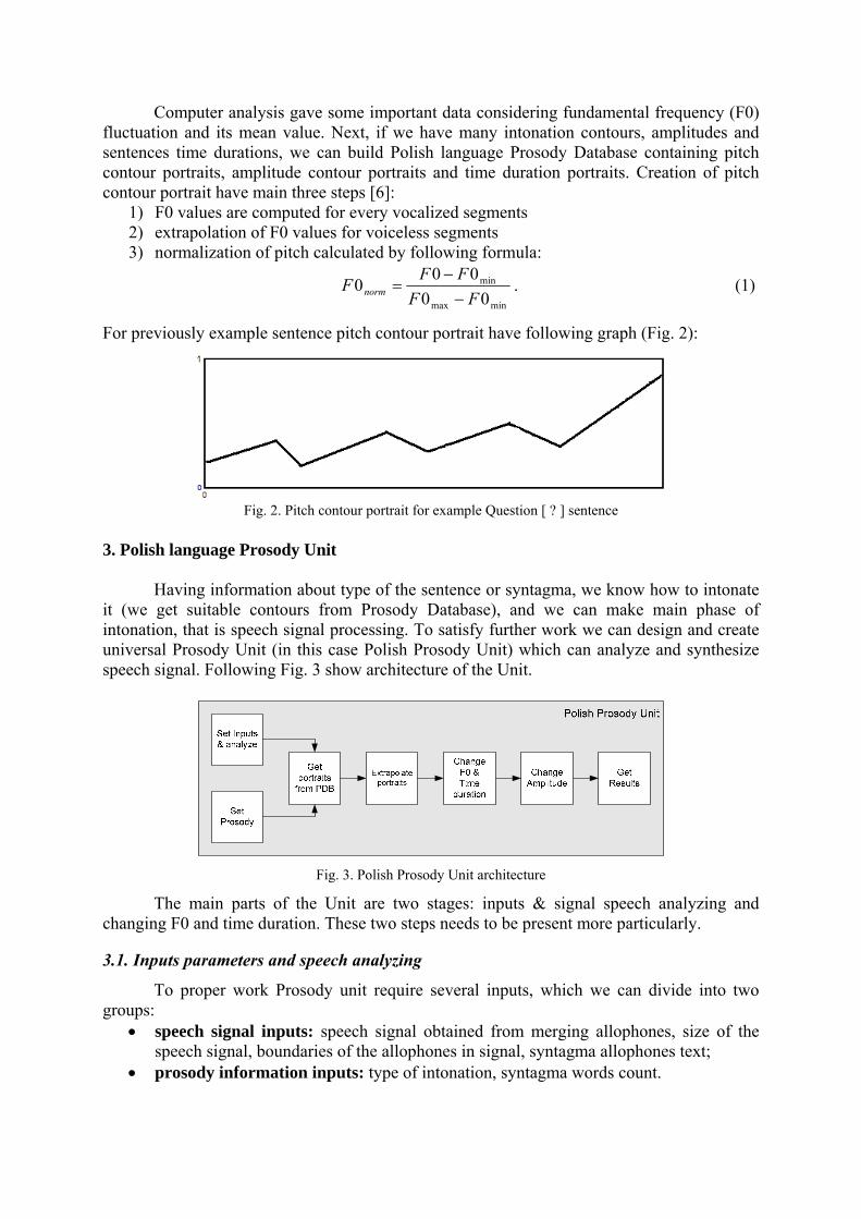
Computer analysis gave some important data considering fundamental frequency (F0) fluctuation and its mean value. Next, if we have many intonation contours, amplitudes and sentences time durations, we can build Polish language Prosody Database containing pitch contour portraits, amplitude contour portraits and time duration portraits. Creation of pitch contour portrait have main three steps [6]:

1) F0 values are computed for every vocalized segments 2) extrapolation of F0 values for voiceless segments 3) normalization of pitch calculated by following formula:

minmax

min

00000FF

FFF norm −−

= . (1)

For previously example sentence pitch contour portrait have following graph (Fig. 2):

Fig. 2. Pitch contour portrait for example Question [ ? ] sentence

3. Polish language Prosody Unit

Having information about type of the sentence or syntagma, we know how to intonate it (we get suitable contours from Prosody Database), and we can make main phase of intonation, that is speech signal processing. To satisfy further work we can design and create universal Prosody Unit (in this case Polish Prosody Unit) which can analyze and synthesize speech signal. Following Fig. 3 show architecture of the Unit.

Fig. 3. Polish Prosody Unit architecture

The main parts of the Unit are two stages: inputs & signal speech analyzing and changing F0 and time duration. These two steps needs to be present more particularly.

3.1. Inputs parameters and speech analyzing

To proper work Prosody unit require several inputs, which we can divide into two groups:

• speech signal inputs: speech signal obtained from merging allophones, size of the speech signal, boundaries of the allophones in signal, syntagma allophones text;

• prosody information inputs: type of intonation, syntagma words count.

Analysis part consists over computation of normalized F0 and amplitude portraits for given syntagma. If we need to compute F0 for given vowel or tonal consonant allophone (extracted form signal thanks to boundaries and text) we can use following method.

A reliable and simple way for estimate of fundamental frequency for long, clean, stationary speech signals is to use the cepstrum. The cepstrum is a Fourier analysis of the logarithmic amplitude spectrum of the signal:

( )( )XWFFTIFFTC fun *(log10= , (2)

where X – input allophone signal; Wfun – Hamming window function. 3.2. F0 and Time Duration transforms

Our prosody processor unit may change three parameters of speech signal: time duration, fundamental frequency and amplitude. The main part of Prosody Unit is TD-PSOLA module. Thanks it we’re can modify time and tone of vowels or tonal consonants.

TD-PSOLA algorithm have three main steps: 1) Find pitch marks; 2) Detect which frames of vowel or tonal allophone (according pitch marks) are

voiced and which are unvoiced; 3) Find new positions of pitch marks, find frames to be repeated or deleted and make

signal synthesis with overlap-add according factors obtained from portraits.

4. Results and discussion The paper is focused on architecture of Polish Prosody Unit which use several digital signal processing methods to transform neutral speech signal (obtained from allophones) into intonated speech sound. Pitch and amplitude contours for various types and subtypes (dependent from signal length/words count) intonation in Polish language were created by procedure described in 2.2. Taking all of above described techniques we building module (DLL) which can be added into TTS system. Following figures presents some interesting results.

Fig. 4. Example neutral sentence intonation contour

Above Fig. 4 present intonation contour for neutral sentence signal obtained from

synthesis (merging) of allophones. There is any intonation practically. Next, the sentence was subject into Prosody Unit and on output we obtained new synthesized sentence with changed (added Question) intonation. Fig. 5 presents intonation contour for new sentence.

Fig. 5. Example neutral sentence intonation contour after Prosody Unit

Feedback test prove, that neutral speech signal passed by Prosody Unit is not already

monotonous and artificial. New synthesized speech is more similar to human natural voice. Conclusion

In this paper we presented the Prosody Unit to modify neutral speech signal for

obtaining intonation effects in Polish language speech synthesis. The obtained results can be applied in further research in linguistics, especially, in the

study of phonetics and prosody of the Polish language, in expanding the theoretical and practical framework for multilingual speech communication systems.

It is of paramount importance to create systems like the speech synthesizer. Speech synthesizers facilitate work and speech synthesis itself opens new horizons and allows further development of information processing technologies.

Acknowledgements This paper was supported by the European Commission under grant INTAS Ref.

number 04-77-7404. The author would like to express thanks for their support.

References

1. Lobanov B., Karnevskaya H. MW Speech Synthesis from Text. Proc. of the XII International Congress of Phonetic Sciences. Aix-en-Provense, Franсe, 1991, pp. 406-409.

2. Shpilewski E., Piurkowska B., Rafalko J., Lobanov B., Kiselov V., Tsirulnik L. Polish TTS in Multi-Voice Slavonic Languages Speech Synthesis System, Proceedings of the 9th International Conference SPECOM’2004, Saint Petersburg, Russia, 2004, pp. 565-570.

3. Popowski K., Rafałko J., Piórkowska B., Szpilewski E. Using wavelet compression of allophone database for Polish language TTS system, Proceedings of the 10th International Conference SPECOM’2005, Patras, Greece, pp. 305-308.

4. Popowski K., Szpilewski E. Application of vowel allophones transforms for sentence intonation in Polish TTS system, Proceedings of the 11th International Conference SPECOM’2006, Saint Petersburg, Russia, 2006, pp. 265-269.

5. Piórkowska B., Rafałko J., Lesiński W., Szpilewski E. Sentence Intonation for Polish Language, SASR Workshop 2005, Krakow, Poland.

6. Lobanov B., Tsirulnik L., Zhadinets D., Piorkovska B., Rafalko J., Szpilevsky E. Language-Specific Application of Intonation Contours in Russian and Polish Multilingual TTS Synthesis, Proceedings of the 10th International Conference SPECOM’2005, Patras, Greece, pp. 317-320.

MODIFICATION OF BACK-PROPAGATION ALGORITHM FOR ELIMINATION OF BACKWARD CALCULATIONS

V. Ptitchkin

Belarusian State University of Informatics and Radioelectronics, Minsk, Belarus

The method for determination of gradient of quadratic quality index of multi-layer neural network in one forward passage is proposed. In stead of backward sequential calculation of synaptic matrices of each layer of neural network, parallel calculation of these matrices is proposed, which can be combined with forward calculations.

Introduction Back-propagation algorithm (BPA) still remains the most widely used algorithm of

learning of multi-layer neural networks (MLNN). This algorithm implements gradient method of optimization of quadratic quality index of network in the space of its parameters.

Determination of derivatives of output coordinates on the basis of parameters is based on the chain rule of differentiation of composite functions, determining recurrent nature of procedure of determination of derivatives of the output coordinate on the basis of MLNN parameters. This circumstance hinders description of the algorithm in the analytical form, its generalization for non-differentiable activation functions (AFs) [1] and, in general, any ways of AF approximation for development of approximate methods of MLNN analysis and synthesis [2].

The main purpose of this investigation is the proof of absence of principal necessity of the second (backward) passage for determination of derivatives; we think that this fact is important not only from the methodological point of view, but also for the further generalizations of BPA.

1. Description of Multi-layer Neural Networks in Matrix Form Any neuron, neuron layer or even MLNN can be described by the set of states, input

coordinates and output coordinates, which are described by vectors S, U and Y respectively, and by two equations, transition equation AU B S += and output equation )( SFY = . The latter equation means, in fact, the set of one-dimensional functions (AF) )(sfy jjj = , characterizing each neuron separately.

Let Uj, Yj and Sj are the vectors of input coordinates, output coordinates and states of jth layer of MLNN, m is the number of layers. Then, 1- ii YU = (1 ≤ i ≤ m), Y0 is the input of MLNN, Ym is the output.

Let’s represent the description of MLNN with sequential connections in the following form:

1−+= iiii YA B S , )( ii f SY = , mi ,1= . (1)

After AF linearization, the relation between coordinates yj and sj of jth neuron can be described as skqy jjjj += , and the relation between respective vectors can be described in the following form:

iiii SK Q Y += , mi ,1= , (2)

where Qi is the column of free terms, and Ki is the diagonal matrix of coefficients of linearization of AF of ith layer neurons.

2. Coefficients of Linearization of Dependencies between Coordinates For regular using of matrix notation, let’s introduce extended description of columns

by adding zero coordinate, which is identically equal to one. For example, let’s consider the extended description of vector )'x ..., ,x ,(x n21=X as vector )''(1, 1 XX = . Here, ' is symbol of transposition. Then, the state equation of any layer can be described as 1)( UA BS = or

111 UAS = , where A1 is the extended description of (B A) matrix. Let’s describe the affinities (1), (2) in the following form:

⎟⎟⎠

⎞⎜⎜⎝

⎛⎟⎟⎠

⎞⎜⎜⎝

⎛=⎟⎟

⎠

⎞⎜⎜⎝

⎛

−YABS 1

1011

iiii, ⎟⎟

⎠

⎞⎜⎜⎝

⎛⎟⎟⎠

⎞⎜⎜⎝

⎛=⎟⎟

⎠

⎞⎜⎜⎝

⎛

SKQY iiii

1011, mi ,1= ,

⎟⎟⎠

⎞⎜⎜⎝

⎛⎟⎟⎠

⎞⎜⎜⎝

⎛=⎟⎟

⎠

⎞⎜⎜⎝

⎛

−YHDY 1

1011

iiii, iiii BK Q D += , iii AK H = , mi ,1= .

The latter equation can be described even in shorter form YAS 1

111

−= iii , SKY 111iii = , YHY 1

111

−= iii , AKH 111iii = ,

to make obvious the relation between the sequence of connections of MLNN layers and the sequence of matrices in the product

YAKAKAKYHHHY 10

11

11

11

11

1110

11

11

11 LL −−− == mmmmmmm . The dependencies of the output coordinate on the coordinates of intermediate layer are

also of interest: 1

111111 YAKAKY −= iiimmm L , 111

11

1111 SKAKAKY iiiimmm ++= L , )1( mi ≤≤ ,

both separately and jointly. For example, 111 SKY mmm = , SKAKY 1

11

1111 −−= mmmmm , 1

21

21

11

1111 SKAKAKY −−−−= mmmmmmm , ….

The matrix ratios of transfer between the extended vectors can be denoted by the unique names, in order to distinguish the result of matrix product from the sequence of products of some other matrices, e.g.

111

11

111 KAKAKD iiijjji ++= L , ( ji < ). Then, linearized description of dependence of the output coordinate on the input

vector of ith layer and on the state vector of this layer can be written in the following form: YADY 1 1

111

i imim −= , SDY 111imim = .

Using the block representation of the latter matrix mentioned, the relation between the vectors considered can be described in the following form:

⎟⎟⎠

⎞⎜⎜⎝

⎛⎟⎟⎠

⎞⎜⎜⎝

⎛=⎟⎟

⎠

⎞⎜⎜⎝

⎛

SDBY imimim

1011, SDBY imimim += , KAKAKD iiimmmi 11 ++= L , ( mi < ).

It should be noted that the expressions obtained are not dependent on the way of linearization of non-linear dependencies, i.e. AF. Only the characteristic of accuracy of approximate linear description of any dependencies, both AF and the output coordinates, on the MLNN states, which are the arguments of AF, is dependent on the way of such linearization. In turn, the characteristic of accuracy of description of before-mentioned dependencies shall determine the domain and way of their application.

Considering the sequence of expressions of matrix transfer ratios KD mmm = , KAKD 1)1( −− = mmmmm , KAKAKD 211)2( −−−− = mmmmmmm , … (3)

it’s not difficult to note that the relation KADD 1)()1( −−−−−− = imimimmimm is available.

So, the expressions of coefficients of linearization of network coordinates as functions of other coordinates can be described in matrix form, both using the recurrent function and not using it. For the small number of layers, the recurrent function, most likely, should not be used, because saving of memory achieved by using this function would not compensate complication of the algorithm.

3. Determination of Derivatives of Output Coordinates in Relation to the Network Parameters

Because the main subject of discussion in this paper is the another realization of

classic BPA, let’s consider the coefficients of AF linearization as the derivatives of before-mentioned function.

In such a case, non-linear function (1) is used only for determination of numerical values of Y*

i on the basis of numerical values of S*i . In turn, pair of equations (1) makes it

possible to determine the sequences of values of state vectors S*i and output vectors Y*

i , characterizing each layer separately and the neural network as a whole.

Then, the components of column Qi and diagonal matrix Ki can be determined. In case of using Taylor series, these components can be determined rather simply for any jth layer, irrespective of the number of layer where it is located.

Therefore, to determine the matrix of coefficients of AF linearization for the neurons of ith layer in the vicinity of the specific values of states S*

i , it’s enough to differentiate the AF of each neuron for the particular value of its state and to form the diagonal matrix consisting of the values obtained. The columns of free terms can be determined in equally simple way, using the operation of component-wise product of vectors:

SSYQ ** *).(- iiii f ′= , )(diag *SK ii f ′= . (4) The latter expressions are intended only for determining the linearization coefficients

in the vicinity of values Y*i , S*

i , i.e. for calculation of respective derivatives. Therefore, any linearized equations can be described by deviations:

SSS *iii −=∂ , YYY *

iii −=∂ , YAS ∂=∂ −1iii , SKY ∂=∂ iii . Taking this result in consideration, it’s not difficult to explain that the arbitrary

component d mnij of matrix Dmn is equal to the derivative of ith coordinate of vector Ym in

relation to jth component of vector Sn in the point S*n . To calculate the gradient of the quality

index, the derivatives of the output coordinates Ym in relation to the arguments of activation functions Sn are of special interest.

Indeed, the variables, which are the arguments of the activation function of some neuron (or neuron layer), are the linear combinations of the input variables of this neuron (or neuron layer), with the coefficients equal to the parameters of neuron (or the parameters of neurons of the layer), or, vice versa, the linear combinations of parameters with the coefficients equal to the values of the output vector of previous layer.

Because the value of bias of any neuron is included in the expression of AF with the coefficient equal to one, the derivatives of the output coordinate in relation to the argument of AF of some neuron or in relation to the value of bias of this neuron are equal.

To simplify the considerations, let’s consider only the case of one-dimensional output coordinate of MLNN. Determination of its derivatives in relation to the parameters (values of biases and synaptic coefficients) of jth layer DA1

j can be described in one expression:

)'''()'1(''' * 1* 1*11

1 YDDYDYDDA −−− === jmjmjjmjjmjj . (5)

The result obtained, after multiplication by the value of error, and the step of learning must be subtracted from the current value of matrix )( AB ii , in order to obtain its new value, during optimization of the quadratic quality index using the gradient method.

Let’s explain that calculation of derivative matrices DA1j can be carried out also

forward, when not all matrices Dmj are calculated. Let’s explain this fact for the three-layer neural network. For 3=m , taking into consideration the expressions (3), the expressions (5) can be described in the following form:

'' *1231

3 YKDA = , '''' *113321

2 YKAKDA = , '''''' *10332211

1 YKAKAKDA = . (6)

4. Example BPA is described in the special literature in sufficient details. The detailed examples of

calculation for each step of the algorithm are available. Let’s use one such example [3] to compare the calculations implementing the scheme of BPA, proposed in this paper, and the classic scheme of BPA.

Let’s consider three-layer network described by the following expressions:

)exp(11)(

ssfy

iii −+== , ( ) ⎟⎟

⎠

⎞⎜⎜⎝

⎛ −−=

332222

11 AB , ( ) ⎟⎟⎠

⎞⎜⎜⎝

⎛−

−−=

222423

22 AB ,

( ) ( )13233 −=AB , ( )'9.01.0*0 =Y , 8.0,9.0,3 === ηtm .

For the same values of the input vector Y*0 , desired value of the output signal t and

learning step (norm) η, let’s determine the increment of parameters of this network for its optimization using the gradient method, in order to compare the procedure, proposed in this paper, with the classic one [3].

The latter procedure involves sequential determination of values of state vectors and output coordinates forward:

)'5.00()'1)(( *01

*1 == YABS 1 , )'993.05.0()( *

1*1 == SY f , )'987.0973.1(*

2 −=S , )'728.0122.0()( *

2*2 == SY f , 906.0*

3 −=S , 288.0)( *3

*3 == SY f , ε = 0.9 – 0.288 = 0.612.

However, the increments of matrices of the network parameters are determined backward. For this purpose, calculated values of output coordinates Y*

i are used. The results of these calculations are presented in [3]. Let’s explain that calculation of these increments can be combined with forward calculations, i.e. the backward passage is not critically necessary.

Immediately after calculation of the column of states of the first layer S*1 using (4), the matrix K1 can be calculated. As a rule, the values of derivative of sigmoidal AF, for particular value of the argument, are determined on the basis of appropriate values of AF itself, i.e. Y*1 value, but, in any case, determination of this matrix is completed after the analysis of operation of the first layer.

By exactly the same way, after completion of the analysis of the second layer, the matrix K2 can be calculated, and, after the analysis of the third layer, the matrix K3 . For the example under consideration

0067.025.0diag)993.01(993.0)5.01(5.0diag1 =−−=K , 198.0107.0diag)728.01(728.0)122.01(122.0diag2 =−−=K , K3 = 0.205.

After calculation of these matrices, all the multiplicands of expressions of derivatives in relation to the parameters of neurons of each layer (6) are determined. After multiplying, the following results are obtained:

⎟⎟⎠

⎞⎜⎜⎝

⎛−−−−−−

=0011.00001.00012.00113.00013.00126.01

1DA , ⎟⎟⎠

⎞⎜⎜⎝

⎛=

0403.00203.00406.00653.00329.00658.01

2DA ,

)149.0025.0205.0()728.0122.01(205.0)'1(''' *233

*1233

13 ==== YDYDDA . For determination of the increments of parameters of each layer, these matrices must

be multiplied by the value of error and learning step, εη: ( ) DAAB 1iii εη=∆ .

The result of multiplying of matrices DA1i , obtained before, by the constant factor εη =

= 0.612*0.8= 0.4896 is exactly equal to the result obtained in [3]; this fact demonstrates that the backward passage can be eliminated from implementation of modified BPA.

It’s obvious that calculation of increment matrices, on the basis of the derivative matrices, is not necessary: to calculate new value of matrix of parameters of each layer, only the value of the respective derivative and the proportionality coefficient εη are required.

It’s obvious also that the derivative matrices can be calculated sequentially: after calculation of matrix K1 , the first multiplicand '' 21 AK in the expression of matrix DA1

1 can

be calculated; after calculation of matrix K2 , the second multiplicand '' 32 AK in the expression of matrix DA1

1 (the first multiplicand in the expression of matrix DA12 ) can be

calculated, etc.

Conclusion The developed method of determination of gradient of MLNN quadratic quality index

does not involve recurrent relations between the derivatives. As a result, it is proved that the second (backward) passage is not critically necessary for calculation of derivatives. Instead, the main multiplicand of the gradient can be calculated, which, for obtaining the numeric value of the gradient, must be multiplied by the value of error. The main multiplicand can be calculated in parallel with calculation of the error.

References

1. Ptitchkin V.A. Application of Back-propagation Algorithm for Multi-layer Neural Networks with Threshold Activation Functions. Proceedings of the 8th International Conference on Pattern Recognition and Information Processing (PRIP’05), 18-20 May, Minsk, 2005, pp. 432-437.

2. Ptitchkin V.A. Analysis of Multi-Layer Neural Networks Using Methods of Statistical Linearization and Polynomial Approximation // Neural Computers: Development, Application, 1, 2004, pp. 5-18.

3. Callan R. The essence of Neural Networks. Prentice Hall Europe, 1999.

PROCESS OF AUTOMATIC OPTICAL MUSIC RECOGNITION

A. Rajs University Of Technology And Life Sciences, Bydgoszcz, Poland,

arajs@utp.edu.pl

This article shows process of automatic Optical Music Recognition basic on four steps. It suggest effective methods based on morphological transformations and associative memory (Hopfield’s network).

Introduction

Automatic visional systems are unreeled and improved from many years so that the area of applying them expands constantly. The tendency is extorting the realization of such systems of processing images in the digital form at the same time to storing the information, which, outside processing the image from the analogue figure to digital, his qualities will also enable proofreading (for example reduction in the noise of the image). Systems of automatic Optical Music Recognition (OMR) are an example of such systems. They are finding application at the digitization of the musical notation, for processing the handwritten musical notation to printed, as well as at automatic inserting notes into devices reconstructing sound.

Introducing the process of recognizing to the musical notation is an aim of the this work and suggesting using for the identification of symbols of the associative memory.

1. Principle of automatic recognizing the musical notation The musical notation is quite complicated and before all diverse set frequently one another of dependent signs (Fig. 1).

Fig. 1. Example of the musical notation

Systems automatically recognizing the musical notation four functional blocks which

they are realizing are being built in the support [1, 3]: • staff line identification and dismissing her (Fig. 2); • uncovering the location (of staff line identified on the base in the previous stage) of

musical symbols; • identification of these symbols; • outlining semantic relations between musical symbols and their regulation in the

accepted form through existing programs for notes edition.

The first functional block – you will remove uncovering putting the staff line and her perhaps to be carried out in basing for morphological transformations dilate and of erode.

The character of the digital image containing the musical notation should to analysis be characterized by coming properties:

• putting the staff line must in results of the canvassing of the image be horizontal (putting the staff line is making it impossible under the angle correct dismissing her as well as the more late location and the identification of symbols),

• the beat depth of the image containing the musical notation should take out 1 bit (set of black and white pixels),

• to make an assumption also that transformations will be taking place on black pixels and white are creating the background.

It is possible mathematically for monochrome objects to bequeath the operation to erosion into the coming way [2]:

( ) ( ) ( ), ,min min,

monoE L SE L m n Lm n SE SE

= =∈

, (1)

where: L(m,n) – brightness of the point about coordinate (m,n),

SE – structural template for erosion. By analogy mathematically written operation of dilatation has expressions for

monochrome objects [2]:

( ) ( ) ( ), ,max max,

monoD L SE L m n Lm n SE SE

= =∈

, (2)

where: L(m,n) – brightness of the point about coordinate (m,n),

SE – structural template for dilatation. The received image basing on the expressions (1) and (2) was shown in the Fig. 2.

Fig. 2. Musical notation after the operation of uncovering and removing of staff line

The second stage - uncovering the location (of staff identified on the base in the

previous stage) of musical symbols is most often realized on the base of the recursive flood-fill algorithm (Fig. 3) [6].

Fig. 3. Musical notation after the operation of uncovering putting musical symbols

A stage identifying musical symbols is most important stage. The identification of musical symbols can be realized by traditional ways, however the subject of the identification isn't often perfect to insults very much – symbols aren't reflecting the shape e.g. already the in full moon of their primal trademarks. Little disorders of features of the object aren't writing it off for the possibility for the identification. Based algorithms are fit very well at this target on neural networks. It is possible to carry using the neural network for the identification out of processing called classification where the set of input signals is composed of a few classes (classes must have the explicit division), and the sorter should in the reply report about the class which the starting signal belongs to. However a different group of neural networks which is reconstructing the signal taught earlier exists. This group it is for the memory associative – reconstructing the information encrypted earlier in the memory is coming in them. The principles of operation consist in pairing the image off (of signal) entrance around some from remembered in the memory. Process so was called the auto association.

The musical notation contains the very rich combination of signs. Outside many musical symbols (notes, keys, rhythmical signs, and the like) many variants of their record exist (notes can e.g. have flags directed up or into the bottom). The structure can for very notation be extended less or more (see Fig. 1). Therefore a set of basic signs was determined in the aim of avoiding construction of the big standard of the associative memory (of basic objects) which it is possible to fold appropriate musical signs from. The harvest of these objects was described on the Fig. 4.

Fig. 4. Set of a dozen or so basic objects (primitives) to construction of musical signs

To recognizing established standards, given to inputs in the binary form can be used the associative memory. Hopfield neural networks carrying teaching with the supervision out are fit for an implementation of such a memory e.g.

All outputs signals are being treated as inputs xi(k) = yi(k-1) and all inputs carrying back signals for all neurons. He isn't feedback the neuron with his personal access (wij = 0 when i = j). However he exists possibility of influencing by the outputs signal from the given neuron on one's value in coupling the future by the feedback of additional mediating neurons. Action of additional neurons is having a stabilizing effect on such a signal very much. The matrix of factors of the arrangement is symmetrical (wij = wji) what means that coefficient determining joining the neuron i-th with j-th the same value has what j-th with i-th. A thorough description of the principles of operation of the Hopfield's network is found in [4].

A capacity which is a maximum number of remembered and reconstructed with the mistake determined maximally models is very important for the associative memory for her with the parameter. Hebb’s rules, the maximum capacity of the memory are making the 13.8% of the number of neurons forming the memory for the mistake taking the 1% out and at using in the process of teaching associative. This capacity can surrender to making smaller as a result of the wrong initial state of the network which more distant copying the mistake is causing as a result of feedbacks what is tantamount with making the capacity of the memory smaller [5].

Fig. 5. General Diagram of the Hopfield’s network

Outlining semantic relations between musical symbols and their regulation in the accepted form are with the last stage through existing programs for notes edition. Semantic

relations concern such properties as levels of sounds stepping out in the range, duration of bar, stepping out and kinds of pauses, etc.

Conclusion

The process of automatic recognizing the musical notation consists of four stages and each of them can be realized apart in leaning processing the image against known or modified methods. Suggested solutions are model. Research are showing that it is possible to improve individual stages of the process of optical music recognizing.

References

1. Bainbridge, D., Bell T. An extensible optical music recognition system. Australian Computer Science Communications 18 (1), 1996, pp. 308-317.

2. Tadeusiewicz R., Korohoda P. Komputerowa analiza i przetwarzanie obrazów. Wydawnictwo Fundacji Postępu Telekomunikacji, Kraków, 1997.

3. Bainbridge D. Optical music recognition: A generalised approach. Paper read at Second New Zealand Computer Science Graduate Conference, 1996.

4. Nasrabadi N.M., Wei Li. Object Recognition by a Hopfield Neural Network. IEEE Zhns. on Systems, Man, and Cybernetics, Nov. 1991, vol. 21, no 6, pp. 1523-1535.

5. Tadeusiewicz R. Sieci neuronowe.(Neural networks) Akademicka Oficyna Wydawnicza RM, Warszawa, 1993.

6. Pavlidis T. Algorithms for Graphics and Image Processing. Rockville, MD: Computer Science Press, 1982.

CORRELATION FILTERS FOR RECOGNITION OF MOVING OBJECTS

Erika M. Ramos-Michel,1 Vitaly Kober,1,2 I.A. Ovseevich2

1 Department of Computer Sciences, Division of Applied Physics CICESE, Ensenada, B.C. 22860, Mexico, rmichel@cicese.mx, vkober@cicese.mx

2 Institute for Information Transmissions Problems of RAS Moscow, Bolshoi Karetnii 19

New generalized correlation filters for reliable recognition of moving and noisy objects are derived. The filters design takes into account information about motion blurring and sensor’s additive noise. Computer simulation results obtained with the proposed filters are compared with those of various correlation filters in terms of recognition performance.

Introduction Since the pioneering work of VanderLugt [1] much research has been undertaken to

derive correlation filters for reliable object recognition. The correlation operation has several advantages such as follows: it can be effectively implemented in an optical setup as well as a linear, shift-invariant filter with the use of a fast digital Fourier transform. To carry out reliable recognition various correlation filters for two kinds of mathematical signal models (overlapping and nonoverlapping) of input scenes were proposed [2, 3]. Using the overlapping model the optimal filter (OF) [4] and phase-only filter (POF) [5] were derived, whereas the nonoverlapping model was exploited for deriving of the generalized optimum filter (GOF) [6] and generalized phase-only filter (GPOF) [7]. Note that all these filters are sensitive to optical degradations (blurring), noise and distortions on captured images. There are a few works in pattern recognition that deal with particular cases of the degradations [3, 8, 9].

In this paper, we propose new correlation filters for recognition of motion blurred objects additionally corrupted with additive Gaussian noise. The paper is organized as follows. In Section 1, we present new generalized filters. Computer simulation results are provided and discussed in Section 2. Finally, our conclusions are presented.

1. Generalized correlation filters for recognition of moving objects During the process of image formation a captured image may be degraded

homogenously or non-homogeneously. An inhomogeneous degradation only affects a part of the image. For instance, during the capturing an object to be recognized is moving across a fixed background. The input scene may be additionally corrupted with additive noise that is always present in sensors.

Let us consider a uniform motion blurring: object moves from left to right with a constant horizontal velocity V during the time capture interval [0, T]. The impulse response of the blurring degradation can be expressed as follows [10]:

( ) 1 , 0mh x x LL= ≤ ≤ , (1)

where L=VT is the displacement interval in pixels. For clarity and simplicity one-dimensional notation is used. Assume that the input

scene s(x) contains a moving target t(x-x0) located at unknown coordinate x0, spatially disjoint background scene b(x), and additive noise n(x):

( ) ( ) ( ) ( ) ( ) ( )0 0 0, m bs x x t x x h x b x w x x n x= − • + − + , (2)

where “” denotes the convolution operation, hd(x) is the impulse response given by (1), ( ) ( ) ( )0 01b t mw x x w x x h x− = − − • , and ( )tw x is a support function of the target defined as

unity within the target area and zero elsewhere. The filter design is based on the following assumptions. b(x) is a realization from a wide-stationary random process and µb is its expected

value. The coordinate x0 is a random variable with a uniform probability density function. B0(ω) is the power spectral density of (b(x) - µb), and it is calculated as:

( ) ( ) ( ) 2

0 bB b x V xω µ= −⎡ ⎤⎣ ⎦F , (3)

where ⋅F denotes the Fourier transform, b(x) is considered as an ergodic process, and V(x) is a sinusoidal window that is utilized to avoid border affects and to obtain a better estimation of the power spectral density. Actually, other windows can be used as well for the estimation.

n(x) is a zero mean random process with the power spectral density N(ω). It is assumed that the wide-sense stationary noise b(x), the additive noise n(x) and

the target location x0 are statistically independent of each other. T(ω), ( )bW ω , and Hm(ω) are the Fourier transforms of t(x), ( )bw x , and hm(x),

respectively. The filter output y(x) is given by ( ) ( ) ( )0 0, , *y x x s x x h x= , where h(x) is a linear

filter that optimizes a criterion of interest. Next, two optimal filters GOFNHD and GPOFNHD with respect to different criteria are derived. The criterion peak-to-output-energy ratio (POE) is defined as the ratio of the expected squared value of the correlation peak to the average expected value of the output-signal energy [6]. By maximizing the criterion, we obtain,

( ) ( ) ( ) ( )

( ) ( ) ( ) ( ) ( ) ( )

*

2 20

12

d b bNHD

m b b b

T H WGOF

T H W B W N

ω ω µ ωω

α ω ω µ ω ω ω ωπ

+⎡ ⎤⎣ ⎦=⎛ ⎞+ + • +⎜ ⎟⎝ ⎠

. (4)

Here, “*” denotes complex conjugate, and α is a normalizing constant [3]. A modified version of the generalized phase-only filter that maximizes the light efficiency (defined as the ratio of light intensity in the correlation plane to the total light leaving the input) can be expressed as

( ) ( ) ( ) ( )( ) ( ) ( )

*m b b

NHDm b b

T H WGPOF

T H Wω ω µ ω

ωω ω µ ω

+⎡ ⎤⎣ ⎦=+

. (5)

In the next section we present our computer simulation results. All correlation filters were implemented using the fast Fourier transform.

2. Computer simulations In our experiments the background b(x) and the target image t(x) possess

characteristics given in Table 1. The signal range is [0-255]. The input scene is degraded as follows: 1) several values of L are used: 3, 5, 7, 9, 11, and 15 pixels, 2) for each value of L, additive white Gaussian noise (AWGN) with zero mean and the following standard deviations (σn): 5, 10, 15, 20, 25, 30, 35, 40, and 42.67 is added to the input scene.

Table 1 Parameters of the used images

Parameters Background Background with four false objects

Target

Mean 115.73 114.63 48.67 Standard Deviation 39.69 39.86 26.24

Size (pixels) 256 × 256 256 × 256 17 × 27

Fig. 1, a shows a test input scene containing four false objects and a target degraded with L=11 pixels. Fig. 1, b shows the positions of the objects.

a) b)

Fig. 1. Test input scene containing four false objects and a moving target with L=11 pixels (a); positions of the target marked by the arrow and the false objects (b)

The ability of a filter to discriminate a target against other objects in the input scene

can be measured with discrimination capability (DC). If the target is embedded into a background that contains false objects the DC is expressed as follows:

( )( )

2

2

0,01

0,0

B

T

cDC

c= − , (6)

where cB is the maximum in the correlation plane over the background area to be rejected, and cT is the maximum in the correlation plane over the area of target position. The accuracy of target localization can be characterized with the help of a distance error between a known exact position of the target ( ),T Tx y and a position ( ),T Tx y% % of the maximum value in the correlation plane over the area of object to be recognized,

( ) ( )2 2DE T T T Tx x y y= − + −% % . (7)

Computer simulation results when the input scene is degraded with L=3, 5, 7, 9, 11, and 15 are shown in Figs. 2, a, b. For each value of L, 20 statistical trials (varying randomly the position of the target) were carried out. In these experiments, the following filters are used: OF, POF, GOF, GPOF, GOFNHD, and GPOFNHD. According to the both criteria the best filters are the GPOFNHD and GOFNHD, respectively, whereas the OF and POF fail to recognize the target.

Next, we additionally corrupt the input scene with additive noise. 20 statistical trials randomly varying the position of the target and 30 statistical trials for each standard deviation were carried out. Figs. 3, a, b show the performance of the filters with respect to the DC and the distance error when L=15. It can be seen, that the GOFNHD is the best filter because it is able to recognize the target for all applied degradations.

Recognition of the Target in Blurred Scene with Respect to the DC

0.0

0.1

0.2

0.3

0.4

0.5

0.6

0.7

0.8

L=3 L=5 L=7 L=9 L=11 L=15

DC

GOFGPOFGOF_NHDGPOF_NHD

Recognition of the Target in Blurred Scene Respect to the Distance Error

0

2

4

6

8

L=3 L=5 L=7 L=9 L=11 L=15

Pix

GOFGPOFGOF_NHDGPOF_NHD

a) b)

Fig. 2. Filters performance with respect to: (a) DC and (b) distance errors, when the input scene is degraded with blurring L=15

Recognition of the Target in Degraded Scene with L=15 Pixels and AWGN with Respect to the DC

0.0

0.1

0.2

0.3

0.4

0.5

5 10 20 30 40 42.67 StD

DC

GOFGPOFGOF_NHDGPOF_NHD

Recognition of the Target in Degraded Scene with L=15 Pixels and AWGN with Respect

to the Distance Error

0

2

4

6

8

10

12

14

5 10 20 30 40 42.67 StD

PixGOFGPOFGOF_NHDGPOF_NHD

a) b)

Fig. 3. Filters performance with respect to: (a) DC and (b) distance errors of localization, when the input scene is degraded with blurring L=15 and additive noise

Conclusion Two new generalized filters for reliable recognition of moving objects in input scenes

degraded with additive noise were proposed. The computer simulation results demonstrated superiority in the performance in terms of discrimination capability and distance errors of the suggested filters comparing with various correlation filters. The obtained filters also possess good robustness to additive input noise.

References

1. VanderLugt A.B. Signal Detection by Complex Filtering. IEEE Trans. Inf. Theory, vol. 10, 1964, pp. 139-135.

2. Vijaya-Kumar B.V.K., Hassebrook L. Performance Measures for Correlation Filters. Applied Optics, vol. 29, no 20, 1990, pp. 2997-3006.

3. Kober V., Campos J. Accuracy of Location Measurement of a Noisy Target in a Nonoverlapping Background. Journal OSA, vol. 13, no 8, 1996, pp. 1653-1666.

4. Yaroslavsky L.P. Optical Correlators with (-k)th-Law Nonlinearity: Optimal and Suboptimal Solutions. Applied Optics, vol. 34, no 20, 1995, pp. 3924-3932.

5. Ahouzi E., Campos J., Yzuel M.J. Phase-Only Filter with Improved Discrimination. Journal OSA (A), vol. 19, no 17, 1994, pp. 1340-1342.

6. Javidi B., Wang J. Design of Filters to Detect a Noisy Target in Nonoverlapping Background Noise. Journal OSA, vol. 11, no 10, 1994, pp. 2604-2612.

7. Seong Y.K., Choi T.S. Optimal-Trade-Off Filters for Noise Robustness, Peak Sharpness, and Light Efficiency in Nonoverlapping Background Noise. Optical Engineering, vol. 39, no 2, 2000, pp. 472-477.

8. Navarro R., Nestares O., Valles J.J. Bayesian pattern recognition in optically degraded noisy images. Journal of Optics A: Pure and Applied Optics, vol. 6, 2004, pp. 36-42.

9. Chan F., Towghi N., Pan L., Javidi B. Distortion-Tolerant Minimum-Mean-Squared-Error Filter for Detecting Noisy Targets in Environmental Degradation. Optical Engineering, vol. 39, 2000, pp. 2092-2100.

10. Biemond J., Lagendijk R.L., Mersereau R.M. Iterative Methods for Image Deblurring. Proceedings of the IEEE, vol. 78, no 5, 1990, pp. 856-883.

SIGNAL RECONSTRUCTION AT ITS UNIFORM SAMPLING WITH FOURIER SERIES∗

A.L. Reznik, V.M. Efimov

Institute of Automation and Electrometry, SB RAS, Novosibirsk, Russia, reznik@iae.nsk.su

Formulas for sampling functions at signal interpolation with Fourier series over uniformly disposed signal and its derivative are given. Average dispersion of steady random signal interpolation is analyzed.

Introduction

Fourier series are often used for a harmonic analysis of signal over a set of its uniform samplings (N is odd).

( ) ( ),sincos2

1

10

)0( 22∑−

=∆∆ ++=

N

kkk ktbktaatf NN

ππ (1)

where constants kaa ,0 and kb (their total number coincides with the number of samplings N) are determined according to the well known relations:

( ) ( ) ( ) ( ) ( ) ( )1 1

2 20 0 0

01 1

2 2

12

12

2 21 2 2N N

k kN Nn nn

N

NN Na f n , a f n cos kn,b f n sin kn.

N N N

− −

− −=− =−=−

−

−

π π= ∆ = ∆ = ∆∑ ∑ ∑ (2)

Introducing (2) into (1), and changing summation order, one obtains relation (1) is a theorem for the periodic signal reading:

( )( ) ( )( )( )( )∑

−

−−=

∆−

∆−∆=

∆

∆2

1

21

00 .sin

sinN

NnntN

ntnftf

Nπ

π (3)

Interpolation functions for the limited spectrum signal reconstruction by the set of uniformly coming samplings of signal and its derivative have been obtained elsewhere [1]. Below we use the same scheme for the periodic signal reconstruction in order to obtain formulas for the corresponding sampling functions and reconstruction error dispersion at intermediate frequencies.

1. Sampling functions and interpolation formulas

Sampling functions for the uniform set of periodic signal values and its derivatives are derived from the corresponding relations for the same set characterizing the limited spectrum signal [1] using well known relations:

∗ This study was supported by Russian Foundation of Basic Researches (grant 06-01-00653), by

Presidium of Russian Academy of Sciences (Program 14.1/2006), and by Siberian Branch of RAS (Integration Project 3.9/2006).

( )( ) ( )∑

∞

−∞=−

−

−−=

+nr

rr

r adad

ran,ctg

!111

1

1ππ (4)

( )( )

( ) ( )∑∞

−∞=−

−

−−=

+

−

nr

rr

r

na

dad

ran.eccos

!111

1

1ππ (5)

1. Let us consider the case, when for signal reconstruction we use its values obtained in period ( )( ) ,0 ∆−∆ nfN where 1,0 −= Nn . Since

( )( ) ( )( ),00 ∆+= kNtftf (6) classic sampling theorem

( )( ) ( )( )( )

( )∑∞

∞− ∆−

∆−∆=

∆

∆ ,sin00

nt

ntnftf π

π (7)

is transformed as follows:

( )( )( )( ) ( ) ( )

( )∑ ∑−

=

∞

−∞= ∆−∆−−

∆−∆=

=

∆∆

1

0

0

0

.1sinN

n k

kN

kNntntnf

tf

ππ (8)

Using relation (5) for odd N, and relation (4) for even N at 1=r after simple transforms we obtain interpolation formulas (3) using sampling functions for the periodic signal and formula (9):

( )( ) ( )( )( )( )

( )∑−

=∆−

∆−

∆−∆= ∆

∆

∆1

0

00 .cossin

sinN

nnt

ntN

ntnftf N

N

ππ

π (9)

Let us note that although relations (3) and (9) well describe the periodic signal by its values they are not convenient for the signal reconstruction at intermediate frequencies. This follows from the fact that condition (6) makes signal discontinuous.

Improvement happens when one uses ( )tkkt NN )12(sin,2cos −∆∆ππ as basis functions.

In this case the discontinuity of odd interpolation terms over the ends of period N∆ disappears, and samplings theorem is:

( )( ) ( ) ( )( )

( )( ) ( ) ( )( )

02 1

2 1

2 12 1

12 2 1

12 1

N( )

n N( N )

( N )

( N )( N )

sin t nf ( n )f ( t ) cos t nN sin t n

sin t ncos t n ,

N sin t n

=−

π∆ π

+ ∆π+ ∆

π∆ π

+ ∆π+ ∆

⎛ − ∆∆ ⎜= + − ∆ +⎜ + − ∆⎝

⎞+ ∆⎟+ − + ∆⎟+ + ∆ ⎠

∑ (10)

when number (2N+1) is odd and

( )( ) ( )( )

( )( ) ( )( )

0

1

2 12 122 2 1

2 22 12 2

2 12 2 1

2 22 12 2

12 2

12

N( )

n ( N )

nnn

NnN

nn

NnN

sin tf ( )f ( t ) cos t

N sin t

sin tcos t ,

N sin t

=− −

π −−∆ π −

∆π −∆

π −∆ π −

∆π −∆

⎛ − ∆∆⎜= + − ∆ −⎜ − ∆⎝

⎞+ ∆⎟− − + ∆⎟+ ∆ ⎠

∑ (11)

when number (2N) is even.

2. For the uniform sets of readings of the signal and its first derivative, when signal spectrum is limited by frequency ∆π , and interval between a pair of readings is ∆2 , theorem is written as [1]:

( ) ( ) ( )( )

( ) ( )( ) ( ) ( ) .2

!122

22sin 1

0

3

0

2

2∑∞

−∞= ⎭⎬⎫

⎩⎨⎧

∆−∆

+∆⎥⎥⎦

⎤

⎢⎢⎣

⎡

∆−

∆−=

∆

∆

n

ntnfnfnt

nttf π

π (12)

If signal is periodic with a period of ∆2N , then it follows from equations (4) and (12) that independently of whether N is odd or even, theorem (12) turns to equation:

( ) ( ) ( )( )

( ) ( )

( ) ( ) ( ) ( )

21

0 0

0

1

2

2

2 2

22

2

2 2 2 21

N

n N

N N

sin t nf t f n

N sin t n

f n N sin t n cos t n .!

−

=

π∆π∆

π π∆ ∆

⎡ ⎤− ∆ ⎧= ∆ +⎢ ⎥ ⎨− ∆ ⎩⎢ ⎥⎣ ⎦

⎫∆ ∆ ⎪+ − ∆ − ∆ ⎬π ⎪⎭

∑ (13)

Apparently, at ∞→N relation (13) transforms to relation (12), since

( ) ( ),22sin2lim 2 ∆−=∆−∆

∆∞→ntntN NN

ππ

and ( ) .12coslim 2 =∆−∆∞→ntNN

π

Calculating cosine-sine coefficients for formula (1) using (13) we obtain:

( ) ( )∑−

=

∆=1

0

00 ,21 N

n

nfN

a

( ) ( ) ( ) ( ) ( ) ( )∑∑−

=

−

=

∆∆

−∆−

=+=1

0

11

0

02

10 ,sin22cos2)(2 22N

n

N

nkkk knnf

Nknnf

NkNaaa NN

πππ

(14)

( ) ( ) ( ) ( ) ( ) ( ) ( )∑∑−

=

−

=

∆∆

+∆−

=+=1

0

11

0

02

10 ,cos22sin22 22N

n

N

nkkk knnf

Nknnf

NkNbbb NN

πππ

Convergence of (13) over intermediate frequencies is not satisfying as well.

2. Dispersion of reconstruction error

Dispersion of reconstruction error is determined by relation:

( ) ( )∫∞

∞−

= ωεωωε 22fSd , (15)

where ( )ωfS - is the spectral density of reconstructed signal, ( )ωε 2 - is dispersion of error of signal reconstruction at certain frequency ω .

Value ( )ωε 2 may be calculated using either reference functions or standard frequency expansions. The latter seem to be more preferable, since unlike frequency functions, sampling functions are not orthogonal.

1. Let us consider error dispersion value, when signal is reconstructed using theorem (3). In this case

( ) ( )21

2 22

01

2

2 21N N

i tk k

kNN Ndt e a a cos kt b sin kt .

N

∆ −

− ω

=∆−

π π∆ ∆ε ω = − − +

∆ ∑∫ (16)

Here value ( )( ) ∆−=∆ nienf ω0 according to (2). According to Fig. 1, signal expansion (3) is not good enough to describe signal

containing the intermediate frequencies. At frequencies ( )212 1 −≤≤= N

N kkπω error dispersion is equal to zero.

Fig. 1. Error dispersion at signal reconstruction with formula (3) depending on the signal period

With basis functions ( )tkkt NN )12(sin,2cos −∆∆

ππ error dispersion ( )ωε 2 is not oscillating, but increases with the growing frequency. Relation (11) well reproduces the intermediate signal frequencies (Fig. 2).

Fig. 2. Error dispersion at signal reconstruction with formula (11) depending on the signal period

2. Let us consider given pairs of signal values and its derivative in abscissa ( )1,02 −=∆ Nnn , while signal is reconstructed according to formula (13). In this case let

us use a standard bandwidth signal expansion, wherein expansion constants are determined by

relation (14), where ( )( ) ∆−=∆ nienf 20 2 ω and ( )( ) ∆−−=∆ nieinf 21 2 ωω are derivative values. Computation results are given in Fig. 3.

Fig. 3. Error dispersion at signal reconstruction with formula (13) depending on the signal period

Conclusion

Fig. 1 and 3 show that at frequencies ∆< πω signal reconstruction with interpolation formulas (3) and (13) is not successful due. Therefore, re-sampling is needed. When N is large enough at frequencies above the Nyquist one formula (13) is equivalent to formula (12) with regard to reconstruction accuracy, and formula (3) is similar to the standard sampling theorem (7) (see [2]).

Sampling theorem (11) reproduces frequencies well enough at ∆< πω , while at higher frequencies is equivalent to the standard sampling theorem (7) for the non-periodic signal. Most likely at re-sampling it may be used to build a FIR-filter according to procedure described elsewhere [3].

References

1. Hurgin Yu.I., Yuakovlev V.P. Finishing functions in physical and technical applications. Moscow, Nauka, GRFML, 1971.

2. Efimov V.M., Reznik A.L., Vas’kov S.T. Error dispersion at signal reconstruction at additional use of signal derivative samples, Avtometriya, 6, 2004, pp. 110-119.

3. Efimov V.M., Reznik A.L., Torgov A.V. Comparative estimation of polynomial interpolators at a uniform sampling of signals, Avtometriya, 6, 2001, pp. 24-31.

RECONSTRUCTION OF SUPER RESOLUTION IMAGES WITH MINIMUM DISPERSION∗

A.L. Reznik, V.M. Efimov, A.A. Soloview

Institute of Automatics and Electrometry SB RAS, Novosibirsk, Russia, reznik@iae.nsk.su

Described is a method for the spatial solution of a problem related to image reconstruction by a sequence of observed low resolution images, differing by the mutual coordinate shift. Algorithms and computation scheme are built so that signal with the least dispersion is chosen among all digital signals fitting the registered observation system.

Introduction

In many fields of applied or practical informatics it is necessary to estimate ideal initial signal or image by the results of measurements carried out with low resolution photo matrices. Photo matrices with high spatial resolution are rather expensive, especially for infra-red (IR) spectra, and there are many problems with the manufacturing of receivers.

Let us try to solve the problem of image reconstruction with high spatial resolution using a regulated subpixel scanning, when initial signal is restored by a set of images, each obtained with a trajectory shift of registering photo matrix with discretion less than the linear size of photo element (or integrating aperture). Therefore, with a set of digital images shifted with respect to each other so that shift value is less than the linear size of the integrating element of photo matrix, we should estimate initial image to obtain its maximum high spatial resolution by the optimum processing method.

Typical approaches [1-5] use various numerical optimization procedures providing solutions with a minimal norm [6]. We shall search for the solution with the minimum dispersion (energy), which in general case is not the same. Below we show in what cases these solutions coincide, and give constructive algorithms for their fast revealing in linear and two-dimensional cases.

1. Reconstruction of a digital signal with minimum dispersion (one-dimensional case)

As we have already mentioned problems of reconstruction of signal with minimum norm and signal with minimum dispersion basing on the same observation by a subpixel scanning of initial image may have non coinciding solutions.

Let us show that under certain conditions upon the linear size of restored field these solutions indeed coincide, and let us also give constructive algorithm accelerating signal reconstruction with no addressing to giant matrices.

Let us consider registering scheme shown on Fig. 1. Here number N, corresponding to dimension of restored vector X = (x1 ,x2 ,…, xN ), is a multiple to a number of elements of resolution l that get into the integrating aperture. This means that scanning field size (for one dimensional case it is interval size N) is larger by whole number fold than the size of aperture l, i.e. N=n×l.

∗ This study was supported by Russian Foundation of Basic Researches (grant 06-01-00653), by

Presidium of Russian Academy of Sciences (Program 14.1/2006), and by Siberian Branch of RAS (Integration Project 3.9/2006).

Fig. 1. Scheme for linear signal registering. l – size of scanning aperture-integrator. I1 , I2 ,…, I(n-1)l+1

are measurements

Let us write the set of equations corresponding to observation vector I =(I1 , I2 ,…, I(n-1)l+1 ) as follows

⎪⎪⎩

⎪⎪⎨

⎧

=+++

=+++=+++

+−+−+−

+

.1)1(2)1(1)1(

2132

21

lnnllnln

l

ll

Ixxx

IxxxIxxx

K

M

K

K

(1)

Apparently, in this case the average value of signal

NIIII

Nxxxxxx

Nxxx

x lnllnllnlllN 1)1(12111)1(21121 )()()( +−+++−+ ++++=

+++++++++=

+++=

KKKKKK (2)

is a constant expressed through the elements of observation vector I and independent of variables xi. Now using (2), we are able to prove directly that search for the norm minimizing solution is equivalent to the search for dispersion minimizing solution. Let us note that in the first case (minimized norm solution) one should minimize expression

.min1

22 ⇒=∑=

N

iixx (3)

In the similar manner let us write and transform expression for dispersion

( ) ( ).min

11

11

11

11 2

21)1(1211

1

2

1

2 ⇒−−

=++++

−−⎟⎟⎠

⎞⎜⎜⎝

⎛−

=−−

= +−++

==∑∑ constx

NNIIII

Nx

Nxx

ND lnllN

ii

N

iix

K. (4)

The obtained relation differs from (3) only by a constant multiple and additional summand independent of variables xi . Therefore problems (4) and (3) has the same solution. Therefore, at a size of restored field N = n×l norm minimization solution (3) and dispersion minimization solution (4) are equivalent. The minimum of expression (3) is attained with the following values of variables:

.11)1(11)1)(2(12 2

1211)1(211 ∑

−

=+++−⎭⎬⎫

⎩⎨⎧

⎥⎦⎤

⎢⎣⎡ −−−+⎥⎦

⎤⎢⎣⎡ +−−

+⎥⎦⎤

⎢⎣⎡+⎥⎦

⎤⎢⎣⎡ −−+⎥⎦

⎤⎢⎣⎡ −−+−

=n

iililln I

ninI

nllinI

nlI

nnI

nlnlnx (5)

( ) ( )[ ] ).1,,2(,)1(1 2

01211 −=−−−−−−= ∑

−

=+++++ liIIIIsn

nxx

n

sslslislisli K (6)

., ),,(1

11 Nlj

j

ljqqljj xIx K=∑

−

+−=+− −= (7)

2. Minimum dispersion image reconstruction (two-dimensional case)

Reconstruction of a two-dimensional field with minimum dispersion by a sequence of low resolution images shifted against each other is carried out as follows.

It first we need to build an estimate for the elements of image X=(xmn), following conditions

)

) ( )

11

2

1 1 1 1

1 1 1 11

12

j li l

pq ijp i q j

N N M N

pq pqp q p q

( i , ,M l ; j , ,M l );

x I ,

x x min, where x x .MN

+ −+ −

= =

= = = =

= − + = − +=

− ⇒ =

∑ ∑

∑∑ ∑∑

K K

(8)

In a discrete case for reconstructing field X=(xmn), m=1,…,M; n=1,…,N by the

observed data represented by matrix I=(Iij), i=1,…,M-l+1; j=1,…,N-l+1, under condition that filed size is multiple to the linear size l of integrating aperture, i.e. when M=ml и N=nl, problem solution is found by factorization twice stepwise applying the above described procedure for the linear case. For this purpose let us build new vectors

( ),,,, 21 jMjjj yyy K=y j=1,…,N-l+1:

∑=

−+ ==l

rrjkjk Mkxy

11, ),,1(, K , (9)

and then for each j=1,…,N-l+1 we solve linear case by the above described algorithm:

)

) ( )1

1

2

1 1

1 11

12

l

j ,k i kjiM M

ij j j jii i

( k , ,M l );

y I ,

y y min, where y y .M

+ −=

= =

= − +=

− ⇒ =

∑

∑ ∑

K

(10)

In conclusion, as we have found all elements of solution (10) by “columns”, and e.g. have determined all variables yjk (j=1,…,N-l+1; k=1,…,M), initial image reconstruction comes as a result of independent solution of M linear problems for each k=1,…,M:

)

) ( )1

1

2

1 1

1 11

12

l

k , j r jkr

N N

kq k k kqq q

( j , , N l );

x y ,

x x min, where x x .N

+ −=

= =

= − +=

− ⇒ =

∑

∑ ∑

K

(11)

This algorithm was checked with a large number of real and artificially constructed control digital images. Reconstruction quality was good in most of cases. Let's note, that improvement of the spatial resolution of the restored image in comparison with the spatial resolution of observed images demands square-law increase in amount of measurements. This problem is not a insuperable one due to the following reasons. First, time spent on reconstruction of images 512×512 elements in size using a moderate capacity personal computer never exceeds several seconds. Second, computations matrices used to perform all mathematical operations may be calculated beforehand, and algorithms computation capacity is essentially reduced. Fig. 2 exemplifies image reconstruction with the described procedure.

a) b) c)

Fig. 2. Minimum energy image reconstruction: a) initial image; b) one of observed low resolution image; c) minimum energy reconstructed image

If the sizes of a restored field are not harmonized with the sizes of the scanning

aperture (i.e. if M or N are not multiple l), the decision possessing the minimum norm, differs from the decision possessing the minimum dispersion. Let’s demonstrate it with the following example. Let we need to reconstruct field X=(xmn) with a dimension of 3×3 elements according to observed data

⎪⎪⎩

⎪⎪⎨

⎧

=+++=+++=+++=+++

.2233322322

2132312221

1223221312

1122211211

IxxxxIxxxxIxxxxIxxxx

(12)

Thus, it is required to solve a two-dimensional task of restoration for M=3; N=3; l=2. Direct calculations show that image with minimum norm, which corresponds observation system (12), is

⎟⎟⎟⎟⎟⎟⎟⎟

⎠

⎞

⎜⎜⎜⎜⎜⎜⎜⎜

⎝

⎛

×−−×−−×−−

×−−××−−

×−−×−−×−−

=

TTT

TTT

TTT

IIIIIIIIIIII

IIIIIIIIIIII

IIIIIIIIIIII

);;;()4;2;2;1();;;()2;2;1;1();;;()2;4;1;2(

);;;()2;1;2;1();;;()1;1;1;1();;;()1;2;1;2(

);;;()2;1;4;2();;;()1;1;2;2();;;()1;2;2;4(

91X

222112112221121122211211

222112112221121122211211

222112112221121122211211

(13)

while image with minimum dispersion (energy) corresponding to the same system of observations, may be represented as

⎟⎟⎟⎟⎟⎟⎟⎟

⎠

⎞

⎜⎜⎜⎜⎜⎜⎜⎜

⎝

⎛

×−−×−−×−−

×−−××−−

×−−×−−×−−

=

TTT

TTT

TTT

IIIIIIIIIIII

IIIIIIIIIIII

IIIIIIIIIIII

);;;()23;9;9;7();;;()11;11;5;5();;;()9;23;7;9(

);;;()11;5;11;5();;;()3;3;3;3();;;()5;11;5;11(

);;;()9;7;23;9();;;()5;5;11;11();;;()7;9;9;23(

481X

222112112221121122211211

222112112221121122211211

222112112221121122211211

(14)

For example, if 36 22211211 ==== IIII , then reconstructed with minimum norm and corresponding to observation system (12) image is

11 12 13

21 22 23

31 32 33

4 8 48 16 84 8 4

x ; x ; xx ; x ; xx ; x ; x .

= = == = == = =

(15)

Naturally, image (15) is characterized by a higher dispersion than image reconstructed via scheme (14):

,9;9;99;9;99;9;9

333231

232221

131211

=========

xxxxxxxxx

(16)

as image (16) has zero-dispersion, while norm of image (15)

8)4848168484(31

31 222222222

2

3

1

23

12)15( =++++++++=== ∑∑

== jij

ixx

is less than norm of image (16):

.99931

31 2

2

3

1

23

12)16( =×== ∑∑

== jij

ixx

Conclusion

At present we develop our method for improving spatial resolution of mutually shifted low resolution images in several directions. Now we work on the case, when integrating aperture is not uniform. We have also obtained rather promising results building optimum algorithms for reconstructing any size images.

References

1. Peleg Sh., Keren D., Schweitzer L. Improving Image Resolution Using Subpixel Motion, Pattern Recognition Letters 5, 1987, pp. 223-226.

2. Choi H., Munson D.C. Analysis and Design of Minimax-Optimal Interpolators, IEEE Transactions on Signal processing, vol. 46, no 6, June 1998, pp.1571-1579.

3. Stromer Th. Computationally Attractive Recognition of Bandlimited Images from Irregular Samples, IEEE Transactions on Signal processing, vol. 6, no 4, April 1997, pp. 540-548.

4. Marvasti F. Nonuniform Sampling, Advanced Topics in Shannon Sampling and Interpolation Theory. New York: Springer-Verlag, 1993, pp.121-156.

5. Yen J.L. On Nonuniform Sampling of Bandlimited Signals, IRE Trans. Circuit Theory, vol. CX-3, dec.1956, pp. 251-257.

6. Pratt W.K. Digital Image Processing. New York:3 John Wiley and Sons, 1978.

A PRACTICAL APPROACH TO THE SPELL CHECKERS COMPARISON

Е.А. Rigkov, O.S. Seredin Tula State University, Tula, Russia

This paper addresses the problem of rating quality for spell checker systems. We introduce quality characteristics for rating quality of these systems. The paper also contains comparative test results both for commercial spell checkers and for experimental spell system.

Introduction The developers of spell checker systems want to test designed algorithms for ascertain the quality of their systems and to compare it with analogues. Unfortunately, authors, who describe performance of their spell checkers present nondescript test results [1, 3, 4]. It is difficult to assess be sure in quality of spell checkers unambiguously and objectively based on these test results. The goal of this paper is the description of the approach to spell checkers comparison in the manner, which is applicable for quality assessment of an arbitrary systems. 1. Principals of the spell checkers comparison It is necessary to start with selecting characteristics which define spell checker quality. A spell checker operates in two stages: error detection and than error correction. Despite objective characteristics like processing time, memory usage etc. are very important for final program, they are not the key characteristics of a spell checker algorithm.

At first glance it seems that the more words will be marked as erroneous on the first stage the better. However it is not always true because on the second stage every marked word needs a correction by an error correction algorithm. As a result, if a correct word is marked as erroneous (so-called “false alarm” of algorithm) then on the correction stage this correct word could be corrupted in an error correction attempt. Which parameters characterize quality of spell checker systems and how to estimate them? Before answering this question we need to define a model of “incorrect” text and corresponding to it etalon text. These models will be used to assess various spell checkers. For testing we need to corrupt some etalon words and try to find and fix these corruptions. The corrupted text may be obtained from the etalon one by applying editing operations such as insertions, deletions, and substitutions of the letters in etalon words. There are many different models of the text corruption. Indeed, in the case of keyboard input, or text recognition by an optical character recognition (OCR) system, or text recovery from corrupted e-mails, distribution of typical errors may be different. During analysis of keyboard inputted text most likely errors are letter permutations (changing letter subsequence in word), omissions, and typing one letter instead of other one, which located close on keyboard. While analysis of text which was retrieved from an optical character recognition system there are merging errors (two letters merge to one and vice versa). Also letter may be recognized incorrectly. For example, instead of letter “w” an OCR could produce two letters “v”, and letter “i” could be recognized as “l”. Finally, a text of e-mails usually does not contain some letters after several conversions on internet servers. This happen because some symbols are not present in some character code pages. In spite of the fact that nowadays all spell checking systems use common spelling algorithms for all situations, results could be different for different type of text corruption.

2. Description of the comparison technique Here is the formal description of our approach to the spell checkers comparison. Some authors suggest using similar characteristics [2, 5]. Lets us consider an etalon test text as a set of words. Let us corrupt b words (using some text corruption model) from this set and launch an error detection algorithm. The ideal algorithm should detect exactly b words with errors. But a real algorithm can detect f words; and that number f can be smaller or bigger then b. From this f words only b’ (b’ ≤ b) have introduced errors – “true alarms”, and f - b’ words have no errors – “false alarms”. After detecting these f words the correction algorithm tries to correct them. But it can correct only k words from f (including wrong correction). In this case only m words from b (m ≤ b) are really corrected, and k - m words are corrupted again. Now let us state the main characteristics of spell checker systems. (Symbol → shows parameter value for ideal algorithm):

• Error detection: 1. The ratio of the number of detected words with errors to the total number

of words with errors: b’ / b → 1. 2. The number of “false alarms” while detecting erroneous words (the correct

word was appointed as incorrect): |b - f| / b → 0. • Error correction:

1. The ratio of the number of a right corrected words to the total number of erroneous words: m / b → 1.

2. The number of wrongly corrected words (corrected word is different from etalon word): 1 - m / k → 0.

Therefore the ideal algorithm for spell checker has next parameters: • the number of “false alarms” and the number of wrong corrections are equal to 0; • the ratios of numbers of detected and aright corrected words to the total incorrect

words are equal to 1. For more convenient estimation of comparison algorithm let us convert all 4

characteristics into percentage values: 0% – if an algorithm completely fails parameter and 100% otherwise. The overall performance rate for an algorithm calculated as an arithmetical mean of these four parameters in percents.

The test results for some arbitrary spell checker algorithm are presented bellow in Table. Table

Characteristics of a Spell checker

Error detection Error correction The ratio of the number of detected words with

errors to the total number of words with errors

The number of “false alarms” while detecting of

erroneous words

The ratio of the number aright corrections to the total number of words

with errors

The number of false wrongly corrected words

797 / 900 = 0.88 |900-1303|/900 = 0.45 232 / 900 = 0.25 1 - 232/ 791 = 0.71 → 1 → 0 → 1 → 0

(0.88 · 100%) = 88% (0.55 · 100%) =55% (0.25 · 100%) = 25% (0.29 · 100%) = 29%

The overall performance (88% + 55% + 25% + 29%) / 4 = 49%

From the etalon set of 12146 words b=900 words were corrupted. On the error detection stage f=1303 words were marked as containing errors. But only b’=797 corrections have true errors. The algorithm corrected k=791 words but only m=232corections aright.

It is necessary to say that in some circumstances some spell checkers characteristics cold have higher priorities that other. Let us consider the situation when some a spell checker system corrects all incorrect words in a text and these corrections aright. However, on the error detection stage all words in the text were marked as erroneous. It is obvious that first, third, and fourth characteristics are equal to 100%, but the second one (if the relative amount of error words is not large) is close to 0%. In this way, the total rating of the spell checker system is equal to (100% + 0% + 100% + 100%) / 4 = 75%. In this situation it is reasonable to build overall rating based only on third and fourth characteristics. 3. The real spell checkers comparison

We have tested several real spell checkers by the described method. Task of the research are:

• establishing the reason of low quality of existing systems; • investigate similarities between different systems results for purpose of merging of

spell checkers into one more complex spell checker; • estimating spell checking quality for different text corruption models.

In this article we examine only the first task, because similarity analysis and text corruption will take a more detailed research which we a planning to do in future.

Results of the spell checkers comparison are presented in Fig. 1 (1 word analysis) and Fig. 2 (3 word analysis).

Fig. 1. Results of spell checkers comparison (1 word analysis)

Fig. 2. Results of spell checkers comparison (3 word analysis)

Testing was done using two different settings of the test system. In the first case a

word was declared as correct if it was found on the first position in the candidate list. In the second case a words was declared as correct if it was found on first, second or third positions in the candidate list.

For the quality rating of spell checker systems we used Russian text of average book size. Each fifth word in the text was corrupted by a special algorithm. The obtained damaged text was analyzed by different spell checkers, which tried to detect and correct errors. Special monitoring system were used to calculate performance characteristics.

Systems participating in the test are listed below. Undisputed leaders are open source dictionary based spell checkers ASpell and MySpell (based on ASpell). Another dictionary based spell checker embedded into the Microsoft Word also was high in the list. Older version of Microsoft Word spell checker (CSAPI) shows very poor results. Experimental spell checkers based on n-gram and n-gram-morpheme approach instead of dictionary occupied last places in the list. Conclusions

The analysis of the testing results allows us to produce the following conclusion. Problems of the current spell checkers consist not only in selection of corrected word from a candidate list. The generation of a candidate list is a problematic task. Would the correct word always generated, but not positioned first in the list the priority task will be word ranking. However, as testing with analysis of first three words illustrated, the correct word could not be in the beginning of candidate list. It means that candidate list generation is a priority task as well.

The results described in this paper are not final. Currently authors are developing different text corruption models and other methods of spell checkers comparison. References

1. Andrew R. Golding. A Bayesian hybrid method for context-sensitive spelling correction // In Proc. Third Workshop on Very Large Corpra, Cambridge, MA, 1995, pp. 39-53.

2. Deorowicz S., Ciura M.G. Correcting spelling errors by modelling their causes, International Journal of Applied Mathematics and Computer Science, 2005, 15(2), pp. 275–285.

3. Oflazer K. Error-tolerant finite-state recognition with applications to morphological analysis and spelling correction // Computational Linguistics, vol. 22, 1996.

4. Kukich K. Techniques for Automatically Correcting Words in Text // ACM Computing Surveys, vol. 24, no 4, December 1992, pp. 377-435.

5. Kyongho Min, William H. Wilson, Yoo-Jin Moon. Typographical and orthographical spelling error correction, Proceedings of Second International Conference on Language Resources and Evaluation (LREC-2000), Athens, Greece: European Language Resources Association, 2000, pp. 1781-1785.

MOBILE-COMMERCE INTENTION TO USE VIA SMS IN THE BANKING SECTOR IN KUWAIT: TEST OF COMPETING MODELS

K. Rouibah, S. Ould-Ali

College of Business Administration, Kuwait University, Kuwait

This study compares the explanatory power of six competing IT acceptance models to predict SMS intention to use in Kuwait. These six models are: Theory of reasoned action, theory of panned behavior, technology acceptance model, decomposed theory of planed behavior, Nysveen’s et al. model (Nysveen et al., 2005), and a new model proposed by the authors. Data collected from 171 users in Kuwait were used to compare these models using regression analyses. The results show that the decomposed theory of planed behavior has the largest explanatory power of SMS intention to use in the banking sector, followed by the new proposed model. Results also reveal that TAM and TRA have the least explanatory power. Several implications for IT/IS acceptance research and mobile banking management practices are discussed.

Introduction With the widespread of new ICT around the world studies dedicated to mobile device

adoption increased (Nysveen et al., 2005, Yi et al., 2006). Over the past few years, m-commerce defined "as transactions done over mobile devices", has emerged as an efficient alternative to conduct transactions via mobile devises. Even though m-commerce represents a small fraction of e-commerce, that percentage is steadily growing over the last five years. From less than $2 million in 2000, it has reached $23 millions in 2005. The growth is facilitated by the cost reduction of used communication channels. According to Kamel and Assem (Kamel et al., 2003), cost of banking transactions handled by different communication channels are the following: $2.5 for transactions in bank's branch, $1 by telephone, $0.4 by ATM, $0.24 by mobile phone (SMS), and $0.1 by internet. While these statements show that internet and SMS –based transactions are the cheapest communication channels, the volume of different e-commerce activities in the Arab world is very low compared to those outside the Arab region. For example, the growth of e-commerce is 8% in the Arab region while it is 30% world wide. In addition, while the volume of ecommerce in Kuwait is very low (B2C accounts $225 million and B2B $726 million), it reaches $3 trillion in the world (B2B accounts 80%).

In order to increase the m-commerce in the Arab world, this study focused on intention to use SMS. This paper focused on this subject for four main reasons. First, recently, the growing influence of SMS has attracted significant attention. As a convenient and low-cost mobile communication technology, SMS is experiencing very rapid growth. In 2001, 700 million mobile phone users worldwide sent an average of 20 billion SMS messages every month (Xu et al., 2003). Indeed, the volume of SMS messages sent in December 2001 was 30 billion worldwide, and 100 billion by 2008. In Europe, Norway leads the region with an average of 47 messages sent per month per user in 2001 while Philippines lead the Asia-Pacific region with 336 SMS messages (Xu et al., 2003). The largest volume of SMS use is in Europe. It reached a $14 billion dollar market in 2004. Second, SMS has different benefits. For example, it can be used to conduct bank transactions over mobile devices as well as to conduct mobile payment based on SMS1. Third, although millions of dollars have been spent on building mobile banking systems (including usage of SMS), reports on mobile banking

1 M-net is mobile payment technology that is recently introduced in Kuwait. It enables users to conduct transactions based on mobile devices.

show that potential users may not be using the systems, despite their availability. Fourth, searching the academic literature through ScienceDirect also returns few related articles.

While many past studies focused on different applications and services offered by technology of mobile devices, less studies focused on short message service (SMS) adoption (Karlsen et al., 2001; Reid and Reid 2004; Yan et al., 2006; Baron et al., 2006; Nysveen et al., 2005; Leung 2006), and very few papers used well-know theories, including TAM (Yan et al., 2006; Baron et al., 2006), TAM and TRA (Nysveen et al., 2005).

Thus, research is needed to identify the factors determining users' acceptance of SMS. For this purpose this study compared six (06) well known IT acceptance models: Theory of Acceptance Model-TAM (Davis 1989), Theory of Planned Behavior-TPB (Ajzen 1991) Theory of Reasoned Actions-TRA (Ajzen and Fishbein 1980), Decomposed Theory of Planed Behavior-DTPB (Taylor and Todd 1995); Nysveen’s et al. model (2005), and the integrated model (Yi et al., 2006).

1. Research Methodology The instrument used in thus this study consisted of a questionnaire of 38 questions,

each representing a component of the research model. All the variables in the research model were operational zed using standard scales from past literature on IS/IT acceptance. Target subjects were students from the age of sixteen and above who had banking transactions using SMS. The technique of sampling was non-probability convenient sampling method. It was used because it was a viable alternative and also due to the constraint of time, speed, costs and convenience in order to obtain enough respondents. The questionnaires were distributed to students. These questionnaires were handed over by hand to quicken the collection process.

Analysis of the sample indicates that female respondents percentage (56.3%) is larger than that of male. 55.6 of respondents are students while 44.4 % are students who worked per time in private organizations. 62.3% have less than three years at their college. 98% of the respondents owned a mobile phone, 16.1% owned a pager, while a very small percentage owned a PDA (3.5%) and pen-based (1.6%). In average 54.5% (the cumulative of those who agreed and strongly agreed) use SMS to check their bank's account, 55% use SMS instead of calling the call center of their banks, while 56.2% use SMS to check their past bank’s transactions. All these kind of usages reveals that SMS is mostly used to check their bank’s transactions.

In order to ensure that the variables were internally consistent; reliability assessment was carried out using Cronbach’s alpha. A low value (i.e. α close to 0) implies that the variables are not internally related in the manner expected. Reliability analyses show all variables exhibit Cronbach’s alpha values between 0.95 and 0.96. In addition, results showed that all the eight variables, the composed the six IT acceptance models (Perceived Expressiveness - PEX, Perceived Enjoyment - PE, Perceived Usefulness - PU, Perceived Ease of Use – PEOU, Subjective Norm - SN, Attitude toward Use - ATU, Perceived Behavioral Control - PBC, and Behavioral Intention - BI) had mean values higher than three, indicating that on the average most respondents agreed to the items set in the questionnaire.

2. Results Factor analysis was conducted to confirm the existence and relevance of the existing

variables. A total of six factors were identified. These factors explained 73.39 of the total variance. This pattern of validity is consistent with much prior research (e.g. see Taylor and Todd 1995).

After the factor analysis was performed, regression analyses were carried out to determine the relationships between variables of the models. 2.1. Predicting Behavioral Intention to use SMS based on TRA model

Results indicate that attitude toward behavior and subjective norm have a positive direct effect on BI to adopt SMS in the banking sector, successively with (ß = 0.370, t = = 5.250, p < 0.01) and (ß = 0.264, t = 3.742, p < 0.01). Attitude plays more significant role in predicting BI than subjective norm. Results also reveal that 27% of the variation in the BI to use SMS is explained by these two variables. These results are similar to those of Davis (1989) in the use of MS Word, but are small than Shih and Fang (2004) in the banking sector. Therefore TRA is still valid in the case of SMS.

2.2. Predicting Behavioral Intention to use SMS based on TPB model

Results only two variables (attitude, perceived behavioral control) exert a positive direct effect on BI, successively with (ß = 0.164, t = 2.636, p < 0.01), and (ß = 0.576, t = 8.986, p < 0.01). However, subjective norm has no effect on BI. Moreover, 50.4% of the variation in BI is caused by the two variables (ATT and PBC). This variance is smaller than Taylor and Todd (1995) in the case of competing resource center usage, Shih and Fang about e-banking. However the variance explained by this study model is bigger than that of Chau and Hu (2001) in the telemedicine. Moreover, we can observe that TPB produces more variance than does TRA. In addition, PBC seems to play the strongest direct effect on BI. This result reveals also that attitude loses its dominance in TPB in profit of PBC. Accordingly TPB is not fully valid in predicting SMS in the banking sector.

2.3. Predicting acceptance of SMS based on TAM model

Predicting behavioral intention using TAM: Results indicate that the three variables (attitude, PU and PEOU) exert a significant positive direct effect on BI successively with (ß = = 0.204, t = 3.264, p < 0.01), (ß = 0.197, t = 3.151, p < 0.01), and (ß = 0.518, t = 8.303, p < 0.10). The three variables contribute to explain 33.7% of the total variance in BI. Three observations can be highlighted. First, the effect of PEOU on BI is the strongest followed by attitude, and then by PU. Second, the effect of PU on BI is over 2.6 times that of the effect of PU on BI, which is contradicts the trends in prior TAM research. Third, the explanatory power of TAM is less than that of TPB but higher than TRA. The study's results reveal that the variance explained is smaller than those of Davis (1989), Taylor and Todd (1995) and Chau and Hu (2001).

Predicting attitude and PU: Results indicates that PEOU (ß = 0.493, t = 7.523, p < 0.01) exerts more influence on attitude than does PU (ß = 0.197, t = 2.921, p < 0.01). These two variables contribute to explain 27.1% of the total variance in attitude. Moreover results indicate that PEOU affect positively PU (ß = 0.774, t = 15.882, p < 0.01) and PEOU contributes to explain (R2= 60%) of the variance of PU. This is in line with much prior TAM research.

2.4. Predicting SMS Acceptance Using the DTPB model

Predicting behavioral intention using: Results (see annex) indicate that the four variables (attitude, PU, SN and PBC) exert a positive effect on BI successively with (ß = 0.795, t = 27.402, p < 0.01), (ß = 0.121, t = 4.131, p < 0.01), (ß = 0.200, t = 6.211, p < 0.01), and (ß = 0.205, t = 6.423, p < 0.01). The four variables contribute to explain 86.3 %

of the total variance in BI. The following observations can be highlighted. The effect of attitude on BI is the strongest followed by PBC, which reveals that attitude gain its dominance over PBC when PU and PEOU are integrated in the DTPB. Third, the explanatory power of decomposed TPB is higher than three previous models (TRA, TPB, and TAM). Finally the variance explained by the study model is higher than any previous that used DTPB including (Taylor and Todd 1995, Chau and Hu 2001; Shih, and K. Fang 2004).

Predicting attitude and PU using DTPB: Similar to TAM, results (see annex) indicate that PEOU exerts more influence on attitude (ß = 0.493, t = 7.523, p < 0.01) than does PU (ß = 0.191, t = 8.921, p < 0.01). These two variables contribute to explain 27.1% of the total variance in attitude. Similarly to TAM, results indicate that PEOU is a determinant of PU (ß = 0.774, t = 15.882, p < 0.01) and PEOU contributes to explain (R2= 60%) of the variance of PU. This is in line with much prior TAM research.

2.5. Predicting SMS Using Nysveen’s Model

Predicting behavioral intention using SMS: Table 5 indicates that only three out of six variables of Nysveen’s et al., model (perceived enjoyment, attitude, and PEOU) exert a positive direct effect on BI successively with (ß = 0.152, t = 4.32, p < 0.01), (ß = 0.169, t = 2.719, p < 0.01), (ß = 0.345, t = 3.921, p < 0.01) and. Three did not posit any significant relationships. These are: perceived expressiveness (ß = 0.090, t = .923, p < 0.01), PU (ß = 0.128, t = 0.901, p < 0.01), and SN (ß = 0.056, t = 0.694, p < 0.01). The three variables contribute to explain 34.7 % of the total variance in BI. The following observations can be highlighted. Among variables that have significant relationships with BI, PEOU exerts the strongest effect. This result contradict previous findings of Nysveen et al. who found that perceived enjoyment exerts the strongest effect on BI for female and perceived expressiveness for male users. The effect of attitude on BI is minimized with the absence of PBC. Social norm has no effect on BI as was the case of TRA and the case of Nysveen’s et al. model for male users. Moreover, the explanatory power of Nysveen’s et al. model: is higher than TRA and TAM, but less than TPB, and DTPB. Finally, the application of Nysveen’s et al. model on SMS intention to use SMS in Kuwait produces slightly different results than in Norway and the variance explained by its application in Kuwait is far less than its application in Norway for female (71%) and male users (68%).

Predicting attitude and PU using SMS: Results indicate that among four variables that are hypothesized to affect ATT: perceived expressiveness (ß = 0.225, t = 2.291, p < 0.01), perceived enjoyment (ß = 0.042, t = 0.381, p < 0.01), PU (ß = 0.137, t = 2.038, p < 0.01), and PEOU (ß = 0.347, t = 4.094, p < 0.01), three only exert a significant influence on BI. These are: perceived expressive, PU and PEOU. Among these variables, PEOU exerts more influence on attitude, followed by perceived expressiveness. The three variables contribute to explain 30.5% of the total variance in attitude. Similarly to TAM, results indicate that PEOU is a determinant of PU (ß = 0.774, t = 15.882, p < 0.01) and PEOU contributes to explain (R2= 60%) of the variance of PU. 2.6. The New Model-based on the modification of

This new model is based on previous of the unified model proposed by Yi et al. (2005).

Predicting behavioral intention using the new proposed model: Results (see annex) indicate that only two out of six variables model exert a positive direct effect on BI successively. These are PEOU (ß = 0.138, t = 2.297, p < 0.01), and PBC (ß = 0.558, t = 7.624, p < 0.01). The two variables contribute to explain 51.2 % of the total variance in BI. This is

similar to results' study of Yi et al. even though the current study removes two constructs from their study (personal innovativeness and result demonstrability) and included attitude in the modified model. Four did not posit any significant relationships. These are: Perceived enjoyment (ß = 0.047, t = 0.658, p < 0.01), attitude (ß = 0.112, t = 1.919, p < 0.01), PU (ß = 0.116, t = 1.890, p < 0.01), SN (ß = 0.047, t = 0.658, p < 0.01). The following observations can be highlighted. Among the two variables that have significant relationships with BI, PBC exerts the strongest effect. The explanatory power of this new model is higher than TRA, TAM, TPB, and Nysveen’s et al. (2005), but less than of DTPB.

Predicting attitude, PU, PE, PEX and PEOU using new model: Results (see annex) indicate the three variables that are hypothesized to affect ATT all have significant influence on BI: PU (ß = 0.187, t = 2.574, p < 0.01), perceived enjoyment (ß = 0.221, t = 3.038, p < 0.01), and PEOU (ß = 0.284, t = 4.073, p < 0.01). Among these three variables, the effect of PEOU is stronger than that of PU and perceived enjoyment. In addition, the three variables explain 17.4% of attitude’s variance.

With regard to PU, the three variables perceived expressiveness (ß = 0.192, t = 3.578, p < 0.01), SN (ß = 0.426, t = 7.549, p < 0.01), and PEOU (ß = 0.408, t = 7.085, p < 0.01) all have significant influence on PU. These three variables explain 53.6% of the total variance of PU. SN plays the strongest effect on PU followed by PU. This result contradicts most studies (in particular TAM findings) With regard to perceived enjoyment (PE), the two hypothesized variables: Perceived expressiveness (ß = 0.510, t = 8.546, p < 0.01), and PEOU (ß = 0.318, t = 5.328, p < 0.01), have significant influence on PE. These variables explain 42% of the total variance of PE. But results show the effect of perceived expressiveness is larger than that of PEOU. Finally PBC affect positively PEOU (ß = 0.552, t = 8.599, p < 0.01) and explain 30% of the total variance of PEOU.

In summary, the best explanatory model is the decomposed TPB (R2=86.3%), followed by the new proposed model (R2= 51.2%), TPB (R2=50.4%), Nyvseen model (R2=34.7%), TAM (R2= 33.7%), and TRA (R2=27%).

Conclusion This study compares the explanatory power of six competing IT acceptance models to

predict SMS intention to use in Kuwait. These models are: TRA, TPB, TAM, DTPB, Nysveen’s et al., model, and a new model proposed by the authors. Major findings of the paper are of three. First, results indicate that TRA, TAM, TPB, and DTPB are all valid in predicting intention to use SMS. Second, the application of Nysveen et al. model is, however, not valid in Kuwait. Third, DTPB model produces the highest explained variance, followed by the model proposed by the authors in this paper, and followed by TPB model. TRA and TAM show the least explained variance. Fourth, results indicate the absence of a surrogate (i.e. variable that exerts the strongest effect on behavioral intention to use SMS) across the six models. Indeed, results indicate that attitude exerts the strongest effect in TRA, DTPB, Nysveen's et al. model, and the new proposed model; while PEOU exerts the strongest effect in TAM, and PBC the strongest effect in TPB.

TRA application variation in the BI to use SMS is explained by these two variables. Therefore TRA is still valid in the case of SMS.

References

1. Ajzen, Fishbein M. Understanding attitudes and predicting social behavior, Englewood Cliffs, NJ: Prentice-Hall, 1980.

2. Ajzen. The Theory of Planned Behavior, Organizational Behavior and Human Decision Processes, 50, 1991, pp. 179-211.

3. Baron S., Patterson A., Harris K. Beyond technology acceptance: understanding consumer practice, International Journal of Service Industry Management, 17(2), 2006, pp. 111-136.

4. Chau P.Y.K., Hu P.J. Information Technology Acceptance by Professionals: A Model Comparison Approach, Decision Sciences, 32(4), 2001, pp. 699-719.

5. Davis F.D. Perceived Usefulness, Perceived Ease Of Use, and User Acceptance of Information Technology, MIS Quarterly, 13, 1989, pp. 983-1003.

6. Kamel S., Assem A. Assessing the Introduction of Electronic Banking in Egypt Using the Technology Acceptance Model, Annals of Cases On Information Technology. Hershey: Idea Group Publishing, 2003, pp. 1-25.

7. Karlsen M.E., Helgemo I., Gripsrud M. Useful, cheap and fun: A survey of teenagers demands for mobile telephony. Research Report, Norway: Telenor R&D, 2001.

8. Leung L. Unwillingness-to-communicate and college students’ motives in SMS mobile messaging. Telematics and Informatics (Forthcoming).

9. Nysveen H., Pedersen P.E., Thorbornsen H. Intention to use mobile services: Antecedents and cross-service comparison, Journal of the Academy of Marketing Science, 33(3), 2005, pp. 330-346.

10. Reid F.J.M., Reid D.J. Text appeal: the psychology of SMS texting and its implications for the design of mobile phone interfaces, Campus-Wide Information Systems, 21(5), 2004, pp. 196-200.

11. Shih Y., Fang K. The use of a decomposed theory of planned behavior to study Internet banking in Taiwan, Internet Research, 14 (3), 2004, pp. 213-223.

12. Taylor S., Todd P.A. Understanding information technology usage: a test of competing models, Information System Research, 6(2), 1995, pp. 144-174.

13. Xu H., Teo H.H., Wang H. Foundations of SMS Commerce Success: Lessons from SMS Messaging and Co-opetition. Proc. 36th Hawaii International Conference on System Sciences, 2003.

14. Yan X., Gong M., Thong J.Y.L. Two tales of one service: user acceptance of short message service (SMS) in Hong Kong and China, Info, 8(1), 2006, pp. 16-28.

15. Yi M.Y., Jackson J.D., Park J.S., Probst J.C. Understanding information technology acceptance by individual professionals: toward an integrative view, Information & Management, 43, 2006, pp. 350-363.

SIMPLICIAL-LATTICE MODEL AND METRIC-TOPOLOGICAL CONSTRUCTIONS

G.G. Ryabov, V.A. Serov

Moscow State University, Moscow, Russia

In simulation computer systems for large scientific and technical projects a computing core (set of numerical tools), environment of realization and simulation control are frequently considered from positions general metrics-topological structure and immersing such structure into real type of computer system which structure also has the specificity. Observable methods convergence in such field is caused by using many fundamental notions and achievements of combinatorial topology, differential geometry, geometry of numbers, theory of groups and graph theory. The variant of through realization of such approach from mathematical models up to the numerical results received on tool system is considered in the paper.

Introduction

Realization of discrete models for metric-topological approximations (first of all Euclidean space) is connected with two main difficulties. Firstly one is mathematical correctness of numerical interpretation for classical theoretical basis. Secondly it’s necessary to get very large computing resources for receiving significant results. The following goals were put at creation of described tool system:

1. Theoretical fundamentality of initial notions and methods [1-4]. 2. Maximal usage of symmetries in the memory structure organization and

calculations. 3. Getting numerical results. The number of models for simplicial and lattice structures is created on the basis of

two main sets: Zn - set of integer points (points with integer coordinates) and Vn-set of prime edges-intervals (incidental to integer points and not having internal integer points). These models make a basis of the tool system, allowing representing, storing, analyzing, transforming and synthesizing objects as the simplicial complexes – polyhedrons, admitting the control of topological invariants, and connecting with lattice structures for approximation to the Euclidean metrics. The common diagram of positions in described questions can be presented as:

Authors leaned on the results stated in works on the following subjects: axiomatics of fininite topology [6], metric approximations on lattice and cellular structures [11, 15], models of a global polyhedrization [10], discrete analogues of homotopic transformations [9], synthesis and transformations of triangulation and mesh structures [13].

1. Transforms unit cube on itself and construction of translated polyhedrization Splitting of 3D unit cube into six pyramids (3D simplexes) equal volume is widely

used. The construction is induced by carrying out of six (collinear in pairs) diagonals in parallel faces and a “big”diagonal ((0,0,0), (1,1,1)) (Fig. 1). Such construction can be considered as result of six transforms (projecting) of a cube with a diagonal ((0,0,0), (1,1,1)) in space R3 on subspaces (planes) R2 in which cube faces lay.

A general view of such transforms: ξ =Aix + bij, i=1,2,3; j=1,2; (projecting along xi),

Ai - 1-diagonal square matrix with 0 on i-th position, bi1-zero vector, bi2-with one, distinct from 0, an element 1 on i-th position. Images of a diagonal ((0,0,0), (1,1,1)) in faces and “big” diagonal induce normal splitting of a cube on six 3D simplexes, twelve 2D simplexes (triangles in faces), twelve 1D simplexes (edges of the cube) and eight 0D simplexes (vertexes of the cube) at such projectings. The cube is a geometrical complex [1] at such splitting. The simplexes of all dimensions do not contain internal integer points, i.e. are prime simplexes.

Let's distribute the received splitting into all unit cubes in R3 with vertexes in the integer points by parallel displacement. It’s possible to speak about an infinite geometrical complex in R3 on prime simplexes. We can associate a set (complex) of simplexes with each integer point common for the simplexes. Such complex is a simplicial star of a point and polyhedron corresponds to it. The polyhedron is strictly convex [2] with 24 faces, 14 vertexes on bound and 36 edges in this example. As pairs triangular faces lay in one plane, it’s possible to consider a parallelohedron (14 tops, 24 edges and 12 faces), homeomorphic to rombododecahedron. The term cubododecahedron is used sometimes (Fig. 1, b).

Translation of anyone such polyhedron on any integer vector completely coincides with the same in our construction. Such polyhedrization R3 is translated, and cubododecahedron itself is translated polyhedron.

Fig. 1. Construction of simplicial star (а) and translated polyhedron (b), congruented, not convex polyhedron (с)

Similar projections in subspaces (as hyperplanes of faces) of dimensions n-1, n-2, … 2

with corresponding matrixes of transformations should be considered for n-dimensional unit cube in Rn with diagonal (1,1,…1). nD polyhedron has 2n-2 vertexes and 2(n!+(2n-1-1)(n-1)!) simplexes. Different types of polyhedrization are possible for R3: congruented (coincidence by translation and rotation) (Fig. 2, c), pair-translated (polyhedrization by two types of polyhedrons) and others [14]. Homotopic transformations [5, 14] are realized on the simplicial complexes of polyhedrization.

2. Transforms Zn on itself and construction of lattice fan Sets of vectors corresponding to nonreducible proper fractions are used widely in

models for Euclidean metric approximation in Z2. Enumeration and ordering of such fractions are represented by Farey sequences - Ф (k) ( k-order of sequence, all fractions in sequence have a denominator less k and are ordered on increase) . 0/1 and 1/1 are correct nonreducible fractions under definition [3]. The basic graph construction for each point in Z2 consists of the vectors (as edges) corresponding Ф (k) for 0,π/4 and symmetric images around the point. It’s possible to approach the shortest paths between integer points (as vertexes) to Euclidean length on such graphs with growing k [7, 12].

It is possible to consider the construction of such fan of prime vectors around (0,0) as set of transforms Z2 on the own subsets. We shall designate through Z2φ1,φ2 at φ2 > φ1; φ2, φ1 < π /2 set of the integer points in sector φ2 - φ1. Then the vectors, corresponding to fractions Ф (k) (numerator - coordinate y, denominator - coordinate х) will break set Z20,π/4 on N (k)-1 sectors, where N (k) - number of members in Ф(k). Let be two neighboring members in Ф(k) are equal ai/bi and ai+1/bi+1 and φi= arctan(ai/bi), φi+1= arctan(ai+1/bi+1), i = 1,2,..,N(k)-1. We shall consider transformation Z20,π/2 (with all 1-edges between the integer points), represented by a matrix:

Аi = 1

1

i i

i i

b ba a

+

+

⎛ ⎞⎜ ⎟⎝ ⎠

.

It is not difficult to be convinced, that Z2φi,φi+1= Ai Z20,π/2 and from the basic property of next fractions Ф(k) follows |ai+1bi - aibi+1|=1, that corresponds | |Ai| |=1. As elements of matrix Аi are integers and determinant equals 1, it’s unitary matrix above a ring of integers with all inherent group properties [4]. We shall note only the most essential property: such transformation keeps the areas, i.e. each unit square from Z2 transforms in a parallelogram with vertexes - the integer points and the area equals 1. Thus, the set Ai Z2 0,π/2 is set of lattices in sectors with the basic vectors corresponding to the neighboring

fractions in Ф(k), and covers Z20,π/4: Z20,π/4 = U1-)k(N

1=iAi Z20,π/2.

Symmetric display (also linear transformation) concerning a line y=x delivers construction in Z2π/4,π/2. Then three rotations of set Z20,π/4 U Z2π/4,π/2 complete construction of lattice fan around (0,0) (Fig. 2, a). Construction is translated in each point Z2. It is possible to consider the formed graph as nonoriented. The shortest path between the integer points is determined as graph edges with weight (Euclidean length). Analogue of nondeductible fraction in a multidimensional case will be vector with components - integer numbers, not having common divider more 1. It is possible to set the more general problem. Let ∆ is maximal relative inaccuracy between the shortest path in lattice fan and Euclidean length for any pair of the integer points. It’s necessary to construct set of matrixes of analogue transformations and to determine all basic vectors for such lattice fan by that. Such constructions are realized by a method fan triangulation, analogue of nonreducible fractions generation [8]. 3D basic vectors and faces between them, forming a triangulation under ∆=0.01, are shown by projections to unit sphere (Fig. 2, b), and for 4D and ∆=0.1 projection - first on 4D unit sphere, and then in 3D subspace, the triangulation is located inside a unit 3D ball (Fig. 2, c).

Fig. 2. 2D lattice fan for Ф(3) (a), sphere projecting of 3D lattice fan ∆=0.01 (b), double projecting (4D unit sphere, 3D unit ball) of 4D lattice fan ∆=0.1 (c)

3. Tool system

The system is written in C++ for windows platform. The following basic macro

operations are realized in system as the prototype of the topological processor: 1. System adjustment depending on sizes of general lattice and polyhedron type. 2. Generation lattice fan by given inaccuracy ∆. 3. Displays set of barrier - defects in simplicial-lattice model. 4. Running of a metric wave on set of lattice fans (vertexes weighting for search of the

shortest paths from a set – source) and construction of equidistant graph (set of achievable vertexes with weights and edges on which the shortest paths are realized).

5. Compression and expansion of simplicial complexes without destruction of topological invariants under given conditions.

6. Allocation triangular bounds in simplicial complex. 7. Displaying by OpenGL and VRML software tools. The basic features for a desktop class: 1. The allowable sizes of lattices are up to 200х200х200. 2. Translated

constructions give possibility to store in memory the only copy of simplicial star (polyhedron) and 1/48 (1/233!) part of the only lattice fan copy. 3. Due to tabulated storage in operative memory of all possible (214=16К) situations on bound of polyhedron, operation of the topological analysis is carried out for one step. 4. Visualization by means of OpenGL and VRML.

As a mini-example of a variational problem, we shall consider the following statement. To construct triangular sphere as a removed on equal distance (in view of detour of the set barrier) from the center (x, y, z) set under given ∆-relative inaccuracy of difference from Euclidean metrics and provided that sphere has no of barrier elements. At the given statement consistently all macro operations of the topological processor 1-2-3-4-5-6-7 are carried out. For a lattice 50х50х50, the center (21,18,21) and two barrier - parallelepipeds for the decision of a problem on РС (Intel Celeron 2,66 GHz, 512 MB RAM) was required on macro operations: 1-3 <0,01 s; 4-33s; 5-61s; 6-29s; 7-1s. One of possible decisions is shown on (Fig. 3).

Tool system was applied effectively in 3d tomography segmentation and generation of minimal surfaces.

.

Fig. 3. Triangular sphere (“apple”) is macro operations result of topological processor in lattice 50x50x50. Centre is located between two right-angle barriers. ∆=0.01

Conclusion

Completed emulation of operations on desktop and universality of main models give possibility ND realizations (N=4,5,6) in super computer.

System transfer on the super computer cluster of the Moscow State University is planned with the purpose:

1. Opportunities of the 3D problems decision on lattices up to 2000х2000х2000 (20003), 4D-3004, 5D-1005, 6D-506.

2. Realizations of the parallelism potentially close to cellular automatic devices. 3. Connection of the 4D, 5D, 6D visualization block.

References

1. Pontryagin L. Foundations of Combinatorial Topology. Dover Publications Inc., 1999.

2. Cassels J.W.S. An introduction to the geometry of numbers. Springer-Verlag, 1959. 3. Chandrasekharan K. Introduction to analytic number theory. Springer-Verlag, 1968. 4. Gelfand I.M. Lectures on linear algebra. Dover Publications Inc., 1989. 5. Ryabov G.G. Discrete finite sets and their transformations. Moscow: IPMCE Press,

1969. 6. Kovalevsky V.A. Finite topology as applied to image analysis. Computer Vision,

Graphics and image Processing, vol. 46, 1989, pp. 141-161. 7. Ryabov G.G. Models of commutation properties for computer constructions.

Moscow: IPMCE Press, 1989. 8. Hamann B. A data reduction scheme for triangulated surfaces. Computer Aided

Geometric Design, vol. 11, n. 2, 1994, pp. 197-214. 9. Couprie M., Bertrand G. Simplicity surfaces: a new definition of surfaces in Z3. In

SPIE Proceedings, vol. 3454, 1998, pp. 40-51.

10. Kenmochi Y., Imiya A. Discrete polyhedrization of a lattice point set, LNCS, Springer Berlin-Heidelberg, vol. 2243, 2001, pp.148-160.

11. Strand R., Borgefors G. Weighted distance transforms for volume images digitized in elongated voxel grids. Pattern Recognition Letters, vol. 25, n. 5, 2004, pp. 571-580.

12. Ryabov G.G. Routing on lattice-cellular structures. Numerical methods and programmming, vol. 5, no 1, 2004, pp. 107-117.

13. Аlliez P., Cohen-Steiner D., Yvinec M., Desbrun M. Variational tetrahedral meshing. In SIGGRAPH Proceedings, vol. 24, no 3, 2005, pp. 617-625.

14. Ryabov G.G. Metric and topological waves on lattices. Moscow: Moscow University Press, 2005.

15. Klette R., Li F. Shortest paths in a cuboidal world, LNCS, Springer Berlin-Heidelberg, vol. 4040, 2006, pp. 415-429.

16. Ryabov G.G., Serov V.A. The mapping of integer sets and Euclidean approximations. Numerical methods and programmming, vol. 8, no 1, 2007, pp. 10-19.

FACE DETECTION ALGORITHMS FOR VIDEO-SURVEILLANCE SYSTEMS

A. Sachenko1, I. Paliy1, Y. Kurylyak1, V. Kapura1, R. Sadykhov2, D. Lamovsky2 1 Ternopil National Economic University, Research Institute of Intelligent

Computer Systems, Ternopil, Ukraine; 2 Computer Department of the Belarusian State University of Informatics and

Radioelectronics, Minsk, Republic of Belarus

The paper describes some face detection algorithms for video-surveillance systems using motion detection, skin color segmentation and neural network-based face detection. The motion detection and segmentation using skin color label promising video-frame areas which may contain faces. Then, the ensemble of retinally connected neural networks performs the classification of the rest video-frame image windows using improved face search strategy across scale and position. The proposed search strategy applies inverse image scale pyramid, adaptive scanning step and window acceptance to decrease the number of windows which should be processed by the classifier.

Introduction Human face detection (FD) is a very important quick-developing research area which

has a wide range of applications, like face recognition, video-conference, content-based image retrieval, video-surveillance, etc. FD is also a challenging task because of facial variability in scale, location, orientation and pose. The earlier FD methods, based on human-coded rules or facial features, difficulty handle cluttered scenes with complex background and detect a lot of false positives [1]. Some facial features like a skin color may be used to select face candidate regions which extremely reduces the search area [2]. Then these regions may be processed by more complex and accurate classifier. Motion information from video flow may further reduce the search space [1]. More recent FD methods show excellent results on benchmark test sets with variable faces in uncontrolled environment. Sung and Poggio developed a distribution-based approach for FD which was the first accurate appearance-based method [3]. Training examples are gathered from creation of virtual faces and bootstrapping, normalized using masking, illumination gradient correction and histogram equalization, and grouped into the face and non-face clusters. Multilayer neural network is applied to classify image subwindows using the distances from an input pattern to each face and non-face cluster.

The first advanced neural network-based approach that reported results on a large and difficult dataset was by Rowley et al. [4]. It becomes de-factor the standard for evaluation with other upright frontal FD approaches. Their system incorporates face knowledge in a retinally connected neural network, looking at windows of 20x20 pixels. In their single neural network implementation, there are two copies of a hidden layer with 26 units, where 4 units look at 10x10 pixel subregions, 16 look at 5x5 subregions, and 6 look at 20x5 pixels overlapping horizontal stripes. The input window is pre-processed like in the Sung and Poggio’s system [3]. The image is scanned with a moving 20x20 window at every possible position and scale with a subsampling factor of 1.2. To reduce the number of false alarms, they combine multiple neural networks with an arbitration strategy.

In this paper we propose some algorithms that may be applicable for video-surveillance systems: the motion detection algorithm that uses sigma-delta filtration as well as the skin color segmentation algorithm which uses image color balance enhancement, skin detection in several colorspaces and morphological operations. Further neural network-based FD process, adapted from [4], is performed using improved face search strategy across scale and position which allow reducing the number of handled windows especially in the case of

large faces presence. Training set for neural network is formed in bootstrap manner not only for non-faces but also for faces. This provides to draw a distinction between two classes more precisely.

The rest of this paper is organized as follows: first, we describe face candidate selection algorithms which are based on skin color and motion segmentation, in section 2 the improved neural network-based method is described in details and in the last section the conclusions and the future directions of our research are given.

1. Face Candidate Selection

1.1. Face candidate selection using motion detection

Motion detection (MD) is the process of areas estimation where motion is present at the current frame of video sequence. To perform MD we use background modeling. Each frame is compared with the current model to estimate motion areas and also is used for the model update. We use the probabilistic model of background that presented in [5]. It bases on so called sigma-delta filtration to estimate each parameter of the model. The model consists of two estimations: estimation of the mean value in each point and estimation of the variation in each point of the frame. These parameters are computed using next equations:

⎩⎨⎧

<−>+

=−−

−−

),()(1)(),()(1)(

)(11

11

xxfwhenxxxfwhenx

xttt

tttt µµ

µµµ (1)

)()()( xxfx ttt µ−=∆ , (2)

⎩⎨⎧

<∆−>∆+

=−−

−−

),(*)(1)(),(*)(1)(

)(11

11

xVdxwhenxVxVdxwhenxV

xVttt

tttt (3)

where µt(x) and Vt(x) are estimations of mean value in point x and variation in this point respectively, ft(x) is a value of point x in current frame and d is a threshold.

Parameter Vt(x) is sought to the value which is in d times bigger than difference ∆t(x). Thus, we can estimate foreground regions in points where the next inequality is valid:

)()( xVx tt >∆ . (4)

We use described method for areas of motion estimation (Fig. 1). We also perform operations of dilatation and erosion with Euclidean and square kernels accordingly in order to remove noise and extend areas. Good result is estimated only when a great movement is observed in the scene. In the other case it means that a face position (if a face was detected previously) is changed insignificantly. We add face regions detected at pervious frames to the current areas of interest in order to correct these face positions at the current frame.

a)

b)

c)

Fig. 1. The motion segmentation results: current frame (a), estimated areas of motion (b) and masked frame with areas of interest (c)

1.2. Face candidate selection using skin color segmentation

The human skin has a characteristic color, allows fast processing of the input image and is highly robust to geometric variations of the face pattern. In this work we use pixel segmentation with explicitly defined skin region boundaries as it is simple, fast and exact enough [2]. There are a few color spaces for segmentation tasks: RGB, nRGB, HSV, TSL, HSI, YIQ, YCbCr and other. Our experiments show that the best segmentation is provided by the combination of RGB and TSL colorspaces. The usage of the additional spaces (YCbCr, YIQ) allow to reject some more backgrounds pixels, but the speed of segmentation block executing will fall down. As result SC segmentation allows extremely reduce a face search area and speedup the whole FD process in 5-20 times depending on input image (Fig. 2).

a)

b)

c)

d)

e)

f)

Fig. 2. Segmentation results of input image (a) using RGB (b), TSL (c),YCbCr (d), YIQ (e) color spaces and the result of their combination (f)

Color balancing is performed before the segmentation to adjust color distribution. The

segmentation is followed by the morphological operations in order to improve an image quality.

2. Improved Neural Network-Based Face Detection Method

2.1. Neural network training algorithm

The images for training set were collected from the Internet, scaled and cropped to the size of 20x20 pixels. The training set was extended using virtual examples creation in 28 times by mirroring, rotating, scaling, translating and blurring each of the original face samples. Unlike classical virtual examples creation procedure described in [3, 4] we translate training face samples by 0.5 and 1 pixel vertically and horizontally purposely, to increase the default window scanning step to 2 pixels and also used blurring operation to extend the training set with cinema-like faces (in a video-flow faces are usually blurred from one frame to another). The active training algorithm was used for the ensemble of retinally connected neural networks [4] with a bootstrapping procedure extended on faces. The active training algorithm consists of the following steps, adapted from [4]:

1. Create an initial training set by randomly selecting 500 face images from the whole face set and generating 500 random non-face images. Apply the preprocessing steps to each of these images.

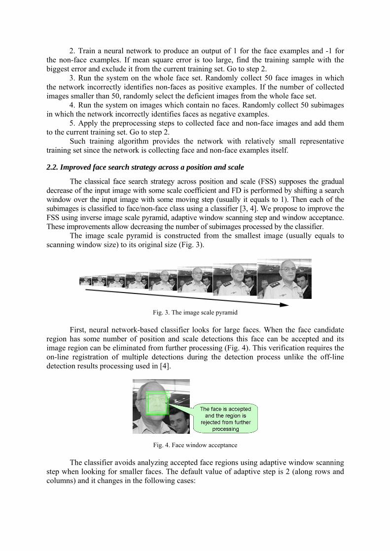
2. Train a neural network to produce an output of 1 for the face examples and -1 for the non-face examples. If mean square error is too large, find the training sample with the biggest error and exclude it from the current training set. Go to step 2.

3. Run the system on the whole face set. Randomly collect 50 face images in which the network incorrectly identifies non-faces as positive examples. If the number of collected images smaller than 50, randomly select the deficient images from the whole face set.

4. Run the system on images which contain no faces. Randomly collect 50 subimages in which the network incorrectly identifies faces as negative examples.

5. Apply the preprocessing steps to collected face and non-face images and add them to the current training set. Go to step 2.

Such training algorithm provides the network with relatively small representative training set since the network is collecting face and non-face examples itself.

2.2. Improved face search strategy across a position and scale

The classical face search strategy across position and scale (FSS) supposes the gradual decrease of the input image with some scale coefficient and FD is performed by shifting a search window over the input image with some moving step (usually it equals to 1). Then each of the subimages is classified to face/non-face class using a classifier [3, 4]. We propose to improve the FSS using inverse image scale pyramid, adaptive window scanning step and window acceptance. These improvements allow decreasing the number of subimages processed by the classifier.

The image scale pyramid is constructed from the smallest image (usually equals to scanning window size) to its original size (Fig. 3).

Fig. 3. The image scale pyramid

First, neural network-based classifier looks for large faces. When the face candidate

region has some number of position and scale detections this face can be accepted and its image region can be eliminated from further processing (Fig. 4). This verification requires the on-line registration of multiple detections during the detection process unlike the off-line detection results processing used in [4].

Fig. 4. Face window acceptance The classifier avoids analyzing accepted face regions using adaptive window scanning

step when looking for smaller faces. The default value of adaptive step is 2 (along rows and columns) and it changes in the following cases:

• face-like region (region with a deficient number of multiple detections) is found: the step decreases to 1;

• face candidate is found: the step essentially increases one-time and then sets to its default value;

• accepted region is found: the step essentially increases one-time. The improved FSS allows accelerating FD process by diminishing of the scanning

subimages number in 4 and more times especially when input images contain large faces.

Conclusions and Future Works This paper presents some face candidate selection algorithms and improved neural

network-based method for video- surveillance systems. Face candidate detection is performed using the skin color and motion. The improved active training algorithm allows neural network working with the relatively small representative training set. The proposed face search strategy accelerates the face detection process in 4 and more times using the inverse image scale pyramid, adaptive window scanning step, window acceptance, and is perfectly suitable for input images with large faces.

Our future research will be focused on further speedup of the face search process by construction of classifier’s cascade, like in [7], where some preliminary face candidate selectors will be applied to the input image before the strong neural network-based classifier.

Acknowledgment The authors are grateful for the support to the Fundamental Researches State Fund of

Ukraine and Fundamental Researches State Fund of the Republic of Belarus, as the above results were obtained as a part of joint research project “Development of methods and algorithms of face detection and recognition for real-time video-supervision systems”.

References

1. Ming Hsuan Yang, Recent Advances in Face Detection, IEEE ICPR 2004 Tutorial, Cambridge, United Kingdom, August 22, 2004.

2. Vezhnevets V., Sazonov V., Andreeva A. A Survey on Pixel-Based Skin Color Detection Techniques, Graphics and Media Laboratory, Faculty of Computational Mathematics and Cybernetics, Moscow State University, Moscow, Russia, 2003.

3. Sung K.K., Poggio T. Example-based learning for view-based human face detection, IEEE Transactions on Pattern Analysis and Machine Intelligence, vol. 20, no. 1, 1998, pp. 39-51.

4. Rowley H., Baluja S., Kanade T. Neural network-based face detection. In IEEE Patt. Anal. Mach. Intell., vol. 20, 1998, pp. 22-38.

5. Manzanera A., Richefeu J.C. A Robust and Computationally Efficient Motion Detection Algorithm Based on Sigma-Delta Background Estimation. In ICVGIP Proceedings, 2004, pp. 46-51.

6. Peer P., Kovac J., Solina F. Human Skin Colour Clustering for Face Detection, EUROCON 2003 - International Conference on Computer as a Tool, Eds. B. Zajc, Ljubljana, Slovenia, September 2003, vol. 2, pp. 144-148.

7. Viola P., Jones M. Robust Real-Time Face Detection, International Journal of Computer Vision 57(2), 2004, pp. 137-154.

EFFECT OF FIELD SAMPLES DISPLACEMENT ON MULTI-FREQUENCY MICROWAVE IMAGING

V. Semenchik, V. Pahomov, S. Kurilo

Belarusian State University, Minsk, Belarus

The phenomenon of measured field samples displacement occurs under specific conditions of microwave imaging field measurements. It results in true field measurement point displacement from its expected position. The effect of the phenomenon on image reconstruction is investigated. Image reconstruction algorithm modification compensating the displacement is presented.

Introduction Microwave imaging is a way of non-destructive object inner structure investigation

and visualizing of optically hidden objects. During microwave imaging experiment the object or media under investigation is subjected to microwave radiation, field scattered by electric or magnetic heterogeneities is measured. Field values obtained are processed by image recon-struction algorithm to obtain object or media properties distribution image.

The first important step in microwave imaging is obtaining scattered field map. Both configuration and accuracy of field measurements play significant role in further image re-construction. Generally it’s desirable to know exact field values on closed surface around area being investigated, but this is impossible in real conditions. Both measurement surface limita-tion and inaccuracy of measurements affect reconstructed image quality.

Most microwave imaging techniques deal with field values measured in certain points. In our experimental imaging system [1] field values are measured on rectangular plane; at that transmitting antenna moves coupled with receiving one. The imaging system is designed to use multiple frequencies of harmonic illuminating wave. This improves image reconstruction quality, particularly increases imaging system radial resolution. The reconstruction algorithm [2] assumes that field values obtained using different illuminating field frequencies are meas-ured in exactly the same point.

Previous version of imaging system hardware based on backward-wave tubes was not capable to rapidly switch illumination wave frequency. This resulted in multiple scans neces-sity in order to carry out multi-frequency experiment. Recently we have improved our expe-rimental imaging system by introducing Agilent HP 8722ET network analyzer [3]. The essen-tial difference between previous imaging system and new one is multi-frequency data mea-surement scheme. The new imaging system measures all multi-frequency data in one frame scan. It increases measurement speed but results in field samples displacement phenomenon.

Field samples displacement occurs because imaging system caret is moving during measurement frequency sweep performed by network analyzer. As a result the caret moves at certain distance from true sample position when the highest frequency sample is measured at the end of sweep. This results in measured field distribution distortion and will obviously cause distortion in images reconstructed.

Our experiments show that highest frequency sample displacement can be as high as 60% of aperture sampling step, which is up to 15% of the wavelength. This displacement causes significant phase error. This will eventually decrease multi-frequency image recon-struction quality, because multi-frequency reconstruction algorithm is very sensitive to phase information.

1. Samples Displacement Effect Analysis Scanning scheme should be taken into consideration in order to evaluate samples dis-

placement effect. The experimental imaging system performs scanning in zigzag path, i.e. odd lines are scanned in forward direction while others are in even. This is shown in Fig. 1.

Fig. 1. Scanning path of the experimental imaging system

The first step in image reconstruction algorithm is Fourier transform of measured field data. That’s why we have chosen to compensate samples displacement in frequency domain. Given ( )nm yxp , is complex field value measured at ( )nm yx , aperture point described by n-th line and m-th column (m=1..N, n=1..N) for certain frequency. First we assume that samples displacement phenomenon is absent. The discrete Fourier transform of field distribution can be represented as

( ) ( ) ( ) ( )

( ) ( )

2 1 1 1

1

, , , ;

, ,

x y xm n m m m n n n m m m n n n n m

n n

xn m m m m n

P F p x y F F p x y F p

p F p x y

′ ′ ′ ′ ′ ′ ′→ → → →′→

′ ′→

⎡ ⎤⎡ ⎤= = =⎡ ⎤ ⎡ ⎤⎣ ⎦ ⎣ ⎦⎣ ⎦ ⎣ ⎦

= ⎡ ⎤⎣ ⎦

ω ω ω

ω (1)

where [ ]2

nnmmF′→′→ stands for two-dimensional discrete Fourier transform and [ ]1

mmF ′→ and

[ ]1nnF ′→ stand for one-dimensional discrete Fourier transform along x and y coordinates re-

spectively, xm′ω and y

n′ω are spatial frequency values. Let’s assume that n-th line samples are displaced by the same n∆ quantity along the

line. The field spectrum calculated will be:

( ) ( ) ( )

( ) ( )

2 2

1 1 1

, , ,

, .

x ym n m m m n m m m n n

n n n n

xn n m m m n n n n n m

P F p x y F p x y

F F p x y F p

ω ω

ω

′ ′ ′ ′∆ → ∆ →′ ′→ →

∆′ ′ ′ ′→ → →

⎡ ⎤ ⎡ ⎤= = + ∆ =⎣ ⎦ ⎣ ⎦

⎡ ⎤⎡ ⎤⎡ ⎤= + ∆ =⎣ ⎦⎣ ⎦ ⎣ ⎦

(2)

This equation can be rewritten taking care of displacement theorem [4]. The theorem is usually formulated for continuous signal, but it’s easy to obtain the following expression for sampled signal spectrum (consider one-dimensional transform):

( ) ( ) ( ) ( )exp expx x xn m n m n n m

kp i i M k p M kω ω ω ω ω

∞∆

′ ′ ′=−∞

⎡ ⎤= ∆ ⋅ − ∆ ⋅ ∆ ⋅ − ∆ ⋅⎣ ⎦∑ , (3)

where ∆ω is frequency domain sampling step. When ignoring aliasing effects (assuming k=0) the displacement theorem is similar to

one for continuous signal. Using it we arrive to

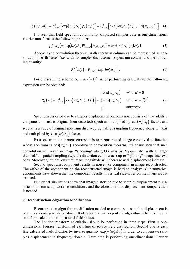
( ) ( ) ( ) ( ) ( )1 1 1, exp exp ,x y x x xm n n n m n n m n n m n m m m nP F i p F i F p x yω ω ω ω ω′ ′ ′ ′ ′ ′ ′ ′∆ → → →

⎡ ⎤ ⎡ ⎤⎡ ⎤= ∆ = ∆ ⎣ ⎦⎣ ⎦ ⎣ ⎦ . (4)

It’s seen that field spectrum columns for displaced samples case is one-dimensional Fourier transform of the following product:

( ) ( ) ( )[ ] ( ) ( )xmnn

xmnmmmn

xm

xmn piyxpFip ′′′→′′

∆ ∆=∆= ωωωω exp,exp 1 . (5)

According to convolution theorem, n′-th spectrum column can be represented as con-volution of n′-th “true” (i.e. with no samples displacement) spectrum column and the follow-ing quantity:

( ) ( )1 expx xn m n n m nP F iω ω∆′ ′ ′ ′→

⎡ ⎤= ∆⎣ ⎦ . (6)

For our scanning scheme ( )0 1 nn∆ = ∆ ⋅ − . After performing calculations the following

expression can be obtained:

( ) ( )( )( )( )

0

10 0

cos 0

exp 1 sin 20

xm

nd x xm n n m m

when n

NP n F i i when n

otherwise

ω

ω ω

′

′ ′ ′ ′→

⎧ ′∆ =⎪⎪⎡ ⎤′ ′= ∆ − = ∆ =⎨⎢ ⎥⎣ ⎦ ⎪⎪⎩

. (7)

Spectrum distorted due to samples displacement phenomenon consists of two additive components – first is original (non-distorted) spectrum multiplied by ( )0cos x

mω ′∆ factor, and

second is a copy of original spectrum displaced by half of sampling frequency along yω axis and multiplied by ( )0sin x

mi ω ′∆ factor. First spectrum component corresponds to reconstructed image convolved to function

whose spectrum is ( )0cos xmω ′∆ according to convolution theorem. It’s easily seen that such

convolution will result in image “smearing” along OX axis by 2s0 quantity. With s0 larger than half of spatial sampling step, the distortion can increase up to “splitting” image into two ones. Moreover, it’s obvious that image magnitude will decrease with displacement increase.

Second spectrum component results in noise-like component in image reconstructed. The effect of the component on the reconstructed image is hard to analyze. Our numerical experiments have shown that the component results in vertical side-lobes on the image recon-structed.

Numerical simulations show that image distortion due to samples displacement is sig-nificant for our setup working conditions, and therefore a kind of displacement compensation is needed.

2. Reconstruction Algorithm Modification Reconstruction algorithm modification needed to compensate samples displacement is

obvious according to stated above. It affects only first step of the algorithm, which is Fourier transform calculation of measured field values.

The Fourier transform calculation should be performed in three steps. First is one-dimensional Fourier transform of each line of source field distribution. Second one is each line calculated multiplication by inverse quantity ( )n

xmi ∆− ′ωexp in order to compensate sam-

ples displacement in frequency domain. Third step is performing one-dimensional Fourier

transform for each column of distribution obtained in second step. The rest of reconstruction algorithm remains the same. Its details are described in [2].

Note that we can calculate inverse Fourier transform immediately after third step of algorithm described above. In this case field map without samples displacement will be ob-tained. This effect can be used to compensate similar phenomenon in other imaging applica-tions, e.g. video frames de-interlacing.

3. Experimental investigations An approach proposed was tested against experimental data. The sample object image

reconstruction has been carried out. Field values obtained during experiment were treated twice. Firstly ordinary reconstruction algorithm was applied, i.e. no samples displacement was taken into account. Then modified algorithm was applied.

Field values were measured in the following conditions. The object investigated was small metallic circle of 5mm in diameter; the distance to the object was 7cm. The aperture size was 32-by-32 points situated at 1-by-1 cm rectangular grid nodes. Eleven equally spaced frequencies in 8.5 GHz to 13.5 GHz range were used for illumination.

It was assumed that time interval between different frequencies measurements during the sweep is equal. Imaging system caret moves uniformly. Thus, field samples displacement for different frequencies linearly depends on frequency index. The displacement is maximal for highest frequency because network analyzer sweeps from lowest frequencies to highest. This is worst case because phase error due to samples displacement is even higher at highest frequency.

Background of the object was measured as part of experiment. Field measurements were performed under the same conditions but without the object itself. These values were subtracted from corresponding values obtained when the object was present. This compen-sated both antennas coupling and background reflections.

The algorithm described in chapter 2 was used to calculate Fourier transform of field data. The transform algorithm as well as rest of image reconstruction algorithm was imple-mented in MATLAB [5] environment.

It could be noticed that similar samples displacement compensation effect could be achieved using interpolation techniques. But interpolation methods typically are much more computationally complex. We tried to use MATLAB interpolation algorithm (‘griddata’ function with ‘v4’ interpolation method) to compensate samples displacement and have ob-tained similar final results as with algorithm proposed, but computational time of the algo-rithm have increased in more than 100 times. Opposed to this, our algorithm practically does not increase image reconstruction computational complexity.

Results of image reconstruction are presented in Fig. 2. Data are represented as one-dimensional slice graphs of reconstructed object function. Slices are put through samples nearest to true object position. Slice along X-axis (horizontal one) is shown in Fig. 2, a and slice along Y-axis (vertical one) is shown on Fig. 2, b. Data for both regular and modified algorithm are plot at the same figures. Thick solid line shows slice of image reconstructed with algorithm proposed, while thin line with squares shows slice of image reconstructed with regular algorithm.

It’s clearly seen that samples displacement phenomenon results in reconstructed image dis-tortion. Note that distortion occurs along vertical axis while field samples are displaced along hori-zontal axis. Roughly this can be explained with the fact that horizontal samples displacement along causes field spectrum distortion along vertical axis as described above. Also the figures show that image distortion disappears almost completely when samples displacement is compensated using algorithm proposed.

-0.15 -0.1 -0.05 0 0.05 0.1 0.15

0.2

0.4

0.6

0.8

1

-0.15 -0.1 -0.05 0 0.05 0.1 0.15

0.2

0.4

0.6

0.8

1

Fig. 2. Dot object image slices: a) horizontal slice (X-axis); b) vertical slice (Y-axis)

Conclusion Replacing high-frequency part of out experimental imaging system by introducing HP

8722ET network analyzer increases much imaging system performance and applicability. Particularly scanning time for multi-frequency case has been reduced significantly.

But specifics of multi-frequency measurements using network analyzer in addition to peculiarities of scanning subsystem results in samples displacement phenomenon. This leads to reconstructed image distortion when ignored. Our experiments show that distortion occurs along axis opposite to one which displacement occurs along.

We’ve modified regular reconstruction algorithm in order to compensate samples dis-placement. The essence of modification is that samples displacement is compensated in fre-quency domain using displacement theorem. The modification almost does not increase re-construction algorithm computational complexity.

The effectiveness of modified algorithm was tested on experimental data. The distor-tion of image reconstructed caused by samples displacement disappears almost completely when applying modified algorithm.

References

1. Semenchik V., Pahomov V., Kurilo S. Microwave Imaging System. Proceedings of VII Computer Data Analysis and Modeling International Conference, Minsk, Belarus, 2004, pp. 266-269.

2. Semenchik V., Pahomov V., Kurilo S. Multi-frequency microwave imaging. Pro-ceedings of Fifth International Kharkov Symposium on Physics and Engineering of Micro-waves, Millimeter and Submillimeter Waves, Kharkov, Ukraine, 2004, pp. 193-195.

3. Agilent Technologies 8719ET/20ET/22ET/8719ES/20ES/22ES Network Analyzers User’s Guide. Agilent Technologies, Inc., 2002.

4. Dyke Phillip P.G. An Introduction to Laplace Transforms and Fourier Series. Springer, 1999.

5. MATLAB release 14 help. MathWorks inc., 2004: http://www.mathworks.com.

REGULARIZATION IN IMAGE RECOGNITION: THE PRINCIPLE OF DECISION RULE SMOOTHING

O. Seredin 1, V. Mottl 2

1 Tula State University, Tula, Russia; 2 Computing Center of the Russian Academy of Science, Moscow, Russia

A technique of training regularization in image recognition is considered. The main idea underlying this investigation consists in overcoming the small sample size problem by adding an subsidiary a priori information on interrelation among the image elements.

Introduction

It is typical for data analysis problems that several features measured at an object are not independent of each other. Image and signal recognition are glowing examples of this kind of data analysis problems.

First, in this kind of problems, the number of features is essentially greater than the number of objects in a training set of typical size. Second, the specificity of feature registration usually implies their linear ( , 1,..., )tx t T= =x , or spatial ( , 1,..., , 1,..., )tsx t T s S= = =x ordering. Third, the hypothesis that the features are “smooth” along the order axes is suitable in many cases, i.e., close values are typical for closely related features ( , )t tx x ±δ or ,( , )ts t sx x ′ ′′±δ ±δ . As for signal analysis, smoothly ordered features are usually the result of measuring the same physical value along an axis with a sufficiently small step. In the case of images, smoothness of features implies minor difference between brightness values at adjacent elements of the pixel grid.

The large number of features leads to the small sample problem well known in data analysis – a decision rule which exactly separates the objects of the training set has poor extrapolation properties. Two ways of solving this problem may be distinguished, namely, reduction of the feature space dimensionality, usually, by feature selection [1], and imposing constraints on the class of decision rules as a means of training regularization [2]. In this paper, we keep to the latter approach. To improve the prediction power of a pattern recognition algorithm, we suggest to take into account the known specificity of the respective kind of objects, namely, the ordering of features and their smoothness.

In many algorithms, the result of training is the vector of coefficients of a discriminant hyperplane immediately in the linear space of features or in a secondary linearized space. The idea of regularization we propose in this paper is utilization of the fact that any coefficient of the discriminant hyperplane is associated with some feature. If the positions of two features in the structure of an object (immediately successive values of a signal or adjacent pixels of an image) are close to each other, the corresponding coefficients of the discriminant hyperplane must also not be too different. Thereby, among the entire set of decision rules correctly fitting the trainer’s data, we choose only the subset that satisfies some a priori constraint.

In paper [3], this regularization principle is applied to the signal recognition problem in terms of the popular support vector algorithm (SVM). In this paper, we evolve this technique as applied to images.

1. The idealized image recognition problem

The problem of face verification is a typical two-class images recognition problem. Some examples of normalized and scaled face images are shown in Fig. 1.

Fig. 1

The gray level values of the elements of the pixel grid serve as the features of an image: ( ; 1,..., , 1,..., ) n

tsx t T s S R= = = ∈x , n TS= . Even if we deal with relatively small images, the dimension of the resulting feature space is so huge that no training set can exceed it in size. For instance, if if 60T = and 40S = , the feature space dimension will be

2400n = . If we apply the principle of linear decision rule, it will be mathematically expressed as a

2400-dimensional direction vector which is, actually, an image:

( ; 1,..., , 1,..., ) ntsa t T s S R= = = ∈a ,

1 1

0 1,0 2.

T STts tst s

classb a x bclass= =

> →⎧+ = + ⎨< →⎩∑ ∑a x (1)

A pictorial representation of the optimal discriminant hyperplane, to be strict, its direction vector, computed by Vapnik’s SVM principle [4] for the above ten images (Fig. 1) is shown in Fig. 2.

Fig. 2

The coefficients of the discriminant hyperplane shown in Fig. 2 are not sufficiently

smooth. At the same time, as we believe, it is just ignoring minor individual details of the training-set images what essentially contributes to good prediction properties of a recognition technique. A face image basically consists of quite large areas of forehead, eyes, cheeks, nose, and too excessive attention to inessential details (birthmarks, wrinkles, face expression) does not improve the prediction.

2. The mathematical principle of smoothness-based training regularization

Let ( , ), 1,...,j jg j N=x , ,( , 1,..., , 1,..., )j ts jx t T s S= = =x , 1, 1jg ∈ − be a training set from a universe containing two classes of images. The most popular SVM criterion of finding the optimal discriminant hyperplane ( ; 1,..., , 1,..., ) n

tsa t T s S R= = = ∈a (1) for two subsets set of objects whose convex hulls do not intersect lead to the well known quadratic programming problem in the feature space [4]:

T

S

2

1 1 1 1

,1 1

min;

( ) 1 , 0, 1,..., .

N T S NT

j ts jj t s j

T ST

j j j ts ts j j jt s

C a C

g b g a x b j N

= = = =

= =

⎧+ δ = + δ →⎪

⎪⎨

⎛ ⎞⎪ + = + ≥ − δ δ ≥ =⎜ ⎟⎪ ⎝ ⎠⎩

∑ ∑∑ ∑

∑∑

a a

a x (2)

It is convenient to solve this problem in the dual form with respect to the nonnegative Lagrange multipliers ( , 1,..., )j j Nλ = at the inequality constraint associated with the objects of training set:

, ,

1 1 1 1 1

1

1 max;2

0, 0 2, 1,..., .

N N N T S

j j k ts j ts k j kj j k t s

Nj j jj

g g x x

g C j N

= = = = =

=

⎧ ⎛ ⎞λ − λ λ →⎪ ⎜ ⎟⎪ ⎝ ⎠⎨

⎪ λ = ≤ λ ≤ =⎪⎩

∑ ∑∑ ∑∑

∑ (3)

The direction vector of the optimal discriminant hyperplane a (discriminant image) is the linear combination of the support training-set feature vectors (support images)

,: 0jts j j ts jja g xλ >

= λ∑ with coefficients j jg λ produced by non-zero Lagrange multipliers

0jλ > . The discriminant image completely specifies the recognition rule applicable to any new image (1).

In this work, our aim is to modify the standard SVM criterion with the purpose to incorporate the available a priori information on the sought discriminant image, namely, the assumption that its mutually adjacent elements must not differ significantly from each other.

To formalize the notion of “close” elements of the pixel grid, we consider the Euclidian distance between pair of pixels in the discrete image plane

2 2, ( ) ( ) 0ts t sd t t s s′ ′ ′ ′= − + − ≥ , and introduce, on its basis, a nonnegative proximity function

, 0ts t sp ′ ′ ≥ . The form of this function is rather arbitrary and is to be tried experimentally. Some examples of proximity functions which define nonzero proximity only for adjacent elements are shown in Fig. 3.

,,

,

1, 2,

0, 2,ts t s

ts t s

ts t s

dp

d

′ ′

′ ′

′ ′

⎧ ≤⎪= ⎨>⎪⎩

,

,,

1, 1,

0, 1,ts t s

ts t sts t s

dp

d′ ′

′ ′′ ′

≤⎧⎪= ⎨ >⎪⎩

Fig. 3

We define the regularized training criterion as including an additional penalty upon the difference between spatially close coefficients of the discriminant image (discriminant hyperplane) in the following form:

2 2,

1 1 1 1 1 1 1

2,

1 1 1 1 1 1 1

( )

min.

T S T S T S N

ts ts t s ts t s jt s t s t s j

T S T S T S N

ts ts t s ts t s jt s t s t s j

a p a a C

a b a a C

′ ′ ′ ′′ ′= = = = = = =

′ ′ ′ ′′ ′= = = = = = =

+ γ − + δ =

= + γ + δ →

∑∑ ∑∑∑∑ ∑

∑∑ ∑∑∑∑ ∑ (4)

Here ( ),ts t sb ′ ′=B is the matrix ( )TS TS× responsible for the smoothness of the discriminant

image

11 1 11

11

2

TS

j TSj

TS

TS TS TS TS jj

p p p

p p p

=

=

⎛ ⎞− + −⎜ ⎟⎜ ⎟⎜ ⎟=⎜ ⎟⎜ ⎟− − +⎜ ⎟⎝ ⎠

∑

∑

B

L

M O M

L

,

and the parameter 0γ≥ sets the regularization degree. The dual optimization problem corresponding to (4) will have the form

, , ,1

1 1 1 1 1 1

1

1 max;2

0, 0 2, 1,..., ,

N N T S T SN

j j k ts t s ts j ts k j kjj k t s t s

Nj j jj

g g f x x

g C j N

′ ′=′ ′= = = = = =

=

⎧ ⎛ ⎞λ − λ λ →⎪ ⎜ ⎟⎪ ⎝ ⎠⎨

⎪ λ = ≤ λ ≤ =⎪⎩

∑ ∑∑ ∑∑∑∑

∑ (5)

where ( )1,( ) ts t sf−′ ′= + γ =F I B is the dual regularization matrix ( )TS TS× .

3. Experimental study

For the experimental study, we used a data set from the well known collection BioID Face DB (http://www.humanscan.de). For the two-class recognition problem considered in this paper, we chose images of two person. Some examples of these images are shown in Fig. 1. The data base contains 236 face images of the selected two persons. We conducted 100 experiments, in each of which 10 images were randomly chosen as the training set, 5 images of the first and the second person. The remaining 226 images we used for testing. The averaged result is presented in Table.

Table Usual SVM training – smoothness coefficient 0γ =

An example of the optimal discriminant hyperplane: Average error rate in the test sets: 8,7%

Regularized SVM training – smoothness coefficient 10γ =

An example of the optimal discriminant hyperplane: Average error rate in the test sets: 5,7%

Of special interest is the choice of the regularization parameter 0γ ≥ . It is seen from (2) that the regularized training criterion turns into the standard one if 0γ = . We studied the dependence of the error rate in test set and the leave-one-out error in the training set from the values of γ . The results are shown in Fig. 4. It is seen that positive penalty values lead to improving the extrapolation properties.

0

2

4

6

8

10

12

14

16

0 0,01 0,05 0,1 0,5 1 5 10 50 100 500Regularization parameter

%

Error in the test set Leave-one-out error tn the training set

Fig. 4

Conclusion

A new method of overcoming the small-sample problem in image recognition is proposed. The idea of the method is incorporating a penalty on the non-smoothness of decision rule coefficients into the standard SVM training criterion. Experiments with face images has shown that the proposed modification essentially improves the prediction power of the SVM recognition rule.

This work is supported by the Russian Foundation for Basic Research, Grants 05-01-00679, 06-01-08042, 06-01-00412, 06-07-89249, and INTAS Grant 04-77-7347.

References

1. Guyon I., Elisseeff A., An Introduction to Variable and Feature Selection, Journal of Machine Learning Research 3, 2003, pp. 1157-1182.

2. Juwei Lu, Plataniotis K.N., Venetsanopoulos A.N. Regularization Studies of Linear Discriminant Analysis in Small Sample Size Scenarios with Application to Face Recognition, Pattern Recognition Letter, vol. 26, issue 2, 2005, pp. 181-191.

3. Seredin O.S., Dvoenko S.D., Krasotkina O.V., Mottl V.V. Machine Learning for Signal Recognition by the Criterion of Decision Rule Smoothness. Pattern Recognition and Image Analysis, vol. 11, no 1, 2001, pp. 87–90.

4. Vapnik V. Statistical Learning Theory, New York: Wiley, 1998.

PIN-BOX PHANTHOM RAPID ULTRASOUND CALIBRATION

R. Sergeev 1, 2, A. Kryvanos 3, A. Belevich 4 1Faculty of Applied Mathematics and Computer Science,

Belarus State University, Minsk, Belarus; 2 United Institute of Informatics Problems, National Academy of Sciences of Belarus,

Minsk, Belarus; 3 Institute for Computational Medicine, Universities of Mannheim and Heidelberg,

Mannheim, Germany; 4 Institute of Trauma and Orthopaedics, Minsk, Belarus

A combination of the standard B-Mode transducer with a spatial localizer realizes a 3D ultrasound (US) system and provides new opportunities in diagnostics and treatment. This paper describes a calibration method for freehand US systems Calibration techniques usually include manual or semi-automatic steps that imply experienced user assistance. The proposed method is designed to make it easier for inexperienced users to perform calibration in automatic mode and to know that they have got a reliable result.

Introduction Ultrasound imaging techniques has become very popular in various clinical

applications. In order to provide the physicians with a 3D real-time visualization of the internal anatomy, individual 2D US images must be assembled into 3D volumes and then the position of surgical tools are related with respect to the reconstructed US volume. Using US as a guidance modality for surgical procedures would require tracking the imaging probe with a spatial localizer (tracking device). A fixed transformation between the US beam and the tracking device needs to be determined, so that arbitrary image pixels can be referenced in a global frame. Obtaining this fixed transformation is referred to as ultrasound calibration.

According to the currently known calibration methods, an object of known geometrical properties (phantom) is scanned by the US probe and then the unknown transformation that maximizes the similarity between the US images and the actual phantom is computed. 1. Mathematical Formulation

To perform calibration and reconstruction, four coordinate systems are involved. In these notations P is a coordinate system of the cropped B-scan plane with coordinate

origin at the top left hand corner of the image. The y-axis is in the beam direction, x-axis in the lateral direction, and z-axis is in the elevation direction, out of the plane of the B-scan. R is the coordinate system of the position sensor receiver, T is the coordinate system of transmitter, and C is the coordinate system of reconstruction volume (phantom coordinates).

During reconstruction, each pixel in the B-scan has to be located with respect to the reconstruction volume C by means of the transformation between different coordinate systems. First, each pixel scan plane location is transformed to the coordinate system of the receiver R, then to the transmitter T and finally to the reconstruction volume C.

A notation BAT is used for the transformation matrix from coordinate system A to B . The final transformation can be expressed as the multiplication of homogeneous transformation matrices:

PRPTRCTC XTTTX ⋅⋅⋅= , (1)

where Xc=(x,y,z,1)T, Xp=(sxu,syv,0,1)T, xs and ys are scale factors with units of mm/pixel, u and v are column and row indices of the pixel in the cropped image.

A transformation between two coordinate systems has six degrees of freedom: three rotations and three translations. Each of the transformation matrices plays a different role in reconstruction. TRT is derived directly from the position sensor readings. CTT is included largely as a matter of convenience. RPT must be determined by calibration. The scale factors

xs and ys could be derived from the axis markings on the B-scan. Once CX has been found for every pixel, the voxels of C can be set according to the intensities of the pixels they intersect.

1.1. Phantom design

Geometrical models of phantoms proposed in the literature are different. The cross-wire and three-wire [1, 2] phantoms require long time of acquisition and are hard to automate, while the single wall as in Cambridge phantom which is automatic repeatable method or Hopkins phantom are expansive and time-consuming in creation [3].

In our approach a wired pin-box phantom is used. In general this allows to conduct all calibration procedure from one B-scan and to develop entirely automatic and quick calibration algorithm.

2. Materials and Methods 2.1. Phantom

We propose to use a kind of wired phantom called pin-box. The pin-box phantom consists of a 100x100x95 mm box with 30 copper wires of 0.3 mm diameter, which is showed in Fig. 1. The wires are stretched along the box and fastened in the front and back faces of the cube regularly located in 5x6 way. Then the whole construction is filled with warm water at room temperature. To obtain a scan image for calibration we put the probe in a certain location. For this purpose the box contains two parallel wires fastened in the side faces of the box and used as markers to specify the scan plane.

2.2. Image acquisition

Images are acquired using a 5-8 MHz transducer with a linear array of 128 piezo elements. Four light reflective markers of a special geometry are mounted on the US probe (Fig. 2). B-Mode scans are synchronized with an optical tracking device (Polaris, NDI) and stored on a hard disk in BMP format. The transformation matrix taken from the spatial localizer is stored in ASCII file under similar name as the corresponding US scan.

Fig. 1. The pin-box phantom Fig. 2. The US Transducer with four markers

During the scanning process operator moves the probe in order to match the scan beam with two marker wires fastened in the side faces and thus the scan plane as well. Image is captured in this position.

2.3. Feature extraction

After the image acquisition step, the scan is processed and the phantom features are extracted. The whole procedure of image processing is conducted in the automatic.

In order to find the centers of the wires in the scan we use principal-components analysis. At the preliminary step the input image is filtered from noise using thresholding. The value of the threshold is calculated from the image histogram. Then area opening with a large threshold value is applied to distinguish the images of two guiding wires that should be located horizontally in the US scan. Thus we get a set of connected components that correspond to these wires. The centers of masses ( )

ii cc vu , are calculated for each element of the set and used to obtain the covariance matrix. This matrix is calculated from the whole set of connected components derived in this step:

( )( )∑ ∑= ∈

−−−

=N

1i Ix

Tcjcj1

icj

iixxxx

1M1Σ , (2)

where ( )iii ccc vux ,= - center of masses of i -th connected component, ( )jjj vux ,= - pixel

coordinates, icI - set of pixels in the i -th connected component, N - connected components

number in the image, M - pixel number in all connected components. Next we apply area opening with a small threshold value to clear the image from noise

and keep blobs (connected components) that are supposed to be the phantom wires. Note that we do not consider connected components that were included into the first set in the previous step. As we got a new set of blobs the centers of masses ( )

ii cc vu , of the components are calculated and the covariance matrix 2Σ is obtained according to formula (2) for the blob set.

Covariance matrices 1Σ , 2Σ are used to find axes of inertia of the corresponding set of connected components. Let 2i1i λλ ≥ be eigenvalues of matrix iΣ , and 2

2i1i R∈ψψ , are the corresponding eigenvectors. According to the principal-components analysis the axes of inertia are formed by covariance matrix eigenvectors.

Consider the second blob set, its covariance matrix 2Σ and the corresponding eigenvectors. To recognize the supposed wire's centers in the scan the coordinate origin for each blob is considered at the center of masses ( )

ii cc vu , . In that case it is assumed that the wire's center lies at the intersection point of the inertia axis corresponding to the maximal eigenvalue and the upper border of the blob.

Before the next step US scan should be rotated to make the images of guiding wires located horizontally in the scan and thus to make wire's centers placed along vertical and horizontal lines according to the structure of the phantom. For this purpose covariance matrix

1Σ is used and matrix ⎟⎟⎠

⎞⎜⎜⎝

⎛=

T12

T11R

ψ

ψ is applied to the whole scan as a rotation matrix (Fig. 3).

Then true and false wire observations have to be separated. A method used is based on the fact that for each true observation ix at least several points jx exist such that constraint

jixxx ji ≠≤−= ,α∆ is satisfied. A probabilistic approach is developed to find this threshold value α .

Thereafter remained true observations are grouped into classes corresponding to a certain line along which true wire centers should be concentrated. Starting from the top of the scan we put any two observations ix and jx into different classes if γ∆ >−= ji xxx ,

( )dγγ = , where d is a distance between neighboring columns of wires in the real phantom and γ is a control parameter. These steps are both conducted for x and y coordinates of the objects in the image.

a) b) c)

Fig. 3. US scan processing procedure: a) initial US scan; b) filtered US scan using threshholding;

c) US scan after rotation matrix R has been applied Recall that according to a phantom structure the wire centers in each raw and column

should lie on appropriate horizontal or vertical line. Based on observations in each class we use a linear regression model to find the lines along which the assumed wires are located:

εθ += XY , (3)

where an unknown parameter vector θ defines a specific line, X is a matrix of x coordinates of observations, Y is a vector of y coordinates and ε is a measurement error. To estimate vector θ the least-squares minimization technique is applied:

( ) 1T TX X X Y−

θ =)

. (4)

Intersections of the regression lines are used then to clear the sample from false observations: for each intersection only the closest observation is remained. Afterwards linear regression is computed again. This approach is especially useful if some wires have not been recognized at the previous steps. In this case missed wire's centers will be placed at the intersections of the regression lines (Fig. 4).

a) b)

Fig. 4. A processed US scan: a) initial US scan; b) processed scan, recognized wire's centers

are marked with white

2.4. Optimization routine

Recall that the calibration transformation has translation, rotation and scaling components. We force the two scaling factors to be equal and compute them separately from the translation and rotation.

Since there is no exact solution of the calibration problem, the minimum residual error is used to solve the overdetermined system of equations. There are two approaches, the iterative and the closed-form methods. In both approaches, CTT and TRT are given by the tracking device and RPT is an unknown calibration matrix. The following method is used in the report:

C1

CT1

TRPRPC1

CT1

TR XTTYXTXTT −−−− =→= ; 2* minarg PRPTRP XTYT

RP

−= . (5)

3. Results

In our experiments the calibration matrix has been calculated from several different

US scans of the pin-box phantom. To verify the matrix two point objects were used. We compared their known spatial coordinates with the reconstructed from a set of validating scans. Standard deviation and RMS calibration error were used as a measure of accuracy. Results are shown in Table.

Table Validation of calibration matrix

real

coordinates, mm

estimated coordinates,

mm

standard deviation in n

experiments, mm

root mean squared error in n

experiments, mm

real distance,

mm

estimated distance,

mm

distance std, mm

object 1

[78.7182, 33.5768, 0.0109]

[78.9076, 33.9645, 0.3852]

[0.3071, 0.7778, 0.6253] ( n = 12)

1.1225 ( n =12) 56.4

± 0.1 56.4989 0.4183 object

2

[22.3137, 33.8744, 0.0112]

[22.4121, 33.4133, 0.6744]

[0.1963, 0.3450, 0.0887] ( n =5)

0.9807 ( n =5)

Discussion and Conclusion

Experiments have shown that accuracy of calibration strongly depends on the

precision of measurements of real phantom parameters. Minor errors in measurements could lead to different results and different calibration accuracy even if the same approach and the same phantom were used. Therefore the more precise initial data results in more accurate calibration matrix and reconstruction. The advantages of the proposed method are relative simplicity of implementation, quickness and possibility to conduct the whole procedure just from one B-scan.

References

1. Prager W., Rohling R.N., Gee A.H., Berman L. Rapid Calibration for 3-D Freehand Ultrasound, Ultrasound in Med. & Biol., vol. 24, no 6, 1998, pp. 855-869.

2. Mercier L., Lang T., Linkseth F., Collins D.L. A Review of Calibration Techniques for Freehand 3-D Ultrasound Systems, Ultrasound in Med. & Biol., vol. 31, no 4, 2005, pp. 449-471.

3. Hsu P-W., Prager R.W., Gee A.H., Treece G.M. Rapid, Easy and Reliable Calibration for Freehand 3D Ultrasound, CUED/F-INFENG/TR 534, 2005.

OBSERVATION PURPOSEFUL PROJECTION TO THE CLASS NUMBER DIMENTION SPACE WITH INTERCLASS DISTANCES INVARIANCE

E. Serikova

Belarusian State University, Minsk, Belarus

The problem of reducing the dimensionality in multivariate statistical classification is considered. New transformation of the initial feature space to the space with dimension equals to class number is obtained by purposeful projection method. Proposed transformation does not change the Mahalanobis interclass distances.

Introduction: mathematical model Let random observation N

N Rxxx ∈′= ),...,( 1 from 2≥L classes ,..., 1 LΩΩ be registered in the feature space NR . Introduce the notation: ,...,10 LSd =∈ is an unknown random index of the class, to which the observation x belongs:

0 0 >== iidP π , Si∈ ( 1...1 =++ Lππ ), (1)

where Sii ∈π are prior class probabilities [1,2]. Under fixed id =0 ( Si∈ ) the observation NRx∈ is described by the conditional probability density function:

0)( ≥xpi , NRx∈ : ∫ =NR i dxxp 1)( , Si∈ .

Classes Sii ∈Ω are completely determined by introduced characteristics ( ) Siii p ∈⋅,π . The statistical classification problem [1, 2] consists in construction of decision rule

(DR) Sxdd ∈= )( for classifying a random observation NRx∈ . This DR is the estimation of true class number Sd o ∈ the observation x belongs.

However, often in practice the initial feature space is redundant. It means that its dimension N is too large [1, 2] and new sample ,..., 1 nyyY = must be constructed from

sample X : *

* ),...,()( 1N

NRyyxfy ∈′== , NN ≤* , so as classification Sydd ∈= )( remains

acceptable. In the theory of statistical classification the set of linear transformations of the initial

feature space NR is offered:

*

: NN RRAxy →= , NN ≤* , (2)

where A is the )( * NN × -matrix of transformation obtained from extremum conditions for various classes separability criteria. These criteria are usually formulated using dispersion matrixes inside and between classes [1, 2]. However, the main disadvantage of known criteria is absence of direct connection with the risk value (probability of error classification

)(P))(( odxddrr ≠=⋅= ), the main efficiency criterion in statistical classification. Using the method of purposeful projection [1], we shall offer new "compressing"

transformation of kind (2) which set as the purpose to transform initial feature space NR to the space

*NR with dimension equals to class number L ( LN =* ), and directly connected with probability of error classification through interclass distances. Because of such

transformation make sense, when dimension of initial feature space is not less, than class number L , everywhere further we assume, that LN ≥ .

In this paper the well-known Fisher model [1, 2] of multivariate normal (Gaussian)

distribution mixture is investigated:

),|()( Σ= iNi xnxp µ , NRx∈ , Si∈ , (3)

where ),|( ΣiN xn µ is N -variate Gaussian probability density function with mathematical mean vector |E idx o

i ==µ (so called “centre” [1, 2] of the class iΩ ) and covariance ( NN × )-matrix |))((E idxx o

ii =′−−=Σ µµ ( ( ) 0det ≠Σ ), common for all classes.

1. Purposeful projection of observation to the class number dimension feature space

We shall carry out transition from the initial feature space NR to the space with dimension equals to class number L . Let ),...,( 1 ′= Lyyy be the "compressed" observation obtained from ),...,( 1 ′= Nxxx using (2):

LN RRAxy →= : , (4) where )( NL × -matrix of transformation )( 1 ′= LaaA MKM consists from vectors Si

Ni Ra ∈∈ ,

each of which is the decision of a corresponding extreme problem ( Si∈ ):

);,;(maxarg µµ iRa

i aJaN∈

= (5)

)),(()())((),;( 1 µµµµµµ −′Σ′′−′= −iii aaaaaJ ∑

∈

=Si

iiµπµ .

In (5) N -vectorµ is so-called "general center" of classes in initial feature space: E x=µ and ),;( µµ iaJ is the Mahalanobis distances square [1, 2] from "center" of i -th

class to "general center" of classes after linear transformation xa′ of observation NRx∈ . It is considered, that under fixed id o = , under the conditions of Fisher model (1), (3) initial observation x has normal distribution with mathematical mean vector iµ and covariance matrix Σ , and linear transformation keeps normal distribution [3], changing only its parameters on ia µ′ and aa Σ′ accordingly.

The sense of transformations (4), (5) consists in the following. The "compressed" observation

),...,(),...,( 11 ′′′=′= xaxayyy LL

consists of features xay ii ′= , Si∈ , each of which is a maximum of Mahalanobis distance in the transformed feature space from "center" of a corresponding class to "general center" of classes on the class of linear transformations xa′ , NRa∈ .

Theorem 1. Under the conditions of Fisher model (1), (3) the solution of i -th ( Si∈ ) extreme problem (5) is the vector:

.)()(/)( 11 µµµµµµ −Σ′−−Σ= −−iiiia (6)

Corollary 1. Under the conditions of Fisher model (1), (3) transformation (4), (6) of

initial feature space to the space with dimension equals to class number does not change Mahalanobis distances from " general center " to "centers" of classes.

2. Investigation of Mahalanobis interclass distances in the transformed feature space and risk value

According to the theorem 1 matrix A of transformation (4) can be presented in the

following form:

2/111 ),...,diag( −− Σ∆∆= CA L , (7)

where ),;1()()( 1 µµµµµµ iiii J=−Σ′−=∆ − , Si∈ is the Mahalanobis distance from

i-th "center" of classes to "general center" in the initial feature space NR , ( NL× )-matrix )( 1 ′= LccC MKM consists of lines

Nii Rc ∈′Σ′−= − )()( 2/1µµ , Si∈ . (8)

Under the conditions of Fisher model (1), (3) observation LRy∈ received according to linear transformation (4), (7) has the following conditional mathematical mean vector ("center" of classes in the transformed feature space) and covariance matrix:

iLioL

i CAidy µµµ 2/111 ),...,diag(|E −− Σ∆∆==== , Si∈ ; (9)

11

11 ),...,diag(),...,diag(|))((E −− ∆∆′∆∆=′Σ==′−−=Σ LL

oLi

Li

L CCAAidyy µµ .

As before observation LRy∈ is described by Fisher model with another parameters

SiLi ∈µ and LΣ .

For the Mahalanobis distance between classes iΩ and jΩ in initial space NR the following representation is true:

)()()()( 1jijijijixijN cccc −′−=−Σ′−=∆ − µµµµ , Sji ∈≠ . (10)

Taking into account (8), (9) we can calculate the Mahalanobis distance between classes iΩ and jΩ in the transformed space with dimension equals to class number L ( Sji ∈≠ ):

)()()()()()( 11jiji

Lj

Li

LLj

LiyijL ccCCCCcc −′′′−=−Σ′−=∆ −− µµµµ . (11)

For existence of inverse ( LL× )-matrix CC ′ it is necessary that the rank ( NL × )-matrix C ( LN ≥ ) was equal to L : LCCC ==′ rankrank .

Let us apply known inequality to the rank of matrixes product to matrix )( 2/1 ′= −ΣMC , )( 1 ′−−= µµµµ LM MKM :

)(rank,rankminrank)(rankrank 2/12/1 ′≤≤−′+ −− ΣΣ MCNM .

It is followed from result above that MMC ′== rankrankrank , because of N=′−Σ )(rank 2/1 , LM ≤rank .

Finally, for existence of inverse ( LL× )-matrix CC ′ it is enough that

LL =−− )(rank 1 µµµµ MKM . (12)

Theorem 2. If the condition (12) is satisfied, the Mahalanobis distance (11) in the transformed according to (4), (6) feature space LR ( NL ≤ ) coincides with the corresponding distance (10) in the initial feature space:

xijNyijL ∆=∆ , Sji ∈≠ .

Let )(P,oN

oNox dxdr ≠= be the well-known Bayesian decision rule (BDR) [1, 2] in

the initial feature space: ),,|(maxarg)( Σ=

∈iNi

Si

No xnxd µπ NRx∈ ,

and )(P,oL

oL

oy dydr ≠= be BDR in the transformed according to (4), (6) feature space:

),,|(maxarg)( LLiLi

Si

Lo ynyd Σ=

∈µπ LRy∈ .

The risk value of BDR in the transformed feature space can increase only: 0,, ≥−=∆ N

oxL

oyL

o rrr , and the increment of risk Lor∆ is describing efficiency of such

transformation. The small Lor∆ means effective transformation.

According to result from [4] for risks Noxr , , L

oyr , the following estimations are true:

∑∑≠∈∈

⎟⎟⎠

⎞⎜⎜⎝

⎛

∆−

∆−Φ≤

ijSj xijN

jixijN

Sii

Noxr

)/ln(2,

πππ , ∑∑

≠∈∈

⎟⎟⎠

⎞⎜⎜⎝

⎛

∆−

∆−Φ≤

ijSj yijL

jiyijL

Sii

Loyr

)/ln(2,

πππ , (13)

and in the case of two classes ( 2=L ) in (13) exact equality is true, where )(⋅Φ - is the

standard Gaussian distribution function: ( )∫ ∞−−=Φ

zdz ωω

π2/exp

21)( 2 , Rz∈ .

Theorem 3. Under the conditions of Fisher model (1), (3), if the condition (12) is satisfied the transformation (4), (6) of initial feature space with dimension N to the space with dimension equals to number of classes NL ≤ , in the case of two classes ( 2=L ) does not increase probability of error classification:

⎟⎟⎠

⎞⎜⎜⎝

⎛∆

+∆

−Φ+⎟⎟⎠

⎞⎜⎜⎝

⎛∆

−∆

−Φ==12

21122

12

21121,,

)/ln(2

)/ln(2 xN

xN

xN

xNNox

Loy rr

πππ

πππ .

In the case of class number 2>L for risk Loyr , the following estimation is true:

∑∑≠∈∈

⎟⎟⎠

⎞⎜⎜⎝

⎛

∆−

∆−Φ≤

ijSj xijN

jixijN

Sii

Loyr

)/ln(2,

πππ .

3. General view of transformation to the class number dimension space with interclass distances invariance and its connection with linear discriminant functions

We shall notice, that calculation of interclass distances (10), (11) in the initial and

transformed feature spaces and the proof of the theorem 2 do not depend on a kind of matrix ,...,diag 1 L∆∆ and vector of classes "general center" ∑∈

=Si iiµπµ . This fact allows to

present general view of transformation to the space with dimension equals to class number which does not change interclass distances.

Theorem 4. Under the conditions of Fisher model (1), (3) linear transformation LN

Sii RRyxyy →== ∈ :)()( :

,)( 1ioiii qxsy +Σ′−= −µµ Si∈ ,

does not change the Mahalanobis interclass distances, if

LoLo =−− )(rank 1 µµµµ MKM ,

where No R∈µ , Siii sRs ∈≠∈ 0, , Sii Rq ∈∈ are certain values.

BDR for Fisher model (1), (3) in the initial feature space can be presented in the form [1, 2]:

)(maxarg),|(maxarg)( xxnxd iSi

iNiSi

No δµπ

∈∈=Σ= , NRx∈ ,

where functions

iiiii xx πµµµδ ln21)( 11 +Σ′−Σ′= −− , Si∈ ,

are linear discriminant functions [1, 2]. Corollary 2. Under the conditions of Fisher model (1), (3) transformation

LLL Rxxyyy ∈′=′= ))(),...,((),...,( 11 δδ , NRx∈ ,

does not change the Mahalanobis interclass distances, if

LL =)(rank 1 µµ MKM .

Conclusion

New transformation of the initial feature space to the space with dimension equals to class number is obtained by purposeful projection method. Proposed transformation does not change the Mahalanobis interclass distances.

Experimental validation was performed on actual data of oncological disease. The dimension of initial feature space was equal to twelve ( )12N .= It was necessary to define missing of disease or presence of one of three cancer stages (number of classes 4=L ) for

new incoming observations by carry out discriminant analysis of training sample ,..., 1 nxxX = with size 140=n .

Risk estimation from (13) in the transformed according to (4), (6) feature space with dimension 4* == LN was equal to 0.0152 and was coincides with estimation of risk in the initial feature space.

The practical application of proposed method allows to appreciably reduce the dimension of initial feature space, while retaining high classification quality.

References

1. Aivazyan S.A., Buchstaber V.M., Yenyukov I.S., Meshalkin L.D. Applied statistics: Classification and Dimensionality Reduction. Moskow, Finansy i Statistika, 1989.

2. Fukunaga K. Introduction to statistical pattern recognition. New York, Academic Press, 1990.

3. Anderson Y.W. An Introduction to Multivariate Statistical Analysis. New York, Viley, 1963.

4. Serikova E., Zhuk E. New effective algorithm for stepwise principle components selection in discriminant analysis. From Data and Information Analysis to Knowledge Engineering / Ed. Spiliopoulou M., Kruse R., Borgelt C., Nurnberger A., Gaul W. Berlin Heidelberg: Springer Verlag, 2006, pp. 142-149.

FINGERPRINT MATCHING BASED ON SINGULAR POINT EXTRACTION

A. Shafranskaya United Institute of Informatics Problems, National Academy of Science of Belarus; Faculty of Applied Mathematics and Computer Science, Belarus State University,

Minsk, Belarus

The paper considers fingerprint segmentation and matching algorithm. The proposed matching algorithm based on the extraction of the core point uses a bank of Gabor filters to capture both local and global features of the fingerprint in a compact fixed length characteristic vector. Calculation of Euclidian distance between two corresponding characteristic vectors constitutes matching process.

Introduction

It is desirable to obtain representations for fingerprints, which are scale, translation, and rotation invariant. Scale invariance is not a significant problem since most fingerprint images could be scaled as per the dpi specification of sensors. Rotation and translation invariance could be accomplished by establishing a reference frame based on the intrinsic fingerprint characteristics, which are rotation and translation invariant [1, 2].

We use the core point as a reference point of the fingerprint. The five main steps in our algorithm are the following:

1. Fingerprint segmentation. We extract the informative part from the original fingerprint image.

2. Reference point extraction and region of interest tessellation. 3. Filtering the region of interest in 8 different directions using a bank of Gabor

filters. 4. Feature vector calculation based on estimation of average absolute deviation of

pixel intensity from the mean in each sector of the ROI. 5. Calculation of Euclidian distance between two corresponding feature vectors.

Fingerprint segmentation

Up to a half of the original fingerprint image contains useless information, i.e. background of the image. In order to speed-up matching process and to improve its quality we apply a fingerprint segmentation stage (Fig. 1).

Fingerprint itself can be considered as a sequence of black and white lines (ridges and valleys), having a high deviation of pixel intensity. Image background is formed by gray pixels that have practically identical intensity values. Therefore using grayscale information of the part of the image one can determine whether this part belongs to foreground or background.

Segmentation stage has the following steps: 1. Divide input image into non-overlapping blocks of size w*w. 2. For each block (i,j) compute deviation of intensity level from the mean value

dev_bl(i,j). If dev_bl(i,j)<inten_threshold then block (i,j) is assigned to background and filled in with zero value, otherwise it is assigned to foreground and remains unchanged.

original image resulting image

Fig. 1. Example of fingerprint segmentation The size of the block w is determined according to the average inter-ridge distance;

each block should contain 3-5 ridges. If w is too small some parts of fingerprint are removed, whereas if w is too large not all background is removed.

Reference point extraction

Core point is a point of the highest curvature in the concave ridge flow, to find it we need to estimate a vector field of the image as follows:

1. Divide image into non-overlapping blocks of size w*w. 2. Compute partial derivatives ( )jix ,∂ and ( )jiy ,∂ at each pixel. 3. Estimate vector value in each block centered at pixel (i,j) using the following

equations: / 2/ 2

/ 2 / 2

( , ) ,( , ) ( , )2j wi w

x x yk i w l j w

i j k l k lν++

= − = −

= ∑ ∑ ∂ ∂

/ 2/ 2 2 2

/ 2 / 2

( , ) ,( ( , ) ( , ))j wi w

y yxk i w l j w

i j k l k lν++

= − = −

= ∂∑ ∑ −∂

( )( )

,( , ) 1/ 2 .,

y

x

i jO i j arctg i j

νν

⎛ ⎞= ⎜ ⎟

⎝ ⎠

Then the core point can be found as follows: 1. Estimate the vector field O as described above using a window size w*w. 2. Smooth it in a local neighborhood and obtain O’. 3. Evaluate the sine component of O’:

( )( )jiOji ,sin),( ′=ε .

4. For each pixel (i,j) in ε estimate value: ( ) ( ) ( ), , ,

I II

A i j i j i jR Rε ε= +∑ ∑ .

The geometry of regions IR and IIR is designed to capture the maximum curvature in concave ridges (Fig. 2, here pixels are shown as colored squares).

Fig. 2. Regions for integrating ε pixel intensities for A(i,j)

5. Find the maximum value in A and assign its coordinate to the reference point. For more accuracy we apply this procedure several times using windows of different

size. In our experiments, we used three iterations with w=12, 6, 4 pixels respectively (Fig. 3).

Fig. 3. Example of core point extraction

The region of interest (Fig. 4) is defined as a collection of all sectors Si, where each sector is computed as follows:

( ) 1, ( 1) ( 2), , 1 , 1 ,i i i iix y b T r b T x N y MS θ θ θ += + ≤ < + ≤ < ≤ ≤ ≤ ≤

where,

[ ]

( ) ( )( ) ( )( )

,( mod ) 2 / ),

2 2,

,

i

i

p p

p p

T i ki k k

r x x y y

arctg y y x x

θ π

θ

== ∗

= − + −

= − −

b is the width of each band, k is the number of sectors in each band, and 0,1, , ( 1)i B k= −K , where B is the number of concentric bands around the reference point ( , )p px y .

Fig. 4. ROI tessellated into sectors

Filtering

To remove the effect of sensor noise and gray level deformation due to finger pressure differences we apply normalization of the region of interest before filtering with an even symmetric Gabor filter:

( ) ( )2 2

2 2, ; , exp 1/ 2 cos 2 ,

sin cos ,cos sin ,

x y

x yG x y f fx

x x yy x y

θ πδ δ

θ θθ θ

⎧ ⎫⎡ ⎤′ ′⎪ ⎪ ′= − +⎢ ⎥⎨ ⎬⎢ ⎥⎪ ⎪⎣ ⎦⎩ ⎭

′ = +′ = −

here f is the frequency of the sinusoidal plane wave along the direction θ from the x-axis, and δx and δy are the space constants of the Gaussian envelope along x and y axes, respectively.

We have used eight different values for θ (0, 22.5, 45, 67.5, 90, 112.5, 135, 157.5) with respect to the x-axis. The normalized region of interest in a fingerprint image is convolved with each of these eight filters to produce a set of eight filtered images (Fig. 5). To speed up the filtering process, we convolve pixels only with those values in the filter mask whose absolute value is greater than 0.05.

Fig. 5. Filtered sequence

Feature vector

In each sector of each filtered image we define the feature value as the average absolute deviation from the mean:

( )1 , ,i

i i ini

V F x y Pnθ θ θ

⎛ ⎞= −⎜ ⎟

⎝ ⎠∑

where Fiθ(x,y) is the θ-direction filtered image for sector Si, ni is the number of pixels in Si and Piθ is the mean value of pixel intensity in Fiθ(x,y) for Si.

The sequence of feature values calculated in each sector in eight different directions θ∈0, 22.5, 45, 67.5, 90, 112.5, 135, 157.5 defines a feature vector.

Matching

Fingerprint matching is based on finding the Euclidean distance between the corresponding feature vectors [3, 4]. The translation invariance in feature vector is established by the reference point extraction. The approximate rotation invariance is achieved by cyclic rotation of the feature vector.

Conclusion and Experimental Results

Fingerprints of 100 different people are stored in our database, eight different images for each finger of the person. To evaluate a biometric identification system, there are a couple of criteria. The FAR (False Accepted Rate) is a statistical measure of the number of impostors to be accepted by a biometric system. The FRR (False Rejected Rate) is a statistical measure of the likelihood of genuine users being rejected by a system. A picture presented in Fig. 6 depicts FAR and FRR dependence on the threshold distance value. Here the optimal threshold for distance value is approximately 16000.

0102030405060708090

100

6000 8000 10000 12000 14000 16000 18000 20000 22000 24000

False Rejected Rate False Accepted Rate

Fig. 6. FAR and FRR

References 1. Maltoni D., Maio D., Jain A.K., Prabhakar S. Handbook of Fingerprint

Recognition, Springer Verlag, June 2003. 2. Ross A. Information Fusion in Fingerprint Authentication, Ph.D. Thesis, 2003. 3. Jain A.K., Prabhakar S., Hong L. Pankanti S. FingerCode: A Filterbank for

Fingerprint Representation and Matching, Proc. IEEE Conference on CVPR, Colorado, vol. 2, June 23-25, 1999, pp. 187-193.

4. Ross A., Jain A.K., Reisman J. A hybrid fingerprint matcher, in Proc. ICPR, 2002.

ON ROBUSTNESS OF MULTIVARIATE BAYESIAN FORECASTING UNDER DISTORTIONS OF PRIORS IN THE WEIGHTED C-METRIC

P. Shlyk, A. Kharin

Belarusian State University, Minsk, Belarus

The robustness of the multivariate Bayesian forecasting model under the weighted C-metric distortions of priors is investigated. The explicit form for the guaranteed upper risk is obtained. The results of the comparative analysis of the guaranteed upper risk and the upper risk functionals are given.

Introduction The Bayesian approach is widely applied to both forecasting and classification

problem solving [1]. The Bayesian technique allows improving the quality of the models by incorporating a priori knowledge, which is often available. Using prior information is especially effective in case of a small size sample. This has implications in a wide variety of information processing areas: from the social sciences, medical sciences, financial markets and commerce to computer science and bioinformatics. As in practice prior information is potentially imperfect, robustness analysis [2] of the model is necessary in order to make proper inference under distortions of hypothetical models.

1. Forecasting Model Suppose that the vector of observations ( ) TnT

1tt RXx x ×= ⊆∈= stochastically depends

on θ with the hypothetical conditional probability density function (p.d.f.) ( )θxp0 , where mR⊆Θ∈θ is the unobserved vector of model parameters with the hypothetical p.d.f. ( )θπ 0 .

The problem is to forecast the vector nRYy ⊆∈ that stochastically depends on x and θ with the hypothetical conditional p.d.f. ( )θ,0 xyg .

Let us analyze robustness of the model in case of the following distortions. Suppose that the parameters vector θ is distributed according to an unknown p.d.f. ( ) Π∈θπ ε , where Π is a set of admissible distorted p.d.f.s of θ , defined using the weighted C-metric:

,0: +≤≤Π=Π εεε ( ) ( ) ( )( ) εππρπ επεε =⋅⋅⋅=Π Θ ,: 0

)(C

0

; (1)

( ) ( )( ) ( ) ( )

( )0 ,sup, 0

00

)C(0

≥−

=⋅⋅ +Θ∈

Θ εθπ

θπθπππρ

ε

θ

επ .

2. Guaranteed Upper Risk Functional The performance of a prediction statistics (p.s.) ( ) YXf →⋅ : can be characterized by

the risk functional ( ) ( )( ) ( )( ) ( )∫∫=⋅⋅

XY

yxyxsyxfsfr dd,,, 2 εε ρ , (2)

where ( )⋅⋅,ρ is a distance function in nR ; ( )⋅εs is the joint p.d.f. of x and y :

( ) ( ) ( ) ( ) θθπθθ εε d,, 00 xpxygyxs ∫Θ

= .

The functional ( )⋅*r is the guaranteed upper risk functional if ( )( )

( )( ) ( )( )⋅⋅=⋅

∈⋅

ε

εsfrfr

Ss,sup* , (3)

where S is a set of admissible densities ( )⋅εs . The functional ( )⋅+r is an upper risk functional if

( ) ( )( ) ( )( ) ( ) Ssfrsfr ∈⋅∀⋅≤⋅ +εε ,, . (4)

The p.s. ( )⋅*f is +r -robust with respect to the upper risk functional ( )⋅+r if ( )( )

( )( )( )⋅=⋅ +⋅+ frfr

finf* . The p.s. ( )⋅*f is robust if it minimizes the guaranteed upper risk

functional: ( )( )( )

( )( )⋅=⋅⋅

frfrf *** inf .

Denote ⋅0E as the mathematical expectation calculated for the hypothetical model. The functional ( )⋅0r is the hypothetical risk functional:

( )( ) ( )( ) ( )( ) ( )∫∫∫Θ

==⋅XY

dxdydyxsyxfyxffr θθρρ ,,,E 02200 ; (5)

( ) ( ) ( ) Θ∈∈∈= θθθθ Y,X,,,, 000 yxxpxygyxs .

Denote the p.s. ( )⋅0f as the Bayesian p.s. [3]: ( ) xyxf 00 E= . It was proved [4] that in case of distortions (1) the functional

( ) ( ) ( )⋅+=⋅ ++ 01 rr ε (6)

is the upper risk functional and the Bayesian p.s. ( )⋅0f is +r -robust with respect to ( )⋅+r . Let us introduce the following notation:

( )( ) ( ) ( )( ) Θ∈=⋅ ∫∫ θρθθ ,dd,,; 201

XY

xyyxfyxsfr ; (7)

( )( ) +∈≥⋅Θ∈=Θ Rzzfrz ,;: 1 θθ , ( )⎪⎭

⎪⎬⎫

⎪⎩

⎪⎨⎧

=∈= ∫Θ

+ 21:min 0

*

z

dRzz θθπ ,

where ( ) UuuV ∈,1 is the indicator function of a set UV ⊆ . Theorem. Let the hypothetical priors be distorted according to (1), where the

distortion level [ ]1,0∈+ε , and a distorted p.d.f. ( ) Π∈⋅επ may have only first-order discontinuities. Then for a p.s. ( ) ( )( ) ∞<⋅→⋅ frYXf 0,: the functional

( )( ) ( )( ) ( )( ) ( ) ( )( ) ( ) ⎟⎟

⎠

⎞

⎜⎜

⎝

⎛⋅−⋅+⋅=⋅ ∫∫

ΘΘΘ+

** \

01

010* ;;

zz

dfrdfrfrfr θθπθθθπθε (8)

is the guaranteed upper risk functional, and it is reached at the distorted p.d.f.

( ) ( ) ( )( )( ) ( ) Θ∈⋅−+= ΘΘΘ+ θθπθθεθπ ,111 0\

*** zz

. (9)

Proof. Denote ( ) ( ) ( ) .,0 Θ∈−= θθπθπθδπ ε From (1) it follows that

( ) ( ) Θ∈≤ + θθπεθδπ ,0 . (10)

Taking into account (2), (5), (7), the problem of finding the guaranteed upper risk is equivalent to the following optimization problem:

( )( ) ( )( ) [ ]

( ) ( ) ( )( )⎪

⎪

⎩

⎪⎪

⎨

⎧

=

Θ∈≤≤−

→⋅

∫

∫

Θ

∈⋅Θ +

.0

;,

;max;

00

,0,1

θθδπ

θθεπθδπθεπ

θθδπθεεδπ

d

dfr

(11)

Find a solution of the problem (11) for the fixed [ ]+∈ εε ,0 . Denote ( ) 0: ≥Θ∈=Θ+ θδπθ . Consider the solution of (11) in the form ( ) ( ) ( )( ) ( )θπθθεθδπ 0

\11++ ΘΘΘ −= . It follows

that ( )210 =∫

+Θ

θθπ d from the last constraint in (11). Hence, we infer that the problem criterion

is maximized at *zΘ=Θ+ . Taking into account the hypothetical risk definition (5) and its

finiteness in the theorem conditions, we maximize the problem criterion by [ ]+∈ εε ,0 and obtain the theorem results (8), (9). • The theorem allows finding the maximum possible increment of the forecast risk under the concerned distortions of the hypothetical forecasting model. It is rather difficult to minimize the functional (8) by ( )⋅f as classical optimization methods are not applicable to this problem. Corollary 1. Under the conditions of the theorem the difference between the upper risk (6) and the guaranteed upper risk (8) functionals is

( )( ) ( )( ) ( )( ) ( )∫ΘΘ

++ ⋅=⋅−⋅*\

01* ;2

z

dfrfrfr θθπθε .

Corollary 2. Under the conditions of the theorem the following inequalities hold:

( )( ) ( )( ) ))((2 0** ⋅≤≤⋅−⋅ +++ frzfrfr εε . (12)

Conclusion

The upper bounds (12) allow drawing a conclusion about “closeness” of +r -robustness and robustness properties under the concerned model of distortions. Hence, taking into account +r -robustness of the Bayesian p.s. [4], we can presume its “closeness” to the robust p.s.

The robustness of the Bayesian p.s. was investigated by Monte-Carlo simulation in case of two-dimensional AR(1) model under distortions of parameters distribution, defined using the weighted C-metric. Simulation results match the theoretical inferences.

References

1. Denison D., Holmes C., Mallick B., Smith A. Bayesian Methods for Nonlinear Classification and Regression. Wiley, London, 2002.

2. Huber P. Robust Statistics. Wiley, New York, 1981. 3. Handbook of Applicable Mathematics. Vol. VI. Statistics / Ed. E. Lloyd. Wiley,

Chichester, 1984. 4. Kharin A., Shlyk P. On Robustness of Multivariate Bayesian Forecasting under

Functional Distortions of Prior Probability Density Functions. BSU Bulletin, vol. 2 (ser. 1), 2006, pp. 103-107 (in Russian).

DENOISING OF MAGNETIC RESONANCE IMAGING IMAGES USING CURVELET TRANSFORM

R. Sivakumar

Sri Krishna College of Engineering and Technology Kuniamuthur, Coimbatore, Tamilnadu, India

A special member of the emerging family of multiscale geometric transforms is the curvelet transform which was developed in the last few years in an attempt to overcome inherent limitations of traditional multistage representations such as wavelets. The Magnetic Resonance Imaging images were denoised using both wavelet and curvelet transform and results are presented in this paper. It has been found that the cuvelet transform outperforms the wavelet transform in terms of signal noise ratio.

Introduction Medical images are generally of low contrast and they often have a complex type of

noise due to various acquisition, transmission, storage and display devices and also because of application of different types of quantization, reconstruction and enhancement algorithms. All medical images contain visual noise. The presence of noise gives an image a mottled, grainy, textured or snowy appearance. Image noise comes from a variety of sources. No imaging method is free of noise, but noise is much more prevalent in certain types of imaging procedures than in others. Nuclear images are generally the noisiest. Noise is also significant in Magnetic Resonance Imaging (MRI), Computer Tomograph (CT) and ultrasound imaging. Although noise gives an image a generally undesirable appearance, the most significant factor is that noise can cover and reduce the visibility of certain features within the image. The loss of visibility is especially significant for low-contrast objects.

Over the last decade there has been abundant interest in wavelet methods for noise removal in signals and images. The basic steps include very simple ideas like thresholding of the orthogonal wavelet coefficients of the noisy data, followed by reconstruction. Later substantial improvements in perceptual quality were obtained by translation invariant methods based on thresholding of an undecimated wavelet transform. Recently, tree-based wavelet de-noising methods were developed in the context of image de-noising, which exploit the tree structure of wavelet coefficients and the so-called parent-child correlations that are present in wavelet coefficients of images with edges. Subsequently many investigators have experimented with variations on the basic schemes, modifications of thresholding functions, level-dependent thresholding, block thresholding, adaptive choice of threshold, Bayesian conditional expectation nonlinearities and so on [1-2].

A special member of the emerging family of multiscale geometric transforms is the curvelet transform which was developed in the last few years in an attempt to overcome inherent limitations of traditional multistage representations such as wavelets. The curvelet transform, like the wavelet transform, is a multiscale transform, with frame elements indexed by scale and location parameters. The transform was designed to represent edges and other singularities along curves much more efficiently than traditional transforms, i.e. using many fewer coefficients for a given accuracy of reconstruction. Thus, in order to represent an edge to squared error; 1/N requires 1/N wavelets and only about 1/√N curvelets [3-7]. This paper presents the image de-noising on different MRI using both wavelet transform and curvelet transform. The performances of both the transforms are compared in terms of Peak Signal to Noise Ratio (PSNR) and the results are presented.

Materials and Method 50 MRI images of brain, vertebrae, fetus, ankle and chest images were denoised using

curvelet and wavelet transforms. Various types of noises like the Random noise, Gaussian noise, Salt, Pepper and speckle noise were added to these images.

• A Noise factor of 30 is used for random noise. • In case of Gaussian white noise, the mean is 0 and variance is 0.01. • The noise density used in case of salt and pepper noise is 0.05. • A multiplicative noise factor of 0.04 is used in case of speckle noise.

Wrapping function [8] with a decomposition level of 8 was used for denoising the images using curvelet transform. Hard thresholding is applied to the coefficients after decomposition. For the coarse scale elements a value of 3*sigma is used and in case of fine scale elements a value of 4*sigma is applied and coefficients which exceed the specified level of thresholding were discarded and the remaining coefficients were used to reconstruct the image using the inverse wrapping function [8]. In case of wavelet transform, Symmlet 8 wavelet available in Wavelab with the decomposition level of 8 was used for denoising. The thresholding values were calculated using the functions available in Wavelab and denoising of the medical images were performed.

The PSNR of the images denoised is compared using wavelet and curvelet transform for each type of noise mentioned above. Then the mean and standard deviation of each noise was calculated.

Results and Discussion Fifty MRI scan images of the Brain, Vertebrae, Foetus,Ankle and Chest have been

used for denoising. Random noise, Gaussian White noise, Salt & Pepper noise and Speckle noise have been added to these MRI scan images and they have been denoised using both the Curvelet transform and the Wavelet transform and the corresponding results were obtained. The PSNR values for the Curvelet denoised and Wavelet denoised images have been calculated. The Brain image containing the above specified four noises have been denoised using these two transforms and the outputs along with the PSNR values have been shown in Fig. 1-4.

In Fig. 1 and 2, we find that the Curvelet denoised image has a high PSNR value compared to the Wavelet denoised image. In these two figures the curves and edges are recovered more perfectly in case of the Curvelet whereas it appears blurred in the Wavelet denoised image. The Curvelet denoising of images containing Salt & Pepper noise shows a lesser PSNR value compared to the Wavelet denoised image. In this case, though the curves and edges are reconstructed well the noise is not removed completely. The difference in PSNR between the medical images denoised using both the transforms is significant for all noises except the Salt & Pepper noise.

From the analysis done we have found that denoising using the Curvelet transform recovers the original image from the noisy one using lesser coefficients than denoising using the Wavelet transform. The Wrapping based Curvelet transform technique was found to be conceptually simpler, faster and far less redundant than the existing techniques. This technique was found to be invertible with the rapid inversion algorithm of the same complexity.

In all cases it was found that the Curvelet transform outperforms the Wavelet transform in terms of PSNR and the Curvelet denoised images appear visually more pleasant than the Wavelet denoised images. The Curvelet transform provides high PSNR values and can remove the Random and Gaussian white noises from medical images very efficiently than the Wavelet transform. The Curvelet transform does not effectively remove the Salt & Pepper noise and Speckle noise from the medical images, and so Curvelet transform is not suited for removal of these two noises though it recovers the curves and edges perfectly.

Original image

100 200 300 400

100

200

300

400

Noisy image(Random noise)

100 200 300 400

100

200

300

400

Denoised image(Curvelet)

100 200 300 400

100

200

300

400

Denoised image(Wavelet)

100 200 300 400

100

200

300

400

Fig. 1. Denoising of an MRI scan image (Brain) with Random noise Original image

100 200 300 400

100

200

300

400

Noisy image(Gaussian noise)

100 200 300 400

100

200

300

400

Denoised image(Curvelet)

100 200 300 400

100

200

300

400

Denoised image(Wavelet)

100 200 300 400

100

200

300

400

Fig. 2. Denoising of an MRI scan image (Brain) Gaussian noise

Original image

100 200 300 400

100

200

300

400

Noisy image(Salt & Pepper noise)

100 200 300 400

100

200

300

400

Denoised image(Curvelet)

100 200 300 400

100

200

300

400

Denoised image(Wavelet)

100 200 300 400

100

200

300

400

Fig. 3. Denoising of an MRI scan image (Brain) with Salt & Pepper noise

Original image

100 200 300 400

100

200

300

400

Noisy image(Speckle noise)

100 200 300 400

100

200

300

400

Denoised image(Curvelet)

100 200 300 400

100

200

300

400

Denoised imge(Wavelet)

100 200 300 400

100

200

300

400

Fig. 4. Denoising of an MRI scan image (Brain) with Speckle noise

References

1. Fodor I.K., Kamath C. Denoising through Wavelet Shrinkage: An Empirical Study, SPIE Journal on Electronic Imaging, vol. 12, no 1, 2003, pp. 151-160.

2. Malfait M., Roose D. Wavelet-based image denoising using a Markov random field a priorimodel, IEEE Transactions on Image Processing, vol. 6, no 4, 1997, pp. 549–565.

3. Starck J.L., Candes E., Donoho D.L. The Curvelet Transform for Image Denoising", IEEE Transactions on Image Processing, vol. 1, no 6, 2002, pp. 670–684.

4. Starck J.L., Candes E., Murtagh F., Donoho D.L. Gray and Color Image Contrast Enhancement by the Curvelet Transform, IEEE Transaction on Image Processing, vol. 12, no 6, 2003, pp. 706–717.

5. Starck J.L., Candès E.J., Donoho D.L. The Curvelet Transform for Image Denoising, IEEE Transactions on Image Processing, vol. 11, no 6, 2002, pp. 670-684.

6. Candes E.J., Demanet L., Donoho D.L., Lexing Y. Fast Discrete Curvelet Transforms, 2005, www.curvelet.org/papers/FDCT.pdf.

7. Donoho D.L., Duncan M.R. Digital Curvelet Transform Strategy, Implementation and Experiments, 1999, www.curvelet.org/papers/DCvT99.pdf.

8. Candes E.J., Demanet L., Donoho D.L., Lexing Y., www.curvelet.org.

CONTEXT-DRIVEN OPERATIONAL DECISION MAKING IN HUMANITARIAN LOGISTICS: METHODOLOGY AND CASE STUDY

A. Smirnov, A. Kashevnik, T. Levashova, N. Shilov

St. Petersburg Institute for Informatics and Automation of the Russian Academy of Sciences, St. Petersburg, Russia

The paper presents a methodology for building decision support systems in the area of humanitarian logistics. The methodology is based on three level knowledge representation: application domain knowledge described via an application ontology, problem model and current situation model described via abstract and operational contexts respectively. The methodology has been implemented in a prototype. Usage of the prototype for a disaster relief and evacuation as one of the basic humanitarian logistics scenarios is presented.

Introduction

User-centric decision support is of high importance for disaster relief & evacuation operations where multiple participants have to collaborate in the most efficient way and the coalition is often unstable (participants may leave and come on a continuous basis). The quality of decision making depends upon the quality of information at hand. Problems with information (outdated, incomplete, unreliable, etc.) are a major constraint in decision making. The practice shows that one of the most difficult steps in responding for such situations is providing for the right relief supplies to the people in need at the right time. At the same time delivering of too much supplies or wrong supplies means losing time and money [1]. Therefore, humanitarian logistics standing for processes and systems involved in mobilizing people, resources, skills and knowledge to help vulnerable people affected by natural disasters and complex emergencies, is central for disaster relief [2].

Logistics systems play an important role in humanitarian operations. An intelligent decision support based on the technology of knowledge management may significantly enhance the logistics system abilities (e.g., reduce costs and times of delivery of the supplies) [3]. The paper describes an approach to information fusion based on context management to support decision making for humanitarian logistics operations. Based on the information provided by different sources various subtasks of the humanitarian logistics problem are solved. For example, GIS provides information for creation of efficient routing plans (as one of the major logistics tasks in disaster relief and evacuation operations) under given constraints and preferences. The paper describes application of the approach to a case study from the area of disaster relief and evacuation (in the case study a fire and a car accident are considered as possible disasters). The approach is implemented as a prototype of a role-based decision support system (DSS) based on the concept of open services in a distributed environment.

1. Context-Driven Methodology

The methodology presented proposes integration of environmental information and domain knowledge in a context of current situation. It is done through linkage of representation of this knowledge with semantic models of information sources providing information about the environment. The methodology (Fig. 1) considers context as a problem model based on the knowledge extracted from the application domain and formalized within an application ontology by a set of constraints. The set of constraints, additionally to the constraints describing domain knowledge, includes information about the environment and

various preferences (user defined constraints) of the user concerning the problem solving. Humanitarian logistics as a coalition operation assumes different user roles. The methodology takes into account different user roles as different levels of user responsibility. The problem is modelled by two types of contexts: abstract and operational. Abstract context is an ontology-based model integrating information and knowledge relevant to the problem. Operational context is an instantiation of the abstract context with data provided by the information sources.

Fig. 1. Context-driven decision support

The methodology proposes a two-level framework (Fig. 2) of context-driven information integration for operational decision making. The first level addresses activities over a pre-starting procedure of the decision support system (DSS) as creation of semantic models for DSS’ components; accumulating domain knowledge; linking domain knowledge with the information sources; creation of an application ontology describing a macro-situation; indexing a set of available e-documents against the application ontology. This level is supported, if required, by the subject experts, knowledge and ontology engineers.

Set of problem solutions

Abstractcontext

User

Request

Application ontology

Operational context

Knowledge-based problem model

Instantiated problem model

Information source

Values

Relevant information source

Current information

Problem solving

Ontology managementContext management

Constraint satisfaction

Capture of decisions

Request problem definition

Decision

Context management

Relevant knowledge

Ontology library

Reference

Reference

Level 1

Profiling

Level 2

Fig. 2. Conceptual framework of ontology-driven information integration for operational decision making

Application Ontology

Current SituationApplication Domain

Problem

Problem Model (Abstract Context)

Operational Context

Decision

The second level focuses on decision making supported by DSS. This level addresses request recognition; abstract context creation; operational context producing; identification of relevant e-documents; generation of a set of problem solutions; and making a decision by the user. Both levels of the framework require maintenance of user profile.

A detailed description of the approach can be found in [4, 5].

2. Case Study

In the presented case study the application ontology is considered to exist [6]. In the implemented case study three user roles are considered: dispatcher, decision maker and medical / firefighting brigade leader (brigade leader). The dispatcher submits a request to generate an abstract context. The decision maker is working with the generated abstract context. User preference revealing is not shown.

At the first stage the dispatcher enters a request about a disaster (in the case study a fire and a car accident are considered as possible disasters). He / she chooses the situation type, enters its location, potential number of victims and additional description. These parameters identify the abstract context and set constraints on some of the variables. The abstract context based on this request is built and saved in the context archive. An appropriate task is created for the decision maker.

When the decision maker logs in into the system he / she can see current tasks and their statuses. When an unsolved task is activated the abstract context is filled with information from the sources thus an operational context is built. The information includes: (i) road network of the region provided by a GIS, (ii) current weather conditions provided by a weather service, (iii) available medical and firefighting brigades, (iv) their locations provided by the brigades themselves (e.g., using GPS), as well as (v) hospitals and their current capacities. Based on this information the following calculations are preformed: (i) calculation of the number of required firefighting brigades, (ii) availability of roads (some of them can be flooded in case of rain), and (iii) limitations on usage of helicopters (e.g., in case of a strong wind). These calculations are a part of the fusion process. At this stage some of the solutions that are not feasible are eliminated (e.g., solutions with helicopters are eliminated in case of strong wind).

The current situation is presented to the decision maker (Fig. 3). He / she can add additional constraints (e.g., optimization by time) and launch the solution generation. At this stage the following calculations are performed: (i) search for the shortest route for each brigade, (ii) search for the shortest routes to hospitals, (iii) creation of the evacuation schedule meeting the requirements set by the decision maker. This is the second part of the knowledge fusion process when feasible solutions are generated based on information from different sources and available problem-solving methods (e.g., shortest route calculation).

The solutions are presented to the decision maker (an example solution is shown in Fig. 4). Based on the final decision the system forms tasks for the brigades. Brigade leaders can either accept or decline the tasks. In the latter case the task is considered to be unresolved and is passed to the decision maker for making another decision.

The approach has been implemented as a prototype. The prototype has a distributed architecture and is based on usage of Web-services for communication and information exchange between its components. The interfaces are Web-based what enables using Web browsers (from PCs, PDA or mobile phones) for working with the system. Fragments of the screenshots of the prototype can be seen in Fig. 3 and Fig. 4. The presented in the figures scenario has the following dimensions: 9 victims, 8 medical brigades, 8 firefighting brigades and 4 hospitals. The generation of feasible solutions (including collecting of necessary information) takes about 10 seconds.

Fig. 3. Current situation presented to the decision maker

Fig. 4. Solution presented to the decision maker

Conclusion

The paper describes an approach to information fusion based on usage of ontologies and contexts for knowledge representation. The problem is described via an application ontology, which is built as a result of fusion of structural (from domain ontologies) and problem solving (from task & methods ontologies) knowledge. Application of contexts makes it possible to reduce the problem domain in accordance with the task being considered, user role and current situation. Due to usage of the notation of object-oriented constraint networks, fusion of parametric knowledge / information from different sources is achieved by applying constraint satisfaction and propagation technologies implemented in various solver engines. It is also shown that GIS is one of the key information sources in the area of humanitarian logistics. Application of the developed approach is illustrated via a case study of disaster relief and evacuation.

Acknowledgements

The paper is due to the research carried out as a part of CRDF partner project # RUM2-1554-ST-05, projects funded by grants # 05-01-00151 and # 06-07-89242 of the Russian Foundation for Basic Research, as well as projects # 16.2.35 of the research program "Mathematical Modelling and Intelligent Systems", # 1.9 of the research program “Fundamental Basics of Information Technologies and Computer Systems” of the Russian Academy of Sciences.

References

1. Humanitarian Logistics: Getting the Right Relief to the Right People at the Right Time, Fact Sheets, Fritz Institute, 2005. Available at: http://www.fritzinstitute.org/ /fact_sheets/f_s-hls.html. Accessed May, 2005.

2. Scott P., Rogova G. Crisis management in a Data Fusion Synthetic Task Environment. In: Proceedings of the 7th Conference on Multisource Information Fusion (Fusion 2004), 2004.

3. Pechoucek M., Rehak M., Rollo M., Sislak D., Tozicka J. Solving Coordination Inaccessibility in Coalition Operations. In: Knowledge Systems for Coalition Operations (Pechoucek M., Tate A., eds.), 2004, pp. 99–114.

4. Smirnov A., Pashkin M., Levashova T., Chilov N. Fusion-Based Knowledge Logistics for Intelligent Decision Support in Network-Centric Environment. International Journal of General Systems, December 2005, vol. 34, no 6, pp. 673–690.

5. Smirnov A., Pashkin M., Chilov N., Levashova T. Constraint-driven methodology for context-based decision support. Journal of Decision Systems, 2005, vol. 14, no 3, pp. 279–301.

6. Smirnov A., Levashova T., Shilov N. Context-Driven Decision Support for Megadisaster Relief. Journal of Emergency Management, vol. 4-5, September/October, 2006, pp. 51-56.

MODEL OF ORGANIZATIONAL STRUCTURE OF LOGISTICS SYSTEM THAT USES B2B INTERNET SOLUTION

V.F. Strelchonok1, I. Osobskaya2

1Baltic International Academy, Riga, Latvia; 2SIA “BAGUA”, Riga, Latvia,

irina.osobskaya@bagua.lv

Effective using of logistic resources is impossible without dynamical management of information flows about collaboration between market subjects and goods movements [1]. Core of dynamical flow management in terms of virtual logistic center is optimization of collaboration using Internet technologies without interruptions, collisions and in time (JIT) with logistics costs minimization [2].

Without having dynamical flow management in virtual logistic center realization of this concept becomes useless, as information flows will not reflect actual situation.

Theory of waiting systems (TWS) allows to made analytical estimations and simulation of collaboration of different system subjects simultaneously. Offered solution consider virtual logistics center from TWS point of view, as multiphase system. Obviously, that such approach simplifies reality a bit, but it is required for further research of the matter.

Main target of work is development of model of organizational structure of logistics system that uses B2B Internet solution, based on theory of waiting systems.

This solution should allow to: – Maximally automate data exchange between collaboration subjects, based on

ability of modern ERP, DSS and SCM-systems to exchange data using Internet technologies, in XML and other data formats.

– Change subject collaboration system to make it more flexible, keeping advantages of optimization of logistics flows reached today between wholesalers, logistics centers and other subjects of collaboration (B2B). Subjects of such collaboration are not only transportation utilities, distribution and logistics centers, but also wholesalers and customer that are interested in decreasing logistics costs.

Advantage of such system is that every member of it has an access to of all the features that exceeds any regional logistics center possibilities. Ideally we can talk about common European logistics center that have regional units.

In terms of developing model we consider that company that wants to buy some products (for example, after receiving orders in web-shops), can collaborate with offer (supply) information system that includes sellers that offers products on this market, transportation utilities, distribution and logistics centers that are placed in different geographical points. For sellers and buyers array of real logistics centers and transportation utilities are synthesized into one. System is not just offering few variants of collaboration on purchasing level, but also shows possible solution for transporting and allocation in distribution or logistics centers that, for its turn, give corresponding information using, among others, mobile devices with access to Internet-based system depending on type of transport and features of logistics center in point shipping or arrival (chosen by customers, by type of delivery, with no route analysis). It is considered that demand of logistics center resources and choosing of point of arrival, as well as type of product and terms of delivery are stochastic with normal deviation. As demand is accidental, there is possible shortage of logistics resources. Moreover, system sometimes won’t be able to find ready-to-use model that describes optimal solution. So it is necessary to make system to offer multiple versions of

solution so customer can choose suitable variant. For a beginning it was decided to restrict model to Baltic region only (Latvia, Lithuania and Estonia).

Developing of this model allows starting of second step of previously defined task – organizational and methodological optimization of B2B-based logistics system. Optimization in terms of this system will be made by two variables – terms and price of delivery. These variables will be managing variables of model.

This work reflects results of doctoral research made in cooperation with Dr. sc. ing V.F. Strelchenok.

References

1. Sergeev V., Kizim A., Elyashevich P. Global logistics systems, Business Press, 2001, pp. 9-15.

2. Kizim A., Isaulova S. Model of collaboration of regional subjects of transport&logistics system in coordination of logistics centers with virtual procedures, methods of cost valuation in virtual transport logistics, Finances & Credit #010, 2004, pp. 54-60.

DECISION MAKING PROCESS FORMALIZING FOR THE COMPETITIVE MACHINE TOOLS CONCEPTUAL DESIGNING

D. Svirsky, A. Firsov

Vitebsk State Technological University, Vitebsk, Belarus

The paper deals with an actual problem of competitive machine tools conceptual design. The offered approach to its decision is based on both QFD and IDEF formal modeling methods use.

Introduction The competitive equipment development and manufacture is the primary goal of

machine-tool industry. The modern metal-cutting machine tool concerns to a class of a complex high technology production. Therefore development of the machine tool is connected to the big share of risk of not quite commercially successful goods creation. In turn the machine tool quality and competitiveness are pawned at a stage of its conceptual designing on the base of understanding of the equipment creation purposes, the contents of solved tasks and principles of a projected product effective utilization. A device conceptual designing stage includes the steps of the pre-design researches as well as a development of both the request for proposal and the technical offer. Thus the following tasks are solving:

- the process equipment design stages sequence and contents are determined; - the technical parameters corresponding to requirements of competitiveness of the

projected process equipment are coming to light; - the basic technical decisions which are providing a level of accepted characteristics

are formed. There are good reasons for increase of the machine tools conceptual designing

procedures efficiency by their automation.

1. Proposed methodology

A presence of essentially creative procedures on an early stage of the machine tool development complicates an automation of its conceptual designing. The author’s approach to the problem decision is based on functional/cost (ABC) [1] and qualimetric analysis with use of so called “Quality Function Deployment” (QFD) method [2] and the elements of modeling in “ICAM Definition language” (IDEF) [3] notation.

The general circuit of formation of conceptual model of the metal-cutting equipment is shown on Fig. 1. A competitive product designing begins from revealing the consumer’s need for it. QFD is a systematic process for motivating a business to focus on its customers. It is used to identify and resolve issues involved in providing products, processes, services and strategies which will more than satisfy their customers. This is the process of understanding what the customer wants, how important these benefits are, and how well different providers of products that address these benefits are perceived to perform. This is a prerequisite to QFD because it is impossible to consistently provide products which will attract customers unless producer (designer) has a very good understanding of what they want. The technical function is the most important component of the “Quality function” of the machinery and is determined by its operation purpose. In turn it has the certain hierarchical structure and is subdivided on external and internal functions which will be realized by the projected equipment (Fig. 2).

Only the internal functions determining a skeleton of structure of the projected

equipment are taken into account during functional and structural modeling. The external functions parameters are the initial directive data for a choice and specification of the internal functions. A main problem arising at a stage of conceptual designing is a correct transition from external to internal functions. This difficult procedure is formalized as follows. The variants of functional models of the equipment are created by means of IDEF technique, and the key parameters of these models come to light with the help of a QFD-method in view of requirements of potential consumers.

2. Technique description A modified QFD-method application is reduced to consecutive filling of the fields of a

matrix (Fig. 3) of the of the consumer requirements (CR) and engineering characteristics (EC) coordination, the subsequent calculation of weight factors of influence CR on EC, and the

Fig. 2. Device functions hierarchy

Technical function of a device

External functions Internal functions

Main Basic Additional Auxiliary

Operation purpose

Functional and structural

modeling in IDEF

Functional modeling on QFD base

Kinematics and layout structural modeling

Determination of criteria for a choice of

the equipment components

Synthesis of the variants of the technical

decisions

ABC analysis of the technical decisions

Conceptual model of the projected equipment

Fig. 1. The general circuit of a conceptual designing

projected equipment parameters optimum values determination on the basis of these factors and influence of EC against each other.

Fig. 3. The matrix of a transit from the consumer requirements to the engineering characteristics

CR are specified and ranged according to the degree of their importance for consumers

in the fields 1) and 2) at the first stage. Approximately constancy of CR in the machine-tool industry is its distinctive feature. Further EC for which values determination the matrix is formed are entered in a field 3). Only the characteristics which assign a level of the parameters of the modules determining a structure of kinematical and layout circuits of the projected equipment are put down in the list of EC.

At the second stage the fields of CR direct influence on ER are filled, where the field 4) corresponds to influence CR on EC, the field 5) meets to mutual influence CR against each other, and the field 6) corresponds with mutual influence of EC against each other. The corresponding expert estimation of influence (µ(CRi, CRi+k), or µ(CRi, ECj), or µ(ECj, ECj+m)) allowing to determine a degree of influence of CR and EC against each other is noted down in each cell during fields 4), 5), and 6) filling.

At the third stage the latent influences of all CR and EC are determined as follows:

М2АВ = CRA М1АВ ECВ, (1)

where CRA – a matrix of mutual influence CR against each other (i.e. a field (5)), М1АВ – a matrix of estimations of direct influence CR on ER (i.e. a field (4), ECВ – a matrix of mutual influence of ER against each other (i.e. a field (6), М2АВ – a matrix which is taking into account the CR secondary (latent) influences on ER. The sign ‘’ – represents a symbol of the mathematical operation allowing to determine the influence presence.

The example of a composition is shown on Fig. 4 where cells of line CRi (matrix CRA) and column ECj (matrix М1АВ) are compared.

According to the circuit the estimation of a cell µ(CRi, ECj) in matrix CRA М1АВ is carried out as follows:

µ(CRi, ECj) = (µ(CRi, CR1) Λ µ(CR1, ECj)) V (µ(CRi, CR2) Λ µ (CR2, ECj)) V V (µ(CRi, CR 3) Λ µ(CR3, ECj)) V… V (µ(CRi, CRk-1) Λ µ(CRk-1, ECj)) V V (µ(CRi CRk) Λ µ(CRk, ECj)) = = (+0,3 Λ +1) V (+0,4 Λ –0,4) V(0 Λ –0,8) V … V (–0,5 Λ –0,9) V (+0,5 Λ +0,6) = = +0,3 V –0,4 V 0 V … V –0,5 V +0,5 = –0,5.

where the symbols ‘Λ’ and ‘V’ mean a choice of the minimal (or maximal) modulus value from two elements accordingly.

Fig. 4. Example of CR determination

The sign at comparison is determined as follows: if values are compared on a minimum, than a sign is accepted as at estimation in matrix М1АВ; if values are compared on a maximum, than a sign is accepted as at CR estimation having a higher rank. For example:

µ(CRi, CR2) Λ µ (CR2, ERj) = +0,4 Λ –0,4 = –0,4; (µ(CRi, CRk-1) Λ µ(CRk-1, ERj)) V (µ(CRi, CRk) Λ µ(CRk, ERj)) = –0,5 V +0,5 = –0,5.

CR influences on EC are specified, and the values of М2АВ matrix estimations are

determined. For this purpose the matrix of the result of a multiplication CRA and М1АВ is united with a matrix of the mutual influence ECВ according with the above-stated principle. It is necessary to note that secondary influences on EC values can change essentially (down to change of a sign) the primary estimations of CR influence to EC (in matrix М1АВ).

The factors values of weight are determined, and the estimations of EC mutual influence are specified in the field (7) at the fourth stage. Then EC optimum values determining the parameters of the equipment kinematical and layout circuits are computed.

The matrix of the CR coordination with EC filling and the projected equipment structure modeling are carried out simultaneously. The process is executed consistently from of functional and structural model drawing up to formation of structural models of kinematics and configuration on its basis.

The following rules are taken into account during functional and structural modeling: 1) the graphic representation of a model is carried out as a hierarchy of the block

diagrams for an information presentation compactness providing; 2) the accuracy of the transitions between the elements of a model is provided because

a technological sequence of an operation of the projected equipment is maintained; 4) the procedures step-by-step caring out provides the effective processes of the model

development, its viewing and integration. As a matter of fact a device functional model is a set of graphic diagrams describing it at one

or several levels of abstraction in IDEF notation as it is shown in Fig. 5. The blocks incorporate to each other with the help of the arrows going from an output of one block to the mechanism, an input and/or a control of another. Each operation has the realization mechanism representing unit or a detail in the projected machine-tool. These mechanisms can be the standard, unified purchased details and units, but the original details and assembly units at absence of those.

Fig. 5. The block of functional and structural model Kinematics and layout structural modeling is carried out on the basis of the functional

and structural model. These models are formed by overlapping of units revealed on a stage of functional and structural synthesis in conditions assumed on a stage of determination of criteria for the equipment components choice. Further the choice of the technical decisions corresponding to each component of received models is made and variants of their 3D models are made. The choice of an optimum variant of the technical decision is carried out with the help of the technique of ABC analysis.

Conclusion The developed approach to early design stages modeling allows formalizing rather

creative and complex process of the various kinds of the technological equipment conceptual designing and basic technical decisions making. Thus process is represented as two simultaneously carried out procedures:

1) the QFD-modeling which allows quantitatively estimating a qualitative influence of requirements of the potential consumers on a structure of the projected equipment;

2) functional and structural modeling (on IDEF base) which allows carrying out correct consecutive transition from a device functions to its configuration.

References

1. Miles L. Techniques of value analysis and engineering. N.Y. McGraw-Hill, 1972. 2. Lu M., Madu C. N., Kuei C., & Winokur D. Integrating QFD, AHP, and

benchmarking in strategic marketing. Journal of Business and Industrial Marketing, vol. 9, no 1, 1994, pp. 41-50.

3. Marca D., McGowan C. SADT: Structured Analysis and Design Technique. N.Y. McGraw-Hill, 1988.

Operation function

Mechanism

Inputs

Control

Output

AN INTELLIGENT BIST MECHANISM FOR MEMS FAULT DETECTION

J. Tanha, R. Asgary

Payam Noor University, Iran Tanha@pnu.ac.ir, R_Asgary@iust.ac.ir

Diversity of application fields and properties of new materials generate new failure mechanisms in Micro electro Mechanical Systems (MEMS). Now if we take into account the lessons from the past in microelectronics, we note that failure analysis played a major rule not only in development time reduction but also in qualification and reliability evaluation

Most of the researches which have been done in MEMS reliability are about new material properties and fabrication technologies. Only a few fault detection methods have been introduced for fault detection in MEMS. Some of these methods can be used only for special MEMS. Additionally most of them need a precise model of system. In this paper a new intelligent method is proposed for fault detection in MEMS. In addition some parts of proposed neural network are changed in order to implement it as a BIST mechanism.

Introduction

Micro Electro Mechanical Systems (MEMS) are new multidomain systems consist of electrical and non electrical parts fabricated beside each other. After about 25 years of MEMS invention, they are used in different fields of science, engineering, medical and space. As for microelectronics the fabrication of devices embedding MEMS takes advantages of collective fabrication techniques on semiconductor wafers giving not only the cost reduction typical of scale economics but also the increased sensing accuracy of micron scale devices. There are different fabrication technologies, surface micromachining, bulk micromachining and LIGA method. In each technology special methods are used to construct different mechanical and non electrical parts on the wafer. Moving parts are one of the most important features of MEMS. These may be beam, gears, hinges, reflective layers. These new components and other kinds of chemical, optical and magnetic parts which may be found in MEMS create a new class of faults not seen in microelectronic devices before [1, 2]. Wide variety of new faults and different MEMS fabrication technologies are motivations to find a BIST mechanism to detect faults automatically.

In our previous works different intelligent methods have been compared to detect faults in MEMS [3, 4].The best neural network was Robust Heteroscedastic Probabilistic Neural Network (RHPNN) which is a feed forward four layer neural network. For increasing the fault coverage of RHPNN, Learning Vector Quantization (LVQ) has been used as a data pre classification and clustering stage. The simulation results showed that combination of LVQ and RHPNN can detect most of the faults well [5]. One of the disadvantages of neural networks as a BIST mechanism is high computational cost of them. In this paper we use a second degree approximation of Gaussian functions in second layer which is the most important layer of LVQ-RHPNN. Gaussian functions have complex calculations and there are many problems in implementation of this kind of functions. Using a simpler function instead of Gaussian functions help us to implement intelligent BIST in MEMS easier. Simulation results show that changing Gaussian functions hasn't any important effect on fault coverage. 1. Fault Detection Methods

Generally speaking, fault detection methods can be categorized in two classes; model-based methods and pattern recognition methods. In model-based methods, a behavioral or mathematical model of system is used. Different faults are considered in model and effect of

each one on the outputs or other parts of system are analyzed. The drawback of this method is high calculation cost and difficulties in finding the proper model.

In another fault detection method, faulty and fault free data are analyzed as different input patterns which are given to a pattern recognition system. Output of the system, defines whether patterns are faulty or fault free. Different artificial intelligent methods can be used as a pattern recognition system. First, the system is trained by learning data set, and then it is used for classification of MEMS data to define whether it is faulty or not.

In our previous works, different neural networks like Radial Basis Function (RBF), Multi Layer Perceptron (MLP), wavelet Neural Network (WNN), Probabilistic Neural Network (PNN), Robust Heteroscedastic Probabilistic Neural network (RHPNN) and combination of fuzzy or genetic algorithms with neural networks have been investigated [6-9]. A proper fault detection mechanism must satisfy these conditions:

- Classify fault free and all faulty cases with different distances from each other. - Classification must be done with respect to parametric variation and probabilistic

properties of data. - The ability to detect new faults which have not been learned already.

2. LVQ-RHPNN Fault Detection Mechanism

Different neural networks have been compared in MEMS fault detection. The best one was RHPNN which can detect most of the faults. The major disadvantage of RHPNN is its weakness in detecting the faults near to fault free patterns. After training RHPNN it defines some Gaussian kernel functions which show the probability density function of different faulty subclasses and fault free class. It can detect the faults which are far from fault free Gaussian kernel functions correctly. But sometimes it makes mistake for faults which are near to fault free kernels [6]. For solving this problem combination of LVQ and RHPNN is proposed [5]. Using LVQ as an extra classification stage improves the fault coverage.

RHPNN is shown in Fig. 1. It is a feed forward four layer neural network which classifies data based on Parzen window estimator:

1

( ) arg ( ) ,max jBayes jj kx xg f

≤ ≤

⎛ ⎞= ⎜ ⎟

⎝ ⎠α (1)

where x is a d-dimensional pattern, g(x) is the class index of x, the a priori probability of class j ( kj ≤≤1 ) is jα and the conditional probability density function of class j is fj [10]. The object of the RHPNN is to estimate the values of fj. This is done using a mixture of Gaussian kernel functions. The first layer is input layer in which the number of cells is equal to dimensions of input data.

Fig. 1. Feed forward four layer RHPNN

The most important part of RHPNN is second layer which consists of Gaussian kernel functions with different centers and variances. The term 'Heteroscedastic' is used because of different variances. In simpler case that all variances are equal, 'Homoscedastic' term is used. During training phase all variances and centers are defined. Each Gaussian kernel function calculates the probability density function of each class:

2

,2 2/ 2,, ,

1( ) exp .(2 ) 2

i j

di ji j i j

xx cp

⎛ ⎞−⎜ ⎟= −⎜ ⎟⎜ ⎟⎝ ⎠

πσ σ

(2)

Only one cell is considered for class number one which is fault free class. The other

cells belong to faulty classes. βij are connecting weights which connect second layer cells to third layer. There are only two cells in third layer, one for fault free class and the other for faulty class. Each of them calculates the sum of the probability density function values in second layer cells as shown in equation (3):

1 , ,( ) ( ),1 .Mj

i i jj i jx x j kf p== ≤ ≤∑ β (3)

There is only one cell in fourth layer which compares fij values produced by third

layer. The larger value defines which class should be selected. As it can be seen, all of the calculations are summation or multiplication except Gaussian functions in second layer. Implementation hardware to calculate Gaussian functions is difficult and expensive. In next section a simpler function is used to calculate probability density function easier. 3. Simplified Gaussian Kernel Functions

First LVQ-RHPNN is trained by training patterns set as mentioned in Ref [5]. Then each Gaussian kernel function is simplified and replaced by a simple function. The simplest function is a linear function as:

hij(x) =aij x+ bij. (4)

In this case, Gaussian function is replaced by a simple and easy function but the

simulation results show that the fault coverage decreases dramatically. So a higher degree function is used;

hij(x)=aij x2+bij x+dij, (5)

aij, bij and dij are real constants which are determined to fit Gaussian function in a least square sense. They are the optimum values which minimize the error between Gaussian and hij(.) function. For each cell in second layer, βij fij(.) is a Gaussian function which is estimated by a second degree function. These values are used in probability density function calculation in LVQ-RHPNN fault detection mechanism. As shown in Fig. 2, for input values more than 3σ, hij(.) is not a good estimation of Gaussian function. In addition for some x values, hij(x) is negative in contrast with actual value of probability density function which is always positive.

To solve this problem a small constant value, 0.001, is considered for x values larger than 3σ. So;

2 3 ;0.001 3 .

ij ij ijij

a x b x d for xH

for x⎧ + + ≤⎪= ⎨ ≥⎪⎩

σσ

(6)

Fig. 2. Comparison of Gaussian and polynomial functions

Gaussian function values for large values of x are very small positive numbers not

zero. Similarly, hij(.) is equal to 0.001, for large x values. Using equation (6) probability density function is calculated easier and it is always positive. 4. Simulation Results

First of all a rich training pattern set is collected. These faulty and fault free patterns can be achieved by experiment or by fault simulation methods. In this paper, a RF MEMS simulator, EM3DS6.2.14, has been used to simulate different faulty and fault free patterns.

Most common MEMS faults are stiction, curvature, fatigue and brittle, etch variation and contamination. These faults are simulated by EM3DS6.2.14. Connecting separate parts to each other, deforming some metallic parts, disconnecting and separating of uniform and connected parts, changing wideness and length of metallic parts are considered for stiction, curvature, fatigue/brittle and etch variants, respectively. In addition changing the substrate resistance, magnetic and electric properties, shorts and opens have been simulated by software and different faulty responses have been produced. For each faulty response and also for each fault free response, some small parametric changes have been considered in order to model parametric variations due to process changes. Every faulty or fault free data is a pattern which is given to neural network. Based on training knowledge, neural network classifies input patterns as faulty or fault free patterns.

For RF MEMS shown in Fig. 2, S parameters have been calculated and used for training and testing of neural networks. The real and imaginary parts of S11 or combination of real, imaginary or magnitude of S11, S12 have been used to make 1, 2, 4 and 6 dimensional data.

Fig 3. RF Low Pass Filter structure

A rich training set is used to train LVQ-RHPNN as mentioned in our previous works [5]. During training, all centers, variances and connecting weights are determined. All fij(.) functions are estimated by minimum least square method to determine aij, bij and dij values.

Then all test patterns are given to LVQ-RHPNN. LVQ-RHPNN results and simplified LVQ-RHPNN results are compared as shown in Fig. 4.

Fig. 4. Comparison of original and simplified LVQ-RHPNN

Simulation results show very small decrease in fault coverage percentage. Due to large

elimination of calculation cost and time it can be concluded that displacing Gaussian functions by a polynomial of degree two is a good method to simplify the LVQ-RHPNN fault detection mechanism. Conclusion

Regarding to incomplete knowledge of microscopic mechanisms and physics of

failures in MEMS, intelligent methods seem to be a good candidate for MEMS fault detection. Although most of the researches in MEMS are focused in fabrication fields, but it is necessary to find some fault detection methods to detect different faults in fabrication stage and application fields.

Comparison different neural networks in MEMS fault detection lead us to a powerful fault detection method. One of the most important bottle necks to implement LVQ-RHPNN as hardware in MEMS, is high calculation cost of Gaussian functions. In this paper a simple second order polynomial is presented to be used instead of Gaussian functions. Simulation results show that this displacement has a small effect on fault coverage. Acknowledgment

Thanks of MEM Research company for free demo version of EM3DS6.2.14. References

1. Lawrence C.Wagner. Trends in Failure Analysis, Microelectronic Reliability, PERGAMON, no 43, 2003, pp. 1369-1375.

2. Brown S., Arsdell W.V., Muhlstein C.L. Material Reliability in MEMS Devices, Int. Conf. Solid-StateSensors and Actuators, TRANSDUSERS'97, Chicago, 1997, pp. 591-593.

3. Asgary R., Mohammadi K. Pattern Recognition and Fault Detection in MEMS, 4th International Conference on Computer Recognition System, CORES'05, May 2005, pp. 877-884.

4. Asgary R., Mohammadi K. Using Modified Robust Heteroscedastic Probabilistic Neural Network for Fault detection in MEMS, 13th Iranian conference on electrical engineering, Iran, 2005, pp. 1-6.

5. Asgary R., Mohammadi K. Improving Network Reliability Using Neural Networks, International Symposium on Telecommunications (IEEE), Iran, Sep. 2005.

6. Asgary R., Mohammadi K. Using Fuzzy probabilistic Neural Network for Fault Detection in MEMS, Fifth International Conference on Intelligent System Design and Application, Poland, Sep. 2005.

7. Asgary R., Mohammadi K. MEMS Fault Detection using Probabilistic Neural Network, Conference on Intelligent Systems, Kerman, Iran, 2004.

8. Asgary R., Mohammadi, K. Initialized RHPNN for fault detection in MEMS, 8th International Conference on pattern Recognition and Information Processing, Minsk, May 2005.

9. Asgary R., Mohammadi K. Analog Fault Detection Using a Neuro Fuzzy Pattern Recognition Method, International Conference on Artificial Neural Network, Poland, Sep. 2005.

10. Yang Z., Zwolinski. Applying A Robust Heteroscedastic Probabilistic Neural Network to Analog Fault Detection and Classification, IEEE Trans. Computer-Aided Design of Integrated Circuits and Systems, vol. 19, no 1, 2000, pp. 142-151.

THE ANALYSIS OF TWO-DIMENSIONAL OBJECT MOVEMENT BY LOCAL METHOD BASED ON OPTICAL MEASUREMENTS

M. Tatur, D. Dovnar, Yu. Lebedinsky, I. Zakharov

“Intellectual Processors” Ltd., Minsk, Belarus; tatur@i-proc.com

The using local methods for optical flow determination for the description of two-dimensional solid object movement by means of an instant axis of rotation is presented. For the description of time and coordinates derivatives of intensity the multipoint noise-resistant derivatives for image processing are used. Results of numeric simulations show possibility of moving object velocity determination for problem of image tracking.

Introduction

At present detection and recognition from optical measurements of moving objects are important practical problems. One of the effective velocity determination method is to find velocity distribution over observation field [1]. This method, for example, has been successfully used for the analysis of deformation and moving of biological objects [2]. The method is based on the minimization of integrated characteristics in the spatial zone of image and therefore is related to global methods of velocities field calculation. Another method is based on finding of a minimum error in a small zone of image and it is named as a local method [3].

The intensity conservation law, which is carried out for extended object movement on the uniform background is a basis for both above mentioned methods and is used as

( ) 0,=

dtyxdI , (1)

where ( )yxI , is the intensity distribution over observation field. Application of the Eq. (1) in each point of observation field leads to the Equation:

( ) ( ) ( ) 0,,,=

∂∂

+∂

∂+

∂∂

xyxIv

xyxIv

tyxI

yx , (2)

where xv , yv are velocities projections onto axis X and Y in the point ( )yx, respectively. Obviously, it is enough of Eq. (2) for the description of point one-dimensional

movement along one of coordinate axes. But even in this simple case there are the computing difficulties connected with instability of numerical differentiation operations. In general cases of movement the additional conditions, which are imposed on velocities values, can be used to receive the unique and stable solution. For example, the harmonic condition 0=∆v is peculiar to slow liquids flows [1].

A rigid object here and after is named as the object. For translational displacement of the object, when all its points during each time have the same velocity the Eq. (2) can be written for any point of the object. Then the system from two linear equations for object points ( )11, yx and ( )22 , yx accordingly allows determine stable solution for both velocities projections if the module of the system determinant is big value.

Any two-dimensional movement of the object can be described in every moment of time only for three instant parameters of rotary motion. Angular velocity ω of rotation and instantaneous value of rotation axis position ( )00 , yx in coordinates plane can be used as these parameters. Then for determination of three movement parameters it is necessary to use at least three points of the object to receive a system, which consists of three linear equations.

Such way we have to consider at least two possible reasons of instability in the solution: the instability of procedure of experimental functions differentiation and possible zero values of determinant of system from three linear equations. 1. Two-dimensional movement of the object

Let us the value of the intersection point of instantaneous rotation axis with coordinate plane is equal ( )00 , yx , instantaneous angular velocity of the object rotation around of this axis is equal ω . Then we can write

( )0yyvx −−= ω , (3) ( )0xxvy −=ω . (4)

After substitution these velocities values into Eq. (2) we receive the Equation in the object point ( )11, yx as

( ) ( ) ( )+

∂∂

+∂

∂−

∂∂

xyxI

yx

yxIy

tyxI 11

01111 ,,,

ωω ( ) ( ) 0,, 110

11 =∂

∂−

∂∂

yyxIx

yyxIx ωω . (5)

After transformation we can write Eq. (5) as

( ) ( ) ( )=

∂∂

−∂

∂+

∂∂

011

01111 ,,,1 x

yyxIy

xyxI

tyxI

ω( ) ( ) x

yyxIy

xyxI

∂∂

−∂

∂ 1111 ,, . (6)

The similar equations we can receive for two other points. As result we have the system

( ) ( ) ( ) ( ) ( )

( ) ( ) ( ) ( ) ( )

( ) ( ) ( ) ( ) ( )⎪⎪⎪

⎩

⎪⎪⎪

⎨

⎧

∂∂

−∂

∂=

∂∂

−∂

∂+

∂∂

∂∂

−∂

∂=

∂∂

−∂

∂+

∂∂

∂∂

−∂

∂=

∂∂

−∂

∂+

∂∂

,,,,,,1

,,,,,,1

,,,,,,1

33330

330

3333

22220

220

2222

11110

110

1111

xy

yxIyx

yxIxy

yxIyx

yxIt

yxI

xy

yxIyx

yxIxy

yxIyx

yxIt

yxI

xy

yxIyx

yxIxy

yxIyx

yxIt

yxI

ω

ω

ω

(7)

which consists of three linear algebraic equations for determination of three unknown

00 ,,/1 yxω . To increase solution stability it is possible to use the redefined systems from greater

number of the equations [4]. In difference from equations system for local linear velocities, addition of new equations in (7) does not change values of unknown, because the given values are identical to all points of a solid object. The system can include any number of the equations in any points of the object (excepting borders). Thus, the weight coefficients are not required for specification velocity value in the given point. Such solution has high stability to noise due to the big number of the equations but does not demand knowledge of the big number of values of intensity in small spatial zone. Nevertheless, in some cases for high noise level the additional modification of system is necessary. 2. Stable differentiation

To increase an accuracy of derivatives calculation the expressions for multipoints

numerical differentiation were used [5]. Such differentiation is insensitive to random errors of

measured data. These expressions can be found by differentiation of the mean-squared approximated by polynomials image. In accordance to [5], we can write:

( )( )( )121

31,++∆

≈∂

∂MMMxx

yxI k ( )∑−=

+

M

Mjjk yxjI , , (8)

where x∆ is distance between readings on the axis x . The errors, which appeared when we use given Equations, can be divided into two

kinds. The first kind: kγ∆ are noise errors provided by errors in initial data. The second kind:

kI ′∆ are errors of approximation of the numerical differentiation operator of Eq. (8). We can show, that for M selection can be used the next expression:

( )767

2

3,2−

∆⎥⎥⎦

⎤

⎢⎢⎣

⎡′′′

= xI

Mθσ , (9)

where ( )xMxxxM kk ∆++∆−∈ ,θ is the sum of the first kind error dispersion and square of the second kind error is minimal,

[ ] ( ) 74

76

78

12,0 xID k ∆′′′≤∆ θσγ , (10)

( ) 74

76

78

' 28,0 xIIk ∆′′′≤∆ θσ . (11)

Here 2σ is dispersion of initial data I errors, and [ ]kD γ∆ is errors dispersion after

application of the operator (8). If 0→∆x , then both of the errors kinds tend to zero (for condition of M selection by (9)). Therefore we can name the operator (8) as stable. Expressions (10) and (11) show, that the greatest errors from application of the numerical operator (8) can be expected on sharp borders of moving objects and for big intensity variations on its surface.

3. Numeric simulation

For numerical simulation the object, which has shape of ellipse is used. The intensity distribution on coordinates in ellipse corresponds to height ellipsoid of rotation, either to a cone with the base of ellipsoid. The center of the ellipse clockwise rotates around of coordinates origin. An angle between the line, which connects coordinates origin O(0, 0) and the center of the ellipse, and the long axis of the ellipse is equal to 30 degrees. Intensity distribution for the case of ellipsoid is shown in Fig. 1. Calculations show that without noise all rotation parameters (angular speed and coordinates of the rotation axis) can be found with high accuracy by application of the given algorithm inside of the object, but can have errors on the borders. The velocity vector for the given zone, which is calculated from (3), (4) can be found on the basis of these parameters. Velocity in boundary zones may be differed from true by size and direction. But in zones where the velocity direction agree closely with true, its module is calculated with satisfactory accuracy. Therefore in the further Figures the velocity direction in the chosen points only will be shown. The exact value of the velocity vector should be perpendicular the straight line connecting the zone of velocity calculation with a point (0, 0), where the rotations axis is located too.

Fig. 1. Intensity distribution in the initial object

The appearance of noise leads to random orientation of the velocity vector. The incrensement of number of the equations in system (7) due to inclusion of new points in corresponding of zone calculation improves results (Fig. 2). At this time expansion of a zone of calculation increases boundary zone where results are incorrect.

a) b)

Fig. 2. The direction of velocities calculated on the basis of Eq. (7)

In Fig. 2, a we can see the results of calculation when there are four equations in system (7), in Fig. 2, b – 16 equations. Points are chosen, correspondently, in squares 2х2 and 4х4. The distance between points is 4 readings. The derivatives are calculated on the basis of Eq. (8) for 2=M . The rotation axis of the ellipses (Fig. 2), on the top left corner of each figure (the same as point O in Fig. 1). Directions of velocities are shown by arrows.

Fig. 3. The velocities field for calculation (the right-hand derivatives at the left)

Another method of velocities field calculation improvement for noised images is related to a choice of multipoints derivatives (8). Calculations show, that the best accuracy for value 2=M . In this case we can get better accuracy in comparison with the right-hand derivatives, which is used in basic algorithms (Fig. 3). The ellipse rotation axis is the same as in Fig. 2.

Conclusion

In the work for optical flow determination for the description of two-dimensional object movement the local methods by means of an instant axis of rotation were presented. For the description of time and coordinates derivatives of intensity the multipoint noise-resistant derivatives for image processing are used. Results of numeric simulations show possibility of moving object velocity determination for problem of image tracking. Proposed approach, which based on multipoints derivative, can be effectively used for solution of problem of two-dimensional movement of the object. And insensitivity to noise makes it possible to use received results for task of remote sensing (e.g. night vision) and machine vision applications.

References

1. Horn B., Schunck B. G. Determining optical flow. Artifical Intellect, vol. 17, 1981, pp. 185-203.

2. Germain F., Doisy A., Ronot X., Tracqui P. Characterization of Cell Deformation and Migration Using a Parametric Estimation of Image Motion. IEEE Transactions on biomedical enginttring, vol. 46, n. 5, 1999, pp. 584-599.

3. Lucas B. D., Kanade T. An iterative image registration technique with an application to stereo vision. In Proceedings of Imaging understanding workshop, 1981, pp. 121-130.

4. Tikhonov A.N., Arsenin V.Y. Solutions of Ill-Posed Problems. Wiley, New York, 1977.

5. Korn G., Korn T. Mathematical Handbook for Scientists and Engineers, Moscou, Science, 1978.

PITCH DETECTION METHOD BASED ON HARMONIC TO NOISE RATIO AND AVERAGE MAGNITUDE DIFFERENCE FUNCTION FOR VOICE CONVERSION

Thai Trung Kien

Computer Engineering Department Belarusian State University of Informatics and Radio Electronics,

kientt@bsuir.unibel.by

Voiced/Unvoiced decision and accurate pitch detection based on Harmonic to Noise Ratio is represented in this paper. Based on Short-time Fourier Transform, Harmonic plus Noise Model (HNM), the Harmonic to noise Ratio (HNR) is calculated, which will be used to decide frame is voiced or unvoiced from candidate pitches. If frame has HNR greater than threshold then it is decided voiced frame, maximum HNR value correspond to candidate pitch will give most accurate pitch. The candidate pitches are estimated by using conventional method: average magnitude difference function (AMDF). Results showed that the proposed method is good when we use it for pitch scale modification, speech synthesis in voice conversion system by using harmonic plus noise model.

Introduction

Pitch detection also to know as fundamental frequency, which is focused for many years and now it will be investigated. Its overall view was considered in [1, 8]. At here the authors divided pitch detection methods into three groups: time domain methods, frequency domain methods, statistical methods which are methods based on time and frequency domain properties of speech signal. Each method group has its advantages and disadvantages. The result in [8] showed that the time-domain and hybrid pitch detector had greatest difficulty with the low-pitched speaker whereas the spectral pitch detector (cepstrum) had the greatest difficulty with the high-pitched speakers, and voiced-unvoiced decision is a problem with all methods. In order to improve voiced-unvoiced decision, in [8] the author proposed new voicing decision method, which is considered using a multi-feature voiced/unvoiced classification algorithm based on statistical analysis of cepstral peak, zero-crossing rate, and energy of short-time segments of the speech signal. The voiced – unvoiced decision also is problem of algorithm in [10], which was implemented in Praat application. Other pitch detection method based on tuning to its harmonic was proposed in [2], which is a robust method. It use shorter interval of the analysis, pitch correlated spectrum smoothing, adaptive clipping threshold computation, more effective procedure of high noise bands separation, less computing complicity. In order to perform accurate estimation, the scheme of the closed-loop pitch estimation is showed in [3]. Harmonic to noise ratio (HNR) also is used to find optimal pitch track, which maximizes HNR coefficient.

Based on problems, which are showed in [1, 8] we focus to study how to reduce minimum error. The rest of the correspondence is organized as follows. In section 1, a detailed description of the Harmonic to Noise Ratio algorithm is presented. In section 2, the pitch candidate determination algorithm based on a conventional method is discussed. In section 3, the diagram of proposed algorithm is showed, and next section is experimented result. Concluding remarks are given in section 5.

1. Harmonic to Noise Ratio

In order to calculate HNR we consider the Fourier Transform, which is the standard method of converting a signal from the time domain to the frequency domain. For each if signal is periodic, it is represented by a set of discrete samples. This is known as the Discrete Fourier Transform (DFT), which is represented mathematically by equation (1). There is also an Inverse Discrete Fourier Transform, shown in equation (2).

X(k) = ∑−

=

−1

0

/2)(N

n

Nkjnenx π for k = 0,1.., K -1; (1)

)(nx = ∑−

=

1

0

/2)(K

k

NkjnekX π for n = 0,1.., N -1. (2)

From this point, we assume that each speech segment has candidate fundamental frequency ω0 and the number of harmonic is K, based on equation (1), (2) we will synthesize speech segment when we known candidate fundamental frequency.

)(nx = ∑−

=

1

0

0)(K

k

njkekX ω for n = 0,1.., N -1, (3)

where )(nx is called harmonic part and error part is defined as below:

e(n) = )(nx - )(nx . (4)

The Harmonic to noise Ratio is log ratio between energy of harmonic part and energy of noise part as below:

HNR = 10*lg10e

h

EE

. (5)

Based on HNR, the segment is decided voiced segment if the HNR greater than threshold and vice versa the segment is decided unvoiced segment. In practice the threshold of HNR is chosen in range [-10, 0]. As we known about cepstral pitch detection method, the pitch period is position where peak is the greater but in practice this decision some time is not exact. The position of exact pitch period can be second max peak or third max peak …This is observed by using Inverse Fourier Transform (equation 3) as example below (Fig. 1).

Fig. 1. Inverse Fourier Transform by using the first local max peak (the first candidate pitch)

and the second local max peak (the second candidate pitch)

In this example, we can observe that the position of the second local max peak has the best pitch period exacter than pitch period of the first local peak. This is presented by HNR, i.e. the greater HNR the bester. This case the HNR is used to choose accurate pitch 2. Candidate pitch estimation

In order to estimate candidate pitch, we use average magnitude difference function (AMDF) method, which is based on time domain. The AMDF is a variation of autocorrelation function analysis where, instead of correlating the input speech at various delays (where multiplications and summations are formed at each value), a difference signal is formed between the delayed speech and the original, and at each delay value the absolute magnitude is taken. Unlike the autocorrelation or cross-correlation function, however, the AMDF calculations require no multiplications, a desirable property for real-time applications, see more [4, 5]. For each frame k, the short-term difference function AMDF is defined as follows:

∑=

+−=N

innn jixix

NjF

1|)()(|1)( , Maxlagj ≤≤1 , (6)

where Maxlag is the maximum number of AMDF value generated in each frame. The difference function is expected to have a strong local minimum if the lag j is equal to or very close to the fundamental period. For each frame, the lag for which the AMDF is a global minimum is a strong candidate for the pitch period of that frame (Fig. 2).

Fig. 2. Pitch period detection by using AMDF method

3. Pitch Detection From point of view above, below are steps for this process: 1. Signal speech is framed; each frame has length 240 samples. The update frame

has length 120 sample 2. Pre-decide voiced-unvoiced can be applied. For each frame, the high energy is

calculated from 2000 Hz to half sample rate and low energy is calculated from 50Hz to 2000 Hz, after that they are used to calculate high low energy ratio. This step can reject frames of fricative and decide preliminary voiced or unvoiced and.

3. Using conventional pitch detection methods to find candidate pitches. In practice we used AMDF as described above. For AMDF method maximum 6 candidate pitches can be chosen depend on property of signal frame.

4. Based on candidate pitches, the HNR ratio is calculate and maximum the HNR ratio is chosen.

5. Maximum the HNR ratio is compared with HNR threshold. Threshold of HNR can be chosen in range [-10: 0], our experiment threshold equal -7 is chosen. If

Maximum the HNR ratio greater than threshold then correlative candidate pitches is the most accurate pitch of frame. Conversely frame is decided unvoiced. The previous pitch is used to correct pitch range for finding next candidate pitches. 4. Experiment Results

In order to estimate result, we use definition of error parameters in [8]. The parameters are: voiced to unvoiced rate, unvoiced to voiced rate, gross pitch error, mean of fine pitch error. We assume that the true pitch of a frame is f0(m) and estimated pitch of a frame is f0e(m), where m = 1 … M. M is number of frame of utterance. If f0(m) <> 0 and f0E(m) = 0 then Voiced to Unvoiced Rate is defined. If f0(m) = 0 and f0E(m) <> 0 then Unvoiced to Voiced Rate is defined. The Gross pitch error is defined if f0(m) ≠ 0, f0E(m) ≠ 0, and e(m) = | f0(m) - f0E(m) | ≥ 10. Fine pitch error is defined if e(m) < 10, when Mean of Fine Pitch Error is defined:

∑=

=N

jjme

Ne

1)(1 , (7)

where N is number of fine pitch error of utterance. The set of six speakers is collected into database for testing (3 males and 3 females). Speech signal is sampled at 8Kz, length of frame is 240 samples, and upgraded length is 120 samples. Threshold of HNR can be chosen in range [-10: 0], our experiment threshold equal -7 is chosen. In here:

- CEP-HNR is cepstrum based pitch detection using HNR; - AUC-HNR is autocorrelation based pitch detection using HNR; - AMDF-HNR is AMDF based pitch detection using HNR.

The result is showed in Table 1, and Table 2. Table 1

Gross Pitch Error

Speaker CEP-HNR (%) AUC-HNR (%) AMDF-HNR (%) M1 0.00 0.00 0.00 M2 0.00 0.00 0.00 M3 0.31 0.00 0.00 F1 0.66 0.33 0.33 F2 1.87 1.40 0.93 F3 3.36 3.08 2.80

Sum 6.20 4.81 4.06

Table 2 Mean of Fine Pitch Error

Speaker CEP-HNR AUC-HNR AMDF-HNR M1 1.80 1.74 1.59 M2 1.23 1.02 0.97 M3 1.38 1.07 1.00 F1 2.81 2.50 2.04 F2 2.24 1.84 1.77 F3 2.71 1.71 1.60

Averg 2.10 1.65 1.50 The proposed method is compared with conventional cepstrum method (CEP), Autocorrelation method (AUC) in [9], the result is showed in Table 3.

Table 3 Total Gross Pitch Error, Average Fine Pitch Error, and Voiced-Unvoiced Rate Error,

and Unvoiced – Voiced Rate Error of voices 6 speakers

Pitch method GER (%) Averg.Fine VUV (%) UVV (%) CEP 23.25 3.93 6.44 91.87 AUC 23.81 4.16 5.88 72.23

CEP-HNR 6.20 2.10 4.96 22.02 AUC-HNR 4.81 1.65 5.46 22.83

AMDF-HNR 4.06 1.50 4.23 22.74 Conclusion

In this study, voiced-unvoiced decision and accurate pitch determination algorithm

based on AMDF and Harmonic to Noise Ratio is proposed and tested. By combining with pitch perception results, this algorithm can effectively reduce the gross error rate resulting and unvoiced to voice rate error. In practice the proposed method is combined with HNM for pitch scale modification, speech synthesis in voice conversion system, the result is high quality. Acknowledgment

This work was made possible by the advice, experience, and support of Computer

Engineering Department of Belarusian State University of Informatics and Radio Electronics. I would like to thank Prof. A. A. Petrovsky his advices and supporting. References

1. Gerhard D. Pitch extraction and Fundamental Frequency- History and Current

Techniques, Technical Report TR-CS 2003-06, November 2003. 2. Sercov V., Petrovsky A. The method of pitch frequency detection on the base of

tuning to its harmonics, Eusipco No9, Rhodes , GRECE (08/09/1998) 1998, pp. 1137-1140. 3. Zubrycki P., Pavlovec A., Petrovsky A. Analysis-by-Synthesis Parameters

Estimation In The Harmonic Coding Framework By Pitch Tracking DFT", XI Symposium AES “New trends in Video and Audio”, Białystok, Poland, September 20-22, 2006.

4. Ross M., Shaffer H., Cohen A., Freudberg R., Manley H. Average magnitude difference function pitch extractor. IEEE Trans. on Acoustics, Speech and Signal Processing, ASSP-22(5), 1974, pp. 353-362.

5. Ying, G.S., Jamieson, L.H., Mitchell, C.D. A Probabilistic Approach to AMDF Pitch Detection, Proceedings of the 1996 International Conference on Spoken Language Processing, Philadelphia, PA, Oct., 1996, pp. 1201-1204.

6. Ahmadi S., Spanias A.S. Cepstrum-Based Pitch Detection Using a New Statistical V/UV Classification Algorithm, IEEE Transactions on speech and audio processing, vol. 7, no. 3, May 1999.

7. Xuejing S. A pitch determination algorithm based on subharmonic-to-harmonic ratio, In ICSLP-2000, vol. 4, pp. 676-679.

8. Rabiner L.A., Cheng M.J., Rosenberg A.E., McGonegal C.A. A Comparative Performance Study of Several Pitch Detection Algorithms, Transactions on Acoustics, Speech, and Signal Processing, ASSP-24, 1976, pp. 399-418.

9. Loizou P. Colea: A matlab software tool for speech analysis. [Online] Retrieved March 18, 2003, http://www.utdallas.edu/~loizou/speech/colea.htm.

10. Boersma P. Accurate short-term analysis of the fundamental frequency and the harmonics-to-noise ratio of a sampled sound, Proceedings of the Institute of Phonetic Sciences 17, University of Amsterdam, 1993, pp. 97-110.

IMAGE ANALYSIS THESAURUS. VERSION 1.0

Yu. Trusova Dorodnicyn Computing Centre, Russian Academy of Sciences,

Moscow, Russia

The problem of lexical and semantic support of the knowledge base for the system for automation of scientific research in image processing, analysis and understanding is discussed. The main contribution is the image analysis thesaurus which has been developed as a main tool for solving this problem. A structure of the thesaurus and functional characteristics of the basic version of the thesaurus are described. Lexical categories of terms and relationships between terms in the domain of image processing, analysis and recognition are considered. The thesaurus was implemented as an autonomous program module. The description of the thesaurus module and its use are provided.

Introduction The problem of scientific research automation in the subject domain of image

processing, analysis and understanding is one of the fundamental problems of computer science. Universal systems designed for image processing, analysis, and understanding which are not related to a specific subject domain attract a lot of interest. A knowledge base is the most important component of such systems. It contains knowledge on the image processing, on the classes of scenes analyzed, and on the available computational methods [3]. For efficient information retrieval in the knowledge base it is necessary to have a tool for semantic interpretation and matching of textual object descriptions and user queries. In practice a domain thesaurus can be used to solve the problem. The relationships between terms fixed in the thesaurus help to specify and extend the user query for more successful information retrieval.

The paper is devoted to the description of the image analysis thesaurus which is being developed in the Dorodnicyn Computing Center of the Russian Academy of Sciences. Its first application is an inclusion as a module in the knowledge base for the "Black Square" software system for the automation of scientific research in image processing, analysis, recognition, and understanding (KBBS) [4]. KBBS is aimed at the support and automation of solving problems of image analysis, estimation, understanding, and recognition. The automation depends extremely on solving the following main problems: 1) automation of image analysis algorithm retrieval; 2) automation of algorithm development and combination; 3) algorithms performance evaluation on the basis of their effectiveness, accuracy, and programmability. To solve these problems it is necessary to use a thesaurus on image processing, analysis, and understanding.

Analysis of the literature testifies that till the present time no thesauri were developed for the domain of image processing, analysis, and recognition. “Image Analysis Thesaurus. Version 1.0” (IAT 1.0) compensates the lack. The thesaurus presented is being used to solve the following tasks: classification of algorithms and tasks of image processing, analysis, understanding and recognition; generation of the descriptions of algorithms and tasks of image processing, analysis, understanding, and recognition; automation of information retrieval; classification and retrieval of bibliographic and reference data.

One of the IAT 1.0 distinctive features is that it can be used not only as a part of KBBS, but also as a separate linguistic resource. IAT 1.0 is a bilingual and contains terms and their definitions in two languages (Russian and English).

The IAT 1.0 was applied for automation of early diagnosis of hematological diseases on the base of cytological specimens. The application confirmed its efficiency. Its details will be described in future.

1. The Use of IAT 1.0 In general, a thesaurus is a controlled vocabulary of terms and relationships between

them. The thesaurus structure, its lexical content and program implementation depend on subject domain specificity and tasks to be solved [1].

IAT 1.0 can be used as a stand-alone reference book on image processing, analysis and recognition. It contains definitions of terms and references. IAT 1.0 can be recommended to both professional and non-professional users. In particular, it will help those users who are not specialists in the subject domain to use efficiently KBBS.

The basic version of IAT 1.0 contains 1538 terms, including 230 terms in "Image" section, 634 terms in "Image Processing" section, 464 terms in "Image Analysis" section, and 210 terms in "Pattern Recognition" section. The maximum number of hierarchy levels is 6.

The following kinds of sources were used for vocabulary construction: 1) existing lists of terms, including dictionaries, glossaries, encyclopedias, etc.; 2) different texts from which terms can be extracted, including paper titles, abstracts, indexes, book contents; 3) domain experts, specialists. Below the main functional characteristics of the IAT 1.0 in the framework of its use in KBBS is considered.

1.1. Descriptions of Algorithms

Textual description of an algorithm in KBBS consists of a name of a task (goal), a name of an algorithm, description of input and output data, context and references. For that terms of the following functional categories are included in IAT 1.0:

a) "Objects", which includes: • names of image types (e.g., aspect image, range image, 2D image,

quantized image, etc.); • names of image elements (e.g., contour, region, pixel, etc.);

b) "Tasks", which includes: • names of classes of image processing tasks (e.g., image enhancement,

image restoration, image quantization, etc.); • names of classes of image analysis tasks (e.g., image segmentation, texture

analysis, etc.); • names of classes of pattern recognition problems, including names of

image recognition tasks (e.g., feature selection, error estimation, etc.); c) "Instruments", which includes:

• names of classes of image processing instruments (methods, algorithms, techniques, operations, functions, operators, transformations) (e.g., median filtering, Hough transform, etc.);

• names of classes of image analysis instruments (methods) (e.g., contour-based shape descriptor, region growing method, etc.);

• names of classes of pattern recognition methods, including names of classes of image recognition techniques (e.g., maximum likelihood decision rule, cluster assignment function, etc.);

d) "Properties", which includes: • names of instrument properties (e.g., hexagonal sampling grid, structuring

element, convolution kernel, etc.); • names of image description elements (e.g., brightness, color model,

contrast difference, etc.). The example of algorithm description is as follows. 1. Task name: median filtering. 2. Task goal: noise removing. 3. Input data: gray-level image (image depth: 8 bpp; image width: 1024 pixels; image

height: 1024 pixels). 4. Result: gray-level image (image depth: 8 bpp; image width: 1024 pixels; image

height: 1024 pixels). 5. Operator name: mediana. Each element of the description is, in turn, an object characterized by a set of

properties. The latter for such objects can be described by IAT 1.0 descriptors. 1.2. Classifications of Algorithms and Tasks

For automation of image processing, analysis and recognition the uniform descriptions of standard and solved tasks were included in the KBBS.

General classification of tasks of image processing, analysis and recognition is based on representation of tasks in the form of a sequence of operations. In this sequence each operation corresponds to a task of image processing, analysis, and recognition.

Task classification in the KBBS is developed on the basis of the IAT 1.0. The classification is based on the functional hierarchical classification of algorithms for basic operations of image processing, analysis and recognition.

The following lists are examples of hierarchical classification of thesaurus terms related to image processing operations (a) and image processing tasks (b):

a) image processing operation geometric image processing operation linear image processing operation mathematics-based image processing operation

arithmetic-based image processing operation image addition image blending image division image multiplication image subtraction

morphology-based image processing operation neighborhood image processing operation non-linear image processing operation point image processing operation smoothing image processing operation ...

b) image processing task image compression image enhancement

contrast enhancement histogram equalization ...

edge enhancement image sharpening image smoothing noise suppression

image preprocessing image restoration ...

1.3. Planning and Control of Problem Solving

The main objective of the KBBS is the support of planning and control of problem

solving. To this end, the logical and pragmatic relationships between terms representing task descriptions and solution techniques should be defined and included into the thesaurus.

According to the specificity of the domain IAT 1.0 contains the following basic relationships between descriptors:

• image type – image description element (e.g., video-image - aspect ratio); • process – applied instrument (e.g., edge detection – Hueckel edge operator); • image transformation – result (e.g., thresholding - binary image); • applied instrument – instrument characteristic (e.g., morphologic dilation operator

- structuring element); • applied instrument – result (e.g., edge detector – edge map); • image type – image acquisition technique; • image type – image transformation.

1.4. Applied Terminology of IAT 1.0 The IAT 1.0 was experimentally tested on the problems connected with automation of

cytological image analysis. The applied part of the thesaurus includes the following hematological terms: names of blood cells classes; names of cells parts and organs; names of cells morphological characteristics; morphological characteristics values; names of physiological processes in blood; diagnostic terms.

As a source of hematological terminology we used atlases of blood cells and tumors of lymphatic system [6]. The number of term records is more than 350.

The relationships between hematological descriptors are defined by standard for thesauri relationships [5] – hierarchical generic and whole-part relationships. Other specific relations between terms are defined by associative relationships (e.g., relations between names of morphological characteristics and characteristic values, relations between characteristics and names of blood cells classes, and relations between blood cells classes and diagnostic terms).

2. Program Implementation The IAT 1.0 module was implemented in Visual FoxPro 7.0 and provides the

following functions: visualizating and editing of the hierarchical structure of terms; adding and editing of terms, descriptors and records; adding and editing of relationships between terms; context searching in the database of a thesaurus.

The IAT 1.0 module consists of the database of a thesaurus, software tools for database control, a user interface, a database interface, a LAN interface, and an Internet interface.

The database of the IAT 1.0 contains descriptor records and the following main tables: the table of descriptors; the table of terms; the table of definitions; the table of relations between terms; the table of the types of relations; the table of languages; the table of user interfaces, and index files.

The user interface (see Fig.) is employed to present a system of definitions, to visualize the hierarchical structure of terms and other types of relations between the terms, to add and edit the records of a thesaurus, to formulate queries, and to represent the search results. Detailed description of the IAT 1.0 module is presented in [2].

Conclusion At present we are developing the Internet reference-providing information resource on

image processing, analysis and recognition (IRPIR) based on the presented thesaurus. The IRPIR will contain: 1) a reference book in the field of image processing, analysis, and recognition in the form of a thesaurus; 2) a bibliographic database of descriptions of papers and monographs, and web links to the electronic publications in the given domain; 3) tools for

relevant information retrieval on the Internet; 4) a catalogue of Internet resources on image processing, analysis, and recognition including web links to electronic libraries, bibliographic databases, websites of institutions, scientific centers, laboratories and IT companies involved in research and development in the field of image processing and analysis, websites of publishing houses, and a regularly updated list of relevant conferences with their websites.

Fig. IAT 1.0 User Interface

Acknowledgments This work was supported by the Russian Foundation for Basic Research (project nos.

05-07-08000, 06-01-81009, and 06-07-89203), by the project of the Program of the Presidium of the Russian Academy of Sciences “Fundamental Problems of Computer Science and Information Technologies” and by a cooperative grant of the Russian Academy of Sciences and the National Research Council of Italy.

References

1. Aitchison J., Gilchrist A., Bawden D. Thesaurus construction and use: a practical manual. 4th edition. London: Aslib, 2002.

2. Beloozerov V.N., Gurevich I.B., Gurevich N.G., et al. Thesaurus for Image Analysis: Basic Version. Pattern Recognition and Image Analysis: Advances in Mathematical Theory and Applications, vol. 13, no 4, 2003, pp. 556-569.

3. Bertino E., Catania B., Zarri G.P. Intelligent Database Systems. ACM Press, 2001. 4. Gurevich I.B., Khilkov A.V., Koryabkina I.V., et al. An Open General-Purposes

Research System for Automating the Development and Application of Information Technologies in the Area of Image Processing, Analysis, and Evaluation. Pattern Recognition and Image Analysis: Advances in Mathematical Theory and Applications, vol. 16, no 4, 2006, pp. 530-563.

5. ISO-5964. Documentation - Guidelines for the establishment and development of multilingual thesauri, 1985.

6. Vorob’ev A.I. (ed.). Atlas “Tumors of lymphatic system”. Hematological Scientific Center of the Russian Academy of Medical Sciences, 2001.

PALM PARAMETERS RECOGNITION BASED ON STEREO MATE IMAGE ANALYSIS1

A. Tsiskaridze

Moscow Institute of Physics and Technology, Moscow, Russia

The paper presents an approach to the contactless human palm parameters recognition based on processing the stereo mate images got from two video cameras. The proposed method requires relatively cheap standard equipment and technology. While relaxing the restrictions on positioning the palm in front of the camera, this method at the same time makes it possible to increase the palm parameters measurement quality.

Introduction Creating reliable and yet rather inexpensive devices for person identification becomes

a problem of current importance attracting steadily increasing attention both of scientists and designers. First, it is closely related to the most profound challenges of image processing and recognition; on the other hand, it is briskly demanded by the integration processes in the so-ciety and the realities of the today's world.

While conventional methods such as fingerprint scans and face recognition are still prevailing and intensively developing, their association with the police makes some people feel an unconscious discomfort. Among the alternate approaches those based on geometrical features of the palm are the most commonly considered to the moment. The systems of identi-fication created on this ground occupy, by different estimations, from 10 up to 13 percent from all biometric devices used worldwide today and they are rapidly progressing. Up to now the palm parameters are mainly measured by means of specialized contact devices (Fig. 1). Apart from their considerable cost, these devices, when installed in public areas, may cause both psychological and hygienic inconveniences – one can hardly accept touching what dozens or even hundreds of people have already touched.

Fig. 1. Palm scanning device

1 This work was supported by the Russian Foundation for Basic Research, project no. 05-01-00542

An effective method for comparing flexible objects suggested in [1] made it possible to succeed in developing cheap contactless technologies using standard equipment – a person-al computer and a Web-camera connected to it. The palm is positioned in front of the camera, and its silhouette image is processed by a computer and compared to the pattern stored in the database.

In [2] the above-mentioned approach based on so-called circular decomposition was applied, with some modification, to the problem of comparing palm silhouettes. The sil-houette of a palm with the fingers is considered as a set of fat lines, each of them representing the trace left by a circle of variable radius with the centre moving along some curve – the axis of the fat line. The pack of the axes forms the skeleton of the image that plays important role in computer graphics. Comparison of skeletons is not enough for palm identification. The main idea of the approach using circular decomposition is to take into account the "width" of the object along its skeleton.

1. Problem posing Experiments show, that this method allows describing with enough precision the geo-

metrical characteristics of a palm; however it imposes rather rigid restrictions on positioning the palm in front of the camera. During contactless scanning there may occur significant dis-tortions caused by nonorthogonality of the palm plane and the sighting line. In addition, al-though the fingers may be freely disposed relatively to each other, they all should also be as orthogonal to this line as possible. Bending a finger makes the picture essentially three-dimensional and this effect cannot be naturally compensated by flat transformations of the corresponding fat line.

To create the systems allowing less restricted positioning, in the present paper the ad-vanced approach is offered based on the use of stereo mate images from two video cameras. This enables us to get the "correct" silhouette of the palm having its two stereo mate sil-houettes. The correct silhouette is that of the palm with straightened fingers orthogonal to the sighting line.

2. Techniques used The suggested approach includes several steps. a) Calibrating cameras [3]. Calibration means determining the position of the cameras in a certain coordinate sys-

tem and adjusting their internal parameters. This is achieved by placing the sample object (a unit cube with rectangular grid on the sides) in front of the cameras and identifying similar points of both images. Then we calculate the coefficients allowing later on to reconstruct the spatial coordinates of any point on the stereo mate images (Fig. 2).

Fig. 2. Cube stereo mate

b) Getting stereo mate binary images. Each image is separately segmented; the palm silhouette is obtained and converted to

binary raster image (Fig. 3).

Fig. 3. The silhouettes received from two cameras

c) Constructing continuous skeletons of both images. The skeleton of a figure is defined as a geometric locus of the centers of the circles in-

scribed in it. Constructing a skeleton is a challenging task described in [4].

Fig. 4. Skeletons of obtained silhouettes

Next we have to choose a model for a finger. In this paper we consider a finger to be a

three-dimensional fat line representing the trace of the sphere of a variable radius moving along a continuous curve. Assuming as a first approximation that the palm’s sighting line does not deflect significantly from the optical axis of the camera we may consider the finger silhouette skeleton to coincide with the image of the axis of the finger as a spatial fat line (Fig. 4).

d) Identifying skeletons points and calculating spatial disposition of the axes.

Under the made assumptions, it is possible to reconstruct the spatial axis of a finger using skeletons of the stereo mate of its silhouettes. To do this we need to introduce the well known notion of epipolar line. Let A be any point on one of the flat images. There exists a corresponding straight line in the space which is projected to this point. Epipolar line for point A is defined as the image of this straight line on the other flat image. Having chosen a point on a skeleton, its stereo mate can be found as the intersection of the other skeleton with the epipolar line of this point. Using these techniques we can identify corresponding points of skeletons that make up stereo mates and thus determine spatial disposition of the axes for all the fingers (Fig. 5).

Fig. 5. Identification of stereo mate points for skeletons

e) "Straightening" the fingers. Having determined the spatial disposition of a finger’s axis we can calculate finger’s

width as a function of the length parameter. The length is measured in the three-dimensional space along the finger’s axis and the width is computed by means of simple geometric con-siderations using the radii of the circles inscribed in the silhouettes. This is sufficient for “straightening” the fingers, i.e. for drawing them as fat lines with the axes represented by the segments of the appropriate length (Fig. 6).

Fig. 6. Straightened fingers in the chosen coordinate system

3. Results obtained The following chart (Fig. 7) displays two graphs of width function, computed for two

different placements of the same finger. One can verify that the difference does not exceed 5% of the finger’s width.

0

0.2

0.4

0.6

0.8

1

1.2

1.4

0 2 4 6 8 10

Fig. 7. Graphs of width function

Having "straightened" the fingers and turning the palm orthogonal to the sighting line we reduce the problem to the contactless case with one camera mentioned at the beginning of this paper. Experiments show that the proposed approach relaxing the restrictions on position-ing the palm at the same time makes it possible to increase the palm measurement quality. On the other hand, they also make clear that maximal divergences are observed, as expected, for considerably bended fingers at the places of their bending.

Conclusion There are several factors influencing the quality of the model. More precise analysis of

these factors and taking them into account during the calculations may appear useful. The main sources of errors are:

• The assumption that the finger represents a spatial fat line (actually even to rough approximation it is obvious that the profile of the finger is rather an ellipse than a circle, with all consequences following from this fact);

• The assumption that the image of the spatial axis of a finger coincides with the ske-leton of its flat silhouette (this is only approximately true even for spherical model of the fin-ger);

• Disregarding the fact that, when bended, the finger changes its shape becoming stretched on its external side and compressed and folded on its internal side;

• Accumulation of rounding errors according to the chosen procedure of calculation. To increase the accuracy it is intended to consider more complicated spatial models of

the palm with the fingers, to develop appropriate methods for more accurate positioning the finger’s axis image on the plane, to implement advanced computing schemes reducing calcu-lation errors.

References

1. Mestetskiy L., Semenov A. Image Shape Comparing by Circular Representation. In Proceedings of International Conference Graphicon’2004, Moscow, 2004.

2. Mestetskiy L.M., Semenov A.B. Palm Shape Comparison Based on Fat Curves. Pattern Recognition and Image Analysis, vol. 15, n. 4, 2005, pp. 680-683.

3. David A. Forsyth, Jean Ponce Computer Vision: A Modern Approach. Prentice Hall, 2003.

4. Mestetskiy L. The Continuous Skeleton of The Digital Binary Image. In Proceed-ings of International Conference Graphicon’1998, Moscow, 1998.

HEURISTICS FOR DETECTION OF AN ALLOTMENT AMONG UNKNOWN NUMBER OF FUZZY CLUSTERS

D.A. Viattchenin

United Institute of Informatics Problems, National Academy of Sciences of Belarus, Minsk, Belarus

The paper deals in a preliminary way with the problem of fuzzy clustering with unknown number of classes. Basic concepts of the AFC-method of fuzzy clustering are considered. Parameters of the method are described. Heuristics for detecting the allotment among unknown number of fuzzy clusters are proposed. Some preliminary results are made and ways of further investigations are stated.

Introduction Clustering is a process aiming at grouping a set of objects into classes according to the

characteristics of data so that objects within a cluster have high similarity in comparison to one another and objects in different clusters is dissimilar. Fuzzy sets theory gives an idea of uncertainty of belongings which is described by a membership function. Fuzzy clustering methods have been applied effectively in image processing, data analysis, symbol recognition and modeling. The best known approach to fuzzy clustering is the method of fuzzy c-means, developed by Bezdek [1]. The fuzzy c-means algorithm is the basis of the family of fuzzy clustering algorithms. The family of objective function-based fuzzy clustering algorithms includes

• fuzzy c-means algorithm (FCM): spherical clusters of approximately the same size; • Gustafson-Kessel algorithm (GK): ellipsoidal clusters with approximately the same

size; there are also axis-parallel variants of this algorithm; can also be used to detect lines; • Gath-Geva algorithm (GG): ellipsoidal clusters with varying size; there are also

axis-parallel variants of this algorithm; can also be used to detect lines; • fuzzy c-varieties algorithm (FCV): detection of linear manifolds, that is infinite

lines in 2D data; • fuzzy c-shells algorithm (FCS): detection of circles; • fuzzy c-spherical shells algorithm (FCSS): detection of circles; • fuzzy c-rings algorithm (FCR): detection of circles; • fuzzy c-quadric shells algorithm (FCQS): detection of ellipsoids; • fuzzy c-rectangular shells algorithm (FCRS): detection of rectangles and variants

thereof. These fuzzy clustering algorithms were proposed by different authors and they are

described in Hoeppner, Klawonn, Kruse and Runkler [2]. The most widespread approach in fuzzy clustering is the optimization approach.

However, heuristic algorithms are very effective in some cases, because heuristic algorithms of fuzzy clustering are simple. Some heuristic clustering algorithms are based on a definition of a cluster concept and these algorithms are called algorithms of direct classification or direct clustering algorithms. A direct fuzzy clustering method was outlined by Viattchenin [3], where a basic version of direct fuzzy clustering algorithm was described. A detection of a unique allotment among given number c of fuzzy α -clusters is the aim of classification. So, the basic version of the algorithm, which is presented in [3] can be called the D-AFC(c)-algorithm.

The goal of the paper is a consideration of possibilities of an elaboration of the direct fuzzy clustering algorithm based on the concept of allotment for unknown number of fuzzy clusters. An idea of a leap in similarity values for finding of the appropriate tolerance threshold can be useful for the aim. Basic concepts of the fuzzy clustering method based on the concept of allotment among fuzzy clusters are considered. Parameters of direct fuzzy clustering procedures are described. Two heuristics for finding the appropriate value of the tolerance threshold are formulated. Some preliminary conclusions are made.

1. Basic Concepts Let us remind the basic concepts of the fuzzy clustering method based on the concept

of allotment among fuzzy clusters, which was proposed in [3]. The concept of fuzzy tolerance is the basis for the concept of fuzzy α -cluster. That is why definition of fuzzy tolerance must be considered in the first place. Let ,..., 1 nxxX = be the initial set of elements and

]1,0[: →× XXT some binary fuzzy relation on ,..., 1 nxxX = with Xxxxx jijiT ∈∀∈ ,],1,0[),(µ being its membership function.

Definition 1. The fuzzy tolerance is the fuzzy binary intransitive relation which possesses the symmetricity property

Xxxxxxx jiijTjiT ∈∀= ,),,(),( µµ , (1)

and the reflexivity property

Xxxx iiiT ∈∀= ,1),(µ . (2)

Let T be a fuzzy tolerance on X and α be α -level value of T , ]1,0(∈α . Columns or lines of fuzzy tolerance matrix are fuzzy sets ,..., 1 nAA . Let ,..., 1 nAA be fuzzy sets on X , which are generated by a fuzzy tolerance T .

Definition 2. The α -level fuzzy set ],1[,,)(|))(,()( nlXxxxxA iiAiAil

ll ∈∈≥= αµµα is

fuzzy α -cluster. So ,,],1,0(, 1)(

nlll AAAAA K∈∈⊆ αα and liµ is the membership degree of

the element Xxi ∈ for some fuzzy α -cluster ],1[],1,0(,)( nlAl ∈∈αα . Value of α is the tolerance threshold of fuzzy α -clusters elements.

The membership degree of the element Xxi ∈ for some fuzzy α -cluster ],1[],1,0(,)( nlAl ∈∈αα can be defined as a

⎪⎩

⎪⎨

⎧∈

=else

Axx liiA

lil

,0

),( αµµ , (3)

where an α -level ]1,0(,)(| ∈≥∈= ααµα iAil xXxA l of a fuzzy set lA is the support of the

fuzzy α -cluster lA )(α . So, condition )( )(ll ASuppA αα = is met for each fuzzy α -cluster

],1[],1,0(,)( nlAl ∈∈αα . The membership degree can be interpreted as a degree of typicality of an element to a fuzzy α -cluster.

Definition 3. If T is a fuzzy tolerance on X , where X is the set of elements, and ,..., )(

1)(

nAA αα is the family of fuzzy α -clusters for some ]1,0(∈α , then the point lle Aατ ∈ , for

which l

ilix

le Ax

iαµτ ∈∀= ,maxarg (4)

is called a typical point of the fuzzy α -cluster ],1[],1,0(,)( nlAl ∈∈αα . A fuzzy α -cluster can have several typical points. That is why symbol e is the index

of the typical point. Definition 4. Let ]1,0(,2,,1|)( )( ∈≤≤== αα

α ncclAXR lz be a family of fuzzy α -

clusters for some value of tolerance threshold ]1,0(, ∈αα , which are generated by some fuzzy tolerance T on the initial set of elements ,..., 1 nxxX = . If a condition

Xxi

c

lli ∈∀>∑

=,0

1µ (5)

is met for all ncclAl ≤= ,,1,)(α , then the family is the allotment of elements of the set

,..., 1 nxxX = among fuzzy α -clusters 2,,1, )( ncclAl ≤≤=α for some value of the tolerance threshold ]1,0(, ∈αα .

It should be noted that several allotments )(XRzα can exist for some tolerance

threshold ]1,0(, ∈αα . That is why symbol z is the index of an allotment. The condition (5) requires that every object nixi ,1, = must be assigned to at least one

fuzzy α -cluster ncclAl ≤= ,,1,)(α with the membership degree higher than zero. The condition

nc ≤≤2 requires that the number of fuzzy α -clusters in )(XRzα must be more than two.

Otherwise, the unique fuzzy α -cluster will contain all objects with different positive membership degrees.

If some allotment ]1,0(,,,1|)( )( ∈≤== ααα ncclAXR lz corresponds to the formulation

of a concrete problem, then this allotment is an adequate allotment. In particular, if a condition

cXRcardXRAXcardAcard zzl

c

l

l =∈∈∀≥∑=

))((],1,0(),(),()( )(1

αααα α , (6)

and a condition

]1,0(,,,,)( )()( ∈≠∀≤∩ ααααα mlAAwAAcard mlml , (7)

are met for all fuzzy clusters clAl ,1,)( =α of some allotment

]1,0(,,,1|)( )( ∈≤== ααα ncclAXR lz then the allotment is the allotment among particularly

separate fuzzy clusters [4]. Obviously, that if 0=w in conditions (6) and (7) then a condition

XAc

l

l ==U

1α , (8)

and a condition ]1,0(,,,,0)( )()( ∈≠∀=∩ ααααα mlAAAAcard mlml (9)

are met for all fuzzy clusters clAl ,1,)( =α of some allotment

]1,0(,,,1|)( )( ∈≤== ααα ncclAXR lz among fully separate fuzzy clusters [3].

The adequate allotment )(XRzα for some value of tolerance threshold ]1,0(, ∈αα is a

family of c fuzzy clusters which should satisfy either the conditions (6) and (7) or the conditions (8) and (9). So, the set )(cB of adequate allotments must be constructed in the D-AFC(c)-algorithm executing process and a unique allotment )(* XR must be selected from the class of possible solutions )(cB of the classification problem. The general plan of the D-AFC(c)-algorithm is described in [3].

2. Parameters of Classification Problems The number c of fuzzy clusters in the allotment sought )(* XR must be fixed and the

number is the parameter of the D-AFC(c)-algorithm. Some other parameters of a clustering procedure can be considered [3].

Firstly, the tolerance threshold can be determined a priori, so that allotments ]1,0(,,,1|)( )( ∈≤== αα

α ncclAXR lz are constructed for every ]1*,[, ααα ∈ , where *α is the

tolerance threshold, defined by the researcher. Secondly, the maximal number *w of elements in the intersection area of fuzzy

clusters in the allotment among particularly separate fuzzy clusters can be considered as a parameter of the algorithm.

Thirdly, a researcher can determine the minimal number of elements in a fuzzy cluster.

If u is a minimal number in a fuzzy cluster, then cluAcard l ,1,)( =∀≥α , where

( )ll ASuppA )(αα = for each fuzzy cluster ]1,0(,,1,)( ∈= αα clAl . A cluster is non-empty set of

elements. That is why, if the parameter u is not determined, then 1=u . However, the number c of classes in an allotment can be unknown. So, a problem of

detecting the unique allotment among unknown number of fuzzy clusters is arising.

3. Heuristics for Detecting the Threshold Appropriate Value A unique allotment among unknown number of fuzzy clusters can be selected from the

set of allotments which depends on the tolerance threshold. An idea of a leap in similarity values for finding of the appropriate value lα of the tolerance threshold can be useful for the aim. The idea was used by Viattchenin, Matskevich and Sharamet [6] for D-AFC-TC-algorithm elaboration. An ordered sequence 10 10 ≤<<<<<< Zαααα KK l of the tolerance threshold values must be constructed for the solving of the problem of the decomposition of fuzzy relations. Algorithms of fuzzy tolerances decomposition and the sequence

10 10 ≤<<<<<< Zαααα KK l constructing are proposed by Viattchenin [5]. Thus, some value lα of the tolerance threshold must be revealed in the sequence

10 10 ≤<<<<<< Zαααα KK l . For the purpose, two heuristics can be useful [6]. Every heuristic can be described as a three-step procedure.

First heuristic can be described as follows:

1. Values 1−−= lll ααg must be computed for all values 1,,1, −= ZKllα in the sequence 10 10 ≤<<<<<< Zαααα KK l .

2. The value lα which corresponds with l for some 1,,1,max −= Zg Kll must be

selected. 3. If a few maximal lg values are obtained in the set 1,,1, −= Zg Kll , then the

value lα which corresponds with the minimal value of the index l must be selected. Second heuristic can be presented as follows:

1. Values l

ll α

α 1−=g must be computed for all values 1,,1, −= ZKllα in the

sequence 10 10 ≤<<<<<< Zαααα KK l . 2. The value lα which corresponds with l for some 1,,1,min −= Zg Kll must be

selected. 3. If a few minimal lg values are obtained in the set 1,,1, −= Zg Kll , then the

value lα which corresponds with the minimal value of the index l must be selected. In general, different values of the appropriate value lα of the tolerance threshold can

be revealed by different heuristics. Using of a concrete heuristic depends on a concrete classification problem.

Conclusion The approach of elaboration of the family of fuzzy clustering algorithms based on the

concept of allotment among fuzzy clusters for an unknown number of fuzzy clusters in the sought allotment is outlined in the present paper. The approach based on the idea of a leap in similarity values. For the purpose, two heuristics were proposed for detecting of the appropriate value of tolerance threshold.

However, these heuristics must be investigated. Numerical experiments shows that different values of the tolerance threshold are appropriate for different heuristics. Moreover, a problem of classification must be formulated for different families of parameters in a case of an unknown number of classes.

Acknowledgements I am grateful to Dr. Jan W. Owsinski and Prof. Janusz Kacprzyk for their useful

remarks during the paper preparation. I would like to thank the Director of the Systems Research Institute of the Polish Academy of Sciences for the possibility of conducting the investigations and the Mianowski Fund and Siemens for financial support.

References

1. Bezdek J.C. Pattern Recognition with Fuzzy Objective Function Algorithms. New York: Plenum Press, 1981.

2. Hoeppner F., Klawonn F., Kruse R., Runkler T. Fuzzy Cluster Analysis: Methods for Classification, Data Analysis and Image Recognition. Chichester: Wiley Intersciences, 1999.

3. Viattchenin D.A. A new heuristic algorithm of fuzzy clustering. Control & Cybernetics, vol. 33, 2004, pp. 323-340.

4. Viattchenin D.A. On the number of fuzzy clusters in the allotment. In: CDAM’2004: Proceedings of the Seventh International Conference (September 6-10, 2004, Minsk), vol. 1, 2004, pp. 198-201.

5. Viattchenin D.A. Fast algorithms of fuzzy tolerances decomposition and their modifications for the construction of initial allotments in the AFC-method of fuzzy clustering. Proceedings of The Military Academy of The Republic of Belarus, vol. 8, 2005, pp. 62-67. (In Russian).

6. Viattchenin D.A., Matskevich A., Sharamet A. A direct AFC-TC-algorithm of construction of the allotment among unknown number of fuzzy cluster and its application to decision making processes. Bulletin of The Military Academy of The Republic of Belarus, vol. 11, 2006, pp. 32-37. (In Russian).

AN APPLICATION OF ALGORITHMS BASED ON THE CONCEPT OF ALLOTMENT AMONG FUZZY CLUSTERS TO IMAGE SEGMENTATION

D.A. Viattchenin1, D. Novikau1, A. Damaratski2

1 United Institute of Informatics Problems, National Academy of Sciences of Belarus, Minsk, Belarus;

2 GIS Research and Engineering Centre, Minsk, Belarus;

The paper deals with the problem of segmentation of an satellite image into regions An approach to image segmentation using of unsupervised fuzzy clustering algorithms based on the concept of allotment among fuzzy clusters is outlined. Results of application of algorithms to a real image which was taken by the NOAA satellite are presented. These results are compared with those obtained from the FCM fuzzy clustering algorithm on the same image. As demonstrated by the preliminary experimental results, fuzzy clustering algorithms based on the concept of allotment are effective in image segmentation.

Introduction Cluster analysis divides data into groups, called clusters, such that similar data objects

belong to the same cluster and dissimilar data objects to different clusters. The resulting data partition improves data understanding and reveals its internal structure. Clustering methods are called also automatic classification methods and numeral taxonomy methods.

Fuzzy clustering is a way in pattern recognition. The idea of fuzzy approach to clustering problems was proposed by Bellman, Kalaba and Zadeh [1]. Heuristic methods of fuzzy clustering, hierarchical methods of fuzzy clustering and optimization methods of fuzzy clustering were proposed by different authors. Fuzzy clustering methods are described at length, for instance, by Miyamoto [2].

Objective function-based fuzzy clustering algorithms are the most widespread methods in fuzzy clustering. However, heuristic algorithms of fuzzy clustering display low level of a complexity. Some heuristic clustering algorithms are based on a definition of a cluster concept and the aim of these algorithms is cluster detection conform to a given definition. Such algorithms are called algorithms of direct classification or direct clustering algorithms. An outline for a new heuristic method of fuzzy clustering was presented in Viattchenin [3], where a basic version of direct fuzzy clustering algorithm was described and the version was called the AFC-algorithm. The basic version of direct fuzzy clustering algorithm requires that the number c of fuzzy α -clusters be fixed. That is why the version of the algorithm, which is presented in [4] can be called the D-AFC(c)-algorithm. The D-AFC(c)-algorithm can be considered as a basis for a family of clustering procedures. In particular, the D-AFC-TC-algorithm was developed by Viattchenin, Matskevich and Sharamet [5].

The main goal of the paper is a consideration of possibilities of an application of the D-AFC(c)-algorithm and the D-AFC-TC-algorithm to image segmentation problem. For the purpose, basic concepts of the fuzzy clustering method based on the concept of allotment among fuzzy clusters are considered. The data preprocessing methods are presented. Illustrative examples of application of the D-AFC(c)–algorithm and the D-AFC-TC-algorithm to a real image in Lithuania are given and these results are compared with those obtained from the FCM fuzzy clustering algorithm on the same image. Some final remarks are stated.

1. Basic Concepts Let us remind the basic concepts of the fuzzy clustering method based on the concept

of allotment among fuzzy clusters, which was proposed in [4]. Let T be a fuzzy tolerance on X , that is the fuzzy binary intransitive symmetric and reflexive relation on X and α be α -level value of T , ]1,0(∈α . Let ,..., 1 nAA be fuzzy sets on X , which are generated by a fuzzy tolerance T .

Definition 1. The α -level fuzzy set ],1[,,)(|))(,()( nlXxxxxA iiAiAil

ll ∈∈≥= αµµα is

fuzzy α -cluster. So ,,],1,0(, 1)(

nlll AAAAA K∈∈⊆ αα and liµ is the membership degree of

the element Xxi ∈ for some fuzzy α -cluster ],1[],1,0(,)( nlAl ∈∈αα . Value of α is the tolerance threshold of fuzzy α -clusters elements.

The membership degree of the element Xxi ∈ for some fuzzy α -cluster ],1[],1,0(,)( nlAl ∈∈αα can be defined as a

⎪⎩

⎪⎨

⎧∈

=else

Axx liiA

lil

,0

),( αµµ , (1)

where an α -level ]1,0(,)(| ∈≥∈= ααµα iAil xXxA l of a fuzzy set lA is the support of the

fuzzy α -cluster lA )(α . The membership degree can be interpreted as a degree of typicality of an element to a fuzzy α -cluster.

Definition 2. Let ]1,0(,2,,1|)( )( ∈≤≤== ααα ncclAXR lz be a family of fuzzy α -

clusters for some value of tolerance threshold ]1,0(, ∈αα , which are generated by some fuzzy tolerance T on the initial set of elements ,..., 1 nxxX = . If a condition

Xxi

c

lli ∈∀>∑

=,0

1µ (2)

is met for all ncclAl ≤= ,,1,)(α , then the family is the allotment of elements of the set

,..., 1 nxxX = among fuzzy α -clusters 2,,1, )( ncclAl ≤≤=α for some value of the tolerance threshold ]1,0(, ∈αα .

It should be noted that several allotments )(XRzα can exist for some tolerance

threshold ]1,0(, ∈αα . That is why symbol z is the index of an allotment. The condition (2) requires that every object nixi ,1, = must be assigned to at least one

fuzzy α -cluster ncclAl ≤= ,,1,)(α with the membership degree higher than zero. The condition

nc ≤≤2 requires that the number of fuzzy α -clusters in )(XRzα must be more than two.

Otherwise, the unique fuzzy α -cluster will contain all objects with different positive membership degrees. So, detection of a unique allotment among given number c of fuzzy clusters is the aim of classification.

The set )(cB of adequate allotments is constructed in the D-AFC(c)-algorithm executing process and a unique allotment )(* XR is selected from the class of possible solutions )(cB of the classification problem. The general plan of the D-AFC(c)-algorithm is described in [4].

The D-AFC-TC-algorithm uses an operation of fuzzy tolerance transitive closure [5] and the algorithm based on the heuristic of a leap in similarity values for finding of the appropriate tolerance threshold. Notable, that the matrix of normalized data

mtnixX txmn i

,,1,,,1)],([ KK ===× µ is the matrix of initial data for the D-AFC-TC-algorithm [5]. A unique allotment among unknown number of fuzzy clusters is the result of classification problem solving based on the D-AFC-TC-algorithm.

2. The Data Preprocessing

The matrix of fuzzy tolerance njixxT jiT ,,1,)],,([ K== µ is the matrix of initial data for the D-AFC(c)-algorithm. However, the data can be presented as a matrix of attributes

[ ], 1, , , 1, ,tn m iX x i n t m× = = =) )

K K , where the value tix) is the value of the t -th attribute for i -

th object. The data can be normalized as follows:

max

tt ii t

ii

xxx

=)

) . (3)

So, each object can be considered as a fuzzy set nixi ,,1, K= and

mtnixx tx

ti i

,,1,,,1],1,0[)( KK ==∈= µ are their membership functions. The matrix of

coefficients of pair wise dissimilarity between objects njixxI jiI ,,1,)],,([ K== µ can be obtained after application of some distance to the matrix of normalized data

mtnixX txmn i

,,1,,,1)],([ KK ===× µ . The most widely used distances for fuzzy sets

njixx ji ,,1,,, K= in ,..., 1 nxxX = are: • The normalized Hamming distance:

∑=

=−=m

t

tx

txji njixx

mxxl

ji1

,1,|,)()(|1),( µµ , (4)

• The normalized Euclidean distance:

( ) njixxm

xxem

t

tx

txji ji

,1,,)()(1),(1

2=−= ∑

=µµ , (5)

• The squared normalized Euclidean distance:

( ) njixxm

xxm

t

tx

txji ji

,1,,)()(1),(1

2=−= ∑

=µµε . (6)

The matrix of fuzzy tolerance njixxT jiT ,,1,)],,([ K== µ can be obtained after application of complement operation

njixxxx jiIjiT ,,1,),,(1),( K=∀−= µµ (7)

to the matrix of fuzzy intolerance njixxI jiI ,,1,)],,([ K== µ .

A distance must be given as a parameter of the D-AFC-TC-algorithm for the data classification.

3. Experimental Results Let us consider an application of the D-AFC(c)-algorithm and the D-AFC-TC-

algorithm to the image segmentation. Notable that the normalized Euclidean distance (5) was taken for the data preprocessing for the D-AFC(c)-algorithm using and the distance was selected as a parameter of the D-AFC-TC-algorithm.

Three lakes in Lithuania presented on the image which is presented in Fig. 1, a. The image was taken by the NOAA satellite. Fuzzy clustering algorithms were applied to the 1828× pixels picture. So, a number of objects for classification are 504 and the brightness intensity was selected as a unique feature for classification. Detection of the lakes is the aim of the experiment.

Three classes were detected by the D-AFC-TC-algorithm. Results allowing three fuzzy classes with the D-AFC-TC-algorithm are presented in Fig. 1, b, c, d.

a)

b)

c) d)

Fig. 1. Original image from the NOAA satellite and results using the D-AFC-TC-algorithm: the first class (b); the second class (c); the third class (d)

Fig. 1, b shows two lakes. Shapes of two lakes and one lake are presented in Fig. 1, c. A background is shown in Fig. 1, d. So, lakes can be detected by unification of the first class and second class. Three classes were taken as a parameter for experiments with the D-AFC(c)-algorithm and the FCM fuzzy clustering algorithm. Results obtained from using the D-AFC(c)-algorithm are shown in Fig. 2.

a) b) c)

Fig. 2. Results using the D-AFC(c)-algorithm: the first class (a); the second class (b); the third class (c)

Lakes are shown in Fig. 2, a. Fig. 2, b presents shapes of lakes and Fig. 2, c shows the

background. Notable, that three lakes presented by one class. Fig. 3 shows the segmentation of the original image using the FCM algorithm. A α -

core of each fuzzy cluster was distinguished after the FCM algorithm application to an original image. The concept of the α -core of a fuzzy cluster was introduced in [3].

a) b) c)

Fig. 3. Results using the FCM algorithm: the first class (a); the second class (b); the third class (c)

Every class is presented by a α -core of corresponding fuzzy cluster. Lakes are shown

in Fig. 3, a, Fig. 3, b shows shapes of lakes and a part of a background. A part of a background is presented in Fig. 3, c. Notable, that results using the D-AFC(c)-algorithm similar to results using the FCM algorithm. From figures we see that the D-AFC(c)-algorithm is able to produce better segmentation than the other algorithms.

Conclusion In the note we consider basic concepts of unsupervised fuzzy clustering

algorithms presented in [4, 5] and their application to a real image from the NOAA satellite. A comparison of these results with results of application of the FCM algorithm of fuzzy clustering is made. Results are compared with those obtained from the FCM algorithm on the same image, showing the high accuracy of the approach to fuzzy clustering which proposed in [4].

References

1. Bellman R., Kalaba R., Zadeh L.A. Abstraction and pattern classification. Journal of Mathematical Analysis and Applications, vol. 13, 1966, pp. 1-7.

2. Miyamoto S. Fuzzy Sets in Information Retrieval and Cluster Analysis. Dordrecht: Kluwer Academic Publishers, 1990.

3. Viattchenin D.A. Methodological Aspects of Fuzzy Clustering Application to Data Analysis Problems. In: Proceedings of the Sixth ISTC Scientific Advisory Committee Seminar (September 15-17, 2003, Moscow), vol. 1, 2003, pp. 286-293.

4. Viattchenin D.A. A new heuristic algorithm of fuzzy clustering. Control & Cybernetics, vol. 33, 2004, pp. 323-340.

5. Viattchenin D.A., Matskevich A., Sharamet A. A direct AFC-TC-algorithm of construction of the allotment among unknown number of fuzzy cluster and its application to decision making processes. Bulletin of The Military Academy of The Republic of Belarus, vol. 11, 2006, pp. 32-37. (In Russian).

CONSTRUCTION OF THREE-DIMENSIONAL MODELS FROM IMAGES USING PARALLEL SYSTEMS

A.N. Volkovich1, D.V. Zhuk2, A.V. Tuzikov1 1 United Institute of Informatics Problems, National Academy of Sciences of Belarus;

2 Byelorussian State University

Procedures of automatic construction of three-dimensional models from stereo images are discussed. Disparity map generation algorithms are analyzed from the point of their parallel realization.

Introduction Nowadays application of computer three-dimensional models for visualization of

objects is widely used. Manual construction of models faced to great expenses. Using special equipment for scanning three-dimensional objects is not always possible because of limited scanning depth.

One of the alternative approaches in construction of three-dimensional models of real objects is based on using stereo images [1, 2]. Stereo images are two or more digital images on which the same object is captured from differing positions. This approach does not impose restrictions on object size. It can be a small object as well as a terrestrial landscape.

Two approaches for retrieval of three-dimensional information from images are applied: 1) using some characteristic attributes of the represented objects (such as object corners [3] etc.), 2) using dense disparity maps. The main drawback of the first approach is a limited set of points for which the three-dimensional structure is restored. This method yields comprehensible results when reconstructed objects have a simple structure like reconstruction of buildings. In the case of more complex objects, this method does not give a necessary level of details necessary for creation of high-realistic models, and is used as a rule at a stage of image preparation for processing by algorithms of dense disparity map construction. These algorithms allow to find for each point of one image a corresponding point on the second image or to determine that such point is not present [4].

1. Preparation of images At the initial step of scene reconstruction procedure a set of corresponding points is

found in the given images based on comparison of their neighborhoods. The points should satisfy epipolar constraints. Epipolar constraints are described in a closed form by the fundamental matrix F. It is a singular 3×3 matrix of rank 2. The fundamental matrix can be computed from a set of corresponding points which can be defined in turn either manually or automatically. The automatic procedures of finding corresponding points always generate false correspondences which strongly influence on the accuracy of fundamental matrix computation. Therefore the procedures of fundamental matrix estimation from correspondences are usually iterative and use RANSAC algorithm to eliminate false corresponding pairs.

Image rectification is performed to simplify epipolar geometry and to reduce computational complexity of 3D scene reconstruction algorithms. The epipolar lines on rectified images are parallel to x-axis and have the same ordinates on both images. The fundamental matrix has the following simple form for a pair of rectified images

0 0 00 0 10 1 0

F⎡ ⎤⎢ ⎥= −⎢ ⎥⎢ ⎥⎣ ⎦

A special projective transformation is performed for every image to rectify them. Transferring epipole to the point at infinity (1,0,0) makes the epipole lines parallel to the x-axis. This transformation is determined ambiguously therefore a pair of projective transformation is chosen to minimize the introduced projective distortions. Let H and Н' be a pair of projective transformations applied to images I and I'. A strategy of choice of a pair of coordinated projective transformations H and Н' consists in a choice of transformation Н' which transfers epipole е' to the point at infinity and then to find a coordinated with it transformation H minimizing the following sum:

2( , )i i

id Hx H'x'∑ ,

where ( , )i id x x ′ denotes the distance between points.

2. Disparity map computation algorithms Dense disparity map construction algorithms can be divided into two groups: the local

ones dealing with small neighborhoods of points for searching correspondences and global ones dealing with image lines or with the entire images. Local algorithms are effective enough, however they are sensitive to locally ambiguous regions (for example, to regions with a homogeneous structure). Global algorithms are less sensitive to such regions, however they are more computationally intensive [4].

3. Block algorithm Block matching algorithm belongs to local algorithms and is the most simple in

realization and performance. It determines a disparity, comparing a small region (block) around a point in the first image with regions on the second image. The sum of squares of differences of intensities and the sum of absolute differences of intensities are often used as a measure of block similarity.

In spite of algorithm simplicity it takes computer time for processing high resolution images, such as aerial photographs or satellite photos. Therefore to accelerate the algorithm one can use clusters or supercomputer systems to perform processing in a parallel mode. A problem of parallel implementation of block matching algorithm is not complicated. One of the possible solutions is to divide the image into equal parts. Every image segment is processed on its own computation unit. Such division allows to reduce considerably expenses of memory and volumes of the information transferred through the network. This approach allows using system resources in an efficient way.

4. Dynamic programming algorithm Dynamic programming algorithm for disparity map construction belongs to global

algorithms [5]. This algorithm works with pairs of corresponding lines on both images, considering them irrespective of other lines. To implement this algorithm in a parallel way one can divide the images into “strips” according to the number of available processors. Then every processor is responsible for the corresponding strips in both images.

5. Maximum flow algorithm This algorithm consists in reduction of disparity map computation problem to finding

maximal flow in a special graph [6]. In this formulation matching space is represented with a graph G = (V, E), where V is a vertex set and E is an edge set. Vertex set is defined as

* , V V s t= U ,

* ( , , ) : 0 ,0 ,0 size size sizeV x y d x x y y d d= ≤ < ≤ < ≤ ≤ ,

where s is the source, t is a sink, (xsize, ysize) is the base image size and dsize is a maximum disparity. Internally the mesh is six-connected. Source is connected with all vertices with zero disparity (Vfront vertices) and sink is connected with all vertices having dsize disparity (Vback vertices). So the edge set can be defined as:

label penalty in outE E E E E= U U U ,

:),( frontin VuusE ∈= , ),,( backout VutuE ∈= ,

),1,0,0(:),( ** ±=−×∈= vuVVvuElabel ( ) ( ) ( ) * *

penalty d d x y x yE u,v V V : u v and v ,v N u ,v ,= ∈ × = ∈

where (ux, uy, ud) and (vx, vy, vd) are the x, y and d components of nodes u and v; N(ux, uy) is the neighborhood of pixel (x, y), which can be defined as )1,(),,1(),( ±±= yxyxyxN . The set labelE expresses the pixel matching cost, the set penaltyE expresses the smoothness constraint.

The edge capacity c(u, v) can be defined as

0 if ( , ) ,if ( , ) or ( , ) ,

( ) if ( , ) and ,( , )( ) if ( , ) and ,

if ( , ) ,

in out

label d d

label d d

penalty

u v Eu v E u v E

cost u u v E u vc u vcost v u v E u vK u v E

∉⎧⎪∞ ∈ ∈⎪⎪ ∈ <= ⎨⎪ ∈ >⎪

∈⎪⎩

where K is a smoothness factor.

By computing the maximum flow over G we can obtain the minimum cut Cmin isolating the source and the sink. This cut can be converted to the disparity map by defining disparity L(x, y) at pixel (x, y) as the smallest d component of the nodes from min labelC EI having form ((x, y, d), (x, y, d+1)) or ((x, y, d+1), (x, y, d)).

This algorithm demands significant expenses of computer time. One can split the image into part to implement the algorithm in parallel for smaller graphs. To reduce mistakes appeared using such parallelization one should organize image splitting with overlap zones.

6. Restoration of three-dimensional model A scene reconstruction algorithm from two images generally contains the following

steps: 1. Calculating a fundamental matrix. 2. Calculating camera matrices using the fundamental matrix. 3. Calculating a point in space for each pair of corresponding points of streoimages. Without any information on parameters of camera and reconstructed object it is

possible to process the reconstruction with accuracy up to projective transformation. Using the additional information from images it is possible to reduce ambiguity. Additional information about internal camera parameters allows reconstruction accuracy up to similarity transformation.

Conclusion

The considered steps of reconstruction process allow receiving a detailed model of reconstructed scene using only information containing in images. An important feature of this process is a creation of dense disparity map. We discussed several disparity map algorithms differing in complexity, quality of results obtained and capability of parallel implementation. Block matching and dynamic programming algorithms can be easily implemented on a parallel computer in contract to the maximal flow algorithm. Since reconstruction of real 3D scenes based on several images a very computationally expensive problem it is of interest to continue investigations of parallel algorithm development either for the whole process or for its most laborious parts.

The presented algorithms are essential for three-dimensional geoinformation system creation as well as for many applications including remote sensing data processing, 3-D navigators etc.

References

1. Hartley R., Zisserman A. Multiple View Geometry in Computer Vision, Cambridge University Press, 2001, p. 624.

2. Fougeras O., Luong Q.-T. The Geometry of Multiple Images. The MIT Press, 2001, p. 646.

3. Harris C., Stephens M. A combined corner and edge detector // Proc. 4th Alvey Vision Conference (Manchester), 1988, pp.147-151.

4. Scharstein D., Szeliski R. A taxonomy and evaluation of dense two-frame stereo correspondence algorithms // International Journal of Computer Vision, vol. 47, no 1-3, 2002, pp. 7-42.

5. Intille S., Bobick A. Large occlusion stereo // International Journal of Computer Vision, vol. 33, no 3, 1999, pp. 181-200.

6. Roy S. Stereo without epipolar lines: A maximum-flow formulation. International Journal of Computer Vision, vol. 34, no 2/3, 1999, pp. 147-161.

DESIGN AUTOMATION OF TEXT LABELS RECOGNITION SYSTEMS

E.M. Voskresenskiy Institute of Management and Information Technologies (branch of SPbSPU),

Cherepovets, Russia

The article describes problems of text labels recognition systems development and methods of design automation. The construction mechanism of the various recognition systems is offered.

Introduction

Recognition of text labels on a complex background is one of the major directions of computer vision. It is applied in the most various areas such as recognition of identification labels on vehicles, containers, text labels on paper carriers (monetary denominations, documents), etc.

Now the majority of text labels recognition systems (further – recognition system, RS) are developed without any automation. For increase efficiency of projecting various RS it is necessary to develop a toolkit.

By development of such systems there are 3 primary goals: 1. Marking the data (digital images and video) for training and testing RS. 2. Development and tuning of algorithms. 3. Assembly a RS from a set of algorithms.

Decision procedures of each of these tasks can be partially or entirely automated.

1. Modern technologies of RS development

Great deal of modern RS is implemented as software product ready for service. For example there are systems for car license plates recognition or railway cars marks identification. Also software libraries intended for embedding in other systems are produced. Usually such libraries give some freedom to the software developers to implement RS but no more. Certainly all developers of RS want to minimize charges, however nowadays RS creation makes slight handicraft process impression.

Main stages of the RS developing are as follows: 1.Future RS functionality and requirements are defined (probability of recognition P,

time of recognition T, etc.). 2. RS development data preparation. 3. RS provisional project drawing up which describes localization, segmentation,

recognition and decision-making algorithms and connections between them. 4. Algorithms development. 5. RS assembling from separate algorithms. 6. Testing RS to know its characteristics, algorithm set adjustment. 7. If characteristics of the RS appear unsatisfactory steps 3-7 are again implemented. 8. RS software product release. It’s clear that RS development is a long-term iterative process which is limited to

experience of developers. The main disadvantages of such «not automated» approach are follows:

1. Long duration of the development process. Stages 3-7 require as a rule unpredictable amount of time.

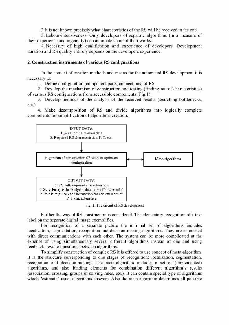
2.It is not known precisely what characteristics of the RS will be received in the end. 3. Labour-intensiveness. Only developers of separate algorithms (in a measure of

their experience and ingenuity) can automate some of their works. 4. Necessity of high qualification and experience of developers. Development

duration and RS quality entirely depends on the developers experience.

2. Construction instruments of various RS configurations

In the context of creation methods and means for the automated RS development it is necessary to:

1. Define configuration (component parts, connections) of RS. 2. Develop the mechanism of construction and testing (finding-out of characteristics)

of various RS configurations from accessible components (Fig.1). 3. Develop methods of the analysis of the received results (searching bottlenecks,

etc.). 4. Make decomposition of RS and divide algorithms into logically complete

components for simplification of algorithms creation.

Fig. 1. The circuit of RS development

Further the way of RS construction is considered. The elementary recognition of a text

label on the separate digital image exemplifies. For recognition of a separate picture the minimal set of algorithms includes

localization, segmentation, recognition and decision-making algorithms. They are connected with direct communications with each other. The system can be more complicated at the expense of using simultaneously several different algorithms instead of one and using feedback - cyclic transitions between algorithms.

To simplify construction of complex RS it is offered to use concept of meta-algorithm. It is the structure corresponding to one stages of recognition: localization, segmentation, recognition and decision-making. The meta-algorithm includes a set of (implemented) algorithms, and also binding elements for combination different algorithm’s results (association, crossing, groups of solving rules, etc.). It can contain special type of algorithms which "estimate" usual algorithms answers. Also the meta-algorithm determines all possible

algorithms interfaces. Actually, the meta-algorithm is a set of details for RS designing (Fig. 2). There is example of meta-algorithm for a stage of localization:

МАlocalization = A1, … ,Am, AE1, … ,AEn , ∩, ∪, AI1,… AIk , (1) where: Ai – some algorithm of localization, AEi – some evaluative algorithm. AIi – group of solving rules. Interfaces are defined by algorithms.

Fig. 2. Structure of meta-algorithm

Full set K for designing various RS configurations is set of meta-algorithms:

K = МАlocalization, МАsegmentation, МАrecognition, МАdecision-making . (2) Other component of any complex system is connections between algorithms. In the

context of RS development it is offered to divide them on direct and feedback. First type is data flows connection (the output of the previous algorithm is an input of the following). Second is circle connection between decision-making algorithm and others. Feedback are necessary in cases when one "pass" through algorithms has not given result, and there is a hope that, having processed a picture with other algorithms (or with other parameters), result will be better.

It is offered to represent RS configuration as a graph G which vertexes are elements from meta-algorithms. All connections between algorithms are defined by interfaces of algorithms. If output interface of component (algorithm) A coincides with input of component B then corresponding vertexes can be connected by an arch.

Such graph will represent every possible configuration of RS. The task of system of automatic RS designing is searching all (or the limited number of) configurations with the purpose of finding the best variant according to requirements.

Conclusion

The suggested system will allow to decrease duration of RS development due to automation of designing and testing. In case of presence a lot of realized algorithms it is not required significant efforts from algorithm developers.

It is necessary to note, that the described project still is had been designing. The following important problem is development of RS designing algorithm, which will process content of meta-algorithms and marked data. The elementary decision is exhaustive search of possible variants of graph G and an estimation of each configuration with some set of test images. But in practice it can appear unacceptable because of time restrictions. Therefore there is necessity for an intellectual algorithm which would work for comprehensible time.

References

1. Zhuravlev Yu. I., Ryazanov V.V., Senko O.V. «RECOGNITION». Mathematical methods. Program system. Practice. FAZIS, 2006.

2. Gonzales R., Woods R., Digital image processing. TechnoSphere, 2005. 3. Materials of IX International conference «Intellectual systems and computer

science». MSU, 2006, pp. 74-78.

A MULTI-SCENE ADAPTIVE VIDEO-BASED TRAFFIC FLOW DETECTION SYSTEM

Zeng-Jia Yan, Hao Zhang, Hua-Dong Meng, Yi-Min Liu, Xi-Qin Wang*

Intelligent Transportation Information Systems Laboratory, Department of Electronic Engineering, Tsinghua University, Beijing 100084, China

*Corresponding author: wangxq_ee@tsinghua.edu.cn

Video-based traffic flow detection (VTFD) is currently one of the most active research topics in video-based detection area. It provides transportation departments with parameters of traffic flow, so that traffic flow analysis and control are feasible. This paper introduces the processing framework of VTFD including following steps: 1) Motion detection; 2) object recognition and classification; 3) object tracking; 4) traffic data collection. In this paper, fundamental and main difficulties of VTFD are reviewed. Moreover, key technologies of a real-time, multi-scene adaptive VTFD system – TH-VTD system, are introduced in this paper. In the end, several technology prospects are presented.

Introduction Video-based 1traffic flow detection (VTFD) systems emerged in the late 80s of the last

century. Because of its significant advantages, accuracy, flexibility and low-cost, VTFD has a wide range of applications in Intelligent Transportation Systems (ITS). Based on the general processing framework of object motion analysis, this paper illustrates the fundamentals of VTFD in section 1. In section 2, two important issues, object occlusion handling and cast shadow subtraction are discussed. The last section focuses on the multi-scene adaptive VTFD system, TH-VTD and relevant technologies.

1. Fundamental A typical structure of VTFD systems is shown in Fig. 1. The Digital Image Processing

(DIP) part is the core part of the framework. It includes four steps: environment modeling, moving object detection, object recognition and classification and object tracking.

Fig. 1. Frameworks of VTFD Moving object detection, comprised of background learning and motion segmentation,

is implemented to distinguish moving region from background. Background learning [1] is aimed to get the background information from image sequences. Motion Segmentation detects regions corresponding to moving objects. Background subtraction [1], temporal differencing [2] and optical Flow [3] are three most common methods.

Object recognition is the process of identifying the individuality of objects and estimating their properties. It includes two steps: object classification and recognition. Object classification is

aimed to simplify subsequent processes. The simplest classification is to discriminate vehicle and background. Autoscope [12] adopts this classification to calculate the traffic flow. VIEWS [4] classifies vehicles into hatchback, saloon and lorry. The recognition process is implemented by matching between the image features extracted from input images and the given models. Object recognition is divided into four categories: region-based recognition [5], active contour-based method recognition [6], model-based recognition [4] and local feature-based recognition [7].

Object tracking aims at detecting the motion information of a moving object from a video sequence. Popular mathematical tools for tracking [8] include the Kalman filter, the Particle filter, the dynamic Bayesian network, etc. In recent years, object tracking achieves progresses in group tracking [3] and multi-view tracking [10].

Traffic flow parameters, which are collected through above processes, are sent to upper layer systems, such as traffic signal systems. Advanced traffic flow analysis can be conducted after establishment of traffic database.

2. Difficulties and relevant developments in VTFD Object occlusion reasoning and cast shadow elimination are of most challenging issues

in VTFD. Detailed discussion about the two problems is as follows.

2.1. Object occlusion handling Object occlusion is caused by overlapping of adjacent objects, and will cause object

recognition unable to work. Advanced algorithms are generally along three directions: 1) Improve the object recognition. Empirical conclusions suggest that model or local

feature-based methods are more robust than active contour-based and region-based methods (see the revolution of PATH [5, 6 and 7]). 2) Object occlusion detection method is aimed to detect the presence of occlusion. Pang [11] proposes a geometrical model to illustrate the contour difference between single vehicle and several overlapping vehicles, so that to detect occlusion. 3) Tracking. Generally, object occlusion is temporary. Thus, occlusive objects can be distinguished via their motion difference (see PATH97 [6]).

2.2. Cast shadow elimination The cast shadow, which is usually detected as moving objects since it is adhered to the

vehicle, raises difficulties for VTFD. Current methods of shadow detection are roughly classified into two categories: pixel-based method and geometrical model-based method.

Pixel-based shadow detection method classifies shadow and moving object regions pixel by pixel. SAKBOT [1], the first effective pixel-based shadow detection system, studied the chromatic of cast shadow. ATON [13] introduces probabilistic functions to describe the model of shadow, background and moving objects. Geometrical model-based method is good at reflecting prior knowledge about the shape of vehicles and the adjacent relation between vehicles and their shadows. Koller [14] introduces a 3D model and considers shadows as part of the vehicle model. In [15], a 2D joint vehicle/shadow model of six types is proposed for robust vehicle detection and tracking.

3. TH-VTD traffic flow detection system The practical environment of traffic scenes is very complex. New generation VTFD

systems are required to work effectively in various conditions despite the variation of

illumination and traffic congestion. The TH-VTD system is able to adaptively work in day/night and congested/free traffic conditions, and provides a novel solution to shadow handling.

3.1. Traffic flow detection under low illumination condition Most VTFD systems fail to work in low illumination (typically at night). TH-VTD

devises a vehicular light detection algorithm based on two observations: (1) the illumination of light area is very high; (2) the lights have clear edges, and the reflection of lights on road does not. Fig. 2. shows the vehicular light detection: (a) is the original figure; (b) is the light area; (c) is the illumination histogram in the area shown in (b). According to (c), illuminations of light area pixels are obviously higher than pixels’. Thus, lights can be extracted by thresholding.

Fig. 2. Light detection The light detection algorithm works well under various test cases. However, this method

is limited to vehicles with two lights open.

3.2. Occlusion handling: line segment detection Congested traffic condition usually goes with frequent vehicle occlusions. TH-VTD

system devises a line segment detection method to detect vehicles in congested traffic scenes. When the camera is specified at a certain angle, a vehicle has 4 distinct horizontal line

segments, as shown in Fig. 3, a. The horizontal line segment, one kind of local feature, is capable of working under partial occlusion.

The line segment detection procedure is shown as Fig. 3, b ~ d. Fig. 3, c shows the edge detection result of (b). Fig. 3, d presents the accumulative edge intensity distribution, which is generated from intensity accumulation of (c). The positions of horizontal lines are detected from thresholding on (c).

Fig. 3. Line segmentation detection Fig. 4. Eight types of the joint vehicle/shadow models

The line segment-based traffic flow detection distinctly boosts the performance of the

VTFD system in congested condition. The largest defect is the strict constraint on the camera.

3.3. Contour-based shadow segmentation TH-VTD system exploits a region-based method to detect the cast shadow of a moving

vehicle from a monocular traffic image sequence. Various cast shadow formations are well described by eight types of simplified

vehicle/shadow joint contour model in terms of the geometric feature of the joint contour consisted of a vehicle and its cast shadow. The joint contour model is shown in Fig. 4. For the simple situations, Type-1 to Type-4, TH-VTD adopts the ideas from [16] and proposes a method based on luminance difference analysis.

Novel algorithms are devised for the handling in complex situations, Type-5 to Type-8. Based on the simplified vehicle/shadow joint contour model, we propose a two-step method: first, estimate the environmental parameters of current traffic scene through analysis of illumination distributions of abundant passing vehicles and, second, extract geometrical information of the contour model to detect the boundary between vehicles and their associated shadows.

One such process is illustrated in Fig. 5. The background learning method is adopted from [4] and the outer contour extraction is implemented by OpenCV [16]. Douglas-Peucker algorithm [17] is used to simplify extracted contour. In Fig. 5, d, features of simplified contour are analyzed: (1) T is the only concave point in up-left region; (2) R is one of the rightest points and at the middle height; (3) M and N are the ends of the top side. After successful location of these four points, the key point P can be calculated via using their geometrical information. The final output is shown in Fig. 5, f.

Fig. 5. Frameworks of contour-based method

The proposed algorithm provides a novel solution to vehicle cast shadow segmentation with high accuracy; moreover, since the contour-based method is only interested in several points on the outer contour, the computation load is largely reduced.

The successful handling of low illumination, congested traffic and vehicle cast shadow makes TH-VTD a multi-scene adaptive system. The system has worked in real

time and is demonstrated to have excellent performance. The processing was done at a frame rate of 15 fps, which is sufficient for real-time applications.

Conclusion This paper proposes an overview of the fundamental of VTFD. An advanced VTFD

system, TH-VTD, is introduced in details. In future, following potential applications deserve greater attention of researchers: (1) Information confusion between video and other senor; (2) Multi-scale and multi-resolution video-based surveillance [10]; (3) Understanding of traffic behavior and scenario parsing [18]. The future advancement of TH-VTD system will be taken through these three directions.

References

1. Prati A. Detecting moving shadows: Algorithms and evaluation. IEEE Transactions on Pattern Analysis and Machine Intelligence, 2003, 25(7), pp. 918-923.

2. Collins R. T. A system for video surveillance and monitoring. Carnegie Mellon Univ., Pittsburgh, PA, Tech. Rep. 2000, CMU-RI-TR-00-12.

3. Ji W. P., Guo B.L. Detecting traffic volume statistics based on virtual coil with optical flow method. Computer Simulation, 2004, 21, pp. 109-110.

4. Tan Tieniu, Sullivan G.D., Baker K.D. Model-based localization and recognition ofroad vehicles. International Journal of Computer Vision, 1998, 27(1), 1998, pp. 5-25.

5. Malik J., Russell S., Weber J., Huang T., Koller D. A machine vision based surveillance system for California roads. Univ. of California, Berkeley, PATH project MOU-83 Final Rep., 1994, Nov.

6. Malik J., Russell S. Traffic Surveillance and Detection Technology Development: New Traffic Sensor Technology. UCB, California PATH Research Final Rep., 1997,UCB-ITS-PRR-97-6.

7. Coifman B., Beymer D., McLauchlan P., Malik J. A real-time computer vision system for vehicle tracking and traffic surveillance. Transportation Res. Part C, 1998, 6(4), pp. 271-288.

8. Hu Weiming, Tan Tieniu. A survey on visual surveillance of object motion and behaviors. IEEE Trans. on Systems, Man and Cybernetics–Part C: Appplications and Reviews, 2004, 34(3).

9. Pece E.C. Generative-model-based tracking by cluster analysis of image differences. Robotics and Autonomous Systems, 2002, 39(3-4), pp. 181-194.

10. Hampaur A., Brown L., Connell J., Ekin A., Haas N., Lu M. Smart video surveillance. IEEE Signal Processing Magazine, 2005, 22(2), pp. 38-51.

11. Pang C. C. C, Lam W. W. L, Yung N. H. C. A Novel Method for Resolving Vehicle Occlusion in a Monocular Traffic-Image Sequence. IEEE Trans. On Intelligent Transportation Systems, 2004, 5(40).

12. Panos, Michalopoulos G. Vehicle detection video through image processing: The Autoscope System. IEEE Transactions on Vehicular Technology, 1991, 40(1), pp. 21-29.

13. Mikic I., Cosman P., Kogut G., Trivedi M. M. Moving shadow and object detection in traffic scenes. Proceedings of Int’l Conference on Pattern Recognition, Sept. 2000.

14. Koller D., Daniilidis K., Nagel H. H. Model-based object tracking in monocular image sequences of road traffic scenes. International Journal of Computer Vision, 1993, 10, pp. 257-281.

15. Yoneyama A. Moving cast shadow elimination for robust vehicle extraction based on 2D joint vehicle/shadow models. Proc. IEEE Conf. on AVSS 2003, pp. 229-236.

16. OpenCV. Intel OpenCV computer vision library. 17. Jonathan de Halleux. A C++ implementation of Douglas-Peucker Line

Approximation Algorithm. http://www.codeproject.com/cpp/dphull.asp. 18. Zheng Haipeng, Meng Huadong, Wang Xiqin, Zhang Hao. Qualitative Modeling of

Vehicle Behavior for Scenario Parsing. IEEE Conference on Intelligent Transportation Systems, 2006.

DEVELOPING A RESCUE ROBOT WITH THE SONAR SYSTEM

M. Yousefkhani1, H. Sanandaji2 1Department of Computer & IT, PAYAME NOOR University, Tehran, Iran;

2Sprott School of Business, Carlton University, Ottawa, Canada, mdyusef@yahoo.com

Every year there are a number of people losing their lives in the accidents, thus the Robocop leaders decided to add a category within the world Robocop championship, named Rescue Robots. These robots can do the exploration and the rescue action within the events such as natural events, earthquakes, volcanoes, and fire. The objective of this research paper is to study and develop the issues which are related to the process of developing the so-called robots, also developing a sample of the rescue robot with the Sonar Sensor, which can scan the environment and not to contact with the barriers on its way. For moving these robots we have used the DC electro motors.

Introduction

A robot is a mechanical structure which can work independently. Intelligent robots are those which can do the actions without a repeatable pattern, and a logical reasoning. These days the role of the robots in doing the regular actions is very eye-catching. Auto manufacturers, aircraft painters, and such industries are the regular examples. Minesweeper robots are kind of robots which can operate, instead of people within the highly dangerous environment. The other kind of dangerous tasks which are harmful for people is rescue operations. As long as the rescue operation is taking place within the unstable environment, presence of worker can be harmful for him. The objective of this project is developing a multitask team which has the capability of Teleoperation, and has a wireless, serial connection among them. Teleoperation

Teleoperation is used when a man is controlling the robot from the control center.

Teleoperation is a proper solution for controlling the remote system. In the mean time there are three intelligent templates for the robots: 1. Hierarchical template. 2. Reaction template. 3. Reaction-Measurement template. The different templates used in robotic are defined in two categories: • The relationship among the first three parts of the robots. • The processed method of the sensed data and their distribution in the system. The hierarchical template is the oldest template of the robotic [1]. The other template –

the reaction template, is derived form the first one. The newest template in the robotic is the third one – reaction-measurement. The developed robots on this template have the structure which made of two parts of plan and sense-act [2]. Robot development

Simultaneously after defining a suitable template for a specific task, the very first

stage of the development process is the intelligence center. But just after that the right tool must be selected. For defining the method of the template's functionality it seems better to

define the visioning. This segment is defining an algorithm for its implementation. What we tried to refer by this is, defining the basic method of organizing the control system. Selecting the useful parts for developing the rescue robots

For the mentioned robots to do the rescue missions correctly they require the high

processing speed and this relates to the operation environment. As long as the path finding algorithms got more complex, the processing requirements became more complex, too. So the mentioned robots must get equipped as well as possible in order to reach the highest performance.

In this project the developed robots are implemented on the mechanical structure which is designed for the remote controlling toys. The dimensions of this plastic mechanical structure are 15x25 centimeters. The so-called dimensions are not that suitable for implementing the different parts of the robot, because they were not designed for this job. For designing the robots there are three essential steps:

1) sensors; 2) processing and planning unit; 3) motors.

Sensors

The toy robots require being in touch with their environment in order to have a clear

vision from the event scene [1, 4]. Two major items for the sensing facilities become crucial in the rescue operation:

1) finding the path in the unclear and unrecognizable environment; 2) the capability of recognizing the injured people. In order to solve the first problem, we can use the communication link and with using

the image recording facilities and implementing a Teleoperation structure we can send the event scene's information to the control unit, and also with the visioning ability of the operator, we can recognize the injuries within the event scene. According to the unclear conditions of the event scene and the unrecognized existing barriers, the robots have to find their way and avoid the probable accidents which could be harmful for them. It is important to consider that the communication link delay is reducing the accuracy of the Teleoperation. For the robots to have a clear image from the event scene, it is proper to use one of the two kinds of sensors for barrier recognition:

1. infrared distance recognition sensor; 2. SONAR.

The robot's processor

The robot's designer can chose one of the two path-finding systems within the unclear

event scene, either Teleoperation system or automated path finding algorithm in which the robot requires powerful processors. In using the first method the received images from the environment have to be processed in the way that we will be able to use the maximum band width of the communication link between the robot and the control center. In using the second one the existing algorithms are required to do the complex processes on the collected data from the event scene [3, 5].

In accordance with the mentioned reasoning and the in hand facilities for developing the robots the considerable alternatives are:

1) using a micro-controller such as AT89C51; 2) using the FPGA chip; 3) using the SOC with the powerful processing core. The first alternative was applicable in some stages of the project, but referring to its

low processing abilities and also its low capacity to implement the control programs on it, its usage became ineligible. The second alternative which is using the FPGA chip seems a good option but the problem is, reaching the high capacity chips for using in robots is difficult and also the cost of using these kinds of chips in the pilot tests are high.

Finally according to the possibility of using the SOCs with the compatible processing core, with the Intel 80386, the mentioned alternative has been selected.

These systems satisfy the requirements of the project, and also they are user friendly because they were developed based on the PC structure, thus programming on them are similar to DOS based programming in the regular PCs.

Toy robots and their components

The toy robots are designed base on the hierarchical robotic template, in which the

different components are sense, plan, and operation. These robots are used within the event scene. The processor should update the robot's operations in every stage, thus the newly collected data should be transferred to the robot's processor through it's sensor in every stage. We used the infrared distance recognition batch as the sensor and the distance recognition system. For using these batches, we should connect their socket into a processor or a circuit with the timing capability and digital signal generator. A couple legs of the so-called four leg socket are for the power source and the other two are for data collection [6]. Selecting the electrical-vocal signal transducer

It is possible to use several transducers for the Polaroid board. All of these transducers

work the same as each other; the only difference is the environment and the sonar's application. The most regular transducer which is highly used in Robotic is IGT.

Graph 1. Frequency reflection of the sent signal Graph 2. Frequency reflections of the received signal Graph 1 illustrates the voltage's surface of the sent signal from the transducer within

the frequency range of 20 to 100 kilohertz. Graph 2 illustrates the voltage's surface of the received signal within the 20 to 100 kilohertz frequency range (Graph 3).

Using sonar in toy robots For implementing the sonar sample, firstly we need to start the control unit and then

do the distance calculations. Regularly we use the microcontrollers for implementing the control unit. Generally speaking the following microcontrollers' series seem proper: 68HC11, PIC, AVR and Basic X. another method which we have used as the control core in this project is executing the FPGA for initialing and controlling sonar.

DC motors and their circuits

Fig. 1. Robot diagram block Fig. 2. The outside vision of the relay along it inter-circuit

As it is obvious from the above diagram, for moving the robot in this plan, it uses 2 motors, one for the right axel and the other for the left one. Thus for each motor, it needs a separate motion circuit.

There are many methods for building the mentioned motion circuit. One of the common methods is using the H-Bridge circuit. This circuit is in the packed batches which came in different shapes. The most simple and the cheapest type of this circuit is L298N chip. The problem of this circuit is lack of generating enough current for moving the robot. The motion circuit is in the following picture in Fig. 3.

Fig. 3. The robot motion circuit Graph 3. IGT transducer's elastic template The main idea in using this motion circuit is, when robot sees a barrier, SW1 which is

open in the normal situation, will be closed. The close SW1 means the robot has to change its direction. This signal will send to both of the motion circuits. D2 and D3 diodes are for isolation of the two motion circuits from each other. For setting the 2 circuits functionality in the way that the robot can change its direction when the barriers exit, we've used a couple of timers which had implemented by the RC network. The RC circuit saves the voltage for a

defined time period, depending on the resistor's size and the capacity of the capacitor. In this circuit we can set this time with a potentiometer and controlling the resistor of the RC circuit.

We've used a high capacity FPGA for creating a processing unit within the robots for using a sonar system. We have used the Flex10k chip in this project for not having the optimization constrained in processing the sonar echo.

Testing and running the system

The objective of this part of the project is installing and starting up the distance

recognition system on toy robots and doing the rescue operation based on the collected data form the sensors. Now we want to start up an integrated system using the ready parts.

Prior to the discussion about the starting up of this project, we will present the robot's diagram block, in order to understand the robot's application completely.

As it is obvious from the above diagram block, the robot starts its job with exploring the event place, which is called place-exploration. In this operation using the sonar sensor the robot will search the environment and see the barriers, it informs the control center about the barriers and their location, thus the control center will send the command of changing the direction. On the other hand if the robot hits something, the situation will be checked by the contact sensor, and the control center will be informed either. In fact the control unit will do a kind of judgment on the robot's actions. Conclusion and Future Work

The rescue robots are widely used nowadays. And there are many researches upon them, making them more powerful. For improving the efficiency of the toy robots in order to make them applicable in the rescue situations, there are two methods:

- Improving the software and using a path finding algorithm. - Improving toy robot's sensing power and hardware. We can use this algorithm, because in the implementing stage we executed the

distance recognition system. The hardware of the robots has the ability to accept the heavy calculations. Using this hardware we can execute many algorithms.

For improving the capabilities of them, we can do the following: 1. Using camera for transforming the image from the event place. We can use the

MPEG chip, for instance, which is capable of compressing different formats. 2. Increasing the number of sonar sensors in the system. With 4 sensors we can

improve the robots abilities in knowing the event place – read the surrounding barriers, for instance.

3. Using the other sensors such as hit sensor. This can change the robot's direction if the other sensors were broken.

References

1. Murphy R. An Introduction to AI Robotics, MIT Press, V2, 2003. 2. Mazidi M.A., Mazidi J.G. The 8051 Microcontroller and Embeded Systems,

Prentice-Hall, V2, 2002. 3. Ulivi G., Poloni M. Fuzzy logic and autonomous vehicles: experiments in

ultrasonic vision, Fuzzy Sets and Systems, 2003.

4. Dubois D., Prade H. Combination of fuzzy information in the framework of possibility theory, Data Fusion in Robotics and Machine Intelligence, New York, Academic Press, 1999.

5. Gasós J., Mart´ın A. Mobile robot localization using fuzzy maps, Lecture Notes in Artificial Intelligence, Berlin, Springer, 1996.

6. http://www.acroname.com/robotics. 7. http://www.robofolio.com/sonar, http://www.robotroom.com/sonar.

REMOTE-SENSING SUNSPOT IMAGES FUSION FOR SOLAR MAGNETIC COIL TRAJECTORIES DETECTION

Mahdi Yousefkhani1, Mana Tarjoman2, Behtash Moradi3

1Department of Computer Eng. & IT, Payame Noor University, Tehran, Iran; 2Electrical and Computer Eng. Group, Tarbiat Modares University, Iran;

3Department of Computer Eng. & IT, Payame Noor University, Tehran, Iran, mdyusef@yahoo.com

Solar sunspot images of year 2003 that is taken with SOHO satellite is downloaded and these images is converted to binary images so that 1 represent white color and 0 represent black color. Images fusion with multiplying pixel by pixel of images is done for daily sunspot images to achieve a bright sight about sunspot trajectories on the sun surface.

Introduction

The Sun is a source of light and heat for life on Earth. Our ancestors realized that their lives depended upon the Sun and they held the Sun in reverent awe. We still recognize the importance of the Sun and find the Sun to be awe inspiring. In addition we seek to understand how it works, why it changes, and how these changes influence us here on planet Earth. The Sun was much dimmer in its youth and yet the Earth was not frozen. The quantity and quality of light from the Sun varies on time scales from milli-seconds to billions of years. During recent sunspot cycles the total solar irradiance has changed by about 0.1% with the sun being brighter at sunspot maximum. Some of these variations most certainly affect our climate but in uncertain ways. The Sun is the source of the solar wind; a flow of gases from the Sun that streams past the Earth at speeds of more than 500 km per second (a million miles per hour). Disturbances in the solar wind shake the Earth's magnetic field and pump energy into the radiation belts. Regions on the surface of the Sun often flare and give off ultraviolet light and x-rays, that heat up the Earth's upper atmosphere. This Space Weather can change the orbits of satellites and shorten mission lifetimes. Solar as a gas and plasma clouds of ions have very mysteries properties and some of magnetic field properties such as 11 year cyclic behavior of it, is well-known for every one. Also it's a well-known property for scientist that based on Magneto Hydro Dynamic (MHD) model of solar core, the particles of solar have very complicated motions such as meridional flows, etc. sunspots are the places on the sun surface which are darker than other regions and have more compact magnetic fluxes. Sunspot images taken by SOHO satellite shows those sunspots have 27 day rotation over the sun surface. Many image fusion methods are used for remote-sensing image fusion applications [3]. Appropriate image fusion methods such as discrete packet wavelets and pulse coupled neural networks and fuzzy logic image fusion are used in [4, 5]. In this study, we will propose two image fusion methods that can be used for detecting a trajectory that an object travels through it.

We used one of these methods for detection of trajectories that sunspots move through them. The method is applied for first three months sunspot images1 of the year 2003 and based on this study we found that:

1. Although sunspot changes patterns usually have not shown any regular paths, but the total trajectory shows the regular belts like path.

2. Result of image fusion of these three months shows that sunspots with approximately same degree of intensities have the same trajectories.

1 Sunspots images were downloaded from address: www.spaceweather.com.

3. Variation of solar magnetic fields has chaotic paths varying with time. First we introduce two fusion methods and then show the simulation result for one of

the methods for sunspots images fusion and finally the concluding remark is considered. Method Description and Simulation

The first year of 21 century containing several extreme geomagnetic storms and events

is the year 2003; we select this year for studying the behavior of sunspot rotation on the sun surface.

Two image fusion methods could be used for sunspot trajectories detection. The first one employs binary images that 0 and 1 represent the black and white respectively. In this method pixel based multiplication of same Cartesian coordinated images is used as fusion operator. If any of two images contains a spot on it at a certain coordinate, then its binary value will be zero for that coordinate in fused image.

The second method is based on selection of minimum value between pixels of two or more images at the same coordinate. This one is more effective for color image fusion. Both methods are explained in detail as follows:

A. Method 1 At first, the colored image should be converted to a binary image with 0, 1 pixel values

considering the following formula:

⎩⎨⎧

=≠

=0,00,1

ij

ijbinary

PP

P (1)

Then the result of fusion of pixel by pixel of two image is computed:

imagesbinaryPPP image

jiimageji

Fusedji ;2

,1

,. ×= (2)

where i, j are the x, y Coordinate of images. If in two image in the same coordinate (x, y), one

image has a white point ( 11, =imageyxP ) and the other image a black point ( 02

, =imageyxP ), then

the result fused image has a black pixel in this coordinate according to equation 2.

B. Method 2 Another fusion method is based on the minimum value selection of pixel (i,j) of image 1 and

image 2:

),min( 2,

1,.

imageji

imageji

Fusedji PPP = (3)

where FusedjiP , denoted the value of pixel at coordinate (i, j) of fused images. The fused images is

a color image that in each coordinate, the darker pixel between the same-coordinate pixels of two images would be selected as the fused pixel. This fusion method is illustrated for two color images in Fig.1 according to equation 3.

The total procedure for this achievement is depicted in Fig.1 and this method of fusion is applied for all images of each month and the result of such image fusion method for trajectory detection of sunspot rotation is shown in Fig. 2 for January, February, March, April of year 2003 separately and finally the fusion result of images of Fig. 2 is shown in Fig. 3. According to this figure we found that the sunspots with approximately the same intensity of magnetic flux over this four month have certain orbit around the sun. These results show that

;

.

,

,

sunspots do not appear at random over the surface of the sun but are concentrated in two latitude bands on either side of the equator. Magnetic fields within the Sun are stretched out and wound around the Sun by differential rotation - the change in rotation rate as a function of latitude and radius within the Sun. This is called the omega-effect and also twisting of the magnetic field lines is caused by the effects of the Sun's rotation as shown in Fig. 4. This is called the alpha-effect that looks like a twisted loop as shown in Fig. 4. Although sunspots themselves produce only minor effects on solar emissions, the magnetic activity that accompanies the sunspots can produce dramatic changes in the ultraviolet and soft x-ray emission levels. These changes over the solar cycle have important consequences for the Earth's upper atmosphere and also for global climate of the earth.

The result of min method fusion for January, February, March and April 2003 is depicted in Fig. 5 that respect to Fig. 2 (multiplication) method is a more soft image and the result of total fusion the these first month is depicted in Fig. 6:

Fig. 1. Block Diagram of proposed method for fusion of remote-sensing sunspot images

That shows this method of fusion of remote-sensing sunspot images could also reveal

the trajectories of sunspot rotation over the sun surface. With this new point of view about of solar magnetic field rotation such as this note that may be the total amount of solar magnetic field on the surface on that plane that cross the meridional is near zero or is very low. Another benefice of such insight is that the solar rotation profiler is crucial for testing theories of angular momentum transport within the sun and the other stars. Also such analysis could help physicist to have better thought about the interaction of electromagnetic interaction of sun with plasma and gases bearing the sun as well-known as Magneto Hydro Dynamic of the sun. Even small-scale magnetic field of the sun had shown large-scale coronal heating effect [2], and as a result larger coronal mass ejection and as a result due to geomagnetic storms and disturbances with more intensity that cause to many serious problems for satellite and other human technical systems on the earth such as power grids that occur before on March 14, 1989 that lead to power black-out on Quebec and Canada, resulting in the loss of over 20,000 megawatts of

power production capacity. The blackout cut electric power to several million people for many hours. Then it's seen reasonable to analysis the solar activity and the most visible feature of its sunspot for better understanding about its activity in order to support our technical systems and also our life. Most of methods analyze the solar activity as temporal behavior or on the other hand time series that in which time would happen an extreme storms.

Although it's important to predict the temporal behavior of solar geomagnetism, the spatial analysis of sun also is at the great important in our point of view because the position and trajectories that most stronger magnetic fields (sunspots) are placed give a bright insight about of position of interplanetary space that a geomagnetic storm would happen.

Fig. 2. Result of fusion of sunspot images of January, February, March, April 2003 (each month separately) with normalized pixel by pixel multiplication method

Fig. 3. Result of fusion of sunspot images for four month of 2003 (January – April)

Fig. 5. Result of fusion of sunspot images of January, February, March, April 2003 (each month separately) with minimum value selection pixel by

pixel of two color image

Fig. 4. Omega effect of solar magnetic field (left), Alpha effect of solar magnetic field (right)

Fig. 6. Result of minimum value fusion of sunspot images for four month of 2003 (January – April)

Conclusion

In this study a simple image fusion method was proposed for detection of sunspot

trajectories over the sun sphere and we found that in each month or 27 day cycle the sunspots with different degree of magnetic flux density are placed in two sides of the sun sphere and also the trajectories are lie on certain height with respect to meridional of sun and for every month also the trajectories only have different paths in this two regions around sun that indicate on chaotic behavior of sun electromagnetic fields.

References

1. Timothy M. Brown. Solar rotation as a function of depth and latitude, nature, vol. 317, 17 October 1985.

2. Schrijver C. J. et. al. Large-scale coronal heating by the small-scale magnetic field of the Sun, nature, vol. 394, 9 July 1998.

3. Hai-Hui Wang, Jla-Xiong Peng, Wel Wu. A Fusion Algorithm of Remote-Sensing Image Based on Discrete Wavelet Packet, Proceedings of the Second International Conference on Machine Learning and Cybernetics, Wan, 2-5 November 2003.

4. Randy P. Broussard, Steven K. Rogers, Mark E. Oxley, Gregory L. Tarr. Physiologically Motivated Image Fusion for Object Detection using a Pulse coupled Neural Network, IEEE Transactions on Neural Networks, vol. 10, no 3, May 1999.

5. Harpreet Singh, Jytoi Raj, Gulsheen Kaur, Thomas Meizler. Image Fusion using Fuzzy Logic and Applications, Fuzzy-IEEE 2004.

CRITERIA OF INFORMATIVENESS AND SUITABILITY OF A SUBSET OF ATTRIBUTES, BASED ON THE SIMILARITY FUNCTION

N.G. Zagorujko, I.A. Borisova, O.A. Kutnenko Institute of Mathematics of the Siberian Branch of the Russian Academy of Science

Novosibirsk, Russia

For an estimation of informativeness of separate attributes or their subsystems it is offered to use average value normalized functions of an similarity (NSF) objects of training sample to the pattern. This criterion differs from criterion in the form of number of correctly recognized objects higher connection with results of recognition of control sample, a greater noise stability, an opportunity to estimate suitability of the chosen attributes and reliability of recognition of control object.

Introduction

In 1933 A.N. Kolmogorov has published work [1] in which has paid attention to problem of a choice of a subset informative predictors for regression in a case when the quantity of potential predictors is equal or exceeds quantity of observable objects. If predictors depend from each other the choice of the most informative subset from big initial quantity represents NP-difficult problem. But business is not only in it. There are tasks in which the main part of characteristics has no the direct relation to criterion function and plays a role of casual noise. Than more such characteristics and the less observable objects, the probability of selection of a "pseudo-informative" noisily predictors is more. Last years the urgency the problem of a choice of an informative subset of attributes and estimations of its suitability for regression analysis and pattern recognition has strongly increased. Real tasks of recognition, for example, in genetics in which the small number (tens) objects of training sample is described by big number of characteristics (tens thousand) began to meet. The success in the decision of this problem depends on the answer to three questions:

1. How procedure of search the subsystems of attributes is organized? 2. How an informativeness subsystem of attributes is estimated? 3. How a suitability (no randomness) subsystem of attributes is estimated? The greatest part of known procedures of search is based on use the ideas of "greedy"

algorithm: the best attribute gets out, to it the best partner from remained is added, to this pair the best third of remained is added, etc. So algorithms of construction the logic decision functions [2] are arranged. Steadier to hit in a local optimum are methods of iterative type in which procedures of escalating of number of attributes alternate with procedures of elimination of a part from earlier chosen attributes. As examples of algorithms of such iterative type algorithms AdDel [3] and GRAD [4] can serve. So the first component of success in the decision of a attributes choice problem has undergone appreciable development last years.

To the second and third components connected with criteria of informativeness and a no randomness of subsystems, the smaller attention was paid. In the given work attempt to find such internal properties of attribute subsystems on which it would be possible to judge about them informativeness and suitability is made. We will try to distinguish the subsystems naturally connected with the solved task, from the subsystems which have arisen from a casual combination of rustling attributes.

1. Probability of a casual choice In a problem of pattern recognition of healthy patients from a pattern of cancer

patients initial data represented the table of 74 objects (50 healthy and 24 sick patients) and 822 genetic attributes [5]. It has been checked up individual informativeness of each attribute separately and all pairs attributes, and then 100 most informative attributes and 100 most informative pairs attributes have been chosen. The quantity of mistakes at recognition of 74 training objects on each of 100 separate attributes changed from 16 up to 26. Mistakes for each of 100 best pairs attributes were from 9 up to 14.

It was interesting to answer a following question: what will be informativeness separate attributes and their pair combinations if all attributes to generate the random-number generator? For the answer to it the casual table of the size 74*822 has been generated. The objects have been casually divided into two patterns - with 50 and 24 objects. It was found out, that each of 100 most informative attributes found in this table recognize sample with the same mistakes - from 16 up to 26. Each of 100 best pairs casual attributes have given some other result - from 10 up to 16 mistakes.

From these results it is visible, that at a plenty of attributes N and small number of objects M in subsystem of n the most informative casual rustling attributes can get with a high probability.

Let's pay now attention to a following question: what criterion informativeness an attribute it will be most effective to protect us from a casual choice?

2. Comparison of informativeness criteria

In the experiments described above, as well as in the majority of existing methods, as

an estimation informativeness subsystems U the quantity of correctly recognized objects of training sample served. The decision rule on which the control object z concerned to the first pattern, has been based on value of function of a similarity

1 2 1 1 2( ) ( )F r r r r= − + ,

where 1r and 2r - distances from control object z up to the nearest neighbors of the first and second patterns. If F>0, the decision was accepted in favor of the first pattern, and on the contrary. The size F varies within the limits of from +1 up to -1. Those objects which settle down in a close environment of the objects and are considerably removed from objects of other patterns, have higher value of function F, than the peripheral objects close to other patterns. Hence, by using F of the object z it is possible to judge correctness of its recognition.

If accumulate values F on all objects and to divide the sum on M the received size sF will characterize average remoteness of objects of training sample from boundary lines on which F=0. From here there was an idea to compare among themselves two criteria of informativeness - number of correctly recognized objects of training sample (U) and average value of function a similarity ( sF ).

The third criterion follows from Fisher's offer to estimate informativeness of attributes by the distance between population means of patterns, divided on the sum of their dispersions:

1 2 1 2( ).Q µ µ σ σ= − +

It three criteria - U, sF and Q - were compared in following modeling experiment. Initial data consisted of M=200 objects of two patterns (on 100 objects of each pattern) in

N=100-dimensional space. Attributes were generated so that they possessed different informativeness. As a result about 30 attributes appeared to some extent informative, and other attributes were generated by the random-number generator and were obviously not informative. Under this table algorithm AdDel the most informative subsystems of dimension n (from 1 up to 22) got out. For training on 35 objects of each pattern got out casually. On the control the others 130 objects were shown.

To reliability of recognition of control sample at use of criteria U, sF and Q, average on 10 experiments, are shown on fig. 1. It is visible, that the attributes chosen by criterion Q, better the chosen by criterion U, but is worse chosen on function of a similarity F. It is possible to explain it to that measures Q and sF depend on characteristics of separate boundary objects less, than a measure U. In turn, Fisher's Q measure is focused on division of normal distributions by means of linear decision functions while the measure sF adapts for features of distribution of training sample and corresponds to more powerful piecewise-linear dividing border.

0,7

0,72

0,74

0,76

0,78

0,8

0,82

0,84

0,86

0,88

0,9

1 3 5 7 9 11 13 15 17 19 21

UFsQ

Fig. 1. Results of a choice of subsystems of attributes at use of three criteria: on number of mistakes (U), on function of a similarity ( sF ) and by Fisher's Q criterion

3. A noise stability of informativeness criteria

Criteria U and sF were investigated on stability to handicaps. For this purpose the

initial table of the previous experiment was deformed by noise of different intensity and at each noise level (from 0,05 up to 0,3) the best subsystems by these criteria got out. Results are presented in Fig. 2 from which it is visible, that the criterion sF is steadier, than criterion U. Criterion U inspires the overestimated expectations. Results on the control show a high degree of correlation of criterion sF with the results received on training. It testifies about high prognostic properties of this criterion.

0,6

0,7

0,8

0,9

1

1,1

0,05 0,1 0,15 0,2 0,25 0,3

Fs

U

Fs

U

Fig. 2. Results of training and recognition by criteria U and sF at different levels of noise. Thin lines are training, fat - the control

4. An estimation of "no randomness" of the chosen subsystems For comparison of these results with cleanly casual results the random-number

generator with uniform distribution had been generated 10 tables of the same size M=200, N=100. Two patterns (on 100 objects) have been received by a method of a casual choice. On this noisily data for each dimension of subsystems n the most informative attributes got out and values of criterion sF were defined. It has appeared, that they lay in «a casual corridor» with borders from 0,61 up to 0,67. Values sF for the subsystems found under the initial table, lie considerably above this corridor and consequently can be considered not casual.

From these results it is possible to formulate the following practical recommendation. Under training table N*M value sF for the best subsystem from n attributes is defined. Then a series of casual tables with the same values N*M is formed and on them there are values sF for the "best" subsystems of the same dimension n. If the value sF for the initial table gets in limits of values sF for casual tables it is possible to consider, that the chosen attributes X are «pseudo informative». They do not reflect natural connections with the target characteristic. To trust in decisions which will be received on these subsystems on control sample, it is impossible.

On distance between value of criterion sF of the subsystem chosen in the real table, and borders of "a casual corridor», received on a set of casual tables of the same size, it is possible to judge "no randomness" or "suitability" of the chosen subsystems.

5. Check on real data

For confirmation of advantages of criterion sF before criterion U on real tasks

experiment with spectral data has been lead. Training sample consisted of two patterns on 25 objects chosen casually from the real table of two classes of substances. From initial set of 1024 spectral characteristics two lists were formed of 46 most informative "secondary" attributes in the form of not overlapped sites of a spectrum. One list included the attributes selected by criterion U, and the second - by criterion sF . Then all of n attributes of each list were used for recognition of 200 control objects (on 100 objects of each pattern). Reliability of recognition on each of 46 most informative attributes is presented on Fig. 3.

Fig. 3. Reliability P of recognition of control sample on each of 46 most informative attributes ordered on informativeness. The top curve corresponds to a choice by criterion sF , bottom - on U

These results also confirm advantage of a choice of attributes on average value of

function of a similarity ( sF ) before widespread choice on number of correctly recognized objects of training sample (U).

Conclusion 1. For an estimation informativeness of attributes or feature systems it is necessary to

use not quantity of correctly recognized objects of training sample (U), but average value of function sF of similarity of objects of training sample to the patterns.

2. The values of a measure sF received on the training table, and on a series of casual tables of the same size, allow receiving a degree of "suitability", "no randomness" chosen subspace of attributes.

3. Value of function F of similarity of control object to this or that pattern enables to estimate a confidence of correctness of this decision. References

1. Kolmogorov A.N. To a question on suitability of the forecast formula founded by statistical way. - Factory laboratory, 1933, no 1, pp. 164-167.

2. Lbov G.S., Startceva N.G. Logic decision function and questions of statistical stability of decisions. Novosibirsk: Ed. Institute of Mathematics of the Siberian Branch of the Russian Academy of Science, 1999.

3. Zagoruiko N.G. Applied methods of the of data and knowledge analysis. Novosibirsk: Ed. Institute of Mathematics of the Siberian Branch of the Russian Academy of Science, 1999.

4. Zagoruiko N.G., Kutnenko O.A. Algorithm GRAD for a choice of attributes // Proc. of VIII Intern. Conferences “Application of the multivariate statistical analysis in economy and an estimation of quality”. Ed. MESI, Moscow, 2006, pp.81-89.

5. Alves A., Zagoruiko N., Okun O., Kutnenko O., Borisova I. Predictive Analysis of Gene Data from Human SAGE Libraries // Proceedings of the Workshop W10 “Discovery Challenge” ECML/PKDD-2005, Porto, Portugal. Edited by Petr Berka and Bruno Cremilleux, Universite de Caen, France, pp. 60-71.

INFLUENCE OF STATES NUMBER OF MULTI-STATE SYSTEM TO RELIABILITY MEASURES

E. Zaitseva1, V. Levashenko1, K. Matiaško1, N.N. Govjadinova2

1University of Žilina, Žilina, Slovakia 2Belarus State Economic University, Minsk, Belarus

The reliability of Multi-State System is analyzed in this paper. In a Multi-State System, both the system and its components may experience more than two reliability states. We propose the Dynamic Reliability Indices for reliability analysis of this system. Mathematical tools of the Multiple-Valued Logic (the Logical Differential Calculus in particular) were used for definition of these indices in paper. They estimate influence upon the Multi-State System reliability by the state of a system component. In this paper we investigate failure of system that is caused by change of system components efficiencies.

Introduction Reliability Analysis plays significant role in information technology, because

reliability has been considered as an important measure in many technical systems [1, 2]. As a rule the Reliability Analysis problem of a technical system is: given the characteristics of system components, compute a measure of system reliability. Different system model are used for calculation of the measure of system reliability.

Discrete probability models are typically employed in reliability analysis. There are two types of these models: Binary System and Multi-State System (MSS). In the most commonly studied model to which are investigated, system and system component can take on one of two states: failure or functioning. This model is named Binary-State System. Many problem of the these system have been settled. But this approach fails to describe many situations where the system can have more than two distinct states [2–4]. MSS has proposed alternative decision for reliability analysis of technical system. In a MSS, both the system and its components may experience more than two states, for example, completely failed, partially functioning, functioning and perfect functioning (Fig. 1). The MSS is frequently required for applied problem. But reliability analysis for MSS is a complex subject in reliability [1–4].

Perfect functioning Real-world component Functioning multi-state component

Partly functioning binary-state component Completely failed t

Fig. 1. Interpretation of functioning of binary-state and multi-state elements

There are some tools for system reliability estimation that it is interpreted as MSS

[1-3]. We have been developed structure function tool for computation system reliability measures. A structure function of MSS declared system reliability (state) depending on system components efficiencies (states). Thus the structure function does not allow to estimate the dynamic behavior of the MSS in traditional interpretation [1-3]. Only in papers [4, 5] have been considered algorithms for analysis of dynamic behavior of MSS by structure function. But these algorithms have high computational complexity. We propose the approach for estimation of dynamic properties of the MSS reliability based on its structure function by the Dynamic Reliability Indices (DRIs). DRIs are calculated with respect to structure function by the Logical Differential Calculus of Multiple-Valued Logic (MVL). Basic and theoretical

conceptions of this approach were determined in [6, 7]. These indices characterize the change of the MSS reliability that is caused by the change of a component state (component efficiency). We analyze MSS reliability for different types of system structure (parallel, series and k-out-of-n) in previous investigations [8-10] that are typically employed in Reliability Analysis. In papers [11, 12] DRIs have been investigation for change of MSS reliability that are caused by simultaneous changes of fixed system components.

In this paper we investigate the influence of number of reliability state for system and components by DRIs.

1. Direct Partial Logic Derivative for reliability analysis of MSS

A MSS and each of n components can be in one of m possible states: from the complete failure (it is 0) to the perfect functioning (it is m-1). A structure function of MSS permits to define the system reliability (system state) depending on its components xi (i = 1, …, n) state:

φ(x1, …, xn) = φ(x): 0, …, m-1n → 0, …, m-1. (1)

Every system component xi is characterized by probability of the performance rate form 0 to m-1:

pi, si = Prxi = si, si = 0, …, m-1. (2)

We use next assumptions for structure function (1) that are peculiar to reliability analysis [1-3, 6, 7]: (a) a structure function φ(s) is monotone and φ(s)=s (s∈0, …, m-1); (b) all components are s-independent and are relevant to the system; (c) a structure function φ(s) is a MVL function.

The assumption (c) allows applying MVL tools for reliability analysis of the MSS [6, 7]. In particular, we use the Direct Partial Logic Derivatives (Logical Differential Calculus) that permit to estimate dynamic properties of MVL function: they reflect the change in the value of the function when the values of variables change.

A Direct Partial Logic Derivatives ∂φ(j→h)/∂xi(a→b) of a structure function φ(x) with respect to variable xi reflects the fact of changing of function (system reliability) from j to h when the value of variable xi (i-th component states) is changing from a to b:

∂φ(j→h)/∂xi(a→b) = 1, if ( , ) ( , ) ;

0, in the other case,i im a j b h− φ = φ =⎧

⎨⎩

&x x (3)

where φ(ai, x) = φ(x1,…, xi-1, a, xi+1,…, xn) and φ(bi, x) = φ(x1,…, xi-1, b, xi+1,…, xn); j, h a, b ∈ 0, …, m-1.

For analysis of changes of several components states at the same time using a Direct Partial Logic Derivatives with respect to variables vector [11, 12]:

∂φ(j→h)/∂x(p)(a(p)→b(p)) = 1 11, if ( , , , ) ( , , , ) ;

0, in the other case,p pi i i im a a j b b h− φ = φ =⎧⎪

⎨⎪⎩

&K Kx x. (4)

where p is number of component that changes states and the vector x(p) is named “system components efficiency vector”.

The Direct Partial Logic Derivatives (3) and (4) can be used for analysis of dynamic properties of a MSS by the structure function of this system. And note, the derivative (3) is special case of derivative (4) if parameter of components number p = 1.

2. Modelling of MSS failure and repair by Direct Partial Logic Derivative

MSS failure have been defined depending on a change of one system component states with relation to Direct Partial Logic Derivatives of a structure function φ(x) of n variables with respect to variable xi (3) in paper [5, 6]. But system failure that is caused by diminutions of fixed component efficiency is more general case [11, 12]. In Direct Partial Logic Derivative terminology the MSS failure according the deterioration of several components states is represented as the changing of the function value φ(x) from j into zero and as decrease of a system components efficiency vector x(p) from a(p) to b(p): ∂φ(j→0)/∂x(p)(a(p)→b(p)), where a(p) = (

1( , , )

pi ia aK ) and , 0, ..., 1j ji ia b m∈ − , 1, ...,

j ji ia b j p> = . Because the structure function is monotone (assumption (a)) the MSS failure is

declared by a change function φ(x) from “1” into zero and decreases of every of p system components efficiency from

jia to )1( −jia :

∂φ(1→0)/∂x(p)(a(p)→ (p)a~ ), (5)

where 1 1

( , ..., ) (( 1), ..., ( 1))p pi i i ia a a a= = − −% % %(p)a and 1, ..., ( 1)

jia m∈ − . The MSS repair can be considered in some versions that depend on refit of failed system

components. It is attained by replacements or renewals of failed system components. In the first case the availability of p failed system components changes from zero into (m-1) and from zero into some level b ∈ 1, …, m-1 in the second case. We consider the first case in more detail. The MSS repair is declared in Direct Partial Logic Derivative terminology is defined as the structure function change from 0 into h (φ(x): 0 → h) and as p failed system components changes from 0 into (m-1):

∂φ(0→h)/∂x(p)(0→(m-1)), (6)

where )0,...,0( 321p

=0 and ))1(),...,1((44 344 21

p

mm −−=−1)(m ; h∈1, …, m-1.

3. The Dynamic Reliability Indices (DRIs)

Some groups of DRIs for the estimation of change influence one of system components on the change of system reliability are considered in paper [5, 11]. One of these groups is Component Dynamic Reliability Indices (CDRIs). CDRIs are declared as a probability of the MSS failure and repair if state of the i-th system component changes or states of p fixed components change.

Definition 1. CDRIs are probabilities of MSS failure that are caused by decrease of efficiency of fixed system components:

( ) ∏=

⋅=p

jaiaff jj

pρP1

,)( ρ(p)x , (7)

where fρ is number of system states when the vector x(p) value change from a(p) to (p)a~ forces the system failure and calculated as numbers of nonzero Direct Partial Logic Derivative (5):

fρ ≡ ∂φ(1→0)/∂x(p)(a(p)→ (p)a~ ) ≠ 0; (8)

ρa is number of system states “1” when 1

( , , , )pi ia aφ K x = 1; pi,a is declared in (2).

Definition 2. CDRIs are probabilities of MSS repair that are caused by replacement of fixed system components:

1( )

0 ,01 1

( ) ,j

pmh

r r ih j

P p−

= =

⎛ ⎞= ρ ρ ⋅⎜ ⎟⎝ ⎠∑ ∏(p)x (9)

where )(hrρ declares number of boundary system states and is calculated by Direct Partial

Logic Derivative (6): )(h

rρ ≡ ∂φ(0→h)/∂x(p)(0→(m-1)) ≠ 0; (10)

ρ0 is number of zero system states ( ),0,,0(1

xpii Kφ = 0); pi , 0 is declared in (2).

Definition 3. DIRIs for MSS failure are probabilities of MSS failure that are caused by decreases of efficiency of any p system components:

( )∏∑−

−=1

)()( )(1)(z

pf

z

pff xPxPP , (11)

where Pf(x(p)) is CDRIs for MSS failure (7); ⎯x(p) is system components efficiency vector for

which ⎯x(p)≠x(p); z is number of combinations of n things taken p:!)!(

!ppn

npn

−=⎟⎟

⎠

⎞⎜⎜⎝

⎛ , that

determines number of vectors x(p) for the structure function which consist of n components. Definition 4. DIRIs for MSS repair that are caused by replacements of any p system

components:

( )∏∑−

−=1

)()( )(1)(z

pr

z

prr xPxPP , (12)

where Pr(x(p)) is CDRIs for MSS repair (9). The assumption (b) for structure function of MSS that all components are independent

and relevant to the system takes account for DIRIs definition.

4. Influence of states number of MSS reliability to DRIs

Consider system reliability measures depending on number of MSS states (efficiency levels). We realized two experiments to analyse an influence of number of system state m of structure function (1) to DRIs. Firstly, CDIR’s and DIRIs are calculated for a MSS failure for different values of parameter m. Typical types of MSS (serials, parallel and k-out-of-n) have been estimated. Secondly, we calculated these indices for MSS repair. Some experimental results are in diagrams (Fig. 2, a for system failure and Fig. 2, b for system repair).

Note, we use next transform between system with different values of parameter m:

,,

,( 1) ,( 2)

, if 0, .., 2;

, if 1, i

i

i i

i s ii s

i m i m i

p s mp

p p s m− −

= −⎧⎪= ⎨ + = −⎪⎩ % %

%

% % (13)

where m = ( m~ + 1); m and m~ are numbers of reliability states; isip , is i-th component

probability for state si if the MSS has m efficiency levels; isip ,

~ is i-th component probability for state si if the MSS has m~ efficiency levels.

Therefore probability of system failure and system repair increases if number of system reliability states m decreases. And maximal value of probability of system failure and repair is for Binary-State System. So, application of MSS allows to improve measure system reliability by DRIs.

00,10,20,30,40,50,60,70,80,9

1 m=2 m=3 m=4

0

0,2

0,4

0,6

0,8

1 m=2 m=3 m=4

a) b)

Fig. 2. Influence of states number of system discrete model on reliability analysis

5. Acknowledgments

This work was partially supported by grants of Scientific Grant Agency of the Ministry of Education of Slovak Republic and the Slovak Academy of Science (Vega 1/3084/06, MVTS Bil/Fín/SR/ŽU/06, ŽU/05 VV_MVTS13).

References

1. Lisnianski G. Levitin, Multi-State System Reliability. Assessment, optimization and applications, World scientific, 2003.

2. Ball M.O., Colbourn C.J., Provan J. Network Reliability. In: Ball, M.O., Colbourn, C.J. (eds): Handbooks in OR &MS, vol. 7, Elsevier Science, 1995, pp. 673-762.

3. Ushakov. Handbook of Reliability Engineering, Wiley, New York, 1994. 4. Boedigheimer R., Kapur K. Customer-driven reliability models for multistate

coherent systems. IEEE Trans. Reliability, vol. 43, no 1, 1994, pp. 46–50. 5. Xue J., Yang K. Dynamic reliability analysis of coherent multistate Systems. IEEE

Trans. on Reliability, vol. 44, no 4, 1995, pp. 683–688. 6. Zaitseva E. Dynamic reliability indices for Multi-State System. Journal of dynamic

system & geometric theories, vol. 1, no 2, 2003, pp. 213–222. 7. Matiaško K., Zaitseva E., Kovalik Š., Levashenko V. Analysis of dynamic

behaviour of Multi-State System. Journal of Electrical Engineering, vol. 56, no 11-12, November-December, 2005, pp. 306–312.

8. Zaitseva E., Levashenko V., Matiasko K. Failure analysis of series and parallel Multi-State System. Maintenance and Reliability, vol. 30, no 2, 2006, pp. 29-32.

9. Zaitseva E., Levashenko V., Matiaško K., Puuronen S. Dynamic reliability analysis of the k-out-of-n Multi-State System. Proc. of the IEEE 35th Int. Symp. on Multiple-Valued Logic, 19-21 May, Calgary, Canada, 2005, pp. 264-269.

10. Zaitseva E., Levashenko V. Dynamic Reliability Indices for parallel, series and k-out-of-n Multi-State System, Proc. of the IEEE 52nd Annual Reliability & Maintainability Symposium (RAMS). 23-26 January, Newport Beach, CA, USA, 2006.

11. Zaitseva E., Matiasko K., Puuronen S. Reliability of Multi-State system against changes of some system components states, Proc. of European Safety and Reliability Conference (ESREL 2006), 18-22 September, Estoril, Portugal, 2006, pp. 1745-1752.

12. Zaitseva E., Puuronen S. Investigation of influence of some system component states changes to system reliability, Proc. of the 6th Int. Conf. on Reliability and Statistics in Transportation and Communication (RelStat 2006), 25-28 October, Riga, Latvia, 2006, pp. 23-38.

IMAGING SYSTEM PARAMETERS IDENTIFICATION FOR IMAGE SUPER-RESOLUTION RESTORATION

I. Zakharov, D. Dovnar

Institute of Technology of Metals of NAS of Belarus, Mogilev, Belarus, zakharov@ieee.org

For identification of point spread function of an imaging system and additive noise parameters the information from analyzed images and knowledge about its nature were used. For this purposeе the edge spread function was extracted from images where edges are contained. In the work a methodology of system parameters determination is described and tested for satellite images super-resolution restoration. Results of experiments on image processing show high efficiency of proposed algorithm for satellite remote sensing applications.

Introduction Images received from a satellite very often are distorted (blurred and noised) because

of atmospheric light scattering and also optoelectronic system limits image resolution. For improving image quality can be used algorithms of image restoration, filtration and super-resolution. Many methods for this purpose are developed [1, 2]. In this work we use probabilistic method of image restoration, which is optimal in the sense of minimal mean squared error of image restoration [3].

As usually for image restoration it is required knowledge about point spread function (PSF) and noise of imaging process. Although there is the case when PSF is known from a manufacturer of optoelectronic imaging system, but for successful application such system in different conditions of image formation (e.g. changing of atmospheric PSF) we have to develop approach, which makes it possible to find PSF and characteristics of noise for high quality restoration of image. This problem is actual in many fields: remote sensing, medical imaging, non-destructive testing and others. For solution problem of image restoration without PSF knowledge the several approaches are exist. Some of them are based on determination of PSF parametrically with using image analysis [4, 5]. Also there are blind deconvolution methods which estimate parameters of probabilistic characteristics of original image and PSF [6, 7]. As a posteriori information in some approaches of super-resolution image restoration an interpolated version of initial image is used.

The main aim of our work is to determinate PSF and noise dispersion for purpose image restoration in satellite remote sensing. For PSF determination a priori knowledge about smoothness and continuousness of point spread function was used. To find parameters of PSF remote sensing system (which includes focal-plane array, atmosphere-lenses) we analyzed observed image where edges and lines are presented. Given parameters are necessary for realization of image restoration method [3, 8]. Received PSF can be compared with Gaussian, which is often used for describing atmospheric blur [4, 9]. For noise parameters estimation we can apply model of additive non-correlated noise and to determine its dispersion from image analysis. After parameters determination we can apply them for purpose of noise filtration and super-resolution image restoration from several multi-spectral satellite images.

1. Determination of PSF and noise dispersion The PSF represents how the imaging system transfers an image of point source,

described by delta-function. For analysis of PSF of imaging system (in our case for remote sensing system) can be used any image. Because in any image the PSF of system is included

[9]. In practice for PSF determination the image of object which has a simple geometrical form (e.g. line, strip) or border may be used.

For optoelectronic system, which is based on focal-plane array (FPA) the PSF should be measured in two dimensions. Because of the FPA is space-variant system and its photosensitivity element can have different properties in directions of coordinate axes of image row and column (X and Y) [9]. The usage a slanted edge target, as the test image, makes it possible to get sampled edge profile, which is Edge Spread Function (ESF). The first derivative of such ESF is Line Spread Function (LSF). The LSF is identical to one-dimensional integral of two-dimensional PSF, which can be considered as PSF alone direction. To find the PSF in two dimensions we should find ESF in X and Y directions.

a) b)

c)

Fig. 1. Initial Image (a), ESF (b) and PSF (c) of remote sensing system In the given work the analysis of images contained edge (Fig. 1, a) for calculation of

imaging system PSF is used. As usually for satellite observation there are many images of objects such as fields and rivers which have sharp borders. Given objects can be found by a user or by edge detection algorithms [10]. After edge detection we can find LSF (e.g. for X direction) followed by determination ESF (Fig 1, b):

dxxESFdxLSF ))(()( = . (1)

In Fig. 1, a images form Landsat-7, which was used for PSF calculation are shown by white rectangulars. After ESF recalculation to LSF by Eq. (1) from edge of every image we can find the PSF(x) as identical to LSF(x). The level of noise in the image is minimized by averaging over many initial images. In Fig. 1, c point spread functions are shown by several ways as dots, asterisks and diamond. By solid line the approximation of PSF by Gaussian is shown. Such way the measured PSF can be used for restoration and to remove blur in images received from remote sensing system. Also the two-dimensional PSF can be found from multiple oriented in different directions LSF by Fourier slice theorem [11].

Noise dispersion, which is used in image restoration algorithm, also can be found from an image part with uniform intensity distribution with assumption of noise model as additive non-correlated [3, 12]. With usage of Equations for non-correlated probabilistic

values we can find averaged noise dispersion γ from

2,, γδγγ kiik = , (2)

where ik γγ , are values of noise for k-th and i-th pixels, ki,δ is (Dirac) delta-function.

2. Image Restoration When edge data is used to determinate the PSF, the differentiation step (1) amplifies

the noise. A parametric fitting of the functional form of the ESF directly to the measured edge data can be applied to avoid errors of PSF determination [11]. In our experiments the Gaussian approximation of PSF shape gives satisfying results. For image super-resolution restoration from several multi-spectral images we have found PSF and noise dispersion for every image and put them into algorithm of image restoration [13].

a)

b)

c)

d)

Fig. 2. Super-resolution restoration with usage determined parameters of PSF and noise: a) initial images (panchromatic and green spectrum); b) and c are interpolated images a to size of result

image d which was restored from four multi-spectral images Results of image super-resolution restoration with usage determined parameters of

PSF and dispersion of noise are shown in Fig. 2. From four initial multispectral images Fig. 2, a, was restored image Fig. 2, d. For comparison interpolated images a to size of result are shown in Fig. 2, b, c. As you can see the interpolated panchromatic image (Fig. 2, b) has lower resolution than super-resolved image (Fig. 2, d).

Conclusion In the work the methodology of imaging system parameters determination is described

and tested for task of multi-spectral images super-resolution restoration. Results of

experiments on image processing show high efficiency of proposed approach for satellite remote sensing applications without knowledge of imaging system parameters. Also this approach can be applied to many fields, where image quality improving is required. Received results can be effectively used for purpose of noise filtration and super-resolution image restoration for many tasks: medical imaging, non-destructive testing and others.

The comparison of determined PSF with Gaussian, which is often used for approximation of PSF atmosphere, shows good agreement with experiment. Such way the identified PSF can be used for restoration of images received from remote sensing system.

Main feature of the developed approach for PSF and noise parameters determination is its sufficiency for image restoration by optimal method in the sense mean-squared restoration error [3, 8, 13]. Proposed approach makes it possible algorithms realization for automatic parameters determination on the basis of edge or others features in image detection.

References

1. Banham M.R., Katsagellos A.K. Digital image restoration. IEEE Signal Processing Magazine, 1997, pp. 24-41.

2. Lagendijk R.L., Biemond J. Basic methods for image restoration and identification. Handbook of image and video processing: 2–nd edition. Elsevier Academic Press, Burlington, MA, 2005, pp. 167-181.

3. Dovnar D.V., Predko K.G. The using of orthogonalization of basis function images for regularized signal restoration. J. Comp. Math. and Math. Physics, IAPC, vol. 26, no 7, 1986, pp. 981-993.

4. Forster B.C., Best P. Estimation of SPOT P–mode point spread function and derivation of a deconvolution filter. J. of the Photogrammetry and Remote Sensing. 1994, no 49, pp. 32–42.

5. Reeves S.J., Mersereau R.M. Blur identification by the method of generalized cross–validation. IEEE Trans. on Image Processing, vol. 1, no 6. 1992, pp. 119-123.

6. Kundur D., Hatzinakos D. Blind image deconvolution. IEEE Signal Processing Magazine, vol. 13, no 3, 1996, pp. 43-64.

7. Giannakis G.B., W. Heath R.W. Blind identification of multichannel FIR blurs and perfect image restoration. IEEE Trans. on Image Processing, vol. 9, no 11, 2000, pp. 1877-1896.

8. Zakharov I., Dovnar D., Lebedinsky Y. Super-resolution image restoration from several blurred images formed in various conditions. Proc. of IEEE International Confe-rence on Image Processing, Barcelona, Spain, September 14–17, vol. II, 2003, pp. 315–318.

9. Valentuk A.N, Predko K.G. Optical image in remote sensing. – Minsk: Nauka i Technika, 1991 (In Russian).

10. Heath M., Sarkar S., Sanocki T., Bowyer K.W. A robust visual method for assessing the relative performance of edge-detection algorithms. IEEE Transactions on Pattern Analysis and Machine Intelligence, vol. 19, no 12, 1997, pp. 1338-1359.

11. Cui L.C., Miyake Y. PSF estimation by gradient descent fit to the ESF. In SPIE Proceedings, vol. 6059, 2006, CD-ROM.

12. Pugachev V.S. Probabilistic theory and mathematical statistics. – M.: Nauka, 1979 (In Russian).

13. Zakharov I.L. Algorithm of restoration of images, registered by focal-plane arrays. Informatics, no 2, 2006, pp. 64-72 (In Russian).

STEREO CORRESPONDENCE AS AN ASSIGNMENT PROBLEM

D. Zhuk, A. Tuzikov United Institute of Informatics Problems, National Academy of Sciences of Belarus,

Minsk, Belarus

An algorithm for calculating dense disparity map for stereo images is proposed. In this algorithm stereo correspondence problem is formulated in terms of an assignment problem. The algorithm processes each image scan-line individually similar to dynamic programming approach to dense stereo correspondence problem, however unlike dynamic programming, it does not rely on ordering constraint.

Introduction The stereo correspondence problem consists in determining the locations in each

image that are the projection of the same physical point in space. The displacement of a projected point in one image with respect to the other is termed disparity. The set of all disparities between two images is called a disparity map. Once disparity map is identified a detailed three-dimensional model of the depicted scene can be reconstructed provided camera matrices are known, so stereo correspondence problem plays an important role in overall problem of three-dimensional model reconstruction from several images. Correctness of disparity map is a key to successful model reconstruction.

Because of ambiguities involved in matching process (e.g. occlusion, specular reflections, lack of texture) various constrains (e.g. epipolar geometry) and assumptions (e.g. image brightness constancy and surface smoothness) are commonly exploited. Usage of epipolar constraint reduces correspondence search region to a single line for a given image point. This makes epipolar constraint extensively used by different correspondence methods. Usually it is assumed that input images are rectified to make use of epipolar constraint most efficient [1].

Depending on the exploited constraints, stereo correspondence methods can be classified as local or global ones [2]. Constraints on a small number of pixels surrounding a pixel of interest are called local constraints, while constraints on scan-lines or on the entire image are called global constraints. Block matching and feature matching methods are examples of local correspondence methods. Methods based on dynamic programming or graph cuts are representatives of global correspondence methods. Local methods can be very efficient, but they are sensitive to locally ambiguous regions, such as occlusion regions or regions with uniform texture. Global methods can be less sensitive to these problems, however these methods are more computationally expensive.

Block matching method calculates disparity at a point in one image by comparing a small region around that point (the template) with a series of small regions extracted from the other image (the search region). The following metrics are commonly used to compare image regions: normalized cross-correlation, sum of absolute or squared differences, rank transform. A limitation of this method is that uniqueness of matches is only enforced for one image, while points in the other image might get matched to multiple points. This method does not detect occlusions and so provides correspondences for each pixel in the reference image.

Methods utilizing dynamic programming approach work by computing the minimum-cost path through the matrix of all pairwise matching costs between two corresponding scan-lines. In [3] occlusions are explicitly handled by assigning corresponding state to the pixel of the path based on the occlusion cost. A uniqueness of matches is also guarantied by this method. Dynamic programming approach requires enforcing ordering (or monotonicity) constraint: if object A is to the left of object B in the left image then A will be on the left of B

on the right image. Thus this constraint requires that the relative ordering of pixels on a scan-line remain the same between two views (Fig. 1, a), which may not be the case in scenes containing narrow foreground objects (Fig. 1, b).

a) b)

Fig. 1. Ordering constraint: a) ordering of pixels remains the same between two views; b) narrow foreground object changes ordering

Consider pixel correspondences in the scan-lines of two images I (reference image)

and I' as illustrated in Fig. 2, a. Possible result of block matching method is illustrated in Fig. 2, b: all pixels of the reference image I have a match in image I' due to lack of occlusion handling, and some pixels in image I' have more than one corresponding pixels in image I since uniqueness constraint is not enforced. Ordering constraint does not allow dynamic programming method to calculate correct disparity map in this case: some pixels could either be classified as occluded or incorrectly matched (Fig. 2, c).

a) b) c)

Fig. 2. Matching pixels: a) true matches; b) block matching; c) dynamic programming

Thus ordering constraint restricts usage of dynamic programming approach to a certain

class of scenes. Removing this constraint could be useful in some applications however. Proposed assignment problem based approach works with individual scan-lines of the images and provides unique matches and occlusion support similar to dynamic programming approach. It eliminates use of ordering constraint and thus can be useful for reconstruction of scenes which do not satisfy this constraint, such as scenes with narrow objects in front of cameras.

Stereo correspondence as an assignment problem In its most general form, an assignment problem is formulated as follows. There are a

number of agents and a number of tasks. Any agent can be assigned to perform any task, incurring some cost that may vary depending on the agent-task assignment. It is required to perform all tasks by assigning exactly one agent to each task in such a way that the total cost

I

I'

A B

P1 P2

A

B

P1 P2

of the assignment is minimized. This problem can be solved in O(n3) time using the Hungarian algorithm. The first version of this algorithm, known as the Hungarian method, was invented and published by H. Kuhn [4].

Stereo correspondence problem can be formulated in terms of an assignment problem. Let each pixel pi in scan-line of image I represent a task ti, and each pixel p'j in image I' represent an agent aj. The cost cij of processing task ti by agent aj is defined as a cost of matching respective pixels c(pi, p'j):

⎩⎨⎧

∞+≤≤′

=otherwise,,

;0 if),,( maxddppcc ijji

ij

where dij is a disparity value for pi and p'j, dmax – maximum disparity value. Occlusions can be supported by adding alternative agent a'i for each task ti with processing cost cocc.

This can be summarized in a form of table as shown below. Table

a1 a2 a3 a4 a5 a6 … am–1 am a'1 a'2 … a'n–1 a'n t1 c11 c12 c13 c14 +∞ +∞ … +∞ +∞ cocc +∞ … +∞ +∞ t2 +∞ c22 c23 c24 c25 +∞ … +∞ +∞ +∞ cocc … +∞ +∞ … … … … … … … … … … … … … … … tn +∞ +∞ +∞ +∞ +∞ +∞ … cnm–1 cnm +∞ +∞ … +∞ cocc

The requirement of having exactly one agent assigned to each task, while having each agent perform at most one task, enforces uniqueness constraint. Additional set of agents a'i deals with occlusions. Thus the solution of formulated assignment problem can be easily converted to a disparity map:

- if task ti is assigned to the agent aj then pixel pi matches pixel p'j; - if task ti is assigned to the agent a'i then pixel pi is occluded; - if none of the tasks is assigned to the agent aj then pixel p'j is occluded. The result of calculating disparity using the proposed method compared to the results

of block matching and dynamic programming is illustrated in Fig. 3.

a) b) c) d)

Fig. 3. Disparity map reconstruction results: a) reference image; b) block matching; c) dynamic programming; d) assignment problem

There is a major difference between dynamic programming and assignment problem

methods in the way of treating occlusion cost. Occlusion cost in the dynamic programming affects the smoothness of the disparity map (high occlusion cost results in constant disparity images throughout the image). Assignment problem based method uses occlusion cost to avoid matches with high matching cost. As demonstrated in Fig. 3, c, d, similar occlusion regions have been detected by these methods. The disparity map calculated with the proposed

method in many regions resembles the disparity map calculated with block matching method (Fig. 3, b) with some improvements due to enforced uniqueness constraint.

Tests on the images with narrow objects in front of cameras demonstrate capability of the proposed method to correctly detect occlusions and disparity in the regions with ordering constraint violation. However, because of absence of smoothness constraint, disparity detection error could be too high in the remaining regions compared to dynamic programming method.

Conclusion The proposed assignment problem based stereo images matching method supports

occluded regions detection and calculates dense disparity maps taking uniqueness constraint into account. The method improves disparity map quality in locally ambiguous regions compared to block matching method due to uniqueness constraint enforcement. However tests of this method demonstrate that there could be false matches leading to disparity detection error propagation throughout the remaining part of the scan-line. Thus further improvements of the algorithm might include adding of smoothness constraint.

References

1. Hartley R., Zisserman A. Multiple View Geometry in Computer Vision. Cambridge University Press, 2001.

2. Brown M., Burschka D., Hager G. Advances in computational stereo. IEEE Transactions on Pattern Analysis and Machine Intelligence, vol. 25, n. 8, 2003, pp. 993-1008.

3. Bobick A., Intille S. Large Occlusion Stereo. International Journal of Computer Vision, vol. 33, n. 3, 1999, pp. 181-200.

4. Kuhn H. The Hungarian method for the assignment problem. Naval Research Logistics, vol. 2, 1955, pp. 83-97.

AUTHOR INDEX

A Ablameyko S. 55 Asgary R. 193 B Bausova I. 35, 40 Belevich A. 156 Belotserkovsky A. 45 Berzins G. 35, 40 Borisova I.A. 257 Bucha V. 51 D Damaratski A. 226 Davidov Yu. 6 Dimentman D. 6 Dobrogowski W. 51, 55 Doudkin A. 60, 83 Dovnar D. 199, 267 E Efimov V.M. 114, 119 F Fatemizadeh E. 12 Firsov A. 188 G Ganchenko V. 83 Govjadinova N.N. 262 K Kapura V. 141 Kashevnik A. 181 Kharin A. 173 Kober V. 109 Krivonos O. 156 Kurakin A. 23 Kurilo S. 146 Kurylyak Y. 141 Kutnenko O.A. 257 L Lamovsky D. 141 Lebedinsky Yu. 199 Levashenko V. 262

Levashova T. 181 Liu Y.-M. 240 M Matiaško K. 262 Maziewski A. 51, 55 Meng H.-D. 240 Minachin V. 6 Mohammadiha N. 12 Monich Y. 18 Moradi B. 252 Mottl V. 23, 151 Murashov D. 6, 29 N Nechval K.N. 35, 40 Nechval N.A. 35, 40 Nedzved A. 45, 51, 55 Novikau D. 226 O Osobskaya I. 186 Otwagin A. 60 Ould-Ali S. 129 Ovseevich I.A. 109 P Pahomov V. 146 Pakhomov А. А. 66 Paliy I. 141 Pavlovets A. 71 Petrovsky A. 71, 83 Petrovsky A.B. 77 Polozkov Y. 89 Popowski K. 94 Potapov А.А. 66 Ptitchkin V. 99 Purgailis M. 35, 40 R Rajs A. 104 Ramos-Michel E.M. 109 Reznik A.L. 114, 119 Rigkov Е.А. 124 Rouibah K. 129 Ryabov G.G. 135

S Sachenko A. 141 Sadykhov R. 141 Sanandaji H. 246 Semenchik V. 146 Seredin O.S. 124, 151 Sergeev R. 156 Serikova E. 162 Serov V.A. 135 Shafranskaya A. 168 Shilov N. 181 Shlyk P. 173 Sivakumar R. 176 Skiltere D. 40 Smirnov A. 181 Soloview A.A. 119 Starovoitov V. 18 Strelchonok V. 35, 186 Svirsky D. 89, 188 Szpilewski E. 94 T Tanha J. 193 Tarjoman M. 252 Tatarchuk A. 23 Tatur M. 199 Tekielak M. 55 Thai T. K. 204 Trusova Yu. 210 Tsiskaridze A. 215 Tuzikov A. 232, 271 V Vatkin M. 83 Viattchenin D.A. 220, 226 Volkovich A.N. 232 Voskresenskiy E.M. 236 Vosoughi Vahdat B. 12 W Wang X.-Q. 240 Y Yan Z.-J. 240 Yousefkhani M. 246, 252 Z Zagorujko N.G. 257 Zaitseva E. 262

Zakharov I. 199, 267 Zhang H. 240 Zhuk D.V. 232, 271

CONTENTS Minachin V., Murashov D., Davidov Yu., Dimentman D. Reconstruction of Historic Images Taken in 1900’s by the Technique of Triple Color Photography: Problems and Suggested Solutions ……………………………………………………………………..... 6 Mohammadiha N., Vosoughi Vahdat B., Fatemizadeh E. A Machine Vision Measurement of Still Billet Camber During Molding Process ……………………………

12

Monich Y., Starovoitov V. Multispectral Image Enhancement by Non-Linear Adaptive Techniques ………………………………………………………………………………... 18

Mottl V., Tatarchuk A., Kurakin A. Kernel-Based Ordinal Regression ……………………. 23

Murashov D. Combining Global and Local Information for Segmenting Specimen Images …………………………………………………………………………………….. 29 Nechval K.N., Nechval N.A., Bausova I., Berzins G., Purgailis M., Strelchonok V. Real-Time Detection of Developing Cracks in Jet Engine Rotors via Recognition of Vibration Signal Changes ………………………………………………………………… 35 Nechval N.A., Nechval K.N., Bausova I., Berzins G., Purgailis M., Skiltere D. Recognition of Changes in a Model Structure of Noisy Autoregressive Process ………… 40 Nedzved A., Belotserkovsky A. Calculation of Object Characteristics of Endoscopic Images by the Example of Appendix ……………………………………………………... 45 Nedzved A., Bucha V., Dobrogowski W., Maziewski A. Seat Influence Area Extraction from Magnetoptics Images ……………………………………………………………….. 51 Nedzved A., Dobrogowski W., Ablameyko S., Tekielak M., Maziewski A. Features of Magnetic Structure Analysis in Software “Zubr” ………………………………………… 55 Otwagin A., Doudkin A. Parallel Processing of Integrated Circuits Layouts Images ……. 60 Pakhomov А. А., Potapov А. А. The Development of Scaling Effects in Fractal Theory and Iterative Procedures for Processing of the Distorted Images ………………………… 66 Pavlovets A., Petrovsky A. Voice Conversion as a Part of the Voice Analysis / Synthesis System Based on the Periodic-Aperiodic Decomposition of Speech …………………….. 71

Petrovsky A.B. Multiset Approach to Multi-Attribute Clustering ………………………... 77 Petrovsky A., Doudkin A., Ganchenko V., Vatkin M. Potato Disease Detection Using Color Leaves Characteristics ……………………………………………………………... 83 Polozkov Y., Svirsky D. Irregular Surface Digital Model Reconstruction by Computer Aided Image Processing ………………………………………………………………….. 89 Popowski K., Szpilewski E. Prosody Unit for Polish Natural Text-to-Speech Synthesis System …………………………………………………………………………………….. 94 Ptitchkin V. Modification of Back-Propagation Algorithm for Elimination of Backward Calculations ……………………………………………………………………………….. 99

Rajs A. Process of Automatic Optical Music Recognition ……………………………….. 104 Ramos-Michel E.M., Kober V., Ovseevich I.A. Correlation Filters for Recognition of Moving Objects …………………………………………………………………………… 109 Reznik A.L., Efimov V.M. Signal Reconstruction at its Uniform Sampling with Fourier Series ……………………………………………………………………………………… 114 Reznik A.L., Efimov V.M., Soloview A.A. Reconstruction of Super Resolution Images with Minimum Dispersion ………………………………………………………………... 119

Rigkov Е.А., Seredin O.S. A Practical Approach to the Spell Checkers Comparison …… 124

Rouibah K., Ould-Ali S. Mobile-Commerce Intention to Use via SMS in the Banking Sector in Kuwait: Test of Competing Models ……………………………………………. 129 Ryabov G.G., Serov V.A. Simplicial-Lattice Model and Metric-Topological Constructions ……………………………………………………………………………... 135 Sachenko A., Paliy I., Kurylyak Y., Kapura V., Sadykhov R., Lamovsky D. Face Detection Algorithms for Video-Surveillance Systems …………………………………... 141 Semenchik V., Pahomov V., Kurilo S. Effect of Field Samples Displacement on Multi-Frequency Microwave Imaging ……………………………………………………. 146 Seredin O., Mottl V. Regularization in Image Recognition: the Principle of Decision Rule Smoothing …………………………………………………………………………... 151 Sergeev R., Kryvanos A., Belevich A. Pin-Box Phanthom Rapid Ultrasound Calibration …... 156 Serikova E. Observation Purposeful Projection to the Class Number Dimention Space with Interclass Distances Invariance ……………………………………………………... 162 Shafranskaya A. Fingerprint Matching Based on Singular Point Extraction ……………. 168 Shlyk P., Kharin A. On Robustness of Multivariate Bayesian Forecasting Under Distortions of Priors in the Weighted C-Metric …………………………………………... 173 Sivakumar R. Denoising of Magnetic Resonance Imaging Images Using Curvelet Transform …………………………………………………………………………………. 176 Smirnov A., Kashevnik A., Levashova T., Shilov N. Context-Driven Operational Decision Making in Humanitarian Logistics: Methodology and Case Study …………….. 181 Strelchonok V.F., Osobskaya I. Model of Organizational Structure of Logistics System that Uses B2B Internet Solution ………………………………………………………….. 186 Svirsky D., Firsov A. Decision Making Process Formalizing for the Competitive Machine Tools Conceptual Designing …………………………………………………..... 188 Tanha J., Asgary R. An Intelligent Bist Mechanism for Mems Fault Detection ………... 193

Tatur M., Dovnar D., Lebedinsky Yu., Zakharov I. The Analysis of Two-Dimensional Object Movement by Local Method Based on Optical Measurements …………………... 199 Thai T. K. Pitch Detection Method Based on Harmonic to Noise Ratio and Average Magnitude Difference Function for Voice Conversion …………………………………... 204 Trusova Yu. Image Analysis Thesaurus. Version 1.0 ……………………………………. 210 Tsiskaridze A. Palm Parameters Recognition Based on Stereo Mate Image Analysis …...

215

Viattchenin D.A. Heuristics for Detection of an Allotment among Unknown Number of Fuzzy Clusters …………………………………………………………………………….. 220 Viattchenin D.A., Novikau D., Damaratski A. An Application of Algorithms Based on the Concept of Allotment among Fuzzy Clusters to Image Segmentation ……………….. 226 Volkovich A.N., Zhuk D.V., Tuzikov A.V. Construction of Three-Dimensional Models from Images Using Parallel Systems ……………………………………………………... 232 Voskresenskiy E.M. Design Automation of Text Labels Recognition Systems …………. 236 Yan Z.-J., Zhang H., Meng H.-D., Liu Y.-M., Wang X.-Q. A Multi-Scene Adaptive Video-Based Traffic Flow Detection System …………………………………………….. 240 Yousefkhani M., Sanandaji H. Developing a Rescue Robot with the Sonar System …… 246

Yousefkhani M., Tarjoman M., Moradi B. Remote-Sensing Sunspot Images Fusion forSolar Magnetic Coil Trajectories Detection ……………………………………………… 252 Zagorujko N.G., Borisova I.A., Kutnenko O.A. Criteria of Informativeness and Suitability of a Subset of Attributes, Based on the Similarity Function ………………….. 257 Zaitseva E., Levashenko V., Matiaško K., Govjadinova N.N. Influence of States Number of Multi-State System to Reliability Measures ………………………………….. 262 Zakharov I., Dovnar D. Imaging System Parameters Identification for Image Super-Resolution Restoration ……………………………………………………………………. 267 Zhuk D., Tuzikov A. Stereo Correspondence as an Assignment Problem ……………….. 271 Author index …………………………………………………………………………….. 275