A Methodology for Rapid Illumination-Invariant

Face Recognition using Image Processing Filters

Ognjen Arandjelovic a, Roberto Cipollab

aTrinity College

University of Cambridge

Cambridge, CB2 1TQ

United Kingdom

E-mail: oa214@eng.cam.ac.uk

Tel: +44 (0) 1223-339926

bDepartment of Engineering

University of Cambridge

Cambridge, CB2 1PZ

United Kingdom

Preprint submitted to Elsevier Science 2 February 2008

Abstract

Achieving illumination invariance in the presence of large pose changes remains one of the

most challenging aspects of automatic face recognition from low resolution imagery. In this

paper we propose a novel recognition methodology for their robust and efficient matching.

The framework is based on outputs of simple image processing filters that compete with un-

processed greyscale input to yield a single matching score between two individuals. Specif-

ically, we show how the discrepancy of the illumination conditions between query input and

training (gallery) data set can be estimated implicitly and used to weight the contributions

of the two competing representations. The weighting parameters are representation-specific

(i.e. filter-specific), but not gallery-specific. Thus, the computationally demanding, learning

stage of our algorithm is offline-based and needs to be performed only once, making the

added online overhead minimal. Finally, we describe an extensive empirical evaluation of

the proposed method in both a video and still image-based setup performed on 5 databases,

totalling 333 individuals, over 1660 video sequences and 650 still images, containing ex-

treme variation in illumination, pose and head motion. On this challenging data set our

algorithm consistently demonstrated a dramatic performance improvement over traditional

filtering approaches. We demonstrate a reduction of 50–75% in recognition error rates, the

best performing method-filter combination correctly recognizing 97% of the individuals.

Key words: Face recognition, Illumination, Invariance, Filters, Video, Image processing

2

1 Introduction

In this paper we are interested in the problem of accurately recognizing human

faces in the presence of large and unpredictable illumination changes. Our aim

is to do this in a setup realistic for most practical applications, that is, without

overly constraining the conditions in which data is acquired. Most often, this means

that the amount of available training data is limited and the image quality (spatial

resolution) low.

In conditions such as these, invariance to changing lighting is perhaps the most sig-

nificant practical challenge for face recognition algorithms. The illumination setup

in which recognition is performed is in most cases impractical to control, its physics

difficult to accurately model and recover, with face appearance differences due to

varying illumination often larger in magnitude than those differences between in-

dividuals [1]. Additionally, the nature of most real-world applications is such that

prompt, often real-time system response is needed, demanding appropriately effi-

cient as well as robust matching algorithms.

In this paper we describe a novel framework for rapid recognition under varying

illumination, based on simple image filtering techniques. The proposed method-

ology is very general and we demonstrate that it offers a dramatic performance

improvement when used with a wide range of filters and different baseline match-

ing algorithms, without sacrificing their computational efficiency. The framework is

based around two parallel pipelines: one matching unprocessed input imagery, the

other matching filtered data. These are fusedat the decision level, relative contribu-

tions of the two representations being conditioned on the similarity of illumination

conditions between the compared data sets. By formulating the problem of estimat-

3

ing this similarity in a discriminative manner, the entirety of online computation is

performed in the closed-form, making the proposed sequence matching extremely

efficient.

1.1 Paper organization

The remainder of this paper is organized as follows. In the next section we review

relevant previous work and emphasize its key limitations that are addressed by our

work; an overview of the use of image processing filters in face recognition is given

in Section 2.1. Section 3 describes each of the main components of the proposed

system in detail: the main premise of the paper is introduced in Section 3 and the

proposed solution in Sections 3.1 and 3.1.1. Our empirical evaluation methodology,

data sets used and the performance of the proposed algorithm are reported and

discussed in Section 4. The paper is concluded with a summary and an outline of

promising directions for future research in Section 5.

2 Relevant previous work

Illumination invariant face recognition is a very active research area, as witnessed

by the diversity in the approaches proposed in the literature. It is out of scope of

this paper to present a detailed review of the whole body of work on this topic.

Instead, we focus on a number of methods that typify the most influential research

directions and, indeed, their main limitations that we seek to improve on. For recent

surveys of the face recognition field, one may start from [2,3].

4

Model priors

Recognition decision

Known persons database

...

Model parameterrecovery

Classification

Offline training

Fig. 1.A diagram of the main components of a generic face recognition system. The “Modelparameter recovery” and “Classification” stages can be seen as mutually complementary:(i) a complex model that explicitly separates extrinsic (pose, illumination...) and intrinsic(shape, albedo) appearance variables places most of the workload on the former stage,while the classification of the representation becomes straightforward; in contrast, (ii) sim-plistic models have to resort to more statistically sophisticated approaches to matching.

Representations in face recognition The choice of representation, that is, the

model used to describe a person’s face is central to the problem of automatic

face recognition. Consider the components of a generic face recognition system

schematically shown in Figure 1.

A number of influential approaches in the literature employ suitably complex,gen-

erative facial and scene models that allow for explicit separation of extrinsic and

intrinsic variables which affect the observed appearance. The appeal of these meth-

ods is clear: after intrinsic face parameters are estimated, their classification to one

of the known classes is typically straightforward. On the other hand, although a

rather diverse variety of models has been proposed, in most cases their inherent

complexity makes parameter recovery impossible using a closed-form expression

(“Model parameter recovery”in Figure 1). Rather, fitting is performed through

an iterative optimization scheme. A large subclass of this group are 3D model-

based approaches, epitomized by the3D Morphable Modelof Blanz and Vetter

[4] [5] [6]. The shape and texture of a query face are recovered through gradient

5

descent by minimizing the discrepancy between the observed and predicted appear-

ance. Gradient descent is also employed in a rather different, sparse approach of

Elastic Bunch Graph Matching[7] [8] [9], in which it is the placements of fiducial

features, corresponding to bunch graph nodes, and the locations of local texture de-

scriptors that are estimated. In contrast, theGeneric Shape-Illumination Manifold

method operates on the appearance manifold level, using a genetic algorithm to es-

timate a manifold-to-manifold mapping that preserves pose [10]. Another popular

group are photometric stereo approaches [11] [12] [13] [14] [15] [16]. While the

early applications of the “illumination cone constraint” [11] on the appearance of

a single Lambertian surface were limited by training data requirements, promising

results are reported by the more recent, generalized photometric stereo methods

[13] [14] [16] which in addition exploit class-specific constraints of face shape and

albedo.

One of the main limitations of most generative-model group of methods arises due

to the existence of local minima in the model fitting stage, of which there are usually

many [17]. The key problem is that if the estimated model parameters correspond to

a local minimum, classification is performed not merely on noise-contaminated but

rather entirelyincorrectdata. An additional unappealing feature of these methods is

that it is also not possible to determine if model fitting had failed in such a manner.

The alternative approach is to employ a simple face appearance model and put

greater emphasis on the classification stage whereby illumination is effectively

learnt through a discriminative rather than generative framework. This general di-

rection has several advantages which make it attractive from a practical standpoint.

Firstly, model parameter estimation can now be performed as a closed-form com-

putation, which is not only more efficient, but also void of the issue of fitting failure

such that can happen in an iterative optimization scheme. This allows for more pow-

6

erful statistical classification, thus clearly separating well understood and explicitly

modelled stages in the image formation process, from those that are more easily

learnt implicitly from training exemplars. This is the methodology followed in this

paper.

2.1 Image processing filters

Most relevant to the material presented in this paper are illumination-normalization

methods that can be broadly described as quasi illumination-invariantimage filters.

Amongst the most used ones in the face recognition literature are high-pass [18]

and locally-scaled high-pass filters [19], directional derivatives [1] [20] [21] [22],

Laplacian-of-Gaussian filters [1], region-based gamma intensity correction filters

[23] [24], edge-maps [1] and various wavelet-based filters [25] [26] [27]. These are

most commonly based on simple image formation models, for example modelling

illumination as a spatially low-frequency band of the Fourier spectrum and identity-

based information as high-frequency [18] [28], see Figure 2. Methods of this group

can be applied in a straightforward manner to either single or multiple-image face

recognition and are often extremely efficient. However, due to the simplistic nature

of the underlying models, in general they do not perform well in the presence of

extreme illumination changes [1].

While developing faster, more robust and discriminative filters is still an area of

active ongoing research [29], the primary focus of this paper is different and can

be seen as complementary. In essence, the question we are asking is if one can do

better withexistingfilters by a more careful use of all the available data.

7

person-specific appearanceDiscriminative,

effectsIllumination

Ene

rgy

Spatial frequency

Noise

Original image:

Grayscale

Edge map

Band-pass

X-derivative

Y-derivative

Laplacian

of Gaussian

(a) (b)

Fig. 2. (a) One of the simplest generative model used for face recognition: images areassumed to consist of the low-frequency band that mainly corresponds to illuminationchanges, mid-frequency band which contains most of the discriminative, personal infor-mation and white noise. (b) The results of several most popular image filters operatingunder the assumption of the frequency model.

3 Proposed method details

The framework proposed in this paper is motivated by our previous research and

the findings first published in [10]. Four face recognition algorithms, theGeneric

Shape-Illuminationmethod [10], theConstrained Mutual Subspace Method[30],

the commercial systemFaceItand aKullback-Leibler Divergence-based matching

method, were evaluated on a large database using (i) raw greyscale imagery, (ii)

high-pass (HP) filtered imagery and (iii) the Self-Quotient Image (QI) represen-

8

tation [19]. Both the high-pass and even further Self Quotient Image representa-

tions produced an improvement in recognition for all methods over raw grayscale,

as shown in Figure 3, which is consistent with previous findings in the literature

[1] [18] [28] [19].

Raw greyscale High−pass filtered Quotient image

0.3

0.4

0.5

0.6

0.7

0.8

0.9

1

(a) MSM

Raw greyscale High−pass filtered Quotient image

0.5

0.6

0.7

0.8

0.9

1

(b) CMSM

Fig. 3. Performance of the (a) Mutual Subspace Method and the (b) Constrained MutualSubspace Method using raw greyscale imagery, high-pass (HP) filtered imagery and theSelf-Quotient Image (QI), evaluated on over1300 video sequences with extreme illumina-tion, pose and head motion variation (as reported in [10]). Shown are the average perfor-mance and± one standard deviation intervals.

Of importance to this work is that it was also examined in which cases these filters

help and how much depending on the data acquisition conditions. It was found

that recognition rates using greyscale and either the HP or the QI filter negatively

correlated (withρ ≈ −0.7), as illustrated in Figure 4. This finding was observed

consistently across the result of the four algorithms, all of which employ mutually

drastically different underlying models.

This is an interesting result: it means that while on average both representations

increase the recognition rate, they actuallyworsenit in “easy” recognition condi-

tions when no normalization is actually needed. The observed phenomenon is well

understood in the context of energy of intrinsic and extrinsic image differences and

9

0 5 10 15 20−0.5

−0.4

−0.3

−0.2

−0.1

0

0.1

0.2

0.3

0.4

0.5

Test index

Rel

ativ

e re

cogn

ition

rat

e

Performance improvementUnpprocessed recognitionrate relative to mean

Fig. 4. A plot of the performance improvement with HP and QI filters against the per-formance of unprocessed, raw imagery across different illumination combinations used intraining and test. The tests are shown in the order of increasing raw data performance foreasier visualization.

noise (see [31] for a thorough discussion). Higher than average recognition rates

for raw input correspond to small changes in imaging conditions between training

and test, and hence lower energy of extrinsic variation. In this case, filters cannot

increase signal-to-noise ratio, and generally decrease it, worsening the algorithm

performance, see Figure 5 (a). On the other hand, when the imaging conditions be-

tween training and test data are very different, normalization of extrinsic variation

is the dominant filtering effect and performance is improved, see Figure 5 (b).

This is an important observation: it suggests that the performance of a method that

uses either of the representations can be increased if the extent of change of illu-

mination conditions between new data and training data is known. In this paper we

propose a novel, learning-based framework to do this.

10

Frequency

Sig

nal e

nerg

y

Intrinsic variationExstrinsic variationNoise

Filter

Frequency

Sig

nal e

nerg

y

Intrinsic variationExtrinsic variationNoise

(a) Similar acquisition conditions between sequences

Frequency

Sig

nal e

nerg

y

Intrinsic variationExtrinsic variationNoise

Filter

Frequency

Sig

nal e

nerg

y

Intrinsic variationExtrinsic variationNoise

(b) Different acquisition conditions between sequences

Fig. 5.A conceptual illustration of the distributions of intrinsic, extrinsic and noise signalenergies across frequencies in the cases when training and test data acquisition conditionsare (a) similar and (b) different, before (left) and after (right) band-pass filtering.

3.1 Adaptive framework

In this section, our goal is to first extract information on the change in illumination

conditions in which data was acquired, and then use it to optimally exploit raw

and filtered imagery in casting the recognition decision. Explicit recovery of the

lighting setup description is difficult: the space of parameters is generally very large

(illumination sources can vary in number, position, direction and type) and their

interaction with potentially complex scene surface properties make the problem ill-

posed. Instead, we propose to infer the change, or rather the magnitude of its effects

11

on the observed appearance, directly from image-based comparisons.

Let {X1, . . . ,XN} be a database of known individuals,X0 the query input corre-

sponding to one of the gallery classes, andρ(X0,Xi) ∈ [0, 1] andF (Xi), respec-

tively, a given similarity function and a quasi illumination-invariant filter. Note that

we make no assumptions on the nature of training or test data. EachXi can either

be a single image, an image set or a sequence. Equally, we do not concern ourselves

with the form ofρ(X0,Xi) – the aim of this paper is not to devise a better way of

comparing two face images (say). Rather, given a way to perform such a compari-

son, we are interested in optimally combining appearance and filter-based similar-

ities. However, we do restrict ourselves to considering only the problem of illumi-

nation invariance. As argued previously (see Section 1) this is a problem causing

greater practical difficulties than varying pose. Thus, we assume that the robustness

to pose is accomplished either by virtue of variability in data itself (e.g. as in [40]),

or through a pose-invariantρ(X0,Xi).

We propose to express the degree of beliefη(X0,Xi) ∈ [0, 1] that two face sets

X0 andXi belong to the same person as a weighted combination of similarities

between the corresponding unprocessed and filtered data:

η(X0,Xi) = α∗ρ(X0,Xi)+

(1− α∗)ρ(F (X0), F (Xi)) (1)

In the light of the previous results and discussion,α∗ ought to be large (closer

to 1.0) when the query and the corresponding gallery data are acquired in similar

illuminations, and small (closer to0.0) when in very different ones. Thus,α∗ is not

a constant but rather a function of the similarity functionρ, filter F , as well as data.

12

We show thatα∗ can be effectively learnt as

α∗ ≡ α∗(µ), (2)

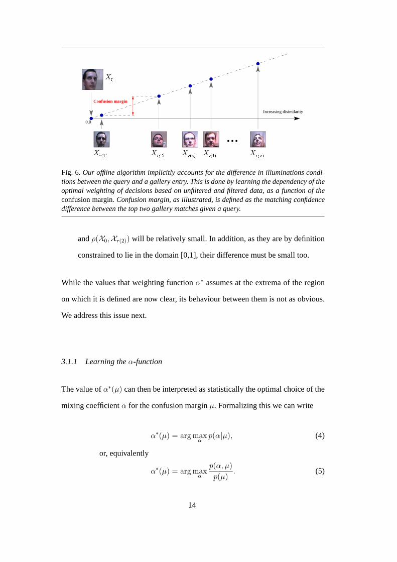
whereµ is theconfusion margin. We define the confusion margin as the difference

between the similarities of the query dataX0 and the two gallery individualsXi

most similar to it. Formally, ifr(i) is the index of thei-th best match forX0 using

the similarity functionρ:

µ = ρ(X0,Xr(1))− ρ(X0,Xr(2)), (3)

as illustrated in Figure 6. Intuitively, given a sensible similarity functionρ, the

confusion margin quantifies the confidence that the top ranking match using un-

processed imagery is indeed the correct one. To see why this is the case, let us

consider the two extreme cases, when query data and the corresponding gallery

data are acquired in (i) the same illumination conditions, and (ii) extremely differ-

ent illumination conditions.

i Same illumination conditions

In this case, the similarity of the query data and the corresponding gallery data

is nearly perfect (close to 1.0) and the correct match by identity is retrieved

first. We can then write|1 − ρ(X0,Xr(1))| ¿ |1 − ρ(X0,Xr(2))| and from the

definition (3) it is clear that the confusion margin is large.

ii Extremely different illumination conditions

In this case, intrapersonal appearance changes due to illumination will be

greater than interpersonal variations [1], and consequently neither of the top

matches will correspond in identity to the query data. Thus, bothρ(X0,Xr(1))

13

Confusion margin

0.0

(4)rX(3)rX )n(rX

...(2)rX(1)rX

Increasing disimilarity

0X

Fig. 6.Our offline algorithm implicitly accounts for the difference in illuminations condi-tions between the query and a gallery entry. This is done by learning the dependency of theoptimal weighting of decisions based on unfiltered and filtered data, as a function of theconfusion margin. Confusion margin, as illustrated, is defined as the matching confidencedifference between the top two gallery matches given a query.

andρ(X0,Xr(2)) will be relatively small. In addition, as they are by definition

constrained to lie in the domain [0,1], their difference must be small too.

While the values that weighting functionα∗ assumes at the extrema of the region

on which it is defined are now clear, its behaviour between them is not as obvious.

We address this issue next.

3.1.1 Learning theα-function

The value ofα∗(µ) can then be interpreted as statistically the optimal choice of the

mixing coefficientα for the confusion marginµ. Formalizing this we can write

α∗(µ) = arg maxα

p(α|µ), (4)

or, equivalently

α∗(µ) = arg maxα

p(α, µ)

p(µ). (5)

14

Under the assumption of a uniform prior on the confusion margin,p(µ)

p(α|µ) ∝ p(α, µ), (6)

and

α∗(µ) = arg maxα

p(α, µ). (7)

Thus, the problem of inferring the optimal weighting functionα∗ is in fact reduced

to the estimation of a 2D probability density function.

Proposed methodology To learn theα-functionα∗(µ) as defined in (4), we first

need an estimatep(α, µ) of the joint probability densityp(α, µ) as per (7). The

main difficulty of this problem is of practical nature: in order to obtain an accu-

rate estimate using one of the many off-the-shelf density estimation techniques, a

prohibitively large training database would be needed to ensure a well sampled dis-

tribution. Instead, we propose a heuristic alternative which, we will show, allows

us to do this from a small offline training corpus which comprises individuals im-

aged in various illumination conditions. It is important to emphasize that this data

is used only for the purpose of estimating theα-function and has no relation (or

rather, need not have any) to the set of gallery individuals. This logical separation

of training data and the fact that offline training needs to be performed only once,

means on the one hand (i) that we can collect an offline corpus containing represen-

tative lighting variation, while on the other (ii) allowing us to perform recognition

with both gallery and query data acquired in a single arbitrary illumination condi-

tion each.

The key idea that makes it possible for us to accurately estimatep(α, µ) while dras-

tically reducing the amount of offline training data, lies in the use of domain spe-

15

cific knowledge of the properties ofp(α, µ), employed to constrain the estimation

process. Our algorithm is based on an iterative incremental update of the density,

initialized as a uniform density over a discrete grid on the domainα, µ ∈ [0, 1], as

in Figure 8. Then, using the offline data corpus, we iteratively simulate matching of

an “unknown”, query person against a set of provisional gallery individuals which

are randomly drawn from the offline training database.

An iteration Specifically, in each iteration we randomly chooseY0, i.e. a particu-

lar individual in a specific illumination which serves as a query, and similarly, a set

of individuals{Y1, . . . ,YM} which in the simulation have the role of gallery data.

Using the similarity metricρ() and the filterF (), we can compute the similarity

betweenY0 and eachYi, which also gives us the value of the confusion marginµ,

as well as the similarity betweenF (Y0) and eachF (Yi). The combined similarity

scoreη(Y0,Yi) is then computed for each possible value ofα or, remembering that

alpha is restricted to a discrete gridα = k∆α, for each value ofk ∈ [0..1/∆α]:

ηi ≡ η(Y0,Yi) = k∆αρ(Y0,Yi) + (1− k∆α)ρ(F (Y0), F (Yi)) (8)

Since the ground truth identities of all persons in the offline database are known, we

can quantify how well a particular value ofα performed by considering the result-

ing similarity ηc of Y0 and the correct match amongst the{Yi}, and the similarity

ηr(1) of Y0 and the individual actually deemed most similar in (8),Yr(1). The greater

the ratioηc/ηr(1), the better the choice ofα is. Densityp(α, µ) is then incremented

proportionally toηc/ηr(1) to reflect higher confidence in the particular value ofα

for the observedµ.

The proposed offline learning algorithm is summarized using pseudo-code in Fig-

16

ure 7 with a typical evolution ofp(α, µ) shown in Figure 8. The final stage of the

offline learning in our method involves imposing the monotonicity constraint on

α∗(µ) and smoothing of the result, see Figure 9.

On the fusion constraints As a final theoretical point, we wish to discuss the

space of functions that our fusion is constrained to by the equation (1) and the

proposed algorithm for learning the mixing functionα∗.

On the surface, (1) appears to be a linear combination of similarities of unpro-

cessed and filtered data,ρ(X0,Xi) andρ(F (X0), F (Xi)). However, it is important

to recognize thatα∗ is not constant but rather a function of the confusion margin

µ, which itself is by definition dependent onρ(X0,X1), . . . , ρ(X0,XN). On the one

hand, this observation makes rigourous theoretical analysis very difficult but, on the

other, provides the functional flexibility that is necessary given that no assumptions

are made on the form ofρ. Put differently, any monotonically non-decreasing func-

tion of ρ could be substituted forρ, since this transformation would only affect the

the magnitudeof the confusion margin, but not the gallery orderingr(i) in (3). As

a consequence, assuming adequate training data and noting the non-parametric na-

ture of the proposed algorithm for the estimation ofα∗, our fusion algorithm would

still converge to the effectively same solution for the fusionη.

17

Input : training dataD(person, illumination),

filtered dataF (person, illumination),

similarity functionρ.

Output : estimatep(α, µ).

1: Initialization

p(α, µ) = 0

2: Simulated matching iteration

for all illuminationsi, j and personsp

3: Confusion margin

µ = ρ(D(p, i), D(r1, j))− ρ(D(p, i), D(r2, j))

4: Iteration

for all k = 0, . . . , 1/∆α, α = k∆α

5: Quantify performance of α

δ(k∆α) = αρ(D(p,i),D(p,j))+(1−α)ρ(F (p,i),F (p,j))maxp6=q [αρ(D(p,i),D(q,j))+(1−α)ρ(F (p,i),F (q,j))]

6: Update density estimate

p(k∆α, µ) = p(k∆α, µ) + δ(k∆α)

7: Smooth the output

p(α, µ) = p(α, µ) ∗Gσ=0.05

8: Normalize to unit integral

p(α, µ) = p(α, µ)/∫α

∫µ p(α, µ)dµdα

Fig. 7. A summary of the main part of the proposed offline training algorithm used toestimate the joint probability density functionp(α, µ). Note that for the reasons of clarityand brevity, at places a somewhat different notation is used in the pseudo-code above fromthat in the main text; please refer to the algorithm header.

18

0

0.2

0.4

0.6

0.8

1

00.2

0.40.6

0.81

−1

−0.5

0

0.5

1

1.5

(a) Initialization

0

0.2

0.4

0.6

0.8

1

00.2

0.40.6

0.81

0

0.2

0.4

0.6

0.8

1

1.2

x 10−3

(b) Iteration 100

0

0.2

0.4

0.6

0.8

1

00.2

0.40.6

0.81

0

2

4

6

8

x 10−4

(c) Iteration 200

0

0.2

0.4

0.6

0.8

1

00.2

0.40.6

0.81

0

2

4

6

8

x 10−4

(d) Iteration 300

0

0.2

0.4

0.6

0.8

1

00.2

0.40.6

0.81

0

2

4

6

8

x 10−4

(e) Iteration 400

0

0.2

0.4

0.6

0.8

1

00.2

0.40.6

0.81

0

2

4

6

8

x 10−4

(f) Iteration 500

Fig. 8.The estimate of the joint densityp(α, µ) through 500 iterations for a band-pass filterused for the evaluation of the proposed framework in Section 4.1.

19

0 0.2 0.4 0.6 0.8 10

0.1

0.2

0.3

0.4

0.5

0.6

0.7

0.8

0.9

1

Confusion margin µ

α−fu

nctio

n α* (µ

)

(a) Rawα∗(µ) estimate

0 0.2 0.4 0.6 0.8 10

0.1

0.2

0.3

0.4

0.5

0.6

0.7

0.8

0.9

1

Confusion margin µ

α−fu

nctio

n α* (µ

)

(b) Monotonicα∗(µ) estimate

0 0.2 0.4 0.6 0.8 10

0.1

0.2

0.3

0.4

0.5

0.6

0.7

0.8

0.9

1

Confusion margin µ

α−fu

nctio

n α* (µ

)

(c) Final smooth and monotonicα∗(µ)

0

0.2

0.4

0.6

0.8

1

00.2

0.40.6

0.81

0

0.2

0.4

0.6

0.8

1

x 10−3

Confusion margin µ

Mixing parameter α

(d) Alpha density mapP (α, µ)

Fig. 9.Typical estimates of theα-function plotted against confusion marginµ. The estimateshown was computed using 40 individuals in 5 illumination conditions for a Gaussianhigh-pass filter. As expected,α∗ assumes low values for small confusion margins and highvalues for large confusion margins (see(1)).

4 Empirical evaluation

In the preceding sections we dealt with theoretical aspects of the proposed frame-

work. To empirically test the main premises of our work and the effectiveness of

the described methodology, we evaluated its performance on 1662 video sequences

of head motion, as well as 650 still images, collected from five databases totalling

333 individuals:

20

Cambridge Face Database (CamFace),with 100 individuals of varying age and

ethnicity, and equally represented genders. For each person in the database we

collected 7 video sequences of the person in arbitrary motion (significant trans-

lation, yaw and pitch, negligible roll), each in a different multiple light source

illumination setting, see Figure 10 (a) and 11, at 10fps and320× 240 pixel res-

olution (face size≈ 60 pixels)1 .

Toshiba Face Database (ToshFace),kindly provided to us by Toshiba Corp. This

database contains 60 individuals of varying age, mostly male Japanese, and 10

sequences per person. Each sequence corresponds to a different multiple light

source illumination setting, at 10fps and320 × 240 pixel resolution (face size

≈ 60 pixels), see Figure 10 (b).

Face Video Database,freely available fromhttp://synapse.vit.iit.nrc.

ca/db/video/faces/cvglab and described in [32]. Briefly, it contains 11

individuals and 2 sequences per person, little variation in illumination, but ex-

treme and uncontrolled variations in pose and motion, acquired at 25fps and

160× 120 pixel resolution (face size≈ 45 pixels), see Figure 10 (c).

Faces96,the most challenging subset of the University of Essex face database,

freely available fromhttp://cswww.essex.ac.uk/mv/allfaces/faces96.

html . It contains 152 individuals, most 18–20 years old and a single 20-frame

sequence per person in196 × 196 pixel resolution (face size≈ 80 pixels). The

users were asked to approach the camera while performing arbitrary head mo-

tion. Although the illumination throughout each sequence, there is some vari-

1 A thorough description of the University of Cambridge face database with examples ofvideo sequences is available athttp://mi.eng.cam.ac.uk/ ∼oa214/ .

21

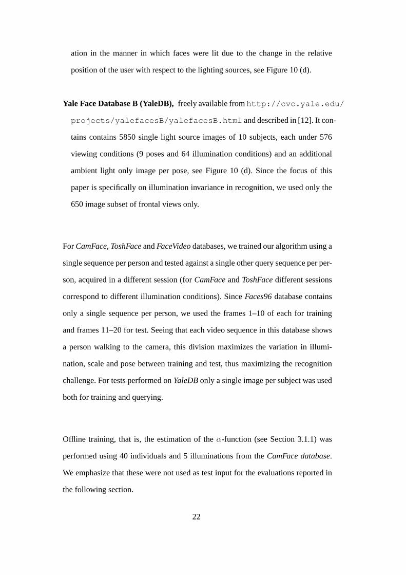
ation in the manner in which faces were lit due to the change in the relative

position of the user with respect to the lighting sources, see Figure 10 (d).

Yale Face Database B (YaleDB),freely available fromhttp://cvc.yale.edu/

projects/yalefacesB/yalefacesB.html and described in [12]. It con-

tains contains 5850 single light source images of 10 subjects, each under 576

viewing conditions (9 poses and 64 illumination conditions) and an additional

ambient light only image per pose, see Figure 10 (d). Since the focus of this

paper is specifically on illumination invariance in recognition, we used only the

650 image subset of frontal views only.

ForCamFace, ToshFaceandFaceVideodatabases, we trained our algorithm using a

single sequence per person and tested against a single other query sequence per per-

son, acquired in a different session (forCamFaceandToshFacedifferent sessions

correspond to different illumination conditions). SinceFaces96database contains

only a single sequence per person, we used the frames 1–10 of each for training

and frames 11–20 for test. Seeing that each video sequence in this database shows

a person walking to the camera, this division maximizes the variation in illumi-

nation, scale and pose between training and test, thus maximizing the recognition

challenge. For tests performed onYaleDBonly a single image per subject was used

both for training and querying.

Offline training, that is, the estimation of theα-function (see Section 3.1.1) was

performed using 40 individuals and 5 illuminations from theCamFace database.

We emphasize that these were not used as test input for the evaluations reported in

the following section.

22

(a) Cambridge Face Database

(b) Toshiba Face Database

(c) Face Video Database

(d) Faces 96 Database

(e) Yale Database

Fig. 10.Representative samples from the five data sets used for evaluation in this paper;(a)-(d) are collections of video sequences and the frames shown for each are from a singlesequence, while for (e) we show a cross section through the illumination variation presentin the data set.

23

(a) CamFace

(b) ToshFace

Fig. 11.An illustration of variation of lighting conditions in our databases. Shown are 2faces lit with (a) illuminations 1–7 from database FaceDB100 and (b) illuminations 1–10from database FaceDB60. It is important to emphasize that the actual appearance effects ofthe same illumination setup were different between different individuals (or even betweendifferent session of the same individual) due to ad lib chosen body position with respect tothe mounted camera.

Data acquisition. The discussion so far focused on recognition using fixed-scale

face images. For all video-based databases we used a cascaded detector [33] for

localization of faces across scale in cluttered images. The detector was trained using

roughly roughly fronto-parallel views. Detected faces were rescaled to the unform

resolution of50× 50 pixels.

Although the cascaded face detector was successful onYaleDBas well, we decided

on a different approach to data extraction. Specifically, we manually localized the

24

centres of eyes and the mouth, and then affine registered all faces to the same ge-

ometric frame (as in e.g.[18]). This was done because unlike in the other four data

sets, inYaleDBpose was strictly controlled for each subject but not between sub-

jects. Since our face detector is not rotation invariant, there would have been a

possibility of learning to discriminate between poses, rather than individuals them-

selves.

Methods and representations. The proposed framework was evaluated using the

following filters (illustrated in Figure 12):

• Gaussian high-pass filtered images [18] [28] (HP):

F1(X) ≡ XH = X− (X ∗Gσ=1.5), (9)

• local intensity-normalized high-pass filtered images – similar to the Self-Quotient

Image [19] (QI):

F2(X) ≡ XQ = XH ./ XL ≡ XH ./ (X−XH), (10)

the division being element-wise,

• distance-transformed edge map [10] [34] (ED):

F3(X) ≡ XED =DistanceTransform[XE

](11)

≡ DistanceTransform[Canny(X)

], (12)

• Laplacian-of-Gaussian [1] (LG):

F4(X) ≡ XL = X ∗ ∇Gσ=3, (13)

25

RW HP QI ED LG DX DY

Fig. 12. Examples of the evaluated face representations: raw greyscale input (RW),high-pass filtered data (HP), the Quotient Image (QI), distance-transformed edge map(ED), Laplacian-of-Gaussian filtered data (LG) and the two principal axis derivatives (DXand DY).

where∗ denotes convolution, and

• directional grey-scale derivatives [1] [20] (DX, DY):

F5(X) ≡Xx = X ∗ ∂

∂xGσx=3 (14)

F6(X) ≡Xy = X ∗ ∂

∂yGσy=3. (15)

Video sequence matching For baseline classification on the video-based databases,

we used twocanonical correlations-based [35] [36] methods which have gained

considerable attention in recent literature on face recognition from video. These

are:

• Mutual Subspace Method (MSM)of Yamaguchi and Fukui [30], and

• Constrained MSM (CMSM)[30] used in a state-of-the-art commercial system

FacePassr [37].

These were chosen as fitting the main premise of the paper, due to their efficiency,

numerical stability and generalization robustness [38]. We now briefly summarize

the procedure in which the two methods were used for matching.

26

We represent each face image as a raster-ordered pixel array, and each sequence of

detected faces as a data matrixd ∈ RD×N , each column corresponding to a single

image. Principal Component Analysis (PCA) of the cross-correlation matrixC =

ddT is used to extract the main modes of appearance variation, as the eigenvectors

corresponding to the largest eigenvalues. Note that PCA was appliedwithoutmean

subtraction. We used 6D subspaces, as sufficiently expressive to on average explain

over 90% of data variation within intrinsically low-dimensional face appearance

changes within a set.

In MSM, the similarity between two subspaces (each corresponding to a face mo-

tion video sequencedi) is computed as the mean of the first 3 principal correlations

ω1...3 between them:

ρ(di,dj) =1

3

∑

k=1...3

ωk (16)

If Bi andBj are orthonormal basis matrices corresponding to the subspaces, then

writing the Singular Value Decomposition (SVD) of the matrixBTi Bj:

M = BTi Bj = UΣVT . (17)

Thek-th canonical correlationωk is then given by thek-th singular value ofM i.e.

Σk,k, and thek-th pair of principal vectorsuk andvk by, respectively,BiU and

BjV [39], see Figure 13. In CMSM, the computation of canonical correlations is

preceded with linear projection of the two subspaces to theConstraint Subspace,

see the original publication for more detail [30]. In our empirical evaluation, we

estimate the Constraint Subspace using gallery training data.

27

QI ED LGRW HP DX DY

(a)

(b)

(c)

Fig. 13. (a) The first pair of principal vectors (top and bottom) corresponding to the se-quences (b) and (c) (every 4th detection is shown for compactness), for each of the 7 rep-resentations used in the empirical evaluation described in this paper. A higher degree ofsimilarity between the two vectors indicates a greater degree of illumination invariance ofthe corresponding filter.

28

Still image matching Since pose was strictly controlled in this data set, we com-

pared two still images of faces extracted fromYaleDBusing a simple matching

procedure, analogous to that previously employed on video. Ifxi andxj are two

images as raster-ordered pixel arrays, their similarity is computed as the cosine of

the angle between them:

ρ(xi,xj) = xTi xj /|xi||xj| (18)

For brevity, we shall refer to this as the COS distance.

4.1 Results

To establish baseline performance, we performed recognition on all data sets using

raw greyscale data first. A summary is shown in Table 1. As these results illus-

trate,CamFace, ToshFaceandYaleDBwere found to be very challenging, primar-

ily due to extreme variations in illumination between training and query data, as

well within sequences in the case of the former two databases. The performance on

Face VideoandFaces96databases was significantly better. This can be explained

by noting that the first major source of appearance variation present in these sets,

the scale, is normalized for in the data extraction stage; the remainder of the ap-

pearance variation is dominated by pose changes, to which MSM and CMSM are

particularly robust to [40] [38]. This confirms the premise that varying illumination

indeed does represent the main difficulty in achieving robust face recognition when

the data acquisition setup is unconstrained.

Next we evaluated the two methods with each of the 6 filter-based face represen-

tations. The recognition results for theCamFace, ToshFace, Faces96andYaleDB

29

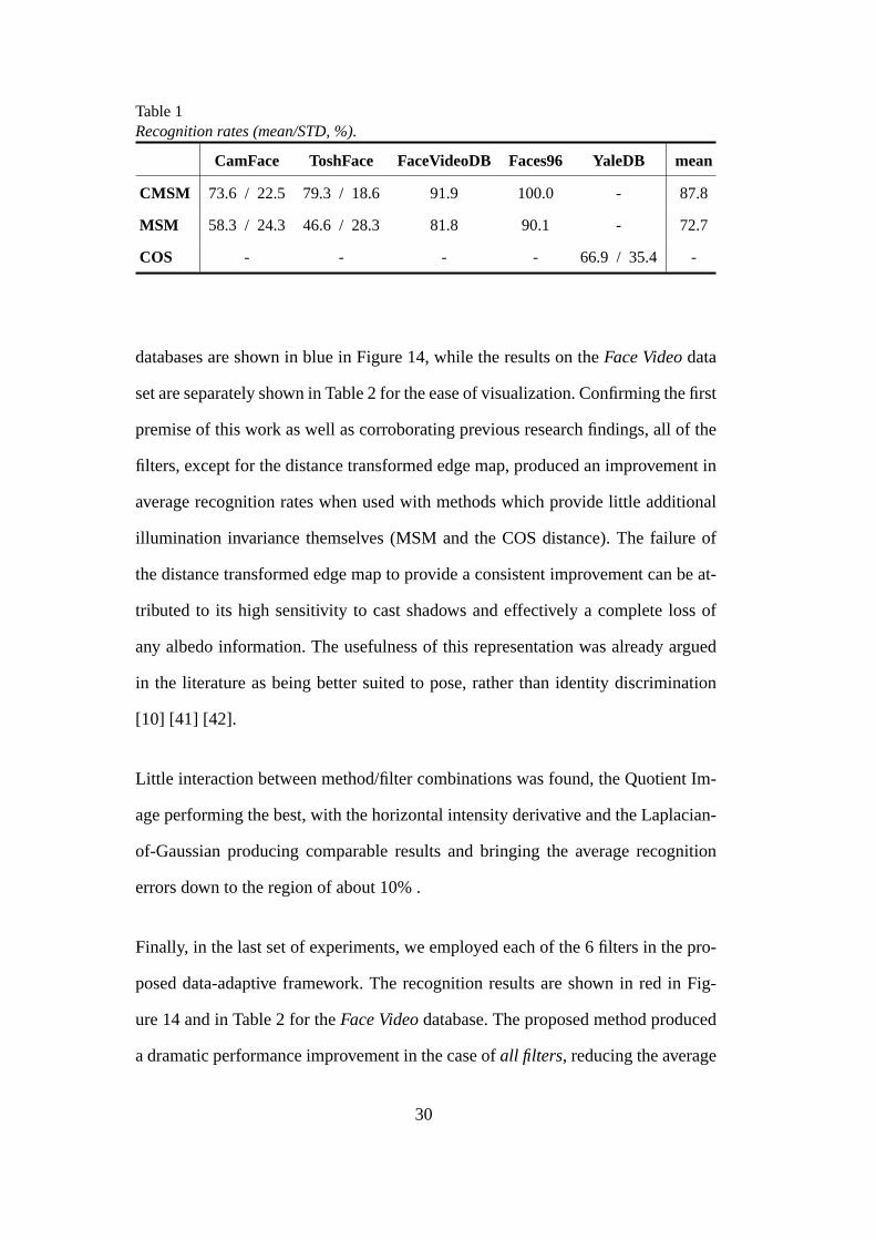
Table 1Recognition rates (mean/STD, %).

CamFace ToshFace FaceVideoDB Faces96 YaleDB mean

CMSM 73.6 / 22.5 79.3 / 18.6 91.9 100.0 - 87.8

MSM 58.3 / 24.3 46.6 / 28.3 81.8 90.1 - 72.7

COS - - - - 66.9 / 35.4 -

databases are shown in blue in Figure 14, while the results on theFace Videodata

set are separately shown in Table 2 for the ease of visualization. Confirming the first

premise of this work as well as corroborating previous research findings, all of the

filters, except for the distance transformed edge map, produced an improvement in

average recognition rates when used with methods which provide little additional

illumination invariance themselves (MSM and the COS distance). The failure of

the distance transformed edge map to provide a consistent improvement can be at-

tributed to its high sensitivity to cast shadows and effectively a complete loss of

any albedo information. The usefulness of this representation was already argued

in the literature as being better suited to pose, rather than identity discrimination

[10] [41] [42].

Little interaction between method/filter combinations was found, the Quotient Im-

age performing the best, with the horizontal intensity derivative and the Laplacian-

of-Gaussian producing comparable results and bringing the average recognition

errors down to the region of about 10% .

Finally, in the last set of experiments, we employed each of the 6 filters in the pro-

posed data-adaptive framework. The recognition results are shown in red in Fig-

ure 14 and in Table 2 for theFace Videodatabase. The proposed method produced

a dramatic performance improvement in the case ofall filters, reducing the average

30

Table 2FaceVideoDB, mean error (%).

RW HP QI ED LG DX DY

MSM 0.00 0.00 0.00 0.00 9.09 0.00 0.00

MSM-AD 0.00 0.00 0.00 0.00 0.00 0.00 0.00

CMSM 0.00 9.09 0.00 0.00 0.00 0.00 0.00

CMSM-AD 0.00 0.00 0.00 0.00 0.00 0.00 0.00

recognition error rate to only 3% in the case of CMSM/Quotient Image combina-

tion. This is a very high recognition rate for such unconstrained conditions (see

Figure 10), small amount of training data per gallery individual and the degree of

illumination variation between training and query data. An improvement in the ro-

bustness to illumination changes can also be seen in the significantly reduced stan-

dard deviation of the recognition, as shown in Figure 14. Finally, it should be em-

phasized that the demonstrated improvement is obtained with a negligible increase

in the computational cost as all time-demanding learning is performed offline.

4.2 Failure modes

In the discussion of failure modes of the described framework, it is necessary to

distinguish between errors introduced by aparticular image processing filter used,

and the fusion algorithm itself. As generally recognized across literature (e.g. see

[1]), qualitative inspection of incorrect recognitions using filtered representations

indicates that the main difficulties are posed by those illumination effects which

most significantly deviate from the underlying frequency model (see Section 2.1)

such as: cast shadows, specularities (especially commonly observed for users with

glasses) and photo-sensor saturation.

31

On the other hand, any failure modes of our fusion framework were difficult to

clearly identify, due to such a low frequency of erroneous recognition decisions.

Even these were in virtually all of the cases due to overly confident decisions in the

filtered pipeline. Overall, this makes the methodology proposed in this paper ex-

tremely promising as a robust and efficient way of matching face appearance image

sets, and suggests that future work should concentrate on developing appropriately

robust image filters that can deal with more complex illumination effects.

5 Conclusions

In this paper we described a novel framework for automatic face recognition in the

presence of varying illumination, primarily applicable to matching face sets or se-

quences. The framework is based on simple image processing filters that compete

with unprocessed greyscale input to yield a single matching score between individ-

uals. By performing all numerically consuming computation offline, our method

both (i) retains the matching efficiency of simple image filters, but (ii) with a greatly

increased robustness, as all online processing is performed in closed-form. Evalu-

ated on a large, real-world data corpus, the proposed framework was shown to be

successful in both video and still image-based recognition across a wide range of

variation in illumination.

As suggested by our experimental results, the main direction for future work is to

develop more robust image processing filters without a great loss of computational

efficiency. Specifically, we are investigating the use of colour invariants and photo-

metric camera models with the aim of achieving unified detection and elimination

of specularities, cast shadows and points of photo-sensor saturation.

32

Acknowledgements

We would like to thank Trinity College Cambridge and the Toshiba Corporation for

their kind support for our research, the volunteers whose face videos were entered

in our face database and Cambridge Commonwealth Trust.

References

[1] Y Adini, Y. Moses, and S. Ullman. Face recognition: The problem of compensatingfor changes in illumination direction.IEEE Transactions on Pattern Analysis andMachine Intelligence (PAMI), 19(7):721–732, 1997.

[2] S. Kong, J. Heo, B. Abidi, J. Paik, and M. Abidi. Recent advances in visual andinfrared face recognition – a review.Computer Vision and Image Understanding(CVIU), 97(1):103–135, 2005.

[3] W. Zhao, R. Chellappa, P. J. Phillips, and A. Rosenfeld. Face recognition: A literaturesurvey.ACM Computing Surveys, 35(4):399–458, 2004.

[4] V. Blanz and T. Vetter. A morphable model for the synthesis of 3D faces.In Proc.Conference on Computer Graphics (SIGGRAPH), pages 187–194, 1999.

[5] S. Romdhani, V. Blanz, and T. Vetter. Face identification by fitting a 3D morphablemodel using linear shape and texture error functions.In Proc. European Conferenceon Computer Vision (ECCV), pages 3–19, 2002.

[6] V. Blanz and T. Vetter. Face recognition based on fitting a 3D morphable model.IEEETransactions on Pattern Analysis and Machine Intelligence (PAMI), 25(9):1063–1074,2003.

[7] D. S. Bolme. Elastic bunch graph matching. Master’s thesis, Colorado StateUniversity, 2003.

[8] C. Kotropoulos, A. Tefas, and I. Pitas. Frontal face authentication using morphologicalelastic graph matching.IEEE Transactions on Image Processing, 9(4):555–560, April2000.

[9] L. Wiskott, J-M. Fellous, N. Kruger, and C. von der Malsburg. Face recognition byelastic bunch graph matching.Intelligent Biometric Techniques in Fingerprint andFace Recognition, pages 355–396, 1999.

[10] O. Arandjelovic and R. Cipolla. Face recognition from video using the generic shape-illumination manifold. In Proc. European Conference on Computer Vision (ECCV),4:27–40, May 2006.

33

[11] P. N. Belhumeur and D. J. Kriegman. What is the set of images of an object under allpossible illumination conditions?International Journal of Computer Vision (IJCV),28(3):245–260, 1998.

[12] A. S. Georghiades, P. N. Belhumeur, and D. J. Kriegman. From few to many:Illumination cone models for face recognition under variable lighting and pose.IEEETransactions on Pattern Analysis and Machine Intelligence (PAMI), 23(6):643–660,2001.

[13] S. Zhou, G. Aggarwal, R. Chellappa, and D. Jacobs. Appearance characterization oflinear lambertian objects, generalized photometric stereo, and illumination-invariantface recognition.IEEE Transactions on Pattern Analysis and Machine Intelligence(PAMI), 29(2):230–245, 2007.

[14] M. Nishiyama and O. Yamaguchi. Face recognition using the classified appearance-based quotient image.In Proc. IEEE International Conference on Automatic Face andGesture Recognition (FGR), pages 49–54, 2006.

[15] T. Riklin-Raviv and A. Shashua. The quotient image: Class based re-rendering andrecognition with varying illuminations.IEEE Transactions on Pattern Analysis andMachine Intelligence (PAMI), 23(2):219–139, 2001.

[16] R. Basri, D. Jacobs, and I. Kemelmacher. Photometric stereo with general, unknownlighting. International Journal of Computer Vision (IJCV), 72(3):239–257, 2007.

[17] S. Romdhani and T. Vetter. Efficient, robust and accurate fitting of a 3D morphablemodel. In Proc. IEEE International Conference on Computer Vision (ICCV), pages59–66, 2003.

[18] O. Arandjelovic and A. Zisserman. Automatic face recognition for film characterretrieval in feature-length films.In Proc. IEEE Conference on Computer Vision andPattern Recognition (CVPR), 1:860–867, June 2005.

[19] H. Wang, S. Z. Li, and Y. Wang. Face recognition under varying lighting conditionsusing self quotient image.In Proc. IEEE International Conference on Automatic Faceand Gesture Recognition (FGR), pages 819–824, 2004.

[20] M. Everingham and A. Zisserman. Automated person identification in video.In Proc.IEEE International Conference on Image and Video Retrieval (CIVR), pages 289–298,2004.

[21] Y. Gao and M. K. H. Leung. Face recognition using line edge map.IEEE Transactionson Pattern Analysis and Machine Intelligence (PAMI), 24(6):764–779, 2002.

[22] B. Takacs. Comparing face images using the modified Hausdorff distance.PatternRecognition, 31(12):1873–1881, 1998.

[23] O. Arandjelovic and R. Cipolla. An illumination invariant face recognition systemfor access control using video.In Proc. IAPR British Machine Vision Conference(BMVC), pages 537–546, September 2004.

[24] S. Shan, W. Gao, B. Cao, and D. Zhao. Illumination normalization for robust facerecognition against varying lighting conditions.In Proc. IEEE International Workshopon Analysis and Modeling of Faces and Gestures, pages 157–164, 2003.

34

[25] C. Garcia, G. Zikos, and G. Tziritas. A wavelet-based framework for face recognition.In Proc. European Conference on Computer Vision (ECCV), pages 1–7, 1998.

[26] B. Kepenekci.Face Recognition Using Gabor Wavelet Transform.PhD thesis, TheMiddle East Technical University, 2001.

[27] P. Jonathon Phillips. Matching pursuit filters applied to face identification.IEEETransactions on Image Processing, 7(8):1150–1164, August 1998.

[28] A. Fitzgibbon and A. Zisserman. On affine invariant clustering and automatic castlisting in movies.In Proc. European Conference on Computer Vision (ECCV), pages304–320, 2002.

[29] B. V. K. Vijayakumar, X. Chunyan, and S. Marios. Correlation filters for largepopulation face recognition .In Proc. SPIE Confeence on Biometric Technology forHuman Identification, 6539, 2007.

[30] K. Fukui and O. Yamaguchi. Face recognition using multi-viewpoint patterns for robotvision. International Symposium of Robotics Research, 2003.

[31] X. Wang and X. Tang. Unified subspace analysis for face recognition.In Proc. IEEEInternational Conference on Computer Vision (ICCV), 1:679–686, 2003.

[32] D. O. Gorodnichy. Associative neural networks as means for low-resolution video-based recognition.In Proc. International Joint Conference on Neural Networks, 2005.

[33] P. Viola and M. Jones. Robust real-time face detection.International Journal ofComputer Vision (IJCV), 57(2):137–154, 2004.

[34] J. Canny. A computational approach to edge detection.IEEE Transactions on PatternAnalysis and Machine Intelligence (PAMI), 8(6):679–698, 1986.

[35] R. Gittins. Canonical Analysis: A Review with Applications in Ecology.Springer-Verlag, 1985.

[36] H. Hotelling. Relations between two sets of variates.Biometrika, 28:321–372, 1936.

[37] Toshiba. Facepass.www.toshiba.co.jp/mmlab/tech/w31e.htm .

[38] T-K. Kim, O. Arandjelovic, and R. Cipolla. Boosted manifold principal angles forimage set-based recognition.Pattern Recognition, 40(9):2475–2484, September 2007.

[39] A. Bjorck and G. H. Golub. Numerical methods for computing angles between linearsubspaces.Mathematics of Computation, 27(123):579–594, 1973.

[40] O. Arandjelovic, G. Shakhnarovich, J. Fisher, R. Cipolla, and T. Darrell. Facerecognition with image sets using manifold density divergence.In Proc. IEEEConference on Computer Vision and Pattern Recognition (CVPR), 1:581–588, June2005.

[41] D. M. Gavrila. Pedestrian detection from a moving vehicle.In Proc. EuropeanConference on Computer Vision (ECCV), 2:37–49, 2000.

[42] B. Stenger, A. Thayananthan, P. H. S. Torr, and R. Cipolla. Filtering using a tree-based estimator.In Proc. IEEE International Conference on Computer Vision (ICCV),2:1063–1070, 2003.

35

RW HP QI ED LG DX DY0

5

10

15

20

25

30

35

40

45

Method

Err

or r

ate,

mea

n (%

)MSMMSM−ADCMSMCMSM−AD

RW HP QI ED LG DX DY0

5

10

15

20

25

Method

Err

or r

ate,

std

(%

)

MSMMSM−ADCMSMCMSM−AD

(a) CamFace

RW HP QI ED LG DX DY0

10

20

30

40

50

60

Method

Err

or r

ate,

mea

n (%

)

MSMMSM−ADCMSMCMSM−AD

RW HP QI ED LG DX DY0

5

10

15

20

25

30

Method

Err

or r

ate,

std

(%

)

MSMMSM−ADCMSMCMSM−AD

(b) ToshFace

RW HP QI ED LG DX DY0

5

10

15

20

25

Method

Err

or r

ate,

mea

n (%

)

MSMMSM−AD

(c) Faces96

RW HP QI ED LG DX DY0

10

20

30

40

50

60

Method

Err

or r

ate,

mea

n (%

)

COSCOS−AD

RW HP QI ED LG DX DY0

5

10

15

20

25

30

35

Method

Err

or r

ate,

mea

n (%

)

COSCOS−AD

(d) YaleDB

Fig. 14.Error rate statistics. The proposed framework (-AD suffix) dramatically improvedrecognition performance on all method/filter combinations, as witnessed by the reductionin both error rate averages and their standard deviations. The results of CMSM on Faces96are not shown as it performed perfectly on this data set.

36