Learning How to Extract Rotation-Invariant and Scale-Invariant Features from Texture Images

Hindawi Publishing CorporationEURASIP Journal on Advances in Signal ProcessingVolume 2008, Article ID 691924, 15 pagesdoi:10.1155/2008/691924

Research ArticleLearning How to Extract Rotation-Invariant andScale-Invariant Features from Texture Images

Javier A. Montoya-Zegarra,1, 2 Joao Paulo Papa,2 Neucimar J. Leite,2

Ricardo da Silva Torres,2 and Alexandre X. Falcao2

1 Computer Engineering Department, Faculty of Engineering, San Pablo Catholic University, Av. Salaverry 301,Vallecito, Arequipa, Peru

2 Institute of Computing, The State University of Campinas, 13083-970 Campinas, SP, Brazil

Correspondence should be addressed to Javier A. Montoya-Zegarra, [email protected]

Received 2 October 2007; Revised 1 January 2008; Accepted 7 March 2008

Recommended by C. Charrier

Learning how to extract texture features from noncontrolled environments characterized by distorted images is a still-open task.By using a new rotation-invariant and scale-invariant image descriptor based on steerable pyramid decomposition, and a novelmulticlass recognition method based on optimum-path forest, a new texture recognition system is proposed. By combining thediscriminating power of our image descriptor and classifier, our system uses small-size feature vectors to characterize textureimages without compromising overall classification rates. State-of-the-art recognition results are further presented on the Brodatzdata set. High classification rates demonstrate the superiority of the proposed system.

Copyright © 2008 Javier A. Montoya-Zegarra et al. This is an open access article distributed under the Creative CommonsAttribution License, which permits unrestricted use, distribution, and reproduction in any medium, provided the original work isproperly cited.

1. INTRODUCTION

An important low-level image feature used in humanperception as well as in recognition is texture. In fact,the study of texture has found several applications rangingfrom texture segmentation [1] to texture classification [2],synthesis [3, 4], and image retrieval [5, 6].

Although various authors have attempted to define whattexture is [7, 8], there still does not exist a commonlyaccepted definition. However, the basic property presentedin every texture consists in a small elementary patternrepeated periodically or quasiperiodically in a given region(pixel neighborhood) [9, 10]. The repetition of those imagepatterns generates some visual cues, which can be identified,for example, as being directional or nondirectional, smoothor rough, coarse or fine, uniform or nonuniform [11, 12].Figures 1–4 show some examples of these types of visual cues.Note that each texture can be associated with one or morevisual cues.

Further, texture images are typically classified as beingeither natural or artificial. Natural textures are related tononman-made objects and among others they include, forexample, brick, grass, sand, and wood patterns. On the other

side, artificial textures are related to man-made objects suchas architectural, fabric, and metal patterns.

Regardless of its classification type, texture images maybe characterized by their variations in scale or directionality.Scale variations imply that textures may look quite differentwhen varying the number of scales. This effect is analogousto increase or decrease the image resolution. The bigger orthe smaller the scales are, the more different the imagesare. This characteristic is related to the coarseness presentedin texture images and can be understood as the spatialrepetition period of the local pattern [13]. Finer textureimages are characterized by small repetition periods, whereascoarse textures present larger repetition periods. In addition,oriented textures may present different principal directionsas the images rotate. This happens because textures are notalways captured from the same viewpoint.

On the other hand, work on texture characterizationcan be divided into four major categories [1, 14]: struc-tural, statistical, model-based, and spectral. For structuralmethods, texture images can be thought as being a set ofprimitives with geometrical properties. Their objective istherefore to find the primitive elements as well as the formalrules of their spatial placements. Example of this kind of

2 EURASIP Journal on Advances in Signal Processing

Figure 1: Directional versus nondirectional visual cues.

Figure 2: Smooth versus rough visual cues.

methods can be found in the works of Julesz [15] andTuceryan [16]. In addition, statistical methods study thespatial gray-level distribution in the textural patterns, so thatstatistical operations can be performed in the distributionsof the local features computed at each pixel in the image.Statistical methods include among others the gray-level co-occurrence matrix [17], second-order spatial averages, andthe autocorrelation function [18]. Further, the objective ofthe model-based methods is to capture the process thatgenerated the texture patterns. Popular approaches in thiscategory include Markov random fields [19, 20], fractal [21],and autoregressive models [22]. Finally, spectral methodsperform frequency analysis in the image signals to revealspecific features. Examples of this may include Law’s [23, 24]and Gabor’s filters [25].

Although many of these techniques obtained goodresults, most of them have not been widely evaluated innoncontrolled environments, which may be characterizedby texture images having (1) small interclass variations,that is, textures belonging to different classes may appearquite similar, especially in terms of their global patterns(coarseness, smoothness, etc.) and the patterns may present(2) image distortions such as rotations or scales. In thissense, texture pattern recognition is a still-open task. Thenext challenge in texture classification should be, therefore,to achieve rotation-invariant and scale-invariant featurerepresentations for noncontrolled environments.

Some of these challenges are faced in this work. Morespecifically, we focus on feature representation and recogni-tion. In feature representation, we wish to emphasize someopen questions, such as how to model the texture images sothat the relevant information is captured despite of the image

Figure 3: Fine versus coarse visual cues.

Figure 4: Uniform versus nonuniform visual cues.

distortions, and how to keep low-dimensional feature vectorsso that texture recognition applications are facilitated, wheredata storage capacity is a limitation. In feature recognition,we wish to choose a technique that handles multiplenonseparable classes with minimal computational time andsupervision. To deal with the challenges in feature extraction,we propose a new texture image descriptor based on steer-able pyramid decomposition, which encodes the relevanttexture information in small-size feature vectors includingrotation-invariant and scale-invariant characterizations. Toaddress the feature recognition requirements, we are usinga novel multiclass object recognition method based on theoptimum-path forest [26].

Roughly speaking, a steerable pyramid is a method bywhich images are decomposed into a set of multiscale, andmultiorientation image subbands, where the basis functionsare directional derivative operators [27]. Our motivation inusing steerable pyramids relies on that, unlike other imagedecomposition methods, the feature coefficients are lessaffected by image distortions. Furthermore, the optimum-path forest classifier is a recent approach that handlesnonseparable classes without the necessity of using boostingprocedures to increase its performance, resulting thus in afaster and more accurate classifier for object recognition.By combining the discriminating power of our imagedescriptor and classifier, our system uses small-size featurevectors to characterize texture images without compromisingoverall classification rates. In this way, texture classificationapplications, where data storage capacity is a limitation, arefurther facilitated.

A previous version of our texture descriptor has beenproposed for texture recognition, using only rotation-

Javier A. Montoya-Zegarra et al. 3

Inputimage

Outputimage

H0 H0

L0 L0B0

B1

Bn

L1

B0

B1

Bn

L1

......

2 2

Figure 5: First-level steerable pyramid decomposition using noriented bandpass filters.

invariant properties [28]. In the present work, the proposeddescriptor has not only rotation-invariant properties, butalso scale-invariant properties. The descriptor with bothproperties was previously evaluated for content-based imageretrieval [29], but this is the first time it is being demon-strated for texture recognition. The optimum-path forestclassifier was first presented in [30] and first evaluated fortexture recognition in [28]. Improvements in its learningalgorithm and evaluation with several data sets have beenmade in [26] for other properties rather than texture.The present work is using this most recent version of theoptimum-path forest classifier for texture recognition. Weare providing more details about the methods, more datasets, and a more in deep analysis of the results: rotation-and scale-invariance analyses, accuracy of classification withdifferent descriptors, and the mean computational time ofthe proposed system.

The outline of this work is as follows. In Section 2, webriefly review the fundamentals of the steerable pyramiddecomposition. Section 3 describes how texture imagesare characterized to obtain rotation-invariant and scale-invariant representations. Section 4 describes the optimum-path forest classifier method. The experimental setup con-ducted in our study is presented in Section 5. In Section 6,experimental results on several data sets are presentedand used to demonstrate the recognition accuracy of oursystem. Comparisons with state-of-the-art texture featurerepresentations and classifiers are further discussed. Finally,some conclusions are drawn in Section 7.

2. STEERABLE PYRAMID DECOMPOSITION

The steerable pyramid decomposition is a linear multireso-lution image decomposition method by which an image issubdivided into a collection of subbands localized at differentscales and orientations [27]. Using a high- and low-passfilter (H0, L0) the input image is initially decomposed intotwo subbands: a high- and a low-pass subband, respectively.Further, the low-pass subband is decomposed into K-oriented band-pass portions B0, . . . ,BK−1, and into a low-pass subband L1. The decomposition is done recursively bysubsampling the lower low-pass subband (LS) by a factor of2 along the rows and columns. Each recursive step capturesdifferent directional information at a given scale. Consider-

ing the polar-separability of the filters in the Fourier domain,the first low- and high-pass filters, are defined as [31]

L0(r) = L(r/2)2

,

H0(r) = H(r

2

),

(1)

where r, θ are the polar frequency coordinates. The raisedcosine low- and high-pass transfer functions denoted as L,H , respectively, are computed as follows:

L(r) =

⎧⎪⎪⎪⎪⎪⎪⎨⎪⎪⎪⎪⎪⎪⎩

2 r ≤ π

4,

2cos(π

2log2

(4rπ

))π

4< r <

π

2,

0 r ≥ π

2,

Bk(r, θ) = H(r)Gk(θ), k ∈ [0,K − 1].

(2)

Bk(r, θ) represents the kth directional bandpass filter usedin the iterative stages, with radial and angular parameters,defined as

H(r) =

⎧⎪⎪⎪⎪⎪⎪⎨⎪⎪⎪⎪⎪⎪⎩

1 r ≥ π

2,

cos(π

2log2

(2rπ

))π

4< r <

π

2,

0 r ≤ π

4

Gk(θ) =

⎧⎪⎪⎨⎪⎪⎩αK

(cos(θ − πk

K

))K−1 ∣∣∣∣θ − πk

K

∣∣∣∣ < π

2,

0 otherwise,

(3)

where αk= 2(k−1)((K − 1)!/√K[2(K − 1)]!).

Figure 5 depicts a steerable pyramid decompositionusing only one scale and n orientations.

3. TEXTURE FEATURE REPRESENTATION

This section describes the proposed modification of steerablepyramid decomposition to obtain rotation-invariant andscale-invariant representations, used further to characterizethe texture images.

3.1. Texture representation

Roughly speaking, texture images can be seen as a setof basic repetitive primitives characterized by their spatialhomogeneity [32]. By applying statistical measures, thisinformation is extracted and used to capture the relevantimage content into feature vectors. More precisely, byconsidering the presence of homogeneous regions in textureimages, we use the mean (μmn) and standard deviation (σmn)of the energy distribution of the filtered images (Smn). Givenan image I(x, y), its steerable pyramid decomposition isdefined as

Smn(x, y) =∑x1

∑y1

I(x1, y1

)Bmn

(x − x1, y − y1

), (4)


where Bmn denotes the directional bandpass filters at stagem = 0, 1, . . . , S − 1 and orientation n = 0, 1, . . . ,K − 1. Theenergy distribution (E(m,n)) of the filtered images at scale mand at orientation n is defined as

E(m,n) =∑x

∑y

∣∣Smn(x, y)∣∣. (5)

Additionally, the mean (μmn) and standard deviation(σmn) of the energy distributions are found as follows:

μmn = 1MN

Emn(x, y),

σmn =√√√√ 1MN

∑x

∑y

(∣∣Smn(x, y)∣∣− μmn

)2,

(6)

where M and N denote the height and width of the input

image, respectively. The corresponding feature vector (�f ) isdefined by using the mean and standard deviation as featureelements. It is denoted as

�f = [μ00, σ00,μ01, σ01, . . . ,μS−1K−1, σS−1K−1]. (7)

The dimensionality of the feature vectors depends on thenumber of scales (S) and on the number of orientations (K)considered during image decomposition. The feature vectordimensionality is computed by multiplying the number ofscales and orientations by factor of 2 (2× S×K). This factorcorresponds to the mean and standard deviation computedin each filtered image.

3.2. Rotation-invariant representation

Rotation-invariant representation is achieved by computingthe dominant orientation of the texture images followed byfeature alignment. The dominant orientation (DO) is definedas the orientation with the highest total energy across thedifferent scales considered during image decomposition [33].It is computed by finding the highest accumulated energyfor the K different orientations considered during imagedecomposition:

DOi = max{E(R)

0 ,E(R)1 , . . . ,E(R)

K−1

}, (8)

where i is the index where the dominant orientationappeared and

E(R)n =

S−1∑m=0

E(m,n), n = 0, 1, . . . ,K − 1. (9)

Note that each E(R)n covers a set of filtered images at

different scales but at same orientation.Finally, rotation-invariance is obtained by shifting circu-

larly feature elements within the same scales, so that firstelements at each scale correspond to dominant orientations.

As an example, let �f be a feature vector obtained by usinga pyramid decomposition with S = 2 scales and K = 3orientations:

�f = [μ00, σ00,μ01, σ01,μ02, σ02;μ10, σ10,μ11, σ11,μ12, σ12].

(10)

Now suppose that the dominant orientation appears at indexi = 1 (DOi=1), thus the rotation-invariant feature vector,after feature alignment, is represented as follows:

�f R = [μ01, σ01,μ02, σ02,μ00, σ00;μ11, σ11,μ12, σ12,μ10, σ10].

(11)

3.3. Scale-invariant representation

Similarly, scale-invariant representation is achieved by find-ing the scale with the highest total energy across thedifferent orientations (dominant scale). For this purpose, thedominant scale (DS) at index i is computed as follows:

DSi = max{E(S)

0 ,E(S)1 , . . . ,E(S)

S−1

}, (12)

where E(S)m denotes the accumulated energies across the S

different scales:

E(S)m =

K−1∑n=0

E(m,n), m = 0, 1, . . . , S− 1. (13)

Note that each E(S)m covers a set of filtered images at

different orientations for each scale. As an example, let �fbe, again, the feature vector obtained by using a pyramiddecomposition with S = 2 scales and K = 3 orientations:

�f = [μ00, σ00,μ01, σ01,μ02, σ02μ10, σ10,μ11, σ11,μ12, σ12].(14)

By supposing that the dominant scale was found at indexi = 1 (second scale in the image decomposition), its scale-invariant version, after feature alignment, is defined as

�f S = [μ10, σ10,μ11, σ11,μ12, σ12;μ00, σ00,μ01, σ01,μ02, σ02].

(15)

For both rotation-invariant and scale-invariant repre-sentations, the feature alignment process is based on theassumption that to classify textures, images should be rotatedso that their dominant orientations/scales are the same.Further, it has been proved that image rotation in spatialdomain is equivalent to circular shift of feature vectorelements [34].

4. TEXTURE FEATURE RECOGNITION

This section aims to describe the most recent version ofthe optimum-path forest (OPF) classifier [26], which is animportant part of the texture recognition system proposedin this work. Previous works have demonstrated that OPFcan be more effective and much faster than artificial neuralnetworks [35] and support vector machines [26, 30, 35].The OPF approach works by modeling the patterns as beingnodes of a graph in the feature space, where every pair of


INPUT: A λ -labeled training set Z1, prototypes Ω ⊂ Z1

and the pair (v,d) for feature vector and distancecomputations.

OUTPUT: Optimum-path forest P, cost map C and label mapL.

AUXILIARY: Priority queue Q and cost variable cst.1. For each s ∈ Z1 \Ω, set C(s) ← +∞.2. For each s ∈ Ω, do3. C(s) ← 0, P(s) ← nil, L(s) ← λ(s), and insert s in Q.4. While Q is not empty, do5. Remove from Q a sample s such that C(s) is minimum.6. For each t ∈ Z1 such that t /=s and C(t) > C(s), do7. Compute cst ← max{C(s),d(s, t)}.8. If cst < C(t), then9. If C(t) /= +∞, then remove t from Q.10. P(t) ← s, L(t) ← L(s), C(t) ← cst,11. and insert t in Q.

Algorithm 1: OPF algorithm.

nodes is connected by an arc (complete graph). This classifiercreates a discrete optimal partition of the feature spacesuch that any unknown sample can be classified accordingto this partition. This partition is an optimum-path forestcomputed in Rn by the image foresting transform (IFT)algorithm [36]. The OPF classifier extends the IFT from theimage domain to the feature space, where the samples maybe images, contours, or any other abstract entities.

Let Z1, Z2, and Z3 be, respectively, the training, eval-uation, and test sets with |Z1|, |Z2|, and |Z3| samples,respectively. Let λ(s) be the function that assigns the correctlabel i, i = 1, 2, . . . , c, from class i to any sample s ∈ Z1 ∪Z2 ∪ Z3. Z1 and Z2 are labeled sets used to the design of theclassifier and the unseen set Z3 is used to compute the finalaccuracy of the classifier. Let Ω ⊂ Z1 be a set of prototypes ofall classes (i.e., key samples that best represent the classes).Let v be an algorithm which extracts n attributes (textureproperties) from any sample s ∈ Z1 ∪ Z2 ∪ Z3 and returnsa vector�v(s) ∈ Rn. The distance d(s, t) between two samples,s and t, is the one between their feature vectors �v(s) and �v(t)(e.g., Euclidean or any other valid metric).

Let (Z1,A) be a complete graph whose the nodes arethe samples in Z1. We define a path as being a sequence ofdistinct samples π = 〈s1, s2, . . . , sk〉, where (si, si+1) ∈ A for1 ≤ i ≤ k − 1. A path is said to be trivial if π = 〈s1〉.We assign to each path π a cost f (π) given by a path-costfunction f . A path π is said to be optimum if f (π) ≤ f (π′)for any other path π′, where π and π′ end at the same samplesk. We also denote by π·〈s, t〉 the concatenation of a pathπ with terminus at s and an arc (s, t). The OPF algorithmuses the path-cost function fmax, for the reason explained inSection 4.1,

fmax(〈s〉) =⎧⎨⎩

0 if s ∈ Ω,

+∞ otherwise,

fmax(π·〈s, t〉) = max{fmax(π),d(s, t)

}.

(16)

We can observe that fmax(π) computes the maximumdistance between adjacent samples in π, when π is not atrivial path.

The OPF algorithm assigns one optimum path P∗(s)from Ω to every sample s ∈ Z1, forming an optimum-pathforest P (a function with no cycles which assigns to eachs ∈ Z1 \ Ω, its predecessor P(s) in P∗(s), or a marker nilwhen s ∈ Ω). Let R(s) ∈ Ω be the root of P∗(s) which canbe reached from P(s). The OPF algorithm computes for eachs ∈ Z1, the cost C(s) of P∗(s), the label L(s) = λ(R(s)), andthe predecessor P(s), as follows.

Lines 1–3 initialize maps and insert prototypes in Q.The main loop computes an optimum path from Ω toevery sample s in a nondecreasing order of cost (lines 4–11). At each iteration, a path of minimum cost C(s) isobtained in P when we remove its last node s from Q(line 5). Lines 8–11 evaluate if the path that reaches anadjacent node t through s is cheaper than the current pathwith terminus t and update the position of t in Q, C(t),L(t), and P(t) accordingly. The label L(s) may be differentfrom λ(s), leading to classification errors in Z1. The trainingfinds prototypes with zero classification errors in Z1, asfollows.

4.1. Training phase

We say that Ω∗ is an optimum set of prototypes whenAlgorithm 1 propagates the labels L(s) = λ(s) for every s ∈Z1·Ω∗ can be found by exploiting the theoretical relationbetween minimum-spanning tree (MST) and optimum-pathtree for fmax [37]. The training essentially consists of findingΩ∗ and an OPF classifier rooted at Ω∗.

By computing an MST in the complete graph (Z1,A),we obtain a connected acyclic graph whose nodes are allsamples in Z1 and the arcs are undirected and weighted bythe distance d between the adjacent sample feature vectors.This spanning tree is optimum in the sense that the sum


INPUT: Training and evaluation sets, Z1 and Z2, labeledby λ, number T of iterations, and the pair (v,d)for feature vector and distance computations.

OUTPUT: Learning curve L and the best OPF classifier,represented by the predecessor map P, cost mapC, and label map L.

AUXILIARY: False positive and false negative arrays, FP andFN, of sizes c, and list LM of misclassifiedsamples.

1. For each iteration I = 1, 2, . . . ,T , do2. LM ← ∅

3. Compute Ω∗ ⊂ Z1 as in Section 4.1 and P, L, C4. by Algorithm 1.5. For each class i = 1, 2, . . . , c, do6. FP(i) ← 0 and FN(i) ← 0.7. For each sample t ∈ Z2, do8. Find s∗ ∈ Z1 that satisfies (17).9. If L(s∗) /=λ(t), then10. FP(L(s∗)) ← FP(L(s∗)) + 1.11. FN(λ(t)) ← FN(λ(t)) + 1.12. LM ← LM∪ t.13. Compute L(I) by (20) and save P, L, and C.14. While LM /=∅

15. LM ← LM \ t16. Replace t by randomly objects of the same class17. in Z1, except the prototypes.18. Select the instance P, L, C of highest accuracy.

Algorithm 2: Learning algorithm.

of its arc weights is minimum as compared to any otherspanning tree in the complete graph. In the MST, every pairof samples is connected by a single path which is optimumaccording to fmax. The optimum prototypes are the closestelements in the MST with different labels in Z1. By removingthe arcs between different classes, their adjacent samplesbecome prototypes in Ω∗ and Algorithm 1 can computean optimum-path forest with zero classification errors inZ1.

It is not difficult to see that the optimum paths betweenclasses should pass through the same removed arcs ofthe minimum-spanning tree. The choice of prototypes asdescribed above blocks these passages, avoiding samplesof any given class to be reached by optimum paths fromprototypes of other classes. Given that several methodsfor graph-based clustering are based on MST, the relationbetween MST and minimum-cost path tree for fmax [37]makes interesting connections among the supervised OPFclassifier, these unsupervised approaches, and the previousworks on watershed-based/fuzzy-connected segmentations[36, 38–43].

4.2. Classification

For any sample t ∈ Z3, the OPF considers all arcs connectingt with samples s ∈ Z1, as if t was part of the graph.Considering all possible paths from Ω∗ to t, we find theoptimum path P∗(t) from Ω∗ and label t with the class

λ(R(t)) of its most strongly connected prototype R(t) ∈ Ω∗.This path can be identified incrementally by evaluating theoptimum cost C(t) as

C(t) = min{max{C(s),d(s, t)}}, ∀s ∈ Z1. (17)

Let the node s∗ ∈ Z1 be the one that satisfies the aboveequation (i.e., the predecessor P(t) in the optimum pathP∗(t)). Given that L(s∗) = λ(R(t)), the classification simplyassigns L(s∗) to t. An error occurs when L(s∗) /= λ(t).

4.3. Learning algorithm

The performance of the OPF classifier improves when theclosest samples from different classes are included in Z1,given that the prototypes will come from them, working assentinels on the boundaries between classes. On the otherhand, the computational time and storage cost increase withthe size of the training set. This section then describes howto improve the OPF performance without increasing thenumber of samples in Z1.

Algorithm 2 is a simple learning procedure, but veryeffective. In each iteration, a set Z1 is used for training andthe classification is performed on Z2. The best prototypes areassumed to be among the misclassified samples of Z2. So, thealgorithm randomly replaces misclassified samples of Z2 bynonprototypes samples of Z1, and training and classificationare repeated during a few iterations. The algorithm outputsa learning curve, which reports the accuracy values of each


OPF’s instance during learning, and the instance with thehighest accuracy (which is usually the last one).

Lines 2–6 perform variable initialization and trainingon Z1. The classification on Z2 is performed in lines 7–12,updating the arrays of false positive and false negative foraccuracy computation (line 13). Misclassified samples of Z2

are stored in a list LM in line 12, and they are replaced bynonprototype samples ofZ1 in lines 14–17. The OPF instancewith the highest accuracy is then selected in line 18.

The accuracy L(I) of a given iteration I , I = 1, 2, . . . ,T ,is measured by taking into account that the classes may havedifferent sizes in Z2 (similar definition is applied for Z3). LetNZ2(i), i = 1, 2, . . . , c, be the number of samples in Z2 fromeach class i. We define

ei,1 = FP(i)∣∣Z2∣∣− ∣∣NZ2(i)

∣∣ ,

ei,2 = FN(i)∣∣NZ2(i)∣∣ , i = 1, . . . , c,

(18)

where FP(i) and FN(i) are the false positives and falsenegatives, respectively. That is, FP(i) is the number ofsamples from other classes that were classified as being fromthe class i in Z2, and FN(i) is the number of samples fromthe class i that were incorrectly classified as being from otherclasses in Z2. The errors ei,1 and ei,2 are used to define

E(i) = ei,1 + ei,2, (19)

where E(i) is the partial sum error of class i. Finally, theaccuracy L(I) of the classification is written as

L(I) = 2c −∑ci=1E(i)

2c= 1−

∑ci=1E(i)

2c. (20)

5. EXPERIMENTS

5.1. Data sets

To evaluate the accuracy of our system, thirteen textureimages obtained from the standard Brodatz database wereselected. Before being digitized, each of the 512×512 textureimages was rotated at different degrees [44]. Figure 6 displaysthe nonrotated version of each of the texture images.

From this database, three different image data setswere generated: nondistorted, rotated-set, and scaled-set. Thenondistorted image data set was constructed from texturepatterns at 0 degrees. Each texture image was partitionedinto sixteen 128× 128 nonoverlapping subimages. Thus, thisdata set comprises 208 (13 × 16) different images. Imagesbelonging to this data set will be used in the learning stageof our classifier. Note that in previous works related totexture recognition [45, 46], rotated or scaled-versions of thepatterns were included in both the training and classificationphases [47]. However, more recently works suggest that therecognition algorithms should perform well, even by havingduring the training phase nondistorted training samples,which means patterns without rotations or scales [48, 49].

The second image data set referred to as rotated-set wasgenerated to evaluate the rotation-invariance capabilities of

our approach. It is further subdivided into two data sets:rotated-set A and rotated-set B. The rotated image data setA was generated by selecting the four 128 × 128 innermostsubimages from texture images at 0, 30, 60, and 120 degrees.A total number of 208 images were generated (13 × 4 × 4).In addition, in the case of the rotated image data set B, weselected the four 128 × 128 innermost subimages of therotated image textures (512 × 512) at 0, 30, 60, 90, 120, 150,and 200 degrees. This led to 364 (13× 4× 7) data set images.The first data set was initially used to test our system underthe presence of few texture oriented images, whereas thesecond one was used to show how our systems performs byincreasing the number of texture oriented images.

On the other side, the scaled image data set was parti-tioned into two data sets: scaled-set A and scaled-set B. Inthe scaled-set A, the 512× 512 nonrotated textures were firstpartitioned into four 256 × 256 nonoverlapping subimages.Each partitioned subimage was further scaled by using fourdifferent factors, ranging from 0.6 to 0.9 with 0.1 interval.This led to 208 (13 × 4 × 4) scaled images. To generatethe scaled-set B, each of the four partitioned subimages wasscaled by using seven different factors, ranging from 0.6 to 1.2with 0.1 interval. In this way, 364 (13× 4× 7) scaled imageswere generated.

5.2. Similarity measure for classification

Similarity between images is obtained by computing thedistance of their corresponding feature vectors (recallSection 3). The smaller the distance, the more similar theimages. Given the query image (i), and the target image ( j) inthe data set, the distance between the two patterns is definedas [50]

d(i, j) =∑m

∑n

dmn(i, j), (21)

where

dmn(i, j) =∣∣∣∣∣μimn − μ

jmn

α(μmn

)∣∣∣∣∣ +

∣∣∣∣∣σimn − σ

jmn

α(σmn

)∣∣∣∣∣, (22)

α(μmn) and α(σmn) denote the standard deviations of therespective features over the entire data set. They are used forfeature normalization purposes.

6. EXPERIMENTAL RESULTS

Three series of experiments were conducted to demonstratethe discriminating power of our system for recognizingtexture patterns. By considering that a recognition system iscomprised of two mainly parts (feature extraction module aswell as feature recognizer module), each of those parts wasevaluated.

In the first series of experiments (Section 6.1), we firstevaluated the effectiveness of the proposed rotation-invariantfeature representation against two other approaches: theconventional pyramid decomposition [51] and with a recentproposal based on Gabor wavelets [33]. To evaluate the effec-tiveness of the feature recognizer module, we compared the


Figure 6: Texture images from the Brodatz data set used in our experiments. From left to right, and from top to bottom, they include Bark,Brick, Bubbles, Grass, Leather, Pigskin, Raffia, Sand, Straw, Water, Weave, Wood, and Wool.

recognition accuracy of the novel OPF multiclass classifieragainst the well-known support vector machines technique.For those purposes, we used the rotated image data sets A andB.

The second series of experiments (Section 6.2) are usedto evaluate the scale-invariant properties in our featureextraction module. Effectiveness of the multiclass recogni-tion method under the presence of scale-invariant featuresare further discussed. Again, we used the conventionalsteerable pyramid decomposition [51] and the Gaborwavelets [50] as references for comparing the scale-invariantproperties of our method. SVMs are used for evaluatingthe classification accuracy of our feature recognizer module.Further, scaled image data sets A and B were used in this setof experiments.

In both series of experiments, we used steerable pyramidshaving different decomposition levels (S = 2, 3, 4) at severalorientations (K = 4, 5, 6, 7, 8). Our experiments agree with

[52] in that the most relevant textural information in imagesis contained in the first two levels of decomposition, sincelittle recognition improvement is achieved by varying thenumber of scales during image decomposition. Therefore,we focus our discussions on image decompositions having(S = 2, 3) scales.

Given that the performance of the OPF classifiercan increase using a third set in a learning algorithm(Section 6.3), we also employed this same procedure to theSVM approach. The constraints in lines 16-17 of Algorithm 2refer to keep the prototypes out of the sample interchangingprocess between Z1 and Z2 for the OPF. We do the samewith the support vectors in SVM. However, they may beselected for interchanging in future iterations if they areno longer prototypes or support vectors. For SVM, weuse the LibSVM package [53] with radial basis function(RBF) kernel, parameter optimization, and the one-versus-one strategy for the multiclass problem to implement line 3.


3S−

8K

3S−

7K

3S−

6K

3S−

5K

3S−

4K

2S−

8K

2S−

7K

2S−

6K

2S−

5K

2S−

4K

S: scaleK : orientation

70

80

90

100

Ave

rage

clas

sifi

cati

onra

te(%

)

Rotation-invariance classification analysis using SVM

Gabor waveletsConventional steerable pyramidProposed method

Figure 7: Classification accuracy comparison using the SVMclassifier obtained in rotated data set A using (S = 2, 3) scales with(K = 4, 5, 6, 7, 8) orientations for Gabor wavelets, conventionalsteerable pyramid decomposition, and our method.

The experiments evaluate the accuracy on Z3 and thecomputational time of each classifier, OPF and SVM. In allexperiments, the data sets were divided into three parts: atraining set Z1 with 20% of the samples, an evaluation setZ2 with 30% of the samples, and a test set Z3 with 50% ofthe samples. These samples were randomly selected and eachexperiment was repeated 10 times with different sets Z1, Z2,and Z3 to compute the mean accuracy.

Recall that an important motivation in our study is touse small-size feature vectors, in order to (1) show that therecognition accuracy of our approach is not compromised,and (2) facilitate texture recognition applications where datastorage capacity is a limitation.

6.1. Effectiveness of the rotation invariancerepresentation

To analyze the texture characterization capabilities of ourfeature extraction method against the conventional pyramiddecomposition and the Gabor wavelets, we used Gaussiankernel support vector machines (SVMs) as texture classi-fication mechanisms (note that the SVM parameters wereoptimized by using the cross-validation method).

Figure 7 compares the recognition accuracy obtainedby those three methods in the rotated data set A, whereasFigure 8 depicts the recognition accuracy obtained in therotated data set B. From both Figures, it can be seenthat our image descriptor outperforms mostly the othertwo approaches, regardless of the number of scales ororientations considered during feature vector extraction.

In the case of the rotated data set A, the higher classifi-cation accuracies achieved by our method were obtained byusing 7 orientations, which corresponds to image rotationsin steps of 25.71◦. By considering two and three decompo-

3S−

8K

3S−

7K

3S−

6K

3S−

5K

3S−

4K

2S−

8K

2S−

7K

2S−

6K

2S−

5K

2S−

4K


70

80

90

100

Ave

rage

clas

sifi

cati

onra

te(%

)

Rotation-invariance classification analysis using SVM


Figure 8: Classification accuracy comparison using the SVMclassifier obtained in rotated data set B using (S = 2, 3) scales with(K = 4, 5, 6, 7, 8) orientations for Gabor wavelets, conventionalsteerable pyramid decomposition, and our method.

sition levels (S = 2, 3), those accuracies are, respectively,100% and 97.31%. The equivalent classification accuraciesobtained by the Gabor wavelets are 90.36% and 93.90%(S = 2, 3; K = 7), whereas for the conventional steerablepyramid those accuracies are 89.67% and 90.36%. Notethat the classification accuracies obtained by using K =6, 7, 8 orientations are very close to each other. Therefore, toguarantee low-dimensionality feature vectors, we set S = 2and K = 6 as the most appropriate parameter combinationsfor our rotation-invariant image descriptor.

In the case of the rotated-set B, the higher classificationaccuracies achieved by our descriptor were again obtainedby using 7 orientations. Classification rates of 95.86% and95.73% correspond respectively to feature vectors withS = 2, 3 scales and K = 7 orientations. Further, it isfound that both Gabor wavelets and conventional steerablepyramid decomposition present lower classification rates,being, respectively, 91.05%, 95.35% for the first method and84.22%, 84.23% for the second one. As stated in the resultsobtained in rotated data set A, the classification accuraciesare very close to each other, when using K = 6, 7 or K = 8orientations. From those results, we can reinforce that themost appropriate parameter settings for our descriptor areS = 2 scales and K = 6 orientations.

Furthermore, from the bar graphs shown in Figures 7and 8, the highest classification rate obtained by the Gabormethod is as good as the one obtained by our descriptor.However, this rate is obtained at S = 3 scales, whereas ourproposed descriptor achieves the same performance usingonly S = 2 scales. In this sense, an important advantage ofour method is its high performance rate at low-size featurevectors.

Our objective now is to demonstrate the recognitionimprovement of our novel classifier over the SVM approach.


3S−

8K

3S−

7K

3S−

6K

3S−

5K

3S−

4K

2S−

8K

2S−

7K

2S−

6K

2S−

5K

2S−

4K


70

80

90

100

Ave

rage

clas

sifi

cati

onra

te(%

)

Rotation-invariance classification analysis using SVM and OPF

Proposed image descriptor with SVMProposed image descriptor with OPF

Figure 9: Classification accuracy comparison using the SVMclassifier obtained in rotated data set A using (S = 2, 3) scales with(K = 4, 5, 6, 7, 8) orientations for Gabor wavelets, conventionalsteerable pyramid decomposition, and our method.

3S−

8K

3S−

7K

3S−

6K

3S−

5K

3S−

4K

2S−

8K

2S−

7K

2S−

6K

2S−

5K

2S−

4K


70

80

90

100

Ave

rage

clas

sifi

cati

onra

te(%

)

Rotation-invariance classification analysis using SVM and OPF


Figure 10: Classification accuracy comparison using the SVMclassifier obtained in rotated data set B using (S = 2, 3) scales with(K = 4, 5, 6, 7, 8) orientations for Gabor wavelets, conventionalsteerable pyramid decomposition, and our method.

From Figure 9 it can be seen, that for almost all featureextraction configurations, the recognition rates of the OPFclassifier are higher than those of the SVM classifier. Thelatter method presents the same recognition rates as theones of the OPF classifier when using S = 2 scales andK = 6, 7 orientations. In the case of the image rotateddata set B, our classifier yields better recognition ratesfor all feature extraction configurations (see Figure 10). Byconsidering that it was found that the most appropriateparameter settings for our descriptor are S = 2 scales

3S−

8K

3S−

7K

3S−

6K

3S−

5K

3S−

4K

2S−

8K

2S−

7K

2S−

6K

2S−

5K

2S−

4K


70

80

90

100

Ave

rage

clas

sifi

cati

onra

te(%

)

Scale-invariance classification analysis using SVM


Figure 11: Classification accuracy comparison using the SVMclassifier obtained in scaled data set A using (S = 2, 3) scales with(K = 4, 5, 6, 7, 8) orientations for Gabor wavelets, conventionalsteerable pyramid decomposition, and our method.

and K = 6 orientations, it is worth to mention that, byusing this configuration, the recognition accuracy obtainedby the OPF classifier is 98.49% in comparison with thecorresponding accuracy of 95.48% obtained by the SVMclassifier.

6.2. Effectiveness of the scale invariancerepresentation

Figures 11 and 12 display the classification accuracy of ourscale-invariant image descriptor against the conventionalpyramid decomposition and the Gabor wavelets in thescaled image data sets A and B, respectively. Those Figuresdemonstrate the classification accuracy improvement of ourimage descriptor over both methods.

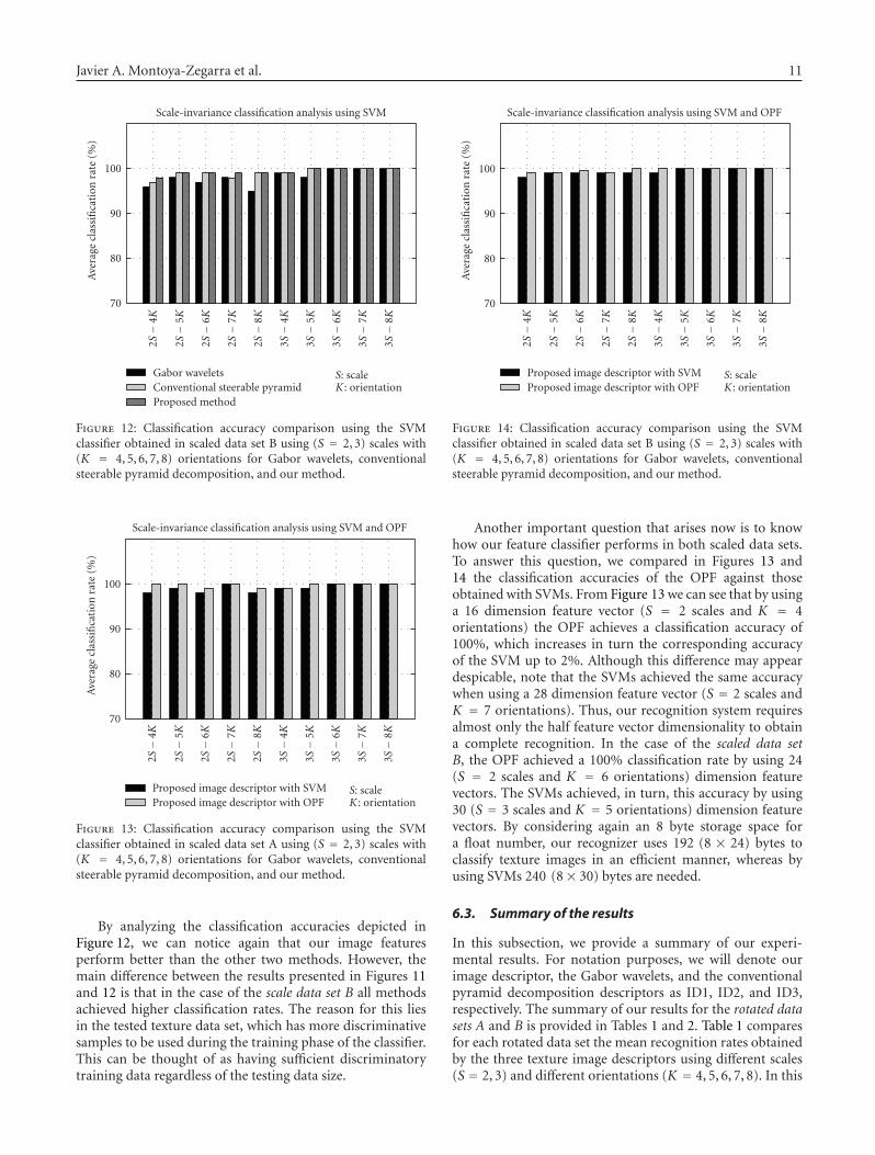
From Figure 11 it can be noticed that by using just S =2 scales and K = 7 orientations, our feature extractionalgorithm achieves a classification rate of 100%. This samerate is achieved by the other two methods, but at the cost ofhaving larger image feature vectors. To obtain a classificationrate of 100%, both pyramid decomposition and Gaborwavelets need at least S = 3 scales. Recalling Section 3.1,the feature vector dimensionality is obtained by multiplyingthe number of scales and orientations by a factor of 2, sincewe considered the mean and standard deviation as featurecomponents. In this way, the dimensionality of our featurevectors is of size of 28 (2 × 2 × 7) elements, in comparisonwith a size of 42 (2×3×7) elements of their analogous featurevectors. By considering that the typical storage space of afloat number is equal to 8 bytes, each of our feature vectorsrequires only 224 bytes to be stored, in comparison with the336 bytes required for their analogous feature vectors. In thisway, our image descriptor requires 66.7% less storage spacethan the one belonging to the compared descriptors.


3S−

8K

3S−

7K

3S−

6K

3S−

5K

3S−

4K

2S−

8K

2S−

7K

2S−

6K

2S−

5K

2S−

4K


70

80

90

100

Ave

rage

clas

sifi

cati

onra

te(%

)

Scale-invariance classification analysis using SVM


Figure 12: Classification accuracy comparison using the SVMclassifier obtained in scaled data set B using (S = 2, 3) scales with(K = 4, 5, 6, 7, 8) orientations for Gabor wavelets, conventionalsteerable pyramid decomposition, and our method.

3S−

8K

3S−

7K

3S−

6K

3S−

5K

3S−

4K

2S−

8K

2S−

7K

2S−

6K

2S−

5K

2S−

4K


70

80

90

100

Ave

rage

clas

sifi

cati

onra

te(%

)

Scale-invariance classification analysis using SVM and OPF


Figure 13: Classification accuracy comparison using the SVMclassifier obtained in scaled data set A using (S = 2, 3) scales with(K = 4, 5, 6, 7, 8) orientations for Gabor wavelets, conventionalsteerable pyramid decomposition, and our method.

By analyzing the classification accuracies depicted inFigure 12, we can notice again that our image featuresperform better than the other two methods. However, themain difference between the results presented in Figures 11and 12 is that in the case of the scale data set B all methodsachieved higher classification rates. The reason for this liesin the tested texture data set, which has more discriminativesamples to be used during the training phase of the classifier.This can be thought of as having sufficient discriminatorytraining data regardless of the testing data size.

3S−

8K

3S−

7K

3S−

6K

3S−

5K

3S−

4K

2S−

8K

2S−

7K

2S−

6K

2S−

5K

2S−

4K


70

80

90

100

Ave

rage

clas

sifi

cati

onra

te(%

)

Scale-invariance classification analysis using SVM and OPF


Figure 14: Classification accuracy comparison using the SVMclassifier obtained in scaled data set B using (S = 2, 3) scales with(K = 4, 5, 6, 7, 8) orientations for Gabor wavelets, conventionalsteerable pyramid decomposition, and our method.

Another important question that arises now is to knowhow our feature classifier performs in both scaled data sets.To answer this question, we compared in Figures 13 and14 the classification accuracies of the OPF against thoseobtained with SVMs. From Figure 13 we can see that by usinga 16 dimension feature vector (S = 2 scales and K = 4orientations) the OPF achieves a classification accuracy of100%, which increases in turn the corresponding accuracyof the SVM up to 2%. Although this difference may appeardespicable, note that the SVMs achieved the same accuracywhen using a 28 dimension feature vector (S = 2 scales andK = 7 orientations). Thus, our recognition system requiresalmost only the half feature vector dimensionality to obtaina complete recognition. In the case of the scaled data setB, the OPF achieved a 100% classification rate by using 24(S = 2 scales and K = 6 orientations) dimension featurevectors. The SVMs achieved, in turn, this accuracy by using30 (S = 3 scales and K = 5 orientations) dimension featurevectors. By considering again an 8 byte storage space fora float number, our recognizer uses 192 (8 × 24) bytes toclassify texture images in an efficient manner, whereas byusing SVMs 240 (8× 30) bytes are needed.

6.3. Summary of the results

In this subsection, we provide a summary of our experi-mental results. For notation purposes, we will denote ourimage descriptor, the Gabor wavelets, and the conventionalpyramid decomposition descriptors as ID1, ID2, and ID3,respectively. The summary of our results for the rotated datasets A and B is provided in Tables 1 and 2. Table 1 comparesfor each rotated data set the mean recognition rates obtainedby the three texture image descriptors using different scales(S = 2, 3) and different orientations (K = 4, 5, 6, 7, 8). In this


Table 1: Mean recognition rates for the three different textureimage descriptors using Gaussian-kernel support vector machinesas classifiers in the rotated data sets A and B.

Rotated Scales (S)/ID1 ID2 ID3

data set orientations (K)

A (S = 2; K = 4,5,6,7,8) 95.89% 93.19% 93.19%

A (S = 3; K = 4,5,6,7,8) 97.99% 92.36% 97.92%

B (S = 2; K = 4,5,6,7,8) 92.30% 85.30% 91.29%

B (S = 3; K = 4,5,6,7,8) 96.70% 85.76% 96.67%

Table 2: Mean recognition rates for the proposed rotation-invariant texture image descriptor using both OPF and SVMclassifiers in the rotated datasets A and B.

Rotated Scales (S)/OPF SVM


A (S = 2; K = 4,5,6,7,8) 98.89% 95.89%

A (S = 3; K = 4,5,6,7,8) 98.61% 97.99%

B (S = 2; K = 4,5,6,7,8) 97.35% 92.30%

B (S = 3; K = 4,5,6,7,8) 96.74% 96.70%

Table 3: Mean recognition rates for the three different textureimage descriptors using Gaussian-kernel support vector machinesas classifiers in the scaled data sets A and B.

Scaled Scales (S)/ID1 ID2 ID3


A (S = 2; K = 4,5,6,7,8) 98.78% 93.19% 97.04%

A (S = 3; K = 4,5,6,7,8) 99.67% 99.66% 96.05%

B (S = 2; K = 4,5,6,7,8) 99.35% 97.12% 99.90%

B (S = 3; K = 4,5,6,7,8) 99.95% 99.83% 99.44%

Table 4: Mean recognition rates for the proposed scale-invarianttexture image descriptor using both OPF and SVM classifiers in thescaled data sets A and B.

Scaled Scales (S)/OPF SVM


A (S = 2; K = 4,5,6,7,8) 99.03% 98.78%

A (S = 3; K = 4,5,6,7,8) 99.89% 99.67%

B (S = 2; K = 4,5,6,7,8) 99.58% 99.35%

B (S = 3; K = 4,5,6,7,8) 100% 99.95%

set of experiments, we used Gaussian-kernel support vectormachines (SVMs) as texture classification mechanisms. Fromour results, it can be noticed that our texture imagedescriptor performs better regardless of the data set used,or the image decomposition parameters considered duringfeature extraction (number of scales and orientations).Furthermore, as it can be seen in Table 2, the OPF classifierimproves the recognition accuracies obtained by the SVMclassifier in all of our experiments. The summarized resultsfor the scale data sets A and B are presented in Tables 3 and4. As we can see, our proposed recognition system performsagain better than the previously mentioned approaches inboth feature extraction and classification tasks.

908070605040302010

Training set percentage (%)

80

85

90

95

100

105

Ave

rage

clas

sifi

cati

onra

te(%

)

OPF rotate-invariance analysis curve for rotated dataset A

Gabor waveletsConventional steerable pyramidProposed image descriptor

Figure 15: Average classification accuracy versus number oftraining samples in rotated data set A.

908070605040302010


80

85

90

95

100

105

Ave

rage

clas

sifi

cati

onra

te(%

)

OPF rotate-invariance analysis curve for rotated dataset B


Figure 16: Average classification accuracy versus number oftraining samples in rotated data set B.

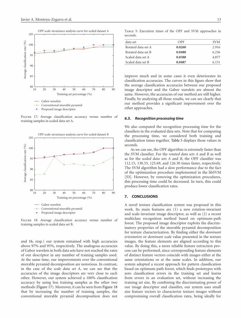
6.4. Training sample classification rates

The achieved performances of our feature classifier usingdifferent number of training samples are shown graphicallyin Figures 15–18. The y-axis denotes the achieved averageclassification rate, whereas the x-axis represents the numberof training samples considered. Each unique line belongsto each of the evaluated image descriptors (Gabor wavelets,conventional steerable pyramid decomposition, and ourmethod). From those Figures we can see that almost allimage descriptors attain reasonably good results even byusing small-dimensional feature vectors (85%+). However,the superiority of our system can be clearly seen. Note thatin the case of the rotated data sets A and B (Figures 15


908070605040302010


80

85

90

95

100

105

Ave

rage

clas

sifi

cati

onra

te(%

)

OPF scale-invariance analysis curve for scaled dataset A


Figure 17: Average classification accuracy versus number oftraining samples in scaled data set A.

908070605040302010


80

85

90

95

100

105

Ave

rage

clas

sifi

cati

onra

te(%

)

OPF scale-invariance analysis curve for scaled dataset B


Figure 18: Average classification accuracy versus number oftraining samples in scaled data set B.

and 16, resp.) our system remained with high accuraciesabove 97% and 95%, respectively. The analogous accuraciesof Gabor wavelets in both data sets have not reached the ratesof our descriptor in any number of training samples used.At the same time, our improvements over the conventionalsteerable pyramid decomposition are notorious. In contrast,in the case of the scale data set A, we can see that theaccuracies of the image descriptors are very close to eachother. However, our system achieved a 100% classificationaccuracy by using less training samples as the other twomethods (Figure 17). Moreover, it can be seen from Figure 18that by increasing the number of training samples, theconventional steerable pyramid decomposition does not

Table 5: Execution times of the OPF and SVM approaches inseconds.

data set OPF SVM

Rotated data set A 0.0260 2.916

Rotated data set B 0.0480 6.256

Scaled data set A 0.0388 4.877

Scaled data set B 0.0487 6.151

improve much and in some cases it even deteriorates itsclassification accuracies. The curves in this figure show thatthe average classification accuracies between our proposedimage descriptor and the Gabor wavelets are almost thesame. However, the accuracies of our method are still higher.Finally, by analyzing all those results, we can see clearly thatour method provides a significant improvement over theother approaches.

6.5. Recognition processing time

We also computed the recognition processing time for theclassifiers in the evaluated data sets. Note that for computingthe processing time, we considered both training andclassification times together. Table 5 displays those values inseconds.

As we can see, the OPF algorithm is extremely faster thanthe SVM classifier. For the rotated data sets A and B as wellas for the scaled data sets A and B, the OPF classifier was112.15, 130.33, 125.69, and 126.30 times faster, respectively.The SVM algorithm had a slow performance due to the factof the optimization procedure implemented in the libSVM[53]. However, by removing the optimization procedures,this processing time could be decreased. In turn, this couldproduce lower classification rates.

7. CONCLUSIONS

A novel texture classification system was proposed in thiswork. Its main features are (1) a new rotation-invariantand scale-invariant image descriptor, as well as (2) a recentmulticlass recognition method based on optimum-pathforest. The proposed image descriptor exploits the discrim-inatory properties of the steerable pyramid decompositionfor texture characterization. By finding either the dominantorientation or dominant scale value presented in the textureimages, the feature elements are aligned according to thisvalue. By doing this, a more reliable feature extraction pro-cess can be performed, since corresponding feature elementsof distinct feature vectors coincide with images either at thesame orientations or at the same scales. In addition, oursystem adopted a recent approach for pattern classificationbased on optimum-path forest, which finds prototypes withzero classification errors in the training set and learnsfrom errors in an evaluation set, without increasing thetraining set size. By combining the discriminating power ofour image descriptor and classifier, our system uses smallsize feature vectors to characterize texture images withoutcompromising overall classification rates, being ideally for


real-time applications or for applications where data storagecapacity is a limitation.

State-of-the-art results on four image data sets derivedfrom the standard Brodatz database were further discussed.For the rotation-invariance evaluation, our method obtaineda mean classification rate of 98.89% in comparison with amean accuracy of 95.89% obtained by using SVMs in therotated data set A. In the case of the rotated data set B, thoserates are 97.35% and 92.30%, respectively. Concerning thescale-invariance evaluation, our system improves classifica-tion rates from 98.78% to 99.03% in the case of the scaleddata set A, whereas in the scaled data set B those rates areimproved from 99.35% to 99.58%.

Further, the OPF multiclass classifier outperformed theSVM in the four data sets. It is a new promising graphtool for pattern recognition, which differs from traditionalapproaches in that it does not use the idea of feature spacegeometry, therefore, better results in overlapped databasesare achieved.

ACKNOWLEDGMENTS

The authors would like to thank CNPq (Grants 302427/2004-0, 134990/2005-6, 477039/2006-5, and 311309/2006-2),Webmaps II CNPq project, FAPESP (Grant 03/14096-8),Microsoft Tablet PC Technology and Higher Educationproject, as well as CAPES/COFECUB (Grant 392/08) fortheir financial support. They would also like to thank theanonymous reviewers for their comments.

REFERENCES

[1] T. R. Reed and J. M. H. Dubuf, “A review of recent texturesegmentation and feature extraction techniques,” CVGIP:Image Understanding, vol. 57, no. 3, pp. 359–372, 1993.

[2] M. Unser, “Texture classification and segmentation usingwavelet frames,” IEEE Transactions on Image Processing, vol. 4,no. 11, pp. 1549–1560, 1995.

[3] B. Balas, “Attentive texture similarity as a categorizationtask: comparing texture synthesis models,” Pattern RecognitionSociety, vol. 41, no. 3, pp. 972–982, 2008.

[4] F. Wu, C. Zhang, and J. He, “An evolutionary system for near-regular texture synthesis,” Pattern Recognition, vol. 40, no. 8,pp. 2271–2282, 2007.

[5] A. W. M. Smeulders, M. Worring, S. Santini, A. Gupta, andR. Jain, “Content-based image retrieval at the end of the earlyyears,” IEEE Transactions on Pattern Analysis and MachineIntelligence, vol. 22, no. 12, pp. 1349–1380, 2000.

[6] Y. Liu, D. Zhang, G. Lu, and W.-Y. Ma, “A survey of content-based image retrieval with high-level semantics,” PatternRecognition, vol. 40, no. 1, pp. 262–282, 2007.

[7] R. M. Pickett, “Visual analyses of texture in the detectionand recognition of objects,” in Picture Processing and Psy-chopictorics, B. C Lipkin and A. Rosenfeld, Eds., pp. 289–308,Academic Press, New York, NY, USA, 1970.

[8] J. K. Hawkins, “Textural properties for pattern recognition,”in Picture Processing and Psychopictorics, B. C. Lipkin and A.Rosenfeld, Eds., pp. 347–370, Academic Press, New York, NY,USA, 1970.

[9] A. K. Jain and K. Karu, “Learning texture discriminationmasks,” IEEE Transactions on Pattern Analysis and MachineIntelligence, vol. 18, no. 2, pp. 195–205, 1996.

[10] B. Jahne, Digital Image Processing, Springer, London, UK, 5thedition, 2002.

[11] J. Wu, Rotation invariant classification of 3D surface tex-ture using photometric stereo, Ph.D. thesis, Department ofComputer Science, School of Mathematical and ComputerSciences, Heriot-Watt University, Edinburgh, UK, 2003.

[12] Jiahua Wu and M. J. Chantler, “Combining gradient andalbedo data for rotation invariant classification of 3D surfacetexture,” in Proceedings of the 9th IEEE International Confer-ence on Computer Vision (ICCV ’03), vol. 2, pp. 848–855, Nice,France, October 2003.

[13] W. K. Pratt, Digital Image Processing: PIKS Inside, John Wiley& Sons, Los Altos, Calif, USA, 3rd edition, 2001.

[14] G. L. Gimel’farb and A. K. Jain, “On retrieving textured imagesfrom an image database,” Pattern Recognition, vol. 29, no. 9,pp. 1461–1483, 1996.

[15] B. Julesz, “Texton gradients: the texton theory revisited,”Biological Cybernetics, vol. 54, no. 4-5, pp. 245–251, 1986.

[16] M. Tuceryan and A. K. Jain, “Texture segmentation usingVoronoi polygons,” IEEE Transactions on Pattern Analysis andMachine Intelligence, vol. 12, no. 2, pp. 211–216, 1990.

[17] R. M. Haralick, “Statistical and structural approaches totexture,” Proceedings of the IEEE, vol. 67, no. 5, pp. 786–804,1979.

[18] K. R. Castleman, Digital Image Processing, Prentice-Hall,Englewood-Cliffs, NJ, USA, 1996.

[19] G. R. Cross and A. K. Jain, “Markov random field texturemodels,” IEEE Transactions on Pattern Analysis and MachineIntelligence, vol. 5, no. 1, pp. 25–39, 1983.

[20] R. C. Dubes and A. K. Jain, “Random field models in imageanalysis,” Journal of Applied Statistics, vol. 16, no. 2, pp. 131–164, 1989.

[21] A. P. Pentland, “Fractal-based description of natural scenes,”IEEE Transactions on Pattern Analysis and Machine Intelligence,vol. 6, no. 6, pp. 661–674, 1984.

[22] J. Mao and A. K. Jain, “Texture classification and segmentationusing multiresolution simultaneous autoregressive models,”Pattern Recognition, vol. 25, no. 2, pp. 173–188, 1992.

[23] A. C. Bovik, M. Clark, and W. S. Geisler, “Multichannel textureanalysis using localized spatial filters,” IEEE Transactions onPattern Analysis and Machine Intelligence, vol. 12, no. 1, pp.55–73, 1990.

[24] A. K. Jain and F. Farrokhnia, “Unsupervised texture segmen-tation using Gabor filters,” Pattern Recognition, vol. 24, no. 12,pp. 1167–1186, 1991.

[25] K. Laws, Textured image segmentation, Ph.D. thesis, Depart-ment of Electrical Engineering, University of Southern Cali-fornia, Los Angeles, Calif, USA, 1980.

[26] J. P. Papa, A. X. Falcao, C. T. N. Suzuki, and N. D. A.Mascarenhas, “A discrete approach for supervised patternrecognition,” in Proceedings of the 12th International Workshopon Combinatorial Image Analysis (IWCIA ’08), Buffalo, NY,USA, April 2008.

[27] W. T. Freeman and E. H. Adelson, “The design and use ofsteerable filters,” IEEE Transactions on Pattern Analysis andMachine Intelligence, vol. 13, no. 9, pp. 891–906, 1991.

[28] J. A. Montoya-Zegarra, J. P. Papa, N. J. Leite, R. da Silva Torres,and A. X. Falcao, “Rotation-invariant texture recognition,” inProceedings of the 3rd International Symposium on Advancesin Visual Computing (ISVC ’07), vol. 4842 of Lecture Notesin Computer Science, pp. 193–204, Springer, Lake Tahoe, Nev,USA, November 2007.

[29] J. A. Montoya-Zegarra, N. J. Leite, and R. da Silva Torres,“Rotation-invariant and scale-invariant steerable pyramid


decomposition for texture image Retrieval,” in Proceedings ofthe 20th Brazilian Symposium on Computer Graphics and ImageProcessing (SIBGRAPI ’07), pp. 121–128, IEEE ComputerSociety, Belo Horizonte, MG, Brazil, October 2007.

[30] J. P. Papa, A. X. Falcao, P. A. V. Miranda, C. T. N. Suzuki, andN. D. A. Mascarenhas, “Design of robust pattern classifiersbased on optimum-path forests,” in Proceedings of the 8thInternational Symposium on Mathematical Morphology and ItsApplications to Signal and Image Processing (ISMM ’07), pp.337–348, MCT/INPE, Rio de Janeiro, Brazil, October 2007.

[31] J. Portilla and E. P. Simoncelli, “Parametric texture modelbased on joint statistics of complex wavelet coefficients,”International Journal of Computer Vision, vol. 40, no. 1, pp. 49–70, 2000.

[32] A. del Bimbo, Visual Information Retrieval, Morgan Kauf-mann, San Francisco, Calif, USA, 1st edition, 1999.

[33] S. Arivazhagan, L. Ganesan, and S. P. Priyal, “Texture classifi-cation using Gabor wavelets based rotation invariant features,”Pattern Recognition Letters, vol. 27, no. 16, pp. 1976–1982,2006.

[34] D. Zhang, A. Wong, M. Indrawan, and G. Lu, “Content basedimage retrieval using Gabor texture features,” in Proceedings ofthe 1st IEEE Pacific-Rim Conference on Multimedia (PCM ’00),pp. 392–395, Sydney, Australia, December 2000.

[35] J. P. Papa, A. X. Falcao, P. A. V. Miranda, C. T. N. Suzuki,and N. D. A. Mascarenhas, “A new pattern classifier basedon optimum path forest,” Tech. Rep. IC-07-13, Institute ofComputing, State University of Campinas, Sao Paulo, Brazil,May 2007.

[36] A. X. Falcao, J. Stolfi, and R. de Alencar Lotufo, “The imageforesting transform: theory, algorithms, and applications,”IEEE Transactions on Pattern Analysis and Machine Intelligence,vol. 26, no. 1, pp. 19–29, 2004.

[37] C. Allene, J. Y. Audibert, M. Couprie, J. Cousty, and R. Keriven,“Some links between min-cuts, optimal spanning forests andwatersheds,” in Proceedings of the 8th International Symposiumon Mathematical Morphology and Its Applications to Signal andImage Processing (ISMM ’07), pp. 253–264, MCT/INPE, Rio deJaneiro, Brazil, October 2007.

[38] P. K. Saha and J. K. Udupa, “Relative fuzzy connectednessamong multiple objects: theory, algorithms, and applicationsin image segmentation,” Computer Vision and Image Under-standing, vol. 82, no. 1, pp. 42–56, 2001.

[39] S. Beucher and F. Meyer, “The morphological approach tosegmentation: the watershed,” in Mathematical Morphology inImage Processing, pp. 433–481, Marcel Dekker, New York, NY,USA, 1993.

[40] L. Vincent and P. Soille, “Watersheds in digital spaces: anefficient algorithm based on immersion simulations,” IEEETransactions on Pattern Analysis and Machine Intelligence, vol.13, no. 6, pp. 583–598, 1991.

[41] R. Lotufo and A. X. Falcao, “The ordered queue and theoptimality of the watershed approaches,” in Proceedings of theInternational Symposium on Mathematical Morphology (ISMM’00), vol. 18, pp. 341–350, Kluwer Academic Publishers, PaloAlto, Calif, USA, June 2000.

[42] R. Audigier and R. Lotufo, “Seed-relative segmentation ro-bustness of watershed and fuzzy connectedness approaches,”in Proceedings of the 20th Brazilian Symposium on ComputerGraphics and Image Processing (SIBGRAPI ’07), pp. 61–68,IEEE CPS, Belo Horizonte, MG, Brazil, October 2007.

[43] R. Audigier and R. Lotufo, “Watershed by image forestingtransform, tie-zone, and theoretical relationship with otherwatershed definitions,” in Proceedings of the 8th International

Symposium on Mathematical Morphology and Its Applicationsto Signal and Image Processing (ISMM ’07), pp. 277–288,MCT/INPE, Rio de Janeiro, Brazil, October 2007.

[44] University of Southern California Signal, Institute I.P.,“Rotated textures,” March 2007, http://sipi.usc.edu/services/database/Database.html.

[45] T. N. Tan, “Rotation invariant texture features and their use inautomatic script identification,” IEEE Transactions on PatternAnalysis and Machine Intelligence, vol. 20, no. 7, pp. 751–756,1998.

[46] G. M. Haley and B. S. Manjunath, “Rotation-invariant textureclassification using a complete space-frequency model,” IEEETransactions on Image Processing, vol. 8, no. 2, pp. 255–269,1999.

[47] F. Lahajnar and S. Kovacic, “Rotation-invariant texture clas-sification,” Pattern Recognition Letters, vol. 24, no. 9-10, pp.1151–1161, 2003.

[48] M. Pietikainen, T. Ojala, and Z. Xu, “Rotation-invarianttexture classification using feature distributions,” PatternRecognition, vol. 33, no. 1, pp. 43–52, 2000.

[49] T. Ojala, M. Pietikainen, and T. Maenpaa, “Multiresolutiongray-scale and rotation invariant texture classification withlocal binary patterns,” IEEE Transactions on Pattern Analysisand Machine Intelligence, vol. 24, no. 7, pp. 971–987, 2002.

[50] B. S. Manjunath and W. Y. Ma, “Texture features for browsingand retrieval of image data,” IEEE Transactions on PatternAnalysis and Machine Intelligence, vol. 18, no. 8, pp. 837–842,1996.

[51] E. P. Simoncelli and W. T. Freeman, “The steerable pyramid: aflexible architecture for multi-scale derivative computation,”in Proceedings of the 2nd IEEE International Conference onImage Processing (ICIP ’95), vol. 3, pp. 444–447, Washington,DC, USA, October 1995.

[52] M. N. Do and M. Vetterli, “Wavelet-based texture retrievalusing generalized Gaussian density and Kullback-Leibler dis-tance,” IEEE Transactions on Image Processing, vol. 11, no. 2,pp. 146–158, 2002.

[53] C. C. Chang and C.J. Lin, “LIBSVM: a library for supportvector machines,” 2001, http://www.csie.ntu.edu.tw/∼cjlin/libsvm/.

Learning How to Extract Rotation-Invariant and Scale-Invariant Features from Texture Images

Documents

Transcript of Learning How to Extract Rotation-Invariant and Scale-Invariant Features from Texture Images