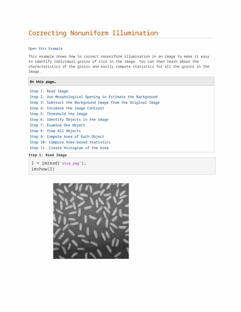
Correcting Nonuniform Illumination

Open this Example

This example shows how to correct nonuniform illumination in an image to make it easy to identify individual grains of rice in the image. You can then learn about the characteristics of the grains and easily compute statistics for all the grains in the image.

On this page…

Step 1: Read ImageStep 2: Use Morphological Opening to Estimate the BackgroundStep 3: Subtract the Background Image from the Original ImageStep 4: Increase the Image ContrastStep 5: Threshold the ImageStep 6: Identify Objects in the ImageStep 7: Examine One ObjectStep 8: View All ObjectsStep 9: Compute Area of Each ObjectStep 10: Compute Area-based StatisticsStep 11: Create Histogram of the AreaStep 1: Read Image

I = imread('rice.png');imshow(I)

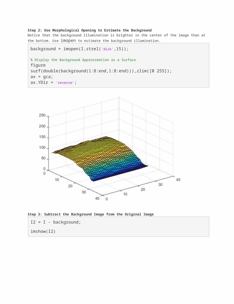
Step 2: Use Morphological Opening to Estimate the BackgroundNotice that the background illumination is brighter in the center of the image than atthe bottom. Use imopen to estimate the background illumination.background = imopen(I,strel('disk',15));

% Display the Background Approximation as a Surfacefiguresurf(double(background(1:8:end,1:8:end))),zlim([0 255]);ax = gca;ax.YDir = 'reverse';

Step 3: Subtract the Background Image from the Original Image

I2 = I - background;

imshow(I2)

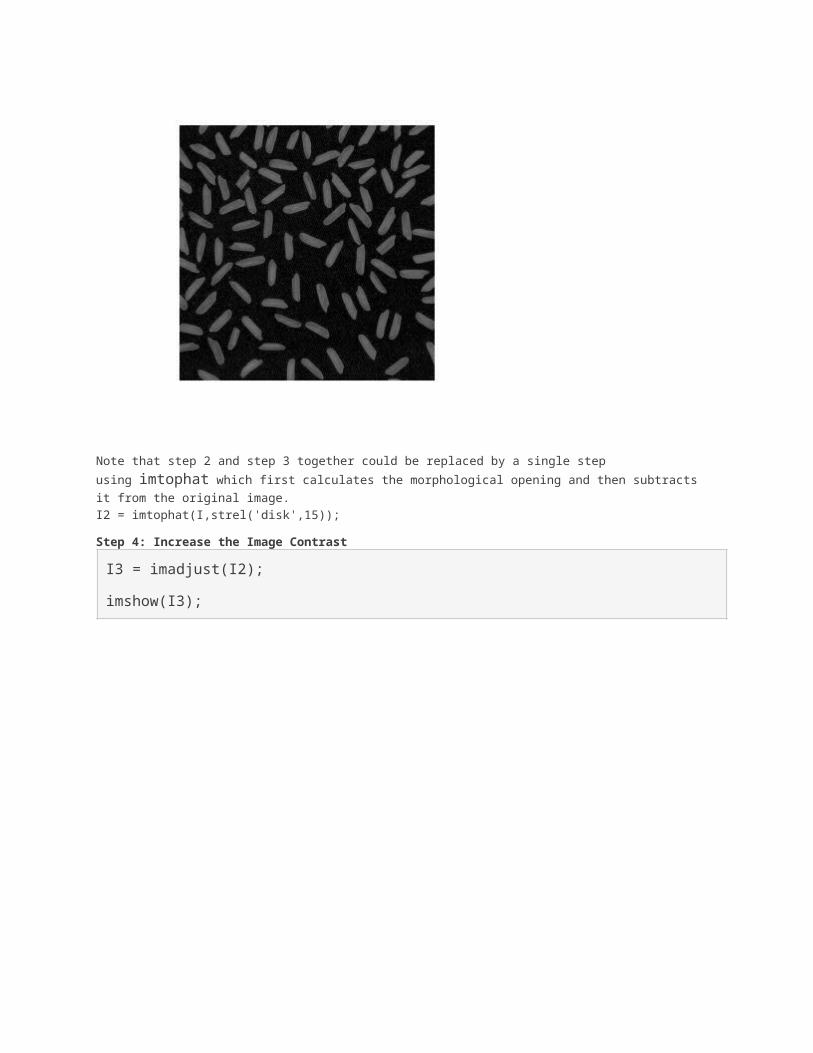
Note that step 2 and step 3 together could be replaced by a single step using imtophat which first calculates the morphological opening and then subtracts it from the original image.I2 = imtophat(I,strel('disk',15));

Step 4: Increase the Image Contrast

I3 = imadjust(I2);

imshow(I3);

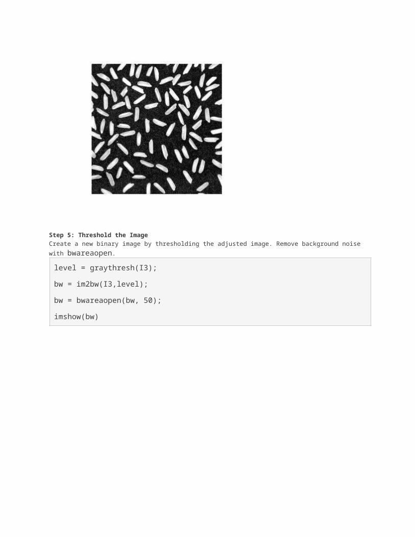
Step 5: Threshold the ImageCreate a new binary image by thresholding the adjusted image. Remove background noise with bwareaopen.level = graythresh(I3);

bw = im2bw(I3,level);

bw = bwareaopen(bw, 50);

imshow(bw)

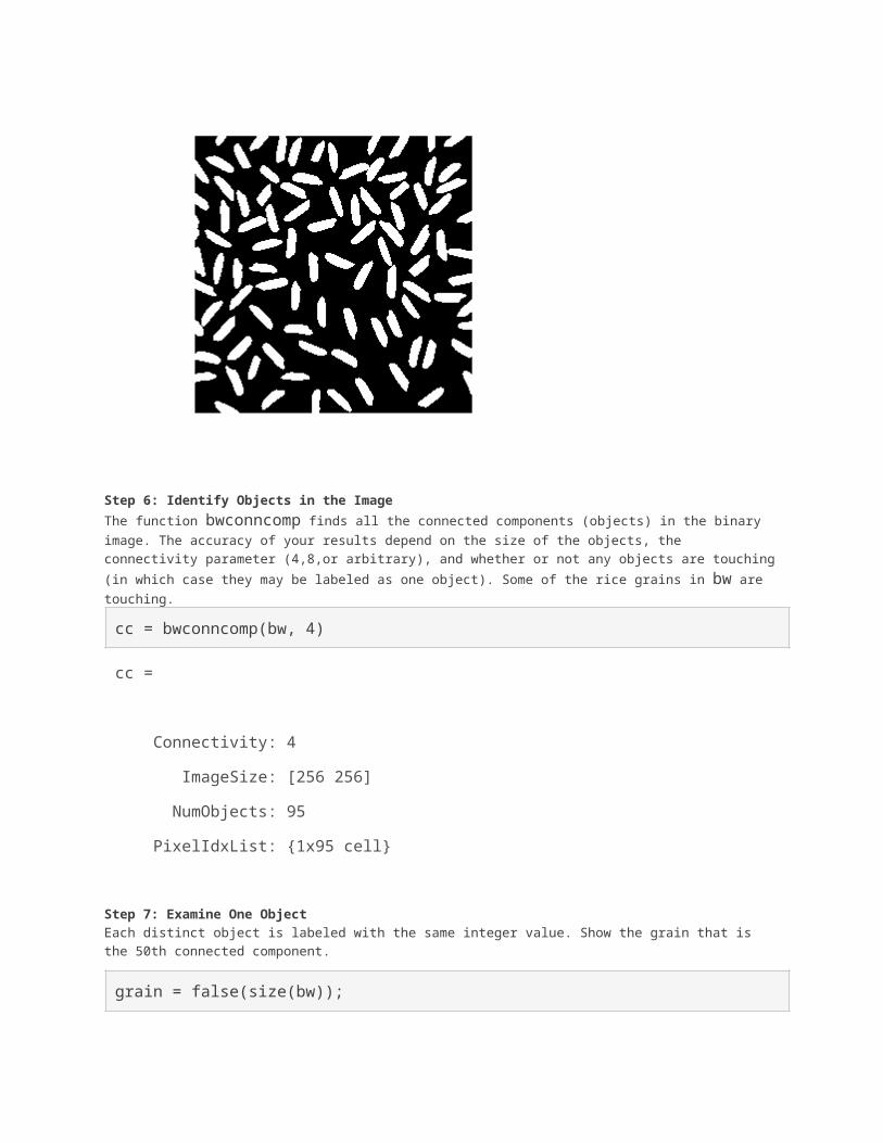
Step 6: Identify Objects in the ImageThe function bwconncomp finds all the connected components (objects) in the binary image. The accuracy of your results depend on the size of the objects, the connectivity parameter (4,8,or arbitrary), and whether or not any objects are touching(in which case they may be labeled as one object). Some of the rice grains in bw are touching.

cc = bwconncomp(bw, 4)

cc =

Connectivity: 4

ImageSize: [256 256]

NumObjects: 95

PixelIdxList: {1x95 cell}

Step 7: Examine One ObjectEach distinct object is labeled with the same integer value. Show the grain that is the 50th connected component.

grain = false(size(bw));

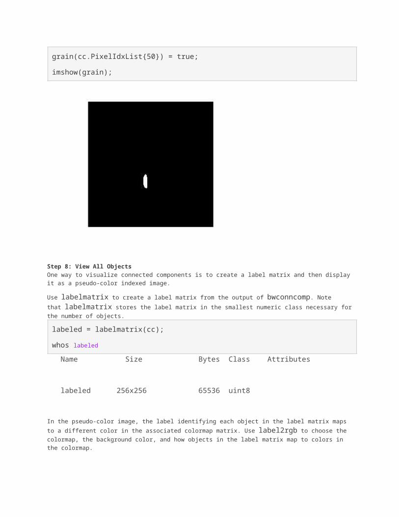
grain(cc.PixelIdxList{50}) = true;

imshow(grain);

Step 8: View All ObjectsOne way to visualize connected components is to create a label matrix and then displayit as a pseudo-color indexed image.

Use labelmatrix to create a label matrix from the output of bwconncomp. Note that labelmatrix stores the label matrix in the smallest numeric class necessary forthe number of objects.

labeled = labelmatrix(cc);

whos labeled Name Size Bytes Class Attributes

labeled 256x256 65536 uint8

In the pseudo-color image, the label identifying each object in the label matrix maps to a different color in the associated colormap matrix. Use label2rgb to choose the colormap, the background color, and how objects in the label matrix map to colors in the colormap.

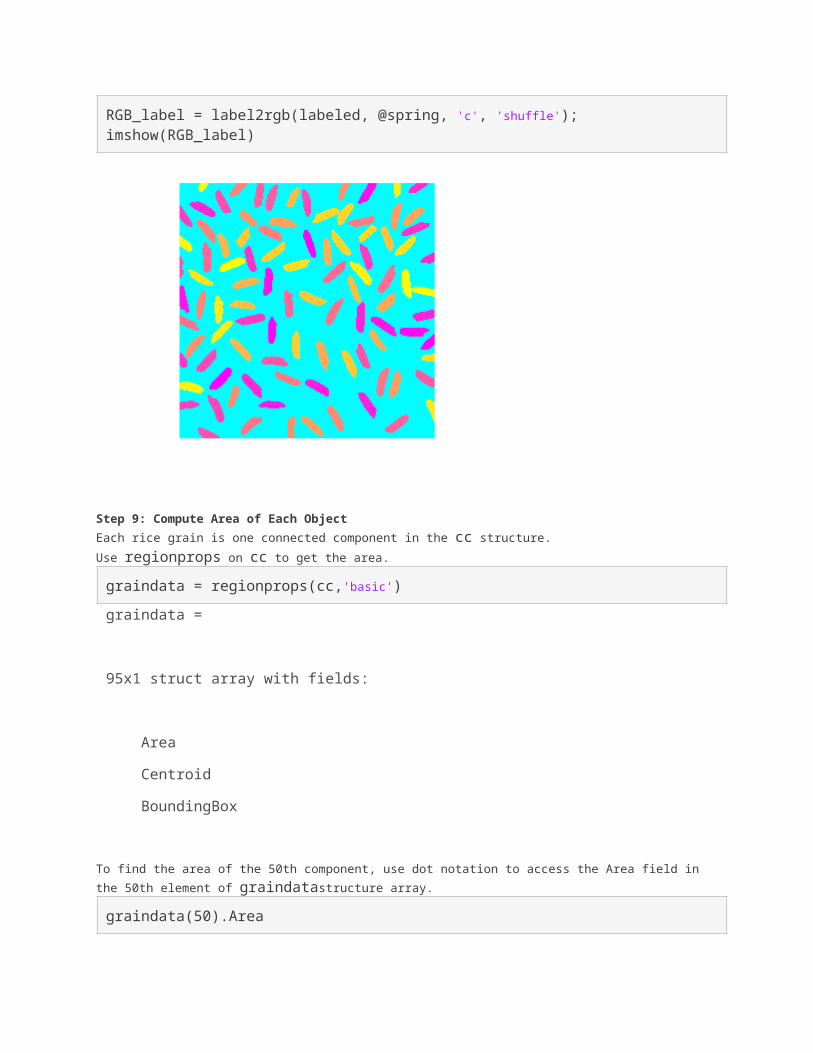
RGB_label = label2rgb(labeled, @spring, 'c', 'shuffle');imshow(RGB_label)

Step 9: Compute Area of Each ObjectEach rice grain is one connected component in the cc structure. Use regionprops on cc to get the area.graindata = regionprops(cc,'basic')graindata =

95x1 struct array with fields:

Area

Centroid

BoundingBox

To find the area of the 50th component, use dot notation to access the Area field in the 50th element of graindatastructure array.graindata(50).Area

ans =

194

Step 10: Compute Area-based StatisticsCreate a new vector allgrains, which holds the area measurement for each grain.grain_areas = [graindata.Area];

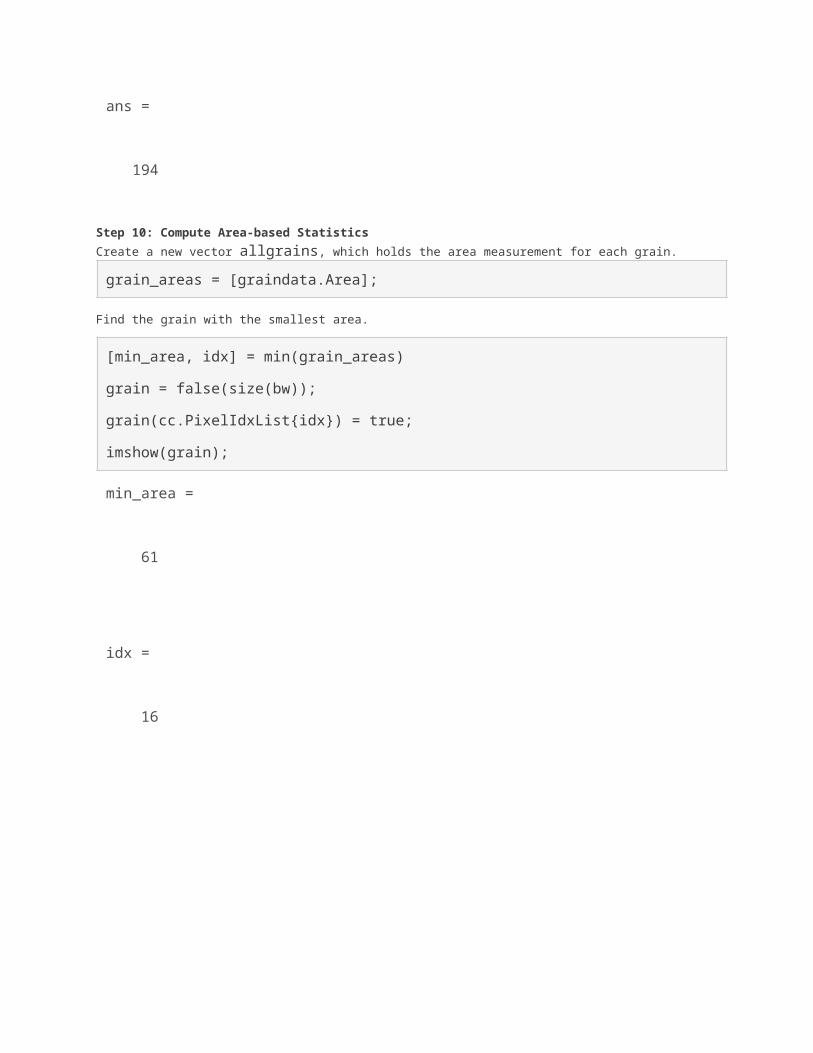
Find the grain with the smallest area.

[min_area, idx] = min(grain_areas)

grain = false(size(bw));

grain(cc.PixelIdxList{idx}) = true;

imshow(grain);

min_area =

61

idx =

16

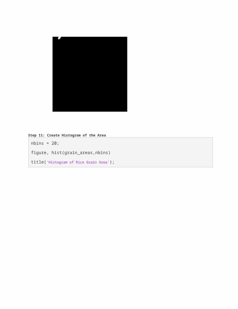
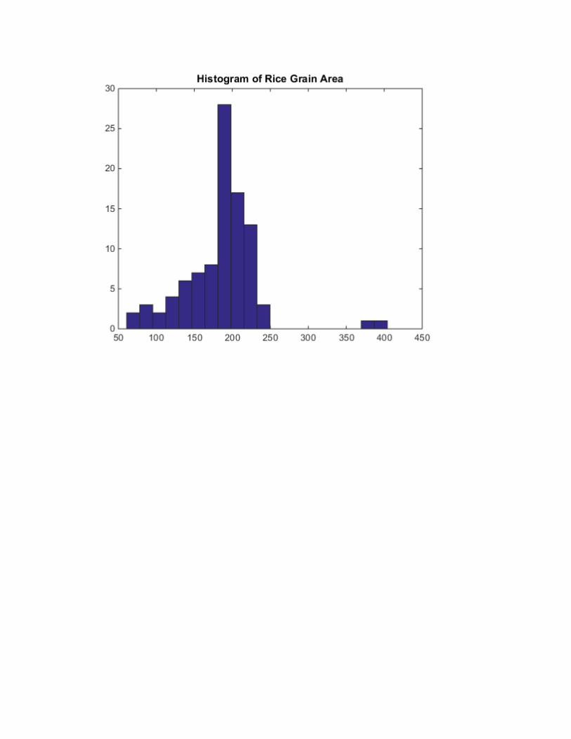
Step 11: Create Histogram of the Area

nbins = 20;

figure, hist(grain_areas,nbins)

title('Histogram of Rice Grain Area');