C.I.R.E.D.

Centre International de Recherches sur l'Environnement et le Développement UMR 8568 CNRS / EHESS / ENPC / ENGREF

/ CIRAD / MÉTÉO FRANCE 45 bis, avenue de la Belle Gabrielle F-94736 Nogent sur Marne CEDEX

Tel : (33) 1 43 94 73 73 / Fax : (33) 1 43 94 73 70 www.centre-cired.fr

DOCUMENTS DE TRAVAIL / WORKING PAPERS

No 39-2012

Correcting the ‘self-trade’ issue in the GTAPAgg software Technical Paper Meriem Hamdi-Cherif Frédéric Ghersi April 2012

CIRED Working Papers Series

CIRED Working Papers Series

Correcting the ‘self-trade’ issue in the GTAPAgg software Technical Paper

Abstract

The successive versions of the GTAP databases are provided with GTAPAgg, a programme that computes values of the series of the database for any regional and sectoral aggregation. A ‘self-trade’ issue arises from the fact that GTAPAgg aggregates the several series concerned with international trade, like any other series, by simply summing them up: the resulting series include a share of exports and imports happening between the aggregated regions, which should rather be treated as economic flows internal to the region resulting from the aggregation process.

This paper details a method that aims at solving this shortcoming, and discusses the importance of doing so. A first section puts the research question into context and discusses its likely importance when using GTAP as a calibration dataset for computable general equilibrium modelling. A second section details the analytics of the method proposed to correct the aggregation process, in the broader framework of a programme extending GTAPAgg to the production of national account matrixes in the standard United Nations format. An appendix provides the code of the extended aggregation programme developed.

Keywords: Input-Output Tables, Trade Analysis, Computable General Equilibrium, Data Aggregation.

La correction du problème de “self trade” dans le logiciel GTAPAgg. Article technique

Résumé

Les versions successives de la base de données GTAP sont livrées avec le programme d’agrégation GTAPAgg. Ce programme calcule les valeurs des séries de la base de données pour tout niveau d’agrégation régional ou sectoriel mais fait une impasse majeure : les valeurs d'importation et d'exportation de l'agrégat de deux zones sont calculées par simple sommation des valeurs de chacune des zones, sans correction de leur commerce bilatéral. Les séries résultant de l’agrégation comportent donc une part d’exportations et d’importations qui s’effectuent entre les régions agrégées, alors qu’elles devraient être traitées comme des échanges économiques internes à la région qui résulte du processus d’agrégation.

Cet article expose une méthode qui permet de corriger ce défaut, et discute de l’importance de le faire. Une première section replace la question dans son contexte et examine son importance, en particulier lorsque la base de données GTAP est utilisée pour calibrer des modèles d’équilibre général calculable. Une seconde section expose la méthode proposée pour (i) corriger le processus d’agrégation et (ii) construire un programme d’extension de GTAPAgg qui permet la production de matrices de comptabilités sociales sous le format standard des Nations Unies. Enfin, une annexe présente le code de ce « nouveau » programme d’agrégation.

Mots-Clés : Tableaux Entrées-Sorties, Commerce International, Équilibre Général Calculable, Agrégation de données.

CIRED Working Papers Series

CIRED Working Papers Series

5

Correcting the ‘self-trade’ issue in the GTAPAgg software

Technical Paper

Meriem Hamdi-Cherif 1, Frédéric Ghersi 2

CIRED

April 2012

Abstract

The successive versions of the GTAP databases are provided with GTAPAgg, a programme that computes

values of the series of the database for any regional and sectoral aggregation. A ‘self-trade’ issue arises

from the fact that GTAPAgg aggregates the several series concerned with international trade, like any

other series, by simply summing them up: the resulting series include a share of exports and imports

happening between the aggregated regions, which should rather be treated as economic flows internal to

the region resulting from the aggregation process.

This paper details a method that aims at solving this shortcoming, and discusses the importance of doing

so. A first section puts the research question into context and discusses its likely importance when using

GTAP as a calibration dataset for computable general equilibrium modelling. A second section details the

analytics of the method proposed to correct the aggregation process, in the broader framework of a

programme extending GTAPAgg to the production of national account matrixes in the standard United

Nations format. An appendix provides the code of the extended aggregation programme developed.

Keywords: Input-Output Tables, Trade Analysis, Computable General Equilibrium, Data Aggregation.

Correspondence Address:

Meriem Hamdi-Cherif

CIRED, 45 bis avenue de la Belle Gabrielle, 94736 Nogent-sur-Marne CEDEX , France.

Tel: +33 1 43 94 73 74

Email: hcmeriem@centre-cired.fr

1 Research fellow at CIRED. Meriem Hamdi-Cherif’s work was supported by the Chair ‘Modeling for sustainable development’,

led by MINES ParisTech, École des Ponts ParisTech, AgroParisTech and ParisTech, and financed by ADEME, EDF, Renault, Schneider Electric and Total. The views expressed in this article are those of the authors and do not necessarily reflect the views of the above-mentioned institutions. 2 Chargé de Recherche (Research fellow) CNRS (Centre National de la Recherche Scientifique), CIRED.

6

Table of Contents *

Abstract ................................................................................................................................................... 5

Keywords ................................................................................................................................................ 5

Correspondence Address .......................................................................................................................... 5

Table of Contents ..................................................................................................................................... 6

I Introduction ..................................................................................................................................... 7

II The ‘self-trade’ issue in GTAP: what it is and what is at stake .......................................................... 7

III A method to correct the ‘self-trade’ issue .................................................................................... 11

III.1 Overview of a new aggregation procedure to correct the ‘self-trade’ issue ............................... 11

III.2 Input Output tables construction: the GTAP dataset needed .................................................... 12

III.3 Detailed description of the ‘self-trade’ correction method and the IO table construction .......... 14

III.3.1 GTAP data importation ................................................................................................... 15

III.3.2 Details of the procedure .................................................................................................. 17

Aggregated matrices calculation ................................................................................................. 18

Separation of the regions ............................................................................................................ 18

Internal bilateral trade correction ................................................................................................ 19

Calculation of the ‘self-trade’ shares ....................................................................................... 20

Recalculation of exportations and FOB importations ............................................................... 20

Recalculation of trade exchange taxes ..................................................................................... 21

Imports transportation costs processing ................................................................................... 22

Construction of an IO table from the output matrices: ............................................................. 22

IV Appendix ................................................................................................................................... 24

IV.1 Comments .............................................................................................................................. 24

IV.2 The Scilab main program of the revisited GTAPAgg procedure: GTAPagg_Scilab.sce ............ 25

V References ..................................................................................................................................... 58

*active document

7

I Introduction

The GTAPAgg programme that aggregates regional data from the GTAP 7 database does so under the

simplest assumptions regarding international trade, i.e. by summing up the export and import series of

each aggregated region. This raises a crucial problem when using GTAP to calibrate CGE models—as is

commonly done considering that the GTAP database offers a unique consistent picture of economic flows

across sectors and regions at a global level. Basically, auto-imports and auto-exports, corresponding to

imports and exports of an aggregated region to (from) itself are not brought to zero by GTAPAgg, and the

shares of each detailed expenditure that are imported are not corrected.

The purpose of this paper is to present a detailed aggregation routine correcting this ‘self-trade’ problem.

A first section puts the research question into context and discusses its likely importance when using

GTAP as a calibration dataset for computable general equilibrium modelling. The contribution of the

correction is illustrated on an example: a European Union IO table with and without ‘self-trade’ is given,

with comments on implications that not correcting for ‘self-trade’ can generate.

A second section details the method proposed to correct the aggregation process, in the broader

framework of a programme extending GTAPAgg to the production of national accounting matrixes in the

standard United Nations format. The correction procedure is indeed embedded in the development of a

Scilab3 programme that automatically generates balanced input-output tables based on the GTAP7

database, for any aggregation of regions, sectors and factors. The comprehensive Scilab programme is

provided in the appendix to make it accessible to the GTAP network.

II The ‘self-trade’ issue in GTAP: what it is and what is at stake

As a global network of researchers and policymakers, the Global Trade Analysis Project (GTAP) helps

and allows many economists to conduct quantitative analysis of international policy issues since 1992.

The project is coordinated by the Centre for Global Trade Analysis in Purdue University’s Department of

Agricultural Economics.4

The GTAP network cooperates to produce the database that is probably the most used in general

equilibrium modelling exercises.5 GTAP has indeed the unique characteristic of providing a

comprehensive and harmonized global database at a remarkable level of detail: in the 7th version, 57

sectors and 113 regions cover the entire global economic activity for the year 2004.6 The GTAP website

3 Scilab is a freeware version of MatLab. 4 www.gtap.org.

5 https://www.gtap.agecon.purdue.edu/databases/default.asp.

6 Previous versions provide data for the reference years 2001, 1997, 1995 and 1992.

8

provides regional and sector listings7 and chapter 2, section 2.2.3 of the GTAP 7 Data Base

Documentation details the sector definitions (Badri Narayanan et al., 2008).

The success of the project is largely due to the voluntary contributions of hundreds of partner

organizations and researchers across the world. Indeed, this global network groups more than 6700

researchers in more than 150 countries (Hertel and Walmsley, 2008).

As the quantitative analysis of global policy issues is increasingly widespread, and the general equilibrium

modelling community growing, the use of such an exhaustive and comprehensive database is gaining

ground. GTAP is not only a unique endeavour, it also has high scientific standards, its construction and

maintenance being governed by the following principles: Public Availability, Regular Updates, Broad

Participation, Comparative Advantage, Documentation and Replicability and Quality Assurance (ibid).

The database describes, among other things, bilateral trade flows, production, consumption and

intermediate use of goods and services. Most data are given as dollar values (2004 USD) except for some

energy data that are also available in quantities (million tons of oil equivalent, MTOE).

The successive versions of the databases are provided with GTAPAgg, a programme that computes values

of the series of the database for any region, sector and factor aggregation. From a practical point of view, a

modeller willing to use GTAP data for calibration purposes naturally turns to this user-friendly software:

in a few seconds, the aggregated database is produced, with any required numbers of regions, sectors and

factors8 (smaller than or equal to respectively 113, 57 and 5). The folders that constitute this new database

are automatically bundled into a ZIP archive. Most of the files that are produced with GTAPAgg are

stored in a particular format, the Header Array or HAR format. Nevertheless, the data is easily sent to a

spreadsheet by using the Copy button to send a report of the aggregation to the clipboard (Horridge,

2008).

Besides energy use data and time-series trade data, the two main files in the .ZIP archive are basedata.har

and baseview.har. The detail of the series needed to build a comprehensive set of Input-Output (IO) tables

is given in section III.2. Throughout the following paper, reference will be made to the different series by

using prefixes: “bd.” for the series basedata.har and “bv.” for the series baseview.har.

The most important feature of the GTAP database, that which accounts for its particular relevance to CGE

modelling, is that it is strictly balanced: at the regional level, where each of the 57 sectors are balanced in

income and expenditure, for each of its 113 regions; and the international level, where bilateral trade flows

data across all regions strictly compensate. Indeed, particular efforts have been made by the GTAP team

to collect and scrutinise national or regional data to build ‘local’ IO tables that have been taken into

account as important contribution to the GTAP database (Huff et al., 2000); then the GTAP team has put

much effort on reconciling bilateral trade data coming from many different sources to combine them in a

consistent way into the database (Gehlhar, 1996).

7 Respectively https://www.gtap.agecon.purdue.edu/databases/regions.asp?Version=7.211 and

https://www.gtap.agecon.purdue.edu/databases/v7/v7_sectors.asp. 8 Endowment commodities.

9

However, the GTAPAgg programme that aggregates regional data from the database has one limitation: it

aggregates the several series concerned with international trade like any other series, by simply summing

them up. As a consequence, the resulting series include a share of exports and imports happening between

the aggregated regions, which should rather be treated as trade flows internal to the region resulting from

the aggregation process: auto-imports (auto-exports) corresponding to importations (exportations) of an

aggregated region to (from) itself are not brought down to zero, and the imported shares of each detailed

expenditure is not corrected. This ‘self-trade’ issue is best illustrated with a straightforward example: the

global IO table for one region (the world), one good, and one factor that a use of GTAPAgg limited to the

arrangement of the series it provides, produces (Table 1).

Intermediate Consumption

Consumption of households

Public consumption

Investment Exports Total

Expenditure

Intermediate consumption

39.4 (6.8)

25.2 (2.8)

7.1 (0.2)

8.7 (1.4)

10.5 90.9

1ary

factor payments

32.5

Taxes 8.5

(0.7)

Imports 10.5

Total Resource

90.9

Table 1 A global IO table aggregated from GTAPAgg (in thousand billion 2004 USD) In parenthesis: expenditures or taxes on imported goods

The aggregated world thus exhibits global exports and imports to itself that amount to 26% of its GDP

(10.5 over 41.0, the sum of primary factor payments and taxes); indeed the detail of the uses of these

imports is readily available (in parenthesis in table 1). Of course for the world aggregated as one region all

goods are domestic ones, and any user confronted to such figures is bound to identify the self-trade issue.

The aggregate import and export data can then simply be dropped. This is without consequence on the

balance of the table since the two values quite opportunistically match—they indeed strictly describe the

same set of economic flows.9 Consequently the detail of the domestic or imported sources of expenditures

and taxes can be ignored.

Now the self-trade issue and its settlement are much less obvious when any regional aggregation beyond

the specific global case is considered. To illustrate this, the aggregation of the 27 member states of the

European Union, based on the same undiscerning use of GTAPAgg, is provided and commented upon

(Table 2). In this latter case a database user, particularly one not directly interested in trade issues, or not

familiar enough with them to have a notion of the amounts at stake,10

could easily overlook his mistake:

9 Note that by accounting for global exports and imports Table 1 is thus overestimating total global resources and total global

expenditures by $10.5 trillion. 10 The likelihood of the figures is all the harder to assess as goods are disaggregated.

10

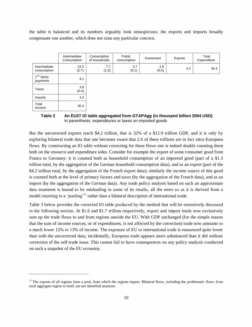
the table is balanced and its numbers arguably look unsuspicious; the exports and imports broadly

compensate one another, which does not raise any particular concern.

Intermediate Consumption

Consumption of households

Public consumption

Investment Exports Total

Expenditure

Intermediate consumption

13.3 (2.7)

7.7 (1.3)

2.7 (0.1)

2.6 (0.5)

4.2 30.4

1ary

factor payments

9.1

Taxes 3.8

(0.4)

Imports 4.2

Total Income

30.4

Table 2 An EU27 IO table aggregated from GTAPAgg (in thousand billion 2004 USD) In parenthesis: expenditures or taxes on imported goods

But the uncorrected exports reach $4.2 trillion, that is 32% of a $12.9 trillion GDP, and it is only by

exploring bilateral trade data that one becomes aware that 2.6 of these trillions are in fact intra-European

flows. By constructing an IO table without correcting for these flows one is indeed double counting them

both on the resource and expenditure sides. Consider for example the export of some consumer good from

France to Germany: it is counted both as household consumption of an imported good (part of a $1.3

trillion total, by the aggregation of the German household consumption data), and as an export (part of the

$4.2 trillion total, by the aggregation of the French export data); similarly the income source of this good

is counted both at the level of primary factors and taxes (by the aggregation of the French data), and as an

import (by the aggregation of the German data). Any trade policy analysis based on such an approximate

data treatment is bound to be misleading in some of its results, all the more so as it is derived from a

model resorting to a ‘pooling’11

rather than a bilateral description of international trade.

Table 3 below provides the corrected IO table produced by the method that will be extensively discussed

in the following section. At $1.6 and $1.7 trillion respectively, export and import totals now exclusively

sum up the trade flows to and from regions outside the EU. With GDP unchanged (for the simple reason

that the sum of income sources, or of expenditures, is not affected by the correction) trade now amounts to

a much lower 12% to 13% of income. The exposure of EU to international trade is reassessed quite lower

than with the uncorrected data; incidentally, European trade appears more unbalanced than it did without

correction of the self-trade issue. This cannot fail to have consequences on any policy analysis conducted

on such a snapshot of the EU economy.

11 The exports of all regions form a pool, from which the regions import. Bilateral flows, including the problematic flows from each aggregate region to itself, are not identified anymore.

11

Intermediate Consumption

Consumption of households

Public consumption

Investment Exports Total

Expenditure

Intermediate consumption

13.3 (1.1)

7.7 (0.5)

2.7 (0.0)

2.6 (0.2)

1.6 27.8

1ary

factor payments

9.1

Taxes 3.8

(0.1)

Imports 1.7

Total Income

27.8

Table 3 An EU27 IO table aggregated from GTAPAgg, with correction of the ‘self-trade’ flows (in thousand billion 2004 USD) In parenthesis: expenditures or taxes on imported goods

III A method to correct the ‘self-trade’ issue

This section details the method proposed to tackle the ‘self-trade’ issue, in the broader framework of a

programme extending GTAPAgg to the production of IO tables in the System of National Accounts

(SNA), the standard United Nations format (UN, 1993). A first subsection exposes a broad outline of the

method developed. A second subsection details how to construct IO tables from the raw GTAP series, by

precisely identifying which of the series or elements thereof are to be used, and how they should be

organised. A third and final subsection provides the detailed description of the method used to correct the

aggregation problem that has been identified.

III.1 Overview of a new aggregation procedure to correct the ‘self-trade’ issue

This subsection provides an overview of the method used to correct the ‘self-trade’ issue of the GTAPAgg

programme before entering into the details given in subsection III.3. The description bellow relies on

concepts of National Account Systems that are evoked in subsection III.2 (Input Output tables

construction: the GTAP dataset needed)

The input-output table of any aggregated region is corrected in a 5-step process:

The ‘self trade’ shares of the free-on-board (FOB) imports and the exports at world price (the two

shares must indeed amount to the same: the exports of one region to itself must equal its imports from

itself) are subtracted from their raw aggregate totals. This does not affect the balance of expenditures

and resources for each good; however it affects that of the imported variant of each good: imports on

the resource side become smaller than the consumption of imported goods on the expenditure side.

On the resource side, the ‘self trade’ shares of the import and the export taxes are subtracted and

reallocated to a new tax category—the status of these border taxes internal to the region resulting from

the aggregation is indeed quite specific.

12

Still on the resource side, a share (cf. infra) of the taxes on the imported good consumption is

reallocated to the taxes on the domestic good consumption; this increases the unbalance between

resource and expenditure for the imported goods.

On the expenditure side, a share (cf. infra) of the intermediate and final consumptions of the imported

variant of each good is reallocated to its domestic variant: this restores the resource-expenditure

balance for the imported goods.

On the expenditure side, a share of the exports of transportation services specifically linked to

international trade is reallocated to the domestic intermediate consumption of transportation goods

(goods 48, 49 and 50 of the database). Since GTAP does not identify what part of the ‘self-import’

transportation is undertaken by businesses of the self-importing region, this part is set proportional to

the participation of the region to these international transportation activities. This deserves an

illustration: a region i is performing an amount m of the transport costs of a good j, costs that are

related to ‘self trade’ importations of this good. We thus subtract this amount m from its total imports

(in cost-insurance-freight, CIF, terms); we then transfer it to the three transport intermediate

consumptions of the production of the good j; this transfer is done in proportion of their part in the

total of the international transport operated by i; we finally correct the expenditures by subtracting the

same amounts from exports of these three transportation goods.

For each region the shares to be reallocated under points 3 and 4 above are identical, defined as the

aggregate share of the ‘self-trade’ part in the sum of imports FOB, the transportation costs of international

exchanges, and import taxes.

III.2 Input Output tables construction: the GTAP dataset needed

Before detailing the GTAP series that allow building balanced IO tables, let us quickly recall a few

notions and concepts concerning the National Accounts.12

The National Accounts—and the IO tables (or

Social Accounting Matrixes) that synthesize them—are based on a balance between expenditures and

resources. This equilibrium has to be verified for all the goods13

considered, summing up:

On the expenditure side, the intermediate consumptions (57 productions in GTAP, including the

production of good in question), the final consumptions (1 representative Household, 1 government

and 1 investing sector) and exports (nominal exports and transportation services specifically linked to

international trade).

On the resources side, the factor consumptions (5 factors), the taxes and the imports (nominal imports

and their international transport costs).

12 Linked to the GTAP database in terms of the number of goods and factors. 13 When it comes to any modelling with a connection to ‘quantity’ problems such as energy balances or environmental pollutions, a disaggregation by goods rather than by production sectors is more relevant. Incidentally this requires some caution in the transposition of modelling results to industrial branches, because of joint production issues.

13

The GTAP series that allow reconstituting this equilibrium, i.e. the GTAP dataset needed to build

balanced IO tables, is the following:14

Intermediate Consumptions: valued at market price (tax-free valuation):

Intermediates - Firms' Imports at Market Prices (bd13 – VIFM - without taking the CGDS15

) ;

Intermediates - Firms' Domestic Purchases at Market Prices (bd14— VDFM without taking the

CGDS) ;

Final Consumptions (Households, Governments, and CGDS): valued at Agents prices (including all

taxes):

Intermediates - Household Imports at Agents' Prices (bd26 - VIPA) ;

Intermediates - Household Domestic Purchases at Agents' Prices (bd27 - VDPA) ;

Intermediates - Government Imports at Agents' Prices (bd28 - VIGA) ;

Intermediates - Government Domestic Purchases at Agents' Prices (bd29 - VDGA) ;

Intermediates - Firms' Imports at Agents' Prices (bd15 – VIFA – taking CGDS) ;

Intermediates - Firms' Domestic Purchases at Agents' Prices (bd16 - VDFA taking CGDS).

Exports: sum of exports at world price and exports of transportation services specifically linked to

international trade:

Decomposition of exports at world prices16

(bv11 – BI01: In the selection bar for regions, the

exporting region is the left one. In order to obtain the export total of the selected region, the

modeller must select Sum REG in the right selection bar for regions);

Trade - Exports for International Transportation, Market Prices (bd23 - VST).

Factors Consumptions: valued at market price (this valuation takes into account capital depreciation—

fixed capital consumption—, but GTAP does not indicate how to disaggregate this data between the

different productions):

Endowments - Firms' Purchases at Market Prices (bd18 - VFM)

14 Each series is mentioned as a part of the file BaseData (bd) or BaseView (bv) followed by its line number in the file, as well as the GTAP Header code, e.g. bd13 – VIFM for the series number 13 of the file BaseData.har whose the Header code is VIFM:

Intermediates - Firms' Imports at Market Prices. The number and file (bd or bv) are related to the version 7 of the GTAP database. For the previous versions only the names of the series remain the same. 15 This refers to the consumption of the different goods that are immobilized in CGDS. 16

Note that the ‘self-trade’ issue is observable in this series: the exports from one region to its self are not equal to zero.

14

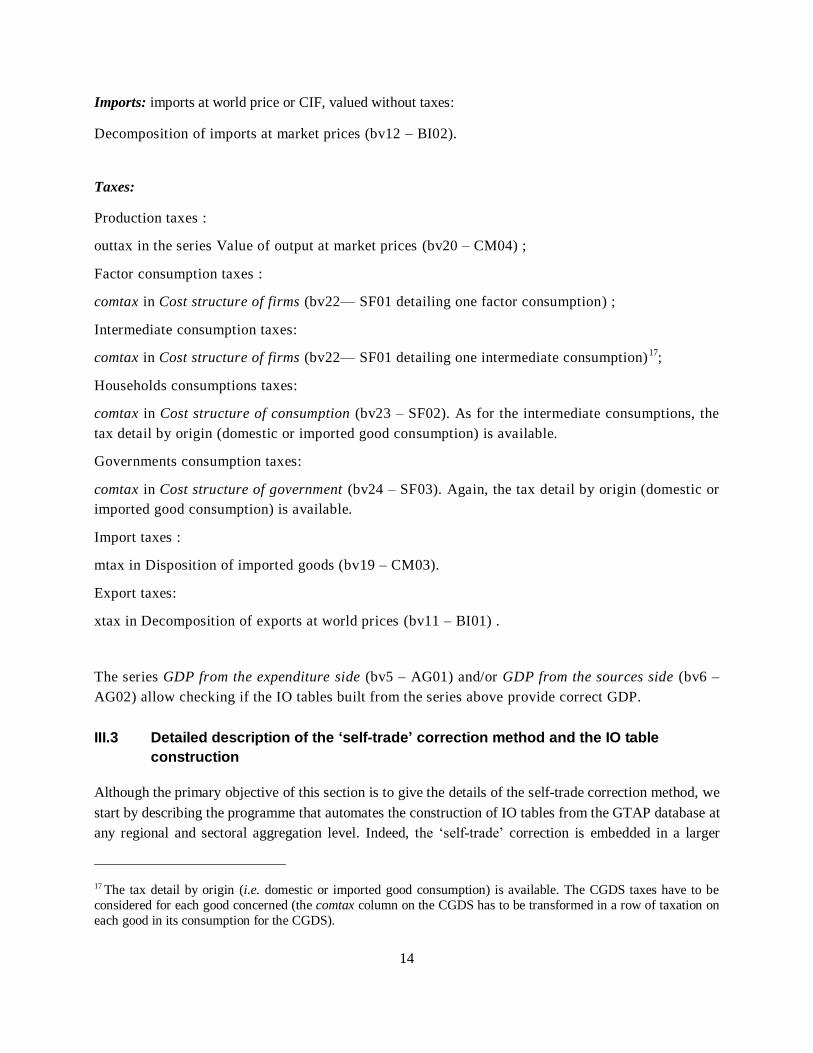
Imports: imports at world price or CIF, valued without taxes:

Decomposition of imports at market prices (bv12 – BI02).

Taxes:

Production taxes :

outtax in the series Value of output at market prices (bv20 – CM04) ;

Factor consumption taxes :

comtax in Cost structure of firms (bv22— SF01 detailing one factor consumption) ;

Intermediate consumption taxes:

comtax in Cost structure of firms (bv22— SF01 detailing one intermediate consumption)17

;

Households consumptions taxes:

comtax in Cost structure of consumption (bv23 – SF02). As for the intermediate consumptions, the

tax detail by origin (domestic or imported good consumption) is available.

Governments consumption taxes:

comtax in Cost structure of government (bv24 – SF03). Again, the tax detail by origin (domestic or

imported good consumption) is available.

Import taxes :

mtax in Disposition of imported goods (bv19 – CM03).

Export taxes:

xtax in Decomposition of exports at world prices (bv11 – BI01) .

The series GDP from the expenditure side (bv5 – AG01) and/or GDP from the sources side (bv6 –

AG02) allow checking if the IO tables built from the series above provide correct GDP.

III.3 Detailed description of the ‘self-trade’ correction method and the IO table

construction

Although the primary objective of this section is to give the details of the self-trade correction method, we

start by describing the programme that automates the construction of IO tables from the GTAP database at

any regional and sectoral aggregation level. Indeed, the ‘self-trade’ correction is embedded in a larger

17 The tax detail by origin (i.e. domestic or imported good consumption) is available. The CGDS taxes have to be

considered for each good concerned (the comtax column on the CGDS has to be transformed in a row of taxation on

each good in its consumption for the CGDS).

15

programme that finally leads to the construction of balanced IO tables delivered under a csv or xls format.

The method is exposed in two main parts: a first part details the data extracted from GTAP to be used in

the programme; the second part describes how the programme operates.

III.3.1 GTAP data importation

The “one-to-one” aggregations of the GTAPAgg programme (without any regional, sectoral and factor

aggregation) produce the raw data that are used by the IO table building programme.

These data are stored as matrices in 16 .sce files:

Conso_Interm_Imp.sce holds the 57x58 matrices of the intermediate consumptions of imported goods.

These matrices are extracted from the series bd13-VIFM, Intermediates - Firms' Imports at Market Prices.

GTAP gives 113 matrices of size 57x58 (57 is the sector number; the 58th column gives CGDS at market

prices) that are stored in the scilab list C. The 113 intermediate consumptions matrices strictly speaking

(CGDS excluded, thus of size 57x57) are stored in a second scilab list: CI_imp. In this list of 113

elements, each element k (a matrix 57x57) details the intermediate consumptions of imported goods for

each sector of the region k.

Conso_Interm_Dom.sce holds the 57x58 matrices of the intermediate consumptions of domestic goods.

These matrices are extracted from the series bd14-VDFM Intermediates -Firms' Domestic Purchases at

Market Prices. Similarly to Conso_Interm_Imp.sce, the data are stored in the scilab list CC, then without

the CGDS in the list CI_dom, thus obtaining 113 matrices of the intermediate consumptions of domestic

goods.

Conso_Menages.sce18

holds two matrices of size 57x113: C_25 for the household consumptions of

domestic goods and C_26 for the household consumptions of imported goods. These matrices are

respectively extracted from the series bd26-VIPA Intermediates - Household Imports at Agents' Prices

and bd27-VDPA Intermediates - Household Domestic Purchases at Agent' Prices.

Conso_AP.sce19

holds two matrices of size 57x113: C_28 for the government consumptions of domestic

goods and C_27 for the government consumptions of imported goods. These matrices are respectively

extracted from the series bd28 - VIGA Intermediates - Government Imports at Agents' Prices and bd29 –

VDGA Intermediates - Government Domestic Purchases at Agent' Prices.

Conso_FBCF.sce20

holds two matrices of size 57x113: C_14 for the CGDS consumptions of imported

goods and C_15 for the CGDS consumptions of domestic goods. These matrices are respectively extracted

from the series bd15-VIFA Intermediates - Firms' Imports at Agents' Prices and bd16- VDFA

Intermediates - Firms' Domestic Purchases at Agents' Prices.

Export_Import.sce holds the exports and imports matrices: XX, of size 57x113, contains the exports at

world price, extracted from the series bv11 – BI01 Decomposition of exports at world prices. x_Trans, of

18 Ménages is French for households. A further/international version of the paper will translate all variable names. 19 AP refers to Administrations Publiques, the French for Public Administrations. This is Government consumption. 20 FBCF is the French equivalent of CGDS.

16

size 3 goods x 113 regions, contains exports of transportation services specifically linked to international

trade extracted from the series bd23-VST Trade - Exports for International Transportation, Market

Prices. The three goods in question are the three types of transport that are distinguished in the GTAP

database. To obtain a matrix XX_Trans of size 57x113, x_Trans is concatenated with two zero matrices,

x1_Trans and x2_Trans. MM_fob, of size 57x113, contains the imports at world price without transports

costs (free-on-board). It is extracted from the series bv13-BI03 Decomposition of CIF values, data fob.

MM_Trans, of size 57x113, contains the transport costs of the imports above. It is also extracted from the

series bv13-BI03 Decomposition of CIF values, but taking the trans data. The sum the two last matrices is

the data impcost from the series bv12-BI02 Decomposition of imports at market prices. The data could

simply be taken to this series, but the transport costs detail (impcost = trans + fob) is necessary for the

‘self-imports’ and ‘self-exports’ correction.

Exports.sce holds a 57 elements scilab list Export. Each element is a matrix 113x113 extracted from the

series bv11-BI01 Decomposition of exports at world prices .Each matrix details the exports (taxes

included) of one of the 57 goods, from any of the 113 regions (the exporting region is the column data) to

any other (the export destination is the row data). These matrices are stored to allow correcting the trade

balances aggregations as done by GTAPAgg.

Imports_Fob.sce holds a 57 elements scilab list Import_fob. Each element is a matrix 113x113 extracted

from the series bv13-BI03 Decomposition of CIF value .Each matrix details the free-on-board imports of

one of the 57 goods, by any one of the 113 regions (the importing region is the data in column) from any

other one (the origin of the importation is the row data). Like the previous ones, these matrices are stored

to allow correcting the aggregation of the trade balances.

Imports_Transp.sce holds 57 matrices that will be used to correct the transportation costs of the imports.

Similarly to the previous file, these matrices are stored in the scilab list Import_Tran and they are

extracted from the series bv13-BI03, taking the trans data (instead of fob in the previous file).

Conso_Fact.sce holds 113 matrices of size 5x58 (factors x production, the 58th production corresponds to

the CGDS). These matrices detail the factor consumptions by region and production; they are extracted

from the series bd18-VFM Endowments - Firm's Purchases at Market Prices. The data are stored in the

scilab list F, then in the list CFact (excluding the CGDS). Each element k (i.e. each matrix) represents the

factor consumptions of region k in each of the 57 production.

Taxes1.sce holds the matrices of the taxes on production, household and government consumption. The

production tax matrix T_13, of size 57x113, is extracted from the series bv20-CM04 Value of output at

Market Prices, taking the data outtax. The consumption taxes are extracted from the series bv23-SF02

Cost structure of consumption and bv24-SF03Cost structure of government, taking the data comtax. A

distinction is done between the taxes on domestic goods consumptions (57x113 matrices: T_16_Dom for

households and T_17_Dom for governments) and those on imported goods consumptions (57x113

matrices: T_16_Imp for households and T_17_Imp for governments).

Taxes2_Dom.sce holds the matrices of the taxes on the intermediate consumptions and on the

CGDS of domestic products. It also holds the matrices of the taxes on the factor consumptions.

These data are extracted from the series bv22-SF01 Cost structure of firms. GTAP provides 113

matrices of size 62x58 that are stored in the scilab list TT. From this list are extracted:

17

The 113 matrices 5x57 of factors consumptios taxes, list T_ConsFact ;

The 113 matrices 57x57 of the taxes on the intermediates consumptions of domestic goods, list

T_CI_dom ;

The 113 matrices 1x57 of the taxes on the CGDS of domectic products, list T_FBCF_dom.

Taxes2_Imp.sce holds the matrices of the taxes on the intermediate consumptions and on the CGDS of

imported products. They are extracted from the same series bv22-SF01 Cost structure of firms. The 113

matrices 62x58 given by GTAP are stored in the scilab list T. From T, are extracted, in way similar to the

extraction in the previous file, the scilab lists T_CI_imp and T_FBCF_imp.

Taxes3.sce holds two matrices, of size 57x113, of the export and import taxes. The first, T_xtax, is

extracted from the series bv11-BI01 Decomposition of exports at world prices, taking the data xtax. The

second, T_mtax, is extracted from the series bv12-BI02 Decomposition of imports at market prices, taking

the data mtax.

xtax.sce holds 57 matrices of size 113x113, stored in the scilab list xtax. This file takes the data from

T_xtax (c.f previous file) and details bilateral trade (one matrix per good allows to determine which tax is

applied to the exports of this good, for each exporting region—row data—to any other destination—

column data).

mtax.sce, like the file xtax.sce, completes the T_mtax data by presenting bilateral trade. Each one of the

57 matrices of mtax gives the tax applied on the importation of a good of any importing region (column

data) from any origin (row data).

Like the files Exports.sce, Imports_Fob.sce and Imports_Transp.sce, the file xtax.sce and mtax.sce are

used for the treatment of the self-imports and the self-exports as aggregation proceeds.

III.3.2 Details of the procedure

As mentioned before, the GTAPAgg program produces a ZIP folder that contains the main information

needed. Among other things, this ZIP folder contains a text file under the format .agg. Scilab extracts from

this file the following parameters:

P, N, K represent respectively the new number of sectors, regions and factors, depending on the

aggregation scheme decided upon by the user;

b and B are text vectors that contain respectively the names of the disaggregated sectors (of size 57)

and the name of the aggregated sectors (of size P);

r and R are text vectors that contain respectively the names of the disaggregated regions (of size 113)

and the name of the aggregated regions (of size N);

f and Fact are text vectors that contain respectively the names of the disaggregated factors (of size 5)

and the name of the aggregated factors (of size K);

18

Aggregated matrices calculation

From these parameters, two matrices are defined: Masc1 and Masc2. They indicate the membership of a

disaggregated region (resp. a sector) to a new aggregated one, and they are constituted of 0 and 1. Their

mathematic product with the various data matrices provides a new group of aggregated data according to

the aggregation level desired by the database user. Therefore, all the data of size 113 (resp. 57) become of

size N (resp. P), defining two aggregated groups of matrices.

The first group is constituted of matrices that are stored in a list of N elements (one element per

aggregated region):

CI_imp_Agg, CI_dom_Agg, T_CI_imp_Agg and T_CI_dom_Agg, of size PxP: contain the

intermediate consumptions of imported and domestic goods, as well as the taxes on these

consumptions.

CFact_Agg and T_ConsFact_Agg, of size KxP, contain the factors consumptions and the taxes on

these consumptions.

T_FBCF_dom_Agg and T_FBCF_imp_Agg, of size 1xP, contain the taxes on the CGDS of domestic

and imported goods.

The second group is constituted of matrices of size PxN (only one matrix for all the aggregated regions):

M_fob_Agg, M_Trans_Agg, X_Agg and X_Trans_Agg contain the fob imports, their transportation

costs, the fob exports and the exports of transportation services specifically linked to international

trade.

C_25_Agg and C_26_Agg contain the household’s consumptions of respectively imported and

domestic goods.

C_27_Agg and C_28_Agg contain the governments’ consumptions of respectively imported and

domestic goods.

C_14_Agg and C_15_Agg contain the CGDS of respectively imported and domestic goods.

T_13 contains the production taxes.

T_16_DomAgg and T_16_ImpAgg contain the taxes on the households’ consumptions of domestic

and imported goods.

T_17_DomAgg and T_17_ImpAgg contain the taxes on the governments’ consumptions of domestic

and imported goods.

T_mtaxAgg and T_xtaxAgg contain the exports and imports taxes.

Separation of the regions

Once regional and sectoral aggregations have been done on the raw data matrices, the columns of the new

matrices of the second group above are separated to obtain, for each data (consumptions, taxes, etc.), one

vector per aggregated region. In the rest of the text, the following abbreviations (notations) will be used in

the names of the matrices:

19

C: consumption,

CI: intermediate consumptions,

T: taxes,

Hsld: Households,

G or AP: Governments,

X or x: exports,

M or m: imports,

Imp, Dom: imported goods, domestic goods,

Trans or Tran: transports,

corr: corrected,

i: aggregated region index, 1 < i < N.

Based on this convention, the aggregated data vectors are stored in the following scilab lists:

C_Hsld_imp(i), C_Hsld_dom(i)

C_G_imp(i), C_G_dom(i)

C_FBCF_imp(i), C_FBCF_dom(i)

x(i), X_Trans(i)

m_fob(i), M_Trans(i)

Tmtax(i), Txtax(i)

Tprod(i)

THsld_Dom(i), THsld_Imp(i)

TG_Dom(i), TG_Imp(i)

Note that a simple concatenation of these lists allows the construction of an IO table. However, the ‘self-

trade’ issue is still to be corrected.

Internal bilateral trade correction

The correction of the internal bilateral trade occurs after the aggregation process is done, through the

subtraction of the ‘self’ shares from the totals of imports, exports, taxes and transport costs, then through

the transfer of these shares to other posts of the IO table.

20

Obviously, this correction operation must respect the sectoral balances of the IO table on one hand, and on

the other hand it also has to respect the general equilibrium between expenditures and resources in terms

of importations (the sum of imported goods consumptions has to be equal to the imports including taxes).

Calculation of the ‘self-trade’ shares

We start with the sectoral aggregations (from 57 to P sectors) concerning the following lists:

Export, Import_fob, Import_Tran, mtax and xtax.

We thus obtain P matrices of size 113x113 that detail bilateral trade, taxes and transport costs.

Then, for each aggregated region i, we build the P-“self”-vectors:

Auto_X(i),

Auto_M_fob(i),

Auto_M_Trans(i),

Auto_xtax(i),

Auto_mtax(i).

These vectors contain respectively the exports, FOB imports, transport costs of these imports, export taxes

and import taxes of all the regions aggregated in region i between themselves. For example, considering

two regions A and B aggregated into a region C: Auto_X(C) is the sum of exports from A to A, from A to

B, from B to B and from B to A.

This operation produce, for each aggregated region, the amounts that are to be transferred from foreign

trade to domestic trade.

However, an important question remains concerning the allocation of the transport costs of the trade that

becomes domestic. Indeed, even if GTAP indicates the participation of each country in the international

commodities transports, and gives the transport costs supported by each international trade flow, it does

not assign each of these transport costs to any particular region. In other words, we do not know what

share of the transport costs of the ‘self-imports’ Auto_M_Trans(i) of an aggregated region i is really

carried out by this region. We settle this uncertainty by assuming that this share is proportional to the

participation of the region i into international transportation activities. The result of this rule is stored in

the vector Part_AutoM_Trans(i).

Recalculation of exportations and FOB importations

For each aggregated region i, we remove the ‘self’ share from exports and imports to obtain two new P-

vectors:

x_corr(i) = x(i) – Auto_X(i)

m_fob_corr(i) = m_fob(i) – Auto_M_fob(i)

21

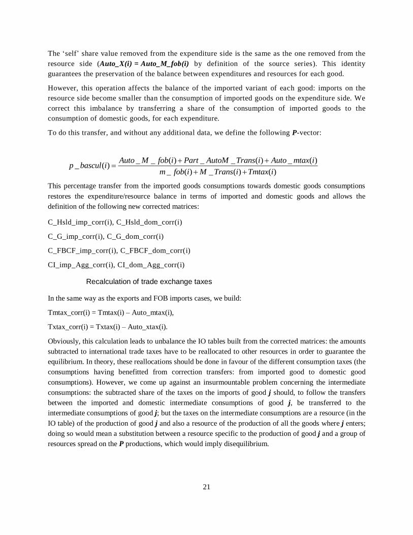
The ‘self’ share value removed from the expenditure side is the same as the one removed from the

resource side (Auto_X(i) = Auto_M_fob(i) by definition of the source series). This identity

guarantees the preservation of the balance between expenditures and resources for each good.

However, this operation affects the balance of the imported variant of each good: imports on the

resource side become smaller than the consumption of imported goods on the expenditure side. We

correct this imbalance by transferring a share of the consumption of imported goods to the

consumption of domestic goods, for each expenditure.

To do this transfer, and without any additional data, we define the following P-vector:

_ _ ( ) _ _ ( ) _ ( )_ ( )

_ ( ) _ ( ) ( )

Auto M fob i Part AutoM Trans i Auto mtax ip bascul i

m fob i M Trans i Tmtax i

This percentage transfer from the imported goods consumptions towards domestic goods consumptions

restores the expenditure/resource balance in terms of imported and domestic goods and allows the

definition of the following new corrected matrices:

C_Hsld_imp_corr(i), C_Hsld_dom_corr(i)

C_G_imp_corr(i), C_G_dom_corr(i)

C_FBCF_imp_corr(i), C_FBCF_dom_corr(i)

CI_imp_Agg_corr(i), CI_dom_Agg_corr(i)

Recalculation of trade exchange taxes

In the same way as the exports and FOB imports cases, we build:

Tmtax_corr(i) = Tmtax(i) – Auto_mtax(i),

Txtax_corr(i) = Txtax(i) – Auto_xtax(i).

Obviously, this calculation leads to unbalance the IO tables built from the corrected matrices: the amounts

subtracted to international trade taxes have to be reallocated to other resources in order to guarantee the

equilibrium. In theory, these reallocations should be done in favour of the different consumption taxes (the

consumptions having benefitted from correction transfers: from imported good to domestic good

consumptions). However, we come up against an insurmountable problem concerning the intermediate

consumptions: the subtracted share of the taxes on the imports of good j should, to follow the transfers

between the imported and domestic intermediate consumptions of good j, be transferred to the

intermediate consumptions of good j; but the taxes on the intermediate consumptions are a resource (in the

IO table) of the production of good j and also a resource of the production of all the goods where j enters;

doing so would mean a substitution between a resource specific to the production of good j and a group of

resources spread on the P productions, which would imply disequilibrium.

22

To avoid this problem, we create a new entry in the IO table: Auto_TMX(i) corresponds to the amount

levied on the goods that have crossed an internal border (among countries of the same aggregated region

i) between their production and their consumption.

Auto_TMX(i) = Auto_mtax(i) + Auto_xtax(i).

The choice is then left to the IO table user concerning the final treatment of this particular levy.

Imports transportation costs processing

The correction of the transport costs linked to the importations of an aggregated region i is simply

obtained through the following P-vector:

M_Trans_corr(i) = M_trans(i) Part_AutoM_Trans(i)

This operation, as the previous one, unbalances the IO table built with the corrected data. In order to

rebalance them, we transfer the transport costs (subtracted proportionally to the participation in

international transport) to the intermediate consumption of transport goods (goods number 48, 49 and 50

in the raw GTAP database).

To determine which one of their 3 consumptions benefits from the transfer,21

we make the transfers

proportionally to their participation in the total of the international transport activities of the considered

region, and correct the X_Trans(i) vector accordingly.This deserves an illustration: : a region i is

performing an amount m of the transport costs of a good j, costs that are related to ‘self trade’

importations of this good. We thus subtract this amount m from M_trans(i) ; we then transfer it to the

three transport intermediate consumptions of the production of the good j; this transfer is done in

proportion of their part in the total of the international transport operated by i (X_Trans_Agg(i)); we

finally correct the expenditures by subtracting the same amounts from exports of these three transportation

goods, thus creating the new matrix X_Trans_corr(i).

Construction of an IO table from the output matrices:

For each region i, the balanced and corrected IO table is constructed from the matrices and the vectors

obtained via the calculations described above and after a last series of manipulations such as matrices

concatenations and grouping, and the addition of some intermediate sums (to allow a better visualisation

of the tables).

On the expenditure side, we finally obtain:

The intermediate consumptions of each good, by origin (domestic or imported): CI_Tot_emplois(i),

horizontal concatenation of the matrices CI_imp_Tot(i) and CI_dom_Tot(i).

The final consumptions (households, governments and CGDS): C_Hsld_Tot(i), C_G_Tot(i),

C_FBCF_Tot(i);

21 Note that this last rule is obviously irrelevant if the sectoral aggregation retained does not distinguish between the 3 goods.

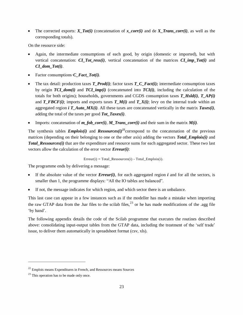
23

The corrected exports: X_Tot(i) (concatenation of x_corr(i) and de X_Trans_corr(i), as well as the

corresponding totals).

On the resource side:

Again, the intermediate consumptions of each good, by origin (domestic or imported), but with

vertical concatenation: CI_Tot_ress(i), vertical concatenation of the matrices CI_imp_Tot(i) and

CI_dom_Tot(i).

Factor consumptions·C_Fact_Tot(i).

The tax detail: production taxes T_Prod(i); factor taxes T_C_Fact(i); intermediate consumption taxes

by origin TCI_dom(i) and TCI_imp(i) (concatenated into TCI(i), including the calculation of the

totals for both origins); households, governments and CGDS consumption taxes T_Hsld(i), T_AP(i)

and T_FBCF(i); imports and exports taxes T_M(i) and T_X(i); levy on the internal trade within an

aggregated region i T_Auto_MX(i). All these taxes are concatenated vertically in the matrix Taxes(i),

adding the total of the taxes per good Tot_Taxes(i).

Imports: concatenation of m_fob_corr(i), M_Trans_corr(i) and their sum in the matrix M(i).

The synthesis tables Emplois(i) and Ressources(i)22

correspond to the concatenation of the previous

matrices (depending on their belonging to one or the other axis) adding the vectors Total_Emplois(i) and

Total_Ressources(i) that are the expenditure and resource sums for each aggregated sector. These two last

vectors allow the calculation of the error vector Erreur(i):

Erreur(i) = Total_Ressources(i) - Total_Emplois(i).

The programme ends by delivering a message:

If the absolute value of the vector Erreur(i), for each aggregated region i and for all the sectors, is

smaller than 1, the programme displays: “All the IO tables are balanced”.

If not, the message indicates for which region, and which sector there is an unbalance.

This last case can appear in a few instances such as if the modeller has made a mistake when importing

the raw GTAP data from the .har files to the scilab files,23

or he has made modifications of the .agg file

‘by hand’.

The following appendix details the code of the Scilab programme that executes the routines described

above: consolidating input-output tables from the GTAP data, including the treatment of the ‘self trade’

issue, to deliver them automatically in spreadsheet format (csv, xls).

22 Emplois means Expenditures in French, and Ressources means Sources

23 This operation has to be made only once.

24

IV Appendix

IV.1 Comments

Scilab is a freeware version of Matlab: the comprehensive Scilab programme gives free access to the

correction of the ‘self-trade’ phenomenon as described above. The programme is valid whatever the

version of GTAP, provided the user changes the number of regions at the top of the code.

This programme has already been used for the calibration of two CGE models: IMACLIM-S (Ghersi et al.,

2009) and IMACLIM-R (Sassi et al., 2010).

The Scilab code is given with French comments. A translated version of the code will be given in a further

version of the paper.

The coming and final version of this article will include a last section before the Appendix, that will

illustrate the importance of the ‘self-trade’ correction by comparing the conclusions of some policy

analysis conducted either on the uncorrected, or on the corrected EU IO table.

The successive steps to run the programme are:

1. Download Scilab.exe

2. Create a folder : GTAP_ScilabFolder

3. Create the .sce files described in section III.3.1 through the importation of the different matrices

from basedata.harr and baseview.harr files (with the “one to one”aggregation level) then put

them in the folder GTAP_ScilabFolder.

4. Create the text aggregation file .agg and copy it in the folder GTAP_ScilabFolder

5. Make the following changes in the main programme GTAPagg_Scilab.sce:

a. Currently, the variable gtap_version is equal to 7 (it refers to the version of GTAP), so

if the modeller is using another version (5 or 6), he just has to change the value of this

variable.

b. Define the trajectory of the work directory, workdir = ’………\ GTAP_ScilabFolder’;

6. Create the subfolder csv_ IOTables in the folder GTAP_ScilabFolder. This subfolder is

intended to hold the csv IO tables that will be created (One csv file per new aggregated region).

7. Copy the text of the section IV.2 bellow (the main programme) in any text editor to create the file

GTAPagg_Scilab.sce

8. Run this main programme GTAPagg_Scilab.sce from the scilab widow:

exec(GTAPagg_Scilab.sce)

After a few seconds, the csv files corresponding to the new aggregated regions’ IO tables, for the

chosen sectoral aggregated level and obviously including the self-trade correction are at disposal in

the folder csv_ IOTables.

25

IV.2 The Scilab main program of the revisited GTAPAgg procedure:

GTAPagg_Scilab.sce

26

////////////////////////////////////////////////////////////////////////////////////////////////////////////////////////////////////////////////////

// Ce programme repose sur les données du prgme GtapAgg ( Version 7,6 et 5)

//

// Partant de 57 Biens/113 (87 ou 66) Régions/5facteurs,

//

// ce prgm est destiné à fabriquer des TES équilibrés quelque soit l'agrégation de biens, de regions et de facteurs que l'utilisateur aura choisi///

/////////////////////////////////////////////////////////////////////////////////

gtap_version = 7;

workdir = '...\GTAP_ScilabFolder';

chdir(workdir);

stacksize(150000000);

//Ce programme part de la lecture d'un fichier .agg issu de GTAP où sont définies les agrégations voulues

Aggregations = input("Please enter the the name of the aggregations file: ","s");

//Lecture du fichier.agg

Txt = read(Aggregations,-1,1,'(a)');

Section = grep(Txt,'=');

P = Section(3)-Section(2)-1; // le nouveau nombre de Biens

N = Section(7)-Section(6)-1; // le nouveau nombre de Régions

27

K = Section(11)-Section(10)-1; // le nouveau nombre de Facteurs

if gtap_version == 5 then numREG = 66;// 1997 //// de la serie "Trade-Exports for International Transportation,MP" BaseDATA

elseif gtap_version == 6 then numREG = 87; //2001

elseif gtap_version == 7 then numREG = 113; //2004

end

Masc1 = zeros(numREG,N);

Masc2 = zeros(P,57);

//Matrices Textes des nouveaux Biens/Régions/Facteurs

B = part(Txt(Section(2)+1:Section(3)-1),[1:13]);

R = part(Txt(Section(6)+1:Section(7)-1),[1:13]);

Fact = part(Txt(Section(10)+1:Section(11)-1),[1:13]);

//Matrices Textes des enciens Biens/Régions/Facteurs

b = part(Txt(Section(4)+1:Section(5)-1),[50:62]);

r = part(Txt(Section(8)+1:Section(9)-1),[50:62]);

f = part(Txt(Section(12)+1:Section(13)-1),[50:62]);

//Remplissage des "masques"

28

for i=1:P

for j=1:57

if B(i)==b(j) then Masc2(i,j)=1;

end

end

end

for i=1:numREG

for j=1:N

if r(i)==R(j) then Masc1(i,j)=1;

end

end

end

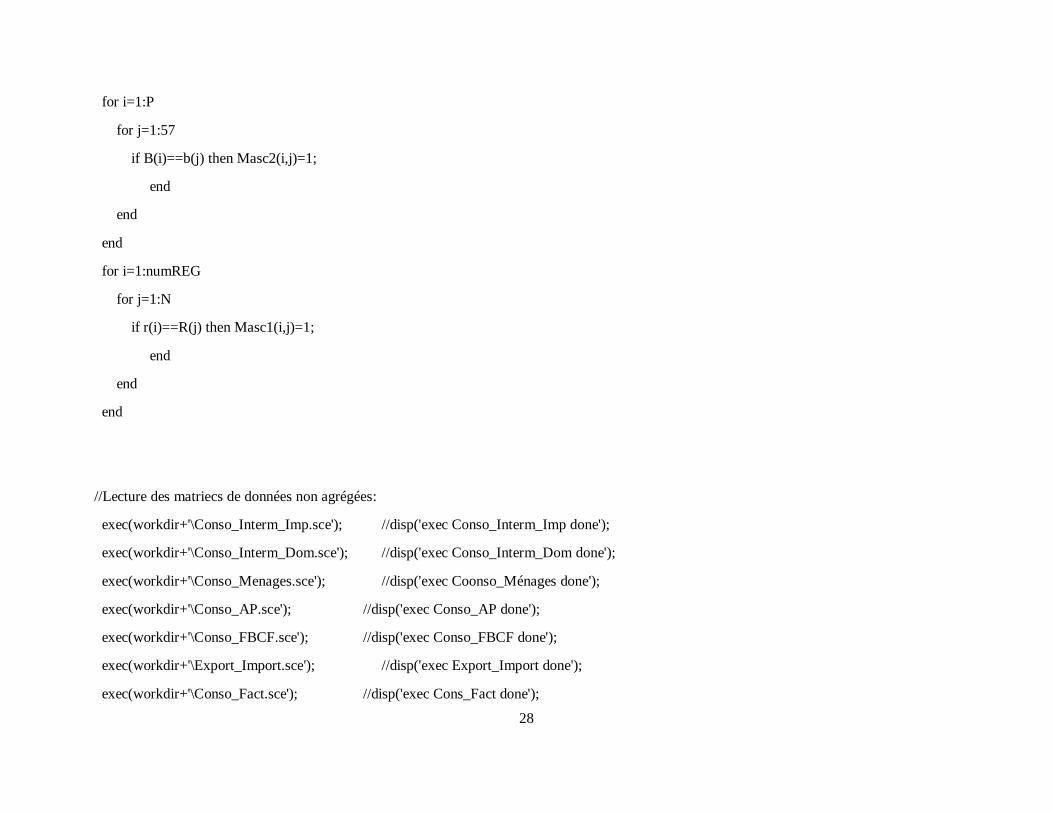
//Lecture des matriecs de données non agrégées:

exec(workdir+'\Conso_Interm_Imp.sce'); //disp('exec Conso_Interm_Imp done');

exec(workdir+'\Conso_Interm_Dom.sce'); //disp('exec Conso_Interm_Dom done');

exec(workdir+'\Conso_Menages.sce'); //disp('exec Coonso_Ménages done');

exec(workdir+'\Conso_AP.sce'); //disp('exec Conso_AP done');

exec(workdir+'\Conso_FBCF.sce'); //disp('exec Conso_FBCF done');

exec(workdir+'\Export_Import.sce'); //disp('exec Export_Import done');

exec(workdir+'\Conso_Fact.sce'); //disp('exec Cons_Fact done');

29

exec(workdir+'\Taxes1.sce'); //disp('exec Taxes1 done');

exec(workdir+'\Taxes2_Dom.sce'); //disp('exec Taxes2_Dom done');

exec(workdir+'\Taxes2_Imp.sce'); //disp('exec Taxes2_Imp done');

exec(workdir+'\Taxes3.sce'); //disp('exec Taxes3 done');

exec(workdir+'\Exports.sce'); //Pour la correction de la part "Auto-Export" et "Auto-Import_fob"...cf les fichiers

exec(workdir+'\Imports_Fob.sce');

exec(workdir+'\Imports_Transp.sce');

exec(workdir+'\mtax.sce'); //Pour la correction de la part "Auto-mtax" et "Auto-xtax"...cf les fichiers

exec(workdir+'\xtax.sce');

exec(workdir+'\Epargne.sce'); //disp('exec Epargne done');

//Calcul des matrices aggrégées:

//Conso Intermediaires(de produits domestiques et importés)+ Conso de Facteurs:

Som_CI_imp = list();

Som_CI_dom = list();

CI_imp_Agg = list(); CI_imp_Agg_corr = list();

CI_dom_Agg = list(); CI_dom_Agg_corr = list();

30

Som_CFact = list();

CFact_Agg = list();

for j=1:N

Som_CI_imp(j) = zeros(57,57);

Som_CI_dom(j) = zeros(57,57);

Som_CFact(j) = zeros(5,57);

for i=1:numREG

if Masc1(i,j) == 1 then

Som_CI_imp(j)= Som_CI_imp(j)+CI_imp(i) ;

Som_CI_dom(j)= Som_CI_dom(j)+CI_dom(i) ;

Som_CFact(j) = Som_CFact(j)+CFact(i);

end

end

CI_imp_Agg(j)= Masc2*Som_CI_imp(j)*Masc2'; //voir plus loin CI_imp_Agg_corr

CI_dom_Agg(j)= Masc2*Som_CI_dom(j)*Masc2'; //voir plus loin CI_dom_Agg_corr

CFact_Agg(j) = Som_CFact(j)*Masc2';

end

//Importations:

M_fob_Agg = Masc2*MM_fob*Masc1; //les Importations sans les couts de Transport!!!

M_Trans_Agg = Masc2*MM_Trans*Masc1;

//Exportattions:

31

X_Agg = Masc2*XX*Masc1; // au prix mondial!!!

X_Trans_Agg = Masc2*XX_Trans*Masc1; //des services de transports Internationnaux

//Consommations Finales:

C_25_Agg = Masc2*C_25*Masc1; //Conso Ménages de produits Imp

C_26_Agg = Masc2*C_26*Masc1; //Conso Ménages de produits Dom

C_27_Agg = Masc2*C_27*Masc1; //Conso AP produits Imp

C_28_Agg = Masc2*C_28*Masc1; //Conso AP produits Dom

C_14_Agg = Masc2*C_14*Masc1; //Conso FBCF produits Imp

C_15_Agg = Masc2*C_15*Masc1; //Conso FBCF produits Dom

//TAXES:

///"Simples à traiter"

T_13_Agg = Masc2*T_13*Masc1; // Outtax sur la Production

T_16_DomAgg = Masc2*T_16_Dom*Masc1; // Sur la conso des Ménages produits Dom

T_16_ImpAgg = Masc2*T_16_Imp*Masc1; // Sur la conso des Ménages produits Imp

T_17_DomAgg = Masc2*T_17_Dom*Masc1; // Sur la conso des AP produits Dom

T_17_ImpAgg = Masc2*T_17_Imp*Masc1; // Sur la conso des AP produits Imp

T_mtaxAgg = Masc2*T_mtax*Masc1; // Sur les Importations

T_xtaxAgg = Masc2*T_xtax*Masc1; // Sur les Exportations

//Comtax sur: la Conso de Facteurs/la FBCF(dom et imp)/et les Conso Intermédiaires(dom et imp)

32

Som_T_ConsFact=list();

T_ConsFact_Agg=list();

Som_T_FBCF_dom=list();

Som_T_FBCF_imp=list();

T_FBCF_dom_Agg=list();

T_FBCF_imp_Agg=list();

Som_T_CI_dom = list();

T_CI_dom_Agg = list();

Som_T_CI_imp = list();

T_CI_imp_Agg = list();

for j=1:N

Som_T_ConsFact(j)=zeros(5,57);

Som_T_FBCF_dom(j)=zeros(1,57);

Som_T_FBCF_imp(j)=zeros(1,57);

Som_T_CI_dom(j) = zeros(57,57);

Som_T_CI_imp(j) = zeros(57,57);

for i=1:numREG

if Masc1(i,j) == 1 then

Som_T_ConsFact(j) = Som_T_ConsFact(j)+T_ConsFact(i);

Som_T_FBCF_dom(j) = Som_T_FBCF_dom(j)+T_FBCF_dom (i);

Som_T_FBCF_imp(j) = Som_T_FBCF_imp(j)+T_FBCF_imp (i);

Som_T_CI_dom(j)= Som_T_CI_dom(j)+T_CI_dom(i) ;

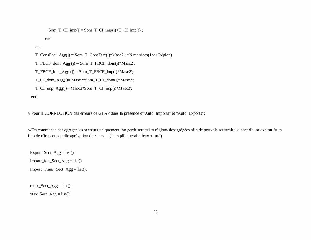
33

Som_T_CI_imp(j)= Som_T_CI_imp(j)+T_CI_imp(i) ;

end

end

T_ConsFact_Agg(j) = Som_T_ConsFact(j)*Masc2'; //N matrices(1par Région)

T_FBCF_dom_Agg (j) = Som_T_FBCF_dom(j)*Masc2';

T_FBCF_imp_Agg (j) = Som_T_FBCF_imp(j)*Masc2';

T_CI_dom_Agg(j)= Masc2*Som_T_CI_dom(j)*Masc2';

T_CI_imp_Agg(j)= Masc2*Som_T_CI_imp(j)*Masc2';

end

// Pour la CORRECTION des erreurs de GTAP dues la présence d'"Auto_Imports" et "Auto_Exports":

///On commence par agréger les secteurs uniquement, on garde toutes les régions désagrégées afin de pouvoir soustraire la part d'auto-exp ou Auto-

Imp de n'importe quelle agrégation de zones.....(jmexplihquerai mieux + tard)

Export_Sect_Agg = list();

Import_fob_Sect_Agg = list();

Import_Trans_Sect_Agg = list();

mtax_Sect_Agg = list();

xtax_Sect_Agg = list();

34

for i=1:P //j'avais 57 matrices, now j'en ai P

Export_Sect_Agg(i)=[];

Import_fob_Sect_Agg(i)=[];

Import_Trans_Sect_Agg(i)=[];

mtax_Sect_Agg(i)=[];

xtax_Sect_Agg(i)=[];

for j=1:57

if Masc2(i,j) == 1 then

Export_Sect_Agg(i) = Export_Sect_Agg(i) + Export(j);

Import_fob_Sect_Agg(i) = Import_fob_Sect_Agg(i) + Import_fob(j);

Import_Trans_Sect_Agg(i) = Import_Trans_Sect_Agg(i) + Import_Tran(j);

mtax_Sect_Agg(i) = mtax_Sect_Agg(i) + mtax(j);

xtax_Sect_Agg(i) = xtax_Sect_Agg(i) + xtax(j);

end

end

end

//Construction des TES:

//Declaration des Vriables "list":

35

C_Hsld_imp = list(); C_Hsld_dom = list(); C_Hsld =list(); C_Hsld_Tot = list();

C_Hsld_imp_corr = list(); C_Hsld_dom_corr = list();

C_G_imp = list(); C_G_dom = list(); C_G = list(); C_G_Tot = list();

C_G_imp_corr = list(); C_G_dom_corr = list();

C_FBCF_imp = list(); C_FBCF_dom = list(); C_FBCF = list();C_FBCF_Tot = list();

C_FBCF_imp_corr = list(); C_FBCF_dom_corr = list();

x = list(); Auto_X = list(); x_corr = list();

X_Trans = list(); X_Trans_corr = list();

X = list(); X_Tot = list();

CI_imp_Tot = list(); CI_dom_Tot = list();

CI_emplois = list(); ci_tot_emp = list(); CI_Tot_emplois = list();

CI_ressources = list(); ci_tot_ress = list(); CI_Tot_ressources = list();

C_Fact_Tot = list();

m_fob = list(); m_fob_corr = list(); Auto_M_fob = list();

M_Trans = list(); M_Trans_corr = list(); Auto_M_Trans = list();

M = list();M_Tot = list();

36

p_bascul = list();

T_Prod = list();

T_C_Fact = list();

TCI_dom = list(); TCI_imp = list(); TCI = list();

T_FBCF = list();

T_Hsld_dom = list(); T_Hsld_imp = list();T_Hsld = list();

T_AP_dom = list(); T_AP_imp = list();T_AP = list();

T_M = list();

T_X = list();

THsld_Imp_corr = list();

TG_Imp_corr = list();

T_FBCF_imp_Agg_corr = list();

THsld_Dom_corr = list();

TG_Dom_corr = list();

T_FBCF_dom_Agg_corr = list();

T_CI_imp_Agg_corr = list();

37

T_CI_dom_Agg_corr = list();

Tprod = list();

THsld_Dom = list();

THsld_Imp = list();

TG_Dom = list();

TG_Imp = list();

Tmtax = list(); Auto_mtax = list(); Tmtax_corr = list();

Txtax = list(); Auto_xtax = list(); Txtax_corr = list();

Auto_TMX = list(); T_Auto_MX = list();

Taxes = list(); Tot_Taxes = list();

Emplois = list(); Total_Emplois = list() ;

Ressources = list(); Total_Ressources = list();

Erreur = list();

xtr_Agg = list();

xtrans1 = list();

xtrans2 = list();

xtrans3 = list();

38

xtr48 = list();

xtr49 = list();

xtr50 = list();

part_AutoM_Trans = list();

CI_dom_Agg_corr_Trans = list();

bascul_XTransp = list();

for k=1:numREG

xtr(k) = x_Trans(1,k) + x_Trans(2,k) + x_Trans(3,k);

end

for j=1:N

///Séparation des Régions pour chaque "série"

//Coté Emplois:

C_Hsld_imp(j) = C_25_Agg(:,j); //Ce sont des vecteurs colonne ( P éléments)

C_Hsld_dom(j) = C_26_Agg(:,j);

C_G_imp(j) = C_27_Agg(:,j);

C_G_dom(j) = C_28_Agg(:,j);

C_FBCF_imp(j) = C_14_Agg(:,j);

39

C_FBCF_dom(j) = C_15_Agg(:,j);

x(j) = X_Agg(:,j);

X_Trans(j) = X_Trans_Agg(:,j);

//Coté Ressources:

m_fob(j) = M_fob_Agg(:,j); //Ce sont tjrs des vect colonnes (P éléments)que l'on transposera + tard

M_Trans(j) = M_Trans_Agg(:,j);

Tmtax(j) = T_mtaxAgg(:,j);

Txtax(j) = T_xtaxAgg(:,j);

Tprod(j) = T_13_Agg(:,j);

THsld_Dom(j) = T_16_DomAgg(:,j);

THsld_Imp(j) = T_16_ImpAgg(:,j);

TG_Dom(j) = T_17_DomAgg(:,j);

TG_Imp(j) = T_17_ImpAgg(:,j);

/// Suite des CORRECTIONS

//// Corection des Exportations: Soustraction pour chaque région de la part "Auto-Exportation"

//// Corection des Importations: Soustraction pour chaque région de la part "Auto-Importation"

40

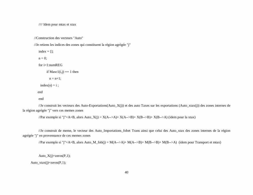
//// Idem pour mtax et xtax

//Construction des vecteurs "Auto"

//Je retiens les indices des zones qui constituent la région agrégée "j"

index = [];

n = 0;

for i=1:numREG

if Masc1(i,j) == 1 then

n = n+1;

index(n) = i ;

end

end

//Je construit les vecteurs des Auto-Exportations(Auto_X(j)) et des auto Taxes sur les exportations (Auto_xtax(j)) des zones internes de

la région agrégée "j" vers ces memes zones

//Par exemple si "j"=A+B, alors Auto_X(j) = X(A-->A)+ X(A-->B)+ X(B-->B)+ X(B-->A) (idem pour la xtax)

//Je construit de meme, le vecteur des Auto_Importations_fobet Trans ainsi que celui des Auto_xtax des zones internes de la région

agrégée "j" en provennance de ces memes zones

//Par exemple si "j"=A+B, alors Auto_M_fob(j) = M(A-->A)+ M(A-->B)+ M(B-->B)+ M(B-->A) (idem pour Transport et mtax)

Auto_X(j)=zeros(P,1);

Auto_xtax(j)=zeros(P,1);

41

Auto_M_fob(j)=zeros(P,1);

Auto_M_Trans(j)=zeros(P,1);

part_AutoM_Trans(j)=zeros(P,1);

Auto_mtax(j)=zeros(P,1);

CI_imp_Agg_corr(j)=zeros(P,P);

CI_dom_Agg_corr(j)=zeros(P,P);

T_CI_imp_Agg_corr(j)=zeros(P,P);

T_CI_dom_Agg_corr(j)=zeros(P,P);

for k=1:P

for s=1:size(index,'r')

for t=1:size(index,'r')

//Auto-X du bien agrégé "k" pour la zone agrégée "j"

Auto_X(j)(k) = Auto_X(j)(k) + Export_Sect_Agg(k)(index(s),index(t)); //X du bien agrégé "k" de la

//zone t vers s

Auto_xtax(j)(k) = Auto_xtax(j)(k) + xtax_Sect_Agg(k)(index(s),index(t));

//Auto-M du bien agrégé "k" pour la zone agrégée "j"

Auto_M_fob(j)(k) = Auto_M_fob(j)(k) + Import_fob_Sect_Agg(k)(index(s),index(t));

42

Auto_M_Trans(j)(k) = Auto_M_Trans(j)(k) + Import_Trans_Sect_Agg(k)(index(s),index(t));

Auto_mtax(j)(k) = Auto_mtax(j)(k) + mtax_Sect_Agg(k)(index(s),index(t));

end

end

end

///Cas de M_Trans: On ne retire qu'une part de Auto_M_Trans:

if gtap_version == 5 then XTrans_Monde = 211372.74;// 1997 //// de la serie "Trade-Exports for International Transportation,MP"

BaseDATA

elseif gtap_version == 6 then XTrans_Monde = 234441.71; //2001

elseif gtap_version == 7 then XTrans_Monde = 362713.343750; //2004

end

//xtr(j) = x_Trans(1,j) + x_Trans(2,j) + x_Trans(3,j) (j zone desagégée)

xtr_Agg(j)=0;

xtrans1(j)=0;

xtrans2(j)=0;

xtrans3(j)=0;

43

for i=1:numREG

// agrégation des régions pour les participations au transport international(biens de transp 48,49,50)

if Masc1(i,j)== 1 then

xtr_Agg(j) = xtr_Agg(j) + xtr(i);

xtrans1(j) = xtrans1(j) + x_Trans(1,i);

xtrans2(j) = xtrans2(j) + x_Trans(2,i);

xtrans3(j) = xtrans3(j) + x_Trans(3,i);

end

end

xtr48(j) = xtrans1(j)/ xtr_Agg(j); // xtr48(j) = x_Trans(1,j)/xtr(j);

xtr49(j) = xtrans2(j)/ xtr_Agg(j); // xtr49(j) = x_Trans(2,j)/xtr(j);

xtr50(j) = xtrans3(j)/ xtr_Agg(j); // xtr50(j) = x_Trans(3,j)/xtr(j);

//Pour k=1:P part_AutoM_Trans(j)(k)=( xtr(j)/XTrans_Monde )* Auto_M_Trans(j)(k);

part_AutoM_Trans(j) = ( xtr_Agg(j)/XTrans_Monde )* Auto_M_Trans(j);

//// Corection des Exportations: Soustraction pour chaque région de la part "Auto-Exportation"

//J'effectue ma soustraction pour x

x_corr(j) = x(j) - Auto_X(j);

44

//// Correction des Importations: Soustraction pour chaque région de la part "Auto-Importation"

//J'effectue mes soustractions pour m_fob (pour M_Trans voir plus loin)

m_fob_corr(j) = m_fob(j) - Auto_M_fob(j);

//pour M_Trans voir plus loin

// Pour rééquilibrer les TES

////Calcul du "pourcentage de basculement"(Coté Emplois:de Cons_M vers Cons_D /Coté Ressources: de TCm vers TCD ):

////p_bascul% pour chaque bien i:

p_bascul(j) = (Auto_M_fob(j) + part_AutoM_Trans(j) + Auto_mtax(j))./(m_fob(j) + M_Trans(j) + Tmtax(j));

//// Basculement de Conso de produits Importés vers Conso de produits Domestiques

// Pour les Conso Finales:

// Je retire p% des CFM

C_Hsld_imp_corr(j) = C_Hsld_imp(j) - (p_bascul(j).*C_Hsld_imp(j));

C_G_imp_corr(j) = C_G_imp(j) - (p_bascul(j).*C_G_imp(j));

C_FBCF_imp_corr(j) = C_FBCF_imp(j) - (p_bascul(j).*C_FBCF_imp(j));

// je rajoute p% des CFM aux CFD

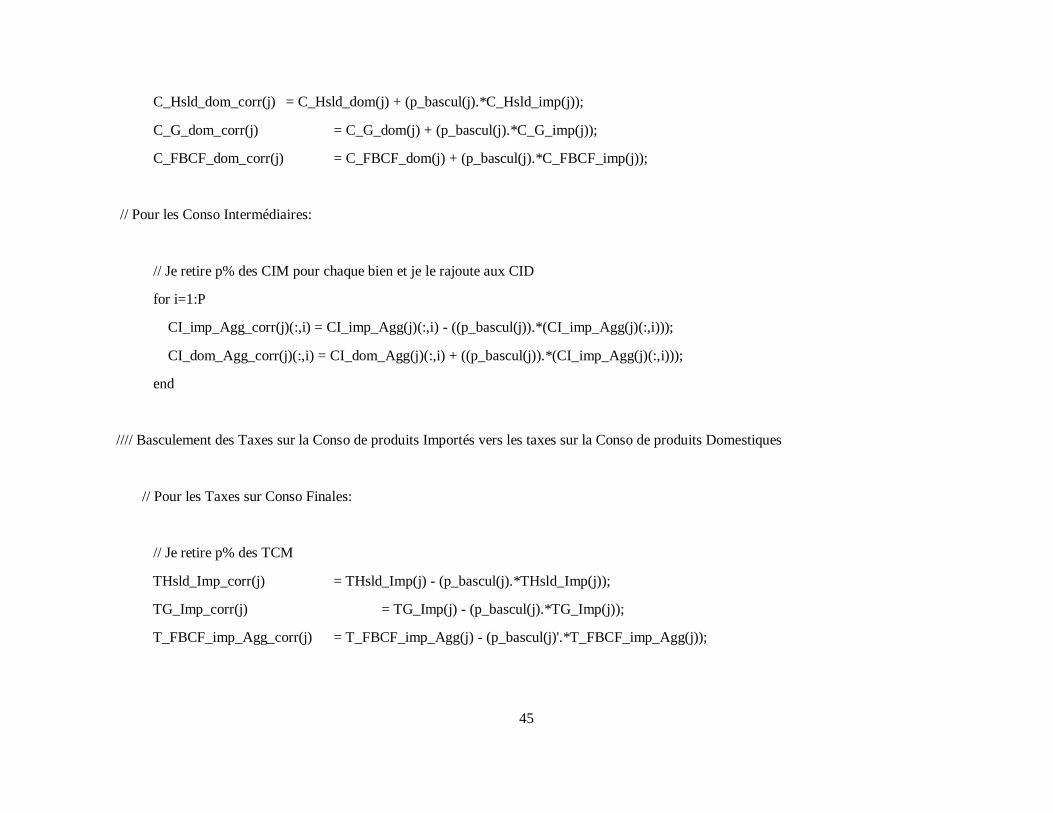
45

C_Hsld_dom_corr(j) = C_Hsld_dom(j) + (p_bascul(j).*C_Hsld_imp(j));

C_G_dom_corr(j) = C_G_dom(j) + (p_bascul(j).*C_G_imp(j));

C_FBCF_dom_corr(j) = C_FBCF_dom(j) + (p_bascul(j).*C_FBCF_imp(j));

// Pour les Conso Intermédiaires:

// Je retire p% des CIM pour chaque bien et je le rajoute aux CID

for i=1:P

CI_imp_Agg_corr(j)(:,i) = CI_imp_Agg(j)(:,i) - ((p_bascul(j)).*(CI_imp_Agg(j)(:,i)));

CI_dom_Agg_corr(j)(:,i) = CI_dom_Agg(j)(:,i) + ((p_bascul(j)).*(CI_imp_Agg(j)(:,i)));

end

//// Basculement des Taxes sur la Conso de produits Importés vers les taxes sur la Conso de produits Domestiques

// Pour les Taxes sur Conso Finales:

// Je retire p% des TCM

THsld_Imp_corr(j) = THsld_Imp(j) - (p_bascul(j).*THsld_Imp(j));

TG_Imp_corr(j) = TG_Imp(j) - (p_bascul(j).*TG_Imp(j));

T_FBCF_imp_Agg_corr(j) = T_FBCF_imp_Agg(j) - (p_bascul(j)'.*T_FBCF_imp_Agg(j));

46

// je rajoute p% des TCFM aux TCFD

THsld_Dom_corr(j) = THsld_Dom(j) + (p_bascul(j).*THsld_Imp(j));

TG_Dom_corr(j) = TG_Dom(j) + (p_bascul(j).*TG_Imp(j));

T_FBCF_dom_Agg_corr(j) = T_FBCF_dom_Agg(j) + (p_bascul(j)'.*T_FBCF_imp_Agg(j));

// Pour les Taxes sur les Conso Intermédiaires:

// Je retire p% des TCIM pour chaque bien et je le rajoute aux TCID

for i=1:P

T_CI_imp_Agg_corr(j)(:,i) = T_CI_imp_Agg(j)(:,i) - (p_bascul(j).*T_CI_imp_Agg(j)(:,i));

T_CI_dom_Agg_corr(j)(:,i) = T_CI_dom_Agg(j)(:,i) + (p_bascul(j).*T_CI_imp_Agg(j)(:,i));

end

//// Corection des Taxes sur les M et X: Soustraction pour chaque région de la part "Auto" des xtax et mtax

Tmtax_corr(j) = Tmtax(j) - Auto_mtax(j);

Txtax_corr(j) = Txtax(j) - Auto_xtax(j);

//Pour réequilibrer les TES

//On rajoute Une nouvelle taxe dans notre TES:

47

Auto_TMX(j) = Auto_mtax(j)+Auto_xtax(j);

////Correction M_Trans ( retrait de la partie "auto-M_Tans" selon les explication du papier...!!!

//Correction M_Trans ( on lui enleve la part qui correspond a des Auto frais de Transports)

M_Trans_corr(j) = M_Trans(j) - part_AutoM_Trans(j);

// Réequilibrage du TES : (Basculement vers CI_dom et retrait de Xtrans )

//Basculement vers CI_dom

CI_dom_Agg_corr_Trans(j) = CI_dom_Agg_corr(j);

for i=1:P

if Masc2(i,48) == 1 then

for k=1:P

CI_dom_Agg_corr_Trans(j)(i,k) = CI_dom_Agg_corr_Trans(j)(i,k) + (xtr48(j)*part_AutoM_Trans(j)(k) );

end

end

if Masc2(i,49) == 1 then

48

for k=1:P

CI_dom_Agg_corr_Trans(j)(i,k) = CI_dom_Agg_corr_Trans(j)(i,k) + (xtr49(j)*part_AutoM_Trans(j)(k) );

end

end

if Masc2(i,50) == 1 then

for k=1:P

CI_dom_Agg_corr_Trans(j)(i,k) = CI_dom_Agg_corr_Trans(j)(i,k) + (xtr50(j)*part_AutoM_Trans(j)(k) );

end

end

end

// retrait de la part "auto" correspondante dans Xtrans

bascul_XTransp(j) = sum( (CI_dom_Agg_corr_Trans(j)- CI_dom_Agg_corr(j)),'c');

X_Trans_corr(j) = X_Trans(j) - bascul_XTransp(j);

////Coté Emplois:

///Concaténation des Matrices ( Produits Imp avec Produits Dom et X avec X-Transport)(matrices P*2)

C_Hsld(j) = [ C_Hsld_imp_corr(j) C_Hsld_dom_corr(j)];

49

C_G(j) = [ C_G_imp_corr(j) C_G_dom_corr(j) ];

C_FBCF(j) = [ C_FBCF_imp_corr(j) C_FBCF_dom_corr(j)];

X(j) = [ x_corr(j) X_Trans_corr(j)];

///Les meme données concaténées avec les totaux "correspondants" ( matrices (P+1)*3 )

C_Hsld_Tot(j) = [ C_Hsld(j) sum(C_Hsld(j),'c') ; sum(C_Hsld(j),'r') sum(C_Hsld(j))];

C_G_Tot(j) = [ C_G(j) sum(C_G(j),'c') ; sum(C_G(j),'r') sum(C_G(j))];

C_FBCF_Tot(j) = [ C_FBCF(j) sum(C_FBCF(j),'c') ; sum(C_FBCF(j),'r') sum(C_FBCF(j))];

X_Tot(j) = [ X(j) sum(X(j),'c') ; sum(X(j),'r') sum(X(j))];

///De meme pour les Consommations Intermédiaires ( Totaux pour matrice Imp, Totaux pour matrice Dom, Concaténation des 2 matries

(P+1)*(P+1) --->> 1 matrice (P+1)*(2P+2)--->>Puis concaténation avec le vect TotalCI(P+1)--->> 1 matrice (P+1)*(2P+3)

CI_imp_Tot(j) = [ CI_imp_Agg_corr(j) sum(CI_imp_Agg_corr(j),'c') ; sum(CI_imp_Agg_corr(j),'r') sum(CI_imp_Agg_corr(j))];

//(P+1)*(P+1)

CI_dom_Tot(j) = [ CI_dom_Agg_corr_Trans(j) sum(CI_dom_Agg_corr_Trans(j),'c') ; sum(CI_dom_Agg_corr_Trans(j),'r')

sum(CI_dom_Agg_corr_Trans(j))];

CI_emplois(j) = [ CI_imp_Tot(j) CI_dom_Tot(j) ]; //(P+1)*(2P+2)

ci_tot_emp(j) = CI_emplois(j)(:,P+1)+ CI_emplois(j)(:,2*P+2); //vect(P+1)

CI_Tot_emplois(j) = [ CI_emplois(j) ci_tot_emp(j) ]; // (P+1)*(2P+3)

////Coté Ressources: (on procède de la meme maniere,en prenant concatenation en ligne cette fois(au lieu de colonnes)

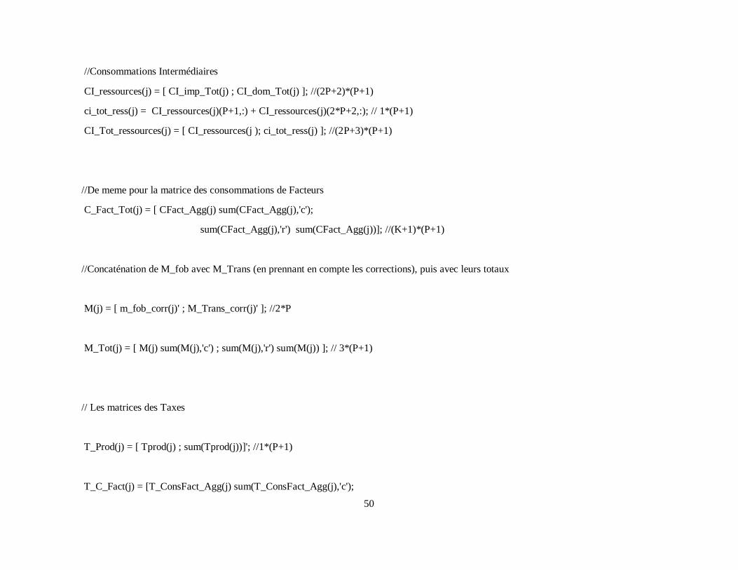
50

//Consommations Intermédiaires

CI_ressources(j) = [ CI_imp_Tot(j) ; CI_dom_Tot(j) ]; //(2P+2)*(P+1)

ci_tot_ress(j) = CI_ressources(j)(P+1,:) + CI_ressources(j)(2*P+2,:); // 1*(P+1)

CI_Tot_ressources(j) = [ CI_ressources(j ); ci_tot_ress(j) ]; //(2P+3)*(P+1)

//De meme pour la matrice des consommations de Facteurs

C_Fact_Tot(j) = [ CFact_Agg(j) sum(CFact_Agg(j),'c');

sum(CFact_Agg(j),'r') sum(CFact_Agg(j))]; //(K+1)*(P+1)

//Concaténation de M_fob avec M_Trans (en prennant en compte les corrections), puis avec leurs totaux

M(j) = [ m_fob_corr(j)' ; M_Trans_corr(j)' ]; //2*P

M_Tot(j) = [ M(j) sum(M(j),'c') ; sum(M(j),'r') sum(M(j)) ]; // 3*(P+1)

// Les matrices des Taxes

T_Prod(j) = [ Tprod(j) ; sum(Tprod(j))]'; //1*(P+1)

T_C_Fact(j) = [T_ConsFact_Agg(j) sum(T_ConsFact_Agg(j),'c');

51

sum(T_ConsFact_Agg(j),'r') sum(T_ConsFact_Agg(j))]; //(K+1)*(P+1);

TCI_dom(j) = [T_CI_dom_Agg_corr(j) sum(T_CI_dom_Agg_corr(j),'c');

sum(T_CI_dom_Agg_corr(j),'r') sum(T_CI_dom_Agg_corr(j))]; //(P+1)*(P+1)

TCI_imp(j) = [T_CI_imp_Agg_corr(j) sum(T_CI_imp_Agg_corr(j),'c');

sum(T_CI_imp_Agg_corr(j),'r') sum(T_CI_imp_Agg_corr(j))]; //(P+1)*(P+1)

TCI(j) = [ TCI_dom(j);

TCI_imp(j);

TCI_dom(j)(P+1,:)+ TCI_imp(j)(P+1,:)]; //(2P+3)*(P+1)

T_FBCF(j) = [T_FBCF_dom_Agg_corr(j) sum(T_FBCF_dom_Agg_corr(j));

T_FBCF_imp_Agg_corr(j) sum(T_FBCF_imp_Agg_corr(j));

T_FBCF_dom_Agg_corr(j)+T_FBCF_imp_Agg_corr(j) sum(T_FBCF_dom_Agg_corr(j)+T_FBCF_imp_Agg_corr(j))]; //3*(P+1)

T_Hsld_dom(j) = [ THsld_Dom_corr(j)' sum(THsld_Dom_corr(j))]; //1*(P+1)

T_Hsld_imp(j) = [ THsld_Imp_corr(j)' sum(THsld_Imp_corr(j))]; //1*(P+1)

T_Hsld(j) = [ T_Hsld_dom(j) ;

T_Hsld_imp(j);

T_Hsld_dom(j)+T_Hsld_imp(j) ]; //3*(P+1)

52

T_AP_dom(j) = [ TG_Dom_corr(j)' sum(TG_Dom_corr(j))]; //1*(P+1)

T_AP_imp(j) = [TG_Imp_corr(j)' sum(TG_Imp_corr(j))]; //1*(P+1)

T_AP(j) = [ T_AP_dom(j) ; T_AP_imp(j);

T_AP_dom(j)+T_AP_imp(j) ]; //3*(P+1)

T_M(j) = [ Tmtax_corr(j)' sum(Tmtax_corr(j)) ]; //1*(P+1)

T_X(j) = [ Txtax_corr(j)' sum(Txtax_corr(j)) ]; //1*(P+1)

T_Auto_MX(j) = [ Auto_TMX(j)' sum( Auto_TMX(j))];

Tot_Taxes(j) = [T_Prod(j)+T_C_Fact(j)(K+1,:)+TCI(j)(2*P+3,:)+T_FBCF(j)(3,:)+T_Hsld(j)(3,:)+ T_AP(j)(3,:)+ T_M(j)+ T_X(j) +

T_Auto_MX(j)]; //1*(P+1)

Taxes(j) = [T_Prod(j); T_C_Fact(j); TCI(j); T_FBCF(j); T_Hsld(j); T_AP(j); T_M(j); T_X(j); T_Auto_MX(j) ; Tot_Taxes(j) ];

//(17+K+(2*P))*(P+1)

///Concaténation des matrices coté Emplois:

//Calcul de la Somme des emplois:

Total_Emplois(j) = ci_tot_emp(j) + C_Hsld_Tot(j)(:,3) + C_G_Tot(j)(:,3) + C_FBCF_Tot(j)(:,3) + X_Tot(j)(:,3);

Emplois(j) = [ CI_Tot_emplois(j) C_Hsld_Tot(j) C_G_Tot(j) C_FBCF_Tot(j) X_Tot(j) Total_Emplois(j) ];

53

///Concaténation des matrices coté Ressources:

//Calcul de la Somme des Ressources:

Total_Ressources(j) = ci_tot_ress(j) + C_Fact_Tot(j)(K+1,:) + M_Tot(j)(3,:) + Tot_Taxes(j) ;

Ressources(j) = [ CI_Tot_ressources(j); C_Fact_Tot(j);M_Tot(j); Taxes(j);Total_Ressources(j)];

///Calcul de l'erreur:

Erreur(j) = Total_Ressources(j)'-Total_Emplois(j);

///Le plafond d'erreur toléré est placé à 1 (en absolu)

a=%T;

if abs(Erreur(j))<=1 then aaaaaa = 12; //ça sert a rien mais tampis

else a=%F;

disp('Attention! Le TES de la Région '''+string(j)+''' est déséquilibré')

end

end

if a==%T then disp('Tous les TES sont équilibrés (avec une erreur(Ress-Empl) < 1)'); end

//Construction des TES******Transfert des Résultats vers des fichiers Excel://

// Ce programme permet de construire des TES sous format csv à partir des Matrices issues de GTAP Scilab.

54

chdir('workdir\csv_ IOTables'); //La ou se trouvent les fichiers Excel

Vide1=[]; for i=1:((2*P)+4), Vide1(i)=' '; end; Vide1=(Vide1)';//vect ligne

Vide2=[]; for i=1:(3*P+2*K+32), for j=1:(P+16), Vide2(i,j)=' ';end; end;

//Coté Emplois

Titre1 = [' ',' ',B','Tot',B','Tot',' ','1','1',' ','1','1',' ','FBCF','FBCF',' ','1','1',' ',' '];

Titre2 = [' ',' ','Imp',Vide1(1:P),'Dom',Vide1(1:P),'Tot CI','Imp','Dom','Tot Hsld','Imp','Dom','Tot G','Imp','Dom','Tot FBCF','X','Transport', 'Tot

X','Tot Emplois'];

Titre3 = ['CI',Vide1,'C_Hsld',Vide1(1:2),'C_AP',Vide1(1:2),'FBCF',Vide1(1:2),'X',Vide1(1:3)];

Titre_Emplois = [Titre3;Titre2;Titre1 ];

//Coté Ressources

//Pour TES entier:

Tr1 = [B;'Tot';'Tot CI';'Cons Fact';Fact;'Tot VA';'M_FOB';'Transport';'Tot';'T_Prod';'T_Fact';Fact;'Tot';'T_CI';B;'Tot';B;'Tot';'Tot

TCI';'T_FBCF';'dom';'imp';'Tot';'T_CHsld';'dom';'imp';'Tot';'T_CAP';'dom';'imp';'Tot';'Mtax';'Xtax';'T_Auto_MX';'Tot Taxes';''];

// Tr2 = ['dom';(Vide1(1:(P+1)))';'VA';(Vide1(1:(K+1)))';'M';' ';'

';'Taxes';(Vide1(1:(K+3)))';'dom';(Vide1(1:P))';'imp';(Vide1(1:P))';(Vide1(1:6))';(Vide1(1:6))';(Vide1(1:4))';' '; 'Tot Ressources'];

Tr2 = ['dom';(Vide1(1:(P+1)))';'VA';(Vide1(1:(K+1)))';'M';' ';' ';'Taxes';(Vide1(1:(K)))';' ';' ';'

';'dom';(Vide1(1:P))';'imp';(Vide1(1:P))';(Vide1(1:6))';(Vide1(1:6))';(Vide1(1:4))';' '; 'Tot Ressources'];

55

//Pour Tableau des Ressources seul:

Ttr1 = [ ' ';B;'Tot';Tr1];

Ttr2 = [ 'CI';'imp';(Vide1(1:P))';Tr2];

//Pour chaque région "j";on associe un Tableau "Emplois", un Tableau "Ressources" et le TES:

Tab_Empl=list();

Part= list();

Ress1=list(); Tab_Ress1=list();

Ress2=list(); Tab_Ress2=list();

Tab_Empl_err = list();

TES=list();

for j=1:N

//Emplois:

Tab_Empl(j) = [Titre_Emplois;(Vide1(1:(P+1)))',[B;'Tot'],string(Emplois(j))];

//Ressources:

56

Part(j) = [

Vide1(1:(P+1));string(C_Fact_Tot(j));string(M_Tot(j));string(T_Prod(j));Vide1(1:(P+1));string(T_C_Fact(j));Vide1(1:(P+1));string(TCI(j));Vide1

(1:(P+1));string(T_FBCF(j));Vide1(1:(P+1));string(T_Hsld(j));Vide1(1:(P+1));string([T_AP(j); T_M(j); T_X(j);T_Auto_MX(j); Tot_Taxes(j)

]);string(Total_Ressources(j))];

//Pour TES entier:

Ress2(j) = [string(CI_dom_Tot(j)); string(ci_tot_ress(j)) ;Part(j)];

Tab_Ress2(j) = [[Tr2,Tr1,Ress2(j)];['Erreur = ','Ress-Empl',string(Erreur(j)')]];

[ ' ' ; 'Erreur = Ress-Empl' ; string(Erreur(j)) ];

Tab_Empl_err(j) = [ Tab_Empl(j),[ 'Erreur =';'Ress-Empl' ; ' ' ; string(Erreur(j)) ]];

//les TES:

TES(j) = [ Tab_Empl_err(j) ; [Tab_Ress2(j) , Vide2] ];

form='';

for i=1:(size(TES(j),'c')- 1)

form=form + '%s;' ;

end;

form=form+'%s\n';

v=mopen('TEScorr_'+string(R(j))+'.csv' ,'w');

57

mfprintf(v,form,TES(j));

mclose(v);

end

58

V References

Badri Narayanan G., Betina V. Dimaranan and Robert A. McDougall. 2008. Guide to the GTAP Data

Base- Chapter 2 of GTAP 7 Data Base Documentation. Global Trade, Assistance, and Production: The GTAP 7 Data Base, Center for Global Trade Analysis, Purdue University. Badri Narayanan G. and Terrie

L. Walmsley, Editors.

Gehlhar, Mark J. 1996. “Reconciling Bilateral Trade Data for Use in GTAP” GTAP Technical Paper No.

10, Center for Global Trade Analysis, Purdue University.

Ghersi, F. 2009, “IMACLIM-S : Impact Assessment of Climate Policies”, in Gerlagh, R., Bosetti, V.,

Schleicher, S. (ed.), Modeling Sustainable Development, Edward Elgar, Cheltenham, pp. 161-171.

Ghersi F., Thubin C., Combet E. 2009, “The IMACLIM-S Model version 2.3”, CIRED working paper,

http://www.imaclim.centre-cired.fr/IMG/pdf/IMACLIM-S_31aug09Eng.pdf

Hertel, Thomas W and Walmsley, Terrie L. 2008. “Introduction”- Chapter 1 of GTAP 7 Data Base

Documentation. Global Trade, Assistance, and Production: The GTAP 7 Data Base, Center for Global

Trade Analysis, Purdue University. Badri Narayanan G. and Terrie L. Walmsley, Editors.

Horridge M. 2008. “GTAPAgg: Data Aggregation Program”- Chapter 5 of GTAP 7 Data Base

Documentation. Global Trade, Assistance, and Production: The GTAP 7 Data Base, Center for Global

Trade Analysis, Purdue University. Badri Narayanan G. and Terrie L. Walmsley, Editors.

Huff Karen, McDougall Robert and Walmsley Terrrie. 2000. “Contributing Input-Output Tables to the

GTAP Data Base” GTAP Technical Paper No. 1, Release 4.2, Center for Global Trade Analysis, Purdue

University.

McDonald, Scott and Thierfelder, Karen. 2004. “Deriving a Global Social Accounting Matrix from GTAP

Versions 5 and 6 Data” GTAP Technical Paper No. 22, Center for Global Trade Analysis, Purdue

University.

Peterson, Everest B. 2006. “GTAP-M: A GTAP Model and Data Base that Incorporates Domestic

Margins” GTAP Technical Paper No. 26, Center for Global Trade Analysis, Purdue University.

Sassi O., Crassous R., Hourcade J.-C., Gitz V., Waisman H., Guivarch C., 2010. ‘Imaclim-R : a modelling

framework to simulate sustainable development pathways’, International Journal of Global

Environmental Issues Vol 10, n°1, p 5-24.

UN, (1993). System of National Accounts 1993. UN: New York.

CIRED Working Papers Series