Learning Subsequential Transducers for Pattern Recognition Interpretation Tasks

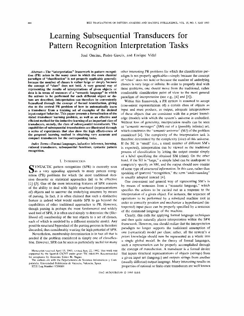
448 IEEE TRANSACTIONS ON PATTERN ANALYSIS AND MACHINE INTELLIGENCE, VOL. 15, NO. 5, MAY 1993

Learning Subsequential Transducers for Pattern Recognition Interpretation Tasks

Jose Oncina, Pedro Garcia, and Enrique Vidal

Abstract-The “interpretation” framework in pattern recognition (PR) arises in the many cases in which the more classical paradigm of “classification” is not properly applicable generally because the number of classes is rather large or simply because the concept of “class” does not hold. A very general way of representing the results of interpretations of given objects or data is in terms of sentences of a “semantic language” in which the actions to be performed for each different object or da- tum are described. Interpretation can therefore be conveniently formalized through the concept of formal transduction, giving rise to the central PR problem of how to automatically learn a transducer from a training set of examples of the desired input-output behavior. This paper presents a formalization of the stated transducer learning problem, as well as an effective and efficient method for the inductive learning of an important class of transducers, namely, the class of subsequential transducers. The capabilities of subsequential transductions are illustrated through a series of experiments that also show the high effectiveness of the proposed learning method in obtaining very accurate and compact transducers for the corresponding tasks.

Index Terms-Formal languages, inductive inference, learning, rational transducers, subsequential functions, syntactic pattern recognition.

I. INTRODUCTION

YNTACTIC pattern recognition (SPR) is currently seen S as a very appealing approach to many pattern recognition (PR) problems for which the most traditional deci- sion-theoretic or statistical approaches fail to be effective [1]-[3]. One of the most interesting features of SPR consists of the ability to deal with highly structured (representations of) objects and to uncover the underlying structure by means of parsing. In fact, it is often claimed that such a distinctive feature is indeed what would enable SPR to go beyond the capabilities of other traditional approaches to PR. However, though parsing is perhaps the most fundamental and widely used tool of SPR, it is often used simply to determine the (like- lihood of) membership of the test objects to a set of classes, each of which is modeled by a different syntactic model. Any possible structural byproduct of the parsing process is therefore discarded, thus considerably wasting the high potential of SPR.

Nevertheless, membership determination is in fact all that is needed if the problem considered is simply one of classification. However, SPR can be seen as particularly useful for many

Manuscript received April 15, 1991; revised June 22, 1992. This work was supported by the Spanish ClCYT under grant TIC-0448189. Recommended for acceptance by Associate Editor M. Nagao.

The authors are with the Departamento de Sistemas lnformaticos y Com- putacion, Universidad Politecnica de Valencia, Valencia, Spain.

IEEE Log Number 9208009.

other interesting PR problems for which the classification paradigm is not properly applicable-simply because the concept of “class” does not hold or because the number of underlying classes is very large or infinite. In order to properly deal with these problems, one should move from the traditional, rather comfortable classification point of view to the most general paradigm of interpretation (see e.g., [4] and [5]) .

Within this framework, a PR system is assumed to accept (convenient representations of) a certain class of objects as input and must produce, as output, adequate interpretations of these objects that are consistent with the a priori knowledge (model) with which the system’s universe is embodied. Without loss of generality, interpretation results can be seen as “semantic messages” (SM) out of a (possibly infinite) set, which constitutes the “semanfic universe” (SU) of the problem considered [4]. The complexity of the interpretation task is therefore determined by the complexity (size) of this universe. If the SU is “small” (i.e., a small number of different SM’s is expected), interpretation can be viewed as the traditional process of classification by letting the output consist simply of a label specifying the obtained SM (class). On the other hand, if the SU is ‘‘large,’’ a simple label can be inadequate to completely specify an SM, and the output should now consist of some type of structured information. In this case, rather than speaking of (pattern) “recognition,” the term “understanding” is usually adopted instead [4].

One convenient and general way of representing SM’s is by means of sentences from a “semantic language,” which specifies the actions to be carried out as a response to the interpretation of a given object. For instance, the sequence of operations to be performed by a robotized machine tool in order to correctly position and mechanize a hypothesized (in- terpreted) input piece can be properly specified by a sentence of the command language of the machine.

Clearly, this calls for applying formal language techniques and then quite naturally places interpretation within the SPR framework. However, one should realize that the interpretation paradigm no longer supports the traditional assumption of one (syntactical) model per class; rather, all the system’s a priori knowledge should now be represented as a whole into a single global model. In the theory of formal languages, such a representation can be properly accomplished through the concept of transduction. A transducer is a formal device that inputs structural representations of objects (strings) from a given input set (language) and outputs strings from another (usually different) output language. Many interesting results on properties of rational or finite-state transducers are well known

0162-8828/93$03.00 0 1993 IEEE

ONCINA et al.: LEARNING SUBSEQUENTIAL TRANSDUCERS FOR PR TASKS 449

from the classical theory of formal languages (sec e.g., [6]), and some examples of their application to SPR are often given in the textbooks of SPR [ l ] , [2]. However, for the transduction framework to be really fruitful, it is absolutely necessary to first solve the important problem of how to learn or “train ” these models from known instances of input-output strings.

This problem, which is central from a PR point of view, has very rarely been dealt with in the literature. Apart from the particular treatment involved in Gold’s study of the complexity of automata identification [7], only very limited and/or heuristic work seems to have been carried out so far. Perhaps one of the earliest works is that of Velenturf [8], in which a (nonincremental) algorithm is proposed to obtain a (reduced) Mealy machine, which is compatible with the given training data. If the source transducer is a (canonical) n-state Mealy machine and the training data contains all the input-utput pairs of lengths smaller than 271. - 1, then the algorithm is shown to identify a machine that is exactly equivalent to the source transducer. Another related work is that of Luneau et al. [9], in which a heuristic incremental procedure is proposed to infer Moore machines. Apart from the “heuristic” nature of this method, an important drawback is that the obtained transducers are not guaranteed to be compatible with the training data. One still more recent reference to the transducer inference problem is given in [lo] in relation to a context- free grammar inference technique. The main drawback of all these works, however, is that they are strictly restricted to the inference of sequential transductions that, as will be discussed below, introduce strong limitations that are inadmissible in many cases of interest. Finally, Vidal et al. [ l l ] proposed a (heuristic) methodology for the inference of transducers, which was reminiscent of the “morphic generator grammatical inference methodology” (MGGI) [20] for the inference of general regular languages. Although this work was based on rather sound theoretical arguments and produced interesting empirical results, no properties of identifiability were given, and the (heuristic) application of the methodology to each particular task required considerable skills on the part of the designer.

In this paper, we present a first step towards a formalization of the transducer learning (TL) problem from the point of view of its applicability within the interpretation paradigm. We have adopted a framework that is somewhat similar to that of grammatical inference (GI) [12]-[ 151, though one should realize that many important differences between GI and TL exist. In particular, we have tried to develop our work in the same direction as that of the so-called “characterizable” methods of GI [14], [16]-[17], that is, we have identified a (characterized) class of transductions and have developed a TL method that, under suitable conditions and using only positive presentations of input-output pairs, can be proved to correctly identify such a class.

This class is the class of subsequential transductions that is a subclass of the most general rational or finite-state transductions and properly contains the class of sequential transductions [6]. A sequential transduction is one that pre- serves the increasing length prefixes of input4utput strings. Although this can be considered as a rather “natural property”

of tranductions, there are many real-world situations in which such a strict sequentiality is clearly inadmissible. The class of subsequential transductions makes this restriction milder, therefore allowing application in quite interesting practical situations.

Although a detailed theoretical study of the subsequential TL problem has been carried out [18], (221, only those key formal issues needed for a convenient description of the proposed approach will be dealt with here. Instead, greater attention will be devoted to presenting the results in such a way that their possible application to pattern recognition problems can be easily understood. For this purpose, examples are used throughout the paper to clarify concepts and results. In addition, a number of experiments that illustrate both the usefulness of subsequential transduction and the ability of our lerning methods to actually obtaining the corresponding tranducers from positive training data will be presented.

I t should be emphasized that both the methods and the experiments presented in the forthcoming sections are mainly aimed at illustrating the great potential of the proposed approach to the interpretation problems in PR. Obviously (rather direct), further developments of the methods introduced here, such as stochastic and/or error correcting extensions, are required before these methods can be properly applied to the kind of noisy and distorted data usually encountered in real PR situations. Nevertheless, we consider that the contents of this paper constitute, in fact, a required first step toward a new framework that would eventually launch SPR beyond the boundaries of the classification paradigm.

11. MATHEMATICAL BACKGROUND AND NOTATION

Let X be a finite set or alphabet and X* the free monoid over X . For any string .I: E X*, 1 . ~ 1 denotes the length of 2, and X is the symbol for the string of length zero. For every :r3 y E X * , :txj is the concatenation of :E and y, with lzyl = IzI + IyI. If is a string in X * , then X * u denotes the set of all strings of X * that end with U ; i.e., X*,u = {.r E X * : 7 ~ 7 1 = :I;, 7~ E X*}. Similarly, ,uX* = { x E X ” : <u!o = X . I I E X*}. On the other hand, Vx E X * . Pr ( : r ) denotes the set ofprefixes or left factors of :r, that is Pr(.c) = ( 1 1 E X * : 7 ~ 2 1 = : r ,u E X*}. Given ‘71,. ii E X*, with E Pr(~ri), the right quotient 7 1 , - ~ 7 i is the suffix of 7) that results after eliminating its prefix 11, that is, ‘ f i ,p l rI = U li = 7 1 , ’ ~ . Given a set L C X * , the longest common prefuc of I, is denoted as l q ( L ) , where

lrp(1,) z iffsw E nrELPr( . r ) A ifw’

(11:’ E nrEr,Pr(.r) + 1d1 5 I i 1 ~ 1 ) .

In general, a transduction from X* to Y * is a relation t 2 (X* x Y * ) . In what follows, only those transductions that are (partial) functions from X * to Y * will be considered. For a partial function t : X * + I-*. Dorri,(t) denotes the subset of X * , where t is defined. In order to simplify the forthcoming presentation and without loss of generality, all the functions t will be assumed to be defined on X, with t ( A ) = A. A function t is finite if Dom(t ) is finite.

A finite state or rational transducer r is defined as a six- tuple 7 = ( Q . X . Y , ~ ~ . Q F . E ) , where Q is a finite set of


states, qo E Q is the initial state, QF C Q is a set of final states, and E is a finite subset of ( C ) x X * x Y* x C)) whose elements are called edges. Associated with an edge (q ’ , 2 , y3 q ) , there is a transition (4’. r. (I) E (Q x Ik* x ()), which corresponds to the conventional concept in automata.

A sequential transducer is a rational transducer in which E.c (Q x X x Y * x Q ) . QF = Q and (I!. a. 1 1 . 7.). ((I. a. I ! . s) E + (U = I ) A 7’ = %s) (determinism condition) [6]. Corre- spondingly, Q F can be omitted, and a sequential transducer is completely specified as a five-tuple 7 = (C).X.Y.qo.E). Sequential transducers are also called “generalized sequential machines” (GSM’s), from which Mealy and Moore machines are restricted instances.

A path in a sequential transducer T is a sequence of edges ! I r l . ( I , , ) . ( I 1 E

E X , y; E Y * . 1 5 i 5 7 ~ . Whenever the intermediate 7r

states involved in a path are not of particular will be written as 7r = ( q o . :1’1 .1:2 . . . .r,, . :VI !/2

IT, be the set of all possible paths over 7 . The transduction realized by a sequential transducer T is the partial function t : X * + Y* defined as t(:r) = !J iff 3(qo..r. !I. (I) E r IT.

Sequential transduction has the property of preserving left factors, that is, t ( X ) = X and if f ( c i o ) exists, then t ( / I / ! ) E t(u)Y *. Such a seemingly “natural” property (a restriction, in fact), however, can be quite inadmissible in many cases of interest. For instance, there are finite functions that are not sequential. In order to make this restriction milder. the following extension is introduced [6].

A subsequential transducer is defined as a six-tuple T = (Q. X. 1’. qo. E . U ) , where 7’ = ((2. A-. Y. q o . E ) is a sequential transducer, and U : (2 + I.’* is a (partial) function that assigns output strings to the states of 7 ’ . The partial function t : X * + Y * that is realized by T is defined as t ( :r) = y a ( q ) iff cr(q) is defined, and (qo. .r . ! / . q ) E TIT. The class of subsequential functions properly contains the class of sequential functions. In the same way as for conventional finite transducers, a subsequential transducer can be represented as a graph with the only difference that nodes are labeled as pairs

By using an additional input symbol “#,” not in X, to mark the end of the input strings, any subsequential transduction t : X* + Y * can be obtained as a restriction to A$**# of a sequential transduction f’ : ( X U { # } ) * + IT* SO that V.1; E X*. t ( :c ) = t’(:r#) [6]. If 7 = ( Q . A-. I-. qo. E . U ) is a subsequential transducer that realizes t , then t’ can be realized by the sequential transducer 7’ = ( C 2 . X U (#}.I’.clo.E’), where E’ = E U {((I. # . U ( ( I ) . ( I ~ ) : q E C ) } . Note that any given subsequential transducer admits several different sequential representations. For instance, an alternative to the above sequential representation of T can be obtained by adding an extra state ij for every state q of C ) and replacing every ((I. #> a(q ) , qo) in E’ for ((1. #. a(q ) . (I). In what follows, the term “subsequential transducer” will be used, at convenience, either to denote a subsequential transducer as defined by (Q9 X, Y , qo. E , a ) or a sequential representation thereof. Fig. 1 shows an example of a subsequential transducer and a sequential representation.

( q o . :I:i. r / i . ( I i ) (qi . Z 2 . TJ2. (12) ’ ‘ ’ ( ( Ir7 - i .

(q .a(q) ) , where (I E 0.

Fig. I . Subsequential transducer of Example 1 and a sequential representation.

Example 1: The function f : {n}* - {b .c}* defined by

R = 0 t(.”) = b”+1 71 odd r b c 71 even

is subsequential, but not sequential, since it does not preserve left factors. The function f is realized by the subsequential transducer 7 = (Q. X, Y. qo, E . a) in which t) = { q [ ) . q l . q 2 } . v X = { n } , v Y = {b .c} . rE = { ( q o . u . b 2 . q 1 ) . ( q ~ . a . X . q 2 ) . ( q 2 . a . b 2 . q 1 ) } , and a(q0) = X . ~ ( q l ) = X . U ( I ~ ? ) = c. The graph of 7 and that of a

0 Following, e.g., [ 121 and [ 141, an appropriate framework for

thc TL problem can be established as follows: Let f : X * +

I.-* be a partial recursive function, a TL algorithm A is said to identify f in the limit if, for any (positive) presentation of the input-output pairs (graph) of f , A converges to a transducer 7 that realizes a function y : X’ 4 Y* such that V.r E D o 7 n ( f ) . , y ( : r ) = f ( . r ) .

sequential representation of 7 are shown in Fig. 1.

111. ONWARD SUBSEQUENTIAL TRANSDUCERS

The TL algorithm to be presented in the next section requires some additional new concepts to be introduced. An onward subsequential transducer (OST) is one in which the output strings are assigned to the edges in such a way that they are as “close” to the initial state as they can be. Formally, a subsequential transducer 7 = ((2. X . Y. ( I O . E , a) is an OST if

VT) E C ) - { q o } k p ( { y € E’*l(p.n.y.q) E E } U { a ( p ) } ) = A.

Much in the same way as happens in regular languages, any subsequential transduction admits a characterization in terms of a canonical transducer in onward form; in other words, for any subsequential transduction t , there exists an OST that has a minimum number of states and is unique up to isomorphism. Let ~ ( t ) denote such a transducer. A construction for ~ ( t ) can be developed using the concept of set of tails:

Let f : X* + Y* be a partial function, and let z E X*. The set of tuils of :I’ in t . T,(:r) is defined as

Tt(.r) = {(y. /j)lt(.r:y) = ‘ / / , U . 1L = I c p ( t ( z X * ) ) }

with T t ( x ) = (4 if .I‘ f Pr.(Do7ra(f)). I t can be seen that if f is subsequential, the number of

different sets of tails in {T+(:r;)l.r E Pr(Dom( t ) ) } is finite [ 181. Therefore, these sets can be used to build a subsequential transducer ~ ( t ) = (0. X. I*. I/[). E . cr) as follows:

() = {Tt(,L)l,/, E P7.(D0711(1))}: qo = T,(X):

E = { ( T+ ( .I’ ) . (1,. Icp ( f ( .I: X * ) ) 1 cp( t (sax * ) ) . Tt (.m)) ITt (r). Tt (:In) E C)}

ONCINA er al.: LEARNING SUBSEQUENTIAL TRANSDUCERS FOR PR TASKS 45 1

Fig. 2. Canonical transducer for the subsequential function of Example 2.

if r E Dom(t) otherwise.

It can be easily seen [18] that such a transducer is onward and that any other OST for t either has a greater number of states or is isomorphic to ~ ( t ) .

Example 2: Let t : {a}* --+ {b ,c}* be a function defined as in Example 1. The different sets of tails are:

Tt(X) = { ( A X ) } U { ( a 2 n + V n + * ) l n 2 O}

U {(a2n,b2nc) (n 2 l}

U {(a2n.b2n)Jn 2 1)

T t ( a ) = {(X ,X) } U { ( ~ ~ ~ + ‘ . b ~ ” c ) l n 2 0)

Tt(a2) = { ( A , c ) } U {(a2n+l. b211+*)171 2 o} U { ( a z n , b2TL~)In 2 1)

Tt(a2n- l ) = Tt(a) ,n 2 1

T t ( P ) = T+(a2) . n > 1

and the canonical OST that realizes t , which is shown in Fig. 2, is isomorphic with the corresponding transducer shown in

The transduction learning algorithm to be presented in the next section requires a finite sample of input-output pairs T c (X’ x Y’), which is assumed to be nonambiguous or single-valued, i.e., ( T , y) , (r, y’) E T + y = y’. Such a sample can be properly represented by a “tree subsequential transducer” (TST) r = (Q, X , Y, qo, E , U ) , with

Fig. 1. 0

Q U ( u , L ‘ ) ~ ~ P ~ ( 7 ~ ) . 40 = E = ((711, a, A, ?un) lu~, 1110 E Q } .

A possible sequential representation r’ of this TST can be of T and extending its set of states obtained by eliminating

and edges as follows:

Q’ = Q U { ? L # ~ ( ? L . 71) E T } : E’ = EU { ( T ~ . # , ~ I , ? L # ) ~ ( ? ~ . ~ I ) E T } .

Whenever such a sequential representation is used, the training pairs ( U , 11) will be written as (U#, 71).

Given T , an onward tree subsequential transducer (OTST) representing T , O T S T ( T ) can be obtained by building an OST equivalent to the TST of T. Let r’ = (Q’, X U { #}, Y, 40, E’) be a given (sequential representation) of a TST. In order to obtain the OTST equivalent to r’, the states of r’ must be considered in an orderly fashion, starting from the leaves and in each state q # q ~ :

i f ru = Icp(71 E Y * l ( q , a , i i . ~ ) E E’} A W # Xthen

1) substitute every outgoing edge of q : (q ,a .7uz3r ) for ( q . a , 2 . T )

(b)

Fig. 3. Tree subsequential transducer (TST): (a) Onward tree subsequential transducer OTST(T); (b) representing the sample T = { (#. A) . ( a # . hb). ( n o # . hhf ). ( r m # . hbbb). (ocrrco#. bbbhf ) } .

2) substitute the ingoing edge of q : ( p , b , y , q ) for

Example3: Let T = {(#.X).(u#,bb),(au#,bbc).(a~a#, bbbb), (aana#, bbbbc)}. This sample has been drawn from the transduction in Example 1. Sequential representations of the

n

( P , b , Y7‘I ,4) .

TST of T and OTST(T) are as shown in Fig. 3.

Iv. THE TRANSDUCER LEARNING ALGORITHM

Let T C ( X * # x Y * ) be a finite single-valued training set. The proposed algorithm consists of a nonincremental procedure that starts building the OTST(T),r = ( Q , X U { #}, Y, 40, E ) and then proceeds by orderly trying the merge of states of r. This state merging may result in transducers that are not subsequential as defined in Section 11. In particular, they may often violate the condition of determinism: (4, a , 7 4 T ) , ( q , a, 71, s ) E E + (U = 71 A T = s). In these cases, we may still insist on preserving the subsequential nature of the resulting transducers. For this to be possible, some output (sub)strings associated with the edges of r often need to be “pushed back” towards the leaves of T in a process that, to a limited extent, reverses the forward (sub)string displacements carried out to transform the initial TST associated with T into T . The test as to whether a transducer T is subsequential, as defined in Section 11, is assumed to be supplied by a (hypothetical) procedure “subseq” that takes a transducer and outputs true if such a property holds or false otherwise. One should realize, however, that when embedded in the algorithm to be described below, such a test can be carried out at no cost as a byproduct of the remaining operations of the core of the algorithm.

The merging process mentioned above requires the states of r to be successively taken into account in a lexicographic order of the names given to these states through the TST construction (Section 111) [18]. Let “<” be such an order on Q, with first(r) and Inst(.r) being the first and last states with respect to “<,” and Vq E Q - { l a s t ( r ) } , and let nezt(r,q) denote the state that immediately follows q in the order “<.” The merging of any two states q‘ ,q E Q, with q’ < q, results in a new transducer r’ = (Q’, X U {#}, Y, 90, E’) in which the state q no longer exists in Q’, and all the outgoing edges of q in E are assigned to q’ in E’. Let r’ = merge(r,q’q)


z f.

2‘ = push_back(2,b,(a~,a,bb,a~))

Fig. 4. Example of a push-back operation

INPUT: Single-valued finite set of input-output pairs T c (X’# x Y * )

OUTPUT: Onward Subsequential Transducer 7 consistent with ’I 7 := OTST(T) q:=first(7 )

while q < h r ( 7 ) do

q:= nexr(7.q);

while p < q do

p:= firsr(7 );

7,:= 7

7 := merge(7.p.q) while -subseq(r ) do

let (r,a,v.s), (r,a.w,t) be two edges of 7

if ((vtw) and (a=#)) or (s<q and ve Pr(w)) then exit while

u:= /cp(v,w)

7 := push-buck(7, u-‘v,(r,a,v,s)) 7 := pirsh-buck(7. u-’w,(r,a,w,t)) 7 := mer;qe(T,s,t)

that violate the subseq condition, with s < t

end while Ihsubseci(7 )I/ i f -subseq(T ) then 7 := 7’ else exit while

p:= ne.rr(7 .pj end while I/ p < q I/ i f -subseq(r j then 7 := ‘5’

end while 11 q < lusr(‘c)//

end IIOSTIAII

Fig. 5 . Transducer inference algorithm

represent this merging operation that is quite similar to the merging of states in finite-state automata [16].

The process of “pushing back” output substrings in a transducer 7 = (Q, X U { #}. Y, qo, E ) requires more explanation. Let q E Q be a state of 7 and (q ’ .n , i i i ,q ) E E (one of‘) its ingoing edge(s). If 71. E Y’ is a prefix of 711, then the suffix i i = ?~- l i i i can be “pushed back” to behind q and distributed throughout all the outgoing edges of q to produce another transducer 7’ = ( Q . X U { #}, Y. qo. E’) as follows (see Fig. 4):

E’= ( E - { ( q ’ . f l , 7 I i ) , q ) } ) U { ( q ’ . f 1 , t ~ . ~ ) }

U { ( q . b.7)z.r) : ( q . b . 2 . r ) E E } .

Let T’ = push-back ( 7 . 7 1 , (9’. 0. t i ) , q ) ) denote this operation for which the following equivalence property can be easily established [18]:

If ti = A or if (q’. a. 111, q ) is the only edge that enters q and o # #, then transductions are preserved, and the transducer T’ is equivalent to T .

The algorithm that performs the above outlined procedures is called the “onward subsequential transducer inference algorithm (OSTIA)” and is formally presented in Fig. 5.

The computational cost of this algorithm can easily be shown to be polynomial. Let n = C(r,y)ET 1x1, m = iiiax(,,y)ET I’yl and IC = 1x1 be parameters measuring the size of the input training set T. The initial TST of T has a number of states that is linear with n,. The initial O T S T ( T ) has the same number of states, and its construction requires computing time that grows linearly with 71, . ni, . k .

The two outer while loops of OSTIA entail, in principle, a total number of iterations that is quadratic with the number of states of the initial transducer r = OTST(T)-hence, with rb. This could be considered exceedingly pessimistic since many states could rapidly be eliminated from 7 by successive merge operations. Nevertheless, a worst case can be identified in which, after having carried out all possible merge operations of the inner while loop and having exhausted all the remaining states, this loop is exited without success (if condition). In this case, the inner loop would perform, at most, O ( n ) iterations, resulting in an O ( n 3 ) total number of executions of the core of the algorithm. Except for l cp and push-back, all the other operations involved in the OSTIA can be easily implemented to run with unit cost, that is, computing time independent of 71. r n . and k . The l cp operation can also be easily implemented to work in O(711.) time, whereas push-back may require O ( k ) steps if string indexes rather than actual (sub)strings are used to represent the input-output substrings of the edges of T .

This amounts to a total cost in O ( 7 1 1 + k ) for the core operations and a total computing time that can be bounded as 0(7r3(7n + k ) + nrrak). Obviously, in many cases of interest, this bound is, in fact, pessimistic. Real empirical timing results will be shown in Section VI.

The correctness of this algorithm is also clear. The proof starts by realizing that the property q < t results in being a loop invariant of the algorithm. Given the tree structure of the initial OTST, along with the order in which states are considered for merging, this invariant implies that only one edge can enter the state t . Correspondingly, from the above equivalence property, the push-back operation involving t is always transduction preserving. On the other hand, the other push-back operation, which involves the state s, can only be executed in two very precise situations: 1) s < q, in which case 71 E Pr(71~) and thus I L - ~ = X or 2 ) q < s, which implies that only one edge can enter s. Therefore, the equivalence property guarantees that, in both cases, the operation also results in being transduction preserving. Since the initial OTST is obviously consistent with T , proceeding by induction, we see that every iteration yields a transducer r that is subsequential and consistent with T .

Similar arguments support the assertion that the resulting transducer is onward. The initial OTST is obviously onward, which is a property that is clearly preserved by the successive executions of the operation “7ne7.,9e(~, p . q).” However, the two push-back operations (which aim at trying to recover the subseq condition after its possible violation by the merge of two states) may result in losing the onward property. However, in this case, the subsequent “merge(r, s . t)” operation directly restores the property, yielding again an onward transducer.

Following this discussion, it can be seen that the OSTIA produces a subsequential transducer that is a state-merging- based generalization of the initial subsequential tree transducer

ONCINA el ul.: LEARNING SUBSEQUENTIAL TRANSDUCERS FOR PR TASKS 453

( g )

Fig. 6. Some key steps of the OSTIA as applied to the OTST in Fig. 3(h)

representing the given sample T . This generalization, however, tends to progressively shrink as T gets larger and includes more training pairs that are “representative” of the unknown (subsequential) transduction from which T is assumed to have been drawn. As will be discussed in the next section, this leads to the important result that using the OSTIA, the class of subsequential functions can be identified in the limit.

Using the training pairs of Example 3, Fig. 6 illustrates some key steps of the OSTIA. Starting from the OTST of Fig. 3(b), the algorithm attempts the merging of states X and #. Fig. 6(a) shows the resulting transducer. Then, OSTIA goes on trying the merging of states fr. with X (Fig. 6(b)). This transducer has the two edges (A, n , bb. A) and (A. a. A. o n ) that violate the subseq condition. Given that X < n and, bb $! Pv(X) the innermost loop of OSTIA is exited, and states X and a# are merged in the previous transducer (Fig. 6(a)), resulting in the transducer of Fig. 6(c). The next step tries the merging of the states X and an. The existence of edges ( X . # . A , X ) and (A, #. c, a.#) (Fig. 6(d)) causes the exit of the innermost loop of OSTIA. Similarly, the attempt of merging the states n and aa is unsuccessful. After merging the states X with no# and given the imposibility of merging X with nao, Fig. 6(e) shows the result of the merging of the states non with n . The edges

(0. a. A, aa) and ( a , ( I , c , nnno) of the :suiting transduce violate the subseq condition; nevertheless Irp( { A. r } ) = A, and the operations piLsh-bnrk(r. A, ( a , a , A, aa)) and p i~~h-bnck ( r . c, ( a . a . c, naan)) produce the transducer shown in Fig. 6(f). The rest of the work carried out by the innermost loop of OSTIA finally leads to the subsequential transducer of Fig. 6(g) that is the inferred result from the training sample of Example 3.

v. IDENTIFICATION O F SUBSEQUENTIAL TRANSDUCTIONS IN THE LIMIT

In this section, we will show how the OSTIA identifies the class of subsequential functions from positive data (input-output pairs) in the limit. To this end, we start defining a finite representative sample T of a total subsequential function t. We will show that the transducer O T S T ( T ) contains a subset of states (referred to as kernel), which induces a subtree in O T S T ( T ) that contains representations of every and all the edges of the canonical OST of t , ~ ( t ) . This result will allow us to establish that if a representative sample is input to OSTIA, then the output will be r ( t ) . Given that any positive presentation of t will eventually include a representative sample, the property of the identification in the limit will result.

454 IEEE TRANSACTIONS ON PAlTERN ANALYSIS AND MACHlNt INTELLIGENCE, VOL. 15, NO. 5, MAY 1993

In what follows, only the main arguments of the proofs will be sketched. A full account of the complete results can be found in [18].

Definition I: Let t : X * + Y* be a subsequential function. The string U] is a short prefix of t iff ‘(11 E P r ( D o m ( f ) ) , and Vv E X * ( T t ( w ) = Tt(71) + 71 2 U)). The set of short prefixes of t is denoted SP( t ) .

The set S P ( t ) includes a short prefix for every different set of tails in {Tt(w)lw E P r ( D o m ( t ) ) ) . Given that the sets of tails are just the states of the canonical OST of t (Section H I ) , the set of short prefixes constitutes a minimal set of shortest strings that allow reaching every state of ~ ( t ) .

Definition 2: Let t : X * -+ Y* be a subsequential function. The kernel of t is the set K ( t ) = ( S P ( f ) X fl Pr(D07r1(1))) U

In other words, K ( t ) contains the empty string along with the extensions of all of the strings in S P ( t ) with all the symbols in X , as long as these extensions are prefixes of strings in the domain of t .

Definition 3: Given a total subsequential function t : X* -+

I”, a sample T of t is said to be representative of t iff

{ A > .

1) v71, E K ( t ) 3(71.?/1) E TI?/, E Pr(lf) 2 ) Q71, E S P ( t ) Q71 E K ( t ) ( T ~ ( u ) # Tt( / l ) 3

3 ( 1 L 7 1 1 , U’lli’), (71111, 71’1”’’) E TI (711, 711’) E Tt(U). (? l l , 711”) E Tt(7J). 11’’ # //)”)

3 ) Q7L E K ( f ) 3(?L’/l, ?/,”!)’), (1L711. 1/, ’7/1’) E T ( ( 7 1 , I ! ) , (711. 711’) E T ~ ( u ) , l ~ p ( { 7 ~ ’ . 111’)) A.

Example 4: The set of short prefixes of the transduction t of Example 1 is S P ( t ) = {A, a. na} (c.f., Example 2) , and the kernel is K ( t ) = { A , a. r i a , aao,}. An example of a representative sample is T = { ( A , A), (0,. bo). ( M I L 6 6 r : ) . (i,(ia> b666),

0 In the theorems given below, condition 1) of Definition

3 will guarantee that all the states and transitions of the canonical OST ~ ( t ) are represented in OTST(T) . Condition 2 ) will distinguish those states of O T S T ( T ) for which the corresponding states of r ( t ) are different. Finally, condition 3) will make i t possible that for every state of OTST(T) that is reachable by a string in the kernel of f , the edges will be identical to the corresponding edges in T ( t ) .

In the forthcoming theorems the following notation will be used: TT = (QT .X .Y .A .ET>(TT) , and 7 ( t ) = ( Q t , X, Y, qo. Et: o t ) will denote the OTST(T) and the canonical OST of t , respectively; T; = (Qi . X U { # }. 1’. A. E ? ) will denote the OST obtained after the ith iteration of the outermost while loop of the OSTIA with input T c (X*# x

Theorem 1: Let T be a representative sample of t : X ” +

Y * . A function cp : QT + Q, exists such that Vu. MI, E

K ( t ) ((U, a , 71, 7 m ) E ET e ( c p ( 7 ~ ) . a. I J . ~ ( w I , ) ) E E t ) , and

Proof: If $11. E K ( t ) and t’ : X ” -+ Y* is the finite function realized by q-, the third condition for a representative sample (Definition 3) allows us to establish that k p ( t ’ ( u X * ) ) = l c p ( t ( u X * ) ) . Then, by defining p : QT 3 Q , as q(u) = Tt(u).u E QT and using the first condition of representative sample (Definition 3), the theorem follows. 0

(naan, 6 6 6 6 ~ ) ) (c.f., Example 3).

Y *).

vu E K ( t ) OT(?L) = cr t (cp(71 , ) ) .

Theorem 2: Let (I E Q; be the state of T? considered in the i + 1 iteration of the outermost while loop of OSTIA, let (2: = {q’ E C);Jq’ < q } , and let T! = (Q:.XU {#}.Y.X,El) be the subtransducer induced by Q:. If T is a representative sample of a total subsequential function t : X * - Y*, then T: is isomorphic with a sequential representation of a subtransducer of T ( t ) .

Proof: Let p : Q: + Qt be defined as p(u) = I”,(!/). 11, E Q:. By induction in the number of iterations and given that the second condition of the definition of representative sample guarantees us that OSTIA will perform the merge of two states only if both have the same image with 9. we can establish that

a) ( U . ( I , . I I . ( 1 0 ) E I?: 3 (p(u). (1,. 1 1 . ~ ( u o , ) ) E Et b) ( 1 1 . #. 1 ’ . I / # ) E E: 3 ( T ~ ( ~ ( I L ) ) = 71

and, using an appropriate sequential representation, the theorem follows. 0

Corolary 1: If the input to OSTIA is a representative sample of a total function t , then the output is an OST that is isomorphic with T ( t ) .

Theorem 3: Using the OSTIA, the class of subsequential functions can be identified in the limit with positive presentation.

Proof: I f t : X* -+ 1” is a total function, then any positive presentation of t will eventually include a representative sample. Hence, OSTIA will converge to a subsequential transducer that is isomorphic with ~ ( t ) . If t is not total, the second condition of the definition of representative sample is not guaranteed. Correspondingly, OSTIA may merge states that are associated to states of T ( f ) that are different from each other. However, in this case, no finite information sequence can effectively distinguish such states. Thus, OSTIA would converge to a subsequential transducer T that realizes a function t’ such that V.r E Do,rri.(t) t ‘ ( x ) = t ( : r : ) , which is precisely the condition assessing the identification of t in the limit (Section 11). 0

VI. EXPERIMENTS

Theoretical properties assessing the adequate behavior in the limit (convergence) of subsequential transduction identification using the OSTIA have been discussed in the previous section. However, from PR viewpoint, results concerning finite data behavior seem to be of greater interest. In order to obtain such results and at the same time illustrate the capabilities of subsequential transduction and their OSTIA learning, a number of experiments have been carried out. Some of these experiments and their results will be presented in this section.

For thc first group of experiments, the task of translating roman numerals into their decimal representation has been chosen. I t should be taken into account that such a task can by no means be supported by pure sequential transduction since many input-utput pairs exist in which identical input prefixes must lead to different output substrings. As will be seen below, subsequential transduction casily overcomes this difficulty, allowing the task to be properly accomplished.

For the first experiment, a series of 50 increasing-size random training sets, each including the previous ones, were

ONCINA el al.: LEARNING SUBSEQUENTIAL TRANSDUCERS FOR PR TASKS

20

16 2

12: . 8 -

4 -

0 , .

455

. * * ’ . * * I * . . I - - 2000

1600

,’, - 1200 . . I - 800

L 400

..’,

I_. . .... .*I. .... ... - . , .._-.--- r-..

. . , . . . , . . . , . . . , . . . 0

(HI# , 3) (LXXIV#,74)

(IV#, 4) (XCV#, 95) (VI#, 6) (CXV#, 11 5) (IX#, 9) (CDII#, 402) (XI#. 11 j (CMLXXXIX#,YBV) (XIX#, 19) (MCXI#, 1111)

(XLII#. 42) (MMMMMMMMDCCCLXXXVIII#. 8888)

Fig. 7. Sample of selected training pairs tor the roman to decimal translation task.

(%j Roman to Decimal ~~ ~ Edges ~ States

1 0?

10’

loo

10-1

10

IO’ 0 2000 4000 6000 8000 10000

Tninmg Pam

-Time (sec.) - Edge\

Fig. 8. Behavior of the OSTIA in the roman to decimal tran4ation task.

drawn from a uniform distribution in the range of (roman and decimal) numbers from 1 to 1O4- l . The random procedure was prevented from generating repeated samples, and the test set consisted of all the roman numerals from 1 to 10’-1 that were not included in the corresponding training sets. Some selected training pairs are shown in Fig. 7.

Every training set was submitted, in turn, to the OSTIA, and each resulting subsequential transducer was used to translate all the roman-numeral strings of the test set. The results of this experiment appear in Fig. 8. The items shown are a) the test-set error rates, b) the sizes of the learnt transducers, and c) the computing time required for each execution of the OSTIA, on a - 25 mips conventional RISC computer (HP 9000/835).

It is worth noting that with small training sets, the inferred transducers tend to be rather large and error prone, whereas both sizes and errors reduce dramatically as enough source structure is made available through the training data. More specifically, learning can be considered almost completely

v 1:

&!?&- Fig. 9. Part of the subsequential transducer that was learned for the roman to decimal translation task. The part shown corectly translates the roman numbers from I to 99. The initial state is marked as ‘‘(IO.” and the dashed lines correspond to cdgcs of the remaining parts (not shown) of the whole transducer.

accomplished (97% performance) after having seen approximately 3000 random training pairs.

I t should be taken into account that these results were obtained without concern as to how “relevant” the (random) training data were for the considered learning task. The existence of a “minimal” relevant training set (representative sample) has been proven in the last section; however, without a priori knowledge of the source transduction, theory does not seem to provide us with adequate means to identify such a set in practice. In order to empirically investigate how small the training set could become if appropriately selected, an additional experiment was carried out involving the following greedy procedure. First, starting with a transducer learned from a first training pair “(1, l )” the test data was submitted in numerical order to transduction until one roman-numeral string that was incorrectly translated appeared. Then, this string, along with its correct decimal transduction, was used as a training pair. The first phase of this procedure stopped when all the strings were correctly translated. In the second phase, the roman numeral (training) pairs that were selected in the first phase were considered, in turn, to see whether they could be discarded without change in the inferred transducer. After this second phase, a representative sample of 210 roman- decimal pairs that led to the correct identification of an exact subsequential transducer that was identical to the one obtained in the previous experiment with a random training set of 9000 pairs was identified. A portion of this transducer is shown in Fig. 9.

A second group of experiments was concerned with the task of translating english numbers in the 0 . . . 10‘-1 range into their conventional decimal representation. Although this task is rather better suited to sequential transduction than that of the roman-decimal task, there are also in this case situations that prevent pure sequentiality, e.g., “ninety” + ‘‘90,’’ “nineteen”

456

Fig.

i

IEEE TRANSACTIONS ON PATTERN ANALYSIS AND MACHINE INTELLIGENCE. VOL. 15, NO. 5, MAY

~ ~ + - - Edges -States

(%) English to Decimal (nine#, 9) (ninety#,90) (nineteen#, 19) (ninehundred#, 900) (nineteenthousandandeight#, 19008) (ninehundredthousandandeighteen#, 9000 18) (twohundredandthirteenthousandandtwelve#, 2 130 12) (fourhundredandonethousandeighthundred#, 40 1800) (eighthundredandeightthousandeighthundredandseven#, 808807) (sixhundredandseventeenthousandsixhundredandsixteen#, 6 176 16) (threehundredandninetyfivethousandonehun~edandsixtythree#, 395 163) (sevenhundredandeighteenthousandsevenhundredandseventeen#, 7 187 17)

10. Sample of selected training pairs for the english to decimal translation task.

"1 9," etc. The experimental framework was similar to that of the previous experiments, except that in this case, the numbers were randomly drawn from a nonuniform distribution in which the lengths of the decimal strings were (approximately) equiprobable. In this case, 60 training sets of sizes increasing from 200 up to 12 000 were used, and the test set consisted of the whole range of 10' different english-number strings except those used for training. In order to approach the conditions of phonemic recognition, these strings were written with no separating blanks between the different words, which considerably increased the difficulty of the task. Fig. 10 shows some training pairs that have been selected from the training material. The results appear in Fig. 11, which shows the same items as Fig. 8, with similar behavior. In this case, learning can be considered almost completely accomplished (97% performance) after having seen approximately 2500 random training pairs. In addition, a greedy procedure similar to the one described above was carried out, ending with a representative sample of 260 input-utput pairs with which a perfect transducer is obtained that is exactly the same as that obtained from 11 600 random training pairs.

Apart from these experiments, many other similar experiments involving these and many other tasks were carried out. For instance, number translation from english to Spanish and from Spanish to decimal were successfully, learned from english-Spanish pairs and spanish-decimal pairs, respectively, even though Spanish number rules entail different nonse- quentialities and are more involved than the corresponding rules in english [21]. In addition, transducers that imple- ment integer division of a decimal number by an arbitrary divisor and (reversed) multiplication by an arbitrary fac- tor were easily learned with the OSTIA from data-result examples [19]. The behavior of the OSTIA, which is ob- served in all these experiments, was rather similar to that shown in the experiments described above. The presentation of these experiments has been omitted here for the sake of brevity.

The last group of experiments was aimed at establishing some empirical worst-case results on the computational re- quirements of the OSTIA. Although a worst-case polynomial behavior was easily deduced from the properties of the OSTIA (Section IV), a tighter upper bound seems rather difficult to establish theoretically. Nevertheless, i t should be clear that worst-case behavior would be exhibited for training data

1000

too

0 ZOO0 4000 6000 8ooO IO000 12000 Training Purr

100

50

800

600

400

200

1993

0 2000 4000 6000 8000 10000 12000 Training P a n

Fig. 11. Behavior of the OSTIA for the english to decimal translation task.

corresponding to nonsubsequential transduction. In other case, when enough source transducer structure is represented in the training data, the state merging process (quickly) reduces the (large) number of states of the initial OTST, leading to the quasi-linear, low-computing-time growing rates shown in Figs. 8 and 11 for sufficiently large training sets. Therefore, in order to empirically investigate the OSTIA computing-time growth, an experiment involving nonsubsequential transduction was carried out.

The chosen task was that of reversing strings (representing decimal numbers in the 10' range), which by no means might properly be accomplished by subsequential transduction. Using a similar experimental setup as in the previous experiments, the OSTIA was presented with 20 training sets of sizes increasing from 200 up to 4000. Moreover, in order to (as much as possible) approach an absolute worst-case data conditioning for the OSTIA, the training data were presented in strict number ordering within each training set. Obviously, in this case, no appropriate transducer was ever obtained, leading to a 100% error rate for those strings not used for training. The computing times required by the OSTIA in this case are presented in Fig. 12 along with the corresponding sizes of the inferred transducers. A second-degree polynomial that was least-squared fitted to the experimental values is also shown. I t is worth noting that although a first-degree fit would clearly be inappropriate, the quadratic coefficient of the fitted polynomial is relatively small, and for the range of sizes considered, a cubic coefficient would have not improved the fit.

ONCINA et al.: LEARNING SUBSEQUENTIAL TRANSDUCERS FOR PR TASKS

~ ~ -~ ~ Edges Time (sec.) Decimal to Reverse Decimal -states . 250 4

100.

Fig. 12. Worst-case behavior of the OSTIA as applied to a nonsubsequential transduction learning task. A second-degree polynomial: Time = 1 . G . 1 0 ~ ’ r ~ 2 + 0 . 0 0 0 1 3 r ~ +0.2.59.5 is least squared fitted to the computing times.

VII. DISCUSSION AND CONCLUSION

The results of the experiments described in the last section clearly indicate both the versatility of subsequential transduction and the effectiveness of the OSTIA to learn subsequential transducers from training input-utput examples. For those (small) training sets that do not convey enough structure of the unknown source transduction, the transducers produced by OSTIA tend to be rather large and error prone; however, very compact and accurate solutions are always obtained once the training data contain a very small number of relevant input-output pairs. The existence of such small sets of relevant training data was shown through some of the experiments reported in the last section, and some theoretical results regarding what a “relevant” set of input-output training pairs is (representative sample) were presented in Section V. However, the only practical hint these results seem to suggest is that such training data should contain the “simplest” (usually also the shortest) transduction examples, and how to actually choose adequate and small sets of training data remains an open issue of practical concern. In any case, by relying on chance alone, good results (i.e., low error rates) tend to be obtained with reasonably small sets of training pairs.

Another important issue is related to the partial-function nature of the transductions dealt with by OSTIA. Since no (positive) sample can effectively help teaching how to “correctly” translate (“incorrect”) strings that are not in the domain of a function of this type, any learning device is granted the freedom of conveniently generalizing the training data by means of allowing arbitrary translation of these strings. For instance, the OSTIA-learned transducer of Fig. 9 outputs the string “84” in response to the input string “VIIIIV,” which is not a correct roman numeral and therefore is not expected to be submitted for transduction in the test phase. Obviously, since this string is not in the domain of the transduction to be learned, it could never have the chance to appear in any (positive) presentation, thus impeding learning to yield just the string “error” as a response. Apart from the rather obvious use of such a type of “negative” input-utput examples (with output = “error”), we may try to overcome this problem by attempting an identification (or at lest an adequate restriction) of the function domain, either by using a priori

457

knowledge or by means of more conventional grammatical interference methods. Although we have not yet fully pursued this approach, we have reason to believe that any available knowledge of the transduction domain could significantly help not only to produce more “natural” transduction results in undefined cases but also to make the learning task being considered even easier.

Apart from training-data selection and domain definition, two other interesting (practical) issues remain to be investigated. First, since the OSTIA is essentially a nonincremental learning algorithm, the possibility of small incremental adap- tation to new training data of a transducer that was already fairly well established from previous (nonincremental) OSTIA learning should be worth studying. Second, the possibility of incorporating an appropriate (also learned) error model into the learned transducers, as well as making the resulting transducers stochastic, needs be investigated if dealing with real and natural data such as speech or images is required.

In any case, we think that the work presented in this paper constitutes a required step that would eventually allow many real interpretation tasks to be dealt with under the transduction framework of syntactic pattern recognition.

REFERENCES

R. C. Gonzilez and M. G. Thomason, Syntactic Pattern Recognition, An Introduction. MA: Addison-Wesley, 1978. K. S. Fu, Syntactic Pattern Recognition and Applications. Englewood Cliffs, NJ: Prentice-Hall, 1982. L. Miclet, Structural Methods rn Pattern Recognition. Oxford, UK: North-Oxford Academic, 1986. R. de Mori (chairman) et al . , “Report of the working group B: Waveform and speech recognition,” in Proc. NATO Adv. Res. Workshop Syntactic Structural Putt. Recogn., (Barcelona), Oct. 1986; in Syntactical and Structural Pattern Recognition. (G. Ferrate, T. Pavlidis, A. San Feliu, and H. Bunke, Eds.). New York: Springer-Verlag, 1988, pp. 446451. J . C. Simon, E. Backer, and J. Sallantin, “A structural approach to pattern recognition,” Signal Processing, no. 2, pp. 5-22, 1980. J . Berstel, Transductions and Context-Free Languages. Stuttgart: Teub- ner, 1979. E. M. Gold, “Complexity of automation identification from given data” Inform. Contr., vol. 37, pp, 302-320, 1978. L. P. J. Velenturf, “Inference of sequential machines from sample computation,” IEEE Trans Comput., vol. 27, pp. 167-170, 1978. P. Luneau, M. Richetin, and C. Cayla, “Sequential learning from input4utput behavior,” Roboticu, vol. I , pp. 151-159, 1984. Y. Takada, “ ( k “ I t i c d 1 inference for even linear languages based on control sets,” Inform. Processing Lett., vol. 28, no. 4, pp. 193-199, 1988. E. Vidal, P. Garcia, and E. Segarra, “Inductive learning of finite- state transducers for the interpretation of unidimensional objects,” in Structural Pattern Analysis, (R. Mohr, T. Pavlidis, and A. San Feliu, Eds.). E. M. Gold, “Language identification in the limit,” Inform. Contr., vol. 10, pp. 447474, 1967. K. S. Fu and T. I-. Booth, “Grammatical inference: Introduction and survey,” IEEE Trans. Syst. Man Cybern., vol. SMC-5, pp. 95-111; 409423 , pt. I , 2 1975. D. Angluin and C. H. Smith, “Inductive inference: Theory and methods,” Comput. Surveys, vol. 1s. no. 3, pp. 237-269, 1983. L. Miclct, “Grammatical inference,” in Syntactic and Structural Pattern Recognition (H. Bunke and A. San Feliu, Eds.). New York: World Scientific, 1990, pp. 237-290. D. Angluin, “Inference of reversible languages,” J . ACM, vol. 29, no. 3, pp. 741-765, 1982. P. Garcia and E. Vidal, “Inference of k-testable languages in the strict sense and application to syntactic pattern recognition” IEEE Trans. Putt. Anal. Machine Intell.. vol. 12, no. 9, pp. 920-925, 1990. J . Oncina and P. Garcia, “Inductive learning of subsequential functions,” Univ. PolitCcnia de Valencia, Tcch. Rep. DSlC 11-34, 1991.

New York: World Scientific, 1990, pp. 17-35.


I191 A. M. Corbi. “Estudio de un algoritmo de inferencia de transduc- tores subsecuenciales,” Facultad de Informatica, Univ. PolitCcnica de Valencia, Proyecto fin de carrera, 1991.

[20] P. Garcia, E. Vidal, and F. Casacuberta. “Local languages, the successor

of regular grammars,” IEEE Trans. Pattern Anal. Machine Intell., vol. PAMI-9 no. 6, pp. 841-845, 1987.

1211 J. Oncina, P. Garcia, and E. Vidal, “Transducer learning in pattern recognition,” in Proc 11th IAPR Int. Con5 Putt. Recogn., 1992.

[22] J. Oncina, “Aprendizaje de lenguajes regulares y funciones subsecucn- ciales,” Ph.D. dissertation, Univ. PolitCcnica de Valencia, 1991.

Pedro Garcia received the Licenciado in Ciencias Fisicas degree in 1976 from the University of Va- lencia and the Doctor of computer science degree in 1988 from the Polytechnic University of Valencia

In 1987, he joined the Department of Informatic Systems and Computation (DSIC) of the UPV and has been teaching in the Computer Science Faculty of the University since that time. He is a member of the Pattern Recognition and Artificial Intelligence research group in the DSIC, where he is working on

several scientific projects. His current fields of interest include computational learning theory and their application to syntactic pattern recognition.

Dr. Garcia is a member of the ACM, the EATCS, and the Spanish

method, and a step towards a general methodology for the inference (UPV).

Jose Oncina received the Licenciatura in Cien- Association for ’ cias Fisicas degree in 1986 from the Universitv society Of i’ an

Complutense of Madrid, Spain, and the Doctor of computer science degree in 1991 trom the Polytech- nic University of Valencid (UPV), Spain

Since 1987, he has been with the Depdrtment of Informatic Systems dnd Computdtion (DSIC) at the UPV and has been teaching in the Computer Sciencc College of the University He is also a member of the Pattern Recognition and Artificial intelligence Research group in the DSIC, where he I $ working

on several scientific projects He is CO-duthor of a number of scientific publications in journals and congresses on the subject\ of algorithmic ledrning and grammatical inference

Recognition and Image Analysis (AERFAI), which thc IAPR.

Enrique Vidal received the Licenciado en Ciencias Fisicas degree in 1978 and the Doctor en Ciencias Fisicas degree in 1985, both from the University of Valencia.

From 1972 to 1978, he was with several com- panies, working in electronics and computer engi- neering. In 1978, he joined the Computer Center of the University of Valencia, where he served as a systems analyst, and in 1981, he also joined the Department of Electronics and Informatics of the same university as an honorary collaborator. Since

then, he coordinated, in both centers, a research group in the field of automatic speech recognition. In 1986, he joined the Department of Informatics Systems and Computation (DSIC) of the Polytechnic University of Valencia and has been chair professor in the Computer Science Faculty of the University. His current fields of interest include statistical and syntactic pattern recognition and their applications to automatic speech recognition, where he is especially concerned with grammatical inference and, in general, with automatic learning methodologies.

Dr. Vidal is a member of the International Association for Pattern Recogni- tion (IAPR) and the Spanish Association for Artificial Intelligence (AEPIA). He also serves as a member of the governing board of the Spanish Association for Pattern Recognition and Image Analysis (AERFAI), which is an affiliate society of the IAPR.

Learning Subsequential Transducers for Pattern Recognition Interpretation Tasks

Documents

Transcript of Learning Subsequential Transducers for Pattern Recognition Interpretation Tasks