Machine learning and pattern recognition Part 2: Classifiers

Machine learning and pattern recognition Part 2: Classifiers

Iris bulbeux I. histrio (Photo F. Virecoulon). Iris nain botaniqueI. pumila attica (Virecoulon).Grand iris 'Ecstatic Echo'. http://www.iris-bulbeuses.org/iris/

Tarik AL ANI, Département Informatique et Télécommunication, ESIEE-ParisE-mail : [email protected]

Url: http://www.esiee.fr/~alanit

The machine learningwas largely devoted to solvingproblems related todata mining, text categorisation[6],biomedicalproblems such asdata analysis[7], Magneticresonance imaging[8, 9], signal processing[10], speechrecognition [11, 12], image processing[13-19] and otherfields.

0. Training-based modelling

fields.

In general, the machine learning or pattern recognition isused as a technique for data, pattern or a physical processmodelling.

18/03/2014 1

It is only after• the rawdata acquisition,• preprocessing,• extraction and selection of most informative features fromarepresentativedata

0. Training-based modelling

18/03/2014 2

representativedata

(see the first part of this course “RF1”) that we are finally ready tochoose the type of a classifier and its correspondent training algorithmto construct a model of the object or process of our interest.

Supervised learning frameworkConsider the problemof separating (according to some given criterion by aline, a hyperplan, ..) a set of training vectors {piq∈ RR} i∈{1, 2, …, nq}, q∈{1, 2, …, Q}, called training feature vectorswhere Q is the maximumnumber of classes. Given a set of pairs (piq, yiq), i = 1, 2, …,nq, q =1, 2,…,Q:

Supervised learning0. Training-based modelling0. Training-based classifiers and regressors

),y ,(p ),y ,(p ),y ,(p { D11 1n1n21211111 …=

18/03/2014 3

nq could be the same∀q.yiq is thedesired output(target) corresponding to the input feature vectorpiq,in class q. For example, yiq ∈ [0, 1] or yiq ∈ [-1, 1] in 2-D classification or yiq∈ R in regression.

)}y ,(p ),y ,(p ),y ,(p

...

),y ,(p ),y ,(p ),y ,(p

),y ,(p ),y ,(p ),y ,(p { D

QQ

22

11

nn2Q2Q1Q1Q

2n2n22221212

1n1n21211111

QQ…

…

…=

In theory, the problemof classification (or regression) is tofind a functionf that maps anRx1 input feature vector to anoutput: classlabel (in classification case) or toreal-valued(in regression case), in which information is encoded in anappropriate manner.

0. Training-based classifiers and regressors

18/03/2014 4

py

y = f(p)

Feature input space Output space

Once the problem of classification (orregression) is defined, a varietyofmathematical tools suchas optimizationalgorithms canbe usedto build a model.


18/03/2014 5

The classificationproblemRecall that a classifier considers a set of feature vectors {pi

∈ RR} (or scalars)i =1, 2, .., N, fromobjects or a processes,each of which belongs to a known class q,q ∈ {1, ..., Q}.This set is called thetraining feature vectors. Once theclassifier is trained, the problem is then to assignto new


18/03/2014 6

classifier is trained, the problem is then to assignto newgiven feature vectors (field feature vectors) pi ∈ RR= [p1 p2

… pR]T, i∈{1, 2, .., M}, the best class labels (classifier) orthe best real value (regressor).

In this course we focus more on the classification problem.

Example : Classifications of Iris flowers

TheFisher's Iris data is a set ofmultivariate data introduced by SirRonald Aylmer Fisher (1936) as anexample of discriminate analysis.

Sir Ronald Aylmer Fisher FRS (17 February 1890 – 29 July 1962) was an English statistician, evolutionary biologist, eugenicist and geneticist.http://en.wikipedia.org/wiki/Ronald_A._Fisher


18/03/2014 7

http://en.wikipedia.org/wiki/Ronald_A._Fisher

Iris bulbeux I. histrio (Photo F. Virecoulon). Iris nain botaniqueI. pumila attica (Virecoulon).Grand iris 'Ecstatic Echo'. http://www.iris-bulbeuses.org/iris/

In botany, asepalis one of the leafy, generally green, which togethermade up the chalice and supports the flower corolla.

A petal is a floral piece that surrounds the reproductive systems offlowers. Constituting one of the foliose which together made up thepetals of a flower, it is a modified leaf.

Example : Classifications of Iris flowers (cont.)


18/03/2014 8

The data consists of 50 samples fromeach of threespecies of Iris flowers . (Iris setosa, Iris virginica etIris versicolor ). Four features were measured foreach sample: thelength and width of sepals andpetals, in centimetres. Iris setosa

Example : Classifications of Iris flowers (cont.)


Ls Ws Lp Wp

5.1000 3.5000 1.4000 0.20004.9000 3.0000 1.4000 0.20004.7000 3.2000 1.3000 0.2000

species =

'setosa''setosa''setosa'

123

The data set contains 3 classes

18/03/2014 9

Iris versicolor

Iris virginica

………………… ….7.0000 3.2000 4.7000 1.40006.4000 3.2000 4.5000 1.50006.9000 3.1000 4.9000 1.50005.5000 2.3000 4.0000 1.3000

4.7000 3.2000 1.3000 0.20004.6000 3.1000 1.5000 0.2000

…………………6.3000 3.3000 6.0000 2.50005.8000 2.7000 5.1000 1.90007.1000 3.0000 5.9000 2.10006.3000 2.9000 5.6000 1.8000

'setosa''setosa'

'versicolor''versicolor''versicolor''versicolor'

'virginica''virginica''virginica''virginica'

….

34..

51525354..1011021031104.150 5.9000 3.0000 5.1000 1.8000

………………… ….'virginica'

contains 3 classes where each class refers to a type of iris plant. One class is linearly separable from the other 2; class2 and class 3 ('versicolor‘ and 'virginica') are NOT linearly separable from each other.

1) Statistical Pattern Recognitionapproaches [26]Several approches, the most important:1.1 Bayes classifier[26]1.2 Naive Bayes classifier[26]1.3 Linear and Quadratic Discriminant Analysis[26]1.4 Support vector machines(SVM) [1, 2, 26]1.5 Hidden Markov models(HMMs) [27, 26 , 31, 32]

0. Training-based classifiers

18/03/2014 10

1.5 Hidden Markov models(HMMs) [27, 26 , 31, 32]2) Neural networks[26]3) Decision trees[26]In this course, we introduce only1.1, 1.2, 1.4 and2.

Although the most common pattern recognition algorithmsare classified as statistical approaches against neuralnetwork approaches, it is possible to showthat they areclosely related and even that there is a certain equivalencerelation between statistical approaches and theircorrespondingneuralnetworks.

1.Statistical classifiers

18/03/2014 11

correspondingneuralnetworks.

1.1 Bayes classifierWe introducethetechniquesinspiredby Bayesdecisiontheory.

Thomas Bayes(c. 1701 – 7 April 1761) was anEnglish mathematician and Presbyterian minister,known for having formulated a specific case ofthe theorem that bears his name: Bayes' theorem.Bayes never published what would eventuallybecome his most famous accomplishment; hisnotes were edited and published after his death byRichard Price.http://en.wikipedia.org/wiki/Thomas_Bayes


18/03/2014 12

We introducethetechniquesinspiredby Bayesdecisiontheory.In statistical approaches, feature instances (data samples) are treated asrandom variables (scalars or vectors) drawn froma probabilitydistribution, where each instance has a certain probability of belongingto a class determined by its probability distribution in the class. Tobuild a classifier, these distributions must be either known in advanceor to be learned fromdata.

The feature vectorpi belongingto class cq isconsideredas anobservationdrawnat randomfrom a conditional probability distributionover the class cq, pr(pi|cq).Remark: Pr is the probability in the discrete

1.Statistical classifiers1.1Bayes classifier

18/03/2014 13

Remark: Pr is the probability in the discretefeature case or the probabilitydensityfunctionin the continuous feature case.

This distribution is called likelihood: it is theconditionnal probability to observe a featurevectorpi, giventhe true class is cq.


Maximum a posteriori probability(MAP)Two cases:1. All classes have equalprior probabilities pr(cq).In this case, the class with the greatestlikelihood ismore likely to be the right class, i.e., theposteriorprobability which is the conditionalprobability that

18/03/2014 14

2. All classes have not always equalpriorprobabilities (some classes may be inherently morelikely. The likelihood is then converted by theBayestheoremto aposterior probability pr(cq|pi),

probability which is the conditionalprobability thatthe true class is cq*, given the feature vectorpi.

{ }Qqqcprcpr qiq

iq ..., 3, 2, 1,,),(max)( ** ∈= pp

Bayes theorem:

∑=

=∩

= Q

qqqi

qqi

i

qiiq

cprcpr

cprcpr

pr

cprcpr

1

)()(

)()(

)(

)()(

p

p

p

pp

a posteriori probability

a priori probabilitylikelihood


18/03/2014 15

evidence( total probability )

Note that theevidence

is the same for all classes, and therefore its value isinconsequential to the final classification.

∑=

=Q

qqqii cprcprpr

1

)()()( pp

The prior probabilitycan be estimatedfrom aprior experience. If suchan experiment is notpossible, it canbe estimated:

- either by the ratios betweenthe numbersof


18/03/2014 16

- either byconsideringthat all these probabilitiesare equal if the number of features is not enoughto make this estimation.

- either by the ratios betweenthe numbersoffeatures ineachclass andthe total number offeatures;

A classifier constructedin this way is usuallycalledBayes classifieror Bayes decisionrule,and it can be shown that this classifier isoptimal, with minimal error in the statisticalsense.


18/03/2014 17

sense.

More general form

This approchconsider that all the errors areequally costly, and try then to minimise theexpectedrisk R(aq|pi), the expectedloss of


18/03/2014 18

expectedrisk R(aq|pi), the expectedloss oftakingactionaq.

While takingactionaq, usuallyconsideredtheselection of a classcq, refusing to take anaction may also be consideredas anactionallowing the classifierto not makea decision


18/03/2014 19

allowing the classifierto not makea decisionif the estimatedrisk of doingsois smaller thanthat toselect one of the classes.

Theexpected riskcan be calculated by

whereλ(cq|cq' ) is the loss incurred in taking actioncq when the correct class iscq' .

∑=

=Q

qqqqq cprcccR

1'

'' )()()( pp λ


18/03/2014 20

i1

i0)(

'

'

'

≠=

=qqf

qqfcc

qqλ

If one associate an actionaq as the selection ofcq ,and if all the errors are equally costly, thezero-onelossis obtained

This loss functionassigns noloss to correctclassification and assigns a loss of 1 tomisclassification. The riskcorrespondingto this loss functionis then

)(1)()( ppp cprcprcR −== ∑


18/03/2014 21

proving that the class that maximises theposterior probability minimises theexpectedrisk .

)(1)()(

,,1'

'

' ppp q

Qqqq

qq cprcprcR −== ∑=≠⋯

Out of the three terms in theoptimal Bayes decisionrule, the evidence is unnecessary, thepriorprobability can be easily estimated, but we have notmentioned howto obtain the key third term, thelikelihood.


Yet, it is this critical likelihood term whoseestimation is usually very difficult, particularly forhigh dimensional data, renderingBayes classifierimpractical for most applications of practicalinterest.

18/03/2014 22

One cannot discard theBayes classifieroutright,however, as several ways exist in which it can stillbe used:(1) If the likelihood is known, it is the optimalclassifier;


18/03/2014 23

(2) if the form of the likelihood functionis known(e.g., Gaussian), but its parameters are unknown,they can be estimated using the parametricapproach:maximum likelihood estimation (MLE )[26]*;* See Appendix in the first part of lecture (RF1).

(3) even the formof the likelihood functioncan be estimatedfrom the training data using non parametric approach, forexample, by usingParzen windows[1]*, however, thisapproach becomes computationally expensive asdimensionality increases;


* See the first part of lecture (RF1).18/03/2014 24

(4) theBayes classifiercan be used as a benchmark againstthe performance of newclassifiers by using artificiallygenerated data whose distributions are known.

1.2 Naïve Bayes classifierAs mentioned above, the main disadvantage of theBayesclassifieris the difficulty in estimating thelikelihood (class-conditional) probabilities, particularly for high dimensionaldata because of thecurse of dimensionality, where a largenumber of training instances should be available to obtain areliable estimate of the correspondingmultidimensional


reliable estimate of the correspondingmultidimensionalprobability density function(pdf) assuming that featurescould be statistically dependent on each other.

18/03/2014 25

∏=

=R

iqiq cpprcpr

1

)()(p

There is highly practical solution to this problem, however, and that is to assume class-conditional independence of the primitives pi in p = [p1, …, pR]T

whichyieldstheso-calledNaïveBayesclassifier.

1.Statistical classifiers1.2Naïve Bayes classifier

whichyieldstheso-calledNaïveBayesclassifier.This equation basically requires that theith primitive pi ofinstancep, is independent of all other primitives inp, giventhe class information.

18/03/2014 26

It should be notedthat this is not as nearlyrestrictive as assumingfull independence, thatis,


is,

∏=

=R

iipprpr

1

)()(p

18/03/2014 27

The classification rule corresponding to theNaïve Bayesclassifier is then to compute thediscriminant functionrepresenting posterior probabilities as

∏=

=R

iqiqq cpprcprg

1

)()()(p


for each classe cq, and then choosing the class for which thediscriminant functiongq(p) is largest. The main advantageof this approach is that it only requiresunivariate densitiespr(pi|cq) to be computed, which are much easier to computethan the multivariate densitiespr(p|cq).

=i 1

18/03/2014 28

In practice,NaïveBayeshas beenshownto provide respectable performance,comparablewith that of neural networks,even under mild violations of the


even under mild violations of theindependenceassumptions.

18/03/2014 29

1.3 Linear and Quadratic DiscriminantAnalysis

1.3.1Linear discriminant analysis(LDA)

In the first part of this course (RF1), we introduced the principle of


LDA that can be used for linear classification. In the following wewill deal briefly with the problems of its practical implementation asa classifier.

18/03/2014 30

In practice, the means and covariances of a given class arenot known. They can, however, be estimated on the basis oftraining. Either the estimate ofmaximumlikelihood eitherthe estimation ofmaximuma posteriorican be used insteadof exact values in the equations given in the first part of thecourse.

1.Statistical classifiers1.3 Linear andQuadratic Discriminant Analysis


Although the estimate of the covariance can be consideredas optimal in some sense, this does not mean that theresulting discrimination obtained by substituting theseparameters is optimal in all directions, even if thehypothesis of a normal distribution of classes is correct.

18/03/2014 31

Another complication in the application ofLDA andFisher discrimination to real data occurs when thenumber of features in the feature vector of eachclass is greater than the number of instances in thisclass. In this case,the estimateof the covariance



class. In this case,the estimateof the covariancedoes not have full rank, and therefore can not beinversed.

18/03/2014 32

There are a number of methods to address this problem:

�The first is to use a pseudo inverse instead of the usualinverse of the matrixSW.

�The second is to use aShrinkage estimatorof thecovariancematrix, using a parameterδ ∈[0, 1] called



covariancematrix, using a parameterδ ∈[0, 1] calledshrinkage intensityor regularisation parameter. For moredetails, see e.g., [29, 30].

18/03/2014 33

1.3.2Quadratic Discriminant Analysis(QDA)A quadratic classifier is used in machine learningand statistical classification to classify data fromtwo or more classes of objects or events by aquadricsurface(*). This is a moregeneralversionof


quadricsurface(*). This is a moregeneralversionofthe linear classifier.

18/03/2014 34

A second-order algebraic surface given by the general equation:

Quadratic surfaces are also called quadrics, and there are 17 standard-form types. A quadratic surfaceintersects every plane in a (proper or degenerate) conic section. In addition, the cone consisting of alltangents from a fixed point to a quadratic surface cuts everyplane in a conic section, and the points ofcontact of this cone with the surface form a conic section

In statistics,If p is a feature vector consistingof R randomfeatures, andA is a RxR squarsymetricmatrix, thenthescalarquantitypTAp


1.3.2Quadratic Discriminant Analysis(QDA)

symetricmatrix, thenthescalarquantitypTApis knownas quadratic formin p.

18/03/2014 35

The classificationproblem

For a quadratic classifier, the correct classification issupposed to be of second degree in the features, then theclass cq will be decided on the basis ofquadraticdiscriminant function:



discriminant function:g(p) = pTAp+bTp+c

18/03/2014 36

In the special case where each feature vector consists of two features(R = 2), this means that the surfaces of separation of the classes areconic sections (a line, a circle or an ellipse, a parabola or a hyperbola).For more details, see e.g., [26].

Types of conique sections: 1. Parabola, 2. Circle or ellipse, 3. Hyperbolahttp://en.wikipedia.org/wiki/File:Conic_sections_with_plane.svg



18/03/2014 37


Run Matlab1. In the Matlab menu click on "Help".

A separate help window will be open then click on "product help", wait for theopeningof thewindowthatdisplaysall thetoolboxes

Using Statistics Matlab toolbox for linear, quadratic and naïve Bayes classifiers

18/03/2014 38

openingof thewindowthatdisplaysall thetoolboxes

2. In the search command field on the left, type "classification". You get tutorial onclassification at the right side of this window:

3. Start with the introduction and follow the tutorial whichguides you on using thesemethods by clicking each time the arrow at the bottom right. Learn the use of thetwo methods introduced in the lecture: "Naive Bayes Classification" and"Discriminant analysis".

Exercise: explore the other methods.

1.Statistical classifiers1.3 Linear, quadratic and naïve Bayes classifiers

18/03/2014 39

Since the year 1990,Support Vector Machines(SVM), was a majortheme in the theoretical development and applications (see forexample [1-5]). The theory ofSVM is based on the combinedcontributions of theoptimisation theory, statistical learning, kerneltheory and thealgorithmic. Recently, the SVMs, has been appliedsuccessfullyto solveproblemsin differentareas.

1.4 Support vector machines (SVM)1.Statistical classifiers

18/03/2014 40

successfullyto solveproblemsin differentareas.

Vladimir Vapnik is a leading developer of the theory of SVM.http://clrc.rhul.ac.uk/people/vlad/

1.4 Support vector machines(SVM)


Letpi : input feature vector (point), pi = [p1 p2 … pR]T, R= maximum number of attributes, i∈{1, 2, …, nq}

18/03/2014 41

attributes, i∈{1, 2, …, nq}P = [p1 p2 … pQ], Q = maximum number of classes (q∈ {1, 2, …, Q}w: weight vector (trained classifierparameters):w = [w1 w2 … wR]T

1. Given a couple (P,yd) of input matrix (P) containing the feature vectors of all classes (P=[pi], pi ∈ RR i = 1, 2 , …, (n1+ n2+…+nQ)) and desired output vector (yd =[y1d, y2d, …, y(n1+ n2+…+nQ)d])

2. when an inputpi is presented to the classifier, the stable output yi of theclassifier is calculated;

3. the error vectorE = [e1, e2 , …, e(n1+ n2+…+nQ)]= [y1-y1d, y2-y2d, …, y(n1+ n2+…+nQ)- y(n1+ n2+…+nQ)d]

is calculated;

2. Neural networks1.Statistical classifiers1.4 Support vector machines(SVM)

General scheme for training a classifier

1. E is minimised by adjusting the vectorw using a specific trainingalgorithmbased on some optimisation method.

18/03/2014 42

error ei = yi-yid

yid

yipi

Classifier parameters(weights)

w

Training algorithm

Traditional optimisation approaches apply a procedure basedon theMinimum mean square error(MMSE) between thedesired result (desired classifier output: yd = +1 for samplespi from class 1 and yd = -1 for samplespj from class 2) andthe real result (classifier output: yi) .



18/03/2014 43

Two-class caseThe decision hypersurface in theR-dimensional feature space is ahyperplane, that is thelinear discriminant function

g(p) = wTp+b = 0whereb is known as thethresholdor biais. Let p1 andp2 two points

Linear discriminant functionsand decision hyperplanes



p1 2

on the decision hyperplanes,

then the following is validwT p1 +b = wT p2 +b = 0� wT (p1 - p2) = 0.Since the difference vectorp1 - p2 obviously lies on the decisionhyperplane (for anyp1, p2), it is apparent fromthe final expressionthat thevectorw is always orthogonal to the decision hyperplane.

18/03/2014 44

Hyperplane with Biais = b

p2

p1

WTp +b = 0w

p2

p1

Let w1 > 0, w2 > 0 and b < 0. Thenwe can demonstrate that

Linear discriminant functionsand decision hyperplanesTwo-class case



ww

bbb =

+=

22

21 ww

),(z

p2

w

p-b/w2 d

18/03/2014 45

22

21 ww

)();,(d

+=

+=

p

w

pwpw

gbb

T

i.e., |g(p)| is a measure of the Euclidean distance of the pointp fromthe decision hyperplane. On one side of the planeg(p) takes positivevalues and on the other negative. In the special case thatb = 0, thehyperplane passes through the origin.

p1

w

-b/w1

z

Two-class linear SVM

Hyperplane passes throughthe origin, angle = 90

WTp = 0

p1

angle < 90WTp1 > 0

p2

If the the hyperplane pass through the origin:



pthe origin, angle = 90p1

p2

angle > 90WTp2 < 0

p1

18/03/2014 46

Let w1 > 0, w2 > 0 and b < 0. Thenwe can demonstrate that

Linear discriminant functionsand decision hyperplanesTwo-class case



ww

bbb ==),(z

p2

w

p-b/w2 d

If the hyperplane is biased (does not pass through the origin), thediscriminant functionis then:g(p) = wTp+b = 0.

18/03/2014 47

22

21 ww

)();,(d

+=

+=

p

w

pwpw

gbb

T

ww b =

+=

22

21 ww

),(z

i.e., |g(p)| is a measure of the Euclidean distance of the point p fromthe decision hyperplane. On one side of the planeg(p) takes positivevalues and on the other negative. In the special case thatb = 0, thehyperplane passes through the origin.

p1

w

-b/w1

z

Support vectors classifier(SVC)Traditional approach of adjusting separation planGeneralisation capacity:The main question nowis how to find a separation hyperplane toclassify the data in an optimal way? What we really want is toreduce the minimumprobability of misclassification for classifying aset of featurevectors(field feature vectors) that are different from



18/03/2014 48

set of featurevectors(field feature vectors) that are different fromthose used to adjust the weight parameters andb of the hyperplane(i.e. thetraining feature vectors).

Suppose two possible hyperplane solutions:Both hyperplanes do the job for the training set. However, which one of thetwo hyperplanes one choose as the classifier for operation in practice, wheredata outside the training set (fromfield data set) will be fed to it? No doubtthe answer is: the full-line one.



No doubt the answer is: the full-line one: thishyperplane leaves more space on either side, sothat data in both classescan move a bit more

p2

18/03/2014 49

that data in both classescan move a bit morefreely, with less risk of causing an error. Thussuch a hyperplane can be trusted more, when itis faced with the challenge of operating withunknown data, i.e. increasing the generalisationperformance of the classifier.Now we can accept that a very sensible choicefor the hyperplane classifier would be the onethat leaves the maximummargin from bothclasses. p1

Linear classifiers

We consider that the data is linearly separableand wish tofind the best line (or hyperplane) separating theminto twoclasses: 1 class ,1y 1, class ,1 i

∈∀−=⇒−≤+

∈∀+=⇒+≥+ iiT b ppw

1.4 Support vector machines(SVM)Support vectors classifier(SVC)


18/03/2014 50

The hypothesis space is then defined by the set of functions(decision surfaces):

yi = fw, b = sign(wTpi+b), yi∈{-1, 1}If the parametersw and b are calibrated by the sameamount, then the decision surface will not be changed inthis case.

2 class ,1y 2, class,1 i ∈∀−=⇒−≤+ iiT b ppw

Why the number x is +1 or -1 in |wTpi+b| ≥ x and not anynumber|x|?The parameter x can take any value, which means that the two planscan be close or distant fromone another. By setting the value of x, andby dividing both sides of the above equation by x, we obtain ± 1 onthe right side. However, the direction and position in space of thehyperplanein thetwo casesdonot change.



18/03/2014 51

hyperplanein thetwo casesdonot change.WTp+b = 0

WTp+b = +1

WTp+b = -1

The same applies to the hyperplane described by the equationwTpi+b= 0. Normalising by a constant value x has no effect on the points thatare on (and define) the hyperplane.

To avoid this redundancy, and to match each decisionsurface to a unique pair (w, b) it is appropriate to constrainthe parametersw, b by

The setof hyperplanesdefinedby this constraintarecalled

1min =+ biT

i

pw



18/03/2014 52

The setof hyperplanesdefinedby this constraintarecalledcanonical hyperplane [1]. This constraint is just anormalisation that is suitable for the optimization problem.

Here we assume that the data are linearly separable, which means thatwe can drawa line on a graph p1 vs. p2 separating the two classeswhenR = 2 and a hyperplane on the graphs ofp1, p2,…, pR whenR >2. As we showbefore, the distance fromthe nearest instance in thedata set to the line or the hyperplane to be equal to

w

pwpw

bb

iT

i

+=);,(d

Separation line or hyperplane with bias = b



18/03/2014 53

wpw b i =);,(d

p2

p1

WTp +b = 0

w

WTp = 0

pi

pi

The optimal separating hyperplane is the one that minimisesthe mean square error(mse) between the desired result (+1or -1) and actual results obtained when classifying the givendata into 2 classes 1 and 2 respectively.



18/03/2014 54

This mse criterion turns out to be optimal when thestatistical properties of the data are Gaussian. But if thedata is not Gaussian, the result will be biased.

Example: In the following Figure, two Gaussian clusters of data areseparated by a hyperplane. It is adjusted using a minimummsecriterion. Samples of both classes have the minimumpossible meansquared distance to the hyperplaneswTp + b = ±1.



wTp+b = 0wTp+b = +1

18/03/2014 55

wTp+b = -1

Example (Cont.)But in the following figure, the same procedure is applied to a data set(non-Gaussian or Gaussian corrupted by some outliers that are farfrom the centre group, thus biasing the result.

WTp+b =+1WTp+b = 0



WTp+b = -1

18/03/2014 56

SVM approach

In the classical classification approaches, it is consideredthat the classification error is committed by a point if it ison the wrong side of the decision hyperplane formed by theclassifier. In the SVM approachmore constraintswill be



18/03/2014 57

classifier. In the SVM approachmore constraintswill beimposed: not only instances on the wrong side of theclassifier that contribute to the counting of the error, butalso any instance that is betweenwTp+b = ± 1, even if it ison the right side of the classifier. Only instances that areoutside these limits and on the right side of the classifierdoes not contribute to the cost of error counting.

Exemple: two overlapping classes and two linear classifiers denotedby a dash-dotted and a solid line, respectively. For both cases, thelimits have been chosen to include five points. Observe that for thecase of the “dash-dotted” classifier, in order to include five points themargin had to be made narrow.



18/03/2014 58



Imagine that the open and filled circles in the previous Figure arehouses in two nearby villages and that a road must be constructed inbetween the two villages. One has to decide where to construct the roadso that it will be as wide as possible and incur the least cost (in thesense of demolishing the smallest number of houses). No sensibleengineer would choose the “dash-dotted” option.

18/03/2014 59

The idea is similar with designing a classifier. It should be“placed” betweenthe highly populated (high probability density) areas of the two classes and ina region that is sparse in data, leaving the largest possiblemargin. This isdictated by the requirement for good generalization performance that anyclassifier has to exhibit. That is, the classifier must exhibit good errorperformance when it is faced with data outside the training set (validation,test or field data).

To solve the above problem, we maintain always the assumption that dataare separable without misclassification by a linear hyperplane. Theoptimality criterion is: put theseparation hyperplaneas far as possibleaway from the nearest instances, but keeping all the instances in theirgood side.

Separation hyperplaneWTp+b = 0



18/03/2014 60

(*) CAUTION : In some books and papers, the margin is considered as the distance 2d.

This translates in:maximizing the margind between the separationhyperplane and the nearest instances, but now placing themarginhyperplaneswTp+b = ± 1 into the separation margin.



Separation hyperplaneWTp+b = 0

WTp+b = +1

WTp+b = -1

18/03/2014 61

WTp+b = -1

One can reformulate the SVMcriterion as:maximize the distance dbetween the separating hyperplane and the nearest samples subjectto the constraints

yi [wTpi+ b] ≥ 1

wheryi∈ [+1, -1] is theclasslabelassociatedto theinstancespi.



wheryi∈ [+1, -1] is theclasslabelassociatedto theinstancespi.

18/03/2014 62

Themargin width (= 2d) between the margin hyperplanes is

wher ||.|| (sometimes denoted||.||2) denotes the Euclidian norm.Demonstration :

ww

22),( == dbM

pwpwwpp

);,(dmax);,(dmaxb) ,( 1,1,

+==−=

bbM iy

iy iiii



18/03/2014 63

w

pwpww

w

pw

w

pw

pp

pp

pp

2

)maxmax(1

maxmax

1,1,

1,1,

1,1,

=

+++=

++

+=

=−=

=−=

=−=

bb

bb

iT

yi

T

y

iT

y

iT

y

yy

iiii

iiii

iiii

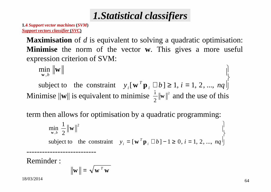
Maximisation of d is equivalent to solving a quadratic optimisation:Minimise the norm of the vector w. This gives a more usefulexpression criterion of SVM:

Minimise ||w|| is equivalentto minimise andtheuseof this21w



=≥+ nqiby iT

i

b

...,,2,1,1][ constraint thesubject to

min,

pw

ww

18/03/2014 64

Minimise ||w|| is equivalentto minimise andtheuseof this

termthen allows for optimisation by a quadratic programming:

---------------------------Reminder :

www T=

2w

=≥−+= nqiby iT

i

b

...,,2,1,01][ constraint thesubject to

2

1min

2

,

pw

ww



In practical situations, the samples are not linearly separable, sotheprevious constraint cannot be satisfied. For that reason,slackvariables must be introduced to account for the non separablesamples [33]. Then, the optimization criterion consist of minimizingthe (primal) functional [33, 21].

+ ∑Cnq1

min2 ξw

18/03/2014 65

For a simple introduction on the derivation ofSVM optimizationprocedures, see for example [20-23].

=>−≥+=

+ ∑=

nc ,i

by

C

i

iiT

i

ii

b

,,3,210,with

1][ constraint thesubject to

2

1min

1,

⋯ξξ

ξ

pw

ww

If the instancepi is correctly classified by the hyperplane, and it isoutside the margin, its correspondingslack variableis ξi = 0. If itis well classified but it is into the margin, then 0 <ξi < 1. If thesample is misclassified, thenξi > 1. The value ofC is a trade-offbetween the maximization of the margin and theminimization of the errors.



18/03/2014 66

minimization of the errors.

SVM of 2 non linearly separable classes

Once the criterion of optimality has been established, weneed a method for finding the parameter vectorw whichmeets it. The optimization problemin the last equations is aclassicalconstrained optimization problem.



In order to solve this a optimization problem, one mustapply a Lagrange optimizationprocedure with as manyLagrange multipliersλi as constraints [22].

18/03/2014 67

Optimal estimation of w (for demonstration, see for example [34,21])Minimise the cost is a compromise between a large margin and afew margin errors. The solution is given as a weighted average ofinstances of learning:

ii

nq

i y pw ∑=* λ



18/03/2014 68

The coefficientsλi, with 0 ≤ λi ≤ C are theLagrange multipliersofthe optimisation task and they are zero for all instances outside ofthe margin and on the right side of the classifier. These instances donot contribute to the determination of the direction of the classifier(direction of hyperplanes defined byw). The rest of the instances,with non zeroλi, which contribute to the construction ofw*, arecalledsupport vectors.

iii

i y pw ∑=

=1

λ

Selecting a value for the parameterCThe free parameter C controls the relative importance ofminimizing the norm of w (which is equivalent to maximizingthe margin) and satisfying the margin constraint for each datapoint. The margin of the solution increases as C decreases. This isnatural, because reducing C makes the margin termin equation



18/03/2014 69

more important.In practice, several SVMclassifiers must be trained, usingtraining as well as testing data with different values of C (e.g.,start frommin. to max. in {0.1, 0.2, 0.5, 1, 2, 20}) and select theclassifier which gives the minimumtest error.

∑=

+nc

iiC

1

2

2

1 ξw

Estimation of bAny instancepi

s which is a support vector as well as its desiredresponseyi

s satisfy :yi

s [w*Tpis+ b] ≥ 1

or 1)( =+∑∈

byy sj

Tj

Sjjj

si ppλ



18/03/2014 70

s is the index set of support vectors whereλi > 0. Multiplying by yis

and using (yis)2 =1

Instead of using an arbitrarily support vectorpjs, it is better to use the

average over all support vectors in S:

∈Sj

sj

Tj

Sjjj

si

si

sj

Tj

Sjjj

si yybybyy pppp ∑∑

∈∈

−==+ λλ then ,)()( 2

)(1 s

jTj

Si Sjjj

si

s

yyN

b pp∑ ∑∈ ∈

−= λ

Practical implementation of the SVM algorithm for theseparation of 2 linearly separable classesCreate a matrixH, with Hij = yiyjpi

Tpj, i, j = 1, 2, …,nc

1. select a value for the parameter C (start frommin tomax, e.g. C in {0.1, 0.2, 0.5, 1, 2, 20})

2. find Λ={λ1, λ2, …, λnc} suchasthequantity



18/03/2014 71

2. find Λ={λ1, λ2, …, λnc} suchasthequantity

is maximised (using a quadratic programming solver)subject to the constraints

0 ≤ λi ≤ C ∀iand

iTi

nc

ii H λλλ

2

1

1

−∑=

01

=∑=

i

nc

ii yλ

Practical implementation of the SVM algorithm for the separation of 2 linearlyseparable classes (Cont.)

4. Calculate5. Determine the set of support vectors S by finding the

indexes such that 0 <λi ≤ C ∀i6. Calculate7. Each new vector pi is classified by the following

ii

nq

ii y pw ∑

=

=1

* λ

)(1 s

jTj

Si Sjjj

si

s

yyN

b pp∑ ∑∈ ∈

−= λ



18/03/2014 72

7. Each new vector pi is classified by the followingevaluation:

8. Calculate the training and the test errors using test data.9. Repeat fromstep 1 (construct another classifier) with a

next value of C10. Choose the best classifier that minimises the test error

with minimumnumber of support vectors.

2 class ,1y,1 If

1 class ,1y ,1 If

i

i

∈−=−≤+

∈+=≥+

iiT

iiT

b

b

ppw

ppw

Example [20] : Linear SVM classifier(SVC) in MATLAB

An easy way to programa linear SVC is to use the MATLAB quadraticprogramming "quadprog.m". First, generate a set of data in twodimensions with fewinstances fromtwo classes with this simple code:p = [randn(1,10)-1 randn(1,10)+1;randn(1,10)-1 randn(1,10)+1]';y = [- ones(1,10) ones(1,10)]' ;



y = [- ones(1,10) ones(1,10)]' ;

This generates a matrix of line vectors n = 20 in two dimensions. Westudy the performance of theSVCon a non-separable set. The first 10samples are labeled as vectors of class 1, and the rest as vectors of class-1.

18/03/2014 73

%%Linear Support Vector Classifier%%%%%%%%%%%%%%%%%%%%%%%%%% Data Generation %%%%%%%%%%%%%%%%%%%%%%%%%%x=[randn(1,10)-1 randn(1,10)+1;randn(1,10)-1 randn(1,10)+1]';y=[-ones(1,10) ones(1,10)]';%%%%%%%%%%%%%%%%%%%%%%%%%%% SVC Optimization %%%%%%%%%%%%%%%%%%%%%%%%%%%R=x*x'; % Dot productsY=diag(y);

%%%%%%%%%%%%%%%%%%%%%%%%% Representation %%%%%%%%%%%%%%%%%%%%%%%%%data1=x(find(y==1),:);data2=x(find(y==-1),:);svc=x(find(alpha>e),:);plot(data1(:,1),data1(:,2),'o')hold onplot(data2(:,1),data2(:,2),'*')plot(svc(:,1),svc(:,2),'s')



Y=diag(y);H=Y*R*Y+1e-6*eye(length(y)); % Matrix H regularizedf=-ones(size(y)); a=y'; K=0;Kl=zeros(size(y));C=100; % Functional Trade-offKu=C*ones(size(y));alpha=quadprog(H,f,[],[],a,K,Kl,Ku); % Solverw=x'*(alpha.*y); % Parameters of the Hyperplane

%%% Computation of the bias b %%%e=1e-6; % Tolerance to errors in alphaind=find(alpha>e & alpha<C-e) % Search for 0 < alpha_i < Cb=mean(y(ind) - x(ind,:)*w) % Averaged result

plot(svc(:,1),svc(:,2),'s')% Separating hyperplaneplot([-3 3],[(3*w(1)-b)/w(2) (-3*w(1)-b)/w(2)])% Margin hyperplanesplot([-3 3],[(3*w(1)-b)/w(2)+1 (-3*w(1)-b)/w(2)+1],'--')plot([-3 3],[(3*w(1)-b)/w(2)-1 (-3*w(1)-b)/w(2)-1],'--')

%%%%%%%%%%%%%%%%%%%%%%%%%%%%%%% Test Data Generation %%%%%%%%%%%%%%%%%%%%%%%%%%%%%%%x=[randn(1,10)-1 randn(1,10)+1;randn(1,10)-1 randn(1,10)+1]';y=[-ones(1,10) ones(1,10)]';y_pred=sign(x*w+b); %Testerror=mean(y_pred~=y); %Error Computation

18/03/2014 74



Generated data.

18/03/2014 75

The values of Lagrange multipliersλi. Circles and squares correspond to circles and stars ofthe data in the previous and the next figures.

18/03/2014 76



18/03/2014 77

Resulting margin and separating hyperplanes. Support vectors are marked by squares.

LinearSupport vectors regressor(LSVR)

A linear regressor is a function f(p) = wTp+b which allows for anapproximation of a mapping fromset of vectorsp ∈RR to a set ofscalars y∈R.


18/03/2014 78Linear egression

wTp+b

Instead of trying to classify newvariables into twocategories y = ± 1, we nowwant to predict a real-valuedoutput y∈R.

1.4 Support vector machines(SVM)Linear Support vectors regressor(LSVR)


18/03/2014 79

The main idea of a SVRis to find a function which fits thedata with a deviation less than a given quantityε for everysingle pairpi , yi . At the same time, we want the solutionto have a minimumnormw. This means that SVRdoes notminimize errors less thanε, but only higher errors.

Formulation of the SVR

The idea to adjust the linear regressor can be formulated in thefollowing primal functional, in which we minimize the normof wplus the total error.

)(1 '2 ξξ ++= ∑

n

CL w



Subject to the constraints

)(2

1 '

1

2 ξξ ++= ∑=i

ip CL w

0, '

'

≥

+≤++−

+≤−−

ii

iiT

i

iiT

i

by

by

ξξεξ

εξpw

pw

18/03/2014 80



i

Concept ofε- insensitivity.Only instances out of (margin/2) ±ε willhave a nonzero slack variable, so they will be the only ones that willbe part of the solution.

18/03/2014 82

The functional is intended to minimize the sumof the slack variables. Only losses of samples for which the error is greater

thanε appear, so the solution will be only function of those samples.The applied cost function is a linear one, so the described procedureis equivalent to the application of the so-calledVapnik or ε-insensitive cost function

' and ii ξξ



−−=+=

>−

<=

εξεξ

εεε

',f

0)(

iiii

ii

i

i

eeor

ee

eel

Vapnikor ε-insensitive cost function.

18/03/2014 83

This procedure is similar to the one applied to SVC.In principle, we should force the errors to be lessthanε and we minimize the normof the parameters.Nevertheless, in practical situations, it may be notpossibleto force all the errorsto be lessthan ε. In



possibleto force all the errorsto be lessthan ε. Inorder to be able to solve the functional, weintroduce slack variables on the constraints, andthen we minimize them.

18/03/2014 84

To solve this constrained optimization problem, we canapply Lagrange optimization procedure to convert it intoan unconstrained one. The resulting dual formulation forthis dual functional is [20-23, 34] :

))()(()()(2

1 '

1

'''

1 1

ελλλλλλλλ ii

nc

iiiijij

Tii

nc

i

nc

ii yLd +−−+−−−= ∑∑∑

== =

pp



with the additional constraint

2 11 1 ii i∑∑∑

== =

Cii ≤−≤ )(0 'λλ

18/03/2014 85

The important result of this derivation is that the expressionof the parameters w is

and

In order to find the bias,we just needto recall that for all samples

ii

nc

ii pw )( '

1

λλ −= ∑=

0)( '

1

=−∑=

i

nc

ii λλ



In order to find the bias,we just needto recall that for all samplesthat lie in one of the two margins, the error is exactlyε for thosesamplesλi et λ'i < C. Once these samples are identified, we can solveb from the following equations

C

by

by

ii

iT

i

iT

i

<

=+++−

=+−−

'i ,for which instances for the

0

0

λλεε

p

pw

pw

18/03/2014 86

In matrix notation we get

Where R is the dot product matrixThis functional can be maximized using the same procedure used for



][ jTi pp

ε1λλyλλλλRλλ )()()()(2

1 '''' +−−+−−−= TTLd

SVC. Very small eigenvalues may eventually appear in the matrix, soit is convenient to numerically regularize it by adding a smalldiagonal matrix to it. The functional becomes

where is a regularisation constant. This numerical regularization isequivalent to the application of a modified version of the costfunction.

18/03/2014 87

εγ 1λλyλλλλIRλλ )()()]([)(2

1 '''' +−−+−+−−= TTLd

We need to compute the dot product matrixR and then the product

but the Lagrange multipliersλi et λ'i should be split to be identifiedafter the optimization. To achieve this we use the equivalent form



− − λIIRRλT

)]([)( ''λλIRλλ −+− γT

We can use the Matlab function quadprog.m to solve the optimizationproblem.

18/03/2014 88

−−

+

−−

''λ

λ

II

II

RR

RR

λ

λγ

T

Exemple [20] : SVRlinéaire en MATLABWe start by writing a simple linear model of the form

y (xi) = axi + b + ni (15)where xi is a random variable and ni is a Gaussian process. P = rand(100,1) % Generate 100 uniform instances between -1 et 1y =1.5*P+1+0.1*randn(100,1) % Linear model plus noise



Generated data.

18/03/2014 89

%% Linear SupportVector Regressor%%%%%%%%%%%%%%%%%%%%%%%%%% Data Generation %%%%%%%%%%%%%%%%%%%%%%%%%%x=rand(30,1); % Generate 30 samplesy=1.5*x+1+0.2*randn(30,1); % Linear model plus noise%%%%%%%%%%%%%%%%%%%%%%%%%%% SVR Optimization %%%%%%%%%%%%%%%%%%%%%%%%%%%R_=x*x';R=[R_ -R_;-R_ R_];a=[ones(size(y')) -ones(size(y'))];y2=[y;-y];

%%%%%%%%%%%%%%%%%%%%%%%%% Representation %%%%%%%%%%%%%%%%%%%%%%%%%plot(x,y,'.') % All datahold onind=find(abs(beta)>e);plot(x(ind),y(ind),'s') % Support Vectorsplot([0 1],[b w+b]) % Regression lineplot([0 1],[b+epsilon w+b+epsilon],'--') % Marginsplot([0 1],[b-epsilon w+b-epsilon],'--')plot([0 1],[1 1.5+1],':') % True model}



y2=[y;-y];H=(R+1e-9*eye(size(R,1)));epsilon=0.1; C=100;f=-y2'+epsilon*ones(size(y2'));K=0;K1=zeros(size(y2'));Ku=C*ones(size(y2'));alpha=quadprog(H,f,[],[],a,K,K1,Ku); % Solverbeta=(alpha(1:end/2)-alpha(end/2+1:end));w=beta'*x;%% Computation of bias b %%e=1e-6; % Tolerance to errors inalphaind=find(abs(beta)>e & abs(beta)<C-e) % Search for% 0 < alpha_i < Cb=mean(y(ind) - x(ind,:)*w) % Averaged result

18/03/2014 90



Results : Continuous line: SVR; Dotted line: real linear model; Dashed lines: margins; squarepoints: support vectors. Figure adapted from [20]

18/03/2014 91

1.Classificateurs statistiques1.Classificateurs statistiquesLMCSVM

Linear multiclass SVM(LMCSVM)Although mathematical generalisations for the multiclasscase are available, the task tends to become rather complex.When more than two classes are present, there are severaldifferent approaches that evolve around the 2-class case.

18/03/2014 92

The more used methods are calledone versus allandoneversus one.These techniques are not tailored to the SVM. They aregeneral and can be used with any classifier developed forthe 2-class problem.

One-versus-all

The methodone-versus-allis used to buildQ binary classifiers byassigning a label to instances fromone class and a label -1 toinstances fromall others. For example, in 4 classes problem, weconstruct4 binaryclassifiers:

1.4 Support vector machines(SVM)Linear multiclass SVM(LMCSVM)


18/03/2014 93

construct4 binaryclassifiers:{ c1/{c2, c3, c4}, c2/{c1, c3, c4} , c3/{c1, c2, c4}, c4/{c1, c2, c3}}.

For each one of the classes, we seek to design an optimal discriminantfunction,gq(p), q = 1, 2, . . . , Q, so that

gq(p) > gq’ (p), ∀q’ ≠ q, if p ∈ cq .Adopting the SVM methodology, we can design the discriminantfunctions so thatgq(p) = 0 to be the optimal hyperplane separatingclasscq from all the others. Thus, each classifier is designed to give

gq(p) > 0 for p ∈ cq andgq(p) < 0 otherwise.

According to the one-against-all method,Q classifiers have to bedesigned. Each one of themis designed to separate one class fromtherest. For the SVMparadigm, we have to designQ linear classifiers:

QkbkiTk ..., 2, 1, , =+pw

For example,to designclassifierc , we considerthe training dataof



18/03/2014 94

For example,to designclassifierc1, we considerthe training dataofall classes other thanc1 to form the second class. Obviously, unless anerror is committed we expect all points fromclassc1 to result in

and the data fromthe rest of the classes to result in negativeoutcomes.

,111 +≥+ biTpw

1 ,1 ≠−≤+ mbmiTmpw

Qlmbbc miTmli

Tlli ,,2,1 , if in classified is ⋯=≠∀+>+ pwpwp

The classifier giving the highest margin wins the vote. :

A drawback ofone-against-allis that after the training thereare regions in the space, where no training data lie, forwhich more than one hyperplanegives a positive value or



{ })(max arg if in assign ''q

ppqq gqc =

18/03/2014 95

which more than one hyperplanegives a positive value orall of themresult in negative values.



One-versus-oneThe more widely used methodone-versus-oneconstructsQ(Q − 1) /2binary classifiers (each classifier separates a pair of classes.)byconfronting each one of theQ classes. For example, in 4 classesproblem, we construct 6 binary classifiers :

{{ c1/c2}, { c1/c3} , { c1/c4} , { c2/c3} , { c2/c4} , { c3/c4}}.In 3 classesproblem,weconstruct3 binaryclassifiers:

18/03/2014 96

In 3 classesproblem,weconstruct3 binaryclassifiers:{{ c1/c2}, { c1/c3}, { c2/c3}}.

In the classification phase, the instance to classify is analysed by eachclassifier and a majority vote determines its class. The obviousdisadvantage of the technique is that a relatively large number ofbinary classifiers has to be trained. In [Plat 00] a methodology issuggested that may speed up the procedure.[Plat 00] Platt J.C., Cristianini N., Shawe-Taylor J. “Large margin DAGs for the multiclass classification,” inAdvances in Neural InformationProcessing,(Smola S.A.,LeenT.K.,Muller K.R., eds.),Vol. 12, pp. 547–553, MIT Press, 2000.

1.4.1Nonlinear SVM


Non linear mapping of the feature vectors (p) in a high-dimensional spaceWe adopt the philosophy of non-linear mapping of feature vectors in aspace of higher dimension, where we expect, with high probability, thatthe classes are linearly separable (*). This is guaranteed by the famoustheoremof Cover[34, 35].

18/03/2014 97

theoremof Cover[34, 35].

(*) See http://www.youtube.com/watch?v=3liCbRZPrZA

1.Statistical classifiers1.4 Support vector machines(SVM)1.4.1 Nonlinear SVM

Non-linear low dimensional

Linear high dimensional

18/03/2014 98

dimensional space (p) Non-linear

Kernel function

φ(p)

Linear SVMdimensional

space (p)

1.4 Support vector machines(SVM)1.4.1 Nonlinear SVM


Mapping from: p ∈ RR --- φ (p ) --------> p’ ∈ RH

where the dimension of H is greater thanR, depending on thechoice of the nonlinear functionφ ( · ).

In addition, if the functionφ ( · ) is carefully chosen froma known

18/03/2014 99

family of functions that have specific desirable properties, the inner(or dot) product <φ (pi), φ (pj) > between the spaces correspondingto two input vectorspi, pj can be written as

< φ (pi), φ (pj) > = k(pi, pj)where < · , · > denotes the inner product in H and k (·, ·) is a knownfunction, calledkernel function.



In other words, inner products in high-dimensional space canbe made in terms of the kernel function acting in the originalspace of lowdimension. The space H associated with k (·, ·)is known asreproducing kernel Hilbert space(RKHS) [35,36].

18/03/2014 100

36].



Two typical examples of kernel function:(a)Radial basis function(RBF), is a real-valued function

k(pi, pj) = φ(||pi - pj ||)

The norm is usually the Euclideandistance,althoughother distance

18/03/2014 101

The norm is usually the Euclideandistance,althoughother distancefunctions are also possible. The sums of radial functions are typicallyused to approximate a given function. This approximation process canalso be interpreted as a kind of simple neural network.



Exampls of RBFs : Let r = ||pi-pj ||

Gaussian: , where σ a user-defined parameter which specifies the decay rate of k(pi, pj) twards zero.

Multiquadratic:

2

2

)( σϕr

er−

=

2)(1)( rr εϕ +=

18/03/2014 102

Multiquadratic:

Inverse quadratic:

Inverse multiquadratic:

Spline polyharmonique :

Special spline polyharmonic (thin plate spline) :

2)(1)( rr εϕ +=

2)(1

1)(

rr

εϕ

+=

2)(1

1)(

rr

εϕ

+=

... 6, 4, 2,ln(r),)(

... 5, 3, 1,,)(

====

krr

krrk

k

ϕϕ

ln(r))( 2rr =ϕ



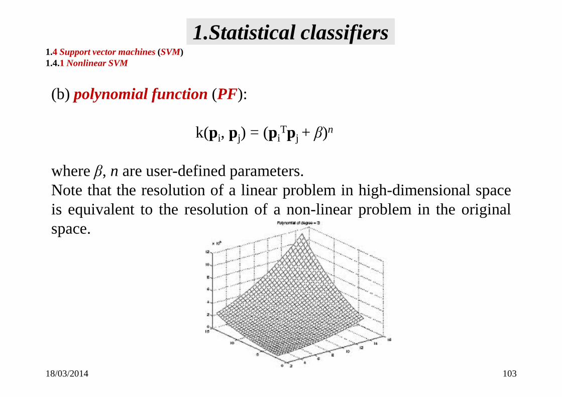
(b) polynomial function(PF):

k(pi, pj) = (piTpj + β)n

whereβ, n are user-defined parameters.Note that the resolutionof a linear problemin high-dimensionalspace

18/03/2014 103

Note that the resolutionof a linear problemin high-dimensionalspaceis equivalent to the resolution of a non-linear problemin the originalspace.



Although a classifier (linear) is formed in the space RKHS,due to the non-linearity of the mapping functionφ (·), themethod is equivalent to a nonlinear function in the originalspace.

Moreover,sinceeachoperationcanbe expressedin inner

18/03/2014 104

Moreover,sinceeachoperationcanbe expressedin innerproducts, the explicit knowledge ofφ (·) is not necessary.All that is necessary is to adopt the kernel function whichdefines the inner product.



(c) Sigmoïde

(d) Dirichlet)tanh(),( µγ += j

TijiK pppp

)))(2/1sin((),( jin

Kpp

pp−+

=

18/03/2014 105

)2/)sin((2

)))(2/1sin((),(

ji

jiji

nK

pp

pppp

−−+

=

More on Nonlinear PCA(NLPCA): http://www.nlpca.de/

Construction of a nonlinear SVC

The solution to the linear SVC is given by a linear combination of asubset of training data:

If, beforeoptimizationdatais mappedinto a Hilbert space,then the

ii

nc

ii y pw ∑

=

=1

λ



18/03/2014 106

If, beforeoptimizationdatais mappedinto a Hilbert space,then thesolution becomes

(A)

whereφi is a mapping nonlinear function.

ii

nc

ii y ϕλ∑

=

=1

w

The parameter vectorw is a combination of vectorsinto the Hilbert space, but recall that manytransformationsφ(・) are unknown. Thus, we maynot have an explicit formfor them. But the problemcan still be solved, because the SVMjust needs thedot productsof the vector,andnot an explicit form



dot productsof the vector,andnot an explicit formof them.

18/03/2014 107

We cannot use this expressionyj = wT φ (pj) + b (B)

because the parametersw are in an infinite-dimensional space, so no explicit expression existsfor them. However, by substituting equation (A) inequation(B), weobtain



equation(B), weobtain

(C)bKybyy jii

nc

iiji

Ti

nc

iij +=+= ∑∑

==

),()()(11

pppp λϕϕλ

18/03/2014 108

In linear algebra, the Gramian matrix (or Grammatrixor Gramian) of a set of vectorsv1, …, vn in an innerproduct space is the Hermitian matrix of innerproducts, whose entries are given by

(D)Jørgen Pedersen Gram (June 27, 1850 – April 29, 1916) was a Danish actuary and mathematician

== n

n

Gvvvvvv

vvvvvv

vvvv,,,

,,,

,),( 22212

12111

⋯

⋯



(D)Danish actuary and mathematician who was born in Nustrup, Duchy of Schleswig, Denmark and died in Copenhagen, Denmarkhttp://en.wikipedia.org/wiki/J%C3%B8rgen_Pedersen_Gram

==

nnnn

njijiG

vvvvvv

vvvv

,,,

,),(

21

22212

⋯

⋮⋮⋮

⋯

18/03/2014 109

The resultingSVMcan nowbe expressed directly in termsof the Lagrange multipliers and the Kernel dot products. Inorder to solve the dual functional which determines theLagrange multipliers, the transformed vectorsφ(pi) andφ(pj) are not required either, but only theGram matrix K ofthedot productsbetweenthem. Again, thekernelis usedto



thedot productsbetweenthem. Again, thekernelis usedtocompute this matrix

Ki j = K(pi, p j) (E)

18/03/2014 110

Once this matrix has been computed, solving for a nonlinear SVMisas easy as solving for a linear one, as long as the matrix is positivedefinite. It can be shown that if the kernel fits theMercer theorem,the matrix will be positive definite [25].

In order to compute the biasb, we can still make use of theexpression (yj (wTpi+ b) − 1 = 0), but for the nonlinear SVC itbecomes nc

∑



becomes

We just need to extractb from expression (F) and average it for allsamples withλi < C.

. lequelpour

01)),((

01))()((

1

1

C

bKyy

byy

ij

jii

nc

iij

jiT

i

nc

iij

<∀

=−+

=−+

∑

∑

=

=

λ

λ

ϕϕλ

p

pp

pp

(F)

18/03/2014 111(*) Explicit conditions that must be met for a kernel function: it must be symmetric, positive semi-definite.

Example [20] : Nonlinear Support Vector Classifier(NLSVC) inMATLABIn this example, we try to classify a set of data whichcannot be reasonably classified using a linear hyperplane.We generate a set of 40 training vectors using this codek=20; %Numberof trainingdataperclass



k=20; %Numberof trainingdataperclassro=2*pi*rand(k,1);r=5+randn(k,1);x1=[r.*cos(ro) r.*sin(ro)];x2=[randn(k,1) randn(k,1)];x=[x1;x2];y=[-ones(1,k) ones(1,k)]';

18/03/2014 112

Example: NLSVC (cont.)

We generate a set of 100 test vectors using this codektest=50; %Nombre de données de test par classro=2*pi*rand(ktest,1);r=5+randn(ktest,1);

1.4 Support vector machines(SVM)1.4.1 Nonlinear SVM-SVC


r=5+randn(ktest,1);p1=[r.*cos(ro) r.*sin(ro)];p2=[randn(ktest,1) randn(ktest,1)];ptest=[p1;p2];ytest=[-ones(1,ktest) ones(1,ktest)]' ;

18/03/2014 113


x2



An example of generated data.

x2

x1

18/03/2014 114

The steps of the SVCprocedure :

1. Calculate the inner product matrix Ki j = K(pi, p j)Since we want a non-linear classifier, we compute the innerproductmatrixusingakernel.




productmatrixusingakernel.�Choose a kernelIn this example, we choose a Gaussian kernel

22

1 vec

,),(

σγ

γ

=

= −−

a

eK ji

ji

pppp

18/03/2014 115

The steps of the SVCprocedure (cont.)

nc=2*k; % Number of datasigma=1; % Parameter of the kernelD=buffer(sum([kron(x,ones(nc,1))- kron(ones(1,nc),x')'].^2,2),nc,0)




D=buffer(sum([kron(x,ones(nc,1))- kron(ones(1,nc),x')'].^2,2),nc,0)% This is a recipe for fast computation% of a matrix of distances in MATLAB% using the Kronecker productR=exp(-D/(2*sigma)); % kernel matrix

* In mathematics theKronecker product is an operation on a matrix. This is a special case of thetensor product. It is so named in honor of the German mathematician Leopold Kronecker.

18/03/2014 116

The steps of the SVCprocedure (cont.)

2. Optimisation procedureOnce the matrix has been obtained, the optimization procedure isexactly equal to the one for the linear case, except for the fact that wecannothaveanexplicit expressionfor theparametersw.




cannothaveanexplicit expressionfor theparametersw.

18/03/2014 117

Example: NLSVC (cont.) training

%%%%%%%%%%%%%%%%%%%%%%%%%% Data Generation %%%%%%%%%%%%%%%%%%%%%%%%%%k=20; %Number of training data perclassro=2*pi*rand(k,1);r=5+randn(k,1);x1=[r.*cos(ro) r.*sin(ro)];x2=[randn(k,1) randn(k,1)];x=[x1;x2];

D=buffer(sum([kron(x,ones(N,1))...- kron(ones(1,N),x')'].^2,2),N,0);% This is a recipe for fast computation% of a matrix of distances in MATLABR=exp(-D/(2*sigma)); % Kernel MatrixY=diag(y);H=Y*R*Y+1e-6*eye(length(y)); % Matrix H regularizedf=-ones(size(y)); a=y'; K=0;Kl=zeros(size(y));C=100; % Functional Trade-offKu=C*ones(size(y));e=1e-6; % Tolerance to% errors in alphaalpha=quadprog(H,f,[],[],a,K,Kl,Ku); % Solver



Cont.

x=[x1;x2];y=[-ones(1,k) ones(1,k)]';ktest=50; %Number of test data per classro=2*pi*rand(ktest,1);r=5+randn(ktest,1);x1=[r.*cos(ro) r.*sin(ro)];x2=[randn(ktest,1) randn(ktest,1)];xtest=[x1;x2];ytest=[-ones(1,ktest) ones(1,ktest)]';%%%%%%%%%%%%%%%%%%%%%%%%%%% SVC Optimization %%%%%%%%%%%%%%%%%%%%%%%%%%%N=2*k; % Number of datasigma=2; % Parameter of the kernel

alpha=quadprog(H,f,[],[],a,K,Kl,Ku); % Solverind=find(alpha>e);x_sv=x(ind,:); % Extraction of the support% vectorsN_SV=length(ind); % Number of SV%%% Computation of the bias b %%%ind=find(alpha>e & alpha<C-e); % Search for% 0 < alpha_i < CN_margin=length(ind);D=buffer(sum([kron(x_sv,ones(N_margin,1)) ...- kron(ones(1,N_SV),x(ind,:)')'].^2,2),N_margin,0);% Computation of the kernel matrixR_margin=exp(-D/(2*sigma));y_margin=R_margin*(y(ind).*alpha(ind));b=mean(y(ind) - y_margin); % Averaged result

18/03/2014 118

SVM Non linéaire - SVC

%%%%%%%%%%%%%%%%%%%%%%%%%%%%%% Support Vector Classifier %%%%%%%%%%%%%%%%%%%%%%%%%%%%%%N_test=2*ktest; % Number of test data%%Computation of the kernel matrix%%D=buffer(sum([kron(x_sv,ones(N_test,1))...- kron(ones(1,N_SV),xtest')'].^2,2),N_test,0);% Computation of the kernel matrixR_test=exp(-D/(2*sigma));

x_grid=[kron(g,ones(length(g),1)) kron(ones(length(g),1),g)];N_grid=length(x_grid);D=buffer(sum([kron(x_sv,ones(N_grid,1))...- kron(ones(1,N_SV),x_grid')'].^2,2),N_grid,0);% Computation of the kernel matrixR_grid=exp(-D/(2*sigma));y_grid=(R_grid*(y(ind).*alpha(ind))+b);contour(g,g,buffer(y_grid,length(g),0),[0 0]) %



Example: NLSVC (cont.) test

Cont.

R_test=exp(-D/(2*sigma));% Output of the classifiery_output=sign(R_test*(y(ind).*alpha(ind))+b);errors=sum(ytest~=y_output) % Error Computation%%%%%%%%%%%%%%%%%%%%%%%%% Representation %%%%%%%%%%%%%%%%%%%%%%%%%data1=x(find(y==1),:);data2=x(find(y==-1),:);svc=x(find(alpha>e),:);plot(data1(:,1),data1(:,2),'o')hold onplot(data2(:,1),data2(:,2),'*')plot(svc(:,1),svc(:,2),'s')g=(-8:0.1:8)'; % Grid between -8 and 8

contour(g,g,buffer(y_grid,length(g),0),[0 0]) % Boundary draw

18/03/2014 119

NLSVM



Separating boundary, margins and support vectors for the nonlinear SVC example

18/03/2014 120

Non linear Support vectors regressor(NLSVR)

The solution of linear SVR

Its nonlinear counterpart will have the expression

ii

nc

ii pw )( '

1

λλ −= ∑=

'nc

pw ϕλλ −= ∑



Following the same procedure as in the SVC, one can find theexpression of the nonlinear SVR

The construction of a nonlinear SVR is almost identical to theconstruction of the nonlinear SVC.Exercise: write a Matlab code of thisNLSVR.

)()( '

1ii

nc

ii pw ϕλλ −= ∑

=

bKby ji

nc

iiiji

Tnc

iiij +−=+−= ∑∑

==

),()()()()(1

'

1

' pppp λλϕϕλλ

18/03/2014 121

Some useful Web sites on SVM:

http://svmlight.joachims.org/http://www.support-vector-machines.org/index.html

1.4 Support vector machines(SVM)1.4.1 Nonlinear SVM-SVR


18/03/2014 122

2. Neural networks

18/03/2014 123

The artificial neural networks (ANN) are composed of simpleelements which operate in parallel. These elements are inspired bybiological nervous systems. As in nature, the connections betweenthese elements largely determine the functioning of the network.

We can build a neural network to performa particular function byadjusting the connections (weights) between the elements.In the following, we will usethe Matlab toolbox, version2011a or

2. Neural networks

In the following, we will usethe Matlab toolbox, version2011a ormore recent versions to illustrate this course. More details, see1.Neural Network Toolbox™, Getting Started Guide2.Neural Network Toolbox™, User’s Guide

18/03/2014 124

An RN is an assembly of elementary processing elements. Processingcapacity of the network is stored as weights of interconnectionsobtained by a process of adaptation or training froma set of trainingexamples.

Types of neural networks :

1. Perceptron(P) one or more (adaline) formal neuronsin one layer;

3. Static networkssuch as "Radial Basis Functions neural networks (RBFNN)"with one layer without feedback to the input layer.

3.1 Generalizedregressionneural network(GRNN)

2. Static networks such as "multilayer feed forward neural networks" (MLFFNR ) "multilayer perceptron" (MLP) or without feedback from outputs to the first input layer;

2. Neural networks

7. Dynamic neural networks (DNN)

6. Self-Organizing neural networks(SONN) or competitive neural networks(CNN)

5. Recurrent networkswith one layer and total connectivity (Associative networks)

4. Partially recurrent multilayer feed forward networks(PRFNN) (Elman orJourdan) where only the outputs are looped to the first layer.

3.1 Generalizedregressionneural network(GRNN)3.2Probabilistic neural networks(PNN)

18/03/2014 125

Supervised training: Given couples of input featur vectors P and their

associated desired outputs (targets) Yd

(P,Yd) = ([p1, p2, …, pN]RxN, [yd1, yd2, …, ydN]SxN)

2. Neural networksTypes of neural networks

and error matrixE = [E1, E2, …, EN] containing error vectorEi = [e1, e2, …, eS]T = Y i - Ydi

18/03/2014 126

1. Given a couple of input and desired output vectors (p,yd) ;2. when an inputp is presented to the network, the activations of

neurons are calculated once the network is stabilized;3. the errorsEi are calculated;4. Ei are minimized by a given training algorithm.

2. Neural networksTypes of neural networks 1. Perceptron(cont.)

yd

18/03/2014 127

Error Ei

Fig. 1. Training of neural network.(Figure adapted from « Neural Network Toolbox™ 6 User’s Guide », by TheMathWorks, Inc.

ypi

Input Neuron without bias Input Neuron with bias(scalar) (scalar)

One neuron with one scalar input

1. Perceptron (P) one or more formalneuronswith one layer

2. Neural networks

Biological neuron

Types of neural networks (cont.)

p : input (scalar)ω : weight(scalar)b : bias (scalar), considered as a threshold with constant input =1,it acts as anactivation threshold of the neuron.n : activationof the neuron, sum of the weighted inputs, n =wp, or n =wp+bf : transfert functionor activation function)

18/03/2014 128

Biological neuron

Transfert functionStep functionA = hardlim(N) andA = hardlims(N)takes anSxQ matrix of SN-element net inputcolumn vectors and returns anSxQ matrix Aof output vectors with a 1 in each positionwhere the corresponding element ofN was 0or greater, and 0 elsewhere.

A

N


A = 1 if N > 0A = 0 if N < =0

Example :N = -5:0.1:5;A = hardlim(N)plot(N,A)

N

Example :N = -5:0.1:5;A = hardlims(N)plot(N,A)

A = 1 if N > 0A = -1 if N < = 0

N

A

18/03/2014 129

Positive saturating linear transferfunctionA = satlin(N) andA = satlins(N)takes anSxQ matrix of S N-elementnet input column vectors and returnsan SxQ matrix A of output vectorswhere each element ofA is 1 whereNis 1 or greater,N where N is in the

A

N


A = 1 if N > 0A = 0 if N < =0

is 1 or greater,N where N is in theinterval [0 1], and 0 whereN is 0 orless.

Example :N = -5:0.1:5;A = satlin(N)plot(N,A)

N

Example :N = -5:0.1:5;A = satlins(N)plot(N,A)

A = 1 if N > 0A = -1 if N < =0

A

N18/03/2014 130

Linear transfert function

A = purelin (N) = N

takes anSxQ matrix of S N-element net input column vectors and returns anSxQmatrixA of output vectors equal toN.


Example :N = -5:0.1:5;A = purlin(N);plot(N,A)

A

N

18/03/2014 131

Logarithmic sigmoid transfer functionA = logsig(N)logsig(N) (=1/(1+exp(-N))]) takes anSxQ matrix ofSN-element netinput column vectors and returns anSxQ matrixA of output vectors, whereeach element of N in is squashed fromtheinterval[-inf inf] to theinterval[0 1]


theinterval[-inf inf] to theinterval[0 1]with an "S-shaped" function.

18/03/2014 132

Example :N = -5:0.01:5;plot(N,logsig(N))set(gca,'dataaspectratio',[1 1 1],'xgrid','on','ygrid','on')

Symmetric sigmoid transfer functionA = transig(N)transig(N) (=[ 2/(1+exp(-2*N))]-1) takes anSxQ matrixof S N-element net input column vectors andreturns anSxQ matrix A of output vectors, whereeach element ofN in is squashed fromthe interval[-inf inf] to the interval [-1 1] with an "S-shaped"function.


function.

18/03/2014 133

Example :N = -5:0.01:5;plot(N,transig(N))set(gca,'dataaspectratio',[111],'xgrid','on','ygrid','on')

One neuron with feature vector inputFeature vector input(R features)

Neuron with bias

f

+1

−1∑

s

1x

2x1w

2w

inputs

weightsw0+1 output

y


P : feature vector input : P=[p1 p2 … pR]’ (’ denotes Transpose)W : weight vector: W=[w1,1 w1,2 … w1,R]b : bias(scalaire), considered as a thresholdwith constant input =1n : activationof the neuron, sum of the weighted inputs:

f : transfer function(or activation function)a : output, a = f(n)

neuron formal onefor 1,1

=+=+⋅= ∑=

jbpwbnR

jjiPW

18/03/2014 134

Abbreviated Notation

feature vector input Neuron with bias(R features)


18/03/2014 135

Linear separation of classesCritical condition of separation:activation = threshold

Let b = -w0

W.x = w0 an equation of a straight line decision

• In 2D space if w > 0 we obtain a straight line equation


• In 2D space if w0 > 0 we obtain a straight line equation with a slope given by

2

1

w

wp −=

2

01

2

12 w

wp

w

wp +−=

p1

p2

1

0

w

w2

0

w

w Decision line

18/03/2014 136

Example of 2D input space with 2 classes (class 1:, classe 2: )

w1= w2=1, seuilw0=1,5

0000

outputactivationp2p1


p2

(0,1) (1,1)

(1,0)

p = [p1 p2]

1211

0101

0110

0000

p1

18/03/2014 137

Matlab demo: To study the effect of changing the bias (b)for a given weight (w) or vice versa, type in the Matlabwindow:

>> nnd2n1


>> nnd2n1

18/03/2014 138

Abbreviated model of one layer composed of S neurons

2. Neural networks

IW 1, 1

Number of the input layer

Number of layer containing the weighted sum units layer

Feature vector One weighted sum One outputinput layer layer layer

Feature vector One weighted sum One outputinput layer layer layer(R features) (Sweighted sum units) (S transfer functions )

Types of neural networks 1. Perceptron(cont.)

18/03/2014 139

input layer layer layer(R features) (Sweighted sum units) (Stransfer functions )

HistoricalADALINE (Single Layer Feedforward Networks)

unit 1

.

. .

f

+1+1

--11∑

s1x

Nx

0ω

1ω

Nω

-1Input Xe

bias

quantifier

Algorithm delta

S

-1+1

e

d(Xe)+1 -1


. .

. .

unit n f

+1+1

--11∑

s1x

Nx

0ω

1ω

Nω

-1Input Xe

bias

quantifier

Algorithm delta

S

-1+1

e

d(Xe)+1 -1

18/03/2014 140

Supervised training: Given couples of input featur vectors P and their associated desired

outputs (targets) Yd

(P,Yd) = ([p1, p2, …, pN]RxN, [yd1, yd2, …, ydN]SxN)

and error matrixE = [E1, E2, …, EN] containing error vector

Ei = [e1, e2, …, eS]T = Y i - Ydi

2. Neural networks

Input layer of R features One layer of Sneurons

Types of neural networks 1. Perceptron(cont.)

18/03/2014 141

Input layer of R features One layer of Sneurons

pi (a training example: R-input feature vector)

y1

y2

yS

-

-

-

e1

e2

eS

outputs Errors Desired outputslayerY i layerEi layer ydi

yd1

yd2

ydS

1. Given a couple of input and desired output vectors (p,yd) ;2. when an inputp is presented to the network, the activations of

neurons are calculated once the network is stabilized;3. the errorsEi are calculated;4. Ei are minimized by a given training algorithm.


yd

18/03/2014 142

Error Ei

Fig. 1. Training of neural network.(Figure adapted from « Neural Network Toolbox™ 6 User’s Guide », by TheMathWorks, Inc.

ypi

2. Static networks: "multilayer feed forward neuralnetworks" (MLFFNR ) or "multilayerperceptron" (MLP) without feedback fromoutputs to the first input layer

• Some nonlinear problems (or logical, e.g. exclusive or)arenot resolvableby one-layerperceptron:

2. Neural networksTypes of neural networks(cont.)

arenot resolvableby one-layerperceptron:

Solution� One or more intermediate layers (hidden) areadded between the input and output layers to allownetworks to create its own representation of entries. Inthis case it is possible to approximate a nonlinearfunction or performany sort of logic function.

18/03/2014 143

Model with two formal neurons

α : λε πασ δ � αδαπτατιον;

f i et fj : fonctions d’activation ; si et sj : valeurs d’activation;xn : une composante d’entrée au réseau

ωιϕ : ποιδσ σψναπτιθυε

f jw0 g-1

w

bias weights

1 neurone1 neurone

2. Neural networksTypes of neural networks 2. MLP (cont.)

if jw0

+1+1

--11

+1+1

--11

Hidden layer Output layer

∑ ∑

jg

is js jy1x

Nx

ijw

iw0

iw1

Niw

Inputs

18/03/2014 144

2. Neural networksTypes of neural networks 2. MLP (cont.)

-

-e

e

y1

y2

y

yd1

yd2

Input layer of R features One output layer of Sneurons

18/03/2014 145

One or more hidden layers

-e

eoutputs Errors Desired outputslayerY i layerEi layer ydi

yS ydS

pi (a training example: R-input feature vector)

3. Static networks: "Radial basis functions neuralnetworks" (RBFNN) with one layer without feedbackto the input layer

The RBF may require more neurons than that in FFNR(needs only one hidden layer), but often they can betrainedmorequickly thanFFNR. Thesenetworkswork

2. Neural networksTypes of neural networks (cont.)

trainedmorequickly thanFFNR. Thesenetworksworkwell for a limited number of training examples.

18/03/2014 146

RBFs can be used for:

• Regression:Generalized regression networks(GRNN)

2. Neural networksTypes of neural networks 3. RBFNN (cont.)

• Classification:Probabilistic neural networks(PNN)

18/03/2014 147

3.1Generalized regression networks(GRNN)An arbitrary continuous function can be approximated by a linearcombination of a large number of well-chosen Gaussian functions.

Regression: build a good approximation of a function that isknown only by a finite number of "experimental" lownoisy couples {xi, yi}

y


Local Regression: the Gaussian basis affect only small areasaround their mean values .

y

x

18/03/2014 148

This network can be used for classification problems. When aninput is presented, the first Radial basis layer calculates thedistances between the input vector and weight vector and produce avector, multiplied by the bias.


Matlab NN toolbox

18/03/2014 149

3.2 Probabilistic neural networks (PNN)

This network can be used for classification problems. When an input ispresented,

• the first layer calculates the distances between the inputvector and all trainingvectors and produces a vector whose elements describe how this input vectoris close to each training vector.

• the second layer adds these

contributionsfor eachclassof inputs


contributionsfor eachclassof inputs

to produce at the output of the network

a vector of probabilities.

• Finally, a competition transfer function in the output of the second layerselects the maximum of these probabilities, and produces a 1for thecorresponding class and a 0 for the other classes.

Ματλαβ ΝΝ τοολβοξ

18/03/2014 150

General Remarks:

• Replicate the function throughout the data space meansscaning the space by a large number of Gaussians.

• In practice,theRBF is centredandnormalised:


• In practice,theRBF is centredandnormalised:

)exp()( PPP Tf −=

18/03/2014 151

• RBF networks are inefficient:- in a large input feature space (R) - on very noisy data. Local reconstruction of the function prevents the network to "averaging" noise on the whole space (compared with Linear Regression, whose objective is precisely to average out the noise on


whose objective is precisely to average out the noise on the data).

18/03/2014 152

• Training RBF networks

– Training by optimization procedures: considerablecomputation time - very slowor impossible trainingin practice

Solution: useheuristic training� approximation theconstructionof an RBF network is quick and easy


constructionof an RBF network is quick and easybut they are less efficient than multilayer perceptronsnetworks (MLP).

18/03/2014 153

Conclusion on RBFNN:

• Used as a credible alternative to MLP on problems not toodifficult.

• Speed and ease of use

For more on RBFNN, see

[I] Chen, S., C.F.N. Cowan,and P.M. Grant, "OrthogonalLeast SquaresLearning


[I] Chen, S., C.F.N. Cowan,and P.M. Grant, "OrthogonalLeast SquaresLearningAlgorithm for Radial Basis Function Networks," IEEE Transactions on NeuralNetworks, Vol. 2, No. 2, March 1991, pp. 302-309.

http://eprints.ecs.soton.ac.uk/1135/1/00080341.pdf

[II] P.D. Wasserman, Advanced Methods in Neural Computing, New York: Van Nostrand Reinhold, 1993, on pp. 155-61 and pp. 35-55, respectively.

18/03/2014 154

4. Partially recurrent multilayer feed forwardnetworks (PRFNN) (Elman or Jourdan)where only the outputs are looped to the firstlayer.


These are networks of type "feedforward" except that afeedback is performed between the output layer andhidden layer or between the hidden layers themselvesthrough additional layers calledstatelayer (Jordan) orcontextlayer (Elman).

18/03/2014 155

Since the information processing in recurrentnetworks depends on network condition at theprevious iteration, these networks can then beused to model temporal sequences (dynamicsystem).

2. Neural networksTypes of neural networks 4. PRFNN (cont.)

system).

18/03/2014 156

Jordan network [Jordan 86a, b]

State

units


Input layer One hidden layer Output layer Desired output layer

p y-

-

e

e

e

yd

e:error

18/03/2014 157

Elman network [Elman 1990]

In this case an additional layer of context unitsis introduced. The inputs of these units are theactivations of units in the hidden layer.


18/03/2014 158


Context

units

1.0

1.0

18/03/2014 159

p y-

-

e

e

e

yd

e : error

Input layer One hidden layer Output layer Desired output layer

Extended Elman network

However, there is a limitation in the Elmannetwork. It cannot deal with complex structuresuch as a long distance dependency, so thefollowing extension:


18/03/2014 160

The extension of number of generations in context layers

5. Recurrent networks(RNN) with one layerand total connectivity (Associative networks)

Training type: non supervised

In these models each neuron is connected to all othersand theoretically(but not in practice)has a return on


and theoretically(but not in practice)has a return onitself. These models are not motivated by a biologicalanalogy but by their analogy with statistical mechanics.

18/03/2014 161

13w

12w

23w

21w

32w

31w

2. Neural networksTypes of neural networks 5. RNN (cont.)

ii

Réseau entièrement connecté(une seule couche).

ii--11

i+1i+1

1+iiw

1−iiw

p y => p y

f

f

f11 +− iiw

Transferfunctionsum fii neuron i ijw

•

•

•

• weights ∑

∑

∑

∑

13w

18/03/2014 162

6. Self-Organizing neural networks (SONN) or competitive neural networks (CNN) These networks are similar to static monolayer networks except that there are connections, usually with negative signs, between the output units.


Input layer Output layer

p y

18/03/2014 163

Training:• A set of examples is presented to the networks, one

example at a time.• For each presented example, the weights are modified.• If a degradedversion of one of these example is

2. Neural networksTypes of neural networks 6. SONN (cont.)

18/03/2014

• If a degradedversion of one of these example ispresented later to the networks, the networks will thenrebuild the degraded example.

164

Through these connections the output units tend to have acompetition to represent the current example presented tothe input networks.

Function fitting andpattern recognition problemsIn fact, it is proved that a simple neural network can adapt to all thepractical functions.

Defining a probleme

To define a fitting problem, arrange a set of Q input vectors as columns of a matrix.Then,arrangeanotherseriesof Q targetvectors(theright outputvectorsfor eachof

Supervised learning2. Neural networks

Then,arrangeanotherseriesof Q targetvectors(theright outputvectorsfor eachofinput vectors) in a second matrix.

For example, a logic « AND » function: Q=4;Inputs= [0 1 0 1;

0 0 1 1]; Outputs = [0 0 0 1];

18/03/2014 165

We can construct an ANN in 3 different fashions:

• Using command-line function*

• Using graphical user interface, nftool **

• Using nntool, ***

* “Using Command-LineFunctions” , Neural Network Toolbox™6 User’s Guide », 1992–2009 by TheMathWorks, Inc. , page 1-7,

Supervised learning 2. Neural networks

** “Using the NeuralNetwork Fitting Tool GUI”, Neural Network Toolbox™ 6 User’s Guide », 1992–2009 by “Graphical User Interface”, The MathWorks, Inc., page 1-13,

** “Graphical User Interface”, Neural Network Toolbox™ 6 User’s Guide », 1992–2009 by TheMathWorks, Inc., page 3-23.

18/03/2014 166

The majority of methods are provided by default when you create anetwork.

You can override the default functions for processing inputs andoutputs when you call a creation network function, or by settingnetwork properties after creating the network.

net.inputs{1}.processFcns: property of the network to display thelist of inputprocessingfunctions.

Input-output processing unitsSupervised learning 2. Neural networks

list of inputprocessingfunctions.

net.outputs{2}.processFcns: property of the network to display thelist of output processing functions of a 2-layer network.

You can use these properties to change the processing functions thatapply to inputs-outputs of your network (but Matlab recommendsusing the default properties).

18/03/2014 167

Several functions have default settings which define theiroperations. You can access or change the ith parameter ofthe input or output:

net.inputs{1}.processParams{i} for functions of inputprocessing

net.outputs{2}. processParams{i} for functions of output

Input-output processing units


net.outputs{2}. processParams{i} for functions of outputprocessing of a 2-layer network.

18/03/2014 168

For the networks MLP the default functions are:IPF – Structure of the input processing functions.

Default : IPF={'fixunknowns ','removeconstantrows','mapminmax'}.

OPF - Structure of the output processing functions.Default : OPF = {'removeconstantrows','mapminmax'}.

fixunknowns : This functionsavestheunknowndata(representedin



fixunknowns : This functionsavestheunknowndata(representedinthe user data with NaNvalues ) in a numerical formfor the network.It preserves information about which values are known and whichvalues are unknown.

removeconstantrows : this function removes rows with constantvalues in a matrix.

18/03/2014 169

Pre- and post-processing in Matlab:

1. Min andMax (mapminmax)Prior to training, it is often useful to calibrate the inputs and targets sothat they are always in a specified range, e.g., [-1,1] (normalizedinputs and targets).[pn,ps] = mapminmax(p);



[pn,ps] = mapminmax(p);[tn,ts] = mapminmax(t);

net = train(net,pn,tn); % training a created network an = sim(net,pn); % simulation (an : normalised outputs)

18/03/2014 170

To convert the outputs to the same units of the original targets :

a = mapminmax(`reverse',an,ts);

If mapminmaxis already used to preprocess the data of training set,then whenever the trained network is used with newentries, theseentries must be pre-processed withmapminmax:

Let « pnew» anewinputsetto alreadytrainednetwork



Let « pnew» anewinputsetto alreadytrainednetwork

pnewn =mapminmax('apply',pnew,ps);

anewn =sim(net,pnewn);

anew= mapminmax(`reverse',anewn,ts);

18/03/2014 171

2. Meanandstandard deviation(mapstd)

4. Principal Component Analysis(processpca)

5. Processing unknown inputs(fixunknowns)

6. Processing unknown targets(or “Don't Care”) ( fixunknowns)

7. Post-training analysis(postreg)



18/03/2014 172

The performance of a trained network can be measured in some sensby the errors on the training, validation and test sets but it is oftenuseful to further analyse the performance of the network response.One way to do this is to performlinear regression.

a =sim(net,p);

[m,b,r] = postreg(a,t)

m : slope



m : slope

b = intersection of the best straight line (relating outputs to targetsvalues) with the y-axis

r = Pearson’s correlation coefficient

18/03/2014 173

PERCEPTRON


18/03/2014 174

Creation of one-layer perceptron withR inputsandSoutputs:

net = newp(p,t,tf,lf)p : RxQ1 matrix of Q1 input feature vectors, each of Rinput features.

t : SxQ2 matrix ofQ2 target vecteursa = 1 if n > 0

Perceptron


tf : “Transfer function”, default = 'hardlim'.

lf : “Learning function”, default = 'learnp'

a = 1 if n > 0a = 0 if n < =0

18/03/2014 175

Classification example:% DEFINITION

% Creation of a new perceptron using net = newp(pr,s,tf,lf)

% Description

% Perceptrons are used to solve simple problems of classification

% (i.e. linearly separable classes)

% net = newp(pr,s,tf,lf)

% pr - Rx2 matrix of min and max values of R input elements.

% s - Nombre de neurones.

% tf – transfer function, default = 'hardlim': Hard limit transfer function..

E=1;

Iter=0;

% sse: Sum squared error performance function

while (sse(E)>.1)&(iter<1000)

[net,Y,E] = adapt(net,p,t);% adapt: adapter le réseau de neurones

iter = iter+1;

end

% Display the final values of the network

w=net.IW{1,1}

b=net.b{1}

% TEST

test = rand(2,1000)*15;

ctest = sim(net,test);

figure

% scatter: Scatter/bubble plot.

% scatter(X,Y,S,C) displays colored circles at the locations specified by thevectors X and Y (same size).

Perceptron

Supervised learning

2. Neural networks

% lf – training function, default = 'learnp': Perceptron weight/biaslearningfunction.

p1 = 7*rand(2,50);

p2 = 7*rand(2,50)+5;

p = [p1,p2];

t = [zeros(1,50),ones(1,50)];

pr = minmax(p); % pr is Rx2 is a matrix of min and max values of thematrix pmm of dim (RxQ)

net = newp(pr,t,'hardlim','learnpn');

% Display the initial values of the network

w0=net.IW{1,1}

b0=net.b{1}

% S determine the surface of each mark (in points ^ 2)

% C determine the colors of the markers

% 'filled' filling the markers

scatter(p(1,:),p(2,:),100,t,'filled')

hold on

scatter(test(1,:),test(2,:),10,ctest,'filled');

hold off

% plotpc (W,B): Draw a classification line

% W - SxR weight matrix (R <= 3).

% B - Sx1 bias vector

plotpc(net.IW{1},net.b{1});

% Plot Regression

figure

[m,b,r] = postreg(y,t);

18/03/2014 176

Example (cont):

>> run(‘perceptron.m')

w0 = 0 0

b0 = 0

w = 17.5443 12.6618

Perceptron


b = -175.3625

18/03/2014 177

Linear regression:

Perceptron


18/03/2014 178

Data structure

To study the effect of data formats on the network structureThere are two main types of input vectors: those that are independentof time or concurrent vectors(e.g., static images), and those thatoccur sequentially in time orsequential vectors(e.g., time signals ordynamic images).

Perceptron


For concurrent vectors, the ordering of vectors is not important, andif there is a number of networks operating in parallel (staticnetworks), we can present one input vector to each network. Forsequential vectors, the order in which the vectors appear isimportant. So, networks used in this case are calleddynamicnetworks.

18/03/2014 179

Simulation with input concurrent vectorsin batch modeWhen the presentation order of inputs is not important, thenall these inputs can beintroduced simultaneously (batch mode). For example, assume that the targetvalues produced by the network are 100, 50, -100, and 25.Q=4

These networks have neither a delaynor a feedback.

PerceptronStatic network


Static network

Q=4

P = [1 2 2 3; 2 1 3 1]; % form a batch matrixPt1=[100], t2=[50], t3=[-100], t4=[25],T = [100 50 -100 25]; % form a batch matrixT

W = [1 2], b = [0]; % assign values to weights and to b (without training)net.IW{1,1} = W; net.b{1} = b;net = newlin(P, T); % all the input vectors and their target values are given at a timey = sim(net,P); after simulation, we obtain: y = 5 4 8 5

P T

18/03/2014 180

Simulation with input concurrent vectors in batch mode (cont.)

p1 t1

p2 t2

In the previous network a single matrixcontaining all the concurrent vectors is presentedto the network, and the network producedsimultaneouslya single matrix of vectorsin the

PerceptronStatic network


p3 t3

p4 t4

simultaneouslya single matrix of vectorsin theoutput .

The result would be the same if there were fournetworks operating in parallel and each networkhas received one of the input vectors andproduces one output. The ordering of inputvectors is not important, because they do notinteract with each other.

18/03/2014 181

Simulation with inputs inincremental modeWhen the order of presentation of inputs is important, then these inputs may beintroduced sequentially (on-line mode). The network have a delay. For examplep1=[1], p2=[2], p3=[3], p4=[4]

P = {1 2 3 4};% form a « cell array », input sequence

Supposethetargetvaluesaregivenin theorder10, 3, 3, -7 :

These networks have a delayand feedback.

2. Neural networks

Dynamic networkPerceptron

Supervised learning

Supposethetargetvaluesaregivenin theorder10, 3, 3, -7 :

t (1)=[10], t(2)=[3], t(3)=[3], t(4)=[-7],

T = { 10, 3, 3, -7};

net = newlin(P, T, [0 1]); % create the network with a delay

of 0 and 1

net.biasConnect = 0;

W=[1 2];

net.IW{1,1} = [1 2]; % assign weights

y = sim(net, P);

After simulation we obtain « cell array », output sequence: y= [1] [4] [7] [10]

t(t)

18/03/2014 182

The presentation order of inputs is important when they are presented as asequence. In this case, the current output is obtained by multiplying the currentinput by 1 and the previous input by 2 and by adding the result.If you were tochange the order of inputs, the obtained numbers in the output change.

PerceptronDynamic network


Dynamic network

t(t)

18/03/2014 183

Simulation with input concurrent vectors inIncrémental mode

Although this choice is irrational, we can always use a dynamicnetwork with input concurrent vectors (the order of presentation isnot important).

PerceptronDynamic network


Dynamic network

p1=[1], p2=[2], p3=[3], p4=[4]

P = [1 2 3 4]; % formPy = sim(net, P); % create the network without delay ([0 0])

After simulation we obtain « cell array », output sequence: y= 1 2 3 4

18/03/2014 184

Entrée couche 1 couche 2 couche 3

Supervised learning 2. Neural networksMultiple Layers Neural Network (MLNN )

orFeed-forword backpropagation network (FFNN)

18/03/2014 185

Input layer 1 layer 2 layer 3

FFNN


18/03/2014 186

Creating a MLNNwith N layers:Feedforward neural network.

Two (or more) layer feedforward networks can implement any finiteinput-output function arbitrarily well given enough hidden neurons.

feedforwardnet(hiddenSizes,trainFcn) takes a 1xN vector of N hiddenlayer sizes, and a backpropagation training function, and returnsa feed-forward neural network with N+1 layers.

Input, output and output layers sizes are set to 0. These sizes willautomatically be configured to match particular data by train. Or the

Multiple Layers Neural Network (MLNN ) orFeed-forword backpropagation network (FFNN )

automatically be configured to match particular data by train. Or theuser can manually configure inputs and outputs with configure.

Defaults are used if feedforwardnet is called with fewer arguments.The default arguments are (10,'trainlm ').

Here a feed-forward network is used to solve a simple fitting problem:

[x,t] = simplefit_dataset;net = feedforwardnet(10);net = train(net,x,t);view(net)y = net(x);perf = perform(net,t,y)

18/03/2014 187

Suppose, for example you have data froma housingapplication [HaRu78]. This is to design a network topredict the value of a house (in 1000 U.S. dollars) given13 features of geographic information and real estate.

Example 1: Regression: Regression


We have a total of 506 examples of houses for whichwe have these 13 features and their associated values ofthe market..

[HaRu78] Harrison, D., and Rubinfeld, D.L., “Hedonic prices and the demand for clean air,” J. Environ. Economics & Management, Vol. 5, 1978, pp. 81-102.

18/03/2014 188

Givenp input vectors andt target vectorsload housing;% Load the dataP (13x506 batch input matrix) andt (1x506 batch target matrix)

[Pmm, Ps] = mapminmax(P); % assign the values min and max of the rows in the matrixP with values in [-1 1]

[tmm, ts] = mapminmax(t);

Divide data into three sets: training, validation, and testing. Thevalidation set is used to ensure that there will be no overfitting in thefinal results. The test set provides an independent measure of trainingdata. Take20% of the datafor thevalidationsetand20% for the test

Example 1 (cont.)MLNN orFFNN

data. Take20% of the datafor thevalidationsetand20% for the testset, leaving 60% for the training set. Choose sets randomly fromtheoriginal data.[trainV, val, test] = dividevec(pmm, tmm, 0.20, 0.20); % 3 structures : training (60%), validation (20%) and testing (20%)

pr = minmax(pmm); % pr is Rx2 matrix of min and max values of theRxQ matrix Pmm

net = newff(pr , [20 1]); % create a « feed-forward backpropagation network » with onehidden layer of20 neurons and one output layer with 1 neuron. The default training functionis 'trainlm'

18/03/2014 189

• Training vectors set(trainV.P) : presented to the network duringtraining and the network is adjusted according to its errors.

• validation vectors set(trainV.T, valid) : used to measure thegeneralisation of the network and interrupt the learning when thegeneralisation stops to improve.

• test vectors set(trainV.T, test) : They have no effect on trainingandthusprovideanindependentmeasureof networkperformance

MLNN orFFNN Example 1 (cont.)

andthusprovideanindependentmeasureof networkperformanceduring and after training.

[net, tr]=train(net, trainV.P, trainV.T, [ ], [ ] , val,test);

Structures des ensembles de validation et de test

ensemble d’apprentissage

% Train a neural network. Cette fonction présentesimultanément tous les vecteurs d’entrée et de ciblesau réseau en mode « batch ». Pour évaluer lesperformances, elle utilise la fonctionmse (meansquared error).netest la structure du réseau obtenu,tr est training record (epoches et performance)

18/03/2014 190


18/03/2014 191

The training is stopped at iteration 9because the performance measured bymse) of thevalidation start increasingafter this iteration.


Performance quite sufficient.

• training several times will produce different results due to different initial conditions.• The mean square error (mse) is the average of squares of the difference between outputs (standard) and targets. Zero means no error, while an error more than 0.6667 signifies high error.

18/03/2014 192

Analysis of the network response

Present the entire set of data to the network (training, validation and test) andperform a linear regression between network outputs after they were brought back tothe original range of outputs and related targets.

ymm = sim(net, Pmm); % simulate an ANNy = mapminmax('reverse',ymm, ts); % Replacethe values between[-1 1] of the

20

Pmm

netymm


y = mapminmax('reverse',ymm, ts); % Replacethe values between[-1 1] of thematrix ymmby their real minimal and maximale[m, b, r] = postreg(y, t); % Make a linear regression between the outputs and thetargets.m – Slope of the linear regression.b – Y-intercept of the linear regression.r – value of the linear regression.

18/03/2014 193

The regression r of values measuresthe correlation between the outputs(not normalised) and targets. A valuer of 1 means a perfect relationship, 0a randomrelationship.


The output follow the target, r = 0.9. If greater accuracy is required, then:

- Reset the weights and the bias of the network again using the functions init (net) andtrain

- Increase the number of neurons in the hidden layer

- Increase the number of training feature vectors

- Increase the number of features if more useful information are available

- Try another training algorithm

18/03/2014 194

Suppose you want to classify a tumor as benign ormalignant, based on uniformity of cell size, clumpthickness, mitosis(*), etc.. We have 699 cases ofexamples where we have nine types of features and their

Example 2: classification


correct classification as benign or malignant.

(*) Definition:Mitosis is the process by which a eukaryotic cell separates the chromosomes in its cell nucleus into two identical sets, in two separate nuclei.

18/03/2014 195

Defining the problem

To define the problemof pattern recognition, arrange a setof Q input vectors as columns in a matrixand Q targetvectors so that they indicate the classes to which the inputvectors are assigned (labels). There are two approaches tocreatethetargetvectors.

Exemple 2 (suite)MLNN orFFNN

createthetargetvectors.

One approach can be used when there are only two classes; youset each scalar target value to either 1 or 0, indicating whichclass the corresponding input belongs to. For instance, youcandefine the exclusive-or classification problemas follows:inputs = [0 1 0 1; 0 0 1 1];targets = [0 1 0 1];

18/03/2014 196

Alternately, target vectors can have N elements, where for each target vector, oneelement is 1 and the others are 0. This defines a problem whereinputs are to beclassified into N different classes. For example, the following lines show how todefine a classification problem that divides the corners ofa 5-by-5-by-5 cube intothree classes:

• The origin (the first input vector) in one class• The corner farthest from the origin (the last input vector) in a second class• All other points in a third class

Exemple 2 (suite)MLNN orFFNN

• All other points in a third class

inputs = [0 0 0 0 5 5 5 5; 0 0 5 5 0 0 5 5; 0 5 0 5 0 5 0 5];targets = [1 0 0 0 0 0 0 0; 0 1 1 1 1 1 1 0; 0 0 0 0 0 0 0 1];

Classification problems involving only two classes can be represented using

either format. The targets can consist of either scalar 1/0 elements or two-element vectors, with one element being 1 and the other element being 0.

To continue this example see Neural Network Toolbox™, Getting Started Guide

18/03/2014 197

[1] V. Vapnik, The Nature of Statistical Learning Theory, Springer–Verlag, NY, 1995.[2] V. Vapnik, Statistical Learning Theory, Adaptive and Learning Systems for Signal Processing,Communications, and Control, JohnWiley & Sons, 1998.[3] N. Cristianini and J. Shawe-Taylor,An Introduction To Support Vector Machines (and other kernel-based learning methods), Cambridge University Press, UK, 2000.[4] K. R. Müller, S. Mika, G. Rätsch, K. Tsuda, and B. Schölkopf, “An introduction to kernel-basedlearning algorithms,”IEEE Transactions on Neural Networks, vol. 12, no. 2,pp. 181–202, March2001.doi:org/10.1109/72.914517[5] J. Shawe-Taylor and N. Cristianini,Kernel Methods for Pattern Analysis, Cambridge UniversityPress, 2004.[6] T. Joachims, “Text categorization with support vector machines: learning with many relevantfeatures,”in Proceedingsof ECML-98, 10th EuropeanConferenceon MachineLearning,C. Nédellec

References

features,”in Proceedingsof ECML-98, 10th EuropeanConferenceon MachineLearning,C. Nédellecand C. Rouveirol, Eds., Chemnitz, DE, 1998, no. 1398, pp. 137–142, Springer Verlag, Heidelberg, DE.[7] S. Mukherjee, P. Tamayo, D. Slonim, A. Verri, T. Golub, J.Mesirov, and T. Poggio, “Support vectormachine classification of microarray data,” Tech. Report CBCL Paper 182/AI Memo 1676 MIT. 1999.[8] S. LaConte, S. Strother,V. Cherkassky, J.Anderson, and X. Hu, “Support vector machines for temporal classification of block design fmri data,” Neuroimage, vol. 26, pp. 317–329, March 2005.doi:org/10.1016/j.neuroimage.2005.01.048[9] M. Martinez-Ramon and S. Posse, “Fast estimation of optimal resolution in classification spaces forfmri pattern recognition,” Neuroimage, vol. 31, no. 3, pp. 1129–1141, July2006.doi:org/10.1016/j.neuroimage.2006.01.022

18/03/2014 198

[10] J. L. Rojo-A´ lvarez, G. Camps-Valls, M. Mart´ınez-Ramoń, A. Navia-Va´zquez, and A. R.Figueiras-Vidal, “A Support Vector Framework for Linear Signal Processing,”Signal Processing, vol. 85,no. 12, pp. 2316–2326, December2005.doi:org/10.1016/j.sigpro.2004.12.015[11] A. Ganapathiraju, J. Hamaker, and J. Picone, “Applications of support vector machines to speechrecognition,” IEEETransactions on SignalProcessing, vol. 52, no. 8, pp. 2348–2355,2004.doi:org/10.1109/TSP.2004.831018.[12] J. Picone, “Signal modeling techniques in speech recognition,” IEEE Proceedings, vol. 81,no. 9, pp.1215–1247, 1993.doi:org/10.1109/5.237532[13] M. Pontil and A. Verri, “Support vector machines for 3D object recognition,”IEEE Transactions onPattern Analysis and Machine Intelligence, vol. 6, pp. 637–646, 1998.[14] K. I. Kim, M.O. Franz, and B. Schölkopf, “Iterative kernel principal component analysis for imagemodeling,” IEEE Transactionson PatternAnalysisand MachineIntelligence,vol. 27, no. 9, pp. 1351–

References(cont.)

modeling,” IEEE Transactionson PatternAnalysisand MachineIntelligence,vol. 27, no. 9, pp. 1351–1366, 2005.doi:org/10.1109/TPAMI.2005.181[15] D. Cremers, “Shape statistics in kernel space for variational image segmentation,”PatternRecognition, vol. 36, no. 9, pp. 1929–1943, 2003.doi:org/10.1016/S0031-3203(03)00056-6[16] G. Camps-Valls and L. Bruzzone, “Kernel-based methodsfor hyperspectral image classification,”IEEE Transactions on Geoscience and Remote Sensing, vol. 43, no. 6, pp. 1351–1362, June2005.doi:org/10.1109/TGRS.2005.846154[17] G.Gómez-Pérez,G. Camps-Valls, J.Gutiérrez, and J. Malo, “Perceptual adaptive insensitivity forsupport vector machine image coding,”IEEE Transactions on NeuralNetworks,vol. 16, no. 6, pp. 1574–1581, November 2005.doi:org/10.1109/TNN.2005.857954

18/03/2014 199

[18] G. Camps-Valls, L. Gomez-Chova, J. Muñoz-Mar´ı, J. Vila-Francés, and J. Calpe-Maravilla, “Composite kernels forhyperspectral image classification,” IEEEGeoscience and Remote Sensing Letters, vol. 3, no. 1, pp. 93–97, January 2006.doi:org/10.1109/LGRS.2005.857031[19] G. Camps-Valls, J. L. Rojo-A´ lvarez, and M. Martıńez-Ramoń, Eds., Kernel Methods in Bioengineering, Image andSignal Processing, Idea Group Inc., 1996.[20] Manel Martıńez-Ramoń and Christos Cristodoulou, "Support Vector Machines for Antenna Array Processing andElectromagnetics" , A Publication in the Morgan & Claypool Publishers series.[21] Tristan Fletcher. Support Vector Machines Explained http://www.tristanfletcher.co.uk/SVM%20Explained.pdfhttp://citeseerx.ist.psu.edu/viewdoc/download?doi=10.1.1.122.3829&rep=rep1&type=pdf[22] D. P. Bersekas, Constrained Optimization and LagrangeMultipler Methods, - NAcademic Press, 1982.[23] Tristan Fletcher, Support Vector Machines Explained,http://www.tristanfletcher.co.uk/SVM%20Explained.pdf[24] R. Courant and D. Hilbert, Methods of Mathematical Phisics, Interscience, 1953.[25] M. A. Aizerman, E´ . M. Braverman, and L. I. Rozonoe´r, “Theoretical foundations ofthe potential function method in pattern recognition learning,” Automation and Remote

References(cont.)

the potential function method in pattern recognition learning,” Automation and RemoteControl, vol. 25, pp. 821–837, 1964.[26] R. Duda, P. Hart, and D. Stork, Pattern Classification, 2nd ed. New York: Wiley, 2000.[27] http://www.cs.ubc.ca/~murphyk/Bayes/rabiner.pdf[28] Neural Network User’s Guide, Mathworks[29] Friedman (1989)Regularized Discriminant AnalysisIn: Journal of the American Statistical Association84(405): 165–175 [30] M. Ahdesmäki and K. Strimmer (2010) Feature selection in omics prediction problems using cat scores and false nondiscovery rate control, Annals of Applied Statistics: Vol. 4: No. 1, pp. 503-519.[31] http://tigpbp.iis.sinica.edu.tw/05_Spring/access to all/20050408part1.ppt[32] http://tigpbp.iis.sinica.edu.tw/05_Spring/access to all/20050408part2.ppt[33] C. Cortes and V. Vapnik. Support vector networks. Machine Learning, 20:273 – 297, 1995.[34] Cover, T.M. (1965). "Geometrical and Statistical properties of systems of linear inequalities with applications in pattern recognition". IEEE Transactions on Electronic ComputersEC-14: 326–334.[35] Theodoridis S., Koutroumbas K. Pattern Recognition, 4th ed., Academic Press, 2009.

18/03/2014 200

Machine learning and pattern recognition Part 2: Classifiers

Documents

Transcript of Machine learning and pattern recognition Part 2: Classifiers