New Methods to Generate Neutral Images for Spatial Pattern Recognition

New Methods to Generate Neutral Imagesfor Spatial Pattern Recognition

Niels Liebisch1, Geoffrey Jacquez1, Pierre Goovaerts2, and Andreas Kaufmann1

1 Biomedware, Inc., 516 N. State Street, Ann Arbor, MI 48104, USA2 Department of Civil and Environmental Engineering, University of Michigan, Ann

Arbor, MI 48109, USA

Abstract. Three new methods are developed to generate neutral spatialmodels for pattern recognition on raster data. The first method employsGenetic Programming (GP), the second Sequential Gaussian Simulation(SGS), and the third Conditional Pixel Swapping (CPS) in order to pro-duce sets of “neutral images” that provide a probabilistic assessment ofhow unlikely an observed spatial pattern on a target image is under thenull hypothesis. The sets of neutral images generated by the three meth-ods are found to preserve different aspects of spatial autocorrelation onthe target image. This preliminary research demonstrates the feasibilityof using neutral image generation in spatial pattern recognition.

1 Introduction

Statistical Pattern Recognition is widely used in almost all spatial analysis soft-ware and appropriate null spatial models are an important component of tests forspatial pattern. Tests for spatial pattern proceed by calculating a statistic (e.g.,spatial cluster statistic, autocorrelation statistic, etc) that quantifies a relevantaspect of an image’s spatial pattern. The value of this statistic is then comparedto the distribution of that statistic’s value under a null spatial model. This pro-vides a probabilistic assessment of how unlikely an observed spatial pattern isunder the null hypothesis [9] [4].

But what should the null hypothesis be? There is a long tradition of usingcomplete spatial randomness (CSR) as the null spatial model, but this approachhas been criticized as unrealistic since physical, biological, and social systemsare rarely, if ever random.

Suppose two spatial systems, the first in which a spatial process (e.g., mi-gration) is operating, the second in which the process is absent. Both systemsinclude a common spatial process (diffusion) that operates regardless of the pres-ence or absence of migration. The term “Neutral Model” captures the notion ofa common, underlying process other than complete spatial randomness. Prob-abilistic pattern recognition then seeks to identify spatial patterns above andbeyond that observed under the neutral model.

The identification of spatial patterns above and beyond that observed un-der the neutral model proceeds as follows: Starting from a given target image,the neutral signature is quantified. Using this signature, a set of neutral images

M.J. Egenhofer and D.M. Mark (Eds.): GIScience 2002, LNCS 2478, pp. 181–195, 2002.c© Springer-Verlag Berlin Heidelberg 2002

182 Niels Liebisch et al.

is created by one of the methods described in this paper. Histograms with thedistribution of the spatial pattern statistic of the neutral images can then becompared to the value of the spatial pattern statistic on the target image toprovide a probabilistic assessment of how unlikely an observed spatial pattern isunder the neutral model. This paper is concerned with identification and simu-lation of neutral spatial models that maintain aspects of the spatial structure ofa target image.

1.1 Neutral Image Generation Methods

In principle there are many different methods possible to create neutral images.In this work we develop and experiment with three different methods that createa set of neutral images for a given target image of the same size: Genetic Pro-gramming, Sequential Gaussian Simulation, and Conditional Pixel Swapping.

Genetic Programming, in particular Symbolic regression, is used to evolveequations out of basic mathematical functions. These equations are then used todraw neutral images by supplying the pixel coordinates as input. The evolutionof the equations proceeds by selection for certain spatial structures derived fromthe target images.

Sequential Gaussian Simulation (SGS) is another method for generating neu-tral images, which in this context are sometimes called realizations or simula-tions [3]. SGS is an algorithm for generating realizations of a multivariate Gaus-sian field. The grid locations are randomly picked for simulation and the valuesare influenced by neighboring, original data values (obtained by sampling at thesite) and by neighboring, already-generated values. The simulation process isconstrained by the distribution function describing the original data values insuch a way that each simulation will conform to the original distribution func-tion (i.e., the histogram of the original data and the simulated field will be verysimilar).

Each variable is simulated sequentially according to its normal ccdf (locallyconditioned cumulative distribution function). The conditioning data consists ofall original data and all previously simulated values found within a neighbor-hood of the location being simulated. The grid locations are randomly pickedfor simulation. The value generated for any grid location is influenced by neigh-boring, original data values (obtained by sampling at the site) and by neigh-boring, already-generated values. The simulation process is constrained by thedistribution function describing the original data values in such a way that eachsimulation (total grid) will conform to the original distribution function (i.e., ahistogram of the original data and a simulated field will be very similar). Be-cause the CDF/PDF at all unsampled locations is influenced by its neighboringsimulated values, the final simulation incorporates spatial continuity patternsinferred from the original data.

Conditional Pixel Swapping is based on the idea of simulated annealing. Neu-tral images are produced by initializing a random image with the same histogramas the target image. Each pixel of the image is then regarded as a discrete cell,

New Methods to Generate Neutral Images for Spatial Pattern Recognition 183

and its value is swapped with another cell if this swapping improves the spatialstructure as compared to the target.

1.2 Organization of the Paper

This paper starts with a general description of the statistical criteria (e.g. spatialautocorrelation functions) that are used in order to create neutral images withthe new methods. Then a detailed description of the three methods is given.Spatial pattern recognition statistics are examples of possible applications ofneutral images and their targets. Two of those methods, in particular boundarydetection methods, are described next. The paper concludes with experimentalapplications for all three methods and discussion of the results.

2 Statistical Criteria

The following statistical criteria are used for producing neutral images that pre-serve certain spatial aspects of the target.

2.1 Anselin’s Local Moran

The local Moran test detects local spatial autocorrelation. It is related to Moran’sI, a test for global spatial autocorrelation [5]. The local Moran decomposesMoran’s I into contributions for each location, termed LISAs, for Local Indi-cators of Spatial Association. These indicators detect clusters of either similaror dissimilar values around a given observation.

The sum of LISAs for all observations is proportional to the global Moran’sI. Thus, there can be two interpretations of LISA statistics, as indicators of localspatial clusters and as a diagnostic for outliers in global spatial patterns.Anselin [1] defines a local Moran statistic for observation i:

Ii = (xi − x̄)∑

wij(xj − x̄) (1)

where xi and xj are the x-values in area i or j and x̄ is the mean value. wij isa weight denoting the strength of connection between areas i and j, developedfrom neighbor information. This weight ensures that only neighboring values ofxi are considered in the statistic, and weights are standardized to adjust for thenumber of neighbors.

The local Moran statistic Ii will be positive when values at neighboringlocations are similar, and negative if they are dissimilar.

2.2 Global Moran’s I

The global Moran’s I is the sum of the LISAs of all pixels in the image. Sincethe LISAs can be positive or negative, depending on the spatial autocorrelationwith the neighbors, the values can cancel each other out. Hence, some spatialinformation is lost when the global Moran’s I is used.


2.3 Distribution of Local Moran’s I Values

One effect of using the global Moran’s I in generation of neutral spatial images isthat boundaries between correlated pixel values tend to be less sharp. The reasonis that the images converge towards a global value, and the local structuresare not considered. A way to deal with this problem is to keep track of thedistribution of local Moran’s I values. In other words, to construct a histogramfor the whole image with bins for certain LISA values. When the algorithmis faithful to this histogram, the sharper boundaries in the target image areconserved. This approach has been tested in several applications in this research.

2.4 Bearing Correlogram

The Bearing Correlogram is a method for analyzing directional spatial autocorre-lation that was developed by Rosenberg [7]. It is derived from the non directionalmeasure of spatial autocorrelation, the local Moran’s test. Tests like the localMoran are sometimes called one dimensional, as opposed to the Bearing Correl-ogram, which is considered two-dimensional, because it regards directionality inits statistics.

The Bearing Correlogram uses a non binary weight matrix, where the weightindicates not only the distance class involved but also the degree of alignmentbetween the bearing of the two points and a fixed bearing.

The computation starts with the standard distance classes used in non di-rectional correlograms. Each distance class has an associated weight matrix. Foreach distance class, each entry of its weight matrix, wij , is multiplied by thesquared cosine of the angle between the points i and j, and a fixed bearing. Ifthe original weights matrix was binary, this would not affect the 0 entries withinthe matrix, but down-weight the 1s based on their lack of association with thedirection tested. I is calculated normally using the new weights matrix. In thecurrent implementation no distance classes are used, and the values are onlyweighted by their contribution to the regarded angle. The procedure is repeatedfor a set of fixed bearings.

3 Null Model Algorithms

Three methods for the creation of neutral images are now described.

3.1 Genetic Programming

In its original form, Genetic Programming (GP) is the creation of computer pro-grams by means of artificial evolution. The basic operation of GP is conceptuallysimple: (1) maintain a population of solutions to a problem, (2) select the bettersolutions for recombination with each other, and (3) use their offspring to replacepoorer solutions. The combination of selection process and innovation generallyleads to improved solutions, often the best found to date by any method. A goodoverview of the state of the art in this area is given by Banzhaf [2].


In this particular application the term Symbolic Regression is more appro-priate. Symbolic Regression is a specialized form of Genetic Programming wherethe evolution is done on mathematical functions instead of whole computer pro-grams. More specifically, in this application functions are used to draw neutralimages are evolved.

The functions created by GP consist of general mathematical and trigonomet-ric functions. The specific function set that was used is [-,*,/,log,sqrt,sin,cos,exp].The evolved equations can be evaluated to create neutral images by taking the xand y coordinates of a two dimensional image as the input. Depending on thosecoordinates, the function will compute a color value for each individual pixel inthe image.

The evolution of functions proceeds as follows: The initial population of equa-tions is created with random combinations of the function sets described above.Then the equations are evaluated by computing the pixel values resulting fromeach equation for the neutral images and storing them in a two dimensional ar-ray of values. These values are then compared to the values of the target imageby computing the sum of the squared differences for each neutral image. Thissum depends on the statistical criteria that is evaluated in the current run. Theneutral images are then ranked according to their fitness and a new generation iscreated by selecting the fittest (i.e., smallest errors) members of the populationto produce offspring.

The evolution is continued for a preset number of generations. In this applica-tion it turned out to be of advantage to use a high number of individuals for eachgeneration and a relatively low number of generations. Typical GP parameterswere generation sizes of 1000 individuals and run times of 100 generations.

3.2 Sequential Gaussian Simulation

SGS is a straightforward algorithm for generating realizations of a multivari-ate Gaussian field. Consider the simulation of the continuous attribute z atN nodes u′

j of a grid (not necessarily regular) conditional to the data set{z(uα), α = 1, . . . , n}. Sequential Gaussian simulation [8] proceeds as follows:

1. The first step is to check the appropriateness of the multiGaussian RandomFunction model, which calls for a prior transform of z-data into y-data witha standard normal cdf using the normal score transform.

2. The simulation is then performed in the normal space, that is on the y-data.The traditional implementation is the following:(a) Define a random path visiting each node of the grid only once.(b) At each node uj , determine the parameters (mean mY (uj) and variance

σ2Y (uj)) of the Gaussian conditional cumulative distribution function

(ccdf) of the variable Y . This step requires solving a system of linearequations (kriging system) to compute the weights assigned to surround-ing observations when deriving the ccdf mean (kriging estimate) andvariance (kriging variance):


mY (uj) =n∑

α=1

λ(uα) y(l)(uα)

σ2Y (uj) = 1 −

n∑

α=1

λ(uα) · C(uα − uj)

(c) Sample randomly the ccdf and add the simulated value to the condition-ing data set.

(d) Proceed to the next node along the random path, and repeat the twoprevious steps.

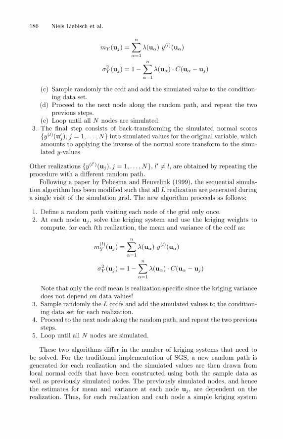
(e) Loop until all N nodes are simulated.3. The final step consists of back-transforming the simulated normal scores

{y(l)(u′j), j = 1, . . . , N} into simulated values for the original variable, which

amounts to applying the inverse of the normal score transform to the simu-lated y-values

Other realizations {y(l′)(uj), j = 1, . . . , N}, l′ �= l, are obtained by repeating theprocedure with a different random path.

Following a paper by Pebesma and Heuvelink (1999), the sequential simula-tion algorithm has been modified such that all L realization are generated duringa single visit of the simulation grid. The new algorithm proceeds as follows:

1. Define a random path visiting each node of the grid only once.2. At each node uj , solve the kriging system and use the kriging weights to

compute, for each lth realization, the mean and variance of the ccdf as:

m(l)Y (uj) =

n∑

α=1

λ(uα) y(l)(uα)

σ2Y (uj) = 1 −

n∑

α=1

λ(uα) · C(uα − uj)

Note that only the ccdf mean is realization-specific since the kriging variancedoes not depend on data values!

3. Sample randomly the L ccdfs and add the simulated values to the condition-ing data set for each realization.

4. Proceed to the next node along the random path, and repeat the two previoussteps.

5. Loop until all N nodes are simulated.

These two algorithms differ in the number of kriging systems that need tobe solved. For the traditional implementation of SGS, a new random path isgenerated for each realization and the simulated values are then drawn fromlocal normal ccdfs that have been constructed using both the sample data aswell as previously simulated nodes. The previously simulated nodes, and hencethe estimates for mean and variance at each node uj , are dependent on therealization. Thus, for each realization and each node a simple kriging system


has to be solved, resulting in a total of N×L kriging systems. In contrast, thenew implementation uses the same random path for all realizations and so thelocations of data and previously simulated nodes to be taken into account forthe construction of the local ccdfs are the same for all realizations. At each gridnode it therefore suffices to determine the kriging weights once.

3.3 Conditional Pixel Swapping

Proposed by Jacquez, this approach produces neutral images by modifying in-crementally a randomly generated image in a way that increases the similaritybetween it and the target image. We experimented with four measures of spatialauto-correlation with this method, the global Moran’s I statistic and three otherstatistics based on Moran’s I: the Moran correlogram, a directional correlogramthat is sensitive to directional trends in an image, and the histogram of localMoran statistics. Each of these statistics is the sum of the local statistics asso-ciated with each pixel. This provided an efficient way of calculating the effectof modifying the values of individual pixels on the global statistic: If the valueof pixel i is changed this will affect the local statistic at i, as well as the localstatistics of neighboring pixels that are contingent on the value at i. If we calcu-lated the difference between these local statistics (at i and its affected neighbors)before and after pixel i is changed, we knew the change of the image’s globalstatistic as well. Thus our general approach was the following:

– Generate an initial neutral image at random. We accomplished this by settingeach pixel of the neutral image to the value of randomly chosen pixels in thetarget. Other methods could be used to avoid sampling biases.

– Calculate the spatial autocorrelation statistic for the target and the initialneutral image.

– Swap two, randomly chosen pixels of the neutral image and calculate theeffect on the neutral image’s spatial statistic. If the new statistic is a bettermatch to the target’s the swap is kept. When histograms were used to rep-resent the images’ spatial autocorrelation swaps were kept if the sum of thesquares of the differences of the bin heights was reduced.

– If the improvement to the neutral image’s statistic after the last swap isgreater than some threshold, continue the swapping process. Otherwise, stop.

There were several ways to create neutral images from a given random imagewith the same histogram. One possibility was to visit all cells sequentially andchange them according to the spatial structure desired. The disadvantage is thatthe spatial structure just created for each cell can be destroyed by changing thenext cell in sequence. A way to limit this disadvantage is to visit all cells inrandom order. This way a change only takes place when it improves the spatialstructure of the neutral image.


4 Pattern Recognition Statistics

The following two edge detection methods were applied on the target and neutralimages as an application for spatial pattern recognition.

4.1 Wombling

Methods for delineating difference boundaries are called wombling Techniques[10], and are calculated from Boundary Likelihood Values (BLV) to identifyboundary elements. BLVs measure the spatial rate of change. Locations wherevariable values change rapidly are more likely to be part of a boundary; theselocations have higher BLVs. The locations that have the highest BLV values areBoundary Elements (BEs) and are considered part of the boundary. CandidateBEs become part of the boundary when their BLVs exceed established thresh-olds. In crisp wombling, those BLVs with values above the threshold are assigneda Boundary Membership Value (BMV) of 1 (non-BEs have BMV = 0). In fuzzywombling, BMVs can range between 0 and 1 and indicate partial membershipin the boundary. The next step in delineating crisp difference boundaries is toconnect BEs to create subboundaries. BEs are connected only if they are adja-cent. With raster wombling, connection is based on the gradient angle of twoadjacent BEs.

4.2 Gaussian Difference Boundaries

The second method that was used to detect significant edges in an image firsttransformed the pixel values into Gaussian space, then calculated the significantz-score difference for a specified alpha level, and finally examined all pairs ofadjacent pixels to determine which had significant z-score differences.

In order to transform the pixel values it was necessary to sort and rank allthe values in the image first. Each rank, r, could then be mapped to a z-scoreby dividing it by the number of ranks(pixels) and calculating the value of theinverse cumulative normal distribution function at p = r/rtotal − 0.5/rtotal.

Next, the distribution resulting from the difference of two random variablesis N [0,

√2], so that a significant difference in z scores could be calculated by

determining the z-score corresponding to a specified alpha level using the inversec.d.f. described above and multiplying by

√2.

Identifying the significant boundaries between pixels was simply a matter ofcomparing each difference in adjacent pixels’ z-scores to the calculated cutoff.Finally, significant boundaries are connected to form a collection of boundarieswith varying length and branchedness.

5 Prototype Applications

A Prototype application that employed the aforementioned methods was de-veloped using C++ and a graphical user interface implemented with Microsoft


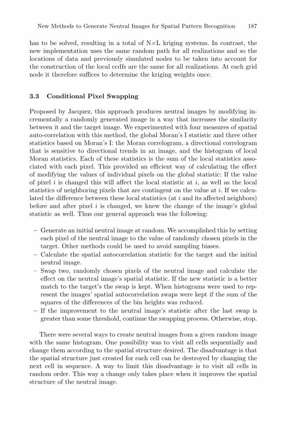
Fig. 1. Example Target Image (left) and Neutral Image (right) created with GeneticProgramming. The Target is a Satellite Image of South Eastern Michigan showing theDetroit and Windsor metropolitan areas

Foundation Classes. The user could load an example target image into the pro-totype and chose one of the three methods for the creation of neutral models.Once the neutral models were created the user could apply statistical patternrecognition as described above. An example application for each of the methodsis discussed in following sections.

5.1 Genetic Programming

For small images GP was able to reproduce the target image with surprisingaccuracy. The accuracy depended almost exclusively on the GP parameters: Themore time in generations, and the more individuals per generation were given tothe GP, the more accurate reproduction of the target image was possible.

A first example of a target image was the 50x50 grey scale image shown inFigure 1 on the left. It was a Satellite Image of South Eastern Michigan showingthe Detroit and Windsor metropolitan areas. The spatial criteria used here forthe creation of neutral images for this example were the distribution of pixelvalues of the target image, which is the most stringent criteria. The best imagethat resulted from this criteria is shown in Figure 1 on the right.

Then neutral images were created using a Bearing Correlogram as the spatialstructure to be preserved. A typical set of images created by the GP in thismanner is shown in Figure 2.

5.2 Sequential Gaussian Simulation

An example for Sequential Gaussian Simulations is shown in Figure 3. The neu-tral image preserved the distribution and size of the lighter spots in the targetimage very well. SGS was able to produce a large number of neutral images in ashort time, because once the kriging weights were computed only once and thesame random path was used for each realization.

5.3 Conditional Pixel Swapping

The first example of CPS was a of 100x100 grey scale image taken from a 1 meterresolution satellite as shown in Figure 4 (top). The criteria used for the resulting


Fig. 2. Images created from Bearing Corellogram with Genetic Programming

Fig. 3. Target (left) and Neutral Image created with Gaussian Sequential Simulation

set of neutral images was the bearing correlogram, using two bearings of zeroand ninety degrees. A neighborhood range of 4 rows of Moore’s neighborhood(full ring of neighbors) was used. The neutral images could reproduce the spatialstructure of the target images (number and size of white spots) very well.

The range of neighbors included in the Bearing Correlogram has an influenceon the spatial structure of the neutral images. In all applications the Mooreneighborhood was regarded. If more neighbors are included the neutral imagesturn out to have larger spots and the boundaries are not as sharp as with lessneighbors. Consequently, the neutral images shown in Figure 4 have less sharperboundaries within the clusters. Furthermore, in this image 4 angles are regardedat the same time. Because of this, the directionality of the neutral images is notso distinctive as in the following images.

As a second example, the algorithm was used to create neutral images fromthe simple Global Moran’s I of the target image shown in Figure 5 (top). Again,the neutral images show a distribution of dark and white spots, and clusteringthat is very similar to the target.

The same target image was used for the next test shown in Figure 6. This timehowever, the neutral images were produced on basis of the Bearing Correllogram.The Bearing for this Bearing Correlogram was taken to be the angle of thestrongest directionality in the target image. The resulting neutral images showa strong directionality from the lower left to the upper right of the picture. The


Fig. 4. CPS Neutral images created from Bearing Correlogram with a range of 4 neigh-bors

Fig. 5. CPS Neutral Images created from conservation of global Moran’s I of target.On top target image and image resulting from random sampling from histogram

clustering and distribution of dark and bright pixel values however is again veryclose to the target image.

The following set of figures shows how CPS was used to produce neutralimages for a larger target, which in turn were used for statistical pattern recog-nition with edge detection. Figure 7 shows the target image displayed in theprototype application. The Wombling method has been applied to this imageand the edges are shown on top of the original image. Wombling has also beenapplied to a set of 50 neutral images, one of which is shown in Figure 8. Again,the edges are displayed on top of the neutral images. Figure 9 finally shows ahistogram of the detected sub boundary lengths for the neutral images com-pared to the sub boundary lengths of the target image. It is obvious that thesub boundary lengths of the target image are significantly longer than those ofthe neutral images. This implies that the target image has an underlying process


Fig. 6. CPS Neutral images created from Bearing Correlogram, using only the angleof strongest directionality

Fig. 7. Edgedetection on target image

that is more complex or different from the spatial structure created under theneutral hypothesis.

Finally, there is an example that demonstrates the application of neutralmodels at a very small scale. The target image is a microscopic picture of twofilament systems taken from a body cell. This image is shown together with aCPS neutral image in Figure 10. The neutral image was produced with bearingscorresponding to the directionality of the original image.


Fig. 8. Edgedetection on neutral image

6 Summary and Conclusions

Three methods were developed that produced sets of neutral images that pre-served certain spatial structures on a target image such as local autocorrelation,global autocorrelation, or directional autocorrelation.

Each of the methods had different advantages and disadvantages in regardto the quality of the neutral images and the speed of their creation. GeneticProgramming had the advantage of producing very diverse neutral images thatdiffered greatly from the original image but still conserved the required spatialproperty. The disadvantage was that it would take a long time for them toevolve, especially for larger target images. Sequential Gaussian Simulation hadthe advantage of being able to create large images quickly. It also conserved therequired spatial properties and was able to work with different spectral bandsand on different areas of the target image. The disadvantage of SGS was that itwas difficult to automatically fit an appropriate variogram model to the targetimage. Conditional Pixel Swapping method was very flexible and could alsowork on large images. The resulting neutral images looked close to the originalimage. Due to its relative simplicity, speed, and good results, this seemed to bea promising method.

As a test for spatial pattern recognition statistics, two methods were devisedfor edge detection: Wombling and Gaussian Differencing. They could easily de-tect interesting features in the target images and support those quantitativelyby comparison with the neutral images.

Why should one use a neutral model that incorporates some spatial autocor-relation as opposed to CSR ? In real world systems, complete spatial randomnessis an extraordinary exception that is rarely observed. Employing CSR as a null


Fig. 9. Comparison on sub boundary lengths on target and neutral images

Fig. 10. CPS Filaments Example with a range of 2 neighbors, Bearing Correlogram,angle 90 degrees

hypothesis in spatial pattern recognition poses a “strawman” that will almostcertainly be rejected. The scientific value of such a simplistic null hypothesis istherefore quite small, since rejecting a simplistic null hypothesis has little inferen-tial yield. The neutral models we have presented capture spatial autocorrelationsignatures representative of real world systems. They make it possible to test forspatial patterns above and beyond that observed in the absence of an alternativespatial process (e.g. boundary formation). This strengthened inference structureis expected to lead to scientific insights that are not possible using untenableand unreasonable null hypothesis such as CSR.


This preliminary research demonstrated the feasibility of using neutral imagegeneration in statistical pattern recognition. Our future research will focus onthe application of these techniques to large multivariate spatial fields arisingfrom high resolution hyper spectral images.

Acknowledgments

This research was funded by National Cancer Institute grant R43CA92807 toBiomedware Inc, under the Innovation in Biomedical Information Science andTechnology Initiative at the National Institutes of Health. The contents of thispublication are those of the authors and do not necessarily represent the officialviews of the National Cancer Institute.

References

1. Anselin, L. (1995), Local Indicators of Spatial Association-LISA, GeographicalAnalysis, 27:93–115.

2. Banzhaf, W., Nordin, P., Keller, R., and Francone, F. (1998), Genetic Program-ming, An Introduction, Morgan Kaufmann Publischers, Inc., San Francisco, CA.

3. Goovaerts, P. (1997), Geostatistics for Natural Resources Evaluation, Oxford Uni-versity Press, New York, NY.

4. Gustafson, E. (1998), Quantifying Landscape Spatial Pattern: What is the Stateof the Art? Ecosystems (1): 143-156.

5. Moran, P. (1950), Notes on Continuous Stochastic Phenomena, Biometrika 37:17-23.

6. Pebesma, E. and Heuvelink, G. (1999), Latin Hypercube Sampling of GaussianRandom Fields, Technometrics, 41: 303-312.

7. Rosenberg, M. (1998), The Bearing Correlogram: A New Method of AnalyzingDirectional Spatial Autocorrelation, Geographical Analysis, 33(3): 267-278

8. Verly, G. (1986), MultiGaussian Kriging—A Complete Case Study, in: R. Ramani,ed., Proceedings of the 19th International APCOM Symposium: Society of MiningEngineers, Littleton, CO, pp. 283–298.

9. Waller, L. and Jacquez, G. (1995), Disease Models Implicit in Statistical Tests ofDisease Clustering, Epidemiology, 6(6): 584-590.

10. Womble, W. (1951), Differential Systematics, Science, 114, 315-322.

New Methods to Generate Neutral Images for Spatial Pattern Recognition

Documents

Transcript of New Methods to Generate Neutral Images for Spatial Pattern Recognition