Topological Histogram Reduction TowardsColour Segmentation

Eduard Vazquez, Ramon Baldrich, Javier Vazquez, and Maria Vanrell

Computer Vision Center, Dept. Ciencies de la Computacio. Edifici O, UniversitatAutonoma de Bacelona. 08193 Bellaterra (Barcelona), Spain

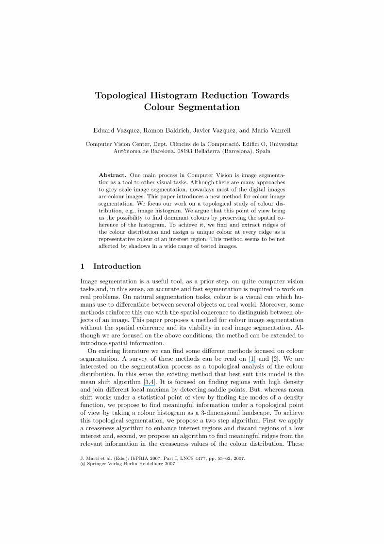
Abstract. One main process in Computer Vision is image segmenta-tion as a tool to other visual tasks. Although there are many approachesto grey scale image segmentation, nowadays most of the digital imagesare colour images. This paper introduces a new method for colour imagesegmentation. We focus our work on a topological study of colour dis-tribution, e.g., image histogram. We argue that this point of view bringus the possibility to find dominant colours by preserving the spatial co-herence of the histogram. To achieve it, we find and extract ridges ofthe colour distribution and assign a unique colour at every ridge as arepresentative colour of an interest region. This method seems to be notaffected by shadows in a wide range of tested images.

1 Introduction

Image segmentation is a useful tool, as a prior step, on quite computer visiontasks and, in this sense, an accurate and fast segmentation is required to work onreal problems. On natural segmentation tasks, colour is a visual cue which hu-mans use to differentiate between several objects on real world. Moreover, somemethods reinforce this cue with the spatial coherence to distinguish between ob-jects of an image. This paper proposes a method for colour image segmentationwithout the spatial coherence and its viability in real image segmentation. Al-though we are focused on the above conditions, the method can be extended tointroduce spatial information.

On existing literature we can find some different methods focused on coloursegmentation. A survey of these methods can be read on [1] and [2]. We areinterested on the segmentation process as a topological analysis of the colourdistribution. In this sense the existing method that best suit this model is themean shift algorithm [3,4]. It is focused on finding regions with high densityand join different local maxima by detecting saddle points. But, whereas meanshift works under a statistical point of view by finding the modes of a densityfunction, we propose to find meaningful information under a topological pointof view by taking a colour histogram as a 3-dimensional landscape. To achievethis topological segmentation, we propose a two step algorithm. First we applya creaseness algorithm to enhance interest regions and discard regions of a lowinterest and, second, we propose an algorithm to find meaningful ridges from therelevant information in the creaseness values of the colour distribution. These

J. Martı et al. (Eds.): IbPRIA 2007, Part I, LNCS 4477, pp. 55–62, 2007.c© Springer-Verlag Berlin Heidelberg 2007

56 E. Vazquez et al.

ridges will represent the most representative colours, or dominant colours presentin the image.

The paper is organized as follows: section 2 introduces the method and justifiesthe ridge concept; section 3 introduces our two-steps algorithm;. Section 4 showssome results, discussing the parameters in the operator, and conclusions andfurther work can be found on section 5.

2 Method Outline

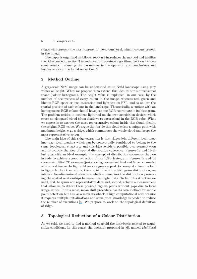
A grey-scale NxM image can be understood as an NxM landscape using greyvalues as height. What we propose is to extend this idea at our 3-dimensionalspace (colour histogram). The height value is explained, in our case, by thenumber of occurrences of every colour in the image, whereas red, green andblue in RGB space or hue, saturation and lightness on HSL, and so on, are thespatial position of each colour in the landscape. Theoretically, a surface with anhomogeneous RGB colour should have just one RGB coordinate in its histogram.The problem resides in incident light and on the own acquisition devices whichcause an elongated cloud (from shadows to saturation) in the RGB cube. Whatwe expect is to extract the most representative colour inside this cloud, ideally,the original RGB value. We argue that inside this cloud exists a unique path withmaximum height, e.g., a ridge, which summarizes the whole cloud and keeps themost representative colour.

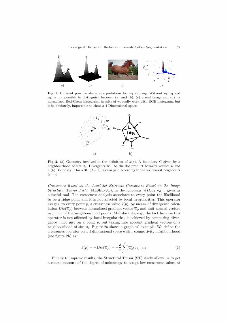
The main idea of this ridge extraction is that ridges join different local max-ima, e.g., local maxima which can be conceptually considered to belong to thesame topological structure, and this idea avoids a possible over-segmentationand introduces the idea of spatial distribution coherence. Figures 1a and 1b il-lustrates with an ideal example this concept of distribution coherence that weinclude to achieve a good reduction of the RGB histogram. Figures 1c and 1dshow a simplified 2D example (just showing normalized Red and Green channels)with a real image. In figure 1d we can guess a peak for every dominant colourin figure 1c. In other words, there exist, inside the histogram distribution, anintrinsic low-dimensional structure which summarizes the distribution preserv-ing the spatial relationships between meaningful data. To find this structure weneed, first, to spurn non representative data and, second, achieve a measurementthat allow us to detect these possible highest paths without gaps due to localirregularities. In this sense, mean shift procedure has its own method for saddlepoint detection but has, as a main drawback, a high computational cost becauseit requires multiple initializations and some prior knowledge is needed to reducethe number of executions [5]. We propose to work on the topological definitionof ridge.

3 Topological Reduction of a Colour Distribution

As we told, we need to find a method to avoid the drawbacks related to acqui-sition conditions. In this sense, the operator proposed in [6], named Multilocal

Topological Histogram Reduction Towards Colour Segmentation 57

a) b) c) d)

Fig. 1. Different possible shape interpretations for m1 and m2. Without p1, p2 andp3, is not possible to distinguish between (a) and (b); (c) a real image and (d) itsnormalized Red-Green histogram, in spite of we really work with RGB histogram, butit is, obviously, impossible to show a 4-Dimensional space.

a) b)

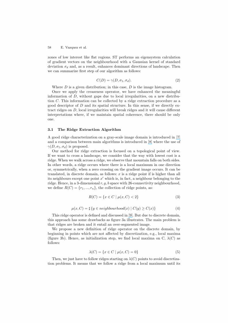
Fig. 2. (a) Geometry involved in the definition of k(p). A boundary C given by aneighbourhood of size σ1. Divergence will be the dot product between vectors w andn.(b) Boundary C for a 3D (d = 3) regular grid according to the six nearest neighbours(r = 6).

Creassenes Based on the Level-Set Extrinsic Curvatures Based on the ImageStructural Tensor Field (MLSEC-ST), in the following γ(D, σ1, σd) , gives usa useful tool. The creaseness analysis associates to every point the likelihoodto be a ridge point and it is not affected by local irregularities. This operatorassigns, to every point p, a creaseness value k(p), by means of divergence calcu-lation Div(wp) between normalized gradient vector wp and unit normal vectorsn1, ..., nr of the neighbourhood points. Multilocality, e.g., the fact because thisoperator is not affected by local irregularities, is achieved by computing diver-gence , not just on a point p, but taking into account gradient vectors of aneighbourhood of size σi. Figure 2a shows a graphical example. We define thecreaseness operator on a d-dimensional space with r-connectivity neighbourhood(see figure 2b) as:

k(p) = −Div(wp) = −d

r

r∑

k=1

wtk(σi) · nk (1)

Finally to improve results, the Structural Tensor (ST) study allows us to geta coarse measure of the degree of anisotropy to assign low creaseness values at

58 E. Vazquez et al.

zones of low interest like flat regions. ST performs an eigensystem calculationof gradient vectors on the neighbourhood with a Gaussian kernel of standarddeviation σd and, as a result, enhances dominant directions of landscape. Thenwe can summarize first step of our algorithm as follows:

C(D) = γ(D, σ1, σd). (2)

Where D is a given distribution; in this case, D is the image histogram.Once we apply the creaseness operator, we have enhanced the meaningful

information of D, without gaps due to local irregularities, on a new distribu-tion C. This information can be collected by a ridge extraction procedure as agood descriptor of D and its spatial structure. In this sense, if we directly ex-tract ridges on D, local irregularities will break ridges and it will cause differentinterpretations where, if we maintain spatial coherence, there should be onlyone.

3.1 The Ridge Extraction Algorithm

A good ridge characterization on a gray-scale image domain is introduced in [7]and a comparison between main algorithms is introduced in [8] where the use ofγ(D, σ1, σd) is proposed.

Our method for ridge extraction is focused on a topological point of view.If we want to cross a landscape, we consider that the way with lowest cost is aridge. When we walk across a ridge, we observe that mountain falls on both sides.In other words, a ridge occurs where there is a local maximum in one directionor, symmetrically, when a zero crossing on the gradient image occurs. It can betranslated, in discrete domain, as follows: x is a ridge point if is higher than allits neighbours except one point x′ which is, in fact, a neighbour belonging to theridge. Hence, in a 3-dimensional r, g, b space with 26-connectivity neighbourhood,we define R(C) = {r1, ..., rn}, the collection of ridge points, as:

R(C) = {x ∈ C | μ(x, C) < 2} (3)

μ(x, C) = � {y ∈ neighbourhood(x) | C(y) ≥ C(x)} (4)

This ridge operator is defined and discussed in [9]. But due to discrete domain,this approach has some drawbacks as figure 3a illustrates. The main problem isthat ridges are broken and it entail an over-segmented image.

We propose a new definition of ridge operator on the discrete domain, bybeginning in points which are not affected by discretization, e.g., local maxima(figure 3b). Hence, as initialization step, we find local maxima on C, λ(C) asfollows:

λ(C) = {x ∈ C | μ(x, C) = 0} (5)

Then, we just have to follow ridges starting on λ(C) points to avoid discretiza-tion problems. It means that we follow a ridge from a local maximum until its

Topological Histogram Reduction Towards Colour Segmentation 59

a) b) c)

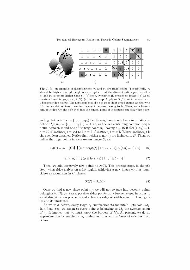
Fig. 3. (a) an example of discretization: r1 and r2 are ridge points. Theoretically r2

should be higher than all neighbours except r1, but the discreatization process takesp1 and p2 as points higher than r2. (b),(c) A synthetic 2D creaseness image: (b) Localmaxima found in gray, e.g., λ(C). (c) Second step: Applying R(C) points labeled with4 become ridge points. The next step should be to go to light grey squares labeled with3.8, but we do not take these into account because belong to Ω. Then, we achieve astraight ridge. On the next step just the central point of the square can be a ridge point.

ending. Let neigh(x) = {n1, ..., n26} be the neighbourhood of a point x. We alsodefine Ω(x, nj) = {ω1, ..., ωr} ,j = 1..26, as the set containing common neigh-bours between x and one of its neighbours nj ; having r = 16 if dist(x, nj) = 1,r = 10 if dist(x, nj) =

√2 and r = 6 if dist(x, nj) =

√3. Where dist(x, nj) is

the euclidean distance. Notice that neither x nor nj are included in Ω. Then, wedefine the ridge points in a creaseness image C, as:

λz(C) = λz−1(C)⋃

{n ∈ neigh(l) | l ∈ λz−1(C), μ′(l, n) = 0} (C) (6)

μ′(x, nj) = � {y ∈ Ω(x, nj) | C(y) ≥ C(nj)} (7)

Then, we add iteratively new points to λ(C). This process stops, in the pthstep, when ridge arrives on a flat region, achieving a new image with as manyridges as mountains in C. Hence:

R(C) = λp(C) (8)

Once we find a new ridge point nj, we will not to take into account pointsbelonging to Ω(x, nj) as a possible ridge points on a further steps, in order toavoid discretization problems and achieve a ridge of width equal to 1 as figure3b and 3c illustrates.

As we told before, every ridge rj summarizes its mountain, lets said, Mj .In a final step, we assign to every point x belonging to Mj the average colourof rj . It implies that we must know the borders of Mj . At present, we do anapproximation by making a rgb cube partition with a Voronoi calculus fromridges.

60 E. Vazquez et al.

a) b)

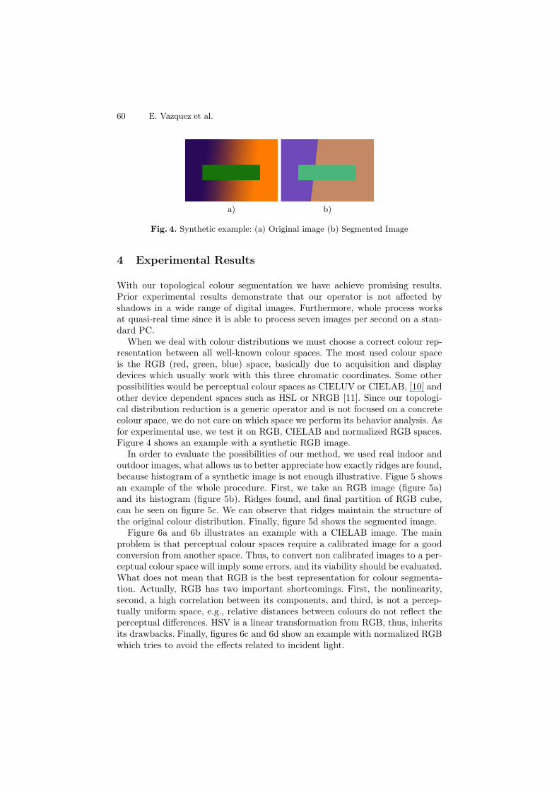
Fig. 4. Synthetic example: (a) Original image (b) Segmented Image

4 Experimental Results

With our topological colour segmentation we have achieve promising results.Prior experimental results demonstrate that our operator is not affected byshadows in a wide range of digital images. Furthermore, whole process worksat quasi-real time since it is able to process seven images per second on a stan-dard PC.

When we deal with colour distributions we must choose a correct colour rep-resentation between all well-known colour spaces. The most used colour spaceis the RGB (red, green, blue) space, basically due to acquisition and displaydevices which usually work with this three chromatic coordinates. Some otherpossibilities would be perceptual colour spaces as CIELUV or CIELAB, [10] andother device dependent spaces such as HSL or NRGB [11]. Since our topologi-cal distribution reduction is a generic operator and is not focused on a concretecolour space, we do not care on which space we perform its behavior analysis. Asfor experimental use, we test it on RGB, CIELAB and normalized RGB spaces.Figure 4 shows an example with a synthetic RGB image.

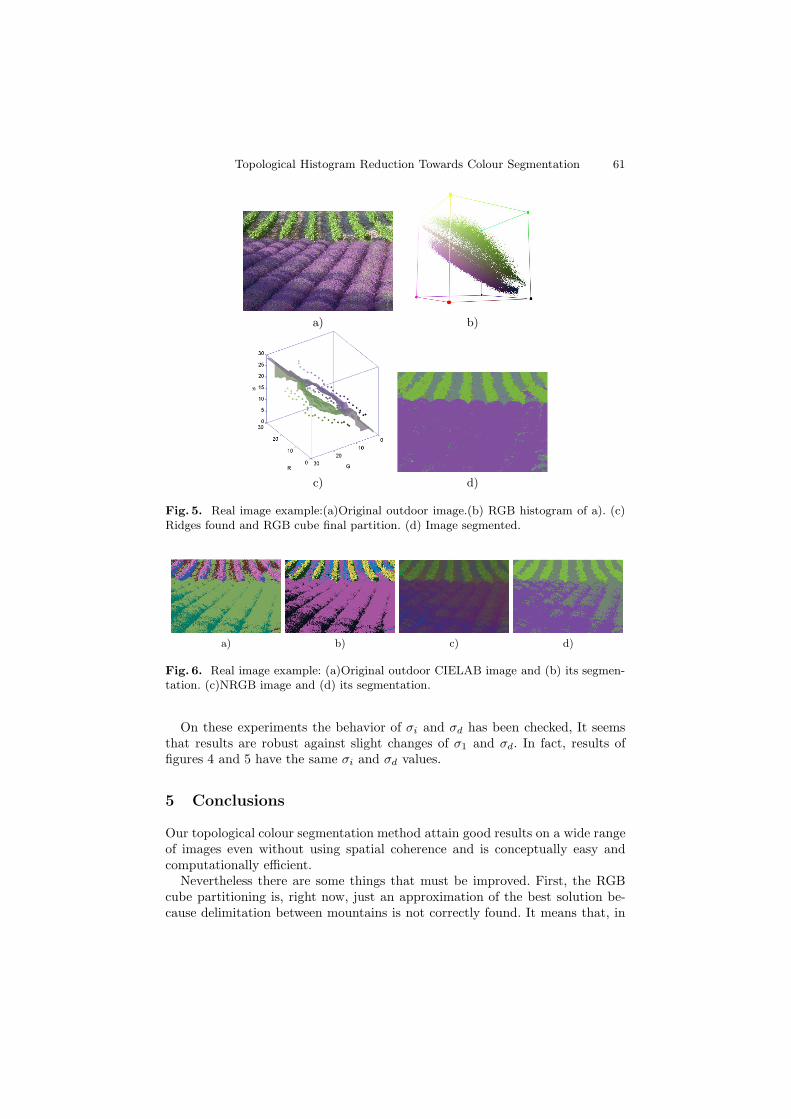
In order to evaluate the possibilities of our method, we used real indoor andoutdoor images, what allows us to better appreciate how exactly ridges are found,because histogram of a synthetic image is not enough illustrative. Figue 5 showsan example of the whole procedure. First, we take an RGB image (figure 5a)and its histogram (figure 5b). Ridges found, and final partition of RGB cube,can be seen on figure 5c. We can observe that ridges maintain the structure ofthe original colour distribution. Finally, figure 5d shows the segmented image.

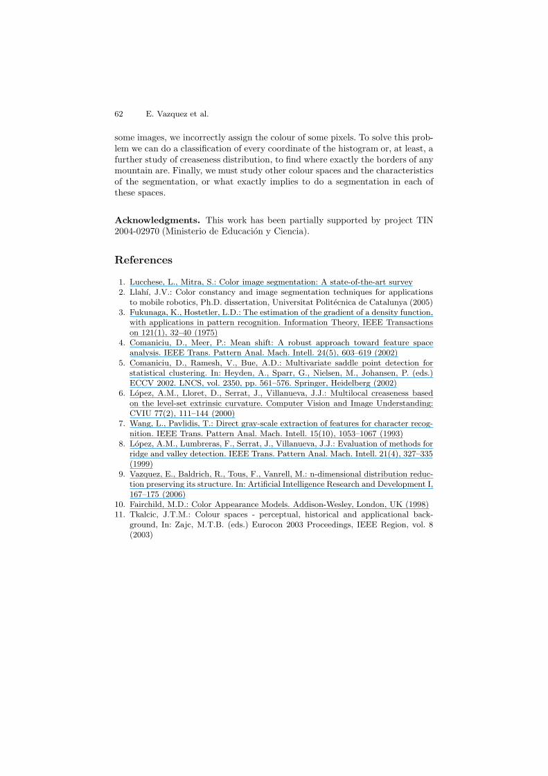
Figure 6a and 6b illustrates an example with a CIELAB image. The mainproblem is that perceptual colour spaces require a calibrated image for a goodconversion from another space. Thus, to convert non calibrated images to a per-ceptual colour space will imply some errors, and its viability should be evaluated.What does not mean that RGB is the best representation for colour segmenta-tion. Actually, RGB has two important shortcomings. First, the nonlinearity,second, a high correlation between its components, and third, is not a percep-tually uniform space, e.g., relative distances between colours do not reflect theperceptual differences. HSV is a linear transformation from RGB, thus, inheritsits drawbacks. Finally, figures 6c and 6d show an example with normalized RGBwhich tries to avoid the effects related to incident light.

Topological Histogram Reduction Towards Colour Segmentation 61

a) b)

c) d)

Fig. 5. Real image example:(a)Original outdoor image.(b) RGB histogram of a). (c)Ridges found and RGB cube final partition. (d) Image segmented.

a) b) c) d)

Fig. 6. Real image example: (a)Original outdoor CIELAB image and (b) its segmen-tation. (c)NRGB image and (d) its segmentation.

On these experiments the behavior of σi and σd has been checked, It seemsthat results are robust against slight changes of σ1 and σd. In fact, results offigures 4 and 5 have the same σi and σd values.

5 Conclusions

Our topological colour segmentation method attain good results on a wide rangeof images even without using spatial coherence and is conceptually easy andcomputationally efficient.

Nevertheless there are some things that must be improved. First, the RGBcube partitioning is, right now, just an approximation of the best solution be-cause delimitation between mountains is not correctly found. It means that, in

62 E. Vazquez et al.

some images, we incorrectly assign the colour of some pixels. To solve this prob-lem we can do a classification of every coordinate of the histogram or, at least, afurther study of creaseness distribution, to find where exactly the borders of anymountain are. Finally, we must study other colour spaces and the characteristicsof the segmentation, or what exactly implies to do a segmentation in each ofthese spaces.

Acknowledgments. This work has been partially supported by project TIN2004-02970 (Ministerio de Educacion y Ciencia).

References

1. Lucchese, L., Mitra, S.: Color image segmentation: A state-of-the-art survey2. Llahı, J.V.: Color constancy and image segmentation techniques for applications

to mobile robotics, Ph.D. dissertation, Universitat Politecnica de Catalunya (2005)3. Fukunaga, K., Hostetler, L.D.: The estimation of the gradient of a density function,

with applications in pattern recognition. Information Theory, IEEE Transactionson 121(1), 32–40 (1975)

4. Comaniciu, D., Meer, P.: Mean shift: A robust approach toward feature spaceanalysis. IEEE Trans. Pattern Anal. Mach. Intell. 24(5), 603–619 (2002)

5. Comaniciu, D., Ramesh, V., Bue, A.D.: Multivariate saddle point detection forstatistical clustering. In: Heyden, A., Sparr, G., Nielsen, M., Johansen, P. (eds.)ECCV 2002. LNCS, vol. 2350, pp. 561–576. Springer, Heidelberg (2002)

6. Lopez, A.M., Lloret, D., Serrat, J., Villanueva, J.J.: Multilocal creaseness basedon the level-set extrinsic curvature. Computer Vision and Image Understanding:CVIU 77(2), 111–144 (2000)

7. Wang, L., Pavlidis, T.: Direct gray-scale extraction of features for character recog-nition. IEEE Trans. Pattern Anal. Mach. Intell. 15(10), 1053–1067 (1993)

8. Lopez, A.M., Lumbreras, F., Serrat, J., Villanueva, J.J.: Evaluation of methods forridge and valley detection. IEEE Trans. Pattern Anal. Mach. Intell. 21(4), 327–335(1999)

9. Vazquez, E., Baldrich, R., Tous, F., Vanrell, M.: n-dimensional distribution reduc-tion preserving its structure. In: Artificial Intelligence Research and Development I,167–175 (2006)

10. Fairchild, M.D.: Color Appearance Models. Addison-Wesley, London, UK (1998)11. Tkalcic, J.T.M.: Colour spaces - perceptual, historical and applicational back-

ground, In: Zajc, M.T.B. (eds.) Eurocon 2003 Proceedings, IEEE Region, vol. 8(2003)