Durham E-Theses

Solitons in low-dimensional sigma models

Gladikowski, Jens

How to cite:

Gladikowski, Jens (1997) Solitons in low-dimensional sigma models, Durham theses, Durham University.Available at Durham E-Theses Online: http://etheses.dur.ac.uk/5077/

Use policy

The full-text may be used and/or reproduced, and given to third parties in any format or medium, without prior permission orcharge, for personal research or study, educational, or not-for-pro�t purposes provided that:

• a full bibliographic reference is made to the original source

• a link is made to the metadata record in Durham E-Theses

• the full-text is not changed in any way

The full-text must not be sold in any format or medium without the formal permission of the copyright holders.

Please consult the full Durham E-Theses policy for further details.

Academic Support O�ce, Durham University, University O�ce, Old Elvet, Durham DH1 3HPe-mail: e-theses.admin@dur.ac.uk Tel: +44 0191 334 6107

http://etheses.dur.ac.uk

Solitons in Low-Dimensional Sigma Models

by

Jens Gladikowski

The copyright of this thesis rests with the author. No quotation from it should be published without the written consent of the author and information derived from it should be acknowledged.

Thesis presented for the Degree of Doctor of Philosophy

at the University of Durham

Department of Mathematical Sciences

University of Durham

England

August 1997

I 6 DEC 1997

T O M Y P A R E N T S

Preface

This thesis summarizes work done by the author between October 1994 and July 1997 in

the Department of Mathematical Sciences at the University of Durham. No part of it has been

previously submitted for any degree at this or any other University.

With the exceptions of chapter 1 and the introductions to each chapter, this material is believed

to be original work, unless otherwise stated. The contents of chapter 2 derives from a paper that

has been published in Zeitschrift fiir Physik [l]. The material of chapter 4 is the result of a

collaboration with Meik Hellmund and is to appear in Physical Review D [2]. Parts of chapter 5 .

were also done in collaboration with Meik Hellmund.

There are a number of people who I wish to thank for making my stay in Durham enjoyable

and productive. First and foremost I am deeply grateful to my supervisor Wojtek Zakrzewski for

his constant encouragement, careful guidance and frankness. I am also very much indebted to

Meik Hellmund for his genuine friendship and many valuable conversations. It is a pleasure to

acknowledge various members of the Department of Mathematical Sciences for their interest in my

work and their constructive criticism, especially I wish to thank Jacek Dziarmaga, Bernard Piette

and Richard Ward. Also many thanks to Uli Harder for his irresistable outspokenness.

I thank the Department of Mathematical Sciences and the Engineering and Physical Sciences

Research Council for Research Studentships.

The copyright of this thesis rests with the author. No quotation from it should be published

without his prior written consent and information derived from it should be acknowledged.

Abstract

Solitons in Low-Dimensional Sigma Models

Jens Gladikowski

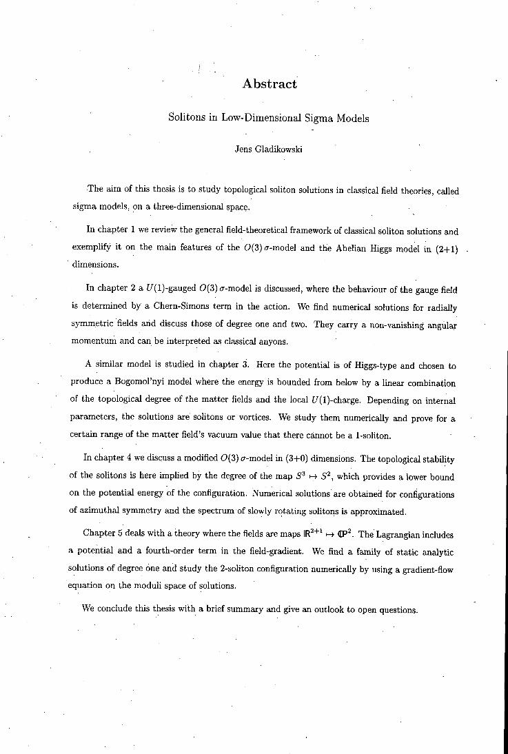
The aim of this thesis is to study topologiccil soliton solutions in classical field theories, called

sigma models, on a three-dimensional space.

In chapter 1 we review the general field-theoretical framework of classical soliton solutions and

exemplify it on the main features of the 0(3)<T-model and the Abelian Higgs model in (2-1-1)

• dimensions.

In chapter 2 a ?7(l)-gauged 0(3) cr-model is discussed, where the behaviour of the gauge field

is determined by a Chern-Simons term in the action. We find numerical solutions for radially

symmetric fields and discuss those of degree one and two. They carry a non-vanishing angular

momentum and can be interpreted as classical anyons.

A similar model is studied in chapter 3. Here the potential is of Higgs-type and chosen to

produce a Bogomol'nyi model where the energy is bounded from below by a linear combination

of the topological degree of the matter fields and the local f/(l)-charge. Depending on internal

parameters, the solutions are solitons or vortices. We study them numerically and prove for a

certain range of the matter field's vacuum value that there cannot be a 1-soliton.

In chapter 4 we discuss a modified 0(3) cr-model in (3-1-0) dimensions. The topological stability

of the solitons is here imphed by the degree of the map 5^ S , which provides a lower bound

on the potential energy of the configuration. Numerical solutions are obtained for configurations

of azimuthal symmetry and the spectrum of slowly rotating soUtons is approximated.

Chapter 5 deals with a theory where the fields are maps IR "*" 1-4 IP' . The Lagrangian includes

a potential and a fourth-order term in the field-gradient. We find a family of static analytic

solutions of degree one and study the 2-soliton configuration numerically by using a gradient-flow

equation on the moduli space of solutions.

We conclude this thesis with a brief summary and give an outlook to open questions.

Contents

1 A Review of Topological Solitons 3

. 1.1 Solitons in Classical Field Theories 3

L2 The 0(3) cr-model and its Relatives 7

1.3 The Abelian Higgs model 16

2 Topological Chern-Simons Solitons in the 0(3) cr-model 21

2.1 Introduction 21

2.2 The Chern-Simons 0(3) a-model 26

2.3 Bogomol'nyi Bound in the Gauged Model 29

2.4 Static Fields of Radial Symmetry . 31

2.5 Asymptotic Behaviour of the Fields 34

,2.6 Numerical Methods 36

2.7 Numerical Results 37

2.8 Conclusions 44

3 Self-Dual Solitons in a Gauged 0(3) CT-model 45

3.1 Introduction 45

3.2 The Self-Dual Chern-Simons 0(3) cr-model , 49

3.3 Topological Solitons in the Range u > 1 54

3.4 Topological Solitons and Vortices for 0 < f < 1 - 58

3.5 Conclusions 59

4 Static Solitons with Non-Zero Hopf Number 64

4.1 Geometry of the Hopf Map 66

4.2 Early Work 70

4.3 Hopf Maps and Toroidal Ansatz 73

C O N T E N T S

4.4 Numerical Results 76

4.5 Spinning Hopfions ; - 78

4.6 Conclusions 79

Appendix 81

5 Solitons in the OP^ Baby Skyrme Model 86

5.1 OP^-^-models Revisited , 88

5.2 The OP^ baby Skyrme Model . . , 93

5.3 Solutions to the OP^ Skyrme Model 94

5.4 Numerical Results and Outlook ; 100

Appendix 105

General Conclusions 108

Bibliography 110

Chapter 1

A Review of Topological Solitons

1.1 Solitons in Classical Field Theories

The general aim .of this thesis is to explore classical solutions to certain non-linear field theories,

called sigma models. If these solutions are non-singular, of finite energy and localised in space they

will be called solitons. Solitons as such are abstractions of inherently non-linear wave phenomena

whose description is related to several branches of pure mathematics and connects them to both

physical theories and observations, the latter being exemplified by non-linear water waves, shock

waves in a plasma medium, ATP-transport in muscles and non-linear electric pulses.

The theory of solitons is thus a prime example of a general tendency in contemporciry theoretical

physics, namely the increasing interchange of ideas and concepts between pure mathematics and

physics. The work on the border between these two areas has been proven fruitful and inspiring

for both sides. To mention just two relevant examples, many notions of Algebraic Topology and

Differential Geometry, such as homotopy and (co-) homology groups or index theorems, are crucial

for the physicists' understanding of soliton theory, while on the mathematics side the discovery of

the inverse scattering transform — one of the main analytic tools in soliton theory — was inspired

by a physical question that resulted in the initial value problem for the KdV equation [3]. It is in this

spirit that the work presented in this thesis is motivated partly by the pure mathematical interest

of finding solutions to a well-defined analytical problem irrespective of its physical applications

and partly by the. experimental evidence of non-linear waves in the broadest sense.

With the definition given above, solitons characteristically possess particle-like features and

quite naturally physicists became intrigued by solitons in field theories and their applications to

1.1 Solitons in Classical Field Theories

• particle physics. A prominent example of this is the Skyrme model. Being soniewhat inspired

by Kelvin's idea of a classical continuum theory of matter, Skyrme constructed, beginning in

1961, the first non-linear field theory for the description of barybnic matter, or more precisely, for

fermions as solitons in a mesonic background field [4, 5]. Although being somehow overshadowed

by the dramatic success of Quantum Chromodynamics (QCD) in the 1970's, Skyrme's model was

revived in the early 1980's by Witten, who proposed it to be a good candidate for an effective

theory in the low-energy range of QCD, which is beyond perturbation theory [6]. Witten's seminal

proposal has inspired many subsequent investigations of the Skyrme and related models at both the

classical and quantum mechanical level (see [7] for a comprehensive review). In a sense, some of the

work presented in this thesis can be seen as spin-ofl?' of research performed on the Skyrme-model,

although we are not directly interested .in applications to nuclear physics. The Skyrme model is

an example of a (modified) non-linear sigma model, the main objects of study of this thesis and

its investigation has revealed many connections to other fundamental theories such as Yang-Mills

and Yang-Mills-Higgs theory in (4-1-0) and (3-H) dimensions respectively. Below we will introduce

two lower-dimensional relatives of these theories, the 0(3) cr-model and the Abelian Higgs model,

but first we lay out the general field-theoretical framework for their description.

Solitons can be divided into two, almost disjoint, classes, corresponding to the origin of their

stability. In one class, which is historically older, the solutions are called integrable and the

governing equation(s) have an infinite number of quantities that are dynamically conserved. By

definition, for the model to be integrable, these conserved quantities have to be in involution.

Examples of integrable theories are the KdV-equation and the non-linear Schrodinger equation.

Solitons in an integrable model cannot be rich in their dynamics: for two coUiding solitons anything

more than a shift of their phase is prohibited by the conservation laws. This makes solitons in

integrable models less interesting from the particle physics point of view, where one is interested in

non-trivial scattering, vibrations, radiation and the like, but there are many other areas in science

where these solitons provide a fertile ground for various applications: hydrodynamics, plasma-

physics and mathematical biology are just some of them. Generally speaking, integrable models

are rare, especially if additional conditions (such as Lorentz-invariance) are imposed and most

of them are confined to (1-1-1) dimensions. Integrability usually impUes certain restrictions on

the parameters of the model and one can say that the set of integrable models is of "measure

zero" in the space of theories. Nevertheless these models carry important conceptual weight: the

soliton solutions (if they can be found) can often be studied in analytical depth, and in a quantum

theory — which-, however, has to be defined for solitons — they offer, at least in principle, a

1.1 Solitons in Classiccil Field Theories

non-perturbative description which contrasts the perturbative approaches that are common in

Quantum Field Theories.

. For the other class of soHtons, it is the topology of the theories' configuration space that can

guarantee the solitons' stability. To be more precise, consider a classical field <j), which is defined

as a smooth map from the physical space-time X = {x, t} into the field-manifold $, where x and

t denote the space- and time-coordinates respectively; (p • X i-y ^. The (classical) configuration

space C is the infinite-dimensional space of all fields cj) &t a, fixed time t. Consistently, we will

frequently call a time-independent map a configuration. One defines a functional V[<j)] on the

configuration space, which is called the potential energy and maps C t-i- IR. Its finiteness is essential

to allow for a meaningful physical interpretation of a field theory and we will henceforth impose

this condition. For the theories considered in this thesis, an important consequence of y[4>] < oo

is that C decomposes into disjoint subsets C^, with integer N, which are separated by an infinite

potential barrier:

oo c= [ j C (1.1)

N=-oo

Elements of Ci are usually called 1-solitons, or simply solitons, and fields in the sector Cq are by

definition topologically equivalent to the vacuum. The index N occurs under various names in

the literature, such as degree of the map or topological charge. For the theories studied here it

provides a lower bound on the potential energy V[(j)].

The topology of the configuration space is canonically described in terms of homotopy groups [8].

Consider two maps </>i(x) and 02(x) between two mcinifolds M and TV, 0i,2 : M. They

are called homotopic if there exists a continuous map (j> : M x 11-^ Af, I = [0,1], such that

(^i(x) — (f>{x,0) and ( 2(x) = i (x, 1). The map 0(x,^),f e [0,1] is called the homotopy. A set of

homotopic maps forms an equivalence class which is an element of the corresponding homotopy

group. These are usually denoted 7r„(A/') and they are composed of equivalence classes of maps

5" Jsf. For n = 0,1 there is a simple geometrical interpretation of the homotopy group. The

relation TToiM) = 0 implies the arcwise connectedness of while 7ri(A/') = 0 means, that loops on

Af can be contracted to a point (trivialised), in this case TV is called simply connected.

Homotopy i also the concept by which a time-evolution of the fields is incorporated. Let

, ( 2 e C N , then a continuous change of ^ from 0 to 1 defines a trajectory in C described by the

homotopy (j>{x,^), which leads from <j}i to <f)2- The parameter ^ can be interpreted as physical time

so that the homotopy is a "time-dependent" field.

1.1 Solitons in Classical Field Theories

Finiteness of V[(j)] makes it necessary to impose certain boundary conditions on the

fields, such that (plx.) as |x| —• oo. Here <poo lies in the vacuum manifold defined as

= {(j): |x| 0 0 , y[(/>] < D O } . Any smooth change into another topological sector of the con­

figuration space would have to change the field at the boundary smoothly from one vacuum sector

into a different one and by doing so the configuration would have to overcome an infinite potential

barrier, which is prohibited by assumption. Therefore fields that belong to a certain CN cannot be

deformed smoothly into a different Cs, which in particular implies their stability against deforma­

tion into a configuration of arbitrary low energy, because of the above mentioned bound. This is

the field-theoretical analogue to particle conservation in classical mechanics.

Topological solitons can be divided further into two different species, according to their topolog­

ical classification. In the first category, the finiteness of the potential energy imphes that the field at

the boundary of the physical space (at a fixed time) is in an equivalence class which is a non-triviaJ

element of the homotopy group that describes the map into $v.c. Denote the boundary of X at an

arbitrary but fixed time t as dX^, then the field at infinity <f>cx> • dXt i-> where for the theories

of interest to us X, = IR'' and hence 9X, = 5''"^ , the sphere at infinity, while ^ .c is homeomor-

phic to S"^. Then the topology of the configuration is described by T T ^ - I ( $ , . , : ) = T^d-i{S"^), which

equals zero for d — 1 < m and Z for d — 1 = m. Examples for latter theories are Yang-Mills theory

for d = 4 (which has instantons as solutions), Yang-Mills-Higgs theory for d = 3 (monopoles) and

the Abelian Higgs model for d = 2 (vortices). These theories can have solutions, for a specific

choice of their parameters, where the potential energy is proportional to the magnitude of the

corresponding homotopy index N.

Alternatively, $v.c might consist just of a single point (poo- This means, all of gets mapped

to (poo aJid Xt can be one-point compactified to 5**. The fields fall into equivalence classes which

are elements of nd{^) and the topology is due to the interior of X,. Such configurations are

generally referred to as "textures", a name that stems from extended sohtonic structures in solid

state physics.

To describe textures topologically and can employ a useful theorem which relates the homotopy

group of the configuration space C to the homotopy group of the field space In d space-

dimensions ^ :

7r*(C)=7rfc+d($). (1.2)

'Strictly, this formula is true only for base-point preserving maps (f>. All of the fields that are of interest to us

are of this type.

1.2 The 0(3)CT-model and its Relatives

Thus, if A; = 0, the topology of the texture is 'related to the disconnectedness of the configuration

space. Examples are the Skyrme model for d = 3 and the 0(3) cr-model for d=2. The homotopy

index again provides a bound on the energy, which is, however, not saturated in the case of the

Skyrme model.

Because of their conceptual relevance for the theories discussed in this thesis we will introduce

below one model from each of the two classes for d= 2, namely the 0(3) cr-model and the Abelian

Higgs model.

1.2 The 0(3) a-model and its Relatives

Much of the work presented in this thesis is based on the non-linear 0(3) cr-model and its modifica­

tions. Therefore we introduce.it here in greater detail, but it also provides an excellent pedagogical

example of a field theory which supports topological soliton solutions. The concepts discussed here

are of relevance in various other theories, however, the 0(3) cr-model in (2-1-0) dimensions is special

in the sense that it belongs to the few theories with topological solitons where the solutions to the

Euler-Lagrange equations are analytically known. For the purpose of a well-composed introduction

we first give some general background on -models before we proceed to the 0(3) cr-model.

The original work on cr-models goes back to Gell-Mann and Levy, who introduced them in

nuclear physics to describe the decay of the pion [9]. However, the sohton solutions which the

model yields did not play a role in these theories, where interactions are described in terms of

current algebras. Only later the soliton contents was discovered to be of great interest, partly as

toy-models for higher-dimensional theories which seemed hard to tackle directly and partly in their

own right as models in condensed matter physics and string theory, see the reviews in [10, 11].

The non-linear cr-models are real, scalar, non-linear field theories where the fields are maps

<!> : X^^. (1.3)

Here X is the (d + l)-dimensional space-time with metric T) and $ the field-space which is a

Riemannian manifold with metric g. The following action defines the non-linccir cr-model:

S=^Jd''xdtgM''d0<pV'^, (1.4)-

where we denote da = d/dx°'. Here and throughout this thesis we assume the usual summation

convention for repeated indices. We are interested in theories where X is a three-dimensional real

1.2 The 0(3) CT-model and its Relatives

manifold, which has either a Euchdean or Minkowskian metric. Therefore T] is flat and its signature

is implied by the choice of space-time indices. We denote space indices in Euclidean space by latin

characters i,j, k... (running from 1 to d) and those in Minkowski space by greek indices a,0,-y...

(from 0 to d). Indices in target space are a, 6, c... The equations of motion derived from the

variation of (1.4) are

dad''(P'' + ridc<p''d^(l>' = 0 , (1.5)

where Fj^ is the Christoffel symbol, defined in the usual way [12]. For a flat target manifold F^^ = 0

and the equations of motion are the wave-equation for every component (pa- Solutions to (1.5) are

known in the mathematical literature as harmonic maps.

An alternative way to describe the curvature of the target space is by imposing a constraint

to the fields (p and thinking of the target space as being embedded in Euclidean space. This

leads to non-linear equations of motion despite g being flat. We discuss this procedure on the

0(3)CT-model in (2-f-l) dimensions, where X = IR "*" and $ = 5 . Thus, the physical space is of

signature {+, - , - ) such that the Lagrangian L = T-V, where T is the kinetic energy functional,

defined on the tangent bundle of C and V is the potential energy functional as above. The field

(p : IR "*" 5^ is a three-component vector constrained to unit-length, <pa(p'^ = 1, (a = 1,2,3).

To shorten the notation, we use (p = {(pi,(p2,^3)- Then the Lagrange-function L becomes

L = T.-V=^j d^xdt<i>d'<P-'^ j d'xdi(f>-d'<P, (1.6)

where the dot-product is taken in field-space. This model is the relativistic extension of the contin­

uum version of the Heisenberg ferromagnet. It is called the 0(3) a-model because the Lagrangian

(1.6) and the constraint are invariant under global 0(3)-rotations of the fields. From the sym­

metries point of view, the field-manifold is described by the action of a space-dependent matrix

R € 50(3) on a constant unit vector, say n, where all the fields obtained by those 50(2)-rotations

which are orthogonal to n are identified. Thus the field-manifold $ is described by the coset space

50(3)/50(2). To describe the topology of this coset space one can employ a useful formula from

homotopy theory, namely

(I) = TTi (if) , if 7 r i (G)=0 , (1.7)

where G is a Lie-group and if is a closed subgroup. For the 0(3) cr-model one can use the

universal covering group of 50(3) which is SU{2), and deduce 7r2(5£/(2) /[ /( l)) = 7ri({/(l)) = Z .

1.2 The 0(3) cr-model and its Relatives

This discussion might seem a bit artificial — after all 7r2(5^) = TL — but it serves nicely to

illustrate (1.7), which is why we give it here.

In the Lagrangian formulation of the theory one must take care of the constraint by including

a term ~ A(0 • 0 - 1), where A is the Lagrange multiplier. This leads to the following equations

of motion

9„(a"0x0) = o, (1.8)

where the cross-product is taken in field-space. Note that (1.8) is a conservation law for the current

Topological Degree

As mentioned earlier, finiteness of the action induces the model's topology which is for the

0(3) cr-model characterized by 7r2(5^) = Z . For a given class of homotopicaJly equivalent maps

0 : 5^ 5|, the homotopy index can be computed using a simple formula from Differential Ge­

ometry [13]. This formula is valid for any maps / : 5" i-> 5", n > 0 and we give therefore in

generality. Let w .be the invariant volume form on target S", then the degree iV = deg[/] equcds

the normalized integral of the pullback of w by /*, integrated over base 5", the compactified

physical space:

N = j I j u.. (1.9)

This formula nicely illustrates the interpretation of N as the multiplicity of coverings of the target

5". In this thesis we mostly work in the coordinate representation of all quantities and give the

abstract versions for completeness only.

Therefore, in coordinates, the topological charge-density of the 0(3) cr-model is given by

f*Lj = ^*u! = eij<f) • di(j) X dj(t> and.

N = ^ J d^x<j) di<{>xd2<i>, (1.10)

where 1,2 indicate cartesian coordinates xi,X2 on IR . Solutions with A' = 1 are called sohtons,

those with N = —I anti-solitons.

Bogomol'nyi Trick and Soliton Solutions

The equations of motion (1.8) are second-order partial differential equations. However, there is a

procedure to find fields that describe absolute minima of V[(p] within a certain — and therefore

1.2 The 0(3) (7-modeI and its Relatives 10

solutions to the variational equations — by solving rsf-order differential equations. The argument goes back to Bogomol'nyi [14] and uses {di(f)±(px d2(pf > 0. If this inequality is expanded and integrated over IR , one obtains:

]- f d^x{di(t>f + {d2<pf >T [ d''x(P-di(Pxd2<l> =>

-I (1.11) V[(p] >47r|Ar|.

where the sign ambiguity has been absorbed into the magnitude of N. The equality is clearly

satisfied if and only if

di(p = T(P X d2(p., (1.12)

which defines the points of (anti-) self-duality. Self-duality is an important concept in many theories

and we shall come back to it and explain it further in chapter 3. The solutions of (1.12) have a

potential energy-density which equals the topological charge-density. To find these solutions, it is

convenient to introduce a complex valued field, W, which is obtained by stereographic projection

of 5 | from (for definiteness) the north pole:

The W's are called inhomogeneous coordinates on CP , the one-dimensional complex projective

space. This space consists of equivalence classes of points z G I'^, with the equivalence relation

z ~ Xz, \ being complex. The W's have two real degrees of freedom, therefore they are not

subject to any constraint. This alternative description of the 0(3) tj-model is possible because of

the exceptional property of 5^ = dP , which implies that 5^ admits a complex structure. The

self-dual equations (1.12) for W take a remarkably simple form if written in terms of a complex

coordinate a;± = i i ± ix2 on the physical space. Let dx^,dx. denote the derivatives with respect

to 2;+,x_; it then holds from (1.12):

dx^W = 0. (1.14)

From this it is clear that W is an (anti-) holomorphic function [15]. Thus W can be expressed as

a rational function of degree, say, n and formula (1.10), in terms of W, yields a topological degree

of N = n. A rational function of degree n has in general (4n -I- 2) real parameters which determine

the soliton's size, shape, position, orientation and various internal degrees of freedom. However,

not all of those parameters lead to physically distinct solutions in the sense that they describe

1.2 The 0(3) cr-model and its Relatives 11

configurations which differ only by certain (global) symmetries. To identify these symmetries is an important problem which is well-known from gauge theories such as Yang-Mills theory in (4-t-O) dimensions and Yang-Mills-Higgs theory in (3-1-1) dimensions. Here the Lagrange function (1.6) is invariant under global 0(3)-rotations which removes three real parameters. Thus the "true" parameter space for minimum energy solitons is 4n - 1-dimensional. Hence the holomorphic one-soliton solution has three real parameters and can be written as

( +) = r - V ' (1-15) X + -Xo

where XQ is complex and defines a pole of W, such that it can be identified with the soliton's

position in the particle physics sense; n is real and a measure for the decay of the energy density

around XQ , hence it is a criterion the size of the soliton.

The 4n — 1 parameter family of solutions spans a submanifold within the correspondirig C„,

namely the surface where the potential energy is minimal. Following an idea by Manton [16], this

surface, called moduli-space, is used to describe the low-energy dynamics of solitons, where their

time-evolution is approximated by a geodesic motion on the moduh space. The corresponding

metric is induced by the kinetic energy functional. We will introduce this method more detailed

in chapter 5 in the context of CP -models.

The 0(3) (T-model is relativistically invariant and thus moving solutions can be obtained from static

ones by Lorentz-boosting them into a moving frame. Again, the topology remains untouched by

this procedure and provides a conserved quantity, the degree.

The Hobart-Derrick Theorem

The Hobart-Derrick theorem is a very useful general argument which rules out that static solutions

in certain theories are non-singular and non-trivial configurations [17,18]. The input of the theorem

is simply the Lagrangian that defines the theory and the argument itself is fairly straightforward,

based on behaviour of the potential energy under scaling of the space coordinate. Its proof is

rather short but also very instructive. We demonstrate it on the example of a theory whose fields

are real vectors ( o, (a = 1... A' ). The 0(3) cr-model is a special case for N = 3, \<f>\ = 1. Consider

the following potential energy functional V[(l>] in d space-dimensions:

V[<p] = Jd^x [di4>ad'<P'' + U{4>)] = V2[<t>] + U[<t>], (1.16)

[i = l . . . d ) , where U[(i)] is an arbitrary potential (a positive definite functional which does not

include derivatives of (p). V[<f)\ can be thought of defining a surface in the theory's configuration

1.2 The 0(3)(r-model and its Relatives 12

space where extrema of this surface are solutions to the Euler-Lagrange equations derived from (1.16):

W „ = | ^ . (1.17)

Let 0 be such a solution. For those theories whose configuration space C decomposes into disjoint

subspaces in the way described above, one has to think of as being an extrema of V[(p] within

a certain C N . In other words, ^ carries an index A^. Now consider a generalization of to a one-

parameter family of fields with parameter A, such that ^x{x.) = 0(Ax). Under this transformation

one finds

V[$x] = X'-''V2[4>] + X-'mi]. (1.18)

V[4>] is now a function of A and for solutions to (1.17) it takes an extremum with respect to A,

which is by assumption realised for A = 1. This implies:

dV[(P] = 0

^=1 (1.19) = i2-d)V2[$]-dU{4>].

Because V2 [<?!'] and U[(p] are both positive definite functionals, it depends on the space-dimension

d whether the equation above can be satisfied. This leads to the following cases:

1. d = 1. One obtains immediately

V2[^] = U[4>], (1.20)

which means that in one space-dimension the potential U[(p] is necessary for non-trivial

solutions, because without its presence the field $ had to be constant everywhere to yield

v2m=o.

2. d = 2. This case is particularly interesting form our viewpoint, because it includes the

0(3)(7-model in (2-t-l) dimensions. Equation (1.19) gives

U[4>] = 0. (1.21)

In two dimensions V2 [(p] is conformally invariant which in particular implies that it is invariant

under a scaling transformation x .-+ Ax. Therefore a change of A is a zero-mode of the energy

and the solution 4> does not correspond to a configuration of a definite size: the soliton is in

1.2 T h e 0 (3 )g -mode l and its Relatives 13

a neutrally stable state. I f a potential U is added, the fields which are in one of the minima of U are energetically favoured (we call them (j>^^^) and the minimum of the potential energy is where ^ = (j>^^^ everywhere, unless some other conserved quantity like a topological charge prevents this. In this case, the configuration becomes singular. I t is interesting to study the dynamical behaviour of solutions to V2[(j)]. For the 0(3) cr-model the evolution of its solutions have been studied numerically and analytically with the result that under perturbations the solitons shrink at a rate ~ Ijt^ to a singular configuration ^ [19]. In order to allow stable, finite-sized solutions to the 0(3) cr-model and various other theories, several modifications are possible; they wil l be mentioned below.

3. d > 3. Because V2[(j>] and U[(p] are positive definite, one reads off (1.19):

V2[4>] = U[$\ = Q. (1.22)

Therefore in d > 3 dimensions, the only solutions.are the vacuum fields. This can be redeemed

by the inclusion of higher derivative terms into ^[i ;*] , which scale as {d-n), where n is the

number of the derivatives. Especially interesting is the case d = 3, n = 4, because this is the

modification of the cr-models that corresponds to the Skyrme-model. We wil l come back to .

this in chapter 4.

Modified 0(3) a-models

In this subsection we present some proposals to overcome the dilemma of unstable solutions by

modifying sigma models. For definiteness we again refer to the 0(3) a-model, but the concepts

laid out here are applicable to most 0{N)a- or (IP^~^ models.

From the Hobart-Derrick theorem above it follows, that in d = 2 space-dimensions there are no

. stable static, non-singular solutions to the pure 0(3) tr-model. The questions therefore is, whether

there are modifications to this model which preserve Lorentz-invariance, but brejik the scale in-

variance of the LagrangiEin'(1.6), so that the configuration can be stable and lead to interesting

dynamics. I t seems, that there are at least three different ways of resolving the problem, each of

which is worth studying in its own right.

•• One can adapt the idea of Skyrme, who used that in d = 3 a quadratic and a quartic term in

the field-gradient have opposite scaling behaviour, see point 3) above. In d = 2 dimensions, a

By this we mean that the peak of the energy density ~ l/(t - t^) , where tc is some critical blow-up time.

1.2 T h e 0{3) a-model and its R.elatives 14

higher-order term in the field-gradient breaks the conformal invariance of the 0.(3) cr-model, but energetically favours small scales (A -> 0 in the notation above), in other words the solution wil l spread out in space. To counter-balance this effect, a potential can be added to the Lagrange function. Because one usually is interested in low-energy dynamics where the field-gradients are small on a relativistic scale, the next to leading order, which is positive definite, is a term V4[<j)] ~ {di4>)'^, by which we mean any combinations of four derivatives. The same energy considerations as above then result in a definite scale for the solution 4> and for minimal energy solutions one obtains the Virial-theorem:

VS] = U[^]. (1.23)

The choices for V4[<j)] and U[4>] are not unique a priori. With respect to Vil^i], however,

one usually wants to preserve the model's global 0(3)-invariance. Also, in a relativistic

extension of the theory, the kinetic energy T should not include terms higher than quadratic

in its time-derivatives, in order to allow for a Hamiltonian interpretation of the equations of

motion.

This excludes all fourth-order terms except FapF"^ = ^ „ ^ ( 5 a 0 x 5/30 • 0)^, which we

wil l call Skyrme-term, in analogy to its (3-1-1)-dimensional counterpart. I t is composed of a

tensor Fa^, the dual of which Ba = £ap-,F0-y/2 is trivially conserved (9qS" = 0), due to the

antisymmetry of F. The zero-component of B is the topological charge density M, integrand

of (1.10), with the geometrical interpretation given above. There is an interesting geometrical

interpretation of the Skyrme energy functional due to Manton [16], which one can adapt to

two dimensions and which we wil l give in chapter 5. In chapters 4 and 5 we investigate models

in (3-1-0) and (2-t-l) dimensions respectively, which are modified by additional fourth-order

terms. I t is obvious that the addition of any positive definite term such as a potenticJ or

the Skyrme term wil l increase the potential energy and the Bogomol'nyi bound will not be

saturated any longer.

• Unstable static solutions can possibly be stable dynamically. This would imply a fine bal­

ance between the forces that act on the soliton and favour its shrinkage and the forces of

inertia such as a centrifugal force, that t ry to deform the solution in the opposite way. One

can achieve this by including a potentieil term in the action (which favours a shrinking),

and a time-dependent phase to the fields, which, however, leaves the energy density time-

independent. This is very much in the spirit of Coleman's Q-balls in (3-t-l) dimensions, where

1.2 T h e 0(3) cr-model and its Relatives . 15

the stability of the solution is guaranteed by a global conserved charge and the rotation of

the fields takes place in the corresponding symmetry direction.

• The model's scale invariance can in principle be broken by the introduction of a new field that

is coupled to the 0(3)-field. This can be a gauge field with the obvious physical motivation of

coupling electrodynamics or non-Abelian gauge-dynamics to the model. Of course, the fact

that the scale invariance is broken does not automatically imply the stability of the solution.

However, usually the gauge field's dynamics is subject to some constraint such as Gauss' law

which might imply stability. Alternatively, global quantities like the electric charge or flux

can form a bound on the energy, thus also indicating stability. This is what we investigate

in chapters 2 and 3. The Abelian Higgs model, to be described below, is an example of such

a theory, although its solutions are not "textures".

Unfortunately, all these modifications suffer from an essential setback, namely that they usueilly

destroy the integrability of the 0(3) cr-model, although in some cases analytic static solutions to

modified models are known. For almost none of the models discussed in this thesis even static

solutions are analytically known. I t is therefore necessary to approximate the solutions, especially

i f one is interested in time-dependent solutions. This can be done by an exclusively numericd

procedure to solve the variational equations, which are given by a set of coupled PDE's. For

radially or otherwise symmetrical solutions, the static system can often effectively be reduced

to a lower-dimensional problem and sometimes to solving an ODE. For general time-dependent

solutions, where no such reduction is possible, a popular method is to discretize the equations of

motions on a spatial grid while the time-evolution is described by an ordinary differential equation

for each gridpoint. I t is interesting to ask, how the topologiccJ features of the model behave under

this discretization. A priori there is no topology on a grid, by definition. Also, the choice of a

lattice theory whose continuum limit is known, is not unique. However, i t has been possible to

construct theories on a grid which preserve the topological features of the 0(3) cr-model and the

0(3) baby-Skyrme model, in particular the topological bound on the energy [20, 21].

As mentioned above, another method to approximate time-dependence is by employing a moduli

space approximation for those models whose analytic solutions can be found. The time-evolution

is then described by an initial value problem for ordinary differential equations in terms of the

solutions paxameter. This corresponds to a geodesic motion along a trajectory in the space of

solutions with minimal potential energy.

1.3 T h e Abel ian Higgs model 16

1.3 The Abelian Higgs model

The Abelian Higgs model in (2+1) dimensions is a field theory which involves a complex scalar

field and a U(l)-valued gauge field. I t has sohton solutions called vortices which find an application

in the theory of superconductors. These solutions can also be seen as orthogonal projections of

their three-dimensional counterparts, the static solutions to the (3-l-l)-dimensional Abehan Higgs

model, which are a simple model for a cosmic string. Although we are not presenting any research

on the Abelian Higgs model in this thesis, i t is a useful theory to introduce some fundamental

concepts of which we will make much use in later chapters. These concepts are:

• The gauge principle. The theory is invariant under local i7(l)-transformations of the fields.

Due to Noether's theorem this implies a conserved (electric) charge.

• The spontaneous breakdown of a local symmetry and the Higgs mechanism. I t is employed

to generate massive gauge fields without destroying the model's gauge invariance.

• The Bogomol'nyi l imit which yields self-dual equations, the solutions of which minimize the

potential energy.

• The stability of configurations due to a topologically conserved quantity (the flux).

• The existence of multi-soli ton solutions.

• A phase transition in the theory's parameter space, i.e. a transition between qucditatively

different behaviour of the sohton solutions.

The purpose of this section is thus to set out these notions in more detail on a concrete example.

The physical space X = IR^"*"', the Higgs field 0 is a map <i> : X 'i. and the gauge field Aa e U{1).

As before, the space-time metric is of signature (-I-, - , - ) . The relativistic version of the Abelian

Higgs model is defined by the action:

S^T-V = j (fxdt \{D::f){D"'t>) - \Fa0F"^ - J (I^P - a ' f , (1.24)

where the covariant derivative £>„ = da + iAa- The bar denotes complex conjugation. The

electromagnetic coupling has been put to unity and the parameters a and A are real. The field-

strength Fap is given by

Fap = -i [Dc, Dp] = dcAp - dpAc . (1.25)

1.3 T h e Abel ian Higgs model 17

The magnetic field B corresponds to the only spatial component Fu- I f the plane of motion is

embedded into IR^, B i t can be thought of pointing perpendicular out of i t . The Lagrangian C,

the integrand of (1.24), is invariant under

(1.26) Aa ' Aa- daXi^, t) ,

where x (x ,^ ) is a smooth, differentiable function, mapping IR "*"' i - ^ IR. Under these gauge trans­

formations, the field-strength Fap is unchanged and the covariant derivative

Da{e'^4>) =e'^Da{cP) , (1.27)

such that the C remains invariant. The gauge degree of freedom can be removed by fixing the

gauge. A popular choice is the temporal gauge AQ = 0, which does not, however, imply that the

Euler-Lagrange equation for vanishes. This equation, called Gauss' law, has to be imposed as

a constraint on the solutions:

didtAi + i ( a t # -dtH) = 0. (1.28)

Note that Gauss' law is automatically satisfied for static fields dtAi = dt(j> = 0.

For finite energy solutions the Higgs potential U ~ (|(/)p - a^)^ has to vanish at spatial infinity.

Hence the Higgs field at infinity (f>oo = ag, where g is a pure phase, i.e. 5 e (7(1). In the same

limit , the covariant derivative Di(j) must approach zero. This implies for the gauge field Ai:

Ai{x)-^ ig~'dig + o(^^^ , as | x | ^ o o . (1.29)

g maps Sg Sg and can be represented as exp{i2TTh{9)), where 6 is the angular coordinate on IR .

Single valuedness of g requires h(0) — h{2Tr) + n, where n € Z . In other words, $ ^ . 0 , the vacuum

manifold of the theory is a circle of radius |a) so that the Higgs field at infinity is homotopic to

Hm < : 5] ^ . (1.30)

Such maps can be classified by the homotopy group 7ri(S^) = Z . Thus the configuration space

consists of disjoint sectors which are labeled by the winding number of the Higgs field at infinity.

1.3 T h e Abel ian Higgs model 18

Elements of the sector with winding number n = 1 are called vortices, those with n = - 1 anti-vortices. The model is relativistic, hence vortices and anti-vortices are expected to show the same physical characteristics. More concretely, there is a (discrete) symmetry of £ , namely a reflection of the space-vector x on, say, the xi-axis, which transforms vortices into anti-vortices and vice versa.

As mentioned earUer in this introduction, the vortices of the Abelian Higgs model are topo-

logically of the same type as instantons (d = 4) or monopoles (d = 3). By this we mean that

the topology of the theory is determined by fields which are maps from the boundary dX, of the

physical space into the field-vacuum. For SU{2) monopoles in IR "*" the boundary is a two-

sphere 5^ which is mapped into the vacuum manifold of the Higgs-triplet. The Higgs vector lies

on a two-sphere of radius v, where v is the equivalent of a above. Hence monopoles are classi­

fied by7r2(S^) = Z where the integer is the monopole number. This is to be contrasted to the

0(A'^) cr-model, where the topology arises from the interior of the physical space.

Higgs mechanism

The Higgs mechanism is applied in gauge theories where the Lagrangian shows a symmetry which

is broken in the ground state of the theory. The aim is to create massive gauge bosons without

destroying the model's gauge symmetry. This interpretation in terms of particle physics is quantum

mechanical in the sense that one talks about fluctuations axound the classical ground state, but

spontaneous symmetry breakdowns occur in many classical systems as well. In the model defined

above, the Higgs field at infinity <j>oo = ag, such that there is a circle of energetically degenerate

ground states. The explicit choice of the vacuum field breaks this symmetry sponteineously. This

gives a mass to the Higgs field which is due to fluctuations orthogonal to the symmetry direction.

Near the vacuum one approximates (/> = a+x+i^ which leads in the notation above to a mass =

|A| |aj. According to the Goldstone theorem, the spontaneous breakdown of a continuous symmetry

also leads to a massless (zero-energy) mode, corresponding to fluctuations in the symmetry direction

(described by However, this degree of freedom can be re-interpreted by performing a locail gauge

transformation. Such a transformation removes the massless mode from the particle spectrum and

replaces it with what corresponds to the longitudinal direction of polarisation of the gauge field,

thus giving the gauge field the correct (three) degrees of freedom. This procedure is called the

Higgs mechanism.

Another implication, due to the broken gauge symmetry is that the magnetic flux <t> is quantized

1.3 T h e Abel ian Higgs model 19

and the winding number obtains a direct physical interpretation, namely the number of flux-quanta

the solution carries. The only non-zero component of Ai at infinity is Ae = dh/rdO, which leads

to: •

<t>n^ J d'^xB = ^ dl-A^2TT^^ d9h'{9)=2TTn => ri = ^ , (1.31)

where we used (1.29). Note that the flux-quantisation here is a purely classical process. Also note

that by continuity the Higgs field must vanish somewhere on the plane of motion.

Bogomol'ny bound

Similar to the 0(3) <T-model, i t is possible to establish an algebraic relation between the static

energy of the fields and the topological degree. The self-dual limit is A = 1, such that

a2 +-^'t>n+ bound, terms. V[ct>,Ai] = ^ J d^x ( i ? i ^ ± i D 2 ^ ) ( £ ' i ^ ± 2 Z ? 2 < ^ ) + ( i 5 ± ^ ( | ^ | ' - a 2 ) ^

(1.32)

The boundary terms vanish for the boundary conditions which were imposed above on ^ and Ai.

Since the integrand is clearly positive definite and the magnetic flux <!>„ is fixed by (1.31) for a

given topological sector of the configuration space, it follows that V is minimized if the square

brackets vanish. This is the case i f and only if

D,<t> = ^iD2<j>, 5 = T ^ ( | 0 p - a 2 ) ' . (1.33)

The solutions to these equations, being minima of ^ i ] , also satisfy the second-order Euler-

Lagrange equations derived from (1.24). Moreover, i t has been shown by Taubes [22] that all

solutions of the static Euler-Lagrange equations are also solutions of (1.33).

Prom (1.32) we immediately read off a lower bound on the potential energy

2 Vn>\\'^n\. (1.34)

with the equality holding only for solutions of the Bogomol'nyi equations. Note that the Bogo-

mol'nyi equations correspond to the point A = 1 in parameter space. I t has been shown numerically

that vortices repel each other for A > 1 while they mutually attract for A < 1. At the point of

self-diiEdity A = 1 the vortices are free. In terms of the potential energy V i t can be shown,

that Vn{\) > nVi{l) for A > 1 and K»(A) > X^Vnil) for A < 1 [23]. Both these inequalities are

strict [24].

1.3 T h e Abel ian Higgs model 20

The absence of any potential between static solutions is a typical feature of self-dual solutions

which is also present for 5i7(2)-monopoles in the BPS-hmit and can be understood quantum

mechanically [25]. Due to the Higgs mechanism, both the gauge field Ac and the scalar </) are

massive fields. At the self-dual point A = 1, the attractive forces of the scalar field balance the

repulsive force of the gauge field. Therefore the vortices are force-free, the space of minimal energy

solutions, the moduli space, has no potential. In other words, for A = 1 the energy has zero-modes

which stem from the translational degrees of freedom, because energetically it is irrelevant where

the vortices are positioned relative to each other.

I t has been established, that the zeros of the Higgs field are the only zero-modes of the solution

and thus they are natural coordinates on the moduli space. The potential energy of a vortex

peakes around these zeros which makes them an obvious choice to describe the vortex' position.

Taubes proved that for every n-tuple of positions { x i , X 2 , . . . , x „ } , x^ e IR^, i = l , . . . , n there

is a solution to (1.33). where (^(xj) are the zeros of 0 on the plane ^. The moduU space is thus

2n-dimensional. In the case where two or more of the x,- coincide, the zeros of the Higgs have to

be counted with multiplicity, the physical picture being that the vortices sit on top of each other.

Let m be the multiplicity of a zero at , then by encircling the point x^ on an arbitrarily small

circle, the Higgs field wi l l acquire a phase of 27rm. Strictly speaking, the notion of a "position" of

a vortex is only well-defined for sufficiently separated vortices which do not overlap. However, the

Higgs field is massive and therefore falls off exponentially from the zero of. the Higgs, such that the

interpretation of separated vortices as independent "particles" is incorrect only by an exponential

factor. Note that the exponential decay also implies a size for the vortex, which is a measure for

the rapidity of the fall-off. This is to be contrasted to the 0(3) cr-model, the underlying difference

being that (1.32) is not scale invariant.

I t has not been possible to find analytic solutions to the Bogomol'nyi equations (1.33), in

contrast to its (3-l-l)-dimensional counterpart, Yemg-Mills-Higgs theory, where monopole solutions

can be constructed. Therefore the actual vortex solutions have to be obtained numerically. For

radially symmetric solutions, the following ansatz in polar coordinates (r, 6) is used

<P = 9f{r), Ae=nb{r), ^ . = 0 . (1-35)

This leads to the boundary conditions 6(0) = /(O) = 0 and 6(oo) = l , / ( oo ) = o.

•'This choice of coordinates leads to conical singularities in the moduli space. See [26] how this problem can be

resolved.

1.3 T h e Abel ian Higgs model 20

Interestingly, i f the model is put on a hyperbolic space, the equations of motion are equivalent

to the Liquville equation whose solutions are well known [27].

As indicated earlier, the applications of planar vortices are mainly due to non-relativistic theo­

ries in condensed matter physics, more precisely superconductivity. The potential energy V (1.32)

is formally equivalent to the free energy of a Ginzburg-Landau theory. The Higgs field is there

interpreted as a microscopic order-parameter and the two phases A < 1 and A > 1 correspond

to type-I and type-II superconductivity respectively. This shows why the dynamics of vortices is

important in their applications. In the self-dual limit numerical results have been obtained in a

geodesic approximation by Samols [28], who found an approximation for the metric on the moduli

space, and by Speight [23]. The scattering of vortices in a perturbation theory near the self-ducd

l imit was studied by Shah [29]. There the moduli space has a potential and the true ground state

of the energy is given by configurations that coalesce or, on a compact space, form a lattice, de­

pending on the phase their are in. Another interesting results that has been obtained is that no

mixed vortex-antivortex solutions exist. Dynamically, a vortex-antivortex pair annihilates, unless

they have a non-zero relative angular momentum, in which case they can form a bound state by

rotating around each other.

The rest of this thesis is laid out as follows. In chapter 2 we investigate a.gauged 0(3) cr-model

where the behaviour of the gauge field is determined by a Chern-Simons term. We find the static

solutions to the model which carry a non-vanishing angular momenturn. The potential in this

model is chosen such that the solitons can be thought of being coupled to a constant external

magnetic field. In chapter 3 we investigate a similar model which has self-dual solutions. In this

case, the Bogomol'nyi bound is given by a linear combination of the topological 0(3) cr-bound and

the local I7(l)-charge. We discuss radially symmetric solutions which we computed numerically.

Chapter 4 is concerned with an 0(3) a-model in three space-dimensions. Such a model can have

topological stable solitons because the third homotopy group of 5^ is isomorphic to the group of

integers and this integer provides a lower bound on the static energy. We find minimal energy

solutions numerically for topological charge one and two and discuss their shapes and energies.

We also approximate the angular momentum of a slowly rotating soliton. In chapter 5 we study a

generalisation of the IP^ model, the (EP baby Skyrme-model. We find a family of analytic solutions

for the one-soliton and study the two-soliton configuration using a gradient flow equation on the

moduli space. The thesis ends with a short chapter presenting further conclusions and outlining

some open questions. .

Chapter 2

Topological Chern-Simons Solitons

in the 0(3) cr-model

2.1 Introduction

In (2-fl)-dimensional space-time there is an alternative way to the Maxwell term of introducing

dynamics^to a gauge theory. This alternative expression is the Chern-Simons (CS-) term, which is

a topological term that is not invariant under under discrete symmetry operations like parity and

time reflection. For an Abelian gauge field Ac, £ f / ( l ) , the CS-Lagrangian is given by

C^cs^'^e'^'^'A.dpA,, (2.1)

while for a non-Abelian which takes values in the algebra of a Lie-group G

^ ^ s - ^ e ^ ^ ' ^ ^ ^ ^ ^ + l/abce^^-'A^A^A^, (2.2)

(a is the group index), where fabc are the structure constants of G and summation over repeated

indices is assumed, as usual. Pure CS-theories are examples of topological field theories which

means that they do not depend on the local properties of the underlying space-time metric. Let

this metric be gap, then the invariant volume element carries a factor ~ i/ |det g\ while the an­

tisymmetric tensor Sapj transforms as ^/\detg\ \ hence both factors cancel in the action and

consequently CS-actions depend only on global properties.

Chern-Simons terms were originally introduced in Differential Geometry to describe the topol­

ogy of vector-bundles. A well-known example relevant to physics is the instanton number of four-

2.1 Introduction 22

dimensional Yang-Mills theory, which is given by the second Chern-number [12]. The connection to the three-dimensional CS-term is made by writing the topological charge-density of the instanton number as a total divergence of a Euclidean four-current. The zero-component (or rather, fourth component) of this current is equivalent to the CS-term.

As an aside we remark that non-Abelian CS-theories are used to describe invariants of knots [30],

(2-|-l)-dimensional gravity [31] and integrable models [32].

We wil l concentrate on the Abelian version and henceforth drop the indices (NA/A) that

distinguish it from the non-Abelian theory. The Abelian CS-action is invariant under small gauge

transformations while the Lagrange density is not. Under Aa Aa + daX, X = t) being a

real, non-singular, differentiable function on IR "*" , Cos transforms as

Cos ^ Ccs + e^'^-'daixdpA^). (2.3)

The term created by the gauge transformation is a surface term and vanishes for a small gauge

transformation, i.e. if the function x goes smoothly to a constant at infinity.

From the general field-theoretical point of view i t is interesting to observe, that a CS-term in

combination with a Maxwell term gives rise to a massive gauge theory [33]. In detail, consider the

Lagrangian

Its Euler-Lagrange equations are given by

-^daF''^ + Ke''l^''Fa-r = 0. (2.5)

where the field-strength is defined in the usual way Fap = daAp — dpAa. Using this and defining

the dual field-strength F" = e°'^''Fpy/2, one can easily see that daF" = 0, which is the Bianchi-

identity. I f one inserts the dual field-strength into (2.5) and employs daF" = 0, after taking a

derivative da,

-\dad''F"' + KdaF''^ = 0 (2.6)

is obtained. I f the equation of motion (2.5) is substituted for the second term and the definition

of the dual field-strength is inserted, one finds

{dad" + e\'^) F-^ = 0 . (2.7)

2.1 Introduction 23

This is the massive Klein-Gordon equation for the dual field F'"', describing a boson of rest-mass

e^K. In the limit of /t -4 0 (vanishing CS-term) one is, of course, left with the usual wave equation

of electrodynamics.

However, most of the recent interest in theories which include CS-terms originates in their

ability to create fractional statistics (that is quantum statistics that is neither fermi nor bose). To

explain this in more detail, consider a theory with a conserved current ja (that can be Noether or

topological), coupled to a CS-gauge field Aa,

r = - A „ r + f e^^^^a^^^T , • (2.8)

from which the following equations of motion are derived

= K£"^^5^A^ . (2.9)

After fixing the gauge one can solve this relation for Aj in terms of j". This shows that Ay is

just a convenient abbreviation to describe a self-interaction of the current j". In other words,

the CS-term does not introduce independent dynamics for the gauge field A'^, i t really defines a

constraint. I f in (2.9) the a = 0 component of is integrated over dPx, one obtains an important

relation between the conserved charge associated with jo, denoted Qj and the flux 4>cs that stems

f rom the CS-gauge field:

0 , = -«<J>cs. (2.10)

This is the CS-version of Gauss' law. Because of this relation particles in a theory (2.8) are

sometimes called charge-flux composites. In a quantum mechanical description, the term Aaj"^

generates an Aharonov-Bohm phase on the wave function of a particle which winds around a flux-

tube of strength <t>cs- This phase is proportional to the CS-coupUng which is not quantized or

otherwise restricted ^ and therefore can generate an arbitrary phase, labeled by the flux which is

encircled. The particles which are subject to such a non-standard phase are called anyons (see [34]

for a review of fractional statistics and its physical implications).

To introduce the notion of fractional statistics from a geometrical point of view, consider the

trajectory of two identical particles winding around each other. In space-dimensions d > 3 the

winding angle (by which we mean the number of interchanges counted in multiples of IT) is defined

'This is true only for Abelian CS-theories. In the non-Abelian (quantum mechanical) version K has to be

quantized to make exp(iSc.) gauge invariant.

2.1 Introduction 24

mod 27r and thus allowing only for fermi or bose statistics. In two dimensions, however, this angle

can be summed up as the particles continue to move around each other. By defining a map of this

angle to the interval [0,2n] one obtains wave-functions with any phase, hence the term anyons.

Now consider a set of two identical, point-like particles on I R ^ " ' ' \ described by the centre of

mass vector R with respect to the origin and their relative position r. The statistics of the two

particles is entirely described by the time evolution of r, which can take values on all of I R ^ except

r = 0, to consistently allow for phases other than zero. The two identical particles cannot be

distinguished and therefore one also has to identify their permutation, Z 2 . Hence the two-particle

configuration space C2 is

I R 2 - {0} C2 = —^A^ • (2.11) 2 ;

This space is multiple-connected, since

7r i (C2) = Z^ (2.12)

which means that there are sets of trajectories (consisting of two particle trajectories), which have

the same initial and final positions in space-time but are not homotopic to each other and thus they

cannot be smoothly transformed into one another, see Fig. 2.1. One can think of these trajectories

as being knots embedded in a three-dimensional space-time. In the path-integral formulation a

different weight is given to every homotopically different path in the configuration space and this

weight is the anyonic phase.

fig. 2.1: Two topologically distinct trajectories in IR^+'. In IR^+', similar paths could be deformed

into each other.

For an n-particle configuration, i t is straightforward to generahze (2.11). Let {Oj} denote the

set of positions where any i particles coincide (and thus their relative vectors are identically zero)

2.1 Introduction 25

and Pn is the group of all permutations of the ri-particle set. Then C„ = (IR^" - XliiOiD/^Pn and

7ri(C„) is given by the braid group Bn- Consequently, the statistics of the configuration is in the

n-particle case described by the (one-dimensional) representations of 5 „ , which is a generalization

of the permutation group P„ whose representations describe fermi/bose statistics in d > 3.

One of the most important physical applications of particles with fractional statistics is the

Fractional Quantum Hall Effect (FQHE). I t occurs in special semiconducting devices which are

exposed to high magnetic fields and low temperatures. At a heterojunction between two layers

the sample is effectively reduced to a two-dimensional system of electrons. Theoretically, the

FQHE can be described as a hierarchy of quasiparticles, where the quasiparticles are local density

fluctuations in an otherwise homogeneous band-structure of electrons. A universal parameter to

label the FQHE is the filling fraction and the quasiparticles carry charges proportional to i t . By

describing an adiabatical motion in a closed loop the quasiparticle obtain a Berry-phase on their

wave-function. This phase is proportional to the quasiparticles' charge or, due to (2.10), to its flux

and thus fractional.

Here we investigate a CS-theory which is based on the gauged non-linear 0(3) cr-model. The

interest in gauged sigma models goes back to early work by Faddeev [35]. His idea was revived

later for the description of charged baryons in the Skyrme model [36]. I t was first proposed by

Dzyaloshinskii et.al. to use a CS-action in order to stabilise solitons in a Heisenberg antiferromag-

net [37]. The greater computational power that became available during recent years lead to a

reexamination of gauged sigma models and their soliton solutions. Much work has been done on

this since the original proposals, especially on the 0(3) cr/tP^-model, starting with the work by

Nardelli and later Aitchinson et. al. [38, 39]. This lead to a stream of papers, many of which are

concerned with self-dual models in (2-fO) and (1-1-1) dimensions. These self-dual models play a

very important role on general physical grounds and will be discussed in the next chapter.

In this chapter we consider a static classical CS-model, whose potential term preserves the gauge

symmetry and is chosen to produce exponentially localized configurations. They carry fractioncd

angular momentum and have a lower topological bound on the energy which is, however, not

saturated. We solve the equations of motion numerically for radially symmetric fields and study

the dependence of the solutions on the coupling strength to the gauge field. We also look at two

solitons on top of each other and on their mutual attraction dependent on their coupling. The

asymptotic behaviour of the fields is studied analytically and conclusions about intersoliton forces

are drawn. '

2.2 T h e Chern-Simons 0(3) g-model 26

Recently, static solitons were found in a gauged dP'-model which includes a CS-term and a

potential term equivalent to the one considered here [40]. In its ungauged version the CP^-model

represents merely a different choice of fields to the 0(3) tr-model. In [40], however, the gauged

symmetry is the internal U{1) symnietry of the two-component complex (EP vector which lies

on 5^. Therefore we expect our solutions to be different to the ones presented in [40], but it is

nevertheless instructive to compare them.

2.2 The Chern-Simons 0(3) cr-model

We consider the following Lagraiigian of a gauged 0(3) a-model, defined on X - IR^"'"^ I t contains

a potential term and the behaviour of the Abelian gauge field Aa is governed by a CS-term

£ = i {Da(/>f - '^e'^^-^daApA^ - ^'{1 -n.<l>). (2.13)

The fields 0 are three-component real vectors and subject to the constraint (^-0 = 1, hence they

take values on the two-sphere 5^. We have suppressed the Lagrangian multiplier in (2.13) and the

metric is flat, as before, and of signature diag(4-, - , - ) . We chose units in which the velocity of

light c = 1. K and p are real coefficients of dimension length and 1/length respectively and for

dimensional reasons the Lagrange density should be thought of as being multiphed by an overall

factor of dimension energy. We fix our mass scale by putting this factor to one. We borrow from

the notation of nuclear physics and refer frequently to 5 | as iso-space and to 0 as matter fields (in

distinction to the gauge fields). The potential term in (2.13) reduces the symmetry of the model

to 0(2)i,o, i.e. to rotations and reflections perpendicular to the vector n. I t is this symmetry that

is to be gauged and by choosing n = (0,0,1) we select the 50(2)i.o subgroup which consists of

unimodular rotations about the z-axis. Its generator A can be written as

/ 0 - 1 0 \

A = (2.14) 1 0 0

\ 0 0 0 y Note that A0 = n x 0. Consider a real, non-singular, diflFerentiable function x{^,t) on iR "*" The

gauge transformation under which the quadratic and the potential term are invariant, axe

0 -^e->^^(j), (2.15)

Aa -^Aa+ daX •

2.2 T h e Chern-Simons 0(3) cr-model 27

Da<j} is the covariant derivative and given by:

Dc(f) = dccp + A^in X (P), (2.16)

such that Da {e~^^(p) — e~^^Da<p, as required. The ungauged Lagrangian shows symmetry under

combined reflections in space and iso-space:

P : {xuX2) ^ {-xi,X2) and C: {(f>i,<l)2) ^ { - ( p u h ) , (2.17)

which can be thought of as a parity operation and charge conjugation. The CS-term breaks

the parity symmetry explicitly by changing its sign under P. I t also breaks the time-reflection

symmetry which corresponds to Ao{t) Ao{-t) and A{t) -A{-t). However, the Lagrangian

is still symmetric under CPT.

The potential term can be thought of physically as an analogue to a Zeeman term which couples

the spin fields 0 to an external, constant magnetic field of strength /i^ in n-direction. Such terms

can occur in the description of the Quantum Hall Effect.

Finite energy requires that the potential term and the covariant derivative vanish at spatial infinity.

Hence we impose:

l im 0(x) = n . (2.18)

This boundary condition allows to one-point compactify IR' such that fields (p ase effectively maps:

cf> : S!^Sl. (2.19)

As mentioned above, these maps are elements of homotopy classes which form a group isomorphic

to the group of integers. This integer can be written as the integral over the zero-component of a

topologically conserved current

la = -^eap-y4>-{d^(pxd-'<(>), (2.20)

such that the degree is obtained from

N = j ( f x l o , . (2.21)

2.2 T h e Chern-Simons 0(3) cr-model 28

where the range of integration is IR^, see formula (1.10). The current (2.20) is the topological current of the fields in the ungauged 0(3) cr-model and obviously not gauge invariant. We will therefore address this question in detail below.

The equations of motion derived from (2.13) can be written in terms of the matter current Ja

and the electromagnetic current ja

3a=Da<pX(t>, ja = n-Ja. (2.22)

The Euler-Lagrange equations are

DaJ" = M ^ ( n x 0 ) , (2.23)

ja = -Kec0yd^A->. (2.24)

. Note that by equation (2.24) the gauge fields are completely deteirmined by first-order equations

which illustrates our earlier remark that they do not have own dynamics in the strict sense. Equa­

tion (2.24) for a = 0 is Gauss' law

Do(p • (n x cp) ^ KB , (2.25)

where we have used B = eoijd'A^, taking £012 = 1- Note that, since - 1 < n • < 1 i t follows that

\Ao\ > \KB\ for static fields. The equation of motion (2.24) implies for non-singular Aa that the

electromagnetic current is conserved {daj" = 0 ) . I t can be written conveniently as ja = (p,i),

where p is the charge density of the soliton while j denotes its electric current. By inserting (2.22),

the Lagrangian (2.13) can be expressed in terms of j ^ :

£ = i ( a , 0 • 9 « 0 ) - - i A „ A " ( l - ( n - 0 ) 2 ) - M ' ( l - n : , / . ) . (2.26)

This shows explicitly that the gauge fields Aa are coupled to the electromagnetic current j° which

is to be contrasted to the gauged Chern-Simons system considered by Wilczek and Zee [41], where

an U{1) gauge field was coupled to the topological current.

The electric field E and the magnetic field B are related to ja as follows:

5 = - ^ , E,=eij^-. (2.27)

The first equation leads to the relation (2.10) between the magnetic flux 4> and the electric charge

Q of the configuration

2.3 Bogomornyi Bound in the Gauged Model 29

(2.28)

The theory's energy-momentum tensor is obtained by the variation of the Lagrangian with respect

to the space-time metric rjap

Tc0 = {Dc(t>) • {D0<t>) - Vap (^liD^4>) • (D-'cP) - ^2(1 - n • 0 ) ) . "(2.29)

The integral over the component Too is the sum of kinetic and potential energy of the soliton:

Ecs[(p, A] = j ( f x {Do<t>? + \ {Di4>f + t f { l - n • 0 ) . (2.30)

Note that the Chern-Simons term does not contribute directly to the energy because of its metric

independence. The rotational symmetry of the Lagrangian leads to a conserved angular momentum

M of the soliton

M = j cfx{xAp), (2.31)

where the wedge-product stands for Xip2 —p\X2- I f the plane of motion is embedded into IR^ one

can think of M as a vector pointing perpendicular out of i t . The components of the momentum

density p are given by

•pi = Toi = Do<pDi(j). (2.32)

Due to the gauge field the momentum is non-vanishing even for static fields and so is the angular

momentum.

2.3 Bogomol'nyi Bound in the Gauged Model

Next we give a proof that Ecs, the energy of the configurations, is bounded from below by a

topologically conserved quantity. This is not obvious, because the gauged pure 0(3) cr-model does

not have a lower bound on the energy, unlike its ungauged counterpart where the solutions saturate

the Bogomol'nyi l imit . In our argument we adapt a proof by Schroers for the Maxwell-gauged selj-

dual 0(3) CT-model [42]. Because we wish this section to be self-contained, we repeat below parts

of the analysis given in this reference. We employ an auxiliary energy functional E^„^[(t),A] which

is of Bogomol'nyi type. First, we show that the energy gap between Ecs and is positive and

then complete the argument by demonstrating that £J.„» > 4TT\N\.

2.3 Bogomol'nyi Bound in the Gauged Model 30

reads as:

E^^^[<P,A] = ^ j f x B ' + {Di<l)f+il-n-4>f. (2.33)

In order to be consistent in the notatioii of dimensions, both the potential term and the magnetic

field must be thought of as being multiplied by a parameter of dimension 1 /length squared and

length respectively. For the above model to be self-dual, these couplings are algebraically related

and can consistently be put to one.

To relate Ecs to one first observes that for Ecs, - o ^ K?B^, due to Gauss' law (2.25).

Now we carry out a rescaling of x in Ecs, namely x ->• K X , which transforms B ^ B/K? and

0 ( x ) -> 0(«;x). The potential term then transforms into «;^/x^(l - n - < ) and is greater than

(1 - n • 0 ) if K > Let us consider this case first, while we deal with K < 1 / f j , below.

To verify that E.„„ is smaller than Ecs we use that since 0 < (1 - n • 0 ) < 2, i t follows that

{1 - n • (f>) > ^{1 - n- 0)^ and one sees that for E^^^ holds

Ecs > E.„ , if K > . (2.34)

In the case K < we assess an energy bound by multiplication of each individual term in the

energy density with K^/U^. This gives

E C S > K V ^ - E „ „ , if K<l/n. (2.35)

This already proves the bound for Ecs, but i t is instructive to see in detail that the functional E . „

defines a Bogomol'nyi model. To derhonstrate this, we rewrite E.u, as

E _ [ B , 0 ] = i J S x {Di<{>±(l) X D2<t>f + (B :f (1 - n - (P)f ± J c f x L o . (2.36)

Lo is composite of the cross-terms and can be interpreted as the zero-component of the solitons

gauge invariant, conserved topological current:

• La = \ec.p-y{<p-{D'^(f>xD''<P) + d'^A-'il-n-<P)) . (2.37)

Up to a surface term, this current is equivalent to la, the topological current of the ungauged

0(3) (T-model (2.20). I f the solutions are required to have finite energy, then 0 must tend to zero

faster than 1/r as r goes to infinity, hence i t follows by Stokes' theorem that the corresponding

2.4 Static Fields of Radia l Symmetry 31

surface term integrates to zero. In order to saturate the Bogomol'nyi bound, both squares in (2.36) have to vanish, such that the following two (anti-) self-dual equations are read off

DKP = T4> X D2(f), B = ±{l-n-(P). (2.38)

These equations were discussed in [42] for a special choice of the fields in the context of a Maxwell-

baby Skyrrhe model. There it was shown that they yield a one-parameter family of solutions which

are degenerate in their energy but differ in their magnetic flux.

By using the sign ambiguity in front of the integral over LQ in (2.36), we can restrict our

discussion to the case B > 0 and the upper sign without a loss of generality. Equation (2.36) then

implies

£ .ux > J dPxLo = ^TT\N\ . (2.39)

The equality holds for self-dual solutions.

2.4 Static Fields of Radial Symmetry

To find soliton solutions in our model we exploit the symmetries of (2.30) with the aim to reduce

the two-dimensional static problem to a one-dimensional system, which is governed by ordinary

differential equations.

According to the "principle of symmetric criticality", sometimes also called "Coleman-Palais"

theorem, given a functioned with a certain (global) symmetry, solutions of that symmetry can be

found by variation of the functional of fields invariant under this symmetry. These solutions will

also be stationary points of the energy functional of "non-restricted" (i.e. non-invariant) fields

[43]. In abstract terms this corresponds to finding equivariant fields, that is maps which satisfy

<(>{x) = RcPig-'x), (2.40)

where g £ G, the group under which the functional is invariant and R is an operator in a certain

representation of G.

The energy functional (2.30) is symmetric under global 0(2)-rotations in space and iso-space

separately, however, fields of such a symmetry are necessarily of degree zero. The maximal compact

symmetry group with non-vanishing degree for the fields <f) is given by

0 = d i a g [ 0 ( 2 ) ^ ® 0 ( 2 ) ^ ] . (2.41)

2.4 Static Fields of Radia l Symmetry • 32

Fields of that symmetry which are invariant under combined rotation in space and iso-space are called hedgehog fields, in analogy to the diag[0(3) (8> 0(3)] invariant Polyakov-'t Hooft ansatz for 5f/(2)-monopoles. Hedgehog configurations are also used in the Skyrme-model in (3-1-1) dimen­sions [44, 45, 46], where they are the appropriate ansatz for the solution of topological charge one.

In (2-M) dimensions, symmetry under G implies that one of the two angles which parametrize

the target 5 | is identified with d, the polar angle on IR^ (up to a multiplicative constant). Due to

our choice of the gauged a;i/i2-plane, we can write

' sin / ( r ) cosn^

sin / ( r ) sinn^

\ cos/(r) /

(2.42)

For this field, the topological charge density, the integrand of (2.21), equals

'o = £ ^ / s i n / . , (2.43)

By integration one easily sees that n = -N. We will refer to finite energy solutions of degree one

simply as CS-solitons. Note that the Lagrangian (2.13) is invariant under n -> - n hence solitons

and anti-solitons wil l exhibit the same physical features, as expected in a relativistic model. We

therefore do not strictly distinguish between them and adopt a somewhat sloppy notation.

The next step is to find a suitable ansatz for the gauge field Aa- We use the most general

ansatz which can lead to radially symmetric and static electromagnetic fields:

Ao = nv(r), Ag, = na{r), Ar = h{r)t, (2.44)

where t denotes the time and the factor n is introduced for convenience. We fix our gauge by

putting Ar = 0 and obtain the equations

(2.45)

= 4 ^ s i n V . (2.46)

2.4 Static Fields of Radia l Symmetry 33

Gauss' law (2.25) reads in terms of a and v.

1 a =--rvsm'^f. (2.47)

Finite energy requires that Dai(j)) 0 as r oo. To guarantee this and the regularity of the

fields at the origin, we impose the following boundary conditions

a ( 0 ) = 0 , / (0) = 7r, viQ)^vo, (2.48)

l im / ( r ) = 0, lim a(r) = , lim v{r) = Voo , r-»oo r-^oo r^oo

where VQ, VOO and Ooo are constants. W i t h these boundary conditions i t is clear that constant fields

a and v are not a solution of (2.46) and (2.47), which can be shown by contradiction. I f a were a

constant i t would have to be zero everywhere in which case (2.46) implies that v is not a constant

which in turn, via (2.47) leads to a non-constant a. A similar argument applies for the case of v

being constant. Hence the equations of motion will not lead to vanishing flux and charge.

The energy Ecs is given as the integral over the energy density e, which reads in terms of the

fields/, a and u (2.30)

e = V + T r.2 s m V + M ' ( l - c o s / ) .

For the angular momentum (2.31) we obtain.

M =-7r/cAfaoo(aoo + 2Af). (2.50)

Hence we see that the angular momentum of the soliton is fractional (because i t depends on K

and Coo) and in that sense the solitons are anyons. The electromagnetic fields (2.27) are radially

symmetric by construction and in terms of the gauge field can be written as

B = N j , Er = Nv'. (2.51)

The electric charge and magnetic flux are not topologicadly quantized (unlike in the AbeUan Higgs

model, for instance) and depend on the model's parameters

<t> = N [ rdrde - = -2TrNaoo = - - . . (2.52) J T li

(2.49)

2.5 Asymptotic Behaviour of the Fields 34

2.5 Asymptotic Behaviour of the Fields

The boundary conditions (2.48) allow to derive asymptotic solutions to the equations of motion

(2.45). By approximating sin / « / and cos/ « 1 for large r, the equation for / ( r ) simplifies to

/ + = . ^ , . ) / , ,2.53,

where

k"" = t x ' - n \ l , . (2.54)

The asymptotic values of / depend on the value k takes. There are three possible cases.

1.) > \nVao\, k real.

The solutions to (2.53) for real k are given by modified Bessel functions / ( r ) ~ K-mikT),

m — n{aoo + 1), with the asymptotic behaviour

/ ~ - ^ e - * ^ (2.55)

This shows that k can be interpreted as the effective mass of the matter fields <p, being a measure

of the inverse decay-length of the profile function.

The asymptotics of the field are determined by the potential term which defines the theory's vacuum

structure. Therefore i t is not a surprise that the soliton's matter field looks asymptotically like the

baby Skyrmion investigated in [47], where the same potential term was used.

2.) n < \nvoo\, k imaginary.

This case leads to oscillating fields with an amplitude that falls off proportional to 1/^/r in leading

order. The substitution k = ik in (2.55) verifies this instantly and shows that k is proportional to

the inverse wavelength of the oscillations. The energy density of these solutions is asymptotically

proportional to 1/r in leading order and hence the energy of these solitons is infinite. This, of

course, is not a physically relevant solution so that we impose the following constraint on the

solutions:

I H > H o c | - - (2.56)

2 . 5 Asymptotic Behaviour of the Fields 3 5

3.) / i = |nt;oo|, k = 0.

The critical case involves a vanishing exponential such that the proflle function / ~ 1/r. The energy

of these solutions is also infinite, because the leading term in the energy density is proportional to

vlof^- Numerically we find that all these solutions occur but restrict our discussion to the case 1.),

which has solutions of finite energy.

For the electric and the magnetic fleld we find in the asymptotic limit of large r, using expression

(2.55)

Er^-e-''^ B ~ i e - " ^ (2.57) r r

This shows that the electromagnetic fields fall off much faster than the matter field / . Therefore

the electromagnetic interactions are expected to be negligible in the context of long-range forces

between the solitons. The electric field is a vector lying in the plane of motion while the magnetic

field 5 is a pseudoscalar and can be thought of as pointing perpendicular out of the plane of motion

(again, i f i t is thought of embedded into IR^). The asymptotic behaviour of B is similar to the

magnetic field of Skyrme-Maxwell solitons as discussed in [48], where it was argued that such a

magnetic field resembles a magnetic dipole in two-dimensional electrodynamics.

For small r , the fields can be approximated by power series

/ w T T + c r W , u « u o + d r 2 H , a^gr^^"^+\ (2.58)

where c and VQ are free parameters while d and g are given as functions of n, K, C and VQ. Note that

for finite energy solutions c and vo are not completely independent on each other. Finite energy

solutions define a subset of solutions which satisfy specific boundary conditions (2.48) on the fields.

These boundary conditions limit the parameter range not only separately for each field but also

— as a result of the coupled equations of motion — mutually.

For the Skyrme-Maxwell solitons [48] it was found that the electromagnetic short-range inter­

action decreases the energy per soliton and leads, in particular, to stronger bound 2-soUton states.

Here, having a non-zero electrical charge distribution we expect this eff'ect to be weakened by the

inner repulsion of the soliton's electric field.

Interestingly, the asymptotic behaviour of the fields (2.58) imphes that both the electric and

the magnetic field vanish at the origin. For the energy density e not to be divergent at the origin,

B and E have to approach zero faster than r l " ' for small r.

2.6 Numerical Methods 36

2.6 Numerical Methods

We solved the set of equations (2.45) numerically by using a shooting method and a relaxation

method.

The shooting method is a systematic trial-and-error method for the numerical integration of

boundary-value problems, in which the free parameters of the integration are adjusted until the

required boundary conditions are met. To illustrate this procedure, consider a family of functions

g{r,^) which is to be integrated within the closed interval [ri ,r2] and depends on a parameter ^.

If , say, the boundary condition at r2 is g{r2,0 = and is to be met by the variation of the

function g at r j , one can start with an initial guess for the parameter's range at r i . Denote this

range H = : < ^ < then E corresponds to a range of values ^2(0 = 5(r2 ,0 . ^ ^ ^•

Given that h is within the interval [52(^min),p2(^max)], one can find the value | that corresponds to

h = 32(0 by bisecting E or by Newton's method until the required accuracy is achieved.

Here, however, we have two parameters to vary (c and VQ in (2.58) ) which are indirectly

dependent on each other and therefore i t is not obvious which method should be used to determine

both simultaneously and with efficiency. To find a systematic approach, we took two large ranges

for both c and VQ and put a grid on the range of VQ . This grid typically consists of 200 points and

to find c for each point we applied the shooting method described above. The boundary conditions

on the fields were always met by a subset of points on the grid VQ- For this subset we obteiined

the energy Ecs (2.30) as a function of VQ and used this information to place a finer grid around

the global minimum of E[vo]. This process was continued iteratively until the difference of VQ for

subsequent iterations was within the limit of the imposed precision (which was of order 10~^).

We obtained a quasi-periodical structure for Ecs dependent on VQ, showing many local minima,

however the global minimum E^i„ = E{VQ '") was in all cases given by the local minimum closest

to t;o = 0 with v^'" > 0.

The relaxation method, on the other hand, works on basis of the diffusion equation. Here the

fields axe initially "guessed" and then undergo a dissipative time-evolution, determined by a linear

first-order time-derivative. This ensures that the energy is decreasing during time-evolution. I f the

Euler-Lagrange equation (2.45) is written as F { f , a, v) = 0, then the dissipative equation is given

by

- D f ^ = F { f , a , v ) , (2.59)

where D is a positive real coefficient which determines the rapidity with which the energy decreases.

Similar expressions are used in the equations for o and v. Although the relaxation method is strictly

2 . 7 Numerical Results 3 7

defined only for elliptic differential equations, we could employ it successfully here. The initial fields are chosen in such a way that their boundary conditions are satisfied and the boundary remains fixed as the fields "relax". We used this method to solve the coupled set of equations (2.45)-(2.47) on several grids containing between 700 and 2000 points. For the range of integration r 6 [0, r„ . , ] we took 7 - ^ . , , = 10 or r „ „ = 15, dependent on the shape of the sohton. For both the shooting method and the time evolution in the relaxation method we used a fourth-order Runge-Kutta integration routine. While the stepwidth for the shooting method was typically dx = 0.01, the gridspacing dx in the relaxation method is related to the time-step dt by dx = dt^ 12.- We used several values between dt = 10"" and dt = 10~^.

2.7 Numerical Results

In order to perform the numerical integration we had to fix the parameters in our model. Using

geometric units in which the energy and length are of unit one, we aye left with ^i and K to be

fixed. However, the parameter space is in fact one-dimensional which can be verified by carrying

out a rescaling x - > K X , B B/K?. This leads to a redefinition of the coupling to the potential

which is the only remaining parameter. Thus we can fix p, for all our computations without loss

of genera,lity. We choose n = s/oX, a value which allows to compare our numerical values with

the ones obtained in the Skyrme-Maxwell model [48] and in the gauged (EP model [40], where the

same value had been used.

We looked at the dependence oh K of solutions of degree N = 1 and N — 2. This parameter

determines the strength of the CS-term and is proportional to the square root of the inverse

coupling to the gauge field, Aa Aaj^fk.

Fig. 2.2 shows the dependence of the static energy or mass on K. Small K , which corresponds to

strong coupling, leads to fighter solitons for both the one-soUton and the two-soliton. For large

K the energy Ecs tends to a constant but remains relatively close the the Bogomol'nyi bound,

staying below 1.1 (in units of 47r|A''|) for the one-soliton and the two-soliton. Thus our solitons are

significantly lighter than gauged baby Skyrmions, which for weak coupling tend to ESM = 1-546.

The energy gap arises partly due to the Skyrme term which is not present here.

I t is particularly interesting to look at the relative energy per soliton. The energy difference

A E = E^ - 2E^ can be interpreted as binding and excess energy of the 2-soliton for A E < 0

and . A E > 0 respectively. In case A E < 0 the solitons form bound states while for A E > 0

we expect that solitons on top of each other are unstable under perturbations and experience a

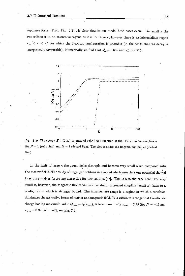
2.7 Numerical Results 38

repulsive force. From Fig. 2.2 it is clear that in our model both cases occur. For small K the

two-soliton is in an attractive regime as it is for large K, however there is an intermediate region

< K < for which the 2-soliton configuration is unstable (in the sense that its decay is

energetically favourable). Numerically we find that = 0.632 and = 2.215.

100

fig. 2.2: The energy Ecs (2.30) in units of 47r|A''| as a function of the Chern-Simons coupling K

for N = 1 (solid line) and iV = 2 (dotted line). The plot includes the Bogomornyi bound (dashed

line).

In the l imit of large K the gauge fields decouple and become very small when compared with

the matter fields. The study of ungauged solitons in a model which uses the same potential showed

that pure matter forces are attractive for two solitons [47]. This is also the case here. For very

small K, however, the magnetic flux tends to a constant. Increased coupling (small K) leads to a

configuration which is stronger bound. The intermediate range is a regime in which a repulsion

dominates the attractive forces of matter and magnetic field. I t is within this range that the electric

charge has its maximum value Q„„ - ( 3 ( « m . , ) , where numerically K „ „ - 0.75 (for N = - 1 ) and

K^^^ = 0.92 (iV = - 2 ) , see Fig. 2.3.

2.7 Numerical Results 39

K 0.4

100

flg. 2.3: The electric charge Q (2.52) in units of 2IT\N\ as a function of the Chern-Simons coupling

parameter K for iV = 1 (solid diamonds) and N = 2 (triangles up).

In showing such a behaviour, CS-solitons resemble the vortices of the Abelian Higgs model where

a similar transition between repulsive and attractive regime occurs, depending on the strength of

the potential term. The shape of our soliton solution shows a strong dependence on K, which is

foreseeable by the interpretation of /t as a coupling parameter to the gauge field. Increased magnetic

flux, as i t occurs for small K, in the Skyrme-Maxwell model is known to cause more localized

configurations [48]. On the other end of the scale, for large K the electromagnetic interaction is

only very weakly coupled. I f the asymptotic value K = oo is taken, the Lagrangian reduces to

the 0(3)cr-model term plus the potential term, such defining a configuration which is known to be

unstable against shrinkage due to the Hobart-Derrick theorem [17, 18]. Actually taking the Umit

therefore leads to a different model.

Figs; 2.4-2.7 show the energy density, profile function and gauge field for several values of K.

In agreement with our expectations one sees that for laige K the soliton becomes more localized.

This illustrates that the potential term in the Lagrangian favours a shrinkage of the soliton. For

decreasing K the soliton tends to spread out and reaches its maximum width at /c « 1. On the other

hand, for smaller K the soliton becomes more localized again. This can also be seen in Figs. 2.4-2.5.

2.7 Numerical Results 40

20.0

10.0

flg. 2.4: The energy density e (2.49) as a function of r foT N = -1 and K - 0.3 (long-dashed),

K = 0.4 (dotted) and K. = K'„ = 0.632 (solid).

For very small K, both the gauge fields a and v tend to functions that are singular at the

origin, in particular, a tends to - 1 everywhere except at r = 0, which is fixed by the boundary

conditions. In that the behaviour of a is similar to the gauge field in the Skyrme-Maxwell model.

We conjecture that the origin of this coincidence is the particular ansatz chosen for the gauge field,

which leads to terms proportional to (a -f-1)^ in the energy density, thus making the value a = - 1

exceptional. The limit of strong coupling therefore also leads to a dynamically quantised flux

(2.52) and in addition implies via (2.52) that the electric charge vanishes for K 0. From (2.58)

i t follows that the electric and the magnetic fleld form a ring, a feature usually seen for 2-solitons.

flg. 2.5: The profile function / as a function of r foi N = -1 and K = = 0.632 (solid),/c = 2

(dashed), K = 0.4 (dotted).

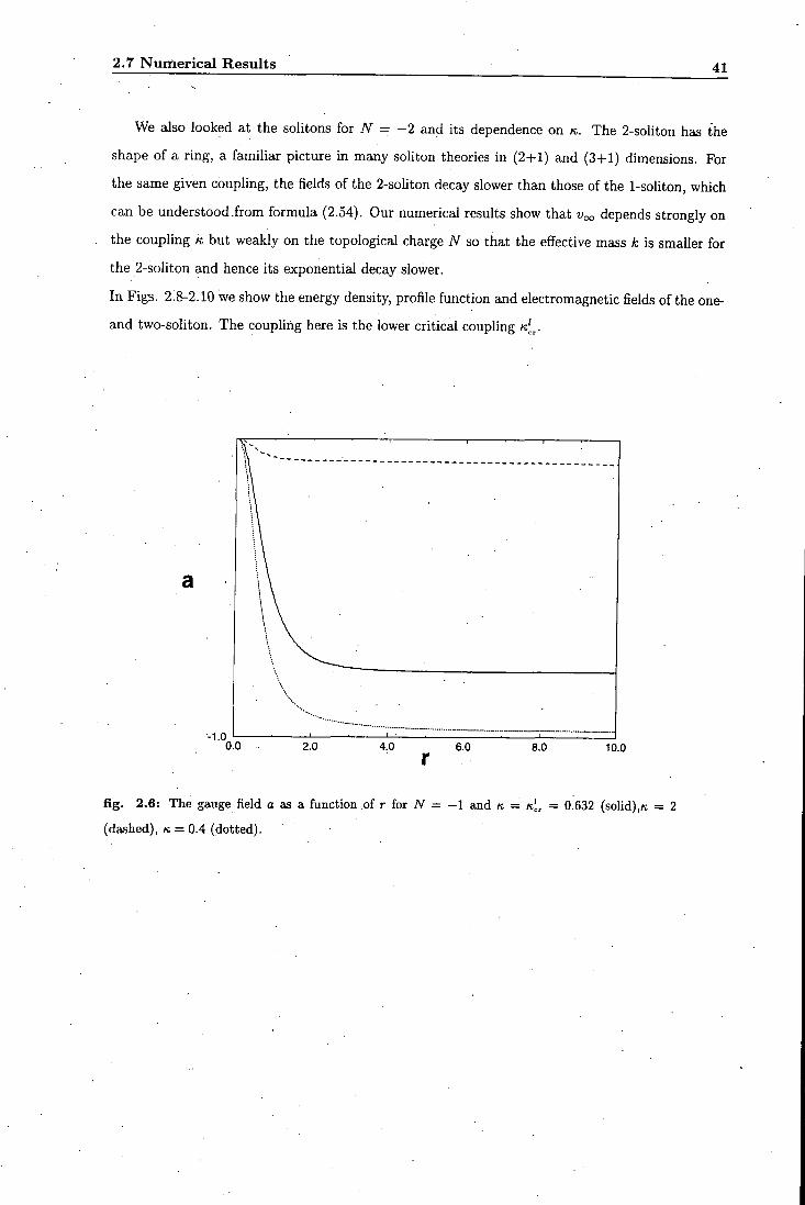
2.7 Numerical Results 41

We also looked at the soUtons for N = - 2 and its dependence on K. The. 2-soliton has the

shape of a ring, a familiar picture in many sohton theories in (2+1) and (3+1) dimensions. For

the same given coupling, the fields of the 2-soliton decay slower than those of the 1-soliton, which

can be understood .from formula (2.54). Our numerical results show that Voo depends strongly on

the coupling K but weakly on the topological charge N so that the effective mass k is smaller for

the 2-soliton and hence its exponential decay slower.

In Figs. 2.8-2.10 we show the energy density, profile function and electromagnetic fields of the one-

and two-soliton. The coupling here is the lower critical coupling

- 1 . 0 0 . 0 2 . 0 4 . 0 6 . 0 8 . 0 1 0 . 0

flg. 2.6: The gauge field a as a function of r foi N = -1 and K = = 0.632 (soIid),K = 2

(dashed), K = 0.4 (dotted).

2.7 Numerical Results 42

flg. 2.7: The gauge field ?; as a function of r for N = -1 and « = K.[, - 0.632 (soUd),« = 2

(dashed), K = 0.4 (dotted).

3 0 . 0

2 0 . 0

1 0 . 0

flg. 2.8: The energy density e (2.49) as a function of r for K = K[, = 0.632, AT = -1 (solid) and

iV = - 2 (dashed).

2.7 Numerical Results 43

1 5 . 0

fig. 2.9: The profile function / as a function of r for « = K[, = 0.632, N =-1 (solid) and = -2

(dashed).

fig. 2.10: The radial component of the magnetic field Er as a function of r for « = K]., = 0.632,

iV = -1 (solid) and AT = -2 (dashed).

2.8 Conclusions 44

2.8 Conclusions

We have studied classical static soliton solutions in an C'(3)a'-Chern-Simons system with unbroken

(7(1) gauge symmetry. The solitons have an electric charge which shows a unique maximum

dependent on the coupling to the gauge field. The magnetic flux in the model is effectively quantised

in the l imit of strong coupling while the angular momentum of the solitons is fractional such that

they can be seen as classical anyons.

In the case of two solitons sitting on top of each other, the model has a repulsive and two

attractive phases, depending on the parameter which couples the gauge and matter fields. This

has interesting consequences for interactions of multisolitons. In the repulsive regime they will pre­

sumably try to move away from each other and for a finite region this would lead to a configuration

similar to an Abrikosov-lattice with solitons in equidistant and fixed positions. Such configurations

occur in the description of type-II superconductors, although the theoretical description there is

given in a non-relativistic model.

In the attractive regime, however, solitons which are not too widely separated from each other

wil l be likely to coalesce. In this context i t is worth investigating whether the solitons of higher

winding number show a similar dependence on the coupling, in particular whether their critical

couplings and K ^ , are of the same value as they are here. The inter-soliton forces at large and

medium distances wil l be dominated by the matter fields, because the electromagnetic fields decay

faster by a factor of e"*''. Thus, the interactions should be asymptotically well described by the

dipole picture developed in [47]. A fu l l numerical simulation of the time-dependent fields is not an

easy task and one could therefore start with a study of truncated dynamics. As an example for

such an investigation it would be interesting to look at rotating CS-soIitons. Due to the hedgehog

ansatz for the matter fields, a rotation in space is equivalent to a rotation in iso-space and thus it

can be imposed by making Q a function of time. I f one wants to take into account the back-reaction

to the matter fields, / ( r ) had to become time-dependent and would be deformed due to centrifugal

forces. Such investigations would also be interesting in compaxison to the ungauged spinning baby

Skyrmions described in [49].

Chapter 3

Self-Dual Solitons in a Gauged

0(3) cr-model

3.1 Introduction

The concept of self-duality is applied for the construction of a class of theories in which certain

terms in the action and their couplings are not free but constrained by relations between each

other. I f these relations are satisfied — thus defining the self-dual fields — some positive valued

Junctionals (usually the potential energy) take their minima. The equations of motion at the point

of self-duality are reduced to first-order differenticil equations, which are more accessible to cin

a;nalytic investigation and, in some cases, can be solved expUcitly.

The notion of self-ducdity (sd) originates in Yang-Mills (YM-) field theory. Historically, Yang

and Mills introduced the idea of making the global SU(2) iso-spin symmetry of nuclear physics local.

I t has later turned out that in four-dimensional Euclidean space pure YM-theory possesses classical,

finite-action solutions to the sd-equations. These solutions are called instantons. The YM-action,

on its own, does not describe any known physical system, but apart from its conceptual value

i t is of course one of the fundamental building-blocks of the Standard Model. More interestingly,

from our viewpoint, YM-theory shows various relations to other important models with topological

soliton solutions. This is our main reason for describing i t here in more detail (see also [50] for a

review).

The model is defined on X = IR"*, the coordinates of which are {xi,X2,X3,Xi). The su{2) gauge

field Ai = A^aa/{2i), (a = 1,2,3) is«in its adjoint representation and the field-strength is given

3.1 I n t r o d u c t i o n 46

by Fij = diAj - djAi + [Ai,Aj], (here i , j = 1,2,3,4), while aa denotes the Paufi matrices. Taking

the coupling-strength to unity, the YM-action can be written as

5vM = - I d'x Tr {FijF'^) ,

where the trace is taken over the group index. Now the Bogomol'nyi trick is applied and introducing

the dual field-strength Fij = eijkiFkt/2, the action is rewritten,

Syu = - \ j d^x TT (^Fij T Fi^y T J d^x Tr [f^F'^) . (3.1)

To guarantee finite action, the gauge field Ai at the boundary of the physical space dX =

has to be a pure gauge Ai = U~^diU, where U = U{a.) e SU{2) depends on a set of coordinates

a = (Qi,Q2,a3), which parametrise S^. Therefore (7 : 5 ^ i-4 SU{2), which is topologically

and hencie U falls into a homotopy class that corresponds to 7r3(5^) — TL. Consequently, the

configuration space of the theory is composed of disjoint subsets labeled by their integer-valued

index which counts the winding of the gauge field at infinity. This also illustrates our earlier claim

that YM-instantons are topologically of the same type as vortices in the Abelian Higgs model.

We denote the degree, often called Pontrjagin index, by k. Its analytic expression is given by

a multiple of the second integral in (3.1). Therefore (3.1) yields:

where c is the normalization constant, c = STT' . Within each topological sector labelled by k, 5YM

is absolutely minimized and the bound saturated at the points of self-duality

Fij = ±Fij . (3.2)

The solution to this equation of index A; = ± 1 is called the (anti-) instanton. Solutions to the

sd-equation are known for all k and, being a minimum of the action, they also solve the Euler-

Lagrange equations of motion DiFij = diFij + [Ai,Fij] = 0. The converse is in general not true,

there can be saddle-point solutions to the equations of motion which are not self-dual.

As mentioned above, one reason for the interest in YM-theory stems from its mcinifold relations

to various other theories, which are usually established by some form of dimensional reduction.

Probably the most important of these is the connection to three-dimensional Yang-Mills-Higgs

(YMH-) theory. In essence, if the four-dimensional YM-fields are made independent of, say, 14

and is identified with the Higgs field in its adjoint representation, the theory is equivalent

3.1 I n t r o d u c t i o n . 47

to YMH-theory in three space-dimensions which has — in the limit of vanishing Higgs potential — self-dual soliton solutions known as BPS-monopoles.

The sdYM equations are also related to the notion of integrability in lower dimensions. In

a space of signature -h, —, —), the sdYM equations can be dimensionally reduced to (l+l)

or (2-f-l) dimensions and reinterpreted as consistency conditions for systems of complex linear

differential equations. These systems often resemble the Cauchy-Riemann equations and thus

relate the problem to the theory of holomorphic functions. A prominent example where this

method can be applied is the chiral model [51, 52].

Our third example relates the sdYM-theory to the model we discuss in this chapter, that

is to self-dual Chern-Simons (sdCS-) theories. The 5C/(2)-sdYM equations, again reduced from

(2-1-2) dimensions, yield non-relativistic, non-Abelian sdCS equations in (2-1-1) dimensions, see

ref. [53]. The matter fields here are complex scalar fields ip. Non-relativistic sdCS-theories are

relevant in condensed matter physics, as indicated in chapter 2. Self-duality requires in this case

a fourth-order Higgs potential ( / ( I V ' D N R ~ I ^ C - The matter equation of motion is the non-linear

Schrodinger equation and the sd-solutions are static solutions of the corresponding Euler-Lagrange

equations. For an Abelian gauge field these solutions are of zero energy [54]. Interestingly, the

sd-equations can be solved explicitly for an Abelian as well as for a non-Abelian gauge field [55].

In the Abelian case the equations can be combined to the Liouville equation, while in the more

general non-Abelian case they become Toda field equations.

Relativistic sdCS-theories, on the other hand, do not have known analytic solutions.

These theories include a sixth-order potential with degenerate symmetric/asymmetric vacua

which allows for (non-) topological solitons as well as for (non-) topological vortices:

U{\ip\)n ~ I'i/'Pdi^P - I^P)^ [56, 57, 58]. In the sd-Iimit the Higgs' mass equals the mass of the

gauge field. Abelian and non-Abelian versions have been investigated and in both cases the Bogo-

mol'nyi bound is given by a t f ( l ) chaxge. I t would be interesting to know if non-Abelicin models

with more complicated bounds, like a linear combination of various charges or EPS-type bounds,

can be constructed. To the best of our knowledge this has not been done yet. In the non-Abelian

relativistic sdCS-model the Higgs- and gauge field spectra are rather rich and their masses can dif­

fer. However, for su(A^)-valued gauge fields they are given as (integer or half-integer) multiples of

the same fundamental mass scale m = i/^//c, ( K being the CS-coupling). For completeness we also

w^ant to mention that these sd-models have been generalized to accommodate a Maxwell/Yang-

Mills term, thus giving the gauge field some true dynamics. To make such a model self-dual, a

3.1 I n t r o d u c t i o n 48

neutral scalar field has to be introduced [59].

I t is an amusing observation that for all those models the self-dual bound, or a modification of

i t , provides a bound on the energy even if the coupUngs are perturbed. Take the energy functional

E[(l),Aa]sD = ^27=1 '^i°Ei[4>,^a] with positive definite Ei[(j),Aa] arid let the sd-couplings > 0

for all i. For solutions of the sd-equations, denoted {4>,Aa), i t holds in the A^-soliton sector that

EsD[4>,-^a] = C N . > 0, where C N is a constant. Now use coupling constants which are different

from the sd-limit: / t f = « f ° ( l ± Mi/(1 + Mi))i Mt > 0 for all i. Then one obtains for the energy

E+= E,, + Y , ^ E i > c . , i=i

- - - - - g l ^ - '

/ n \ " f 1 = 11(1+/^*) E s « " ^ ' n ( i + / ^ i ) ^ (3-3)

\*;=1 / t=l ( J = E , J f [ { i + n k ) \ + ( n ( i + M * ) ) x ^ L f £ ; j n ( i + M j ) - i

\k=l /

In both cases the bound is insaturable for non-trivial fields, because its saturation would imply

that each Ei vanishes individually, which means that the fields are constant.

In this chapter we present a relativistic sdCS-theory which is based on the 0(3) cr-model [38].

I t is similar to the relativistic scalar CS-Higgs- (CSH-) model discussed above in that i t exhibits

a symmetric and an asymmetric vacuum which are degenerate. The gauged 0(3) a-model has a

self-dual realization for Maxwell-dynamics, as shown by Schroers [42]. In this model the gauge

symmetry remains unbroken, hence the flux is not quantized and the topologiccd bound is entirely

due to the topology of the matter fields. However, the gauged 0(3) u-model exhibits two conserved

charges: the topologically conserved degree of the matter field (j) and the dynamically conserved

Noether charge arising from local gauge symmetry. In this chapter we pursue the idea to find a

self-dual model where the energy-bound is given by a linear combination of these two cheirges. For

the construction of this theory we apply the Bogomol'nyi argument described above. In contrast to

the Bogomol'nyi equations of the pure 0(3) cr-model, the self-dual equations in our model cannot

be solved analytically. Nevertheless, because they are of first order, an analysis of them is more

accessible than one of the second-order Euler-Lagrange equations.

3.2 T h e Se l f -Dual Chern-Simons 0(3) cr-model 49

The non-relativistic version of the theory discussed below is potentially interesting as a model

for planar ferromagnets. In this context the field (p is interpreted as a spin vector and the Euler-

Lagrange equations are the gauged Landau-Lifshitz equations. Such a model was investigated

very recently in [60] where it was shown that it yields a variety of topological and non-topological

soliton solutions. I f a background charge is included, it turns out that for a specific value of this

charge the soliton solutions are the same as those in the (non-relativistic) Abehan sdCS-theory, as

discussed by Jackiw and Pi [61].

3.2 The Self-Dual Chern-Simons 0(3) a-model

Our model is defined by the following Lagrangian on (2-l-l)-dimensional Minkowski space of sig­

nature (-f-, - , - ) :

. £ = ^ ( Z ? a 0 ) ( i ? " < / > ) ± | e " ' ' ^ ^ a 5 ^ ^ - i ^ ( n - 0 ) , (3.4)

where we omit the Lagrangian multiplier. 4> is the 0(3)<T-model matter field introduced above

and Aa 6 U{\), n = (0,0,1). W i t h respect to the covariant derivative and the indices, we use the

same notation as in chapter 2. For the moment, we leave the sign of the Chern-Simons coupling

K arbitrary. Being interested in static sd-configurations, we consider the energy functional for

time-independent fields, which can be written as

£^cs[^,0] = y"rf 'a: i( / lg(nx 0)2+.( i? i0)2 + ( i )20)2)+[ / [< / . ] . (3.5)

Gauss' law yields AQ ^=KB/{n x 0)^, B = diA2 - 52^1- Using this to to eliminate AQ and

chosing the potential W(n • <p) = \n x <j>f {u - n • 0)2/(2«;^), f > 0, we can rewrite the energy

j (fxiDi(f>-(l>xD2(l> + B{l-n(t>))±{u-l) J cf x B .

As shown in chapter 2, the second integral is proportional to deg[0], the degree of the map

0 : 5^ i-> 5^. The third integral gives a multiple of the magnetic flux <J>, which is due to Gauss'

law proportional to the electric charge and therefore conserved in time. The electric charge-density

is here p = Ao{n x 0)^ . The integrand of the first term, in (3.6) clearly is positive definite, from

which we derive the following bound on the energy:

3.2 T h e Se l f -Dual Chern-Simons 0(3) CT-model 50

£;cs > 47r|deg[0]| + ( z / - l)|<t.|. (3.7)

Here the sign ambiguities of « and in the square brackets in (3.6) were removed by taking the

magnitude of deg[</>] and <1>. The energy bound (3.7) is a conserved quantity and therefore solutions

which saturate i t will have the same Ecs throughout their time-evolution ^.

Due to the choice of the potential U, the model exhibits two or three degenerate vacua, de­

pending on v. In radial coordinates {r,6):

a) u>l, l im </>(r) = ± n ,

b) v<l, l im 0 ( r ) = ± n or limn ( f ) = u. . 1—>oo r-+oo

0 . 1 5

0 .05

(3.8)

fig. 3.1: Higgs potential U = sin^ r{i> - cosr)^, where 4>3 = cosr, r = y/x^+y^ € [0, TT). U = 0.1.

For 1/ — 1 both cases coincide. We refer to the vacua < = ± n as symmetric vacua and to

n • (f> = u as an asymmetric vacuum.

'Note that Ecs is not simply the potential energy because it includes contributions from the temporal part of

the covariant derivative of 0. •

3.2 T h e Se l f -Dual Chern-Simons 0(3) tr-model 51

a) Topology for > 1

This case gives rise to soliton solutions with the degree of the map N = d eg [0 ] being integer valued.

The gauge symmetry remains unbroken and hence the flux is not quantized. I f the degree N j^O,

we speak of topological solitons. For N = 0 there is no topologically preserved quantity, the energy

of the solutions is proportional to the flux which in turn is proportional to the ^-component of the

gauge field at infinity. These are non-topological solitons.

b) Topology for v < 1

This case allows for any of the three vacua where the symmetric pha^e is analogue to case a). In

the asymmetric phase the vacuum manifold of the field is a circle of radius V ' l - in the. plane

03 - u, i.e. 0 O O = limr-+oo </> = (<Aioi <^Li'^)- The model's local C/(l)-symmetry gets spontaneously

broken by the choice of the vacuum (j>l^, (jy^ and the magnetic flux is quantized. One can combine

(j>l^ 1 (l>lo i^to ^ complex scalar field, ip = <I>1^ + i(j>1^ and proceed in the discussion analogously to

the Abelian Higgs model of section 1.3, such that </? vexp{iM6). The covariant derivative then

becomes Dup = di}p + lAup and for i t to vanish at infinity, the ^-component of the gauge field has

to satisfy:

l i m ^ , ( r , ^ ) = i i M = _ J M L = _ M . (3.9) r->oo ^ ' |n X 0 1

Hence the boundary of the physical space ( 5 ^ ) gets mapped onto the circle (j>3 = i> and such

maps are classified by 7ri(5^) = Z , giving them an integer degree M . We call solutions of degree

M > 0 topological vortices. Note that the map 0 is not surjective any longer and that one cannot

one-point compactify IR^ to 5^, because the fields at infinity are not constant. The notion of a

degree 'K2{S^) in the way we used i t so far is therefore not applicable. However, formula (1.10) for

N produces a value of A'' < 1 which can be visualised as the firaction of target 5^ that is covered

by 0 .

Hence there are two topological charges of relevance in our model: TT2{S'^) for the symmetric

vacuum and 7ri(5^) for the asymmetric vacuum of case b). We will discuss solutions to cases a)

and b) in detail below.

To find these, solutions, we study the Bogomol'nyi equations of our model. The static energy

functional (3.6) is minimized and the. bound saturated if and only if the first integral vanishes.

This leads to the following sd-equations:

3.2 T h e Se l f -Dua l Chern-Simons 0(3) a-model 52

Di<f> =zf(pxD24>, (3.10)

^ ^ _^|nx(/>p(t/-n-q!>)

For further discussion it. is helpful to rephrase these equations in terms of coordinates on the

complex projective space IP^. The coordinates of IP^ are scalar fields depending on the coordinates

of the plane of motion, for which the complex variables x+ = xi + ix2 and x_ = x i - 1x2 are

introduced. Let W be such a complex field, related to <p through the stereographic projection from

the south pole of 5 ^ onto the complex plane:

Then the Bogomol'nyi equations in terms of W are:

where the covariant derivative is now DiW = diW + iAjW. After some algebraic manipulations

these two equations can be rewritten as a second-order equation for W:

a.^._w.a.^wa.w = S } m ± M ^ , 3 , 3 ,

From this equation i t is immediately clear that W cannot be a (anti-) holomorphic function. We

did not succeed in solving this equation and to progress numerically we resort to an appropriate

ansatz for the fields. The same symmetry considerations as discussed in the previous chapter apply

for the matter fields and hence we make use of ansatz (2.42) again. We restrict ourselves further

and use for the gauge field the rotationdly symmetric ansatz Ag = na(r). Then the sd-equations

(3.10) become

f = -n sm / , (3.14)

, rsin^f. a ' = 5 — ( 1 / - C O S / ) .

riK^

For the fields to be well-defined at the origin and for the energy to be finite, one has to impose the

following boundary conditions, similar to (2.48):

a(0) = 0, l im a(r) = aco, /(O) = T H I T T , l im / ( r ) = m27r, (3.15)

3.2 T h e Se l f -Dua l Chern-Simons 0(3) cr-model 53

for the symmetric phase and

lim cos/(r) = u (3.16) r—>oo

for the asymmetric phase. In the symmetric phase, fields 0 which satisfy these boundary conditions

are of degree N = (cos(mi7r) - cos(m27r))n/2. For simplicity we restrict ourselves to m i = 1, m2 =

0. In the asymmetric phase we find <I> = -27rM and iV = -{v + l)n/2.

The classical vacuum structure of the model is the starting point of any quantum mechanical

approximation for the mass-spectra of the particles. We expand the potential for the fields close

to the vacuum and obtain for the symmetric vacuum <l>^ = ± n a mass of = | i / - 1|/|«;| and

a massless gauge boson. In the asymmetric phase the Higgs effect takes place. I t gives a mass

(1 - I''^)/\K\ to the gauge field and to the Higgs particle (which corresponds to the 03-degree of

freedom). The fact that the masses of the scalar and the vector particle cu:e the same is not a

coincidence. In , the M > 1 sector of the configuration space the vortices do not exercise any

mutual forces, because i f they did, their static energy would not be constant (unless repulsive and

attractive forces cancel each other in the potential energy, which is unlikely). However, having a

magnetic field and non-Unear matter fields, i t is not obvious how this effect occurs. The standard

interpretation for BPS-monopoles (where the Higgs and photon are massless in the sd-limit) is

that in the Bogomol'nyi l imit the attractive matter-forces are just compensated by the repulsive

magnetic forces [25].

The solutions to our model also have a non-vanishing angular momentum. I t is determined by

the quadratic term in the action and the CS-term only and i t does not depend on the potential.

Therefore the angular momentum M in the sd-model is the same as in the non-sd-model of chapter 2,

cf.(2.31) . In table 3.1 we summarize some of the features of the theory that were mentioned so

far.

The energy-density (3.6) can be expressed in terms of our ansatz (3.14), which yields:

JTU 1 1 /•^2 f f , 2 ^ 2 , n2(a + l ) ^ s i n V sin-'fiu-cosf)^] E[f,a] = ^ J d x i ^ f + « - ^ + - + j . (3.17)

For the numerical treatment i t is important to know, the asymptotic behaviour of the fields for

small r . We approximate the fields around the origin by a power series and obtain:

{u + l)a' 2(|n|+l) . .3l8^

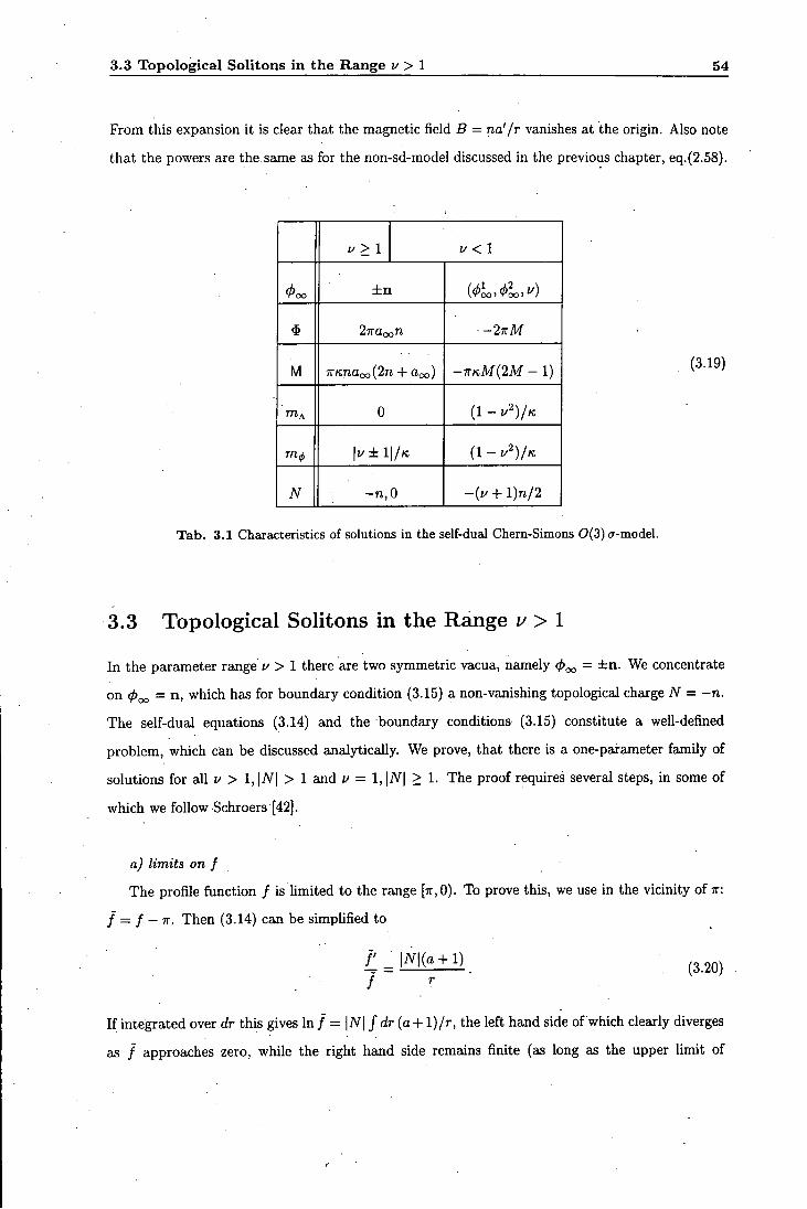
3.3 Topolog ica l Soli tons i n the Rsmge u > I 54

From this expansion it is clear that the magnetic field B = na'/r vanishes at the origin. Also note

that the powers are the same as for the non-sd-model discussed in the previous chapter, eq.(2.58).

u > 1 u < 1

± n

2Traoon —2nM

M TTKnaoo{2n + C Q O ) -7r /cM(2M - I )

mA 0

| I / ± 1 | / K

N - n , 0 - ( i / - | - l ) n / 2

(3.19)

T a b . 3.1 Characteristics of solutions in the self-dual Chern-Simons 0(3) cr-model.

3.3 Topological Solitons in the Range u > 1

In the parameter rcinge i/ > 1 there axe two symmetric vacua, namely </)^ = ± n . We concentrate

on = n , which has for boundary condition (3.15) a non-vanishing topological charge N = -n.

The self-dual equations (3.14) £ind the boundary conditions (3.15) constitute a well-defined

problem, which can be discussed analytically. We prove, that there is a one-parameter family of

solutions for all u > 1,\N\ > 1 and f = 1, |iV| > 1. The proof requires several steps, in some of

which we follow Schroers [42].

limits on f

The profile function / is hmited to the range [7r,0). To prove this, we use in the vicinity of TT:

f = f -IT. Then (3.14) can be simplified to

/ ' | i V | ( a + l )

/ (3.20)

I f integrated over dr this gives In / = |iV| / dr {a+l)/r, the left hand side of which clearly diverges

as / approaches zero, while the right hand side remains finite (as long as the upper limit of

3.3 Topological Solitons in the Range i/ > 1 55

integration is finite). This means that if f > TT for any value of r > 0, then it will be larger than TT for all r . But this excludes the possibility of meeting its boundary condition at infinity, hence / < TT. I f / is replaced by / , the above argument also shows, that / > 0, for all r, hence

0 < / <7r . (3.21)

b) limits on a

From (3.14) it follows, that a' < 0 for all r , hence a is a monotonically decreasing function.

Moreover, using 0 < sin^ fiu - cos f ) <ii^ + 1) it follows that a' > -{u + l ) r / ( | A f | K 2 ) . Hence, for

a given R 6 [0, oo), by using the mean value theorem and (3.15), we find

|iV| R < aiR) < 0. (3.22)

c) lower limit on a

If u > 1 i t is easy to show that a > - I . For if i t became smaller than - 1 at a certain R then

the derivative of / would change its sign so that / would increase. Since a is a decreasing function

for all r , / would increase for all r > i? and could not meet its boundary value at infinity. Hence

a > - l .

d) asymptotic behaviour

The first three steps of the proof tell us that the boundary value for a, Coo S (0, - 1 ] . By using

that / becomes small for large r, we approximate the fields in eq. (3.14) by a power series in r.

For / we find / ~ / i 7 - ~ l ^ l ( ° ~ + ^ ' , / i being positive and constant. This inserted into the second

sd-equation yields a ~ \N\f?{u - i ) r -2 l^ l (a<»+i )+2 and a ~ | iV | / 2 ( i / - i)r-MN\{a^+i)+2 for > i

and 1/ = 1 respectively. Hence, for a to converge, we find two cases:

' ^ > 1 : a o o > 1 ^ - 1 , i / = l : a o o > ^ - 1 . (3.23)

While the first case rules out the possibility of a one-soliton solution due to the boundaiies on a,

there is no such restriction for i / = 1. I t is interesting to note, that the result for i / > 1 coincides

with the result for the sd-Skyrme-Maxwell system [42]. The case v = 1 was in fact discussed before

in ref. [62] as the first sdCS-0(3) cr-model. However, to the best of our knowledge, the announced

numerical results of the model for i / = 1 never appeared in print. We present our solutions in the

next section. .

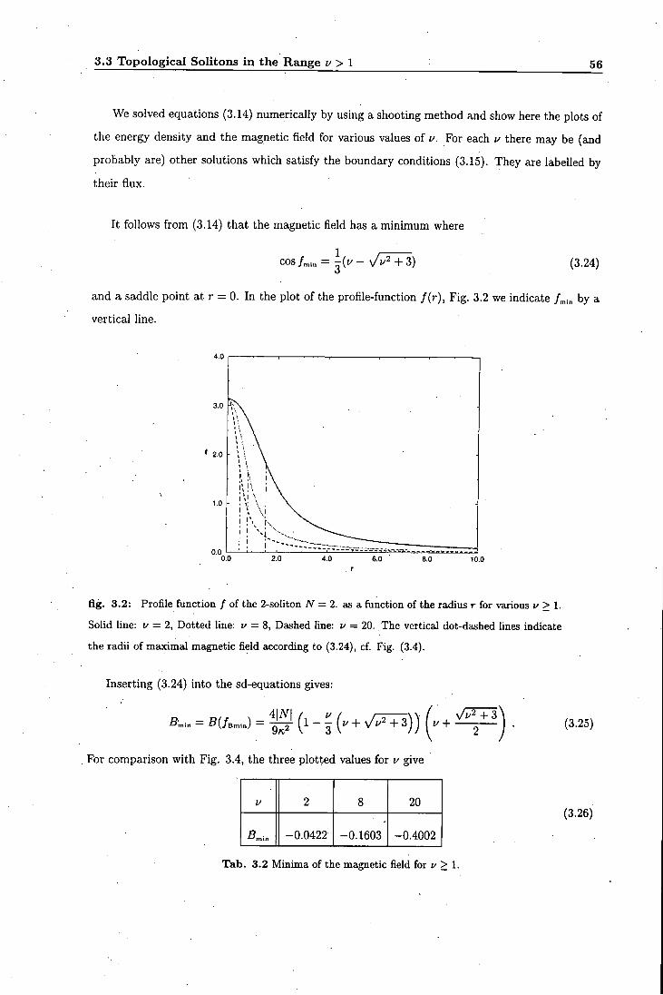
3.3 Topological Solitons in the Range u > 1 56

We solved equations (3.14) numerically by using a shooting method and show here the plots of

the energy density and the magnetic field for various values of u. For each i/ there may be (and

probably are) other solutions which satisfy the boundary conditions (3.15). They are labelled by

their flux.

I t follows from (3.14) that the magnetic field has a minimum where

cos (3.24)

and a saddle point at r = 0. In the plot of the profile-function f{r), Fig. 3.2 we indicate by a

vertical line.

10.0

fig. 3.2: Profile function / of the 2-soliton N = 2. as a function of the radius r for various f > 1.

Solid line: u = 2, Dotted line: i/ = 8, Dashed fine: v — 20. The vertical dot-dashed lines indicate

the radii of maximal magnetic field according to (3.24), of Fig. (3.4).

Inserting (3.24) into the sd-equations gives:

For comparison with Fig. 3.4, the three plotted values for i / give

2 8 20

-0.0422 -0.1603 -0.4002

(3.25)

(3.26)

T a b . 3.2 Minima of the magnetic field for v > l .

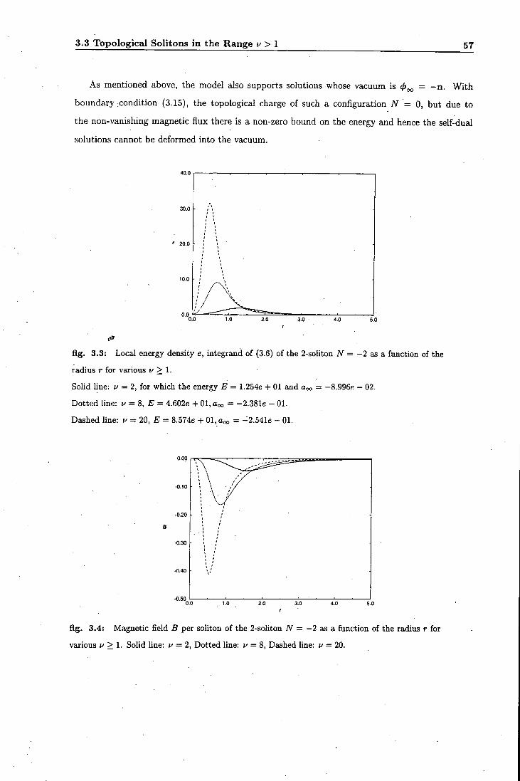
3.3 Topological Solitons in the Range u > 1 57

As mentioned above, the model also supports solutions whose vacuum is 0 ^ = - n . With

boundary condition (3.15), the topological charge of such a configuration N = 0, but due to

the non-vanishing magnetic fiux there is a non-zero bound on the energy and hence the self-ducd

solutions cannot be deformed into the vacuum.

fig. 3.3: Local energy density e, integrand of (3.6) of the 2-sofiton iV = - 2 as a function of the

radius r for various v >1.

Solid line: i/ = 2, for which the energy E = 1.254e + 01 and Ooo = -8.996e - 02.

Dotted line: u = 8, E = 4.602e -I- 01, Ooo = -2.381e - 01.

Dashed line: u = 20, E = 8.574e -I- 01, aoo = -2.541e - 01.

-0.10

fig. 3.4: Magnetic field B per sofiton of the 2-soliton iV = —2 as a function of the radius r for

various v > I. Solid line: i/ = 2, Dotted line: i/ = 8, Dashed line: i/ = 20.

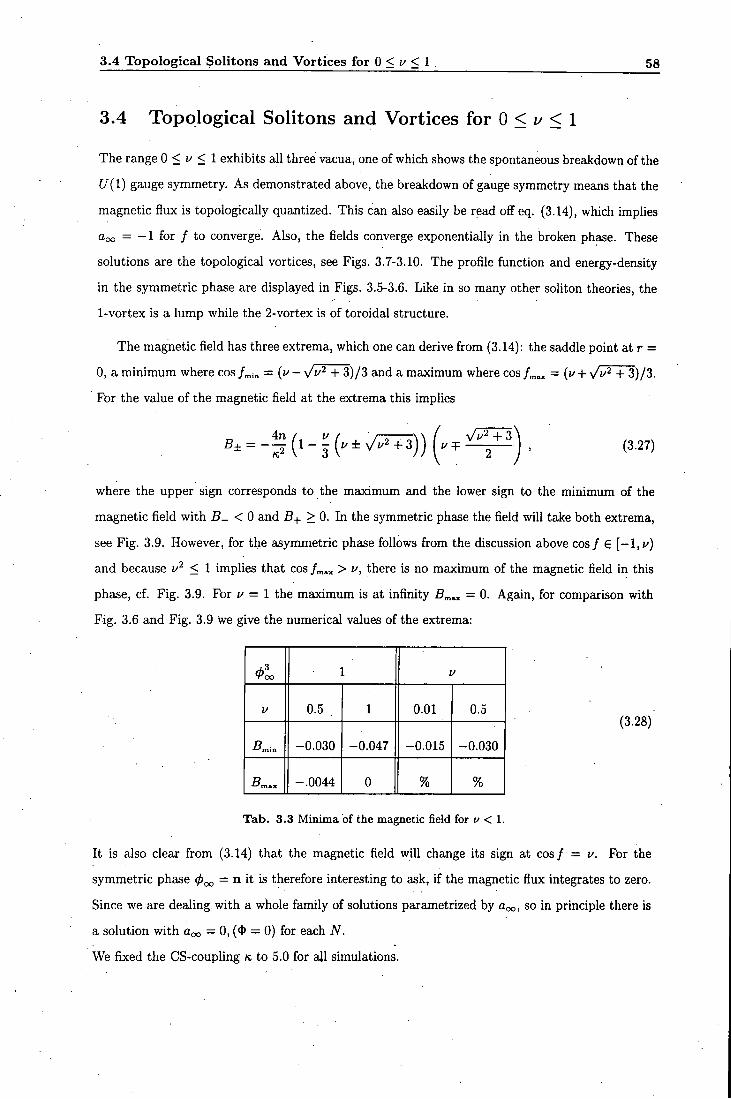
3.4 Topologica l Soli tons and Vort ices for 0 < i/ < 1 58

3.4 Topological Solitons and Vortices for 0 < i' < 1

The range 0 <i/ <l exhibits all three vacua, one of which shows the spontaneous breakdown of the

{ / ( I ) gauge symmetry. As demonstrated above, the breakdown of gauge symmetry means that the

magnetic flux is topologically quantized. This can also easily be read off eq. (3.14), which implies

floo = - 1 for / to converge. Also, the fields converge exponentially in the broken phase. These

solutions are the topological vortices, see Figs. 3.7-3.10. The profile function and energy-density

in the symmetric phase are displayed in Figs. 3.5-3.6. Like in so many other soliton theories, the

1-vortex is a lump while the 2-vortex is of toroidal structure.

The magnetic field has three extrema, which one can derive from (3.14): the saddle point at r =

0, a minimum where cos = {u- \Jv'^ + 3)/3 and a maximum where cos - {y + \/v'^ -\- 3)/3.

For the value of the magnetic field at the extrema this implies

(3.27)

where the upper sign corresponds to the maximum and the lower sign to the minimum of the

magnetic field with 5_ < 0 and 5 + > 0. In the symmetric phase the field will take both extrema,

see Fig. 3.9. However, for the asymmetric phase follows from the discussion above cos/ € [ - l , f )

and because z/ < 1 implies that cos / „ „ > v, there is no maximum of the magnetic field in this

phase, cf. Fig. 3.9. For i / = 1 the maximum is at infinity = 0. Again, for comparison with

Fig. 3.6 and Fig. 3.9 we give the numerical values of the extrema:

4>l 1 f

u 0.5 , 1 0.01 0.5

-0.030 -0.047 -0.015 -0.030

-.0044 0 % %

(3.28)

T a b . 3.3 Minima of the magnetic field for u < 1.

I t is also clear from (3.14) that the magnetic field will change its sign at cos/ = u. For the

symmetric phase (p^ = n it is therefore interesting to ask, if the magnetic flux integrates to zero.

Since we are dealing, with a whole family of solutions parametrized by aoo, so in principle there is

a solution with = 0, (<J> = 0) for each iV.

We fixed the CS-coupling K to 5.0 for ajl simulations.

3.5 Conclusions 59

3.5 Conclusions

We obtained static sd-solutions in a CS-0(3) cr-model in (2+1) dimensions. The vacuum structure

of the model allows for solitons and vortices which can be either topological or non-topological.

Due to the Higgs-effect, the flux is quantized in the asymmetric phase where the topological charge

is non-integer. The elementary study of sdCS-solitons/vortices undertaken in this chapter provides

a first step to a more general investigation of such solutions. In fact, much work on gauged sigma

models has been done since this work was completed, often adapting ideas and techniques used in

the Abelian Higgs model or scalar CSH-theories.

An interesting problem is, whether one could find solutions in this model with a topological

charge \N\ > 1 (in the symmetric phase, or | M | > 1 in the asymmetric phase) which are not on

top of each other. Of course, such solutions would not be radially symmetric any longer and their

energy-density could peak at up to | iV | ( |M | ) several distant points in the plane, ( x i , . . . , I | A ^ | ) . I t

is natural to identify these points of maximal energy density with the positions of the solitons.

These would be the canonical coordinates on the AT-soliton moduh space. Due to the degeneracy

of their energy, there is no potential and hence there are no forces within such a configuration. In

principle, the A/^-sbliton low-energy dynamics can be described by a moduli space approximation,

which is, however, a non-trivial task due to the lack of explicit solutions. For the Abelian Higgs

model i t has been possible to to find a numerical scheme of computing the metric on the moduli

space which is largely based on the behaviour of the Higgs field around its zeros [28]. However, for

the scalar sdCS-theory any such attempts have failed so far.

Related work has been done in [63], where the static sdCS 0(3) cr-model was studied for 1/ = 1 and

away from the self-dual l imit . For two solitons on top of each other i t was found that there is an

attractive and a repulsive phase depending on the coupling to the potential. In this, these results

resemble very much the Abelian Higgs model.

In models like ours, which show several disconnected and degenerate vaciia, there is the possibil­

i ty of domain wall solutions which connect these vacua. The scalar sdCSH-theory supports domain

walls as shown in [56]. In two space-diiriensions the wall either separates two infinite regions and

is therefore infinitely long or i t surrounds a finite region in space. In the latter case the stabihty of

the domain wall solutions against contraction or expansion is an interesting problem. Dynamically,

the energy for a given flux wil l be minimized with respect to the radius of the enclosed domain.

I t was found for the sdCSH that the resulting condition on the fields is satisfied by sd-solutions,

i f the flux is large enough to stabilise the wall from collapse. I t would be interesting to perform

3.5 Conclusions 60

similar studies in our model.

Recently, domain wall solutions in (1+1) dimensions have been studied on a dimensionally reduced

scalar sdCS model [64] and very recently in the sdCS-0(3) a-model [65], a model equivalent to the

one discussed above, but for u = I. These are sd-theories where the Bogomol'nyi bound is given

by a BPS-like bound with the two involved charges being the topological and the Noether charge.

Self-dual models can often be generalized to models with N = 2 supersymmetry (no relation to

the A' above), where the central charge gives the Bogomol'nyi bound. For the scalar sdCS-theory

this was discussed in [66] and for the model discussed here in a recent publication [67].

Another popular idea is to generalize sd-gauged models by including an anomalous magnetic

moment interaction. This is usually done by including a terra proportional to the (dual) field-

strength in the covariant derivative. For the scalar sdCS-model one has to introduce such an

interaction to allow for simultaneous Maxwell/Yang-Mills interaction [68]. Alternatively, a neutral

scalar field can be introduced [59], as mentioned in the introduction to this chapter. For the sdCS

0(3) a-model such anomalous interactions have been studied by Ghosh [69], with the result that

the matter equations reduce to the Liouville equation and hence they are integrable. Interestingly,

this implies that these solutions are scale invariant, unlike the ones discussed here.

Finally, one can generalize the target manifold of the model to dP^ (again, no relation to the

A' above) and the gauge group to a non-AbeUan one. The condition for obtaining a non-trivial

bound is to have at least a global U{1) symmetry left [38, 70, 71]. The gauge group is a proper

subgroup of SU{N + 1) and the energy bound is given again by the linear combination of Noether

and topological charge. The vacuum structure if such models is rich and depends on parameters

like the boundary value of the matter field and the representations of matter and gauge fields.

After much of the work of this chapter was completed, I became aware that similar results

have be.obtained previously [72, 73]. The essence of this work and the one presented here — the

construction of a sd-potential and the numerical discussion using radially symmetric fields — is the

same, although .details of the exposition vary. In particular, both papers [72, 73] fail to mention

the absence of solutions for |A^| = 1, > 1.

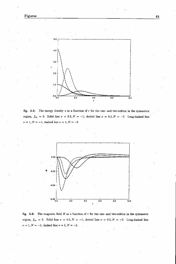
Figures 61

fig. 3.5: The energy density e as a function of T for the one- and two-soliton in the symmetric

region, foo = 0. SoUd line = 0.5,^ = -1; dotted Une i/ = 0.5, N = -2 . Long-dashed Une

u=l,N = -l\ dashed line v = l,N - -2.

0.00

-0.02

-0.04 h

-0.06

• 1 .— 1 1 1 . 1 1

^ ' \ ""-^ _ — .^^f^^;,^^^ ..

\ \ \ / / N L / \ > / ' / ^ -\ \ ' /

\ ^-'1 / ' \ / / ' \ i y \ 1 \ 1

- \ 1 \ 1 \ 1

1 1 1 1 1 1

0.0 2.0 4.0 6.0 8.0 10.0

fig. 3.6: The magnetic field 5 as a function of r for the one- and two-soliton in the symmetric

region, /<» = 0. Sohd line u = 0.5, N = —1; dotted line u = 0.5, N = —2. Long-dashed line

1/ = 1, Af = -1; dashed line v = 1,N = -2 . .

Figures 62

30.0

flg. .3.7: The profile function / as a function of r for the one- and two-soliton in the asymmetric

region, foo = aiccosu. Solid line v = 0.01, TV = -1; dotted line u — 0.5, N — -1. Dashed line

V = 0.01, = -2; Long-dashed line v = 0.5, N = -2 .

-0.4

-0.6

-0.8

-1.0 50.0

fig. 3.8: The gauge field a as a function of r for the one- and two-soliton in the asymmetric

region, /oo = arccosfc'. Solid line v = 0.01, iV = —1; dotted line u = 0.5, N = —1. Dashed line

1/ = 0.01, N = -2; Long-dashed line u - 0.5, iV = -2.

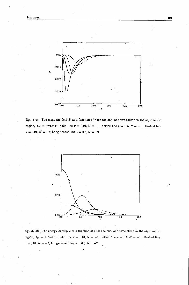
Figures 63

0.000

-0.010

-0.020

-0.030

-0.040 50.0

fig. 3.9: The magnetic field B as a function of r for the one- and two-soliton in the asymmetric

region, foo = arccost'. Solid line u = 0.01, N = -1; dotted line u = 0.5, iV = -1. Dashed hne

u = 0.01, N = -2; Long-dashed line i/ = 0.5, N = -2 .

15.0 20.0

fig. 3.10: The energy density e as a function of r for the one- and two-soliton in the asymmetric

region, foo — arccosi/. Solid line v = 0.01, AT = -1; dotted line i/ = 0.5, N — -1. Dashed line

u = 0.01, iV = -2; Long-dashed line u = 0.5, N = -2 .

Chapter 4

Static Solitons with Non-Zero

Hopf Number

The non-linear 0(3) cr-model in (3-l-l)-dimensional space-time is a scalar field-theory whose static

fields are maps IR^ U { 0 0 } 5^. They can be classified by a homotopy invariant called the Hopf

number. On general geometrical grounds, soliton solutions with higher Hopf number are expected

to be of complicated, knotted structure. Knots are smooth embeddings of closed loops in IR^ and

are related to various problems in modern theoretical physics [32]. The systematic study of knots

was originally inspired in the 19th century by Kelvin's idea of describing atoms as knots composed

of ether [74], where the variety of distinct knots was supposed to take account of the different

chemical elements. Kelvin's proposal resulted in an analysis of knots by Tait [75], which for many

years defined the essence of mathematical knot theory. Although there are many examples of

knotted structures on a macro- and mesoscopic scale, for a long time there were no further efforts

to find a microscopic (that is atoraistic) theory involving knots and knot theory remained of interest

mainly for pure mathematicians.

Prom the modern nuclear physics point of view, particles modelled by knotted configurations

are conceptually much in the spirit of Skyrme's original intention to describe nucleons as vortices

in a mesonic fluid [4, 5], although of course the historic development was reverse and Skyrme was

reportedly influenced by Kelvin's work. The recent interest in knot theory provides therefore a

nice example for the cyclic evolution of science. This interest is largely fueled by work of Jones and

Witten, who outlined connections of topological field theories, such as non-Abelian Chern-Simons

theories, to knot theory and integrable models [32].

65

With respect to elementary particles one can imagine that knotted structures find an application

in (cosmic and fundamental) string-theories, where the excitations of the string might be described

by vibrations of a knotted configuration [76]. There are also proposals for knots in the description

of gluonic flux-tiibes in QCD, which could confine quarks. At present, these are just proposals

and no details have been worked out, but there are other — physical and biological — systems

where the occurrence of knotted structures seems more apparent. Examples for such systems are

DNA-chains [77], nematic liquid crystals or vortex structures in ^He superfluid [78]. There are

clearly many interesting applications of knotted structures but only little can be said so far about

promising field theoretical attempts to describe these configurations. The earliest proposal for a

model in which stable solutions with non-vanishing Hopf number can occur, goes back some time

to L.D. Faddeev [79]. I t was shown later that the Hopf-number provides a lower topological bound

on the potential energy of the Faddeev model [80]. However, despite several attempts which will

be described below, no actual solutions to the variational equations of this model were obtained.

This is undoubtedly due to the fact that very little can be done analytically and most of the results-

wil l have to be due to numerical simulations.

In this chapter we mainly study classical static solutions of Hopf-number one and two. In the

next section we give an introduction to the geometry of the Hopf map. This is followed by a

brief summary of previous work in the field. Our model is defined in section 4.3 where also an

ansatz of azimuthal symmetry is introduced which is later used for numerical computations. In

section 4.4 we present our numerical results which are minima of the potential energy functional for

Hopf-number one and two. We discuss the shapes and binding energies of the solutions as well as

their relation to solitons in (2-l-l)-dimensional theories. Our model has a self-interaction coupling

parameter and we study the dependence of the energy on this coupling. In addition, the effect of

a symmetry-breaking potential term is described. In section 4.5 we give a simple approximation

for the excitation spectrum of a soliton slowly rotating around its axis of symmetry. We conclude

with section 4.6 where we also remark on possible further investigations.

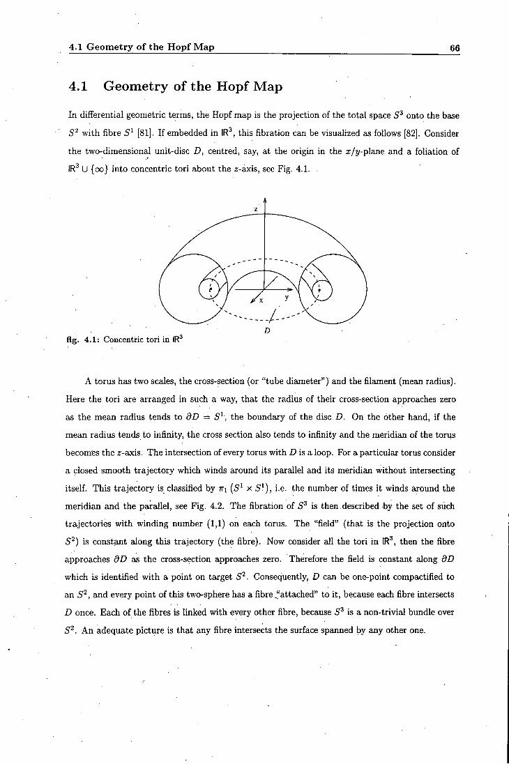
4.1 Geometry of the Hopf Map 66

4.1 Geometry of the Hopf Map

In differential geometric terms, the Hopf map is the projection of the total space onto the base

5^ with fibre 5^ [81]. I f embedded in IR^, this fibration can be visualized as follows [82]. Consider

the two-dimensional unit-disc D, centred, say, at the origin in the x/y-plane and a foliation of

IR^ U {oo} into concentric tori about the z-axis, see Fig. 4.1.

flg. 4.1: Concentric tori in IR

A torus has two scales, the cross-section (or "tube diameter") and the filament (mean radius).

Here the tori are arranged in such a way, that the radius of their cross-section approaches zero

as the mean radius tends to dD = 5^, the boundary of the disc D. On the other hand, i f the

mean radius tends to infinity, the cross section also tends to infinity and the meridian of the torus

becomfes the z-axis. The intersection of every torus with D is a loop. For a particular torus consider

a closed smooth trajectory which winds around its parallel and its meridian without intersecting

itself. This trajectory is classified by TTI (5^ x 5^), i.e. the number of times i t winds around the

meridian and the parallel, see Fig. 4.2. The fibration of 5^ is then .described by the set of such

trajectories with winding number (1,1) on each torus. The "field" (that is the projection onto

5^) is constant along this trajectory (the fibre). Now consider all the tori in IR^, then the fibre

approaches dD as the cross-section approaches zero. Therefore the field is constant along dD

which is identified with a point on target 5^. Consequently, D can be one-point compactified to

an 5^, and every point of this two-sphere has a fibre ^'attached" to i t , because each fibre intersects

D once. Each of the fibres is linked with every other fibre, because 5^ is a non-trivial bundle over

5^. An adequate picture is that any fibre intersects the surface spanned by any other one.

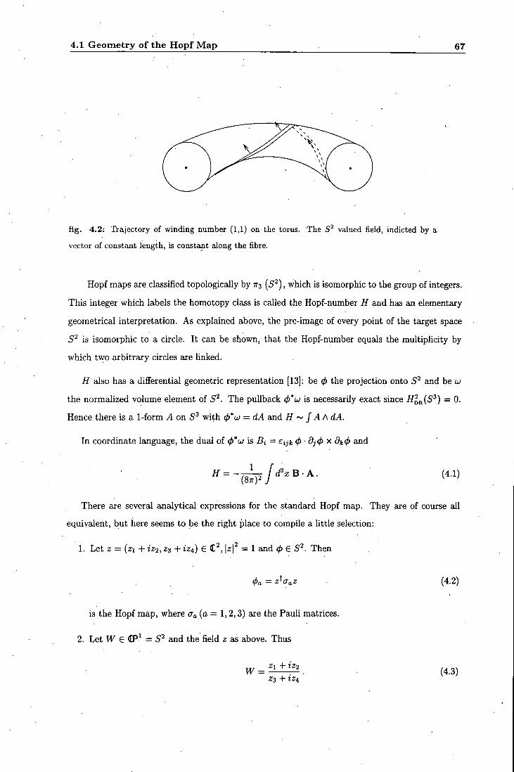
4.1 Geometry of the Hopf Map 67

fig. 4.2: Trajectory of winding number (1,1) on the torus. The 5^ valued field, indicted by a

vector of constant length, is constant along the fibre.

Hopf maps are classified topologically by TTS (5^) , which is isomorphic to the group of integers.

This integer which labels the homotopy class is called the Hopf-number H and has an elementary

geometrical interpretation. As explained above, the pre-image of every point of the target space

5^ is isomorphic to a circle. I t can be shown, that the Hopf-number equals the multiplicity by

which two arbitrary circles are linked.

H also has a differential geometric representation [13]: be 0 the projection onto 5^ and be u

the normalized volume element of 5^. The pullback (f)*uj is necessarily exact since H'^^iS^) = 0.

Hence there is a 1-form A on 5^ with (j>*u = dA and ~ / A A dA.

In coordinate language, the dual of (p'oj is Bi = Sijk <f) • djtp x dk4> and

H

There are several analytical expressions for the standard Hopf map. They are of course all

equivalent, but here seems to be the right place to compile a little selection:

1. Let z = (zi +iz2,Z3 +iz4) € <L'^,\zf = 1 and 0 € 5^. Then

(pa = z^a-az (4.2)

is the Hopf map, where CTQ ( O = 1,2,3) are the Pauli matrices.

2. Let W e<EP^ = and the field z as above. Thus

W = '-^±^. (4.3) . Z3+tZi

4.1 Geometry of the Hopf Map 68

The connection to the fields </> is given by stereographic projection onto the complex plane.

By inserting (4.2) into (4.4) one obtains expression (4.3).

3. Let R e S0(3) and a function of the four-dimensional, space-dependent, unit vector TIQ =

(no,n). In components:

Rah = 5ab + 2(na Ub - v?5ab) - 2ea6c"' ' o • (4.5)

I f this matrix is applied to a constant vector, say, c=(0,0,1), the Hopf map is obtadned and

one can identify <l>a = Rab c*. A short calculation verifies that this map is equivalent to (4.2)

with no being replaced by zi, n i by Z2 and so on.

In the course of this chapter we are not just interested in the standard Hopf map but in a

map which "deforms" the standard Hopf map in such a way that its topology is preserved but the

fields correspond to a minimum of a positive valued functional. To achieve this, we let the field

z e S'^ become space-dependent, i.e. z(r), r e IR^. For finite energy, we will restrict ourselves to

configurations which tend to constants at spatial infinity. This allows us to compactify IR^ U { 0 0 }

to Si, such that

z : S l ^ S ] . . (4.6)

This means that there are now two topological invariants to be considered: firstly the Hopf-

number arising from (4.2) and secondly the degree of (4.6), being characterized by 1:^(8^) = 2 .

Diagrammatically this is described by

SI ^ Si

Denote the degree of the map z,k = deg[z]. Then a theorem in Algebraic Geometry states that

d e g [ 0 o z ] = fcdeg[0] = A;F[8].

From the geometrical considerations given above i t seems obvious that the problem is canon-

ically described by toroidal coordinates {T],P,a,a). The map to more conventional cylindrical

coordinates {r,z,a) is given by: .

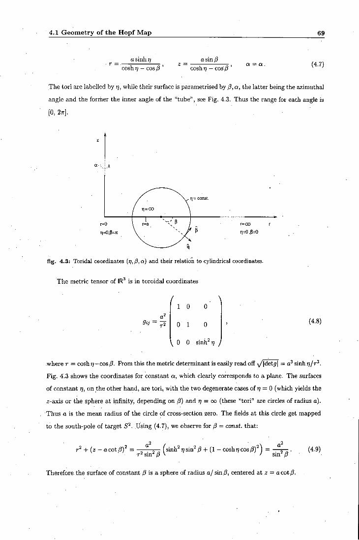
4.1 Geometry of the Hopf Map 69

a sinh 77 asin/3 cosh T) — cos P coshr; — cos/? a = a . (4.7)

The tori are labelled by 77, while their surface is parametrised by /3, a, the latter being the azimuthal

angle and the forrher the inner angle of the "tube", see Fig. 4.3. Thus the range for each angle is

[0, 27r].

ri= const

r=co i1=0,P=it ti=0,p=0

fig. 4.3: Toridal coordinates (77,/?, a) and their relation to cylindrical coordinates.

The metric tensor of IR is in toroidal coordinates

/ . \ 1 0 0

0 1 0

\ 0 0 sinh^T] )

(4.8)

where T = cosh 7; - cos ,9. From this the metric determinant is easily read off y jde tg l = sinh T J / T ^ .

Fig. 4.3 shows the coordinates for constant a, which clearly corresponds to a plane. The surfaces

of constant 77, on the other hand, are tori, with the two degenerate cases of 77 = 0 (which yields the

z-axis or the sphere at infinity, depending on /?) and 77 = 00 (these "tori" are circles of radius a).

Thus a is the mean radius of the circle of cross-section zero. The fields at this circle get mapped

to the south-pole of target S^. Using (4.7), we observe for /3 = const, that:

2 2 4 - ( z - a c o t ^ ) ^ = , " „ fs inh^77sin2 /3- l - (1 -cosh77COs ,8)^) = . (4.9)

T-'sin /3 ^ ' sm p

Therefore the surface of constant /? is a sphere of radius a/sm/3, centered at z = ocot/3.

4.2 E a r l y Work 70

4.2 Early Work

There are some previous attempts to find soliton solutions which are topologically stable due to

their fields being of non-zero H. The direct approach of solving the complete equations of motion

for any such theory in three space dimensions involves finding solutions of a set of coupled PDE's for

two functions (the coordinates on the target manifold), depending on the three space coordinates

each. This seems hopeless analytically and is of considerable effort numerically. Therefore the

common strategy was so far to truncate the configuration space and to investigate only fields of

certain symmetries, which seem inherent to the problem. I t will be explained below that the

results obtained in these models cannot be quantitatively correct. However, the discussion of these

theories gives a good introduction to the subject and points out relevant problems that should be

addressed, which is why we include a review here.

Following Faddeev's initial proposal, some of the first applications where fields of non-zero

H have been investigated, are effective field-theories for three-dimensional ferromagnets [83] and

superfluid ^He [78]. In such theories of Ginzburg-Landau type, the fields are order-parameters and

their time-evolution is governed by a first-order time-derivative of the fields. To first approximation,

the static energy is expressed by second-order terms of the field-gradient. For a ferromagnet one

can formulate the theory in terms of the normalized magnetization n — M(r)/Mo, r £ IR , where

Mo is the saturation magnetization. To allow (semi-) localized configurations, the magnetization

has to be homogeneous as |r| ->• oo, thus one can one-point compactify IR^ to 5^. Since = 1:

n-.S^^S'^. (4.10)

For an isotropic ferromagnet the first approximation to the static energy is given by

V[n] oc j ( f x {diuf . (4.11)

The miniraa of this functional are harmonic maps. As shown in ref. [84], all non-constant harmonic

maps are orthogonal projections IR^ IR , followed by a harmonic map IR^ i-> 5^ and therefore

have infinite energy. Consistently, simple scaling arguments along the line of the Hobart-Derrick

theorem show that, without further constraints, the solutions are unstable against rescaling.

Related work was performed by deVega [85], where toroidal configurations are investigated in

the general context of classical field-theory. The energy functional is there equivalent to (4.11) but

by contrast the fields are interpreted as free classical fields. The ring size of the torus is a parameter

4.2 E a r l y Work • 71

of the energy which has to be minimized with respect to i t . Scaling arguments show that for a

functional of type (4.11) this is the case when the ring size goes to zero. In this paper i t was shown

that the addition of a Skyrme-term provides the energy with bounds and the configuration .with

non-zero radius. Both the bounds and the radius are estimated numerically. For the computation,

an ansatz in toroidal coordinates {r],0,a) with unit Hopf-number is proposed:

+ # 2 =sin / (77 )e ' (^+ '* ' , <f>3 = cos/{T]). (4.12)

The possible relevance of toroidal excitations (or "vortex excitations" as they are sometimes called)

in Weinberg-Salam-Higgs theory was outlined in [86], where it was shown that the theory supports

configurations for which the Higgs-field is expelled from a toroidal region. The model's constituents

are two fields, the Higgs and a neutral vector boson. The latter gives rise to a non-zero flux which

is trapped inside the torus. I t turns out that this flux is too strong for the vortex to be stable (i.e.

i t overcomes the Higgs pressure which tends to collapse the vortex) and hence the vortex decays.

For the actual computation ansatz (4.12) was used.

Another interesting possible application for toroidal configurations in non-linear sigma models

was given in ref. [87]. There the Lagrangian was constructed as an effective chiraJ theory for the

description of low-energy hadron dynamics - and in that attempt as being similar to the Skyrme

model. The hope was there to model possible superheavy fermions in the few TeV range as bound

states of solitons. Consequently, some aspects of Hopf solitons (or Hopfions, as we will call them)

in the Skyrme model were investigated [88, 89, 90]. I t is interesting to see how the Hopfion fits

into the framework of the Skyrme model. The Skyrme model is an effective chiral model where the

static fields are maps U : i-y SU{2). They can be written in a quaternionic basis tTa = ( l l , i < T )

using the four-vector (/>a .= (< o, 0 ) :

C/ = CTa<^". (4.13)

WU = 1 implies (j)a<f>°' = 1 due to the algebraic properties of the Pauli matrices. From U a

conserved chiral current can be constructed Li = U^diU. This current is invariant under left

transition 6U = eU, where e is an element of the algebra su(2). In terms of Li the potential energy

density V of the Skyrme model is

V = V2 + V4 = - ^ I V LiL' + ^^Tr[Li, Lj] [L* , U] , (4.14)

where / and CQ are free parameters. For finite energy one has to impose the boundary condition

U 1 (or to any other constant matrix) as r ^ oo. Then IR^ can be one-point compactified to

4.2 E a r l y Work 72

5^ and the Skyrmion's ^ static energy or mass, the integral over V, is bounded from below by a

multiple of the homotopy index of 7r3(5^) = Z . This index B is interpreted as the baryon number

of the soliton and its integrand is given by

B=^TTe^^''{L,LjL,). (4.15)

In the Skyrme model, Hopfions can principally be constructed by restricting the field-manifold to

5^, e.g. by setting </)o = 0. This new model also possesses a lower topological bound on the potential

energy (the integral over (4.14)) but now the bound is given in terms of the Hopf-number [80]. I t

holds

V>c\H\^ , (4.16)

wi th positive non-zero c [91].

The baryon density B necessarily vanishes upon "Hopfization" (i.e. restriction of the target

manifold to 5^). Thus the soliton configurations can be thought of as being composite of a

Skyrmion with B = H and an anti-Skyrmion with B = -H. In paper ref. [88], a hedgehog ansatz

is employed in the 5 = 1 sector to map IR^ i-> 5^. This is followed by a standard Hopf map (4.2).

More explicitly, he U = exp( i / ( r )<T • f ) , where r is the radial unit vector. Then a new field W{x)

can be defined, such that

W^iUdsU^. (4.17)

The field W e SU{2) and from i t a new current Li € su{2) can be constructed,

Li = W^diW = U{a3Lia3-Li)U^. (4.18)

as Lias describes a rotation of Li by n around the a = 3 axes in iso-space. This means that a U{1)

degree of freedom has been singled out in (4.18) and since SU{2)/U{1) = 5^, i t follows that W is

a map to 5^. One can therefore think of this Hopf model as being a i7(l)-gauged Skyrme model.

A further attempt for a computation of a solution with i f 7 0 in the Skyrme model was made

in [92, 93] where again ansatz (4.12) was employed. There i t was in addition suggested to generalize

the quartic term in (4.14) by using all possible forth-order Lorentz covariant terms and giving them

different couplings (although one of these couplings can be scaled away). Introducing couplings gi

and 92,

'The soliton solution of topological charge one is called the Skyrmion. •

4.3 Hopf Maps and Toroidal Ansatz 73

V4 = gi Tr [Li, Lj] [L', U] + 52 TV ( L i ) ' {Ljf . (4.19)

I t was argued that for such a model, after "Hopfization" the parameter ranges for gi and g2 which

support hedgehog Skyrmions also support Hopfions [88].

To find an adequate description of nuclear matter which is based on solitons, they have to be

quantised in the sense that quantum fluctuations around a classical configuration are computed.

The eigenvalues of the energy fluctuation tensor (the second variation of the energy with respect

to the flelds) determine whether the soliton is in a stable state. The energy of the fluctuations is

proportional to the squared frequency of the oscillations around the classical ground state, which

is given by the Hopf-soliton. For negative eigenvalues this frequency becomes imaginary and thus

the fluctuations grow exponentially in time, indicating an unstable configuration. This turns out

to be the case in for the (unit) Hopf-soliton in the Skyrme model as shown in [90]. This work also

uses ansatz (4.12).

However, all the previous work described so far suffers from an essential problem. I t relies on

ansatze (4.12) and (4.17); however, i t was shown in [89] that both ansatze are not consistent with

the equations of motion, in the sense that these do not permit a consistent separation of the vari­

ables in the variational equations. Therefore the results obtained in these papers cannot be correct

quantitatively. On the other hand, solitons with a small Hopf-number (one or two) are expected

to exhibit some symmetry and both ansatze (4.12) and (4.17) might be good approximations to

the actual static solutions.

4.3 Hopf Maps and Toroidal Ansatz

We are almost exclusively interested in static solutions and therefore we define our model by the

following potential energy functional on IR^, with V4 given essentially by (4.19) (we renamed the

couplings)

V [0 ] = A I d \ \ {di4>f + I {did, X di<i>f + I {di<l>f {dj<t>? . (4.20)

For g2 = ^ this is equivalent to the static energy of the Faddeev-Skyrme model [35, 80]. The

vector 0 is the 0(3) cr-model field introduced in chapter 1. The cross-product is taken in field-

space and the coordinate indices i,j run from 1 to 3. For the reasons laid out in section 4.2 we

include the fourth-order terms in the field-gradient, more precisely the most general combination

of global 0(3)-invariant fourth-order terms. The minimum energy configurations will then not be

4.3 Hopf Maps and Toroidal Ansatz 74

described by harmonic maps, but will be of a definite scale. The parameter A is a constant of dimension energy/length and determines the model's energy unit. The couplings gi and 32 are of dimension (length)^. The ratio 91/52 is the only physically relevant coupling since an overall scaling of gi and 92 can be absorbed by a rescaling of length and energy units. Using {di(f> x 5j0)^ = (di<f)f {djCpf - {di(f) • dj4>f and the inequality

2 {di<t>: djc(>f > {di<t>f {djcpf > E ^^i^ • ^^f ' (4-21) i j i j ij

one sees that the allowed ranges for the coupling constants are 92 > 0 and gi > -2g2- We prove

the first .inequality in the appendix to this chapter, while the second inequality is a version of the

Schwarz inequality for the vectors dicj).

As before for finite energy solutions we require n as |x| 00, where n is a constant unit

vector. Thus IR^ can be one-point compactified to 5^ and the fields 4> are maps

0 : 5^ ^ (4.22)

As mentioned above, i t was proved in [80] that the energy eq. (4.20) has a lower topological bound

in terms of H. For gi > 0 i t is given by (4.16)

V>Kc\H\^'\ (4.23)

where c = ^i{2T:f3^l^._

At this point i t is instructive to look at the symmetries of the field. I t was shown in ref. [91]

that the maximal subgroup of 0{3)x ® 0 (3 ) / under which fields with non-vanishing Hopf-number

can be invatriant is ,

G = d i ag [0 (2 )x®C»(2 ) / ] . (4.24)

Here 0{2)x and 0 (2 ) / denote rotations about a fixed axis in space and iso-space respectively. We

choose the z- and (/13-axis as the axes of symmetry. According to the Coleman-Palais theorem we

expect to find the minimal energy solution in the class of G-invcu:iant configurations [7]. Therefore

we use the most general G-invariant ansatz, written in terms of two functions •w{(,i, ^2) and i ; ( ^ i , ^2)-

They depend on coordinates 1 and 2 which form an orthogoucd coordinate system together with

a, the angle around the z-axis:

(f>i+i<f>2 = v /1 -w2 ( ^ j_^3 ) e i (N"+' ' (« i . 6 ) ) ^ ,j>s=wi^u^2). (4.25)

4.3 Hopf Maps and Toroidal Ansatz 75

We have checked the consistency of this ansatz with the variational equations derived from (4.20). The components (pi and (1)2 have to vanish along the z-axis for the field to be well-defined. This is realized by setting 0(0 ,0 ,z ) = n = (0, 0, 1), which also defines the vacuum state of the theory. In order to describe a non-trivial map, 0 has to be surjective. Hence there is at least one point xo with 0(xo) = - n . Under the action of G, X Q represents a circle around the z-axis. We fix our coordinate system such that this circle lies in the xy-pla,ne and define initially a = |xo|. On every trajectory from the circle to the z-axis or infinity, w{^i,^2) runs at least once from - 1 to 1. Therefore the surfaces of constant w are homeomorphic to tori, in agreement with the discussion given above.

This structure prompts us to choose toroidal coordinates {r,z,a,a), see (4.7), and to identify

6 = '7!^2 = /3- The function w{ri,/3) is subject to the boundary conditions w{O,0) = l,w{oo,P) =

- 1 and is periodic in p. V{T], /3) is an angle around (pj and can include windings around p. Therefore

we set v{ri,P) = MP + voir},P) where vo{P) : i-¥ is homotopic to the constant map. Since v

is ill-defined for tz; = ± 1 , i t is not restricted by any boundary condition at 77 = 0, oo.

The "potential" A and the "field-strength" B for this ansatz are given by

Aa= 2 ^ ! — N { w - l ) , A0 = 2-iM + vo){w + l ) , , A,, ^ 2-v'o{w +1), a Sinn 7/ a a

2 . 2 2 Bc= 2'!^{w'{M + vo)-v'ow), B0 = -2 ^ Nw', g „ = 2 „ . Nw,

a^^- ^ ' " . ^ a2smh77 ' a2smh77 (4.26)

where the dot and prime denote derivatives with respect to P and 77 respectively. Note that the

field A is well defined on all of IR . The gauge has been chosen such that Aa vanishes for 77 = 0

(where the coordinate a is ill-defined) and analogously Ap vanishes for 77 = 00.

Eq. (4.1) then gives H = N M in agreement with the linking number interpreta.tion of H given

above. The potential energy (4.20) of ansatz (4.25) is given by

9, ( • NV

2 Va- sinh 77" + 7 ^ ( ^ r - T 2 - ( V " ' ) ' + (V«;xVt;)=

^ ^ + {I - W^) ( {Vv)^ +

(4.27)

4.4 Numerical Results 76

In toroidal coordinates the gradient includes a factor a~^ . Hence the term quadratic in the gradients is proportional to a while the quartic terms are inverse proportional to i t . For soliton solutions, the energy functional has to be varied with respect to.w,v and a.

4.4 Numerical Results

The variational equations for eq. (4.27) are highly non-linear coupled PDE's and numerically hard

to tackle. Therefore we solved the problem by a minimization of the potential energy functional

which was discretized on an (77, /?) grid. The search for the minimum in a high-dimensionaJ space

is feasible using the NETLIB routine ve08 with an algorithm described in [94]. This method is

applicable i f the objective function is a sum / ( x ) = ^ / i ( x ) of simpler functions / i , each of which

is non-constant only for a few components of the (multi-dimensional) vector x. Thus the Hessian

rhatrix is very sparse and can be updated locally. This saves a considerable amount of memory

and time compared to a more naive implementation of a conjugate gradient search.

We obtain field-configurations as displayed in Fig. 4.4 where the Hopf-number equals 1. In

this plot the field <f) is viewed from above the north pole of target 5^. Iso-vectors in the northern

hemisphere terminate in a cross, those in the southern hemisphere in a dot. The toroidal structure

of the fields is clearly visible. Also note that the fields in the southern hemisphere span a torus

indeed.

There is an interesting interpretation of such configurations in terms of the 0(3) cr-model

in (2+1) dimensions, the solutions of which we call (anti-) baby Skyrmions. The fields in the

positive and negative i-halfplane of Figs. 4.4-4.6 are baby Skyrmions and anti-baby Skyrmions

respectively. This can be understood in the following way. Wilczek and Zee [41] show that a (2+1)-

dimensional configuration of Hopf-number one can be produced by creating a baby Skyrmion/anti-

baby Skyrmion pair from the vacuum, rotating the (anti-) Skyrmion adiabatically by 27r and then

annihilating the pair. In our model time corresponds to the third space dimension, hence Figs. 4.4-

4.6 displays a "snapshot" at the time when the anti-baby Skyrmion is rotated by n. Baby Skyrmions

are classified by a homotopy invariant Q e Z due to 7r2(5^) = Z . The analytic expression for Q

is given by

Q = ^ / cFx(t> di(t>xd2(l), (4.28) 47r J

where 1 and 2 denote cartesian coordinates in IR^, see (1.10). The topological charge density is half

the Q-component of B (4.1). The integral over the whole plane vanishes because the contributions

4.4 Numerical Results 77

for negative and for positive x exactly cancel. However, i f integrated over the positive hsilfplane only (4.28) yields the baby Skyrmion number for ansatz (4.25):

1 r^'" r°° o?

where we use Ba of (4.26).

Next we turn to Hopfions of topological charge two. For parametrisation (4.25) there are two

ways of creating a Hopfion with H = 2, namely by setting either A' or M to 2. Both cases

correspond to two Hopfions sitting on top of each other. In order to determine which configuration

represents the true ground state we computed their energies and found that the configuration with

A'' = 2, M = 1 yields the lower energy for all couplings. The interpretation of the i f = 2 solutions'

in terms of a (2+l)-dimensional soliton/anti-soliton pair is equivalent to the one given above for

the 1-Hopfion. Because the multiplicity of the azimuthal rotation is N = 2 for the 2-Hopfion, the

anti-baby Skyrmion in the negative x-halfplane (see Fig. 4.5) has a relative angle of n compared

to the anti-baby Skyrmion of Fig. 4.4.

I t is instructive to investigate how the' inclusion of a potential term U[<p] alters the configuration.

Its energy can be lowered by rescaling x Ax, (A 0) under which U -> X^U. This means that

the potential term induces a "shrinkage" of the configuration in the sense that the favoured position

of the fields is closer to their vacuum value. This effect is counter-balanced by the higher-order

derivatives in the energy functional (4.20), compare the discussion given in chapter 1.

Any potential explicitly breaks the model's global 0(3) symmetry because 0(3) acts transitively

on the target space. We chose U = m? J dPx (1 — n • </»), where the parameter m is of dimension

(length) ~^ and, in a quantum version of the theory, becomes the mass of the elementary excitations.

The minimum energy solution for m = 4 can be seen in Fig. 4.6. The tube-like region where the

field is in the southern hemisphere has clearly shrunk. Adding a linear potential term also means

that the fields fall oflF exponentially at large distances. The reason is that the equations of motion

become in the asymptotic l imit those of the massive Klein-Gordon equation.

The fields of minimal energy correspond, via (4.20), to distributions of the potential energy

which are displayed in Figs. 4.7-4.8. Despite the toroidal structure of the fields, we find that the

potential energy for the Hopfion of iif = 1 is lump-shaped, see Fig. 4.7. Although unexpected, this

is not entirely unlikely, because the field changes far more rapidly within the disc (x( < a than

outside i t . Hence the gradient energy, which determines the energy distribution can be concentrated

in the vicinity of the origin.

4.5 Spinning Hopflons 78

I f the potential term U becomes very large compared to the gradient terms one expects the energy to become more localized around the filament where the fields are far away from the vacuum. We observe this transition to a toroidal energy distribution at m « 4 for 51 = 1, 2 = 0.

The energy distribution of the 2-Hopfion is of toroidal shape (for all m), as shown in Fig. 4.8.

I t is a common feature in many soliton theories that solutions of topological charge two are tori,

notably for Skyrmions, baby Skyrmions and magnetic monopoles. The numerical values for the

potential energy V are plotted in Fig. 4.9, which also shows the topological bound eq. (4.16). For

a pure Skyrme coupling we obtain energies of 197A and 2 * 158A for the 1-Hopfion and 2-Hopfion

respectively. Moreover, i t turns out that for all couplings the 2-Hopfion has a lower energy per

topological unit than the 1-Hopfion. I t is interesting to ask whether the 2-Hopfion is in a stable

state or likely to decay into two Hopfions of charge one. The potential energy equals the negative

force integrated from zero to infinity. The negative mass gap between the 2-Hopfion and two single

Hopfions therefore means that at least in a finite region in space the forces must be attractive. I f

this attractive range includes the region of small r , the relative distance of the two Hopfions, then

the toroidal configuration Fig. 4.8 is stable under perturbations. Naturally, there can be a range

of r in which the forces are repulsive, however, an investigation of such interactions would require

a fu l l (3+l)-dimensional simulation which is beyond our present means. Also note that the gap

between the energies per Hopfion is largest when the fourth-order terms are purely the Skyrme

term. On the other hand, for gi -2^2, (i-e. 3 -> 1) the energy of the quartic terms tends to

zero. Hence, by taking the limit the energy of the soliton vanishes as a consequence of the above

mentioned Hobart-Derrick theorem.

4.5 Spinning Hopfions

Finally, we study the effect of a slow rotation around the axis of symmetry. For this we use a

Lorentz-invaxiant extension of our model into (3+l)-dimensional space-time. The energy of the

rotating Hopfion E = T -\-V, where V is the potential energy given by eq. (4.20) and T is the

kinetic energy functional:

T [0] = A y d'x \ {dt(i>f + ^ {dt<t> X dict>f + ^ (dt(l>f idict>f + 0 [{dt<l>)') . (4. 30)

In the spirit of a moduli space approximation we assume that the configuration does not alter its

shape due to the rotation ("rigid rotor"), i.e. i t is given at any time by a static solution (see [7]

for a review on similar treatment of the Skyrmion). T is then given by, including second-order

4.6 Conclusions 79

terms only, T = Jijw'u^/2, where Jij is the tensor of inertia. For simplicity, we restrict ourselves to rotations around the z-axis, i.e. J = Jaa, w = w^. We then impose time dependence on the azimuthal angle hy a a+ j^t with constant velocity w. T leads to a term in the energy that is proportional to w^:

E=^u;' + V, (4.31)

where terms 0{LJ*) are neglected. Using (4.25), J is given by

J = 27rA / drjdP J [ 2 1 - w^ 2 \ l - u i ^ \

+ [iVvr + ^ — r T - i i - w ' )

(4.32)

J can be measured explicitly on the individual solution. We plotted the values hi H = I and

H = 2 in Fig. 4.10. The moment of inertia per Hopfion is always larger for the H = 1 solution,

with an increasing gap for decreasing g. This should be compared with the dependence of V on g.

The functional V (4.20) is invariant under a-rotations while the fields of ansatz (4.25) £ire

clearly not. Therefore, upon quantization, the coordinate a describes a zero-mode and requires

treatment as a collective coordinate. This .is similar to the problem of the rotating radially sym­

metric Skyrmion. In analogy to the Skyrine model we therefore use, as a first approximation, the

spectrum obtained by a straightforward quantization. The canonical momentum is / = i ^ , (ft = 1)

and the rotational energy T = —l^/2J. I t is then trivial to solve the eigenvalue problem Tip = Xijj, 2

which gives A„ =

The rotations around the x i - and a;2-axis are also zero-modes of the potential energy. However,

because of'the symmetry z -¥ -z one would have to identify configurations that differ by an angle

of TT, which means that only even eigenvalues are allowed.

4.6 Conclusions

We have studied topological sohtons in a generalized non-linear 0(3) cr-model in three space

dimensions. Physically one may think of them as a model for hadronic matter or topological

defects in a condensed matter system. By using a general ansatz for the fields we obtained explicit

numerical solutions for soliton number one and two. Unexpectedly, the energy of the 1-Hopfion

is distributed as a lump. We also observed that two solitons sitting on top of each other have a

4.6 Conclusions 80

lower energy than two infinitely separated solitons, thus indicating an attractive range between two lumps.

As far as the relation to knot theory is concerned, the 2-Hopfion is a torus which is the simplest

form of a knot, the so-called "unknot". However, this feature also occurs for Skyrmions and BPS-

monopoles. From the numerical evidence of the 1-Hopfion we conclude that, although the field-

configuration of higher topological charges might be of knotted structure, the potential energy

distribution may well be of much simpler shape. To decide this, a genuine three-dimensional

simulation is necessary.

There are several interesting questions which remain unanswered. In particular, the stability

of Hopfions of higher topological charge deserves some scrutiny. I t is worthwhile asking how

multi-solitons which sit on top of each other, or at least are very close, behave under induced

perturbations. In analogy to planar 0(3) a-models there might be several decay channels into less

symmetric configurations [47].

At the opposite end of the scale, i t would be instructive to look in greater detail at the interac­

tion potential of two or more well-separated Hopfions. This is also interesting in comparison to the

well-studied dynamics of Skyrmions and monopoles. Clearly, a first step in such an investigation

would be to determine the asymptotic fields of the Hopf soliton. I t seems obvious that inter-soliton

forces wil l depend on the orientation of the Hopfions.

The complete description of Hopfion dynamics would require a huge numerical eff'ort which

can, however, possibly be reduced by an appropriate approximation scheme. For Bogomol'nyi

solitons, the low-energy behaviour can be approximated via the truncation of the dynamics to the

moduli space. Although our numerical results show that Hopfions are not of Bogomol'nyi type,

given that the static forces between them are weak, there is a chance that their dynamics can be

described by some kind of moduli space approximation, in analogy to Skyrmions (which are also

not of Bogomol'nyi type).

Finally, i t seems worth to study spinning Hopfions in a more sophisticated way. This should

include an assessment of the back-reaction of the rotation on the matter fields. From this one

expects a non-trivial shift of the energy levels in the rotation spectrum and possibly radiation of

excessive energy.

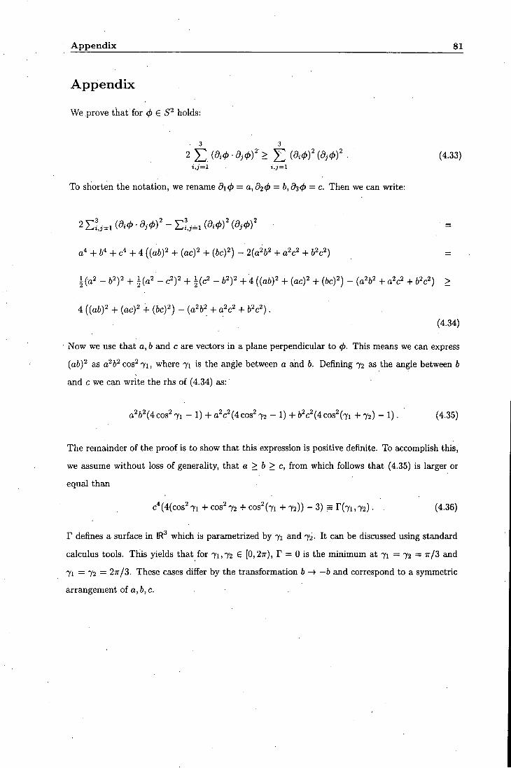
Appendix 81

Appendix

We .prove that"for < € 5^ holds:

3 3

2 ^ {di(t> • dj<l>f > J2 i9i<f>f {d^cff . (4.33) t , j= i i,j=i

To shorten the notation, we rename d\(j> = a,d2<p = h,dz(f> = c. Then we can write:

a" + 6" + c" + 4 ((ai.)2-t-(ac)2 + (6c)^) - 2(a262 + 2 2 + 2 2)

i(a2 - b y + |(a2 - c2)2 + i(c2 - 62)2 + 4 ((^J)2 + (^c)2 _^, ^f,^j2^ _ ( 2 2 + 2 2 + 2 2) >

4 ((a6)2 + (0C)2 + (&C)2) - (a262 + 2 2 + 2 2) (4,34)

Now we use that a, b and c are vectors in a plane perpendicular to (f). This means we can express

(a6)2 as a262 cos2 7i, where 71 is the angle between a and 6. Defining 72 as the angle between b

and c we can write the rhs of (4.34) as: a'^b'^iicos^ 71 - 1) + a2c2(4cos2 72 - 1) -f- 62c2(4cos2(7i -|- 72) - 1) . (4.35)

The remainder of the proof is to show that this expression is positive definite. To accomphsh this,

we assume without loss of generality, that a > 6 > c, from which follows that (4.35) is larger or

equal than

c''(4(cos2 7i-|-cos2 72 4 -cos2 (7 i+72) ) -3 ) s r (7 i , 72 ) . . (4.36)

F defines a surface in IR^ which is parametrized by 71 and 72. I t can be discussed using standard

calculus tools. This yields that for 71,72 £ [0,27r), F = 0 is the minimum at 71 =: 72 = 7r/3 and

7i = 72 = 27r/3. These cases differ by the transformation b —b and correspond to a symmetric

arrangement of a, b, c.

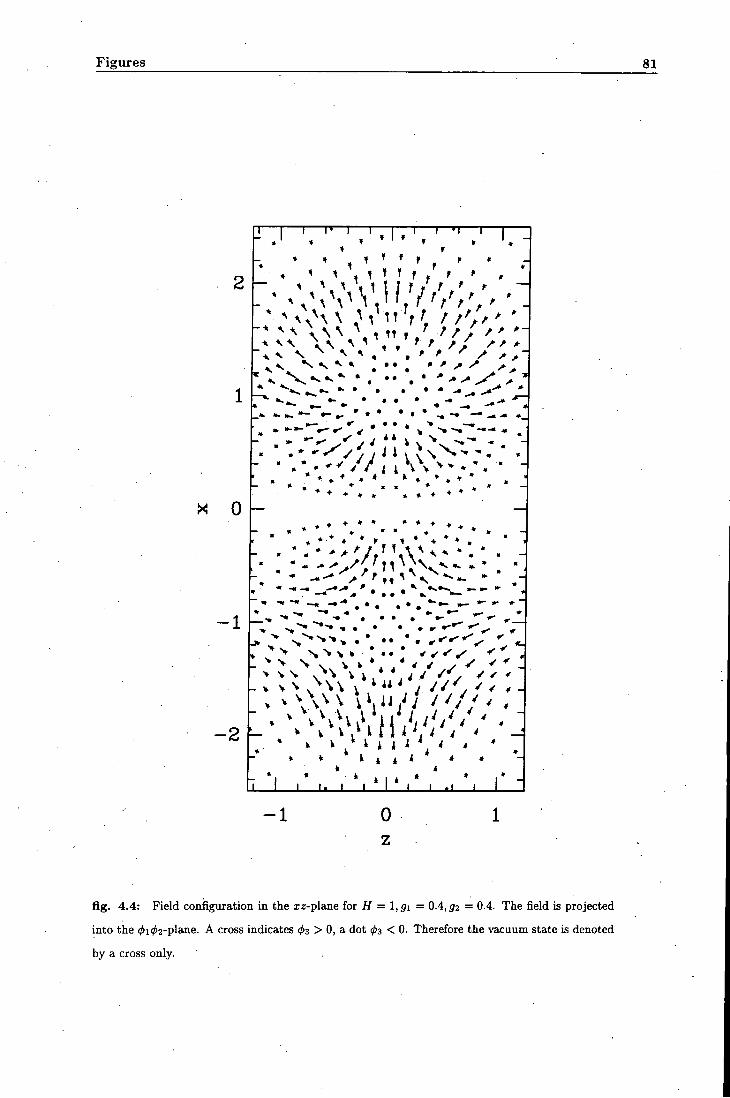
Figures 81

2 -

1

1^ 0

. v A w / / / / v ,

. * . V ^ I i , i ^ . ' , « » * 4 4 * ^ »

k i - * i V * » I * * • i ' -

-1 0 z

fig. 4.4: Field configiiration in the xz-plane for = = 0.4,^2 = 0.4. The field is projected

into the 0i(^2-plane. A cross indicates (^3 > 0, a dot 03 < 0. Therefore the vacuum state is denoted

by a cross only.

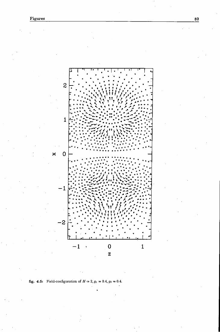
Figures 82

X 0

-1

- 2

' • . . » • * * J * . I \ > • • • • . " 1

— + • • • » » . . » » • • • •

+ + • * • « » « » » • • • +

' * ' L JLLL _1_U L i .

-1 0 z

fig. 4.5: Field-configiiration of H = 2, ffi = 0.4, = 0.4.

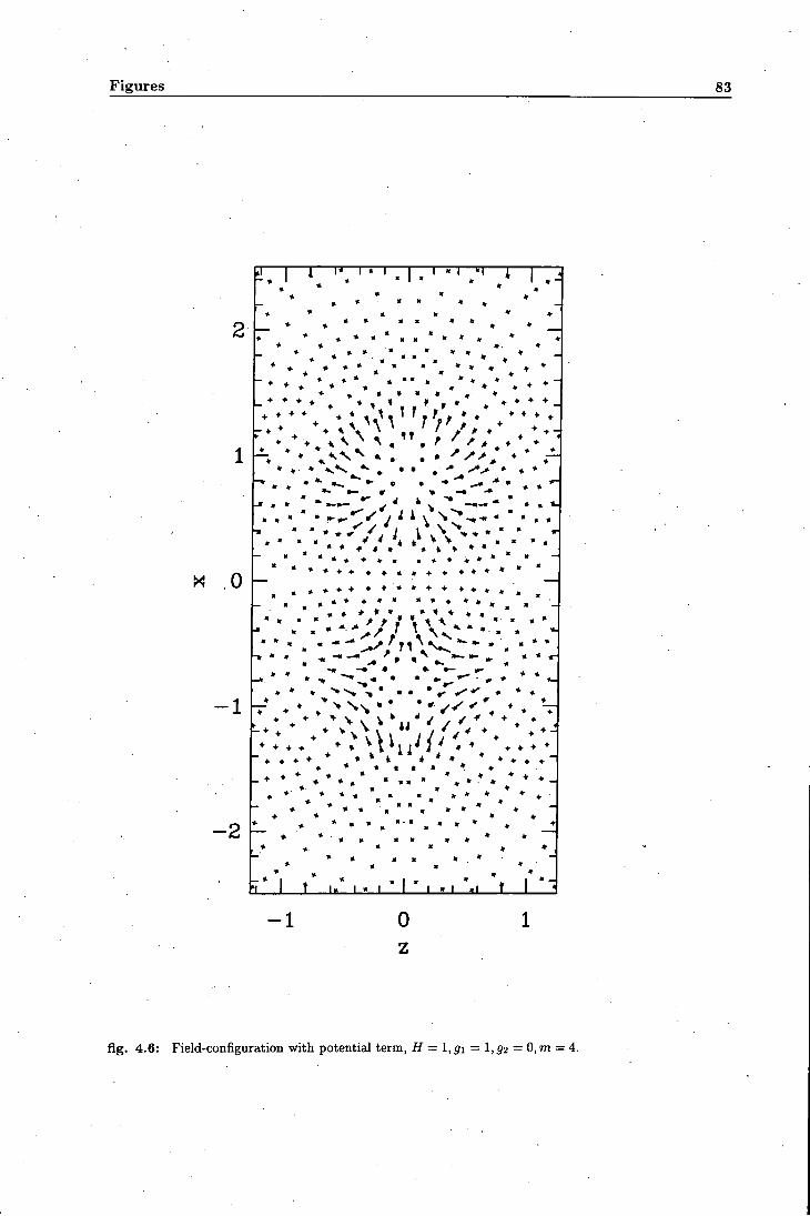
Figures 83

••** * * ' 1 f.f * * * * * *

» « • " • / ^ ^ v "^r*-*- * " • . «

\- « - »

X .0

-1

- 2

• * • « * • • * • » - . -\

« " • ' V n X

• » • * » ^ • • r* » • •

« 1 1 * . . . . o • • • » • « « - • • • . • •

• * « , . . , . » *

I 1 I " I ' I ' I « I d I L -1 0

z

fig. 4.6: Field-configuration with potential term, i f = 1,31 = 1,52 = 0,m = 4.

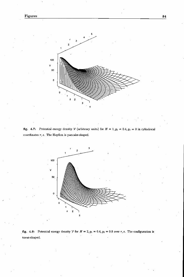
Figures 84

100

50

fig. 4.7: Potential energy density V (arbitrary units) for H = l,gi = 0.4,^2 = 0 in cylindrical

coordinates r, z. The Hopfion is pancake-shaped.

100

50

fig. 4.8: Potential energy density V ioi H = 2,gi = 0.4,^2 = 0.8 over r,z. The configuration is

torus-shaped.

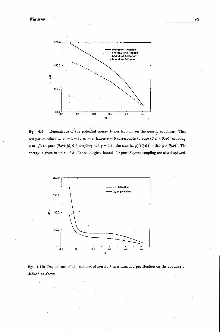
Figures 85

200.0

1500

100.0

50.0

energy of 1-Hopfion energy/2 of 2-Hopfion

X bound for 1-Hopfion • bound for 2-Hopfion

-0.1 0.1 0.3 0.5 0.7 0.9

fig. 4.9: Dependence of the potential energy V per Hopfion on the quartic couplings. They

are parametrized as gi = 1 — 85,32 = g- Hence 5 = 0 corresponds to pure (9i</> x dj<j)Y coupling,

g = 1/3 to pure (5i</»)^(a,0)^ coupling and 5 = 1 to the case (di(l>)^{dj<j))^ - 2(5(0 x dj<l>)^. The

energy is given in units of A. The topological bounds for pure Skyrme coupling are also displayed.

2 0 0 . 0

150.0

S 100 .0

50.0

0.0

J of 1-Hopfion

J« of 2-Hopfion

-0.1 0.1 0.3 0.5 0.7 0.9

fig. 4.10: Dependence of the moment of inertia J in a-direction per Hopfion on the coupling g,

defined as above.

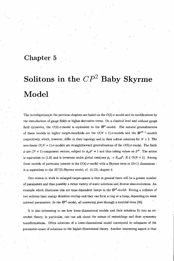
Chapter 5

Solitons in the CP^ Baby Skyrme

Model

The investigations.in the previous chapters are based on the 0(3) cr-model and its modifications by

the introduction of gauge fields or higher-derivative terms. On a classical level and without gauge

field dynamics, the 0(3)(T-model is equivalent to the dP^-model. The natural generalizations

of these models to higher target-manifolds are the 0(A'' + l)(T-models and the IP^'^-models

respectively, which, however, differ in their topology and in their soliton solutions for N > 2. The

non-linear 0{N + 1) cr-models are straightforward generalizations of the 0(3) cr-model. The fields

(j) are {N + l)-component vectors, subject to (j>a<j)'^ = 1 and thus taking values on . The action

is equivalent .to (1.6) and is invariant under global rotations (pa Rab4>^, R € 0{N + 1). Among

these models of particular interest is the 0(4) cr-model with a Skyrme term in (3+1) dimensions :

i t is equivalent to the 5J7(2)-Skyrme model, cf. (4.13), chapter 4.

One reason to work in enlarged target-spaces is that in general there wil l be a greater number

of parameters and thus possibly a richer variety of static solutions and diverse time-evolutions. An

example which illustrates this are time-dependent lumps in the (IP'^-model. During a collision of

two solitons their energy densities overlap and they can form a ring or a lump, depending on some

internal parameters. In the dP^-model, all scattering goes through a toroidal state [95].

I t is also interesting to see how lower-dimensional models and their solutions fit into an ex­

tended theory, in particular, one can ask about the nature of embeddings and their symmetry

transformations. Often solutions of a lower-dimensional model correspond to subspaces of the

parameter-space of solutions to the higher-dimensional theory. Another interesting aspect is that

87

the number of possible terms in the action for a given set of conditions, such as Lorentz-invariance,

global symmetries or positiveness, can increase with the dimension of the target-manifold, thus

adding to the choice of models. These are some of the questions that we address in this chapter.

I t is often difficult though, to examine all these problems for a general and therefore a good

tactics is to start looking at small A'' first, which can indicate more general features in an inductive

way. Consequently, we concentrate here on the flP^-model, but first we review some known gener2d

properties of the CP^"^-models.

The ([P''^~^-models in (2-1-1) dimensions are an obvious object of interest for various reasons.

Their static solutions are known analytically, which allows to model their low-energy dynamics by

a moduli space approximation. This was investigated some time ago by Ward [52] for the (IP^-

model, by Stokoe and Zakrzewski for (IP^~^-model [96] and later more detailed for the (EP^-model

by Leese [97]. For the (EP baby Skyrme model a moduU space approximation was performed

by Sutcliffe [98]. I t was generally found that in a head-on coUision two solitons can scatter at

right angles or back to back depending on the initial conditions, although the complete discussion

in [97] shows that the details are more subtle and other scattering angles are possible. Right angle

scattering of two solitons was also observed in studies on the dynamics of solitons in a dP'^-model

by Piette et al. in [95]. There the dynamics were altered by adding a term that involves three

derivatives which are contracted by an antisymmetric tensor Eijk, thus making this term metric-

independent. Such a term resembles the Hopf-term of the flP^-model, but by contrast for CP' i t is

not a total derivative and thus contributes to the equations of motion. Consequently, i t alters the

dynamics of the solitons and this happens by giving them a non-zero angular . momentUni.

Another interesting observation was made by Hindmarsh in [99]. There i t was shown that the

IP^-^-model can be obtained from an extended Abelian Higgs model in (2-1-1) dimensions, where

the domain of the fields is C^ . For a specific choice of the gauge potential and in the limit of small

momenta, the model can be mapped to the dP'^-^-model with a Skyrme term. The Mcixwell term

in the action of the Abelian Higgs model under this transformation corresponds to the Skyrme

term.

In this chapter we mainly study a related model, namely the (EP^-model in (2-1-1) dimensions

with a Skyrme term. Here the solitons are stabilized by a potential and fourth-order terms in

the action, which are however, not unique for dP^. We find a family of analytic static one-soliton

solutions and study the two-soliton configuration numerically in a gradient-flow equation on the

moduli space.

5.1 OP^-^-models Revisited 88

5.1 CP^-i-models Revisited

dP^-i-models are examples of theories where the field-space is given by a Grassmanian manifold.

This is a complex manifold which describes an M-dimensional subspace of the A'^-dimensional

complex Euclidean space C'^. I t can be written as a coset G{M,N):

The complex projective spaces are the sets of lines through the origin in C and correspond to

M = 1. The canonical coordinates on C'^ are the homogeneous or cartesian coordinates z =

{zi,... ,ZN)- According to the definition given above, dP''"^ can be described as the complex

space in which all the z that differ by a complex number are identified, z ~ Xz,z ^ 0,\ £ d.

Therefore

( [ P ^ - i = ( c ^ - f O } ) / ! ' , (5.2)

where C* is the group of non-zero complex numbers. In order to write the (IP^~^-model in

terms of homogeneous coordinates, one has to impose the equivalence relation z ~ Xz. The

first step is to fix the magnitude of z by setting zh = 1 which restricts the field to values on

g2N-i _ u{N)/UiN - 1). Geometrically, this sphere is a C/(l)-bundle over base-space (IP'^~\

which illustrates formula (5.1) for M = 1. The second step is thus to impose local C/(l)-gauge

invariance on the action which removes any dependence of the model on the corresponding phase.

Consequently, the usual quadratic expression daZ^d°'z/2 in the Lagrangian is replaced by

(5.3)

where the dagger indicates hermitian conjugation and the covariant derivative is

DaZ = daZ + lAaZ . (5.4)

(a = 0,1,2). The equations of motion for Aa yield:

Aa^iz^daz, (5.5)

which also shows that the dP^'^^-models are a non-linear theory. Although Aa is not an indepen­

dent field and in particular not related to any electromagnetic interactions, because of the formal

5.1 CP^-^-models Revisited 89

analogy, we wil l refer to i t as a gauge field and generally adopt the notation of gauge theory. The model (5.3) has a global 5C/(A'')-symmetry, resulting in A''2 - 1 conserved global charges and the local [/(l)-symmetry.

The projective space CP^"^ can also be described in terms of the inhomogeneous coordinates

W. In a, region where Za ^0, they are defined as follows

W = {wi,...,WN-i) = — , (5.6) Za Za Za Zo

which is by construction independent on the choice of the representative z of the equivalence class;

let z, z be elements of such class: zj/za = Azj/Aza = Zf,/za- On a patch which includes Z Q = 0,

but Zc 7 0 one defines:

W = {wi,...,WN-i) = — • (5.7) Zc Zc Zc Zc

In the regions, where both patches overlap, the transformation between the inhomogeneous coor­

dinates W and W is obtained by

W = ^ W . (5.8) Za

The complex projective space (IP^~^ is a Kahler manifold. This implies that there is a her-

mitian metric T^I and associated with this metric is a closed, antisymmetric and xea\. two-form

Vt = T^idz°- A dz*, d f l = 0. In terms of the cartesian coordinates on I ^ , r „ j is given by:

^ab - ZaZb / , n\ rab = • (5-9)

This expression is called the Fubini-Study metric and is the natural metric on (!P^~\ if embedded

i n C ^ .

The Kahler potential, which corresponds to (5.9), is patchwise defined. In a region Ua, where

Z a ? 0 i t is / , , 2 , ,

Ka=\n (5.10)

such that

The imposition of the phase invariance for homogeneous coordinates is equivalent to changing the

metric on C'^ from the flat-space metric to the Fubini-Study metric, i.e.

5.1 OP^-^-models Revisited 90

a„faa"z6J°' ' ^ a „ f a 9 " 2 6 r " \ (5.12)

which can be verified by using (5.5). From the topological point of view the existence of solitons

in the CP^"^-model on IR' is based on

7r2 ( ( I P ^ - i j = Z , i V > l . (5.13)

The non-triviality of this homotopy stems from the topology of maps from the (compactified) plane

to IP^ subspaces of <[P'^~^. ExpHcitly, the degree is given by

Q = ^ I d'xsij (Diz)^ {Djz) . (5.14)

Here, to avoid confusion with the target-space dimension N, we changed our notation and we have

called the topological charge Q rather than TV as before. Interestingly, there are two ways to look

at the topological charge in the (IP^~^-models. For finite energy, the covariant derivative has to-

vanish at spatial infinity

For the gauge field this implies

lim DiZ = 0. (5.15) |x|->oo

= Va. . (5.16) Za

Ai is real and independent on a, which leads to

lim z = Zooc'"^"'*), (5.17)

where Zoo is a fixed unit-vector and 6 is the polar angle on IR^. In analogy to the AbeUan Higgs

model, single-valuedness of z implies /i(27r) = /i(0) + n, n 6 Z . Thus there is an associated

topological charge which stems from 7r i (5^) ^ 0 and counts the winding number of the gauge field

at infinity:

Q = :^^^^cl0Ae = ^ihi2n)-hm=n. (5.18)

The relation to formula (5.14) can be established using Stokes' theorem, the integrand of (5.14)

corresponds to the "magnetic field" F12 = diA2 - d2Ai.

A l l the! pure (IP^~^-models are of Bogomol'nyi-type and the corresponding argument generalizes

almost trivially from CP^ The potential energy can be written as:

5.1 C P ^ - i - m o d e l s Revisited 91

Minima are obtained for

V[z] = \ j d'^x |£»iz ± iD2z\' T 47re •

(£»! ± iD2)z = D±z = 0,

(5.19)

(5.20)

where D±z indicates tlie derivative with respect to x± = xi ± ix2- The n-sohton solutions to this

equation can be written in terms of (anti-) holomorphic functions P„:

Pn_ \Pn\

(5.21)

where, in fu l l generality, for a holomorphic Pn

Pn = (5.22)

V XNix+-a^) . . . ( x + - a ^ ) J

I t is interesting to ask, how many of the parameters (Ar, a f ) , (r, s = 1 . . . TV; z = 1 . . . n) correspond

to physically distinct fields, in other words, we ask for the dimension of the n-soliton moduli space.

The way i t is written above, P„ has 2 i V ( n + l ) real parameters. Two of these are redundant because

the model lives on the projective space, i.e. z ~ Xz; the f/(l)-gauge degree of freedom and further

two real parameters, corresponding to a choice of the origin in IR^ should also not be counted. The

multiplicative factors in front of each component can be transformed to unity by using the global

S?7(iV)-symmetry. This removes a further {2N - 2) degrees of freedom, leaving 2Nn - 1.

S k y r m e t e r m s

I t has been mentioned before in this thesis that in space-dimensions greater than one there has

to be a higher-order derivative term in the Lagrangian in order to allow non-singular solutions. I f

one imposes the constraint that such a term respects the symmetries of the theory (global SU{N)

and local f / ( l ) ) and includes only second-order terms of derivatives with respect to any variable

(especially the time-derivative), one is left for dP^^^-models with two generically different Skyrme

terms which can be written in terms of the tensor Aap [100]:

Aap = {Daz)^(D0z). (5.23)

5.1 CP^~^-models Revisited 92

Note that Aap — Apa and hence A is hermitian. Now we decompose Aap into its real symmetric and its imaginary antisymmetric part:

Fa/3 = -i{Aci3 - Apa) = - 2 I m {Ac0) = i [zlzp - z^Zc^ = d^Ap - dpA^ = [D* , Dp] _ ,

Gcp = Aap + Apc = 2Re {Acp) = z^zp + z^z^ + 2Ao,Ap = [D^, Dp]^ , (5.24)

such that Aap = {Gap + iFap)l2. To shorten the notation we have introduced here Za = dz/dx°.

F and G are inanifestly gauge invariant and can be included in the Lagrangian as

£4° = i ( T r G f - ^ ' I V G ^ Cl = \TT F \ (5.25)

Giving the fourth-order terms different couplings fXp and /XQ respectively, the (IP^~^ Skyrme model

is defined by:

C.= C2 + tJ,oC^ + fJ^rCl + firjU. (5.26)

£4 is what is usually called the Skyrme term. For iV = 2 it turns out that £4 and £4 are

equivalent [100]. This can be indicated by using the equivalence of the CP^ and the 0(3) cr-model.

In the latter model the fields are three-component real vectors (f) e S^. The relation to the z-fields

is given by the Hopf map = z^aaZ, (a = 1,2,3) where (TQ are the PauU matrices, cf. (4.2). Then

the following equalities hold:

{TvG)'= 8Zaida<p-d-cl>f ,

T^G'= 8Za0{da<l^-dpcf>f , (^-^^^

T^F'= ^Ea0ida(f>xdp<f>)\

To derive this we can use

CT'^CT* ' = 2(5'^'J*' - (5'J(J*', <Vj"(7 ," '"e°'"= = 4(<J''(J '"(J'=" - 5'"5^*d'"'), ' (5.28)

(a, 6, c = 1,2,3). The equation £4 = £4 is then equivalent to the Lagrange identity:

ida(t> • d"(l>f - {da(t> • dpcpf = {da(t> X dp<l>f . (5.29)

I t is interesting to ask for the geometrical interpretations of the fourth-order terms £4 and £4.

We showed above that the integral ovei* the "field-strength" F12 is integer valued and counts the

5.2 T h e C P ^ baby Skyrme Model 93

windings of the gauge field at infinity. A priori there is no topological invariant related to G. As

a possible way of thinking about the geometry of the model (5.26) we remind ourselves of the

geometrical way in which Manton described the potential energy in the Skyrme model [101]. The

argument is very general and does not even require the target-manifold to be a Lie-group; it applies

to any Riemannian manifold. Given a map / between two such manifolds M and Af endowed with

orthonormal frames e' and /c° respectively, the Jacobi matrix of the map / is

Jkr = e l 5 i / " < . (5.30)

Using this, one defines a strain tensor D = J j t , which is a measure of the local deformation

induced by the map. I t is constructed in a way such that it carries only indices of the base-space.

Hence the number of its invariants (eigenvalues) equals the dimension mof M, the physical space.

Manton showed, that the potential energy functional of the Skyrme model (where M = IR^ and

Af = S^) can be expressed in terms of eigenvalues of D. Geometrically, the quadratic term in the

energy is a measure for the distortion due to changes in the length of the local frame vectors while

the Skyrme term indicates how the area spanned by two respective vectors gets deformed due to

the map. This is to say, the Skyrme term energetically favours isometrics.

For the case of interest to us M = IR^, Af = €^ and f = z. Given, that K^KJ = r"* is

the Fubini-Study metric on I ^ , one finds that the potential energy can be expressed in a sim­

ilar fashion to the Skyrme model, where Aij plays the role of Dij. In two space-dimensions

(Tr Ay - TT A'^ = 2det A and the potential energy that corresponds to C2 + C° + £4 can be

expressed as

V= J (fx^Tr A + ^det A. (5.31)

5.2 The CP^ baby Skyrme Model Equipped with the general framework described above, we will now investigate a concrete example,

namely the CP^ Skyrme model. According to (5.1), the CP^-manifold is described by

We define the inhomogeneous coordinates on the patch, where zi ^ 0, W = {z2,zz)lz\ = {w,v),

related to the cartesian coordinates z = {zi,Z2,Z'i) as follows:

5.3 Solutions to the C P ^ Skyrme Model 94

In terms of W, the tensor Aap becomes:

Aa0 = { ( l + IM^) ^aVp + ( l + M^) WaWp ' VWWaVp - WVVaWp} , (5.34)

where M = 1 -I- + |i;p and Wa = dW/dx" for each component of W. The Lagrangian £2 is,

in terms of 1^:

• , 1 2M2 { k a P + K P + k a V - WalfP} , (5.35)

where the summation over a is assumed. The difference of the fourth-order terms is proportional

to

AC, = C2 - CI ^ iiA^A^0 - AapA^'^) . (5.36)

For tirne-independent fields, this difference can be expressed in terms of W as follows :

4 2 AC4 = \Wa:^Vx2 - Wx^Vxil • (5.37)

Let W — W^^ + tW,^ where the index a indicates the component (a = 1,2; = u;, = v) then

A £ 4 = 0 i f

dW^_dW^ dW^__dW^ .dxi ~ dx2 ' dx2 " dxi '

which are the Cauchy-Riemann equations. Therefore the two fourth-order terms are identical for

static holomorphic functions and especially for solutions to the pure dP^-model.

5.3 Solutions to the CP^ Skyrme Model

We know that the static solutions of the pure (IP^-model are given in terms of rational functions

(5.22). The question naturally arises, whether one can find static analytic solutions to a model

which includes a Skyrme term and a potential term. A systematic method is to use the freedom

in the choice of the potential and reconstruct i t from the equations of motion for a given ajisatz

of the fields. For dP^ Skyrme models there is a slightly more elegant method; one can adapt the

Bogomol'nyi argument where the potential energy density is given by

V=^iDiz)^ {D'z) + ^F^^ + ti^U. (5.39)

5.3 Solutions to the C P ^ Skyrme Model 95

We rewrite the potential energy as

Kp, = j c f x ^ (D.z ± iD2zy {D,z ± iD2z) + ^ (F^2 ± ' ^ ^ ^ )

=F47rQ T y/JiUfj^ Jd^x F12VU.

(5.40)

I t can be shown that the last term also describes the topology 7r2(5^) and is, in this sense, equivalent

to the topological charge Q [102]. We know that the term P12 is proportional to the topologicd

charge density (5.14), the pullback of the volume form on 5^. Geometrically, multiplication with

the scalar function \/U changes the "shape" of the target 5^ but not its topology and corresponds to

a renormalization of the volume element on target 5^. Therefore one finds two self-dual equations,

the solutions of which saturate the modified Bogomol'nyi bound

Fi2 = ^2.f^y/U, Diz = ^iD2Z. (5.41)

From the first equation, a potential can be constructed for a given holomorphic field which will

automatically satisfy the second. In the dP^-model the field W consists of one complex component

w and for w = Xx+ the potential U = 8/(1 -I- \w\'^)'^ was found to satisfy (5.41), [102].

For higher <IP^~\ N > 2, this trick does not work any longer, the term Pi2\/z7 is in general

not a total derivative (or, in differential geometric terms, not a closed two-form). However, one

can, for a given holomorphic field, construct a potential which satisfies the variational equations.

Solutions to these equations will not saturate the Bogomol'nyi bound and their stability or in­

stability wi l l have to be shown be different methods.. Returning to the dP^-model, for the field

one finds the potential

together with the constraint

w = X{x+ — a), V = b, (5.43)

» = 8 ' ' " I " ' ' ' . (5.44) (1-I-|i;|2 + ^ 2 ) "

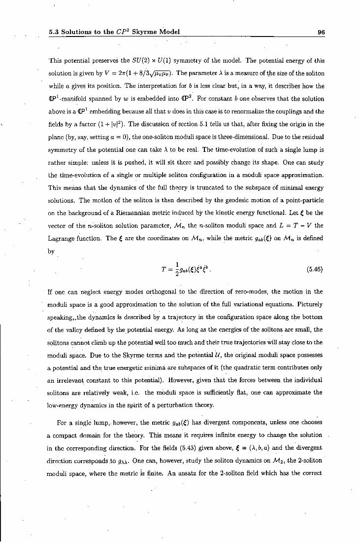
5.3 Solutions to the C P ^ Skyrme Model 96

This potential preserves the SU{2) x U{1) symmetry of the model. The potential energy of this solution is given hyV = 2TT{1 + SlZ^/JT^). The parameter A is a measure of the size of the soliton while a gives its position. The interpretation for b is less clear but, in a way, it describes how the CP -manifold spanned by w is embedded into CP^. For constant b one observes that the solution above is a (IP^ embedding because all that v does in this case is to renormalize the couplings and the fields by a factor (1 4- lup). The discussion of section 5.1 tells us that, after fixing the origin in the plane (by, say, setting a = 0), the one-solitbn moduli space is three-dimensional. Due to the residual symmetry of the potential one can take A to be real. The time-evolution of such a single lump is rather simple: unless i t is pushed, i t wil l sit there and possibly change its shape. One can study the time-evolution of a single or multiple soliton configuration in a moduli space approximation. This means that the dynamics of the ful l theory is truncated to the subspace of minimal energy solutions. The motion of the soliton is then described by the geodesic motion of a point-particle on the background of a Riemannian metric induced by the kinetic energy functional. Let ^ be the vector of the n-soliton solution parameter, Mn the n-soliton moduli space and L = T - 1 the Lagrange function. The i are the coordinates on Mn, while the metric gab{(,) on Mn is defined by

T=\9ab{i)ei'. (5.46)

I f one can nieglect energy modes orthogonal to the direction of zero-modes, the motion in the

moduU space is a good approximation to the solution of the ful l variational equations. Picturely

speaking,.the dynamics is described by a trajectory in the configuration space along the bottom

of the valley defined by the potential energy. As long as the energies of the soUtons are smEill, the

solitons cannot cUmb up the potential well too much and their true trajectories will stay close to the

moduli space. Due to the Skyrme terms and the potential U, the original moduU space possesses

a potential and the true energetic minima are subspaces of i t (the quadratic term contributes only

an irrelevant constant to this potential). However, given that the forces between the individual

solitons are relatively weak, i.e. the moduli space is sufficiently flat, one can approximate the

low-energy dynamics in the spirit of a perturbation theory.

For a single lump, however, the metric gab{.i) has divergent components, unless one chooses

a compact domain for the theory. This means i t requires infinite energy to change the solution

in the corresponding direction. For the fields (5.43) given above, ^ = (A, 6, a) and the divergent

direction corresponds to ^AA- One can, however, study the soliton dynamics on M2, the 2-soliton

moduli space, where the metric is finite. An ansatz for the 2-soUton field which has the correct

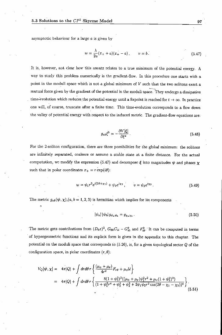
5.3 Solutions to the C P ^ Skyrme Model 97

asymptotic behaviour for a large a is given by

w = •^{x++ a){x+- a), v-b. (5.47)

I t is, however, not clear how this ansatz relates to a true minimum of the potential energy. A

way to study this problem numerically is the gradient-flow. In this procedure one starts with a

point in the moduli space which is not a global minimum of V such that the two solitons exert a

mutual force given by the gradient of the potential in the moduli space. They undergo a dissipative

time-evolution which reduces.the potential energy until a fixpoint is reached for t oo. In practice

one wi l l , of course, truncate after a finite time. This time-evolution corresponds to a flow down

the valley of potential energy with respect to the induced metric. The gradient-flow equations are:

» . « * = - ^ . (5.48,

For the 2-soliton configuration, there are three possibilities for the global minimum: the solitons

are infinitely separated, coalesce or assume a stable state at a finite distance. For the actual

computation, we modify the expression (5.47) and decompose ^ into magnitudes V aJid phases x

such that in polar coordinates x+ = rexp(i^) :

; w = ')pir'^e''-^^+^'^+^26'"^^' v = ip3e'^''. (5.49)

The metric gab{tp, b= 1,2,3) is hermitian which implies for its components

o

IV'ail^(.|5V'.06 =ffx«X6 • • (5-50)

The metric gets contributions from {DQZ)^, GQOGH - Gfo and F^Q. 'lt can be computed in terms

of hypergeometric functions and its explicit form is given in the appendix to this chapter. The

potential on the moduli space that corresponds to (5.26), is, for a given topological sector Q of the

configuration space, in polar coordinates ir,6):

Vq[^,X]= 47r|Q|+ Idrddrl^^-^^^^^Fre+fi^U •

- 47rM + y d ^ ^ f ^ | ( i ^ ^ 2 , 4 + ^ 2 + ^ 2 + 2 i A i t / ' 2 r 2 c o s ( 2 e - X i - X 2 ) ) M • (5.51)

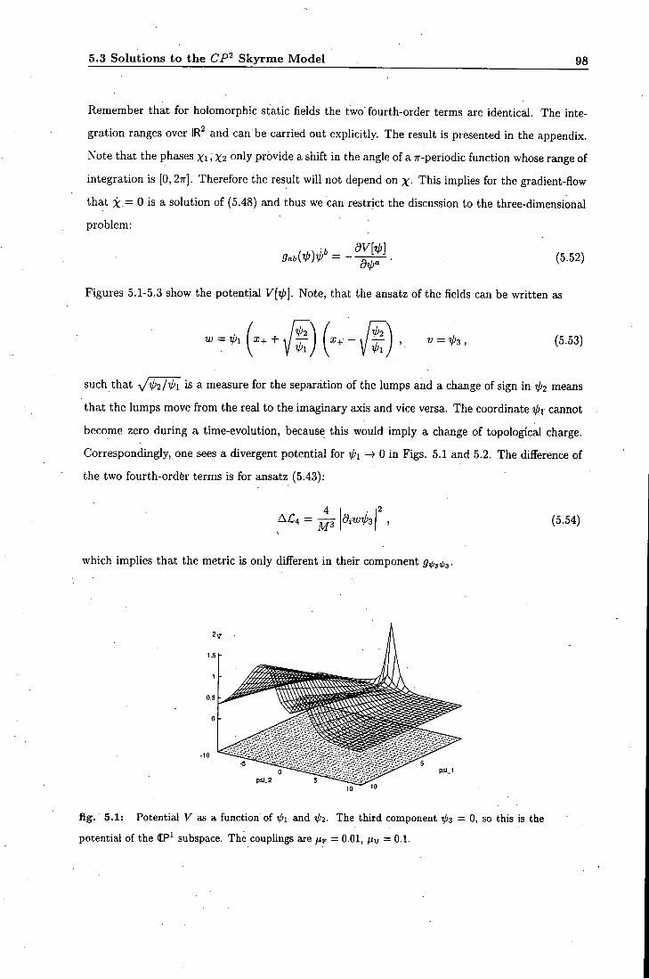
5.3 Solutions to the C P ^ Skyrme Model 98

Remember that for holomorphic static fields the two fourth-order terms are identical. The inte­

gration ranges over IR' and can be carried out explicitly. The result is presented in the appendix.

Note that the phases xi > X2 only provide a shift in the angle of a 7r-periodic function whose range of

integration is [0,27r]. Therefore the result wi l l not depend on x- This implies for the gradient-flow

that X = 0 is a solution of (5.48) and thus we can restrict the discussion to the three-dimensional

problem:

;,6_ dV[^] dtp"

(5.52)

Figures 5.1-5.3 show the potential Note, that the ansatz of the fields can be written as

w = ipi [x+ + (5.53)

such that ^/ip2p'h is a measure for the separation of the lumps and a change of sign in ip2 means

that the lumps move from the real to the imaginary axis and vice versa. The coordinate tpt cannot

become zero during a time-evolution, because this would imply a change of topological charge.

Correspondingly, one sees a divergent potential for ^ i—> 0 in Figs. 5.1 and 5.2. The difference of

the two fourth-order terms is for ansatz (5.43):

A £ 4 = M3 (5.54)

which implies that the metric is only different in their component 5 3 3.

fig. 5.1: Potential V as a function of Vi and ^2- The third component ips — 0, so this is the

potential of the CP^ subspace. The couplings are HF = 0.01, = 0.1.

5.3 Solutions to the C P ^ Skyrme Model 99

fig. 5.2: Potential V as a function of "1 and ip3- In this plot ip2 = 0.1. The couplings are

fxp = 0.01, nv = 0.1.

fig. 5.3: Potential K as a function of t/ij and ips- In this plot tpi = 0.1. The couplings are

flF = 0.01, flu = 0.1.

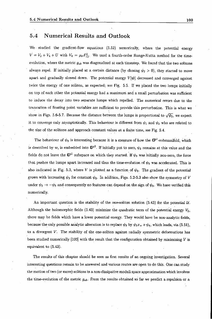
5.4 Numerical Results and Outlook 100

5.4 Numerical Results and Outlook

We studied the gradient-flow equations (5.52) numerically, where the potential energy

V = V2 + V4 +U with Vi = fj,FFi2- We used a fourth-order Runge-Kutta method for the time-

evolution, where the metric Qat was diagonalized at each timestep. We found that the two solitons

always repel. I f initially placed at a certain distance (by chosing V'2 > 0), they started to move

apart and gradually slowed down. The potential energy V[tj)] decreased and converged against

twice the energy of one soliton, as expected; see Fig. 5.5. I f we placed the two lumps initially

on top of each other the potenticd energy had a maximum and a small perturbation was sufficient

to induce the decay into two separate lumps which repelled. The numerical errors due to the

truncation of floating point variables are sufficient to provide this perturbation. This is what we

show, in Figs. 5.6-5.7. Because the distance between the lumps is proportional to y/i)2, we expect

i t to converge only asymptotically. This behaviour is different from ipi and ips who are related to

the size of the solitons and approach constant values at a flnite time, see Fig. 5.4.

The behaviour of ip3 is interesting because i t is a measure of how the dP^-submanifold, which

is described by w, is embedded into flP^. I f initially put to zero, ip3 remains at this value and the

flelds do not leave the dP^ subspace on which they started. I f ip3 was initially non-zero, the force

that pushes the lumps apart increased and thus the time-evolution of V'2 was accelerated. This is

also indicated in Fig. 5.3, where V is plotted as a function of i/'s- The gradient of the potential

grows wi th increasing ip3 for constant t/)2. In addition. Figs. 5.2-5.3 also show the symmetry of V

under tp3 -•03 and consequently no features can depend on the sign of xp3. We have verified this

numerically.

An important question is the stability of the one-soliton solution (5.43) for the potential U.

Although the holomorphic fields (5.43) minimize the quadratic term of the potential energy V2,

there may be fields which have a lower potential energy. They would have be non-analytic fields,

because the only possible analytic alteration is to replace ip3 by ip3X++ip4, which leads, via (5.51),

to a divergent V. The stability of the one-soliton against radially symmetric deformations has

been studied numerically [103] with the result that the configuration obtained by minimizing V is

equivalent to (5.43).

The results of this chapter should be seen as first results of an ongoing investigation. Severad

interesting questions remain to be answered and various routes are open to do this. One can study

the motion of two (or more) solitons in a non-dissipative moduli space approximation which involves

the time-evolution of the metric gab- From the results obtained so far we predict a repulsion or a

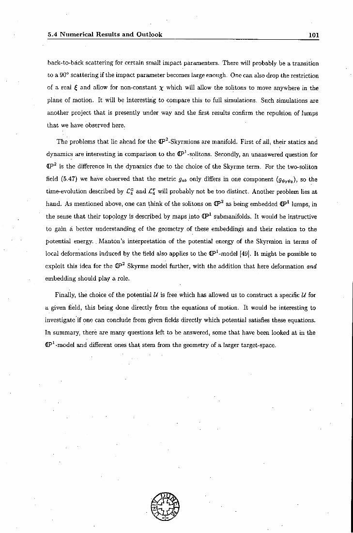
5.4 Numerical Results and Outlook 101

back-to-back scattering for certain small impact paramenters. There will probably be a transition to a 90° scattering i f the impact parameter becomes large enough. One can also drop the restriction of a real ^ and allow for non-constant x which will allow the solitons to move anywhere in the plane of motion. I t wil l be interesting to compare this to ful l simulations. Such simulations are another project that is presently under way and the first results confirm the repulsion of lumps that we have observed here.

The problems that lie ahead for the CP^-Skyrmions are manifold. First of all, their statics £md

dynamics are interesting in comparison to the (EP^-solitons. Secondly, an unanswered question for

dP^ is the difference in the dynamics due to the choice of the Skyrme term. For the two-soliton

field (5.47) we have observed that the metric gab only differs in one component (g^s^j), so the

time-evolution described by £4 and £4 will probably not be too distinct. Another problem lies at

hand. As mentioned above, one can think of the solitons on dP^ as being embedded IP^ lumps, in

the sense that their topology is described by maps into dP^ submanifolds. I t would be instructive

to gain a better understanding of the geometry of these embeddings and their relation to the

potential energy. . Manton's interpretation of the potential energy of the Skyrmion in terms of

local deformations induced by the field also applies to the dP^-model [49]. I t might be possible to

exploit this idea for the dP' Skyrme model further, with the addition that here deformation and

embedding should play a role.

Finally, the choice of the potential Li is free which has allowed us to construct a specific U for

a given field, this being done directly from the equations of motion. I t would be interesting to

investigate if one can conclude from given fields directly which potential satisfies these equations.

In summary, there are many questions left to be answered, some that have been looked at in the

dP^-model and different ones that stem from the geometry of a larger target-space.

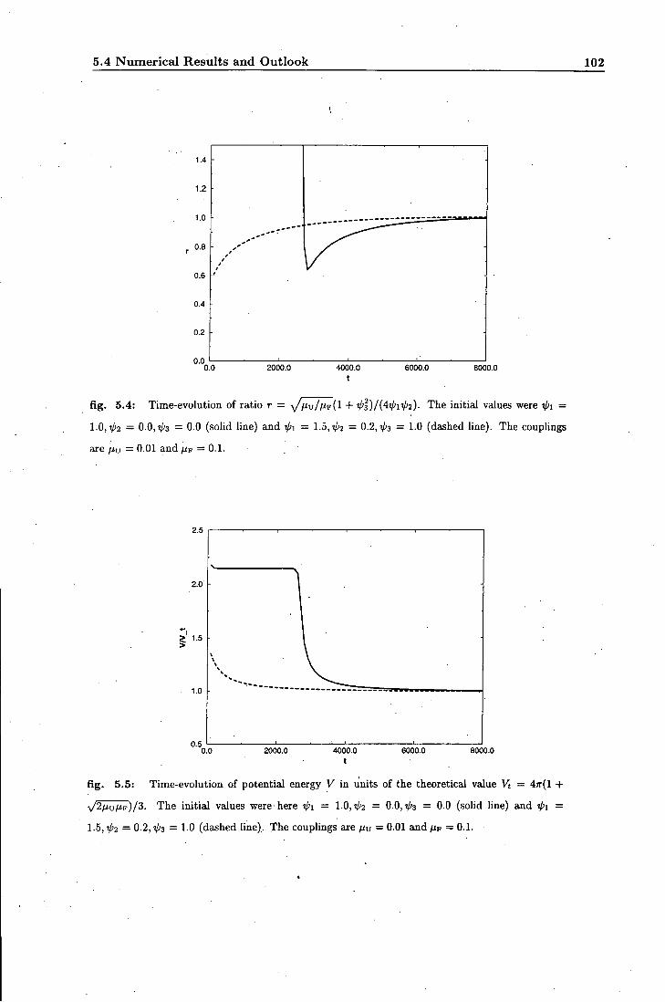
5.4 Numerical Results and Outlook 102

2000.0 4000.0 6000.0 8000.0

fig. 5.4: Time-evolution of ratio r = y/ny/fipil + '/'3)/(4V'iV'2). The initial values were rpi =

l.0,tp2 - 0.0, ip3 = 0.0 (solid line) and ipi = 1.5, -2 = 0.2, "3 = 1-0 (dashed line). The couplings

are /iu = 0.01 and fip - 0.1.

2000.0 4000.0 6000.0 8000.0

flg. 5.5: Time-evolution of potential energy V in units of the theoreticeil vcilue Vt = 47r(l -1-

y/2nuij.p)/3. The initial values were here ipi = 1.0, V'2 = 0.0, "3 = 0.0 (soUd line) and ipi =

1.5, i/'2 = 0.2, Va = 10 (dashed line).. The couplings are /Ju = 0.01 and ftp = 0.1.

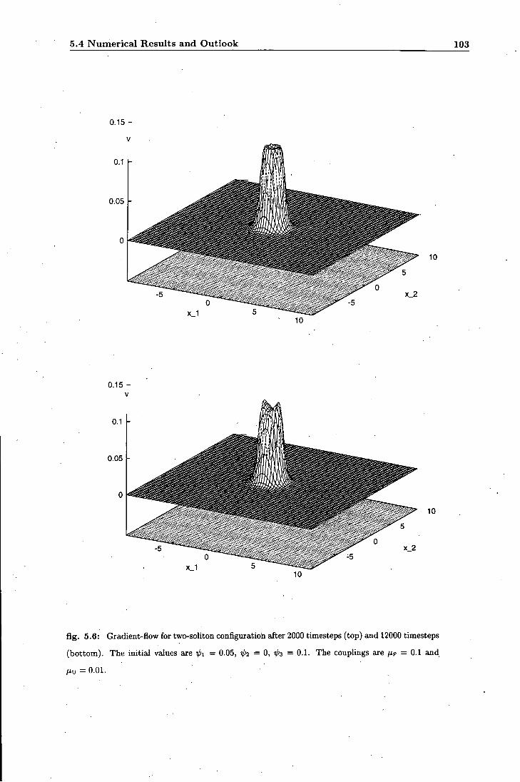
5.4 Numerical Results and Outlook 103

0.15

0.05

10

X 1 -5

10

x_2

0.05

0.15 -

^ ^ ^ ^ 10

fig. 5.6: Gradient-flow for two-soliton configuratioh after 2000 timesteps (top) and 12000 timesteps

(bottom). The initial values are = 0.05, xp2 = 0, tps = 0.1. The couplings are ftp = 0.1 and

Hu = 0.01.

5.4 Numerical Results and Outlook 104

0.4 .-

10

0.25^

10

fig. 5.7: Gradient-flow for two-soliton configuration of Fig.5.6 after 14000 timesteps (top) and

40000 timesteps (bottom).

Appendix 105

Appendix Potential

The potential on the moduli space can be written in terms of an auxiliary function L'^{ijj2,ip3),

defined as

i:ni^.M = B ( ^ ^ , 2 r n - ^ ) 2 F [ ^ ^ , r n - ^ , (5.55)

where £ = (1 -I - ^ | - V '2 ) / ( l + V'l + V'D- such that \E\ < 1. B is here the Beta-function and 2F1

the hypergeometric function. The potential on the moduli space V[iJ)] can be expressed as a series

in L^. In the following expression m = 7/2 for all L and will be omitted.

V[^]= 4 7 r ( l + V | ) ' {

^i{8^l°l" + 2A^f{l + ^P3^+3i>2^)l'^ +

2Ai;l (1 + V'l + SV'I) (1 + ^1 + ^2) L« + 8 (1 + ^ 3 ' + ^i' L^) + ' (5.56)

( V i ' (1 + ^ 3 ' ) ' + 3 V i ^ (1 + Vs' + 3^2' ) (1 + L«+

3 V i ' ( 1 + V s ' + 3^2' ) (1 + ^ 3 ' + V ' 2 ' ) (1 + V ' 3 ' ) ' L 5 +

( 1 + V 3 ' + V 2 ' ) ' ( 1 + V ' 3 ' ) ' L ^ ) }

where ^ = HF + Ha-

Metric

We denote the six components of the metric as gab = 9^^^^^ ( " i ^ = 1>2,3) and express them

generally as

9ab = K a b ' £ R ± l l , (5.57) mn

where Rmni'^) is a coefficient matrix that is given below.

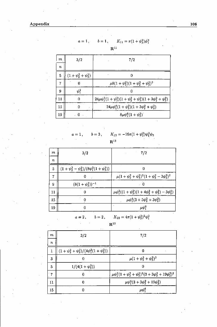
Appendix 106

a = 1 , 6 = 1 , Kn=TT{l+^l)i)l

R "

m 3 / 2 7 / 2

n

5 0

7 0 / . 8 ( 1 - F ^ 3 2 ) ( 1 + V | + ^ I ) '

9 0

1 1 0 2 4 M V ? ( 1 + i / ' | )( l + ^1 + V ' i ) ( i + 3V| + i'l)

1 5 0 24fii>t{l + r3){l +3^2+^3)

1 9 0 .

a = l , b = 3, X i 3 = -167r(l-f-t/'2)V?^3

R13

m

n

3 / 2 • 7 / 2

5 0

7 0 M(l + V l + ^ i ) ' ( l + V ' | - 3 V ' | ) '

9 ( 8 ( 1 + ^ -1))- 0

1 1 0 M^2((l + ^2)(i + 4^2 + ^2) _ 3 ^ 4 )

1 5 0 / / ^ J ( 3 + 5V'| + 3V'|)

1 9 0

a = 2, 6 = 2 , i 22 = 47r(l + t/.|)2V'2

R22

m

n

3 / 2 7 / 2

1 ( l + ^ | + V | ) / ( 4 V ' 2 ( i + ^ 2 ) ) 0

3 0 M i + V l + V ' i ) '

5 1/(4(1+ V'I)) 0

7 0 / .v?(i+v-i+ i ' ln^+3^1 + i9vi )2

1 1 0

1 5 0

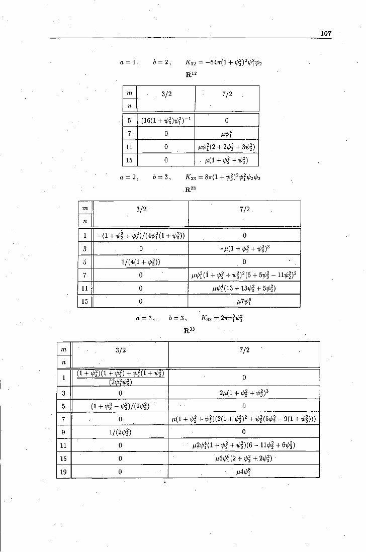
107

a = 1, 6 = 2 , Ki2 = -6M^ + ^l)^^!i'2 Ri2

m 3/2 7/2

n

5 ( 1 6 ( 1 + 0

7 0

11 0

15 0 . / i ( l+V2+V' i )

a = 2 , 6 = 3. i f23 = 87r( l + T/'|)2V'iV2V'3

m

n

3/2 7/2

1 - ( i + V | + vi)/(4V'?(i + V'i)) 0

3 0

5 1/(4(1 +VI)) . 0

7 0 /tV?(l + i-l + V | ) ' ( 5 + 5i>l - llt/ D^

1 1 0 /iV^(13 +13^-1+ 5V'|)

15 0

a = 3,

m

n

3/2 7/2

1 (i + vi)( i + V2 ) + v i ( i + V'2 )

(2V'?Vl) 0

3 0 2M1 + V|+V'I) '

5 (i + V'|-t/'l)/(2Vi) • 0

7 0 + rPl + Vi)(2(l + V|)2 + ^2(5^2 _ + ^2)))

9 1/(2 1) 0

1 1 0 /i2i/ .4(i + v l + ^32)(6 - 11^1 + 6t/;|)

15 0 M6V'?(2 + V|+.2V'|) •

19 . 0

General Conclusions

The theories studied in this thesis describe various aspects of statics and dynamics of extended

objects in relativistic cr-models, therefore it makes sense to look back and summarize what features

they have in common and what future research might be of relevance to all of them.

Almost ail the objects discussed here are "textures" which owe their topological stabihty to

the behaviour of the fields at the interior of the physical space. The topological charge provides

a bound on the potential energy and prevents the lumps of non-zero degree from decaying into

radiation during their time-evolution. Thus all the models studied here can have solutions that

are in principle suitable to model dynamical interactions.

Two areas of further study are of common interest to all of the theories, albeit for different

physical reasons. The first one of these is the investigation of solutions of higher topological degree,

especially non-radially symmetric solutions and their time^dependence. Foi: the self-dual solutions

of chapter 3 this would be interesting in comparison to the well-studied vortices of the Abelian Higgs

model. Perturbation theory around the self-dual point will lead to forces between the separated

lumps who will begin to move under the influence of this force. For the Hopfion described in

chapter 4 there is, for higher topological charges, the possibility that knot-like structures occur:

the dynamics of "multi-knots" would be interesting in various contexts such as the behaviour

of cosmic strings and their scattering. Open questions include the existence of bound states, the

dynamics of rotating Hopfions and generally the structure of the moduli space of the theory. These

are also questions of interest to the flP^ baby Skyrme model of chapter 5. Furthermore, for the

Hopf-model one can think of an extended theory which includes Skyrmions and Hopfions. Their

interactions could be diverse and promise a rich playground for investigations. Some topological

properties of such a theory have been looked at in [104].

The second area of interest that is shared between the models is a quantum mechanical de­

scription of the solutions. We have not discussed such work at all here (apart from a brief aside in

109

chapter 4), but clearly this is a question of gireat interest. To construct a quantum field theory for

solitons is a hard task and the general approach used so far has involved the truncation of the the­

ory to a finite-dimensional system and quantization of the degrees of freedom in the moduli space.

Semiclassical computations of fluctuations around the classical ground state have been performed

in the Skyrme model, where one method involved the analysis of the vibrational normal modes

and the study of the Fourier spectrum of the fields after a perturbation; Similar techniques should

be applicable to the models described in this thesis, especially the Hopfions.

Each of the theories that we discussed is interesting in its own right but they might also

provide ideas for investigations of the other models that we have studied. For instance, it would

be interesting to look at a ?7(l)-gauged Hopfion and to compare it to a gauged Skyrmion. It would

also be instructive to see if one can construct a better bound on the potential energy for such a

model. On the other hand, it is an interesting problem to impose an angular time-dependence on

the fields in the models of chapter 2 and 3, similar to the Hopfion or to Coleman's Q-balls.

To summarize, despite the obvious differences between the various models described in this

thesis, they represent many interesting areas of research and provide inspiration for further inves­

tigations.

Bibliography

[1] J. Gladikowski. "Topological Chern-Simons Vortices in the 0(3) a-model". Z. Phys.,

C73:181, 1996.

[2] J. Gladikowski and M. Hellmund. "Static Solitons with Non-Zero Hopf Number" . to appear

in Phys. Rev. D.

[3] P.O. Drazin and R.S. Johnson. Solitons: an Introduction. Cambridge University Press,

Trumpington Street, Cambridge, 1989.

[4] T.H.R. Skyrme. "A Nonlinear Field Theory". Proc. Roy. Soc. Land., A260:127, 1961.

[5] T.H.R. Skyrme. "A Unified Field Theory of Mesons and Baryons". Nucl. Phys., 31:556,

1962.

[6] E. Witten. "Current Algebra, Baryons and Quark Confinement". Nucl. Phys., B223:433,

1983.

[7] V. G. Makhanov, Y.P. Rybakov and V.I . Sanyuk. The Skyrme Model. Springer-Verlag, Berlin

Heidelberg, 1993.

[8] P.J. Hilton. Introduction to Homotopy theory. Cambridge University Press, Trumpington

Street, Cambridge, 1964.

[9] M. Gell-Mann and M. Levy. "The Axial Vector Current in Beta Decay". Nouvo Cimento,

16:705, 1960.

[10] A.M. Polyakov. Gauge Fields and Strings. Cambridge University Press, Trumpington Street,

Cambridge, 1989.

[11] W.J. Zakrzewski. Low Dimensional Sigma Models. Adam Hilger, Bristol and Philadelphia,

1989.

B I B L I O G R A P H Y 111

[12] M. Nakahara. Geometry, Topology and Physics. Institute of Physics Publishing, Techno House, Bristol, 1990.

[13] R. Bott and L.W. Tu. Differential Forms in Algebraic Topology. Springer-Verlag, Berlin

Heidelberg, 1982.

[14] E. M. Bogomol'nyi. "The StabiHty of Classical Solutions". Sov. J: Nucl. Phys., 24:449, 1976.

[15] A.Belavin and A.M. Polyakov. "Metastable States of Two-Dimensional Isotropic Ferromag-

nets". JETP. Lett, 22:245, 1975. Pisma ZETF 22:503.

[16] N.S. Manton. "A Remark on the Scattering of BPS-Monopoles". Phys: Lett, 110B:54, 1982.

[17] R. Hobart. "On the Instablility of a Class of Unitary Field Models". Proc. Phys. Soc. Lond.,

82:201, 1963.

[18] G.H. Derrick. "Comments on Non-Linear Wave-Equations as Models for Elementary Parti­

cles". J. Moi/i. P/ii/s., 5:1252, 1964.

[19] B. Piette and W.J. Zakrzewski. "Shrinking of Solitons in the (2-l-l)-dimensionaI Sigma

Model". Nonlinearity, 9:897, 1996.

[20] R.S. Ward. "Stable Topological Skyrmions on the 2D Lattice". Lett Math. Phys., 35:385,

1995.

[21] R.S. Ward. "Bogomol'nyi Bounds for Two-Dimensional Lattice Systems". Comm. Math.

Phys., 184:397, 1996.

[22] Clifford and Taubes. Vortices and Monopoles. Birkhauser, Bristol, New York, 1980.

[23] M.J. Speight. On the Dynamics of Topological Solitons. PhD thesis, Durham University,

1995.

[24] L. Jacobs and C. Rebbi. "Interactions of Superconducting Vortices". Phys. Rev., B 19:4486,

1979.

[25] N.S. Manton. "The Force between't Hooft-Polyakov Monopoles". Nucl. Phys., B 126:525,

1977.

[26] N.S. Manton. "Vortices and Anyons". Phys. Rev. Lett, 67:1462, 1991.

[27] I.A.B. Strachan. "Low-Velocity Scattering of Vortices in a Modified Abelian Higgs Model".

J. Math. Phys., 33:102, 1992.

B I B L I O G R A P H Y J12

[28] T.M. Samols. "Vortex Scattering". Comm. Math. Phys., 145:149, 1992.

[29] P.A. Shah. "Vortex Scattering at Near-critical Coupling". Nucl. Phys., B429:259, 1994.

[30] E. Corrigan. "Knot Physics". Physics World, June 1993.

[31] S. Deser, R. Jackiw and S. Templeton. "Topologically Massive Gauge Theories". Ann. Phys.

NY, 140:372, 1982.

[32] M. Atiyah. The Geometry and Physics of Knots. Cambridge University Press, Trumpington

Street, Cambridge, 1990.

[33] S. Deser and R. Jackiw. "Self-Duality of Topological Massive Gauge Theories". Phys. Lett.,

8139:371, 1984.

[34] F. Wilczek. Fractional Statistics and Anyon Superconductivity. World Scientific, PO Box

128, Farrer Road, Singapore 9128, 1990.

[35] L.D. Faddeev. "Some Comments on the Many Dimensional Solitons". Lett. Math. Phys.,

1:289, 1976.

[36] G.S. Adkins, C.R. Nappi and E. Witten. "Static Properties of Nucleons in the Skyrme

Model". Nucl. Phys., B228:552, 1983.

[37] I.E. Dzyaloshinskii, A.M. Polyakov and P.B. Wiegmann. "Neutral Fermions in Paramagnetic

Insulators". Phys. Lett, A127:112, 1988.

[38] G. Nardelli. "Magnetic Vortices'From a Non-Linear Sigma Model with Local Symmetry".

Phys. Rev. Lett, 73:2524, 1994.

[39] M.A. Mehta, J.A. Davis and I.J.R. Aitchinson. " Stable Soliton Solutions of the CP Model

with a Chern-Simons Term". Phys.^Lett, B281:86, 1992.

[40] B.M.A.G. Piette, D.H. Tchrakian and W.J. Zakrzewski. " Chern-Simons Solitons in a CP

Model". P/iys. ie« . , B339:95, 1994.

[41] F. Wilczek and A.Zee. "Linking Number, Spin and Statistics of Solitons". Phys. Rev. Lett.,

51:2250, 1983.

[42] B.J. Schroers. "Bogomol'nyi Solitons in a Gauged 0(3) cr-Model". Phys. Lett, B356:291,

1995.

B I B L I O G R A P H Y 113

[43] S. Coleman. Aspects of Symmetry. Cambridge University Press, Trumpington Street, Cam­bridge, 1985.

[44] J.J.M. Verbaarschot et.al. "Symmetry And Quantization Of The Two Skyrmion System:

The Case Of The Deuteron". Nucl. Phys., A468:520, 1986.

[45] V.B. Kopeliovich and B.E. Stern. " Exotic Skyrmions". Pis'ma v ZhETF, 45:165, 1987.

[46] H. Weigel, B. Schwesinger and G. Holzwarth. "Exotic Baryon Number B = 2 States In The

SU(2)-Skyrme Model ". Phys. Lett, B168:321, 1986.

[47] B.M.A.G. Piette, B.J. Schroers and W.J. Zakrzewski. "Multisolitons in a Two-Dimensionad

Skyrme Model". Z. Phys., C 65:165, 1995.

[48] J. Gladikowski, B. Piette and B.J. Schroers. "Skyrme-Maxwell Solitons in (2-f-l) dimensions".

Phys. Rev., D53:844, 1996. '

[49] B.M.A.G: Piette, B.J. Schroers and W.J. Zakrzewski. "Dynamics of Baby Skyrmions". Nucl.

Pftj/s., B439:205, 1995.

[50] R. Rajaraman. Solitons and Instantons. North Holland, Elsevier Science Publishers B.V.

P.O. Box 211, 1000 AE Amsterdam, The Netherlands, 1982.

[51] V.E. Zakharov and A.V. Mikailov. "Example of Nontrivial Soliton Interaction in Classical

Field Theory". JE^TP, 47:1017, 1978.

[52] R.S. Ward. "Slowly Moving Lumps in the dP Model in (2-t-l) Dimensions". Phys. Lett.,

8158:424,1985.

[53] G. Dunne. "Self-Dual Chern-Simons Theories". In Lecture Notes in Physics, m36. Springer-

Verlag, July 1995.' hep-th/9410065.

[54] R. Jackiw arid S.Y. Pi. "Classical and Quanta! Nonrelativistic Chern-Simons Theory". Phys.

Rev., D 42:3500, 1990. erratum ibid. D 48, 3929 (1990).

[55] G.V. Dunne, R. Jackiw, S.Y. Pi and C.A. Trugenberger. "Self-dual Chern-Simons Solitons

and Two-Dimensional Nonlinear Equations". Phys. Rev., D 43:1332, 1996.

[56] R. Jackiw, K. Lee and E.J. Weinberg. "Self-Dual Chern-Simons Solitons". Phys. Rev., D

42:3488, 1990.

B I B L I O G R A P H Y . 114

[57] J. Hong, Y. Kim and P.Y. Pac. "Multivortex solutions of the Abelian Chern-Simons-Higgs theory". Phys. Rev. Lett, 64:2230, 1990.

[58] R. Jackiw and E.J. Weinberg. "Self-dual Chern-Simons Vortices"; Phys. Rev. Lett, 64:2234,

1990.

[59] C. Lee, K. Lee and H. Min. "Self-dual Maxwell-Chern-Simons Solutions". Phys. Lett,

B252:79, 1990.

[60] Y. Kim, P. Oh and C. Rim. "Self-dual Chern-Simons Solitons in the Planar Ferromagnet".

Technical Report SNUTP 97-020, Seoul Nat. Univ., Korea, 1997. hep-th/9703193.

[61] R. Jackiw and S.Y. Pi. "Soliton Solutions to the Gauged Nonlinear Schrodinger Equation

on the Plane". Phys. Rev. Lett, 64:2969, 1990.

[62] P.K. Ghosh and S.K. Ghosh. "Topological and Nontopological Solitons in a Gauged 0(3) a-

model with Chern-Simons Term". Phys. Lett, B366:199, 1996.

[63] K. Arthur. "Interaction Energy of Chern-Simons Vortices in the Gauged 0(3) a-model".

Phys. Lett, B385:181, 1996.

[64] H. Kao, K. Lee and T. Lee. "The BPS Domain-Wall Solution in Self-Dual Chern-Simons-

Higgs systems". Phys. Rev., D 55:6447, 1997.

[65] P.K. Ghosh. "Solitons in (l+l)-dimensional Gauged Sigma Models". Technical Report

MRI-PHY/97-01, Mehta Research Inst., 1997. hep-th/9701132.

[66] C. Lee, K. Lee and E.J. Weinberg. "Supersymmetry and Self-Dual Chern-Simons Systems".

Phys. Lett., B243:105, 1990.

[67] K. Kimm and B. Sul. ' "N=2 Supersymmetric gauged 0(3) CT-model". Technical Report

SNUTP 97-038, Seoul National Univ., 1997. hep-th/9703185.

[68] M. Torres. "Bogomol'nyi Limit for Nontopological Sohtons in a Chern-Simons Model with

Anomalous Magnetic Moment". Phys. Rev., D 46:2295, 1992.

[69] P.K. Ghosh. "Exact Self-Dual Solutions in a Gauged 0(3) cr-model with Anomalous Magnetic

Moment Interaction". Phys. Lett., B381:237, 1996.

[70] K. Kimm, K. Lee and T. Lee. "The Self-Dual Chern-Simons dP^ Models". Phys. Lett,

B380:303, 1996.

B I B L I O G R A P H Y 115

[71] P.K. Ghosh. "Self-Dual Gauged CP^ Models". Phys. Lett, B384:185, 1996.

[72] K. Kimm, K. Lee and T.Lee. "Anyonic Bogomol'nyi Solitons in a Gauged 0(3) cr-model".

Phys. Rev., D 53:4436, 1996.

[73] K. Arthur, D.H. Tchrakian and Y. Yang. "Topological and Non-Topological Self-Dual Chern-

Simons Solitons in a Gauged 0(3) a-model". Phys. Rev., D 54:5245, 1996.

[74] W.H. Thomson. Trans. R. Soc. Edinb., 25:217, 1869.

[75] P.G. Tait. On Knots I, II, III, in Scientific Papers. Cambridge University Press, Trumpington

Street, Cambridge, 1898.

[76] M. Hindmarsh and T.W.B. Kibble. "Cosmic Strings". Rep. Prog. Phys., 58, 1995.

[77] D.W.L. Summers. "Knot Theory and DNA". Proc. Symp. Appl. Math., 45, 1991.

[78] G.E. Volovik and V.P. Mineev. "Particle-Like Solutions in Superfluid He Phases". JETP,

46, 1977. .

[79] L.D. Faddeev. "Quantisation of Solitons". Technical Report lAS-print 75-QS70, IAS Prince­

ton, 1975.

[80] A . $ . BaKyjieHKO H JI.B. KanHTaHCKHii . "YCTOMMBOCT COJIHTOHOB B S HejiHHeiiHOH

CT-MOAejiH". HoKJia^Li AKaAeMHH nayK CCCP, 246:840, 1979.

[81] H. Hopf. "tiber die Abbildungen der dreidimensionalen Sphare auf die Kugelflache". Math.

Ann., 104:637, 1931.

[82] A.T. Fomenko. Differential Geometry and Topology. Consultants Bureau, New York, London,

1987.

[83] I.E. Dzyloshinskii and BiA. Ivanoy. "Localized Topological Solitons in a Ferromagnet". JETP

Lett, 29:540, 1979.

[84] P. Baird and J.C. Wood. "Bernstein Theorem for Harmonic Morphisms from IR and 5^".

Math. Ann., 280:579, 1988.

[85] H.J. de Vega. "Closed Vortices and the Hopf Index in Classical Field Theory". Phys. Rev.,

D 18:2945, 1977.

[86] K. Huang and R. Tipton. "Vortex Excitations in the Weinberg-Salam Theory". Phys. Rev.,

D 23:3050, 1981.

B I B L I O G R A P H Y 116

[87] J.M. Gipson and H.C. Tze. "Possible Heavy Solitons in the Strongly Coupled Higgs Sector". Nucl. Phys.,B183:524, 1980.

[88] K.F. Fujii, S. Otsuki and F. Toyoda. "Solitons with the Hopf Index versus Skyrmions in

SU(2)-Nonlinear Sigma Model". Lett Progr. Theor. Phys., 73:1287, 1985.

[89] A. Kundu. "Hedgehog and Toroidal Solitons of the Skyrme Model". Phys: Lett, B171:67,

1986.

[90] Z. Hlousek and J. Shertzer. "On the Stability of the Skyrme Model Soliton with Unit Hopf

Charge". Phys. Rev., D 37:1279, 1987.

[91] A. Kundu and Y.P. Rubakov. "Closed Vortex-Type SoHtons with Hopf Index". J. Phys., A

15:269, 1982.

[92] U.G. Meissner. "Toroidal Solitons with Unit Hopf Charge". Phys. Lett, B154:190, 1985.

[93] Y.S. Wu and A.Zee. "A Closed String (or Ring) SoUton Configuration with Non-Zero Hopf

Number". Nucl. Phys., B324:623, 1989.

[94] A. Griewank and P.L. Toint. "Partitioned Variable Metric Updates for Large Structured

Optimization Problems". Numer. Math., 39:119, 1982.

[95] B. Piette, M.S.S. Rashid and W.J. Zakrzewski. "Soliton Scattering in the dP^ Model".

Nonlinearity, 6:1077, 1993.

[96] I . Stokoe and W.J. Zakrzewski. "Dynamics of Solutions of the dP^-^ Models in (2+1)

Dimensions". Z. Phys., C 34:491, 1987.

[97] R.A. Leese.. "Low Energy Scattering of Solitons in the IP^ Model ". Nucl. Phys., B344:33,

1990.

[98] P.M. Sutcliffe. "The Interaction of Skyrme-Like Lumps in (2+1) Dimensions". Nonlinearity,

4:1109, 1991.

[99] M, Hindmarsh. "Semilocal Topological Defects". Nucl. Phys., B392:461, 1993.

[100] J.A; De Azcarraga, M.S. Rashid and W.J. Zakrzewski. "Skyrme-like and Topological Terms

in Sigma Models". J. Math. Phys., 32:1921, 1991.

[101] N.S. Manton. "Geometry of Skyrmions". Comm. Math. Phys., 111:469, 1987.

B I B L I O G R A P H Y 117

[102] B. Piette and W.J. Zakrzewski. "Skyrmion Dynamics in (2-1-1) Dimensions". Technical Report DTP-93/41, CPT Durham, UK, 1993.

[103] M. Hellmund J. Gladikowski. in preparation.

[104] L. Brekke, S. J. Hughes and T.D. Imbo. "Rings and Balls". Int J. Mod. Phys., A9:3523,

1994.