
Quadratic Solitons: New Possibility for All-optical Switching
19
CSIRO PUBLISHING Australian Journal of Physics Volume 52, 1999 © CSIRO Australia 1999 A journal for the publication of original research in all branches of physics www.publish.csiro.au/journals/ajp All enquiries and manuscripts should be directed to Australian Journal of Physics CSIRO PUBLISHING PO Box 1139 (150 Oxford St) Collingwood Telephone: 61 3 9662 7626 Vic. 3066 Facsimile: 61 3 9662 7611 Australia Email: [email protected] Published by CSIRO PUBLISHING for CSIRO Australia and the Australian Academy of Science
-
Upload
independent -
Category
Documents
-
view
2 -
download
0
Transcript of Quadratic Solitons: New Possibility for All-optical Switching

C S I R O P U B L I S H I N G
Australian Journal of Physics
Volume 52, 1999© CSIRO Australia 1999
A journal for the publication of original research in all branches of physics
w w w. p u b l i s h . c s i r o . a u / j o u r n a l s / a j p
All enquiries and manuscripts should be directed to Australian Journal of PhysicsCSIRO PUBLISHINGPO Box 1139 (150 Oxford St)Collingwood Telephone: 61 3 9662 7626Vic. 3066 Facsimile: 61 3 9662 7611Australia Email: [email protected]
Published by CSIRO PUBLISHINGfor CSIRO Australia and
the Australian Academy of Science

Aust. J. Phys., 1999, 52, 697–714.
Quadratic Solitons: New Possibility
for All-optical Switching∗
A. V. Buryak and V. V. Steblina
School of Mathematics and Statistics, Australian Defence Force Academy,Canberra, ACT 2600, Australia.Optical Sciences Centre, Research School of Physical Sciences and Engineering,Australian National University, Canberra, ACT 0200, Australia.
Abstract
We discuss potential applications of quadratic optical solitons for all-optical switching in bulkquadratic nonlinear media. Among the major phenomena investigated are soliton scattering,spiralling, fusion, and also power exchange between the colliding solitons.
1. General Introduction
The communications network ... will enable the consciousness of ourgrandchildren to flicker like lightning back and forth across the faceof this planet. They will be able to go anywhere and meet anyone atany time without stirring from their homes. All the museums andlibraries of the world will be extensions of their living rooms.
Arthur C. Clarke, Voices from the Sky,(Harper & Row, 1965)
The author of ‘2001: A Space Odyssey’ would no doubt be pleased thathis vision of a world connected by instantaneous communications did arrive aspredicted. This leap from vision to reality has been exponential, not gradual.The most sweeping changes in communications over the past three decades havebeen compressed into the short space of the past few years. Bit by bit, theEarth’s surface is being criss-crossed by a network of optical fibres, connectingcountries across oceans, and connecting cities across vast distances. In the modern‘information society’, large-capacity and reliable local, national and internationaltelecommunications networks pave the way for the convergence of computers,advanced communications, information and entertainment. Before a nationalinformation superhighway can emerge, the ‘roads’ must be widened and the‘freight’ – text, data, images, voice or video signals – must be digitised, packagedand tagged so that it can be bussed speedily and accurately from end to end.
Modern telecommunications networks rely on the unmatched capacity ofsilica-based optical fibres to carry information. Currently optical fibre links are
∗ Refereed paper based on the Bragg Lecture presented by AVB on 28 September 1998 at the13th AIP National Congress held in Fremantle, Western Australia.
q CSIRO 1999 0004-9506/99/040697$10.00
Matthew J Bosworth
10.1071/PH98117

698 A. V. Buryak and V. V. Steblina
replacing traditional copper cabling in the world’s infrastructure. Copper coaxialcables are inadequate for transmitting high-volume data, whereas optical fibreshave essentially unlimited capacity. In a practical network, the majority ofoptical fibres are still interconnected by electronic devices, which provide necessaryswitching and signal processing functions. Therefore, significant limitations onthe bit-rate capacity and cost of these hybrid networks are imposed by the speedof electronic processing and the need to convert signals from light to electricityand back to light again. This is one reason why current optical fibre systemsutilise only a minute fraction of available capacity.
An ultimate goal for fibre optics is the creation of all-optical networks that runentirely in glass. Unlike existing fibre optic networks, which convert light signalsto electronic form in order to amplify or switch them, the all-optical network isentirely photonic. It will carry information-bearing laser-light pulses in dozens ofwavelengths to create tens of thousands of channels that can be switched andguided by simple photonic devices.
Historically, the new era in integrated photonics research started in 1969, whenthe concept of integrated optics was proposed (Miller 1969). Research on opticalintegrated circuits (OIC), where certain electronic functions were replaced withphotonic equivalents, started in the early 1970s, when various materials andprocessing techniques for waveguides were investigated. Through this research,the main features of glass, LiNbO3, polymer and semiconductor waveguides wererevealed. Recent developments in optical planar waveguides, especially in theburied channel waveguide (BCW) technology (see e.g. Kawachi 1990) representa major step towards the super-capacity, super-fast ‘transparent’ optical fibrenetworks of the future.
Nowadays the vast majority of optical fibres and passive optical processingelements are used as linear devices (i.e. their characteristics do not depend on theintensity of the incident signal) (Snyder and Love 1983). Linear optical devicesare very versatile and cover a broad range of network applications includingpower splitting, coupling and wavelength multiplexing/demultiplexing of signals.Although they are ideal for some processing duties, linear waveguide devices are,by definition, unsuitable for power switching. The key to developing photonicswitches is the discovery of nonlinear optical materials whose refractive index canvary rapidly in response to changing light intensity. Two principal schemes ofnonlinear switching devices are shown in Fig. 1. Clearly, an intensity-dependentresponse is necessary in both of the cases presented.
Initially the optical materials with a cubic nonlinear response (so-called Kerror χ(3) materials) were proposed for ultra-high-speed signal processing (see e.g.Stegeman et al . 1988). By now many types of nonlinear all-optical devices[e.g. nonlinear optical couplers (Jensen 1982; Friberg et al . 1988), nonlinearMach–Zehnder interferometers (Baek et al . 1995) and nonlinear mode-mixers(Wa et al . 1988) etc.] have been designed and implemented experimentally.Despite all this progress it has been realised that the overall material propertiesrequired for the applications mentioned are very stringent, and to date onlya few suitable materials have been identified. Unfortunately, the value of theKerr-type nonlinearity of conventional (silica-based) optical materials is verysmall, and this makes it difficult to design and produce highly efficient andcompact nonlinear optical devices for use at acceptably low intensities. Among

Quadratic Solitons 699
the organic χ(3) optical materials (polymers) the situation is encouraging, butfar from perfect: organic materials with high electronic Kerr nonlinearities arelossy and not environmentally stable. For this reason researchers have not beenvery optimistic about effective signal processing using Kerr-type nonlinear devicesunder realistic conditions.
(a)
Fast pulse train
(b)
Fast pulse train
Control pulse
������������Fig. 1. Two principal schemes for nonlinear switching devices.
However, recent studies of nonlinear wave propagation in a different medium,namely quadratic (or χ(2)) optical materials, have made many researchers moreoptimistic. The second-order nonlinearity is traditionally associated with second-harmonic generation (SHG; Schubert and Wilhelmi 1986), and was not, untilrecently, seen as a source of self-guiding and switching phenomena. This viewhas now changed, and it has been demonstrated (De Salvo et al . 1992) thatunder certain conditions χ(2) nonlinear materials can behave very similarly toconventional Kerr materials, due to so-called cascaded χ(2) nonlinear effects,producing very high effective nonlinearities. The newly discovered cascadingphenomenon is opening up opportunities for novel nonlinear switching schemes.
The active experimental research on cascaded χ(2) nonlinear effects renewedinterest in the fundamental concept of guiding light by light itself , which had beensuggested and developed in the 1980s (see e.g. Azimov et al . 1987; Shen et al .1988). This concept takes advantage of spatial solitons, which are self-guidingoptical beams existing due to the balance between diffraction and nonlinearity.Stable spatial solitons open up exciting prospects of creating reconfigurableguiding structures in nonlinear optical materials. Spatial solitons have attractedsubstantial research interest because of their potential applications in all-opticalswitching (see e.g. Segev and Stegeman 1998). In general it is well known that(1+1)-dimensional solitons [see Fig. 2, which presents the schematics of (1+1)-and (2+1)-dimensional solitons] are expected to interact (attract, repel, etc.) aseffective particles (Gorshkov and Ostrovsky 1981; Karpman and Solov’ev 1981).However, the most promising schemes for all-optical switching can be based onnon-planar soliton collisions and steering in a bulk medium (Steblina et al .1998), where full advantage can be taken of the three-dimensional geometry.

700 A. V. Buryak and V. V. Steblina
Although (2+1)-dimensional solitons of a pure Kerr medium are unstable andcannot be employed for soliton switching, recent experimental discoveries ofstable (2+1)-dimensional solitons in different nonlinear media (Torruellas et al .1995; Duree et al . 1993; Tikhonenko et al . 1995) have renewed interest inthree-dimensional interactions between solitary beams.
Slab waveguide Bulk material
(1+1)-dimensional soliton (2+1)-dimensional soliton
Fig. 2. Qualitative pictures of (1+1)- and (2+1)-dimensional spatial solitons.
Among other types of spatial self-guiding beams, χ(2) solitons are especiallyattractive for all-optical switching, because the nonlinear response of quadraticmedia occurs on an ultra-fast time scale of femtoseconds (see e.g. the recent reviewby Stegeman et al . 1996). Head-on (planar) collisions of (2+1)-dimensional χ(2)
solitons have previously been investigated numerically (Buryak et al . 1995; Leoet al . 1997a, 1997b); it was shown that soliton collisions depend strongly on theinitial relative phase between the beams, similar to the case of one-wave non-Kerrsolitons described by the generalised nonlinear Schrodinger equation. When therelative phase between the two colliding solitons is zero, they attract each otherand finally fuse into a single soliton of a larger amplitude. The amplitude ofthis ‘fused’ soliton oscillates due to the excitation of a soliton internal mode(Etrich et al . 1996). However, when the two interacting solitons are significantlyout of phase, the interaction between them can be repulsive, and both solitons,after exchanging some energy, survive after the collision. Switching in slab χ(2)
waveguides and bulk crystals based on head-on soliton collisions has been recentlyobserved experimentally (Baek et al . 1997; Costantini et al . 1998). Non-planarcollisions of χ(2) solitons have not been addressed previously, except our earlierLetter (Steblina et al . 1998).
In spite of all this recent progress, no systematic theory of non-planar solitoninteractions in a bulk medium has been developed so far. In the majority ofprevious investigations, the theoretical analysis has been limited to direct numericalsimulations only, which, on their own, usually fail to give general predictions orconclusions. In this paper we generalise the effective particle approach (EPA) ofGorshkov and Ostrovsky (1981) to describe non-planar collisions of optical beamsin a bulk nonlinear medium, taking the case of (2+1)-dimensional χ(2) solitons asan important and practical example. We demonstrate several regimes of non-planarsoliton collisions, including scattering, spiralling, fusion and power exchange.Our model allows significant simplification of the analysis of beam interactions,and also provides an important physical insight. On the other hand, very goodagreement is achieved with the results obtained by direct numerical modelling.

Quadratic Solitons 701
2. Model Formulation and Summary of Stability Results
We consider beam propagation in lossless χ(2) nonlinear media under appropriateconditions for type I SHG (two-wave parametric mixing). In esu, the system ofequations that describes the interaction of the first fundamental (ω1 = ω) andsecond (ω2 = 2ω) harmonics in a weakly anisotropic medium with χ(2) nonlinearsusceptibility has the following form [see Menyuk and Torner (1994) for detailsof the derivation]:
2ik1∂E1
∂z+∇2
⊥E1 +8πω2
1
c2χ(2)E2E
∗1e−iδkz = 0,
2ik2∂E2
∂z+∇2
⊥E2 +16πω2
1
c2χ(2)E2
1eiδkz = 0,
(1)
where E1 and E2 are the complex scalar electric field amplitude envelopes, theasterisk denotes complex conjugation, ∇2
⊥ = ∂2/∂x2 for the (1+1)-dimensionalcase of slab waveguide geometry, or ∇2
⊥ = ∂2/∂x2 +∂2/∂y2 for (2+1)-dimensionalbulk media; δk ≡ (2k1 − k2) ≡ 2[n(ω) − n(2ω)]ω/c is the wavevector mismatchbetween the first and second harmonics, n is the linear refractive index of themedium; z is the longitudinal coordinate parallel to the direction of propagation,x and y are the transverse coordinates, and the χ(2) coefficient is proportional tothe relevant element of the corresponding nonlinear susceptibility tensor. Notethat the system (1) is only valid when the spatial walk-off is negligible, althoughthis can also be taken into account (see e.g. Menyuk and Torner 1994; Buryakand Kivshar 1995).
Normalising the transverse coordinates in terms of the beam radius R0 (it canbe defined in various ways, e.g. as the half-width at the 1/e intensity point), thenx = R0x, y = R0y. The longitudinal coordinate is normalised as z = Rdz, i.e. inunits of the diffraction length Rd ≡ 2R2
0k1. If we define R0 as the half-width atthe 1/e intensity point, then a Gaussian-shaped beam |E1|2 ∼ exp[−(x2 + y2)/R2
0]will spread as R2
0(z) = R20(0)[1 + (2z/Rd)2] in a linear isotropic medium. Finally,
the fields E1 and E2 are normalised according to
E1 =vc2
16πω21χ
(2)R20
,
E2 =wc2
8πω21χ
(2)R20
eiδkRdz,
(2)
to get the normalised system
i∂v
∂z+∂2v
∂x2 +∂2v
∂y2 + wv∗ = 0,
iσ∂w
∂z+∂2w
∂x2 +∂2w
∂y2 − σ∆w +v2
2= 0,
(3)

702 A. V. Buryak and V. V. Steblina
where ∆ ≡ Rdδk is the dimensionless mismatch parameter, and σ ≡ k2/k1 = 2 ·0for the case of spatial solitons. We will call σ and ∆ the system parameters.These parameters are fixed by the experimental setup. We note that we useequations (3), rather than other forms of normalised equations [e.g. the formused by Buryak et al . (1995)], because the former system leads to much simplerequations for soliton interaction.
Although the system (3) is not integrable analytically, it possesses severalintegrals of motion. Among these integrals, the Manley–Rowe (power) invariantis especially important for our analysis:
Q =
∞∫−∞
∞∫−∞
(|v|2 + 2σ|w|2
)dx dy . (4)
There are also two momentum-type invariants and a Hamiltonian invariant.The number of integrals of motion of the evolution system is closely related
to the number of internal parameters of the respective soliton families (Gorshkovand Ostrovsky 1981). Usually each of the energy- and momentum-type invariantscorresponds to the existence of one internal soliton parameter. In this instancewe can expect equations (3) to have a three-parameter bright soliton family. Inorder to find this three-parameter family explicitly, we represent the v and wcomponents as
v(x, y, z) = V (x− Cxz, y − Cyz, z)eiβz,
w(x, y, z) = W (x− Cxz, y − Cyz, z)e2iβz,(5)
and then find (e.g. numerically) complex stationary , i.e. z-independent, localisedsolutions of the system
∂2V
∂x2 +∂2V
∂y2 − iCx∂V
∂x− iCy
∂V
∂y− βV +WV ∗ = 0,
∂2W
∂x2 +∂2W
∂y2 − iσCx∂W
∂x− iσCy
∂W
∂y− σ(2β + ∆)W +
V 2
2= 0 . (6)
In equations (6) we have introduced the real internal soliton parameters β, Cxand Cy, which, in contrast to the system parameters σ and ∆, may changeduring soliton evolution and interactions. The soliton parameter β is thenonlinearly-induced shift of the propagation constant, whereas Cx and Cy aretwo components of the soliton velocity.
For fixed σ and ∆, complex stationary soliton solutions of equations (6)are defined by values of the internal soliton parameters β, Cx and Cy, andcan be written down as Vs(β,Cx, Cy;x, y), Ws(β,Cx, Cy;x, y). If all possiblezero-velocity stationary solitons Vs(β, 0, 0;x, y), Ws(β, 0, 0;x, y) are known [suchsoliton solutions have been found both numerically and semi-analytically (Buryaket al . 1995; Steblina et al . 1995)] then for σ = 2 we can find non-zero velocity
Quadratic Solitons 703
solitons of equations (6) using the well-known gauge invariance property (Buryaket al . 1995). Indeed, by direct substitution, one can show that
Vs(β,Cx, Cy;x, y) = Vs
(β − C2
x
4−C2y
4, 0, 0;x, y
)ei(Cxx+Cyy)/2,
Ws(β,Cx, Cy;x, y) = Ws
(β − C2
x
4−C2y
4, 0, 0;x, y
)ei(Cxx+Cyy). (7)
The ‘moving’ solitons given by equations (7) can be used as initial conditions innumerical analysis of soliton collisions.
The full-scale theoretical analysis of the existence and stability of single brightsolitons described by equations (3) is beyond the scope of this work. However,for completeness of the presentation, we present major results below. Detailedanalysis of this and similar problems can be found in Buryak et al . (1995, 1996)and Pelinovsky et al . (1995).
It is possible to show that the domain of soliton existence is given by(β − C2
x
4−C2y
4
)> max
(0,−∆
2
). (8)
Using an analysis similar to that reported by Buryak et al . (1996), one can showthat for the most interesting and physically relevant case of σ = 2, the conditionof soliton stability is given by the simple formula
∂Q
∂β> 0 , (9)
where Q ≡ Q(β − C2x/4 − C2
y/4, 0, 0), which means that one has to calculatethe invariant (energy) on a fundamental family of radially symmetric stationarysoliton solutions {Vs(β −C2
x/4−C2y/4, 0, 0;x, y),Ws(β −C2
x/4−C2y/4, 0, 0;x, y)}.
Analysis of the behaviour of the power invariant Q (verified by direct numericalsimulations) shows that the unstable χ(2) spatial solitons can only exist for∆ < 0, whereas for ∆ ≥ 0 all solitons are stable. This result holds both for(2+1)-dimensional (Buryak et al . 1995) and (1+1)-dimensional (Pelinovsky et al .1995) cases.
3. Different Regimes of Soliton Interactions
Using the methods of Gorshkov and Ostrovsky (1981), we can derive a generalsystem of ordinary differential equations (ODEs) for the soliton parameters,describing the adiabatic interaction of two almost identical solitons in a bulkχ(2) medium. This is based on two major assumptions: (i) that the relativedistance R between solitons is large (RÀ 1, the approximation of well-separatedsolitons), and (ii) the relative soliton velocity C is small (C ¿ 1). Below we givean outline of the derivation procedure, omitting the technical details which canbe found in Buryak and Steblina (1999).
704 A. V. Buryak and V. V. Steblina
We take two well-separated one-soliton solutions of equations (3) as the zerothapproximation of a nonstationary two-soliton solution. Then we allow all internalparameters of both solitons to depend on a slow variable Z (where Z ≡ εz)and look for an asymptotic two-soliton solution of equations (3) in the form ofinfinite series, with ε being a small parameter of the asymptotic procedure. Thisapproach is self-consistent only if certain compatibility conditions are satisfied.These compatibility conditions lead to a system of ODEs that is a lot simplerthan the original model (3), but is still too complex to provide immediatephysical insight. However, this system can be simplified further using additionalassumptions.
Let us consider two initially identical solitons, which are located symmetricallyabout the coordinate centre (0, 0) in the (x, y) plane, and have oppositeinitial velocities. In other words, initially C
(1)x = −C(2)
x , C(1)y = −C(2)
y , withsuperscripts (1) and (2) referring to first and second solitons respectively. Usingthese assumptions we can obtain the following analytic system for adiabaticallychanging soliton parameters:
−∂Q(1)
∂β(1)φ(1) + 1
2
∂U
∂φ(1)= 0,
−∂Q(2)
∂β(2)φ(2) + 1
2
∂U
∂φ(2)= 0,
Q(1)
2x(1) + 1
2
∂U
∂x(1)= 0,
Q(2)
2x(2) + 1
2
∂U
∂x(2)= 0,
Q(1)
2y(1) + 1
2
∂U
∂y(1)= 0,
Q(2)
2y(2) + 1
2
∂U
∂y(2)= 0,
(10)
where φ(j)(z), x(j)(z) and y(j)(z) denote soliton phases and centre positions, andthe potential U can be written in terms of soliton overlap integrals. The exactdefinition of the potential U will be given below.
(3a) Effective Particle Approach
System (10) has the form of the classical mechanics problem for twoparticles interacting in three-dimensional space. However, each of these effective
Quadratic Solitons 705
particles has a variable anisotropic mass, and M(j)φ 6= M
(j)x = M
(j)y . In addition,
M(j)φ ≡ −2∂Q(j)/∂β(j) is always negative, because the stability condition (9) for
single solitons requires ∂Q(j)/∂β(j) > 0.We now multiply the first of equations (10) by ∂Q(2)/∂β(2) the second by
∂Q(1)/∂β(1), and subtract the resulting equations from each other. Applying asimilar procedure to the other two pairs of equations in the system (10), weobtain
Mφφ+∂U
∂φ= 0,
MXX +∂U
∂X= 0,
MY Y +∂U
∂Y= 0,
(11)
where Mφ ≡ −2Q(1)
β(1)Q(2)
β(2)/(Q(1)
β(1) + Q(2)
β(2)), Q(j)
β(j) ≡ ∂Q(j)/∂β(j), MX = MY ≡Q(1)Q(2)/(Q(1) +Q(2)), φ ≡ φ(2) − φ(1), X ≡ x(2) − x(1) and Y ≡ y(2) − y(1), i.e.φ is the relative phase between the solitons, X and Y being the separationsbetween solitons in the x and y directions respectively.
The reduction of equations (10) to (11) is self-consistent if Mφ, MX , andMY depend only on ∆β ≡ β(2) − β(1) or are constants. In this subsection weassume all effective masses to be constants, i.e. Mφ = Mφ(β0), MX = MX(β0)and MY = MY (β0), where β0 ≡ β(1)(z = 0) = β(2)(z = 0), prohibiting powerexchange between the solitons. Violation of this assumption and soliton powerexchange are addressed in the next subsection.
Following the standard methods of classical mechanics (see e.g. Goldstein 1980),the dimensionality of equation (11) can be reduced using cylindrical coordinates(R,φ), where R ≡
√X2 + Y 2 is the relative distance between the interacting
beams. The final equations can then be presented in the form
Mφφ+∂Ueff
∂φ= 0; MRR+
∂Ueff
∂R= 0 , (12)
which corresponds to the effective two-dimensional Lagrangian
L = 12MR R
2 + 12Mφ φ
2 − Ueff(R,φ) . (13)
The elements of the effective mass matrix for the case of two identical solitonsare defined as
MR ≡ π∞∫
0
{|Vs(r)|2 + 2σ|Ws(r)|2}rdr,
Mφ ≡ − 2∂MR/∂β , (14)

706 A. V. Buryak and V. V. Steblina
where the integrand is calculated for the fundamental one-soliton stationarysolutions of radial symmetry that are involved in the interaction. The effectivepotential energy has the form
Ueff(R,φ) =MRS
2C20
2R2 + U1(R) cos (φ) + U2(R) cos (2φ) , (15)
where the overlap integrals U1 and U2 are given by
U1(R) ≡ −2
∞∫−∞
∞∫−∞
[W (2)s V (2)
s V (1)s +W (1)
s V (1)s V (2)
s
]dx dy,
U2(R) ≡ −∞∫−∞
∞∫−∞
[V (2)s
2W (1)s + V (1)
s
2W (2)s
]dx dy,
where V(1)s = Vs(β, 0, 0;x − R/2, y), W
(1)s = Ws(β, 0, 0;x − R/2, y), V
(2)s =
Vs(β, 0, 0;x+ R/2, y) and W(2)s = Ws(β, 0, 0;x+ R/2, y). The impact parameter
S defines the distance between the trajectories of non-interacting solitons, andC0 ≡ R(z = 0) is the relative velocity between the solitons prior to the interaction.
When the distance between the interacting solitons is relatively large, thesoliton interaction is determined by their tail asymptotics, which can be foundanalytically (except for constant factors A and B) as V (j)(r) = (A/
√r) exp (−
√βr),
W (j)(r) = (B/√r) exp [−
√σ(2β + ∆)r] for σ(2β + ∆) ≤ 4β, and W (j)(r) =
A2/{r[σ(2β + ∆) − 4β]} exp (−2√βr) for σ(2β + ∆) > 4β. The asymptotic
expressions for the functions U1 and U2 can be also estimated analytically, e.g.
U1(R) ≈ −K1A2(β)1/4 exp (−
√βR)/
√R , (16)
where the positive parameter K1 is fitted numerically. We found that for a largerange of parameters ∆ and β, K1 = 20 ·8 ± 0 ·2. The situation with U2(R) ismore complicated. For
√σ(∆ + 2β) < 2
√β (i.e. ∆ < 0 for σ = 2), the potential
U2(R) ∼ exp [−√σ(∆ + 2β)R], whereas for
√σ(∆ + 2β) ≥ 2
√β (i.e. ∆ ≥ 0 for
σ = 2), the potential U2(R) ∼ exp [−2√βR]. In both cases further numerical
fitting is necessary. We found that for the ∆ < 0, σ = 2 case,
U2(R) ≈ −K2B2[2(∆ + 2β)]1/4 exp [−
√2(∆ + 2β)R]/
√R , (17)
where again the positive parameter K2 is fitted numerically to be K2 = 20 ·0 ±1 ·0,although the accuracy of this approximation is clearly worse than that for equation(16). For the ∆ ≥ 0, σ = 2 case, U2(R) ¿ U1(R) and usually can be ignored.

Quadratic Solitons 707
However, for the combination of parameter values discussed in this paper (∆ = 1,β = 0 ·5), we still adopted the following fitting formulas for both U1(R) andU2(R):
U1(R) = − 2330 ·0 exp(−0 ·7071 R)/√R,
U2(R) = − 8216 ·0 exp(−1 ·4142 R) , (18)
which are a good approximation for R > 5 ·0.The effective mechanical model defined by the Lagrangian (13) can be used to
generate a physical picture of soliton dynamics predicting the outcome of solitoncollisions. Importantly, interaction forces depend strongly on the relative phaseφ. For simplicity, we first consider the case when U2 ¿ U1 (which is alwaystrue for ∆ > 0) and φ = 0, π. In the case of out-of-phase collisions (φ = π),the ‘centrifugal force’ defined by the first term of the effective potential Ueff ,and the direct interaction force defined by the second term U1(R) cos (φ), areboth repulsive. Therefore the effective particle cannot reach the force centre, i.e.solitons cannot fuse (see Fig. 3a). The interaction scenario is very different forin-phase soliton collisions (φ = 0). An interplay between a repulsive ‘centrifugal’force and an attractive interaction force leads to two qualitatively different regimesshown schematically in Fig. 3b. For low relative velocities (and/or sufficientlylarge values of the impact parameter S), solitons cannot overcome the centrifugalpotential barrier, and they spiral about each other. At higher velocities (and/orsmaller values of the impact parameter S) solitons can closely approach eachother and fusion may occur.
2
4
6
0
Ueff
8 12 16
R20 8 12 16 20
reflection
(a)
φ = π
fall onto the force centre
reflection
φ = 0
(b)
-0.5
0
0.5
1
-1
Ueff
R
Fig. 3. Qualitative sketch of the effective interaction potentialUeff(R,φ) for (a) the out-of-phase interaction (φ = π) and (b) thein-phase interaction (φ = 0).
The numerical analysis of this paper is based on the standard split-step beampropagation method (see e.g. Taha and Ablowitz 1984), where we use a 256× 256grid with periodic boundary conditions and step size ∆z = 0 ·005. Our directnumerical modelling of equations (3) confirms the predictions of the approximatemodel given by the Lagrangian (13). Figs 4a–4c present characteristic examples

708 A. V. Buryak and V. V. Steblina
Y
X
S
(a)
θ
SY
X
(b)
S
(c)
Y
X
Fig. 4. Sequences of soliton positions in the (X,Y ) plane shown at different propagationdistances for (a) soliton scattering (φ = π, S = 3 ·6), (b) soliton reflection via spiralling(φ = 0, S = 11 ·6), and (c) soliton fusion (φ = 0, S = 11 ·0). All results are obtained forβ = 0 ·5, ∆ = 1 ·0 and C0 = 0 ·2. Here and in subsequent figures only the positions of thefirst harmonic components are shown (the second harmonic components always closely followthe corresponding first harmonic components).

Quadratic Solitons 709
of the soliton interaction, including soliton scattering (4a), soliton spiralling (4b),and soliton fusion (4c). The corresponding three-dimensional views of solitonspiralling and soliton fusion are shown in Fig. 5. All of the types of solitoninteraction predicted by the analytical model have been observed in the numerics.To make a quantitative comparison, we integrated the dynamical model forthe relative coordinate and phase following from equation (13), applying thetechniques of the well-known scattering theory of classical mechanics (Goldstein1980). Fig. 6 compares the results of our analytical model with those of a directnumerical experiment, showing the dependence of the scattering angle θ on thesoliton impact parameter S. Good agreement is found even for the case of initialrelative velocity C0 = 0 ·2.
(a) (b)
Fig. 5. Three-dimensional view of soliton interactions. In (a) the parametersare the same as in Fig. 4b; in (b) they are the same as in Fig. 4c).
0 2 4 6 8 10 120
25
50
75
100
125
150
175
Impact parameter, S
Sca
tterin
g an
gle,
θ (d
egre
es)
φ = π
Fig. 6. Soliton scattering angle θ versus impact parameter S (see definitions in Fig. 4a)for out-of-phase collisions (φ = π). Solid line: analytical results; dots: results of numericalsimulations. Results are obtained for β = 0 ·5, ∆ = 1 ·0, and C0 = 0 ·2.

710 A. V. Buryak and V. V. Steblina
(3b) Power Exchange between Colliding Solitons
To describe the power exchange between the interacting solitons, we approximateQ(1) and Q(2) as linear functions of β(1) and β(2), respectively. This leads to thefollowing dependences of Q(1) and Q(2) on ∆β [∆β ≡ β(2) − β(1)]:
Q(1) = Q− 12
∂Q
∂β0
∆β; Q(2) = Q+ 12
∂Q
∂β0
∆β , (19)
where ∂Q/∂β0 ≡ ∂Q/∂β|β=β0 , β ≡ (β(2) + β(1))/2 and Q ≡ Q(1)(β0) = Q(2)(β0).Equations (19) are consistent with total energy conservation: Q(1) +Q(2) = 2Q =const. Using (19), we find that
Mφ = −Qβ0 = const,
MX = MY = Q/2−Q2β0
(∆β)2/8 . (20)
Thus for small changes of relative phase φ (implying that ∆β = φ is also small),all of the masses Mφ, MX and MY are constants, correct to order (∆β)2. Thesequalitative arguments show why we can assume the masses to be constants inequations (11).
We can calculate the small power exchange between harmonics by simplyintegrating equations (12), and measuring ∆β = φ at some z sufficiently far afterthe collision region. In general, after the interaction we have ∆β 6= 0 for anysoliton collision with initial φ0 6= 0, π. The exchanged power is then given by
∆Q =∂Q
∂β0
∆β , (21)
where ∂Q/∂β0 is calculated for either of the two identical solitons prior to theirinteraction. Fig. 7 gives an example of soliton collision with significant powerexchange.
It is evident from Fig. 7 that, after the collision, the relative soliton velocity hasincreased. This can be readily explained using dynamical invariants of equations(12). Consider the total energy of the two particles approaching each other froma sufficiently large distance:
Hin = 12MR R
2 + 12Mφ φ
2 . (22)
In equation (22) we have neglected the potential energy of interaction, Ueff(R,φ).The total energy Hout long after the interaction has the same form as Hin andmust retain the same value as before the interaction. Accordingly, since φ2 > 0and Mφ < 0, the growth of φ has to be compensated for by the growth ofrelative velocity R. This explains the widening of scattering angles after solitoninteraction which has been observed in our numerical simulations (e.g. Fig. 7) andby others (e.g. Snyder et al . 1998), and provides us with a potentially importanttool for soliton acceleration.
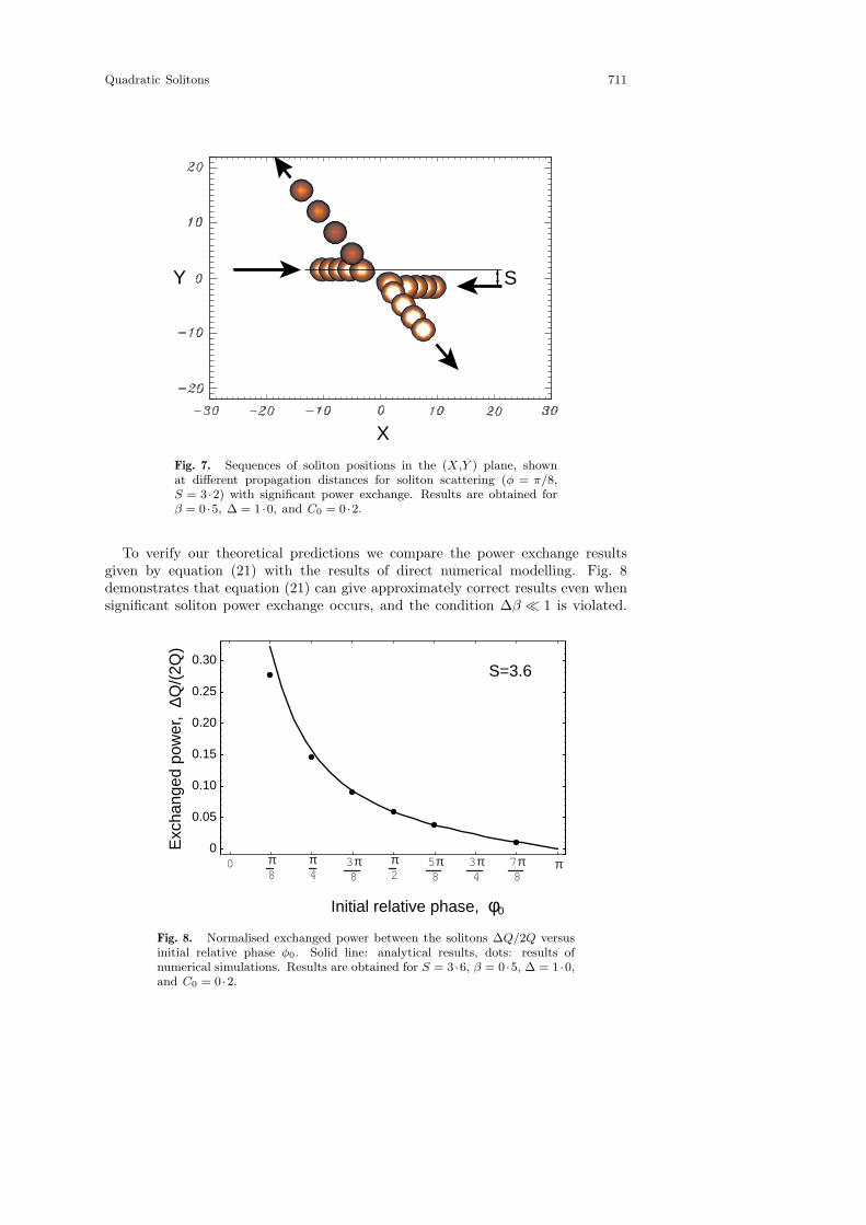
Quadratic Solitons 711
X
Y S
Fig. 7. Sequences of soliton positions in the (X,Y ) plane, shownat different propagation distances for soliton scattering (φ = π/8,S = 3 ·2) with significant power exchange. Results are obtained forβ = 0 ·5, ∆ = 1 ·0, and C0 = 0 ·2.
To verify our theoretical predictions we compare the power exchange resultsgiven by equation (21) with the results of direct numerical modelling. Fig. 8demonstrates that equation (21) can give approximately correct results even whensignificant soliton power exchange occurs, and the condition ∆β ¿ 1 is violated.
Initial relative phase, φ0
Exc
hang
ed p
ower
, ∆Q
/(2Q
)
0
0.05
0.10
0.15
0.20
0.25
0.30
0 π8
π4
3π8
π2
5π8
3π4
7π8
π
S=3.6
Fig. 8. Normalised exchanged power between the solitons ∆Q/2Q versusinitial relative phase φ0. Solid line: analytical results, dots: results ofnumerical simulations. Results are obtained for S = 3 ·6, β = 0 ·5, ∆ = 1 ·0,and C0 = 0 ·2.

712 A. V. Buryak and V. V. Steblina
(3c) Stability of Spiralling Configurations
Using the analytical model, we can investigate the possibility of stable spirallingconfigurations (or bound states) similar to those observed for incoherently interactingphotorefractive solitons (Shih et al . 1997; Buryak et al . 1999). For two (2+1)-dimensional χ(2) solitons interacting coherently with a positive phase mismatchand U1 À U2, the model (13) predicts the existence of a local minimum in Rof the effective interaction potential Ueff(R) at φ = 0 and R0 ∼ 1. However, theapproximate model (13) is valid only for weakly overlapping solitons when R islarge and, therefore, this minimum is physically unrealisable, being located in theregion of soliton fusion. In the opposite situation of negative phase matching,U1 and U2 may become comparable, and in a certain range of parameters wefind a shallow local minimum of the potential Ueff(R) at φ = π and R0 À 1. Aspiralling configuration of two solitons, corresponding to such a local minimum,would be stable if both mass coefficients (masses) were positive. Unfortunately,stability of the single solitons involved in the interaction always requires thatMφ < 0 [see the condition (9)], and therefore this extremum is a saddle pointin the space (R,φ), implying the instability of the corresponding bound states.Indeed, we have not been able to observe such states in extensive direct numericalmodelling of equations (3). We expect this to be a rather general phenomenon,valid for other types of solitary waves interacting coherently, which, however, hasnot been previously addressed in the literature.
4. Physical Estimates
In order to provide parameter values for the experimental observation of χ(2)
soliton collisions, we need to estimate two key parameters, the minimum intensityrequired for soliton formation and the minimum interaction length necessary forthe observation of switching.
An expression estimating the minimum intensity has recently been obtained(Buryak et al . 1997), and is given by
Imin =Gk1
ω51 [χ(2)]2R4
0
, (23)
where R0 is the soliton width [defined in Buryak et al . (1997) as full widthat half maximum for E2 harmonic amplitude], χ(2) is the effective quadraticcoefficient, k1 and ω1 are the wave-number and frequency, respectively, for thefundamental harmonic, and G is a constant that does not depend on the materialor the experimental setup parameters. For example, let us take typical values fortype II SHG in KTP, similar to the ones reported by Torruellas et al . (1995):R0 = 10µm, ω1/c = 6 ·13 × 104 cm−1, k1 = 10 ·5µm−1 and χ(2) = 6 pm V−1.Using the formalism of Buryak et al . (1997), we obtain Imin ≈ 14 ·0 GW cm−2
for (2+1)-dimensional solitons.Our numerical results indicate that the minimum interaction length Lmin
necessary for switching is about 10 normalised propagation distance units, i.e. ofthe order of 10 diffraction lengths. Again, taking the experimental parametersas R0 = 10µm and k1 = 10 ·5µm−1, we can calculate that Rd ≈ 2 mm. Thus theminimum necessary crystal length in physical units is Lmin = 10Rd ≈ 2 cm.

Quadratic Solitons 713
We point out that our values of Imin and Lmin give an estimate from below.Our calculations are based on the assumption that the laser beams initially matchexactly each of the corresponding soliton components. Breaking this condition,e.g. by generating χ(2) solitons without seeding of the second harmonic, shouldslightly increase the required threshold intensity and interaction length. On theother hand, the use of new materials and/or phase-matching techniques can leadto much higher values of the effective χ(2) parameter which, in turn, significantlydecreases Imin, or (if R0 is decreased) Lmin. For example, the use of the so-calledquasi-phase-matching (QPM) technique (see e.g. Fejer et al . 1992; Miller et al .1997) can increase the value of the effective χ(2) parameter for conventionalnonlinear crystals by up to 50 pm V−1, thus lowering the required laser intensityto Imin ∼ 100 MW cm−2. The use of semiconductor optical materials (plusquantum-well-based QPM) can lead to even higher effective χ(2) nonlinearities(Ueno et al . 1997), thus reducing the required Imin further, potentially allowingsoliton-based all-optical switching to be achieved at the intensity level of just afew MW cm−2.
5. Conclusions
In this paper we have analysed non-planar collisions of (2+1)-dimensionalχ(2) solitons and demonstrated a controllable soliton-based all-optical switchingdetermined by the initial soliton states, i.e. the soliton velocities, the relativephase, and the impact parameter. We have derived an effective mechanical modelthat provides a physical description of soliton collisions in terms of an effectiveparticle in a central force. This model has been fully confirmed by the resultsof direct numerical simulations. The phenomena of χ(2) soliton scattering andpower exchange may find applications in ultra-fast all-optical signal processingand switching in a bulk medium. Our approach can be readily generalised forthe analysis of interactions of higher-dimensional solitons (including the so-called‘light bullets’; Malomed et al . 1997) in χ(2) materials and other types of nonlinearmedia.
Acknowledgments
The authors are grateful to Yu. S. Kivshar, B. A. Malomed and M. Segevfor useful discussions and suggestions. Both authors acknowledge support fromthe Australian Research Council.
References
Azimov, B. S., Sukhorukov, A. P., and Truhov, D. V. (1987). Bull. Russ. Acad. Sci. (Phys.)51, 19.
Baek, Y., Schiek, R., and Stegeman, G. I. (1995). Opt. Lett. 20, 2168.Baek, Y., Schiek, R., Stegeman, G. I., Baumann, I., and Sohler, W. (1997). Opt. Lett. 22,
1550.Buryak, A. V., and Kivshar, Yu. S. (1995). Phys. Lett. A 197, 407.Buryak, A. V., and Steblina, V. V. (1999). J. Opt. Soc. Am. B 16, 245.Buryak, A. V., Kivshar, Yu. S., and Steblina, V. V. (1995). Phys. Rev. A 52, 1670.Buryak, A. V., Kivshar, Yu. S., and Trillo, S. (1996). Phys. Rev. Lett. 77, 5210.Buryak, A. V., Kivshar, Yu. S., and Trillo, S. (1997). J. Opt. Soc. Am. B 14, 3110.Buryak, A. V., Kivshar, Yu. S., Shih, M., and Segev, M. (1999). Phys. Rev. Lett. 82, 81.Costantini, B., De Angelis, C., Barthelemy, A., Bourliaguet, B., and Kermene, V. (1998). Opt.
Lett. 23, 424.

714 A. V. Buryak and V. V. Steblina
De Salvo, R., Hagan, D. J., Sheik-Bahae, M., Stegeman, G. I., and Van Stryland, E. W.(1992). Opt. Lett. 17, 28.
Duree, G. C., Shultz, J. L., Salamo, G. J., Segev, M., Yariv, A., Crosignani, B., Di Porto, P.,Sharp, E. J., and Neurgaonkar, R. R. (1993). Phys. Rev. Lett. 71, 553.
Etrich, C., Peschel, U., Lederer, F., Malomed, B., and Kivshar, Yu. S. (1996). Phys. Rev. E54, 4321.
Fejer, M. M., Magel, G. A., Jundt, D. H., and Byer, R. L. (1992). IEEE J. Quant. Electron.28, 2631.
Friberg, S. R., Weiner, A. M., Silberberg, Y., Sfez, B. G., and Smith, P. S. (1988). Opt. Lett.13, 904.
Goldstein, H. (1980). ‘Classical Mechanics’, Chap. 3 (Addison–Wesley: Reading, Mass.).Gorshkov, K. A., and Ostrovsky, L. A. (1981). Physica D 3, 428.Jensen, S. M. (1982). IEEE J. Quant. Electron. QE-18, 1580.Karpman, V. I., and Solov’ev, V. V. (1981). Physica D 3, 487.Kawachi, M. (1990). Opt. Quant. Electron. 22, 391.Leo, G., Assanto, G., and Torruellas, W. E. (1997a). Opt. Commun. 134, 223.Leo, G., Assanto, G., and Torruellas, W. E. (1997b). Opt. Lett. 22, 7.Malomed, B., Drummond, P., He, H., Berntson, A., Anderson, D., and Lisak, M. (1997). Phys.
Rev. E 56, 4725.Menyuk, C. R., Schiek, R., and Torner, L. (1994). J. Opt. Soc. Am. B 11, 2434.Miller, G. D., Batchko, R. G., Tulloch, W. M., Weise, D. R., Fejer, M. M., and Byer, R. L.
(1997). Opt. Lett. 22, 1834.Miller, S. E. (1969). Bell Syst. Tech. J. 48, 2059.Pelinovsky, D. E., Buryak, A. V., and Kivshar, Yu. S. (1995). Phys. Rev. Lett. 75, 591.Schubert, M., and Wilhelmi, B. (1986). ‘Nonlinear Optics and Quantum Electronics’ (Wiley:
New York).Segev, M., and Stegeman, G. I. (1998). Phys. Today 51, 42 and references therein.Shen, T. P., Stegeman, G. I., and Maradudin, A. A. (1988). Appl. Phys. Lett. 52, 1.Shih, M., Segev, M., and Salamo, G. (1997). Phys. Rev. Lett. 78, 2551.Snyder, A. W., and Love, J. D. (1983). ‘Optical Waveguide Theory’ (Chapman and Hall:
London).Snyder, A. W., Buryak, A. V., and Mitchell, D. J. (1998). Opt. Lett. 23, 4.Steblina, V. V., Kivshar, Yu. S., Lisak, M., and Malomed, B. A. (1995). Opt. Commun. 118,
345.Steblina, V. V., Kivshar, Yu. S., and Buryak, A. V. (1998). Opt. Lett. 23, 156.Stegeman, G. I., Wright, E. M., Finlayson, N., Zanoni, R., and Seaton, C. T. (1988). J.
Lightwave Technol. 6, 953.Stegeman, G. I., Hagan, D. J., and Torner, L. (1996). J. Opt. Quant. Electron. 28, 1691.Taha, T. P., and Ablowitz, M. J. (1984). J. Comp. Phys. 55, 203.Tikhonenko, V., Christou, J., and Luther-Davies, B. (1995). J. Opt. Soc. Am. B 12, 2046.Torruellas, W. E., Wang, Z., Hagan, D. J., Van Stryland, E. W., Stegeman, G. I., Torner, L.,
and Menyuk, C. R. (1995). Phys. Rev. Lett. 74, 5036.Ueno, Y., Stegeman, G. I., and Tajima, K. (1997). Jpn J. Appl. Phys. 36, L613.Wa, P. Li Kam, Robson, P. N., Roberts, J. S., Pate, M. A., and David, J. P. R. (1988). Appl.
Phys. Lett. 52, 2013.
Manuscript received 23 December 1998, accepted 6 April 1999