Geodesic equations and their numerical solution in Cartesian coordinates on a triaxial

ellipsoid

G. Panou and R. Korakitis

Department of Surveying Engineering, National Technical University of Athens, Zografou Campus,

15780 Athens, Greece

Abstract: In this work, the geodesic equations and their numerical solution in Cartesian

coordinates on an oblate spheroid, presented by Panou and Korakitis (2017), are generalized on

a triaxial ellipsoid. A new exact analytical method and a new numerical method of converting

Cartesian to ellipsoidal coordinates of a point on a triaxial ellipsoid are presented. An extensive

test set for the coordinate conversion is used, in order to evaluate the performance of the two

methods. The direct geodesic problem on a triaxial ellipsoid is described as an initial value

problem and is solved numerically in Cartesian coordinates. The solution provides the Cartesian

coordinates and the angle between the line of constant 𝜆 and the geodesic, at any point along the

geodesic. Also, the Liouville constant is computed at any point along the geodesic, allowing to

check the precision of the method. An extensive data set of geodesics is used, in order to

demonstrate the validity of the numerical method for the geodesic problem. We conclude that a

complete, stable and precise solution of the problem is accomplished.

Keywords: geometrical geodesy, direct geodesic problem, ellipsoidal coordinates, coordinates

conversion, Liouville’s constant

1. Introduction

It is known that a triaxial ellipsoid is used as a model in geodesy and other interdisciplinary

sciences, even in medicine. For example, it is used as a geometrical and physical model of the

Earth and other celestial objects. Also, it is used as a geometrical model of the cornea and retina

of the human eye (Aguirre 2018). Other applications of a triaxial ellipsoid are mentioned in Panou

et al. (2016).

In order to describe a problem using a triaxial ellipsoid as model, it is necessary to introduce a

triaxial coordinate system (see Panou 2014, Panou et al. 2016). In many applications the

ellipsoidal coordinate system is used, which is a triply orthogonal system. Comments on the

variants of the ellipsoidal coordinates are presented in Panou (2014). It is important that the

ellipsoidal coordinates constitute an orthogonal net of curves on the triaxial ellipsoid.

In this work, the general exact analytical method of converting the Cartesian coordinates to the

ellipsoidal coordinates, presented by Panou (2014), is specified for points exclusively on the

surface of a triaxial ellipsoid. Another exact analytical method is described in Baillard (2013).

Furthermore, a new numerical method of converting the Cartesian coordinates (𝑥, 𝑦, 𝑧) to

ellipsoidal coordinates (𝛽, 𝜆), which is based on the method of least squares, is presented. We

note that another numerical method is developed by Bektaş (2015), which is also presented in

Florinsky (2018). The precision of the exact analytical methods, which involve complex

expressions, suffer when one approaches singular points and/or when executed on a computer

with limited precision. On the other hand, numerical methods, which essentially involve iterative

approximations, can be more precise but the execution time, difficult to predict, may be longer.

Traditionally, there are two problems concerning geodesics on a triaxial ellipsoid: (i) the direct

problem: given a point 𝛴0 on a triaxial ellipsoid, together with a direction 𝛼0 and the geodesic

distance 𝑠01 to a point 𝛴1, determine the point 𝛴1 and the direction 𝛼1 at this point, and (ii) the

inverse problem: given two points 𝛴0 and 𝛴1 on a triaxial ellipsoid, determine the geodesic

distance 𝑠01 between them and the directions 𝛼0, 𝛼1 at the end points. These problems have a

long history, as reviewed by Karney (2018a).

There are several methods of solving the above two problems. In general, the methods make use

of the elliptic integrals presented by Jacobi (1839), where the integrands are expressed in a

variant of the ellipsoidal coordinates, e.g. Bespalov (1980), Klingenberg (1982), Baillard (2013),

Karney (2018b) and include a constant presented by Liouville (1844). On the other hand, there

are methods which make use of the differential equations of the geodesics on a triaxial ellipsoid,

e.g. Holmstrom (1976), Knill and Teodorescu (2009) and Panou (2013). Finally, Shebl and Farag

(2007) use the technique of conformal mapping in order to approximate a geodesic on a triaxial

ellipsoid. Because the elliptic integrals of the classical work of Jacobi (1839) have singularities,

the methods which use them are preferable in the study of the qualitative characteristics of the

geodesics, as presented in Arnold (1989), together with excellent illustrations by Karney

(2018b). On the other hand, differential equations of the geodesics can be directly solved using

an approximate analytical method (Holmstrom 1976) or a numerical method (Knill and

Teodorescu 2009). It is worth emphasizing that, as presented in Panou and Korakitis (2017),

geodesic equations expressed in Cartesian coordinates are insensitive to singularities. Although

Holmstrom (1976) expressed the geodesic equations on a triaxial ellipsoid in Cartesian

coordinates, his approximate analytical solution is of low precision.

In this work, the geodesic equations and their numerical solution in Cartesian coordinates on a

triaxial ellipsoid are presented. Since the numerical solution involves computations at many

points along the geodesic, it can be used as a convenient and efficient approach to trace the full

path of the geodesic. Also, part of this solution constitutes the solution of the direct geodesic

problem. Furthermore, in contrast to Holmstrom (1976), we make use of the ellipsoidal

coordinates which are involved in Liouville equation, allowing to check the precision of the

method.

2. Ellipsoidal to Cartesian coordinates conversion and vice versa

2.1. From ellipsoidal to Cartesian coordinates

A triaxial ellipsoid in Cartesian coordinates is described by

𝑥2

𝑎𝑥2 +

𝑦2

𝑎𝑦2 +

𝑧2

𝑏2 = 1, 0 < 𝑏 < 𝑎𝑦 < 𝑎𝑥 (1)

where 𝑎𝑥, 𝑎𝑦 and 𝑏 are its three semi-axes. The linear eccentricities are given by

𝐸𝑥 = √𝑎𝑥2 − 𝑏2, 𝐸𝑦 = √𝑎𝑦

2 − 𝑏2, 𝐸𝑒 = √𝑎𝑥2 − 𝑎𝑦

2 (2)

with 𝐸𝑒2 = 𝐸𝑥

2 − 𝐸𝑦2. The Cartesian coordinates (𝑥, 𝑦, 𝑧) of a point on the triaxial ellipsoid can be

obtained from the ellipsoidal coordinates (𝛽, 𝜆) by the following expressions (Jacobi 1839)

𝑥 =𝑎𝑥

𝐸𝑥𝐵1 2⁄ 𝑐𝑜𝑠𝜆 (3)

𝑦 = 𝑎𝑦𝑐𝑜𝑠𝛽𝑠𝑖𝑛𝜆 (4)

𝑧 =𝑏

𝐸𝑥𝑠𝑖𝑛𝛽𝐿1 2⁄ (5)

where

𝐵 = 𝐸𝑥2𝑐𝑜𝑠2𝛽 + 𝐸𝑒

2𝑠𝑖𝑛2𝛽 (6)

and

𝐿 = 𝐸𝑥2 − 𝐸𝑒

2𝑐𝑜𝑠2𝜆 (7)

while −𝜋 2⁄ ≤ 𝛽 ≤ +𝜋 2⁄ and −𝜋 < 𝜆 ≤ +𝜋. At the umbilical points, i.e. when 𝛽 = ±𝜋 2⁄ and 𝜆 =

0 or 𝜆 = +𝜋, from Eqs. (3)-(5) we get the Cartesian coordinates 𝑥 = ±𝑎𝑥𝐸𝑒

𝐸𝑥, 𝑦 = 0, 𝑧 = ±𝑏

𝐸𝑦

𝐸𝑥.

Further details on the ellipsoidal coordinates, along with their geometrical interpretation, are

presented in Panou (2014). Finally, in the case of an oblate spheroid, where 𝑎𝑥 = 𝑎𝑦 ≡ 𝑎, i.e. 𝐸𝑥 =

𝐸𝑦 ≡ 𝐸 and 𝐸𝑒 = 0, Eqs. (3)-(5) reduce to well-known expressions (see Heiskanen and Moritz

1967).

2.2. From Cartesian to ellipsoidal coordinates

2.2.1. Exact analytical method

The ellipsoidal coordinates (𝛽, 𝜆) can be obtained from the Cartesian coordinates (𝑥, 𝑦, 𝑧) of a

point on the triaxial ellipsoid by solving the following quadratic equation in 𝑡 (see Panou 2014)

𝑡2 + 𝑐1𝑡 + 𝑐0 = 0 (8)

where

𝑐1 = 𝑥2 + 𝑦2 + 𝑧2 − (𝑎𝑥2 + 𝑎𝑦

2 + 𝑏2) (9)

and

𝑐0 = 𝑎𝑥2𝑎𝑦

2 + 𝑎𝑥2𝑏2 + 𝑎𝑦

2𝑏2 − (𝑎𝑦2 + 𝑏2)𝑥2 − (𝑎𝑥

2 + 𝑏2)𝑦2 − (𝑎𝑥2 + 𝑎𝑦

2)𝑧2 (10)

with two real roots, which can be expressed as

𝑡1 = 𝑐0 𝑡2⁄ (11)

and

𝑡2 = (−𝑐1 + √𝑐12 − 4𝑐0) 2⁄ (12)

The connection between the roots 𝑡1, 𝑡2 and the ellipsoidal coordinates (𝛽, 𝜆) is given by the

relations

𝑡1 = 𝑎𝑦2𝑠𝑖𝑛2𝛽 + 𝑏2𝑐𝑜𝑠2𝛽 (13)

𝑡2 = 𝑎𝑥2𝑠𝑖𝑛2𝜆 + 𝑎𝑦

2𝑐𝑜𝑠2𝜆 (14)

where 𝑏2 ≤ 𝑡1 ≤ 𝑎𝑦2 and 𝑎𝑦

2 ≤ 𝑡2 ≤ 𝑎𝑥2, while 𝑡1 = 𝑡2 = 𝑎𝑦

2 at the umbilical points. Inverting Eqs.

(13) and (14) results in

𝛽 = 𝑎𝑟𝑐𝑡𝑎𝑛 (√𝑡1−𝑏2

𝑎𝑦2−𝑡1

) = 𝑎𝑟𝑐𝑐𝑜𝑡 (√𝑎𝑦

2−𝑡1

𝑡1−𝑏2) (15)

𝜆 = 𝑎𝑟𝑐𝑡𝑎𝑛 (√𝑡2−𝑎𝑦

2

𝑎𝑥2−𝑡2

) = 𝑎𝑟𝑐𝑐𝑜𝑡 (√𝑎𝑥

2−𝑡2

𝑡2−𝑎𝑦2) (16)

where the conventions with regard to the proper quadrant for the 𝛽 and 𝜆 need to be applied

from the signs of 𝑥, 𝑦 and 𝑧. In the case of an oblate spheroid, corresponding expressions have

been presented in Heiskanen and Moritz (1967).

2.2.2. Numerical method

Assuming that the Cartesian coordinates 𝑥, 𝑦 and 𝑧 of a point on the triaxial ellipsoid are

measurements, the method of least squares (Ghilani and Wolf 2006) may be employed to obtain

the best estimates of the ellipsoidal coordinates 𝛽 and 𝜆. This technique requires writing Eqs. (3)-

(5) in the form

𝑎𝑥

𝐸𝑥𝐵1 2⁄ 𝑐𝑜𝑠𝜆 = 𝑥 + 𝜐1 (17)

𝑎𝑦𝑐𝑜𝑠𝛽𝑠𝑖𝑛𝜆 = 𝑦 + 𝜐2 (18)

𝑏

𝐸𝑥𝑠𝑖𝑛𝛽𝐿1 2⁄ = 𝑧 + 𝜐3 (19)

which are non-linear equations and hence the solution process is iterative. This means that

approximate values of ellipsoidal coordinates are assumed, corrections are computed and the

approximate values are updated. The process is repeated until the corrections become negligible.

The linear approximation of Eqs. (17)-(19) can be represented in matrix form as

𝐉 [𝛿𝛽𝛿𝜆

] = 𝛅𝓵 + 𝛖 (20)

where

𝐉 =

[ 𝜕𝑥

𝜕𝛽

𝜕𝑥

𝜕𝜆

𝜕𝑦

𝜕𝛽

𝜕𝑦

𝜕𝜆

𝜕𝑧

𝜕𝛽

𝜕𝑧

𝜕𝜆]

(21)

is a 3 × 2 matrix containing the partial derivatives (Jacobian matrix)

𝜕𝑥

𝜕𝛽= −

𝑎𝑥𝐸𝑦2

2𝐸𝑥

𝑠𝑖𝑛(2𝛽)

𝐵1 2⁄ 𝑐𝑜𝑠𝜆 (22)

𝜕𝑦

𝜕𝛽= −𝑎𝑦𝑠𝑖𝑛𝛽𝑠𝑖𝑛𝜆 (23)

𝜕𝑧

𝜕𝛽=

𝑏

𝐸𝑥𝑐𝑜𝑠𝛽𝐿1 2⁄ (24)

𝜕𝑥

𝜕𝜆= −

𝑎𝑥

𝐸𝑥𝐵1 2⁄ 𝑠𝑖𝑛𝜆 (25)

𝜕𝑦

𝜕𝜆= 𝑎𝑦𝑐𝑜𝑠𝛽𝑐𝑜𝑠𝜆 (26)

𝜕𝑧

𝜕𝜆=

𝑏𝐸𝑒2

2𝐸𝑥𝑠𝑖𝑛𝛽

𝑠𝑖𝑛(2𝜆)

𝐿1 2⁄ (27)

computed from the approximate ellipsoidal coordinates 𝛽0 and 𝜆0,

𝛅𝓵 = [𝑥 − 𝑥0

𝑦 − 𝑦0

𝑧 − 𝑧0

] (28)

is a 3 × 1 vector of terms which are “given Cartesian coordinates – computed Cartesian

coordinates from the approximate ellipsoidal coordinates using Eqs. (3)-(5)” and 𝛖 is a 3 × 1

vector of residuals. The corrections to the approximate ellipsoidal coordinates are the elements

of the solution vector

[𝛿𝛽𝛿𝜆

] = 𝐍−1𝐉T𝛅𝓵 (29)

where

𝐍 = 𝐉T𝐉 = [𝑛11 𝑛12

𝑛21 𝑛22] (30)

and hence

𝐍−1 =1

𝑛11𝑛22−𝑛12𝑛21[

𝑛22 −𝑛12

−𝑛21 𝑛11] (31)

One should note that the determinant of matrix 𝐍 (𝑛11𝑛22 − 𝑛12𝑛21) equals zero at the umbilical

points. The updated values of the approximate ellipsoidal coordinates are

[𝛽𝜆] = [

𝛽0

𝜆0] + [

𝛿𝛽𝛿𝜆

] (32)

The residuals are computed from Eq. (20) and an estimate of the variance factor �̂�02 can be

computed using the following equation

�̂�02 = 𝛖T𝛖 (33)

The iterative process is terminated when the corrections 𝛿𝛽 and 𝛿𝜆 become negligible. Another

criterion of ending the iterative process is the convergence of the variance factor �̂�02 which, in the

case of measurements of equal precision, is an estimate of the variance of the Cartesian

coordinates computed from the adjustment (a posteriori). Finally, the variance-covariance matrix

of the computed ellipsoidal coordinates is given by

�̂�[𝛽𝜆]= �̂�0

2𝐍−1 (34)

Comparing the previous two methods, we note that the operations in the exact analytical method

lead to a loss of accuracy for points near the planes 𝑥 = 0, 𝑦 = 0 and 𝑧 = 0. Also, the importance

of the numerical method is that we avoid the degeneracy of the variable 𝑡2 in Eq. (16), which may

yield inaccurate results, since the intervals of variation of the coordinates 𝛽 and 𝜆 remain

invariants as a triaxial ellipsoid transforms to an oblate spheroid, where 𝑡2 = 𝑎2. Therefore, the

values resulting from the exact analytical method can be considered as initial, approximate

ellipsoidal coordinates in the numerical method. However, because Eqs. (3)-(5) are numerically

stable, the results of both methods can be checked by comparing the resulting Cartesian

coordinates (𝑥0, 𝑦0, 𝑧0) with the given Cartesian coordinates (𝑥, 𝑦, 𝑧), e.g. by the simple formula

𝛿𝑟 = √(𝑥 − 𝑥0)2 + (𝑦 − 𝑦0)2 + (𝑧 − 𝑧0)2 (35)

3. Geodesic equations

The geodesic initial value problem, expressed in Cartesian coordinates on a triaxial ellipsoid,

consists of determining a geodesic, parametrized by its arc length 𝑠, 𝑥 = 𝑥(𝑠), 𝑦 = 𝑦(𝑠), 𝑧 = 𝑧(𝑠),

with angles 𝛼 = 𝛼(𝑠) along it, between the line of constant 𝜆 and the geodesic, which passes

through a given point 𝛴0(𝑥(0), 𝑦(0), 𝑧(0)) in a known direction (given angle 𝛼0 = 𝛼(0)) and has

a certain length 𝑠01.

Now, we consider a triaxial ellipsoid which is described in Cartesian coordinates (𝑥, 𝑦, 𝑧) by

𝑆(𝑥, 𝑦, 𝑧) =̇ 𝑥2 +𝑦2

1−𝑒𝑒2 +

𝑧2

1−𝑒𝑥2 − 𝑎𝑥

2 = 0 (36)

where the squared eccentricities 𝑒𝑥2 and 𝑒𝑒

2 are given by

𝑒𝑥2 = (𝑎𝑥

2 − 𝑏2) 𝑎𝑥2⁄ , 𝑒𝑒

2 = (𝑎𝑥2 − 𝑎𝑦

2) 𝑎𝑥2⁄ (37)

It is well-known, from the theory of differential geometry, that the principal normal to the

geodesic must coincide with the normal to the triaxial ellipsoid (Struik 1961), i.e.

𝑑2𝑥 𝑑𝑠2⁄

𝜕𝑆 𝜕𝑥⁄=

𝑑2𝑦 𝑑𝑠2⁄

𝜕𝑆 𝜕𝑦⁄=

𝑑2𝑧 𝑑𝑠2⁄

𝜕𝑆 𝜕𝑧⁄= −𝑚 (38)

where 𝑚 is a function of 𝑠. From these equations, together with Eq. (36), it is possible to

determine 𝑥(𝑠), 𝑦(𝑠), 𝑧(𝑠) and 𝑚(𝑠). Using Eq. (36), Eqs. (38) become

1

𝑥

𝑑2𝑥

𝑑𝑠2 =1−𝑒𝑒

2

𝑦

𝑑2𝑦

𝑑𝑠2 =1−𝑒𝑥

2

𝑧

𝑑2𝑧

𝑑𝑠2 = −2𝑚 (39)

Differentiating Eq. (36), we have

𝑥𝑑𝑥

𝑑𝑠+

𝑦

1−𝑒𝑒2

𝑑𝑦

𝑑𝑠+

𝑧

1−𝑒𝑥2

𝑑𝑧

𝑑𝑠= 0 (40)

and a further differentiation yields

𝑥𝑑2𝑥

𝑑𝑠2 +𝑦

1−𝑒𝑒2

𝑑2𝑦

𝑑𝑠2 +𝑧

1−𝑒𝑥2

𝑑2𝑧

𝑑𝑠2 = −[(𝑑𝑥

𝑑𝑠)2+

1

1−𝑒𝑒2 (

𝑑𝑦

𝑑𝑠)2+

1

1−𝑒𝑥2 (

𝑑𝑧

𝑑𝑠)2] (41)

Hence, from Eqs. (39) and (41), we obtain

𝑚 =ℎ

2𝐻 (42)

where

𝐻 = 𝑥2 +𝑦2

(1−𝑒𝑒2)

2 +𝑧2

(1−𝑒𝑥2)

2 (43)

and

ℎ = (𝑑𝑥

𝑑𝑠)2+

1

1−𝑒𝑒2 (

𝑑𝑦

𝑑𝑠)2+

1

1−𝑒𝑥2 (

𝑑𝑧

𝑑𝑠)2

(44)

Substituting Eq. (42) into Eqs. (39), we obtain the geodesic equations in Cartesian coordinates on

a triaxial ellipsoid

𝑑2𝑥

𝑑𝑠2 +ℎ

𝐻𝑥 = 0 (45)

𝑑2𝑦

𝑑𝑠2 +ℎ

𝐻

𝑦

1−𝑒𝑒2 = 0 (46)

𝑑2𝑧

𝑑𝑠2 +ℎ

𝐻

𝑧

1−𝑒𝑥2 = 0 (47)

which are subject to the initial conditions

𝑥0 = 𝑥(0), 𝑑𝑥

𝑑𝑠|0

=𝑑𝑥

𝑑𝑠(0) (48)

𝑦0 = 𝑦(0), 𝑑𝑦

𝑑𝑠|0

=𝑑𝑦

𝑑𝑠(0) (49)

𝑧0 = 𝑧(0), 𝑑𝑧

𝑑𝑠|0

=𝑑𝑧

𝑑𝑠(0) (50)

where expressions for the values of the derivatives at point 𝛴0(𝑥0, 𝑦0, 𝑧0) are produced below.

Hence, the direct geodesic problem is described as an initial value problem in Cartesian

coordinates on a triaxial ellipsoid by Eqs. (45) to (50).

4. Numerical solution

In order to solve the above problem, the system of three non-linear second order ordinary

differential equations (Eqs. (45) to (47)) is rewritten as a system of six first-order differential

equations:

𝑑

𝑑𝑠(𝑥) =

𝑑𝑥

𝑑𝑠 (51)

𝑑

𝑑𝑠(𝑑𝑥

𝑑𝑠) = −

ℎ

𝐻𝑥 (52)

𝑑

𝑑𝑠(𝑦) =

𝑑𝑦

𝑑𝑠 (53)

𝑑

𝑑𝑠(𝑑𝑦

𝑑𝑠) = −

ℎ

𝐻

𝑦

1−𝑒𝑒2 (54)

𝑑

𝑑𝑠(𝑧) =

𝑑𝑧

𝑑𝑠 (55)

𝑑

𝑑𝑠(𝑑𝑧

𝑑𝑠) = −

ℎ

𝐻

𝑧

1−𝑒𝑥2 (56)

This system can be integrated on the interval [0, 𝑠] using a numerical method, such as Runge-

Kutta (see Butcher 1987). The step size 𝛿𝑠 is given by 𝛿𝑠 = 𝑠 𝑛⁄ , where 𝑛 is the number of steps.

For the variables 𝑥, 𝑦 and 𝑧, the initial conditions are 𝑥0, 𝑦0 and 𝑧0, respectively. To obtain the

required derivatives, we proceed to describe the unit vectors to a geodesic through a point

𝛴(𝑥, 𝑦, 𝑧) on a triaxial ellipsoid (see Fig. 1).

Figure 1: Unit vectors to a geodesic through a point 𝛴 on a triaxial ellipsoid: 𝛔 tangent to the

geodesic, 𝐧 normal to the triaxial ellipsoid, 𝐩 tangent to the line of constant 𝛽, 𝐪 tangent to the

line of constant 𝜆.

Let 𝛔 be a unit vector tangent to an arbitrary geodesic through 𝛴. Then, we can express 𝛔 in terms

of the unit vectors 𝐩, 𝐪 and the angle 𝛼 between the line of constant 𝜆 and the geodesic (Fig. 1):

𝛔 = (𝑑𝑥

𝑑𝑠,𝑑𝑦

𝑑𝑠,𝑑𝑧

𝑑𝑠) = 𝐩𝑠𝑖𝑛𝛼 + 𝐪𝑐𝑜𝑠𝛼 (57)

The unit vector normal to a triaxial ellipsoid (using the gradient operator and Eqs. (36), (43)) can

be expressed as (Fig. 1):

𝐧 = (𝑛1, 𝑛2, 𝑛3) = (𝑥

𝐻1 2⁄ ,𝑦

(1−𝑒𝑒2)𝐻1 2⁄ ,

𝑧

(1−𝑒𝑥2)𝐻1 2⁄ ) (58)

The unit vector 𝐩 = (𝑝1, 𝑝2, 𝑝3), tangent to the line of constant 𝛽, can be determined using Eqs.

(25)-(27) and Eqs. (7) and (14) (Fig. 1):

𝑝1 = −(𝐿

𝐹𝑡2)1 2⁄ 𝑎𝑥

𝐸𝑥𝐵1 2⁄ 𝑠𝑖𝑛𝜆 (59)

𝑝2 = (𝐿

𝐹𝑡2)1 2⁄

𝑎𝑦𝑐𝑜𝑠𝛽𝑐𝑜𝑠𝜆 (60)

𝑝3 =1

(𝐹𝑡2)1 2⁄

𝑏𝐸𝑒2

2𝐸𝑥𝑠𝑖𝑛𝛽𝑠𝑖𝑛(2𝜆) (61)

where

𝐹 = 𝐸𝑦2𝑐𝑜𝑠2𝛽 + 𝐸𝑒

2𝑠𝑖𝑛2𝜆 (62)

Also, this vector can be expressed in terms of Cartesian coordinates with the help of Eqs. (13) and

(14):

𝑝1 = −𝑠𝑔𝑛(𝑦) (𝐿

𝐹𝑡2)1 2⁄ 𝑎𝑥

𝐸𝑥𝐸𝑒𝐵1 2⁄ √𝑡2 − 𝑎𝑦

2 (63)

𝑝2 = 𝑠𝑔𝑛(𝑥) (𝐿

𝐹𝑡2)1 2⁄ 𝑎𝑦

𝐸𝑦𝐸𝑒√(𝑎𝑦

2 − 𝑡1)(𝑎𝑥2 − 𝑡2) (64)

𝑝3 = 𝑠𝑔𝑛(𝑥)𝑠𝑔𝑛(𝑦)𝑠𝑔𝑛(𝑧)1

(𝐹𝑡2)1 2⁄

𝑏

𝐸𝑥𝐸𝑦√(𝑡1 − 𝑏2)(𝑡2 − 𝑎𝑦

2)(𝑎𝑥2 − 𝑡2) (65)

where

𝐵 =𝐸𝑥

2

𝐸𝑦2 (𝑎𝑦

2 − 𝑡1) +𝐸𝑒

2

𝐸𝑦2 (𝑡1 − 𝑏2) (66)

𝐿 = 𝑡2 − 𝑏2 (67)

and

𝐹 = 𝑡2 − 𝑡1 (68)

while 𝑠𝑔𝑛(𝑥) = 1 if 𝑥 > 0, 𝑠𝑔𝑛(𝑥) = −1 if 𝑥 < 0 and 𝑠𝑔𝑛(0) = 0 .

However, vector 𝐩 has singularities at the umbilical points, where we can simply set 𝐩 =

(𝑝1, 𝑝2, 𝑝3) = (0,±1, 0). Finally, in the case of an oblate spheroid, Eqs. (59)-(61) reduce to the

expressions (Panou and Korakitis 2017)

𝐩 = (𝑝1, 𝑝2, 𝑝3) = (−𝑠𝑖𝑛𝜆, 𝑐𝑜𝑠𝜆, 0) (69)

and Eqs. (63)-(65) can be replaced by

𝐩 = (𝑝1, 𝑝2, 𝑝3) = (−𝑦

√𝑥2+𝑦2,

𝑥

√𝑥2+𝑦2, 0) (70)

The unit vector 𝐪 = (𝑞1, 𝑞2, 𝑞3), tangent to the line of constant 𝜆, can now be determined as the

cross product of unit vectors 𝐧 and 𝐩, i.e. 𝐪 = 𝐧 × 𝐩 (Fig. 1):

𝑞1 = 𝑛2𝑝3 − 𝑛3𝑝2 (71)

𝑞2 = 𝑛3𝑝1 − 𝑛1𝑝3 (72)

𝑞3 = 𝑛1𝑝2 − 𝑛2𝑝1 (73)

Finally, substituting the vectors 𝐩 and 𝐪 into Eq. (57), we obtain the required values of the

derivatives at point 𝛴0(𝑥0, 𝑦0, 𝑧0)

𝑑𝑥

𝑑𝑠|0

= 𝑝1(0)𝑠𝑖𝑛𝛼0 + 𝑞1(0)𝑐𝑜𝑠𝛼0 (74)

𝑑𝑦

𝑑𝑠|0

= 𝑝2(0)𝑠𝑖𝑛𝛼0 + 𝑞2(0)𝑐𝑜𝑠𝛼0 (75)

𝑑𝑧

𝑑𝑠|0

= 𝑝3(0)𝑠𝑖𝑛𝛼0 + 𝑞3(0)𝑐𝑜𝑠𝛼0 (76)

5. Angles and Liouville’s constant

Taking the scalar product of Eq. (57) successively with 𝐩 and 𝐪 and dividing the resulting

equations, yields the angle at which the geodesic cuts the curve of constant 𝜆

𝛼 = 𝑎𝑟𝑐𝑡𝑎𝑛 (𝑃

𝑄) = 𝑎𝑟𝑐𝑐𝑜𝑡 (

𝑄

𝑃) (77)

where

𝑃 = 𝐩 · 𝛔 = 𝑝1𝑑𝑥

𝑑𝑠+ 𝑝2

𝑑𝑦

𝑑𝑠+ 𝑝3

𝑑𝑧

𝑑𝑠 (78)

𝑄 = 𝐪 · 𝛔 = 𝑞1𝑑𝑥

𝑑𝑠+ 𝑞2

𝑑𝑦

𝑑𝑠+ 𝑞3

𝑑𝑧

𝑑𝑠 (79)

Note that Eqs. (77) involve all the variables 𝑥, 𝑑𝑥 𝑑𝑠⁄ , 𝑦, 𝑑𝑦 𝑑𝑠⁄ , 𝑧 and 𝑑𝑧 𝑑𝑠⁄ , which are obtained

by the numerical integration.

Along a geodesic on a triaxial ellipsoid, the Liouville equation holds (Liouville 1844)

𝐸𝑦2𝑐𝑜𝑠2𝛽𝑠𝑖𝑛2𝛼 − 𝐸𝑒

2𝑠𝑖𝑛2𝜆𝑐𝑜𝑠2𝛼 = 𝑐 (80)

where 𝑐 is the Liouville constant. Also, this equation can be expressed in terms of Cartesian

coordinates with the help of Eqs. (13) and (14):

𝑎𝑦2 − (𝑡1𝑠𝑖𝑛

2𝛼 + 𝑡2𝑐𝑜𝑠2𝛼) = 𝑐 (81)

At any value of the independent variable 𝑠, we can estimate the difference 𝛿𝑐 = 𝑐 − 𝑐0 between

the computed value 𝑐 and the known value 𝑐0 at point 𝛴0, from the given 𝛽0, 𝜆0 and 𝛼0, by means

of Liouville’s equation (Eq. (80)). Furthermore, because the numerical integration is performed

in space, we can compute, at any value of 𝑠, the function 𝑆, given by Eq. (36). Therefore, we can

check both the precision of the method and of the numerical integration, since the difference 𝛿𝑐

and the function 𝑆 should be zero (meters squared) at any point along the geodesic on a triaxial

ellipsoid.

6. Numerical experiments

6.1. Test set for coordinates conversion

In order to validate the two methods of conversion presented above and to evaluate their

performance, we used an extensive test set of points. This is a set of 1725 points on a triaxial

ellipsoid, distributed into ten groups, as described in Table 1, where N stands for the number of

points in each group. For simplicity and without loss of generality, 𝛽 and 𝜆 were chosen in

[0°, 90°].

Table 1: Description of the points in the test set

Group 𝛽 𝜆 Case Ν 1 5° − 85° every 5° 5° − 85° every 5° 1st octant 289 2 0° 0° − 90° every 5° 𝑥𝑦 − plane 19 3 5° − 85° every 5° 0° 𝑥𝑧 − plane 17 4 90° 5° − 90° every 5 18 5 89.0° − 89.9…9°

up to 14 decimals 1.0° − 0.0…1° up

to 14 decimals near umbilic 225

6 5° − 85° every 5° 90° 𝑦𝑧 − plane 17 7 1.0° − 0.0…1° up

to 14 decimals 0° − 90° every 5° near 𝑥𝑦 − plane 285

8 0° − 90° every 5° 1.0° − 0.0…1° up to 14 decimals

near 𝑥𝑧 − plane 285

9 89.0° − 89.9…9° up to 14 decimals

0° − 90° every 5° 285

10 0° − 90° every 5° 89.0° − 89.9…9° up to 14 decimals

near 𝑦𝑧 − plane 285

Using a triaxial ellipsoid with 𝑎𝑥 = 6378172 m, 𝑎𝑦 = 6378103 m and 𝑏 = 6356753 m, (Ligas

2012) the Cartesian coordinates for any point were computed using Eqs. (3)-(5).

All algorithms were coded in C++, were compiled by the open-source GNU GCC compiler (at Level

2 optimization) and employing the open-source “libquadmath”, the GCC Quad-Precision Math

Library, which provides a precision of 33 digits. In contrast, use of the C++ long-double standard

type (referred simply as double in the following sections) provides a precision of 18 digits. The

codes were executed on a personal computer running a 64-bit Linux Debian operating system.

The main characteristics of the hardware were: Intel Core i5-2430M CPU (clocked at 2.4 GHz)

and 6 GB of RAM.

6.1.1. Results

The exact analytical method was applied using double and quad precision and the Cartesian

coordinates 𝑥, 𝑦 and 𝑧 as input data. From the resulting 𝛽0 and 𝜆0 at any point, we computed the

differences 𝛿𝛽 = 𝛽 − 𝛽0 and 𝛿𝜆 = 𝜆 − 𝜆0 and recorded the 𝑚𝑎𝑥|𝛿𝛽| and the 𝑚𝑎𝑥|𝛿𝜆| for every

Group. Furthermore, the results at any point were converted back to Cartesian coordinates, we

computed the value 𝛿𝑟 using Eq. (35) and recorded the 𝑚𝑎𝑥|𝛿𝑟| for every Group. All results are

presented in Table 2.

Table 2: Performance of the exact analytical method using double and quad precision

Group double quad 𝑚𝑎𝑥|𝛿𝛽| (") 𝑚𝑎𝑥|𝛿𝜆| (") 𝑚𝑎𝑥𝛿𝑟 (m) 𝑚𝑎𝑥|𝛿𝛽| (") 𝑚𝑎𝑥|𝛿𝜆| (") 𝑚𝑎𝑥𝛿𝑟 (m)

1 1.27 · 10−6 1.38 · 10−4 4.13 · 10−4 5.14 · 10−21 1.04 · 10−18 2.80 · 10−18

2 1.66 · 10−2 1.54 · 10−1 4.78 1.05 · 10−9 9.45 · 10−21 3.23 · 10−8

3 5.40 · 10−7 2.44 8.44 4.62 · 10−21 6.44 · 10−8 6.55 · 10−7 4 9.32 · 10−1 1.46 · 10−2 6.44 1.41 · 10−7 1.72 · 10−16 6.33 · 10−7 5 50.6 8.90 · 102 8.08 1.63 · 10−2 2.86 · 10−1 6.97 · 10−7 6 1.24 · 10−7 5.24 · 10−1 8.33 3.27 · 10−21 1.04 · 10−7 5.87 · 10−7 7 1.81 · 10−2 3.10 · 10−1 9.59 1.05 · 10−9 1.89 · 10−8 5.85 · 10−7 8 50.6 8.90 · 102 10.6 1.55 · 10−2 2.50 · 10−1 7.11 · 10−7 9 50.6 8.90 · 102 10.8 1.63 · 10−2 2.86 · 10−1 6.97 · 10−7

10 2.01 · 10−1 3.56 10.4 2.16 · 10−8 1.97 · 10−7 6.68 · 10−7

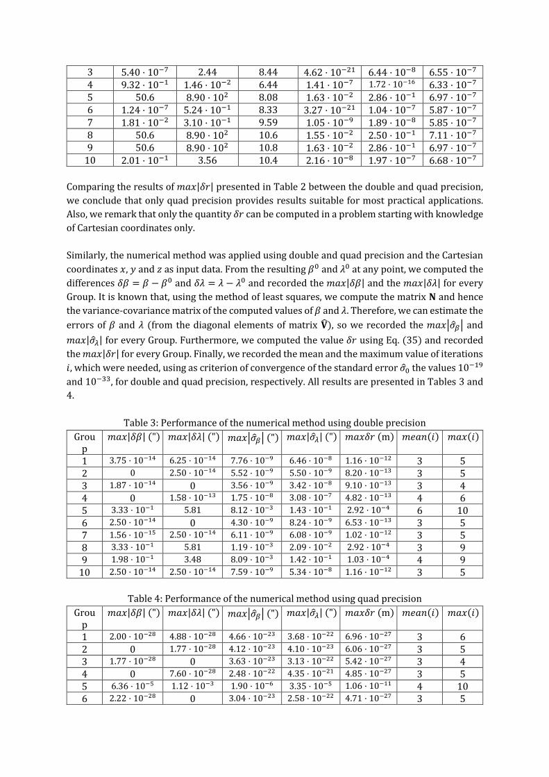
Comparing the results of 𝑚𝑎𝑥|𝛿𝑟| presented in Table 2 between the double and quad precision,

we conclude that only quad precision provides results suitable for most practical applications.

Also, we remark that only the quantity 𝛿𝑟 can be computed in a problem starting with knowledge

of Cartesian coordinates only.

Similarly, the numerical method was applied using double and quad precision and the Cartesian

coordinates 𝑥, 𝑦 and 𝑧 as input data. From the resulting 𝛽0 and 𝜆0 at any point, we computed the

differences 𝛿𝛽 = 𝛽 − 𝛽0 and 𝛿𝜆 = 𝜆 − 𝜆0 and recorded the 𝑚𝑎𝑥|𝛿𝛽| and the 𝑚𝑎𝑥|𝛿𝜆| for every

Group. It is known that, using the method of least squares, we compute the matrix 𝐍 and hence

the variance-covariance matrix of the computed values of 𝛽 and 𝜆. Therefore, we can estimate the

errors of 𝛽 and 𝜆 (from the diagonal elements of matrix �̂�), so we recorded the 𝑚𝑎𝑥|�̂�𝛽| and

𝑚𝑎𝑥|�̂�𝜆| for every Group. Furthermore, we computed the value 𝛿𝑟 using Eq. (35) and recorded

the 𝑚𝑎𝑥|𝛿𝑟| for every Group. Finally, we recorded the mean and the maximum value of iterations

𝑖, which were needed, using as criterion of convergence of the standard error �̂�0 the values 10−19

and 10−33, for double and quad precision, respectively. All results are presented in Tables 3 and

4.

Table 3: Performance of the numerical method using double precision

Group

𝑚𝑎𝑥|𝛿𝛽| (") 𝑚𝑎𝑥|𝛿𝜆| (") 𝑚𝑎𝑥|�̂�𝛽| (") 𝑚𝑎𝑥|�̂�𝜆| (") 𝑚𝑎𝑥𝛿𝑟 (m) 𝑚𝑒𝑎𝑛(𝑖) 𝑚𝑎𝑥(𝑖)

1 3.75 · 10−14 6.25 · 10−14 7.76 · 10−9 6.46 · 10−8 1.16 · 10−12 3 5 2 0 2.50 · 10−14 5.52 · 10−9 5.50 · 10−9 8.20 · 10−13 3 5 3 1.87 · 10−14 0 3.56 · 10−9 3.42 · 10−8 9.10 · 10−13 3 4 4 0 1.58 · 10−13 1.75 · 10−8 3.08 · 10−7 4.82 · 10−13 4 6 5 3.33 · 10−1 5.81 8.12 · 10−3 1.43 · 10−1 2.92 · 10−4 6 10 6 2.50 · 10−14 0 4.30 · 10−9 8.24 · 10−9 6.53 · 10−13 3 5 7 1.56 · 10−15 2.50 · 10−14 6.11 · 10−9 6.08 · 10−9 1.02 · 10−12 3 5 8 3.33 · 10−1 5.81 1.19 · 10−3 2.09 · 10−2 2.92 · 10−4 3 9 9 1.98 · 10−1 3.48 8.09 · 10−3 1.42 · 10−1 1.03 · 10−4 4 9

10 2.50 · 10−14 2.50 · 10−14 7.59 · 10−9 5.34 · 10−8 1.16 · 10−12 3 5

Table 4: Performance of the numerical method using quad precision

Group

𝑚𝑎𝑥|𝛿𝛽| (") 𝑚𝑎𝑥|𝛿𝜆| (") 𝑚𝑎𝑥|�̂�𝛽| (") 𝑚𝑎𝑥|�̂�𝜆| (") 𝑚𝑎𝑥𝛿𝑟 (m) 𝑚𝑒𝑎𝑛(𝑖) 𝑚𝑎𝑥(𝑖)

1 2.00 · 10−28 4.88 · 10−28 4.66 · 10−23 3.68 · 10−22 6.96 · 10−27 3 6 2 0 1.77 · 10−28 4.12 · 10−23 4.10 · 10−23 6.06 · 10−27 3 5 3 1.77 · 10−28 0 3.63 · 10−23 3.13 · 10−22 5.42 · 10−27 3 4 4 0 7.60 · 10−28 2.48 · 10−22 4.35 · 10−21 4.85 · 10−27 3 5 5 6.36 · 10−5 1.12 · 10−3 1.90 · 10−6 3.35 · 10−5 1.06 · 10−11 4 10 6 2.22 · 10−28 0 3.04 · 10−23 2.58 · 10−22 4.71 · 10−27 3 5

7 1.80 · 10−29 2.22 · 10−28 3.95 · 10−23 3.94 · 10−23 6.51 · 10−27 3 5 8 5.55 · 10−5 9.76 · 10−4 8.45 · 10−11 1.48 · 10−9 8.13 · 10−12 3 9 9 6.83 · 10−5 1.20 · 10−3 3.01 · 10−10 5.28 · 10−9 1.23 · 10−11 3 8

10 2.22 · 10−28 8.87 · 10−29 4.49 · 10−23 5.69 · 10−22 6.72 · 10−27 3 6

Comparing the results of 𝑚𝑎𝑥|𝛿𝑟| presented in Tables 3 and 4 between the double and quad

precision, we conclude that both precisions can give results suitable for most practical

applications (better than 1 mm for double and 1 nm for quad precision).

6.2. Data set for geodesics

In order to evaluate the performance of the presented method with respect to stability and

precision, we used an extensive data set of 150000 geodesics for a triaxial ellipsoid with 𝑎𝑥 =

6378172 m, 𝑎𝑦 = 6378103 m and 𝑏 = 6356753 m (Ligas 2012). The geodesics of the set were

distributed into five groups (A – E) with different qualitative characteristics, as described in

Tables 5 – 9. Each geodesic of the data set was defined by the values of 𝛽0 (in degrees), 𝜆0 (in

degrees), 𝛼0 (clockwise from 𝜆 = constant in degrees) and 𝑠01 (in meters). Furthermore, 𝛽0, 𝜆0

and 𝛼0 were taken to be multiples of 10−12 deg and 𝑠01 a multiple of 0.1 μm in

[0 m, 20003987.55893028 m], where the upper bound for the 𝑠01 is the geodesic distance

between opposite umbilical points (i.e. the half arc length of the ellipse with axes 𝑎𝑥 and 𝑏).

Table 5: Description of the geodesics in the Group A

Group A: 𝛽0 ∈ (0°, 90°), 𝜆0 = −90°, 𝛼0 ∈ [0°, 180°]

Subgroup Case Number

A.1 randomly distributed 5000

A.2 nearly antipodal 5000

A.3 short distances 5000

A.4 𝛽0 ≅ 90° (one end near 𝑧 = 𝑏) 5000

A.5 𝛽0 ≅ 90° & 𝑠01 ≅ 20003879 m

(both ends near opposite 𝑧 = 𝑏)

5000

A.6 𝛼0 ≅ 0° or 𝛼0 ≅ 180° 5000

A.7 𝛽0 ≅ 0° & 𝛼0 ≅ 90° 5000

A.8 𝛼0 ≅ 90° 5000

A.9 𝛼0 = 90° 5000

Table 6: Description of the geodesics in the Group B

Group B: 𝛽0 ∈ (0°, 90°), 𝜆0 = 0°, 𝛼0 ∈ [0°, 180°], 𝑐0 ≥ 0

Subgroup Case Number

B.1 randomly distributed 5000

B.2 nearly antipodal 5000

B.3 short distances 5000

B.4 𝛽0 ≅ 90° (one end near an umbilic point) 5000

B.5 𝛽0 ≅ 90° & 𝑠01 ≅ 20003988 m

(both ends near opposite umbilical points)

5000

B.6 𝛼0 ≅ 0° or 𝛼0 ≅ 180° 5000

B.7 𝛽0 ≅ 0° & 𝛼0 ≅ 90° 5000

B.8 𝛼0 ≅ 90° 5000

B.9 𝛼0 = 90° 5000

Table 7: Description of the geodesics in the Group C

Group C: 𝛽0 = 90°, 𝜆0 ∈ (0°, 90°], 𝛼0 ∈ [90°, 270°], 𝑐0 ≤ 0

Subgroup Case Number

C.1 randomly distributed 5000

C.2 nearly antipodal 5000

C.3 short distances 5000

C.4 𝜆0 ≅ 90° (one end near 𝑧 = 𝑏) 5000

C.5 𝜆0 ≅ 0° (one end near an umbilic point) 5000

C.6 𝜆0 ≅ 90° & 𝑠01 ≅ 20003879 m

(both ends near opposite 𝑧 = 𝑏)

5000

C.7 𝜆0 ≅ 0° & 𝑠01 ≅ 20003988 m

(both ends near opposite umbilical points)

5000

C.8 𝜆0 = 45° & 𝛼0 ≅ 180° 5000

C.9 𝛼0 = 90° 5000

Table 8: Description of the geodesics in the Group D

Group D (Umbilical geodesics): 𝛽0 = 90°, 𝜆0 = 0°, 𝛼0 ∈ [0°, 180°], 𝑐0 = 0

Subgroup Case Number

D.1 randomly distributed 4639

D.2 𝛼0 every 0.5°, 𝑠01 = 20003987.55893028 m 361

Table 9: Description of the geodesics in the Group E

Group E: 𝛽0 ∈ (−90°, 90°), 𝜆0 ∈ (−180°, 180°), 𝛼0 ∈ (0°, 360°),

𝑠01 ∈ (1000 m, 20003879 m)

Case Number

randomly distributed 10000

6.2.1. Results

The direct geodesic problem in Cartesian coordinates was solved using the input data 𝛽0, 𝜆0, 𝛼0

and 𝑠01. At the starting point, the Cartesian coordinates (𝑥0, 𝑦0, 𝑧0) were computed using Eqs. (3)-

(5) and the Liouville constant 𝑐0 using Eq. (80). For each geodesic in the data set, the unit vector

𝐩 was computed using Eqs. (59)-(61) and the system of first-order differential equations (Eqs.

(51)-(56)) was integrated using the fourth-order Runge-Kutta numerical method (see Butcher

1987) with 20000 steps. This number of steps was chosen because the effects of the number of

steps for the same problem on an oblate spheroid were studied in the work of Panou and Korakitis

(2017). All algorithms were coded and executed on the system described in section 6.1.

The results 𝑥1, 𝑦1 and 𝑧1 at the end point were converted to ellipsoidal coordinates 𝛽1 and 𝜆1 using

the numerical method of subsection 2.2.2. Then, the unit vector 𝐩 was computed using Eqs. (59)-

(61) and the angle 𝛼1 from Eq. (77). Also, the Liouville constant 𝑐1 was computed using Eq. (80)

and the difference 𝛿𝑐1 = 𝑐1 − 𝑐0 recorded. Furthermore, we recorded the value 𝑆1 of the function

𝑆, given by Eq. (36). Detailed results of the maximum values of |𝛿𝑐1| and |𝑆1| for each subgroup

in double and quad precision are presented in Tables 10 – 14. We emphasize that the value of 𝑆1

is affected by the precision of the numerical integration (which depends on the number of steps),

while the value of 𝛿𝑐1 is mostly affected by the errors of the conversion of Cartesian to ellipsoidal

coordinates at the end point.

Table 10: Results in the Group A

Subgroup double quad

𝑚𝑎𝑥|𝛿𝑐1| (m2) 𝑚𝑎𝑥|𝑆1| (m

2) 𝑚𝑎𝑥|𝛿𝑐1| (m2) 𝑚𝑎𝑥|𝑆1| (m

2)

A.1 1.83 · 10−6 1.21 · 10−3 1.17 · 10−11 5.05 · 10−7

A.2 1.59 · 10−6 1.20 · 10−3 6.07 · 10−12 5.32 · 10−7

A.3 5.07 · 10−5 2.23 · 10−2 3.63 · 10−21 1.42 · 10−18

A.4 6.00 · 10−9 1.21 · 10−3 1.37 · 10−16 4.86 · 10−7

A.5 5.65 · 10−9 1.29 · 10−3 6.13 · 10−17 5.18 · 10−7

A.6 2.33 · 10−10 1.06 · 10−3 1.50 · 10−19 4.67 · 10−7

A.7 7.45 · 10−8 1.07 · 10−3 2.09 · 10−19 1.66 · 10−7

A.8 1.86 · 10−6 1.30 · 10−3 9.19 · 10−12 4.68 · 10−7

A.9 2.65 · 10−6 1.29 · 10−3 9.17 · 10−12 5.18 · 10−7

Table 11: Results in the Group B

Subgroup double quad

𝑚𝑎𝑥|𝛿𝑐1| (m2) 𝑚𝑎𝑥|𝑆1| (m

2) 𝑚𝑎𝑥|𝛿𝑐1| (m2) 𝑚𝑎𝑥|𝑆1| (m

2)

B.1 2.07 · 10−6 9.92 · 10−4 1.17 · 10−11 5.07 · 10−7

B.2 1.87 · 10−6 1.63 · 10−3 6.04 · 10−12 5.35 · 10−7

B.3 2.87 · 10−5 2.14 · 10−2 3.45 · 10−21 1.53 · 10−18

B.4 8.45 · 10−8 1.08 · 10−3 1.85 · 10−13 4.82 · 10−7

B.5 9.17 · 10−8 1.44 · 10−3 7.08 · 10−16 5.22 · 10−7

B.6 6.62 · 10−12 9.46 · 10−4 1.50 · 10−19 4.73 · 10−7

B.7 7.45 · 10−8 1.14 · 10−3 2.07 · 10−19 1.66 · 10−7

B.8 2.16 · 10−6 1.53 · 10−3 9.19 · 10−12 4.64 · 10−7

B.9 1.78 · 10−6 1.50 · 10−3 9.19 · 10−12 5.13 · 10−7

Table 12: Results in the Group C

Subgroup double quad

𝑚𝑎𝑥|𝛿𝑐1| (m2) 𝑚𝑎𝑥|𝑆1| (m

2) 𝑚𝑎𝑥|𝛿𝑐1| (m2) 𝑚𝑎𝑥|𝑆1| (m

2)

C.1 8.26 · 10−8 1.11 · 10−3 1.83 · 10−13 4.98 · 10−7

C.2 8.15 · 10−8 1.37 · 10−3 1.39 · 10−15 5.22 · 10−7

C.3 3.16 · 10−7 3.83 · 10−2 4.58 · 10−23 1.57 · 10−18

C.4 5.44 · 10−9 1.14 · 10−3 1.33 · 10−16 4.95 · 10−7

C.5 9.25 · 10−8 1.13 · 10−3 1.83 · 10−13 4.93 · 10−7

C.6 5.70 · 10−9 1.27 · 10−3 5.95 · 10−17 5.18 · 10−7

C.7 8.69 · 10−8 1.45 · 10−3 7.08 · 10−16 5.22 · 10−7

C.8 1.25 · 10−8 1.39 · 10−3 9.28 · 10−14 5.13 · 10−7

C.9 3.44 · 10−24 1.10 · 10−3 2.58 · 10−53 5.11 · 10−7

Table 13: Results in the Group D

Subgroup double quad

𝑚𝑎𝑥|𝛿𝑐1| (m2) 𝑚𝑎𝑥|𝑆1| (m

2) 𝑚𝑎𝑥|𝛿𝑐1| (m2) 𝑚𝑎𝑥|𝑆1| (m

2)

D.1 9.23 · 10−8 1.08 · 10−3 1.85 · 10−13 5.13 · 10−7

D.2 5.88 · 10−8 1.28 · 10−3 6.97 · 10−16 5.22 · 10−7

Table 14: Results in the Group E

double quad

𝑚𝑎𝑥|𝛿𝑐1| (m2) 𝑚𝑎𝑥|𝑆1| (m

2) 𝑚𝑎𝑥|𝛿𝑐1| (m2) 𝑚𝑎𝑥|𝑆1| (m

2)

2.30 · 10−6 1.88 · 10−3 1.06 · 10−11 4.97 · 10−7

From the results of Tables 10 – 14 we conclude that our method is almost independent of the

qualitative characteristics of each geodesic (the order of magnitude of values remains almost the

same).

In order to study in detail the differences between the double and quad precision, taking into

account the precision of the input data, we searched for the geodesics of the whole set where the

differences in the results at the end point were larger than 10−6 m for the 𝑥1, 𝑦1, 𝑧1 and 10−10 deg

for the 𝛽1, 𝜆1 and 𝛼1. Only 436 geodesics were found, distributed in the subgroups as follows: 10

in B.5, 53 in C5, 11 in C.7, 1 in D.1 and 361 in D.2. In all these cases, one or both umbilical points

are involved.

In addition, in order to examine the stability of the method and, furthermore, to obtain an

estimate of the precision of the results, we modified the distance 𝑠01 by 10−7 m in all groups of

the dataset (except, of course, subgroup D2, where 𝑠01 is fixed). After performing the new

computation, we found that the differences in the values of (𝑥1 , 𝑦1 , 𝑧1) were always bounded by

10−7 m, therefore we conclude that 20000 steps in the numerical integration are adequate. With

regard to the value of 𝛼1, most differences were of the order 10−10 deg or less, except for

geodesics close to umbilical points, where the differences were up to 10−3 deg (subgroup B5).

These expected differences are due to the rapid change of the (𝛽, 𝜆) coordinate grid in the vicinity

of the umbilical points and to the limited accuracy in the determination of 𝛽1, 𝜆1 and,

subsequently, of the vector p. In most cases, however, knowledge of the angle 𝛼1 and/or the

Liouville constant is not required.

Finally, using only Cartesian coordinates in the algorithm, we computed vector 𝐩 with Eqs. (63)-

(65) and the Liouville constant with Eq. (81). Then, we repeated the computation of the data set

and Table 15 presents some of the corresponding results. It is remarkable that, using Cartesian

coordinates for the computation of vector 𝐩, we are led to a great loss of accuracy. This result is

expected, since Eqs. (63)-(65) are numerically ill-behaved for a small difference between the 𝑎𝑥

and 𝑎𝑦 axes. In addition, in this case the computed vector 𝐩 is a space vector not necessarily

confined to the tangent plane of the triaxial ellipsoid.

Table 15: Results using Eqs. (63)-(65) and Eq. (81)

Subgroup quad

𝑚𝑎𝑥|𝛿𝑐1| (m2) 𝑚𝑎𝑥|𝑆1| (m

2)

A.1 5.79 · 107 12.6

E 1.70 · 10−1 4.97 · 10−7

7. Concluding remarks

A numerical solution of the geodesic initial value problem in Cartesian coordinates on a triaxial

ellipsoid has been presented. The advantage of the proposed method is that it is a generalization

of the method presented by Panou and Korakitis (2017) and hence can be used for a triaxial

ellipsoid with arbitrary axes.

Comparing the results of using the vector 𝐩 in ellipsoidal and Cartesian coordinates, we conclude

that only expressing the vector 𝐩 in ellipsoidal coordinates provides satisfactory results, i.e.

works in the entire range of input data, it is stable and precise, so it is recommended for use.

However, this requires the conversion of the Cartesian to ellipsoidal coordinates, therefore a new

numerical method has been presented which is adequate to provide excellent results. In any case,

it would be interesting to get a knowledge of the performance of other methods of conversion

(e.g. Bektaş 2015).

Acknowledgement: The authors wish to thank Professor G. K. Aguirre, Perelman School of

Medicine, University of Pennsylvania, for indicating to us his work “A model of the entrance pupil

of the human eye” (https://github.com/gkaguirrelab/gkaModelEye), where the method

presented here can be used. Also, we wish to thank Mr. O. Korakitis, Barcelona Supercomputer

Center, for his assistance in exploiting the capabilities of the Quad-Precision Math Library.

References

Aguirre G.K., 2018. A model of the entrance pupil of the human eye. bioRxiv.

https://doi.org/10.1101/325548. Accessed 01 October 2018.

Arnold V.I., 1989. Mathematical methods of classical mechanics, 2nd ed. Springer-Verlag, New

York.

Baillard J.-M., 2013. Geodesics on a triaxial ellipsoid for the HP-41. hp41programs.

http://hp41programs.yolasite.com/geod3axial.php

Bektaş S., 2015. Geodetic computations on triaxial ellipsoid. International Journal of Mining

Science 1, 25-34.

Bespalov N.A., 1980. Methods for solving problems of spheroidal geodesy. Nedra, Moscow (in

Russian).

Butcher J.C., 1987. The numerical analysis of ordinary differential equations: Runge-Kutta and

general linear methods. Wiley, New York.

Florinsky I.V., 2018. Geomorphometry on the surface of a triaxial ellipsoid: towards the solution

of the problem. International Journal of Geographical Information Science 32, 1558-1571.

Ghilani C.D., Wolf P.R. 2006. Adjustment computations: spatial data analysis, 4th ed. John Wiley &

Sons, New Jersey.

Heiskanen W.A., Moritz H., 1967. Physical geodesy. W.H. Freeman and Co., San Francisco and

London.

Holmstrom J.S., 1976. A new approach to the theory of geodesics on an ellipsoid. Navigation,

Journal of The Institute of Navigation 23, 237-244.

Jacobi C.G.J., 1839. Note von der geodätischen linie auf einem ellipsoid und den verschiedenen

anwendungen einer merkwürdigen analytischen substitution. Journal für die reine und

angewandte Mathematik 19, 309-313.

Karney C.F.F., 2018a. A geodesic bibliography. GeographicLib 1.49.

https://geographiclib.sourceforge.io/geodesic-papers/biblio.html. Accessed 01 October 2018.

Karney C.F.F., 2018b. Geodesics on a triaxial ellipsoid. GeographicLib 1.49.

http://geographiclib.sourceforge.net/html/triaxial.html. Accessed 01 October 2018.

Knill O., Teodorescu M., 2009. Caustic of ellipsoid.

http://www.math.harvard.edu/~knill/caustic/exhibits/ellipsoid/index.html. Accessed 01

October 2018.

Klingenberg W., 1982. Riemannian geometry. Walter de Gruyter, Berlin, New York.

Ligas M., 2012. Two modified algorithms to transform Cartesian to geodetic coordinates on a

triaxial ellipsoid. Studia Geophysica et Geodaetica 56, 993-1006.

Liouville J., 1844. De la ligne géodésique sur un ellipsoïde quelconque. Journal de mathématiques

pures et appliquées 1re série 9, 401-408.

Panou G., 2013. The geodesic boundary value problem and its solution on a triaxial ellipsoid.

Journal of Geodetic Science 3, 240-249.

Panou G., 2014. A study on geodetic boundary value problems in ellipsoidal geometry. Ph.D.

Thesis, Department of Surveying Engineering, National Technical University of Athens, Greece.

Panou G., Korakitis R., Delikaraoglou D., 2016. Triaxial coordinate systems and their geometrical

interpretation. In: Fotiou A., Paraschakis I. and Rossikopoulos D. (Eds.), Measuring and Mapping

the Earth. Dedicated volume in honor of Professor Emeritus C. Kaltsikis, Ziti editions,

Thessaloniki, Greece, 126-135.

Panou G., Korakitis R., 2017. Geodesic equations and their numerical solutions in geodetic and

Cartesian coordinates on an oblate spheroid. Journal of Geodetic Science 7, 31-42.

Shebl S.A., Farag A.M., 2007. An inverse conformal projection of the spherical and ellipsoidal

geodetic elements. Survey Review 39, 116-123.

Struik D.J., 1961. Lectures on classical differential geometry, 2nd ed. Dover, New York.