Cartesian Control of two Link Robot Manipulator

(Labiew’s Term Project)

Aghil Jafari

1232020002

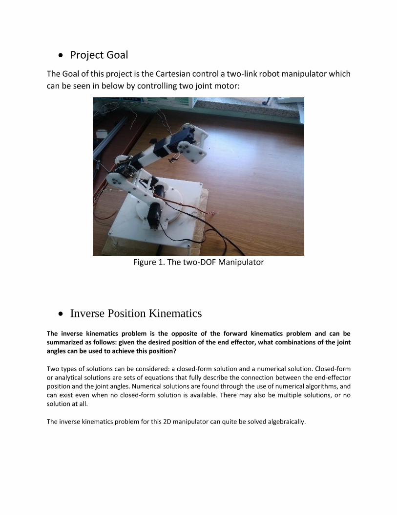
Project Goal

The Goal of this project is the Cartesian control a two-link robot manipulator which

can be seen in below by controlling two joint motor:

Figure 1. The two-DOF Manipulator

Inverse Position Kinematics

The inverse kinematics problem is the opposite of the forward kinematics problem and can be summarized as follows: given the desired position of the end effector, what combinations of the joint angles can be used to achieve this position?

Two types of solutions can be considered: a closed-form solution and a numerical solution. Closed-form or analytical solutions are sets of equations that fully describe the connection between the end-effector position and the joint angles. Numerical solutions are found through the use of numerical algorithms, and can exist even when no closed-form solution is available. There may also be multiple solutions, or no solution at all.

The inverse kinematics problem for this 2D manipulator can quite be solved algebraically.

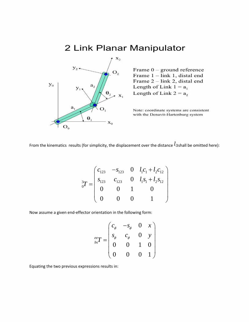
From the kinematics results (for simplicity, the displacement over the distance shall be omitted here):

123 123 1 1 2 12

123 123 1 1 2 123

0

0

0

0 0 1 0

0 0 0 1

c s l c l c

s c l s l sT

Now assume a given end-effector orientation in the following form:

0

0

0 0 1 0

0 0 0 1

ee

bs

c s x

s c yT

Equating the two previous expressions results in:

123

123

1 1 2 12

1 1 2 12

c c

s s

x l c l c

y l s l s

As:

12 1 2 1 2

12 1 2 1 2

c c c s s

s c s s c

squaring both the expressions for and and adding them, leads to:

2 2 2 2

1 2 1 2 22x y l l l l c

Solving for leads to:

2 2 2 2

1 22

1 22

x y l lc

l l

while equals:

2

2 21s c

and, finally, :

2 2 2tan2( , )A s c

Note: The choice of the sign for corresponds with one of the two solutions in the figure above.

The expressions for and may now be solved for . In order to do so, write them like this:

1 1 2 1

1 1 2 2

x k c k s

y k s k c

where , and .

Let:

2 2

1 2

tan 2 2, 1

r k k

A k k

Then:

1

2

cos

sin

k r

k r

Applying these to the above equations for and :

1 1

1 1

/ cos sin

/ cos sin

x r c s

y r s c

Or

1

1

cos( )

sin( )

x

r

y

r

Thus:

1 tan2 ,A y x

Hence:

1 2 1tan2 , tan2 ,A y x A k k

Note: If , actually becomes arbitrary.

may now be solved from the first two equations for and :

3 1 2 1 2tan 2( , )A s c

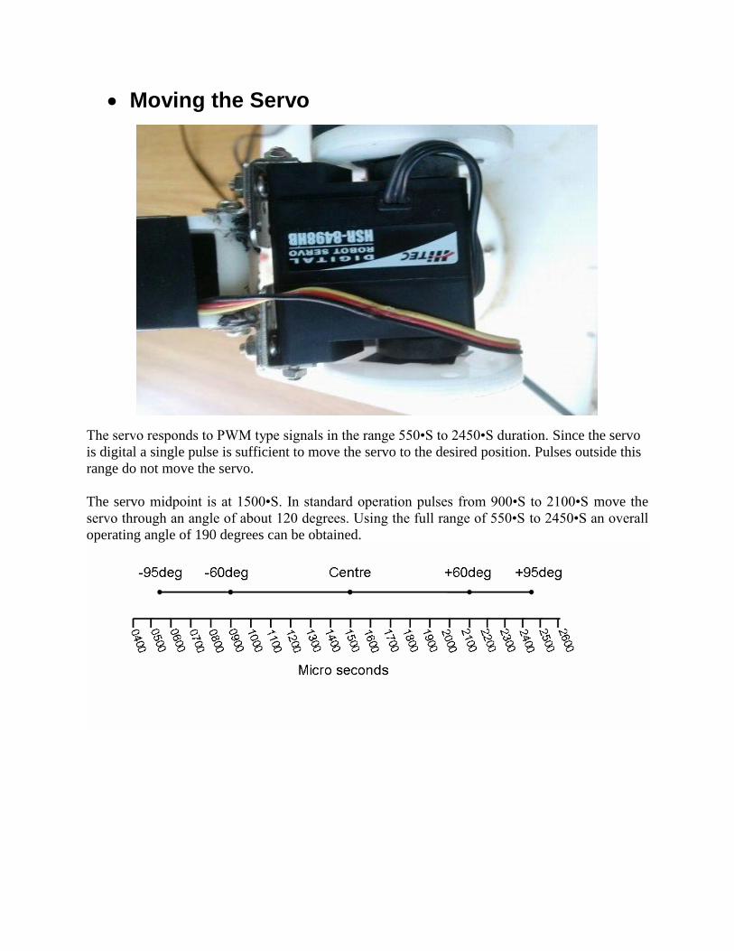
Moving the Servo

The servo responds to PWM type signals in the range 550•S to 2450•S duration. Since the servo

is digital a single pulse is sufficient to move the servo to the desired position. Pulses outside this

range do not move the servo.

The servo midpoint is at 1500•S. In standard operation pulses from 900•S to 2100•S move the

servo through an angle of about 120 degrees. Using the full range of 550•S to 2450•S an overall

operating angle of 190 degrees can be obtained.

Experimental implementation

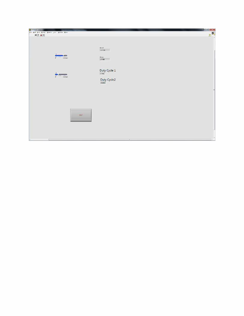
Interface of Labiew

In this implementation we just need to enter (X,Z), and it will calculate 1 and 2 , then based on the

calculated angles it will apply appropriate Duty cycles.

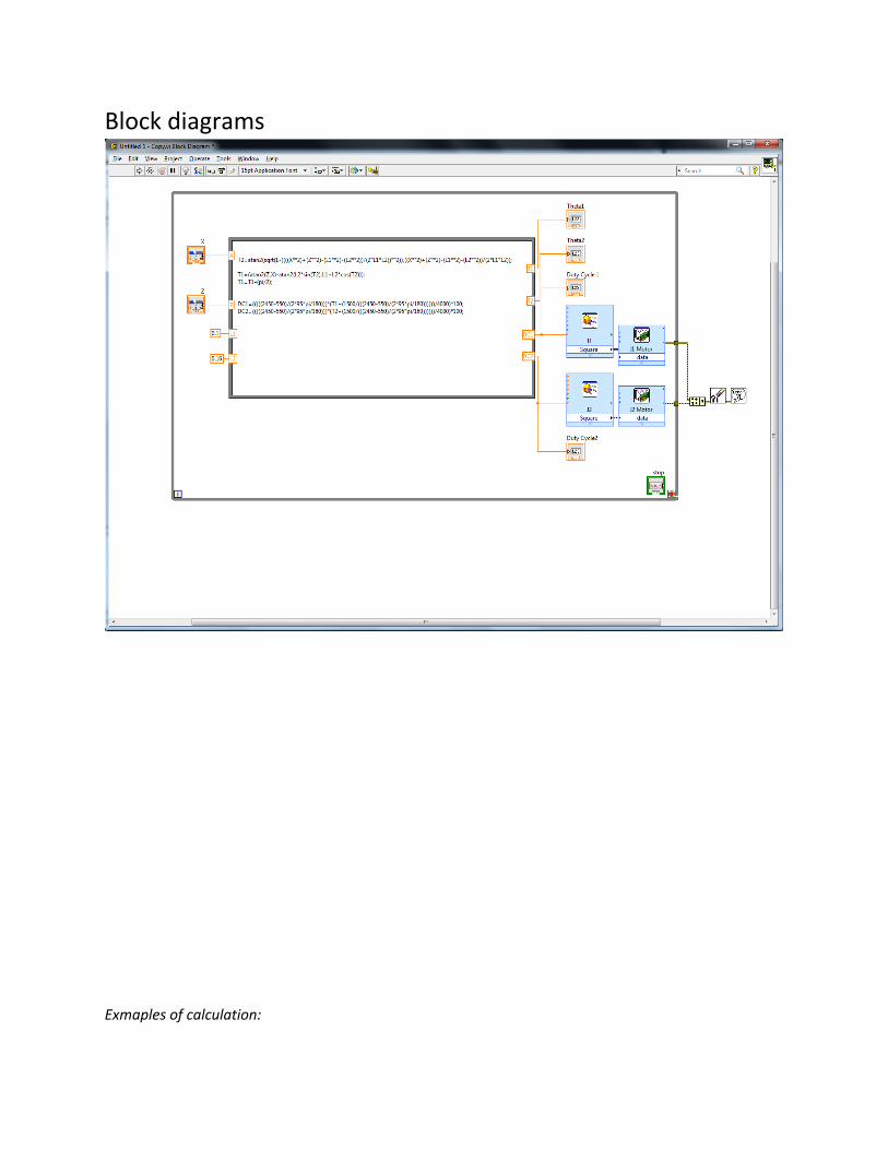
Block diagrams

Exmaples of calculation: