IEEE TRANSACTIONS ON NEURAL NETWORKS, VOL. 7, NO. 6, NOVEMBER 1996 1401

On Adaptive Trajectory Tracking of a Robot Manipulator Using Inversion o-f Its Neural Emulator

Laxmidhar Behera. Madan Gopal, and Santanu Chaudhury

Abstract-This paper is concerned with the design of a neuro- adaptive trajectory tracking controller. The paper presents a new control scheme based on inversion of a feedforward neural model of a roh'ot arm. The proposed control scheme requires two modules. Tlhe first module consists of an appropriate feed- forward neural imodel of forward dynamics of the robot arm that continuously accounts for the changes in the robot dynamics. The second module implements an efficient network inversion algorithm that computes the control action by inverting the neural model. In this paper, a new extended Kalman filter (EKF) based network inversion scheme is proposed. The scheme is evaluated through comparison with two other schemes of network inversion: gradient search in input space and Lyapunov function approach. Using these three inversion schemes the proposed controller was implemented for trajectory tracking control of a two-link manipulator. Simulation results in all cases confirm the efficacy of control input prediction using network inversion. Comparison of the inversion algorithms in terms of tracking accuracy showed the superior performance of the EKF based inversion scheme over others.

I. INTRODUCTION

OBOT manipulators are characterized by complex non- R linear dynamical structures with inherent unmodeled dynamics and unstructured uncertainties. These features make the designing of controllers for manipulators a difficult task in the framework. of classical adaptive and nonadaptive control [ I]-[4]. Artificial neural networks offer promising possibilities for providing better solutions to robot tracking problems, primarily because of their excellent capability to learn any complex mapping from training examples [ 5 ] , [6]. Simulation and experimental results of a number of investigators such as Narendra and Parthasarathy [7], Miller et al. [SI, Goldberg and Pearlmutter [9], Miyamoto et al. [ IO], Bassi and Bekey 11 11, Gomi and Kawato 1121, and others have confirmed the potential of these networks in the area of dynamic modeling and control of nonlinear systems.

The existing literature on neural control of robot manip- ulators reveals that most of these applications are based on learning inverse dynamics of a robot arm. Some of these learning schemes of inverse dynamics can be summarized as follows. In direct inverse modeling of robot manipulators [8], 191. the network is trained using input-output data of the plant in a reverse fashion (i.e., joint angle 0 + input torque 7 )

directly. In the case of forward and inverse modeling [ 131, the

Manuscript received March 28, 1994; revised March 1, 1995 and May IO,

The authors ire with the Department of Electrical Engineering, Indian

Publisher Item Identifier S 1045-9227(96)07459-0.

1996.

Institute of Technology Delhi, Hauz Khas, New Delhi 110 016 India.

forward m,odel is learned by monitoring the input toque vector ~ ( t ) and output joint position vector Q(t) of the manipulator. Next, the desired trajectory d d ( t ) is fed to the inverse model to calculate the feedforward motor command ~ f f ( t ) . The resulting error in the trajectory B d ( t ) - B(t) is backpropagated through the forward model to calculate the command error, which is then used as the error signal for training the inverse model. The feedback error learning scheme of Miyamoto et al. [lo] uses feedback torque as the error signal to train the inverse dynamic model of the robot arm. These inverse models compute t.he feedforward torque given a desired trajectory, and feedback stabilizing signal is actuated by a simple potential difference (PD) controller.

In our present work, a different approach is proposed where instead of training a separate network to learn the inverse dynamics, we directly perform the iterative inversion of a forward model of a robot arm to generate control action on- line. This approach avoids a separate scheme of providing a feedback stabilizing signal [8], [9], [ 141. The motivating factor for this work is to see the feasibility of implementing direct inversion of a neural network to actuate on-line control signal, an approach that has got little attention in control literature. This approach also provides an alternative to backpropagation of utility as proposed by Werbos [ 151 and Nguyen and Widrow [ 161, which are basically off-line schemes.

Iterative inversion of multilayered neural networks based on gradient search in input space was first proposed by Linden and Kindermann [17]. This work shows that iterative inversion of a neural network model is possible by ascribing backpropagated errors in network output to errors in the network input signal. This technique has been extended to adaptive control of simple linear systems by Hoskins et al. [ 1 81. Lee [ 191 has proposed a network inversion scheme based on the L,yapunov function approach in application to pattern recognition problems. Extension of this technique to on-line inversion of neural networks to predict control input is not reported in the literature. Keeping these facts in mind, in this paper we have explored the applications of the above two inversion schemes to robot tracking problems. In an attempt to search for a fast and robust inversion scheme, we have proposed an extended Kalman filter (EKF) based inversion algorithm for radial basis function network model of multi- input/multioutput (MIMO) systems. The proposed inversion scheme was motivated by the algorithm proposed by Iiguni et al. [2.O] and Scalero and Tepedelenlioglu [21] for training feedforward networks. Since EKF was found to be fast and efficient for training multilayered networks (MLN's), EKF

1045-9227/96$05.00 0 19961 IEEE

1402 IEEE TRANSACTIONS ON NEURAL NETWORKS, VOL. I, NO. 6, NOVEMBER 1996

based inversion is expected to give better performance for on-line inversion applications.

The proposed controller based on each of the three different approaches of network inversion is implemented for a two-link robot manipulator. The forward dynamics of the manipulator is modeled by a radial basis function network (RBFN) network. The RBFN model is trained by input-output data generated in the robot workspace using a simple PD controller. Experiments were carried out to evaluate the efficiency of each inversion algorithm in terms of root mean square (rms) tracking errors by varying the initial conditions and changing the upper-bound on the number of iterations allowed per sampling interval to predict the control input. These experiments indicate that the performance of the EKF based inversion scheme is better than the other two. The present paper is organized in the following manner. Section 11 describes the nonlinear dynamic modeling using an RBFN and the corresponding learning mechanism. Three different schemes of network inversion are presented in Section 111. The structure of the proposed robot trajectory controller is explained in Section IV. In Section V, we provide the simulation results by implementing a proposed neuro-adaptive controller for tracking control of the two-link manipulator. Finally, concluding remarks are given in Section VI.

11. RBFN MODEL OF FORWARD DYNAMICS OF ROBOT ARM Consider a class of nonlinear discrete time dynamical sys-

tems described by

4 k + 1) = M k ) , 4 k ) I (1)

where z ( k ) E R'L and u ( k ) E Rp represent, respectively, state and input vectors of the system at the kth sampling instant. The states of the system are assumed to be accessible and nonlinear function f ( . ) is assumed to be unknown.

The unknown mapping I ( . ) can be learned using either an MLN or RBF network. In MLN, activation of output layer neurons has a highly nonlinear relationship with the network parameters. Training algorithms based on recursive least squares methods [22] or the EKF approach [20], [21] are consequently computationally intensive. The popular back- propagation algorithm is prone to local minima trap and relatively slow in convergence. On the other hand, RBF network response is a linear function of its weights. This allows us to choose any of the least squares methods to train the network. In general, the leaming in RBFN is fast. As we require the neural emulator to account for continuous changes in plant dynamics, RBFN is preferred over MLN.

A. Neural Modeling o f f (.) Using RBFN

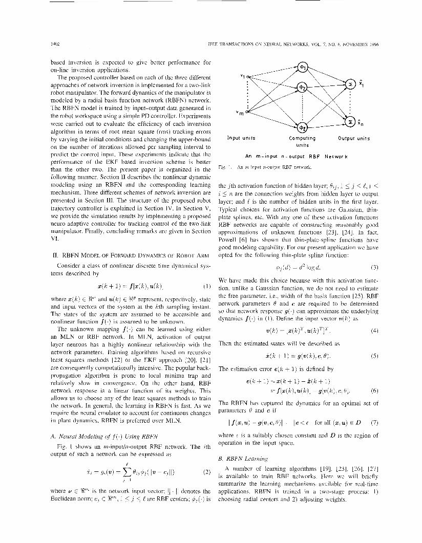
output of such a network can be expressed as Fig. 1 shows an m-inputln-output RBF network. The ith

P

oi zz ,qi(u) = C 0ij4,f(iIv - cjli) ( 2 )

where v E X" is the network input vector; 1 1 . 1 1 denotes the Euclidean norm; cJ E R" , 1 5 j 5 e are RBF centers; $ j ( . ) is

j=l

Input unirs Computing Ourpur u n i t s u n i t s

An m - i n p u t n - o u t p u t RBF N e t w o r k

Fig. 1. An m input n-output RBF network

the j t h activation function of hidden layer; d i J , 1 5 j 5 e , 1 5 i 5 n are the connection weights from hidden layer to output layer; and L is the number of hidden units in the first layer. Typical choices for activation functions are Gaussian, thin- plate splines, etc. With any one of these activation functions RBF networks are capable of constructing reasonably good approximations of unknown functions [23], [24]. In fact, Powell [6] has shown that thin-plate-spline functions have good modeling capability. For our present application we have opted for the following thin-plate spline function:

(3)

We have made this choice because with this activation func- tion, unlike a Gaussian function, we do not need to estimate the free parameter, i.e., width of the basis function [25]. RBF network parameters 0 and c are required to be determined so that network response g( .) can approximate the underlying dynamics f(.) in (1). Define the input vector w ( k ) as

4j ( d ) = d2 log d.

w(k) = [.(k)';u(k)T]'. (4)

i ( k + 1) = g ( v ( k ) ; c ; 0 ) .

Then the estimated states will be described as

( 5 )

The estimation error e(k + 1) is defined by

e ( k + 1) = z ( k + 1) - 2 ( k + 1) = f [ z ( k ) , 4 k ) l - q [ v ( k ) , c, 01. (6)

The RBFN has captured the dynamics for an optimal set of parameters 8 and c if

llf(2,u) - g(v, c, H ) J l = Ile < E for all (x; U ) E D (7)

where E is a suitably chosen constant and D is the region of operation in the input space.

B. RBFN Learning

A number of leaming algorithms [19], [23], [26], [271 is available to train RBF networks. Here we will briefly summarize the learning mechanisms available for real-time applications. RBFN is trained in a two-stage process: 1) choosing radial centers and 2) adjusting weights.

BEHERA et al.: ON ADAPTIVE TRAJECTORY TRACKING 1403

The radial centers are chosen in such a manner that these centers suitably sample the network input domain and should be able to track the changing pattern of data. One of the practices is to use an n-means clustering technique to update the RBF centers as suggested by Moody and Darken [28]. In this work we have chosen these centers to be of uniform random distribution over the input space.

Because the response of the network is linear with respect to its weights, the recursive least squares methods may be used for adjusting weights. In the following we provide the recursive least squares algorithm (RLS) that has been employed in the present work.

The ith output of the RBFN described earlier can be written as

2i = $TQ;, i = I,... , T L (8)

where E R‘ is the output vector of the hidden layer; 0i E Re is the connection weight vector from the hidden units to the ith output unit. The weight update equations as per RLS algorithm are described ,as

e@) =e,@ - 1) + P(k)$(k - 1)

P ( k ) = P ( k - 1) - P(k - l)$h(k - 1)[1+ q5(k - 1)T ’ [s;(k) - q5(k - l y & ( k - l)]

. P ( k - l)d(k - l)]-h$(k - 1 ) T P ( k - 1)

(9)

(10)

where P ( k ) E Initial value P(0) is taken as 201 for the present application and that of weight vector 0; can be assigned to zero or small random numbers.

111. NETWORK INVERSION ALGORITHMS

In this section, we present three different network inversion schemes which are useful for applications in control. The RBFN model I as given by ( 5 ) ] represents a nonlinear mapping from m-dimensional input space to n-dimensional output space where 12 < m(m = p + n) . The objective of inverse operation on this model is to predict only p-inputs out of m number of total inputs. The remaining n inputs are known a priori (present system states). Thus the inverse mapping can be mathematically expressed as

G ( k ) = g - l [ z ( k ) , x ” ( k + l ) ,c ,Q] (1 1)

where z d ( k + 1) is the desired output activation. This shows that basically we are performing invenion mapping 9 - I : !JP + W where p < n for the N-link robot manipulator tracking control ( p = N , n = 2 N ) .

These inversion algorithms carry out the mapping given in (1 1) by updating input activation i ( k ) iteratively until desired output activation is achieved or the number of iterations reaches a maximum, t,,, within a sampling interval. This upper-bound trlldX, therefore, should be determined on the basis of the sampling interval and the computation time required per iteration. It is clear from this discussion that speed of convergence of the inversion algorithm can be measured by the number of iterations required to produce the de?ired output. The initial guess of the input activation G ( k ) during each sampling interval is taken as the input activation i ( k - 1)

predicted in the previous sampling instant. For the case of first sampling interval, the initial guess is selected arbitrarily from the input space.

A. Gradient Search (GS) in Input Space The iterative inversion of the RBF network can be carried

out using the gradient descent algorithm as proposed by Linden and Kindermann [17]. The iterative rule is given as

3E + .[.;t(k) - i i-yk)] (12) G t + l ( k ) = .;E(k) - 17- 3u: ( k )

where t refers to iterative step, 7 is the learning gain, and a! is the momentum rate. The error function is given by E = 112 C:=.=,(xp - 2%)’. To prevent the input activation i ( k ) from growing without limit, the input is conlsidered as an output of a “pseudoneuron” with a limited output range [171.

For the RBF network shown in Fig. 1, with thin-plate-spline activation function, dE/du , can be expressed as

and

k=l

where d ( k ) = ((‘U - c k / ( ~

B. Inverse Mapping Following Lyapunov Function (LF) Approach

The inverse mapping based on the Lyapunov function as a general means of achieving a recall process for selective attention as applicable to a pattern recognition process has been presented by Lee [19]. We adapt the same concept for control applications in the following way.

The Lyapunov function candidate V is chosen to be a quadratic error function in desired trajectories given by

V = $kTx where x = zd - 3 . (15)

Here, xd is the desired output activation and 3 is the actual output activation of the RBFN model. The time dlerivative of the Lyapunov function is given by

1404 IEEE TRANSACTIONS ON NEURAL NETWORKS, VOL I , NO. 6, NOVEMBER 1996

Theorem I : If an arbitrary initial input activation u(0) is updated by

U * (t ') = u(0) + U d t (17) .i' where

then x converges to zero under the condition that U exists along the convergence trajectory.

Proof Substitution for U from (1 8) into (1 6) we have

v = -115$ 5 0 (19)

where V < 0 for all 2 # 0 and Q.E.D. The iterative input activation update rule based on (17) can be given as

= 0 iff 2 = 0.

&(t) = U( t ~ 1) + @(t - 1) (20)

where p is a small constant representing the update rate.

C. EKF-Based Inversion Algorithm

The EKF-based algorithm was proposed for training of MLN's by Iiguni et al. [20], Scalero and Tepedelenlioglu [21], and others. Here we propose a decoupled form of the inversion algorithm based on the EKF approach for RBF networks.

EKF is a method of estimating the state vector. Here, the unknown input vector u ( k ) is considered as the state vector to be estimated. The input vector of RBFN has m-components out of which n-inputs, i.e., the present state vector of the system ~ ( k ) are known at the kth sampling instant. Remaining p components ( u ( k ) ) of the input vector 'U are estimated through the inversion process. During the iterative inversion of the network, RBFN parameters c and 6' are held constant. So, RBFN output can be expressed as

The individual update of an input U, can be decoupled from other updates if we assume that other ( p - 1) inputs are known a priori. In other words, estimates of these ( p - 1) inputs obtained in the previous iteration can be used for the update of the ith input in the present iteration. The inversion scheme presented here is based on this assumption.

Let the output vector and desired output vector of RBFN corresponding to the tth iteration and kth sampling instant be 3 ( k . t ) and ~ ' ( k + I), respectively. The RBFN can be expressed by the following nonlinear system equations as a function of the ith input ( k has been dropped from the argument list for convenience):

Here, [ ( t ) is assumed as a white noise vector with n x n covariance matrix R(t). The application of EKF to (22) and (23) gives the following real-time learning algorithm [29]:

i i ; ( t) = i i i ( t - 1) + K;(t)[& - q t ) ] Kz(t) =Pi(t - I)Hi(t)T[Hi(t)P,(t - l )Hi( t )T + R, ( t ) ]y

P,(t) = Pz(t - 1) - Pi(t - 1)Ki( t )H,( t )

(24)

(25) (26)

where Ki( t ) , the (I x n) matrix, is called the Kalman gain and H i ( t ) , the ( n x 1) matrix, is defined as

The j th element of H,( t ) can be expressed for the case of thin-plate-spline activation function as follows:

The expression for 30,/3u, is given in (14). During the inversion process as each output of the feedforward network is considered to be an independent function of control inputs only (23) , the output covariance matrix R(t) can safely be assumed to be diagonal matrix X I . This assumption avoids the matrix inversion involved in (25). Applying the matrix inversion lemma. we have

j' (29) Pz(t - l )H,( t )Hi( t )T

x + P;(t - I )Hi ( t )THi ( t ) = - I- ; [

The inversion algorithm is simplified as

As covariance matrix R(t) is unknown a priori, X is estimated on-line using the following recursion [20]:

i ( t ) = i ( t - 1) + w ( t )

where ~ ( t ) = l/t. This inversion algorithm, as indicated before, is decoupled

in nature with respect to input updates. Decoupling of pre- diction of inputs can help in parallel implementation of the algorithm which is very important advantage for real-time applications.

BEHERA et al.: ON PiDAPTIVE TRAJECTORY TRACKING

k 4 1

1405

Fig. 2.

5

4

3

2

1

0

Fig. 3.

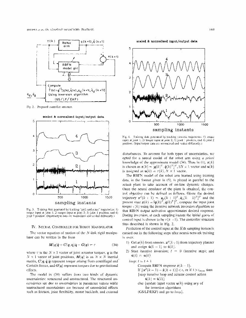
Proposed controller structure.

scalcxi dc normallsed input/output data

r - r

c n ,

I 1 I

500 1000 1500

sampling instants Training data generated by tracking "pick and place" traiectories: I )

torque input at joint 1;-2) torque input at join; 2; 3 ) joint I posiiion; and 4) joint 2 position. (JnpuVoutput data are normalized and scaled differently.)

Iv. NEURAL CONTROLLER FOR ROBOT MANIPULATOR

The vector equation of motion of the N-link rigid manipu- lator can be written in the form

M(q)ii + c ( q . 4 4 + G(q) = 7 (34)

where 7 is the N x 1 vector of joint actuator torques, q is the N x 1 vector of joint positions, M ( q ) is an N x N inertial matrix, C(q, 4)Q represent torque arising from centrifugal and Coriolis forces, and G(g) represent torques due to gravitational effects.

The model in (34) suffers from two kinds of dynamic uncertainties: structured and unstructured. The structured un- certainties are due to uncertainties in parameter values while unstructured uncertainties are because of unmodeled effects such as friction, joint flexibility, motor backlash, and external

5

4

3

2

1

0

Fig. 4.

waled h normalised input/output dah

I 1

i- 4

I- 4

I I I 1 1 500 1000 1500

sampling instants Training data generated by tracking sinusoid trajectories: I ) torque

input at joint 1; 2) torque input at joint 2; 3) joint 1 position; and 4) joint 2 position. (Input/output data are normalized and scaled differently.)

disturbances. To account for both types of uncertainties, we opted for a neural model of the robot arm using a priori knowledge of the approximate model (34). Thus in (l), z ( k ) is chosen as z ( k ) = [ q ( k ) T ! 4 ( k ) T ] T , 2N x 1 vector and u(k) is assigned as u ( k ) = ~ ( k ) , N x 1 vector.

The RBFN model of the robot arm learned using training data, in the format given in (3, is placed in parallel to the actual plant to take account of on-line dynamic changes. Once the neural emulator of the plant is obtained, the con- trol objective can be defined as follows. Given the desired trajectory z d ( k + 1) = [ q d ( k + l ) T , Q d ( k + l)T:IT and the present state z ( k ) = [ q ( k ) T , q(k)'IT, compute the input joint torque ~ ( k ) using the iterative network inversion algorithm so that RBFN output activation approximates desired response. During inversion, at each sampling instant the initial guess of control input is chosen to be .r(k - 1). The controller structure thus described is shown in Fig. 2.

Prediction of the control input at the Kth sampling instant is carried out in the following steps after neural-network training is over.

1) Get z ( k ) from sensors, z d ( k + l ) from trajectory planner

2) Start iterative inversion; t = 0 (iterative step); and and assign ii(k - 1) to i ( k ) .

&(t) = & ( k )

loop: f = t + l Compute RBFN response k (k + 1). If I ( z" (k + 1) - k (k + 1)11 < E, or if t >. t,,,, then {stop iterative loop and actuate control action

else {update input vector u ( k ) using any of

(GS/LF/EKF) and go to loop}.

q k ) = i ( t ) }

the inversion algorithms

1406 IEEE TRANSACTIONS ON NEURAL NETWORKS, VOL. 7, NO. 6, NOVEMBER 1996

0.1

0.05

0 _ . m 9 -0.05 ;i;

2 -0.1 0 &.I

-0.15 i: Zi 2 -0 .2 k Y

-0.25

-0.3

-0.35

tracking performance of inversion schemes(Joint 1 )

.’ cs -LF - _ _ EKF ----- EKF(AR)

0 50 100 150 200 250 300

sampling instants

Fig. 5. Position tracking of joint 1 using inversion algorithms GS, LF, EKF, and EKF (after retraining of RBFN model)

tracking performance of inversion schemes(Joint 2) 0.15

1

-0.1 L 1

50 100 150 200 250 300 0

sampling instants

Fig. 6. Position tracking of joint 2 using inversion algorithms GS, LF, EKF, and EKF (after retraining of RBFN model).

V. SIMULATION RESULTS

of freedom manipulator used by Slotine and Li [l] are used for input-output data generation and controller structure is obtained based on these sets of data only. The robot arm dynamics can be written explicitly as

where C21 = cos(qz - ql),S21 = sin(q2 - 41). The four

and ‘.O2’ kg-m2, As an example, the dynamic equations of the two-degree- parameters a1,a21 a31 and a4 are taken as 0.15, 0.04, 0.033

On-Line Data Generation

BEHERA et al.: ON .ADAPTIVE TRAJECTORY TRACKING 1407

-101 I I I I 0 50 100 150 200 250 300

Sompling instants

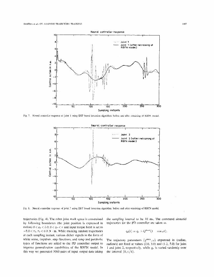
Fig. 7. Neural controller response of joint 1 using EKF based inversion algorithm: before and after retraining of RBFN model.

Neural controller response 10

8

6 RBFN model) Joint 2 (at ter retraining ot

i 4 e .E 2 t 0 .- t o 0 4

- 2 4-

0 U -4

- 6

- 8

10 0 50 100 150 200 250 300

Sompling instants

Fig. 8. Neural controller response of joint 2 using EKF based inversion algorithm: before and after retraining of RBFN model.

trajectories (Fig. 4). The robot joint work space is constrained by following boundaries (the joint position is expressed in radian) 0 < 41 < 5.0,0 < 42 < 7 and input torque limit is set to

at each sampling instant, various dither signals in the form of white noise, impulses, step functions, and ramp and parabolic types of functions are added to the PD controller output to improve generalization capabilities of the RBFN model. In this way we generated 3000 pairs of input-output data taking

the sampling interval to be 10 ms. The command sinusoid trajectories for the PD controller are taken as

-8.0 < 7 1 , ~ ~ < 8.0 N . m. While tracking random trajectories q d ( t ) = qr + Qmdx(l - COS&).

The trajectory parameters ( p a x I U ) expressed in (radian, radianh) are fixed at values (2.0, 3.0) and (1.2, 5.0) for joint 1 and joint 2, respectively, while qr is varied randomly over the interval (0,7r/4).

1408 IEEE TRANSACTIONS ON NEURAL NETWORKS, VOL I, NO 6, NOVEMBER 1996

8.0,S.O

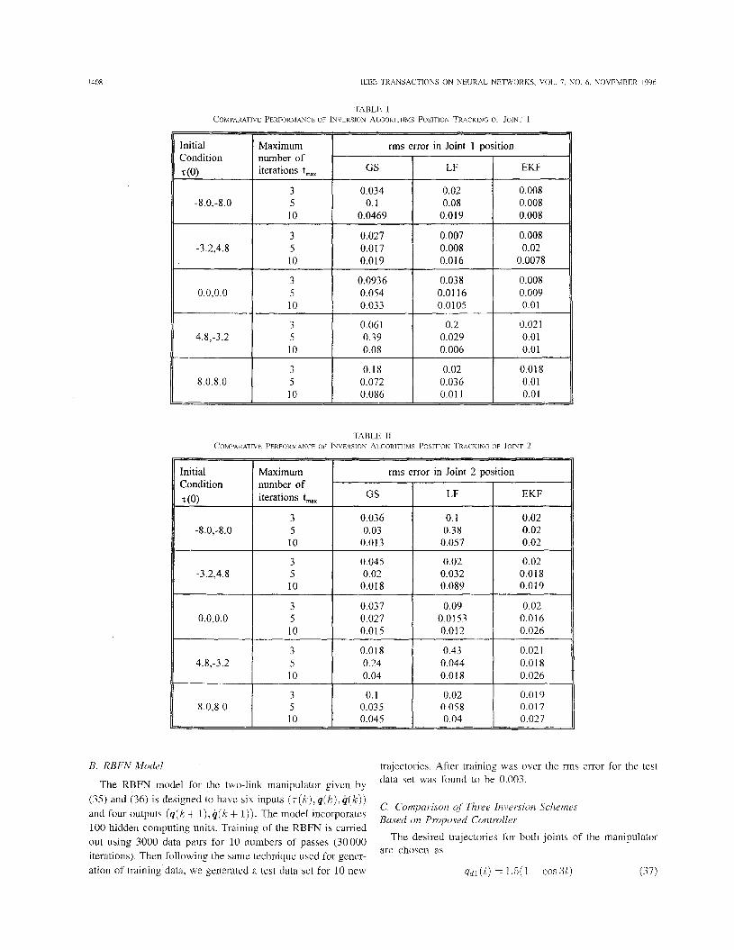
TABLE I COMPARATIVE PERFORMANCE OF INVERSION ALGORITHMS POSITION TRACKING OF JOINT 1

5 0.072 0.036 0.01 10 0.086 0.01 1 0.01

Initial Maximum Condition number of T (0) iterations t-

3 -8.0,-8.0 5

10

3

10

3 0.0,o.o 5

10

3 4.8,-3.2 5

10

3 8.0,8.0 5

10

-3.2,4.8 5

rms error in Joint 2 position

GS LF EKF

0.036 0.1 0.02 0.03 0.38 0.02

0.013 0.057 0.02

0.045 0.02 0.02 0.02 0.032 0.018

0.018 0.089 0.019

0.037 0.09 0.02 0.027 0.0153 0.016 0.015 0.012 0.026

0.018 0.43 0.021 0.24 0.044 0.0 18 0.04 0.018 0.026

0.1 0.02 0.019 0.035 0.058 0.017 0.045 0.04 0.027

B. RBFN Model trajectories. After training was over the rms error for the test data set was found to be 0.003.

C. Comparison of Three Inversion Schemes Bused on Proposed Controller

are chosen as

The RBFN model for the two-link manipulator given by (35) and (36) is designed to have six inputs ( r ( k ) , q(,k), q ( k ) ) and four outputs ( q ( k + l), k ( k + 1)). The model incorporates 100 hidden computing units. Training of the RBFN is carried

numbers of passes (30000 iterations). Then following the same technique used for gener-

using 3ooo data pairs for The desired trajectories for both joints of the manipulator

ation of training data, we generated a test data set for 10 new q d l ( t ) = 1.5(1 - COS^^) (37)

BEHERA ef al.: ON ADAPTIVE TRAJECTORY TRACKING

Initial Maximum Condition number of

iterations t,, T (0) 3

-8.0,-8.0 5 10

3 -3.2,4.8 5

10

1409

rms error in Joint 1 velocity

GS LF EKF

0.093 0.05 0.012 0.085 0.16 0.012 0.043 0.028 0.012

0.058 0.035 0.012 0.042 0.032 0.02 0.028 0.04 0.012

TABLE I11 COMPARATIVE PERFORMANCE OF INVLRSION ALGORITHMS VELOCITY TRACKING OF JOINT 1

8.0,8.0 3 0.13 0.045 0.02 5 0.077 0.065 0.0 168 10 0.123 0.029 0.01 5

3 0.092 0.068 0.013 1 :O 1 0.034 1 0.027 I :::: 0.0,o.o 0.054 0.022

Initial Condition T (0)

-8.0,-8.0

-3.2,4.8

3 0.054 0.26 0.021 4.8,-3.2 0.196 0.034 0.01 1 1 :O 1 0.094 1 0.017 1 0.014

Maximum number of iterations t,,

rms error in Joint 2 velocity

GS LF EKF

3 0.06 0.093 0.01 1 5 0.034 0.21 0.01 10 0.017 0.056 0.0099

3 0.021 0.049 0.01 5 0.0 14 0.05 1 0.01 10 0.012 0.07 0.01

0.0,o.o

4.8,-3.2

8.0,S.O

3 0.038 0.088 0.016 5 0.01 7 0.038 0.01 1 10 0.014 0.029 0.009

3 0.021 0.5 0.018 5 0.145 0.055 0.01 1 10 0.0499 0.03 1 0.014

3 0.09 0.065 0.018 5 0.029 0.074 0.018 10 0.06 0.048 0.016

(1$2 ( t ) = (1 - cos 5 t ) . (38)

The control algorithm presented in Section IV is imple- mented for all three inversion algorithms. For the gradient search scheme the leaming rate is fixed at 1 .O. The Lyapunov function-based inversion scheme, as given in (18) and (20), is implementetl choosing ~ to be o. 1 , The initial values for implementation of the EKF-based inversion algorithm [(30)-(33)] are selected as = p2 = 1.0 and X(0) = 0.05. In all the cases, the initial condition for control input at the first

sampling instant is chosen as ~ ( 0 ) = [ O 7 O I T N . m, and the maximum number of iterations per sampling interval is kept at

Tracking performance of all the schemes are compared in Figs. 5 and 6 in terms of joint tracking error. Position tracking errors for joint 1 is shown in Fig. 5 while Fig. 6 shows position tracking errors for joint 2. The controller responses for joints 1 and 2 are shown in Figs. 7 and 8, respectively, for the Case of the EKF approach. The proposed controller is found to be stable in all the cases though tracking errors are relatively

1410

Trajectory Parameters

q," qzma 0 1 0 2

1 .o 1 .o 2.0 2.0

IEEE TRANSACTIONS ON NEURAL NETWORKS, VOL. I, NO. 6, NOVEMBER 1996

rms error in Joint 1 velocity

GS LF EKF

0.038 0.01 78 0.045

TABLE V GENERALIZATION CAPABILITY OF PROPOSED CONTROLLER POSITION TRACKING OF JOINT 1

1.5

0.5

1.5

TABLE VI GENERALIZATION CAPABILITY OF PROPOSED CONTROLLER POSITION TRACKING OF JOINT 2

~ ~ ~~ ~~ ~

1 .o 3.0 5.0 0.034 0.027 0.013

0.5 1 .o 4.0 0.034 0.022 0.033

1 .o 3.0 3.0 0.067 0.027 0.029

TABLE VI1 GENERALIZATION CAPABILITY OF PROPOSED CONTROLLER VELOCITY TRACKING OF JOINT 1

1 .o 1 .o 2.0 3.0 0.094 0.028 0.045

large. The error is found to be maximum in the case of GS and minimum in the case of EKF.

Further study was done to evaluate comparative perfor- mances of each algorithm by varying the initial condition ~ ( 0 ) and allowable number of maximum iteration t,,, for the following reasons. Earlier we mentioned that each inversion algorithm computes input ? ( k ) starting with initial guess ?(k - 1) as predicted in the previous sampling instant. But when k = 1, the initial condition is not known a priori. So we are left with the option of choosing arbitrary an initial condition from the input space. Thus the effect of the initial condition in control input prediction is noteworthy. The second

parameter t,,, (maximum allowable number of iterations per sampling interval) is important because the control input must be predicted using a fixed number of iterations within the sampling interval.

To study the comparative performance of inversion algorithms, we selected five arbitrary initial conditions as ~ ( 0 ) = [-8.0, -8.OlT; [-3.2, 4.8IT; [0, O I T ; [4.8, -3.2IT; and [8.0, 8.OIT, respectively. The parameter t,,, maximum number of iterations per sampling interval, is varied at three different values 3, 5, and 10, respectively. The root-mean- square (rms) error over each trajectory is observed while implementing the proposed controller to track the trajectories

BEHERA et al.: ON ADAPTIVE TRAJECTORY TRACKING

1 .o

1411

GS LF 0 1 0 2

2.0 2.0 0.038 0.028 0.035

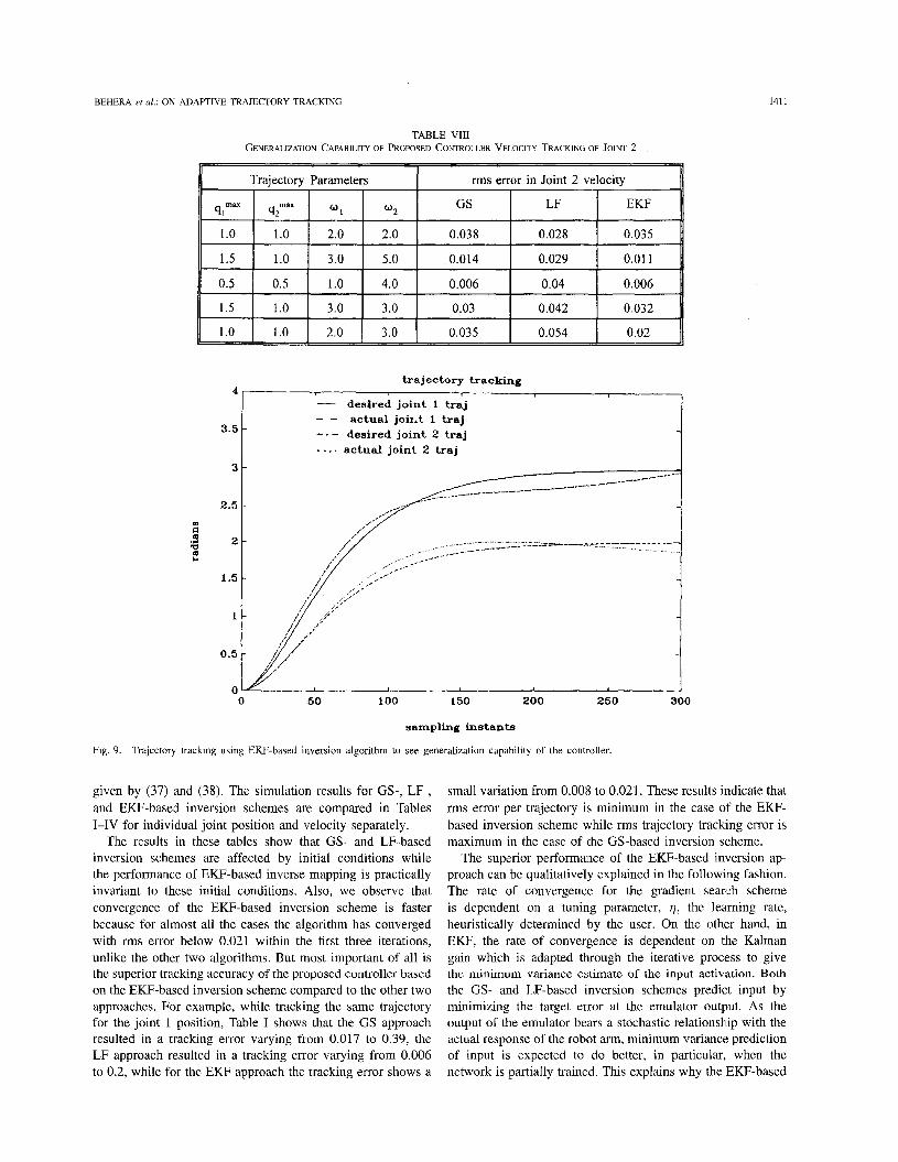
TABLE VI11 GENERALIZATION CAPABILITY OF PROPOSED CONTROLLER VELOCITY TRACKING OF JOINT 2

1.5

0.5

1.5

1 .o 3.0 5.0 0.014 0.029 0.01 1

0.5 1 .o 4.0 0.006 0.04 0.006

1 .o 3.0 3.0 0.03 0.042 0.032

1 .o 1 .o 2.0 3.0 0.035 0.054 0.02

4

3.5

3

2.5 m

4 2 m

1.5

1

0.5

0

trajectory tracking

- deslred joint 1 traj - - actual joiilt 1 traj -. - desired joint 2 traj . . . actual joint 2 traj

0 50 100 150 200 250 300

sampling instants

Fig. 9. Trajectory tracking using EKF-based inversion algorithm to see generalization capability of the controller.

given by (37) and (38). The simulation results for GS-, LF-, and EKF-based inversion schemes are compared in Tables I-IV for individual joint position and velocity separately.

The results in these tables show that GS- and LF-based inversion schemes are affected by initial conditions while the performance of EKF-based inverse mapping is practically invariant to these initial conditions. Also, we observe that convergence of the EKF-based inversion scheme is faster because for almost all the cases the algorithm has converged with rms error. below 0.021 within the first three iterations, unlike the other two algorithms. But most important of all is the superior tracking accuracy of the proposed controller based on the EKF-based inversion scheme compared to the other two approaches. For example, while tracking the same trajectory for the joint 1 position, Table I shows that the GS approach resulted in a tracking error varying from 0.017 to 0.39, the LF approach resulted in a tracking error varying from 0.006 to 0.2, while for the EKF approach the tracking error shows a

small variation from 0.008 to 0.021. These results indicate that rms error per trajectory is minimum in the case of the EKF- based inversion scheme while rms trajectory tracking error is maximum in the case of the GS-based inversion scheme.

The superior performance of the EKF-based inversion ap- proach can be qualitatively explained in the following fashion. The rate of convergence for the gradient search scheme is dependent on a tuning parameter, q, the learning rate, heuristically determined by the user. On the other hand, in EKF, the rate of convergence is dependent on tlhe Kalman gain which is adapted through the iterative process to give the minimum variance estimate of the input activation. Both the GS- and LF-based inversion schemes predict input by minimizing the target error at the emulator output. As the output of the emulator bears a stochastic relationship with the actual response of the robot arm, minimum variance prediction of input is expected to do better, in particular, when the network is partially trained. This explains why the EKF-based

1412

Trajectory Parameters

IEEE TRANSACTIONS ON NEURAL NETWORKS, VOL. 7, NO. 6, NOVEMBER 1996

rms error in Joint 1 position

91- 42- 0 1 a 2

1 .o 1 .o 2.0 2.0

GS LF EKF

0.012 0.0046 0.00s

0.5

1.5

1 .o

~~ ~

0.0027 0.5 1 .o 4.0 0.004 0.004

1 .o 3.0 3.0 0.009 0.004 0.003

1 .o 2.0 3.0 0.003 0.009 0.007

TABLE X GENERALIZATION CAPABILITY OF PROPOSED CONTROLLER POSITION TRACKING OF JOINT 2 AFTER RETRAINING OF RBFN MODEL

41-

1 .o

II Trajectory Parameters I rms error in Joint 2 position II GS LF EKF

1 .o 2.0 2.0 0.01 1 0.007 0.013

42- 0 1 w2

1.5

0.5

1 .5

1 .0

1 .o 3.0 5.0 0.017 0.007 0.007

0.5 1 .o 4.0 0.004 0.007 0.004

1 .o 3.0 3.0 0.033 0.010 0.013

1 .o 2.0 3.0 0.006 0.013 0.010

TABLE XI GENERALIZATION CAPABILITY OF PROPOSED CONTROLLER VELOCITY TRACKING OF JOINT 1 AFTER RETRAINING OF RBFN MODEL

Trajectory Parameters

41- e- 0 1 0 2

1 .o 1 .0 2.0 2.0

rms error in Joint 1 velocity

GS LF EKF

0.03 0.007 0.0027

1.5

0.5

1.5

1 .o 3.0 5.0 0.004 0.013 0.006

0.5 1 .o 4.0 0.0037 0.010 0.0026

1 .o 3.0 3.0 0.015 0.012 0.006

approach performed better in terms of both tracking accuracy and convergence speed.

1 .O

D. Generalization Capability of the Controller

To study the generalization capability of the proposed controller in tracking any arbitrary trajectory we performed the following simulation. The desired trajectory for each joint is chosen as

1 .o 2.0 3.0 0.004 0.0095 0.004

q d l ( t ) = q y X ( 1 - cos w1t) & 2 ( t ) = q y y l - coswzt) .

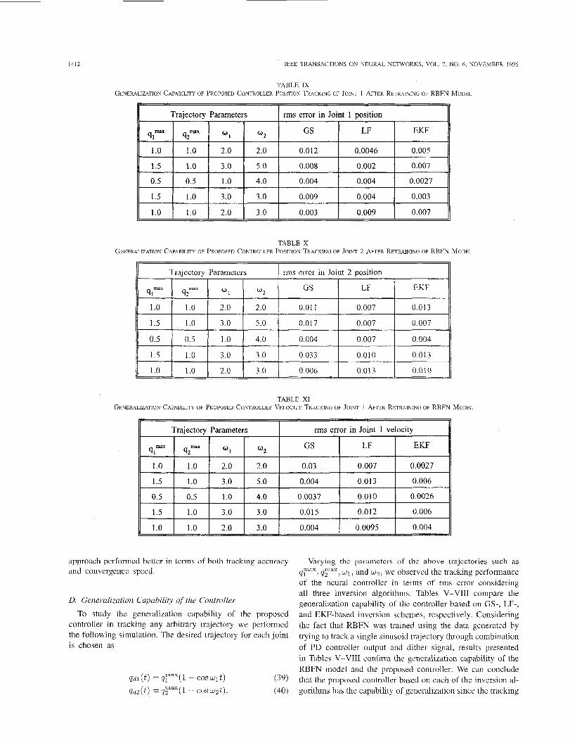
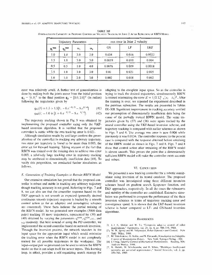
Varying the parameters of the above trajectories such as q?"", qydx, w ~ . and w2; we observed the tracking performance of the neural controller in terms of rms error considering all three inversion algorithms. Tables V-VI11 compare the generalization capability of the controller based on GS-, LF-, and EKF-based inversion schemes, respectively. Considering the fact that RBFN was trained using the data generated by trying to track a single sinusoid trajectory through combination of PD controller output and dither signal. results presented in Tables V-VI11 confirm the generalization capability of the RBFN model and the proposed controller. We can conclude that the proposed controller based on each of the inversion al- gorithms has the capability of generalization since the tracking

BEHERA et al.: ON ADAPTIVE TRAJECTORY TRACKING

1 .o 1 .O 2.0 2.0 0.034 0.016 0.0022

1.5 1 .o 3.0 5.0 0.0019 0.010 0.004 1

TABLE XI1 GENERALIZATION CAPABILITY OF PROPOSED CONTROLLER VELOCITY TRACKING OF JOINT 2 AFTER RETRAINING OF RBFN

0.5

1 .O

1413

0.019 1 I/ 1 .o 4.0 0.0076

3.0 3.0 0.01 0.021

MODEL

Trajectory Parameters rms error in Joint 2

GS LF EKF

error was relatively small. A further test of generalization is done by making both the joints move from the initial position qd = [ O , O ] T to the final position qd = [3.0,2.0IT (in radian) following the trajectories given by

q d l ( t ) = 1.5 + 1.5[1. + 6.e-t/.3 - 8.et/.4] (41) qd2(t) = 1.0 + [I + ~ l . 3 - ~ / . 4 1 . (42)

The trajectory tracking shown in Fig. 9 was obtained by implementing the proposed controller using only the EKF- based inversion algorithm. It is verified that the proposed controller is stable while the rms tracking error is 0.021.

Although simulation results by and large confirm the gener- alization of the controller in tracking any arbitrary trajectory, rms error per trajectory is found to be more than 0.003, the error set for forward learning. Taking account of the fact that RBFN was traiined over the training data to achieve rms error 0.003, a relatively large tracking error in trajectory tracking may be attribuled to dimensionally insufficient data [18]. To verify this proposition, we conducted further simulations as follows.

E. Generation of Training Examples to Retrain RBFN Model

Our extensive simulation has proved that the proposed con- troller is robust and stable in tracking any arbitrary trajectory though tracking accuracy is not good. Referring to Figs. 7 and 8, we can also see that the controller response based on the EKF approach is not smooth as expected (generally desired continuous smooth trajectory response is backed by a smooth control action as far as adaptive and nonadaptive schemes are concerned). These facts indicate the partial training of the RBFN model. So we generated new examples (3000 data pairs) tracking 10 more trajectories, represented by (39) and (40) obtained by varying the parameters qyx, q p , w1, and w2 randomly. But here instead of using the PD controller, we implemented the neural controller based on network inversion. Through the inversion process, the network searches in the input space for the appropriate input which would minimize the tracking error when the RBFN model is not completely trained for all possible trajectories in the workspace. The input-output pair so generated can be used to retrain the RBFN model so that it can adapt itself for newer inputs. This learning loop, in effect, provides a self-organizing search strategy for

adapting to the complete input space. So as the controller is trying to track the desired trajectories, simultaneously RBFN is trained minimizing the error E = 1 / 2 C$,,(X, --IL”,)~. After the training is over, we repeated the experiment described in the previous subsection. The results are presented in Tables IX-XII. Significant improvement in tracking accuracy verified our presumption of dimensionally insufficient data being the cause of the partially trained RBFN model. The same tra- jectories given by (37) and (38) were again tracked by the neural controller using the EKF-based inversion scheme, and trajectory tracking is compared with earlier schemes as shown in Figs. 5 and 6. The average rms error is now 0.006 while previously it was 0.0134. The controller response in the present case is compared with the response obtained before retraining of the RBFN model as shown in Figs. 7 and 8. Figs. 7 and 8 show that control action after retraining of the RBFN model is almost smooth. This proves the point that a dimensionally sufficient RBFN model will make the controller more accurate and robust.

VI. CONCLUSION

We presented a new tracking controller for a robotic manip- ulator using inversion of its neural emulator. The proposed controller was investigated using three different inversion schemes based on gradient search, Lyapunov function, and EKF approaches, respectively. In all the cases the robustness and stability of the controller are established. Extensive simu- lation was performed to compare the performance of the three inversion schemes in terms of trajectory tracking error and convergence speed. It is shown that the EKF-based inversion scheme is better compared to LF- and GS-based inversion algorithms.

REFERENCES

111 J.-J. E. Slotine and W. Li, “Composite adaptive control of robot manipulators,” Automatica, vol. 25, no. 4, pp. 509-519, 1989.

[2] M. W. Spong and M. Vidyasagar, Robot Dynamics and Control. New York: Wiley, 1989.

131 M. Vukobratovc, D. Stokic, and N. Kircanski, Nonadaptive and Adaptive Control of Manipulation Robots. New York: Springer-Verlag, 1985.

[ 41 J. Craig, Adaptive Control ofMechanical Manipulators. Reading, MA: Addison-Wesley, 1988.

151 K. Hornik, M. Stinchcombe, and H. White, “Multilayer feedforward networks are universal approximators,” Neural Networks, vol. 2, pp. 356-366, 1989.

1414 IEEE TRANSACTIONS ON NEURAL NETWORKS, VOL. I, NO. 6, NOVEMBER 1996

[6j M. J. D. Powell, “Radial basis function approximations to polynomials,” in Proc. 12th Biennial Numerical Analysis Con$, 1987, pp. 223-241.

[7] K. S. Narendra and K. Parthasarathy, “Identification and control of dynamic systems using neural networks,” IEEE Trans. Neural Networks, vol. 1, pp. 4-27, 1990.

[8] W. T. Miller, F. H. Glanz, and L. G. Kraft, 111, “Application of a general learning algorithm to the control of robotic manipulators,” Int. J. Robot. Res., pp. 84-98, 1987.

[9] K. Y. Goldberg and B. A. Pearlmutter, “Using backpropagation with temporal windows to learn the dynamics of the CMU direct drive arm 11,” in Advances in Neural Information Processinx Systems, D. S .

[27] C.-L. Chen, W.-C. Chen, and F.-Y. Chang, “Hybrid learning algorithm for Gaussian potential function networks,” IEE Proc.-D, vol. 140, no. 6, Nov. 1993.

[28] J. Moody and C. Darken, “Fast learning in networks for locally tuned processing units,” Neural Computa., vol. 1, pp. 281-294, 1989.

[29] A. H. Jazwinski, Stochastic Process and Filtering Theory. New York: Academic, 1970.

I -.

Touretzky, Ed. [lo] H. Miyamoto, M. Kawato, T. Setoyama, and R. Suzuki, “Feedback error

learning neural networks for trajectory control of a robotic manipulator,” Neural Networks, vol. 1, pp. 251-265, 1988.

[1 1 j D. Bassi and G. Bekey, “High precision position control by Cartesian trajectory feedback and connectionist inverse dynamics feedforward,” in Proc. Int. Joint Con$ Neural Networks, Washington, D.C., 1989, pp. 325-332.

[12j H. Gomi and M. Kawato, “Neural-network control for a closed loop system using feedback error learning,” Neural Networks, vol. 6, pp. 933-946, 1993.

[13] M. I. Joradan, “Supervised learning and systems with excess degree of freedom,” Univ. Massachusetts, Amherst, COINS Tech. Rep. 88-27.

[14] A. Y. Zomaya and T. M. Nabhan, “Centralised and decentralised neuro- adaptive robot controllers,” Neural Networks, vol. 6, pp. 223-244, 1993.

[15] P. J. Werbos, “Beyond regression: New tools for prediction and analysis in the behavior science,” Ph.D. dissertation, Harvard Univ., Cambridge, MA, 1974.

[16] D. Nguyen and B. Widrow, “Neural networks for self learning control systems,” Int. J. Contr., vol. 54, no. 6, pp. 1439-1451, 1991.

[17] A. Linden and J. Kindermann, “Inversion of multilayer nets,” in IJCNN, Washington, D.C., June 1989, pp. I1 425-11 430.

[18] D. A. Hoskins, J. N. Hwang, and J. Vagners, “Iterative inversion of neural networks and its application to adaptive control,” IEEE Trans. Neural Networks, vol. 3, pp. 292-301, 1992.

[19] S. Lee, “Supervised learning with Gaussian potential,” in Neural Net- works for Sinnal Processinn, B. Kosko, Ed. Ennlewood Cliffs, NJ:

San Mateo, CA: Morgan Kaufmann, 1989.

Prentiie-Hal< 1992. 1201 Y. Iiguni, H. Sakai, and H. Tokumaru, “A real time learning algorithm

for a-multilayered neural network based on extended Kalman- filter,” IEEE Trans. Signal Processing, vol. 40, Apr. 1992.

[21] R. S. Scaler0 and N. Tepedelenlioglu, “A fast new algorithm for training feedforward neural networks,” ZEEE Trans. Signal Processing, vol. 40, Jan. 1992.

[22] S. Chen, S. A. Billings, and P. M. Grant, “Nonlinear system identifica- tion using neural networks,”Znt. J. Contr., vol. 51, no. 6, pp. 1191-1214, 1990.

[23] S. Chen, C. F. N. Cowan, and P. M. Grant, “Orthogonal least squares learning algorithm for radial basis function networks,” IEEE Trans. Neural Networks, vol. 2, pp. 302-309, Mar. 1991.

[24] T. A. Poggio and F. Girosi, “Networks for approximation and learning,” Proc. IEEE, vol. 78, no. 9, pp. 1481-1497, Sept. 1990.

[25] P. E. An, M. Brown, and C. J. Harris, “Comparative aspects of neural network algorithms for on-line modeling of dynamic processes,” in Proc. Inst. Mech. Eng., Part I , vol. 207, 1993, pp. 223-241.

1261 S. Chen, S. A. Billings, and P. M. Grant, “Recursive hybrid algorithm for nonlinear system identification using radial basis function networks,” Int. J. Contr., vol. 55, no. 5 , pp. 1051-1070, 1992.

Laxmidhar Behera was born in January 1967. He received the bachelor’s degree and master’s degree in electrical engineering from the Regional Engi- neering College (REC), Rourkela, India, in 1988 and 1990, respectively. He carried out his doctoral research at the Indian Institute of Technology, Delhi, from 1991 to 1995.

He worked as a Lecturer at the REC from 1990 to 1991. At present, he is working as an Assistant Professor at the Birla Institute of Technology and Science. Pilani. He is now activelv associated with

the research work carried out at ‘the Centre for Robotics, BITS, Pilani. His areas of interests are intelligent robotics, neural networks, adaptive fuzzy control, and evolutionary computation.

Madan Gopal is a Professor in the Department of Electrical Engineering at the Indian Institute of Technology, Delhi. He has approximately 60 research publications to his credit. He has guided many research projects leading to the award of Ph.D. degrees. His cunent research interests are in the areas of robotics, neural networks, and fuzzy control. He is the author of four books in control engineering. He is the author of a video course in control engineering, distributed through the Founda-

’ ~ tion for Innovation and Technology Transfer, Delhi. Dr Gopal is a Fellow of the Institution of Engineers, India

Santanu Chaudhury received the B Tech degree in electronics and electrical communication engineer- ing and the Ph D In degree in computer science and engineering from the Indian Institute of Technology, Kharagpur, in 1984 and 1989, respectively

He is currently an Associate Professor in the Department of Electrical Engineering at the Indian Institute of Technology, Delhi HIS research interests are neural networks, pattern recognition, and com- puter vision

Dr Chaudhury was a recipient of the INSA (Indian National Science Academy) Young Scientist’s Medal in 1993