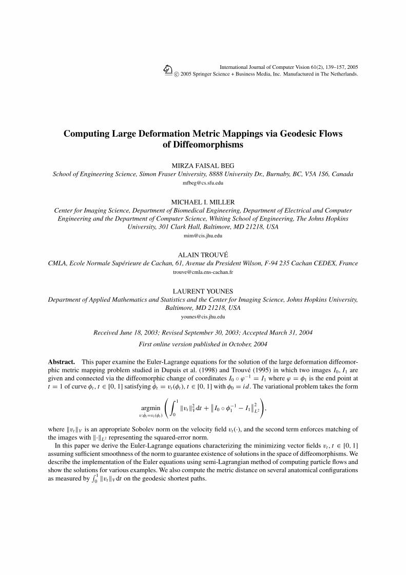
International Journal of Computer Vision 61(2), 139–157, 2005c© 2005 Springer Science + Business Media, Inc. Manufactured in The Netherlands.

Computing Large Deformation Metric Mappings via Geodesic Flowsof Diffeomorphisms

MIRZA FAISAL BEGSchool of Engineering Science, Simon Fraser University, 8888 University Dr., Burnaby, BC, V5A 1S6, Canada

mfbeg@cs.sfu.edu

MICHAEL I. MILLERCenter for Imaging Science, Department of Biomedical Engineering, Department of Electrical and Computer

Engineering and the Department of Computer Science, Whiting School of Engineering, The Johns HopkinsUniversity, 301 Clark Hall, Baltimore, MD 21218, USA

mim@cis.jhu.edu

ALAIN TROUVECMLA, Ecole Normale Superieure de Cachan, 61, Avenue du President Wilson, F-94 235 Cachan CEDEX, France

trouve@cmla.ens-cachan.fr

LAURENT YOUNESDepartment of Applied Mathematics and Statistics and the Center for Imaging Science, Johns Hopkins University,

Baltimore, MD 21218, USAyounes@cis.jhu.edu

Received June 18, 2003; Revised September 30, 2003; Accepted March 31, 2004

First online version published in October, 2004

Abstract. This paper examine the Euler-Lagrange equations for the solution of the large deformation diffeomor-phic metric mapping problem studied in Dupuis et al. (1998) and Trouve (1995) in which two images I0, I1 aregiven and connected via the diffeomorphic change of coordinates I0 ◦ ϕ−1 = I1 where ϕ = φ1 is the end point att = 1 of curve φt , t ∈ [0, 1] satisfying φt = vt (φt ), t ∈ [0, 1] with φ0 = id. The variational problem takes the form

argminv:φt =vt (φt )

( ∫ 1

0‖vt‖2

V dt + ∥∥I0 ◦ φ−11 − I1

∥∥2L2

),

where ‖vt‖V is an appropriate Sobolev norm on the velocity field vt (·), and the second term enforces matching ofthe images with ‖·‖L2 representing the squared-error norm.

In this paper we derive the Euler-Lagrange equations characterizing the minimizing vector fields vt , t ∈ [0, 1]assuming sufficient smoothness of the norm to guarantee existence of solutions in the space of diffeomorphisms. Wedescribe the implementation of the Euler equations using semi-Lagrangian method of computing particle flows andshow the solutions for various examples. We also compute the metric distance on several anatomical configurationsas measured by

∫ 10 ‖vt‖V dt on the geodesic shortest paths.

140 Beg et al.

Keywords: computational anatomy, Euler-Lagrange equation, variational optimization, deformable template,metrics

1. Introduction

The last decade has witnessed tremendous develop-ments in medical imaging technologies which aredelivering exquisitely detailed pictures of humananatomy. The acquisition of structural imagery viaMagnetic resonance imaging (MRI), anisotropic or ori-entational imagery via Diffusion Tensor Magnetic Res-onance Imaging (DTMRI) and functional activationimagery via Functional Magnetic Resonance Imaging(fMRI) among others is routine. These capabilities havein turn spurred the development of mathematics andalgorithms for analysis of the information containedin these images. A recurring theme in biomedical im-age analysis is registration; the variability in humananatomy is not an exception but a rule and hence theneed to transform the image data into standard coor-dinates to facilitate analysis and generalize results toa large subset of the population. The goal of registra-tion is to compute a transformation ϕ : � → � where� ⊆ R

n is the domain (n = 2 for 2D or n = 3 for 3D)on which the data (structural, orientational and func-tional) are defined. Let images representing this data befunctions I :� → R

d defined on �. Structural imagesacquired via MRI are scalar valued d = 1, color imagessuch as RGB are vector valued d = 3 and anisotropyor orientational images acquired from DTMRI are ma-trix valued. Since the diffusion tensor is symmetric,these can be taken to be vector valued d = 5. LetI0 and I1 denote the template and target images. Thetransformation of the template image I0 under sucha transformation is the pullback image defined to beϕ.I0 = I0 ◦ ϕ−1 = I0(ϕ−1). The transformations in-crease in dimensionality from low dimensional globaltransformations specified by a few parameters such asthe affine transformations to the high dimensional non-rigid transformations which are specified at each pointof the image domain.

The early attempts to compute high-dimensionalnon-rigid transformations in the medical image set-ting resulted in the development of the elastic match-ing strategy by Broit, Bajcsy and co-workers (Broit,1981; Bajcsy and Broit, 1982; Bajcsy et al., 1983) anddevelopment on these lines continues as this modelis refined and specialized to various applications. Inthis setting, the transformation ϕ is linearized aroundthe coordinate system of the exemplar or template

coordinate system and generated from a displacementvector field u:� → R

n such that ϕ(x) = x + u(x) orϕ−1(x) = x − u(x) for all points x ∈ �. The trans-formed template image I0 then becomes I0(ϕ−1(x)) =I0(x −u(x)), ∀x ∈ �. The “goodness” of the transfor-mation is measured by a cost of the form

E2(I0, I1, ϕ) = ‖I0 ◦ ϕ−1 − I1‖2L2

where ‖·‖L2 is the standard L2 norm of square inte-grable functions ‖ f ‖2

L2 = ∫�

| f (x)|2dx . The optimaltransformation is the one that minimizes this cost andthe optimal vector field u that generates such a trans-formation is, from among the many possible solutions,chosen to be the one with the highest smoothness. Themeasurement of smoothness is achieved by specifyingthe norm on the space of vector fields of the domain �

to be defined through a differential operator L by:

E1(u) = ‖Lu‖2L2

where L is commonly chosen to be a differential opera-tor of the form L = (−α�+ γ )In×n . In the variationalsetting (a very nice discussion is in Amit (1994)), theoptimal displacement vector field is computed by op-timization of the cost

argminu

‖Lu‖2L2 + 1

σ 2‖I0 ◦ ϕ−1 − I1‖2

L2 .

This approach of generating transformations from dis-placement vector fields has been an important de-velopment in computing non-rigid high dimensionaltransformations of medical imagery allowing for com-parison of anatomy in a standard coordinate system.One of the limitations of this approach is that there areno explicit constraints that ensure that the transforma-tions computed are one-to-one or invertible. Indeed, insome cases (Christensen, 1994) folding of the grid overitself can occur thereby destroying the neighbourhoodstructure which is essential for the study of anatomy.This method of computing transformations is known asthe small deformations approach as valid transforma-tions of anatomy using this linearized model via dis-placement vector fields are computed when the imagesare seperated by small deformations of the domain.

It is of considerable interest to compute transforma-tions which are not only invertible but also preserve

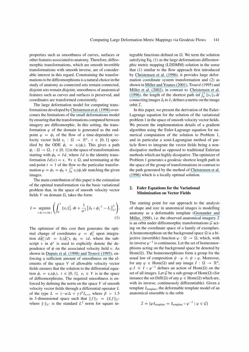
Computing Large Deformation Metric Mappings via Geodesic Flows 141

properties such as smoothness of curves, surfaces orother features associated to anatomy. Therefore, diffeo-morphic transformations, which are smooth invertibletransformations with smooth inverse, are of consider-able interest in this regard. Constraining the transfor-mations to be diffeomorphisms is a natural choice in thestudy of anatomy as connected sets remain connected,disjoint sets remain disjoint, smoothness of anatomicalfeatures such as curves and surfaces is preserved, andcoordinates are transformed consistently.

The large deformation model for computing trans-formations developed by Christensen et al. (1996) over-comes the limitations of the small deformations modelby ensuring that the transformations computed betweenimagery are diffeomorphic. In this setting, the trans-formation ϕ of the domain is generated as the end-point ϕ = φ1 of the flow of a time-dependent ve-locity vector field vt : � → R

n, t ∈ [0, 1] spec-ified by the ODE φt = vt (φt ). This gives a pathφt : � → �, t ∈ [0, 1] in the space of transformationsstarting with φ0 = I d , where I d is the identity trans-formation I d(x) = x, ∀x ∈ �, and terminating at theend-point t = 1 of the flow to the particular transfor-mation ϕ = φ1 = φ0 + ∫ 1

0 vt (φt )dt matching the givenimages.

The main contribution of this paper is the estimationof the optimal transformation via the basic variationalproblem that, in the space of smooth velocity vectorfields V on domain �, takes the form:

v = argminv:φt =vt (φt )

(∫ 1

0‖vt‖2

V dt + 1

σ 2

∥∥I0 ◦ φ−11 − I1

∥∥2L2

).

(1)

The optimizer of this cost then generates the opti-mal change of coordinates ϕ = φv

1 upon integra-tion dφv

t /dt = vt (φvt ), φ0 = id , where the sub-

script v in φv is used to explicitly denote the de-pendence of φ on the associated velocity field v. Asshown in Dupuis et al. (1998) and Trouve (1995), en-forcing a sufficient amount of smoothness on the el-ements of the space V of allowable velocity vectorfields ensures that the solution to the differential equa-tion φt = vt (φt ), t ∈ [0, 1], vt ∈ V is in the spaceof diffeomorphisms. The required smoothness is en-forced by defining the norm on the space V of smoothvelocity vector fields through a differential operator Lof the type L = (−α� + γ )β In×n where β > 1.5in 3-dimensional space such that ‖ f ‖V = ‖L f ‖L2

where ‖·‖L2 is the standard L2 norm for square in-

tegrable functions defined on �. We term the solutionsatisfying Eq. (1) as the large deformations diffeomor-phic metric mapping (LDDMM) solution in the sensethat (1) similar to the flow approach first introducedby Christensen et al. (1996), it provides large defor-mation coordinate system transformation and (2) asshown in Miller and Younes (2001), Trouve (1995) andMiller et al. (2002), in contrast to Christensen et al.(1996), the length of the shortest path inf

∫ 10 ‖vt‖V dt

connecting images I0 to I1 defines a metric on the imageorbit I.

In this paper, we present the derivation of the Euler-Lagrange equation for the solution of the variationalproblem 1 in the space of smooth velocity vector fields.We present the implementation details of a gradientalgorithm using the Euler-Lagrange equation for nu-merical computation of the solution to Problem 1,and in particular a semi-Lagrangian method of par-ticle flows to integrate the vector fields being a non-dissipative method as opposed to traditional Eulerianmethods which are highly dissipative. The optimizer ofProblem 1 generates a geodesic shortest length path inthe space of the group of transformations in contrast tothe path generated by the method of Christensen et al.(1996) which is a locally optimal solution.

2. Euler Equations for the VariationalMinimization on Vector Fields

The starting point for our approach to the analysisof shape and size in anatomical images is modellinganatomy as a deformable template (Grenander andMiller, 1998), i.e. the observed anatomical imagery Iis an orbit under diffeomorphic transformations G act-ing on the coordinate space of a family of exemplars.A homeomorphism on the background space � is a bi-jective (invertible) function ϕ : � → �, which, withits inverse ϕ−1 is continuous. Let the set of homeomor-phisms acting on the background space be denoted byHom(�). The homeomorphisms form a group for theusual law of composition ψ · ϕ

.= ψ ◦ ϕ. Moreover,for any ϕ ∈ Hom(�) and any image I : � → R

d ,ϕ.I

.= I ◦ ϕ−1 defines an action of Hom(�) on theset of all images. Let G be a sub-group of Hom(�) (forinstance the set Diff(�) of any ϕ ∈ Hom(�) which are,with its inverse, continuously differentiable). Given atemplate Itemplate, the deformable template model of ananatomical ensemble is the orbit

I .= {ϕ Itemplate = Itemplate ◦ ϕ−1 | ϕ ∈ G}

142 Beg et al.

of Itemplate under the action of G. The orbit I beinghomogenous under the action of the elements of Gwhich are bijective mappings implies that images inthe anatomical ensemble I are topologically equiva-lent i.e. they possess the same sub-structures and forany two images I0, I1 ∈ I, there exists a ϕ ∈ G thatregisters the given images I1 = ϕ I0.

Given two images, the first task is to find the par-ticular element ϕ ∈ G that registers the given imagesI1 = ϕ I0 = I0 ◦ϕ−1. In the large deformations setting,this element is estimated as the end point of the flowassociated to a smooth time-dependent vector field. Letv : [0, 1] → V be a time-dependent velocity vector-field where V is a Hilbert space of smooth, compactlysupported vector fields on �. Let such a velocity vectorfield define the evolution of a curve φv : [0, 1] → Gvia the evolution equation

d

dtφv

t (x) = vt(φv

t (x))

(2)

where the subscript in φv is used to explicitly denotethe dependence of φ on the associated velocity field v.The initial point of the curve φv at t = 0 is φv

0 = I d ∈G where I d is the identity transformation I d(x) =x, ∀x ∈ �. The end point of the curve φv at time t = 1is the particular diffeomorphism φv

1 = ϕ ∈ G that linksthe given datasets I0 and I1 such that I1 = I0 ◦ϕ−1 andit is this element ϕ that we compute as the end point φv

1associated to a flow v. Thus, we seek a time-dependentvelocity vector fieldv which when integrated via Eq. (2)generates the particular diffeomorphism matching thegiven image datasets.

Let the notation φs,t : � → � denote the compo-sition φs,t = φt ◦ (φs)−1. The interpretation of φs,t (y)is that it is the position at time t of a particle that isat position y at time s. Therefore φv

1 (x) = φv0,1(x) is

the function that denotes the position at time t = 1 ofparticle that is at position x at time 0. Let the Jacobianof mapping φs,t , the matrix composed with the spacederivatives of φs,t , be denoted by Dφs,t .

To solve the variational problem 1, we first need tocompute the variation of the mapping φv

1,0 under theperturbation of v ∈ L2([0, 1], V ) by h ∈ L2([0, 1], V )which we state in the following lemma.

Lemma 2.1. The variation of mapping φvs,t when v ∈

L2([0, 1], V ) is perturbed along h ∈ L2([0, 1], V ) is

given by:

∂hφvs,t = αs,t = lim

ε→0

φv+εhs,t − φv

s,t

ε

= Dφvs,t

∫ t

s

(Dφv

s,u

)−1hu ◦ φv

s,u du. (3)

Proof: We provide a proof under the assumption thatthe derivative with respect to ε in Eq. (3) exists and pro-ceed to its identification. The proof of existence can becarried on by standard ordinary differential equations(ODE) arguments. We have

dφv+εhs,t

dt= vt ◦ φv+εh

s,t + εht ◦ φv+εhs,t .

Computing the differential in ε at ε = 0 yields

d

dt∂hφ

vs,t = Dφv

s,tvt∂hφ

vs,t + ht ◦ φv

s,t (4)

Thus, ∂hφvs,t is the solution of a non-homogeneous dif-

ferential equation, and it suffices to show that the lastexpression in 3 is a solution of the same equation withthe correct condition ∂hφ

vs,s = 0, but this is an obvious

computation, using the fact that

d

dtDφv

s,t = Dφvs,tvt Dφv

s,t ,

which simply comes from computing the space differ-ential of dφv

s,t/dt = vt ◦φs,t . Note that this identity alsoprovides the solution of the homogeneous equation as-sociated to 4, so that 3 can also be directly identifiedby variation of the constant.

Existence of the transformations generated viaEq. (2) depend on the smoothness constraints placed onvector fields allowed in V (Dupuis et al., 1998; Trouve,1995). One choice to ensure existence of solutions inthe space of diffeomorphisms for the ordinary differ-ential equation (ODE) 2 has been to construct V asthe completion of the space of smooth, compactly-supported vector fields for the inner-product definedthrough a differential operator L (denoting its adjointas L†) given by:

〈 f, g〉V.= 〈L f, Lg〉L2 = 〈L†L f, g〉L2 , (5)

where 〈, 〉L2 is the usual L2-product for square inte-grable vector-fields on �. With V defined in this way,the flow ofv ∈ L1([0, 1], V ) generates the sub-group of

Computing Large Deformation Metric Mappings via Geodesic Flows 143

diffeomorphismsG .= {ϕ |ϕ = φv1 , v ∈ L1([0, 1], V )}

that are the end-points of flows associated to elementsv ∈ L1([0, 1], V ) (the technical details associated withthis construction have been published in Dupuis etal. (1998) and Trouve (1995)). From the assumptionsplaced in the construction of V , a compact self-adjointoperator operator K : L2(�, R

d ) → V is uniquelydefined by

〈a, b〉L2 = 〈K a, b〉V . (6)

and together with 5, one gets for any smooth vectorfield f ∈ V that

K (L†L) f = f. (7)

The variational problem for dense image matchingis now stated and solved in the space of vector fieldsV .

Theorem 2.1. Given a continuously differentiableidealized template image I0 and a noisy observation ofanatomy I1, then v ∈ L2([0, 1], V ) for inexact match-ing of I0 and I1 is given by

v = arginfv∈L2([0,1],V )

E(v).=

∫ 1

0‖vt‖2

V dt

+ 1

σ 2

∥∥I0 ◦ φv1,0 − I1

∥∥2L2 (8)

which satisfies the Euler-Lagrange equation given by

2vt − K

(2

σ 2

∣∣Dφvt,1

∣∣ ∇ J 0t

(J 0

t − J 1t

)) = 0 (9)

where J 0t

.= I0 ◦ φt,0, J 1t

.= I1 ◦ φt,1.

Proof: Let the velocity v ∈ L2([0, 1], V ) beperturbed by an ε amount along direction h ∈L2([0, 1], V ). The Gateaux variation ∂h E(v) of the en-ergy functional is related to its Frechet derivative ∇v Eby

∂h E(v) = limε→0

E(v + εh) − E(v)

ε

=∫ 1

0〈∇v Et , ht 〉V dt.

The variation of E1(v) = ∫ 10 ‖vt‖2

V dt is given by:

∂h E1(v) = 2∫ 1

0〈vt , ht 〉V dt.

Variation of E2(v) = 1σ 2 ‖I0 ◦ φv

1,0 − I1‖2L2 is

∂h E2(v) = 2

σ 2

⟨I0 ◦ φv

1,0 − I1, DI0 ◦ φv1,0∂hφ

v1,0

⟩L2

(a)= 2

σ 2

⟨I0 ◦ φv

1,0 − I1, DI0 ◦ φv1,0

×(

−Dφv1,0

∫ 1

0

(Dφv

1,t

)−1ht ◦ φv

1,t dt

)⟩L2

(b)= −2

σ 2

∫ 1

0

⟨(I0 ◦ φv

1,0 − I1, D(I0 ◦ φv

1,0

)× (

Dφv1,t

)−1ht ◦ φv

1,t

⟩L2 dt

with (a) where subsitution of ∂hφv1,0 is made using

Lemma 2.1 and in (b) collecting D(I0 ◦ φv1,0) = DI0 ◦

φv1,0 Dφv

1,0. Setting φv1,t (y) = x i.e. φv

t,1(x) = y, givesthe Jacobian change of variables |Dφv

t,1(x)|dx = dy.With this, φv

1,0 → φv1,0 ◦ φv

t,1 = φvt,0 and substituting in

above, we get:

∂h E2(v)

= −2

σ 2

∫ 1

0

⟨∣∣Dφvt,1

∣∣(I0 ◦ φvt,0 − I1 ◦ φv

t,1

),

D(I0 ◦ φv

t,0

)ht

⟩L2 dt

= −2

σ 2

∫ 1

0

⟨∣∣Dφvt,1

∣∣(J 0t − J 1

t

)∇ J 0t , ht

⟩L2 dt

= −∫ 1

0

⟨K

(2

σ 2

∣∣Dφvt,1

∣∣(J 0t − J 1

t

)∇ J 0t

), ht

⟩V

dt.

Collecting terms, the gradient of the energy functionalis thus

(∇v Et )V = 2vt − K

(2

σ 2

∣∣Dφvt,1

∣∣∇ J 0t

(J 0

t − J 1t

)),

(10)

where the subscript V in (∇v Et )V indicates the gradientis in the space V . The optimizing velocity field satisfiesthe Euler-Lagrange equation

∂h E(v) =∫ 1

0

⟨2vt − K

×(

2

σ 2

∣∣Dφvt,1

∣∣∇ J 0t

(J 0

t − J 1t

)), ht

⟩V

dt = 0 (11)

Since h is arbitrary in L2([0, 1], V ) we get equalityEq. (9).

The optimal vector field for 8 is calculated by using thegradient 10 in a standard gradient descent algorithm. As

144 Beg et al.

we shall see in the next section, the optimization vectorfields assign a metric

∫ 10 ‖vt‖V dt on I and we denote

the algorithm based on this gradient as the large de-formation diffeomorphic metric mapping (LDDMM)algorithm.

3. Numerical Implementationof LDDMM Algorithm

This section presents the discretization and implemen-tation details of the estimation of the optimizing vectorfields. Let � = [0, 1]2/[0, 1]3 represent the 2D/3Dbackground space. Let the discretized flow generatingthe diffeomorphism be indexed by the discretized in-dex t j ∈ [0, T ], j ∈ [0, N ], the size of a timestep beingδt such that T = N × δt . Assume piecewise-constantvelocities in the discretized time intervals. Let vk

t j(y)

and φkt j

(y) denote the velocity field and the mappingfor the kth iteration of the gradient algorithm and thej th timestep along the discretized flow. Let I0 = J 0

0be the image at t = 0 of the flow being mapped to theimage I1 = J T

T at time index t = T of the flow.

3.1. Gradient Descent Scheme Based Optimization

The variational optimization of the energy functional(Eq. (8)) is performed in a standard steepest descentscheme

vk+1 = vk − ε∇vkt j

E (12)

where the discretized version of the gradient ∇v E fromEq. (10) is given by

∇vkt j

Ekt j

(y) = 2vkt j

(y) − 2

σ 2K

(∣∣Dφkt j ,T (y)

∣∣D J 0t j

(y)

∗ (J 0

t j(y) − J T

t j(y)

)). (13)

The discretized energy becomes

E(vk) =N−1∑j=0

∥∥vkt j

∥∥2Vδt + 1

N1 N2 N3

×∑y∈�

∣∣J 0T (y) − J T

T (y)∣∣2

(14)

and the length of the path from the identity to the esti-mated matching diffeomorphism φT at simulation in-

dex k becomes

Length(I d, φvk

T

) =N−1∑j=0

∥∥vkt j

∥∥V δt. (15)

3.2. Choice of Operator L and Evaluationof L†L, (L†L)−1

Let discretized functions f (x) and g(x) be definedf, g : � ⊂ Z

n → Rn on the discrete lattice � ⊂ Z

n

and which satisfy equation

L†L f = g. (16)

The operator L is chosen to be of the Cauchy-Naviertype, L

.= −α∇2 + γ I where I is the identity oper-ator and ∇2 = ∂2

∂x2 + ∂2

∂y2 + ∂2

∂z2 is the Laplacian op-erator. The coefficient α enforces smoothness, highervalues ensure solutions of high regularity, and the co-efficient γ is chosen to be positive so that the op-erator is non-singular. As well, as more anatomiesare mapped in future, we will use the statistics ofthe anatomical mappings to choose these coefficients(Grenander and Miller, 1998). We assume periodicboundary conditions, in which case L is self-adjointL = L†. Given the discretized function f , to calcu-late the function g via Eq. (16), write the discretizedversion for L f (x) using finite differences on a periodicdomain.

g(x1, x2, x3)

= (−α∇2 + γ ) f (x1, x2, x3)

= −α

(f (x1 + x1, x2, x3) − 2 f (x1, x2, x3) + f (x1 − x1, x2, x3)

x21

+ f (x1, x2 + x2, x3) − 2 f (x1, x2, x3) + f (x1, x2 − dx2, x3)

x22

+ f (x1, x2, x3 + x3) − 2 f (x1, x2, x3) + f (x1, x2, x3 − x3)

x23

)

+ γ f (x1, x2, x3) (17)

where x1 = 1/N1, x2 = 1/N2, x3 = 1/N3 arethe discretization of the domain � to the unit-cube.The operator L†L = L2 may be evaluated by L(L f ))or by explicitly writing out the discretized version ofL2 f on the lines of Eq. (17). Given the function g(x),function f (x) is evaluated using the Eq. (16) by solv-ing f = (L†L)−1g. This computation is efficientlyachieved in the Fourier domain: if F et G are thediscrete Fourier transforms of f et g, Eq. (17) yields

Computing Large Deformation Metric Mappings via Geodesic Flows 145

G(k) = A(k)2 F(k) where frequency k = (k1, k2, k3)and A(k) = γ +2α

∑3i=1( 1−cos(2π xi ki )

x2i

). Thus given g,Eq. (17) is solved by taking the fourier transform, yield-ing G, dividing each G(k) by A(k)2 and then computingthe inverse Fourier transform of the result to yield f .

3.3. Integration of Velocity Field to Generate Maps

Given the velocity fields, we need to compute the dif-feomorphisms (φv

t )−1 that we denote as φvt,0. The equa-

tion of evolution of this function is derived by differ-entiation with respect to time (φv

t )−1 ◦ φvt (x) = x for

all x ∈ � giving:

∂

∂t

(φv

t

)−1 ◦ φvt (x) + D

(φv

t

)−1 ◦ φvt (x)

d

dtφv

t (x) = 0

∂

∂t

(φv

t

)−1 ◦ φvt (x) + D

(φv

t

)−1 ◦ φvt (x) vt ◦ φv

t (x) = 0

∂φvt,0

∂t(y) + Dφv

t,0(y) vt (y)(a)= 0

where the derivative d/dt(φvt ) is given by definition

to be vt ◦ φvt , D stands for the Jacobian operator, and

(a) follows from change of variables φvt (x) = y and

finally changing back to the notation used throughoutthe paper that (φv

t )−1. This differential equation is inthe Eulerian frame of reference, it is an example of atransport equation where the flow is observed at thefixed regular Cartesian mesh (note that the velocity isspecified on the grid points y ∈ � at each time t)by following a new set of particles corresponding tothose that are at the regular mesh points at each dis-cretized time instant. In contrast, the Lagrangian equa-tion presented in (Eq. (2)), flow is observed by follow-ing the streamlines of the flow of particles, this leadsto computations that are on a regular Cartesian meshto start with but evolve to become computations on anunstructured mesh. A straightforward computation ofthe solution to the equation in the Eulerian frame ofreference, since one needs to compute the function φv

t,ois to approximate the derivative by corresponding fi-nite differences and propogate the solution from timet to time t + 1 starting with known solution at timet = 0 which is the identity map. This scheme is knownas the Eulerian scheme. The solution to (Eq. (2)) alsoapproximated by standard finite differences is calleda Lagrangian scheme. The issue here is the choice ofthe size of a timestep. On one hand, in the interestof accuracy, the timestep of discretization needs to besmall, on the other hand, overly small timesteps lead

to large computation times and thus impractical. Eu-lerian schemes have the disadvantage that the size oftimestep is restricted by issues related to CFL stability(Morton and Mayers, 1996) whereas Lagrangianschemes are computational stable and provide good tol-erance to numerical-accuracy related errors for choiceof larger size timestep compared to Eulerian schemes.On the other hand, Lagrangian schemes are more in-volved to implement due to the need to track particleswhose trajectories evolve away from their starting po-sitions on a regular grid.

Semi-Lagrangian schemes (Staniforth and Cote,1991) are a hybrid between these two schemes, theyinvolve following the streamlines for a timestep withthe streamlines chosen at each timestep to be those thatend on the regular grid at the next timestep. This allowsthe choice of larger timesteps which are an advantage ofLagrangian schemes and data computation on a regulargrid, which are an advantage of the Eulerian numeri-cal schemes. We have implemented a two-step semi-Langrangian scheme with iterative backward trajectorycalculation which are described in Staniforth and Cote(1991). Given the velocity field vk

t j(y) for all discretized

timesteps along the flow t j , j ∈ [0, N −1], δt = T/N ,the semi-Lagrangian based scheme to solve the trans-port equations governing the evolution of the mappingsφv

t j ,0(y), φv

t j ,T(y) are the equations:

φvt j ,0(y) = φv

t j−1,0(y − α) (18)

φvt j ,T (y) = φv

t j+1,T (y + α). (19)

where α is the displacement in one-timestep of follow-ing the streamlines with appropriate velocity v∗

t j ±0.5(y)at the mid-point of the interval [t j−1, t j ) for Eq. (18) and[t j , t j+1) for Eq. (19). Various schemes to estimate thevelocity at the mid-point are described in Staniforthand Cote (1991), and we choose the simple approxi-mation v∗

t j±0.5(y) = vt j (y) based on the assumption of

piece-wise constant velocity in discretized time inter-vals. Given this velocity, the displacement α is itera-tively calculated using the formula:

α

2= δt

2v∗

t j±0.5

(y − α

2

)(20)

with the data for non-cartesian grid points being ob-tained by bi/tri-linear interpolation.

146 Beg et al.

3.4. Constant Speed Reparametrizationof Velocity Vector Field

The minimizer of 8 is constant speed (‖vt‖V = con-stant) since it is a geodesic. This property can be nu-merically achieved by time reparametrization (Carmo,1976), and doing this in parallel to gradient descent cansignificantly reduce the convergence time. We use thefollowing procedure. Define normalized length func-tion s : [0, T ] → [0, T ] given by

st = T

Length

∫ t

0‖vt‖V dt

with Length = ∫ T0 ‖vt‖V dt . Define the inverse function

h : [0, T ] → [0, T ] given by ht = s−1t so that sht = t

and ht = 1/sht Then, define vt = htvht , which has,by construction constant norm, ‖vt‖V = Length/T .Since the Schwartz inequality implies

∫ T

0‖vt‖2

V dt ≥ Length2/T

this operation can only reduce the geodesic energy,whereas φv

t = φvht

, implying φvT = φv

T and the secondterm of E(v), given in Eq. (8) is left unchanged. Thusthe total energy after reparametrization monotonicallydecreases.

3.5. The Large DeformationMetric-Matching Algorithm

The matching algorithm initializes with iteration k = 0,vk

t j= 0, ∇vk Et j = 0, φt j ,0 = I d, φt j ,T = I d ∀t j ∈

[0, T ]. For each iteration k = 1, 2, . . . K iterate thefolowing:

(1) Calculate new estimate of velocity vk+1 = vk −ε∇vk E .

(2) Reparametrize the velocity field to be constantspeed. This is done every 10 simulations.

(3) Calculate for j = N − 1 to j = 0 the mappingφk+1

t j ,T(y) using Eq. (19).

(4) Calculate for j = 0 to j = N − 1 the mappingφk+1

t j ,0(y) using Eq. (18).

(5) Calculate for j = 0 to j = N − 1 the imageJ 0

t j= I0 ◦ φk+1

t j ,0.

(6) Calculate for j = N − 1 to j = 0 the imageJ 1

t j= I1 ◦ φk+1

t j ,T.

(7) Calculate for j = 0 to j = N − 1 the gradient ofthe image D J 0

t j.

(8) Calculate for for j = 0 to j = N −1 the Jacobianof the transformation |Dφt j |.

(9) Calculate for j = 0 to j = N − 1 the gradient∇vk+1 E for vk+1 using Eq. (10).

(10) Calculate the norm of the new gradient ‖∇vk+1 E‖.Stop if below threshold.

(11) Calculate the new Energy using Eq. (14).(12) If the number of simulations greater than specified

number then Stop. Else re-iterate with k = k + 1.(13) Denote the final velocity field as v which gives

the estimate of the desired optimizer of Eq. (8).(14) Calculate the length of the path on the manifold

using Eq. (15). This is the length of the geodesicand hence the estimated metric between the givenimages.

3.6.∫ 1

0 ‖vt‖V dt Defines a Metric on I

The metric distance between any two points ϕ0, ϕ1 ∈G comes from the geodesic length of the curveφv

t ∈ G, t ∈ [0, 1] associated to a vector fieldv ∈ L2([0, 1], V ) given by

∫ 10 ‖vt‖V dt with end-points

ϕ0 = φv0 and ϕ1 = φv

1 . The following construction(Dupuis et al., 1998; Miller and Younes, 2001; Trouve,1995).

ρG(ϕ0, ϕ1).= inf

{ ∫ 1

0‖vt‖V dt | ϕ1 = φv

1 ◦ ϕ0

}(21)

defines a distance on G for which G is complete. Fromthe definition of the distance ρG and the construction ofG, we get immediately the following right-invarianceproperty:

ρG(ϕ0, ϕ1) = ρG(ϕ0 ◦ ϕ, ϕ1 ◦ ϕ).

Proposition 3.1. The function ρI : I × I → R+defined on the anatomical ensemble I by:

ρI (I0, I1).= inf{ρG(Id, ϕ) | I1 = I0 ◦ ϕ−1, ϕ ∈ G}.

is positive, symmetric and satisfies the triangle-inequality.

Proof: The distance ρI (I0, I1) inherits the propertiesof positivity and symmetry from the distance ρG . Italso satisfies the triangle-inequality if the distance ρG

Computing Large Deformation Metric Mappings via Geodesic Flows 147

is right-invariant to the stabilizer of the template, whichis satisfied here by construction as ρG is invariant to theentire group G (Miller and Younes, 2001). From theresults of Dupuis et al., Trouve and Younes, it can beshown that the infimum is attained with ρI (I0, I1) =0 ⇒ I0 = I1 and thus ρI is a metric on I (Younes,1999).

Intuitively, if the images of the given anatomies areclose, then the diffeomorphic transformation needed toregister the images will be closer to the identity trans-formation and the corresponding distance between im-ages as defined in Eq. (3.1) will be smaller than if thegiven images are far away. The distance presented onlydeals with the deformation aspects, and is not invari-ant by rigid transformations, which is not an issue formany application, for which rigid registration is given,or at least may be recovered by standard algorithms.

It also turns out that the critical points v ∈L2([0, 1], V ) of the length functional

∫ 10 ‖vt‖V dt

are also the critical points of the energy functional∫ 10 ‖vt‖2

V dt with the additional property that they areof constant speed giving that

ρ2G(ϕ0, ϕ1) = inf

{ ∫ 1

0‖vt‖2

V dt | ϕ1

= φv1 ◦ ϕ0, ‖vt‖V = constant

}

the proof for which is found in Carmo (1993). There-fore, the length of the vector field satisfying the Euler-Lagrange Eq. (10) being the variational optimizer of8 gives the metric distance between images I0 andI0 ◦φv

1,0. The problem which is dealt with in this paper,i.e. the minimization of∫ 1

0‖vt‖2

V dt + 1

σ 2

∥∥I0 ◦ φv1,0 − I1

∥∥2L2

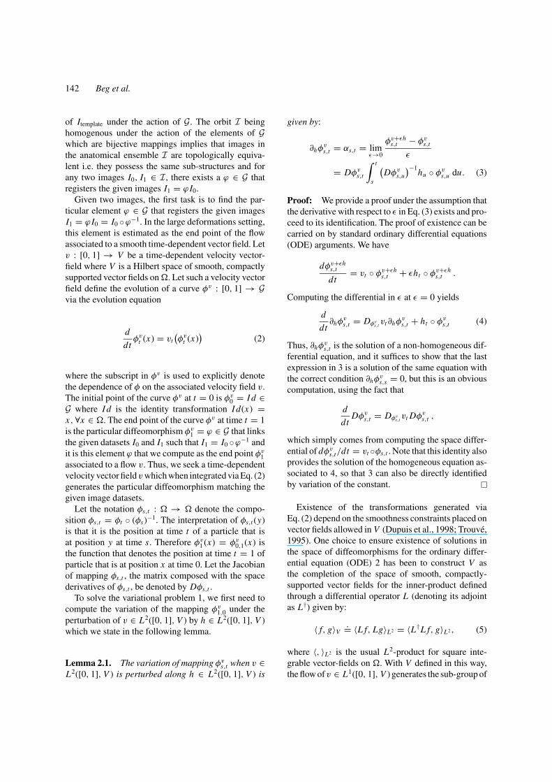
Figure 1. “Parallel Translation Experiment”. Shown is image I0 composed with the diffeomorphisms at discretized instants t j , j = 6, 12, 19on the geodesic path to the image I1 and the corresponding metric distance for the image with respect to image I0.

can be seen as an approximation of the exact matchingproblem which corresponds to the computation of ρG ,taking into account possible inaccuracies in the obser-vation of I1.

4. Numerical Results

We first present the application of the LDDMM algo-rithm to compute a geodesic path between two givenimages, and the metric estimated for the pair. The algo-rithm is implemented in C++ to work on 2D imagesas well as 3D volumes and parallelized using MPI toexecute on an IBM RS6000-SP computer to take ad-vantages of larger memory and concurrent parallel pro-cessing for computations. The time interval of the flowis discretized, unless stated otherwise, into 20 steps,with each step being of length δt = 0.1.

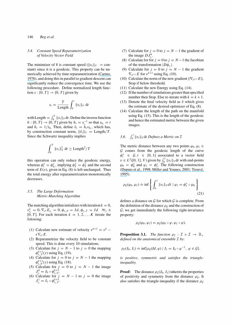
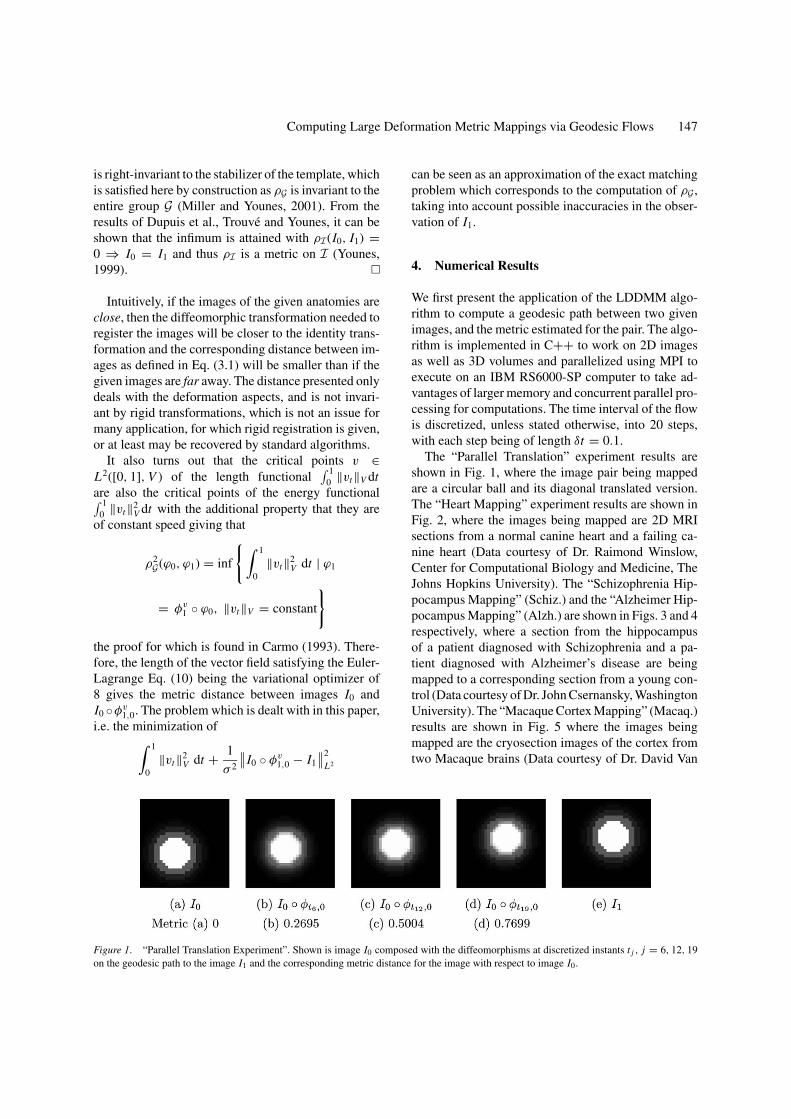
The “Parallel Translation” experiment results areshown in Fig. 1, where the image pair being mappedare a circular ball and its diagonal translated version.The “Heart Mapping” experiment results are shown inFig. 2, where the images being mapped are 2D MRIsections from a normal canine heart and a failing ca-nine heart (Data courtesy of Dr. Raimond Winslow,Center for Computational Biology and Medicine, TheJohns Hopkins University). The “Schizophrenia Hip-pocampus Mapping” (Schiz.) and the “Alzheimer Hip-pocampus Mapping” (Alzh.) are shown in Figs. 3 and 4respectively, where a section from the hippocampusof a patient diagnosed with Schizophrenia and a pa-tient diagnosed with Alzheimer’s disease are beingmapped to a corresponding section from a young con-trol (Data courtesy of Dr. John Csernansky, WashingtonUniversity). The “Macaque Cortex Mapping” (Macaq.)results are shown in Fig. 5 where the images beingmapped are the cryosection images of the cortex fromtwo Macaque brains (Data courtesy of Dr. David Van

148 Beg et al.

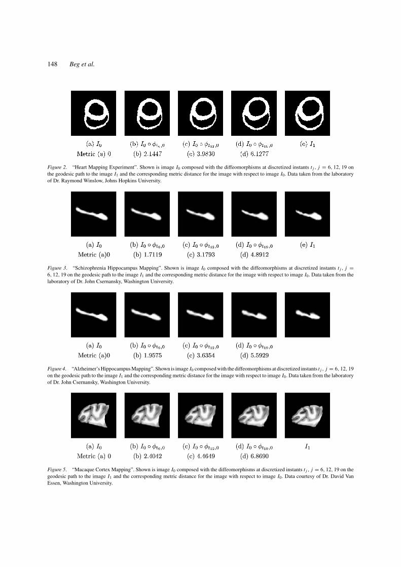
Figure 2. “Heart Mapping Experiment”. Shown is image I0 composed with the diffeomorphisms at discretized instants t j , j = 6, 12, 19 onthe geodesic path to the image I1 and the corresponding metric distance for the image with respect to image I0. Data taken from the laboratoryof Dr. Raymond Winslow, Johns Hopkins University.

Figure 3. “Schizophrenia Hippocampus Mapping”. Shown is image I0 composed with the diffeomorphisms at discretized instants t j , j =6, 12, 19 on the geodesic path to the image I1 and the corresponding metric distance for the image with respect to image I0. Data taken from thelaboratory of Dr. John Csernansky, Washington University.

Figure 4. “Alzheimer’s Hippocampus Mapping”. Shown is image I0 composed with the diffeomorphisms at discretized instants t j , j = 6, 12, 19on the geodesic path to the image I1 and the corresponding metric distance for the image with respect to image I0. Data taken from the laboratoryof Dr. John Csernansky, Washington University.

Figure 5. “Macaque Cortex Mapping”. Shown is image I0 composed with the diffeomorphisms at discretized instants t j , j = 6, 12, 19 on thegeodesic path to the image I1 and the corresponding metric distance for the image with respect to image I0. Data courtesy of Dr. David VanEssen, Washington University.

Computing Large Deformation Metric Mappings via Geodesic Flows 149

Table 1. Summary of parameters used for the 2D image matching experiments as well as the final error inimage overlap after the mapping relative to the error before the mapping, metric distance, number of iterationsfor convergence and execution time.

Experiment (image size) L Image error (%) Est. metric Iter. Exec. time

“Parallel Translation” (32 × 32) −0.01∇2 + 0.1I 1.97 0.769 70 0.2 min

“Heart Mapping” (80 × 80) −0.01∇2 + I 7.12 6.122 159 3.7 min

“Schiz.” (64 × 64) −0.01∇2 + I 3.01 4.891 277 4.2 min

“Alzh.” (64 × 64) −0.01∇2 + I 2.69 5.592 255 3.9 min

“Macaq.” (80 × 80) −0.01∇2 + I 3.64 6.869 134 3.2 min

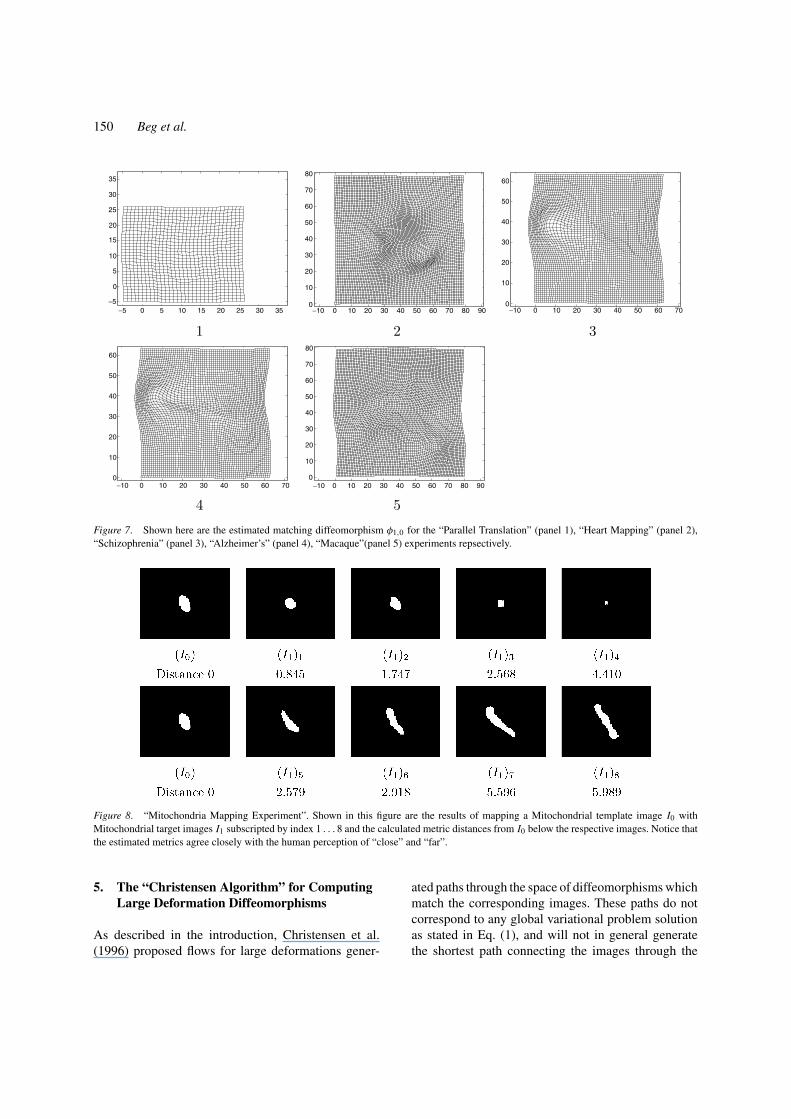
Essen, Washington University). The 2D experimentswere run on a single processor, Table 1 shows parame-ters and data from these experiments. The “Mitochon-dria Mapping” experiment results (Fig. 8) show thesegmented mitochondria shapes from high resolutionmicrographs that were mapped to a single image andthe estimated metrics for operator L = −0.01∇2 + I .The results of mapping 3D hand-segmented volumestaken from Alzheimers and Schizophrenia populationsare shown in the Fig. 9. The 3D images are of dimen-sions 80 pixels by 128 by 128 pixels and the operatorL = −0.01∇2 + 0.1I was used for the mapping. Ex-cept for the “Parallel Translation” experiment, all otherimages were registered using the software “Analyze”(Robb, 1999) to remove rigid rotation and translation

Figure 6. The velocity field along the discretized flow vt j , j = 0 . . . 19 are superposed on a single figure for each of the “Parallel Translation”(panel 1), “Heart Mapping” (panel 2), “Schizophrenia” (panel 3), “Alzheimer’s” (panel 4), “Macaque” (panel 5) experiments respectively. Noticethat the velocity is smooth in space. Also interesting to note is that the velocity field is quite smooth in time as well.

prior to the experiment. Execution times depend on thesize of images and the number of iterations needed toreach convergence. For 2D images of the size 64 × 64,the execution time of the algorithm is of the order ofa few minutes on a single processor. For 3D images ofthe size 80 × 128 × 128, execution time ranges fromhalf an hour to a few hours running on 8 processors.

For each of these experiments, the sequence com-prising the image I0 composed with the diffeomor-phisms at discretized instants t j , j = 6, 12, 19 on thegeodesic path to the image I1 are shown in Figs. 1–4. Figure 6 shows the vector plot of the superpo-sition of velocity fields estimated for the flow, andFig. 7 the estimated mapping φ1,0 for each of theseexperiments.

150 Beg et al.

−5 0 5 10 15 20 25 30 35−5

0

5

10

15

20

25

30

35

−10 0 10 20 30 40 50 60 70 80 900

10

20

30

40

50

60

70

80

−10 0 10 20 30 40 50 60 700

10

20

30

40

50

60

−10 0 10 20 30 40 50 60 700

10

20

30

40

50

60

−10 0 10 20 30 40 50 60 70 80 900

10

20

30

40

50

60

70

80

Figure 7. Shown here are the estimated matching diffeomorphism φ1,0 for the “Parallel Translation” (panel 1), “Heart Mapping” (panel 2),“Schizophrenia” (panel 3), “Alzheimer’s” (panel 4), “Macaque”(panel 5) experiments repsectively.

Figure 8. “Mitochondria Mapping Experiment”. Shown in this figure are the results of mapping a Mitochondrial template image I0 withMitochondrial target images I1 subscripted by index 1 . . . 8 and the calculated metric distances from I0 below the respective images. Notice thatthe estimated metrics agree closely with the human perception of “close” and “far”.

5. The “Christensen Algorithm” for ComputingLarge Deformation Diffeomorphisms

As described in the introduction, Christensen et al.(1996) proposed flows for large deformations gener-

ated paths through the space of diffeomorphisms whichmatch the corresponding images. These paths do notcorrespond to any global variational problem solutionas stated in Eq. (1), and will not in general generatethe shortest path connecting the images through the

Computing Large Deformation Metric Mappings via Geodesic Flows 151

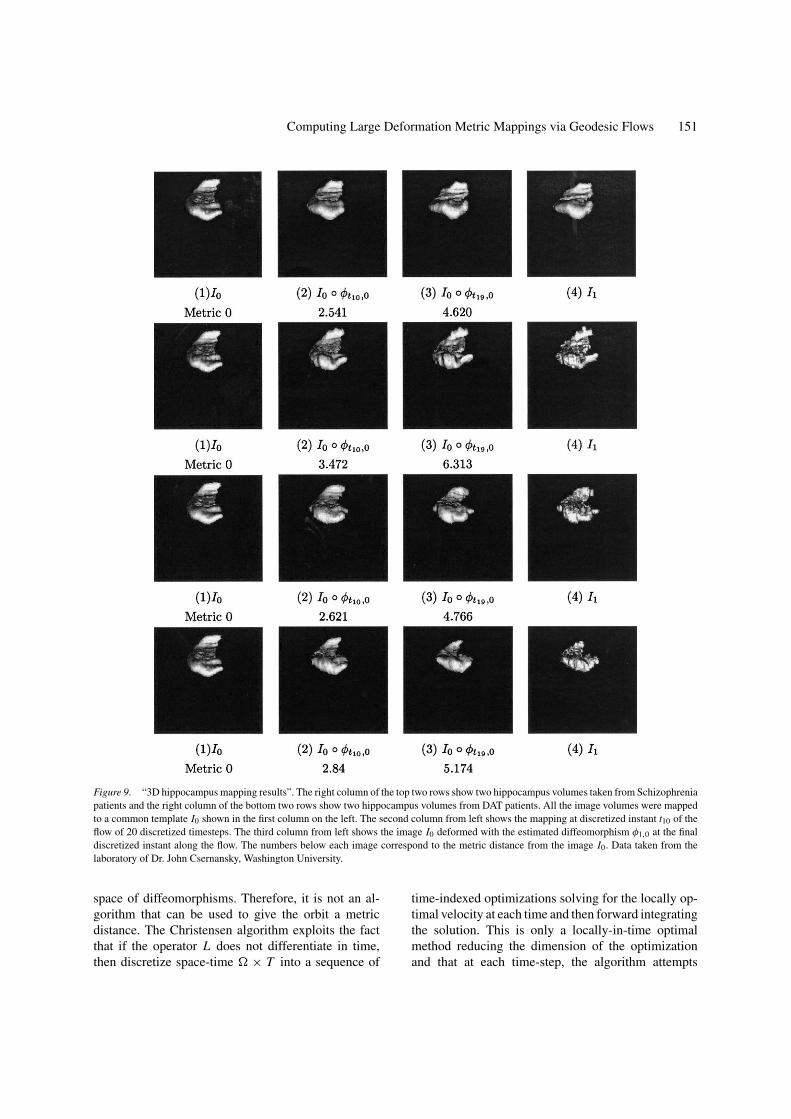
Figure 9. “3D hippocampus mapping results”. The right column of the top two rows show two hippocampus volumes taken from Schizophreniapatients and the right column of the bottom two rows show two hippocampus volumes from DAT patients. All the image volumes were mappedto a common template I0 shown in the first column on the left. The second column from left shows the mapping at discretized instant t10 of theflow of 20 discretized timesteps. The third column from left shows the image I0 deformed with the estimated diffeomorphism φ1,0 at the finaldiscretized instant along the flow. The numbers below each image correspond to the metric distance from the image I0. Data taken from thelaboratory of Dr. John Csernansky, Washington University.

space of diffeomorphisms. Therefore, it is not an al-gorithm that can be used to give the orbit a metricdistance. The Christensen algorithm exploits the factthat if the operator L does not differentiate in time,then discretize space-time � × T into a sequence of

time-indexed optimizations solving for the locally op-timal velocity at each time and then forward integratingthe solution. This is only a locally-in-time optimalmethod reducing the dimension of the optimizationand that at each time-step, the algorithm attempts

152 Beg et al.

to greedily reach the target. The transformation φ1,0

registering the given anatomical images is generatedfrom velocity fields which are assumed piecewise con-stant within quantized time increments of size δ, k =0, . . . , K , tk = kδ, k = 0, . . . , K = T

δ. The locally

optimal velocity fields satisfy the partial differentialequation

L†Lvt + bt = 0 (22)

where the function bt : � → Rn is given by

bt (x) = −ζ(J 0

t (x) − J 11 (x)

)∇ J 0t (x), (23)

where J 0t = I0 ◦ φt,0 and J 1

1 = I1 and ζ is someconstant. The time-indexed sequence of locally optimalvelocity fields vt j are integrated to yield the sequence oftransformations φv

t j, j = 0, 1, 2, . . . , which are points

along a path on the manifold of diffeomorphisms fromthe identity transformation to the point φ1,0, the lengthof which is

∫ 10 ‖vt‖V dt .

One way to interpret this method is to explore theconnection to the search for the optimizer of the costin the space of diffeomorphisms G (Trouve, 1998).Rewrite Eq. (8) as a function on G to be

E(φ) = ρG(id, φ1)2︸ ︷︷ ︸E1(φ)

+ 1

σ 2‖I0 ◦ φ1,0 − I1‖2

L2︸ ︷︷ ︸E2(φ)

(24)

and now the matching diffeomorphism is sought bya search in the space of diffeomorphisms G. Supposethat the optimization for the matching diffeomorphismφ1 proceeds on the manifold with the estimate φt attime t being the candidate as the end-point of a curveφ : [0, t] → G joining all previous estimated pointswith φ0 = id ∈ G. The length of the curve traversedis then

∫ t0 ‖vt‖V dt ≥ ρG(id, φt ) and this provides an

upper-bound on the metric distance ρG(id, φt ) as thecurve traversed is not necessarily the geodesic. Let thecost for traversing this curve from the identity to φt ∈ Gon the manifold be denoted by Wt where

Wt = Length(id, φt )2 + E2(φt )

≥ ρG(id, φt )2 + E2(φt ) (25)

where Length(id, φt ) is the length of the curve φ withendpoints id, φt ∈ G. The local optimization processseeks the velocity vt such that moving along directionvt ◦ φt at the point φt on the manifold leads to the lowestincrease of the cost Wt+dt at t + dt . Since Wt+dt =

(Length(id, φt ) + ‖vt‖V dt)2 + E2(φt+dt ), which wecan rearrange and simplify to the first order as

Wt+dt = Wt + 2‖vt‖V × dt × Length(id, φt )

+ ∂vt ◦φt E2(φt ), (26)

where ∂vt ◦φt E2(φt ) is the change in E2 at the point φt

along the direction vt ◦ φt . Fixing ‖vt ◦ φt‖Tφt G = 1i.e. ‖vt‖V = 1, the local optimizer vt ◦ φt ∈ TφtG thatminimizes ∂vt ◦φt E2(φt ) is given by

vt ◦ φt = argmin‖vt ‖V =1

(∂vt ◦φt E2(φt )

= 〈∇E2(φt ), vt ◦ φt 〉Tφt G)

(27)

= −∇E2(φt )

= Opposite the direction of steepest increase

(28)

⇒ vt = −∇E2(φt ) ◦ φ−1t (29)

More formally, this can interpreted as a gradient de-scent on the manifold of diffeomorphisms (Trouve,1998) as:

∂φt

∂t= vt ◦ φt = −∇E2(φt ). (30)

The computation of ∇E2(φt ) is done by writing

∂vt ◦φt E2(φt )

(a)= −2

σ 2〈I0 ◦ φt,0 − I1, D(I0 ◦ φt,0)vt 〉L2 (31)

(b)= −2

σ 2

⟨K

((J 0

t − J 11

)∇ J 0t

), vt

⟩V (32)

(c)= 〈∇E2(φt ), vt ◦ φt 〉Tφt G(d)= ⟨∇E2(φt ) ◦ φ−1

t , vt⟩V

(33)

where (a) follows from differentiating the cost E2, (b)from writing the transpose and changing the notation∇ J 0

t = D(J 0t )t = D(I0 ◦φt,0)t along with transferring

the gradient from space L2 to space V using Eq. (6), (c)from definition of the gradient in the tangent space TφtGat pointφt , (d) from transferring the inner-product to thetangent space V = TidG at the identity of the manifold.This is a Riemannian (sometimes called “natural”) gra-dient in the space of diffeomorphisms equipped withthe right invariant metric, applied to for the data termor the fitting term E2. Comparing Eqs. (29), (32) and

Computing Large Deformation Metric Mappings via Geodesic Flows 153

(33), we get that

vt = −∇E2(φt ) ◦ φ−1t = 2

σ 2K

((J 0

t − J 11

)∇ J 0t

)(34)

is the optimizer for the incremental local cost givenin Eq. (24). Rearrangement of Eq. (34) provides thePDE in Eqs. (22) and the body force function 23 es-tablishing the connection of the PDE formulation andthe Riemannian gradient on the fitting term for the localoptimization of the matching cost in the space of diffeo-morphisms. The regularization provided by the opera-tor K gives this gradient numerically stable behaviourin finite time (of course, the limit behavior is unstable,because the regularization term ρ(id, φv)2 is not takeninto account). Henceforth, we denote this algorithmproposed by Christensen et al. as the “Christensen” orthe “GEC” algorithm summarized as following.

(1) Initialize: t j = 0, vt j = 0, φt j = I d.(2) Integrate the velocity field vt j to compute the map

φt j+1,0. Adjust the time-step of integration δt suchthat the largest displacement is within one pixel inmagnitude.

(3) Use estimated φt j+1,0 to compute cost E2(φt j+1,0).This cost quantifies the amount of registration ofI0 and I1 under the estimated mapping.

(4) If E2 < Threshold, STOP.(5) Using Eq. (23), calculate the body force bt j+1 .(6) Solve Eq. (22) for local optimizer vt j+1 using FFT-

based inversion giving vt j+1 = −K (bt j+1 ).(7) Set j = j + 1 and go to step (2).(8) On STOP, set time t j = 1, and number of steps

taken N = j .

Figure 10. Comparing the “LDDMM” and the “GEC” algorithms. Shown is the Image Error (solid line—“LDDMM” algorithm, dotted line—“GEC” algorithm) as a percentage of error before the transformation via the estimated mapping versus the distance of the path on the manifoldjoining the identity of the diffeomorphisms to the estimated mapping. In the left panel is the results from the “Parallel Translation” experiment,in the middle panel is the “Macaque Cortex Mapping” experiment and the right panel shows the results from the “Heart Mapping” experiment.

Our implementation of the above algorithm also in-cludes the template propogation feature as originallydescribed by Christensen et al. (see (1996) for de-tails) to handle large deformations where the computedtransformations approach local singularity on a dis-cretized spatial grid and thus lead to numerical preci-sion errors in interpolating concatenated transforma-tions. Note that the “demons” algorithm, proposed byThirion (1998), carries the same purpose (minimiza-tion of E2), but the GEC algorithm has the advantageof performing a true gradient descent, for a suitable Rie-mannian structure, and always remain within a spaceof smooth diffeomorphisms.

5.1. Comparison of the LDDMM Algorithmwith the GEC Algorithm

Figures 10 and 11 show results for three experimentswith the “LDDMM” and the “GEC” algorithms. Theexperiments were terminated when estimated map-pings from both made the image mismatch error com-parable. Figure 10 shows the image mismatch error asa function of the estimated distance on the manifold ofthe estimated transformation from the identity. At thesame “distance” from the target image, as measured bycomparable values of image mismatch error shown inTable 2, the “LDDMM” algorithm (solid line) estimatesa transformation whose distance from the identity isshorter than that estimated by the “GEC” algorithm(dotted line).

Figure 11 shows the velocity field and the map-pings generated using the two algorithms. The map-pings generated by both algorithms, by visual in-spection, look very similiar. The velocity fields

154 Beg et al.

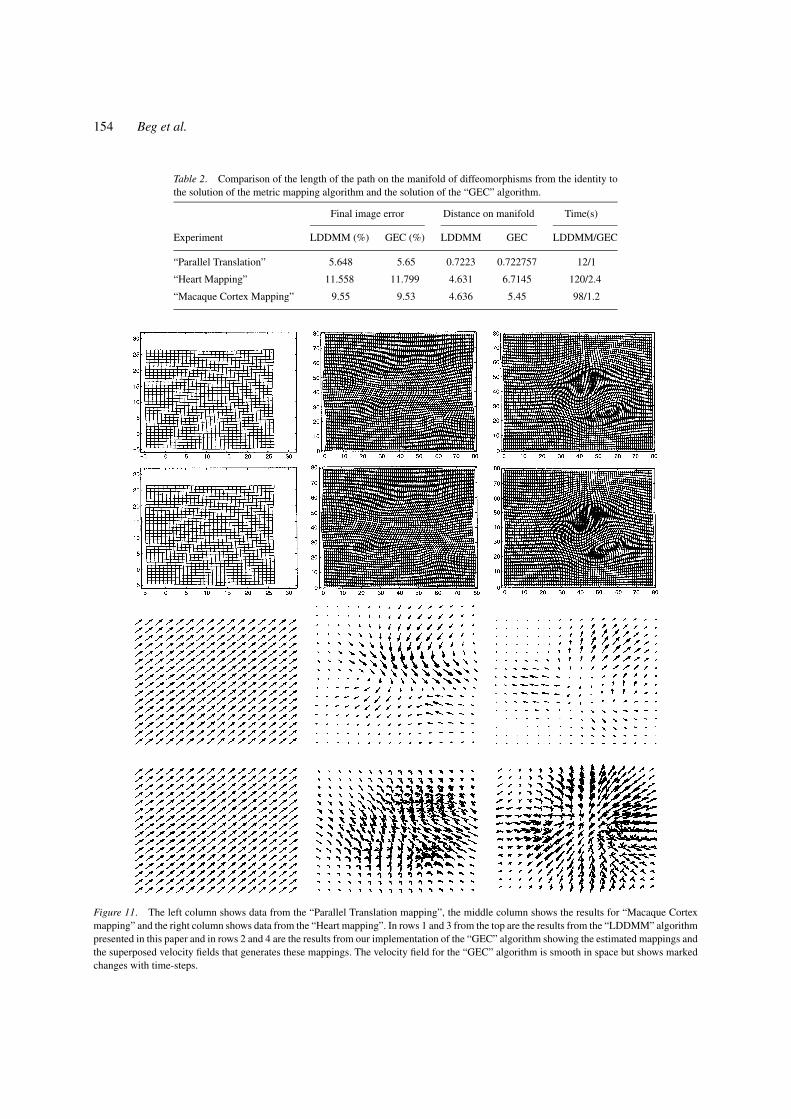
Table 2. Comparison of the length of the path on the manifold of diffeomorphisms from the identity tothe solution of the metric mapping algorithm and the solution of the “GEC” algorithm.

Final image error Distance on manifold Time(s)

Experiment LDDMM (%) GEC (%) LDDMM GEC LDDMM/GEC

“Parallel Translation” 5.648 5.65 0.7223 0.722757 12/1

“Heart Mapping” 11.558 11.799 4.631 6.7145 120/2.4

“Macaque Cortex Mapping” 9.55 9.53 4.636 5.45 98/1.2

Figure 11. The left column shows data from the “Parallel Translation mapping”, the middle column shows the results for “Macaque Cortexmapping” and the right column shows data from the “Heart mapping”. In rows 1 and 3 from the top are the results from the “LDDMM” algorithmpresented in this paper and in rows 2 and 4 are the results from our implementation of the “GEC” algorithm showing the estimated mappings andthe superposed velocity fields that generates these mappings. The velocity field for the “GEC” algorithm is smooth in space but shows markedchanges with time-steps.

Computing Large Deformation Metric Mappings via Geodesic Flows 155

estimated by the two algorithms are different however.The superposition of velocity fields in time on a sin-gle plot for both algorithms reveals that for the “LD-DMM” algorithm, the velocity fields are smooth notonly in space, but also in time, whereas the velocityfields are smooth in space for the “GEC” algorithm butwidely varying from one time-step to another. The dis-tance traversed on the manifold to reach those points isshorter for the “LDDMM” algorithm than the “GEC”algorithm.

6. Discussion

6.1. Hilbert Gradient Versus L2 Gradient

Notice that the gradient presented in Eq. (10) is com-puted according to the inner product on V , and werefer to it as a Hilbert gradient, which we would like tocompare to its variant in the space L2. Let L2(�, R

n)be the space of square-integrable vector fields on �

with the usual L2 product 〈·, ·〉L2 . Using Eqs. (5)and (7), in a weak sense, we can rephrase Eq. (11)as

∂h E(v) =∫ 1

0

⟨2(L†L)vt

−(

2

σ 2

∣∣Dφvt,1

∣∣∇ J 0t

(J 0

t − J 1t

)), ht

⟩L2

dt = 0

giving the L2 gradient of the cost to be

(∇v Et )L2 = 2(L†L)vt −(

2

σ 2

∣∣Dφvt,1

∣∣∇ J 0t

(J 0

t − J 1t

)).

Set the term bt = −2σ 2 |Dφv

t,1|∇ J 0t (J 0

t − J 1t ) and write

the two gradients in space V and space L2(�, Rn) with

this simplification as being

(∇v Et )V = 2vt + Kbt

(∇v Et )L2 = 2(L†L)vt + bt

From this expression, it is clear that the Hilbert gradientcan be deduced from the L2-gradient by applying thecompact operator K , yielding in this way much morestable computations. Another way to interpret this is byan expansion in an orthonormal basis for L2(�, R

n).Let the self adjoint operator (L†L) be diagonalized inthe orthonormal basis (wi )i∈N with eigenvalues given

by (λi )i∈N. The expression for (∇v Et )L2 becomes:

(∇v Et )L2 =∑i∈N

( 〈 2(L†L)vt , wi 〉L2 + 〈 bt , wi 〉L2 )wi

=∑i∈N

( λi 〈 2vt , wi 〉L2 + 〈 bt , wi 〉L2 )wi

(35)

In the other case, expansion of K bt in the same basisgives

Kbt =∑i∈N

〈 Kbt , wi 〉L2 wi =∑i∈N

〈 bt , Kwi 〉L2 wi

=∑i∈N

〈bt , wi 〉L2

λiwi

and the gradient (∇v Et )V becomes

(∇v Et )V =∑i∈N

(〈2vt , wi 〉L2 + 〈bt , wi 〉L2

λi

)wi

(36)

The operator K is compact, therefore the eigenvalues1/λi → 0 as i → ∞ and hence λi → ∞ as i →∞. The difference in behavior of the two gradientscome from the multiplication or division of the basiscoefficients with the eigen-values λi . Consequently, inEq. (35), the high frequency coefficients are amplifiedwhereas in Eq. (36) they are smoothed. The numericalunstability of the L2 gradient clearly derives from thishigh-frequency amplification.

The gradient derived for the presented cost in thespace V is compared to the more traditional gradientin the space L2 and we show that the L2 gradient isunstable due to its high-frequency amplification. As aresult, these gradients differ markedly in their numeri-cal properties. We have implemented both of these gra-dients numerically and found that the Sobolev gradientis much more stable than the corresponding gradient inthe space L2.

6.2. The Metric Structure on I

The highlight of LDDMM algorithm presented is thecomputation of the metric distance between given im-ages coming from the computation of a geodesic pathon the manifold of diffeomorphisms connecting the im-ages. This method is based on following a gradient-descent based scheme with a Hilbert gradient in the

156 Beg et al.

space V of vector fields for the global variational opti-mization of the proposed cost 1. We present the deriva-tion and implementation details of this gradient algo-rithm and denote it as the LDDMM algorithm. Thevelocity vector field solving this variational problemdefines a “geodesic” path on the manifold of diffeo-morphisms and the length of this path is a metricdistance between the images connected via the dif-feomorphism at the end point of the flow i.e. I0 andI0 ◦ φ1,0.

We compare the matching obtained by our gradientmethod optimizing over the entire flow in L2([0, 1], V )to the Christensen method of generating locally optimalflows via a viscous-fluid PDE formulation which prob-ably is one of the most efficient greedy methods inthis context. We also discuss an interpretation of thismethod as generating a locally optimal velocity basedon the Hilbert gradient of the fitting term. This methodgenerates a path on the manifold of diffeomorphisms,not necessarily the shortest path, but one for whichthe incremental cost at each step is minimized. Com-paring the velocity field generated by these two meth-ods, we see that the field generated by our gradientoptimizing over the entire flow produces a field thatis smooth in space and time, whereas the Christensenmethod produces a field that is smooth in space but notas markedly smooth with incremental steps in time,which is to be expected from this local-in-time opti-mization method. The distance generated by the Chris-tensen method provides an upper bound for the metricdistance. We show experiments using the two methodsfor comparing these properties.

In conclusion, we have presented in this paper thederivation and numerical implementation of a newgradient-based method for computing dense imagebased mappings solving a global variational problemas stated in 1 and estimating metrics for images. Wealso present results for applying this method to a sev-eral biological shapes in 2D as well as 3D. The metricsestimated for Mitochondrial shapes provide a quan-tification on relative distance between images whichcan be compared to human intuition and seems to bein agreement with it. This method provides a quanti-tative measurement tool that can be used to computemany such metric distances for images mapped to acommon anatomical reference image to build the dis-tribution of these metrics in the population. This willallow the comparison of images quantifying relative“close” and “far”, providing information that may beof potential use in aiding clinical diagnosis and treat-

ment. This algorithm is also directly applicable to non-rigid dense registration of color images or DT im-ages and the calculation of metric distance on theseorbits.

Acknowledgments

We thank Drs. John Csernansky and David Van Es-sen of Washington University for providing the data onhippocampal and Macaque shapes, and Dr. RaimondWinslow of the Johns Hopkins University for provid-ing heart data. We thank IBM for technical support andTim Kaiser at SDSC for help with parallel implemen-tation and optimization on the SP. We also acknowl-edge the use of “Analyze” software from the MayoFoundation in this research. This work has been sup-ported by P01-AG03991-16, 2-R01-MH56584-04A1,1-P41-RR15241-01A1, NIH Grants RO1-MH525158-01A1, NSF BIR-9 424264, NIH 1R01-MH60883-01,NIH 1P20-MH62113001A1.

References

Amit, Y. 1994. A nonlinear variational problem for image matching.SIAM Journal on Scientific Computing, 15(1):207–224.

Bajcsy, R. and Broit, C. 1982. Matching of deformed images. InProc. 6th Int. Joint Conf. Patt. Recog., pp. 351–353.

Bajcsy, R., Lieberson, R., and Reivich, M. 1983. A computerizedsystem for the elastic matching of deformed radiographic imagesto idealized atlas images. Journal of Computer Assisted Tomogra-phy, 7(4):618–625.

Broit, C. 1981. Optimal registration of deformed images. PhD thesis,University of Pennsylvania.

Do Carmo, M.P. 1976. Differential geometry of curves and surfaces.Prentice-Hall Engineering/Science/Mathematics.

Do Carmo, M.P. 1993. Riemannian Geometry. Birkhauser.Christensen, G.E., Rabbitt, R.D., and Miller, M.I. 1996. Deformable

templates using large deformation kinematics. IEEE Transactionson Image Processing, 5(10):1435–1447.

Christensen, G. 1994. Deformable shape models for anatomy. PhDThesis, Dept. of Electrical Engineering, Sever Institute of Tech-nology, Washington Univ., St. Louis, MO.

Dupuis, P., Grenander, U., and Miller, M.I. 1998. Variational prob-lems on flows of diffeomorphisms for image matching. Quarterlyof Applied Mathematics, LVI:587–600.

Grenander, U. and Miller, M.I. 1998. Computational anatomy: Anemerging discipline. Quarterly of Applied Mathematics, 56:617–694.

Miller, M.I., Trouve, A., and Younes, L. 2002. On the metrics andEuler-Lagrange equations of computational anatomy. Annual Re-view of Biomedical Engineering, 4:375–405.

Miller, M.I. and Younes, L. 2001. Group actions, homeomorphisms,and matching: A general framework. International Journal ofComputer Vision, 41:61–84.

Computing Large Deformation Metric Mappings via Geodesic Flows 157

Morton, K.W. and Mayers, D.F. 1996. Numerical Solution of PartialDifferential Equations. Cambridge University Press, University ofCambridge.

Robb, R.A. 1999. Biomedical Imaging, Vizualization and Analysis.John Wiley and Sons, Inc., New York, NY.

Staniforth, A. and Cote, J. 1991. Semi-lagrangian integrationschemes for atmospheric models-a review. Monthly Weather Re-view, 119:2206–2223.

Thirion, J.-P. 1998. Image matching as a diffusion process: An

analogy with maxwell’s demons. Medical Image Analysis,2(3):243–260.

Trouve, A. 1995. An infinite dimensional group approach for physicsbased models in patterns recognition. Preprint.

Trouve, A. 1998. Diffeomorphic groups and pattern match-ing in image analysis. Int. J. Computer Vision, 28:213–221.

Younes, L. 1999. Optimal matching between shapes via elastic de-formations. Image and Vision Computing, 17:381–389.