Geodesic Deviation Equation in f(R) Gravity

Alejandro Guarnizo, 1 Leonardo Castaneda 2 & Juan M. Tejeiro 3

Grupo de Gravitacion y Cosmologıa, Observatorio Astronomico Nacional,Universidad Nacional de Colombia

Bogota-Colombia

Abstract

In this paper we study the Geodesic Deviation Equation (GDE) in metric f(R) gravity. We startgiving a brief introduction of the GDE in General Relativity in the case of the standard cosmology.Next we generalize the GDE for metric f(R) gravity using again the FLRW metric. A generalizationof the Mattig relation is also obtained. Finally we give and equivalent expression to the Dyer-Roederequation in General Relativity in the context of f(R) gravity.

Keywords: Geodesic Deviation, Modified Theories of Gravity, f(R) gravity.

Accepted for Publication in General Relativity and Gravitation

DOI: 10.1007/s10714-011-1194-6

1 Introduction

In the context of General Relativity (GR), the curvature and geometry of the space-time play a fun-damental role: instead of forces acting in the Newtonian theory we have the space-time curved by thematter fields [1]. The space-time could be represented by a pair (M,g) with M a 4-dimensional mani-fold and g a metric tensor on it, the curvature is described by the Riemann tensor R, and the Einsteinfield equations tell us how this curvature depends on the matter sources. We can see the effects of thecurvature in a space-time through the Geodesic Deviation Equation (GDE) [2]-[4]; this equation give usthe relative acceleration of two neighbor geodesics [5],[6]. The GDE gives an elegant description of thestructure of a space-time, and all the important relations (Raychaudhuri equation, Mattig Relation, etc)could be obtained solving the GDE for timelike, null and spacelike geodesic congruences.

Even GR is the most widely accepted gravity theory and it has been tested in several field strengthregimes, is not the only relativistic theory of gravity [7]. In the last decades several generalizations of theEinstein field equations have been proposed [8],[9]. Within these extended theories of gravity nowadays asubclass, known as f(R) theories, are an alternative for classical problems, as the accelerated expansionof the universe, instead of Dark Energy and Quintessence models [10]-[16]. f(R) theories of gravity arebasically extensions of the usual Einstein-Hilbert action in GR with an arbitrary function of the Ricciscalar R [17]-[19].

In the context of Palatini f(R) gravity the GDE had been studied in [20], where they get the modi-fied Raychaudhuri equation. Our aim in this paper is to obtain the GDE in the metric context of f(R)gravity, and study some particular cases, we also obtain the generalized Mattig relation which is an usefulequation to measure cosmological distances. Through this paper we use the sign convention (−,+,+,+)and geometrical units with c = 1.

1aguarnizot@unal.edu.co2lcastanedac@unal.edu.co3jmtejeiros@unal.edu.co

1

arX

iv:1

010.

5279

v3 [

gr-q

c] 3

May

201

1

2 Field equations in f(R) gravity

As we mentioned above the modified theories of gravity have been studied in order to explain the accel-erated expansion of the universe, among other problems in gravity. A family of these theories is modifiedf(R) gravity, which consists in a generalization of the Einstein-Hilbert action (Lagrangian L[g] = R−2Λ),with an arbitrary function of the Ricci scalar (L[g] = f(R)) [11],[19]. Again, we consider the space-timeas a pair (M,g) with g a Lorentzian metric onM; the relation of the Ricci scalar and the metric tensoris given assuming a Levi-Civita connection on the manifold. i.e. a Christoffel symbol. Then the actioncould be written with a boundary term as [21]

S =

∫Vd4x√−gf(R) + 2

∮∂Vd3y ε

√|h|f ′(R)K + SM , (2.1)

here h is the determinant of the induced metric, K is the trace of the extrinsic curvature on the boundary∂V, ε is equal to +1 if ∂V is timelike and −1 if ∂V is spacelike (it is assumed that ∂V is nowhere null),and κ = 8πG. Finally SM is the action for the matter fields. Variation of this action with respect to gαβ

gives the following field equations [21], which are equivalent for those without boundaries given in [22]

f ′(R)Rαβ −f(R)

2gαβ + gαβf

′(R)−∇α∇βf ′(R) = κTαβ , (2.2)

where = ∇σ∇σ, f ′(R) = df(R)/dR; the energy-momentum tensor is defined by

Tαβ ≡ −2∂LM∂gαβ

+ LMgαβ = − 2√−g

δSMδgαβ

, (2.3)

being LM the lagrangian for all the matter fields, we also have the conservation equation ∇αTαβ = 0.Contracting with gαβ we have for the trace of the field equations

f ′(R)R− 2f(R) + 3f ′(R) = κT, (2.4)

with T = gαβTαβ . From equation (2.2) we can write

Rαβ =1

f ′(R)

[κTαβ +

f(R)

2gαβ − gαβf ′(R) +∇α∇βf ′(R)

], (2.5)

and from (2.4)

R =1

f ′(R)

[κT + 2f(R)− 3f ′(R)

]. (2.6)

It is possible to write the field equations in f(R) gravity, in the form of Einstein equations with aneffective energy-momentum tensor [15]

Gαβ ≡ Rαβ −1

2Rgαβ

=κTαβf ′(R)

+ gαβ[f(R)−Rf ′(R)]

2f ′(R)+

[∇α∇βf ′(R)− gαβf ′(R)]

f ′(R), (2.7)

orGαβ =

κ

f ′(R)

(Tαβ + T effαβ

), (2.8)

with

T effαβ ≡1

κ

[[f(R)−Rf ′(R)]

2gαβ + [∇α∇β − gαβ]f ′(R)

]. (2.9)

which could be interpreted as an fluid composed by curvature terms.

2

3 Geodesic Deviation Equation

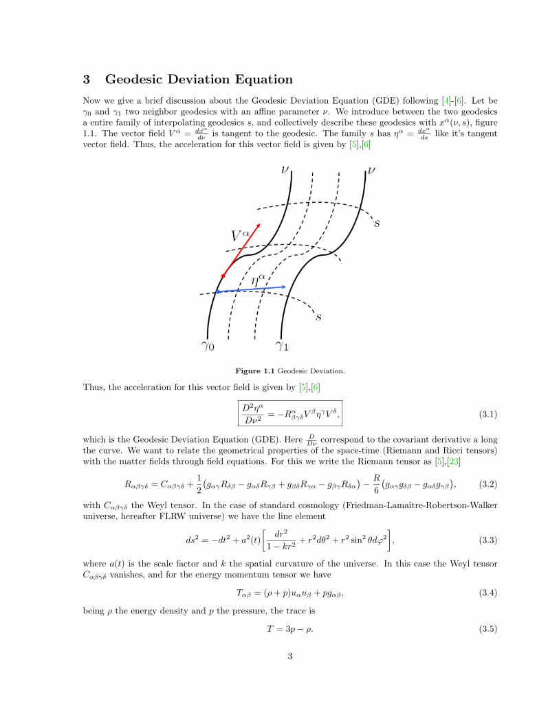
Now we give a brief discussion about the Geodesic Deviation Equation (GDE) following [4]-[6]. Let beγ0 and γ1 two neighbor geodesics with an affine parameter ν. We introduce between the two geodesicsa entire family of interpolating geodesics s, and collectively describe these geodesics with xα(ν, s), figure1.1. The vector field V α = dxα

dν is tangent to the geodesic. The family s has ηα = dxα

ds like it’s tangentvector field. Thus, the acceleration for this vector field is given by [5],[6]

Figure 1.1 Geodesic Deviation.

Thus, the acceleration for this vector field is given by [5],[6]

D2ηα

Dν2= −RαβγδV βηγV δ, (3.1)

which is the Geodesic Deviation Equation (GDE). Here DDν correspond to the covariant derivative a long

the curve. We want to relate the geometrical properties of the space-time (Riemann and Ricci tensors)with the matter fields through field equations. For this we write the Riemann tensor as [5],[23]

Rαβγδ = Cαβγδ +1

2

(gαγRδβ − gαδRγβ + gβδRγα − gβγRδα

)− R

6

(gαγgδβ − gαδgγβ

), (3.2)

with Cαβγδ the Weyl tensor. In the case of standard cosmology (Friedman-Lamaıtre-Robertson-Walkeruniverse, hereafter FLRW universe) we have the line element

ds2 = −dt2 + a2(t)

[dr2

1− kr2+ r2dθ2 + r2 sin2 θdϕ2

], (3.3)

where a(t) is the scale factor and k the spatial curvature of the universe. In this case the Weyl tensorCαβγδ vanishes, and for the energy momentum tensor we have

Tαβ = (ρ+ p)uαuβ + pgαβ , (3.4)

being ρ the energy density and p the pressure, the trace is

T = 3p− ρ. (3.5)

3

The standard form of the Einstein field equations in GR (with cosmological constant) is

Rαβ −1

2Rgαβ + Λgαβ = κTαβ , (3.6)

then we can write the Ricci scalar R and the Ricci tensor Rαβ using (3.4)

R = κ(ρ− 3p) + 4Λ, (3.7)

Rαβ = κ(ρ+ p)uαuβ +1

2

[κ(ρ− p) + 2Λ

]gαβ , (3.8)

from these expressions the right side of equation (3.1) is written as [4]

RαβγδVβηγV δ =

[1

3(κρ+ Λ)ε+

1

2κ(ρ+ p)E2

]ηα, (3.9)

with ε = V αVα and E = −Vαuα. This equation is known as Pirani equation [3]. The GDE and somesolutions for spacelike, timelike and null congruences has been studied in detail in [4], which gives someimportant result concerning cosmological distances also showed in [23]. Our purpose here is to extendthese results from the modified field equations in metric f(R) gravity.

4 Geodesic Deviation Equation in f(R) Gravity

The starting point are the expressions for the Ricci tensor and the Ricci scalar from the field equationsin f(R) gravity, equations (2.5) and (2.6) respectively. Using the expression (3.2) we can write

Rαβγδ = Cαβγδ +1

2f ′(R)

[κ(Tδβgαγ − Tγβgαδ + Tγαgβδ − Tδαgβγ) + f(R)

(gαγgδβ − gαδgγβ

)+(gαγDδβ−gαδDγβ +gβδDγα−gβγDδα

)f ′(R)

]− 1

6f ′(R)

(κT + 2f(R) + 3f ′(R)

)(gαγgδβ−gαδgγβ

),

(4.1)

where we defined the operator

Dαβ ≡ ∇α∇β − gαβ. (4.2)

Thus rising the first index in the Riemann tensor and contracting with V βηγV δ, the right side of theGDE could be written as

RαβγδVβηγV δ = CαβγδV

βηγV δ +1

2f ′(R)

[κ(Tδβδ

αγ − Tγβδαδ + T α

γ gβδ − T αδ gβγ) + f(R)

(δαγ gδβ − δαδ gγβ

)+(δαγDδβ − δαδ Dγβ + gβδD α

γ − gβγD αδ

)f ′(R)

]V βηγV δ

− 1

6f ′(R)

(κT + 2f(R) + 3f ′(R)

)(δαγ gδβ − δαδ gγβ

)V βηγV δ, (4.3)

In the following section we explicitly show the steps in order to find the GDE in f(R) gravity usingFLRW metric, our purpose is compare with the results from GR in the limit case f(R) = R− 2Λ.

4

4.1 Geodesic Deviation Equation for the FLRW universe

Using the FLRW metric as background we have

Rαβ =1

f ′(R)

[κ(ρ+ p)uαuβ +

(κp+

f(R)

2

)gαβ +Dαβf ′(R)

], (4.4)

R =1

f ′(R)

[κ(3p− ρ) + 2f(R)− 3f ′(R)

], (4.5)

with these expressions the Riemann tensor could be written as

Rαβγδ =1

2f ′(R)

[κ(ρ+ p)

(uδuβgαγ − uγuβgαδ + uγuαgβδ − uδuαgβγ

)+

(κp+

κρ

3+f(R)

3+ f ′(R)

)(gαγgδβ − gαδgγβ

)+ (gαγDδβ − gαδDγβ + gβδDγα − gβγDδα)f ′(R)

],

(4.6)

If the vector field V α is normalized, it implies V αVα = ε, and

RαβγδVβV δ =

1

2f ′(R)

[κ(ρ+ p)

(gαγ(uβV

β)2 − 2(uβVβ)V(αuγ) + εuαuγ

)+

(κp+

κρ

3+f(R)

3+f ′(R)

)(εgαγ − VαVγ

)+ (gαγDδβ − gαδDγβ + gβδDγα − gβγDδα)f ′(R)V βV δ

],

(4.7)

rising the first index in the Riemann tensor and contracting with ηγ

RαβγδVβηγV δ =

1

2f ′(R)

[κ(ρ+ p)

((uβV

β)2ηα − (uβVβ)V α(uγη

γ)− (uβVβ)uα(Vγη

γ) + εuαuγηγ)

+

(κp+

κρ

3+f(R)

3+f ′(R)

)(εηα−V α(Vγη

γ))+[(δαγDδβ−δαδ Dγβ+gβδD α

γ −gβγD αδ )f ′(R)

]V βV δηγ

],

(4.8)

with E = −Vαuα, ηαuα = ηαVα = 0 [4] it reduces to

RαβγδVβηγV δ =

1

2f ′(R)

[κ(ρ+ p)E2 + ε

(κp+

κρ

3+f(R)

3+ f ′(R)

)]ηα

+1

2f ′(R)

[[(δαγDδβ − δαδ Dγβ + gβδD α

γ − gβγD αδ )f ′(R)

]V βV δ

]ηγ . (4.9)

From the FLRW metric the expression for the Ricci scalar is

R = 6

[a

a+

(a

a

)2

+k

a2

]= 6

[H + 2H2 +

k

a2

], (4.10)

where we have used the definition for the Hubble parameter H ≡ aa . We see that R is only a function of

time, and only time derivatives in the operators Dαβ will not vanishing. The non-vanishing operators are

f ′(R) = −∂20f′(R)− 3H∂0f

′(R),

= −f ′′(R)R− f ′′′(R)R2 − 3Hf ′′(R)R, (4.11)

5

D00 = −3H∂0f′(R),

= −3Hf ′′(R)R, (4.12)

Dij = 2Hgij∂0f′(R) + gij∂

20f′(R),

= 2Hgijf′′(R)R+ gij(f

′′(R)R+ f ′′′(R)R2), (4.13)

being gij the spatial components of the FLRW metric and R = ∂0R. With these results is easy to showthat the the total contribution of the operators in (4.9) is(

δαγDδβ − δαδ Dγβ + gβδD αγ − gβγD α

δ

)f ′(R)V βV δηγ = ε

(5Hf ′′(R)R+ f ′′(R)R+ f ′′′(R)R2

)ηα, (4.14)

then the expression for RαβγδVβηγV δ reduces to

RαβγδVβηγV δ =

1

2f ′(R)

[κ(ρ+ p)E2 + ε

(κp+

κρ

3+f(R)

3+ 2Hf ′′(R)R

)]ηα, (4.15)

which is the generalization of the Pirani equation. In the particular case f(R) = R − 2Λ the previousequation reduces to (3.9).

The GDE in f(R) gravity from equation (3.1) is

D2ηα

Dν2= − 1

2f ′(R)

[κ(ρ+ p)E2 + ε

(κp+

κρ

3+f(R)

3+ 2Hf ′′(R)R

)]ηα, (4.16)

as we expect the GDE induces only a change in the magnitude of the deviation vector ηα, which alsooccurs in GR. This result is expected from the form of the metric, which describes an homogeneousand isotropic universe. For anisotropic universes, like Bianchi I, the GDE also induces a change in thedirection of the deviation vector, as shown in [24].

4.2 GDE for fundamental observers

In this case we have V α as the four-velocity of the fluid uα. The affine parameter ν matches with theproper time of the fundamental observer ν = t. Because we have temporal geodesics then ε = −1 andalso the vector field are normalized E = 1 , thus from (4.15)

Rαβγδuβηγuδ =

1

2f ′(R)

[2κρ

3− f(R)

3− 2Hf ′′(R)R

]ηα, (4.17)

if the deviation vector is ηα = `eα, isotropy implies

Deα

Dt= 0, (4.18)

andD2ηα

Dt2=d2`

dt2eα, (4.19)

using this result in the GDE (3.1) with (4.17) gives

d2`

dt2= − 1

2f ′(R)

[2κρ

3− f(R)

3− 2Hf ′′(R)R

]`. (4.20)

6

In particular with ` = a(t) we have

a

a=

1

f ′(R)

[f(R)

6+Hf ′′(R)R− κρ

3

]. (4.21)

This equation could be obtained as a particular case of the generalized Raychaudhuri equation givenin [25]. Is possible to obtain the standard form of the modified Friedmann equations [19] from thisRaychaudhuri equation giving

H2 +k

a2=

1

3f ′(R)

[κρ+

(Rf ′(R)− f(R))

2− 3Hf ′′(R)R

], (4.22)

and

2H + 3H2 +k

a2= − 1

f ′(R)

[κp+ 2Hf ′′(R)R+

(f(R)−Rf ′(R))

2+ f ′′(R)R+ f ′′′(R)R2

]. (4.23)

4.3 GDE for nulll vector fields

Now we consider the GDE for null vector fields past directed. In this case we have V α = kα, kαkα = 0,

then equation (4.15) reduces to

Rαβγδkβηγkδ =

1

2f ′(R)κ(ρ+ p)E2 ηα, (4.24)

that can be interpreted as the Ricci focusing in f(R) gravity. Writing ηα = ηeα, eαeα = 1, eαu

α =eαk

α = 0 and choosing an aligned base parallel propagated Deα

Dν = kβ∇βeα = 0, the GDE (4.16) reducesto

d2η

dν2= − 1

2f ′(R)κ(ρ+ p)E2 η. (4.25)

In the case of GR discussed in [4], all families of past-directed null geodesics experience focusing, providedκ(ρ+ p) > 0, and for a fluid with equation of state p = −ρ (cosmological constant) there is no influencein the focusing [4]. From (4.25) the focusing condition for f(R) gravity is

κ(ρ+ p)

f ′(R)> 0. (4.26)

A similar condition over the function f(R) was established in order to avoid the appearance of ghosts[10],[26], in which f ′(R) > 0. We want to write the equation (4.25) in function of the redshift parameterz. For this the differential operators is

d

dν=dz

dν

d

dz, (4.27)

d2

dν2=dz

dν

d

dz

(d

dν

),

=

(dν

dz

)−2[−(dν

dz

)−1d2ν

dz2

d

dz+

d2

dz2

]. (4.28)

In the case of null geodesics

(1 + z) =a0

a=

E

E0−→ dz

1 + z= −da

a, (4.29)

7

with a the scale factor, and a0 = 1 the present value of the scale factor. Thus for the past directed case

dz = (1 + z)1

a

da

dνdν = (1 + z)

a

aE dν = E0H(1 + z)2 dν, (4.30)

Then we getdν

dz=

1

E0H(1 + z)2, (4.31)

andd2ν

dz2= − 1

E0H(1 + z)3

[1

H(1 + z)

dH

dz+ 2

], (4.32)

writing dHdz as

dH

dz=dν

dz

dt

dν

dH

dt= − 1

H(1 + z)

dH

dt, (4.33)

the minus sign comes from the condition of past directed geodesic, when z increases, ν decreases. Wealso use dt

dν = E0(1 + z). Now, from the definition of the Hubble parameter H

H ≡ dH

dt=

d

dt

a

a=a

a−H2, (4.34)

and using the Raychaudhuri equation (4.21)

H =1

f ′(R)

[f(R)

6+Hf ′′(R)R− κρ

3

]−H2, (4.35)

thend2ν

dz2= − 3

E0H(1 + z)3

[1 +

1

3H2f ′(R)

(κρ

3− f(R)

6−Hf ′′(R)R

)]. (4.36)

Finally, the operator d2ηdν2 is

d2η

dν2=(EH(1 + z)

)2[d2η

dz2+

3

(1 + z)

[1 +

1

3H2f ′(R)

(κρ

3− f(R)

6−Hf ′′(R)R

)]dη

dz

], (4.37)

and the GDE (4.25) reduces to

d2η

dz2+

3

(1 + z)

[1 +

1

3H2f ′(R)

(κρ

3− f(R)

6−Hf ′′(R)R

)]dη

dz+

κ(ρ+ p)

2H2(1 + z)2f ′(R)η = 0, (4.38)

The energy density ρ and the pressure p considering the contributions from matter an radiation could bewritten in the following way

κρ = 3H20 Ωm0(1 + z)3 + 3H2

0 Ωr0(1 + z)4, κp = H20 Ωr0(1 + z)4, (4.39)

where we have used pm = 0 and pr = 13ρr. Thus the GDE could be written as

d2η

dz2+ P(H,R, z)

dη

dz+Q(H,R, z)η = 0, (4.40)

with

P(H,R, z) =4Ωm0(1 + z)3 + 4Ωr0(1 + z)4 + 3f ′(R)Ωk0(1 + z)2 + 4ΩDE − Rf ′(R)

6H20

(1 + z)(Ωm0(1 + z)3 + Ωr0(1 + z)4 + f ′(R)Ωk0(1 + z)2 + ΩDE

) , (4.41)

8

Q(H,R, z) =3Ωm0(1 + z) + 4Ωr0(1 + z)2

2(Ωm0(1 + z)3 + Ωr0(1 + z)4 + f ′(R)Ωk0(1 + z)2 + ΩDE

) . (4.42)

and H given by the modified field equations (4.22)

H2 =1

f ′(R)

[H2

0 Ωm0(1 + z)3 +H20 Ωr0(1 + z)4 +

(Rf ′(R)− f(R))

6−Hf ′′(R)R

]− k

a2,

H2 = H20

[1

f ′(R)

(Ωm0(1 + z)3 + Ωr0(1 + z)4 + ΩDE

)+ Ωk(1 + z)2

], (4.43)

where

ΩDE ≡1

H20

[(Rf ′(R)− f(R))

6−Hf ′′(R)R

], (4.44)

and

Ωk0 = − k

H20a

20

. (4.45)

In order to solve (4.40) it is necessary to write R and H in function of the redshift. First we define theoperator

d

dt=dz

da

da

dt

d

dz= −(1 + z)H

d

dz, (4.46)

then the Ricci is [16]

R = 6

[a

a+

(a

a

)2

+k

a2

],

= 6

[2H2 + H +

k

a2

],

= 6

[2H2 − (1 + z)H

dH

dz+ k(1 + z)2

],

if we want H = H(z) is necessary to fix the form of H(z) or either a specific form of the f(R) function.This point has been studied in [16] and the method to fix the form of H(z) and find the form of the f(R)function by observations is given in [27].

In the particular case f(R) = R − 2Λ, implies f ′(R) = 1, f ′′(R) = 0. The expression for ΩDE re-duces to

ΩDE =1

H20

[(R−R+ 2Λ)

6

]=

Λ

3H20

≡ ΩΛ, (4.47)

then the quantity ΩDE generalizes the Dark Energy parameter. The Friedmann modified equation (4.43)reduces to the well know expression in GR

H2 = H20

[Ωm0(1 + z)3 + Ωr0(1 + z)4 + ΩΛ + Ωk(1 + z)2

], (4.48)

the expressions P, and Q reduces to

P(z) =4Ωr0(1 + z)4 + (7/2)Ωm0(1 + z)3 + 3Ωk0(1 + z)2 + 2ΩΛ

(1 + z)(Ωr0(1 + z)4 + Ωm0(1 + z)3 + Ωk0(1 + z)2 + ΩΛ

) , (4.49)

Q(z) =2Ωr0(1 + z)2 + (3/2)Ωm0(1 + z)

Ωr0(1 + z)4 + Ωm0(1 + z)3 + Ωk0(1 + z)2 + ΩΛ. (4.50)

9

and the GDE for null vector fields is

d2η

dz2+

4Ωr0(1 + z)4 + (7/2)Ωm0(1 + z)3 + 3Ωk0(1 + z)2 + 2ΩΛ

(1 + z)(Ωr0(1 + z)4 + Ωm0(1 + z)3 + Ωk0(1 + z)2 + ΩΛ

) dηdz

+2Ωr0(1 + z)2 + (3/2)Ωm0(1 + z)

Ωr0(1 + z)4 + Ωm0(1 + z)3 + Ωk0(1 + z)2 + ΩΛη = 0. (4.51)

The Mattig relation in GR is obtained in the case ΩΛ = 0 and writing Ωk0 = 1−Ωm0 −Ωr0 which gives[4]

d2η

dz2+

6 + Ωm0(1 + 7z) + Ωr0(1 + 8z + 4z2)

2(1 + z)(1 + Ωm0z + Ωr0z(2 + z))

dη

dz+

3Ωm0 + 4Ωr0(1 + z)

2(1 + z)(1 + Ωm0z + Ωr0z(2 + z))η = 0, (4.52)

then, the equation (4.40) give us a generalization of the Mattig relation in f(R) gravity.

In a spherically symmetric space-time, like in FLRW universe, the magnitude of the deviation vectorη is related with the proper area dA of a source in a redshift z by dη ∝

√dA, and from this, the definition

of the angular diametral distance dA could be written as [28]

dA =

√dA

dΩ, (4.53)

with dΩ the solid angle. Thus the GDE in terms of the angular diametral distance is

d2 df(R)A

dz2+

4Ωm0(1 + z)3 + 4Ωr0(1 + z)4 + 3f ′(R)Ωk0(1 + z)2 + 4ΩDE − Rf ′(R)6H2

0

(1 + z)(Ωm0(1 + z)3 + Ωr0(1 + z)4 + f ′(R)Ωk0(1 + z)2 + ΩDE

) d df(R)A

dz

+3Ωm0(1 + z) + 4Ωr0(1 + z)2

2(Ωm0(1 + z)3 + Ωr0(1 + z)4 + f ′(R)Ωk0(1 + z)2 + ΩDE

) df(R)A = 0, (4.54)

where we denote the de angular diametral distance by df(R)A , to emphasize that any solution of the

previous equation needs a specific form of the f(R) function, or either a form of H(z). This equationsatisfies the initial conditions (for z ≥ z0)

df(R)A (z, z0)

∣∣∣∣z=z0

= 0, (4.55)

d df(R)A

dz(z, z0)

∣∣∣∣z=z0

=H0

H(z0)(1 + z0), (4.56)

being H(z0) the modified Friedmann equation (4.43) evaluated at z = z0.

5 Dyer-Roeder like Equation in f(R) Gravity

Finally we get an important relation that is a tool to study cosmological distances also in inhomogeneousuniverses. The Dyer-Roeder equation gives a differential equation for the diametral angular distance dAas a function of the redshift z [29]. The standard form of the Dyer-Roeder equation in GR can be givenby [30],[31]

(1 + z)2F(z)d2 dAdz2

+ (1 + z)G(z)d dAdz2

+H(z)dA = 0 (5.1)

withF(z) = H2(z) (5.2)

10

G(z) = (1 + z)H(z)dH

dz+ 2H2(z) (5.3)

H(z) =3α(z)

2Ωm0(1 + z)3 (5.4)

with α(z) is the smoothness parameter, which gives the character of inhomogeneities in the energy density[28]. There have been some studies about the influence of the smoothness parameter α in the behaviorof dA(z) [28],[30],[32]. In order to obtain the Dyer-Roeder like equation in f(R) gravity we follow [28].

First, we note that the terms containing the derivatives of df(R)A in equation (4.54) comes from the

transformation ddν −→

ddz and the term with only d

f(R)A comes from the Ricci focusing (4.24). Then

following [29],[30] we introduce a mass-fraction α (smoothness parameter) of matter in the universe, andthen we replace only in the Ricci focusing ρ −→ αρ. Thus following our arguments to obtain the equation(4.40), and considering the case Ωr0 = 0 we get

(1 + z)2 d2 d

f(R), DRA

dz2+ (1 + z)

4Ωm0(1 + z)3 + 3f ′(R)Ωk0(1 + z)2 + 4ΩDE − Rf ′(R)6H2

0(Ωm0(1 + z)3 + f ′(R)Ωk0(1 + z)2 + ΩDE

) d df(R), DRA

dz

+3α(z)Ωm0(1 + z)3

2(Ωm0(1 + z)3 + f ′(R)Ωk0(1 + z)2 + ΩDE

) df(R), DRA = 0. (5.5)

where we denote the Dyer-Roeder distance in f(R) gravity by df(R), DRA . This Dyer-Roeder also satis-

fies the conditions (4.55) and (4.56), and it reduces to the standard form of GR in the case f(R) = R−2Λ.

Is important to notice that the f(R) function and it’s derivatives appear explicitly in (4.54) and (5.5),being this a big difference respect to the case of GR. Another feature for these theories is the role of thedark energy parameter ΩDE , which contains the higher order terms of the field equations4. However, inorder to show the effects of the higher order terms, is necessary, as we stressed above, fix either H(z) off(R). Further studies are necessary to quantify these effects.

6 Conclusions and Discussion

We have studied the Geodesic Deviation Equation (GDE) in the metric formalism of f(R) gravity, start-ing for this from the form of the Ricci tensor and the Ricci scalar with the modified field equations. Ageneralized expression for the force term (Pirani equation) is obtained for f(R) gravity (for the FLRWuniverse), as well as the generalized GDE, both expressions reduce to the standard forms in the casef(R) = R − 2Λ. Then, we consider two particular cases, the GDE for fundamental observers and theGDE for null vector field past directed.

The case of fundamental observers give us the Raychaudhuri equation and from this the standard formof the modified field equations with the FLRW metric as background. The null vector field case giveus more important results: a generalization of the Mattig relation, the differential equation for the di-ametral angular distance in f(R) gravity, and as extension we consider also the Dyer-Roeder like equation.

Another important result comes from the definition of the Ricci focusing: in the case of GR (in theFLRW space-time) we have a focusing for past-directed null geodesics for the condition κ(ρ + p) > 0,here the condition is given by κ(ρ+ p)/f ′(R) > 0.

In the other hand, the general equation (4.3) is the starting point for important issues in f(R) grav-ity, as singularity theorems [33] and gravitational lensing [28]. We could study also the GDE for more

4From equation (4.44) the terms containing time derivatives of the Ricci scalar comes from the operator D00, equation(4.12), which gives the fourth order terms in the field equations of f(R) gravity.

11

general space-times (like Bianchi models) and for different forms of the energy-momentum tensor, in thecontext of f(R) gravity.

Finally, the solution of equations (4.54) and (5.5) allows a different test for cosmological observables(areas, volumes, proper distances, etc.) in f(R) gravity, being an alternative method to constrain somemodels through cosmological probes.

References

[1] C. W. Misner, K. S. Thorne, and J. H. Wheeler. Gravitation. W. H. Freeman and Company, 1973.

[2] J. L. Synge. On the Deviation of Geodesics and Null Geodesics, Particularly in Relation to theProperties of Spaces of Constant Curvature and Indefinite Line Element. Ann. Math. 35:705 (1934).

[3] F. A. E. Pirani. On the Physical Significance of the Riemann Tensor. Acta Phys. Polon. 15:389(1956).

[4] G. F. R. Ellis and H. Van Elst. Deviation of geodesics in FLRW spacetime geometries (1997). Preprintin [arXiv:gr-qc/9709060v1].

[5] R. M. Wald, General Relativity. The University of Chicago Press, 1984.

[6] E. Poisson, A Relativist’s Toolkit - The Mathematics of Black-Hole Mechanics. Cambridge UniversityPress, 2004.

[7] C. Corda. Interferometric detection of gravitational waves: the definitive test for General Relativity.Int. J. Mod. Phys. D 18:2275-2282 (2009). Preprint in [arXiv:0905.2502].

[8] H-J. Schmidt. Variational derivatives of arbitrarily high order and multi-inflation cosmological mod-els. Class. Quantum. Grav. 7:1023-1031 (1990).

[9] D. Wands. Extended gravity theories and the Einstein-Hilbert action. Class. Quant. Grav. 11:269-280(1994). Preprint in [arXiv:gr-qc/9307034].

[10] A. De Felice and S. Tsujikawa. f(R) Theories. Living Rev. Relativity 13:3 (2010).[http://www.livingreviews.org/lrr-2010-3].

[11] S. Nojiri and S. D. Odintsov. Modified gravity as an alternative for Lambda-CDM cosmology. J.Phys. A 40:6725-6732 (2007). Preprint in [arXiv:hep-th/0610164].

[12] A. Borowiec, W. Godlowski, and M. Szydlowski. Dark matter and dark energy as a effects of ModifiedGravity. ECONF C0602061 :09 (2006). Preprint in [arXiv:astro-ph/0607639v2].

[13] R. Durrer and R. Maartens. Dark energy and dark gravity: theory overview. Gen. Relativ. Gravit.40:301-328 (2008).

[14] S. Nojiri and S. D. Odintsov. Introduction to Modified Gravity and Gravitational Alter-native for Dark Energy. Int. J. Geom. Meth. Mod. Phys. 4:115-146 (2007). Preprint in[arXiv:hep-th/0601213].

[15] S. Capozziello, S. Carloni and A. Troisi. Quintessence without scalar fields. Recent Res. Dev. Astron.Astrophys. 1, 625 (2003). Preprint in [arXiv:astro-ph/0303041].[arXiv:astro-ph/0303041]

[16] S. Capozziello and M. Francaviglia. Extended theories of gravity and their cosmological and astro-physical applications. Gen. Relativ. Gravit. 40:357-420 (2008). Preprint in [arXiv:0706.1146v2].

12

[17] V. Faraoni. f(R) gravity: successes and challenges (2008). Preprint in [arXiv:0810.2602].

[18] T. P. Sotiriou. 6+1 lessons from f(R) gravity. J. Phys. Conf. Ser. 189:012039 (2009). Preprint in[arXiv:0810.5594].

[19] T.P. Sotiriou and V. Faraoni. f(R) Theories Of Gravity (2008). Preprint in [arXiv:0805.1726v4].

[20] F. Shojai and A. Shojai. Geodesic Congruences in the Palatini f(R) Theory. Phys. Rev. D 78:104011(2008). Preprint in [arXiv:0811.2832v1].

[21] A. Guarnizo, L. Castaneda and J. M. Tejeiro. Boundary term in metric f(R) gravity: field equationsin the metric formalism. Gen. Relativ. Gravit. 42:2713-2728 (2010). Preprint in [arXiv:1002.0617].

[22] H. A. Buchdahl. Non-linear Lagrangians and cosmological theory. Mon. Not. R. astr. Soc. 150:1-8(1970).

[23] G. F. R. Ellis and H. Van Elst. Cosmological models (Cargese lectures 1998). Preprint in[arXiv:gr-qc/9812046v5].

[24] D. L. Caceres, L. Castaneda, J. M. Tejeiro. Geodesic Deviation Equation in Bianchi Cosmologies. J.Phys. Conf. Ser. 229:012076 (2010). Preprint in [arXiv:0912.4220v1].

[25] S. Rippl, H. van Elst, R. Tavakol and D. Taylor. Kinematics and dynamics of f(R) theories of gravity.Gen. Relativ. Gravit. 28:193 (1996)

[26] A. Starobinsky. Disappearing cosmological constant in f(R) gravity. J. Exp. Theor. Phys. Lett.86:157-163 (2007). Preprint in [arXiv:0706.2041v2].

[27] S. Capozziello, V. F. Cardone, and A. Troisi. Reconciling dark energy models with f(R) theories.Phys. Rev. D. 71:043503 (2005).

[28] P. Schneider, J. Ehlers and E. E. Falco. Gravitational Lenses. Springer-Verlag, 1999.

[29] C. C. Dyer and R. C. Roeder. The Distance-Redshift Relation for Universes with no IntergalacticMedium. ApJ 174:L115 (1972). [http://adsabs.harvard.edu/abs/1972ApJ...174L.115D]

[30] L. Castaneda. Effect of the cosmological constant in the probability of gravitational lenses. M.Sc.Thesis, 2002. Universidad Nacional de Colombia.

[31] T. Okamura and T. Futamase. Distance-Redshift Relation in a Realistic Inhomogeneous Universe.Prog. Theor. Phys. 122:511-520 (2009). Preprint in [arXiv:10905.1160v2].

[32] E. V. Linder. Isotropy of the microwave background by gravitational lensing. Astron. Astrophys.206, 199-203 (1988)

[33] S. Hawking and G. F. R. Ellis. The large scale structure of space-time. Cambridge University Press(1973)

13