Analysis of Planar Shapes Using Geodesic Paths onShape Spaces ∗

Eric Klassen † Anuj Srivastava ‡ Washington Mio § Shantanu Joshi ¶

Abstract

For analyzing shapes of planar, closed curves, we propose differential geometric rep-resentations of curves using their direction functions and curvature functions. Shapesare represented as elements of infinite-dimensional spaces and their pairwise differencesare quantified using the lengths of geodesics connecting them on these spaces. We usea Fourier basis to represent tangents to the shape spaces and then use a gradient-basedshooting method to solve for the tangent that connects any two shapes via a geodesic.Using the Surrey fish database, we demonstrate some applications of this approach: (i)interpolation and extrapolations of shape changes, (ii) clustering of objects accordingto their shapes, (iii) statistics on shape spaces, and (iv) Bayesian extraction of shapesin low-quality images.

Keywords: shape metrics, geodesic paths, shape statistics, intrinsic mean shapes, shape-based clustering, shape interpolation.

1 Introduction

Shapes play a pivotal role in understanding objects in terms of their behavior and character-istics, such as their growth, health, identity, and functionality. Quantitative characterizationof shapes is emerging as a major area of research, which will impact diverse applications.Despite a pressing need for analyzing shapes in many problems, the current methods arelimited in their scope and performance. Although shapes are frequently referred to in theliterature, consistent mathematical treatments of shapes are relatively limited. Only a lim-ited number of papers provide specific definitions of shapes or shape spaces, or follow itup with a statistical analysis. It is noteworthy that the notion of shape exists in manybranches of science with different meanings attached to it. Although the existence of thesediverse notions of shape may be a reason behind the absence of formal treatments, a lack ofsophisticated mathematical tools is also an important factor.

∗This research has been supported in part by the grants NSF DMS-0101429, ARO DAAD19-99-1-0267,and NMA 201-01-2010. This paper was presented in part at 4th EMMCVPR, Lisbon, 2003.

†Department of Mathematics, Florida State University, Tallahassee, FL 32306‡Department of Statistics, Florida State University, Tallahassee, FL 32306§Department of Mathematics, Florida State University, Tallahassee, FL 32306.¶Department of Electrical Engineering, Florida State University, Tallahassee, FL 32306.

1

Among the papers that explicitly study shapes, a major limitation in many of them isthe use of landmarks to define shapes. Shapes are often encoded by a coarse sampling of theobjects’ boundaries, and the outcome and accuracy of the ensuing shape analysis is heavilydependent on the choices made. In addition, it is usually difficult to automate the selection ofthese landmarks. A more fundamental approach is to represent the continuous boundaries ascurves, and then study their shapes. (Of course, any computer implementation will requirean eventual discretization, but there are distinct advantages to the philosophy of discretiz-ing as late as possible.) However, this approach requires dealing with infinite-dimensionalRiemannian manifolds, spaces for which tools such as optimization, random sampling, andhypothesis testing are not frequently available. Our goal is to develop mathematical for-mulations, optimization strategies, and statistical procedures to fundamentally address theoutstanding issues in the study of continuous, planar shapes.

1.1 Motivations for Shape Analysis

Tools for efficient shape analysis will impact many areas such as computer vision, structuralgenomics, medical imaging, and computational topology. The issue of representing, ana-lyzing, estimating and tracking shapes is central to many problems in these applications.Recognition of objects using observed images is also a well publicized problem in computervision. Images provide information about shapes of the objects and reflectance functions(textures) associated with the objects’ surfaces. Analyzing the shapes of contours can pro-vide important clues about the identities of the objects. For instance, an algorithm foranalyzing shapes can help automate recognition of marine animals using contours of theirappearances in images. In practice, where shapes are to be inferred from low-quality data,statistical formulations and inferences become very important. The importance of statisticalinferences in general computer vision is well documented although one needs to emphasizethe same need for a comprehensive statistical analysis of shapes. From computing averagesand variations of given shapes to testing shape hypotheses from give data, standard tools forstatistical analysis need to be extended to formal shape spaces. Also, note that the scope ofany shape theory need not be restricted to image analysis. Although image understandingforms an important application of shape analysis, a theory should be more general in itsscope.

1.2 Past Work in Shape Analysis

Historically, there have been many exemplary efforts in characterization and quantificationof shapes. Efforts by Kendall [14], Bookstein [2], Mardia [7], and Kent [15] have resultedin an elegant statistical theory of shapes. A common theme here is that objects are rep-resented using a finite number of salient points or landmarks (points in a Euclidean space,R2 or R3) and one establishes equivalences with respect to the transformations that leaveshapes unchanged. Shape invariant transformations are rigid rotations, translations, andnon-rigid uniform scaling. The resulting quotient space, R2n/(SO(2)×R2 ×R+) (assumingn landmarks in R2 for planar shapes), is a finite-dimensional Riemannian manifold, oftencalled a shape manifold; different shapes correspond to elements of this space and quantifica-tion of shape differences is achieved via a Riemannian metric on this space (for example, the

2

Procrustean metric). An important aspect of this work is its maturity to statistical frame-works. Researchers have defined probability distributions on these shape manifolds and havesought statistical approaches for shape estimation. In these approaches, the registration ofcorresponding points is often done manually although there are some exceptions [5].

In Grenander’s formulation [9] shapes are considered as points on some infinite-dimensionaldifferentiable manifold, and the variations between the shapes are modeled by the actionof Lie groups (deformations) on this manifold. Low-dimensional groups, such as rotation,translation and scaling, keep the shapes unchanged, while high-dimensional diffeomorphismgroups smoothly change the object shapes ([30, 21, 10]), a central idea behind deformabletemplate theory [9]. One limitation of this approach is the need to consider action of diffeo-morphism group on R2 and R3. The cost of computing diffeomorphisms is high, especiallywhen only the contours need be analyzed. Another active area of research in image analysishas been the use of level sets and active contours in characterizing object boundaries. How-ever, the focus here is on solving partial differential equations (PDEs) for shape extraction,driven by image features under smoothness constraints, and statistical analysis of shapes inthis framework is still incipient [6, 20]. In general, the equivalence relations specifying shapeinvariance are seldom made explicit and the notion of geodesic paths has gained only limitedattention. Cohen et al. [4] perform curve matching by connecting points using individualgeodesic paths derived from level set considerations. In case the problem is limited to com-puting shape metrics, many extrinsic metrics or even their approximations have been used[23] without the use of a formal statistical framework. However, a statistical formulation re-quires an intrinsic approach to shape analysis. An interesting method for comparing planarshapes using bimorphisms is presented in [28], although the definition of a shape is quitebroad here.

1.3 Our Approach

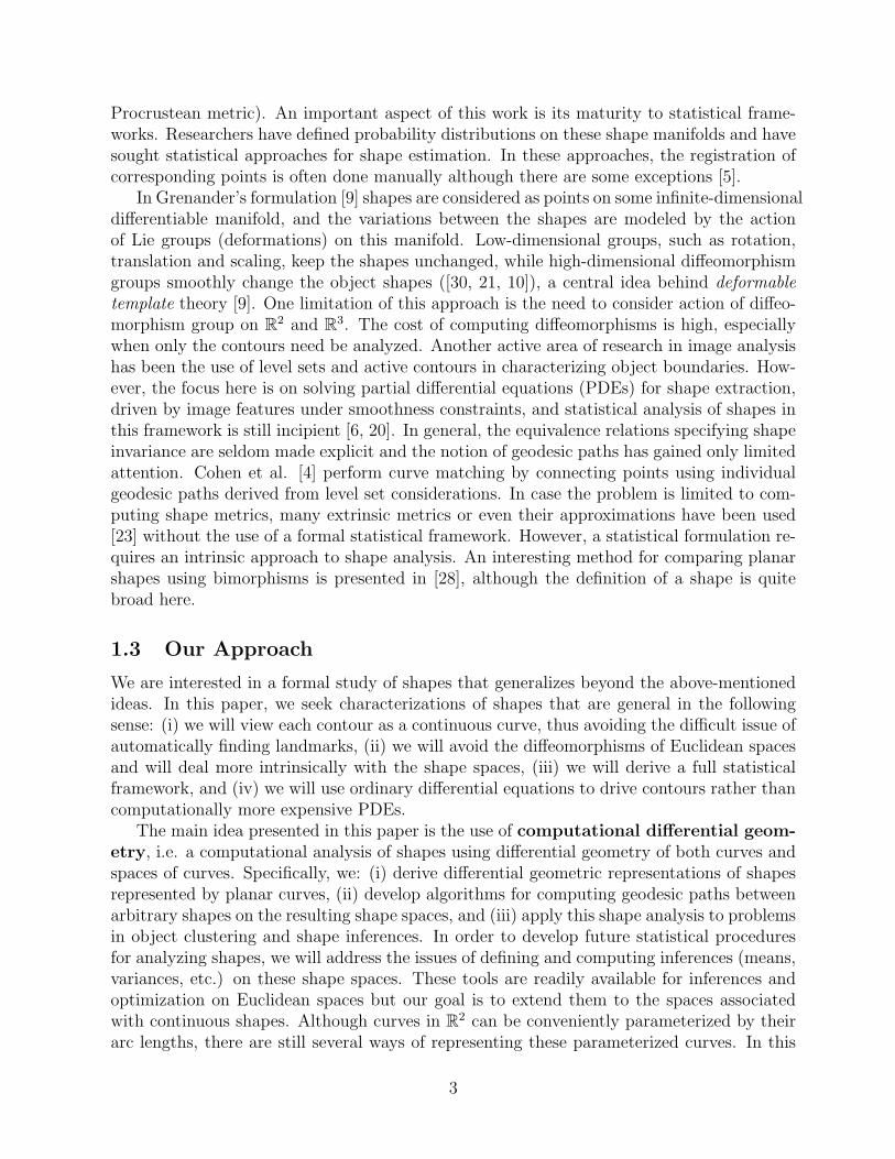
We are interested in a formal study of shapes that generalizes beyond the above-mentionedideas. In this paper, we seek characterizations of shapes that are general in the followingsense: (i) we will view each contour as a continuous curve, thus avoiding the difficult issue ofautomatically finding landmarks, (ii) we will avoid the diffeomorphisms of Euclidean spacesand will deal more intrinsically with the shape spaces, (iii) we will derive a full statisticalframework, and (iv) we will use ordinary differential equations to drive contours rather thancomputationally more expensive PDEs.

The main idea presented in this paper is the use of computational differential geom-etry, i.e. a computational analysis of shapes using differential geometry of both curves andspaces of curves. Specifically, we: (i) derive differential geometric representations of shapesrepresented by planar curves, (ii) develop algorithms for computing geodesic paths betweenarbitrary shapes on the resulting shape spaces, and (iii) apply this shape analysis to problemsin object clustering and shape inferences. In order to develop future statistical proceduresfor analyzing shapes, we will address the issues of defining and computing inferences (means,variances, etc.) on these shape spaces. These tools are readily available for inferences andoptimization on Euclidean spaces but our goal is to extend them to the spaces associatedwith continuous shapes. Although curves in R2 can be conveniently parameterized by theirarc lengths, there are still several ways of representing these parameterized curves. In this

3

paper we study two such representations: one using the direction functions and anotherusing the curvature functions, and analyze the two resulting shape spaces.

The remaining paper is organized as follows. In Section 2, we describe geometric repre-sentations of closed, planar curves and in Section 3 we study the geometries of the resultingshape spaces, including the construction of geodesics on them. In Section 4, we present nu-merical methods for finding geodesics (on shape spaces) connecting any two arbitrary shapes.Some applications demonstrating these tools are presented in Section 5.

2 Geometric Representations of Planar Shapes

We consider objects whose boundaries are given by closed curves with a single component,viewed as closed immersed curves in the plane R2. Curves that differ by orientation pre-serving rigid motions (rigid rotation and translation in R2) and uniform scaling (of R2) areconsidered to represent the same shape, so we will need representations that are invariantto these transformations. Scaling can be quickly resolved by fixing the length of the curvesto be, say, 2π but other invariances require some consideration.

Curves are assumed to be parameterized by arclength (using notation α:R → R2) withperiod 2π and satisfy |α′(s)| = 1, for every s. In this paper, the term periodic will al-ways mean periodic with period 2π. The two coordinate functions of α are denoted as(α1(s), α2(s)). Associated with each α, there is a tangent indicatrix v:R → S1 ⊂ R2 givenby v(s) = α′(s), where S1 denotes the unit circle. We can write the tangent indicatrix in theform v(s) = α′(s) = ejθ(s), where θ:R → R and j =

√−1. We are identifying R2 with thecomplex plane C in the usual way. We refer to θ as a direction function or angle functionfor the given curve. For each s, θ(s) gives the angle that the vector α′(s) makes with thepositive x-axis. If v is continuous and we require θ to be continuous, then the above relationdetermines θ up to the addition of an integer multiple of 2π. The curvature of α at s ∈ R isdefined by κ(s) = θ′(s). κ is completely determined by α, assuming α is twice differentiable.Note that κ is periodic, while θ is not necessarily periodic; however θ(s + 2π)− θ(s) = 2πnfor some integer n. This integer is called the rotation index of the curve, and measureshow many times the tangent vector rotates as the curve is traversed one time. It is wellknown that if α is a smooth simple closed curve (i.e., α is periodic, and for all s, t ∈ [0, 2π),s 6= t ⇒ α(s) 6= α(t)) then the rotation index of α is ±1 (See e.g. [3], p. 396), where the signdepends on the direction in which the curve is traversed. Because we are primarily interestedin simple closed curves, we will restrict our attention in this paper to the set of curves ofrotation index 1. While this set is larger than the set of simple closed curves, it contains theset of simple closed curves as an open subset. We use this larger set because it is complete(i.e., it contains its own limit points), and hence is a much better manifold on which to dodifferential geometry (e.g., geodesics exist and can be extended infinitely in either direction[16]).

In this paper we use L2 to denote the space of all real-valued functions R → R whichhave period 2π and are square integrable on [0, 2π]. Also, we will use the inner product

〈f1, f2〉 =∫ 2π

0f1(s)f2(s)ds on L2, and let ‖f‖ denote the norm

√〈f, f〉 for f ∈ L2. This

choice of metric implies a measurement of the “bending” energy in going from one shape toanother. There are at least two ways of representing planar curves: one using the direction

4

function θ and another using the curvature function κ. We will analyze shapes under boththese representations.

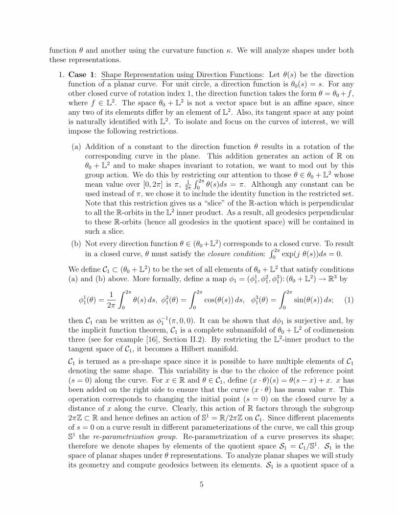
1. Case 1: Shape Representation using Direction Functions: Let θ(s) be the directionfunction of a planar curve. For unit circle, a direction function is θ0(s) = s. For anyother closed curve of rotation index 1, the direction function takes the form θ = θ0 +f ,where f ∈ L2. The space θ0 + L2 is not a vector space but is an affine space, sinceany two of its elements differ by an element of L2. Also, its tangent space at any pointis naturally identified with L2. To isolate and focus on the curves of interest, we willimpose the following restrictions.

(a) Addition of a constant to the direction function θ results in a rotation of thecorresponding curve in the plane. This addition generates an action of R onθ0 + L2 and to make shapes invariant to rotation, we want to mod out by thisgroup action. We do this by restricting our attention to those θ ∈ θ0 + L2 whosemean value over [0, 2π] is π, 1

2π

∫ 2π

0θ(s)ds = π. Although any constant can be

used instead of π, we chose it to include the identity function in the restricted set.Note that this restriction gives us a “slice” of the R-action which is perpendicularto all the R-orbits in the L2 inner product. As a result, all geodesics perpendicularto these R-orbits (hence all geodesics in the quotient space) will be contained insuch a slice.

(b) Not every direction function θ ∈ (θ0+L2) corresponds to a closed curve. To result

in a closed curve, θ must satisfy the closure condition:∫ 2π

0exp(j θ(s))ds = 0.

We define C1 ⊂ (θ0 + L2) to be the set of all elements of θ0 + L2 that satisfy conditions(a) and (b) above. More formally, define a map φ1 = (φ1

1, φ21, φ

31): (θ0 + L2) → R3 by

φ11(θ) =

1

2π

∫ 2π

0

θ(s) ds, φ21(θ) =

∫ 2π

0

cos(θ(s)) ds, φ31(θ) =

∫ 2π

0

sin(θ(s)) ds; (1)

then C1 can be written as φ−11 (π, 0, 0). It can be shown that dφ1 is surjective and, by

the implicit function theorem, C1 is a complete submanifold of θ0 + L2 of codimensionthree (see for example [16], Section II.2). By restricting the L2-inner product to thetangent space of C1, it becomes a Hilbert manifold.

C1 is termed as a pre-shape space since it is possible to have multiple elements of C1

denoting the same shape. This variability is due to the choice of the reference point(s = 0) along the curve. For x ∈ R and θ ∈ C1, define (x · θ)(s) = θ(s− x) + x. x hasbeen added on the right side to ensure that the curve (x · θ) has mean value π. Thisoperation corresponds to changing the initial point (s = 0) on the closed curve by adistance of x along the curve. Clearly, this action of R factors through the subgroup2πZ ⊂ R and hence defines an action of S1 = R/2πZ on C1. Since different placementsof s = 0 on a curve result in different parameterizations of the curve, we call this groupS1 the re-parametrization group. Re-parametrization of a curve preserves its shape;therefore we denote shapes by elements of the quotient space S1 = C1/S1. S1 is thespace of planar shapes under θ representations. To analyze planar shapes we will studyits geometry and compute geodesics between its elements. S1 is a quotient space of a

5

Hilbert manifold C1; S1 is also a manifold at all points except the set of shapes withrotational symmetries, a negligible set.

We are defining two curves to have the same shape if they differ by rescaling and/or anorientation-preserving rigid motion. Depending on the application, one may wish toallow orientation-reversing rigid motions as well. Handling this would require removingan additional Z2-action, which would not be difficult. However, we don’t pursue itfurther.

2. Case 2: Shape Representation using Curvature Functions: We can also representclosed planar curves of length 2π and rotation index 1 by their curvature functionsκ. Clearly, κ has to be periodic. Condition (a) below gives the restriction on therotation index, and condition (b) guarantees that the curve is closed.

(a) Since the rotation index is 1, we have 〈κ, 1〉 =∫ 2π

0κ(s) ds = θ(2π)− θ(0) = 2π.

(b) If θ(s) is an angle function of a curve α with curvature κ, α(2π) − α(0) =∫ 2π

0ejθ(s) ds, and using θ(s) =

∫ s

0κ(x) dx,

α(2π)− α(0) =

∫ 2π

0

cos

(∫ s

0

κ(x) dx

)ds + j

∫ 2π

0

sin

(∫ s

0

κ(x) dx

)ds.

Thus, the closure condition is:∫ 2π

0cos

(∫ s

0κ(x) dx

)ds = 0 and

∫ 2π

0sin

(∫ s

0κ(x) dx

)ds =

0.

We define a pre-shape space C2 ⊂ L2 as the collection of all curvature functionsκ ∈ L2 satisfying conditions in items (a) and (b). Formally, define a map φ2 =

(φ12, φ

22, φ

32):L2 → R3 by φ1

2(κ) =∫ 2π

0κ(s)ds, φ2

2(κ) =∫ 2π

0cos(

∫ s

0κ(x)dx)ds, and

φ32(κ) =

∫ 2π

0sin(

∫ s

0κ(x)dx)ds such that C2 = φ−1

2 (2π, 0, 0); C2 is a submanifold ofL2 with codimension three. The change of initial point can be viewed as an action ofthe unit circle S1 on C2 and the shape space S2 is the quotient space C2/S1.

S1 and S2 are two shape spaces corresponding to two different representations of the planarshapes. They differ in their geometry and hence in the ensuing characterization of shapes.We will derive algorithms for analyzing shapes under both representations.

3 Geometries of Pre-Shape Spaces

Our goal is to analyze shapes and perform statistical inferences on the shape spaces S1

and S2. An important tool in that process is a technique for computing geodesic pathsbetween arbitrary points on the pre-shape spaces C1 and C2. Complicated geometries of C1,C2 disallow analytical expressions for geodesics. Since each of these spaces has been definedas a submanifold of a larger affine space (C1 ⊂ (θ0 +L2) and C2 ⊂ L2), one can approximategeodesics in C1 and C2 by drawing infinitesimal tangent lines in the larger affine spaces, andthen projecting them onto the preshape spaces. It is essentially a discrete implementationof the Euler method. Therefore, we need a mechanism for projecting points from θ0 + L2

to C1 and from L2 to C2. In order to perform these projections, we will need to specify thetangent spaces, or equivalently the normal spaces, on these manifolds.

6

3.1 Tangents and Normals to Preshape Spaces

Rather than specifying the tangent spaces on these manifolds, it is easier to describe thespaces of normals to C1 and C2, inside L2. (Note that both L2 and θ0 + L2 have L2 as theirtangent space.) The normal spaces in the two cases are calculated using the φ maps asfollows.Case 1: For the map φ1 : θ0 + L2 → R3 as specified in Eqn. 1, the directional derivativedφ1, at a point θ ∈ θ0 + L2 and in the direction of an f ∈ L2, is given by:

dφ11(f) =

1

2π

∫ 2π

0

f(s) ds =

⟨f,

1

2π

⟩, dφ2

1(f) = −∫ 2π

0

sin(θ(s))f(s)ds = −〈f, sin(θ)〉

dφ31(f) =

∫ 2π

0

cos(θ(s))f(s)ds = 〈f, cos(θ)〉 . (2)

This calculation implies that dφ1:L2 → R3 is surjective for any θ as claimed earlier. By Eqn.2, a vector f ∈ L2 is tangent to C1 at θ if and only if f is orthogonal to the subspace spannedby {1, sin(θ), cos(θ)}, and hence, these three functions span the normal space at θ ∈ C1.Implicitly, the tangent space is given as: Tθ(C1) = {f ∈ L2|f ⊥ span{1, cos(θ), sin(θ)}}.Case 2: Similar to the previous case, the derivative of the map φ2 : L2 7→ R3 is found tobe: dφ1

2(f) = 〈f, 1〉, dφ22(f) = 〈f, α2〉,and dφ3

2(f) = 〈f,−α1〉. Here α(s) = (α1(s), α2(s)) isa curve with curvature function κ, and α(0) = α(2π) = (0, 0). As earlier, dφ2:L2 → R3 issurjective and a vector f ∈ L2 is tangent at κ to the level set φ2 containing κ if and onlyif f is orthogonal to the subspace spanned by {1, α1, α2}. The tangent space is given by:Tκ(C2) = {f ∈ L2|f ⊥ span{1, α1, α2}}.

3.2 Projections on Preshape Spaces

Given arbitrary points in L2, we need a mechanism for finding the nearest points on themanifolds C1 and C2. We will do so using the notion of level sets of the maps φi in Ci, fori = 1, 2. The theoretical idea is to move in directions perpendicular to the level sets suchthat their images under φi form a straight line in R3. However, assuming that the points areclose to C1, one can use a faster algorithm as described below.Case 1: Consider the set φ−1

1 (b) = {θ ∈ θ0 + L2|φ1(θ) = b}, for a point b ∈ R3, as a levelset of φ1. Of course, the level set for b1 = (π, 0, 0) is the preshape space C1. If we are at apoint θ ∈ φ−1

1 (b), we define a displacement dθ that takes us closest to C1 moving orthogonalto level sets. Since φ1 maps L2 to R3, the Jacobian dφ1 maps the tangent space Tθ(L2) tothe tangent space Tb(R3) = R3. Set dθ to be the normal vector at θ which takes φ1(θ + dθ)to the desired point b1 ∈ R3, and is approximated to the first order as follows. Define aJacobian matrix J1 as:

J1 =

⟨12π

, 1⟩ ⟨

12π

, sin(θ)⟩ ⟨

12π

, cos(θ)⟩

−〈sin(θ), 1〉 − 〈sin(θ), sin(θ)〉 − 〈sin(θ), cos(θ)〉〈cos(θ), 1〉 〈cos(θ), sin(θ)〉 〈cos(θ), cos(θ)〉

∈ R3×3 , (3)

and the residual vector to be r1(θ) = b1−φ1(θ). Then, the desired tangent vector is given by:dθ = β1 + β2 sin(θ) + β3 cos(θ), where β = J1(θ)

−1r1(θ). Update the curve using θ = θ + dθ,and iterate till the norm |r1(θ)| converges to zero. Denote this projection by P1 : L2 7→ C1.

7

Case 2: Since φ2 maps L2 to the space R3, the Jacobian dφ2 maps the tangent space Tκ(L2)to the tangent space Tφ2(κ)(R3) = R3. The appropriate displacement dκ is found as follows.Define the Jacobian matrix

J2 =

2π 〈1, α1〉 〈1, α2〉−2πd2 + 〈1, α2〉 − 〈d2, α1〉+ 〈α2, α1〉 − 〈d2, α2〉+ 〈α2, α2〉2πd1 + 〈1, α1〉 〈d1, α1〉 − 〈α1, α1〉 〈d1, α2〉 − 〈α1, α2〉

∈ R3×3 . (4)

and the residual vector r2(κ) = b2− φ2(κ), where b2 = (2π, 0, 0). Set dκ = β1 + β2α1 + β3α2,where β = J2(κ)−1r2(κ). Update using κ = κ + dκ and iterate till |r2(κ)| becomes smallenough. Denote this projection by P2 : L2 7→ C2.

3.3 Geodesics On Preshape Spaces

Parameterized curves are now represented by elements of a preshape space (C1 or C2). Wewish to construct the “most efficient” deformation from one of these curves to the other. Anatural formulation of “most efficient” is simply to construct the shortest path between thecorresponding points in the preshape space with respect to the Riemannian metric given bythe L2 inner product on the tangent space, i.e., a length-minimizing geodesic. Length ofgeodesic provides an intrinsic metric on a Riemannian manifold. We remind the reader thata geodesic on a manifold embedded in a Euclidean space is defined to be a constant speedcurve on the manifold, whose acceleration vector is always perpendicular to the manifold.It is known that given any two points on a complete manifold, there exists a shortest pathbetween them, and that path is a geodesic. It is also true that geodesics on a completemanifold can be extended infinitely far in both directions. (See for example [16].)

There are other approaches to interpolating between closed curves (see for example [24]).Our geodesic construction has several advantages: it is defined for all pairs of closed curves(not just relatively close ones), and it is guaranteed to give a path of closed curves. It isinteresting to ask whether, given two simple (i.e., with no self-crossings) closed curves, theinterpolating geodesic will always consist of simple closed curves. The answer is no! However,in practice, it is rare for a geodesic between two simple close curves to pass through a curvethat crosses itself. In fact, it does not happen for any of the shapes studied in this paper.Another issue is that there may be multiple geodesics on a manifold connecting the sametwo points. Although our algorithm finds a geodesic, the issue of it being the shortest needsfurther investigation. Experimental results obtained so far seem to support a hypothesisthat our geodesics are the shortest ones.

We now construct geodesic paths on the preshape spaces. We will approximate geodesicson C1 or C2 by taking small increments in the larger space (θ0+L2 or L2), and then projectingback to C1 or C2 using P1 or P2.

1. Case 1: Let θ ∈ C1, and f ∈ Tθ(C1) be a tangent vector. We want to generate a geodesicpath (generated by a one-parameter flow) starting from θ and with tangent vector fat θ; denote this flow by Ψ(θ, t, f) where t is the time parameter. We will evaluate thisflow for discrete times t = ∆, 2∆, 3∆, . . . , for a small ∆ > 0. Setting Ψ(θ, 0, f) = θ,take the first increment to reach θ+∆f in L2 and apply the projection P1 to this point.Set Ψ(θ, ∆, f) = P1(θ + ∆f) to get the next point along the geodesic. Iterating this

8

process provides successive points along the geodesic Ψ in C1. One remaining issue isthat we need to transport the tangent vector f to the next point along the geodesic toperform iterations. This can be achieved by orthogonally projecting f to the tangentspace at the next point, thereby achieving a discrete version of the requirement thatthe acceleration vector of a geodesic should be perpendicular to the manifold. Afterprojecting f to the next tangent space, we renormalize it to keep the “speed” of thegeodesic constant. For example, let θ̃ be a point along the geodesic path; we wantto find f̃ that is tangent to C1 at θ̃ and is a parallel transport of f . This can beaccomplished using:

f̃ = ‖f‖ g

‖g‖ , where g = f −3∑

k=1

〈f, hk〉hk , (5)

and where hks form an orthonormal basis of the normal space: span{1, cos(θ̃), sin(θ̃)}.An algorithm summarizing the steps for constructing a geodesic path on C1 is as follows:

Algorithm 1 Start with a point θ ∈ C1 and a direction f ∈ Tθ(C1). Set l = 0 andΨ(θ, l∆, f) = θ, and choose a small ∆ > 0.

(a) Add increment Ψ(θ, l∆, f) + ∆f and set Ψ(θ, (l + 1)∆, f) = P1(Ψ(θ, l∆, f) + ∆f).

(b) Transport f to the new point by using Ψ(θ, (l + 1)∆, f) for θ̃ in Eqn. 5.

(c) Set l = l + 1. Go to step (a) with f = f̃ .

It can be shown that for ∆ → 0, Ψ converges to a geodesic path on C1.

2. Case 2: The construction of geodesics on C2 is similar to the previous case with thedirection functions replaced by the curvature functions. The only difference is that, inEqn. 5, the hks form an orthonormal basis of the space span{1, α̃1, α2}, where α̃ is thecurve generated by the curvature function κ̃ to which the tangent is being transported.

3.4 Geodesics On Shape Spaces

Since the shape spaces S1 and S2 are quotient spaces of the corresponding preshape spacesunder actions of S1 by isometries, the problem of finding geodesics in S1 and S2 reduces tothe problem of finding geodesics in the corresponding preshape spaces which are orthogonalto the S1 orbits. The fact that S1 acts by isometries also implies that if a geodesic in apreshape space is orthogonal to one S1 orbit, then it is orthogonal to all S1 orbits which itmeets and, hence, projects to a geodesic in the corresponding shape space.Case 1: To find a geodesic in C1 which is orthogonal to the S1-orbits, we simply restrict theallowable tangent directions to be orthogonal to the S1-orbits, i.e. use only those f ∈ Tθ(C1)which are perpendicular to Tθ(S1(θ)). It can be shown that this one-dimensional spaceis spanned by 1 − θ′, and hence, f should be orthogonal to 1 − θ′. (Here we restrict tothose elements of C1 that have continuous first derivative.) The algorithm for constructinggeodesics in S1 is identical to Algorithm 1 except that in Eqn. 5 the vector g is now

9

given by: g = f − ∑4k=1 〈f, hk〉hk, where hks form an orthonormal basis of the space

span{1, cos(θ̃), sin(θ̃), θ̃′}.Case 2: The construction of geodesics on S2 is similar except that the basis of Tκ(S1(κ)) isgiven by κ′. Hence, Algorithm 1 applies except that in Eqn. 5 the hks form an orthonormalbasis of the space span{1, α1, α2, κ

′}, where α = (α1, α2) is the curve generated by thecurvature function κ. Note the assumption that the curvature functions have first derivatives.

4 Numerical Methods for Finding Geodesics

So far we have described a technique for approximating geodesic paths in the two shapespaces. However, the main task of finding a geodesic path between any two given shapesstill remains. This problem can be stated as follows:Problem Statement: Given two elements θ1, θ2 ∈ S1, or κ1, κ2 ∈ S2, how does oneconstruct a geodesic flow such that it starts from one and reaches the other, or a re-parametrization of the other, in unit time.Case 1: Let Ψ be the desired one-parameter flow from θ1 to θ2. For any f ∈ Tθ1(S1), Algo-rithm 1 generates a geodesic path in S1. Therefore, the real issue is to find that appropriatedirection f ∈ Tθ1(S1) such that a geodesic in that direction passes through the S1-orbit ofθ2. In other words, the problem is to solve for an f ∈ Tθ1(C1) such that Ψ(θ1, 0, f) = θ1 andΨ(θ1, 1, f) = s · θ2, for some s ∈ S1. One can treat the search for this appropriate directionas an optimization problem over the Tθ1(S1). The cost function for minimizing is given bythe functional: H[f ] = infs∈S1 ‖Ψ(θ1, 1, f)−(s ·θ2)‖2, and we are looking for that f ∈ Tθ1(S1)for which: (i) H[f ] is zero and (ii) ‖f‖ is minimum among all such tangents. Since the spaceTθ1(S1) is infinite dimensional, this optimization is not straightforward.

One idea is to use a finite-dimensional approximation of the elements of Tθ1(S1) to findthe optimal direction. Since f ∈ L2, it has a Fourier decomposition and we can solvethe optimization problem over a finite number of Fourier coefficients. Approximate anyf ∈ Tθ1(S1) according to f(s) ≈ ∑m

n=0(an cos(ns) + bn sin(ns)), for a large positive integerm. The cost function modifies to: H̃ : R2m+1 7→ R+,

H̃(a, b) = infs∈S1

‖Ψ(θ1, 1,m∑

n=0

an cos(ns) + bn sin(ns))− (s · θ2)‖2 . (6)

We have used a simple gradient approach to solve for the optimal direction via their Fouriercoefficients. The paper [19] describes an elegant technique, to solve the inf part in definitionof H̃, that can be adopted in our gradient solution for efficiency.

Shown in Figure 1 are three examples of geodesics between θ1 on the left and the targetshape θ2 on the right. Drawn in between are shapes denoting equally spaced points alongthe geodesic paths. We emphasize that by construction, the alignment of shapes is fullyautomatic. In other words, one cannot achieve a shorter geodesic between the shapes byrotating, translating, scaling, or re-parameterizing either of the two shapes. The search forthe optimal tangent is fast; it takes less than a second on a Pentium IV processor in a matlabenvironment for m = 50 and for 100 points used to discretize curves.Case 2: Shown in Figure 2 is an example of a geodesic path in S2.

10

0 2 4 6 8 10 12

0

1

2

0 2 4 6 8 10 12

0

1

2

0 2 4 6 8 10 12

0

1

2

Figure 1: Examples of evolving one shape into another via geodesics. Leftmost shape is θ1,rightmost is θ2, and intermediate shapes are equi-spaced points along the geodesic.

0 5 10 15

0

1

2

Figure 2: Evolution of shapes along a geodesic path in S2

.

5 Applications of Shape Analysis

There are many interesting applications of the shape theory proposed here. An importantadvantage of this approach is that it provides geodesic paths between arbitrary shapes onthe shape spaces. These paths can be used to interpolate between shapes, extrapolatea shape change, and compute a mean shape under a probability distribution on shapes.Furthermore, it can lead to tools for sophisticated statistical inferences such as confidenceinterval estimation, hypothesis testing, and Monte Carlo techniques on such shape spaces.

To illustrate these ideas, we present the following applications: (i) interpolations andextrapolations in shape spaces, (ii) clustering of planar objects according to their shapes,and (ii) computation of shape statistics, such as mean and variance, and (iv) extractionof objects in images using a prior on their shapes. We also suggest a simple probabilitydistribution on the shape space for modeling shape variations.

To demonstrate our ideas, we have utilized a database of fish shapes generated by theresearchers at Univ of Surrey, UK [23]. This database consists of the boundary points of

11

approximately 1100 marine creatures, each hand-extracted from their pictures. Before wedescribe these applications, we discuss some implementation issues:

1. Data Pre-Processing: We have represented shapes via their direction functions θ ∈S1 or the curvature functions κ ∈ S2. However, the available coordinate data mayneither be uniformly sampled nor have the required curve length. Therefore, similar tothe ideas presented in [17], we need to preprocess the raw data to obtain an appropriaterepresentation of each shape.

Let pi ∈ R2, i = 1, 2, . . . , m be an ordered collection of points on an objects’ boundary.Define the chords vi = pi+1−pi, chord lengths ci = ‖vi‖, and set sk =

∑ki=1 ci. Compute

the tangent angles φi = tan−1(vi+1/vi), taking care that |φi − φi+1| is minimized overall 2rπ translations of φi+1. Having obtained a collection of pairs {si, φi} , we fit alocally-smooth function (cubic-spline in this paper) through these points. We can nowre-sample this function uniformly for the desired number of points, say T . Fixing thespacing between these points to be δ = 2π

T, and forcing the mean of the sampled values

to be π, we obtain a representation θ ∈ S1. Taking its derivative provides a κ ∈ S2.A coordinate function for this shape can be obtained using αi+1 = αi + exp(−jθi)δ,j =

√−1. Figure 3 shows some examples of the pre-processing: for each pair the leftpanels show the original data and the right panels show the shapes after smoothingand re-sampling. These examples involve a significant reduction in data points, e.g.leftmost is a reduction from 1037 points to 100 points.

50 100 150 200 250 300

0

50

100

150

200

0 0.2 0.4 0.6 0.8 1 1.2 1.4 1.6

−0.6

−0.4

−0.2

0

0.2

0.4

0.6

20 40 60 80 100 120

20

30

40

50

60

70

80

90

100

0 0.2 0.4 0.6 0.8 1

−0.6

−0.5

−0.4

−0.3

−0.2

−0.1

0

0.1

0.2

0.3

s 0 50 100 15020

40

60

80

100

120

140

160

180

200

−0.5 0 0.5 1 1.5

−0.8

−0.6

−0.4

−0.2

0

0.2

0.4

0.6

0.8

Figure 3: Object boundaries before and after preprocessing.

2. Inner Products: The inner product between two tangent functions is approximatedusing the finite sum: 〈f1, f2〉 =

∫ 2π

0f1(s)f2(s)ds ≈ ∑T

i=1 f1(iδ)f2(iδ)δ, where δ = 2π/T .

There are three different “discretizations” used in this analysis of shapes: (i) approxima-tion of continuous geodesics by discretized paths, with a step size of ∆ (Section 3.3), (ii)approximation of tangent functions f(s) ∈ Tθ1(S) by their Fourier representation (Section4), and (iii) approximation of the direction functions θ(s) by uniformly spaced samples(pre-processing). The strategy for choosing the discretization parameters is straightforward:choose them as finely as you can keeping in mind the resulting computational complexity.Beyond a certain stage the improvement in performance will be overtaken by the increase incomputational cost.

5.1 Interpolation and Extrapolation on Shape Spaces

Interpolation between shapes is useful in several applications. As an example, given twoparallel slices of a 3D scan of an anatomical shape, we may want to find a surface that best

12

interpolates between the given shapes. Also, in the case of time varying shapes, one may beinterested in estimating intermediate shapes given shapes at two different times. Similarly,given an observed sequence of time-varying shapes, one may be interested in predicting afuture shape following similar shape changes, and tools for shape extrapolation are needed.We demonstrate the use of geodesic flows in shape interpolation and extrapolation. Shownin Figure 4 is a geodesic path in S1 between the two fishes drawn in bold lines. Shapes inbetween the two can be used to interpolate between them, and the shapes on the right canbe used to predict future shapes along that path.

0 5 10 15 20

0

1

2

3

Figure 4: Interpolation and extrapolation on the shape space given the two bold shapes.

5.2 Clustering and Recognition of Shapes

In many applications, the goal is to classify and cluster objects according to their shapes.Examples include object classification, shape-based database searches, and object detectionin images. Here we use the length of geodesic connecting two shapes as a metric on theshape space. In this implementation, we have used m = 50 Fourier components to representthe tangent vectors. To illustrate the task of clustering objects using this metric, we haveapplied a clustering algorithm described in [12] to the 100 shapes shown in Fig 9. Seeking25 clusters, the result is presented in the table below, and some sample clusters are shownin the Figure 5 where each row represents a cluster. The choice of number of clusters can bebased on a complexity penalty or possibly a mixture model [8]. A similar clustering resultfor 25 shapes from Kimia shape database, clustered into six clusters, is shown in Figure 6.

Cluster # 1 2 3 4 5 6 7 8 9 10 11 12 13 14 15 16 17 18 19 20 21 22 23 24 25Cluster Elements 57 18 20 25 80 30 40 90 2 7 5 27 6 1 46 4 15 19 3 9 28 33 71 13 12

66 50 37 31 92 47 63 94 8 34 29 65 55 32 74 43 38 42 16 11 48 41 76 39 1475 82 86 61 96 10 67 35 77 58 85 44 52 56 23 21 53 54 87 60 3693 84 100 64 17 91 51 79 89 95 62 24 22 81 68 98 69 4997 78 59 70 26 88 83 72

45 9973

13

Cluster 1

Cluster 4

Cluster 11

Cluster 14

Cluster 19

Cluster 25

Figure 5: Some sample clusters from the clustering result. Each row shows a cluster.

5.3 Statistical Analysis of Shapes

Similar to [7], our interest lies in Bayesian inferences on shapes given noisy (perhaps image-based) data. Towards that goal we are interested in imposing probability distributions on theshape spaces S1 and S2, with techniques for computing mean shapes and variances aroundmean shapes. The Riemannian structures on these shape spaces enable us to perform sucha statistical analysis. In the interest of brevity, we describe the procedures only for S1; S2

can be handled similarly.

5.3.1 Computation of Mean Shapes

There are at least two ways of defining a “mean” value for a random variable that takesvalues on S1. The first definition, called extrinsic mean, involves embedding the manifold ina vector space, computing the Euclidean mean in that space, and then projecting it downto the manifold [1, 26]. The other definition, called the intrinsic mean or the Karcher mean([1, 29, 13]) does not require a Euclidean embedding. Let d(θi, θj) denote the length of thegeodesic from θi to θj in S1. To calculate the Karcher mean of shapes {θ1, . . . , θn} in S1,define the variance function V : S1 → R by V (θ) =

∑ni=1 d(θ, θi)

2. Then, define the Karchermean of the given shapes to be any point µ ∈ S1 for which V (µ) is a local minimum. Inthe case of Euclidean spaces this definition agrees with the usual sample mean. Since S1 iscomplete, the intrinsic mean as defined above always exists. However, there may be certainsets of points for which µ is not unique.We now review the algorithm given in [29] for finding a Karcher mean for a given set ofpoints. If the points {θ1, . . . , θn} are clustered fairly close together (relative to the curvatureof S1), it has been proven that the Karcher mean exists, is unique, and can be found by the

14

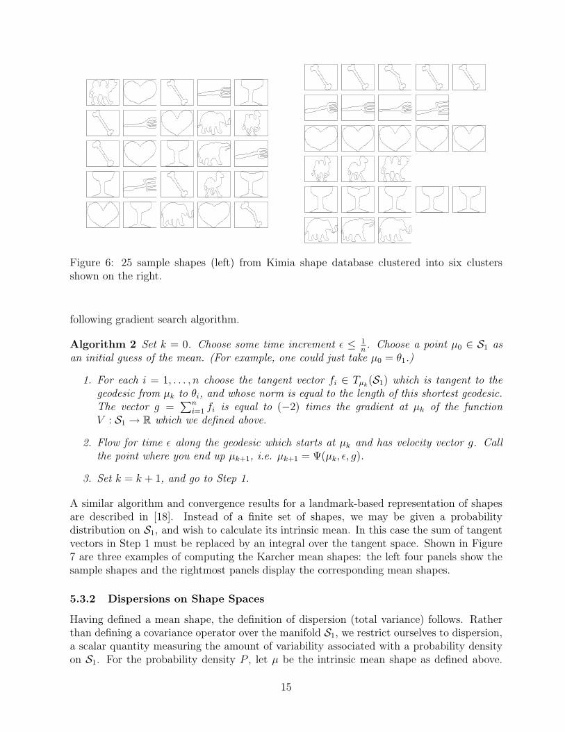
Figure 6: 25 sample shapes (left) from Kimia shape database clustered into six clustersshown on the right.

following gradient search algorithm.

Algorithm 2 Set k = 0. Choose some time increment ε ≤ 1n. Choose a point µ0 ∈ S1 as

an initial guess of the mean. (For example, one could just take µ0 = θ1.)

1. For each i = 1, . . . , n choose the tangent vector fi ∈ Tµk(S1) which is tangent to the

geodesic from µk to θi, and whose norm is equal to the length of this shortest geodesic.The vector g =

∑ni=1 fi is equal to (−2) times the gradient at µk of the function

V : S1 → R which we defined above.

2. Flow for time ε along the geodesic which starts at µk and has velocity vector g. Callthe point where you end up µk+1, i.e. µk+1 = Ψ(µk, ε, g).

3. Set k = k + 1, and go to Step 1.

A similar algorithm and convergence results for a landmark-based representation of shapesare described in [18]. Instead of a finite set of shapes, we may be given a probabilitydistribution on S1, and wish to calculate its intrinsic mean. In this case the sum of tangentvectors in Step 1 must be replaced by an integral over the tangent space. Shown in Figure7 are three examples of computing the Karcher mean shapes: the left four panels show thesample shapes and the rightmost panels display the corresponding mean shapes.

5.3.2 Dispersions on Shape Spaces

Having defined a mean shape, the definition of dispersion (total variance) follows. Ratherthan defining a covariance operator over the manifold S1, we restrict ourselves to dispersion,a scalar quantity measuring the amount of variability associated with a probability densityon S1. For the probability density P , let µ be the intrinsic mean shape as defined above.

15

−0.5 0 0.5 1 1.5−0.4

−0.2

0

0.2

0.4

0.6

0.8

1

1.2

1.4

1.6

−1 −0.5 0 0.5 1 1.5

0

0.5

1

1.5

2

−1 −0.5 0 0.5 10

0.2

0.4

0.6

0.8

1

1.2

1.4

1.6

1.8

2

−1 −0.5 0 0.5 1 1.50

0.2

0.4

0.6

0.8

1

1.2

1.4

1.6

1.8

2

−1.5 −1 −0.5 0 0.5 1 1.50

0.5

1

1.5

2

2.5

−1 −0.5 0 0.5 1

−0.4

−0.2

0

0.2

0.4

0.6

0.8

−1 −0.5 0 0.5 1

−0.6

−0.4

−0.2

0

0.2

0.4

0.6

0.8

1

−1 −0.5 0 0.5 1

−0.4

−0.2

0

0.2

0.4

0.6

0.8

1

1.2

−1 −0.8 −0.6 −0.4 −0.2 0 0.2 0.4 0.6 0.8 1−0.5

0

0.5

1

−1 −0.5 0 0.5 1

−0.6

−0.4

−0.2

0

0.2

0.4

0.6

0.8

1

1.2

−1 −0.8 −0.6 −0.4 −0.2 0 0.2 0.4 0.6 0.8 10

0.2

0.4

0.6

0.8

1

1.2

1.4

1.6

1.8

−1 −0.5 0 0.5 10

0.5

1

1.5

2

−1 −0.5 0 0.5 10

0.2

0.4

0.6

0.8

1

1.2

1.4

1.6

1.8

−1 −0.5 0 0.5 10

0.2

0.4

0.6

0.8

1

1.2

1.4

1.6

1.8

2

−1 −0.5 0 0.5 10

0.2

0.4

0.6

0.8

1

1.2

1.4

1.6

1.8

2

Figure 7: Karcher means (right panels) of the four shapes given in left panels for each row.

Then, for any θ ∈ S1, define fθ ∈ Tµ(C1) to be the vector tangent to the geodesic which joinsµ to the S1-orbit of θ and is orthogonal to the S1-orbit of µ. If θ1, θ2, . . . , θn are samplesfrom a probability distribution, then the sample dispersion is defined as: ρ̂ = 1

n

∑ni=1 ‖fθi‖2,

e.g. ρ̂ = 2.808 for the four fishes shown in the middle row, first four panels, of Figure 7.

5.3.3 Probability Distributions on Shape Spaces

An important issue for statistical analysis of shapes is the definition of a probability measureon the preshape space or the shape space. Given a reference measure, or a base measure onthese spaces, only the probability density P remains to be specified. There are several waysof doing so; our approach is to select a mean shape µ ∈ S1 and impose a probability densityon the tangent (vector) space Tµ(S1). This measure can be inherited by S1 via the geodesicflow, f ∈ Tµ(S1) 7→ Ψ(µ, 1, f) ∈ S1. Since Tµ(S1) is an infinite-dimensional space, a finiteapproximation is needed to specify a probability density. A truncated Fourier series used toestimate the direction function in Section 4 provides a finite approximation. Let a = (a, b)be the vector of coefficients used in approximating the direction f ; then a probability densityfunction on a ∈ R2m+1 implicitly provides a density on S1 via the geodesic flow. In this paperwe use P (a) to be a multivariate normal with mean zero and a covariance matrix ρ2I.

5.4 Shape Extraction

Extraction of shapes from cluttered or partially-obscured images is a difficult problem. Lackof clear data in such problems limits performance in shape inferences, and some additionalknowledge is sought. In case the shapes are known apriori to belong to a family of shapes,this additional knowledge can help improve shape extraction performance. The frameworkdeveloped in this paper is ideally suited to pose and solve Bayesian inferences on shapespaces using low quality images. One can define a prior probability on S1 and combine itwith a likelihood function to infer new shapes from the resulting posterior.

So far our analysis has focused on shape, a property that is invariant to nuisance variablessuch as rotations, translations, and scalings. However, shapes appear in images at specificvalues of nuisance variables, and the process of object discovery should involve either es-

16

timation or integrating out of these nuisance variables (see for example [11]), in additionto estimation of shapes in S. Let X denote the space of nuisance variables; for exampleX = SE(2) × R+, where SE(2) is the special Euclidean group modeling rigid transforma-tions. Then, the likelihood term is a function of both the shape θ ∈ S and the nuisancevariable x ∈ X , while the prior depends only on shape θ. The choice of likelihood functionand the nature of prior is important to the extraction performance. In this paper, our goalis to demonstrate the use of our geometric approach and we do so by choosing a simple like-lihood function and a “Gaussian” prior given in Section 5.3.3 (for details refer to [25]). Wehave used a gradient-based approach to estimate (θ, x) by maximizing the posterior densityon S × X . Shown in Figure 8 are two sets of examples of this MAP estimation. For eachcase, panels on top row show the original image (left), the obscured image (middle), and theprior mean shape (right). The second row of panels show MAP estimates of (θ, x) for anincreasing influence of the prior. In these experiments, the likelihood function, or the datamodel, is based on a simplistic bi-Gaussian model, i.e. the interior pixels and the exteriorpixels are assumed normal with different means and variances.

50 100 150 200 250 300 350

20

40

60

80

100

120

140

16050 100 150 200 250 300 350

20

40

60

80

100

120

140

160

50 100 150 200 250 300 350

20

40

60

80

100

120

140

16050 100 150 200 250 300 350

20

40

60

80

100

120

140

16050 100 150 200 250 300 350

20

40

60

80

100

120

140

16050 100 150 200 250 300 350

20

40

60

80

100

120

140

160

50 100 150 200 250 300

20

40

60

80

100

120

140

16050 100 150 200 250 300

20

40

60

80

100

120

140

160

50 100 150 200 250 300

20

40

60

80

100

120

140

16050 100 150 200 250 300

20

40

60

80

100

120

140

16050 100 150 200 250 300

20

40

60

80

100

120

140

16050 100 150 200 250 300

20

40

60

80

100

120

140

160

Figure 8: Bayesian shape extraction: MAP shapes using increasing prior strengths.

6 Strengths and Limitations

Strengths: Major strengths of the shape analysis presented in this paper are as follows. (i)Continuous shapes are compared modulo rigid rotations, translations, and uniform scalings.The notion of shape is well separated from shape preserving transformations. (ii) Thisapproach does not require landmarks or association between landmarks to compare shapes;nor does it require computing diffeomorphisms of R2. (iii) Curve evolutions in shape space

17

follow ordinary differential equations, and not partial differential equations used commonly inactive contour methods, thus leading to computational efficiency. (iv) It utilizes the intrinsic(Riemannian) geometry of the shape space, and hence leads to well defined statistics, suchas means and covariances, on shape spaces. In contrast, methods that rely on extrinsicanalysis, e.g. using L2 metric between curvature functions to compare shapes of curves, donot lead to well-defined statistics. (v) This approach extends easily to analysis of curvesand other problems dealing with constrained curves in Rn, e.g. computation of elasticae inRn[22, 27]. (vi) Our choice of metric on shape spaces relates to measuring the “bending”energy in changing one shape to another. Since that can be done for any two shapes, weneed not restrict to nearby shapes for computing statistics.Limitations: Some limitations of this approach as presented in this paper is as follows: (i)Our metric measures the “bending” energy and does not allow for stretching. Following [24],we would like an extension that measures a combination of bending and stretching energies,and formulate inferences on that framework. (ii) In this paper we have used a Fourierbasis of representing elements of tangent spaces; one expects improvement in computationalperformance using more local bases, such as wavelets, especially in image analysis. (iii)As stated in Section 2, our shape space includes curves that cross themselves. However,in practice, it is infrequent to have a geodesic connecting two simple closed curves goingthrough a shape that crosses itself. (iv) Although this analysis easily extends to shapes ofcurves in R3, it does not carry over to shapes of surfaces in R3. (v) Our definition of shapeis restricted to the boundaries of the objects, and does not involve modeling the interiors.In some papers, interior pixels are also included in the definition of shapes of objects. (vi)The proposed method does not handle a change in the topology of the shapes, e.g. splittingof a closed curve into two closed curves. A possible approach to account for such changes isto solve for shapes in the space ∪∞n=1Sn

1 although it needs further investigation.

References

[1] R. Bhattacharya and V. Patrangenaru. Nonparametric estimation of location anddispersion on Riemannian manifolds. Journal for Statistical Planning and Inference,108:23–36, 2002.

[2] F. L. Bookstein. Size and shape spaces for landmark data in two dimensions. StatisticalScience, 1:181–242, 1986.

[3] M. P. Do Carmo. Differential Geometry of Curves and Surfaces. Prentice Hall, Inc.,1976.

[4] I. Cohen and I. Herlin. Tracking meteorological structures through curve matching usinggeodesic paths. In Proceedings of ICCV, pages 396–401, 1998.

[5] D. Cremers, T. Kohlberg, and C. Schnorr. Nonlinear shape statistics in Mumford-Shah based segmentation. In European conference on computer vision, pages 93–108,Copenhagen, Denmark, June 2002.

18

Figure 9: A collection of 100 shapes used for clustering experiment.

[6] D. Cremers and S. Soatto. A pseudo distance for shape priors in level set segmentation.In 2nd IEEE Workshop on Variational, Geometric, and Level Set Methods in ComputerVision, France, 2003.

[7] I. L. Dryden and K. V. Mardia. Statistical Shape Analysis. John Wiley & Son, 1998.

[8] M. A. T. Figueiredo and A. K. Jain. Unsupervised learning of finite mixture models.IEEE Transactions on Pattern Analysis and Machine Intelligence, 24(3), 2002.

[9] U. Grenander. General Pattern Theory. Oxford University Press, 1993.

[10] U. Grenander and M. I. Miller. Computational anatomy: An emerging discipline. Quar-terly of Applied Mathematics, LVI(4):617–694, 1998.

[11] U. Grenander, A. Srivastava, and M. I. Miller. Asymptotic performance analysis ofbayesian object recognition. IEEE Transactions of Information Theory, 46(4):1658–1666, 2000.

[12] S. Joshi and A. Srivastava. A geometric approach to shape clustering and learning. InProc. of 12th IEEE Workshop on Statistical Signal Processing, 2003.

19

[13] H. Karcher. Riemann center of mass and mollifier smoothing. Communications on Pureand Applied Mathematics, 30:509–541, 1977.

[14] David G. Kendall. Shape manifolds, procrustean metrics and complex projective spaces.Bulletin of London Mathematical Society, 16:81–121, 1984.

[15] J. T. Kent and K. V. Mardia. Shape, procrustes tangent projections and bilateralsymmetry. Biometrika, 88:469–485, 2001.

[16] S. Lang. Fundamentals of Differential Geometry. Springer, 1999.

[17] L. J. Latecki and R. Lakamper. Shape similarity measure based on correspondence ofvisual parts. IEEE Trans. on Pattern Analysis and Machine Intelligence, 22(19):1185–1190, 2000.

[18] H. Le. Locating frechet means with application to shape spaces. Advances in AppliedProbability, 33(2):324–338, 2001.

[19] J. S. Marques and A. J. Abrantes. Shape alignment - optimal initial point and poseestimation. Pattern Recognition Letters, 18:49–53, 1997.

[20] P. Maurel and G. Sapiro. Dynamic shapes average. In 2nd IEEE Workshop on Varia-tional, Geometric, and Level Set Methods in Computer Vision, France, 2003.

[21] M. I. Miller and L. Younes. Group actions, homeomorphisms, and matching: A generalframework. International Journal of Computer Vision, 41(1/2):61–84, 2002.

[22] W. Mio, A. Srivastava, and E. Klassen. Interpolation by elastica in Euclidean spaces.Quarterly of Applied Mathematics, to appear, 2003.

[23] F. Mokhtarian, S. Abbasi, and J. Kittler. Efficient and robust shape retrieval by shapecontent through curvature scale space. In Proceedings of First International Conferenceon Image Database and MultiSearch, pages 35–42, 1996.

[24] T. B. Sebastian, P. N. Klein, and B. B. Kimia. On aligning curves. IEEE Transactionson Pattern Analysis and Machine Intelligence, 25(1):116–125, 2003.

[25] A. Srivastava, S. Joshi, W. Mio, and X. Liu. A geometric approach to shape clustering,learning and testing. Technical Report TC03, Department of Statistics, Florida StateUniversity, 2003.

[26] A. Srivastava and E. Klassen. Monte Carlo extrinsic estimators for manifold-valuedparameters. IEEE Trans. on Signal Processing, 50(2):299–308, February 2001.

[27] A. Srivastava, W. Mio, E. Klassen, and X. Liu. Goemetric analysis of constrained curvesfor image understanding. In Proceedings of Second IEEE Workshop on Variational,Geometric, and Level Sets Methods in Computer Vision, Nice, France, October 2003.

[28] H. D. Tagare, D. O’Shea, and D. Groisser. Non-rigid shape comparison of plane curvesin images. Journal of Mathematical Imaging and Vision, 16:57–68, 2002.

20

[29] R. P. Woods. Characterizing volume and surface deformations in an atlas framework.Technical Report, Department of Neurology and Physiology, UCLA, 2002.

[30] L. Younes. Optimal matching between shapes via elastic deformations. Journal of Imageand Vision Computing, 17(5/6):381–389, 1999.

21