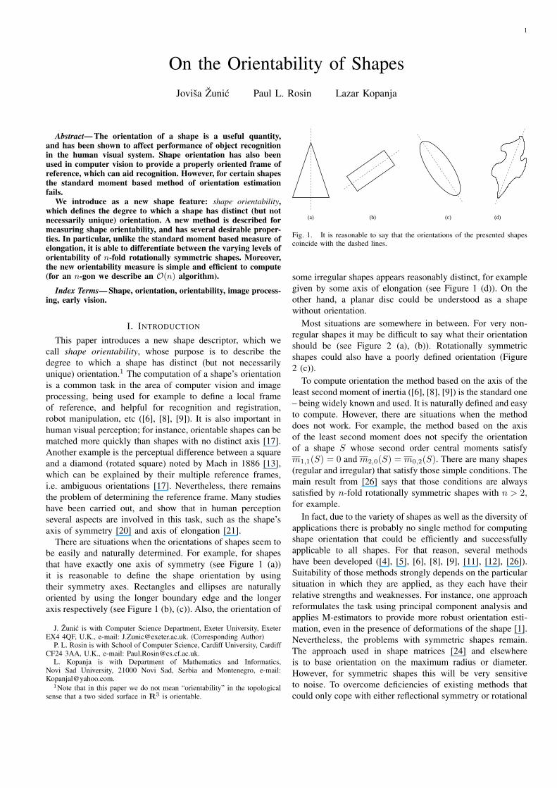
1

On the Orientability of Shapes

Jovisa Zunic Paul L. Rosin Lazar Kopanja

Abstract— The orientation of a shape is a useful quantity,and has been shown to affect performance of object recognitionin the human visual system. Shape orientation has also beenused in computer vision to provide a properly oriented frame ofreference, which can aid recognition. However, for certain shapesthe standard moment based method of orientation estimationfails.

We introduce as a new shape feature: shape orientability,which defines the degree to which a shape has distinct (but notnecessarily unique) orientation. A new method is described formeasuring shape orientability, and has several desirable proper-ties. In particular, unlike the standard moment based measure ofelongation, it is able to differentiate between the varying levels oforientability of n-fold rotationally symmetric shapes. Moreover,the new orientability measure is simple and efficient to compute(for an n-gon we describe an O(n) algorithm).

Index Terms— Shape, orientation, orientability, image process-ing, early vision.

I. INTRODUCTION

This paper introduces a new shape descriptor, which we

call shape orientability, whose purpose is to describe the

degree to which a shape has distinct (but not necessarily

unique) orientation.1 The computation of a shape’s orientation

is a common task in the area of computer vision and image

processing, being used for example to define a local frame

of reference, and helpful for recognition and registration,

robot manipulation, etc ([6], [8], [9]). It is also important in

human visual perception; for instance, orientable shapes can be

matched more quickly than shapes with no distinct axis [17].

Another example is the perceptual difference between a square

and a diamond (rotated square) noted by Mach in 1886 [13],

which can be explained by their multiple reference frames,

i.e. ambiguous orientations [17]. Nevertheless, there remains

the problem of determining the reference frame. Many studies

have been carried out, and show that in human perception

several aspects are involved in this task, such as the shape’s

axis of symmetry [20] and axis of elongation [21].

There are situations when the orientations of shapes seem to

be easily and naturally determined. For example, for shapes

that have exactly one axis of symmetry (see Figure 1 (a))

it is reasonable to define the shape orientation by using

their symmetry axes. Rectangles and ellipses are naturally

oriented by using the longer boundary edge and the longer

axis respectively (see Figure 1 (b), (c)). Also, the orientation of

J. Zunic is with Computer Science Department, Exeter University, ExeterEX4 4QF, U.K., e-mail: J.Zunic@exeter.ac.uk. (Corresponding Author)

P. L. Rosin is with School of Computer Science, Cardiff University, CardiffCF24 3AA, U.K., e-mail: Paul.Rosin@cs.cf.ac.uk.

L. Kopanja is with Department of Mathematics and Informatics,Novi Sad University, 21000 Novi Sad, Serbia and Montenegro, e-mail:Kopanjal@yahoo.com.

1Note that in this paper we do not mean “orientability” in the topologicalsense that a two sided surface in R3 is orientable.

(a) (b) (c) (d)

Fig. 1. It is reasonable to say that the orientations of the presented shapescoincide with the dashed lines.

some irregular shapes appears reasonably distinct, for example

given by some axis of elongation (see Figure 1 (d)). On the

other hand, a planar disc could be understood as a shape

without orientation.

Most situations are somewhere in between. For very non-

regular shapes it may be difficult to say what their orientation

should be (see Figure 2 (a), (b)). Rotationally symmetric

shapes could also have a poorly defined orientation (Figure

2 (c)).

To compute orientation the method based on the axis of the

least second moment of inertia ([6], [8], [9]) is the standard one

– being widely known and used. It is naturally defined and easy

to compute. However, there are situations when the method

does not work. For example, the method based on the axis

of the least second moment does not specify the orientation

of a shape S whose second order central moments satisfy

m1,1(S) = 0 and m2,0(S) = m0,2(S). There are many shapes

(regular and irregular) that satisfy those simple conditions. The

main result from [26] says that those conditions are always

satisfied by n-fold rotationally symmetric shapes with n > 2,for example.

In fact, due to the variety of shapes as well as the diversity of

applications there is probably no single method for computing

shape orientation that could be efficiently and successfully

applicable to all shapes. For that reason, several methods

have been developed ([4], [5], [6], [8], [9], [11], [12], [26]).

Suitability of those methods strongly depends on the particular

situation in which they are applied, as they each have their

relative strengths and weaknesses. For instance, one approach

reformulates the task using principal component analysis and

applies M-estimators to provide more robust orientation esti-

mation, even in the presence of deformations of the shape [1].

Nevertheless, the problems with symmetric shapes remain.

The approach used in shape matrices [24] and elsewhere

is to base orientation on the maximum radius or diameter.

However, for symmetric shapes this will be very sensitive

to noise. To overcome deficiencies of existing methods that

could only cope with either reflectional symmetry or rotational

2

symmetry, Shen and Ip [22], [23] developed a method for

estimating the number and orientation of both types of axes

of symmetry. However, it requires several tuning parameters,

but the computation of many high order generalized complex

moments.

As mentioned, rotationally symmetric polygons have a

poorly defined orientation. Moreover, even for regular poly-

gons (see Figure 2 (d) and (e)) it is debatable whether they

are orientable or not. For instance, is a square an orientable

shape? The same question arises not only for any regular n-

gon, but also for shapes having several axes of symmetry

(Figure 2 (f)), and n-fold (n > 2) rotational symmetric shapes.

If the answer is “yes, those shapes are orientable”, how should

the shapes (d), (e), and (f) from Figure 2 be ranked with

respect to their orientability? This is another question that is

of interest and applicable in the area of shape analysis and

shape classification.

Note that the rotation-symmetric and reflective-symmetric

shapes appear very often not only in industry (as machine

made products) but also in nature (e.g. human face, crystals).

The related problems (detection of axes of symmetry, for

example) are intensively studied in the literature [2], [7], [14],

[18], [23], but some attention has been given to the algebraic

structure produced by symmetry operations on planar shapes

(see [9] for a short overview).

(a) (b) (c) (d) (e) (f)

Fig. 2. It is not quite clear what the orientation of the shapes (a), (b), and(c) should be. The dashed lines seem to be reasonable candidates to representthe orientation of the shapes (d), (e), and (f). In the case of the square it isdebatable whether the preference should be given to the diagonals or to thevertical (or horizontal) line.

Problems caused by digitization process. The shape ori-

entation problem becomes more complex taking into account

that in computer vision and image processing tasks real shapes

are replaced with their digitizations. Some specific problems

arise when working with digital shapes. Let us mention just

two of them:

– Due to the applied digitization process it is possible that

some “non-orientable” objects have digitizations whose

orientation can be easily computed when the standard

method (equation (5)) is applied.

– On the other hand, it is also possible that some orientable

objects have digitizations which are not orientable.

The impact of digitization effects on the change in the

computed shape orientation is illustrated by the example of

a digitized disc and a digitized square. Even though real

discs and squares are not “orientable” shapes (see Lemma 1)

it could happen that after digitization the obtained discrete

point sets have the orientation computable in the standard

manner (described in the next section). We demonstrate that

the computed orientation could depend strongly on:

(a) shape position with respect to the digitization grid;

(b) applied picture resolution.

The effect of item (a) is illustrated by Figure 3. The same disc

is translated into 6 different positions and then digitized. The

orientation of the digital disc is not well-defined (in the sense

of equation (5)) for positions displayed at Figure 3 (a) and

(d), while the digital discs displayed at Figure 3, (b), (c), (e),

and (f), have the measured orientations ϕ = π/2, ϕ = π/2,

ϕ = π/4, and ϕ = π − 12 · arctan 3

4 , respectively – when

equation (5) is applied. We use such a simple example in order

to be able to check the results by hand. A higher resolution (or

equivalently, a bigger disc is digitized) leads to a larger number

of computed orientations which can be obtained if the disc

changes its position w.r.t. digitization grid. As an illustration:

we have digitized 32 real discs having the radius equal to 10,

whose center positions have been chosen randomly. For each

choice of center position we have computed the orientation of

the obtained digital disc (applying equation (5)). The computed

orientations (in the range [−π/2, π/2])

0.05 0.03 -0.06 -0.59 0.75 -0.01 -0.23 -0.720.13 0.00 0.22 -0.57 -0.06 0.29 -0.61 0.63

-0.41 -0.56 -0.29 0.00 0.023 0.14 -0.32 0.110.16 -0.01 0.78 -0.74 -0.55 -0.05 0.61 0.25

show that the computed orientation strongly depends on the

disc position with respect to the digitization grid.

In Figure 4, the same square is presented in two digital

images having different resolutions. In the first case, the

standard method does not specify what the orientation of the

obtained digital square should be. In the second case, the

orientation can be computed easily.

.

.

.

.

.

...

...

..

.

. ..

..

.

.

.

(b)(a) (c)

(d) (e) (f)

.

..

.

...

..

.

....

.

Fig. 3. There are 6 non-isometric digitizations of a disc having the radius√2 on a binary picture with resolution 1 (i.e., one pixel per measure unit).

. .. ...

.

. ...... .... ..

.....

. .. ..

..

.

.

..

..

..

..

. . . . .. ..

...

.

..

..

.

.

.

. . ..Fig. 4. The same square is presented in digital pictures having differentresolutions.

Problems caused by noise effects. Similar problems to

the above can be caused by noise effects, as well. For

instance, consider a square aligned with the coordinate axes.

As mentioned, the standard method does not give any answer

as to what the orientation of such a square should be. Adding

a single protruding pixel to the boundary can cause the

computed orientation to lie anywhere in the range [−π/2, π/2]depending on its location. As an example, for a 10× 10 grid

3

of pixels adding one pixel to the horizontal or vertical edge

gives the following computed orientations:

0.88 1.00 1.14 1.30 1.48 -1.48 -1.30-1.14 -1.00 -0.88 -0.69 -0.57 -0.43 -0.27-0.09 0.09 0.27 0.43 0.57 0.69

Problems caused by the nature of shape. Most of the

problems are caused by the nature of the shapes, i.e. because

of their inherent inability to be oriented. In Figure 5 (a1), (b1),

and (c1) three starfish images are presented. Their boundaries

are extracted and presented in Figure 5 (a2), (b2), and (c2).

Even though we expected to have the computed orientations

for shapes from Figure 5 (a1) (i.e. (a2)) and Figure 5 (b1)

(i.e. (b2)) to be very similar (or even coincident) we have

obtained (by the standard method) the computed orientations

as: −13.7 degrees and 0.4 degrees, respectively. For the shape

from Figure 5 (c1) (i.e (c2)) we expected a slightly different

orientation. But again, the computed orientation of −36.6 is

too far from our expectation.

(a1) (b1) (c1)

(a2) (b2) (c2)

Fig. 5. The differences in estimated orientation of these shapes is due totheir deviations from symmetry caused by different viewing angles, naturaldeformations and variations in the starfish, and noise.

Our conclusion is that the above results for estimated ori-

entation are not realistic simply because the presented shapes

cannot be easily oriented – or, in our terms, they should have

a low measured orientability.

Problem description. In order to deal with the problems

mentioned previously, it is not enough to determine whether

the orientation can be computed or not (i.e. does the formula

or algorithm used give a result or not?). Rather, it would be

more useful to see how stable the solution is. For this purpose

we will define shape orientability as a new shape descriptor.

The main purpose of it is to suggest an answer to the question:

Is the computed orientation just a consequence of digitization

or noise effects or is it an inherent property of the considered

shape? We want to describe a shape’s orientability as a new

shape descriptor that would measure very low orientability

values in the cases presented above. As a consequence, a low

measure of orientability would suggest that the orientations

presented in the previous experiments cannot be accepted

as realistic ones – i.e. the reference frame for such shapes

should be selected in a more appropriate way or higher quality

images must be provided. A second requirement is that we

want very elongated ellipses and rectangles to have a very

high orientability. Two extreme cases should be circles (with

measured orientability equal to 0) and straight line segments

(with measured orientability equal to 1).

Organization of the paper. In Section 2 we give a short

overview of the most standard method for shape orientation

(i.e. the method based on the axis of the least second moment)

and characterize some situations when the method is not

applicable.

After that, in Section 3, we discuss some intuitive orientabil-

ity measures that come from the standard definition of shape

orientation and we define a new orientability measure. That is

the main result of the paper. The defined orientability measure

is invariant with respect to similarity transformations, it is nor-

malized to be a number from [0, 1), and it distinguishes a circle

as having the lowest possible measured orientability that is

equal to 0. Also, there is no shape with measured orientability

equal to 1, but shapes having measured orientability arbitrary

close to 1 can be constructed. For example, a rectangle with

the edge lengths 1 and a has the measured orientability tending

to 1 as a → ∞ (see Section 6 and Figure 14).

Section 4 describes an O(n) procedure for the computation

of the new orientability measure of simple n-gons. Some

experimental results are shown in Section 5, while Section

6 contains concluding remarks.

II. STANDARD METHOD FOR COMPUTING ORIENTATION

In this section we give a short overview of the method which

is mostly used in practice for computing orientation (not the

orientability computation!) including a lemma that shows that

this method cannot be effective when applied to shapes that

have several axes of symmetry, for example.

The standard approach defines the orientation by the so

called axis of the least second moment ([6], [8]). That is the

line which minimizes the integral of the squares of distances

of the points (belonging to the shape) to the line. The integral

is

I(S, ϕ, ρ) =

∫

S

∫

r2(x, y, ϕ, ρ)dxdy (1)

where r(x, y, ϕ, ρ) is the perpendicular distance from the point

(x, y) to the line given in the form

x · cosϕ− y · sinϕ = ρ.

It can be shown that the line that minimizes I(S, ρ, ϕ) passes

through the centroid (xc(S), yc(S)) of the shape S where

(xc(S), yc(S)) =

(

∫∫

Sxdxdy

∫∫

Sdxdy

,

∫∫

Sydxdy

∫∫

Sdxdy

)

.

In other words, without loss of generality, we can assume that

the origin is placed at the centroid, and so the required line

minimizing I(S, ρ, ϕ), passes through the origin – i.e., we can

set ρ = 0. In this way, the shape orientation problem can be

reformulated to the problem of determining ϕ for which the

function F (ϕ, S) defined as2

F (ϕ, S) = I(S, ϕ, ρ = 0) =

∫

S

∫

(x · sinϕ− y · cosϕ)2dxdy

2The squared distance of a point (x, y) to the line X ·cosϕ−Y ·sinϕ = 0is (x sinϕ− y cosϕ)2.

4

reaches the minimum. Once again, we assume that the origin

coincides with the center of gravity of S.

Further, if the central geometric moments mp,q(S) are

defined as usual by:

mp,q(S) =

∫

S

∫

(x− xc(S))p · (y − yc(S))

q dx dy,

and if (xc(S), yc(S)) = (0, 0) then we have

F (ϕ, S) = (sinϕ)2·m2,0(S)−sin(2·ϕ)·m1,1,(S)+(cosϕ)2·m0,2(S).(2)

The minimum of the function F (ϕ, S) can be computed easily.

Setting the first derivative F ′(x, S) to zero, we have

F ′(ϕ, S) = sin(2ϕ)·(m2,0(S)−m0,2(S))−2·cos(2ϕ)·m1,1(S) = 0.

That easily gives that the required angle ϕ, but also the angle

ϕ+ π/2, satisfies the equation

sin(2ϕ)

cos(2ϕ)=

2 ·m1,1(S)

m2,0(S)−m0,2(S). (3)

Consequently, by using (2) and (3), the maximum and mini-

mum of F (ϕ, S) are as follows

max{F (S, ϕ) | ϕ ∈ [0, 2π]} =

m2,0(S)+m0,2(S)+√

4·(m1,1(S))2+(m2,0(S)−m0,2(S))2

2

and

min{F (S, ϕ) | ϕ ∈ [0, π]} =

m2,0(S)+m0,2(S)−√

4·(m1,1(S))2+(m2,0(S)−m0,2(S))2

2 .

The ratio between maxϕ∈[0,π)

F (ϕ, S) and minϕ∈[0,π)

F (ϕ, S)

E(S) = max{F (ϕ, S) | ϕ ∈ [0, 2 · π]}min{F (ϕ, S) | ϕ ∈ [0, 2 · π]} (4)

is well known as the elongation of the shape S, and can also

be expressed as

E(S) =√

Φ2(S)

Φ1(S)

where Φ1(S) and Φ2(S) are the first two rotation and trans-

lation moment invariants [16].

Let us mention that, when working with digital objects

which are actually digitizations of real shapes, the central

geometric moments mp,q(S) are replaced with their discrete

analogue, i.e., with so called central discrete moments. Since

the digitization on the integer grid Z2 of a real shape S

consists of all pixels whose centers are inside S it is natural to

approximate mp,q(S) by the central discrete moment µp,q(S)which is defined as

µp,q(S) =∑

(i,j)∈S∩Z2

(i− xcd(S))p · (j − ycd(S))

q,

where (xcd(S), ycd(S)) =

∑

(x,y)∈S∩Z2

x

∑

(x,y)∈S∩Z2

1,

∑

(x,y)∈S∩Z2

y

∑

(x,y)∈S∩Z2

1

is

the centroid of discrete shape S ∩ Z2.

Some details about the efficiency of the approximation

mp,q(S) ≈ µp,q(S) can be found in [10].

By replacing the geometric moments in (3) with the corre-

sponding discrete moments we obtain the equation

sin(2ϕ)

cos(2ϕ)=

2 · µ1,1(S)

µ2,0(S)− µ0,2(S)(5)

which describes the angle ϕ which is used as an approximate

orientation of the shape S, i.e., the angle which is used to

describe the orientation of discrete shape S ∩ Z2. It is worth

noting that equation (5) can be derived easily if the orientation

of the discrete set (a finite number point set) S∩Z2 is defined

by the line (passing the origin) which minimizes the total sum∑

(i,j)∈S∩Z2(i · sinϕ− j · cosϕ)2) of squares of distances of

points from S ∩ Z2 to this line.

In other words, the equality (5) can be derived as a

consequence when trying to solve the following optimization

problem

min

∑

(i,j)∈S∩Z2

(i · sinϕ− j · cosϕ)2 | ϕ ∈ [0, π]

(6)

assuming that the centroid(

xcd(S ∩ Z2), ycd(S ∩ Z

2)

) coin-

cides with the origin.

So, the standard method is very simple (in both “real” and

“discrete” versions) and it comes from a natural definition

of the shape orientation. However, it is not always effective.

The next lemma is a direct consequence of Theorem 1 from

[26]. It is related to n-fold rotationally symmetric shapes –

i.e., such shapes which are identical to themselves after being

rotated through any multiple of 2πn, and it shows that the

standard method does not always give a clear result for the

shape orientation.

Lemma 1: If a given shape S is n-fold rotationally sym-

metric, with n > 2, then F (ϕ, S) is a constant function.

Remark. Lemma 1 implies that

• F (ϕ, S) = 12 · (m2,0(S) +m0,2(S)) for all ϕ ∈ [0, π);

• E(S) = 1

hold for all n-fold rotationally symmetric shapes with n > 2(trivially, this includes shapes that have more than two axes of

symmetry). In other words, the standard method does not tell

us what the orientation of shapes from Figure 2(c)-(f) should

be, or more generally, what the orientation is for any such

rotationally symmetric shape. Also, for all such shapes the

measured elongation is 1 (measured in the range [1,∞) as

defined by (4)). So, such shapes have the minimum possible

measured elongation – i.e., the same measured elongations as

a circle. That is not a desirable property if we would like to

understand a circle as the least elongated shape rather than

such shapes as Figure 2(c)-(f).

III. MEASURING SHAPE ORIENTABILITY

In this section we consider what quantity can be used to

describe shape orientability – to be used as an inherent shape

property.

Intuitively, it can be assumed that shapes with high mea-

sured elongation are more orientable than shapes with lower

5

measured elongation. Thus, the elongation E(S) (see (4)) can

be used to estimate shape orientability. Since E(S) ∈ [1,∞),in order to have the measured orientability between 0 and 1,

we can measure the orientability as:

1− 1

E(S) . (7)

Several other measures can be derived from the function

F (ϕ, S), as well. For example, it is intuitively very clear that

a bigger ratio between:

– the area of the region bounded by: the coordinate axes,

line y = minϕ∈[0,π)

F (ϕ, S), and line x = π,

and

– the area of region bounded by: the coordinate axes, line

y = F (ϕ, S), and line x = π,

should indicate a lower shape orientability. So, we can give

the following definition.

Definition 1: For a given shape S its orientability DF (S)can be measured as

DF (S) = 1− π ·min{F (S, ϕ) | ϕ ∈ [0, π)}∫ π

0F (S, ϕ) · dϕ

=

√

4 · (m1,1(S))2 + (m2,0(S)−m0,2(S))2

m2,0(S) +m0,2(S).

Note 1: Let the principal moments of inertia of a region

are denoted by I1 and I2. Then another measure of elongation

that is found in the literature ([16]) can be expressed as

I1 − I2I1 + I2

=

√

4 · (m1,1(S))2 + (m2,0(S)−m0,2(S))2

m2,0(S) +m0,2(S).

That is, although it is derived according to different criteria,

it results in the identical formula to DF .

Obviously, DF (S) is easily computable and well-motivated.

However, it is clear that all shape orientability measures

based on F (ϕ, S) are limited by the result of Lemma 1, i.e.,

DF (S) = 1−1/E(S) = 0 for all n-fold rotationally symmetric

shapes with n > 2. In some situations (applications) a new

measure for shape orientability is required that does not have

that disadvantage.

We now define such a measure. When dealing with rota-

tionally symmetric shapes that have several axes of symmetry,

such shapes do not necessarily have identical measured ori-

entability, as would result when using 1−1/E(S) and DF (S),for example.

x

y

P

θ

θR(S, )

Fig. 6. The rectangle R(S, θ) is the minimum area rectangle which includesthe given shape (shaded area) and whose edges make an angle θ with thecoordinate axes.

Definition 2: For a given shape S let R(S, θ) be the

minimal rectangle whose edges make an angle θ with the

coordinate axes and which includes S (see Figure 6) and let

A(R(S, θ)) be the area of R(S, θ). Let

Amin(S) = minθ∈[0,π)

{ A(R(S, θ)) }

and

Amax(S) = maxθ∈[0,π)

{ A(R(S, θ)) } .

Then, we define the orientability measure D(S) of the shape

S as:

D(S) = 1− Amin(S)

Amax(S).

The next theorem describes some desirable properties of

D(S).Theorem 1: The newly defined measure for shape ori-

entability has the following properties:

a) D(S) ∈ [0, 1) for any shape S;

b) A circle has the measured orientability equal to 0;

c) The measured orientability is invariant with respect to

similarity transformations.

Proof. a) The statement follows easily because 0 <Amin(S) ≤ Amax(S) holds for any shape S.

b) If S is a circle then Amin(S) = Amax(S) and conse-

quently D(S) = 0.c) Let T be a similarity transformation represented by a

matrix T. Let a given shape S. The area of the transformed

shape T (S) satisfies A(T (S)) = det(T) · A(S), but also

A(T (R(S, θ))) = det(T) · A(R(S, θ)), for any angle θ.Thus, Amin(T (S)) = det(T) ·Amin(S) and Amax(T (S)) =det(T) · Amax(S) which finally gives D(T (S)) = D(S). ✷

The new orientability measure of a shape S introduced by

Definition 2 is very convenient for numerical computation. A

required precision can be reached if A(R(S, 0)),A(R(S, πN)),

A(R(S, 2 · πN)), . . . , A(R(S, (N −1) · π

N)), are computed for

a sufficiently large N . The exact computation of D(S) when

the measured shape S is a polygon will be described in detail

in the next section.

The main objection to D(S) could be that shapes having the

same convex hull have the same measured orientability. That

is a disadvantage particularly when D(S) is used as a shape

descriptor in some classification tasks. A slight modification

of Definition 2 would ensure that a given non-convex shape

does not have the measured orientability equal to the measured

orientability of its convex hull. So, we give the next definition.

Definition 3: For a given shape S let Amin(S) and

Amax(S) be defined as in Definition 2 and let A(S) denotes

the area of S. Then, for any real number α ∈ [0, 1] we define

the orientability measure Dα(S) of the shape S as:

Dα(S) = 1− Amin(S)− α ·A(S)

Amax(S)− α ·A(S).

Note 2: The orientability measure Dα also has the desirable

properties listed in Theorem 1.

IV. COMPUTATION OF Dα(P ) WHEN P IS A SIMPLE

POLYGON

From Definition 2 and Definition 3, it is obvious that numer-

ical computation of the orientability Dα(S) is straightforward.

6

An arbitrary precision could be reached, although of course

higher precision requires higher time complexity.

On the other hand, in particular applications we work with

discrete point sets which are discretisations of real shapes.

The boundaries of such shapes are necessarily assumed to be

polygonal lines – defined in different ways depending on the

particular application. In the rest of this section we will assume

that considered shapes are bounded by simple polygons and

will show that the computation of their orientabilities is

possible in linear time with respect to the number of vertices

on their boundary.

So, given a simple polygon P , in order to determine Dα(P )we have to compute the minimum possible area Amin(P ) of

a rectangle enclosing a given polygon P and the maximum

possible area Amax(P ) of a rectangle enclosing the polygon

P . The construction of a rectangle enclosing P and having the

area Amin(P ) is already studied in the literature and various

approaches exist [3], [15], [25]. The well known result from

[3] says that the minimum area rectangle that includes Phas one edge that is parallel to an edge of the convex hull

of P (denoted as CH(P )). By using this fact and applying

the orthogonal calipers technique presented in [25], the area

Amin(P ) can be computed in O(n) time where n denotes the

number of edges of P .

The same statement does not hold for a maximum area

rectangle enclosing a given polygon P . A trivial counterex-

ample is a square. Indeed, if P is a square then CH(P )and the minimum area enclosing rectangle coincide, while

the maximum area enclosing rectangle has edges making a

π/4 angle with edges of P . But, we will show that it is still

possible to use the orthogonal calipers technique to determine

Amax(P ).We briefly present the orthogonal calipers technique. A line

L is a line of support of P if the interior of P lies completely

to one side of L. A pair of vertices is an antipodal pair if

it admits parallel lines of support. Preparata and Shamos’

algorithm [19] generates all antipodal pairs by a procedure

which resembles rotating a pair of dynamically adjustable

parallel support lines once around the polygon P in order

to compute the diameter of P (the diameter of P is defined

to be the greatest distance between parallel lines of support

of P ). This idea is generalized in [25] where two orthogonal

pairs of line supports (named orthogonal calipers) are formed

around the polygon solving several geometric problems. What

is important for us is that the same procedure can be used here

in order to obtain the intervals

[β1, β2], [β2, β3], . . . , [βm−1, βm], [βm, β1+2π], m ≤ n (8)

such that:

– Four vertices of an n-gon P (more precisely, four vertices

of CH(P )) forming two pairs of antipodal points remain

the antipodal points while one of the support lines has the

slope α ∈ [βi, βi+1], i = 1, . . . ,m− 1;

– Those four points belong to support lines forming the

orthogonal calipers.

Note 3: For any angle βi ∈ {β1, β2, . . . , βm} ⊂ [0, 2π]there is an edge ei of CH(P ) such that after rotation by the

AH

C

D

E

G

I

K

L

x

y

F

B

φ

F’

F’’

J

γγ

δδ1 2+

2δ

2δ+δ1

L’

1δ I’

J’

K’

Fig. 7. Illustrating the generation of the orthogonal calipers.

angle βi the edge ei becomes parallel to one of coordinate

axes.

We refer to Figure 7 for an illustration. Let δ1 be the angle

between

the positively oriented x-axis and the edge [AB]. Also, let

δ2 = min{6 (JBC), 6 (KDE), 6 (GFL), 6 (HGI)} (i.e., δ2is the minimum angle between the bounding rectangle and the

counterclockwise edges at the antipodal points) – in a situation

as in Figure 7, δ2 = 6 (KDE).

If the line l(I, J) is chosen to be a support line then B,Fand D,G are the antipodal pairs which determine two orthogo-

nal pairs of line supports: l(I, J), l(L,K) and l(J,K), l(I, L).If the support line l(I, J) is rotated into a new position around

the vertex B then the pairs B,F and D,G remain antipodal

while the rotation γ angle varies from 0 to δ2 (see Figure 7).

(Remark: In the sense of Note 3, we can chose β1 = δ1, which

would imply β2 = δ1 + δ2.)

For γ ∈ [0, δ2] the height d(L′I ′) of the minimal rectangle

L′I ′J ′K ′ that circumscribes P is

d(L′I ′) = d(F, F ′) · cos(φ+ γ) for γ ∈ [0, δ2]. (9)

and it varies from d(F, F ′) to d(F, F ′′), where d(X,Y ) is

the Euclidean distance between points X and Y . The angle φdepends only on the four chosen antipodal points. In the case

presented in Figure 7, φ can be computed from B,F,D, and

G, or equivalently, φ is determined by the interval [β1, β2] (by

β1 and β2, as well).

Analogously, the width d(I ′J ′) of the same rectangle is of

the form

d(I ′J ′) = d(G,G′′) · cos(ω + γ) (10)

where γ ∈ [0, δ2] and ω is a fixed angle which can be

computed from δ1 and δ2 (i.e., from β1 and β2).

Thus, the area of the rectangle L′I ′J ′K ′ (i.e., the rectangle

R(P, γ) in the sense of Definition 2) is

A((R(P, γ)) =

d(F, F ′) · cos(φ+ γ) · d(G,G′) · cos(ω + γ). (11)

7

π 2π angle

area

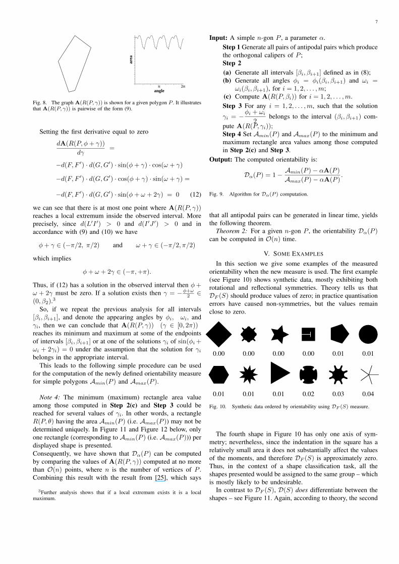
Fig. 8. The graph A(R(P, γ)) is shown for a given polygon P . It illustratesthat A(R(P, γ)) is pairwise of the form (9).

Setting the first derivative equal to zero

dA(R(P, φ+ γ))

dγ=

−d(F, F ′) · d(G,G′) · sin(φ+ γ) · cos(ω + γ)

−d(F, F ′) · d(G,G′) · cos(φ+ γ) · sin(ω + γ) =

−d(F, F ′) · d(G,G′) · sin(φ+ ω + 2γ) = 0 (12)

we can see that there is at most one point where A(R(P, γ))reaches a local extremum inside the observed interval. More

precisely, since d(L′I ′) > 0 and d(I ′J ′) > 0 and in

accordance with (9) and (10) we have

φ+ γ ∈ (−π/2, π/2) and ω + γ ∈ (−π/2, π/2)

which implies

φ+ ω + 2γ ∈ (−π,+π).

Thus, if (12) has a solution in the observed interval then φ+ω + 2γ must be zero. If a solution exists then γ = −φ+ω

2 ∈(0, β2).

3

So, if we repeat the previous analysis for all intervals

[βi, βi+1], and denote the appearing angles by φi, ωi, and

γi, then we can conclude that A(R(P, γ)) (γ ∈ [0, 2π))reaches its minimum and maximum at some of the endpoints

of intervals [βi, βi+1] or at one of the solutions γi of sin(φi+ωi + 2γi) = 0 under the assumption that the solution for γibelongs in the appropriate interval.

This leads to the following simple procedure can be used

for the computation of the newly defined orientability measure

for simple polygons Amin(P ) and Amax(P ).

Note 4: The minimum (maximum) rectangle area value

among those computed in Step 2(c) and Step 3 could be

reached for several values of γi. In other words, a rectangle

R(P, θ) having the area Amin(P ) (i.e. Amax(P )) may not be

determined uniquely. In Figure 11 and Figure 12 below, only

one rectangle (corresponding to Amin(P ) (i.e. Amax(P ))) per

displayed shape is presented.

Consequently, we have shown that Dα(P ) can be computed

by comparing the values of A(R(P, γ)) computed at no more

than O(n) points, where n is the number of vertices of P .

Combining this result with the result from [25], which says

3Further analysis shows that if a local extremum exists it is a localmaximum.

Input: A simple n-gon P , a parameter α.

Step 1 Generate all pairs of antipodal pairs which produce

the orthogonal calipers of P ;

Step 2

(a) Generate all intervals [βi, βi+1] defined as in (8);

(b) Generate all angles φi = φi(βi, βi+1) and ωi =ωi(βi, βi+1), for i = 1, 2, . . . ,m;

(c) Compute A(R(P, βi)) for i = 1, 2, . . . ,m.

Step 3 For any i = 1, 2, . . . ,m, such that the solution

γi = −φi + ωi

2belongs to the interval (βi, βi+1) com-

pute A(R(P, γi));Step 4 Set Amin(P ) and Amax(P ) to the minimum and

maximum rectangle area values among those computed

in Step 2(c) and Step 3.

Output: The computed orientability is:

Dα(P ) = 1− Amin(P )− αA(P )

Amax(P )− αA(P ).

Fig. 9. Algorithm for Dα(P ) computation.

that all antipodal pairs can be generated in linear time, yields

the following theorem.

Theorem 2: For a given n-gon P , the orientability Dα(P )can be computed in O(n) time.

V. SOME EXAMPLES

In this section we give some examples of the measured

orientability when the new measure is used. The first example

(see Figure 10) shows synthetic data, mostly exhibiting both

rotational and reflectional symmetries. Theory tells us that

DF (S) should produce values of zero; in practice quantisation

errors have caused non-symmetries, but the values remain

close to zero.

0.00 0.00 0.00 0.00 0.01 0.01

0.01 0.01 0.01 0.02 0.03 0.04

Fig. 10. Synthetic data ordered by orientability using DF (S) measure.

The fourth shape in Figure 10 has only one axis of sym-

metry; nevertheless, since the indentation in the square has a

relatively small area it does not substantially affect the values

of the moments, and therefore DF (S) is approximately zero.

Thus, in the context of a shape classification task, all the

shapes presented would be assigned to the same group – which

is mostly likely to be undesirable.

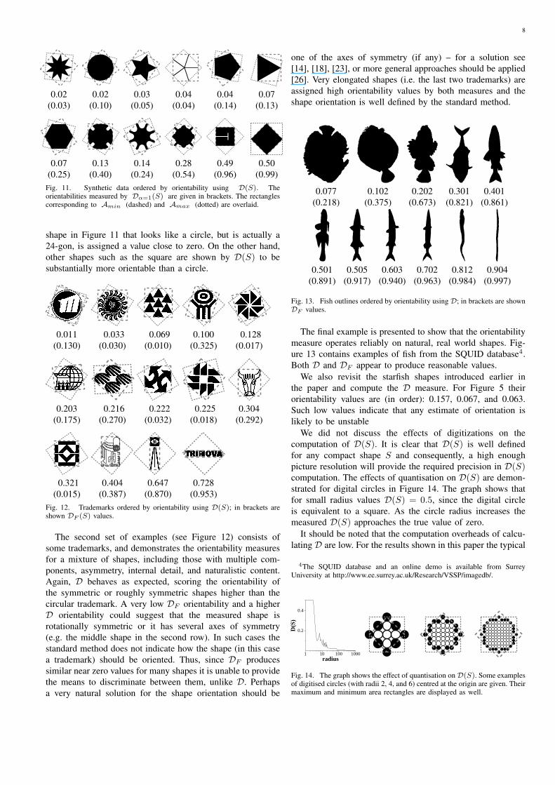
In contrast to DF (S), D(S) does differentiate between the

shapes – see Figure 11. Again, according to theory, the second

8

0.02

(0.03)

0.02

(0.10)

0.03

(0.05)

0.04

(0.04)

0.04

(0.14)

0.07

(0.13)

0.07

(0.25)

0.13

(0.40)

0.14

(0.24)

0.28

(0.54)

0.49

(0.96)

0.50

(0.99)

Fig. 11. Synthetic data ordered by orientability using D(S). Theorientabilities measured by Dα=1(S) are given in brackets. The rectanglescorresponding to Amin (dashed) and Amax (dotted) are overlaid.

shape in Figure 11 that looks like a circle, but is actually a

24-gon, is assigned a value close to zero. On the other hand,

other shapes such as the square are shown by D(S) to be

substantially more orientable than a circle.

0.011

(0.130)

0.033

(0.030)

0.069

(0.010)

0.100

(0.325)

0.128

(0.017)

0.203

(0.175)

0.216

(0.270)

0.222

(0.032)

0.225

(0.018)

0.304

(0.292)

0.321

(0.015)

0.404

(0.387)

0.647

(0.870)

0.728

(0.953)

Fig. 12. Trademarks ordered by orientability using D(S); in brackets areshown DF (S) values.

The second set of examples (see Figure 12) consists of

some trademarks, and demonstrates the orientability measures

for a mixture of shapes, including those with multiple com-

ponents, asymmetry, internal detail, and naturalistic content.

Again, D behaves as expected, scoring the orientability of

the symmetric or roughly symmetric shapes higher than the

circular trademark. A very low DF orientability and a higher

D orientability could suggest that the measured shape is

rotationally symmetric or it has several axes of symmetry

(e.g. the middle shape in the second row). In such cases the

standard method does not indicate how the shape (in this case

a trademark) should be oriented. Thus, since DF produces

similar near zero values for many shapes it is unable to provide

the means to discriminate between them, unlike D. Perhaps

a very natural solution for the shape orientation should be

one of the axes of symmetry (if any) – for a solution see

[14], [18], [23], or more general approaches should be applied

[26]. Very elongated shapes (i.e. the last two trademarks) are

assigned high orientability values by both measures and the

shape orientation is well defined by the standard method.

0.077 0.102 0.202 0.301 0.401

(0.218) (0.375) (0.673) (0.821) (0.861)

0.501 0.505 0.603 0.702 0.812 0.904

(0.891) (0.917) (0.940) (0.963) (0.984) (0.997)

Fig. 13. Fish outlines ordered by orientability using D; in brackets are shownDF values.

The final example is presented to show that the orientability

measure operates reliably on natural, real world shapes. Fig-

ure 13 contains examples of fish from the SQUID database4.

Both D and DF appear to produce reasonable values.

We also revisit the starfish shapes introduced earlier in

the paper and compute the D measure. For Figure 5 their

orientability values are (in order): 0.157, 0.067, and 0.063.

Such low values indicate that any estimate of orientation is

likely to be unstable

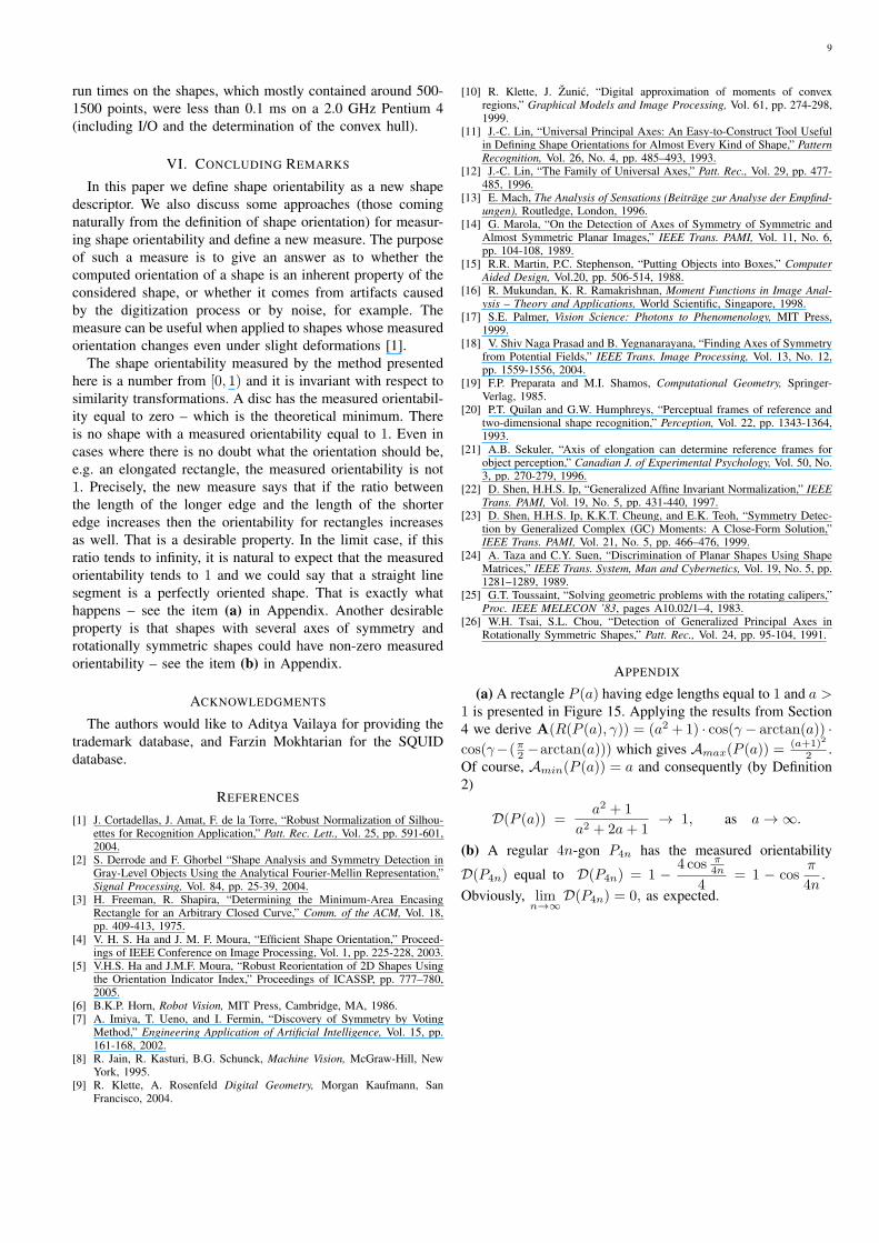
We did not discuss the effects of digitizations on the

computation of D(S). It is clear that D(S) is well defined

for any compact shape S and consequently, a high enough

picture resolution will provide the required precision in D(S)computation. The effects of quantisation on D(S) are demon-

strated for digital circles in Figure 14. The graph shows that

for small radius values D(S) = 0.5, since the digital circle

is equivalent to a square. As the circle radius increases the

measured D(S) approaches the true value of zero.

It should be noted that the computation overheads of calcu-

lating D are low. For the results shown in this paper the typical

4The SQUID database and an online demo is available from SurreyUniversity at http://www.ee.surrey.ac.uk/Research/VSSP/imagedb/.

1 10 100 1000radius

0.2

0.4

D(S

)

Fig. 14. The graph shows the effect of quantisation on D(S). Some examplesof digitised circles (with radii 2, 4, and 6) centred at the origin are given. Theirmaximum and minimum area rectangles are displayed as well.

9

run times on the shapes, which mostly contained around 500-

1500 points, were less than 0.1 ms on a 2.0 GHz Pentium 4

(including I/O and the determination of the convex hull).

VI. CONCLUDING REMARKS

In this paper we define shape orientability as a new shape

descriptor. We also discuss some approaches (those coming

naturally from the definition of shape orientation) for measur-

ing shape orientability and define a new measure. The purpose

of such a measure is to give an answer as to whether the

computed orientation of a shape is an inherent property of the

considered shape, or whether it comes from artifacts caused

by the digitization process or by noise, for example. The

measure can be useful when applied to shapes whose measured

orientation changes even under slight deformations [1].

The shape orientability measured by the method presented

here is a number from [0, 1) and it is invariant with respect to

similarity transformations. A disc has the measured orientabil-

ity equal to zero – which is the theoretical minimum. There

is no shape with a measured orientability equal to 1. Even in

cases where there is no doubt what the orientation should be,

e.g. an elongated rectangle, the measured orientability is not

1. Precisely, the new measure says that if the ratio between

the length of the longer edge and the length of the shorter

edge increases then the orientability for rectangles increases

as well. That is a desirable property. In the limit case, if this

ratio tends to infinity, it is natural to expect that the measured

orientability tends to 1 and we could say that a straight line

segment is a perfectly oriented shape. That is exactly what

happens – see the item (a) in Appendix. Another desirable

property is that shapes with several axes of symmetry and

rotationally symmetric shapes could have non-zero measured

orientability – see the item (b) in Appendix.

ACKNOWLEDGMENTS

The authors would like to Aditya Vailaya for providing the

trademark database, and Farzin Mokhtarian for the SQUID

database.

REFERENCES

[1] J. Cortadellas, J. Amat, F. de la Torre, “Robust Normalization of Silhou-ettes for Recognition Application,” Patt. Rec. Lett., Vol. 25, pp. 591-601,2004.

[2] S. Derrode and F. Ghorbel “Shape Analysis and Symmetry Detection inGray-Level Objects Using the Analytical Fourier-Mellin Representation,”Signal Processing, Vol. 84, pp. 25-39, 2004.

[3] H. Freeman, R. Shapira, “Determining the Minimum-Area EncasingRectangle for an Arbitrary Closed Curve,” Comm. of the ACM, Vol. 18,pp. 409-413, 1975.

[4] V. H. S. Ha and J. M. F. Moura, “Efficient Shape Orientation,” Proceed-ings of IEEE Conference on Image Processing, Vol. 1, pp. 225-228, 2003.

[5] V.H.S. Ha and J.M.F. Moura, “Robust Reorientation of 2D Shapes Usingthe Orientation Indicator Index,” Proceedings of ICASSP, pp. 777–780,2005.

[6] B.K.P. Horn, Robot Vision, MIT Press, Cambridge, MA, 1986.[7] A. Imiya, T. Ueno, and I. Fermin, “Discovery of Symmetry by Voting

Method,” Engineering Application of Artificial Intelligence, Vol. 15, pp.161-168, 2002.

[8] R. Jain, R. Kasturi, B.G. Schunck, Machine Vision, McGraw-Hill, NewYork, 1995.

[9] R. Klette, A. Rosenfeld Digital Geometry, Morgan Kaufmann, SanFrancisco, 2004.

[10] R. Klette, J. Zunic, “Digital approximation of moments of convexregions,” Graphical Models and Image Processing, Vol. 61, pp. 274-298,1999.

[11] J.-C. Lin, “Universal Principal Axes: An Easy-to-Construct Tool Usefulin Defining Shape Orientations for Almost Every Kind of Shape,” Pattern

Recognition, Vol. 26, No. 4, pp. 485–493, 1993.[12] J.-C. Lin, “The Family of Universal Axes,” Patt. Rec., Vol. 29, pp. 477-

485, 1996.[13] E. Mach, The Analysis of Sensations (Beitrage zur Analyse der Empfind-

ungen), Routledge, London, 1996.[14] G. Marola, “On the Detection of Axes of Symmetry of Symmetric and

Almost Symmetric Planar Images,” IEEE Trans. PAMI, Vol. 11, No. 6,pp. 104-108, 1989.

[15] R.R. Martin, P.C. Stephenson, “Putting Objects into Boxes,” Computer

Aided Design, Vol.20, pp. 506-514, 1988.[16] R. Mukundan, K. R. Ramakrishnan, Moment Functions in Image Anal-

ysis – Theory and Applications, World Scientific, Singapore, 1998.[17] S.E. Palmer, Vision Science: Photons to Phenomenology, MIT Press,

1999.[18] V. Shiv Naga Prasad and B. Yegnanarayana, “Finding Axes of Symmetry

from Potential Fields,” IEEE Trans. Image Processing, Vol. 13, No. 12,pp. 1559-1556, 2004.

[19] F.P. Preparata and M.I. Shamos, Computational Geometry, Springer-Verlag, 1985.

[20] P.T. Quilan and G.W. Humphreys, “Perceptual frames of reference andtwo-dimensional shape recognition,” Perception, Vol. 22, pp. 1343-1364,1993.

[21] A.B. Sekuler, “Axis of elongation can determine reference frames forobject perception,” Canadian J. of Experimental Psychology, Vol. 50, No.3, pp. 270-279, 1996.

[22] D. Shen, H.H.S. Ip, “Generalized Affine Invariant Normalization,” IEEE

Trans. PAMI, Vol. 19, No. 5, pp. 431-440, 1997.[23] D. Shen, H.H.S. Ip, K.K.T. Cheung, and E.K. Teoh, “Symmetry Detec-

tion by Generalized Complex (GC) Moments: A Close-Form Solution,”IEEE Trans. PAMI, Vol. 21, No. 5, pp. 466–476, 1999.

[24] A. Taza and C.Y. Suen, “Discrimination of Planar Shapes Using ShapeMatrices,” IEEE Trans. System, Man and Cybernetics, Vol. 19, No. 5, pp.1281–1289, 1989.

[25] G.T. Toussaint, “Solving geometric problems with the rotating calipers,”Proc. IEEE MELECON ’83, pages A10.02/1–4, 1983.

[26] W.H. Tsai, S.L. Chou, “Detection of Generalized Principal Axes inRotationally Symmetric Shapes,” Patt. Rec., Vol. 24, pp. 95-104, 1991.

APPENDIX

(a) A rectangle P (a) having edge lengths equal to 1 and a >1 is presented in Figure 15. Applying the results from Section

4 we derive A(R(P (a), γ)) = (a2 +1) · cos(γ − arctan(a)) ·cos(γ−(π2 −arctan(a))) which gives Amax(P (a)) = (a+1)2

2 .

Of course, Amin(P (a)) = a and consequently (by Definition

2)

D(P (a)) =a2 + 1

a2 + 2a+ 1→ 1, as a → ∞.

(b) A regular 4n-gon P4n has the measured orientability

D(P4n) equal to D(P4n) = 1 − 4 cos π4n

4= 1 − cos

π

4n.

Obviously, limn→∞

D(P4n) = 0, as expected.

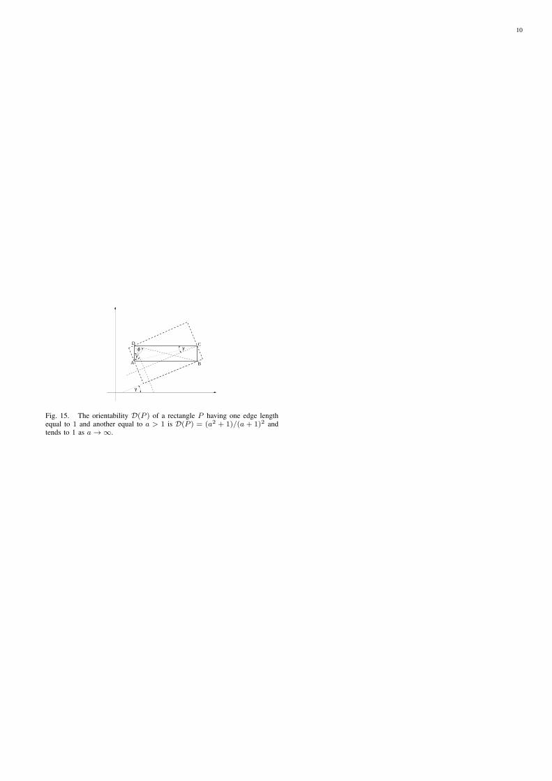
10

γ

γϕ

γ

A B

CD

Fig. 15. The orientability D(P ) of a rectangle P having one edge lengthequal to 1 and another equal to a > 1 is D(P ) = (a2 + 1)/(a + 1)2 andtends to 1 as a → ∞.