Physica D 237 (2008) 2599–2615www.elsevier.com/locate/physd

Computation of derivatives of the rotation number for parametric families ofcircle diffeomorphisms

Alejandro Luque, Jordi Villanueva∗

Departament de Matematica Aplicada I, Universitat Politecnica de Catalunya, Diagonal 647, 08028 Barcelona, Spain

Received 25 July 2007; received in revised form 22 February 2008; accepted 28 March 2008Available online 4 April 2008

Communicated by J. Stark

Abstract

In this paper we present a numerical method to compute derivatives of the rotation number for parametric families of circle diffeomorphismswith high accuracy. Our methodology is an extension of a recently developed approach to compute rotation numbers based on suitable averagesof iterates of the map and Richardson extrapolation. We focus on analytic circle diffeomorphisms, but the method also works if the maps aredifferentiable enough. In order to justify the method, we also require the family of maps to be differentiable with respect to the parameters and therotation number to be Diophantine. In particular, the method turns out to be very efficient for computing Taylor expansions of Arnold Tongues offamilies of circle maps. Finally, we adapt these ideas to study invariant curves for parametric families of planar twist maps.c© 2008 Elsevier B.V. All rights reserved.

PACS: 02.30.Mv; 02.60.-x; 02.70.-c

Keywords: Families of circle maps; Derivatives of the rotation number; Numerical approximation

1. Introduction

The rotation number, introduced by Poincare, is an importanttopological invariant in the study of the dynamics of circlemaps and, by extension, invariant curves for maps or twodimensional invariant tori for vector fields. For this reason,several numerical methods for approximating rotation numbershave been developed during the last years. We refer tothe works [3,4,8,13,14,21,24,31] as examples of methods ofdifferent nature and complexity. This last ranges from puredefinition of the rotation number to sophisticated and involvedmethods like frequency analysis. The efficiency of thesemethods varies depending if the approximated rotation numberis rational or irrational. Moreover, even though some of themcan be very accurate in many cases, they are not adequatefor every kind of application, for example due to violation oftheir assumptions or due to practical reasons, like the requiredamount of memory.

∗ Corresponding author. Tel.: +34 934015887; fax: +34 934011713.E-mail addresses: alejandro.luque@upc.edu (A. Luque),

jordi.villanueva@upc.es (J. Villanueva).

0167-2789/$ - see front matter c© 2008 Elsevier B.V. All rights reserved.doi:10.1016/j.physd.2008.03.047

Recently, a new method for computing Diophantine rotationnumbers of circle diffeomorphisms with high precision atlow computational cost has been introduced in [27]. Thismethod is built assuming that the circle map is conjugate toa rigid rotation in a sufficiently smooth way and, basically,it consists in averaging the iterates of the map together withRichardson extrapolation. This construction takes advantage ofthe geometry and dynamics of the problem, so it turns out to bevery efficient in multiple applications. The method is speciallysuited if we are able to compute iterates of the map with a highprecision, for example if we can work with computer arithmetichaving a large number of decimal digits.

The goal of this paper is to extend the method of [27] inorder to compute derivatives of the rotation number with respectto parameters in families of circle diffeomorphisms. We followthe same averaging-extrapolation process applied to derivativesof iterates of the map. To this end, we require the family tobe differentiable with respect to parameters. Hence, we areable to obtain accurate variational information at the same timethat we approximate the rotation number. Consequently, themethod allows us to study parametric families of circle maps

2600 A. Luque, J. Villanueva / Physica D 237 (2008) 2599–2615

from a point of view that is not given by any of the previouslymentioned methods.

From a practical point of view, circle diffeomorphismsappear in the study of quasi-periodic invariant curves for maps.In particular, for planar twist maps, any such a curve inducesa circle diffeomorphism in a direct way just by projectingthe iterates on the angular variable. Then, using approximatederivatives of the rotation number, we can continue theseinvariant curves numerically with respect to parameters bymeans of the Newton method. The methodology presented isan alternative to more common approaches based on solvingthe invariance equation numerically, interpolation of the map orapproximation by periodic orbits (see for example [5,7,12,28]).Furthermore, using the variational information obtained, we areable to compute asymptotic expansions relating parameters andinitial conditions that correspond to curves of fixed rotationnumber.

Finally, we point out that the method can be formallyextended to deal with maps on the torus with a Diophantinerotation vector. However, in order to apply the method to thestudy of quasi-periodic tori for symplectic maps in higherdimensions, there is not an analogue of the twist conditionto guarantee a well defined projection of iterates on thestandard torus. Then, our interest is immediately focusedon a generalization of the method in the case of non-twistmaps with folded invariant curves (for example, so-calledmeanderings [29]). These and other extensions will be objectof future research [22].

Contents of the paper are organized as follows. In Section 2we recall some fundamental facts about circle maps and webriefly review the method of [27]. In Section 3 we describethe method for the computation of derivatives of the rotationnumber. The rest of the paper is devoted to illustrate the methodthrough several applications. Concretely, in Section 4 we studythe Arnold family of circle maps. Finally, in Section 5 wefocus on the computation and continuation of invariant curvesfor planar twist maps and, in particular, we present somecomputations for the conservative Henon map.

2. Notation and previous results

All the results presented in this section can be found in thebibliography, but we include them for self-consistency of thetext. Concretely, in Section 2.1 we recall the basic definitions,notations and properties of circle maps that we need in the paper(we refer to [9,18] for more details and proofs). On the otherhand, in Section 2.2 we review briefly the method of [27] forcomputing rotation numbers of circle diffeomorphisms.

2.1. Circle diffeomorphisms

Let T = R/Z be the real circle which inherits both a groupstructure and a topology by means of the natural projectionπ : R → T (also called the universal cover of T). We denoteby Diffr

+(T), r ∈ [0, +∞) ∪ {∞, ω}, the group of orientation-preserving homeomorphisms of T of class Cr . Concretely, ifr = 0 it is the group of homeomorphisms of T; if r ≥ 1, r ∈

(0, ∞) \ N, it is the group of Cbrc-diffeomorphisms whose brc-th derivative verifies a Holder condition with exponent r − brc;if r = ω it is the group of real analytic diffeomorphisms.

Given f ∈ Diffr+(T), we can lift f to R by π obtaining a Cr

map f that makes the following diagram commute

π ◦ f = f ◦ π.

Moreover, we have f (x + 1) − f (x) = 1 (since f isorientation-preserving) and the lift is unique if we ask forf (0) ∈ [0, 1). Accordingly, from now on we choose the liftwith this normalization so we can omit the tilde without anyambiguity.

Definition 2.1. Let f be the lift of an orientation-preservinghomeomorphism of the circle such that f (0) ∈ [0, 1). Then therotation number of f is defined as the limit

ρ( f ) := lim|n|→∞

f n(x0) − x0

n,

that exists for all x0 ∈ R, is independent of x0 and satisfiesρ( f ) ∈ [0, 1).

Let us remark that the rotation number is invariant underorientation-preserving conjugation, i.e., for every f, h ∈

Diff0+(T) we have that ρ(h−1

◦ f ◦ h) = ρ( f ). Furthermore,given f ∈ Diff2

+(T) with ρ( f ) ∈ R \ Q, Denjoy’s theoremensures that f is topologically conjugate to the rigid rotationRρ( f ), where Rθ (x) = x +θ . That is, there exists η ∈ Diff0

+(T)

making the following diagram commute

f ◦ η = η ◦ Rρ( f ). (1)

In addition, if we require η(0) = x0, for fixed x0, then theconjugacy η is unique.

All the ideas and algorithms described in this paper makeuse of the existence of such conjugation and its regularity. Letus remark that, although smooth or even finite differentiabilityis enough, in this paper we are concerned with the analytic case.Moreover, it is well known that regularity of the conjugationdepends also on the rational approximation properties of ρ( f ),so we will focus on Diophantine numbers.

Definition 2.2. Given θ ∈ R, we say that θ is a Diophantinenumber of (C, τ ) type if there exist constants C > 0 and τ ≥ 1such that∣∣∣1 − e2π ikθ

∣∣∣−1≤ C |k|

τ , ∀k ∈ Z∗.

We will denote by D(C, τ ) the set of such numbers and by Dthe set of Diophantine numbers of any type.

A. Luque, J. Villanueva / Physica D 237 (2008) 2599–2615 2601

Although Diophantine sets are Cantorian (i.e., compact,perfect and nowhere dense) a remarkable property is that R \Dhas zero Lebesgue measure. For this reason, this condition fitsvery well in practical issues and we do not resort to otherweak conditions on small divisors such as the Brjuno condition(see [33]).

The first result on the regularity of conjugacy (1) isdue to Arnold [2] but we also refer to [16,19,30,33] forlater contributions. In particular, theoretical support of themethodology is provided by the following result:

Theorem 2.3 (Katznelson and Ornstein [19]). If f ∈

Diffr+(T) has Diophantine rotation number ρ( f ) ∈ D(C, τ )

for τ + 1 < r , then f is conjugated to Rρ( f ) by means ofa conjugacy η ∈ Diffr−τ−ε

+ (T), for any ε > 0. Note thatDiffω+(T) = Diffω−τ−ε

+ (T) while the domain of analyticity isreduced.

2.2. Computing rotation numbers by averaging and extrapola-tion

We review here the method developed in [27] forcomputing Diophantine rotation numbers of analytic circlediffeomorphisms (the Cr case is similar). This method is highlyaccurate with low computational cost and it turns out to be veryefficient when combined with multiple precision arithmeticroutines. The reader is referred there for a detailed discussionand several applications.

Let us consider f ∈ Diffω+(T) with rotation numberθ = ρ( f ) ∈ D. Notice that we can write the conjugacy ofTheorem 2.3 as η(x) = x + ξ(x), ξ being a 1-periodic functionnormalized in such a way that ξ(0) = x0, for a fixed x0 ∈ [0, 1).Now, by using the fact that η conjugates f to a rigid rotation, wecan write the following expression for the iterates under the lift:

f n(x0) = f n(η(0)) = η(nθ) = nθ +

∑k∈Z

ξke2π iknθ , (2)

∀n ∈ Z, where the sequence {ξk}k∈Z denotes the Fourier coef-ficients of ξ . Then, the above expression gives us the followingformula

f n(x0) − x0

n= θ +

1n

∑k∈Z∗

ξk(e2π iknθ− 1),

to compute θ modulo terms of order O(1/n). Unfortunately,this order of convergence is very slow for practical purposes,since it requires a huge number of iterates if we want to com-pute θ with high precision. Nevertheless, by averaging the iter-ates f n(x0) in a suitable way, we can manage to decrease theorder of this quasi-periodic term.

As a motivation, let us start by considering the sum of thefirst N iterates under f , that has the following expression (weuse (2) to write the iterates)

S1N ( f ) :=

N∑n=1

( f n(x0) − x0) =N (N + 1)

2θ − N

∑k∈Z∗

ξk

+

∑k∈Z∗

ξke2π ikθ (1 − e2π ik Nθ )

1 − e2π ikθ,

and we observe that the new factor multiplying θ growsquadratically with the number of iterates, while it appears alinear term in N with constant A1 = −

∑k∈Z∗

ξk . Moreover,the quasi-periodic sum remains uniformly bounded since θ isDiophantine and η is analytic (use Lemma 2.4 with p = 1).Thus, we obtain

2N (N + 1)

S1N ( f ) = θ +

2N + 1

A1 +O(1/N 2), (3)

that allows us to extrapolate the value of θ with an errorO(1/N 2) if, for example, we compute SN ( f ) and S2N ( f ).

In general, we introduce the following recursive sums forp ∈ N

S0N ( f ) := f N (x0) − x0, S p

N ( f ) :=

N∑j=1

S p−1j ( f ). (4)

Then, the result presented in [27] says that under the abovehypotheses, the following averaged sums of order p

S pN ( f ) :=

(N + p

p + 1

)−1

S pN ( f ) (5)

satisfy the expression

S pN ( f ) = θ +

p∑l=1

Apl

(N + p − l + 1) · · · (N + p)+ E p(N ), (6)

where the coefficients Apl depend on f and p but are

independent of N . Furthermore, we have the followingexpressions for them

Apl = (−1)l(p − l + 2) · · · (p + 1)

∑k∈Z∗

ξke2π ik(l−1)θ

(1 − e2π ikθ )l−1 ,

E p(N ) = (−1)p+1 (p + 1)!

N · · · (N + p)

×

∑k∈Z∗

ξke2π ikpθ (1 − e2π ik Nθ )

(1 − e2π ikθ )p.

Finally, the remainder E p(N ) is uniformly bounded by anexpression of order O(1/N p+1). This follows immediatelyfrom the next standard lemma on small divisors.

Lemma 2.4. Let ξ ∈ Diffω+(T) be a circle map that can beextended analytically to a complex strip B∆ = {z ∈ C :

|Im(z)| < ∆}, with |ξ(z)| ≤ M up to the boundary of the strip.If we denote {ξk}k∈Z the Fourier coefficients of ξ and considerθ ∈ D(C, τ ), then for any fixed p ∈ N we have∣∣∣∣∣∑k∈Z∗

ξke2π ikpθ (1 − e2π ik Nθ )

(1 − e2π ikθ )p

∣∣∣∣∣ ≤e−π∆

1 − e−π∆4MC p

( τp

π∆e

)τp.

To conclude this survey, we describe implementation of themethod and discuss the expected behavior of the extrapolationerror. In order to make Richardson extrapolation we assume, forsimplicity, that the total number of iterates is a power of two.Concretely, we select an averaging order p ∈ N, a maximumnumber of iterates N = 2q , for some q ≥ p, and compute the

2602 A. Luque, J. Villanueva / Physica D 237 (2008) 2599–2615

averaged sums {S pN j

( f )} j=0,...,p with N j = 2q−p+ j . Then, wecan use formula (6) to obtain θ by neglecting the remaindersE p(N j ) and solving the resulting linear set of equations for theunknowns θ, Ap

1 , . . . , App.

However, let us point out that, due to the denominators(N j + p − l + 1) · · · (N j + p), the matrix of this linear systemdepends on q , and this is inconvenient if we want to repeat thecomputations using a different number of iterates. Nevertheless,we note that expression (6) can be written alternatively as

S pN ( f ) = θ +

p∑l=1

Apl

N l + E p(N ), (7)

for certain { Apl }l=1,...,p, also independent of N , and with

a new remainder E p(N ) that differs from E p(N ) only byterms of order O(1/N p+1). Then, by neglecting the remainderE p(N ) in Eq. (7), we can obtain θ by solving a new (p +

1)-dimensional system of equations, independent of q, forthe unknowns θ, Ap

1 /21(q−p), . . . , App/2p(q−p). Therefore, the

rotation number can be computed as follows

θ = Θq,p( f ) +O(2−(p+1)q), (8)

where Θq,p is an extrapolation operator, that is given by

Θq,p( f ) :=

p∑j=0

cpj S p

2q−p+ j ( f ), (9)

and the coefficients {cpj } j=0,...,p are

cpl = (−1)p−l 2l(l+1)/2

δ(l)δ(p − l), (10)

where we define δ(n) := (2n− 1)(2n−1

− 1) · · · (21− 1) for

n ≥ 1 and δ(0) := 1.

Remark 2.5. Note that the dimension of this linear systemand the asymptotic behavior of the error only depend on theaveraging order p. For this reason, in [27] p is called theextrapolation order. However, this is not always the case whencomputing derivatives of the rotation number. As we discussin Section 3, the extrapolation order is in general less than theaveraging order.

As far as the behavior of the error is concerned, using (8) wehave that

|θ − Θq,p( f )| ≤ c/2q(p+1),

for certain constant c, independent of q , that we estimateheuristically as follows. Let us compute Θq−1,p( f ) andΘq,p( f ). Since Θq,p( f ) is a better approximation of θ , it turnsout that

c ∼ 2(q−1)(p+1)|Θq,p( f ) − Θq−1,p( f )|.

Then, we obtain the expression

|θ − Θq,p( f )| ≤ν

2p+1 |Θq,p( f ) − Θq−1,p( f )|, (11)

where ν is a “safety parameter” whose role is to preventoscillations in the error as a function of q due to the quasi-periodic part. In every numerical computation we take ν = 10.For more details on the behavior of the error we refer to [27].

Now, we comment on two sources of error to take intoaccount in the implementation of the method:

• The sums S pN j

( f ) are evaluated using the lift rather than the

map itself. Of course, this makes the sums S pN j

( f ) increase

(actually they are of order O(N p+1)) and is recommendedto store their integer and decimal parts separately in order tokeep the desired precision.

• If the required number of iterates increases, we have tobe aware of round-off errors in evaluation of the iterates.For this reason, when implementing the above schemein a computer, we use multiple-precision arithmetics. Thecomputations presented in this paper have been performedusing a C++ compiler and multiple arithmetic has beenprovided by the routines double–double and quad-doublepackage of [17], which include a double–double data typeof approximately 32 decimal digits and a quadruple-doubledata type of approximately 64 digits.

Along this section we have required the rotation numberto be Diophantine. Of course, if θ ∈ Q Eq. (6) is not validsince, in general, the dynamic of f are not conjugate to a rigidrotation. Anyway, we can compute the sums S p

N ( f ) and it turnsout that the method works as well as for Diophantine numbers.We can justify this behavior from the known fact that, for anycircle homeomorphism of rational rotation number, every orbitis either periodic or its iterates converge to a periodic orbit(see [9,18]). Then the iterates of the map tend toward periodicpoints, and for such points, one can see that the averaged sumsS p

N ( f ) also satisfy an expression like (7) with an error of thesame order, and this is all we need to perform the extrapolation.In fact, the worst situation appears when computing irrationalrotation numbers that are “close” to rational ones (see also thediscussion in Section 4.1).

3. Derivatives of the rotation number with respect toparameters

Now we adapt the method already described in Section 2in order to compute derivatives of the rotation number withrespect to parameters (assuming that they exist). For the sakeof simplicity, we introduce the method for one-parameterfamilies of circle diffeomorphisms, albeit the construction canbe adapted to deal with multiple parameters (we discuss thissituation in Remark 3.3). Thus, consider µ ∈ I ⊂ R 7→ fµ ∈

Diffω+(T) depending on µ in a regular way. Rotation numbersof the family { fµ}µ∈I induce a function θ : I → [0, 1) givenby θ(µ) = ρ( fµ). Then our goal is to numerically approximatethe derivatives of θ at a given point µ0.

Let us remark that the function θ is only continuous in C0-topology and, actually, the rotation number depends on µ ina very non-smooth way: generically, there exists a family ofdisjoint open intervals of I , with dense union, such that θ

A. Luque, J. Villanueva / Physica D 237 (2008) 2599–2615 2603

takes constant rational values on these intervals (a so-calledDevil’s Staircase). However, θ ′(µ) is defined for any µ suchthat θ(µ) 6∈ Q (see [15]).

Higher order derivatives are defined in “many” points inthe sense of Whitney. Concretely, let J ⊂ I be the subsetof parameters such that θ(µ) ∈ D (typically a Cantor set).Then, from Theorem 2.3, there exists a family of conjugaciesµ ∈ J 7→ ηµ ∈ Diffω+(T), satisfying fµ ◦ ηµ = ηµ ◦ Rθ(µ),that is unique if we fix ηµ(0) = x0. Then, if fµ is Cd with

respect to µ, the Whitney derivatives D jµηµ and D j

µθ , forj = 1, . . . , d , can be computed by taking formal derivativeswith respect to µ on the conjugacy equation and solving smalldivisor equations thus obtained. Actually, we know that if wedefine J (C, τ ) as the subset of J such that θ(µ) ∈ D(C, τ ), forcertain C > 0 and τ ≥ 1, then the maps µ ∈ J (C, τ ) 7→ ηµ

and µ ∈ J (C, τ ) 7→ θ can be extended to Cs functions onI , where s depends on d and τ , provided that d is big enough(see [32]).

As it is shown in Section 3.1, when we extend the method forcomputing the d-th derivative of θ , in general, we are forced toselect an averaging order p > d and the remainder turns out tobe of orderO(1/N p−d+1). Nevertheless, if the rotation numberis known to be constant as a function of the parameters, we canavoid previous limitations. Concretely, in this case we can selectany averaging order p, independent of d , since the remainder isnow of order O(1/N p+1). Of course, if the rotation number isconstant, then the derivatives of θ are all zero and the fact thatwe can obtain them with better precision seems to be irrelevant.However, from the computation of these vanishing derivatives,we can derive information about other involved objects. Thisis the case of many applications in which this methodologyturns out to be very useful (two examples are worked out inSections 4.3 and 5.3).

3.1. Computation of the first derivative

We start by explaining how to compute the first derivative ofθ . For notational convenience, from now on we fix µ0 such thatθ(µ0) ∈ D and we omit the dependence on µ as a subscriptin families of circle maps. In addition, let us recall that wecan write any conjugation as η(x) = x + ξ(x) and denote by{ξk}k∈Z the Fourier coefficients of ξ . Finally, we denote the firstderivatives as θ ′

= Dµθ and ξ ′

k = Dµξk .As we did in Section 2.2, we begin by computing the first

averages (of the derivatives of the iterates) in order to illustratethe idea of the method. Thus, we proceed by formally takingderivatives with respect to µ at both sides of Eq. (2)

Dµ f n(x0) = nθ ′+

∑k∈Z

ξ ′

ke2π iknθ+ 2π inθ ′

∑k∈Z

kξke2π iknθ .

Then, notice that a factor n appears, multiplying the secondquasi-periodic sum. However, if we perform recursive sums,we can still manage to control the growth of this term due tothe quasi-periodic part. Let us compute the sum

DµS1N ( f ) :=

N∑n=1

Dµ( f n(x0) − x0)

=N (N + 1)

2θ ′

− N∑k∈Z∗

ξ ′

k

+

∑k∈Z∗

ξ ′

ke2π ikθ (1 − e2π ik Nθ )

1 − e2π ikθ

+ 2π iθ ′∑k∈Z∗

kξk

×Ne2π ik(N+2)θ

− (N + 1)e2π ik(N+1)θ+ e2π ikθ

(1 − e2π ikθ )2 .

Hence, we observe that the method is still valid, even thoughfor θ ′

6= 0 the quasi-periodic sum is bigger than expected apriori. Indeed, we obtain the following formula

2N (N + 1)

DµS1N ( f ) = θ ′

+O(1/N ), (12)

that is similar to Eq. (3), but notice that the term 2A1/(N + 1)

has been included in the remainder since there are oscillatoryterms of the same order. Proceeding as in Section 2.2, weintroduce recursive sums for derivatives of the iterates

DµS pN ( f ) := Dµ( f N (x0) − x0),

DµS pN ( f ) :=

N∑j=1

DµS p−1j ( f ),

and their corresponding averaged sums of order p

Dµ S pN ( f ) :=

(N + p

p + 1

)−1

DµS pN ( f ).

Finding an expression like (12) for p > 1 is quitecumbersome to do directly, since the computations are veryinvolved. However, the computation is straightforward if wetake formal derivatives at both sides of Eq. (6). The resultingexpression reads as

Dµ S pN ( f ) = θ ′

+

p∑l=1

Dµ Apl

(N + p − l + 1) · · · (N + p)

+ DµE p(N ),

where the new coefficients are Dµ Apl = (−1)l(p − l +

2) · · · (p + 1)Dµ Al with

Dµ Al =

∑k∈Z∗

e2π ik(l−1)θ

(1 − e2π ikθ )l−1

(ξ ′

k +2π ik(l − 1)ξkθ

′

1 − e2π ikθ

),

and the new remainder is

DµE p(N ) = (−1)p+1 (p + 1)!

N · · · (N + p)

∑k∈Z∗

e2π ikpθ

(1 − e2π ikθ )p

×

{ξ ′

k(1 − e2π ik Nθ ) + 2π ikξkθ′

×

(p

1 − e2π ik Nθ

1 − e2π ikθ− Ne2π ikpNθ

)}.

2604 A. Luque, J. Villanueva / Physica D 237 (2008) 2599–2615

Assuming that θ(µ0) ∈ D and θ ′(µ0) 6= 0, we can obtainbounds analogous to those of Lemma 2.4 and conclude thatthe remainder satisfies DµE p(N ) = O(1/N p). Moreover, weobserve that the coefficient Dµ Ap

p corresponds to a term of thesame order, so we have to redefine the remainder in order toinclude this term. Hence, as we did in Eq. (7), we can arrangethe unknown terms and obtain

Dµ S pN ( f ) = θ ′

+

p−1∑l=1

Dµ Apl

N l +O(1/N p),

where {Dµ Apl }l=1,...,p−1 are derivatives of { Ap

l }l=1,...,p−1 thatappear in Eq. (7).

Finally, we can extrapolate an approximation to θ ′ usingRichardson’s method of order p − 1 as in Section 2.2.Concretely, if we compute N = 2q iterates, we can approximatethe derivative of the rotation number by means of the followingformula

θ ′=

p−1∑j=0

cp−1j Dµ S p

2q−p+1+ j ( f ) +O(2−pq), (13)

where the coefficients {cp−1j } j=0,...,p−1 are given by (10).

3.2. Computation of higher order derivatives

The goal of this section is to generalize formula (13) toapproximate Dd

µθ for any d , when they exist. Then, we assumethat the family µ 7→ f ∈ Diffω+(T) depends Cd -smoothly withrespect to the parameter. As usual, we define the recursive sumsfor the d-derivative and their averages of order p as

DdµS0

N ( f ) := Ddµ( f n(x0) − x0),

DdµS p

N ( f ) :=

N∑j=0

DdµS p−1

j ( f ),

and

Ddµ S p

N ( f ) :=

(N + p

p + 1

)−1

DdµS p

N ( f ),

respectively. As before, we relate these sums to Ddµθ by taking

formal derivatives in Eq. (6), thus obtaining

Ddµ S p

N ( f ) = Ddµθ +

p∑l=1

Ddµ Ap

l

(N + p − l + 1) · · · (N + p)

+ DdµE p(N ). (14)

It is immediate to check that, if θ(µ0) ∈ D and Ddµθ(µ0) 6=

0, the remainder DdµE p(N ) is of order O(1/N p−d+1), so this

expression makes sense if the averaging order satisfies p > d.

Remark 3.1. Notice that in order to work with reasonablecomputational time and round-off errors, p cannot be takenarbitrarily large. Consequently, there is a (practical) limitationin the computation of high order derivatives.

In addition, as it was done for the first derivative, theremainder Dd

µE p(N ) must be redefined in order to include theterms corresponding to l ≥ p − d + 1 in Eq. (14). Then we canextrapolate Dd

µθ by computing N = 2q iterates and solvingthe linear (p − d + 1)-dimensional system associated to thefollowing rearranged equation

Ddµ S p

N ( f ) = Ddµθ +

p−d∑l=1

Ddµ Ap

l

N l +O(1/N p−d+1). (15)

Since the averaging order p and the extrapolation order p−ddo not coincide, let us define the extrapolation operator of orderm for the d-derivative as

Θdq,p,m( f ) :=

m∑j=0

cmj Dd

µ S p2q−m+ j ( f ), (16)

where coefficients {cmj } j=0,...,m are given by (10). Therefore,

according to the formula (15), we can approximate the d-thderivative of the rotation number as

Ddµθ = Θd

q,p,p−d( f ) +O(2−(p−d+1)q).

Furthermore, as explained in Section 2.2, by comparing theapproximations that correspond to 2q−1 and 2q iterates, weobtain the following heuristic formula for the extrapolationerror:

|Ddµθ − Θd

q,p,p−d( f )| ≤ν

2p−d+1 |Θdq,p,p−d( f )

−Θdq−1,p,p−d( f )|, (17)

where, once again, ν is a “safety parameter” that we take asν = 10.

Remark 3.2. Up to this point we have assumed that Ddµθ 6= 0

at the computed point. However, if we know a priori thatDr

µθ = 0 for r = 1, . . . , d, then Eq. (14) holds with thefollowing expression for the remainder:

DdµE p(N ) = (−1)p+1 (p + 1)!

N · · · (N + p)

×

∑k∈Z∗

Ddµξk

e2π ikpθ (1 − e2π ik Nθ )

(1 − e2π ikθ )p,

which now is of order O(1/N p+1). As in Section 2, this allowsus to approximate Dd

µθ with the same extrapolation order as theaveraging order p. Indeed, we obtain

0 = Ddµθ = Θd

q,p,p( f ) +O(2−(p+1)q),

and we observe that the order d is not limited by p.

The case remarked above is very interesting since we knowthat many applications can be modeled as a family of circlediffeomorphisms of fixed rotation number. The possibilities ofthis approach are illustrated by computing the Taylor expansionof Arnold Tongues (Section 4.3) and the continuation ofinvariant curves for the Henon map (Section 5.3).

A. Luque, J. Villanueva / Physica D 237 (2008) 2599–2615 2605

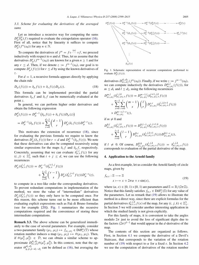
3.3. Scheme for evaluating the derivatives of the averagedsums

Let us introduce a recursive way for computing the sumsDd

µ S pN ( f ) required to evaluate the extrapolation operator (16).

First of all, notice that by linearity it suffices to computeDd

µ( f n(x0)) for any n ∈ N.

To compute the derivatives of f n= f ◦

(n)· · · ◦ f , we proceed

inductively with respect to n and d . Thus, let us assume that thederivatives Dr

µ( f n−1(x0)) are known for a given n ≥ 1 and forany r ≤ d . Then, if we denote z := f n−1(x0), our goal is tocompute Dr

µ( f (z)) for r ≤ d by using the known derivatives ofz.

For d = 1, a recursive formula appears directly by applyingthe chain rule

Dµ( f (z)) = ∂µ f (z) + ∂x f (z)Dµ(z). (18)

This formula can be implemented provided the partialderivatives ∂µ f and ∂x f can be numerically evaluated at thepoint z.

In general, we can perform higher order derivatives andobtain the following expression

Ddµ( f (z)) = Dd−1

µ

(∂µ f (z) + ∂x f (z)Dµ(z)

)= Dd−1

µ (∂µ f (z)) +

d−1∑r=0

(d − 1

r

)Dr

µ(∂x f (z))Dd−rµ (z).

This motivates the extension of recurrence (18), sincefor evaluating the previous formula we require to know thederivatives Dr

µ(∂x f (z)) for r < d and Dd−1µ (∂µ f (z)). We note

that these derivatives can also be computed recursively usingsimilar expressions for the maps ∂x f and ∂µ f , respectively.

Concretely, assuming that we can evaluate ∂i, jµ,x f (z) for any

(i, j) ∈ Z2+ such that i + j ≤ d , we can use the following

recurrences

Drµ(∂

i, jµ,x f (z)) = Dr−1

µ (∂i+1, jµ,x f (z))

+

r−1∑s=0

(r − 1

s

)Ds

µ(∂i, j+1µ,x f (z))Dr−s

µ (z),

to compute in a tree-like order the corresponding derivatives.To prevent redundant computations in implementation of themethod, we store the value of “intermediate” derivativesDr

µ(∂i, jµ,x f (z)) so they only have to be computed once. For

this reason, this scheme turns out to be more efficient thanevaluating explicit expressions such as Faa di Bruno formulas(see for example [20]). Fig. 1 summarizes the recursivecomputations required and the convenience of storing theseintermediate computations.

Remark 3.3. The above scheme can be generalized immedi-ately to the case of several parameters. For example, considera two-parameter family (µ1, µ2) 7→ fµ1,µ2 ∈ Diffω+(T) whoserotation number induces a map (µ1, µ2) 7→ θ(µ1, µ2). Then,if θ(µ0

1, µ02) ∈ D, we can obtain a similar scheme to ap-

proximate Dd1,d2µ1,µ2θ(µ0

1, µ02). In this context, note that the op-

erator Θd1,d2q,p,p−d1−d2

can be defined as (16), but averaging the

Fig. 1. Schematic representation of recurrent computations performed toevaluate Dd

µ( f (z)).

derivatives Dd1,d2µ1,µ2( f n(x0)). Finally, if we write z := f n−1(x0),

we can compute inductively the derivatives Dm,lµ1,µ2

( f (z)), form ≤ d1 and l ≤ d2, using the following recurrences

Dm,lµ1,µ2

(∂i, j,kµ1,µ2,x f (z)) = Dm−1,l

µ1,µ2(∂

i+1, j,kµ1,µ2,x f (z))

+

m−1∑s=0

l∑r=0

(m − 1

s

)(l

r

)Ds,r

µ1,µ2(∂

i, j,k+1µ1,µ2,x f (z))

× Dm−s,l−rµ1,µ2

(z),

if m 6= 0 and

D0,lµ1,µ2

(∂i, j,kµ1,µ2,x f (z)) = D0,l−1

µ1,µ2(∂

i, j+1,kµ1,µ2,x f (z))

+

l−1∑r=0

(l − 1

r

)D0,r

µ1,µ2(∂

i, j,k+1µ1,µ2,x f (z))D0,l−r

µ1,µ2(z),

if l 6= 0. Of course, D0,0µ1,µ2

(∂i, j,kµ1,µ2,x f (z)) = ∂

i, j,kµ1,µ2,x f (z)

corresponds to evaluation of the partial derivative of the map.

4. Application to the Arnold family

As a first example, let us consider the Arnold family of circlemaps, given by

fα,ε : S −→ Sx 7−→ x + 2πα + ε sin(x),

(19)

where (α, ε) ∈ [0, 1)×[0, 1) are parameters and S = R/(2πZ).Notice that this family satisfies fα,ε ∈ Diffω+(S) for any value ofthe parameters. Let us remark that (19) allows to illustrate themethod in a direct way, since there are explicit formulas for thepartial derivatives ∂

i, j,kα,ε,x f (x) of the map, for any (i, j, k) ∈ Z3

+.In Section 5 we will consider another interesting application inwhich the studied family is not given explicitly.

For this family of maps, it is convenient to take the anglesmodulo 2π just to avoid the loss of significant digits due tothe factors (2π)d−1 that would appear in the d-derivative of themap.

The contents of this section are organized as follows.First, in Section 4.1 we compute the derivative of a Devil’sStaircase, that corresponds to the variation of the rotationnumber of (19) with respect to α for a fixed ε. In Section 4.2we use the computation of derivatives of the rotation number

2606 A. Luque, J. Villanueva / Physica D 237 (2008) 2599–2615

Fig. 2. Devil’s Staircase α 7→ ρ( fα) (top-left) and its derivative (top-right) for the Arnold family with ε = 0.75. The plots in the bottom correspond to somemagnifications of the top-right one.

to approximate the Arnold Tongues of the family (19) bymeans of the Newton method. Furthermore, we compute theasymptotic expansion of these tongues and obtain pseudo-analytical expressions for the first coefficients, as a function ofthe rotation number.

4.1. Stepping up to a Devil’s staircase

Let us fix the value of ε ∈ [0, 1) and consider the one-parameter family { fα}α∈[0,1) given by Eq. (19), i.e. fα := fα,ε.Let us recall that we can establish an ordering in this familysince the normalized lifts satisfy fα1(x) < fα2(x) for all x ∈ Rif and only if α1 < α2. Then, we conclude that the functionα 7→ ρ( fα) is monotone increasing. In particular, for α1 < α2such that ρ( fα1) ∈ R \ Q we have ρ( fα1) < ρ( fα2). Onthe other hand, if ρ( fα1) ∈ Q, there is an interval containingα1 giving the same rotation number. As the values of α forwhich fα has a rational rotation number are dense in [0, 1) (thecomplement is a Cantor set), there are infinitely many intervalswhere ρ( fα) is locally constant. Therefore, the map α 7→ ρ( fα)

gives rise to a “staircase” with a dense number of stairs, that isusually called a Devil’s Staircase (we refer to [9,18] for moredetails).

To illustrate the behavior of the method we have computedthe above staircase for ε = 0.75. The computations have beenperformed by taking 104 points of α ∈ [0, 1), using 32-digitarithmetics (double–double data type from [17]), and a fixedaveraging order p = 8. In addition, we estimate the error inthe approximation of ρ( fα) and Dαρ( fα) using formulas (11)and (17), respectively. Then, we stop the computations for

a tolerance of 10−26 and 10−24, respectively, using at most222

= 4194304 iterates.Let us discuss the results obtained. First, we point out

that only 11.4% of the selected points have not reached theprevious tolerances for 222 iterates. Moreover, we observe thatthe rotation number for 98.8% of the points has been obtainedwith an error less that 10−20, while the estimated error in thederivatives is less than 10−18 for 97.7% of the points. Let usfocus in α = 0.3377, that is one of the “bad” points. Theestimated errors for the rotation number and the derivativeat this point are of order 10−18 and 10−9, respectively. Weobserve that, even though this rotation number is irrational(the derivative does not vanish), it is very close to the rational105/317, since |317 · Θ22,9( f0.3377) − 105| ' 4.2 × 10−6.

In Fig. 2 we show α 7→ ρ( fα) and its derivative α 7→

Dαρ( fα) for those points that satisfy that the estimated error isless than 10−18 and 10−16, respectively. We recall that rationalvalues of the rotation number correspond to constant intervalsin the top-left plot, and note that by looking at the derivative(top-right plot) we can visualize the density of the stairs betterthan looking at the staircase itself. We remark that both theserational rotation numbers and their vanishing derivatives havebeen computed as well as in the Diophantine case.

Moreover, at the bottom of the same figure, we plot somemagnifications of the derivative to illustrate non-smoothnessof a Devil’s Staircase. Concretely, the plot in the bottom-left corresponds to 105 values of α ∈ [0.2, 0.3] using thesame implementation parameters as before. Once again, if theestimated error is bigger than 10−16 the point is not plotted.Finally, on the right plot we give another magnification for 106

A. Luque, J. Villanueva / Physica D 237 (2008) 2599–2615 2607

Fig. 3. Left: Graph of the derivatives ε 7→ Dαρ(α(ε), ε) and ε 7→ Dερ(α(ε), ε) along Tθ , for θ = (√

5 − 1)/2. The solid curve corresponds to (Dαρ − 1) and thedashed one to (20 · Dερ). Right: error (estimated using (11)) in log10 scale in the computation of these derivatives.

values of α ∈ [0.282, 0.292] that are computed with p = 7,and allowing at most 221

= 2097152 iterates. In this case,points that correspond to the branch in the left (i.e. close toα = 0.2825), are typically computed with an error 10−10.

4.2. Newton method for computing the Arnold Tongues

Since fα,ε ∈ Diffω+(S), we obtain a function (α, ε) 7→

ρ(α, ε) := ρ( fα,ε) given by the rotation number. Then, theArnold Tongues of (19) are defined as the sets Tθ = {(α, ε) :

ρ(α, ε) = θ}, for any θ ∈ [0, 1). It is well known that if θ ∈ Q,then Tθ is a set with interior; otherwise, Tθ is a continuous curvewhich is the graph of a function ε 7→ α(ε), with α(0) = θ . Inaddition, if θ ∈ D, the corresponding tongue is given by ananalytic curve (see [25]).

Using the method described in Section 2.2, some ArnoldTongues Tθ of Diophantine rotation number were approximatedin [27] by means of the secant method. Now, since we cancompute derivatives of the rotation number, we are able torepeat the computations using a Newton method. To do that, wefix θ ∈ D and solve the equation ρ(α, ε)−θ = 0 by continuingthe known solution (θ, 0) with respect to ε. Indeed, we fixa partition {ε j } j=0,...,K of [0, 1), and compute a numericalapproximation α∗

j for every α(ε j ).To this end, assume that we have a good approximation α∗

j−1to α(ε j−1) and let us first compute an initial approximation forα(ε j ). Taking derivatives in the equation ρ(α(ε), ε) − θ = 0we obtain

Dαρ(α(ε), ε)α′(ε) + Dερ(α(ε), ε) = 0. (20)

Thus, we can approximate α′(ε j−1) by computing numericallythe derivatives Dαρ and Dερ at (α∗

j−1, ε j−1). Hence, we obtain

an approximated value α(0)j = α∗

j−1 + α′(ε j−1)(ε j − ε j−1) forα(ε j ). Next, we apply the Newton method

α(n+1)j = α

(n)j −

ρ(α(n)j , ε j ) − θ

Dαρ(α(n)j , ε j )

,

and stop when we converge to a value α∗

j that approximatesα(ε j ).

Computations are performed using 64 digits (quadruple-double data type from [17]) and, in order to compare with the

results obtained in [27], we select the same parameters in theimplementation. In particular, we take a partition ε j = j/Kwith K = 100 of the interval [0, 1), we select an averagingorder p = 9 and allow at most 223

= 8388608 iteratesof the map. The required tolerances are taken as 10−32 forcomputation of the rotation number (we use (11) to estimate theerror) and 10−30 for convergence of the Newton method. Letus remark that computations are done without any prescribedtolerance for computation of derivatives Dαρ and Dερ, eventhough we check, using (17), that the extrapolation is donecorrectly.

Let us discuss the results obtained for θ = (√

5 − 1)/2.As expected, the number of iterates of the Newton method isless than the ones required by the secant method. Concretely,we perform from 2 to 3 corrections as we approach the criticalvalue ε = 1, while using the secant method we need at least 4steps to converge. However, we observe that computation of thederivatives Dαρ and Dερ fails if we take ε = 1, even thoughthe secant method converges after 18 iterations. This is totallyconsistent since we know that fα,1 ∈ Diff0

+(T) but is still ananalytic map, and that the conjugation to a rigid rotation is onlyHolder continuous (see [8,34]).

In Fig. 3(left) we plot the derivatives ε 7→ Dαρ(α(ε), ε)

and ε 7→ Dερ(α(ε), ε) evaluated on the previous tongue. Weobserve that the derivatives have been normalized in order to fittogether in the same plot. On the other hand, in the right plot weshow the estimated error in the computation of these derivatives(obtained from Eq. (17)). In the worst case, ε = 0.99, we obtainerrors of order 10−27 and 10−29 for Dαρ and Dερ, respectively.

4.3. Computation of the Taylor expansion of the ArnoldTongues

As we have mentioned in Section 4.2, if θ ∈ D then theArnold Tongue Tθ of (19) is given by the graph of an analyticfunction α(ε), for ε ∈ [0, 1). Then, we can expand α at theorigin as

α(ε) = θ +α′(0)

1!ε +

α′′(0)

2!ε2

+ · · · +α(d)(0)

d!εd

+O(εd+1), (21)

2608 A. Luque, J. Villanueva / Physica D 237 (2008) 2599–2615

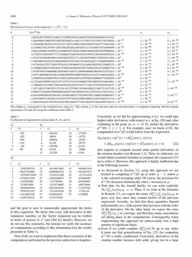
Table 1

Derivatives of 2πα(ε) at the origin for θ = (√

5 − 1)/2

d 2πα(d)(0) e1 e2

0 3.883222077450933154693731259925391915269339787692096599014776434 – –1 5.289596087298835974306750728481413682115174017433159533705768026 × 10−54 2 × 10−50 5 × 10−54

2 −1.944003667801032197325141712953470682792841985057545477738933600 × 10−1 7 × 10−50 2 × 10−53

3 6.353866339253870417285870622952031667026712174414003758743809499 × 10−52 3 × 10−48 6 × 10−52

4 9.865443989835495993231949890783720243438883460505483297079900562 × 10−1 2 × 10−47 5 × 10−51

5 4.733853534850495777271526084574485398105534790325269345544052633 × 10−49 2 × 10−45 5 × 10−49

6 −1.451874181864020963416053802229271731186248529989217665545212404 × 101 6 × 10−45 1 × 10−48

7 −1.986768674642925514096249083525472601734104441662711304098209993 × 10−47 7 × 10−44 2 × 10−47

8 1.673363822376717001078781931538386967523434046199355922539083323 × 101 8 × 10−42 2 × 10−45

9 −5.559060362825539878039137008326038842079877436013501651866007318 × 10−44 2 × 10−40 6 × 10−44

10 1.974679484744669888248485084754876332689468886829840384314732615 × 104 2 × 10−39 4 × 10−43

11 4.019718902900154426125206309959051888079502318143227318836414835 × 10−42 1 × 10−38 4 × 10−42

12 3.594891944526889578314748272295019294147597687816868847742850594 × 105 6 × 10−37 –13 −4.123166034989923032518732576715313341946051550138603536248010821 × 10−39 2 × 10−35 4 × 10−39

14 2.198602821435568153883567054383394767567371744732559263055644337 × 106 3 × 10−33 –15 1.307318024754974551233761145122558811543944190022138837513637182 × 10−35 6 × 10−32 1×10−35

16 −4.009257214040427899940043656551946700300230713255210114705187412 × 1010 4 × 10−31 –17 −6.641638995605492204184114438636683272452899190211080822408603857 × 10−33 4 × 10−29 7×10−33

18 −2.582559893723659427522610275977697024396910000154382754643273110 × 1012 1 × 10−27 –19 −4.366235264281358239242428788236090577328510850575386329987344515 × 10−30 2 × 10−26 4×10−30

The column e1 corresponds to the estimated error using (11). The column e2 is the real error, that for even derivatives is computed comparing with the analyticexpressions (25) and (26) using the coefficients from Table 2.

Table 2Coefficients for trigonometric polynomials P3, P4 and P5

P3 P4j a j j a j j a j

1 −105 0 −360150 14 −1776253 825 2 40950 16 −147705 −465 4 469630 18 347557 −315 6 91140 20 497359 120 8 −378700 22 −53235

11 −60 10 67165 24 1890012 215355 26 −3150

P5

j a j j a j j a j

1 33992959770 21 46136915685 41 60596619303 −96457394880 23 −28888862310 43 −44226519755 107920471050 25 23182141500 45 12172110307 −47792873520 27 −24695086815 47 6516864909 −1102024980 29 7313756940 49 −826836885

11 3276815850 31 14354738685 51 40472964013 −38366469540 33 −20342636055 53 −11265156015 97991931555 35 13721635620 55 1778112017 −74144022120 37 −4249642635 57 −127008019 −11687638410 39 −3152375100

and the goal is now to numerically approximate the termsin this expansion. We know that every odd derivative in thisexpansion vanishes, so the Taylor expansion can be writtenin terms of powers in ε2 (see [26] for details). However, wedo not use this symmetry, but instead we verify the accuracyof computations according to this information (see the resultspresented in Table 1).

First of all, we want to emphasize that direct extension of thecomputations performed in the previous subsection is hopeless.

Concretely, as we did for approximating α′(ε), we could takehigher order derivatives with respect to ε at Eq. (20) and, afterevaluating at the point (α, ε) = (θ, 0), isolate the derivativesα(r)(0), 1 ≤ r ≤ d. For example, once we know α′(0), thecomputation of α′′(0) would follow from the expression

Dαρ(α(ε), ε)α′′(ε) + (D2αρ(α(ε), ε)α′(ε)

+ 2Dα,ερ(α(ε), ε))α′(ε) + D2ερ(α(ε), ε) = 0, (22)

that requires to compute second order partial derivatives ofthe rotation number (see Remark 3.3). Then, by induction, wewould obtain recurrent formulas to compute the expansion (21)up to order d. However, this approach is highly inefficient dueto the following reasons:

• As discussed in Section 3.2, using this approach we arelimited in computing α(r)(0) up to order p − 1, where pis the selected averaging order. Of course, the precision forα(r)(0) decreases dramatically when r increases to p.

• Note that, for the Arnold family, we can write explicitlyDα( f n

α,ε(x0))|(θ,0) = n. Then, if we look at the formulasin Remark 3.3, we expect the terms Dm,l

α,ε ( f nα,ε(x0))|(θ,0) to

grow very fast, since they contain factors of the previousexpression. Actually, we find that these quantities dependpolynomially on n, with a power that increases with the orderof the derivative. On the other hand, we expect the sumsDm,l

α,ε S pN ( fα,ε) to converge, and therefore many cancelations

are taking place in the computations. Consequently, whenimplementing this approach we unnecessarily lose a highnumber of significant digits.

• Even if we could compute Dm,lα,ε ρ(θ, 0) up to any order,

it turns out that generalization of Eq. (22) for computingα(r)(0) is badly conditioned. Concretely, derivatives of therotation number increase with order, giving rise to a large

A. Luque, J. Villanueva / Physica D 237 (2008) 2599–2615 2609

propagation of errors. Actually, the round-off errors increaseso fast that, in practice, we cannot go beyond order 5 in thecomputation of (21) with the above methodology.

Therefore, we have to approach the problem in a differentway. Concretely, our idea is to use the fact that therotation number is constant on the tongue combined withRemark 3.2. To this end, we consider the one-parameter family{ fα(ε),ε}ε∈[0,1) of circle diffeomorphisms, where the graphof α parametrizes the tongue Tθ . For this family, we haveρ( fα(ε),ε) = θ for any ε ∈ [0, 1), and hence, from Remark 3.2we read the expression

0 = Θdq,p,p( fα(ε),ε) +O(2−(p+1)q), (23)

where p is the averaging order, we use 2q iterates and Θdq,p,p

is the extrapolation operator (16) that, in this case, dependson derivatives of α(ε) up to order d . With this idea in mind,the aim of the following paragraphs is to show how we canisolate inductively these derivatives at ε = 0 from the previousequation.

Let us start by describing how to approximate thefirst derivative α′(0). As mentioned above, we have towrite Θ1

q,p,p( fα(ε),ε)|ε=0 in terms of α′(0) and we notethat, by linearity, it suffices to work with the expressionDε( f n

α(ε),ε(x0))|ε=0. To do that, we write

f (x) = 2πα(ε) + g(x), g(x) = x + ε sin(x),

in order to uncouple the dependence on α in the circle map.Observe that, as usual, we omit dependence on the parameter inthe maps. Using this notation, we have:

Dε( f (x0)) = 2πα′(ε) + ∂εg(x0),

Dε( f 2(x0)) = 2πα′(ε)

+ ∂εg( f (x0)) + ∂x g( f (x0))Dε( f (x0))

= 2πα′(ε){1 + ∂x g( f (x0))} + ∂εg( f (x0))

+ ∂x g( f (x0))∂εg(x0).

Similarly, we can proceed inductively and split the derivative ofthe nth iterate, Dε( f n(x0)), in two parts, one of them havinga factor 2πα′(ε). Moreover, if we set ε = 0 in Dε( f n(x0)),then it is clear that, with the exception of the previous factor,the resulting expression does not depend on α′(0) but only onα(0) = θ .

Now, we generalize the above argument to higherorder derivatives. Let us assume that α′(0), . . . , α(d−1)(0)

are known, and isolate the derivative α(d)(0) from Ddε

( f n(x0))|ε=0. We claim that the following formula holds

Ddε ( f n(x0))|ε=0 = 2πnα(d)(0) + gd

n , (24)

where the factor 2πn comes from the fact that ∂x g|ε=0 = 1,and gd

:= {gdn }n∈N is a sequence that only requires the known

derivatives α(r)(0), for r < d . Concretely, let us obtain the termgd

n of the sequence by induction with respect to n. Once again,it is straightforward to write

Ddε ( f n(x0)) = Dd−1

ε (2πα′(ε) + ∂εg( f n−1(x0))

+ ∂x g( f n−1(x0))Dε( f n−1(x0)))

= 2πα(d)(ε) + Dd−1ε (∂εg( f n−1(x0)))

+

d−1∑r=0

(d − 1

r

)Dr

ε(∂x g( f n−1(x0)))Dd−rε ( f n−1(x0)).

We note that the term r = 0 in this expression containsDd

ε ( f n−1(x0)). Then, if we set ε = 0 and replace inductivelythe previous term by Eq. (24), we find that

gdn = Dd−1

ε (∂εg( f n−1(x0)))|ε=0 +

d−1∑r=1

(d − 1

r

)× Dr

ε(∂x g( f n−1(x0)))Dd−rε ( f n−1(x0))|ε=0 + gd

n−1

and let us remark that, as mentioned, this expression isindependent of α(d)(0).

We conclude the explanation of the method by describingthe extrapolation process that allows us to approximate thesederivatives. To this end, we introduce an extrapolation operatoras (9) for the sequence gd . Indeed, we extend the recursivesums (4) and the averaged sums (5) for this sequence, thusobtaining

Θq,p(gd) :=

p∑j=0

cpj S p

2q−p+ j (gd).

Recalling that Ddε θ vanishes, we obtain from Eq. (23) that

Θdq,p,p( f )|ε=0 = 2πα(d)(0) + Θq,p(g

d) = O(2−(p+1)q).

Therefore, the Taylor expansion (21) follows fromsequential computation of α(d)(0) by means of the expression

α(d)(0) = −1

2πΘq,p(g

d) +O(2−(p+1)q).

Let us discuss some of the results obtained. The followingcomputations are performed using 64 digits (quadruple-doubledata type from [17]). Implementation parameters are selectedas p = 11, q = 23 and any tolerance is required in theextrapolation error (which is estimated by means of (11)).

In Table 1 we show the computations of 2πα(d)(0), for0 ≤ d ≤ 19, that correspond to the Arnold Tongue associatedto θ = (

√5 − 1)/2.

In addition, we use the above computations to obtainformulas, depending on θ , for the first coefficients of (21).To make this dependence explicit, we introduce the notationαr (θ) := α(2r)(0), where (ε, α(ε)) parametrizes the ArnoldTongue Tθ . Analytic expressions for these coefficients can befound, for example, by solving the conjugation equation ofdiagram (1) using Lindstedt series. However, the complexityof the symbolic manipulations required for carrying theabove computations is very large. In particular, the first twocoefficients, whose computation is detailed in [26], are

α1(θ) =cos(πθ)

22π sin(πθ),

α2(θ) = −3 cos(4πθ) + 9

25π (sin(πθ))2 sin(2πθ).

(25)

2610 A. Luque, J. Villanueva / Physica D 237 (2008) 2599–2615

From these formulas and a heuristic analysis of the smalldivisors equations to be solved for computing the remainingcoefficients, we make the following guess for αr (θ):

αr (θ)

=Pr (θ)

2c(r)π(sin(πθ))2r−1(sin(2πθ))2r−2

···(sin((r−1)πθ))2 sin(rπθ), (26)

where c(r) is a natural number and Pr is a trigonometricpolynomial of the form

Pr (θ) =

dr∑j=1

a j cos( jπθ),

with integer coefficients and degree dr = 2r+1− r − 2 that

coincides with the degree of the denominator. In addition, thecoefficients a j vanish except for indexes j such that j ≡

dr (mod 2).In order to obtain the coefficients of Pr , we have computed

Taylor expansions of the Arnold Tongues for 120 differentrotation numbers. Concretely, we have selected quadraticirrationals θa,b = (

√b2 + 4b/a − b)/2, for 1 ≤ a ≤ b ≤ 5,

that have periodic continued fraction given by θa,b = [0; a, b].Then, we fix the value of c(r) and perform a minimum square fitfor coefficients a j . We validate the computations if the solutioncorresponds to integer numbers, or we otherwise increasec(r). In order to detect if a j ∈ Z, we require an arithmeticprecision higher than 64 digits. These computations have beenimplemented in PARI-GP (available at [1]) using 100-digitarithmetics.

Following the above idea, we have obtained expressionsfor the next three coefficients. Concretely, we find the valuesc(3) = 10, c(4) = 19, and c(5) = 38. On the other hand,the corresponding polynomials Pr are given in Table 2. Thecomparison between these pseudo-analytical coefficients andthe values computed numerically for θ = (

√5−1)/2 are shown

in column e2 of Table 1, obtaining a very good agreement. Letus observe that coefficients of Pr grow very fast with respectto r , and the same occurs to c(r). Indeed, the values thatcorrespond to r = 6 are too large to be computed with theselected precision, due to the loss of significant digits.

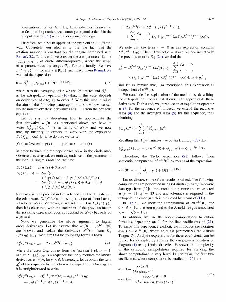
Finally, we also compare truncated Taylor expansions withthe numerical approximation of the Arnold Tongue for θ =

(√

5 − 1)/2, computed using the Newton method. To this end,we perform the computation of Section 4.2 for ε ∈ [0, 0.1],using quadruple-double precision, an averaging order p = 9and requiring tolerances of 10−42 for the computation of therotation number, and 10−40 for convergence of the Newtonmethod. In all the computations, we allow at most 223 iterates ofthe map. Then, in Fig. 4 we compare the approximated tonguewith Taylor expansions truncated at orders 2, 4, 6, 8 and 10.

5. Study of invariant curves for planar twist maps

In this last section we deal with a classical problemin dynamical systems that arise in many applications: thestudy of quasi-periodic invariant curves for planar maps.Concretely, we focus on the context of so-called twist maps,

Fig. 4. Comparison between the numerical expressions of α(ε) for the ArnoldTongue Tθ , with θ = (

√5 − 1)/2, obtained using the Newton method and the

truncated Taylor expansion (21) up to order d. Concretely we plot, as a functionof ε, the difference in log10 scale between these quantities. The curves from topto bottom correspond, respectively, to d = 2, 4, 6, 8 and 10.

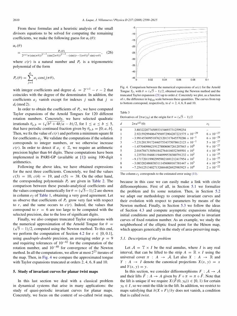
Table 3

Derivatives of 2πα(y0) at the origin for θ = (√

5 − 1)/2

d 2πα(d)(0) e1

0 3.8832220774509331546937312599254 –1 2.9215929940647956972904287221575 × 10−29 6 × 10−27

2 −3.9914536995187621201317645570286 × 10−1 6 × 10−28

3 −7.2312013917244657534375078612123 × 10−1 5 × 10−27

4 −1.4570409862191278806067261207843 × 100 9 × 10−27

5 2.0167847130561842764416032369501 × 101 4 × 10−26

6 1.2357011948811946999538300791232 × 102 1 × 10−25

7 −9.1717201199029959021691212417954 × 101 2 × 10−25

8 −3.0832824868383111456060167381447 × 103 4 × 10−24

9 −7.2541251340271326844826925983923 × 104 2 × 10−22

The column e1 corresponds to the estimated error using (11).

because in this case we can easily make a link with circlediffeomorphisms. First of all, in Section 5.1 we formalizethe problem and fix some notation. Then, in Section 5.2we adapt our methodology to compute invariant curves andtheir evolution with respect to parameters by means of theNewton method. Finally, in Section 5.3 we follow the ideasof Section 4.3 and compute asymptotic expansions relatinginitial conditions and parameters that correspond to invariantcurves of fixed rotation number. As an example, we study theneighborhood of the elliptic fixed point for the Henon map,which appears generically in the study of area-preserving maps.

5.1. Description of the problem

Let A = T × I be the real annulus, where I is any realinterval, that can be lifted to the strip A = R × I using theuniversal cover π : A → A. Let also X : A → R andY : A → I denote the canonical projections X (x, y) = xand Y (x, y) = y.

In this section, we consider diffeomorphisms F : A → Aand their lifts F : A → A given by F ◦ π = π ◦ F . Note thatthe lift is unique if we require X (F(0, y0)) ∈ [0, 1) for certainy0 ∈ I , so we omit the tilde in the lift. In addition, we restrict tomaps satisfying that ∂(X ◦ F)/∂y does not vanish, a conditionthat is called twist.

A. Luque, J. Villanueva / Physica D 237 (2008) 2599–2615 2611

Assume that F : A → A is a twist map having an invariantcurve Γ , homotopic to the circle T × {0}, of rotation numberθ ∈ R \ Q. Concretely, there exists an embedding γ : R → A,such that Γ = γ (R), satisfying γ (x + 1) = γ (x) + (1, 0) forall x ∈ R, and making the following diagram commute

F(γ (x)) = γ (x + θ). (27)

Since F is a twist map, the Birkhoff Graph Theorem(see [11]) ensures that Γ is a Lipschitz graph over its projectionon the circle T × {0}, and hence the dynamics on Γ inducesa circle homeomorphism fΓ simply by projecting the iterates,i.e., fΓ (X (γ (x))) = X (F(γ (x))). We observe that, if F and γ

are Cr -diffeomorphisms, then fΓ ∈ Diffr+(T).

From now on, we fix an angle x0 ∈ T and identify invariantcurves with points y0 ∈ I . Then, if (x0, y0) belongs to aninvariant curve Γ , we also denote the previous circle map as fy0

instead of fΓ . Of course, the parameterization γ is unknownin general, so we do not have an expression for fy0 . But wecan evaluate the orbit (xn, yn) = Fn(x0, y0) and considerxn = f n

y0(x0). We recall that this orbit is the only thing we

need to compute numerically the rotation number θ using themethod of [26] (reviewed in Section 2.2).

Remark 5.1. If the map F does not satisfy the twist condition,their invariant curves are not necessarily graphs over the circleT × {0}. Of course, if Γ is an invariant curve of F , itsdynamics still induces a circle diffeomorphism, even though itsconstruction is not so obvious. Since the non-twist case presentsanother difficulties and it has interest of its own, we plan toadapt the method to consider the general situation in subsequentwork [22].

If F is a Cr -integrable twist map, then there is a Cr -familyof invariant curves of F satisfying (27), and y0 7→ fy0 is aone-parameter family in Diffr

+(T). In this case, we obtain a Cr -function y0 ∈ I 7→ ρ( fy0). Of course, this is not the generalsituation and, actually, we do not expect this function to bedefined for every y0 ∈ I . Nevertheless, in many problems wehave a family of invariant curves defined on a Cantor subsetJ ⊂ I having positive Lebesgue measure and we still havedifferentiability of ρ( fy0) in the sense of Whitney. For example,if the map F is a perturbation of an integrable twist map that issymplectic or satisfies the intersection condition, KAM theoryestablishes (under other general assumptions) the existence ofsuch a Cantor family of invariant curves (we refer to [6,23]).

For practical purposes, even if a point (x0, y0) ∈ A does notbelong to a quasi-periodic invariant curve, we can compute theorbit xn = f n

y0(x0) = X (Fn(x0, y0)), even though fy0 is not a

circle diffeomorphism. Then, we can also compute the averagedsums S p

N ( fy0) of these iterates but we cannot guarantee ingeneral that Θq,p( fy0) converges when q → ∞. Nevertheless,if (x0, y0) is an initial condition close enough to an invariantcurve of Diophantine rotation number θ , we expect Θq,p( fy0)

to converge to a number close to θ , due to the existence ofneighboring invariant curves for a set of large relative measure(that is called condensation phenomena in KAM theory). Onthe other hand, if (x0, y0) belongs to a periodic island, thenwe expect Θq,p( fy0) to converge to the winding number ofthe “central” periodic orbit. Finally, we recall that the Aubry-Mather theorem (we refer to [11]) states that F has orbits ofall rotation numbers, so it can occur that the method convergesif (x0, y0) corresponds to a periodic orbit or to a ghost curve(Cantori).

On the other hand, in order to approximate derivatives ofthe rotation number by means of Θd

q,p,p−d( fy0), we have tocompute derivatives of iterates xn . However, as we do not havean explicit formula for the induced map fy0 , the scheme forcomputing derivatives of the iterates is slightly different fromthe one presented in Section 3.3. Modified recurrences aredetailed in the moment that they are required.

5.2. Numerical continuation of invariant curves

Let us consider α : Λ ⊂ R 7→ Fα a one-parameterfamily of twist maps on A, that induces a function (α, y0) ∈

U ⊂ Λ × I 7→ ρ( fα,y0) differentiable in the sense ofWhitney. In this situation, we can compute derivatives of thisfunction (at the points where they exist) by using the method ofSection 3. Our goal now is to use these derivatives to computenumerically invariant curves of Fα by means of the Newtonmethod, similarly as we did in Section 4.2 for computing theArnold Tongues.

Concretely, let Γα0 be an invariant curve of rotation numberθ ∈ D for the map Fα0 . Then, given any α close to α0, wewant to compute the curve Γα , invariant under Fα , having thesame rotation number. Once we have fixed an angle x0 ∈ T, weidentify the invariant curve Γα by the point (x0, y(α)) ∈ Γα .Then, our purpose is to solve, with respect to y, the equationρ( fα,y) = θ by continuing the known solution (α0, y(α0)) ∈

Λ× I . We just remark that, when solving this equation by meansof the Newton method, we have to prevent us from falling intoa resonant island, where the rotation number is locally constantaround this point.

Now, in order to approximate numerically Dαρ and Dy0ρ,we have to discuss the computation of derivatives of the iterates,i.e. Dα(xn) and Dy0(xn), where xn = f n

α,y0(x0). Omitting the

dependence on the parameter α in the family of twist maps, wedenote F1 = X ◦ F and F2 = Y ◦ F , and we obtain the recurrentexpression

Dy0(xn) = ∂x F1(zn−1)Dy0(xn−1) + ∂y F1(zn−1)Dy0(yn−1),

(28)

where zn := (xn, yn). Furthermore, Dy0(yn) follows froma similar expression replacing F1 by F2. According to ourconvention of fixing x0 ∈ T, the computations have to beinitialized by Dy0(x0) = 0 and Dy0(y0) = 1. Analogousformulas hold for Dα(xn):

Dα(xn) = ∂α F1(zn−1) + ∂x F1(zn−1)Dα(xn−1)

+ ∂y F1(zn−1)Dα(yn−1),

2612 A. Luque, J. Villanueva / Physica D 237 (2008) 2599–2615

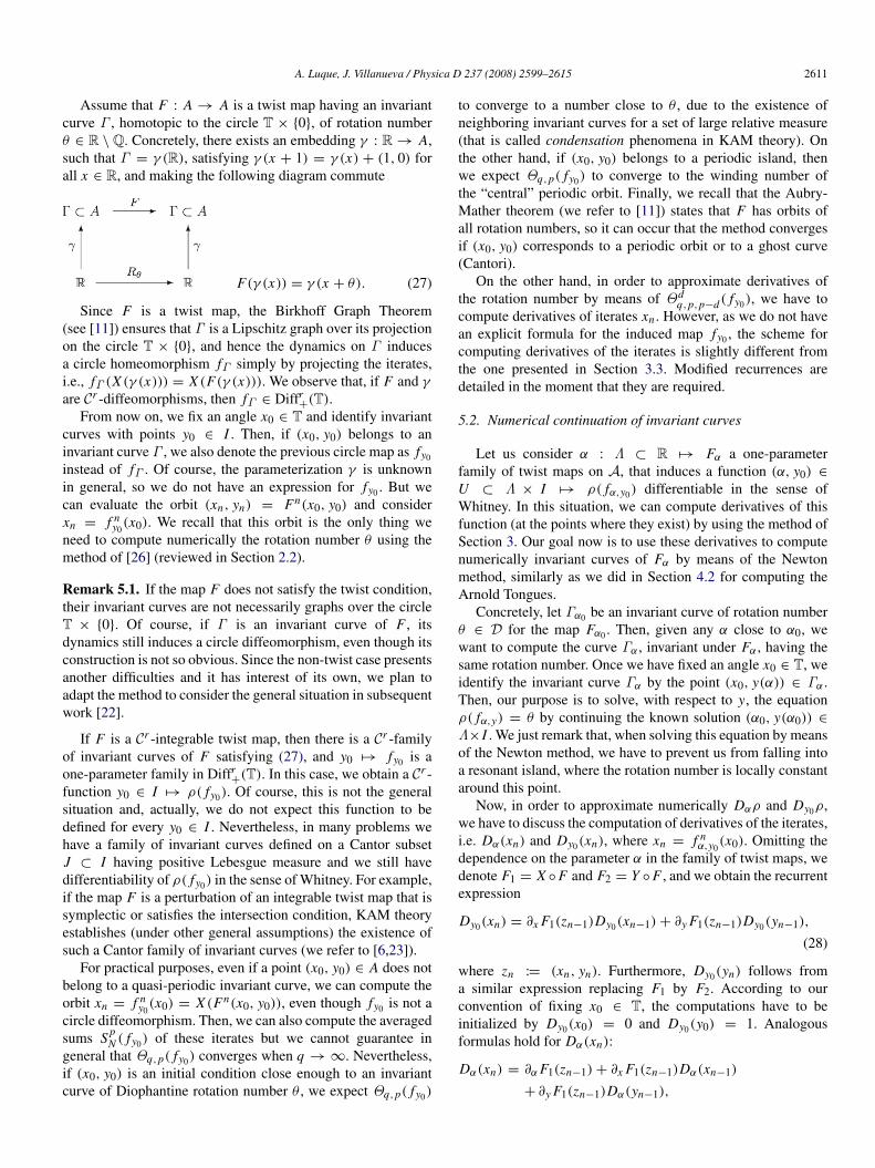
Fig. 5. Left: Numerical continuation of y0 (horizontal axis) with respect to α (vertical axis) of the invariant curve of rotation number θ = (√

5 − 1)/2 for the Henonmap (29). Right: Difference in log10 scale between α(y0) in the left plot and its truncated Taylor expansion (32) up to order d (see Table 3). The curves from top tobottom correspond, respectively, to d = 2, 4, 6 and 8.

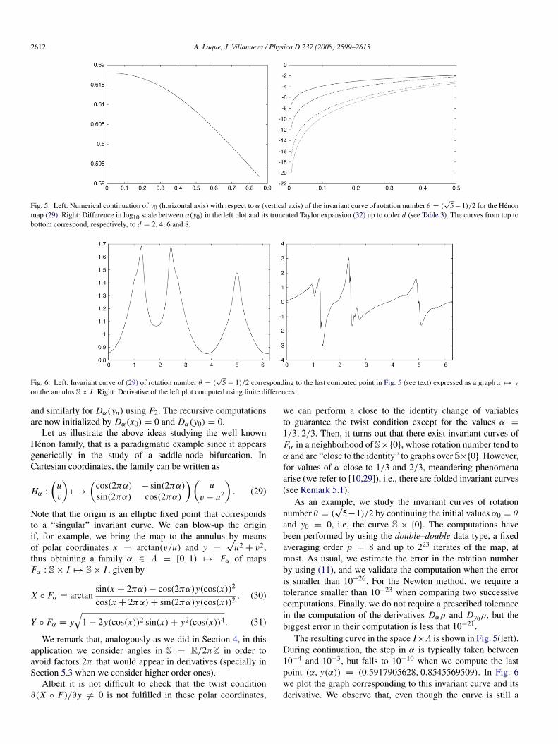
Fig. 6. Left: Invariant curve of (29) of rotation number θ = (√

5 − 1)/2 corresponding to the last computed point in Fig. 5 (see text) expressed as a graph x 7→ yon the annulus S× I . Right: Derivative of the left plot computed using finite differences.

and similarly for Dα(yn) using F2. The recursive computationsare now initialized by Dα(x0) = 0 and Dα(y0) = 0.

Let us illustrate the above ideas studying the well knownHenon family, that is a paradigmatic example since it appearsgenerically in the study of a saddle-node bifurcation. InCartesian coordinates, the family can be written as

Hα :

(uv

)7−→

(cos(2πα) − sin(2πα)

sin(2πα) cos(2πα)

)(u

v − u2

). (29)

Note that the origin is an elliptic fixed point that correspondsto a “singular” invariant curve. We can blow-up the originif, for example, we bring the map to the annulus by meansof polar coordinates x = arctan(v/u) and y =

√u2 + v2,

thus obtaining a family α ∈ Λ = [0, 1) 7→ Fα of mapsFα : S × I 7→ S × I , given by

X ◦ Fα = arctansin(x + 2πα) − cos(2πα)y(cos(x))2

cos(x + 2πα) + sin(2πα)y(cos(x))2 , (30)

Y ◦ Fα = y√

1 − 2y(cos(x))2 sin(x) + y2(cos(x))4. (31)

We remark that, analogously as we did in Section 4, in thisapplication we consider angles in S = R/2πZ in order toavoid factors 2π that would appear in derivatives (specially inSection 5.3 when we consider higher order ones).

Albeit it is not difficult to check that the twist condition∂(X ◦ F)/∂y 6= 0 is not fulfilled in these polar coordinates,

we can perform a close to the identity change of variablesto guarantee the twist condition except for the values α =

1/3, 2/3. Then, it turns out that there exist invariant curves ofFα in a neighborhood of S×{0}, whose rotation number tend toα and are “close to the identity” to graphs over S×{0}. However,for values of α close to 1/3 and 2/3, meandering phenomenaarise (we refer to [10,29]), i.e., there are folded invariant curves(see Remark 5.1).

As an example, we study the invariant curves of rotationnumber θ = (

√5−1)/2 by continuing the initial values α0 = θ

and y0 = 0, i.e, the curve S × {0}. The computations havebeen performed by using the double–double data type, a fixedaveraging order p = 8 and up to 223 iterates of the map, atmost. As usual, we estimate the error in the rotation numberby using (11), and we validate the computation when the erroris smaller than 10−26. For the Newton method, we require atolerance smaller than 10−23 when comparing two successivecomputations. Finally, we do not require a prescribed tolerancein the computation of the derivatives Dαρ and Dy0ρ, but thebiggest error in their computation is less that 10−21.

The resulting curve in the space I×Λ is shown in Fig. 5(left).During continuation, the step in α is typically taken between10−4 and 10−3, but falls to 10−10 when we compute the lastpoint (α, y(α)) = (0.5917905628, 0.8545569509). In Fig. 6we plot the graph corresponding to this invariant curve and itsderivative. We observe that, even though the curve is still a

A. Luque, J. Villanueva / Physica D 237 (2008) 2599–2615 2613

graph, this parameterization is close to have a vertical tangency,so our approach is not suitable for continuing the curve.However, since fractalization of the curve has not occurred,we expect that it still exists beyond this point. To continue thefamily of curves in this situation it is convenient to use anotherapproach (see Remark 5.1).

5.3. Computing expansions with respect to parameters

In the same situation of Section 5.2, our aim now is to usevariational information of the rotation number to compute theTaylor expansion at the origin of Fig. 5(left). Notice that in theselected example α′(0) = 0, so we work with the expansion ofthe function α(y0) rather than y0(α).

In general, if (x0, y∗

0 ) is a point on an invariant curve ofrotation number θ for a twist map Fα∗ , then we consider theexpansion

α(y0) = α∗+ α′(y∗

0 )(y0 − y∗

0 ) +α′′(y∗

0 )

2!(y0 − y∗

0 )2+ · · · ,

(32)

that corresponds to the value of the parameter for which (x0, y0)

is contained in an invariant curve of Fα(y0) having the samerotation number. We know that if θ ∈ D and the family Fα isanalytic, then Eq. (32) is an analytic function around y∗

0 . Onceagain, during the rest of the section, we omit the dependenceon the parameter α in the family of twist maps, and we denoteF1 = X ◦ F and F2 = Y ◦ F .

As in Section 4.3, we use that the family y0 7→ fα(y0),y0 ∈

Diffω+(S) induced by y0 7→ Fα(y0) has constant rotation number,together with Remark 3.2. Concretely, for any integer d ≥ 1 wehave

0 = Θdq,p,p( fα(y0),y0) +O(2−(p+1)q), (33)

where Θdq,p,p is the extrapolation operator (16). We observe that

the value of Θdq,p,p( fy0) at the point y∗

0 only depends on thederivatives α(r)(y∗

0 ) up to r ≤ d . We use this fact to computeinductively these derivatives from Eq. (33). To achieve this, wehave to isolate them from Dd

y0(xn)|y0=y∗

0for any d ≥ 1, as we

discuss through the next paragraphs.The following formula generalizes (28):

Ddy0

(xn) =

d−1∑j=0

(d − 1

j

){D j

y0(∂α F1(zn−1))α(d− j)(y0)

+ D jy0(∂x F1(zn−1))Dd− j

y0 (xn−1)

+ D jy0(∂y F1(zn−1))Dd− j

y0 (yn−1)}

, (34)

while a similar equation holds for Ddy0

(yn) replacing F1 by F2.Moreover, as in Section 3.3, we compute the derivatives Dr

y0of ∂α F1(zn−1), ∂x F1(zn−1) and ∂y F1(zn−1) by means of thefollowing recurrent expression

Dry0

(∂k,l,mα,x,y Fi (zn−1))

=

r−1∑j=0

(r − 1

j

){D j

y0(∂k+1,l,mα,x,y Fi (zn−1))α

(r− j)(y0)

+ D jy0(∂

k,l+1,mα,x,y Fi (zn−1))Dr− j

y0 (xn−1)

+ D jy0(∂

k,l,m+1α,x,y Fi (zn−1))Dr− j

y0 (yn−1)}

,

which only requires evaluation of the partial derivatives of F1and F2 with respect to α, x and y.

Using the above expressions, we reproduce the inductiveargument of Section 4.3. Let us assume that the valuesα′(y∗

0 ), . . . , α(d−1)(y∗

0 ) are known. Then, we observe that if weset y0 = y∗

0 and α = α∗ in Eq. (34), the only term containingthe derivative α(d)(y∗

0 ) is the one corresponding to j = 0. Byinduction, it is easy to find that

Ddy0

(xn)|y0=y∗

0= X d

n α(d)(y∗

0 ) + X dn ,

Ddy0

(yn)|y0=y∗

0= Yd

n α(d)(y∗

0 ) + Ydn ,

where the coefficients X dn , X d

n , Ydn and Yd

n are obtainedrecursively and only depend on the derivatives α(r)(y∗

0 ), with

r < d. Concretely, X dn and X d

n satisfy

X dn = (∂α F1(zn−1) + ∂x F1(zn−1)X d

n−1

+ ∂y F1(zn−1)Ydn−1)|y0=y∗

0,

X dn =

(∂x F1(zn−1)X d

n−1 + ∂y F1(zn−1)Ydn−1

+

d−1∑j=1

(d − 1

j

){D j

y0(∂α F1(zn−1))α(d− j)(y0)

+ D jy0(∂x F1(zn−1))Dd− j

y0 (xn−1)

+ D jy0(∂y F1(zn−1))Dd− j

y0 (yn−1)}

)|y0=y∗

0,

and similar equations hold for Ydn and Yd

n replacing F1 by F2.These sequences are initialized as

X 10 := X 1

0 := Y10 := 0, Y1

0 := 1, and

X d0 := X d

0 := Yd0 := Yd

0 := 0, for d > 1.

Finally, if we evaluate the extrapolation operator Θq,p forthe sequences X d

= {X dn }n=1,...,N and X d

= {X dn }n=1,...,N ,

then we obtain from (33) the following expression

α(d)(y∗

0 ) = −Θq,p(X d)

Θq,p(X d)+O(2−(p+1)q).

Now, we apply this methodology to the Henon family α ∈

Λ = [0, 1) 7→ Fα given by (30) and (31). In particular, wefix x0 = 0 and compute the expansion Eq. (32) at y∗

0 = 0corresponding to invariant curves of rotation number α∗

= θ =

(√

5 − 1)/2.Observe that the derivatives of this map are hard to compute

explicitly, so we have to introduce another recursive scheme forthem. Moreover, in order to reduce the number of computations,we use that the iterates of (0, 0) are xn = 2πnθ and yn = 0.

We detail the computations of ∂k,l,mα,x,y(Y ◦ Fα) at the point

(α, x, y) = (θ, xn, 0), while the derivatives of X ◦ Fα

satisfy completely analogous expressions. Let us introduce the

2614 A. Luque, J. Villanueva / Physica D 237 (2008) 2599–2615

function

g(x, y) = 1 − 2y(cos(x))2 sin(x) + y2(cos(x))4,

so we can write Y ◦ Fα(x, y) = y√

g(x, y). First, we observethat for any s ∈ Q we have ∂

k,l,mα,x,y(ygs)|y=0 = 0 provided k 6= 0

or m = 0. Otherwise, the required derivatives can be computedby means of the following recurrent expressions

∂ l,mx,y (ygs) = ∂ l,m−1

x,y (gs)

+ sl∑

i=0

m−1∑j=0

(l

i

)(m − 1

j

)∂

i, jx,y(ygs−1)∂

l−i,m− jx,y (g)

and

∂ l,mx,y (gs) = s

l∑i=0

m−1∑j=0

(l

i

)(m − 1

j

)∂

i, jx,y(ygs−1)∂

l−i,m− jx,y (g).

Finally, we observe that the derivatives ∂l−i,m− jx,y (g) can be

computed easily by expanding the function as a trigonometricpolynomial

g(x, y) = 1 −y

2(sin(3x) + sin(x))

+y2

2

(34

+ cos(2x) +14

cos(4x)

).

Computations are performed by using double–double datatype, p = 7 and 221 iterates, at most. We stop the computationsif the estimated error is less than 10−25. Derivatives of theexpansion (32) and their estimated error, are given in Table 3.Finally, in order to verify the results, we compare truncatedexpansions of the curve with the numerical approximationcomputed in Section 5.2. The deviation is plotted in log10 scalein Fig. 5(right).

Acknowledgements

We wish to thank Rafael de la Llave, Tere M. Searaand Joaquim Puig for interesting discussions and suggestions.We are also very grateful to Rafael Ramırez-Ros forintroducing and helping us in the PARI-GP software.Finally, we acknowledge the use of EIXAM, the UPCApplied Math cluster system for research computing (seehttp://www.ma1.upc.edu/eixam/), and in particular Pau Roldanfor his support in the use of the cluster. The authors havebeen partially supported by the Spanish MCyT/FEDER grantMTM2006-00478. Moreover, the research of A.L. has beensupported by the Spanish phD grant FPU AP2005-2950.

References

[1] PARI/GP Development Headquarter. http://pari.math.u-bordeaux.fr/.[2] V.I. Arnold, Small denominators. I. Mapping the circle onto itself, Izv.

Akad. Nauk SSSR Ser. Mat. 25 (1961) 21–86.[3] H. Broer, C. Simo, Resonance tongues in Hill’s equations: A geometric

approach, J. Differential Equations 166 (2) (2000) 290–327.[4] H. Bruin, Numerical determination of the continued fraction expansion of

the rotation number, Physica D 59 (1–3) (1992) 158–168.

[5] E. Castella, A Jorba, On the vertical families of two-dimensional tori nearthe triangular points of the bicircular problem, Celestial Mech. Dynam.Astronom. 76 (1) (2000) 35–54.

[6] R. de la Llave, A tutorial on KAM theory, in: Smooth Ergodic Theory andits Applications (Seattle, WA, 1999), in: Proc. Sympos. Pure Math., vol.69, Amer. Math. Soc., 2001, pp. 175–292.

[7] R. de la Llave, A. Gonzalez, A Jorba, J. Villanueva, KAM theory withoutaction-angle variables, Nonlinearity 18 (2) (2005) 855–895.

[8] R. de la Llave, N.P. Petrov, Regularity of conjugacies between criticalcircle maps: An experimental study, Experiment. Math. 11 (2) (2002)219–241.

[9] W. de Melo, S. van Strien, One-dimensional dynamics, in: Ergebnisseder Mathematik und ihrer Grenzgebiete (3) (Results in Mathematics andRelated Areas (3)), vol. 25, Springer-Verlag, Berlin, 1993.

[10] H.R. Dullin, J.D. Meiss, D. Sterling, Generic twistless bifurcations,Nonlinearity 13 (1) (2000) 203–224.

[11] C. Gole, Symplectic Twist Maps: Global Variational Techniques, WorldScientific Publishing, 2001.

[12] G. Gomez, A Jorba, J. Masdemont, C. Simo, Study of Poincare maps fororbits near Lagrangian points, ESA-ESOC contract 8711/91/D/IM/(SC),Darmstadt, Germany, 1993.

[13] G. Gomez, A Jorba, C. Simo, J. Masdemont, Advanced methods fortriangular points, in: Dynamics and Mission Design near Libration Points.vol. IV, in: World Scientific Monograph Series in Mathematics, vol. 5,World Scientific Publishing Co. Inc., River Edge, NJ, 2001.

[14] G. Gomez, J.M. Mondelo, C. Simo, Refined Fourier analysis: Procedures,error estimates and applications. Preprint 2001. Available electronicallyat: http://www.maia.ub.es/dsg/2001/.

[15] M.R. Herman, Mesure de Lebesgue et nombre de rotation, in: Geometryand Topology (Proc. III Latin Amer. School of Math., Inst. Mat. PuraAplicada CNPq, Rio de Janeiro, 1976), in: Lecture Notes in Math., vol.597, Springer, Berlin, 1977, pp. 271–293.

[16] M.R. Herman, Sur la conjugaison differentiable des diffeomorphismes ducercle a des rotations, Inst. Hautes Etudes Sci. Publ. Math. (49) (1979)5–233.

[17] Y. Hida, X. Li, D.H. Bailey, (QD, double–double and quad doublepackage), http://crd.lbl.gov/˜dhbailey/mpdist/.

[18] A. Katok, B. Hasselblatt, Introduction to the Modern Theoryof Dynamical Systems, in: Encyclopedia of Mathematics and itsApplications, vol. 54, Cambridge University Press, 1995.

[19] Y. Katznelson, D. Ornstein, The differentiability of the conjugation ofcertain diffeomorphisms of the circle, Ergodic Theory Dynam. Systems9 (4) (1989) 643–680.

[20] S.G. Krantz, H.R. Parks, A primer of real analytic functions,in: Birkhauser Advanced Texts: Basler Lehrbucher. (Birkhauser AdvancedTexts: Basel Textbooks), second edn, Birkhauser Boston Inc., Boston,MA, 2002.

[21] J. Laskar, C. Froeschle, A. Celletti, The measure of chaos by the numericalanalysis of the fundamental frequencies. Application to the standardmapping, Physica D 56 (2–3) (1992) 253–269.

[22] A. Luque, J. Villanueva, Numerical computation of rotation numbers forquasi-periodic planar curves (in preparation).

[23] J. Moser, On invariant curves of area-preserving mappings of an annulus,Nachr. Akad. Wiss. Gottingen Math.-Phys. Kl. II 1962 (1962) 1–20.

[24] R. Pavani, A numerical approximation of the rotation number, Appl.Math. Comput. 73 (2–3) (1995) 191–201.

[25] E. Risler, Linearisation des perturbations holomorphes des rotations etapplications, Mem. Soc. Math. Fr. (N.S.) 77 (1999) viii+102.

[26] T.M. Seara, J. Villanueva, Numerical computation of the asymptotic sizeof the rotation domain for the Arnold family. Preprint 2007. Availableelectronically at: http://www.ma1.upc.edu/recerca/2006-2007.html.

[27] T.M. Seara, J. Villanueva, On the numerical computation of Diophantinerotation numbers of analytic circle maps, Physica D 217 (2) (2006)107–120.

[28] C. Simo, Effective computations in celestial mechanics and astrodynam-ics, in: Modern Methods of Analytical Mechanics and their Applications(Udine, 1997), Springer, Vienna, 1998, pp. 55–102.

A. Luque, J. Villanueva / Physica D 237 (2008) 2599–2615 2615

[29] C. Simo, Invariant curves of analytic perturbed nontwist area preservingmaps, Regul. Chaotic Dyn. 3 (3) (1998) 180–195. J. Moser at 70 (inRussian).

[30] Ya.G. Sinaı, K.M. Khanin, Smoothness of conjugacies of diffeomor-phisms of the circle with rotations, Uspekhi Mat. Nauk. 44 (1(265))(1989) 57–82. 247.

[31] M. van Veldhuizen, On the numerical approximation of the rotationnumber, J. Comput. Appl. Math. 21 (2) (1988) 203–212.

[32] J. Vano, A Nash-Moser implicit function theorem with Whitney regularityand applications, Ph.D. Thesis, University of Texas at Austin; 2002.Available electronically at: http://hdl.handle.net/2152/655.

[33] J.C. Yoccoz, Conjugaison differentiable des diffeomorphismes du cercledont le nombre de rotation verifie une condition diophantienne, Ann. Sci.Ecole Norm. Sup. (4) 17 (3) (1984) 333–359.

[34] J.C. Yoccoz, Il n’y a pas de contre-exemple de Denjoy analytique, C. R.Acad. Sci. Paris Ser. I Math. 298 (7) (1984) 141–144.