Rotation: Part 1

January 12, 2016

A simple account is given for rotational motionabout a fixed axis, emphasizing the analogy with lin-ear motion. All the laws for rotational motion canbe derived from Newton’s laws for point particles.

Contents

1 Kinematics 1

1.1 Coordinates and displacement . . . . 1

1.2 Angular velocity and frequency . . . 1

1.3 Angular acceleration . . . . . . . . . 2

1.4 Laws of kinematics . . . . . . . . . . 3

2 Kinetic energy and moment of inertia 3

2.1 Single particle . . . . . . . . . . . . . 3

2.2 Rigid body . . . . . . . . . . . . . . 4

2.3 Moment of inertia . . . . . . . . . . 4

3 Torque and analog of Newton’s secondlaw 4

3.1 Concept of generalized force . . . . . 4

3.2 Torque . . . . . . . . . . . . . . . . . 4

3.3 Analog of Newton’s second law . . . 5

3.4 Angular momentum . . . . . . . . . 6

3.5 Summary . . . . . . . . . . . . . . . 7

4 Condition for rotational equilibrium 7

4.1 Simple example . . . . . . . . . . . . 7

4.2 From Newton’s laws . . . . . . . . . 7

4.3 Directly using work . . . . . . . . . . 8

4.4 Principle of virtual work* . . . . . . 8

A Verifying the energy 8

B Euler–Lagrange equation* 9

1 Kinematics

Rotational motions are common: wheels and gyro-scopes; planets moving around the sun, the moonaround the earth; the sun, the earth or the moonrotating around its own axis; electrons movingaround the nucleus; electrons and nuclei spinningaround their own axes. The laws of physics for ro-tational motion are parallel to those for linear mo-tion, and moreover can be derived from the latter.Here we start with kinematics — the description ofmotion as a function of time.

1.1 Coordinates and displacement

CoordinateConsider a particle constrained to move along acircle of radius r, say on the x–y plane. Since theradius is fixed, its position (at any time t) can bespecified by an angle φ (Figure 1a). A rigid body(e.g., a gramophone record or DVD) rotating on aplane can likewise be described by a single angle φ(Figure 1b).

UnitAngular coordinates are measured in radians.

DisplacementIf over a time interval from t1 to t2 the coordinatechanges from φ1 to φ2, then the angular displace-ment is

∆φ = φ2 − φ1 (1)

1.2 Angular velocity and frequency

Angular velocityIf there is an angular displacement ∆φ in a time∆t = t2−t1, then the average angular velocity dur-ing this interval is

ωav =∆φ

∆t(2)

1

In the limit of infinitesimal time intervals, this be-comes the instantaneous angular velocity

ω =dφ

dt(3)

The unit of ω is

[ω] = rad s−1 = s−1 (4)

The simpler form is also correct since the radian(as the ratio of two lengths, an arc and a radius)has no units.

FrequencyFor an object in rotational motion, the frequency fis the number of cycles of rotation per unit time.The unit of f is

[f ] = cycles s−1 ≡ Hz (5)

Sometimes “cycle” is understood, and Hz is identi-fied with s−1; but see remark below.

If the period of rotational motion is T , then thefrequency is 1 cycle per time T , i.e.,

f = 1/T (6)

Since there are 2π radians in one cycle,

ω = 2πf = 2π/T (7)

Although f may be more familiar from elementarystudies, in physics we tend to use ω, for two reasons.

• Formulas are simpler; see below.

• The angular velocity ω can be defined instan-taneously, whereas it is not clear how to definef if the motion covers less than one cycle.

Caveat about unitsThe relationship (7) would suggest that ω and fhave the same units, namely s−1. However, pleasenote the following.

• We never use Hz for ω. It is best to think ofHz as cycles per second.

• Likewise, it is best to think of 2π in (7) not asa pure number, but 2π radians per cycle.

Problem 1Find the angular frequency ω (in units of s−1) forthe following motions.(a) The earth rotating about its own axis once aday.1

(b) An engine running at 3 000 rpm.(c) The pulsar PSR B1937+21 spinning around itsown axis with a period of 1.558 ms. §

Relationship with tangential velocityA point mass is constrained to move on a circle ofradius r; its angular displacement in a short timeinterval ∆t is ∆φ and the linear displacement is(Figure 2)

∆s = r∆φ (8)

Dividing by ∆t, we get the relationship betweenthe instantaneous linear velocity v and the angularvelocity ω:

v = r ω (9)

This is the first of many formulas relating corre-sponding quantities in linear and circular motion,all involving a factor of r.

Problem 2The tyres of a car have an outer radius of 300 mm.The engine is running at 3000 rpm, and is con-nected to the wheels by two sets of gears. The firstset (in 4th gear) has a ratio of 1:1 (one turn of theengine leads to one turn of the transmission axle);the second set has a ratio of 3.4:1 (3.4 turns of thetransmission axle leads to one turn of the wheel).(a) What is the angular velocity ω of the tyres?(b) What is the velocity v of the rim of the tyreswith respect to the wheel axle, in m s−1?(c) This is also the speed of the car; express theanswer in km h−1. §

Problem 3Suppose the pulsar in Problem 1(c) has a radius of10 km. What is the linear velocity at the surface?§

1.3 Angular acceleration

If the angular velocity changes, we need the conceptof angular acceleration α, defined in the obvious

1Actually the period relative to the fixed stars is about1/365 = 0.27% less than 1 day = 86400 s.

2

way:

α =dω

dt(10)

Problem 4The pulsar PSR J1603-7202 has a period of T =0.014 841 952 015 466 8 s, and the period increasesby ∆T = 5.0× 10−13 s in ∆t = 1 year.2

(a) Find α in units of s−1, by calculating ω1 andω2 at a time ∆t apart. (You will need a calculatoraccurate to many digits.)(b) A better method is to note that ωT = 2π, fromwhich ∆ω/ω = −∆T/T , and hence

α =∆ω

∆t= −ω∆T

∆t T= − 2π

T 2

∆T

∆t(11)

This allows an easier evaluation. §

1.4 Laws of kinematics

Angular coordinate, angular velocity and angularacceleration are related to one another in exactlythe same way as for the corresponding linear vari-ables. For example, if the angular acceleration isuniform, then in obvious notation

ω = ω0 + αt

φ = φ0 + ω0t+1

2αt2

= φ0 +1

2(ω0 + ω)t

ω2 − ω20 = 2α(φ− φ0) (12)

where the subscript 0 indicates initial values. Theseare the analogs of the familiar formulas for linearmotion:

v = v0 + at

x = x0 + v0t+1

2at2

= x0 +1

2(v0 + v)t

v2 − v20 = 2a(x− x0) (13)

All these can be remembered through the followingtable of correspondences.

2http://www.atnf.csiro.au/outreach/education/everyone/pulsars/index.html

quantity linear rotationalcoordinate x φ

velocity v ωacceleration a α

Table 1. Correspondence between linear and ro-tational kinematics

In particular, everything we have learnt aboutsolving linear kinematics can be copied over — forexample, if a rule is given to calculate α, then themotion is completely solved.

2 Kinetic energy and momentof inertia

Next we consider dynamics. To lead towards theanalog of force for angular coordinates, the key con-cepts are energy and work — which as scalars areindependent of what coordinates we use.

2.1 Single particle

Motion in a planeConsider one particle of mass m moving in a circleof radius r, on the x–y plane (Figure 3a). TheKE is

K =1

2mv2 (14)

Using (9), we get

K =1

2m(ωr)2 =

1

2(mr2)ω2 (15)

Position shifted from the planeNow consider a more general case. The mass m isat a position

~r = x i + y i + z k (16)

Imagine that it is a point on a cylinder rotatingabout the z-axis (Figure 3b). Obviously it is theperpendicular distance to the z-axis that matters,while the z coordinate itself is irrelevant. In otherwords, the formula for the kinetic energy should be

K =1

2m(ωr⊥)2 =

1

2(mr2⊥)ω2 (17)

where

r2⊥ = x2 + y2 (18)

is the square of the perpendicular distance to theaxis.

3

2.2 Rigid body

Now generalize to a rigid body, which can bethought of as a collection of point masses mα atpositions ~rα.3 Using (17) for each point mass andadding up, we find that the total KE is

K =∑α

1

2mαr

2α,⊥ ω

2

=1

2

(∑α

mαr2α,⊥

)ω2 (19)

The factor ω2 is the same for every particle, i.e., itis independent of α, and can be taken out of thesummation. Thus we define the bracket as

I =∑α

mαr2α,⊥ (20)

in terms of which we have

K = (1/2)Iω2 (21)

analogous to K = (1/2)mv2 for linear motion.

Note that I depends on the distribution of mass,but is independent of motion.

2.3 Moment of inertia

The quantity I, called the moment of inertia, isdefined with respect to an axis — only when wespecify the axis can we talk about the perpendicu-lar distance r⊥. Because of (21), I plays the role ofthe mass m in rotational motion.

case object axis βa rod end 1/3b rod center 1/12c hollow sphere diameter 2/3d solid sphere diameter 2/5e hollow cylinder axis 1f solid cylinder axis 1/2

Table 2. The moments of inertia of various uni-form bodies expressed as I = βMR2, where R iseither the length of a rod or the radius of a sphereor cylinder.

3Particles will be labelled by α, β etc., leaving i, j, k etc.for Cartesian indices.

If a rigid body has a total mass M and a typi-cal dimension R (transverse to the axis concerned),then obviously

I = βMR2 (22)

where β = O(1) is a pure number. A detaileddiscussion about moments of inertia is given later.Here we simply quote some useful results (Figure4).

3 Torque and analog of New-ton’s second law

The central idea in linear motion is

force = mass× acceleration (23)

We need a rotational analog, schematically of theform

“angular force”

= moment of inertia

× angular acceleration (24)

The question is: what is the “angular force” —which we shall call the torque and denote as τ?

3.1 Concept of generalized force

In the linear case, the work done for a small dis-placement is

∆W = F ∆x (25)

From this, we can think of force as work done perlinear displacement. This leads us to define the “an-gular force” as work done per angular displacement,in other words, by the formula

∆W = τ ∆φ (26)

This idea is applicable to the generalized forcecorresponding to any generalized coordinate q.

3.2 Torque

Consider a rigid body, with a force ~F applied at apoint P a distance r from the axis in question (Fig-ure 5a). The rigid body rotates by a small angular

4

displacement ∆φ. The point P moves (tangentially,i.e., perpendicular to the radius vector) by

∆s = r∆φ (27)

The work done depends on one component of theforce, F⊥: the component that is tangential, orin other words perpendicular to the radius vector.Thus

∆W = F⊥∆s = F⊥ (r∆φ) (28)

Comparison with (26) identifies τ as

τ = rF⊥ (29)

which is called the torque, or moment, or momentof force.

It is equivalent to use the formula

τ = r⊥F (30)

where F is the magnitude of the force (without pro-jecting any components), and r⊥ is the perpendic-ular distance from the axis to the line of the force(Figure 5b).

If several forces act on a rigid body, the nettorque is calculated as the sum of the individualtorques. The sign convention should follow that ofangular displacement: if anticlockwise rotation isdenoted by positive ∆φ, then any torque tendingto cause a rotation in the anticlockwise (clockwise)sense is regarded as positive (negative).

Problem 5A billiard ball has a diameter of 56 mm and a massof 0.16 kg. The cue stick strikes the ball at a point40 mm above the table, and delivers a horizontalforce of 1.0 × 103 N during a short contact timeof 0.3 ms. What is the torque causing rotationabout the center, in the short contact time? (Someof the information provided is not needed for thiscalculation.) §

3.3 Analog of Newton’s second law

Consider a rigid body subject to an external forceand hence an external torque. If in a short timeinterval ∆t, there is an angular displacement ∆φ,then the work done is

∆W = τ ∆φ (31)

On the other hand, the increase in kinetic energyis

∆K =dK

dt∆t =

d

dt

(1

2Iω2

)∆t

=1

2I · 2ω dω

dt∆t = I

dω

dt∆φ (32)

By the conservation of energy, ∆W = ∆K. Can-celling a common factor of ∆φ gives

τ = Idω

dt(33)

Recognizing α = dω/dt, we get

τ = Iα (34)

the analog of F = ma.We may make a number of remarks.

• The rotational analog to Newton’s second lawhas been derived. It follows from Newton’slaws for point particles in linear motion.4

• The generalization to several external forcesand torques is obvious.

• The effect of a force on a rigid body depends onthe point of application of the force. Changingthe point of application changes the torque.

• There are two important (and related) as-sumptions in the above derivation. (a) Thebody is assumed rigid, i.e., its shape does notchange, so I is a constant and we have freelymoved it out of the time derivative. (b) Theinternal forces (between different parts of thebody) do no work. For a spinning ice-skaterbringing in her arms close to the body, neitherof the two conditions would hold. The gener-alization to these situations will be given later.

Problem 6A mass m is hung at the end of a light string woundaround a light pulley of radius R, mass M and mo-ment of inertia βMR2 (Figure 6). The mass mwill fall down with an acceleration a and the pulleywill have an angular acceleration α. The tension inthe string is T . These are the three unknowns.

4This last restriction is actually unnecessary. For a singleparticle, the motion over a short time interval is necessarilylinear.

5

(a) Write an equation for a.(b) Write an equation for α.(c) What is the relationship between a and α?(d) Hence solve for a. It will be some dimensionlessratio multiplied by the acceleration due to gravityg. §

3.4 Angular momentum

Motivation and definitionNewton’s second law is

F = ma = mdv

dt=

d

dt(mv) (35)

which leads to the definition of (linear) momentum

p = mv (36)

in terms of which

F =dp

dt(37)

In particular the momentum is conserved if thereis no external force. For several particles, the totalmomentum is the sum of the individual momenta.

Likewise, we now have the rotational analog (34)

τ = Iα = Idω

dt=

d

dt(Iω) (38)

which naturally leads to the definition of the angu-lar momentum

L = Iω (39)

in terms of which

τ = dL/dt (40)

In particular the angular momentum is conservedif there is no external torque. If there are severalbodies, then the total angular momentum is thesum of the individual angular momenta. The abovestill assumes that I is a constant.

Another expression for angular momentumConsider a point mass m in circular motion at ra-dius r. Then, I = mr2, and the velocity is v = rω,so

L = Iω = (mr2)(v/r) = r(mv) = rp (41)

Generalizing to the case where the momentum isnot necessarily tangential, the angular momentumcan be defined as

L = rp⊥ (42)

where p⊥ is the component of p perpendicular tothe radius vector. This formula is very similar to(29). The formula can also be generalized to asystem of many particles, by adding up the RHS.These remarks are just to lay a foundation for thelater discussion using vectors.

More general statementIt turns out that the formulas (39) and (40) (butnot (33) or (34)) remain valid even if the body isnot rigid and the internal forces do work. Thus ingeneral

τ =dL

dt=

d

dt(Iω) 6= I

dω

dt(43)

The proof is given in a later module, but we canimmediately study some applications.

Problem 7An ice skater with her arms stretched out has amoment of inertia I1 = 3.0 kg m2, and is spinningat 0.5 revolutions per second. She brings her armsclose to the body, reducing the moment of inertiato I2 = 0.5 kg m2. Assume friction from the ice isnegligible.(a) What will be the new rate of spinning, in revo-lutions per second?(b) By how much has the rotational kinetic energyincreased?(c) Where does the extra energy come from? Atheoretical account is given in Appendix A. §

Problem 8Go back to the situation described in Problem 5.(a) What is the linear acceleration a during thetime of contact with the cue stick? What is linearvelocity v of the ball immediately after this period?(The force due to the stick is very large and lasts avery short interval. During this interval, all otherforces, e.g., due to friction, can be neglected.)(b) What is the torque about the center of massduring the time of contact with the cue stick?(c) What is the angular acceleration α during thisperiod? What is the angular velocity ω immedi-ately after this period? See the last Section aboutthe moment of inertia of a solid sphere.

6

(d) The velocity of the bottom of the ball relativeto the center is −rω, where r is the radius; see(9); the minus sign indicates it is opposite to themovement of the center of mass (in the case thatthe stick strikes at a point higher than the center).Thus the velocity of the bottom of the ball relativeto the table is vb = v − ωr. Is vb = 0 immediatelyafter the ball has been struck? If vb = 0, we saythe ball is rolling without slipping. §

Problem 9We generalize the above problem. A billiard ballis struck horizontally by the stick in the mannerdescribed, at a point h = γr above the table. Whatmust be the value of γ if the ball then rolls withoutslipping? It should be obvious that 1 < γ < 2. §

3.5 Summary

All the result in this Section can be summarized bycompleting the table of correspondences.

quantity linear rotationalinertia m Iforce F τ

momentum p L

Table 3. Correspondence between linear and ro-tational dynamics

4 Condition for rotationalequilibrium

4.1 Simple example

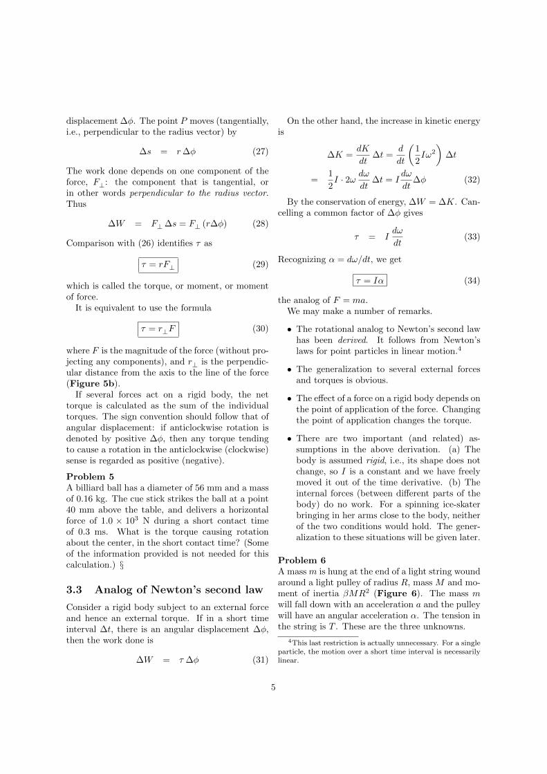
We start the discussion with a simple example.Figure 7a shows a stick AB of negligible weight,with length ` = 0.8 m, pivoted at some point P ,with

AP = r1 , PB = r2 (44)

and r1 + r2 = `. Weights W1 = 5 N and W2 = 3N are applied at the two ends. Where should thepivot be if the stick is in equilibrium?

You have probably learnt that the condition is

W1r1 = W2r2 (45)

which in this case leads to r1 = 0.3 m, r2 = 0.5m. In elementary courses, the condition (45) wouldbe introduced “intuitively” or as an experimental

result. In this Section, we see how such resultsfollow from and fit into the formalism derived.

Incidentally, quantities with one factor of the dis-tance are called moments. The distances ri arecalled moment arms. Thus the equilibrium con-dition is said to be the balance of moments.

4.2 From Newton’s laws

About the pivotFirst, let us choose a sign convention: torques tend-ing to cause rotation in the anticlockwise direction(i.e., in the direction of increasing φ) are taken to bepositive. Then, referring to Figure 7a and imag-ining P to be the axis, we have

τ1 = W1r1 , τ2 = −W2r2 (46)

So the condition (45) is equivalent to saying τ =τ1 + τ2 = 0, which follows simply from the condi-tion that there is no angular acceleration. In otherwords, the condition of balanced moments followsfrom the rotational analog of Newton’s second law— it is not an independent law of physics.

Force due to the pivotBut wait. There is a third force in the problem: thepivot must be exerting an upwards force of magni-tude F = W1 + W2 (Figure 7b). Why can weignore F in the above analysis?

The answer is that we are taking P as the axis;thus the moment arm for this force is zero; it con-tributes zero torque. This is a reason for preferringto take moments about the pivot — we do not needto worry about the unknown force.

Taking another originBut in our derivation of the laws of rotation, wenever said that the axis (or origin) must be thepivot. What if we take the axis to be some arbitrarypoint O a distance c to the left of A (Figure 7c)?Then we have three forces, and three torques, asshown in the following table. The torque in the3rd column is the magnitude, and the sign in the4th column follows the convention described above.

force moment arm torque signW1 c W1c −F c+r1 F (c+r1) +W2 c+r1+r2 W2(c+r1+r2) −

Table 4. Forces and torques; refer to Figure 7c.

7

The net torque is then

τ = −W1c+ F (c+ r1)−W2(c+ r1 + r2)

≡ Ac+B (47)

We leave the rest of the analysis as a Problem.

Problem 10If the net torque is zero for every choice of c, thenwe would have two conditions, namely A = 0 andB = 0. Show that these respectively correspondto (a) the net force being zero, and (b) the nettorque being zero about the pivot. Or turning itaround, given these two conditions, then the nettorque about any point is zero. §

4.3 Directly using work

Let us redo this example, without using the laws ofrotational motion, but directly from the conceptsof work and energy. Suppose the stick is in equilib-rium. Then by adding an infinitesimal force (andhence doing negligible work), we can tilt the stickslightly, so that the points A and B move by ∆s1and ∆s2 (Figure 8). Since the overall work donemust be zero, we have, taking care of signs,

0 = W1∆s1 −W2∆s2

= (W1r1 −W2r2) ∆φ (48)

which directly gives the condition for equilibrium.The beauty of this method is that the ratio of

forces (a question of dynamics) is given in terms ofthe ratio of displacements ∆s1 and ∆s2 — whichis purely a matter of geometry.

4.4 Principle of virtual work*

* This part is not needed for rotations, and can beskipped.

We take this opportunity to discuss the underly-ing idea of the above method more generally, goingbeyond the case of rotations. Since the displace-ments are imagined and not real, they are calledvirtual displacements, and the corresponding workis called the virtual work. The principle of virtualwork states that for a system in equilibrium, thevirtual work due to a virtual displacement is zero.

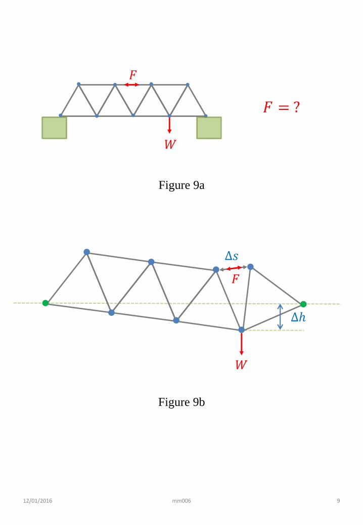
We illustrate the power of this idea by an exam-ple. Figure 9a shows a bridge formed by steel bars

(the lines) freely connected by hinges (the circles).Each bar has the same length `. The bridge itselfhas negligible weight and an external weight W ishung at the point shown. Find the compressiveforce F in the bar shown.

The conventional approach would be as follows.There are 15 bars; let the force in each (compres-sion or tension) be F1, . . . F15. There are two ver-tical forces Y1, Y2 at the two supports and also twohorizontal forces X1, X2. There are 15 + 2 + 2 = 19unknowns. There are 9 hinges. The conditions forthe net force being zero (two components) at eachhinge lead to 18 conditions, which determine the19 variables up to one unknown, namely we canpush with equal and opposite horizontal forces atthe two supports, i.e., X1 7→ X1 +k, X2 7→ X2−k.If we solve this huge algebraic system, we can findall the Fi, including the one of interest. The systembecomes even larger if the bridge has more sections.

Now we can do it another way. Imagine that thebar in question is not rigid. Imagine two relatedvirtual displacements: (a) the weight sinks down byan amount ∆h and (b) the bar in question shrinksby an amount ∆s (Figure 9b). Since the totalwork done must be zero, we have

W ∆h = F ∆s (49)

giving

F

W=

∆h

∆s(50)

Although the RHS still looks complicated, it is apurely geometric problem — which can be solvedby drawing pictures if necessary.

In the displacements that we imagine, most ofthe forces do not do any work. Therefore in theapplication of the principle of virtual work, theseforces do not appear. In a sense, this principle isexactly equivalent to doing the algebra to eliminatereference to these forces.

Appendix

A Verifying the energy

Go back to Problem 7. As the ice skater brings inher arms, decreasing I, ω goes up, and also K. Pre-sumably the increase in K comes from work done in

8

drawing in the arms. Can we check quantitativelythat this is the case?

To do so, consider a model or proxy (Figure10). A mass m is constrained by a string and ro-tates around a circle of radius r on a smooth table.The string goes through a hole in the table, andsomeone exerts a force F on the string, equal tothe centrifugal pseudo force due to the circular mo-tion. Now increase F a tiny bit, to bring the radialmotion to a smaller radius. What is the increase inK?

We can write K in several different ways:

K =1

2Iω2 =

1

2Lω =

L2

2I(51)

The last form is most convenient, because only oneof the factors will vary — L is constant becausethere is no torque. Then

∆K = − L2

2I2∆I

= − (mr2ω)2

2(mr2)2·∆(mr2)

= − (1/2)ω2 ·m (2r∆r)

= −mω2r ·∆r= F ∆r = ∆W (52)

In proceeding to the last line, we have used thefact that F must in magnitude equal the centrifugalpseudo force mω2r, and the minus sign indicatesthat it is radially inwards. This derivation showsthat the increase in the rotational KE is exactlyequal to the work done in drawing the mass in to asmaller radius. (Note ∆r < 0 if the mass is drawninwards.)

B Euler–Lagrange equation*

*This appendix contains material that is intendedonly for those who want an introduction to an ad-vanced topic, much beyond what is normally taughtin Year 1.

The approach taken in this module to derive anequation of motion for φ (a second-order differen-tial equation) is quite general, and can be applied— with one small trick — to many systems, in factleading to the Lagrangian formalism and the Euler–Lagrange (EL) equation. In order to help students

make this connection, a brief sketch is provided fora system with one variable, as an appetizer thatmotivates the proper study of Lagrangian mechan-ics in later courses.

ExampleIn order to illustrate the sort of situations thatmight appear, consider a roller-coaster of mass mmoving freely on a set of rails in the x–y plane (xhorizontal, y vertical). The profile of the rails is(Figure 11)

y = h(x) (53)

This system is described by only one independentvariable, namely x. The KE is

K =1

2m(v2x + v2y

)=

1

2m

[(dx

dt

)2

+

(dy

dx

dx

dt

)2]

=1

2m[1 + h′(x)2]x2

≡ 1

2M(x)x2 (54)

There is an apparently position-dependent mass.This example motivates the assumption that theKE can also depend on the coordinate, but alwaysstays quadratic in the velocity.

Generalized coordinateTo emphasize that the coordinate under considera-tion need not be a Cartesian coordinate, we denoteit as a generalized coordinate q. Based on the moti-vation above, we assume that the KE depends bothon coordinate and its derivative (“velocity”):

K = K(q, q) (55)

Key ideaThe key idea, as in Section 3.3, is to equate theincrease in KE to the work done: ∆K = ∆W . Wenow make the additional assumption that the forcesare conservative, so there is a potential energy

U = U(q) (56)

depending only on the coordinate. Then

d

dt(K + U) = 0 (57)

9

Next we want to write (57) in a different form, re-lying on the fact that K is quadratic in q, for whichwe need the lemma below.

LemmaFor a function f(z) which is homogeneous in itsargument, with order n, i.e., f(z) ∝ zn, then(

zd

dz

)f(z) = nf(z) (58)

which is easily verified.A small digression: This lemma may seem like

using a sledgehammer to crack a nut, but has a use-ful generalization to multiple variables z1, . . . , zK ,in which case the operator to consider is

D ≡∑α

zα∂

∂zα(59)

For example, this operator acting on say

f(z1, z2) = az21 + bz1z2 + cz22 (60)

will just give the overall factor 2.

Re-writing the total energyGiven the above lemma, and the fact that K isquadratic in q, we have

q∂K

∂q= 2K (61)

or

K = q∂K

∂q−K (62)

Putting this into (57), we get

d

dt

(q∂K

∂q−K + U

)= 0 (63)

We make two further changes. First of all, thelast two terms lead us to define

L(q, q) = K − U (64)

Secondly, in the first term we may as well replaceK by L, since the additional piece is ∂U/∂q = 0 —the PE is independent of velocity. Then we get thefollowing equation for the conservation of energy

d

dt

(q∂L

∂q− L

)= 0 (65)

In fact, the quantity in brackets is called the Hamil-tonian of the system.

Equation of motionLet us write out (65) in detail. We have[

q∂L

∂q+d

dt

(∂L

∂q

)q

]−[∂L

∂qq +

∂L

∂qq

]= 0 (66)

where for the first term we have differentiated thetwo factors one at a time, and for the second termwe have use the chain rule:

d

dtf(zj(t)) =

∑j

∂f

∂zj

dzjdt

(67)

for f = L, z1 = q, z2 = q.In (66) the two terms involving q cancel, and q in

the two remaining terms can be factored out, finallygiving the Euler–Lagrange equation of motion:

d

dt

(∂L

∂q

)− ∂L

∂q= 0 (68)

This is a second-order differential equation for q(t).The above arguments can be generalized to manydegrees of freedom.

DiscussionWe make several remarks about the derivation.

• Newton’s second law works only in Cartesiancoordinates, whereas the Euler–Lagrange (EL)equation relies only on energy conservation,and therefore works for generalized coordi-nates. In other words, the EL equation takesthe same form upon an arbitrary (not neces-sarily linear) transformation of coordinates.

• As in the example of the roller coaster, thereare constraint forces (normal to the rails tokeep the carriage on the rails). These forceshave to be included in Newton’s second law.But since they do no work, they are not in-volved in the derivation above using energy,and hence the EL equation can be applied withno regard for constraint forces.

• Without the little trick in (62), we would notbe able to cancel the q terms. This trick mayseem like magic the first time you see it.5

5A more systematic way to understand this trick is as

10

• This trick works only if K is quadratic in thevelocity. What if this condition is not satis-fied? Then the problem goes beyond New-tonian mechanics. But there is some furthermagic. In that case, the starting point (basedon K + U) is no longer valid, but the finalanswer (the EL equation) remains valid, for asuitable choice of L. This is the case for mag-netic forces, for example.

The material in this Appendix goes much beyonda first course in physics. It is included to emphasizeone point only: the approach adopted for treatingrotations is a very general one.

follows. Define p = ∂L/∂q and H(q, q, p) = qp − L. Thenthe rate of change of H contains three terms, including(∂H/∂q)q. So the fact that q does not appear is the sameas the usual one in Lagrangian mechanics that H so definedis independent of q.

11

12/01/2016 mm006 1

𝑦

𝑥

𝜙𝑟

𝑦

𝑥

𝑧

𝜙

Figure 1a

Figure 1b

12/01/2016 mm006 2

𝑟 Δ𝑠

Δ𝜙

Figure 2

12/01/2016 mm006 3

𝑟

𝑣𝜔

Figure 3a

𝑟

𝑟⊥

𝑧

𝑂

𝜔

Figure 3b

𝑚

𝑚

12/01/2016 mm006 4

𝑅

𝛽 =1

3𝛽 =

1

12

𝑅

𝛽 =2

3𝛽 =

2

5

𝛽 = 1 𝛽 =1

2

Figure 4a Figure 4b

Figure 4c Figure 4d

Figure 4e Figure 4f

𝑅 𝑅

𝑅 𝑅

Δ𝜙

12/01/2016 mm006 5

𝑟

Δ𝑠

𝐹𝐹⊥

𝑃

𝑟

𝑃𝑟

𝐹

𝐹⊥

𝑂

𝑃𝑟

𝐹

𝑂𝑟⊥

Figure 5a

Figure 5b

12/01/2016 mm006 6

𝑚

𝑅𝑀

𝑇

𝑎

𝛼

Figure 6

𝐼 = 𝛽𝑀𝑅2

12/01/2016 mm006 7

𝐴 𝐵𝑃

𝑟1 𝑟2

0.8 m

𝑊2 = 3 N𝑊1 = 5 N

Figure 7a

Figure 7b

𝐹

𝑊2𝑊1

𝑟1 𝑟2

𝑊2𝑊1

𝐹

𝑂

𝑐

Figure 7c

12/01/2016 mm006 8

Δ𝑠1

Δ𝑠2

𝑊1

𝑊2

Figure 8

12/01/2016 mm006 9

𝐹

𝑊

𝐹 = ?

Figure 9a

Figure 9b

Δ𝑠

𝑊

𝐹

Δℎ

12/01/2016 mm006 10

𝐹

𝑟

Figure 10

12/01/2016 mm006 11

𝑥

𝑦

𝑦 = ℎ(𝑥)

𝑚

Figure 11