
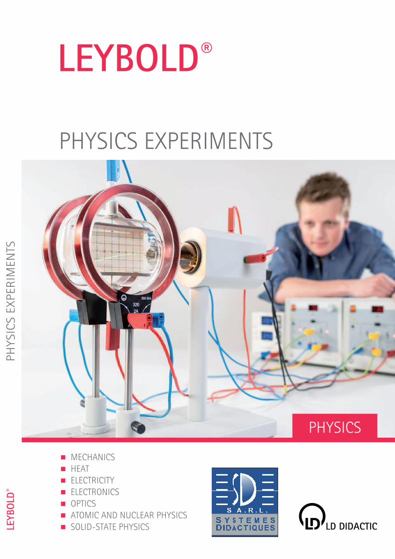
PHYSICS EXPERIMENTS
324
PHYSICS EXPERIMENTS PHYSICS EXPERIMENTS PHYSICS MECHANICS HEAT ELECTRICITY ELECTRONICS OPTICS ATOMIC AND NUCLEAR PHYSICS SOLID-STATE PHYSICS
-
Upload
khangminh22 -
Category
Documents
-
view
0 -
download
0
Transcript of PHYSICS EXPERIMENTS
PHYSICS EXPERIMENTS
PH
YS
ICS
EX
PER
IMEN
TS
PHYSICS
MECHANICS
HEAT
ELECTRICITY
ELECTRONICS
OPTICS
ATOMIC AND NUCLEAR PHYSICS
SOLID-STATE PHYSICS
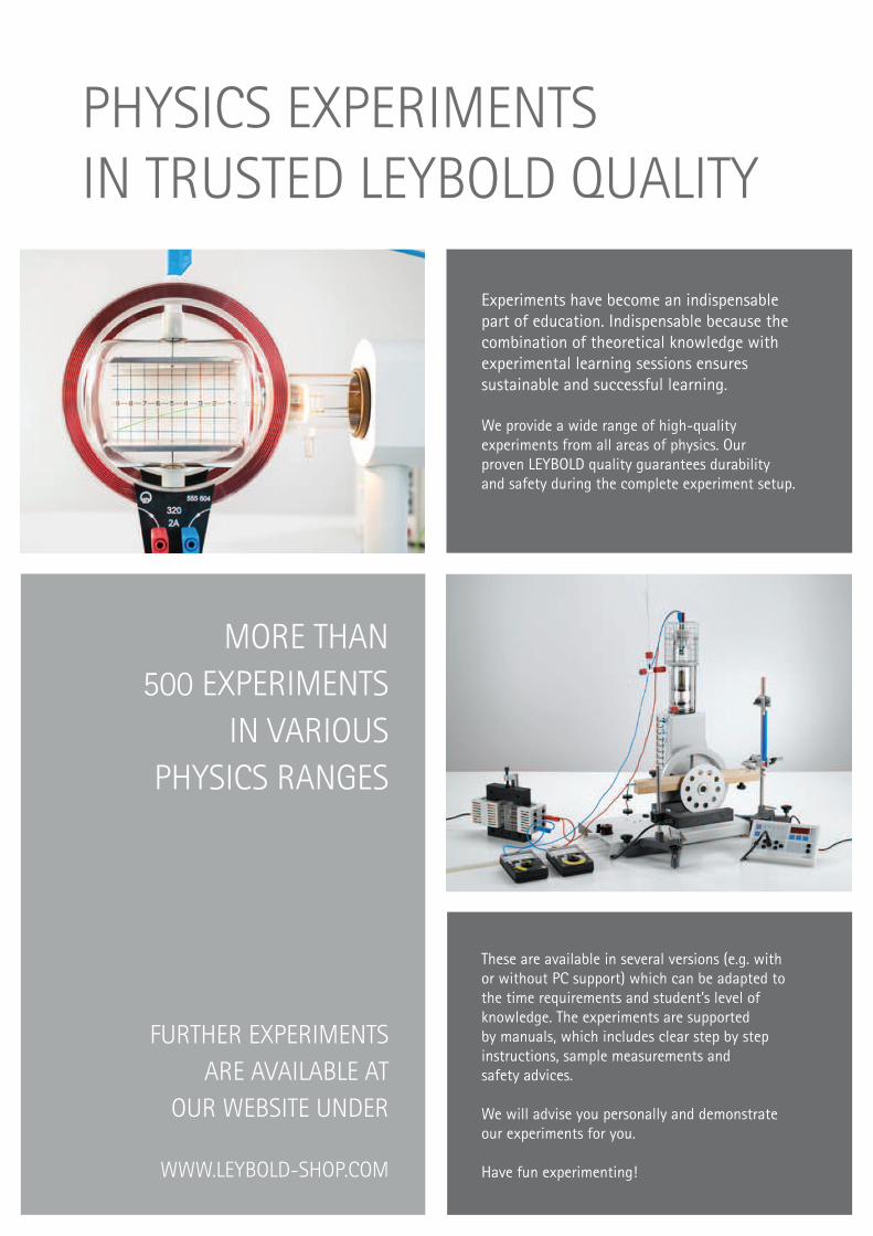
PHYSICS EXPERIMENTS
IN TRUSTED LEYBOLD QUALITY
MORE THAN
500 EXPERIMENTS
IN VARIOUS
PHYSICS RANGES
FURTHER EXPERIMENTS
ARE AVAILABLE AT
OUR WEBSITE UNDER
WWW.LEYBOLD-SHOP.COM
Experiments have become an indispensable part of education. Indispensable because the combination of theoretical knowledge with experimental learning sessions ensures sustainable and successful learning.
We provide a wide range of high-quality experiments from all areas of physics. Our proven LEYBOLD quality guarantees durability and safety during the complete experiment setup.
These are available in several versions (e.g. with or without PC support) which can be adapted to the time requirements and student’s level of knowledge. The experiments are supported by manuals, which includes clear step by step instructions, sample measurements and safety advices.
We will advise you personally and demonstrate our experiments for you.
Have fun experimenting!
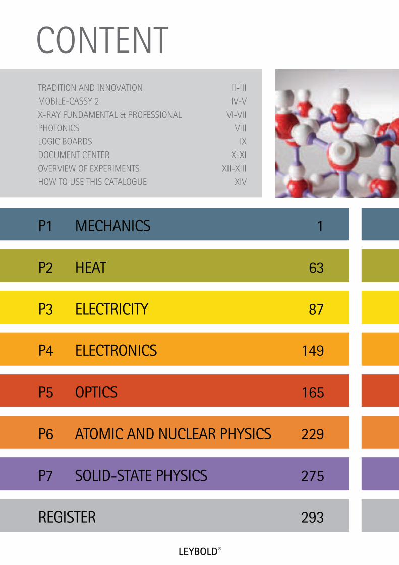
CONTENT
TRADITION AND INNOVATION II-III
MOBILE-CASSY 2 IV-V
X-RAY FUNDAMENTAL & PROFESSIONAL VI-VII
PHOTONICS VIII
LOGIC BOARDS IX
DOCUMENT CENTER X-XI
OVERVIEW OF EXPERIMENTS XII-XIII
HOW TO USE THIS CATALOGUE XIV
P1 MECHANICS 1
P2 HEAT 63
P3 ELECTRICITY 87
P4 ELECTRONICS 149
P5 OPTICS 165
P6 ATOMIC AND NUCLEAR PHYSICS 229
P7 SOLID-STATE PHYSICS 275
REGISTER 293

II WWW.LEYBOLD-SHOP.COM
The LD DIDACTIC Group is a
world-leading manufacturer of
high-quality scientific and technical
training systems.
Our teaching systems have been making a
decisive contribution to the transfer of
knowledge in schools, further education
colleges and universities, and also in the
industrial sector, for generations.
Founded in 1850 in Cologne, LD DIDACTIC
can look back on 160 years of company
history. This former subsidiary of LEYBOLD,
a Cologne company of long-standing
tradition, sees itself as an innovative
supplier of quality products and sells
these products and complete solutions
under the brand names LEYBOLD,
ELWE Technik and FEEDBACK.
Our many years of experience and our
innovative technical potential combined
with the close cooperation with teachers
and trainers from the relevant fields enable
us to offer targeted solution to our customers
and at the same time make complex topics
in biology, chemistry, physics and technology
transparent for the student.
TRADITION AND INNOVATIONEXPERIMENTS FOR STUDENT PRACTICALS AND
DEMONSTRATIONS FOR MORE THAN 160 YEARS
1898
1973
2004
1991
2014
DEMO-MULTIMETER
DEMO-MULTIMETER
III
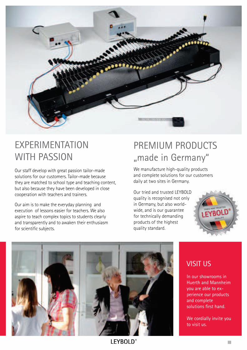
EXPERIMENTATION
WITH PASSION
Our staff develop with great passion tailor-made
solutions for our customers. Tailor-made because
they are matched to school type and teaching content,
but also because they have been developed in close
cooperation with teachers and trainers.
Our aim is to make the everyday planning and
execution of lessons easier for teachers. We also
aspire to teach complex topics to students clearly
and transparently and to awaken their enthusiasm
for scientific subjects.
PREMIUM PRODUCTS
„made in Germany“ We manufacture high-quality products
and complete solutions for our customers
daily at two sites in Germany.
Our tried and trusted LEYBOLD
quality is recognised not only
in Germany, but also world-
wide, and is our guarantee
for technically demanding
products of the highest
quality standard.
D
VISIT US
In our showrooms in
Huerth and Mannheim
you are able to ex-
perience our products
and complete
solutions first hand.
We cordially invite you
to visit us.
IV
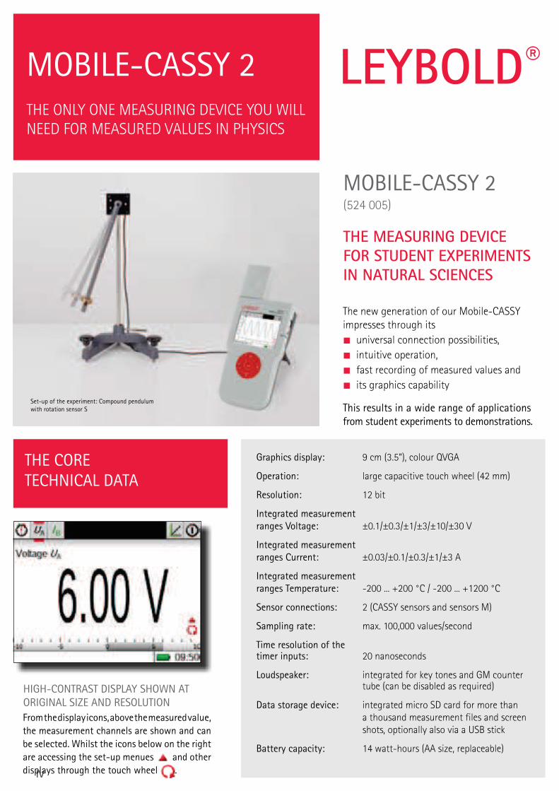
MOBILE-CASSY 2 (524 005)
THE MEASURING DEVICE
FOR STUDENT EXPERIMENTS
IN NATURAL SCIENCES
MOBILE-CASSY 2
THE ONLY ONE MEASURING DEVICE YOU WILL NEED FOR MEASURED VALUES IN PHYSICS
The new generation of our Mobile-CASSY impresses through its
universal connection possibilities,
intuitive operation,
fast recording of measured values and
its graphics capability
This results in a wide range of applications
from student experiments to demonstrations.
From the display icons, above the measured value,
the measurement channels are shown and can
be selected. Whilst the icons below on the right
are accessing the set-up menues and other
displays through the touch wheel .
Graphics display: 9 cm (3.5“), colour QVGA
Operation: large capacitive touch wheel (42 mm)
Resolution: 12 bit
Integrated measurement
ranges Voltage: ±0.1/±0.3/±1/±3/±10/±30 V
Integrated measurement
ranges Current: ±0.03/±0.1/±0.3/±1/±3 A
Integrated measurement
ranges Temperature: -200 ... +200 °C / -200 ... +1200 °C
Sensor connections: 2 (CASSY sensors and sensors M)
Sampling rate: max. 100,000 values/second
Time resolution of the timer inputs: 20 nanoseconds
Loudspeaker: integrated for key tones and GM counter tube (can be disabled as required)
Data storage device: integrated micro SD card for more than a thousand measurement files and screen shots, optionally also via a USB stick
Battery capacity: 14 watt-hours (AA size, replaceable)
Set-up of the experiment: Compound pendulum
with rotation sensor S
THE CORE
TECHNICAL DATA
HIGH-CONTRAST DISPLAY SHOWN AT
ORIGINAL SIZE AND RESOLUTION
V
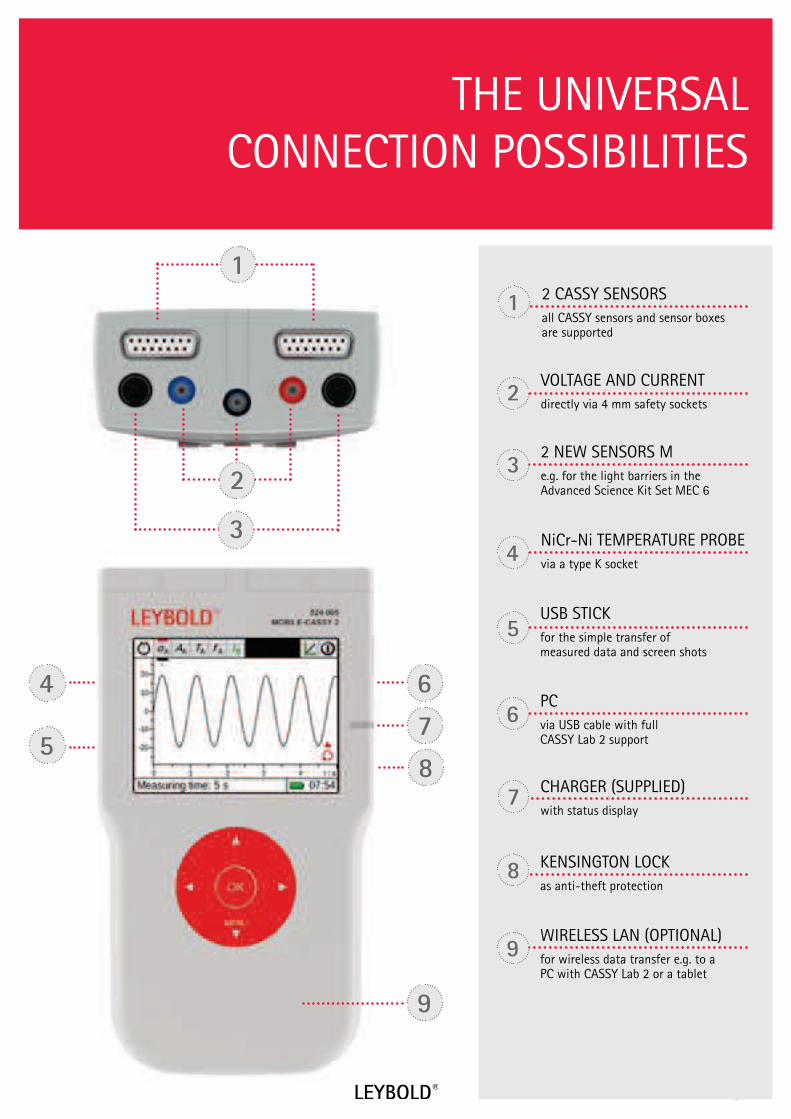
THE UNIVERSAL CONNECTION POSSIBILITIES
2 CASSY SENSORS
all CASSY sensors and sensor boxes are supported
1
NiCr-Ni TEMPERATURE PROBE
via a type K socket4
USB STICK
for the simple transfer of measured data and screen shots
5
PC
via USB cable with full CASSY Lab 2 support
6
1
2
VOLTAGE AND CURRENT
directly via 4 mm safety sockets2
2 NEW SENSORS M
e.g. for the light barriers in the Advanced Science Kit Set MEC 6
3
KENSINGTON LOCK
as anti-theft protection 8
WIRELESS LAN (OPTIONAL)
for wireless data transfer e.g. to a PC with CASSY Lab 2 or a tablet
9
4
9
5
6
7
8CHARGER (SUPPLIED)
with status display7
3

VI
FOR EVERY REQUIREMENT AND EVERY BUDGET
BASICEQUIPMENT
The LEYBOLD X-ray system has a modular structure and enables the individual
configuration of the separate appliances, so that you only buy what you actually need.
In addition to the basic equipment, you can choose your accessories for basic experiments
(FUNDAMENTAL Experiments) or advanced applications (PROFESSIONAL Experiments)
depending on the experiment requirements.
X-RAY APPARATUS
The X-ray apparatus is available in two
variants - as a basic apparatus or as a
complete apparatus with a Mo tube,
goniometer and NaCl monocrystal. If you
wish to use other tubes, the X-ray basic
apparatus is the most flexible solution.
You can extend the X-ray apparatus with
a drawer for your accessories irrespective
of this.
TUBES
In addition to the Mo tube, there are
other tubes, which are more suitable for
special areas of application, e.g. Cu tube
for Debye-Scherrer diagrams, Ag tube for
X-ray fluorescence due to its high
energy K-lines, W or Au tubes for
radiation and computed tomography
due to their high intensity.
Goniometer
No matter whether you are
interested in Bragg spectra,
X-ray energy spectra or computed
tomography, you will be happy
with the precision and high
resolution of the goniometer.
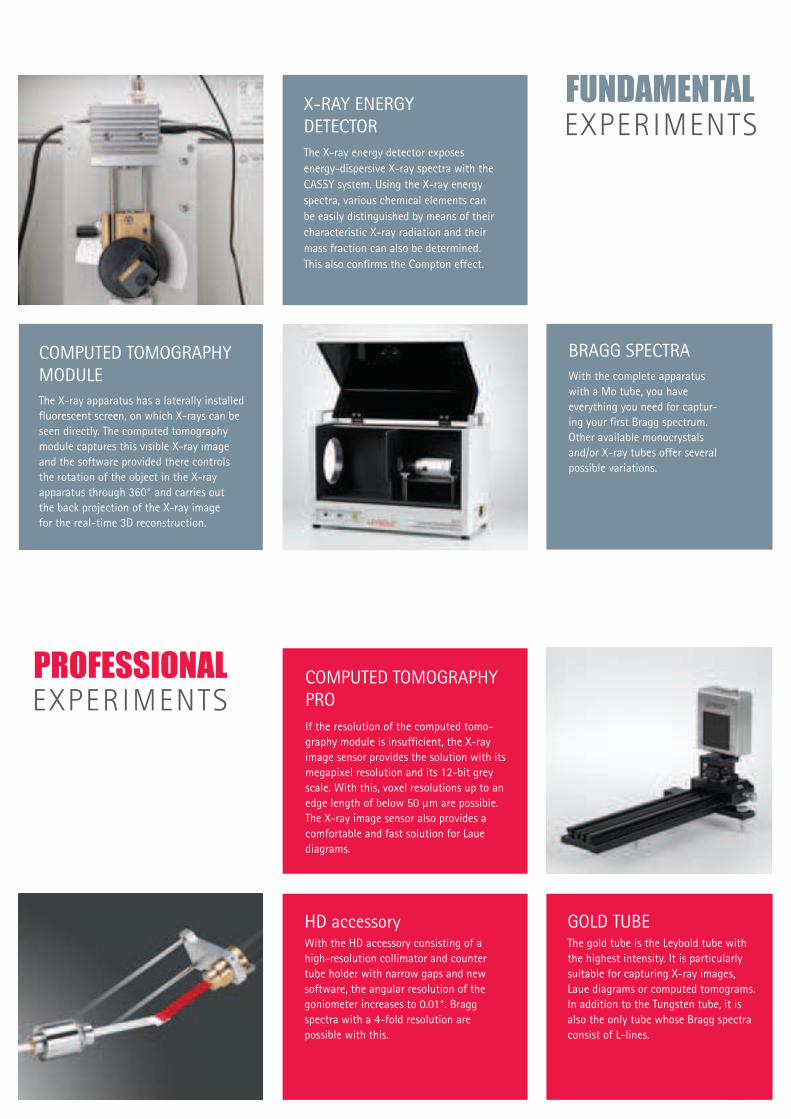
VII
HD accessory
With the HD accessory consisting of a
high-resolution collimator and counter
tube holder with narrow gaps and new
software, the angular resolution of the
goniometer increases to 0.01°. Bragg
spectra with a 4-fold resolution are
possible with this.
COMPUTED TOMOGRAPHY PRO
If the resolution of the computed tomo-
graphy module is insufficient, the X-ray
image sensor provides the solution with its
megapixel resolution and its 12-bit grey
scale. With this, voxel resolutions up to an
edge length of below 50 µm are possible.
The X-ray image sensor also provides a
comfortable and fast solution for Laue
diagrams.
GOLD TUBEThe gold tube is the Leybold tube with
the highest intensity. It is particularly
suitable for capturing X-ray images,
Laue diagrams or computed tomograms.
In addition to the Tungsten tube, it is
also the only tube whose Bragg spectra
consist of L-lines.
X-RAY ENERGY DETECTOR
The X-ray energy detector exposes
energy-dispersive X-ray spectra with the
CASSY system. Using the X-ray energy
spectra, various chemical elements can
be easily distinguished by means of their
characteristic X-ray radiation and their
mass fraction can also be determined.
This also confirms the Compton effect.
COMPUTED TOMOGRAPHY MODULE
The X-ray apparatus has a laterally installed
fluorescent screen, on which X-rays can be
seen directly. The computed tomography
module captures this visible X-ray image
and the software provided there controls
the rotation of the object in the X-ray
apparatus through 360° and carries out
the back projection of the X-ray image
for the real-time 3D reconstruction.
BRAGG SPECTRA
With the complete apparatus
with a Mo tube, you have
everything you need for captur-
ing your first Bragg spectrum.
Other available monocrystals
and/or X-ray tubes offer several
possible variations.
VIII WWW.LEYBOLD-SHOP.COM
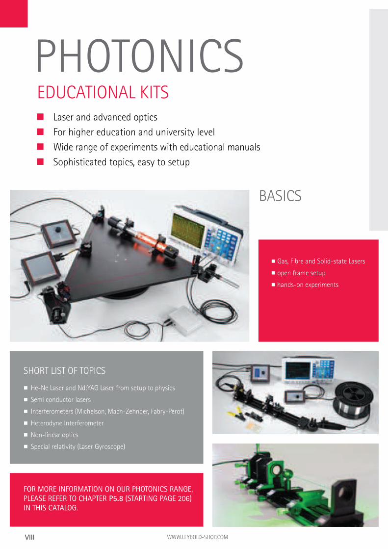
Laser and advanced optics
For higher education and university level
Wide range of experiments with educational manuals
Sophisticated topics, easy to setup
PHOTONICSEDUCATIONAL KITS
BASICS
Gas, Fibre and Solid-state Lasers
open frame setup
hands-on experiments
SHORT LIST OF TOPICS
He-Ne Laser and Nd:YAG Laser from setup to physics
Semi conductor lasers
Interferometers (Michelson, Mach-Zehnder, Fabry-Perot)
Heterodyne Interferometer
Non-linear optics
Special relativity (Laser Gyroscope)
FOR MORE INFORMATION ON OUR PHOTONICS RANGE,
PLEASE REFER TO CHAPTER P5.8 (STARTING PAGE 206)
IN THIS CATALOG.

IX
LOGIC BOARDS
LOGIC BOARD 1 (571 401)
Introducing the basic logic gates (AND, OR, NOT, NAND, XOR) used in digital electronics. These are used to investigate the laws of logical operations (de Morgan’s law, associative law and distributive law) and non-feedback logic circuits (switch networks). Finally simple flip-flop circuits with feedback are assembled to study storage of information.
Switch states are indicated by means of an LED at each output.
GATES: AND OR NOT NAND XOR
FLIP-FLOPS: RS-flip-flop D-flip-flop RC module for construction of a multivibrator
LOGIC BOARD 2 (571 402)
The second board is used for advanced topics. The adders are investigated as practical examples of combinatorical logic (logic circuits without feedback). Various flip-flop circuits add students’ knowledge on circuits with feedback like shift registers or latches. Applications of digital tech-nology will be investigated, e.g. multiplexing, demultiplex-ing and the topics of digital-to analogue and analogue-to-digital conversion are covered.
GATES: NOT NAND
FLIP-FLOPS: RS-flip-flop D-flip-flop
ADDITIONAL: RC module for construction of a multivibrator Adders AD converter/DA converter 7 segment display
FOR MORE INFORMATION ON OUR LOGIC BOARDS, PLEASE REFER TO CHAPTER P4.5.1 TO 4.5.3 IN THIS CATALOG.
THE ENTRY INTO THE DIGITAL ELECTRONICS!

X
DIE ELEKTRONISCHE
LEYBOLD-BIBLIOTHEK
Anzeige und Verwaltung von Schülerversuchslitera-
tur,
Anleitungen für Demonstrationsversuche
oder Gebrauchsanweisungen in einem Programm
Automatische Aktualisierung aller Dokumente durch
kostenlose Online-Updates
Komfortable fehlertolerante Schlagwort- und
Katalognummernsuche
EXPERIMENT INSTRUCTIONS
THE DOCUMENT CENTER IS
THE ELECTRONIC LEYBOLD
LIBRARY
For information on experiments
for students and demonstration experiments
For operation manuals DOWNLOAD THE
DOCUMENT CENTER
FREE OF CHARGE:
WWW.LD-DIDACTIC.COM

XI
THE DOCUMENT CENTER OFFERS
Leaflets (demonstration instructions) with link to CASSY LAB 2 and Spektralab
Experiments for students as interactive pdf files:
Easy-to-understand worksheets for students
Complete information with experiment results for teachers
Ability to go from student to teacher version and back with one mouse click
Student documents can be filled out on the computer and stored or printed out as a protocol
Sorted into literature packages – facilitates and encourages the compilation of own test series
Free-of-charge online update of literature packages following initial acquisition
HOW DOES IT WORK?The literature packages are clearly displayed in a table of contents, which is structured to guide you to the document you need. The more literature packages you have installed, the more entries are listed in the table of contents. Once the system has been installed, the documents can be set to update automatically if desired.
The convenient, fault-tolerant search function helps you find the right document rapidly.
Student version with typewriter tool for filling out protocols on the computer
Teacher version with an example of the solution and notes about the experiments
IN THE DOCUMENT CENTER
XII WWW.LEYBOLD-SHOP.COM
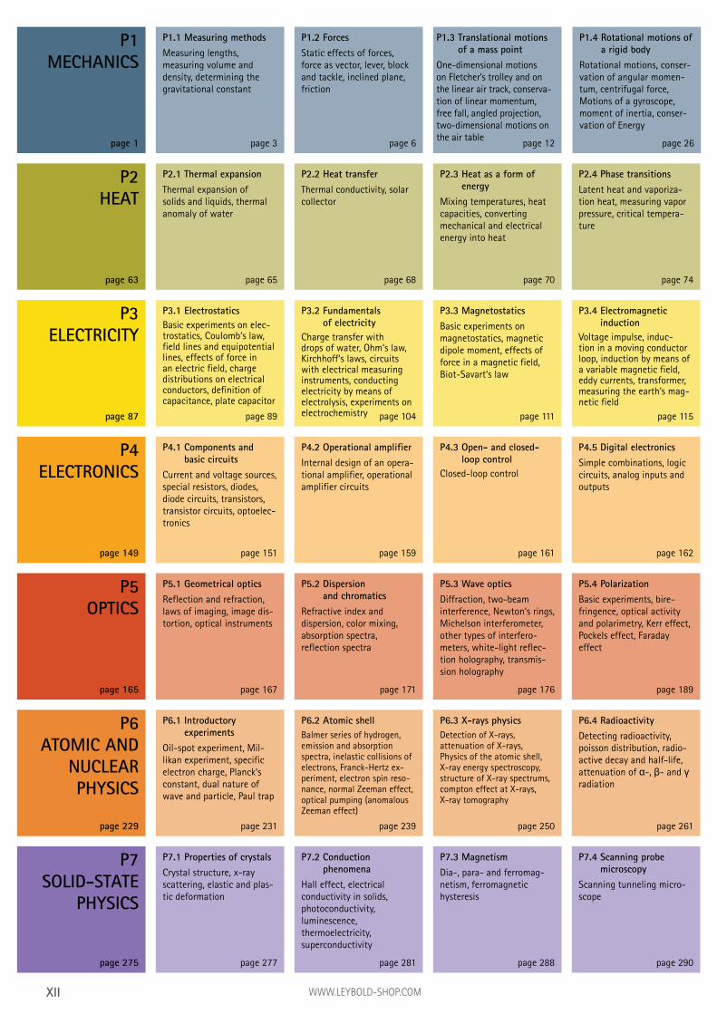
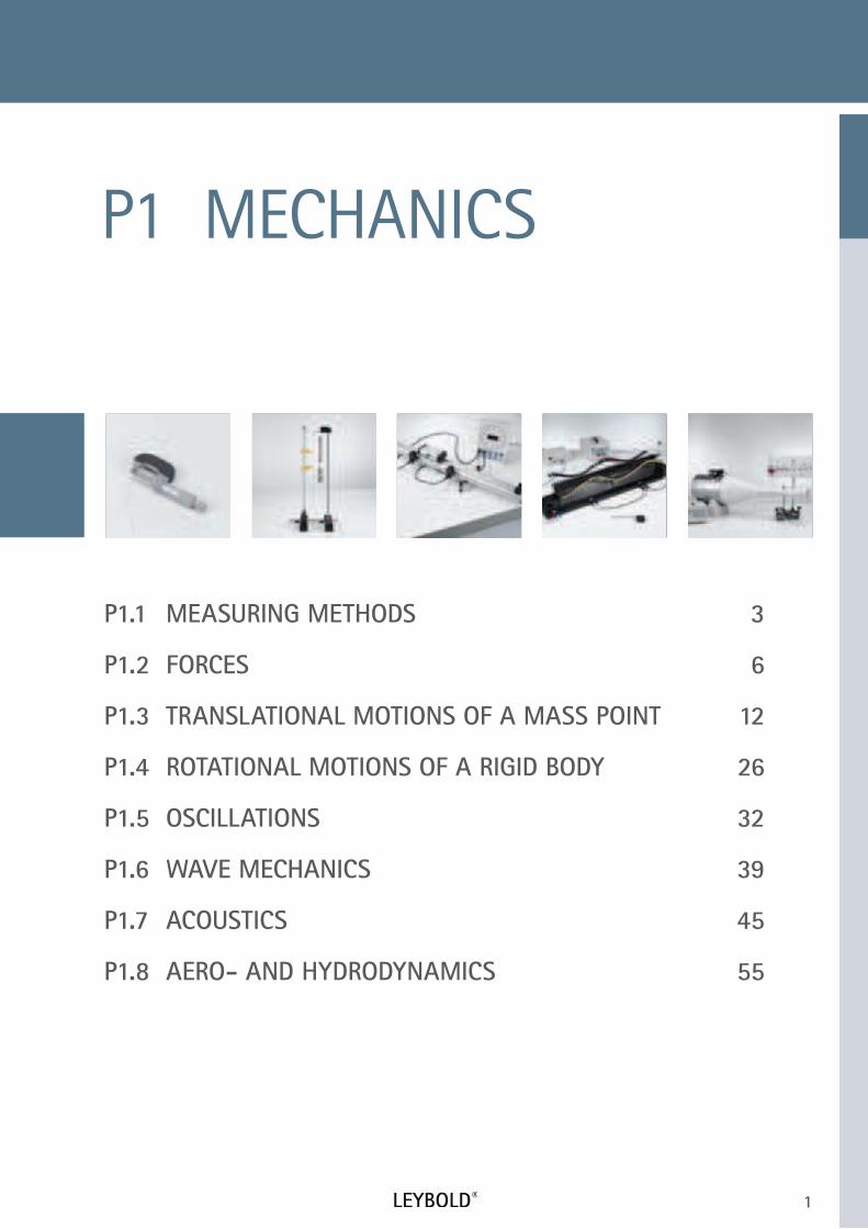
P1
MECHANICS
page 1
P1.1 Measuring methods
Measuring lengths,measuring volume and density, determining the gravitational constant
page 3
P1.2 Forces
Static effects of forces, force as vector, lever, block and tackle, inclined plane, friction
page 6
P1.4 Rotational motions of
a rigid body
Rotational motions, conser-vation of angular momen-tum, centrifugal force, Motions of a gyroscope, moment of inertia, conser-vation of Energy
page 26page 12
P2
HEAT
page 63
P2.1 Thermal expansion
Thermal expansion of solids and liquids, thermal anomaly of water
page 65
P2.2 Heat transfer
Thermal conductivity, solar collector
page 68
P2.4 Phase transitions
Latent heat and vaporiza-tion heat, measuring vapor pressure, critical tempera-ture
page 74
P2.3 Heat as a form of
energy
Mixing temperatures, heat capacities, converting mechanical and electrical energy into heat
page 70
P3
ELECTRICITY
page 87
P3.1 Electrostatics
Basic experiments on elec-trostatics, Coulomb‘s law, field lines and equipotential lines, effects of force in an electric field, charge distributions on electrical conductors, definition of capacitance, plate capacitor
page 89
P3.2 Fundamentals
of electricity
Charge transfer with drops of water, Ohm‘s law, Kirchhoff‘s laws, circuits with electrical measuring instruments, conducting electricity by means of electrolysis, experiments on electrochemistry page 104
P3.4 Electromagnetic
induction
Voltage impulse, induc-tion in a moving conductor loop, induction by means of a variable magnetic field, eddy currents, transformer, measuring the earth’s mag-netic field
page 115
P3.3 Magnetostatics
Basic experiments on magnetostatics, magnetic dipole moment, effects of force in a magnetic field, Biot-Savart‘s law
page 111
P4
ELECTRONICS
page 149
P4.1 Components and
basic circuits
Current and voltage sources, special resistors, diodes, diode circuits, transistors, transistor circuits, optoelec-tronics
page 151
P4.2 Operational amplifier
Internal design of an opera-tional amplifier, operational amplifier circuits
page 159
P4.3 Open- and closed-
loop control
Closed-loop control
page 161
P5
OPTICS
page 165
P5.1 Geometrical optics
Reflection and refraction, laws of imaging, image dis-tortion, optical instruments
page 167
P5.2 Dispersion
and chromatics
Refractive index and dispersion, color mixing, absorption spectra, reflection spectra
page 171
P5.4 Polarization
Basic experiments, bire-fringence, optical activity and polarimetry, Kerr effect, Pockels effect, Faraday effect
page 189
P5.3 Wave optics
Diffraction, two-beam interference, Newton‘s rings, Michelson interferometer, other types of interfero- meters, white-light reflec-tion holography, transmis-sion holography
page 176
P6
ATOMIC AND
NUCLEAR
PHYSICS
page 229
P6.1 Introductory
experiments
Oil-spot experiment, Mil-likan experiment, specific electron charge, Planck‘s constant, dual nature of wave and particle, Paul trap
page 231
P6.2 Atomic shell
Balmer series of hydrogen, emission and absorption spectra, inelastic collisions of electrons, Franck-Hertz ex-periment, electron spin reso-nance, normal Zeeman effect, optical pumping (anomalous Zeeman effect)
page 239
P6.4 Radioactivity
Detecting radioactivity, poisson distribution, radio-active decay and half-life, attenuation of -, - and radiation
page 261
P6.3 X-rays physics
Detection of X-rays, attenuation of X-rays, Physics of the atomic shell, X-ray energy spectroscopy, structure of X-ray spectrums, compton effect at X-rays, X-ray tomography
page 250
P7
SOLID-STATE
PHYSICS
page 275
P7.1 Properties of crystals
Crystal structure, x-ray scattering, elastic and plas-tic deformation
page 277
P7.2 Conduction
phenomena
Hall effect, electrical conductivity in solids, photoconductivity, luminescence, thermoelectricity, superconductivity
page 281
P7.4 Scanning probe
microscopy
Scanning tunneling micro-scope
page 290
P7.3 Magnetism
Dia-, para- and ferromag-netism, ferromagnetic hysteresis
page 288
P1.3 Translational motions
of a mass point
One-dimensional motions on Fletcher’s trolley and on the linear air track, conserva-tion of linear momentum, free fall, angled projection, two-dimensional motions on the air table
P4.5 Digital electronics
Simple combinations, logic circuits, analog inputs and outputs
page 162

XIII
P1.5 Oscillations
Simple and compound pendulum, harmonic oscil-lations, torsion pendulum, coupling of oscillations
page 32
P1.6 Wave mechanics
Transversal and longitudi-nal waves, wave machine, circularly polarized waves, propagation of water waves, interference of water waves, resonances
page 39
P1.7 Acoustics
Sound waves, oscillations of a string, wavelength and velocity of sound, reflection of ultrasonic waves, inter-ference of ultrasonic waves, Acoustic Doppler effect, fourier analysis, ultrasound in media
page 45
P1.8 Aero- and
hydrodynamics
Barometric measurements, bouyancy, viscosity, surface tension, introductory experiments on aerodynam-ics, measuring air resistance, measurements in a wind tunnel
page 55
P2.5 Kinetic theory
of gases
Brownian motion of mol-ecules, gas laws, specific heat of gases, real gases
page 77
P2.6 Thermodynamic cycle
Hot-air engine: qualitative and quantitative experi-ments, heat pump
page 81
P3.5 Electrical machines
Basic experiments on electrical machines, electric generators, electric motors, three-phase machines
page 122
P5.5 Light intensity
Quantities and measuring methods of lighting engi-neering, laws of radiation
page 195
P6.5 Nuclear physics
Demonstrating paths of particles, Rutherford scat-tering, Nuclear magnetic resonance, spectroscopy, spectroscopy, Compton ef-
fect, properties of radiation particles
page 265
P7.5 Applied solid-state
physics
X-ray fluorescence analysis
page 292
P.6.6 Quantum physics
Quantum optics, particles
page 272
P5.6 Velocity of light
Measurement according to Foucault/Michelson, measuring with short light pulses, measuring with an electronically modulated signal
page 198
P5.7 Spectrometer
Prism spectrometer, grating spectrometer
page 202
P5.8 Photonics
Basic Optics, optical appli-cations, optical imaging and colour, laser basics, solid state laser, optical fibres, technical applications
page 206
P3.6 DC and AC circuits
Circuit with capacitor, cir-cuit with coil, impedances, measuring-bridge circuits, measuring AC voltages and AC currents, electrical work and power, electromechani-cal devices
page 126
P3.7 Electromagnetic oscil-
lations and waves
Electromagnetic oscillator cir-cuit, decimeter-range waves, propagation of decimeter-range waves along lines, microwaves, propagation of microwaves along lines, directional characteristic of dipole radiation page134
P3.9 Electrical
conduction in gases
Spontaneous and non-spontaneous discharge, gas discharge at reduced pressure, cathode rays and canal rays
page 145
P3.8 Free charge
carriers in a vacuum
Tube diode, tube triode, Maltese-cross tube, Perrin tube, Thomson tube
page 140
XIV WWW.LEYBOLD-SHOP.COM
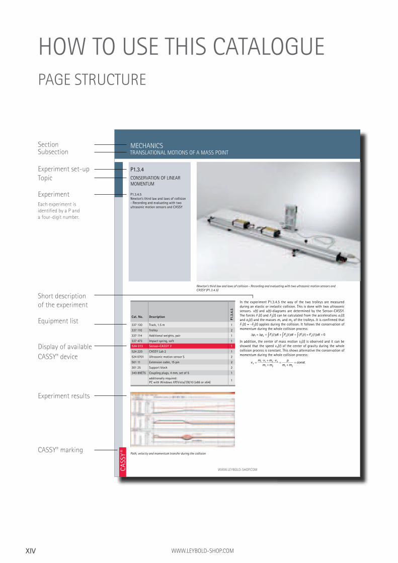
HOW TO USE THIS CATALOGUE
PAGE STRUCTURE
SectionSubsection
Topic
Experiment
Each experiment is
identified by a P and
a four-digit number.
Short description
of the experiment
Equipment list
Experiment set-up
Experiment results
20 WWW.LEYBOLD-SHOP.COMCA
SSY ®
CONSERVATION OF LINEAR
MOMENTUM
P1.3.4.5 Newton‘s third law and laws of collision - Recording and evaluating with two ultrasonic motion sensors and CASSY
In the experiment P1.3.4.5 the way of the two trolleys are measured during an elastic or inelastic collision. This is done with two ultrasonic sensors. v(t) and a(t)-diagrams are determined by the Sensor-CASSY. The forces F1(t) and F2(t) can be calculated from the accelerations a1(t) and a2(t) and the masses m1 and m2 of the trolleys. It is confirmed that F1(t) = -F2(t) applies during the collision. It follows the conservation of momentum during the whole collision process:
∆ ∆p p F t dt F t dt F t F t dt1 2 1 2 1 2 0+ = + = + =∫ ∫ ∫( ) ( ) ( ( ) ( ))
In addition, the center of mass motion s3(t) is observed and it can be showed that the speed v3(t) of the center of gravity during the whole collision process is constant. This shows alternative the conservation of momentum during the whole collision process:
vm v m v
m m
p
m mconst
3
1 1 2 2
1 2 1 2
=⋅ + ⋅
+=
+= .
MECHANICS
Newton‘s third law and laws of collision - Recording and evaluating with two ultrasonic motion sensors and
CASSY (P1.3.4.5)
Cat. No. Description
P1.3
.4.5
337 130 Track, 1.5 m 1
337 110 Trolley 2
337 114 Additional weights, pair 1
337 473 Impact spring, soft 1
524 013 Sensor-CASSY 2 1
524 220 CASSY Lab 2 1
524 0701 Ultrasonic motion sensor S 2
501 11 Extension cable, 15 pin 2
301 25 Support block 2
340 89ET5 Coupling plugs, 4 mm, set of 5 1
additionally required: PC with Windows XP/Vista/7/8/10 (x86 or x64)
1
Path, velocity and momentum transfer during the collision
TRANSLATIONAL MOTIONS OF A MASS POINT
P1.3.4
CASSY® marking
Display of available
CASSY® device
1
P1.1 MEASURING METHODS 3
P1.2 FORCES 6
P1.3 TRANSLATIONAL MOTIONS OF A MASS POINT 12
P1.4 ROTATIONAL MOTIONS OF A RIGID BODY 26
P1.5 OSCILLATIONS 32
P1.6 WAVE MECHANICS 39
P1.7 ACOUSTICS 45
P1.8 AERO- AND HYDRODYNAMICS 55
P1 MECHANICS
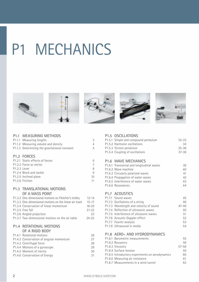
2 WWW.LEYBOLD-SHOP.COM
P1.1 MEASURING METHODS
P1.1.1 Measuring lengths 3
P1.1.2 Measuring volume and density 4
P1.1.3 Determining the gravitational constant 5
P1.2 FORCES
P1.2.1 Static effects of forces 6
P1.2.2 Force as vector 7
P1.2.3 Lever 8
P1.2.4 Block and tackle 9
P1.2.5 Inclined plane 10
P1.2.6 Friction 11
P1.3 TRANSLATIONAL MOTIONS
OF A MASS POINT
P1.3.2 One-dimensional motions on Fletcher’s trolley 12-14
P1.3.3 One-dimensional motions on the linear air track 15-17
P1.3.4 Conservation of linear momentum 18-20
P1.3.5 Free fall 21-22
P1.3.6 Angled projection 23
P1.3.7 Two-dimensional motions on the air table 24-25
P1.4 ROTATIONAL MOTIONS
OF A RIGID BODY
P1.4.1 Rotational motions 26
P1.4.2 Conservation of angular momentum 27
P1.4.3 Centrifugal force 28
P1.4.4 Motions of a gyroscope 29
P1.4.5 Moment of inertia 30
P1.4.6 Conservation of Energy 31
P1.5 OSCILLATIONS
P1.5.1 Simple and compound pendulum 32-33
P1.5.2 Harmonic oscillations 34
P1.5.3 Torsion pendulum 35-36
P1.5.4 Coupling of oscillations 37-38
P1.6 WAVE MECHANICS
P1.6.1 Transversal and longitudinal waves 39
P1.6.2 Wave machine 40
P1.6.3 Circularly polarized waves 41
P1.6.4 Propagation of water waves 42
P1.6.5 Interference of water waves 43
P1.6.6 Resonances 44
P1.7 ACOUSTICS
P1.7.1 Sound waves 45
P1.7.2 Oscillations of a string 46
P1.7.3 Wavelength and velocity of sound 47-49
P1.7.4 Reflection of ultrasonic waves 50
P1.7.5 Interference of ultrasonic waves 51
P1.7.6 Acoustic Doppler effect 52
P1.7.7 Fourier analysis 53
P1.7.8 Ultrasound in media 54
P1.8 AERO- AND HYDRODYNAMICS
P1.8.1 Barometric measurements 55
P1.8.2 Bouyancy 56
P1.8.3 Viscosity 57-58
P1.8.4 Surface tension 59
P1.8.5 Introductory experiments on aerodynamics 60
P1.8.6 Measuring air resistance 61
P1.8.7 Measurements in a wind tunnel 62
P1 MECHANICS
3
MEASURING LENGTHS
P1.1.1.1 Using a caliper gauge with vernier
P1.1.1.2 Using a micrometer screw
P1.1.1.3 Using a spherometer to determine bending radii
MEASURING METHODS
MECHANICS
Cat. No. Description
P1.1
.1.1
P1.1
.1.2
P1.1
.1.3
311 54 Precision vernier callipers 1
311 83 Precision micrometer 1
550 35 Copper resistance wire, 0.2 mm diam., 100 m 1
550 39 Brass resistance wire, 0.5 mm diameter, 50 m 1
311 86 Spherometer 1
460 291 Plane mirror, 11.5 cm x 10 cm 1
662 092 Cover slips 1
664 154 Watch glass dish, 80 mm diam. 1
664 157 Watch glass dish, 125 mm diam. 1
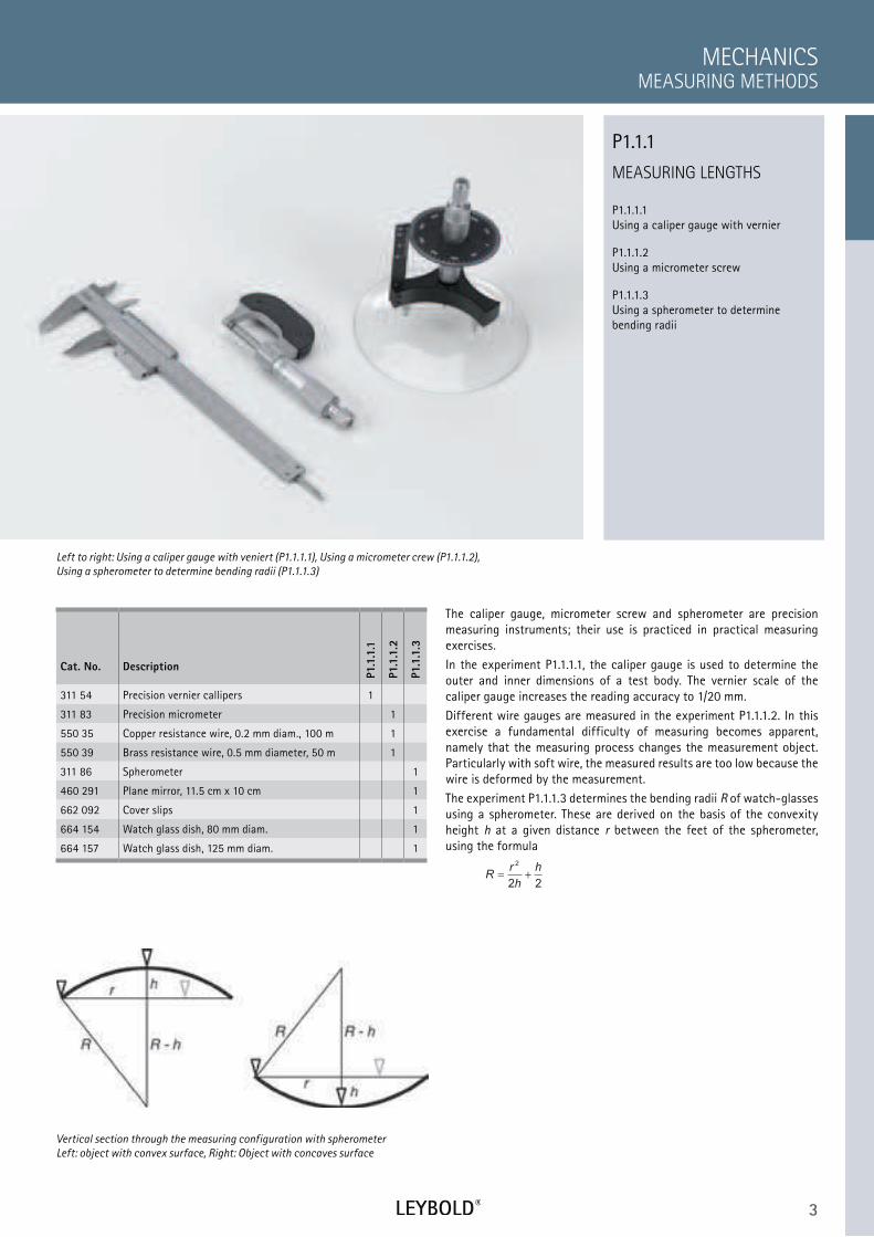
The caliper gauge, micrometer screw and spherometer are precision measuring instruments; their use is practiced in practical measuring exercises.
In the experiment P1.1.1.1, the caliper gauge is used to determine the outer and inner dimensions of a test body. The vernier scale of the caliper gauge increases the reading accuracy to 1/20 mm.
Different wire gauges are measured in the experiment P1.1.1.2. In this exercise a fundamental difficulty of measuring becomes apparent, namely that the measuring process changes the measurement object. Particularly with soft wire, the measured results are too low because the wire is deformed by the measurement.
The experiment P1.1.1.3 determines the bending radii R of watch-glasses using a spherometer. These are derived on the basis of the convexity height h at a given distance r between the feet of the spherometer, using the formula
Rr
h
h= +
2
2 2
Left to right: Using a caliper gauge with veniert (P1.1.1.1), Using a micrometer crew (P1.1.1.2),
Using a spherometer to determine bending radii (P1.1.1.3)
P1.1.1
Vertical section through the measuring configuration with spherometer
Left: object with convex surface, Right: Object with concaves surface
4 WWW.LEYBOLD-SHOP.COM
MEASURING VOLUME AND
DENSITY
P1.1.2.1 Determining the volume and density of solids
P1.1.2.2 Determining the density of liquids using the plumb bob
P1.1.2.3 Determining the density of liquids using the pycnometer after Gay-Lussac
P1.1.2.4 Determining the density of air
Depending on the respective aggregate state of a homogeneous sub-stance, various methods are used to determine its density
m
V
m V: mass, : volume
The mass and volume of the substance are usually measured separately. To determine the density of solid bodies, a weighing is combined with a volume measurement. The volumes of the bodies are determined from the volumes of liquid which they displace from an overflow vessel. In the experiment P1.1.2.1, this principle is tested using regular bodies for which the volumes can be easily calculated from their linear dimensions.
To determine the density of liquids, the plumb bob is used in the experiment P1.1.2.2. The measuring task is to determine the densities of water-ethanol mixtures. The Plumb bob determines the density from the buoyancy of a body of known volume in the test liquid.
To determine the density of liquids, the pyknometer after Gay-Lussac is used in the experiment P1.1.2.3. The measuring task is to determine the densities of water-ethanol mixtures. The pyknometer is a pear-shaped bottle in which the liquid to be investigated is filled for weighing. The volume capacity of the pyknometer is determined by weighing with a liquid of known density (e.g. water).
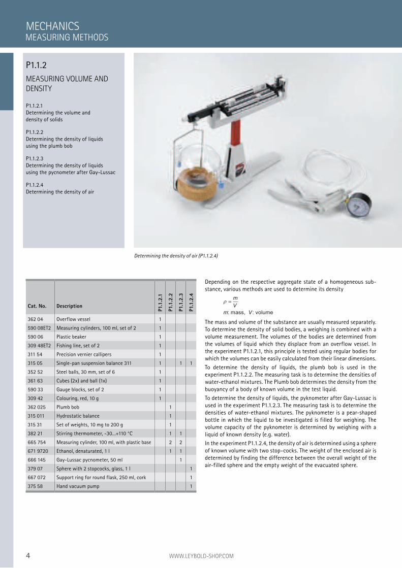
In the experiment P1.1.2.4, the density of air is determined using a sphere of known volume with two stop-cocks. The weight of the enclosed air is determined by finding the difference between the overall weight of the air-filled sphere and the empty weight of the evacuated sphere.
MECHANICS
Determining the density of air (P1.1.2.4)
Cat. No. Description
P1.1
.2.1
P1.1
.2.2
P1.1
.2.3
P1.1
.2.4
362 04 Overflow vessel 1
590 08ET2 Measuring cylinders, 100 ml, set of 2 1
590 06 Plastic beaker 1
309 48ET2 Fishing line, set of 2 1
311 54 Precision vernier callipers 1
315 05 Single-pan suspension balance 311 1 1 1
352 52 Steel balls, 30 mm, set of 6 1
361 63 Cubes (2x) and ball (1x) 1
590 33 Gauge blocks, set of 2 1
309 42 Colouring, red, 10 g 1
362 025 Plumb bob 1
315 011 Hydrostatic balance 1
315 31 Set of weights, 10 mg to 200 g 1
382 21 Stirring thermometer, -30...+110 °C 1 1
665 754 Measuring cylinder, 100 ml, with plastic base 2 2
671 9720 Ethanol, denaturated, 1 l 1 1
666 145 Gay-Lussac pycnometer, 50 ml 1
379 07 Sphere with 2 stopcocks, glass, 1 l 1
667 072 Support ring for round flask, 250 ml, cork 1
375 58 Hand vacuum pump 1
MEASURING METHODS
P1.1.2
5
DETERMINING THE
GRAVITATIONAL CONSTANT
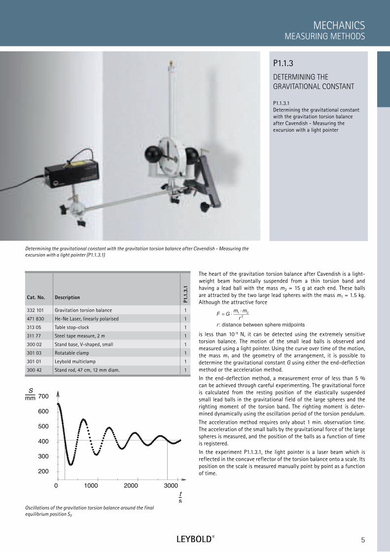
P1.1.3.1
Determining the gravitational constant
with the gravitation torsion balance
after Cavendish - Measuring the
excursion with a light pointer
MEASURING METHODS
MECHANICS
Cat. No. Description
P1.1
.3.1
332 101 Gravitation torsion balance 1
471 830 He-Ne Laser, linearly polarised 1
313 05 Table stop-clock 1
311 77 Steel tape measure, 2 m 1
300 02 Stand base, V-shaped, small 1
301 03 Rotatable clamp 1
301 01 Leybold multiclamp 1
300 42 Stand rod, 47 cm, 12 mm diam. 1
The heart of the gravitation torsion balance after Cavendish is a light-
weight beam horizontally suspended from a thin torsion band and
having a lead ball with the mass m2 = 15 g at each end. These balls
are attracted by the two large lead spheres with the mass m1 = 1.5 kg.
Although the attractive force
F Gm m
r
r
= ⋅⋅
1 2
2
: distance between sphere midpoints
is less than 10-9 N, it can be detected using the extremely sensitive
torsion balance. The motion of the small lead balls is observed and
measured using a light pointer. Using the curve over time of the motion,
the mass m1 and the geometry of the arrangement, it is possible to
determine the gravitational constant G using either the end-deflection
method or the acceleration method.
In the end-deflection method, a measurement error of less than 5 %
can be achieved through careful experimenting. The gravitational force
is calculated from the resting position of the elastically suspended
small lead balls in the gravitational field of the large spheres and the
righting moment of the torsion band. The righting moment is deter-
mined dynamically using the oscillation period of the torsion pendulum.
The acceleration method requires only about 1 min. observation time.
The acceleration of the small balls by the gravitational force of the large
spheres is measured, and the position of the balls as a function of time
is registered.
In the experiment P1.1.3.1, the light pointer is a laser beam which is
reflected in the concave reflector of the torsion balance onto a scale. Its
position on the scale is measured manually point by point as a function
of time.
Determining the gravitational constant with the gravitation torsion balance after Cavendish - Measuring the
excursion with a light pointer (P1.1.3.1)
P1.1.3
Oscillations of the gravitation torsion balance around the final
equilibrium position SII
6 WWW.LEYBOLD-SHOP.COM
STATIC EFFECTS OF FORCES
P1.2.1.1 Expansion of a helical spring
P1.2.1.2 Bending of a leaf spring
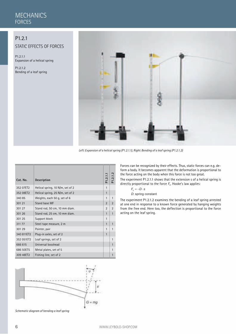
Forces can be recognized by their effects. Thus, static forces can e.g. de-form a body. It becomes apparent that the deformation is proportional to the force acting on the body when this force is not too great.
The experiment P1.2.1.1 shows that the extension s of a helical spring is directly proportional to the force Fs. Hooke’s law applies:
F D s
D
s= − ⋅
: spring constant
The experiment P1.2.1.2 examines the bending of a leaf spring arrested at one end in response to a known force generated by hanging weights from the free end. Here too, the deflection is proportional to the force acting on the leaf spring.
MECHANICS
Left: Expansion of a helical spring (P1.2.1.1), Right: Bending of a leaf spring (P1.2.1.2)
Cat. No. Description
P1.2
.1.1
P1.2
.1.2
352 07ET2 Helical spring, 10 N/m, set of 2 1
352 08ET2 Helical spring, 25 N/m, set of 2 1
340 85 Weights, each 50 g, set of 6 1 1
301 21 Stand base MF 2 2
301 27 Stand rod, 50 cm, 10 mm diam. 2 2
301 26 Stand rod, 25 cm, 10 mm diam. 1 1
301 25 Support block 1
311 77 Steel tape measure, 2 m 1 1
301 29 Pointer, pair 1 1
340 811ET2 Plug-in axles, set of 2 1
352 051ET2 Leaf springs, set of 2 1
666 615 Universal bosshead 1
686 50ET5 Metal plates, set of 5 1
309 48ET2 Fishing line, set of 2 1
Schematic diagram of bending a leaf spring
FORCES
P1.2.1
7
FORCE AS VECTOR
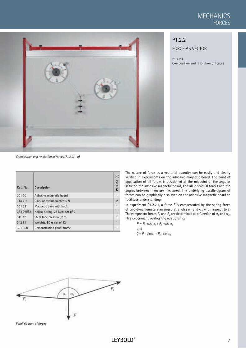
P1.2.2.1 Composition and resolution of forces
FORCES
MECHANICS
Cat. No. Description
P1.2
.2.1
(b)
301 301 Adhesive magnetic board 1
314 215 Circular dynamometer, 5 N 2
301 331 Magnetic base with hook 1
352 08ET2 Helical spring, 25 N/m, set of 2 1
311 77 Steel tape measure, 2 m 1
342 61 Weights, 50 g, set of 12 1
301 300 Demonstration panel frame 1
The nature of force as a vectorial quantity can be easily and clearly verified in experiments on the adhesive magnetic board. The point of application of all forces is positioned at the midpoint of the angular scale on the adhesive magnetic board, and all individual forces and the angles between them are measured. The underlying parallelogram of forces can be graphically displayed on the adhesive magnetic board to facilitate understanding.
In experiment P1.2.2.1, a force F is compensated by the spring force of two dynamometers arranged at angles 1 and 2 with respect to F. The component forces F1 and F2 are determined as a function of 1 and 2. This experiment verifies the relationships
F F F
F F
= ⋅ + ⋅
= ⋅ + ⋅
1 1 2 2
1 1 2 20
cos cos
sin sin
α α
α α
and
Composition and resolution of forces (P1.2.2.1_b)
P1.2.2
Parallelogram of forces
8 WWW.LEYBOLD-SHOP.COM
LEVER
P1.2.3.1
One-sided and two-sided lever
P1.2.3.2
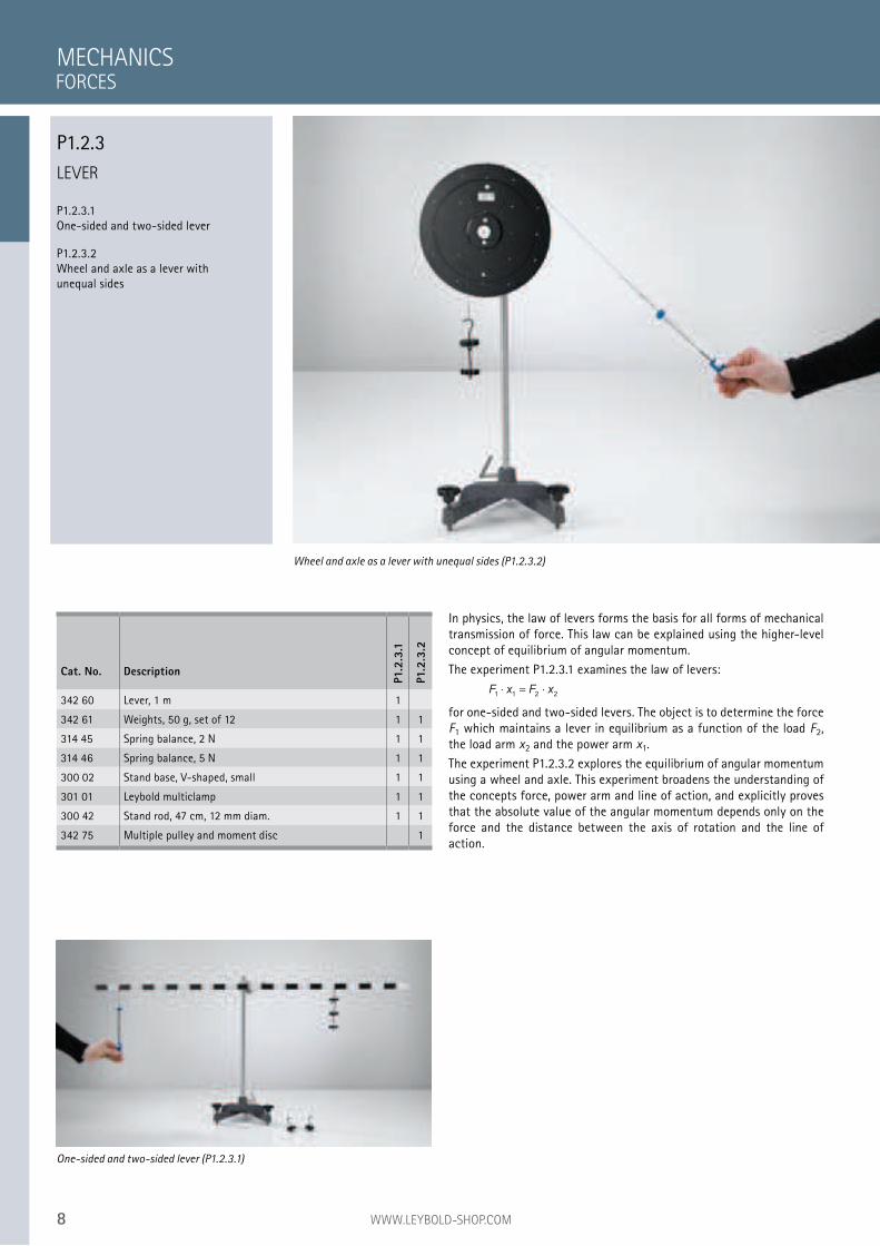
Wheel and axle as a lever with
unequal sides
In physics, the law of levers forms the basis for all forms of mechanical
transmission of force. This law can be explained using the higher-level
concept of equilibrium of angular momentum.
The experiment P1.2.3.1 examines the law of levers:
F x F x1 1 2 2⋅ = ⋅
for one-sided and two-sided levers. The object is to determine the force
F1 which maintains a lever in equilibrium as a function of the load F2,
the load arm x2 and the power arm x1.
The experiment P1.2.3.2 explores the equilibrium of angular momentum
using a wheel and axle. This experiment broadens the understanding of
the concepts force, power arm and line of action, and explicitly proves
that the absolute value of the angular momentum depends only on the
force and the distance between the axis of rotation and the line of
action.
MECHANICS
Wheel and axle as a lever with unequal sides (P1.2.3.2)
Cat. No. Description
P1.2
.3.1
P1.2
.3.2
342 60 Lever, 1 m 1
342 61 Weights, 50 g, set of 12 1 1
314 45 Spring balance, 2 N 1 1
314 46 Spring balance, 5 N 1 1
300 02 Stand base, V-shaped, small 1 1
301 01 Leybold multiclamp 1 1
300 42 Stand rod, 47 cm, 12 mm diam. 1 1
342 75 Multiple pulley and moment disc 1
One-sided and two-sided lever (P1.2.3.1)
FORCES
P1.2.3
9
BLOCK AND TACKLE
P1.2.4.1
Fixed pulley, loose pulley and block and
tackle as simple machines
FORCES
MECHANICS
Cat. No. Description
P1.2
.4.1
342 28 Block and tackle D 1
315 36 Set of weights, 0.1 kg to 2 kg 1
300 01 Stand base, V-shaped, large 1
300 41 Stand rod, 25 cm, 12 mm Ø 1
300 44 Stand rod, 100 cm, 12 mm diam. 1
301 01 Leybold multiclamp 1
314 181 Precision dynamometer, 20 N 1
341 65 Pulley 2*
* additionally recommended
The fixed pulley, loose pulley and block and tackle are classic examples of
simple machines. Experiments with these machines represent the most
accessible introduction to the concept of work in mechanics.
In the experiment P1.2.4.1, the block and tackle is set up on the lab
bench using a stand base. The block and tackle can be expanded to
three pairs of pulleys and can support loads of up to 20 N. The pulleys
are mounted virtually friction-free in ball bearings.
Fixed pulley, loose pulley and block and tackle as simple machines (P1.2.4.1)
P1.2.4
Setup with block and tackle
10 WWW.LEYBOLD-SHOP.COM
INCLINED PLANE
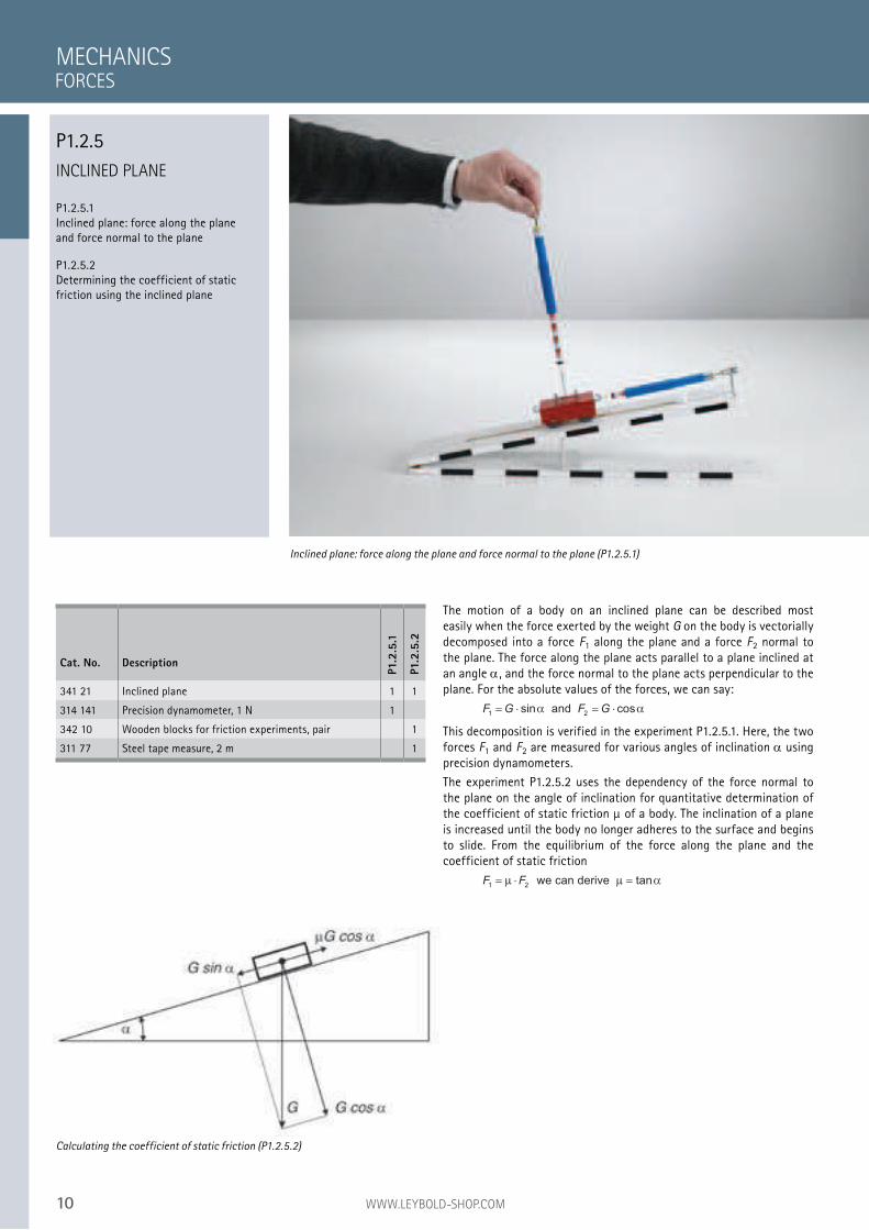
P1.2.5.1
Inclined plane: force along the plane
and force normal to the plane
P1.2.5.2
Determining the coefficient of static
friction using the inclined plane
The motion of a body on an inclined plane can be described most
easily when the force exerted by the weight G on the body is vectorially
decomposed into a force F1 along the plane and a force F2 normal to
the plane. The force along the plane acts parallel to a plane inclined at
an angle , and the force normal to the plane acts perpendicular to the
plane. For the absolute values of the forces, we can say:
F G F G1 2= ⋅ = ⋅sin cosα α and
This decomposition is verified in the experiment P1.2.5.1. Here, the two
forces F1 and F2 are measured for various angles of inclination using
precision dynamometers.
The experiment P1.2.5.2 uses the dependency of the force normal to
the plane on the angle of inclination for quantitative determination of
the coefficient of static friction µ of a body. The inclination of a plane
is increased until the body no longer adheres to the surface and begins
to slide. From the equilibrium of the force along the plane and the
coefficient of static friction
F F1 2= ⋅ =µ µ α we can derive tan
MECHANICS
Inclined plane: force along the plane and force normal to the plane (P1.2.5.1)
Cat. No. Description
P1.2
.5.1
P1.2
.5.2
341 21 Inclined plane 1 1
314 141 Precision dynamometer, 1 N 1
342 10 Wooden blocks for friction experiments, pair 1
311 77 Steel tape measure, 2 m 1
Calculating the coefficient of static friction (P1.2.5.2)
FORCES
P1.2.5
11
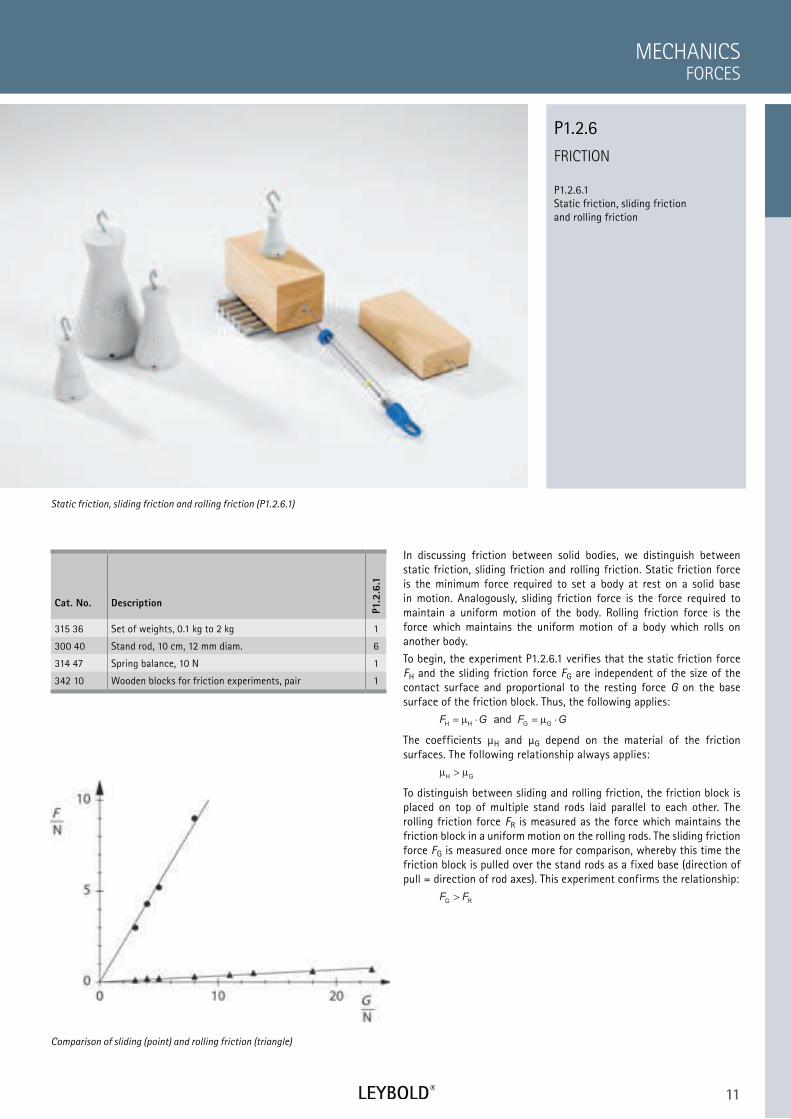
FRICTION
P1.2.6.1 Static friction, sliding friction and rolling friction
FORCES
MECHANICS
Cat. No. Description
P1.2
.6.1
315 36 Set of weights, 0.1 kg to 2 kg 1
300 40 Stand rod, 10 cm, 12 mm diam. 6
314 47 Spring balance, 10 N 1
342 10 Wooden blocks for friction experiments, pair 1
In discussing friction between solid bodies, we distinguish between static friction, sliding friction and rolling friction. Static friction force is the minimum force required to set a body at rest on a solid base in motion. Analogously, sliding friction force is the force required to maintain a uniform motion of the body. Rolling friction force is the force which maintains the uniform motion of a body which rolls on another body.
To begin, the experiment P1.2.6.1 verifies that the static friction force FH and the sliding friction force FG are independent of the size of the contact surface and proportional to the resting force G on the base surface of the friction block. Thus, the following applies:
F G F GH H G G
and = ⋅ = ⋅µ µ
The coefficients µH and µG depend on the material of the friction surfaces. The following relationship always applies:
µ µH G>
To distinguish between sliding and rolling friction, the friction block is placed on top of multiple stand rods laid parallel to each other. The rolling friction force FR is measured as the force which maintains the friction block in a uniform motion on the rolling rods. The sliding friction force FG is measured once more for comparison, whereby this time the friction block is pulled over the stand rods as a fixed base (direction of pull = direction of rod axes). This experiment confirms the relationship:
F FG R
Static friction, sliding friction and rolling friction (P1.2.6.1)
P1.2.6
Comparison of sliding (point) and rolling friction (triangle)
12 WWW.LEYBOLD-SHOP.COM
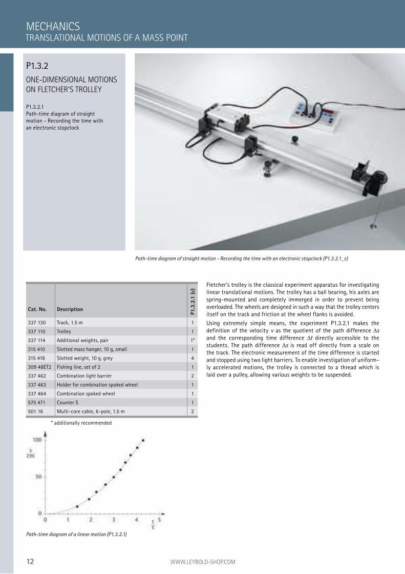
ONE-DIMENSIONAL MOTIONS
ON FLETCHER’S TROLLEY
P1.3.2.1
Path-time diagram of straight
motion - Recording the time with
an electronic stopclock
Fletcher’s trolley is the classical experiment apparatus for investigating
linear translational motions. The trolley has a ball bearing, his axles are
spring-mounted and completely immerged in order to prevent being
overloaded. The wheels are designed in such a way that the trolley centers
itself on the track and friction at the wheel flanks is avoided.
Using extremely simple means, the experiment P1.3.2.1 makes the
definition of the velocity v as the quotient of the path difference s
and the corresponding time difference t directly accessible to the
students. The path difference s is read off directly from a scale on
the track. The electronic measurement of the time difference is started
and stopped using two light barriers. To enable investigation of uniform-
ly accelerated motions, the trolley is connected to a thread which is
laid over a pulley, allowing various weights to be suspended.
MECHANICS
Path-time diagram of straight motion - Recording the time with an electronic stopclock (P1.3.2.1_c)
Cat. No. Description
P1.3
.2.1
(c)
337 130 Track, 1.5 m 1
337 110 Trolley 1
337 114 Additional weights, pair 1*
315 410 Slotted mass hanger, 10 g, small 1
315 418 Slotted weight, 10 g, grey 4
309 48ET2 Fishing line, set of 2 1
337 462 Combination light barrier 2
337 463 Holder for combination spoked wheel 1
337 464 Combination spoked wheel 1
575 471 Counter S 1
501 16 Multi-core cable, 6-pole, 1.5 m 2
* additionally recommended
Path-time diagram of a linear motion (P1.3.2.1)
TRANSLATIONAL MOTIONS OF A MASS POINT
P1.3.2
13 CA
SSY ®
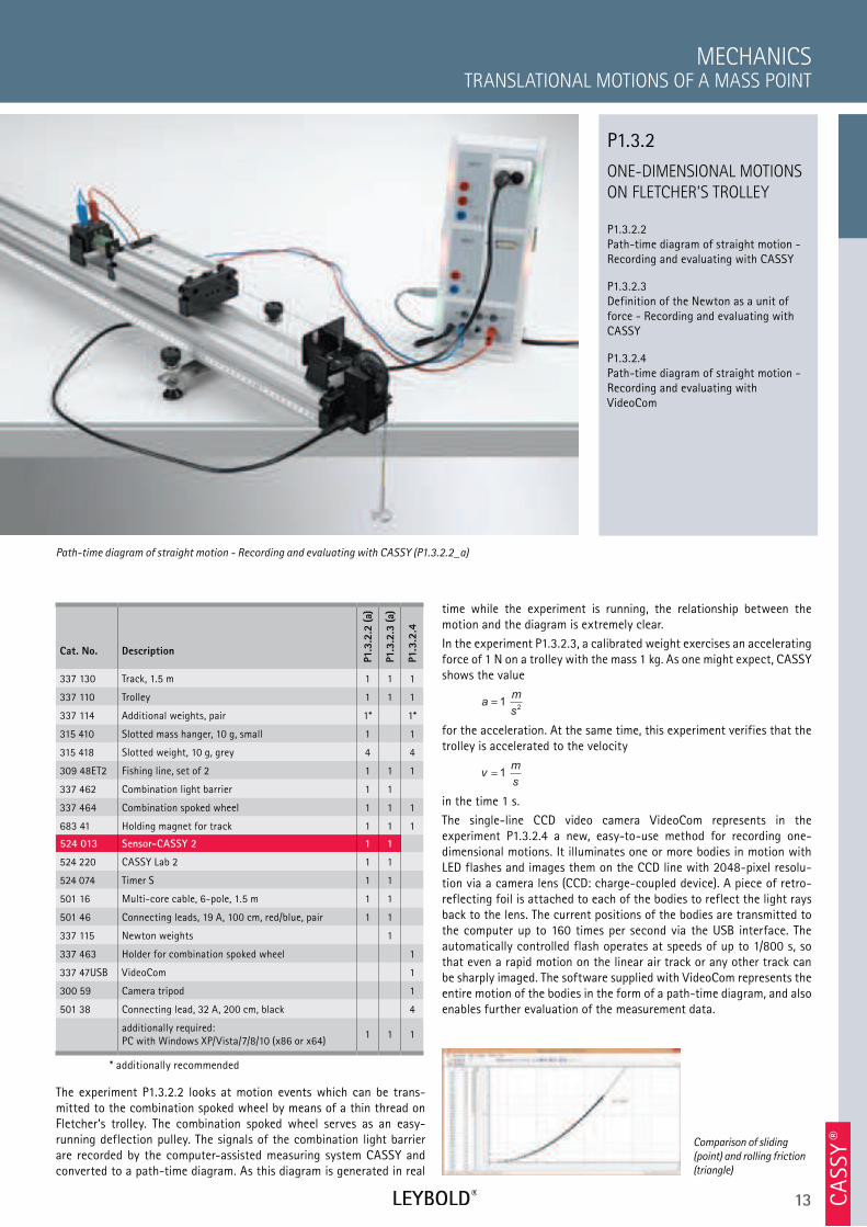
ONE-DIMENSIONAL MOTIONS
ON FLETCHER’S TROLLEY
P1.3.2.2 Path-time diagram of straight motion - Recording and evaluating with CASSY
P1.3.2.3 Definition of the Newton as a unit of force - Recording and evaluating with CASSY
P1.3.2.4 Path-time diagram of straight motion - Recording and evaluating with VideoCom
TRANSLATIONAL MOTIONS OF A MASS POINT
MECHANICS
Cat. No. Description
P1.3
.2.2
(a)
P1.3
.2.3
(a)
P1.3
.2.4
337 130 Track, 1.5 m 1 1 1
337 110 Trolley 1 1 1
337 114 Additional weights, pair 1* 1*
315 410 Slotted mass hanger, 10 g, small 1 1
315 418 Slotted weight, 10 g, grey 4 4
309 48ET2 Fishing line, set of 2 1 1 1
337 462 Combination light barrier 1 1
337 464 Combination spoked wheel 1 1 1
683 41 Holding magnet for track 1 1 1
524 013 Sensor-CASSY 2 1 1
524 220 CASSY Lab 2 1 1
524 074 Timer S 1 1
501 16 Multi-core cable, 6-pole, 1.5 m 1 1
501 46 Connecting leads, 19 A, 100 cm, red/blue, pair 1 1
337 115 Newton weights 1
337 463 Holder for combination spoked wheel 1
337 47USB VideoCom 1
300 59 Camera tripod 1
501 38 Connecting lead, 32 A, 200 cm, black 4
additionally required: PC with Windows XP/Vista/7/8/10 (x86 or x64)
1 1 1
* additionally recommended
The experiment P1.3.2.2 looks at motion events which can be trans-mitted to the combination spoked wheel by means of a thin thread on Fletcher‘s trolley. The combination spoked wheel serves as an easy- running deflection pulley. The signals of the combination light barrier are recorded by the computer-assisted measuring system CASSY and converted to a path-time diagram. As this diagram is generated in real
Path-time diagram of straight motion - Recording and evaluating with CASSY (P1.3.2.2_a)
P1.3.2
time while the experiment is running, the relationship between the motion and the diagram is extremely clear.
In the experiment P1.3.2.3, a calibrated weight exercises an accelerating force of 1 N on a trolley with the mass 1 kg. As one might expect, CASSY shows the value
am
s1
2
for the acceleration. At the same time, this experiment verifies that the trolley is accelerated to the velocity
vm
s1
in the time 1 s.
The single-line CCD video camera VideoCom represents in the experiment P1.3.2.4 a new, easy-to-use method for recording one- dimensional motions. It illuminates one or more bodies in motion with LED flashes and images them on the CCD line with 2048-pixel resolu-tion via a camera lens (CCD: charge-coupled device). A piece of retro-reflecting foil is attached to each of the bodies to reflect the light rays back to the lens. The current positions of the bodies are transmitted to the computer up to 160 times per second via the USB interface. The automatically controlled flash operates at speeds of up to 1/800 s, so that even a rapid motion on the linear air track or any other track can be sharply imaged. The software supplied with VideoCom represents the entire motion of the bodies in the form of a path-time diagram, and also enables further evaluation of the measurement data.
Comparison of sliding
(point) and rolling friction
(triangle)
CA
SSY ®
14 WWW.LEYBOLD-SHOP.COMCA
SSY ®
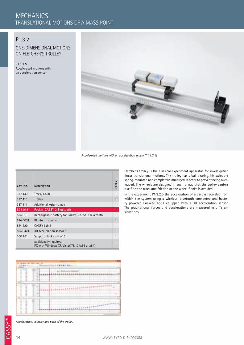
ONE-DIMENSIONAL MOTIONS
ON FLETCHER’S TROLLEY
P1.3.2.5 Accelerated motions with an acceleration sensor
Fletcher’s trolley is the classical experiment apparatus for investigating linear translational motions. The trolley has a ball bearing, his axles are spring-mounted and completely immerged in order to prevent being over-loaded. The wheels are designed in such a way that the trolley centers itself on the track and friction at the wheel flanks is avoided.
In the experiment P1.3.2.5 the acceleration of a cart is recorded from within the system using a wireless, bluetooth connected and batte-ry powered Pocket-CASSY equipped with a 3D acceleration sensor. The gravitational forces and accelerations are measured in different situations.
MECHANICS
Accelerated motions with an acceleration sensor (P1.3.2.5)
Cat. No. Description
P1.3
.2.5
337 130 Track, 1.5 m 1
337 110 Trolley 1
337 114 Additional weights, pair 1
524 018 Pocket-CASSY 2 Bluetooth 1
524 019 Rechargeable battery for Pocket-CASSY 2 Bluetooth 1
524 0031 Bluetooth dongle 1
524 220 CASSY Lab 2 1
524 0424 3D acceleration sensor S 1
300 761 Support blocks, set of 6 1
additionally required: PC with Windows XP/Vista/7/8/10 (x86 or x64)
1
Acceleration, velocity and path of the trolley
TRANSLATIONAL MOTIONS OF A MASS POINT
P1.3.2
15 CA
SSY ®
ONE-DIMENSIONAL MOTIONS
ON THE LINEAR AIR TRACK
P1.3.3.1 Path-time diagram of straight motion - Recording the time with forked light barrier
TRANSLATIONAL MOTIONS OF A MASS POINT
MECHANICS
Cat. No. Description
P1.3
.3.1
(a)
P1.3
.3.1
(d)
337 501 Air track 1 1
337 53 Air supply 1 1
667 823 Power controller 1 1
311 02 Metal rule, 1 m 1 1
337 46 Fork-type light barrier 1 2
501 16 Multi-core cable, 6-pole, 1.5 m 1 2
524 013 Sensor-CASSY 2 1
524 220 CASSY Lab 2 1
524 074 Timer S 1
501 46 Connecting leads, 19 A, 100 cm, red/blue, pair 1
575 471 Counter S 1
additionally required: PC with Windows XP/Vista/7/8/10 (x86 or x64)
1
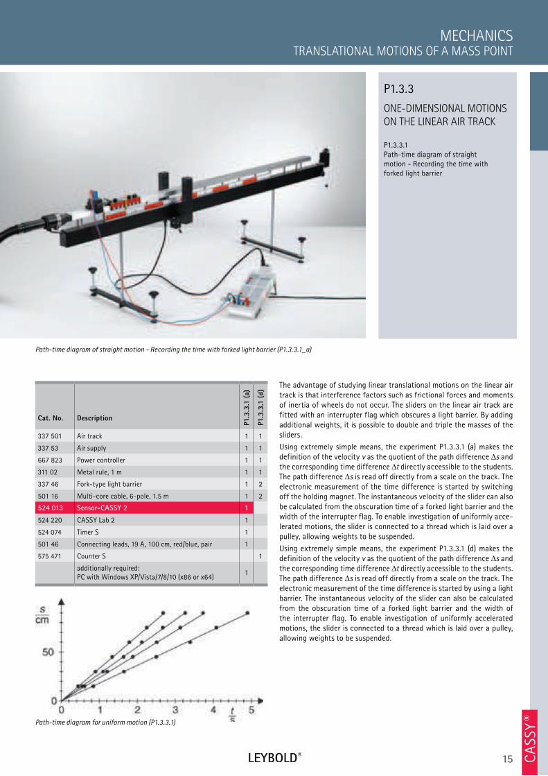
The advantage of studying linear translational motions on the linear air track is that interference factors such as frictional forces and moments of inertia of wheels do not occur. The sliders on the linear air track are fitted with an interrupter flag which obscures a light barrier. By adding additional weights, it is possible to double and triple the masses of the sliders.
Using extremely simple means, the experiment P1.3.3.1 (a) makes the definition of the velocity v as the quotient of the path difference s and the corresponding time difference t directly accessible to the students. The path difference s is read off directly from a scale on the track. The electronic measurement of the time difference is started by switching off the holding magnet. The instantaneous velocity of the slider can also be calculated from the obscuration time of a forked light barrier and the width of the interrupter flag. To enable investigation of uniformly acce-lerated motions, the slider is connected to a thread which is laid over a pulley, allowing weights to be suspended.
Using extremely simple means, the experiment P1.3.3.1 (d) makes the definition of the velocity v as the quotient of the path difference s and the corresponding time difference t directly accessible to the students. The path difference s is read off directly from a scale on the track. The electronic measurement of the time difference is started by using a light barrier. The instantaneous velocity of the slider can also be calculated from the obscuration time of a forked light barrier and the width of the interrupter flag. To enable investigation of uniformly accelerated motions, the slider is connected to a thread which is laid over a pulley, allowing weights to be suspended.
Path-time diagram of straight motion - Recording the time with forked light barrier (P1.3.3.1_a)
P1.3.3
Path-time diagram for uniform motion (P1.3.3.1)
16 WWW.LEYBOLD-SHOP.COMCA
SSY ®
ONE-DIMENSIONAL MOTIONS
ON THE LINEAR AIR TRACK
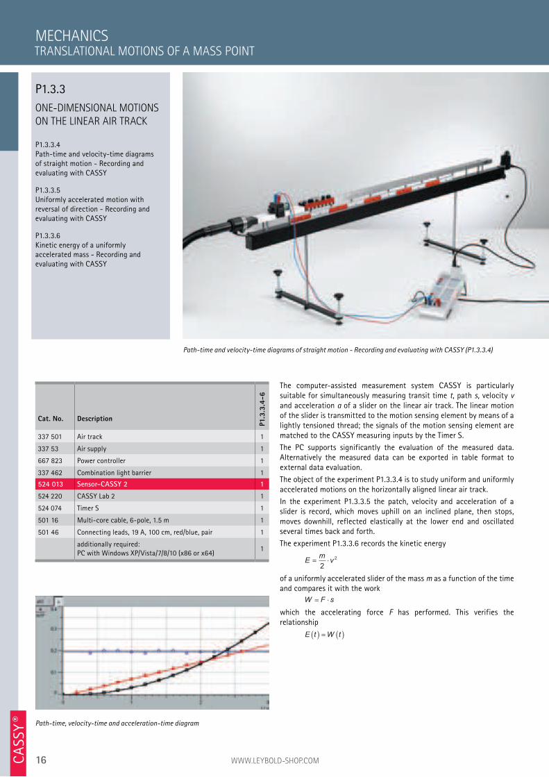
P1.3.3.4 Path-time and velocity-time diagrams of straight motion - Recording and evaluating with CASSY
P1.3.3.5 Uniformly accelerated motion with reversal of direction - Recording and evaluating with CASSY
P1.3.3.6 Kinetic energy of a uniformly accelerated mass - Recording and evaluating with CASSY
The computer-assisted measurement system CASSY is particularly suitable for simultaneously measuring transit time t, path s, velocity v and acceleration a of a slider on the linear air track. The linear motion of the slider is transmitted to the motion sensing element by means of a lightly tensioned thread; the signals of the motion sensing element are matched to the CASSY measuring inputs by the Timer S.
The PC supports significantly the evaluation of the measured data. Alternatively the measured data can be exported in table format to external data evaluation.
The object of the experiment P1.3.3.4 is to study uniform and uniformly accelerated motions on the horizontally aligned linear air track.
In the experiment P1.3.3.5 the patch, velocity and acceleration of a slider is record, which moves uphill on an inclined plane, then stops, moves downhill, reflected elastically at the lower end and oscillated several times back and forth.
The experiment P1.3.3.6 records the kinetic energy
Emv= ⋅
2
2
of a uniformly accelerated slider of the mass m as a function of the time and compares it with the work
W F s= ⋅
which the accelerating force F has performed. This verifies the relationship
E t W t( ) = ( )
MECHANICS
Path-time and velocity-time diagrams of straight motion - Recording and evaluating with CASSY (P1.3.3.4)
Cat. No. Description
P1.3
.3.4
-6
337 501 Air track 1
337 53 Air supply 1
667 823 Power controller 1
337 462 Combination light barrier 1
524 013 Sensor-CASSY 2 1
524 220 CASSY Lab 2 1
524 074 Timer S 1
501 16 Multi-core cable, 6-pole, 1.5 m 1
501 46 Connecting leads, 19 A, 100 cm, red/blue, pair 1
additionally required: PC with Windows XP/Vista/7/8/10 (x86 or x64)
1
Path-time, velocity-time and acceleration-time diagram
TRANSLATIONAL MOTIONS OF A MASS POINT
P1.3.3
CA
SSY ®
17
ONE-DIMENSIONAL MOTIONS
ON THE LINEAR AIR TRACK
P1.3.3.7 Confirming Newton‘s first and second laws for linear motions - Recording and evaluating with VideoCom
P1.3.3.8 Uniformly accelerated motion with reversal of direction - Recording and evaluating with VideoCom
P1.3.3.9 Kinetic energy of a uniformly accelerated mass - Recording and evaluating with VideoCom
TRANSLATIONAL MOTIONS OF A MASS POINT
MECHANICS
Cat. No. Description
P1.3
.3.7
-9
337 501 Air track 1
337 53 Air supply 1
667 823 Power controller 1
337 47USB VideoCom 1
300 59 Camera tripod 1
311 02 Metal rule, 1 m 1
501 38 Connecting lead, 32 A, 200 cm, black 4
additionally required: PC with Windows XP/Vista/7/8/10 (x86 or x64)
1
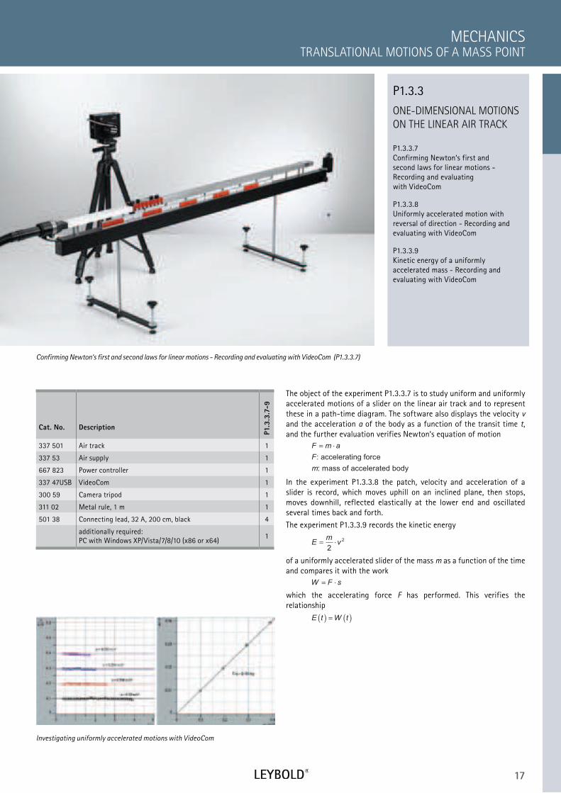
The object of the experiment P1.3.3.7 is to study uniform and uniformly accelerated motions of a slider on the linear air track and to represent these in a path-time diagram. The software also displays the velocity v and the acceleration a of the body as a function of the transit time t, and the further evaluation verifies Newton‘s equation of motion
F m a
F
m
= ⋅
: accelerating force
: mass of accelerated body
In the experiment P1.3.3.8 the patch, velocity and acceleration of a slider is record, which moves uphill on an inclined plane, then stops, moves downhill, reflected elastically at the lower end and oscillated several times back and forth.
The experiment P1.3.3.9 records the kinetic energy
Emv= ⋅
2
2
of a uniformly accelerated slider of the mass m as a function of the time and compares it with the work
W F s= ⋅
which the accelerating force F has performed. This verifies the relationship
E t W t( ) = ( )
Confirming Newton‘s first and second laws for linear motions - Recording and evaluating with VideoCom (P1.3.3.7)
P1.3.3
Investigating uniformly accelerated motions with VideoCom
18 WWW.LEYBOLD-SHOP.COM
CONSERVATION OF LINEAR
MOMENTUM
P1.3.4.1
Energy and linear momentum in elastic
collision - Measuring with two forked
light barriers
P1.3.4.2
Energy and linear momentum in
inelastic collision - Measuring with
two forked light barriers
P1.3.4.3
Rocket principle: conservation of
momentum and reaction
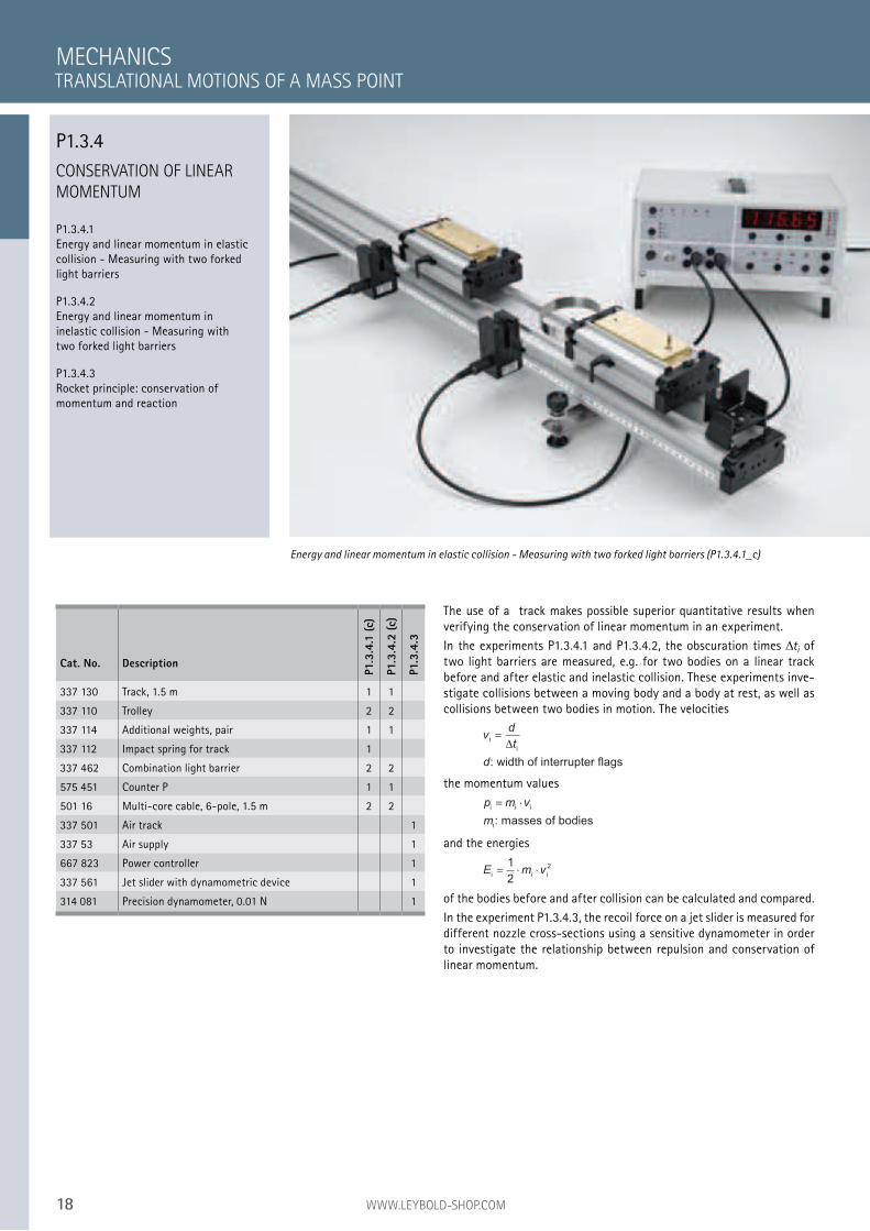
The use of a track makes possible superior quantitative results when
verifying the conservation of linear momentum in an experiment.
In the experiments P1.3.4.1 and P1.3.4.2, the obscuration times ti of
two light barriers are measured, e.g. for two bodies on a linear track
before and after elastic and inelastic collision. These experiments inve-
stigate collisions between a moving body and a body at rest, as well as
collisions between two bodies in motion. The velocities
vd
t
d
i
i
: width of interrupter flags
=∆
the momentum values
p m v
m
i i i
i: masses of bodies
= ⋅
and the energies
E m vi i i= ⋅ ⋅1
2
2
of the bodies before and after collision can be calculated and compared.
In the experiment P1.3.4.3, the recoil force on a jet slider is measured for
different nozzle cross-sections using a sensitive dynamometer in order
to investigate the relationship between repulsion and conservation of
linear momentum.
MECHANICS
Energy and linear momentum in elastic collision - Measuring with two forked light barriers (P1.3.4.1_c)
Cat. No. Description
P1.3
.4.1
(c)
P1.3
.4.2
(c)
P1.3
.4.3
337 130 Track, 1.5 m 1 1
337 110 Trolley 2 2
337 114 Additional weights, pair 1 1
337 112 Impact spring for track 1
337 462 Combination light barrier 2 2
575 451 Counter P 1 1
501 16 Multi-core cable, 6-pole, 1.5 m 2 2
337 501 Air track 1
337 53 Air supply 1
667 823 Power controller 1
337 561 Jet slider with dynamometric device 1
314 081 Precision dynamometer, 0.01 N 1
TRANSLATIONAL MOTIONS OF A MASS POINT
P1.3.4
19
CONSERVATION OF LINEAR
MOMENTUM
P1.3.4.4 Newton‘s third law and laws of collision - Recording and evaluating with VideoCom
TRANSLATIONAL MOTIONS OF A MASS POINT
MECHANICS
Cat. No. Description
P1.3
.4.4
(a)
337 130 Track, 1.5 m 1
337 110 Trolley 2
337 114 Additional weights, pair 1
337 112 Impact spring for track 2
337 47USB VideoCom 1
300 59 Camera tripod 1
additionally required: PC with Windows XP/Vista/7/8/10 (x86 or x64)
1
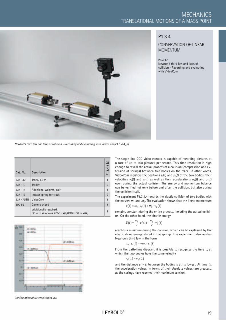
The single-line CCD video camera is capable of recording pictures at a rate of up to 160 pictures per second. This time resolution is high enough to reveal the actual process of a collision (compression and ex-tension of springs) between two bodies on the track. In other words, VideoCom registers the positions s1(t) and s2(t) of the two bodies, their velocities v1(t) and v2(t) as well as their accelerations a1(t) and a2(t) even during the actual collision. The energy and momentum balance can be verified not only before and after the collision, but also during the collision itself.
The experiment P1.3.4.4 records the elastic collision of two bodies with the masses m1 and m2. The evaluation shows that the linear momentum
p t m v t m v t( ) = ⋅ ( ) + ⋅ ( )1 1 2 2
remains constant during the entire process, including the actual collisi-on. On the other hand, the kinetic energy
E tm
v tm
v t( ) = ⋅ ( ) + ⋅ ( )1
1
2 2
2
2
2 2
reaches a minimum during the collision, which can be explained by the elastic strain energy stored in the springs. This experiment also verifies Newton‘s third law in the form
m a t m a t1 1 2 2⋅ ( ) = − ⋅ ( )
From the path-time diagram, it is possible to recognize the time t0 at which the two bodies have the same velocity
v t v t1 0 2 0( ) = ( )
and the distance s2 - s1 between the bodies is at its lowest. At time t0, the acceleration values (in terms of their absolute values) are greatest, as the springs have reached their maximum tension.
Newton‘s third law and laws of collision - Recording and evaluating with VideoCom (P1.3.4.4_a)
P1.3.4
Confirmation of Newton‘s third law
20 WWW.LEYBOLD-SHOP.COMCA
SSY ®
CONSERVATION OF LINEAR
MOMENTUM
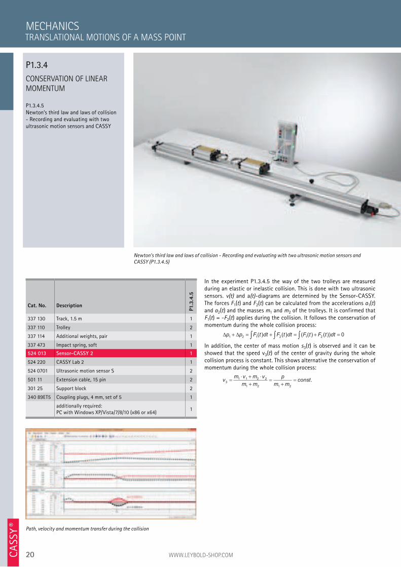
P1.3.4.5 Newton‘s third law and laws of collision - Recording and evaluating with two ultrasonic motion sensors and CASSY
In the experiment P1.3.4.5 the way of the two trolleys are measured during an elastic or inelastic collision. This is done with two ultrasonic sensors. v(t) and a(t)-diagrams are determined by the Sensor-CASSY. The forces F1(t) and F2(t) can be calculated from the accelerations a1(t) and a2(t) and the masses m1 and m2 of the trolleys. It is confirmed that F1(t) = -F2(t) applies during the collision. It follows the conservation of momentum during the whole collision process:
∆ ∆p p F t dt F t dt F t F t dt1 2 1 2 1 2 0+ = + = + =∫ ∫ ∫( ) ( ) ( ( ) ( ))
In addition, the center of mass motion s3(t) is observed and it can be showed that the speed v3(t) of the center of gravity during the whole collision process is constant. This shows alternative the conservation of momentum during the whole collision process:
vm v m v
m m
p
m mconst
3
1 1 2 2
1 2 1 2
=⋅ + ⋅
+=
+= .
MECHANICS
Newton‘s third law and laws of collision - Recording and evaluating with two ultrasonic motion sensors and
CASSY (P1.3.4.5)
Cat. No. Description
P1.3
.4.5
337 130 Track, 1.5 m 1
337 110 Trolley 2
337 114 Additional weights, pair 1
337 473 Impact spring, soft 1
524 013 Sensor-CASSY 2 1
524 220 CASSY Lab 2 1
524 0701 Ultrasonic motion sensor S 2
501 11 Extension cable, 15 pin 2
301 25 Support block 2
340 89ET5 Coupling plugs, 4 mm, set of 5 1
additionally required: PC with Windows XP/Vista/7/8/10 (x86 or x64)
1
Path, velocity and momentum transfer during the collision
TRANSLATIONAL MOTIONS OF A MASS POINT
P1.3.4
21
FREE FALL
P1.3.5.1
Free fall: time measurement with the
contact plate and the counter S
TRANSLATIONAL MOTIONS OF A MASS POINT
MECHANICS
Cat. No. Description
P1.3
.5.1
336 23 Contact plate, large 1
336 21 Holding magnet 1
336 25 Holding magnet adapter with a release mechanism 1
575 471 Counter S 1
301 21 Stand base MF 2
301 26 Stand rod, 25 cm, 10 mm diam. 3
300 46 Stand rod, 150 cm, 12 mm diam. 1
301 01 Leybold multiclamp 2
311 23 Scale with pointers 1
501 25 Connecting lead, 32 A, 50 cm, red 1
501 26 Connecting lead, 32 A, 50 cm, blue 1
501 35 Connecting lead, 32 A, 200 cm, red 1
501 36 Connecting lead, 32 A, 200 cm, blue 1
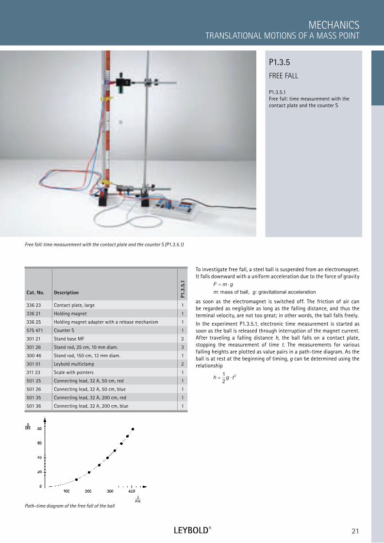
To investigate free fall, a steel ball is suspended from an electromagnet.
It falls downward with a uniform acceleration due to the force of gravity
F m g
m g
= ⋅
: mass of ball, : gravitational acceleration
as soon as the electromagnet is switched off. The friction of air can
be regarded as negligible as long as the falling distance, and thus the
terminal velocity, are not too great; in other words, the ball falls freely.
In the experiment P1.3.5.1, electronic time measurement is started as
soon as the ball is released through interruption of the magnet current.
After traveling a falling distance h, the ball falls on a contact plate,
stopping the measurement of time t. The measurements for various
falling heights are plotted as value pairs in a path-time diagram. As the
ball is at rest at the beginning of timing, g can be determined using the
relationship
h g t= ⋅1
2
2
Free fall: time measurement with the contact plate and the counter S (P1.3.5.1)
P1.3.5
Path-time diagram of the free fall of the ball
22 WWW.LEYBOLD-SHOP.COMCA
SSY ®
FREE FALL
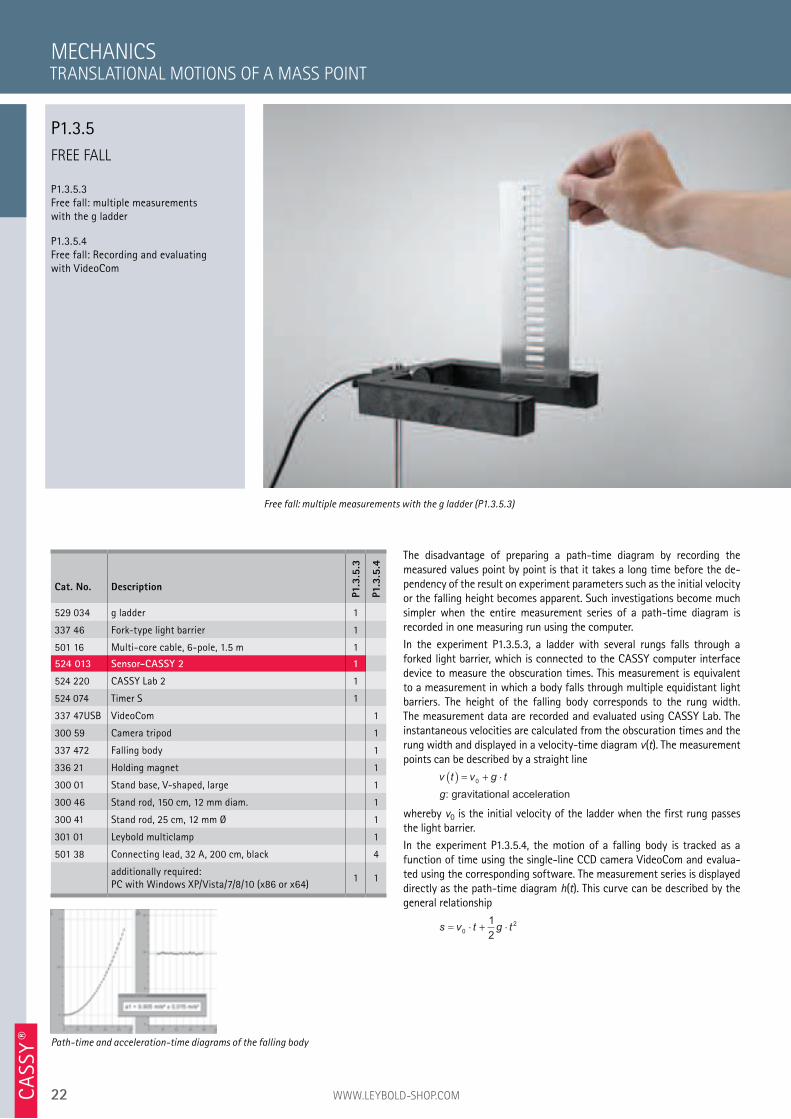
P1.3.5.3 Free fall: multiple measurements with the g ladder
P1.3.5.4 Free fall: Recording and evaluating with VideoCom
The disadvantage of preparing a path-time diagram by recording the measured values point by point is that it takes a long time before the de-pendency of the result on experiment parameters such as the initial velocity or the falling height becomes apparent. Such investigations become much simpler when the entire measurement series of a path-time diagram is recorded in one measuring run using the computer.
In the experiment P1.3.5.3, a ladder with several rungs falls through a forked light barrier, which is connected to the CASSY computer interface device to measure the obscuration times. This measurement is equivalent to a measurement in which a body falls through multiple equidistant light barriers. The height of the falling body corresponds to the rung width. The measurement data are recorded and evaluated using CASSY Lab. The instantaneous velocities are calculated from the obscuration times and the rung width and displayed in a velocity-time diagram v(t). The measurement points can be described by a straight line
v t v g t
g
( ) = + ⋅0
: gravitational acceleration
whereby v0 is the initial velocity of the ladder when the first rung passes the light barrier.
In the experiment P1.3.5.4, the motion of a falling body is tracked as a function of time using the single-line CCD camera VideoCom and evalua-ted using the corresponding software. The measurement series is displayed directly as the path-time diagram h(t). This curve can be described by the general relationship
s v t g t= ⋅ + ⋅0
21
2
MECHANICS
Free fall: multiple measurements with the g ladder (P1.3.5.3)
Cat. No. Description
P1.3
.5.3
P1.3
.5.4
529 034 g ladder 1
337 46 Fork-type light barrier 1
501 16 Multi-core cable, 6-pole, 1.5 m 1
524 013 Sensor-CASSY 2 1
524 220 CASSY Lab 2 1
524 074 Timer S 1
337 47USB VideoCom 1
300 59 Camera tripod 1
337 472 Falling body 1
336 21 Holding magnet 1
300 01 Stand base, V-shaped, large 1
300 46 Stand rod, 150 cm, 12 mm diam. 1
300 41 Stand rod, 25 cm, 12 mm Ø 1
301 01 Leybold multiclamp 1
501 38 Connecting lead, 32 A, 200 cm, black 4
additionally required: PC with Windows XP/Vista/7/8/10 (x86 or x64)
1 1
Path-time and acceleration-time diagrams of the falling body
TRANSLATIONAL MOTIONS OF A MASS POINT
P1.3.5
23
ANGLED PROJECTION
P1.3.6.1 Point-by-point recording of the projection parabola as a function of the speed and angle of projection
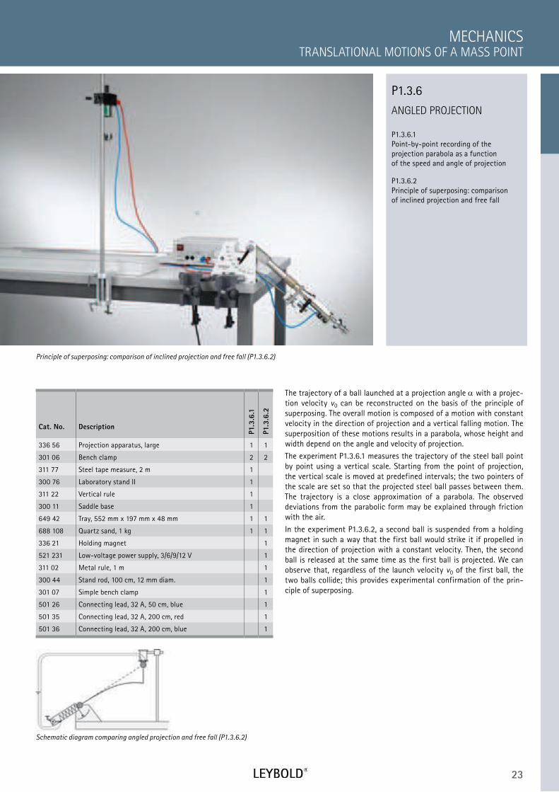
P1.3.6.2 Principle of superposing: comparison of inclined projection and free fall
TRANSLATIONAL MOTIONS OF A MASS POINT
MECHANICS
Cat. No. Description
P1.3
.6.1
P1.3
.6.2
336 56 Projection apparatus, large 1 1
301 06 Bench clamp 2 2
311 77 Steel tape measure, 2 m 1
300 76 Laboratory stand II 1
311 22 Vertical rule 1
300 11 Saddle base 1
649 42 Tray, 552 mm x 197 mm x 48 mm 1 1
688 108 Quartz sand, 1 kg 1 1
336 21 Holding magnet 1
521 231 Low-voltage power supply, 3/6/9/12 V 1
311 02 Metal rule, 1 m 1
300 44 Stand rod, 100 cm, 12 mm diam. 1
301 07 Simple bench clamp 1
501 26 Connecting lead, 32 A, 50 cm, blue 1
501 35 Connecting lead, 32 A, 200 cm, red 1
501 36 Connecting lead, 32 A, 200 cm, blue 1
The trajectory of a ball launched at a projection angle with a projec-tion velocity v0 can be reconstructed on the basis of the principle of superposing. The overall motion is composed of a motion with constant velocity in the direction of projection and a vertical falling motion. The superposition of these motions results in a parabola, whose height and width depend on the angle and velocity of projection.
The experiment P1.3.6.1 measures the trajectory of the steel ball point by point using a vertical scale. Starting from the point of projection, the vertical scale is moved at predefined intervals; the two pointers of the scale are set so that the projected steel ball passes between them. The trajectory is a close approximation of a parabola. The observed deviations from the parabolic form may be explained through friction with the air.
In the experiment P1.3.6.2, a second ball is suspended from a holding magnet in such a way that the first ball would strike it if propelled in the direction of projection with a constant velocity. Then, the second ball is released at the same time as the first ball is projected. We can observe that, regardless of the launch velocity v0 of the first ball, the two balls collide; this provides experimental confirmation of the prin-ciple of superposing.
Principle of superposing: comparison of inclined projection and free fall (P1.3.6.2)
P1.3.6
Schematic diagram comparing angled projection and free fall (P1.3.6.2)
24 WWW.LEYBOLD-SHOP.COM
TWO-DIMENSIONAL MOTIONS
ON THE AIR TABLE
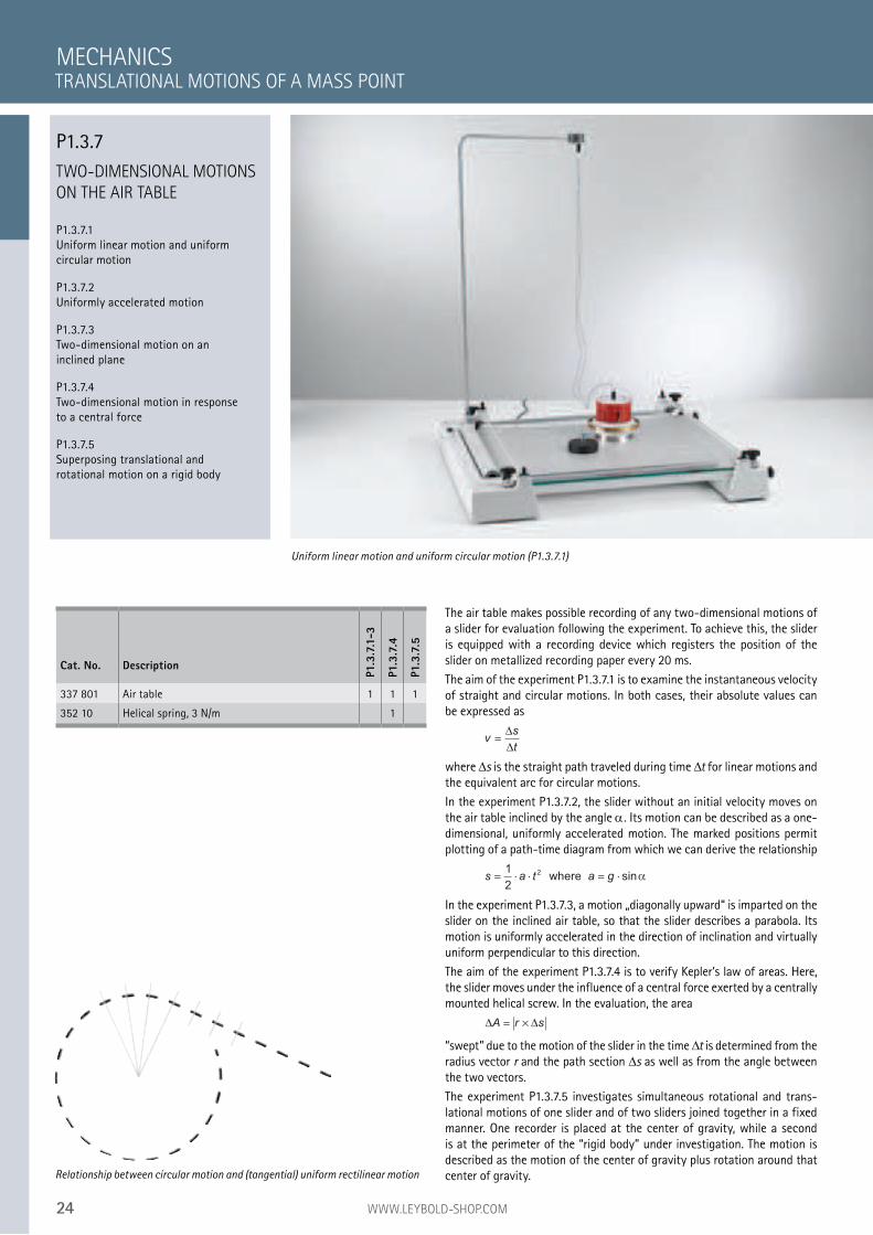
P1.3.7.1 Uniform linear motion and uniform circular motion
P1.3.7.2 Uniformly accelerated motion
P1.3.7.3 Two-dimensional motion on an inclined plane
P1.3.7.4 Two-dimensional motion in response to a central force
P1.3.7.5 Superposing translational and rotational motion on a rigid body
MECHANICS
Uniform linear motion and uniform circular motion (P1.3.7.1)
Cat. No. Description
P1.3
.7.1
-3
P1.3
.7.4
P1.3
.7.5
337 801 Air table 1 1 1
352 10 Helical spring, 3 N/m 1
Relationship between circular motion and (tangential) uniform rectilinear motion
TRANSLATIONAL MOTIONS OF A MASS POINT
P1.3.7
The air table makes possible recording of any two-dimensional motions of a slider for evaluation following the experiment. To achieve this, the slider is equipped with a recording device which registers the position of the slider on metallized recording paper every 20 ms.
The aim of the experiment P1.3.7.1 is to examine the instantaneous velocity of straight and circular motions. In both cases, their absolute values can be expressed as
vs
t=∆
∆
where s is the straight path traveled during time t for linear motions and the equivalent arc for circular motions.
In the experiment P1.3.7.2, the slider without an initial velocity moves on the air table inclined by the angle . Its motion can be described as a one-dimensional, uniformly accelerated motion. The marked positions permit plotting of a path-time diagram from which we can derive the relationship
s a t a g= ⋅ ⋅ = ⋅1
2
2 where sinα
In the experiment P1.3.7.3, a motion „diagonally upward“ is imparted on the slider on the inclined air table, so that the slider describes a parabola. Its motion is uniformly accelerated in the direction of inclination and virtually uniform perpendicular to this direction.
The aim of the experiment P1.3.7.4 is to verify Kepler’s law of areas. Here, the slider moves under the influence of a central force exerted by a centrally mounted helical screw. In the evaluation, the area
∆ ∆A r s= ×
“swept” due to the motion of the slider in the time t is determined from the radius vector r and the path section s as well as from the angle between the two vectors.
The experiment P1.3.7.5 investigates simultaneous rotational and trans-lational motions of one slider and of two sliders joined together in a fixed manner. One recorder is placed at the center of gravity, while a second is at the perimeter of the “rigid body” under investigation. The motion is described as the motion of the center of gravity plus rotation around that center of gravity.
25
TWO-DIMENSIONAL MOTIONS
ON THE AIR TABLE
P1.3.7.6
Two-dimensional motion of two
elastically coupled bodies
P1.3.7.7
Experimentally verifying the equality
of a force and its opposing force
P1.3.7.8
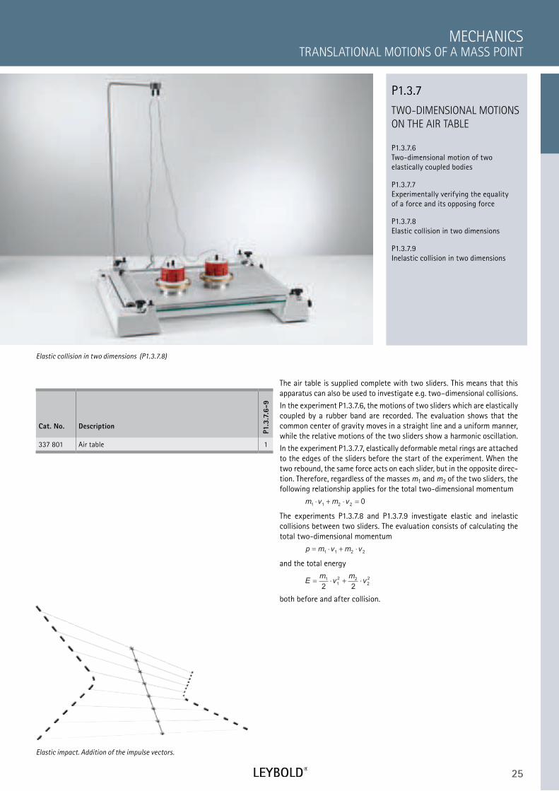
Elastic collision in two dimensions
P1.3.7.9
Inelastic collision in two dimensions
TRANSLATIONAL MOTIONS OF A MASS POINT
MECHANICS
Cat. No. Description
P1.3
.7.6
-9
337 801 Air table 1
The air table is supplied complete with two sliders. This means that this
apparatus can also be used to investigate e.g. two–dimensional collisions.
In the experiment P1.3.7.6, the motions of two sliders which are elastically
coupled by a rubber band are recorded. The evaluation shows that the
common center of gravity moves in a straight line and a uniform manner,
while the relative motions of the two sliders show a harmonic oscillation.
In the experiment P1.3.7.7, elastically deformable metal rings are attached
to the edges of the sliders before the start of the experiment. When the
two rebound, the same force acts on each slider, but in the opposite direc-
tion. Therefore, regardless of the masses m1 and m2 of the two sliders, the
following relationship applies for the total two-dimensional momentum
m v m v1 1 2 2
0⋅ + ⋅ =
The experiments P1.3.7.8 and P1.3.7.9 investigate elastic and inelastic
collisions between two sliders. The evaluation consists of calculating the
total two-dimensional momentum
p m v m v= ⋅ + ⋅1 1 2 2
and the total energy
Em
vm
v= ⋅ + ⋅1
1
2 2
2
2
2 2
both before and after collision.
Elastic collision in two dimensions (P1.3.7.8)
P1.3.7
Elastic impact. Addition of the impulse vectors.
26 WWW.LEYBOLD-SHOP.COMCA
SSY ®
ROTATIONAL MOTIONS
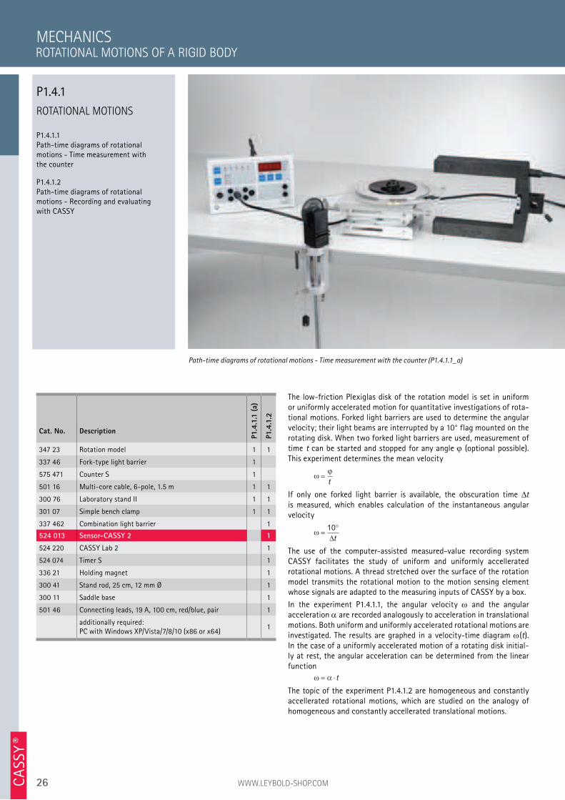
P1.4.1.1 Path-time diagrams of rotational motions - Time measurement with the counter
P1.4.1.2 Path-time diagrams of rotational motions - Recording and evaluating with CASSY
The low-friction Plexiglas disk of the rotation model is set in uniform or uniformly accelerated motion for quantitative investigations of rota-tional motions. Forked light barriers are used to determine the angular velocity; their light beams are interrupted by a 10° flag mounted on the rotating disk. When two forked light barriers are used, measurement of time t can be started and stopped for any angle (optional possible). This experiment determines the mean velocity
ωϕ
=t
If only one forked light barrier is available, the obscuration time t is measured, which enables calculation of the instantaneous angular velocity
ω =°10
∆t
The use of the computer-assisted measured-value recording system CASSY facilitates the study of uniform and uniformly accellerated rotational motions. A thread stretched over the surface of the rotation model transmits the rotational motion to the motion sensing element whose signals are adapted to the measuring inputs of CASSY by a box.
In the experiment P1.4.1.1, the angular velocity and the angular acceleration are recorded analogously to acceleration in translational motions. Both uniform and uniformly accelerated rotational motions are investigated. The results are graphed in a velocity-time diagram (t). In the case of a uniformly accelerated motion of a rotating disk initial-ly at rest, the angular acceleration can be determined from the linear function
ω α= ⋅ t
The topic of the experiment P1.4.1.2 are homogeneous and constantly accellerated rotational motions, which are studied on the analogy of homogeneous and constantly accellerated translational motions.
MECHANICS
Path-time diagrams of rotational motions - Time measurement with the counter (P1.4.1.1_a)
Cat. No. Description
P1.4
.1.1
(a)
P1.4
.1.2
347 23 Rotation model 1 1
337 46 Fork-type light barrier 1
575 471 Counter S 1
501 16 Multi-core cable, 6-pole, 1.5 m 1 1
300 76 Laboratory stand II 1 1
301 07 Simple bench clamp 1 1
337 462 Combination light barrier 1
524 013 Sensor-CASSY 2 1
524 220 CASSY Lab 2 1
524 074 Timer S 1
336 21 Holding magnet 1
300 41 Stand rod, 25 cm, 12 mm Ø 1
300 11 Saddle base 1
501 46 Connecting leads, 19 A, 100 cm, red/blue, pair 1
additionally required: PC with Windows XP/Vista/7/8/10 (x86 or x64)
1
ROTATIONAL MOTIONS OF A RIGID BODY
P1.4.1
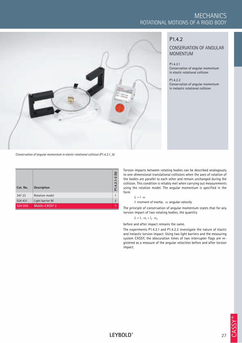
27 CA
SSY ®
CONSERVATION OF ANGULAR
MOMENTUM
P1.4.2.1
Conservation of angular momentum
in elastic rotational collision
P1.4.2.2
Conservation of angular momentum
in inelastic rotational collision
ROTATIONAL MOTIONS OF A RIGID BODY
MECHANICS
Cat. No. Description
P1.4
.2.1
-2 (
b)
347 23 Rotation model 1
524 431 Light barrier M 2
524 005 Mobile-CASSY 2 1
Conservation of angular momentum in elastic rotational collision (P1.4.2.1_b)
P1.4.2
Torsion impacts between rotating bodies can be described analogously
to one-dimensional translational collisions when the axes of rotation of
the bodies are parallel to each other and remain unchanged during the
collision. This condition is reliably met when carrying out measurements
using the rotation model. The angular momentum is specified in the
form
L l
I
= ⋅ ω
ω: moment of inertia, : angular velocity
The principle of conservation of angular momentum states that for any
torsion impact of two rotating bodies, the quantity
L l l= ⋅ + ⋅1 1 2 2ω ω
before and after impact remains the same.
The experiments P1.4.2.1 and P1.4.2.2 investigate the nature of elastic
and inelastic torsion impact. Using two light barriers and the measuring
system CASSY, the obscuration times of two interrupter flags are re-
gistered as a measure of the angular velocities before and after torsion
impact.
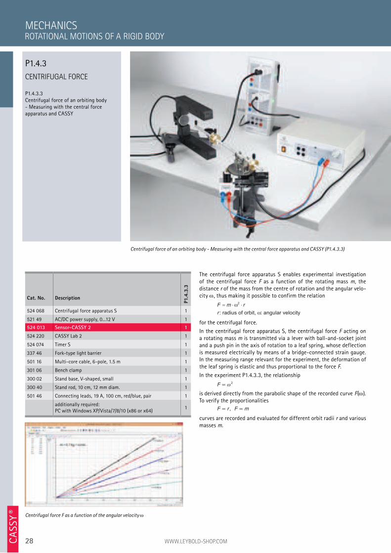
28 WWW.LEYBOLD-SHOP.COMCA
SSY ®
CENTRIFUGAL FORCE
P1.4.3.3 Centrifugal force of an orbiting body - Measuring with the central force apparatus and CASSY
The centrifugal force apparatus S enables experimental investigation of the centrifugal force F as a function of the rotating mass m, the distance r of the mass from the centre of rotation and the angular velo-city , thus making it possible to confirm the relation
F m r
r
= ⋅ ⋅ω
ω
2
: radius of orbit, : angular velocity
for the centrifugal force.
In the centrifugal force apparatus S, the centrifugal force F acting on a rotating mass m is transmitted via a lever with ball-and-socket joint and a push pin in the axis of rotation to a leaf spring, whose deflection is measured electrically by means of a bridge-connected strain gauge. In the measuring range relevant for the experiment, the deformation of the leaf spring is elastic and thus proportional to the force F.
In the experiment P1.4.3.3, the relationship
F2
is derived directly from the parabolic shape of the recorded curve F( ). To verify the proportionalities
F r F m,
curves are recorded and evaluated for different orbit radii r and various masses m.
MECHANICS
Centrifugal force of an orbiting body - Measuring with the central force apparatus and CASSY (P1.4.3.3)
Cat. No. Description
P1.4
.3.3
524 068 Centrifugal force apparatus S 1
521 49 AC/DC power supply, 0...12 V 1
524 013 Sensor-CASSY 2 1
524 220 CASSY Lab 2 1
524 074 Timer S 1
337 46 Fork-type light barrier 1
501 16 Multi-core cable, 6-pole, 1.5 m 1
301 06 Bench clamp 1
300 02 Stand base, V-shaped, small 1
300 40 Stand rod, 10 cm, 12 mm diam. 1
501 46 Connecting leads, 19 A, 100 cm, red/blue, pair 1
additionally required: PC with Windows XP/Vista/7/8/10 (x86 or x64)
1
Centrifugal force F as a function of the angular velocity
ROTATIONAL MOTIONS OF A RIGID BODY
P1.4.3
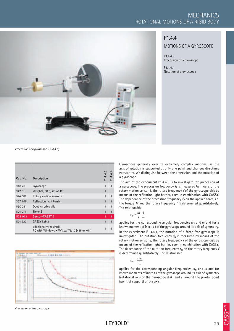
29 CA
SSY ®
MOTIONS OF A GYROSCOPE
P1.4.4.3 Precession of a gyroscope
P1.4.4.4 Nutation of a gyroscope
ROTATIONAL MOTIONS OF A RIGID BODY
MECHANICS
Cat. No. Description
P1.4
.4.3
P1.4
.4.4
348 20 Gyroscope 1 1
342 61 Weights, 50 g, set of 12 1
524 082 Rotary motion sensor S 1 1
337 468 Reflection light barrier 1 1
590 021 Double spring clip 1 1
524 074 Timer S 1 1
524 013 Sensor-CASSY 2 1 1
524 220 CASSY Lab 2 1 1
additionally required: PC with Windows XP/Vista/7/8/10 (x86 or x64)
1 1
Gyroscopes generally execute extremely complex motions, as the axis of rotation is supported at only one point and changes directions constantly. We distinguish between the precession and the nutation of a gyroscope.
The aim of the experiment P1.4.4.3 is to investigate the precession of a gyroscope. The precession frequency fP is measured by means of the rotary motion sensor S, the rotary frequency f of the gyroscope disk by means of the reflextion light barrier, each in combination with CASSY. The dependance of the precession frequency fP on the applied force, i.e. the torque M and the rotary frequency f is determined quantitatively. The relationship
ωω
P
M
I= ⋅
1
applies for the corresponding angular frequencies P and and for a known moment of inertia I of the gyroscope around its axis of symmetry.
In the experiment P1.4.4.4, the nutation of a force-free gyroscope is investigated. The nutation frequency fN is measured by means of the rotary motion sensor S, the rotary frequency f of the gyroscope disk by means of the reflextion light barrier, each in combination with CASSY. The dependance of the nutation frequency fN on the rotary frequency f is determined quantitatively. The relationship
ωω
N
l
l=
⋅
⊥
applies for the corresponding angular frequencies N and and for known moments of inertia I of the gyroscope around its axis of symmetry (rotational axis of the gyroscope disk) and I around the pivotal point (point of support) of the axis.
Precession of a gyroscope (P1.4.4.3)
P1.4.4
Precession of the gyroscope
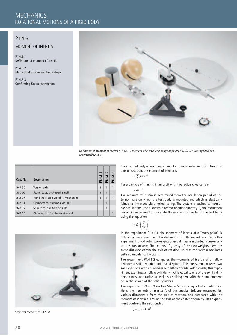
30 WWW.LEYBOLD-SHOP.COM
MOMENT OF INERTIA
P1.4.5.1
Definition of moment of inertia
P1.4.5.2
Moment of inertia and body shape
P1.4.5.3
Confirming Steiner’s theorem
For any rigid body whose mass elements mi are at a distance of r i from the
axis of rotation, the moment of inertia is
l m ri i
i
= ⋅∑ 2
For a particle of mass m in an orbit with the radius r, we can say
l m r= ⋅2
The moment of inertia is determined from the oscillation period of the
torsion axle on which the test body is mounted and which is elastically
joined to the stand via a helical spring. The system is excited to harmo-
nic oscillations. For a known directed angular quantity D, the oscillation
period T can be used to calculate the moment of inertia of the test body
using the equation
l DT
= ⋅
2
2
π
In the experiment P1.4.5.1, the moment of inertia of a ”mass point” is
determined as a function of the distance r from the axis of rotation. In this
experiment, a rod with two weights of equal mass is mounted transversely
on the torsion axle. The centers of gravity of the two weights have the
same distance r from the axis of rotation, so that the system oscillates
with no unbalanced weight.
The experiment P1.4.5.2 compares the moments of inertia of a hollow
cylinder, a solid cylinder and a solid sphere. This measurement uses two
solid cylinders with equal mass but different radii. Additionally, this expe-
riment examines a hollow cylinder which is equal to one of the solid cylin-
ders in mass and radius, as well as a solid sphere with the same moment
of inertia as one of the solid cylinders.
The experiment P1.4.5.3 verifies Steiner’s law using a flat circular disk.
Here, the moments of inertia IA of the circular disk are measured for
various distances a from the axis of rotation, and compared with the
moment of inertia IS around the axis of the center of gravity. This experi-
ment confirms the relationship
I I M aA S− = ⋅
2
MECHANICS
Definition of moment of inertia (P1.4.5.1), Moment of inertia and body shape (P1.4.5.2), Confirming Steiner’s
theorem (P1.4.5.3)
Cat. No. Description
P1.4
.5.1
P1.4
.5.2
P1.4
.5.3
347 801 Torsion axle 1 1 1
300 02 Stand base, V-shaped, small 1 1 1
313 07 Hand-held stop watch I, mechanical 1 1 1
347 81 Cylinders for torsion axle, set 1
347 82 Sphere for the torsion axle 1
347 83 Circular disc for the torsion axle 1
ROTATIONAL MOTIONS OF A RIGID BODY
P1.4.5
Steiner‘s theorem (P1.4.5.3)
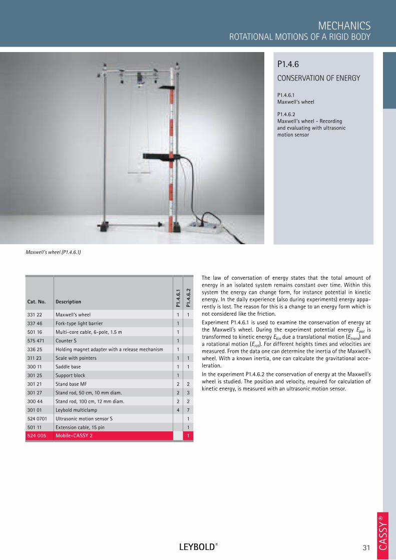
31 CA
SSY ®
CONSERVATION OF ENERGY
P1.4.6.1 Maxwell‘s wheel
P1.4.6.2 Maxwell‘s wheel - Recording and evaluating with ultrasonic motion sensor
ROTATIONAL MOTIONS OF A RIGID BODY
MECHANICS
Cat. No. Description
P1.4
.6.1
P1.4
.6.2
331 22 Maxwell‘s wheel 1 1
337 46 Fork-type light barrier 1
501 16 Multi-core cable, 6-pole, 1.5 m 1
575 471 Counter S 1
336 25 Holding magnet adapter with a release mechanism 1
311 23 Scale with pointers 1 1
300 11 Saddle base 1 1
301 25 Support block 1
301 21 Stand base MF 2 2
301 27 Stand rod, 50 cm, 10 mm diam. 2 3
300 44 Stand rod, 100 cm, 12 mm diam. 2 2
301 01 Leybold multiclamp 4 7
524 0701 Ultrasonic motion sensor S 1
501 11 Extension cable, 15 pin 1
524 005 Mobile-CASSY 2 1
The law of conversation of energy states that the total amount of energy in an isolated system remains constant over time. Within this system the energy can change form, for instance potential in kinetic energy. In the daily experience (also during experiments) energy appa-rently is lost. The reason for this is a change to an energy form which is not considered like the friction.
Experiment P1.4.6.1 is used to examine the conservation of energy at the Maxwell’s wheel. During the experiment potential energy Epot is transformed to kinetic energy Ekin due a translational motion (Etrans) and a rotational motion (Erot). For different heights times and velocities are measured. From the data one can determine the inertia of the Maxwell’s wheel. With a known inertia, one can calculate the gravitational acce-leration.
In the experiment P1.4.6.2 the conservation of energy at the Maxwell’s wheel is studied. The position and velocity, required for calculation of kinetic energy, is measured with an ultrasonic motion sensor.
Maxwell‘s wheel (P1.4.6.1)
P1.4.6
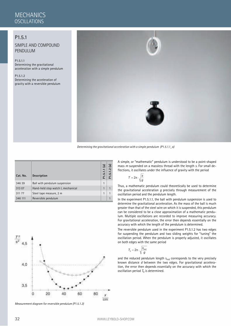
32 WWW.LEYBOLD-SHOP.COM
SIMPLE AND COMPOUND
PENDULUM
P1.5.1.1
Determining the gravitational
acceleration with a simple pendulum
P1.5.1.2
Determining the acceleration of
gravity with a reversible pendulum
A simple, or “mathematic” pendulum is understood to be a point-shaped
mass m suspended on a massless thread with the length s. For small de-
flections, it oscillates under the influence of gravity with the period
Ts
g= ⋅2π
Thus, a mathematic pendulum could theoretically be used to determine
the gravitational acceleration g precisely through measurement of the
oscillation period and the pendulum length.
In the experiment P1.5.1.1, the ball with pendulum suspension is used to
determine the gravitational acceleration. As the mass of the ball is much
greater than that of the steel wire on which it is suspended, this pendulum
can be considered to be a close approximation of a mathematic pendu-
lum. Multiple oscillations are recorded to improve measuring accuracy.
For gravitational acceleration, the error then depends essentially on the
accuracy with which the length of the pendulum is determined.
The reversible pendulum used in the experiment P1.5.1.2 has two edges
for suspending the pendulum and two sliding weights for “tuning” the
oscillation period. When the pendulum is properly adjusted, it oscillates
on both edges with the same period
Ts
gred
02= ⋅π
and the reduced pendulum length sred corresponds to the very precisely
known distance d between the two edges. For gravitational accelera-
tion, the error then depends essentially on the accuracy with which the
oscillation period T0 is determined.
MECHANICS
Determining the gravitational acceleration with a simple pendulum (P1.5.1.1_a)
Cat. No. Description
P1.5
.1.1
(a)
P1.5
.1.2
(a)
346 39 Ball with pendulum suspension 1
313 07 Hand-held stop watch I, mechanical 1 1
311 77 Steel tape measure, 2 m 1 1
346 111 Reversible pendulum 1
Measurement diagram for reversible pendulum (P1.5.1.2)
OSCILLATIONS
P1.5.1
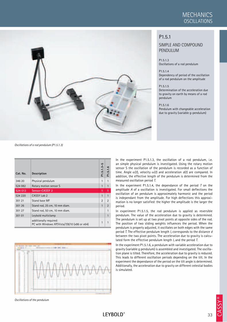
33 CA
SSY ®
SIMPLE AND COMPOUND
PENDULUM
P1.5.1.3 Oscillations of a rod pendulum
P1.5.1.4 Dependency of period of the oscillation of a rod pendulum on the amplitude
P1.5.1.5 Determination of the acceleration due to gravity on earth by means of a rod pendulum
P1.5.1.6 Pendulum with changeable acceleration due to gravity (variable g-pendulum)
OSCILLATIONS
MECHANICS
Cat. No. Description
P1.5
.1.3
-5
P1.5
.1.6
346 20 Physical pendulum 1 1
524 082 Rotary motion sensor S 1 1
524 013 Sensor-CASSY 2 1 1
524 220 CASSY Lab 2 1 1
301 21 Stand base MF 2 2
301 26 Stand rod, 25 cm, 10 mm diam. 1 2
301 27 Stand rod, 50 cm, 10 mm diam. 1
301 01 Leybold multiclamp 1
additionally required: PC with Windows XP/Vista/7/8/10 (x86 or x64)
1 1
In the experiment P1.5.1.3, the oscillation of a rod pendulum, i.e. an simple physical pendulum is investigated. Using the rotary motion sensor S the oscillation of the pendulum is recorded as a function of time. Angle (t), velocity (t) and acceleration a(t) are compared. In addition, the effective length of the pendulum is determined from the measured oscillation period T.
In the experiment P1.5.1.4, the dependance of the period T on the amplitude A of a oscillation is investigated. For small deflections the oscillation of an pendulum is approximately harmonic and the period is independant from the amplitude. For high deflections this approxi-mation is no longer satisfied: the higher the amplitude is the larger the period.
In experiment P1.5.1.5, the rod pendulum is applied as reversible pendulum. The value of the acceleration due to gravity is determined. The pendulum is set up at two pivot points at opposite sides of the rod. The position of two sliding weights influences the period. When the pendulum is properly adjusted, it oscillates on both edges with the same period T. The effective pendulum length lr corresponds to the distance d between the two pivot points. The acceleration due to gravity is calcu-lated form the effective pendulum length lr and the period T.
In the experiment P1.5.1.6, a pendulum with variable acceleration due to gravity (variable g pendulum) is assembled and investigated. The oscilla-tion plane is tilted. Therefore, the acceleration due to gravity is reduced. This leads to different oscillation periods depending on the tilt. In the experiment the dependance of the period on the tilt angle is determined. Additionally, the acceleration due to gravity on different celestial bodies is simulated.
Oscillations of a rod pendulum (P1.5.1.3)
P1.5.1
Oscillations of the pendulum
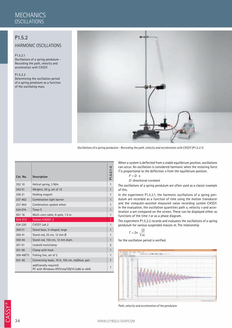
34 WWW.LEYBOLD-SHOP.COMCA
SSY ®
HARMONIC OSCILLATIONS
P1.5.2.1 Oscillations of a spring pendulum - Recording the path, velocity and acceleration with CASSY
P1.5.2.2 Determining the oscillation period of a spring pendulum as a function of the oscillating mass
When a system is deflected from a stable equilibrium position, oscillations can occur. An oscillation is considered harmonic when the restoring force F is proportional to the deflection x from the equilibrium position.
F D x
D
= ⋅
: directional constant
The oscillations of a spring pendulum are often used as a classic example of this.
In the experiment P1.5.2.1, the harmonic oscillations of a spring pen-dulum are recorded as a function of time using the motion transducer and the computer-assisted measured value recording system CASSY. In the evaluation, the oscillation quantities path x, velocity v and acce-leration a are compared on the screen. These can be displayed either as functions of the time t or as a phase diagram.
The experiment P1.5.2.2 records and evaluates the oscillations of a spring pendulum for various suspended masses m. The relationship
TD
m= ⋅2π
for the oscillation period is verified.
MECHANICS
Oscillations of a spring pendulum - Recording the path, velocity and acceleration with CASSY (P1.5.2.1)
Cat. No. Description
P1.5
.2.1
-2
352 10 Helical spring, 3 N/m 1
342 61 Weights, 50 g, set of 12 1
336 21 Holding magnet 1
337 462 Combination light barrier 1
337 464 Combination spoked wheel 1
524 074 Timer S 1
501 16 Multi-core cable, 6-pole, 1.5 m 1
524 013 Sensor-CASSY 2 1
524 220 CASSY Lab 2 1
300 01 Stand base, V-shaped, large 1
300 41 Stand rod, 25 cm, 12 mm Ø 1
300 46 Stand rod, 150 cm, 12 mm diam. 1
301 01 Leybold multiclamp 2
301 08 Clamp with hook 1
309 48ET2 Fishing line, set of 2 1
501 46 Connecting leads, 19 A, 100 cm, red/blue, pair 1
additionally required: PC with Windows XP/Vista/7/8/10 (x86 or x64)
1
Path, velocity and acceleration of the pendulum
OSCILLATIONS
P1.5.2
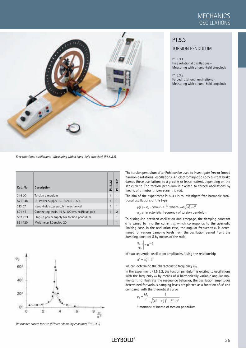
35
TORSION PENDULUM
P1.5.3.1 Free rotational oscillations - Measuring with a hand-held stopclock
P1.5.3.2 Forced rotational oscillations - Measuring with a hand-held stopclock
OSCILLATIONS
MECHANICS
Cat. No. Description
P1.5
.3.1
P1.5
.3.2
346 00 Torsion pendulum 1 1
521 546 DC Power Supply 0 ... 16 V, 0 ... 5 A 1 1
313 07 Hand-held stop watch I, mechanical 1 1
501 46 Connecting leads, 19 A, 100 cm, red/blue, pair 1 2
562 793 Plug-in power supply for torsion pendulum 1
531 120 Multimeter LDanalog 20 1
Free rotational oscillations - Measuring with a hand-held stopclock (P1.5.3.1)
P1.5.3
Resonance curves for two different damping constants (P1.5.3.2)
The torsion pendulum after Pohl can be used to investigate free or forced harmonic rotational oscillations. An electromagnetic eddy current brake damps these oscillations to a greater or lesser extent, depending on the set current. The torsion pendulum is excited to forced oscillations by means of a motor-driven eccentric rod.
The aim of the experiment P1.5.3.1 is to investigate free harmonic rota-tional oscillations of the type
ϕ ϕ ω ω ω δ
ω
δt t e
t( ) = ⋅ ⋅ −− ⋅
0
2
0
cos where =
: characteristic freq
0
2
uuency of torsion pendulum
To distinguish between oscillation and creepage, the damping constant is varied to find the current I0 which corresponds to the aperiodic
limiting case. In the oscillation case, the angular frequency is deter-mined for various damping levels from the oscillation period T and the damping constant by means of the ratio
ϕ
ϕ
δn
n
eT
+ − ⋅=1 2
of two sequential oscillation amplitudes. Using the relationship
ω ω δ2
0
2 2= −
we can determine the characteristic frequency 0.
In the experiment P1.5.3.2, the torsion pendulum is excited to oscillations with the frequency by means of a harmonically variable angular mo-mentum. To illustrate the resonance behavior, the oscillation amplitudes determined for various damping levels are plotted as a function of 2 and compared with the theoretical curve
ϕ
ω ω δ ω0
0
2
0
22
2 2
1= ⋅
−( ) + ⋅
M
l
I: moment of inertia of torsion penddulum

36 WWW.LEYBOLD-SHOP.COMCA
SSY ®
TORSION PENDULUM
P1.5.3.3 Free rotational oscillations - Recording with CASSY
P1.5.3.4 Forced harmonic and chaotic rotational oscillations - Recording with CASSY
The computer-assisted CASSY measured-value recording system is ideal for recording and evaluating the oscillations of the torsion pendulum. The numerous evaluation options enable a comprehensive comparison between theory and experiment. Thus, for example, the recorded data can be displayed as path-time, velocity-time and acceleration-time diagrams or as a phase diagram (path-velocity diagram).
The aim of the experiment P1.5.3.3 is to investigate free harmonic rotational oscillations of the general type
ϕ ϕ ω ϕ ω
ω ω δ
ω
δt t t e
t( ) = ⋅ + ⋅ ⋅
= −
−( ( ) cos ( ) sin ).
0 0
0
2 2where
where : 0 ccharacteristic frequency of torsion pendulum
This experiment investigates the relationship between the initial deflection (0) and the initial velocity (0). In addition, the damping constant is varied in order to find the current l0 which corresponds to the aperiodic limiting case.
To investigate the transition between forced harmonic and chaotic oscillations, the linear restoring moment acting on the torsion pendu-lum is deliberately altered in the experiment P1.5.3.4 by attaching an additional weight to the pendulum. The restoring moment now corres-ponds to a potential with two minima, i.e. two equilibrium positions. When the pendulum is excited at a constant frequency, it can oscillate around the left minimum, the right minimum or back and forth between the two minima. At certain frequencies, it is not possible to predict when the pendulum will change from one minimum to another. The torsion pendulum is then oscillating in a chaotic manner.
MECHANICS
Free rotational oscillations - Recording with CASSY (P1.5.3.3)
Cat. No. Description
P1.5
.3.3
P1.5
.3.4
346 00 Torsion pendulum 1 1
521 546 DC Power Supply 0 ... 16 V, 0 ... 5 A 1 1
524 013 Sensor-CASSY 2 1 1
524 220 CASSY Lab 2 1 1
524 082 Rotary motion sensor S 1 1
501 46 Connecting leads, 19 A, 100 cm, red/blue, pair 1 2
562 793 Plug-in power supply for torsion pendulum 1
531 120 Multimeter LDanalog 20 1
additionally required: PC with Windows XP/Vista/7/8/10 (x86 or x64)
1 1
Potential energy of double pendulum with and without additional mass
OSCILLATIONS
P1.5.3
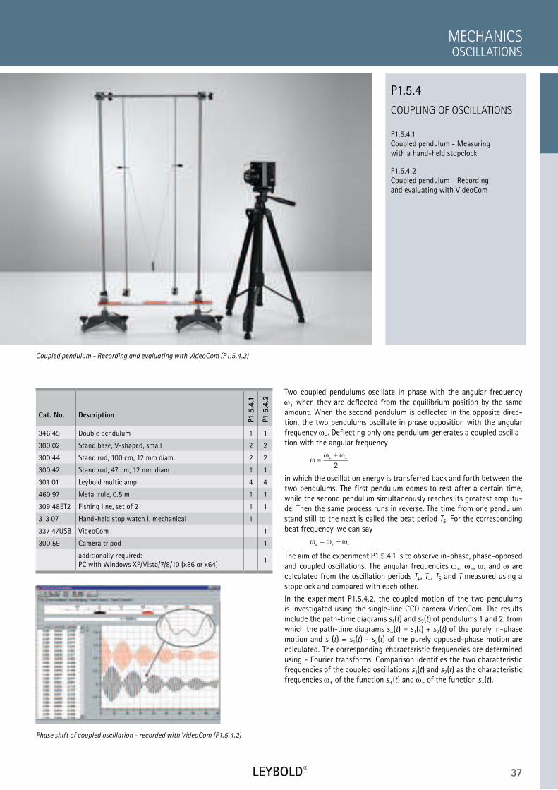
37
COUPLING OF OSCILLATIONS
P1.5.4.1 Coupled pendulum - Measuring with a hand-held stopclock
P1.5.4.2 Coupled pendulum - Recording and evaluating with VideoCom
OSCILLATIONS
MECHANICS
Cat. No. Description
P1.5
.4.1
P1.5
.4.2
346 45 Double pendulum 1 1
300 02 Stand base, V-shaped, small 2 2
300 44 Stand rod, 100 cm, 12 mm diam. 2 2
300 42 Stand rod, 47 cm, 12 mm diam. 1 1
301 01 Leybold multiclamp 4 4
460 97 Metal rule, 0.5 m 1 1
309 48ET2 Fishing line, set of 2 1 1
313 07 Hand-held stop watch I, mechanical 1
337 47USB VideoCom 1
300 59 Camera tripod 1
additionally required: PC with Windows XP/Vista/7/8/10 (x86 or x64)
1
Coupled pendulum - Recording and evaluating with VideoCom (P1.5.4.2)
P1.5.4
Phase shift of coupled oscillation - recorded with VideoCom (P1.5.4.2)
Two coupled pendulums oscillate in phase with the angular frequency
+ when they are deflected from the equilibrium position by the same amount. When the second pendulum is deflected in the opposite direc-tion, the two pendulums oscillate in phase opposition with the angular frequency –. Deflecting only one pendulum generates a coupled oscilla-tion with the angular frequency
ωω ω
=+
+ −
2
in which the oscillation energy is transferred back and forth between the two pendulums. The first pendulum comes to rest after a certain time, while the second pendulum simultaneously reaches its greatest amplitu-de. Then the same process runs in reverse. The time from one pendulum stand still to the next is called the beat period TS. For the corresponding beat frequency, we can say
ω ω ωs= −
+ −
The aim of the experiment P1.5.4.1 is to observe in-phase, phase-opposed and coupled oscillations. The angular frequencies +, –, s and are calculated from the oscillation periods T+, T–, TS and T measured using a stopclock and compared with each other.
In the experiment P1.5.4.2, the coupled motion of the two pendulums is investigated using the single-line CCD camera VideoCom. The results include the path-time diagrams s1(t) and s2(t) of pendulums 1 and 2, from which the path-time diagrams s+(t) = s1(t) + s2(t) of the purely in-phase motion and s–(t) = s1(t) - s2(t) of the purely opposed-phase motion are calculated. The corresponding characteristic frequencies are determined using - Fourier transforms. Comparison identifies the two characteristic frequencies of the coupled oscillations s1(t) and s2(t) as the characteristic frequencies + of the function s+(t) and + of the function s–(t).
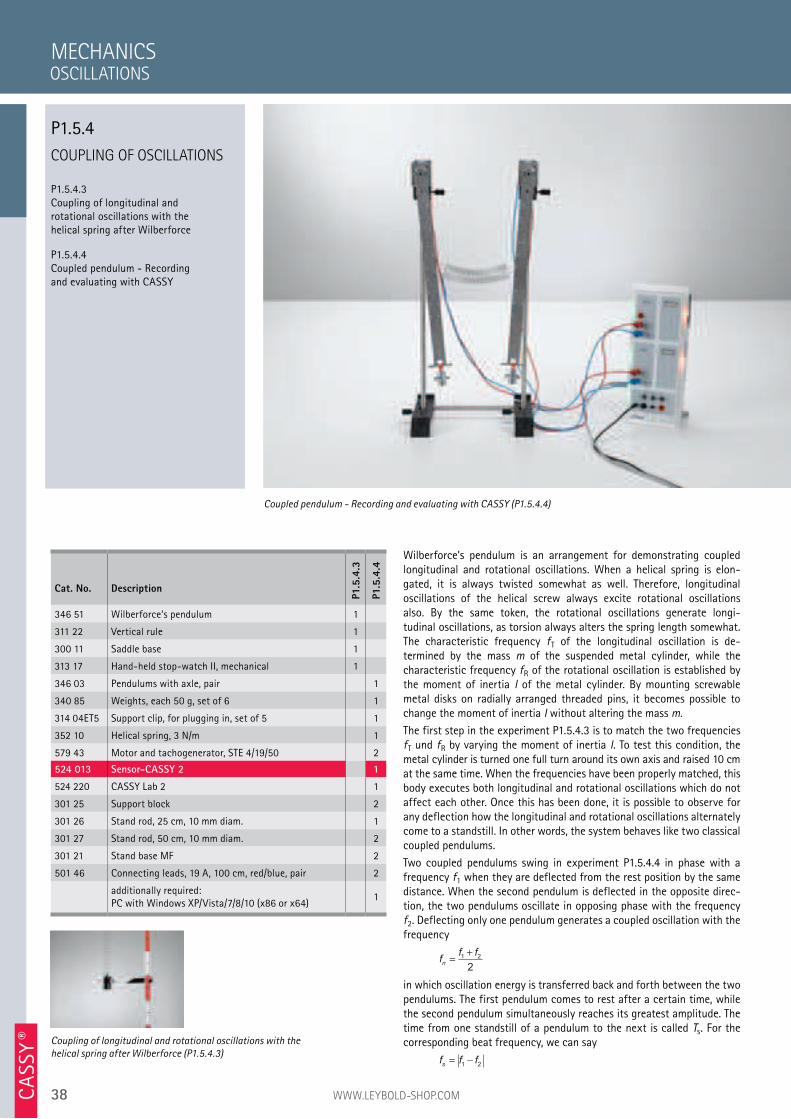
38 WWW.LEYBOLD-SHOP.COMCA
SSY ®
COUPLING OF OSCILLATIONS
P1.5.4.3 Coupling of longitudinal and rotational oscillations with the helical spring after Wilberforce
P1.5.4.4 Coupled pendulum - Recording and evaluating with CASSY
Wilberforce’s pendulum is an arrangement for demonstrating coupled longitudinal and rotational oscillations. When a helical spring is elon-gated, it is always twisted somewhat as well. Therefore, longitudinal oscillations of the helical screw always excite rotational oscillations also. By the same token, the rotational oscillations generate longi- tudinal oscillations, as torsion always alters the spring length somewhat. The characteristic frequency fT of the longitudinal oscillation is de- termined by the mass m of the suspended metal cylinder, while the characteristic frequency fR of the rotational oscillation is established by the moment of inertia I of the metal cylinder. By mounting screwable metal disks on radially arranged threaded pins, it becomes possible to change the moment of inertia I without altering the mass m.
The first step in the experiment P1.5.4.3 is to match the two frequencies fT und fR by varying the moment of inertia I. To test this condition, the metal cylinder is turned one full turn around its own axis and raised 10 cm at the same time. When the frequencies have been properly matched, this body executes both longitudinal and rotational oscillations which do not affect each other. Once this has been done, it is possible to observe for any deflection how the longitudinal and rotational oscillations alternately come to a standstill. In other words, the system behaves like two classical coupled pendulums.
Two coupled pendulums swing in experiment P1.5.4.4 in phase with a frequency f1 when they are deflected from the rest position by the same distance. When the second pendulum is deflected in the opposite direc-tion, the two pendulums oscillate in opposing phase with the frequency f2. Deflecting only one pendulum generates a coupled oscillation with the frequency
ff f
n=
+1 2
2
in which oscillation energy is transferred back and forth between the two pendulums. The first pendulum comes to rest after a certain time, while the second pendulum simultaneously reaches its greatest amplitude. The time from one standstill of a pendulum to the next is called Ts. For the corresponding beat frequency, we can say
f f fs= −
1 2
MECHANICS
Coupled pendulum - Recording and evaluating with CASSY (P1.5.4.4)
Cat. No. Description
P1.5
.4.3
P1.5
.4.4
346 51 Wilberforce‘s pendulum 1
311 22 Vertical rule 1
300 11 Saddle base 1
313 17 Hand-held stop-watch II, mechanical 1
346 03 Pendulums with axle, pair 1
340 85 Weights, each 50 g, set of 6 1
314 04ET5 Support clip, for plugging in, set of 5 1
352 10 Helical spring, 3 N/m 1
579 43 Motor and tachogenerator, STE 4/19/50 2
524 013 Sensor-CASSY 2 1
524 220 CASSY Lab 2 1
301 25 Support block 2
301 26 Stand rod, 25 cm, 10 mm diam. 1
301 27 Stand rod, 50 cm, 10 mm diam. 2
301 21 Stand base MF 2
501 46 Connecting leads, 19 A, 100 cm, red/blue, pair 2
additionally required: PC with Windows XP/Vista/7/8/10 (x86 or x64)
1
Coupling of longitudinal and rotational oscillations with the
helical spring after Wilberforce (P1.5.4.3)
OSCILLATIONS
P1.5.4
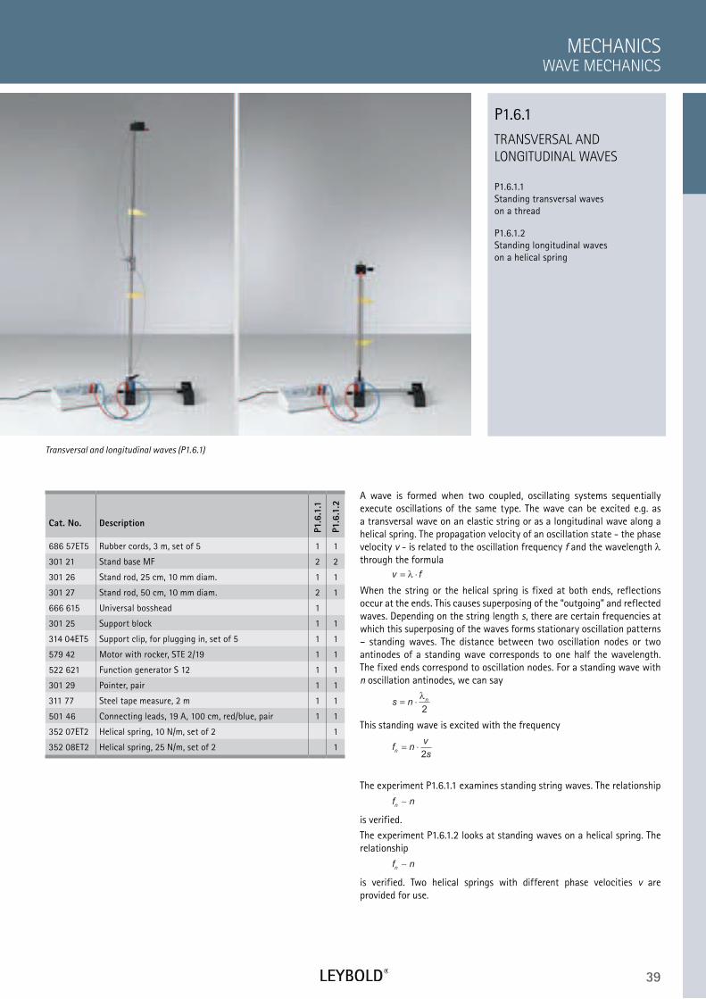
39
TRANSVERSAL AND
LONGITUDINAL WAVES
P1.6.1.1 Standing transversal waves on a thread
P1.6.1.2 Standing longitudinal waves on a helical spring
WAVE MECHANICS
MECHANICS
Cat. No. Description
P1.6
.1.1
P1.6
.1.2
686 57ET5 Rubber cords, 3 m, set of 5 1 1
301 21 Stand base MF 2 2
301 26 Stand rod, 25 cm, 10 mm diam. 1 1
301 27 Stand rod, 50 cm, 10 mm diam. 2 1
666 615 Universal bosshead 1
301 25 Support block 1 1
314 04ET5 Support clip, for plugging in, set of 5 1 1
579 42 Motor with rocker, STE 2/19 1 1
522 621 Function generator S 12 1 1
301 29 Pointer, pair 1 1
311 77 Steel tape measure, 2 m 1 1
501 46 Connecting leads, 19 A, 100 cm, red/blue, pair 1 1
352 07ET2 Helical spring, 10 N/m, set of 2 1
352 08ET2 Helical spring, 25 N/m, set of 2 1
A wave is formed when two coupled, oscillating systems sequentially execute oscillations of the same type. The wave can be excited e.g. as a transversal wave on an elastic string or as a longitudinal wave along a helical spring. The propagation velocity of an oscillation state - the phase velocity v - is related to the oscillation frequency f and the wavelength through the formula
v f= ⋅λ
When the string or the helical spring is fixed at both ends, reflections occur at the ends. This causes superposing of the “outgoing” and reflected waves. Depending on the string length s, there are certain frequencies at which this superposing of the waves forms stationary oscillation patterns – standing waves. The distance between two oscillation nodes or two antinodes of a standing wave corresponds to one half the wavelength. The fixed ends correspond to oscillation nodes. For a standing wave with n oscillation antinodes, we can say
s nn= ⋅
λ
2
This standing wave is excited with the frequency
f nv
sn= ⋅
2
The experiment P1.6.1.1 examines standing string waves. The relationship
f nn∼
is verified.
The experiment P1.6.1.2 looks at standing waves on a helical spring. The relationship
f nn∼
is verified. Two helical springs with different phase velocities v are provided for use.
Transversal and longitudinal waves (P1.6.1)
P1.6.1
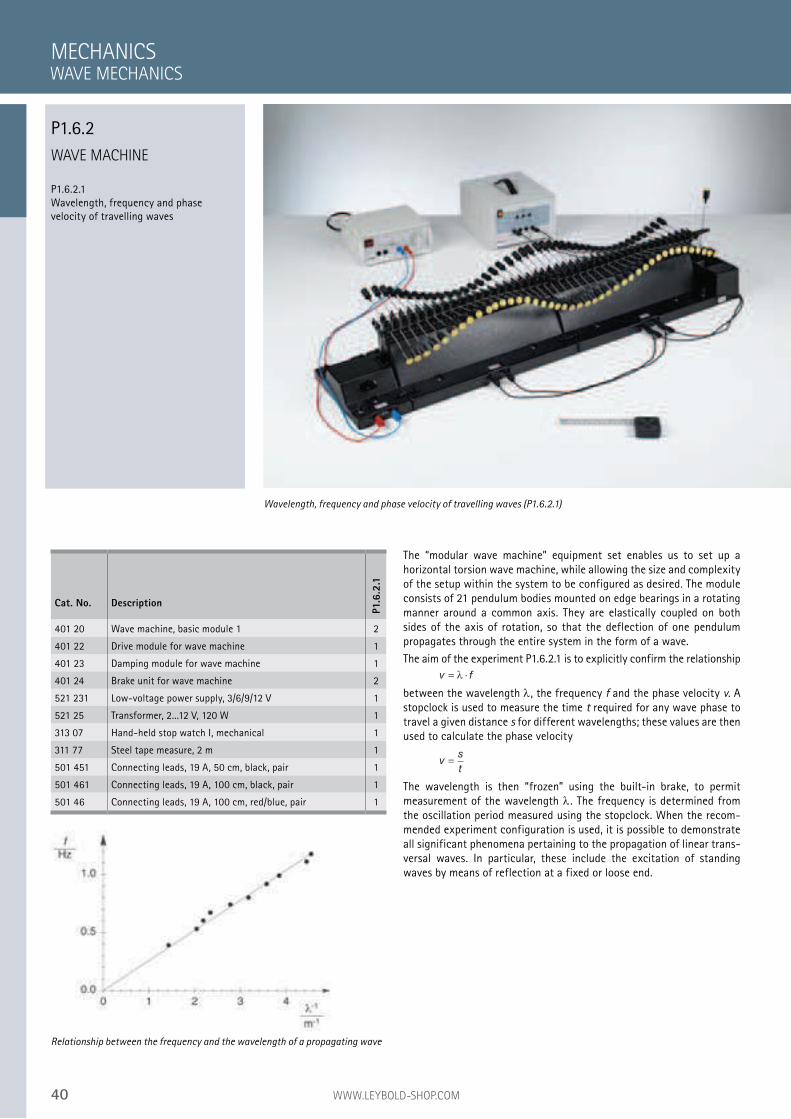
40 WWW.LEYBOLD-SHOP.COM
WAVE MACHINE
P1.6.2.1 Wavelength, frequency and phase velocity of travelling waves
The “modular wave machine” equipment set enables us to set up a horizontal torsion wave machine, while allowing the size and complexity of the setup within the system to be configured as desired. The module consists of 21 pendulum bodies mounted on edge bearings in a rotating manner around a common axis. They are elastically coupled on both sides of the axis of rotation, so that the deflection of one pendulum propagates through the entire system in the form of a wave.
The aim of the experiment P1.6.2.1 is to explicitly confirm the relationship
v f= ⋅λ
between the wavelength , the frequency f and the phase velocity v. A stopclock is used to measure the time t required for any wave phase to travel a given distance s for different wavelengths; these values are then used to calculate the phase velocity
vs
t
The wavelength is then “frozen” using the built-in brake, to permit measurement of the wavelength . The frequency is determined from the oscillation period measured using the stopclock. When the recom-mended experiment configuration is used, it is possible to demonstrate all significant phenomena pertaining to the propagation of linear trans-versal waves. In particular, these include the excitation of standing waves by means of reflection at a fixed or loose end.
MECHANICS
Wavelength, frequency and phase velocity of travelling waves (P1.6.2.1)
Cat. No. Description
P1.6
.2.1
401 20 Wave machine, basic module 1 2
401 22 Drive module for wave machine 1
401 23 Damping module for wave machine 1
401 24 Brake unit for wave machine 2
521 231 Low-voltage power supply, 3/6/9/12 V 1
521 25 Transformer, 2...12 V, 120 W 1
313 07 Hand-held stop watch I, mechanical 1
311 77 Steel tape measure, 2 m 1
501 451 Connecting leads, 19 A, 50 cm, black, pair 1
501 461 Connecting leads, 19 A, 100 cm, black, pair 1
501 46 Connecting leads, 19 A, 100 cm, red/blue, pair 1
Relationship between the frequency and the wavelength of a propagating wave
WAVE MECHANICS
P1.6.2
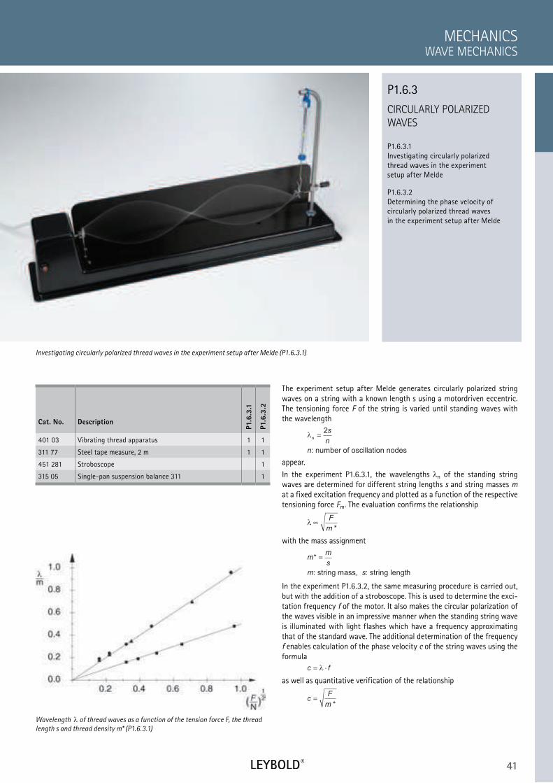
41
CIRCULARLY POLARIZED
WAVES
P1.6.3.1
Investigating circularly polarized
thread waves in the experiment
setup after Melde
P1.6.3.2
Determining the phase velocity of
circularly polarized thread waves
in the experiment setup after Melde
WAVE MECHANICS
MECHANICS
Cat. No. Description
P1.6
.3.1
P1.6
.3.2
401 03 Vibrating thread apparatus 1 1
311 77 Steel tape measure, 2 m 1 1
451 281 Stroboscope 1
315 05 Single-pan suspension balance 311 1
The experiment setup after Melde generates circularly polarized string
waves on a string with a known length s using a motordriven eccentric.
The tensioning force F of the string is varied until standing waves with
the wavelength
λn
s
n
n
=2
: number of oscillation nodes
appear.
In the experiment P1.6.3.1, the wavelengths n of the standing string
waves are determined for different string lengths s and string masses m
at a fixed excitation frequency and plotted as a function of the respective
tensioning force Fm. The evaluation confirms the relationship
λ ∝F
m *
with the mass assignment
mm
s
m s
*
: string mass, : string length
In the experiment P1.6.3.2, the same measuring procedure is carried out,
but with the addition of a stroboscope. This is used to determine the exci-
tation frequency f of the motor. It also makes the circular polarization of
the waves visible in an impressive manner when the standing string wave
is illuminated with light flashes which have a frequency approximating
that of the standard wave. The additional determination of the frequency
f enables calculation of the phase velocity c of the string waves using the
formula
c f= ⋅λ
as well as quantitative verification of the relationship
cF
m *
Investigating circularly polarized thread waves in the experiment setup after Melde (P1.6.3.1)
P1.6.3
Wavelength of thread waves as a function of the tension force F, the thread
length s and thread density m* (P1.6.3.1)
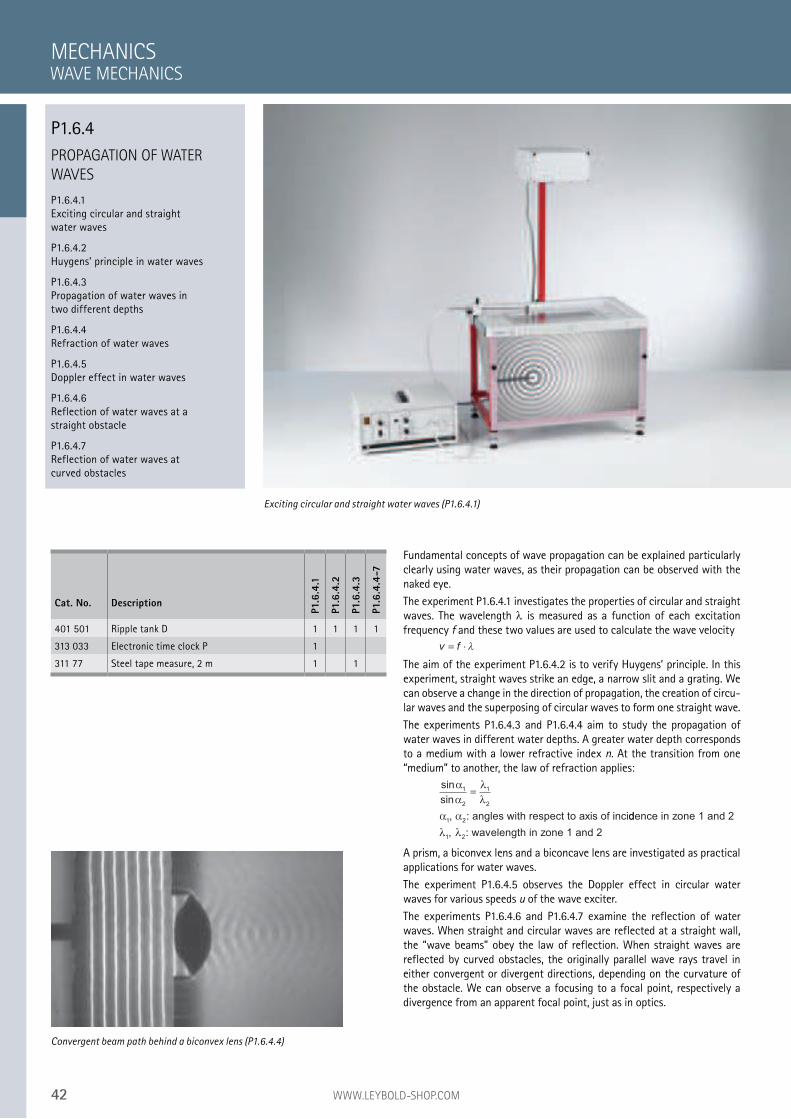
42 WWW.LEYBOLD-SHOP.COM
PROPAGATION OF WATER
WAVES
P1.6.4.1
Exciting circular and straight
water waves
P1.6.4.2
Huygens’ principle in water waves
P1.6.4.3
Propagation of water waves in
two different depths
P1.6.4.4
Refraction of water waves
P1.6.4.5
Doppler effect in water waves
P1.6.4.6
Reflection of water waves at a
straight obstacle
P1.6.4.7
Reflection of water waves at
curved obstacles
MECHANICS
Exciting circular and straight water waves (P1.6.4.1)
Cat. No. Description
P1.6
.4.1
P1.6
.4.2
P1.6
.4.3
P1.6
.4.4
-7
401 501 Ripple tank D 1 1 1 1
313 033 Electronic time clock P 1
311 77 Steel tape measure, 2 m 1 1
Convergent beam path behind a biconvex lens (P1.6.4.4)
WAVE MECHANICS
P1.6.4
Fundamental concepts of wave propagation can be explained particularly
clearly using water waves, as their propagation can be observed with the
naked eye.
The experiment P1.6.4.1 investigates the properties of circular and straight
waves. The wavelength is measured as a function of each excitation
frequency f and these two values are used to calculate the wave velocity
v f= ⋅
The aim of the experiment P1.6.4.2 is to verify Huygens’ principle. In this
experiment, straight waves strike an edge, a narrow slit and a grating. We
can observe a change in the direction of propagation, the creation of circu-
lar waves and the superposing of circular waves to form one straight wave.
The experiments P1.6.4.3 and P1.6.4.4 aim to study the propagation of
water waves in different water depths. A greater water depth corresponds
to a medium with a lower refractive index n. At the transition from one
“medium” to another, the law of refraction applies:
sin
sin
α
α
λ
λ
α α
1
2
1
2
1 2
=
, : angles with respect to axis of inciddence in zone 1 and 2
: wavelength in zone 1 and 21λ λ, 2
A prism, a biconvex lens and a biconcave lens are investigated as practical
applications for water waves.
The experiment P1.6.4.5 observes the Doppler effect in circular water
waves for various speeds u of the wave exciter.
The experiments P1.6.4.6 and P1.6.4.7 examine the reflection of water
waves. When straight and circular waves are reflected at a straight wall,
the “wave beams” obey the law of reflection. When straight waves are
reflected by curved obstacles, the originally parallel wave rays travel in
either convergent or divergent directions, depending on the curvature of
the obstacle. We can observe a focusing to a focal point, respectively a
divergence from an apparent focal point, just as in optics.
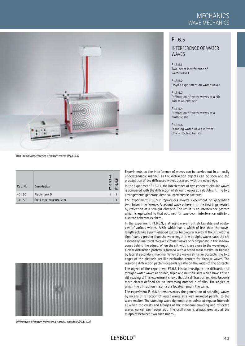
43
INTERFERENCE OF WATER
WAVES
P1.6.5.1
Two-beam interference of
water waves
P1.6.5.2
Lloyd’s experiment on water waves
P1.6.5.3
Diffraction of water waves at a slit
and at an obstacle
P1.6.5.4
Diffraction of water waves at a
multiple slit
P1.6.5.5
Standing water waves in front
of a reflecting barrier
WAVE MECHANICS
MECHANICS
Cat. No. Description
P1.6
.5.1
-4
P1.6
.5.5
401 501 Ripple tank D 1 1
311 77 Steel tape measure, 2 m 1
Two-beam interference of water waves (P1.6.5.1)
P1.6.5
Diffraction of water waves at a narrow obstacle (P1.6.5.3)
Experiments on the interference of waves can be carried out in an easily
understandable manner, as the diffraction objects can be seen and the
propagation of the diffracted waves observed with the naked eye.
In the experiment P1.6.5.1, the interference of two coherent circular waves
is compared with the diffraction of straight waves at a double slit. The two
arrangements generate identical interference patterns.
The experiment P1.6.5.2 reproduces Lloyd’s experiment on generating
two-beam interference. A second wave coherent to the first is generated
by reflection at a straight obstacle. The result is an interference pattern
which is equivalent to that obtained for two-beam interference with two
discrete coherent exciters.
In the experiment P1.6.5.3, a straight wave front strikes slits and obsta-
cles of various widths. A slit which has a width of less than the wave-
length acts like a point-shaped exciter for circular waves. If the slit width is
significantly greater than the wavelength, the straight waves pass the slit
essentially unaltered. Weaker, circular waves only propagate in the shadow
zones behind the edges. When the slit widths are close to the wavelength,
a clear diffraction pattern is formed with a broad main maximum flanked
by lateral secondary maxima. When the waves strike an obstacle, the two
edges of the obstacle act like excitation centers for circular waves. The
resulting diffraction pattern depends greatly on the width of the obstacle.
The object of the experiment P1.6.5.4 is to investigate the diffraction of
straight water waves at double, triple and multiple slits which have a fixed
slit spacing d. This experiment shows that the diffraction maxima become
more clearly defined for an increasing number n of slits. The angles at
which the diffraction maxima are located remain the same.
The experiment P1.6.5.5 demonstrates the generation of standing waves
by means of reflection of water waves at a wall arranged parallel to the
wave exciter. The standing wave demonstrates points at regular intervals
at which the crests and troughs of the individual traveling and reflected
waves cancel each other out. The oscillation is always greatest at the
midpoint between two such nodes.
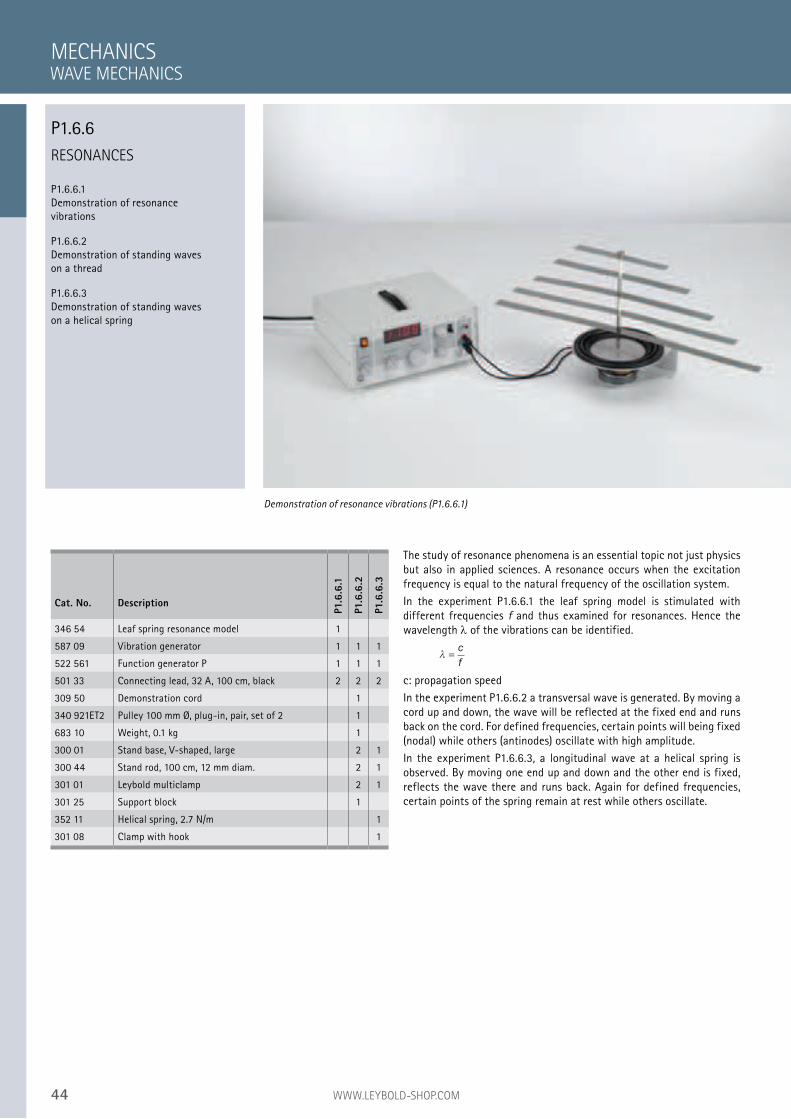
44 WWW.LEYBOLD-SHOP.COM
RESONANCES
P1.6.6.1 Demonstration of resonance vibrations
P1.6.6.2 Demonstration of standing waves on a thread
P1.6.6.3 Demonstration of standing waves on a helical spring
The study of resonance phenomena is an essential topic not just physics but also in applied sciences. A resonance occurs when the excitation frequency is equal to the natural frequency of the oscillation system.
In the experiment P1.6.6.1 the leaf spring model is stimulated with different frequencies f and thus examined for resonances. Hence the wavelength of the vibrations can be identified.
c
f
c: propagation speed
In the experiment P1.6.6.2 a transversal wave is generated. By moving a cord up and down, the wave will be reflected at the fixed end and runs back on the cord. For defined frequencies, certain points will being fixed (nodal) while others (antinodes) oscillate with high amplitude.
In the experiment P1.6.6.3, a longitudinal wave at a helical spring is observed. By moving one end up and down and the other end is fixed, reflects the wave there and runs back. Again for defined frequencies, certain points of the spring remain at rest while others oscillate.
MECHANICS
Demonstration of resonance vibrations (P1.6.6.1)
Cat. No. Description
P1.6
.6.1
P1.6
.6.2
P1.6
.6.3
346 54 Leaf spring resonance model 1
587 09 Vibration generator 1 1 1
522 561 Function generator P 1 1 1
501 33 Connecting lead, 32 A, 100 cm, black 2 2 2
309 50 Demonstration cord 1
340 921ET2 Pulley 100 mm Ø, plug-in, pair, set of 2 1
683 10 Weight, 0.1 kg 1
300 01 Stand base, V-shaped, large 2 1
300 44 Stand rod, 100 cm, 12 mm diam. 2 1
301 01 Leybold multiclamp 2 1
301 25 Support block 1
352 11 Helical spring, 2.7 N/m 1
301 08 Clamp with hook 1
WAVE MECHANICS
P1.6.6
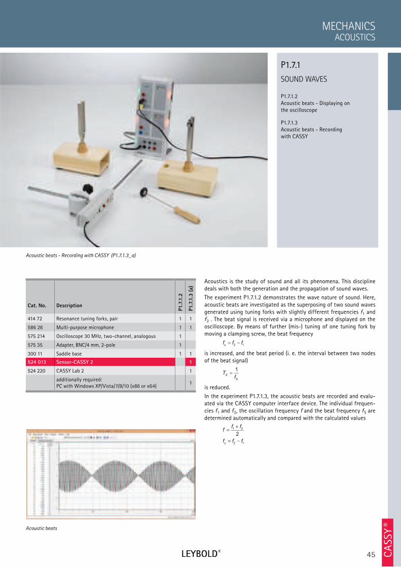
45 CA
SSY ®
SOUND WAVES
P1.7.1.2 Acoustic beats - Displaying on the oscilloscope
P1.7.1.3 Acoustic beats - Recording with CASSY
ACOUSTICS
MECHANICS
Cat. No. Description
P1.7
.1.2
P1.7
.1.3
(a)
414 72 Resonance tuning forks, pair 1 1
586 26 Multi-purpose microphone 1 1
575 214 Oscilloscope 30 MHz, two-channel, analogous 1
575 35 Adapter, BNC/4 mm, 2-pole 1
300 11 Saddle base 1 1
524 013 Sensor-CASSY 2 1
524 220 CASSY Lab 2 1
additionally required: PC with Windows XP/Vista/7/8/10 (x86 or x64)
1
Acoustics is the study of sound and all its phenomena. This discipline deals with both the generation and the propagation of sound waves.
The experiment P1.7.1.2 demonstrates the wave nature of sound. Here, acoustic beats are investigated as the superposing of two sound waves generated using tuning forks with slightly different frequencies f1 and f2 . The beat signal is received via a microphone and displayed on the oscilloscope. By means of further (mis-) tuning of one tuning fork by moving a clamping screw, the beat frequency
f f fs= −
2 1
is increased, and the beat period (i. e. the interval between two nodes of the beat signal)
Tf
S
S
1
is reduced.
In the experiment P1.7.1.3, the acoustic beats are recorded and evalu-ated via the CASSY computer interface device. The individual frequen-cies f1 and f2, the oscillation frequency f and the beat frequency fS are determined automatically and compared with the calculated values
ff f
f f fs
=+
= −
1 2
2 1
2
Acoustic beats - Recording with CASSY (P1.7.1.3_a)
P1.7.1
Acoustic beats
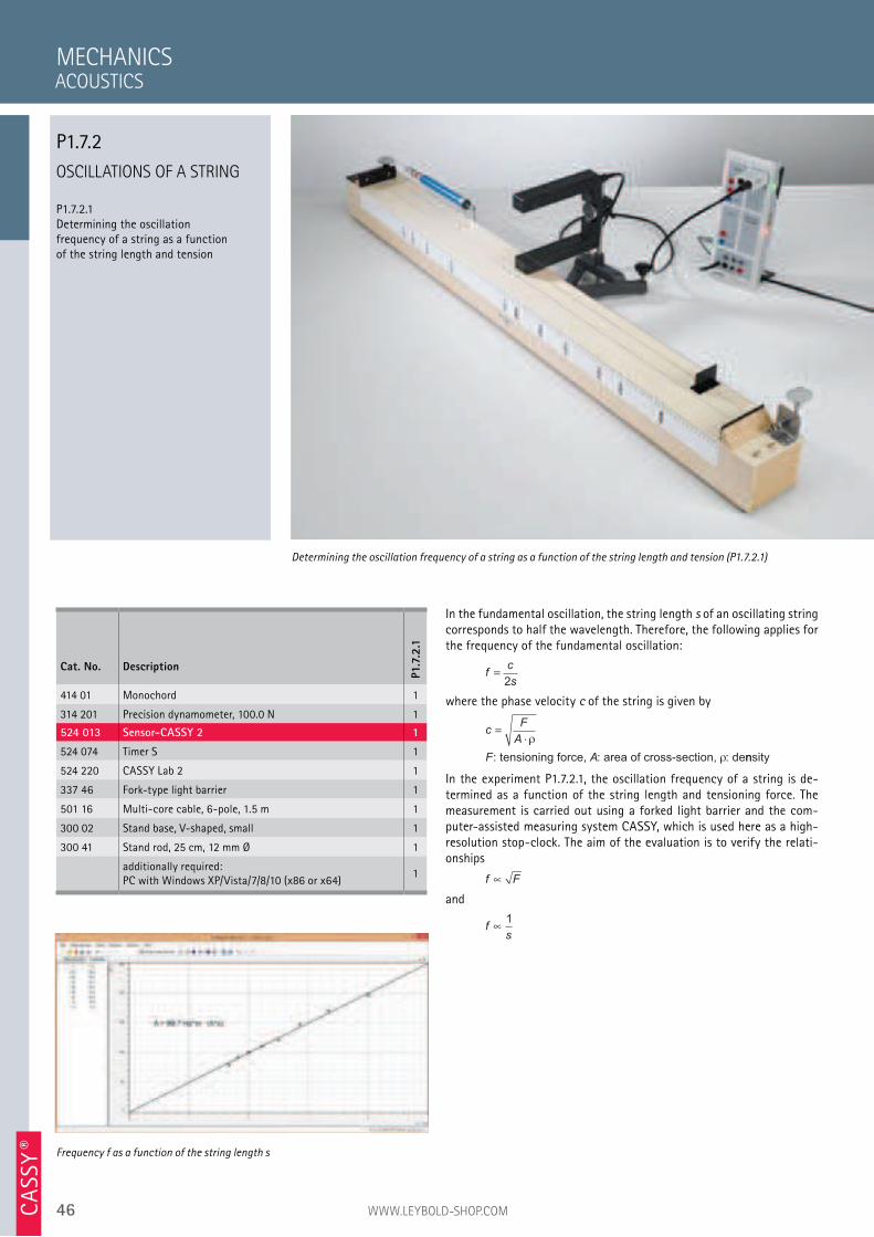
46 WWW.LEYBOLD-SHOP.COMCA
SSY ®
OSCILLATIONS OF A STRING
P1.7.2.1 Determining the oscillation frequency of a string as a function of the string length and tension
In the fundamental oscillation, the string length s of an oscillating string corresponds to half the wavelength. Therefore, the following applies for the frequency of the fundamental oscillation:
fc
s2
where the phase velocity c of the string is given by
cF
A
F A
=⋅ ρ
ρ: tensioning force, : area of cross-section, : dennsity
In the experiment P1.7.2.1, the oscillation frequency of a string is de-termined as a function of the string length and tensioning force. The measurement is carried out using a forked light barrier and the com-puter-assisted measuring system CASSY, which is used here as a high-resolution stop-clock. The aim of the evaluation is to verify the relati-onships
f F
and
fs
1
MECHANICS
Determining the oscillation frequency of a string as a function of the string length and tension (P1.7.2.1)
Cat. No. Description
P1.7
.2.1
414 01 Monochord 1
314 201 Precision dynamometer, 100.0 N 1
524 013 Sensor-CASSY 2 1
524 074 Timer S 1
524 220 CASSY Lab 2 1
337 46 Fork-type light barrier 1
501 16 Multi-core cable, 6-pole, 1.5 m 1
300 02 Stand base, V-shaped, small 1
300 41 Stand rod, 25 cm, 12 mm Ø 1
additionally required: PC with Windows XP/Vista/7/8/10 (x86 or x64)
1
Frequency f as a function of the string length s
ACOUSTICS
P1.7.2
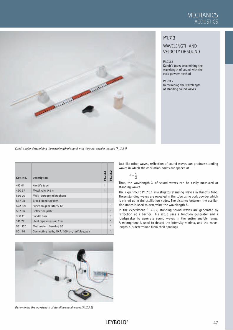
47
WAVELENGTH AND
VELOCITY OF SOUND
P1.7.3.1 Kundt‘s tube: determining the wavelength of sound with the cork-powder method
P1.7.3.2 Determining the wavelength of standing sound waves
ACOUSTICS
MECHANICS
Cat. No. Description
P1.7
.3.1
P1.7
.3.2
413 01 Kundt‘s tube 1
460 97 Metal rule, 0.5 m 1
586 26 Multi-purpose microphone 1
587 08 Broad-band speaker 1
522 621 Function generator S 12 1
587 66 Reflection plate 1
300 11 Saddle base 3
311 77 Steel tape measure, 2 m 1
531 120 Multimeter LDanalog 20 1
501 46 Connecting leads, 19 A, 100 cm, red/blue, pair 1
Just like other waves, reflection of sound waves can produce standing waves in which the oscillation nodes are spaced at
d =λ
2
Thus, the wavelength of sound waves can be easily measured at standing waves.
The experiment P1.7.3.1 investigates standing waves in Kundt’s tube. These standing waves are revealed in the tube using cork powder which is stirred up in the oscillation nodes. The distance between the oscilla-tion nodes is used to determine the wavelength .
In the experiment P1.7.3.2, standing sound waves are generated by reflection at a barrier. This setup uses a function generator and a loudspeaker to generate sound waves in the entire audible range. A microphone is used to detect the intensity minima, and the wave-length is determined from their spacings.
Kundt‘s tube: determining the wavelength of sound with the cork-powder method (P1.7.3.1)
P1.7.3
Determining the wavelength of standing sound waves (P1.7.3.2)
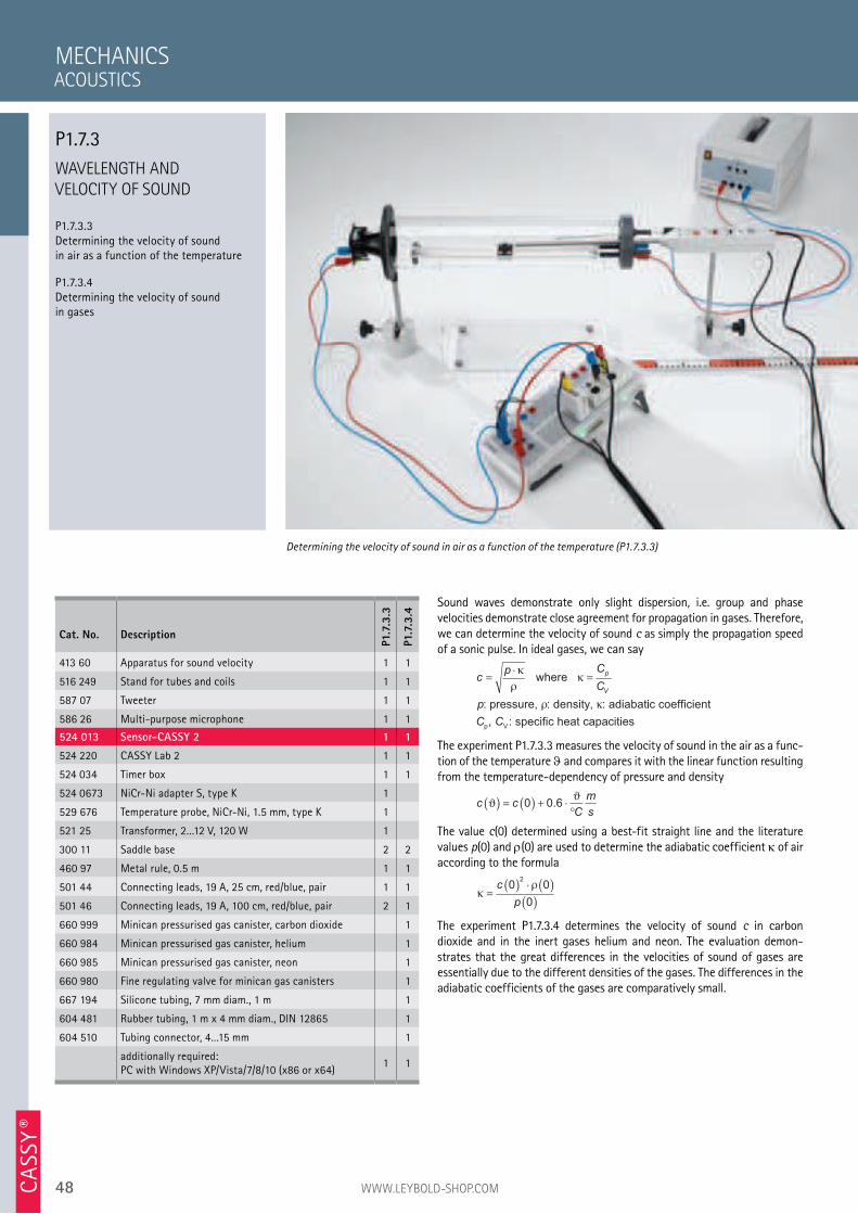
48 WWW.LEYBOLD-SHOP.COMCA
SSY ®
WAVELENGTH AND
VELOCITY OF SOUND
P1.7.3.3 Determining the velocity of sound in air as a function of the temperature
P1.7.3.4 Determining the velocity of sound in gases
MECHANICS
Determining the velocity of sound in air as a function of the temperature (P1.7.3.3)
Cat. No. Description
P1.7
.3.3
P1.7
.3.4
413 60 Apparatus for sound velocity 1 1
516 249 Stand for tubes and coils 1 1
587 07 Tweeter 1 1
586 26 Multi-purpose microphone 1 1
524 013 Sensor-CASSY 2 1 1
524 220 CASSY Lab 2 1 1
524 034 Timer box 1 1
524 0673 NiCr-Ni adapter S, type K 1
529 676 Temperature probe, NiCr-Ni, 1.5 mm, type K 1
521 25 Transformer, 2...12 V, 120 W 1
300 11 Saddle base 2 2
460 97 Metal rule, 0.5 m 1 1
501 44 Connecting leads, 19 A, 25 cm, red/blue, pair 1 1
501 46 Connecting leads, 19 A, 100 cm, red/blue, pair 2 1
660 999 Minican pressurised gas canister, carbon dioxide 1
660 984 Minican pressurised gas canister, helium 1
660 985 Minican pressurised gas canister, neon 1
660 980 Fine regulating valve for minican gas canisters 1
667 194 Silicone tubing, 7 mm diam., 1 m 1
604 481 Rubber tubing, 1 m x 4 mm diam., DIN 12865 1
604 510 Tubing connector, 4...15 mm 1
additionally required: PC with Windows XP/Vista/7/8/10 (x86 or x64)
1 1
ACOUSTICS
P1.7.3
Sound waves demonstrate only slight dispersion, i.e. group and phase velocities demonstrate close agreement for propagation in gases. Therefore, we can determine the velocity of sound c as simply the propagation speed of a sonic pulse. In ideal gases, we can say
cp C
C
p
p
V
=⋅
=κ
ρκ
ρ κ
where
: pressure, : density, : adiabatiic coefficient
, : specific heat capacitiesp VC C
The experiment P1.7.3.3 measures the velocity of sound in the air as a func-tion of the temperature and compares it with the linear function resulting from the temperature-dependency of pressure and density
c cC
m
sϑ
ϑ( ) = ( ) + ⋅
°0 0 6.
The value c(0) determined using a best-fit straight line and the literature values p(0) and (0) are used to determine the adiabatic coefficient of air according to the formula
κρ
=( ) ⋅ ( )
( )
c
p
0 0
0
2
The experiment P1.7.3.4 determines the velocity of sound c in carbon dioxide and in the inert gases helium and neon. The evaluation demon-strates that the great differences in the velocities of sound of gases are essentially due to the different densities of the gases. The differences in the adiabatic coefficients of the gases are comparatively small.
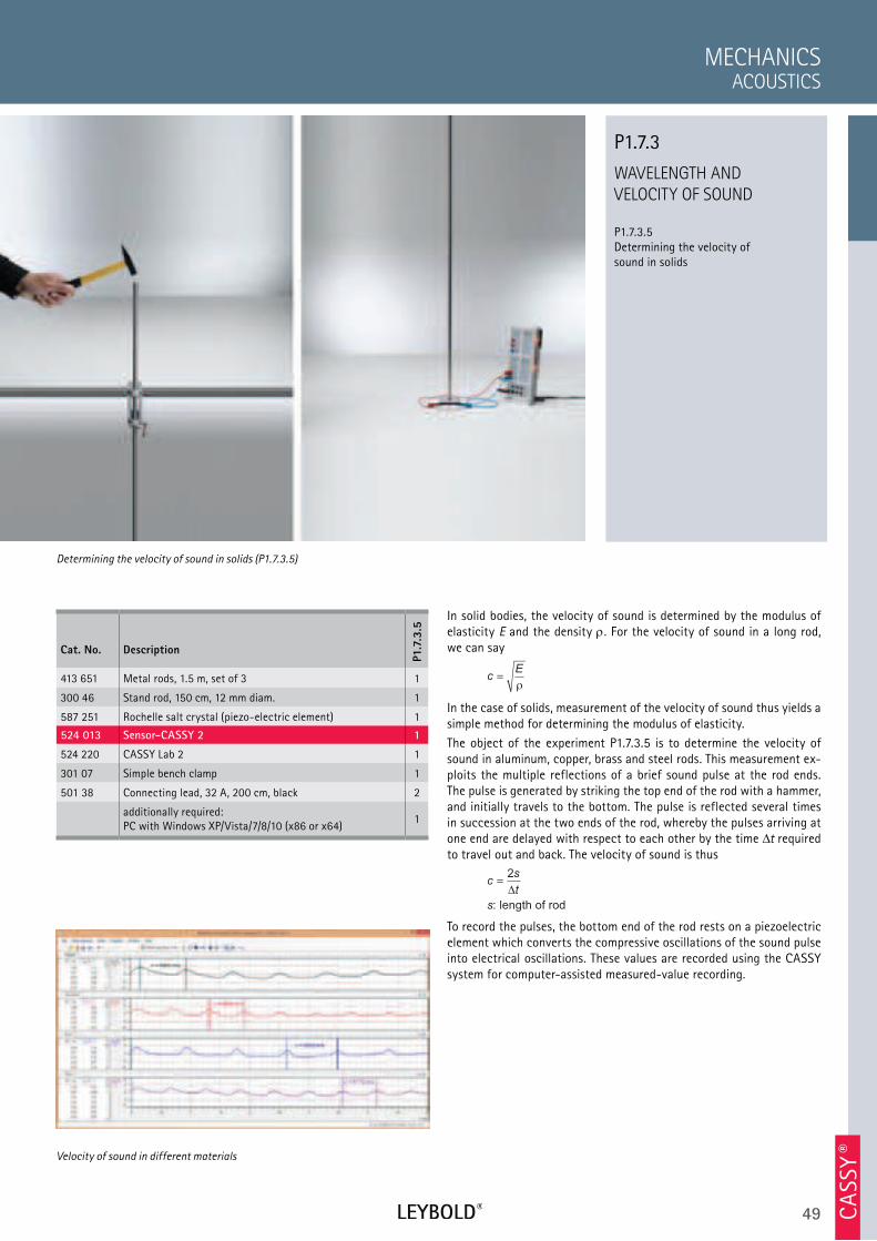
49 CA
SSY ®
WAVELENGTH AND
VELOCITY OF SOUND
P1.7.3.5 Determining the velocity of sound in solids
ACOUSTICS
MECHANICS
Cat. No. Description
P1.7
.3.5
413 651 Metal rods, 1.5 m, set of 3 1
300 46 Stand rod, 150 cm, 12 mm diam. 1
587 251 Rochelle salt crystal (piezo-electric element) 1
524 013 Sensor-CASSY 2 1
524 220 CASSY Lab 2 1
301 07 Simple bench clamp 1
501 38 Connecting lead, 32 A, 200 cm, black 2
additionally required: PC with Windows XP/Vista/7/8/10 (x86 or x64)
1
Determining the velocity of sound in solids (P1.7.3.5)
P1.7.3
Velocity of sound in different materials
In solid bodies, the velocity of sound is determined by the modulus of elasticity E and the density . For the velocity of sound in a long rod, we can say
cE
=ρ
In the case of solids, measurement of the velocity of sound thus yields a simple method for determining the modulus of elasticity.
The object of the experiment P1.7.3.5 is to determine the velocity of sound in aluminum, copper, brass and steel rods. This measurement ex-ploits the multiple reflections of a brief sound pulse at the rod ends. The pulse is generated by striking the top end of the rod with a hammer, and initially travels to the bottom. The pulse is reflected several times in succession at the two ends of the rod, whereby the pulses arriving at one end are delayed with respect to each other by the time t required to travel out and back. The velocity of sound is thus
cs
t
s
=2
∆
: length of rod
To record the pulses, the bottom end of the rod rests on a piezoelectric element which converts the compressive oscillations of the sound pulse into electrical oscillations. These values are recorded using the CASSY system for computer-assisted measured-value recording.
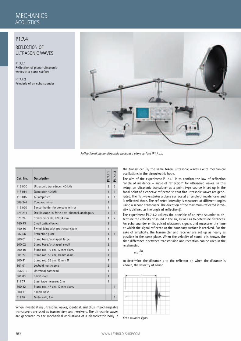
50 WWW.LEYBOLD-SHOP.COM
REFLECTION OF
ULTRASONIC WAVES
P1.7.4.1 Reflection of planar ultrasonic waves at a plane surface
P1.7.4.2 Principle of an echo sounder
When investigating ultrasonic waves, identical, and thus interchangeable transducers are used as transmitters and receivers. The ultrasonic waves are generated by the mechanical oscillations of a piezoelectric body in
MECHANICS
Reflection of planar ultrasonic waves at a plane surface (P1.7.4.1)
Cat. No. Description
P1.7
.4.1
P1.7
.4.2
416 000 Ultrasonic transducer, 40 kHz 2 2
416 014 Generator, 40 kHz 1 1
416 015 AC amplifier 1 1
389 241 Concave mirror 1
416 020 Sensor holder for concave mirror 1
575 214 Oscilloscope 30 MHz, two-channel, analogous 1 1
575 24 Screened cable, BNC/4 mm 1 2
460 43 Small optical bench 2
460 40 Swivel joint with protractor scale 1
587 66 Reflection plate 1 1
300 01 Stand base, V-shaped, large 1
300 02 Stand base, V-shaped, small 2
300 40 Stand rod, 10 cm, 12 mm diam. 1
301 27 Stand rod, 50 cm, 10 mm diam. 1
300 41 Stand rod, 25 cm, 12 mm Ø 1
301 01 Leybold multiclamp 2
666 615 Universal bosshead 1
361 03 Spirit level 1
311 77 Steel tape measure, 2 m 1
300 42 Stand rod, 47 cm, 12 mm diam. 1
300 11 Saddle base 3
311 02 Metal rule, 1 m 1
Echo sounder signal
ACOUSTICS
P1.7.4
the transducer. By the same token, ultrasonic waves excite mechanical oscillations in the piezoelectric body.
The aim of the experiment P1.7.4.1 is to confirm the law of reflection “angle of incidence = angle of reflection” for ultrasonic waves. In this setup, an ultrasonic transducer as a point-type source is set up in the focal point of a concave reflector, so that flat ultrasonic waves are gene-rated. The flat wave strikes a plane surface at an angle of incidence and is reflected there. The reflected intensity is measured at different angles using a second transducer. The direction of the maximum reflected inten-sity is defined as the angle of reflection .
The experiment P1.7.4.2 utilizes the principle of an echo sounder to de-termine the velocity of sound in the air, as well as to determine distances. An echo sounder emits pulsed ultrasonic signals and measures the time at which the signal reflected at the boundary surface is received. For the sake of simplicity, the transmitter and receiver are set up as nearly as possible in the same place. When the velocity of sound c is known, the time difference t between transmission and reception can be used in the relationship
cs
t
2
to determine the distance s to the reflector or, when the distance is known, the velocity of sound.
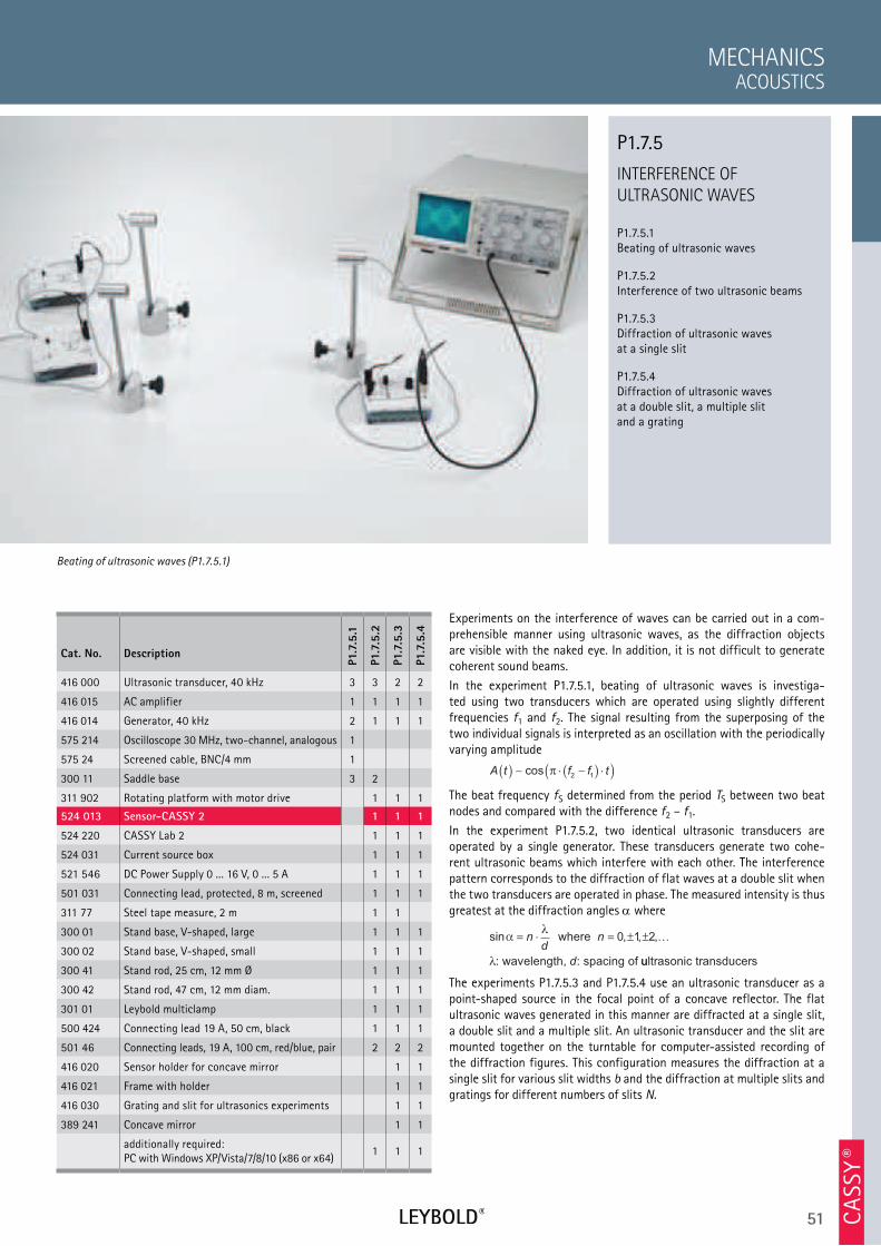
51 CA
SSY ®
INTERFERENCE OF
ULTRASONIC WAVES
P1.7.5.1 Beating of ultrasonic waves
P1.7.5.2 Interference of two ultrasonic beams
P1.7.5.3 Diffraction of ultrasonic waves at a single slit
P1.7.5.4 Diffraction of ultrasonic waves at a double slit, a multiple slit and a grating
ACOUSTICS
MECHANICS
Cat. No. Description
P1.7
.5.1
P1.7
.5.2
P1.7
.5.3
P1.7
.5.4
416 000 Ultrasonic transducer, 40 kHz 3 3 2 2
416 015 AC amplifier 1 1 1 1
416 014 Generator, 40 kHz 2 1 1 1
575 214 Oscilloscope 30 MHz, two-channel, analogous 1
575 24 Screened cable, BNC/4 mm 1
300 11 Saddle base 3 2
311 902 Rotating platform with motor drive 1 1 1
524 013 Sensor-CASSY 2 1 1 1
524 220 CASSY Lab 2 1 1 1
524 031 Current source box 1 1 1
521 546 DC Power Supply 0 ... 16 V, 0 ... 5 A 1 1 1
501 031 Connecting lead, protected, 8 m, screened 1 1 1
311 77 Steel tape measure, 2 m 1 1
300 01 Stand base, V-shaped, large 1 1 1
300 02 Stand base, V-shaped, small 1 1 1
300 41 Stand rod, 25 cm, 12 mm Ø 1 1 1
300 42 Stand rod, 47 cm, 12 mm diam. 1 1 1
301 01 Leybold multiclamp 1 1 1
500 424 Connecting lead 19 A, 50 cm, black 1 1 1
501 46 Connecting leads, 19 A, 100 cm, red/blue, pair 2 2 2
416 020 Sensor holder for concave mirror 1 1
416 021 Frame with holder 1 1
416 030 Grating and slit for ultrasonics experiments 1 1
389 241 Concave mirror 1 1
additionally required: PC with Windows XP/Vista/7/8/10 (x86 or x64)
1 1 1
Experiments on the interference of waves can be carried out in a com-prehensible manner using ultrasonic waves, as the diffraction objects are visible with the naked eye. In addition, it is not difficult to generate coherent sound beams.
In the experiment P1.7.5.1, beating of ultrasonic waves is investiga-ted using two transducers which are operated using slightly different frequencies f1 and f2. The signal resulting from the superposing of the two individual signals is interpreted as an oscillation with the periodically varying amplitude
A t f f t( ) ⋅ −( ) ⋅( )∼ cos π2 1
The beat frequency fS determined from the period TS between two beat nodes and compared with the difference f2 – f1.
In the experiment P1.7.5.2, two identical ultrasonic transducers are operated by a single generator. These transducers generate two cohe-rent ultrasonic beams which interfere with each other. The interference pattern corresponds to the diffraction of flat waves at a double slit when the two transducers are operated in phase. The measured intensity is thus greatest at the diffraction angles where
sin , , ,αλ
λ
= ⋅ = ± ±nd
n
d
where
: wavelength, : spacing of
0 1 2…
uultrasonic transducers
The experiments P1.7.5.3 and P1.7.5.4 use an ultrasonic transducer as a point-shaped source in the focal point of a concave reflector. The flat ultrasonic waves generated in this manner are diffracted at a single slit, a double slit and a multiple slit. An ultrasonic transducer and the slit are mounted together on the turntable for computer-assisted recording of the diffraction figures. This configuration measures the diffraction at a single slit for various slit widths b and the diffraction at multiple slits and gratings for different numbers of slits N.
Beating of ultrasonic waves (P1.7.5.1)
P1.7.5
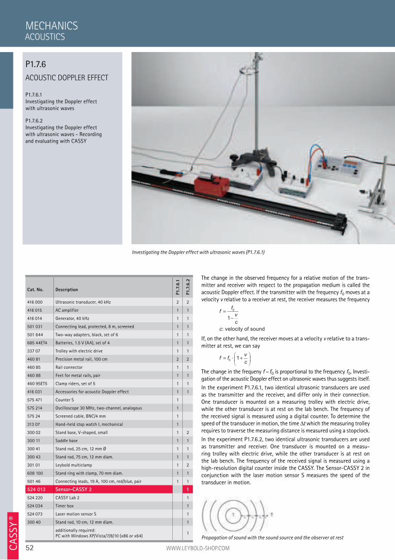
52 WWW.LEYBOLD-SHOP.COMCA
SSY ®
ACOUSTIC DOPPLER EFFECT
P1.7.6.1 Investigating the Doppler effect with ultrasonic waves
P1.7.6.2 Investigating the Doppler effect with ultrasonic waves - Recording and evaluating with CASSY
The change in the observed frequency for a relative motion of the trans-mitter and receiver with respect to the propagation medium is called the acoustic Doppler effect. If the transmitter with the frequency f0 moves at a velocity v relative to a receiver at rest, the receiver measures the frequency
ff
v
c
c
=
−
0
1
: velocity of sound
If, on the other hand, the receiver moves at a velocity v relative to a trans-mitter at rest, we can say
f fv
c= ⋅ +
0
1
The change in the frequeny f – f0 is proportional to the frequency f0. Investi-gation of the acoustic Doppler effect on ultrasonic waves thus suggests itself.
In the experiment P1.7.6.1, two identical ultrasonic transducers are used as the transmitter and the receiver, and differ only in their connection. One transducer is mounted on a measuring trolley with electric drive, while the other transducer is at rest on the lab bench. The frequency of the received signal is measured using a digital counter. To determine the speed of the transducer in motion, the time t which the measuring trolley requires to traverse the measuring distance is measured using a stopclock.
In the experiment P1.7.6.2, two identical ultrasonic transducers are used as transmitter and receiver. One transducer is mounted on a measu-ring trolley with electric drive, while the other transducer is at rest on the lab bench. The frequency of the received signal is measured using a high-resolution digital counter inside the CASSY. The Sensor-CASSY 2 in conjunction with the laser motion sensor S measures the speed of the transducer in motion.
MECHANICS
Investigating the Doppler effect with ultrasonic waves (P1.7.6.1)
Cat. No. Description
P1.7
.6.1
P1.7
.6.2
416 000 Ultrasonic transducer, 40 kHz 2 2
416 015 AC amplifier 1 1
416 014 Generator, 40 kHz 1 1
501 031 Connecting lead, protected, 8 m, screened 1 1
501 644 Two-way adapters, black, set of 6 1 1
685 44ET4 Batteries, 1.5 V (AA), set of 4 1 1
337 07 Trolley with electric drive 1 1
460 81 Precision metal rail, 100 cm 2 2
460 85 Rail connector 1 1
460 88 Feet for metal rails, pair 1 1
460 95ET5 Clamp riders, set of 5 1 1
416 031 Accessories for acoustic Doppler effect 1 1
575 471 Counter S 1
575 214 Oscilloscope 30 MHz, two-channel, analogous 1
575 24 Screened cable, BNC/4 mm 1
313 07 Hand-held stop watch I, mechanical 1
300 02 Stand base, V-shaped, small 1 2
300 11 Saddle base 1 1
300 41 Stand rod, 25 cm, 12 mm Ø 1 1
300 43 Stand rod, 75 cm, 12 mm diam. 1 1
301 01 Leybold multiclamp 1 2
608 100 Stand ring with clamp, 70 mm diam. 1 1
501 46 Connecting leads, 19 A, 100 cm, red/blue, pair 1 1
524 013 Sensor-CASSY 2 1
524 220 CASSY Lab 2 1
524 034 Timer box 1
524 073 Laser motion sensor S 1
300 40 Stand rod, 10 cm, 12 mm diam. 1
additionally required: PC with Windows XP/Vista/7/8/10 (x86 or x64)
1Propagation of sound with the sound source and the observer at rest
ACOUSTICS
P1.7.6
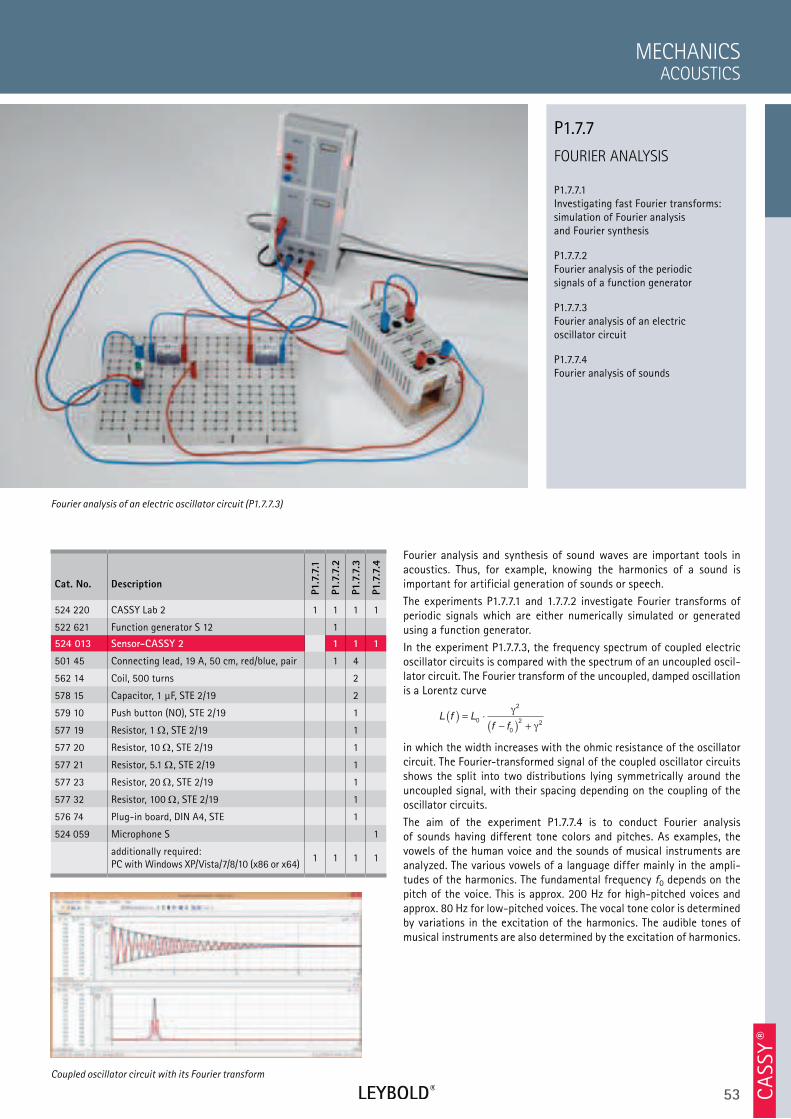
53 CA
SSY ®
FOURIER ANALYSIS
P1.7.7.1 Investigating fast Fourier transforms: simulation of Fourier analysis and Fourier synthesis
P1.7.7.2 Fourier analysis of the periodic signals of a function generator
P1.7.7.3 Fourier analysis of an electric oscillator circuit
P1.7.7.4 Fourier analysis of sounds
ACOUSTICS
MECHANICS
Cat. No. Description
P1.7
.7.1
P1.7
.7.2
P1.7
.7.3
P1.7
.7.4
524 220 CASSY Lab 2 1 1 1 1
522 621 Function generator S 12 1
524 013 Sensor-CASSY 2 1 1 1
501 45 Connecting lead, 19 A, 50 cm, red/blue, pair 1 4
562 14 Coil, 500 turns 2
578 15 Capacitor, 1 µF, STE 2/19 2
579 10 Push button (NO), STE 2/19 1
577 19 Resistor, 1 , STE 2/19 1
577 20 Resistor, 10 , STE 2/19 1
577 21 Resistor, 5.1 , STE 2/19 1
577 23 Resistor, 20 , STE 2/19 1
577 32 Resistor, 100 , STE 2/19 1
576 74 Plug-in board, DIN A4, STE 1
524 059 Microphone S 1
additionally required: PC with Windows XP/Vista/7/8/10 (x86 or x64)
1 1 1 1
Fourier analysis and synthesis of sound waves are important tools in acoustics. Thus, for example, knowing the harmonics of a sound is important for artificial generation of sounds or speech.
The experiments P1.7.7.1 and 1.7.7.2 investigate Fourier transforms of periodic signals which are either numerically simulated or generated using a function generator.
In the experiment P1.7.7.3, the frequency spectrum of coupled electric oscillator circuits is compared with the spectrum of an uncoupled oscil-lator circuit. The Fourier transform of the uncoupled, damped oscillation is a Lorentz curve
L f L
f f( ) = ⋅
−( ) +0
2
0
2 2
γ
γ
in which the width increases with the ohmic resistance of the oscillator circuit. The Fourier-transformed signal of the coupled oscillator circuits shows the split into two distributions lying symmetrically around the uncoupled signal, with their spacing depending on the coupling of the oscillator circuits.
The aim of the experiment P1.7.7.4 is to conduct Fourier analysis of sounds having different tone colors and pitches. As examples, the vowels of the human voice and the sounds of musical instruments are analyzed. The various vowels of a language differ mainly in the ampli-tudes of the harmonics. The fundamental frequency f0 depends on the pitch of the voice. This is approx. 200 Hz for high-pitched voices and approx. 80 Hz for low-pitched voices. The vocal tone color is determined by variations in the excitation of the harmonics. The audible tones of musical instruments are also determined by the excitation of harmonics.
Fourier analysis of an electric oscillator circuit (P1.7.7.3)
P1.7.7
Coupled oscillator circuit with its Fourier transform
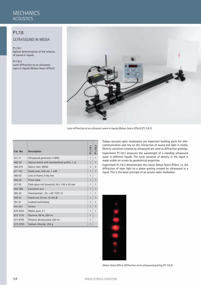
54 WWW.LEYBOLD-SHOP.COM
ULTRASOUND IN MEDIA
P1.7.8.1 Optical determination of the velocity of sound in liquids
P1.7.8.2 Laser diffraction at an ultrasonic wave in liquids (Debye-Sears-Effect)
Todays acousto-optic modulators are important building parts for tele-communication and rely on the interaction of sound and light in media. Density variations created by ultrasound are used as diffraction gratings.
Experiment P1.7.8.1 measures the wavelength of a standing ultrasound wave in different liquids. The local variation of density in the liquid is made visible on screen by geometrical projection.
Experiment P1.7.8.2 demonstrates the classic Debye-Sears-Effect, i.e. the diffraction of laser light by a phase grating created by ultrasound in a liquid. This is the basic principle of an acusto-optic modulator.
MECHANICS
Laser diffraction at an ultrasonic wave in liquids (Debye-Sears-Effect) (P1.7.8.2)
Cat. No. Description
P1.7
.8.1
P1.7
.8.2
417 11 Ultrasound generator, 4 MHz 1 1
460 32 Optical bench with standardised profile, 1 m 1 1
460 374 Optics rider, 90/50 5 4
471 791 Diode laser, 635 nm, 1 mW 1 1
460 02 Lens in frame, f=50 mm 1
460 25 Prism table 1 1
477 02 Plate glass cell (cuvette), 50 x 100 x 50 mm 1 1
460 380 Cantilever arm 1 1
382 35 Thermometer, -10...+50 °C/0.1 K 1 1
300 41 Stand rod, 25 cm, 12 mm Ø 1 1
301 01 Leybold multiclamp 1 1
441 531 Screen 1 1
675 3410 Water, pure, 5 l 1 1
672 1210 Glycerin, 99 %, 250 ml 1
671 9740 Ethanol, denaturated, 250 ml 1
673 5700 Sodium chloride, 250 g 1
Debye-Sears Effect, Diffraction at an ultrasound grating (P1.7.8.2)
ACOUSTICS
P1.7.8
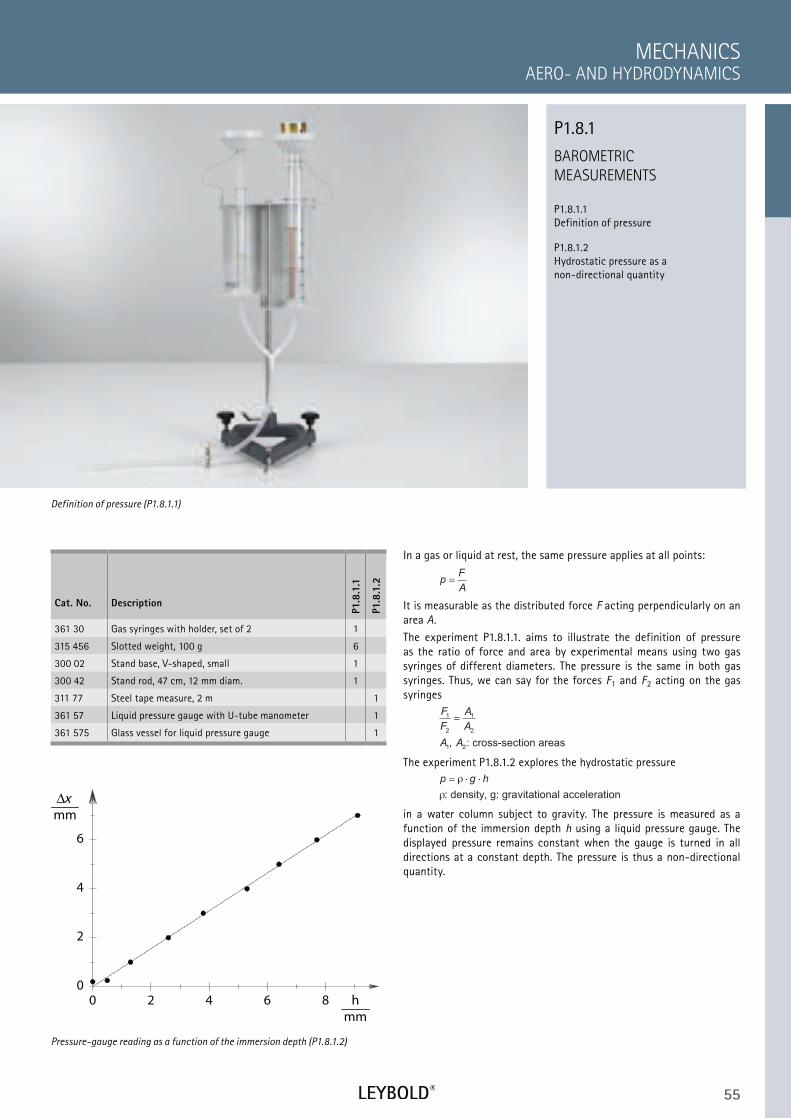
55
0 2 4 6 8 h
mm
0
2
4
6
∆x
mm
BAROMETRIC
MEASUREMENTS
P1.8.1.1
Definition of pressure
P1.8.1.2
Hydrostatic pressure as a
non-directional quantity
AERO- AND HYDRODYNAMICS
MECHANICS
Cat. No. Description
P1.8
.1.1
P1.8
.1.2
361 30 Gas syringes with holder, set of 2 1
315 456 Slotted weight, 100 g 6
300 02 Stand base, V-shaped, small 1
300 42 Stand rod, 47 cm, 12 mm diam. 1
311 77 Steel tape measure, 2 m 1
361 57 Liquid pressure gauge with U-tube manometer 1
361 575 Glass vessel for liquid pressure gauge 1
In a gas or liquid at rest, the same pressure applies at all points:
pF
A
It is measurable as the distributed force F acting perpendicularly on an
area A.
The experiment P1.8.1.1. aims to illustrate the definition of pressure
as the ratio of force and area by experimental means using two gas
syringes of different diameters. The pressure is the same in both gas
syringes. Thus, we can say for the forces F1 and F2 acting on the gas
syringes
F
F
A
A
A A
1
2
1
2
1 2, : cross-section areas
The experiment P1.8.1.2 explores the hydrostatic pressure
p g h= ⋅ ⋅ρ
ρ: density, g: gravitational acceleration
in a water column subject to gravity. The pressure is measured as a
function of the immersion depth h using a liquid pressure gauge. The
displayed pressure remains constant when the gauge is turned in all
directions at a constant depth. The pressure is thus a non-directional
quantity.
Definition of pressure (P1.8.1.1)
P1.8.1
Pressure-gauge reading as a function of the immersion depth (P1.8.1.2)
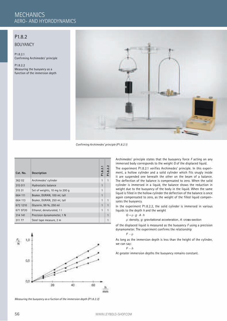
56 WWW.LEYBOLD-SHOP.COM
BOUYANCY
P1.8.2.1
Confirming Archimedes’ principle
P1.8.2.2
Measuring the buoyancy as a
function of the immersion depth
Archimedes’ principle states that the buoyancy force F acting on any
immersed body corresponds to the weight G of the displaced liquid.
The experiment P1.8.2.1 verifies Archimedes’ principle. In this experi-
ment, a hollow cylinder and a solid cylinder which fits snugly inside
it are suspended one beneath the other on the beam of a balance.
The deflection of the balance is compensated to zero. When the solid
cylinder is immersed in a liquid, the balance shows the reduction in
weight due to the buoyancy of the body in the liquid. When the same
liquid is filled in the hollow cylinder the deflection of the balance is once
again compensated to zero, as the weight of the filled liquid compen-
sates the buoyancy.
In the experiment P1.8.2.2, the solid cylinder is immersed in various
liquids to the depth h and the weight
G g A h
g A
= ⋅ ⋅ ⋅ρ
ρ: density, : gravitational acceleration, : crosss-section
of the displaced liquid is measured as the buoyancy F using a precision
dynamometer. The experiment confirms the relationship
F ∼
As long as the immersion depth is less than the height of the cylinder,
we can say:
F h∼
At greater immersion depths the buoyancy remains constant.
MECHANICS
Confirming Archimedes’ principle (P1.8.2.1)
Cat. No. Description
P1.8
.2.1
P1.8
.2.2
362 02 Archimedes‘ cylinder 1 1
315 011 Hydrostatic balance 1
315 31 Set of weights, 10 mg to 200 g 1
664 111 Beaker, DURAN, 100 ml, tall 1
664 113 Beaker, DURAN, 250 ml, tall 1 1
672 1210 Glycerin, 99 %, 250 ml 1 1
671 9720 Ethanol, denaturated, 1 l 1 1
314 141 Precision dynamometer, 1 N 1
311 77 Steel tape measure, 2 m 1
Measuring the buoyancy as a fuction of the immersion depth (P1.8.2.2)
AERO- AND HYDRODYNAMICS
P1.8.2
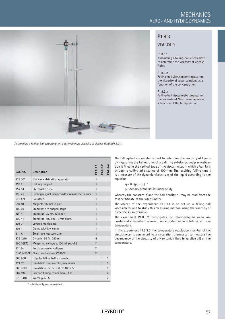
57
VISCOSITY
P1.8.3.1 Assembling a falling-ball viscosimeter to determine the viscosity of viscous fluids
P1.8.3.2 Falling-ball viscosimeter: measuring the viscosity of sugar solutions as a function of the concentration
P1.8.3.3 Falling-ball viscosimeter: measuring the viscosity of Newtonian liquids as a function of the termperature
AERO- AND HYDRODYNAMICS
MECHANICS
Cat. No. Description
P1.8
.3.1
P1.8
.3.2
P1.8
.3.3
379 001 Guinea-and-feather apparatus 1
336 21 Holding magnet 1
352 54 Steel ball, 16 mm 1
336 25 Holding magnet adapter with a release mechanism 1
575 471 Counter S 1
510 48 Magnets, 35 mm Ø, pair 1
300 01 Stand base, V-shaped, large 1
300 41 Stand rod, 25 cm, 12 mm Ø 1
300 44 Stand rod, 100 cm, 12 mm diam. 1
301 01 Leybold multiclamp 1
301 11 Clamp with jaw clamp 1
311 77 Steel tape measure, 2 m 1
672 1210 Glycerin, 99 %, 250 ml 6
590 08ET2 Measuring cylinders, 100 ml, set of 2 1*
311 54 Precision vernier callipers 1*
OHC S-200E Electronic balance, CS200E 1*
665 906 Höppler falling ball viscometer 1 1
313 07 Hand-held stop watch I, mechanical 1 1
666 7681 Circulation thermostat SC 100-S5P 1
667 194 Silicone tubing, 7 mm diam., 1 m 2
675 3410 Water, pure, 5 l 2
* additionally recommended
The falling-ball viscometer is used to determine the viscosity of liquids by measuring the falling time of a ball. The substance under investiga-tion is filled in the vertical tube of the viscosimeter, in which a ball falls through a calibrated distance of 100 mm. The resulting falling time t is a measure of the dynamic viscosity of the liquid according to the equation
η ρ ρ
ρ
= ⋅ −( ) ⋅K t1 2
2: density of the liquid under study
whereby the constant K and the ball density 1 may be read from the test certificate of the viscosimeter.
The object of the experiment P1.8.3.1 is to set up a falling-ball viscosimeter and to study this measuring method, using the viscosity of glycerine as an example.
The experiment P1.8.3.2 investigates the relationship between vis-cosity and concentration using concentrated sugar solutions at room temperature.
In the experiment P1.8.3.3, the temperature regulation chamber of the viscosimeter is connected to a circulation thermostat to measure the dependency of the viscosity of a Newtonian fluid (e. g. olive oil) on the temperature.
Assembling a falling-ball viscosimeter to determine the viscosity of viscous fluids (P1.8.3.1)
P1.8.3
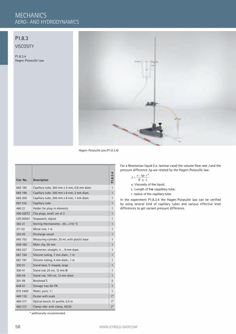
58 WWW.LEYBOLD-SHOP.COM
VISCOSITY
P1.8.3.4 Hagen-Poiseuille Law
For a Newtonian liquid (i.e. laminar case) the volume flow rate J and the pressure difference p are related by the Hagen-Poiseuille law:
Jp r
L=
⋅ ⋅
⋅ ⋅
π
η
η
∆4
8
: Viscosity of the liquid,
L: Length of thee cappillary tube,
r: radius of the capillary tube
In the experiment P1.8.3.4 the Hagen-Poiseuille law can be verified by using several kind of capillary tubes and various effective level differences to get variant pressure difference.
MECHANICS
Hagen-Poiseuille Law (P1.8.3.4)
Cat. No. Description
P1.8
.3.4
665 195 Capillary tube, 300 mm x 5 mm, 0.8 mm diam. 1
665 196 Capillary tube, 300 mm x 8 mm, 2 mm diam. 1
665 205 Capillary tube, 300 mm x 8 mm, 1 mm diam. 1
667 510 Capillary tube 1
460 21 Holder for plug-in elements 1
590 02ET2 Clip plugs, small, set of 2 1
LDS 00001 Stopwatch, digital 1
382 21 Stirring thermometer, -30...+110 °C 1
311 02 Metal rule, 1 m 1
362 05 Discharge vessel 1
665 752 Measuring cylinder, 25 ml, with plastic base 1
608 160 Mohr clip, 50 mm 1
665 227 Connector, straight, 4 ... 8 mm diam. 1
667 194 Silicone tubing, 7 mm diam., 1 m 1
667 197 Silicone tubing, 4 mm diam., 1 m 1
300 01 Stand base, V-shaped, large 1
300 41 Stand rod, 25 cm, 12 mm Ø 1
300 44 Stand rod, 100 cm, 12 mm diam. 1
301 09 Bosshead S 2
648 01 Storage tray S8-FN 1
675 3400 Water, pure, 1 l 1
460 135 Ocular with scale 1*
460 317 Optical bench, S1 profile, 0.5 m 1*
460 312 Clamp rider with clamp, 45/35 2*
* additionally recommended
AERO- AND HYDRODYNAMICS
P1.8.3
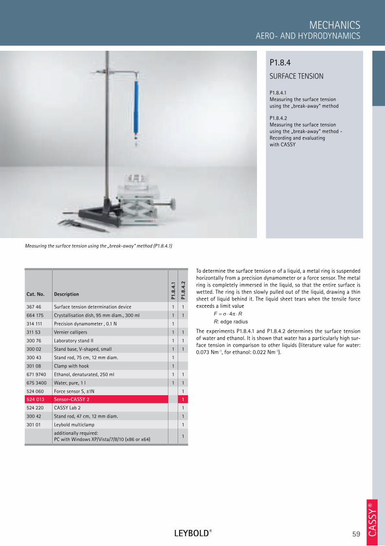
59 CA
SSY ®
SURFACE TENSION
P1.8.4.1 Measuring the surface tension using the „break-away“ method
P1.8.4.2 Measuring the surface tension using the „break-away“ method - Recording and evaluating with CASSY
AERO- AND HYDRODYNAMICS
MECHANICS
Cat. No. Description
P1.8
.4.1
P1.8
.4.2
367 46 Surface tension determination device 1 1
664 175 Crystallisation dish, 95 mm diam., 300 ml 1 1
314 111 Precision dynamometer , 0.1 N 1
311 53 Vernier callipers 1 1
300 76 Laboratory stand II 1 1
300 02 Stand base, V-shaped, small 1 1
300 43 Stand rod, 75 cm, 12 mm diam. 1
301 08 Clamp with hook 1
671 9740 Ethanol, denaturated, 250 ml 1 1
675 3400 Water, pure, 1 l 1 1
524 060 Force sensor S, ±1N 1
524 013 Sensor-CASSY 2 1
524 220 CASSY Lab 2 1
300 42 Stand rod, 47 cm, 12 mm diam. 1
301 01 Leybold multiclamp 1
additionally required: PC with Windows XP/Vista/7/8/10 (x86 or x64)
1
To determine the surface tension of a liquid, a metal ring is suspended horizontally from a precision dynamometer or a force sensor. The metal ring is completely immersed in the liquid, so that the entire surface is wetted. The ring is then slowly pulled out of the liquid, drawing a thin sheet of liquid behind it. The liquid sheet tears when the tensile force exceeds a limit value
F R
R
= ⋅ ⋅σ π4
: edge radius
The experiments P1.8.4.1 and P1.8.4.2 determines the surface tension of water and ethanol. It is shown that water has a particularly high sur-face tension in comparison to other liquids (literature value for water: 0.073 Nm-1, for ethanol: 0.022 Nm-1).
Measuring the surface tension using the „break-away“ method (P1.8.4.1)
P1.8.4
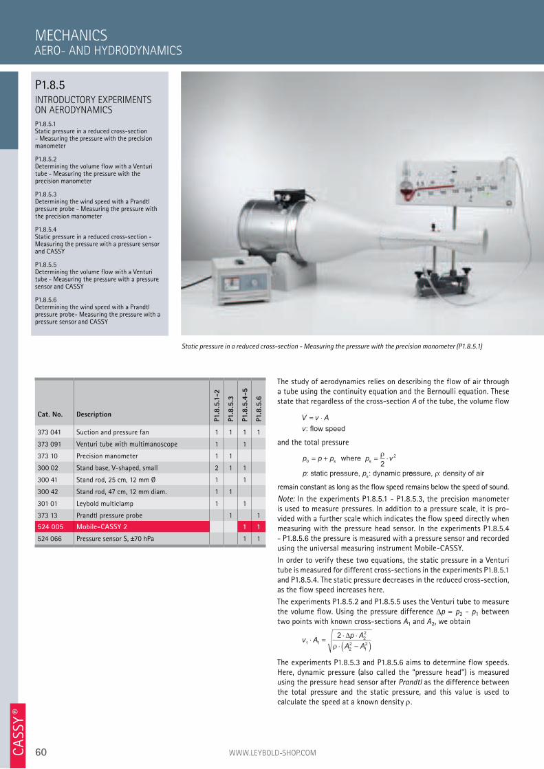
60 WWW.LEYBOLD-SHOP.COMCA
SSY ®
MECHANICS
Static pressure in a reduced cross-section - Measuring the pressure with the precision manometer (P1.8.5.1)
Cat. No. Description
P1.8
.5.1
-2
P1.8
.5.3
P1.8
.5.4
-5
P1.8
.5.6
373 041 Suction and pressure fan 1 1 1 1
373 091 Venturi tube with multimanoscope 1 1
373 10 Precision manometer 1 1
300 02 Stand base, V-shaped, small 2 1 1
300 41 Stand rod, 25 cm, 12 mm Ø 1 1
300 42 Stand rod, 47 cm, 12 mm diam. 1 1
301 01 Leybold multiclamp 1 1
373 13 Prandtl pressure probe 1 1
524 005 Mobile-CASSY 2 1 1
524 066 Pressure sensor S, ±70 hPa 1 1
AERO- AND HYDRODYNAMICS
P1.8.5INTRODUCTORY EXPERIMENTS
ON AERODYNAMICS
P1.8.5.1 Static pressure in a reduced cross-section - Measuring the pressure with the precision manometer
P1.8.5.2 Determining the volume flow with a Venturi tube - Measuring the pressure with the precision manometer
P1.8.5.3 Determining the wind speed with a Prandtl pressure probe - Measuring the pressure with the precision manometer
P1.8.5.4 Static pressure in a reduced cross-section - Measuring the pressure with a pressure sensor and CASSY
P1.8.5.5 Determining the volume flow with a Venturi tube - Measuring the pressure with a pressure sensor and CASSY
P1.8.5.6 Determining the wind speed with a Prandtl pressure probe- Measuring the pressure with a pressure sensor and CASSY
The study of aerodynamics relies on describing the flow of air through a tube using the continuity equation and the Bernoulli equation. These state that regardless of the cross-section A of the tube, the volume flow
V v A
v
.
= ⋅
: flow speed
and the total pressure
p p p p v
p p
0
2
2= + = ⋅s s
s
where
: static pressure, : dynamic pr
ρ
eessure, : density of airρ
remain constant as long as the flow speed remains below the speed of sound.
Note: In the experiments P1.8.5.1 - P1.8.5.3, the precision manometer is used to measure pressures. In addition to a pressure scale, it is pro-vided with a further scale which indicates the flow speed directly when measuring with the pressure head sensor. In the experiments P1.8.5.4 - P1.8.5.6 the pressure is measured with a pressure sensor and recorded using the universal measuring instrument Mobile-CASSY.
In order to verify these two equations, the static pressure in a Venturi tube is measured for different cross-sections in the experiments P1.8.5.1 and P1.8.5.4. The static pressure decreases in the reduced cross-section, as the flow speed increases here.
The experiments P1.8.5.2 and P1.8.5.5 uses the Venturi tube to measure the volume flow. Using the pressure difference p = p2 - p1 between two points with known cross-sections A1 and A2, we obtain
v Ap A
A A1 1
2
2
2
2
1
2
2⋅ =
⋅ ⋅
⋅ −( )∆
ρ
The experiments P1.8.5.3 and P1.8.5.6 aims to determine flow speeds. Here, dynamic pressure (also called the “pressure head”) is measured using the pressure head sensor after Prandtl as the difference between the total pressure and the static pressure, and this value is used to calculate the speed at a known density .
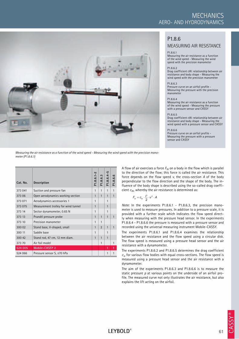
61 CA
SSY ®
MEASURING AIR RESISTANCE
P1.8.6.1 Measuring the air resistance as a function of the wind speed - Measuring the wind speed with the precision manometer
P1.8.6.2 Drag coefficient cW: relationship between air resistance and body shape - Measuring the wind speed with the precision manometer
P1.8.6.3 Pressure curve on an airfoil profile - Measuring the pressure with the precision manometer
P1.8.6.4 Measuring the air resistance as a function of the wind speed - Measuring the pressure with a pressure sensor and CASSY
P1.8.6.5 Drag coefficient cW: relationship between air resistance and body shape - Measuring the wind speed with a pressure sensor and CASSY
P1.8.6.6 Pressure curve on an airfoil profile - Measuring the pressure with a pressure sensor and CASSY
AERO- AND HYDRODYNAMICS
MECHANICS
Cat. No. Description
P1.8
.6.1
-2
P1.8
.6.3
P1.8
.6.4
-5
P1.8
.6.6
373 041 Suction and pressure fan 1 1 1 1
373 06 Open aerodynamics working section 1 1 1 1
373 071 Aerodynamics accessories 1 1 1
373 075 Measurement trolley for wind tunnel 1 1
373 14 Sector dynamometer, 0.65 N 1 1
373 13 Prandtl pressure probe 1 1 1 1
373 10 Precision manometer 1 1
300 02 Stand base, V-shaped, small 1 2 1 1
300 11 Saddle base 1 1
300 42 Stand rod, 47 cm, 12 mm diam. 1 1 1
373 70 Air foil model 1 1
524 005 Mobile-CASSY 2 1 1
524 066 Pressure sensor S, ±70 hPa 1 1
A flow of air exercises a force FW on a body in the flow which is parallel
to the direction of the flow; this force is called the air resistance. This
force depends on the flow speed v, the cross-section A of the body
perpendicular to the flow direction and the shape of the body. The in-
fluence of the body shape is described using the so-called drag coeffi-
cient cW, whereby the air resistance is determined as:
F c v Aw w= ⋅ ⋅ ⋅
2
2
Note: In the experiments P1.8.6.1 - P1.8.6.3, the precision mano-
meter is used to measure pressures. In addition to a pressure scale, it is
provided with a further scale which indicates the flow speed direct-
ly when measuring with the pressure head sensor. In the experiments
P1.8.6.4 - P1.8.6.6 the pressure is measured with a pressure sensor and
recorded using the universal measuring instrument Mobile-CASSY.
The experiments P1.8.6.1 and P1.8.6.4 examines the relationship
between the air resistance and the flow speed using a circular disk.
The flow speed is measured using a pressure head sensor and the air
resistance with a dynamometer.
The experiments P1.8.6.2 and P1.8.6.5 determines the drag coefficient
cw for various flow bodies with equal cross-sections. The flow speed is
measured using a pressure head sensor and the air resistance with a
dynamometer.
The aim of the experiments P1.8.6.3 and P1.8.6.6 is to measure the
static pressure p at various points on the underside of an airfoil pro-
file. The measured curve not only illustrates the air resistance, but also
explains the lift acting on the airfoil.
Measuring the air resistance as a function of the wind speed - Measuring the wind speed with the precision mano-
meter (P1.8.6.1)
P1.8.6
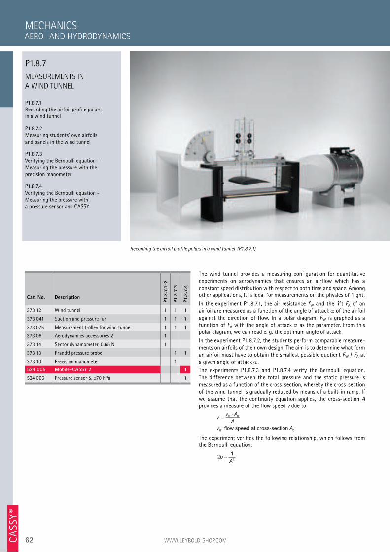
62 WWW.LEYBOLD-SHOP.COMCA
SSY ®
MEASUREMENTS IN
A WIND TUNNEL
P1.8.7.1 Recording the airfoil profile polars in a wind tunnel
P1.8.7.2 Measuring students’ own airfoils and panels in the wind tunnel
P1.8.7.3 Verifying the Bernoulli equation - Measuring the pressure with the precision manometer
P1.8.7.4 Verifying the Bernoulli equation - Measuring the pressure with a pressure sensor and CASSY
The wind tunnel provides a measuring configuration for quantitative experiments on aerodynamics that ensures an airflow which has a constant speed distribution with respect to both time and space. Among other applications, it is ideal for measurements on the physics of flight.
In the experiment P1.8.7.1, the air resistance fW and the lift FA of an airfoil are measured as a function of the angle of attack of the airfoil against the direction of flow. In a polar diagram, FW is graphed as a function of FA with the angle of attack as the parameter. From this polar diagram, we can read e. g. the optimum angle of attack.
In the experiment P1.8.7.2, the students perform comparable measure-ments on airfoils of their own design. The aim is to determine what form an airfoil must have to obtain the smallest possible quotient FW / FA at a given angle of attack .
The experiments P1.8.7.3 and P1.8.7.4 verify the Bernoulli equation. The difference between the total pressure and the static pressure is measured as a function of the cross-section, whereby the cross-section of the wind tunnel is gradually reduced by means of a built-in ramp. If we assume that the continuity equation applies, the cross-section A provides a measure of the flow speed v due to
vv A
A
v A
=⋅0 0
0 0: flow speed at cross-section
The experiment verifies the following relationship, which follows from the Bernoulli equation:
pA∼
1
2
MECHANICS
Recording the airfoil profile polars in a wind tunnel (P1.8.7.1)
Cat. No. Description
P1.8
.7.1
-2
P1.8
.7.3
P1.8
.7.4
373 12 Wind tunnel 1 1 1
373 041 Suction and pressure fan 1 1 1
373 075 Measurement trolley for wind tunnel 1 1 1
373 08 Aerodynamics accessories 2 1
373 14 Sector dynamometer, 0.65 N 1
373 13 Prandtl pressure probe 1 1
373 10 Precision manometer 1
524 005 Mobile-CASSY 2 1
524 066 Pressure sensor S, ±70 hPa 1
AERO- AND HYDRODYNAMICS
P1.8.7

63
P2.1 THERMAL EXPANSION 65
P2.2 HEAT TRANSFER 68
P2.3 HEAT AS A FORM OF ENERGY 70
P2.4 PHASE TRANSITIONS 74
P2.5 KINETIC THEORY OF GASES 77
P2.6 THERMODYNAMIC CYCLE 81
P2 HEAT

64 WWW.LEYBOLD-SHOP.COM
P2.1 THERMAL EXPANSION
P2.1.1 Thermal expansion of solids 65
P2.1.2 Thermal expansion of liquids 66
P2.1.3 Thermal anomaly of water 67
P2.2 HEAT TRANSFER
P2.2.1 Thermal conductivity 68
P2.2.2 Solar collector 69
P2.3 HEAT AS A FORM OF ENERGY
P2.3.1 Mixing temperatures 70
P2.3.2 Heat capacities 71
P2.3.3 Converting mechanical energy into heat 72
P2.3.4 Converting electrical energy into heat 73
P2.4 PHASE TRANSITIONS
P2.4.1 Latent heat and vaporization heat 74
P2.4.2 Measuring vapor pressure 75
P2.4.3 Critical temperature 76
P2.5 KINETIC THEORY OF GASES
P2.5.1 Brownian motion of molecules 77
P2.5.2 Gas laws 78
P2.5.3 Specific heat of gases 79
P2.5.4 Real gases 80
P2.6 THERMODYNAMIC CYCLE
P2.6.1 Hot-air engine: qualitative experiments 81-82
P2.6.2 Hot-air engine: quantitative experiments 83-84
P2.6.3 Heat pump 85
P2 HEAT
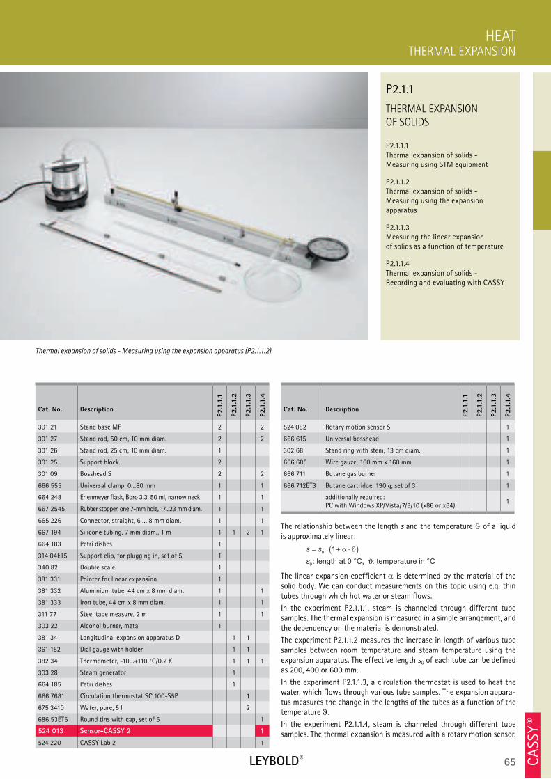
65 CA
SSY ®
THERMAL EXPANSION
OF SOLIDS
P2.1.1.1 Thermal expansion of solids - Measuring using STM equipment
P2.1.1.2 Thermal expansion of solids - Measuring using the expansion apparatus
P2.1.1.3 Measuring the linear expansion of solids as a function of temperature
P2.1.1.4 Thermal expansion of solids - Recording and evaluating with CASSY
THERMAL EXPANSION
HEAT
Cat. No. Description
P2.1
.1.1
P2.1
.1.2
P2.1
.1.3
P2.1
.1.4
301 21 Stand base MF 2 2
301 27 Stand rod, 50 cm, 10 mm diam. 2 2
301 26 Stand rod, 25 cm, 10 mm diam. 1
301 25 Support block 2
301 09 Bosshead S 2 2
666 555 Universal clamp, 0...80 mm 1 1
664 248 Erlenmeyer flask, Boro 3.3, 50 ml, narrow neck 1 1
667 2545 Rubber stopper, one 7-mm hole, 17...23 mm diam. 1 1
665 226 Connector, straight, 6 ... 8 mm diam. 1 1
667 194 Silicone tubing, 7 mm diam., 1 m 1 1 2 1
664 183 Petri dishes 1
314 04ET5 Support clip, for plugging in, set of 5 1
340 82 Double scale 1
381 331 Pointer for linear expansion 1
381 332 Aluminium tube, 44 cm x 8 mm diam. 1 1
381 333 Iron tube, 44 cm x 8 mm diam. 1 1
311 77 Steel tape measure, 2 m 1 1
303 22 Alcohol burner, metal 1
381 341 Longitudinal expansion apparatus D 1 1
361 152 Dial gauge with holder 1 1
382 34 Thermometer, -10...+110 °C/0.2 K 1 1 1
303 28 Steam generator 1
664 185 Petri dishes 1
666 7681 Circulation thermostat SC 100-S5P 1
675 3410 Water, pure, 5 l 2
686 53ET5 Round tins with cap, set of 5 1
524 013 Sensor-CASSY 2 1
524 220 CASSY Lab 2 1
The relationship between the length s and the temperature of a liquid is approximately linear:
s s
s
= ⋅ + ⋅( )0
0
1 α ϑ
ϑ: length at 0 °C, : temperature in °C
The linear expansion coefficient is determined by the material of the solid body. We can conduct measurements on this topic using e.g. thin tubes through which hot water or steam flows.
In the experiment P2.1.1.1, steam is channeled through different tube samples. The thermal expansion is measured in a simple arrangement, and the dependency on the material is demonstrated.
The experiment P2.1.1.2 measures the increase in length of various tube samples between room temperature and steam temperature using the expansion apparatus. The effective length s0 of each tube can be defined as 200, 400 or 600 mm.
In the experiment P2.1.1.3, a circulation thermostat is used to heat the water, which flows through various tube samples. The expansion appara-tus measures the change in the lengths of the tubes as a function of the temperature .
In the experiment P2.1.1.4, steam is channeled through different tube samples. The thermal expansion is measured with a rotary motion sensor.
Thermal expansion of solids - Measuring using the expansion apparatus (P2.1.1.2)
P2.1.1
Cat. No. Description
P2.1
.1.1
P2.1
.1.2
P2.1
.1.3
P2.1
.1.4
524 082 Rotary motion sensor S 1
666 615 Universal bosshead 1
302 68 Stand ring with stem, 13 cm diam. 1
666 685 Wire gauze, 160 mm x 160 mm 1
666 711 Butane gas burner 1
666 712ET3 Butane cartridge, 190 g, set of 3 1
additionally required: PC with Windows XP/Vista/7/8/10 (x86 or x64)
1
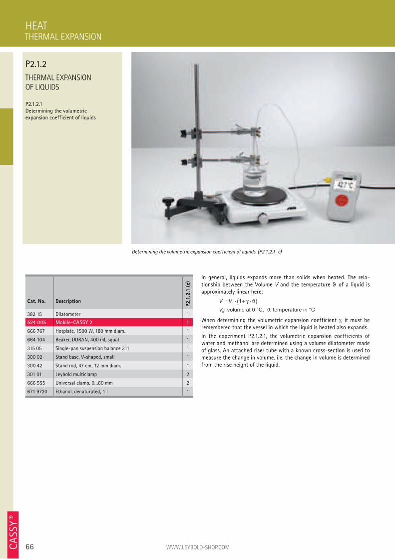
66 WWW.LEYBOLD-SHOP.COMCA
SSY ®
THERMAL EXPANSION
OF LIQUIDS
P2.1.2.1
Determining the volumetric
expansion coefficient of liquids
In general, liquids expands more than solids when heated. The rela-
tionship between the Volume V and the temperature of a liquid is
approximately linear here:
V V
V
= ⋅ + ⋅( )0
0
1 γ ϑ
ϑ: volume at 0 °C, : temperature in °C
When determining the volumetric expansion coefficient , it must be
remembered that the vessel in which the liquid is heated also expands.
In the experiment P2.1.2.1, the volumetric expansion coefficients of
water and methanol are determined using a volume dilatometer made
of glass. An attached riser tube with a known cross-section is used to
measure the change in volume. i.e. the change in volume is determined
from the rise height of the liquid.
HEAT
Determining the volumetric expansion coefficient of liquids (P2.1.2.1_c)
Cat. No. Description
P2.1
.2.1
(c)
382 15 Dilatometer 1
524 005 Mobile-CASSY 2 1
666 767 Hotplate, 1500 W, 180 mm diam. 1
664 104 Beaker, DURAN, 400 ml, squat 1
315 05 Single-pan suspension balance 311 1
300 02 Stand base, V-shaped, small 1
300 42 Stand rod, 47 cm, 12 mm diam. 1
301 01 Leybold multiclamp 2
666 555 Universal clamp, 0...80 mm 2
671 9720 Ethanol, denaturated, 1 l 1
THERMAL EXPANSION
P2.1.2
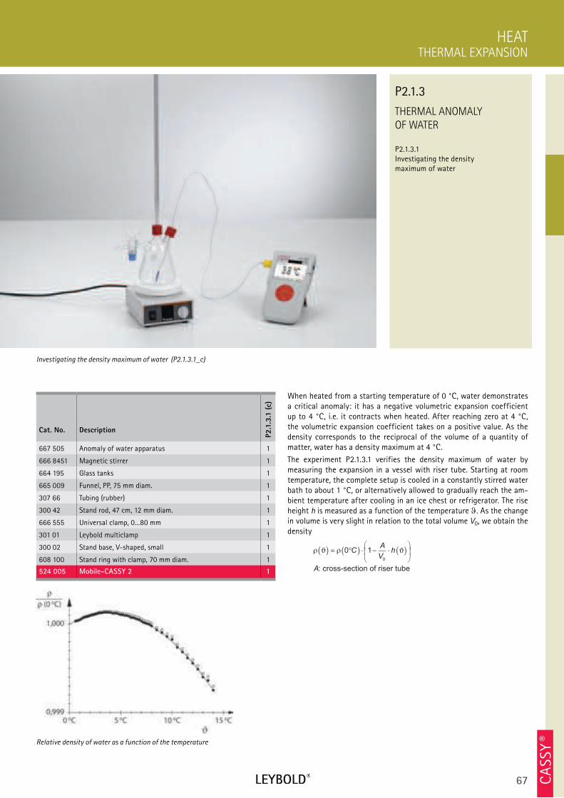
67 CA
SSY ®
THERMAL ANOMALY
OF WATER
P2.1.3.1 Investigating the density maximum of water
THERMAL EXPANSION
HEAT
Cat. No. Description
P2.1
.3.1
(c)
667 505 Anomaly of water apparatus 1
666 8451 Magnetic stirrer 1
664 195 Glass tanks 1
665 009 Funnel, PP, 75 mm diam. 1
307 66 Tubing (rubber) 1
300 42 Stand rod, 47 cm, 12 mm diam. 1
666 555 Universal clamp, 0...80 mm 1
301 01 Leybold multiclamp 1
300 02 Stand base, V-shaped, small 1
608 100 Stand ring with clamp, 70 mm diam. 1
524 005 Mobile-CASSY 2 1
When heated from a starting temperature of 0 °C, water demonstrates a critical anomaly: it has a negative volumetric expansion coefficient up to 4 °C, i.e. it contracts when heated. After reaching zero at 4 °C, the volumetric expansion coefficient takes on a positive value. As the density corresponds to the reciprocal of the volume of a quantity of matter, water has a density maximum at 4 °C.
The experiment P2.1.3.1 verifies the density maximum of water by measuring the expansion in a vessel with riser tube. Starting at room temperature, the complete setup is cooled in a constantly stirred water bath to about 1 °C, or alternatively allowed to gradually reach the am-bient temperature after cooling in an ice chest or refrigerator. The rise height h is measured as a function of the temperature . As the change in volume is very slight in relation to the total volume V0, we obtain the density
ρ ϑ ρ ϑ( ) = °( ) ⋅ − ⋅ ( )
0 1
0
CA
Vh
A: cross-section of riser tube
Investigating the density maximum of water (P2.1.3.1_c)
P2.1.3
Relative density of water as a function of the temperature
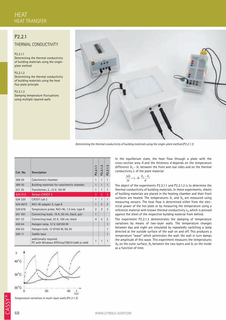
68 WWW.LEYBOLD-SHOP.COMCA
SSY ®
THERMAL CONDUCTIVITY
P2.2.1.1 Determining the thermal conductivity of building materials using the single-plate method
P2.2.1.2 Determining the thermal conductivity of building materials using the heat flux plate principle
P2.2.1.3 Damping temperature fluctuations using multiple-layered walls
In the equilibrium state, the heat flow through a plate with the cross-section area A and the thickness d depends on the temperature difference 2 - 1 between the front and rear sides and on the thermal conductivity of the plate material:
∆
∆
Q
tA
d= ⋅ ⋅
−λ
ϑ ϑ2 1
The object of the experiments P2.2.1.1 und P2.2.1.2 is to determine the thermal conductivity of building materials. In these experiments, sheets of building materials are placed in the heating chamber and their front surfaces are heated. The temperatures 1 and 2 are measured using measuring sensors. The heat flow is determined either from the elec-trical power of the hot plate or by measuring the temperature using a reference material with known thermal conductivity 0 which is pressed against the sheet of the respective building material from behind.
The experiment P2.2.1.3 demonstrates the damping of temperature variations by means of two-layer walls. The temperature changes between day and night are simulated by repeatedly switching a lamp directed at the outside surface of the wall on and off. This produces a temperature “wave” which penetrates the wall; the wall in turn damps the amplitude of this wave. This experiment measures the temperatures
A on the outer surface, Z between the two layers and I on the inside as a function of time.
HEAT
Determining the thermal conductivity of building materials using the single-plate method (P2.2.1.1)
Cat. No. Description
P2.2
.1.1
P2.2
.1.2
P2.2
.1.3
389 29 Calorimetric chamber 1 1 1
389 30 Building materials for calorimetric chamber 1 1 1
521 25 Transformer, 2...12 V, 120 W 1 1 1
524 013 Sensor-CASSY 2 1 1 1
524 220 CASSY Lab 2 1 1 1
524 0673 NiCr-Ni adapter S, type K 1 2 2
529 676 Temperature probe, NiCr-Ni, 1.5 mm, type K 2 3 3
501 451 Connecting leads, 19 A, 50 cm, black, pair 1
501 33 Connecting lead, 32 A, 100 cm, black 4 2 2
450 64 Halogen lamp, 12 V, 50/100 W 1
450 63 Halogen bulb, 12 V/100 W, G6.35 1
300 11 Saddle base 1
additionally required: PC with Windows XP/Vista/7/8/10 (x86 or x64)
1 1 1
Temperature variations in multi-layer walls (P2.2.1.3)
HEAT TRANSFER
P2.2.1
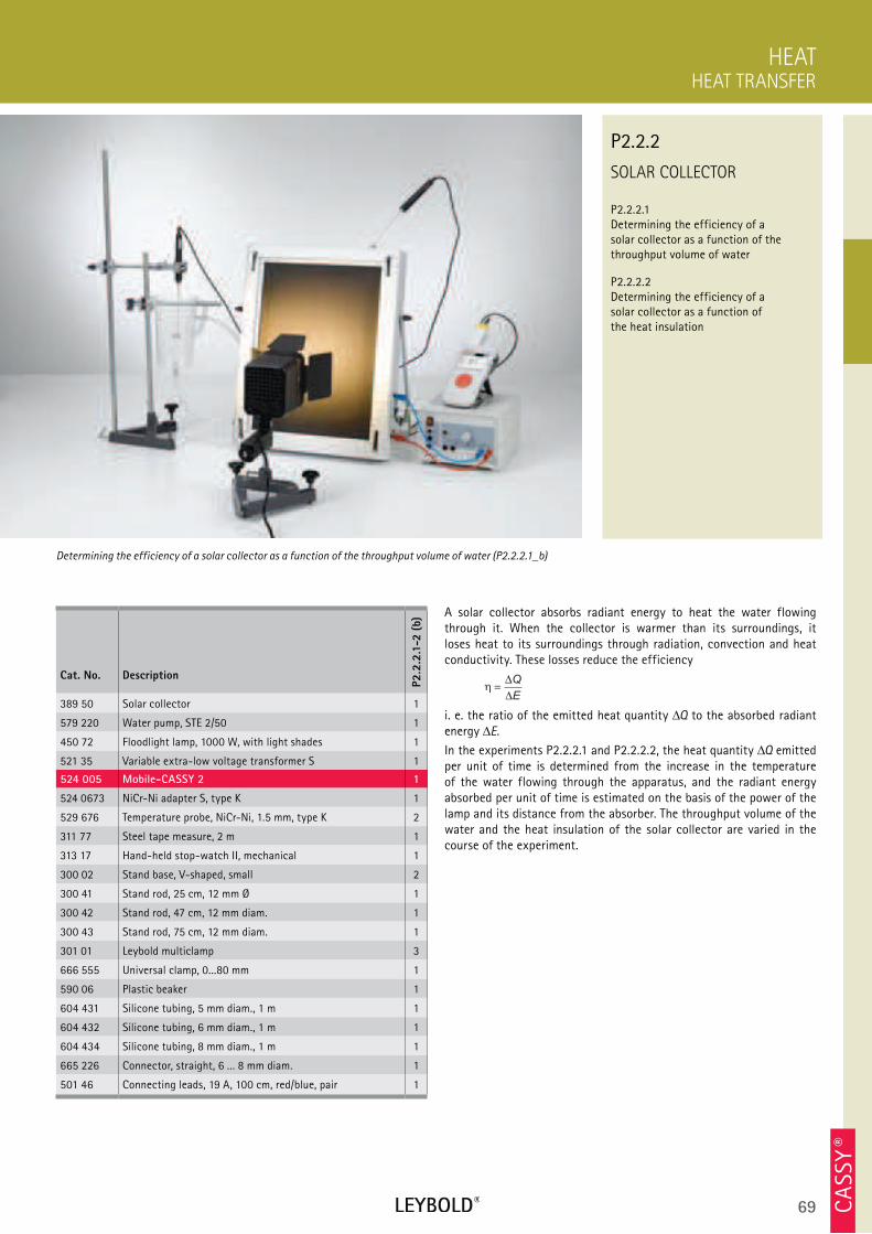
69 CA
SSY ®
SOLAR COLLECTOR
P2.2.2.1 Determining the efficiency of a solar collector as a function of the throughput volume of water
P2.2.2.2 Determining the efficiency of a solar collector as a function of the heat insulation
HEAT TRANSFER
HEAT
Cat. No. Description
P2.2
.2.1
-2 (
b)
389 50 Solar collector 1
579 220 Water pump, STE 2/50 1
450 72 Floodlight lamp, 1000 W, with light shades 1
521 35 Variable extra-low voltage transformer S 1
524 005 Mobile-CASSY 2 1
524 0673 NiCr-Ni adapter S, type K 1
529 676 Temperature probe, NiCr-Ni, 1.5 mm, type K 2
311 77 Steel tape measure, 2 m 1
313 17 Hand-held stop-watch II, mechanical 1
300 02 Stand base, V-shaped, small 2
300 41 Stand rod, 25 cm, 12 mm Ø 1
300 42 Stand rod, 47 cm, 12 mm diam. 1
300 43 Stand rod, 75 cm, 12 mm diam. 1
301 01 Leybold multiclamp 3
666 555 Universal clamp, 0...80 mm 1
590 06 Plastic beaker 1
604 431 Silicone tubing, 5 mm diam., 1 m 1
604 432 Silicone tubing, 6 mm diam., 1 m 1
604 434 Silicone tubing, 8 mm diam., 1 m 1
665 226 Connector, straight, 6 ... 8 mm diam. 1
501 46 Connecting leads, 19 A, 100 cm, red/blue, pair 1
A solar collector absorbs radiant energy to heat the water flowing through it. When the collector is warmer than its surroundings, it loses heat to its surroundings through radiation, convection and heat conductivity. These losses reduce the efficiency
η =∆
∆
Q
E
i. e. the ratio of the emitted heat quantity Q to the absorbed radiant energy E.
In the experiments P2.2.2.1 and P2.2.2.2, the heat quantity Q emitted per unit of time is determined from the increase in the temperature of the water flowing through the apparatus, and the radiant energy absorbed per unit of time is estimated on the basis of the power of the lamp and its distance from the absorber. The throughput volume of the water and the heat insulation of the solar collector are varied in the course of the experiment.
Determining the efficiency of a solar collector as a function of the throughput volume of water (P2.2.2.1_b)
P2.2.2
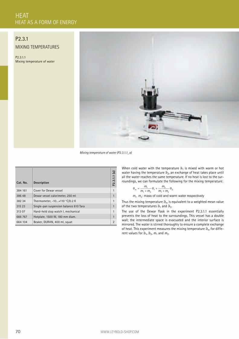
70 WWW.LEYBOLD-SHOP.COM
MIXING TEMPERATURES
P2.3.1.1 Mixing temperature of water
When cold water with the temperature 1 is mixed with warm or hot water having the temperature 2, an exchange of heat takes place until all the water reaches the same temperature. If no heat is lost to the sur-roundings, we can formulate the following for the mixing temperature:
ϑ ϑ ϑm
m
m m
m
m m
m m
=+
++
1
1 2
12
1 2
2
1 2, : mass of cold and warm water rrespectively
Thus the mixing temperature m is equivalent to a weighted mean value of the two temperatures 1 and 2.
The use of the Dewar flask in the experiment P2.3.1.1 essentially prevents the loss of heat to the surroundings. This vessel has a double wall; the intermediate space is evacuated and the interior surface is mirrored. The water is stirred thoroughly to ensure a complete exchange of heat. This experiment measures the mixing temperature m for diffe-rent values for 1, 2, m1 and m2.
HEAT
Mixing temperature of water (P2.3.1.1_a)
Cat. No. Description
P2.3
.1.1
(a)
384 161 Cover for Dewar vessel 1
386 48 Dewar vessel calorimeter, 250 ml 1
382 34 Thermometer, -10...+110 °C/0.2 K 1
315 23 Single-pan suspension balance 610 Tara 1
313 07 Hand-held stop watch I, mechanical 1
666 767 Hotplate, 1500 W, 180 mm diam. 1
664 104 Beaker, DURAN, 400 ml, squat 2
HEAT AS A FORM OF ENERGY
P2.3.1
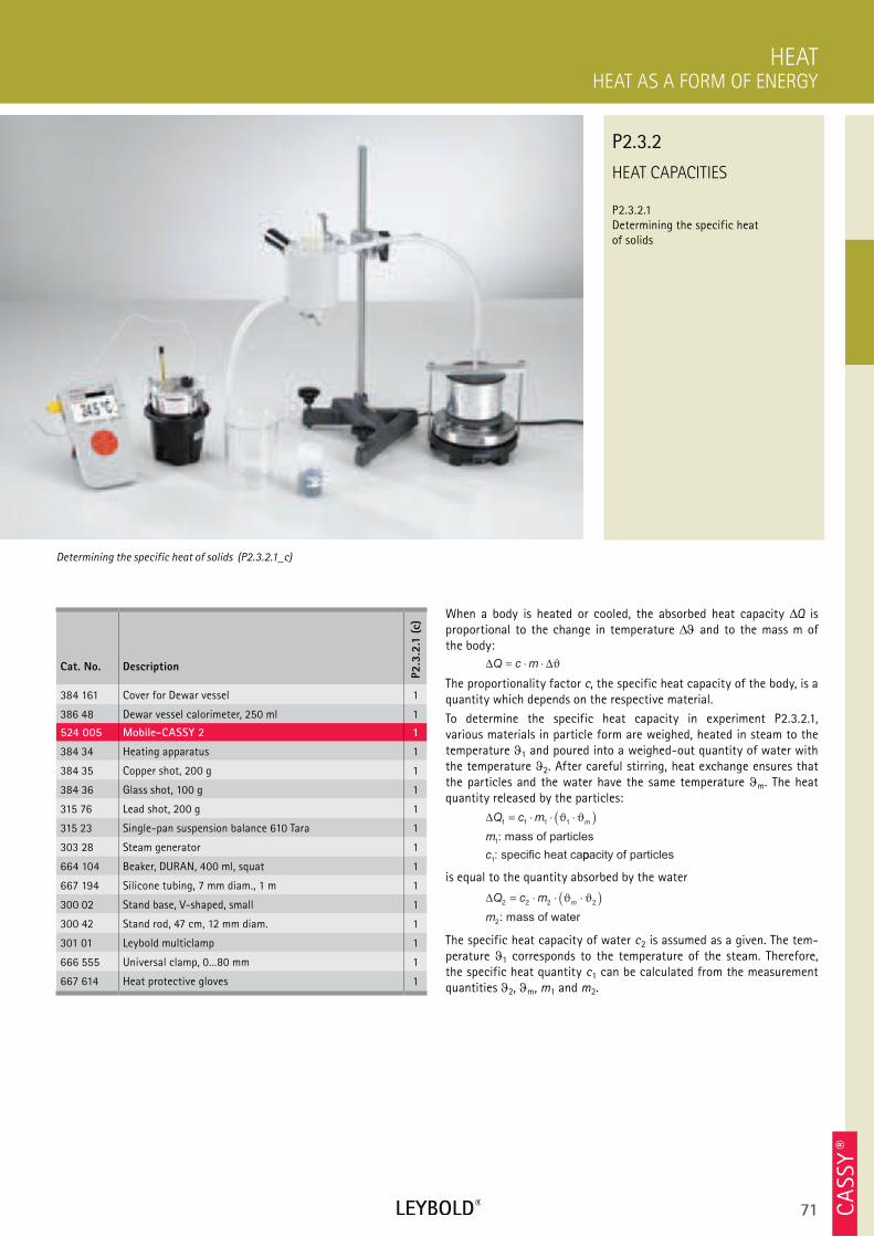
71 CA
SSY ®
HEAT CAPACITIES
P2.3.2.1
Determining the specific heat
of solids
HEAT AS A FORM OF ENERGY
HEAT
Cat. No. Description
P2.3
.2.1
(c)
384 161 Cover for Dewar vessel 1
386 48 Dewar vessel calorimeter, 250 ml 1
524 005 Mobile-CASSY 2 1
384 34 Heating apparatus 1
384 35 Copper shot, 200 g 1
384 36 Glass shot, 100 g 1
315 76 Lead shot, 200 g 1
315 23 Single-pan suspension balance 610 Tara 1
303 28 Steam generator 1
664 104 Beaker, DURAN, 400 ml, squat 1
667 194 Silicone tubing, 7 mm diam., 1 m 1
300 02 Stand base, V-shaped, small 1
300 42 Stand rod, 47 cm, 12 mm diam. 1
301 01 Leybold multiclamp 1
666 555 Universal clamp, 0...80 mm 1
667 614 Heat protective gloves 1
When a body is heated or cooled, the absorbed heat capacity Q is
proportional to the change in temperature and to the mass m of
the body:
∆ ∆Q c m= ⋅ ⋅ ϑ
The proportionality factor c, the specific heat capacity of the body, is a
quantity which depends on the respective material.
To determine the specific heat capacity in experiment P2.3.2.1,
various materials in particle form are weighed, heated in steam to the
temperature 1 and poured into a weighed-out quantity of water with
the temperature 2. After careful stirring, heat exchange ensures that
the particles and the water have the same temperature m. The heat
quantity released by the particles:
∆Q c m
m
c
m1 1 1 1
1
1
= ⋅ ⋅ ⋅( )ϑ ϑ
: mass of particles
: specific heat cappacity of particles
is equal to the quantity absorbed by the water
∆Q c m
m
m2 2 2 2
2
= ⋅ ⋅ ⋅( )ϑ ϑ
: mass of water
The specific heat capacity of water c2 is assumed as a given. The tem-
perature 1 corresponds to the temperature of the steam. Therefore,
the specific heat quantity c1 can be calculated from the measurement
quantities 2, m, m1 and m2.
Determining the specific heat of solids (P2.3.2.1_c)
P2.3.2

72 WWW.LEYBOLD-SHOP.COMCA
SSY ®
CONVERTING MECHANICAL
ENERGY INTO HEAT
P2.3.3.1 Converting mechanical energy into heat energy - Recording and evaluating measured values manually
P2.3.3.2 Converting mechanical energy into heat energy - Recording and evaluating with CASSY
Energy is a fundamental quantity of physics. This is because the various forms of energy can be converted from one to another and are thus equivalent to each other, and because the total energy is conserved in the case of conversion in a closed system.
These experiments P2.3.3.1 und P2.3.3.2 show the equivalence of mechanical and heat energy. A hand crank is used to turn various calorimeter vessels on their own axes, and friction on a nylon belt causes them to become warmer. The friction force is equivalent to the weight G of a suspended weight. For n turns of the calorimeter, the mechanical work is thus
W G n d
d
n= ⋅ ⋅ ⋅π
: diameter of calorimeter
This results in an increase in the temperature of the calorimeter which corresponds to the specific heat capacity
Q m c
c m
n n
n
= ⋅ ⋅ −( )ϑ ϑ
ϑ
0
: specific heat capacity, : mass,
: tempeerature after turnsn
To confirm the relationship
Q Wn n
the two quantities are plotted together in a diagram. In the experiment P2.3.3.1, the measurement is conducted and evaluated manually point by point. The experiment P2.3.3.2 takes advantage of the computer-assisted measuring system CASSY.
HEAT
Converting mechanical energy into heat energy - Recording and evaluating measured values manually (P2.3.3.1_a)
Cat. No. Description
P2.3
.3.1
(a)
P2.3
.3.2
388 00 Equivalent of heat, basic apparatus 1 1
388 01 Water calorimeter 1 1
388 02 Copper-block calorimeter 1 1
388 03 Aluminium-block calorimeter 1 1
388 04 Aluminium-block calorimeter, large 1 1
388 05 Thermometer for calorimeters, +15...35 °C/0.2 K 1
388 24 Weight, 5 kg 1 1
524 013 Sensor-CASSY 2 1
524 220 CASSY Lab 2 1
524 074 Timer S 1
524 0673 NiCr-Ni adapter S, type K 1
529 676 Temperature probe, NiCr-Ni, 1.5 mm, type K 1
337 46 Fork-type light barrier 1
501 16 Multi-core cable, 6-pole, 1.5 m 1
300 02 Stand base, V-shaped, small 1
301 11 Clamp with jaw clamp 1
300 40 Stand rod, 10 cm, 12 mm diam. 1
300 41 Stand rod, 25 cm, 12 mm Ø 1
301 07 Simple bench clamp 1
additionally required: PC with Windows XP/Vista/7/8/10 (x86 or x64)
1
HEAT AS A FORM OF ENERGY
P2.3.3
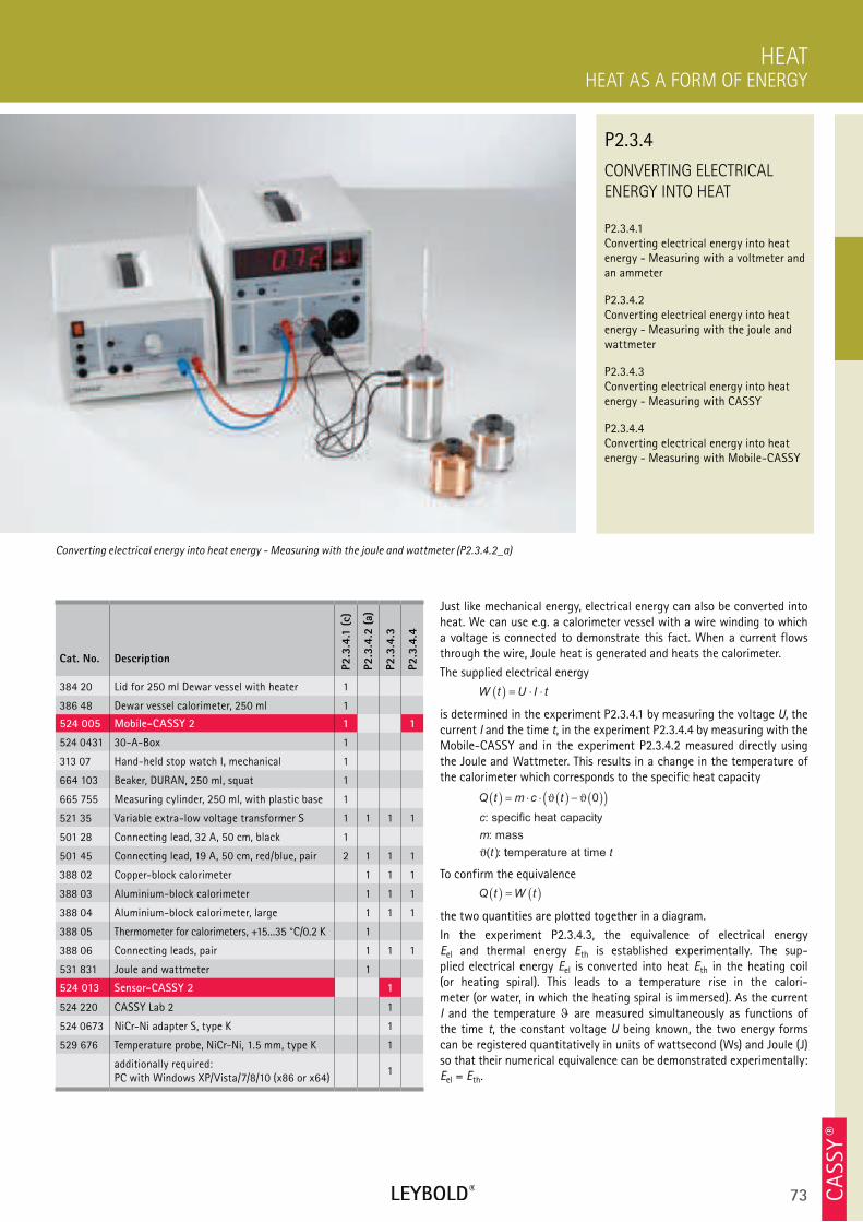
73 CA
SSY ®
CONVERTING ELECTRICAL
ENERGY INTO HEAT
P2.3.4.1 Converting electrical energy into heat energy - Measuring with a voltmeter and an ammeter
P2.3.4.2 Converting electrical energy into heat energy - Measuring with the joule and wattmeter
P2.3.4.3 Converting electrical energy into heat energy - Measuring with CASSY
P2.3.4.4 Converting electrical energy into heat energy - Measuring with Mobile-CASSY
HEAT AS A FORM OF ENERGY
HEAT
Cat. No. Description
P2.3
.4.1
(c)
P2.3
.4.2
(a)
P2.3
.4.3
P2.3
.4.4
384 20 Lid for 250 ml Dewar vessel with heater 1
386 48 Dewar vessel calorimeter, 250 ml 1
524 005 Mobile-CASSY 2 1 1
524 0431 30-A-Box 1
313 07 Hand-held stop watch I, mechanical 1
664 103 Beaker, DURAN, 250 ml, squat 1
665 755 Measuring cylinder, 250 ml, with plastic base 1
521 35 Variable extra-low voltage transformer S 1 1 1 1
501 28 Connecting lead, 32 A, 50 cm, black 1
501 45 Connecting lead, 19 A, 50 cm, red/blue, pair 2 1 1 1
388 02 Copper-block calorimeter 1 1 1
388 03 Aluminium-block calorimeter 1 1 1
388 04 Aluminium-block calorimeter, large 1 1 1
388 05 Thermometer for calorimeters, +15...35 °C/0.2 K 1
388 06 Connecting leads, pair 1 1 1
531 831 Joule and wattmeter 1
524 013 Sensor-CASSY 2 1
524 220 CASSY Lab 2 1
524 0673 NiCr-Ni adapter S, type K 1
529 676 Temperature probe, NiCr-Ni, 1.5 mm, type K 1
additionally required: PC with Windows XP/Vista/7/8/10 (x86 or x64)
1
Just like mechanical energy, electrical energy can also be converted into heat. We can use e.g. a calorimeter vessel with a wire winding to which a voltage is connected to demonstrate this fact. When a current flows through the wire, Joule heat is generated and heats the calorimeter.
The supplied electrical energy
W t U I t( ) = ⋅ ⋅
is determined in the experiment P2.3.4.1 by measuring the voltage U, the current I and the time t, in the experiment P2.3.4.4 by measuring with the Mobile-CASSY and in the experiment P2.3.4.2 measured directly using the Joule and Wattmeter. This results in a change in the temperature of the calorimeter which corresponds to the specific heat capacity
Q t m c t
c
m
t
( ) = ⋅ ⋅ ( ) − ( )( )ϑ ϑ
ϑ
0
: specific heat capacity
: mass
: ( ) ttemperature at time t
To confirm the equivalence
Q t W t( ) = ( )
the two quantities are plotted together in a diagram.
In the experiment P2.3.4.3, the equivalence of electrical energy Eel and thermal energy Eth is established experimentally. The sup-plied electrical energy Eel is converted into heat Eth in the heating coil (or heating spiral). This leads to a temperature rise in the calori- meter (or water, in which the heating spiral is immersed). As the current I and the temperature are measured simultaneously as functions of the time t, the constant voltage U being known, the two energy forms can be registered quantitatively in units of wattsecond (Ws) and Joule (J) so that their numerical equivalence can be demonstrated experimentally: Eel = Eth.
Converting electrical energy into heat energy - Measuring with the joule and wattmeter (P2.3.4.2_a)
P2.3.4
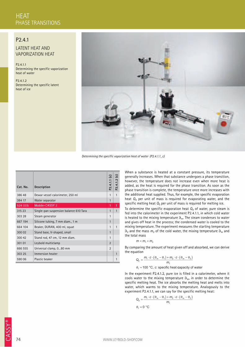
74 WWW.LEYBOLD-SHOP.COMCA
SSY ®
LATENT HEAT AND
VAPORIZATION HEAT
P2.4.1.1
Determining the specific vaporization
heat of water
P2.4.1.2
Determining the specific latent
heat of ice
When a substance is heated at a constant pressure, its temperature
generally increases. When that substance undergoes a phase transition,
however, the temperature does not increase even when more heat is
added, as the heat is required for the phase transition. As soon as the
phase transition is complete, the temperature once more increases with
the additional heat supplied. Thus, for example, the specific evaporation
heat QV per unit of mass is required for evaporating water, and the
specific melting heat QS per unit of mass is required for melting ice.
To determine the specific evaporation heat QV of water, pure steam is
fed into the calorimeter in the experiment P2.4.1.1, in which cold water
is heated to the mixing temperature m. The steam condenses to water
and gives off heat in the process; the condensed water is cooled to the
mixing temperature. The experiment measures the starting temperature
2 and the mass m2 of the cold water, the mixing temperature m and
the total mass
m m m= +1 2
By comparing the amount of heat given off and absorbed, we can derive
the equation
Qm c m c
m
c
V
m m=
⋅ ⋅ −( ) + ⋅ ⋅ −( )
≈
1 1 2 2
1
1 100
ϑ ϑ ϑ ϑ
ϑ °C, : specific heat ccapacity of water
In the experiment P2.4.1.2, pure ice is filled in a calorimeter, where it
cools water to the mixing temperature m, in order to determine the
specific melting heat. The ice absorbs the melting heat and melts into
water, which warms to the mixing temperature. Analogously to the
experiment P2.4.1.1, we can say for the specific melting heat:
Qm c m c
mS
m m=
⋅ ⋅ −( ) + ⋅ ⋅ −( )
=
1 1 2 2
1
10
ϑ ϑ ϑ ϑ
ϑ °C
HEAT
Determining the specific vaporization heat of water (P2.4.1.1_c)
Cat. No. Description
P2.4
.1.1
(c)
P2.4
.1.2
(c)
386 48 Dewar vessel calorimeter, 250 ml 1 1
384 17 Water separator 1
524 005 Mobile-CASSY 2 1 1
315 23 Single-pan suspension balance 610 Tara 1 1
303 28 Steam generator 1
667 194 Silicone tubing, 7 mm diam., 1 m 1
664 104 Beaker, DURAN, 400 ml, squat 1 1
300 02 Stand base, V-shaped, small 1
300 42 Stand rod, 47 cm, 12 mm diam. 1
301 01 Leybold multiclamp 2
666 555 Universal clamp, 0...80 mm 2
303 25 Immersion heater 1
590 06 Plastic beaker 1
PHASE TRANSITIONS
P2.4.1
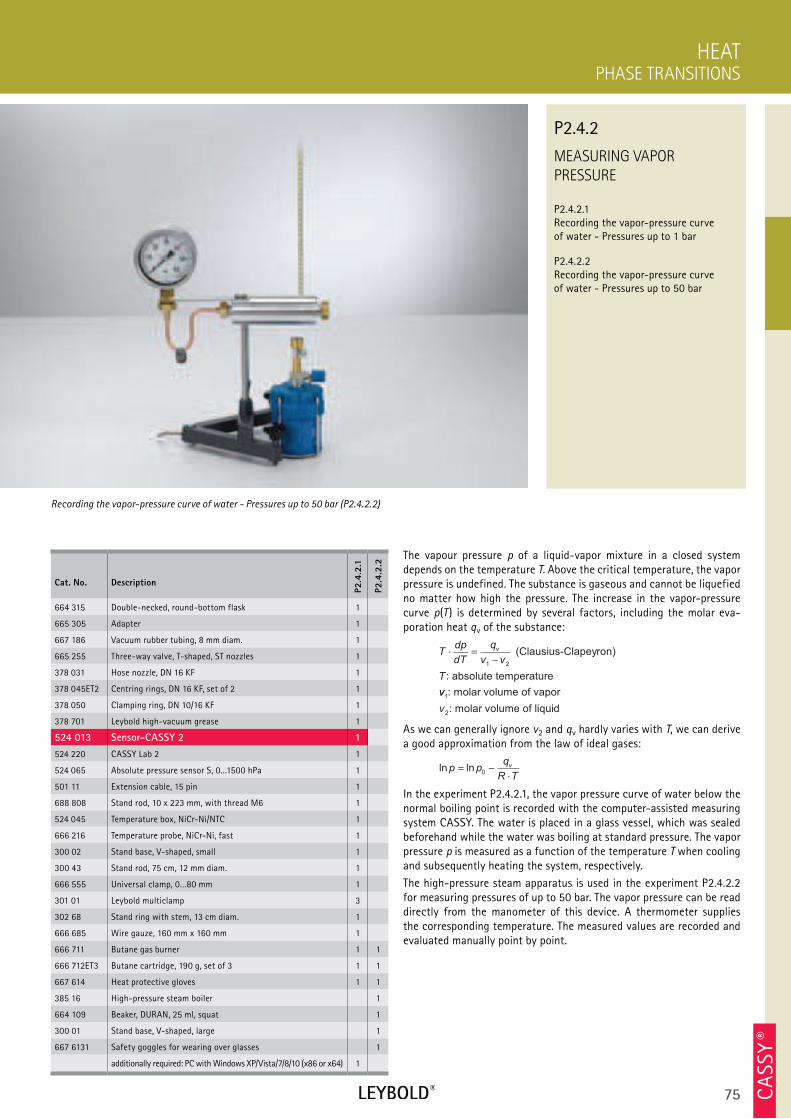
75 CA
SSY ®
MEASURING VAPOR
PRESSURE
P2.4.2.1 Recording the vapor-pressure curve of water - Pressures up to 1 bar
P2.4.2.2 Recording the vapor-pressure curve of water - Pressures up to 50 bar
PHASE TRANSITIONS
HEAT
Cat. No. Description
P2.4
.2.1
P2.4
.2.2
664 315 Double-necked, round-bottom flask 1
665 305 Adapter 1
667 186 Vacuum rubber tubing, 8 mm diam. 1
665 255 Three-way valve, T-shaped, ST nozzles 1
378 031 Hose nozzle, DN 16 KF 1
378 045ET2 Centring rings, DN 16 KF, set of 2 1
378 050 Clamping ring, DN 10/16 KF 1
378 701 Leybold high-vacuum grease 1
524 013 Sensor-CASSY 2 1
524 220 CASSY Lab 2 1
524 065 Absolute pressure sensor S, 0...1500 hPa 1
501 11 Extension cable, 15 pin 1
688 808 Stand rod, 10 x 223 mm, with thread M6 1
524 045 Temperature box, NiCr-Ni/NTC 1
666 216 Temperature probe, NiCr-Ni, fast 1
300 02 Stand base, V-shaped, small 1
300 43 Stand rod, 75 cm, 12 mm diam. 1
666 555 Universal clamp, 0...80 mm 1
301 01 Leybold multiclamp 3
302 68 Stand ring with stem, 13 cm diam. 1
666 685 Wire gauze, 160 mm x 160 mm 1
666 711 Butane gas burner 1 1
666 712ET3 Butane cartridge, 190 g, set of 3 1 1
667 614 Heat protective gloves 1 1
385 16 High-pressure steam boiler 1
664 109 Beaker, DURAN, 25 ml, squat 1
300 01 Stand base, V-shaped, large 1
667 6131 Safety goggles for wearing over glasses 1
additionally required: PC with Windows XP/Vista/7/8/10 (x86 or x64) 1
The vapour pressure p of a liquid-vapor mixture in a closed system depends on the temperature T. Above the critical temperature, the vapor pressure is undefined. The substance is gaseous and cannot be liquefied no matter how high the pressure. The increase in the vapor-pressure curve p(T ) is determined by several factors, including the molar eva-poration heat qv of the substance:
Tdp
dT
q
v v
T
v⋅ =−1 2
(Clausius-Clapeyron)
: absolute temperature
vv
v
1
2
: molar volume of vapor
: molar volume of liquid
As we can generally ignore v2 and qv hardly varies with T, we can derive a good approximation from the law of ideal gases:
ln lnp pq
R Tv= −⋅
0
In the experiment P2.4.2.1, the vapor pressure curve of water below the normal boiling point is recorded with the computer-assisted measuring system CASSY. The water is placed in a glass vessel, which was sealed beforehand while the water was boiling at standard pressure. The vapor pressure p is measured as a function of the temperature T when cooling and subsequently heating the system, respectively.
The high-pressure steam apparatus is used in the experiment P2.4.2.2 for measuring pressures of up to 50 bar. The vapor pressure can be read directly from the manometer of this device. A thermometer supplies the corresponding temperature. The measured values are recorded and evaluated manually point by point.
Recording the vapor-pressure curve of water - Pressures up to 50 bar (P2.4.2.2)
P2.4.2
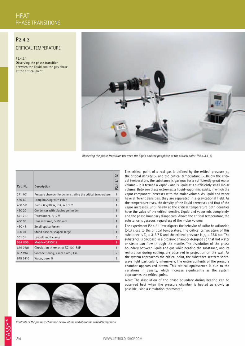
76 WWW.LEYBOLD-SHOP.COMCA
SSY ®
CRITICAL TEMPERATURE
P2.4.3.1 Observing the phase transition between the liquid and the gas phase at the critical point
The critical point of a real gas is defined by the critical pressure pc, the critical density c and the critical temperature TC. Below the criti-cal temperature, the substance is gaseous for a sufficiently great molar volume - it is termed a vapor - and is liquid at a sufficiently small molar volume. Between these extremes, a liquid-vapor mix exists, in which the vapor component increases with the molar volume. As liquid and vapor have different densities, they are separated in a gravitational field. As the temperature rises, the density of the liquid decreases and that of the vapor increases, until finally at the critical temperature both densities have the value of the critical density. Liquid and vapor mix completely, and the phase boundary disappears. Above the critical temperature, the substance is gaseous, regardless of the molar volume.
The experiment P2.4.3.1 investigates the behavior of sulfur hexafluoride (SF6) close to the critical temperature. The critical temperature of this substance is TC = 318.7 K and the critical pressure is pc = 37.6 bar. The substance is enclosed in a pressure chamber designed so that hot water or steam can flow through the mantle. The dissolution of the phase boundary between liquid and gas while heating the substance, and its restoration during cooling, are observed in projection on the wall. As the system approaches the critical point, the substance scatters short-wave light particularly intensively; the entire contents of the pressure chamber appears red-brown. This critical opalescence is due to the variations in density, which increase significantly as the system approaches the critical point.
Note: The dissolution of the phase boundary during heating can be observed best when the pressure chamber is heated as slowly as possible using a circulation thermostat.
HEAT
Observing the phase transition between the liquid and the gas phase at the critical point (P2.4.3.1_c)
Cat. No. Description
P2.4
.3.1
(c)
371 401 Pressure chamber for demonstrating the critical temperature 1
450 60 Lamp housing with cable 1
450 511 Bulbs, 6 V/30 W, E14, set of 2 1
460 20 Condenser with diaphragm holder 1
521 210 Transformer, 6/12 V 1
460 03 Lens in frame, f=100 mm 1
460 43 Small optical bench 1
300 01 Stand base, V-shaped, large 1
301 01 Leybold multiclamp 3
524 005 Mobile-CASSY 2 1
666 7681 Circulation thermostat SC 100-S5P 1
667 194 Silicone tubing, 7 mm diam., 1 m 2
675 3410 Water, pure, 5 l 2
Contents of the pressure chamber: below, at the and above the critical temperatur
PHASE TRANSITIONS
P2.4.3
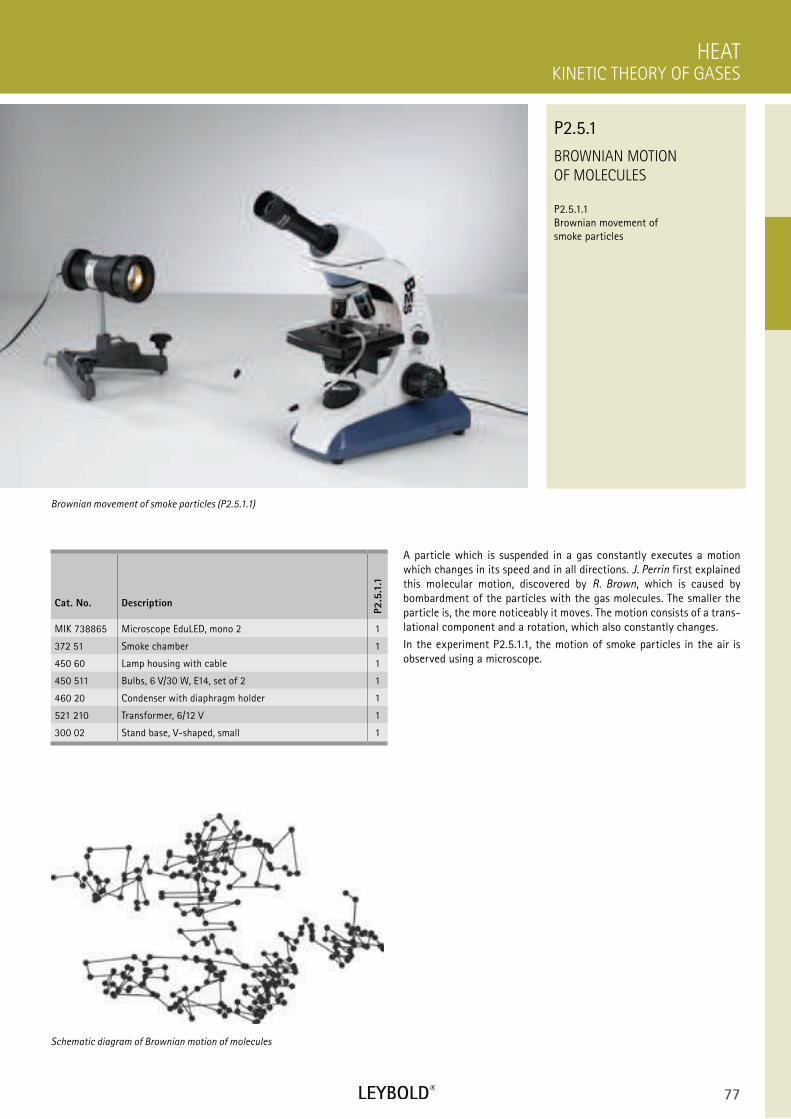
77
BROWNIAN MOTION
OF MOLECULES
P2.5.1.1 Brownian movement of smoke particles
KINETIC THEORY OF GASES
HEAT
Cat. No. Description
P2.5
.1.1
MIK 738865 Microscope EduLED, mono 2 1
372 51 Smoke chamber 1
450 60 Lamp housing with cable 1
450 511 Bulbs, 6 V/30 W, E14, set of 2 1
460 20 Condenser with diaphragm holder 1
521 210 Transformer, 6/12 V 1
300 02 Stand base, V-shaped, small 1
A particle which is suspended in a gas constantly executes a motion which changes in its speed and in all directions. J. Perrin first explained this molecular motion, discovered by R. Brown, which is caused by bombardment of the particles with the gas molecules. The smaller the particle is, the more noticeably it moves. The motion consists of a trans-lational component and a rotation, which also constantly changes.
In the experiment P2.5.1.1, the motion of smoke particles in the air is observed using a microscope.
Brownian movement of smoke particles (P2.5.1.1)
P2.5.1
Schematic diagram of Brownian motion of molecules
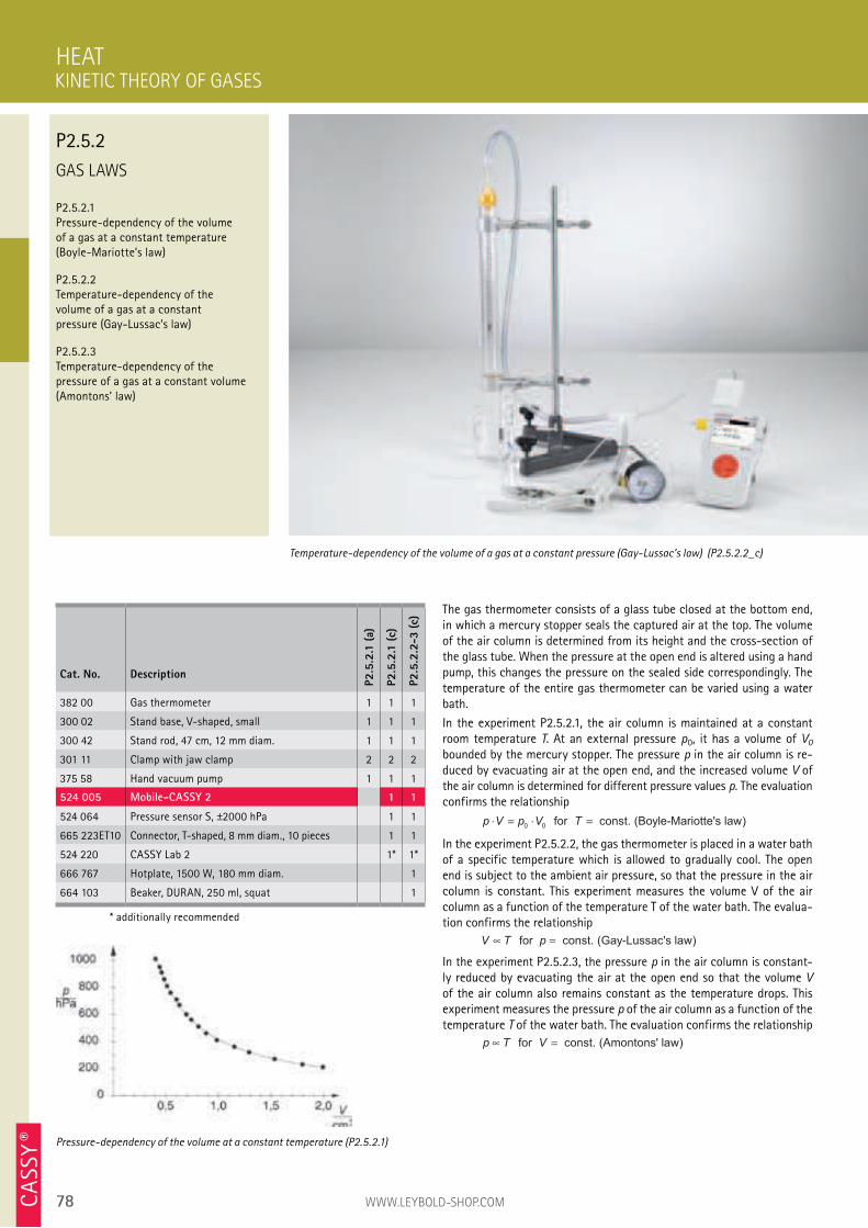
78 WWW.LEYBOLD-SHOP.COMCA
SSY ®
GAS LAWS
P2.5.2.1 Pressure-dependency of the volume of a gas at a constant temperature (Boyle-Mariotte’s law)
P2.5.2.2 Temperature-dependency of the volume of a gas at a constant pressure (Gay-Lussac’s law)
P2.5.2.3 Temperature-dependency of the pressure of a gas at a constant volume (Amontons’ law)
The gas thermometer consists of a glass tube closed at the bottom end, in which a mercury stopper seals the captured air at the top. The volume of the air column is determined from its height and the cross-section of the glass tube. When the pressure at the open end is altered using a hand pump, this changes the pressure on the sealed side correspondingly. The temperature of the entire gas thermometer can be varied using a water bath.
In the experiment P2.5.2.1, the air column is maintained at a constant room temperature T. At an external pressure p0, it has a volume of V0 bounded by the mercury stopper. The pressure p in the air column is re-duced by evacuating air at the open end, and the increased volume V of the air column is determined for different pressure values p. The evaluation confirms the relationship
p V p V T⋅ = ⋅ =0 0 for const. (Boyle-Mariotte's law)
In the experiment P2.5.2.2, the gas thermometer is placed in a water bath of a specific temperature which is allowed to gradually cool. The open end is subject to the ambient air pressure, so that the pressure in the air column is constant. This experiment measures the volume V of the air column as a function of the temperature T of the water bath. The evalua-tion confirms the relationship
V T p∝ = for const. (Gay-Lussac's law)
In the experiment P2.5.2.3, the pressure p in the air column is constant-ly reduced by evacuating the air at the open end so that the volume V of the air column also remains constant as the temperature drops. This experiment measures the pressure p of the air column as a function of the temperature T of the water bath. The evaluation confirms the relationship
p T V∝ = for const. (Amontons' law)
HEAT
Temperature-dependency of the volume of a gas at a constant pressure (Gay-Lussac’s law) (P2.5.2.2_c)
Cat. No. Description
P2.5
.2.1
(a)
P2.5
.2.1
(c)
P2.5
.2.2
-3 (
c)
382 00 Gas thermometer 1 1 1
300 02 Stand base, V-shaped, small 1 1 1
300 42 Stand rod, 47 cm, 12 mm diam. 1 1 1
301 11 Clamp with jaw clamp 2 2 2
375 58 Hand vacuum pump 1 1 1
524 005 Mobile-CASSY 2 1 1
524 064 Pressure sensor S, ±2000 hPa 1 1
665 223ET10 Connector, T-shaped, 8 mm diam., 10 pieces 1 1
524 220 CASSY Lab 2 1* 1*
666 767 Hotplate, 1500 W, 180 mm diam. 1
664 103 Beaker, DURAN, 250 ml, squat 1
* additionally recommended
Pressure-dependency of the volume at a constant temperature (P2.5.2.1)
KINETIC THEORY OF GASES
P2.5.2
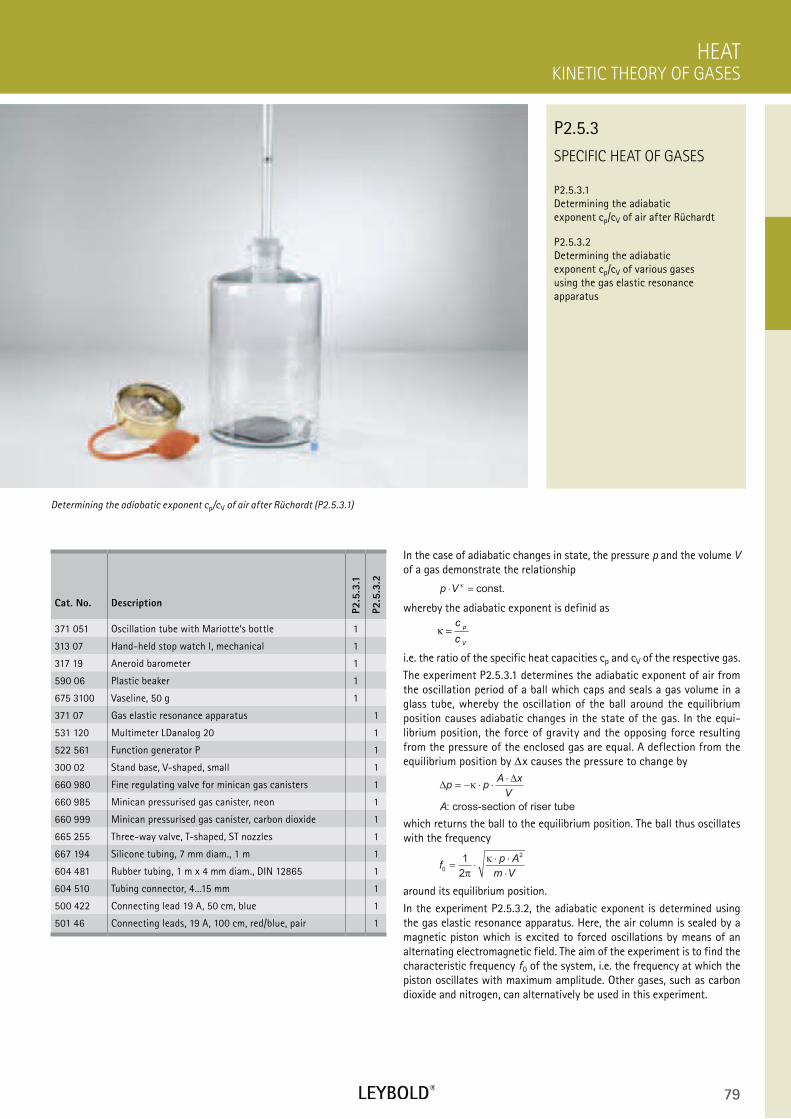
79
SPECIFIC HEAT OF GASES
P2.5.3.1 Determining the adiabatic exponent cp/cV of air after Rüchardt
P2.5.3.2 Determining the adiabatic exponent cp/cV of various gases using the gas elastic resonance apparatus
KINETIC THEORY OF GASES
HEAT
Cat. No. Description
P2.5
.3.1
P2.5
.3.2
371 051 Oscillation tube with Mariotte‘s bottle 1
313 07 Hand-held stop watch I, mechanical 1
317 19 Aneroid barometer 1
590 06 Plastic beaker 1
675 3100 Vaseline, 50 g 1
371 07 Gas elastic resonance apparatus 1
531 120 Multimeter LDanalog 20 1
522 561 Function generator P 1
300 02 Stand base, V-shaped, small 1
660 980 Fine regulating valve for minican gas canisters 1
660 985 Minican pressurised gas canister, neon 1
660 999 Minican pressurised gas canister, carbon dioxide 1
665 255 Three-way valve, T-shaped, ST nozzles 1
667 194 Silicone tubing, 7 mm diam., 1 m 1
604 481 Rubber tubing, 1 m x 4 mm diam., DIN 12865 1
604 510 Tubing connector, 4...15 mm 1
500 422 Connecting lead 19 A, 50 cm, blue 1
501 46 Connecting leads, 19 A, 100 cm, red/blue, pair 1
In the case of adiabatic changes in state, the pressure p and the volume V of a gas demonstrate the relationship
p V⋅ =κ
const.
whereby the adiabatic exponent is definid as
κ =
c
c
p
V
i.e. the ratio of the specific heat capacities cp and cV of the respective gas.
The experiment P2.5.3.1 determines the adiabatic exponent of air from the oscillation period of a ball which caps and seals a gas volume in a glass tube, whereby the oscillation of the ball around the equilibrium position causes adiabatic changes in the state of the gas. In the equi-librium position, the force of gravity and the opposing force resulting from the pressure of the enclosed gas are equal. A deflection from the equilibrium position by x causes the pressure to change by
∆∆
p pA x
V
A
= − ⋅ ⋅⋅
κ
: cross-section of riser tube
which returns the ball to the equilibrium position. The ball thus oscillates with the frequency
fp A
m V0
21
2= ⋅
⋅ ⋅
⋅π
κ
around its equilibrium position.
In the experiment P2.5.3.2, the adiabatic exponent is determined using the gas elastic resonance apparatus. Here, the air column is sealed by a magnetic piston which is excited to forced oscillations by means of an alternating electromagnetic field. The aim of the experiment is to find the characteristic frequency f0 of the system, i.e. the frequency at which the piston oscillates with maximum amplitude. Other gases, such as carbon dioxide and nitrogen, can alternatively be used in this experiment.
Determining the adiabatic exponent cp/cV of air after Rüchardt (P2.5.3.1)
P2.5.3
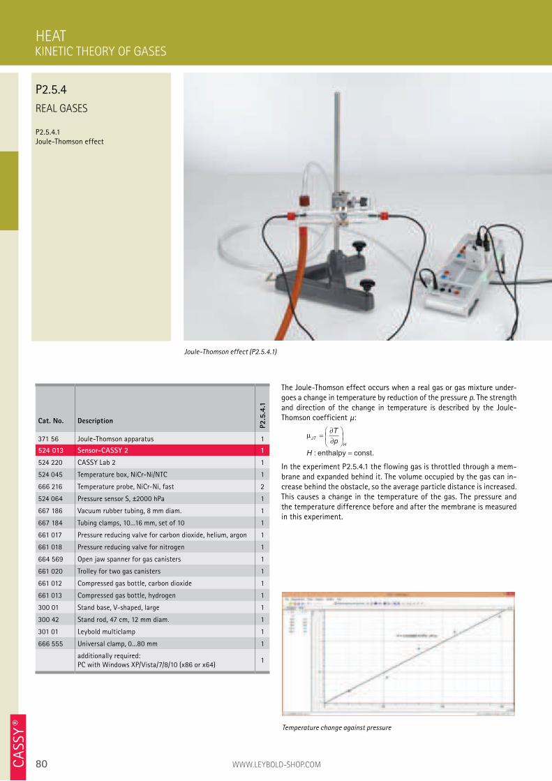
80 WWW.LEYBOLD-SHOP.COMCA
SSY ®
REAL GASES
P2.5.4.1 Joule-Thomson effect
The Joule-Thomson effect occurs when a real gas or gas mixture under-goes a change in temperature by reduction of the pressure p. The strength and direction of the change in temperature is described by the Joule-Thomson coefficient µ:
µJT
H
T
p
H
=∂∂
=
enthalpy const. :
In the experiment P2.5.4.1 the flowing gas is throttled through a mem-brane and expanded behind it. The volume occupied by the gas can in-crease behind the obstacle, so the average particle distance is increased. This causes a change in the temperature of the gas. The pressure and the temperature difference before and after the membrane is measured in this experiment.
HEAT
Joule-Thomson effect (P2.5.4.1)
Cat. No. Description
P2.5
.4.1
371 56 Joule-Thomson apparatus 1
524 013 Sensor-CASSY 2 1
524 220 CASSY Lab 2 1
524 045 Temperature box, NiCr-Ni/NTC 1
666 216 Temperature probe, NiCr-Ni, fast 2
524 064 Pressure sensor S, ±2000 hPa 1
667 186 Vacuum rubber tubing, 8 mm diam. 1
667 184 Tubing clamps, 10...16 mm, set of 10 1
661 017 Pressure reducing valve for carbon dioxide, helium, argon 1
661 018 Pressure reducing valve for nitrogen 1
664 569 Open jaw spanner for gas canisters 1
661 020 Trolley for two gas canisters 1
661 012 Compressed gas bottle, carbon dioxide 1
661 013 Compressed gas bottle, hydrogen 1
300 01 Stand base, V-shaped, large 1
300 42 Stand rod, 47 cm, 12 mm diam. 1
301 01 Leybold multiclamp 1
666 555 Universal clamp, 0...80 mm 1
additionally required: PC with Windows XP/Vista/7/8/10 (x86 or x64)
1
Temperature change against pressure
KINETIC THEORY OF GASES
P2.5.4
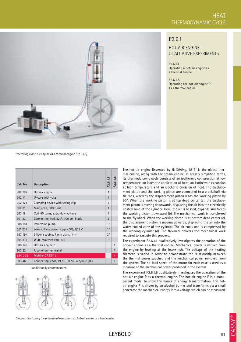
81 CA
SSY ®
HOT-AIR ENGINE:
QUALITATIVE EXPERIMENTS
P2.6.1.1 Operating a hot-air engine as a thermal engine
P2.6.1.5 Operating the hot-air engine P as a thermal engine
THERMODYNAMIC CYCLE
HEAT
Cat. No. Description
P2.6
.1.1
P2.6
.1.5
388 182 Hot-air engine 1
562 11 U-core with yoke 1
562 121 Clamping device with spring clip 1
562 21 Mains coil, 500 turns 1
562 18 Coil, 50 turns, extra-low voltage 1
501 33 Connecting lead, 32 A, 100 cm, black 2
388 181 Immersion pump 1*
521 231 Low-voltage power supply, 3/6/9/12 V 1*
667 194 Silicone tubing, 7 mm diam., 1 m 2*
604 313 Wide-mouthed can, 10 l 1*
388 176 Hot-air engine P 1
303 22 Alcohol burner, metal 1
524 005 Mobile-CASSY 2 1
501 46 Connecting leads, 19 A, 100 cm, red/blue, pair 1
* additionally recommended
The hot-air engine (invented by R. Stirling, 1816) is the oldest ther-mal engine, along with the steam engine. In greatly simplified terms, its thermodynamic cycle consists of an isothermic compression at low temperature, an isochoric application of heat, an isothermic expansion at high temperature and an isochoric emission of heat. The displace-ment piston and the working piston are connected to a crankshaft via tie rods, whereby the displacement piston leads the working piston by 90°. When the working piston is at top dead center (a), the displace-ment piston is moving downwards, displacing the air into the electrically heated zone of the cylinder. Here, the air is heated, expands and forces the working piston downward (b). The mechanical work is transferred to the flywheel. When the working piston is at bottom dead center (c), the displacement piston is moving upwards, displacing the air into the water-cooled zone of the cylinder. The air cools and is compressed by the working cylinder (d). The flywheel delivers the mechanical work required to execute this process.
The experiment P2.6.1.1 qualitatively investigates the operation of the hot-air engine as a thermal engine. Mechanical power is derived from the engine by braking at the brake hub. The voltage of the heating filament is varied in order to demonstrate the relationship between the thermal power supplied and the mechanical power removed from the system. The no-load speed of the motor for each case is used as a measure of the mechanical power produced in the system.
The experiment P2.6.1.5 qualitatively investigates the operation of the hot-air engine P as a thermal engine. The hot-air engine P is a trans-parent model to show the basics of energy transformation. The hot-air engine P is driven by an alcohol burner and transforms via a small generator the mechanical energy into a voltage which can be measured.
Operating a hot-air engine as a thermal engine (P2.6.1.1)
P2.6.1
Diagram illustrating the principle of operation of a hot-air engine as a heat engine
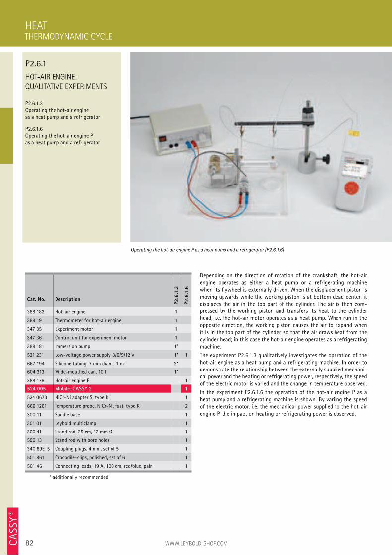
82 WWW.LEYBOLD-SHOP.COMCA
SSY ®
HOT-AIR ENGINE:
QUALITATIVE EXPERIMENTS
P2.6.1.3 Operating the hot-air engine as a heat pump and a refrigerator
P2.6.1.6 Operating the hot-air engine P as a heat pump and a refrigerator
Depending on the direction of rotation of the crankshaft, the hot-air engine operates as either a heat pump or a refrigerating machine when its flywheel is externally driven. When the displacement piston is moving upwards while the working piston is at bottom dead center, it displaces the air in the top part of the cylinder. The air is then com-pressed by the working piston and transfers its heat to the cylinder head, i.e. the hot-air motor operates as a heat pump. When run in the opposite direction, the working piston causes the air to expand when it is in the top part of the cylinder, so that the air draws heat from the cylinder head; in this case the hot-air engine operates as a refrigerating machine.
The experiment P2.6.1.3 qualitatively investigates the operation of the hot-air engine as a heat pump and a refrigerating machine. In order to demonstrate the relationship between the externally supplied mechani-cal power and the heating or refrigerating power, respectively, the speed of the electric motor is varied and the change in temperature observed.
In the experiment P2.6.1.6 the operation of the hot-air engine P as a heat pump and a refrigerating machine is shown. By variing the speed of the electric motor, i.e. the mechanical power supplied to the hot-air engine P, the impact on heating or refrigerating power is observed.
HEAT
Operating the hot-air engine P as a heat pump and a refrigerator (P2.6.1.6)
Cat. No. Description
P2.6
.1.3
P2.6
.1.6
388 182 Hot-air engine 1
388 19 Thermometer for hot-air engine 1
347 35 Experiment motor 1
347 36 Control unit for experiment motor 1
388 181 Immersion pump 1*
521 231 Low-voltage power supply, 3/6/9/12 V 1* 1
667 194 Silicone tubing, 7 mm diam., 1 m 2*
604 313 Wide-mouthed can, 10 l 1*
388 176 Hot-air engine P 1
524 005 Mobile-CASSY 2 1
524 0673 NiCr-Ni adapter S, type K 1
666 1261 Temperature probe, NiCr-Ni, fast, type K 2
300 11 Saddle base 1
301 01 Leybold multiclamp 1
300 41 Stand rod, 25 cm, 12 mm Ø 1
590 13 Stand rod with bore holes 1
340 89ET5 Coupling plugs, 4 mm, set of 5 1
501 861 Crocodile-clips, polished, set of 6 1
501 46 Connecting leads, 19 A, 100 cm, red/blue, pair 1
* additionally recommended
THERMODYNAMIC CYCLE
P2.6.1
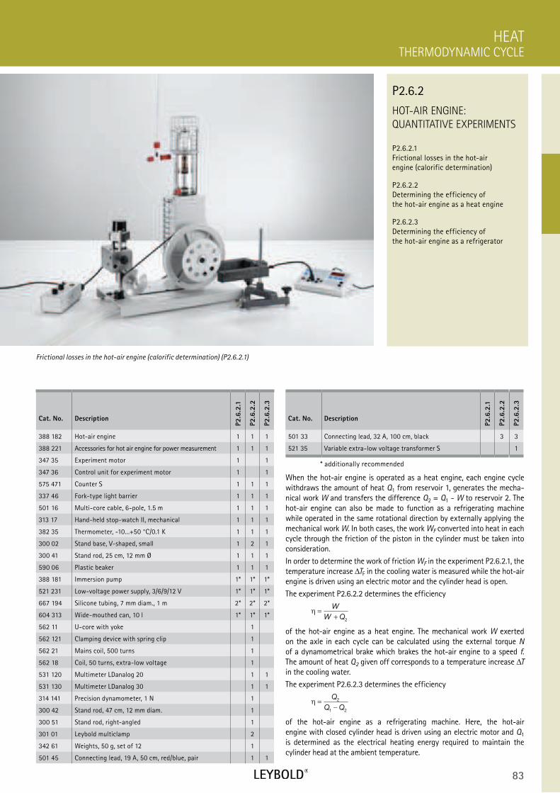
83
HOT-AIR ENGINE:
QUANTITATIVE EXPERIMENTS
P2.6.2.1 Frictional losses in the hot-air engine (calorific determination)
P2.6.2.2 Determining the efficiency of the hot-air engine as a heat engine
P2.6.2.3 Determining the efficiency of the hot-air engine as a refrigerator
THERMODYNAMIC CYCLE
HEAT
Cat. No. Description
P2.6
.2.1
P2.6
.2.2
P2.6
.2.3
388 182 Hot-air engine 1 1 1
388 221 Accessories for hot air engine for power measurement 1 1 1
347 35 Experiment motor 1 1
347 36 Control unit for experiment motor 1 1
575 471 Counter S 1 1 1
337 46 Fork-type light barrier 1 1 1
501 16 Multi-core cable, 6-pole, 1.5 m 1 1 1
313 17 Hand-held stop-watch II, mechanical 1 1 1
382 35 Thermometer, -10...+50 °C/0.1 K 1 1 1
300 02 Stand base, V-shaped, small 1 2 1
300 41 Stand rod, 25 cm, 12 mm Ø 1 1 1
590 06 Plastic beaker 1 1 1
388 181 Immersion pump 1* 1* 1*
521 231 Low-voltage power supply, 3/6/9/12 V 1* 1* 1*
667 194 Silicone tubing, 7 mm diam., 1 m 2* 2* 2*
604 313 Wide-mouthed can, 10 l 1* 1* 1*
562 11 U-core with yoke 1
562 121 Clamping device with spring clip 1
562 21 Mains coil, 500 turns 1
562 18 Coil, 50 turns, extra-low voltage 1
531 120 Multimeter LDanalog 20 1 1
531 130 Multimeter LDanalog 30 1 1
314 141 Precision dynamometer, 1 N 1
300 42 Stand rod, 47 cm, 12 mm diam. 1
300 51 Stand rod, right-angled 1
301 01 Leybold multiclamp 2
342 61 Weights, 50 g, set of 12 1
501 45 Connecting lead, 19 A, 50 cm, red/blue, pair 1 1
When the hot-air engine is operated as a heat engine, each engine cycle withdraws the amount of heat Q1 from reservoir 1, generates the mecha-nical work W and transfers the difference Q2 = Q1 - W to reservoir 2. The hot-air engine can also be made to function as a refrigerating machine while operated in the same rotational direction by externally applying the mechanical work W. In both cases, the work WF converted into heat in each cycle through the friction of the piston in the cylinder must be taken into consideration.
In order to determine the work of friction WF in the experiment P2.6.2.1, the temperature increase TF in the cooling water is measured while the hot-air engine is driven using an electric motor and the cylinder head is open.
The experiment P2.6.2.2 determines the efficiency
η =+
W
W Q2
of the hot-air engine as a heat engine. The mechanical work W exerted on the axle in each cycle can be calculated using the external torque N of a dynamometrical brake which brakes the hot-air engine to a speed f. The amount of heat Q2 given off corresponds to a temperature increase T in the cooling water.
The experiment P2.6.2.3 determines the efficiency
η =−
Q
Q Q
2
1 2
of the hot-air engine as a refrigerating machine. Here, the hot-air engine with closed cylinder head is driven using an electric motor and Q1 is determined as the electrical heating energy required to maintain the cylinder head at the ambient temperature.
Frictional losses in the hot-air engine (calorific determination) (P2.6.2.1)
P2.6.2
Cat. No. Description
P2.6
.2.1
P2.6
.2.2
P2.6
.2.3
501 33 Connecting lead, 32 A, 100 cm, black 3 3
521 35 Variable extra-low voltage transformer S 1
* additionally recommended

84 WWW.LEYBOLD-SHOP.COMCA
SSY ®
HOT-AIR ENGINE:
QUANTITATIVE EXPERIMENTS
P2.6.2.4 pV diagram of the hot-air engine as a heat engine - Recording and evaluating with CASSY
Thermodynamic cycles are often described as a closed curve in a pV diagram (p: pressure, V: volume). The work added to or withdrawn from the system (depending on the direction of rotation) corresponds to the area enclosed by the curve.
In the experiment P2.6.2.4, the pV diagram of the hot air engine as a heat engine is recorded using the computer-assisted measured value recording system CASSY. The pressure sensor measures the pressure p in the cylinder and a displacement sensor measures the position s, from which the volume is calculated, as a function of the time t. The measured values are displayed on the screen directly in a pV diagram. In the further evaluation, the mechanical work performed as piston friction per cycle
W p dV= − ⋅∫and from this the mechanical power
P W f
f
= ⋅
: no-load speed
are calculated and plotted in a graph as a function of the no-load speed.
HEAT
pV diagram of the hot-air engine as a heat engine - Recording and evaluating with CASSY (P2.6.2.4)
Cat. No. Description
P2.6
.2.4
388 182 Hot-air engine 1
562 11 U-core with yoke 1
562 121 Clamping device with spring clip 1
562 21 Mains coil, 500 turns 1
562 18 Coil, 50 turns, extra-low voltage 1
524 013 Sensor-CASSY 2 1
524 220 CASSY Lab 2 1
524 082 Rotary motion sensor S 1
524 064 Pressure sensor S, ±2000 hPa 1
309 48ET2 Fishing line, set of 2 1
352 08ET2 Helical spring, 25 N/m, set of 2 1
501 33 Connecting lead, 32 A, 100 cm, black 2
388 181 Immersion pump 1*
521 231 Low-voltage power supply, 3/6/9/12 V 1*
667 194 Silicone tubing, 7 mm diam., 1 m 2*
604 313 Wide-mouthed can, 10 l 1*
additionally required: PC with Windows XP/Vista/7/8/10 (x86 or x64)
1
* additionally recommended
pV diagram of the hot air engine
THERMODYNAMIC CYCLE
P2.6.2
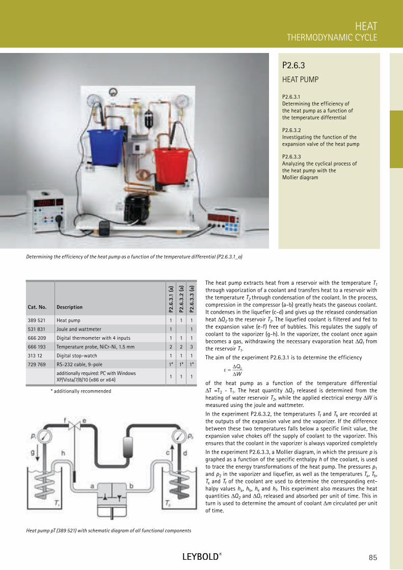
85
HEAT PUMP
P2.6.3.1 Determining the efficiency of the heat pump as a function of the temperature differential
P2.6.3.2 Investigating the function of the expansion valve of the heat pump
P2.6.3.3 Analyzing the cyclical process of the heat pump with the Mollier diagram
THERMODYNAMIC CYCLE
HEAT
Cat. No. Description
P2.6
.3.1
(a)
P2.6
.3.2
(a)
P2.6
.3.3
(a)
389 521 Heat pump 1 1 1
531 831 Joule and wattmeter 1 1
666 209 Digital thermometer with 4 inputs 1 1 1
666 193 Temperature probe, NiCr-Ni, 1.5 mm 2 2 3
313 12 Digital stop-watch 1 1 1
729 769 RS-232 cable, 9-pole 1* 1* 1*
additionally required: PC with Windows XP/Vista/7/8/10 (x86 or x64)
1 1 1
* additionally recommended
The heat pump extracts heat from a reservoir with the temperature T1
through vaporization of a coolant and transfers heat to a reservoir with the temperature T2 through condensation of the coolant. In the process, compression in the compressor (a-b) greatly heats the gaseous coolant. It condenses in the liquefier (c-d) and gives up the released condensation heat Q2 to the reservoir T2. The liquefied coolant is filtered and fed to the expansion valve (e-f) free of bubbles. This regulates the supply of coolant to the vaporizer (g-h). In the vaporizer, the coolant once again becomes a gas, withdrawing the necessary evaporation heat Q1 from the reservoir T1.
The aim of the experiment P2.6.3.1 is to determine the efficiency
ε =∆
∆
Q
W
2
of the heat pump as a function of the temperature differential T =T2 - T1. The heat quantity Q2 released is determined from the
heating of water reservoir T2, while the applied electrical energy W is measured using the joule and wattmeter.
In the experiment P2.6.3.2, the temperatures Tf and Th are recorded at the outputs of the expansion valve and the vaporizer. If the difference between these two temperatures falls below a specific limit value, the expansion valve chokes off the supply of coolant to the vaporizer. This ensures that the coolant in the vaporizer is always vaporized completely
In the experiment P2.6.3.3, a Mollier diagram, in which the pressure p is graphed as a function of the specific enthalpy h of the coolant, is used to trace the energy transformations of the heat pump. The pressures p1 and p2 in the vaporizer and liquefier, as well as the temperatures Ta, Tb, Te and Tf of the coolant are used to determine the corresponding ent- halpy values ha, hb, he and hf. This experiment also measures the heat quantities Q2 and Q1 released and absorbed per unit of time. This in turn is used to determine the amount of coolant m circulated per unit of time.
Determining the efficiency of the heat pump as a function of the temperature differential (P2.6.3.1_a)
P2.6.3
Heat pump pT (389 521) with schematic diagram of all functional components
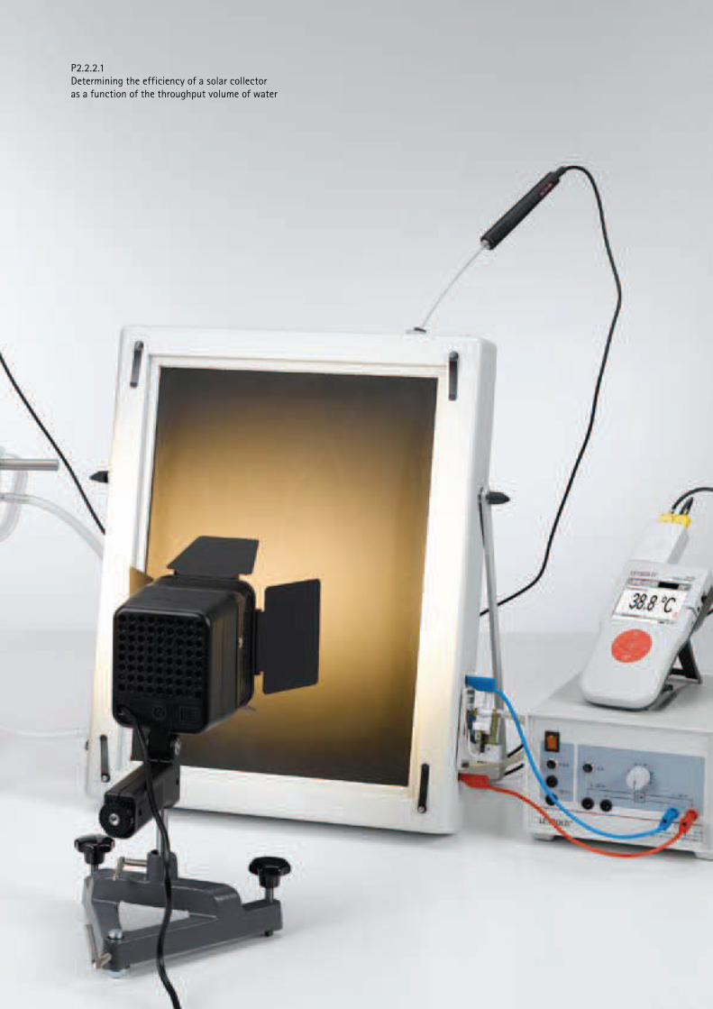
P2.2.2.1
Determining the efficiency of a solar collector
as a function of the throughput volume of water
87
P3.1 ELECTROSTATICS 89
P3.2 FUNDAMENTALS OF ELECTRICITY 104
P3.3 MAGNETOSTATICS 111
P3.4 ELECTROMAGNETIC INDUCTION 115
P3.5 ELECTRICAL MACHINES 122
P3.6 DC AND AC CIRCUITS 126
P3.7 ELECTROMAGNETIC OSCILLATIONS AND WAVES 134
P3.8 FREE CHARGE CARRIERS IN A VACUUM 140
P3.9 ELECTRICAL CONDUCTION IN GASES 145
P3 ELECTRICITY

88 WWW.LEYBOLD-SHOP.COM
P3.1 ELECTROSTATICS
P3.1.1 Basic experiments on electrostatics 89-90
P3.1.2 Coulomb’s law 91-93
P3.1.3 Field lines and equipotential lines 94-96
P3.1.4 Effects of force in an electric field 97-98
P3.1.5 Charge distributions on electrical conductors 99
P3.1.6 Definition of capacitance 100
P3.1.7 Plate capacitor 101-103
P3.2 FUNDAMENTALS OF ELECTRICITY
P3.2.1 Charge transfer with drops of water 104
P3.2.2 Ohm’s law 105
P3.2.3 Kirchhoff’s laws 106-107
P3.2.4 Circuits with electrical measuring instruments 108
P3.2.5 Conducting electricity by means of electrolysis 109
P3.2.6 Experiments on electrochemistry 110
P3.3 MAGNETOSTATICS
P3.3.1 Basic experiments on magnetostatics 111
P3.3.2 Magnetic dipole moment 112
P3.3.3 Effects of force in a magnetic field 113
P3.3.4 Biot-Savart’s law 114
P3.4 ELECTROMAGNETIC INDUCTION
P3.4.1 Voltage impulse 115
P3.4.2 Induction in a moving conductor loop 116
P3.4.3 Induction by means of a variable magnetic field 117
P3.4.4 Eddy currents 118
P3.4.5 Transformer 119-120
P3.4.6 Measuring the earth’s magnetic field 121
P3.5 ELECTRICAL MACHINES
P3.5.1 Basic experiments on electrical machines 122
P3.5.2 Electric generators 123
P3.5.3 Electric motors 124
P3.5.4 Three-phase machines 125
P3.6 DC AND AC CIRCUITS
P3.6.1 Circuit with capacitor 126
P3.6.2 Circuit with coil 127
P3.6.3 Impedances 128
P3.6.4 Measuring-bridge circuits 129
P3.6.5 Measuring AC voltages and AC currents 130
P3.6.6 Electrical work and power 131-132
P3.6.7 Electromechanical devices 133
P3.7 ELECTROMAGNETIC OSCILLATIONS
AND WAVES
P3.7.1 Electromagnetic oscillator circuit 134
P3.7.2 Decimeter-range waves 135
P3.7.3 Propagation of decimeter-range waves along lines 136
P3.7.4 Microwaves 137
P3.7.5 Propagation of microwaves along lines 138
P3.7.6 Directional characteristic of dipole radiation 139
P3.8 FREE CHARGE CARRIERS IN A VACUUM
P3.8.1 Tube diode 140
P3.8.2 Tube triode 141
P3.8.3 Maltese-cross tube 142
P3.8.4 Perrin tube 143
P3.8.5 Thomson tube 144
P3.9 ELECTRICAL CONDUCTION IN GASES
P3.9.1 Spontaneous and non-spontaneous discharge 145
P3.9.2 Gas discharge at reduced pressure 146
P3.9.3 Cathode rays and canal rays 147
P3 ELECTRICITY
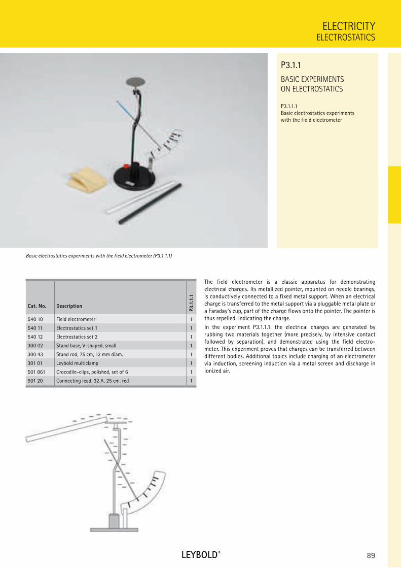
89
BASIC EXPERIMENTS
ON ELECTROSTATICS
P3.1.1.1 Basic electrostatics experiments with the field electrometer
ELECTROSTATICS
ELECTRICITY
Cat. No. Description
P3.1
.1.1
540 10 Field electrometer 1
540 11 Electrostatics set 1 1
540 12 Electrostatics set 2 1
300 02 Stand base, V-shaped, small 1
300 43 Stand rod, 75 cm, 12 mm diam. 1
301 01 Leybold multiclamp 1
501 861 Crocodile-clips, polished, set of 6 1
501 20 Connecting lead, 32 A, 25 cm, red 1
The field electrometer is a classic apparatus for demonstrating electrical charges. Its metallized pointer, mounted on needle bearings, is conductively connected to a fixed metal support. When an electrical charge is transferred to the metal support via a pluggable metal plate or a Faraday’s cup, part of the charge flows onto the pointer. The pointer is thus repelled, indicating the charge.
In the experiment P3.1.1.1, the electrical charges are generated by rubbing two materials together (more precisely, by intensive contact followed by separation), and demonstrated using the field electro- meter. This experiment proves that charges can be transferred between different bodies. Additional topics include charging of an electrometer via induction, screening induction via a metal screen and discharge in ionized air.
Basic electrostatics experiments with the field electrometer (P3.1.1.1)
P3.1.1
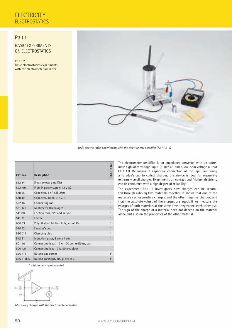
90 WWW.LEYBOLD-SHOP.COM
BASIC EXPERIMENTS
ON ELECTROSTATICS
P3.1.1.2 Basic electrostatics experiments with the electrometer amplifier
The electrometer amplifier is an impedance converter with an extre-mely high-ohm voltage input ( 1013 ) and a low-ohm voltage output ( 1 ). By means of capacitive connection of the input and using a Faraday’s cup to collect charges, this device is ideal for measuring extremely small charges. Experiments on contact and friction electricity can be conducted with a high degree of reliability.
The experiment P3.1.1.2 investigates how charges can be separa-ted through rubbing two materials together. It shows that one of the materials carries positive charges, and the other negative charges, and that the absolute values of the charges are equal. If we measure the charges of both materials at the same time, they cancel each other out. The sign of the charge of a material does not depend on the material alone, but also on the properties of the other material.
ELECTRICITY
Basic electrostatics experiments with the electrometer amplifier (P3.1.1.2_a)
Cat. No. Description
P3.1
.1.2
(a)
532 14 Electrometer amplifier 1
562 791 Plug-in power supply, 12 V AC 1
578 25 Capacitor, 1 nF, STE 2/19 1
578 10 Capacitor, 10 nF, STE 2/19 1
532 16 Connecting rod 1
531 120 Multimeter LDanalog 20 1
541 00 Friction rods, PVC and acrylic 1
541 21 Leather 1
686 63 Polyethylene friction foils, set of 10 1
546 12 Faraday‘s cup 1
590 011 Clamping plug 1
542 51 Induction plate, 8 cm x 4 cm 1
501 46 Connecting leads, 19 A, 100 cm, red/blue, pair 1
500 424 Connecting lead 19 A, 50 cm, black 1
666 711 Butane gas burner 1*
666 712ET3 Butane cartridge, 190 g, set of 3 1*
* additionally recommended
Measuring charges with the electrometer amplifier
ELECTROSTATICS
P3.1.1
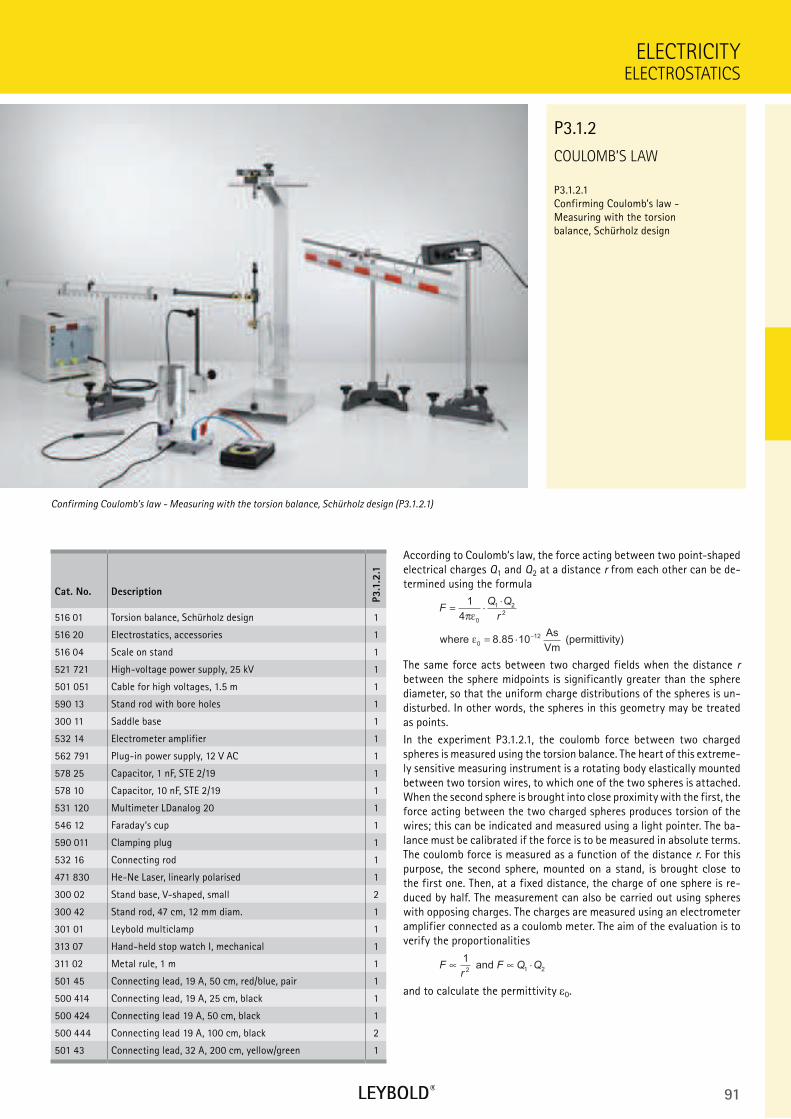
91
COULOMB’S LAW
P3.1.2.1 Confirming Coulomb’s law - Measuring with the torsion balance, Schürholz design
ELECTROSTATICS
ELECTRICITY
Cat. No. Description
P3.1
.2.1
516 01 Torsion balance, Schürholz design 1
516 20 Electrostatics, accessories 1
516 04 Scale on stand 1
521 721 High-voltage power supply, 25 kV 1
501 051 Cable for high voltages, 1.5 m 1
590 13 Stand rod with bore holes 1
300 11 Saddle base 1
532 14 Electrometer amplifier 1
562 791 Plug-in power supply, 12 V AC 1
578 25 Capacitor, 1 nF, STE 2/19 1
578 10 Capacitor, 10 nF, STE 2/19 1
531 120 Multimeter LDanalog 20 1
546 12 Faraday‘s cup 1
590 011 Clamping plug 1
532 16 Connecting rod 1
471 830 He-Ne Laser, linearly polarised 1
300 02 Stand base, V-shaped, small 2
300 42 Stand rod, 47 cm, 12 mm diam. 1
301 01 Leybold multiclamp 1
313 07 Hand-held stop watch I, mechanical 1
311 02 Metal rule, 1 m 1
501 45 Connecting lead, 19 A, 50 cm, red/blue, pair 1
500 414 Connecting lead, 19 A, 25 cm, black 1
500 424 Connecting lead 19 A, 50 cm, black 1
500 444 Connecting lead 19 A, 100 cm, black 2
501 43 Connecting lead, 32 A, 200 cm, yellow/green 1
According to Coulomb‘s law, the force acting between two point-shaped electrical charges Q1 and Q2 at a distance r from each other can be de-termined using the formula
FQ Q
r= ⋅
⋅
= ⋅−
1
4
8 85 10
0
1 2
2
0
12
πε
εwhere As
Vm (permittivity).
The same force acts between two charged fields when the distance r between the sphere midpoints is significantly greater than the sphere diameter, so that the uniform charge distributions of the spheres is un-disturbed. In other words, the spheres in this geometry may be treated as points.
In the experiment P3.1.2.1, the coulomb force between two charged spheres is measured using the torsion balance. The heart of this extreme-ly sensitive measuring instrument is a rotating body elastically mounted between two torsion wires, to which one of the two spheres is attached. When the second sphere is brought into close proximity with the first, the force acting between the two charged spheres produces torsion of the wires; this can be indicated and measured using a light pointer. The ba-lance must be calibrated if the force is to be measured in absolute terms. The coulomb force is measured as a function of the distance r. For this purpose, the second sphere, mounted on a stand, is brought close to the first one. Then, at a fixed distance, the charge of one sphere is re-duced by half. The measurement can also be carried out using spheres with opposing charges. The charges are measured using an electrometer amplifier connected as a coulomb meter. The aim of the evaluation is to verify the proportionalities
Fr
F Q Q∝ ∝ ⋅1
2 1 2 and
and to calculate the permittivity 0.
Confirming Coulomb’s law - Measuring with the torsion balance, Schürholz design (P3.1.2.1)
P3.1.2
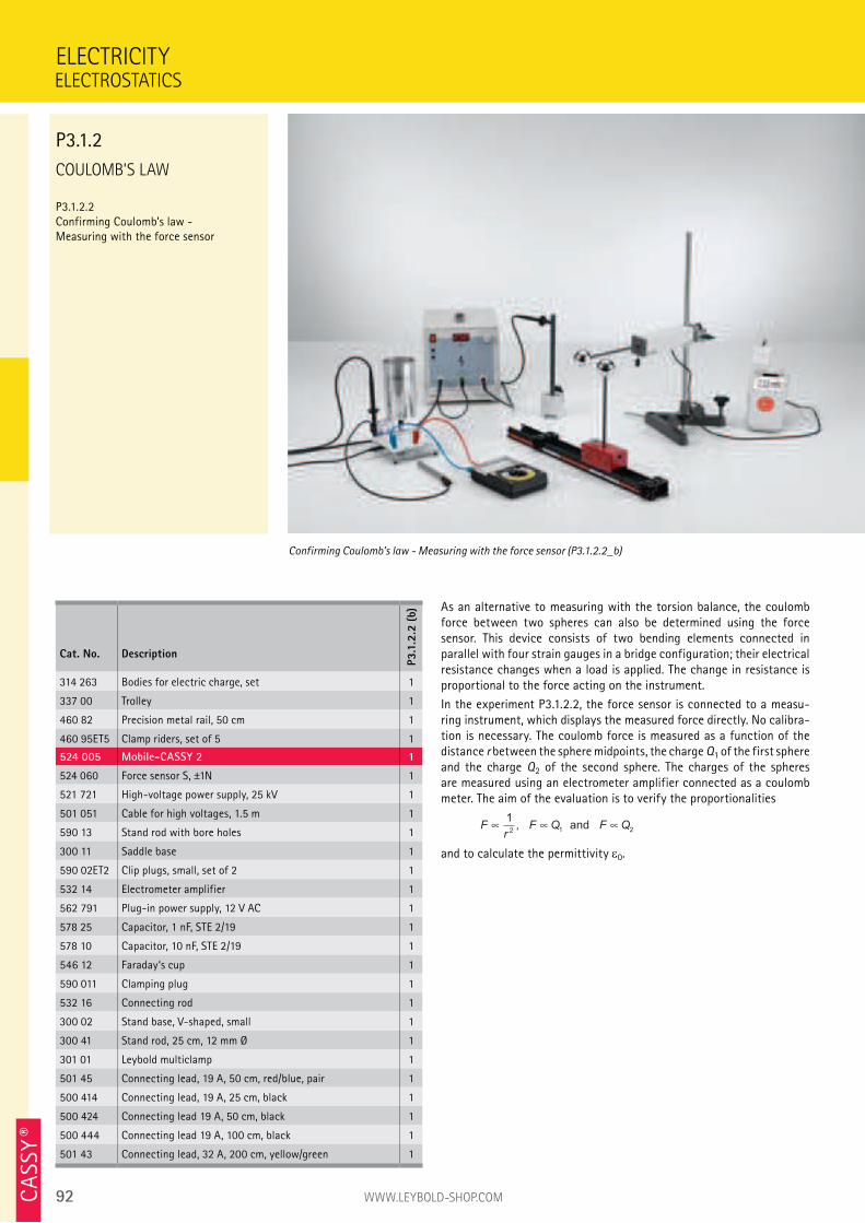
92 WWW.LEYBOLD-SHOP.COMCA
SSY ®
COULOMB’S LAW
P3.1.2.2 Confirming Coulomb’s law - Measuring with the force sensor
As an alternative to measuring with the torsion balance, the coulomb force between two spheres can also be determined using the force sensor. This device consists of two bending elements connected in parallel with four strain gauges in a bridge configuration; their electrical resistance changes when a load is applied. The change in resistance is proportional to the force acting on the instrument.
In the experiment P3.1.2.2, the force sensor is connected to a measu-ring instrument, which displays the measured force directly. No calibra-tion is necessary. The coulomb force is measured as a function of the distance r between the sphere midpoints, the charge Q1 of the first sphere and the charge Q2 of the second sphere. The charges of the spheres are measured using an electrometer amplifier connected as a coulomb meter. The aim of the evaluation is to verify the proportionalities
Fr
F Q F Q12 1 2, and
and to calculate the permittivity 0.
ELECTRICITY
Confirming Coulomb’s law - Measuring with the force sensor (P3.1.2.2_b)
Cat. No. Description
P3.1
.2.2
(b)
314 263 Bodies for electric charge, set 1
337 00 Trolley 1
460 82 Precision metal rail, 50 cm 1
460 95ET5 Clamp riders, set of 5 1
524 005 Mobile-CASSY 2 1
524 060 Force sensor S, ±1N 1
521 721 High-voltage power supply, 25 kV 1
501 051 Cable for high voltages, 1.5 m 1
590 13 Stand rod with bore holes 1
300 11 Saddle base 1
590 02ET2 Clip plugs, small, set of 2 1
532 14 Electrometer amplifier 1
562 791 Plug-in power supply, 12 V AC 1
578 25 Capacitor, 1 nF, STE 2/19 1
578 10 Capacitor, 10 nF, STE 2/19 1
546 12 Faraday‘s cup 1
590 011 Clamping plug 1
532 16 Connecting rod 1
300 02 Stand base, V-shaped, small 1
300 41 Stand rod, 25 cm, 12 mm Ø 1
301 01 Leybold multiclamp 1
501 45 Connecting lead, 19 A, 50 cm, red/blue, pair 1
500 414 Connecting lead, 19 A, 25 cm, black 1
500 424 Connecting lead 19 A, 50 cm, black 1
500 444 Connecting lead 19 A, 100 cm, black 1
501 43 Connecting lead, 32 A, 200 cm, yellow/green 1
ELECTROSTATICS
P3.1.2
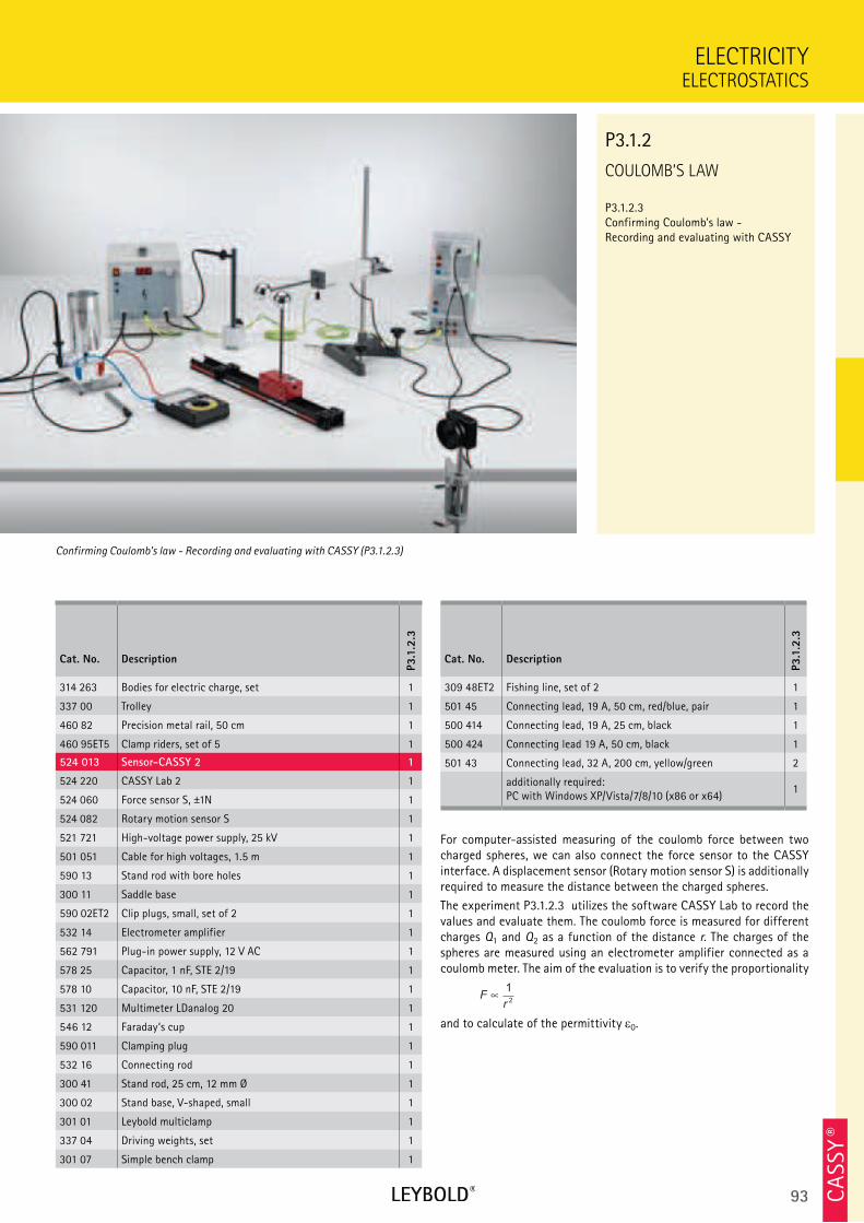
93 CA
SSY ®
COULOMB’S LAW
P3.1.2.3 Confirming Coulomb’s law - Recording and evaluating with CASSY
ELECTROSTATICS
ELECTRICITY
Cat. No. Description
P3.1
.2.3
314 263 Bodies for electric charge, set 1
337 00 Trolley 1
460 82 Precision metal rail, 50 cm 1
460 95ET5 Clamp riders, set of 5 1
524 013 Sensor-CASSY 2 1
524 220 CASSY Lab 2 1
524 060 Force sensor S, ±1N 1
524 082 Rotary motion sensor S 1
521 721 High-voltage power supply, 25 kV 1
501 051 Cable for high voltages, 1.5 m 1
590 13 Stand rod with bore holes 1
300 11 Saddle base 1
590 02ET2 Clip plugs, small, set of 2 1
532 14 Electrometer amplifier 1
562 791 Plug-in power supply, 12 V AC 1
578 25 Capacitor, 1 nF, STE 2/19 1
578 10 Capacitor, 10 nF, STE 2/19 1
531 120 Multimeter LDanalog 20 1
546 12 Faraday‘s cup 1
590 011 Clamping plug 1
532 16 Connecting rod 1
300 41 Stand rod, 25 cm, 12 mm Ø 1
300 02 Stand base, V-shaped, small 1
301 01 Leybold multiclamp 1
337 04 Driving weights, set 1
301 07 Simple bench clamp 1
For computer-assisted measuring of the coulomb force between two charged spheres, we can also connect the force sensor to the CASSY interface. A displacement sensor (Rotary motion sensor S) is additionally required to measure the distance between the charged spheres.
The experiment P3.1.2.3 utilizes the software CASSY Lab to record the values and evaluate them. The coulomb force is measured for different charges Q1 and Q2 as a function of the distance r. The charges of the spheres are measured using an electrometer amplifier connected as a coulomb meter. The aim of the evaluation is to verify the proportionality
Fr
1
2
and to calculate of the permittivity 0.
Confirming Coulomb’s law - Recording and evaluating with CASSY (P3.1.2.3)
P3.1.2
Cat. No. Description
P3.1
.2.3
309 48ET2 Fishing line, set of 2 1
501 45 Connecting lead, 19 A, 50 cm, red/blue, pair 1
500 414 Connecting lead, 19 A, 25 cm, black 1
500 424 Connecting lead 19 A, 50 cm, black 1
501 43 Connecting lead, 32 A, 200 cm, yellow/green 2
additionally required: PC with Windows XP/Vista/7/8/10 (x86 or x64)
1
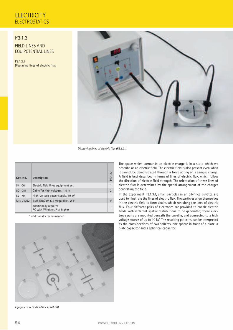
94 WWW.LEYBOLD-SHOP.COM
FIELD LINES AND
EQUIPOTENTIAL LINES
P3.1.3.1
Displaying lines of electric flux
The space which surrounds an electric charge is in a state which we
describe as an electric field. The electric field is also present even when
it cannot be demonstrated through a force acting on a sample charge.
A field is best described in terms of lines of electric flux, which follow
the direction of electric field strength. The orientation of these lines of
electric flux is determined by the spatial arrangement of the charges
generating the field.
In the experiment P3.1.3.1, small particles in an oil-filled cuvette are
used to illustrate the lines of electric flux. The particles align themselves
in the electric field to form chains which run along the lines of electric
flux. Four different pairs of electrodes are provided to enable electric
fields with different spatial distributions to be generated; these elec-
trode pairs are mounted beneath the cuvette, and connected to a high
voltage source of up to 10 kV. The resulting patterns can be interpreted
as the cross-sections of two spheres, one sphere in front of a plate, a
plate capacitor and a spherical capacitor.
ELECTRICITY
Displaying lines of electric flux (P3.1.3.1)
Cat. No. Description
P3.1
.3.1
541 06 Electric field lines equipment set 1
501 051 Cable for high voltages, 1.5 m 2
521 70 High-voltage power supply, 10 kV 1
MIK 74702 BMS EcoCam 5.5 mega pixel, WiFi 1*
additionally required:
PC with Windows 7 or higher1
* additionally recommended
Equipment set E-field lines (541 06)
ELECTROSTATICS
P3.1.3
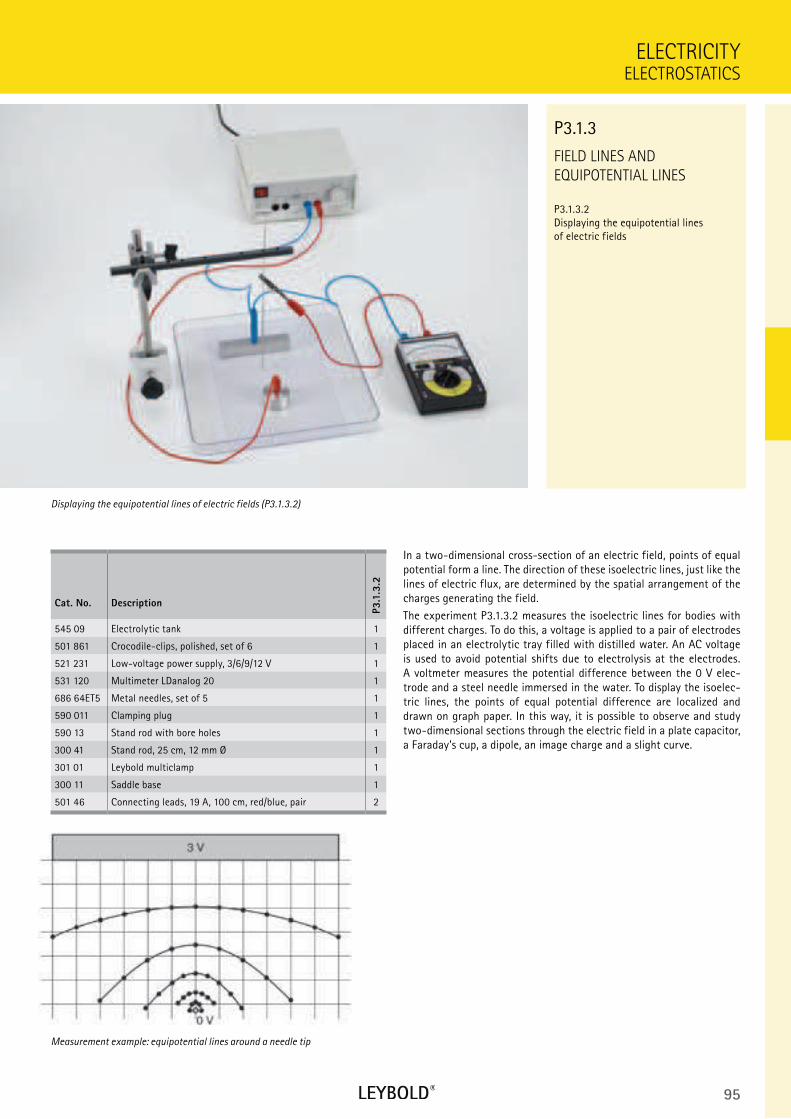
95
FIELD LINES AND
EQUIPOTENTIAL LINES
P3.1.3.2 Displaying the equipotential lines of electric fields
ELECTROSTATICS
ELECTRICITY
Cat. No. Description
P3.1
.3.2
545 09 Electrolytic tank 1
501 861 Crocodile-clips, polished, set of 6 1
521 231 Low-voltage power supply, 3/6/9/12 V 1
531 120 Multimeter LDanalog 20 1
686 64ET5 Metal needles, set of 5 1
590 011 Clamping plug 1
590 13 Stand rod with bore holes 1
300 41 Stand rod, 25 cm, 12 mm Ø 1
301 01 Leybold multiclamp 1
300 11 Saddle base 1
501 46 Connecting leads, 19 A, 100 cm, red/blue, pair 2
In a two-dimensional cross-section of an electric field, points of equal potential form a line. The direction of these isoelectric lines, just like the lines of electric flux, are determined by the spatial arrangement of the charges generating the field.
The experiment P3.1.3.2 measures the isoelectric lines for bodies with different charges. To do this, a voltage is applied to a pair of electrodes placed in an electrolytic tray filled with distilled water. An AC voltage is used to avoid potential shifts due to electrolysis at the electrodes. A voltmeter measures the potential difference between the 0 V elec-trode and a steel needle immersed in the water. To display the isoelec-tric lines, the points of equal potential difference are localized and drawn on graph paper. In this way, it is possible to observe and study two-dimensional sections through the electric field in a plate capacitor, a Faraday’s cup, a dipole, an image charge and a slight curve.
Displaying the equipotential lines of electric fields (P3.1.3.2)
P3.1.3
Measurement example: equipotential lines around a needle tip
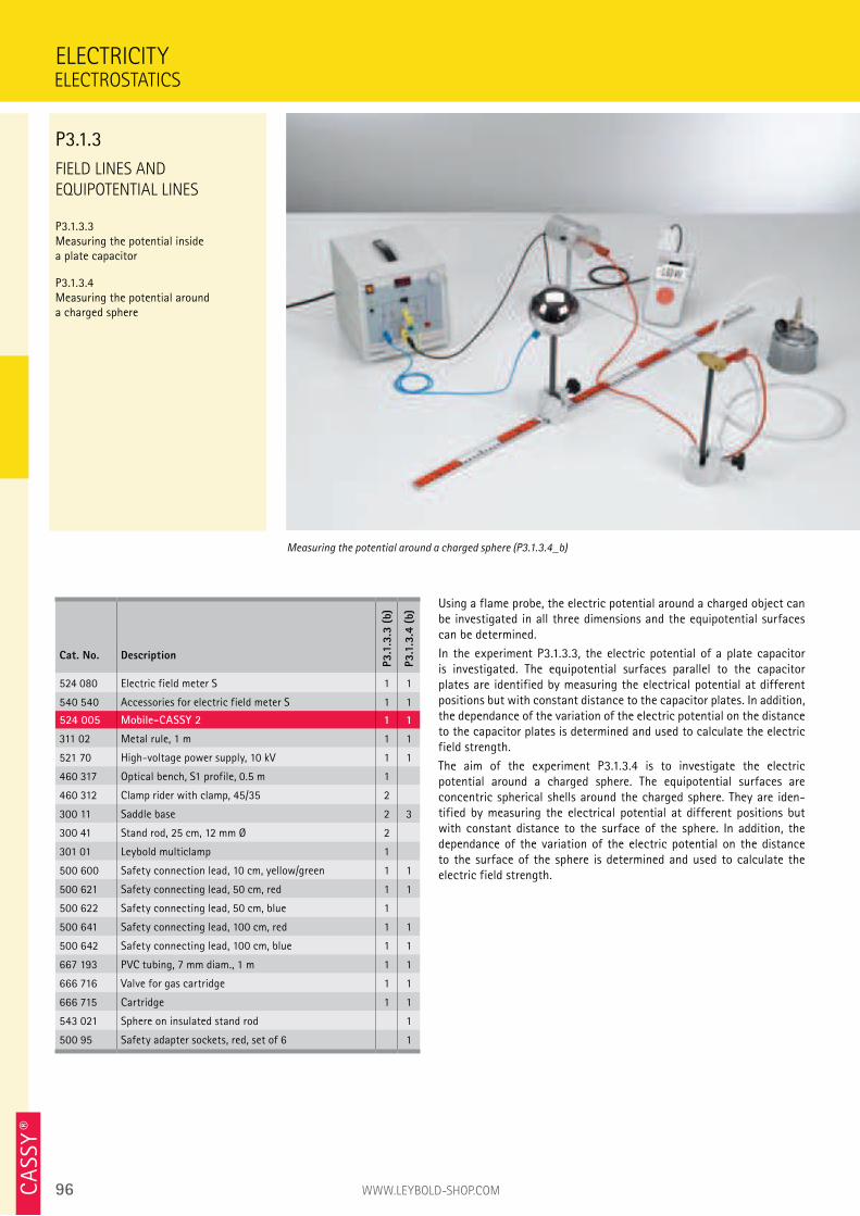
96 WWW.LEYBOLD-SHOP.COMCA
SSY ®
FIELD LINES AND
EQUIPOTENTIAL LINES
P3.1.3.3 Measuring the potential inside a plate capacitor
P3.1.3.4 Measuring the potential around a charged sphere
Using a flame probe, the electric potential around a charged object can be investigated in all three dimensions and the equipotential surfaces can be determined.
In the experiment P3.1.3.3, the electric potential of a plate capacitor is investigated. The equipotential surfaces parallel to the capacitor plates are identified by measuring the electrical potential at different positions but with constant distance to the capacitor plates. In addition, the dependance of the variation of the electric potential on the distance to the capacitor plates is determined and used to calculate the electric field strength.
The aim of the experiment P3.1.3.4 is to investigate the electric potential around a charged sphere. The equipotential surfaces are concentric spherical shells around the charged sphere. They are iden-tified by measuring the electrical potential at different positions but with constant distance to the surface of the sphere. In addition, the dependance of the variation of the electric potential on the distance to the surface of the sphere is determined and used to calculate the electric field strength.
ELECTRICITY
Measuring the potential around a charged sphere (P3.1.3.4_b)
Cat. No. Description
P3.1
.3.3
(b)
P3.1
.3.4
(b)
524 080 Electric field meter S 1 1
540 540 Accessories for electric field meter S 1 1
524 005 Mobile-CASSY 2 1 1
311 02 Metal rule, 1 m 1 1
521 70 High-voltage power supply, 10 kV 1 1
460 317 Optical bench, S1 profile, 0.5 m 1
460 312 Clamp rider with clamp, 45/35 2
300 11 Saddle base 2 3
300 41 Stand rod, 25 cm, 12 mm Ø 2
301 01 Leybold multiclamp 1
500 600 Safety connection lead, 10 cm, yellow/green 1 1
500 621 Safety connecting lead, 50 cm, red 1 1
500 622 Safety connecting lead, 50 cm, blue 1
500 641 Safety connecting lead, 100 cm, red 1 1
500 642 Safety connecting lead, 100 cm, blue 1 1
667 193 PVC tubing, 7 mm diam., 1 m 1 1
666 716 Valve for gas cartridge 1 1
666 715 Cartridge 1 1
543 021 Sphere on insulated stand rod 1
500 95 Safety adapter sockets, red, set of 6 1
ELECTROSTATICS
P3.1.3
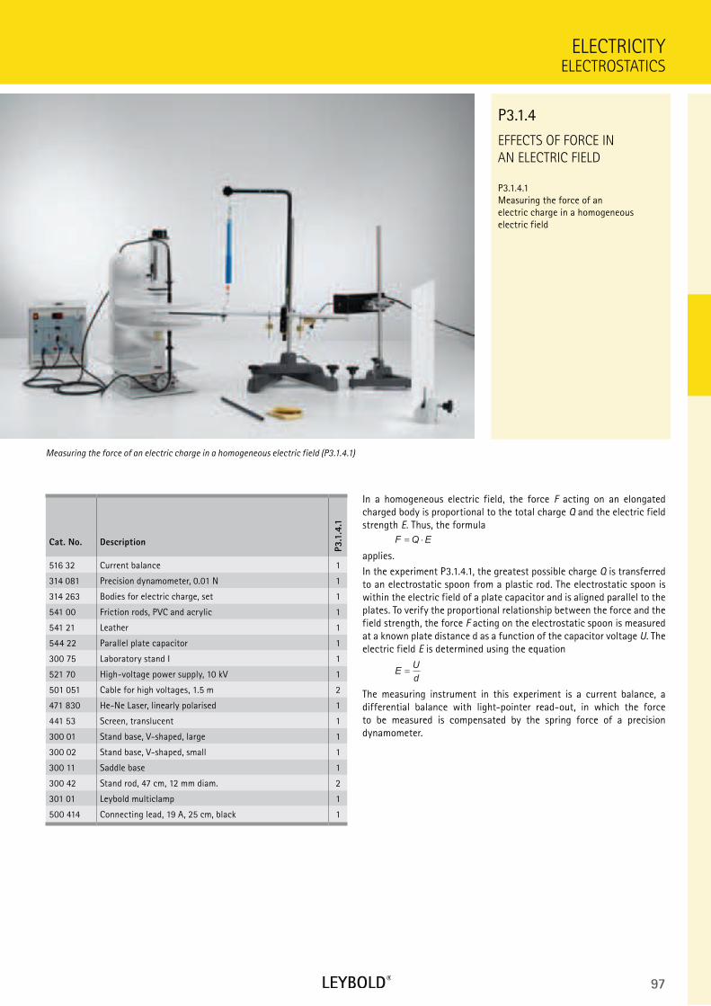
97
EFFECTS OF FORCE IN
AN ELECTRIC FIELD
P3.1.4.1
Measuring the force of an
electric charge in a homogeneous
electric field
ELECTROSTATICS
ELECTRICITY
Cat. No. Description
P3.1
.4.1
516 32 Current balance 1
314 081 Precision dynamometer, 0.01 N 1
314 263 Bodies for electric charge, set 1
541 00 Friction rods, PVC and acrylic 1
541 21 Leather 1
544 22 Parallel plate capacitor 1
300 75 Laboratory stand I 1
521 70 High-voltage power supply, 10 kV 1
501 051 Cable for high voltages, 1.5 m 2
471 830 He-Ne Laser, linearly polarised 1
441 53 Screen, translucent 1
300 01 Stand base, V-shaped, large 1
300 02 Stand base, V-shaped, small 1
300 11 Saddle base 1
300 42 Stand rod, 47 cm, 12 mm diam. 2
301 01 Leybold multiclamp 1
500 414 Connecting lead, 19 A, 25 cm, black 1
In a homogeneous electric field, the force F acting on an elongated
charged body is proportional to the total charge Q and the electric field
strength E. Thus, the formula
F Q E= ⋅
applies.
In the experiment P3.1.4.1, the greatest possible charge Q is transferred
to an electrostatic spoon from a plastic rod. The electrostatic spoon is
within the electric field of a plate capacitor and is aligned parallel to the
plates. To verify the proportional relationship between the force and the
field strength, the force F acting on the electrostatic spoon is measured
at a known plate distance d as a function of the capacitor voltage U. The
electric field E is determined using the equation
EU
d
The measuring instrument in this experiment is a current balance, a
differential balance with light-pointer read-out, in which the force
to be measured is compensated by the spring force of a precision
dynamometer.
Measuring the force of an electric charge in a homogeneous electric field (P3.1.4.1)
P3.1.4
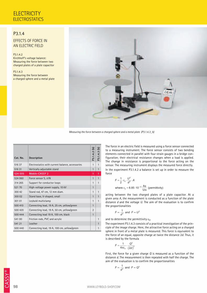
98 WWW.LEYBOLD-SHOP.COMCA
SSY ®
EFFECTS OF FORCE IN
AN ELECTRIC FIELD
P3.1.4.2 Kirchhoff’s voltage balance: Measuring the force between two charged plates of a plate capacitor
P3.1.4.3 Measuring the force between a charged sphere and a metal plate
ELECTRICITY
Measuring the force between a charged sphere and a metal plate (P3.1.4.3_b)
Cat. No. Description
P3.1
.4.2
(b)
P3.1
.4.3
(b)
516 37 Electrostatics with current balance, accessories 1 1
516 31 Vertically adjustable stand 1 1
524 005 Mobile-CASSY 2 1 1
524 060 Force sensor S, ±1N 1 1
314 265 Support for conductor loops 1 1
521 70 High-voltage power supply, 10 kV 1
300 42 Stand rod, 47 cm, 12 mm diam. 1 1
300 02 Stand base, V-shaped, small 1 1
301 01 Leybold multiclamp 1 1
500 410 Connecting lead, 19 A, 25 cm, yellow/green 1
500 420 Connecting lead, 19 A, 50 cm, yellow/green 2
500 444 Connecting lead 19 A, 100 cm, black 1
541 00 Friction rods, PVC and acrylic 1
541 21 Leather 1
500 440 Connecting lead, 19 A, 100 cm, yellow/green 1
ELECTROSTATICS
P3.1.4
The force in an electric field is measured using a force sensor connected to a measuring instrument. The force sensor consists of two bending elements connected in parallel with four strain gauges in a bridge con-figuration; their electrical resistance changes when a load is applied. The change in resistance is proportional to the force acting on the sensor. The measuring instrument displays the measured force directly.
In the experiment P3.1.4.2 a balance is set up in order to measure the force
FU
dA= ⋅ ⋅ ⋅
= ⋅−
1
2
8 85 10
0
2
2
0
12
ε
εwhere As
Vm (permittivity).
acting between the two charged plates of a plate capacitor. At a given area A, the measurement is conducted as a function of the plate distance d and the voltage U. The aim of the evaluation is to confirm the proportionalities
Fd
and F U1
2
2
and to determine the permittivity 0.
The experiment P3.1.4.3 consists of a practical investigation of the prin-ciple of the image charge. Here, the attractive force acting on a charged sphere in front of a metal plate is measured. This force is equivalent to the force of an equal, opposite charge at twice the distance 2d. Thus, it is described by the formula
FQ
d= ⋅
( )
1
4 20
2
2πε
First, the force for a given charge Q is measured as a function of the distance d. The measurement is then repeated with half the charge. The aim of the evaluation is to confirm the proportionalities
Fd
F Q1
2
2 and
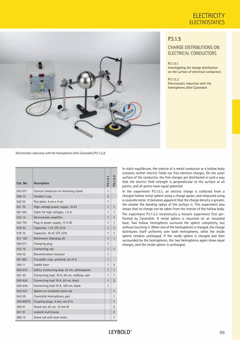
99
CHARGE DISTRIBUTIONS ON
ELECTRICAL CONDUCTORS
P3.1.5.1 Investigating the charge distribution on the surface of electrical conductors
P3.1.5.2 Electrostatic induction with the hemispheres after Cavendish
ELECTROSTATICS
ELECTRICITY
Cat. No. Description
P3.1
.5.1
P3.1
.5.2
543 071 Conical conductor on insulating stand 1
546 12 Faraday‘s cup 2
542 52 Test plate, 4 cm x 4 cm 1
521 70 High-voltage power supply, 10 kV 1 1
501 051 Cable for high voltages, 1.5 m 1 1
532 14 Electrometer amplifier 1 1
562 791 Plug-in power supply, 12 V AC 1 1
578 25 Capacitor, 1 nF, STE 2/19 1 1
578 10 Capacitor, 10 nF, STE 2/19 1 1
531 120 Multimeter LDanalog 20 1 1
590 011 Clamping plug 1
532 16 Connecting rod 1 1
540 52 Demonstration insulator 1
501 861 Crocodile-clips, polished, set of 6 1
300 11 Saddle base 1 3
500 610 Safety connecting lead, 25 cm, yellow/green 1 1
501 45 Connecting lead, 19 A, 50 cm, red/blue, pair 1 1
500 424 Connecting lead 19 A, 50 cm, black 1 2
500 444 Connecting lead 19 A, 100 cm, black 1
543 021 Sphere on insulated stand rod 1
543 05 Cavendish hemispheres, pair 1
340 89ET5 Coupling plugs, 4 mm, set of 5 1
300 41 Stand rod, 25 cm, 12 mm Ø 2
301 01 Leybold multiclamp 2
590 13 Stand rod with bore holes 1
In static equilibrium, the interior of a metal conductor or a hollow body contains neither electric fields nor free electron charges. On the outer surface of the conductor, the free charges are distributed in such a way that the electric field strength is perpendicular to the surface at all points, and all points have equal potential.
In the experiment P3.1.5.1, an electric charge is collected from a charged hollow metal sphere using a charge spoon, and measured using a coulomb meter. It becomes apparent that the charge density is greater, the smaller the bending radius of the surface is. This experiment also shows that no charge can be taken from the interior of the hollow body.
The experiment P3.1.5.2 reconstructs a historic experiment first per-formed by Cavendish. A metal sphere is mounted on an insulated base. Two hollow hemispheres surround the sphere completely, but without touching it. When one of the hemispheres is charged, the charge distributes itself uniformly over both hemispheres, while the inside sphere remains uncharged. If the inside sphere is charged and then surrounded by the hemispheres, the two hemispheres again show equal charges, and the inside sphere is uncharged.
Electrostatic induction with the hemispheres after Cavendish (P3.1.5.2)
P3.1.5
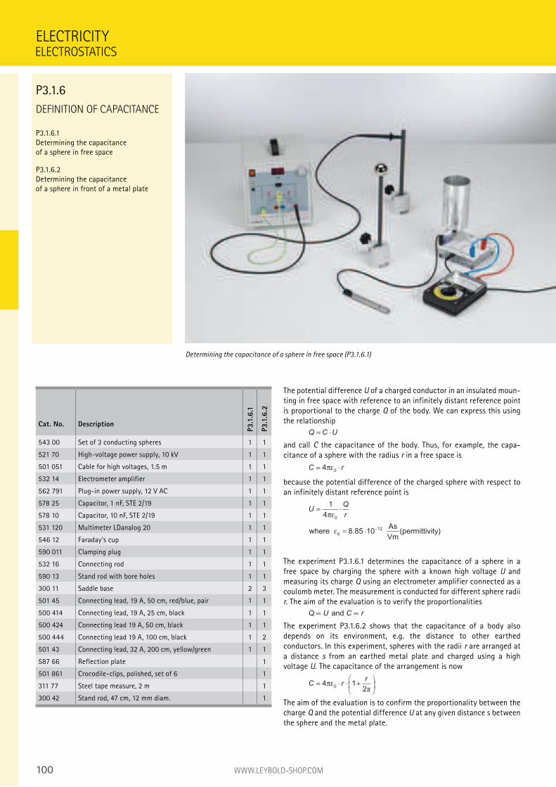
100 WWW.LEYBOLD-SHOP.COM
DEFINITION OF CAPACITANCE
P3.1.6.1 Determining the capacitance of a sphere in free space
P3.1.6.2 Determining the capacitance of a sphere in front of a metal plate
The potential difference U of a charged conductor in an insulated moun-ting in free space with reference to an infinitely distant reference point is proportional to the charge Q of the body. We can express this using the relationship
Q C U= ⋅
and call C the capacitance of the body. Thus, for example, the capa-citance of a sphere with the radius r in a free space is
C r= ⋅40
πε
because the potential difference of the charged sphere with respect to an infinitely distant reference point is
UQ
r= ⋅
= ⋅−
1
4
8 85 10
0
0
12
πε
εwhere As
Vm(permittivity).
The experiment P3.1.6.1 determines the capacitance of a sphere in a free space by charging the sphere with a known high voltage U and measuring its charge Q using an electrometer amplifier connected as a coulomb meter. The measurement is conducted for different sphere radii r. The aim of the evaluation is to verify the proportionalities
Q U C r and
The experiment P3.1.6.2 shows that the capacitance of a body also depends on its environment, e.g. the distance to other earthed conductors. In this experiment, spheres with the radii r are arranged at a distance s from an earthed metal plate and charged using a high voltage U. The capacitance of the arrangement is now
C rr
s= ⋅ ⋅ +
4 1
20
πε
The aim of the evaluation is to confirm the proportionality between the charge Q and the potential difference U at any given distance s between the sphere and the metal plate.
ELECTRICITY
Determining the capacitance of a sphere in free space (P3.1.6.1)
Cat. No. Description
P3.1
.6.1
P3.1
.6.2
543 00 Set of 3 conducting spheres 1 1
521 70 High-voltage power supply, 10 kV 1 1
501 051 Cable for high voltages, 1.5 m 1 1
532 14 Electrometer amplifier 1 1
562 791 Plug-in power supply, 12 V AC 1 1
578 25 Capacitor, 1 nF, STE 2/19 1 1
578 10 Capacitor, 10 nF, STE 2/19 1 1
531 120 Multimeter LDanalog 20 1 1
546 12 Faraday‘s cup 1 1
590 011 Clamping plug 1 1
532 16 Connecting rod 1 1
590 13 Stand rod with bore holes 1 1
300 11 Saddle base 2 3
501 45 Connecting lead, 19 A, 50 cm, red/blue, pair 1 1
500 414 Connecting lead, 19 A, 25 cm, black 1 1
500 424 Connecting lead 19 A, 50 cm, black 1 1
500 444 Connecting lead 19 A, 100 cm, black 1 2
501 43 Connecting lead, 32 A, 200 cm, yellow/green 1 1
587 66 Reflection plate 1
501 861 Crocodile-clips, polished, set of 6 1
311 77 Steel tape measure, 2 m 1
300 42 Stand rod, 47 cm, 12 mm diam. 1
ELECTROSTATICS
P3.1.6
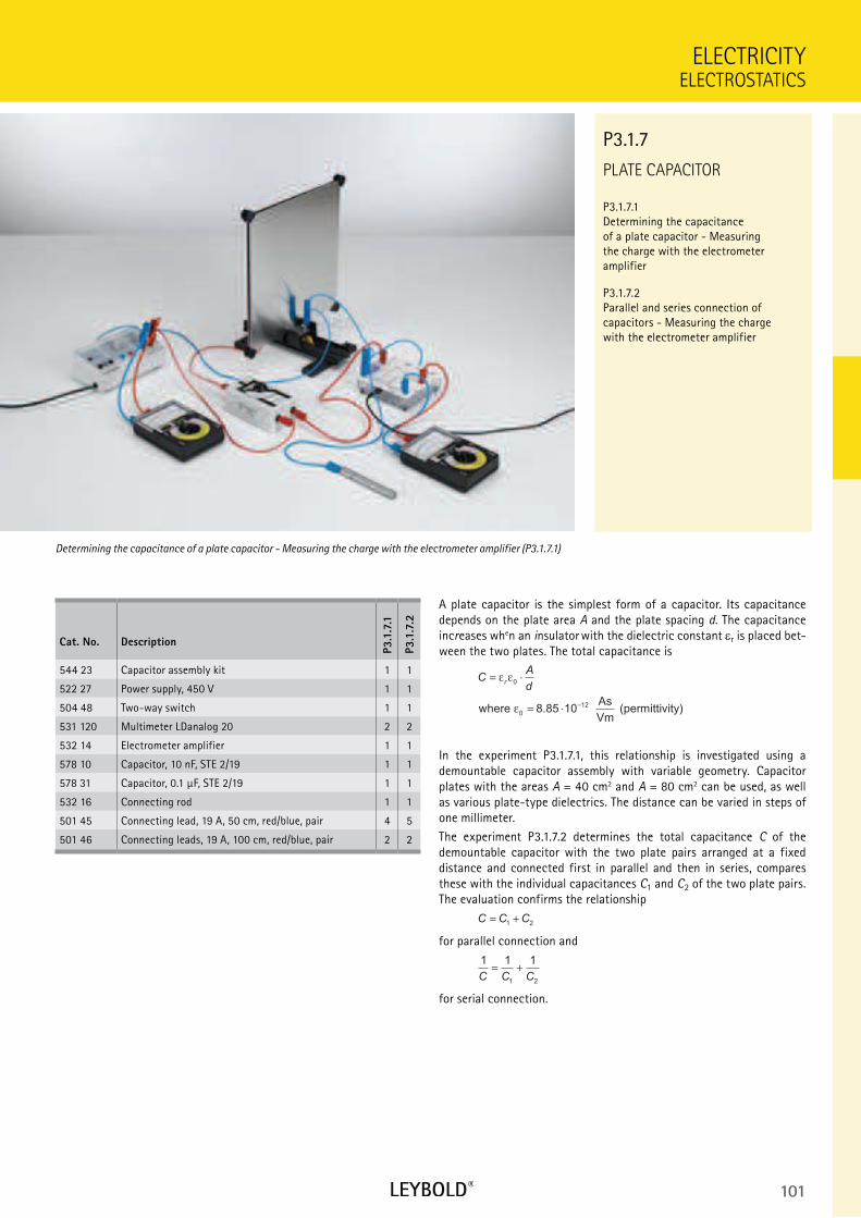
101
PLATE CAPACITOR
P3.1.7.1 Determining the capacitance of a plate capacitor - Measuring the charge with the electrometer amplifier
P3.1.7.2 Parallel and series connection of capacitors - Measuring the charge with the electrometer amplifier
ELECTROSTATICS
ELECTRICITY
Cat. No. Description
P3.1
.7.1
P3.1
.7.2
544 23 Capacitor assembly kit 1 1
522 27 Power supply, 450 V 1 1
504 48 Two-way switch 1 1
531 120 Multimeter LDanalog 20 2 2
532 14 Electrometer amplifier 1 1
578 10 Capacitor, 10 nF, STE 2/19 1 1
578 31 Capacitor, 0.1 µF, STE 2/19 1 1
532 16 Connecting rod 1 1
501 45 Connecting lead, 19 A, 50 cm, red/blue, pair 4 5
501 46 Connecting leads, 19 A, 100 cm, red/blue, pair 2 2
Determining the capacitance of a plate capacitor - Measuring the charge with the electrometer amplifier (P3.1.7.1)
P3.1.7
A plate capacitor is the simplest form of a capacitor. Its capacitance depends on the plate area A and the plate spacing d. The capacitance increases when an insulator with the dielectric constant r is placed bet-ween the two plates. The total capacitance is
CA
dr
= ⋅
= ⋅−
ε ε
ε
0
0
128 85 10where As
Vm (permittivity).
In the experiment P3.1.7.1, this relationship is investigated using a demountable capacitor assembly with variable geometry. Capacitor plates with the areas A = 40 cm2 and A = 80 cm2 can be used, as well as various plate-type dielectrics. The distance can be varied in steps of one millimeter.
The experiment P3.1.7.2 determines the total capacitance C of the demountable capacitor with the two plate pairs arranged at a fixed distance and connected first in parallel and then in series, compares these with the individual capacitances C1 and C2 of the two plate pairs. The evaluation confirms the relationship
C C C= +1 2
for parallel connection and
1 1 1
1 2C C C
= +
for serial connection.
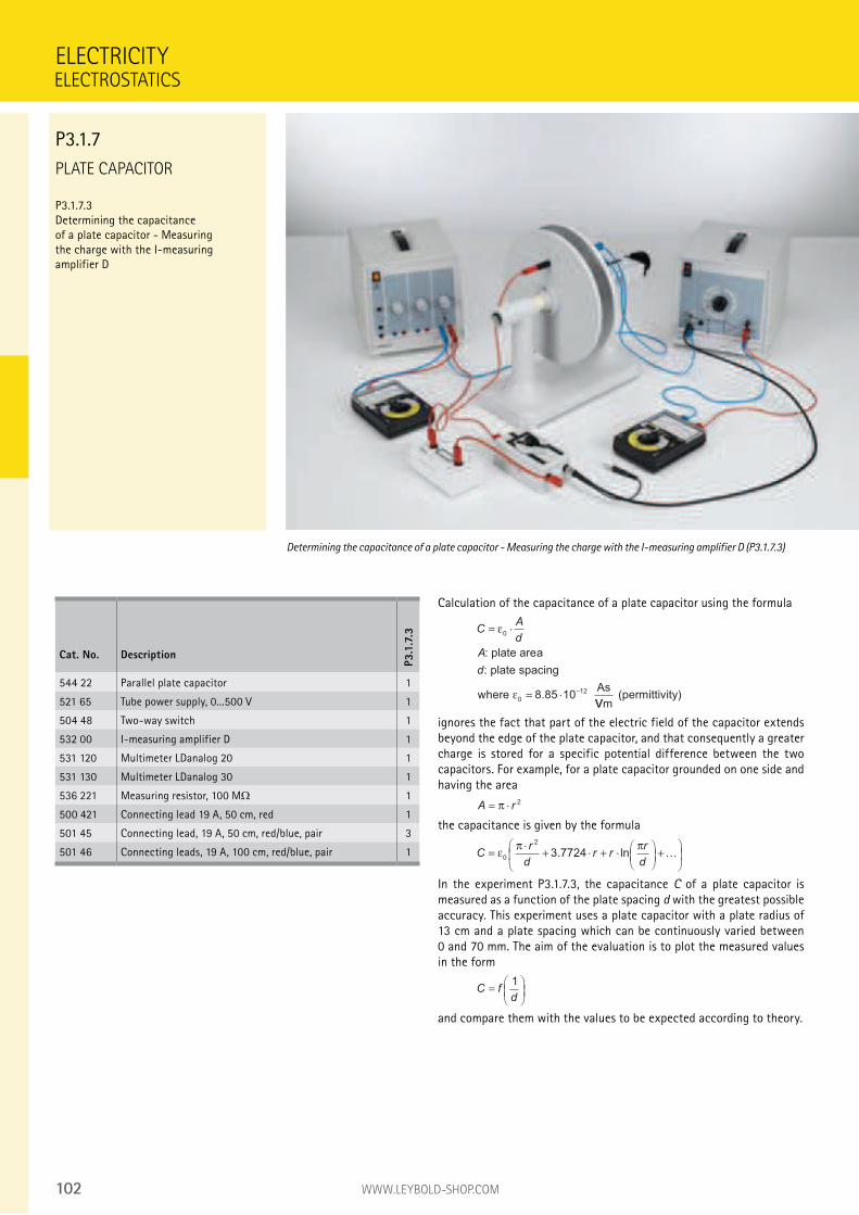
102 WWW.LEYBOLD-SHOP.COM
PLATE CAPACITOR
P3.1.7.3 Determining the capacitance of a plate capacitor - Measuring the charge with the I-measuring amplifier D
ELECTRICITY
Determining the capacitance of a plate capacitor - Measuring the charge with the I-measuring amplifier D (P3.1.7.3)
Cat. No. Description
P3.1
.7.3
544 22 Parallel plate capacitor 1
521 65 Tube power supply, 0...500 V 1
504 48 Two-way switch 1
532 00 I-measuring amplifier D 1
531 120 Multimeter LDanalog 20 1
531 130 Multimeter LDanalog 30 1
536 221 Measuring resistor, 100 M 1
500 421 Connecting lead 19 A, 50 cm, red 1
501 45 Connecting lead, 19 A, 50 cm, red/blue, pair 3
501 46 Connecting leads, 19 A, 100 cm, red/blue, pair 1
ELECTROSTATICS
P3.1.7
Calculation of the capacitance of a plate capacitor using the formula
CA
d
A
d
= ⋅
= ⋅−
ε
ε
0
0
128 85 10
: plate area
: plate spacing
where As
.VVm
(permittivity)
ignores the fact that part of the electric field of the capacitor extends beyond the edge of the plate capacitor, and that consequently a greater charge is stored for a specific potential difference between the two capacitors. For example, for a plate capacitor grounded on one side and having the area
A r= ⋅π2
the capacitance is given by the formula
Cr
dr r
r
d=
⋅+ ⋅ + ⋅
+
ε
π π0
2
3 7724. ln …
In the experiment P3.1.7.3, the capacitance C of a plate capacitor is measured as a function of the plate spacing d with the greatest possible accuracy. This experiment uses a plate capacitor with a plate radius of 13 cm and a plate spacing which can be continuously varied between 0 and 70 mm. The aim of the evaluation is to plot the measured values in the form
C fd
=
1
and compare them with the values to be expected according to theory.
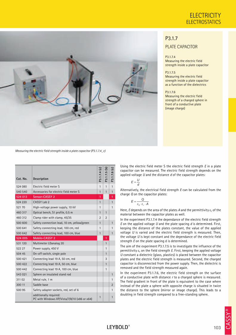
103 CA
SSY ®
PLATE CAPACITOR
P3.1.7.4 Measuring the electric field strength inside a plate capacitor
P3.1.7.5 Measuring the electric field strength inside a plate capacitor as a function of the dielectrics
P3.1.7.6 Measuring the electric field strength of a charged sphere in front of a conductive plate (image charge)
ELECTROSTATICS
ELECTRICITY
Cat. No. Description
P3.1
.7.4
(c)
P3.1
.7.5
(b)
P3.1
.7.6
(c)
524 080 Electric field meter S 1 1 1
540 540 Accessories for electric field meter S 1 1 1
524 013 Sensor-CASSY 2 1 1
524 220 CASSY Lab 2 1 1
521 70 High-voltage power supply, 10 kV 1 1
460 317 Optical bench, S1 profile, 0.5 m 1 1
460 312 Clamp rider with clamp, 45/35 2 2
500 600 Safety connection lead, 10 cm, yellow/green 1 1
500 641 Safety connecting lead, 100 cm, red 1 1
500 642 Safety connecting lead, 100 cm, blue 1 1
524 005 Mobile-CASSY 2 1
531 120 Multimeter LDanalog 20 1
522 27 Power supply, 450 V 1
504 45 On-off switch, single pole 1
500 421 Connecting lead 19 A, 50 cm, red 3
500 422 Connecting lead 19 A, 50 cm, blue 1
500 442 Connecting lead 19 A, 100 cm, blue 1
543 021 Sphere on insulated stand rod 1
311 02 Metal rule, 1 m 1
300 11 Saddle base 2
500 95 Safety adapter sockets, red, set of 6 1
additionally required: PC with Windows XP/Vista/7/8/10 (x86 or x64)
1 1
Using the electric field meter S the electric field strength E in a plate capacitor can be measured. The electric field strength depends on the applied voltage U and the distance d of the capacitor plates:
EU
d
Alternatively, the electrical field strength E can be calculated from the charge Q on the capacitor plates:
EQ
Ar
=⋅ ⋅ε ε
0
Here, E depends on the area of the plates A and the permittivity r of the material between the capacitor plates as well.
In the experiment P3.1.7.4 the dependance of the electric field strength E on the applied voltage U and the plate spacing d is determined. First, keeping the distance of the plates constant, the value of the applied voltage U is varied and the electric field strength is measured. Then, the voltage U is kept constant and the dependance of the electric field strength E on the plate spacing d is determined.
The aim of the experiment P3.1.7.5 is to investigate the influence of the permittivity r on the field strength E. First, keeping the applied voltage U constant a dielectric (glass, plastics) is placed between the capacitor plates and the electric field strength is measured. Second, the charged capacitor is disconnected from the power supply. Then, the dielectric is removed and the field strength measured again.
In the experiment P3.1.7.6, the electric field strength on the surface of a conductive plate with distance r to a charged sphere is measured. The field gradient in front of the plate is equivalent to the case where instead of the plate a sphere with opposite charge is situated in twice the distance to the sphere (mirror or image charge). This leads to a doubling in field strength compared to a free-standing sphere.
Measuring the electric field strength inside a plate capacitor (P3.1.7.4_c)
P3.1.7
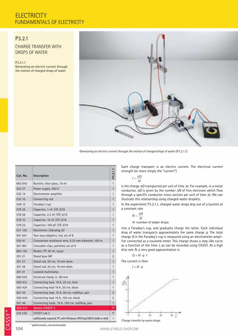
104 WWW.LEYBOLD-SHOP.COMCA
SSY ®
CHARGE TRANSFER WITH
DROPS OF WATER
P3.2.1.1 Generating an electric current through the motion of charged drops of water
Each charge transport is an electric current. The electrical current strength (or more simply the “current”)
IQ
t=∆
∆
is the charge Q transported per unit of time t. For example, in a metal conductor, Q is given by the number N of free electrons which flow through a specific conductor cross-section per unit of time t. We can illustrate this relationship using charged water droplets.
In the experiment P3.2.1.1, charged water drops drip out of a burette at a constant rate
ɺNN
t
N
=∆
∆
: number of water drops
into a Faraday’s cup, and gradually charge the latter. Each individual drop of water transports approximately the same charge q. The total charge Q in the Faraday’s cup is measured using an electrometer ampli-fier connected as a coulomb meter. This charge shows a step-like curve as a function of the time t, as can be recorded using CASSY. At a high drip rate N, a very good approximation is
Q N q t= ⋅ ⋅ɺ
The current is then
I N q= ⋅ɺ
ELECTRICITY
Generating an electric current through the motion of charged drops of water (P3.2.1.1)
Cat. No. Description
P3.2
.1.1
665 843 Burette, clear glass, 10 ml 1
522 27 Power supply, 450 V 1
532 14 Electrometer amplifier 1
532 16 Connecting rod 1
546 12 Faraday‘s cup 1
578 25 Capacitor, 1 nF, STE 2/19 1
578 26 Capacitor, 2.2 nF, STE 2/19 1
578 10 Capacitor, 10 nF, STE 2/19 1
578 22 Capacitor, 100 pF, STE 2/19 1
531 120 Multimeter LDanalog 20 1
501 641 Two-way adapters, red, set of 6 1
550 41 Constantan resistance wire, 0.25 mm diameter, 100 m 1
501 861 Crocodile-clips, polished, set of 6 1
664 120 Beaker, PP, 50 ml, squat 1
301 21 Stand base MF 2
301 27 Stand rod, 50 cm, 10 mm diam. 1
301 26 Stand rod, 25 cm, 10 mm diam. 1
301 01 Leybold multiclamp 1
666 555 Universal clamp, 0...80 mm 1
500 412 Connecting lead, 19 A, 25 cm, blue 1
500 424 Connecting lead 19 A, 50 cm, black 1
501 45 Connecting lead, 19 A, 50 cm, red/blue, pair 2
500 444 Connecting lead 19 A, 100 cm, black 2
501 46 Connecting leads, 19 A, 100 cm, red/blue, pair 1
524 013 Sensor-CASSY 2 1*
524 220 CASSY Lab 2 1*
additionally required: PC with Windows XP/Vista/7/8/10 (x86 or x64) 1
* additionally recommended
Charge transfer by water drops
FUNDAMENTALS OF ELECTRICITY
P3.2.1
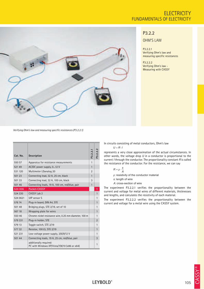
105 CA
SSY ®
OHM’S LAW
P3.2.2.1 Verifying Ohm’s law and measuring specific resistances
P3.2.2.2 Verifying Ohm’s law - Measuring with CASSY
FUNDAMENTALS OF ELECTRICITY
ELECTRICITY
Cat. No. Description
P3.2
.2.1
P3.2
.2.2
550 57 Apparatus for resistance measurements 1
521 49 AC/DC power supply, 0...12 V 1
531 120 Multimeter LDanalog 20 2
501 23 Connecting lead, 32 A, 25 cm, black 1
501 33 Connecting lead, 32 A, 100 cm, black 3
501 46 Connecting leads, 19 A, 100 cm, red/blue, pair 1
524 006 Pocket-CASSY 1
524 220 CASSY Lab 2 1
524 0621 UIP sensor S 1
576 74 Plug-in board, DIN A4, STE 1
501 48 Bridging plugs, STE 2/19, set of 10 1
567 18 Wrapping plate for wires 1
550 46 Chrome-nickel resistance wire, 0.25 mm diameter, 100 m 1
579 331 Plug-in holder, STE 2
579 13 Toggle switch, STE 2/19 1
577 32 Resistor, 100 , STE 2/19 1
521 231 Low-voltage power supply, 3/6/9/12 V 1
501 44 Connecting leads, 19 A, 25 cm, red/blue, pair 3
additionally required: PC with Windows XP/Vista/7/8/10 (x86 or x64)
1
In circuits consisting of metal conductors, Ohm’s law
U R I= ⋅
represents a very close approximation of the actual circumstances. In other words, the voltage drop U in a conductor is proportional to the current I through the conductor. The proportionality constant R is called the resistance of the conductor. For the resistance, we can say
Rs
A
s
= ⋅ρ
ρ: resistivity of the conductor material
: length of wire
: cross-section of wireA
The experiment P3.2.2.1 verifies the proportionality between the current and voltage for metal wires of different materials, thicknesses and lengths, and calculates the resistivity of each material.
The experiment P3.2.2.2 verifies the proportionality between the current and voltage for a metal wire using the CASSY system.
Verifying Ohm’s law and measuring specific resistances (P3.2.2.1)
P3.2.2
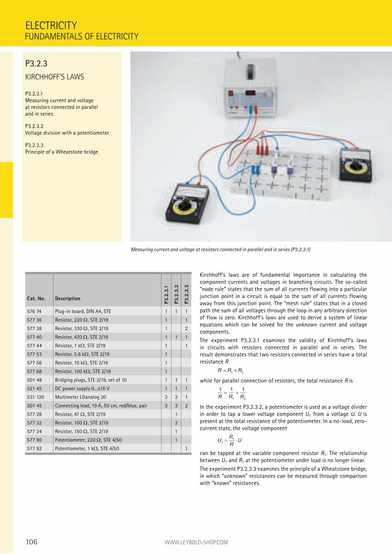
106 WWW.LEYBOLD-SHOP.COM
KIRCHHOFF’S LAWS
P3.2.3.1 Measuring current and voltage at resistors connected in parallel and in series
P3.2.3.2 Voltage division with a potentiometer
P3.2.3.3 Principle of a Wheatstone bridge
Kirchhoff’s laws are of fundamental importance in calculating the component currents and voltages in branching circuits. The so-called “node rule” states that the sum of all currents flowing into a particular junction point in a circuit is equal to the sum of all currents flowing away from this junction point. The “mesh rule” states that in a closed path the sum of all voltages through the loop in any arbitrary direction of flow is zero. Kirchhoff’s laws are used to derive a system of linear equations which can be solved for the unknown current and voltage components.
The experiment P3.2.3.1 examines the validity of Kirchhoff’s laws in circuits with resistors connected in parallel and in series. The result demonstrates that two resistors connected in series have a total resistance R
R R R= +1 2
while for parallel connection of resistors, the total resistance R is
1 1 1
1 2R R R
= +
In the experiment P3.2.3.2, a potentiometer is used as a voltage divider in order to tap a lower voltage component U1 from a voltage U. U is present at the total resistance of the potentiometer. In a no-load, zero-current state, the voltage component
UR
RU
1
1= ⋅
can be tapped at the variable component resistor R1. The relationship between U1 and R1 at the potentiometer under load is no longer linear.
The experiment P3.2.3.3 examines the principle of a Wheatstone bridge, in which “unknown” resistances can be measured through comparison with “known” resistances.
ELECTRICITY
Measuring current and voltage at resistors connected in parallel and in series (P3.2.3.1)
Cat. No. Description
P3.2
.3.1
P3.2
.3.2
P3.2
.3.3
576 74 Plug-in board, DIN A4, STE 1 1 1
577 36 Resistor, 220 , STE 2/19 1 1
577 38 Resistor, 330 , STE 2/19 1 2
577 40 Resistor, 470 , STE 2/19 1 1 1
577 44 Resistor, 1 k , STE 2/19 1 1
577 53 Resistor, 5.6 k , STE 2/19 1
577 56 Resistor, 10 k , STE 2/19 1
577 68 Resistor, 100 k , STE 2/19 1
501 48 Bridging plugs, STE 2/19, set of 10 1 1 1
521 45 DC power supply 0...±15 V 1 1 1
531 120 Multimeter LDanalog 20 2 2 1
501 45 Connecting lead, 19 A, 50 cm, red/blue, pair 3 3 2
577 28 Resistor, 47 , STE 2/19 1
577 32 Resistor, 100 , STE 2/19 2
577 34 Resistor, 150 , STE 2/19 1
577 90 Potentiometer, 220 , STE 4/50 1
577 92 Potentiometer, 1 k , STE 4/50 1
FUNDAMENTALS OF ELECTRICITY
P3.2.3
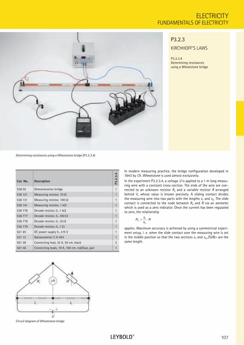
107
KIRCHHOFF’S LAWS
P3.2.3.4 Determining resistances using a Wheatstone bridge
FUNDAMENTALS OF ELECTRICITY
ELECTRICITY
Cat. No. Description
P3.2
.3.4
536 02 Demonstration bridge 1
536 121 Measuring resistor, 10 1
536 131 Measuring resistor, 100 1
536 141 Measuring resistor, 1 k 1
536 776 Decade resistor, 0...1 k 1
536 777 Decade resistor, 0...100 1
536 778 Decade resistor, 0...10 1
536 779 Decade resistor, 0...1 1
521 45 DC power supply 0...±15 V 1
531 13 Galvanometer C.A 403 1
501 28 Connecting lead, 32 A, 50 cm, black 3
501 46 Connecting leads, 19 A, 100 cm, red/blue, pair 1
In modern measuring practice, the bridge configuration developed in 1843 by Ch. Wheatstone is used almost exclusively.
In the experiment P3.2.3.4, a voltage U is applied to a 1 m long measu-ring wire with a constant cross-section. The ends of the wire are con-nected to an unknown resistor Rx and a variable resistor R arranged behind it, whose value is known precisely. A sliding contact divides the measuring wire into two parts with the lengths s1 and s2. The slide contact is connected to the node between Rx and R via an ammeter which is used as a zero indicator. Once the current has been regulated to zero, the relationship
Rs
sR
x= ⋅1
2
applies. Maximum accuracy is achieved by using a symmetrical experi-ment setup, i. e. when the slide contact over the measuring wire is set in the middle position so that the two sections s1 and s2</SUB> are the same length.
Determining resistances using a Wheatstone bridge (P3.2.3.4)
P3.2.3
Circuit diagram of Wheatstone bridge
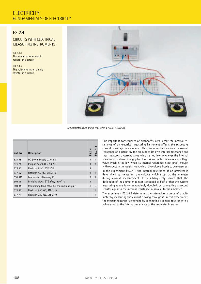
108 WWW.LEYBOLD-SHOP.COM
CIRCUITS WITH ELECTRICAL
MEASURING INSTRUMENTS
P3.2.4.1 The ammeter as an ohmic resistor in a circuit
P3.2.4.2 The voltmeter as an ohmic resistor in a circuit
One important consequence of Kirchhoff’s laws is that the internal re-sistance of an electrical measuring instrument affects the respective current or voltage measurement. Thus, an ammeter increases the overall resistance of a circuit by the amount of its own internal resistance and thus measures a current value which is too low whenever the internal resistance is above a negligible level. A voltmeter measures a voltage value which is too low when its internal resistance is not great enough with respect to the resistance at which the voltage drop is to be measured.
In the experiment P3.2.4.1, the internal resistance of an ammeter is determined by measuring the voltage which drops at the ammeter during current measurement. It is subsequently shown that the deflection of the ammeter pointer is reduced by half, or that the current measuring range is correspondingly doubled, by connecting a second resistor equal to the internal resistance in parallel to the ammeter.
The experiment P3.2.4.2 determines the internal resistance of a volt-meter by measuring the current flowing through it. In this experiment, the measuring range is extended by connecting a second resistor with a value equal to the internal resistance to the voltmeter in series.
ELECTRICITY
The ammeter as an ohmic resistor in a circuit (P3.2.4.1)
Cat. No. Description
P3.2
.4.1
P3.2
.4.2
521 45 DC power supply 0...±15 V 1 1
576 74 Plug-in board, DIN A4, STE 1 1
577 33 Resistor, 82 , STE 2/19 3
577 52 Resistor, 4.7 k , STE 2/19 1 1
531 110 Multimeter LDanalog 10 2 2
501 48 Bridging plugs, STE 2/19, set of 10 1
501 45 Connecting lead, 19 A, 50 cm, red/blue, pair 3 3
577 75 Resistor, 680 k , STE 2/19 1
577 71 Resistor, 220 k , STE 2/19 1
FUNDAMENTALS OF ELECTRICITY
P3.2.4
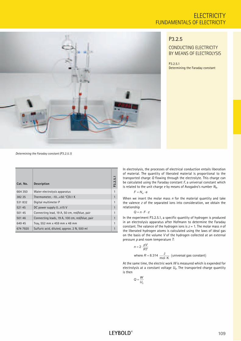
109
CONDUCTING ELECTRICITY
BY MEANS OF ELECTROLYSIS
P3.2.5.1 Determining the Faraday constant
FUNDAMENTALS OF ELECTRICITY
ELECTRICITY
Cat. No. Description
P3.2
.5.1
664 350 Water electrolysis apparatus 1
382 35 Thermometer, -10...+50 °C/0.1 K 1
531 832 Digital multimeter P 1
521 45 DC power supply 0...±15 V 1
501 45 Connecting lead, 19 A, 50 cm, red/blue, pair 1
501 46 Connecting leads, 19 A, 100 cm, red/blue, pair 1
649 45 Tray, 552 mm x 459 mm x 48 mm 1
674 7920 Sulfuric acid, diluted, approx. 2 N, 500 ml 1
In electrolysis, the processes of electrical conduction entails liberation of material. The quantity of liberated material is proportional to the transported charge Q flowing through the electrolyte. This charge can be calculated using the Faraday constant F, a universal constant which is related to the unit charge e by means of Avogadro’s number NA.
F N eA
= ⋅
When we insert the molar mass n for the material quantity and take the valence z of the separated ions into consideration, we obtain the relationship
Q n F z= ⋅ ⋅
In the experiment P3.2.5.1, a specific quantity of hydrogen is produced in an electrolysis apparatus after Hofmann to determine the Faraday constant. The valance of the hydrogen ions is z = 1. The molar mass n of the liberated hydrogen atoms is calculated using the laws of ideal gas on the basis of the volume V of the hydrogen collected at an external pressure p and room temperature T:
npV
RT
R
= ⋅
=⋅
( )
2
8 314where J
mol K universal gas constant.
At the same time, the electric work W is measured which is expended for electrolysis at a constant voltage U0. The transported charge quantity is then
QW
U0
Determining the Faraday constant (P3.2.5.1)
P3.2.5
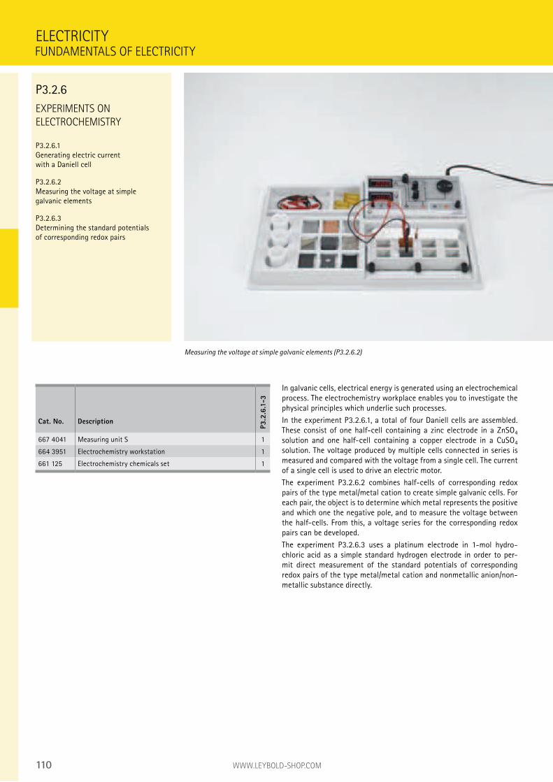
110 WWW.LEYBOLD-SHOP.COM
EXPERIMENTS ON
ELECTROCHEMISTRY
P3.2.6.1 Generating electric current with a Daniell cell
P3.2.6.2 Measuring the voltage at simple galvanic elements
P3.2.6.3 Determining the standard potentials of corresponding redox pairs
In galvanic cells, electrical energy is generated using an electrochemical process. The electrochemistry workplace enables you to investigate the physical principles which underlie such processes.
In the experiment P3.2.6.1, a total of four Daniell cells are assembled. These consist of one half-cell containing a zinc electrode in a ZnSO4 solution and one half-cell containing a copper electrode in a CuSO4 solution. The voltage produced by multiple cells connected in series is measured and compared with the voltage from a single cell. The current of a single cell is used to drive an electric motor.
The experiment P3.2.6.2 combines half-cells of corresponding redox pairs of the type metal/metal cation to create simple galvanic cells. For each pair, the object is to determine which metal represents the positive and which one the negative pole, and to measure the voltage between the half-cells. From this, a voltage series for the corresponding redox pairs can be developed.
The experiment P3.2.6.3 uses a platinum electrode in 1-mol hydro-chloric acid as a simple standard hydrogen electrode in order to per-mit direct measurement of the standard potentials of corresponding redox pairs of the type metal/metal cation and nonmetallic anion/non- metallic substance directly.
ELECTRICITY
Measuring the voltage at simple galvanic elements (P3.2.6.2)
Cat. No. Description
P3.2
.6.1
-3
667 4041 Measuring unit S 1
664 3951 Electrochemistry workstation 1
661 125 Electrochemistry chemicals set 1
FUNDAMENTALS OF ELECTRICITY
P3.2.6
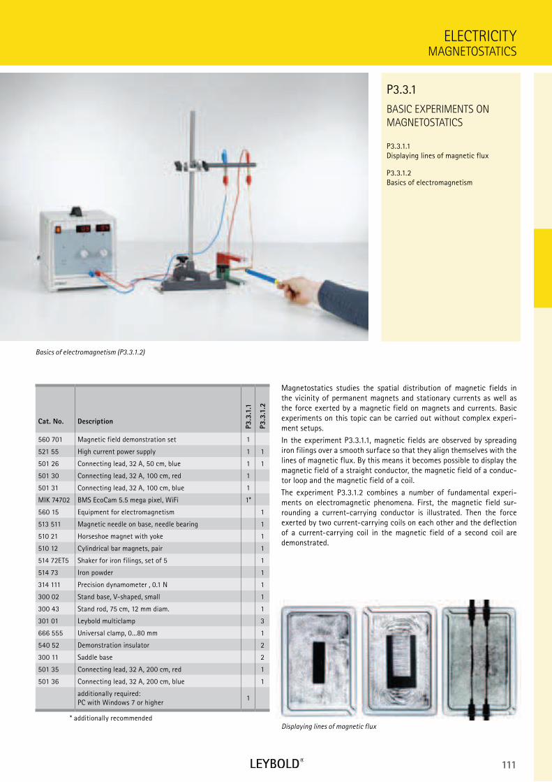
111
BASIC EXPERIMENTS ON
MAGNETOSTATICS
P3.3.1.1
Displaying lines of magnetic flux
P3.3.1.2
Basics of electromagnetism
MAGNETOSTATICS
ELECTRICITY
Cat. No. Description
P3.3
.1.1
P3.3
.1.2
560 701 Magnetic field demonstration set 1
521 55 High current power supply 1 1
501 26 Connecting lead, 32 A, 50 cm, blue 1 1
501 30 Connecting lead, 32 A, 100 cm, red 1
501 31 Connecting lead, 32 A, 100 cm, blue 1
MIK 74702 BMS EcoCam 5.5 mega pixel, WiFi 1*
560 15 Equipment for electromagnetism 1
513 511 Magnetic needle on base, needle bearing 1
510 21 Horseshoe magnet with yoke 1
510 12 Cylindrical bar magnets, pair 1
514 72ET5 Shaker for iron filings, set of 5 1
514 73 Iron powder 1
314 111 Precision dynamometer , 0.1 N 1
300 02 Stand base, V-shaped, small 1
300 43 Stand rod, 75 cm, 12 mm diam. 1
301 01 Leybold multiclamp 3
666 555 Universal clamp, 0...80 mm 1
540 52 Demonstration insulator 2
300 11 Saddle base 2
501 35 Connecting lead, 32 A, 200 cm, red 1
501 36 Connecting lead, 32 A, 200 cm, blue 1
additionally required:
PC with Windows 7 or higher1
* additionally recommended
Magnetostatics studies the spatial distribution of magnetic fields in
the vicinity of permanent magnets and stationary currents as well as
the force exerted by a magnetic field on magnets and currents. Basic
experiments on this topic can be carried out without complex experi-
ment setups.
In the experiment P3.3.1.1, magnetic fields are observed by spreading
iron filings over a smooth surface so that they align themselves with the
lines of magnetic flux. By this means it becomes possible to display the
magnetic field of a straight conductor, the magnetic field of a conduc-
tor loop and the magnetic field of a coil.
The experiment P3.3.1.2 combines a number of fundamental experi-
ments on electromagnetic phenomena. First, the magnetic field sur-
rounding a current-carrying conductor is illustrated. Then the force
exerted by two current-carrying coils on each other and the deflection
of a current-carrying coil in the magnetic field of a second coil are
demonstrated.
Basics of electromagnetism (P3.3.1.2)
P3.3.1
Displaying lines of magnetic flux
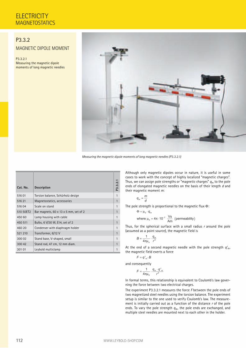
112 WWW.LEYBOLD-SHOP.COM
MAGNETIC DIPOLE MOMENT
P3.3.2.1 Measuring the magnetic dipole moments of long magnetic needles
Although only magnetic dipoles occur in nature, it is useful in some cases to work with the concept of highly localized “magnetic charges”. Thus, we can assign pole strengths or “magnetic charges” qm to the pole ends of elongated magnetic needles on the basis of their length d and their magnetic moment m:
qm
dm
The pole strength is proportional to the magnetic flux :
Φ = ⋅
= ⋅ ( )−
µ
µ π
0
0
74 10
qm
where Vs
Am permeability
Thus, for the spherical surface with a small radius r around the pole (assumed as a point source), the magnetic field is
Bq
ro
m= ⋅1
42πµ
At the end of a second magnetic needle with the pole strength q’m, the magnetic field exerts a force
F q Bm
= ⋅'
and consequently
Fq q
rm m= ⋅⋅1
40
2πµ
'
In formal terms, this relationship is equivalent to Coulomb’s law gover-ning the force between two electrical charges.
The experiment P3.3.2.1 measures the force F between the pole ends of two magnetized steel needles using the torsion balance. The experiment setup is similar to the one used to verify Coulomb’s law. The measure-ment is initially carried out as a function of the distance r of the pole ends. To vary the pole strength qm, the pole ends are exchanged, and multiple steel needles are mounted next to each other in the holder.
ELECTRICITY
Measuring the magnetic dipole moments of long magnetic needles (P3.3.2.1)
Cat. No. Description
P3.3
.2.1
516 01 Torsion balance, Schürholz design 1
516 21 Magnetostatics, accessories 1
516 04 Scale on stand 1
510 50ET2 Bar magnets, 60 x 13 x 5 mm, set of 2 1
450 60 Lamp housing with cable 1
450 511 Bulbs, 6 V/30 W, E14, set of 2 1
460 20 Condenser with diaphragm holder 1
521 210 Transformer, 6/12 V 1
300 02 Stand base, V-shaped, small 1
300 42 Stand rod, 47 cm, 12 mm diam. 1
301 01 Leybold multiclamp 1
MAGNETOSTATICS
P3.3.2
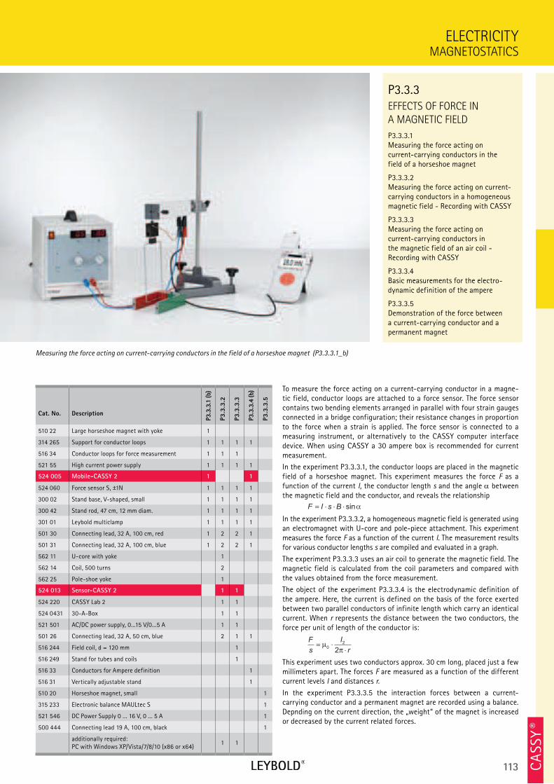
113 CA
SSY ®
EFFECTS OF FORCE IN
A MAGNETIC FIELD
P3.3.3.1 Measuring the force acting on current-carrying conductors in the field of a horseshoe magnet
P3.3.3.2 Measuring the force acting on current-carrying conductors in a homogeneous magnetic field - Recording with CASSY
P3.3.3.3 Measuring the force acting on current-carrying conductors in the magnetic field of an air coil - Recording with CASSY
P3.3.3.4 Basic measurements for the electro-dynamic definition of the ampere
P3.3.3.5 Demonstration of the force between a current-carrying conductor and a permanent magnet
MAGNETOSTATICS
ELECTRICITY
Cat. No. Description
P3.3
.3.1
(b)
P3.3
.3.2
P3.3
.3.3
P3.3
.3.4
(b)
P3.3
.3.5
510 22 Large horseshoe magnet with yoke 1
314 265 Support for conductor loops 1 1 1 1
516 34 Conductor loops for force measurement 1 1 1
521 55 High current power supply 1 1 1 1
524 005 Mobile-CASSY 2 1 1
524 060 Force sensor S, ±1N 1 1 1 1
300 02 Stand base, V-shaped, small 1 1 1 1
300 42 Stand rod, 47 cm, 12 mm diam. 1 1 1 1
301 01 Leybold multiclamp 1 1 1 1
501 30 Connecting lead, 32 A, 100 cm, red 1 2 2 1
501 31 Connecting lead, 32 A, 100 cm, blue 1 2 2 1
562 11 U-core with yoke 1
562 14 Coil, 500 turns 2
562 25 Pole-shoe yoke 1
524 013 Sensor-CASSY 2 1 1
524 220 CASSY Lab 2 1 1
524 0431 30-A-Box 1 1
521 501 AC/DC power supply, 0...15 V/0...5 A 1 1
501 26 Connecting lead, 32 A, 50 cm, blue 2 1 1
516 244 Field coil, d = 120 mm 1
516 249 Stand for tubes and coils 1
516 33 Conductors for Ampere definition 1
516 31 Vertically adjustable stand 1
510 20 Horseshoe magnet, small 1
315 233 Electronic balance MAULtec S 1
521 546 DC Power Supply 0 ... 16 V, 0 ... 5 A 1
500 444 Connecting lead 19 A, 100 cm, black 1
additionally required: PC with Windows XP/Vista/7/8/10 (x86 or x64)
1 1
To measure the force acting on a current-carrying conductor in a magne-tic field, conductor loops are attached to a force sensor. The force sensor contains two bending elements arranged in parallel with four strain gauges connected in a bridge configuration; their resistance changes in proportion to the force when a strain is applied. The force sensor is connected to a measuring instrument, or alternatively to the CASSY computer interface device. When using CASSY a 30 ampere box is recommended for current measurement.
In the experiment P3.3.3.1, the conductor loops are placed in the magnetic field of a horseshoe magnet. This experiment measures the force F as a function of the current I, the conductor length s and the angle between the magnetic field and the conductor, and reveals the relationship
F I s B= ⋅ ⋅ ⋅ sinα
In the experiment P3.3.3.2, a homogeneous magnetic field is generated using an electromagnet with U-core and pole-piece attachment. This experiment measures the force F as a function of the current I. The measurement results for various conductor lengths s are compiled and evaluated in a graph.
The experiment P3.3.3.3 uses an air coil to generate the magnetic field. The magnetic field is calculated from the coil parameters and compared with the values obtained from the force measurement.
The object of the experiment P3.3.3.4 is the electrodynamic definition of the ampere. Here, the current is defined on the basis of the force exerted between two parallel conductors of infinite length which carry an identical current. When r represents the distance between the two conductors, the force per unit of length of the conductor is:
F
s
I
r= ⋅
⋅µ
π0
2
2
This experiment uses two conductors approx. 30 cm long, placed just a few millimeters apart. The forces F are measured as a function of the different current levels I and distances r.
In the experiment P3.3.3.5 the interaction forces between a current- carrying conductor and a permanent magnet are recorded using a balance. Depnding on the current direction, the „weight“ of the magnet is increased or decreased by the current related forces.
Measuring the force acting on current-carrying conductors in the field of a horseshoe magnet (P3.3.3.1_b)
P3.3.3
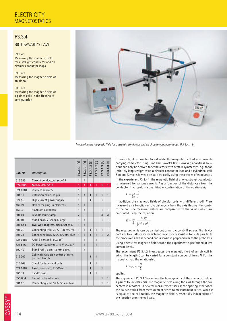
114 WWW.LEYBOLD-SHOP.COMCA
SSY ®
BIOT-SAVART’S LAW
P3.3.4.1
Measuring the magnetic field
for a straight conductor and on
circular conductor loops
P3.3.4.2
Measuring the magnetic field of
an air coil
P3.3.4.3
Measuring the magnetic field of
a pair of coils in the Helmholtz
configuration
In principle, it is possible to calculate the magnetic field of any current-
carrying conductor using Biot and Savart’s law. However, analytical solu-
tions can only be derived for conductors with certain symmetries, e.g. for an
infinitely long straight wire, a circular conductor loop and a cylindrical coil.
Biot and Savart’s law can be verified easily using these types of conductors.
In the experiment P3.3.4.1, the magnetic field of a long, straight conductor
is measured for various currents I as a function of the distance r from the
conductor. The result is a quantitative confirmation of the relationship
BI
r= ⋅µ
π
0
2
In addition, the magnetic fields of circular coils with different radii R are
measured as a function of the distance x from the axis through the center
of the coil. The measured values are compared with the values which are
calculated using the equation
BI R
R x
= ⋅⋅
+( )
µ0
2
2 223
2
The measurements can be carried out using the combi B sensor. This device
contains two Hall sensors which one is extremely sensitive to fields parallel to
the probe axis and the second one is sensitive perpendicular to the probe axis.
Using a sensitive magnetic field sensor, the experiment is performed at low
current levels.
The experiment P3.3.4.2 investigates the magnetic field of an air coil in
which the length L can be varied for a constant number of turns N. For the
magnetic field the relationship
B IN
L= ⋅ ⋅µ
0
applies.
The experiment P3.3.4.3 examines the homogeneity of the magnetic field in
a pair of Helmholtz coils. The magnetic field along the axis through the coil
centers is recorded in several measurement series; the spacing a between
the coils is varied from measurement series to measurement series. When a
is equal to the coil radius, the magnetic field is essentially independent of
the location x on the coil axis.
ELECTRICITY
Measuring the magnetic field for a straight conductor and on circular conductor loops (P3.3.4.1_b)
Cat. No. Description
P3.3
.4.1
(b)
P3.3
.4.1
(c)
P3.3
.4.2
(b)
P3.3
.4.2
(c)
P3.3
.4.3
(b)
P3.3
.4.3
(c)
516 235 Current conductors, set of 4 1 1
524 005 Mobile-CASSY 2 1 1 1 1 1 1
524 0381 Combi B sensor S 1
501 11 Extension cable, 15 pin 1 1 1 1 1 1
521 55 High current power supply 1 1 1
460 21 Holder for plug-in elements 1 1
460 43 Small optical bench 1 1 1 1
301 01 Leybold multiclamp 2 3 3 3
300 01 Stand base, V-shaped, large 1 1 1 1
501 644 Two-way adapters, black, set of 6 1 1
501 30 Connecting lead, 32 A, 100 cm, red 1 1 1 1 1 1
501 31 Connecting lead, 32 A, 100 cm, blue 1 1 1 1 1 2
524 0383 Axial B sensor S, ±0.3 mT 1 1 1
521 546 DC Power Supply 0 ... 16 V, 0 ... 5 A 1 1 1
300 43 Stand rod, 75 cm, 12 mm diam. 1
516 242Coil with variable number of turns
per unit length1 1
516 249 Stand for tubes and coils 1 1
524 0382 Axial B sensor S, ±1000 mT 1 1
300 11 Saddle base 1 1
555 604 Pair of Helmholtz coils 1 1
501 26 Connecting lead, 32 A, 50 cm, blue 1 1
MAGNETOSTATICS
P3.3.4
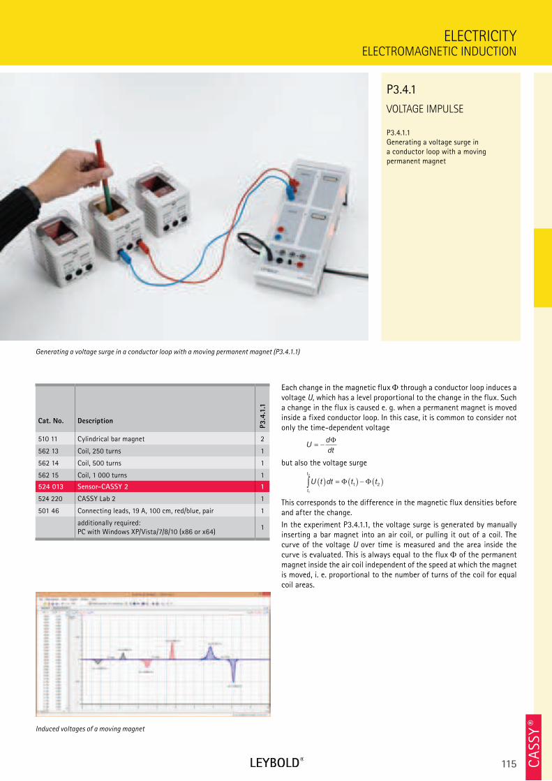
115 CA
SSY ®
VOLTAGE IMPULSE
P3.4.1.1 Generating a voltage surge in a conductor loop with a moving permanent magnet
ELECTROMAGNETIC INDUCTION
ELECTRICITY
Cat. No. Description
P3.4
.1.1
510 11 Cylindrical bar magnet 2
562 13 Coil, 250 turns 1
562 14 Coil, 500 turns 1
562 15 Coil, 1 000 turns 1
524 013 Sensor-CASSY 2 1
524 220 CASSY Lab 2 1
501 46 Connecting leads, 19 A, 100 cm, red/blue, pair 1
additionally required: PC with Windows XP/Vista/7/8/10 (x86 or x64)
1
Each change in the magnetic flux through a conductor loop induces a voltage U, which has a level proportional to the change in the flux. Such a change in the flux is caused e. g. when a permanent magnet is moved inside a fixed conductor loop. In this case, it is common to consider not only the time-dependent voltage
Ud
dt= −
Φ
but also the voltage surge
U t dt t t
t
t
( ) = ( ) − ( )∫ Φ Φ1 2
1
2
This corresponds to the difference in the magnetic flux densities before and after the change.
In the experiment P3.4.1.1, the voltage surge is generated by manually inserting a bar magnet into an air coil, or pulling it out of a coil. The curve of the voltage U over time is measured and the area inside the curve is evaluated. This is always equal to the flux of the permanent magnet inside the air coil independent of the speed at which the magnet is moved, i. e. proportional to the number of turns of the coil for equal coil areas.
Generating a voltage surge in a conductor loop with a moving permanent magnet (P3.4.1.1)
P3.4.1
Induced voltages of a moving magnet
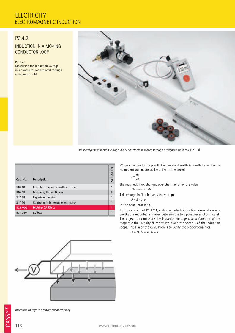
116 WWW.LEYBOLD-SHOP.COMCA
SSY ®
INDUCTION IN A MOVING
CONDUCTOR LOOP
P3.4.2.1
Measuring the induction voltage
in a conductor loop moved through
a magnetic field
When a conductor loop with the constant width b is withdrawn from a
homogeneous magnetic field B with the speed
vdx
dt
the magnetic flux changes over the time dt by the value
d B b dxΦ = − ⋅ ⋅
This change in flux induces the voltage
U B b v= ⋅ ⋅
in the conductor loop.
In the experiment P3.4.2.1, a slide on which induction loops of various
widths are mounted is moved between the two pole pieces of a magnet.
The object is to measure the induction voltage U as a function of the
magnetic flux density B, the width b and the speed v of the induction
loops. The aim of the evaluation is to verify the proportionalities
U B U b U v, ,
ELECTRICITY
Measuring the induction voltage in a conductor loop moved through a magnetic field (P3.4.2.1_b)
Cat. No. Description
P3.4
.2.1
(b)
516 40 Induction apparatus with wire loops 1
510 48 Magnets, 35 mm Ø, pair 6
347 35 Experiment motor 1
347 36 Control unit for experiment motor 1
524 005 Mobile-CASSY 2 1
524 040 µV box 1
Induction voltage in a moved conductor loop
ELECTROMAGNETIC INDUCTION
P3.4.2
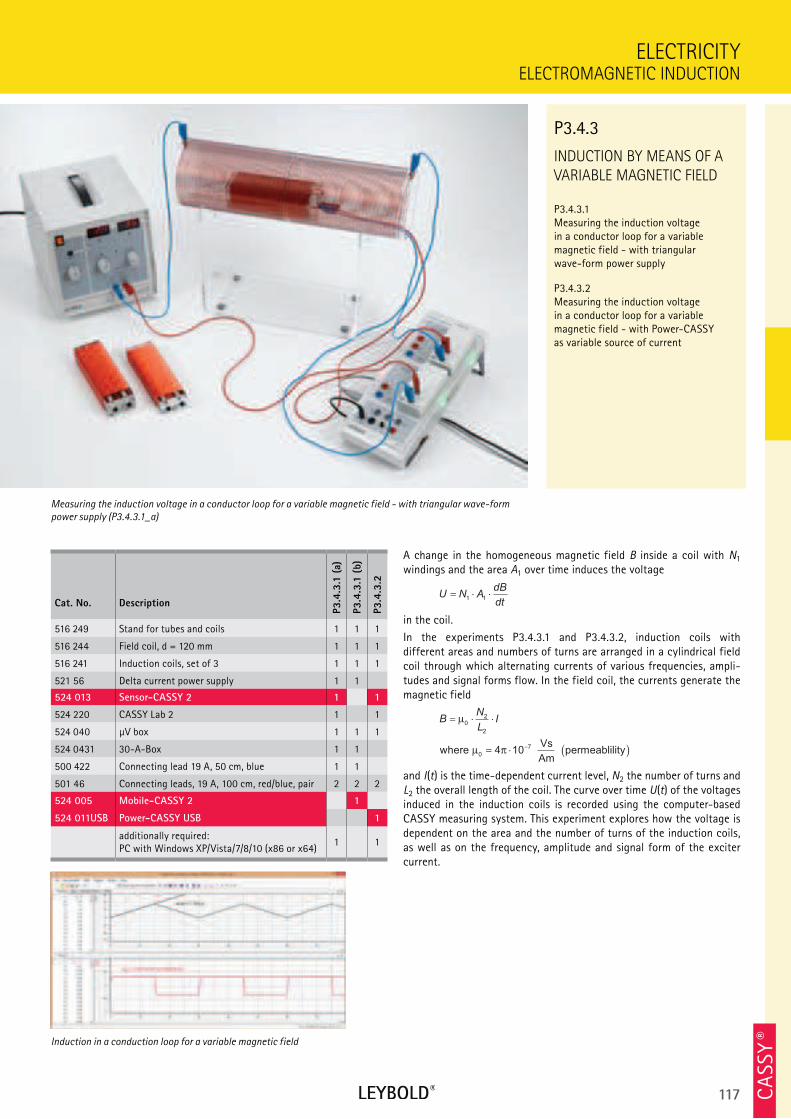
117 CA
SSY ®
INDUCTION BY MEANS OF A
VARIABLE MAGNETIC FIELD
P3.4.3.1 Measuring the induction voltage in a conductor loop for a variable magnetic field - with triangular wave-form power supply
P3.4.3.2 Measuring the induction voltage in a conductor loop for a variable magnetic field - with Power-CASSY as variable source of current
ELECTROMAGNETIC INDUCTION
ELECTRICITY
Cat. No. Description
P3.4
.3.1
(a)
P3.4
.3.1
(b)
P3.4
.3.2
516 249 Stand for tubes and coils 1 1 1
516 244 Field coil, d = 120 mm 1 1 1
516 241 Induction coils, set of 3 1 1 1
521 56 Delta current power supply 1 1
524 013 Sensor-CASSY 2 1 1
524 220 CASSY Lab 2 1 1
524 040 µV box 1 1 1
524 0431 30-A-Box 1 1
500 422 Connecting lead 19 A, 50 cm, blue 1 1
501 46 Connecting leads, 19 A, 100 cm, red/blue, pair 2 2 2
524 005 Mobile-CASSY 2 1
524 011USB Power-CASSY USB 1
additionally required: PC with Windows XP/Vista/7/8/10 (x86 or x64)
1 1
A change in the homogeneous magnetic field B inside a coil with N1 windings and the area A1 over time induces the voltage
U N AdB
dt= ⋅ ⋅
1 1
in the coil.
In the experiments P3.4.3.1 and P3.4.3.2, induction coils with different areas and numbers of turns are arranged in a cylindrical field coil through which alternating currents of various frequencies, ampli-tudes and signal forms flow. In the field coil, the currents generate the magnetic field
BN
LI= ⋅ ⋅
= ⋅ ( )−
µ
µ π
02
2
0
74 10where Vs
Am permeablility
and I(t) is the time-dependent current level, N2 the number of turns and L2 the overall length of the coil. The curve over time U(t) of the voltages induced in the induction coils is recorded using the computer-based CASSY measuring system. This experiment explores how the voltage is dependent on the area and the number of turns of the induction coils, as well as on the frequency, amplitude and signal form of the exciter current.
Measuring the induction voltage in a conductor loop for a variable magnetic field - with triangular wave-form
power supply (P3.4.3.1_a)
P3.4.3
Induction in a conduction loop for a variable magnetic field
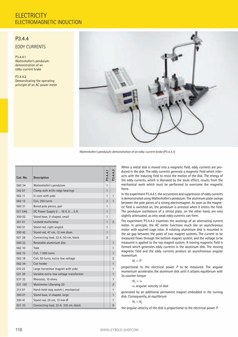
118 WWW.LEYBOLD-SHOP.COM
EDDY CURRENTS
P3.4.4.1
Waltenhofen’s pendulum:
demonstration of an
eddy-current brake
P3.4.4.2
Demonstrating the operating
principle of an AC power meter
When a metal disk is moved into a magnetic field, eddy currents are pro-
duced in the disk. The eddy currents generate a magnetic field which inter-
acts with the inducing field to resist the motion of the disk. The energy of
the eddy currents, which is liberated by the Joule effect, results from the
mechanical work which must be performed to overcome the magnetic
force.
In the experiment P3.4.4.1, the occurrence and suppression of eddy currents
is demonstrated using Waltenhofen’s pendulum. The aluminum plate swings
between the pole pieces of a strong electromagnet. As soon as the magne-
tic field is switched on, the pendulum is arrested when it enters the field.
The pendulum oscillations of a slitted plate, on the other hand, are only
slightly attenuated, as only weak eddy currents can form.
The experiment P3.4.4.2 examines the workings of an alternating current
meter. In principle, the AC meter functions much like an asynchronous
motor with squirrel-cage rotor. A rotating aluminium disk is mounted in
the air gap between the poles of two magnet systems. The current to be
measured flows through the bottom magnet system, and the voltage to be
measured is applied to the top magnet system. A moving magnetic field is
formed which generates eddy currents in the aluminum disk. The moving
magnetic field and the eddy currents produce an asynchronous angular
momentum
N P1
proportional to the electrical power P to be measured. The angular
momentum accelerates the aluminum disk until it attains equilibrium with
its counter-torque
N2 ∝ ω
ω: angular velocity of disk
generated by an additional permanent magnet embedded in the turning
disk. Consequently, at equilibrium
N N1 2
the angular velocity of the disk is proportional to the electrical power P.
ELECTRICITY
Waltenhofen’s pendulum: demonstration of an eddy-current brake (P3.4.4.1)
Cat. No. Description
P3.4
.4.1
P3.4
.4.2
560 34 Waltenhofen‘s pendulum 1
342 07 Clamp with knife-edge bearings 1
562 11 U-core with yoke 1 1
562 13 Coil, 250 turns 2 1
560 31 Bored pole pieces, pair 1
521 546 DC Power Supply 0 ... 16 V, 0 ... 5 A 1
300 02 Stand base, V-shaped, small 1
301 01 Leybold multiclamp 1 2
300 51 Stand rod, right-angled 1
300 42 Stand rod, 47 cm, 12 mm diam. 1
501 28 Connecting lead, 32 A, 50 cm, black 3
560 32 Rotatable aluminium disc 1
562 10 Yoke 1
562 15 Coil, 1 000 turns 1
562 18 Coil, 50 turns, extra-low voltage 2
562 34 Coil holder 1
510 22 Large horseshoe magnet with yoke 1
521 39 Variable extra-low voltage transformer 1
537 32 Rheostat, 10 ohms 1
531 120 Multimeter LDanalog 20 2
313 07 Hand-held stop watch I, mechanical 1
300 01 Stand base, V-shaped, large 1
300 41 Stand rod, 25 cm, 12 mm Ø 1
501 33 Connecting lead, 32 A, 100 cm, black 9
ELECTROMAGNETIC INDUCTION
P3.4.4
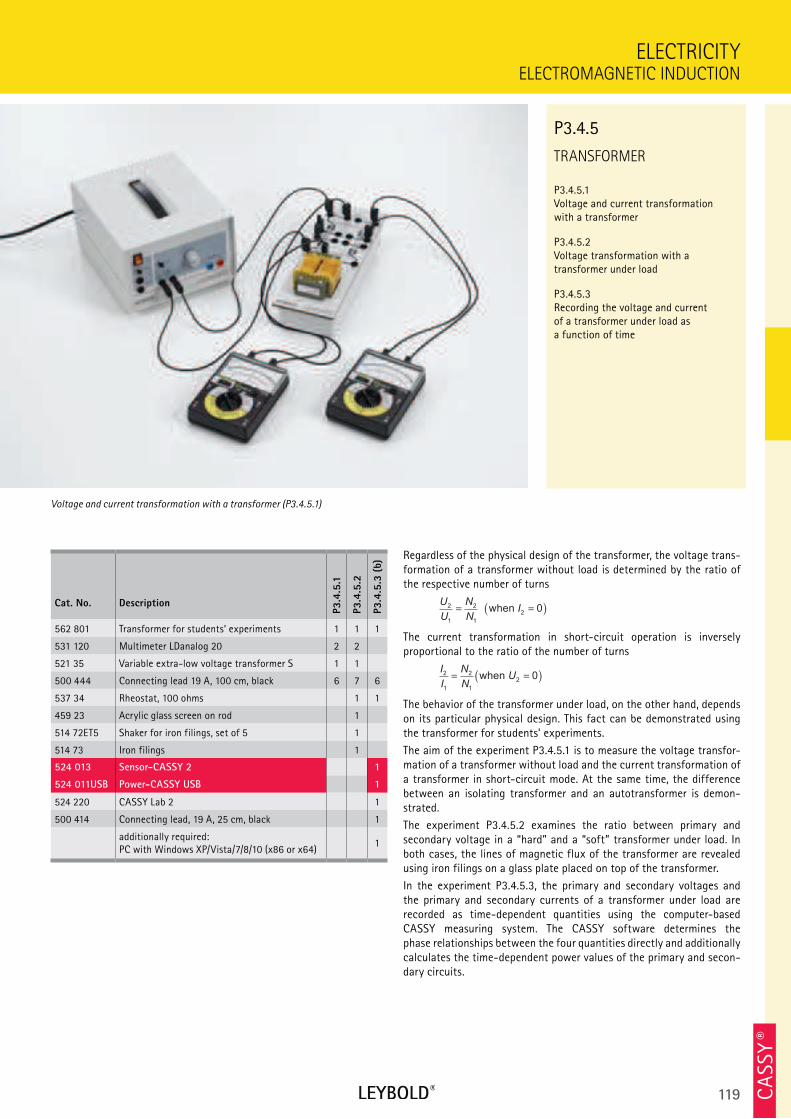
119 CA
SSY ®
TRANSFORMER
P3.4.5.1 Voltage and current transformation with a transformer
P3.4.5.2 Voltage transformation with a transformer under load
P3.4.5.3 Recording the voltage and current of a transformer under load as a function of time
ELECTROMAGNETIC INDUCTION
ELECTRICITY
Cat. No. Description
P3.4
.5.1
P3.4
.5.2
P3.4
.5.3
(b)
562 801 Transformer for students‘ experiments 1 1 1
531 120 Multimeter LDanalog 20 2 2
521 35 Variable extra-low voltage transformer S 1 1
500 444 Connecting lead 19 A, 100 cm, black 6 7 6
537 34 Rheostat, 100 ohms 1 1
459 23 Acrylic glass screen on rod 1
514 72ET5 Shaker for iron filings, set of 5 1
514 73 Iron filings 1
524 013 Sensor-CASSY 2 1
524 011USB Power-CASSY USB 1
524 220 CASSY Lab 2 1
500 414 Connecting lead, 19 A, 25 cm, black 1
additionally required: PC with Windows XP/Vista/7/8/10 (x86 or x64)
1
Regardless of the physical design of the transformer, the voltage trans-formation of a transformer without load is determined by the ratio of the respective number of turns
U
U
N
NI
2
1
2
1
20= =( ) when
The current transformation in short-circuit operation is inversely proportional to the ratio of the number of turns
I
I
N
NU
2
1
2
1
20= =( )when
The behavior of the transformer under load, on the other hand, depends on its particular physical design. This fact can be demonstrated using the transformer for students’ experiments.
The aim of the experiment P3.4.5.1 is to measure the voltage transfor-mation of a transformer without load and the current transformation of a transformer in short-circuit mode. At the same time, the difference between an isolating transformer and an autotransformer is demon-strated.
The experiment P3.4.5.2 examines the ratio between primary and secondary voltage in a “hard” and a “soft” transformer under load. In both cases, the lines of magnetic flux of the transformer are revealed using iron filings on a glass plate placed on top of the transformer.
In the experiment P3.4.5.3, the primary and secondary voltages and the primary and secondary currents of a transformer under load are recorded as time-dependent quantities using the computer-based CASSY measuring system. The CASSY software determines the phase relationships between the four quantities directly and additionally calculates the time-dependent power values of the primary and secon-dary circuits.
Voltage and current transformation with a transformer (P3.4.5.1)
P3.4.5
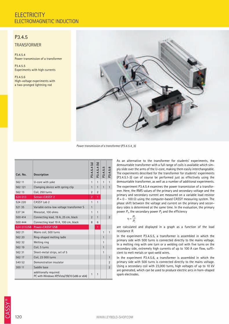
120 WWW.LEYBOLD-SHOP.COMCA
SSY ®
TRANSFORMER
P3.4.5.4 Power transmission of a transformer
P3.4.5.5 Experiments with high currents
P3.4.5.6 High-voltage experiments with a two-pronged lightning rod
ELECTRICITY
Power transmission of a transformer (P3.4.5.4_b)
Cat. No. Description
P3.4
.5.4
(a)
P3.4
.5.4
(b)
P3.4
.5.5
P3.4
.5.6
562 11 U-core with yoke 1 1 1 1
562 121 Clamping device with spring clip 1 1 1 1
562 13 Coil, 250 turns 2 2
524 013 Sensor-CASSY 2 2 1
524 220 CASSY Lab 2 1 1
521 35 Variable extra-low voltage transformer S 1
537 34 Rheostat, 100 ohms 1 1
500 414 Connecting lead, 19 A, 25 cm, black 2 1 2
500 444 Connecting lead 19 A, 100 cm, black 8 6
524 011USB Power-CASSY USB 1
562 21 Mains coil, 500 turns 1 1
562 20 Ring-shaped melting ladle 1
562 32 Melting ring 1
562 19 Coil, 5 turns 1
562 31 Sheet-metal strips, set of 5 1
562 17 Coil, 23 000 turns 1
540 52 Demonstration insulator 2
300 11 Saddle base 2
additionally required: PC with Windows XP/Vista/7/8/10 (x86 or x64)
1 1
ELECTROMAGNETIC INDUCTION
P3.4.5
As an alternative to the transformer for students’ experiments, the demountable transformer with a full range of coils is available which sim-ply slide over the arms of the U-core, making them easily interchangeable. The experiments described for the transformer for students’ experiments (P3.4.5.1-3) can of course be performed just as effectively using the demountable transformer, as well as a number of additional experiments.
The experiment P3.4.5.4 examines the power transmission of a transfor-mer. Here, the RMS values of the primary and secondary voltage and the primary and secondary current are measured on a variable load resistor R = 0 - 100 using the computer-based CASSY measuring system. The phase shift between the voltage and current on the primary and secon-dary sides is determined at the same time. In the evaluation, the primary power P1, the secondary power P2 and the efficiency
η =P
P
2
1
are calculated and displayed in a graph as a function of the load resistance R.
In the experiment P3.4.5.5, a transformer is assembled in which the primary side with 500 turns is connected directly to the mains voltage. In a melting ring with one turn or a welding coil with five turns on the secondary side, extremely high currents of up to 100 A can flow, suffi-cient to melt metals or spot-weld wires.
In the experiment P3.4.5.6, a transformer is assembled in which the primary side with 500 turns is connected directly to the mains voltage. Using a secondary coil with 23,000 turns, high voltages of up to 10 kV are generated, which can be used to produce electric arcs in horn-shaped spark electrodes.
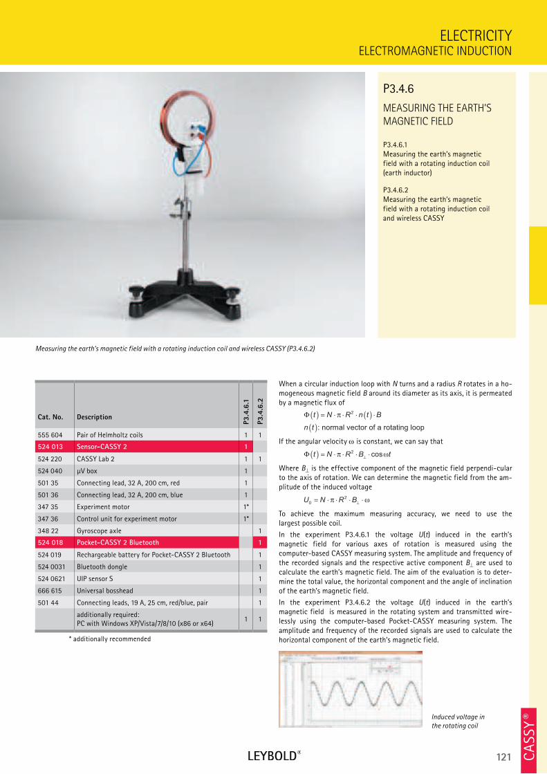
121 CA
SSY ®
MEASURING THE EARTH’S
MAGNETIC FIELD
P3.4.6.1 Measuring the earth’s magnetic field with a rotating induction coil (earth inductor)
P3.4.6.2 Measuring the earth’s magnetic field with a rotating induction coil and wireless CASSY
ELECTROMAGNETIC INDUCTION
ELECTRICITY
Cat. No. Description
P3.4
.6.1
P3.4
.6.2
555 604 Pair of Helmholtz coils 1 1
524 013 Sensor-CASSY 2 1
524 220 CASSY Lab 2 1 1
524 040 µV box 1
501 35 Connecting lead, 32 A, 200 cm, red 1
501 36 Connecting lead, 32 A, 200 cm, blue 1
347 35 Experiment motor 1*
347 36 Control unit for experiment motor 1*
348 22 Gyroscope axle 1
524 018 Pocket-CASSY 2 Bluetooth 1
524 019 Rechargeable battery for Pocket-CASSY 2 Bluetooth 1
524 0031 Bluetooth dongle 1
524 0621 UIP sensor S 1
666 615 Universal bosshead 1
501 44 Connecting leads, 19 A, 25 cm, red/blue, pair 1
additionally required: PC with Windows XP/Vista/7/8/10 (x86 or x64)
1 1
* additionally recommended
When a circular induction loop with N turns and a radius R rotates in a ho-mogeneous magnetic field B around its diameter as its axis, it is permeated by a magnetic flux of
Φ t N R n t B
n t
( ) = ⋅ ⋅ ⋅ ( ) ⋅
( )
π 2
: normal vector of a rotating loop
If the angular velocity is constant, we can say that
Φ t N R B t( ) = ⋅ ⋅ ⋅ ⋅⊥
π ω2cos
Where B is the effective component of the magnetic field perpendi-cular to the axis of rotation. We can determine the magnetic field from the am-plitude of the induced voltage
U N R B0
2= ⋅ ⋅ ⋅ ⋅
⊥π ω
To achieve the maximum measuring accuracy, we need to use the largest possible coil.
In the experiment P3.4.6.1 the voltage U(t) induced in the earth’s magnetic field for various axes of rotation is measured using the computer-based CASSY measuring system. The amplitude and frequency of the recorded signals and the respective active component B are used to calculate the earth’s magnetic field. The aim of the evaluation is to deter-mine the total value, the horizontal component and the angle of inclination of the earth’s magnetic field.
In the experiment P3.4.6.2 the voltage U(t) induced in the earth’s magnetic field is measured in the rotating system and transmitted wire-lessly using the computer-based Pocket-CASSY measuring system. The amplitude and frequency of the recorded signals are used to calculate the horizontal component of the earth‘s magnetic field.
Measuring the earth’s magnetic field with a rotating induction coil and wireless CASSY (P3.4.6.2)
P3.4.6
Induced voltage in
the rotating coil
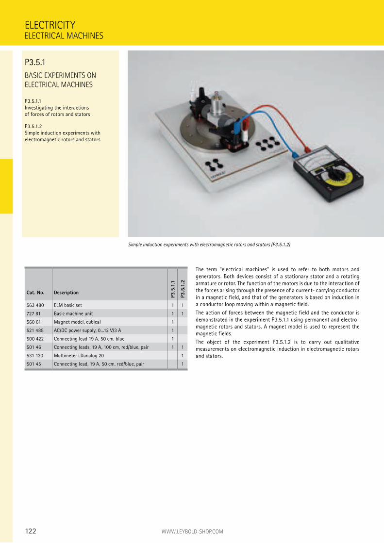
122 WWW.LEYBOLD-SHOP.COM
BASIC EXPERIMENTS ON
ELECTRICAL MACHINES
P3.5.1.1 Investigating the interactions of forces of rotors and stators
P3.5.1.2 Simple induction experiments with electromagnetic rotors and stators
The term “electrical machines” is used to refer to both motors and generators. Both devices consist of a stationary stator and a rotating armature or rotor. The function of the motors is due to the interaction of the forces arising through the presence of a current- carrying conductor in a magnetic field, and that of the generators is based on induction in a conductor loop moving within a magnetic field.
The action of forces between the magnetic field and the conductor is demonstrated in the experiment P3.5.1.1 using permanent and electro-magnetic rotors and stators. A magnet model is used to represent the magnetic fields.
The object of the experiment P3.5.1.2 is to carry out qualitative measurements on electromagnetic induction in electromagnetic rotors and stators.
ELECTRICITY
Simple induction experiments with electromagnetic rotors and stators (P3.5.1.2)
Cat. No. Description
P3.5
.1.1
P3.5
.1.2
563 480 ELM basic set 1 1
727 81 Basic machine unit 1 1
560 61 Magnet model, cubical 1
521 485 AC/DC power supply, 0...12 V/3 A 1
500 422 Connecting lead 19 A, 50 cm, blue 1
501 46 Connecting leads, 19 A, 100 cm, red/blue, pair 1 1
531 120 Multimeter LDanalog 20 1
501 45 Connecting lead, 19 A, 50 cm, red/blue, pair 1
ELECTRICAL MACHINES
P3.5.1
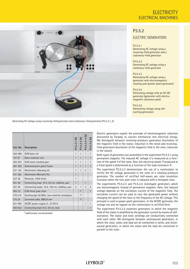
123
ELECTRIC GENERATORS
P3.5.2.1 Generating AC voltage using a revolving-field generator and a stationary-field generator
P3.5.2.2 Generating DC voltage using a stationary-field generator
P3.5.2.3 Generating AC voltage using a generator with electromagnetic rotating pole (power-plant generator)
P3.5.2.4 Generating voltage with an AC-DC generator (generator with electro-magnetic stationary pole)
P3.5.2.5 Generating voltage using self- exciting generators
ELECTRICAL MACHINES
ELECTRICITY
Cat. No. Description
P3.5
.2.1
(b)
P3.5
.2.2
(b)
P3.5
.2.3
-4 (
b)
P3.5
.2.5
(b)
563 480 ELM basic set 1 1 1 1
727 81 Basic machine unit 1 1 1 1
563 303 ELM hand-cranked gear 1 1 1 1
301 300 Demonstration panel frame 1 1 1 1
531 120 Multimeter LDanalog 20 1 1 2 1
531 282 Multimeter Metrahit Pro 1
537 36 Rheostat, 1000 ohms 1
501 45 Connecting lead, 19 A, 50 cm, red/blue, pair 1 1
501 46 Connecting leads, 19 A, 100 cm, red/blue, pair 2 1 2 2
563 23 ELM three-pole rotor 1* 1
575 214 Oscilloscope 30 MHz, two-channel, analogous 1*
575 24 Screened cable, BNC/4 mm 1*
521 485 AC/DC power supply, 0...12 V/3 A 1 1
500 422 Connecting lead 19 A, 50 cm, blue 1
* additionally recommended
Electric generators exploit the principle of electromagnetic induction discovered by Faraday to convert mechanical into electrical energy. We distinguish between revolving-armature generators (excitation of the magnetic field in the stator, induction in the rotor) and revolving-field generators (excitation of the magnetic field in the rotor, induction in the stator).
Both types of generators are assembled in the experiment P3.5.2.1 using permanent magnets. The induced AC voltage U is measured as a func-tion of the speed f of the rotor. Also, the electrical power P produced at a fixed speed is determined as a function of the load resistance R.
The experiment P3.5.2.2 demonstrates the use of a commutator to rectify the AC voltage generated in the rotor of a rotating-armature generator. The number of rectified half-waves per rotor revolution increases when the two-pole rotor is replaced with a threepole rotor.
The experiments P3.5.2.3 and P3.5.2.4 investigate generators which use electromagnets instead of permanent magnets. Here, the induced voltage depends on the excitation current of the magnetic field. The excitation current can be used to vary the generated power without changing the speed of the rotor or the frequency of the AC voltage. This principle is used in power-plant generators. In the AC/DC generator, the voltage can also be tapped via the commutator in rectified form.
The experiment P3.5.2.5 examines generators in which the magnetic field of the stator is amplified by the generator current by means of self-excitation. The stator and rotor windings are conductively connected with each other. We distinguish between serieswound generators, in which the rotor, stator and load are all connected in series, and shunt-wound generators, in which the stator and the load are connected in parallel to the rotor.
Generating AC voltage using a revolving-field generator and a stationary-field generator (P3.5.2.1_b)
P3.5.2
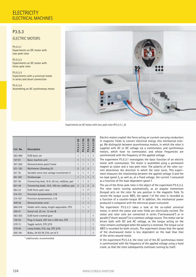
124 WWW.LEYBOLD-SHOP.COM
ELECTRIC MOTORS
P3.5.3.1 Experiments on DC motor with two-pole rotor
P3.5.3.2 Experiments on DC motor with three-pole rotor
P3.5.3.3 Experiments with a universal motor in series and shunt connection
P3.5.3.4 Assembling an AC synchronous motor
Electric motors exploit the force acting on current-carrying conductors in magnetic fields to convert electrical energy into mechanical ener-gy. We distinguish between asynchronous motors, in which the rotor is supplied with AC or DC voltage via a commutator, and synchronous motors, which have no commutator, and whose frequencies are synchronized with the frequency of the applied voltage.
The experiment P3.5.3.1 investigates the basic function of an electric motor with commutator. The motor is assembled using a permanent magnet as stator and a two-pole rotor. The polarity of the rotor cur-rent determines the direction in which the rotor turns. This experi-ment measures the relationship between the applied voltage U and the no-load speed f0 as well as, at a fixed voltage, the current I consumed as a function of the load-dependent speed f.
The use of the three-pole rotor is the object of the experiment P3.5.3.2. The rotor starts turning automatically, as an angular momentum (torque) acts on the rotor for any position in the magnetic field. To record the torque curve M(f ), the speed f of the rotor is recorded as a function of a counter-torque M. In addition, the mechanical power produced is compared with the electrical power consumed.
The experiment P3.5.3.3 takes a look at the so-called universal motor, in which the stator and rotor fields are electrically excited. The stator and rotor coils are connected in series (“serieswound”) or in parallel (“shunt-wound”) to a common voltage source. This motor can be driven both with DC and AC voltage, as the torque acting on the rotor remains unchanged when the polarity is reversed. The torque curve M(f ) is recorded for both circuits. The experiment shows that the speed of the shuntwound motor is less dependent on the load than that of the series-wound motor.
In the experiment P3.5.3.4, the rotor coil of the AC synchronous motor is synchronized with the frequency of the applied voltage using a hand crank, so that the rotor subsequently continues running by itself.
ELECTRICITY
Experiments on DC motor with two-pole rotor (P3.5.3.1_b)
Cat. No. Description
P3.5
.3.1
(b)
P3.5
.3.2
(b)
P3.5
.3.3
(b)
P3.5
.3.4
(b)
563 480 ELM basic set 1 1 1 1
727 81 Basic machine unit 1 1 1 1
301 300 Demonstration panel frame 1 1 1 1
531 120 Multimeter LDanalog 20 2 2 2
521 35 Variable extra-low voltage transformer S 1 1 1 1
451 281 Stroboscope 1 1 1 1
501 45 Connecting lead, 19 A, 50 cm, red/blue, pair 1 1 2
501 46 Connecting leads, 19 A, 100 cm, red/blue, pair 2 2 2 2
563 23 ELM three-pole rotor 1 1*
314 151 Precision dynamometer, 2 N 1 1
314 161 Precision dynamometer, 5 N 1 1
309 50 Demonstration cord 1 1
666 470 Holder with clamp, height-adjustable, CPS 1 1
300 41 Stand rod, 25 cm, 12 mm Ø 1 1
563 303 ELM hand-cranked gear 1
726 50 Plug-in board, 297 mm x 300 mm, STE 1
579 13 Toggle switch, STE 2/19 1
579 06 Lamp holder, E10, top, STE 2/19 1
505 181 Bulbs, 24 V/3 W, E10, set of 5 1
* additionally recommended
ELECTRICAL MACHINES
P3.5.3
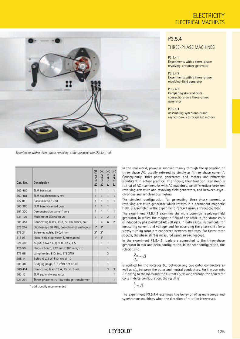
125
THREE-PHASE MACHINES
P3.5.4.1 Experiments with a three-phase revolving-armature generator
P3.5.4.2 Experiments with a three-phase revolving-field generator
P3.5.4.3 Comparing star and delta connections on a three-phase generator
P3.5.4.4 Assembling synchronous and asynchronous three-phase motors
ELECTRICAL MACHINES
ELECTRICITY
Cat. No. Description
P3.5
.4.1
(b)
P3.5
.4.2
(b)
P3.5
.4.3
(b)
P3.5
.4.4
(b)
563 480 ELM basic set 1 1 1 1
563 481 ELM supplementary set 1 1 1 1
727 81 Basic machine unit 1 1 1 1
563 303 ELM hand-cranked gear 1 1 1
301 300 Demonstration panel frame 1 1 1 1
531 120 Multimeter LDanalog 20 3 3 2 1
501 451 Connecting leads, 19 A, 50 cm, black, pair 3 4 6 2
575 214 Oscilloscope 30 MHz, two-channel, analogous 1* 1*
575 24 Screened cable, BNC/4 mm 2* 2*
313 07 Hand-held stop watch I, mechanical 1* 1*
521 485 AC/DC power supply, 0...12 V/3 A 1 1
726 50 Plug-in board, 297 mm x 300 mm, STE 1
579 06 Lamp holder, E10, top, STE 2/19 3
505 14 Bulbs, 6 V/3 W, E10, set of 10 1
501 48 Bridging plugs, STE 2/19, set of 10 1
500 414 Connecting lead, 19 A, 25 cm, black 3 3
563 12 ELM squirrel-cage rotor 1
521 291 Three-phase extra-low voltage transformer 1
* additionally recommended
In the real world, power is supplied mainly through the generation of three-phase AC, usually referred to simply as “three-phase current”. Consequently, three-phase generators and motors are extremely significant in actual practice. In principle, their function is analogous to that of AC machines. As with AC machines, we differentiate between revolving-armature and revolving-field generators, and between asyn-chronous and synchronous motors.
The simplest configuration for generating three-phase current, a revolving-armature generator which rotates in a permanent magnetic field, is assembled in the experiment P3.5.4.1 using a threepole rotor.
The experiment P3.5.4.2 examines the more common revolving-field generator, in which the magnetic field of the rotor in the stator coils is induced by phase-shifted AC voltages. In both cases, instruments for measuring current and voltage, and for observing the phase shift for a slowly turning rotor, are connected between two taps. For faster rotor speeds, the phase shift is measured using an oscilloscope.
In the experiment P3.5.4.3, loads are connected to the three-phase generator in star and delta configuration. In the star configuration, the relationship
U
U
aa
a0
3
is verified for the voltages Uaa between any two outer conductors as well as Ua0 between the outer and neutral conductors. For the currents I1 flowing to the loads and the currents I2 flowing through the generator coils in delta configuration, the result is
I
I
1
2
3
The experiment P3.5.4.4 examines the behavior of asynchronous and synchronous machines when the direction of rotation is reversed.
Experiments with a three-phase revolving-armature generator (P3.5.4.1_b)
P3.5.4
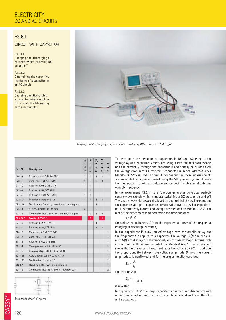
126 WWW.LEYBOLD-SHOP.COMCA
SSY ®
CIRCUIT WITH CAPACITOR
P3.6.1.1 Charging and discharging a capacitor when switching DC on and off
P3.6.1.2 Determining the capacitive reactance of a capacitor in an AC circuit
P3.6.1.3 Charging and discharging a capacitor when switching DC on and off - Measuring with a mutlimeter
To investigate the behavior of capacitors in DC and AC circuits, the voltage UC at a capacitor is measured using a two-channel oscilloscope, and the current IC through the capacitor is additionally calculated from the voltage drop across a resistor R connected in series. Alternatively a Mobile-CASSY 2 is used. The circuits for conducting these measurements are assembled on a plug-in board using the STE plug-in system. A func-tion generator is used as a voltage source with variable amplitude and variable frequency.
In the experiment P3.6.1.1, the function generator generates periodic square-wave signals which simulate switching a DC voltage on and off. The square-wave signals are displayed on channel I of the oscilloscope, and the capacitor voltage or capacitor current is displayed on oscilloscope chan-nel II. Alternatively current and voltage are recorded by Mobile-CASSY. The aim of the experiment is to determine the time constant
τ = ⋅R C
for various capacitances C from the exponential curve of the respective charging or discharge current IC.
In the experiment P3.6.1.2, an AC voltage with the amplitude U0 and the frequency f is applied to a capacitor. The voltage UC(t) and the cur-rent IC(t) are displayed simultaneously on the oscilloscope. Alternatively current and voltage are recorded by Mobile-CASSY. The experiment shows that in this circuit the current leads the voltage by 90°. In addition, the proportionality between the voltage amplitude U0 and the current amplitude I0 is confirmed, and for the proportionality constant
ZU
IC
0
0
the relationship
Zf C
C= −
⋅
1
2π
is revealed.
In experiment P3.6.1.3 a large capacitor is charged and discharged with a long time constant and the process can be recorded with a multimeter and a stopclock.
ELECTRICITY
Charging and discharging a capacitor when switching DC on and off (P3.6.1.1_a)
Cat. No. Description
P3.6
.1.1
(a)
P3.6
.1.1
(b)
P3.6
.1.2
(a)
P3.6
.1.2
(b)
P3.6
.1.3
576 74 Plug-in board, DIN A4, STE 1 1 1 1 1
578 15 Capacitor, 1 µF, STE 2/19 3 3 3 3
577 40 Resistor, 470 , STE 2/19 1 1
577 44 Resistor, 1 k , STE 2/19 1 1
577 48 Resistor, 2.2 k , STE 2/19 1 1
522 621 Function generator S 12 1 1 1 1
575 214 Oscilloscope 30 MHz, two-channel, analogous 1 1
575 24 Screened cable, BNC/4 mm 2 2
501 46 Connecting leads, 19 A, 100 cm, red/blue, pair 1 3 1 3
524 005 Mobile-CASSY 2 1 1
577 19 Resistor, 1 , STE 2/19 1
577 20 Resistor, 10 , STE 2/19 1 1
578 16 Capacitor, 4.7 µF, STE 2/19 1
578 12 Capacitor, 10 µF, STE 2/50 1
577 76 Resistor, 1 M , STE 2/19 1
582 81 Change-over switch, STE 4/50 1
501 48 Bridging plugs, STE 2/19, set of 10 1
521 485 AC/DC power supply, 0...12 V/3 A 1
531 120 Multimeter LDanalog 20 1
313 07 Hand-held stop watch I, mechanical 1
501 45 Connecting lead, 19 A, 50 cm, red/blue, pair 2
Schematic circuit diagram
DC AND AC CIRCUITS
P3.6.1
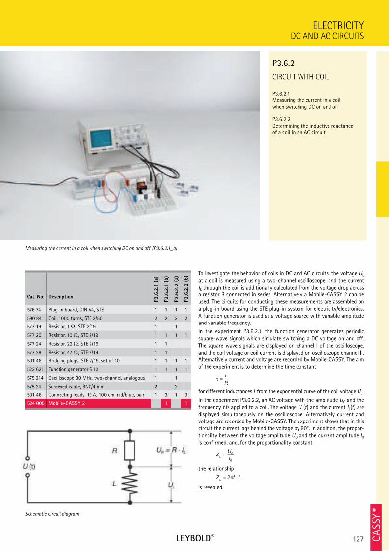
127 CA
SSY ®
CIRCUIT WITH COIL
P3.6.2.1 Measuring the current in a coil when switching DC on and off
P3.6.2.2 Determining the inductive reactance of a coil in an AC circuit
DC AND AC CIRCUITS
ELECTRICITY
Cat. No. Description
P3.6
.2.1
(a)
P3.6
.2.1
(b)
P3.6
.2.2
(a)
P3.6
.2.2
(b)
576 74 Plug-in board, DIN A4, STE 1 1 1 1
590 84 Coil, 1000 turns, STE 2/50 2 2 2 2
577 19 Resistor, 1 , STE 2/19 1 1
577 20 Resistor, 10 , STE 2/19 1 1 1 1
577 24 Resistor, 22 , STE 2/19 1 1
577 28 Resistor, 47 , STE 2/19 1 1
501 48 Bridging plugs, STE 2/19, set of 10 1 1 1 1
522 621 Function generator S 12 1 1 1 1
575 214 Oscilloscope 30 MHz, two-channel, analogous 1 1
575 24 Screened cable, BNC/4 mm 2 2
501 46 Connecting leads, 19 A, 100 cm, red/blue, pair 1 3 1 3
524 005 Mobile-CASSY 2 1 1
To investigate the behavior of coils in DC and AC circuits, the voltage UL at a coil is measured using a two-channel oscilloscope, and the current IL through the coil is additionally calculated from the voltage drop across a resistor R connected in series. Alternatively a Mobile-CASSY 2 can be used. The circuits for conducting these measurements are assembled on a plug-in board using the STE plug-in system for electricity/electronics. A function generator is used as a voltage source with variable amplitude and variable frequency.
In the experiment P3.6.2.1, the function generator generates periodic square-wave signals which simulate switching a DC voltage on and off. The square-wave signals are displayed on channel I of the oscilloscope, and the coil voltage or coil current is displayed on oscilloscope channel II. Alternatively current and voltage are recorded by Mobile-CASSY. The aim of the experiment is to determine the time constant
τ =L
R
for different inductances L from the exponential curve of the coil voltage UL.
In the experiment P3.6.2.2, an AC voltage with the amplitude U0 and the frequency f is applied to a coil. The voltage UL(t) and the current IL(t) are displayed simultaneously on the oscilloscope. Alternatively current and voltage are recorded by Mobile-CASSY. The experiment shows that in this circuit the current lags behind the voltage by 90°. In addition, the propor-tionality between the voltage amplitude U0 and the current amplitude I0 is confirmed, and, for the proportionality constant
ZU
IL
0
0
the relationship
Z f LL= ⋅2π
is revealed.
Measuring the current in a coil when switching DC on and off (P3.6.2.1_a)
P3.6.2
Schematic circuit diagram
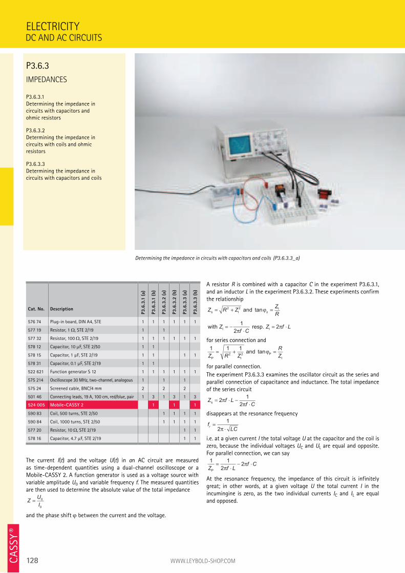
128 WWW.LEYBOLD-SHOP.COMCA
SSY ®
A resistor R is combined with a capacitor C in the experiment P3.6.3.1, and an inductor L in the experiment P3.6.3.2. These experiments confirm the relationship
Z R ZZ
Rss I
I and = + =2 2
tanϕ
with resp. I IZf C
Z f L= −⋅
= ⋅1
22
ππ
for series connection and
1 1 1
2 2Z R Z
R
ZP I
P
I
and = + =tanϕ
for parallel connection.
The experiment P3.6.3.3 examines the oscillator circuit as the series and parallel connection of capacitance and inductance. The total impedance of the series circuit
Z f Lf C
s= ⋅ −
⋅2
1
2π
π
disappears at the resonance frequency
fLC
r=
⋅
1
2π
i.e. at a given current I the total voltage U at the capacitor and the coil is zero, because the individual voltages UC and UL are equal and opposite. For parallel connection, we can say1 1
22
Z f Lf C
P
=⋅
− ⋅π
π
At the resonance frequency, the impedance of this circuit is infinitely great; in other words, at a given voltage U the total current I in the incumingine is zero, as the two individual currents IC and IL are equal and opposed.
IMPEDANCES
P3.6.3.1 Determining the impedance in circuits with capacitors and ohmic resistors
P3.6.3.2 Determining the impedance in circuits with coils and ohmic resistors
P3.6.3.3 Determining the impedance in circuits with capacitors and coils
ELECTRICITY
Determining the impedance in circuits with capacitors and coils (P3.6.3.3_a)
Cat. No. Description
P3.6
.3.1
(a)
P3.6
.3.1
(b)
P3.6
.3.2
(a)
P3.6
.3.2
(b)
P3.6
.3.3
(a)
P3.6
.3.3
(b)
576 74 Plug-in board, DIN A4, STE 1 1 1 1 1 1
577 19 Resistor, 1 , STE 2/19 1 1
577 32 Resistor, 100 , STE 2/19 1 1 1 1 1 1
578 12 Capacitor, 10 µF, STE 2/50 1 1
578 15 Capacitor, 1 µF, STE 2/19 1 1 1 1
578 31 Capacitor, 0.1 µF, STE 2/19 1 1
522 621 Function generator S 12 1 1 1 1 1 1
575 214 Oscilloscope 30 MHz, two-channel, analogous 1 1 1
575 24 Screened cable, BNC/4 mm 2 2 2
501 46 Connecting leads, 19 A, 100 cm, red/blue, pair 1 3 1 3 1 3
524 005 Mobile-CASSY 2 1 1 1
590 83 Coil, 500 turns, STE 2/50 1 1 1 1
590 84 Coil, 1000 turns, STE 2/50 1 1 1 1
577 20 Resistor, 10 , STE 2/19 1 1
578 16 Capacitor, 4.7 µF, STE 2/19 1 1
DC AND AC CIRCUITS
P3.6.3
The current I(t) and the voltage U(t) in an AC circuit are measured as time-dependent quantities using a dual-channel oscilloscope or a Mobile-CASSY 2. A function generator is used as a voltage source with variable amplitude U0 and variable frequency f. The measured quantities are then used to determine the absolute value of the total impedance
ZU
I
0
0
and the phase shift between the current and the voltage.
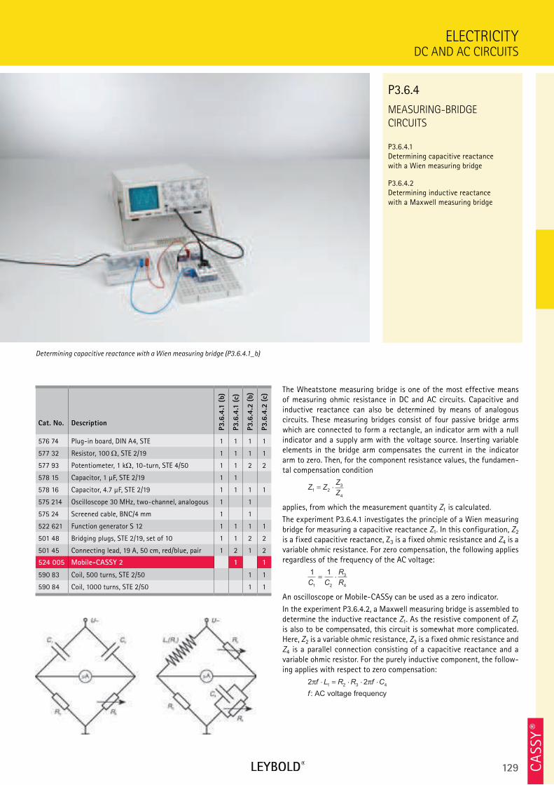
129 CA
SSY ®
MEASURING-BRIDGE
CIRCUITS
P3.6.4.1 Determining capacitive reactance with a Wien measuring bridge
P3.6.4.2 Determining inductive reactance with a Maxwell measuring bridge
DC AND AC CIRCUITS
ELECTRICITY
Cat. No. Description
P3.6
.4.1
(b)
P3.6
.4.1
(c)
P3.6
.4.2
(b)
P3.6
.4.2
(c)
576 74 Plug-in board, DIN A4, STE 1 1 1 1
577 32 Resistor, 100 , STE 2/19 1 1 1 1
577 93 Potentiometer, 1 k , 10-turn, STE 4/50 1 1 2 2
578 15 Capacitor, 1 µF, STE 2/19 1 1
578 16 Capacitor, 4.7 µF, STE 2/19 1 1 1 1
575 214 Oscilloscope 30 MHz, two-channel, analogous 1 1
575 24 Screened cable, BNC/4 mm 1 1
522 621 Function generator S 12 1 1 1 1
501 48 Bridging plugs, STE 2/19, set of 10 1 1 2 2
501 45 Connecting lead, 19 A, 50 cm, red/blue, pair 1 2 1 2
524 005 Mobile-CASSY 2 1 1
590 83 Coil, 500 turns, STE 2/50 1 1
590 84 Coil, 1000 turns, STE 2/50 1 1
The Wheatstone measuring bridge is one of the most effective means of measuring ohmic resistance in DC and AC circuits. Capacitive and inductive reactance can also be determined by means of analogous circuits. These measuring bridges consist of four passive bridge arms which are connected to form a rectangle, an indicator arm with a null indicator and a supply arm with the voltage source. Inserting variable elements in the bridge arm compensates the current in the indicator arm to zero. Then, for the component resistance values, the fundamen-tal compensation condition
Z ZZ
Z1 2
3
4
= ⋅
applies, from which the measurement quantity Z1 is calculated.
The experiment P3.6.4.1 investigates the principle of a Wien measuring bridge for measuring a capacitive reactance Z1. In this configuration, Z2 is a fixed capacitive reactance, Z3 is a fixed ohmic resistance and Z4 is a variable ohmic resistance. For zero compensation, the following applies regardless of the frequency of the AC voltage:
1 1
1 2
3
4C C
R
R= ⋅
An oscilloscope or Mobile-CASSy can be used as a zero indicator.
In the experiment P3.6.4.2, a Maxwell measuring bridge is assembled to determine the inductive reactance Z1. As the resistive component of Z1 is also to be compensated, this circuit is somewhat more complicated. Here, Z2 is a variable ohmic resistance, Z3 is a fixed ohmic resistance and Z4 is a parallel connection consisting of a capacitive reactance and a variable ohmic resistor. For the purely inductive component, the follow-ing applies with respect to zero compensation:
2 21 2 3 4π πf L R R f C
f
⋅ = ⋅ ⋅ ⋅
: AC voltage frequency
Determining capacitive reactance with a Wien measuring bridge (P3.6.4.1_b)
P3.6.4
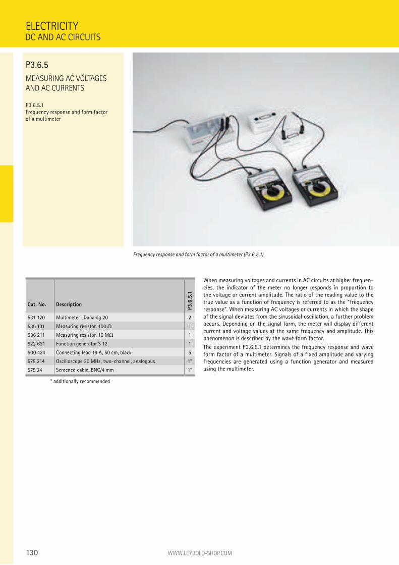
130 WWW.LEYBOLD-SHOP.COM
MEASURING AC VOLTAGES
AND AC CURRENTS
P3.6.5.1 Frequency response and form factor of a multimeter
When measuring voltages and currents in AC circuits at higher frequen-cies, the indicator of the meter no longer responds in proportion to the voltage or current amplitude. The ratio of the reading value to the true value as a function of frequency is referred to as the “frequency response”. When measuring AC voltages or currents in which the shape of the signal deviates from the sinusoidal oscillation, a further problem occurs. Depending on the signal form, the meter will display different current and voltage values at the same frequency and amplitude. This phenomenon is described by the wave form factor.
The experiment P3.6.5.1 determines the frequency response and wave form factor of a multimeter. Signals of a fixed amplitude and varying frequencies are generated using a function generator and measured using the multimeter.
ELECTRICITY
Frequency response and form factor of a multimeter (P3.6.5.1)
Cat. No. Description
P3.6
.5.1
531 120 Multimeter LDanalog 20 2
536 131 Measuring resistor, 100 1
536 211 Measuring resistor, 10 M 1
522 621 Function generator S 12 1
500 424 Connecting lead 19 A, 50 cm, black 5
575 214 Oscilloscope 30 MHz, two-channel, analogous 1*
575 24 Screened cable, BNC/4 mm 1*
* additionally recommended
DC AND AC CIRCUITS
P3.6.5
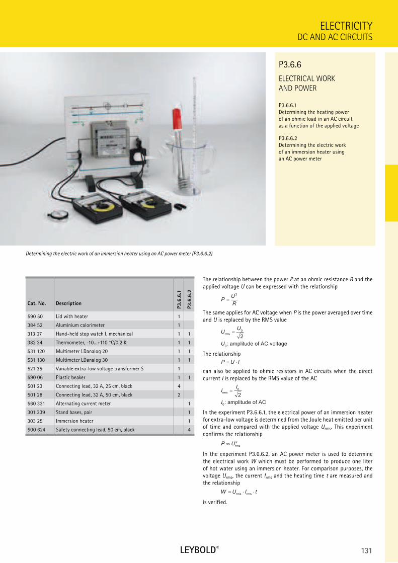
131
ELECTRICAL WORK
AND POWER
P3.6.6.1 Determining the heating power of an ohmic load in an AC circuit as a function of the applied voltage
P3.6.6.2 Determining the electric work of an immersion heater using an AC power meter
DC AND AC CIRCUITS
ELECTRICITY
Cat. No. Description
P3.6
.6.1
P3.6
.6.2
590 50 Lid with heater 1
384 52 Aluminium calorimeter 1
313 07 Hand-held stop watch I, mechanical 1 1
382 34 Thermometer, -10...+110 °C/0.2 K 1 1
531 120 Multimeter LDanalog 20 1 1
531 130 Multimeter LDanalog 30 1 1
521 35 Variable extra-low voltage transformer S 1
590 06 Plastic beaker 1 1
501 23 Connecting lead, 32 A, 25 cm, black 4
501 28 Connecting lead, 32 A, 50 cm, black 2
560 331 Alternating current meter 1
301 339 Stand bases, pair 1
303 25 Immersion heater 1
500 624 Safety connecting lead, 50 cm, black 4
Determining the electric work of an immersion heater using an AC power meter (P3.6.6.2)
P3.6.6
The relationship between the power P at an ohmic resistance R and the applied voltage U can be expressed with the relationship
PU
R
2
The same applies for AC voltage when P is the power averaged over time and U is replaced by the RMS value
UU
U
rms
: amplitude of AC voltage
0
0
2
The relationship
P U I= ⋅
can also be applied to ohmic resistors in AC circuits when the direct current I is replaced by the RMS value of the AC
II
I
rms
: amplitude of AC
0
0
2
In the experiment P3.6.6.1, the electrical power of an immersion heater for extra-low voltage is determined from the Joule heat emitted per unit of time and compared with the applied voltage Urms. This experiment confirms the relationship
P Urms
2
In the experiment P3.6.6.2, an AC power meter is used to determine the electrical work W which must be performed to produce one liter of hot water using an immersion heater. For comparison purposes, the voltage Urms, the current Irms and the heating time t are measured and the relationship
W U I t= ⋅ ⋅rms rms
is verified.
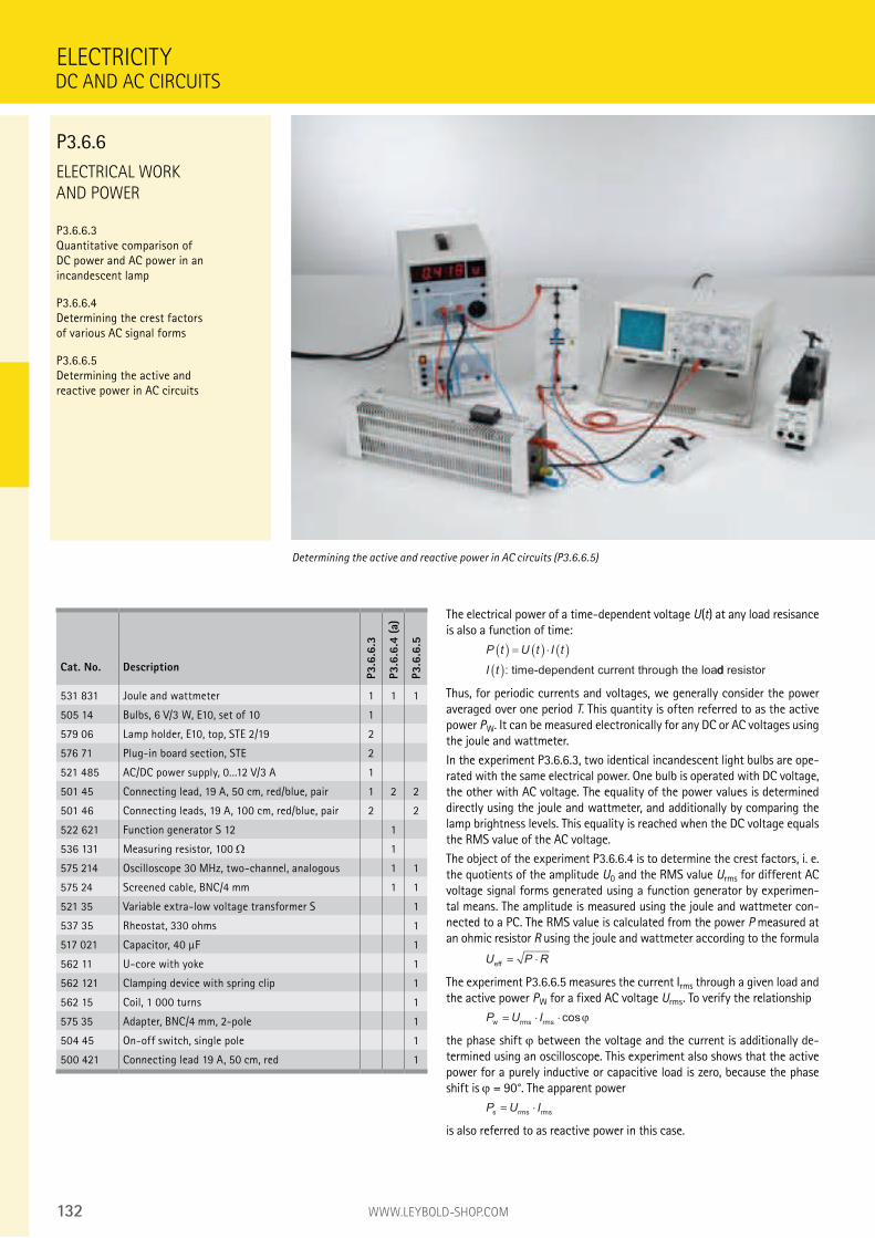
132 WWW.LEYBOLD-SHOP.COM
ELECTRICAL WORK
AND POWER
P3.6.6.3 Quantitative comparison of DC power and AC power in an incandescent lamp
P3.6.6.4 Determining the crest factors of various AC signal forms
P3.6.6.5 Determining the active and reactive power in AC circuits
ELECTRICITY
Determining the active and reactive power in AC circuits (P3.6.6.5)
Cat. No. Description
P3.6
.6.3
P3.6
.6.4
(a)
P3.6
.6.5
531 831 Joule and wattmeter 1 1 1
505 14 Bulbs, 6 V/3 W, E10, set of 10 1
579 06 Lamp holder, E10, top, STE 2/19 2
576 71 Plug-in board section, STE 2
521 485 AC/DC power supply, 0...12 V/3 A 1
501 45 Connecting lead, 19 A, 50 cm, red/blue, pair 1 2 2
501 46 Connecting leads, 19 A, 100 cm, red/blue, pair 2 2
522 621 Function generator S 12 1
536 131 Measuring resistor, 100 1
575 214 Oscilloscope 30 MHz, two-channel, analogous 1 1
575 24 Screened cable, BNC/4 mm 1 1
521 35 Variable extra-low voltage transformer S 1
537 35 Rheostat, 330 ohms 1
517 021 Capacitor, 40 µF 1
562 11 U-core with yoke 1
562 121 Clamping device with spring clip 1
562 15 Coil, 1 000 turns 1
575 35 Adapter, BNC/4 mm, 2-pole 1
504 45 On-off switch, single pole 1
500 421 Connecting lead 19 A, 50 cm, red 1
DC AND AC CIRCUITS
P3.6.6
The electrical power of a time-dependent voltage U(t) at any load resisance is also a function of time:
P t U t I t
I t
( ) = ( ) ⋅ ( )
( ): time-dependent current through the loadd resistor
Thus, for periodic currents and voltages, we generally consider the power averaged over one period T. This quantity is often referred to as the active power PW. It can be measured electronically for any DC or AC voltages using the joule and wattmeter.
In the experiment P3.6.6.3, two identical incandescent light bulbs are ope-rated with the same electrical power. One bulb is operated with DC voltage, the other with AC voltage. The equality of the power values is determined directly using the joule and wattmeter, and additionally by comparing the lamp brightness levels. This equality is reached when the DC voltage equals the RMS value of the AC voltage.
The object of the experiment P3.6.6.4 is to determine the crest factors, i. e. the quotients of the amplitude U0 and the RMS value Urms for different AC voltage signal forms generated using a function generator by experimen-tal means. The amplitude is measured using the joule and wattmeter con-nected to a PC. The RMS value is calculated from the power P measured at an ohmic resistor R using the joule and wattmeter according to the formula
U P Reff
= ⋅
The experiment P3.6.6.5 measures the current Irms through a given load and the active power PW for a fixed AC voltage Urms. To verify the relationship
P U Iw rms rms= ⋅ ⋅ cosϕ
the phase shift between the voltage and the current is additionally de-termined using an oscilloscope. This experiment also shows that the active power for a purely inductive or capacitive load is zero, because the phase shift is = 90°. The apparent power
P U Is rms rms= ⋅
is also referred to as reactive power in this case.
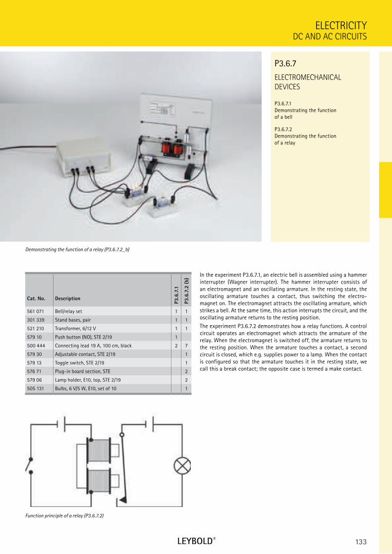
133
ELECTROMECHANICAL
DEVICES
P3.6.7.1 Demonstrating the function of a bell
P3.6.7.2 Demonstrating the function of a relay
DC AND AC CIRCUITS
ELECTRICITY
Cat. No. Description
P3.6
.7.1
P3.6
.7.2
(b)
561 071 Bell/relay set 1 1
301 339 Stand bases, pair 1 1
521 210 Transformer, 6/12 V 1 1
579 10 Push button (NO), STE 2/19 1
500 444 Connecting lead 19 A, 100 cm, black 2 7
579 30 Adjustable contact, STE 2/19 1
579 13 Toggle switch, STE 2/19 1
576 71 Plug-in board section, STE 2
579 06 Lamp holder, E10, top, STE 2/19 2
505 131 Bulbs, 6 V/5 W, E10, set of 10 1
In the experiment P3.6.7.1, an electric bell is assembled using a hammer interrupter (Wagner interrupter). The hammer interrupter consists of an electromagnet and an oscillating armature. In the resting state, the oscillating armature touches a contact, thus switching the electro-magnet on. The electromagnet attracts the oscillating armature, which strikes a bell. At the same time, this action interrupts the circuit, and the oscillating armature returns to the resting position.
The experiment P3.6.7.2 demonstrates how a relay functions. A control circuit operates an electromagnet which attracts the armature of the relay. When the electromagnet is switched off, the armature returns to the resting position. When the armature touches a contact, a second circuit is closed, which e.g. supplies power to a lamp. When the contact is configured so that the armature touches it in the resting state, we call this a break contact; the opposite case is termed a make contact.
Demonstrating the function of a relay (P3.6.7.2_b)
P3.6.7
Function principle of a relay (P3.6.7.2)
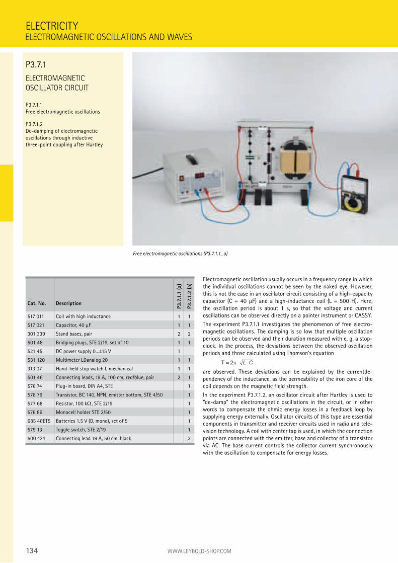
134 WWW.LEYBOLD-SHOP.COM
ELECTROMAGNETIC
OSCILLATOR CIRCUIT
P3.7.1.1 Free electromagnetic oscillations
P3.7.1.2 De-damping of electromagnetic oscillations through inductive three-point coupling after Hartley
Electromagnetic oscillation usually occurs in a frequency range in which the individual oscillations cannot be seen by the naked eye. However, this is not the case in an oscillator circuit consisting of a high-capacity capacitor (C = 40 µF) and a high-inductance coil (L = 500 H). Here, the oscillation period is about 1 s, so that the voltage and current oscillations can be observed directly on a pointer instrument or CASSY.
The experiment P3.7.1.1 investigates the phenomenon of free electro-magnetic oscillations. The damping is so low that multiple oscillation periods can be observed and their duration measured with e. g. a stop-clock. In the process, the deviations between the observed oscillation periods and those calculated using Thomson’s equation
T = ⋅ ⋅2π L C
are observed. These deviations can be explained by the currentde-pendency of the inductance, as the permeability of the iron core of the coil depends on the magnetic field strength.
In the experiment P3.7.1.2, an oscillator circuit after Hartley is used to “de-damp” the electromagnetic oscillations in the circuit, or in other words to compensate the ohmic energy losses in a feedback loop by supplying energy externally. Oscillator circuits of this type are essential components in transmitter and receiver circuits used in radio and tele-vision technology. A coil with center tap is used, in which the connection points are connected with the emitter, base and collector of a transistor via AC. The base current controls the collector current synchronously with the oscillation to compensate for energy losses.
ELECTRICITY
Free electromagnetic oscillations (P3.7.1.1_a)
Cat. No. Description
P3.7
.1.1
(a)
P3.7
.1.2
(a)
517 011 Coil with high inductance 1 1
517 021 Capacitor, 40 µF 1 1
301 339 Stand bases, pair 2 2
501 48 Bridging plugs, STE 2/19, set of 10 1 1
521 45 DC power supply 0...±15 V 1
531 120 Multimeter LDanalog 20 1 1
313 07 Hand-held stop watch I, mechanical 1 1
501 46 Connecting leads, 19 A, 100 cm, red/blue, pair 2 1
576 74 Plug-in board, DIN A4, STE 1
578 76 Transistor, BC 140, NPN, emitter bottom, STE 4/50 1
577 68 Resistor, 100 k , STE 2/19 1
576 86 Monocell holder STE 2/50 1
685 48ET5 Batteries 1.5 V (D, mono), set of 5 1
579 13 Toggle switch, STE 2/19 1
500 424 Connecting lead 19 A, 50 cm, black 3
ELECTROMAGNETIC OSCILLATIONS AND WAVES
P3.7.1
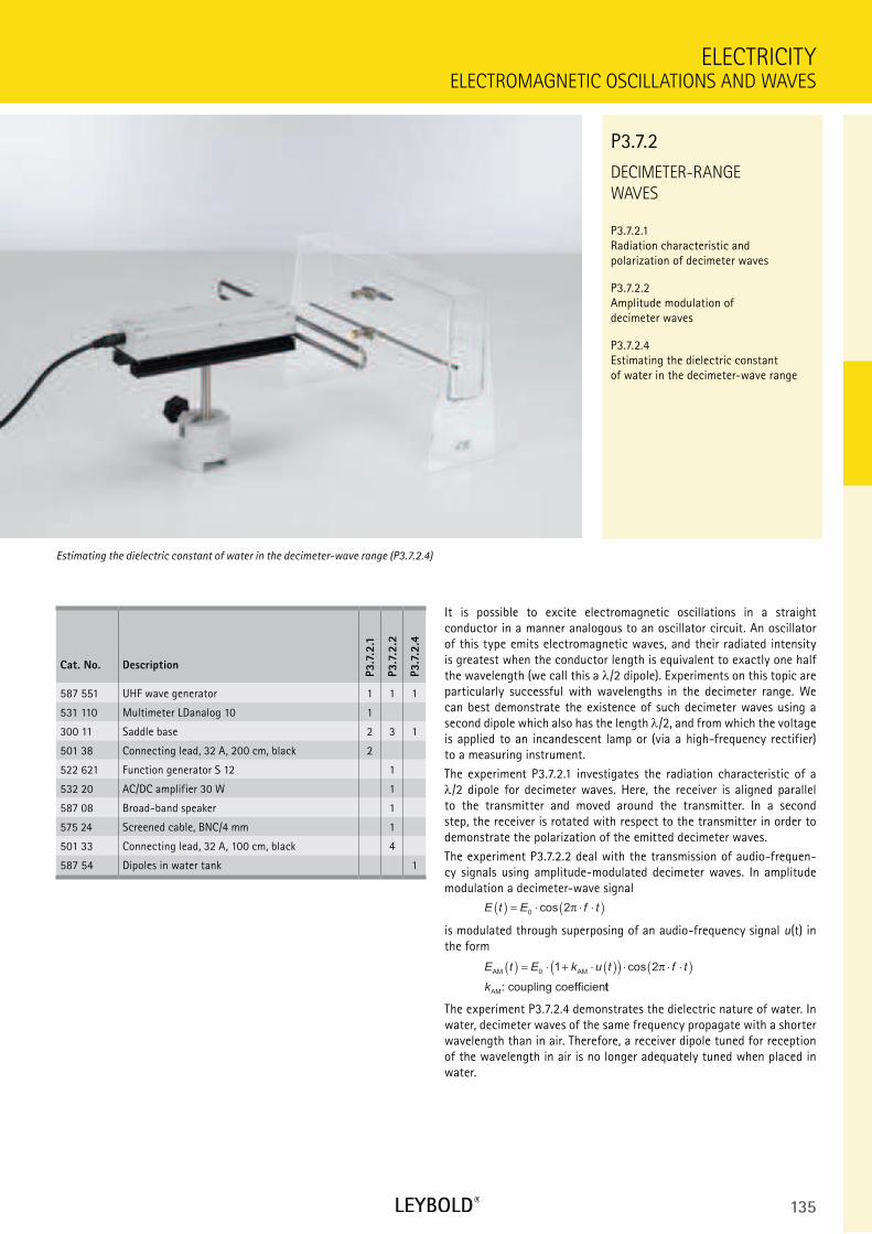
135
DECIMETER-RANGE
WAVES
P3.7.2.1 Radiation characteristic and polarization of decimeter waves
P3.7.2.2 Amplitude modulation of decimeter waves
P3.7.2.4 Estimating the dielectric constant of water in the decimeter-wave range
ELECTROMAGNETIC OSCILLATIONS AND WAVES
ELECTRICITY
Cat. No. Description
P3.7
.2.1
P3.7
.2.2
P3.7
.2.4
587 551 UHF wave generator 1 1 1
531 110 Multimeter LDanalog 10 1
300 11 Saddle base 2 3 1
501 38 Connecting lead, 32 A, 200 cm, black 2
522 621 Function generator S 12 1
532 20 AC/DC amplifier 30 W 1
587 08 Broad-band speaker 1
575 24 Screened cable, BNC/4 mm 1
501 33 Connecting lead, 32 A, 100 cm, black 4
587 54 Dipoles in water tank 1
It is possible to excite electromagnetic oscillations in a straight conductor in a manner analogous to an oscillator circuit. An oscillator of this type emits electromagnetic waves, and their radiated intensity is greatest when the conductor length is equivalent to exactly one half the wavelength (we call this a /2 dipole). Experiments on this topic are particularly successful with wavelengths in the decimeter range. We can best demonstrate the existence of such decimeter waves using a second dipole which also has the length /2, and from which the voltage is applied to an incandescent lamp or (via a high-frequency rectifier) to a measuring instrument.
The experiment P3.7.2.1 investigates the radiation characteristic of a /2 dipole for decimeter waves. Here, the receiver is aligned parallel
to the transmitter and moved around the transmitter. In a second step, the receiver is rotated with respect to the transmitter in order to demonstrate the polarization of the emitted decimeter waves.
The experiment P3.7.2.2 deal with the transmission of audio-frequen-cy signals using amplitude-modulated decimeter waves. In amplitude modulation a decimeter-wave signal
E t E f t( ) = ⋅ ⋅ ⋅( )02cos π
is modulated through superposing of an audio-frequency signal u(t) in the form
E t E k u t f t
k
AM AM
AM: coupling coefficien
( ) = ⋅ + ⋅ ( )( ) ⋅ ⋅ ⋅( )0 1 2cos π
tt
The experiment P3.7.2.4 demonstrates the dielectric nature of water. In water, decimeter waves of the same frequency propagate with a shorter wavelength than in air. Therefore, a receiver dipole tuned for reception of the wavelength in air is no longer adequately tuned when placed in water.
Estimating the dielectric constant of water in the decimeter-wave range (P3.7.2.4)
P3.7.2
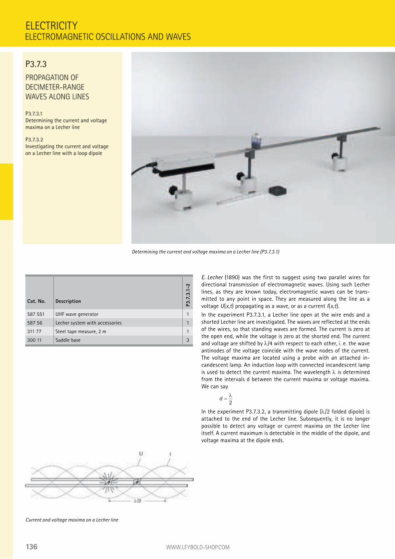
136 WWW.LEYBOLD-SHOP.COM
PROPAGATION OF
DECIMETER-RANGE
WAVES ALONG LINES
P3.7.3.1 Determining the current and voltage maxima on a Lecher line
P3.7.3.2 Investigating the current and voltage on a Lecher line with a loop dipole
E. Lecher (1890) was the first to suggest using two parallel wires for directional transmission of electromagnetic waves. Using such Lecher lines, as they are known today, electromagnetic waves can be trans-mitted to any point in space. They are measured along the line as a voltage U(x,t) propagating as a wave, or as a current I(x,t).
In the experiment P3.7.3.1, a Lecher line open at the wire ends and a shorted Lecher line are investigated. The waves are reflected at the ends of the wires, so that standing waves are formed. The current is zero at the open end, while the voltage is zero at the shorted end. The current and voltage are shifted by /4 with respect to each other, i. e. the wave antinodes of the voltage coincide with the wave nodes of the current. The voltage maxima are located using a probe with an attached in-candescent lamp. An induction loop with connected incandescent lamp is used to detect the current maxima. The wavelength is determined from the intervals d between the current maxima or voltage maxima. We can say
d =λ
2
In the experiment P3.7.3.2, a transmitting dipole ( /2 folded dipole) is attached to the end of the Lecher line. Subsequently, it is no longer possible to detect any voltage or current maxima on the Lecher line itself. A current maximum is detectable in the middle of the dipole, and voltage maxima at the dipole ends.
ELECTRICITY
Determining the current and voltage maxima on a Lecher line (P3.7.3.1)
Cat. No. Description
P3.7
.3.1
-2
587 551 UHF wave generator 1
587 56 Lecher system with accessories 1
311 77 Steel tape measure, 2 m 1
300 11 Saddle base 3
Current and voltage maxima on a Lecher line
ELECTROMAGNETIC OSCILLATIONS AND WAVES
P3.7.3
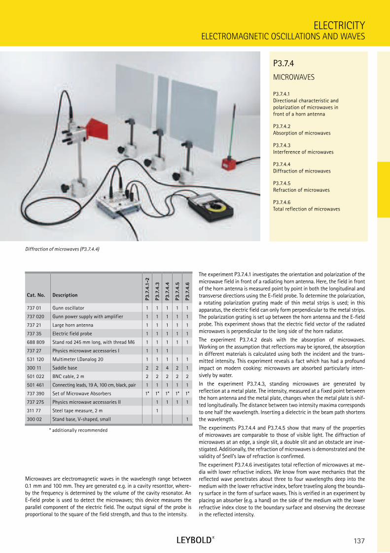
137
MICROWAVES
P3.7.4.1 Directional characteristic and polarization of microwaves in front of a horn antenna
P3.7.4.2 Absorption of microwaves
P3.7.4.3 Interference of microwaves
P3.7.4.4 Diffraction of microwaves
P3.7.4.5 Refraction of microwaves
P3.7.4.6 Total reflection of microwaves
ELECTROMAGNETIC OSCILLATIONS AND WAVES
ELECTRICITY
Cat. No. Description
P3.7
.4.1
-2
P3.7
.4.3
P3.7
.4.4
P3.7
.4.5
P3.7
.4.6
737 01 Gunn oscillator 1 1 1 1 1
737 020 Gunn power supply with amplifier 1 1 1 1 1
737 21 Large horn antenna 1 1 1 1 1
737 35 Electric field probe 1 1 1 1 1
688 809 Stand rod 245 mm long, with thread M6 1 1 1 1 1
737 27 Physics microwave accessories I 1 1 1
531 120 Multimeter LDanalog 20 1 1 1 1 1
300 11 Saddle base 2 2 4 2 1
501 022 BNC cable, 2 m 2 2 2 2 2
501 461 Connecting leads, 19 A, 100 cm, black, pair 1 1 1 1 1
737 390 Set of Microwave Absorbers 1* 1* 1* 1* 1*
737 275 Physics microwave accessories II 1 1 1 1
311 77 Steel tape measure, 2 m 1
300 02 Stand base, V-shaped, small 1
* additionally recommended
Microwaves are electromagnetic waves in the wavelength range between 0.1 mm and 100 mm. They are generated e.g. in a cavity resonttor, where-by the frequency is determined by the volume of the cavity resonator. An E-field probe is used to detect the microwaves; this device measures the parallel component of the electric field. The output signal of the probe is proportional to the square of the field strength, and thus to the intensity.
Diffraction of microwaves (P3.7.4.4)
P3.7.4
The experiment P3.7.4.1 investigates the orientation and polarization of the microwave field in front of a radiating horn antenna. Here, the field in front of the horn antenna is measured point by point in both the longitudinal and transverse directions using the E-field probe. To determine the polarization, a rotating polarization grating made of thin metal strips is used; in this apparatus, the electric field can only form perpendicular to the metal strips. The polarization grating is set up between the horn antenna and the E-field probe. This experiment shows that the electric field vector of the radiated microwaves is perpendicular to the long side of the horn radiator.
The experiment P3.7.4.2 deals with the absorption of microwaves. Working on the assumption that reflections may be ignored, the absorption in different materials is calculated using both the incident and the trans-mitted intensity. This experiment reveals a fact which has had a profound impact on modern cooking: microwaves are absorbed particularly inten-sively by water.
In the experiment P3.7.4.3, standing microwaves are generated by reflection at a metal plate. The intensity, measured at a fixed point between the horn antenna and the metal plate, changes when the metal plate is shif-ted longitudinally. The distance between two intensity maxima corresponds to one half the wavelength. Inserting a dielectric in the beam path shortens the wavelength.
The experiments P3.7.4.4 and P3.7.4.5 show that many of the properties of microwaves are comparable to those of visible light. The diffraction of microwaves at an edge, a single slit, a double slit and an obstacle are inve-stigated. Additionally, the refraction of microwaves is demonstrated and the validity of Snell’s law of refraction is confirmed.
The experiment P3.7.4.6 investigates total reflection of microwaves at me-dia with lower refractive indices. We know from wave mechanics that the reflected wave penetrates about three to four wavelengths deep into the medium with the lower refractive index, before traveling along the bounda-ry surface in the form of surface waves. This is verified in an experiment by placing an absorber (e.g. a hand) on the side of the medium with the lower refractive index close to the boundary surface and observing the decrease in the reflected intensity.
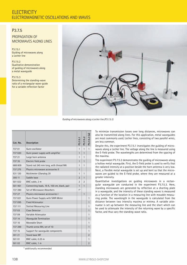
138 WWW.LEYBOLD-SHOP.COM
PROPAGATION OF
MICROWAVES ALONG LINES
P3.7.5.1
Guiding of microwaves along
a Lecher line
P3.7.5.2
Qualitative demonstration
of guiding of microwaves along
a metal waveguide
P3.7.5.3
Determining the standing-wave
ratio of a rectangular wave-guide
for a variable reflection factor
To minimize transmission losses over long distances, microwaves can
also be transmitted along lines. For this application, metal waveguides
are most commonly used; Lecher lines, consisting of two parallel wires,
are less common.
Despite this, the experiment P3.7.5.1 investigates the guiding of micro-
waves along a Lecher line. The voltage along the line is measured using
the E-field probe. The wavelengths are determined from the spacing of
the maxima.
The experiment P3.7.5.2 demonstrates the guiding of microwaves along
a hollow metal waveguide. First, the E-field probe is used to verify that
the radiated intensity at a position beside the horn antenna is very low.
Next, a flexible metal waveguide is set up and bent so that the micro-
waves are guided to the E-field probe, where they are measured at a
greater intensity.
Quantitative investigations on guiding microwaves in a rectan-
gular waveguide are conducted in the experiment P3.7.5.3. Here,
standing microwaves are generated by reflection at a shorting plate
in a waveguide, and the intensity of these standing waves is measured
as a function of the location in a measuring line with movable measu-
ring probe. The wavelength in the waveguide is calculated from the
distance between two intensity maxima or minima. A variable atte-
nuator is set up between the measuring line and the short which can
be used to attenuate the intensity of the returning wave by a specific
factor, and thus vary the standing-wave ratio.
ELECTRICITY
Guiding of microwaves along a Lecher line (P3.7.5.1)
Cat. No. Description
P3.7
.5.1
P3.7
.5.2
P3.7
.5.3
(a)
737 01 Gunn oscillator 1 1 1
737 020 Gunn power supply with amplifier 1 1
737 21 Large horn antenna 1 1
737 35 Electric field probe 1 1
688 809 Stand rod 245 mm long, with thread M6 1 1
737 275 Physics microwave accessories II 1
531 120 Multimeter LDanalog 20 1 1
300 11 Saddle base 2 1
501 022 BNC cable, 2 m 2 2
501 461 Connecting leads, 19 A, 100 cm, black, pair 1 1
737 390 Set of Microwave Absorbers 1*
737 27 Physics microwave accessories I 1
737 021 Gunn Power Supply with SWR Meter 1
737 095 Fixed Attenuator 1
737 111 Slotted Measuring Line 1
737 03 Coax Detector 1
737 09 Variable Attenuator 1
737 14 Waveguide Termination 1
737 10 Moveable Short 1
737 399 Thumb screw M4, set of 10 1
737 15 Support for waveguide components 1
301 21 Stand base MF 2
501 01 BNC cable, 0.25 m 1
501 02 BNC cable, 1 m 2
* additionally recommended
ELECTROMAGNETIC OSCILLATIONS AND WAVES
P3.7.5
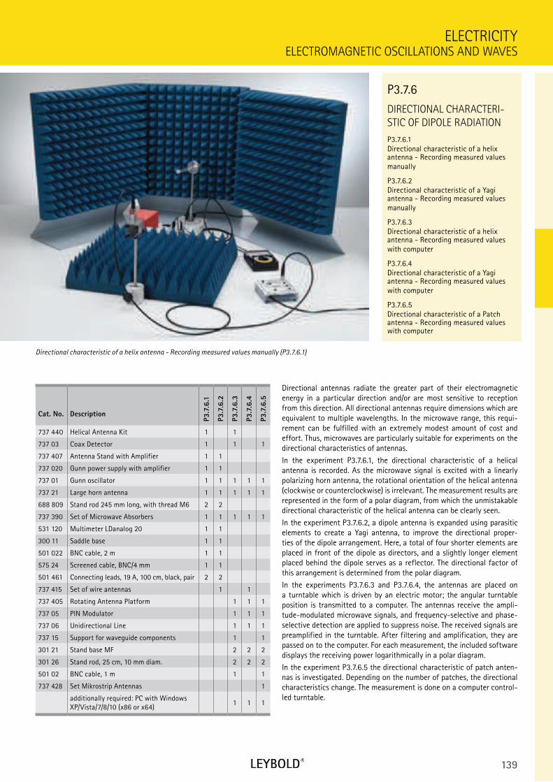
139
DIRECTIONAL CHARACTERI-
STIC OF DIPOLE RADIATION
P3.7.6.1 Directional characteristic of a helix antenna - Recording measured values manually
P3.7.6.2 Directional characteristic of a Yagi antenna - Recording measured values manually
P3.7.6.3 Directional characteristic of a helix antenna - Recording measured values with computer
P3.7.6.4 Directional characteristic of a Yagi antenna - Recording measured values with computer
P3.7.6.5 Directional characteristic of a Patch antenna - Recording measured values with computer
ELECTROMAGNETIC OSCILLATIONS AND WAVES
ELECTRICITY
Cat. No. Description
P3.7
.6.1
P3.7
.6.2
P3.7
.6.3
P3.7
.6.4
P3.7
.6.5
737 440 Helical Antenna Kit 1 1
737 03 Coax Detector 1 1 1
737 407 Antenna Stand with Amplifier 1 1
737 020 Gunn power supply with amplifier 1 1
737 01 Gunn oscillator 1 1 1 1 1
737 21 Large horn antenna 1 1 1 1 1
688 809 Stand rod 245 mm long, with thread M6 2 2
737 390 Set of Microwave Absorbers 1 1 1 1 1
531 120 Multimeter LDanalog 20 1 1
300 11 Saddle base 1 1
501 022 BNC cable, 2 m 1 1
575 24 Screened cable, BNC/4 mm 1 1
501 461 Connecting leads, 19 A, 100 cm, black, pair 2 2
737 415 Set of wire antennas 1 1
737 405 Rotating Antenna Platform 1 1 1
737 05 PIN Modulator 1 1 1
737 06 Unidirectional Line 1 1 1
737 15 Support for waveguide components 1 1
301 21 Stand base MF 2 2 2
301 26 Stand rod, 25 cm, 10 mm diam. 2 2 2
501 02 BNC cable, 1 m 1 1
737 428 Set Mikrostrip Antennas 1
additionally required: PC with Windows XP/Vista/7/8/10 (x86 or x64)
1 1 1
Directional antennas radiate the greater part of their electromagnetic energy in a particular direction and/or are most sensitive to reception from this direction. All directional antennas require dimensions which are equivalent to multiple wavelengths. In the microwave range, this requi-rement can be fulfilled with an extremely modest amount of cost and effort. Thus, microwaves are particularly suitable for experiments on the directional characteristics of antennas.
In the experiment P3.7.6.1, the directional characteristic of a helical antenna is recorded. As the microwave signal is excited with a linearly polarizing horn antenna, the rotational orientation of the helical antenna (clockwise or counterclockwise) is irrelevant. The measurement results are represented in the form of a polar diagram, from which the unmistakable directional characteristic of the helical antenna can be clearly seen.
In the experiment P3.7.6.2, a dipole antenna is expanded using parasitic elements to create a Yagi antenna, to improve the directional proper-ties of the dipole arrangement. Here, a total of four shorter elements are placed in front of the dipole as directors, and a slightly longer element placed behind the dipole serves as a reflector. The directional factor of this arrangement is determined from the polar diagram.
In the experiments P3.7.6.3 and P3.7.6.4, the antennas are placed on a turntable which is driven by an electric motor; the angular turntable position is transmitted to a computer. The antennas receive the ampli-tude-modulated microwave signals, and frequency-selective and phase-selective detection are applied to suppress noise. The received signals are preamplified in the turntable. After filtering and amplification, they are passed on to the computer. For each measurement, the included software displays the receiving power logarithmically in a polar diagram.
In the experiment P3.7.6.5 the directional characteristic of patch anten-nas is investigated. Depending on the number of patches, the directional characteristics change. The measurement is done on a computer control-led turntable.
Directional characteristic of a helix antenna - Recording measured values manually (P3.7.6.1)
P3.7.6
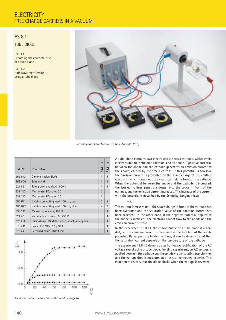
140 WWW.LEYBOLD-SHOP.COM
TUBE DIODE
P3.8.1.1 Recording the characteristic of a tube diode
P3.8.1.2 Half-wave rectification using a tube diode
A tube diode contains two electrodes: a heated cathode, which emits electrons due to thermionic emission, and an anode. A positive potential between the anode and the cathode generates an emission current to the anode, carried by the free electrons. If this potential is too low, the emission current is prevented by the space charge of the emitted electrons, which screen out the electrical field in front of the cathode. When the potential between the anode and the cathode is increased, the isoelectric lines penetrate deeper into the space in front of the cathode, and the emission current increases. This increase of the current with the potential is described by the Schottky-Langmuir law:
I U3
2
This current increases until the space charge in front of the cathode has been overcome and the saturation value of the emission current has been reached. On the other hand, if the negative potential applied to the anode is sufficient, the electrons cannot flow to the anode and the emission current is zero.
In the experiment P3.8.1.1, the characteristic of a tube diode is recor-ded, i.e. the emission current is measured as the function of the anode potential. By varying the heating voltage, it can be demonstrated that the saturation current depends on the temperature of the cathode.
The experiment P3.8.1.2 demonstrates half-wave rectification of the AC voltage signal using a tube diode. For this experiment, an AC voltage is applied between the cathode and the anode via an isolating transformer, and the voltage drop is measured at a resistor connected in series. This experiment reveals that the diode blocks when the voltage is reversed.
ELECTRICITY
Recording the characteristic of a tube diode (P3.8.1.1)
Cat. No. Description
P3.8
.1.1
P3.8
.1.2
555 610 Demonstration diode 1 1
555 600 Tube stand 1 1
521 65 Tube power supply, 0...500 V 1 1
531 120 Multimeter LDanalog 20 2
531 130 Multimeter LDanalog 30 1
500 641 Safety connecting lead, 100 cm, red 5 2
500 642 Safety connecting lead, 100 cm, blue 4 3
536 191 Measuring resistor, 10 k 1
521 40 Variable transformer, 0...250 V 1
575 214 Oscilloscope 30 MHz, two-channel, analogous 1
575 231 Probe 100 MHz, 1:1 / 10:1 1
575 24 Screened cable, BNC/4 mm 1
Anode current IA as a function of the anode voltage UA
FREE CHARGE CARRIERS IN A VACUUM
P3.8.1
141
TUBE TRIODE
P3.8.2.1 Recording the characteristic field of a tube triode
P3.8.2.2 Amplifying voltages with a tube triode
FREE CHARGE CARRIERS IN A VACUUM
ELECTRICITY
Cat. No. Description
P3.8
.2.1
P3.8
.2.2
555 612 Demonstration triode 1 1
555 600 Tube stand 1 1
521 65 Tube power supply, 0...500 V 1 1
531 120 Multimeter LDanalog 20 2
531 130 Multimeter LDanalog 30 1
500 622 Safety connecting lead, 50 cm, blue 1 2
500 641 Safety connecting lead, 100 cm, red 6 3
500 642 Safety connecting lead, 100 cm, blue 4 3
536 251 Measuring resistor, 100 k 1
522 621 Function generator S 12 1
575 214 Oscilloscope 30 MHz, two-channel, analogous 1
575 231 Probe 100 MHz, 1:1 / 10:1 1
575 24 Screened cable, BNC/4 mm 1
In a tube triode, the electrons pass through the mesh of a grid on their way from the cathode to the anode. When a negative voltage UG is applied to the grid, the emission current IA to the anode is reduced; a positive grid voltage increases the anode current. In other words, the anode current can be controlled by the grid voltage.
The experiment P3.8.2.1 records the family of characteristics of the triode, i.e. the anode current IA as a function of the grid voltage UG and the anode voltage UA
The experiment P3.8.2.2 demonstrates how a tube triode can be used as an amplifier. A suitable negative voltage UG is used to set the wor-king point of the triode on the characteristic curve IA(UA) so that the characteristic is as linear as possible in the vicinity of the working point. Once this has been set, small changes in the grid voltage UG cause a change in the anode voltage UA by means of a proportional change in the anode current IA. The ratio:
VU
U
A
G
=δ
δ
is known as the gain.
Recording the characteristic field of a tube triode (P3.8.2.1)
P3.8.2
Characteristic field of a tube triode
142 WWW.LEYBOLD-SHOP.COM
MALTESE-CROSS TUBE
P3.8.3.1
Demonstrating the linear propagation
of electrons in a field-free space
P3.8.3.2
Deflection of electrons in an axial
magnetic field
In the Maltese cross tube, the electrons are accelerated by the anode
to a fluorescent screen, where they can be observed as luminescent
phenomena. A Maltese cross is arranged between the anode and the
fluorescent screen, and its shadow can be seen on the screen. The
Maltese cross has its own separate lead, so that it can be connected to
any desired potential.
The experiment P3.8.3.1 confirms the linear propagation of electrons in
a field-free space. In this experiment, the Maltese cross is connected
to the anode potential and the shadow of the Maltese cross in the
electron beam is compared with the light shadow. We can conclude
from the observed coincidence of the shadows that electrons propa-
gate in a straight line. The Maltese cross is then disconnected from any
potential. The resulting space charges around the Maltese cross give
rise to a repulsive potential, so that the image on the fluorescent
screen becomes larger.
In the experiment P3.8.3.2 an axial magnetic field is applied using an
electromagnet. The shadow cross turns and shrinks as a function of
the coil current. When a suitable relationship between the high voltage
and the coil current is set, the cross is focused almost to a point, and
becomes larger again when the current is increased further. The ex-
planation for this magnetic focusing may be found in the helical path of
the electrons in the magnetic field.
ELECTRICITY
Deflection of electrons in an axial magnetic field (P3.8.3.2)
Cat. No. Description
P3.8
.3.1
P3.8
.3.2
555 620 Maltese cross tube 1 1
555 600 Tube stand 1 1
521 70 High-voltage power supply, 10 kV 1 1
510 48 Magnets, 35 mm Ø, pair 1
500 611 Safety connecting lead, 25 cm, red 1 1
500 621 Safety connecting lead, 50 cm, red 1 2
500 641 Safety connecting lead, 100 cm, red 1 2
500 642 Safety connecting lead, 100 cm, blue 1 2
500 644 Safety connecting lead, 100 cm, black 2 2
555 604 Pair of Helmholtz coils 1
521 546 DC Power Supply 0 ... 16 V, 0 ... 5 A 1
500 622 Safety connecting lead, 50 cm, blue 1
Shadow of the maltese cross on the fluorescent screen
FREE CHARGE CARRIERS IN A VACUUM
P3.8.3
143
PERRIN TUBE
P3.8.4.1
Hot-cathode emission in a
vacuum: determining the polarity
and estimating the specific charge
of the emitted charge carriers
P3.8.4.2
Generating Lissajou figures
through electron deflection in
crossed alternating magnetic fields
P3.8.4.3
Generating Lissajou figures
through electron deflection in
parallel alternating electrical
and magnetic field
FREE CHARGE CARRIERS IN A VACUUM
ELECTRICITY
Cat. No. Description
P3.8
.4.1
P3.8
.4.2
P3.8
.4.3
555 622 Perrin tube 1 1 1
555 600 Tube stand 1 1 1
555 604 Pair of Helmholtz coils 1 1 1
521 70 High-voltage power supply, 10 kV 1 1 1
521 546 DC Power Supply 0 ... 16 V, 0 ... 5 A 1
540 091 Electroscope 1
300 11 Saddle base 1
501 051 Cable for high voltages, 1.5 m 1
500 611 Safety connecting lead, 25 cm, red 1 1 1
500 621 Safety connecting lead, 50 cm, red 2 2 2
500 622 Safety connecting lead, 50 cm, blue 1 1 1
500 641 Safety connecting lead, 100 cm, red 4 3 3
500 642 Safety connecting lead, 100 cm, blue 2 3 3
500 644 Safety connecting lead, 100 cm, black 2 2 2
562 14 Coil, 500 turns 1
521 35 Variable extra-low voltage transformer S 1
522 621 Function generator S 12 1 1
300 761 Support blocks, set of 6 1
521 40 Variable transformer, 0...250 V 1
In the Perrin tube, the electrons are accelerated through an anode with
pin-hole diaphragm onto a fluorescent screen. Deflection plates are
mounted at the opening of the pin-hole diaphragm for horizontal elec-
trostatic deflection of the electron beam. A Faraday’s cup, which is set
up at an angle of 45° to the electron beam, can be charged by the elec-
trons deflected vertically upward. The charge current can be measured
using a separate connection.
In the experiment P3.8.4.1, the current through a pair of Helmholtz
coils is set so that the electron beam is incident on the Faraday’s cup
of the Perrin tube. The Faraday’s cup is connected to an electroscope
which has been pre-charged with a known polarity. The polarity of the
electron charge can be recognized by the direction of electroscope
deflection when the Faraday’s cup is struck by the electron beam. At the
same time, the specific electron charge can be estimated. The following
relationship applies:
e
m
U
B r
U=⋅( )
22
AA : anode voltage
The bending radius r of the orbit is predetermined by the geometry of
the tube. The magnetic field B is calculated from the current I through
the Helmholtz coils.
In the experiment P3.8.4.2, the deflection of electrons in crossed
alternating magnetic fields is used to produce Lissajou figures on the
fluorescent screen. This experiment demonstrates that the electrons
respond to a change in the electromagnetic fields with virtually no lag.
In the experiment P3.8.4.3, the deflection of electrons in parallel elec-
tric and magnetic alternating fields is used to produce Lissajou figures
on the fluorescent screen.
Hot-cathode emission in a vacuum: determining the polarity and estimating the specific charge of the emitted
charge carriers (P3.8.4.1)
P3.8.4
144 WWW.LEYBOLD-SHOP.COM
THOMSON TUBE
P3.8.5.1 Investigating the deflection of electrons in electrical and magnetic fields
P3.8.5.2 Assembling a velocity filter (Wien filter) to determine the specific electron charge
In the Thomson tube, the electrons pass through a slit behind the anode and fall glancingly on a fluorescent screen placed in the beam path at an angle. A plate capacitor is mounted at the opening of the slit diaphragm which can electrostatically deflect the electron beam verti-cally. In addition, Helmholtz coils can be used to generate an external magnetic field which can also deflect the electron beam.
The experiment P3.8.5.1 investigates the deflection of electrons in electric and magnetic fields. For different anode voltages UA, the beam path of the electrons is observed when the deflection voltage UP at the plate capacitor is varied. Additionally, the electrons are deflected in the magnetic field of the Helmholtz coils by varying the coil current I. The point at which the electron beam emerges from the fluorescent screen gives us the radius R of the orbit. When we insert the anode voltage in the following equation, we can obtain an experimental value for the specific electron charge
e
m
U
B r
=⋅( )
2
2
A
whereby the magnetic field B is calculated from the current I.
In the experiment P3.8.5.2, a velocity filter (Wien filter) is constructed using crossed electrical and magnetic fields. Among other things, this configuration permits a more precise determination of the specific electron charge. At a fixed anode voltage UA, the current I of the Helm-holtz coils and the deflection voltage UP are set so that the effects of the electric field and the magnetic field just compensate each other. The path of the beam is then virtually linear, and we can say:
e
m U
U
B d
d
= ⋅⋅
1
2
2
A
P
: plate spacing of the plate capacitorr
ELECTRICITY
Investigating the deflection of electrons in electrical fields (P3.8.5.1)
Cat. No. Description
P3.8
.5.1
-2
555 624 Electron deflection tube 1
555 600 Tube stand 1
555 604 Pair of Helmholtz coils 1
521 70 High-voltage power supply, 10 kV 2
521 546 DC Power Supply 0 ... 16 V, 0 ... 5 A 1
500 611 Safety connecting lead, 25 cm, red 2
500 621 Safety connecting lead, 50 cm, red 1
500 622 Safety connecting lead, 50 cm, blue 1
500 641 Safety connecting lead, 100 cm, red 2
500 642 Safety connecting lead, 100 cm, blue 4
500 644 Safety connecting lead, 100 cm, black 2
Investigating the deflection of electrons in magneetic fields
FREE CHARGE CARRIERS IN A VACUUM
P3.8.5
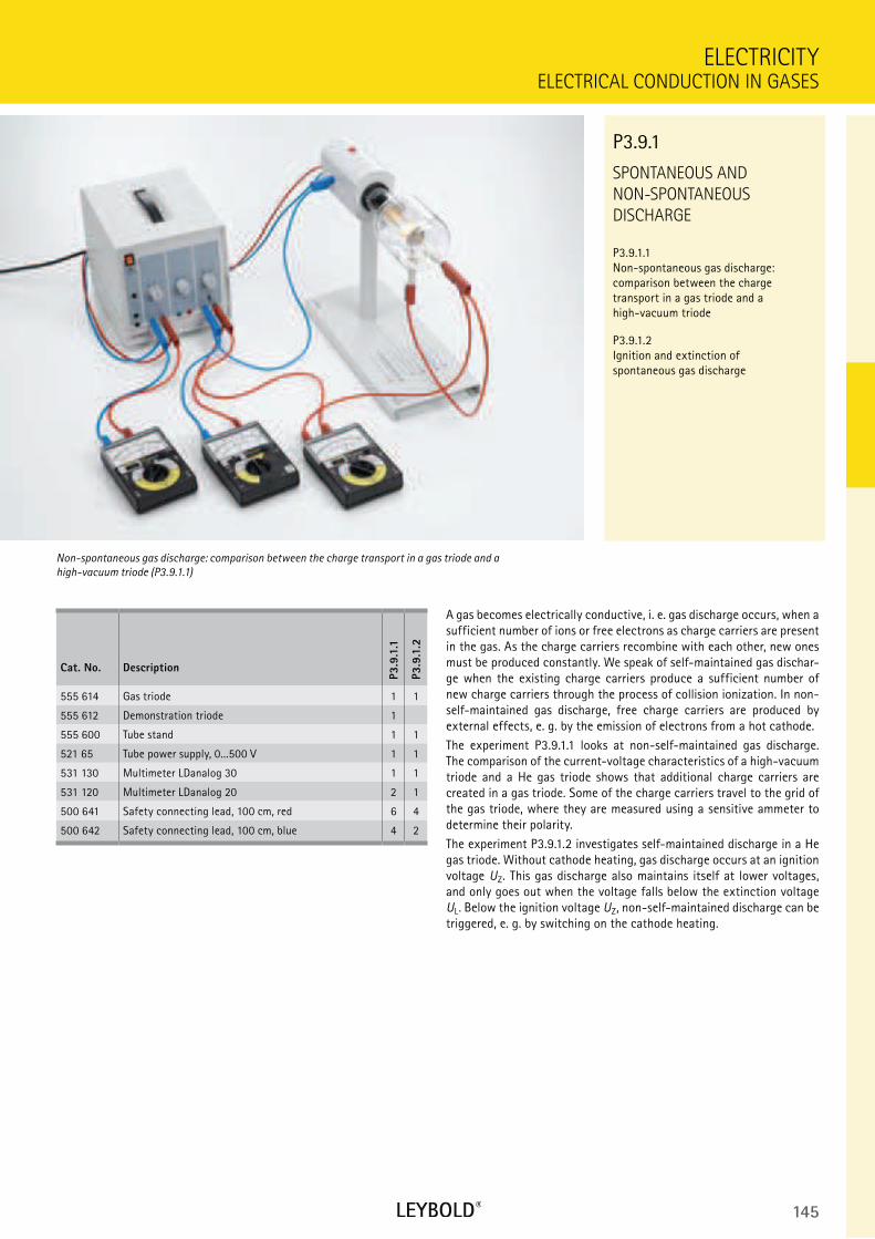
145
SPONTANEOUS AND
NON-SPONTANEOUS
DISCHARGE
P3.9.1.1
Non-spontaneous gas discharge:
comparison between the charge
transport in a gas triode and a
high-vacuum triode
P3.9.1.2
Ignition and extinction of
spontaneous gas discharge
ELECTRICAL CONDUCTION IN GASES
ELECTRICITY
Cat. No. Description
P3.9
.1.1
P3.9
.1.2
555 614 Gas triode 1 1
555 612 Demonstration triode 1
555 600 Tube stand 1 1
521 65 Tube power supply, 0...500 V 1 1
531 130 Multimeter LDanalog 30 1 1
531 120 Multimeter LDanalog 20 2 1
500 641 Safety connecting lead, 100 cm, red 6 4
500 642 Safety connecting lead, 100 cm, blue 4 2
A gas becomes electrically conductive, i. e. gas discharge occurs, when a
sufficient number of ions or free electrons as charge carriers are present
in the gas. As the charge carriers recombine with each other, new ones
must be produced constantly. We speak of self-maintained gas dischar-
ge when the existing charge carriers produce a sufficient number of
new charge carriers through the process of collision ionization. In non-
self-maintained gas discharge, free charge carriers are produced by
external effects, e. g. by the emission of electrons from a hot cathode.
The experiment P3.9.1.1 looks at non-self-maintained gas discharge.
The comparison of the current-voltage characteristics of a high-vacuum
triode and a He gas triode shows that additional charge carriers are
created in a gas triode. Some of the charge carriers travel to the grid of
the gas triode, where they are measured using a sensitive ammeter to
determine their polarity.
The experiment P3.9.1.2 investigates self-maintained discharge in a He
gas triode. Without cathode heating, gas discharge occurs at an ignition
voltage UZ. This gas discharge also maintains itself at lower voltages,
and only goes out when the voltage falls below the extinction voltage
UL. Below the ignition voltage UZ, non-self-maintained discharge can be
triggered, e. g. by switching on the cathode heating.
Non-spontaneous gas discharge: comparison between the charge transport in a gas triode and a
high-vacuum triode (P3.9.1.1)
P3.9.1
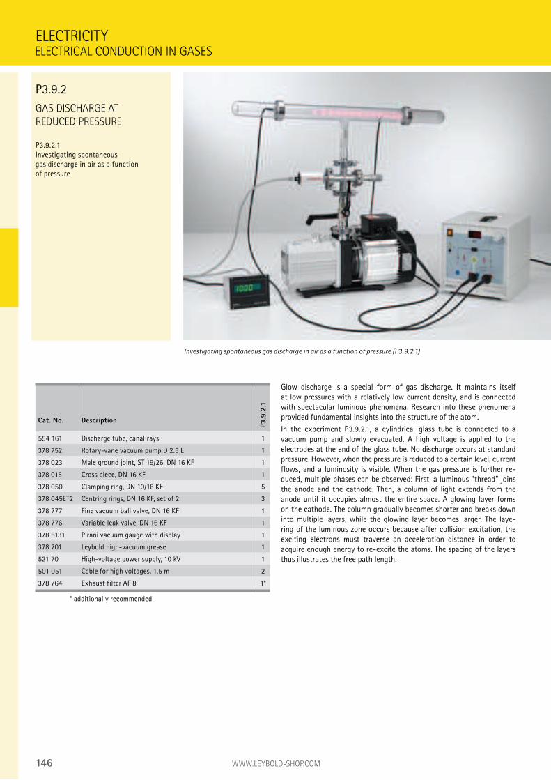
146 WWW.LEYBOLD-SHOP.COM
GAS DISCHARGE AT
REDUCED PRESSURE
P3.9.2.1 Investigating spontaneous gas discharge in air as a function of pressure
Glow discharge is a special form of gas discharge. It maintains itself at low pressures with a relatively low current density, and is connected with spectacular luminous phenomena. Research into these phenomena provided fundamental insights into the structure of the atom.
In the experiment P3.9.2.1, a cylindrical glass tube is connected to a vacuum pump and slowly evacuated. A high voltage is applied to the electrodes at the end of the glass tube. No discharge occurs at standard pressure. However, when the pressure is reduced to a certain level, current flows, and a luminosity is visible. When the gas pressure is further re-duced, multiple phases can be observed: First, a luminous “thread” joins the anode and the cathode. Then, a column of light extends from the anode until it occupies almost the entire space. A glowing layer forms on the cathode. The column gradually becomes shorter and breaks down into multiple layers, while the glowing layer becomes larger. The laye-ring of the luminous zone occurs because after collision excitation, the exciting electrons must traverse an acceleration distance in order to acquire enough energy to re-excite the atoms. The spacing of the layers thus illustrates the free path length.
ELECTRICAL CONDUCTION IN GASES
P3.9.2
Cat. No. Description
P3.9
.2.1
554 161 Discharge tube, canal rays 1
378 752 Rotary-vane vacuum pump D 2.5 E 1
378 023 Male ground joint, ST 19/26, DN 16 KF 1
378 015 Cross piece, DN 16 KF 1
378 050 Clamping ring, DN 10/16 KF 5
378 045ET2 Centring rings, DN 16 KF, set of 2 3
378 777 Fine vacuum ball valve, DN 16 KF 1
378 776 Variable leak valve, DN 16 KF 1
378 5131 Pirani vacuum gauge with display 1
378 701 Leybold high-vacuum grease 1
521 70 High-voltage power supply, 10 kV 1
501 051 Cable for high voltages, 1.5 m 2
378 764 Exhaust filter AF 8 1*
* additionally recommended
ELECTRICITY
Investigating spontaneous gas discharge in air as a function of pressure (P3.9.2.1)
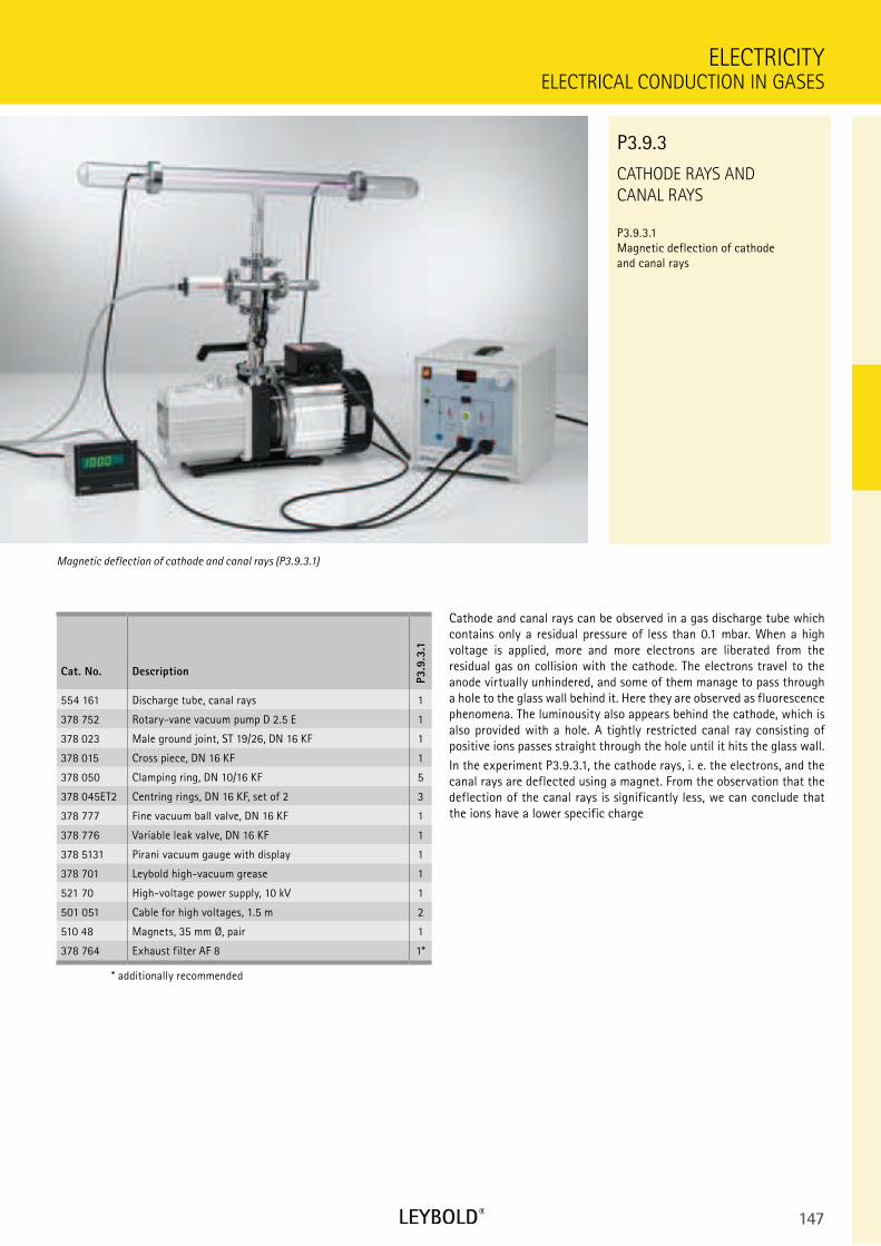
147
CATHODE RAYS AND
CANAL RAYS
P3.9.3.1 Magnetic deflection of cathode and canal rays
ELECTRICAL CONDUCTION IN GASES
ELECTRICITY
Cat. No. Description
P3.9
.3.1
554 161 Discharge tube, canal rays 1
378 752 Rotary-vane vacuum pump D 2.5 E 1
378 023 Male ground joint, ST 19/26, DN 16 KF 1
378 015 Cross piece, DN 16 KF 1
378 050 Clamping ring, DN 10/16 KF 5
378 045ET2 Centring rings, DN 16 KF, set of 2 3
378 777 Fine vacuum ball valve, DN 16 KF 1
378 776 Variable leak valve, DN 16 KF 1
378 5131 Pirani vacuum gauge with display 1
378 701 Leybold high-vacuum grease 1
521 70 High-voltage power supply, 10 kV 1
501 051 Cable for high voltages, 1.5 m 2
510 48 Magnets, 35 mm Ø, pair 1
378 764 Exhaust filter AF 8 1*
* additionally recommended
Cathode and canal rays can be observed in a gas discharge tube which contains only a residual pressure of less than 0.1 mbar. When a high voltage is applied, more and more electrons are liberated from the residual gas on collision with the cathode. The electrons travel to the anode virtually unhindered, and some of them manage to pass through a hole to the glass wall behind it. Here they are observed as fluorescence phenomena. The luminousity also appears behind the cathode, which is also provided with a hole. A tightly restricted canal ray consisting of positive ions passes straight through the hole until it hits the glass wall.
In the experiment P3.9.3.1, the cathode rays, i. e. the electrons, and the canal rays are deflected using a magnet. From the observation that the deflection of the canal rays is significantly less, we can conclude that the ions have a lower specific charge
Magnetic deflection of cathode and canal rays (P3.9.3.1)
P3.9.3
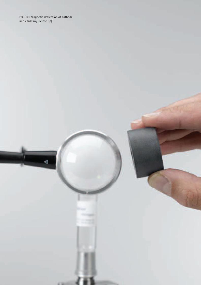
148 WWW.LEYBOLD-SHOP.COM
P3.9.3.1 Magnetic deflection of cathode and canal rays (close up)
149
P4.1 COMPONENTS AND BASIC CIRCUITS 151
P4.2 OPERATIONAL AMPLIFIER 159
P4.3 OPEN- AND CLOSED-LOOP CONTROL 161
P4.5 DIGITAL ELECTRONICS 162
P4 ELECTRONICS

150 WWW.LEYBOLD-SHOP.COM
P4.1 COMPONENTS AND BASIC CIRCUITS
P4.1.1 Current and voltage sources 151-152
P4.1.2 Special resistors 153
P4.1.3 Diodes 154
P4.1.4 Diode circuits 155
P4.1.5 Transistors 156
P4.1.6 Transistor circuits 157
P4.1.7 Optoelectronics 158
P4.2 OPERATIONAL AMPLIFIER
P4.2.1 Internal design of an operational amplifier 159
P4.2.2 Operational amplifier circuits 160
P4.3 OPEN- AND CLOSED-LOOP CONTROL
P4.3.2 Closed-loop control 161
P4.5 DIGITAL ELECTRONICS
P4.5.1 Simple combinations 162
P4.5.2 Logic circuits 163
P4.5.3 Analog inputs and outputs 164
P4 ELECTRONICS
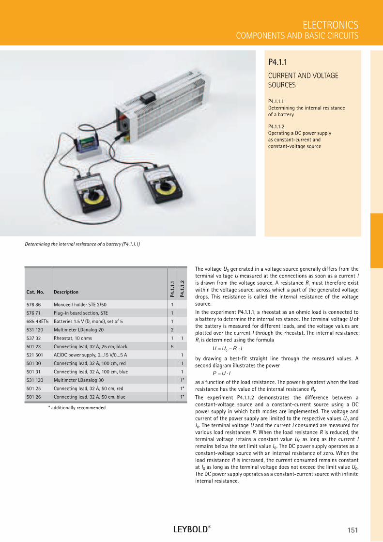
151
CURRENT AND VOLTAGE
SOURCES
P4.1.1.1 Determining the internal resistance of a battery
P4.1.1.2 Operating a DC power supply as constant-current and constant-voltage source
COMPONENTS AND BASIC CIRCUITS
ELECTRONICS
Cat. No. Description
P4.1
.1.1
P4.1
.1.2
576 86 Monocell holder STE 2/50 1
576 71 Plug-in board section, STE 1
685 48ET5 Batteries 1.5 V (D, mono), set of 5 1
531 120 Multimeter LDanalog 20 2
537 32 Rheostat, 10 ohms 1 1
501 23 Connecting lead, 32 A, 25 cm, black 5
521 501 AC/DC power supply, 0...15 V/0...5 A 1
501 30 Connecting lead, 32 A, 100 cm, red 1
501 31 Connecting lead, 32 A, 100 cm, blue 1
531 130 Multimeter LDanalog 30 1*
501 25 Connecting lead, 32 A, 50 cm, red 1*
501 26 Connecting lead, 32 A, 50 cm, blue 1*
* additionally recommended
The voltage U0 generated in a voltage source generally differs from the terminal voltage U measured at the connections as soon as a current I is drawn from the voltage source. A resistance Ri must therefore exist within the voltage source, across which a part of the generated voltage drops. This resistance is called the internal resistance of the voltage source.
In the experiment P4.1.1.1, a rheostat as an ohmic load is connected to a battery to determine the internal resistance. The terminal voltage U of the battery is measured for different loads, and the voltage values are plotted over the current I through the rheostat. The internal resistance Ri is determined using the formula
U U R I= − ⋅0 i
by drawing a best-fit straight line through the measured values. A second diagram illustrates the power
P U I= ⋅
as a function of the load resistance. The power is greatest when the load resistance has the value of the internal resistance Ri.
The experiment P4.1.1.2 demonstrates the difference between a constant-voltage source and a constant-current source using a DC power supply in which both modes are implemented. The voltage and current of the power supply are limited to the respective values U0 and I0. The terminal voltage U and the current I consumed are measured for various load resistances R. When the load resistance R is reduced, the terminal voltage retains a constant value U0 as long as the current I remains below the set limit value I0. The DC power supply operates as a constant-voltage source with an internal resistance of zero. When the load resistance R is increased, the current consumed remains constant at I0 as long as the terminal voltage does not exceed the limit value U0. The DC power supply operates as a constant-current source with infinite internal resistance.
Determining the internal resistance of a battery (P4.1.1.1)
P4.1.1
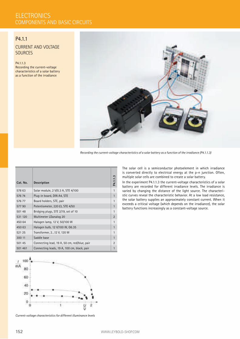
152 WWW.LEYBOLD-SHOP.COM
CURRENT AND VOLTAGE
SOURCES
P4.1.1.3 Recording the current-voltage characteristics of a solar battery as a function of the irradiance
The solar cell is a semiconductor photoelement in which irradiance is converted directly to electrical energy at the p-n junction. Often, multiple solar cells are combined to create a solar battery.
In the experiment P4.1.1.3 the current-voltage characteristics of a solar battery are recorded for different irradiance levels. The irradiance is varied by changing the distance of the light source. The characteri-stic curves reveal the characteristic behavior. At a low load resistance, the solar battery supplies an approximately constant current. When it exceeds a critical voltage (which depends on the irradiance), the solar battery functions increasingly as a constant-voltage source.
ELECTRONICS
Recording the current-voltage characteristics of a solar battery as a function of the irradiance (P4.1.1.3)
Cat. No. Description
P4.1
.1.3
578 63 Solar module, 2 V/0.3 A, STE 4/100 1
576 74 Plug-in board, DIN A4, STE 1
576 77 Board holders, STE, pair 1
577 90 Potentiometer, 220 , STE 4/50 1
501 48 Bridging plugs, STE 2/19, set of 10 1
531 120 Multimeter LDanalog 20 2
450 64 Halogen lamp, 12 V, 50/100 W 1
450 63 Halogen bulb, 12 V/100 W, G6.35 1
521 25 Transformer, 2...12 V, 120 W 1
300 11 Saddle base 1
501 45 Connecting lead, 19 A, 50 cm, red/blue, pair 2
501 461 Connecting leads, 19 A, 100 cm, black, pair 1
Current-voltage characteristics for different illuminance levels
COMPONENTS AND BASIC CIRCUITS
P4.1.1
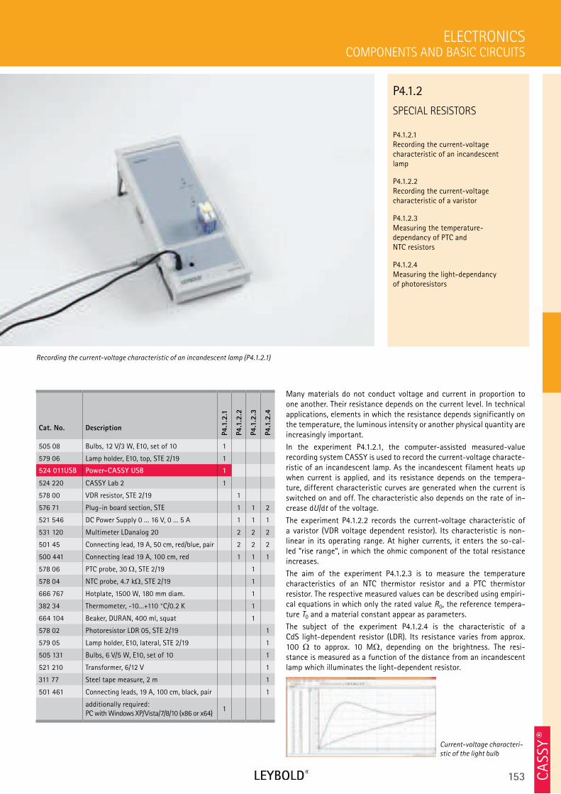
153 CA
SSY ®
SPECIAL RESISTORS
P4.1.2.1 Recording the current-voltage characteristic of an incandescent lamp
P4.1.2.2 Recording the current-voltage characteristic of a varistor
P4.1.2.3 Measuring the temperature- dependancy of PTC and NTC resistors
P4.1.2.4 Measuring the light-dependancy of photoresistors
COMPONENTS AND BASIC CIRCUITS
ELECTRONICS
Cat. No. Description
P4.1
.2.1
P4.1
.2.2
P4.1
.2.3
P4.1
.2.4
505 08 Bulbs, 12 V/3 W, E10, set of 10 1
579 06 Lamp holder, E10, top, STE 2/19 1
524 011USB Power-CASSY USB 1
524 220 CASSY Lab 2 1
578 00 VDR resistor, STE 2/19 1
576 71 Plug-in board section, STE 1 1 2
521 546 DC Power Supply 0 ... 16 V, 0 ... 5 A 1 1 1
531 120 Multimeter LDanalog 20 2 2 2
501 45 Connecting lead, 19 A, 50 cm, red/blue, pair 2 2 2
500 441 Connecting lead 19 A, 100 cm, red 1 1 1
578 06 PTC probe, 30 , STE 2/19 1
578 04 NTC probe, 4.7 k , STE 2/19 1
666 767 Hotplate, 1500 W, 180 mm diam. 1
382 34 Thermometer, -10...+110 °C/0.2 K 1
664 104 Beaker, DURAN, 400 ml, squat 1
578 02 Photoresistor LDR 05, STE 2/19 1
579 05 Lamp holder, E10, lateral, STE 2/19 1
505 131 Bulbs, 6 V/5 W, E10, set of 10 1
521 210 Transformer, 6/12 V 1
311 77 Steel tape measure, 2 m 1
501 461 Connecting leads, 19 A, 100 cm, black, pair 1
additionally required: PC with Windows XP/Vista/7/8/10 (x86 or x64)
1
Many materials do not conduct voltage and current in proportion to one another. Their resistance depends on the current level. In technical applications, elements in which the resistance depends significantly on the temperature, the luminous intensity or another physical quantity are increasingly important.
In the experiment P4.1.2.1, the computer-assisted measured-value recording system CASSY is used to record the current-voltage characte-ristic of an incandescent lamp. As the incandescent filament heats up when current is applied, and its resistance depends on the tempera-ture, different characteristic curves are generated when the current is switched on and off. The characteristic also depends on the rate of in-crease dU/dt of the voltage.
The experiment P4.1.2.2 records the current-voltage characteristic of a varistor (VDR voltage dependent resistor). Its characteristic is non- linear in its operating range. At higher currents, it enters the so-cal-led “rise range“, in which the ohmic component of the total resistance increases.
The aim of the experiment P4.1.2.3 is to measure the temperature characteristics of an NTC thermistor resistor and a PTC thermistor resistor. The respective measured values can be described using empiri-cal equations in which only the rated value R0, the reference tempera-ture T0 and a material constant appear as parameters.
The subject of the experiment P4.1.2.4 is the characteristic of a CdS light-dependent resistor (LDR). Its resistance varies from approx. 100 to approx. 10 M , depending on the brightness. The resi-stance is measured as a function of the distance from an incandescent lamp which illuminates the light-dependent resistor.
Recording the current-voltage characteristic of an incandescent lamp (P4.1.2.1)
P4.1.2
Current-voltage characteri-
stic of the light bulb
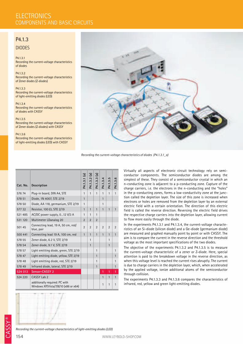
154 WWW.LEYBOLD-SHOP.COMCA
SSY ®
Virtually all aspects of electronic circuit technology rely on semi- conductor components. The semiconductor diodes are among the simplest of these. They consist of a semiconductor crystal in which an n-conducting zone is adjacent to a p-conducting zone. Capture of the charge carriers, i.e. the electrons in the n-conducting and the “holes” in the p-conducting zones, forms a low-conductivity zone at the junc-tion called the depletion layer. The size of this zone is increased when electrons or holes are removed from the depletion layer by an external electric field with a certain orientation. The direction of this electric field is called the reverse direction. Reversing the electric field drives the respective charge carriers into the depletion layer, allowing current to flow more easily through the diode.
In the experiments P4.1.3.1 and P4.1.3.4, the current-voltage characte-ristics of an Si-diode (silicon diode) and a Ge-diode (germanium diode) are measured and graphed manually point by point or with CASSY. The aim is to compare the current in the reverse direction and the threshold voltage as the most important specifications of the two diodes.
The objective of the experiments P4.1.3.2 and P4.1.3.5 is to measure the current-voltage characteristic of a zener or Z-diode. Here, special attention is paid to the breakdown voltage in the reverse direction, as when this voltage level is reached the current rises abruptly. The current is due to charge carriers in the depletion layer, which, when accelerated by the applied voltage, ionize additional atoms of the semiconductor through collision.
The experiments P4.1.3.3 and P4.1.3.6 compares the characteristics of infrared, red, yellow and green light-emitting diodes.
ELECTRONICS
Recording the current-voltage characteristics of diodes (P4.1.3.1_a)
Cat. No. Description
P4.1
.3.1
(a)
P4.1
.3.2
(a)
P4.1
.3.3
(a)
P4.1
.3.4
P4.1
.3.5
P4.1
.3.6
576 74 Plug-in board, DIN A4, STE 1 1 1 1 1 1
578 51 Diode, 1N 4007, STE 2/19 1 1
578 50 Diode, AA 118, germanium, STE 2/19 1 1
577 32 Resistor, 100 , STE 2/19 1 1 1 1 1 1
521 485 AC/DC power supply, 0...12 V/3 A 1 1 1
531 120 Multimeter LDanalog 20 2 2 2
501 45Connecting lead, 19 A, 50 cm, red/blue, pair
2 2 2 2 2 2
500 441 Connecting lead 19 A, 100 cm, red 1 1 1 1 1 1
578 55 Zener diode, 6.2 V, STE 2/19 1 1
578 54 Zener diode, 9.1 V, STE 2/19 1 1
578 57 Light emitting diode, green, STE 2/19 1 1
578 47 Light emitting diode, yellow, STE 2/19 1 1
578 48 Light emitting diode, red, STE 2/19 1 1
578 49 Infrared diode, lateral, STE 2/19 1 1
524 013 Sensor-CASSY 2 1 1 1
524 220 CASSY Lab 2 1 1 1
additionally required: PC with Windows XP/Vista/7/8/10 (x86 or x64)
1 1 1
Recording the current-voltage characteristics of light-emitting diodes (LED)
COMPONENTS AND BASIC CIRCUITS
P4.1.3
DIODES
P4.1.3.1 Recording the current-voltage characteristics of diodes
P4.1.3.2 Recording the current-voltage characteristics of Zener diodes (Z-diodes)
P4.1.3.3 Recording the current-voltage characteristics of light-emitting diodes (LED)
P4.1.3.4 Recording the current-voltage characteristics of diodes with CASSY
P4.1.3.5 Recording the current-voltage characteristics of Zener diodes (Z-diodes) with CASSY
P4.1.3.6 Recording the current-voltage characteristics
of light-emitting diodes (LED) with CASSY
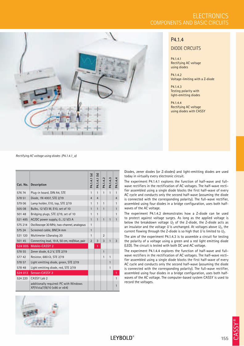
155 CA
SSY ®
DIODE CIRCUITS
P4.1.4.1 Rectifying AC voltage using diodes
P4.1.4.2 Voltage-limiting with a Z-diode
P4.1.4.3 Testing polarity with light-emitting diodes
P4.1.4.4 Rectifying AC voltage using diodes with CASSY
COMPONENTS AND BASIC CIRCUITS
ELECTRONICS
Cat. No. Description
P4.1
.4.1
(a)
P4.1
.4.1
(b)
P4.1
.4.2
P4.1
.4.3
P4.1
.4.4
576 74 Plug-in board, DIN A4, STE 1 1 1 1 1
578 51 Diode, 1N 4007, STE 2/19 4 4 4
579 06 Lamp holder, E10, top, STE 2/19 1 1 1 1
505 08 Bulbs, 12 V/3 W, E10, set of 10 1 1 1 1
501 48 Bridging plugs, STE 2/19, set of 10 1 1 1
521 485 AC/DC power supply, 0...12 V/3 A 1 1 1 1 1
575 214 Oscilloscope 30 MHz, two-channel, analogous 1
575 24 Screened cable, BNC/4 mm 1
531 120 Multimeter LDanalog 20 1 2
501 45 Connecting lead, 19 A, 50 cm, red/blue, pair 2 3 3 1 3
524 005 Mobile-CASSY 2 1
578 55 Zener diode, 6.2 V, STE 2/19 1
577 42 Resistor, 680 , STE 2/19 1 1
578 57 Light emitting diode, green, STE 2/19 1
578 48 Light emitting diode, red, STE 2/19 1
524 013 Sensor-CASSY 2 1
524 220 CASSY Lab 2 1
additionally required: PC with Windows XP/Vista/7/8/10 (x86 or x64)
1
Diodes, zener diodes (or Z-diodes) and light-emitting diodes are used today in virtually every electronic circuit.
The experiment P4.1.4.1 explores the function of half-wave and full-wave rectifiers in the rectification of AC voltages. The half-wave recti-fier assembled using a single diode blocks the first half-wave of every AC cycle and conducts only the second half-wave (assuming the diode is connected with the corresponding polarity). The full-wave rectifier, assembled using four diodes in a bridge configuration, uses both half-waves of the AC voltage.
The experiment P4.1.4.2 demonstrates how a Z-diode can be used to protect against voltage surges. As long as the applied voltage is below the breakdown voltage UZ of the Z-diode, the Z-diode acts as an insulator and the voltage U is unchanged. At voltages above UZ, the current flowing through the Z-diode is so high that U is limited to UZ.
The aim of the experiment P4.1.4.3 is to assemble a circuit for testing the polarity of a voltage using a green and a red light emitting diode (LED). The circuit is tested with both DC and AC voltage.
The experiment P4.1.4.4 explores the function of half-wave and full-wave rectifiers in the rectification of AC voltages. The half-wave recti-fier assembled using a single diode blocks the first half-wave of every AC cycle and conducts only the second half-wave (assuming the diode is connected with the corresponding polarity). The full-wave rectifier, assembled using four diodes in a bridge configuration, uses both half-waves of the AC voltage. The computer-based system CASSY is used to record the voltages.
Rectifying AC voltage using diodes (P4.1.4.1_a)
P4.1.4
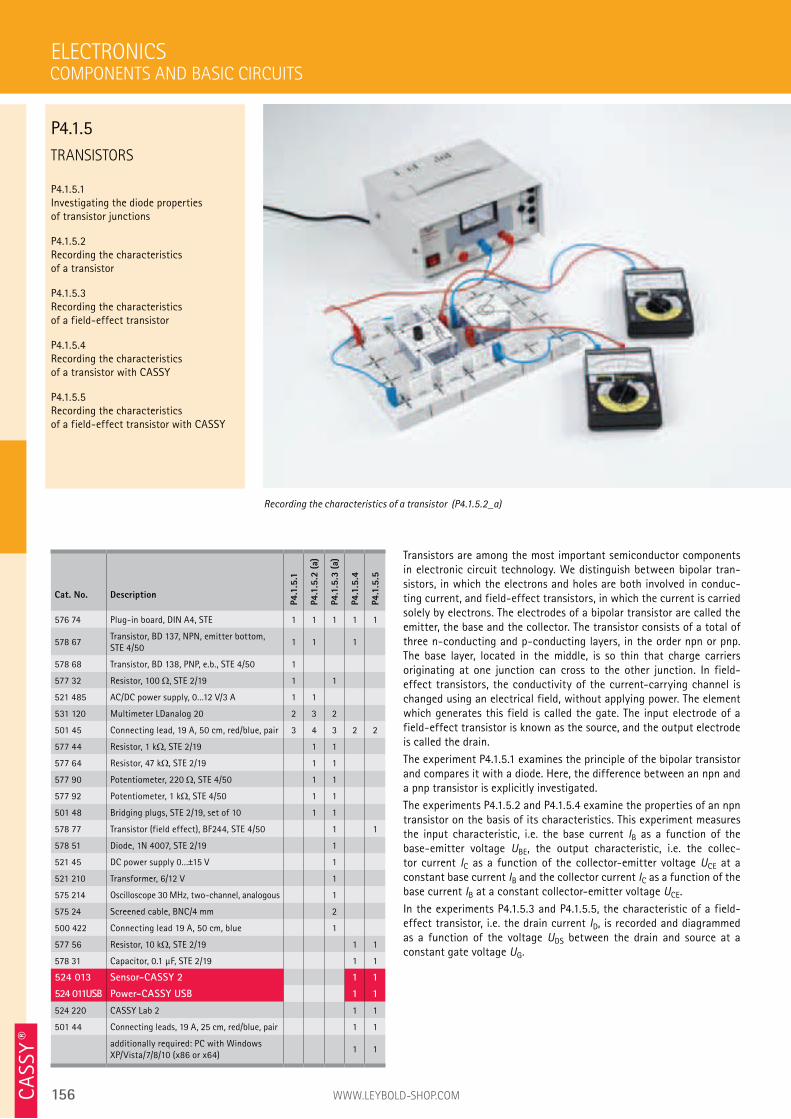
156 WWW.LEYBOLD-SHOP.COMCA
SSY ®
TRANSISTORS
P4.1.5.1 Investigating the diode properties of transistor junctions
P4.1.5.2 Recording the characteristics of a transistor
P4.1.5.3 Recording the characteristics of a field-effect transistor
P4.1.5.4 Recording the characteristics of a transistor with CASSY
P4.1.5.5 Recording the characteristics of a field-effect transistor with CASSY
Transistors are among the most important semiconductor components in electronic circuit technology. We distinguish between bipolar tran-sistors, in which the electrons and holes are both involved in conduc-ting current, and field-effect transistors, in which the current is carried solely by electrons. The electrodes of a bipolar transistor are called the emitter, the base and the collector. The transistor consists of a total of three n-conducting and p-conducting layers, in the order npn or pnp. The base layer, located in the middle, is so thin that charge carriers originating at one junction can cross to the other junction. In field-effect transistors, the conductivity of the current-carrying channel is changed using an electrical field, without applying power. The element which generates this field is called the gate. The input electrode of a field-effect transistor is known as the source, and the output electrode is called the drain.
The experiment P4.1.5.1 examines the principle of the bipolar transistor and compares it with a diode. Here, the difference between an npn and a pnp transistor is explicitly investigated.
The experiments P4.1.5.2 and P4.1.5.4 examine the properties of an npn transistor on the basis of its characteristics. This experiment measures the input characteristic, i.e. the base current IB as a function of the base-emitter voltage UBE, the output characteristic, i.e. the collec-tor current IC as a function of the collector-emitter voltage UCE at a constant base current IB and the collector current IC as a function of the base current IB at a constant collector-emitter voltage UCE.
In the experiments P4.1.5.3 and P4.1.5.5, the characteristic of a field-effect transistor, i.e. the drain current ID, is recorded and diagrammed as a function of the voltage UDS between the drain and source at a constant gate voltage UG.
ELECTRONICS
Recording the characteristics of a transistor (P4.1.5.2_a)
Cat. No. Description
P4.1
.5.1
P4.1
.5.2
(a)
P4.1
.5.3
(a)
P4.1
.5.4
P4.1
.5.5
576 74 Plug-in board, DIN A4, STE 1 1 1 1 1
578 67Transistor, BD 137, NPN, emitter bottom, STE 4/50
1 1 1
578 68 Transistor, BD 138, PNP, e.b., STE 4/50 1
577 32 Resistor, 100 , STE 2/19 1 1
521 485 AC/DC power supply, 0...12 V/3 A 1 1
531 120 Multimeter LDanalog 20 2 3 2
501 45 Connecting lead, 19 A, 50 cm, red/blue, pair 3 4 3 2 2
577 44 Resistor, 1 k , STE 2/19 1 1
577 64 Resistor, 47 k , STE 2/19 1 1
577 90 Potentiometer, 220 , STE 4/50 1 1
577 92 Potentiometer, 1 k , STE 4/50 1 1
501 48 Bridging plugs, STE 2/19, set of 10 1 1
578 77 Transistor (field effect), BF244, STE 4/50 1 1
578 51 Diode, 1N 4007, STE 2/19 1
521 45 DC power supply 0...±15 V 1
521 210 Transformer, 6/12 V 1
575 214 Oscilloscope 30 MHz, two-channel, analogous 1
575 24 Screened cable, BNC/4 mm 2
500 422 Connecting lead 19 A, 50 cm, blue 1
577 56 Resistor, 10 k , STE 2/19 1 1
578 31 Capacitor, 0.1 µF, STE 2/19 1 1
524 013 Sensor-CASSY 2 1 1
524 011USB Power-CASSY USB 1 1
524 220 CASSY Lab 2 1 1
501 44 Connecting leads, 19 A, 25 cm, red/blue, pair 1 1
additionally required: PC with Windows XP/Vista/7/8/10 (x86 or x64)
1 1
COMPONENTS AND BASIC CIRCUITS
P4.1.5
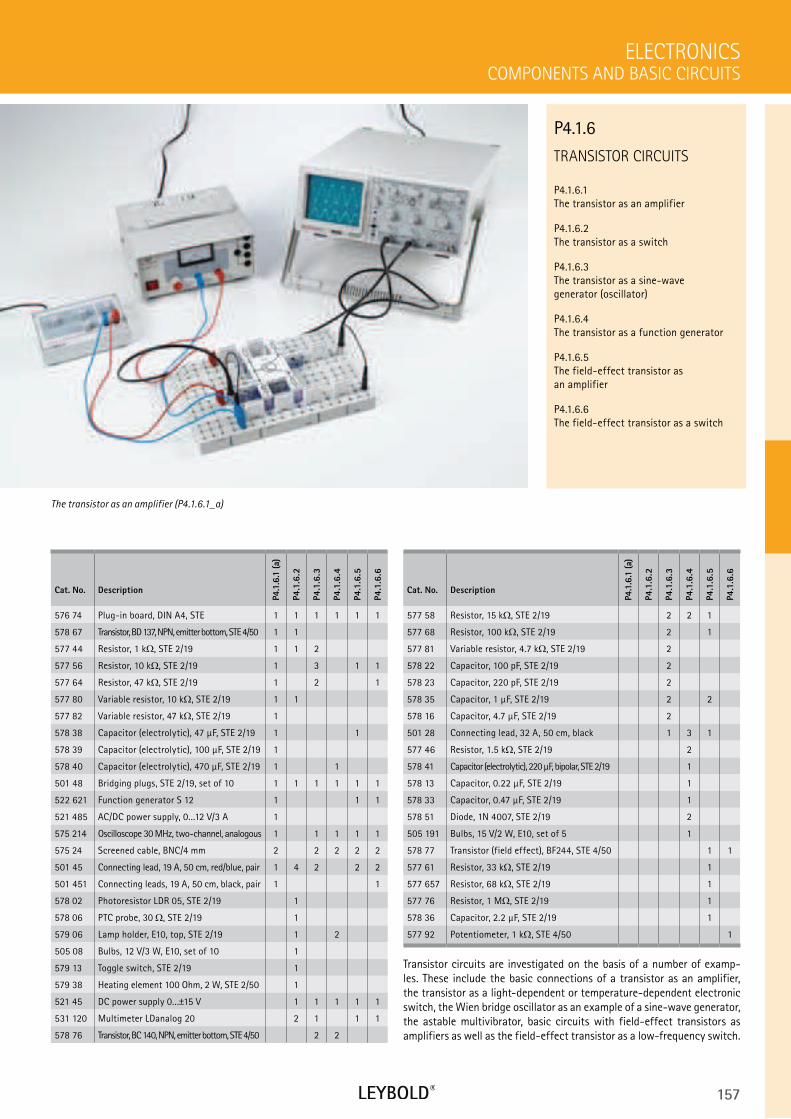
157
TRANSISTOR CIRCUITS
P4.1.6.1 The transistor as an amplifier
P4.1.6.2 The transistor as a switch
P4.1.6.3 The transistor as a sine-wave generator (oscillator)
P4.1.6.4 The transistor as a function generator
P4.1.6.5 The field-effect transistor as an amplifier
P4.1.6.6 The field-effect transistor as a switch
COMPONENTS AND BASIC CIRCUITS
ELECTRONICS
Cat. No. Description
P4.1
.6.1
(a)
P4.1
.6.2
P4.1
.6.3
P4.1
.6.4
P4.1
.6.5
P4.1
.6.6
576 74 Plug-in board, DIN A4, STE 1 1 1 1 1 1
578 67 Transistor, BD 137, NPN, emitter bottom, STE 4/50 1 1
577 44 Resistor, 1 k , STE 2/19 1 1 2
577 56 Resistor, 10 k , STE 2/19 1 3 1 1
577 64 Resistor, 47 k , STE 2/19 1 2 1
577 80 Variable resistor, 10 k , STE 2/19 1 1
577 82 Variable resistor, 47 k , STE 2/19 1
578 38 Capacitor (electrolytic), 47 µF, STE 2/19 1 1
578 39 Capacitor (electrolytic), 100 µF, STE 2/19 1
578 40 Capacitor (electrolytic), 470 µF, STE 2/19 1 1
501 48 Bridging plugs, STE 2/19, set of 10 1 1 1 1 1 1
522 621 Function generator S 12 1 1 1
521 485 AC/DC power supply, 0...12 V/3 A 1
575 214 Oscilloscope 30 MHz, two-channel, analogous 1 1 1 1 1
575 24 Screened cable, BNC/4 mm 2 2 2 2 2
501 45 Connecting lead, 19 A, 50 cm, red/blue, pair 1 4 2 2 2
501 451 Connecting leads, 19 A, 50 cm, black, pair 1 1
578 02 Photoresistor LDR 05, STE 2/19 1
578 06 PTC probe, 30 , STE 2/19 1
579 06 Lamp holder, E10, top, STE 2/19 1 2
505 08 Bulbs, 12 V/3 W, E10, set of 10 1
579 13 Toggle switch, STE 2/19 1
579 38 Heating element 100 Ohm, 2 W, STE 2/50 1
521 45 DC power supply 0...±15 V 1 1 1 1 1
531 120 Multimeter LDanalog 20 2 1 1 1
578 76 Transistor, BC 140, NPN, emitter bottom, STE 4/50 2 2
Transistor circuits are investigated on the basis of a number of examp-les. These include the basic connections of a transistor as an amplifier, the transistor as a light-dependent or temperature-dependent electronic switch, the Wien bridge oscillator as an example of a sine-wave generator, the astable multivibrator, basic circuits with field-effect transistors as amplifiers as well as the field-effect transistor as a low-frequency switch.
The transistor as an amplifier (P4.1.6.1_a)
P4.1.6
Cat. No. Description
P4.1
.6.1
(a)
P4.1
.6.2
P4.1
.6.3
P4.1
.6.4
P4.1
.6.5
P4.1
.6.6
577 58 Resistor, 15 k , STE 2/19 2 2 1
577 68 Resistor, 100 k , STE 2/19 2 1
577 81 Variable resistor, 4.7 k , STE 2/19 2
578 22 Capacitor, 100 pF, STE 2/19 2
578 23 Capacitor, 220 pF, STE 2/19 2
578 35 Capacitor, 1 µF, STE 2/19 2 2
578 16 Capacitor, 4.7 µF, STE 2/19 2
501 28 Connecting lead, 32 A, 50 cm, black 1 3 1
577 46 Resistor, 1.5 k , STE 2/19 2
578 41 Capacitor (electrolytic), 220 µF, bipolar, STE 2/19 1
578 13 Capacitor, 0.22 µF, STE 2/19 1
578 33 Capacitor, 0.47 µF, STE 2/19 1
578 51 Diode, 1N 4007, STE 2/19 2
505 191 Bulbs, 15 V/2 W, E10, set of 5 1
578 77 Transistor (field effect), BF244, STE 4/50 1 1
577 61 Resistor, 33 k , STE 2/19 1
577 657 Resistor, 68 k , STE 2/19 1
577 76 Resistor, 1 M , STE 2/19 1
578 36 Capacitor, 2.2 µF, STE 2/19 1
577 92 Potentiometer, 1 k , STE 4/50 1
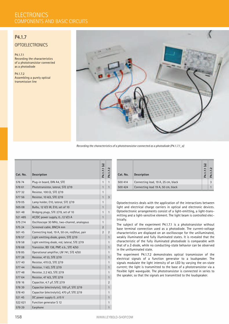
158 WWW.LEYBOLD-SHOP.COM
OPTOELECTRONICS
P4.1.7.1 Recording the characteristics of a phototransistor connected as a photodiode
P4.1.7.2 Assembling a purely optical transmission line
Optoelectronics deals with the application of the interactions between light and electrical charge carriers in optical and electronic devices. Optoelectronic arrangements consist of a light-emitting, a light-trans-mitting and a light-sensitive element. The light beam is controlled elec-trically.
The subject of the experiment P4.1.7.1 is a phototransistor without base terminal connection used as a photodiode. The current-voltage characteristics are displayed on an oscilloscope for the unilluminated, weakly illuminated and fully illuminated states. It is revealed that the characteristic of the fully illuminated photodiode is comparable with that of a Z-diode, while no conducting-state behavior can be observed in the unilluminated state.
The experiment P4.1.7.2 demonstrates optical transmission of the electrical signals of a function generator to a loudspeaker. The signals modulate the light intensity of an LED by varying the on-state current; the light is transmitted to the base of a phototransistor via a flexible light waveguide. The phototransistor is connected in series to the speaker, so that the signals are transmitted to the loudspeaker.
ELECTRONICS
Recording the characteristics of a phototransistor connected as a photodiode (P4.1.7.1_a)
Cat. No. Description
P4.1
.7.1
(a)
P4.1
.7.2
576 74 Plug-in board, DIN A4, STE 1 1
578 61 Phototransistor, lateral, STE 2/19 1 1
577 32 Resistor, 100 , STE 2/19 1
577 56 Resistor, 10 k , STE 2/19 1 3
579 05 Lamp holder, E10, lateral, STE 2/19 1
505 08 Bulbs, 12 V/3 W, E10, set of 10 1
501 48 Bridging plugs, STE 2/19, set of 10 1 1
521 485 AC/DC power supply, 0...12 V/3 A 1
575 214 Oscilloscope 30 MHz, two-channel, analogous 1
575 24 Screened cable, BNC/4 mm 2
501 45 Connecting lead, 19 A, 50 cm, red/blue, pair 2 2
578 57 Light emitting diode, green, STE 2/19 1
578 58 Light emitting diode, red, lateral, STE 2/19 1
578 68 Transistor, BD 138, PNP, e.b., STE 4/50 1
578 85 Operational amplifier, LM 741, STE 4/50 1
577 28 Resistor, 47 , STE 2/19 1
577 40 Resistor, 470 , STE 2/19 1
577 44 Resistor, 1 k , STE 2/19 1
577 48 Resistor, 2.2 k , STE 2/19 1
577 64 Resistor, 47 k , STE 2/19 1
578 16 Capacitor, 4.7 µF, STE 2/19 2
578 39 Capacitor (electrolytic), 100 µF, STE 2/19 1
578 40 Capacitor (electrolytic), 470 µF, STE 2/19 1
521 45 DC power supply 0...±15 V 1
522 621 Function generator S 12 1
579 29 Earphone 1
COMPONENTS AND BASIC CIRCUITS
P4.1.7
Cat. No. Description
P4.1
.7.1
(a)
P4.1
.7.2
500 414 Connecting lead, 19 A, 25 cm, black 3
500 424 Connecting lead 19 A, 50 cm, black 1
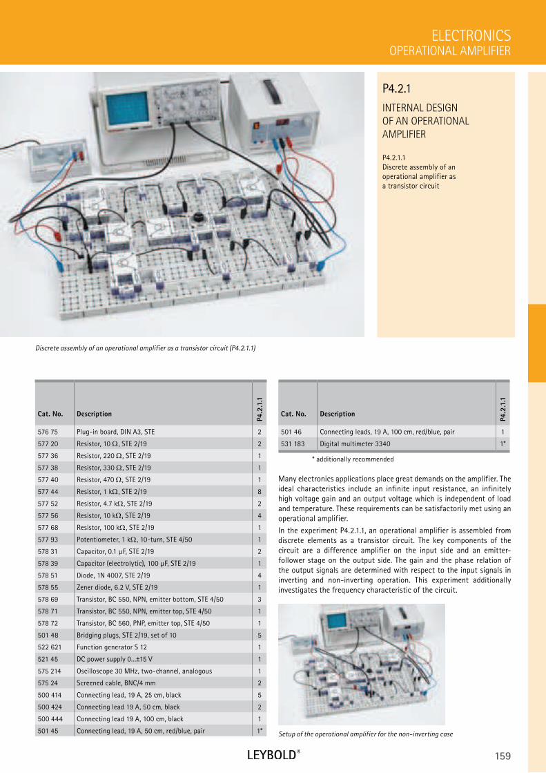
159
Cat. No. Description
P4.2
.1.1
501 46 Connecting leads, 19 A, 100 cm, red/blue, pair 1
531 183 Digital multimeter 3340 1*
* additionally recommended
INTERNAL DESIGN
OF AN OPERATIONAL
AMPLIFIER
P4.2.1.1 Discrete assembly of an operational amplifier as a transistor circuit
OPERATIONAL AMPLIFIER
ELECTRONICS
Cat. No. Description
P4.2
.1.1
576 75 Plug-in board, DIN A3, STE 2
577 20 Resistor, 10 , STE 2/19 2
577 36 Resistor, 220 , STE 2/19 1
577 38 Resistor, 330 , STE 2/19 1
577 40 Resistor, 470 , STE 2/19 1
577 44 Resistor, 1 k , STE 2/19 8
577 52 Resistor, 4.7 k , STE 2/19 2
577 56 Resistor, 10 k , STE 2/19 4
577 68 Resistor, 100 k , STE 2/19 1
577 93 Potentiometer, 1 k , 10-turn, STE 4/50 1
578 31 Capacitor, 0.1 µF, STE 2/19 2
578 39 Capacitor (electrolytic), 100 µF, STE 2/19 1
578 51 Diode, 1N 4007, STE 2/19 4
578 55 Zener diode, 6.2 V, STE 2/19 1
578 69 Transistor, BC 550, NPN, emitter bottom, STE 4/50 3
578 71 Transistor, BC 550, NPN, emitter top, STE 4/50 1
578 72 Transistor, BC 560, PNP, emitter top, STE 4/50 1
501 48 Bridging plugs, STE 2/19, set of 10 5
522 621 Function generator S 12 1
521 45 DC power supply 0...±15 V 1
575 214 Oscilloscope 30 MHz, two-channel, analogous 1
575 24 Screened cable, BNC/4 mm 2
500 414 Connecting lead, 19 A, 25 cm, black 5
500 424 Connecting lead 19 A, 50 cm, black 2
500 444 Connecting lead 19 A, 100 cm, black 1
501 45 Connecting lead, 19 A, 50 cm, red/blue, pair 1*
Many electronics applications place great demands on the amplifier. The ideal characteristics include an infinite input resistance, an infinitely high voltage gain and an output voltage which is independent of load and temperature. These requirements can be satisfactorily met using an operational amplifier.
In the experiment P4.2.1.1, an operational amplifier is assembled from discrete elements as a transistor circuit. The key components of the circuit are a difference amplifier on the input side and an emitter- follower stage on the output side. The gain and the phase relation of the output signals are determined with respect to the input signals in inverting and non-inverting operation. This experiment additionally investigates the frequency characteristic of the circuit.
Discrete assembly of an operational amplifier as a transistor circuit (P4.2.1.1)
P4.2.1
Setup of the operational amplifier for the non-inverting case
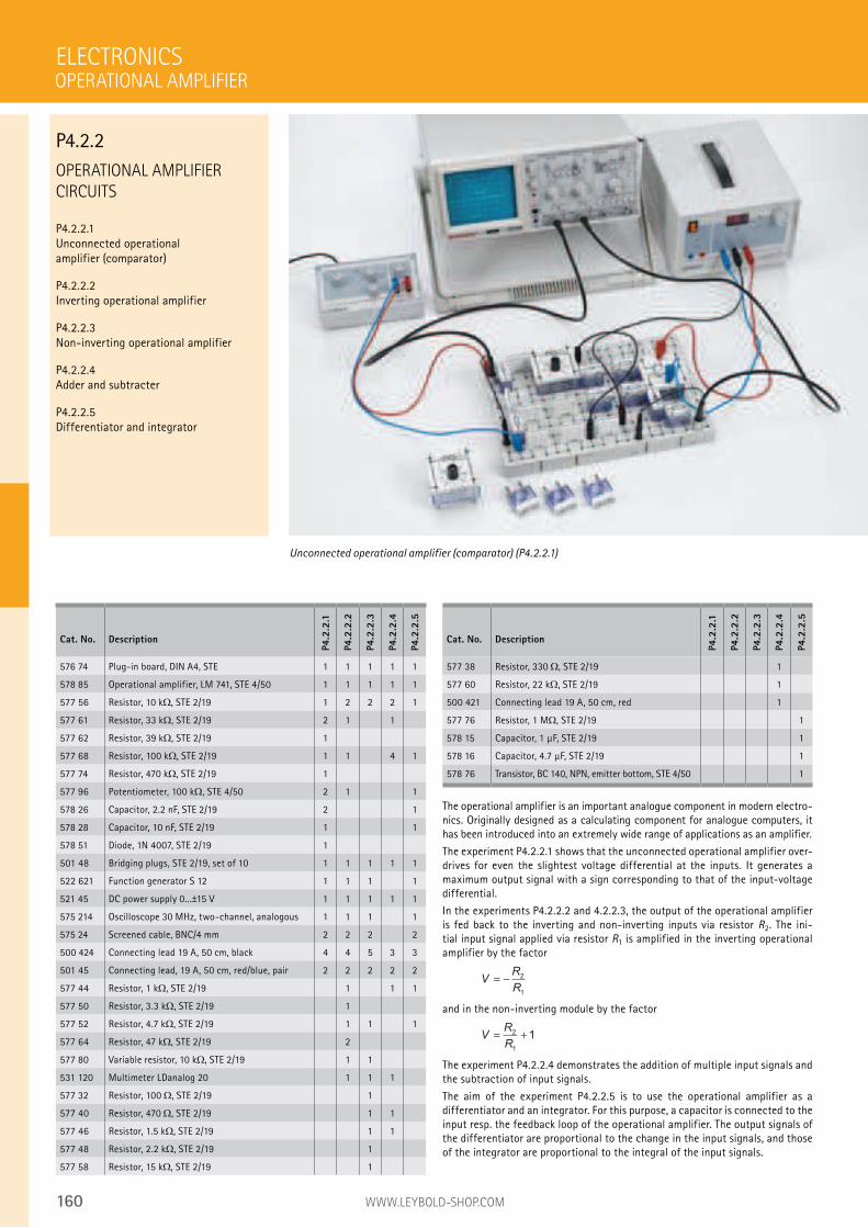
160 WWW.LEYBOLD-SHOP.COM
Cat. No. Description
P4.2
.2.1
P4.2
.2.2
P4.2
.2.3
P4.2
.2.4
P4.2
.2.5
577 38 Resistor, 330 , STE 2/19 1
577 60 Resistor, 22 k , STE 2/19 1
500 421 Connecting lead 19 A, 50 cm, red 1
577 76 Resistor, 1 M , STE 2/19 1
578 15 Capacitor, 1 µF, STE 2/19 1
578 16 Capacitor, 4.7 µF, STE 2/19 1
578 76 Transistor, BC 140, NPN, emitter bottom, STE 4/50 1
OPERATIONAL AMPLIFIER
CIRCUITS
P4.2.2.1 Unconnected operational amplifier (comparator)
P4.2.2.2 Inverting operational amplifier
P4.2.2.3 Non-inverting operational amplifier
P4.2.2.4 Adder and subtracter
P4.2.2.5 Differentiator and integrator
The operational amplifier is an important analogue component in modern electro-nics. Originally designed as a calculating component for analogue computers, it has been introduced into an extremely wide range of applications as an amplifier.
The experiment P4.2.2.1 shows that the unconnected operational amplifier over-drives for even the slightest voltage differential at the inputs. It generates a maximum output signal with a sign corresponding to that of the input-voltage differential.
In the experiments P4.2.2.2 and 4.2.2.3, the output of the operational amplifier is fed back to the inverting and non-inverting inputs via resistor R2. The ini-tial input signal applied via resistor R1 is amplified in the inverting operational amplifier by the factor
VR
R= − 2
1
and in the non-inverting module by the factor
VR
R= +2
1
1
The experiment P4.2.2.4 demonstrates the addition of multiple input signals and the subtraction of input signals.
The aim of the experiment P4.2.2.5 is to use the operational amplifier as a differentiator and an integrator. For this purpose, a capacitor is connected to the input resp. the feedback loop of the operational amplifier. The output signals of the differentiator are proportional to the change in the input signals, and those of the integrator are proportional to the integral of the input signals.
ELECTRONICS
Unconnected operational amplifier (comparator) (P4.2.2.1)
Cat. No. Description
P4.2
.2.1
P4.2
.2.2
P4.2
.2.3
P4.2
.2.4
P4.2
.2.5
576 74 Plug-in board, DIN A4, STE 1 1 1 1 1
578 85 Operational amplifier, LM 741, STE 4/50 1 1 1 1 1
577 56 Resistor, 10 k , STE 2/19 1 2 2 2 1
577 61 Resistor, 33 k , STE 2/19 2 1 1
577 62 Resistor, 39 k , STE 2/19 1
577 68 Resistor, 100 k , STE 2/19 1 1 4 1
577 74 Resistor, 470 k , STE 2/19 1
577 96 Potentiometer, 100 k , STE 4/50 2 1 1
578 26 Capacitor, 2.2 nF, STE 2/19 2 1
578 28 Capacitor, 10 nF, STE 2/19 1 1
578 51 Diode, 1N 4007, STE 2/19 1
501 48 Bridging plugs, STE 2/19, set of 10 1 1 1 1 1
522 621 Function generator S 12 1 1 1 1
521 45 DC power supply 0...±15 V 1 1 1 1 1
575 214 Oscilloscope 30 MHz, two-channel, analogous 1 1 1 1
575 24 Screened cable, BNC/4 mm 2 2 2 2
500 424 Connecting lead 19 A, 50 cm, black 4 4 5 3 3
501 45 Connecting lead, 19 A, 50 cm, red/blue, pair 2 2 2 2 2
577 44 Resistor, 1 k , STE 2/19 1 1 1
577 50 Resistor, 3.3 k , STE 2/19 1
577 52 Resistor, 4.7 k , STE 2/19 1 1 1
577 64 Resistor, 47 k , STE 2/19 2
577 80 Variable resistor, 10 k , STE 2/19 1 1
531 120 Multimeter LDanalog 20 1 1 1
577 32 Resistor, 100 , STE 2/19 1
577 40 Resistor, 470 , STE 2/19 1 1
577 46 Resistor, 1.5 k , STE 2/19 1 1
577 48 Resistor, 2.2 k , STE 2/19 1
577 58 Resistor, 15 k , STE 2/19 1
OPERATIONAL AMPLIFIER
P4.2.2
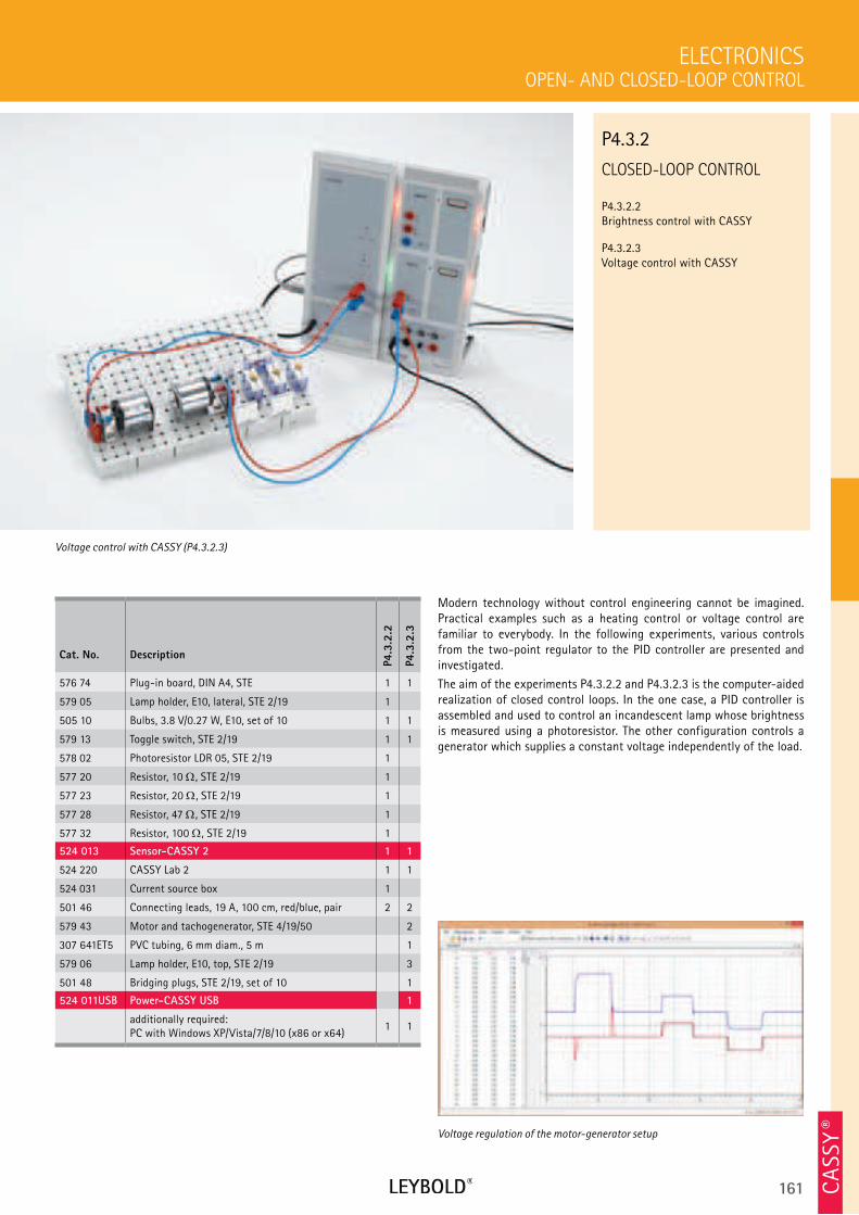
161 CA
SSY ®
CLOSED-LOOP CONTROL
P4.3.2.2 Brightness control with CASSY
P4.3.2.3 Voltage control with CASSY
OPEN- AND CLOSED-LOOP CONTROL
ELECTRONICS
Cat. No. Description
P4.3
.2.2
P4.3
.2.3
576 74 Plug-in board, DIN A4, STE 1 1
579 05 Lamp holder, E10, lateral, STE 2/19 1
505 10 Bulbs, 3.8 V/0.27 W, E10, set of 10 1 1
579 13 Toggle switch, STE 2/19 1 1
578 02 Photoresistor LDR 05, STE 2/19 1
577 20 Resistor, 10 , STE 2/19 1
577 23 Resistor, 20 , STE 2/19 1
577 28 Resistor, 47 , STE 2/19 1
577 32 Resistor, 100 , STE 2/19 1
524 013 Sensor-CASSY 2 1 1
524 220 CASSY Lab 2 1 1
524 031 Current source box 1
501 46 Connecting leads, 19 A, 100 cm, red/blue, pair 2 2
579 43 Motor and tachogenerator, STE 4/19/50 2
307 641ET5 PVC tubing, 6 mm diam., 5 m 1
579 06 Lamp holder, E10, top, STE 2/19 3
501 48 Bridging plugs, STE 2/19, set of 10 1
524 011USB Power-CASSY USB 1
additionally required: PC with Windows XP/Vista/7/8/10 (x86 or x64)
1 1
Modern technology without control engineering cannot be imagined. Practical examples such as a heating control or voltage control are familiar to everybody. In the following experiments, various controls from the two-point regulator to the PID controller are presented and investigated.
The aim of the experiments P4.3.2.2 and P4.3.2.3 is the computer-aided realization of closed control loops. In the one case, a PID controller is assembled and used to control an incandescent lamp whose brightness is measured using a photoresistor. The other configuration controls a generator which supplies a constant voltage independently of the load.
Voltage control with CASSY (P4.3.2.3)
P4.3.2
Voltage regulation of the motor-generator setup
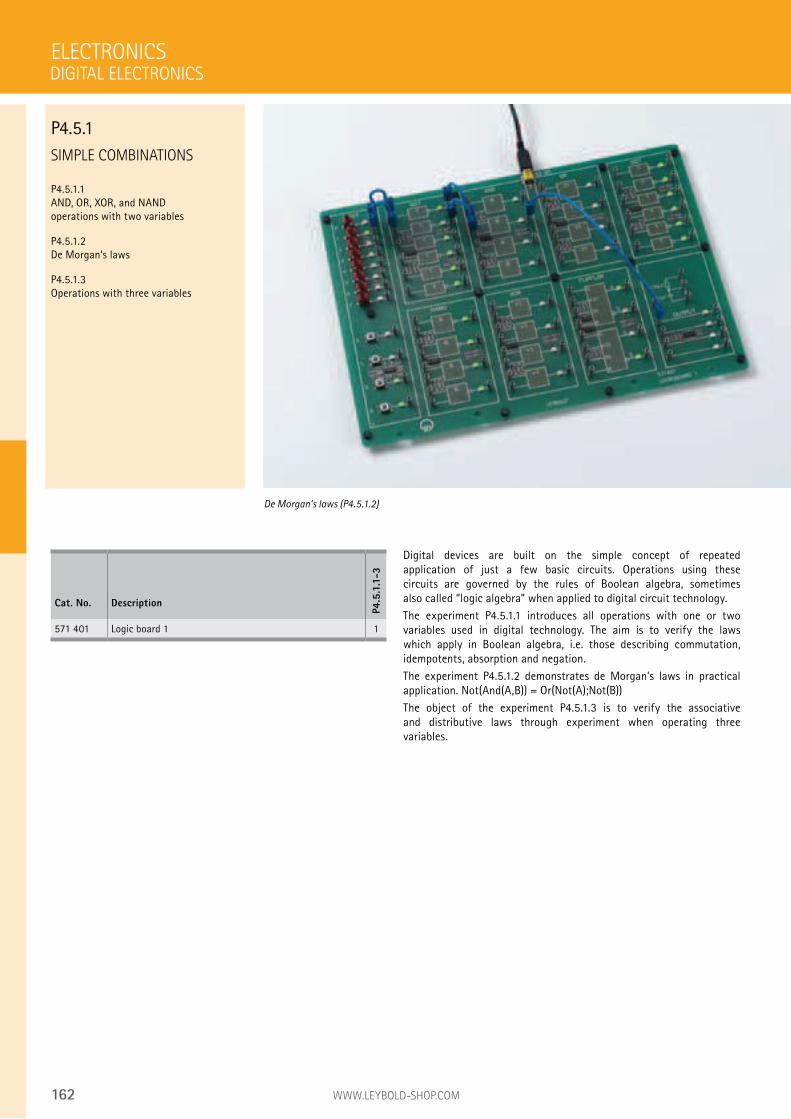
162 WWW.LEYBOLD-SHOP.COM
SIMPLE COMBINATIONS
P4.5.1.1 AND, OR, XOR, and NAND operations with two variables
P4.5.1.2 De Morgan‘s laws
P4.5.1.3 Operations with three variables
Digital devices are built on the simple concept of repeated application of just a few basic circuits. Operations using these circuits are governed by the rules of Boolean algebra, sometimes also called “logic algebra” when applied to digital circuit technology.
The experiment P4.5.1.1 introduces all operations with one or two variables used in digital technology. The aim is to verify the laws which apply in Boolean algebra, i.e. those describing commutation, idempotents, absorption and negation.
The experiment P4.5.1.2 demonstrates de Morgan‘s laws in practical application. Not(And(A,B)) = Or(Not(A);Not(B))
The object of the experiment P4.5.1.3 is to verify the associative and distributive laws through experiment when operating three variables.
ELECTRONICS
De Morgan‘s laws (P4.5.1.2)
Cat. No. Description
P4.5
.1.1
-3
571 401 Logic board 1 1
DIGITAL ELECTRONICS
P4.5.1
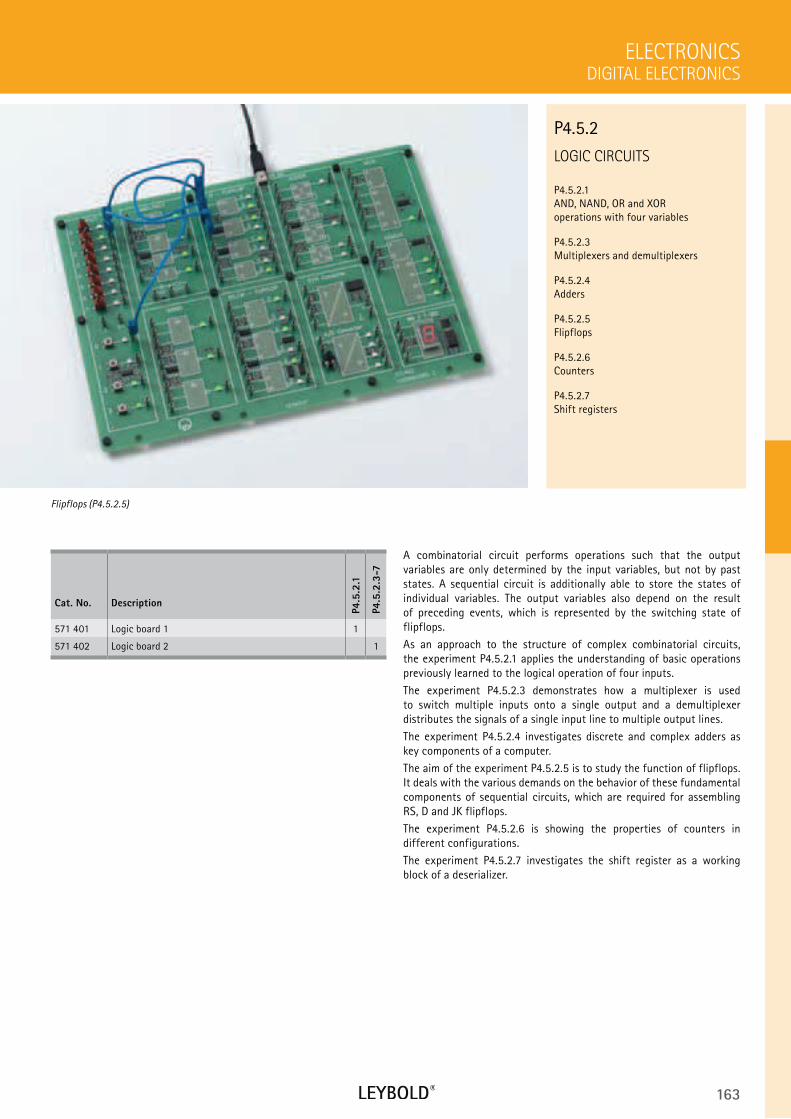
163
LOGIC CIRCUITS
P4.5.2.1
AND, NAND, OR and XOR
operations with four variables
P4.5.2.3
Multiplexers and demultiplexers
P4.5.2.4
Adders
P4.5.2.5
Flipflops
P4.5.2.6
Counters
P4.5.2.7
Shift registers
DIGITAL ELECTRONICS
ELECTRONICS
Cat. No. Description
P4.5
.2.1
P4.5
.2.3
-7
571 401 Logic board 1 1
571 402 Logic board 2 1
A combinatorial circuit performs operations such that the output
variables are only determined by the input variables, but not by past
states. A sequential circuit is additionally able to store the states of
individual variables. The output variables also depend on the result
of preceding events, which is represented by the switching state of
flipflops.
As an approach to the structure of complex combinatorial circuits,
the experiment P4.5.2.1 applies the understanding of basic operations
previously learned to the logical operation of four inputs.
The experiment P4.5.2.3 demonstrates how a multiplexer is used
to switch multiple inputs onto a single output and a demultiplexer
distributes the signals of a single input line to multiple output lines.
The experiment P4.5.2.4 investigates discrete and complex adders as
key components of a computer.
The aim of the experiment P4.5.2.5 is to study the function of flipflops.
It deals with the various demands on the behavior of these fundamental
components of sequential circuits, which are required for assembling
RS, D and JK flipflops.
The experiment P4.5.2.6 is showing the properties of counters in
different configurations.
The experiment P4.5.2.7 investigates the shift register as a working
block of a deserializer.
Flipflops (P4.5.2.5)
P4.5.2
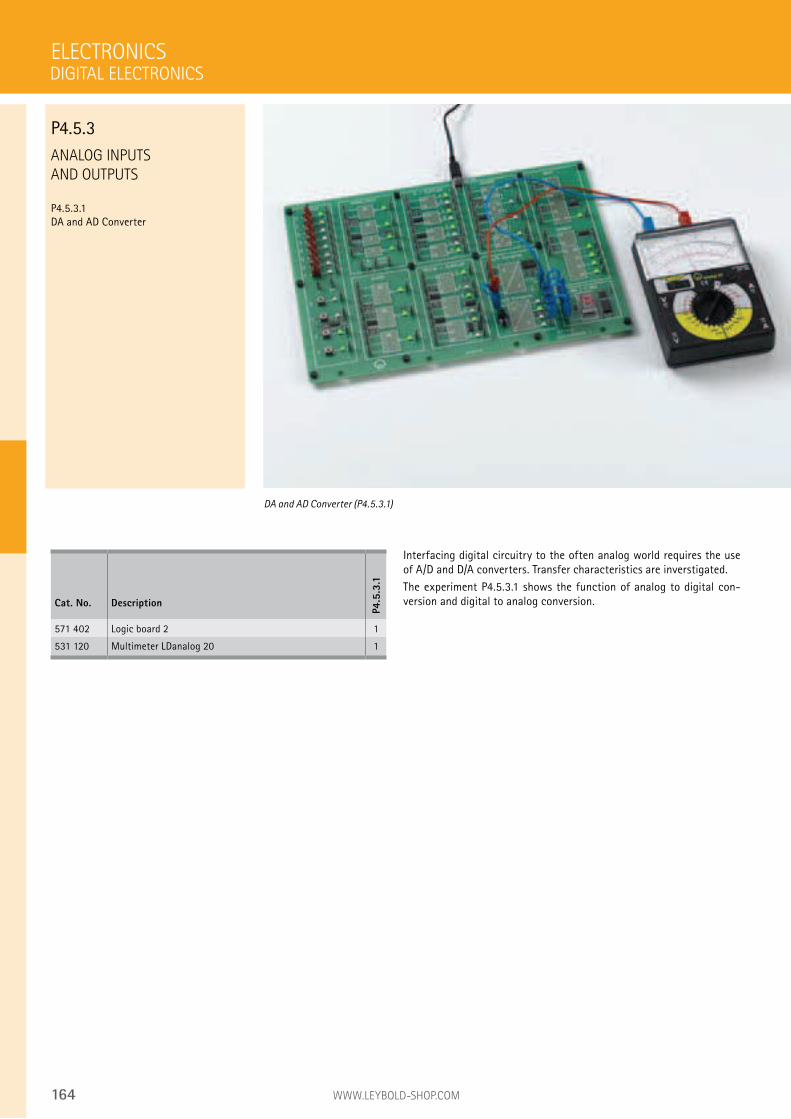
164 WWW.LEYBOLD-SHOP.COM
ANALOG INPUTS
AND OUTPUTS
P4.5.3.1 DA and AD Converter
Interfacing digital circuitry to the often analog world requires the use of A/D and D/A converters. Transfer characteristics are inverstigated.
The experiment P4.5.3.1 shows the function of analog to digital con-version and digital to analog conversion.
ELECTRONICS
DA and AD Converter (P4.5.3.1)
Cat. No. Description
P4.5
.3.1
571 402 Logic board 2 1
531 120 Multimeter LDanalog 20 1
DIGITAL ELECTRONICS
P4.5.3
165
P5.1 GEOMETRICAL OPTICS 167
P5.2 DISPERSION AND CHROMATICS 171
P5.3 WAVE OPTICS 176
P5.4 POLARIZATION 189
P5.5 LIGHT INTENSITY 195
P5.6 VELOCITY OF LIGHT 198
P5.7 SPECTROMETER 202
P5.8 PHOTONICS 206
P5 OPTICS

166 WWW.LEYBOLD-SHOP.COM
P5.1 GEOMETRICAL OPTICS
P5.1.1 Reflection, refraction 167P5.1.2 Laws of imaging 168P5.1.3 Image distortion 169P5.1.4 Optical instruments 170
P5.2 DISPERSION AND CHROMATICS
P5.2.1 Refractive index and dispersion 171P5.2.3 Color mixing 172P5.2.4 Absorption spectra 173-174P5.2.5 Reflection spectra 175
P5.3 WAVE OPTICS
P5.3.1 Diffraction 176-179P5.3.2 Two-beam interference 180P5.3.3 Newton´s Rings 181-182P5.3.4 Michelson interferometer 183-184P5.3.5 Other types of interferometers 185-186P5.3.6 White-light Reflection Holography 187P5.3.7 Transmission Holography 188
P5.4 POLARIZATION
P5.4.1 Basic experiments 189P5.4.2 Birefringence 190P5.4.3 Optical activity, polarimetry 191P5.4.4 Kerr effect 192P5.4.5 Pockels effect 193P5.4.6 Faraday effect 194
P5.5 LIGHT INTENSITY
P5.5.1 Quantities and measuring methods of lighting engineering 195P5.5.2 Laws of radiation 196-197
P5.6 VELOCITY OF LIGHT
P5.6.1 Measurement according to Foucault/Michelson 198P5.6.2 Measuring with short light pulses 199P5.6.3 Measuring with an electronically modulated signal 200-201
P5.7 SPECTROMETER
P5.7.1 Prism spectrometer 202P5.7.2 Grating spectrometer 203-205
P5.8 PHOTONICS
P5.8.2 Basic Optics 206-208P5.8.3 Optical applications 209-211P5.8.4 Optical imaging and colour 212P5.8.5 Laser basics 213-216P5.8.6 Solid state laser 217-219P5.8.7 Optical fibres 220-222P5.8.8 Technical applications 223-227
P5 OPTICS
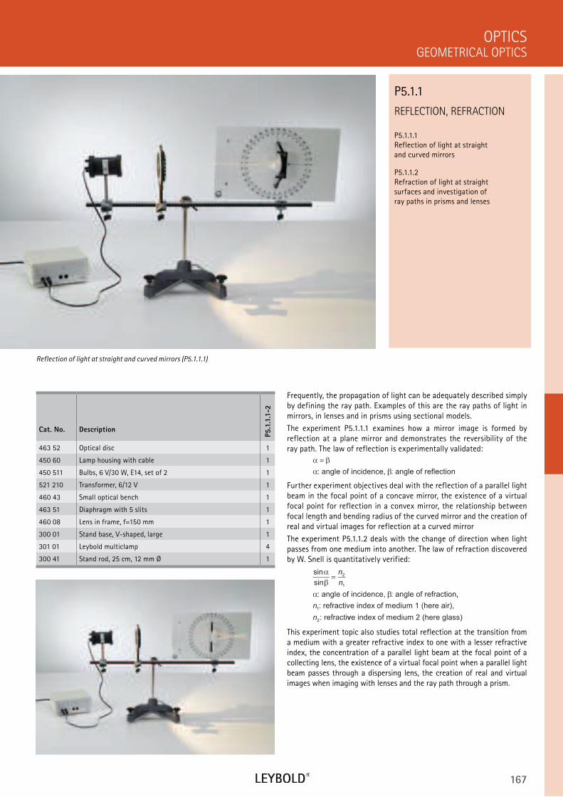
167
REFLECTION, REFRACTION
P5.1.1.1 Reflection of light at straight and curved mirrors
P5.1.1.2 Refraction of light at straight surfaces and investigation of ray paths in prisms and lenses
GEOMETRICAL OPTICS
OPTICS
Cat. No. Description
P5.1
.1.1
-2
463 52 Optical disc 1
450 60 Lamp housing with cable 1
450 511 Bulbs, 6 V/30 W, E14, set of 2 1
521 210 Transformer, 6/12 V 1
460 43 Small optical bench 1
463 51 Diaphragm with 5 slits 1
460 08 Lens in frame, f=150 mm 1
300 01 Stand base, V-shaped, large 1
301 01 Leybold multiclamp 4
300 41 Stand rod, 25 cm, 12 mm Ø 1
Frequently, the propagation of light can be adequately described simply by defining the ray path. Examples of this are the ray paths of light in mirrors, in lenses and in prisms using sectional models.
The experiment P5.1.1.1 examines how a mirror image is formed by reflection at a plane mirror and demonstrates the reversibility of the ray path. The law of reflection is experimentally validated:
α β
α β
=
: angle of incidence, : angle of reflection
Further experiment objectives deal with the reflection of a parallel light beam in the focal point of a concave mirror, the existence of a virtual focal point for reflection in a convex mirror, the relationship between focal length and bending radius of the curved mirror and the creation of real and virtual images for reflection at a curved mirror
The experiment P5.1.1.2 deals with the change of direction when light passes from one medium into another. The law of refraction discovered by W. Snell is quantitatively verified:
sin
sin
α
β
α β
=n
n
2
1
: angle of incidence, : angle of refraction,,
: refractive index of medium 1 (here air),
: refracti
n
n
1
2 vve index of medium 2 (here glass)
This experiment topic also studies total reflection at the transition from a medium with a greater refractive index to one with a lesser refractive index, the concentration of a parallel light beam at the focal point of a collecting lens, the existence of a virtual focal point when a parallel light beam passes through a dispersing lens, the creation of real and virtual images when imaging with lenses and the ray path through a prism.
Reflection of light at straight and curved mirrors (P5.1.1.1)
P5.1.1
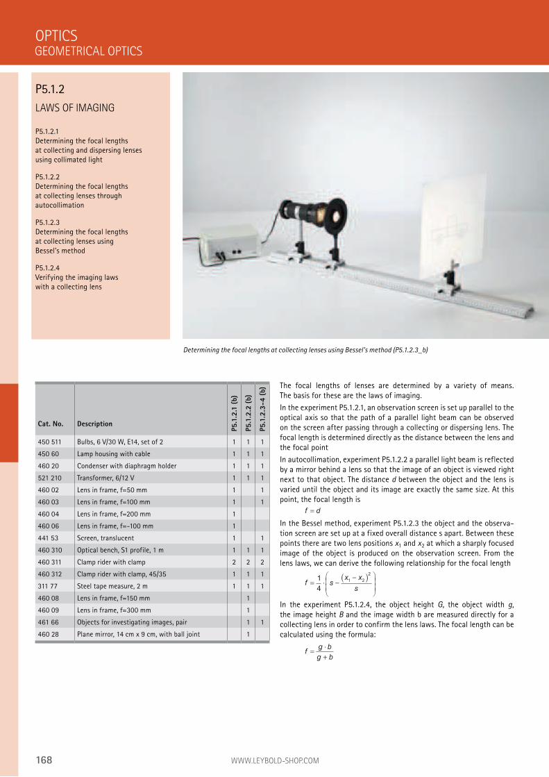
168 WWW.LEYBOLD-SHOP.COM
LAWS OF IMAGING
P5.1.2.1 Determining the focal lengths at collecting and dispersing lenses using collimated light
P5.1.2.2 Determining the focal lengths at collecting lenses through autocollimation
P5.1.2.3 Determining the focal lengths at collecting lenses using Bessel’s method
P5.1.2.4 Verifying the imaging laws with a collecting lens
The focal lengths of lenses are determined by a variety of means. The basis for these are the laws of imaging.
In the experiment P5.1.2.1, an observation screen is set up parallel to the optical axis so that the path of a parallel light beam can be observed on the screen after passing through a collecting or dispersing lens. The focal length is determined directly as the distance between the lens and the focal point
In autocollimation, experiment P5.1.2.2 a parallel light beam is reflected by a mirror behind a lens so that the image of an object is viewed right next to that object. The distance d between the object and the lens is varied until the object and its image are exactly the same size. At this point, the focal length is
f d
In the Bessel method, experiment P5.1.2.3 the object and the observa-tion screen are set up at a fixed overall distance s apart. Between these points there are two lens positions x1 and x2 at which a sharply focused image of the object is produced on the observation screen. From the lens laws, we can derive the following relationship for the focal length
f sx x
s= ⋅ −
−( )
1
4
1 2
2
In the experiment P5.1.2.4, the object height G, the object width g, the image height B and the image width b are measured directly for a collecting lens in order to confirm the lens laws. The focal length can be calculated using the formula:
fg b
g b=
⋅
+
OPTICS
Determining the focal lengths at collecting lenses using Bessel’s method (P5.1.2.3_b)
Cat. No. Description
P5.1
.2.1
(b)
P5.1
.2.2
(b)
P5.1
.2.3
-4 (
b)
450 511 Bulbs, 6 V/30 W, E14, set of 2 1 1 1
450 60 Lamp housing with cable 1 1 1
460 20 Condenser with diaphragm holder 1 1 1
521 210 Transformer, 6/12 V 1 1 1
460 02 Lens in frame, f=50 mm 1 1
460 03 Lens in frame, f=100 mm 1 1
460 04 Lens in frame, f=200 mm 1
460 06 Lens in frame, f=-100 mm 1
441 53 Screen, translucent 1 1
460 310 Optical bench, S1 profile, 1 m 1 1 1
460 311 Clamp rider with clamp 2 2 2
460 312 Clamp rider with clamp, 45/35 1 1 1
311 77 Steel tape measure, 2 m 1 1 1
460 08 Lens in frame, f=150 mm 1
460 09 Lens in frame, f=300 mm 1
461 66 Objects for investigating images, pair 1 1
460 28 Plane mirror, 14 cm x 9 cm, with ball joint 1
GEOMETRICAL OPTICS
P5.1.2
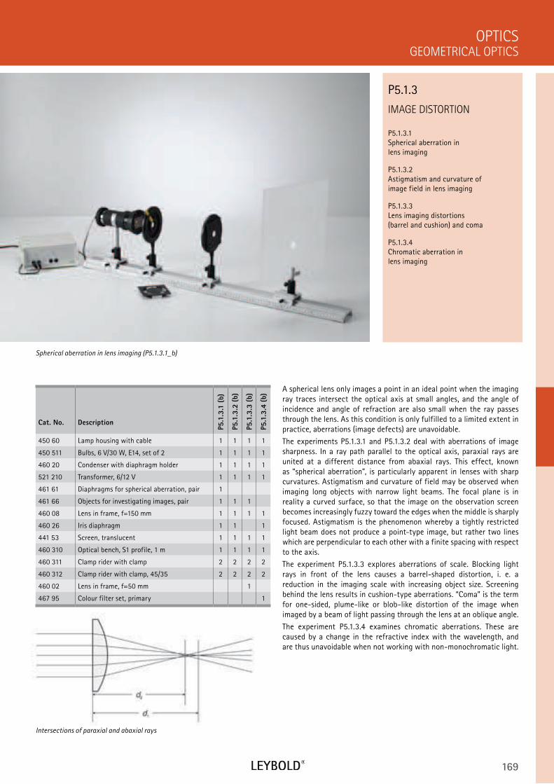
169
IMAGE DISTORTION
P5.1.3.1 Spherical aberration in lens imaging
P5.1.3.2 Astigmatism and curvature of image field in lens imaging
P5.1.3.3 Lens imaging distortions (barrel and cushion) and coma
P5.1.3.4 Chromatic aberration in lens imaging
GEOMETRICAL OPTICS
OPTICS
Cat. No. Description
P5.1
.3.1
(b)
P5.1
.3.2
(b)
P5.1
.3.3
(b)
P5.1
.3.4
(b)
450 60 Lamp housing with cable 1 1 1 1
450 511 Bulbs, 6 V/30 W, E14, set of 2 1 1 1 1
460 20 Condenser with diaphragm holder 1 1 1 1
521 210 Transformer, 6/12 V 1 1 1 1
461 61 Diaphragms for spherical aberration, pair 1
461 66 Objects for investigating images, pair 1 1 1
460 08 Lens in frame, f=150 mm 1 1 1 1
460 26 Iris diaphragm 1 1 1
441 53 Screen, translucent 1 1 1 1
460 310 Optical bench, S1 profile, 1 m 1 1 1 1
460 311 Clamp rider with clamp 2 2 2 2
460 312 Clamp rider with clamp, 45/35 2 2 2 2
460 02 Lens in frame, f=50 mm 1
467 95 Colour filter set, primary 1
A spherical lens only images a point in an ideal point when the imaging ray traces intersect the optical axis at small angles, and the angle of incidence and angle of refraction are also small when the ray passes through the lens. As this condition is only fulfilled to a limited extent in practice, aberrations (image defects) are unavoidable.
The experiments P5.1.3.1 and P5.1.3.2 deal with aberrations of image sharpness. In a ray path parallel to the optical axis, paraxial rays are united at a different distance from abaxial rays. This effect, known as “spherical aberration”, is particularly apparent in lenses with sharp curvatures. Astigmatism and curvature of field may be observed when imaging long objects with narrow light beams. The focal plane is in reality a curved surface, so that the image on the observation screen becomes increasingly fuzzy toward the edges when the middle is sharply focused. Astigmatism is the phenomenon whereby a tightly restricted light beam does not produce a point-type image, but rather two lines which are perpendicular to each other with a finite spacing with respect to the axis.
The experiment P5.1.3.3 explores aberrations of scale. Blocking light rays in front of the lens causes a barrel-shaped distortion, i. e. a reduction in the imaging scale with increasing object size. Screening behind the lens results in cushion-type aberrations. “Coma” is the term for one-sided, plume-like or blob-like distortion of the image when imaged by a beam of light passing through the lens at an oblique angle.
The experiment P5.1.3.4 examines chromatic aberrations. These are caused by a change in the refractive index with the wavelength, and are thus unavoidable when not working with non-monochromatic light.
Spherical aberration in lens imaging (P5.1.3.1_b)
P5.1.3
Intersections of paraxial and abaxial rays
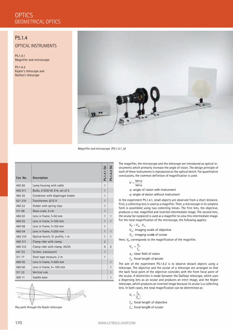
170 WWW.LEYBOLD-SHOP.COM
OPTICAL INSTRUMENTS
P5.1.4.1 Magnifier and microscope
P5.1.4.2 Kepler’s telescope and Galileo’s telescope
The magnifier, the microscope and the telescope are introduced as optical in-struments which primarily increase the angle of vision. The design principle of each of these instruments is reproduced on the optical bench. For quantitative conclusions, the common definition of magnification is used:
V =tan
tan
ψ
ϕ
ψ
ϕ
: angle of vision with instrument
: angle of vvision without instrument
In the experiment P5.1.4.1, small objects are observed from a short distance. First, a collecting lens is used as a magnifier. Then, a microscope in its simplest form is assembled using two collecting lenses. The first lens, the objective, produces a real, magnified and inverted intermediate image. The second lens, the ocular (or eyepiece) is used as a magnifier to view this intermediate image. For the total magnification of the microscope, the following applies:
V V V
V
V
M ob oc
ob
oc
: imaging scale of objective
: imaging scal
= ⋅
ee of ocular
Here, Voc corresponds to the magnification of the magnifier.
Vs
f
s
f
oc0
oc
0
oc
: clear field of vision
: focal length of oocular
The aim of the experiment P5.1.4.2 is to observe distant objects using a telescope. The objective and the ocular of a telescope are arranged so that the back focal point of the objective coincides with the front focal point of the ocular. A distinction is made between the Galilean telescope, which uses a dispersing lens as an ocular and produces an erect image, and the Kepler telescope, which produces an inverted image because its ocular is a collecting lens. In both cases, the total magnification can be determined as:
Vf
f
f
f
Tob
oc
ob
oc
: focal length of objective
: focal lengthh of ocular
OPTICS
Magnifier and microscope (P5.1.4.1_b)
Cat. No. Description
P5.1
.4.1
(b)
P5.1
.4.2
(b)
450 60 Lamp housing with cable 1
450 511 Bulbs, 6 V/30 W, E14, set of 2 1
460 20 Condenser with diaphragm holder 1
521 210 Transformer, 6/12 V 1
460 22 Holder with spring clips 1
311 09 Glass scale, 5 cm 1
460 02 Lens in frame, f=50 mm 1 1
460 03 Lens in frame, f=100 mm 1 1
460 08 Lens in frame, f=150 mm 1
460 04 Lens in frame, f=200 mm 1 1
460 310 Optical bench, S1 profile, 1 m 1 1
460 311 Clamp rider with clamp 2
460 312 Clamp rider with clamp, 45/35 4 2
441 53 Screen, translucent 1
311 77 Steel tape measure, 2 m 1
460 05 Lens in frame, f=500 mm 1
460 06 Lens in frame, f=-100 mm 1
311 22 Vertical rule 1
300 11 Saddle base 1
Ray path through the Kepler telescope
GEOMETRICAL OPTICS
P5.1.4
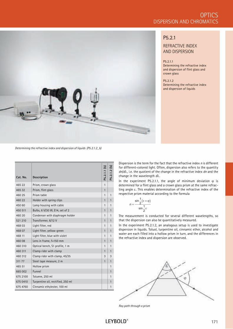
171
REFRACTIVE INDEX
AND DISPERSION
P5.2.1.1 Determining the refractive index and dispersion of flint glass and crown glass
P5.2.1.2 Determining the refractive index and dispersion of liquids
DISPERSION AND CHROMATICS
OPTICS
Cat. No. Description
P5.2
.1.1
(b)
P5.2
.1.2
(b)
465 22 Prism, crown glass 1
465 32 Prism, flint glass 1
460 25 Prism table 1 1
460 22 Holder with spring clips 1 1
450 60 Lamp housing with cable 1 1
450 511 Bulbs, 6 V/30 W, E14, set of 2 1 1
460 20 Condenser with diaphragm holder 1 1
521 210 Transformer, 6/12 V 1 1
468 03 Light filter, red 1 1
468 07 Light filter, yellow-green 1 1
468 11 Light filter, blue with violet 1 1
460 08 Lens in frame, f=150 mm 1 1
460 310 Optical bench, S1 profile, 1 m 1 1
460 311 Clamp rider with clamp 1 1
460 312 Clamp rider with clamp, 45/35 3 3
311 77 Steel tape measure, 2 m 1 1
465 51 Hollow prism 1
665 002 Funnel 1
675 2100 Toluene, 250 ml 1
675 0410 Turpentine oil, rectified, 250 ml 1
675 4760 Cinnamic ethylester, 100 ml 1
Dispersion is the term for the fact that the refractive index n is different for different-colored light. Often, dispersion also refers to the quantity dn/d , i.e. the quotient of the change in the refractive index dn and the change in the wavelength d .
In the experiment P5.2.1.1, the angle of minimum deviation is determined for a flint glass and a crown glass prism at the same refrac-ting angle . This enables determination of the refractive index of the respective prism material according to the formula
n =+( )sin
sin
1
2
1
2
ε ϕ
ε
The measurement is conducted for several different wavelengths, so that the dispersion can also be quantitatively measured.
In the experiment P5.2.1.2, an analogous setup is used to investigate dispersion in liquids. Toluol, turpentine oil, cinnamic ether, alcohol and water are each filled into a hollow prism in turn, and the differences in the refractive index and dispersion are observed.
Determining the refractive index and dispersion of liquids (P5.2.1.2_b)
P5.2.1
Ray path through a prism
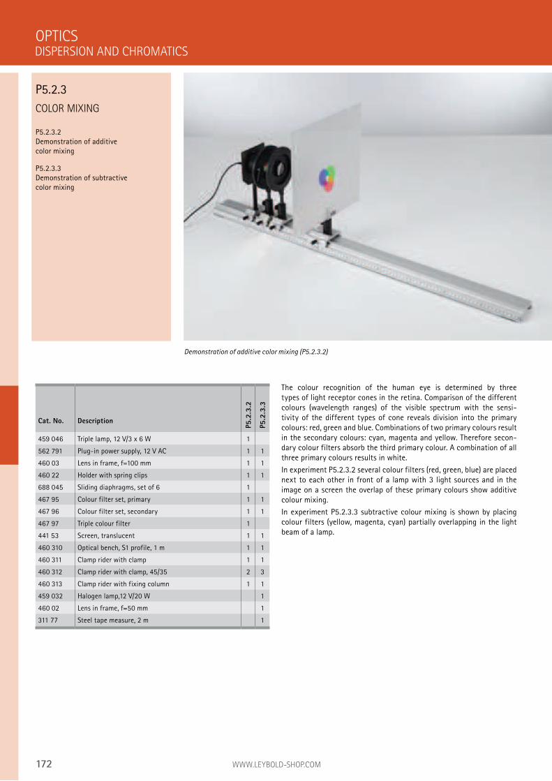
172 WWW.LEYBOLD-SHOP.COM
COLOR MIXING
P5.2.3.2 Demonstration of additive color mixing
P5.2.3.3 Demonstration of subtractive color mixing
The colour recognition of the human eye is determined by three types of light receptor cones in the retina. Comparison of the different colours (wavelength ranges) of the visible spectrum with the sensi-tivity of the different types of cone reveals division into the primary colours: red, green and blue. Combinations of two primary colours result in the secondary colours: cyan, magenta and yellow. Therefore secon-dary colour filters absorb the third primary colour. A combination of all three primary colours results in white.
In experiment P5.2.3.2 several colour filters (red, green, blue) are placed next to each other in front of a lamp with 3 light sources and in the image on a screen the overlap of these primary colours show additive colour mixing.
In experiment P5.2.3.3 subtractive colour mixing is shown by placing colour filters (yellow, magenta, cyan) partially overlapping in the light beam of a lamp.
OPTICS
Demonstration of additive color mixing (P5.2.3.2)
Cat. No. Description
P5.2
.3.2
P5.2
.3.3
459 046 Triple lamp, 12 V/3 x 6 W 1
562 791 Plug-in power supply, 12 V AC 1 1
460 03 Lens in frame, f=100 mm 1 1
460 22 Holder with spring clips 1 1
688 045 Sliding diaphragms, set of 6 1
467 95 Colour filter set, primary 1 1
467 96 Colour filter set, secondary 1 1
467 97 Triple colour filter 1
441 53 Screen, translucent 1 1
460 310 Optical bench, S1 profile, 1 m 1 1
460 311 Clamp rider with clamp 1 1
460 312 Clamp rider with clamp, 45/35 2 3
460 313 Clamp rider with fixing column 1 1
459 032 Halogen lamp,12 V/20 W 1
460 02 Lens in frame, f=50 mm 1
311 77 Steel tape measure, 2 m 1
DISPERSION AND CHROMATICS
P5.2.3
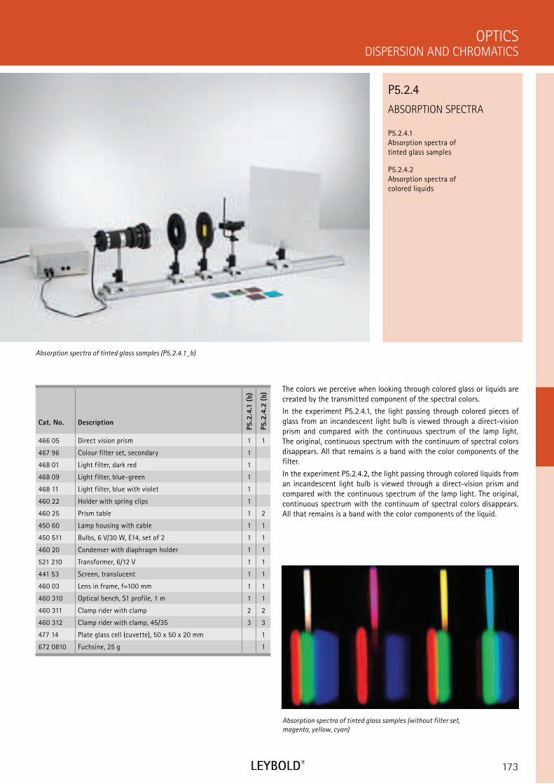
173
ABSORPTION SPECTRA
P5.2.4.1 Absorption spectra of tinted glass samples
P5.2.4.2 Absorption spectra of colored liquids
DISPERSION AND CHROMATICS
OPTICS
Cat. No. Description
P5.2
.4.1
(b)
P5.2
.4.2
(b)
466 05 Direct vision prism 1 1
467 96 Colour filter set, secondary 1
468 01 Light filter, dark red 1
468 09 Light filter, blue-green 1
468 11 Light filter, blue with violet 1
460 22 Holder with spring clips 1
460 25 Prism table 1 2
450 60 Lamp housing with cable 1 1
450 511 Bulbs, 6 V/30 W, E14, set of 2 1 1
460 20 Condenser with diaphragm holder 1 1
521 210 Transformer, 6/12 V 1 1
441 53 Screen, translucent 1 1
460 03 Lens in frame, f=100 mm 1 1
460 310 Optical bench, S1 profile, 1 m 1 1
460 311 Clamp rider with clamp 2 2
460 312 Clamp rider with clamp, 45/35 3 3
477 14 Plate glass cell (cuvette), 50 x 50 x 20 mm 1
672 0810 Fuchsine, 25 g 1
The colors we perceive when looking through colored glass or liquids are created by the transmitted component of the spectral colors.
In the experiment P5.2.4.1, the light passing through colored pieces of glass from an incandescent light bulb is viewed through a direct-vision prism and compared with the continuous spectrum of the lamp light. The original, continuous spectrum with the continuum of spectral colors disappears. All that remains is a band with the color components of the filter.
In the experiment P5.2.4.2, the light passing through colored liquids from an incandescent light bulb is viewed through a direct-vision prism and compared with the continuous spectrum of the lamp light. The original, continuous spectrum with the continuum of spectral colors disappears. All that remains is a band with the color components of the liquid.
Absorption spectra of tinted glass samples (P5.2.4.1_b)
P5.2.4
Absorption spectra of tinted glass samples (without filter set,
magenta, yellow, cyan)
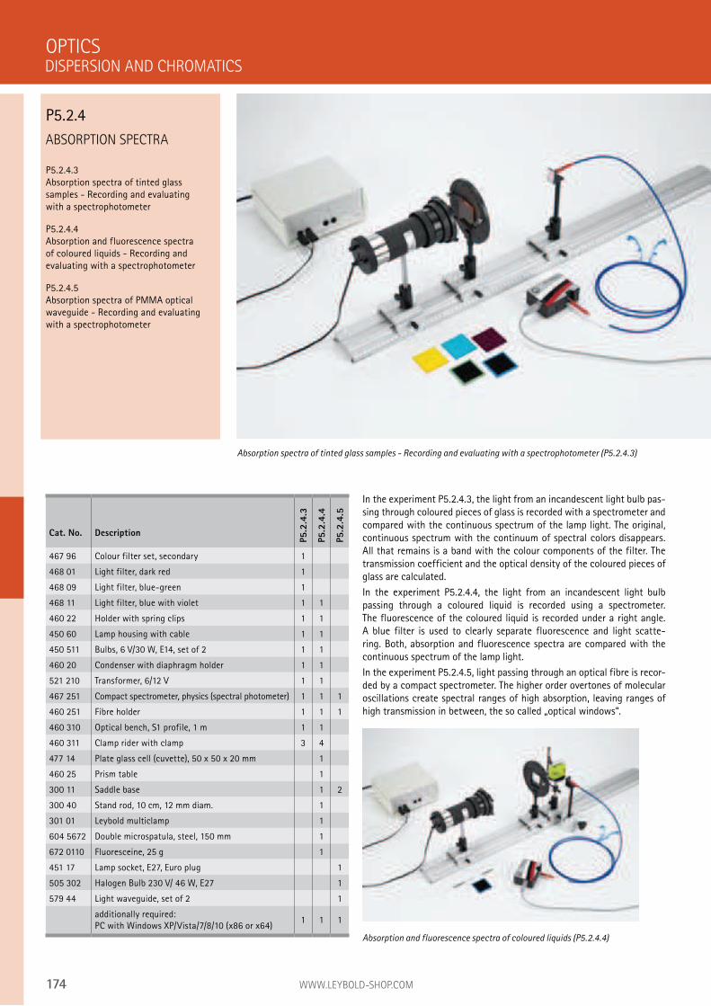
174 WWW.LEYBOLD-SHOP.COM
ABSORPTION SPECTRA
P5.2.4.3 Absorption spectra of tinted glass samples - Recording and evaluating with a spectrophotometer
P5.2.4.4 Absorption and fluorescence spectra of coloured liquids - Recording and evaluating with a spectrophotometer
P5.2.4.5 Absorption spectra of PMMA optical waveguide - Recording and evaluating with a spectrophotometer
In the experiment P5.2.4.3, the light from an incandescent light bulb pas-sing through coloured pieces of glass is recorded with a spectrometer and compared with the continuous spectrum of the lamp light. The original, continuous spectrum with the continuum of spectral colors disappears.All that remains is a band with the colour components of the filter. The transmission coefficient and the optical density of the coloured pieces of glass are calculated.
In the experiment P5.2.4.4, the light from an incandescent light bulb passing through a coloured liquid is recorded using a spectrometer. The fluorescence of the coloured liquid is recorded under a right angle. A blue filter is used to clearly separate fluorescence and light scatte-ring. Both, absorption and fluorescence spectra are compared with the continuous spectrum of the lamp light.
In the experiment P5.2.4.5, light passing through an optical fibre is recor-ded by a compact spectrometer. The higher order overtones of molecular oscillations create spectral ranges of high absorption, leaving ranges of high transmission in between, the so called „optical windows“.
OPTICS
Absorption spectra of tinted glass samples - Recording and evaluating with a spectrophotometer (P5.2.4.3)
Cat. No. Description
P5.2
.4.3
P5.2
.4.4
P5.2
.4.5
467 96 Colour filter set, secondary 1
468 01 Light filter, dark red 1
468 09 Light filter, blue-green 1
468 11 Light filter, blue with violet 1 1
460 22 Holder with spring clips 1 1
450 60 Lamp housing with cable 1 1
450 511 Bulbs, 6 V/30 W, E14, set of 2 1 1
460 20 Condenser with diaphragm holder 1 1
521 210 Transformer, 6/12 V 1 1
467 251 Compact spectrometer, physics (spectral photometer) 1 1 1
460 251 Fibre holder 1 1 1
460 310 Optical bench, S1 profile, 1 m 1 1
460 311 Clamp rider with clamp 3 4
477 14 Plate glass cell (cuvette), 50 x 50 x 20 mm 1
460 25 Prism table 1
300 11 Saddle base 1 2
300 40 Stand rod, 10 cm, 12 mm diam. 1
301 01 Leybold multiclamp 1
604 5672 Double microspatula, steel, 150 mm 1
672 0110 Fluoresceine, 25 g 1
451 17 Lamp socket, E27, Euro plug 1
505 302 Halogen Bulb 230 V/ 46 W, E27 1
579 44 Light waveguide, set of 2 1
additionally required: PC with Windows XP/Vista/7/8/10 (x86 or x64)
1 1 1
Absorption and fluorescence spectra of coloured liquids (P5.2.4.4)
DISPERSION AND CHROMATICS
P5.2.4
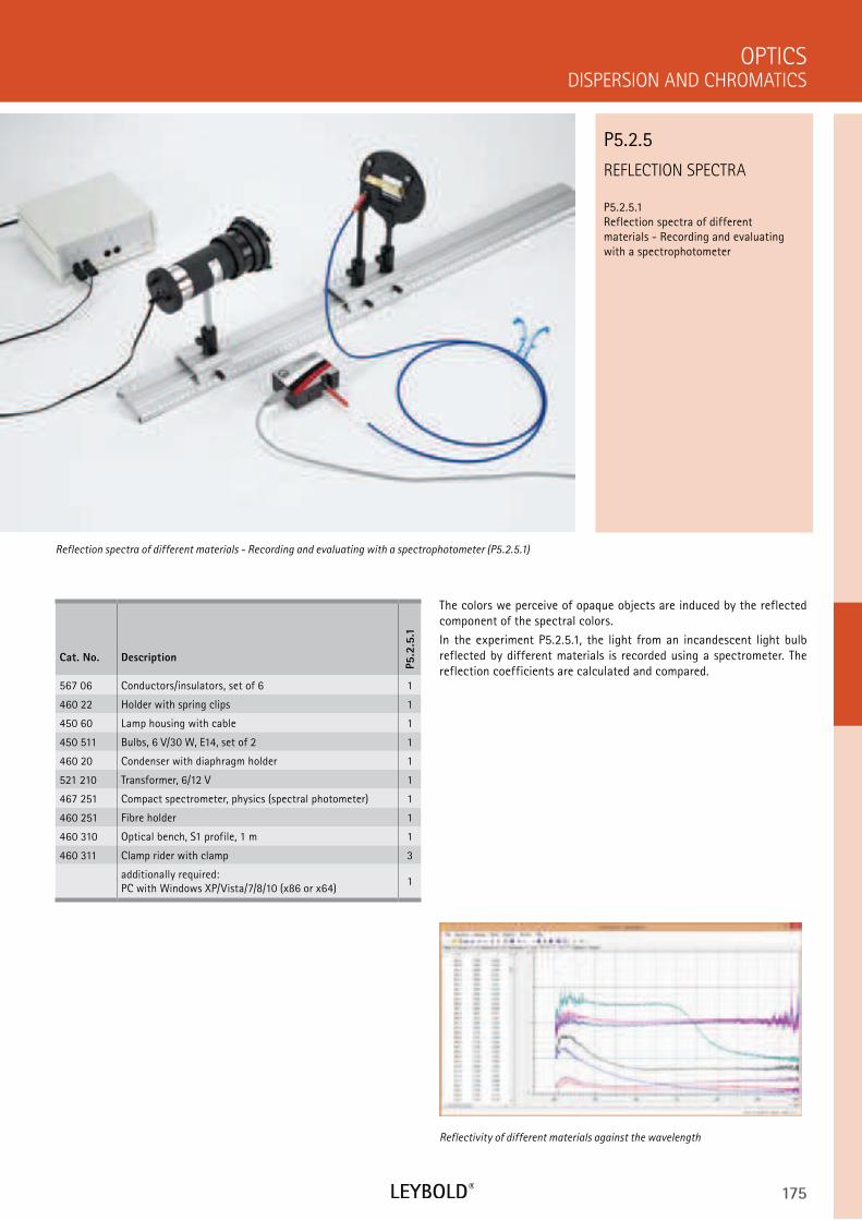
175
REFLECTION SPECTRA
P5.2.5.1 Reflection spectra of different materials - Recording and evaluating with a spectrophotometer
DISPERSION AND CHROMATICS
OPTICS
Cat. No. Description
P5.2
.5.1
567 06 Conductors/insulators, set of 6 1
460 22 Holder with spring clips 1
450 60 Lamp housing with cable 1
450 511 Bulbs, 6 V/30 W, E14, set of 2 1
460 20 Condenser with diaphragm holder 1
521 210 Transformer, 6/12 V 1
467 251 Compact spectrometer, physics (spectral photometer) 1
460 251 Fibre holder 1
460 310 Optical bench, S1 profile, 1 m 1
460 311 Clamp rider with clamp 3
additionally required: PC with Windows XP/Vista/7/8/10 (x86 or x64)
1
The colors we perceive of opaque objects are induced by the reflected component of the spectral colors.
In the experiment P5.2.5.1, the light from an incandescent light bulb reflected by different materials is recorded using a spectrometer. The reflection coefficients are calculated and compared.
Reflection spectra of different materials - Recording and evaluating with a spectrophotometer (P5.2.5.1)
P5.2.5
Reflectivity of different materials against the wavelength
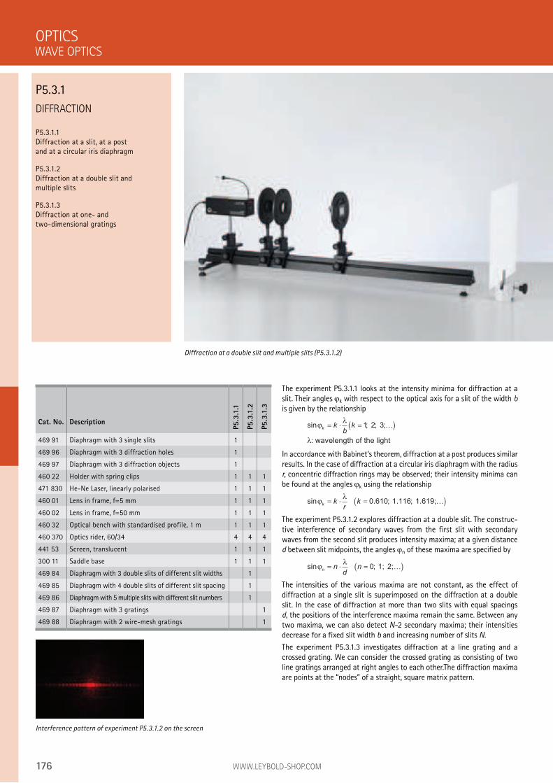
176 WWW.LEYBOLD-SHOP.COM
DIFFRACTION
P5.3.1.1 Diffraction at a slit, at a post and at a circular iris diaphragm
P5.3.1.2 Diffraction at a double slit and multiple slits
P5.3.1.3 Diffraction at one- and two-dimensional gratings
The experiment P5.3.1.1 looks at the intensity minima for diffraction at a slit. Their angles k with respect to the optical axis for a slit of the width b is given by the relationship
sin ; ; ;ϕλ
λ
kkbk= ⋅ =( )1 2 3
: wavelength of the light
…
In accordance with Babinet’s theorem, diffraction at a post produces similar results. In the case of diffraction at a circular iris diaphragm with the radius r, concentric diffraction rings may be observed; their intensity minima can be found at the angles k using the relationship
sin . ; . ;ϕλ
kkr
k= ⋅ =( ) 1.619;0 610 1 116 …
The experiment P5.3.1.2 explores diffraction at a double slit. The construc-tive interference of secondary waves from the first slit with secondary waves from the second slit produces intensity maxima; at a given distance d between slit midpoints, the angles n of these maxima are specified by
sin ;ϕλ
nnd
n= ⋅ =( ) 0 1; 2;…
The intensities of the various maxima are not constant, as the effect of diffraction at a single slit is superimposed on the diffraction at a double slit. In the case of diffraction at more than two slits with equal spacings d, the positions of the interference maxima remain the same. Between any two maxima, we can also detect N-2 secondary maxima; their intensities decrease for a fixed slit width b and increasing number of slits N.
The experiment P5.3.1.3 investigates diffraction at a line grating and a crossed grating. We can consider the crossed grating as consisting of two line gratings arranged at right angles to each other.The diffraction maxima are points at the “nodes” of a straight, square matrix pattern.
OPTICS
Diffraction at a double slit and multiple slits (P5.3.1.2)
Cat. No. Description
P5.3
.1.1
P5.3
.1.2
P5.3
.1.3
469 91 Diaphragm with 3 single slits 1
469 96 Diaphragm with 3 diffraction holes 1
469 97 Diaphragm with 3 diffraction objects 1
460 22 Holder with spring clips 1 1 1
471 830 He-Ne Laser, linearly polarised 1 1 1
460 01 Lens in frame, f=5 mm 1 1 1
460 02 Lens in frame, f=50 mm 1 1 1
460 32 Optical bench with standardised profile, 1 m 1 1 1
460 370 Optics rider, 60/34 4 4 4
441 53 Screen, translucent 1 1 1
300 11 Saddle base 1 1 1
469 84 Diaphragm with 3 double slits of different slit widths 1
469 85 Diaphragm with 4 double slits of different slit spacing 1
469 86 Diaphragm with 5 multiple slits with different slit numbers 1
469 87 Diaphragm with 3 gratings 1
469 88 Diaphragm with 2 wire-mesh gratings 1
Interference pattern of experiment P5.3.1.2 on the screen
WAVE OPTICS
P5.3.1
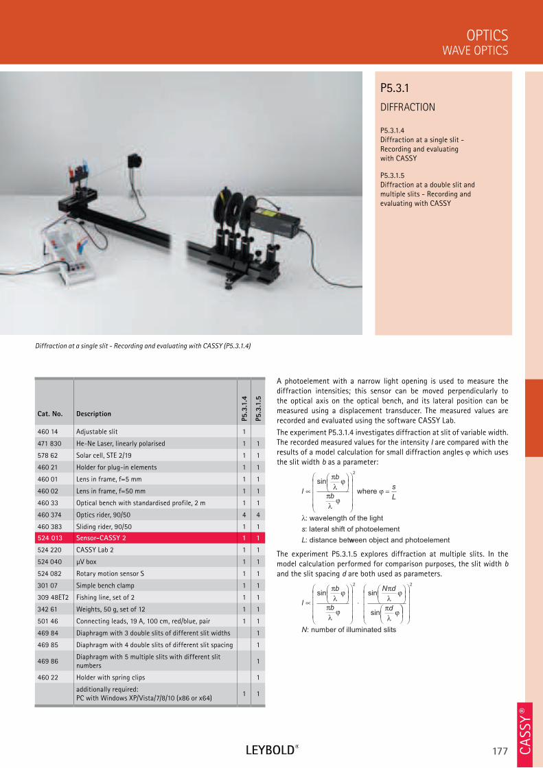
177
DIFFRACTION
P5.3.1.4 Diffraction at a single slit - Recording and evaluating with CASSY
P5.3.1.5 Diffraction at a double slit and multiple slits - Recording and evaluating with CASSY
WAVE OPTICS
OPTICS
Cat. No. Description
P5.3
.1.4
P5.3
.1.5
460 14 Adjustable slit 1
471 830 He-Ne Laser, linearly polarised 1 1
578 62 Solar cell, STE 2/19 1 1
460 21 Holder for plug-in elements 1 1
460 01 Lens in frame, f=5 mm 1 1
460 02 Lens in frame, f=50 mm 1 1
460 33 Optical bench with standardised profile, 2 m 1 1
460 374 Optics rider, 90/50 4 4
460 383 Sliding rider, 90/50 1 1
524 013 Sensor-CASSY 2 1 1
524 220 CASSY Lab 2 1 1
524 040 µV box 1 1
524 082 Rotary motion sensor S 1 1
301 07 Simple bench clamp 1 1
309 48ET2 Fishing line, set of 2 1 1
342 61 Weights, 50 g, set of 12 1 1
501 46 Connecting leads, 19 A, 100 cm, red/blue, pair 1 1
469 84 Diaphragm with 3 double slits of different slit widths 1
469 85 Diaphragm with 4 double slits of different slit spacing 1
469 86Diaphragm with 5 multiple slits with different slit numbers
1
460 22 Holder with spring clips 1
additionally required: PC with Windows XP/Vista/7/8/10 (x86 or x64)
1 1
A photoelement with a narrow light opening is used to measure the diffraction intensities; this sensor can be moved perpendicularly to the optical axis on the optical bench, and its lateral position can be measured using a displacement transducer. The measured values are recorded and evaluated using the software CASSY Lab.
The experiment P5.3.1.4 investigates diffraction at slit of variable width. The recorded measured values for the intensity I are compared with the results of a model calculation for small diffraction angles which uses the slit width b as a parameter:
l
b
b
s
L∝
=sin
πλ
ϕ
πλ
ϕϕ
λ
2
where
: wavelength of the light
: lateral shift of photoelement
: distance bet
s
L wween object and photoelement
The experiment P5.3.1.5 explores diffraction at multiple slits. In the model calculation performed for comparison purposes, the slit width b and the slit spacing d are both used as parameters.
l
b
b
N d
d∝
⋅
sin sin
sin
πλ
ϕ
πλ
ϕ
πλ
ϕ
πλ
ϕ
2
2
N: number of illuminated slits
Diffraction at a single slit - Recording and evaluating with CASSY (P5.3.1.4)
P5.3.1
CA
SSY ®
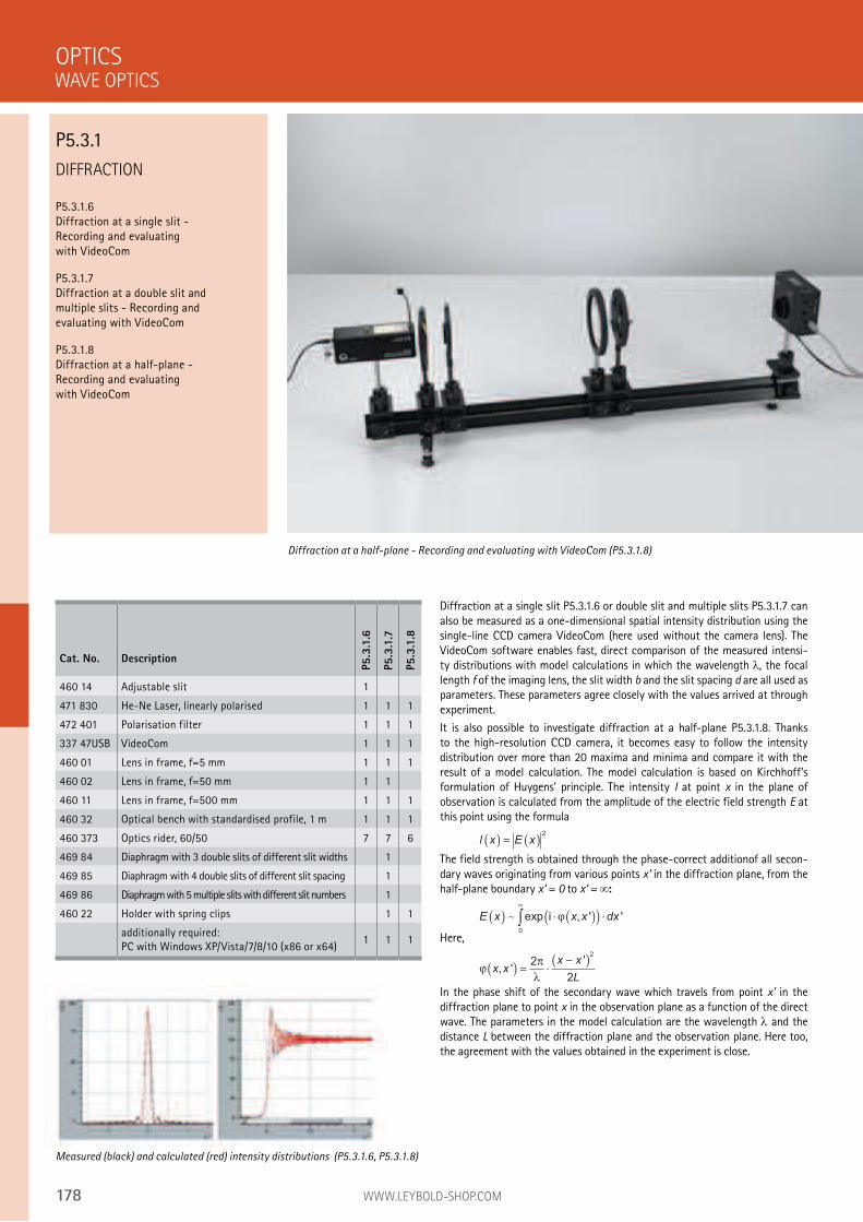
178 WWW.LEYBOLD-SHOP.COM
DIFFRACTION
P5.3.1.6 Diffraction at a single slit - Recording and evaluating with VideoCom
P5.3.1.7 Diffraction at a double slit and multiple slits - Recording and evaluating with VideoCom
P5.3.1.8 Diffraction at a half-plane - Recording and evaluating with VideoCom
Diffraction at a single slit P5.3.1.6 or double slit and multiple slits P5.3.1.7 can also be measured as a one-dimensional spatial intensity distribution using the single-line CCD camera VideoCom (here used without the camera lens). The VideoCom software enables fast, direct comparison of the measured intensi-ty distributions with model calculations in which the wavelength , the focal length f of the imaging lens, the slit width b and the slit spacing d are all used as parameters. These parameters agree closely with the values arrived at through experiment.
It is also possible to investigate diffraction at a half-plane P5.3.1.8. Thanks to the high-resolution CCD camera, it becomes easy to follow the intensity distribution over more than 20 maxima and minima and compare it with the result of a model calculation. The model calculation is based on Kirchhoff’s formulation of Huygens’ principle. The intensity I at point x in the plane of observation is calculated from the amplitude of the electric field strength E at this point using the formula
l x E x( ) = ( )2
The field strength is obtained through the phase-correct additionof all secon-dary waves originating from various points x’ in the diffraction plane, from the half-plane boundary x‘ = 0 to x‘ = :
E x x x dx( ) ⋅ ( )( ) ⋅∞
∫∼ exp , ' 'i ϕ0
Here,
ϕπ
λx x
x x
L, '
'( ) = ⋅
−( )2
2
2
In the phase shift of the secondary wave which travels from point x’ in the diffraction plane to point x in the observation plane as a function of the direct wave. The parameters in the model calculation are the wavelength and the distance L between the diffraction plane and the observation plane. Here too, the agreement with the values obtained in the experiment is close.
OPTICS
Diffraction at a half-plane - Recording and evaluating with VideoCom (P5.3.1.8)
Cat. No. Description
P5.3
.1.6
P5.3
.1.7
P5.3
.1.8
460 14 Adjustable slit 1
471 830 He-Ne Laser, linearly polarised 1 1 1
472 401 Polarisation filter 1 1 1
337 47USB VideoCom 1 1 1
460 01 Lens in frame, f=5 mm 1 1 1
460 02 Lens in frame, f=50 mm 1 1
460 11 Lens in frame, f=500 mm 1 1 1
460 32 Optical bench with standardised profile, 1 m 1 1 1
460 373 Optics rider, 60/50 7 7 6
469 84 Diaphragm with 3 double slits of different slit widths 1
469 85 Diaphragm with 4 double slits of different slit spacing 1
469 86 Diaphragm with 5 multiple slits with different slit numbers 1
460 22 Holder with spring clips 1 1
additionally required: PC with Windows XP/Vista/7/8/10 (x86 or x64)
1 1 1
Measured (black) and calculated (red) intensity distributions (P5.3.1.6, P5.3.1.8)
WAVE OPTICS
P5.3.1
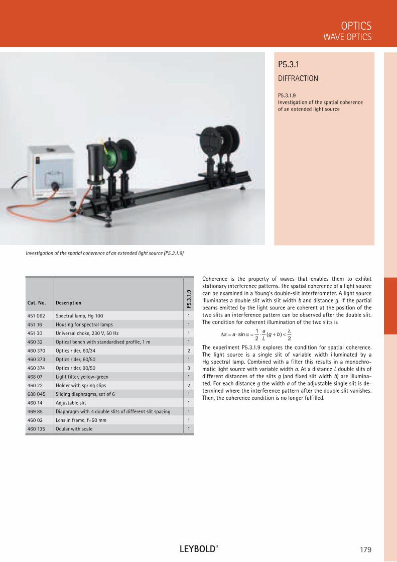
179
DIFFRACTION
P5.3.1.9 Investigation of the spatial coherence of an extended light source
WAVE OPTICS
OPTICS
Cat. No. Description
P5.3
.1.9
451 062 Spectral lamp, Hg 100 1
451 16 Housing for spectral lamps 1
451 30 Universal choke, 230 V, 50 Hz 1
460 32 Optical bench with standardised profile, 1 m 1
460 370 Optics rider, 60/34 2
460 373 Optics rider, 60/50 1
460 374 Optics rider, 90/50 3
468 07 Light filter, yellow-green 1
460 22 Holder with spring clips 2
688 045 Sliding diaphragms, set of 6 1
460 14 Adjustable slit 1
469 85 Diaphragm with 4 double slits of different slit spacing 1
460 02 Lens in frame, f=50 mm 1
460 135 Ocular with scale 1
Coherence is the property of waves that enables them to exhibit stationary interference patterns. The spatial coherence of a light source can be examined in a Young’s double-slit interferometer. A light source illuminates a double slit with slit width b and distance g. If the partial beams emitted by the light source are coherent at the position of the two slits an interference pattern can be observed after the double slit. The condition for coherent illumination of the two slits is
∆s aa
Lg b= ⋅ = ⋅ + <sin ( )α
λ1
2 2
The experiment P5.3.1.9 explores the condition for spatial coherence. The light source is a single slit of variable width illuminated by a Hg spectral lamp. Combined with a filter this results in a monochro-matic light source with variable width a. At a distance L double slits of different distances of the slits g (and fixed slit width b) are illumina-ted. For each distance g the width a of the adjustable single slit is de-termined where the interference pattern after the double slit vanishes. Then, the coherence condition is no longer fulfilled.
Investigation of the spatial coherence of an extended light source (P5.3.1.9)
P5.3.1
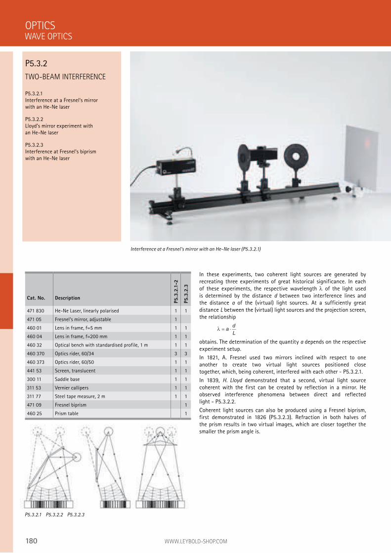
180 WWW.LEYBOLD-SHOP.COM
TWO-BEAM INTERFERENCE
P5.3.2.1 Interference at a Fresnel‘s mirror with an He-Ne laser
P5.3.2.2 Lloyd’s mirror experiment with an He-Ne laser
P5.3.2.3 Interference at Fresnel’s biprism with an He-Ne laser
In these experiments, two coherent light sources are generated by recreating three experiments of great historical significance. In each of these experiments, the respective wavelength of the light used is determined by the distance d between two interference lines and the distance a of the (virtual) light sources. At a sufficiently great distance L between the (virtual) light sources and the projection screen, the relationship
λ = ⋅ad
L
obtains. The determination of the quantity a depends on the respective experiment setup.
In 1821, A. Fresnel used two mirrors inclined with respect to one another to create two virtual light sources positioned close together, which, being coherent, interfered with each other - P5.3.2.1.
In 1839, H. Lloyd demonstrated that a second, virtual light source coherent with the first can be created by reflection in a mirror. He observed interference phenomena between direct and reflected light - P5.3.2.2.
Coherent light sources can also be produced using a Fresnel biprism, first demonstrated in 1826 (P5.3.2.3). Refraction in both halves of the prism results in two virtual images, which are closer together the smaller the prism angle is.
OPTICS
Interference at a Fresnel‘s mirror with an He-Ne laser (P5.3.2.1)
Cat. No. Description
P5.3
.2.1
-2
P5.3
.2.3
471 830 He-Ne Laser, linearly polarised 1 1
471 05 Fresnel‘s mirror, adjustable 1
460 01 Lens in frame, f=5 mm 1 1
460 04 Lens in frame, f=200 mm 1 1
460 32 Optical bench with standardised profile, 1 m 1 1
460 370 Optics rider, 60/34 3 3
460 373 Optics rider, 60/50 1 1
441 53 Screen, translucent 1 1
300 11 Saddle base 1 1
311 53 Vernier callipers 1 1
311 77 Steel tape measure, 2 m 1 1
471 09 Fresnel biprism 1
460 25 Prism table 1
P5.3.2.1 P5.3.2.2 P5.3.2.3
WAVE OPTICS
P5.3.2
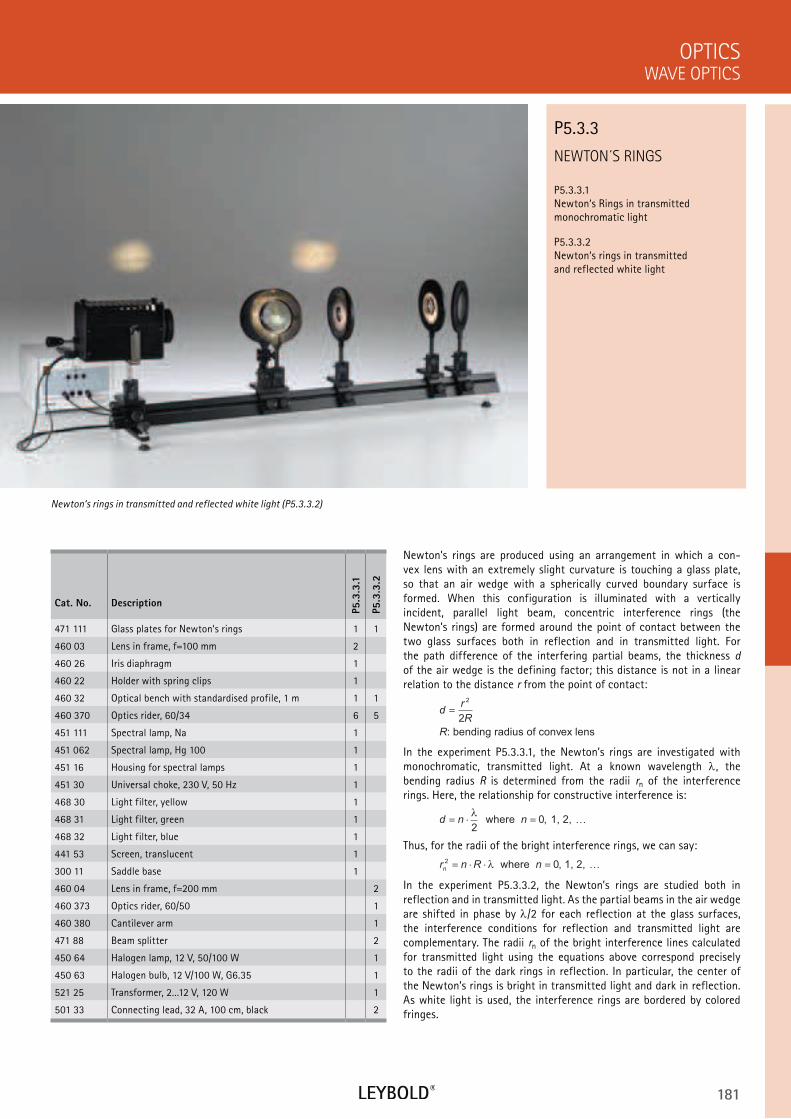
181
NEWTON´S RINGS
P5.3.3.1 Newton‘s Rings in transmitted monochromatic light
P5.3.3.2 Newton‘s rings in transmitted and reflected white light
WAVE OPTICS
OPTICS
Cat. No. Description
P5.3
.3.1
P5.3
.3.2
471 111 Glass plates for Newton‘s rings 1 1
460 03 Lens in frame, f=100 mm 2
460 26 Iris diaphragm 1
460 22 Holder with spring clips 1
460 32 Optical bench with standardised profile, 1 m 1 1
460 370 Optics rider, 60/34 6 5
451 111 Spectral lamp, Na 1
451 062 Spectral lamp, Hg 100 1
451 16 Housing for spectral lamps 1
451 30 Universal choke, 230 V, 50 Hz 1
468 30 Light filter, yellow 1
468 31 Light filter, green 1
468 32 Light filter, blue 1
441 53 Screen, translucent 1
300 11 Saddle base 1
460 04 Lens in frame, f=200 mm 2
460 373 Optics rider, 60/50 1
460 380 Cantilever arm 1
471 88 Beam splitter 2
450 64 Halogen lamp, 12 V, 50/100 W 1
450 63 Halogen bulb, 12 V/100 W, G6.35 1
521 25 Transformer, 2...12 V, 120 W 1
501 33 Connecting lead, 32 A, 100 cm, black 2
Newton’s rings are produced using an arrangement in which a con-vex lens with an extremely slight curvature is touching a glass plate, so that an air wedge with a spherically curved boundary surface is formed. When this configuration is illuminated with a vertically incident, parallel light beam, concentric interference rings (the Newton’s rings) are formed around the point of contact between the two glass surfaces both in reflection and in transmitted light. For the path difference of the interfering partial beams, the thickness d of the air wedge is the defining factor; this distance is not in a linear relation to the distance r from the point of contact:
dr
R
R
2
2
: bending radius of convex lens
In the experiment P5.3.3.1, the Newton’s rings are investigated with monochromatic, transmitted light. At a known wavelength , the bending radius R is determined from the radii rn of the interference rings. Here, the relationship for constructive interference is:
d n n= ⋅ =λ
20 where 1, 2, , …
Thus, for the radii of the bright interference rings, we can say:
r n R nn
20= ⋅ ⋅ =λ where , 1, 2, …
In the experiment P5.3.3.2, the Newton’s rings are studied both in reflection and in transmitted light. As the partial beams in the air wedge are shifted in phase by /2 for each reflection at the glass surfaces, the interference conditions for reflection and transmitted light are complementary. The radii rn of the bright interference lines calculated for transmitted light using the equations above correspond precisely to the radii of the dark rings in reflection. In particular, the center of the Newton’s rings is bright in transmitted light and dark in reflection. As white light is used, the interference rings are bordered by colored fringes.
Newton‘s rings in transmitted and reflected white light (P5.3.3.2)
P5.3.3
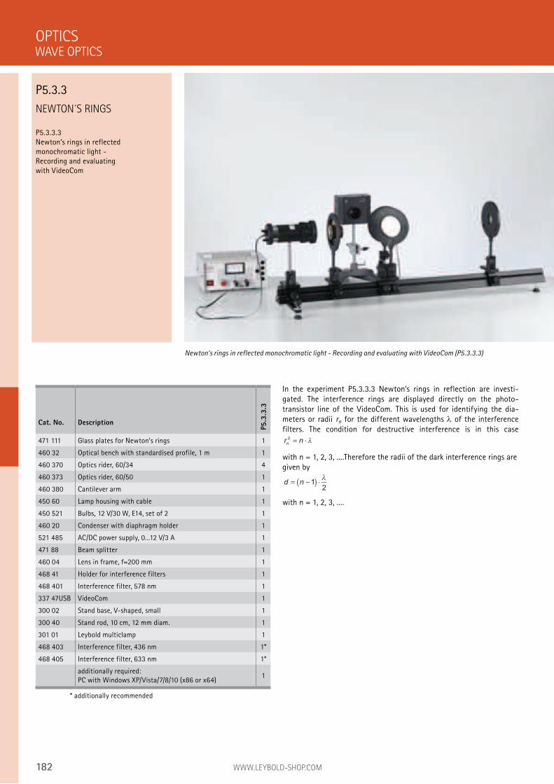
182 WWW.LEYBOLD-SHOP.COM
NEWTON´S RINGS
P5.3.3.3 Newton‘s rings in reflected monochromatic light - Recording and evaluating with VideoCom
In the experiment P5.3.3.3 Newton’s rings in reflection are investi-gated. The interference rings are displayed directly on the photo-transistor line of the VideoCom. This is used for identifying the dia-meters or radii rn for the different wavelengths of the interference filters. The condition for destructive interference is in this case
r nn
2= ⋅
with n = 1, 2, 3, ....Therefore the radii of the dark interference rings are given by
d n= −( ) ⋅12
with n = 1, 2, 3, ....
OPTICS
Newton‘s rings in reflected monochromatic light - Recording and evaluating with VideoCom (P5.3.3.3)
Cat. No. Description
P5.3
.3.3
471 111 Glass plates for Newton‘s rings 1
460 32 Optical bench with standardised profile, 1 m 1
460 370 Optics rider, 60/34 4
460 373 Optics rider, 60/50 1
460 380 Cantilever arm 1
450 60 Lamp housing with cable 1
450 521 Bulbs, 12 V/30 W, E14, set of 2 1
460 20 Condenser with diaphragm holder 1
521 485 AC/DC power supply, 0...12 V/3 A 1
471 88 Beam splitter 1
460 04 Lens in frame, f=200 mm 1
468 41 Holder for interference filters 1
468 401 Interference filter, 578 nm 1
337 47USB VideoCom 1
300 02 Stand base, V-shaped, small 1
300 40 Stand rod, 10 cm, 12 mm diam. 1
301 01 Leybold multiclamp 1
468 403 Interference filter, 436 nm 1*
468 405 Interference filter, 633 nm 1*
additionally required: PC with Windows XP/Vista/7/8/10 (x86 or x64)
1
* additionally recommended
WAVE OPTICS
P5.3.3
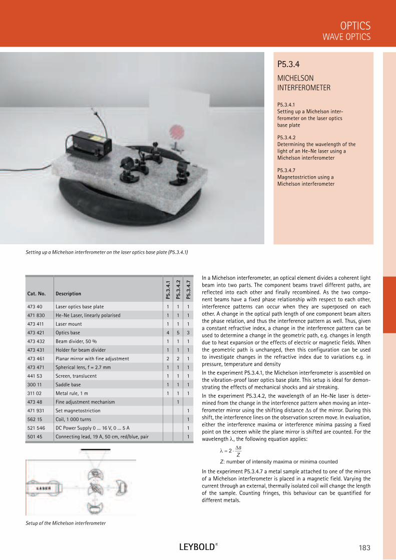
183
MICHELSON
INTERFEROMETER
P5.3.4.1 Setting up a Michelson inter- ferometer on the laser optics base plate
P5.3.4.2 Determining the wavelength of the light of an He-Ne laser using a Michelson interferometer
P5.3.4.7 Magnetostriction using a Michelson interferometer
WAVE OPTICS
OPTICS
Cat. No. Description
P5.3
.4.1
P5.3
.4.2
P5.3
.4.7
473 40 Laser optics base plate 1 1 1
471 830 He-Ne Laser, linearly polarised 1 1 1
473 411 Laser mount 1 1 1
473 421 Optics base 4 5 3
473 432 Beam divider, 50 % 1 1 1
473 431 Holder for beam divider 1 1 1
473 461 Planar mirror with fine adjustment 2 2 1
473 471 Spherical lens, f = 2.7 mm 1 1 1
441 53 Screen, translucent 1 1 1
300 11 Saddle base 1 1 1
311 02 Metal rule, 1 m 1 1 1
473 48 Fine adjustment mechanism 1
471 931 Set magnetostriction 1
562 15 Coil, 1 000 turns 1
521 546 DC Power Supply 0 ... 16 V, 0 ... 5 A 1
501 45 Connecting lead, 19 A, 50 cm, red/blue, pair 1
In a Michelson interferometer, an optical element divides a coherent light beam into two parts. The component beams travel different paths, are reflected into each other and finally recombined. As the two compo-nent beams have a fixed phase relationship with respect to each other, interference patterns can occur when they are superposed on each other. A change in the optical path length of one component beam alters the phase relation, and thus the interference pattern as well. Thus, given a constant refractive index, a change in the interference pattern can be used to determine a change in the geometric path, e.g. changes in length due to heat expansion or the effects of electric or magnetic fields. When the geometric path is unchanged, then this configuration can be used to investigate changes in the refractive index due to variations e.g. in pressure, temperature and density
In the experiment P5.3.4.1, the Michelson interferometer is assembled on the vibration-proof laser optics base plate. This setup is ideal for demon-strating the effects of mechanical shocks and air streaking.
In the experiment P5.3.4.2, the wavelength of an He-Ne laser is deter-mined from the change in the interference pattern when moving an inter-ferometer mirror using the shifting distance s of the mirror. During this shift, the interference lines on the observation screen move. In evaluation, either the interference maxima or interference minima passing a fixed point on the screen while the plane mirror is shifted are counted. For the wavelength , the following equation applies:
λ = ⋅2∆s
Z
Z: number of intensity maxima or minima counted
In the experiment P5.3.4.7 a metal sample attached to one of the mirrors of a Michelson interferometer is placed in a magnetic field. Varying the current through an external, thermally isolated coil will change the length of the sample. Counting fringes, this behaviour can be quantified for different metals.
Setting up a Michelson interferometer on the laser optics base plate (P5.3.4.1)
P5.3.4
Setup of the Michelson interferometer
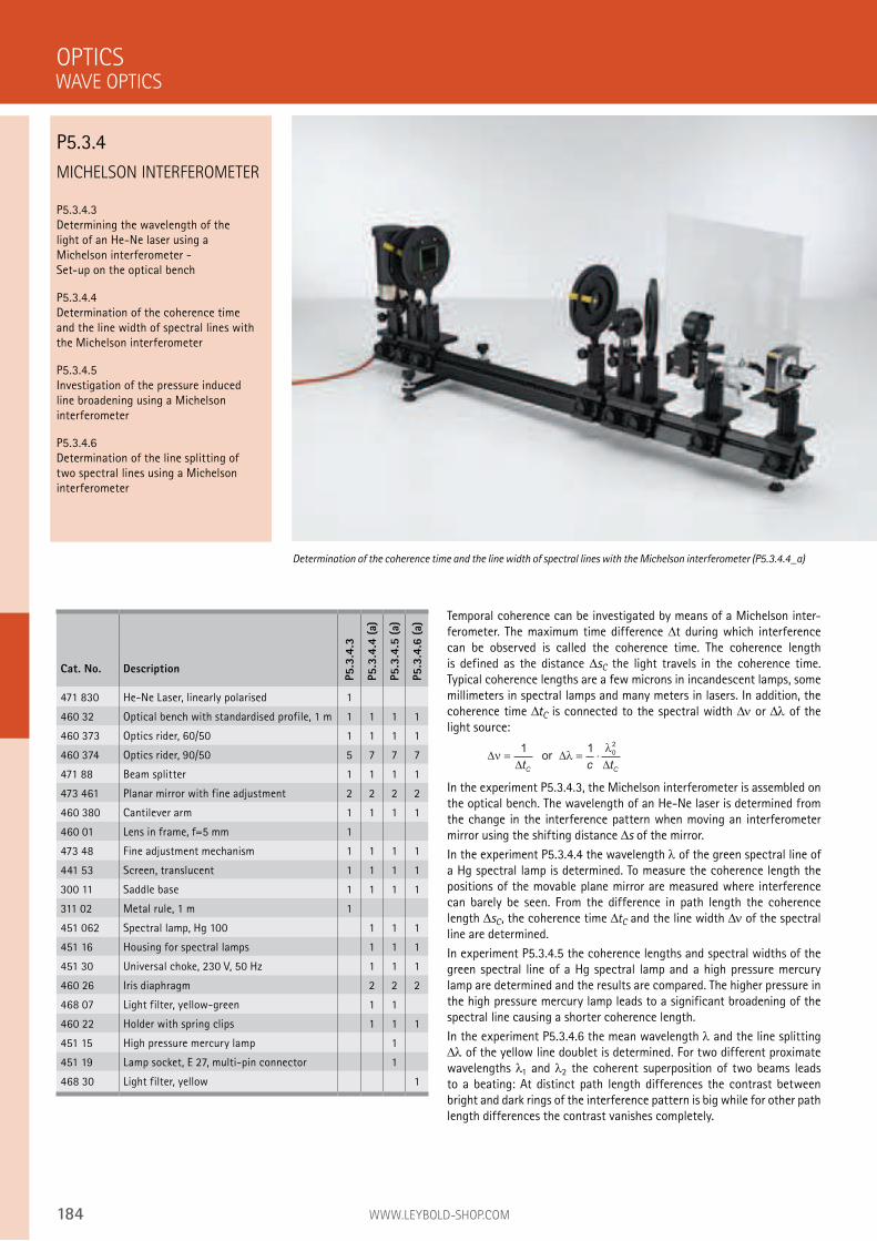
184 WWW.LEYBOLD-SHOP.COM
MICHELSON INTERFEROMETER
P5.3.4.3 Determining the wavelength of the light of an He-Ne laser using a Michelson interferometer - Set-up on the optical bench
P5.3.4.4 Determination of the coherence time and the line width of spectral lines with the Michelson interferometer
P5.3.4.5 Investigation of the pressure induced line broadening using a Michelson interferometer
P5.3.4.6 Determination of the line splitting of two spectral lines using a Michelson interferometer
Temporal coherence can be investigated by means of a Michelson inter-ferometer. The maximum time difference t during which interference can be observed is called the coherence time. The coherence length is defined as the distance sC the light travels in the coherence time. Typical coherence lengths are a few microns in incandescent lamps, some millimeters in spectral lamps and many meters in lasers. In addition, the coherence time tC is connected to the spectral width or of the light source:
∆∆
∆∆
ν λλ
= = ⋅1 1
0
2
t c tC C
or
In the experiment P5.3.4.3, the Michelson interferometer is assembled on the optical bench. The wavelength of an He-Ne laser is determined from the change in the interference pattern when moving an interferometer mirror using the shifting distance s of the mirror.
In the experiment P5.3.4.4 the wavelength of the green spectral line of a Hg spectral lamp is determined. To measure the coherence length the positions of the movable plane mirror are measured where interference can barely be seen. From the difference in path length the coherence length sC, the coherence time tC and the line width of the spectral line are determined.
In experiment P5.3.4.5 the coherence lengths and spectral widths of the green spectral line of a Hg spectral lamp and a high pressure mercury lamp are determined and the results are compared. The higher pressure in the high pressure mercury lamp leads to a significant broadening of the spectral line causing a shorter coherence length.
In the experiment P5.3.4.6 the mean wavelength and the line splitting of the yellow line doublet is determined. For two different proximate
wavelengths 1 and 2 the coherent superposition of two beams leads to a beating: At distinct path length differences the contrast between bright and dark rings of the interference pattern is big while for other path length differences the contrast vanishes completely.
OPTICS
Determination of the coherence time and the line width of spectral lines with the Michelson interferometer (P5.3.4.4_a)
Cat. No. Description
P5.3
.4.3
P5.3
.4.4
(a)
P5.3
.4.5
(a)
P5.3
.4.6
(a)
471 830 He-Ne Laser, linearly polarised 1
460 32 Optical bench with standardised profile, 1 m 1 1 1 1
460 373 Optics rider, 60/50 1 1 1 1
460 374 Optics rider, 90/50 5 7 7 7
471 88 Beam splitter 1 1 1 1
473 461 Planar mirror with fine adjustment 2 2 2 2
460 380 Cantilever arm 1 1 1 1
460 01 Lens in frame, f=5 mm 1
473 48 Fine adjustment mechanism 1 1 1 1
441 53 Screen, translucent 1 1 1 1
300 11 Saddle base 1 1 1 1
311 02 Metal rule, 1 m 1
451 062 Spectral lamp, Hg 100 1 1 1
451 16 Housing for spectral lamps 1 1 1
451 30 Universal choke, 230 V, 50 Hz 1 1 1
460 26 Iris diaphragm 2 2 2
468 07 Light filter, yellow-green 1 1
460 22 Holder with spring clips 1 1 1
451 15 High pressure mercury lamp 1
451 19 Lamp socket, E 27, multi-pin connector 1
468 30 Light filter, yellow 1
WAVE OPTICS
P5.3.4
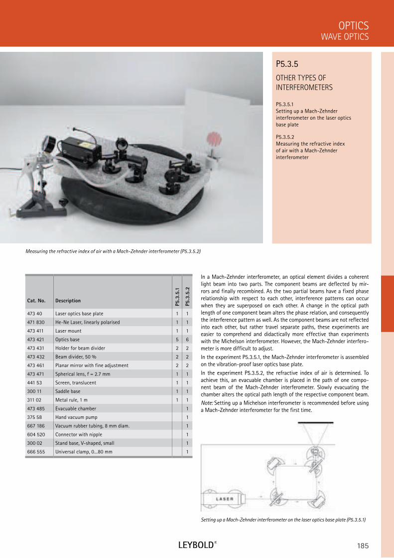
185
OTHER TYPES OF
INTERFEROMETERS
P5.3.5.1
Setting up a Mach-Zehnder
interferometer on the laser optics
base plate
P5.3.5.2
Measuring the refractive index
of air with a Mach-Zehnder
interferometer
WAVE OPTICS
OPTICS
Cat. No. Description
P5.3
.5.1
P5.3
.5.2
473 40 Laser optics base plate 1 1
471 830 He-Ne Laser, linearly polarised 1 1
473 411 Laser mount 1 1
473 421 Optics base 5 6
473 431 Holder for beam divider 2 2
473 432 Beam divider, 50 % 2 2
473 461 Planar mirror with fine adjustment 2 2
473 471 Spherical lens, f = 2.7 mm 1 1
441 53 Screen, translucent 1 1
300 11 Saddle base 1 1
311 02 Metal rule, 1 m 1 1
473 485 Evacuable chamber 1
375 58 Hand vacuum pump 1
667 186 Vacuum rubber tubing, 8 mm diam. 1
604 520 Connector with nipple 1
300 02 Stand base, V-shaped, small 1
666 555 Universal clamp, 0...80 mm 1
In a Mach-Zehnder interferometer, an optical element divides a coherent
light beam into two parts. The component beams are deflected by mir-
rors and finally recombined. As the two partial beams have a fixed phase
relationship with respect to each other, interference patterns can occur
when they are superposed on each other. A change in the optical path
length of one component beam alters the phase relation, and consequently
the interference pattern as well. As the component beams are not reflected
into each other, but rather travel separate paths, these experiments are
easier to comprehend and didactically more effective than experiments
with the Michelson interferometer. However, the Mach-Zehnder interfero-
meter is more difficult to adjust.
In the experiment P5.3.5.1, the Mach-Zehnder interferometer is assembled
on the vibration-proof laser optics base plate.
In the experiment P5.3.5.2, the refractive index of air is determined. To
achieve this, an evacuable chamber is placed in the path of one compo-
nent beam of the Mach-Zehnder interferometer. Slowly evacuating the
chamber alters the optical path length of the respective component beam.
Note: Setting up a Michelson interferometer is recommended before using
a Mach-Zehnder interferometer for the first time.
Measuring the refractive index of air with a Mach-Zehnder interferometer (P5.3.5.2)
P5.3.5
Setting up a Mach-Zehnder interferometer on the laser optics base plate (P5.3.5.1)
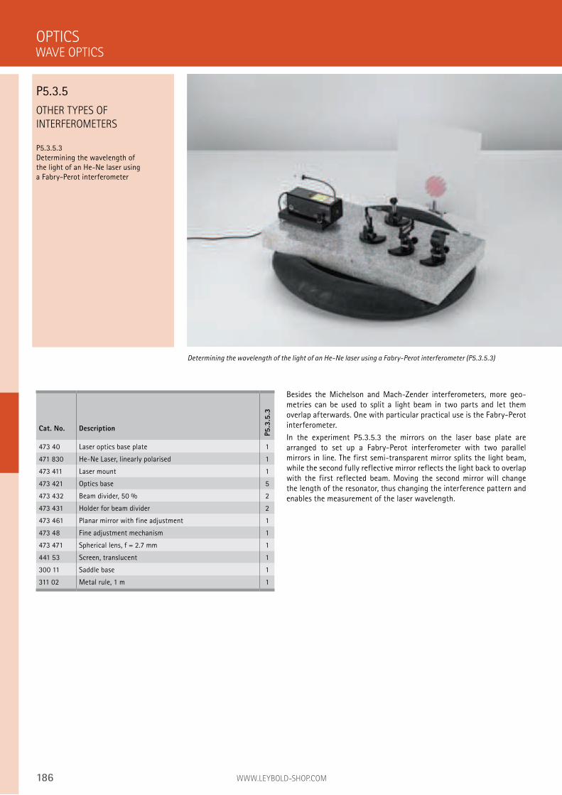
186 WWW.LEYBOLD-SHOP.COM
OTHER TYPES OF
INTERFEROMETERS
P5.3.5.3
Determining the wavelength of
the light of an He-Ne laser using
a Fabry-Perot interferometer
Besides the Michelson and Mach-Zender interferometers, more geo-
metries can be used to split a light beam in two parts and let them
overlap afterwards. One with particular practical use is the Fabry-Perot
interferometer.
In the experiment P5.3.5.3 the mirrors on the laser base plate are
arranged to set up a Fabry-Perot interferometer with two parallel
mirrors in line. The first semi-transparent mirror splits the light beam,
while the second fully reflective mirror reflects the light back to overlap
with the first reflected beam. Moving the second mirror will change
the length of the resonator, thus changing the interference pattern and
enables the measurement of the laser wavelength.
OPTICS
Determining the wavelength of the light of an He-Ne laser using a Fabry-Perot interferometer (P5.3.5.3)
Cat. No. Description
P5.3
.5.3
473 40 Laser optics base plate 1
471 830 He-Ne Laser, linearly polarised 1
473 411 Laser mount 1
473 421 Optics base 5
473 432 Beam divider, 50 % 2
473 431 Holder for beam divider 2
473 461 Planar mirror with fine adjustment 1
473 48 Fine adjustment mechanism 1
473 471 Spherical lens, f = 2.7 mm 1
441 53 Screen, translucent 1
300 11 Saddle base 1
311 02 Metal rule, 1 m 1
WAVE OPTICS
P5.3.5
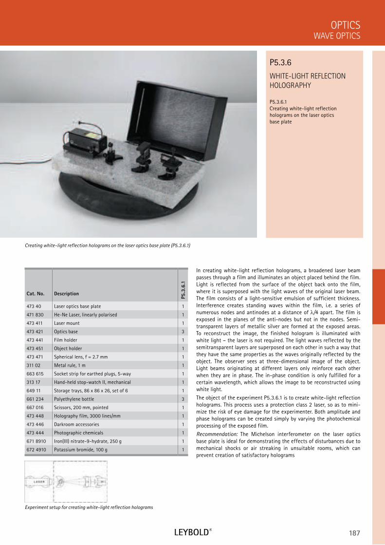
187
WHITE-LIGHT REFLECTION
HOLOGRAPHY
P5.3.6.1 Creating white-light reflection holograms on the laser optics base plate
WAVE OPTICS
OPTICS
Cat. No. Description
P5.3
.6.1
473 40 Laser optics base plate 1
471 830 He-Ne Laser, linearly polarised 1
473 411 Laser mount 1
473 421 Optics base 3
473 441 Film holder 1
473 451 Object holder 1
473 471 Spherical lens, f = 2.7 mm 1
311 02 Metal rule, 1 m 1
663 615 Socket strip for earthed plugs, 5-way 1
313 17 Hand-held stop-watch II, mechanical 1
649 11 Storage trays, 86 x 86 x 26, set of 6 1
661 234 Polyethylene bottle 3
667 016 Scissors, 200 mm, pointed 1
473 448 Holography film, 3000 lines/mm 1
473 446 Darkroom accessories 1
473 444 Photographic chemicals 1
671 8910 Iron(III) nitrate-9-hydrate, 250 g 1
672 4910 Potassium bromide, 100 g 1
In creating white-light reflection holograms, a broadened laser beam passes through a film and illuminates an object placed behind the film. Light is reflected from the surface of the object back onto the film, where it is superposed with the light waves of the original laser beam. The film consists of a light-sensitive emulsion of sufficient thickness. Interference creates standing waves within the film, i.e. a series of numerous nodes and antinodes at a distance of /4 apart. The film is exposed in the planes of the anti-nodes but not in the nodes. Semi-transparent layers of metallic silver are formed at the exposed areas. To reconstruct the image, the finished hologram is illuminated with white light – the laser is not required. The light waves reflected by the semitransparent layers are superposed on each other in such a way that they have the same properties as the waves originally reflected by the object. The observer sees at three-dimensional image of the object. Light beams originating at different layers only reinforce each other when they are in phase. The in-phase condition is only fulfilled for a certain wavelength, which allows the image to be reconstructed using white light.
The object of the experiment P5.3.6.1 is to create white-light reflection holograms. This process uses a protection class 2 laser, so as to mini-mize the risk of eye damage for the experimenter. Both amplitude and phase holograms can be created simply by varying the photochemical processing of the exposed film.
Recommendation: The Michelson interferometer on the laser optics base plate is ideal for demonstrating the effects of disturbances due to mechanical shocks or air streaking in unsuitable rooms, which can prevent creation of satisfactory holograms
Creating white-light reflection holograms on the laser optics base plate (P5.3.6.1)
P5.3.6
Experiment setup for creating white-light reflection holograms
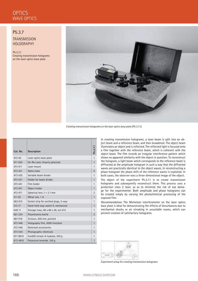
188 WWW.LEYBOLD-SHOP.COM
TRANSMISSION
HOLOGRAPHY
P5.3.7.1 Creating transmission holograms on the laser optics base plate
In creating transmission holograms, a laser beam is split into an ob-ject beam and a reference beam, and then broadened. The object beam illuminates an object and is reflected. The reflected light is focused onto a film together with the reference beam, which is coherent with the object beam. The film records an irregular interference pattern which shows no apparent similarity with the object in question. To reconstruct the hologram, a light beam which corresponds to the reference beam is diffracted at the amplitude hologram in such a way that the diffracted waves are practically identical to the object waves. In reconstructing a phase hologram the phase shift of the reference waves is exploited. In both cases, the observer sees a three-dimensional image of the object.
The object of the experiment P5.3.7.1 is to create transmission holograms and subsequently reconstruct them. This process uses a protection class 2 laser, so as to minimize the risk of eye dama-ge for the experimenter. Both amplitude and phase holograms can be created simply by varying the photochemical processing of the exposed film.
Recommendation: The Michelson interferometer on the laser optics base plate is ideal for demonstrating the effects of disturbances due to mechanical shocks or air streaking in unsuitable rooms, which can prevent creation of satisfactory holograms.
OPTICS
Creating transmission holograms on the laser optics base plate (P5.3.7.1)
Cat. No. Description
P5.3
.7.1
473 40 Laser optics base plate 1
471 830 He-Ne Laser, linearly polarised 1
473 411 Laser mount 1
473 421 Optics base 5
473 435 Variable beam divider 1
473 431 Holder for beam divider 1
473 441 Film holder 1
473 451 Object holder 1
473 471 Spherical lens, f = 2.7 mm 2
311 02 Metal rule, 1 m 1
663 615 Socket strip for earthed plugs, 5-way 1
313 17 Hand-held stop-watch II, mechanical 1
649 11 Storage trays, 86 x 86 x 26, set of 6 1
661 234 Polyethylene bottle 3
667 016 Scissors, 200 mm, pointed 1
473 448 Holography film, 3000 lines/mm 1
473 446 Darkroom accessories 1
473 444 Photographic chemicals 1
671 8910 Iron(III) nitrate-9-hydrate, 250 g 1
672 4910 Potassium bromide, 100 g 1
Experiment setup for creating transmission holograms
WAVE OPTICS
P5.3.7
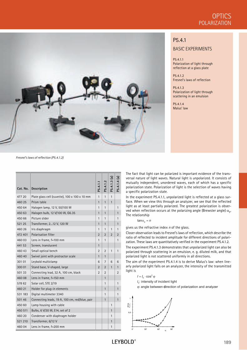
189
BASIC EXPERIMENTS
P5.4.1.1 Polarization of light through reflection at a glass plate
P5.4.1.2 Fresnel’s laws of reflection
P5.4.1.3 Polarization of light through scattering in an emulsion
P5.4.1.4 Malus’ law
POLARIZATION
OPTICS
Cat. No. Description
P5.4
.1.1
P5.4
.1.2
P5.4
.1.3
(a)
P5.4
.1.4
(a)
477 20 Plate glass cell (cuvette), 100 x 100 x 10 mm 1 1 1
460 25 Prism table 1 1 1
450 64 Halogen lamp, 12 V, 50/100 W 1 1 1
450 63 Halogen bulb, 12 V/100 W, G6.35 1 1 1
450 66 Picture slider 1 1 1
521 25 Transformer, 2...12 V, 120 W 1 1 1
460 26 Iris diaphragm 1 1 1 1
472 401 Polarisation filter 2 2 2 2
460 03 Lens in frame, f=100 mm 1 1 1
441 53 Screen, translucent 1
460 43 Small optical bench 2 2 1 1
460 40 Swivel joint with protractor scale 1 1
301 01 Leybold multiclamp 6 7 6 6
300 01 Stand base, V-shaped, large 2 2 1 1
501 33 Connecting lead, 32 A, 100 cm, black 2 2 2
460 08 Lens in frame, f=150 mm 1
578 62 Solar cell, STE 2/19 1 1
460 21 Holder for plug-in elements 1 1
531 183 Digital multimeter 3340 1 1
501 46 Connecting leads, 19 A, 100 cm, red/blue, pair 1 1
450 60 Lamp housing with cable 1
450 511 Bulbs, 6 V/30 W, E14, set of 2 1
460 20 Condenser with diaphragm holder 1
521 210 Transformer, 6/12 V 1
460 04 Lens in frame, f=200 mm 1
The fact that light can be polarized is important evidence of the trans-versal nature of light waves. Natural light is unpolarized. It consists of mutually independent, unordered waves, each of which has a specific polarization state. Polarization of light is the selection of waves having a specific polarization state.
In the experiment P5.4.1.1, unpolarized light is reflected at a glass sur-face. When we view this through an analyzer, we see that the reflected light as at least partially polarized. The greatest polarization is obser-ved when reflection occurs at the polarizing angle (Brewster angle) p. The relationship
tanp
α = n
gives us the refractive index n of the glass.
Closer observation leads to Fresnel’s laws of reflection, which describe the ratio of reflected to incident amplitude for different directions of polari-zation. These laws are quantitatively verified in the experiment P5.4.1.2.
The experiment P5.4.1.3 demonstrates that unpolarized light can also be polarized through scattering in an emulsion, e. g. diluted milk, and that polarized light is not scattered uniformly in all directions.
The aim of the experiment P5.4.1.4 is to derive Malus’s law: when line-arly polarized light falls on an analyzer, the intensity of the transmitted light is
I I
I
= ⋅0
2
0
cos ϕ
ϕ
: intensity of incident light
: angle between ddirection of polarization and analyzer
Fresnel’s laws of reflection (P5.4.1.2)
P5.4.1
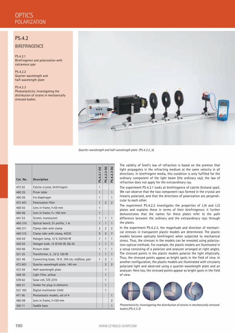
190 WWW.LEYBOLD-SHOP.COM
BIREFRINGENCE
P5.4.2.1 Birefringence and polarization with calcareous spar
P5.4.2.2 Quarter-wavelength and half-wavelength plate
P5.4.2.3 Photoelasticity: Investigating the distribution of strains in mechanically stressed bodies
The validity of Snell’s law of refraction is based on the premise that light propagates in the refracting medium at the same velocity in all directions. In birefringent media, this condition is only fulfilled for the ordinary component of the light beam (the ordinary ray); the law of refraction does not apply for the extraordinary ray.
The experiment P5.4.2.1 looks at birefringence of calcite (Iceland spar). We can observe that the two component rays formed in the crystal are linearly polarized, and that the directions of polarization are perpendi-cular to each other.
The experiment P5.4.2.2 investigates the properties of /4 and /2 plates and explains these in terms of their birefringence; it further demonstrates that the names for these plates refer to the path difference between the ordinary and the extraordinary rays through the plates.
In the experiment P5.4.2.3, the magnitude and direction of mechani-cal stresses in transparent plastic models are determined. The plastic models become optically birefringent when subjected to mechanical stress. Thus, the stresses in the models can be revealed using polariza-tion-optical methods. For example, the plastic models are illuminated in a setup consisting of a polarizer and analyzer arranged at right angles. The stressed points in the plastic models polarize the light elliptically. Thus, the stressed points appear as bright spots in the field of view. In another configuration, the plastic models are illuminated with circularly polarized light and observed using a quarter-wavelength plate and an analyzer. Here too, the stressed points appear as bright spots in the field of view.
OPTICS
Quarter-wavelength and half-wavelength plate (P5.4.2.2_b)
Cat. No. Description
P5.4
.2.1
(b)
P5.4
.2.2
(b)
P5.4
.2.3
(b)
472 02 Calcite crystal, birefringent 1
460 25 Prism table 1 1
460 26 Iris diaphragm 1 1
472 401 Polarisation filter 1 2 2
460 02 Lens in frame, f=50 mm 1
460 06 Lens in frame, f=-100 mm 1
441 53 Screen, translucent 1 1 1
460 310 Optical bench, S1 profile, 1 m 1 1 1
460 311 Clamp rider with clamp 2 2 2
460 312 Clamp rider with clamp, 45/35 5 5 7
450 64 Halogen lamp, 12 V, 50/100 W 1 1 1
450 63 Halogen bulb, 12 V/100 W, G6.35 1 1 1
450 66 Picture slider 1 1 1
521 25 Transformer, 2...12 V, 120 W 1 1 1
501 46 Connecting leads, 19 A, 100 cm, red/blue, pair 1 2 1
472 601 Quarter-wavelength plate, 140 nm 2 2
472 59 Half-wavelength plate 1
468 30 Light filter, yellow 1
578 62 Solar cell, STE 2/19 1
460 21 Holder for plug-in elements 1
531 183 Digital multimeter 3340 1
471 95 Photoelastic models, set of 4 1
460 08 Lens in frame, f=150 mm 2
300 11 Saddle base 1 Photoelasticity: Investigating the distribution of strains in mechanically stressed
bodies (P5.4.2.3)
POLARIZATION
P5.4.2
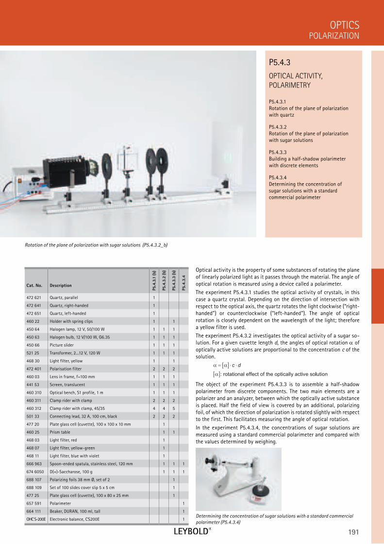
191
OPTICAL ACTIVITY,
POLARIMETRY
P5.4.3.1 Rotation of the plane of polarization with quartz
P5.4.3.2 Rotation of the plane of polarization with sugar solutions
P5.4.3.3 Building a half-shadow polarimeter with discrete elements
P5.4.3.4 Determining the concentration of sugar solutions with a standard commercial polarimeter
POLARIZATION
OPTICS
Cat. No. Description
P5.4
.3.1
(b)
P5.4
.3.2
(b)
P5.4
.3.3
(b)
P5.4
.3.4
472 621 Quartz, parallel 1
472 641 Quartz, right-handed 1
472 651 Quartz, left-handed 1
460 22 Holder with spring clips 1 1
450 64 Halogen lamp, 12 V, 50/100 W 1 1 1
450 63 Halogen bulb, 12 V/100 W, G6.35 1 1 1
450 66 Picture slider 1 1 1
521 25 Transformer, 2...12 V, 120 W 1 1 1
468 30 Light filter, yellow 1 1
472 401 Polarisation filter 2 2 2
460 03 Lens in frame, f=100 mm 1 1 1
441 53 Screen, translucent 1 1 1
460 310 Optical bench, S1 profile, 1 m 1 1 1
460 311 Clamp rider with clamp 2 2 2
460 312 Clamp rider with clamp, 45/35 4 4 5
501 33 Connecting lead, 32 A, 100 cm, black 2 2 2
477 20 Plate glass cell (cuvette), 100 x 100 x 10 mm 1
460 25 Prism table 1 1
468 03 Light filter, red 1
468 07 Light filter, yellow-green 1
468 11 Light filter, blue with violet 1
666 963 Spoon-ended spatula, stainless steel, 120 mm 1 1 1
674 6050 D(+)-Saccharose, 100 g 1 1 1
688 107 Polarizing foils 38 mm Ø, set of 2 1
688 109 Set of 100 slides cover slip 5 x 5 cm 1
477 25 Plate glass cell (cuvette), 100 x 80 x 25 mm 1
657 591 Polarimeter 1
664 111 Beaker, DURAN, 100 ml, tall 1
OHC S-200E Electronic balance, CS200E 1
Optical activity is the property of some substances of rotating the plane of linearly polarized light as it passes through the material. The angle of optical rotation is measured using a device called a polarimeter.
The experiment P5.4.3.1 studies the optical activity of crystals, in this case a quartz crystal. Depending on the direction of intersection with respect to the optical axis, the quartz rotates the light clockwise (“right-handed”) or counterclockwise (“left-handed”). The angle of optical rotation is closely dependent on the wavelength of the light; therefore a yellow filter is used.
The experiment P5.4.3.2 investigates the optical activity of a sugar so-lution. For a given cuvette length d, the angles of optical rotation of optically active solutions are proportional to the concentration c of the solution.
α α
α
= [ ] ⋅ ⋅
[ ]
c d
: rotational effect of the optically active sollution
The object of the experiment P5.4.3.3 is to assemble a half-shadow polarimeter from discrete components. The two main elements are a polarizer and an analyzer, between which the optically active substance is placed. Half the field of view is covered by an additional, polarizing foil, of which the direction of polarization is rotated slightly with respect to the first. This facilitates measuring the angle of optical rotation.
In the experiment P5.4.3.4, the concentrations of sugar solutions are measured using a standard commercial polarimeter and compared with the values determined by weighing.
Rotation of the plane of polarization with sugar solutions (P5.4.3.2_b)
P5.4.3
Determining the concentration of sugar solutions with a standard commercial
polarimeter (P5.4.3.4)
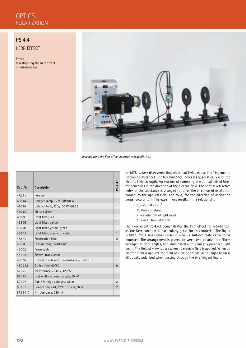
192 WWW.LEYBOLD-SHOP.COM
KERR EFFECT
P5.4.4.1 Investigating the Kerr effect in nitrobenzene
In 1875, J. Kerr discovered that electrical fields cause birefringence in isotropic substances. The birefringence increases quadratically with the electric field strength. For reasons of symmetry, the optical axis of bire-fringence lies in the direction of the electric field. The normal refractive index of the substance is changed to ne for the direction of oscillation parallel to the applied field, and to no for the direction of oscillation perpendicular to it. The experiment results in the relationship
n n K E
K
E
e o− = ⋅ ⋅λ
λ
2
: Kerr constant
: wavelength of light used
: eelectic field strength
The experiment P5.4.4.1 demonstrates the Kerr effect for nitrobenzol, as the Kerr constant is particularly great for this material. The liquid is filled into a small glass vessel in which a suitable plate capacitor is mounted. The arrangement is placed between two polarization filters arranged at right angles, and illuminated with a linearly polarized light beam. The field of view is dark when no electric field is applied. When an electric field is applied, the field of view brightens, as the light beam is elliptically polarized when passing through the birefringent liquid.
OPTICS
Investigating the Kerr effect in nitrobenzene (P5.4.4.1)
Cat. No. Description
P5.4
.4.1
473 31 Kerr cell 1
450 64 Halogen lamp, 12 V, 50/100 W 1
450 63 Halogen bulb, 12 V/100 W, G6.35 1
450 66 Picture slider 1
468 03 Light filter, red 1
468 05 Light filter, yellow 1
468 07 Light filter, yellow-green 1
468 11 Light filter, blue with violet 1
472 401 Polarisation filter 2
460 03 Lens in frame, f=100 mm 1
460 25 Prism table 1
441 53 Screen, translucent 1
460 32 Optical bench with standardised profile, 1 m 1
460 373 Optics rider, 60/50 6
521 25 Transformer, 2...12 V, 120 W 1
521 70 High-voltage power supply, 10 kV 1
501 051 Cable for high voltages, 1.5 m 2
501 33 Connecting lead, 32 A, 100 cm, black 2
673 9410 Nitrobenzene, 250 ml 1
POLARIZATION
P5.4.4
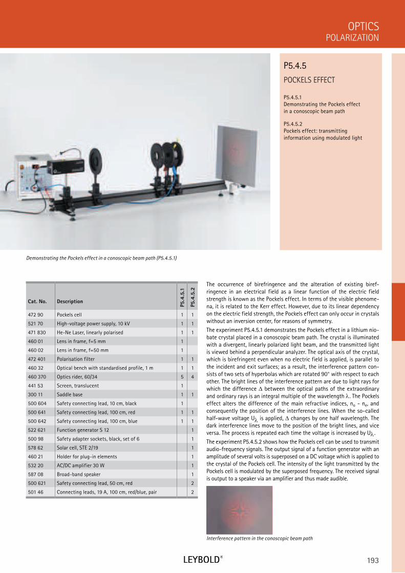
193
POCKELS EFFECT
P5.4.5.1 Demonstrating the Pockels effect in a conoscopic beam path
P5.4.5.2 Pockels effect: transmitting information using modulated light
POLARIZATION
OPTICS
Cat. No. Description
P5.4
.5.1
P5.4
.5.2
472 90 Pockels cell 1 1
521 70 High-voltage power supply, 10 kV 1 1
471 830 He-Ne Laser, linearly polarised 1 1
460 01 Lens in frame, f=5 mm 1
460 02 Lens in frame, f=50 mm 1
472 401 Polarisation filter 1 1
460 32 Optical bench with standardised profile, 1 m 1 1
460 370 Optics rider, 60/34 5 4
441 53 Screen, translucent 1
300 11 Saddle base 1 1
500 604 Safety connecting lead, 10 cm, black 1
500 641 Safety connecting lead, 100 cm, red 1 1
500 642 Safety connecting lead, 100 cm, blue 1 1
522 621 Function generator S 12 1
500 98 Safety adapter sockets, black, set of 6 1
578 62 Solar cell, STE 2/19 1
460 21 Holder for plug-in elements 1
532 20 AC/DC amplifier 30 W 1
587 08 Broad-band speaker 1
500 621 Safety connecting lead, 50 cm, red 2
501 46 Connecting leads, 19 A, 100 cm, red/blue, pair 2
The occurrence of birefringence and the alteration of existing biref-ringence in an electrical field as a linear function of the electric field strength is known as the Pockels effect. In terms of the visible phenome-na, it is related to the Kerr effect. However, due to its linear dependency on the electric field strength, the Pockels effect can only occur in crystals without an inversion center, for reasons of symmetry.
The experiment P5.4.5.1 demonstrates the Pockels effect in a lithium nio-bate crystal placed in a conoscopic beam path. The crystal is illuminated with a divergent, linearly polarized light beam, and the transmitted light is viewed behind a perpendicular analyzer. The optical axis of the crystal, which is birefringent even when no electric field is applied, is parallel to the incident and exit surfaces; as a result, the interference pattern con-sists of two sets of hyperbolas which are rotated 90° with respect to each other. The bright lines of the interference pattern are due to light rays for which the difference between the optical paths of the extraordinary and ordinary rays is an integral multiple of the wavelength . The Pockels effect alters the difference of the main refractive indices, no - ne, and consequently the position of the interference lines. When the so-called half-wave voltage U is applied, changes by one half wavelength. The dark interference lines move to the position of the bright lines, and vice versa. The process is repeated each time the voltage is increased by U .
The experiment P5.4.5.2 shows how the Pockels cell can be used to transmit audio-frequency signals. The output signal of a function generator with an amplitude of several volts is superposed on a DC voltage which is applied to the crystal of the Pockels cell. The intensity of the light transmitted by the Pockels cell is modulated by the superposed frequency. The received signal is output to a speaker via an amplifier and thus made audible.
Demonstrating the Pockels effect in a conoscopic beam path (P5.4.5.1)
P5.4.5
Interference pattern in the conoscopic beam path
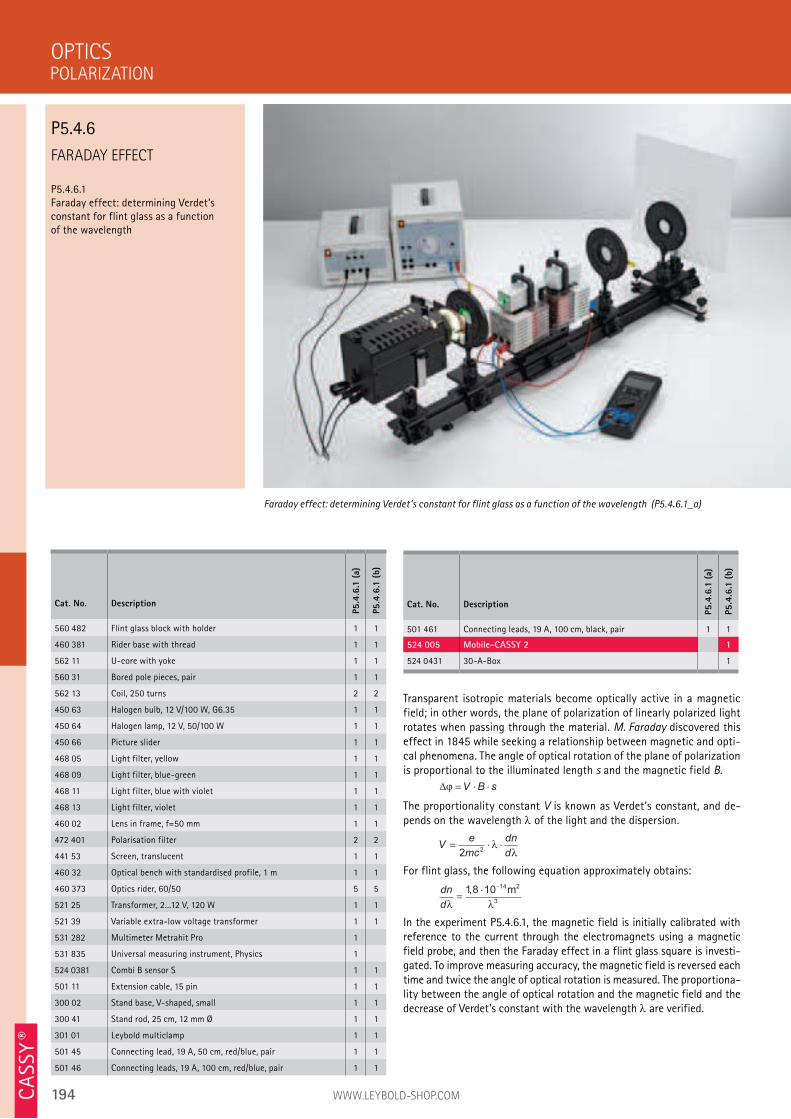
194 WWW.LEYBOLD-SHOP.COM
FARADAY EFFECT
P5.4.6.1 Faraday effect: determining Verdet’s constant for flint glass as a function of the wavelength
Transparent isotropic materials become optically active in a magnetic field; in other words, the plane of polarization of linearly polarized light rotates when passing through the material. M. Faraday discovered this effect in 1845 while seeking a relationship between magnetic and opti-cal phenomena. The angle of optical rotation of the plane of polarization is proportional to the illuminated length s and the magnetic field B.
∆ϕ = ⋅ ⋅V B s
The proportionality constant V is known as Verdet’s constant, and de-pends on the wavelength of the light and the dispersion.
Ve
mc
dn
d= ⋅ ⋅2
2λ
λ
For flint glass, the following equation approximately obtains:
dn
dλ λ=
⋅ −18 10
14 2
3
, m
In the experiment P5.4.6.1, the magnetic field is initially calibrated with reference to the current through the electromagnets using a magnetic field probe, and then the Faraday effect in a flint glass square is investi-gated. To improve measuring accuracy, the magnetic field is reversed each time and twice the angle of optical rotation is measured. The proportiona-lity between the angle of optical rotation and the magnetic field and the decrease of Verdet’s constant with the wavelength are verified.
OPTICS
Faraday effect: determining Verdet’s constant for flint glass as a function of the wavelength (P5.4.6.1_a)
Cat. No. Description
P5.4
.6.1
(a)
P5.4
.6.1
(b)
560 482 Flint glass block with holder 1 1
460 381 Rider base with thread 1 1
562 11 U-core with yoke 1 1
560 31 Bored pole pieces, pair 1 1
562 13 Coil, 250 turns 2 2
450 63 Halogen bulb, 12 V/100 W, G6.35 1 1
450 64 Halogen lamp, 12 V, 50/100 W 1 1
450 66 Picture slider 1 1
468 05 Light filter, yellow 1 1
468 09 Light filter, blue-green 1 1
468 11 Light filter, blue with violet 1 1
468 13 Light filter, violet 1 1
460 02 Lens in frame, f=50 mm 1 1
472 401 Polarisation filter 2 2
441 53 Screen, translucent 1 1
460 32 Optical bench with standardised profile, 1 m 1 1
460 373 Optics rider, 60/50 5 5
521 25 Transformer, 2...12 V, 120 W 1 1
521 39 Variable extra-low voltage transformer 1 1
531 282 Multimeter Metrahit Pro 1
531 835 Universal measuring instrument, Physics 1
524 0381 Combi B sensor S 1 1
501 11 Extension cable, 15 pin 1 1
300 02 Stand base, V-shaped, small 1 1
300 41 Stand rod, 25 cm, 12 mm Ø 1 1
301 01 Leybold multiclamp 1 1
501 45 Connecting lead, 19 A, 50 cm, red/blue, pair 1 1
501 46 Connecting leads, 19 A, 100 cm, red/blue, pair 1 1
POLARIZATION
P5.4.6
Cat. No. Description
P5.4
.6.1
(a)
P5.4
.6.1
(b)
501 461 Connecting leads, 19 A, 100 cm, black, pair 1 1
524 005 Mobile-CASSY 2 1
524 0431 30-A-Box 1
CA
SSY ®
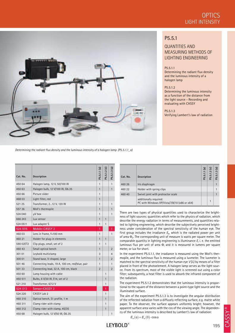
195
QUANTITIES AND
MEASURING METHODS OF
LIGHTING ENGINEERING
P5.5.1.1 Determining the radiant flux density and the luminous intensity of a halogen lamp
P5.5.1.2 Determining the luminous intensity as a function of the distance from the light source - Recording and evaluating with CASSY
P5.5.1.3 Verifying Lambert’s law of radiation
LIGHT INTENSITY
OPTICS
Cat. No. Description
P5.5
.1.1
(a)
P5.5
.1.2
(c)
P5.5
.1.3
(a)
450 64 Halogen lamp, 12 V, 50/100 W 1 1
450 63 Halogen bulb, 12 V/100 W, G6.35 1 1
450 66 Picture slider 1
468 03 Light filter, red 1
521 25 Transformer, 2...12 V, 120 W 1 1
557 36 Moll‘s thermopile 1 1
524 040 µV box 1 1
666 243 Lux sensor 1 1
524 0511 Lux adapter S 1 1
524 005 Mobile-CASSY 2 1 1
460 03 Lens in frame, f=100 mm 1 1
460 21 Holder for plug-in elements 1 1
590 02ET2 Clip plugs, small, set of 2 1 1
460 43 Small optical bench 1 2
301 01 Leybold multiclamp 3 4
300 01 Stand base, V-shaped, large 1 2
501 46 Connecting leads, 19 A, 100 cm, red/blue, pair 1 1
501 33 Connecting lead, 32 A, 100 cm, black 2 2
450 60 Lamp housing with cable 1
450 511 Bulbs, 6 V/30 W, E14, set of 2 1
521 210 Transformer, 6/12 V 1
524 013 Sensor-CASSY 2 1
524 220 CASSY Lab 2 1
460 310 Optical bench, S1 profile, 1 m 1
460 311 Clamp rider with clamp 1
460 312 Clamp rider with clamp, 45/35 1
450 68 Halogen bulb, 12 V/50 W, G6.35 1
There are two types of physical quantities used to characterize the bright-ness of light sources: quantities which refer to the physics of radiation, which describe the energy radiation in terms of measurements, and quantities rela-ted to lighting engineering, which describe the subjectively perceived bright-ness under consideration of the spectral sensitivity of the human eye. The first group includes the irradiance Ee, which is the radiated power per unit of area e. The corresponding unit of measure is watts per square meter. The comparable quantity in lighting engineering is illuminance E, i. e. the emitted luminous flux per unit of area , and it is measured in lumens per square meter, or lux for short.
In the experiment P5.5.1.1, the irradiance is measured using the Moll’s ther-mopile, and the luminous flux is measured using a luxmeter. The luxmeter is matched to the spectral sensitivity of the human eye V ( ) by means of a filter placed in front of the photoelement. A halogen lamp serves as the light sour-ce. From its spectrum, most of the visible light is screened out using a color filter; subsequently, a heat filter is used to absorb the infrared component of the radiation.
The experiment P5.5.1.2 demonstrates that the luminous intensity is propor-tional to the square of the distance between a point-type light source and the illuminated surface.
The aim of the experiment P5.5.1.3 is to investigate the angular distribution of the reflected radiation from a diffusely reflecting surface, e.g. matte white paper. To the observer, the surface appears uniformly bright; however, the apparent surface area varies with the cos of the viewing angle. The dependen-cy of the luminous intensity is described by Lambert’s law of radiation:
E Ee eφ φ( ) = ( ) ⋅0 cos
Determining the radiant flux density and the luminous intensity of a halogen lamp (P5.5.1.1_a)
P5.5.1
Cat. No. Description
P5.5
.1.1
(a)
P5.5
.1.2
(c)
P5.5
.1.3
(a)
460 26 Iris diaphragm 1
460 22 Holder with spring clips 1
460 40 Swivel joint with protractor scale 1
additionally required: PC with Windows XP/Vista/7/8/10 (x86 or x64)
1
CA
SSY ®
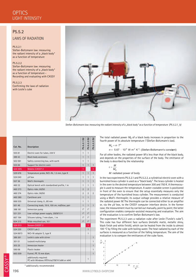
196 WWW.LEYBOLD-SHOP.COM
0 10 20T 4 - T
04
K4
0
1
2
3
4
5
U
µV
LAWS OF RADIATION
P5.5.2.1 Stefan-Boltzmann law: measuring the radiant intensity of a „black body“ as a function of temperature
P5.5.2.2 Stefan-Boltzmann law: measuring the radiant intensity of a „black body“ as a function of temperature - Recording and evaluating with CASSY
P5.5.2.3 Confirming the laws of radiation with Leslie‘s cube
The total radiated power MB of a black body increases in proportion to the fourth power of its absolute temperature T (Stefan-Boltzmann’s law).
M TB= ⋅
= ⋅
σ
σ
4
5.67 10 W m K : (Stefan-Boltzmann's const-8 -2 -4 aant)
For all other bodies, the radiated power M is less than that of the black body, and depends on the properties of the surface of the body. The emittance of the body is described by the relationship
ε =M
M
M
B
: radiated power of body
In the two experiments P5.5.2.1 and P5.5.2.2, a cylindrical electric oven with a burnished brass cylinder is used as a “black body”. The brass cylinder is heated in the oven to the desired temperature between 300 and 750 K. A thermocou-ple is used to measure the temperature. A water-coolable screen is positioned in front of the oven to ensure that the setup essentially measures only the temperature of the burnished brass cylinder. The measurement is conducted using a Moll’s thermopile; its output voltage provides a relative measure of the radiated power M. The thermopile can be connected either to an amplifier or, via the µV box, to the CASSY computer interface device. In the former case, the measurement must by carried out manually, point by point; the latter configuration enables computer-assisted measuring and evaluation. The aim of the evaluation is to confirm Stefan-Boltzmann’s law.
The experiment P5.5.2.3 uses a radiation cube after Leslie (“Leslie’s cube”). This cube has four different face surfaces (metallic matte, metallic shiny, black finish and white finish), which can be heated from the inside to almost 100 °C by filling the cube with boiling water. The heat radiated by each of the surfaces is measured as a function of the falling temperature. The aim of the evaluation is to compare the emittances of the cube faces.
OPTICS
Stefan-Boltzmann law: measuring the radiant intensity of a „black body“ as a function of temperature (P5.5.2.1_b)
Cat. No. Description
P5.5
.2.1
(b)
P5.5
.2.2
(b)
P5.5
.2.3
(b)
555 81 Electric oven for tubes, 230 V 1 1
389 43 Black body accessory 1 1
502 061 Safety connecting box, with earth 1 1
555 84 Support for electric oven 1 1 1
524 005 Mobile-CASSY 2 1 1
529 676 Temperature probe, NiCr-Ni, 1.5 mm, type K 1 1 1
524 040 µV box 1 1 1
557 36 Moll‘s thermopile 1 1 1
460 32 Optical bench with standardised profile, 1 m 1 1 1
460 373 Optics rider, 60/50 2 2
460 374 Optics rider, 90/50 2 2 2
460 380 Cantilever arm 1 1
666 555 Universal clamp, 0...80 mm 1 1
501 46 Connecting leads, 19 A, 100 cm, red/blue, pair 1 1 1
388 181 Immersion pump 1* 1*
521 231 Low-voltage power supply, 3/6/9/12 V 1* 1*
667 194 Silicone tubing, 7 mm diam., 1 m 1* 1*
604 313 Wide-mouthed can, 10 l 1* 1*
524 013 Sensor-CASSY 2 1
524 220 CASSY Lab 2 1
524 0673 NiCr-Ni adapter S, type K 1
389 261 Leslie‘s cube with stirrer 1
301 01 Leybold multiclamp 1
303 25 Immersion heater 1
590 06 Plastic beaker 1
665 009 Funnel, PP, 75 mm diam. 1
additionally required: PC with Windows XP/Vista/7/8/10 (x86 or x64)
1
* additionally recommended
LIGHT INTENSITY
P5.5.2
CA
SSY ®
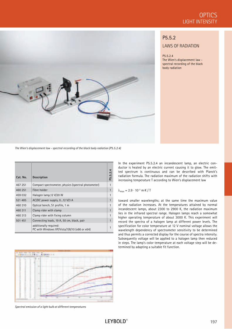
197
LAWS OF RADIATION
P5.5.2.4 The Wien‘s displacement law - spectral recording of the black body radiation
LIGHT INTENSITY
OPTICS
Cat. No. Description
P5.5
.2.4
467 251 Compact spectrometer, physics (spectral photometer) 1
460 251 Fibre holder 1
459 032 Halogen lamp,12 V/20 W 1
521 485 AC/DC power supply, 0...12 V/3 A 1
460 310 Optical bench, S1 profile, 1 m 1
460 311 Clamp rider with clamp 1
460 313 Clamp rider with fixing column 1
501 451 Connecting leads, 19 A, 50 cm, black, pair 1
additionally required: PC with Windows XP/Vista/7/8/10 (x86 or x64)
1
In the experiment P5.5.2.4 an incandescent lamp, an electric con-ductor is heated by an electric current causing it to glow. The emit-ted spectrum is continuous and can be described with Planck‘s radiation formula. The radiation maximum of the radiation shifts with increasing temperature T according to Wien‘s displacement law
max = 2.9 · 10-3 m·K / T
toward smaller wavelengths; at the same time the maximum value of the radiation increases. At the temperatures attained by normal incandescent lamps, about 2300 to 2900 K, the radiation maximum lies in the infrared spectral range. Halogen lamps reach a somewhat higher operating temperature of about 3000 K. This experiment will record the spectra of a halogen lamp at different power levels. The specification for color temperature at 12 V nominal voltage allows the wavelength dependency of spectrometer sensitivity to be determined and thus permits a corrected display for the course of spectra intensity. Subsequently voltage will be applied to a halogen lamp then reduced in steps. The lamp‘s color temperature at each voltage step will be de-termined by adapting a suitable fit function.
The Wien‘s displacement law - spectral recording of the black body radiation (P5.5.2.4)
P5.5.2
Spectral emission of a light bulb at different temperatures
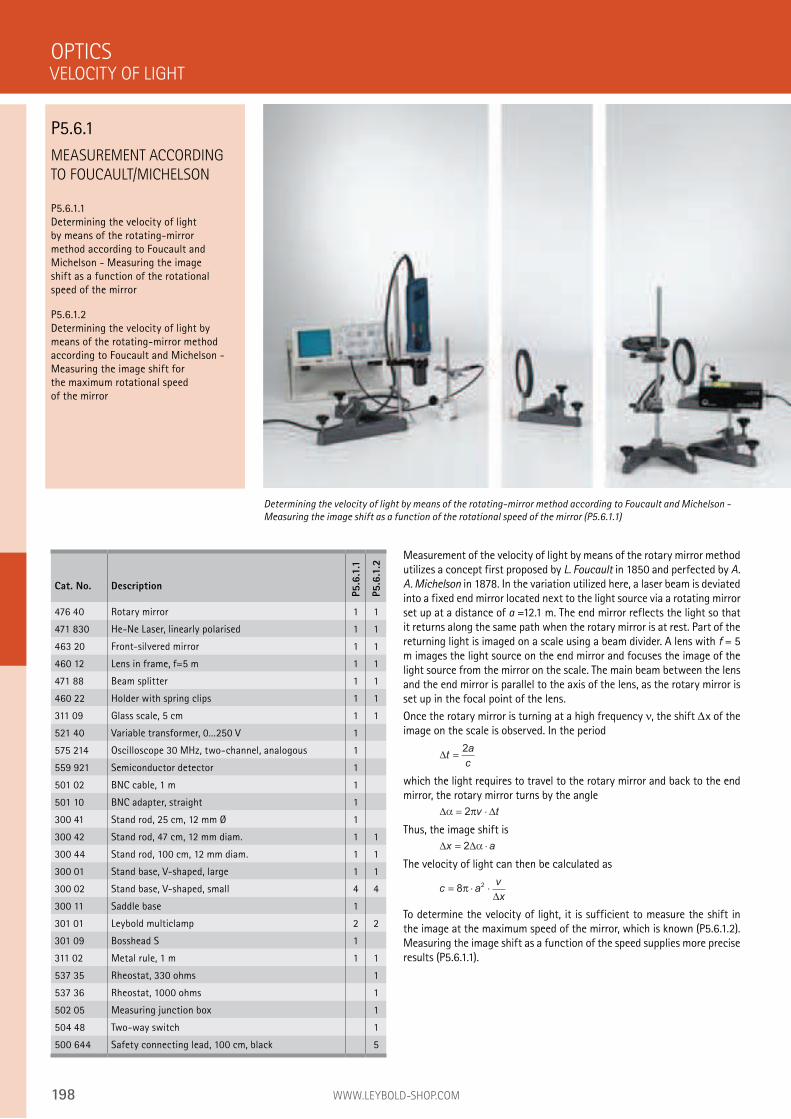
198 WWW.LEYBOLD-SHOP.COM
MEASUREMENT ACCORDING
TO FOUCAULT/MICHELSON
P5.6.1.1 Determining the velocity of light by means of the rotating-mirror method according to Foucault and Michelson - Measuring the image shift as a function of the rotational speed of the mirror
P5.6.1.2 Determining the velocity of light by means of the rotating-mirror method according to Foucault and Michelson - Measuring the image shift for the maximum rotational speed of the mirror
Measurement of the velocity of light by means of the rotary mirror method utilizes a concept first proposed by L. Foucault in 1850 and perfected by A.
A. Michelson in 1878. In the variation utilized here, a laser beam is deviated into a fixed end mirror located next to the light source via a rotating mirror set up at a distance of a =12.1 m. The end mirror reflects the light so that it returns along the same path when the rotary mirror is at rest. Part of the returning light is imaged on a scale using a beam divider. A lens with f = 5 m images the light source on the end mirror and focuses the image of the light source from the mirror on the scale. The main beam between the lens and the end mirror is parallel to the axis of the lens, as the rotary mirror is set up in the focal point of the lens.
Once the rotary mirror is turning at a high frequency , the shift x of the image on the scale is observed. In the period
∆ta
c=2
which the light requires to travel to the rotary mirror and back to the end mirror, the rotary mirror turns by the angle
∆ ∆α π= ⋅2 v t
Thus, the image shift is
∆ ∆x a= ⋅2 α
The velocity of light can then be calculated as
c av
x= ⋅ ⋅8
2π
∆
To determine the velocity of light, it is sufficient to measure the shift in the image at the maximum speed of the mirror, which is known (P5.6.1.2). Measuring the image shift as a function of the speed supplies more precise results (P5.6.1.1).
OPTICS
Determining the velocity of light by means of the rotating-mirror method according to Foucault and Michelson -
Measuring the image shift as a function of the rotational speed of the mirror (P5.6.1.1)
Cat. No. Description
P5.6
.1.1
P5.6
.1.2
476 40 Rotary mirror 1 1
471 830 He-Ne Laser, linearly polarised 1 1
463 20 Front-silvered mirror 1 1
460 12 Lens in frame, f=5 m 1 1
471 88 Beam splitter 1 1
460 22 Holder with spring clips 1 1
311 09 Glass scale, 5 cm 1 1
521 40 Variable transformer, 0...250 V 1
575 214 Oscilloscope 30 MHz, two-channel, analogous 1
559 921 Semiconductor detector 1
501 02 BNC cable, 1 m 1
501 10 BNC adapter, straight 1
300 41 Stand rod, 25 cm, 12 mm Ø 1
300 42 Stand rod, 47 cm, 12 mm diam. 1 1
300 44 Stand rod, 100 cm, 12 mm diam. 1 1
300 01 Stand base, V-shaped, large 1 1
300 02 Stand base, V-shaped, small 4 4
300 11 Saddle base 1
301 01 Leybold multiclamp 2 2
301 09 Bosshead S 1
311 02 Metal rule, 1 m 1 1
537 35 Rheostat, 330 ohms 1
537 36 Rheostat, 1000 ohms 1
502 05 Measuring junction box 1
504 48 Two-way switch 1
500 644 Safety connecting lead, 100 cm, black 5
VELOCITY OF LIGHT
P5.6.1
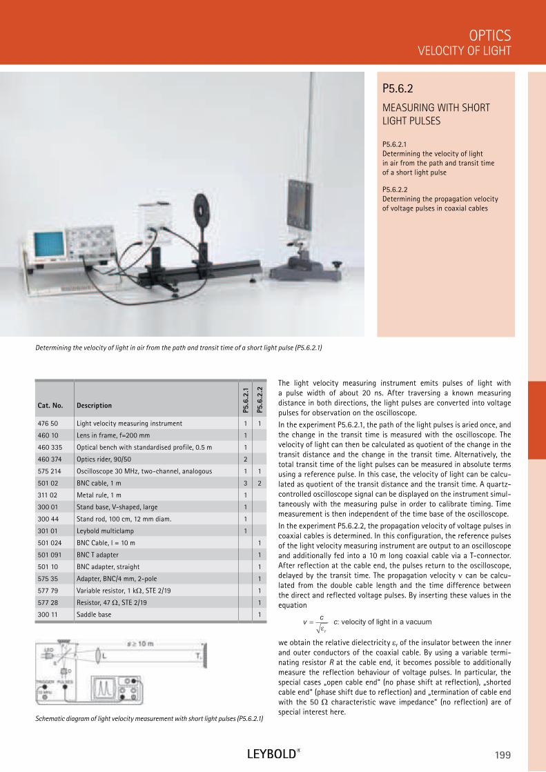
199
MEASURING WITH SHORT
LIGHT PULSES
P5.6.2.1 Determining the velocity of light in air from the path and transit time of a short light pulse
P5.6.2.2 Determining the propagation velocity of voltage pulses in coaxial cables
VELOCITY OF LIGHT
OPTICS
Cat. No. Description
P5.6
.2.1
P5.6
.2.2
476 50 Light velocity measuring instrument 1 1
460 10 Lens in frame, f=200 mm 1
460 335 Optical bench with standardised profile, 0.5 m 1
460 374 Optics rider, 90/50 2
575 214 Oscilloscope 30 MHz, two-channel, analogous 1 1
501 02 BNC cable, 1 m 3 2
311 02 Metal rule, 1 m 1
300 01 Stand base, V-shaped, large 1
300 44 Stand rod, 100 cm, 12 mm diam. 1
301 01 Leybold multiclamp 1
501 024 BNC Cable, l = 10 m 1
501 091 BNC T adapter 1
501 10 BNC adapter, straight 1
575 35 Adapter, BNC/4 mm, 2-pole 1
577 79 Variable resistor, 1 k , STE 2/19 1
577 28 Resistor, 47 , STE 2/19 1
300 11 Saddle base 1
The light velocity measuring instrument emits pulses of light with a pulse width of about 20 ns. After traversing a known measuring distance in both directions, the light pulses are converted into voltage pulses for observation on the oscilloscope.
In the experiment P5.6.2.1, the path of the light pulses is aried once, and the change in the transit time is measured with the oscilloscope. The velocity of light can then be calculated as quotient of the change in the transit distance and the change in the transit time. Alternatively, the total transit time of the light pulses can be measured in absolute terms using a reference pulse. In this case, the velocity of light can be calcu-lated as quotient of the transit distance and the transit time. A quartz-controlled oscilloscope signal can be displayed on the instrument simul-taneously with the measuring pulse in order to calibrate timing. Time measurement is then independent of the time base of the oscilloscope.
In the experiment P5.6.2.2, the propagation velocity of voltage pulses in coaxial cables is determined. In this configuration, the reference pulses of the light velocity measuring instrument are output to an oscilloscope and additionally fed into a 10 m long coaxial cable via a T-connector. After reflection at the cable end, the pulses return to the oscilloscope, delayed by the transit time. The propagation velocity can be calcu-lated from the double cable length and the time difference between the direct and reflected voltage pulses. By inserting these values in the equation
vc
c
r
=ε
: velocity of light in a vacuum
we obtain the relative dielectricity r of the insulator between the inner and outer conductors of the coaxial cable. By using a variable termi-nating resistor R at the cable end, it becomes possible to additionally measure the reflection behaviour of voltage pulses. In particular, the special cases „open cable end“ (no phase shift at reflection), „shorted cable end“ (phase shift due to reflection) and „termination of cable end with the 50 characteristic wave impedance“ (no reflection) are of special interest here.
Determining the velocity of light in air from the path and transit time of a short light pulse (P5.6.2.1)
P5.6.2
Schematic diagram of light velocity measurement with short light pulses (P5.6.2.1)
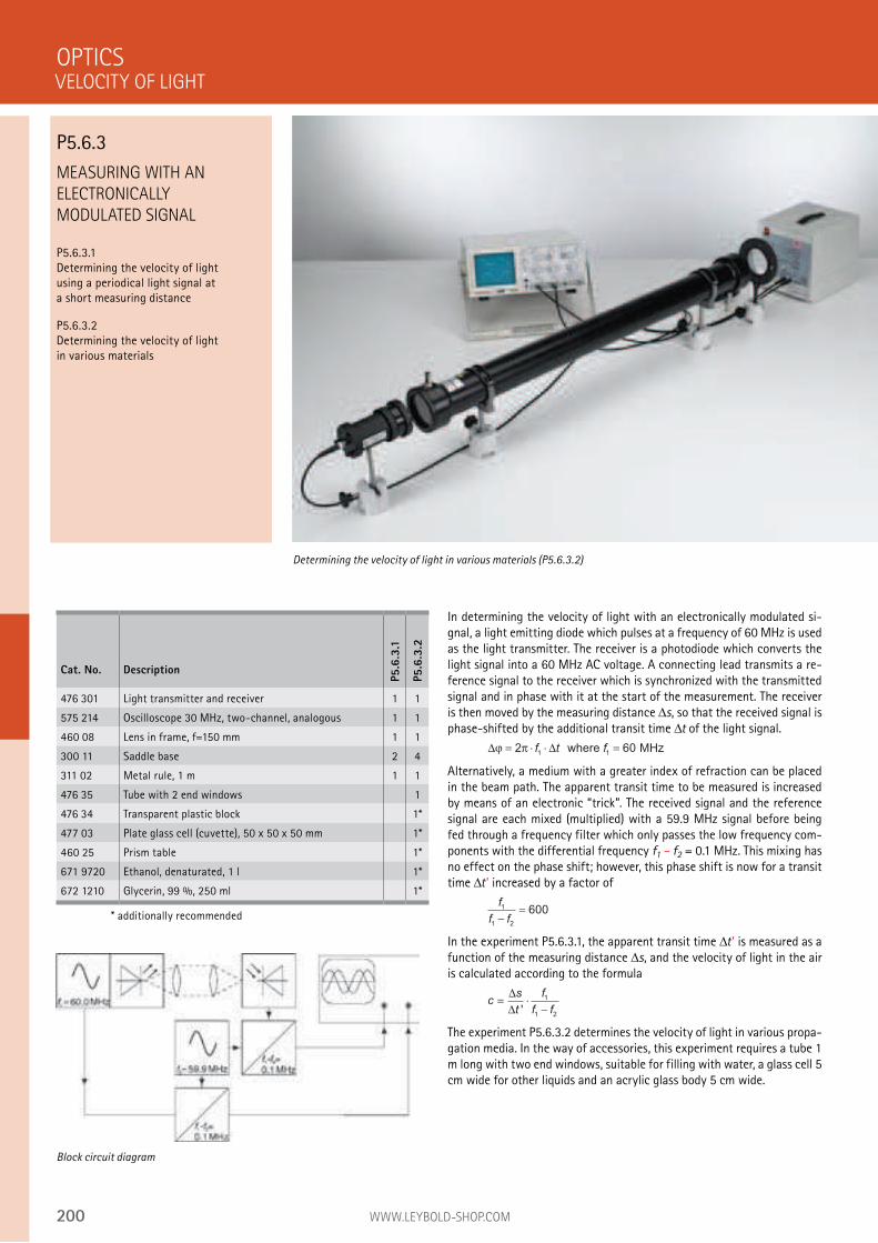
200 WWW.LEYBOLD-SHOP.COM
MEASURING WITH AN
ELECTRONICALLY
MODULATED SIGNAL
P5.6.3.1 Determining the velocity of light using a periodical light signal at a short measuring distance
P5.6.3.2 Determining the velocity of light in various materials
In determining the velocity of light with an electronically modulated si-gnal, a light emitting diode which pulses at a frequency of 60 MHz is used as the light transmitter. The receiver is a photodiode which converts the light signal into a 60 MHz AC voltage. A connecting lead transmits a re-ference signal to the receiver which is synchronized with the transmitted signal and in phase with it at the start of the measurement. The receiver is then moved by the measuring distance s, so that the received signal is phase-shifted by the additional transit time t of the light signal.
∆ ∆ϕ π= ⋅ ⋅ =2 601 1f t f where MHz
Alternatively, a medium with a greater index of refraction can be placed in the beam path. The apparent transit time to be measured is increased by means of an electronic “trick”. The received signal and the reference signal are each mixed (multiplied) with a 59.9 MHz signal before being fed through a frequency filter which only passes the low frequency com-ponents with the differential frequency f1 – f2 = 0.1 MHz. This mixing has no effect on the phase shift; however, this phase shift is now for a transit time t ’ increased by a factor of
f
f f
1
1 2
600−
=
In the experiment P5.6.3.1, the apparent transit time t ’ is measured as a function of the measuring distance s, and the velocity of light in the air is calculated according to the formula
cs
t
f
f f= ⋅
−
∆
∆ '
1
1 2
The experiment P5.6.3.2 determines the velocity of light in various propa-gation media. In the way of accessories, this experiment requires a tube 1 m long with two end windows, suitable for filling with water, a glass cell 5 cm wide for other liquids and an acrylic glass body 5 cm wide.
OPTICS
Determining the velocity of light in various materials (P5.6.3.2)
Cat. No. Description
P5.6
.3.1
P5.6
.3.2
476 301 Light transmitter and receiver 1 1
575 214 Oscilloscope 30 MHz, two-channel, analogous 1 1
460 08 Lens in frame, f=150 mm 1 1
300 11 Saddle base 2 4
311 02 Metal rule, 1 m 1 1
476 35 Tube with 2 end windows 1
476 34 Transparent plastic block 1*
477 03 Plate glass cell (cuvette), 50 x 50 x 50 mm 1*
460 25 Prism table 1*
671 9720 Ethanol, denaturated, 1 l 1*
672 1210 Glycerin, 99 %, 250 ml 1*
* additionally recommended
Block circuit diagram
VELOCITY OF LIGHT
P5.6.3
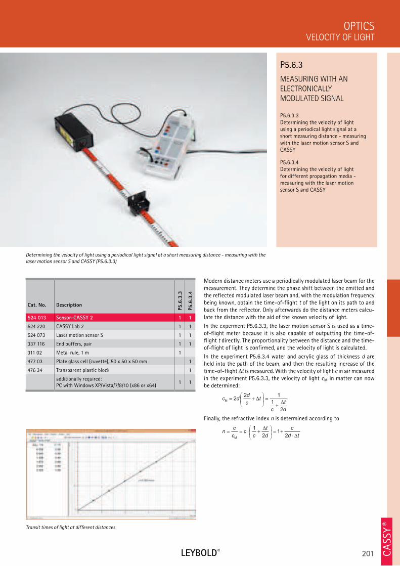
201
MEASURING WITH AN
ELECTRONICALLY
MODULATED SIGNAL
P5.6.3.3 Determining the velocity of light using a periodical light signal at a short measuring distance - measuring with the laser motion sensor S and CASSY
P5.6.3.4 Determining the velocity of light for different propagation media - measuring with the laser motion sensor S and CASSY
VELOCITY OF LIGHT
OPTICS
Cat. No. Description
P5.6
.3.3
P5.6
.3.4
524 013 Sensor-CASSY 2 1 1
524 220 CASSY Lab 2 1 1
524 073 Laser motion sensor S 1 1
337 116 End buffers, pair 1 1
311 02 Metal rule, 1 m 1
477 03 Plate glass cell (cuvette), 50 x 50 x 50 mm 1
476 34 Transparent plastic block 1
additionally required: PC with Windows XP/Vista/7/8/10 (x86 or x64)
1 1
Modern distance meters use a periodically modulated laser beam for the measurement. They determine the phase shift between the emitted and the reflected modulated laser beam and, with the modulation frequency being known, obtain the time-of-flight t of the light on its path to and back from the reflector. Only afterwards do the distance meters calcu-late the distance with the aid of the known velocity of light.
In the experment P5.6.3.3, the laser motion sensor S is used as a time-of-flight meter because it is also capable of outputting the time-of-flight t directly. The proportionality between the distance and the time-of-flight of light is confirmed, and the velocity of light is calculated.
In the experiment P5.6.3.4 water and acrylic glass of thickness d are held into the path of the beam, and then the resulting increase of the time-of-flight t is measured. With the velocity of light c in air measured in the experiment P5.6.3.3, the velocity of light cM in matter can now be determined:
c dd
ct
c
t
d
M= +
=
+2
2 1
1
2
∆∆
Finally, the refractive index n is determined according to
nc
cc
c
t
d
c
d t= = ⋅ +
= +
⋅M
1
212
∆∆
Determining the velocity of light using a periodical light signal at a short measuring distance - measuring with the
laser motion sensor S and CASSY (P5.6.3.3)
P5.6.3
Transit times of light at different distances
CA
SSY ®
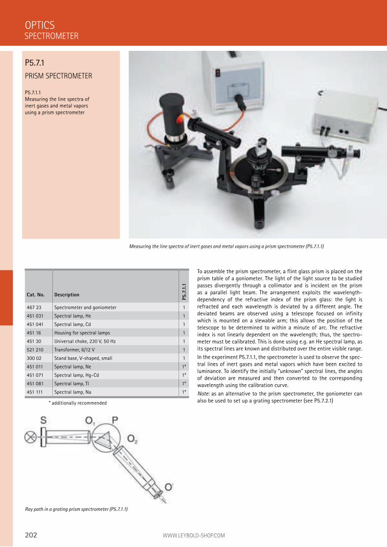
202 WWW.LEYBOLD-SHOP.COM
PRISM SPECTROMETER
P5.7.1.1 Measuring the line spectra of inert gases and metal vapors using a prism spectrometer
To assemble the prism spectrometer, a flint glass prism is placed on the prism table of a goniometer. The light of the light source to be studied passes divergently through a collimator and is incident on the prism as a parallel light beam. The arrangement exploits the wavelength- dependency of the refractive index of the prism glass: the light is refracted and each wavelength is deviated by a different angle. The deviated beams are observed using a telescope focused on infinity which is mounted on a slewable arm; this allows the position of the telescope to be determined to within a minute of arc. The refractive index is not linearly dependent on the wavelength; thus, the spectro-meter must be calibrated. This is done using e.g. an He spectral lamp, as its spectral lines are known and distributed over the entire visible range.
In the experiment P5.7.1.1, the spectrometer is used to observe the spec-tral lines of inert gases and metal vapors which have been excited to luminance. To identify the initially “unknown” spectral lines, the angles of deviation are measured and then converted to the corresponding wavelength using the calibration curve.
Note: as an alternative to the prism spectrometer, the goniometer can also be used to set up a grating spectrometer (see P5.7.2.1)
OPTICS
Measuring the line spectra of inert gases and metal vapors using a prism spectrometer (P5.7.1.1)
Cat. No. Description
P5.7
.1.1
467 23 Spectrometer and goniometer 1
451 031 Spectral lamp, He 1
451 041 Spectral lamp, Cd 1
451 16 Housing for spectral lamps 1
451 30 Universal choke, 230 V, 50 Hz 1
521 210 Transformer, 6/12 V 1
300 02 Stand base, V-shaped, small 1
451 011 Spectral lamp, Ne 1*
451 071 Spectral lamp, Hg-Cd 1*
451 081 Spectral lamp, Tl 1*
451 111 Spectral lamp, Na 1*
* additionally recommended
Ray path in a grating prism spectrometer (P5.7.1.1)
SPECTROMETER
P5.7.1
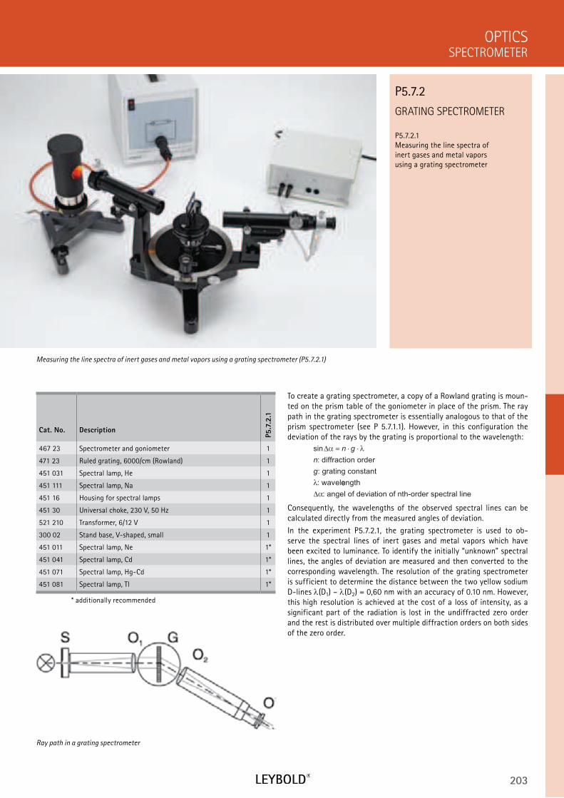
203
GRATING SPECTROMETER
P5.7.2.1 Measuring the line spectra of inert gases and metal vapors using a grating spectrometer
SPECTROMETER
OPTICS
Cat. No. Description
P5.7
.2.1
467 23 Spectrometer and goniometer 1
471 23 Ruled grating, 6000/cm (Rowland) 1
451 031 Spectral lamp, He 1
451 111 Spectral lamp, Na 1
451 16 Housing for spectral lamps 1
451 30 Universal choke, 230 V, 50 Hz 1
521 210 Transformer, 6/12 V 1
300 02 Stand base, V-shaped, small 1
451 011 Spectral lamp, Ne 1*
451 041 Spectral lamp, Cd 1*
451 071 Spectral lamp, Hg-Cd 1*
451 081 Spectral lamp, Tl 1*
* additionally recommended
To create a grating spectrometer, a copy of a Rowland grating is moun-ted on the prism table of the goniometer in place of the prism. The ray path in the grating spectrometer is essentially analogous to that of the prism spectrometer (see P 5.7.1.1). However, in this configuration the deviation of the rays by the grating is proportional to the wavelength:
sin∆α λ
λ
= ⋅ ⋅n g
n
g
: diffraction order
: grating constant
: waveleength
: angel of deviation of nth-order spectral line∆α
Consequently, the wavelengths of the observed spectral lines can be calculated directly from the measured angles of deviation.
In the experiment P5.7.2.1, the grating spectrometer is used to ob-serve the spectral lines of inert gases and metal vapors which have been excited to luminance. To identify the initially “unknown” spectral lines, the angles of deviation are measured and then converted to the corresponding wavelength. The resolution of the grating spectrometer is sufficient to determine the distance between the two yellow sodium D-lines (D1) – (D2) = 0,60 nm with an accuracy of 0.10 nm. However, this high resolution is achieved at the cost of a loss of intensity, as a significant part of the radiation is lost in the undiffracted zero order and the rest is distributed over multiple diffraction orders on both sides of the zero order.
Measuring the line spectra of inert gases and metal vapors using a grating spectrometer (P5.7.2.1)
P5.7.2
Ray path in a grating spectrometer
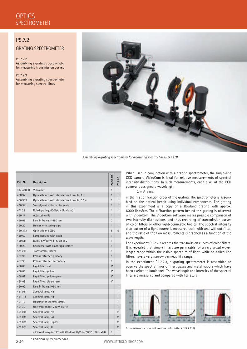
204 WWW.LEYBOLD-SHOP.COM
GRATING SPECTROMETER
P5.7.2.2 Assembling a grating spectrometer for measuring transmission curves
P5.7.2.3 Assembling a grating spectrometer for measuring spectral lines
When used in conjunction with a grating spectrometer, the single-line CCD camera VideoCom is ideal for relative measurements of spectral intensity distributions. In such measurements, each pixel of the CCD camera is assigned a wavelength
λ α= ⋅d sin
in the first diffraction order of the grating. The spectrometer is assem-bled on the optical bench using individual components. The grating in this experiment is a copy of a Rowland grating with approx. 6000 lines/cm. The diffraction pattern behind the grating is observed with VideoCom. The VideoCom software makes possible comparison of two intensity distributions, and thus recording of transmission curves of color filters or other light-permeable bodies. The spectral intensity distribution of a light source is measured both with and without filter, and the ratio of the two measurements is graphed as a function of the wavelength.
The experiment P5.7.2.2 records the transmission curves of color filters. It is revealed that simple filters are permeable for a very broad wave-length range within the visible spectrum of light, while so-called line filters have a very narrow permeability range.
In the experiment P5.7.2.3, a grating spectrometer is assembled to observe the spectral lines of inert gases and metal vapors which have been excited to luminance. The wavelength and intensity of the spectral lines are measured and compared with literature.
OPTICS
Assembling a grating spectrometer for measuring spectral lines (P5.7.2.3)
Cat. No. Description
P5.7
.2.2
(b)
P5
.7.2
.3
337 47USB VideoCom 1 1
460 32 Optical bench with standardised profile, 1 m 1 1
460 335 Optical bench with standardised profile, 0.5 m 1 1
460 341 Swivel joint with circular scale 1 1
471 23 Ruled grating, 6000/cm (Rowland) 1 1
460 14 Adjustable slit 1 1
460 08 Lens in frame, f=150 mm 2 1
460 22 Holder with spring clips 1 1
460 373 Optics rider, 60/50 5 5
450 60 Lamp housing with cable 1
450 511 Bulbs, 6 V/30 W, E14, set of 2 1
460 20 Condenser with diaphragm holder 1
521 210 Transformer, 6/12 V 1
467 95 Colour filter set, primary 1
467 96 Colour filter set, secondary 1
468 03 Light filter, red 1*
468 05 Light filter, yellow 1*
468 07 Light filter, yellow-green 1*
468 09 Light filter, blue-green 1*
460 02 Lens in frame, f=50 mm 1
451 031 Spectral lamp, He 1
451 111 Spectral lamp, Na 1
451 16 Housing for spectral lamps 1
451 30 Universal choke, 230 V, 50 Hz 1
451 011 Spectral lamp, Ne 1*
451 041 Spectral lamp, Cd 1*
451 071 Spectral lamp, Hg-Cd 1*
451 081 Spectral lamp, Tl 1*
additionally required: PC with Windows XP/Vista/7/8/10 (x86 or x64) 1 1
* additionally recommended
Transmissions curves of various color filters (P5.7.2.2)
SPECTROMETER
P5.7.2
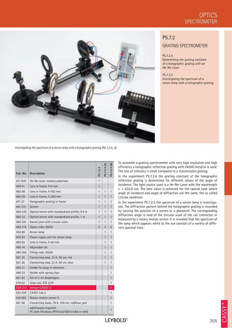
205
GRATING SPECTROMETER
P5.7.2.4 Determining the grating constant of a holographic grating with an He-Ne-Laser
P5.7.2.5 Investigating the spectrum of a xenon lamp with a holographic grating
SPECTROMETER
OPTICS
Cat. No. Description
P5.7
.2.4
P5.7
.2.5
(a)
P5.7
.2.5
(b)
471 830 He-Ne Laser, linearly polarised 1
460 01 Lens in frame, f=5 mm 1
460 08 Lens in frame, f=150 mm 1 1 1
460 09 Lens in frame, f=300 mm 1 1 1
471 27 Holographic grating in frame 1 1 1
441 531 Screen 1 1 1
460 335 Optical bench with standardised profile, 0.5 m 1 1 1
460 32 Optical bench with standardised profile, 1 m 1 1 1
460 341 Swivel joint with circular scale 1 1 1
460 374 Optics rider, 90/50 5 5 6
450 80 Xenon lamp 1 1
450 83 Power supply unit for xenon lamp 1 1
460 02 Lens in frame, f=50 mm 1 1
460 14 Adjustable slit 1 1
460 382 Tilting rider, 90/50 1 1
501 25 Connecting lead, 32 A, 50 cm, red 1 1
501 26 Connecting lead, 32 A, 50 cm, blue 1 1
460 21 Holder for plug-in elements 1
460 22 Holder with spring clips 1
461 62 Set of 2 slit diaphragms 1
578 62 Solar cell, STE 2/19 1
524 013 Sensor-CASSY 2 1
524 220 CASSY Lab 2 1
524 082 Rotary motion sensor S 1
501 46 Connecting leads, 19 A, 100 cm, red/blue, pair 1
additionally required: PC with Windows XP/Vista/7/8/10 (x86 or x64)
1
To assemble a grating spectrometer with very high resolution and high efficiency a holographic reflection grating with 24000 lines/cm is used. The loss of intensity is small compared to a transmission grating.
In the experiment P5.7.2.4 the grating constant of the holographic reflection grating is determined for different values of the angle of incidence. The light source used is a He-Ne-Laser with the wavelength
= 632.8 nm. The best value is achieved for the special case where angle of incidence and angle of diffraction are the same, the so called Littrow condition.
In the experiment P5.7.2.5 the spectrum of a xenon lamp is investiga-ted. The diffraction pattern behind the holographic grating is recorded by varying the position of a screen or a photocell. The corresponding diffraction angle is read of the circular scale of the rail connector or measured by a rotary motion sensor. It is revealed that the spectrum of the lamp which appears white to the eye consists of a variety of diffe-rent spectral lines.
Investigating the spectrum of a xenon lamp with a holographic grating (P5.7.2.5_b)
P5.7.2
CA
SSY ®
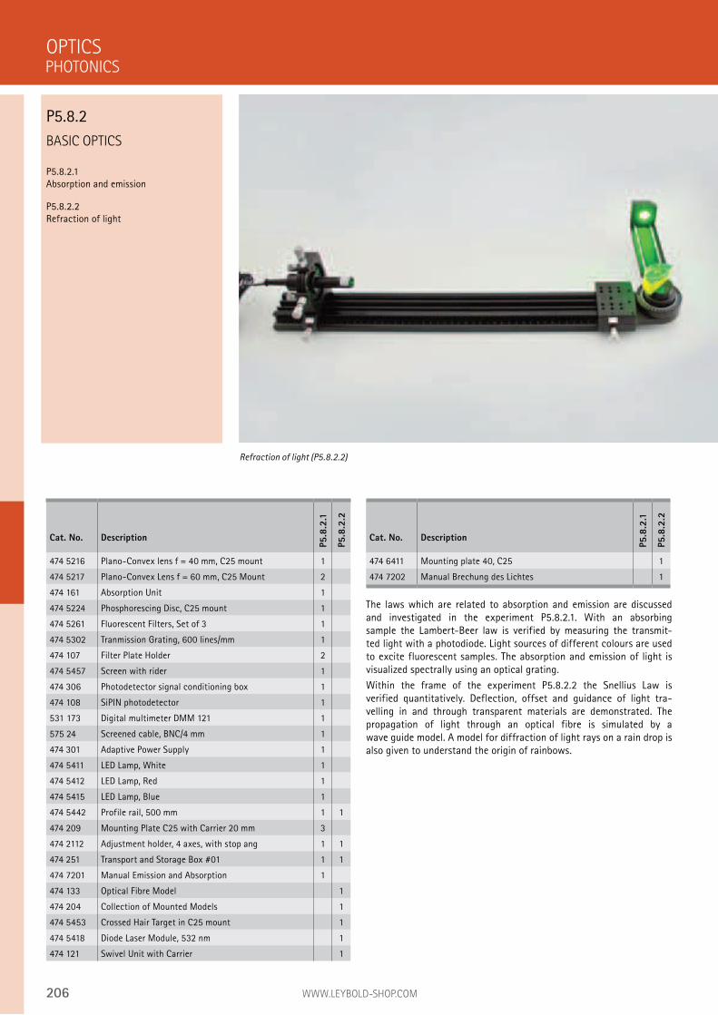
206 WWW.LEYBOLD-SHOP.COM
BASIC OPTICS
P5.8.2.1 Absorption and emission
P5.8.2.2 Refraction of light
The laws which are related to absorption and emission are discussed and investigated in the experiment P5.8.2.1. With an absorbing sample the Lambert-Beer law is verified by measuring the transmit-ted light with a photodiode. Light sources of different colours are used to excite fluorescent samples. The absorption and emission of light is visualized spectrally using an optical grating.
Within the frame of the experiment P5.8.2.2 the Snellius Law is verified quantitatively. Deflection, offset and guidance of light tra-velling in and through transparent materials are demonstrated. The propagation of light through an optical fibre is simulated by a wave guide model. A model for diffraction of light rays on a rain drop is also given to understand the origin of rainbows.
OPTICS
Refraction of light (P5.8.2.2)
Cat. No. Description
P5.8
.2.1
P5.8
.2.2
474 5216 Plano-Convex lens f = 40 mm, C25 mount 1
474 5217 Plano-Convex Lens f = 60 mm, C25 Mount 2
474 161 Absorption Unit 1
474 5224 Phosphorescing Disc, C25 mount 1
474 5261 Fluorescent Filters, Set of 3 1
474 5302 Tranmission Grating, 600 lines/mm 1
474 107 Filter Plate Holder 2
474 5457 Screen with rider 1
474 306 Photodetector signal conditioning box 1
474 108 SiPIN photodetector 1
531 173 Digital multimeter DMM 121 1
575 24 Screened cable, BNC/4 mm 1
474 301 Adaptive Power Supply 1
474 5411 LED Lamp, White 1
474 5412 LED Lamp, Red 1
474 5415 LED Lamp, Blue 1
474 5442 Profile rail, 500 mm 1 1
474 209 Mounting Plate C25 with Carrier 20 mm 3
474 2112 Adjustment holder, 4 axes, with stop ang 1 1
474 251 Transport and Storage Box #01 1 1
474 7201 Manual Emission and Absorption 1
474 133 Optical Fibre Model 1
474 204 Collection of Mounted Models 1
474 5453 Crossed Hair Target in C25 mount 1
474 5418 Diode Laser Module, 532 nm 1
474 121 Swivel Unit with Carrier 1
PHOTONICS
P5.8.2
Cat. No. Description
P5.8
.2.1
P5.8
.2.2
474 6411 Mounting plate 40, C25 1
474 7202 Manual Brechung des Lichtes 1
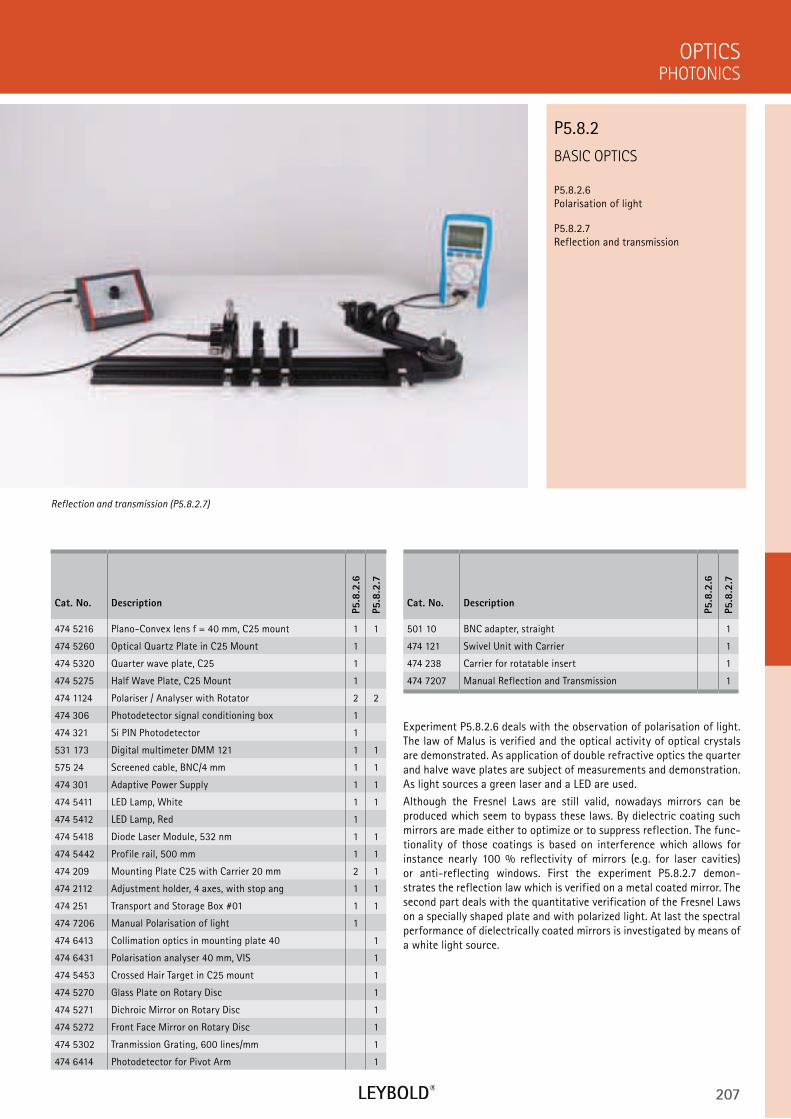
207
BASIC OPTICS
P5.8.2.6 Polarisation of light
P5.8.2.7 Reflection and transmission
PHOTONICS
OPTICS
Cat. No. Description
P5.8
.2.6
P5.8
.2.7
474 5216 Plano-Convex lens f = 40 mm, C25 mount 1 1
474 5260 Optical Quartz Plate in C25 Mount 1
474 5320 Quarter wave plate, C25 1
474 5275 Half Wave Plate, C25 Mount 1
474 1124 Polariser / Analyser with Rotator 2 2
474 306 Photodetector signal conditioning box 1
474 321 Si PIN Photodetector 1
531 173 Digital multimeter DMM 121 1 1
575 24 Screened cable, BNC/4 mm 1 1
474 301 Adaptive Power Supply 1 1
474 5411 LED Lamp, White 1 1
474 5412 LED Lamp, Red 1
474 5418 Diode Laser Module, 532 nm 1 1
474 5442 Profile rail, 500 mm 1 1
474 209 Mounting Plate C25 with Carrier 20 mm 2 1
474 2112 Adjustment holder, 4 axes, with stop ang 1 1
474 251 Transport and Storage Box #01 1 1
474 7206 Manual Polarisation of light 1
474 6413 Collimation optics in mounting plate 40 1
474 6431 Polarisation analyser 40 mm, VIS 1
474 5453 Crossed Hair Target in C25 mount 1
474 5270 Glass Plate on Rotary Disc 1
474 5271 Dichroic Mirror on Rotary Disc 1
474 5272 Front Face Mirror on Rotary Disc 1
474 5302 Tranmission Grating, 600 lines/mm 1
474 6414 Photodetector for Pivot Arm 1
Experiment P5.8.2.6 deals with the observation of polarisation of light. The law of Malus is verified and the optical activity of optical crystals are demonstrated. As application of double refractive optics the quarter and halve wave plates are subject of measurements and demonstration. As light sources a green laser and a LED are used.
Although the Fresnel Laws are still valid, nowadays mirrors can be produced which seem to bypass these laws. By dielectric coating such mirrors are made either to optimize or to suppress reflection. The func-tionality of those coatings is based on interference which allows for instance nearly 100 % reflectivity of mirrors (e.g. for laser cavities) or anti-reflecting windows. First the experiment P5.8.2.7 demon-strates the reflection law which is verified on a metal coated mirror. The second part deals with the quantitative verification of the Fresnel Laws on a specially shaped plate and with polarized light. At last the spectral performance of dielectrically coated mirrors is investigated by means of a white light source.
Reflection and transmission (P5.8.2.7)
P5.8.2
Cat. No. Description
P5.8
.2.6
P5.8
.2.7
501 10 BNC adapter, straight 1
474 121 Swivel Unit with Carrier 1
474 238 Carrier for rotatable insert 1
474 7207 Manual Reflection and Transmission 1
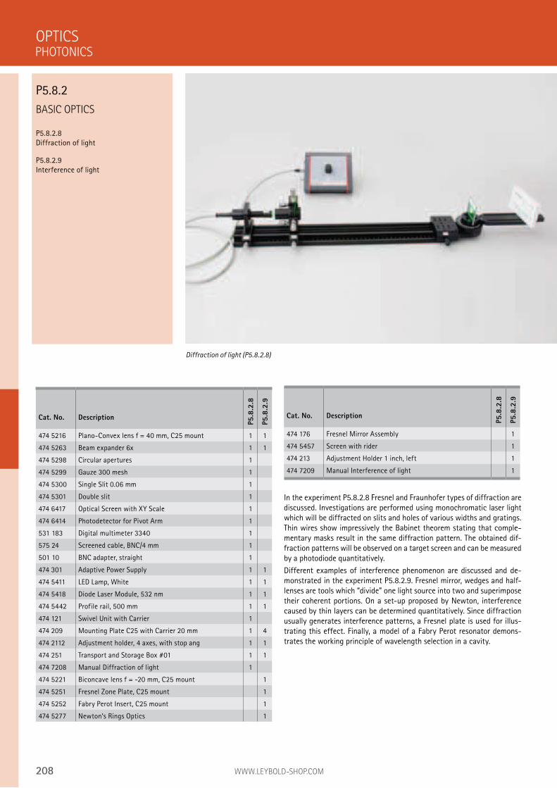
208 WWW.LEYBOLD-SHOP.COM
BASIC OPTICS
P5.8.2.8 Diffraction of light
P5.8.2.9 Interference of light
In the experiment P5.8.2.8 Fresnel and Fraunhofer types of diffraction are discussed. Investigations are performed using monochromatic laser light which will be diffracted on slits and holes of various widths and gratings. Thin wires show impressively the Babinet theorem stating that comple-mentary masks result in the same diffraction pattern. The obtained dif-fraction patterns will be observed on a target screen and can be measured by a photodiode quantitatively.
Different examples of interference phenomenon are discussed and de-monstrated in the experiment P5.8.2.9. Fresnel mirror, wedges and half-lenses are tools which “divide” one light source into two and superimpose their coherent portions. On a set-up proposed by Newton, interference caused by thin layers can be determined quantitatively. Since diffraction usually generates interference patterns, a Fresnel plate is used for illus-trating this effect. Finally, a model of a Fabry Perot resonator demons-trates the working principle of wavelength selection in a cavity.
OPTICS
Diffraction of light (P5.8.2.8)
Cat. No. Description
P5.8
.2.8
P5.8
.2.9
474 5216 Plano-Convex lens f = 40 mm, C25 mount 1 1
474 5263 Beam expander 6x 1 1
474 5298 Circular apertures 1
474 5299 Gauze 300 mesh 1
474 5300 Single Slit 0.06 mm 1
474 5301 Double slit 1
474 6417 Optical Screen with XY Scale 1
474 6414 Photodetector for Pivot Arm 1
531 183 Digital multimeter 3340 1
575 24 Screened cable, BNC/4 mm 1
501 10 BNC adapter, straight 1
474 301 Adaptive Power Supply 1 1
474 5411 LED Lamp, White 1 1
474 5418 Diode Laser Module, 532 nm 1 1
474 5442 Profile rail, 500 mm 1 1
474 121 Swivel Unit with Carrier 1
474 209 Mounting Plate C25 with Carrier 20 mm 1 4
474 2112 Adjustment holder, 4 axes, with stop ang 1 1
474 251 Transport and Storage Box #01 1 1
474 7208 Manual Diffraction of light 1
474 5221 Biconcave lens f = -20 mm, C25 mount 1
474 5251 Fresnel Zone Plate, C25 mount 1
474 5252 Fabry Perot Insert, C25 mount 1
474 5277 Newton‘s Rings Optics 1
PHOTONICS
P5.8.2
Cat. No. Description
P5.8
.2.8
P5.8
.2.9
474 176 Fresnel Mirror Assembly 1
474 5457 Screen with rider 1
474 213 Adjustment Holder 1 inch, left 1
474 7209 Manual Interference of light 1
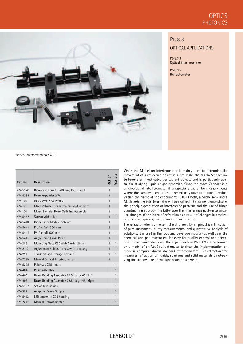
209
OPTICAL APPLICATIONS
P5.8.3.1
Optical interferometer
P5.8.3.2
Refractometer
PHOTONICS
OPTICS
Cat. No. Description
P5.8
.3.1
P5.8
.3.2
474 5220 Biconcave Lens f = -10 mm, C25 mount 1
474 5264 Beam expander 2.7x 1
474 169 Gas Cuvette Assembly 1
474 171 Mach Zehnder Beam Combining Assembly 1
474 174 Mach-Zehnder Beam Splitting Assembly 1
474 5457 Screen with rider 1 1
474 5418 Diode Laser Module, 532 nm 1
474 5441 Profile Rail, 300 mm 2
474 5442 Profile rail, 500 mm 1 1
474 5449 Angle Joint, Cross Piece 1
474 209 Mounting Plate C25 with Carrier 20 mm 3 1
474 2112 Adjustment holder, 4 axes, with stop ang 1 1
474 251 Transport and Storage Box #01 2 1
474 7210 Manual Optical Interferometer 1
474 5225 Polariser, C25 mount 1
474 404 Prism assembly 1
474 405 Beam Bending Assembly 22.5 °deg;- 45°, left 1
474 406 Beam Bending Assembly 22.5 °deg;- 45°, right 1
474 5307 Set of Test Liquids 1
474 301 Adaptive Power Supply 1
474 5413 LED amber in C25 housing 1
474 7211 Manual Refractometer 1
While the Michelson interferometer is mainly used to determine the
movement of a reflecting object in a nm scale, the Mach-Zehnder in-
terferometer investigates transparent objects and is particularly use-
ful for studying liquid or gas dynamics. Since the Mach-Zehnder is a
unidirectional interferometer it is especially useful for measurements
where the samples have to be traversed only once or in one direction.
Within the frame of the experiment P5.8.3.1 both, a Michelson- and a
Mach-Zehnder interferometer will be realized. The former demonstrates
the principle generation of interference patterns and the use of fringe
counting in metrology. The latter uses the interference pattern to visua-
lize changes of the index of refraction as a result of changes in physical
properties of gasses, like pressure or composition.
The refractometer is an essential instrument for empirical identification
of pure substances, purity measurements, and quantitative analysis of
solutions. It is used in the food and beverage industry as well as in the
chemical and pharmaceutical industry for quality control and check-
ups on compound identities. The experiments in P5.8.3.2 are performed
on a model of an Abbé refractometer to show the implementation on
modern, computer driven standard refractometers. This refractometer
measures refraction of liquids, solutions and solid materials by obser-
ving the shadow line of the light beam on a screen.
Optical interferometer (P5.8.3.1)
P5.8.3
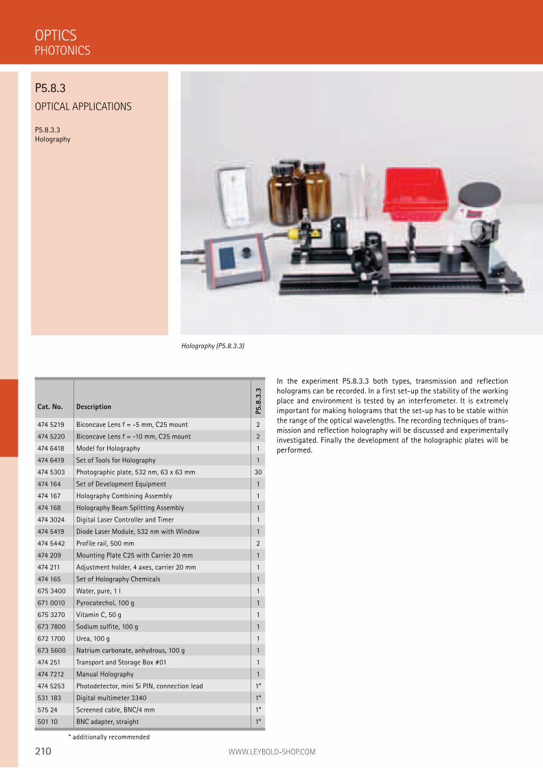
210 WWW.LEYBOLD-SHOP.COM
OPTICAL APPLICATIONS
P5.8.3.3 Holography
In the experiment P5.8.3.3 both types, transmission and reflection holograms can be recorded. In a first set-up the stability of the working place and environment is tested by an interferometer. It is extremely important for making holograms that the set-up has to be stable within the range of the optical wavelengths. The recording techniques of trans-mission and reflection holography will be discussed and experimentally investigated. Finally the development of the holographic plates will be performed.
OPTICS
Holography (P5.8.3.3)
Cat. No. Description
P5.8
.3.3
474 5219 Biconcave Lens f = -5 mm, C25 mount 2
474 5220 Biconcave Lens f = -10 mm, C25 mount 2
474 6418 Model for Holography 1
474 6419 Set of Tools for Holography 1
474 5303 Photographic plate, 532 nm, 63 x 63 mm 30
474 164 Set of Development Equipment 1
474 167 Holography Combining Assembly 1
474 168 Holography Beam Splitting Assembly 1
474 3024 Digital Laser Controller and Timer 1
474 5419 Diode Laser Module, 532 nm with Window 1
474 5442 Profile rail, 500 mm 2
474 209 Mounting Plate C25 with Carrier 20 mm 1
474 211 Adjustment holder, 4 axes, carrier 20 mm 1
474 165 Set of Holography Chemicals 1
675 3400 Water, pure, 1 l 1
671 0010 Pyrocatechol, 100 g 1
675 3270 Vitamin C, 50 g 1
673 7800 Sodium sulfite, 100 g 1
672 1700 Urea, 100 g 1
673 5600 Natrium carbonate, anhydrous, 100 g 1
474 251 Transport and Storage Box #01 1
474 7212 Manual Holography 1
474 5253 Photodetector, mini Si PIN, connection lead 1*
531 183 Digital multimeter 3340 1*
575 24 Screened cable, BNC/4 mm 1*
501 10 BNC adapter, straight 1*
* additionally recommended
PHOTONICS
P5.8.3
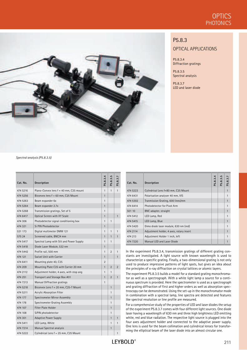
211
OPTICAL APPLICATIONS
P5.8.3.4 Diffraction gratings
P5.8.3.5 Spectral analysis
P5.8.3.7 LED and laser diode
PHOTONICS
OPTICS
Cat. No. Description
P5.8
.3.4
P5.8
.3.5
P5.8
.3.7
474 5216 Plano-Convex lens f = 40 mm, C25 mount 1 1 1
474 5256 Biconvex lens f = 60 mm, C25 Mount 1
474 5263 Beam expander 6x 1
474 5264 Beam expander 2.7x 1
474 5268 Transmission gratings, Set of 5 1
474 6417 Optical Screen with XY Scale 1 1
474 306 Photodetector signal conditioning box 1 1
474 321 Si PIN Photodetector 1
531 173 Digital multimeter DMM 121 1 1 1
575 24 Screened cable, BNC/4 mm 1 1 1
474 5417 Spectral Lamp with Slit and Power Supply 1 1
474 5418 Diode Laser Module, 532 nm 1
474 5442 Profile rail, 500 mm 1 2 1
474 121 Swivel Unit with Carrier 1 1
474 6411 Mounting plate 40, C25 2
474 209 Mounting Plate C25 with Carrier 20 mm 1 2 2
474 2112 Adjustment holder, 4 axes, with stop ang 1 1
474 251 Transport and Storage Box #01 1 2 1
474 7213 Manual Diffraction gratings 1
474 5218 Biconvex Lens f = 20 mm, C25-T Mount 1
474 5211 Acrylic Absorption Filter 1
474 177 Spectrometer Mirror Assembly 1
474 178 Spectrometer Grating Assembly 1
474 107 Filter Plate Holder 1
474 108 SiPIN photodetector 1
474 301 Adaptive Power Supply 1 1
474 5411 LED Lamp, White 1 1
474 7214 Manual Spectral analysis 1
474 5222 Cylindrical Lens f = 25 mm, C25 Mount 1
In the experiment P5.8.3.4, transmission gratings of different grating con-stants are investigated. A light source with known wavelength is used to characterize a specific grating. Finally, a two-dimensional grating is not only used to produce impressive patterns of light spots, but gives an idea about the principles of x-ray diffraction on crystal lattices or atomic layers.
The experiment P5.8.3.5 builds a model for a standard grating monochroma-tor as well as a spectrograph. With a white light lamp a source for a conti-nuous spectrum is provided. Here the spectrometer is used as a spectrograph and grating diffraction of first and higher orders as well as absorption spec-troscopy can be demonstrated. Using the set-up in the monochromator mode in combination with a spectral lamp, line spectra are detected and features like spectral resolution or line profile are measured.
For a comprehensive study of the properties of LED and laser diodes the setup of the experiment P5.8.3.7 comes with four different light sources. One diode laser having a wavelength of 630 nm and three high brightness LED emitting white, red and blue radiation. The respective light source is plugged into the four axes adjustment holder and connected to the adaptive power supply. One lens is used for the beam collimation and cylindrical lenses for transfor-ming the elliptical beam of the laser diode into an almost circular one.
Spectral analysis (P5.8.3.5)
P5.8.3
Cat. No. Description
P5.8
.3.4
P5.8
.3.5
P5.8
.3.7
474 5223 Cylindrical Lens f=80 mm, C25 Mount 1
474 6431 Polarisation analyser 40 mm, VIS 1
474 5302 Tranmission Grating, 600 lines/mm 1
474 6414 Photodetector for Pivot Arm 1
501 10 BNC adapter, straight 1
474 5412 LED Lamp, Red 1
474 5415 LED Lamp, Blue 1
474 5420 Dimo diode laser module, 630 nm (red) 1
474 2114 Adjustment holder, 4 axes, rotary insert 1
474 213 Adjustment Holder 1 inch, left 1
474 7220 Manual LED and Laser Diode 1
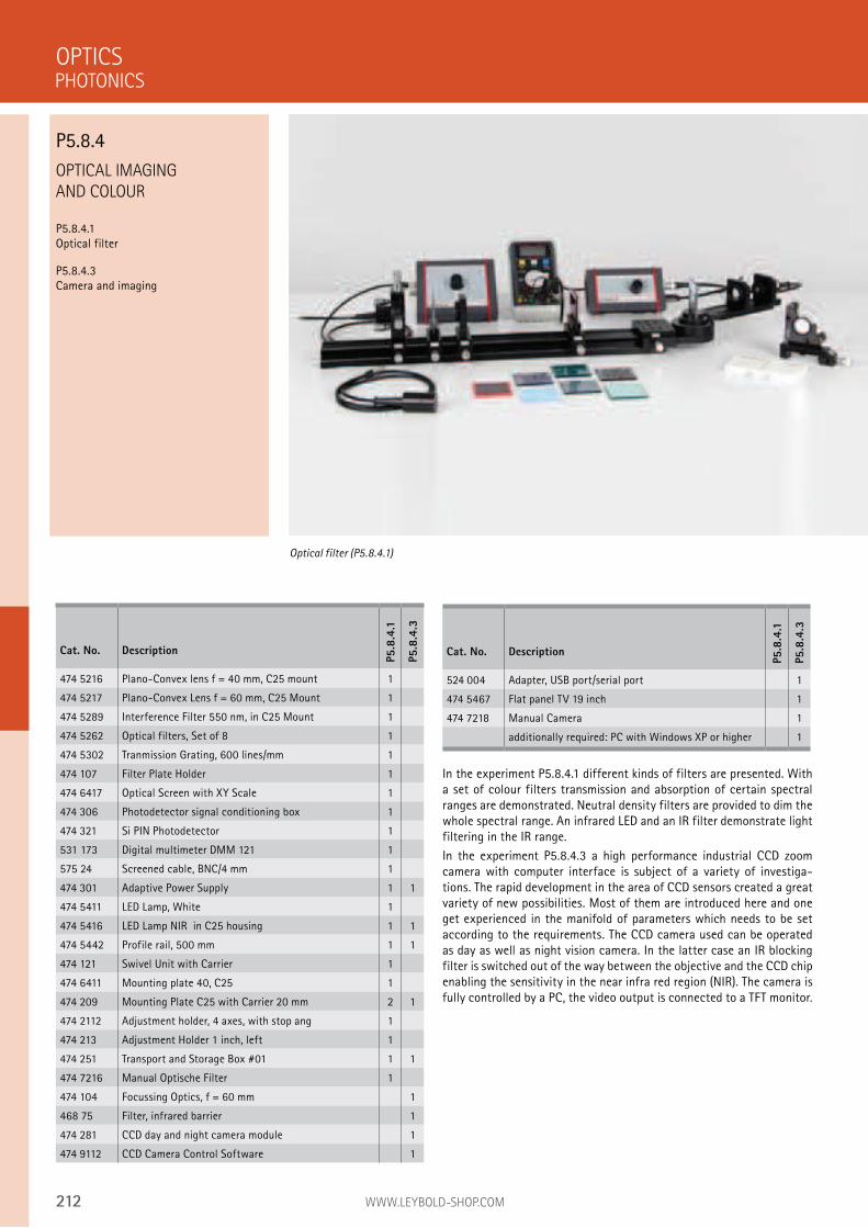
212 WWW.LEYBOLD-SHOP.COM
OPTICAL IMAGING
AND COLOUR
P5.8.4.1 Optical filter
P5.8.4.3 Camera and imaging
In the experiment P5.8.4.1 different kinds of filters are presented. With a set of colour filters transmission and absorption of certain spectral ranges are demonstrated. Neutral density filters are provided to dim the whole spectral range. An infrared LED and an IR filter demonstrate light filtering in the IR range.
In the experiment P5.8.4.3 a high performance industrial CCD zoom camera with computer interface is subject of a variety of investiga-tions. The rapid development in the area of CCD sensors created a great variety of new possibilities. Most of them are introduced here and one get experienced in the manifold of parameters which needs to be set according to the requirements. The CCD camera used can be operated as day as well as night vision camera. In the latter case an IR blocking filter is switched out of the way between the objective and the CCD chip enabling the sensitivity in the near infra red region (NIR). The camera is fully controlled by a PC, the video output is connected to a TFT monitor.
OPTICS
Optical filter (P5.8.4.1)
Cat. No. Description
P5.8
.4.1
P5.8
.4.3
474 5216 Plano-Convex lens f = 40 mm, C25 mount 1
474 5217 Plano-Convex Lens f = 60 mm, C25 Mount 1
474 5289 Interference Filter 550 nm, in C25 Mount 1
474 5262 Optical filters, Set of 8 1
474 5302 Tranmission Grating, 600 lines/mm 1
474 107 Filter Plate Holder 1
474 6417 Optical Screen with XY Scale 1
474 306 Photodetector signal conditioning box 1
474 321 Si PIN Photodetector 1
531 173 Digital multimeter DMM 121 1
575 24 Screened cable, BNC/4 mm 1
474 301 Adaptive Power Supply 1 1
474 5411 LED Lamp, White 1
474 5416 LED Lamp NIR in C25 housing 1 1
474 5442 Profile rail, 500 mm 1 1
474 121 Swivel Unit with Carrier 1
474 6411 Mounting plate 40, C25 1
474 209 Mounting Plate C25 with Carrier 20 mm 2 1
474 2112 Adjustment holder, 4 axes, with stop ang 1
474 213 Adjustment Holder 1 inch, left 1
474 251 Transport and Storage Box #01 1 1
474 7216 Manual Optische Filter 1
474 104 Focussing Optics, f = 60 mm 1
468 75 Filter, infrared barrier 1
474 281 CCD day and night camera module 1
474 9112 CCD Camera Control Software 1
PHOTONICS
P5.8.4
Cat. No. Description
P5.8
.4.1
P5.8
.4.3
524 004 Adapter, USB port/serial port 1
474 5467 Flat panel TV 19 inch 1
474 7218 Manual Camera 1
additionally required: PC with Windows XP or higher 1
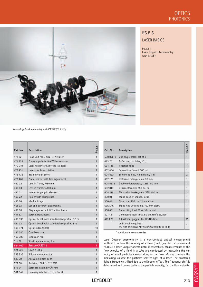
213
LASER BASICS
P5.8.5.1 Laser Doppler Anemometry with CASSY
PHOTONICS
OPTICS
Cat. No. Description
P5.8
.5.1
471 821 Head unit for 5 mW He-Ne laser 1
471 825 Power supply for 5 mW He-Ne-laser 1
470 010 Laser holder for 5 mW He-Ne laser 1
473 431 Holder for beam divider 1
473 432 Beam divider, 50 % 1
473 461 Planar mirror with fine adjustment 1
460 02 Lens in frame, f=50 mm 1
460 03 Lens in frame, f=100 mm 1
460 21 Holder for plug-in elements 1
460 22 Holder with spring clips 2
460 26 Iris diaphragm 1
461 63 Set of 4 different diaphragms 1
469 96 Diaphragm with 3 diffraction holes 1
441 53 Screen, translucent 1
460 335 Optical bench with standardised profile, 0.5 m 1
460 32 Optical bench with standardised profile, 1 m 1
460 374 Optics rider, 90/50 10
460 380 Cantilever arm 1
460 385 Extension rod 1
311 77 Steel tape measure, 2 m 1
524 013 Sensor-CASSY 2 1
524 220 CASSY Lab 2 1
558 835 Silicon photodetector 1
532 20 AC/DC amplifier 30 W 1
577 68 Resistor, 100 k , STE 2/19 1
575 24 Screened cable, BNC/4 mm 1
501 641 Two-way adapters, red, set of 6 1
Laser Doppler anemometry is a non-contact optical measurement method to obtain the velocity of a flow (fluid, gas). In the experiment P5.8.5.1 a laser Doppler anemometer is assembled. Measurements of the flow velocity of a fluid in a tube are conducted by measuring the ve-locity of small particles carried along in the flow. Moving through the measuring volume the particles scatter light of a laser. The scattered light is frequency shifted due to the Doppler effect. The frequency shift is determined and converted into the particle velocity, i.e. the flow velocity.
Laser Doppler Anemometry with CASSY (P5.8.5.1)
P5.8.5
Cat. No. Description
P5.8
.5.1
590 02ET2 Clip plugs, small, set of 2 1
683 70 Reflecting particles, 10 g 1
664 146 Reaction tube 1
602 404 Separation Funnel, 500 ml 1
604 433 Silicone tubing, 7 mm diam., 1 m 2
667 175 Hofmann tubing clamp, 20 mm 1
604 5672 Double microspatula, steel, 150 mm 1
602 010 Beaker, Boro 3.3, 150 ml, tall 1
604 215 Measuring beaker, clear SAN 500 ml 1
300 01 Stand base, V-shaped, large 1
300 44 Stand rod, 100 cm, 12 mm diam. 1
666 546 Stand ring with clamp, 100 mm diam. 1
500 401 Connecting lead, 19 A, 10 cm, red 1
501 45 Connecting lead, 19 A, 50 cm, red/blue, pair 1
471 828 Adjustment goggles for He-Ne-laser 1*
additionally required: PC with Windows XP/Vista/7/8/10 (x86 or x64)
1
* additionally recommended
CA
SSY ®
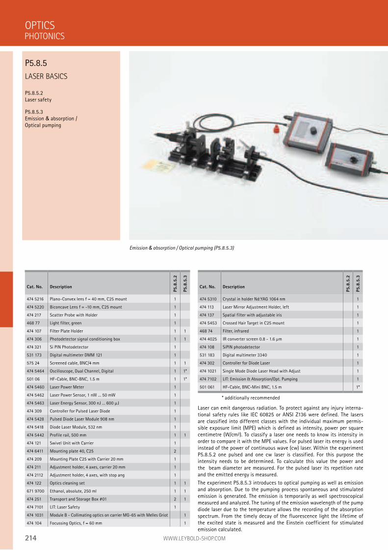
214 WWW.LEYBOLD-SHOP.COM
LASER BASICS
P5.8.5.2 Laser safety
P5.8.5.3 Emission & absorption / Optical pumping
Laser can emit dangerous radiation. To protect against any injury interna-tional safety rules like IEC 60825 or ANSI Z136 were defined. The lasers are classified into different classes with the individual maximum permis-sible exposure limit (MPE) which is defined as intensity, power per square centimetre (W/cm²). To classify a laser one needs to know its intensity in order to compare it with the MPE values. For pulsed laser its energy is used instead of the power of continuous wave (cw) laser. Within the experiment P5.8.5.2 one pulsed and one cw laser is classified. For this purpose the intensity needs to be determined. To calculate this value the power and the beam diameter are measured. For the pulsed laser its repetition rate and the emitted energy is measured.
The experiment P5.8.5.3 introduces to optical pumping as well as emission and absorption. Due to the pumping process spontaneous and stimulated emission is generated. The emission is temporarily as well spectroscopical measured and analyzed. The tuning of the emission wavelength of the pump diode laser due to the temperature allows the recording of the absorption spectrum. From the timely decay of the fluorescence light the lifetime of the excited state is measured and the Einstein coefficient for stimulated emission calculated.
OPTICS
Emission & absorption / Optical pumping (P5.8.5.3)
Cat. No. Description
P5.8
.5.2
P5.8
.5.3
474 5216 Plano-Convex lens f = 40 mm, C25 mount 1
474 5220 Biconcave Lens f = -10 mm, C25 mount 1
474 217 Scatter Probe with Holder 1
468 77 Light filter, green 1
474 107 Filter Plate Holder 1 1
474 306 Photodetector signal conditioning box 1 1
474 321 Si PIN Photodetector 1
531 173 Digital multimeter DMM 121 1
575 24 Screened cable, BNC/4 mm 1 1
474 5464 Oscilloscope, Dual Channel, Digital 1 1*
501 06 HF-Cable, BNC-BNC, 1.5 m 1 1*
474 5460 Laser Power Meter 1
474 5462 Laser Power Sensor, 1 nW ... 50 mW 1
474 5463 Laser Energy Sensor, 300 nJ ... 600 µJ 1
474 309 Controller for Pulsed Laser Diode 1
474 5428 Pulsed Diode Laser Module 908 nm 1
474 5418 Diode Laser Module, 532 nm 1
474 5442 Profile rail, 500 mm 1 1
474 121 Swivel Unit with Carrier 1
474 6411 Mounting plate 40, C25 2
474 209 Mounting Plate C25 with Carrier 20 mm 1
474 211 Adjustment holder, 4 axes, carrier 20 mm 1
474 2112 Adjustment holder, 4 axes, with stop ang 1
474 122 Optics cleaning set 1 1
671 9700 Ethanol, absolute, 250 ml 1 1
474 251 Transport and Storage Box #01 2 1
474 7101 LIT: Laser Safety 1
474 1031 Module B - Collimating optics on carrier MG-65 with Melles Griot 1
474 104 Focussing Optics, f = 60 mm 1
PHOTONICS
P5.8.5
Cat. No. Description
P5.8
.5.2
P5.8
.5.3
474 5310 Crystal in holder Nd:YAG 1064 nm 1
474 113 Laser Mirror Adjustment Holder, left 1
474 137 Spatial filter with adjustable iris 1
474 5453 Crossed Hair Target in C25 mount 1
468 74 Filter, infrared 1
474 4025 IR converter screen 0.8 - 1.6 µm 1
474 108 SiPIN photodetector 1
531 183 Digital multimeter 3340 1
474 302 Controller for Diode Laser 1
474 1021 Single Mode Diode Laser Head with Adjust 1
474 7102 LIT: Emission & Absorption/Opt. Pumping 1
501 061 HF-Cable, BNC-Mini BNC, 1.5 m 1*
* additionally recommended
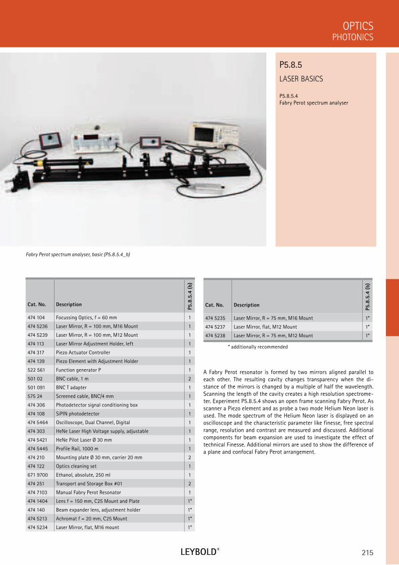
215
LASER BASICS
P5.8.5.4 Fabry Perot spectrum analyser
PHOTONICS
OPTICS
Cat. No. Description
P5.8
.5.4
(b)
474 104 Focussing Optics, f = 60 mm 1
474 5236 Laser Mirror, R = 100 mm, M16 Mount 1
474 5239 Laser Mirror, R = 100 mm, M12 Mount 1
474 113 Laser Mirror Adjustment Holder, left 1
474 317 Piezo Actuator Controller 1
474 139 Piezo Element with Adjustment Holder 1
522 561 Function generator P 1
501 02 BNC cable, 1 m 2
501 091 BNC T adapter 1
575 24 Screened cable, BNC/4 mm 1
474 306 Photodetector signal conditioning box 1
474 108 SiPIN photodetector 1
474 5464 Oscilloscope, Dual Channel, Digital 1
474 303 HeNe Laser High Voltage supply, adjustable 1
474 5421 HeNe Pilot Laser Ø 30 mm 1
474 5445 Profile Rail, 1000 m 1
474 210 Mounting plate Ø 30 mm, carrier 20 mm 2
474 122 Optics cleaning set 1
671 9700 Ethanol, absolute, 250 ml 1
474 251 Transport and Storage Box #01 2
474 7103 Manual Fabry Perot Resonator 1
474 1404 Lens f = 150 mm, C25 Mount and Plate 1*
474 140 Beam expander lens, adjustment holder 1*
474 5213 Achromat f = 20 mm, C25 Mount 1*
474 5234 Laser Mirror, flat, M16 mount 1*
A Fabry Perot resonator is formed by two mirrors aligned parallel to each other. The resulting cavity changes transparency when the di-stance of the mirrors is changed by a multiple of half the wavelength. Scanning the length of the cavity creates a high resolution spectrome-ter. Experiment P5.8.5.4 shows an open frame scanning Fabry Perot. As scanner a Piezo element and as probe a two mode Helium Neon laser is used. The mode spectrum of the Helium Neon laser is displayed on an oscilloscope and the characteristic parameter like finesse, free spectral range, resolution and contrast are measured and discussed. Additional components for beam expansion are used to investigate the effect of technical Finesse. Additional mirrors are used to show the difference of a plane and confocal Fabry Perot arrangement.
Fabry Perot spectrum analyser, basic (P5.8.5.4_b)
P5.8.5
Cat. No. Description
P5.8
.5.4
(b)
474 5235 Laser Mirror, R = 75 mm, M16 Mount 1*
474 5237 Laser Mirror, flat, M12 Mount 1*
474 5238 Laser Mirror, R = 75 mm, M12 Mount 1*
* additionally recommended
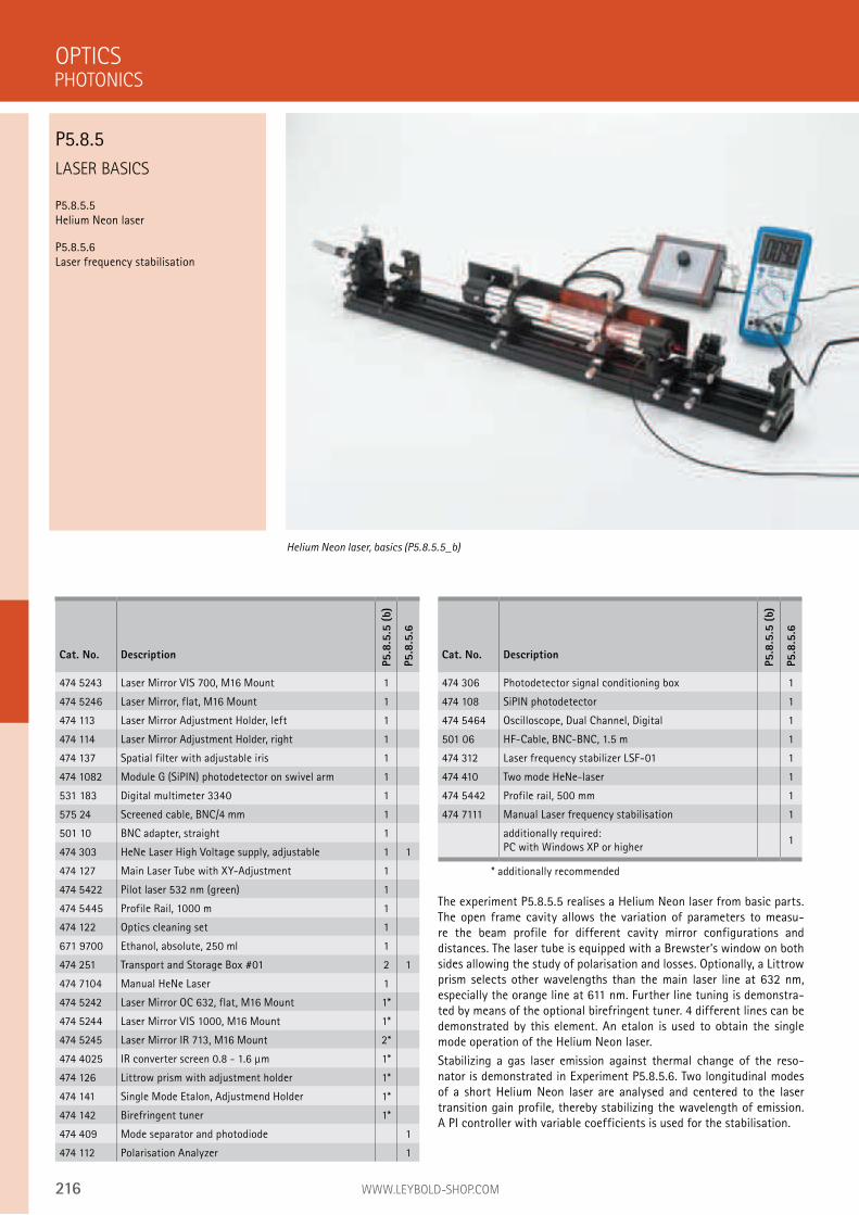
216 WWW.LEYBOLD-SHOP.COM
Cat. No. Description
P5.8
.5.5
(b)
P5.8
.5.6
474 306 Photodetector signal conditioning box 1
474 108 SiPIN photodetector 1
474 5464 Oscilloscope, Dual Channel, Digital 1
501 06 HF-Cable, BNC-BNC, 1.5 m 1
474 312 Laser frequency stabilizer LSF-01 1
474 410 Two mode HeNe-laser 1
474 5442 Profile rail, 500 mm 1
474 7111 Manual Laser frequency stabilisation 1
additionally required: PC with Windows XP or higher
1
* additionally recommended
LASER BASICS
P5.8.5.5 Helium Neon laser
P5.8.5.6 Laser frequency stabilisation
The experiment P5.8.5.5 realises a Helium Neon laser from basic parts. The open frame cavity allows the variation of parameters to measu-re the beam profile for different cavity mirror configurations and distances. The laser tube is equipped with a Brewster‘s window on both sides allowing the study of polarisation and losses. Optionally, a Littrow prism selects other wavelengths than the main laser line at 632 nm, especially the orange line at 611 nm. Further line tuning is demonstra-ted by means of the optional birefringent tuner. 4 different lines can be demonstrated by this element. An etalon is used to obtain the single mode operation of the Helium Neon laser.
Stabilizing a gas laser emission against thermal change of the reso-nator is demonstrated in Experiment P5.8.5.6. Two longitudinal modes of a short Helium Neon laser are analysed and centered to the laser transition gain profile, thereby stabilizing the wavelength of emission. A PI controller with variable coefficients is used for the stabilisation.
OPTICS
Helium Neon laser, basics (P5.8.5.5_b)
Cat. No. Description
P5.8
.5.5
(b)
P5.8
.5.6
474 5243 Laser Mirror VIS 700, M16 Mount 1
474 5246 Laser Mirror, flat, M16 Mount 1
474 113 Laser Mirror Adjustment Holder, left 1
474 114 Laser Mirror Adjustment Holder, right 1
474 137 Spatial filter with adjustable iris 1
474 1082 Module G (SiPIN) photodetector on swivel arm 1
531 183 Digital multimeter 3340 1
575 24 Screened cable, BNC/4 mm 1
501 10 BNC adapter, straight 1
474 303 HeNe Laser High Voltage supply, adjustable 1 1
474 127 Main Laser Tube with XY-Adjustment 1
474 5422 Pilot laser 532 nm (green) 1
474 5445 Profile Rail, 1000 m 1
474 122 Optics cleaning set 1
671 9700 Ethanol, absolute, 250 ml 1
474 251 Transport and Storage Box #01 2 1
474 7104 Manual HeNe Laser 1
474 5242 Laser Mirror OC 632, flat, M16 Mount 1*
474 5244 Laser Mirror VIS 1000, M16 Mount 1*
474 5245 Laser Mirror IR 713, M16 Mount 2*
474 4025 IR converter screen 0.8 - 1.6 µm 1*
474 126 Littrow prism with adjustment holder 1*
474 141 Single Mode Etalon, Adjustmend Holder 1*
474 142 Birefringent tuner 1*
474 409 Mode separator and photodiode 1
474 112 Polarisation Analyzer 1
PHOTONICS
P5.8.5
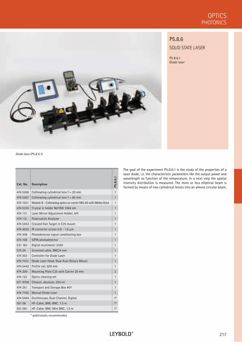
217
SOLID STATE LASER
P5.8.6.1 Diode laser
PHOTONICS
OPTICS
Cat. No. Description
P5.8
.6.1
474 5266 Collimating cylindrical lens f = 20 mm 1
474 5267 Collimating cylindrical lens f = 80 mm 1
474 1031 Module B - Collimating optics on carrier MG-65 with Melles Griot 1
474 5310 Crystal in holder Nd:YAG 1064 nm 1
474 113 Laser Mirror Adjustment Holder, left 1
474 112 Polarisation Analyzer 1
474 5453 Crossed Hair Target in C25 mount 1
474 4025 IR converter screen 0.8 - 1.6 µm 1
474 306 Photodetector signal conditioning box 1
474 108 SiPIN photodetector 1
531 183 Digital multimeter 3340 1
575 24 Screened cable, BNC/4 mm 1
474 302 Controller for Diode Laser 1
474 1012 Diode Laser Head, Dual Axes Rotary Mount 1
474 5442 Profile rail, 500 mm 1
474 209 Mounting Plate C25 with Carrier 20 mm 2
474 122 Optics cleaning set 1
671 9700 Ethanol, absolute, 250 ml 1
474 251 Transport and Storage Box #01 1
474 7105 Manual Diode Laser 1
474 5464 Oscilloscope, Dual Channel, Digital 1*
501 06 HF-Cable, BNC-BNC, 1.5 m 1*
501 061 HF-Cable, BNC-Mini BNC, 1.5 m 1*
* additionally recommended
The goal of the experiment P5.8.6.1 is the study of the properties of a laser diode, i.e. the characteristic parameters like the output power and wavelength as function of the temperature. In a next step the spatial intensity distribution is measured. The more or less elliptical beam is formed by means of two cylindrical lenses into an almost circular beam.
Diode laser (P5.8.6.1)
P5.8.6
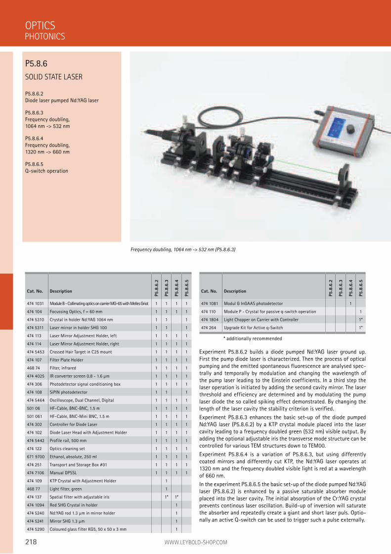
218 WWW.LEYBOLD-SHOP.COM
SOLID STATE LASER
P5.8.6.2 Diode laser pumped Nd:YAG laser
P5.8.6.3 Frequency doubling, 1064 nm -> 532 nm
P5.8.6.4 Frequency doubling, 1320 nm -> 660 nm
P5.8.6.5 Q-switch operation
Experiment P5.8.6.2 builds a diode pumped Nd:YAG laser ground up. First the pump diode laser is characterized. Then the process of optical pumping and the emitted spontaneous fluorescence are analysed spec-trally and temporally by modulation and changing the wavelength of the pump laser leading to the Einstein coefficients. In a third step the laser operation is initiated by adding the second cavity mirror. The laser threshold and efficiency are determined and by modulating the pump laser diode the so called spiking effect demonstrated. By changing the length of the laser cavity the stability criterion is verified.
Experiment P5.8.6.3 enhances the basic set-up of the diode pumped Nd:YAG laser (P5.8.6.2) by a KTP crystal module placed into the laser cavity leading to a frequency doubled green (532 nm) visible output. By adding the optional adjustable iris the transverse mode structure can be controlled for various TEM structures down to TEM00.
Experiment P5.8.6.4 is a variation of P5.8.6.3, but using differently coated mirrors and differently cut KTP, the Nd:YAG laser operates at 1320 nm and the frequency doubled visible light is red at a wavelength of 660 nm.
In the experiment P5.8.6.5 the basic set-up of the diode pumped Nd:YAG laser (P5.8.6.2) is enhanced by a passive saturable absorber module placed into the laser cavity. The initial absorption of the Cr:YAG crystal prevents continous laser oscillation. Build-up of inversion will saturate the absorber and repeatedly create a giant and short laser puls. Optio-nally an active Q-switch can be used to trigger such a pulse externally.
OPTICS
Frequency doubling, 1064 nm -> 532 nm (P5.8.6.3)
Cat. No. Description
P5.8
.6.2
P5.8
.6.3
P5.8
.6.4
P5.8
.6.5
474 1031 Module B - Collimating optics on carrier MG-65 with Melles Griot 1 1 1 1
474 104 Focussing Optics, f = 60 mm 1 1 1 1
474 5310 Crystal in holder Nd:YAG 1064 nm 1 1 1
474 5311 Laser mirror in holder SHG 100 1 1 1
474 113 Laser Mirror Adjustment Holder, left 1 1 1 1
474 114 Laser Mirror Adjustment Holder, right 1 1 1 1
474 5453 Crossed Hair Target in C25 mount 1 1 1 1
474 107 Filter Plate Holder 1 1 1 1
468 74 Filter, infrared 1 1 1 1
474 4025 IR converter screen 0.8 - 1.6 µm 1 1 1 1
474 306 Photodetector signal conditioning box 1 1 1 1
474 108 SiPIN photodetector 1 1 1
474 5464 Oscilloscope, Dual Channel, Digital 1 1 1 1
501 06 HF-Cable, BNC-BNC, 1.5 m 1 1 1 1
501 061 HF-Cable, BNC-Mini BNC, 1.5 m 1 1 1 1
474 302 Controller for Diode Laser 1 1 1 1
474 102 Diode Laser Head with Adjustment Holder 1 1 1 1
474 5442 Profile rail, 500 mm 1 1 1 1
474 122 Optics cleaning set 1 1 1 1
671 9700 Ethanol, absolute, 250 ml 1 1 1 1
474 251 Transport and Storage Box #01 1 1 1 1
474 7106 Manual DPSSL 1 1 1 1
474 109 KTP Crystal with Adjustment Holder 1
468 77 Light filter, green 1
474 137 Spatial filter with adjustable iris 1* 1*
474 1094 Red SHG Crystal in holder 1
474 5240 Nd:YAG rod 1.3 µm in mirror holder 1
474 5241 Mirror SHG 1.3 µm 1
474 5290 Coloured glass filter KG5, 50 x 50 x 3 mm 1
PHOTONICS
P5.8.6
Cat. No. Description
P5.8
.6.2
P5.8
.6.3
P5.8
.6.4
P5.8
.6.5
474 1081 Modul G InGAAS photodetector 1
474 110 Module P - Crystal for passive q-switch operation 1
474 1804 Light Chopper on Carrier with Controller 1*
474 264 Upgrade Kit for Active q-Switch 1*
* additionally recommended
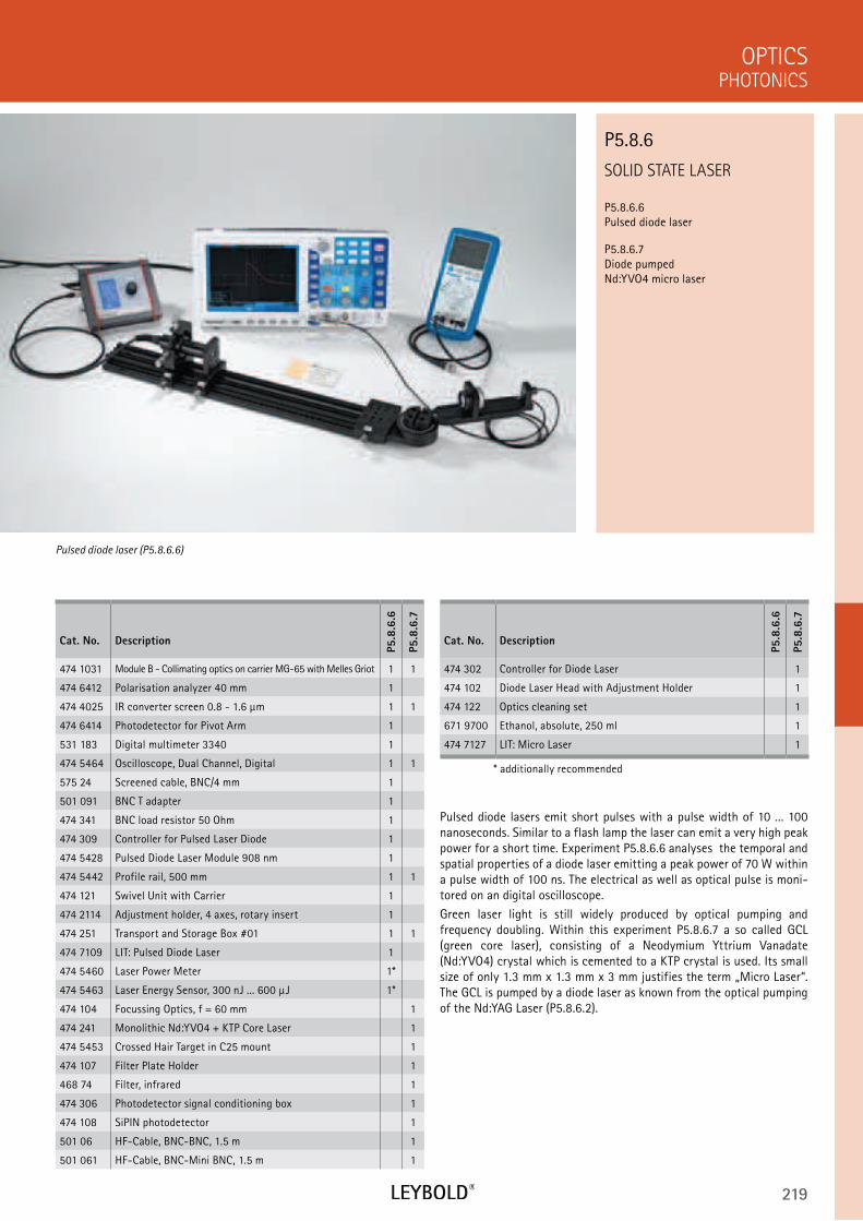
219
Cat. No. Description
P5.8
.6.6
P5.8
.6.7
474 302 Controller for Diode Laser 1
474 102 Diode Laser Head with Adjustment Holder 1
474 122 Optics cleaning set 1
671 9700 Ethanol, absolute, 250 ml 1
474 7127 LIT: Micro Laser 1
* additionally recommended
SOLID STATE LASER
P5.8.6.6 Pulsed diode laser
P5.8.6.7 Diode pumped Nd:YVO4 micro laser
PHOTONICS
OPTICS
Cat. No. Description
P5.8
.6.6
P5.8
.6.7
474 1031 Module B - Collimating optics on carrier MG-65 with Melles Griot 1 1
474 6412 Polarisation analyzer 40 mm 1
474 4025 IR converter screen 0.8 - 1.6 µm 1 1
474 6414 Photodetector for Pivot Arm 1
531 183 Digital multimeter 3340 1
474 5464 Oscilloscope, Dual Channel, Digital 1 1
575 24 Screened cable, BNC/4 mm 1
501 091 BNC T adapter 1
474 341 BNC load resistor 50 Ohm 1
474 309 Controller for Pulsed Laser Diode 1
474 5428 Pulsed Diode Laser Module 908 nm 1
474 5442 Profile rail, 500 mm 1 1
474 121 Swivel Unit with Carrier 1
474 2114 Adjustment holder, 4 axes, rotary insert 1
474 251 Transport and Storage Box #01 1 1
474 7109 LIT: Pulsed Diode Laser 1
474 5460 Laser Power Meter 1*
474 5463 Laser Energy Sensor, 300 nJ ... 600 µJ 1*
474 104 Focussing Optics, f = 60 mm 1
474 241 Monolithic Nd:YVO4 + KTP Core Laser 1
474 5453 Crossed Hair Target in C25 mount 1
474 107 Filter Plate Holder 1
468 74 Filter, infrared 1
474 306 Photodetector signal conditioning box 1
474 108 SiPIN photodetector 1
501 06 HF-Cable, BNC-BNC, 1.5 m 1
501 061 HF-Cable, BNC-Mini BNC, 1.5 m 1
Pulsed diode lasers emit short pulses with a pulse width of 10 ... 100 nanoseconds. Similar to a flash lamp the laser can emit a very high peak power for a short time. Experiment P5.8.6.6 analyses the temporal and spatial properties of a diode laser emitting a peak power of 70 W within a pulse width of 100 ns. The electrical as well as optical pulse is moni-tored on an digital oscilloscope.
Green laser light is still widely produced by optical pumping and frequency doubling. Within this experiment P5.8.6.7 a so called GCL (green core laser), consisting of a Neodymium Yttrium Vanadate (Nd:YVO4) crystal which is cemented to a KTP crystal is used. Its small size of only 1.3 mm x 1.3 mm x 3 mm justifies the term „Micro Laser“. The GCL is pumped by a diode laser as known from the optical pumping of the Nd:YAG Laser (P5.8.6.2).
Pulsed diode laser (P5.8.6.6)
P5.8.6
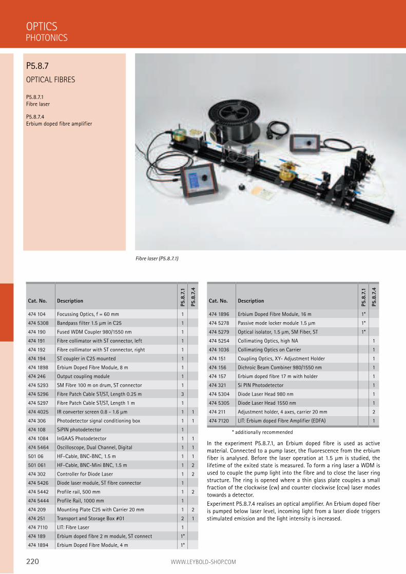
220 WWW.LEYBOLD-SHOP.COM
Cat. No. Description
P5.8
.7.1
P5.8
.7.4
474 1896 Erbium Doped Fibre Module, 16 m 1*
474 5278 Passive mode locker module 1.5 µm 1*
474 5279 Optical isolator, 1.5 µm, SM Fiber, ST 1*
474 5254 Collimating Optics, high NA 1
474 1036 Collimating Optics on Carrier 1
474 151 Coupling Optics, XY- Adjustment Holder 1
474 156 Dichroic Beam Combiner 980/1550 nm 1
474 157 Erbium doped fibre 17 m with holder 1
474 321 Si PIN Photodetector 1
474 5304 Diode Laser Head 980 nm 1
474 5305 Diode Laser Head 1550 nm 1
474 211 Adjustment holder, 4 axes, carrier 20 mm 2
474 7120 LIT: Erbium doped Fibre Amplifier (EDFA) 1
* additionally recommended
OPTICAL FIBRES
P5.8.7.1 Fibre laser
P5.8.7.4 Erbium doped fibre amplifier
In the experiment P5.8.7.1, an Erbium doped fibre is used as active material. Connected to a pump laser, the fluorescence from the erbium fiber is analysed. Before the laser operation at 1.5 µm is studied, the lifetime of the exited state is measured. To form a ring laser a WDM is used to couple the pump light into the fibre and to close the laser ring structure. The ring is opened where a thin glass plate couples a small fraction of the clockwise (cw) and counter clockwise (ccw) laser modes towards a detector.
Experiment P5.8.7.4 realises an optical amplifier. An Erbium doped fiber is pumped below laser level, incoming light from a laser diode triggers stimulated emission and the light intensity is increased.
OPTICS
Fibre laser (P5.8.7.1)
Cat. No. Description
P5.8
.7.1
P5.8
.7.4
474 104 Focussing Optics, f = 60 mm 1
474 5308 Bandpass filter 1.5 µm in C25 1
474 190 Fused WDM Coupler 980/1550 nm 1
474 191 Fibre collimator with ST connector, left 1
474 192 Fibre collimator with ST connector, right 1
474 194 ST coupler in C25 mounted 1
474 1898 Erbium Doped Fibre Module, 8 m 1
474 246 Output coupling module 1
474 5293 SM Fibre 100 m on drum, ST connector 1
474 5296 Fibre Patch Cable ST/ST, Length 0.25 m 3
474 5297 Fibre Patch Cable ST/ST, Length 1 m 1
474 4025 IR converter screen 0.8 - 1.6 µm 1 1
474 306 Photodetector signal conditioning box 1 1
474 108 SiPIN photodetector 1
474 1084 InGAAS Photodetector 1 1
474 5464 Oscilloscope, Dual Channel, Digital 1 1
501 06 HF-Cable, BNC-BNC, 1.5 m 1 1
501 061 HF-Cable, BNC-Mini BNC, 1.5 m 1 2
474 302 Controller for Diode Laser 1 2
474 5426 Diode laser module, ST fibre connector 1
474 5442 Profile rail, 500 mm 1 2
474 5444 Profile Rail, 1000 mm 1
474 209 Mounting Plate C25 with Carrier 20 mm 1 2
474 251 Transport and Storage Box #01 2 1
474 7110 LIT: Fibre Laser 1
474 189 Erbium doped fibre 2 m module, ST connect 1*
474 1894 Erbium Doped Fibre Module, 4 m 1*
PHOTONICS
P5.8.7
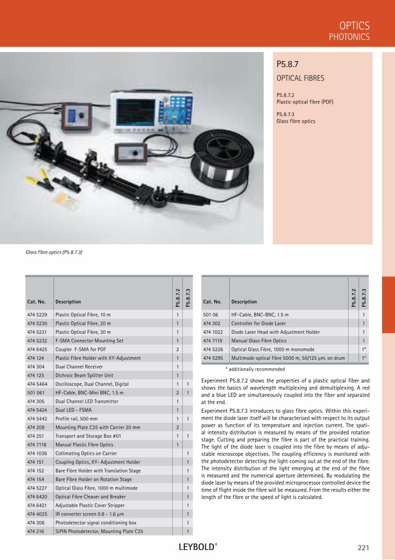
221
Cat. No. Description
P5.8
.7.2
P5.8
.7.3
501 06 HF-Cable, BNC-BNC, 1.5 m 1
474 302 Controller for Diode Laser 1
474 1022 Diode Laser Head with Adjustment Holder 1
474 7119 Manual Glass Fibre Optics 1
474 5226 Optical Glass Fibre, 1000 m monomode 1*
474 5295 Multimode optical fibre 5000 m, 50/125 µm, on drum 1*
* additionally recommended
OPTICAL FIBRES
P5.8.7.2 Plastic optical fibre (POF)
P5.8.7.3 Glass fibre optics
PHOTONICS
OPTICS
Cat. No. Description
P5.8
.7.2
P5.8
.7.3
474 5229 Plastic Optical Fibre, 10 m 1
474 5230 Plastic Optical Fibre, 20 m 1
474 5231 Plastic Optical Fibre, 30 m 1
474 5232 F-SMA Connector Mounting Set 1
474 6425 Coupler F-SMA for POF 2
474 124 Plastic Fibre Holder with XY-Adjustment 1
474 304 Dual Channel Receiver 1
474 125 Dichroic Beam Splitter Unit 1
474 5464 Oscilloscope, Dual Channel, Digital 1 1
501 061 HF-Cable, BNC-Mini BNC, 1.5 m 2 1
474 305 Dual Channel LED Transmitter 1
474 5424 Dual LED - FSMA 1
474 5442 Profile rail, 500 mm 1 1
474 209 Mounting Plate C25 with Carrier 20 mm 2
474 251 Transport and Storage Box #01 1 1
474 7118 Manual Plastic Fibre Optics 1
474 1036 Collimating Optics on Carrier 1
474 151 Coupling Optics, XY- Adjustment Holder 1
474 152 Bare Fibre Holder with Translation Stage 1
474 154 Bare Fibre Holder on Rotation Stage 1
474 5227 Optical Glass Fibre, 1000 m multimode 1
474 6420 Optical Fibre Cleaver and Breaker 1
474 6421 Adjustable Plastic Cover Stripper 1
474 4025 IR converter screen 0.8 - 1.6 µm 1
474 306 Photodetector signal conditioning box 1
474 216 SiPIN Photodetector, Mounting Plate C25 1
Experiment P5.8.7.2 shows the properties of a plastic optical fiber and shows the basics of wavelength multiplexing and demultiplexing. A red and a blue LED are simultaneously coupled into the fiber and separated at the end.
Experiment P5.8.7.3 introduces to glass fibre optics. Within this experi-ment the diode laser itself will be characterised with respect to its output power as function of its temperature and injection current. The spati-al intensity distribution is measured by means of the provided rotation stage. Cutting and preparing the fibre is part of the practical training. The light of the diode laser is coupled into the fibre by means of adju-stable microscope objectives. The coupling efficiency is monitored with the photodetector detecting the light coming out at the end of the fibre. The intensity distribution of the light emerging at the end of the fibre is measured and the numerical aperture determined. By modulating the diode laser by means of the provided microprocessor controlled device the time of flight inside the fibre will be measured. From the results either the length of the fibre or the speed of light is calculated.
Glass fibre optics (P5.8.7.3)
P5.8.7
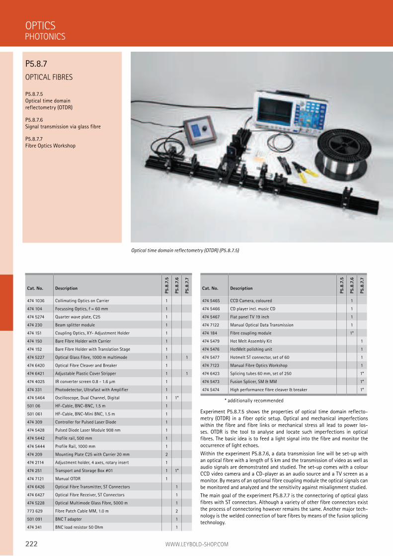
222 WWW.LEYBOLD-SHOP.COM
Cat. No. Description
P5.8
.7.5
P5.8
.7.6
P5.8
.7.7
474 5465 CCD Camera, coloured 1
474 5466 CD player incl. music CD 1
474 5467 Flat panel TV 19 inch 1
474 7122 Manual Optical Data Transmission 1
474 184 Fibre coupling module 1*
474 5479 Hot Melt Assembly Kit 1
474 5476 HotMelt polishing unit 1
474 5477 Hotmelt ST connector, set of 60 1
474 7123 Manual Fibre Optics Workshop 1
474 6423 Splicing tubes 60 mm, set of 250 1*
474 5473 Fusion Splicer, SM & MM 1*
474 5474 High performance fibre cleaver & breaker 1*
* additionally recommended
OPTICAL FIBRES
P5.8.7.5 Optical time domain reflectometry (OTDR)
P5.8.7.6 Signal transmission via glass fibre
P5.8.7.7 Fibre Optics Workshop
Experiment P5.8.7.5 shows the properties of optical time domain reflecto-metry (OTDR) in a fiber optic setup. Optical and mechanical imperfections within the fibre and fibre links or mechanical stress all lead to power los-ses. OTDR is the tool to analyse and locate such imperfections in optical fibres. The basic idea is to feed a light signal into the fibre and monitor the occurrence of light echoes.
Within the experiment P5.8.7.6, a data transmission line will be set-up with an optical fibre with a length of 5 km and the transmission of video as well as audio signals are demonstrated and studied. The set-up comes with a colour CCD video camera and a CD-player as an audio source and a TV screen as a monitor. By means of an optional fibre coupling module the optical signals can be monitored and analyzed and the sensitivity against misalignment studied.
The main goal of the experiment P5.8.7.7 is the connectoring of optical glass fibres with ST connectors. Although a variety of other fibre connectors exist the process of connectoring however remains the same. Another major tech-nology is the welded connection of bare fibres by means of the fusion splicing technology.
OPTICS
Optical time domain reflectometry (OTDR) (P5.8.7.5)
Cat. No. Description
P5.8
.7.5
P5.8
.7.6
P5.8
.7.7
474 1036 Collimating Optics on Carrier 1
474 104 Focussing Optics, f = 60 mm 1
474 5274 Quarter wave plate, C25 1
474 230 Beam splitter module 1
474 151 Coupling Optics, XY- Adjustment Holder 1
474 150 Bare Fibre Holder with Carrier 1
474 152 Bare Fibre Holder with Translation Stage 1
474 5227 Optical Glass Fibre, 1000 m multimode 1 1
474 6420 Optical Fibre Cleaver and Breaker 1
474 6421 Adjustable Plastic Cover Stripper 1 1
474 4025 IR converter screen 0.8 - 1.6 µm 1
474 331 Photodetector, Ultrafast with Amplifier 1
474 5464 Oscilloscope, Dual Channel, Digital 1 1*
501 06 HF-Cable, BNC-BNC, 1.5 m 1
501 061 HF-Cable, BNC-Mini BNC, 1.5 m 1
474 309 Controller for Pulsed Laser Diode 1
474 5428 Pulsed Diode Laser Module 908 nm 1
474 5442 Profile rail, 500 mm 1
474 5444 Profile Rail, 1000 mm 1
474 209 Mounting Plate C25 with Carrier 20 mm 2
474 2114 Adjustment holder, 4 axes, rotary insert 1
474 251 Transport and Storage Box #01 1 1*
474 7121 Manual OTDR 1
474 6426 Optical Fibre Transmitter, ST Connectors 1
474 6427 Optical Fibre Receiver, ST Connectors 1
474 5228 Optical Multimode Glass Fibre, 5000 m 1
773 629 Fibre Patch Cable MM, 1.0 m 2
501 091 BNC T adapter 1
474 341 BNC load resistor 50 Ohm 1
PHOTONICS
P5.8.7
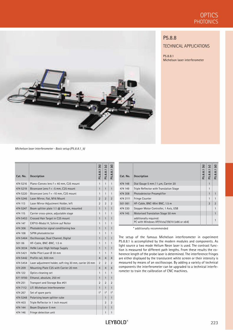
223
Cat. No. Description
P5.8
.8.1
(b)
P5.8
.8.1
(c)
P5.8
.8.1
(d)
474 148 Dial Gauge 5 mm / 1 µm, Carrier 20 1
474 149 Triple Reflector with Translation Stage 1
474 308 Photodetector Preamplifier 1 1
474 3111 Fringe Counter 1 1
501 061 HF-Cable, BNC-Mini BNC, 1.5 m 2 2
474 330 Stepper Motor Controller, 1 Axis, USB 1
474 145 Motorised Translation Stage 50 mm 1
additionally required: PC with Windows XP/Vista/7/8/10 (x86 or x64)
1
* additionally recommended
TECHNICAL APPLICATIONS
P5.8.8.1 Michelson laser interferometer
PHOTONICS
OPTICS
Cat. No. Description
P5.8
.8.1
(b)
P5.8
.8.1
(c)
P5.8
.8.1
(d)
474 5216 Plano-Convex lens f = 40 mm, C25 mount 1 1 1
474 5219 Biconcave Lens f = -5 mm, C25 mount 1 1 1
474 5220 Biconcave Lens f = -10 mm, C25 mount 1 1 1
474 5246 Laser Mirror, flat, M16 Mount 2 2 2
474 113 Laser Mirror Adjustment Holder, left 2 2 2
474 5247 Beam splitter plate 1:1 @ 632 nm, mounted 1 1 1
474 115 Carrier cross-piece, adjustable stage 1 1 1
474 5453 Crossed Hair Target in C25 mount 1 1 1
474 147 EXP10-Modul H, Schirm auf Reiter 1 1 1
474 306 Photodetector signal conditioning box 1 1 1
474 108 SiPIN photodetector 1 1 1
474 5464 Oscilloscope, Dual Channel, Digital 1 1 1
501 06 HF-Cable, BNC-BNC, 1.5 m 1 1 1
474 3034 HeNe Laser High Voltage Supply 1 1 1
474 5421 HeNe Pilot Laser Ø 30 mm 1 1 1
474 5442 Profile rail, 500 mm 4 4 4
474 5454 Laser adjustment holder, soft ring 30 mm, carrier 20 mm 2 2 2
474 209 Mounting Plate C25 with Carrier 20 mm 4 4 4
474 122 Optics cleaning set 1 1 1
671 9700 Ethanol, absolute, 250 ml 1 1 1
474 251 Transport and Storage Box #01 2 2 2
474 7112 LIT: Michelson Interferometer 1 1 1
474 267 Set of spare parts 1* 1* 1*
474 5248 Polarising beam splitter cube 1 1
474 403 Triple Reflector in 1 inch mount 2 2
474 144 Beam Displacer 5 mm 1 1
474 146 Fringe detection unit 1 1
The setup of the famous Michelson interferometer in experiment P5.8.8.1 is accomplished by the modern modules and components. As light source a two mode Helium Neon laser is used. The contrast func-tion is measured for different path lengths. From these results the co-herence length of the probe laser is determined. The interference fringes are either displayed by the translucent white screen or their intensity is measured by means of an oscilloscope. By adding a variety of technical components the interferometer can be upgraded to a technical interfe-rometer to train the calibration of CNC machines.
Michelson laser interferometer - Basic setup (P5.8.8.1_b)
P5.8.8
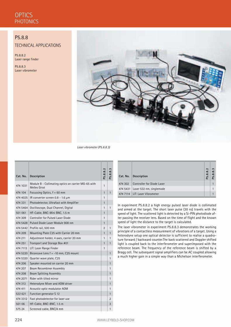
224 WWW.LEYBOLD-SHOP.COM
TECHNICAL APPLICATIONS
P5.8.8.2 Laser range finder
P5.8.8.3 Laser vibrometer
In experiment P5.8.8.2 a high energy pulsed laser diode is collimated and aimed at the target. The short laser pulse (30 ns) travels with the speed of light. The scattered light is detected by a Si-PIN photodiode af-ter passing the receiver lens. Based on the time of flight and the known speed of light the distance to the target is calculated.
The laser vibrometer in experiment P5.8.8.3 demonstrates the working principle of a contactless measurement of vibrations of a target. Using a heterodyne setup one optical detector is sufficient to realise a quadra-ture forward / backward counter.The back scattered and Doppler shifted light is coupled back to the interferometer and superimposed with the reference beam. The frequency of the reference beam is shifted by a Bragg cell. The subsequent signal amplifiers can be AC coupled allowing a much higher gain in a simple way than a Michelson interferometer.
OPTICS
Laser vibrometer (P5.8.8.3)
Cat. No. Description
P5.8
.8.2
P5.8
.8.3
474 1031Module B - Collimating optics on carrier MG-65 with Melles Griot
1
474 104 Focussing Optics, f = 60 mm 1 1
474 4025 IR converter screen 0.8 - 1.6 µm 1
474 331 Photodetector, Ultrafast with Amplifier 1
474 5464 Oscilloscope, Dual Channel, Digital 1 1
501 061 HF-Cable, BNC-Mini BNC, 1.5 m 1
474 309 Controller for Pulsed Laser Diode 1
474 5428 Pulsed Diode Laser Module 908 nm 1
474 5442 Profile rail, 500 mm 2 1
474 209 Mounting Plate C25 with Carrier 20 mm 1 1
474 211 Adjustment holder, 4 axes, carrier 20 mm 1 1
474 251 Transport and Storage Box #01 1 1
474 7113 LIT: Laser Range Finder 1
474 5220 Biconcave Lens f = -10 mm, C25 mount 1
474 5320 Quarter wave plate, C25 1
474 206 Speaker mounted on carrier 20 mm 1
474 207 Beam Recombiner Assembly 1
474 208 Beam Splitting Assembly 1
474 2071 Rider with tilted mirror 1
474 313 Heterodyne Mixer and AOM driver 1
474 411 Acoustic optic modulator AOM 1
522 621 Function generator S 12 1
474 3312 Fast photodetector for laser use 2
501 06 HF-Cable, BNC-BNC, 1.5 m 3
575 24 Screened cable, BNC/4 mm 1
PHOTONICS
P5.8.8
Cat. No. Description
P5.8
.8.2
P5.8
.8.3
474 302 Controller for Diode Laser 1
474 5431 Laser 532 nm, singlemode 1
474 7114 LIT: Laser Vibrometer 1
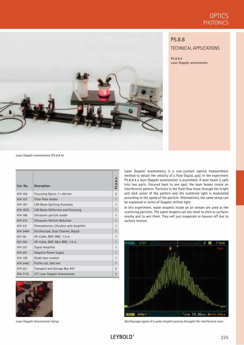
225
TECHNICAL APPLICATIONS
P5.8.8.4 Laser Doppler anemometer
PHOTONICS
OPTICS
Cat. No. Description
P5.8
.8.4
474 104 Focussing Optics, f = 60 mm 2
474 107 Filter Plate Holder 1
474 187 LDA Beam Splitting Assembly 1
474 1876 LDA Beam Deflection and Focussing 1
474 188 Ultrasonic particle seeder 1
474 315 Ultrasonic Particle Nebuliser 1
474 331 Photodetector, Ultrafast with Amplifier 1
474 5464 Oscilloscope, Dual Channel, Digital 1
501 06 HF-Cable, BNC-BNC, 1.5 m 1
501 061 HF-Cable, BNC-Mini BNC, 1.5 m 1
474 351 Signal Amplifier 1
474 301 Adaptive Power Supply 1
474 128 Diode laser module 1
474 5442 Profile rail, 500 mm 1
474 251 Transport and Storage Box #01 2
474 7115 LIT: Laser Doppler Anemometer 1
Laser Doppler anemometry is a non-contact optical measurement method to obtain the velocity of a flow (liquid, gas). In the experiment P5.8.8.4 a laser Doppler anemometer is assembled. A laser beam is split into two parts. Focused back to one spot, the laser beams create an interference pattern. Particles in the fluid flow move through the bright and dark zones of the pattern and the scattered light is modulated according to the speed of the particle. Alternatively, the same setup can be explained in terms of Doppler shifted light.
In this experiment, water droplets inside an air stream are used as the scattering particles. The water droplets are too small to stick to surfaces nearby and to wet them. They will just evaporate or bounce off due to surface tension.
Laser Doppler anemometer (P5.8.8.4)
P5.8.8
Oscilloscope signal of a water droplet passing throught the interference zoneLaser Doppler Anemometer Setup
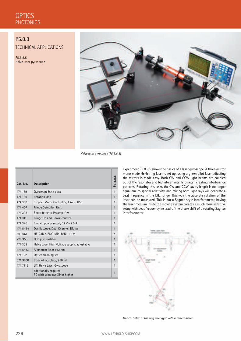
226 WWW.LEYBOLD-SHOP.COM
TECHNICAL APPLICATIONS
P5.8.8.5
HeNe laser gyroscope
Experiment P5.8.8.5 shows the basics of a laser gyroscope. A three-mirror
mono mode HeNe ring laser is set up; using a green pilot laser adjusting
the mirrors is made easy. Both CW and CCW light beams are coupled
out of the resonator and fed into an interferometer, creating interference
patterns. Rotating this laser, the CW and CCW cavity length is no longer
equal due to special relativity, and mixing both light rays will generate a
beat frequency in the kHz range. This way the absolute rotation of the
laser can be measured. This is not a Sagnac style interferometer, having
the laser medium inside the moving system creates a much more sensitive
setup with beat frequency instead of the phase shift of a rotating Sagnac
interferometer.
OPTICS
HeNe laser gyroscope (P5.8.8.5)
Cat. No. Description
P5.8
.8.5
474 159 Gyroscope base plate 1
474 160 Rotation Unit 1
474 330 Stepper Motor Controller, 1 Axis, USB 1
474 407 Fringe Detection Unit 1
474 308 Photodetector Preamplifier 1
474 311 Fringe Up and Down Counter 1
474 346 Plug-in power supply 12 V - 2.5 A 1
474 5464 Oscilloscope, Dual Channel, Digital 1
501 061 HF-Cable, BNC-Mini BNC, 1.5 m 4
728 950 USB port isolator 1
474 303 HeNe Laser High Voltage supply, adjustable 1
474 5423 Alignment laser 532 nm 1
474 122 Optics cleaning set 1
671 9700 Ethanol, absolute, 250 ml 1
474 7116 LIT: HeNe Laser Gyroscope 1
additionally required:
PC with Windows XP or higher1
Optical Setup of the ring laser gyro with interferometer
PHOTONICS
P5.8.8
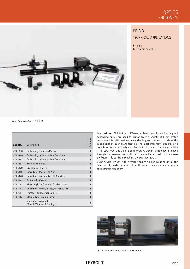
227
TECHNICAL APPLICATIONS
P5.8.8.6 Laser beam analysis
PHOTONICS
OPTICS
Cat. No. Description
P5.8
.8.6
474 1036 Collimating Optics on Carrier 1
474 5266 Collimating cylindrical lens f = 20 mm 1
474 5267 Collimating cylindrical lens f = 80 mm 1
474 5263 Beam expander 6x 1
474 5470 Beammaster BM-7S 1
474 5418 Diode Laser Module, 532 nm 1
474 5420 Dimo diode laser module, 630 nm (red) 1
474 5442 Profile rail, 500 mm 1
474 209 Mounting Plate C25 with Carrier 20 mm 3
474 211 Adjustment holder, 4 axes, carrier 20 mm 1
474 251 Transport and Storage Box #01 1
474 7117 Manual Laser beam analysis 1
additionally required: PC with Windows XP or higher
1
In experiment P5.8.8.6 two different visible lasers plus collimating and expanding optics are used to demonstrate a variety of beam profile measurements with various beam shaping arrangements to show the possibilities of laser beam forming. The most important property of a laser beam is the intensity distribution in the beam. The beam profiler is no CDD type, but a knife edge type: A precise knife edge is moved through the cross-section of the laser beam. As the blade moves across the beam, it is cut from reaching the photodetector.
Using several knives with different angles on one rotating drum, the beam profile can be calculated from the time responses when the knives pass through the beam.
Laser beam analysis (P5.8.8.6)
P5.8.8
Optical setup of a semiconductor laser diode
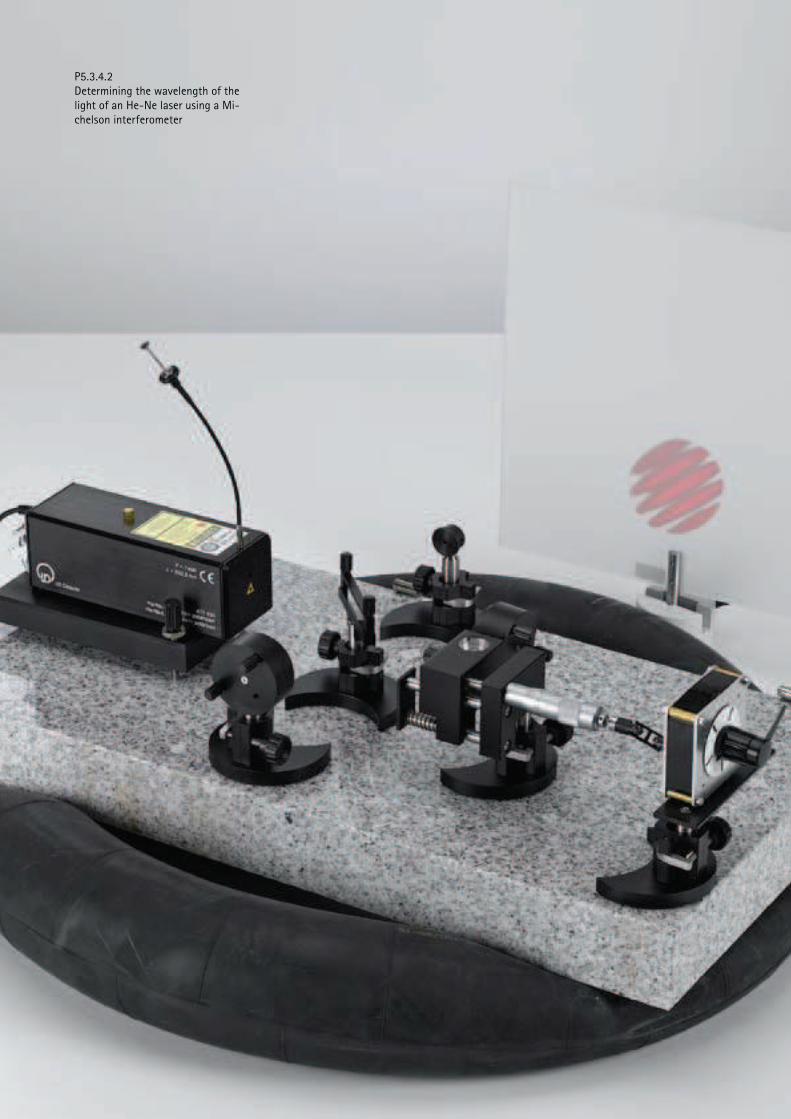
228 WWW.LEYBOLD-SHOP.COM
P5.3.4.2
Determining the wavelength of the
light of an He-Ne laser using a Mi-
chelson interferometer

229
P6.1 INTRODUCTORY EXPERIMENTS 231
P6.2 ATOMIC SHELL 239
P6.3 X-RAY PHYSICS 250
P6.4 RADIOACTIVITY 261
P6.5 NUCLEAR PHYSICS 265
P6.6 QUANTUM PHYSICS 272
P6 ATOMIC AND
NUCLEAR PHYSICS

230 WWW.LEYBOLD-SHOP.COM
P6.1 INTRODUCTORY EXPERIMENTS
P6.1.1 Oil-spot experiment 231P6.1.2 Millikan experiment 232P6.1.3 Specific electron charge 233P6.1.4 Planck’s constant 234-236P6.1.5 Dual nature of wave and particle 237P6.1.6 Paul trap 238
P6.2 ATOMIC SHELL
P6.2.1 Balmer series of hydrogen 239-240P6.2.2 Emission and absorption spectra 241-243P6.2.3 Inelastic collisions of electrons 244P6.2.4 Franck-Hertz experiment 245-246P6.2.6 Electron spin resonance 247P6.2.7 Normal Zeeman effect 248P6.2.8 Optical pumping (anomalous Zeeman effect) 249
P6.3 X-RAY PHYSICS
P6.3.1 Detection of X-rays 250-252P6.3.2 Attenuation of X-rays 253P6.3.3 Physics of the atomic shell 254P6.3.5 X-ray energy spectroscopy 255P6.3.6 Structure of X-ray spectrums 256-257P6.3.7 Compton effect at X-rays 258P6.3.8 X-ray tomography 259-260
P6.4 RADIOACTIVITY
P6.4.1 Detecting radioactivity 261P6.4.2 Poisson distribution 262P6.4.3 Radioactive decay and half-life 263P6.4.4 Attenuation of -, - and radiation 264
P6.5 NUCLEAR PHYSICS
P6.5.1 Demonstrating paths of particles 265P6.5.2 Rutherford scattering 266P6.5.3 Nuclear magnetic resonance 267P6.5.4 spectroscopyP6.5.5 spectroscopy 269
P6.5.6 Compton effect 270P6.5.7 Properties of radiation particles 271
P6.6 QUANTUM PHYSICS
P6.6.1 Quantum optics 272P6.6.2 Particles 273
P6 ATOMIC AND
NUCLEAR PHYSICS
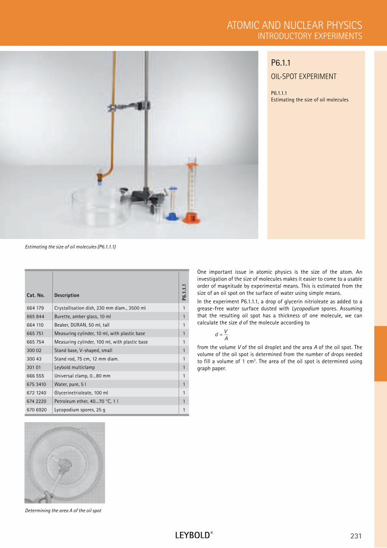
231
OIL-SPOT EXPERIMENT
P6.1.1.1
Estimating the size of oil molecules
INTRODUCTORY EXPERIMENTS
ATOMIC AND NUCLEAR PHYSICS
Cat. No. Description
P6.1
.1.1
664 179 Crystallisation dish, 230 mm diam., 3500 ml 1
665 844 Burette, amber glass, 10 ml 1
664 110 Beaker, DURAN, 50 ml, tall 1
665 751 Measuring cylinder, 10 ml, with plastic base 1
665 754 Measuring cylinder, 100 ml, with plastic base 1
300 02 Stand base, V-shaped, small 1
300 43 Stand rod, 75 cm, 12 mm diam. 1
301 01 Leybold multiclamp 1
666 555 Universal clamp, 0...80 mm 1
675 3410 Water, pure, 5 l 1
672 1240 Glycerinetrioleate, 100 ml 1
674 2220 Petroleum ether, 40...70 °C, 1 l 1
670 6920 Lycopodium spores, 25 g 1
One important issue in atomic physics is the size of the atom. An
investigation of the size of molecules makes it easier to come to a usable
order of magnitude by experimental means. This is estimated from the
size of an oil spot on the surface of water using simple means.
In the experiment P6.1.1.1, a drop of glycerin nitrioleate as added to a
grease-free water surface dusted with Lycopodium spores. Assuming
that the resulting oil spot has a thickness of one molecule, we can
calculate the size d of the molecule according to
dV
A
from the volume V of the oil droplet and the area A of the oil spot. The
volume of the oil spot is determined from the number of drops needed
to fill a volume of 1 cm3. The area of the oil spot is determined using
graph paper.
Estimating the size of oil molecules (P6.1.1.1)
P6.1.1
Determining the area A of the oil spot
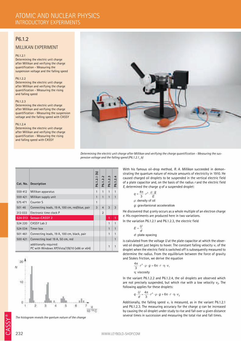
232 WWW.LEYBOLD-SHOP.COM
MILLIKAN EXPERIMENT
P6.1.2.1 Determining the electric unit charge after Millikan and verifying the charge quantification - Measuring the suspension voltage and the falling speed
P6.1.2.2 Determining the electric unit charge after Millikan and verifying the charge quantification - Measuring the rising and falling speed
P6.1.2.3 Determining the electric unit charge after Millikan and verifying the charge quantification - Measuring the suspension voltage and the falling speed with CASSY
P6.1.2.4 Determining the electric unit charge after Millikan and verifying the charge quantification - Measuring the rising and falling speed with CASSY
With his famous oil-drop method, R. A. Millikan succeeded in demon-strating the quantum nature of minute amounts of electricity in 1910. He caused charged oil droplets to be suspended in the vertical electric field of a plate capacitor and, on the basis of the radius r and the electric field E, determined the charge q of a suspended droplet:
q rg
E
g
= ⋅ ⋅⋅4
3
3π ρ
ρ: density of oil
: gravitanional accelerationn
He discovered that q only occurs as a whole multiple of an electron charge e. His experiments are produced here in two variations.
In the variation P6.1.2.1 and P6.1.2.3, the electric field
EU
d
d: plate spacing
is calculated from the voltage U at the plate capacitor at which the obser-ved oil droplet just begins to hover. The constant falling velocity v1 of the droplet when the electric field is switched off is subsequently measured to determine the radius. From the equilibrium between the force of gravity and Stokes friction, we derive the equation
4
363
1
πρ π η
η
⋅ ⋅ ⋅ = ⋅ ⋅ ⋅r g r v
: viscosity
In the variant P6.1.2.2 and P6.1.2.4, the oil droplets are observed which are not precisely suspended, but which rise with a low velocity v2. The following applies for these droplets:
qU
dr g r v⋅ = ⋅ ⋅ ⋅ + ⋅ ⋅ ⋅
4
36
3
2
πρ π η
Additionally, the falling speed v1 is measured, as in the variant P6.1.2.1 and P6.1.2.3. The measuring accuracy for the charge q can be increased by causing the oil droplet under study to rise and fall over a given distance several times in succession and measuring the total rise and fall times.
ATOMIC AND NUCLEAR PHYSICS
Determining the electric unit charge after Millikan and verifying the charge quantification - Measuring the sus-
pension voltage and the falling speed (P6.1.2.1_b)
Cat. No. Description
P6.1
.2.1
(b)
P6.1
.2.2
P6.1
.2.3
P6.1
.2.4
559 412 Millikan apparatus 1 1 1 1
559 421 Millikan supply unit 1 1 1 1
575 471 Counter S 1
501 46 Connecting leads, 19 A, 100 cm, red/blue, pair 3 4 3 3
313 033 Electronic time clock P 2
524 013 Sensor-CASSY 2 1 1
524 220 CASSY Lab 2 1 1
524 034 Timer box 1 1
501 461 Connecting leads, 19 A, 100 cm, black, pair 1 1
500 421 Connecting lead 19 A, 50 cm, red 1
additionally required: PC with Windows XP/Vista/7/8/10 (x86 or x64)
1 1
The histogram reveals the qantum nature of the change
INTRODUCTORY EXPERIMENTS
P6.1.2
CA
SSY ®
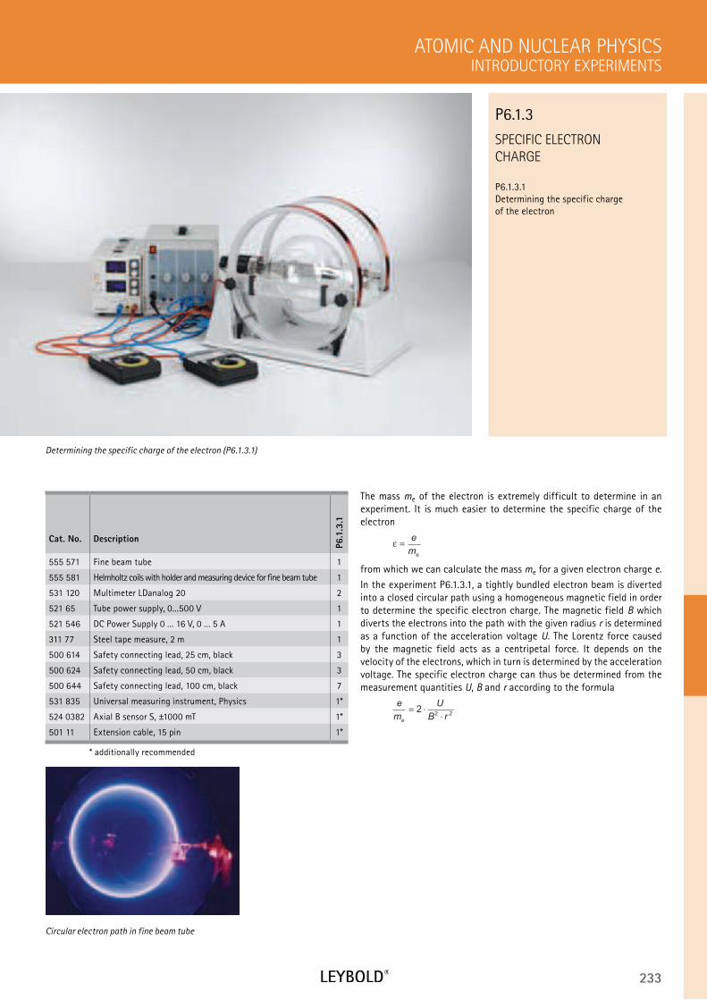
233
SPECIFIC ELECTRON
CHARGE
P6.1.3.1
Determining the specific charge
of the electron
INTRODUCTORY EXPERIMENTS
ATOMIC AND NUCLEAR PHYSICS
Cat. No. Description
P6.1
.3.1
555 571 Fine beam tube 1
555 581 Helmholtz coils with holder and measuring device for fine beam tube 1
531 120 Multimeter LDanalog 20 2
521 65 Tube power supply, 0...500 V 1
521 546 DC Power Supply 0 ... 16 V, 0 ... 5 A 1
311 77 Steel tape measure, 2 m 1
500 614 Safety connecting lead, 25 cm, black 3
500 624 Safety connecting lead, 50 cm, black 3
500 644 Safety connecting lead, 100 cm, black 7
531 835 Universal measuring instrument, Physics 1*
524 0382 Axial B sensor S, ±1000 mT 1*
501 11 Extension cable, 15 pin 1*
* additionally recommended
The mass me of the electron is extremely difficult to determine in an
experiment. It is much easier to determine the specific charge of the
electron
ε =e
me
from which we can calculate the mass me for a given electron charge e.
In the experiment P6.1.3.1, a tightly bundled electron beam is diverted
into a closed circular path using a homogeneous magnetic field in order
to determine the specific electron charge. The magnetic field B which
diverts the electrons into the path with the given radius r is determined
as a function of the acceleration voltage U. The Lorentz force caused
by the magnetic field acts as a centripetal force. It depends on the
velocity of the electrons, which in turn is determined by the acceleration
voltage. The specific electron charge can thus be determined from the
measurement quantities U, B and r according to the formula
e
m
U
B re
= ⋅⋅
22 2
Determining the specific charge of the electron (P6.1.3.1)
P6.1.3
Circular electron path in fine beam tube
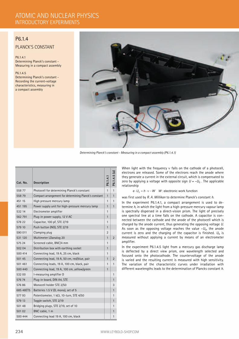
234 WWW.LEYBOLD-SHOP.COM
PLANCK’S CONSTANT
P6.1.4.1 Determining Planck’s constant - Measuring in a compact assembly
P6.1.4.5 Determining Planck’s constant - Recording the current-voltage characteristics, measuring in a compact assembly
When light with the frequency falls on the cathode of a photocell, electrons are released. Some of the electrons reach the anode where they generate a current in the external circuit, which is compensated to zero by applying a voltage with opposite sign U = –U0 . The applicable relationship
e U h W W⋅ = ⋅ −0
ν : electronic work function
was first used by R. A. Millikan to determine Planck’s constant h.
In the experiment P6.1.4.1, a compact arrangement is used to de- termine h, in which the light from a high-pressure mercury vapour lamp is spectrally dispersed in a direct-vision prism. The light of precisely one spectral line at a time falls on the cathode. A capacitor is con-nected between the cathode and the anode of the photocell which is charged by the anode current, thus generating the opposing voltage U. As soon as the opposing voltage reaches the value –U0, the anode current is zero and the charging of the capacitor is finished. U0 is measured without applying a current by means of an electrometer amplifier.
In the experiment P6.1.4.5 light from a mercury gas discharge lamp is deflected by a direct view prism, one wavelength selected and focused onto the photocathode. The countervoltage of the anode is varied and the resulting current is measured with high sensitivity. The variation of the characteristic curves under irradiation with different wavelengths leads to the determination of Plancks constant h.
ATOMIC AND NUCLEAR PHYSICS
Determining Planck’s constant - Measuring in a compact assembly (P6.1.4.1)
Cat. No. Description
P6.1
.4.1
P6.1
.4.5
(a)
558 77 Photocell for determining Planck‘s constant 1 1
558 79 Compact arrangement for determining Planck‘s constant 1 1
451 15 High pressure mercury lamp 1 1
451 195 Power supply unit for high-pressure mercury lamp 1 1
532 14 Electrometer amplifier 1
562 791 Plug-in power supply, 12 V AC 1
578 22 Capacitor, 100 pF, STE 2/19 1
579 10 Push button (NO), STE 2/19 1
590 011 Clamping plug 2
531 120 Multimeter LDanalog 20 1 2
575 24 Screened cable, BNC/4 mm 1
502 04 Distribution box with earthing socket 1
500 414 Connecting lead, 19 A, 25 cm, black 1
501 45 Connecting lead, 19 A, 50 cm, red/blue, pair 1 2
501 461 Connecting leads, 19 A, 100 cm, black, pair 1 1
500 440 Connecting lead, 19 A, 100 cm, yellow/green 1
532 00 I-measuring amplifier D 1
576 74 Plug-in board, DIN A4, STE 1
576 86 Monocell holder STE 2/50 3
685 48ET5 Batteries 1.5 V (D, mono), set of 5 1
577 93 Potentiometer, 1 k , 10-turn, STE 4/50 1
579 13 Toggle switch, STE 2/19 1
501 48 Bridging plugs, STE 2/19, set of 10 1
501 02 BNC cable, 1 m 1
500 444 Connecting lead 19 A, 100 cm, black 1
INTRODUCTORY EXPERIMENTS
P6.1.4
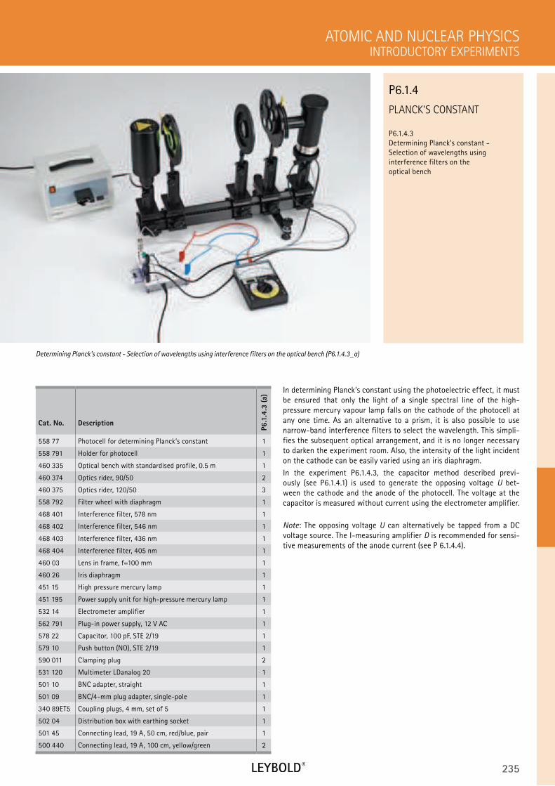
235
PLANCK’S CONSTANT
P6.1.4.3 Determining Planck’s constant - Selection of wavelengths using interference filters on the optical bench
INTRODUCTORY EXPERIMENTS
ATOMIC AND NUCLEAR PHYSICS
Cat. No. Description
P6.1
.4.3
(a)
558 77 Photocell for determining Planck‘s constant 1
558 791 Holder for photocell 1
460 335 Optical bench with standardised profile, 0.5 m 1
460 374 Optics rider, 90/50 2
460 375 Optics rider, 120/50 3
558 792 Filter wheel with diaphragm 1
468 401 Interference filter, 578 nm 1
468 402 Interference filter, 546 nm 1
468 403 Interference filter, 436 nm 1
468 404 Interference filter, 405 nm 1
460 03 Lens in frame, f=100 mm 1
460 26 Iris diaphragm 1
451 15 High pressure mercury lamp 1
451 195 Power supply unit for high-pressure mercury lamp 1
532 14 Electrometer amplifier 1
562 791 Plug-in power supply, 12 V AC 1
578 22 Capacitor, 100 pF, STE 2/19 1
579 10 Push button (NO), STE 2/19 1
590 011 Clamping plug 2
531 120 Multimeter LDanalog 20 1
501 10 BNC adapter, straight 1
501 09 BNC/4-mm plug adapter, single-pole 1
340 89ET5 Coupling plugs, 4 mm, set of 5 1
502 04 Distribution box with earthing socket 1
501 45 Connecting lead, 19 A, 50 cm, red/blue, pair 1
500 440 Connecting lead, 19 A, 100 cm, yellow/green 2
In determining Planck‘s constant using the photoelectric effect, it must be ensured that only the light of a single spectral line of the high- pressure mercury vapour lamp falls on the cathode of the photocell at any one time. As an alternative to a prism, it is also possible to use narrow-band interference filters to select the wavelength. This simpli-fies the subsequent optical arrangement, and it is no longer necessary to darken the experiment room. Also, the intensity of the light incident on the cathode can be easily varied using an iris diaphragm.
In the experiment P6.1.4.3, the capacitor method described previ-ously (see P6.1.4.1) is used to generate the opposing voltage U bet-ween the cathode and the anode of the photocell. The voltage at the capacitor is measured without current using the electrometer amplifier.
Note: The opposing voltage U can alternatively be tapped from a DC voltage source. The I-measuring amplifier D is recommended for sensi-tive measurements of the anode current (see P 6.1.4.4).
Determining Planck’s constant - Selection of wavelengths using interference filters on the optical bench (P6.1.4.3_a)
P6.1.4
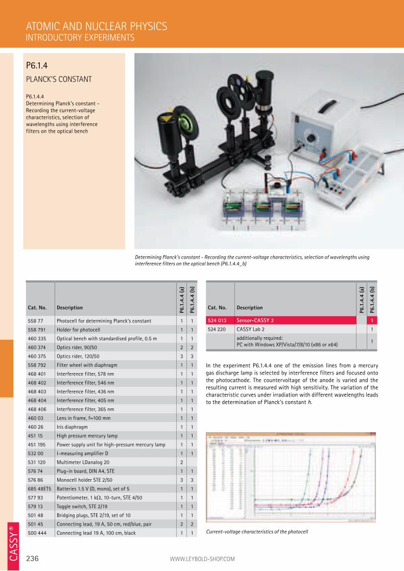
236 WWW.LEYBOLD-SHOP.COM
Cat. No. Description
P6.1
.4.4
(a)
P6.1
.4.4
(b)
524 013 Sensor-CASSY 2 1
524 220 CASSY Lab 2 1
additionally required: PC with Windows XP/Vista/7/8/10 (x86 or x64)
1
PLANCK’S CONSTANT
P6.1.4.4 Determining Planck’s constant - Recording the current-voltage characteristics, selection of wavelengths using interference filters on the optical bench
In the experiment P6.1.4.4 one of the emission lines from a mercury gas discharge lamp is selected by interference filters and focused onto the photocathode. The countervoltage of the anode is varied and the resulting current is measured with high sensitivity. The variation of the characteristic curves under irradiation with different wavelengths leads to the determination of Planck‘s constant h.
ATOMIC AND NUCLEAR PHYSICS
Determining Planck’s constant - Recording the current-voltage characteristics, selection of wavelengths using
interference filters on the optical bench (P6.1.4.4_b)
Cat. No. Description
P6.1
.4.4
(a)
P6.1
.4.4
(b)
558 77 Photocell for determining Planck‘s constant 1 1
558 791 Holder for photocell 1 1
460 335 Optical bench with standardised profile, 0.5 m 1 1
460 374 Optics rider, 90/50 2 2
460 375 Optics rider, 120/50 3 3
558 792 Filter wheel with diaphragm 1 1
468 401 Interference filter, 578 nm 1 1
468 402 Interference filter, 546 nm 1 1
468 403 Interference filter, 436 nm 1 1
468 404 Interference filter, 405 nm 1 1
468 406 Interference filter, 365 nm 1 1
460 03 Lens in frame, f=100 mm 1 1
460 26 Iris diaphragm 1 1
451 15 High pressure mercury lamp 1 1
451 195 Power supply unit for high-pressure mercury lamp 1 1
532 00 I-measuring amplifier D 1 1
531 120 Multimeter LDanalog 20 2
576 74 Plug-in board, DIN A4, STE 1 1
576 86 Monocell holder STE 2/50 3 3
685 48ET5 Batteries 1.5 V (D, mono), set of 5 1 1
577 93 Potentiometer, 1 k , 10-turn, STE 4/50 1 1
579 13 Toggle switch, STE 2/19 1 1
501 48 Bridging plugs, STE 2/19, set of 10 1 1
501 45 Connecting lead, 19 A, 50 cm, red/blue, pair 2 2
500 444 Connecting lead 19 A, 100 cm, black 1 1 Current-voltage characteristics of the photocell
INTRODUCTORY EXPERIMENTS
P6.1.4
CA
SSY ®
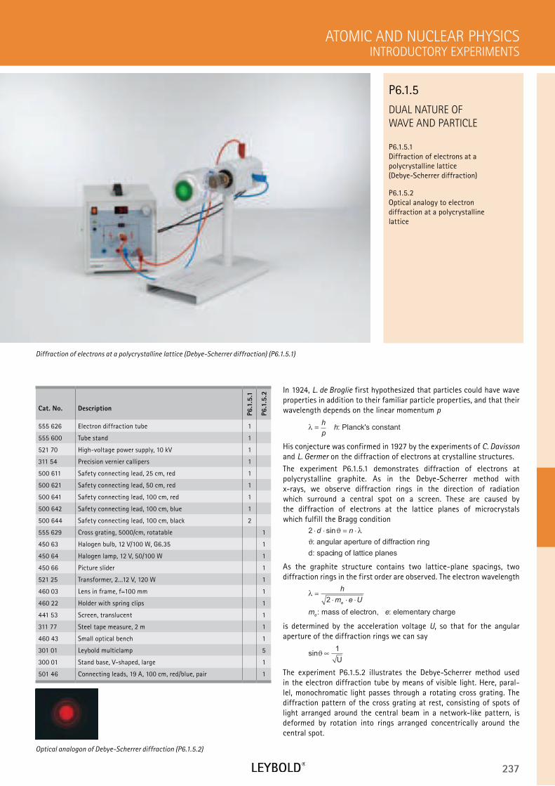
237
DUAL NATURE OF
WAVE AND PARTICLE
P6.1.5.1 Diffraction of electrons at a polycrystalline lattice (Debye-Scherrer diffraction)
P6.1.5.2 Optical analogy to electron diffraction at a polycrystalline lattice
INTRODUCTORY EXPERIMENTS
ATOMIC AND NUCLEAR PHYSICS
Cat. No. Description
P6.1
.5.1
P6.1
.5.2
555 626 Electron diffraction tube 1
555 600 Tube stand 1
521 70 High-voltage power supply, 10 kV 1
311 54 Precision vernier callipers 1
500 611 Safety connecting lead, 25 cm, red 1
500 621 Safety connecting lead, 50 cm, red 1
500 641 Safety connecting lead, 100 cm, red 1
500 642 Safety connecting lead, 100 cm, blue 1
500 644 Safety connecting lead, 100 cm, black 2
555 629 Cross grating, 5000/cm, rotatable 1
450 63 Halogen bulb, 12 V/100 W, G6.35 1
450 64 Halogen lamp, 12 V, 50/100 W 1
450 66 Picture slider 1
521 25 Transformer, 2...12 V, 120 W 1
460 03 Lens in frame, f=100 mm 1
460 22 Holder with spring clips 1
441 53 Screen, translucent 1
311 77 Steel tape measure, 2 m 1
460 43 Small optical bench 1
301 01 Leybold multiclamp 5
300 01 Stand base, V-shaped, large 1
501 46 Connecting leads, 19 A, 100 cm, red/blue, pair 1
In 1924, L. de Broglie first hypothesized that particles could have wave properties in addition to their familiar particle properties, and that their wavelength depends on the linear momentum p
λ =h
ph : Planck's constant
His conjecture was confirmed in 1927 by the experiments of C. Davisson and L. Germer on the diffraction of electrons at crystalline structures.
The experiment P6.1.5.1 demonstrates diffraction of electrons at polycrystalline graphite. As in the Debye-Scherrer method with x-rays, we observe diffraction rings in the direction of radiation which surround a central spot on a screen. These are caused by the diffraction of electrons at the lattice planes of microcrystals which fulfill the Bragg condition
2 ⋅ ⋅ = ⋅d nsinϑ λ
ϑ: angular aperture of diffraction ring
d: spaciing of lattice planes
As the graphite structure contains two lattice-plane spacings, two diffraction rings in the first order are observed. The electron wavelength
λ =⋅ ⋅ ⋅
h
m e U
m e
e
e
2
: mass of electron, : elementary charge
is determined by the acceleration voltage U, so that for the angular aperture of the diffraction rings we can say
sin1
Uϑ ∝
The experiment P6.1.5.2 illustrates the Debye-Scherrer method used in the electron diffraction tube by means of visible light. Here, paral-lel, monochromatic light passes through a rotating cross grating. The diffraction pattern of the cross grating at rest, consisting of spots of light arranged around the central beam in a network-like pattern, is deformed by rotation into rings arranged concentrically around the central spot.
Diffraction of electrons at a polycrystalline lattice (Debye-Scherrer diffraction) (P6.1.5.1)
P6.1.5
Optical analogon of Debye-Scherrer diffraction (P6.1.5.2)
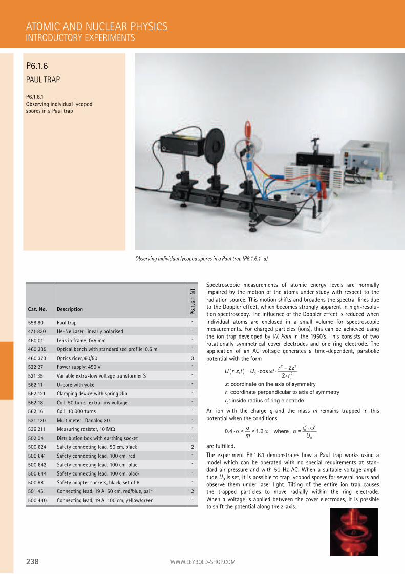
238 WWW.LEYBOLD-SHOP.COM
PAUL TRAP
P6.1.6.1 Observing individual lycopod spores in a Paul trap
Spectroscopic measurements of atomic energy levels are normally impaired by the motion of the atoms under study with respect to the radiation source. This motion shifts and broadens the spectral lines due to the Doppler effect, which becomes strongly apparent in high-resolu-tion spectroscopy. The influence of the Doppler effect is reduced when individual atoms are enclosed in a small volume for spectroscopic measurements. For charged particles (ions), this can be achieved using the ion trap developed by W. Paul in the 1950‘s. This consists of two rotationally symmetrical cover electrodes and one ring electrode. The application of an AC voltage generates a time-dependent, parabolic potential with the form
U r z t U tr z
r
z
, , cos( ) = ⋅ ⋅−
⋅0
2 2
0
2
2
2ω
: coordinate on the axis of ssymmetry
: coordinate perpendicular to axis of symmetryr
r0:: inside radius of ring electrode
An ion with the charge q and the mass m remains trapped in this potential when the conditions
0 4
2
0
. ⋅⋅
α α αω
< < 1.2 where =r0
2q
m U
are fulfilled.
The experiment P6.1.6.1 demonstrates how a Paul trap works using a model which can be operated with no special requirements at stan-dard air pressure and with 50 Hz AC. When a suitable voltage ampli-tude U0 is set, it is possible to trap lycopod spores for several hours and observe them under laser light. Tilting of the entire ion trap causes the trapped particles to move radially within the ring electrode. When a voltage is applied between the cover electrodes, it is possible to shift the potential along the z-axis.
ATOMIC AND NUCLEAR PHYSICS
Observing individual lycopod spores in a Paul trap (P6.1.6.1_a)
Cat. No. Description
P6.1
.6.1
(a)
558 80 Paul trap 1
471 830 He-Ne Laser, linearly polarised 1
460 01 Lens in frame, f=5 mm 1
460 335 Optical bench with standardised profile, 0.5 m 1
460 373 Optics rider, 60/50 3
522 27 Power supply, 450 V 1
521 35 Variable extra-low voltage transformer S 1
562 11 U-core with yoke 1
562 121 Clamping device with spring clip 1
562 18 Coil, 50 turns, extra-low voltage 1
562 16 Coil, 10 000 turns 1
531 120 Multimeter LDanalog 20 1
536 211 Measuring resistor, 10 M 1
502 04 Distribution box with earthing socket 1
500 624 Safety connecting lead, 50 cm, black 2
500 641 Safety connecting lead, 100 cm, red 1
500 642 Safety connecting lead, 100 cm, blue 1
500 644 Safety connecting lead, 100 cm, black 1
500 98 Safety adapter sockets, black, set of 6 1
501 45 Connecting lead, 19 A, 50 cm, red/blue, pair 2
500 440 Connecting lead, 19 A, 100 cm, yellow/green 1
INTRODUCTORY EXPERIMENTS
P6.1.6
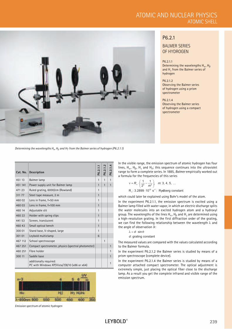
239
BALMER SERIES
OF HYDROGEN
P6.2.1.1 Determining the wavelengths H , H and H from the Balmer series of hydrogen
P6.2.1.2 Observing the Balmer series of hydrogen using a prism spectrometer
P6.2.1.4 Observing the Balmer series of hydrogen using a compact spectrometer
ATOMIC SHELL
ATOMIC AND NUCLEAR PHYSICS
Cat. No. Description
P6.2
.1.1
P6.2
.1.2
P6.2
.1.4
451 13 Balmer lamp 1 1 1
451 141 Power supply unit for Balmer lamp 1 1 1
471 23 Ruled grating, 6000/cm (Rowland) 1
311 77 Steel tape measure, 2 m 1
460 02 Lens in frame, f=50 mm 1
460 03 Lens in frame, f=100 mm 1
460 14 Adjustable slit 1
460 22 Holder with spring clips 1
441 53 Screen, translucent 1
460 43 Small optical bench 1
300 01 Stand base, V-shaped, large 1
301 01 Leybold multiclamp 6
467 112 School spectroscope 1
467 251 Compact spectrometer, physics (spectral photometer) 1
460 251 Fibre holder 1
300 11 Saddle base 1
additionally required: PC with Windows XP/Vista/7/8/10 (x86 or x64)
1
In the visible range, the emission spectrum of atomic hydrogen has four lines, H , H , H and H ; this sequence continues into the ultraviolet range to form a complete series. In 1885, Balmer empirically worked out a formula for the frequencies of this series
ν = ⋅ −
⋅
∞
∞
Rm
m1
2
12 2
,
:
: 3, 4, 5,
R : 3.2899 10 s Ry15 -1
…
ddberg constant
which could later be explained using Bohr’s model of the atom.
In the experiment P6.2.1.1, the emission spectrum is excited using a Balmer lamp filled with water vapor, in which an electric discharge splits the water molecules into an excited hydrogen atom and a hydroxyl group. The wavelengths of the lines H , H and H are determined using a high-resolution grating. In the first diffraction order of the grating, we can find the following relationship between the wavelength and the angle of observation :
λ ϑ= ⋅d
d
sin
: grating constant
The measured values are compared with the values calculated according to the Balmer formula.
In the experiment P6.2.1.2 the Balmer series is studied by means of a prism spectroscope (complete device).
In the experiment P6.2.1.4 the Balmer series is studied by means of a computer attached compact spectrometer. The optical adjustment is extremely simple, just placing the optical fiber close to the discharge lamp. As a result you get the complete infrared and visible range of the emission spectrum.
Determining the wavelengths Ha, H and H from the Balmer series of hydrogen (P6.2.1.1)
P6.2.1
Emission spectrum of atomic hydrogen
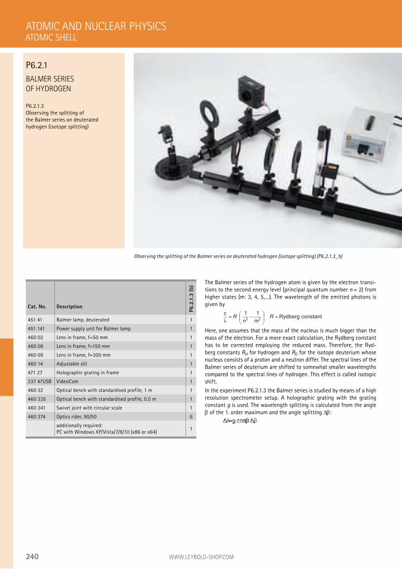
240 WWW.LEYBOLD-SHOP.COM
BALMER SERIES
OF HYDROGEN
P6.2.1.3 Observing the splitting of the Balmer series on deuterated hydrogen (isotope splitting)
The Balmer series of the hydrogen atom is given by the electron transi-tions to the second energy level (principal quantum number n = 2) from higher states (m: 3, 4, 5,...). The wavelength of the emitted photons is given by
cR
n mR
λ= −
= Rydberg constant
1 12 2
Here, one assumes that the mass of the nucleus is much bigger than the mass of the electron. For a more exact calculation, the Rydberg constant has to be corrected employing the reduced mass. Therefore, the Ryd-berg constants RH for hydrogen and RD for the isotope deuterium whose nucleus consists of a proton and a neutron differ. The spectral lines of the Balmer series of deuterium are shifted to somewhat smaller wavelengths compared to the spectral lines of hydrogen. This effect is called isotopic shift.
In the experiment P6.2.1.3 the Balmer series is studied by means of a high resolution spectrometer setup. A holographic grating with the grating constant g is used. The wavelength splitting is calculated from the angle
of the 1. order maximum and the angle splitting :
ATOMIC AND NUCLEAR PHYSICS
Observing the splitting of the Balmer series on deuterated hydrogen (isotope splitting) (P6.2.1.3_b)
Cat. No. Description
P6.2
.1.3
(b)
451 41 Balmer lamp, deuterated 1
451 141 Power supply unit for Balmer lamp 1
460 02 Lens in frame, f=50 mm 1
460 08 Lens in frame, f=150 mm 1
460 09 Lens in frame, f=300 mm 1
460 14 Adjustable slit 1
471 27 Holographic grating in frame 1
337 47USB VideoCom 1
460 32 Optical bench with standardised profile, 1 m 1
460 335 Optical bench with standardised profile, 0.5 m 1
460 341 Swivel joint with circular scale 1
460 374 Optics rider, 90/50 6
additionally required: PC with Windows XP/Vista/7/8/10 (x86 or x64)
1
ATOMIC SHELL
P6.2.1
241
EMISSION AND
ABSORPTION SPECTRA
P6.2.2.1 Displaying the spectral lines of inert gases and metal vapors
P6.2.2.2 Qualitative investigation of the absorption spectrum of sodium
ATOMIC SHELL
ATOMIC AND NUCLEAR PHYSICS
Cat. No. Description
P6.2
.2.1
P6.2
.2.2
451 011 Spectral lamp, Ne 1
451 041 Spectral lamp, Cd 1
451 062 Spectral lamp, Hg 100 1
451 111 Spectral lamp, Na 1 1
451 16 Housing for spectral lamps 1 1
451 30 Universal choke, 230 V, 50 Hz 1 1
471 23 Ruled grating, 6000/cm (Rowland) 1
311 77 Steel tape measure, 2 m 1
460 02 Lens in frame, f=50 mm 1
460 03 Lens in frame, f=100 mm 1
460 14 Adjustable slit 1
460 22 Holder with spring clips 1
441 53 Screen, translucent 1 1
460 43 Small optical bench 1
300 01 Stand base, V-shaped, large 1
301 01 Leybold multiclamp 6 2
450 60 Lamp housing with cable 1
450 511 Bulbs, 6 V/30 W, E14, set of 2 1
521 210 Transformer, 6/12 V 1
300 02 Stand base, V-shaped, small 2
300 11 Saddle base 1
300 42 Stand rod, 47 cm, 12 mm diam. 2
666 711 Butane gas burner 1
666 712ET3 Butane cartridge, 190 g, set of 3 1
666 962 Double-ended spatula, stainless steel, 150 mm 1
673 0840 Magnesia rods, 25 pieces 1
673 5700 Sodium chloride, 250 g 1
When an electron in the shell of an atom or atomic ion drops from an excited state with the energy E2 to a state of lower energy E1, it can emit a photon with the frequency
ν =−E E
h
h
2 1
: Planck's constant
In the opposite case, a photon with the same frequency is absorbed. As the energies E1 and E2 can only assume discrete values, the photons are only emitted and absorbed at discrete frequencies. The totality of the frequencies which occur is referred to as the spectrum of the atom. The positions of the spectral lines are characteristic of the corresponding element.
The experiment P6.2.2.1 disperses the emission spectra of metal vapors and inert gases (mercury, sodium, cadmium and neon) using a high- resolution grating and projects these on the screen for comparison purposes.
In the experiment P6.2.2.2, the flame of a Bunsen burner is alternately illuminated with white light and sodium light and observed on a screen. When sodium is burned in the flame, a dark shadow appears on the screen when illuminating with sodium light. From this it is possible to conclu-de that the light emitted by a sodium lamp is absorbed by the sodium vapor, and that the same atomic components are involved in both absorption and emission.
Displaying the spectral lines of inert gases and metal vapors (P6.2.2.1)
P6.2.2
Emission spectra
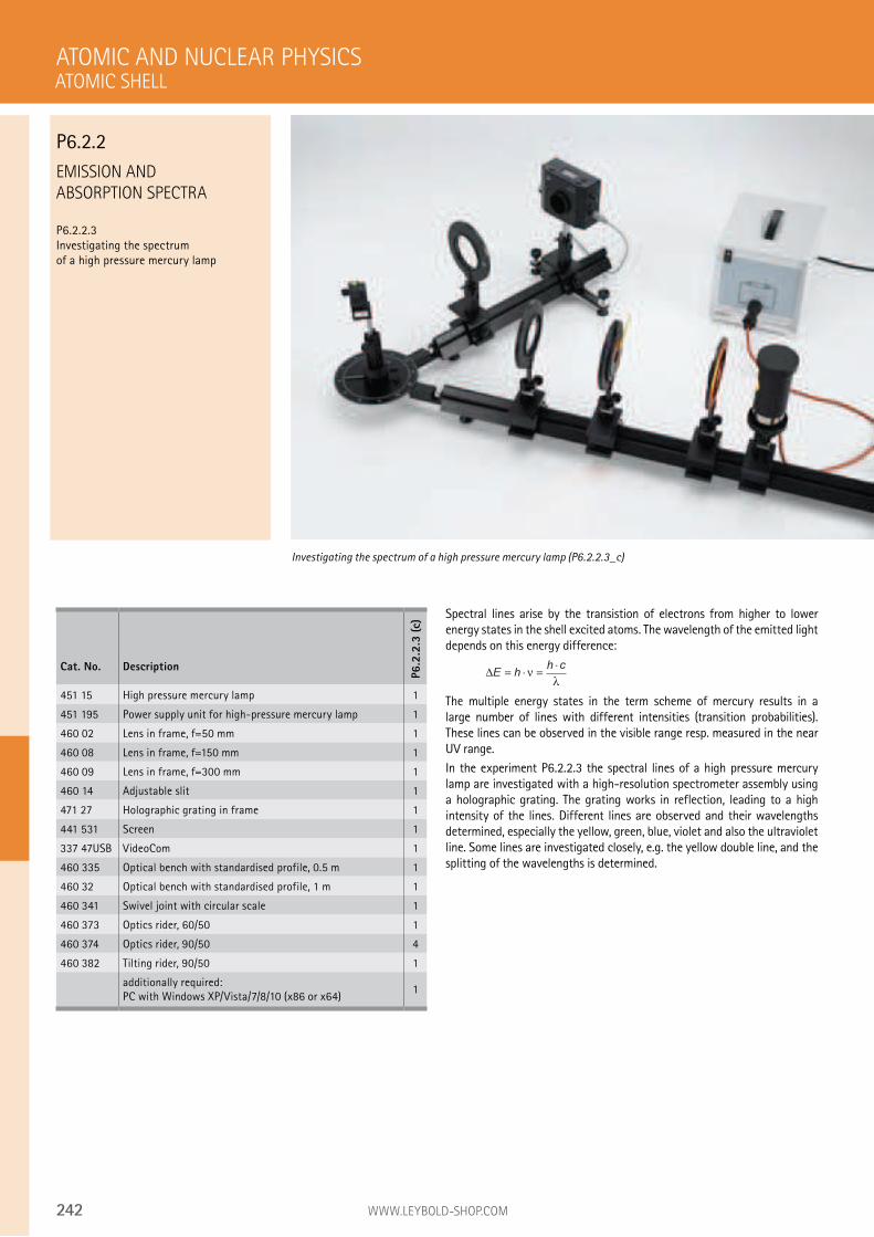
242 WWW.LEYBOLD-SHOP.COM
EMISSION AND
ABSORPTION SPECTRA
P6.2.2.3 Investigating the spectrum of a high pressure mercury lamp
Spectral lines arise by the transistion of electrons from higher to lower energy states in the shell excited atoms. The wavelength of the emitted light depends on this energy difference:
∆E hh c
= ⋅ =⋅
νλ
The multiple energy states in the term scheme of mercury results in a large number of lines with different intensities (transition probabilities). These lines can be observed in the visible range resp. measured in the near UV range.
In the experiment P6.2.2.3 the spectral lines of a high pressure mercury lamp are investigated with a high-resolution spectrometer assembly using a holographic grating. The grating works in reflection, leading to a high intensity of the lines. Different lines are observed and their wavelengths determined, especially the yellow, green, blue, violet and also the ultraviolet line. Some lines are investigated closely, e.g. the yellow double line, and the splitting of the wavelengths is determined.
ATOMIC AND NUCLEAR PHYSICS
Investigating the spectrum of a high pressure mercury lamp (P6.2.2.3_c)
Cat. No. Description
P6.2
.2.3
(c)
451 15 High pressure mercury lamp 1
451 195 Power supply unit for high-pressure mercury lamp 1
460 02 Lens in frame, f=50 mm 1
460 08 Lens in frame, f=150 mm 1
460 09 Lens in frame, f=300 mm 1
460 14 Adjustable slit 1
471 27 Holographic grating in frame 1
441 531 Screen 1
337 47USB VideoCom 1
460 335 Optical bench with standardised profile, 0.5 m 1
460 32 Optical bench with standardised profile, 1 m 1
460 341 Swivel joint with circular scale 1
460 373 Optics rider, 60/50 1
460 374 Optics rider, 90/50 4
460 382 Tilting rider, 90/50 1
additionally required: PC with Windows XP/Vista/7/8/10 (x86 or x64)
1
ATOMIC SHELL
P6.2.2
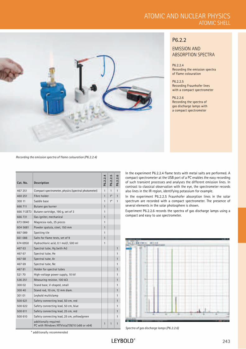
243
EMISSION AND
ABSORPTION SPECTRA
P6.2.2.4 Recording the emission spectra of flame colouration
P6.2.2.5 Recording Fraunhofer lines with a compact spectrometer
P6.2.2.6 Recording the spectra of gas discharge lamps with a compact spectrometer
ATOMIC SHELL
ATOMIC AND NUCLEAR PHYSICS
Cat. No. Description
P6.2
.2.4
P6.2
.2.5
P6.2
.2.6
467 251 Compact spectrometer, physics (spectral photometer) 1 1 1
460 251 Fibre holder 1 1* 1
300 11 Saddle base 1 1* 1
666 711 Butane gas burner 1
666 712ET3 Butane cartridge, 190 g, set of 3 1
666 731 Gas igniter, mechanical 1
673 0840 Magnesia rods, 25 pieces 1
604 5681 Powder spatula, steel, 150 mm 1
667 089 Spotting tile 1
661 088 Salts for flame tests, set of 9 1
674 6950 Hydrochloric acid, 0.1 mol/l, 500 ml 1
467 63 Spectral tube, Hg (with Ar) 1
467 67 Spectral tube, He 1
467 68 Spectral tube, Ar 1
467 69 Spectral tube, Ne 1
467 81 Holder for spectral tubes 1
521 70 High-voltage power supply, 10 kV 1
536 251 Measuring resistor, 100 k 1
300 02 Stand base, V-shaped, small 1
300 40 Stand rod, 10 cm, 12 mm diam. 1
301 01 Leybold multiclamp 1
500 621 Safety connecting lead, 50 cm, red 1
500 622 Safety connecting lead, 50 cm, blue 1
500 611 Safety connecting lead, 25 cm, red 1
500 610 Safety connecting lead, 25 cm, yellow/green 1
additionally required: PC with Windows XP/Vista/7/8/10 (x86 or x64)
1 1 1
* additionally recommended
In the experiment P6.2.2.4 flame tests with metal salts are performed. A compact spectrometer at the USB port of a PC enables the easy recording of such transient processes and analyses the different emission lines. In contrast to classical observation with the eye, the spectrometer records also lines in the IR region, identifying potassium for example.
In the experiment P6.2.2.5 Fraunhofer absorption lines in the solar spectrum are recorded with a compact spectrometer. The presence of several elements in the solar photosphere is shown.
Experiment P6.2.2.6 records the spectra of gas discharge lamps using a compact and easy to use spectrometer.
Recording the emission spectra of flame colouration (P6.2.2.4)
P6.2.2
Spectra of gas discharge lamps (P6.2.2.6)
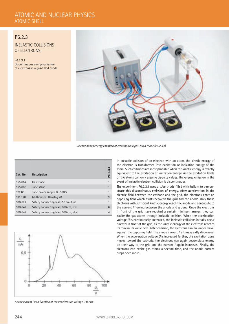
244 WWW.LEYBOLD-SHOP.COM
INELASTIC COLLISIONS
OF ELECTRONS
P6.2.3.1
Discontinuous energy emission
of electrons in a gas-filled triode
In inelastic collision of an electron with an atom, the kinetic energy of
the electron is transformed into excitation or ionization energy of the
atom. Such collisions are most probable when the kinetic energy is exactly
equivalent to the excitation or ionization energy. As the excitation levels
of the atoms can only assume discrete values, the energy emission in the
event of inelastic electron collision is discontinuous.
The experiment P6.2.3.1 uses a tube triode filled with helium to demon-
strate this discontinuous emission of energy. After acceleration in the
electric field between the cathode and the grid, the electrons enter an
opposing field which exists between the grid and the anode. Only those
electrons with sufficient kinetic energy reach the anode and contribute to
the current I flowing between the anode and ground. Once the electrons
in front of the grid have reached a certain minimum energy, they can
excite the gas atoms through inelastic collision. When the acceleration
voltage U is continuously increased, the inelastic collisions initially occur
directly in front of the grid, as the kinetic energy of the electrons reaches
its maximum value here. After collision, the electrons can no longer travel
against the opposing field. The anode current I is thus greatly decreased.
When the acceleration voltage U is increased further, the excitation zone
moves toward the cathode, the electrons can again accumulate energy
on their way to the grid and the current I again increases. Finally, the
electrons can excite gas atoms a second time, and the anode current
drops once more.
ATOMIC AND NUCLEAR PHYSICS
Discontinuous energy emission of electrons in a gas-filled triode (P6.2.3.1)
Cat. No. Description
P6.2
.3.1
555 614 Gas triode 1
555 600 Tube stand 1
521 65 Tube power supply, 0...500 V 1
531 120 Multimeter LDanalog 20 3
500 622 Safety connecting lead, 50 cm, blue 1
500 641 Safety connecting lead, 100 cm, red 6
500 642 Safety connecting lead, 100 cm, blue 4
Anode current I as a function of the acceleration voltage U for He
ATOMIC SHELL
P6.2.3
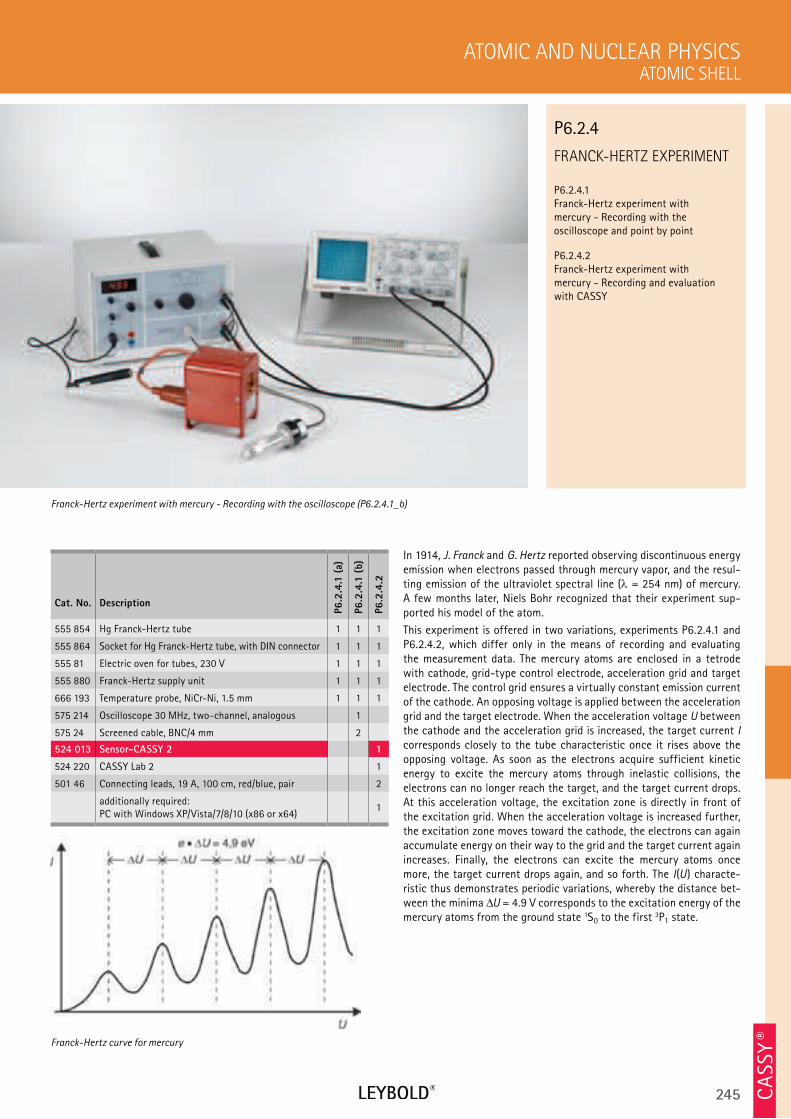
245
FRANCK-HERTZ EXPERIMENT
P6.2.4.1 Franck-Hertz experiment with mercury - Recording with the oscilloscope and point by point
P6.2.4.2 Franck-Hertz experiment with mercury - Recording and evaluation with CASSY
ATOMIC SHELL
ATOMIC AND NUCLEAR PHYSICS
Cat. No. Description
P6.2
.4.1
(a)
P6.2
.4.1
(b)
P6.2
.4.2
555 854 Hg Franck-Hertz tube 1 1 1
555 864 Socket for Hg Franck-Hertz tube, with DIN connector 1 1 1
555 81 Electric oven for tubes, 230 V 1 1 1
555 880 Franck-Hertz supply unit 1 1 1
666 193 Temperature probe, NiCr-Ni, 1.5 mm 1 1 1
575 214 Oscilloscope 30 MHz, two-channel, analogous 1
575 24 Screened cable, BNC/4 mm 2
524 013 Sensor-CASSY 2 1
524 220 CASSY Lab 2 1
501 46 Connecting leads, 19 A, 100 cm, red/blue, pair 2
additionally required: PC with Windows XP/Vista/7/8/10 (x86 or x64)
1
In 1914, J. Franck and G. Hertz reported observing discontinuous energy emission when electrons passed through mercury vapor, and the resul-ting emission of the ultraviolet spectral line ( = 254 nm) of mercury. A few months later, Niels Bohr recognized that their experiment sup-ported his model of the atom.
This experiment is offered in two variations, experiments P6.2.4.1 and P6.2.4.2, which differ only in the means of recording and evaluating the measurement data. The mercury atoms are enclosed in a tetrode with cathode, grid-type control electrode, acceleration grid and target electrode. The control grid ensures a virtually constant emission current of the cathode. An opposing voltage is applied between the acceleration grid and the target electrode. When the acceleration voltage U between the cathode and the acceleration grid is increased, the target current I corresponds closely to the tube characteristic once it rises above the opposing voltage. As soon as the electrons acquire sufficient kinetic energy to excite the mercury atoms through inelastic collisions, the electrons can no longer reach the target, and the target current drops. At this acceleration voltage, the excitation zone is directly in front of the excitation grid. When the acceleration voltage is increased further, the excitation zone moves toward the cathode, the electrons can again accumulate energy on their way to the grid and the target current again increases. Finally, the electrons can excite the mercury atoms once more, the target current drops again, and so forth. The I(U) characte-ristic thus demonstrates periodic variations, whereby the distance bet-ween the minima U = 4.9 V corresponds to the excitation energy of the mercury atoms from the ground state 1S0 to the first 3P1 state.
Franck-Hertz experiment with mercury - Recording with the oscilloscope (P6.2.4.1_b)
P6.2.4
Franck-Hertz curve for mercury
CA
SSY ®
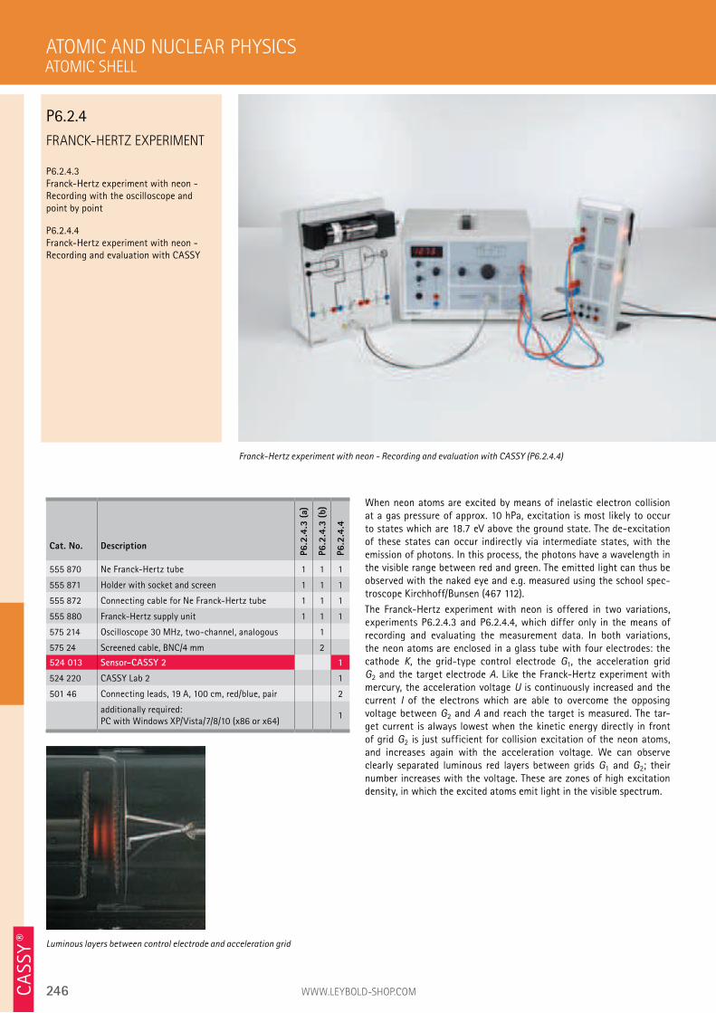
246 WWW.LEYBOLD-SHOP.COM
FRANCK-HERTZ EXPERIMENT
P6.2.4.3 Franck-Hertz experiment with neon - Recording with the oscilloscope and point by point
P6.2.4.4 Franck-Hertz experiment with neon - Recording and evaluation with CASSY
When neon atoms are excited by means of inelastic electron collision at a gas pressure of approx. 10 hPa, excitation is most likely to occur to states which are 18.7 eV above the ground state. The de-excitation of these states can occur indirectly via intermediate states, with the emission of photons. In this process, the photons have a wavelength in the visible range between red and green. The emitted light can thus be observed with the naked eye and e.g. measured using the school spec-troscope Kirchhoff/Bunsen (467 112).
The Franck-Hertz experiment with neon is offered in two variations, experiments P6.2.4.3 and P6.2.4.4, which differ only in the means of recording and evaluating the measurement data. In both variations, the neon atoms are enclosed in a glass tube with four electrodes: the cathode K, the grid-type control electrode G1, the acceleration grid G2 and the target electrode A. Like the Franck-Hertz experiment with mercury, the acceleration voltage U is continuously increased and the current I of the electrons which are able to overcome the opposing voltage between G2 and A and reach the target is measured. The tar-get current is always lowest when the kinetic energy directly in front of grid G2 is just sufficient for collision excitation of the neon atoms, and increases again with the acceleration voltage. We can observe clearly separated luminous red layers between grids G1 and G2; their number increases with the voltage. These are zones of high excitation density, in which the excited atoms emit light in the visible spectrum.
ATOMIC AND NUCLEAR PHYSICS
Franck-Hertz experiment with neon - Recording and evaluation with CASSY (P6.2.4.4)
Cat. No. Description
P6.2
.4.3
(a)
P6.2
.4.3
(b)
P6.2
.4.4
555 870 Ne Franck-Hertz tube 1 1 1
555 871 Holder with socket and screen 1 1 1
555 872 Connecting cable for Ne Franck-Hertz tube 1 1 1
555 880 Franck-Hertz supply unit 1 1 1
575 214 Oscilloscope 30 MHz, two-channel, analogous 1
575 24 Screened cable, BNC/4 mm 2
524 013 Sensor-CASSY 2 1
524 220 CASSY Lab 2 1
501 46 Connecting leads, 19 A, 100 cm, red/blue, pair 2
additionally required: PC with Windows XP/Vista/7/8/10 (x86 or x64)
1
Luminous layers between control electrode and acceleration grid
ATOMIC SHELL
P6.2.4
CA
SSY ®
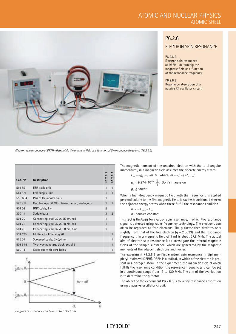
247
ELECTRON SPIN RESONANCE
P6.2.6.2 Electron spin resonance at DPPH - determinig the magnetic field as a function of the resonance frequency
P6.2.6.3 Resonance absorption of a passive RF oscillator circuit
ATOMIC SHELL
ATOMIC AND NUCLEAR PHYSICS
Cat. No. Description
P6.2
.6.2
P6.2
.6.3
514 55 ESR basic unit 1 1
514 571 ESR supply unit 1 1
555 604 Pair of Helmholtz coils 1
575 214 Oscilloscope 30 MHz, two-channel, analogous 1 1
501 02 BNC cable, 1 m 2
300 11 Saddle base 3 2
501 20 Connecting lead, 32 A, 25 cm, red 1
501 25 Connecting lead, 32 A, 50 cm, red 1
501 26 Connecting lead, 32 A, 50 cm, blue 1
531 120 Multimeter LDanalog 20 1
575 24 Screened cable, BNC/4 mm 1
501 644 Two-way adapters, black, set of 6 1
590 13 Stand rod with bore holes 1
The magnetic moment of the unpaired electron with the total angular momentum j in a magnetic field assumes the discrete energy states
E g m B m j j jm j B
B
where
J
T Boh
= − ⋅ ⋅ ⋅ = − − +
= ⋅ −
µ
µ
, , ,
. :
1
9 274 10 24
…
rr's magneton
: factorjg g
When a high-frequency magnetic field with the frequency is applied perpendicularly to the first magnetic field, it excites transitions between the adjacent energy states when these fulfill the resonance condition
h E E
h
⋅ = −νm+1 m
: Planck's constant
This fact is the basis for electron spin resonance, in which the resonance signal is detected using radio-frequency technology. The electrons can often be regarded as free electrons. The g-factor then deviates only slightly from that of the free electron (g = 2.0023), and the resonance frequency in a magnetic field of 1 mT is about 27.8 MHz. The actual aim of electron spin resonance is to investigate the internal magnetic fields of the sample substance, which are generated by the magnetic moments of the adjacent electrons and nuclei.
The experiment P6.2.6.2 verifies electron spin resonance in diphenyl-picryl-hydrazyl (DPPH). DPPH is a radical, in which a free electron is pre-sent in a nitrogen atom. In the experiment, the magnetic field B which fulfills the resonance condition the resonance frequencies can be set in a continuous range from 13 to 130 MHz. The aim of the eva-luation is to determine the g factor.
The object of the experiment P6.2.6.3 is to verify resonance absorption using a passive oscillator circuit.
Electron spin resonance at DPPH - determinig the magnetic field as a function of the resonance frequency (P6.2.6.2)
P6.2.6
Diagram of resonance condition of free electrons
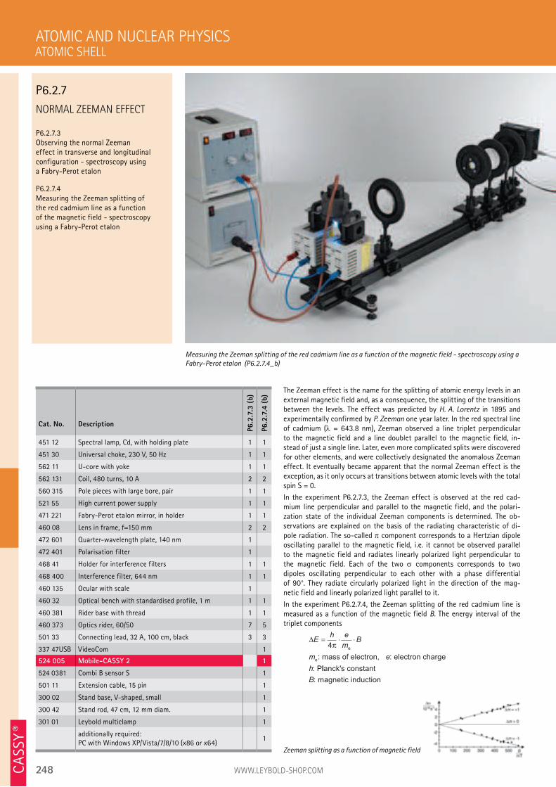
248 WWW.LEYBOLD-SHOP.COM
NORMAL ZEEMAN EFFECT
P6.2.7.3 Observing the normal Zeeman effect in transverse and longitudinal configuration - spectroscopy using a Fabry-Perot etalon
P6.2.7.4 Measuring the Zeeman splitting of the red cadmium line as a function of the magnetic field - spectroscopy using a Fabry-Perot etalon
The Zeeman effect is the name for the splitting of atomic energy levels in an external magnetic field and, as a consequence, the splitting of the transitions between the levels. The effect was predicted by H. A. Lorentz in 1895 and experimentally confirmed by P. Zeeman one year later. In the red spectral line of cadmium ( = 643.8 nm), Zeeman observed a line triplet perpendicular to the magnetic field and a line doublet parallel to the magnetic field, in-stead of just a single line. Later, even more complicated splits were discovered for other elements, and were collectively designated the anomalous Zeeman effect. It eventually became apparent that the normal Zeeman effect is the exception, as it only occurs at transitions between atomic levels with the total spin S = 0.
In the experiment P6.2.7.3, the Zeeman effect is observed at the red cad- mium line perpendicular and parallel to the magnetic field, and the polari-zation state of the individual Zeeman components is determined. The ob-servations are explained on the basis of the radiating characteristic of di-pole radiation. The so-called component corresponds to a Hertzian dipole oscillating parallel to the magnetic field, i.e. it cannot be observed parallel to the magnetic field and radiates linearly polarized light perpendicular to the magnetic field. Each of the two components corresponds to two dipoles oscillating perpendicular to each other with a phase differential of 90°. They radiate circularly polarized light in the direction of the mag- netic field and linearly polarized light parallel to it.
In the experiment P6.2.7.4, the Zeeman splitting of the red cadmium line is measured as a function of the magnetic field B. The energy interval of the triplet components
∆Eh e
mB
m e
h
= ⋅ ⋅4π e
e: mass of electron, : electron charge
: Pllanck's constant
: magnetic inductionB
ATOMIC AND NUCLEAR PHYSICS
Measuring the Zeeman splitting of the red cadmium line as a function of the magnetic field - spectroscopy using a
Fabry-Perot etalon (P6.2.7.4_b)
Cat. No. Description
P6.2
.7.3
(b)
P6.2
.7.4
(b)
451 12 Spectral lamp, Cd, with holding plate 1 1
451 30 Universal choke, 230 V, 50 Hz 1 1
562 11 U-core with yoke 1 1
562 131 Coil, 480 turns, 10 A 2 2
560 315 Pole pieces with large bore, pair 1 1
521 55 High current power supply 1 1
471 221 Fabry-Perot etalon mirror, in holder 1 1
460 08 Lens in frame, f=150 mm 2 2
472 601 Quarter-wavelength plate, 140 nm 1
472 401 Polarisation filter 1
468 41 Holder for interference filters 1 1
468 400 Interference filter, 644 nm 1 1
460 135 Ocular with scale 1
460 32 Optical bench with standardised profile, 1 m 1 1
460 381 Rider base with thread 1 1
460 373 Optics rider, 60/50 7 5
501 33 Connecting lead, 32 A, 100 cm, black 3 3
337 47USB VideoCom 1
524 005 Mobile-CASSY 2 1
524 0381 Combi B sensor S 1
501 11 Extension cable, 15 pin 1
300 02 Stand base, V-shaped, small 1
300 42 Stand rod, 47 cm, 12 mm diam. 1
301 01 Leybold multiclamp 1
additionally required: PC with Windows XP/Vista/7/8/10 (x86 or x64)
1
Zeeman splitting as a function of magnetic field
ATOMIC SHELL
P6.2.7
CA
SSY ®
249
OPTICAL PUMPING
(ANOMALOUS ZEEMAN EFFECT)
P6.2.8.1 Optical pumping: observing the relaxation signal
P6.2.8.2 Optical pumping: measuring and observing the Zeeman transitions in the ground states of Rb-87 with +- and --pumped light
P6.2.8.3 Optical pumping: measuring and observing the Zeeman transitions in the ground states of Rb-85 with +- and --pumped light
P6.2.8.4 Optical pumping: measuring and observing the Zeeman transitions in the ground states of Rb-87 as a function of the magnetic flux density B
P6.2.8.5 Optical pumping: measuring and observing the Zeeman transitions in the ground states of Rb-85 as a function of the magnetic flux density B
P6.2.8.6 Optical pumping: measuring and observing two-quantum transitions
ATOMIC SHELLATOMIC AND NUCLEAR PHYSICS
Cat. No. Description
P6.2
.8.1
P6.2
.8.2
-6
558 823 Rubidium high-frequency lamp 1 1
558 826 Helmholtz coils on rider 1 1
558 833 Absorption chamber with Rb cell 1 1
558 835 Silicon photodetector 1 1
558 836 I/U converter for silicon photodetector 1 1
530 88 Plug-in power unit, 230 V/9.2 V DC 1 1
558 814 Supply unit for optical pumping 1 1
521 45 DC power supply 0...±15 V 1 1
501 02 BNC cable, 1 m 2 3
575 230 Digital storage oscilloscope 722 1 1
531 282 Multimeter Metrahit Pro 1 1
504 48 Two-way switch 1 1
468 000 Line filter, 795 nm 1 1
472 410 Polarisation filter for red radiation 1 1
472 611 Quarter-wavelength plate, 200 nm 1 1
460 021 Lens in frame, f=50 mm 1 1
460 031 Lens in frame, f=100 mm 1 1
460 32 Optical bench with standardised profile, 1 m 1 1
460 370 Optics rider, 60/34 6 6
460 374 Optics rider, 90/50 1 1
666 7681 Circulation thermostat SC 100-S5P 1 1
688 115 Silicone tubing 6 x 2 mm, 5.0 m 1 1
501 28 Connecting lead, 32 A, 50 cm, black 4 4
501 38 Connecting lead, 32 A, 200 cm, black 2 2
675 3410 Water, pure, 5 l 2 2
522 551 Function generator, 1 mHz to 12 MHZ, internal sweep 1
501 022 BNC cable, 2 m 1
The two hyperfine structures of the ground state of an alkali atom with the total angular momentums
F I F I+ −= + = −
1
2
1
2,
split in a magnetic field B into 2F± + 1 Zeeman levels having an energy which can be described using the Breit-Rabi formula
EE
Igm
E m
I
g g
EB
=−
+( )+ ± +
++
=−
⋅
∆ ∆
∆
∆
2 2 1 21
4
2 1
2µ ξ ξ
ξµ µ
K I FF
J B I Kwhere
EE
I m
: hyperfine structure interval
: nuclear spin, : magF nnetic quantum number
: Bohr's magneton, : nuclear maB Kµ µ ggneton
: shell g factor, : nuclear g factorJ Ig g
Transitions between the Zeeman levels can be observed using a method developed by A. Kastler. When right-handed or left-handed circularly polarized light is directed parallel to the magnetic field, the population of the Zeeman level differs from the thermal equilibrium population, i.e. optical pumping occurs, and RF radiation forces transitions between the Zeeman levels.
The change in the equilibrium population when switching from right-handed to left-handed circular pumped light is verified in the experiment P6.2.8.1.
The experiments P6.2.8.2 and P6.2.8.3 measure the Zeeman transitions in the ground state of the isotopes Rb-87 and Rb-85 and determine the nuclear spin I from the number of transitions observed. The observed transitions are classified through comparison with the Breit-Rabi formula.
In the experiments P6.2.8.4 and P6.2.8.5, the measured transition frequencies are used for precise determination of the magnetic field B as a function of the magnet current I. The nuclear g factors gI are derived using the measurement data.
In the experiment P6.2.8.6, two-quantum transitions are induced and observed for a high field strength of the irradiating RF field.
Optical pumping: measuring and observing the Zeeman transitions in the ground states of Rb-87 with +- and --pumped light (P6.2.8.2)
P6.2.8
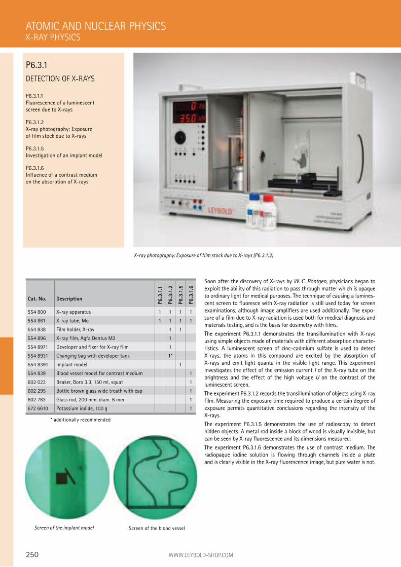
250 WWW.LEYBOLD-SHOP.COM
DETECTION OF X-RAYS
P6.3.1.1
Fluorescence of a luminescent
screen due to X-rays
P6.3.1.2
X-ray photography: Exposure
of film stock due to X-rays
P6.3.1.5
Investigation of an implant model
P6.3.1.6
Influence of a contrast medium
on the absorption of X-rays
Soon after the discovery of X-rays by W. C. Röntgen, physicians began to
exploit the ability of this radiation to pass through matter which is opaque
to ordinary light for medical purposes. The technique of causing a lumines-
cent screen to fluoresce with X-ray radiation is still used today for screen
examinations, although image amplifiers are used additionally. The expo-
sure of a film due to X-ray radiation is used both for medical diagnosis and
materials testing, and is the basis for dosimetry with films.
The experiment P6.3.1.1 demonstrates the transillumination with X-rays
using simple objects made of materials with different absorption characte-
ristics. A luminescent screen of zinc-cadmium sulfate is used to detect
X-rays; the atoms in this compound are excited by the absorption of
X-rays and emit light quanta in the visible light range. This experiment
investigates the effect of the emission current I of the X-ray tube on the
brightness and the effect of the high voltage U on the contrast of the
luminescent screen.
The experiment P6.3.1.2 records the transillumination of objects using X-ray
film. Measuring the exposure time required to produce a certain degree of
exposure permits quantitative conclusions regarding the intensity of the
X-rays.
The experiment P6.3.1.5 demonstrates the use of radioscopy to detect
hidden objects. A metal rod inside a block of wood is visually invisible, but
can be seen by X-ray fluorescence and its dimensions measured.
The experiment P6.3.1.6 demonstrates the use of contrast medium. The
radiopaque iodine solution is flowing through channels inside a plate
and is clearly visible in the X-ray fluorescence image, but pure water is not.
ATOMIC AND NUCLEAR PHYSICS
X-ray photography: Exposure of film stock due to X-rays (P6.3.1.2)
Cat. No. Description
P6.3
.1.1
P6.3
.1.2
P6.3
.1.5
P6.3
.1.6
554 800 X-ray apparatus 1 1 1 1
554 861 X-ray tube, Mo 1 1 1 1
554 838 Film holder, X-ray 1 1
554 896 X-ray film, Agfa Dentus M2 1
554 8971 Developer and fixer for X-ray film 1
554 8931 Changing bag with developer tank 1*
554 8391 Implant model 1
554 839 Blood vessel model for contrast medium 1
602 023 Beaker, Boro 3.3, 150 ml, squat 1
602 295 Bottle brown glass wide treath with cap 1
602 783 Glass rod, 200 mm, diam. 6 mm 1
672 6610 Potassium iodide, 100 g 1
* additionally recommended
Screen of the implant model
X-RAY PHYSICS
P6.3.1
Screen of the blood vessel
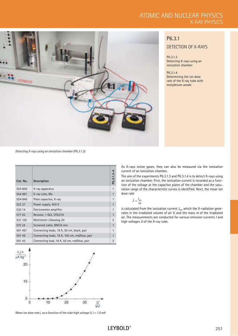
251
DETECTION OF X-RAYS
P6.3.1.3 Detecting X-rays using an ionization chamber
P6.3.1.4 Determining the ion dose rate of the X-ray tube with molydenum anode
X-RAY PHYSICS
ATOMIC AND NUCLEAR PHYSICS
Cat. No. Description
P6.3
.1.3
-4
554 800 X-ray apparatus 1
554 861 X-ray tube, Mo 1
554 840 Plate capacitor, X-ray 1
522 27 Power supply, 450 V 1
532 14 Electrometer amplifier 1
577 02 Resistor, 1 G , STE2/19 1
531 120 Multimeter LDanalog 20 2
575 24 Screened cable, BNC/4 mm 1
501 451 Connecting leads, 19 A, 50 cm, black, pair 1
501 46 Connecting leads, 19 A, 100 cm, red/blue, pair 1
501 45 Connecting lead, 19 A, 50 cm, red/blue, pair 2
As X-rays ionize gases, they can also be measured via the ionization current of an ionization chamber.
The aim of the experiments P6.3.1.3 and P6.3.1.4 is to detect X-rays using an ionization chamber. First, the ionization current is recorded as a func-tion of the voltage at the capacitor plates of the chamber and the satu-ration range of the characteristic curves is identified. Next, the mean ion dose rate
JI
m
ion
is calculated from the ionization current Iion which the X-radiation gene-rates in the irradiated volume of air V, and the mass m of the irradiated air. The measurements are conducted for various emission currents I and high voltages U of the X-ray tube.
Detecting X-rays using an ionization chamber (P6.3.1.3)
P6.3.1
Mean ion dose rate j as a function of the tube high voltage U, I = 1.0 mA
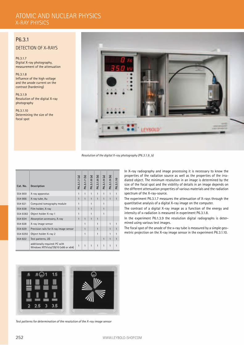
252 WWW.LEYBOLD-SHOP.COM
DETECTION OF X-RAYS
P6.3.1.7 Digital X-ray photography, measurement of the attenuation
P6.3.1.8 Influence of the high voltage and the anode current on the contrast (hardening)
P6.3.1.9 Resolution of the digital X-ray photography
P6.3.1.10 Determining the size of the focal spot
In X-ray radiography and image processing it is necessary to know the properties of the radiation source as well as the properties of the irra-diated object. The minimum resolution in an image is determined by the size of the focal spot and the visbility of details in an image depends on the different attenuation properties of various materials and the radiation spectrum of the X-ray-source.
The experiment P6.3.1.7 measures the attenuation of X-rays through the quantitative analysis of a digital X-ray image on the computer.
The contrast of a digital X-ray image as a function of the energy and intensity of x-radiation is measured in experiment P6.3.1.8.
In the experiment P6.1.3.9 the resolution digital radiographs is deter-mined using various test images.
The focal spot of the anode of the x-ray tube is measured by a simple geo-metric projection on the X-ray image sensor in the experiment P6.3.1.10.
ATOMIC AND NUCLEAR PHYSICS
Resolution of the digital X-ray photography (P6.3.1.9_b)
Cat. No. Description
P6.3
.1.7
(a)
P6.3
.1.7
(b)
P6.3
.1.8
(a)
P6.3
.1.8
(b)
P6.3
.1.9
(a)
P6.3
.1.9
(b)
P6.3
.1.1
0
554 800 X-ray apparatus 1 1 1 1 1 1 1
554 866 X-ray tube, Au 1 1 1 1 1 1 1
554 821 Computed tomography module 1 1 1
554 838 Film holder, X-ray 1 1 1
554 8382 Object holder X-ray 1 1 1 1
554 834 Absorption accessory, X-ray 1 1 1 1
554 828 X-ray image sensor 1 1 1 1
554 829 Precision rails for X-ray image sensor 1 1 1 1
554 8292 Object holder X-ray 2 1 1 1 1
554 822 Test patterns, 2D 1 1 1
additionally required: PC with Windows XP/Vista/7/8/10 (x86 or x64)
1 1 1 1 1 1 1
Test patterns for determination of the resolution of the X-ray image sensor
X-RAY PHYSICS
P6.3.1
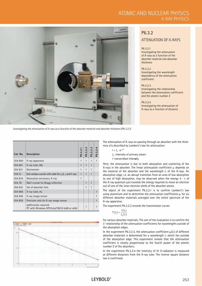
253
ATTENUATION OF X-RAYS
P6.3.2.1 Investigating the attenuation of X-rays as a function of the absorber material and absorber thickness
P6.3.2.2 Investigating the wavelength dependency of the attenuation coefficient
P6.3.2.3 Investigating the relationship between the attenuation coefficient and the atomic number Z
P6.3.2.4 Investigating the attenuation of X-rays as a function of distance
X-RAY PHYSICS
ATOMIC AND NUCLEAR PHYSICS
Cat. No. Description
P6.3
.2.1
P6.3
.2.2
P6.3
.2.3
P6.3
.2.4
554 800 X-ray apparatus 1 1 1 1
554 861 X-ray tube, Mo 1 1 1
554 831 Goniometer 1 1 1
559 01 End-window counter with cable for , , and X-rays 1 1 1
554 834 Absorption accessory, X-ray 1
554 78 NaCl crystal for Bragg reflection 1 1
554 832 Set of absorber foils 1 1
554 866 X-ray tube, Au 1
554 828 X-ray image sensor 1
554 829 Precision rails for X-ray image sensor 1
additionally required: PC with Windows XP/Vista/7/8/10 (x86 or x64)
1 1
The attenuation of X-rays on passing through an absorber with the thick-ness d is described by Lambert‘s law for attenuation:
I I e
I
I
= ⋅ −
0
0
µd
: intensity of primary beam
: transmitted intenssity
Here, the attenuation is due to both absorption and scattering of the X-rays in the absorber. The linear attenuation coefficient µ depends on the material of the absorber and the wavelength of the X-rays. An absorption edge, i.e. an abrupt transition from an area of low absorption to one of high absorption, may be observed when the energy h · of the X-ray quantum just exceeds the energy required to move an electron out of one of the inner electron shells of the absorber atoms.
The object of the experiment P6.3.2.1 is to confirm Lambert‘s law using aluminium and to determine the attenuation coefficients for six different absorber materials averaged over the entire spectrum of the X-ray apparatus.
The experiment P6.3.2.2 records the transmission curves
T λλ
λ( ) =
( )( )I
I0
for various absorber materials. The aim of the evaluation is to confirm the 3 relationship of the attenuation coefficients for wavelengths outside of
the absorption edges.
In the experiment P6.3.2.3, the attenuation coefficient ( ) of different absorber materials is determined for a wavelength which lies outside of the absorption edge. This experiment reveals that the attenuation coefficient is closely proportional to the fourth power of the atomic number Z of the absorbers.
In the experiment P6.3.2.4 the intensity of th X-radiation is measured at different distances from the X-ray tube. The inverse square distance law is confirmed.
Investigating the attenuation of X-rays as a function of the absorber material and absorber thickness (P6.3.2.1)
P6.3.2
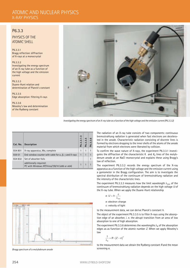
254 WWW.LEYBOLD-SHOP.COM
PHYSICS OF THE
ATOMIC SHELL
P6.3.3.1 Bragg reflection: diffraction of X-rays at a monocrystal
P6.3.3.2 Investigating the energy spectrum of an X-ray tube as a function of the high voltage and the emission current
P6.3.3.3 Duane-Hunt relation and determination of Planck‘s constant
P6.3.3.5 Edge absorption: filtering X-rays
P6.3.3.6 Moseley‘s law and determination of the Rydberg constant
The radiation of an X-ray tube consists of two components: continuous bremsstrahlung radiation is generated when fast electrons are decelera-ted in the anode. Characteristic radiation consisting of discrete lines is formed by electrons dropping to the inner shells of the atoms of the anode material from which electrons were liberated by collision.
To confirm the wave nature of X-rays, the experiment P6.3.3.1 investi-gates the diffraction of the characteristic K and Kß lines of the molyb-denum anode at an NaCl monocrystal and explains these using Bragg‘s law of reflection.
The experiment P6.3.3.2 records the energy spectrum of the X-ray apparatus as a function of the high voltage and the emission current using a goniometer in the Bragg configuration. The aim is to investigate the spectral distribution of the continuum of bremsstrahlung radiation and the intensity of the characteristic lines.
The experiment P6.3.3.3 measures how the limit wavelength min of the continuum of bremsstrahlung radiation depends on the high voltage U of the X-ray tube. When we apply the Duane-Hunt relationship
e U hc
e
c
⋅ = ⋅λmin
: electron charge
: velocity of light
to the measurement data, we can derive Planck‘s constant h.
The object of the experiment P6.3.3.5 is to filter X-rays using the absorp-tion edge of an absorber, i. e. the abrupt transition from an area of low absorption to one of high absorption.
The experiment P6.3.3.6 determines the wavelengths K of the absorption edges as as function of the atomic number Z. When we apply Moseley‘s law
1 2
λσ
K
= ⋅ −( )R Z
to the measurement data we obtain the Rydberg constant R and the mean screening
ATOMIC AND NUCLEAR PHYSICS
Investigating the energy spectrum of an X-ray tube as a function of the high voltage and the emission current (P6.3.3.2)
Cat. No. Description
P6.3
.3.1
-3
P6.3
.3.5
P6.3
.3.6
554 801 X-ray apparatus, Mo, complete 1 1 1
559 01 End-window counter with cable for , , and X-rays 1 1 1
554 832 Set of absorber foils 1
additionally required: PC with Windows XP/Vista/7/8/10 (x86 or x64)
1 1 1
Bragg spectrum of a molybdenum anode
X-RAY PHYSICS
P6.3.3
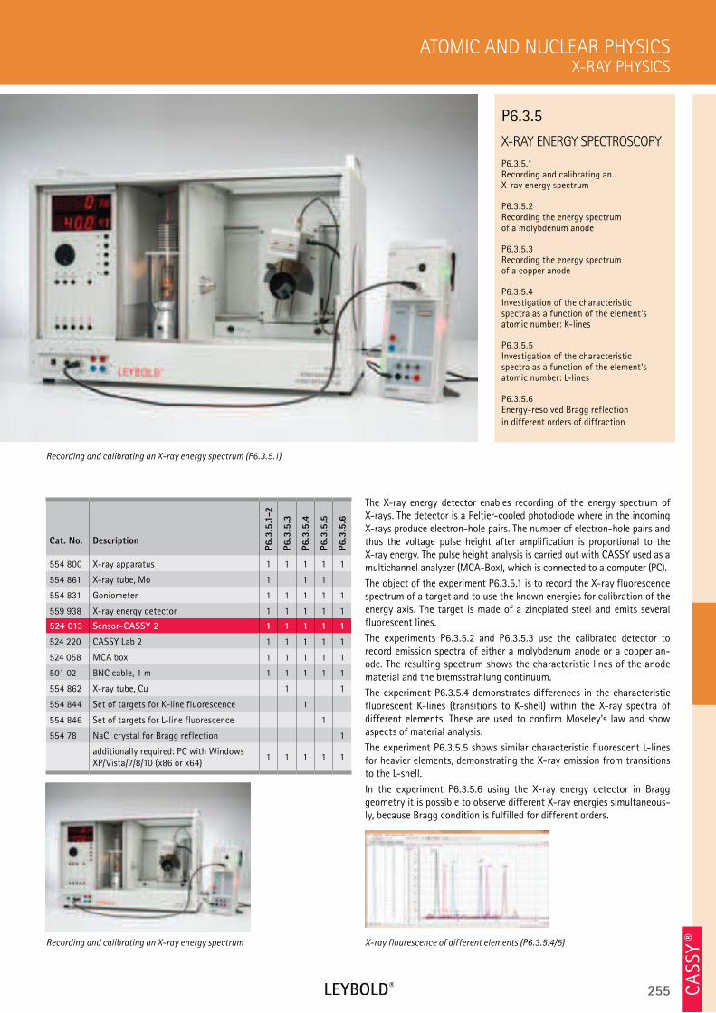
255
X-RAY ENERGY SPECTROSCOPY
P6.3.5.1 Recording and calibrating an X-ray energy spectrum
P6.3.5.2 Recording the energy spectrum of a molybdenum anode
P6.3.5.3 Recording the energy spectrum of a copper anode
P6.3.5.4 Investigation of the characteristic spectra as a function of the element‘s atomic number: K-lines
P6.3.5.5 Investigation of the characteristic spectra as a function of the element‘s atomic number: L-lines
P6.3.5.6 Energy-resolved Bragg reflection
in different orders of diffraction
X-RAY PHYSICS
ATOMIC AND NUCLEAR PHYSICS
Cat. No. Description
P6.3
.5.1
-2
P6.3
.5.3
P6.3
.5.4
P6.3
.5.5
P6.3
.5.6
554 800 X-ray apparatus 1 1 1 1 1
554 861 X-ray tube, Mo 1 1 1
554 831 Goniometer 1 1 1 1 1
559 938 X-ray energy detector 1 1 1 1 1
524 013 Sensor-CASSY 2 1 1 1 1 1
524 220 CASSY Lab 2 1 1 1 1 1
524 058 MCA box 1 1 1 1 1
501 02 BNC cable, 1 m 1 1 1 1 1
554 862 X-ray tube, Cu 1 1
554 844 Set of targets for K-line fluorescence 1
554 846 Set of targets for L-line fluorescence 1
554 78 NaCl crystal for Bragg reflection 1
additionally required: PC with Windows XP/Vista/7/8/10 (x86 or x64)
1 1 1 1 1
The X-ray energy detector enables recording of the energy spectrum of X-rays. The detector is a Peltier-cooled photodiode where in the incoming X-rays produce electron-hole pairs. The number of electron-hole pairs and thus the voltage pulse height after amplification is proportional to the X-ray energy. The pulse height analysis is carried out with CASSY used as a multichannel analyzer (MCA-Box), which is connected to a computer (PC).
The object of the experiment P6.3.5.1 is to record the X-ray fluorescence spectrum of a target and to use the known energies for calibration of the energy axis. The target is made of a zincplated steel and emits several fluorescent lines.
The experiments P6.3.5.2 and P6.3.5.3 use the calibrated detector to record emission spectra of either a molybdenum anode or a copper an-ode. The resulting spectrum shows the characteristic lines of the anode material and the bremsstrahlung continuum.
The experiment P6.3.5.4 demonstrates differences in the characteristic fluorescent K-lines (transitions to K-shell) within the X-ray spectra of different elements. These are used to confirm Moseley’s law and show aspects of material analysis.
The experiment P6.3.5.5 shows similar characteristic fluorescent L-lines for heavier elements, demonstrating the X-ray emission from transitions to the L-shell.
In the experiment P6.3.5.6 using the X-ray energy detector in Bragg geometry it is possible to observe different X-ray energies simultaneous-ly, because Bragg condition is fulfilled for different orders.
Recording and calibrating an X-ray energy spectrum (P6.3.5.1)
P6.3.5
Recording and calibrating an X-ray energy spectrum
CA
SSY ®X-ray flourescence of different elements (P6.3.5.4/5)
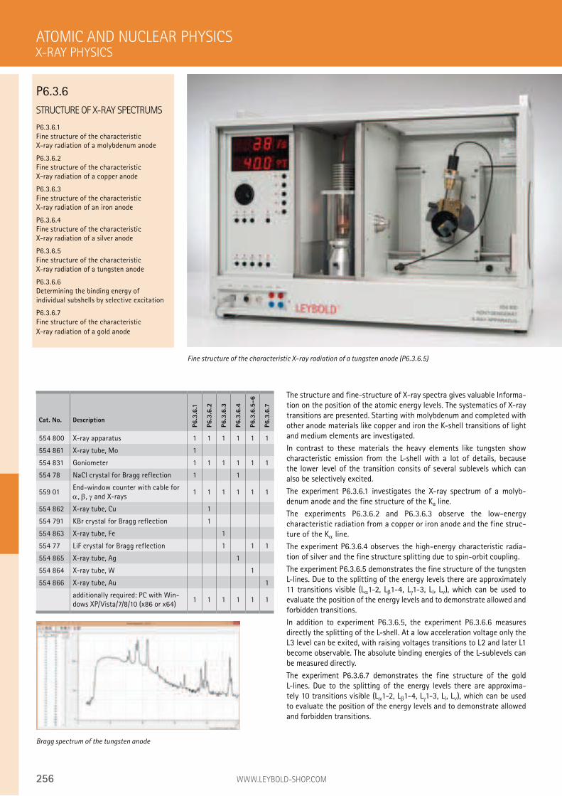
256 WWW.LEYBOLD-SHOP.COM
STRUCTURE OF X-RAY SPECTRUMS
P6.3.6.1 Fine structure of the characteristic X-ray radiation of a molybdenum anode
P6.3.6.2 Fine structure of the characteristic X-ray radiation of a copper anode
P6.3.6.3 Fine structure of the characteristic X-ray radiation of an iron anode
P6.3.6.4 Fine structure of the characteristic X-ray radiation of a silver anode
P6.3.6.5 Fine structure of the characteristic X-ray radiation of a tungsten anode
P6.3.6.6 Determining the binding energy of individual subshells by selective excitation
P6.3.6.7 Fine structure of the characteristic
X-ray radiation of a gold anode
The structure and fine-structure of X-ray spectra gives valuable Informa-tion on the position of the atomic energy levels. The systematics of X-ray transitions are presented. Starting with molybdenum and completed with other anode materials like copper and iron the K-shell transitions of light and medium elements are investigated.
In contrast to these materials the heavy elements like tungsten show characteristic emission from the L-shell with a lot of details, because the lower level of the transition consits of several sublevels which can also be selectively excited.
The experiment P6.3.6.1 investigates the X-ray spectrum of a molyb- denum anode and the fine structure of the Ka line.
The experiments P6.3.6.2 and P6.3.6.3 observe the low-energy characteristic radiation from a copper or iron anode and the fine struc-ture of the K line.
The experiment P6.3.6.4 observes the high-energy characteristic radia-tion of silver and the fine structure splitting due to spin-orbit coupling.
The experiment P6.3.6.5 demonstrates the fine structure of the tungsten L-lines. Due to the splitting of the energy levels there are approximately 11 transitions visible (L 1-2, L 1-4, L 1-3, Ll, L ), which can be used to evaluate the position of the energy levels and to demonstrate allowed and forbidden transitions.
In addition to experiment P6.3.6.5, the experiment P6.3.6.6 measures directly the splitting of the L-shell. At a low acceleration voltage only the L3 level can be exited, with raising voltages transitions to L2 and later L1 become observable. The absolute binding energies of the L-sublevels can be measured directly.
The experiment P6.3.6.7 demonstrates the fine structure of the gold L-lines. Due to the splitting of the energy levels there are approxima-tely 10 transitions visible (L 1-2, L 1-4, L 1-3, Ll, L ), which can be used to evaluate the position of the energy levels and to demonstrate allowed and forbidden transitions.
ATOMIC AND NUCLEAR PHYSICS
Fine structure of the characteristic X-ray radiation of a tungsten anode (P6.3.6.5)
Cat. No. Description
P6.3
.6.1
P6.3
.6.2
P6.3
.6.3
P6.3
.6.4
P6.3
.6.5
-6
P6.3
.6.7
554 800 X-ray apparatus 1 1 1 1 1 1
554 861 X-ray tube, Mo 1
554 831 Goniometer 1 1 1 1 1 1
554 78 NaCl crystal for Bragg reflection 1 1
559 01End-window counter with cable for
, , and X-rays1 1 1 1 1 1
554 862 X-ray tube, Cu 1
554 791 KBr crystal for Bragg reflection 1
554 863 X-ray tube, Fe 1
554 77 LiF crystal for Bragg reflection 1 1 1
554 865 X-ray tube, Ag 1
554 864 X-ray tube, W 1
554 866 X-ray tube, Au 1
additionally required: PC with Win-dows XP/Vista/7/8/10 (x86 or x64)
1 1 1 1 1 1
Bragg spectrum of the tungsten anode
X-RAY PHYSICS
P6.3.6
257
STRUCTURE OF X-RAY SPECTRUMS
P6.3.6.11 High-resolution fine structure of the characteristic X-ray radiation of a molybdenum anode
P6.3.6.12 High-resolution fine structure of the characteristic X-ray radiation of a copper anode
P6.3.6.13 High-resolution fine structure of the characteristic X-ray radiation of an iron anode
P6.3.6.14 High-resolution fine structure of the characteristic X-ray radiation of a silver anode
P6.3.6.15 High-resolution fine structure of the characteristic X-ray radiation of a tungsten anode
P6.3.6.17 High-resolution fine structure of the characteristic X-ray radiation of a gold anode
X-RAY PHYSICS
ATOMIC AND NUCLEAR PHYSICS
Cat. No. Description
P6.3
.6.1
1
P6.3
.6.1
2
P6.3
.6.1
3
P6.3
.6.1
4
P6.3
.6.1
5
P6.3
.6.1
7
554 800 X-ray apparatus 1 1 1 1 1 1
554 861 X-ray tube, Mo 1
554 831 Goniometer 1 1 1 1 1 1
554 835 HD Accessory, X-ray 1 1 1 1 1 1
554 78 NaCl crystal for Bragg reflection 1 1
559 01End-window counter with cable for
, , and X-rays1 1 1 1 1 1
554 862 X-ray tube, Cu 1
554 77 LiF crystal for Bragg reflection 1 1 1 1
554 863 X-ray tube, Fe 1
554 865 X-ray tube, Ag 1
554 864 X-ray tube, W 1
554 866 X-ray tube, Au 1
additionally required: PC with Win-dows XP/Vista/7/8/10 (x86 or x64)
1 1 1 1 1 1
The experiment P6.3.6.11 investigates the high-resolution X-ray spec-trum of a molybdenum anode and the fine structure of the Ka-line.
The experiments P6.3.6.12 and P6.3.6.13 observe the low-energy characteristic radiation from a copper or iron anode and the high- resolution fine structure of the K -line.
The experiment P6.3.6.14 observes the high-energy characteristic radiation of silver and the high-resolution fine structure splitting due to spin-orbit coupling.
The experiment P6.3.6.15 demonstrates the high-resolution fine struc-ture of the tungsten L-lines. Due to the splitting of the energy levels there are approximately 10 transitions visible (L 1-2, L 1-5, L 1-3), which can be used to evaluate the position of the energy levels and to demonstrate allowed and forbidden transitions.
The experiment P6.3.6.17 demonstrates the fine structure of the gold L-lines. Due to the splitting of the energy levels there are approximately 10 transitions visible (L 1-2, L 1-4, L 1-3, Ll, L ), which can be used to evaluate the position of the energy levels and to demonstrate allowed and forbidden transitions.
High-resolution fine structure of the characteristic X-ray radiation of a molybdenum anode (P6.3.6.11)
P6.3.6
Separation of the K 1 and K 2 lines in the Bragg spectrum
258 WWW.LEYBOLD-SHOP.COM
COMPTON EFFECT AT X-RAYS
P6.3.7.1 Compton effect: verifying the energy loss of the scattered X-ray quantum
P6.3.7.2 Compton effect: Measurement the energy of the scattered photons as a function of the scattering angle
At a time (early 1920‘s) when the particle nature of light (photons) suggested by the photoelectric effect was still being debated, the Comp-ton experiment, the scattering of X-rays on weakly bound electrons, in 1923 gave another evidence of particle-like behaviour of X-rays in this process. Compton investigated the scattering of X-rays passing through matter. According to classical physics the frequency of the radiation should not be changed by the scattering process. However, A. H. Compton observed a frequency change for scattered X-rays. He interpreted this in the particle model as a collision of the X-ray photon and an electron of the scattering material. Assuming total energy and momentum to be conserved, energy is transferred from the photon to the electron, so the energy of the scattered photon depends on the scattering angle .
The experiment P6.3.7.1 verifies the Compton shift using the endwindow counter. The change of frequency or wavelength due to the scattering process is apparent as a change of the attenuation of an absorber, which is placed either in front of or behind the scattering body.
The object of the experiment P6.3.7.2 is to record directly the energy spectra of the scattered X-rays with the X-ray energy detector as a func-tion of the scattering angle . The energy E( ) of the scattered photons at different angles is determined and compared with the calculated energy obtained from conservation of energy and momentum by using the relativistic expression for the energy:
EE
E
m c
E
ϑ
ϑ
( ) =+
⋅⋅ −( )
0
0
2
0
1 1 cos
: energy of the photon before thee collision
: mass of electron at rest
: velocity of ligh
m
c tt
ATOMIC AND NUCLEAR PHYSICS
Compton effect: Measurement the energy of the scattered photons as a function of the scattering angle (P6.3.7.2)
Cat. No. Description
P6.3
.7.1
P6.3
.7.2
554 800 X-ray apparatus 1 1
554 861 X-ray tube, Mo 1 1
554 831 Goniometer 1 1
559 01 End-window counter with cable for , , and X-rays 1
554 836 Compton accessory, X-ray 1
554 8371 Compton accessory, X-ray II 1
559 938 X-ray energy detector 1
524 013 Sensor-CASSY 2 1
524 058 MCA box 1
524 220 CASSY Lab 2 1
501 02 BNC cable, 1 m 1
additionally required: PC with Windows XP/Vista/7/8/10 (x86 or x64)
1
Energy shift of the scattered X-rays at different angeles (P6.3.7.2)
X-RAY PHYSICS
P6.3.7
CA
SSY ®
259
X-RAY TOMOGRAPHY
P6.3.8.1 Measurement and presentation of a computed tomogram with the computed tomography module
P6.3.8.2 Computed tomography of simple geometrical objects with the computed tomography module
P6.3.8.3 Medical basics of computed tomography with the computed tomography module
P6.3.8.4 Determining absorption coefficients and Hounsfield units with computed tomography with the computed tomography module
P6.3.8.5 Computed tomography of biological samples with the computed
tomography module
X-RAY PHYSICS
ATOMIC AND NUCLEAR PHYSICS
Cat. No. Description
P6.3
.8.1
P6.3
.8.2
-4
P6.3
.8.5
554 800 X-ray apparatus 1 1 1
554 831 Goniometer 1 1 1
554 866 X-ray tube, Au 1 1 1
554 821 Computed tomography module 1 1 1
554 823 Phantom, 3D 1
554 825 LEGO® adapter 1
additionally required: PC with Windows XP/Vista/7/8/10 (x86 or x64)
1 1 1
In 1972 the first computed tomographic scanner was built by Godfrey Hounsfield who, together with Allan Cormack, was awarded the Nobel Prize in Physiology or Medicine in 1979. The basic idea of computed tomography (CT) is the illumination of an object by X-rays from numerous different angles. Our educational X-ray apparatus allows the illumination of objects by X-rays. The resulting 2D-projections are visualised at the fluorescence screen or with the X-ray image sensor. By turning an ob-ject using the built-in goniometer of the X-ray apparatus, and recording the 2D-projections from each angular step, the computer can reconstruct the object illuminated by X-rays. Our e-learning software visualises the back projection (necessary for reconstructing the computed tomography) concurrently with the scanning process. The 3D-model is then displayed on the PC screen.
Experiment P6.3.8.1 discusses the basics of computed tomography. The computed tomographies of simple geometrical objects are recorded and displayed.
Experiment P6.3.8.2 shows the CT of simple geometrical objects to de-monstrate the basic properties and the resolution power of tomography.
Experiment P6.3.8.3 shows the CT of medical related objects to demon-strate the basic properties of tomography and to investigate possible problems with artefacts and image errors.
Experiment P6.3.8.4 analyses the absorption coefficient of water inside a plastic body to demonstrate the capabilities of CT in distinguishing different kinds of tissues and to calibrate Hounsfield units and it discusses hardening effects of the X-rays.
Experiment P6.3.8.5 analyses the CT of real biological specimens and applies to the results of the previous experiments.
Measurement and presentation of a computed tomogram with the computed tomography module (P6.3.8.1)
P6.3.8
Computed tomography of a Lego figure (P6.3.8.2)
260 WWW.LEYBOLD-SHOP.COM
X-RAY TOMOGRAPHY
P6.3.8.11
Measurement and presentation
of a computed tomogram with
the X-ray image sensor
P6.3.8.12
Computed tomography of simple
geometrical objects with
the X-ray image sensor
P6.3.8.13
Medical basics of computed tomography
with the X-ray image sensor
P6.3.8.14
Determining absorption coefficients
and Hounsfield units with computed
tomography with the X-ray image sensor
P6.3.8.15
Computed tomography of biological
samples with the X-ray image sensor
Experiment P6.3.8.11 discusses the basics of computed tomography. The computed tomographies of simple geometrical objects are recorded and displayed.
Experiment P6.3.8.12 shows the CT of simple geometrical objects to demonstrate the basic properties and the resolution power of tomography.
Experiment P6.3.8.13 shows the CT of medical related objects to demonstrate the basic properties of tomography and to investigate possible problems with artefacts and image errors.
Experiment P6.3.8.14 analyses the absorption coefficient of water inside a plastic body to demonstrate the capabilities of CT in distin-guishing different kinds of tissues and to calibrate Hounsfield units and it discusses hardening effects of the X-rays.
Experiment P6.3.8.15 analyses the CT of real biological specimens and applies to the results of the previous experiments.
ATOMIC AND NUCLEAR PHYSICS
Measurement and presentation of a computed tomogram with the X-ray image sensor (P6.3.8.11)
Cat. No. Description
P6.3
.8.1
1
P6.3
.8.1
2-4
P6.3
.8.1
5
554 800 X-ray apparatus 1 1 1
554 831 Goniometer 1 1 1
554 866 X-ray tube, Au 1 1 1
554 820P Computed Tomography Pro package 1 1 1
554 823 Phantom, 3D 1
additionally required: PC with Windows XP/Vista/7/8/10 (x86 or x64)
1 1 1
X-RAY PHYSICS
P6.3.8
High-resolution computed tomograms of a snail shell
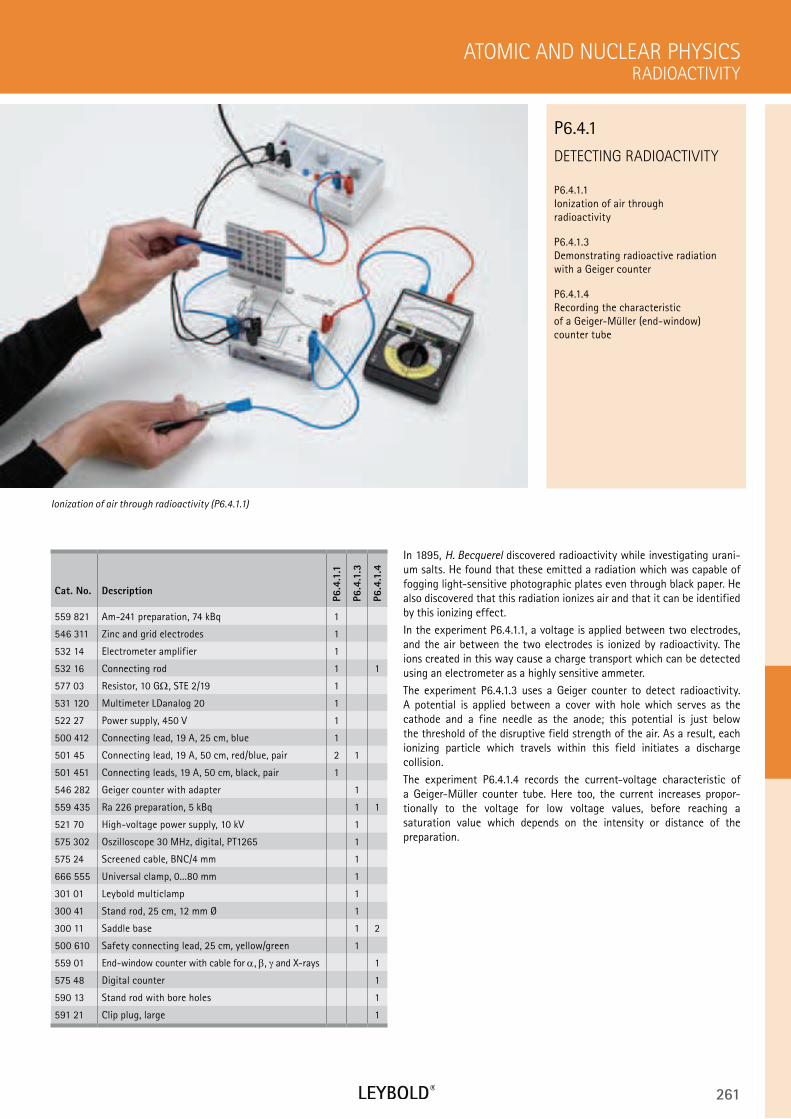
261
DETECTING RADIOACTIVITY
P6.4.1.1 Ionization of air through radioactivity
P6.4.1.3 Demonstrating radioactive radiation with a Geiger counter
P6.4.1.4 Recording the characteristic of a Geiger-Müller (end-window) counter tube
RADIOACTIVITY
ATOMIC AND NUCLEAR PHYSICS
Cat. No. Description
P6.4
.1.1
P6.4
.1.3
P6.4
.1.4
559 821 Am-241 preparation, 74 kBq 1
546 311 Zinc and grid electrodes 1
532 14 Electrometer amplifier 1
532 16 Connecting rod 1 1
577 03 Resistor, 10 G , STE 2/19 1
531 120 Multimeter LDanalog 20 1
522 27 Power supply, 450 V 1
500 412 Connecting lead, 19 A, 25 cm, blue 1
501 45 Connecting lead, 19 A, 50 cm, red/blue, pair 2 1
501 451 Connecting leads, 19 A, 50 cm, black, pair 1
546 282 Geiger counter with adapter 1
559 435 Ra 226 preparation, 5 kBq 1 1
521 70 High-voltage power supply, 10 kV 1
575 302 Oszilloscope 30 MHz, digital, PT1265 1
575 24 Screened cable, BNC/4 mm 1
666 555 Universal clamp, 0...80 mm 1
301 01 Leybold multiclamp 1
300 41 Stand rod, 25 cm, 12 mm Ø 1
300 11 Saddle base 1 2
500 610 Safety connecting lead, 25 cm, yellow/green 1
559 01 End-window counter with cable for , , and X-rays 1
575 48 Digital counter 1
590 13 Stand rod with bore holes 1
591 21 Clip plug, large 1
In 1895, H. Becquerel discovered radioactivity while investigating urani-um salts. He found that these emitted a radiation which was capable of fogging light-sensitive photographic plates even through black paper. He also discovered that this radiation ionizes air and that it can be identified by this ionizing effect.
In the experiment P6.4.1.1, a voltage is applied between two electrodes, and the air between the two electrodes is ionized by radioactivity. The ions created in this way cause a charge transport which can be detected using an electrometer as a highly sensitive ammeter.
The experiment P6.4.1.3 uses a Geiger counter to detect radioactivity. A potential is applied between a cover with hole which serves as the cathode and a fine needle as the anode; this potential is just below the threshold of the disruptive field strength of the air. As a result, each ionizing particle which travels within this field initiates a discharge collision.
The experiment P6.4.1.4 records the current-voltage characteristic of a Geiger-Müller counter tube. Here too, the current increases propor- tionally to the voltage for low voltage values, before reaching a saturation value which depends on the intensity or distance of the preparation.
Ionization of air through radioactivity (P6.4.1.1)
P6.4.1
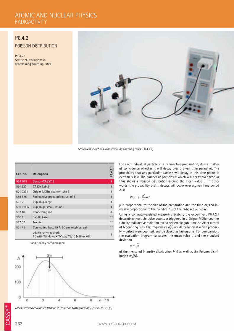
262 WWW.LEYBOLD-SHOP.COM
POISSON DISTRIBUTION
P6.4.2.1 Statistical variations in determining counting rates
For each individual particle in a radioactive preparation, it is a matter of coincidence whether it will decay over a given time period t. The probability that any particular particle will decay in this time period is extremely low. The number of particles n which will decay over time t thus shows a Poisson distribution around the mean value µ. In other words, the probability that n decays will occur over a given time period
t is
W nne
n
µ
µµ( ) = −
!
µ is proportional to the size of the preparation and the time t, and in-versely proportional to the half-life T1/2 of the radioactive decay.
Using a computer-assisted measuring system, the experiment P6.4.2.1 determines multiple pulse counts n triggered in a Geiger-Müller counter tube by radioactive radiation over a selectable gate time t. After a total of N counting runs, the frequencies h(n) are determined at which precise-ly n pulses were counted, and displayed as histograms. For comparision, the evaluation program calculates the mean value µ and the standard deviation
σ µ=
of the measured intensity distribution h(n) as well as the Poisson distri-bution wµ(N).
ATOMIC AND NUCLEAR PHYSICS
Statistical variations in determining counting rates (P6.4.2.1)
Cat. No. Description
P6.4
.2.1
524 013 Sensor-CASSY 2 1
524 220 CASSY Lab 2 1
524 0331 Geiger-Müller counter tube S 1
559 835 Radioactive preparations, set of 3 1
591 21 Clip plug, large 1
590 02ET2 Clip plugs, small, set of 2 1
532 16 Connecting rod 2
300 11 Saddle base 1*
587 07 Tweeter 1*
501 45 Connecting lead, 19 A, 50 cm, red/blue, pair 1*
additionally required: PC with Windows XP/Vista/7/8/10 (x86 or x64)
1
* additionally recommended
Measured and calculated Poisson distribution Histogram: h(n), curve: N · wB (n)
RADIOACTIVITY
P6.4.2
CA
SSY ®
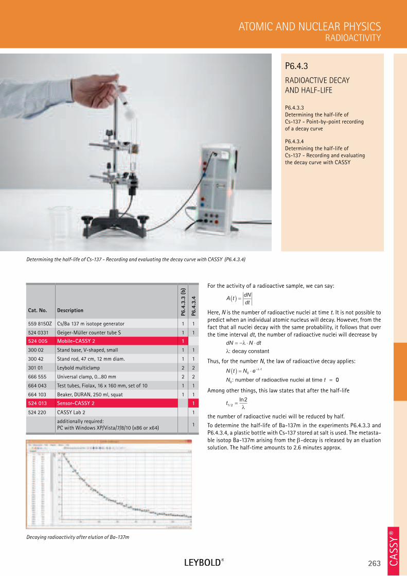
263
RADIOACTIVE DECAY
AND HALF-LIFE
P6.4.3.3 Determining the half-life of Cs-137 - Point-by-point recording of a decay curve
P6.4.3.4 Determining the half-life of Cs-137 - Recording and evaluating the decay curve with CASSY
RADIOACTIVITY
ATOMIC AND NUCLEAR PHYSICS
Cat. No. Description
P6.4
.3.3
(b)
P6.4
.3.4
559 815OZ Cs/Ba 137 m isotope generator 1 1
524 0331 Geiger-Müller counter tube S 1 1
524 005 Mobile-CASSY 2 1
300 02 Stand base, V-shaped, small 1 1
300 42 Stand rod, 47 cm, 12 mm diam. 1 1
301 01 Leybold multiclamp 2 2
666 555 Universal clamp, 0...80 mm 2 2
664 043 Test tubes, Fiolax, 16 x 160 mm, set of 10 1 1
664 103 Beaker, DURAN, 250 ml, squat 1 1
524 013 Sensor-CASSY 2 1
524 220 CASSY Lab 2 1
additionally required: PC with Windows XP/Vista/7/8/10 (x86 or x64)
1
For the activity of a radioactive sample, we can say:
A tdN
dt( ) =
Here, N is the number of radioactive nuclei at time t. It is not possible to predict when an individual atomic nucleus will decay. However, from the fact that all nuclei decay with the same probability, it follows that over the time interval dt, the number of radioactive nuclei will decrease by
dN N dt= − ⋅ ⋅λ
λ: decay constant
Thus, for the number N, the law of radioactive decay applies:
N t N e
N t
t( ) = ⋅
=
− ⋅
0
0
λ
: number of radioactive nuclei at time 00
Among other things, this law states that after the half-life
t1 2
2/
ln=
λ
the number of radioactive nuclei will be reduced by half.
To determine the half-life of Ba-137m in the experiments P6.4.3.3 and P6.4.3.4, a plastic bottle with Cs-137 stored at salt is used. The metasta-ble isotop Ba-137m arising from the -decay is released by an eluation solution. The half-time amounts to 2.6 minutes approx.
Determining the half-life of Cs-137 - Recording and evaluating the decay curve with CASSY (P6.4.3.4)
P6.4.3
Decaying radioactivity after elution of Ba-137m
CA
SSY ®
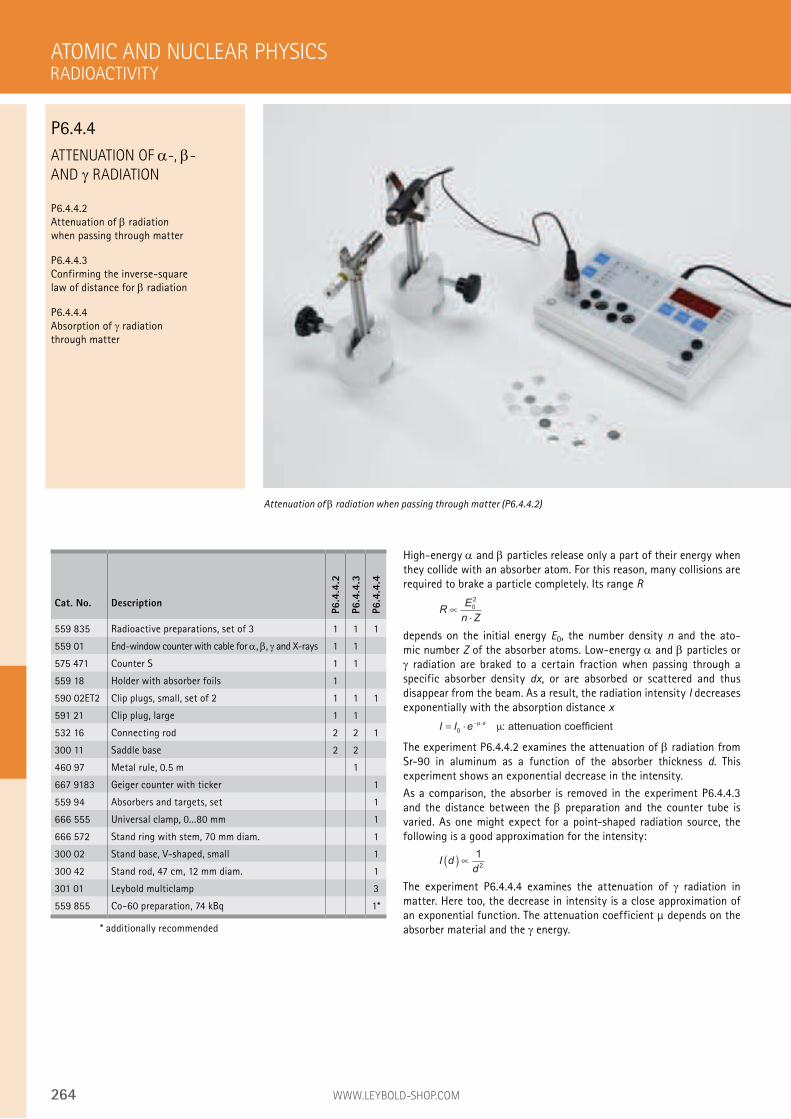
264 WWW.LEYBOLD-SHOP.COM
ATTENUATION OF -, -
AND RADIATION
P6.4.4.2
Attenuation of radiation
when passing through matter
P6.4.4.3
Confirming the inverse-square
law of distance for radiation
P6.4.4.4
Absorption of radiation
through matter
High-energy and particles release only a part of their energy when
they collide with an absorber atom. For this reason, many collisions are
required to brake a particle completely. Its range R
RE
n Z∝
⋅
0
2
depends on the initial energy E0, the number density n and the ato-
mic number Z of the absorber atoms. Low-energy and particles or
radiation are braked to a certain fraction when passing through a
specific absorber density dx, or are absorbed or scattered and thus
disappear from the beam. As a result, the radiation intensity I decreases
exponentially with the absorption distance x
I I ex= ⋅ − ⋅
0
µ µ : attenuation coefficient
The experiment P6.4.4.2 examines the attenuation of radiation from
Sr-90 in aluminum as a function of the absorber thickness d. This
experiment shows an exponential decrease in the intensity.
As a comparison, the absorber is removed in the experiment P6.4.4.3
and the distance between the preparation and the counter tube is
varied. As one might expect for a point-shaped radiation source, the
following is a good approximation for the intensity:
I dd
( ) ∝1
2
The experiment P6.4.4.4 examines the attenuation of radiation in
matter. Here too, the decrease in intensity is a close approximation of
an exponential function. The attenuation coefficient µ depends on the
absorber material and the energy.
ATOMIC AND NUCLEAR PHYSICS
Attenuation of radiation when passing through matter (P6.4.4.2)
Cat. No. Description
P6.4
.4.2
P6.4
.4.3
P6.4
.4.4
559 835 Radioactive preparations, set of 3 1 1 1
559 01 End-window counter with cable for , , and X-rays 1 1
575 471 Counter S 1 1
559 18 Holder with absorber foils 1
590 02ET2 Clip plugs, small, set of 2 1 1 1
591 21 Clip plug, large 1 1
532 16 Connecting rod 2 2 1
300 11 Saddle base 2 2
460 97 Metal rule, 0.5 m 1
667 9183 Geiger counter with ticker 1
559 94 Absorbers and targets, set 1
666 555 Universal clamp, 0...80 mm 1
666 572 Stand ring with stem, 70 mm diam. 1
300 02 Stand base, V-shaped, small 1
300 42 Stand rod, 47 cm, 12 mm diam. 1
301 01 Leybold multiclamp 3
559 855 Co-60 preparation, 74 kBq 1*
* additionally recommended
RADIOACTIVITY
P6.4.4
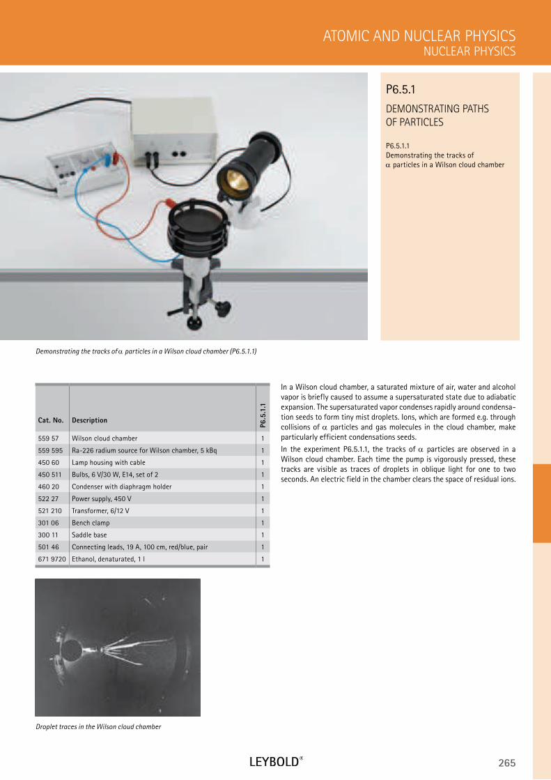
265
DEMONSTRATING PATHS
OF PARTICLES
P6.5.1.1 Demonstrating the tracks of
particles in a Wilson cloud chamber
NUCLEAR PHYSICS
ATOMIC AND NUCLEAR PHYSICS
Cat. No. Description
P6.5
.1.1
559 57 Wilson cloud chamber 1
559 595 Ra-226 radium source for Wilson chamber, 5 kBq 1
450 60 Lamp housing with cable 1
450 511 Bulbs, 6 V/30 W, E14, set of 2 1
460 20 Condenser with diaphragm holder 1
522 27 Power supply, 450 V 1
521 210 Transformer, 6/12 V 1
301 06 Bench clamp 1
300 11 Saddle base 1
501 46 Connecting leads, 19 A, 100 cm, red/blue, pair 1
671 9720 Ethanol, denaturated, 1 l 1
In a Wilson cloud chamber, a saturated mixture of air, water and alcohol vapor is briefly caused to assume a supersaturated state due to adiabatic expansion. The supersaturated vapor condenses rapidly around condensa-tion seeds to form tiny mist droplets. Ions, which are formed e.g. through collisions of particles and gas molecules in the cloud chamber, make particularly efficient condensations seeds.
In the experiment P6.5.1.1, the tracks of particles are observed in a Wilson cloud chamber. Each time the pump is vigorously pressed, these tracks are visible as traces of droplets in oblique light for one to two seconds. An electric field in the chamber clears the space of residual ions.
Demonstrating the tracks of particles in a Wilson cloud chamber (P6.5.1.1)
P6.5.1
Droplet traces in the Wilson cloud chamber
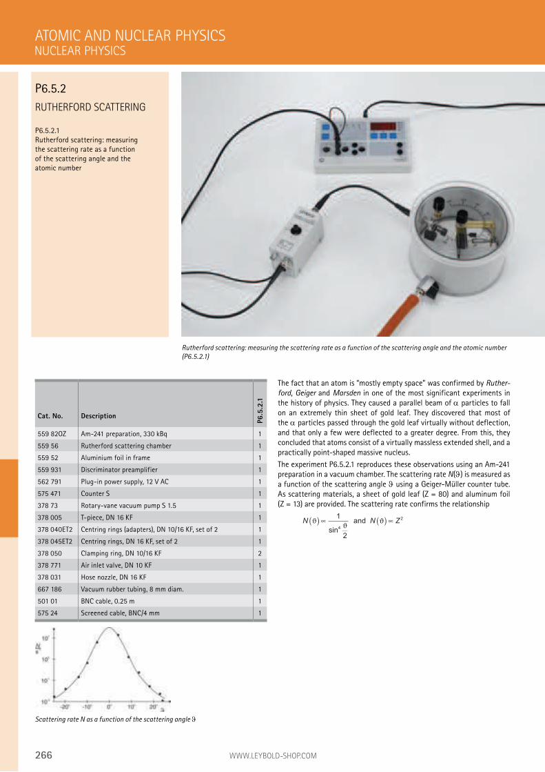
266 WWW.LEYBOLD-SHOP.COM
RUTHERFORD SCATTERING
P6.5.2.1 Rutherford scattering: measuring the scattering rate as a function of the scattering angle and the atomic number
The fact that an atom is “mostly empty space” was confirmed by Ruther-
ford, Geiger and Marsden in one of the most significant experiments in the history of physics. They caused a parallel beam of particles to fall on an extremely thin sheet of gold leaf. They discovered that most of the particles passed through the gold leaf virtually without deflection, and that only a few were deflected to a greater degree. From this, they concluded that atoms consist of a virtually massless extended shell, and a practically point-shaped massive nucleus.
The experiment P6.5.2.1 reproduces these observations using an Am-241 preparation in a vacuum chamber. The scattering rate N( ) is measured as a function of the scattering angle using a Geiger-Müller counter tube. As scattering materials, a sheet of gold leaf (Z = 80) and aluminum foil (Z = 13) are provided. The scattering rate confirms the relationship
N N Zϑϑ
ϑ( ) ∝ ( ) ∝1
2
4
2
sin
and
ATOMIC AND NUCLEAR PHYSICS
Rutherford scattering: measuring the scattering rate as a function of the scattering angle and the atomic number
(P6.5.2.1)
Cat. No. Description
P6.5
.2.1
559 82OZ Am-241 preparation, 330 kBq 1
559 56 Rutherford scattering chamber 1
559 52 Aluminium foil in frame 1
559 931 Discriminator preamplifier 1
562 791 Plug-in power supply, 12 V AC 1
575 471 Counter S 1
378 73 Rotary-vane vacuum pump S 1.5 1
378 005 T-piece, DN 16 KF 1
378 040ET2 Centring rings (adapters), DN 10/16 KF, set of 2 1
378 045ET2 Centring rings, DN 16 KF, set of 2 1
378 050 Clamping ring, DN 10/16 KF 2
378 771 Air inlet valve, DN 10 KF 1
378 031 Hose nozzle, DN 16 KF 1
667 186 Vacuum rubber tubing, 8 mm diam. 1
501 01 BNC cable, 0.25 m 1
575 24 Screened cable, BNC/4 mm 1
Scattering rate N as a function of the scattering angle
NUCLEAR PHYSICS
P6.5.2
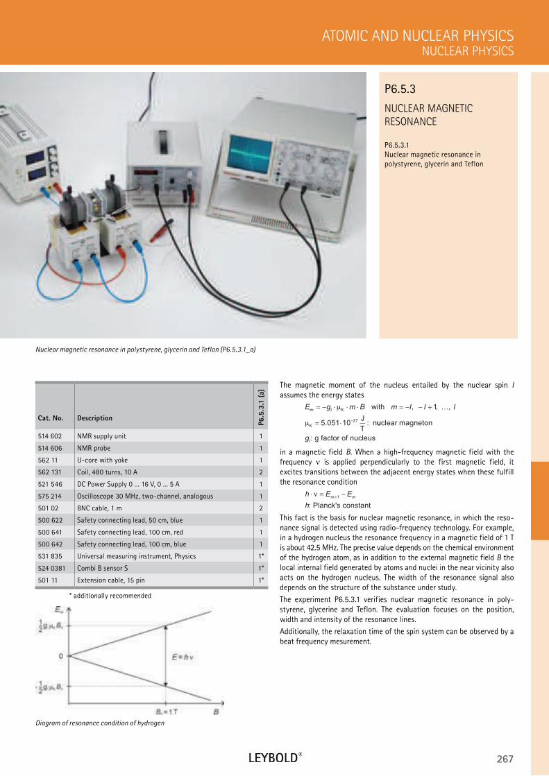
267
NUCLEAR MAGNETIC
RESONANCE
P6.5.3.1
Nuclear magnetic resonance in
polystyrene, glycerin and Teflon
NUCLEAR PHYSICS
ATOMIC AND NUCLEAR PHYSICS
Cat. No. Description
P6.5
.3.1
(a)
514 602 NMR supply unit 1
514 606 NMR probe 1
562 11 U-core with yoke 1
562 131 Coil, 480 turns, 10 A 2
521 546 DC Power Supply 0 ... 16 V, 0 ... 5 A 1
575 214 Oscilloscope 30 MHz, two-channel, analogous 1
501 02 BNC cable, 1 m 2
500 622 Safety connecting lead, 50 cm, blue 1
500 641 Safety connecting lead, 100 cm, red 1
500 642 Safety connecting lead, 100 cm, blue 1
531 835 Universal measuring instrument, Physics 1*
524 0381 Combi B sensor S 1*
501 11 Extension cable, 15 pin 1*
* additionally recommended
The magnetic moment of the nucleus entailed by the nuclear spin I
assumes the energy states
E g m B m I I Im I K
K
with
J
T n
= − ⋅ ⋅ ⋅ = − − +
= ⋅ −
µ
µ
, , ,
. :
1
5 051 10 27
…
uuclear magneton
: g factor of nucleusIg
in a magnetic field B. When a high-frequency magnetic field with the
frequency is applied perpendicularly to the first magnetic field, it
excites transitions between the adjacent energy states when these fulfill
the resonance condition
h E E
h
m m⋅ = −
+ν
1
: Planck's constant
This fact is the basis for nuclear magnetic resonance, in which the reso-
nance signal is detected using radio-frequency technology. For example,
in a hydrogen nucleus the resonance frequency in a magnetic field of 1 T
is about 42.5 MHz. The precise value depends on the chemical environment
of the hydrogen atom, as in addition to the external magnetic field B the
local internal field generated by atoms and nuclei in the near vicinity also
acts on the hydrogen nucleus. The width of the resonance signal also
depends on the structure of the substance under study.
The experiment P6.5.3.1 verifies nuclear magnetic resonance in poly-
styrene, glycerine and Teflon. The evaluation focuses on the position,
width and intensity of the resonance lines.
Additionally, the relaxation time of the spin system can be observed by a
beat frequency mesurement.
Nuclear magnetic resonance in polystyrene, glycerin and Teflon (P6.5.3.1_a)
P6.5.3
Diagram of resonance condition of hydrogen
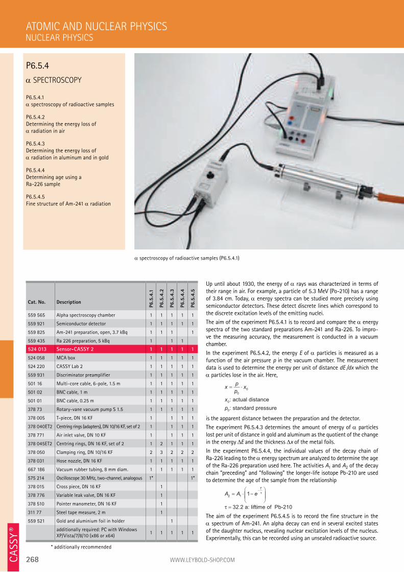
268 WWW.LEYBOLD-SHOP.COM
SPECTROSCOPY
P6.5.4.1 spectroscopy of radioactive samples
P6.5.4.2 Determining the energy loss of
radiation in air
P6.5.4.3 Determining the energy loss of
radiation in aluminum and in gold
P6.5.4.4 Determining age using a Ra-226 sample
P6.5.4.5 Fine structure of Am-241 radiation
Up until about 1930, the energy of rays was characterized in terms of their range in air. For example, a particle of 5.3 MeV (Po-210) has a range of 3.84 cm. Today, energy spectra can be studied more precisely using semiconductor detectors. These detect discrete lines which correspond to the discrete excitation levels of the emitting nuclei.
The aim of the experiment P6.5.4.1 is to record and compare the energy spectra of the two standard preparations Am-241 and Ra-226. To impro-ve the measuring accuracy, the measurement is conducted in a vacuum chamber.
In the experiment P6.5.4.2, the energy E of particles is measured as a function of the air pressure p in the vacuum chamber. The measurement data is used to determine the energy per unit of distance dE /dx which the
particles lose in the air. Here,
xp
px
x
p
= ⋅0
0
0
0
: actual distance
: standard pressure
is the apparent distance between the preparation and the detector.
The experiment P6.5.4.3 determines the amount of energy of particles lost per unit of distance in gold and aluminum as the quotient of the change in the energy E and the thickness x of the metal foils.
In the experiment P6.5.4.4, the individual values of the decay chain of Ra-226 leading to the energy spectrum are analyzed to determine the age of the Ra-226 preparation used here. The activities A1 and A2 of the decay chain “preceding” and “following” the longer-life isotope Pb-210 are used to determine the age of the sample from the relationship
A A e
T
2 11
3
= ⋅ −
=
−τ
τ 2.2 a: liftime of Pb-210
The aim of the experiment P6.5.4.5 is to record the fine structure in the spectrum of Am-241. An alpha decay can end in several excited states
of the daughter nucleus, revealing nuclear excitation levels of the nucleus. Experimentally, this can be recorded using an unsealed radioactive source.
ATOMIC AND NUCLEAR PHYSICS
spectroscopy of radioactive samples (P6.5.4.1)
Cat. No. Description
P6.5
.4.1
P6.5
.4.2
P6.5
.4.3
P6.5
.4.4
P6.5
.4.5
559 565 Alpha spectroscopy chamber 1 1 1 1 1
559 921 Semiconductor detector 1 1 1 1 1
559 825 Am-241 preparation, open, 3.7 kBq 1 1 1 1
559 435 Ra 226 preparation, 5 kBq 1 1 1
524 013 Sensor-CASSY 2 1 1 1 1 1
524 058 MCA box 1 1 1 1 1
524 220 CASSY Lab 2 1 1 1 1 1
559 931 Discriminator preamplifier 1 1 1 1 1
501 16 Multi-core cable, 6-pole, 1.5 m 1 1 1 1 1
501 02 BNC cable, 1 m 1 1 1 1 1
501 01 BNC cable, 0.25 m 1 1 1 1 1
378 73 Rotary-vane vacuum pump S 1.5 1 1 1 1 1
378 005 T-piece, DN 16 KF 1 1 1 1
378 040ET2 Centring rings (adapters), DN 10/16 KF, set of 2 1 1 1 1
378 771 Air inlet valve, DN 10 KF 1 1 1 1
378 045ET2 Centring rings, DN 16 KF, set of 2 1 2 1 1 1
378 050 Clamping ring, DN 10/16 KF 2 3 2 2 2
378 031 Hose nozzle, DN 16 KF 1 1 1 1 1
667 186 Vacuum rubber tubing, 8 mm diam. 1 1 1 1 1
575 214 Oscilloscope 30 MHz, two-channel, analogous 1* 1*
378 015 Cross piece, DN 16 KF 1
378 776 Variable leak valve, DN 16 KF 1
378 510 Pointer manometer, DN 16 KF 1
311 77 Steel tape measure, 2 m 1
559 521 Gold and aluminium foil in holder 1
additionally required: PC with Windows XP/Vista/7/8/10 (x86 or x64)
1 1 1 1 1
* additionally recommended
NUCLEAR PHYSICS
P6.5.4
CA
SSY ®
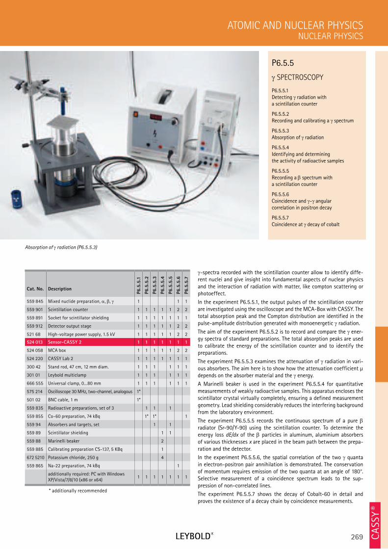
269
SPECTROSCOPY
P6.5.5.1 Detecting radiation with a scintillation counter
P6.5.5.2 Recording and calibrating a spectrum
P6.5.5.3 Absorption of radiation
P6.5.5.4 Identifying and determining the activity of radioactive samples
P6.5.5.5 Recording a spectrum with a scintillation counter
P6.5.5.6 Coincidence and - angular correlation in positron decay
P6.5.5.7 Coincidence at decay of cobalt
NUCLEAR PHYSICS
ATOMIC AND NUCLEAR PHYSICS
Cat. No. Description
P6.5
.5.1
P6.5
.5.2
P6.5
.5.3
P6.5
.5.4
P6.5
.5.5
P6.5
.5.6
P6.5
.5.7
559 845 Mixed nuclide preparation, , , 1 1 1
559 901 Scintillation counter 1 1 1 1 1 2 2
559 891 Socket for scintillator shielding 1 1 1 1 1 1 1
559 912 Detector output stage 1 1 1 1 1 2 2
521 68 High-voltage power supply, 1.5 kV 1 1 1 1 1 2 2
524 013 Sensor-CASSY 2 1 1 1 1 1 1 1
524 058 MCA box 1 1 1 1 1 2 2
524 220 CASSY Lab 2 1 1 1 1 1 1 1
300 42 Stand rod, 47 cm, 12 mm diam. 1 1 1 1 1 1
301 01 Leybold multiclamp 1 1 1 1 1 1
666 555 Universal clamp, 0...80 mm 1 1 1 1 1 1
575 214 Oscilloscope 30 MHz, two-channel, analogous 1*
501 02 BNC cable, 1 m 1*
559 835 Radioactive preparations, set of 3 1 1 1
559 855 Co-60 preparation, 74 kBq 1* 1* 1
559 94 Absorbers and targets, set 1 1
559 89 Scintillator shielding 1 1
559 88 Marinelli beaker 2
559 885 Calibrating preparation CS-137, 5 KBq 1
672 5210 Potassium chloride, 250 g 4
559 865 Na-22 preparation, 74 kBq 1
additionally required: PC with Windows XP/Vista/7/8/10 (x86 or x64)
1 1 1 1 1 1 1
* additionally recommended
-spectra recorded with the scintillation counter allow to identify diffe-rent nuclei and give insight into fundamental aspects of nuclear physics and the interaction of radiation with matter, like compton scattering or photoeffect.
In the experiment P6.5.5.1, the output pulses of the scintillation counter are investigated using the oscilloscope and the MCA-Box with CASSY. The total absorption peak and the Compton distribution are identified in the pulse-amplitude distribution generated with monoenergetic radiation.
The aim of the experiment P6.5.5.2 is to record and compare the ener-gy spectra of standard preparations. The total absorption peaks are used to calibrate the energy of the scintillation counter and to identify the preparations.
The experiment P6.5.5.3 examines the attenuation of radiation in vari-ous absorbers. The aim here is to show how the attenuation coefficient µ depends on the absorber material and the energy.
A Marinelli beaker is used in the experiment P6.5.5.4 for quantitative measurements of weakly radioactive samples. This apparatus encloses the scintillator crystal virtually completely, ensuring a defined measurement geometry. Lead shielding considerably reduces the interfering background from the laboratory environment.
The experiment P6.5.5.5 records the continuous spectrum of a pure radiator (Sr-90/Y-90) using the scintillation counter. To determine the energy loss dE/dx of the particles in aluminum, aluminium absorbers of various thicknesses x are placed in the beam path between the prepa-ration and the detector.
In the experiment P6.5.5.6, the spatial correlation of the two quanta in electron-positron pair annihilation is demonstrated. The conservation of momentum requires emission of the two quanta at an angle of 180°. Selective measurement of a coincidence spectrum leads to the sup- pression of non-correlated lines.
The experiment P6.5.5.7 shows the decay of Cobalt-60 in detail and proves the existence of a decay chain by coincidence measurements.
Absorption of radiation (P6.5.5.3)
P6.5.5
CA
SSY ®
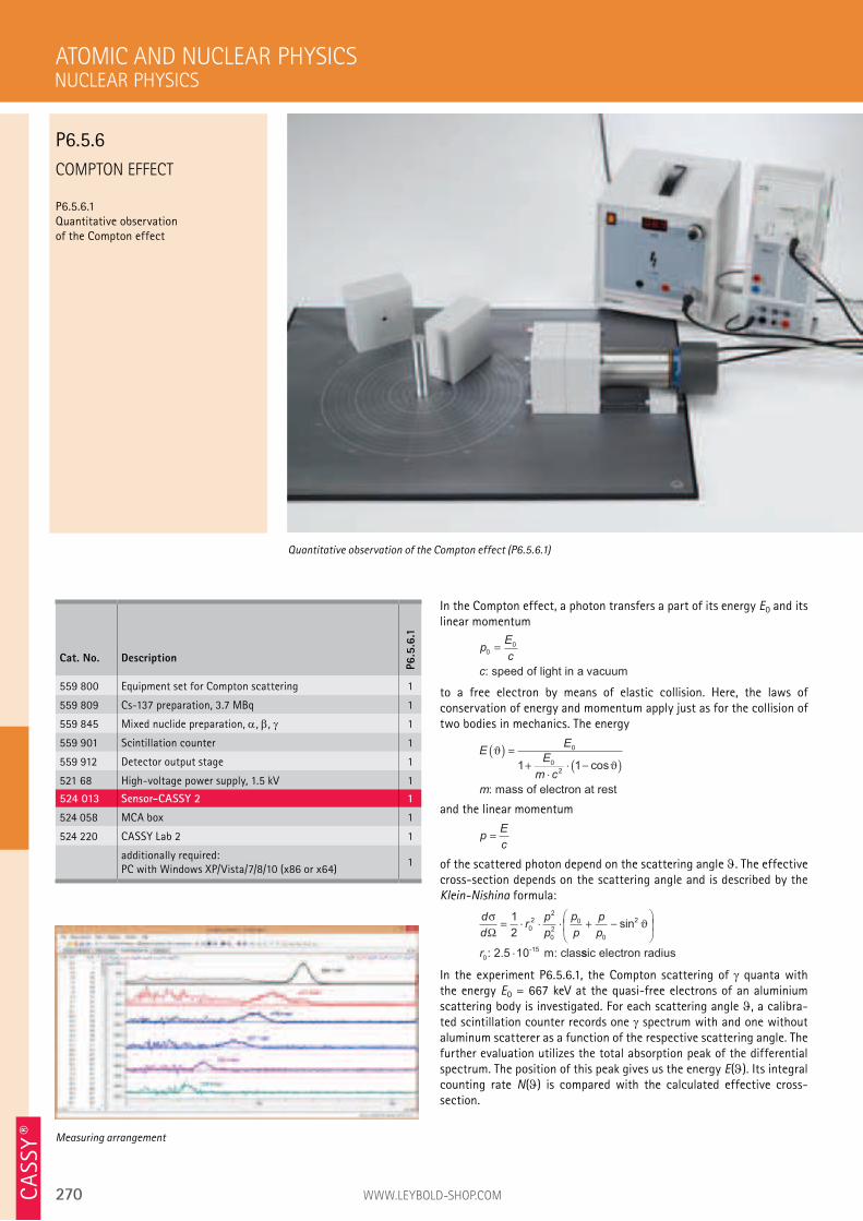
270 WWW.LEYBOLD-SHOP.COM
COMPTON EFFECT
P6.5.6.1 Quantitative observation of the Compton effect
In the Compton effect, a photon transfers a part of its energy E0 and its linear momentum
pE
c
c
00
: speed of light in a vacuum
to a free electron by means of elastic collision. Here, the laws of conservation of energy and momentum apply just as for the collision of two bodies in mechanics. The energy
EE
E
m c
m
ϑ
ϑ
( ) =+
⋅⋅ −( )
0
0
21 1 cos
: mass of electron at rest
and the linear momentum
pE
c
of the scattered photon depend on the scattering angle . The effective cross-section depends on the scattering angle and is described by the Klein-Nishina formula:
d
dr
p
p
p
p
p
p
r
σϑ
Ω= ⋅ ⋅ ⋅ + −
⋅
1
20
2
2
0
2
0
0
2
0
sin
: 2.5 10 m: clas-15
ssic electron radius
In the experiment P6.5.6.1, the Compton scattering of quanta with the energy E0 = 667 keV at the quasi-free electrons of an aluminium scattering body is investigated. For each scattering angle , a calibra-ted scintillation counter records one spectrum with and one without aluminum scatterer as a function of the respective scattering angle. The further evaluation utilizes the total absorption peak of the differential spectrum. The position of this peak gives us the energy E( ). Its integral counting rate N( ) is compared with the calculated effective cross-section.
ATOMIC AND NUCLEAR PHYSICS
Quantitative observation of the Compton effect (P6.5.6.1)
Cat. No. Description
P6.5
.6.1
559 800 Equipment set for Compton scattering 1
559 809 Cs-137 preparation, 3.7 MBq 1
559 845 Mixed nuclide preparation, , , 1
559 901 Scintillation counter 1
559 912 Detector output stage 1
521 68 High-voltage power supply, 1.5 kV 1
524 013 Sensor-CASSY 2 1
524 058 MCA box 1
524 220 CASSY Lab 2 1
additionally required: PC with Windows XP/Vista/7/8/10 (x86 or x64)
1
Measuring arrangement
NUCLEAR PHYSICS
P6.5.6
CA
SSY ®
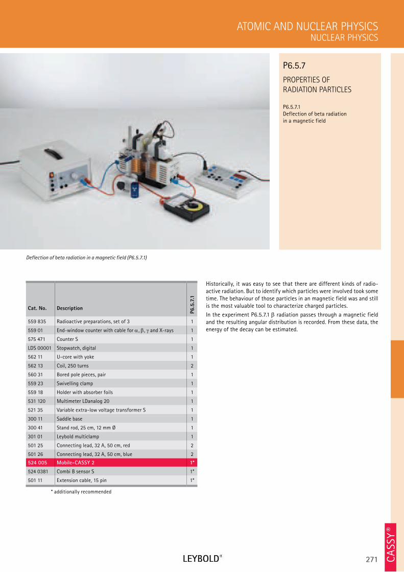
271
PROPERTIES OF
RADIATION PARTICLES
P6.5.7.1
Deflection of beta radiation
in a magnetic field
NUCLEAR PHYSICS
ATOMIC AND NUCLEAR PHYSICS
Cat. No. Description
P6.5
.7.1
559 835 Radioactive preparations, set of 3 1
559 01 End-window counter with cable for , , and X-rays 1
575 471 Counter S 1
LDS 00001 Stopwatch, digital 1
562 11 U-core with yoke 1
562 13 Coil, 250 turns 2
560 31 Bored pole pieces, pair 1
559 23 Swivelling clamp 1
559 18 Holder with absorber foils 1
531 120 Multimeter LDanalog 20 1
521 35 Variable extra-low voltage transformer S 1
300 11 Saddle base 1
300 41 Stand rod, 25 cm, 12 mm Ø 1
301 01 Leybold multiclamp 1
501 25 Connecting lead, 32 A, 50 cm, red 2
501 26 Connecting lead, 32 A, 50 cm, blue 2
524 005 Mobile-CASSY 2 1*
524 0381 Combi B sensor S 1*
501 11 Extension cable, 15 pin 1*
* additionally recommended
Historically, it was easy to see that there are different kinds of radio-
active radiation. But to identify which particles were involved took some
time. The behaviour of those particles in an magnetic field was and still
is the most valuable tool to characterize charged particles.
In the experiment P6.5.7.1 radiation passes through a magnetic field
and the resulting angular distribution is recorded. From these data, the
energy of the decay can be estimated.
P6.5.7
Deflection of beta radiation in a magnetic field (P6.5.7.1)
CA
SSY ®
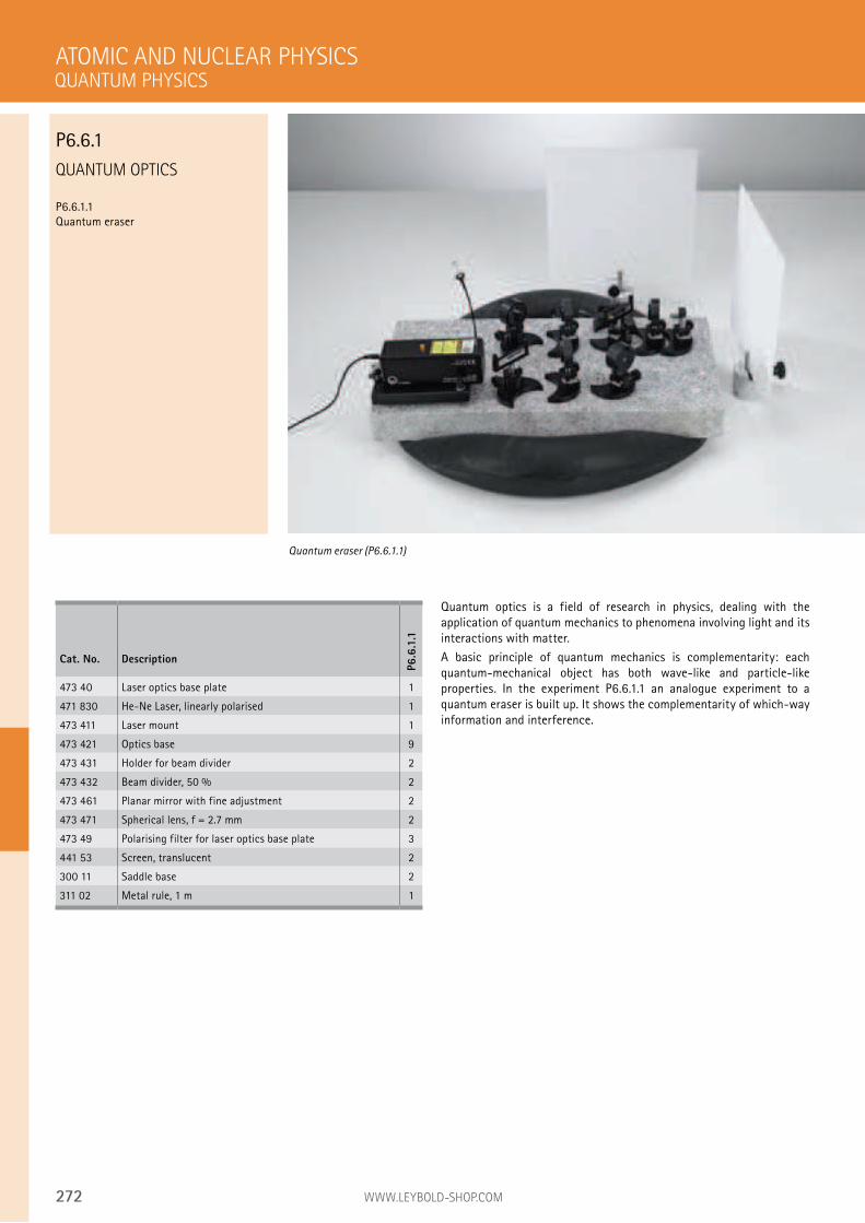
272 WWW.LEYBOLD-SHOP.COM
QUANTUM OPTICS
P6.6.1.1
Quantum eraser
Quantum optics is a field of research in physics, dealing with the
application of quantum mechanics to phenomena involving light and its
interactions with matter.
A basic principle of quantum mechanics is complementarity: each
quantum-mechanical object has both wave-like and particle-like
properties. In the experiment P6.6.1.1 an analogue experiment to a
quantum eraser is built up. It shows the complementarity of which-way
information and interference.
ATOMIC AND NUCLEAR PHYSICS
Quantum eraser (P6.6.1.1)
Cat. No. Description
P6.6
.1.1
473 40 Laser optics base plate 1
471 830 He-Ne Laser, linearly polarised 1
473 411 Laser mount 1
473 421 Optics base 9
473 431 Holder for beam divider 2
473 432 Beam divider, 50 % 2
473 461 Planar mirror with fine adjustment 2
473 471 Spherical lens, f = 2.7 mm 2
473 49 Polarising filter for laser optics base plate 3
441 53 Screen, translucent 2
300 11 Saddle base 2
311 02 Metal rule, 1 m 1
QUANTUM PHYSICS
P6.6.1
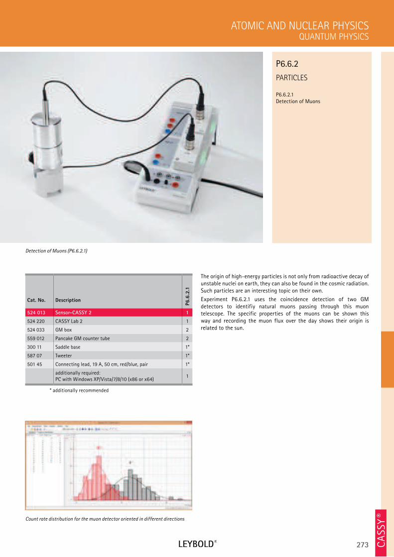
273
PARTICLES
P6.6.2.1 Detection of Muons
QUANTUM PHYSICS
ATOMIC AND NUCLEAR PHYSICS
Cat. No. Description
P6.6
.2.1
524 013 Sensor-CASSY 2 1
524 220 CASSY Lab 2 1
524 033 GM box 2
559 012 Pancake GM counter tube 2
300 11 Saddle base 1*
587 07 Tweeter 1*
501 45 Connecting lead, 19 A, 50 cm, red/blue, pair 1*
additionally required: PC with Windows XP/Vista/7/8/10 (x86 or x64)
1
* additionally recommended
The origin of high-energy particles is not only from radioactive decay of unstable nuclei on earth, they can also be found in the cosmic radiation. Such particles are an interesting topic on their own.
Experiment P6.6.2.1 uses the coincidence detection of two GM detectors to identifiy natural muons passing through this muon telescope. The specific properties of the muons can be shown this way and recording the muon flux over the day shows their origin is related to the sun.
Detection of Muons (P6.6.2.1)
P6.6.2
Count rate distribution for the muon detector oriented in different directions
CA
SSY ®
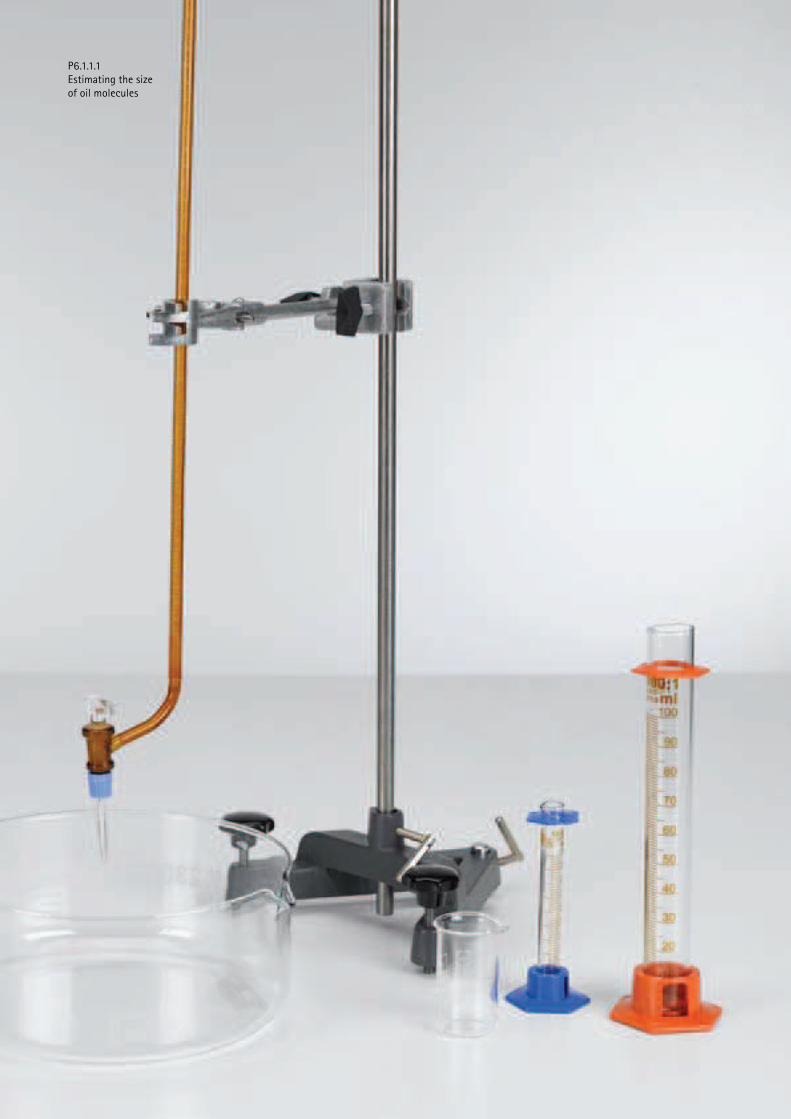
274 WWW.LEYBOLD-SHOP.COM
P6.1.1.1
Estimating the size
of oil molecules

275
P7.1 PROPERTIES OF CRYSTALS 277
P7.2 CONDUCTION PHENOMENA 281
P7.3 MAGNETISM 288
P7.4 SCANNING PROBE MICROSCOPY 290
P7.5 APPLIED SOLID-STATE PHYSICS 292
P7 SOLID-STATE PHYSICS

276 WWW.LEYBOLD-SHOP.COM
P7.1 PROPERTIES OF CRYSTALS
P7.1.1 Crystal structure 277
P7.1.2 X-ray scattering 278-279
P7.1.4 Elastic and plastic deformation 280
P7.2 CONDUCTION PHENOMENA
P7.2.1 Hall effect 281-282
P7.2.2 Electrical conductivity in solids 283
P7.2.3 Photoconductivity 284
P7.2.4 Luminescence 285
P7.2.5 Thermoelectricity 286
P7.2.6 Superconductivity 287
P7.3 MAGNETISM
P7.3.1 Dia-, para- and ferromagnetism 288
P7.3.2 Ferromagnetic hysteresis 289
P7.4 SCANNING PROBE MICROSCOPY
P7.4.1 Scanning tunneling microscope 290-291
P7.5 APPLIED SOLID-STATE PHYSICS
P7.5.1 X-ray fluorescence analysis 292
P7 SOLID-STATE PHYSICS
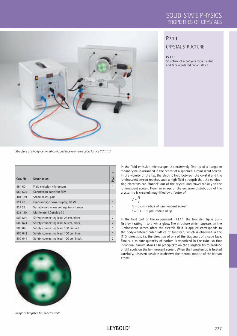
277
CRYSTAL STRUCTURE
P7.1.1.1 Structure of a body-centered cubic and face-centered cubic lattice
PROPERTIES OF CRYSTALS
SOLID-STATE PHYSICS
Cat. No. Description
P7.1
.1.1
554 60 Field emission microscope 1
554 605 Connection panel for FEM 1
301 339 Stand bases, pair 1
521 70 High-voltage power supply, 10 kV 1
521 39 Variable extra-low voltage transformer 1
531 130 Multimeter LDanalog 30 1
500 614 Safety connecting lead, 25 cm, black 2
500 624 Safety connecting lead, 50 cm, black 2
500 641 Safety connecting lead, 100 cm, red 1
500 642 Safety connecting lead, 100 cm, blue 1
500 644 Safety connecting lead, 100 cm, black 2
In the field emission microscope, the extremely fine tip of a tungsten monocrystal is arranged in the center of a spherical luminescent screen. In the vicinity of the tip, the electric field between the crystal and the luminescent screen reaches such a high field strength that the conduc-ting electrons can “tunnel” out of the crystal and travel radially to the luminescent screen. Here, an image of the emission distribution of the crystal tip is created, magnified by a factor of
VR
r
R
r
=
=
= −
5
0 1 0 2
cm: radius of luminescent screen
m: radi. . µ uus of tip
In the first part of the experiment P7.1.1.1, the tungsten tip is puri-fied by heating it to a white glow. The structure which appears on the luminescent screen after the electric field is applied corresponds to the body-centered cubic lattice of tungsten, which is observed in the (110) direction, i.e. the direction of one of the diagonals of a cube face. Finally, a minute quantity of barium is vaporized in the tube, so that individual barium atoms can precipitate on the tungsten tip to produce bright spots on the luminescent screen. When the tungsten tip is heated carefully, it is even possible to observe the thermal motion of the barium atoms.
Structure of a body-centered cubic and face-centered cubic lattice (P7.1.1.1)
P7.1.1
Image of tungsten tip: hot electrode
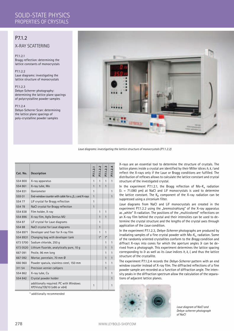
278 WWW.LEYBOLD-SHOP.COM
Laue diagram of NaCl and
Debye-scherrer photograph
of NaCl
X-RAY SCATTERING
P7.1.2.1 Bragg reflection: determining the lattice constants of monocrystals
P7.1.2.2 Laue diagrams: investigating the lattice structure of monocrystals
P7.1.2.3 Debye-Scherrer photography: determining the lattice plane spacings of polycrystalline powder samples
P7.1.2.4 Debye-Scherrer Scan: determining the lattice plane spacings of poly-crystalline powder samples
X-rays are an essential tool to determine the structure of crystals. The lattice planes inside a crystal are identified by their Miller idices h, k, l and reflect the X-rays only if the Laue or Bragg conditions are fulfilled. The distribution of reflexes allows to calculate the lattice constant and crystal structure of the investigated crystal.
In the experiment P7.1.2.1, the Bragg reflection of Mo-Ka radiation ( = 71.080 pm) at NaCl and LiF monocrystals is used to determine the lattice constant. The K component of the X-ray radiation can be suppressed using a zirconium filter.
Laue diagrams from NaCl and LiF monocrystals are created in the experiment P7.1.2.2 using the „bremsstrahlung“ of the X-ray apparatus as „white“ X-radiation. The positions of the „multicolored“ reflections on an X-ray film behind the crystal and their intensities can be used to de-termine the crystal structure and the lengths of the crystal axes through application of the Laue condition.
In the experiment P7.1.2.3, Debye-Scherrer photographs are produced by irradiating samples of a fine crystal powder with Mo-K radiation. Some of the randomly oriented crystallites conform to the Bragg condition and diffract X-rays into cones for which the aperture angles can be de-rived from a photograph. This experiment determines the lattice spacing corresponding to as well as its Laue indices h, k, l, and thus the lattice structure of the crystallite.
The experiment P7.1.2.4 records the Debye-Scherrer pattern with an end window counter instead of X-ray film. The diffracted reflections of a fine powder sample are recorded as a function of diffraction angle. The inten-sity peaks in the diffraction spectrum allow the calculation of the separa-tions of adjacent lattice planes.
SOLID-STATE PHYSICS
Laue diagrams: investigating the lattice structure of monocrystals (P7.1.2.2)
Cat. No. Description
P7.1
.2.1
P7.1
.2.2
P7.1
.2.3
P7.1
.2.4
554 800 X-ray apparatus 1 1 1 1
554 861 X-ray tube, Mo 1 1 1
554 831 Goniometer 1 1
559 01 End-window counter with cable for , , and X-rays 1 1
554 77 LiF crystal for Bragg reflection 1
554 78 NaCl crystal for Bragg reflection 1
554 838 Film holder, X-ray 1 1
554 896 X-ray film, Agfa Dentus M2 1 1
554 87 LiF crystal for Laue diagrams 1
554 88 NaCl crystal for Laue diagrams 1
554 8971 Developer and fixer for X-ray film 1 1
554 8931 Changing bag with developer tank 1* 1*
673 5700 Sodium chloride, 250 g 1 1
673 0520 Lithium fluoride, analytically pure, 10 g 1 1
667 091 Pestle, 96 mm long 1 1
667 092 Mortar, porcelain, 70 mm Ø 1 1
666 960 Powder spatula, stainless steel, 150 mm 1 1
311 54 Precision vernier callipers 1
554 862 X-ray tube, Cu 1
554 842 Crystal powder holder 1
additionally required: PC with Windows XP/Vista/7/8/10 (x86 or x64)
1 1
* additionally recommended
PROPERTIES OF CRYSTALS
P7.1.2
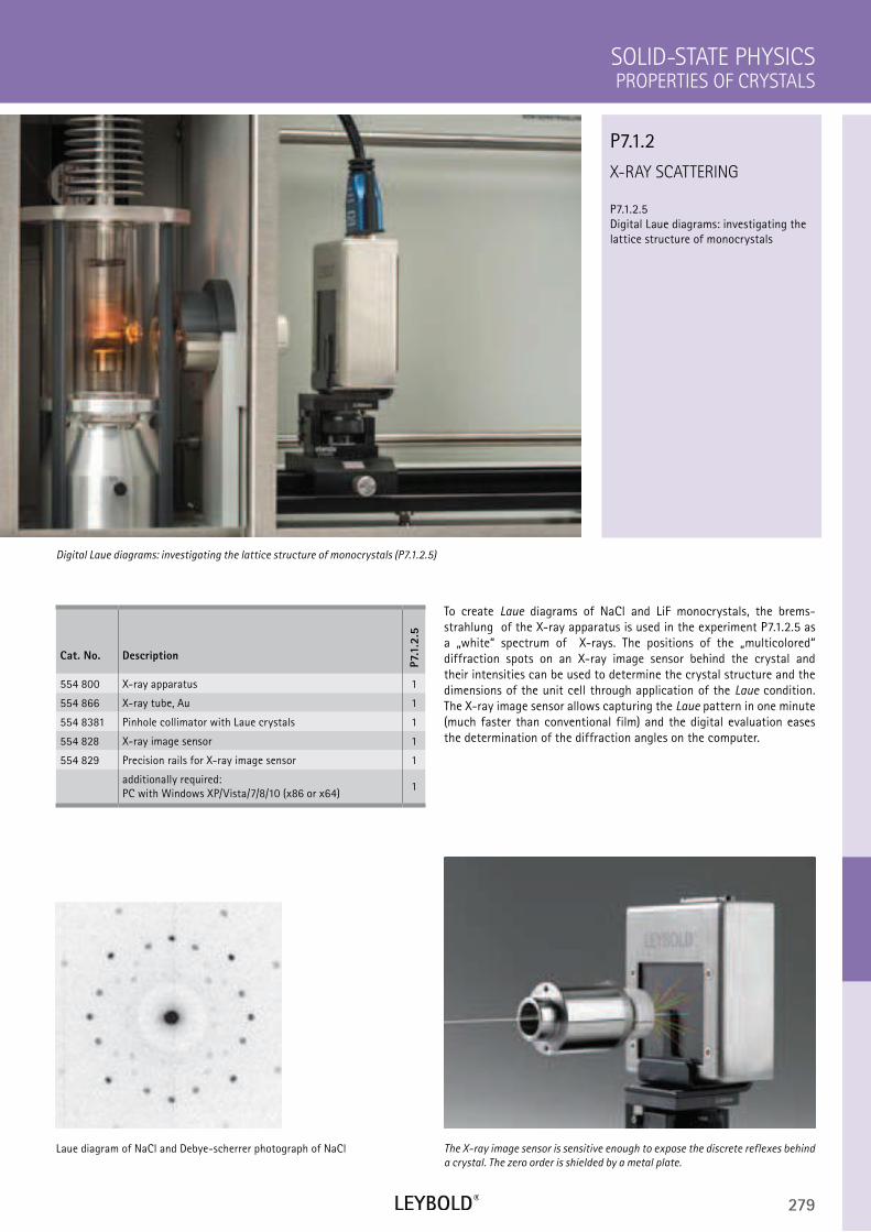
279
X-RAY SCATTERING
P7.1.2.5 Digital Laue diagrams: investigating the lattice structure of monocrystals
PROPERTIES OF CRYSTALS
SOLID-STATE PHYSICS
Cat. No. Description
P7.1
.2.5
554 800 X-ray apparatus 1
554 866 X-ray tube, Au 1
554 8381 Pinhole collimator with Laue crystals 1
554 828 X-ray image sensor 1
554 829 Precision rails for X-ray image sensor 1
additionally required: PC with Windows XP/Vista/7/8/10 (x86 or x64)
1
To create Laue diagrams of NaCl and LiF monocrystals, the brems-strahlung of the X-ray apparatus is used in the experiment P7.1.2.5 as a „white“ spectrum of X-rays. The positions of the „multicolored“ diffraction spots on an X-ray image sensor behind the crystal and their intensities can be used to determine the crystal structure and the dimensions of the unit cell through application of the Laue condition. The X-ray image sensor allows capturing the Laue pattern in one minute (much faster than conventional film) and the digital evaluation eases the determination of the diffraction angles on the computer.
Digital Laue diagrams: investigating the lattice structure of monocrystals (P7.1.2.5)
P7.1.2
Laue diagram of NaCl and Debye-scherrer photograph of NaCl The X-ray image sensor is sensitive enough to expose the discrete reflexes behind
a crystal. The zero order is shielded by a metal plate.
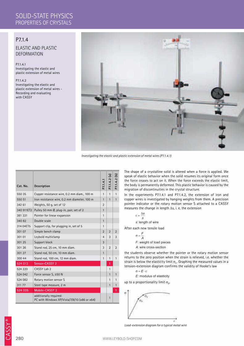
280 WWW.LEYBOLD-SHOP.COM
ELASTIC AND PLASTIC
DEFORMATION
P7.1.4.1 Investigating the elastic and plastic extension of metal wires
P7.1.4.2 Investigating the elastic and plastic extension of metal wires - Recording and evaluating with CASSY
The shape of a crystalline solid is altered when a force is applied. We speak of elastic behavior when the solid resumes its original form once the force ceases to act on it. When the force exceeds the elastic limit, the body is permanently deformed. This plastic behavior is caused by the migration of discontinuities in the crystal structure.
In the experiments P7.1.4.1 and P7.1.4.2, the extension of iron and copper wires is investigated by hanging weights from them. A precision pointer indicator or the rotary motion sensor S attached to a CASSY measures the change in length s, i. e. the extension
ε =∆s
s
s: length of wire
After each new tensile load
σ =F
A
F
A
: weight of load pieces
: wire cross-section
the students observe whether the pointer or the rotary motion sensor returns to the zero position when the strain is relieved, i.e. whether the strain is below the elasticity limit . Graphing the measured values in a tension-extension diagram confirms the validity of Hooke‘s law
σ ε= ⋅E
E: modulus of elasticity
up to a proportionality limit p.
SOLID-STATE PHYSICS
Investigating the elastic and plastic extension of metal wires (P7.1.4.1)
Cat. No. Description
P7.
1.4
.1
P7.
1.4
.2 (
a)
P7.
1.4
.2 (
b)
550 35 Copper resistance wire, 0.2 mm diam., 100 m 1 1 1
550 51 Iron resistance wire, 0.2 mm diameter, 100 m 1 1 1
342 61 Weights, 50 g, set of 12 2
340 911ET2 Pulley 50 mm Ø, plug-in, pair, set of 2 1
381 331 Pointer for linear expansion 1
340 82 Double scale 1
314 04ET5 Support clip, for plugging in, set of 5 1
301 07 Simple bench clamp 2 2 2
301 01 Leybold multiclamp 4 3 3
301 25 Support block 3
301 26 Stand rod, 25 cm, 10 mm diam. 3 2 2
301 27 Stand rod, 50 cm, 10 mm diam. 1
300 44 Stand rod, 100 cm, 12 mm diam. 1 1 1
524 013 Sensor-CASSY 2 1
524 220 CASSY Lab 2 1
524 042 Force sensor S, ±50 N 1 1
524 082 Rotary motion sensor S 1 1
311 77 Steel tape measure, 2 m 1 1
524 005 Mobile-CASSY 2 1
additionally required: PC with Windows XP/Vista/7/8/10 (x86 or x64)
1
Load-extension diagram for a typical metal wire
PROPERTIES OF CRYSTALS
P7.1.4
CA
SSY ®
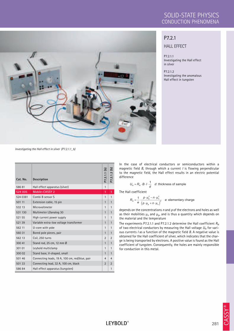
281
HALL EFFECT
P7.2.1.1 Investigating the Hall effect in silver
P7.2.1.2 Investigating the anomalous Hall effect in tungsten
CONDUCTION PHENOMENA
SOLID-STATE PHYSICS
Cat. No. Description
P7.
2.1
.1 (
b)
P7.
2.1
.2 (
b)
586 81 Hall effect apparatus (silver) 1
524 005 Mobile-CASSY 2 1 1
524 0381 Combi B sensor S 1 1
501 11 Extension cable, 15 pin 1 1
532 13 Microvoltmeter 1 1
531 130 Multimeter LDanalog 30 1 1
521 55 High current power supply 1 1
521 39 Variable extra-low voltage transformer 1 1
562 11 U-core with yoke 1 1
560 31 Bored pole pieces, pair 1 1
562 13 Coil, 250 turns 2 2
300 41 Stand rod, 25 cm, 12 mm Ø 1 1
301 01 Leybold multiclamp 1 1
300 02 Stand base, V-shaped, small 1 1
501 46 Connecting leads, 19 A, 100 cm, red/blue, pair 4 4
501 33 Connecting lead, 32 A, 100 cm, black 2 2
586 84 Hall effect apparatus (tungsten) 1
In the case of electrical conductors or semiconductors within a magnetic field B, through which a current I is flowing perpendicular to the magnetic field, the Hall effect results in an electric potential difference
U R B Id
dH H : thickness of sample= ⋅ ⋅ ⋅1
The Hall coefficient
Re
p n
p neH
p n
p n
: elementary charge= ⋅⋅ − ⋅
⋅ + ⋅( )1
2 2
2
µ µ
µ µ
depends on the concentrations n and p of the electrons and holes as well as their mobilities µn and µp, and is thus a quantity which depends on the material and the temperature
The experiments P7.2.1.1 and P7.2.1.2 determine the Hall coefficient RH of two electrical conductors by measuring the Hall voltage UH for vari-ous currents I as a function of the magnetic field B. A negative value is obtained for the Hall coefficient of silver, which indicates that the char-ge is being transported by electrons. A positive value is found as the Hall coefficient of tungsten. Consequently, the holes are mainly responsible for conduction in this metal.
Investigating the Hall effect in silver (P7.2.1.1_b)
P7.2.1
CA
SSY ®
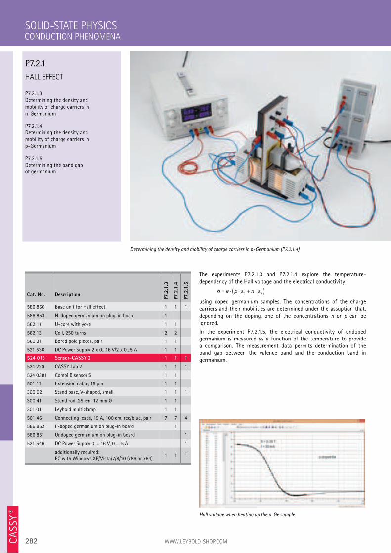
282 WWW.LEYBOLD-SHOP.COM
HALL EFFECT
P7.2.1.3 Determining the density and mobility of charge carriers in n-Germanium
P7.2.1.4 Determining the density and mobility of charge carriers in p-Germanium
P7.2.1.5 Determining the band gap of germanium
The experiments P7.2.1.3 and P7.2.1.4 explore the temperature- dependency of the Hall voltage and the electrical conductivity
σ µ µ= ⋅ ⋅ + ⋅( )e p np n
using doped germanium samples. The concentrations of the charge carriers and their mobilities are determined under the assuption that, depending on the doping, one of the concentrations n or p can be ignored.
In the experiment P7.2.1.5, the electrical conductivity of undoped germanium is measured as a function of the temperature to provide a comparison. The measurement data permits determination of the band gap between the valence band and the conduction band in germanium.
SOLID-STATE PHYSICS
Determining the density and mobility of charge carriers in p-Germanium (P7.2.1.4)
Cat. No. Description
P7.2
.1.3
P7.2
.1.4
P7.2
.1.5
586 850 Base unit for Hall effect 1 1 1
586 853 N-doped germanium on plug-in board 1
562 11 U-core with yoke 1 1
562 13 Coil, 250 turns 2 2
560 31 Bored pole pieces, pair 1 1
521 536 DC Power Supply 2 x 0...16 V/2 x 0...5 A 1 1
524 013 Sensor-CASSY 2 1 1 1
524 220 CASSY Lab 2 1 1 1
524 0381 Combi B sensor S 1 1
501 11 Extension cable, 15 pin 1 1
300 02 Stand base, V-shaped, small 1 1 1
300 41 Stand rod, 25 cm, 12 mm Ø 1 1
301 01 Leybold multiclamp 1 1
501 46 Connecting leads, 19 A, 100 cm, red/blue, pair 7 7 4
586 852 P-doped germanium on plug-in board 1
586 851 Undoped germanium on plug-in board 1
521 546 DC Power Supply 0 ... 16 V, 0 ... 5 A 1
additionally required: PC with Windows XP/Vista/7/8/10 (x86 or x64)
1 1 1
Hall voltage when heating up the p-Ge sample
CONDUCTION PHENOMENA
P7.2.1
CA
SSY ®
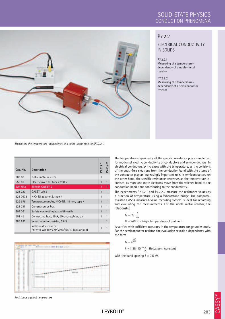
283
ELECTRICAL CONDUCTIVITY
IN SOLIDS
P7.2.2.1 Measuring the temperature- dependency of a noble-metal resistor
P7.2.2.2 Measuring the temperature- dependency of a semiconductor resistor
CONDUCTION PHENOMENA
SOLID-STATE PHYSICS
Cat. No. Description
P7.2
.2.1
P7.2
.2.2
586 80 Noble metal resistor 1
555 81 Electric oven for tubes, 230 V 1 1
524 013 Sensor-CASSY 2 1 1
524 220 CASSY Lab 2 1 1
524 0673 NiCr-Ni adapter S, type K 1 1
529 676 Temperature probe, NiCr-Ni, 1.5 mm, type K 1 1
524 031 Current source box 1 1
502 061 Safety connecting box, with earth 1 1
501 45 Connecting lead, 19 A, 50 cm, red/blue, pair 1 1
586 821 Semiconductor resistor, 5 k 1
additionally required: PC with Windows XP/Vista/7/8/10 (x86 or x64)
1 1
The temperature-dependency of the specific resistance is a simple test for models of electric conductivity of conductors and semiconductors. In electrical conductors, increases with the temperature, as the collisions of the quasi-free electrons from the conduction band with the atoms of the conductor play an increasingly important role. In semiconductors, on the other hand, the specific resistance decreases as the temperature in-creases, as more and more electrons move from the valence band to the conduction band, thus contributing to the conductivity.
The experiments P7.2.2.1 and P7.2.2.2 measure the resistance values as a function of temperature using a Wheatstone bridge. The computer-assisted CASSY measured-value recording system is ideal for recording and evaluating the measurements. For the noble metal resistor, the relationship
R RT
Debye
= ⋅
=
ΘΘ
Θ 240 K: temperature of platinum
is verified with sufficient accuracy in the temperature range under study. For the semiconductor resistor, the evaluation reveals a dependency with the form
R e
k Boltzmann
E
kT∝
= ⋅−
∆
2
231 38 10. :
J
K constant
with the band spacing E = 0.5 eV.
Measuring the temperature-dependency of a noble-metal resistor (P7.2.2.1)
P7.2.2
Resistance against temperature
CA
SSY ®
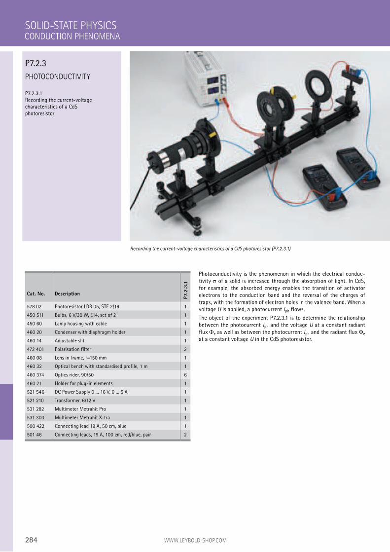
284 WWW.LEYBOLD-SHOP.COM
PHOTOCONDUCTIVITY
P7.2.3.1 Recording the current-voltage characteristics of a CdS photoresistor
Photoconductivity is the phenomenon in which the electrical conduc-tivity of a solid is increased through the absorption of light. In CdS, for example, the absorbed energy enables the transition of activator electrons to the conduction band and the reversal of the charges of traps, with the formation of electron holes in the valence band. When a voltage U is applied, a photocurrent Iph flows.
The object of the experiment P7.2.3.1 is to determine the relationship between the photocurrent Iph and the voltage U at a constant radiant flux e as well as between the photocurrent Iph and the radiant flux e at a constant voltage U in the CdS photoresistor.
SOLID-STATE PHYSICS
Recording the current-voltage characteristics of a CdS photoresistor (P7.2.3.1)
Cat. No. Description
P7.2
.3.1
578 02 Photoresistor LDR 05, STE 2/19 1
450 511 Bulbs, 6 V/30 W, E14, set of 2 1
450 60 Lamp housing with cable 1
460 20 Condenser with diaphragm holder 1
460 14 Adjustable slit 1
472 401 Polarisation filter 2
460 08 Lens in frame, f=150 mm 1
460 32 Optical bench with standardised profile, 1 m 1
460 374 Optics rider, 90/50 6
460 21 Holder for plug-in elements 1
521 546 DC Power Supply 0 ... 16 V, 0 ... 5 A 1
521 210 Transformer, 6/12 V 1
531 282 Multimeter Metrahit Pro 1
531 303 Multimeter Metrahit X-tra 1
500 422 Connecting lead 19 A, 50 cm, blue 1
501 46 Connecting leads, 19 A, 100 cm, red/blue, pair 2
CONDUCTION PHENOMENA
P7.2.3
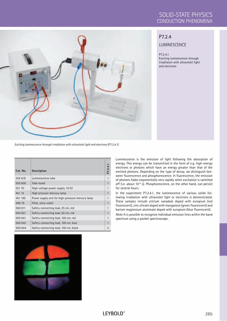
285
LUMINESCENCE
P7.2.4.1 Exciting luminescence through irraditaion with ultraviolet light and electrons
CONDUCTION PHENOMENA
SOLID-STATE PHYSICS
Cat. No. Description
P7.2
.4.1
555 618 Luminescence tube 1
555 600 Tube stand 1
521 70 High-voltage power supply, 10 kV 1
451 15 High pressure mercury lamp 1
451 195 Power supply unit for high-pressure mercury lamp 1
469 79 Filter, ultra-violet 1
500 611 Safety connecting lead, 25 cm, red 1
500 621 Safety connecting lead, 50 cm, red 1
500 641 Safety connecting lead, 100 cm, red 1
500 642 Safety connecting lead, 100 cm, blue 1
500 644 Safety connecting lead, 100 cm, black 2
Luminescence is the emission of light following the absorption of energy. This energy can be transmitted in the form of e.g. high-energy electrons or photons which have an energy greater than that of the emitted photons. Depending on the type of decay, we distinguish bet-ween fluorescence and phosphorescence. In fluorescence, the emission of photons fades exponentially very rapidly when excitation is switched off (i.e. about 10-8
s). Phosphorescence, on the other hand, can persist for several hours.
In the experiment P7.2.4.1, the luminescence of various solids fol-lowing irradiation with ultraviolet light or electrons is demonstrated. These samples include yttrium vanadate doped with europium (red fluorescent), zinc silicate doped with manganese (green fluorescent) and barium magnesium aluminate doped with europium (blue fluorescent).
Note: It is possible to recognize individual emission lines within the band spectrum using a pocket spectroscope.
Exciting luminescence through irraditaion with ultraviolet light and electrons (P7.2.4.1)
P7.2.4
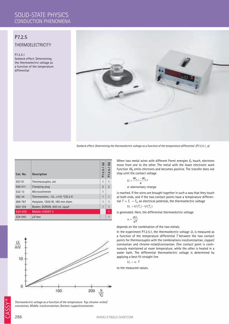
286 WWW.LEYBOLD-SHOP.COM
THERMOELECTRICITY
P7.2.5.1 Seebeck effect: Determining the thermoelectric voltage as a function of the temperature differential
When two metal wires with different Fermi energies EF touch, electrons move from one to the other. The metal with the lower electronic work function WA emits electrons and becomes positive. The transfer does not stop until the contact voltage
UW W
e
e
=−A, 1 A, 2
: elementary charge
is reached. If the wires are brought together in such a way that they touch at both ends, and if the two contact points have a temperature differen-tial T = T1 – T2, an electrical potential, the thermoelectric voltage
U U T U TT= ( ) − ( )1 2
is generated. Here, the differential thermoelectric voltage
α =dU
dT
T
depends on the combination of the two metals.
In the experiment P7.2.5.1, the thermoelectric voltage UT is measured as a function of the temperature differential T between the two contact points for thermocouples with the combinations iron/constantan, copper/ constantan and chrome-nickel/constantan. One contact point is conti-nuously maintained at room temperature, while the other is heated in a water bath. The differential thermoelectric voltage is determined by applying a best-fit straight line
U TT= ⋅α
to the measured values.
SOLID-STATE PHYSICS
Seebeck effect: Determining the thermoelectric voltage as a function of the temperature differential (P7.2.5.1_a)
Cat. No. Description
P7.
2.5
.1 (
a)
P7.
2.5
.1 (
b)
557 01 Thermocouples, set 1 1
590 011 Clamping plug 2 2
532 13 Microvoltmeter 1
382 34 Thermometer, -10...+110 °C/0.2 K 1 1
666 767 Hotplate, 1500 W, 180 mm diam. 1 1
664 104 Beaker, DURAN, 400 ml, squat 1 1
524 005 Mobile-CASSY 2 1
524 040 µV box 1
Thermoelectric voltage as a function of the temperature Top: chrome-nickel/constantan, Middle: iron/constantan, Bottom: cupper/constantan
CONDUCTION PHENOMENA
P7.2.5
CA
SSY ®
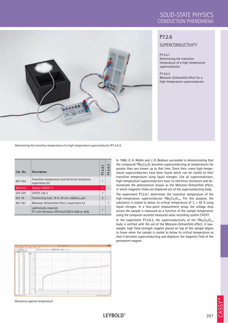
287
SUPERCONDUCTIVITY
P7.2.6.1 Determining the transition temperature of a high-temperature superconductor
P7.2.6.2 Meissner-Ochsenfeld effect for a high-temperature superconductor
CONDUCTION PHENOMENA
SOLID-STATE PHYSICS
Cat. No. Description
P7.2
.6.1
P7.2
.6.2
667 552Transition temperature and electrical resistance, experiment kit
1
524 013 Sensor-CASSY 2 1
524 220 CASSY Lab 2 1
501 45 Connecting lead, 19 A, 50 cm, red/blue, pair 2
667 551 Meissner-Ochsenfeld effect, experiment kit 1
additionally required: PC with Windows XP/Vista/7/8/10 (x86 or x64)
1
In 1986, K. A. Müller and J. G. Bednorz succeeded in demonstrating that the compound YBa2Cu3O7 becomes superconducting at temperatures far greater than any known up to that time. Since then, many high-tempe-rature superconductors have been found which can be cooled to their transition temperature using liquid nitrogen. Like all superconductors, high-temperature superconductors have no electrical resistance and de-monstrate the phenomenon known as the Meissner-Ochsenfeld effect, in which magnetic fields are displaced out of the superconducting body.
The experiment P7.2.6.1 determines the transition temperature of the high-temperature superconductor YBa2Cu3O7-x. For this purpose, the substance is cooled to below its critical temperature of Tc = 92 K using liquid nitrogen. In a four-point measurement setup, the voltage drop across the sample is measured as a function of the sample temperature using the computer-assisted measured value recording system CASSY.
In the experiment P7.2.6.2, the superconductivity of the YBa2Cu3O7-x body is verified with the aid of the Meissner-Ochsenfeld effect. A low-weight, high field-strength magnet placed on top of the sample begins to hover when the sample is cooled to below its critical temperature so that it becomes superconducting and displaces the magnetic field of the permanent magnet.
Determining the transition temperature of a high-temperature superconductor (P7.2.6.1)
P7.2.6
Resistance against temperature
CA
SSY ®
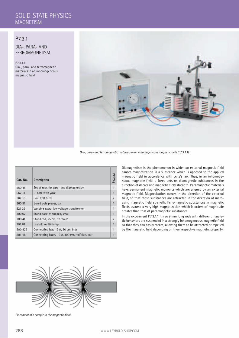
288 WWW.LEYBOLD-SHOP.COM
DIA-, PARA- AND
FERROMAGNETISM
P7.3.1.1 Dia-, para- and ferromagnetic materials in an inhomogeneous magnetic field
Diamagnetism is the phenomenon in which an external magnetic field causes magnetization in a substance which is opposed to the applied magnetic field in accordance with Lenz‘s law. Thus, in an inhomoge-neous magnetic field, a force acts on diamagnetic substances in the direction of decreasing magnetic field strength. Paramagnetic materials have permanent magnetic moments which are aligned by an external magnetic field. Magnetization occurs in the direction of the external field, so that these substances are attracted in the direction of incre-asing magnetic field strength. Ferromagnetic substances in magnetic fields assume a very high magnetization which is orders of magnitude greater than that of paramagnetic substances.
In the experiment P7.3.1.1, three 9 mm long rods with different magne-tic behaviors are suspended in a strongly inhomogeneous magnetic field so that they can easily rotate, allowing them to be attracted or repelled by the magnetic field depending on their respective magnetic property.
SOLID-STATE PHYSICS
Dia-, para- and ferromagnetic materials in an inhomogeneous magnetic field (P7.3.1.1)
Cat. No. Description
P7.3
.1.1
560 41 Set of rods for para- and diamagnetism 1
562 11 U-core with yoke 1
562 13 Coil, 250 turns 2
560 31 Bored pole pieces, pair 1
521 39 Variable extra-low voltage transformer 1
300 02 Stand base, V-shaped, small 1
300 41 Stand rod, 25 cm, 12 mm Ø 2
301 01 Leybold multiclamp 1
500 422 Connecting lead 19 A, 50 cm, blue 1
501 46 Connecting leads, 19 A, 100 cm, red/blue, pair 1
Placement of a sample in the magnetic field
MAGNETISM
P7.3.1
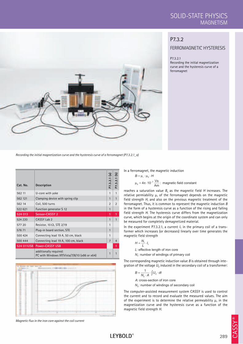
289
In a ferromagnet, the magnetic induction
B Hr
= ⋅ ⋅
= ⋅ −
µ µ
µ π
0
0
74 10Vs
Am magnetic field constant:
reaches a saturation value Bs as the magnetic field H increases. The relative permiability µr of the ferromagnet depends on the magnetic field strength H, and also on the previous magnetic treatment of the ferromagnet. Thus, it is common to represent the magnetic induction B in the form of a hysteresis curve as a function of the rising and falling field strength H. The hysteresis curve differs from the magnetization curve, which begins at the origin of the coordinate system and can only be measured for completely demagnetized material.
In the experiment P7.3.2.1, a current I1 in the primary coil of a trans-former which increases (or decreases) linearly over time generates the magnetic field strength
HN
LI
L
N
= ⋅11
1
: effective length of iron core
: number of windiings of primary coil
The corresponding magnetic induction value B is obtained through inte-gration of the voltage U2 induced in the secondary coil of a transformer:
BN A
U dt
A
N
=⋅
⋅ ⋅∫1
2
2
2
: cross-section of iron core
: number of wiindings of secondary coil
The computer-assisted measurement system CASSY is used to control the current and to record and evaluate the measured values. The aim of the experiment is to determine the relative permeability µr in the magnetization curve and the hysteresis curve as a function of the magnetic field strength H.
FERROMAGNETIC HYSTERESIS
P7.3.2.1 Recording the initial magnetization curve and the hysteresis curve of a ferromagnet
MAGNETISM
SOLID-STATE PHYSICS
Cat. No. Description
P7.
3.2
.1 (
a)
P7.
3.2
.1 (
b)
562 11 U-core with yoke 1 1
562 121 Clamping device with spring clip 1 1
562 14 Coil, 500 turns 2 2
522 621 Function generator S 12 1
524 013 Sensor-CASSY 2 1 1
524 220 CASSY Lab 2 1 1
577 20 Resistor, 10 , STE 2/19 1
576 71 Plug-in board section, STE 1
500 424 Connecting lead 19 A, 50 cm, black 1
500 444 Connecting lead 19 A, 100 cm, black 7 4
524 011USB Power-CASSY USB 1
additionally required: PC with Windows XP/Vista/7/8/10 (x86 or x64)
1 1
Recording the initial magnetization curve and the hysteresis curve of a ferromagnet (P7.3.2.1_a)
P7.3.2
Magnetic flux in the iron core against the coil current
CA
SSY ®
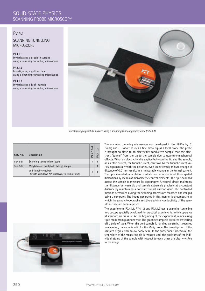
290 WWW.LEYBOLD-SHOP.COM
The scanning tunneling microscope was developed in the 1980‘s by G.
Binnig and H. Rohrer. It uses a fine metal tip as a local probe; the probe is brought so close to an electrically conductive sample that the elec-trons “tunnel” from the tip to the sample due to quantum-mechanical effects. When an electric field is applied between the tip and the sample, an electric current, the tunnel current, can flow. As the tunnel current va-ries exponentially with the distance, even an extremely minute change in distance of 0.01 nm results in a measurable change in the tunnel current. The tip is mounted on a platform which can be moved in all three spatial dimensions by means of piezoelectric control elements. The tip is scanned across the sample to measure its topography. A control circuit maintains the distance between tip and sample extremely precisely at a constant distance by maintaining a constant tunnel current value. The controlled motions performed during the scanning process are recorded and imaged using a computer. The image generated in this manner is a composite in which the sample topography and the electrical conductivity of the sam-ple surface are superimposed.
The experiments P7.4.1.1, P7.4.1.2 and P7.4.1.3 use a scanning tunneling microscope specially developed for practical experiments, which operates at standard air pressure. At the beginning of the experiment, a measuring tip is made from platinum wire. The graphite sample is prepared by tearing off a strip of tape. When the gold sample is handled carefully, it requires no cleaning; the same is valid for the MoS2 probe. The investigation of the samples begins with an overview scan. In the subsequent procedure, the step width of the measuring tip is reduced until the positions of the indi-vidual atoms of the sample with respect to each other are clearly visible in the image.
SCANNING TUNNELING
MICROSCOPE
P7.4.1.1 Investigating a graphite surface using a scanning tunneling microscope
P7.4.1.2 Investigating a gold surface using a scanning tunneling microscope
P7.4.1.3 Investigating a MoS2 sample using a scanning tunneling microscope
SOLID-STATE PHYSICS
Investigating a graphite surface using a scanning tunneling microscope (P7.4.1.1)
Cat. No. Description
P7.4
.1.1
-2
P7.4
.1.3
554 581 Scanning tunnel microscope 1 1
554 584 Molybdenum disulphide (MoS2) sample 1
additionally required: PC with Windows XP/Vista/7/8/10 (x86 or x64)
1 1
SCANNING PROBE MICROSCOPY
P7.4.1
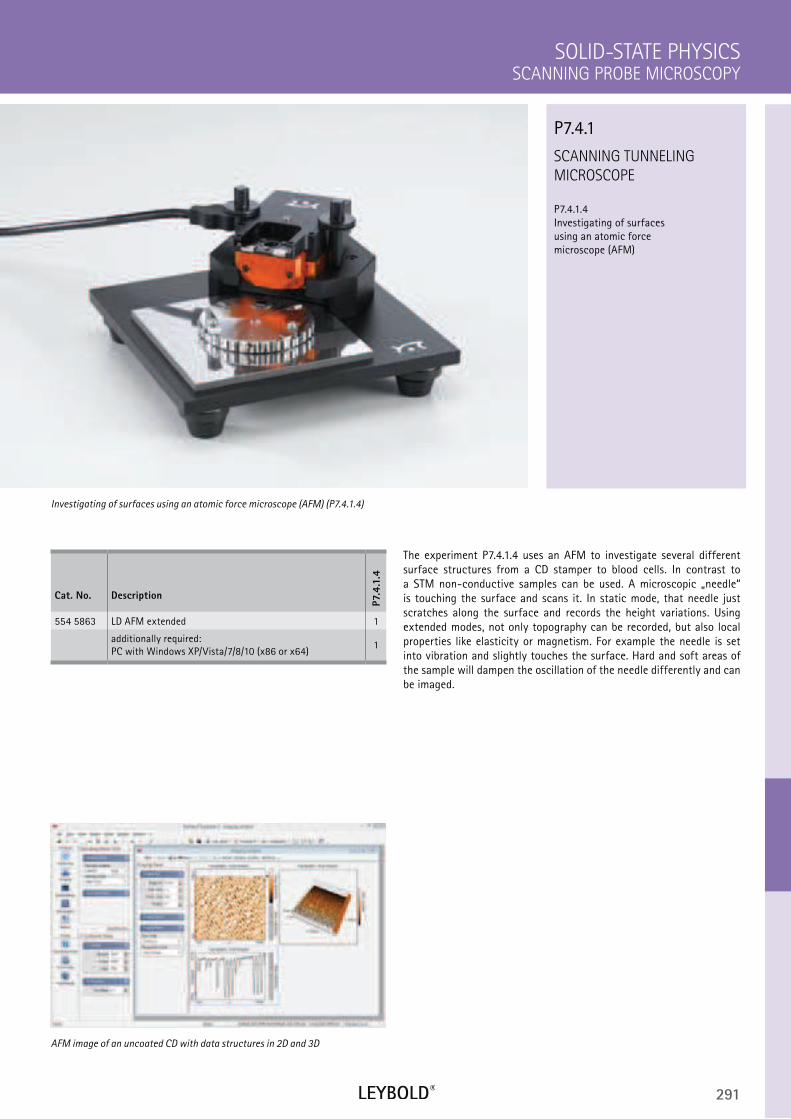
291
SCANNING TUNNELING
MICROSCOPE
P7.4.1.4 Investigating of surfaces using an atomic force microscope (AFM)
SCANNING PROBE MICROSCOPY
SOLID-STATE PHYSICS
Cat. No. Description
P7.4
.1.4
554 5863 LD AFM extended 1
additionally required: PC with Windows XP/Vista/7/8/10 (x86 or x64)
1
The experiment P7.4.1.4 uses an AFM to investigate several different surface structures from a CD stamper to blood cells. In contrast to a STM non-conductive samples can be used. A microscopic „needle“ is touching the surface and scans it. In static mode, that needle just scratches along the surface and records the height variations. Using extended modes, not only topography can be recorded, but also local properties like elasticity or magnetism. For example the needle is set into vibration and slightly touches the surface. Hard and soft areas of the sample will dampen the oscillation of the needle differently and can be imaged.
Investigating of surfaces using an atomic force microscope (AFM) (P7.4.1.4)
P7.4.1
AFM image of an uncoated CD with data structures in 2D and 3D
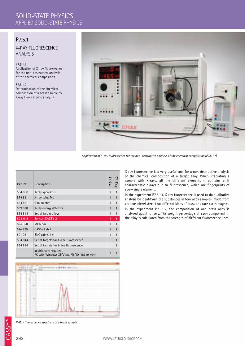
292 WWW.LEYBOLD-SHOP.COM
X-RAY FLUORESCENCE
ANALYSIS
P7.5.1.1 Application of X-ray fluorescence for the non-destructive analysis of the chemical composition
P7.5.1.2 Determination of the chemical composition of a brass sample by X-ray fluorescence analysis
X-ray fluorescence is a very useful tool for a non-destructive analysis of the chemical composition of a target alloy. When irradiating a sample with X-rays, all the different elements it contains emit characteristic X-rays due to fluorescence, which are fingerprints of every single element.
In the experiment P7.5.1.1, X-ray fluorescence is used to do qualitative analysis by identifying the substances in four alloy samples, made from chrome-nickel steel, two different kinds of brass and rare earth magnet.
In the experiment P7.5.1.2, the composition of one brass alloy is analysed quantitatively. The weight percentage of each component in the alloy is calculated from the strength of different fluorescence lines.
SOLID-STATE PHYSICS
Application of X-ray fluorescence for the non-destructive analysis of the chemical composition (P7.5.1.1)
Cat. No. Description
P7.5
.1.1
P7.5
.1.2
554 800 X-ray apparatus 1 1
554 861 X-ray tube, Mo 1 1
554 831 Goniometer 1 1
559 938 X-ray energy detector 1 1
554 848 Set of target alloys 1 1
524 013 Sensor-CASSY 2 1 1
524 058 MCA box 1 1
524 220 CASSY Lab 2 1 1
501 02 BNC cable, 1 m 1 1
554 844 Set of targets for K-line fluorescence 1
554 846 Set of targets for L-line fluorescence 1
additionally required: PC with Windows XP/Vista/7/8/10 (x86 or x64)
1 1
X-Ray fluorescence spectrum of a brass sample
APPLIED SOLID-STATE PHYSICS
P7.5.1
CA
SSY ®

293
P8 REGISTER

REGISTER
294 WWW.LEYBOLD-SHOP.COM
radiation ..............................................................................................264
spectrum .............................................................................................268
radiation ..............................................................................................264
spectrum ..............................................................................................269
radiation ...............................................................................................264
spectrum ..............................................................................................269
3
3D ..............................................................................................................259
A
Abbe refractometer ..............................................................................209
Aberration,chromatic ...........................................................................169
Aberration, lens .....................................................................................169
Absorber, saturable ............................................................................... 218
Absorption ............................................................................ 206, 212, 214
Absorption edge ....................................................................................253
Absorption of radiation ...................................................................269
Absorption of radiation ....................................................................264
Absorption of light................................................................................ 173
Absorption of microwaves .................................................................. 137
Absorption of X-rays ............................................................................253
Absorption spectra ............................................................................... 174
Absorption spectrum ........................................................................... 241
AC power meter ..................................................................................... 118
Acceleration ...............................................................................................15
AC-DC generator ................................................................................... 123
Acousto-optic modulator ..................................................................... 54
Action = reaction .................................................................................... 19
Active power........................................................................................... 132
Activity determination ........................................................................269
AD converter ..........................................................................................164
Adder ........................................................................................................160
Additive colour mixing ........................................................................ 171
Adiabatic exponent ................................................................................ 79
Aerodynamics ....................................................................................60-62
AFM ...........................................................................................................291
Air resistance ........................................................................................... 62
Airfoil .......................................................................................................... 62
Alloy composition .................................................................................292
Amontons‘ law ......................................................................................... 78
Ampere, definition of ........................................................................... 113
Amplifier .................................................................................................. 157
Amplifier, optical ...................................................................................220
Amplitude hologram ............................................................................ 187
Amplitude modulation (AM) .............................................................. 135
AND-Gate ................................................................................................162
Angle of inclination .............................................................................. 121
Angled projection.................................................................................... 23
Angular acceleration .............................................................................. 26
Angular velocity ...................................................................................... 26
Anharmonic oscillation.......................................................................... 36
Annihilation radiation ..........................................................................269
Anomalous Hall effect .........................................................................281
Anomalous Zeeman effect .................................................................249
Anomaly of water ................................................................................... 67
Antenna ..........................................................................................139, 170
Apparent power ..................................................................................... 132
Archimedes‘ principle............................................................................. 56
Astigmatism ............................................................................................169
Atom, size of ...........................................................................................231
Atomic force microscope ....................................................................291
Atomic size ..............................................................................................278
Attenuation .............................................................................................252
Attenuation X-rays ...............................................................................253
Attenuation of , and radiation ................................................264
Autocollimation .....................................................................................167
B
Babinet‘s theorem................................................................................. 176
Balmer series ..........................................................................................239
Balmer-Serie ...........................................................................................239
Band gap ..................................................................................................281
Barrel distortions ..................................................................................169
Beam analysis, Laser ............................................................................227

REGISTER
295
Beam deflection .................................................................................... 211
Beam profiler ..........................................................................................205
Beam, Gaussian .....................................................................................205
Beamsplitter ........................................................................................... 211
Beats .............................................................................................44-45, 51
Bell ............................................................................................................133
Bending .........................................................................................................6
Bending radius ............................................................................................3
Bernoulli equation .................................................................................. 62
Bessel method ........................................................................................ 167
Biot-Savart‘s law ................................................................................... 114
Bipolar transistors .................................................................................156
Biprism .....................................................................................................180
Birefringence ........................................................................190, 192-193
Birefringent tuner ................................................................................. 216
Black body ...............................................................................................196
Block and tackle .........................................................................................9
Bohr‘s magneton ...................................................................................248
Bohr‘s model of the atom ..........................................................244-246
Boyle-Mariotte‘s law ............................................................................. 78
Bragg reflection ....................................................................................254
Braun tube ..............................................................................................143
Break-away method ............................................................................... 59
Breit-Rabi formula ................................................................................249
Bremsstrahlung .....................................................................................254
Brewster angle .......................................................................................189
Bridge rectifier .......................................................................................156
Brightness control ................................................................................160
Brownian motion of molecules ........................................................... 77
Building materials ................................................................................... 68
Buoyancy ................................................................................................... 57
C
Calcite ......................................................................................................190
Calliper gauge .............................................................................................3
Canal rays ................................................................................................ 147
Capacitance of a plate capacitor ..................................................... 101
Capacitance of a sphere .....................................................................100
Capacitive impedance ........................................................126, 128-129
Capacitor ............................................................................... 101-103, 126
Cathode rays .......................................................................................... 147
Cavendish hemispheres ......................................................................... 99
CCD Camera ........................................................................................... 212
Center of gravity ..................................................................................... 24
Central force ............................................................................................ 24
Centrifugal and centripetal force ....................................................... 27
Chaotic oscillation .................................................................................. 36
Characteristic radiation ......................................................................254
Characteristic(s) of a diode ................................................................153
Characteristic(s) of a field-effect transistor .................................156
Characteristic(s) of a glow lamp .......................................................153
Characteristic(s) of a light-emitting diode ....................................153
Characteristic(s) of a photoresistor .................................................284
Characteristic(s) of a phototransistor .............................................158
Characteristic(s) of a solar battery .................................................. 152
Characteristic(s) of a transistor ........................................................156
Characteristic(s) of a tube diode ......................................................140
Characteristic(s) of a tube triode ..................................................... 141
Characteristic(s) of a varistor ............................................................153
Characteristic(s) of a Z-diode ............................................................153
Charge carrier concentration ............................................................281
Charge distribution ................................................................................. 99
Charge transport ...................................................................................104
Charge, electric ...............................................................89-93, 140-144
Chromatic aberration ...........................................................................169
Circular motion ...........................................................................24, 26-27
Circular polarization ................................................................................41
Circular waves .......................................................................................... 42
Cloud chamber .......................................................................................265
Coercive force ........................................................................................289
Coherence ............................................................................179, 184, 208
Coherence length ..................................................................................184
Coherence time ......................................................................................184
Coil ............................................................................................................ 127
Coincidence ............................................................................................269
Collision ........................................................................................18-19, 25

REGISTER
296 WWW.LEYBOLD-SHOP.COM
Color mixing ........................................................................................... 212
Colour filter ............................................................................................ 174
Colour mixing ......................................................................................... 171
Coma .........................................................................................................169
Comparator .............................................................................................160
Complementary colours ...................................................................... 171
Composition of forces ..............................................................................7
Compton effect .....................................................................................254
Compton scattering .............................................................................258
Condensation heat ...................................................................................74
Conductivity ..................................................................................281-283
Conductor, electric ............................................ 99, 105-107, 283-284
Conoscopic image .................................................................................206
Conoscopic ray path ............................................................................193
Conservation of angular momentum ................................................ 27
Conservation of energy .....................................................18, 25, 27, 31
Conservation of linear momentum .......................................18-19, 25
Constant-current source..................................................................... 151
Constant-voltage source .................................................................... 151
Control, closed-loop .............................................................................160
Control, open-loop ...............................................................................160
Cork-powder method ............................................................................. 47
Coulomb‘s law ....................................................................................91-93
Counter ....................................................................................................163
Counter tube ..........................................................................................261
Counting rates, determination of .....................................................262
Coupled pendulums ................................................................................ 37
Coupling of oscillations ......................................................................... 37
Cp, CV ......................................................................................................... 79
Crest factor ............................................................................................. 132
Critical point ............................................................................................. 76
Cross grating .......................................................................................... 176
Crystal lattice ........................................................................................277
Crystal structure ...................................................................................279
CT ...............................................................................................................259
Current source ....................................................................................... 151
Current transformation of a transformer ...................................... 119
Curvature of image...............................................................................169
Curve form factor .................................................................................130
Cushion distortions ...............................................................................169
CW value ................................................................................................... 61
Czerny-Turner monochromator ......................................................... 211
D
DA converter...........................................................................................164
Damped oscillation ................................................................................. 35
Daniell element ...................................................................................... 110
De Broglie wavelength .........................................................................237
Debye temperature ...............................................................................283
Debye-Scherrer diffraction of electrons ........................................237
Debye-Scherrer photograph ..............................................................278
Debye-Sears effect ................................................................................. 54
Decimeter waves ................................................................................... 135
Decomposition of forces ..........................................................................7
Decomposition of white light ............................................................ 171
Deflection of electrons in a magnetic field ......................... 142-144
Deflection of electrons in an electric field ....................................143
Density balance ..........................................................................................4
Density maximum of water .................................................................. 67
Density measuring .....................................................................................4
Density of air ...............................................................................................4
Density of liquids .......................................................................................4
Density of solids .........................................................................................4
Detection of radioactivity ..................................................................261
Detection of X-rays ..............................................................................250
Deuterium spectrum ............................................................................240
D-Flip-Flop ..............................................................................................163
Diamagnetism ........................................................................................288
Dielectric constant ............................................................................... 101
Dielectric constant of water .............................................................. 135
Differentiator .........................................................................................160
Diffraction ...............................................................................................208
Diffraction at a crossed grating ....................................................... 176
Diffraction at a double slit ................................. 43, 51, 137, 176-178
Diffraction at a grating ......................................................... 43, 51, 176
Diffraction at a half-plane ................................................................. 178

REGISTER
297
Diffraction at a multiple grating ............................... 43, 51, 176-177
Diffraction at a pinhole diaphragm ................................................. 176
Diffraction at a post ............................................................................ 176
Diffraction at a single slit ................................... 43, 51, 137, 176-178
Diffraction at a standing wave ........................................................... 54
Diffraction of electrons .......................................................................237
Diffraction of light ...................................................................... 176-178
Diffraction of microwaves .................................................................. 137
Diffraction of ultrasonic waves .......................................................... 51
Diffraction of water waves .................................................................. 43
Diffraction of X-rays ............................................................................254
Diode ...................................................................................... 140, 154-156
Diode characteristic ...........................................................140, 153-154
Diode laser .............................................................................................. 211
Directional characteristic ................................................................... 135
Directional characteristic of antennas ........................................... 139
Dispersion ................................................................................................206
Dispersion of glasses ............................................................................ 171
Dispersion of liquids ............................................................................. 171
Distortions ...............................................................................................169
Doping ......................................................................................................281
Doppler effect ..........................................................................42, 52, 213
Doppler effect, optical ........................................................................225
Dosimetry ................................................................................................ 251
Double mirror .........................................................................................180
Double pendulum .................................................................................... 37
Double slit, diffraction at ................................... 43, 51, 137, 176-178
DPSS Laser .............................................................................................. 218
Dualism of wave and particle ............................................................237
Duane and Hunt‘s law .........................................................................254
Dynamic pressure .................................................................................... 60
E
E, determination of ...............................................................................232
E/m, determination of ..........................................................................144
Earth inductor ........................................................................................ 121
Earth‘s magnetic field .......................................................................... 121
Echo sounder ............................................................................................ 50
Eddy currents ......................................................................................... 118
EDFA ..........................................................................................................220
Edge absorption .....................................................................................254
Edge, diffraction at .............................................................................. 178
Edison effect ..........................................................................................140
Effective voltage ................................................................................... 132
Efficiency of a heat pump .................................................................... 85
Efficiency of a hot air engine .............................................................. 83
Efficiency of a solar collector ............................................................. 69
Efficiency of a transformer ................................................................ 119
Einstein coefficients ............................................................................. 214
Elastic collision ...........................................................................18-19, 25
Elastic deformation ..............................................................................280
Elastic rotational collision .................................................................... 27
Elastic strain constant ..............................................................................6
Electric charge ........................................................ 89-93, 99, 140-144
Electric conductor.............................................. 99, 105-107, 283-284
Electric current as charge transport ...............................................104
Electric energy ........................................................................73, 131-132
Electric field .............................................................................94-98, 103
Electric generator ................................................................................. 123
Electric motor ........................................................................................ 124
Electric oscillator circuit ....................................................................... 53
Electric potential ..................................................................................... 96
Electric power ........................................................................................ 131
Electric work ........................................................................................... 131
Electrical machines.......................................................................122-124
Electrochemistry ................................................................................... 110
Electrolysis ..............................................................................................109
Electromagnet .........................................................................................111
Electromagnetic oscillations ................................................................ 53
Electromechanical devices .................................................................133
Electrometer ............................................................................................. 90
Electron charge......................................................................................232
Electron diffraction ..............................................................................237
Electron holes ..................................................................... 281-282, 284
Electron spin .................................................................................. 247-249
Electron spin resonance ...................................................................... 247

REGISTER
298 WWW.LEYBOLD-SHOP.COM
Electrostatic induction ............................................................89-90, 99
Electrostatics............................................................................................ 90
Elliptical polarization ...........................................................................190
Emission ...................................................................................................206
Emission spectra ...................................................................................243
Emission spectrum ................................................................................ 241
Energy loss of radiation ..................................................................268
Energy spectrum of X-rays .................................................................254
Energy, electrical ....................................................................73, 131-132
Energy, heat .............................................................................................. 73
Energy, mechanical ...........................................9-10, 16-19, 24, 27, 72
Energy, conservation of .............................................. 18-19, 25, 27, 31
Energy, mechanical ................................................................................. 31
Energy-band interval ...........................................................................281
Equilibrium ...................................................................................................8
Equilibrium of angular momentum .......................................................8
Equipotential surface ............................................................................. 96
ESR ............................................................................................................ 247
Evaporation heat ......................................................................................74
Excitation of atoms .....................................................................244-246
Expansion coefficient ............................................................................ 65
F
Fabry Perot.............................................................................................. 215
Fabry-Perot Interferometer ...............................................................186
Falling-ball viscosimeter ....................................................................... 57
Faraday constant ..................................................................................109
Faraday effect ........................................................................................194
Faraday‘s cup ........................................................................................... 99
Feedback ..................................................................................................134
Ferromagnetism.....................................................................................288
FET .............................................................................................................156
Fiber cleaving .........................................................................................221
Fiber laser ................................................................................................220
Fibre .......................................................................................................... 174
Field effect transistor ..........................................................................156
Field emission microscope ..................................................................277
Fieldmill ...................................................................................................... 96
Fine beam tube ......................................................................................233
Fine structure .........................................................................................256
Fine structure, X-ray ............................................................................256
Fixed pulley ..................................................................................................9
Flame colouration .................................................................................243
Flame probe .............................................................................................. 96
Fletcher‘s trolley .......................................................................................12
Flip-Flop ...................................................................................................163
Flow velocity .......................................................................................... 213
Fluorescence ........................................................................................... 174
Fluorescent screen ................................................................................250
Focal point, focal length .....................................................................167
Force ............................................................................................6-9, 11, 13
Force along the plane ............................................................................ 10
Force in an electric field ....................................................................... 98
Force normal to the plane .................................................................... 10
Force, measuring on current-carrying conductors ..................... 113
Forced oscillation .................................................................................... 35
Foucault-Michelson method..............................................................198
Fourier transformation .......................................................................... 53
Franck-Hertz experiment ....................................................................245
Fraunhofer lines .....................................................................................243
Free fall ................................................................................................21-23
Frequency ...........................................32, 35-47, 50-53, 134-135, 137
Frequency doubling .............................................................................. 218
Frequency modulation (FM) ............................................................... 135
Frequency response ..............................................................................130
Fresnel biprism .......................................................................................180
Fresnel mirror .........................................................................................208
Fresnel zone plate .................................................................................208
Fresnel‘s laws .........................................................................................189
Fresnel‘s mirror ......................................................................................180
Friction ....................................................................................................... 10
Friction coefficient ..................................................................................11
Fringe counter ........................................................................................223
Full-wave rectifier ................................................................................156
REGISTER
299
Hall effect ...............................................................................................281
Hammer interrupter .............................................................................133
Harmonic oscillation ....................................................................... 33-36
Heat capacity ........................................................................................... 71
Heat conduction ...................................................................................... 68
Heat energy .............................................................................................. 73
Heat engine................................................................................. 81, 83-84
Heat equivalent, electric ....................................................................... 73
Heat equivalent, mechanical ............................................................... 72
Heat insulation ........................................................................................ 68
Heat pump .................................................................................. 82-83, 85
Helical spring ...............................................................................................6
Helical spring after Wilberforce ......................................................... 38
Helical spring waves ............................................................................... 39
Helium Neon Laser ............................................................................... 216
Helmholtz coils ...................................................................................... 114
He-Ne laser .............................................................................................205
Heterodyne mixing ...............................................................................224
High voltage ........................................................................................... 120
High-temperature superconductor ..................................................287
Hologram ................................................................................................. 187
Holographic grating ..........................................................205, 240, 242
Holography.............................................................................................. 210
Homogeneous electric field ................................................................. 97
Hooke‘s law ..................................................................................................6
Hot-air engine ....................................................................................81-84
Huygens priciple ....................................................................................208
Huygens‘ principle .................................................................................. 42
Hydrogen spectrum ..............................................................................240
Hydrostatic pressure .............................................................................. 55
Hyperfine structure ..............................................................................249
Hysteresis ................................................................................................289
I
Ideal gas ..................................................................................................... 78
Image charge ............................................................................................ 98
Image distortion ....................................................................................169
Impedance ...................................................................................... 126-128
G
Gain profile ............................................................................................. 216
Galilean telescope ................................................................................. 170
Galvanic element ................................................................................... 110
Gas discharge .........................................................................................145
Gas discharge spectra ..........................................................................243
Gas elastic resonance apparatus ........................................................ 79
Gas laser ..................................................................................................205
Gas laws ..................................................................................................... 78
Gas thermometer .................................................................................... 78
Gaussian beam .......................................................................................205
Gay-Lussac‘s law ..................................................................................... 78
Geiger counter .......................................................................................261
Geiger-Müller counter tube ...............................................................261
Generator circuits ................................................................................. 157
Generator, electric ................................................................................ 123
Geometrical optics .......................................................................167-170
Glassfiber.................................................................................................221
Glowing layer .........................................................................................146
Golden rule of mechanics ........................................................................9
Graetz circuit .........................................................................................154
Grating spectrometer..................................................................203-205
Grating, diffraction at ........................................................... 43, 51, 176
Gratings ................................................................................................... 211
Gravitation torsion balance after Cavendish .....................................5
Gravitational acceleration ................................................21-22, 32-33
Gravitational constant .............................................................................5
Gyroscope.................................................................................................. 28
Gyroscope, laser ....................................................................................226
H
H determination ....................................................................................269
H -line .....................................................................................................239
H, determination of ................................................. 234-236, 234, 254
Half-life .................................................................................. 126-127, 263
Half-plane, diffraction at ................................................................... 178
Half-shadow polarimeter .................................................................... 191
Half-wave rectifier ...............................................................................156
REGISTER
300 WWW.LEYBOLD-SHOP.COM
Implant model ........................................................................................250
Inclined plane ........................................................................................... 10
Independence principle ......................................................................... 23
Induction ................................................................................ 115-117, 122
Inductive impedance ....................................................................127-129
Inelastic collision ........................................................................18-19, 25
Inelastic electron collision .........................................................244-246
Inelastic rotational collision ................................................................ 27
Integrator ................................................................................................160
Interference ................................................................179, 208, 215, 272
Interference of light .............................................................................180
Interference of microwaves ............................................................... 137
Interference of ultrasonic waves ........................................................ 51
Interference of water waves ................................................................ 43
Interferometer............................................................................... 183-185
Interferometer........................................................................................209
Interferometer, Fabry-Perot ...............................................................186
Interferometer, heterodyne ................................................................224
Interferometer, Mach-Zehnder .........................................................209
Interferometer, Michelson ..................................................................209
Internal resistance .............................................................. 108, 151-152
Intrinsic conduction .............................................................................281
Inverse-square law of distance .........................................................264
Inverting operational amplifier .........................................................160
Ion dose rate .......................................................................................... 251
Ion trap ....................................................................................................238
Ionization chamber ............................................................................... 251
IR position detector ...................................................................................5
Isoelectric lines ........................................................................................ 95
Isotope splitting ....................................................................................240
J
JK-Flip-Flop ............................................................................................163
Jones Matrix ...........................................................................................206
K
K -line ......................................................................................................254
K-edge ......................................................................................................253
Keplerian telescope .............................................................................. 170
Kerr effect ...............................................................................................192
Kinetic energy .......................................................................................... 16
Kinetic theory of gases....................................................................77-79
Kirchhoff‘s law of radiation ...............................................................196
Kirchhoff‘s laws .....................................................................................106
Kirchhoff‘s voltage balance ................................................................. 98
Klein-Nishina formula .........................................................................270
Kundt‘s tube ............................................................................................. 47
L
Lambert-Beer law .................................................................................206
Lambert‘s law of radiation .................................................................195
Laser ............................................................205, 213-214, 216-220, 226
Laser beam analysis .............................................................................227
Laser doppler Anemometer ................................................................225
Laser doppler anemometry................................................................. 213
Laser gyroscope .....................................................................................226
Laser resonator ...................................................................................... 216
Laser safety ............................................................................................ 214
Laser vibrometer....................................................................................224
Laser, fiber...............................................................................................220
Laser, pulse .............................................................................................224
Laser, pulsed ........................................................................................... 218
Laser, ring ................................................................................................220
Laserdiode ............................................................................................... 217
Latent heat .................................................................................................74
Laue...........................................................................................................279
Laue diagram ..........................................................................................278
Laws of images ......................................................................................167
Laws of radiation ..................................................................................196
LDA ............................................................................................................225
Leaf spring....................................................................................................6
Lecher line ............................................................................................... 136
LED ................................................................................................... 153-155
Length measurement ................................................................................3
Lens aberration ......................................................................................169
Lenses .......................................................................................................206

REGISTER
301
Magnetic moment .................................................................................112
Magnetization curve ............................................................................289
Magnetostriktion ..................................................................................183
Magnets ....................................................................................................111
Magnifier ................................................................................................. 170
Maltese-cross tube .............................................................................. 142
Malus‘ law ...............................................................................................189
Mathematical pendulum ....................................................................... 32
Maxwell measuring bridge ................................................................. 129
Maxwell‘s wheel ...................................................................................... 31
Measuring bridge, Maxwell ................................................................ 129
Measuring bridge, Wheatstone .........................................................106
Measuring bridge, Wien ...................................................................... 129
Measuring range, expanding .............................................................108
Mechanical energy ...........................................9, 16-19, 24-25, 27, 72
Meissner-Ochsenfeld effect ..............................................................287
Melde‘s law ................................................................................................41
Melting heat ..............................................................................................74
Mercury spectrum ................................................................................ 242
Metallic conductor ...............................................................................283
Michelson interferometer ............................. 183-184, 209, 223, 272
Micrometer screw ......................................................................................3
Microscope ............................................................................................. 170
Microwaves ............................................................................................. 137
Millikan experiment .............................................................................232
Mirror, Fresnel ........................................................................................208
Mixing temperature ............................................................................... 70
Mobility of charge carriers .................................................................281
Mode locking ..........................................................................................220
Modulation of light ..............................................................................193
Modulus of elasticity ................................................................................6
Molecular motion .................................................................................... 77
Molecule, size of....................................................................................231
Mollier diagram ....................................................................................... 85
Moment of inertia................................................................................... 28
Monochromator..................................................................................... 211
Moseley‘s law .........................................................................................254
Motions with reversal of direction .............................................. 15-17
Leslie‘s cube ............................................................................................196
Lever ..............................................................................................................8
Lever with unequal sides .........................................................................8
Light emitting diode .................................................................... 153-155
Light guide .............................................................................................. 174
Light waveguide ....................................................................................158
Light, velocity of..................................................................198-199, 201
Light, velocity of....................................................................................200
Line spectrum.............................................................202-203, 239, 241
Linear air track ................................................................................... 15-18
Linear expansion ..................................................................................... 65
Linear motion ........................................................................ 11-13, 15-17
Lines of force............................................................................................ 94
Lines of magnetic force........................................................................111
Littrow condition ..................................................................................205
Littrow prism .......................................................................................... 216
Lloyd‘s experiment .................................................................................. 43
Logic gate ....................................................................................... 162-164
Longitudinal laser modes .................................................................... 215
Longitudinal waves ................................................................................. 39
Loose pulley .................................................................................................9
Luminescence .........................................................................................285
Luminous intensity ...............................................................................195
Luminous zone .......................................................................................146
M
Machine .......................................................................................... 123-125
Machine(s) ............................................................................................... 122
Machine(s), electrical ........................................................................... 125
Machine(s), simple .....................................................................................9
Mach-Zehnder Inderferotmeter ........................................................209
Mach-Zehnder-Interferometer .........................................................185
Magnetic field of a coil ....................................................................... 114
Magnetic field of Helmholtz coils .................................................... 114
Magnetic field the Earth ..................................................................... 121
Magnetic field, earth ........................................................................... 121
Magnetic focusing ................................................................................ 142
Magnetic force ...................................................................................... 113

REGISTER
302 WWW.LEYBOLD-SHOP.COM
Motions, one-dimensional................................................. 11-13, 15-17
Motions, two-dimensional ................................................................... 24
Motions, uniform ....................................................12-13, 15-17, 26-27
Motions, uniformly accelerated ..........................11-13, 15-17, 26-27
Motor, electric........................................................................................ 124
Multimeter ..............................................................................................130
Multiple slit, diffraction at .......................................... 43, 51, 176-178
Multiplexer ..............................................................................................163
Muon ........................................................................................................273
N
Nd:YAG Laser .......................................................................................... 218
n-doped germanium ............................................................................281
Newton rings .......................................................................................... 181
Newton, definition of ............................................................................ 13
Newton‘s experiments with white light ......................................... 171
Newton‘s law ............................................................................................ 25
Newtons rings ........................................................................................208
Night vision ............................................................................................. 212
NMR ..........................................................................................................267
Non-inverting operational amplifier ...............................................160
Non-self-maintained gas discharge ................................................145
Normal Hall effect ................................................................................281
Normal Zeeman effect ........................................................................248
NTC resistor ............................................................................................153
Nuclear magnetic resonance .............................................................267
Nuclear magneton ................................................................................249
Nuclear spin ............................................................................................249
Nutation..................................................................................................... 28
O
Ohmic resistance ..........................................................................105-108
Ohm‘s law ................................................................................................105
Oil spot experiment ..............................................................................231
One-sided lever ...........................................................................................8
Operational amplifier ...........................................................................159
Opposing force......................................................................................... 25
Optical activity ...................................................................................... 191
Optical amplifier ....................................................................................220
Optical analogon ...................................................................................237
Optical cavity .........................................................................................205
Optical pumping .................................................................................... 214
Optical resonator .................................................................................. 215
Optical time domain reflectometry .................................................222
Optical transmission line ....................................................................158
Optoelectronics .....................................................................................158
Orbital spin .............................................................................................248
OR-Gate ...................................................................................................162
Oscillation of a string ............................................................................ 46
Oscillation period ......................................................32, 34-38, 79, 134
Oscillations ...........................................................................32-38, 46, 53
Oscillator ................................................................................................. 157
Oscillator circuit ...................................................................................... 53
OTDR .........................................................................................................222
P
Parallel connection of capacitors ..................................................... 101
Parallel connection of resistors ........................................................106
Parallelogram of forces ............................................................................7
Paramagnetism ......................................................................................288
Paths of particles ..................................................................................265
Path-time diagram ........................................................11-13, 15-17, 26
Paul trap ..................................................................................................238
p-doped germanium ............................................................................281
Peak voltage ........................................................................................... 132
Pendulum, amplitude ............................................................................. 33
Pendulums, coupled ............................................................................... 37
Pendulums, mathematical and physical ........................................... 32
Performance number ............................................................................. 85
Permanent magnets ..............................................................................111
Perrin tube ..............................................................................................143
Phase hologram ..................................................................................... 187
Phase transition .................................................................................74-76
Phase velocity .............................................................................39, 41-42
Phosphorescence ..................................................................................206
Photoconductivity ................................................................................284

REGISTER
303
pV diagram .................................................................................. 81-82, 84
Pyknometer ..................................................................................................4
Q
Q-switch .................................................................................................. 218
Quantum eraser .....................................................................................272
Quantum nature ................................................187, 189-190, 196-197
Quantum nature of charges ...............................................................232
Quartz, right-handed and left-handed polarization ................... 191
R
Radiant flux density .............................................................................195
Radioactive dating ................................................................................268
Radioactive decay .................................................................................263
Radioactivity ..........................................................................................261
Reactance ....................................................................................... 126-128
Reactive power ...................................................................................... 132
Real gas ...................................................................................................... 76
Recoil .......................................................................................................... 18
Rectification ........................................................................ 140, 154-155
Redox pairs ............................................................................................. 110
Reflection ................................................................................................207
Reflection hologram ............................................................................ 210
Reflection of light .................................................................................167
Reflection of microwaves ................................................................... 137
Reflection of ultrasonic waves ........................................................... 50
Reflection of water waves.................................................................... 42
Reflection spectra ................................................................................ 175
Reflection, law of ....................................................................42, 50, 167
Refraction ...............................................................................................206
Refraction of light ................................................................................ 167
Refraction of microwaves................................................................... 137
Refraction of water waves ................................................................... 42
Refraction, law of ................................................................................... 42
Refractive index ........................................42, 171, 185, 189, 200-201
Refractometer ........................................................................................209
Refrigerating machine ........................................................................... 82
Relay .........................................................................................................133
Photodiode ..............................................................................................158
Photoelasticity .......................................................................................190
Photoelectric effect ....................................................................234-236
Photoresistor ..........................................................................................153
Phototransistor ......................................................................................158
Physical pendulum .................................................................................. 32
PID controller .........................................................................................160
Pinhole diaphragm, diffraction at .................................................... 176
Planck‘s constant ...............................................................234-236, 254
Plastic deformation ..............................................................................280
Plastic fibers ...........................................................................................221
Plate capacitor .............................................................................. 101-103
PMMA fibre ............................................................................................ 174
Pockels effect .........................................................................................193
Poisson distribution ..............................................................................262
Polarimeter.............................................................................................. 191
Polarisation .............................................................................................207
Polarity of electrons .............................................................................143
Polarization of decimeter waves ...................................................... 135
Polarization of light .....................................................................189-194
Polarization of microwaves ................................................................ 137
Post, diffraction at ............................................................................... 176
Potentiometer ........................................................................................106
Power plant generator ......................................................................... 123
Power transmission of a transformer .............................................. 120
Precession ................................................................................................. 28
Pressure ..................................................................................................... 55
Primary colours ..................................................................................... 171
Prism spectrometer ..............................................................................202
Prism, Littrow ......................................................................................... 216
Prisms .......................................................................................................206
Projection parabola ................................................................................ 23
Propagation of electrons .................................................................... 142
Propagation of water waves ................................................................ 42
Propagation velocity of voltage pulses ..........................................199
Propagation velocity of waves .....................................................40-42
PTC resistor .............................................................................................153
Pulsed Laser ............................................................................................ 219

REGISTER
304 WWW.LEYBOLD-SHOP.COM
Remanence..............................................................................................289
Resistance ...............................................................................................105
Resistors, special ...................................................................................153
Resonance ................................................................................................. 35
Resonance absorption ......................................................................... 247
Resonator, Laser .................................................................................... 216
Reversing pendulum ............................................................................... 32
Revolving-field generator ................................................................... 123
Rigid body ................................................................................................. 24
Ring laser .................................................................................................220
Rocket principle ....................................................................................... 18
Rolling friction ..........................................................................................11
Rotating the plane of polarization ................................................... 191
Rotating-mirror method .....................................................................198
Rotational motion .............................................................................24-26
Rotational oscillation ............................................................................. 35
Rotor ................................................................................................ 122-125
Rüchardt .................................................................................................... 79
Rutherford scattering ..........................................................................266
Rydberg constant ..................................................................................254
S
Saccharimeter ........................................................................................ 191
Safety, Laser ........................................................................................... 214
Sagnac Interferometer ........................................................................226
Saturable Absorber ............................................................................... 218
Scanning tunnelling microscope ......................................................290
Scattering of quanta.........................................................................270
Scintillation counter .............................................................................269
Second Harmonic generation ............................................................ 218
Secondary colours ................................................................................ 171
Seebeck effect .......................................................................................286
Self-excited generator ......................................................................... 123
Self-maintained gas discharge ..........................................................145
Semiconductor detector .....................................................................268
Semiconductors .....................................................................................283
Series connection of capacitors ....................................................... 101
Series connection of resistors ...........................................................106
SHG ........................................................................................................... 218
Shift register...........................................................................................163
Simple machines ........................................................................................9
Single slit, diffraction at ......................................43, 51, 137, 177-178
Single slit, diffraction at a ................................................................. 176
Slide gauge ..................................................................................................3
Sliding friction ..........................................................................................11
Slit, diffraction at ................................................. 43, 51, 137, 176-178
Snellius‘ law ............................................................................42, 167, 206
Sodium D-lines ......................................................................................203
Solar battery........................................................................................... 152
Solar collector .......................................................................................... 69
Solid state Laser .................................................................................... 214
Sound.......................................................................................................... 53
Sound waves........................................................................44-45, 47-49
Sound, velocity of in air ........................................................................ 48
Sound, velocity of in gases .................................................................. 48
Sound, velocity of in solids .................................................................. 49
Spatial coherence ................................................................................. 179
Special resistors.....................................................................................153
Specific conductivity ...........................................................................283
Specific electron charge ..................................................144, 233, 248
Specific heat ............................................................................................. 71
Specific resistance ................................................................................105
Spectra, absorption .............................................................................. 174
Spectra, reflection ................................................................................ 175
Spectrograph .......................................................................................... 211
Spectrometer .....................................................174-175, 202, 239, 243
Spectrum .................................................................................................202
Speech analysis ....................................................................................... 53
Speed of light .........................................................................................221
Spherical abberation ............................................................................206
Spherical aberration .............................................................................169
Spherometer ................................................................................................3
Spin .........................................................................................247-249, 267
Spring ............................................................................................................6
Spring pendulum ..................................................................................... 34
Standard potentials .............................................................................. 110

REGISTER
305
Standing wave ......................................................... 39, 43, 47, 136-138
Standing-wave ratio ............................................................................138
Static friction ........................................................................................... 10
Static pressure ......................................................................................... 60
Stationary-field generator ................................................................. 123
Stator ............................................................................................... 122-125
Stefan-Boltzmann‘s law ......................................................................196
Steiner‘s law ............................................................................................. 30
Stirling process ..................................................................................81-84
Straight waves ......................................................................................... 42
Subtractive colour mixing .................................................................. 171
Subtractor ...............................................................................................160
Sugar solution, concentration of ...................................................... 191
Superconductivity .................................................................................287
Superpositioning principle .................................................................... 23
Surface tension........................................................................................ 59
Synchronous motor .............................................................................. 124
T
Telescope ................................................................................................. 170
TEM modes ..............................................................................................205
Temperature .............................................................................................. 70
Temperature variations .......................................................................... 68
Terrestrial telescope ............................................................................. 170
Thermal emission in a vacuum ..........................................................143
Thermal expansion of liquids ............................................................... 66
Thermal expansion of solid bodies ..................................................... 65
Thermal expansion of water ................................................................ 67
Thermodynamic cycle ......................................................................81-85
Thermoelectric voltage ........................................................................286
Thermoelectricity ..................................................................................286
Thomson tube ........................................................................................144
Thread waves ............................................................................................ 39
Three-phase generator ........................................................................ 125
Three-phase machine .......................................................................... 125
Three-pole rotor .................................................................................... 124
Time constant L/R ................................................................................. 127
Time constant RC .................................................................................. 126
Tomography ............................................................................................259
Torsion balance ........................................................................................ 91
Torsion collision ....................................................................................... 27
Torsion pendulum, Pohl ......................................................................... 35
Total pressure ........................................................................................... 60
Total reflection ......................................................................................206
Total reflection of microwaves ......................................................... 137
Traffic-light control system ...............................................................160
Transformer ............................................................................................. 119
Transformer under load ....................................................................... 119
Transistor .................................................................................................156
Transit time measurement ..................................................................199
Transition temperature ........................................................................287
Translational motion .............................................................................. 24
Transmission hologram ........................................................................188
Transmission of filters..........................................................................204
Transmitter .............................................................................................. 135
Transversal waves ................................................................................... 39
Transverse modes ..................................................................................205
Triode ........................................................................................................ 141
Tube diode ...............................................................................................140
Tube triode .............................................................................................. 141
Tuning fork ................................................................................................ 44
Two-beam interference ......................................................................... 44
Two-dimensional motion ...................................................................... 24
Two-point regulator .............................................................................160
Two-pole rotor ....................................................................................... 124
Two-pronged lightning rod ................................................................ 120
Two-quantum transitions ...................................................................249
Two-sided lever ...........................................................................................8
Tyndall effect .........................................................................................189
U
Ultrasonic waves .............................................................................. 50-52
Ultrasound................................................................................................. 54
Ultrasound in liquids .............................................................................. 54
Uniform acceleration .............................................11-13, 15-17, 24, 26
Uniform motion ................................................11-13, 15-17, 24, 26-27
REGISTER
306 WWW.LEYBOLD-SHOP.COM
Universal motor ..................................................................................... 124
V
Vapour pressure ....................................................................................... 75
Velocity ...................................................................................11, 13, 15-17
Velocity filter for electrons ................................................................144
Venturi tube .............................................................................................. 60
Verdet‘s constant ..................................................................................194
Vernier ...........................................................................................................3
Vibrometer ..............................................................................................224
VideoCom ................................. 13, 17, 19, 22, 37, 178, 204, 240, 242
Viscosity .................................................................................................... 57
Voltage amplification with a tube triode ....................................... 141
Voltage balance ....................................................................................... 98
Voltage control ......................................................................................160
Voltage divider .......................................................................................106
Voltage pulse .......................................................................................... 115
Voltage series ......................................................................................... 110
Voltage source ....................................................................................... 151
Voltage transformation in a transformer ....................................... 119
Voltage-current characteristic ..........................................................154
Volume flow .............................................................................................. 60
Volume measurement ...............................................................................4
Volumetric expansion ............................................................................ 66
Volumetric expansion coefficient ...................................................... 66
Vowel analysis .......................................................................................... 53
W
Wagner interrupter ............................................................................... 133
Waltenhofen‘s pendulum .................................................................... 118
Water .......................................................................................................... 67
Water waves ............................................................................................. 42
Wave machine .......................................................................................... 40
Waveguide............................................................................................... 138
Wavelength ........................................................ 39-42, 46-47, 183-184
Wavelength multiplex ..........................................................................221
Wavepaltes ..............................................................................................207
Waves ......................... 39-53, 135-139, 176-178, 180-185, 187-188
Wheatstone measuring bridge ..........................................................106
Wheel and axle ...........................................................................................8
White light .............................................................................................. 171
White light reflection hologram ....................................................... 187
Wien measuring bridge ....................................................................... 129
Wilberforce, helical spring ................................................................... 38
Wilson cloud chamber .........................................................................265
Wind speed ............................................................................................... 60
Wind tunnel .............................................................................................. 62
Work, electrical ........................................................73, 81-84, 131-132
Work, mechanical ............................................. 9-10, 16-17, 72, 81-84
X
XOR-Gate ................................................................................................162
X-ray contrast medium .......................................................................250
X-ray fine structure ..............................................................................256
X-ray fluorescence ...............................................................................255
X-ray hardening .....................................................................................252
X-ray photography................................................................................250
X-ray scattering ....................................................................................258
X-ray spectra ..........................................................................................255
X-ray structural analysis .....................................................................278
X-ray tomography .................................................................................259
X-rays ................................................................. 250-255, 278-279, 292
Y
Young‘s experiment .............................................. 43, 51, 137, 176-179
Z
Z-diode ............................................................................................ 153-155
Zeeman effect ........................................................................................248
Zone plate ...............................................................................................208
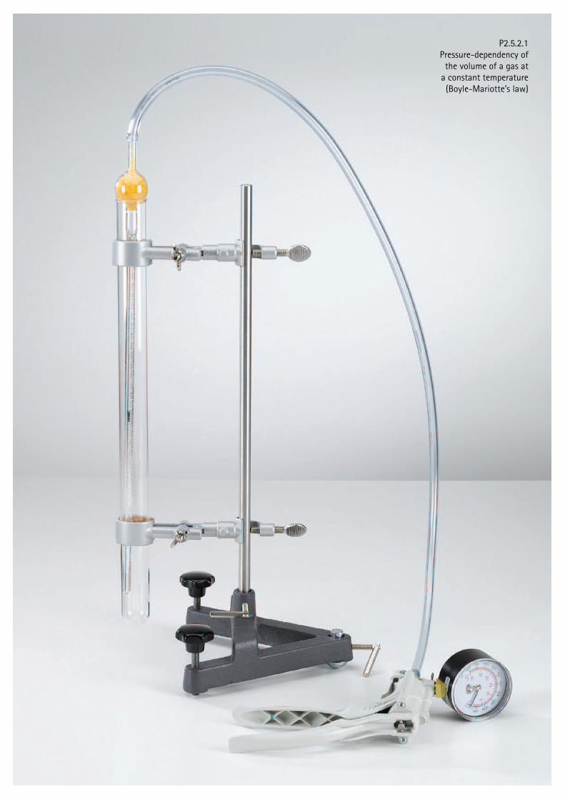
P2.5.2.1 Pressure-dependency of
the volume of a gas at a constant temperature (Boyle-Mariotte’s law)
WWW.LD-DIDACTIC.COM
BRANDS OF THE LD DIDACTIC GROUP
CONTACT
1200300EN
0
7.2
015 L
D
Tech
nic
al det
ails
subje
ct t
o c
hange
wit
hout
noti
ce.
GERMANY:
LD DIDACTIC GmbHLeyboldstr. 150354 HuerthGermanyTel.: +49 2233 604 0Fax: +49 2233 604 222EMail: info@lddidactic.dewww.lddidactic.com
Systèmes DidactiquesSavoie Hexapole - Actipole 3 - Rue Maurice HerzogF 73420 Viviers du LacTél.: +33 (0) 4 56 42 80 70 Fax: +33 (0) 4 56 42 80 71E-Mail: xavier.granjon@systemes-didactiques.frwww.systemes-didactiques.fr