Chaos, Solitons and Fractals 140 (2020) 110223

Contents lists available at ScienceDirect

Chaos, Solitons and Fractals

Nonlinear Science, and Nonequilibrium and Complex Phenomena

journal homepage: www.elsevier.com/locate/chaos

The effect of market confidence on a financial system from the

perspective of fractional calculus: Numerical investigation and circuit

realization

Shu-Bo Chen

a , Hadi Jahanshahi b , Oumate Alhadji Abba

c , J.E. Solís-Pérez

d , Stelios Bekiros e , f , J.F. Gómez-Aguilar g , Amin Yousefpour h , Yu-Ming Chu

i , j , ∗

a School of Science, Hunan City University, Yiyang 4130 0 0, PR China b Department of Mechanical Engineering, University of Manitoba, Winnipeg, R3T 5V6, Canada c Department of Physics, Faculty of Sciences, The University of Maroua, P.O. Box, 814, Maroua, Cameroon d Tecnológico Nacional de México/CENIDET. Interior Internado Palmira S/N, Col. Palmira, C.P.62490, Cuernavaca, Morelos, México e European University Institute, Department of Economics, Via delle Fontanelle, 18, I-50014, Florence, Italy f Rimini Centre for Economic Analysis (RCEA), LH3079, Wilfrid Laurier University, 75 University Ave W., ON, N2L3C5, Waterloo, Canada g CONACyT-Tecnológico Nacional de México/CENIDET. Interior Internado Palmira S/N, Col. Palmira, C.P. 62490, Cuernavaca, Morelos, México h School of Mechanical Engineering, College of Engineering, University of Tehran, Tehran, 14399-57131, Iran i Department of Mathematics, Huzhou University, Huzhou 3130 0 0, PR China j Hunan Provincial Key Laboratory of Mathematical Modeling and Analysis in Engineering, Changsha University of Science & Technology, Changsha 410114,

PR China

a r t i c l e i n f o

Article history:

Received 28 July 2020

Accepted 18 August 2020

Available online 30 September 2020

Keyword:

Chaotic financial system

Market confidence

Fractional calculus, Circuit realization

a b s t r a c t

Modeling and analysis of financial systems have been interesting topics among researchers. The more

precisely we know dynamic of systems, the better we can deal with them. This way, in this paper, we in-

vestigate the effect of market confidence on a financial system from the perspective of fractional calculus.

Market confidence, which is a significant concern in economic systems, is considered, and its effects are

comprehensively investigated. The system has been studied through numerical simulations and analyses,

such as the Lyapunov exponents, bifurcation diagrams, and phase portrait. It is shown that the system

enters chaos through experiencing a cascade of period doublings, and the existence of chaos is verified.

Finally, an analog circuit of the chaotic system is designed and implemented to prove its feasibility in

real-world applications. Also, through the circuit implementation, the effects of different factors on the

behavior of the systems are investigated.

© 2020 The Author(s). Published by Elsevier Ltd.

This is an open access article under the CC BY license ( http://creativecommons.org/licenses/by/4.0/ )

1

s

t

a

f

t

s

j

A

j

p

v

s

o

l

I

d

fi

e

h

0

. Introduction

In the last decades, modeling of economic systems has been the

ubject of intense research [1–3] . Many studies have investigated

he nonlinear behavior of these systems [4] . Significantly, chaos as

particular phenomenon has been observed in these systems and

ormed a new subject in this research field [5] . A detailed study of

he chaotic behavior of systems can reveal regularity hidden in the

eemingly random economic phenomena [6–12] . This way, it pro-

∗ Corresponding author

E-mail addresses: shubo.chen@163.com (S.-B. Chen),

ahanshahi.hadi90@gmail.com (H. Jahanshahi), oumat_oaa@yahoo.fr (O. Alhadji

bba), jesolis@cenidet.edu.mx (J.E. Solís-Pérez), stelios.bekiros@eui.eu (S. Bekiros),

ose.ga@cenidet.tecnm.mx (J.F. Gómez-Aguilar), amin.yusefpour@ut.ac.ir (A. Yousef-

our), chuyuming@zjhu.edu.cn (Y.-M. Chu).

[

m

i

a

m

g

ttps://doi.org/10.1016/j.chaos.2020.110223

960-0779/© 2020 The Author(s). Published by Elsevier Ltd. This is an open access article

ides a perspective of understanding the complexity of economic

ystems as some of their internal structures, rather than accidental

r external behaviors [13] .

Fractional calculus is an effective method for expressing non-

inear dynamics in the fields of physics and engineering [14–16] .

n fact, the features of the fractional calculus are beneficial to

escribe more accurately many real-world phenomena in various

elds such as digital circuits [17] , viscoelastic studies [18] , ferro-

lectric materials [19] , biology [20] , cryptography [21] , economics

22] , etc. Fractional calculus can describe memory effects, and

any variables in economics systems possess memory effects. As

t is obvious, our past economic decisions may affect our present

nd future ones [23] . Thereby, exploiting fractional calculus in the

odeling of economic and financial systems is a rational and ar-

umentative approach [24,25] .

under the CC BY license ( http://creativecommons.org/licenses/by/4.0/ )

2 S.-B. Chen, H. Jahanshahi and O. Alhadji Abba et al. / Chaos, Solitons and Fractals 140 (2020) 110223

Fig. 1. Phase portraits of the financial system (3). (a) state space ( x, y, z ) and (b) state space ( y, z, w ).

Fig. 2. Phase portraits of the fractional financial system (5). (a) state space ( x, y, z ) and (b) state space ( y, z, w ).

p

s

b

k

t

s

s

u

s

t

e

H

c

On the other hand, one of the most critical factors in rescu-

ing or influencing the economic crisis is confidence. Hence, an-

other critical issue that should be considered in the modeling and

study of economic and financial systems is confidence, the con-

fidence of the people [26] . When people lose their confidence in

economic systems, it will bring bout a vicious cycle and chain of

reaction, including reducing production, canceling investment, and

stopping consuming [27,28] . This situation will result in less invest-

ment, less employment, less confidence, more stock of products,

more deficit, and more layoffs. If there exist enough investment

confidence and opportunities, consumers will not save too much.

Also, the confidence in economic systems will be increased by low

interest rates and be lowered by alarming interest rates [29] . Gov-

ernments must do their best to provide a balancing platform that

romotes investments and savings. Investment confidence plays a

ignificant role in fostering investment, and consequently, in the

ehavior of systems. This way, it is meaningful to consider mar-

et confidence in the modeling of financial systems. Nevertheless,

here are a few studies that consider chaotic behavior in finance

ystems with market confidence [30] .

As a substantial part of a robust economic system, financial

ystems must be gotten further attention and researches. Though

p to now, studies have made impressive progress in this field of

tudy, some problems related to the behavior of economic are yet

o be resolved. For instance, a few studies there are in the lit-

rature about economic models that possess market confidence.

ence, more study is required on fractional-order chaotic finan-

ial systems with market confidence to achieve a comprehensive

S.-B. Chen, H. Jahanshahi and O. Alhadji Abba et al. / Chaos, Solitons and Fractals 140 (2020) 110223 3

Fig. 3. Phase portraits of the fractional financial system (11). (a) state space ( x, y, z ) and (b) state space ( y, z, w ).

Fig. 4. Dynamics of the LEs of the fractional financial system in (a) Riemann-Liouville and (b) Liouville-Caputosense.

u

r

m

a

m

fi

c

c

m

fi

t

t

S

s

l

2

D

R

Ra

w

nderstanding of these systems. These issues motivate the present

esearch. The financial systems with market confidence may show

any nonlinear dynamical behaviors, such as bifurcation, chaos,

nd are thoroughly investigated in this study. Besides, the imple-

entation of chaotic systems is a significant area of interest in the

eld of chaos [31-33] . Thus, in order to prove its real existence, the

haotic behavior of the system is also realized through electronic

ircuits.

The article is planned as follows: Section 2 details the mathe-

atical model and dynamical analysis of a fractional-order chaotic

nancial system with market confidence. Nonlinear dynamics of

he system are studied through various tools, including phase por-

raits, bifurcation diagrams, and Lyapunov exponent spectrum in

G

ection 2 . In Section 3 , a circuit implementation is designed to

how the behavior of the system in the real-world application, fol-

owed by conclusions, presented in Section 4 .

. Mathematical preliminaries

efinition 1. Let α ∈ R + and n = � α� . The fractional operator in

iemann-Liouville is given by

L

D

αt f ( t ) =

1

�( n − α)

d n

d t n

t

∫ a

f ( τ )

( t − τ ) α−n +1

dτ, n − 1 < α < n, (1)

here a and t are the operating limits RL a D

αt and �( · ) is the Euler

amma function.

4 S.-B. Chen, H. Jahanshahi and O. Alhadji Abba et al. / Chaos, Solitons and Fractals 140 (2020) 110223

Fig. 5. Bifurcation diagrams for the fractional financial system in (a) Riemann-Liouville and (b) Liouville-Caputo sense.

C

w

3

R

3

R

(

Ga

w

a

f

Ga

w

f

x

w

b

c

f

Definition 2. Let α ∈ R + and n = � α� , the Caputo differential opera-

tor of order α is defined as Eq. (2) :

a D

αt f ( t ) =

1

�( n − α)

t

∫ a

d n

d t n f ( τ ) ( t − τ )

n −α−1 dτ, n − 1 < γ < n,

(2)

for a ≤ x ≤ t.

3. Chaotic financial system with market confidence

Xin and Zhang [30] proposed a chaotic dynamic model by con-

sidering market confidence. This system was presented in a four-

dimensional form and it was obtained from the nonlinear finan-

cial model developed by Huang and Li [3] . To achieve the novel

financial model, the authors proposed four assumptions where

the interest rate ( x ), the market confidence ( w ), the investment

command ( y ), and the price index ( z ) were involved. The above-

mentioned system is given as Eq. (3) :

˙ x = z + ( y − a ) x + m 1 w,

˙ y = 1 − by − x 2 + m 2 w,

˙ z = −x − cz + m 3 w,

˙ w = −xyz,

(3)

where x, y, z, a, b , and c have the same meanings. Besides, m 1 , m 2 ,

and m 3 are the impact factors.

Fig. 1 shows the numerical simulation setting a = 2 . 1 , b = 0 . 01 ,

c = 2 . 6 , m 1 = 8 . 4 , m 2 = 6 . 4 , m 3 = 2 . 2 , and initial conditions x (0) =−0 . 01 , y (0) = 0 . 5 , z(0) = 0 . 004 , and w (0) = −0 . 003 . This was car-

ried out with a step size h = 1 × 10 −2 during 300 s .

3.1. Fractional chaotic financial system

In this section, we get a fractional representation for the system

(3), by generalizing the classical operator d / dt . Therefore, the frac-

tional representation is written as Eq. (4) and it includes the term

memory effect

Q 0

D

αt ( x ) = z + ( y − a ) x + m 1 w,

Q 0

D

αt ( y ) = 1 − by − x 2 + m 2 w,

Q 0

D

αt ( z ) = −x − cz + m 3 w,

Q D

αt ( w ) = −xyz,

(4)

0

here Q denotes the fractional-order in any sense.

.2. Fractional chaotic financial system in Riemann-Liouville sense

By considering Eq. (1) , the fractional financial system in

iemann-Liouville is given as

RL 0 D

αt ( x ) = z + ( y − a ) x + m 1 w,

RL 0 D

αt ( y ) = 1 − by − x 2 + m 2 w,

RL 0 D

αt ( z ) = −x − cz + m 3 w,

RL 0 D

αt ( w ) = −xyz,

(5)

.2.1. Numerical scheme for fractional financial model in

iemann-Liouville sense

To get numerical solutions for the Riemann-Liouville derivative

1), the Grünwald–Letnikov (GL) [34] approximation is carried out

L

D

γt f ( t ) = lim

h → 0

1

h

α

t−a h ∑

k =0

( −1 ) j

(αk

)f ( t − kh ) , (6)

here k is the time increment.

For a wide class of systems, the fractional derivative (1) can be

pproximated by the Eq. (6) . Therefore, we start from a general

orm as Eq. (7)

L

D

γt x ( t ) = f ( x ( t ) , t ) , (7)

hose numerical solution was presented in [35] and it is given as

ollows

( t k ) = f ( x ( t k ) , t k ) h

α −k ∑

j=0

c ( α)

j x (t k − j

), (8)

here c (α) j

, ( j = 0 , 1 , . . . ) are the binomial coefficients computed

y the following expression

( α) 0

= 1 , c ( α)

j =

(1 − 1 + α

j

)c (

α) j−1

. (9)

We consider the Eqs. (8) and (9) to get a numerical solution

or the fractional chaotic financial system in the Riemann-Liouville

S.-B. Chen, H. Jahanshahi and O. Alhadji Abba et al. / Chaos, Solitons and Fractals 140 (2020) 110223 5

Fig. 6. Variables p and q in the fractional financial system (5) for α = 0 . 95 . (a), (c), and (d) show strongly chaotic behaviors for φ1 (t) = x, φ3 (t) = z, and φ4 (t) = w , respec-

tively; (b) depicts chaotic dynamics with φ2 (t) = y .

s

x

F

r

m

=

i

α

3

c

3

L

p

C0

t

ense (5) as Eq. (10)

( t k ) = ( z ( t k ) + ( y ( t k ) − a ) x ( t k ) + m 1 w ( t k ) ) h

α −k ∑

j=0

c ( α)

j x (t k − j

),

y ( t k ) =

(1 − by ( t k ) − x ( t k )

2 + m 2 w ( t k ) )h

α −k ∑

j=0

c ( α)

j y (t k − j

),

z ( t k ) = ( −x ( t k ) − c ( t k ) z ( t k ) + m 3 w ( t k ) ) h

α −k ∑

j=0

c ( α)

j z (t k − j

),

w ( t k ) = ( −x ( t k ) y ( t k ) z ( t k ) ) h

α −k ∑

j=0

c ( α)

j w

(t k − j

),

(10)

ig. 2 depicts the numerical results setting the following pa-

ameters α = 2.1, b = 0.01, c = 2.6, m 1 = 8.4, m 2 = 6.4,

3 = 2.2 and initial conditions x (0) = −0.01, y (0) = 0.5, z (0)

0.004, and w (0) = −0.003. The simulation was achieved

n 300 s with a step size h = 1 ×10 −2 and fra‘ctional order

= 0.95.

.3. Fractional chaotic financial system in Liouville-Caputo sense

Fractional chaotic financial system in the Liouville-Caputo sense

an be defined as follows:

C 0 D

αt ( x ) = z + ( y − a ) x + m 1 w,

C 0 D

αt ( y ) = 1 − by − x 2 + m 2 w,

C 0 D

αt ( z ) = −x − cz + m 3 w,

C 0 D

αt ( w ) = −xyz,

(11)

.3.1. Numerical scheme for fractional financial model in

iouville-Caputo sense

Let us consider a fractional differential equation with the Ca-

uto derivative as Eq. (12)

D

αt x ( t ) = f ( t , x ( t ) ) . (12)

If we apply the fractional calculus fundamental theorem, then

he above-mentioned equation is expressed as a fractional integral

6 S.-B. Chen, H. Jahanshahi and O. Alhadji Abba et al. / Chaos, Solitons and Fractals 140 (2020) 110223

Fig. 7. Variables p and q in the fractional financial system (11) for α = 0 . 95 . (a), (b), (c), and (d) show strongly chaotic behaviors for φ1 (t) = x, φ2 (t) = y, φ3 (t) = z, and

φ4 (t) = w, respectively.

y

equation of the form

x ( t ) − x ( 0 ) =

1

�( α)

t

∫ 0

f ( u, x ( u ) ) ( t − u ) α−1 du. (13)

Reformulating the Eq. (13) and approximating f ( u, x ( u )) by

the two-step Lagrange polynomial interpolation on an interval

[ t k , t k +1 ] , Eq. (14) can be obtained as follows:

x n +1 ( t ) = x 0 +

1

�( α)

n ∑

k =0

(f ( t k , y k )

h

t k +1 ∫ t k

( t − t k −1 ) ( t k +1 − t ) α−1 dt

− f ( t k −1 , y k −1 )

h

t k +1 ∫ t k

( t − t k ) ( t k +1 − t ) α−1 dt

). (14)

Following with the numerical scheme proposed by, we can

compute the numerical simulations for the system (11) as

Eq. (15) :

x n +1 ( t ) = x ( 0 )

+

h

α

�( α + 1 )

n ∑

k =0

(f 1 ( t k , x k , y k , z k , w k )

α + 1

(( n + 1 −k )

α( n −k + 2 + α)

− ( n − k ) α( n − k + 2 + 2 α)

)− f 1 ( t k −1 , x k −1 , y k −1 , z k −1 , w k −1 )

α + 1

×(( n + 1 − k )

α+1 − ( n − k ) α( n − k + 1 + α)

)),

n +1 ( t ) = y ( 0 )

+

h

α

�( α + 1 )

n ∑

k =0

(f 2 ( t k , x k , y k , z k , w k )

α + 1

(( n + 1 −k )

α( n −k + 2 + α)

− ( n − k ) α( n − k + 2 + 2 α)

)− f 2 ( t k −1 , x k −1 , y k −1 , z k −1 , w k −1 )

α + 1

S.-B. Chen, H. Jahanshahi and O. Alhadji Abba et al. / Chaos, Solitons and Fractals 140 (2020) 110223 7

z

w

w

m

m

m

r

a

w

s

4

(

m

4

t

B

a

w

H

t

e

c

2

−

Fig. 8. Fractional-order chain for q = 0 . 95 .

Fig. 9. Fractional-order chain for q = 0 . 9 .

Fig. 10. Fractional-order chain for q = 0 . 85 .

4

(

a

0

p

i

i

a

4

E

d

×(( n + 1 − k )

α+1 − ( n − k ) α( n − k + 1 + α)

)),

n +1 ( t ) = z ( 0 )

+

h

α

�( α + 1 )

n ∑

k =0

(f 3 ( t k , x k , y k , z k , w k )

α + 1

(( n + 1 −k )

α( n −k + 2 + α)

− ( n − k ) α( n − k + 2 + 2 α)

)− f 3 ( t k −1 , x k −1 , y k −1 , z k −1 , w k −1 )

α + 1

×(( n + 1 − k )

α+1 − ( n − k ) α( n − k + 1 + α)

)),

n +1 ( t ) = w ( 0 )

+

h

α

�( α + 1 )

n ∑

k =0

(f 4 ( t k , x k , y k , z k , w k )

α + 1

(( n + 1 −k )

α( n −k + 2 + α)

− ( n − k ) α( n − k + 2 + 2 α)

)− f 4 ( t k −1 , x k −1 , y k −1 , z k −1 , w k −1 )

α + 1

×(( n + 1 − k )

α+1 − ( n − k ) α( n − k + 1 + α)

)), (15)

here

f 1 ( t k −1 , x k −1 , y k −1 , z k −1 , w k −1 ) := z + ( y − a ) x +

1 w, f 2 ( t k −1 , x k −1 , y k −1 , z k −1 , w k −1 ) := 1 − by − x 2 +

2 w, f 3 ( t k −1 , x k −1 , y k −1 , z k −1 , w k −1 ) := −x − cz +

3 w, f 4 ( t k −1 , x k −1 , y k −1 , z k −1 , w k −1 ) := −xyz,

Fig. 3 depicts the numerical results setting the following pa-

ameters α = 2 . 1 , b = 0 . 01 , c = 2 . 6 , m 1 = 8 . 4 , m 2 = 6 . 4 , m 3 = 2 . 2

nd initial conditions x (0) = −0 . 01 , y (0) = 0 . 5 , z(0) = 0 . 004 , and

(0) = −0 . 003 . The simulation was achieved in 300 s with a step

ize h = 1 × 10 −2 and fractional order α = 0 . 95 .

. Criteria to determine chaos

In order to analyze chaotic behaviors in the fractional systems

5) and (11), estimation of the Lyapunov exponents, bifurcation

aps, and 0-1 test were carried out.

.1. Estimation of the Lyapunov exponents

The get Lyapunov exponents for the fractional financial sys-

em in Riemann-Liouville and Liouville-Caputo sense, we use the

enettin-Wolf algorithm presented in [36] . Even when there is not

criterion to choose the normalization moment variable h norm,

e carried out several numerical simulations to choose it.

Fig. 4 shows the numerical results by applying this algorithm.

ere, one can see that we have only one positive exponent and

hree negatives. Therefore, the systems (5) and (11) can be consid-

red chaotic. The final value of the LEs presented in Table 1 were

arried out with the following parameters: a = 2 . 1 , b = 0 . 01 , c = . 6 , m 1 = 8 . 4 , m 2 = 6 . 4 , m 3 = 2 . 2 and initial conditions x (0) =0 . 01 , y (0) = 0 . 5 , z(0) = 0 . 004 , w (0) = −0 . 003 .

Table 1

LEs for the fractional financial systems (5) and

Financial system α λ1

Riemann-Liouville sense (5) 0.95 0.00

Liouville-Caputo sense (11) 0.95 0.00

.2. Bifurcation maps

Fig. 5 shows bifurcation maps for the financial systems (5) and

11) respectively. In these maps, one can see regularity windows

s well as period-doubling cascade where the order α is near to

.95 whereas for the system (11) they are present when α is ap-

roximately 0.96. These bifurcations give place to chaotic behav-

ors. Besides, in the regularity windows presented by two maps, it

s possible to see that there are pitchfork bifurcations. See Figs. 5 a

nd b, where α ∈ (0.95, 1).

.3. 0-1 Test

The 0-1 test provides the following 2-dimensional system as

q. (16)

p ( t + 1 ) = p ( t ) + φ( t + 1 ) cos ( c · n ) , q ( t + 1 ) = q ( t ) + φ( t + 1 ) sin ( c · n ) ,

(16)

erived from φ( t ) for t = 0 , 1 , 2 , . . . , T . Besides, c ∈ (0, 2 π ) is fixed.

(11).

λ2 λ3 λ4

22 -0.0540 -4.6589 -8.7405

79 -0.0127 -2.5937 -4.6544

8 S.-B. Chen, H. Jahanshahi and O. Alhadji Abba et al. / Chaos, Solitons and Fractals 140 (2020) 110223

Fig. 11. Circuit realization of the integer-order financial system.

Table 2

Growth rates for the fractional financial system.

Dynamical system x y z w

Fractional financial system (5) 0.9702 0.8903 0.9686 0.9664

Fractional financial system (11) 0.9643 0.9281 0.9669 0.9688

(

r

L

a

7

f

5

o

For a continuous-time system, the 2-dimensional mean square

displacement is given as follows

M c ( t ) = lim

T →∞

1

T

T

∫ 0

([ p ( t + τ ) − p ( τ ) ]

2 + [ q ( t + τ ) − q ( τ ) ] 2 )dτ,

(17)

where the growth rate is as Eq. (18) :

K = lim

t→∞

log ( M c ( t ) )

log ( t ) . (18)

In the above-mentioned equation, K ≈ 1 means that the system

is chaotic and K ≈ 0 that the system is regular [37] . By approxi-

mating the Eq. (17) by means time series sampled, Eq. (19) can be

obtained as follows:

M c ( n ) = lim

N→∞

1

N

N ∑

j=1

([ p τs ( j + n ) − p τs ( j ) ]

2

+ [ q τs ( j + n ) − q τs ( j ) ] 2 )τ 2

s . (19)

This test was carried out for the systems given in Eqs. (5) and

11) with a sample time τs = 0 . 015 . Table 2 shows the growth

ates for the fractional financial systems in Riemann-Liouville and

iouville-Caputo sense. Here, we can conclude that both systems

re chaotic due to that growth rates are near to 1. Figs. 6 and

show the 0-1 test for Riemann-Liouville and Caputo models for

ractional order α = 0.95.

. Circuit realization

Because fractional calculus does not allow the direct calculation

f the differential operators in time domain, to design a circuit we

S.-B. Chen, H. Jahanshahi and O. Alhadji Abba et al. / Chaos, Solitons and Fractals 140 (2020) 110223 9

Fig. 12. Circuit realization of the fractional-order financial system.

u

d

v

t

o

a

w

a

(

p

q

u

p

c

c

l

sually adopt the method of approximation conversion from time

omain to frequency domain. Based on Bode diagrams, Liu [38] de-

eloped an effective algorithm to approximate the fractional-order

ransfer functions by utilizing frequency-domain techniques. Based

n this, we deduced 1 / s q ( q = 0 . 1 ∼ 0 . 99 ) with discrepancies 2dB

nd 3dB through linear approximation in frequency domain. Here,

e utilize the approximation of 1 / s q ( q = 0 . 1 ∼ 0 . 9 ) with discrep-

ncy of 2dB to design the analog circuits. According to [39] , Eqs.

20-22) can be obtained as follows:

1

s 0 . 95 =

1 . 2834 s 2 + 18 . 6004 s + 2 . 0833

s 3 + 18 . 4738 s 2 + 2 . 6574 s + 0 . 003

(20)

1

s 0 . 9 =

2 . 2675 ( s + 1 . 292 ) ( s + 215 . 4 )

( s + 0 . 01292 ) ( s + 2 . 154 ) ( s + 359 . 4 ) (21)

1

s 0 . 85 =

2 . 743 s 2 + 294 . 7 s + 2810 . 6

s 3 + 184 . 8 s 2 + 897 . 5 s + 114 . 5

(22)

A circuit design where resistors and capacitors are connected in

arallel was proposed in [40] to realize fractional calculus. When

= 0 . 95 , q = 0 . 9 , and q = 0 . 85 , the fractional order chain circuit

nits are shown in Figs. 8–10 .

We select LF353D as the amplifier and AD633JN as the multi-

lier to design the fractional-order circuits. In order to restrict the

hange of state variables to the operating voltage of the analog cir-

uit, the state variables are reduced by 4, 5, 2 and 2 times, namely

et ( x, y, z, w ) → (4 X , 5 Y , 2 Z , 2 W ).

10 S.-B. Chen, H. Jahanshahi and O. Alhadji Abba et al. / Chaos, Solitons and Fractals 140 (2020) 110223

Fig. 13. Phase portraits of the finance system for q = 1 .

S.-B. Chen, H. Jahanshahi and O. Alhadji Abba et al. / Chaos, Solitons and Fractals 140 (2020) 110223 11

Fig. 14. Phase portraits of the finance system for q = 0 . 95 .

12 S.-B. Chen, H. Jahanshahi and O. Alhadji Abba et al. / Chaos, Solitons and Fractals 140 (2020) 110223

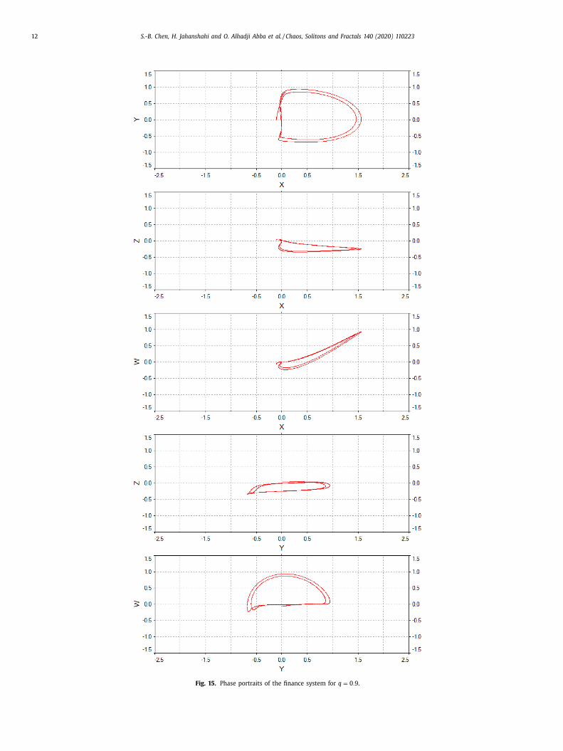
Fig. 15. Phase portraits of the finance system for q = 0 . 9 .

S.-B. Chen, H. Jahanshahi and O. Alhadji Abba et al. / Chaos, Solitons and Fractals 140 (2020) 110223 13

Fig. 16. Phase portraits of the finance system for q = 0 . 85 .

14 S.-B. Chen, H. Jahanshahi and O. Alhadji Abba et al. / Chaos, Solitons and Fractals 140 (2020) 110223

D

i

p

t

p

e

t

A

F

1

R

As a result, the financial system with market confidence can be

rewritten as Eq. (23) : ⎧ ⎪ ⎪ ⎪ ⎪ ⎪ ⎪ ⎪ ⎪ ⎨

⎪ ⎪ ⎪ ⎪ ⎪ ⎪ ⎪ ⎪ ⎩

d q X

d t q =

1

2

Z + 5 X Y − aX +

1

2

m 1 W,

d q Y

d t q =

1

5

− bY − 16

5

X

2 +

2

5

m 2 W,

d q Z

d t q = −2 X − cZ + m 3 W,

d q W

d t q = −20 X Y Z,

(23)

By replacing a, b, c, m 1 , m 2 , and m 3 with their values, the sys-

tem (4) can be shown as Eq. (24) : ⎧ ⎪ ⎪ ⎪ ⎪ ⎪ ⎪ ⎪ ⎪ ⎨

⎪ ⎪ ⎪ ⎪ ⎪ ⎪ ⎪ ⎪ ⎩

d q X

d t q = 0 . 5 Z + 5 X Y − 2 . 1 X + 4 . 2 W,

d q Y

d t q = 0 . 2 − 0 . 01 Y − 3 . 2 X

2 + 2 . 56 W,

d q Z

d t q = −2 X − 2 . 6 Z + 2 . 2 W,

d q W

d t q = −20 X Y Z,

(24)

The schematic circuits of the integer-order and fractional-order

financial system with market confidence are given by Figs. 11 and

12 . The circuit equation is as Eq. (25) : ⎧ ⎪ ⎪ ⎪ ⎪ ⎪ ⎪ ⎪ ⎪ ⎪ ⎨

⎪ ⎪ ⎪ ⎪ ⎪ ⎪ ⎪ ⎪ ⎪ ⎩

d q X

dt =

R 2

R 1 R 4

Z +

R 2

R 1 R 6

X Y − R 2 R 7

R 1 R 3 R 8

X +

R 2

R 1 R 5

W,

d q Y

dt =

R 10

R 9 R 13

0 . 2 − R 10 R 14

R 9 R 11 R 15

Y − R 10 R 14

R 9 R 11 R 16

X

2 +

R 10

R 9 R 12

W,

d q Z

dt = − R 18 R 21

R 17 R 19 R 22

X − R 18 R 21

R 17 R 19 R 23

Y +

R 18

R 17 R 20

W

d q W

dt =

R 25 R 27

R 24 R 26 R 28

X Y Z

(25)

The input supplies are as V cc = +15 V , V ee = −15 V . The values of

the electronic components in Figs. 11 and 12 are chosen to match

the known parameters of the system (23) as follows:

R 1 = R 9 = R 17 = R 24 = 100 k , R 2 = R 7 = R 8 = R 10 = R 11 = R 14 =R 18 = R 19 = R 21 = R 27 = 1 k , R 13 = R 15 = R 25 = R 26 = 10 k , R 3 =4 . 76 k , R 4 = 20 k , R 5 = 2 . 38 k , R 6 = 2 k , R 12 = 3 . 90 k , R 16 =3 . 13 k , R 20 = 4 . 55 k , R 23 = 3 . 85 k , R 28 = 500.

The proposed circuits are designed by using Electronic Work

Bench (EWB). Figs. 13–16 show the obtained phase portraits in ( X,

Y )-plane, ( X, Z )-plane, ( X, W )- plane, ( Y, Z )-plane and ( Y, W )-plane,

respectively.

6. Conclusion

A fractional-order financial system by considering the effects of

market confidence was studied. Using phase portraits, Lyapunov

exponents, and bifurcation diagrams, the dynamical behavior of

the proposed system was investigated. It was demonstrated that

the proposed system goes to chaos through experiencing a cascade

of period doublings, and the existence of chaos is verified. Then,

using the Electronic Work Bench, circuit implementation was suc-

cessfully performed for integer and fractional-order financial sys-

tems to demonstrate the existence of the chaos in the system.

Through circuit realization, it was clearly demonstrated that by

changing the value fractional-order derivative, the system shows

different responses. As a future suggestion, the complexity anal-

ysis could be conducted for the fractional-order chaotic financial

system with market confidence. Also, the presented finance model

can be investigated by a variable-order fractional derivative.

eclaration of Competing Interest

This statement is to certify that no conflict of interest exits

n the submission of this manuscript. Also, the manuscript is ap-

roved for publication by all authors. I would like to declare that

he work described was an original research that has not been

ublished previously, and not under consideration for publication

lsewhere. All the authors listed have approved the manuscript

hat is enclosed.

cknowledgments

The research was supported by the National Natural Science

oundation of China (grant nos. 11971142 , 11401192 , 61673169 ,

1701176 , 11626101 , 11601485 ).

eferences

[1] Kondratenko AV. Physical modeling of economic systems: classical and quan-

tum economies. Available at SSRN 1304630. 2009. [2] Jun-hai M , Yu-Shu C . Study for the bifurcation topological structure and the

global complicated character of a kind of nonlinear finance system (I). Appl

Math Mech 2001;22:1240–51 . [3] Huang D , Li H . Theory and method of the nonlinear economics. Chengdu: Pub-

lishing House of Sichuan University; 1993 . [4] Costanza R , Wainger L , Folke C , Mäler K-G . Modeling complex ecological eco-

nomic systems: toward an evolutionary, dynamic understanding of people andnature. Bioscience 1993;43:545–55 .

[5] Wang S , Bekiros S , Yousefpour A , He S , Castillo O , Jahanshahi H . Synchroniza-tion of fractional time-delayed financial system using a novel type-2 fuzzy ac-

tive control method. Chaos Solitons Fractals 2020;136:109768 .

[6] Wang S , Yousefpour A , Yusuf A , Jahanshahi H , Alcaraz R , He S , et al. Synchro-nization of a non-equilibrium four-dimensional chaotic system using a distur-

bance-observer-based adaptive terminal sliding mode control method. Entropy2020;22:271 .

[7] Yousefpour A , Jahanshahi H . Fast disturbance-observer-based robust integralterminal sliding mode control of a hyperchaotic memristor oscillator. Eur Phys

J Special Top 2019;228:2247–68 .

[8] Chen H , He S , Azucena ADP , Yousefpour A , Jahanshahi H , López MA , et al. Amultistable chaotic jerk system with coexisting and hidden attractors: dynam-

ical and complexity analysis, FPGA-based realization, and chaos stabilizationusing a robust controller. Symmetry 2020;12:569 .

[9] Yousefpour A , Haji Hosseinloo A , Reza Hairi Yazdi M , Bahrami A . Distur-bance observer–based terminal sliding mode control for effective performance

of a nonlinear vibration energy harvester. J Intell Mater Syst Struct 2020

1045389X20922903 . [10] Jahanshahi H , Shahriari-Kahkeshi M , Alcaraz R , Wang X , Singh VP , Pham V-T .

Entropy analysis and neural network-based adaptive control of a non-e-quilibrium four-dimensional chaotic system with hidden attractors. Entropy

2019;21:156 . [11] Jahanshahi H , Rajagopal K , Akgul A , Sari NN , Namazi H , Jafari S . Complete anal-

ysis and engineering applications of a megastable nonlinear oscillator. Int J

Non Linear Mech 2018;107:126–36 . [12] Rajagopal K , Jahanshahi H , Varan M , Bayır I , Pham V-T , Jafari S , et al. A hy-

perchaotic memristor oscillator with fuzzy based chaos control and LQR basedchaos synchronization. AEU-Int J Electron Commun 2018;94:55–68 .

[13] Jahanshahi H , Yousefpour A , Wei Z , Alcaraz R , Bekiros S . A financial hyper-chaotic system with coexisting attractors: dynamic investigation, entropy anal-

ysis, control and synchronization. Chaos Solitons Fractals 2019;126:66–77 .

[14] Jahanshahi H , Yousefpour A , Munoz-Pacheco JM , Moroz I , Wei Z , Castillo O .A new multi-stable fractional-order four-dimensional system with self-excited

and hidden chaotic attractors: dynamic analysis and adaptive synchronizationusing a novel fuzzy adaptive sliding mode control method. Appl Soft Comput

2020;87:105943 . [15] Rajagopal K , Jahanshahi H , Jafari S , Weldegiorgis R , Karthikeyan A , Du-

raisamy P . Coexisting attractors in a fractional order hydro turbine governing

system and fuzzy PID based chaos control. Asian J Control 2020 . [16] Jahanshahi H , Yousefpour A , Munoz-Pacheco JM , Kacar S , Pham V-T , Alsaadi FE .

A new fractional-order hyperchaotic memristor oscillator: dynamic analysis,robust adaptive synchronization, and its application to voice encryption. Appl

Math Comput 2020;383:125310 . [17] Chen D , Chen Y , Xue D . Digital fractional order Savitzky-Golay differentiator.

IEEE Trans Circuits Syst Express Briefs 2011;58:758–62 . [18] Adolfsson K , Enelund M , Olsson P . On the fractional order model of viscoelas-

ticity. Mech Time-Depend Mater 2005;9:15–34 .

[19] Agambayev A , Farhat M , Patole SP , Hassan AH , Bagci H , Salama KN .An ultra-broadband single-component fractional-order capacitor using

MoS2-ferroelectric polymer composite. Appl Phys Lett 2018;113:093505 . [20] Freeborn TJ . A survey of fractional-order circuit models for biology and

biomedicine. IEEE J Emerg Sel Top Circuits Syst 2013;3:416–24 .

S.-B. Chen, H. Jahanshahi and O. Alhadji Abba et al. / Chaos, Solitons and Fractals 140 (2020) 110223 15

[

[

[

[

[

[

[[

[

[

[

[

[

[

[

[

[21] Sadeghian H , Salarieh H , Alasty A , Meghdari A . On the fractional-order ex-tended Kalman filter and its application to chaotic cryptography in noisy envi-

ronment. Appl Math Modell 2014;38:961–73 . 22] Soradi-Zeid S , Jahanshahi H , Yousefpour A , Bekiros S . King algorithm: a novel

optimization approach based on variable-order fractional calculus with appli-cation in chaotic financial systems. Chaos Solitons Fractals 2020;132:109569 .

23] Wang S , He S , Yousefpour A , Jahanshahi H , Repnik R , Perc M . Chaos and com-plexity in a fractional-order financial system with time delays. Chaos Solitons

Fractals 2020;131:109521 .

24] Yousefpour A , Jahanshahi H , Munoz-Pacheco JM , Bekiros S , Wei Z . A fraction-al-order hyper-chaotic economic system with transient chaos. Chaos Solitons

Fractals 2020;130:109400 . 25] Škovránek T , Podlubny I , Petráš I . Modeling of the national economies in

state-space: a fractional calculus approach. Econ Model 2012;29:1322–7 . 26] Earle TC . Trust, confidence, and the 2008 global financial crisis. Risk Anal Int J

2009;29:785–92 .

[27] Nishimura KG . Financial system stability and market confidence. Asian EconPap 2010;9:25–47 .

28] Tonkiss F . Trust, confidence and economic crisis. Intereconomics2009;44:196–202 .

29] Hiltzik M . The new deal: a modern history. Simon and Schuster; 2011 . 30] Xin B , Zhang J . Finite-time stabilizing a fractional-order chaotic fi-

nancial system with market confidence. Nonlinear Dyn 2015;79:1399–

1409 .

[31] Elsonbaty A , Elsaid A , Nour HM . Circuit realization, chaos synchronization andestimation of parameters of a hyperchaotic system with unknown parameters.

J Egyptian Math Soc 2014;22:550–7 . 32] Abooee A , Yaghini-Bonabi HA , Jahed-Motlagh MR . Analysis and circuitry real-

ization of a novel three-dimensional chaotic system. Commun Nonlinear SciNumer Simul 2013;18:1235–45 .

33] Pehlivan I , Uyaro glu Y . A new 3D chaotic system with golden propor-tion equilibria: analysis and electronic circuit realization. Comput Electr Eng

2012;38:1777–84 .

34] Podlubny I. Fractional differential equations: an introduction to fractionalderivatives, fractional differential equations, to methods of their solution and

some of their applications: Elsevier; 1998. 35] Petráš I . Fractional-order nonlinear systems: modeling, analysis and simulation.

Springer Science & Business Media; 2011 . 36] Danca M-F , Kuznetsov N . Matlab code for Lyapunov exponents of fraction-

al-order systems. Int J Bifurc Chaos 2018;28:1850067 .

[37] Gottwald GA , Melbourne I . The 0-1 test for chaos: a review. Chaos detectionand predictability: Springer; 2016. p. 221–47 .

38] Liu C . Circuit theory and applications for fractional-order chaotic systems.Xi’an: Xi’an Jiaotong University Press; 2011 .

39] Cuomo KM , Oppenheim AV . Circuit implementation of synchronized chaoswith applications to communications. Phys Rev Lett 1993;71:65 .

40] Zhe X , Chong-Xin L . Realization of fractional-order Liu chaotic system by a new

circuit unit. Chin Phys B 2008;17:4033–8 .