Propagating Phase Interface with Intermediate Interfacial Phase: Phase Field Approach

Propagating Phase Interface with Intermediate Interfacial Phase: Phase FieldApproach

Kasra MomeniDepartment of Aerospace Engineering, Iowa State University, Ames, Iowa 50011, U.S.A.

Valery I. Levitas∗

Department of Aerospace Engineering, Iowa State University, Ames, Iowa 50011, U.S.A.Department of Mechanical Engineering, Iowa State University, Ames, Iowa 50011, U.S.A. and

Material Science and Engineering, Iowa State University, Ames, Iowa 50011, U.S.A.(Dated: April 12, 2014)

An advanced three-phase phase-field approach (PFA) is suggested for a non-equilibrium phase in-terface which contains an intermediate phase, in particular, a solid-solid interface with a nanometer-sized intermediate melt (IM). Thermodynamic potential in the polar order parameters is developed,which satisfies all thermodynamic equilibrium and stability conditions. Special form of the gradientenergy allowed us to include the interaction of two solid-melt interfaces via intermediate melt andobtain a well-posed problem and mesh-independent solutions. It is proved that for stationary 1Dsolutions to two Ginzburg-Landau equations for three phases, the local energy at each point is equalto the gradient energy. Simulations are performed for β ↔ δ phase transformations (PTs) via IMin HMX energetic material. Obtained energy - IM width dependence is described by generalizedforce-balance models for short- and long-range interaction forces between interfaces but not farfrom the melting temperature. New force-balance model is developed, which describes phase fieldresults even 100K below the melting temperature. The effects of the ratios of width and energiesof solid-solid and solid-melt interfaces, temperature, and the parameter characterizing interactionof two solid-melt interfaces, on the structure, width, energy of the IM and interface velocity aredetermined by finite element method. Depending on parameters, the IM may appear by contin-uous or discontinuous barrierless disordering or via critical nucleus due to thermal fluctuations.The IM may appear during heating and persist during cooling at temperatures well below than itfollows from sharp-interface approach. On the other hand, for some parameters when IM is ex-pected, it does not form, producing an IM -free gap. The developed PFA represents a quite generalthree-phase model and can be extended to other physical phenomena, such as martensitic PTs,surface-induced premelting and PTs, premelting/disordering at grain boundaries, and developingcorresponding interfacial phase diagrams.

2

I. INTRODUCTION

The PTs between two solid phases via nanoscale molten layer, more than 100K below the melting temperature,have been predicted thermodynamically1–3 for β − δ PT in HMX organic crystal and confirmed indirectly but bothqualitatively and quantitatively by sixteen experimental evidences4,5. In particular, equality of predicted activationenergies and melting energies, absence of athermal friction during solid-solid PT, dependence of the rate constanton the heat of fusion, and the interface velocity and concentration of the δ phase versus time, which follow fromthe theory, were confirmed experimentally. While change in interface energy was neglected, the main reason for themelting below the melting temperature was related to the relaxation of the internal stresses generated by relativelylarge volumetric strain for β − δ PT. However, as soon as the material melts, the stresses relax and the stress-freemelt resolidifies into the stable phase at a temperature much below the melting temperature. That is why such a meltwas called the virtual melt and was considered an intermediate transitional state. Thus, during propagation of thesolid 1-melt-solid 2 (S1MS2) interface through the sample, one solid phase melts and resolidifies into another phase.It was predicted that virtual melting would be expected in materials with a complex crystalline structure, and a largetransformation strain tensor in which traditional stress relaxation mechanisms (dislocation nucleation and motion,and twinning) are suppressed.

In6, virtual melting was considered as a mechanism of crystal-crystal PTs and an amorphization for materials withdecreasing melting temperature under pressure (for example, ice, Si, Ge, geological and others materials). It was notnecessarily related to relaxation of internal stresses. Virtual melting was confirmed experimentally for amorphizationin avandia (an important pharmaceutical substance used as an insulin enhancer) in7 during a scanning transitiometerstudy at heating.

A mechanism for crystal-crystal PTs via surface-induced virtual pre-melting and melting was justified thermody-namically and confirmed experimentally in8 for the PT from metastable pre-perovskite to cubic perovskite in PbTiO3

nanofibers, an important ferroelectric material. A theory in8 also introduced the IM , which in contrast to virtual melt,can be in thermodynamic equilibrium with an internally nonhydrostatically stressed solid below melting temperature.Reduction in the interface energy and relaxation of elastic energy provide driving forces for such a melting. Also,during the product crystal growth stage, a quenched melt was experimentally found within the solid-solid interface,which is the first direct experimental confirmation of the crystal-crystal PT via virtual melting or IM.

Virtual melting, as a mechanism of plastic flow and stress relaxation under high strain rate loading of copper andaluminum, was predicted thermodynamically and confirmed by molecular dynamics simulations in9. The thermo-dynamic conditions for the formation of virtual melting or IM were formulated in1,3,6,8 using the sharp interfaceapproach. When size-dependence of the interface energy was taken into account in8, it allowed us to determine thewidth of IM , δ∗. This is similar to force-balance models10–14 applied for other purposes, which takes into accountan additional interaction energy between two interfaces when they get close to each other. Since the width of theIM is on the order of nanometers, i.e., comparable with the width of solid-solid and solid-melt interfaces, and alsobecause melting (disordering) may not be complete, the sharp interface approaches1,3,6,8,15 are oversimplified and donot represent a strict proof of phenomena.

In order to avoid the problems inherent to the sharp interface approach, we have developed a phase field approach(PFA) that resolves finite width interfaces. It represents a justification and a generalization of our PFA presented in16.Thus, in comparison with16, the following significant and novel results are obtained. All thermodynamic equilibriumand instability conditions are explicitly analyzed; generalization of the force-balance models for short range and longrange interaction between interfaces, as well as a new model for these interactions are suggested; phase field modelingof interaction between two SM interfaces was studied in detail and connected to force-balance models; solutions forcritical IM nuclei are found and kinetic conditions for their appearance are determined. An energy integral was foundfor stationary 1D solutions to two Ginzburg-Landau equations for three phases, i.e., for plane interface with IM orfor all critical nuclei. Point-wise equality of the local and the gradient energy was proved. In addition to the abovenew topics, which were not considered in16, the parametric study here is much broader than in16, which revealedsome new effects. In particular, the S1MS2 interface velocity for some parameters is larger than the S1S2 interfacevelocity and IM width does not diverge when the first melting temperature is reached. We neglect mechanics hereand IM is driven by the reduction in interface energy during IM ; effects of internal stresses and interface tension willbe studied in the next paper.

The paper is arranged as follows. The thermodynamics potential for three-phase system with polar order parameters,one of which describes melting and another one solid-solid PT is developed in Section II. It satisfies all desiredthermodynamic equilibrium and instability conditions. The necessity of introducing gradient energy for the S1S2

interface within IM (which sounds counterintuitive) is demonstrated from the point of view of obtaining a well-posedproblem formulation and an objective (i.e., mesh-independent) solution, as well as description of the interactionbetween two SM interfaces. Corresponding Ginzburg-Landau (GL) equations have been formulated. In Section III,analytical solutions for dry solid-solid and SM interfaces and for the determination of energy, width, and velocityof these interfaces are obtained. An energy integral was found for stationary 1D solutions to two GL equations for

3

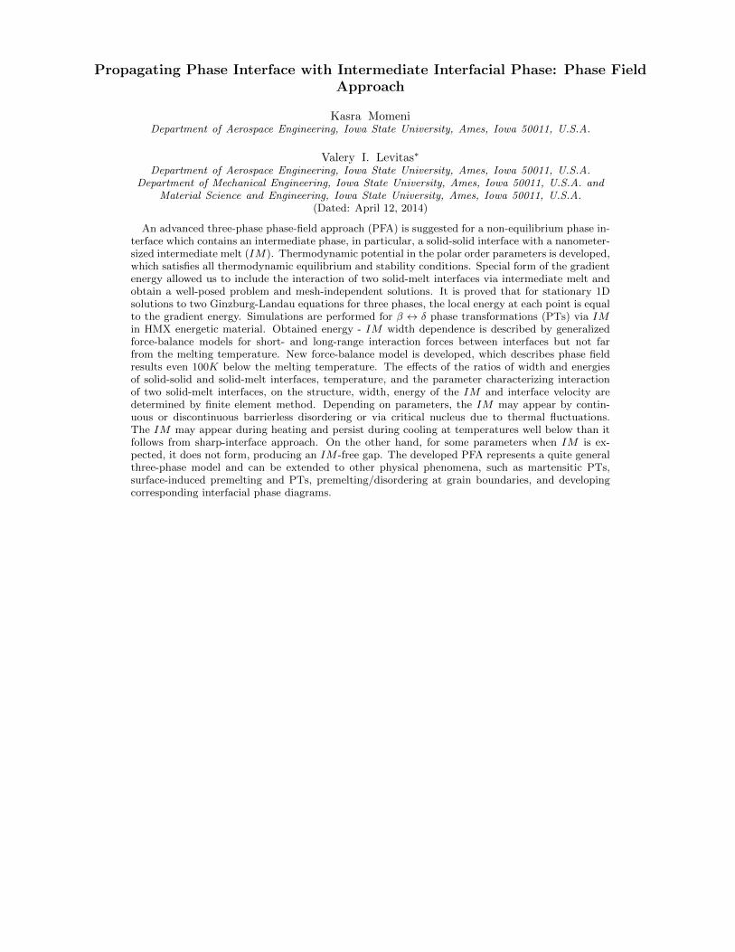
FIG. 1: Contour plot of the local Landau potential ψl = ψθ + ψ in the polar system of the order parameters Υ and ϑ atthermodynamic equilibrium temperature between solid phases θ = θ21e for different instability temperatures of solid phases θ10cand θ20c and corresponding parameters kE and kδ = 1. The 3D plot of the potential surface is shown in (e) along with itscontour plot, for the same parameters as plotted in (a).

three phases, i.e., for plane interface with IM or for all IM critical nuclei. It results in the statement that the excessof the local energy at each point is equal to the gradient energy. In Section IV, material parameters of the modelare calibrated utilizing data for HMX energetic material. Some comparison of numerical and analytical solutions ispresented. Section V is devoted to the generalization of some known force-balance models. The best force-balancemodel describes PFA results even 100K below the melting temperature. The effects of four parameters, namely ratiosof width, kδ, and energies, kE , of S1S2 and SM interfaces, temperature, and parameter characterizing interaction oftwo solid-melt interfaces, on the structure, width, energy of the IM and interface velocity are determined numerically.Depending on parameters, the IM may appear by continuous reversible (without hysteresis) or discontinuous (withhysteresis) disordering. The partial and complete IM may nucleate during heating and is retained during cooling attemperatures significantly below what would be expected from the sharp-interface approach. For some parameterswhen IM is expected, it does not form, producing IM -free gap. In Section VII, the procedure to find the criticalnucleus is described and its size structure is studied in detail using a kinetic criterion. Comparison with other closeapproaches to different phenomena and the possibility of applying the current approach to other phenomena arediscussed in Section VIII.

II. THERMODYNAMIC THEORY

Our objective is to develop the simplest local thermodynamic (Landau) potential to describe PTs between threephases, which reduces to the potential presented in17–19 for PTs between each of the two phases. Some requirementsof the thermodynamic potential in17–19 are related to the effect of stresses on PTs. Since we will include the effect ofstresses in the next paper it is important to include the same requirements even in the stress-free formulation.

A. Thermodynamic potential

In order to develop a thermodynamic potential for PTs between three phases, the polar order parameters areintroduced in a plane with the radial Υ and the angular ϑ order parameters (Fig. 1). In this formulation π ϑ/2 is theangle between the radius vector Υ and the positive first-axis. The origin of the polar coordinate system in the planeof the order parameters, which is described by Υ = 0 for any ϑ, is considered as the reference phase 0. Here phase0 is a melt M , but in general it can be any phase, e.g., austenite for multivariant martensitic transformations18–20.Phases 1 and 2 correspond to (Υ = 1 and ϑ = 0) and (Υ = 1 and ϑ = 1), respectively. In this paper, they willbe considered as solid phases S1 and S2. However, if phase 0 is austenite, phases 1 and 2 can be treated as twomartensitic variants. Contour plots of the local part of the Helmholtz energy ψ and each of thee phases are shownin Fig. 1 for HMX energetic crystals (see Section IV for details of material properties). Each of the S ↔ M PTscorrespond to the variation of Υ between 0 and 1 at a specific ϑ = 0 or 1, while the S1 ↔ S2 PTs correspond tovariation of ϑ between 0 and 1 for Υ = 1.

One of the requirements in17–19 is that each phase corresponds to the extrema of the thermodynamic potential forany temperature θ. In other words, for any temperature θ, equations ∂ψ

∂Υ = ∂ψ∂θ = 0 have roots at M ≡ (Υ = 0 and any

ϑ), S1 ≡ (Υ = 1 and ϑ = 0) and S2 ≡ (Υ = 1 and ϑ = 1). This condition allows one to easily approximate variationof all properties of phases during phase transformation. In particular, it allows one to prescribe a transformation

4

strain tensor independent of temperature17–19. The other requirement is related to the condition for instability ofequilibrium for each phase. The thermodynamic condition for instability is traditionally expressed in terms of thesecond derivatives of the thermodynamic potential. Thus, if the matrix of the second derivatives of ψ with respectto Υ and ϑ ceases to be positive definite for the given phase, this phase loses its stability and transforms to analternative phase. In general, this condition results in very complex equations which do not introduce the desiredinstability condition. Therefore, an additional requirement was formulated in17–19, which significantly simplifies theinstability conditions, which is the cross derivative ∂2ψ(θ,Υ, ϑ)/∂Υ∂ϑ = 0 for M , S1, and S2 at any temperature (seebelow). Then the desired conditions for M → S PT (Eq. (23)) and S1 → S2 PT (Eq. (25)) can be easily satisfied.

It is assumed that the material properties including potential barriers, thermal parts of free energy, and the criticaltemperatures for the loss of stability of each phase are known from either experimental measurements or molecularsimulations. The simplest expression for the Helmholtz free energy within a fourth-degree polynomial that satisfiesall the desired conditions has the following form:Helmholtz Energy

ψ = ψθ + ψθ + ψ∇ = ψl + ψ∇; ψl = ψθ + ψθ. (1)

Thermal Energy

ψθ = Gθ0(θ) + ∆Gθ(θ, ϑ)q(Υ, 0). (2)

Energy Barrier

ψθ = AS0(θ, ϑ)Υ2(1−Υ)2 +A21(θ)ϑ2 (1− ϑ)2q(Υ, aA). (3)

Gradient Energy

ψ∇ = 0.5[βS0(ϑ)|∇Υ|2 + β21φ(Υ, aφ, a0)|∇ϑ|2

]. (4)

Change in Thermal Energy of Phases

∆Gθ(θ, ϑ) = ∆Gθ10 + ∆Gθ21q(ϑ, 0). (5)

Solid-Melt Energy Barrier Coefficient

AS0(θ, ϑ) = A10(θ) +[A20(θ)−A10(θ)

]q(ϑ, aϑ). (6)

Solid-Melt Gradient Energy Coefficient

βS0(ϑ) = β10 +(β20 − β10

)q(ϑ, aβ). (7)

Interpolating Functions

q (y, a) = ay2 − 2(a− 2)y3 + (a− 3)y4; (8)

φ (Υ, aφ, a0) = aφΥ2 − 2 [aφ − 2(1− a0)] Υ3 + [aφ − 3(1− a0)] Υ4 + a0. (9)

In Eqs. (1)-(9), Gθ0(θ) is the thermal energy of the melt, ∆Gθ(θ, ϑ) is the difference in thermal energy between Sand M , ∆Gθs0 (s = 1, 2) is the difference in thermal energy between a specific solid phase Ss and M , and ∆Gθ21 isthe difference in thermal energy between solid S2 and S1; βS0 and β21 are SM and S1S2 gradient energy coefficients,respectively; thus, while capital S in super- and subscripts means solid and usually designates some function of ϑ,small s, s = 1, 2, designates specific solid Ss; A

S0 and A21 are SM and S1S2 energy barrier coefficients, respectively.The interpolation function q (y, a), with y = ϑ or Υ and different values of a (aϑ, aβ , ...) monotonously connectsproperties of phases and satisfies the following conditions

q (0, a) = 0; q (1, a) = 1; ∂q(0, a)/∂y = ∂q(0, a)/∂y = 0; 0 ≤ a ≤ 6. (10)

The first two equations of (10) provide proper change in values of the chosen property; the second two equations allow

one to satisfy conditions ∂ψ∂Υ = ∂ψ

∂θ = 0 for each phase (M or Ss) at any temperature θ and provide smooth transitionfor the property of each phase. The last condition provides monotonous behavior of the function q.

The interpolation function φ (Υ, aφ, a0) satisfies the following conditions:

φ (0, aφ, a0) = a0; φ (1, aφ, a0) = 1; ∂φ (0, aφ, a0)/∂Υ = ∂φ (1, aφ, a0)/∂Υ = 0, (11)

where 0 ≤ aφ ≤ 6 and q (y, a) = φ (y, a, 0). They are the same as conditions for q (y, a) except that φ (Υ, aφ, a0) has

5

0.0 0.2 0.4 0.6 0.8 1.0

0.0

0.2

0.4

0.6

0.8

1.0

0.0 0.2 0.4 0.6 0.8 1.0

0.0

0.2

0.4

0.6

0.8

1.0

y

a0=0 a0=1 a0=2 a0=3 a0=4 a0=5 a0=6

q

y (b)

a0=0 a0=1 a0=2 a0=3 a0=4 a0=5 a0=6

a

(a)

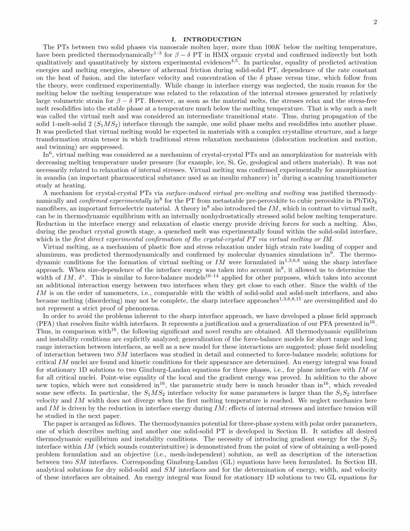
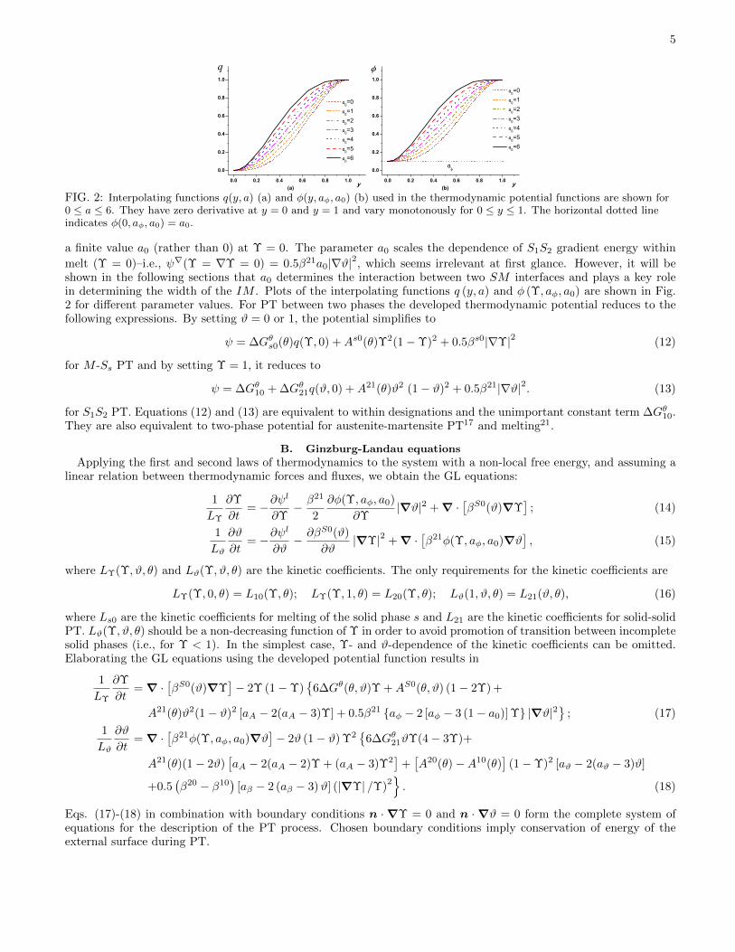
FIG. 2: Interpolating functions q(y, a) (a) and φ(y, aφ, a0) (b) used in the thermodynamic potential functions are shown for0 ≤ a ≤ 6. They have zero derivative at y = 0 and y = 1 and vary monotonously for 0 ≤ y ≤ 1. The horizontal dotted lineindicates φ(0, aφ, a0) = a0.

a finite value a0 (rather than 0) at Υ = 0. The parameter a0 scales the dependence of S1S2 gradient energy within

melt (Υ = 0)–i.e., ψ∇(Υ = ∇Υ = 0) = 0.5β21a0|∇ϑ|2, which seems irrelevant at first glance. However, it will beshown in the following sections that a0 determines the interaction between two SM interfaces and plays a key rolein determining the width of the IM . Plots of the interpolating functions q (y, a) and φ (Υ, aφ, a0) are shown in Fig.2 for different parameter values. For PT between two phases the developed thermodynamic potential reduces to thefollowing expressions. By setting ϑ = 0 or 1, the potential simplifies to

ψ = ∆Gθs0(θ)q(Υ, 0) +As0(θ)Υ2(1−Υ)2 + 0.5βs0|∇Υ|2 (12)

for M -Ss PT and by setting Υ = 1, it reduces to

ψ = ∆Gθ10 + ∆Gθ21q(ϑ, 0) +A21(θ)ϑ2 (1− ϑ)2 + 0.5β21|∇ϑ|2. (13)

for S1S2 PT. Equations (12) and (13) are equivalent to within designations and the unimportant constant term ∆Gθ10.They are also equivalent to two-phase potential for austenite-martensite PT17 and melting21.

B. Ginzburg-Landau equations

Applying the first and second laws of thermodynamics to the system with a non-local free energy, and assuming alinear relation between thermodynamic forces and fluxes, we obtain the GL equations:

1

LΥ

∂Υ

∂t= −∂ψ

l

∂Υ− β21

2

∂φ(Υ, aφ, a0)

∂Υ|∇ϑ|2 + ∇ ·

[βS0(ϑ)∇Υ

]; (14)

1

Lϑ

∂ϑ

∂t= −∂ψ

l

∂ϑ− ∂βS0(ϑ)

∂ϑ|∇Υ|2 + ∇ ·

[β21φ(Υ, aφ, a0)∇ϑ

], (15)

where LΥ(Υ, ϑ, θ) and Lϑ(Υ, ϑ, θ) are the kinetic coefficients. The only requirements for the kinetic coefficients are

LΥ(Υ, 0, θ) = L10(Υ, θ); LΥ(Υ, 1, θ) = L20(Υ, θ); Lϑ(1, ϑ, θ) = L21(ϑ, θ), (16)

where Ls0 are the kinetic coefficients for melting of the solid phase s and L21 are the kinetic coefficients for solid-solidPT. Lϑ(Υ, ϑ, θ) should be a non-decreasing function of Υ in order to avoid promotion of transition between incompletesolid phases (i.e., for Υ < 1). In the simplest case, Υ- and ϑ-dependence of the kinetic coefficients can be omitted.Elaborating the GL equations using the developed potential function results in

1

LΥ

∂Υ

∂t= ∇ ·

[βS0(ϑ)∇Υ

]− 2Υ (1−Υ)

{6∆Gθ(θ, ϑ)Υ +AS0(θ, ϑ) (1− 2Υ) +

A21(θ)ϑ2(1− ϑ)2 [aA − 2(aA − 3)Υ] + 0.5β21 {aφ − 2 [aφ − 3 (1− a0)] Υ} |∇ϑ|2}

; (17)

1

Lϑ

∂ϑ

∂t= ∇ ·

[β21φ(Υ, aφ, a0)∇ϑ

]− 2ϑ (1− ϑ) Υ2

{6∆Gθ21ϑΥ(4− 3Υ)+

A21(θ)(1− 2ϑ)[aA − 2(aA − 2)Υ + (aA − 3)Υ2

]+[A20(θ)−A10(θ)

](1−Υ)2 [aϑ − 2(aϑ − 3)ϑ]

+0.5(β20 − β10

)[aβ − 2 (aβ − 3)ϑ] (|∇Υ| /Υ)

2}. (18)

Eqs. (17)-(18) in combination with boundary conditions n ·∇Υ = 0 and n ·∇ϑ = 0 form the complete system ofequations for the description of the PT process. Chosen boundary conditions imply conservation of energy of theexternal surface during PT.

6

C. Thermodynamic equilibrium and stability conditions for homogeneous states

For homogeneous states the gradient terms disappear and right-hand-side of Eqs. (17)-(18) reduces to ∂ψl/∂Υand ∂ψl/∂ϑ, respectively. It is clear that both derivatives are zero at any temperature for each of the phases–i.e.,for M ≡ {Υ = 0 and any ϑ}, S1 ≡ {Υ = 1 and ϑ = 0} and S2 ≡ {Υ = 1 and ϑ = 1)}. Therefore, each phasecorresponds to thermodynamic equilibrium conditions at any temperature, as we required. The solutions of theequilibrium equations (extremum points of the free energy) along the paths between two solid phases (Υ = 1) are

ϑI = 0; ϑII = 1; ϑIII = 0.5A21/(A21 − 3∆Gθ21), (19)

and for solid-melt interface (ϑ = 0 or 1) they are

ΥI = 0; ΥII = 1; ΥIII = 0.5As0/(As0 − 3∆Gθs0

). (20)

If all three phases are stable or metastable (i.e., represents the local minima of the free energy), the roots ϑIII andΥIII correspond to the local energy maximum or minimax and represent energy barrier between phases. The barrierheight for S1 → S2 PT is

ψ(ϑIII)− ψ(ϑI) =(A21 − 4∆G21

) (ϑIII

)3/2, (21)

and for M → S PT is

ψ(ΥIII)− ψ(ΥI) =(AS0 − 4∆GS0

) (ΥIII

)3/2, (22)

The S2 → S1 and S → M transformation barrier–i.e., ψ(ϑIII) − ψ(ϑII) and ψ(ΥIII) − ψ(ΥII), can be obtained bysubtracting ∆Gθ21 and ∆Gθs0 from equation (21) and (22), respectively.

The mixed derivative is also zero for each of the phases. In this case, the conditions for the loss of stability of eachphase–i.e., PT criteria, simplify to:

M → Ss :∂2ψl(θ,Υ = 0, ϑ = s− 1)

∂Υ2≤ 0→ As0(θ) ≤ 0; (23)

Ss →M :∂2ψl(θ,Υ = 0, ϑ = s− 1)

∂Υ2≤ 0→ As0(θ)− 6∆Gθs0 ≤ 0; (24)

S1 → S2 :∂2ψl(θ,Υ = 1, ϑ = 0)

∂ϑ2≤ 0→ A21(θ) ≤ 0; (25)

S2 → S1 :∂2ψl(θ,Υ = 1, ϑ = 1)

∂ϑ2≤ 0→ A21(θ) + 6∆Gθ21 ≤ 0. (26)

Eqs. (23) and Eq. (25) are desired PT conditions; other two conditions just follow from the potential and arenon-contradictory.

Let us consider some specifications. Thus, let ∆Gθs0 = −∆ss0(θ − θs0e ), where ∆ss0 < 0 is the jump in entropybetween solid phase Ss and melt M and θs0e is the thermodynamic equilibrium melting temperature of Ss. The lineartemperature dependence of ∆Gθ is due to neglecting the difference between specific heats of phases; it can be takeninto account in a standard way. Then ∆Gθ21 = ∆Gθ20 −∆Gθ10 = −∆s20(θ − θ20

e ) + ∆s10(θ − θ10e ) = −∆s21(θ − θ21

e ),where ∆s21 = ∆s20 −∆s10 and θ21

e = (∆s20θ20e −∆s10θ

10e )/∆s21.

The coefficients that determine loss of stability of melt toward Ss are As0(θ) = As0c (θ−θs0c ), where θs0c is the criticaltemperature at which melt loses its stability toward Ss. A similar coefficient between two solid phases is acceptedin a more general form A21(θ) = A21

c (θ) + A21c (θ − θ21

c ) with θ21c designating the critical temperature of the loss of

stability of the phase S1 toward S2. If such a critical temperature exists, e.g., for solid phases with different thermalproperties, then the instability condition (25) requires A21

c = 0. If critical temperature does not exist, e.g., for two

martensitic variants that have the same thermal properties, one has to accept A21(θ) = A21c (θ). In this case instability

can be caused by stresses, which are neglected in the current study. Here, we will focus on the case with A21c = 0.

Then, instability conditions (23)-(26) simplify to the critical temperatures for the loss of stability of each phase,

M → Ss : θ ≤ θs0c ; (27)

Ss →M : θ ≤ θ0sc =

As0c θs0c + 6∆ss0θ

s0e

As0c + 6∆ss0; (28)

S1 → S2 : θ ≤ θ21c ; (29)

S2 → S1 : θ ≤ θ12c =

A12c θ

21c + 6∆s21θ

21e

A21c + 6∆s21

. (30)

7

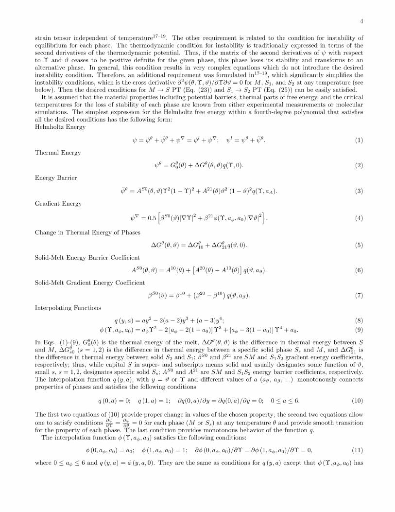
FIG. 3: Mesh dependence of solutions to the GL equations at a0 = 0. Effect of the mesh size on the distribution of the orderparameters, ϑ and Υ, at θ = 492K, for kδ = 1.0 and kE = 4.0, using perturbed S1S2 initial conditions. Solutions are shownfor the entire width of IM (a) and for the zoomed region close to the S1S2 interface within melt (b). Subscripts on the orderparameters indicate the number of elements per equilibrium S1S2 interface width δ21 without melt.

It should be noted that obvious inequality θs0c < θs0e < θ0sc results in As0c < −6∆ss0. If we assume that the equilibrium

temperature is the average of critical temperatures, then we obtain As0c = −3∆ss0 and A21c = −3∆s21. In the next

section, it will be shown that this choice of parameters makes the interface energy and width to be temperatureindependent.

It is worth noting that for the fourth degree polynomial potential for each of the PTs, the next higher order termin local potential energy satisfying all the above requirements to the thermodynamic potentials (i.e., which does notchange thermodynamic equilibrium and instability conditions) is a ninth-degree term

G9(Υ, ϑ) = A9Υ3 (1−Υ)2 ϑ2 (1− ϑ)2. (31)

This term does not change the solution for an interface (and consequently, its width, energy, and velocity) betweenany two phases. It contributes only where all three phases are present, in particular, at S1MS2 interface, and can beused to adjust its energy and width by choosing a proper parameter A9, if such data will be available.

While we cannot prove that the above potential does not possess any other minima than corresponding to M , S1,and S2 (which will result in unwanted spurious phases), numerous calculations at different parameters demonstratethat this is the case. If some exception will be found, an additional term G9 can be used to eliminate it.

D. Well-posedness of problem formulation

In the developed model the S1MS2 diffuse interface corresponds to Υ varying from 1 to 0 and again back to 1, andϑ varies from 0 to 1 (Fig. 3). Variation of ϑ in the completely molten region–i.e., at Υ = 0, from the first glancedoes not have any physical meaning as melt does not have memory of its previous solid phase. This implies that ψ∇

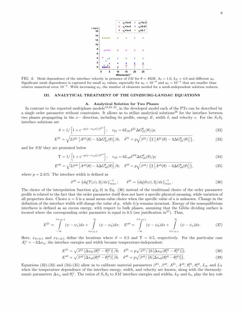
should be independent of ∇ϑ when Υ = 0, i.e., a0 = 0. However, for a0 = 0 energy-minimizing solution correspondsto the sharp solid-solid interface, i.e., ϑ is the step function and Υ = 0 at one point only corresponds to the jump inϑ (Fig. 3). Indeed, for such a solution the contribution of ∇ϑ to the total energy is zero and the size of the region ofhigh energy complete melt (where Υ = 0) is minimized. Such a solution was found for intergranular premelting in22,in which a0 = 0. It is convenient for analytical study as the limit simplified case, but the lack of characteristic sizefor the IM region means that the problem is ill-posed and will lead to catastrophic mesh-dependence of the solutionfor any discretization method. Indeed, finite element solutions to the GL equations demonstrated that the width ofthe region with sharp change in ϑ is approximately equal to the size of a single finite element (Fig. 3) and it tendsto zero (and ∇ϑ → ∞) when element size tends to zero. Interface velocity v also strongly depends on the meshsize (see Fig. 4), leading also to interface trapping, i.e., to a zero interface velocity for a nonzero driving force. Thistrapping reduces with the reduction of the finite element size. Therefore, a0 must be chosen to be greater than zero(and greater than the numerical error, see below) to obtain well-posed formulation. As it will be shown in Section V,parameter a0 allows us to describe the interaction between two solid-melt interfaces.

Note that the interface velocity also strongly depends on the mesh size even for very small but nonzero a0 (see Fig.4), when a0 is comparable to the error of calculation. Thus, for a0 = 10−6, v = 0 for the number of finite elementsper width of the equilibrium S1S2 interface δ21 (without melt), N , smaller than or equal to 25, which, however,means interface trapping rather than mesh-independence of the interface velocity. Indeed, interface velocity is gettingnonzero for N > 200. For a0 = 10−5, mesh-dependence of v can be neglected for N > 20 and trapping occurs atN ≤ 10, and numerical simulations are still quite costly. For a0 = 10−4, mesh-dependence of v can be neglected forN ≥ 5, which is typical for any interface, and trapping occurs at N ≤ 3. For a0 = 0.1 the IM is broad enough andN = 1 is sufficient for a mesh-independent solution.

8

0 5 10 15 20 25

0

2

4

6

8

10

12

14

16

a0=1e-6 a0=1e-3 a0=1e-5 a0=0.01 a0=1e-4 a0=0.1

v (m/s)

#Elements/FIG. 4: Mesh dependence of the interface velocity in presence of IM for θ = 492K, kδ = 1.0, kE = 4.0 and different a0.Significant mesh dependence is captured for small a0 values, especially for a0 = 10−6 and a0 = 10−5 that are smaller thanrelative numerical error 10−4. With increasing a0, the number of elements needed for a mesh-independent solution reduces.

III. ANALYTICAL TREATMENT OF THE GINZBURG-LANDAU EQUATIONS

A. Analytical Solution for Two Phases

In contrast to the reported multiphase models19,23–25, in the developed model each of the PTs can be described bya single order parameter without constraints. It allows us to utilize analytical solutions26 for the interface betweentwo phases propagating in the x− direction, including its profile, energy E, width δ, and velocity v. For the S1S2

interface solutions are

ϑ = 1/[1 + e−p(x−v21t)/δ

21]

; v21 = 6L21δ21∆Gθ21(θ)/p; (32)

E21 =√

2β21[A21(θ)− 3∆Gθ21(θ)

]/6; δ21 = p

√β21/

{2[A21(θ)− 3∆Gθ21(θ)

]}, (33)

and for SM they are presented below

Υ = 1/[1 + e−p(x−vs0t)/δ

s0]

; vs0 = 6Ls0δS0∆Gθs0(θ)/p; (34)

Es0 =√

2βs0[As0(θ)− 3∆Gθs0(θ)

]/6; δs0 = p

√βs0/

{2[As0(θ)− 3∆Gθs0(θ)

]}, (35)

where p = 2.415. The interface width is defined as

δs0 = {dq[Υ(x), 3]/dx}−1max ; δ21 = {dq[ϑ(x), 3]/dx}−1

max . (36)

The choice of the interpolation function q(y, 3) in Eq. (36) instead of the traditional choice of the order parameterprofile is related to the fact that the order parameter itself does not have a specific physical meaning, while variation ofall properties does. Choice a = 3 is a usual mean-value choice when the specific value of a is unknown. Change in thedefinition of the interface width will change the value of p, while δ/p remains invariant. Energy of the nonequilibriuminterfaces is defined as an excess energy, with respect to bulk phases, assuming that the Gibbs dividing surface islocated where the corresponding order parameter is equal to 0.5 (see justification in27). Thus,

E21 =

xϑ=0.5∫−∞

(ψ − ψ1)dx+

∞∫xϑ=0.5

(ψ − ψ2)dx; Es0 =

xΥ=0.5∫−∞

(ψ − ψ0)dx+

∞∫xΥ=0.5

(ψ − ψs)dx. (37)

Here, xϑ=0.5 and xΥ=0.5 define the locations where ϑ = 0.5 and Υ = 0.5, respectively. For the particular caseAijc = −3∆sij , the interface energies and width became temperature-independent:

E21 =√β21 [∆s21(θ21

c − θ21e )] /6; δ21 = p

√β21/ {6 [∆s21(θ21

c − θ21e )]}; (38)

Es0 =√βs0 [∆ss0(θs0c − θs0e )] /6; δs0 = p

√βs0/ {6 [∆ss0(θs0c − θs0e )]}. (39)

Equations (32)-(33) and (34)-(35) allow us to calibrate material parameters β21, βs0, A21, As0, θ21c , θs0c , Lϑ, and LΥ

when the temperature dependence of the interface energy, width, and velocity are known, along with the thermody-namic parameters ∆sij and θije . The ratios of S1S2 to SM interface energies and widths, kE and kδ, play the key role

9

in determining the material response. Using the equations (33) and (35), kE and kδ are:

kE =E21

Es0=

√β21

βs0A21c (θ − θ21

c ) + 3 ∆s21(θ − θ21e )

As0c (θ − θs0c ) + 3 ∆ss0(θ − θs0e ); (40)

kδ =δ21

δs0=

√β21

βs0As0c (θ − θs0c ) + 3 ∆ss0(θ − θs0e )

A21c (θ − θ21

c ) + 3 ∆s21(θ − θ21e )

. (41)

For Aijc = −3∆sij , the equations (40) and (41) reduce to

kE =

√β21

βs0∆s21(θ21

c − θ21e )

∆ss0(θs0c − θs0e ); kδ =

δ12

δs0=

√β21

βs0∆ss0(θs0c − θs0e )

∆s21(θ21c − θ21

e ), (42)

which are temperature independent. Energy of the S1MS2 interface containing IM , E∗, is defined as excess energywith respect to S1 for points with ϑ ≤ 0.5 and with respect to S2 for points with ϑ > 0.5–i.e.,

E∗ =

∫ xϑ=0.5

−∞(ψ − ψs1)dx+

∫ ∞xϑ=0.5

(ψ − ψs2)dx. (43)

B. Energy Integral for Stationary Solutions for Three Phases

It is known that for stationary 1D solutions of the GL equation for two phases, i.e., for plane stationary interfaceor critical nucleus, an energy integral can be found. It results in the statement that the excess of the local energy ateach point is equal to the gradient energy. We will derive an energy integral and prove a similar statement for twoGL equations (14) and (15) and taking into account dependence of βS0(ϑ) and β21(Υ). Thus, Eqs. (14) and (15) forthe stationary case and the 1D case simplify to

∂ψl

∂Υ= −β

21

2

dφ(Υ)

dΥϑ2x +

d(βS0(ϑ)Υx

)dx

; (44)

∂ψl

∂ϑ= −1

2

dβS0(ϑ)

dϑΥ2x +

d(β21φ(Υ)ϑx

)dx

, (45)

where subscript x designates the derivative with respect to x. It is proven in Eq. (A.7) in Appendix that dψl(θ,Υ, ϑ) =dψ∇. Integrating dψl at constant temperature, we obtain

ψl(θ,Υ, ϑ)− ψ0 = ψ∇, (46)

where ψ0 is the integration constant. Consequently, for any stationary solution, the excess of the local energy at eachpoint is equal to the gradient energy.

Stationary interface.—Let us consider a stationary plane interface, when one has solid phase S1 (i.e., ϑ = 0 andΥ = 1) as x → −∞ and S2 (i.e., ϑ = 1 and Υ = 1) as x → ∞. Then both gradients and ψ∇ = 0 for x → ±∞, andboth sides of Eq. (46) are zero, i.e.,

ψ0 = ψl(θ,Υ = 1, ϑ = 0) = G1(θ) = ψl(θ,Υ = 1, ϑ = 1) = G2(θ). (47)

The equality of free energies of phases S1 and S2 means that temperature is equal to the phase equilibrium temperatureθ21e , – i.e., ψ0 = G1(θ21

e ) = G2(θ21e ). Since energy is known to within a constant, one can chose G1(θ21

e ) = G2(θ21e ) = 0

and obtain ψ0 = 0. Similar treatment is valid if we consider the appearance of any third phase at the stationaryinterface between two other phases, at their thermodynamic equilibrium temperature.

Critical nuclei.—Let us consider critical nucleus of one of the phase or two combined phases within another homo-geneous phase or at the interface between two other phases. For all cases, assume that both gradients and ψ∇ = 0for x → ±∞, and both sides of Eq. (46) are again zero –i.e., ψ0 = ψl(θ, x = ±∞). If we consider the appearanceof the third phase at the stationary interface between two other phases, in particular, the critical nucleus of IM atstationary S1S2 interface, then it is possible at the thermodynamic equilibrium temperature of these phases. Anothernontrivial case is nucleation of a compound critical nucleus consisting of two phases within the homogenous matrixof the third phase, see for example Ref28. In this case temperature should not be equal to the phase equilibriumtemperature. The last case, nucleation of one phase within another, is well known from two-phase studies and againtemperature should not be equal to the phase equilibrium temperature.

For all these solutions, namely, the equilibrium interface with the third phase and all critical nuclei, excess energyof the system with respect to the energy of the ground phase or equilibrium phases at x = ±∞, according to Eqs.

10

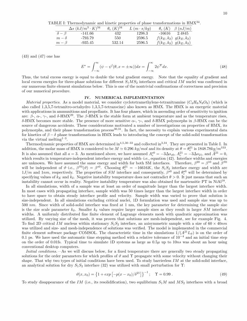
TABLE I: Thermodynamic and kinetic properties of phase transformations in HMX34.

∆s (kJ/m3 ·K)34 θe (K)34 L (m · s/kg) θc (K) β (nJ/m)δ − β -141.66 432 1298.3 -16616 2.4845m− δ -793.79 550 2596.5 f(kE , kδ) g(kE , kδ)m− β -935.45 532.14 2596.5 f(kE , kδ) g(kE , kδ)

(43) and (47) one has

E∗ =

∫ ∞−∞

(ψ − ψl(θ, x = ±∞))dx =

∫ ∞−∞

2ψ∇dx. (48)

Thus, the total excess energy is equal to double the total gradient energy. Note that the equality of gradient andlocal excess energies for three-phase solutions for different S1MS2 interfaces and critical IM nuclei was confirmed inour numerous finite element simulations below. This is one of the nontrivial confirmations of correctness and precisionof our numerical procedure.

IV. NUMERICAL IMPLEMENTATION

Material properties. As a model material, we consider cyclotetramethylene-tetranitramine (C4H8N8O8) (which isalso called 1,3,5,7-tetranitro-octahydro 1,3,5,7-tetrazocine) also known as HMX. The HMX is an energetic materialwith applications in ammunitions and propellants. It has four phases, which in ascending order of sensitivity to ignitionare: β-, α-, γ-, and δ-HMX29. The β-HMX is the stable form at ambient temperature and as the temperature rises,δ-HMX becomes more stable. The presence of more sensitive α-, γ-, and δ-HMX polymorphs in β-HMX can be thesource of dangerous accidents. These considerations motivated a number of investigations on properties of HMX, itspolymorphs, and their phase transformation process30,31. In fact, the necessity to explain various experimental datafor kinetics of β − δ phase transformations in HMX leads to introducing the concept of the solid-solid transformationvia the virtual melting1–3.

Thermodynamic properties of HMX are determined in4,5,30–33 and collected in3,34. They are presented in Table I. Inaddition, the molar mass of HMX is considered to be M ' 0.296 kg/mol and its density at θ = θ21

e is 1848.78kg/m333.

It is also assumed that all a = 3. As mentioned above, we have assumed As0c = −3∆ss0, A21c = −3∆s21, and A21 = 0,

which results in temperature-independent interface energy and width–i.e., equation (42). Interface widths and energiesare unknown. We have assumed the same energy and width for both SM interfaces. Therefore, β20 = β10 and βS0

will be independent of ϑ–i.e., βS0(ϑ) = βs0. Choosing θ21c = −16616K, the S1S2 interface energy and width are

1J/m and 1nm, respectively. The properties of SM interface and consequently, βs0 and θs0c will be determined byspecifying values of kE and kδ. Negative instability temperature does not contradict θ > 0. It just means that such aninstability cannot occur in reality. Negative instability temperature was also obtained for martensitic PT in NiAl18.

In all simulations, width of a sample was at least an order of magnitude larger than the largest interface width.In most cases with propagating interface, sample width was 50 times larger than the largest interface width in orderto have space to obtain steady interface profile and velocity. Sample width was varied to prove that solution issize-independent. In all simulations excluding critical nuclei, 1D formulation was used and sample size was up to500 nm. Since width of solid-solid interface was fixed at 1 nm, the key parameter for determining the sample sizeis the size scale parameter kδ. Smaller kδ values require larger sample sizes as they result in larger SM interfacewidths. A uniformly distributed fine finite element of Lagrange elements mesh with quadratic approximation wasutilized. By varying size of the mesh, it was proven that solutions are mesh-independent, see for example Fig. 4.To find 2D critical IM nucleus within stationary S1S2 interface, an axisymmetric sample with a size of 60 × 40nmwas utilized and size- and mesh-independence of solutions was verified. The model is implemented in the commercialfinite element software package COMSOL. The characteristic time in the simulations 1/(A21Lϑ) is on the order of0.1 ps. We have used the automatic time stepping method with a relative tolerance of 10−4 and an initial time stepon the order of 0.01fs. Typical time to simulate 1D systems as large as 0.5µ up to 10ns was about an hour usingconventional desktop computers.

Initial conditions.—As we will discuss below, for a fixed temperature there are generally two steady propagatingsolutions for the order parameters for which profiles of ϑ and Υ propagate with some velocity without changing theirshape. That why two types of initial conditions have been used. To study barrierless IM at the solid-solid interface,an analytical solution for dry S1S2 interface (32) was utilized with small perturbation for Υ:

ϑ(x, x0) ={

1 + exp[−p(x− x0)/δ21

]}−1; Υ = 0.99 . (49)

To study disappearance of the IM (i.e., its resolidification), two equilibrium S1M and MS2 interfaces with a broad

11

420 450 480 510 540

-600

-500

-400

-300

-200

-100

0

KE=1.933 KE=3.39 Analytical Sol.

v (m/s)

S1M

S1S2

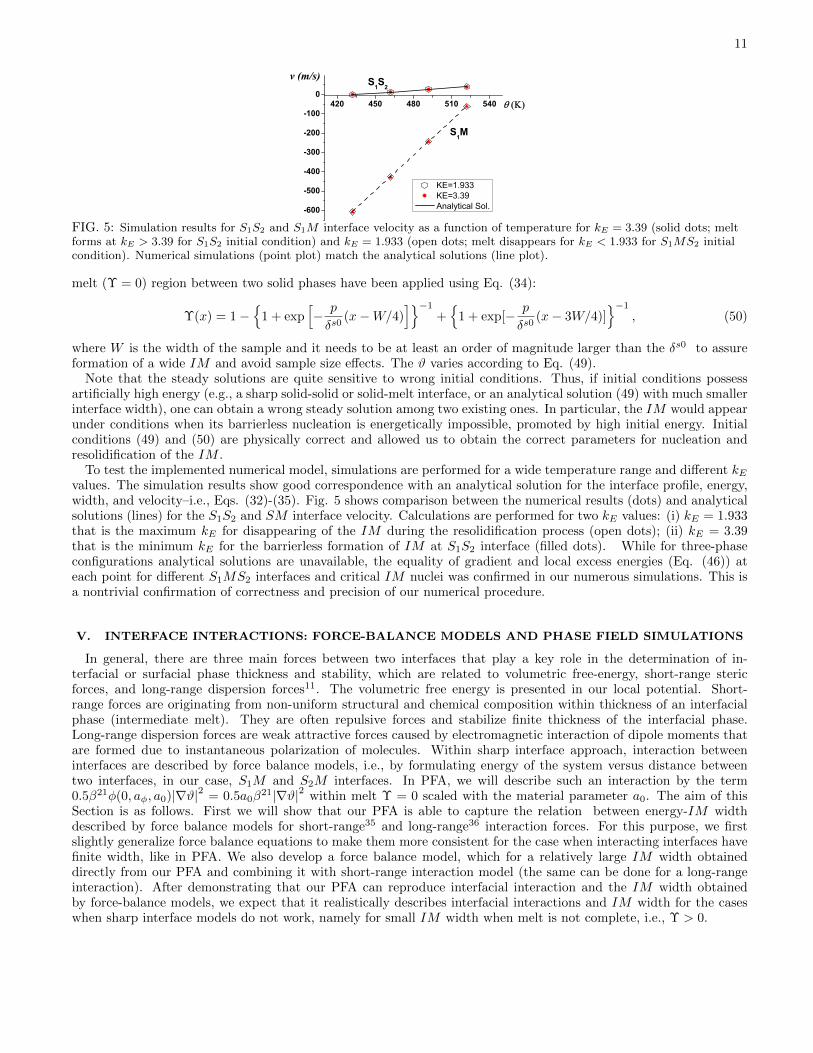
FIG. 5: Simulation results for S1S2 and S1M interface velocity as a function of temperature for kE = 3.39 (solid dots; meltforms at kE > 3.39 for S1S2 initial condition) and kE = 1.933 (open dots; melt disappears for kE < 1.933 for S1MS2 initialcondition). Numerical simulations (point plot) match the analytical solutions (line plot).

melt (Υ = 0) region between two solid phases have been applied using Eq. (34):

Υ(x) = 1−{

1 + exp[− p

δs0(x−W/4)

]}−1

+{

1 + exp[− p

δs0(x− 3W/4)]

}−1

, (50)

where W is the width of the sample and it needs to be at least an order of magnitude larger than the δs0 to assureformation of a wide IM and avoid sample size effects. The ϑ varies according to Eq. (49).

Note that the steady solutions are quite sensitive to wrong initial conditions. Thus, if initial conditions possessartificially high energy (e.g., a sharp solid-solid or solid-melt interface, or an analytical solution (49) with much smallerinterface width), one can obtain a wrong steady solution among two existing ones. In particular, the IM would appearunder conditions when its barrierless nucleation is energetically impossible, promoted by high initial energy. Initialconditions (49) and (50) are physically correct and allowed us to obtain the correct parameters for nucleation andresolidification of the IM .

To test the implemented numerical model, simulations are performed for a wide temperature range and different kEvalues. The simulation results show good correspondence with an analytical solution for the interface profile, energy,width, and velocity–i.e., Eqs. (32)-(35). Fig. 5 shows comparison between the numerical results (dots) and analyticalsolutions (lines) for the S1S2 and SM interface velocity. Calculations are performed for two kE values: (i) kE = 1.933that is the maximum kE for disappearing of the IM during the resolidification process (open dots); (ii) kE = 3.39that is the minimum kE for the barrierless formation of IM at S1S2 interface (filled dots). While for three-phaseconfigurations analytical solutions are unavailable, the equality of gradient and local excess energies (Eq. (46)) ateach point for different S1MS2 interfaces and critical IM nuclei was confirmed in our numerous simulations. This isa nontrivial confirmation of correctness and precision of our numerical procedure.

V. INTERFACE INTERACTIONS: FORCE-BALANCE MODELS AND PHASE FIELD SIMULATIONS

In general, there are three main forces between two interfaces that play a key role in the determination of in-terfacial or surfacial phase thickness and stability, which are related to volumetric free-energy, short-range stericforces, and long-range dispersion forces11. The volumetric free energy is presented in our local potential. Short-range forces are originating from non-uniform structural and chemical composition within thickness of an interfacialphase (intermediate melt). They are often repulsive forces and stabilize finite thickness of the interfacial phase.Long-range dispersion forces are weak attractive forces caused by electromagnetic interaction of dipole moments thatare formed due to instantaneous polarization of molecules. Within sharp interface approach, interaction betweeninterfaces are described by force balance models, i.e., by formulating energy of the system versus distance betweentwo interfaces, in our case, S1M and S2M interfaces. In PFA, we will describe such an interaction by the term0.5β21φ(0, aφ, a0)|∇ϑ|2 = 0.5a0β

21|∇ϑ|2 within melt Υ = 0 scaled with the material parameter a0. The aim of thisSection is as follows. First we will show that our PFA is able to capture the relation between energy-IM widthdescribed by force balance models for short-range35 and long-range36 interaction forces. For this purpose, we firstslightly generalize force balance equations to make them more consistent for the case when interacting interfaces havefinite width, like in PFA. We also develop a force balance model, which for a relatively large IM width obtaineddirectly from our PFA and combining it with short-range interaction model (the same can be done for a long-rangeinteraction). After demonstrating that our PFA can reproduce interfacial interaction and the IM width obtainedby force-balance models, we expect that it realistically describes interfacial interactions and IM width for the caseswhen sharp interface models do not work, namely for small IM width when melt is not complete, i.e., Υ > 0.

12

A. Force-balance models of interface interactions

In the force-balance method10,12 adapted for our problem, an energy of the system is given versus the width of theIM δ∗ , i.e., G(δ∗). This function satisfies the requirements that G(0) = E21 and for δ∗ →∞ one has G(δ∗) = ∆Gδ∗,where ∆G is the bulk excess energy, i.e., the difference between the energy of melt and initial state with two solidphases in the region where IM appeared. The IM can appear if G(δ∗)−G(0) < 0. The equilibrium thickness of theIM , δ∗e , can be found by minimizing the energy function G(δ∗)–i.e. ∂G

∂δ∗ = 0.Long-range interface interaction model.—Long-range London dispersion force is a weak intermolecular force due to

instantaneous polarization of molecules and interaction of fluctuation dipoles36. These forces play a key role in theinterfacial behavior of materials such as ice and molecular substances. The energy for this case is

Glr(δ∗) = 2Es0 + ∆Gδ∗ −∆γ/

[1 + (δ∗/δa)

2], (51)

where δa is a characteristic length and ∆γ = 2Es0 − E21 is the difference between energy of two SM interfaces andS1S2 interface. While this expression satisfies all the above limit cases and is formally noncontradictory for sharpinterface approach, it requires modifications when the finite width of SM interface is taken into account. Let usintroduce the width of a disordered (non-solid) phase, δ, which is calculated as the width where Υ ≤ 0.99, and δintis the width of two SM interfaces. The problem in the application of Eq. (51) for the case with finite width of SMinterface is related to the definition of δ∗. If δ∗ = δ then the condition Glr(0) = E21 is satisfied but ∆G contributeswhen there is no complete melt, which is contradictory. If δ∗ = δ − δint, then there is no nonphysical contributiondue to ∆G when there is no complete melt (δ = δint) but Glr(0) = E21 while we have two SM interfaces. Also, thecondition for the S1S2 interface δ = 0 is not satisfied, i.e., Glr(−δint) 6= E21. We suggest the simplest generalization

Glr = 2Es0 + ∆G (δ − δint)−∆γ/[1 + (δ/δa)

2]. (52)

The bulk term ∆G is multiplied by the width of the complete melt and it disappears when the region with completemelt disappears. Condition ∂Glr/∂δ = 0 results in

∆G+ 2∆γ δ2a δ/

(δ2 + δ2

a

)2= 0, (53)

which is independent of δint. Thus, δint just changes the values of energy by the same amount for any δ. Note that δintwill be determined below from the best fit of energy to PFA simulations rather than from geometric definitions (e.g.,as the width where 0.01 ≤ Υ ≤ 0.99 for each interface or any other range), because different geometric definitions

may give quite different widths. We do not expect that Glr has some specific value for δ = δint, because it followsfrom the phase field solution that it is equal to 2Es0 plus the contribution due to 0.5β21φ(Υ, aφ, a0)|∇ϑ|2, which isnot easy to estimate. We also do not expect that Eq. (51) would work for small δ < δint and incomplete melt. Notethat while describing results of the PFA simulation with some equations, it is important to have a good coincidencefor the position of the minimum of the energy and near this minimum only. Eq. (51) with a single fitting parameterδa does not allow a good description of the PFA simulation results while Eq. (51) does allow (see e.g., Figs. 7 and8). During the fitting procedure for PFA results, δa is determined from the value of the width δ corresponding to theminimum of the energy (53) and δint is obtained from the numerical fitting of the energy curve near the minimum.The same is done for the short-range interaction model.

Short-range interface interaction model.–The short-range interface interactions are due to non-uniform structureand composition of surfacial/interfacial phases. These repulsive forces play a crucial role in stabilizing the finite widthof surfacial/interfacial nanoscale phases in metals and ceramics11,35. In contrast to long-range interactions that canexist even in a uniform structure,the gradient of the chemical and structural origin has a major contribution to theshort-range forces. An energy for the short-range interaction model is defined as

Gsr(δ∗) = 2Es0 + ∆Gδ∗ −∆γ exp (−δ∗/δa) . (54)

Similar to the energy of the long-range interaction, Gsr satisfies all the required conditions for the sharp interfacesbut should be modified to take into account the finite width of the SM interfaces. The more general function is

Gsr = 2Es0 + ∆G (δ − δint)−∆γ exp (−δ/δa) . (55)

which satisfies the same conditions as Glr. An actual width δ is determined by a solution to the equation ∂Gsr/∂δ = 0:

δ = δa ln [−∆γ/ (∆G δa)] , (56)

which is independent of δint, like for the long-range interaction.

13

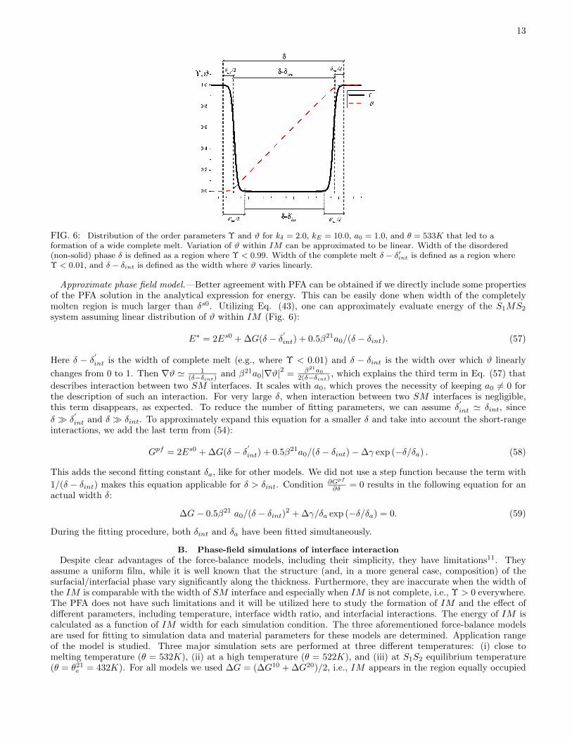
FIG. 6: Distribution of the order parameters Υ and ϑ for kδ = 2.0, kE = 10.0, a0 = 1.0, and θ = 533K that led to aformation of a wide complete melt. Variation of ϑ within IM can be approximated to be linear. Width of the disordered(non-solid) phase δ is defined as a region where Υ < 0.99. Width of the complete melt δ − δ′int is defined as a region whereΥ < 0.01, and δ − δint is defined as the width where ϑ varies linearly.

Approximate phase field model.—Better agreement with PFA can be obtained if we directly include some propertiesof the PFA solution in the analytical expression for energy. This can be easily done when width of the completelymolten region is much larger than δs0. Utilizing Eq. (43), one can approximately evaluate energy of the S1MS2

system assuming linear distribution of ϑ within IM (Fig. 6):

E∗ = 2Es0 + ∆G(δ − δ′

int) + 0.5β21a0/(δ − δint). (57)

Here δ − δ′int is the width of complete melt (e.g., where Υ < 0.01) and δ − δint is the width over which ϑ linearly

changes from 0 to 1. Then ∇ϑ ' 1(δ−δint)

and β21a0|∇ϑ|2 = β21a0

2(δ−δint), which explains the third term in Eq. (57) that

describes interaction between two SM interfaces. It scales with a0, which proves the necessity of keeping a0 6= 0 forthe description of such an interaction. For very large δ, when interaction between two SM interfaces is negligible,this term disappears, as expected. To reduce the number of fitting parameters, we can assume δ

′

int ' δint, since

δ � δ′

int and δ � δint. To approximately expand this equation for a smaller δ and take into account the short-rangeinteractions, we add the last term from (54):

Gpf = 2Es0 + ∆G(δ − δ′

int) + 0.5β21a0/(δ − δint)−∆γ exp (−δ/δa) . (58)

This adds the second fitting constant δa, like for other models. We did not use a step function because the term with

1/(δ − δint) makes this equation applicable for δ > δint. Condition ∂Gpf

∂δ = 0 results in the following equation for anactual width δ:

∆G− 0.5β21 a0/(δ − δint)2 + ∆γ/δa exp (−δ/δa) = 0. (59)

During the fitting procedure, both δint and δa have been fitted simultaneously.

B. Phase-field simulations of interface interaction

Despite clear advantages of the force-balance models, including their simplicity, they have limitations11. Theyassume a uniform film, while it is well known that the structure (and, in a more general case, composition) of thesurfacial/interfacial phase vary significantly along the thickness. Furthermore, they are inaccurate when the width ofthe IM is comparable with the width of SM interface and especially when IM is not complete, i.e., Υ > 0 everywhere.The PFA does not have such limitations and it will be utilized here to study the formation of IM and the effect ofdifferent parameters, including temperature, interface width ratio, and interfacial interactions. The energy of IM iscalculated as a function of IM width for each simulation condition. The three aforementioned force-balance modelsare used for fitting to simulation data and material parameters for these models are determined. Application rangeof the model is studied. Three major simulation sets are performed at three different temperatures: (i) close tomelting temperature (θ = 532K), (ii) at a high temperature (θ = 522K), and (iii) at S1S2 equilibrium temperature(θ = θ21

e = 432K). For all models we used ∆G = (∆G10 + ∆G20)/2, i.e., IM appears in the region equally occupied

14

FIG. 7: Comparison between force-balance models and phase field simulations for θ = 532K and kδ = 1.0. Phase field resultsfor different a0 values (open symbols) are fitted to three force-balance models (solid lines): (a) approximate phase field model,

Gpf ; (b) long-range interaction model, Glr and (c) short-range interaction model, Gsr.



by each of the solid phases. The values of ∆G at each specified temperature are: ∆G = 7.2 GJ/m3 at θ = 532K;∆G = 16 MJ/m3 at θ = 522K, and ∆G = 94 MJ/m3 at θ = 432K. Simulations are performed for β21 = 2.48 J/m,kE = 3.2, and E21 = 1 J/m2, which results in Es0 = 1/3.2 = 0.313 J/m2 and ∆γ = 0.375 J/m2.

Simulations for θ = 532K— Results of the PF simulations for kδ = 1.0 and 1.1 for various a0 are presented inFigs. 7 and 8. Solid lines in these plots are fitting curves based on three force-balance models, with fitting parametersδa and δint presented in Table II. All models reproduce well, not only the value of δ corresponding to the energyminimum (which is not surprising since it was directly fitted), but also values of energy minima and the entire curvein a large range of δ around the energy minimum. While for large δ all models show good fitting, the approximatephase field model shows a broader range of coincidence with simulation results for small δ, for all a0 and both kδ.Increasing a0 increases the repulsive forces between interfaces and consequently, the equilibrium IM width.

Comparing Figs. 7 and 8, it can be concluded that increasing the kδ reduces the equilibrium width of the IM andslightly reduces the fitting range of the models. Characteristic length δa is much smaller for the approximate phasefield model than for the other two models and reduces with increasing a0, while for other models it increases. Thewidth δint that corrects values of the energy in comparison with traditional short-range and long-range interactionmodels is smaller for the short-range interaction and reduces with increasing a0. Thus, the necessity for correctionis evident. The width δint for the approximate phase field model is between that for the short-range and long-rangeinteraction and also reduces with increasing a0.

Simulations for θ = 522K.—For kδ = 1.1, Υ vanishes inside the IM and the region of complete melt is very large.The IM free energy versus width δ is plotted in Fig. 9. The values of parameters fitted to each model are shown inTable II. The reduction of temperature in comparison with θ = 532K increased the IM free energy and decreased theIM width. The smaller IM width has essentially reduced the range of coincidence with simulations for short-rangeand long-range interaction models. However, our approximate phase field model shows very good agreement withsimulations in the entire range of width δ under study. Both widths δint and δa are the smallest for the approximatephase field model and they reduce with an increase in a0.

Simulations for θ = θ21e = 432K.— For kδ = 1.1 and 100K below the melting temperature, Υ > 0 and melt is

15

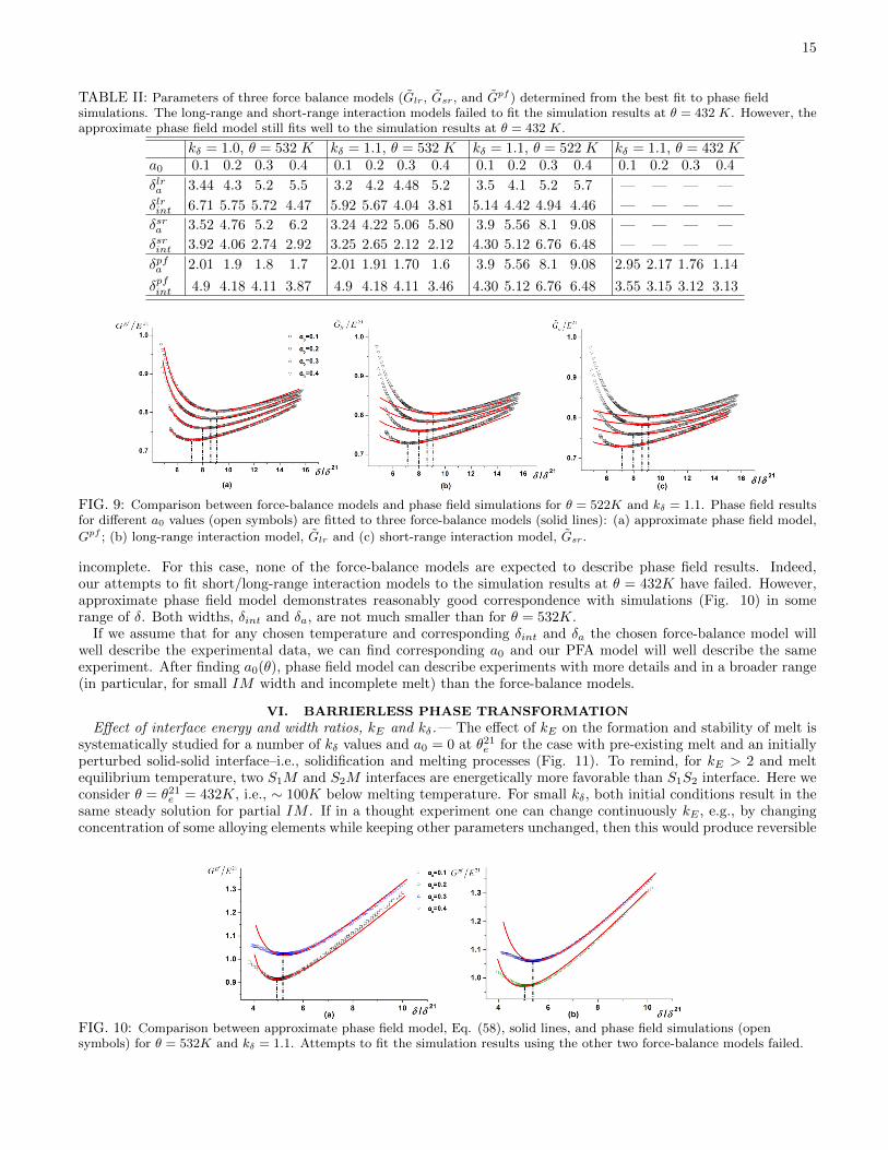
TABLE II: Parameters of three force balance models (Glr, Gsr, and Gpf ) determined from the best fit to phase fieldsimulations. The long-range and short-range interaction models failed to fit the simulation results at θ = 432 K. However, theapproximate phase field model still fits well to the simulation results at θ = 432 K.

kδ = 1.0, θ = 532 K kδ = 1.1, θ = 532 K kδ = 1.1, θ = 522 K kδ = 1.1, θ = 432 Ka0 0.1 0.2 0.3 0.4 0.1 0.2 0.3 0.4 0.1 0.2 0.3 0.4 0.1 0.2 0.3 0.4

δlra 3.44 4.3 5.2 5.5 3.2 4.2 4.48 5.2 3.5 4.1 5.2 5.7 — — — —

δlrint 6.71 5.75 5.72 4.47 5.92 5.67 4.04 3.81 5.14 4.42 4.94 4.46 — — — —

δsra 3.52 4.76 5.2 6.2 3.24 4.22 5.06 5.80 3.9 5.56 8.1 9.08 — — — —

δsrint 3.92 4.06 2.74 2.92 3.25 2.65 2.12 2.12 4.30 5.12 6.76 6.48 — — — —

δpfa 2.01 1.9 1.8 1.7 2.01 1.91 1.70 1.6 3.9 5.56 8.1 9.08 2.95 2.17 1.76 1.14

δpfint 4.9 4.18 4.11 3.87 4.9 4.18 4.11 3.46 4.30 5.12 6.76 6.48 3.55 3.15 3.12 3.13



incomplete. For this case, none of the force-balance models are expected to describe phase field results. Indeed,our attempts to fit short/long-range interaction models to the simulation results at θ = 432K have failed. However,approximate phase field model demonstrates reasonably good correspondence with simulations (Fig. 10) in somerange of δ. Both widths, δint and δa, are not much smaller than for θ = 532K.

If we assume that for any chosen temperature and corresponding δint and δa the chosen force-balance model willwell describe the experimental data, we can find corresponding a0 and our PFA model will well describe the sameexperiment. After finding a0(θ), phase field model can describe experiments with more details and in a broader range(in particular, for small IM width and incomplete melt) than the force-balance models.

VI. BARRIERLESS PHASE TRANSFORMATION

Effect of interface energy and width ratios, kE and kδ.— The effect of kE on the formation and stability of melt issystematically studied for a number of kδ values and a0 = 0 at θ21

e for the case with pre-existing melt and an initiallyperturbed solid-solid interface–i.e., solidification and melting processes (Fig. 11). To remind, for kE > 2 and meltequilibrium temperature, two S1M and S2M interfaces are energetically more favorable than S1S2 interface. Here weconsider θ = θ21

e = 432K, i.e., ∼ 100K below melting temperature. For small kδ, both initial conditions result in thesame steady solution for partial IM . If in a thought experiment one can change continuously kE , e.g., by changingconcentration of some alloying elements while keeping other parameters unchanged, then this would produce reversible

FIG. 10: Comparison between approximate phase field model, Eq. (58), solid lines, and phase field simulations (opensymbols) for θ = 532K and kδ = 1.1. Attempts to fit the simulation results using the other two force-balance models failed.

16

FIG. 11: Intermediate melt formation ∼ 100K below melting temperature. a) Minimum steady value of Υmin withinS1MS2 interface at θ = θ21e = 432K versus kE , for melting (black graphs) and solidification (red graphs) is plotted for severalkδ. For each kδ ≥ 0.7, two different solutions exist in the range of kE within hysteresis loop (between arrows directed up anddown), one of which is Υmin = 1. Outside this loop, for smaller kE , IM does not exist; for larger kE , S1S2 interface does notexist. For small kδ (e.g. for kδ = 0.3), both solutions coincides. b) Profile of the equilibrium distribution of the orderparameter Υ for kδ = 0.3 and multiple kE .

change in the degree of premelting without any hysteresis. For larger kδ, two different initial conditions result in thesame solution for relatively small and large kE only, but with two different nanostructures for intermediate kE . Oneof these two solutions is always just a S1S2 interface. With increasing kE , there is a jump from the S1S2 interface(which ceases to exist) to the second solution with partial or complete IM . With decreasing kE , there is an oppositejump, which occurs for kE < 2, i.e., IM persists under conditions at which it is energetically unfavorable. The twosolutions produce a hysteresis region. This is in contrast to the sharp interface results that do not possess a scaleparameter kδ and has just one solution and formation of melt at kE > 2 near melt equilibrium temperature. For bothof the aforementioned initial conditions, increasing the value of kE promotes the formation and persistence of melt.Width of the hysteresis increases with increasing kδ, starting from zero for small enough kδ values. While formationof a (almost) complete melted phase is observed for large kδ and large enough kE values, for smaller kδ values, onlya partial IM appears for the same kE value.

Formation of IM as a function of kδ has also been studied for a number of kE values at θ21e and 472K and the

results were shown in Fig. 12 for the same two different initial conditions. It is shown that increasing the value ofkE promotes the formation of IM , which is consistent with results presented in Fig. 11. In all these cases, for largekδ two solutions exist, one of each is the S1S2 interface (Υmin = 1) for S1S2 initial conditions and another one is thecomplete or incomplete IM for S1MS2 initial conditions. For small kδ, these solutions coincide, i.e., steady solution isindependent of initial conditions. For large kE ((a) and (c)) and S1MS2 initial conditions, Υmin for IM continuouslyreduces with an increase in kδ and continuously increases with the reduction in kδ along the same line. For S1S2

initial conditions, with reduction in kδ, the solution Υmin = 1 ceases to exist and a jump occurs to the single solutionfor IM . For small kE ((b) and (d)), the behavior is more sophisticated. For small kδ, a nonmonotonous dependence ofΥmin vs. kδ is observed, the same for both initial conditions. Thus, IM formation is promoted by an increase in thekδ up to a certain point, and then it is suppressed for higher kδ values, see the Υ profile in Fig. 13. For large kδ, thesolution Υmin = 1 always exists and there is no jump to IM . For S1MS2 initial conditions, Υmin slightly increaseswith reducing kδ until IM ceases to exist and a jump to Υmin = 1 occurs. For intermediate kδ, the only existingsolution for both initial conditions is Υmin = 1, which is called IM -free gap. The IM-free gap becomes smaller andfinally disappears as kE increases, and is substituted by a continuous reversible PT. In addition, for small kE , theIM does not appear even at low kδ. Structures of IM for different kδ and two temperatures are shown in Fig. 13.

Effect of temperature.— The effect of temperature on the formation of IM is studied during melting and solidificationfor a number of kE and kδ values and a0 = 0 (Fig. 14). As expected, increasing temperature promotes the formationof IM for all kE and kδ values independent of the chosen initial conditions. Increasing kE as well as reducing kδ shiftsthe IM -formation temperature to lower values. For small kδ values, a reversible and continuous melting/solidificationoccurs for all kE values under study (Fig. 14a), at least for θ < θ20

e . For θ20e < θ < θ10

e and some kE , hystereticphenomena are observed, which will be studied in detail elsewhere.

For larger values of kδ, barrierless jump occurs from S1S2 interface to complete IM with increasing temperature.With a reduction in temperature from the IM state, first disordering reduces and then a jump occurs back toS1S2 interface. While for kE = 3.5, IM appears below the melting temperatures θ10

e and θ20e , for smaller kE this

happens with overheating above the melting temperatures for both solid phases. The IM can be retained much belowmelting temperatures, and the resolidification temperature reduces for higher kE values. Width of the temperaturehysteresis curve increases by reducing kE and increasing kδ. Increasing kδ reduces (increases) the solidification

17

FIG. 12: Minimum steady value of Υmin is plotted as a function of kδ at θ21e = 432K ((a) and (b)) and θ21e = 472K ((c) and(d)) and for number of values of kE in the range 2.0 ≤ kE ≤ 2.57 ((b) and (d)) and in the range 2.59 ≤ kE ≤ 3.5 ((a) and (c)).Simulations are performed for melting (symbol-lines) and solidification (lines). For all cases, for large kδ two solutions exist,one of each is Υmin = 1 for S1S2 initial conditions and another one for S1MS2 initial conditions. Arrows designate jumpsfrom one solution (which ceases to exist) to another. For small kδ, these solutions coincide. For small kE ((b) and (d)), forsmall kδ, a nonmonotonous dependence Υmin vs. kδ is observed. For intermediate kδ, the only existing solution for bothinitial conditions is Υmin = 1, which is called IM-free gap.

FIG. 13: Structures of IM as a function of kδ and temperature. The Υ-profile of different IM configurations for various kδvalues, kE = 2.2 ((a) and (c)) and for kE = 2.0 ((b) and (d)) are plotted at θ = 432K ((a) and (b)) and θ = 472K ((c) and(d)). The arrows represent the direction of increase in kδ values. It is shown that below IM -free gap, decreasing kδ firstpromotes formation of IM up to some kδ value and then suppresses IM at lower values. Structure of (almost) complete meltfor two different kδ is plotted at θ = 432K (b) and θ = 472K (d).

18

FIG. 14: Effect of temperature on the formation and retaining of IM . The Υmin for (a) kδ = 0.3, (b) kδ = 1.0, and (c)kδ = 1.1 is plotted at different values of kE . Continuous and reversible (without hysteresis) melting/solidification occurs forkδ = 0.3 and all kE values, at least for θ < θ20e . For kδ = 1.0 (b) and kδ = 1.1 (c), melting and solidification represent thefirst-order transformation with hysteresis loops.

(melting) temperature.Note that when there is no energetic profit from substituting S1S2 interface with two SM interfaces (i.e., kE ≤ 2)

and for a homogeneous solid phase, barrierless nucleation starts at the lattice instability temperature of solid, i.e.,significant overheating may occur. When there is energetic profit (i.e., kE > 2) in the sharp interface approach kδ = 0,melting starts below melting temperature and the width of melt diverges at melting temperature8. Here, significantoverheating above both melting temperatures occurs even for kE = 3 (Fig. 14, b and c). This is because of the scaleeffect, i.e., the effect of the relatively large value of kδ.

Interface energy, width and velocity.— In this section, the effect of interface interactions and scale effect on formationof IM , interface energy, width, and velocity have been studied in detail for a wide temperature range by varying a0

and kδ. Simulations are performed for kδ = 0.3, 1.0, 1.1 and a large enough kE value–i.e., kE = 4.0, to ensure formationof IM in a wide temperature range, 0.65θ21

e < θ < θ20e (Figs. 15 to 18). Solutions for two different initial conditions

coincide for all cases in this Section. It is worth noting that almost a complete melt with a width larger than 1nm isformed at 0.65θ21

e and kδ = 1.0, which is almost 240K below melting temperature.Numerical simulations indicate that the formation of IM is promoted as temperature increases for all a0 values–

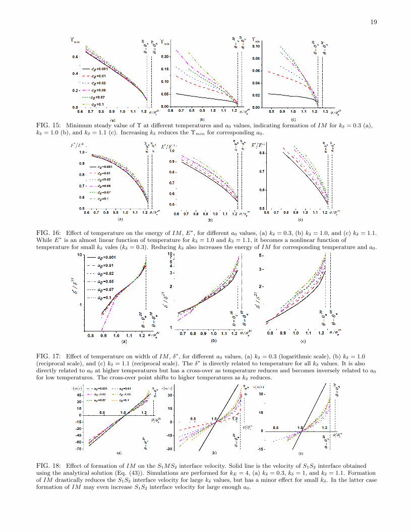
i.e., Υmin and S1MS2 energy are reduced while the width δ∗ increases (Figs. 15 and 16). Energy of IM at elevatedtemperatures, when IM has a large width δ∗, can be approximated as in Eq. (57), i.e., E∗ = 2Es0 + ∆Gδ∗ +0.5β21a0/δ

∗. Here δ∗ can be defined as δ − δint or the distance between points with Υ = 0.5 at two S1M and S2Minterfaces: the difference is small for relatively large δ∗. The equilibrium width of IM is determined by ∂E∗/∂δ∗ = 0,

which results in δ∗ =√

0.5β21a0/∆G. When ∆G→ 0, IM width δ∗ diverges. Note that since ∆G was approximatedas ∆G = (∆G10 + ∆G20)/2, divergence should occur above θ20 but below θ10. This was the case in all simulations(Fig. 15). In contrast, in16 ∆G was taken for phase with lower melting temperature, which lead to IM widthdivergence at θ20. Large δ∗ corresponds to the case that extra interface energy due to interaction of SM interfaces,0.5β21a0/δ

∗, is negligible. The energy of IM reaches the energy of two SM interfaces, which in this case (kE = 4.0)is 0.5E21. Smaller a0 enhances the melting at low temperatures–i.e. reduces Υmin, while at temperatures higher thanθ/θ21

e > 1.1, the effect of a0 either disappears for kδ = 0.3 or getting nonmonotonous for kδ ≥ 1.Increasing kδ reduces the IM energy E∗, and modifies its nonlinear relation with temperature at small kδ to an

approximately linear relation at larger kδ (Fig. 16). IM energy E∗ increases with increasing a0. Width of the IM , δ∗,increases monotonously with increasing temperature, which is consistent with the relation obtained for δ∗. For kδ = 1,width δ∗ increases with increasing a0 for high temperatures θ/θ21

e > 0.85 and reduces for θ/θ21e < 0.85. For kδ = 1.1,

the intersection of δ∗ curves for different a0 occurs in temperature range θ/θ21e > 0.82 width increases with increasing

a0 for high temperatures θ/θ21e > 0.85 and reduces for 1.1 > θ/θ21

e < 0.85. For kδ = 0.3, δ∗ curves for different a0

are very close, except for a0 = 0.5. There is no direct simplified model nor any indication in other plots (Υmin andE∗ vs. θ/θ21

e ) to describe such behavior for δ∗. Therefore, the data presented in Fig. 17 develop new intuition to theproblem and indicate the necessity for further investigation close to the crossover point (at θ/θ21

e ≈ 0.85 for kδ = 1.0).For the simple case of direct PT between two phases, the interface velocity can be calculated using the analytical

solutions (32) and (34) and the numerical solution of the GL equations matches them (Fig. 5). Formation of IMgenerally reduces the interface velocity (Fig. 18) despite the fact that the kinetic coefficient for solid-melt PT ischosen to be twice of that for S1−S2 PT. This reduction grows with increasing kδ. In contrast to linear temperaturedependence of the interface velocity for S1S2 and SM interfaces, the interface velocity for S1S2 interface is a nonlinearfunction of temperature. The interface velocity increases in all cases as the magnitude of interface interaction increases.For small kδ = 0.3, results for any a0 are very close to the S1S2 interface velocity, and for large a0 and close to themelting temperature the S1MS2 interface velocity is even higher than the S1S2 interface velocity (Fig. 18a).

19

FIG. 15: Minimum steady value of Υ at different temperatures and a0 values, indicating formation of IM for kδ = 0.3 (a),kδ = 1.0 (b), and kδ = 1.1 (c). Increasing kδ reduces the Υmin for corresponding a0.

FIG. 16: Effect of temperature on the energy of IM , E∗, for different a0 values, (a) kδ = 0.3, (b) kδ = 1.0, and (c) kδ = 1.1.While E∗ is an almost linear function of temperature for kδ = 1.0 and kδ = 1.1, it becomes a nonlinear function oftemperature for small kδ vales (kδ = 0.3). Reducing kδ also increases the energy of IM for corresponding temperature and a0.

FIG. 17: Effect of temperature on width of IM , δ∗, for different a0 values, (a) kδ = 0.3 (logarithmic scale), (b) kδ = 1.0(reciprocal scale), and (c) kδ = 1.1 (reciprocal scale). The δ∗ is directly related to temperature for all kδ values. It is alsodirectly related to a0 at higher temperatures but has a cross-over as temperature reduces and becomes inversely related to a0for low temperatures. The cross-over point shifts to higher temperatures as kδ reduces.

FIG. 18: Effect of formation of IM on the S1MS2 interface velocity. Solid line is the velocity of S1S2 interface obtainedusing the analytical solution (Eq. (43)). Simulations are performed for kE = 4, (a) kδ = 0.3, kδ = 1, and kδ = 1.1. Formationof IM drastically reduces the S1S2 interface velocity for large kδ values, but has a minor effect for small kδ. In the latter caseformation of IM may even increase S1S2 interface velocity for large enough a0.

20

VII. THERMALLY ACTIVATED INTERMEDIATE MELTING THROUGH CRITICAL NUCLEUS

As it was found above, two different steady solutions may appear for some parameters depending on initial condi-tions, i.e., for a melting or solidification process. They correspond to the local energy minima. Two minima are alwaysseparated by an energy barrier that should be overcome in order to jump from one minimum to another one. Thisindicates the existence of a third solution, corresponding to the minimal energy barrier between two steady solutions,which represents the critical IM nucleus.

If the difference between energy of the IM critical nucleus, Ecn and the ground state is smaller than (40− 80)kbθ,where kb is the Boltzmann constant, then a thermally activated jump from the ground state to the critical nucleus isenergetically possible within reasonable time37. After this, further growth of the critical nucleus, which evolves to thealternative steady nanostructure. Thus, if the initial condition corresponds to the S1S2 interface, then the condition∆Ecnss = Ecn −E21 ≤ (40− 80)kbθ represents nucleation criterion for the IM . If initial structure corresponds to IM ,then the condition ∆Ecnsms = Ecn − E∗ ≤ (40− 80)kbθ represents kinetic criterion for the disappearance of the IM .

Even for the homogeneous nucleation in bulk, the critical nucleus has a size of a few nanometers. An advantageof PFA (nonclassical nucleation model) in comparison with the classical sharp-interface nucleation theory is that thecritical nucleus may represent some intermediate structure (e.g., Υ > 0) rather than complete product phase, whichreduces its energy38. Also, at the critical temperature, when the parent phase loses its stability, the energy of thecritical nucleus tends to zero in PFA, as expected. This cannot be achieved in the sharp interface approach. Forheterogeneous IM nucleation within S1S2 interface, the nucleus size is limited by the interface width and it is alwaysan incomplete melt; thus sharp interface approach is not applicable. A PFA to heterogeneous solid nucleation fromliquid at the wall was considered in39,40.

Because a critical nucleus represents an unstable stationary solution corresponding to the saddle point of the energyfunctional41–43, its finding represents a separate nontrivial problem. Solving the evolutionary time-dependent phasefield equations leads to the local minima of the system and cannot be used for finding the saddle points. Differentmethods were introduced for finding the saddle points of the energy functional, including nudged elastic band44,climb-image nudged elastic band41,45,46, and minimax variational47 techniques, some of which41,47 have been appliedfor PFA. We will use a simple approach based on finding a solution to the stationary GL equations by utilizing anumerical solver for stationary problems rather than by solving non-stationary system of equations. Then if initialconditions are chosen to be close to the solution for the critical nucleus, a stationary solution will represent the criticalnucleus rather than any other solutions corresponding to the local energy minima. This is similar to the approachutilized in39,40 for nucleation at the wall. We limit ourselves to θ = θ21

e , because for other temperatures the interfaceis not stationary and the stationary solver cannot be used. Extension of this approach for non-stationary interfaces byutilizing equations in the frame of reference moving together with S1MS2 interface will be considered elsewhere. Here,a modified Newtonian method48 is utilized for solving the stationary GL equations from an initial condition close tothe final configuration of the critical nuclei. It involves an iterative process with different initial conditions, producedby a chosen function–namely, Eq. (60). For finding the critical nucleus in 1D approximation, the initial conditionfor Υ at the entire S1S2 interface is prescribed by Eq. (60). Such a 1D approximation overestimates an energy of acritical nucleus, which can be reduced by finding a finite size of the nucleus along the S1S2 interface. Axisymmetricproblem formulation with the symmetry axis orthogonal to the interface is an optimal formulation, which allows usto find an actual critical nucleus with economic 2D simulations. For single and multiple 2D axisymmetric criticalnuclei, the initial distribution Υ Eq. (60) is multiplied by a step function along the S1S2 interface to limit the lengthof initial disordered phase along the interface.

The simplest initial condition, which describes IM confined between two solids can be obtained by combining theanalytical solutions for two stationary SsM interfaces (Eq. (32)):

Υcn ={

1 + exp[− (Υ− x0 −W/2) /δ20

]}−1+{

1 + exp[(Υ + x0 −W/2) /δ10

]}−1, (60)

where W is width of the sample, and x0 determines the width of IM . Increasing the values of x0, reduces Υmin. TheS1MS2 profile is plotted in Fig. 19(a) for multiple x0 values at θ = θ21

e = 432K.The proper x0 value which leads to the solution corresponding to the critical nucleus is determined iteratively and

is about 0.3δ21 for the range of studied kE values. Depending on the initial conditions, three different critical nucleiconfigurations are found which correspond to 1D plane interface, single 2D axisymmetric, and multiple axisymmetricconfigurations. The effect of interface energy ratio, kE , on the Υ-profile of critical nucleus at kδ = 1.0 and a0 = 0is studied for 1D planar and 2D axisymmetric problems. For the 1D solution for planar solid-solid interface, the Υ-profile for critical nuclei is shown in Fig. 19(b) along with the stationary solution for stable IM for the correspondingkE values. Solutions for the IM are obtained by solving time-dependent GL equations with the initial conditioncorresponding to perturbed critical nucleus by slightly reducing Υ. It is shown that the degree of disordering of theIM (or critical nucleus) increases (or decreases) with increasing kE . The size of the critical nucleus also gets smalleras kE increases.

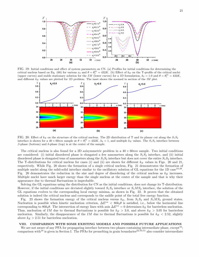
21

FIG. 19: Initial conditions and effect of system parameters on CN. (a) Profiles for initial conditions for determining thecritical nucleus based on Eq. (60) for various x0 and θ = θ21e = 432K. (b) Effect of kE on the Υ-profile of the critical nuclei(upper curves) and stable stationary solution for the IM (lower curves) for a 1D formulation, kδ = 1.0 and θ = θ21e = 432K,and different kE values are plotted for 1D problem. The inset shows the zoomed in section of the IM plot.

FIG. 20: Effect of kE on the structure of the critical nucleus. The 2D distribution of Υ and its planar cut along the S1S2

interface is shown for a 40× 60nm sample at θ = θ21e = 432K, kδ = 1, and multiple kE values. The S1S2 interface betweenβ-phase (bottom) and δ-phase (top) is at the center of the sample.

The critical nucleus is also found for a 2D axisymmetric problem in a 40 × 60nm sample. Two initial conditionsare considered: (i) initial disordered phase is elongated a few nanometers along the S1S2 interface, and (ii) initialdisordered phase is elongated tens of nanometers along the S1S2 interface but does not cover the entire S1S2 interface.The Υ-distributions for critical nucleus for cases (i) and (ii) are shown for different kE values in Figs. 20 and 21,respectively. While Fig. 20 shows the formation of a single critical nucleus, Fig. 21 demonstrates the formation ofmultiple nuclei along the solid-solid interface similar to the oscillatory solution of GL equations for the 1D case19,49.Fig. 20 demonstrates the reduction in the size and degree of disordering of the critical nucleus as kE increases.Multiple nuclei have much larger energy than the single nucleus at the center of the sample and that is why theirappearance due to thermal fluctuations is improbable.

Solving the GL equations using the distribution for CN as the initial conditions, does not change its Υ-distribution.However, if the initial conditions are deviated slightly toward S1S2 interface or S1MS2 interface, the solution of theGL equations evolves to the corresponding local energy minima, as shown in Fig. 22. It proves that the obtainedsolution is indeed the critical nucleus and corresponds to the saddle point of the total free energy function.

Fig. 23 shows the formation energy of the critical nucleus versus kE , from S1S2 and S1MS2 ground states.Nucleation is possible when kinetic nucleation criterion, ∆Ecn < 80kbθ is satisfied, i.e., below the horizontal linecorresponding to 80kbθ. The intersection of energy lines with axis ∆Ecn = 0 determines kE for barrierless nucleation.Thus, nucleation of IM due to thermal fluctuations is possible for kE > 3.0, and above kE > 3.05 for barrierlessnucleation. Similarly, the disappearance of the IM due to thermal fluctuations is possible for kE < 2.52, slightlyabove kE > 2.51 for barrierless nucleation.

VIII. COMPARISON WITH SOME EXISTING MODELS AND POSSIBLE FUTURE APPLICATIONS

We are not aware of any PFA for propagating interface between two phases containing intermediate phase, except16;comparison with16 is given in Section I. The PFAs for premelting in grain boundaries22,50,51 also consider intermediate

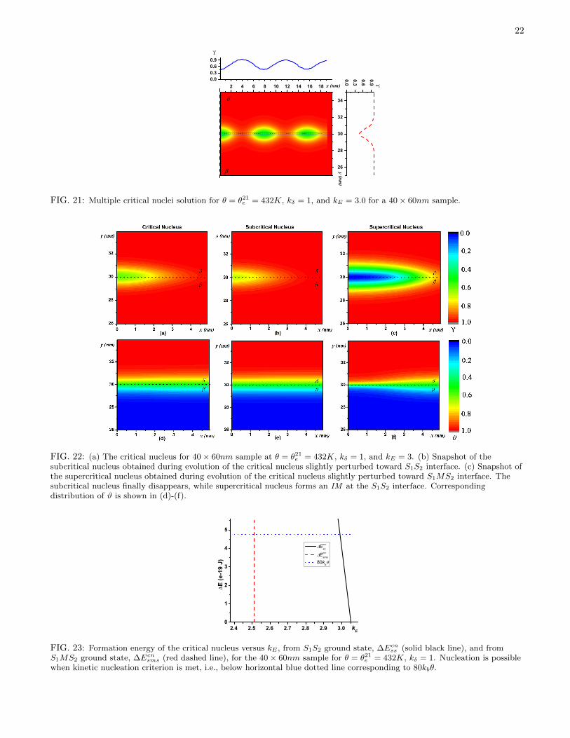
22

2 4 6 8 10 12 14 16 18

26

28

30

32

34

0.1028

30

0.0

0.3

0.6

0.9

y (nm)

0.00.30.60.9

x (nm)

FIG. 21: Multiple critical nuclei solution for θ = θ21e = 432K, kδ = 1, and kE = 3.0 for a 40× 60nm sample.

FIG. 22: (a) The critical nucleus for 40× 60nm sample at θ = θ21e = 432K, kδ = 1, and kE = 3. (b) Snapshot of thesubcritical nucleus obtained during evolution of the critical nucleus slightly perturbed toward S1S2 interface. (c) Snapshot ofthe supercritical nucleus obtained during evolution of the critical nucleus slightly perturbed toward S1MS2 interface. Thesubcritical nucleus finally disappears, while supercritical nucleus forms an IM at the S1S2 interface. Correspondingdistribution of ϑ is shown in (d)-(f).

2.4 2.5 2.6 2.7 2.8 2.9 3.00

1

2

3

4

5

kE

Ecnss

Ecnsms

80k

b

E (e

-19

J)

FIG. 23: Formation energy of the critical nucleus versus kE , from S1S2 ground state, ∆Ecnss (solid black line), and fromS1MS2 ground state, ∆Ecnsms (red dashed line), for the 40× 60nm sample for θ = θ21e = 432K, kδ = 1. Nucleation is possiblewhen kinetic nucleation criterion is met, i.e., below horizontal blue dotted line corresponding to 80kbθ.

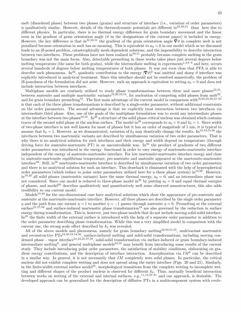
23

melt (disordered phase) between two phases (grains) and structure of interface (i.e., variation of order parameters)is qualitatively similar. However, details of the thermodynamic potentials are different in22,50,51 than here due todifferent physics. In particular, there is no thermal energy difference for grain boundary movement and the linearterm in the gradient of grain orientation angle (ϑ in the designations of the current paper) is included in energy.However, the key difference is that in22,50,51 the gradient of the grain orientation angle ∇∇∇ϑ in complete melt is notpenalized because orientation in melt has no meaning. This is equivalent to a0 = 0 in our model which as we discussedleads to an ill-posed problem, catastrophically mesh dependent solutions, and the impossibility to describe interactionbetween two interfaces. These problems have not been realized in50,51 probably because complete melting in the grainboundary was not the main focus. Also, detectable premelting in these works takes place just several degrees belowmelting temperature (the same for both grains), while the intermediate melting in experiments1,3,6–8 and here, occursseveral hundreds of degrees below melting temperatures of both phases. It was not even clear that PFA is able todescribe such phenomena. In22, quadratic contribution to the energy |∇∇∇ϑ|2 was omitted and sharp ϑ interface wasexplicitly introduced in analytical treatment. Since this interface should not be resolved numerically, the problem ofill-posedness of the formulation did not arise. However, such an approach is equivalent to setting a0 = 0 and does notinclude interaction between interfaces.

Multiphase models are routinely utilized to study phase transformations between three and more phases23,52,between austenite and multiple martensitic variants19,20,53,54, for nucleation of competing solid phases from melt28,and for grain boundary premelting55. The first main advantage of the current model in comparison with19,20,23,28,52–55

is that each of the three phase transformations is described by a single-order parameter, without additional constraintson the order parameters. The second advantage is that we explicitly treat interaction between two interfaces viaintermediate third phase. Also, one of the goals of the multiphase formulation was to avoid any intermediate phasesat the interface between two phases52,55. In28 a structure of the solid phase critical nucleus was obtained which containstraces of the second solid phase at the nucleus surface. The model in28 corresponds to a0 = 0 and kδ = 1. Since widthof two-phase interface is not well known for most of phases but it has an order of magnitude of 1 nm, it is typical toassume that kδ = 1. However, as we demonstrated, variation of kδ may drastically change the results. In19,53,54,56 theinterfaces between two martensitic variants are described by simultaneous variation of two order parameters. That iswhy there is no analytical solution for such interfaces and their energy and width depend on temperature (throughdriving force for austenite-martensite PT) in an uncontrollable way. In56 the product of gradients of two differentorder parameters was introduced in the energy functional in order to vary energy of martensite-martensite interfaceindependent of the energy of austenite-martensite interface. For low martensite-martensite interface energy and closeto austenite-martensite equilibrium temperature, pre-austenite and austenite appeared at the martensite-martensiteinterface56. Still, in56 martensite-martensite interface is described by simultaneous variation of two order parametersand there is no analytical solution for such an interface. This drawback is eliminated with the help of hypersphericalorder parameters (which reduce to polar order parameters utilized here for a three phase system) in19,20. However,in19,20 all solid phases (martensitic variants) have the same thermal energy, a0 = 0, and an intermediate phase wasnot considered. Since our model is reduced to three-phase model in20 by putting a0 = 0 and equal thermal energiesof phases, and model20 describes qualitatively and quantitatively well some observed nanostructures, this also addscredibility to our current model.

Models19,49 for the one-dimensional case have analytical solutions which show the appearance of pre-austenite andaustenite at the martensite-martensite interface. However, all three phases are described by the single order parameterη and the path from one variant η = 1 to another η = −1 passes through austenite η = 0. Premelting at the externalsurface21,57,58 and surface-induced martensitic phase transformation24 are also governed by the reduction in surfaceenergy during transformation. This is, however, just two-phase models that do not include moving solid-solid interface.In25 the finite width of the external surface is introduced with the help of a separate order parameter in addition tothe order parameter describing phase transformation. While this was a very simplified model in comparison with thecurrent one, the strong scale effect described by kδ was revealed.

All of the above models and phenomena, namely for grain boundary melting22,50,51,55, multivariant martensiticand reconstructive PTs19,20,53,54,56, surface-induced melting and solid-solid transformations, including moving con-densed phase - vapor interface21,24,25,57,58, solid-solid transformation via surface-induced or grain boundary-inducedintermediate melting8, and general multiphase models23,52 may benefit from introducing some results of the currentstudy. They include introducing polar order parameters, the satisfaction of stability conditions, elaborating on gra-dient energy contributions, and the description of interface interaction. Amorphization via IM6 can be describedin a similar way. In general, it is not necessarily that IM completely wets solid phases. In particular, the criticalnucleus did not exhibit complete wetting and does not spread along the entire interface (Figs. 20 and 21). Similarly,in the finite-width external surface model25, morphological transitions from the complete wetting to incomplete wet-ting and different shapes of the product nucleus is observed for different kδ. Thus, mutually beneficial interactionbetween works on wetting of the external and internal surfaces, e.g.,11,14,59–61 and our approach, is desirable. Thedeveloped approach can be generalized for the description of diffusive PTs in a multicomponent system with evolv-

24

ing concentration11,14,55,61. An important recent direction is a study of formation of interfacial and intergranularcrystalline or amorphous phases (called complexions)11,13,14,60–68 in ceramic and metallic systems and developing cor-responding interfacial phase diagrams11,14,61. Our PFA after proper generalization and specification can be utilizedfor such studies. Note that other methods have been utilized to model phase transformations and premelting ingrain boundaries, including molecular dynamics67,68 and phase field crystal69–72 methods. They can be applied to theproblem under study as well.

IX. CONCLUDING REMARKS

A three-phase PFA to solid-solid PT via an intermediate phase is developed and utilized to perform a detailednumerical study of the main IM features using finite element method. A thermodynamic potential is formulated withthe help of polar order parameters, which satisfies all desired phase equilibrium and stability conditions. By settingΥ = 1 or ϑ = 0 or 1, this potential reduces to the same two-phase potential suggested in17 and the same correspondingGL equations. Necessity to introduce the gradient energy for solid-solid interface within complete melt, which at firstglance seems contradictory, is justified by necessity to have a well-posed problem and to describe the interactionbetween two solid-melt interfaces. Previous force-balance models for short range and long range interaction forcesbetween two interfaces are generalized for the case that includes finite width interfaces. A new force-balance modelis suggested that better describes results of the phase field simulations significantly below the melting temperatures.We demonstrated that our PFA is able to capture the relation between IM energy and width described by all forcebalance models in some range by choosing proper a0. With the same values a0, PFA should realistically describeinterfacial interactions and IM width for the cases when sharp interface models do not work, namely for small IMwidth or incomplete IM .

Detailed study of the effect of four parameters, namely, kδ, kE , a0, and temperature, on the structure, width, energyof the IM , and velocity of S1MS2 interface is performed by solving time dependent GL equations. While temperatureand energy ratio kE (or kE-related parameters) are parameters that are traditionally considered in surface or grainboundary premelting and melting21,22,51,57,58, two other parameters were unexplored. That is why many results areunexpected and counterintuitive. Thus, for small kδ barrierless IM is reversible and hysteresis-free, and single steadysolution exists independent of initial conditions. For large kδ, in particular, kδ ≥ 1, three solutions exist: stable,metastable, and a critical nucleus between them (unstable), one of them is dry S1S2 interface. For neglected thermalfluctuations, significant overheating even above the melting temperature of solid phases and overcooling to very lowtemperature is observed, i.e., significant hysteresis in melting/solidification exists. The effect of kδ is very nontrivialand depends on kE , a0, and temperature. For relatively large kE , an increase in kδ reduces the degree of disorderingdown to complete melt in the case of S1MS2 initial conditions; at the same time it leads to the appearance of thedry S1S2 solution starting with some kδ. For relatively small kE and for small kδ, dependence of Υmin on kδ isnonmonotonous. Thus, for reversible barrierless melting, Υmin first reduces and then increases reaching 1. For largerkδ barrierless melting does not occur for S1S2 interface initial conditions. At large S1S2, IM can be obtained forS1MS2 initial conditions. For intermediate kδ, IM does not exist for any initial condition forming IM -free gap.Solutions for critical nucleus were found utilizing a stationary solver for time-independent GL equations with theproper choice of initial condition in axisymmetric formulation. Kinetic criterion for its appearance leads to conditionsat which thermally activated nucleation is possible. While multiple critical nuclei have been obtained as well, theirenergy is much larger than energy of the single nucleus near the symmetry axis and their appearance is improbable.Note that the discussed force-balance interaction models have just one energy minimum with respect to IM width.Consequently, they are not applicable to the case with three solutions, for which force-balance interaction modelsshould have two minima separated by a maximum. Development of such models will be considered in the future.That is why based on intuition developed by studying force-balance models, the appearance of partial melt morethan 100 K below melting temperature and retaining melt more than 200 K below the melting temperature, aswell as significant overheating above the melt temperatures of solid phases without melting, looks unexpected andcounterintuitive. Numerical simulations show a significant reduction in the S1S2 interface velocity as IM forms atmoderate to high kδ values. However, a slight increase in the S1S2 interface velocity is observed for small kδ at a hightemperature and large a0 values. The interface velocity is a nonlinear function of a0 and increases as a0 increases.

Some possible generalizations and applications of the developed PFA are discussed in Section VIII. As the nextstep, the effect of internal stresses will be included in the model in a way outlined in16. This will, in particular, allowus to attempt to quantitatively describe interface propagation velocity vs. temperature for β−δ PT in HMX crystals,observed experimentally2,4,5. This will include the formation of the critical nucleus (because interface kinetics iswell described by the phenomenological model for thermally activated propagation), the generation and relaxation ofinternal stresses and interface stresses within propagating interface. Also, the statement that the interface with IMshould be insensitive to the stress field of defect and consequently, exhibit zero athermal resistance, will be checked

25

depending on the degree of disordering within the interface.

ACKNOWLEDGMENTS

The support of NSF (CMMI-0969143), DARPA (W31P4Q-13-1-0010), ARO (W911NF-12-1-0340), ONR (N00014-12-1-0525), and Iowa State University are gratefully acknowledged.

APPENDIX. PROOF OF ENERGY INTEGRAL

Let us prove Eq. (45) using stationary 1D Eqs. (43) and (44). Since for the stationary solution Υ = Υ(x) andϑ = ϑ(x), we can invert x = x(Υ) and x = x(ϑ), and can consider either Υ or ϑ as an independent variable, and alsoexpress Υ = Υ(ϑ) or ϑ = ϑ(Υ). This will be used in the transformations below. Thus, we evaluate in Eq. (43)

d(βS0(ϑ)Υx

)dx

= βS0(ϑ)dΥx

dx+ Υxϑx

dβS0(ϑ)

dϑ; (A.1)

βS0(ϑ)dΥx

dx= βS0(ϑ)Υx

dΥx

dΥ= 0.5βS0(ϑ)

dΥ2x

dΥ=d(0.5βS0(ϑ)Υ2

x)

dΥ− 0.5Υ2

x

dβS0(ϑ)

dΥ

=d(0.5βS0(ϑ)Υ2

x)

dΥ− 0.5Υ2

x

dβS0(ϑ)

dϑ

dϑ

dΥ=d(0.5βS0(ϑ)Υ2

x)

dΥ− 0.5Υxϑx

dβS0(ϑ)

dϑ. (A.2)

Consequently,

d(βS0(ϑ)Υx

)dx

=d(0.5βS0(ϑ)Υ2

x)

dΥ+ 0.5Υxϑx

dβS0(ϑ)

dϑ, (A.3)

and Eq. (46) transforms to

∂ψl

∂Υ= −0.5β21ϑ2

x

dφ(Υ)

dΥ+d(0.5βS0(ϑ)Υ2

x)

dΥ+ 0.5Υxϑx

dβS0(ϑ)

dϑ. (A.4)

Similarly, Eq. (44) transforms to

∂ψl

∂ϑ= −0.5Υ2

x

dβS0(ϑ)

dϑ+d(0.5β21φ(Υ)ϑ2

x

)dϑ

+ 0.5β21Υxϑxdφ(Υ)

dΥ. (A.5)

Next, let us evaluate with the help of Eqs. (A.4) and (A.5) for fixed temperature

dψl =∂ψl

∂ΥdΥ +

∂ψl

∂ϑdϑ = d

(0.5βS0(ϑ)Υ2

x + 0.5β21φ(Υ)ϑ2x

)+

0.5β21ϑx

(dφ(Υ)

dΥΥxdϑ− ϑxdφ(Υ)

)+ 0.5Υx

(dβS0(ϑ)

dϑϑxdΥ−Υxdβ

S0(ϑ)

). (A.6)

Since in the second parenthesis in Eq. (A.6) one has Υxdϑ = dΥϑx, it disappears. Similarly, since in the thirdparenthesis one has ϑxdΥ = dϑΥx, it disappears as well. Then Eq. (A.6) results in

dψl(θ,Υ, ϑ) = dψ∇. (A.7)

∗ [email protected] V. I. Levitas, B. F. Henson, L. B. Smilowitz, and B. W. Asay, Phys. Rev. Lett., 92, 235702 (2004).2 V. I. Levitas, L. B. Smilowitz, B. F. Henson, and B. W. Asay, J. Chem. Phys., 124, 026101 (2006).3 V. I. Levitas, B. F. Henson, L. B. Smilowitz, and B. W. Asay, J. Phys. Chem. B, 110, 10105 (2006).4 B. F. Henson, L. Smilowitz, B. W. Asay, and P. M. Dickson, J. Chem. Phys., 117, 3780 (2002).5 L. Smilowitz, B. F. Henson, B. W. Asay, and P. M. Dickson, J. Chem. Phys., 117, 3789 (2002).6 V. I. Levitas, Phys. Rev. Lett., 95, 075701 (2005).7 S. L. Randzio and A. Kutner, J. Phys. Chem. B, 112, 1435 (2008).8 V. I. Levitas, Z. Ren, Y. Zeng, Z. Zhang, and G. Han, Phys. Rev. B, 85, 220104 (2012).9 V. I. Levitas and R. Ravelo, Proc. Natl. Acad. Sci. U.S.A., 109, 13204 (2012).

10 J. Dash, H. Fu, and J. S. Wettlaufer, Rep. Prog. Phys., 58, 115 (1995).11 J. Luo, Critical Rev. Solid State, 32, 67 (2007).12 J. Dash, A. W. Rempel, and J. S. Wettlaufer, Rev. Mod. Phys., 78, 695 (2006).13 P. R. Cantwell, M. Tang, S. J. Dillon, J. Luo, G. S. Rohrer, and M. P. Harmer, Acta Mater., 62, 1 (2014).

26

14 J. Luo and Y.-M. Chiang, Annu. Rev. Mater. Res., 38, 227 (2008).15 M. J. Grinfeld, Thermodynamic Methods in the Theory of Heterogeneous Systems (Longman Scientific and Technical, 1991).16 V. I. Levitas and K. Momeni, Acta Mater., 65, 125 (2014).17 V. I. Levitas and D. L. Preston, Phys. Rev. B, 66, 134206 (2002).18 V. I. Levitas and D. L. Preston, Phys. Rev. B, 66, 134207 (2002).19 V. I. Levitas, D. L. Preston, and D.-W. Lee, Phys. Rev. B, 68, 134201 (2003).20 V. I. Levitas, A. M. Roy, and D. L. Preston, Phys. Rev. B, 88, 054113 (2013).21 V. I. Levitas and K. Samani, Nat. Commun., 2, 284 (2011).22 M. Tang, W. C. Carter, and R. M. Cannon, Phys. Rev. B, 73, 024102 (2006).23 J. Tiaden, B. Nestler, H. J. Diepers, and I. Steinbach, Physica D, 115, 73 (1998).24 V. I. Levitas and M. Javanbakht, Phys. Rev. Lett., 105, 165701 (2010).25 V. I. Levitas and M. Javanbakht, Phys. Rev. Lett., 107, 175701 (2011).26 V. I. Levitas, D.-W. Lee, and D. L. Preston, Int. J. Plasticity, 26, 395 (2010).27 V. I. Levitas, Phys. Rev. B, 89, 094107 (2014).28 G. I. Toth, J. R. Morris, and L. Granasy, Phys. Rev. Lett., 106, 045701 (2011).29 W. C. McCrone, Analytical Chemistry, 22, 1225 (1950).30 H. Cady, in Analyses of Propellants and Explosives, 17th International Annual Conference of ICT (Kalsruhe, FRG, 1986)

pp. 1–12.31 H. Cady, L. Smith, L. A. S. Laboratory, and U. S. A. E. Commission, Studies on the Polymorphs of HMX (Los Alamos

Scientific Laboratory of the University of California, 1962).32 A. Teetsov and W. McCrone, Microscop. Cryst. Front, 15, 13 (1965).33 R. Menikoff and T. D. Sewell, Combust. Theor. Model., 6, 103 (2002).34 V. I. Levitas, B. F. Henson, L. B. Smilowitz, D. K. Zerkle, and B. W. Asay, J. Appl. Phys., 102, 113520 (2007).35 H. D. Ackler and Y.-M. Chiang, J. Am. Ceram. Soc., 82, 183 (1999).36 R. H. French, J. Am. Ceram. Soc., 83, 2117 (2000).37 D. Porter, Phase Transformation in Metals and Alloys (Van Nostrand Reinhold, 1981).38 J. W. Cahn and J. E. Hilliard, J. Chem. Phys., 28, 258 (1958).39 L. Granasy, T. Pusztai, D. Saylor, and J. A. Warren, Phys. Rev. Lett., 98, 035703 (2007).40 J. A. Warren, T. Pusztai, L. Kornyei, and L. Granasy, Phys. Rev. B, 79, 014204 (2009).41 C. Shen, J. Li, and Y. Wang, Metall. Mater. Trans. A, 39, 976 (2008).42 Y. A. Chu, B. Moran, G. B. Olson, and A. Reid, Metall. Mater. Trans. A, 31, 1321 (2000).43 L. Granasy, T. Borzsonyi, and t. . N. j. . P. y. . . v. . . p. . . Pusztai, Tamas,.44 G. Mills and H. Jonsson, Phys. Rev. Lett., 72, 1124 (1994).45 G. Henkelman and H. Jonsson, J. Chem. Phys., 113, 9978 (2000).46 G. Henkelman, B. P. Uberuaga, and H. Jonsson, J. Chem. Phys., 113, 9901 (2000).47 L. Zhang, L.-Q. Chen, and Q. Du, Phys. Rev. Lett., 98, 265703 (2007).48 P. Deuflhard, Numer. Math., 22, 289 (1974).49 F. Falk, Zeitschrift fur Physik B Condensed Matter, 51, 177 (1983).50 R. Kobayashi, J. A. Warren, and W. C. Carter, Physica D, 140, 141 (2000), ISSN 0167-2789.51 A. E. Lobkovsky and J. A. Warren, Physica D, 164, 202 (2002).52 R. Folch and M. Plapp, Phys. Rev. E, 72, 011602 (2005).53 A. Artemev, Y. Jin, and A. Khachaturyan, Acta Mat., 49, 1165 (2001).54 L.-Q. Chen, Annu. Rev. Mater. Res., 32, 113 (2002).55 Y. Mishin, W. Boettinger, J. Warren, and G. McFadden, Acta Mat., 57, 3771 (2009).56 V. I. Levitas and M. Javanbakht, International journal of materials research, 102, 652 (2011).57 R. Lipowsky, Phys. Rev. Lett., 49, 1575 (1982).58 V. I. Levitas and K. Samani, Phys. Rev. B, 84, 140103 (2011).59 J. W. Cahn, J. Chem. Phys., 66, 3667 (1977).60 M. Baram, D. Chatain, and W. D. Kaplan, Science, 332, 206 (2011).61 J. Luo, J. Am. Ceram. Soc., 95, 2358 (2012).62 J. Luo and Y. M. Chiang, Acta Mater., 48, 4501 (2000).63 A. Avishai and W. D. Kaplan, Acta Mater., 53, 1571 (2005).64 A. Avishai, C. Scheu, and W. D. Kaplan, Acta Mater., 53, 1559 (2005).65 H. Qian, J. Luo, and Y.-M. Chiang, Acta Mater., 56, 862 (2008).66 S.-Y. Chung and S.-J. L. Kang, Acta Mater., 51, 2345 (2003).67 T. Frolov, S. V. Divinski, M. Asta, and Y. Mishin, Phys. Rev. Lett., 110, 255502 (2013).68 T. Frolov, D. L. Olmsted, M. Asta, and Y. Mishin, Nature communications, 4, 1899 (2013).69 T. W. Heo, S. Bhattacharyya, and L.-Q. Chen, Acta Mater., 59, 7800 (2011).70 J. Mellenthin, A. Karma, and M. Plapp, Phys. Rev. B, 78, 184110 (2008).71 A. Adland, A. Karma, R. Spatschek, D. Buta, and M. Asta, Phys. Rev. B, 87, 024110 (2013).72 N. Goldenfeld, B. P. Athreya, and J. A. Dantzig, Phys. Rev. E, 72, 020601 (2005).

Propagating Phase Interface with Intermediate Interfacial Phase: Phase Field Approach

Documents

Transcript of Propagating Phase Interface with Intermediate Interfacial Phase: Phase Field Approach