INTERFACIAL FRACTURE MECHANICS: PATCH REPAIRED ...

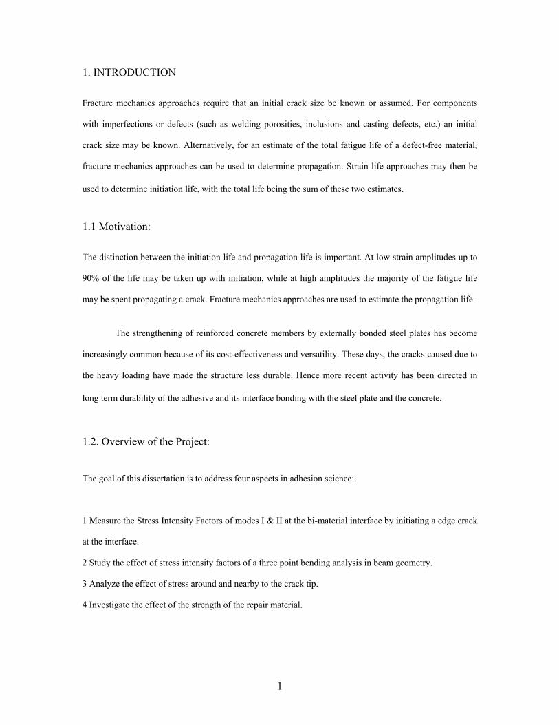
INTERFACIAL FRACTURE MECHANICS: PATCH REPAIRED SYSTEM IN BEAM

BY P.A.SASIKUMAR

INTERNATIONAL INSTITUTE OF INFORMATION TECHNOLOGY HYDERABAD

(Deemed University)

2006

i

INTERFACIAL FRACTURE MECHANICS: PATCH REPAIRED SYSTEM IN BEAM

Project submitted to

INTERNATIONAL INSTITUTE OF INFORMATION TECHNOLOGY HYDERABAD

In partial fulfillment of the requirements for the degree of Master of Technology in Computer Aided Structural Engineering

By

P.A.SASIKUMAR November 2006

ii

CERTIFICATE

It is certified that work contained in the project titled “INTERFACIAL FRACTURE

MECHANICS: A REPAIR PATCH ED SYSTEM IN BEAM” by P.A.Sasikumar has

been carried out under my/our supervision and it is not published elsewhere for a degree.

Supervisor

(Name & Designation)

iii

ABSTRACT: Most of the structures in India were constructed when only simple methods could be used to

properly design them. But now the approach of finite element studies has advanced in such a way that

current analysis procedure for the safety assessment remains the same as those used earlier for the designs.

In this project a numerical study of the Stress Intensity Factors (SIF) (KI, KII) at a bi-material interface of a

repair patched beam loaded in three point bending for mixes of different compressive strengths. These

parameters were determined from the expressions derived by Rice and Sih. These results are compared with

results determined from Franc-2D/L, a two-dimensional fracture mechanics analysis code developed by

Cornell Fracture Group. It is found that the numerical predictions for the SIF were related with the

corresponding results from Franc-2D/L.also determined the effect of the SIF due to the increase in the

crack length. This helps in determining the additional load from the normal load to which the beam can

afford.

iv

ACKNOWLEDGEMENT

It is an accepted fact that learning by experimenting is preferable to learning by rout. It leaves me

to explore facts that interest is while continuously opening up new doors of information that can enlighten

my ideas to new levels. Working on this project has been a continuous learning experience of different

kind. I got an opportunity to face different problems and it provided to be quite a challenge to put my best

efforts in trying to arrive the possible solution. The degree of success is immaterial when compared to

opportunities and experiences one gets to savor.

Thanks to my guide Dr. Venkateshwarulu Mandadi who has given me full freedom in my project

and gave me an opportunity to implement my ideas in this project. This has helped me to learn a new

approach in solving real time problems.

In the beginning it proved to be quite a bit of challenge to free myself from the rigidities that

restrict the scope in the course of the normal curriculum and get into an exploration mode of collecting and

applying the information not provided readymade to me on the platter. However the going was sufficiently

smoothened by my guide and gave me full support to progress on with my project. This went in relieving

me from unnecessary pressure that could have otherwise hampered the rate of my project.

Coming towards the end of my project I want to take every opportunity in expressing my gratitude

to our Coordinator Dr. Ramancharla Pradeep Kumar who have lent me support along the way and has

helped me to bring this project a logical conclusion. Last but not the least I’ve to thank my friends who

have encouraged me and also helped me in getting the recourses for my project.

THANK YOU

P.A.SASIKUMAR

v

TABLE OF CONTENTS

CHAPTER 1 INTRODUCTION...............................................................................................................1

1.1 Motivation.............................................................................................................................1

1.2 Overview of the Project:.......................................................................................................1

1.3 Analysis of a Repair Patch System......................................................................................2

CHAPTER 2. Literature Review:............................................................................................................4

2.1 Crack Tip Fields for a crack on an interface.......................................................................4

2.2 Theory of interface fracture................................................................................................6

CHAPTER 3. Discussions on the results..............................................................................................9

3.1. Effect of uniaxial compressive strength of the repair material………………………….9

3.2 Effect of the interface crack length……………………………………………………..11

CHAPTER 4. Conclusions.................................................................................................................12

CHAPTER 5. References...................................................................................................................13

APPENDIX I: List of Tables

APPENDIX II: List of Figures

vi

LIST OF FIGURES:

Figure No.1a & 1b: Beam specimen……………………………………………………………………..4

Figure No.2: Crack tip at interface……………………………………………………………………….3

Figure No 3a & 3b: Stress - Strain graph near the crack tip

Figure No.4: Modeling of Beam using FRANC-2D/L

Figure No.5a &5b: Behavior of KI & KII modes for different repair patch materials

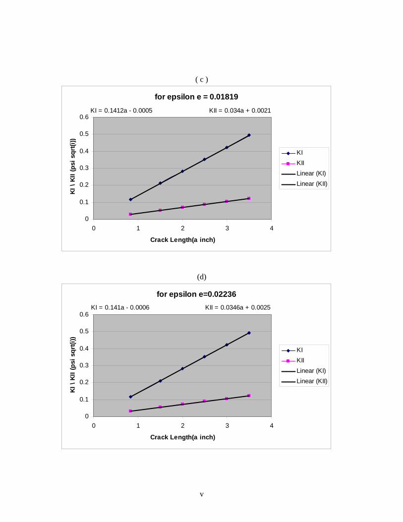
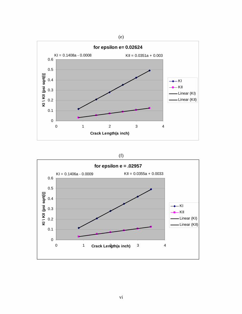
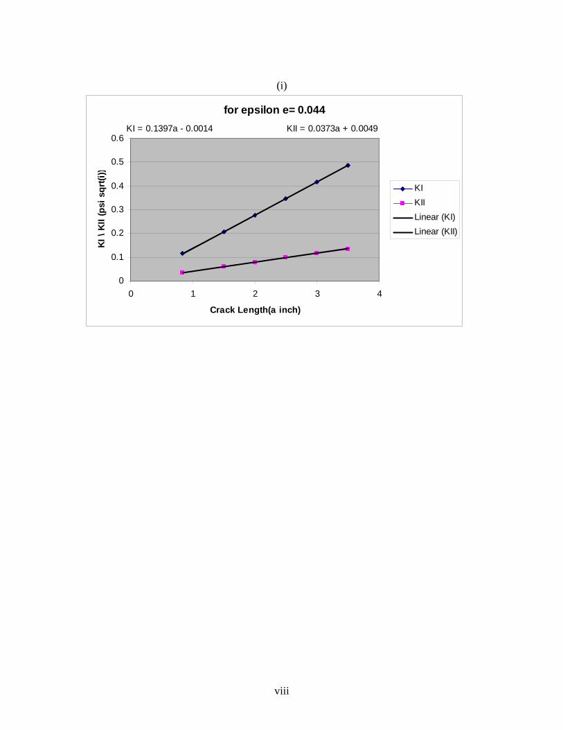
Figure No.6 (a to i): Relation of Stress Intensity Factors (KI & KII) with the crack length keeping the value

of ε as constant.

Figure No.7(a to e): Relation between Stress Intensity Factors (KI & KII) with the ε keeping the crack

length a as constant

LIST OF TABLES:

Table No.1: The Stress Intensity Factors (KI & KII) derived from the FRANC-2D/L code for different

repair material and the for the different parent materials.

Table No.2: Results through the derivations determined by Rice and Sih

vii

1. INTRODUCTION

Fracture mechanics approaches require that an initial crack size be known or assumed. For components

with imperfections or defects (such as welding porosities, inclusions and casting defects, etc.) an initial

crack size may be known. Alternatively, for an estimate of the total fatigue life of a defect-free material,

fracture mechanics approaches can be used to determine propagation. Strain-life approaches may then be

used to determine initiation life, with the total life being the sum of these two estimates.

1.1 Motivation:

The distinction between the initiation life and propagation life is important. At low strain amplitudes up to

90% of the life may be taken up with initiation, while at high amplitudes the majority of the fatigue life

may be spent propagating a crack. Fracture mechanics approaches are used to estimate the propagation life.

The strengthening of reinforced concrete members by externally bonded steel plates has become

increasingly common because of its cost-effectiveness and versatility. These days, the cracks caused due to

the heavy loading have made the structure less durable. Hence more recent activity has been directed in

long term durability of the adhesive and its interface bonding with the steel plate and the concrete.

1.2. Overview of the Project:

The goal of this dissertation is to address four aspects in adhesion science:

1 Measure the Stress Intensity Factors of modes I & II at the bi-material interface by initiating a edge crack

at the interface.

2 Study the effect of stress intensity factors of a three point bending analysis in beam geometry.

3 Analyze the effect of stress around and nearby to the crack tip.

4 Investigate the effect of the strength of the repair material.

1

1.3 Analysis of a Repair Patch System:

In this work a symmetrically loaded simply supported beam comprising of a patch of repair

concrete on the tension side is analyzed using the finite element based on the fracture mechanics theory. A

parametric study is conducted by the varying different parameters such as modulus of elasticity of the

repair concrete, interfacial crack length.

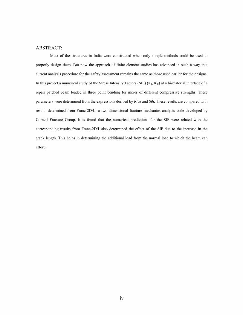
The figure below shows the geometry of the simply supported beam used in this analysis. It

consists of concrete repair material on the tension side of the parent material. It is loaded with the

concentrated load at the center of the beam having a magnitude which satisfies the tensile stress = 0.08. The

parent concrete material is considered to have a uniaxial compressive strength of 20 MPa with constant

Poisson’s ratio of 0.18. Due to symmetry and linearity only half of the beam is analyzed using the finite

element code FRANC-2D/L. the boundary conditions and the applied forces at the ends of the beam are

computed using the strength of materials.

For simulating the damage of the parent concrete beam, horizontal interface cracks between the parent and

repair concrete are assumed to develop from the bottom tip and extended horizontally at the interface

outward towards the support. The repair material is modeled as the linear elastic material having different

elastic modulus.

The finite element method consists of two dimensional, plane stress 8 node isoparametric and 6 node linear

triangular elements. The meshing is done in such a way that they are finer near the crack to the coarser

mesh away from the crack. The computations of SIF are determined through the following methods

1. Displacement Correlation Method

2. J-Integral Method

3. Modified Crack Closure Method.

2

Figure No1.a

FigureNo.1.b

Since the whole beam cannot be analysed in Franc-2D/L, it has been assumed that analyzing for the half of

the beam by applying the loading and the boundary conditions will give the result in terms of the respective

ratios of how we modeled.

Hence the modeling of the beam is done by taking half the length and applying the edge crack at the bi-

material interface.

3

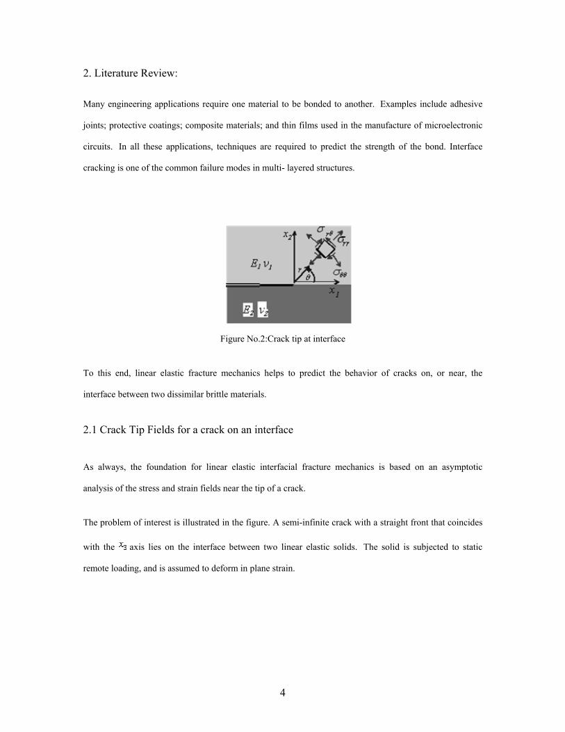
2. Literature Review:

Many engineering applications require one material to be bonded to another. Examples include adhesive

joints; protective coatings; composite materials; and thin films used in the manufacture of microelectronic

circuits. In all these applications, techniques are required to predict the strength of the bond. Interface

cracking is one of the common failure modes in multi- layered structures.

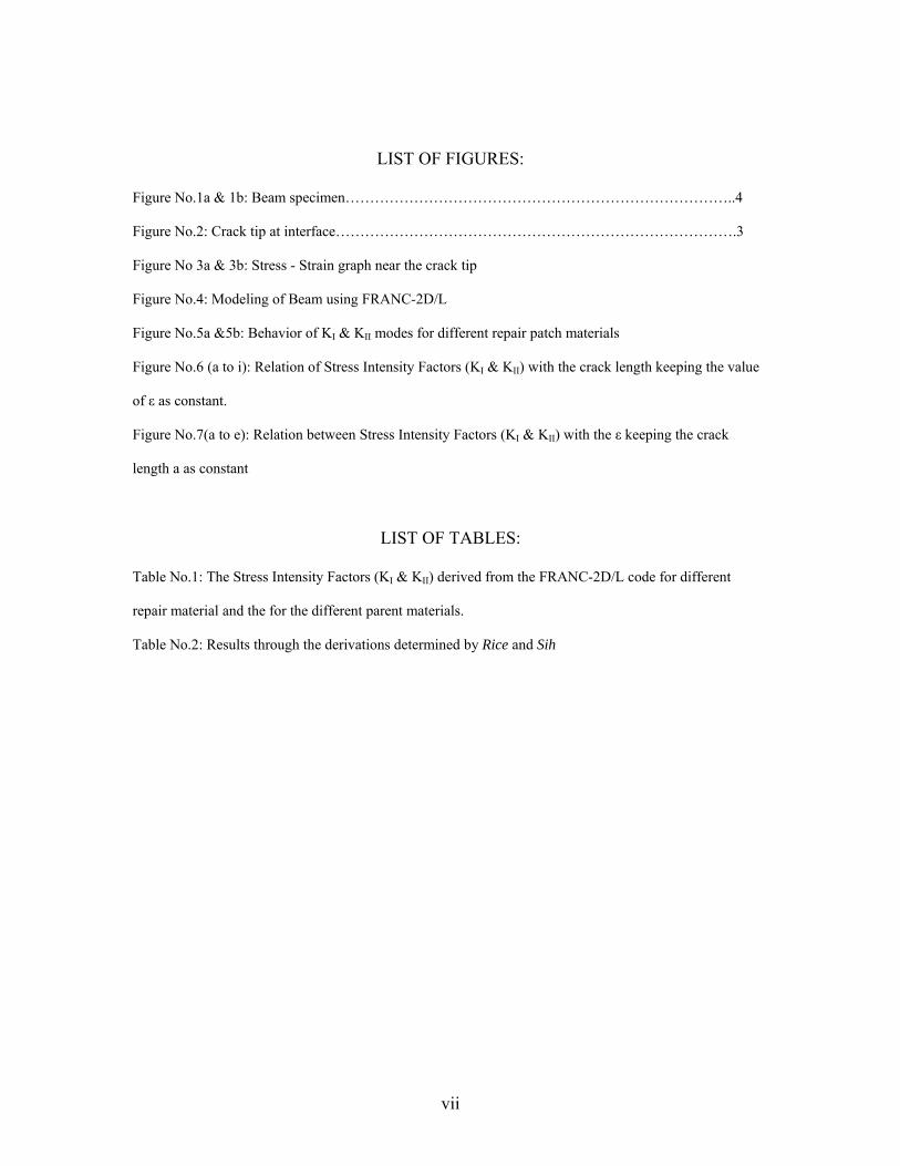
Figure No.2:Crack tip at interface

To this end, linear elastic fracture mechanics helps to predict the behavior of cracks on, or near, the

interface between two dissimilar brittle materials.

2.1 Crack Tip Fields for a crack on an interface

As always, the foundation for linear elastic interfacial fracture mechanics is based on an asymptotic

analysis of the stress and strain fields near the tip of a crack.

The problem of interest is illustrated in the figure. A semi-infinite crack with a straight front that coincides

with the axis lies on the interface between two linear elastic solids. The solid is subjected to static

remote loading, and is assumed to deform in plane strain.

4

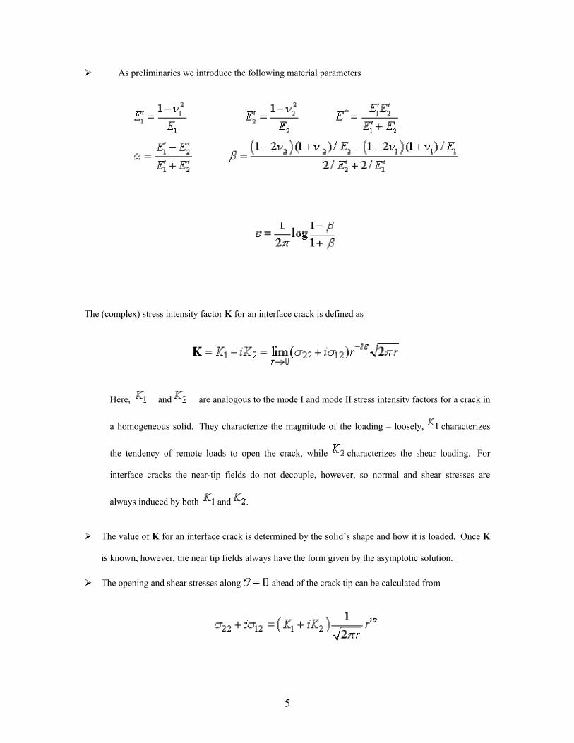
As preliminaries we introduce the following material parameters

The (complex) stress intensity factor K for an interface crack is defined as

Here, and are analogous to the mode I and mode II stress intensity factors for a crack in

a homogeneous solid. They characterize the magnitude of the loading – loosely, characterizes

the tendency of remote loads to open the crack, while characterizes the shear loading. For

interface cracks the near-tip fields do not decouple, however, so normal and shear stresses are

always induced by both and .

The value of K for an interface crack is determined by the solid’s shape and how it is loaded. Once K

is known, however, the near tip fields always have the form given by the asymptotic solution.

The opening and shear stresses along ahead of the crack tip can be calculated from

5

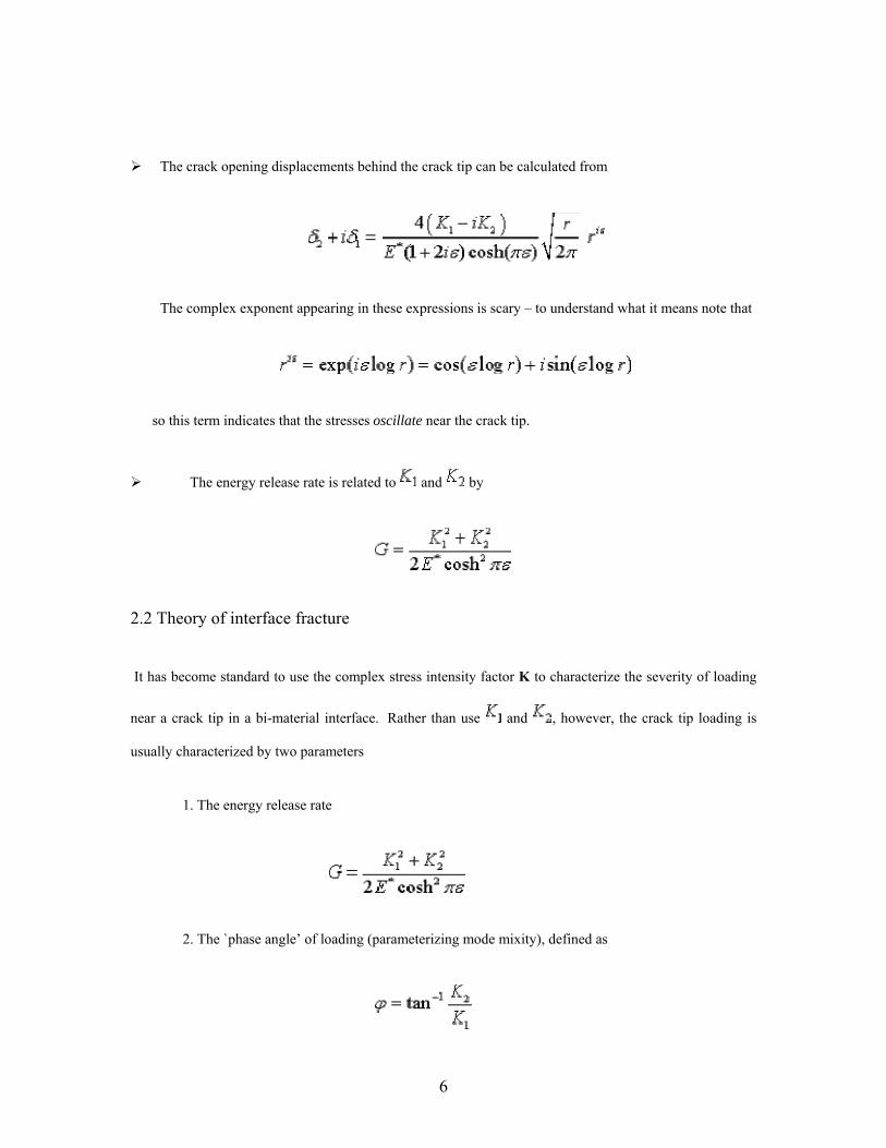
The crack opening displacements behind the crack tip can be calculated from

The complex exponent appearing in these expressions is scary – to understand what it means note that

so this term indicates that the stresses oscillate near the crack tip.

The energy release rate is related to and by

2.2 Theory of interface fracture

It has become standard to use the complex stress intensity factor K to characterize the severity of loading

near a crack tip in a bi-material interface. Rather than use and , however, the crack tip loading is

usually characterized by two parameters

1. The energy release rate

2. The `phase angle’ of loading (parameterizing mode mixity), defined as

6

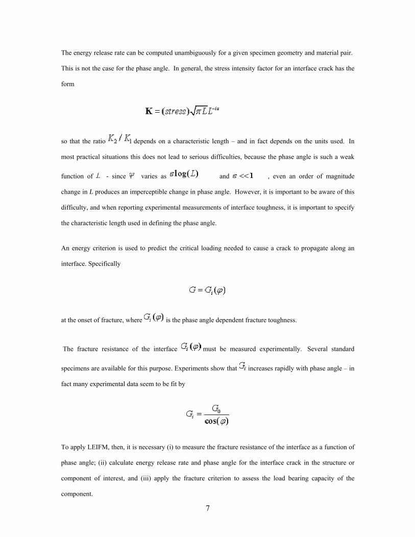
The energy release rate can be computed unambiguously for a given specimen geometry and material pair.

This is not the case for the phase angle. In general, the stress intensity factor for an interface crack has the

form

so that the ratio depends on a characteristic length – and in fact depends on the units used. In

most practical situations this does not lead to serious difficulties, because the phase angle is such a weak

function of - since varies as and , even an order of magnitude

change in L produces an imperceptible change in phase angle. However, it is important to be aware of this

difficulty, and when reporting experimental measurements of interface toughness, it is important to specify

the characteristic length used in defining the phase angle.

An energy criterion is used to predict the critical loading needed to cause a crack to propagate along an

interface. Specifically

at the onset of fracture, where is the phase angle dependent fracture toughness.

The fracture resistance of the interface must be measured experimentally. Several standard

specimens are available for this purpose. Experiments show that increases rapidly with phase angle – in

fact many experimental data seem to be fit by

To apply LEIFM, then, it is necessary (i) to measure the fracture resistance of the interface as a function of

phase angle; (ii) calculate energy release rate and phase angle for the interface crack in the structure or

component of interest, and (iii) apply the fracture criterion to assess the load bearing capacity of the

component.

7

However, the strain energy release rate G computed by dimensionally wrong factors will still is

dimensionally valid.

The expressions for these biomaterial stress intensity factors, derived by Rice and Sih are

KI = {σ[cos (ε log 2a) + 2ε sin(ε log 2a)] + [τ[sin(ε log 2a) - 2ε cos(ε log 2a)]×√a}÷{cosh л ε}

KII = {τ[cos (ε log 2a) + 2ε sin(ε log 2a)] - [σ[sin(ε log 2a) - 2ε cos(ε log 2a)]×√a}÷{cosh л ε}

Where ε = 1/2л ln {[(3-4ν1)/ ((µ1+1)/ µ2)] ÷ [(3-4ν2)/ ((µ2+1)/ µ1)]}

In the above equations, ε is the oscillation index given by the equation above, τ and σ are the normal and

shear stresses along the interface and a is the crack length. When ε ≠0 the stresses oscillate heavily as the

crack tip is approached(r 0). Furthermore, the relative proportion of the interfacial normal and the shear

stresses varies slowly with distance from the crack tip because of the crack tip riε. Thus KI and KII cannot be

decoupled to represent the intensities of the interfacial crack.

8

3 Discussions of Results:

The simply supported repaired beam is analyzed by different parameters such as the interface crack length

and uniaxial compressive strength of the repair material in order to study the effects of the stress intensity

factors.

3.1 Effect of uniaxial compressive strength of the repair material:

In order to study the effect of the strength of the repair material, a parametric study is done by changing the

uniaxial compressive strength of the repair material. The uniaxial compressive strength of the parent

material is kept constant. The thickness of the repair material used is 75mm and the crack length is kept

constant of 1 inch. The Table 1 shows that the KI goes on decreasing with the increase in the compressive

strength of the repair material.

The response of the sliding mode KII is acting in such a way that when the compressive strength of the

repair material is less than the parent material, the KII gets decreased and then increased when the

compressive strength is more than that of the parent material. This behavior shows that the effect of the

repair material should be more when compared with the parent material. When the stress factor is increased

then the load carrying capacity will also gets increased.

The results of the above have been graphically listed below. The decrease in the KI will not have

much effect over this type of loading since the effect of sliding mode will dominate in these cases.

3.2 Effect of the interface crack length:

The mode I and mode II stress intensity factors (KI, KII) obtained for the different interface crack lengths

and different repair mixes using the Rice method. The stress intensity factors are computed near the tip of

the interface crack. The interface crack lies with the origin and extends towards the support.

The interfacial crack length increases at the rate of 0.833 inch till 3.5 inch. From figure, as the crack length

increases the value of KI decreases with the increase in the value of ε and the increase in KII. This implies

that the sliding mode stress intensity factor becomes dominant towards the fracturing process. Also the

9

other point to be noted in this result is that the value of both KI and KII increases with the increase of the

crack length for the same value of ε. This shows that the increase in the KI with the increase in the crack

length will increase the tensile mode which exceeds the maximum tensile stress of the beam. The table 2

and the figures will give the detailed view of the behavior of the SIF of both the modes for the different

repair mixes.

10

4. CONCLUSIONS

Repair and rehabilitation of civil engineering structures are gaining a lot of importance, at the same time

there are very little research done for establishing the performance criteria for the repair materials. This

helps to study the compatibility between the repair material and the parent concrete. In this work the

behavior of the damaged concrete beam which is strengthened by applying a new patch of repair concrete

material in the tensile zone is studied using Fracture Mechanics theory.

1. The SIF at the interfacial crack decreases with the increase in the modulus of elasticity.

2. As the crack length increases the SIF of mode II increases and there is decrease in mode II of SIF.

3. This implies that the sliding mode stress intensity factor becomes dominant towards the fracturing

process.

4. These results of the Stress Intensity Factor help to determine the combination of the parent

concrete and repair material with cost-effectiveness and versatility.

11

5. References

1. Prashant Kumar (1999).” Elements of Fracture Mechanics”

2. Chandra Kishen, J.M. (1993).” An Overview or cracks at the Interface of Two Dissimilar

Materials” Project Report. University of Colorado.

3. Franc-2D/L(1998). “A two dimensional fracture Mechanics analysis code”. Example’s manual,

Cornell Fracture Group, Cornell University

4. N.I. Shabeeb and W.K. Binienda(1999), “Analysis of an Interface Crack for a Functionally Graded

Strip Sandwiched Between Two Homogeneous Layers of Finite Thickness”, University of Akron,

Akron, Ohio, NASA/CR—1999-208874.

5. Jelena M. Veljkovi , Ružica R. Nikoli(2003), “Application of the interface crack concept to

problem of a crack between a thin layer and a substrate”, Faculty of Mechanical Engineering,

Sestre Janji 6, YU 34000 Kragujevac, Yugoslavia, Mechanics, Automatic Control and Robotics

Vol.3, No.13, 2003, pp. 573 - 581.

6. Q.H. Shah, 1M. Azram and M.H. Iliyas(2005), “Predicting the Crack Initiation Fracture

Toughness”, Department of Manufacturing and Materials Engineering, 1Department of Science in

Engineering, International Islamic University Malaysia, Jalan Gombak, 53100 Kuala Lumpur,

Malaysia, Journal of Applied Sciences 5 (2): 253-256, 2005.

7. 1 N.Sukumar,2Z. Y. Huang,3J.-H. Prévost, and 2Z.Suo(2004),” Partition of unity enrichment for

biomaterial interface cracks”, 1Department of Civil and Environmental Engineering, University of

California , One Shields Avenue , 2Department of Mechanical and Aerospace Engineering,

Princeton University, NJ08544, U.S.A.3 Department of Civil and Environmental Engineering,

Princeton University, NJ08544, U.S.A, Int. Jr. Numerical Method Engg 2004; 59:1075–1102

(DOI:10.1002/nme.902).

8. AlanT.Zehnder,Ph.D.(May,2006), “Lecture Notes on Fracture Mechanics”, Dept. of Theoretical

and Applied Mechanics, Cornell University, c/o AlanZehnder,2006.

9. J. M. Chandra Kishen(2005), “Recent developments in safety assessment of concrete gravity

dams”, Department of Civil Engineering, Indian Institute of Science, Bangalore 560 012, India,

CURRENT SCIENCE, VOL. 89, NO. 4, 25 AUGUST 2005.

12

10. S C Hee and A D Jefferson(2004), “Two Dimensional Analysis Of a Gravity Dam Using the

Program FRANC2D”, Cardiff University U.K.

11. Victor E. Saouma, “Lecture Notes in: Fracture Mechanics” Dept. of Civil Environmental and

Architectural Engineering, University of Colorado, Boulder, CO 80309-0428.

12. Richard W. Hertzberg, “Deformation and Fracture Mechanics of Engineering Materials”, Fourth

Edition, Director, Mechanical Research Center, Lehigh University

13

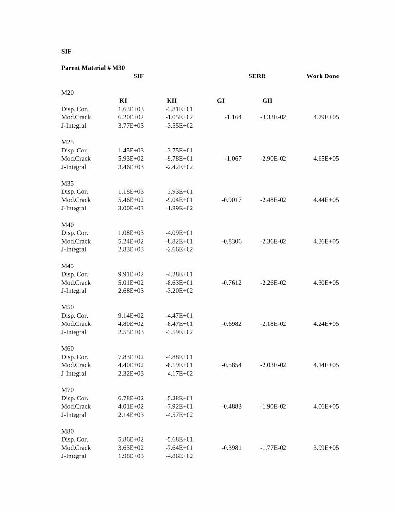
SIF Parent Material # M30 SIF SERR Work Done M20

KI KII GI GII Disp. Cor. 1.63E+03 -3.81E+01 Mod.Crack 6.20E+02 -1.05E+02 -1.164 -3.33E-02 4.79E+05 J-Integral 3.77E+03 -3.55E+02 M25 Disp. Cor. 1.45E+03 -3.75E+01 Mod.Crack 5.93E+02 -9.78E+01 -1.067 -2.90E-02 4.65E+05 J-Integral 3.46E+03 -2.42E+02 M35 Disp. Cor. 1.18E+03 -3.93E+01 Mod.Crack 5.46E+02 -9.04E+01 -0.9017 -2.48E-02 4.44E+05 J-Integral 3.00E+03 -1.89E+02 M40 Disp. Cor. 1.08E+03 -4.09E+01 Mod.Crack 5.24E+02 -8.82E+01 -0.8306 -2.36E-02 4.36E+05 J-Integral 2.83E+03 -2.66E+02 M45 Disp. Cor. 9.91E+02 -4.28E+01 Mod.Crack 5.01E+02 -8.63E+01 -0.7612 -2.26E-02 4.30E+05 J-Integral 2.68E+03 -3.20E+02 M50 Disp. Cor. 9.14E+02 -4.47E+01 Mod.Crack 4.80E+02 -8.47E+01 -0.6982 -2.18E-02 4.24E+05 J-Integral 2.55E+03 -3.59E+02 M60 Disp. Cor. 7.83E+02 -4.88E+01 Mod.Crack 4.40E+02 -8.19E+01 -0.5854 -2.03E-02 4.14E+05 J-Integral 2.32E+03 -4.17E+02 M70 Disp. Cor. 6.78E+02 -5.28E+01 Mod.Crack 4.01E+02 -7.92E+01 -0.4883 -1.90E-02 4.06E+05 J-Integral 2.14E+03 -4.57E+02 M80 Disp. Cor. 5.86E+02 -5.68E+01 Mod.Crack 3.63E+02 -7.64E+01 -0.3981 -1.77E-02 3.99E+05 J-Integral 1.98E+03 -4.86E+02

Results ob

SIF Parent Material # M20 SIF M25

KI Disp. Cor. 1.13E+03 Mod.Crack 5.34E+02 J-Integral 2.91E+03 M30 Disp. Cor. 9.88E+02 Mod.Crack 5.00E+02 J-Integral 2.67E+03 M35 Disp. Cor. 8.77E+02 Mod.Crack 4.70E+02 J-Integral 2.48E+03 M40 Disp. Cor. 7.85E+02 Mod.Crack 4.40E+02 J-Integral 2.33E+03 M45 Disp. Cor. 7.01E+02 Mod.Crack 4.10E+02 J-Integral 2.18E+03 M50 Disp. Cor. 6.29E+02 Mod.Crack 3.81E+02 J-Integral 2.06E+03 M60 Disp. Cor. 5.09E+02 Mod.Crack 3.24E+02 J-Integral 1.85E+03 M70 Disp. Cor. 4.14E+02 Mod.Crack 2.67E+02 J-Integral 1.68E+03 M80 Disp. Cor. 3.30E+02 Mod.Crack 2.00E+02 J-Integral -1.54E+03

APPENDIX I tained from FRANC2D/L

SERR

KII GI GII -4.04E+01 -8.92E+01 -1.059 -2.96E-02 -2.36E+02

-4.28E+01 -8.63E+01 -0.9302 -2.77E-02 -3.22E+02

-4.58E+01 -8.40E+01 -0.8195 -2.62E-02 -3.76E+02

-4.87E+01 -8.20E+01 -0.7208 -2.50E-02 -4.15E+02

-5.18E+01 -7.98E+01 -0.628 -2.37E-02 -4.48E+02

-5.48E+01 -7.78E+01 -0.5408 -2.25E-02 -4.74E+02

-6.05E+01 -7.36E+01 -0.3912 -2.01E-02 -5.15E+02

-6.57E+01 -6.91E+01 -0.2645 -1.78E-02 -5.45E+02

-7.08E+01 -6.42E+01 -0.1482 -1.53E-02 5.70E+02


KI KII GI GII Disp. Cor. 1.48E+03 -3.75E+01 Mod.Crack 5.98E+02 -9.89E+01 -1.19 -3.25E-02 5.12E+05 J-Integral 3.51E+03 -2.66E+02 M30 Disp. Cor. 1.16E+03 -3.96E+01 Mod.Crack 5.41E+02 -8.99E+01 -0.9708 -2.68E+02 4.85E+05 J-Integral 2.96E+03 -2.12E+02 M35 Disp. Cor. 1.04E+03 -4.16E+01 Mod.Crack 5.14E+02 -8.74E+01 -0.8777 -2.54E-02 4.75E+05 J-Integral 2.77E+03 -2.91E+02 M40 Disp. Cor. 9.46E+02 -4.39E+01 Mod.Crack 4.89E+02 -8.54E+01 -0.7952 -2.42E-02 4.67E+05 J-Integral 2.60E+03 -3.44E+02 M45 Disp. Cor. 8.58E+02 -4.64E+01 Mod.Crack 4.64E+02 -8.36E+01 -0.7138 -2.32E-02 4.60E+05 J-Integral 2.45E+03 -3.85E+02 M50 Disp. Cor. 7.83E+02 -4.88E+01 Mod.Crack 4.40E+02 -8.19E+01 -0.6416 -2.23E-02 4.54E+05 J-Integral 2.32E+03 -4.17E+02 M60 Disp. Cor. 6.57E+02 -5.36E+01 Mod.Crack 3.93E+02 -7.86E+01 -0.5131 -2.05E-02 4.44E+05 J-Integral 2.10E+03 -4.65E+02 M70 Disp. Cor. 5.56E+02 -5.82E+01 Mod.Crack 3.48E+02 -7.54E+01 -0.403 -1.89E-02 4.35E+05 J-Integral 1.93E+03 -4.99E+02 M80 Disp. Cor. 4.68E+02 -6.27E+01 Mod.Crack 3.01E+02 -7.18E+01 -0.3012 -1.71E-02 4.28E+05 J-Integral 1.78E+03 -5.28E+02


KI KII GI GII Disp. Cor. 1.76E+03 -3.95E+01 Mod.Crack 6.35E+02 -1.11E+02 -1.131 -3.44E-02 4.54E+05 J-Integral 3.99E+03 -4.16E+02 M25 Disp. Cor. 1.57E+03 -3.78E+01 Mod.Crack 6.12E+02 -1.02E+02 -1.052 -2.94E-02 4.40E+05 J-Integral 3.66E+03 -3.22E+02 m30 Disp. Cor. 1.42E+03 -3.75E+01 Mod.Crack 5.89E+02 -9.69E+01 -0.9751 -2.64E-02 4.29E+05 J-Integral 3.41E+03 -2.22E+02 M40 Disp. Cor. 1.20E+03 -3.91E+01 Mod.Crack 5.49E+02 -9.08E+01 -0.8464 -2.32E-02 4.13E+05 J-Integral 3.03E+03 -1.73E+02 M45 Disp. Cor. 1.10E+03 -4.05E+01 Mod.Crack 5.29E+02 -8.87E+01 -0.785 2.21E-02 4.05E+05 J-Integral 2.87E+03 -2.51E+02 M50 Disp. Cor. 1.03E+03 -4.20E+01 Mod.Crack 5.10E+02 -8.70E+01 -0.7296 -2.13E-02 4.01E+05 J-Integral 2.74E+03 -3.01E+02 M60 Disp. Cor. 8.90E+02 -4.54E+01 Mod.Crack 4.73E+02 -8.43E+01 -0.6293 -2.00E-02 3.91E+05 J-Integral 2.51E+03 -3.70E+02 M70 Disp. Cor. 7.82E+02 -4.88E+01 Mod.Crack 4.39E+02 -8.19E+01 -0.542 -1.88E-02 3.84E+05 J-Integral 2.32E+03 -4.17E+02 M80 Disp. Cor. 6.87E+02 -5.24E+01 Mod.Crack 4.05E+02 -7.95E+01 -0.4609 -1.77E-02 3.77E+05 J-Integral 2.16E+03 -4.54E+02

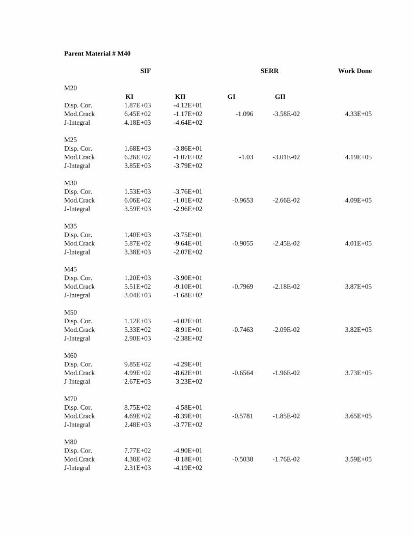
Parent Material # M40 SIF SERR Work Done M20


Parent Material # M45 SIF SERR Work Done M20


Results through the derivations determined by Rice and Sih Table No. 2

nu(psi) k beta epsilon r (inch) theta(angle) Cracklength a (inch) Sigma(psi) Tau(psi)

113983.1 2.389831 0 0 0.1 30 0.833 0.12951 0.028859 127542.4 2.389831 0.023017 0.007329 0.1 30 1.5 0.17379 0.038726 139830.5 2.389831 0.041753 0.0133 0.1 30 2 0.200676 0.044716 150847.5 2.389831 0.057072 0.018189 0.1 30 2.5 0.224362 0.049995

161017 2.389831 0.070123 0.02236 0.1 30 3 0.245777 0.054766 171186.4 2.389831 0.082244 0.026241 0.1 30 3.5 0.265469 0.059154 180508.5 2.389831 0.092619 0.02957 0.1 30 197881.4 2.389831 0.110299 0.035257 0.1 30 213559.3 2.389831 0.124644 0.039888 0.1 30 228813.6 2.389831 0.137342 0.044001 0.1 30

for epsilon -.00733 for epsilon -.02957

a KI KII a KI KII 0.833 0.11783 0.027873 0.833 0.116358 0.032424085

1.5 0.212273 0.049794 1.5 0.209963 0.056802375 2 0.283091 0.066133 2 0.280229 0.074701723

2.5 0.353922 0.082414 2.5 0.350552 0.092372981 3 0.424764 0.098651 3 0.420921 0.109862339

3.5 0.495615 0.114849 3.5 0.491328 0.127200338 for epsilon -.0133 for epsilon -.03526

0.833 0.117485 0.029111 0.833 0.115901 0.033558035 1.5 0.211735 0.051702 1.5 0.20924 0.0585464

2 0.282428 0.068467 2 0.279328 0.07683208 2.5 0.353144 0.085128 2.5 0.349486 0.094846445

3 0.423881 0.101707 3 0.4197 0.112644402 3.5 0.494633 0.118218 3.5 0.489959 0.130262264


0.833 0.117175 0.030117 0.833 0.115505 0.034470095 1.5 0.211249 0.053251 1.5 0.208613 0.059948431

2 0.281826 0.070361 2 0.278546 0.078544004 2.5 0.352437 0.08733 2.5 0.348559 0.096833292

3 0.423075 0.104187 3 0.418636 0.114878247 3.5 0.493736 0.12095 3.5 0.488765 0.132719846


0.833 0.116891 0.030968 0.833 0.115136 0.035271244 1.5 0.210803 0.054562 1.5 0.208028 0.0611794

2 0.281273 0.071963 2 0.277815 0.080046517 2.5 0.351785 0.089192 2.5 0.347692 0.098576474

3 0.422331 0.106283 3 0.41764 0.116837432 3.5 0.492905 0.123259 3.5 0.487646 0.134874486

for epsilon -.02624

0.833 0.116611 0.031754 1.5 0.210362 0.055772

2 0.280725 0.073442 2.5 0.351138 0.09091

3 0.421592 0.108216 3.5 0.492078 0.125388

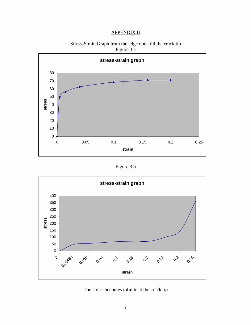
APPENDIX II

Stress-Strain Graph from the edge node till the crack tip Figure 3.a

stress-strain graph

0

10

20

30

40

50

60

70

80

0 0.05 0.1 0.15 0.2 0.25

strain

stre

ss

Figure 3.b

stress-strain graph

0

50

100

150

200

250

300

350

400

0

0.004

830.0

150.0

4 0.1 0.16 0.2 0.2

2 0.3 0.35

strain

stre

ss

The stress becomes infinite at the crack tip

i

ANALYSIS USING FRANC2D/L

Figure No.4

ii

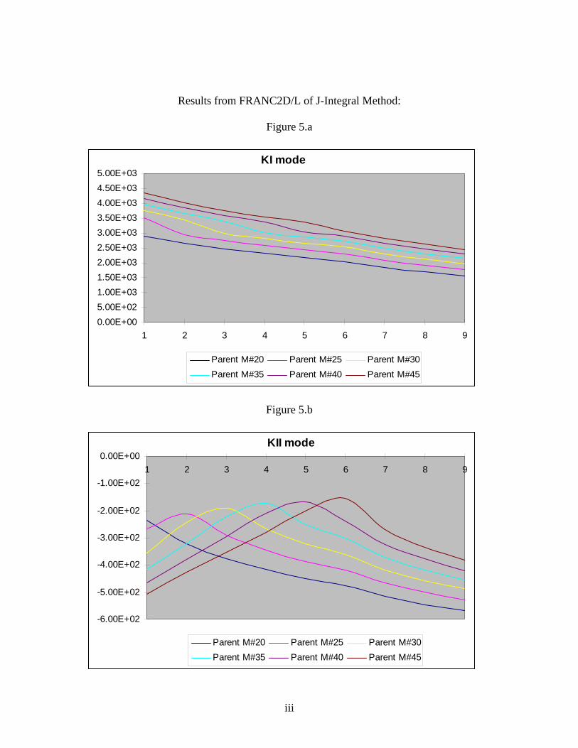
Results from FRANC2D/L of J-Integral Method:

Figure 5.a

KI mode

0.00E+005.00E+021.00E+031.50E+032.00E+032.50E+033.00E+033.50E+034.00E+034.50E+035.00E+03

1 2 3 4 5 6 7 8 9

Parent M#20 Parent M#25 Parent M#30Parent M#35 Parent M#40 Parent M#45

Figure 5.b

KII mode

-6.00E+02

-5.00E+02

-4.00E+02

-3.00E+02

-2.00E+02

-1.00E+02

0.00E+001 2 3 4 5 6 7 8 9

Parent M#20 Parent M#25 Parent M#30Parent M#35 Parent M#40 Parent M#45

iii

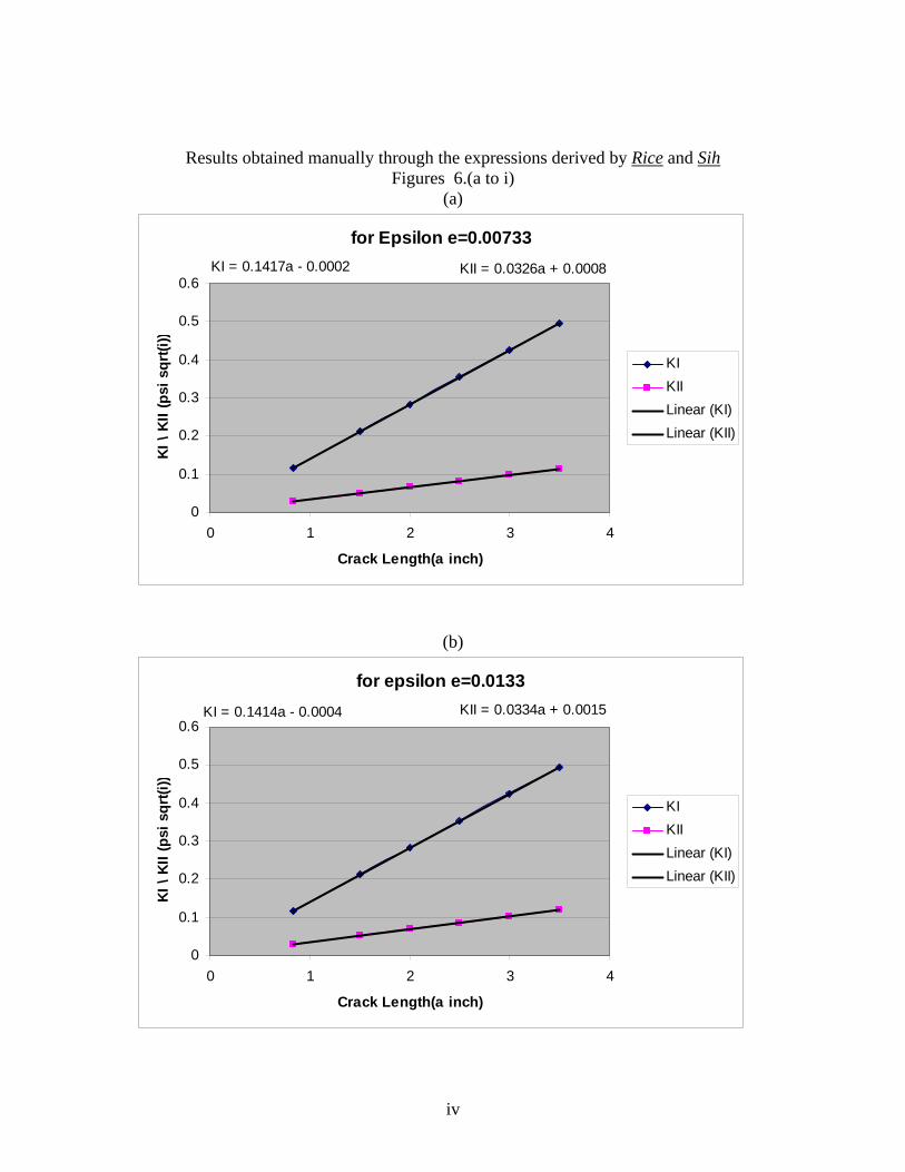
Results obtained manually through the expressions derived by Rice and SihFigures 6.(a to i)

(a)

for Epsilon e=0.00733KI = 0.1417a - 0.0002 KII = 0.0326a + 0.0008

0

0.1

0.2

0.3

0.4

0.5

0.6

0 1 2 3 4

Crack Length(a inch)

KI \

KII

(psi

sqr

t(i))

KIKIILinear (KI)Linear (KII)

(b)

for epsilon e=0.0133KI = 0.1414a - 0.0004 KII = 0.0334a + 0.0015

0

0.1

0.2

0.3

0.4

0.5

0.6

0 1 2 3 4


KI \

KII

(psi

sqr

t(i))


iv

( c )

for epsilon e = 0.01819KI = 0.1412a - 0.0005 KII = 0.034a + 0.0021

0

0.1

0.2

0.3

0.4

0.5

0.6

0 1 2 3 4


KI \

KII

(psi

sqr

t(i))


(d)

for epsilon e=0.02236KI = 0.141a - 0.0006 KII = 0.0346a + 0.0025

0

0.1

0.2

0.3

0.4

0.5

0.6

0 1 2 3 4


KI \

KII

(psi

sqr

t(i))


v

(e)

for epsilon e= 0.02624KI = 0.1408a - 0.0008 KII = 0.0351a + 0.003

0

0.1

0.2

0.3

0.4

0.5

0.6

0 1 2 3 4


KI \

KII

(psi

sqr

t(i))


(f)

for epsilon e = .02957KI = 0.1406a - 0.0009 KII = 0.0355a + 0.0033

0

0.1

0.2

0.3

0.4

0.5

0.6

0 1 2 3 4Crack Length(a inch)

KI \

KII

(psi

sqr

t(i))


vi

(g)

for epsilon e = 0.03526KI = 0.1403a - 0.0011 KII = 0.0362a + 0.0039

0

0.1

0.2

0.3

0.4

0.5

0.6

0 1 2 3 4


KI \

KII

(psi

sqr

t(i))


(h)


0

0.1

0.2

0.3

0.4

0.5

0.6

0 1 2 3 4


KI \

KII

(psi

sqr

t(i))


vii

(i)


0

0.1

0.2

0.3

0.4

0.5

0.6

0 1 2 3 4


KI \

KII

(psi

sqr

t(i))


viii

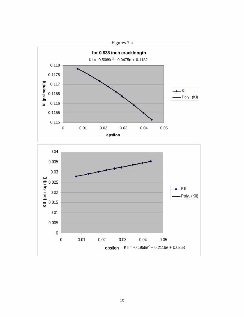
Figures 7.a

for 0.833 inch cracklengthKI = -0.5069e2 - 0.0475e + 0.1182

0.115

0.1155

0.116

0.1165

0.117

0.1175

0.118

0 0.01 0.02 0.03 0.04 0.05

epsilon

KI (p

si s

qrt(i

))

KIPoly. (KI)

KII = -0.1958e2 + 0.2119e + 0.0263

0

0.005

0.01

0.015

0.02

0.025

0.03

0.035

0.04

0 0.01 0.02 0.03 0.04 0.05

epsilon

KII (

psi s

qrt(i

))

KIIPoly. (KII)

ix

Figures 7.b

for 1.5 inch crack length

KI = -0.8278e2 - 0.0733e + 0.2129

0.20750.208

0.20850.209

0.20950.21

0.21050.211

0.21150.212

0.2125

0 0.01 0.02 0.03 0.04 0.05

KIPoly. (KI)

KII = -0.3158e2 + 0.3268e + 0.0474

0

0.01

0.02

0.03

0.04

0.05

0.06

0.07

0 0.01 0.02 0.03 0.04 0.05

epislon

KII

(psi

sqr

t(i))

KIIPoly. (KII)

x

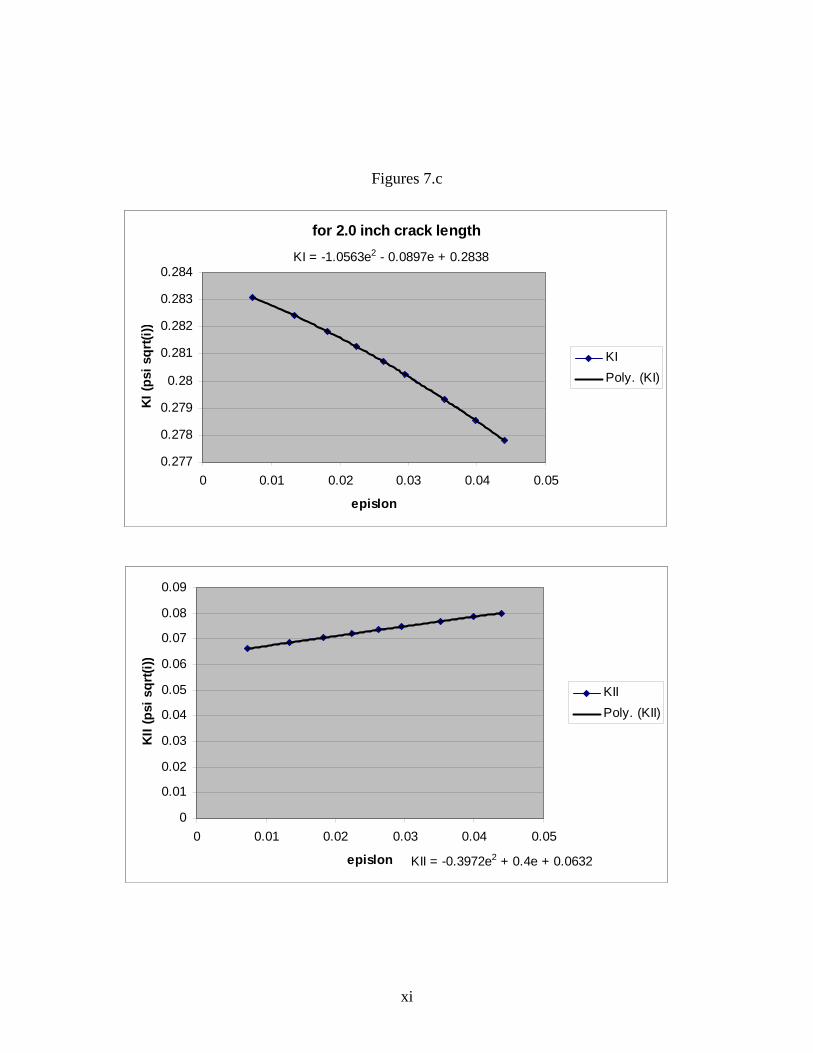
Figures 7.c

for 2.0 inch crack lengthy = -1.0563x2 - 0.0897x + 0.2838

0.277

0.278

0.279

0.28

0.281

0.282

0.283

0.284

0 0.01 0.02 0.03 0.04 0.05

epislon

KI (

psi s

qrt(i

))

KIPoly. (KI)

y = -0.3972x2 + 0.4x + 0.0632

0

0.01

0.02

0.03

0.04

0.05

0.06

0.07

0.08

0.09

0 0.01 0.02 0.03 0.04 0.05

epislon

KII (

psi s

qrt(i

))

KIIPoly. (KII)

for 2.0 inch crack lengthKI = -1.0563e2 - 0.0897e + 0.2838

0.277

0.278

0.279

0.28

0.281

0.282

0.283

0.284

0 0.01 0.02 0.03 0.04 0.05

epislon

KI (p

si s

qrt(i

))

KIPoly. (KI)

KII = -0.3972e2 + 0.4e + 0.0632

0

0.01

0.02

0.03

0.04

0.05

0.06

0.07

0.08

0.09

0 0.01 0.02 0.03 0.04 0.05

epislon

KII

(psi

sqr

t(i))

KIIPoly. (KII)

xi

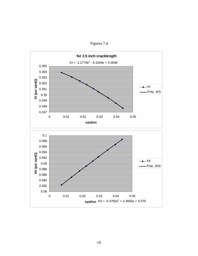
Figures 7.d

for 2.5 inch cracklength

KI = -1.2773e2 - 0.1044e + 0.3548

0.347

0.348

0.349

0.35

0.351

0.352

0.353

0.354

0.355

0 0.01 0.02 0.03 0.04 0.05

epsilon

KI (p

si s

qrt(i

))

KIPoly. (KI)

KII = -0.4782e2 + 0.4655e + 0.079

0.08

0.082

0.084

0.086

0.088

0.09

0.092

0.094

0.096

0.098

0.1

0 0.01 0.02 0.03 0.04 0.05

epsilon

KII

(psi

sqr

t(i))

KIIPoly. (KII)

xii

Figures 7.e

for 3.0 inch cracklength

KI = -1.4938e2 - 0.1177e + 0.4257

0.4170.4180.4190.42

0.421

0.4220.4230.4240.4250.426

0 0.01 0.02 0.03 0.04 0.05

epsilon

KI (p

si s

qrt(i

))

KIPoly. (KI)

KII = -0.5414e2 + 0.5233e + 0.0949

0.095

0.1

0.105

0.11

0.115

0.12

0 0.01 0.02 0.03 0.04 0.05

epsilon

KII

(psi

sqr

t(i))

KIIPoly. (KII)

xiii

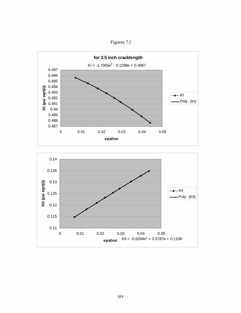
Figures 7.f

for 3.5 inch cracklengthKI = -1.7065e2 - 0.1298e + 0.4967

0.4870.4880.4890.49

0.4910.4920.4930.4940.4950.4960.497

0 0.01 0.02 0.03 0.04 0.05

epsilon

KI (p

si s

qrt(i

))

KIPoly. (KI)

KII = -0.6294e2 + 0.5787e + 0.1106

0.11

0.115

0.12

0.125

0.13

0.135

0.14

0 0.01 0.02 0.03 0.04 0.05

epsilon

KII (

psi s

qrt(i

))

KIIPoly. (KII)

xiv

INTERFACIAL FRACTURE MECHANICS: PATCH REPAIRED ...

Documents

Transcript of INTERFACIAL FRACTURE MECHANICS: PATCH REPAIRED ...