Multi-Scale Patch Aggregation (MPA) for Simultaneous ...
9
Multi-scale Patch Aggregation (MPA) for Simultaneous Detection and Segmentation ∗ Shu Liu † Xiaojuan Qi † Jianping Shi ♭ Hong Zhang † Jiaya Jia † † The Chinese University of Hong Kong ♭ SenseTime Group Limited {sliu, xjqi, hzhang, leojia}@cse.cuhk.edu.hk [email protected] Abstract Aiming at simultaneous detection and segmentation (SD- S), we propose a proposal-free framework, which detect and segment object instances via mid-level patches. We design a unified trainable network on patches, which is followed by a fast and effective patch aggregation algorithm to in- fer object instances. Our method benefits from end-to-end training. Without object proposal generation, computation time can also be reduced. In experiments, our method yields results 62.1% and 61.8% in terms of mAP r on VOC2012 segmentation val and VOC2012 SDS val, which are state- of-the-art at the time of submission. We also report results on Microsoft COCO test-std/test-dev dataset in this paper. 1. Introduction Object detection and semantic segmentation have been core tasks of image understanding for long time. Object de- tection focuses on generating bounding boxes for objects. These boxes may not be accurate enough to localize object- s. Meanwhile semantic segmentation is to predict a more detailed mask in pixel-level for different classes. It howev- er ignores existence of single-object instances. Recently, simultaneous detection and segmentation (S- DS) [14] becomes a promising direction to generate pixel- level labels for every object instance, naturally leading to the next-generation object recognition [24] goal. Accurate and efficient SDS can be used in a lot of disciplines as a fundamental tool, where both pixel-wise label and object instance information can help build robotics, achieve auto- matic driving, enhance surveillance systems, construct in- telligent home, to name a few. SDS is more challenging than object detection and se- mantic segmentation separately. In this task, instance-level information and pixel-wise accurate mask for objects are to be estimated. Nearly all previous work [14, 5, 15, 3] took * This work is supported by a grant from the Research Grants Council of the Hong Kong SAR (project No. 413113). the bottom-up segment-based object proposals [35, 31] as input and modeled the system as classifying proposals with the help of powerful deep convolutional neural networks (DCNNs). Classified proposals are either output or refined in post-processing to produce final results. Issues of Object Proposals in SDS It has been noticed that systems with object-proposal input may be accompa- nied by a few shortcomings. First, generating segment- based proposals takes time. The high-quality proposal generator [31] that was employed in previous SDS work [14, 5, 15, 3] takes about 40 seconds to process one image. It was discussed in [5] that using previous faster segment- based proposals decreases performance. The newest pro- posal generators [30] are not evaluated yet for SDS. Second, the overall SDS performance is bounded by the quality of proposals since they only select provided pro- posals. Object proposals inevitably contain noise regarding missing objects and errors inside each proposal. Last but not least, if a SDS system is independent of object propos- al generation, end-to-end parameter tuning is impossible. Consequently, the system loses the chance to learn feature and structure information from images directly, which how- ever could be important to further improve the system per- formance with information feedback. Our End-to-End SDS Solution To address these issues, we propose a systematically feasible scheme to integrate object proposal generation into the networks, enabling end-to-end training from images to pixel-level labels for instance-aware semantic segmentation. Albeit beautiful in concept, practically establishing suit- able models is difficult due to various scales, aspect ratios, and deformation of objects. In our work, instead of seg- menting objects directly, we propose segmenting and clas- sifying part of or entire objects using many densely locat- ed patches. The mask of an object is then generated by aggregating masks of the overlapping patches in a post- processing step, as shown in Fig. 1. This scheme shares the spirit of mid-level representation [1, 7, 36] and part-based 3141
-
Upload
khangminh22 -
Category
Documents
-
view
0 -
download
0
Transcript of Multi-Scale Patch Aggregation (MPA) for Simultaneous ...
Multi-scale Patch Aggregation (MPA)
for Simultaneous Detection and Segmentation∗
Shu Liu† Xiaojuan Qi† Jianping Shi♭ Hong Zhang† Jiaya Jia†
† The Chinese University of Hong Kong ♭ SenseTime Group Limited
{sliu, xjqi, hzhang, leojia}@cse.cuhk.edu.hk [email protected]
Abstract
Aiming at simultaneous detection and segmentation (SD-
S), we propose a proposal-free framework, which detect and
segment object instances via mid-level patches. We design
a unified trainable network on patches, which is followed
by a fast and effective patch aggregation algorithm to in-
fer object instances. Our method benefits from end-to-end
training. Without object proposal generation, computation
time can also be reduced. In experiments, our method yields
results 62.1% and 61.8% in terms of mAP r on VOC2012
segmentation val and VOC2012 SDS val, which are state-
of-the-art at the time of submission. We also report results
on Microsoft COCO test-std/test-dev dataset in this paper.
1. Introduction
Object detection and semantic segmentation have been
core tasks of image understanding for long time. Object de-
tection focuses on generating bounding boxes for objects.
These boxes may not be accurate enough to localize object-
s. Meanwhile semantic segmentation is to predict a more
detailed mask in pixel-level for different classes. It howev-
er ignores existence of single-object instances.
Recently, simultaneous detection and segmentation (S-
DS) [14] becomes a promising direction to generate pixel-
level labels for every object instance, naturally leading to
the next-generation object recognition [24] goal. Accurate
and efficient SDS can be used in a lot of disciplines as a
fundamental tool, where both pixel-wise label and object
instance information can help build robotics, achieve auto-
matic driving, enhance surveillance systems, construct in-
telligent home, to name a few.
SDS is more challenging than object detection and se-
mantic segmentation separately. In this task, instance-level
information and pixel-wise accurate mask for objects are to
be estimated. Nearly all previous work [14, 5, 15, 3] took
∗This work is supported by a grant from the Research Grants Council
of the Hong Kong SAR (project No. 413113).
the bottom-up segment-based object proposals [35, 31] as
input and modeled the system as classifying proposals with
the help of powerful deep convolutional neural networks
(DCNNs). Classified proposals are either output or refined
in post-processing to produce final results.
Issues of Object Proposals in SDS It has been noticed
that systems with object-proposal input may be accompa-
nied by a few shortcomings. First, generating segment-
based proposals takes time. The high-quality proposal
generator [31] that was employed in previous SDS work
[14, 5, 15, 3] takes about 40 seconds to process one image.
It was discussed in [5] that using previous faster segment-
based proposals decreases performance. The newest pro-
posal generators [30] are not evaluated yet for SDS.
Second, the overall SDS performance is bounded by the
quality of proposals since they only select provided pro-
posals. Object proposals inevitably contain noise regarding
missing objects and errors inside each proposal. Last but
not least, if a SDS system is independent of object propos-
al generation, end-to-end parameter tuning is impossible.
Consequently, the system loses the chance to learn feature
and structure information from images directly, which how-
ever could be important to further improve the system per-
formance with information feedback.
Our End-to-End SDS Solution To address these issues,
we propose a systematically feasible scheme to integrate
object proposal generation into the networks, enabling
end-to-end training from images to pixel-level labels for
instance-aware semantic segmentation.
Albeit beautiful in concept, practically establishing suit-
able models is difficult due to various scales, aspect ratios,
and deformation of objects. In our work, instead of seg-
menting objects directly, we propose segmenting and clas-
sifying part of or entire objects using many densely locat-
ed patches. The mask of an object is then generated by
aggregating masks of the overlapping patches in a post-
processing step, as shown in Fig. 1. This scheme shares the
spirit of mid-level representation [1, 7, 36] and part-based
13141

image densely localized patches aggregation result
Figure 1. Objects overlapped with many densely localized patches. After segmenting objects in different patches, aggregation can be used
to infer complete objects.
model [37, 16]. It is yet different by nature in terms of sys-
tem construction and optimization.
In our scheme, overlapped patches gather different levels
of information for final object segmentation, which makes
the result more robust than prediction from only one input.
Our end-to-end trainable SDS system is thus with output of
semantic segment labels in patches.
Our Contributions Our framework to tackle the SDS
problem makes the following main contributions.
• We propose the strategy to generate dense multi-scale
patches for object parsing.
• Our unified end-to-end trainable proposal-free network
can achieve segmentation and classification simultane-
ously for each patch. By sharing convolution in the
network, computation time is reduced and good quali-
ty results are produced.
• We develop an efficient algorithm to infer the segmen-
tation mask for each object by merging information
from mid-level patches.
We evaluated our method on PASCAL VOC 2012 seg-
mentation validation and VOC 2012 SDS validation bench-
mark datasets. Our method yields state-of-the-art perfor-
mance with reasonably short running time. We also evalu-
ated it on Microsoft COCO test-std and test-dev data. De-
cent performance is achieved based on the VGG-16 network
structure without network ensemble.
2. Related Work
The SDS task is closely related to object detection, se-
mantic segmentation, and proposal generation. We briefly
review them in this section.
Object Detection Object detection has a long history
in computer vision. Before DCNN shows its great abil-
ity for image classification [21, 33], part-based models
[9, 37] were popular. Recent object detection framework-
s [11, 12, 17, 37, 29, 34, 23, 32, 10] are based on DCNN
[21, 33] to classify object proposals. These methods either
take object proposals as independent input [12, 37, 29, 34],
or use the entire image and pool features for each propos-
al [17, 11, 32, 10]. Different from these methods, Ren et
al. [32] unified proposal generation and classification with
shared convolution feature maps. It saves time to generate
object proposals and yields good performance.
Semantic Segmentation DCNNs [21, 33] also boost per-
formance of semantic segmentation [26, 5, 15, 27, 2, 20, 28,
25]. Related methods can be categorized into two streams –
one utilizes DCNNs to classify segment proposals [15, 5]
and the other line is to use fully convolutional network-
s [26, 2, 20, 25] for dense prediction. CRF can be applied in
post-processing [2] or incorporated in the network [20, 25]
to refine segment contours.
SDS SDS is a relatively new topic. Hariharan et al. [14]
presented pioneer work. It took segment-based object pro-
posals [31] as input similar to object detection. Two net-
works – one for bounding boxes and one for masks – were
adopted to extract features. Then features from these net-
works were concatenated and classified by SVM [4].
Hariharan et al. [15] used hyper-column representation
to refine segment masks. But updating all proposals is com-
putationally too costly, especially when complex networks,
such as VGG [33], are deployed. So the method made use
of detection results [12] and a final rescore procedure was
adopted. Chen et al. [3] developed an energy minimization
framework incorporating top-down and bottom-up informa-
3142
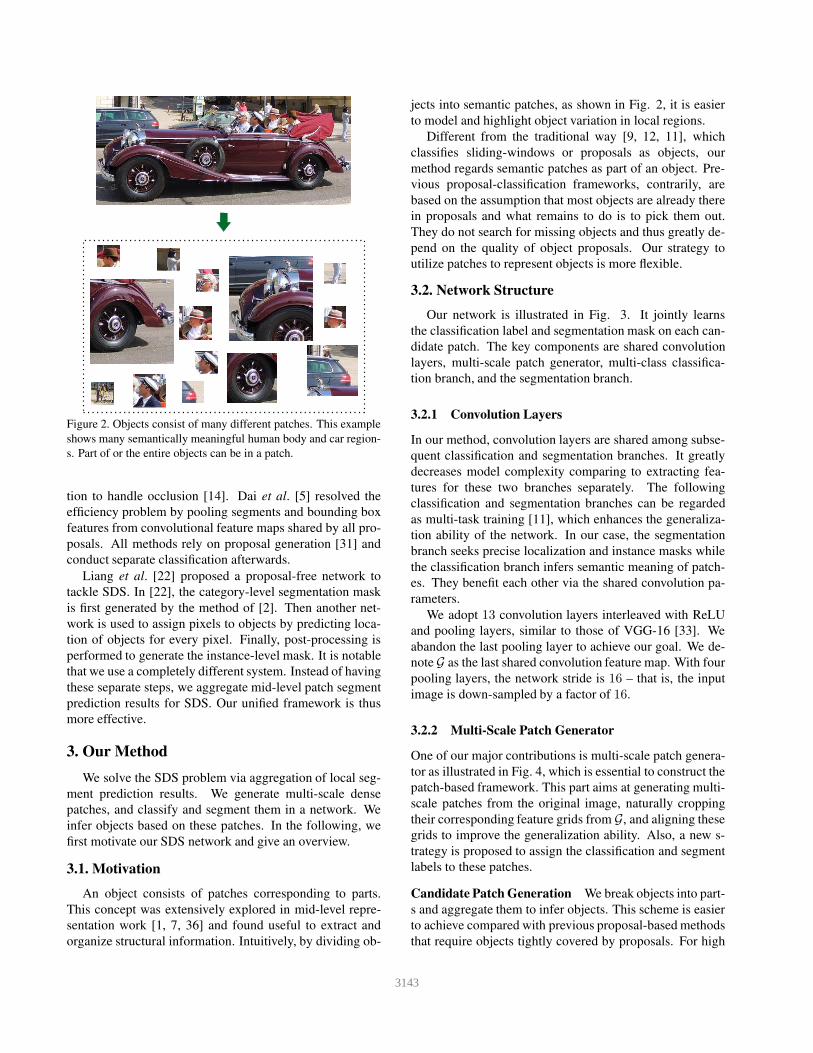
Figure 2. Objects consist of many different patches. This example
shows many semantically meaningful human body and car region-
s. Part of or the entire objects can be in a patch.
tion to handle occlusion [14]. Dai et al. [5] resolved the
efficiency problem by pooling segments and bounding box
features from convolutional feature maps shared by all pro-
posals. All methods rely on proposal generation [31] and
conduct separate classification afterwards.
Liang et al. [22] proposed a proposal-free network to
tackle SDS. In [22], the category-level segmentation mask
is first generated by the method of [2]. Then another net-
work is used to assign pixels to objects by predicting loca-
tion of objects for every pixel. Finally, post-processing is
performed to generate the instance-level mask. It is notable
that we use a completely different system. Instead of having
these separate steps, we aggregate mid-level patch segment
prediction results for SDS. Our unified framework is thus
more effective.
3. Our Method
We solve the SDS problem via aggregation of local seg-
ment prediction results. We generate multi-scale dense
patches, and classify and segment them in a network. We
infer objects based on these patches. In the following, we
first motivate our SDS network and give an overview.
3.1. Motivation
An object consists of patches corresponding to parts.
This concept was extensively explored in mid-level repre-
sentation work [1, 7, 36] and found useful to extract and
organize structural information. Intuitively, by dividing ob-
jects into semantic patches, as shown in Fig. 2, it is easier
to model and highlight object variation in local regions.
Different from the traditional way [9, 12, 11], which
classifies sliding-windows or proposals as objects, our
method regards semantic patches as part of an object. Pre-
vious proposal-classification frameworks, contrarily, are
based on the assumption that most objects are already there
in proposals and what remains to do is to pick them out.
They do not search for missing objects and thus greatly de-
pend on the quality of object proposals. Our strategy to
utilize patches to represent objects is more flexible.
3.2. Network Structure
Our network is illustrated in Fig. 3. It jointly learns
the classification label and segmentation mask on each can-
didate patch. The key components are shared convolution
layers, multi-scale patch generator, multi-class classifica-
tion branch, and the segmentation branch.
3.2.1 Convolution Layers
In our method, convolution layers are shared among subse-
quent classification and segmentation branches. It greatly
decreases model complexity comparing to extracting fea-
tures for these two branches separately. The following
classification and segmentation branches can be regarded
as multi-task training [11], which enhances the generaliza-
tion ability of the network. In our case, the segmentation
branch seeks precise localization and instance masks while
the classification branch infers semantic meaning of patch-
es. They benefit each other via the shared convolution pa-
rameters.
We adopt 13 convolution layers interleaved with ReLU
and pooling layers, similar to those of VGG-16 [33]. We
abandon the last pooling layer to achieve our goal. We de-
note G as the last shared convolution feature map. With four
pooling layers, the network stride is 16 – that is, the input
image is down-sampled by a factor of 16.
3.2.2 Multi-Scale Patch Generator
One of our major contributions is multi-scale patch genera-
tor as illustrated in Fig. 4, which is essential to construct the
patch-based framework. This part aims at generating multi-
scale patches from the original image, naturally cropping
their corresponding feature grids from G, and aligning these
grids to improve the generalization ability. Also, a new s-
trategy is proposed to assign the classification and segment
labels to these patches.
Candidate Patch Generation We break objects into part-
s and aggregate them to infer objects. This scheme is easier
to achieve compared with previous proposal-based methods
that require objects tightly covered by proposals. For high
3143
pool
segmentation branch
classification branch
multi-scalepatch
generator
...
{...
convlayers
reshape
24x24x512
horse
1x1x4096 1x1x21
1x1x2304 1x1x2304
1x1x4096
48x48
384x384x3
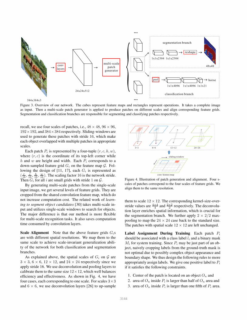
Figure 3. Overview of our network. The cubes represent feature maps and rectangles represent operations. It takes a complete image
as input. Then a multi-scale patch generator is applied to produce patches on different scales and align corresponding feature grids.
Segmentation and classification branches are responsible for segmenting and classifying patches respectively.
recall, we use four scales of patches, i.e., 48× 48, 96× 96,
192×192, and 384×384 respectively. Sliding-windows are
used to generate these patches with stride 16, which make
each object overlapped with multiple patches in appropriate
scales.
Each patch Pi is represented by a four-tuple (r, c, h, w),where (r, c) is the coordinate of its top-left corner while
h and w are height and width. Each Pi corresponds to a
down-sampled feature grid Gi on the feature map G. Fol-
lowing the design of [11, 17], each Gi is represented as
( r16, c16, h16, w16). The scaling factor 16 is the network stride.
Then Gi for all i are small grids with stride 1 on G.
By generating multi-scale patches from the single-scale
input image, we get several levels of feature grids. They are
cropped from the shared convolution feature map, which do
not increase computation cost. The related work of learn-
ing to segment object candidates [30] takes multi-scale in-
put and utilizes single-scale windows to search for objects.
The major difference is that our method is more flexible
for multi-scale recognition tasks. It also saves computation
time consumed by convolution layers.
Scale Alignment Note that the above feature grids Gis
are with different spatial resolutions. We map them to the
same scale to achieve scale-invariant generalization abili-
ty of the network for both classification and segmentation
branches.
As explained above, the spatial scales of Gi on G are
3 × 3, 6 × 6, 12 × 12, and 24 × 24 respectively since we
apply stride 16. We use deconvolution and pooling layers to
calibrate them to the same size 12×12, which well balances
efficiency and effectiveness. As shown in Fig. 4, we have
four cases, each corresponding to one scale. For scales 3×3and 6 × 6, we use deconvolution layers [26] to up-sample
3×3 6×6 12×12 24×24
conv feature map
sliding window
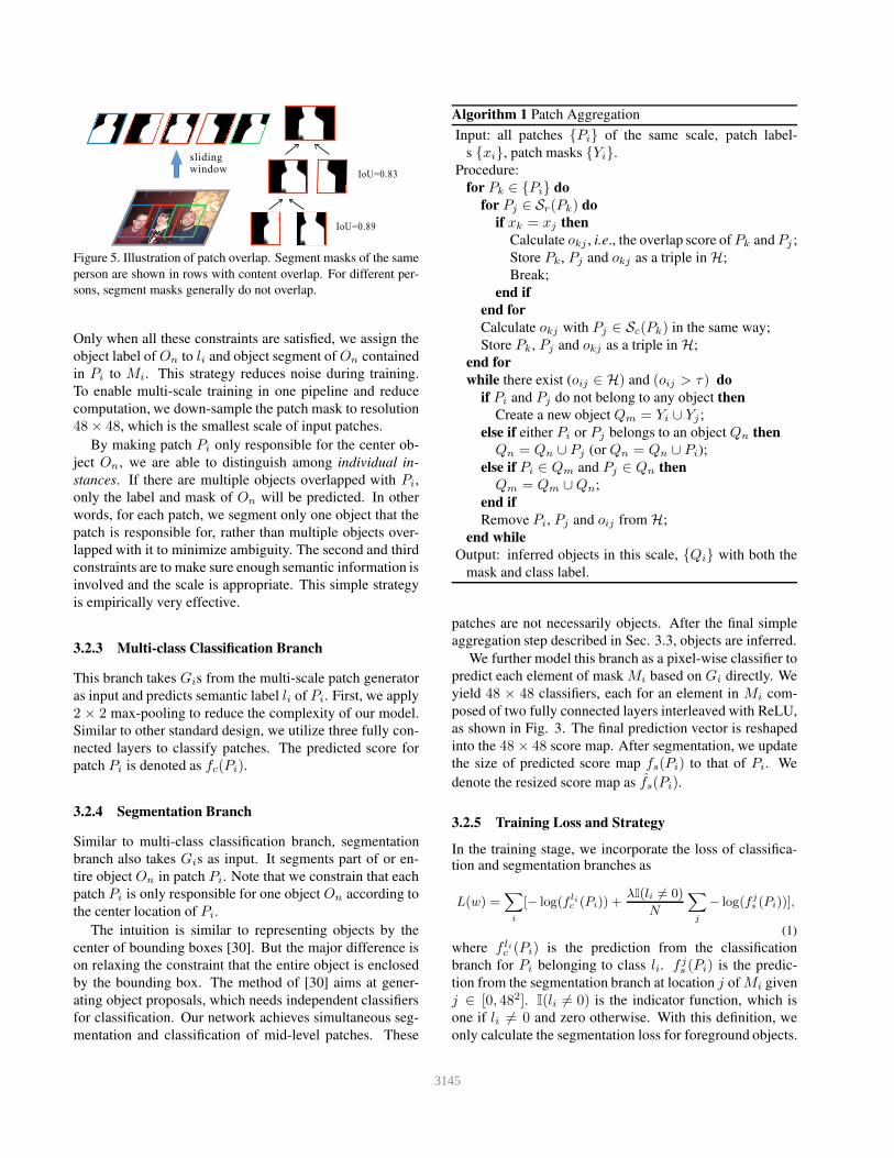
Figure 4. Illustration of patch generation and alignment. Four s-
cales of patches correspond to the four scales of feature grids. We
align them to the same resolution.
them to scale 12× 12. The corresponding kernel-size-over-
stride values are 4×4
4and 2×2
2respectively. The deconvolu-
tion layer enriches spatial information, which is crucial for
the segmentation branch. We further apply 2 × 2/2 max-
pooling to map the 24 × 24 case back to the standard size.
The patches with spatial scale 12× 12 are left unchanged.
Label Assignment During Training Each patch Pi
should be associated with a class label li and a binary mask
Mi for system training. Since Pi may be just part of an ob-
ject, naively cropping labels from the ground-truth mask is
not optimal due to possibly complex object appearance and
boundary shape. We thus design the following rules to more
appropriately assign labels. We give one positive label to Pi
if it satisfies the following constraints.
1. Center of the patch is located on an object On and
2. area of On inside Pi is larger than half of On area and
3. area of On inside Pi is larger than one fifth of Pi area.
3144
IoU=0.89
IoU=0.83
slidingwindow
Figure 5. Illustration of patch overlap. Segment masks of the same
person are shown in rows with content overlap. For different per-
sons, segment masks generally do not overlap.
Only when all these constraints are satisfied, we assign the
object label of On to li and object segment of On contained
in Pi to Mi. This strategy reduces noise during training.
To enable multi-scale training in one pipeline and reduce
computation, we down-sample the patch mask to resolution
48× 48, which is the smallest scale of input patches.
By making patch Pi only responsible for the center ob-
ject On, we are able to distinguish among individual in-
stances. If there are multiple objects overlapped with Pi,
only the label and mask of On will be predicted. In other
words, for each patch, we segment only one object that the
patch is responsible for, rather than multiple objects over-
lapped with it to minimize ambiguity. The second and third
constraints are to make sure enough semantic information is
involved and the scale is appropriate. This simple strategy
is empirically very effective.
3.2.3 Multi-class Classification Branch
This branch takes Gis from the multi-scale patch generator
as input and predicts semantic label li of Pi. First, we apply
2 × 2 max-pooling to reduce the complexity of our model.
Similar to other standard design, we utilize three fully con-
nected layers to classify patches. The predicted score for
patch Pi is denoted as fc(Pi).
3.2.4 Segmentation Branch
Similar to multi-class classification branch, segmentation
branch also takes Gis as input. It segments part of or en-
tire object On in patch Pi. Note that we constrain that each
patch Pi is only responsible for one object On according to
the center location of Pi.
The intuition is similar to representing objects by the
center of bounding boxes [30]. But the major difference is
on relaxing the constraint that the entire object is enclosed
by the bounding box. The method of [30] aims at gener-
ating object proposals, which needs independent classifiers
for classification. Our network achieves simultaneous seg-
mentation and classification of mid-level patches. These
Algorithm 1 Patch Aggregation
Input: all patches {Pi} of the same scale, patch label-
s {xi}, patch masks {Yi}.
Procedure:
for Pk ∈ {Pi} do
for Pj ∈ Sr(Pk) do
if xk = xj then
Calculate okj , i.e., the overlap score of Pk andPj ;
Store Pk, Pj and okj as a triple in H;
Break;
end if
end for
Calculate okj with Pj ∈ Sc(Pk) in the same way;
Store Pk, Pj and okj as a triple in H;
end for
while there exist (oij ∈ H) and (oij > τ ) do
if Pi and Pj do not belong to any object then
Create a new object Qm = Yi ∪ Yj ;
else if either Pi or Pj belongs to an object Qn then
Qn = Qn ∪ Pj (or Qn = Qn ∪ Pi);
else if Pi ∈ Qm and Pj ∈ Qn then
Qm = Qm ∪Qn;
end if
Remove Pi, Pj and oij from H;
end while
Output: inferred objects in this scale, {Qi} with both the
mask and class label.
patches are not necessarily objects. After the final simple
aggregation step described in Sec. 3.3, objects are inferred.
We further model this branch as a pixel-wise classifier to
predict each element of mask Mi based on Gi directly. We
yield 48 × 48 classifiers, each for an element in Mi com-
posed of two fully connected layers interleaved with ReLU,
as shown in Fig. 3. The final prediction vector is reshaped
into the 48× 48 score map. After segmentation, we update
the size of predicted score map fs(Pi) to that of Pi. We
denote the resized score map as fs(Pi).
3.2.5 Training Loss and Strategy
In the training stage, we incorporate the loss of classifica-tion and segmentation branches as
L(w) =∑
i
[− log(f lic (Pi)) +
λI(li 6= 0)
N
∑
j
− log(f js (Pi))],
(1)
where f lic (Pi) is the prediction from the classification
branch for Pi belonging to class li. f js (Pi) is the predic-
tion from the segmentation branch at location j of Mi given
j ∈ [0, 482]. I(li 6= 0) is the indicator function, which is
one if li 6= 0 and zero otherwise. With this definition, we
only calculate the segmentation loss for foreground objects.
3145
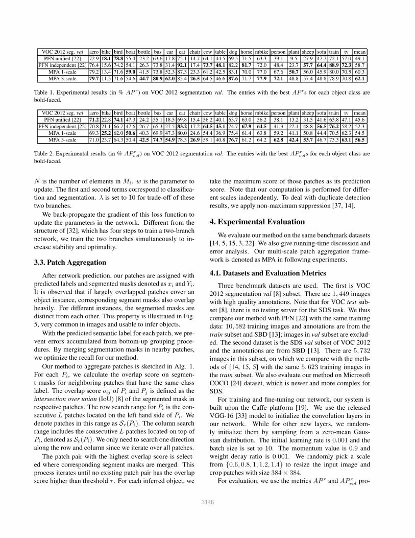
VOC 2012 seg. val aero bike bird boat bottle bus car cat chair cow table dog horse mbike person plant sheep sofa train tv mean
PFN unified [22] 72.9 18.1 78.8 55.4 23.2 63.6 17.8 72.1 14.7 64.1 44.5 69.5 71.5 63.3 39.1 9.5 27.9 47.7 72.1 57.0 49.1
PFN independent [22] 76.4 15.6 74.2 54.1 26.3 73.8 31.4 92.1 17.4 73.7 48.1 82.2 81.7 72.0 48.4 23.7 57.7 64.4 88.9 72.3 58.7
MPA 1-scale 79.2 13.4 71.6 59.0 41.5 73.8 52.3 87.3 23.3 61.2 42.5 83.1 70.0 77.0 67.6 50.7 56.0 45.9 80.0 70.5 60.3
MPA 3-scale 79.7 11.5 71.6 54.6 44.7 80.9 62.0 85.4 26.5 64.5 46.6 87.6 71.7 77.9 72.1 48.8 57.4 48.8 78.9 70.8 62.1
Table 1. Experimental results (in % AP r) on VOC 2012 segmentation val. The entries with the best AP rs for each object class are
bold-faced.
VOC 2012 seg. val aero bike bird boat bottle bus car cat chair cow table dog horse mbike person plant sheep sofa train tv mean
PFN unified [22] 71.2 22.8 74.1 47.3 24.2 55.1 18.5 69.8 15.4 56.2 40.1 63.7 63.0 56.2 38.1 13.2 31.5 41.6 63.8 47.1 45.6
PFN independent [22] 70.8 21.1 66.7 47.6 26.7 65.3 27.5 83.2 17.2 64.5 45.1 74.7 67.9 64.5 41.3 22.1 48.8 56.5 76.2 58.2 52.3
MPA 1-scale 69.3 25.2 62.0 50.6 40.3 69.9 47.3 80.0 24.6 54.4 36.9 75.4 61.4 63.8 59.2 41.1 50.8 44.4 70.5 62.3 54.5
MPA 3-scale 71.0 23.7 64.3 50.4 42.5 74.7 54.9 78.3 26.9 59.1 40.8 76.7 61.2 64.2 62.8 42.4 53.7 46.7 73.3 63.1 56.5
Table 2. Experimental results (in % AP rvol) on VOC 2012 segmentation val. The entries with the best AP r
vols for each object class are
bold-faced.
N is the number of elements in Mi. w is the parameter to
update. The first and second terms correspond to classifica-
tion and segmentation. λ is set to 10 for trade-off of these
two branches.
We back-propagate the gradient of this loss function to
update the parameters in the network. Different from the
structure of [32], which has four steps to train a two-branch
network, we train the two branches simultaneously to in-
crease stability and optimality.
3.3. Patch Aggregation
After network prediction, our patches are assigned with
predicted labels and segmented masks denoted as xi and Yi.
It is observed that if largely overlapped patches cover an
object instance, corresponding segment masks also overlap
heavily. For different instances, the segmented masks are
distinct from each other. This property is illustrated in Fig.
5, very common in images and usable to infer objects.
With the predicted semantic label for each patch, we pre-
vent errors accumulated from bottom-up grouping proce-
dures. By merging segmentation masks in nearby patches,
we optimize the recall for our method.
Our method to aggregate patches is sketched in Alg. 1.
For each Pi, we calculate the overlap score on segmen-
t masks for neighboring patches that have the same class
label. The overlap score oij of Pi and Pj is defined as the
intersection over union (IoU) [8] of the segmented mask in
respective patches. The row search range for Pi is the con-
secutive L patches located on the left hand side of Pi. We
denote patches in this range as Sr(Pi). The column search
range includes the consecutive L patches located on top of
Pi, denoted as Sc(Pi). We only need to search one direction
along the row and column since we iterate over all patches.
The patch pair with the highest overlap score is select-
ed where corresponding segment masks are merged. This
process iterates until no existing patch pair has the overlap
score higher than threshold τ . For each inferred object, we
take the maximum score of those patches as its prediction
score. Note that our computation is performed for differ-
ent scales independently. To deal with duplicate detection
results, we apply non-maximum suppression [37, 14].
4. Experimental Evaluation
We evaluate our method on the same benchmark datasets
[14, 5, 15, 3, 22]. We also give running-time discussion and
error analysis. Our multi-scale patch aggregation frame-
work is denoted as MPA in following experiments.
4.1. Datasets and Evaluation Metrics
Three benchmark datasets are used. The first is VOC
2012 segmentation val [8] subset. There are 1, 449 images
with high quality annotations. Note that for VOC test sub-
set [8], there is no testing server for the SDS task. We thus
compare our method with PFN [22] with the same training
data: 10, 582 training images and annotations are from the
train subset and SBD [13]; images in val subset are exclud-
ed. The second dataset is the SDS val subset of VOC 2012
and the annotations are from SBD [13]. There are 5, 732images in this subset, on which we compare with the meth-
ods of [14, 15, 5] with the same 5, 623 training images in
the train subset. We also evaluate our method on Microsoft
COCO [24] dataset, which is newer and more complex for
SDS.
For training and fine-tuning our network, our system is
built upon the Caffe platform [19]. We use the released
VGG-16 [33] model to initialize the convolution layers in
our network. While for other new layers, we random-
ly initialize them by sampling from a zero-mean Gaus-
sian distribution. The initial learning rate is 0.001 and the
batch size is set to 10. The momentum value is 0.9 and
weight decay ratio is 0.001. We randomly pick a scale
from {0.6, 0.8, 1, 1.2, 1.4} to resize the input image and
crop patches with size 384× 384.
For evaluation, we use the metrics AP r and AP rvol pro-
3146
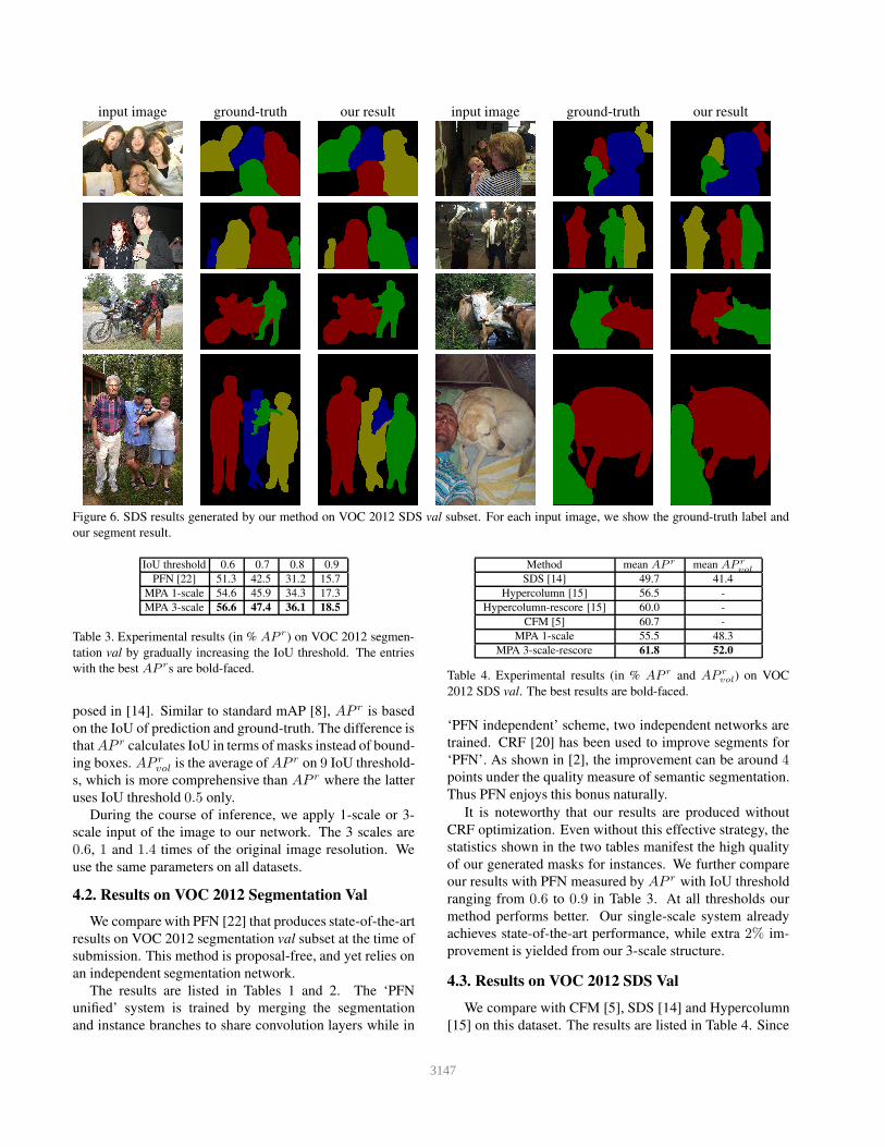
input image ground-truth our result input image ground-truth our result
Figure 6. SDS results generated by our method on VOC 2012 SDS val subset. For each input image, we show the ground-truth label and
our segment result.
IoU threshold 0.6 0.7 0.8 0.9
PFN [22] 51.3 42.5 31.2 15.7
MPA 1-scale 54.6 45.9 34.3 17.3
MPA 3-scale 56.6 47.4 36.1 18.5
Table 3. Experimental results (in % AP r) on VOC 2012 segmen-
tation val by gradually increasing the IoU threshold. The entries
with the best AP rs are bold-faced.
posed in [14]. Similar to standard mAP [8], AP r is based
on the IoU of prediction and ground-truth. The difference is
thatAP r calculates IoU in terms of masks instead of bound-
ing boxes. AP rvol is the average of AP r on 9 IoU threshold-
s, which is more comprehensive than AP r where the latter
uses IoU threshold 0.5 only.
During the course of inference, we apply 1-scale or 3-
scale input of the image to our network. The 3 scales are
0.6, 1 and 1.4 times of the original image resolution. We
use the same parameters on all datasets.
4.2. Results on VOC 2012 Segmentation Val
We compare with PFN [22] that produces state-of-the-art
results on VOC 2012 segmentation val subset at the time of
submission. This method is proposal-free, and yet relies on
an independent segmentation network.
The results are listed in Tables 1 and 2. The ‘PFN
unified’ system is trained by merging the segmentation
and instance branches to share convolution layers while in
Method mean AP r mean AP rvol
SDS [14] 49.7 41.4
Hypercolumn [15] 56.5 -
Hypercolumn-rescore [15] 60.0 -
CFM [5] 60.7 -
MPA 1-scale 55.5 48.3
MPA 3-scale-rescore 61.8 52.0
Table 4. Experimental results (in % AP r and AP rvol) on VOC
2012 SDS val. The best results are bold-faced.
‘PFN independent’ scheme, two independent networks are
trained. CRF [20] has been used to improve segments for
‘PFN’. As shown in [2], the improvement can be around 4points under the quality measure of semantic segmentation.
Thus PFN enjoys this bonus naturally.
It is noteworthy that our results are produced without
CRF optimization. Even without this effective strategy, the
statistics shown in the two tables manifest the high quality
of our generated masks for instances. We further compare
our results with PFN measured by AP r with IoU threshold
ranging from 0.6 to 0.9 in Table 3. At all thresholds our
method performs better. Our single-scale system already
achieves state-of-the-art performance, while extra 2% im-
provement is yielded from our 3-scale structure.
4.3. Results on VOC 2012 SDS Val
We compare with CFM [5], SDS [14] and Hypercolumn
[15] on this dataset. The results are listed in Table 4. Since
3147
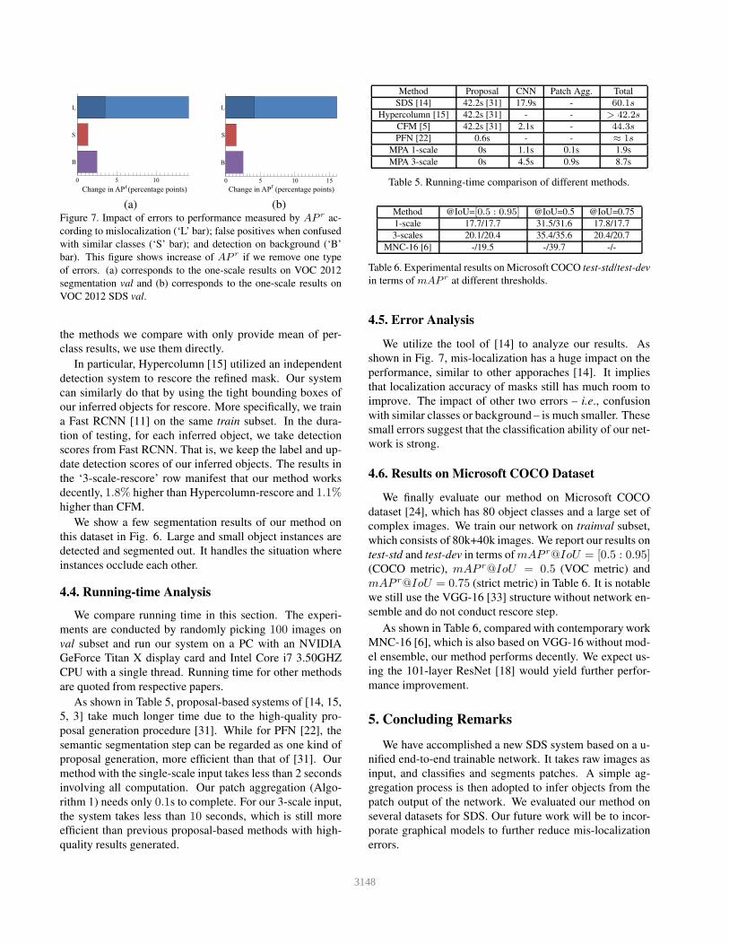
0 5 10
B
S
L
Change in APr(percentage points)
0 5 10 15
B
S
L
Change in APr
(percentage points)
(a) (b)Figure 7. Impact of errors to performance measured by AP r ac-
cording to mislocalization (‘L’ bar); false positives when confused
with similar classes (‘S’ bar); and detection on background (‘B’
bar). This figure shows increase of AP r if we remove one type
of errors. (a) corresponds to the one-scale results on VOC 2012
segmentation val and (b) corresponds to the one-scale results on
VOC 2012 SDS val.
the methods we compare with only provide mean of per-
class results, we use them directly.
In particular, Hypercolumn [15] utilized an independent
detection system to rescore the refined mask. Our system
can similarly do that by using the tight bounding boxes of
our inferred objects for rescore. More specifically, we train
a Fast RCNN [11] on the same train subset. In the dura-
tion of testing, for each inferred object, we take detection
scores from Fast RCNN. That is, we keep the label and up-
date detection scores of our inferred objects. The results in
the ‘3-scale-rescore’ row manifest that our method works
decently, 1.8% higher than Hypercolumn-rescore and 1.1%higher than CFM.
We show a few segmentation results of our method on
this dataset in Fig. 6. Large and small object instances are
detected and segmented out. It handles the situation where
instances occlude each other.
4.4. Runningtime Analysis
We compare running time in this section. The experi-
ments are conducted by randomly picking 100 images on
val subset and run our system on a PC with an NVIDIA
GeForce Titan X display card and Intel Core i7 3.50GHZ
CPU with a single thread. Running time for other methods
are quoted from respective papers.
As shown in Table 5, proposal-based systems of [14, 15,
5, 3] take much longer time due to the high-quality pro-
posal generation procedure [31]. While for PFN [22], the
semantic segmentation step can be regarded as one kind of
proposal generation, more efficient than that of [31]. Our
method with the single-scale input takes less than 2 seconds
involving all computation. Our patch aggregation (Algo-
rithm 1) needs only 0.1s to complete. For our 3-scale input,
the system takes less than 10 seconds, which is still more
efficient than previous proposal-based methods with high-
quality results generated.
Method Proposal CNN Patch Agg. Total
SDS [14] 42.2s [31] 17.9s - 60.1sHypercolumn [15] 42.2s [31] - - > 42.2s
CFM [5] 42.2s [31] 2.1s - 44.3sPFN [22] 0.6s - - ≈ 1s
MPA 1-scale 0s 1.1s 0.1s 1.9s
MPA 3-scale 0s 4.5s 0.9s 8.7s
Table 5. Running-time comparison of different methods.
Method @IoU=[0.5 : 0.95] @IoU=0.5 @IoU=0.75
1-scale 17.7/17.7 31.5/31.6 17.8/17.7
3-scales 20.1/20.4 35.4/35.6 20.4/20.7
MNC-16 [6] -/19.5 -/39.7 -/-
Table 6. Experimental results on Microsoft COCO test-std/test-dev
in terms of mAP r at different thresholds.
4.5. Error Analysis
We utilize the tool of [14] to analyze our results. As
shown in Fig. 7, mis-localization has a huge impact on the
performance, similar to other apporaches [14]. It implies
that localization accuracy of masks still has much room to
improve. The impact of other two errors – i.e., confusion
with similar classes or background – is much smaller. These
small errors suggest that the classification ability of our net-
work is strong.
4.6. Results on Microsoft COCO Dataset
We finally evaluate our method on Microsoft COCO
dataset [24], which has 80 object classes and a large set of
complex images. We train our network on trainval subset,
which consists of 80k+40k images. We report our results on
test-std and test-dev in terms of mAP r@IoU = [0.5 : 0.95](COCO metric), mAP r@IoU = 0.5 (VOC metric) and
mAP r@IoU = 0.75 (strict metric) in Table 6. It is notable
we still use the VGG-16 [33] structure without network en-
semble and do not conduct rescore step.
As shown in Table 6, compared with contemporary work
MNC-16 [6], which is also based on VGG-16 without mod-
el ensemble, our method performs decently. We expect us-
ing the 101-layer ResNet [18] would yield further perfor-
mance improvement.
5. Concluding Remarks
We have accomplished a new SDS system based on a u-
nified end-to-end trainable network. It takes raw images as
input, and classifies and segments patches. A simple ag-
gregation process is then adopted to infer objects from the
patch output of the network. We evaluated our method on
several datasets for SDS. Our future work will be to incor-
porate graphical models to further reduce mis-localization
errors.
3148
References
[1] A. Bansal, A. Shrivastava, C. Doersch, and A. Gupta. Mid-
level elements for object detection. CoRR, abs/1504.07284,
2015.
[2] L.-C. Chen, G. Papandreou, I. Kokkinos, K. Murphy, and
A. L. Yuille. Semantic image segmentation with deep con-
volutional nets and fully connected crfs. In ICLR, 2015.
[3] Y. Chen, X. Liu, and M. Yang. Multi-instance object seg-
mentation with occlusion handling. In CVPR, pages 3470–
3478, 2015.
[4] C. Cortes and V. Vapnik. Support-vector networks. Machine
Learning, 20(3):273–297, 1995.
[5] J. Dai, K. He, and J. Sun. Convolutional feature masking for
joint object and stuff segmentation. In CVPR, pages 3992–
4000, 2015.
[6] J. Dai, K. He, and J. Sun. Instance-aware semantic seg-
mentation via multi-task network cascades. CoRR, ab-
s/1512.04412, 2015.
[7] C. Doersch, A. Gupta, and A. A. Efros. Mid-level visual
element discovery as discriminative mode seeking. In NIPS,
pages 494–502, 2013.
[8] M. Everingham, S. M. A. Eslami, L. V. Gool, C. K. I.
Williams, J. M. Winn, and A. Zisserman. The pascal visual
object classes challenge: A retrospective. IJCV, 111(1):98–
136, 2015.
[9] P. F. Felzenszwalb, D. A. McAllester, and D. Ramanan. A
discriminatively trained, multiscale, deformable part model.
In CVPR, 2008.
[10] S. Gidaris and N. Komodakis. Object detection via a multi-
region & semantic segmentation-aware CNN model. CoRR,
abs/1505.01749, 2015.
[11] R. Girshick. Fast r-cnn. ICCV, 2015.
[12] R. B. Girshick, J. Donahue, T. Darrell, and J. Malik. Rich
feature hierarchies for accurate object detection and semantic
segmentation. In CVPR, pages 580–587, 2014.
[13] B. Hariharan, P. Arbelaez, L. Bourdev, S. Maji, and J. Malik.
Semantic contours from inverse detectors. In ICCV, 2011.
[14] B. Hariharan, P. A. Arbelaez, R. B. Girshick, and J. Malik.
Simultaneous detection and segmentation. In ECCV, pages
297–312, 2014.
[15] B. Hariharan, P. A. Arbelaez, R. B. Girshick, and J. Malik.
Hypercolumns for object segmentation and fine-grained lo-
calization. In CVPR, pages 447–456, 2015.
[16] B. Hariharan, C. L. Zitnick, and P. Dollar. Detecting objects
using deformation dictionaries. In CVPR, pages 1995–2002,
2014.
[17] K. He, X. Zhang, S. Ren, and J. Sun. Spatial pyramid pool-
ing in deep convolutional networks for visual recognition.
CoRR, abs/1406.4729, 2014.
[18] K. He, X. Zhang, S. Ren, and J. Sun. Deep residual learning
for image recognition. CoRR, abs/1512.03385, 2015.
[19] Y. Jia, E. Shelhamer, J. Donahue, S. Karayev, J. Long, R. Gir-
shick, S. Guadarrama, and T. Darrell. Caffe: Convolutional
architecture for fast feature embedding. arXiv preprint arX-
iv:1408.5093, 2014.
[20] P. Krahenbuhl and V. Koltun. Efficient inference in fully
connected crfs with gaussian edge potentials. CoRR, ab-
s/1210.5644, 2012.
[21] A. Krizhevsky, I. Sutskever, and G. E. Hinton. Imagenet
classification with deep convolutional neural networks. In
NIPS, pages 1106–1114, 2012.
[22] X. Liang, Y. Wei, X. Shen, J. Yang, L. Lin, and S. Yan.
Proposal-free network for instance-level object segmenta-
tion. CoRR, abs/1509.02636, 2015.
[23] M. Lin, Q. Chen, and S. Yan. Network in network. CoRR,
abs/1312.4400, 2013.
[24] T. Lin, M. Maire, S. Belongie, L. D. Bourdev, R. B. Girshick,
J. Hays, P. Perona, D. Ramanan, P. Dollar, and C. L. Zitnick.
Microsoft COCO: common objects in context. CoRR, ab-
s/1405.0312, 2014.
[25] Z. Liu, X. Li, P. Luo, C. C. Loy, , and X. Tang. Seman-
tic image segmentation via deep parsing network. In ICCV,
2015.
[26] J. Long, E. Shelhamer, and T. Darrell. Fully convolutional
networks for semantic segmentation. In CVPR, pages 3431–
3440, 2015.
[27] M. Mostajabi, P. Yadollahpour, and G. Shakhnarovich. Feed-
forward semantic segmentation with zoom-out features. arX-
iv preprint arXiv:1412.0774, 2014.
[28] H. Noh, S. Hong, and B. Han. Learning deconvolution
network for semantic segmentation. arXiv preprint arX-
iv:1505.04366, 2015.
[29] W. Ouyang, P. Luo, X. Zeng, S. Qiu, Y. Tian, H. Li, S. Yang,
Z. Wang, Y. Xiong, C. Qian, Z. Zhu, R. Wang, C. C. Loy,
X. Wang, and X. Tang. Deepid-net: multi-stage and de-
formable deep convolutional neural networks for object de-
tection. CoRR, abs/1409.3505, 2014.
[30] P. O. Pinheiro, R. Collobert, and P. Dollar. Learning to seg-
ment object candidates. CoRR, abs/1506.06204, 2015.
[31] J. Pont-Tuset, P. Arbelaez, J. Barron, F. Marques, and J. Ma-
lik. Multiscale combinatorial grouping for image segmenta-
tion and object proposal generation. In arXiv:1503.00848,
March 2015.
[32] S. Ren, K. He, R. Girshick, and J. Sun. Faster r-cnn: Toward-
s real-time object detection with region proposal networks.
NIPS, 2015.
[33] K. Simonyan and A. Zisserman. Very deep convolution-
al networks for large-scale image recognition. CoRR, ab-
s/1409.1556, 2014.
[34] C. Szegedy, W. Liu, Y. Jia, P. Sermanet, S. Reed,
D. Anguelov, D. Erhan, V. Vanhoucke, and A. Rabinovich.
Going deeper with convolutions. CoRR, abs/1409.4842,
2014.
[35] K. E. A. van de Sande, J. R. R. Uijlings, T. Gevers, and
A. W. M. Smeulders. Segmentation as selective search for
object recognition. In ICCV, pages 1879–1886, 2011.
[36] J. Yan, Y. Yu, X. Zhu, Z. Lei, and S. Z. Li. Object detection
by labeling superpixels. In CVPR, pages 5107–5116, 2015.
[37] Y. Zhu, R. Urtasun, R. Salakhutdinov, and S. Fidler.
segDeepM: Exploiting Segmentation and Context in Deep
Neural Networks for Object Detection. In CVPR, 2015.
3149