Some Basics of the Expansion of the Universe,

Cosmic Microwave Background, and

Large-scale Structure of the Universe

Originally Developed for Lecture Notes on

AST396C/PHY396T

Elements of Cosmology

Spring 2011

Eiichiro Komatsu

Texas Cosmology Center & Department of Astronomy

The University of Texas at Austin

Chapter 1

Expansion of the Universe

One of the main goals of cosmology is to figure out how the universe expands as a function of time.

1.1 Expansion and Conservation

To describe the evolution of the average universe, one needs only two kinds of equations:

1. The equation that relates the density and pressure of constituents of the universe (such as

baryons, cold dark matter, photons, neutrinos, dark energy) to the expansion of the universe,

and

2. The equation that describes the energy conservation of the constituents.

Consider a line connecting two arbitrary points in space (which is expanding), and call it L. As the

universe expands, L changes with time. As you will derive in homework using General Relativity,

the equation of motion for L is given by

L(t) = −4πG

3L(t)

∑i

[ρi(t) + 3Pi(t)] , (1.1)

where ρi(t) and Pi(t) are the energy and pressure of the ith component of the universe, respectively.

Here, note that the absolute value of L does not affect the equation of motion for L. Therefore,

one may define a dimensionless “scale factor,” a(t), such that L(t) ≡ a(t)x, where x is a time-

independent separation called a “comoving” separation, which is in units of length. In cosmology,

1

we often encounter the Hubble expansion rate, H(t), which is defined by

H(t) ≡ a(t)

a(t). (1.2)

The dimension of this quantity is 1/(time). The age of the universe can be calculated from the

above definition of H, which gives H(t)dt = da/a. Now, if we know H as a function of a instead of

t, we obtain

t =

∫da

aH(a). (1.3)

Another interpretation of H is found by writing L(t) = H(t)L(t), which tells us that H(t)

gives a relation between the distance, L, and the recession velocity, L. For this reason, it is often

convenient to write H(t) in the following peculiar units:

H(t) = 100 h(t) km/s/Mpc,

where h is a dimensionless quantity. The current observations suggest that the present-day value

of h is h(ttoday) ≈ 0.7.∗

Dividing both sides of equation (1.1) by L and using L(t) = a(t)x, we find one of the key

equations connecting the energy density and pressure to the expansion of the universe:

a(t)

a(t)= −4πG

3

∑i

[ρi(t) + 3Pi(t)] (1.4)

As expected, positive energy density and positive pressure slow down the expansion of the universe.†

This equation cannot be solved unless we know how ρi and Pi depend on time. How ρi depends

on time is given by the energy conservation equation, while how Pi depends on time is usually given

by the equation of state relating Pi to ρi and other quantities.

As you will derive in homework, the energy conservation equation is given by∑i

ρi(t) + 3a(t)

a(t)

∑i

[ρi(t) + Pi(t)] = 0 (1.5)

Equation (1.5) is general and does not assume presence or absence of possible interactions between

different components. If we assume that each component is conserved separately, then we have

ρi(t) + 3a(t)

a(t)[ρi(t) + Pi(t)] = 0, (1.6)

∗The most precise value of h(ttoday) to date from the direct measurement using low-z supernovae and Cepheid

variable stars is h(ttoday) = 0.742± 0.036 (Riess, Macri, et al., ApJ, 699, 539 (2009)).†If we ignore the effect of pressure relative to that of the energy density (which is always a good approximation

for non-relativistic matter), and write ρ(t) in terms of the total mass enclosed with a radius L,∑i ρi(t) = 3M

4πL3 , then

equation (1.1) becomes

L = −GML2

,

which is the familiar Newtonian inverse-square law. Although one must not apply the Newtonian mechanics to

describe the evolution of space (because Newtonian mechanism assumes static space), this is a convenient way to

understand equations (1.1) and (1.4).

2

for each of the ith component. Note that the second term contains the pressure, and thus how the

energy density evolves depends on the pressure.‡

Looking at equations (1.4) and (1.5), one might think that we cannot solve for a(t) unless we

have the equation of state giving Pi(t) as a function of ρi(t) etc. While in general that would

be true, for these equations a little mathematical trick lets us combine equations (1.4) and (1.5)

without knowing the evolution of P (t)!

First, rewrite equation (1.4) as

a(t)

a(t)=

8πG

3

∑i

ρi(t)− 4πG∑i

[ρi(t) + Pi(t)] . (1.7)

Using equation (1.5) on the second term of the right hand side, we get

a(t)

a(t)=

8πG

3

∑i

ρi(t) +4πG

3

a(t)

a(t)

∑i

ρi(t)

a(t)a(t) =8πGa(t)a(t)

3

∑i

ρi(t) +4πGa2(t)

3

∑i

ρi(t)

1

2(a2)· =

4πG(a2)·

3

∑i

ρi(t) +4πGa2(t)

3

∑i

ρi(t). (1.8)

As this has the form of A = BC +BC = (BC)·, it is easy to integrate and obtain:

a2(t) =8πGa2(t)

3

∑i

ρi(t)− κ, (1.9)

where κ is an integration constant, which is in units of 1/(time)2. (A negative sign is for a historical

reason.) Dividing both sides by a2(t), we finally arrive at the so-called Friedmann equation:

a2(t)

a2(t)=

8πG

3

∑i

ρi(t)−κ

a2(t). (1.10)

‡While it is a wrong explanation, it is useful to compare this equation to the first law of thermodynamics:

TdS = dU + PdV,

where T , S, U , and V are the temperature, entropy, internal energy, and volume, respectively. To a very good

accuracy, the entropy is conserved in the universe, dS = 0. The internal energy is U ∝ ρa3 and the volume is V ∝ a3,

and thus

d(ρa3) + Pd(a3) = 0,

which gives

ρ+ 3a

a(ρ+ P ) = 0.

This is a wrong explanation because it assumes that the pressure is doing work as a increases. However, in the

average universe, the pressure is the same everywhere, and thus there is no under-pressure region against which the

pressure can do work. Equation (1.5) must be derived using GR, which you will do in homework, but the above

thermodynamic argument is an amusing way to arrive at the same equation. Also, this gives us some confidence that

it is not crazy to think that the evolution of ρ depends on P .

3

A beauty of this equation is that it is easy to solve, once a time dependence of ρi(t) is known, which

is usually the case.

General Relativity tells us that the integration constant, κ, is equal to ±c2/R2 where R is the

curvature radius of the universe (in units of length) and c the speed of light. When the geometry

of the universe is flat (as suggested by observations), R → ∞ (giving κ → 0), and thus one can

ignore this term. Since we have so much to learn, to save time we will not consider the curvature

of the universe throughout (most of) this lecture:

a2(t)

a2(t)=

8πG

3

∑i

ρi(t) (1.11)

1.2 Solutions of Friedmann Equation

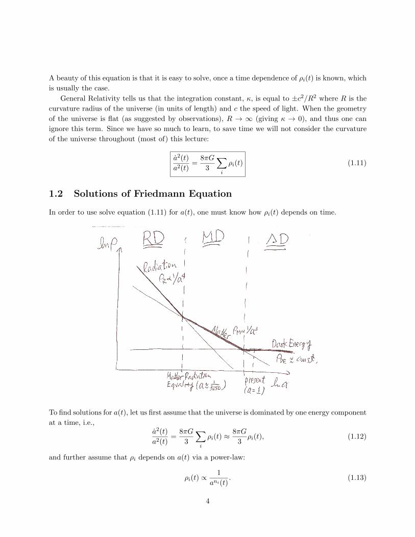
In order to use solve equation (1.11) for a(t), one must know how ρi(t) depends on time.

To find solutions for a(t), let us first assume that the universe is dominated by one energy component

at a time, i.e.,a2(t)

a2(t)=

8πG

3

∑i

ρi(t) ≈8πG

3ρi(t), (1.12)

and further assume that ρi depends on a(t) via a power-law:

ρi(t) ∝1

ani(t). (1.13)

4

Finding the solution is straightforward:

a(t) ∝ t2/ni . (1.14)

This is usually an excellent approximation, except for the transition era where two energy compo-

nents are equally important. There are 3 important cases:

1. Radiation-dominated (RD) era. A radiation component (photons, massless neutrinos, or

any other massless particles) has a large pressure, PR = ρR/3,§ which gives ρR(t) ∝ 1/a4(t),

or nR = 4. We thus obtain

aRD(t) ∝ t1/2. (1.15)

The expansion of the universe decelerates. With this solution, we can relate the age of the

universe to the Hubble expansion rate:

H(t) =a(t)

a(t)=

1

2t. (1.16)

2. Matter-dominated (MD) era. A matter component (baryons, cold dark matter, or any

other non-relativistic particles) has a negligible pressure compared to its energy density, PM ρM , which gives ρM (t) ∝ 1/a3(t), or nM = 3. We thus obtain

aMD(t) ∝ t2/3. (1.17)

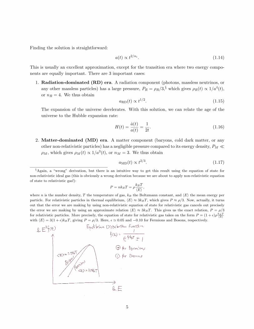
§Again, a “wrong” derivation, but there is an intuitive way to get this result using the equation of state for

non-relativistic ideal gas (this is obviously a wrong derivation because we are about to apply non-relativistic equation

of state to relativistic gas!):

P = nkBT = ρkBT

〈E〉 ,

where n is the number density, T the temperature of gas, kB the Boltzmann constant, and 〈E〉 the mean energy per

particle. For relativistic particles in thermal equilibrium, 〈E〉 ≈ 3kBT , which gives P ≈ ρ/3. Now, actually, it turns

out that the error we are making by using non-relativistic equation of state for relativistic gas cancels out precisely

the error we are making by using an approximate relation 〈E〉 ≈ 3kBT . This gives us the exact relation, P = ρ/3

for relativistic particles. More precisely, the equation of state for relativistic gas takes on the form P = (1 + ε)ρ kBT〈E〉with 〈E〉 = 3(1 + ε)kBT , giving P = ρ/3. Here, ε ' 0.05 and −0.10 for Fermions and Bosons, respectively.

5

The expansion of the universe decelerates. With this solution, we can relate the age of the

universe to the Hubble expansion rate:

H(t) =a(t)

a(t)=

2

3t. (1.18)

3. Constant-energy-density-dominated (ΛD) era. A hypothetical energy component (let’s

call it Λ) whose energy density is a constant over time, nΛ = 0. In this case we cannot use

equation (1.14). Going back to equation (1.12) and setting ρΛ = constant, we get a/a =

constant, whose solution is

aΛD(t) ∝ eHt, (1.19)

where an integration constant, H, is the same as the Hubble expansion rate (which is a

constant for this model). The expansion of the universe accelerates, which must mean that,

according to the acceleration equation (1.4), the pressure of this energy component is negative.

The conservation equation (1.5) tells us that such a component indeed has an enormous

negative pressure given by

PΛ = −ρΛ. (1.20)

While this looks quite strange, we now know that something like this may actually exist

in our universe, as the current observations suggest that the present-day universe is indeed

accelerating.

6

1.3 Equation of State of “Dark Energy” and Density Parameters

The matter has PM ρM ; the radiation has PR = ρR/3; and Λ has PΛ = −ρΛ. This motivates

our writing the equation of state of the ith component in the following simple form:

Pi = wiρi. (1.21)

Here, wi is called the “equation of state parameter,” and can depend on time (although it is usually

taken to be constant).

Why this form? It is important to keep in mind that there is no fundamental reason why we

should use this form. This form is often used either just for convenience, or simply for parametrizing

something we do not know. At the very least, this form is exact for radiation, wR = 1/3, and for

Λ, wΛ = −1. For matter, since wM 1, the exact value does not affect the results very much.

The equation of state parameter is almost exclusively used for parametrizing “dark energy,”

which is supposed to cause the observed acceleration of the universe. If we assume that w for dark

energy, wDE , is constant, then the current observations suggest that (Komatsu, et al., ApJS, 192,

18 (2011))

wDE = −0.98± 0.05 (68% CL). (1.22)

In other words, the energy density of dark energy is consistent with being a constant (wDE = wΛ =

−1).

Determining wDE with better accuracy may tell us something about the nature of dark energy,

especially if wDE 6= 1 is found with high statistical significance, as it would tell us that dark energy

is something dynamical (time-dependent).

Ignoring a potential interaction between dark energy and other components in the universe

(e.g., dark matter), the energy density of dark energy obeys (see equation (1.6))

ρDE(t) + 3a(t)

a(t)(1 + wDE) ρDE(t) = 0, (1.23)

whose solution is ρDE(t) ∝ [a(t)]−3(1+wDE). On the other hand, if we do not assume that wDE is a

constant, then the energy density of dark energy obeys

ρDE(t) + 3a(t)

a(t)[1 + wDE(t)] ρDE(t) = 0, (1.24)

whose solution is

ρDE(t) ∝ e−3∫d ln a[1+wDE(a)]. (1.25)

Putting these results together, we obtain the Friedmann equation for our Universe containing

radiation, matter, and dark energy (but not curvature) as

a2(t)

a2(t)= H2(t) =

8πG

3

[ρM (t0)

a3(t0)

a3(t)+ ρR(t0)

a4(t0)

a4(t)+ ρDE(t0)e

−3∫ a(t)a(t0)

d ln a[1+wDE(a)]], (1.26)

where t0 is some epoch, which is usually taken to be the present epoch.

7

Now, taking t→ t0, we find the present-day expansion rate

H20 ≡ H2(t0) =

8πG

3[ρM (t0) + ρR(t0) + ρDE(t0)] ≡ 8πG

3ρc(t0), (1.27)

which has been determined to be H0 ≈ 70 km/s/Mpc. Here, ρc(t0) is the so-called “critical density”

of the universe, which is equal to the total energy density of the universe when the universe is flat.

The numerical value of the critical density is

ρc(t0) ≡ 3H20

8πG= 2.775× 1011 h2 M Mpc−3. (1.28)

The critical density provides a natural unit for the energy density of the universe, and thus it is

convenient to measure all the energy densities in units of ρc(t0). Defining the so-called density

parameters, Ωi, as

Ωi ≡ρi(t0)

ρc(t0), (1.29)

one can rewrite the Friedmann equation (1.26) in a compact form:

H2(t)

H20

= ΩMa3(t0)

a3(t)+ ΩR

a4(t0)

a4(t)+ ΩDEe

−3∫ a(t)a(t0)

d ln a[1+wDE(a)](1.30)

Basically, most of the literature on cosmology (within the context of General Relativity) use this

equation as the starting point.¶ Taking z = 0, one finds that all the density parameters must sum

to unity:∑

i Ωi = 1.

In summary, the Friedmann equation is a combination of two key equations: (1) the equation

describing how the universe decelerates/accelerates depending on the energy density and pressure of

the constituents, and (2) the equation describing the energy conservation of the constituents. Once

the Friedmann equation is given with the proper right hand side containing the energy densities of

the relevant constituents of the universe, we can find a(t) as a function of time easily.

¶An interesting possibility is that General Relativity may not be valid on cosmological scales. There are scenarios

in which the form of the Friedmann equation is modified. One widely-explored example is the so-called Dvali-

Gabadadze-Porrati (DGP) model (Dvali, Gabadadze & Porrati, Phys. Lett. B485, 208 (2000)). In this scenario, the

Friedmann equation is modified to:

H2(t)− H(t)

rc=

8πG

3

∑i

ρi(t),

where rc is some length scale below which General Relativity is restored. (For r rc, the potential is given by

−GNm/r where GN is the ordinary Newtonian gravitational constant. For r rc, the potential is modified to

−G5m/r2 and decays faster. G5 is the gravitational strength in the 5th dimension.) This model has attracted a huge

attention of the cosmology community, as it was shown that this modified Friedmann equation gives an accelerating

expansion without dark energy. Namely, even when the right hand side contains only matter, the solution for this

equation can still exhibit an accelerating expansion. As this is a quadratic equation for H(t), we can solve it and find

H(t) =1

2

(1

rc±√

1

r2c

+32πG

3ρM (t)

).

At late times when ρ(t) becomes negligible compared to the other term, one of the solutions is given by a(t) ∝ et/rc ,i.e., an exponential, accelerated expansion.

8

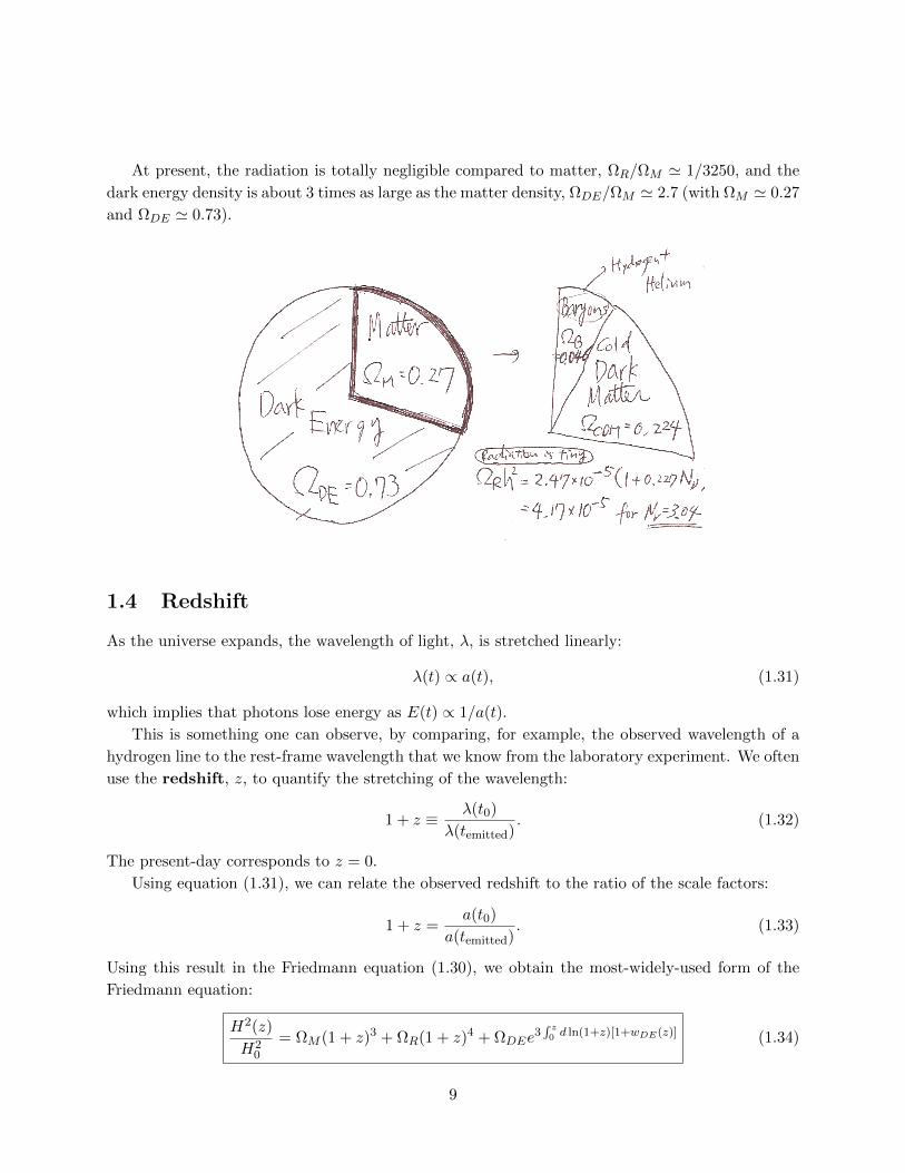
At present, the radiation is totally negligible compared to matter, ΩR/ΩM ' 1/3250, and the

dark energy density is about 3 times as large as the matter density, ΩDE/ΩM ' 2.7 (with ΩM ' 0.27

and ΩDE ' 0.73).

1.4 Redshift

As the universe expands, the wavelength of light, λ, is stretched linearly:

λ(t) ∝ a(t), (1.31)

which implies that photons lose energy as E(t) ∝ 1/a(t).

This is something one can observe, by comparing, for example, the observed wavelength of a

hydrogen line to the rest-frame wavelength that we know from the laboratory experiment. We often

use the redshift, z, to quantify the stretching of the wavelength:

1 + z ≡ λ(t0)

λ(temitted). (1.32)

The present-day corresponds to z = 0.

Using equation (1.31), we can relate the observed redshift to the ratio of the scale factors:

1 + z =a(t0)

a(temitted). (1.33)

Using this result in the Friedmann equation (1.30), we obtain the most-widely-used form of the

Friedmann equation:

H2(z)

H20

= ΩM (1 + z)3 + ΩR(1 + z)4 + ΩDEe3∫ z0 d ln(1+z)[1+wDE(z)] (1.34)

9

From this result, it follows that the best way to determine the equation of state of dark

energy is to measure H(z) over a wide range of z. If we can only measure the expansion

rates at z 1, then Taylor expansion of equation (1.34) with ΩR ΩM and ΩDE ' 1−ΩM gives

H2(z 1)

H20

≈ 1 + 3ΩMz + 3(1 + wDE)(1− ΩM )z. (1.35)

As we know from observations that |1 + wDE | is small (of order 10−1 or less), the third term is

tiny compared to other terms, making it difficult to measure wDE . This is why we need to measure

H(z) over a wide redshift range.

1.5 Alcock-Paczynski Test

We have learned that, in order to determine wDE , we need to measure H(z) over a wide redshift

range. But, how? In principle, one can measure H(z) in the following way.

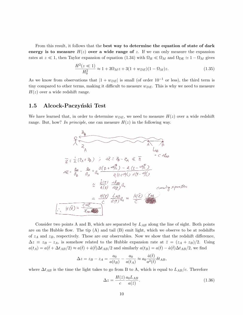
Consider two points A and B, which are separated by LAB along the line of sight. Both points

are on the Hubble flow. The tip (A) and tail (B) emit light, which we observe to be at redshifts

of zA and zB, respectively. These are our observables. Now we show that the redshift difference,

∆z ≡ zB − zA, is somehow related to the Hubble expansion rate at z = (zA + zB)/2. Using

a(tA) = a(t+ ∆tAB/2) ≈ a(t) + a(t)∆tAB/2 and similarly a(tB) = a(t)− a(t)∆tAB/2, we find

∆z = zB − zA =a0

a(tB)− a0

a(tA)≈ a0

a(t)

a2(t)δtAB,

where ∆tAB is the time the light takes to go from B to A, which is equal to LAB/c. Therefore

∆z =H(z)

c

a0LABa(z)

. (1.36)

10

Here, a0LAB/a(z) = xAB is a comoving separation (which is time-independent; a0 is the scale factor

at present). Rewriting the result in terms of H(z) and xAB, we finally find the relation between

what we want to determine, H(z), and the observable, ∆z, as

H(z) =c∆z

xAB(1.37)

This is a beautiful result, but has one problem. In order to use this method, we need to know

the intrinsic comoving separation, xAB, which is not always known. (As a matter of fact, xAB is

not known for most cases.) In other words, this method works if we have the standard ruler, for

which the intrinsic size is known.

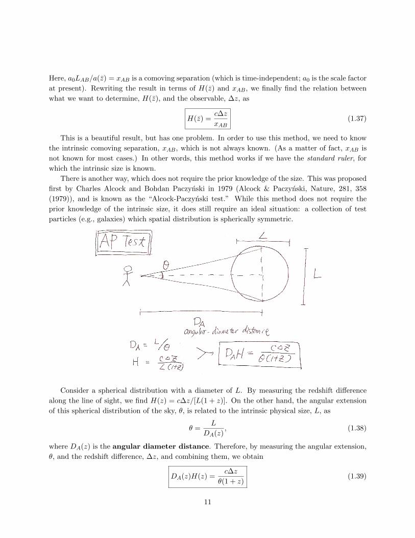
There is another way, which does not require the prior knowledge of the size. This was proposed

first by Charles Alcock and Bohdan Paczynski in 1979 (Alcock & Paczynski, Nature, 281, 358

(1979)), and is known as the “Alcock-Paczynski test.” While this method does not require the

prior knowledge of the intrinsic size, it does still require an ideal situation: a collection of test

particles (e.g., galaxies) which spatial distribution is spherically symmetric.

Consider a spherical distribution with a diameter of L. By measuring the redshift difference

along the line of sight, we find H(z) = c∆z/[L(1 + z)]. On the other hand, the angular extension

of this spherical distribution of the sky, θ, is related to the intrinsic physical size, L, as

θ =L

DA(z), (1.38)

where DA(z) is the angular diameter distance. Therefore, by measuring the angular extension,

θ, and the redshift difference, ∆z, and combining them, we obtain

DA(z)H(z) =c∆z

θ(1 + z)(1.39)

11

The right hand side only contains the observables, and thus the Alcock-Paczynski test allows us to

determine DAH.

A challenge for this method is to find objects whose distribution is spherically symmetric. There

is one known example, which is the distribution of the large-scale structure. We will come back to

this later.

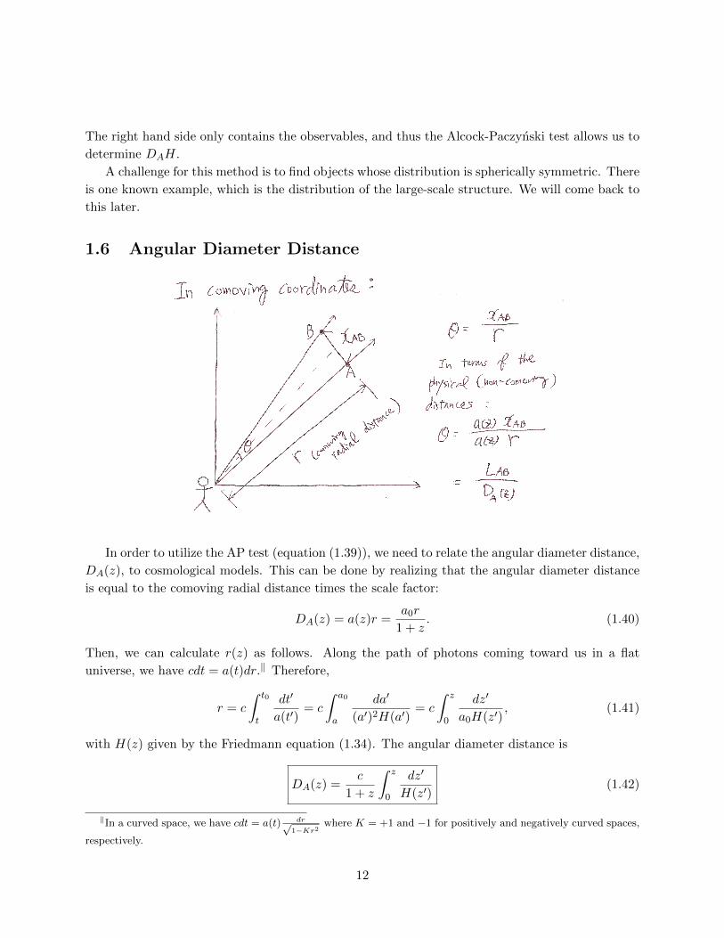
1.6 Angular Diameter Distance

In order to utilize the AP test (equation (1.39)), we need to relate the angular diameter distance,

DA(z), to cosmological models. This can be done by realizing that the angular diameter distance

is equal to the comoving radial distance times the scale factor:

DA(z) = a(z)r =a0r

1 + z. (1.40)

Then, we can calculate r(z) as follows. Along the path of photons coming toward us in a flat

universe, we have cdt = a(t)dr.‖ Therefore,

r = c

∫ t0

t

dt′

a(t′)= c

∫ a0

a

da′

(a′)2H(a′)= c

∫ z

0

dz′

a0H(z′), (1.41)

with H(z) given by the Friedmann equation (1.34). The angular diameter distance is

DA(z) =c

1 + z

∫ z

0

dz′

H(z′)(1.42)

‖In a curved space, we have cdt = a(t) dr√1−Kr2

where K = +1 and −1 for positively and negatively curved spaces,

respectively.

12

Using this result in equation (1.39), we find that the Alcock-Paczynski test provides (in a flat

universe):

H(z)

∫ z

0

dz′

H(z′)=

∆z

θ. (1.43)

As the angular diameter distance is an integral of 1/H(z), it is less sensitive to the equation of

state of dark energy. However, if we have many measurements of DA(z) at various redshifts, we

can effectively differentiate DA(z) with respect to z, obtaining a measurement of 1/H(z). While

we have not yet entered the era where we can do this with the angular diameter distance, we have

been able to do this using the luminosity distances measured out to distant Type Ia supernovae,

as described next.

1.7 Luminosity Distance

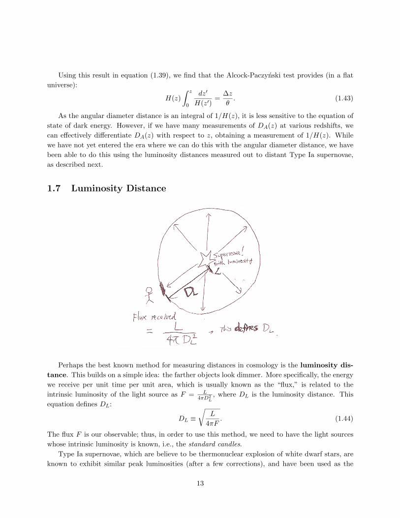
Perhaps the best known method for measuring distances in cosmology is the luminosity dis-

tance. This builds on a simple idea: the farther objects look dimmer. More specifically, the energy

we receive per unit time per unit area, which is usually known as the “flux,” is related to the

intrinsic luminosity of the light source as F = L4πD2

L, where DL is the luminosity distance. This

equation defines DL:

DL ≡√

L

4πF. (1.44)

The flux F is our observable; thus, in order to use this method, we need to have the light sources

whose intrinsic luminosity is known, i.e., the standard candles.

Type Ia supernovae, which are believe to be thermonuclear explosion of white dwarf stars, are

known to exhibit similar peak luminosities (after a few corrections), and have been used as the

13

primary standard candles in the cosmology community. In fact, it was the observation of Type Ia

supernovae which led to the discovery of the acceleration of the universe (Riess et al., AJ, 116, 1009

(1998); Perlmutter et al., ApJ, 517, 565 (1999)).

Now, we must relate DL to cosmological models. To do this, we first note that the energy

emitted by a supernova is diluted by the surface area, which is 4πr2a20. Second, each photon

emitted by a supernova loses energy as E ∝ a/a0 = 1/(1 + z). Third, the rate at which photons

are received per unit time is dilated by a factor of a/a0 = 1/(1 + z) compared to the rate at which

the light was emitted by a supernova. (I.e., we receive fewer photons per second at our location,

relative to the number of photons emitted per second at the source). This leads to the cosmological

inverse-square-law formula:

F =L/(1 + z)2

4πr2a20

. (1.45)

Comparing this formula to the definition of DL above, we conclude that

DL(z) = a0(1 + z)r = (1 + z)2DA(z) (1.46)

This relation, DL(z) = (1 + z)2DA(z), is exact, and does not depend on cosmological models.

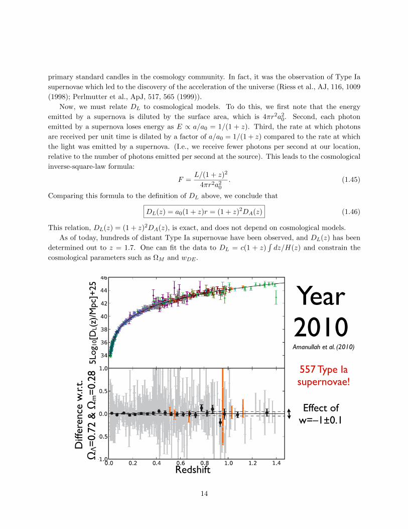
As of today, hundreds of distant Type Ia supernovae have been observed, and DL(z) has been

determined out to z = 1.7. One can fit the data to DL = c(1 + z)∫dz/H(z) and constrain the

cosmological parameters such as ΩM and wDE .

Redshift

5Log

10[D

L(z)

/Mpc

]+25

Diff

eren

ce w

.r.t.

ΩΛ=

0.72

& Ω

m=

0.28

Effect of w=–1±0.1

Year 2010Amanullah et al. (2010)

557 Type Ia supernovae!

14

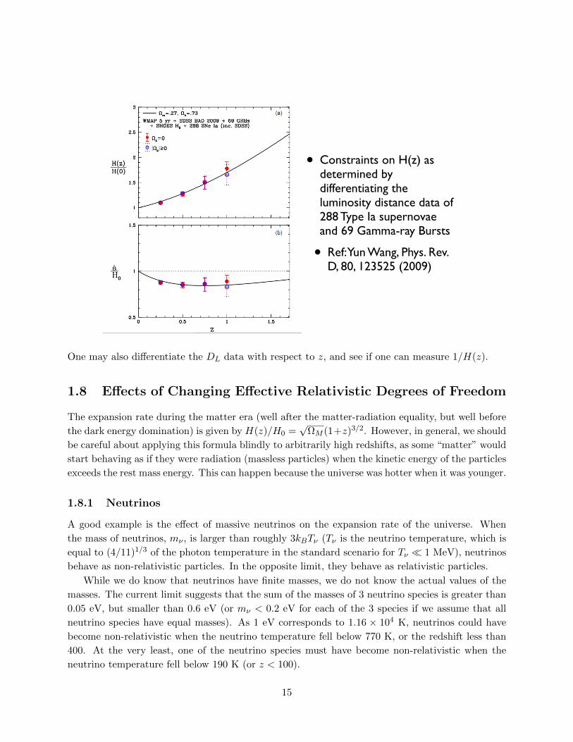
• Constraints on H(z) as determined by differentiating the luminosity distance data of 288 Type Ia supernovae and 69 Gamma-ray Bursts

• Ref: Yun Wang, Phys. Rev. D, 80, 123525 (2009)

One may also differentiate the DL data with respect to z, and see if one can measure 1/H(z).

1.8 Effects of Changing Effective Relativistic Degrees of Freedom

The expansion rate during the matter era (well after the matter-radiation equality, but well before

the dark energy domination) is given by H(z)/H0 =√

ΩM (1+z)3/2. However, in general, we should

be careful about applying this formula blindly to arbitrarily high redshifts, as some “matter” would

start behaving as if they were radiation (massless particles) when the kinetic energy of the particles

exceeds the rest mass energy. This can happen because the universe was hotter when it was younger.

1.8.1 Neutrinos

A good example is the effect of massive neutrinos on the expansion rate of the universe. When

the mass of neutrinos, mν , is larger than roughly 3kBTν (Tν is the neutrino temperature, which is

equal to (4/11)1/3 of the photon temperature in the standard scenario for Tν 1 MeV), neutrinos

behave as non-relativistic particles. In the opposite limit, they behave as relativistic particles.

While we do know that neutrinos have finite masses, we do not know the actual values of the

masses. The current limit suggests that the sum of the masses of 3 neutrino species is greater than

0.05 eV, but smaller than 0.6 eV (or mν < 0.2 eV for each of the 3 species if we assume that all

neutrino species have equal masses). As 1 eV corresponds to 1.16 × 104 K, neutrinos could have

become non-relativistic when the neutrino temperature fell below 770 K, or the redshift less than

400. At the very least, one of the neutrino species must have become non-relativistic when the

neutrino temperature fell below 190 K (or z < 100).

15

As the expansion rate is solely determined by the energy density of the constituents (in a flat

universe), all we need to calculate is the energy density of neutrinos. As neutrinos are Fermions

and were in thermal equilibrium in the early universe, their distribution function is given by the

Fermi-Dirac distribution. Also, as they decoupled from the plasma when neutrinos were still highly

relativistic (when the temperature of the universe was about 2 MeV∼ 20 billion K), their dis-

tribution function will remain the Fermi-Dirac distribution for massless particles, even after

neutrinos became non-relativistic.

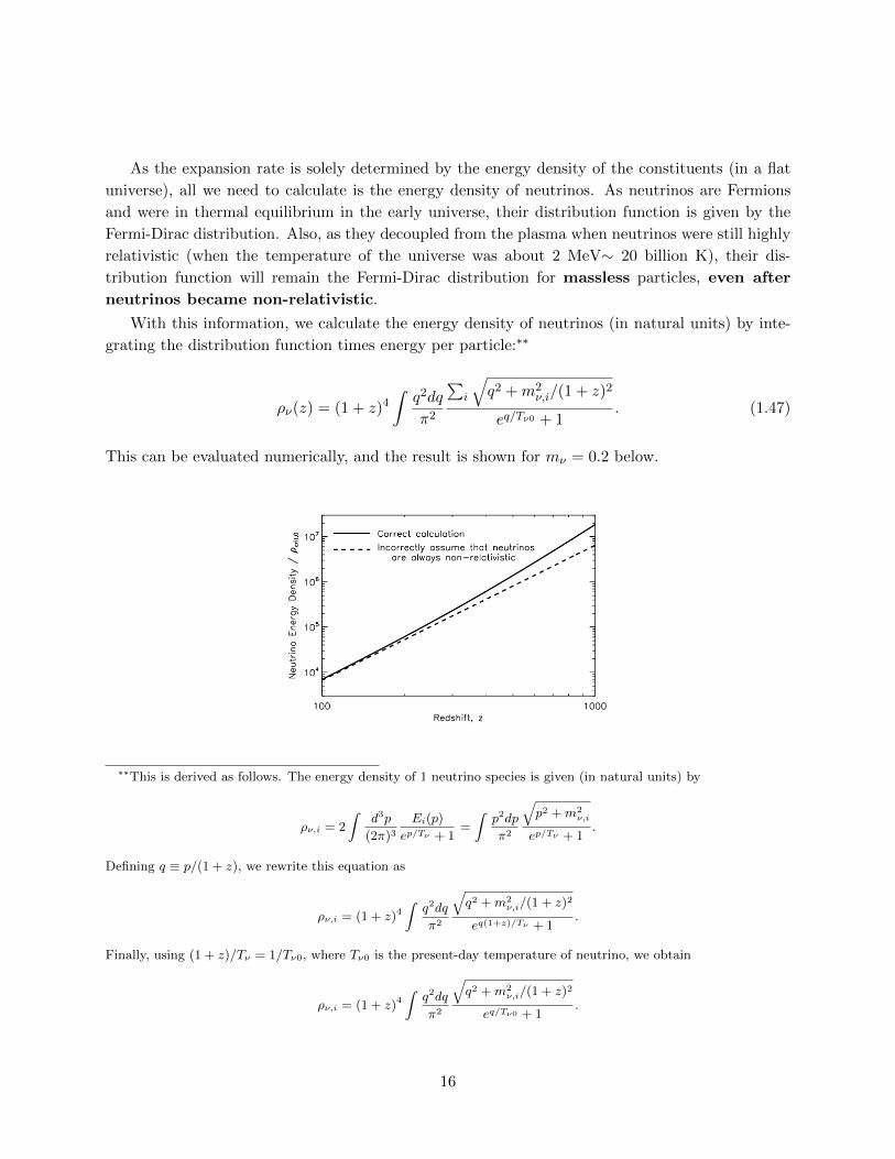
With this information, we calculate the energy density of neutrinos (in natural units) by inte-

grating the distribution function times energy per particle:∗∗

ρν(z) = (1 + z)4

∫q2dq

π2

∑i

√q2 +m2

ν,i/(1 + z)2

eq/Tν0 + 1. (1.47)

This can be evaluated numerically, and the result is shown for mν = 0.2 below.

∗∗This is derived as follows. The energy density of 1 neutrino species is given (in natural units) by

ρν,i = 2

∫d3p

(2π)3

Ei(p)

ep/Tν + 1=

∫p2dp

π2

√p2 +m2

ν,i

ep/Tν + 1.

Defining q ≡ p/(1 + z), we rewrite this equation as

ρν,i = (1 + z)4

∫q2dq

π2

√q2 +m2

ν,i/(1 + z)2

eq(1+z)/Tν + 1.

Finally, using (1 + z)/Tν = 1/Tν0, where Tν0 is the present-day temperature of neutrino, we obtain

ρν,i = (1 + z)4

∫q2dq

π2

√q2 +m2

ν,i/(1 + z)2

eq/Tν0 + 1.

16

1.8.2 General Consideration

As we go farther back in time, various other particles, such as electrons and positrons, become

relativistic, and these effects must be taken into account when calculating the expansion rate.

More specifically, when the temperature of the universe was higher than above 1 MeV, but lower

than 2 times the muon mass (105.7 MeV), the relativistic particles included photons, 3 neutrino

species, electrons, and positrons. And, they all shared the same temperature, T . The energy

density can be found easily by integrating the corresponding distribution functions times energy

per particle. In natural units, we find

ργ = 2

∫p3dp

2π2

1

ep/T − 1=π2

15T 4, (1.48)

ρν = 6

∫p3dp

2π2

1

ep/T + 1=

7π2

40T 4, (1.49)

ρe± = 4

∫p3dp

2π2

1

ep/T + 1=

7π2

60T 4. (1.50)

Here, “2” for photons is the number of helicity states (i.e., left and right circular polarization

states); “6” for neutrinos is the number of helicity state (1; just left-handed neutrinos) times the

number of neutrino species (3) times 2 because we count both neutrinos and anti-neutrinos; and

“4” for electrons/positrons is the number of spin states (2; up and down) times 2 because we count

both electrons and positrons.

It is more common to define the “effective number of relativistic degrees of freedom” by writing

the total radiation energy as

ρR = ργ + ρν + ρe± =π2

30g∗T

4, (1.51)

where

g∗ = 2 +7

8(6 + 4) =

43

4. (1.52)

With this, the expansion rate during the radiation era is given by

H2 =8πG

3ρR =

4π3G

45g∗T

4. (1.53)

Therefore, when we calculate the expansion rate during the radiation era, we must be careful about

how many relativistic degrees of freedom we have in the universe at a given time. For g∗ = 43/4,

we obtain1

H(T )= 1.48

(1 MeV

T

)2

sec. (1.54)

As the age of the universe during the radiation era is t = 1/(2H), we also have

t =1

2H(T )= 0.74

(1 MeV

T

)2

sec (1.55)

Again, this formula is valid only for 1 MeV < T 200 MeV. Above this temperature, we will

need to count muons as relativistic particles, etc.

17

PROBLEM SET 1

1.1 Expansion of the Universe

In this section, we will use Einstein’s General Relativity to derive the equations that describe the

expanding universe. Einstein’s General Relativity describes the evolution of gravitational fields for

a given source of energy density, momentum, and stress (e.g., pressure). Schematically,

[Curvature of Space-time] =8πG

c4[Energy density, Momentum, and Stress]

Here, the dimension of “curvature of space-time” is 1/(length)2, as the curvature is usually defined

as the second derivative of a function with respect to independent variables, and for our application

the independent variables are space-time coordinates: xµ = (ct, x1, x2, x3) for µ = 0, 1, 2, 3.

1.1.1 Space-time Curvature: Left Hand Side of Einstein’s Equation

The coefficient on the right hand side, 8πG/c4, is chosen such that Einstein’s gravitational field

equations reduce to the familiar Poisson equation when gravitational fields are weak and static,

and the space is not expanding: ∇2φN = 4πGρM , where φN is the usual Newtonian potential, and

ρM is the mass density. Let us rewrite it in the following suggestive form:

∇2

(2φNc2

)=

8πG

c4(ρMc

2).

Here, as φN/c2 is dimensionless, and thus the left hand side has the dimension of curvature,

i.e., 1/(length)2. The right hand side contains ρMc2, which is energy density; thus, G/c4 correctly

converts energy density into curvature. Now, this equation tells us something Newton did not know

but Einstein finally figured out: the second derivative of the dimensionless Newtonian potential

times 2 with respect to space coordinates is the curvature of space, and mass deforms space.

In order to calculate curvature of space-time, we need to know how to calculate a distance be-

tween two points. Of course, everyone knows that, in Cartesian coordinates, the distance between

two points in flat space separated by dxi = (dx1, dx2, dx3) is given by dl =√

(dx1)2 + (dx2)2 + (dx3)2,

or

dl2 =3∑i=1

3∑j=1

δijdxidxj , (1.56)

where δij = 1 for i = j and δij = 0 for i 6= j. Since space is flat, the curvature of this space is zero.

This is a consequence of the coefficients of dxidxj on the right hand side of equation (1.56) being

independent of coordinates. In general, when space is not flat but curved, the distance between

two points can be written as

dl2 =3∑i=1

3∑j=1

gij(x)dxidxj , (1.57)

18

where gij(x) is known as the metric tensor. Schematically, the curvature of space is given by the

second derivatives of the metric tensor with respect to space coordinates:

Curvature of Space ∼ ∂2gij∂xk∂xl

.

In General Relativity, we extend this to the curvature of space-time. The distance between two

points in space and time separated by dxµ = (cdt, dx1, dx2, dx3) is given by

ds2 =3∑

µ=0

3∑ν=0

gµν(x)dxµdxν , (1.58)

and

Curvature of Space-time ∼ ∂2gµν∂xµ∂xν

.

Now, let us get into the gory details! The precise definition of space-time curvature, known as the

Riemann curvature tensor, is given by††

Rµνρσ ≡∂Γµνσ∂xρ

− ∂Γµνρ∂xσ

+∑α

ΓανσΓµαρ −∑α

ΓανρΓµασ, (1.59)

where Γ is the so-called Christoffel symbol, also known as the affine connection:

Γµνρ ≡1

2

∑α

gµα(∂gαρ∂xν

+∂gνα∂xρ

− ∂gνρ∂xα

). (1.60)

The metric tensor with the superscripts, gµα, is the inverse of the metric tensor, in the sense that∑α

gµαgαν = δµν ,

where δµν = 1 for µ = ν and zero otherwise.

Question 1.1: For an expanding universe with flat space, the distance between two points in

space is given by, perhaps not surprisingly,

dl2 = a2(t)

3∑i=1

3∑j=1

δijdxidxj , (1.61)

where x denotes comoving coordinates. The scale factor, a(t), depends only on time t. Then,

the distance between two points in space-time is given by

ds2 = −c2dt2 + dl2

= −c2dt2 + a2(t)

3∑i=1

3∑j=1

δijdxidxj . (1.62)

††Different definitions of curvature are used in the literature. Here, we follow the definition used by Misner, Thorne,

and Wheeler, “Gravitation” (1973). Steven Weinberg’s recent textbook, “Cosmology,” uses the opposite sign.

19

Non-zero components of the metric tensor are

g00 = −1; gii = a2(t) for i = 1, 2, 3,

and those of the corresponding inverse are

g00 = −1; gii =1

a2(t)for i = 1, 2, 3.

This metric is known as the Robertson-Walker metric (for flat space), and describes the distance

between two points in space-time of a homogeneous, isotropic, and expanding universe. For this

metric, non-zero components of the affine connection are Γij0 and Γ0ij . Calculate Γij0 and Γ0

ij . The

answers will contain a, a/c, and δij . Once again, our space-time coordinates are xµ = (ct, x1, x2, x3).

Question 1.2: Einstein’s field equations do not use all the components of the Riemann tensor,

but only use a part of it. Specifically, they will use the so-called Ricci tensor:

Rµν ≡∑α

Rαµαν

=∑α

(∂Γαµν∂xα

−∂Γαµα∂xν

)+∑αβ

(ΓβµνΓαβα − ΓβµαΓαβν

), (1.63)

and the Ricci scalar:

R ≡∑µν

gµνRµν . (1.64)

For the above flat Robertson-Walker metric, non-zero components of the Ricci tensor are R00 and

Rij . Calculate R00, Rij , and R. The answers will contain a, a/c, a/c2, and/or δij .

Question 1.3: The left hand side of Einstein’s equation is called the Einstein tensor, denoted

by Gµν , and is defined as

Gµν ≡ Rµν −1

2gµνR. (1.65)

Calculate G00 and Gij .

1.1.2 Stress-Energy Tensor: Right Hand Side of Einstein’s Equation

The precise form of Einstein’s field equation is

Gµν =8πG

c4Tµν , (1.66)

where Tµν is called the stress-energy tensor (also sometimes called “energy-momentum tensor”).

As the name suggests, the components of Tµν represent the following quantities:

• T00: Energy density,

20

• T0i: Momentum, and

• Tij : Stress (which includes pressure, viscosity, and heat conduction).

For a perfect fluid, the stress-energy tensor takes on the following specific form:

Tµν = Pgµν + (ρ+ P )(∑

α gµαuα)(∑

β gνβuβ)

c2, (1.67)

where ρ and P are the energy density and pressure, respectively, and uµ is a four-dimensional

velocity of a fluid element. The spatial components of a four velocity, ui, represent the usual 3-

dimensional velocity of a fluid element, while the temporal component, u0, is determined by the

normalization condition of uµ:

gµνuµuν = −c2. (1.68)

Note that the 3-dimensional velocity, ui, does not contain the apparent motion due to the expansion

of the universe, but only contains the true motion of fluid elements.

Question 1.4: In a homogeneous, isotropic, and expanding universe, fluid elements simply

move along the expansion of the universe, and the 3-dimensional velocity vanishes. (In other

words, fluids are comoving with expansion.) Therefore, such a fluid element has ui = 0, and the

normalization condition gives u0 = c. Non-zero components of the stress-energy tensor are T00 and

Tij . Calculate T00 and Tij for the flat Robertson-Walker metric and comoving fluid.

Question 1.5: Now, we are ready to obtain Einstein’s equations. First, write down G00 =

(8πG/c4)T00 and Gij = (8πG/c4)Tij for the flat Robertson-Walker metric and comoving fluid in

terms of a, a/c, a/c2, and/or δij . Then, by combining these equations, obtain the right hand side of

a2

a2=

a

a=

The first equation is the Friedmann equation, and the second one is the acceleration equation that

we have learned in class (with c = 1).

1.1.3 Energy Conservation

Combining the above equations for a/a and a/a will yield the energy conservation equation, ρ +

3 aa(ρ+ P ) = 0. In other words, the energy conservation is already built into Einstein’s equations.

Question 1.6: Alternatively, one can derive the energy conservation equation directly from

the conservation of the stress-energy tensor. In General Relativity, the “conservation” means that

the covariant derivative (rather than the partial derivative) of the stress-energy tensor vanishes.

0 =∑αβ

gαβTµα;β ≡∑αβ

gαβ

(∂Tµα∂xβ

−∑λ

ΓλαβTµλ −∑λ

ΓλµβTλα

). (1.69)

21

The energy conservation equation is∑

αβ gαβT0α;β = 0, while the momentum conservation equation

is∑

αβ gαβTiα;β = 0. Reproduce ρ+ 3 aa(ρ+ P ) = 0 from

∑αβ g

αβT0α;β = 0.

1.1.4 Cosmological Redshift

Consider a non-relativistic particle, which is moving in a gravitational field with a 3-dimensional

velocity of ui c. The other external forces (such as the electromagnetic force) are absent.

According to General Relativity, the equation of motion of such a particle is

dui

dτ+∑αβ

Γiαβuαuβ = 0, (1.70)

where dτ ≡√−ds2/c is called the proper time. The four-dimensional velocity is given by uµ =

dxµ/dτ ; thus, u0 = cdt/dτ and ui = dxi/dτ .

Question 1.7: Using the affine connection for the flat Robertson-Walker metric, rewrite the

equation of motion in terms of ui = dui/dt, a/a and ui. Show how ui changes with the scale factor, a(t).

22

Chapter 2

Cosmic Microwave Background

2.1 Basic Properties

The cosmic microwave background is the oldest light that one can ever hope to measure directly.

This light delivers the direct information of the physics condition of the universe when the universe

was only 380,000 years old (which is z = 1090).

The important characteristics of the cosmic microwave background are:

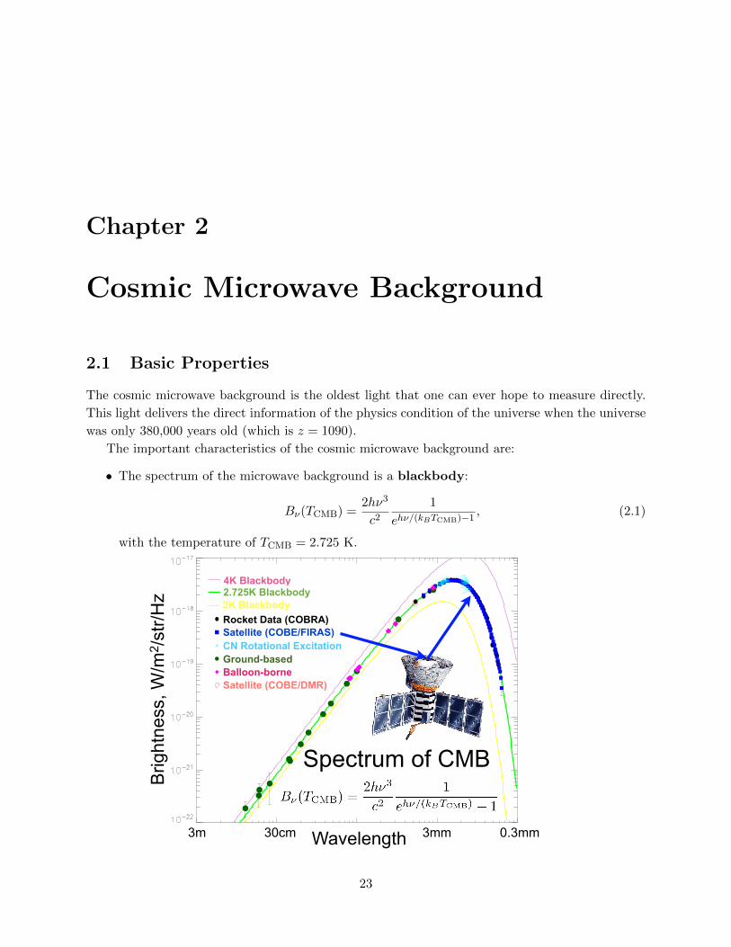
• The spectrum of the microwave background is a blackbody:

Bν(TCMB) =2hν3

c2

1

ehν/(kBTCMB)−1, (2.1)

with the temperature of TCMB = 2.725 K.

Spectrum of CMB

4K Blackbody2.725K Blackbody2K BlackbodyRocket Data (COBRA)Satellite (COBE/FIRAS)CN Rotational ExcitationGround-basedBalloon-borneSatellite (COBE/DMR)

Wavelength 3mm 0.3mm30cm3m

Brig

htne

ss, W

/m2 /s

tr/H

z

23

• The photons of the microwave background are numerous: their number density is nCMB =

410 cm−3,∗ which is about 2 billion times the number density of baryons. We do not quite

know why baryons are so few compared to photons.

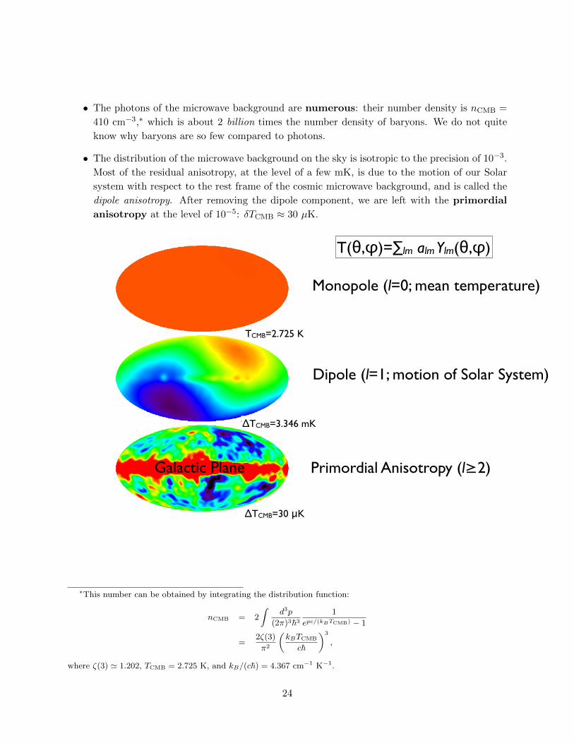
• The distribution of the microwave background on the sky is isotropic to the precision of 10−3.

Most of the residual anisotropy, at the level of a few mK, is due to the motion of our Solar

system with respect to the rest frame of the cosmic microwave background, and is called the

dipole anisotropy. After removing the dipole component, we are left with the primordial

anisotropy at the level of 10−5: δTCMB ≈ 30 µK.

TCMB=2.725 K

ΔTCMB=3.346 mK

ΔTCMB=30 μK

Monopole (l=0; mean temperature)

Dipole (l=1; motion of Solar System)

Primordial Anisotropy (l≥2)Galactic Plane

T(θ,φ)=∑lm alm Ylm(θ,φ)

∗This number can be obtained by integrating the distribution function:

nCMB = 2

∫d3p

(2π)3~3

1

epc/(kBTCMB) − 1

=2ζ(3)

π2

(kBTCMB

c~

)3

,

where ζ(3) ' 1.202, TCMB = 2.725 K, and kB/(c~) = 4.367 cm−1 K−1.

24

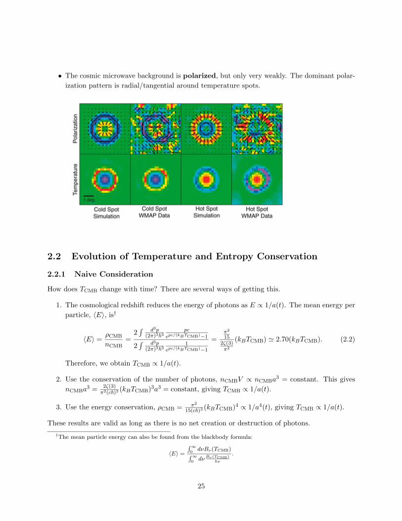
• The cosmic microwave background is polarized, but only very weakly. The dominant polar-

ization pattern is radial/tangential around temperature spots.

2.2 Evolution of Temperature and Entropy Conservation

2.2.1 Naive Consideration

How does TCMB change with time? There are several ways of getting this.

1. The cosmological redshift reduces the energy of photons as E ∝ 1/a(t). The mean energy per

particle, 〈E〉, is†

〈E〉 =ρCMB

nCMB=

2∫ d3p

(2π)3~3pc

epc/(kBTCMB)−1

2∫ d3p

(2π)3~31

epc/(kBTCMB)−1

=π2

152ζ(3)π2

(kBTCMB) ' 2.70(kBTCMB). (2.2)

Therefore, we obtain TCMB ∝ 1/a(t).

2. Use the conservation of the number of photons, nCMBV ∝ nCMBa3 = constant. This gives

nCMBa3 = 2ζ(3)

π2(c~)3 (kBTCMB)3a3 = constant, giving TCMB ∝ 1/a(t).

3. Use the energy conservation, ρCMB = π2

15(c~)3 (kBTCMB)4 ∝ 1/a4(t), giving TCMB ∝ 1/a(t).

These results are valid as long as there is no net creation or destruction of photons.

†The mean particle energy can also be found from the blackbody formula:

〈E〉 =

∫∞0dνBν(TCMB)∫∞

0dν Bν(TCMB)

hν

.

25

2.2.2 Entropy Conservation

Is there a general formula that we can use for calculating the evolution of temperature, even

when there is net creation or destruction of photons? The conservation of entropy provides such

a formula. Roughly speaking, the entropy is proportional to the number of particles, i.e., S ≈kBnV = constant. Because photons are much more numerous than matter particles, the entropy

of the universe is completely dominated by that of photons (and neutrinos, whose number density

is similar to the photon number density).

Let us calculate entropy. We begin with the first-law of thermodynamics, TdS = dU + PdV

(where U is the internal energy), and another thermodynamic equation, V dP = HdT/T = (U +

PV )dT/T (where H = U + PV is the enthalpy). By combining these equations, we obtain

dS = d

(U + PV

T

). (2.3)

Integrating, we get

S =U + PV

T+ constant (2.4)

The integration constant should be chosen such that S = 0 for the absolute zero temperature,

T = 0. We set the integration constant to be zero. Here, both U and P contain all the particles in

the universe, including both radiation and matter: U = UR + UM and P = PR + PM .

• Radiation. For radiation, we have UR = ρRV and PR = ρR/3. We find

SR =4ρRV

3T. (2.5)

Using the mean particle energy, 〈ER〉 = ρR/nR, one may rewrite this result as

SR = kBnRV ×4〈ER〉3kBT

≈ 4kBnRV. (2.6)

Therefore, indeed the entropy is given by the number of particles (times kB). More precisely,

by writing the radiation energy density as

ρR =π2

30g∗

(kBT )4

(c~)3, (2.7)

we obtain

SR = kB

[π2

30g∗

(kBT

c~

)3]V. (2.8)

As the effective number of relativistic degrees of freedom, g∗, can change with time, the

entropy conservation, SR = constant, with V ∝ a3(t) gives

T ∝ 1

g1/3∗ a(t)

(2.9)

Therefore, a simple relation such as T ∝ 1/a(t) holds only when the effective number of

relativistic species does not change, g∗ = constant.

26

• Matter. For matter, we have UM = 32kBnMV T

‡ and PM = nMkBT . We find

SM =5

2kBnMV. (2.10)

Again, indeed the entropy is given by the number of particles (times kB)§, and nR nM(e.g., the number density of photons is 2 billion times that of baryons) guarantees that we

can safely ignore the matter contribution to entropy.

2.2.3 Photon Heating due to Electron-Positron Annihilation

A good example for the temperature change due to the change in g∗ is the electron-positron anni-

hilation:

e+ + e− → γ + γ.

When the temperature of the universe was greater than the rest mass energy of an electron,

0.511 MeV, the pair-creation,

γ + γ → e+ + e−,

also occurred; however, when the universe cooled down below 0.511 MeV, the pair creation no

longer occurred.

In addition, particles behave as if they were relativistic when the temperature is greater than

≈ m/3; thus, electrons and positrons were sufficiently relativistic when the temperature of the

universe was greater than their rest mass energy.

Now, let us apply the entropy conservation:

T2 = T1

(g∗,1g∗,2

)1/3

, (2.11)

where T1 and T2 are the photon temperatures before and after the annihilation, respectively. The

effective numbers of relativistic degrees of freedom are

g∗,1 = 2 +7

8× 4 =

11

2,

g∗,2 = 2,

‡Here, we do not include the mass energy in the internal energy.§This expression, derived from thermodynamics of ideal gas, is only approximate. More rigorous derivation using

the famous Boltzmann’s entropy formula, S = kB lnW , where W is the number of possible states, gives the so-called

Sackur–Tetrode equation for non-relativistic, monatomic ideal gas:

SM = kBnBV

[5

2+ ln

(1

nMΛ3

)],

where Λ ≡ ~√

2π/(mkBT ) is known as the thermal de Broglie length and m is the particle mass. Note that this

formula is valid only when nMΛ3 1 (which means that quantum effects are negligible).

27

before and after the annihilation, respectively. Therefore, we conclude that the annihilation in-

creases the photon temperature by a factor of (11/4)1/3:

T2 = T1

(11

4

)1/3

. (2.12)

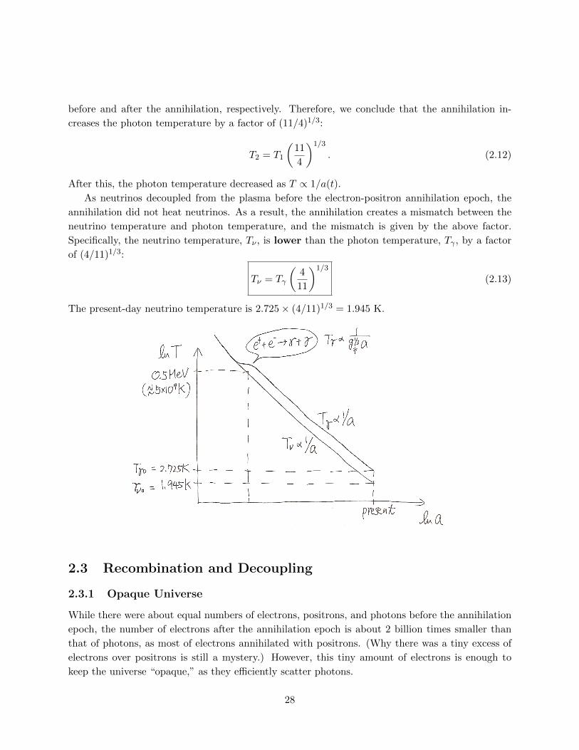
After this, the photon temperature decreased as T ∝ 1/a(t).

As neutrinos decoupled from the plasma before the electron-positron annihilation epoch, the

annihilation did not heat neutrinos. As a result, the annihilation creates a mismatch between the

neutrino temperature and photon temperature, and the mismatch is given by the above factor.

Specifically, the neutrino temperature, Tν , is lower than the photon temperature, Tγ , by a factor

of (4/11)1/3:

Tν = Tγ

(4

11

)1/3

(2.13)

The present-day neutrino temperature is 2.725× (4/11)1/3 = 1.945 K.

2.3 Recombination and Decoupling

2.3.1 Opaque Universe

While there were about equal numbers of electrons, positrons, and photons before the annihilation

epoch, the number of electrons after the annihilation epoch is about 2 billion times smaller than

that of photons, as most of electrons annihilated with positrons. (Why there was a tiny excess of

electrons over positrons is still a mystery.) However, this tiny amount of electrons is enough to

keep the universe “opaque,” as they efficiently scatter photons.

28

• Free electrons can scatter photons efficiently.

• Photons cannot go very far.

protonheliumelectron

photon

Whether the scattering is efficient or not can be quantified by the ratio of the mean free time

of photons, 1/(σTnec), and the Hubble time, 1/H. Here, σT = 6.65 × 10−25 cm2 is the Thomson

scattering cross section, and ne is the number density of free electrons. The scattering is efficient

enough to keep the universe opaque if the mean free time is short compared to the Hubble time,

i.e., H/(σTnec) < 1. In fact, the scattering is so efficient that the universe remains opaque when

the universe is matter-dominated, for which the Hubble rate is given by H = H0

√Ωm(1 + z)3. Let

us calculateH

σTnec=H0

c

√Ωm(1 + z)3

σTnCMB

nCMB

ne. (2.14)

Using nCMB = 410(1+z)3 cm−3, nCMB/ne ≈ 2×109, c/H0 = 2998 h−1 Mpc = 9.25 h−1 ×1027 cm,

and Ωmh2 = 0.13, we obtain

H

σTnec' 0.9× 10−2

(1000

1 + z

)3/2(nCMB/ne2× 109

). (2.15)

Therefore, at z ≈ 103, the mean free time of photons was still only 1% of the Hubble time, and the

universe was still quite opaque.

2.3.2 Neutral Hydrogen Formation and Decoupling

However, at around this epoch (z ≈ 103, or TCMB ≈ 3000 K), the electron number density rapidly

fell relative to nCMB, resulting in the decoupling of photons from the electron scattering. What

happened? At this temperature, the universe was cool enough for electrons to be captured by

protons, forming neutral hydrogen atoms:

p+ e− → H + γ.

Once started, this process rapidly eats electrons, reducing their number density and thus allowing

for photons to propagate freely.

29

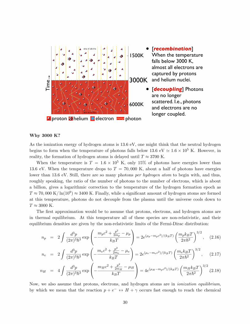
• [recombination] When the temperature falls below 3000 K, almost all electrons are captured by protons and helium nuclei.

• [decoupling] Photons are no longer scattered. I.e., photons and electrons are no longer coupled.

Tim

e1500K

6000K

3000K

proton helium electron photon

Why 3000 K?

As the ionization energy of hydrogen atoms is 13.6 eV, one might think that the neutral hydrogen

begins to form when the temperature of photons falls below 13.6 eV ' 1.6 × 105 K. However, in

reality, the formation of hydrogen atoms is delayed until T ≈ 3700 K.

When the temperature is T = 1.6 × 105 K, only 15% of photons have energies lower than

13.6 eV. When the temperature drops to T = 70, 000 K, about a half of photons have energies

lower than 13.6 eV. Still, there are so many photons per hydrogen atom to begin with, and thus,

roughly speaking, the ratio of the number of photons to the number of electrons, which is about

a billion, gives a logarithmic correction to the temperature of the hydrogen formation epoch as

T ≈ 70, 000 K/ ln(109) ≈ 3400 K. Finally, while a significant amount of hydrogen atoms are formed

at this temperature, photons do not decouple from the plasma until the universe cools down to

T ≈ 3000 K.

The first approximation would be to assume that protons, electrons, and hydrogen atoms are

in thermal equilibrium. At this temperature all of these species are non-relativistic, and their

equilibrium densities are given by the non-relativistic limits of the Fermi-Dirac distribution:

np = 2

∫d3p

(2π)3~3exp

−mpc2 + p2

2mp− µp

kBT

= 2e(µp−mpc2)/(kBT )

(mpkBT

2π~2

)3/2

, (2.16)

ne = 2

∫d3p

(2π)3~3exp

(−mec

2 + p2

2me− µe

kBT

)= 2e(µe−mec2)/(kBT )

(mekBT

2π~2

)3/2

, (2.17)

nH = 4

∫d3p

(2π)3~3exp

−mHc2 + p2

2mH− µH

kBT

= 4e(µH−mpc2)/(kBT )

(mHkBT

2π~2

)3/2

.(2.18)

Now, we also assume that protons, electrons, and hydrogen atoms are in ionization equilibrium,

by which we mean that the reaction p + e− ↔ H + γ occurs fast enough to reach the chemical

30

equilibrium:

µp + µe = µH . (2.19)

(Note that photon’s chemical potential is zero.) This condition lets us combine the above 3 number

densities to obtain the so-called Saha equation:

npnenH

=

(mp

mH

mekBT

2π~2

)3/2

e−(mp+me−mH)c2/(kBT ). (2.20)

Here, the mass difference in the exponential is the binding energy of an hydrogen atom, which is

of course equal to its ionization energy:

BH ≡ (mp +me −mH)c2 = 13.6 eV. (2.21)

Since me ≈ mp/2000 and mp ≈ 1 GeV, we can set mp ≈ mH in the parenthesis in front of the

exponential factor. Finally, the charge neutrality demands ne = np. We thus obtain

n2p

nH≈(mekBT

2π~2

)3/2

e−BH/(kBT ). (2.22)

Now, define the ionization fraction:

X ≡ npnp + nH

, (2.23)

which goes from 1 (fully ionized hydrogen) to 0 (fully neutral hydrogen). The Saha equation now

reads:X2

1−X=

1

np + nH

(mekBT

2π~2

)3/2

e−BH/(kBT ). (2.24)

The goal here is to solve this equation for X as a function of the temperature, T . For this purpose,

it is convenient to relate np + nH to the baryon mass density of the universe. We use the result

from the Big Bang Nucleosynthesis (BBN): 76% of the baryonic mass in the universe after BBN is

contained in protons (and the rest in helium nuclei). Therefore, mp(np + nH) = 0.76ρb. We then

define the time-independent baryon-to-photon ratio:

η ≡ ρbmpnCMB

= 273.9(Ωbh2)× 10−10 (2.25)

which takes on the value η = 6.30×10−10 for Ωbh2 = 0.023. Therefore, there are 1.6 billion photons

per baryon. Note that we have used nCMB = 410 cm−3(T/T0)3 with T0 = 2.725 K for computing

the numerical value of η. Putting all the numerical values in, we finally arrive at the following

dimensionless form of the Saha equation:

X2

1−X=

2.50× 106

ηT−3/2e−1/T (2.26)

31

where T ≡ kBT/BH = T/(157894 K). This is a simple quadratic equation, which can be easily

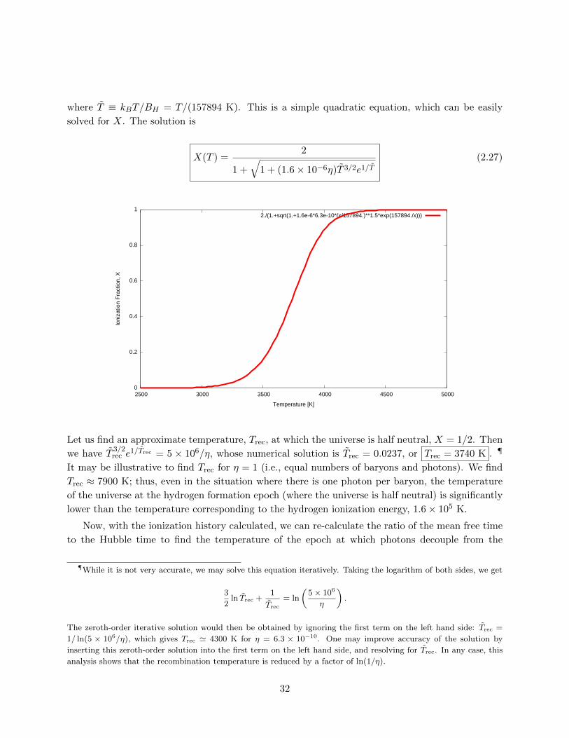
solved for X. The solution is

X(T ) =2

1 +

√1 + (1.6× 10−6η)T 3/2e1/T

(2.27)

0

0.2

0.4

0.6

0.8

1

2500 3000 3500 4000 4500 5000

Ioni

zatio

n Fr

actio

n, X

Temperature [K]

2./(1.+sqrt(1.+1.6e-6*6.3e-10*(x/157894.)**1.5*exp(157894./x)))

Let us find an approximate temperature, Trec, at which the universe is half neutral, X = 1/2. Then

we have T3/2rec e1/Trec = 5 × 106/η, whose numerical solution is Trec = 0.0237, or Trec = 3740 K . ¶

It may be illustrative to find Trec for η = 1 (i.e., equal numbers of baryons and photons). We find

Trec ≈ 7900 K; thus, even in the situation where there is one photon per baryon, the temperature

of the universe at the hydrogen formation epoch (where the universe is half neutral) is significantly

lower than the temperature corresponding to the hydrogen ionization energy, 1.6× 105 K.

Now, with the ionization history calculated, we can re-calculate the ratio of the mean free time

to the Hubble time to find the temperature of the epoch at which photons decouple from the

¶While it is not very accurate, we may solve this equation iteratively. Taking the logarithm of both sides, we get

3

2ln Trec +

1

Trec

= ln

(5× 106

η

).

The zeroth-order iterative solution would then be obtained by ignoring the first term on the left hand side: Trec =

1/ ln(5 × 106/η), which gives Trec ' 4300 K for η = 6.3 × 10−10. One may improve accuracy of the solution by

inserting this zeroth-order solution into the first term on the left hand side, and resolving for Trec. In any case, this

analysis shows that the recombination temperature is reduced by a factor of ln(1/η).

32

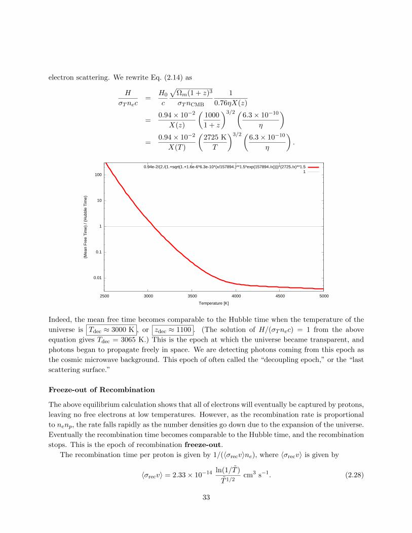
electron scattering. We rewrite Eq. (2.14) as

H

σTnec=

H0

c

√Ωm(1 + z)3

σTnCMB

1

0.76ηX(z)

=0.94× 10−2

X(z)

(1000

1 + z

)3/2(6.3× 10−10

η

)=

0.94× 10−2

X(T )

(2725 K

T

)3/2(6.3× 10−10

η

).

0.01

0.1

1

10

100

2500 3000 3500 4000 4500 5000

(Mea

n Fr

ee T

ime)

/ (H

ubbl

e Ti

me)

Temperature [K]

0.94e-2/(2./(1.+sqrt(1.+1.6e-6*6.3e-10*(x/157894.)**1.5*exp(157894./x))))*(2725./x)**1.51

Indeed, the mean free time becomes comparable to the Hubble time when the temperature of the

universe is Tdec ≈ 3000 K , or zdec ≈ 1100 . (The solution of H/(σTnec) = 1 from the above

equation gives Tdec = 3065 K.) This is the epoch at which the universe became transparent, and

photons began to propagate freely in space. We are detecting photons coming from this epoch as

the cosmic microwave background. This epoch of often called the “decoupling epoch,” or the “last

scattering surface.”

Freeze-out of Recombination

The above equilibrium calculation shows that all of electrons will eventually be captured by protons,

leaving no free electrons at low temperatures. However, as the recombination rate is proportional

to nenp, the rate falls rapidly as the number densities go down due to the expansion of the universe.

Eventually the recombination time becomes comparable to the Hubble time, and the recombination

stops. This is the epoch of recombination freeze-out.

The recombination time per proton is given by 1/(〈σrecv〉ne), where 〈σrecv〉 is given by

〈σrecv〉 = 2.33× 10−14 ln(1/T )

T 1/2cm3 s−1. (2.28)

33

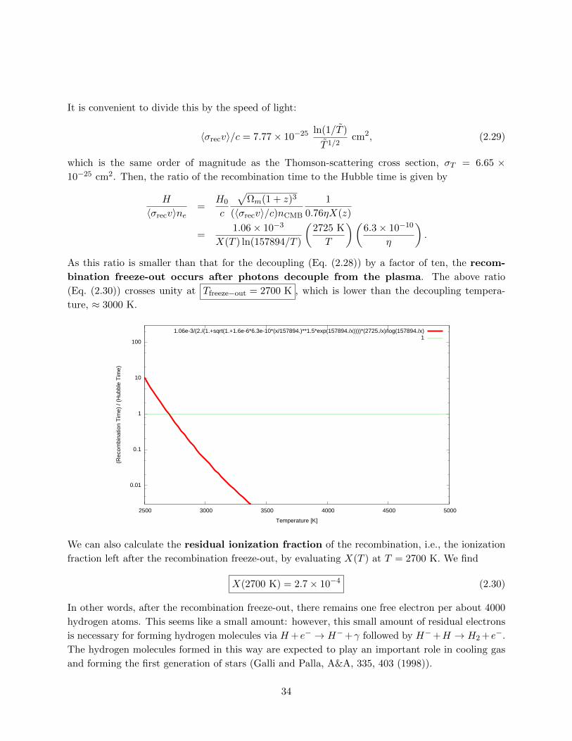
It is convenient to divide this by the speed of light:

〈σrecv〉/c = 7.77× 10−25 ln(1/T )

T 1/2cm2, (2.29)

which is the same order of magnitude as the Thomson-scattering cross section, σT = 6.65 ×10−25 cm2. Then, the ratio of the recombination time to the Hubble time is given by

H

〈σrecv〉ne=

H0

c

√Ωm(1 + z)3

(〈σrecv〉/c)nCMB

1

0.76ηX(z)

=1.06× 10−3

X(T ) ln(157894/T )

(2725 K

T

)(6.3× 10−10

η

).

As this ratio is smaller than that for the decoupling (Eq. (2.28)) by a factor of ten, the recom-

bination freeze-out occurs after photons decouple from the plasma. The above ratio

(Eq. (2.30)) crosses unity at Tfreeze−out = 2700 K , which is lower than the decoupling tempera-

ture, ≈ 3000 K.

0.01

0.1

1

10

100

2500 3000 3500 4000 4500 5000

(Rec

ombi

natio

n Ti

me)

/ (H

ubbl

e Ti

me)

Temperature [K]

1.06e-3/(2./(1.+sqrt(1.+1.6e-6*6.3e-10*(x/157894.)**1.5*exp(157894./x))))*(2725./x)/log(157894./x)1

We can also calculate the residual ionization fraction of the recombination, i.e., the ionization

fraction left after the recombination freeze-out, by evaluating X(T ) at T = 2700 K. We find

X(2700 K) = 2.7× 10−4 (2.30)

In other words, after the recombination freeze-out, there remains one free electron per about 4000

hydrogen atoms. This seems like a small amount: however, this small amount of residual electrons

is necessary for forming hydrogen molecules via H+e− → H−+γ followed by H−+H → H2 +e−.

The hydrogen molecules formed in this way are expected to play an important role in cooling gas

and forming the first generation of stars (Galli and Palla, A&A, 335, 403 (1998)).

34

2.4 Temperature Anisotropy

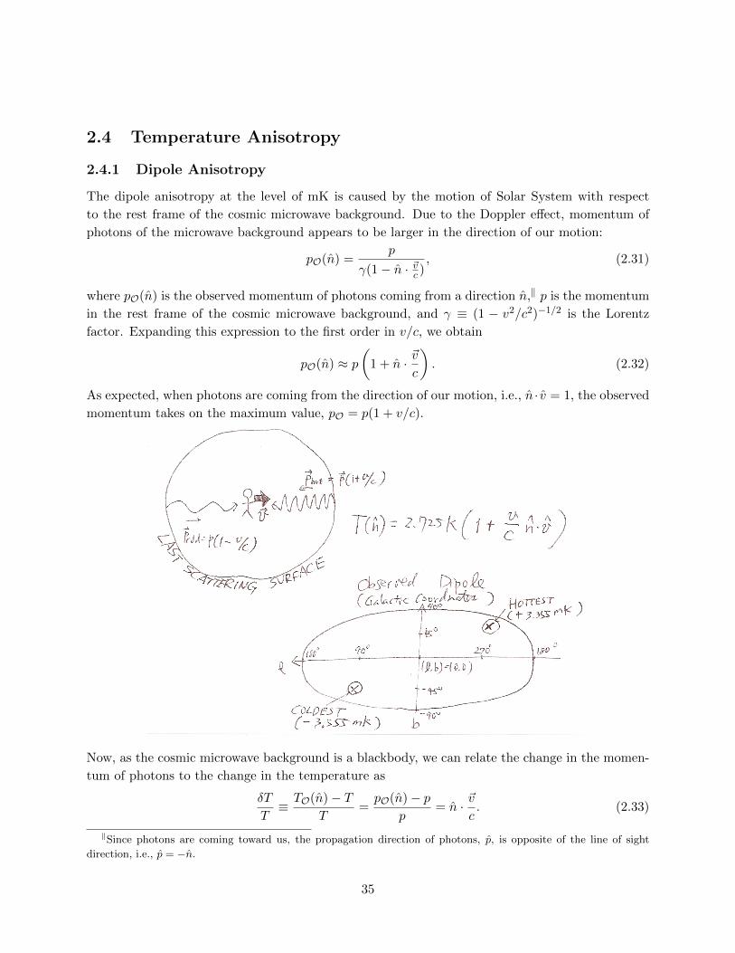
2.4.1 Dipole Anisotropy

The dipole anisotropy at the level of mK is caused by the motion of Solar System with respect

to the rest frame of the cosmic microwave background. Due to the Doppler effect, momentum of

photons of the microwave background appears to be larger in the direction of our motion:

pO(n) =p

γ(1− n · ~vc ), (2.31)

where pO(n) is the observed momentum of photons coming from a direction n,‖ p is the momentum

in the rest frame of the cosmic microwave background, and γ ≡ (1 − v2/c2)−1/2 is the Lorentz

factor. Expanding this expression to the first order in v/c, we obtain

pO(n) ≈ p(

1 + n · ~vc

). (2.32)

As expected, when photons are coming from the direction of our motion, i.e., n · v = 1, the observed

momentum takes on the maximum value, pO = p(1 + v/c).

Now, as the cosmic microwave background is a blackbody, we can relate the change in the momen-

tum of photons to the change in the temperature as

δT

T≡ TO(n)− T

T=pO(n)− p

p= n · ~v

c. (2.33)

‖Since photons are coming toward us, the propagation direction of photons, p, is opposite of the line of sight

direction, i.e., p = −n.

35

This is the formula for the dipole anisotropy. The measured value of dipole in the direction of

motion is δT = 3.355± 0.008 mK (Table 6 of Jarosik et al., ApJS, 192, 14 (2011)). The direction

of motion in Galactic coordinates is (l, b) = (263.99 ± 0.14, 48.26 ± 0.03) (in degrees). This gives

δT/T = 3.355× 10−3/2.725 = 1.23× 10−3. By equating this to v/c, we find∗∗

v = 368 km/s (2.34)

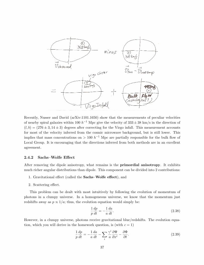
This velocity should be the vector sum of various components:

~v = (~vSun − ~vMW) + (~vMW − ~vLG) + ~vLG, (2.35)

where

1. ~vSun − ~vMW is the orbiting velocity of Solar System with respect to the center of our Galaxy

(Milky Way). This component is known (222.0±5.0 km/s in the direction of (l, b) = (91.1, 0)

degrees), and thus can be subtracted.

2. ~vMW − ~vLG is the velocity of our Galaxy (Milky Way) with respect to the center-of-mass of

Local Group of galaxies. As the dominant masses of Local Group are given by Milky Way and

Andromeda Galaxy (M31), which is a nearby galaxy, this component is small (≈ 80 km/s).

3. ~vLG is the velocity of the center-of-mass of Local Group with respect to the rest frame of

the cosmic microwave background. This component represents the cosmological velocity flow

(called the “bulk flow”).

It turns out that the sum of the first two components, i.e., motion of Sun relative to the center-of-

mass of Local Group, has a magnitude (307 km/s) comparable to the measured velocity, but is in

nearly the opposite direction ((l, b) = (105± 5,−7± 4) degrees; Yahil, Tammann & Sandage, ApJ,

217, 903 (1997)). As a result, the inferred bulk flow component has a large velocity:

vLG = 626± 30 km/s, (2.36)

in the direction of (l, b) = (276± 2, 30± 2) degrees (Sandage, Reindl & Tammann, ApJ, 714, 1441

(2010)).

Who is pulling Local Group? One obvious nearby mass concentration is the Virgo clusters of

galaxies (at 16.5 Mpc). After subtracting an estimate of the infall velocity to Virgo (220 km/s) in

the direction of (l, b) = (283.8, 74.5) degrees, the velocity of Local Group corrected for the Virgo

infall is

vLG = 495± 25 km/s Corrected for Virgo infall (2.37)

in the direction of (l, b) = (275± 2, 12± 4) degrees (Sandage, Reindl & Tammann, ApJ, 714, 1441

(2010)). Therefore, Virgo cannot be solely responsible for the motion of Local Group. We still do

not know who is responsible for this velocity.

∗∗Rotation velocity of Earth around Sun, 30 km/s, has been removed from this value, as this component varies

annually.

36

Recently, Nusser and David (arXiv:1101.1650) show that the measurements of peculiar velocities

of nearby spiral galaxies within 100 h−1 Mpc give the velocity of 333± 38 km/s in the direction of

(l, b) = (276 ± 3, 14 ± 3) degrees after correcting for the Virgo infall. This measurement accounts

for most of the velocity inferred from the cosmic microwave background, but is still lower. This

implies that mass concentrations on > 100 h−1 Mpc are partially responsible for the bulk flow of

Local Group. It is encouraging that the directions inferred from both methods are in an excellent

agreement.

2.4.2 Sachs–Wolfe Effect

After removing the dipole anisotropy, what remains is the primordial anisotropy. It exhibits

much richer angular distributions than dipole. This component can be divided into 2 contributions:

1. Gravitational effect (called the Sachs–Wolfe effect), and

2. Scattering effect.

This problem can be dealt with most intuitively by following the evolution of momentum of

photons in a clumpy universe. In a homogeneous universe, we know that the momentum just

redshifts away as p ∝ 1/a; thus, the evolution equation would simply be:

1

p

dp

dt= −1

a

da

dt. (2.38)

However, in a clumpy universe, photons receive gravitational blue/redshifts. The evolution equa-

tion, which you will derive in the homework question, is (with c = 1)

1

p

dp

dt= −1

a

da

dt−∑i

γi

a

∂Ψ

∂xi− ∂Φ

∂t. (2.39)

37

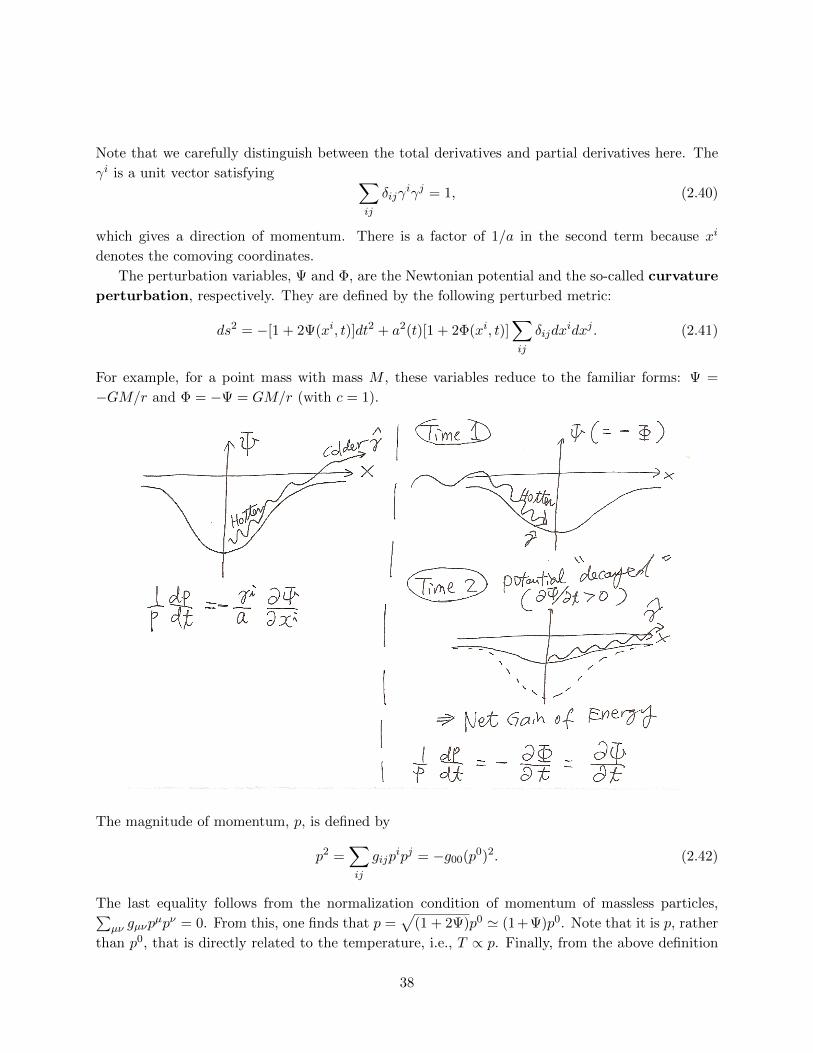
Note that we carefully distinguish between the total derivatives and partial derivatives here. The

γi is a unit vector satisfying ∑ij

δijγiγj = 1, (2.40)

which gives a direction of momentum. There is a factor of 1/a in the second term because xi

denotes the comoving coordinates.

The perturbation variables, Ψ and Φ, are the Newtonian potential and the so-called curvature

perturbation, respectively. They are defined by the following perturbed metric:

ds2 = −[1 + 2Ψ(xi, t)]dt2 + a2(t)[1 + 2Φ(xi, t)]∑ij

δijdxidxj . (2.41)

For example, for a point mass with mass M , these variables reduce to the familiar forms: Ψ =

−GM/r and Φ = −Ψ = GM/r (with c = 1).

The magnitude of momentum, p, is defined by

p2 =∑ij

gijpipj = −g00(p0)2. (2.42)

The last equality follows from the normalization condition of momentum of massless particles,∑µν gµνp

µpν = 0. From this, one finds that p =√

(1 + 2Ψ)p0 ' (1+Ψ)p0. Note that it is p, rather

than p0, that is directly related to the temperature, i.e., T ∝ p. Finally, from the above definition

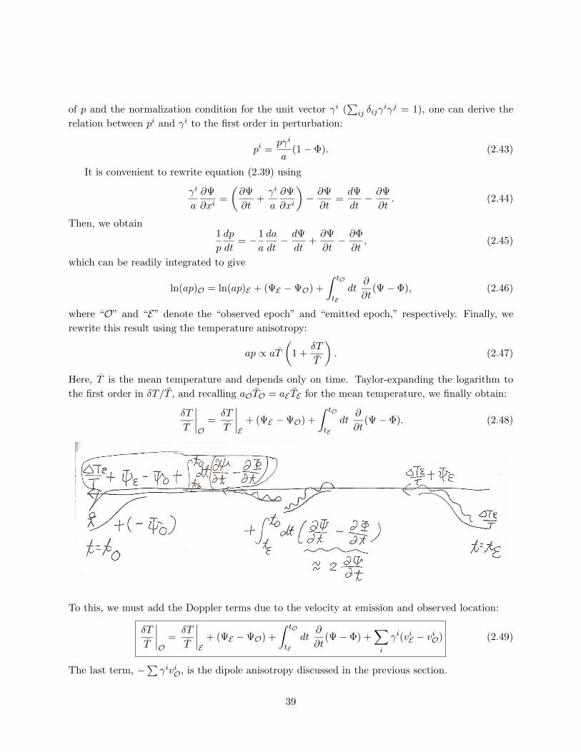
38

of p and the normalization condition for the unit vector γi (∑

ij δijγiγj = 1), one can derive the

relation between pi and γi to the first order in perturbation:

pi =pγi

a(1− Φ). (2.43)

It is convenient to rewrite equation (2.39) using

γi

a

∂Ψ

∂xi=

(∂Ψ

∂t+γi

a

∂Ψ

∂xi

)− ∂Ψ

∂t=dΨ

dt− ∂Ψ

∂t. (2.44)

Then, we obtain1

p

dp

dt= −1

a

da

dt− dΨ

dt+∂Ψ

∂t− ∂Φ

∂t, (2.45)

which can be readily integrated to give

ln(ap)O = ln(ap)E + (ΨE −ΨO) +

∫ tO

tEdt

∂

∂t(Ψ− Φ), (2.46)

where “O” and “E” denote the “observed epoch” and “emitted epoch,” respectively. Finally, we

rewrite this result using the temperature anisotropy:

ap ∝ aT(

1 +δT

T

). (2.47)

Here, T is the mean temperature and depends only on time. Taylor-expanding the logarithm to

the first order in δT/T , and recalling aOTO = aE TE for the mean temperature, we finally obtain:

δT

T

∣∣∣∣O

=δT

T

∣∣∣∣E

+ (ΨE −ΨO) +

∫ tO

tEdt

∂

∂t(Ψ− Φ). (2.48)

To this, we must add the Doppler terms due to the velocity at emission and observed location:

δT

T

∣∣∣∣O

=δT

T

∣∣∣∣E

+ (ΨE −ΨO) +

∫ tO

tEdt

∂

∂t(Ψ− Φ) +

∑i

γi(viE − viO) (2.49)

The last term, −∑γiviO, is the dipole anisotropy discussed in the previous section.

39

This result has a simple interpretation.

1. There was an initial temperature anisotropy at the last scattering surface, δT/T |E (which

remains to be calculated), as well as the Doppler effect,∑γiviE .

2. After the last scattering, photons escape from a potential well, losing energy: δT/T |E + ΨE +∑γiviE .

3. While photons are propagating toward us, photons gain or lose energy depending on how

Ψ− Φ (≈ 2Ψ) changes with time, giving δT/T |E + ΨE +∫ tOtEdt ∂

∂t(Ψ− Φ) +∑γiviE .

4. Finally, photons enter a potential well at our location, ΨO, gaining energy. Also, they receive

the Doppler shift due to our local motion, giving δT/T |E + ΨE − ΨO +∫ tOtEdt ∂

∂t(Ψ − Φ) +∑γi(viE − viO).

In particular, δT/T |E + ΨE −ΨO is usually called the Sachs–Wolfe effect, and∫ tOtEdt ∂

∂t(Ψ−Φ)

is called the integrated Sachs–Wolfe effect. All of these terms were derived by Sachs and Wolfe

in 1967 (Sachs and Wolfe, ApJ, 147, 73 (1967)).

Adiabatic Initial Condition

How do we calculate the initial temperature fluctuation at the last scattering surface, δT/T |E? To

calculate this, we must specify the initial condition for perturbations. In principle, this cannot

be known a priori without using the observational data. There are two widely explored initial

conditions:

• Adiabatic initial condition

• Non-adiabatic initial condition

The current observational data favor the adiabatic initial condition, and we have not yet found

any evidence for non-adiabatic initial condition. Therefore, we shall focus on the adiabatic initial

condition.

What is it? This is the initial condition in which radiation and matter are perturbed in a similar

way. It is called adiabatic, as the entropy density per matter particle is constant (unperturbed):

S/a3

nM∝ T 3

nM= constant, (2.50)

whose variation givesT 3

nM

(3δT

T− δnM

nM

)= 0. (2.51)

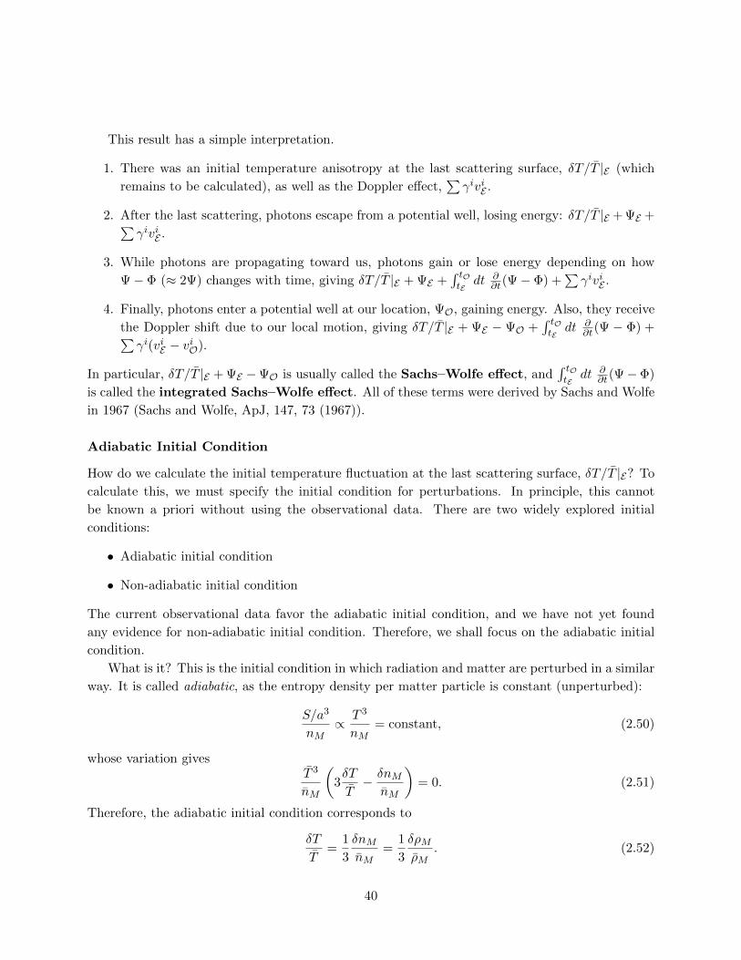
Therefore, the adiabatic initial condition corresponds to

δT

T=

1

3

δnMnM

=1

3

δρMρM

. (2.52)

40

“Non-adiabatic initial conditions” would have δT/T 6= δρM/(3ρM ).

As this is the initial condition, it holds only on very large scales, much larger than the horizon

size at the last scattering surface. While it is not obvious or intuitive, on such large scales, as

you derive in the homework question, the density fluctuation during the matter-dominated era is

related to the Newtonian potential as

δρMρM

= −2Ψ (Matter-dominated & super-horizon). (2.53)

This gives, on large scales, the initial temperature fluctuation of

δT

T

∣∣∣∣E

=1

3

δρMρM

∣∣∣∣E

= −2

3ΨE . (2.54)

Then, the Sachs–Wolfe formula gives

δT

T

∣∣∣∣O

=1

3ΨE + . . . (2.55)

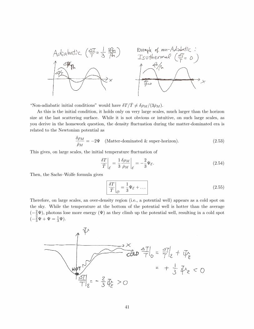
Therefore, on large scales, an over-density region (i.e., a potential well) appears as a cold spot on

the sky. While the temperature at the bottom of the potential well is hotter than the average

(−23Ψ), photons lose more energy (Ψ) as they climb up the potential well, resulting in a cold spot

(−23Ψ + Ψ = 1

3Ψ).

41

Observing the primordial perturbation via the Sachs–Wolfe effect

As you have seen from the homework problem, Ψ = −Φ during the matter era, and both Ψ and Φ

remain constant during the matter era. Therefore, after the decoupling, but before the dark energy

dominated era, the integrated Sachs–Wolfe effect vanishes. In this case the observed temperature

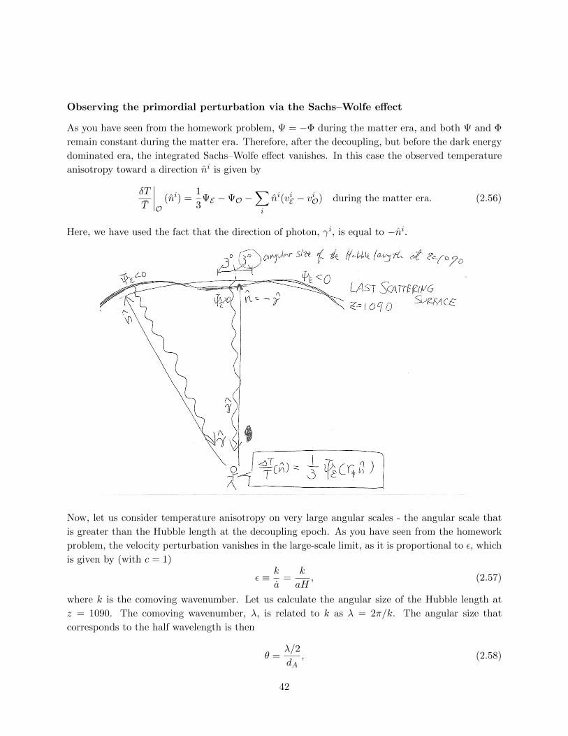
anisotropy toward a direction ni is given by

δT

T

∣∣∣∣O

(ni) =1

3ΨE −ΨO −

∑i

ni(viE − viO) during the matter era. (2.56)

Here, we have used the fact that the direction of photon, γi, is equal to −ni.

Now, let us consider temperature anisotropy on very large angular scales - the angular scale that

is greater than the Hubble length at the decoupling epoch. As you have seen from the homework

problem, the velocity perturbation vanishes in the large-scale limit, as it is proportional to ε, which

is given by (with c = 1)

ε ≡ k

a=

k

aH, (2.57)

where k is the comoving wavenumber. Let us calculate the angular size of the Hubble length at

z = 1090. The comoving wavenumber, λ, is related to k as λ = 2π/k. The angular size that

corresponds to the half wavelength is then

θ =λ/2

dA, (2.58)

42

where dA is the comoving angular diameter distance:

dA ≡ (1 + z)DA = c

∫ z

0

dz′

H(z′)= 14 Gpc for z = 1090. (2.59)

The numerator is the half-wavelength corresponding to the Hubble size:

λH2

=π

kH=

π

aH. (2.60)

For ΩMh2 = 0.13 and ΩRh

2 = 4.17× 10−5, we find

aH =

√ΩMh2(1 + z) + ΩRh2(1 + z)2

3 Gpc= 4.6 Gpc−1 for z = 1090. (2.61)

Therefore, the angular size that corresponds to the Hubble length at z = 1090 is

θ =π

aHdA=

180

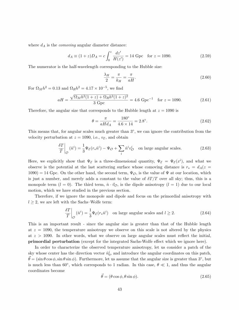
4.6× 14= 2.8. (2.62)

This means that, for angular scales much greater than 3, we can ignore the contribution from the

velocity perturbation at z = 1090, i.e., vE , and obtain

δT

T

∣∣∣∣O

(ni) =1

3ΨE(r∗n

i)−ΨO +∑i

niviO on large angular scales. (2.63)

Here, we explicitly show that ΨE is a three-dimensional quantity, ΨE = ΨE(xi), and what we

observe is the potential at the last scattering surface whose comoving distance is r∗ = dA(z =

1090) = 14 Gpc. On the other hand, the second term, ΨO, is the value of Ψ at our location, which

is just a number, and merely adds a constant to the value of δT/T over all sky; thus, this is a

monopole term (l = 0). The third term, n · ~vO, is the dipole anisotropy (l = 1) due to our local

motion, which we have studied in the previous section.

Therefore, if we ignore the monopole and dipole and focus on the primordial anisotropy with

l ≥ 2, we are left with the Sachs–Wolfe term:

δT

T

∣∣∣∣O

(ni) =1

3ΨE(r∗n

i) on large angular scales and l ≥ 2. (2.64)

This is an important result - since the angular size is greater than that of the Hubble length

at z = 1090, the temperature anisotropy we observe on this scale is not altered by the physics

at z > 1090. In other words, what we observe on large angular scales must reflect the initial,

primordial perturbation (except for the integrated Sachs-Wolfe effect which we ignore here).

In order to characterize the observed temperature anisotropy, let us consider a patch of the

sky whose center has the direction vector ni0, and introduce the angular coordinates on this patch,~θ = (sin θ cosφ, sin θ sinφ). Furthermore, let us assume that the angular size is greater than 3, but

is much less than 60, which corresponds to 1 radian. In this case, θ 1, and thus the angular

coordinates become~θ = (θ cosφ, θ sinφ). (2.65)

43

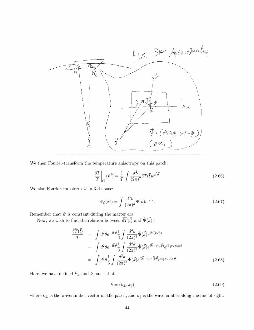
We then Fourier-transform the temperature anisotropy on this patch:

δT

T

∣∣∣∣O

(ni) =1

T

∫d2l

(2π)2δT (~l)ei

~l·~θ. (2.66)

We also Fourier-transform Ψ in 3-d space:

ΨE(xi) =

∫d3k

(2π)3Ψ(~k)ei

~k·~x. (2.67)

Remember that Ψ is constant during the matter era.

Now, we wish to find the relation between δT (~l) and Ψ(~k):

δT (~l)

T=

∫d2θe−i

~l·~θ 1

3

∫d3k

(2π)3Ψ(~k)ei

~k·(r∗n)

=

∫d2θe−i

~l·~θ 1

3

∫d3k

(2π)3Ψ(~k)ei

~k⊥·(r∗~θ)eik‖r∗ cos θ

=

∫d2θ

1

3

∫d3k

(2π)3Ψ(~k)ei(

~k⊥r∗−~l)·~θeik‖r∗ cos θ (2.68)

Here, we have defined ~k⊥ and k‖ such that

~k = (~k⊥, k‖), (2.69)

where ~k⊥ is the wavenumber vector on the patch, and k‖ is the wavenumber along the line of sight.

44

To proceed further, we use the fact that we consider the region in which θ 1 (so that we can

treat a section of the sky as a flat surface):

δT (~l)

T≈

∫d2θ

1

3

∫d3k

(2π)3Ψ(~k)ei(

~k⊥r∗−~l)·~θeik‖r∗ (cos θ ≈ 1)

=1

3

∫d3k

(2π)3Ψ(~k)

[∫d2θei(

~k⊥r∗−~l)·~θ]eik‖r∗

=1

3

∫d3k

(2π)3Ψ(~k)

[(2π)2δ

(2)D (~k⊥r∗ −~l)

]eik‖r∗

=1

3

∫d2k⊥dk‖

(2π)3Ψ(~k)

[(2π)2 δ

(2)D (~k⊥ −~l/r∗)

r2∗

]eik‖r∗

=1

3r2∗

∫dk‖

2πΨ

(~k⊥ =

~l

r∗, k‖

)eik‖r∗ . (2.70)

Finally, there is no way to predict the value of Ψ(~k) for any given value of ~k because Ψ is a

random (stochastic) variable. However, what we can do it to calculate its variance, which is called

the power spectrum:

〈Ψ(~k)Ψ∗(~k)〉 = (2π)3PΨ(k)δ(3)D (~k − ~k′), (2.71)

1

T 2〈δT (~l)δT

∗(~l′)〉 = (2π)2Clδ

(2)D (~l −~l′). (2.72)

The angular power spectrum of the temperature anisotropy, Cl, is an observable quantity.

Therefore, the remaining task is to relate the observable, Cl, to the power spectrum of Φ, PΨ(k).

45

The result is

Cl =1

9r2∗

∫dk‖

2πPΨ

(√l2

r2∗

+ k2‖

). (2.73)

Note that the small-angle approximation, θ 1, corresponds to l 1, as these are related via

l =π

θ. (2.74)

In terms of k and r∗, we have

l = kr∗ = 14

(k

1 Gpc−1

). (2.75)

For example, the multipole that corresponds to the wavenumber of the Hubble horizon size at

z = 1090, aH = 4.6 Gpc−1, is

lH = 64. (2.76)

Therefore, the argument given here is valid only for 1 l 64.

Now, we must make an assumption about the form of PΨ(k). We now believe that primordial

fluctuations were generated during the period of inflation - an exponential expansion of the universe

during a tiny fraction of a second after the birth of the universe. As you will learn from Bhaskar

toward the end of this course, inflation predicts the following power-law form of the initial power

spectrum:

PΨ(k) ∝ kns−4, (2.77)

where ns is called the spectral tilt. The current data give (Komatsu et al., ApJS, 192, 18 (2011))

ns = 0.968± 0.012 (68% CL). As for the normalization of PΨ(k), we usually parametrize it as

PΨ(k) =2π2

k3∆2

Ψ(k0)

(k

k0

)ns−1

, (2.78)

where k0 is some arbitrary pivot wavenumber which is often taken to be k0 = 2 Gpc−1 =

0.002 Mpc−1, and ∆2Φ(k0) is the normalization.

The special case is ns = 1 (which is called the Harrison-Zel’dovich-Peebles spectrum, and

is close to the observed value, ns = 0.968± 0.012), for which

Cl =2π

l21

9∆2

Ψ(k0). (2.79)

This motivates our writing

l2Cl2π

=1

9∆2

Ψ(k0) =1

9

k3PΨ(k)

2π2for ns = 1 (2.80)

Since this quantity does not depend on l, this spectrum (with ns = 1) is called the scale-invariant

spectrum. Note also that k3PΨ(k) does not depend on k. For ns 6= 1, we have ††

l2Cl2π

=1

9∆2

Ψ(k0)

(l

k0r∗

)ns−1 √π2

Γ[(3− ns)/2]

Γ[(4− ns)/2]. (2.84)

††This formula cannot be used for small l (such as l = 2) because we have treated our patch of the sky as a flat

surface, which allowed us to use the familiar Fourier transform. For the full-sky treatment, we must take into account

46

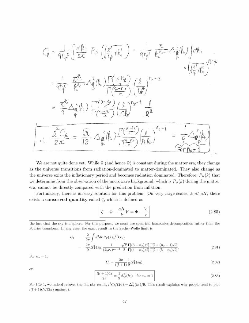
We are not quite done yet. While Ψ (and hence Φ) is constant during the matter era, they change

as the universe transitions from radiation-dominated to matter-dominated. They also change as

the universe exits the inflationary period and becomes radiation dominated. Therefore, PΨ(k) that

we determine from the observation of the microwave background, which is PΨ(k) during the matter

era, cannot be directly compared with the prediction from inflation.

Fortunately, there is an easy solution for this problem. On very large scales, k aH, there

exists a conserved quantity called ζ, which is defined as

ζ ≡ Φ− aH

kV = Φ− V

ε(2.85)

the fact that the sky is a sphere. For this purpose, we must use spherical harmonics decomposition rather than the

Fourier transform. In any case, the exact result in the Sachs–Wolfe limit is

Cl =2

9π

∫k2dkPΨ(k)j2

l (kr∗)

=2π

9∆2

Ψ(k0)1

(k0r∗)ns−1

√π

2

Γ[(3− ns)/2]

Γ[(4− ns)/2]

Γ[l + (ns − 1)/2]

Γ[l + (5− ns)/2]. (2.81)

For ns = 1,

Cl =2π

l(l + 1)

1

9∆2

Ψ(k0), (2.82)

orl(l + 1)Cl

2π=

1

9∆2

Ψ(k0) for ns = 1 (2.83)

For l 1, we indeed recover the flat-sky result, l2Cl/(2π) = ∆2Ψ(k0)/9. This result explains why people tend to plot

l(l + 1)Cl/(2π) against l.

47

This quantity remains constant on k aH regardless of the contents of the universe. It is ζ that

is predicted by theories of inflation. Now, if we plug in the large-scale solution for the velocity

perturbation during the matter era that you find from the homework problem, V = −23εΦ, we find

ζ = Φ +2

3Φ =

5

3Φ = −5

3Ψ during the matter era. (2.86)

Therefore, the Sachs–Wolfe formula is modified to

δT

T

∣∣∣∣O

(ni) = −1

5ζ(r∗n

i) (2.87)

andl2Cl2π

=1

25∆2ζ(k0)

(l

k0r∗

)ns−1 √π2

Γ[(3− ns)/2]

Γ[(4− ns)/2]. (2.88)

The current data give (Komatsu et al., ApJS, 192, 18 (2011))

∆2ζ(k0) = (2.43± 0.09)× 10−9. (2.89)

One should be impressed by these results! Using the observation of the cosmic microwave

background, we were able to measure the amplitude and the scale-dependence of the

initial perturbations generated during inflation. Studying the high-energy world before the

Big Bang became a real science!

0

500

1000

1500

2000

2500

3000

0 10 20 30 40 50 60

Ang

ular

Pow

er S

pect

rum

, l(l+

1)C

l/(2π

) [µK

2 ]

Multipole, l

’bestfit_lensedCls.dat’’wmap_tt_spectrum_7yr_v4p1.txt’

’wmap_binned_tt_spectrum_7yr_v4p1.txt’u 1:4:52.43e-9/25.*(2.725e6)**2*(0.99*(x/14/2)**(0.968-1))

’doppler.dat’’sachswolfe.dat’

48

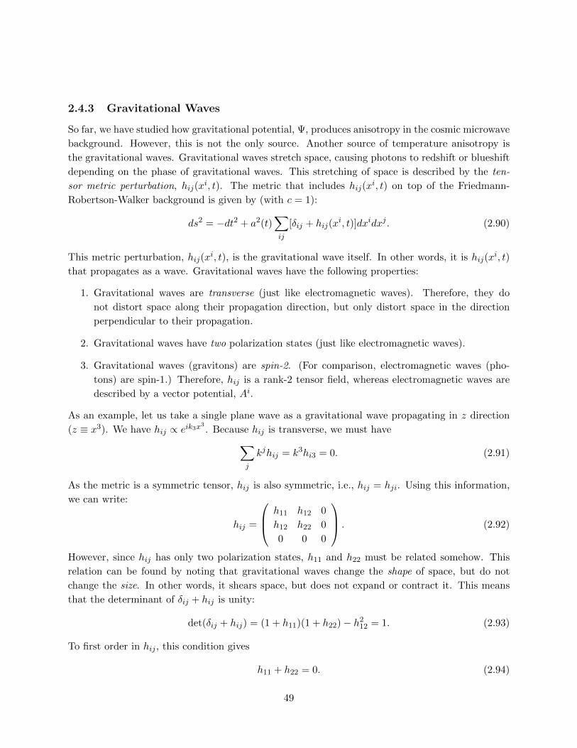
2.4.3 Gravitational Waves

So far, we have studied how gravitational potential, Ψ, produces anisotropy in the cosmic microwave

background. However, this is not the only source. Another source of temperature anisotropy is

the gravitational waves. Gravitational waves stretch space, causing photons to redshift or blueshift

depending on the phase of gravitational waves. This stretching of space is described by the ten-

sor metric perturbation, hij(xi, t). The metric that includes hij(x

i, t) on top of the Friedmann-

Robertson-Walker background is given by (with c = 1):

ds2 = −dt2 + a2(t)∑ij

[δij + hij(xi, t)]dxidxj . (2.90)

This metric perturbation, hij(xi, t), is the gravitational wave itself. In other words, it is hij(x

i, t)

that propagates as a wave. Gravitational waves have the following properties:

1. Gravitational waves are transverse (just like electromagnetic waves). Therefore, they do

not distort space along their propagation direction, but only distort space in the direction

perpendicular to their propagation.

2. Gravitational waves have two polarization states (just like electromagnetic waves).

3. Gravitational waves (gravitons) are spin-2. (For comparison, electromagnetic waves (pho-

tons) are spin-1.) Therefore, hij is a rank-2 tensor field, whereas electromagnetic waves are

described by a vector potential, Ai.

As an example, let us take a single plane wave as a gravitational wave propagating in z direction

(z ≡ x3). We have hij ∝ eik3x3. Because hij is transverse, we must have∑

j

kjhij = k3hi3 = 0. (2.91)

As the metric is a symmetric tensor, hij is also symmetric, i.e., hij = hji. Using this information,

we can write:

hij =

h11 h12 0

h12 h22 0

0 0 0

. (2.92)

However, since hij has only two polarization states, h11 and h22 must be related somehow. This

relation can be found by noting that gravitational waves change the shape of space, but do not

change the size. In other words, it shears space, but does not expand or contract it. This means

that the determinant of δij + hij is unity:

det(δij + hij) = (1 + h11)(1 + h22)− h212 = 1. (2.93)

To first order in hij , this condition gives

h11 + h22 = 0. (2.94)

49

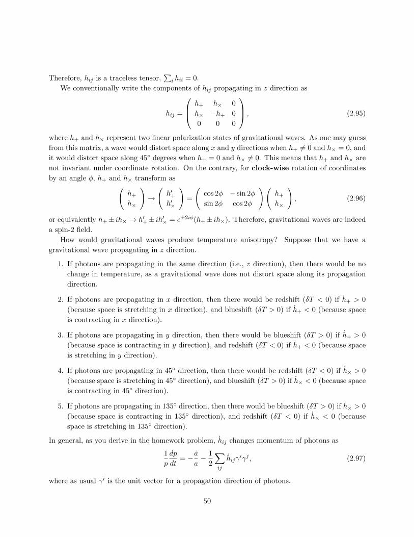
Therefore, hij is a traceless tensor,∑

i hii = 0.

We conventionally write the components of hij propagating in z direction as

hij =

h+ h× 0

h× −h+ 0

0 0 0

, (2.95)

where h+ and h× represent two linear polarization states of gravitational waves. As one may guess

from this matrix, a wave would distort space along x and y directions when h+ 6= 0 and h× = 0, and

it would distort space along 45 degrees when h+ = 0 and h× 6= 0. This means that h+ and h× are

not invariant under coordinate rotation. On the contrary, for clock-wise rotation of coordinates

by an angle φ, h+ and h× transform as(h+

h×

)→

(h′+h′×

)=

(cos 2φ − sin 2φ

sin 2φ cos 2φ

)(h+

h×

), (2.96)

or equivalently h+± ih× → h′+± ih′× = e±2iφ(h+± ih×). Therefore, gravitational waves are indeed

a spin-2 field.

How would gravitational waves produce temperature anisotropy? Suppose that we have a

gravitational wave propagating in z direction.

1. If photons are propagating in the same direction (i.e., z direction), then there would be no

change in temperature, as a gravitational wave does not distort space along its propagation

direction.

2. If photons are propagating in x direction, then there would be redshift (δT < 0) if h+ > 0

(because space is stretching in x direction), and blueshift (δT > 0) if h+ < 0 (because space

is contracting in x direction).

3. If photons are propagating in y direction, then there would be blueshift (δT > 0) if h+ > 0

(because space is contracting in y direction), and redshift (δT < 0) if h+ < 0 (because space

is stretching in y direction).

4. If photons are propagating in 45 direction, then there would be redshift (δT < 0) if h× > 0

(because space is stretching in 45 direction), and blueshift (δT > 0) if h× < 0 (because space

is contracting in 45 direction).

5. If photons are propagating in 135 direction, then there would be blueshift (δT > 0) if h× > 0

(because space is contracting in 135 direction), and redshift (δT < 0) if h× < 0 (because

space is stretching in 135 direction).

In general, as you derive in the homework problem, hij changes momentum of photons as

1

p

dp

dt= − a

a− 1

2

∑ij

hijγiγj , (2.97)

where as usual γi is the unit vector for a propagation direction of photons.

50

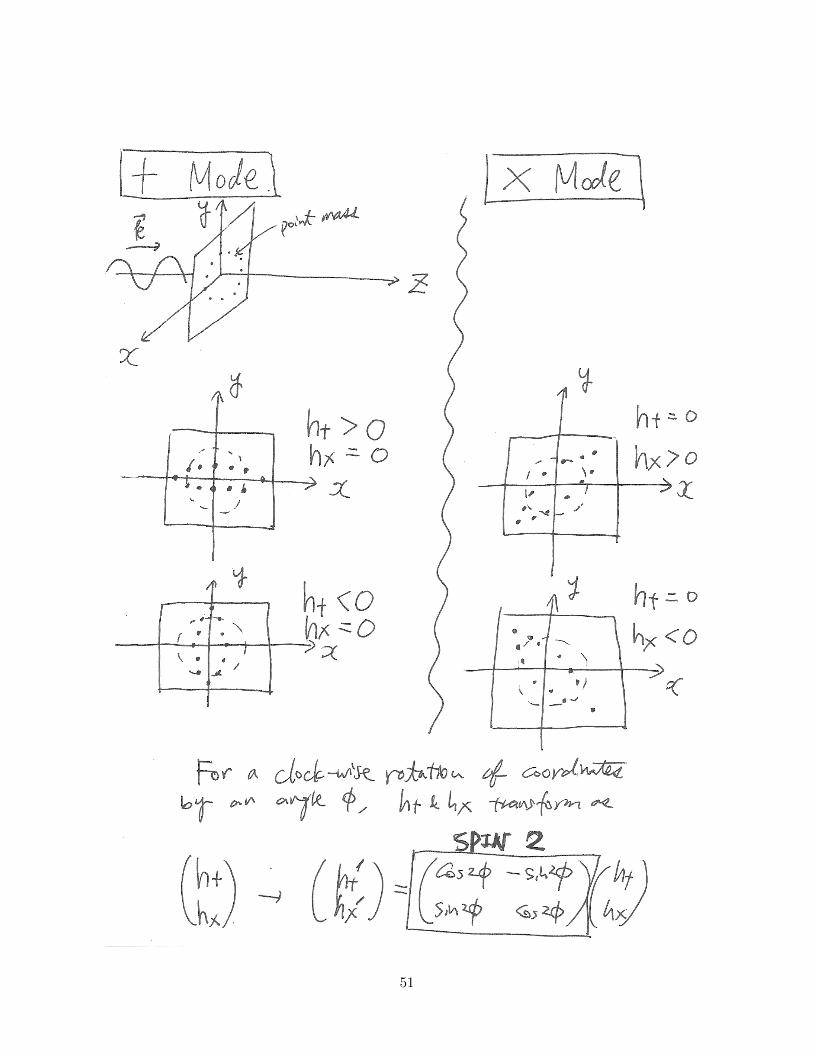
51

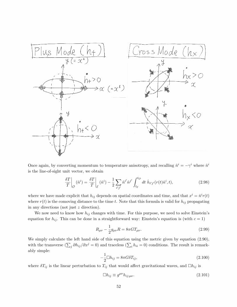
Once again, by converting momentum to temperature anisotropy, and recalling ni = −γi where ni

is the line-of-sight unit vector, we obtain

δT

T

∣∣∣∣O

(ni) =δT

T

∣∣∣∣E

(ni)− 1

2

∑i′j′

ni′nj′∫ tO

tEdt hi′j′(r(t)n

i, t), (2.98)

where we have made explicit that hij depends on spatial coordinates and time, and that xi = nir(t)

where r(t) is the comoving distance to the time t. Note that this formula is valid for hij propagating

in any directions (not just z direction).

We now need to know how hij changes with time. For this purpose, we need to solve Einstein’s

equation for hij . This can be done in a straightforward way: Einstein’s equation is (with c = 1)

Rµν −1

2gµνR = 8πGTµν . (2.99)

We simply calculate the left hand side of this equation using the metric given by equation (2.90),

with the transverse (∑

j ∂hij/∂xj = 0) and traceless (

∑i hii = 0) conditions. The result is remark-

ably simple:

−1

2hij = 8πGδTij , (2.100)

where δTij is the linear perturbation to Tij that would affect gravitational waves, and hij is

hij ≡ gµνhij;µν . (2.101)

52

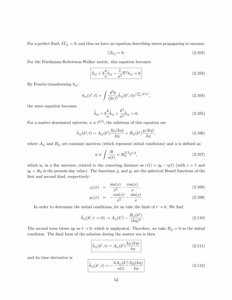
For a perfect fluid, δTij = 0, and thus we have an equation describing waves propagating in vacuum:

hij = 0. (2.102)

For the Friedmann-Robertson-Walker metric, this equation becomes

hij + 3a

ahij −

1

a2∇2hij = 0 (2.103)

By Fourier-transforming hij :

hij(xi, t) =

∫d3k

(2π)3hij(k

i, t)ei∑j k

jxj , (2.104)

the wave equation becomes

¨hij + 3

a

a˙hij +

k2

a2hij = 0. (2.105)

For a matter-dominated universe, a ∝ t2/3, the solutions of this equation are

hij(ki, t) = Aij(k

i)3j1(kη)

kη+Bij(k

i)y1(kη)

kη, (2.106)

where Aij and Bij are constant matrices (which represent initial conditions) and η is defined as

η ≡∫

dt

a(t)= 3t

2/30 t1/3, (2.107)

which is, in a flat universe, related to the comoving distance as r(t) = η0 − η(t) (with c = 1 and

η0 = 3t0 is the present-day value). The functions j1 and y1 are the spherical Bessel functions of the

first and second kind, respectively:

j1(x) =sin(x)

x2− cos(x)

x, (2.108)

y1(x) = −cos(x)

x2− sin(x)

x. (2.109)

In order to determine the initial conditions, let us take the limit of t→ 0. We find

hij(ki, t→ 0)→ Aij(k

i)− Bij(ki)

(kη)3. (2.110)

The second term blows up as t→ 0, which is unphysical. Therefore, we take Bij = 0 as the initial

condition. The final form of the solution during the matter era is then

hij(ki, t) = Aij(k

i)3j1(kη)

kη(2.111)

and its time derivative is

˙hij(k

i, t) = −kAij(ki)

a(t)

3j2(kη)

kη(2.112)

53

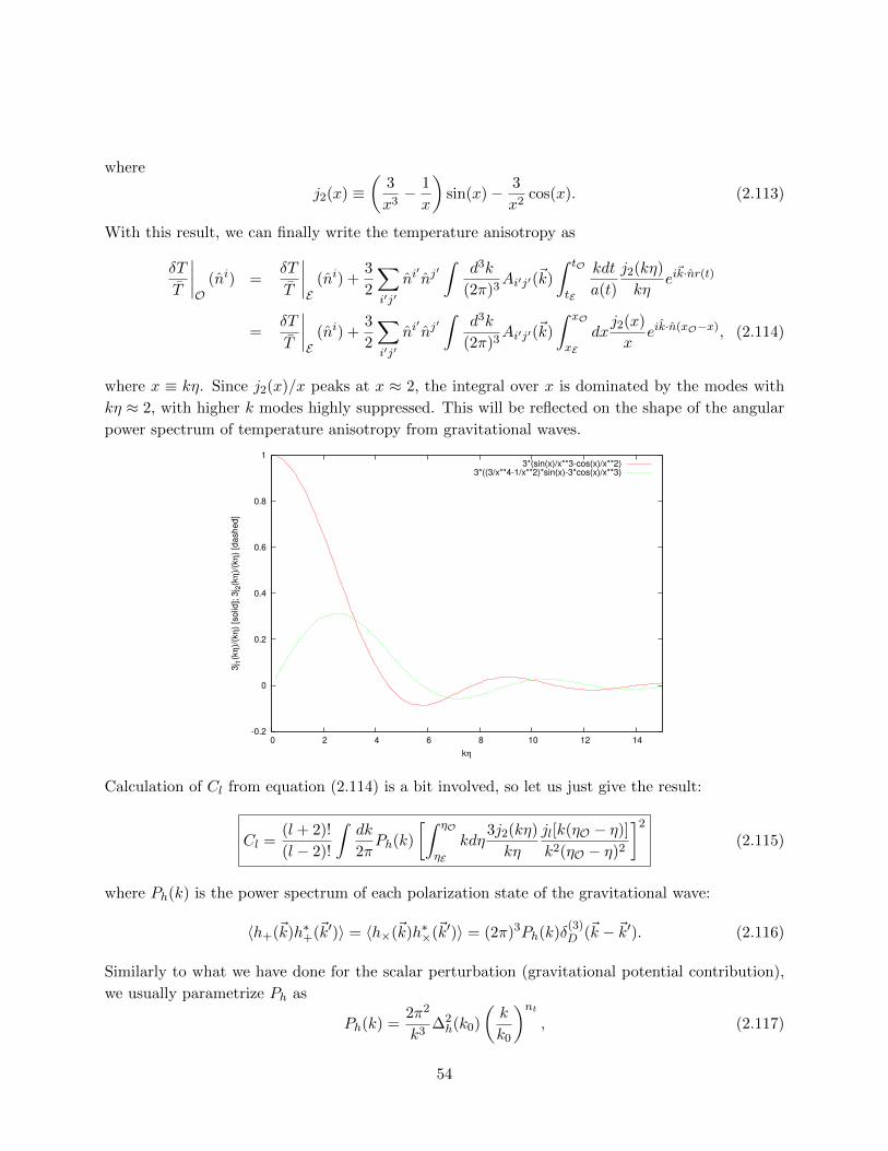
where

j2(x) ≡(

3

x3− 1

x

)sin(x)− 3

x2cos(x). (2.113)

With this result, we can finally write the temperature anisotropy as

δT

T

∣∣∣∣O

(ni) =δT

T

∣∣∣∣E

(ni) +3

2

∑i′j′

ni′nj′∫

d3k

(2π)3Ai′j′(~k)

∫ tO

tE

kdt

a(t)

j2(kη)

kηei~k·nr(t)

=δT

T

∣∣∣∣E

(ni) +3

2

∑i′j′

ni′nj′∫

d3k

(2π)3Ai′j′(~k)

∫ xO

xEdxj2(x)

xeik·n(xO−x), (2.114)

where x ≡ kη. Since j2(x)/x peaks at x ≈ 2, the integral over x is dominated by the modes with

kη ≈ 2, with higher k modes highly suppressed. This will be reflected on the shape of the angular

power spectrum of temperature anisotropy from gravitational waves.

-0.2

0

0.2

0.4

0.6

0.8

1

0 2 4 6 8 10 12 14

3j1(

kη)/(

kη) [

solid

]; 3j

2(kη

)/(kη

) [da

shed

]

kη

3*(sin(x)/x**3-cos(x)/x**2)3*((3/x**4-1/x**2)*sin(x)-3*cos(x)/x**3)

Calculation of Cl from equation (2.114) is a bit involved, so let us just give the result:

Cl =(l + 2)!

(l − 2)!

∫dk

2πPh(k)

[∫ ηO

ηEkdη

3j2(kη)

kη

jl[k(ηO − η)]

k2(ηO − η)2

]2

(2.115)

where Ph(k) is the power spectrum of each polarization state of the gravitational wave:

〈h+(~k)h∗+(~k′)〉 = 〈h×(~k)h∗×(~k′)〉 = (2π)3Ph(k)δ(3)D (~k − ~k′). (2.116)

Similarly to what we have done for the scalar perturbation (gravitational potential contribution),

we usually parametrize Ph as

Ph(k) =2π2

k3∆2h(k0)

(k

k0

)nt, (2.117)

54

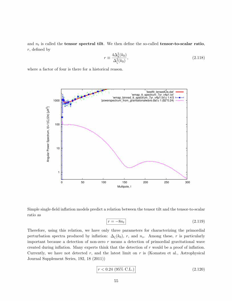
and nt is called the tensor spectral tilt. We then define the so-called tensor-to-scalar ratio,

r, defined by

r ≡4∆2

h(k0)

∆2ζ(k0)

, (2.118)

where a factor of four is there for a historical reason.

1

10

100

1000

0 50 100 150 200 250 300

Ang

ular

Pow

er S

pect

rum

, l(l+

1)C

l/(2π

) [µK

2 ]

Multipole, l

’bestfit_lensedCls.dat’’wmap_tt_spectrum_7yr_v4p1.txt’

’wmap_binned_tt_spectrum_7yr_v4p1.txt’u 1:4:5’powerspectrum_from_gravitationalwave.dat’u 1:($2*0.24)

Simple single-field inflation models predict a relation between the tensor tilt and the tensor-to-scalar

ratio as

r = −8nt (2.119)

Therefore, using this relation, we have only three parameters for characterizing the primordial

perturbation spectra produced by inflation: ∆ζ(k0), r, and ns. Among these, r is particularly

important because a detection of non-zero r means a detection of primordial gravitational wave

created during inflation. Many experts think that the detection of r would be a proof of inflation.

Currently, we have not detected r, and the latest limit on r is (Komatsu et al., Astrophysical

Journal Supplement Series, 192, 18 (2011))

r < 0.24 (95% C.L.) (2.120)

55

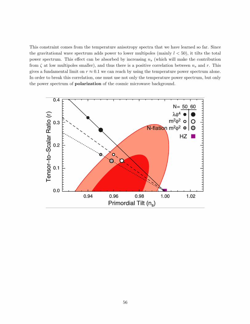
This constraint comes from the temperature anisotropy spectra that we have learned so far. Since

the gravitational wave spectrum adds power to lower multipoles (mainly l < 50), it tilts the total

power spectrum. This effect can be absorbed by increasing ns (which will make the contribution

from ζ at low multipoles smaller), and thus there is a positive correlation between ns and r. This

gives a fundamental limit on r ≈ 0.1 we can reach by using the temperature power spectrum alone.

In order to break this correlation, one must use not only the temperature power spectrum, but only

the power spectrum of polarization of the cosmic microwave background.

56

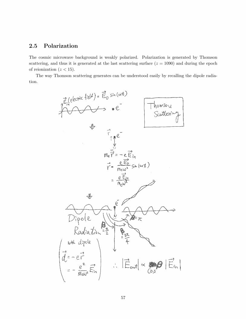
2.5 Polarization

The cosmic microwave background is weakly polarized. Polarization is generated by Thomson

scattering, and thus it is generated at the last scattering surface (z = 1090) and during the epoch

of reionization (z < 15).

The way Thomson scattering generates can be understood easily by recalling the dipole radia-

tion.

57

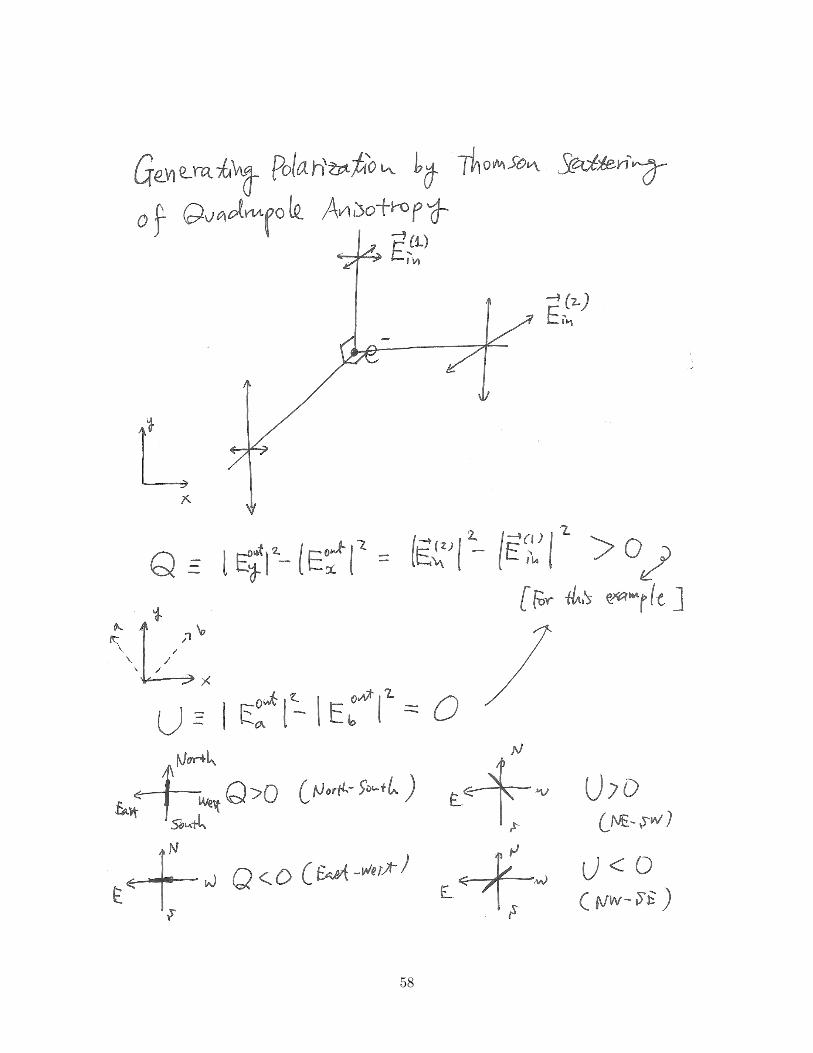
58

Now, let us place an electron at the origin of coordinates, have some temperature anisotropy

around it, and calculate the polarization pattern produced by that electron. It is easy to imagine

this problem by thinking about it from a point of view of the electron at the origin.

Consider the Sachs–Wolfe effect, δT/T = 13Ψ, with Ψ being a plane wave going in z direction.

δT (n)

T=

1

3A cos(kz cos θ), (2.121)

where A > 0 is a constant representing the amplitude of Ψ, and θ is the usual polar angle measured

from the z direction. The origin (z = 0) is hotter (δT > 0).

The polarization produced by a scalar perturbation (such as Ψ) scattered by an electron is given

by

Q+ iU = −√

6

102Y

02 (θ, φ)

∫dΩ

δT (θ, φ)

T(Y 0

2 )∗(θ, φ), (2.122)

Q− iU = −√

6

10−2Y

02 (θ, φ)

∫dΩ

δT (θ, φ)

T(Y 0

2 )∗(θ, φ). (2.123)

Here, Y ml is the spherical harmonics, and 2Y

ml is the spin-2 harmonics. For l = 2 and m = 0, we

have

Y 02 =

√5

16π(3 cos2 θ − 1), (2.124)

2Y0

2 =

√15

32πsin2 θ, (2.125)

−2Y0

2 = 2Y0

2 . (2.126)

Note that, in general, −sYml = (−1)m+s(sY

−ml )∗.

The reason why Q± iU is described by spin-2 harmonics is that Q± iU is the spin-2 quantity.

For a clock-wise rotation of coordinates by an angle ϕ, Q and U transform as(Q

U

)→

(Q′

U ′

)=

(cos 2ϕ − sin 2ϕ

sin 2ϕ cos 2ϕ

)(Q

U

), (2.127)

or equivalently Q ± iU → Q′ ± iU ′ = e±2iϕ(Q ± iU). Therefore, gravitational waves are indeed a

spin-2 field.

First of all, it follows from −2Y0

2 = 2Y0

2 that U = 0. Then, the Q polarization is given by

Q = −√

6

10

√15

32πsin2 θ

∫ 1

−1d cos θ

1

3A cos(kz cos θ)Y 0

2 (θ)

∫ 2π

0dφ

=1

4Aj2(kz) sin2 θ. (2.128)

Therefore, an observer at θ = 0 does not see any polarization, while an observer at θ = π/2 sees

the maximum polarization with Q > 0 (polarization in the north-south direction). All of this can

be understood graphically (see the next page).

59

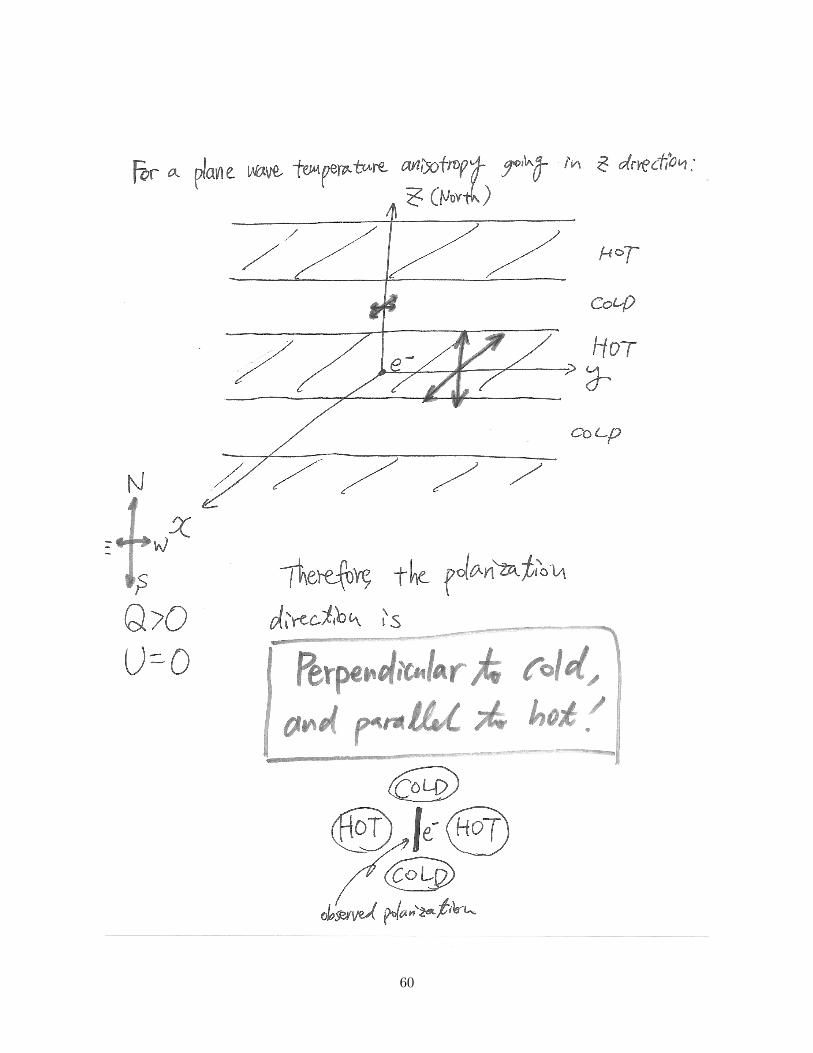
60

PROBLEM SET 2

1.1 Cosmic Microwave Background - I

While the speed of light is kept for completeness below, you may set c = 1 if you wish.

1.1.1 Propagation of photons in a clumpy universe

How does the momentum of photons change as photons propagate through space? First, every

photon suffers from the mean cosmological redshift, and thus its magnitude, p, will decrease as

p ∝ 1/a. In addition, as photons pass through potential wells and troughs, they gain or lose

momentum. Finally, not only the magnitude, p, but also the direction of momentum, γi, will

change when photons are deflected gravitationally.

We can calculate the evolution of four-dimensional momentum, pµ ≡ dxµ/dλ, using the following

geodesic equation:dpµ

dλ+∑αβ

Γµαβpαpβ = 0. (1.129)

Here, λ is a parameter which gives the location along the path of photons. Using p0 = d(ct)/dλ,

one may rewrite the geodesic equation in terms of the total time derivative of pµ:

dpµ

dt+ c

∑αβ

Γµαβpαpβ

p0= 0. (1.130)

In order to calculate Γµαβ, we need to specify the metric. To describe a clumpy universe, we

perturb the Robertson-Walker metric in the following way:

ds2 = −[1 + 2Ψ(t, xi)]c2dt2 + a2(t)[1 + 2Φ(t, xi)]∑ij

δijdxidxj . (1.131)

Here, Ψ is the usual Newtonian potential (divided by c2 to make it dimensionless), and Φ is called

the curvature perturbation. For this metric, all of the components of Γµαβ are non-zero.

From now on, we will assume that the magnitudes of these variables are small: |Ψ| 1 and

|Φ| 1, and calculate everything only up to the first order in these variables.

Question 1.1: Calculate Γ000, Γ0

0i, Γ0ij , Γi00, Γi0j , and Γijk, up to the first order in Φ and Ψ. You

may use the short-hand notation such as

Ψ ≡ ∂Ψ

∂t, Ψ,i ≡

∂Ψ

∂xi.

The components of the metric and its inverse are given by

g00 = −(1 + 2Ψ); g00 = −(1− 2Ψ); gij = a2(1 + 2Φ)δij ; gij =1

a2(1− 2Φ)δij . (1.132)

61

Question 1.2: Write down the geodesic equations in the following form:

dp0

dt= . . . ,

dpi

dt= . . . ,

up to the first order in Φ and Ψ. The final answers should not contain∑

ij δijpipj . You can eliminate

this by using the normalization condition for momentum of massless particles,∑

αβ gαβpαpβ = 0,

which gives, for the above perturbed metric,

a2∑ij

δijpipj = (1− 2Φ + 2Ψ)(p0)2. (1.133)

Question 1.3: Now, we want to derive the evolution equations for the magnitude of momentum,

p, and its direction, γi. First, we define the magnitude as

p2 ≡∑ij

gijpipj . (1.134)

Also, we normalize the direction such that∑ij

δijγiγj = 1. (1.135)

Using this information, write p in terms of p0 and Ψ , and write γi in terms of p, pi, a, and Φ ,

up to the first order in Φ and Ψ.

Question 1.4: Write down the geodesic equations in the following form:

dp

dt= . . . ,

dγi

dt= . . . ,

up to the first order in Φ and Ψ. The answers should not contain p0 or pi. Whenever you

find them, replace them with p and γi, respectively. You can check the result for the deflection

equation, dγi/dt, by making sure that the result satisfies∑

i γidγi/dt = 0. (You can derive this by

differentiating the normalization condition,∑

ij δijγiγj = 1, with respect to time.) Note that the

total time derivative of a variable is related to the partial derivatives as, e.g.,

dΦ

dt= Φ +

∑i

dxi

dtΦ,i = Φ +

∑i

cpi

p0Φ,i. (1.136)

62

1.1.2 Perturbed Conservation Equations For A Pressure-less Fluid

Consider the stress-energy tensor for a perfect fluid. We then take the limit that the pressure is

much less than the energy density, which would be a good approximation for a non-relativistic

fluid. The stress-energy tensor for such a pressure-less fluid is

Tµν = ρ(∑

α gµαuα)(∑

β gνβuβ)

c2. (1.137)

As usual, uµ ≡ dxµ/dτ is a four-dimensional velocity and τ is the proper time.

Suppose that the fluid is moving at a non-relativistic physical three-dimensional velocity of

V i c. By “physical” velocity, we mean

V i ≡ aui = adxi

dτ. (1.138)

We also expand the energy density into the mean, ρ, and the fluctuation around the mean, δ:

ρ = ρ(1 + δ). (1.139)

These perturbation variables, δ and V i/c, are small in the same sense that Φ and Ψ are small. There-

fore, we shall expand everything only up to the first order in Φ, Ψ, δ, and V i/c. For example, Tijis of order (V/c)2, and thus can be ignored. On the other hand, T0i is of order (V/c), and thus

cannot be ignored unless it is multiplied by other perturbation variables.

Question 1.5: Expand the following conservation equations up to the first order in Φ, Ψ, δ,

and V i/c:

1. Energy conservation equation,∑

αβ gαβT0α;β = 0

2. Momentum conservation equation,∑

αβ gαβTiα;β = 0

Use the conservation equation for the mean density, ˙ρ+3 aa ρ = 0, to eliminate the mean contributions

from the above equations, and then rewrite these equations in the following form:

δ = . . . ,

V i

c= . . . .

1.1.3 Large-scale Solutions of Einstein Equations During Matter Era

The energy and momentum conservation equations contain four unknown perturbation variables,

δ, V i, Ψ, and Φ. Therefore, we cannot find solutions unless we have (at least) two more equations.

Such equations are provided by perturbed Einstein equations. Don’t worry - you are not asked to

63

derive them (though I would not stop you from deriving them). Here are the two equations that

can be derived by combining perturbed Einstein equations:‡‡

k2

a2Φ =

4πG

c4ρ

(δ +

3aV

kc2

), (1.140)

Ψ = −Φ. (1.141)

Here, Φ, Ψ, δ, and V are all in Fourier space, i.e., Φ = Φ(~k, t), Ψ = Ψ(~k, t), δ = δ(~k, t), and

V = V (~k, t), and ~k is the comoving wavenumber vector. They are related to the original

variables in position space by, e.g.,

Ψ(~k, t) =

∫d3xΨ(~x, t)e−i

~k·~x, (1.142)

Ψ(~x, t) =

∫d3k

(2π)3Ψ(~k, t)ei

~k·~x. (1.143)

Here, ~k · ~x ≡∑

ij δijkixj . For example, the left hand side of the first perturbed Einstein equation,

(k2/a2)Φ, came from the Laplacian of Φ:

1

a2∇2Φ(~x, t) =

1

a2

∫d3k

(2π)3Φ(~k, t)

(∇2ei

~k·~x)

=1

a2

∫d3k

(2π)3Φ(~k, t)

(−k2ei

~k·~x), (1.144)

where ∇2 ≡∑

ij δij ∂2

∂xi∂xj, and k2 ≡

∑ij δijk

ikj . Also, V in the right hand side of the first

perturbed Einstein equation is defined as V (~k, t) ≡ ik · ~V (~k, t) (where k ≡ ~k/k is a unit vector),

i.e.,

~∇ · ~V (~x, t) =

∫d3k

(2π)3~V (~k, t) ·

(~∇ei~k·~x

)=

∫d3k

(2π)3~V (~k, t) ·

(i~kei

~k·~x)

(1.145)

≡∫

d3k

(2π)3kV (~k, t)ei

~k·~x. (1.146)

Here, ~∇ · ~V ≡∑

k Vk,k.

Now, let us use the above four equations to find solutions for Ψ, Φ, V , and δ. From now on,

we shall drop the tildes on variables in Fourier space for simplicity. It is convenient to change the

independent variable from t to the scale factor, a. Finally, let us define the following variable:

ε(a) ≡ ck

a, (1.147)

‡‡To those who wish to derive these results: the first equation can be obtained by combining perturbed G00 =

(8πG/c4)T00 and G0i = (8πG/c4)T0i, while the second equation can be obtained from the traceless part of Gij =

(8πG/c4)Tij .

64

which goes as ε ∝√a during the matter-dominated era. This quantity is useful, as it is much less

than unity for fluctuations whose wavelength is longer than the Hubble length (≈horizon size):

ε 1 for super-horizon fluctuations, k aH/c,

where H = a/a is the Hubble expansion rate. Therefore, we can find large-scale (long-wavelength;

super-horizon) solutions by consistently ignoring higher-order terms of ε.

Question 1.6: Using the Fourier-space variables and ε, show that the energy- and momentum-

conservation equations can be re-written as follows :

δ′ = − εa

V

c− 3Φ′, (1.148)

V ′

c= −1

a

V

c+ε

aΨ, (1.149)

where the primes denote derivatives with respect to a.

Question 1.7: Using Φ = −Ψ, we now have the following three equations for three unknown

variables:

δ′ = − εa

V

c− 3Φ′, (1.150)

V ′

c= −1

a

V

c− ε

aΦ, (1.151)

ε2Φ =3

2

(δ +

3V

εc

). (1.152)

Once again, during the matter era, ε ∝√a. Solve these equations on super-horizon scales, ε 1,

and show that non-decaying solutions are given by

δ = 2Φ, (1.153)

V

c= −2

3εΦ. (1.154)

By “non-decaying solutions” we mean the solutions that go as ∝ an where n ≥ 0. Finally,

show that Φ (and hence Ψ) is a constant and does not depend on a in the super-horizon limit .

Hint: you cannot ignore ε when two different variables are involved, e.g., A+ εB 6= A, because

you do not know a priori how A compares with B. You can ignore the terms of order ε only when

you are sure that ε is compared to order unity, e.g., A′ + Aa + εAa ≈ A

′ + Aa .

Do not use Mathematica to solve these coupled differential equations! Use your brain, please.

65

PROBLEM SET 3

1.1 Cosmic Microwave Background - II

While the speed of light is kept for completeness below, you may set c = 1 if you wish.

1.1.1 Temperature Anisotropy From Gravitational Waves

Gravitational waves stretch space as they propagate through space. This deformation of space is

characterized by the following metric:

ds2 = −c2dt2 + a2(t)∑ij

(δij + hij)dxidxj ,

where hij is the so-called tensor metric perturbation. (On the other hand, Φ and Ψ that we

have dealt with before are called “scalar metric perturbations”.) The tensor metric perturbation is

symmetric (hij = hji), traceless (∑3

i=1 hii = 0), and transverse (∑3

j=1∂hij∂xj

= 0).

At the first-order of perturbations, scalar and tensor perturbations are decoupled, and thus we

can ignore the scalar perturbations when analyzing the tensor perturbations.

Question 1.1: Write down the geodesic equation for p ≡ (∑

ij gijpipj)1/2 with the metric

given above, up to the first order in hij . Then, by integrating the geodesic equation over time,

derive the formula for the observed temperature anisotropy from gravitational waves as

δT

T

∣∣∣∣O

=δT

T

∣∣∣∣E

+

∫ tO

tEdt (. . . )

where (. . . ) should contain only hij and γi (where γi is the unit vector of the direction of photons,

satisfying∑

ij δijγiγj = 1). Hint: you should check the result by making sure that you can recover

a part of the scalar integrated Sachs–Wolfe effect, −Φ, by using the scalar metric perturbation,

hij = 2Φδij . (You cannot recover the terms containing Ψ because g00 = −1 for the above metric.)

From now on, set δTT

∣∣E = 0.

Question 1.2: Consider a gravitational wave propagating in the z (= x3) direction. For this

special case, the components of the tensor metric perturbation are given by

hij =

h+ h× 0

h× −h+ 0

0 0 0

,

66

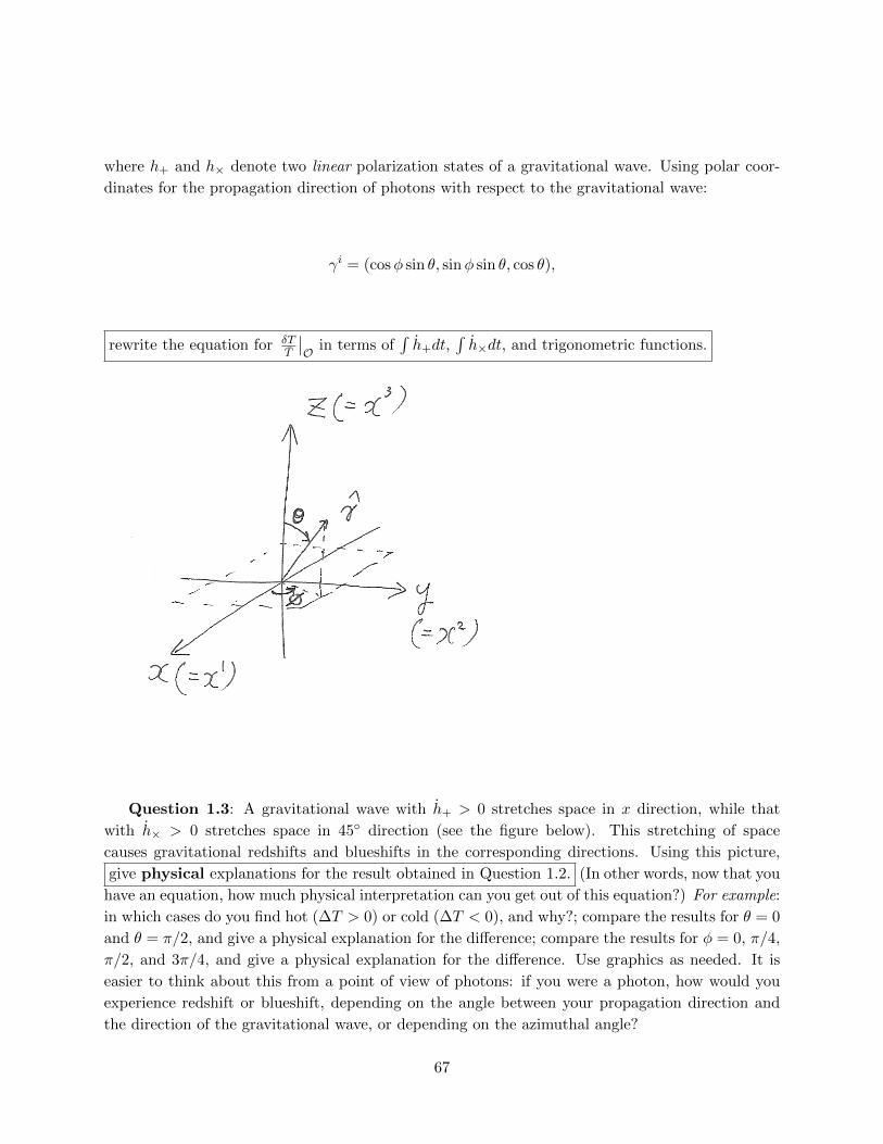
where h+ and h× denote two linear polarization states of a gravitational wave. Using polar coor-

dinates for the propagation direction of photons with respect to the gravitational wave:

γi = (cosφ sin θ, sinφ sin θ, cos θ),

rewrite the equation for δTT

∣∣O in terms of

∫h+dt,

∫h×dt, and trigonometric functions.

Question 1.3: A gravitational wave with h+ > 0 stretches space in x direction, while that

with h× > 0 stretches space in 45 direction (see the figure below). This stretching of space

causes gravitational redshifts and blueshifts in the corresponding directions. Using this picture,

give physical explanations for the result obtained in Question 1.2. (In other words, now that you

have an equation, how much physical interpretation can you get out of this equation?) For example:

in which cases do you find hot (∆T > 0) or cold (∆T < 0), and why?; compare the results for θ = 0

and θ = π/2, and give a physical explanation for the difference; compare the results for φ = 0, π/4,

π/2, and 3π/4, and give a physical explanation for the difference. Use graphics as needed. It is

easier to think about this from a point of view of photons: if you were a photon, how would you

experience redshift or blueshift, depending on the angle between your propagation direction and

the direction of the gravitational wave, or depending on the azimuthal angle?

67

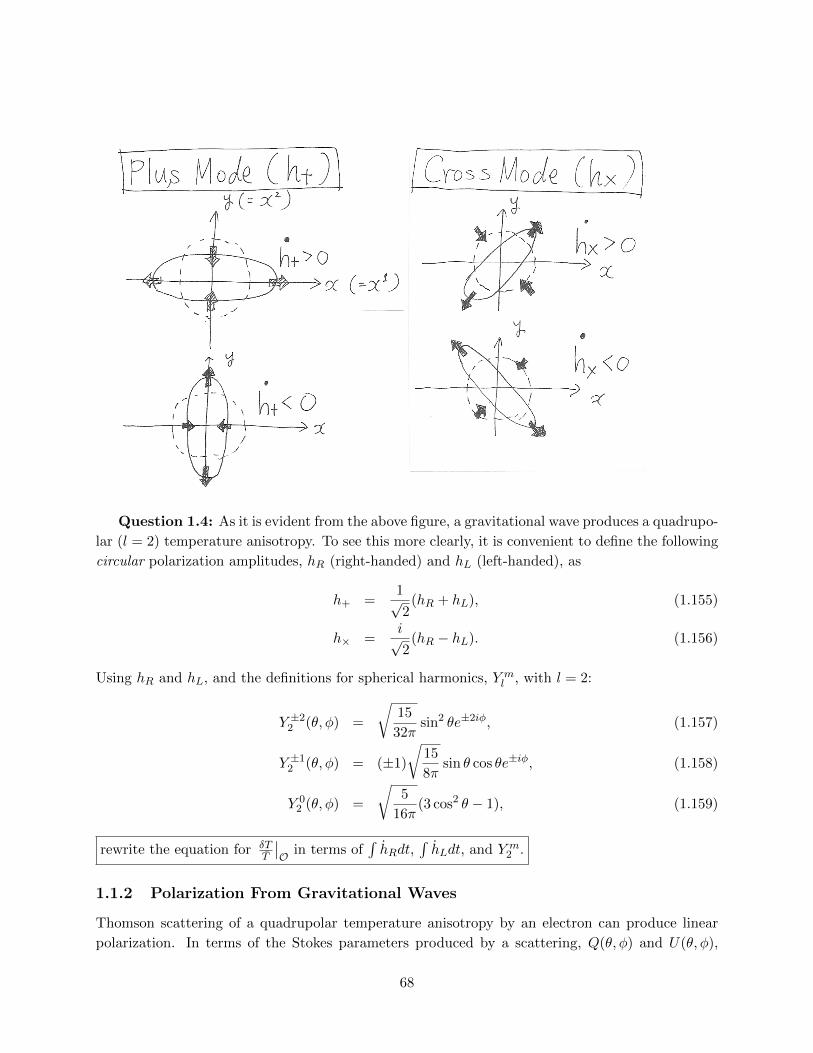
Question 1.4: As it is evident from the above figure, a gravitational wave produces a quadrupo-

lar (l = 2) temperature anisotropy. To see this more clearly, it is convenient to define the following

circular polarization amplitudes, hR (right-handed) and hL (left-handed), as

h+ =1√2

(hR + hL), (1.155)

h× =i√2

(hR − hL). (1.156)

Using hR and hL, and the definitions for spherical harmonics, Y ml , with l = 2:

Y ±22 (θ, φ) =

√15

32πsin2 θe±2iφ, (1.157)

Y ±12 (θ, φ) = (±1)

√15

8πsin θ cos θe±iφ, (1.158)

Y 02 (θ, φ) =

√5

16π(3 cos2 θ − 1), (1.159)

rewrite the equation for δTT

∣∣O in terms of

∫hRdt,

∫hLdt, and Y m

2 .

1.1.2 Polarization From Gravitational Waves

Thomson scattering of a quadrupolar temperature anisotropy by an electron can produce linear

polarization. In terms of the Stokes parameters produced by a scattering, Q(θ, φ) and U(θ, φ),

68

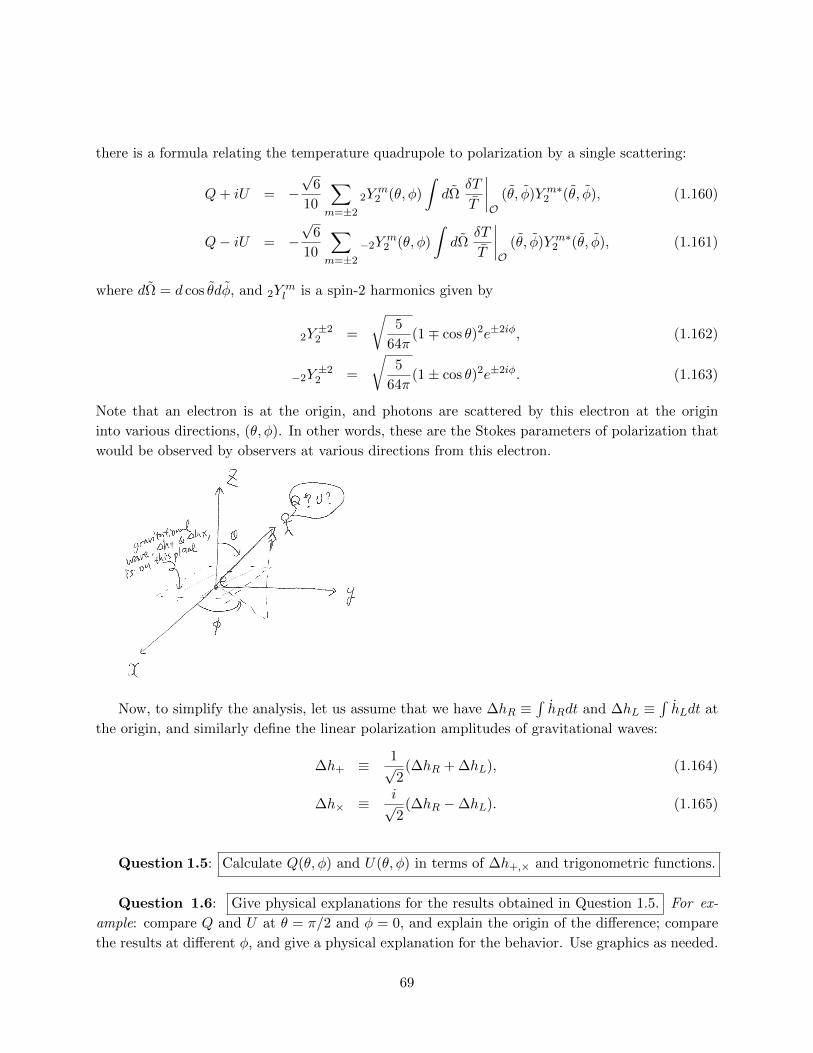
there is a formula relating the temperature quadrupole to polarization by a single scattering:

Q+ iU = −√

6

10

∑m=±2

2Ym

2 (θ, φ)

∫dΩ

δT

T

∣∣∣∣O

(θ, φ)Y m∗2 (θ, φ), (1.160)

Q− iU = −√

6

10

∑m=±2

−2Ym

2 (θ, φ)

∫dΩ

δT

T

∣∣∣∣O

(θ, φ)Y m∗2 (θ, φ), (1.161)

where dΩ = d cos θdφ, and 2Yml is a spin-2 harmonics given by

2Y±2

2 =

√5

64π(1∓ cos θ)2e±2iφ, (1.162)

−2Y±2

2 =

√5

64π(1± cos θ)2e±2iφ. (1.163)

Note that an electron is at the origin, and photons are scattered by this electron at the origin

into various directions, (θ, φ). In other words, these are the Stokes parameters of polarization that

would be observed by observers at various directions from this electron.

Now, to simplify the analysis, let us assume that we have ∆hR ≡∫hRdt and ∆hL ≡

∫hLdt at

the origin, and similarly define the linear polarization amplitudes of gravitational waves:

∆h+ ≡ 1√2

(∆hR + ∆hL), (1.164)

∆h× ≡ i√2

(∆hR −∆hL). (1.165)

Question 1.5: Calculate Q(θ, φ) and U(θ, φ) in terms of ∆h+,× and trigonometric functions.

Question 1.6: Give physical explanations for the results obtained in Question 1.5. For ex-

ample: compare Q and U at θ = π/2 and φ = 0, and explain the origin of the difference; compare

the results at different φ, and give a physical explanation for the behavior. Use graphics as needed.

69

For this problem, it is easier to think about this from a point of view of an electron at the ori-

gin: if you were an electron scattering photons into various directions, what polarization would

you produce depending on the scattering direction and the direction of the gravitational wave, or

depending on the azimuthal angle?

70

Chapter 3

Large-scale Structure of the Universe

In this chapter, we shall learn how matter density fluctuations grow and how structures are formed

in an expanding universe.

3.1 Evolution of Density Fluctuations

3.1.1 Matter Era

Super-horizon solutions

As you saw in the homework problem, the evolution of matter density fluctuations during the

matter era is given by the following 3 equations (with c = 1):

• Energy (Mass) Conservation:

δ′ = − εaV − 3Φ′, (3.1)

where ε ≡ k/a = k/(aH) ∝√a during the matter era, and the primes denote partial deriva-

tives with respect to a, i.e., δ′ ≡ ∂δ/∂a.

• Momentum Conservation:

V ′ = −1

aV − ε

aΦ. (3.2)

• Einstein Equation:

ε2Φ =3

2

(δ +

3V

ε

). (3.3)

Then, we have seen that, on super-horizon scales (ε 1), the solutions are given by

δ = 2Φ = constant, (3.4)

V = −2

3εΦ ∝

√a, (3.5)

Φ = constant. (3.6)

71

These super-horizon solutions were important when computing temperature anisotropy, as the

large-scale temperature anisotropy (Sachs–Wolfe effect and Doppler effect on angular scales larger

than about 3 degrees) is given by these solutions.

Sub-horizon solutions

On the other hand, when studying the large-scale structure of the universe (such as the clustering

of galaxies), we are always dealing with the scales much smaller than the horizon size. Therefore,

let us take the opposite limit, ε 1, and find solutions. In this sub-horizon limit, the equations

become

δ′ = − εaV, (3.7)

V ′ = −1

aV − ε

aΦ, (3.8)

ε2Φ =3

2δ. (3.9)

These equations can be solved easily, and the growing-mode solutions are

δ =2

3ε2Φ ∝ a, (3.10)

V = −2

3εΦ ∝

√a, (3.11)

Φ = constant. (3.12)

There are 3 important observations one can make:

• The matter density perturbation, δ, is constant outside the horizon, but it grows linearly with

a inside the horizon.

• The solution for the matter velocity perturbation, V , is the same in the super-horizon and

sub-horizon limits, and grows as√a at all scales.

• Φ (= −Ψ) is constant both in the super-horizon and sub-horizon limits, and thus it is constant

at all scales.

3.1.2 Radiation Era

Super-horizon solutions

How the matter density perturbations grow during the radiation era? As the energy density in

radiation is much greater than that in matter during the radiation era, we need to take the radiation

72

energy density perturbation in Einstein equation:

δ′ = − εaV − 3Φ′ (3.13)

V ′ = −1

aV − ε

aΦ, (3.14)

ε2Φ =3

2

(δR +

ρMρR

δ +3V

ε

), (3.15)

where ε ≡ k/a = k/(aH) ∝ a during the radiation era. Here, δR is the fractional perturbation

in the radiation energy density, ρR the mean radiation energy density, and ρM the mean matter

energy density. As usual, δ is the fractional perturbation in the matter density.

First, let us look at the super-horizon (ε 1) solutions. On super-horizon scales, the radiation

perturbation δR and the matter perturbation δ are related by the adiabatic initial condition:

δ =3

4δR (super horizon). (3.16)

Since ρM/ρR 1 during the radiation era, this simply means that the term involving ρM/ρR in

Einstein’s equation can be ignored. Therefore, on super-horizon scales, we have

δ′ = − εaV − 3Φ′ (3.17)

V ′ = −1

aV − ε

aΦ (3.18)

ε2Φ =3

2

(4

3δ +

3V

ε

), (3.19)

where we have used δR = 43δ.

Using the same technique we used for the matter era, we can solve these equations to find the

super-horizon solutions during the radiation era:

δ =9

8Φ = constant, (3.20)

V = −1

2εΦ ∝ a, (3.21)

Φ = constant. (3.22)

Therefore, similarly to the matter era, Φ and δ remain constant outside the horizon during the

radiation era. However, the values of Φ and δ are not the same as those during the matter era. In

other words, the values of Φ and δ change when the universe becomes matter dominated.

To see this, recall that, on super horizon scales, there is a conserved quantity ζ given by

ζ ≡ Φ− V

ε. (3.23)

This quantity is given by

ζ = Φ +1

2Φ =

3

2Φ, (3.24)

73

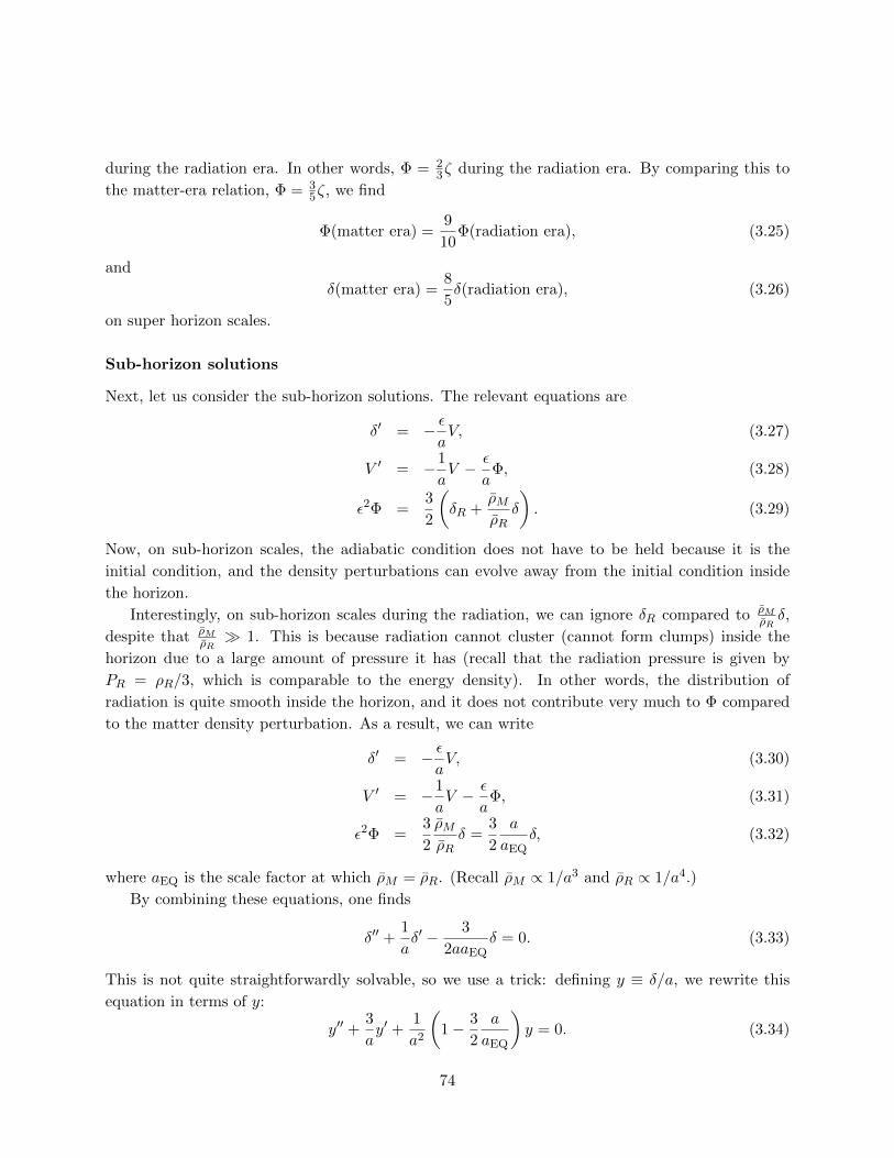
during the radiation era. In other words, Φ = 23ζ during the radiation era. By comparing this to

the matter-era relation, Φ = 35ζ, we find

Φ(matter era) =9

10Φ(radiation era), (3.25)

and

δ(matter era) =8

5δ(radiation era), (3.26)

on super horizon scales.

Sub-horizon solutions

Next, let us consider the sub-horizon solutions. The relevant equations are

δ′ = − εaV, (3.27)

V ′ = −1

aV − ε

aΦ, (3.28)

ε2Φ =3

2

(δR +

ρMρR

δ

). (3.29)

Now, on sub-horizon scales, the adiabatic condition does not have to be held because it is the

initial condition, and the density perturbations can evolve away from the initial condition inside

the horizon.

Interestingly, on sub-horizon scales during the radiation, we can ignore δR compared to ρMρRδ,

despite that ρMρR 1. This is because radiation cannot cluster (cannot form clumps) inside the

horizon due to a large amount of pressure it has (recall that the radiation pressure is given by

PR = ρR/3, which is comparable to the energy density). In other words, the distribution of

radiation is quite smooth inside the horizon, and it does not contribute very much to Φ compared

to the matter density perturbation. As a result, we can write

δ′ = − εaV, (3.30)

V ′ = −1

aV − ε

aΦ, (3.31)

ε2Φ =3

2

ρMρR

δ =3

2

a

aEQδ, (3.32)

where aEQ is the scale factor at which ρM = ρR. (Recall ρM ∝ 1/a3 and ρR ∝ 1/a4.)

By combining these equations, one finds

δ′′ +1

aδ′ − 3

2aaEQδ = 0. (3.33)

This is not quite straightforwardly solvable, so we use a trick: defining y ≡ δ/a, we rewrite this

equation in terms of y:

y′′ +3

ay′ +

1

a2

(1− 3

2

a

aEQ

)y = 0. (3.34)

74

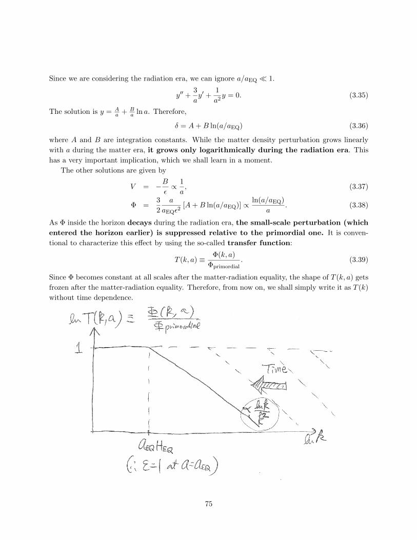
Since we are considering the radiation era, we can ignore a/aEQ 1.

y′′ +3

ay′ +

1

a2y = 0. (3.35)

The solution is y = Aa + B

a ln a. Therefore,

δ = A+B ln(a/aEQ) (3.36)

where A and B are integration constants. While the matter density perturbation grows linearly

with a during the matter era, it grows only logarithmically during the radiation era. This

has a very important implication, which we shall learn in a moment.

The other solutions are given by

V = −Bε∝ 1

a, (3.37)

Φ =3

2

a

aEQε2[A+B ln(a/aEQ)] ∝

ln(a/aEQ)

a. (3.38)

As Φ inside the horizon decays during the radiation era, the small-scale perturbation (which

entered the horizon earlier) is suppressed relative to the primordial one. It is conven-

tional to characterize this effect by using the so-called transfer function:

T (k, a) ≡ Φ(k, a)

Φprimordial. (3.39)

Since Φ becomes constant at all scales after the matter-radiation equality, the shape of T (k, a) gets

frozen after the matter-radiation equality. Therefore, from now on, we shall simply write it as T (k)

without time dependence.

75

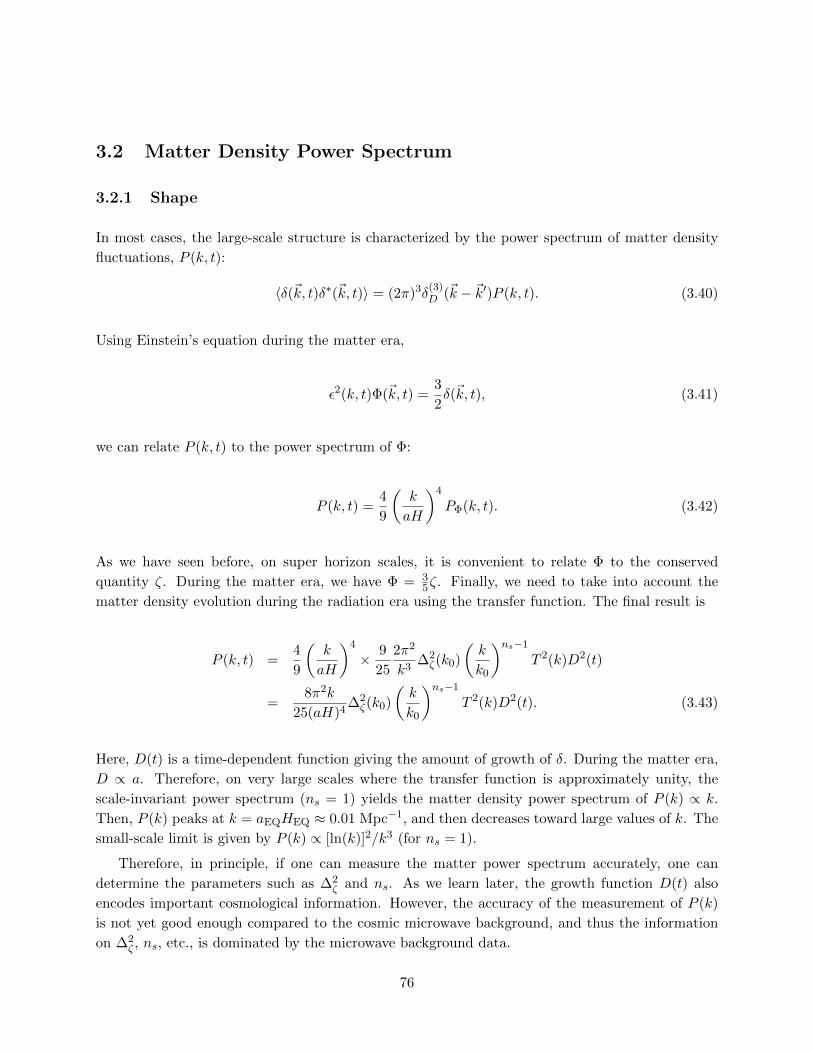
3.2 Matter Density Power Spectrum

3.2.1 Shape

In most cases, the large-scale structure is characterized by the power spectrum of matter density

fluctuations, P (k, t):

〈δ(~k, t)δ∗(~k, t)〉 = (2π)3δ(3)D (~k − ~k′)P (k, t). (3.40)

Using Einstein’s equation during the matter era,

ε2(k, t)Φ(~k, t) =3

2δ(~k, t), (3.41)

we can relate P (k, t) to the power spectrum of Φ:

P (k, t) =4

9

(k

aH

)4

PΦ(k, t). (3.42)

As we have seen before, on super horizon scales, it is convenient to relate Φ to the conserved

quantity ζ. During the matter era, we have Φ = 35ζ. Finally, we need to take into account the

matter density evolution during the radiation era using the transfer function. The final result is

P (k, t) =4

9

(k

aH

)4

× 9

25

2π2

k3∆2ζ(k0)

(k

k0

)ns−1

T 2(k)D2(t)

=8π2k

25(aH)4∆2ζ(k0)

(k

k0

)ns−1

T 2(k)D2(t). (3.43)

Here, D(t) is a time-dependent function giving the amount of growth of δ. During the matter era,

D ∝ a. Therefore, on very large scales where the transfer function is approximately unity, the

scale-invariant power spectrum (ns = 1) yields the matter density power spectrum of P (k) ∝ k.

Then, P (k) peaks at k = aEQHEQ ≈ 0.01 Mpc−1, and then decreases toward large values of k. The

small-scale limit is given by P (k) ∝ [ln(k)]2/k3 (for ns = 1).

Therefore, in principle, if one can measure the matter power spectrum accurately, one can

determine the parameters such as ∆2ζ and ns. As we learn later, the growth function D(t) also

encodes important cosmological information. However, the accuracy of the measurement of P (k)

is not yet good enough compared to the cosmic microwave background, and thus the information

on ∆2ζ , ns, etc., is dominated by the microwave background data.

76

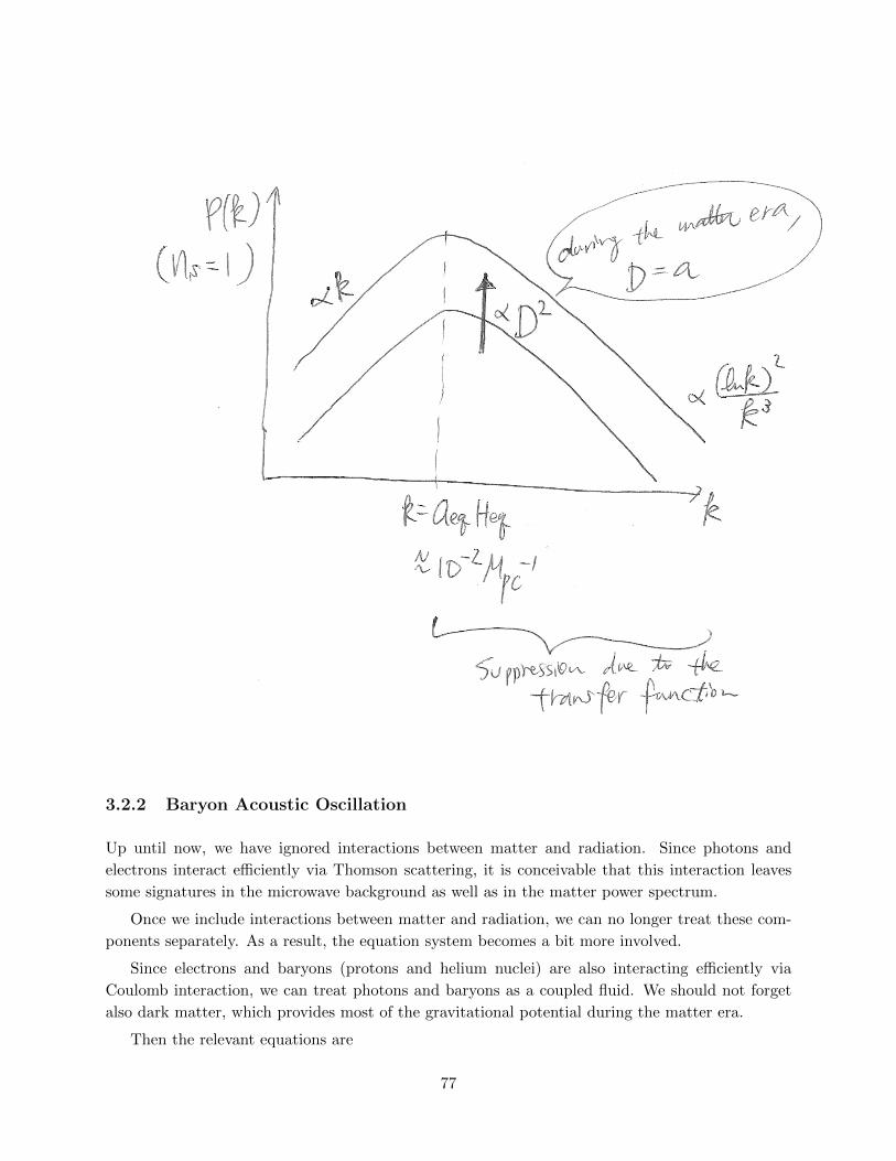
3.2.2 Baryon Acoustic Oscillation

Up until now, we have ignored interactions between matter and radiation. Since photons and

electrons interact efficiently via Thomson scattering, it is conceivable that this interaction leaves

some signatures in the microwave background as well as in the matter power spectrum.

Once we include interactions between matter and radiation, we can no longer treat these com-

ponents separately. As a result, the equation system becomes a bit more involved.

Since electrons and baryons (protons and helium nuclei) are also interacting efficiently via

Coulomb interaction, we can treat photons and baryons as a coupled fluid. We should not forget

also dark matter, which provides most of the gravitational potential during the matter era.

Then the relevant equations are

77

• Energy Conservation:

δD = −kaVD − 3Φ, (3.44)

δB = −kaVB − 3Φ, (3.45)

δγ = −4

3

k

aVγ − 4Φ, (3.46)

where δD, δB, and δγ are the dark matter, baryon, and photon densities, respectively. Since

we consider the matter-dominated era, we shall ignore Φ.

• Momentum Conservation:

VD = − aaVD −

k

aΦ, (3.47)

VB = − aaVB −

k

aΦ +

σTneR

(Vγ − VB), (3.48)

Vγ =1

4

k

aδγ −

k

aΦ + σTne(VB − Vγ), (3.49)

where R is the baryon-to-photon energy density ratio defined as

R ≡ 3ρB4ργ

. (3.50)

• Einstein’s Equation:

k2

a2Φ = 4πG (ρDδD + ρBδB) , (3.51)

where we have ignored the radiation contribution in the right hand side because we are

considering the matter-dominated era.

Now, while there are many equations, one can simplify the equation system considerably when

the coupling between photons and baryons is very efficient. In such a case, baryons and photons

basically move together, i.e., VB ≈ Vγ .

We rewrite Eq. (5.48) as

VB = Vγ −R

σTne

(VB +

a

aVB +

k

aΦ

)≈ Vγ −

R

σTne

(Vγ +

a

aVγ +

k

aΦ

). (3.52)

Here, since we assume that the difference between VB and Vγ is small, we have replaced VB with

Vγ in the right hand side. We then use the photon momentum conservation equation, Eq. (5.49),

78

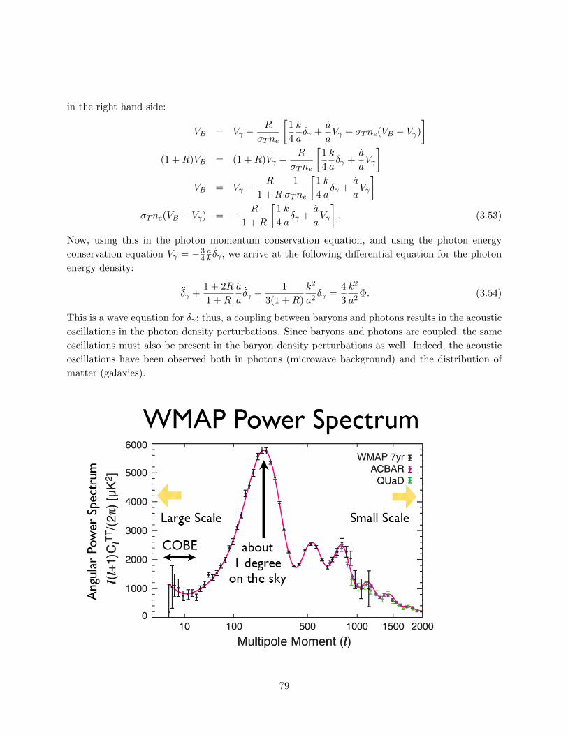
in the right hand side:

VB = Vγ −R

σTne

[1

4

k

aδγ +

a

aVγ + σTne(VB − Vγ)

](1 +R)VB = (1 +R)Vγ −

R

σTne

[1

4

k

aδγ +

a

aVγ

]VB = Vγ −

R

1 +R

1

σTne

[1

4

k

aδγ +

a

aVγ

]σTne(VB − Vγ) = − R

1 +R

[1

4

k

aδγ +

a

aVγ

]. (3.53)

Now, using this in the photon momentum conservation equation, and using the photon energy

conservation equation Vγ = −34ak δγ , we arrive at the following differential equation for the photon

energy density:

δγ +1 + 2R

1 +R

a

aδγ +

1

3(1 +R)

k2

a2δγ =

4

3

k2

a2Φ. (3.54)

This is a wave equation for δγ ; thus, a coupling between baryons and photons results in the acoustic

oscillations in the photon density perturbations. Since baryons and photons are coupled, the same

oscillations must also be present in the baryon density perturbations as well. Indeed, the acoustic

oscillations have been observed both in photons (microwave background) and the distribution of

matter (galaxies).

79

Acoustic Oscillations in CMB

To have a deeper understanding of the structures of the acoustic oscillation, let us focus on the

regime where the oscillation frequency is much greater than the expansion rate of the universe. In

this case, the wave equation simplifies to

δγ +1

3(1 +R)

k2

a2δγ =

4

3

k2

a2Φ. (3.55)

Since Φ = 0 during the matter era, one may rewrite this equation in a suggestive way:

∂2

∂t2

[1

4δγ − (1 +R)Φ

]+k2c2

s

a2

[1

4δγ − (1 +R)Φ

]= 0, (3.56)

where cs is the speed of sound:

c2s ≡

1

3(1 +R)=

1

3(1 + 3ρB4ργ

). (3.57)

Note that this speed of sound is less than that for the relativistic fluid, c2s = 1/3. This is due to

the coupling to baryons: the inertia of baryons reduces the speed of sound of photon-baryon fluid

relative to that of the relativistic fluid. The solution to the above wave equation is

1

4δγ = (1 +R)Φ +A cos(krs) +B sin(krs), (3.58)

where rs is the sound horizon defined by

rs ≡∫ t∗

0

dt

acs(a) = 147 Mpc, (3.59)

for the cosmological parameters best-fit to the WMAP data and t∗ is the decoupling time.

How do we determine the integration constants, A and B? We determine these coefficients by

noting that, on super horizon scales, these solutions should match the adiabatic initial condition:

1

4δγ =

1

3δm =

2

3Φ on super-horizon scales (kcs 1) (3.60)

Therefore,

A =2

3Φ− (1 +R)Φ = −

(1

3+R

)Φ, (3.61)

B = 0, (3.62)

and1

4δγ = (1 +R)Φ−

(1

3+R

)Φ cos(krs). (3.63)

80

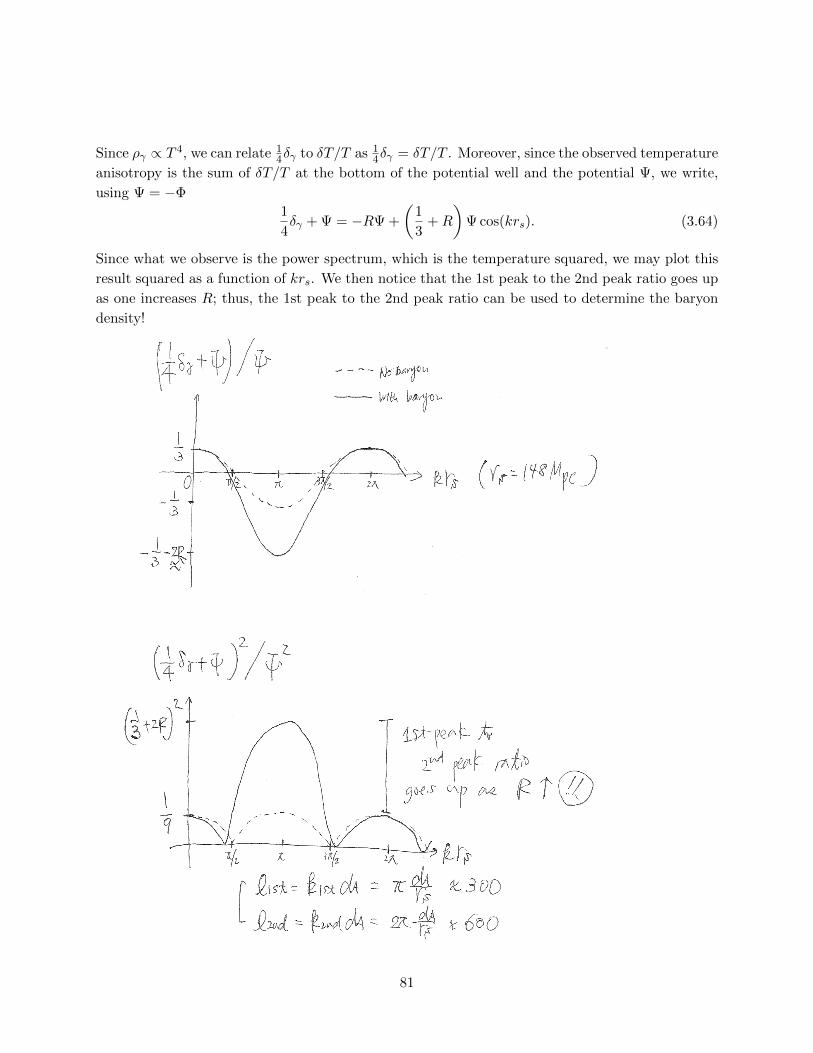
Since ργ ∝ T 4, we can relate 14δγ to δT/T as 1

4δγ = δT/T . Moreover, since the observed temperature

anisotropy is the sum of δT/T at the bottom of the potential well and the potential Ψ, we write,

using Ψ = −Φ

1

4δγ + Ψ = −RΨ +

(1

3+R

)Ψ cos(krs). (3.64)

Since what we observe is the power spectrum, which is the temperature squared, we may plot this

result squared as a function of krs. We then notice that the 1st peak to the 2nd peak ratio goes up

as one increases R; thus, the 1st peak to the 2nd peak ratio can be used to determine the baryon

density!

81

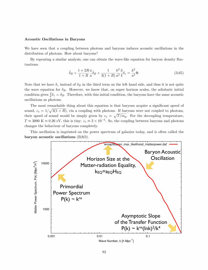
Acoustic Oscillations in Baryons

We have seen that a coupling between photons and baryons induces acoustic oscillations in the

distribution of photons. How about baryons?

By repeating a similar analysis, one can obtain the wave-like equation for baryon density fluc-

tuations:

δB +1 + 2R

1 +R

a

aδB +

1

3(1 +R)

k2

a2

3

4δγ =

k2

a2Φ. (3.65)

Note that we have δγ instead of δB in the third term on the left hand side, and thus it is not quite

the wave equation for δB. However, we know that, on super horizon scales, the adiabatic initial

condition gives 34δγ = δB. Therefore, with this initial condition, the baryons have the same acoustic

oscillations as photons.

The most remarkable thing about this equation is that baryons acquire a significant speed of

sound, cs = 1/√

3(1 +R), via a coupling with photons. If baryons were not coupled to photons,

their speed of sound would be simply given by cs =√T/mp. For the decoupling temperature,

T ≈ 3000 K ≈ 0.26 eV, this is tiny: cs ≈ 2× 10−5. So, the coupling between baryons and photons

changes the behaviour of baryons completely.

This oscillation is imprinted on the power spectrum of galaxies today, and is often called the

baryon acoustic oscillations (BAO).

1000

10000

0.001 0.01 0.1

Mat

ter P

ower

Spe

ctru

m, P

(k) [

Mpc

3 /h3 ]

Wave Number, k [h Mpc-1]

’wmap5baosn_max_likelihood_matterpower.dat’

Primordial Power Spectrum

P(k) ~ kns

Horizon Size at the Matter-radiation Equality,

kEQ=aEQHEQ

Baryon AcousticOscillation

Asymptotic Slopeof the Transfer Function

P(k) ~ kns(lnk)2/k4

82

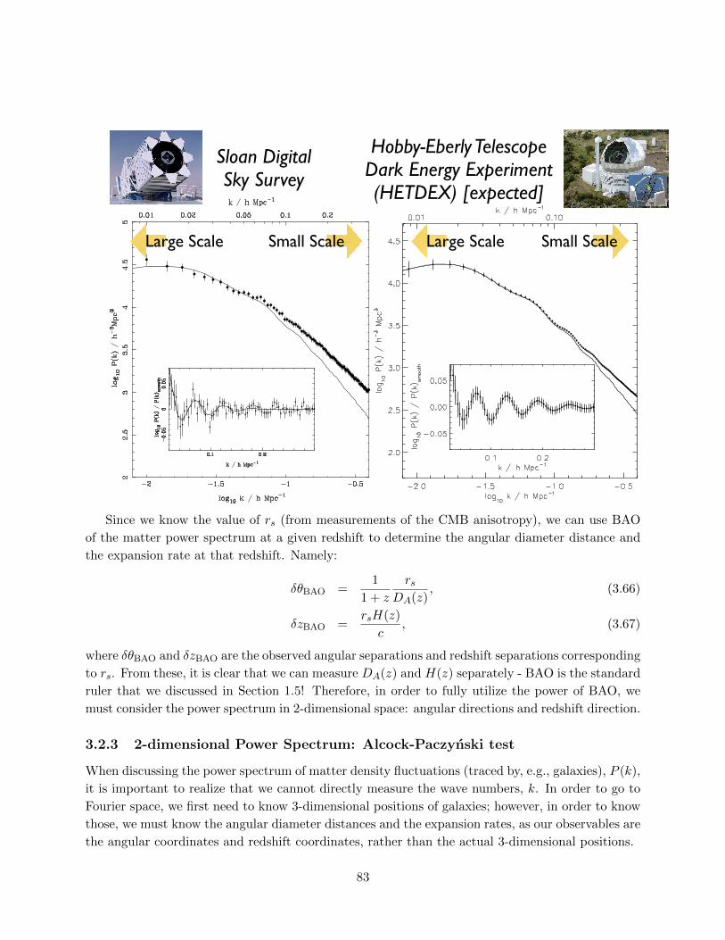
Sloan Digital Sky Survey10 Percival et al.

Fig. 12.— The redshift-space power spectrum recovered from the combined SDSS main galaxy and LRG sample, optimally weighted forboth density changes and luminosity dependent bias (solid circles with 1-! errors). A flat ! cosmological distance model was assumed with"M = 0.24. Error bars are derived from the diagonal elements of the covariance matrix calculated from 2000 log-normal catalogues createdfor this cosmological distance model, but with a power spectrum amplitude and shape matched to that observed (see text for details).The data are correlated, and the width of the correlations is presented in Fig. 10 (the correlation between data points drops to < 0.33 for#k > 0.01 h Mpc!1). The correlations are smaller than the oscillatory features observed in the recovered power spectrum. For comparisonwe plot the model power spectrum (solid line) calculated using the fitting formulae of Eisenstein & Hu (1998); Eisenstein et al. (2006), forthe best fit parameters calculated by fitting the WMAP 3-year temperature and polarisation data, h = 0.73, "M = 0.24, ns = 0.96 and"b/"M = 0.174 (Spergel et al. 2006). The model power spectrum has been convolved with the appropriate window function to match themeasured data, and the normalisation has been matched to that of the large-scale (0.01 < k < 0.06 hMpc!1) data. The deviation from

this low "M linear power spectrum is clearly visible at k >" 0.06 hMpc!1, and will be discussed further in Section 6. The solid circles with1! errors in the inset show the power spectrum ratioed to a smooth model (calculated using a cubic spline fit as described in Percival et al.2006) compared to the baryon oscillations in the (WMAP 3-year parameter) model (solid line), and shows good agreement. The calculationof the matter density from these oscillations will be considered in a separate paper (Percival et al. 2006). The dashed line shows the samemodel without the correction for the damping e$ect of small-scale structure growth of Eisenstein et al. (2006). It is worth noting that thismodel is not a fit to the data, but a prediction from the CMB experiment.

Small ScaleLarge Scale

Hobby-Eberly Telescope Dark Energy Experiment (HETDEX) [expected]

Small ScaleLarge Scale

Since we know the value of rs (from measurements of the CMB anisotropy), we can use BAO

of the matter power spectrum at a given redshift to determine the angular diameter distance and

the expansion rate at that redshift. Namely:

δθBAO =1

1 + z

rsDA(z)

, (3.66)

δzBAO =rsH(z)

c, (3.67)

where δθBAO and δzBAO are the observed angular separations and redshift separations corresponding

to rs. From these, it is clear that we can measure DA(z) and H(z) separately - BAO is the standard

ruler that we discussed in Section 1.5! Therefore, in order to fully utilize the power of BAO, we

must consider the power spectrum in 2-dimensional space: angular directions and redshift direction.

3.2.3 2-dimensional Power Spectrum: Alcock-Paczynski test

When discussing the power spectrum of matter density fluctuations (traced by, e.g., galaxies), P (k),

it is important to realize that we cannot directly measure the wave numbers, k. In order to go to

Fourier space, we first need to know 3-dimensional positions of galaxies; however, in order to know

those, we must know the angular diameter distances and the expansion rates, as our observables are

the angular coordinates and redshift coordinates, rather than the actual 3-dimensional positions.

83

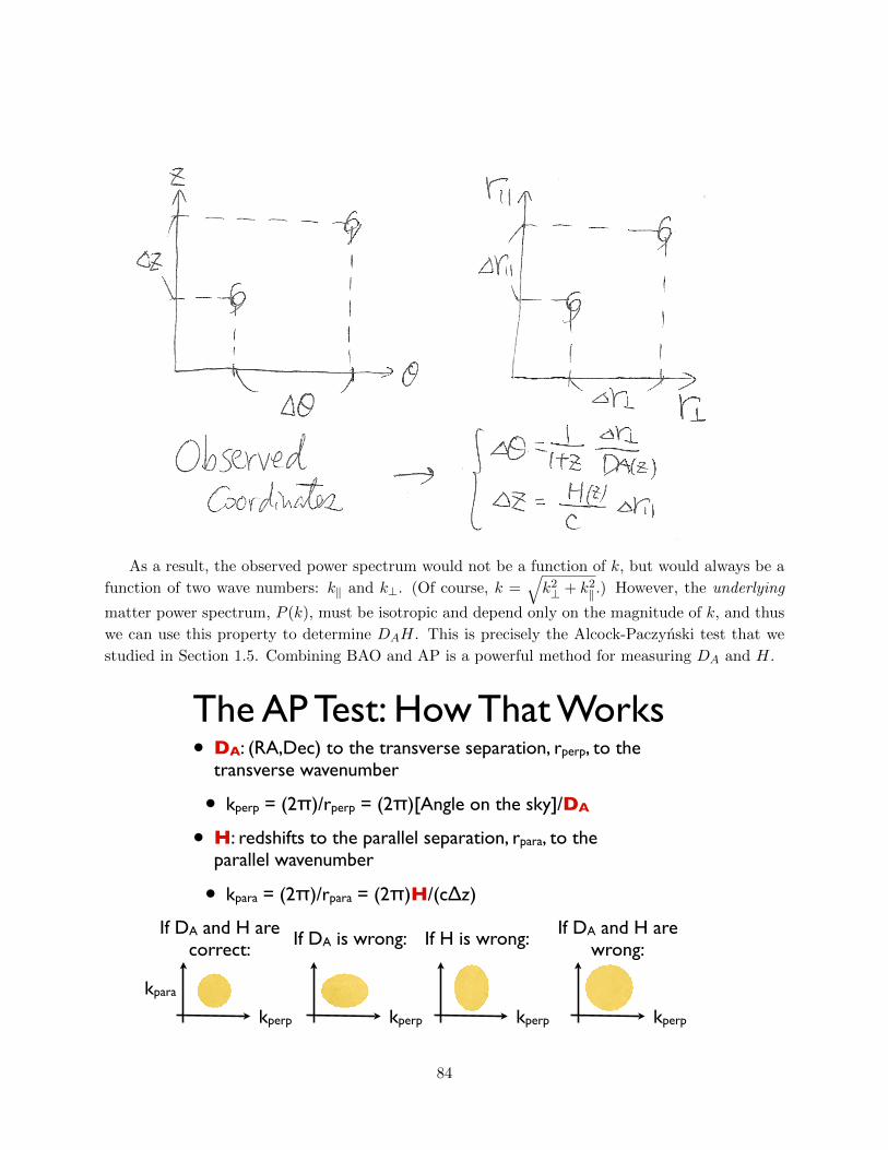
As a result, the observed power spectrum would not be a function of k, but would always be a

function of two wave numbers: k‖ and k⊥. (Of course, k =√k2⊥ + k2

‖.) However, the underlying

matter power spectrum, P (k), must be isotropic and depend only on the magnitude of k, and thus

we can use this property to determine DAH. This is precisely the Alcock-Paczynski test that we

studied in Section 1.5. Combining BAO and AP is a powerful method for measuring DA and H.

• DA: (RA,Dec) to the transverse separation, rperp, to the transverse wavenumber

• kperp = (2π)/rperp = (2π)[Angle on the sky]/DA

• H: redshifts to the parallel separation, rpara, to the parallel wavenumber

• kpara = (2π)/rpara = (2π)H/(cΔz)

The AP Test: How That Works

If DA and H are correct:

kpara

kperp

If DA is wrong:

kperp

If H is wrong:

kperp kperp

If DA and H are wrong:

84

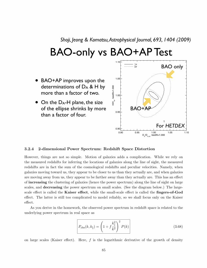
BAO-only vs BAO+AP Test

• BAO+AP improves upon the determinations of DA & H by more than a factor of two.

• On the DA-H plane, the size of the ellipse shrinks by more than a factor of four.

Shoji, Jeong & Komatsu, Astrophysical Journal, 693, 1404 (2009)

0.90 0.95 1.00 1.05 1.10D

A/D

A,ref bestfit=1.000

0.90

0.95

1.00

1.05

1.10

H/H

ref b

estfi

t=1.

000

BAO only

BAO+AP

For HETDEX1

3.2.4 2-dimensional Power Spectrum: Redshift Space Distortion

However, things are not so simple. Motion of galaxies adds a complication. While we rely on

the measured redshifts for inferring the locations of galaxies along the line of sight, the measured

redshifts are in fact the sum of the cosmological redshifts and peculiar velocities. Namely, when

galaxies moving toward us, they appear to be closer to us than they actually are, and when galaxies

are moving away from us, they appear to be farther away than they actually are. This has an effect

of increasing the clustering of galaxies (hence the power spectrum) along the line of sight on large

scales, and decreasing the power spectrum on small scales. (See the diagram below.) The large-

scale effect is called the Kaiser effect, while the small-scale effect is called the fingers-of-God

effect. The latter is still too complicated to model reliably, so we shall focus only on the Kaiser

effect.

As you derive in the homework, the observed power spectrum in redshift space is related to the

underlying power spectrum in real space as

Pobs(k, k‖) =

(1 + f

k2‖

k2

)2

P (k) (3.68)

on large scales (Kaiser effect). Here, f is the logarithmic derivative of the growth of density

85

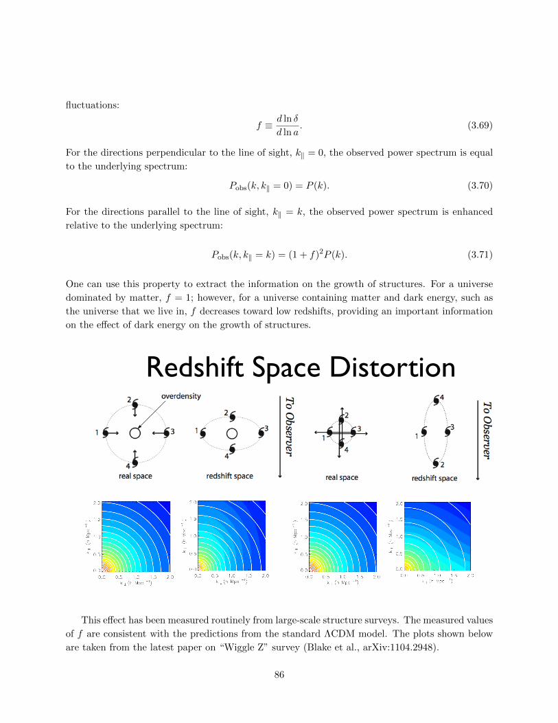
fluctuations:

f ≡ d ln δ

d ln a. (3.69)

For the directions perpendicular to the line of sight, k‖ = 0, the observed power spectrum is equal

to the underlying spectrum:

Pobs(k, k‖ = 0) = P (k). (3.70)

For the directions parallel to the line of sight, k‖ = k, the observed power spectrum is enhanced

relative to the underlying spectrum:

Pobs(k, k‖ = k) = (1 + f)2P (k). (3.71)

One can use this property to extract the information on the growth of structures. For a universe

dominated by matter, f = 1; however, for a universe containing matter and dark energy, such as

the universe that we live in, f decreases toward low redshifts, providing an important information

on the effect of dark energy on the growth of structures.

Redshift Space Distortion

This effect has been measured routinely from large-scale structure surveys. The measured values

of f are consistent with the predictions from the standard ΛCDM model. The plots shown below

are taken from the latest paper on “Wiggle Z” survey (Blake et al., arXiv:1104.2948).

86

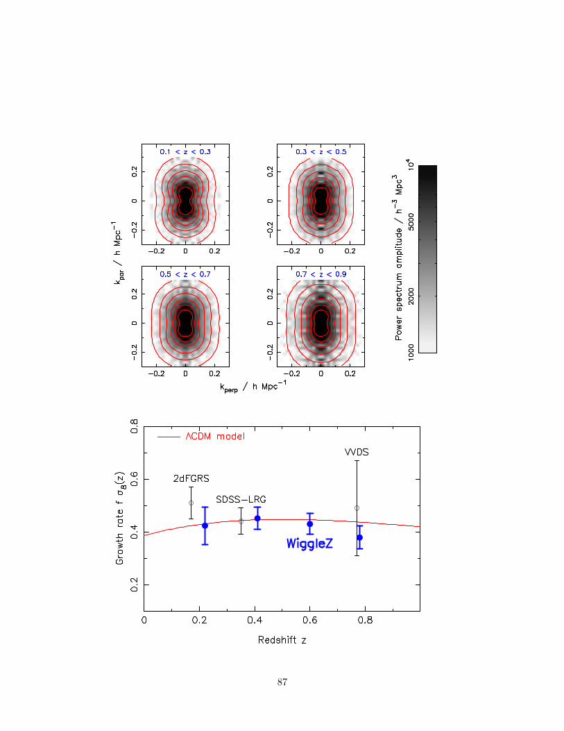
87

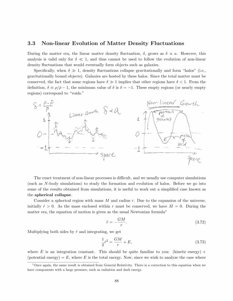
3.3 Non-linear Evolution of Matter Density Fluctuations

During the matter era, the linear matter density fluctuation, δ, grows as δ ∝ a. However, this

analysis is valid only for δ 1, and thus cannot be used to follow the evolution of non-linear

density fluctuations that would eventually form objects such as galaxies.

Specifically, when δ 1, density fluctuations collapse gravitationally and form “halos” (i.e.,

gravitationally bound objects). Galaxies are hosted by these halos. Since the total matter must be

conserved, the fact that some regions have δ 1 implies that other regions have δ < 1. From the

definition, δ ≡ ρ/ρ− 1, the minimum value of δ is δ = −1. These empty regions (or nearly empty

regions) correspond to “voids.”

The exact treatment of non-linear processes is difficult, and we usually use computer simulations

(such as N -body simulations) to study the formation and evolution of halos. Before we go into

some of the results obtained from simulations, it is useful to work out a simplified case known as

the spherical collapse.

Consider a spherical region with mass M and radius r. Due to the expansion of the universe,

initially r > 0. As the mass enclosed within r must be conserved, we have M = 0. During the

matter era, the equation of motion is given as the usual Newtonian formula∗

r = −GMr. (3.72)

Multiplying both sides by r and integrating, we get

1

2r2 =

GM

r+ E, (3.73)

where E is an integration constant. This should be quite familiar to you: (kinetic energy) +

(potential energy) = E, where E is the total energy. Now, since we wish to analyze the case where

∗Once again, the same result is obtained from General Relativity. There is a correction to this equation when we

have components with a large pressure, such as radiation and dark energy.

88

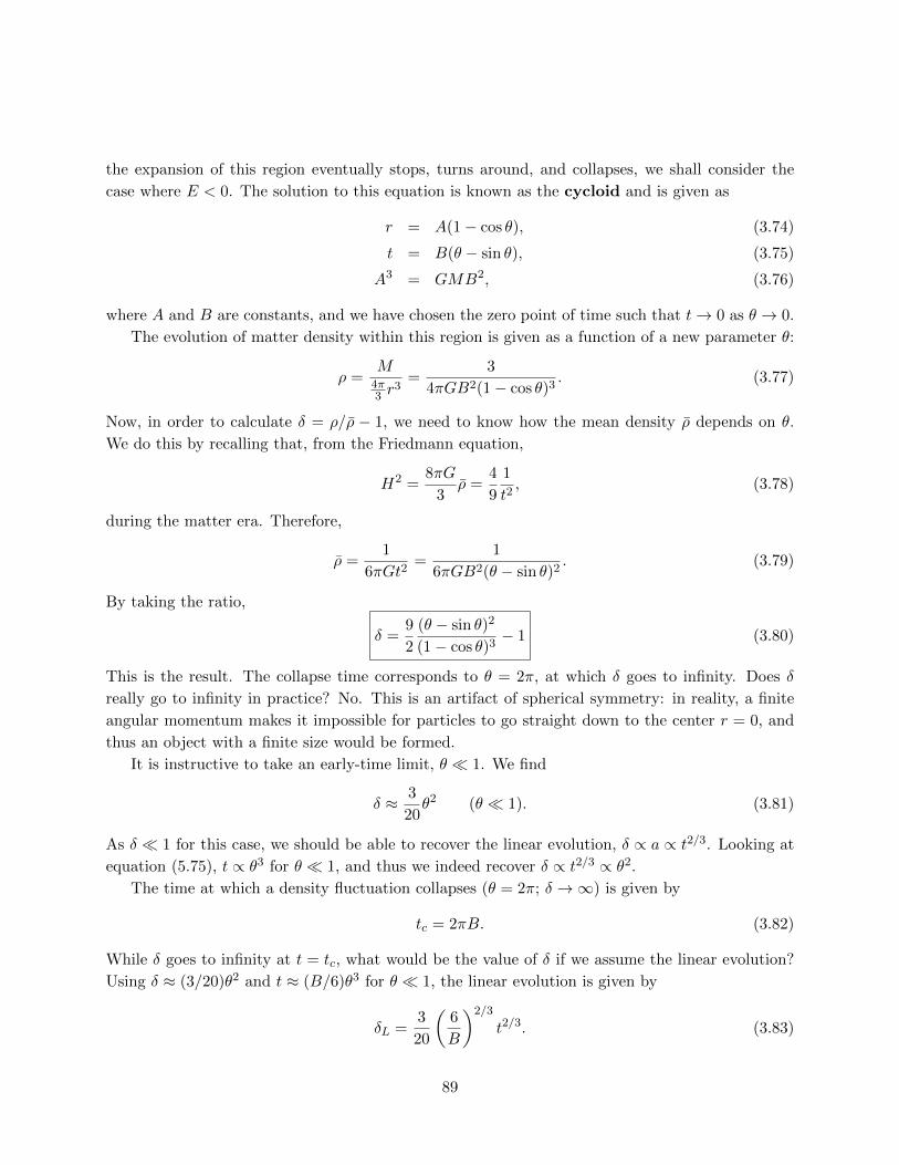
the expansion of this region eventually stops, turns around, and collapses, we shall consider the

case where E < 0. The solution to this equation is known as the cycloid and is given as

r = A(1− cos θ), (3.74)

t = B(θ − sin θ), (3.75)

A3 = GMB2, (3.76)

where A and B are constants, and we have chosen the zero point of time such that t→ 0 as θ → 0.

The evolution of matter density within this region is given as a function of a new parameter θ:

ρ =M

4π3 r

3=

3

4πGB2(1− cos θ)3. (3.77)

Now, in order to calculate δ = ρ/ρ − 1, we need to know how the mean density ρ depends on θ.

We do this by recalling that, from the Friedmann equation,

H2 =8πG

3ρ =

4

9

1

t2, (3.78)

during the matter era. Therefore,

ρ =1

6πGt2=

1

6πGB2(θ − sin θ)2. (3.79)

By taking the ratio,

δ =9

2

(θ − sin θ)2

(1− cos θ)3− 1 (3.80)

This is the result. The collapse time corresponds to θ = 2π, at which δ goes to infinity. Does δ

really go to infinity in practice? No. This is an artifact of spherical symmetry: in reality, a finite

angular momentum makes it impossible for particles to go straight down to the center r = 0, and

thus an object with a finite size would be formed.

It is instructive to take an early-time limit, θ 1. We find

δ ≈ 3

20θ2 (θ 1). (3.81)

As δ 1 for this case, we should be able to recover the linear evolution, δ ∝ a ∝ t2/3. Looking at

equation (5.75), t ∝ θ3 for θ 1, and thus we indeed recover δ ∝ t2/3 ∝ θ2.

The time at which a density fluctuation collapses (θ = 2π; δ →∞) is given by

tc = 2πB. (3.82)

While δ goes to infinity at t = tc, what would be the value of δ if we assume the linear evolution?

Using δ ≈ (3/20)θ2 and t ≈ (B/6)θ3 for θ 1, the linear evolution is given by

δL =3

20

(6

B

)2/3

t2/3. (3.83)

89

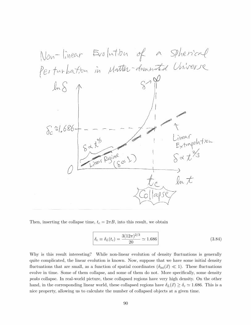
Then, inserting the collapse time, tc = 2πB, into this result, we obtain

δc ≡ δL(tc) =3(12π)2/3

20' 1.686 (3.84)

Why is this result interesting? While non-linear evolution of density fluctuations is generally

quite complicated, the linear evolution is known. Now, suppose that we have some initial density

fluctuations that are small, as a function of spatial coordinates (δini(~x) 1). These fluctuations

evolve in time. Some of them collapse, and some of them do not. More specifically, some density

peaks collapse. In real-world picture, these collapsed regions have very high density. On the other

hand, in the corresponding linear world, these collapsed regions have δL(~x) ≥ δc ' 1.686. This is a

nice property, allowing us to calculate the number of collapsed objects at a given time.

90

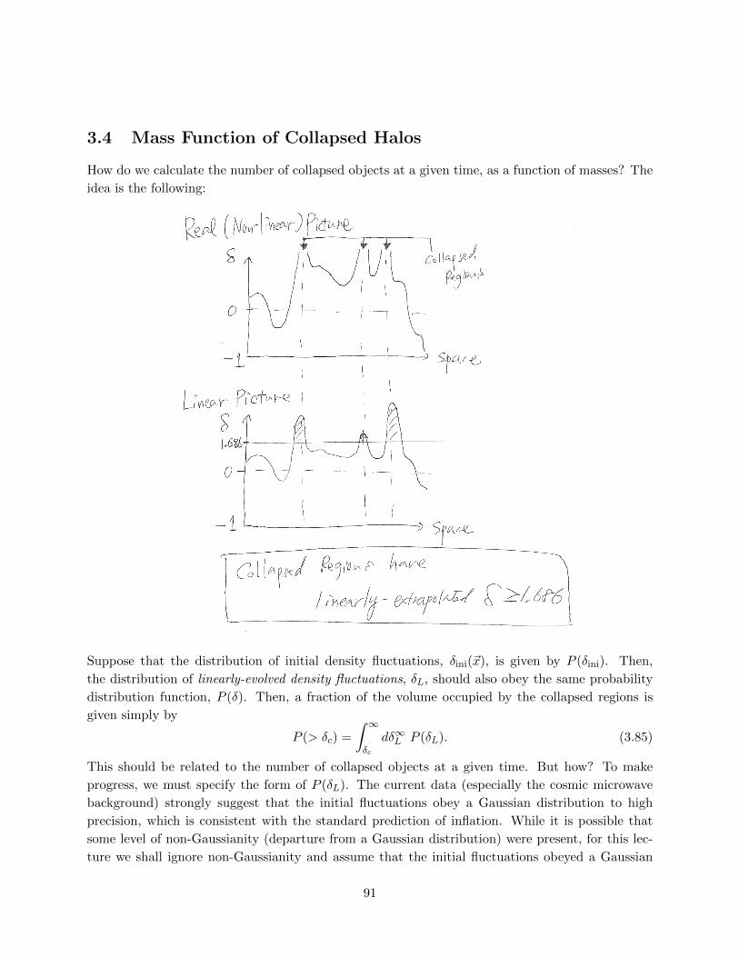
3.4 Mass Function of Collapsed Halos

How do we calculate the number of collapsed objects at a given time, as a function of masses? The

idea is the following:

Suppose that the distribution of initial density fluctuations, δini(~x), is given by P (δini). Then,

the distribution of linearly-evolved density fluctuations, δL, should also obey the same probability

distribution function, P (δ). Then, a fraction of the volume occupied by the collapsed regions is

given simply by

P (> δc) =

∫ ∞δc

dδ∞L P (δL). (3.85)

This should be related to the number of collapsed objects at a given time. But how? To make

progress, we must specify the form of P (δL). The current data (especially the cosmic microwave

background) strongly suggest that the initial fluctuations obey a Gaussian distribution to high

precision, which is consistent with the standard prediction of inflation. While it is possible that

some level of non-Gaussianity (departure from a Gaussian distribution) were present, for this lec-

ture we shall ignore non-Gaussianity and assume that the initial fluctuations obeyed a Gaussian

91

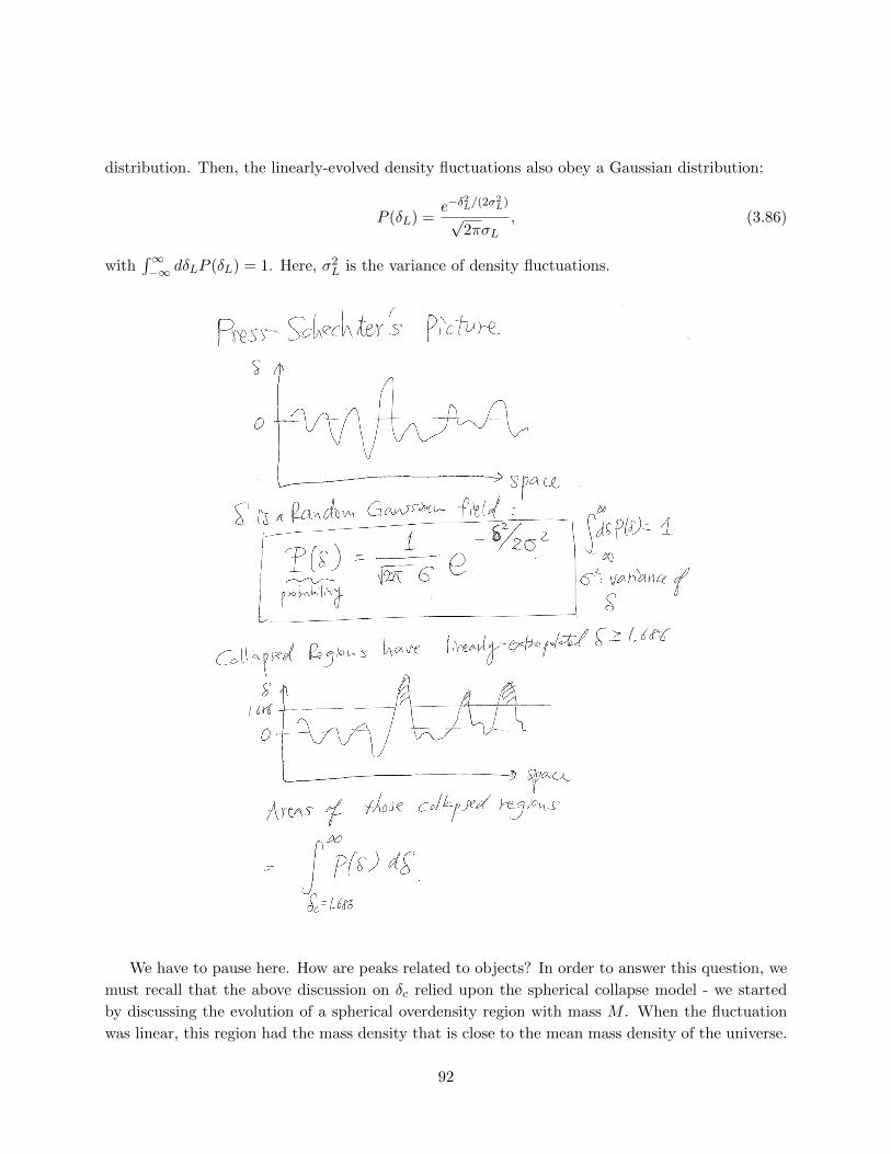
distribution. Then, the linearly-evolved density fluctuations also obey a Gaussian distribution:

P (δL) =e−δ

2L/(2σ

2L)

√2πσL

, (3.86)

with∫∞−∞ dδLP (δL) = 1. Here, σ2

L is the variance of density fluctuations.

We have to pause here. How are peaks related to objects? In order to answer this question, we

must recall that the above discussion on δc relied upon the spherical collapse model - we started

by discussing the evolution of a spherical overdensity region with mass M . When the fluctuation

was linear, this region had the mass density that is close to the mean mass density of the universe.

92

Therefore, the initial comoving radius of this region was given by

R =

(3M

4πρM

)= 4.0 Mpc

(0.135

ΩMh2

M

1013 M

)1/3

, (3.87)

where we have used ρM = 2.775 × 1011ΩMh2 M Mpc−3 (which is the present-day mass density

of the universe). Therefore, for galactic scales (M = 1012 M), R = 1.9 Mpc; for clusters scales

(M = 1015 M), R = 19 Mpc. Again, note that this is not the real radius of objects observed

today with a given mass. Rather, this is the radius that objects would have, if they had the mean

mass density of the universe today. This is the most relevant radius when we talk about the linear

density fluctuations. These regions then expand, turn around, and then contract to form objects

with physical radii much smaller than R given above.

The next step is to find overdense regions that have a certain mass M . In order to do this,

we need to “bin” the density fields with the corresponding radii R. Namely, we first average the

density field as

δR(~x) ≡ 14πR3

3

∫|~r|≤R

d3rδL(~x+ ~r), (3.88)

where R =(

3M4πρM

), and see if the averaged δR exceeds the critical overdensity δc. The Fourier

transform of δR is related to that of the original linear density field δL as

δR(~k) =

∫d3x δR(~x)e−i

~k·~x

=

∫d3x

14πR3

3

∫|~r|≤R

d3r

∫d3k′

(2π)3δL(~k′)ei

~k′·(~x+~r)e−i~k·~x

=1

4πR3

3

∫|~r|≤R

d3r

∫d3k′ δ

(3)D (~k − ~k′)δL(~k′)ei

~k·~r

= δL(~k)1

4πR3

3

∫|~r|≤R

d3r ei~k·~r

= δL(~k)1

2R3

3

∫ R

0r2dr

∫ 1

−1dµ eikrµ

= δL(~k)

[3j1(kR)

kR

], (3.89)

where j1(x) = sin(x)/x2− cos(x)/x is a spherical Bessel function of order 1. Therefore, the Fourier

transform of δR is the Fourier transform of δL times the “window function” given by 3j1(kR)kR .

93

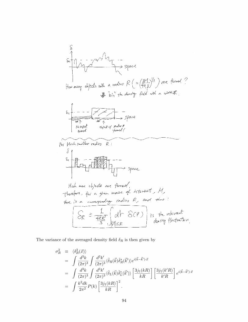
The variance of the averaged density field δR is then given by

σ2R ≡ 〈δ2

R(~x)〉

=

∫d3k

(2π)3

∫d3k′

(2π)3〈δR(~k)δ∗R(~k′)〉ei(~k−~k′)·~x

=

∫d3k

(2π)3

∫d3k′

(2π)3〈δL(~k)δ∗L(~k′)〉

[3j1(kR)

kR

] [3j1(k′R)

k′R

]ei(~k−~k′)·~x

=

∫k2dk

2π2P (k)

[3j1(kR)

kR

]2

.

94

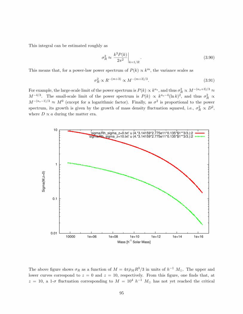
This integral can be estimated roughly as

σ2R ≈

k3P (k)

2π2

∣∣∣∣k=1/R

. (3.90)

This means that, for a power-law power spectrum of P (k) ∝ km, the variance scales as

σ2R ∝ R−(m+3) ∝M−(m+3)/3. (3.91)

For example, the large-scale limit of the power spectrum is P (k) ∝ kns , and thus σ2R ∝M−(ns+3)/3 ≈

M−4/3. The small-scale limit of the power spectrum is P (k) ∝ kns−4(ln k)2, and thus σ2R ∝

M−(ns−1)/3 ≈ M0 (except for a logarithmic factor). Finally, as σ2 is proportional to the power

spectrum, its growth is given by the growth of mass density fluctuation squared, i.e., σ2R ∝ D2,

where D ∝ a during the matter era.

0.01

0.1

1

10

10000 1e+06 1e+08 1e+10 1e+12 1e+14 1e+16

Sig

ma(

M,z

=0)

Mass [h-1 Solar Mass]

’sigma/Rh_sigma_z=0.txt’ u (4.*3.14159*2.775e11*0.135*$1**3/3.):2’sigma/Rh_sigma_z=10.txt’ u (4.*3.14159*2.775e11*0.135*$1**3/3.):2

The above figure shows σR as a function of M = 4πρMR3/3 in units of h−1 M. The upper and

lower curves correspond to z = 0 and z = 10, respectively. From this figure, one finds that, at

z = 10, a 1-σ fluctuation corresponding to M = 104 h−1 M has not yet reached the critical

95

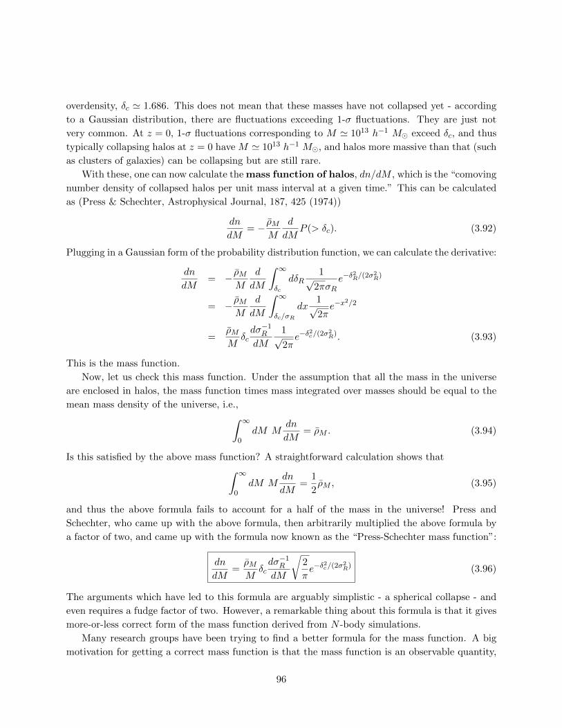
overdensity, δc ' 1.686. This does not mean that these masses have not collapsed yet - according

to a Gaussian distribution, there are fluctuations exceeding 1-σ fluctuations. They are just not

very common. At z = 0, 1-σ fluctuations corresponding to M ' 1013 h−1 M exceed δc, and thus

typically collapsing halos at z = 0 have M ' 1013 h−1 M, and halos more massive than that (such

as clusters of galaxies) can be collapsing but are still rare.

With these, one can now calculate the mass function of halos, dn/dM , which is the “comoving

number density of collapsed halos per unit mass interval at a given time.” This can be calculated

as (Press & Schechter, Astrophysical Journal, 187, 425 (1974))

dn

dM= − ρM

M

d

dMP (> δc). (3.92)

Plugging in a Gaussian form of the probability distribution function, we can calculate the derivative:

dn

dM= − ρM

M

d

dM

∫ ∞δc

dδR1√

2πσRe−δ

2R/(2σ

2R)

= − ρMM

d

dM

∫ ∞δc/σR

dx1√2πe−x

2/2

=ρMM

δcdσ−1

R

dM

1√2πe−δ

2c/(2σ

2R). (3.93)

This is the mass function.

Now, let us check this mass function. Under the assumption that all the mass in the universe

are enclosed in halos, the mass function times mass integrated over masses should be equal to the

mean mass density of the universe, i.e.,∫ ∞0

dM Mdn

dM= ρM . (3.94)

Is this satisfied by the above mass function? A straightforward calculation shows that∫ ∞0

dM Mdn

dM=

1

2ρM , (3.95)

and thus the above formula fails to account for a half of the mass in the universe! Press and

Schechter, who came up with the above formula, then arbitrarily multiplied the above formula by

a factor of two, and came up with the formula now known as the “Press-Schechter mass function”:

dn

dM=ρMM

δcdσ−1

R

dM

√2

πe−δ

2c/(2σ

2R) (3.96)

The arguments which have led to this formula are arguably simplistic - a spherical collapse - and

even requires a fudge factor of two. However, a remarkable thing about this formula is that it gives

more-or-less correct form of the mass function derived from N -body simulations.

Many research groups have been trying to find a better formula for the mass function. A big

motivation for getting a correct mass function is that the mass function is an observable quantity,

96

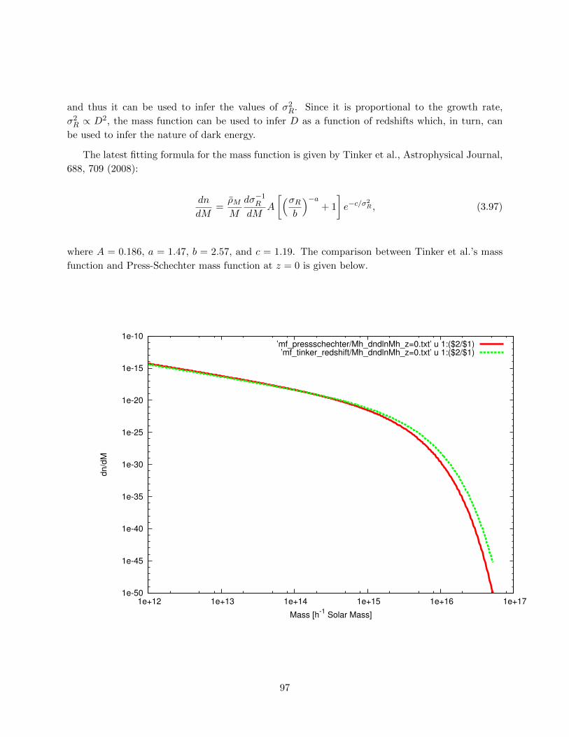
and thus it can be used to infer the values of σ2R. Since it is proportional to the growth rate,

σ2R ∝ D2, the mass function can be used to infer D as a function of redshifts which, in turn, can

be used to infer the nature of dark energy.

The latest fitting formula for the mass function is given by Tinker et al., Astrophysical Journal,

688, 709 (2008):

dn

dM=ρMM

dσ−1R

dMA

[(σRb

)−a+ 1

]e−c/σ

2R , (3.97)

where A = 0.186, a = 1.47, b = 2.57, and c = 1.19. The comparison between Tinker et al.’s mass

function and Press-Schechter mass function at z = 0 is given below.

1e-50

1e-45

1e-40

1e-35

1e-30

1e-25

1e-20

1e-15

1e-10

1e+12 1e+13 1e+14 1e+15 1e+16 1e+17

dn/d

M

Mass [h-1 Solar Mass]

’mf_pressschechter/Mh_dndlnMh_z=0.txt’ u 1:($2/$1)’mf_tinker_redshift/Mh_dndlnMh_z=0.txt’ u 1:($2/$1)

97

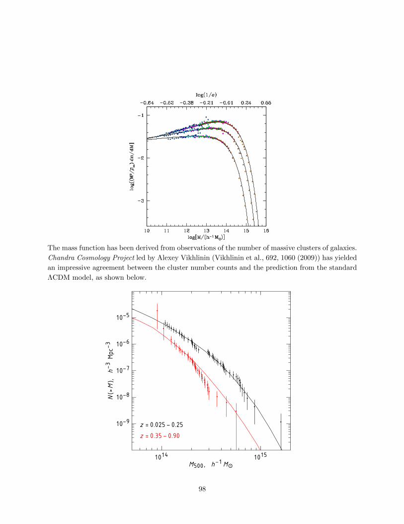
The mass function has been derived from observations of the number of massive clusters of galaxies.

Chandra Cosmology Project led by Alexey Vikhlinin (Vikhlinin et al., 692, 1060 (2009)) has yielded

an impressive agreement between the cluster number counts and the prediction from the standard

ΛCDM model, as shown below.

z = 0.025 − 0.25

1014 1015

10−9

10−8

10−7

10−6

10−5

M500, h−1

M⊙

N(>

M),

h−

3Mpc−

3

z = 0.35 − 0.90

98

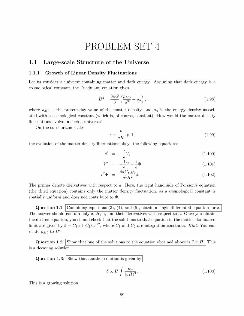
PROBLEM SET 4

1.1 Large-scale Structure of the Universe

1.1.1 Growth of Linear Density Fluctuations

Let us consider a universe containing matter and dark energy. Assuming that dark energy is a

cosmological constant, the Friedmann equation gives

H2 =8πG

3

(ρM0

a3+ ρΛ

), (1.98)

where ρM0 is the present-day value of the matter density, and ρΛ is the energy density associ-

ated with a cosmological constant (which is, of course, constant). How would the matter density

fluctuations evolve in such a universe?

On the sub-horizon scales,

ε ≡ k

aH 1, (1.99)

the evolution of the matter density fluctuations obeys the following equations:

δ′ = − εaV, (1.100)

V ′ = −1

aV − ε

aΦ, (1.101)

ε2Φ =4πGρM0

a3H2δ. (1.102)

The primes denote derivatives with respect to a. Here, the right hand side of Poisson’s equation

(the third equation) contains only the matter density fluctuation, as a cosmological constant is

spatially uniform and does not contribute to Φ.

Question 1.1: Combining equations (3), (4), and (5), obtain a single differential equation for δ.

The answer should contain only δ, H, a, and their derivatives with respect to a. Once you obtain

the desired equation, you should check that the solutions to that equation in the matter-dominated

limit are given by δ = C1a + C2/a3/2, where C1 and C2 are integration constants. Hint: You can

relate ρM0 to H ′.

Question 1.2: Show that one of the solutions to the equation obtained above is δ ∝ H. This

is a decaying solution.

Question 1.3: Show that another solution is given by

δ ∝ H∫

da

(aH)3. (1.103)

This is a growing solution.

99

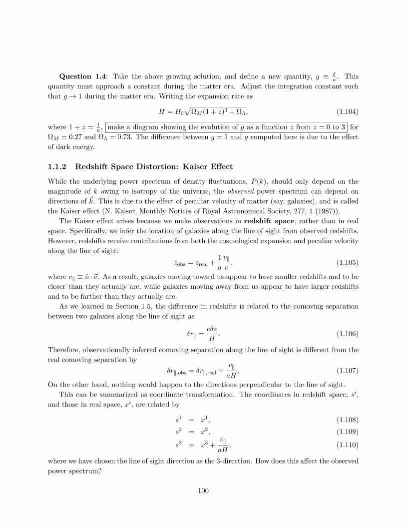
Question 1.4: Take the above growing solution, and define a new quantity, g ≡ δa . This

quantity must approach a constant during the matter era. Adjust the integration constant such

that g → 1 during the matter era. Writing the expansion rate as

H = H0

√ΩM (1 + z)3 + ΩΛ, (1.104)

where 1 + z = 1a , make a diagram showing the evolution of g as a function z from z = 0 to 3 for

ΩM = 0.27 and ΩΛ = 0.73. The difference between g = 1 and g computed here is due to the effect

of dark energy.

1.1.2 Redshift Space Distortion: Kaiser Effect

While the underlying power spectrum of density fluctuations, P (k), should only depend on the

magnitude of k owing to isotropy of the universe, the observed power spectrum can depend on

directions of ~k. This is due to the effect of peculiar velocity of matter (say, galaxies), and is called

the Kaiser effect (N. Kaiser, Monthly Notices of Royal Astronomical Society, 277, 1 (1987)).

The Kaiser effect arises because we make observations in redshift space, rather than in real

space. Specifically, we infer the location of galaxies along the line of sight from observed redshifts.

However, redshifts receive contributions from both the cosmological expansion and peculiar velocity

along the line of sight:

zobs = zreal +1

a

v‖

c, (1.105)

where v‖ ≡ n ·~v. As a result, galaxies moving toward us appear to have smaller redshifts and to be

closer than they actually are, while galaxies moving away from us appear to have larger redshifts

and to be farther than they actually are.

As we learned in Section 1.5, the difference in redshifts is related to the comoving separation

between two galaxies along the line of sight as

δr‖ =cδz

H. (1.106)

Therefore, observationally inferred comoving separation along the line of sight is different from the

real comoving separation by

δr‖,obs = δr‖,real +v‖

aH. (1.107)

On the other hand, nothing would happen to the directions perpendicular to the line of sight.

This can be summarized as coordinate transformation. The coordinates in redshift space, si,

and those in real space, xi, are related by

s1 = x1, (1.108)

s2 = x2, (1.109)

s3 = x3 +v‖

aH, (1.110)

where we have chosen the line of sight direction as the 3-direction. How does this affect the observed

power spectrum?

100

Question 1.5: Since this is merely coordinate transformation, the mass within a unit volume

must be conserved regardless of the choice of the coordinate system. We have

ρsd3s = ρxd

3x, (1.111)

where ρs and ρx are the mass densities in redshift space and real space, respectively. Expanding

these into perturbations,

ρ(1 + δs)d3s = ρ(1 + δx)d3x. (1.112)

Note that the mean density, ρ, is the same in both real space and redshift space. From this, we

obtain

δs =1

|J |(1 + δx)− 1, (1.113)

where |J | is the determinant of the Jacobian matrix:

J ≡

∂s1

∂x1∂s1

∂x2∂s1

∂x3

∂s2

∂x1∂s2

∂x2∂s2

∂x3

∂s3

∂x1∂s3

∂x2∂s3

∂x3

. (1.114)

By expanding equation (16) up to the first order in perturbations (including density and velocity),

find the relation between δs, δx, and v‖. Note that v‖ depends on spatial coordinates xi, whereas

H does not but it depends only on time. Hint: does the result you obtained make sense? What

are the conditions for δs < δx or δs > δx? Can you explain why they are so?

Question 1.6: Now is the time to go to Fourier space. Use

δs =

∫d3k

(2π)3δs,~k

ei~k·~x, (1.115)

δx =

∫d3k

(2π)3δx,~k

ei~k·~x, (1.116)

~v =

∫d3k

(2π)3~v~k e

i~k·~x, (1.117)

(1.118)

and write the relation between δs and δx in Fourier space.† Here, ~v = (v1, v2, v3) and v‖ = v3.

We need to relate v‖ to δx. For this, we can use the mass conservation equation:

δx +1

a~∇ · ~v = 0. (1.119)

Fourier-transforming this, one finds

˙δx,~k

+i~k

a· ~v~k = 0. (1.120)

†If you are careful, you might wonder why we can expand δs using x coordinates, rather than s coordinates. This

is OK up to the first order - since δs is already a perturbation, the difference between x coordinates and s coordinates

would appear only at the second order.

101

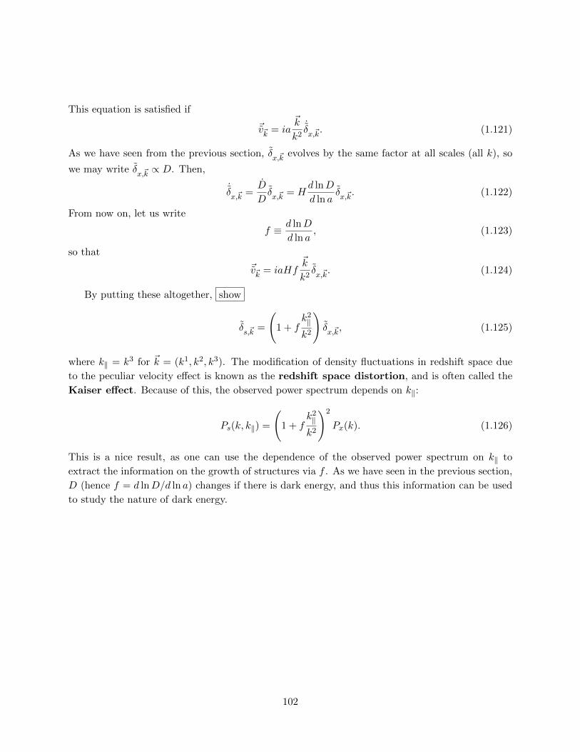
This equation is satisfied if

~v~k = ia~k

k2˙δx,~k. (1.121)

As we have seen from the previous section, δx,~k

evolves by the same factor at all scales (all k), so

we may write δx,~k∝ D. Then,

˙δx,~k

=D

Dδx,~k

= Hd lnD

d ln aδx,~k. (1.122)

From now on, let us write

f ≡ d lnD

d ln a, (1.123)

so that

~v~k = iaHf~k

k2δx,~k. (1.124)

By putting these altogether, show

δs,~k

=

(1 + f

k2‖

k2

)δx,~k, (1.125)

where k‖ = k3 for ~k = (k1, k2, k3). The modification of density fluctuations in redshift space due

to the peculiar velocity effect is known as the redshift space distortion, and is often called the

Kaiser effect. Because of this, the observed power spectrum depends on k‖:

Ps(k, k‖) =

(1 + f

k2‖

k2

)2

Px(k). (1.126)

This is a nice result, as one can use the dependence of the observed power spectrum on k‖ to

extract the information on the growth of structures via f . As we have seen in the previous section,

D (hence f = d lnD/d ln a) changes if there is dark energy, and thus this information can be used

to study the nature of dark energy.

102